simulated convective lines with leading precipitation

VOL. 61, NO. 14 15 JULY 2004J O U R N A L O F T H E A T M O S P H E R I C S C I E N C E S

q 2004 American Meteorological Society 1637

Simulated Convective Lines with Leading Precipitation. Part I: Governing Dynamics

MATTHEW D. PARKER* AND RICHARD H. JOHNSON

Department of Atmospheric Science, Colorado State University, Fort Collins, Colorado

(Manuscript received 3 April 2003, in final form 2 February 2004)

ABSTRACT

This article, the first of two describing a study in which the authors used idealized numerical simulations toinvestigate convective lines with leading precipitation, addresses the dynamics governing the systems’ structuresand individual air parcels’ accelerations within them. It appears that, although unconventional, systems withinflow passing through their line-leading precipitation can be stable and long lived. Lower-tropospheric inflowingair in the simulations ascends, overturns in deep updrafts, and subsequently carries its water content forwardfrom the convective line, where it gives rise to the leading precipitation region. Although relatively strong windshear in the middle and upper troposphere accounts for a component of the downshear acceleration, and henceoverturning, of air parcels in the simulated updrafts, a mature system with leading precipitation also rendersboth persistent and periodic pressure anomalies that contribute just as much. Many of these accelerations, whichgovern the overall system structure, are largely transient and are lost when averaged over multiple convectivecycles. This article explains the dynamics that govern the transient updrafts and downdrafts within the systems,including a precipitation cutoff mechanism that governs their multicellular periods.

1. Introduction

The importance of mesoscale convective systems(MCSs) to the agriculturally prolific central UnitedStates has long been established (e.g., Fritsch et al.1986). However, recent work by Parker and Johnson(2000) has revealed recurring organizational modes forMCSs in this region (Fig. 1), among which are the poor-ly understood convective lines with leading stratiform(LS) precipitation. Parker and Johnson (2004b, hereafterPJ04) outlined a basic conceptual model for front-fedLS (FFLS) systems, as shown in Fig. 2, whose lowertropospheric inflow passes through a region of line-lead-ing precipitation. They noted that these systems haveheretofore received relatively little notice, even thoughthey account for an important fraction of linear MCSsin the central United States (Parker and Johnson 2000).This paper is the first of two addressing the basic struc-tures of FFLS systems, and the dynamics that accountfor and sustain them; the companion paper, Parker andJohnson (2004a), is hereafter referred to as ‘‘Part II.’’It is important to understand the full spectrum of or-ganized convective systems because MCSs’ organiza-tional modes have a direct effect on their propensity to

* Current affiliation: Department of Geosciences, University of Ne-braska at Lincoln, Lincoln, Nebraska.

Corresponding author address: Dr. Matthew Parker, 214 BesseyHall, University of Nebraska at Lincoln, Lincoln, NE 68588-0340.E-mail: [email protected]

produce large local rainfall totals and flooding (Doswellet al. 1996).

Numerical modeling techniques are desirable for at-tacking this problem owing to the paucity of high-res-olution observations (e.g., dual-Doppler wind fields)available for in-depth case studies. FFLS systems areof themselves interesting from a numerical modelingperspective, because previously published works havedocumented simulations that lie roughly within the ap-propriate range of vertical wind shear for FFLS systems,yet in which a long-lived system failed to develop.Among such near misses are simulations by Hane(1973), Thorpe et al. (1982), Seitter and Kuo (1983),Nicholls et al. (1988), Weisman et al. (1988), and Szetoand Cho (1994). In general these systems did not pro-duce large leading precipitation regions, even thoughtheir general structures resembled those of the FFLSsystems in this publication, and were not very longlived. Hane (1973) noted that, ‘‘some rain tends to fallon the right-hand [downshear] side of the cloud [which]creates additional difficulty for the regeneration pro-cess,’’ and Seitter and Kuo (1983) noted that, when‘‘large amounts of liquid water were carried forwardinto the anvil of the storm . . . the fall of this water intothe front of the storm led to excessive loading of theupdraft and caused a rapid decay of the storm.’’ Inter-estingly, Dudhia et al. (1987) claimed that, ‘‘no con-vincing example of steady convection of the pure steer-ing-level [i.e., overturning updraft] type has yet beendemonstrated in two dimensions.’’ Some reasons for theprior failures to simulate FFLS systems may include the

1638 VOLUME 61J O U R N A L O F T H E A T M O S P H E R I C S C I E N C E S

FIG. 1. Schematic reflectivity drawing of idealized life cycles forthree linear MCS archetypes from Parker and Johnson (2000): (a)leading-line TS, (b) convective line with LS, and (c) convective linewith parallel stratiform (PS). Approximate time interval betweenphases: for TS 3–4 h; for LS 2–3 h; for PS 2–3 h. Levels of shadingroughly correspond to 20, 40, and 50 dBZ.

FIG. 2. Conceptual model of a front-fed convective line with leadingprecipitation from PJ04, viewed in a vertical cross section orientedperpendicular to the convective line and parallel to its motion.

manner in which those scientists initiated the convection(i.e., using a bubble instead of a cold pool), their ex-clusion of the ice phase, and/or the possibility that thetemperature and humidity profiles in their environmentswere not appropriate for the destabilization mechanismthat helped to maintain the simulated systems in thepresent study (Part II).

As mentioned by PJ04, the history of squall line andMCS research is grounded largely in a rich sequence ofpapers describing convective lines with trailing strati-form (TS) precipitation. Among the numerous papersaddressing TS systems, authors such as Newton andFankhauser (1964), Houze and Rappaport (1984), Kes-singer et al. (1987), Fankhauser et al. (1992), Grady andVerlinde (1997), and Nachamkin et al. (2000) studiedsystems with at least some FFLS characteristics. These,along with consideration of another well-observed FFLScase, led PJ04 to propose the basic conceptual modelfor the kinematic and reflectivity structures of FFLSsystems in Fig. 2, whose salient features include a meanoverturning updraft and an upper-tropospheric zone ofrear-to-front outflow that feeds the leading precipitationregion. With idealized numerical simulations that com-pared various kinds of LS and TS systems, PJ04 pointedto the importance of the lower-tropospheric and deep-layer wind shear vectors in helping to determine quasi-2D systems’ organizational modes. However, althoughthey produced reasonable FFLS simulations, they wereunable to discuss the systems’ details.

In addition to the above studies, other authors haveused high-resolution, idealized numerical simulations toadvance the dynamical understanding of convectivelines. For example, Yang and Houze (1995) used ide-alized simulations to suggest that the periodic behaviorof multicellular squall lines is attributable to gravity

waves forced by a quasi-steady gust front updraft. Incontrast, Fovell and Tan (1998) simulated an unsteadygust front updraft and attributed the convection’s peri-odic behavior to a cutoff mechanism induced by thebuoyant updrafts themselves. The simulation results ofLin et al. (1998) and Lin and Joyce (2001) led them tosuggest that the middle-tropospheric flow controls thespeed at which the active cells are advected away fromthe gust front updraft, and therefore the period withwhich new convection can be generated. This paper de-scribes a similar effort to learn about convective dy-namics by analyzing high-resolution numerical simu-lations.

In the following section we outline the setup of thenumerical model and describe our analysis techniques.Thereafter, section 3 describes simulated FFLS systems’temporally averaged features, and section 4 describesthe temporally varying dynamics that account for thosefeatures. We conclude this paper with a synthesis ofFFLS systems’ mean and transient behavior in section5. Part II then resumes with discussion of the mechanismthat enables the simulated systems to survive inflow thatpasses through their preline precipitation, as well as theevolution of FFLS systems to other modes and the sen-sitivities of these processes.

2. Methods

a. Numerical model

This paper makes use of idealized numerical simu-lations to describe the basic evolutions and dynamicsof front-fed convective lines with leading precipitation.This work incorporated both 2D and 3D simulationsusing version 4.5.2 of the Advanced Regional PredictionSystem (ARPS), a fully compressible nonhydrostaticmodel developed by the Center for Analysis and Pre-diction of Storms (CAPS) and the University ofOklahoma. The dynamical framework of the ARPS wasdescribed by Xue et al. (1995, 2000, 2001).

The basic 2D configuration of the model for this study

15 JULY 2004 1639P A R K E R A N D J O H N S O N

FIG. 3. Skew T–lnp diagram of the mean MCS temperature andhumidity soundings used in this study, and base-state u-wind profile:full barb 5 5 m s21; half barb 5 2.5 m s21. See Part II for graphicaldepiction of u wind vs height. Bulk thermodynamic variables for thissounding are given in Table 1.

TABLE 1. Bulk thermodynamic variables for the analytic mean MCSsounding. Parcel indices are computed using an unmixed surface airparcel.

Thermodynamic parameter Value

Lifting condensation level (hPa)Level of free convection (hPa)Convective available potential energy (J kg21)Convective inhibition (J kg21)Lifted index (K)Precipitable water (cm)

840795

257723428.4

3.20

was described by PJ04. The configuration of the 3D sim-ulations was identical to that for the 2D simulations, withthe following exceptions. The across-line (x) and vertical(z) dimensions remained 600 and 18 km, respectively, asdescribed by PJ04, but the along-line (y) dimension was300 km. The large along-line extent allowed individualconvective cells to develop at spacings that were intrinsicto the problem rather than those imposed by a smalldomain’s along-line period, and permitted the modeledconvective cells to move and interact with one anothermore naturally, much as real-world convective cellswould when part of a long, quasi-2D line. It also in-creased the number of convective cells on the domain atany time, allowing computation of a greater variety ofair parcel trajectories. In order to explicitly simulate con-vective clouds on the domain, the 3D simulations hadgrid spacings of 2 km. The vertical grid in the 3D modelwas stretched, with an averaged spacing of 643 m, rang-ing from 400 m in the lowest 2 km of the domain to 780m in the stratosphere. The simulations incorporated im-plicit differencing in z and used a large time step of 6 sand a small (acoustic) time step of 3 s.

The 3D simulations incorporated a periodic boundarycondition on the northern and southern edges of thedomain (at the line’s ends) in order to simulate quasi-2D convective lines. As described by PJ04, the centralregions of long but finite-length simulated 3D convec-tive lines behave much like 2D and periodic 3D lines,especially when the environmental wind profile is nearly2D and convection is initiated with a long linear trigger.Open (rather than periodic) y boundary conditions might

be important because they remove the quasi-2D con-straint upon gravity wave dispersion. However, as dis-cussed by PJ04, this constraint likely exists to somedegree in the middle sections of long quasi-2D con-vective lines, in addition to which, tests revealed thatthe simulated convection’s structure and evolution werenot affected much by changing the y boundary condi-tion.

The control simulations did not include Coriolis ac-celerations or radiative effects. Several sensitivity tests,in which the Coriolis parameter ( f ) was set to 1 3 1024

s21 (a typical midlatitude value) revealed that the in-clusion of planetary rotation had little discernable effecton the simulations during their first 6 h (the focus forthe analyses in this publication). The results of the sim-ulations with Coriolis accelerations are not described inthe text. In like manner, a sensitivity test using an in-frared radiation parameterization scheme revealed fewappreciable differences during the first 6 h of the sim-ulation.

The model had a horizontally homogeneous initialcondition, which was defined by a single base-statesounding as described by PJ04 and shown in Fig. 3.The bulk thermodynamic variables that describe themean MCS sounding are summarized in Table 1, andwere discussed by PJ04. The base-state wind profile forthe front-fed LS system control runs was taken as theaverage wind profile of four archetypal front-fed LSsystems (which were among the population of LS MCSssummarized by Parker and Johnson 2000). For sim-plicity, the wind profile was reduced to anchor points,and varied linearly between the values at the anchorpoints. The u-wind values for the control run are plottedin Fig. 3. This profile is truer to observed FFLS systemsthan the simplistic profiles that PJ04 used for their sen-sitivity tests. The control run’s initial state was 2D, andincluded no y wind. Sensitivity tests indicated that theinclusion of a realistic y wind did not substantially affectthe structure or evolution of the periodic 3D simulations.

The method of convective initiation was identical tothat described by PJ04, except that the infinitely long,2-km-deep cold box had a constant buoyancy of 20.1m s22 (which corresponds to a potential temperatureperturbation of 23.2 K in the base-state sounding). Thiswas the minimal cold pool strength that reliably initiateda long-lived convective system. Because the first round


of simulated convection in the model produced muchcolder surface outflow, the later simulated convectionwas fairly independent of the initial trigger. For all ofthe 3D simulations, the cold box included small (#0.1K) random fluctuations in order to help 3D structuresdevelop and amplify. While the initial convection wasfairly 2D, after 2 h of simulation the convective lineswere cellular and remained 3D for the duration of thesimulations.

b. Analysis techniques

As described by PJ04, we carried out analyses of thecomponents of the pressure field, defined as follows.The pressure perturbations can be diagnosed using themethod presented by Wilhelmson and Ogura (1972).Separating into buoyant and dynamic parts (p9 5 1p9B

), following Rotunno and Klemp (1982), yieldsp9D

]2¹ p9 5 (r B); (1)B o]z

2 2 2 2]u ]y ]w ]2¹ p9 5 2r 1 1 2 w (lnr )D o 2 o21 2 1 2 1 2[ ]]x ]y ]z ]z

| ||

extension terms

]y ]u ]u ]w ]y ]w2 2r 1 1 ; (2)o1 2]x ]y ]z ]x ]z ]y

| ||

shear terms

wherein B is the buoyancy and all other variables havetheir conventional meanings; the terms in (2) are labeledfollowing Klemp (1987). In the base-state environmentwith a mean u-wind profile, the linear part of (2) is

du ]wo2¹ p9 5 22r , (3)DL o dz ]x

which is a shear term. The remainder of 2 isp9 p9D DL

the nonlinear part of the dynamic pressure perturbation. In addition to the aforementioned authors, othersp9DNL

(e.g., Schlesinger 1980; Cai and Wakimoto 2001) havealso made use of these and similar formulations in an-alyzing convective dynamics.

In order to make the discussions and labeling simpler,this publication employs abbreviated names for theterms in the decomposed momentum equation, as shownby brackets below. For anelastic, inviscid, irrotationalflow, the equation for motion is

Du 1 r95 2 =p9 2 g .1 2Dt r ro o (4)| |

|ACC

By applying p9 5 1 1 , regrouping the terms,p9 p9 p9B DL DNL

and explicity writing the hydrometeor contribution todensity, (4) becomes

Du 1 r9 1 1gas5 2 =p9 2 g 2 gq 2 =p9 2 =p9 ,B h DL DNL1 2Dt r r r ro o o o| || || || |

| | | |BUOY DRAG ACCDL ACCDNL

| | (5)|

ACCB

wherein is the density perturbation attributable tor9gas

the gaseous constituents and qh is the total hydrometeormixing ratio. The abbreviations in (4) and (5) appearthroughout this article.

To facilitate analysis of air parcels, the model com-puted particle trajectories during the simulations. Be-cause the background total water content in the middleand upper troposphere is quite low, air parcels with highwater content must be transported forward from the con-vective line in order for leading stratiform precipitationto develop, or rearward in order for trailing stratiformprecipitation to develop. Both temporally averagedfields and parcel trajectories (see, e.g., section 4) con-firm that the water in the leading precipitation regionsof the present simulations is attributable primarily to airparcels that have ascended in the convective updrafts.Plus or minus gains and losses from vertical divergencein the precipitation flux, air parcels from the lower tro-posphere carry with them their comparatively high totalwater contents. Therefore, the most suitable way to an-alyze the dynamics that generate a leading or trailingstratiform precipitation region is to analyze the dynam-ics that affect the velocities of individual parcels as theypass through the convective region.

Accordingly, it is worthwhile briefly to describe sim-ple cold pool, updraft, and wind shear configurationsthat account for components of the perturbed pressurefield, in order to provide points of reference for theensuing discussions. In the limit of 1D (= 5 ] /]z),p9 p9B B

(1) represents the hydrostatic equation and is consistentwith a surface cold pool having comparatively highersurface pressure than the undisturbed environment (Fig.4a). Additionally, because ]B/]z . 0 in the upper partsof realistic cold pools, simple consideration of (1) alsoimplies minimized pressure in their upper reaches. Be-cause, in most circumstances, the field has horizontalp9Bstructure and is not hydrostatic, both (a) horizontal ac-celerations occur, and (b) is insufficient to opposep9Bthe negative buoyancy in the cold pool, such that thedense air descends (as depicted by the dashed arrow inFig. 4a). As a result, the accelerations due to buoyancyand , as shown in Fig. 4a, generate a local circulationp9Bthat renders relatively high dynamic pressure near andahead of the cold pool’s gust front and relatively lowpressure in the cold pool’s head (Fig. 4b), owing to low-level convergence ahead of the cold pool’s leading edge[extension terms in Eq. (2)] and to local rotation in thecold pool’s head [shear terms in Eq. (2)]. Following (3),an updraft in a mean-sheared environment exhibits rel-atively high pressure on its upshear side and relatively


FIG. 4. Schematic depiction of simple cold pool, updraft, and windshear configurations that account for components of the perturbedpressure field. Wind streamlines are depicted as solid arrows, buoyantaccelerations are depicted as dashed arrows, and pressure maximaand minima are denoted by H and L, respectively. Subfigures (a)–(f ) are explained in the text. Sizes and magnitudes are not necessarilyscaled quantitatively.

FIG. 5. Hovmoller diagram depicting 3-km-AGL hydrometeor mix-ing ratio (t 5 0–8 h) for 2D FFLS simulation. Levels of shading are0.005, 0.02, 0.08, 0.32, 1.28, and 5.12 g kg21.

low pressure on its downshear side (Fig. 4c). Addition-ally, (1) implies that a bubble of buoyant air exhibitsrelatively high pressure above and relatively low pres-sure below its center (Fig. 4d). The field associatedp9Bwith a buoyant updraft (Fig. 4d) will therefore causedivergence above the updraft, convergence below theupdraft, and subsidence to the sides of the updraft, ren-dering a vortical circulation such as depicted by thearrows in Fig. 4e, which is consistent with locally min-imized pressure via the shear terms in (2). Although itis merely a refinement to the field associated withp9DNL

a simple buoyant updraft (Fig. 4e), for strongly curvedflow fields (in this case updrafts), the pressure minimumon the side nearer to the axis of rotation has an increasedmagnitude, while the pressure minimum on the side far-ther from the axis of rotation has a decreased magnitude(Fig. 4f).

3. Quasi-stable structures

In a 2D simulation using the control sounding andbase-state wind profile (Fig. 3), a long-lived front-fedconvective line with leading precipitation occurred (Fig.5), many aspects of which are quite similar to the FFLSsimulations described by PJ04, whose conclusions willby and large not be repeated here. As can be seen inFig. 5, the leading precipitation region developed withtime throughout the first 4 h of the simulation. Deepconvection was continually initiated above the surfacecold pool in the vicinity of its outflow boundary and,as can be inferred from Fig. 6, each updraft pulse ofthe multicellular system contributed a patch of enhancedwater content to the plume of line-leading hydromete-ors. The persistent periodic phase of the FFLS systemshown in Fig. 6 is of interest because it is quasi stable;in other words, despite the chaotic details of the evolv-ing flow, similar behaviors continue to occur periodi-cally over an extended range of time.1

On average, during the mature phase of the 2D FFLSsystem, air below ;6 km AGL flows westward andpasses through a preline region of cloud and precipi-tation on its way to the convective zone (Fig. 7). Someof this inflowing air ascends and feeds deep convectiveupdrafts while the remainder does not attain a level offree convection and instead passes through the line’smean position, in some cases being cooled and contrib-uting to the surface cold pool (Fig. 7). Notably, it is notclear from Fig. 7 that air below ø4.5 km AGL everparticipates in the deep convective updrafts. This is aresult of averaging; time-dependent air parcel trajec-tories such as A–a in Fig. 8 do ascend in deep updrafts,but other lower-tropospheric inflowing parcels like B–b and C–c in Fig. 8 do not. Indeed, the magnitude of

1 Such a condition has also been referred to as ‘‘quasi equilibrium’’and ‘‘statistically steady,’’ for example, by Fovell and Ogura (1988).


FIG. 6. Total hydrometeor mixing ratio (qh) and cold pool locationfor selected times during the 2D FFLS system’s quasi-stable period;qh thinly contoured and shaded at 0.005, 0.02, 0.08, 0.32, 1.28, and5.12 g kg21; general cold pool position indicated by u9 5 24 Kisopleths (thick contours).

FIG. 7. Mean total hydrometeor mixing ratio (levels of shading are0.02, 0.08, 0.32, and 1.28 g kg21), pressure pertubation (contours,hPa), and wind vectors (m s21, scaled as shown) for the 2D FFLSsimulation.

FIG. 8. Four-hour parcel trajectories typifying commonly observedairstreams for the 2D FFLS simulation. Parcels’ initial positions (att 5 0 min) are indicated by capital letters. Parcels’ final positions (att 5 240 min) are indicated by lower-case letters. Averaged u9 , 22K are shaded to indicate the mean position of the surface cold poolduring the time period. The trajectories’ thicknesses vary in order toassist in differentiating them. The thicknesses have no additionalmeaning.

w in the convective region after temporal averaging (Fig.7) is quite small below 5 km AGL, because this is azone in which both updrafts (i.e., trajectories A–a andE–e) and downdrafts (i.e., trajectories B–b, C–c, andD–d) are fed by both lower- (i.e., A–a, B–b, and C–c)and middle- (i.e., D–d and E–e) tropospheric inflow.Almost all of the updraft trajectories overturn (e.g., A–a and E–e in Fig. 8) and are detrained with significantwesterly velocities (i.e., above 7 km AGL in Fig. 7),carrying at least some of their water content with themand contributing to a persistent leading precipitation re-gion (i.e., east of x 5 0 km in Fig. 7). The mean flowin the middle and upper troposphere to the west of theconvective region is weak, having been decelerated. Afew air parcels, such as F–f in Fig. 8, are entrained intothe deep convection or cross over its mean position.However, an analysis of the mass fluxes through theconvective region (not shown) revealed that the envi-ronmental air above 7 km AGL on the system’s upshearside contributes relatively little to the mass outflux eastof the convective updraft. The predominant flow branchis an overturning updraft that is fed by both the lower-and middle-tropospheric inflow.

Although it is not practical to prepare individual crosssections for the 3D simulations like those in Fig. 6, theplan views of mean tropospheric qh in Fig. 9 reveal thatthe periodic 3D FFLS simulation also exhibits a quasi-stable behavior. In particular, a line of healthy convec-

tion persists, comprising individual convective cells thattemporally develop, mature, and decay. Reassuringly,despite the idealized nature of the simulation and theconstraint of y periodicity, the convective line ‘‘seg-ments’’ shown in Fig. 9 are similar to the reflectivityimages presented by Parker and Johnson (2000, e.g.,their Fig. 6). The periodic 3D system is on averagequasi-2D, evidence for which includes the visually ob-vious slab symmetry of the structures in Fig. 9, thestrong similarity of the along-line means in Fig. 10 tothe temporal means from the 2D simulation in Fig. 7,and the strong similarity of the x–z cross section oftrajectories from the periodic 3D simulation (Fig. 11)to those from the 2D simulation (Fig. 8).

The mean fields in the 2D simulation (Fig. 7) areslightly more perturbed than those in the periodic 3Dsimulation (Fig. 10), which is to be expected given that


FIG. 9. Mean hydrometeor mixing ratio from 0–10 km AGL for periodic 3D FFLS simulation: (a) at t 5 5 h; (b)at t 5 6 h. Levels of shading are 0.005, 0.02, 0.08, 0.32, 1.28, and 5.12 g kg21.

FIG. 10. Mean total hydrometeor mixing ratio (levels of shadingare 0.02, 0.08, 0.32, and 1.28 g kg21), pressure pertubation (contours,hPa), and wind vectors (m s21, scaled as shown) for periodic 3DFFLS simulation.

the temporally averaged areal coverage of convectionin the 3D simulation is somewhat less than in the 2Dsimulation owing to the spacing of its isolated convec-tive cells (as seen in Fig. 9). However, the shapes ofthe qh, p9, and wind fields correspond quite well betweenthe 2D and periodic 3D systems, and the logic of thephysical processes that links them together is un-changed. Of major importance is that, not only are theaveraged fields similar, but the trajectories computed in

the temporally evolving 3D flow field are quasi-2D andcorrespond quite well to those from the 2D simulation;air parcels’ line-parallel motions are minimal (Fig. 11),such that, to a very high order, their basic paths can bedescribed in the x–z plane. In the x–z plane, the 3Dtrajectories (Fig. 11) reveal updrafts that are fed by bothlower- (e.g., trajectories 3, 8, and 9) and middle- (e.g.,trajectories 2 and 6) tropospheric inflow, much like tra-jectories A–a and E–e in Fig. 8, as well as inflowinglower- and middle-tropospheric air parcels that cross theline’s position (e.g., trajectories 1, 4, 5, and 7) and oftenfeed the surface cold pool, much like trajectories B–b,C–c, and D–d in Fig. 8. Although the discussion insection 4 emphasizes the importance of transient ac-celerations and will point out differences between thetransient components of the 2D and periodic 3D sim-ulations, the present analysis also shows that, to firstorder, the quasi-stable characteristics and effects of the2D and periodic 3D systems are the same. In the presentstudy, the lack of meridional flow (Fig. 3), periodicalong-line dimension, and linear initial trigger no doubthelp to reinforce this similarity. Notably, numerous pre-vious studies have also demonstrated the similarity of2D simulations of TS systems to their 3D counterpartsin the real world and in numerical models (e.g., Hane1973; Dudhia et al. 1987; Fovell and Ogura 1988; Ro-tunno et al. 1988).

In the 3D simulations, the main complication to thesystem’s quasi-2D structure is that the convective up-drafts are localized, and do not resemble the infinitely


FIG. 11. ‘‘Shadow’’ depiction of forward trajectories computed for periodic 3D FFLS simulation. The central panelof this figure is an x–y plane view of trajectory positions, the top panel is an x–z cross section of trajectory positions,and the right panel is a z–y cross section of positions. The trajectories begin at the V symbols, and are labeled forreference in the text.

long (in y) slabs of upward motion that occur in the 2Dsimulation. This has three important effects. The first isthat air parcels can pass between the isolated updraftsof the periodic 3D line. Whereas in the 2D simulationthe upper-tropospheric storm-relative flow must becomeapproximately stagnant on the system’s upshear side, in3D the upper-level flow stagnation is very local, thepressure field favors acceleration of air into the channelsbetween active updrafts, and the mean upper-tropo-spheric mass flux across the convective line is approx-imately temporally invariant (not shown). Hence, themean environmental flow in the 5–10-km-AGL layer onthe upshear side of the convective line is much strongerin 3D than in 2D (cf. Figs. 10 and 7). The periodic 3Dleading cloud and precipitation region therefore expe-riences slightly enhanced evaporation and sublimationas environmental flow overtakes the system. This secondimportant effect means that the total hydrometeor loadis somewhat decreased (cf. Figs. 10 and 7), and that themiddle and upper troposphere is less warm (not shown).Accordingly, the quasi-static pressure minimum in the2D case is stronger (e.g., at z ø 4 km AGL, x ø 25km in Fig. 7), rendering comparatively stronger front-to-rear flow between roughly 3 and 6 km AGL (cf. Figs.10 and 7), and a corresponding increase in the heightof the flow reversal (from about 6 km in the periodic3D case to about 7 km in the 2D case; cf. Figs. 10 and7). The final important effect is that the geometry of

the w and buoyancy fields in individual 3D updrafts isdifferent from that of the 2D updrafts. This is very im-portant to the transient local accelerations, and is dis-cussed in detail in section 4b. However, all caveats not-withstanding, from Figs. 10 and 11 it is clear that theperiodic 3D system perturbs and overturns the environ-ment in roughly the same way that the 2D system does.

In a mature convective system, quasi-steady per-turbed pressure fields exist, which in turn induce per-sistent mesoscale circulations. After about 2 h of thecontrol FFLS simulation, the mature convective systemhas had several prominent effects on the local winds(Fig. 12). The updrafts during this time interval occurbetween x 5 215 and x 5 0 km. Above 7 km AGL,dynamic and buoyant pressure maxima above the activebuoyant updrafts have rendered mean storm-top diver-gence. Additionally, in the lowest 1.5 km AGL the buoy-ant pressure maximum associated both with chilling inthe preline precipitation zone (discussed in detail in PartII), and with a persistent, quasi-steady surface cold pool,has produced mean westerly accelerations, which ac-count for westerlies within the cold pool itself and forthe deceleration of the easterly inflowing air to the rightof x 5 0 km. Finally, between 2 and 6 km AGL andeast of x 5 215 km, the wind is strongly perturbed intoan easterly midlevel jet, which is largely a response tothe midlevel pressure minimum that developed (andmoved with the system) eastward in time (Fig. 12). This


FIG. 12. Mean perturbation u wind (vectors, m s21) and perturbationpressure (contours, hPa) for the 2D FFLS simulation from t 5 2–4h. As discussed in the text, the pictured u9 field is long-lived, butrepresents a perturbation with respect to the base state.

FIG. 13. Mean velocities, perturbation pressures, and acceleration terms for simulation 2D FFLS, 2 h 40 min to 3 h 18 min. (a) BUOYcontoured, u and w vectors; (b) p9 contoured, ACC vectors. Vertical velocity of 5 m s21 is shaded. Three representative air parcel trajectories(n, V, and M) are plotted as bold curves. Contour intervals and vector scales are shown for each panel, and vary among panels. Terms aredefined in section 2b.

midlevel low is primarily from beneath the positivelyp9Bbuoyant air exiting the convective cells and forming theleading cloud region, although owing to the curvedp9DNL

overturning flow (as in Fig. 4f) contributes nontriviallyon the downshear flank of the mean updraft’s position.

Because the convective system perturbs the wind fieldin a way that changes the vertical shear for long periodsof time (i.e., much longer than an individual convectivelife cycle), updrafts that occur in the local wind profileexhibit additional dynamic pressure anomalies muchlike those in Fig. 4c; these perturbations are diagnosedas a part of (not shown), because even though thep9DNL

wind perturbations are persistent they nevertheless rep-resent deviations (u9) from the background state. Forthe mature phase of the simulated FFLS system, thevertical wind shear was decreased (became more east-erly) in the lowest 4 km AGL, and was increased (be-came more westerly) in the 4–10-km-AGL layer. From

consideration of (2), this should imply a westwardACCDNL for updrafts in the lowest 4 km, and an east-ward ACCDNL for updrafts in the 4–10-km layer (Fig.12). FFLS systems are unique because their large pres-sure perturbations, which are similarly found in manyMCSs’ stratiform regions, can in this case directly im-pact the inflowing air. Part II discusses how the aboveeffects could lead to evolution or demise of a convectiveline with leading precipitation.

4. Dynamics and kinematics

Having described the properties of the temporally av-eraged FFLS simulations, the paper now turns to theirtemporally varying parts. These transients prove to bevery important to the production of an overturning up-draft and leading precipitation.

a. A typical updraft cycle

This section documents the evolution of the com-ponents of the pressure field for a typical updraft cycleand the resultant accelerations that account for threerepresentative air parcel trajectories from the 2D FFLSsimulation. During the period of interest, approximately2 h 40 min–3 h 18 min, an updraft occurs, followed bya suppressed period, and finally by a second updraft.As shown in Fig. 13, three air parcels (represented byn, V, and M) that approach the convective region withvery similar trajectories and pass through the exact samepoint (x 5 21 km, z 5 730 m AGL) at different times(n at about 2 h 50 min, V at about 2 h 52 min, andM at about 3 h 06 min) follow markedly different tra-jectories through and away from the convective region.Parcel n ascends in the first updraft, whereas V arrivesabout 2 min later and does not ascend. A suppressedperiod ensues, in which no inflowing parcels ascend ina deep updraft. Parcel M then arrives just as the second


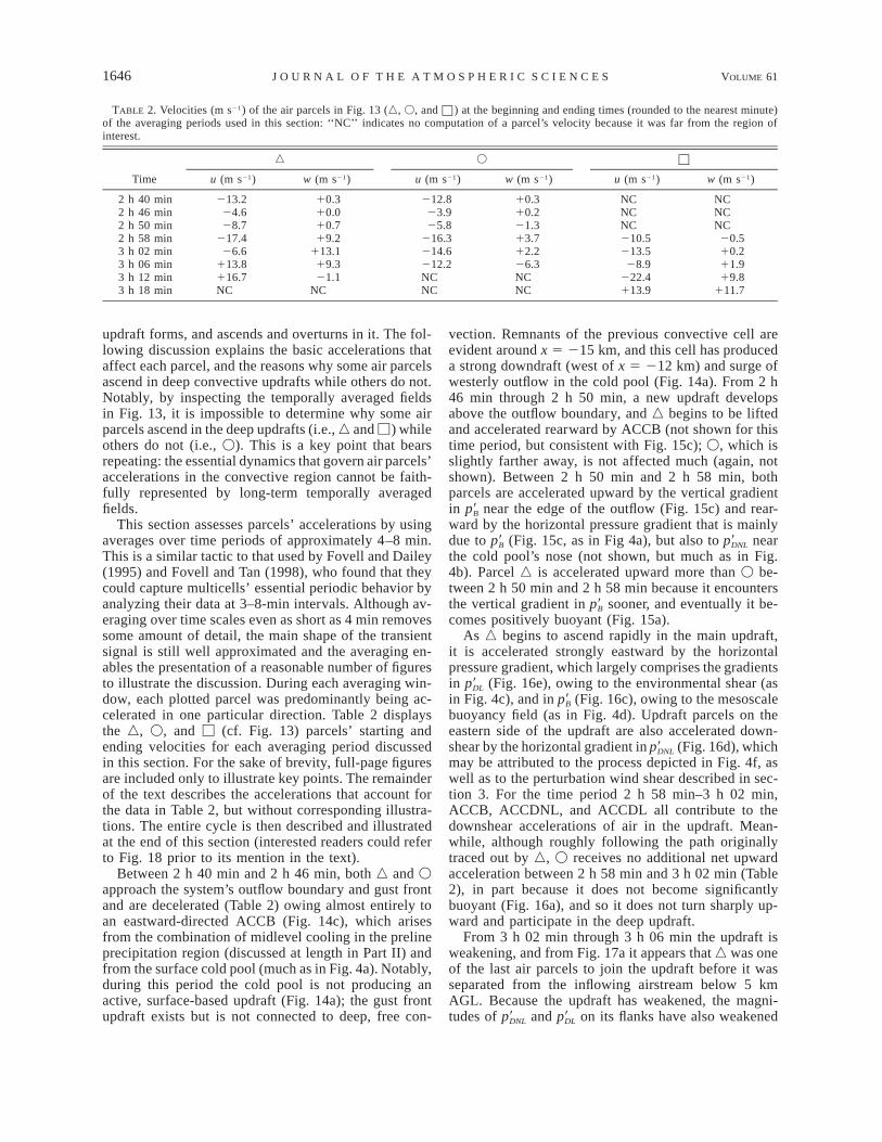
TABLE 2. Velocities (m s21) of the air parcels in Fig. 13 (n, V, and □ ) at the beginning and ending times (rounded to the nearest minute)of the averaging periods used in this section: ‘‘NC’’ indicates no computation of a parcel’s velocity because it was far from the region ofinterest.

Time

n

u (m s21) w (m s21)

V

u (m s21) w (m s21)

□

u (m s21) w (m s21)

2 h 40 min2 h 46 min2 h 50 min2 h 58 min3 h 02 min3 h 06 min3 h 12 min3 h 18 min

213.224.628.7

217.426.6

113.8116.7NC

10.310.010.719.2

113.119.321.1

NC

212.823.925.8

216.3214.6212.2NCNC

10.310.221.313.712.226.3NCNC

NCNCNC210.5213.528.9

222.4113.9

NCNCNC20.510.211.919.8

111.7

updraft forms, and ascends and overturns in it. The fol-lowing discussion explains the basic accelerations thataffect each parcel, and the reasons why some air parcelsascend in deep convective updrafts while others do not.Notably, by inspecting the temporally averaged fieldsin Fig. 13, it is impossible to determine why some airparcels ascend in the deep updrafts (i.e., n and M) whileothers do not (i.e., V). This is a key point that bearsrepeating: the essential dynamics that govern air parcels’accelerations in the convective region cannot be faith-fully represented by long-term temporally averagedfields.

This section assesses parcels’ accelerations by usingaverages over time periods of approximately 4–8 min.This is a similar tactic to that used by Fovell and Dailey(1995) and Fovell and Tan (1998), who found that theycould capture multicells’ essential periodic behavior byanalyzing their data at 3–8-min intervals. Although av-eraging over time scales even as short as 4 min removessome amount of detail, the main shape of the transientsignal is still well approximated and the averaging en-ables the presentation of a reasonable number of figuresto illustrate the discussion. During each averaging win-dow, each plotted parcel was predominantly being ac-celerated in one particular direction. Table 2 displaysthe n, V, and M (cf. Fig. 13) parcels’ starting andending velocities for each averaging period discussedin this section. For the sake of brevity, full-page figuresare included only to illustrate key points. The remainderof the text describes the accelerations that account forthe data in Table 2, but without corresponding illustra-tions. The entire cycle is then described and illustratedat the end of this section (interested readers could referto Fig. 18 prior to its mention in the text).

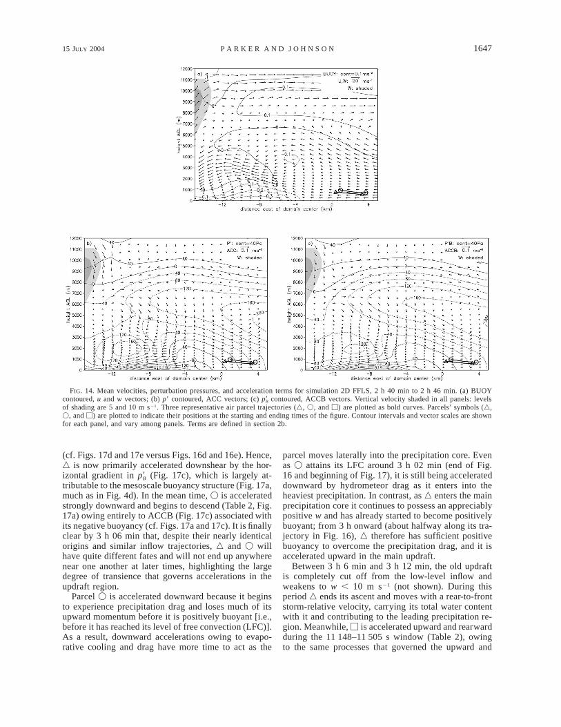
Between 2 h 40 min and 2 h 46 min, both n and Vapproach the system’s outflow boundary and gust frontand are decelerated (Table 2) owing almost entirely toan eastward-directed ACCB (Fig. 14c), which arisesfrom the combination of midlevel cooling in the prelineprecipitation region (discussed at length in Part II) andfrom the surface cold pool (much as in Fig. 4a). Notably,during this period the cold pool is not producing anactive, surface-based updraft (Fig. 14a); the gust frontupdraft exists but is not connected to deep, free con-

vection. Remnants of the previous convective cell areevident around x 5 215 km, and this cell has produceda strong downdraft (west of x 5 212 km) and surge ofwesterly outflow in the cold pool (Fig. 14a). From 2 h46 min through 2 h 50 min, a new updraft developsabove the outflow boundary, and n begins to be liftedand accelerated rearward by ACCB (not shown for thistime period, but consistent with Fig. 15c); V, which isslightly farther away, is not affected much (again, notshown). Between 2 h 50 min and 2 h 58 min, bothparcels are accelerated upward by the vertical gradientin near the edge of the outflow (Fig. 15c) and rear-p9Bward by the horizontal pressure gradient that is mainlydue to (Fig. 15c, as in Fig 4a), but also to nearp9 p9B DNL

the cold pool’s nose (not shown, but much as in Fig.4b). Parcel n is accelerated upward more than V be-tween 2 h 50 min and 2 h 58 min because it encountersthe vertical gradient in sooner, and eventually it be-p9Bcomes positively buoyant (Fig. 15a).

As n begins to ascend rapidly in the main updraft,it is accelerated strongly eastward by the horizontalpressure gradient, which largely comprises the gradientsin (Fig. 16e), owing to the environmental shear (asp9DL

in Fig. 4c), and in (Fig. 16c), owing to the mesoscalep9Bbuoyancy field (as in Fig. 4d). Updraft parcels on theeastern side of the updraft are also accelerated down-shear by the horizontal gradient in (Fig. 16d), whichp9DNL

may be attributed to the process depicted in Fig. 4f, aswell as to the perturbation wind shear described in sec-tion 3. For the time period 2 h 58 min–3 h 02 min,ACCB, ACCDNL, and ACCDL all contribute to thedownshear accelerations of air in the updraft. Mean-while, although roughly following the path originallytraced out by n, V receives no additional net upwardacceleration between 2 h 58 min and 3 h 02 min (Table2), in part because it does not become significantlybuoyant (Fig. 16a), and so it does not turn sharply up-ward and participate in the deep updraft.

From 3 h 02 min through 3 h 06 min the updraft isweakening, and from Fig. 17a it appears that n was oneof the last air parcels to join the updraft before it wasseparated from the inflowing airstream below 5 kmAGL. Because the updraft has weakened, the magni-tudes of and on its flanks have also weakenedp9 p9DNL DL


FIG. 14. Mean velocities, perturbation pressures, and acceleration terms for simulation 2D FFLS, 2 h 40 min to 2 h 46 min. (a) BUOYcontoured, u and w vectors; (b) p9 contoured, ACC vectors; (c) contoured, ACCB vectors. Vertical velocity shaded in all panels: levelsp9Bof shading are 5 and 10 m s21. Three representative air parcel trajectories (n, V, and M) are plotted as bold curves. Parcels’ symbols (n,V, and M) are plotted to indicate their positions at the starting and ending times of the figure. Contour intervals and vector scales are shownfor each panel, and vary among panels. Terms are defined in section 2b.

(cf. Figs. 17d and 17e versus Figs. 16d and 16e). Hence,n is now primarily accelerated downshear by the hor-izontal gradient in (Fig. 17c), which is largely at-p9Btributable to the mesoscale buoyancy structure (Fig. 17a,much as in Fig. 4d). In the mean time, V is acceleratedstrongly downward and begins to descend (Table 2, Fig.17a) owing entirely to ACCB (Fig. 17c) associated withits negative buoyancy (cf. Figs. 17a and 17c). It is finallyclear by 3 h 06 min that, despite their nearly identicalorigins and similar inflow trajectories, n and V willhave quite different fates and will not end up anywherenear one another at later times, highlighting the largedegree of transience that governs accelerations in theupdraft region.

Parcel V is accelerated downward because it beginsto experience precipitation drag and loses much of itsupward momentum before it is positively buoyant [i.e.,before it has reached its level of free convection (LFC)].As a result, downward accelerations owing to evapo-rative cooling and drag have more time to act as the

parcel moves laterally into the precipitation core. Evenas V attains its LFC around 3 h 02 min (end of Fig.16 and beginning of Fig. 17), it is still being accelerateddownward by hydrometeor drag as it enters into theheaviest precipitation. In contrast, as n enters the mainprecipitation core it continues to possess an appreciablypositive w and has already started to become positivelybuoyant; from 3 h onward (about halfway along its tra-jectory in Fig. 16), n therefore has sufficient positivebuoyancy to overcome the precipitation drag, and it isaccelerated upward in the main updraft.

Between 3 h 6 min and 3 h 12 min, the old updraftis completely cut off from the low-level inflow andweakens to w , 10 m s21 (not shown). During thisperiod n ends its ascent and moves with a rear-to-frontstorm-relative velocity, carrying its total water contentwith it and contributing to the leading precipitation re-gion. Meanwhile, M is accelerated upward and rearwardduring the 11 148–11 505 s window (Table 2), owingto the same processes that governed the upward and


FIG. 15. Same as Fig. 14, except for simulation 2D FFLS, 2 h 50 min to 2 h 58 min.

rearward accelerations of n and V; eventually it attainsan LFC and overturns in a new deep updraft. Notably,because the previous updraft (i.e., n’s updraft) has justproduced a strong surge of outflow, a region of stronghorizontal vorticity and a dynamic pressure minimumexists in the cold pool’s head, as in Fig. 4b, which hin-ders M’s ascent. For illustration, such an anomaly in

also occurred as n and V approached the gustp9DNL

front between 2 h 40 min and 2 h 46 min (not explicitlyshown, but consistent with the rotor at x ø 211 km inFig. 14a); however, in that case the parcels were not farenough west to be affected by it before it dissipated.

b. Conceptual model for FFLS multicells

Following the basic processes discussed above, up-drafts in the FFLS simulations are alternately producedand suppressed. The local pressure and buoyancy fieldsfollow similar cycles, and therefore the accelerationsthat affect air parcels in the convective region are alsoperiodic. The general cycle is as follows. 1) Early inthe lifetime of a new updraft, lifting at the edge of thecold pool is enhanced by ACCB and ACCDNL (Fig.18a); this enhancement is largely due to a surge of out-

flow from the previous convective cycle, whichstrengthens the cold pool and intensifies the conver-gence at the gust front. Air parcels are decelerated asthey approach the gust front, providing an extended pe-riod of time for the upward accelerations to impart pos-itive w to the inflowing air parcels. Once air parcelshave ascended over the outflow boundary, they are ac-celerated strongly rearward owing to the horizontal gra-dients in and . Often, the horizontal ACCB isp9 p9DNL B

partly attributable to a minimum below a developingp9Bcloud. 2) Air parcels are accelerated upward toward theirLFCs, and this upward acceleration is largely due to thevertical gradient in at the edge of the cold pool (thisp9Bis how cold pools lift air parcels). As the updraft de-velops at low levels, a downshear-directed ACCDLhelps to provide more erect trajectories (the dashed ar-row in Fig. 18a). The more erect updraft allows air tospend more time in the zone of upward acceleration,and decreases the magnitude of the minimum in p9DNL

over the cold pool head (the weakening of the old down-drafts also is relevant to this decrease). During the activephase of the multicell, many air parcels are lifted totheir LFCs in this way (e.g., n), participate in the mainupdraft, and are accelerated downshear by some com-


FIG. 16. Mean velocities, perturbation pressures, and acceleration terms for simulation 2D FFLS, 2 h 58 min to 3 h 2 min. (a) BUOYcontoured, u and w vectors; (b) p9 contoured, ACC vectors; (c) contoured, ACCB vectors; (d) contoured, ACCDNL vectors; (e)p9 p9B DNL

contoured, ACCDL vectors. Shading, contours, vectors, and plotting of symbols are the same as Fig. 14.p9DL

bination of ACCB, ACCDNL, and ACCDL (Fig. 18b).The system deviates from the classical trailing precip-itation model in that cloud and precipitation particlesare carried forward from the convective updraft owingto air parcels’ large net downshear accelerations. There-

fore, as the convective updraft’s life span progresses,some precipitation begins to fall in advance of the up-draft’s position. 3) Eventually there is a point of cutoff,when inflowing air parcels experience downward ac-celerations owing to hydrometeor loading and evapo-


FIG. 17. Same as Fig. 16, except for simulation 2D FFLS, 3 h 2 min to 3 h 6 min.

rative cooling as they approach the updraft (e.g., V).As their vertical velocities decrease or become negative,they require longer and longer times to reach an LFC,and eventually move almost horizontally and accumu-late downward acceleration until they descend (Fig.18c). At this point, the multicell is suppressed, and noadditional inflowing air parcels join the updraft. Mean-

while, the inflowing air parcels that have been stronglyaccelerated downward compose a downdraft and surgeof outflow that strengthens the cold pool. Once the new-ly cutoff updraft has decayed and the precipitation cur-tain has dissipated sufficiently, the stage is once againset for phase 1 (i.e., for air parcel M, or Fig. 18a).

Notably, convective systems can be multicellular ow-


FIG. 18. Schematic depiction of the FFLS multicellular cycle. (a) Development of a freshupdraft at the outflow boundary/gust front; (b) maturation of the overturning updraft; (c) theupdraft is cut off from the inflow by precipitation. The cold pool and cloud outlines are shownschematically, along with typical airstreams. The LFC and orientation of the deep troposphericshear vector are also shown. In (b), the shaded region represents the mesoscale region of positivebuoyancy associated with the line-leading cloudiness. In (c), the shaded region represents thenewly developed convective precipitation cascade. Pressure maxima and minima are shown with‘‘H’’ and ‘‘L’’ characters: their sizes indicate approximate magnitudes and their subscripts indicatethe pressure components to which they are attributed. The vertical scale is expanded somewhatbelow the LFC and contracted somewhat above the LFC.

ing to effects other than this precipitation cutoff mech-anism [e.g., the episodic entrainment mechanism pro-posed by Fovell and Tan (1998), discussed more later].During experiments in which we eliminated evaporationand water loading from a mature FFLS simulation, thesystem took roughly 1.5 h to become completely uni-

cellular (steady). During that time as the cold pool weak-ened, some other mechanism, such as that described byFovell and Tan (1998), must have accounted for thesystem’s multicellular behavior. However, upon rein-stating water loading, the system immediately becamemulticellular again. In other words, the proposed pre-


FIG. 19. Same as Fig. 13, except for simulation periodic 3D FFLS, y 5 167 km, 6 h.

cipitation cutoff mechanism appears to be sufficient forexplaining the multicellular behavior of FFLS systems,although it is likely augmented by other contributors aswell.

The simulated multicellular cycles typically have pe-riods between about 13 and 16 min (e.g., Fig. 5), whichare comparable to periods reported by other numericalmulticell studies (e.g., Fovell and Ogura 1989; Fovelland Dailey 1995; Fovell and Tan 1998; Lin et al. 1998;Lin and Joyce 2001). Occasionally, longer cycles (upto approximately 30 min) occur, which correspond to aprolonged suppressed phase of the multicell system.However, the active phase of the updraft cycle almostalways lasts for 8–12 min. This time scale is likely setby the thermodynamic environment and the correspond-ing time scale for the production of heavy convectiveprecipitation. Interestingly, Schultz and Trapp (2003)interpreted the general movement and tilt of a cold frontin terms of a similar cycle, which suggests that thisconceptual model may have a somewhat broader ap-plicability.

c. Three-dimensional features

An important and recurring question among dynam-icists and numerical modelers is the degree to which 2Dsimulations capture the essential physical processes of3D systems. To this end, because the important dynam-ics in the updraft region are transient, it is not sufficientmerely to note the similarity of the mean wind andcondensate fields from the 2D and periodic 3D simu-lations (i.e., the similarity of Figs. 7 and 10, as wasdiscussed in section 3). Although, it was not compu-tationally feasible to conduct an exhaustive study of 3Dtrajectories, this section briefly discusses two charac-teristic updrafts from the periodic 3D control simulationand relates them to a foundation provided by previousstudies. After 6 h of the periodic 3D simulation, thesystem had attained a quasi-stable FFLS configuration.This section considers a relatively weak updraft, whose

characteristics are quite similar to those discussed forthe 2D simulations, and a relatively strong updraft (Fig.19), whose characteristics are somewhat different.

Notably, the processes that govern the horizontal de-celeration and upward acceleration of inflowing air par-cels as they approach the gust front are very well ap-proximated by the 2D case. Although the surface coldpool in the periodic 3D simulations is not homogeneous,it still presents a nearly north–south barrier to the inflowair, whose velocity is very nearly due easterly. As aresult of the cold pool’s quasi two-dimensionality, itsassociated and fields are also quasi 2D, and thep9 p9B DNL

basic air parcel accelerations in the vicinity of the out-flow boundary/gust front can be explained almost en-tirely by resorting to the arguments used to explain the2D case. In contrast, however, the system’s updrafts aredistinctly 3D. Due to the inhomogeneities in the surfacecold pool, buoyant updrafts are initiated at individualpoints where the vertical accelerations produced by thecold pool are somewhat enhanced; this stands in contrastto the infinitely long (in y) updrafts produced in 2Dsimulations. Of course, this process also initiates up-drafts at different times along the length of the linebecause the inhomogeneities also contribute to along-line phase shifts in the periodic process described forthe 2D case. As a result of these effects, it is exceedinglyuncommon for slab-like updrafts to develop in the pe-riodic-3D simulations.

Occasionally, the periodic-3D system produces a rel-atively weak updraft whose shape and characteristic wclosely correspond to those of the 2D simulations. These3D updrafts resemble the 2D case (as in Figs. 13–17)in that the radius of curvature for the overturning updraftis fairly small and in that ACCB, ACCDNL, andACCDL all contribute to parcels’ downshear accelera-tions throughout most of the updraft. However, manyof the active updrafts produced by the periodic 3D sys-tem are considerably stronger than those in the 2D case(e.g., Fig. 19a). Schlesinger (1984) discussed physicalreasons for this. As in results of Soong and Ogura


(1973), Yau (1979), and Schlesinger (1984), in our 2Dsimulations, the field cancels about one-half to two-p9Bthirds of the buoyancy force, while in 3D, the fieldp9Bcancels about one-quarter to one-third of the buoyancyforce. As might be anticipated, this yields a positivefeedback. A greater upward ACCB in 3D yields a stron-ger updraft, which in turn implies a greater total con-densation rate and therefore additional updraft buoy-ancy. Hence, most 3D updrafts have considerably largermagnitudes for w, buoyancy (e.g., Fig. 19a), and upwardACCB (not specifically shown).

In comparison to the foregoing discussion of 2D sys-tems, the effects of increased updraft strength upon ac-celerations are as follows. Owing to the large and gen-erally unopposed updraft buoyancy, ACCB within thestrong 3D updraft is nearly vertical, and accounts for acomparatively small downshear acceleration (owing tothe mesoscale buoyancy gradient), which is localized tothe updraft’s extreme downshear edge. Because the up-draft is nearly vertical, and the radius of flow curvatureon the downshear side is quite large, a minimum in

is not specifically favored on the updraft’s down-p9DNL

shear side. Instead, a quasi-symmetrical pair of p9DNL

minima occur, much as in Fig. 4e. Hence, ACCDNLdoes not contribute any appreciable downshear accel-eration to updraft air throughout most of the depth ofthe updraft. As might be anticipated for a stronger up-draft, the downshear ACCDL is much larger (as in Fig.4c), and accounts for almost all of the downshear ac-celerations imposed on air parcels that ascend in theupdraft. It should be emphasized, however, that in ex-tremely strong updrafts the parcel time scale is corre-spondingly shorter, so that the enhanced ACCDL hasless time to act. The net result is that the updraft is erectthroughout most of its depth, and the bulk of the down-shear accelerations experienced by updraft air parcelsoccur very near the updraft’s top (Fig. 19b), where theparcels are moving upward much less rapidly and whereall three components of horizontal acceleration contrib-ute in tandem.

Although more detailed analyses could certainly fur-ther differentiate 2D from 3D dynamics, much of thiswas already covered by Schlesinger (1984) and otherauthors, and will not be repeated here. Despite the ap-parent dissimilarity of the 2D updrafts from many ofthose in the periodic 3D simulations, the important over-arching insights from the 2D analysis are unchanged in3D. In particular, the 3D simulations exhibit updrafts inwhich the air parcels overturn owing to a combinationof ACCB, ACCDNL, and ACCDL, rendering a leadingprecipitation zone. More importantly, the 3D simula-tions exhibit similar periodic behavior to the 2D sim-ulations, and for very similar reasons (the updraft–cut-off–outflow cycle, as in Fig. 18).

d. Comparison to other multicellular theories

The present simulations fall within the broad popu-lation of convective lines that are generally multicellular

and exhibit periodic behavior. Yang and Houze (1995)attributed this periodic behavior to gravity waves forcedby a quasi-steady gust front updraft. In the present sim-ulations, the 2D cases do indeed evince the wavelike wand p9 structures shown by Yang and Houze (e.g., theirFigs. 9 and 10). However, this behavior disappears en-tirely in the periodic 3D simulations. It is unclear wheth-er this result is unique to FFLS systems or simply re-veals a limitation of 2D squall line studies. In contrast,Fovell and Tan (1998) simulated an unsteady gust frontupdraft and attributed the convection’s periodic behaviorto a cutoff mechanism whereby each new buoyant up-draft ‘‘[sows] the seeds of its own demise’’ via a cir-culation like that implied by Figs. 4d and 4e, supressingthe gust front updraft and mixing stable environmentalair into its circulation. Lin et al. (1998) and Lin andJoyce (2001) suggested that the middle troposphericflow controls the speed at which active cells are ad-vected away from the gust front updraft, and thereforethe period with which new convection can be regen-erated. It is tempting to try to relate the precipitationcutoff mechanism in the present simulations to the othercutoff mechanisms in the Fovell and Tan (1998) andLin et al. conceptual models.

In FFLS cases with the aforementioned precipitationcutoff mechanism, the multicell’s period must be strong-ly related to the intrinsic time scales required for theproduction of precipitation and cold downdrafts by con-vective clouds in the environment, which are compli-cated functions of the thermodynamic and kinematicprofiles. Even so, the multicell process in the simula-tions is similar in spirit to those proposed by Fovell andTan (1998) and Lin et al.; inflowing air parcels, whichare spatially and temporally proximate may experiencevastly different outcomes based on the evolving forcing,which in turn is a result of the convection itself. It isnot clear that the updrafts are actually advected rearwardas suggested by Lin et al., but the updrafts do incor-porate some midlevel air with front-to-rear momentum(e.g., trajectory E in Fig. 8). In the present simulations,the inflowing air parcels move rearward through theupdraft forcing and overturn, while the updraft forcingitself moves rearward with respect to the gust front. Asa result, the developing updrafts and precipitation coresin the FFLS simulations still move rearward, much asin the systems studied by Fovell and Tan (1998) andLin et al., despite the fact that the mesoscale structureof the system is quite different. However, in the presentsimulations, the cutoff mechanism associated with pre-cipitation processes appears sufficient to make FFLSsystems multicellular, whereas Fovell and Tan’s (1998)mechanism was more difficult to detect in the analyzedFFLS systems. The fact that the overturning updraft isnot situated directly above the gust front, but develops5–10 km behind it, also makes the simulated systemsvery interesting in the light of the arguments for deeplifting at gust fronts advanced by Rotunno et al. (1988).


We consider the applicability of their local vorticity bal-ance theory in Part II.

5. Conclusions

This work utilized the Advanced Regional PredictionSystem (ARPS) to simulate convective lines with lead-ing precipitation. Using a typical environment for a mid-latitide mesoscale convective system (MCS), and amean wind profile from archetypal cases, the model sim-ulated a front-fed convective line with leading precip-itation (an FFLS system). In both 2D and periodic 3Dsimulations, the FFLS systems were quasi stable, withinflowing air passing through preline precipitation andascending in convective cells that developed periodi-cally. In purely 2D simulations, the leading precipitationregion almost entirely comprises air parcels that haveascended in the convective updrafts. In 3D simulations,however, upper-tropospheric environmental air is ableto flow between convective updrafts and into the prelineregion.

Although this article emphasizes the importance ofthe transient accelerations on updraft air parcels, thesystems also have important persistent effects on theirmesoscale environments. Most notably, owing to a per-sistent pressure minimum that occurs on the line-leadingside of the systems in the middle troposphere (owingto the buoyancy of the leading precipitation region andto the curvature of the overturning mean updraft), thesystems contribute to the development of a front-to-rearmiddle-tropospheric inflow jet. In turn, this midlevel jetconstitutes a decrease in the lower-tropospheric verticalwind shear and an increase in the upper-troposphericwind shear. As a result, the mesoscale quasi-stable flowfield feeds back into the transient accelerations via hor-izontal gradients in nonlinear part of the dynamic pres-sure perturbation ( ), owing to ascent within the per-p9DNL

sistent perturbation wind shear.The accelerations causing inflowing air parcels to as-

cend and overturn in deep convective updrafts are tran-sient, and cannot be realistically extrapolated from tem-porally averaged fields. Inflowing air in the lower tro-posphere is periodically lifted by the buoyant and dy-namic pressure field near the outflow boundary and gustfront. During active phases of the multicellular system,the vertical pressure gradient lifts the air to its level offree convection (LFC); thereafter, the horizontal gra-dients in the buoyant, linear dynamic, and nonlineardynamic pressure fields all contribute to the downshearaccelerations of air parcels in the system updrafts. Thebuoyant part of the downshear-directed acceleration(ACCB) is attributable to the downshear tilt of the buoy-ant updrafts and to the mesoscale gradients in buoyancyassociated with the FFLS system itself. The linear dy-namic part of the downshear-directed acceleration(ACCDL) is attributable to the presence of an updraftin shear. The nonlinear dynamic part of the downshear-directed acceleration (ACCDNL) is attributable to the

curvature of the updraft itself and to the presence of theupdraft in a profile with perturbed vertical shear. Theintegrated effects of these downshear accelerations areoverturning updraft trajectories, with air parcels car-rying their total water content into the preline region,where they begin to compose a leading precipitationregion. Periodic 3D simulations of FFLS systems aresomewhat more complicated than 2D simulations, large-ly because they render localized 3D, rather than slab-symmetric 2D convective updrafts. The updrafts in the3D simulations are stronger and more erect, but thegeneral system properties of the 3D and 2D systems arestill quite similar to one another.

Eventually, for each updraft cycle there is a point ofcutoff when inflowing air parcels experience downwardaccelerations owing to hydrometeor loading as they ap-proach the updraft. Thereafter, a suppressed phase en-sues in which inflowing air cannot attain its LFC abovethe outflow boundary owing to negative buoyancy. Theproduction of a strong downdraft then intensifies thesurface outflow and thereby sets the stage for the nextconvective cycle. So long as the mesoscale pressure fieldremains in its quasi-stable configuration, this processoccurs periodically and comprises an FFLS multicellularconvective system. Owing to this precipitation cutoffmechanism, the period for the multicellular oscillationsappears to be largely determined by the time requiredfor convective cells to produce precipitation and down-drafts. The period in the simulated FFLS systems wastypically about 13–16 min, but was occasionally delayedby longer suppressed phases.

This study represents a first attempt to understand thebasic dynamics of convective lines with leading pre-cipitation. Future work with high-resolution data andmore sophisticated numerical simulations will help infurther evaluating and expanding on these conclusions.In Part II of this paper, we go on to discuss the sensi-tivities of simulated FFLS systems to their environmentsand to other settings in the model, discuss their evo-lution, and explain a mechanism whereby such systemscan be maintained despite inflow that passes throughtheir preline precipitation.

Acknowledgments. The authors gratefully acknowl-edge the suggestions and contributions of M. Moncrieffand M. Weisman of the National Center for AtmosphericResearch (NCAR), R. Fovell of UCLA, as well as theassistance of J. Knievel of Colorado State University(CSU) and NCAR, S. Tulich of CSU, and Z. Eitzen ofCSU and the National Aeronautics and Space Admin-istration. We also thank G. Cordova and R. Taft of CSUfor their help throughout this work. The simulations inthis study were made using the Advanced Regional Pre-diction System (ARPS) developed by the Center forAnalysis and Prediction of Storms (CAPS), Universityof Oklahoma. CAPS is supported by the National Sci-ence Foundation (NSF) and the Federal Aviation Ad-ministration through combined Grant ATM92-20009.


NCAR provided supercomputer facilities and compu-tational time for many of the simulations in this study,and D. Valent of NCAR’s Scientific Computing Divisionwas instrumental in helping us to exploit these resourc-es. NSF funded this research under Grant ATM-0071371.

REFERENCES

Cai, H., and R. M. Wakimoto, 2001: Retrieved pressure field and itsinfluence on the propagation of a supercell thunderstorm. Mon.Wea. Rev., 129, 2695–2713.

Doswell, C. A., III, H. E. Brooks, and R. A. Maddox, 1996: Flashflood forecasting: An ingredients-based methodology. Wea.Forecasting, 11, 560–581.

Dudhia, J., M. W. Moncrieff, and D. W. K. So, 1987: The two-dimensional dynamics of West African squall lines. Quart. J.Roy. Meteor. Soc., 113, 121–146.

Fankhauser, J. C., G. M. Barnes, and M. A. LeMone, 1992: Structureof a midlatitude squall line formed in strong unidirectional shear.Mon. Wea. Rev., 120, 237–260.

Fovell, R. G., and Y. Ogura, 1988: Numerical simulation of a mid-latitude squall line in two dimensions. J. Atmos. Sci., 45, 3846–3879.

——, and ——, 1989: Effect of vertical wind shear on numericallysimulated multicell storm structure. J. Atmos. Sci., 46, 3144–3176.

——, and P. S. Dailey, 1995: The temporal behavior of numericallysimulated multicell-type storms. Part I: Modes of behavior. J.Atmos. Sci., 52, 2073–2095.

——, and P.-H. Tan, 1998: The temporal behavior of numericallysimulated multicell-type storms. Part II: The convective cell lifecycle and cell regeneration. Mon. Wea. Rev., 126, 551–577.

Fritsch, J. M., R. J. Kane, and C. R. Chelius, 1986: The contributionof mesoscale convective weather systems to the warm-seasonprecipitation in the United States. J. Climate Appl. Meteor., 25,1333–1345.

Grady, R. L., and J. Verlinde, 1997: Triple-Doppler analysis of adiscretely propagating, long-lived, High Plains squall line. J.Atmos. Sci., 54, 2729–2748.

Hane, C. E., 1973: The squall line thunderstorm: Numerical exper-imentation. J. Atmos. Sci., 30, 1672–1690.

Houze, R. A., Jr., and E. N. Rappaport, 1984: Air motions and pre-cipitation structure of an early summer squall line over the east-ern tropical Atlantic. J. Atmos. Sci., 41, 553–574.

Kessinger, C. J., P. S. Ray, and C. E. Hane, 1987: The Oklahomasquall line of 19 May 1977. Part I: A multiple Doppler analysisof convective and stratiform structure. J. Atmos. Sci., 44, 2840–2864.

Klemp, J. B., 1987: Dynamics of tornadic thunderstorms. Annu. Rev.Fluid Mech., 19, 369–402.

Lin, Y.-L., and L. E. Joyce, 2001: A further study of the mechanismsof cell regeneration, propagation, and development within two-dimensional multicell storms. J. Atmos. Sci., 58, 2957–2988.

——, R. L. Deal, and M. S. Kulie, 1998: Mechanisms of cell regen-eration, development, and propagation within a two-dimensionalmulticell storm. J. Atmos. Sci., 55, 1867–1886.

Nachamkin, J. E., R. L. McAnelly, and W. R. Cotton, 2000: Inter-actions between a developing mesoscale convective system andits environment. Part I: Observational analysis. Mon. Wea. Rev.,128, 1205–1224.

Newton, C. W., and J. C. Fankhauser, 1964: On the movements of

convective storms, with emphasis on size discrimination in re-lation to water-budget requirements. J. Appl. Meteor., 3, 651–668.

Nicholls, M. E., R. H. Johnson, and W. R. Cotton, 1988: The sen-sitivity of two-dimensional simulations of tropical squall linesto environmental profiles. J. Atmos. Sci., 45, 3625–3649.

Parker, M. D., and R. H. Johnson, 2000: Organizational modes ofmidlatitude mesoscale convective systems. Mon. Wea. Rev., 128,3413–3436.

——, and ——, 2004a: Simulated convective lines with leading pre-cipitation. Part II: Evolution and maintenance. J. Atmos. Sci.,61, 1656–1673.

——, and ——, 2004b: Structures and dynamics of quasi-2D me-soscale convective systems. J. Atmos. Sci., 61, 545–567.

Rotunno, R., and J. B. Klemp, 1982: The influence of the shear-induced pressure gradient on thunderstorm motion. Mon. Wea.Rev., 110, 136–151.

——, ——, and M. L. Weisman, 1988: A theory for strong, long-lived squall lines. J. Atmos. Sci., 45, 463–485.

Schlesinger, R. E., 1980: A three-dimensional numerical model of anisolated thunderstorm. Part II: Dynamics of updraft splitting andmesovortex couplet evolution. J. Atmos. Sci., 37, 395–420.

——, 1984: Effects of the perturbation pressure field in numericalmodels of unidirectionally sheared thunderstorm convection:Two versus three dimensions. J. Atmos. Sci., 41, 1571–1587.

Schultz, D. M., and R. J. Trapp, 2003: Nonclassical cold-frontal struc-ture caused by dry subcloud air in northern Utah during theIntermountain Precipitation Experiment (IPEX). Mon. Wea.Rev., 131, 2222–2246.

Seitter, K. L., and H.-L. Kuo, 1983: The dynamical structure of squall-line type thunderstorms. J. Atmos. Sci., 40, 2831–2854.

Soong, S.-T., and Y. Ogura, 1973: A comparison between axisym-metric and slab-symmetric cumulus cloud models. J. Atmos. Sci.,30, 879–893.

Szeto, K. K., and H.-R. Cho, 1994: A numerical investigation ofsquall lines. Part II: The mechanics of evolution. J. Atmos. Sci.,51, 425–433.

Thorpe, A. J., M. J. Miller, and M. W. Moncrieff, 1982: Two-di-mensional convection in non-constant shear: A model of mid-latitude squall lines. Quart. J. Roy. Meteor. Soc., 108, 739–762.

Weisman, M. L., J. B. Klemp, and R. Rotunno, 1988: Structure andevolution of numerically simulated squall lines. J. Atmos. Sci.,45, 1990–2013.

Wilhelmson, R. B., and Y. Ogura, 1972: The pressure perturbationand the numerical modeling of a cloud. J. Atmos. Sci., 29, 1295–1307.

Xue, M., K. K. Droegemeier, V. Wong, A. Shapiro, and K. Brewster,1995: Advanced Regional Prediction System Version 4.0 UsersGuide. Center for the Analysis and Prediction of Storms, Nor-man, Oklahoma, 380 pp. [Available from ARPS Model Devel-opment Group, CAPS, University of Oklahoma, 100 East Boyd,Norman, OK 73019-0628.]

——, ——, and ——, 2000: The Advanced Regional Prediction Sys-tem (ARPS)—A multiscale nonhydrostatic atmospheric simu-lation and prediction tool. Part I: Model dynamics and verifi-cation. Meteor. Atmos. Phys., 75, 161–193.

——, and Coauthors, 2001: The Advanced Regional Prediction Sys-tem (ARPS)—A multiscale nonhydrostatic atmospheric simu-lation and prediction tool. Part II: Model physics and applica-tions. Meteor. Atmos. Phys., 76, 134–165.

Yang, M.-J., and R. A. Houze Jr., 1995: Multicell squall-line structureas a manifestation of vertically trapped gravity waves. Mon. Wea.Rev., 123, 641–661.

Yau, M. K., 1979: Perturbation pressure and cumulus convection. J.Atmos. Sci., 36, 690–694.

simulated convective lines with leading precipitation

Documents