simple formulas for quasiconformal plane deformations

124

Simple Formulas For Quasiconformal Plane Deformations

YARON LIPMANWeizmann InstituteandVLADIMIR G. KIM and THOMAS A. FUNKHOUSERPrinceton University

We introduce a simple formula for 4-point planar warping that producesprovably good 2D deformations. In contrast to previous work, the newdeformations minimize the maximum conformal distortion and spread thedistortion equally across the domain. We derive closed-form formulas forcomputing the 4-point interpolant and analyze its properties. We further ex-plore applications to 2D shape deformations by building local deformationoperators that use thin-plate splines to further deform the 4-point inter-polant to satisfy certain boundary conditions. Although this modification nolonger has any theoretical guarantees, we demonstrate that, practically, theselocal operators can be used to create compound deformations with fewercontrol points and smaller worst-case distortions in comparisons to thestate-of-the-art.

Categories and Subject Descriptors: I.3.0 [Computer Graphics]: General

General Terms: Algorithms

Additional Key Words and Phrases: Planar warping, deformation, confor-mal, quasiconformal

ACM Reference Format:

Lipman, Y., Kim, V. G., and Funkhouser, T. A. 2012. Simple formulas forquasiconformal plane deformations. ACM Trans. Graph. 31, 5, Article 124(August 2012), 13 pages.DOI = 10.1145/2231816.2231822http://doi.acm.org/10.1145/2231816.2231822

1. INTRODUCTION

Planar (2D) warps and deformations are basic operations in im-age processing with numerous applications, including animation,shape interpolation, registration, media retargeting, image compo-

The authors thank Google, Adobe, Intel, NSERC and NSF (CCF-0937139)for their support.Authors’ addresses: Y. Lipman (corresponding author), Weizmann Institute;email: [email protected]; V. G. Kim and T. A. Funkhouser,Princeton University, Princeton, NJ.Permission to make digital or hard copies of part or all of this work forpersonal or classroom use is granted without fee provided that copies arenot made or distributed for profit or commercial advantage and that copiesshow this notice on the first page or initial screen of a display along withthe full citation. Copyrights for components of this work owned by othersthan ACM must be honored. Abstracting with credit is permitted. To copyotherwise, to republish, to post on servers, to redistribute to lists, or to useany component of this work in other works requires prior specific permissionand/or a fee. Permissions may be requested from Publications Dept., ACM,Inc., 2 Penn Plaza, Suite 701, New York, NY 10121-0701 USA, fax +1(212) 869-0481, or [email protected]© 2012 ACM 0730-0301/2012/08-ART124 $15.00

DOI 10.1145/2231816.2231822http://doi.acm.org/10.1145/2231816.2231822

sition, and art. Planar deformations are also important in 3D geo-metric processing for parametrization and intrinsic deformations ofsurfaces.

Classical methods for planar warping, such as Free-FormDeformations (FFD) [Sederberg and Parry 1986], Thin-PlateSplines (TPS) [Bookstein 1989], and Mean-Value Coordinates(MVC) [Floater 2003] produce warps based on coordinate-wiseinterpolation and therefore do not have any control over local dis-tortions. Locally they can (and do) introduce arbitrary shears andnonuniform scaling, as shown in Figure 1(b), for example.

Recent 2D warping algorithms have put emphasis on control-ling local distortions and thus aim to construct warps that locallypreserve angles. Conformal mappings are in this sense optimal asthey perfectly preserve angles everywhere. For that reason confor-mal maps and their approximations have been used extensively for2D deformations [Igarashi et al. 2005; Lipman et al. 2008; Weberet al. 2009; Weber 2010] and for mesh parameterization [Levy et al.2002; Desbrun et al. 2002]. However, conformal mappings haveonly a small number of degrees of freedom, and cannot, in general,interpolate four or more points and stay injective. For example,Figure 1(d) shows interpolation of four points by Least-SquaresConformal Mapping (LSCM)—note there is a singularity and ex-treme scaling. For this reason, previous deformation techniquesbased on conformal mappings had to forsake either interpolationor injectivity: indeed, Lipman et al. [2008] do not interpolate, theinterpolating version of Weber et al. [2009] is not injective, andWeber [2010] is locally injective but not interpolatory.

Striving to maintain the local shape preservation of conformalmaps while introducing more flexibility, Schaefer et al. [2006] haveconstructed planar interpolants by locally fitting a similarity usingthe Moving Least-Squares (MLS) procedure. Still, guarantees orbounds on how much conformal distortion is actually induced arenot available. In practice, these MLS maps tend to concentrate theconformal distortion at small areas, often resulting in fold-overs andhigh conformal distortions, as shown in Figure 1(c).

The goal of this work is to devise interpolating 2D warpingschemes that have good conformal distortion properties while stillmaintaining properties such as bijectivity and control over scaling.Maps with bounded conformal distortion are called quasiconformal[Ahlfors 2006] and recently, researchers have computed such mapsfor surface registration and parametrization [Zeng et al. 2009, 2010;Zeng and Gu 2011]. In contrast to previous work, we pose two ob-jectives: (1) we wish to minimize the maximal conformal distortion,that is, construct optimal quasiconformal maps, and (2) we wish tospread the conformal distortion evenly. As we demonstrate, theseobjectives lead to deformations that will better preserve local aswell as global properties of shapes.

Although finding an optimal quasiconformal map is in generala very hard task, it turns out, surprisingly, that a closed-form so-lution to this problem can be devised for the particular case of 4interpolation points; see Figure 1(a). The solution is given in terms

ACM Transactions on Graphics, Vol. 31, No. 5, Article 124, Publication date: August 2012.

124:2 • Y. Lipman et al.

Fig. 1. Deformation of a rectangle domain based on four interpolation points placed at the corners (left). The results of four methods are shown (left to right):FPI (this article), MVC [Floater 2003], MLS [Schaefer et al. 2006], LSCM [Levy et al. 2002], and Igarashi et al. [2005].

of a very simple formula, defined as composition of two Mobiustransformations m1, m2 and an affine mapping A

f (z) = m2 ◦ A ◦ m1(z), (1)

where z = x + iy is a complex argument. We will refer to thisformula as the 4-Point Interpolant (FPI).

The FPI has several desirable properties: (1) it is defined analyt-ically and easy to apply, (2) it is infinitely smooth and bijection ofthe plane (possibly with a single point removed), (3) it has constant(equally distributed) conformal distortion everywhere (that is thedifferential of the map has constant ratio of maximal to minimalsingular values), (4) it minimizes the maximal conformal distortionover all possible mappings of a certain class, (5) it has an analyticinverse with the same conformal distortion as the forward mappingeverywhere, and (6) it has closed-form formulas for computingm1, m2, A for any given two sets of four points.

Finding the optimal quasiconformal map for more than 4 inter-polation points is, unfortunately, a much harder problem and we donot provide a solution to that problem in this article. Nevertheless,in this article we demonstrate how the 4-point formula (FPI) canbe practically used as an approximate solution to a more generalclass of deformation operators that satisfy some extra boundaryconditions. In particular, we use the FPI scheme repeatedly as abasic building block for constructing simple and effective deforma-tion operators that are comparable to state-of-the-art deformationalgorithms in terms of deformation quality, simplicity of the algo-rithm, and the amount of input required from the user to guide thedeformation.

2. 4-POINT WARPING

In this section, we present the key ingredient of this article: the4-point interpolant (FPI) formula. Our goal is to answer the fol-lowing question: given an ordered set of four source points Z ={z1, z2, z3, z4} ⊂ C, where C = {x + iy | x, y ∈ R} denotes thecomplex plane, and four target points W = {w1, w2, w3, w4} ⊂ C,what is the “most conformal” way to interpolate these points witha bijective map of the plane? We will show that under certain as-sumptions the FPI minimizes the maximal conformal distortion andtherefore is optimal in the L∞ sense. We will construct formulasto find m1, m2, and A for arbitrary quadruplets Z, W . In the nextsection we will prove, among other properties, that the FPI alsospreads the conformal distortion equally everywhere. We will as-sume, without limiting our discussion, that the quadruplets Z andW are bounding a four-sided polygon and that they are ordered in

counter-clockwise fashion (different order will lead to a differentmap).

2.1 A Simple Case: Parallelograms

In this subsection we present a solution to the “most conformal”mapping problem in the restrictive case that both point sets, Z, W ,consist of corners of two parallelograms, P (ν, ξ ) and P (ν, ξ ) (re-spectively), where by P (ν, ξ ) we denote the interior of a parallel-ogram with corners {0, ν, ν + ξ, ξ} (we can always translate onecorner to the origin).

When looking for an optimal map, one should define a collectionof maps to search in; we want to consider a family of mappingsF = {f }, from which we search for the optimal f ∗ ∈ F , thatis a map that minimizes the maximal conformal distortion, whereconformal distortion is defined at every point as the ratio of themaximal to minimal singular values of the differential of the map(aspect ratio of the ellipse). Since we want our map to be definedon the entire plane, it is natural to think of “tileable” or “periodic”maps. Given two parallelograms P (ν, ξ ) and P (ν, ξ ), a periodicmap is defined by the rule

f (z + mν + nξ ) = f (z) + mν + nξ ,

where m, n ∈ Z (integers). Intuitively, we simply require that themap f is tileable over the lattice defined by the parallelograms; seeFigure 2(a). Furthermore, we will require that f is differentiableacross the boundaries of the parallelogram. Another way to thinkabout these periodic maps is by “stitching” the two opposite sidesof the parallelograms and considering differentiable maps betweenthe two resulting tori.

In this huge collection of periodic maps, there is one special mapthat minimizes the maximal conformal distortion. Interestingly, it isa very simple map: the affine map that takes P (ν, ξ ) to P (ν, ξ ). In theappendix, based on arguments due to Ahlfors [2006], we prove thatevery differentiable periodic map f : P (ν, ξ ) → P (ν, ξ ) must havethe following lower bound on the maximal conformal distortion,denoted here by Kf

Kf ≥ edH (Im(ν/ξ ),Im(ν/ξ)), (2)

where dH (z, w) = log[ |w−z|+|w−z||w−z|−|w−z| ] is the hyperbolic distance in the

upper half-plane. It is not hard to check (and is also shown in theappendix) that the affine map taking P (ν, ξ ) to P (ν, ξ ) achievesthis bound and is therefore optimal.


Simple Formulas for Quasiconformal Plane Deformations • 124:3

Fig. 2. Construction of the FPI; see the text for details.

This observation provides a direct way to produce an interpola-tory and bijective map minimizing the maximal conformal error forfour control points, namely simply use the affine map defined as

A(z) = w1 + �1(z − z1) + �2(z − z1), (3)

where �1, �2 specify the linear transformation L(z) = �1z+�2z on acomplex point (z) determined by solving the following 2 × 2 linearsystem. (

(z2 − z1) (z2 − z1)(z3 − z1) (z3 − z1)

)(�1

�2

)=

(w2 − w1

w3 − w1

)(4)

2.2 The General Case: Quadrilateral

In this subsection, we will present a general solution to the “mostconformal” mapping problem for 4-point interpolants, that is, weconsider the case where Z, W are two general planar quadruplets(counter-clockwise ordered) and ask how to interpolate this datawhile being as conformal as possible in the maximum norm sense.

The key insight that allows us to use the simple solution forparallelograms presented in the previous subsection for general twoquadruplets Z, W , is the observation that, from the conformal pointof view, any quadruplet of points can be seen as corners of somecircular parallelogram.

To understand this statement and how we use it to solve theproblem stated before, let us first define, for any ordered quadrupletZ = {z1, z2, z3, z4} (we will do similarly for W ), circular edges thatwill turn Z into a “parallelogram”.

PROPOSITION 2.1. Given a quadruplet Z = {z1, z2, z3, z4} ⊂ C

(prescribed in counter-clockwise order) there exists a unique fifthpoint z∞ such that the following conditions hold:

(1) There are four circles (where straight lines are considered ascircles with infinite radii) defined by this fifth point and everyconsecutive pair of points zi zi+1. These four circles define fourcircular edges that form the circular parallelogram.

(2) Each pair of opposite arcs define two circles that meet only atthis fifth point (osculant circles).

(3) This extra fifth point is in the exterior of the circular parallelo-gram (“outside” is defined using the order of the points),

Figure 3(a) shows an example where the points Z are shown asblack disks and the unique fifth point is shown in red.

Before we explain how to use the observation or prove it, letus first explain why we call such a circular-edged quadrilateral acircular parallelogram: using a conformal bijective map of the ex-tended plane (the complex plane added with infinity as a legitimatepoint), one can map this circular edged quadrilateral to a standardEuclidean parallelogram. Indeed, taking the fifth point to ∞ via a

Fig. 3. The circular parallelogram shown in red (a), and its Euclideancounterpart (b).

Mobius transformation (to be defined) will leave two pairs of par-allel lines (that only meet at infinity) forming the four corners ofthe Euclidean parallelogram (see Figure 3(b) where we did exactlythat for the example in (a)). In particular, opposite angles in thecircular parallelogram are equal, a characterizing property for Eu-clidean parallelograms. To prove Proposition 2.1 for every orderedquadruplet, we will prove an equivalent statement.

PROPOSITION 2.2. Given a quadruplet Z = {z1, z2, z3, z4} ⊂ C

(prescribed in counter-clockwise order) there exists a unique (up toa similarity transformation) Mobius transformation mZ that takes Zto corners of a parallelogram PZ , while preserving the orientationof the boundary points where Mobius transformations are definedby the formula

m(z) = az + b

cz + d, ad − bc = 0, a, b, c, d ∈ C, (5)

and constitute the group of conformal maps bijectively mapping theextended complex plane onto itself.

Let us explain why Propositions 2.1 and 2.2 are equivalent.

LEMMA 2.3. Proposition 2.1 and Proposition 2.2 are equivalent.

PROOF. First, assuming Proposition 2.2 is true, we can definez∞ = m−1

Z (∞) and the respective inverse image of the two pairsof straight lines forming the parallelogram will provide the desiredcircular parallelogram. In the other direction, assuming Proposi-tion 2.1, we can define mZ to be any Mobius transformation such thatmZ(z∞) = ∞. The conditions on the four circles forming the circu-lar parallelogram will assure that their image under mZ consists oftwo pairs of parallel lines. The uniqueness in both cases is clear.

Next, we explain how the preceding observations are useful tosolve the problem stated earlier. Since a Mobius transformationis a bijective conformal map, using it to map a quadruplet to theparallelogram’s corners does not introduce any conformal distortionand reduces the general problem back to parallelograms, as follows.Consider two general quadruplets, Z, W , and denote by mZ theMobius transformation taking Z to a parallelogram’s corners PZ ,and mW the Mobius transformation taking W to parallelogram’scorners PW . Furthermore, let A be the affine map taking the cornersof one parallelogram PZ to corners of another parallelogram PW , asdefined in Eq. (3). Then our final 4-point interpolant is defined ascomposition of mZ , A, and m−1

W (see Figure 2(b)), that is,

f (z) = m−1W ◦ A ◦ mZ(z), (6)



ALGORITHM 1: quadruplet to parallelogram (Z)

Input: Source points Z = {z1, z2, z3, z4}Output: Mobius transformation m = az+b

cz+d

and a linear map L(z) = z + �z

G = {gj = exp

(i 2πj

n

)}j=0,..,3

M = [Z | 1 | −ZG | −G | −ZG | −G]USV ∗ = SV D(DM)u = V (:, 3) , v = V (:, 4)/* Solve the quadratic equation in t ∈ C */

t2(v6v3 − v4v5) + t(v6u3 + u6v3 − u5v4 − v5u4) +(u6u3 − u5u4) = 0x = u + t1v ; y = u + t2v

/* Two candidate solutions */

a = x1 ; b = x2 ; c = x3 ; d = x4 ; � = x6/x4

a = y1 ; b = y2 ; c = y3 ; d = y4 ; � = y6/y4

Return the solution with the smaller |�|.

ALGORITHM 2: FPI(Z,W )Input: Source points Z = {z1, z2, z3, z4},

Target points W = {w1, w2, w3, w4}Output: FPI transformation f (z) = m−1

W ◦ A ◦ mZ

mZ = quadruplet to parallelogram(Z)mW = quadruplet to parallelogram(W )A = calculate affine map(mZ(Z), mW (W ) )Return f = m−1

W ◦ A ◦ mZ

where the inverse of a Mobius transformation is also a Mobius trans-formation and is calculated by simply inverting the 2×2 coefficientmatrix (a b

c d).The idea is that since Mobius transformations are conformal, they

do not introduce any conformal distortion, and therefore the 4-pointinterpolant f (z), interpolating the two quadruplets Z, W , has thesame conformal distortion as the affine map A, which is known tobe optimal.

The formulas for finding a Mobius transformation mZ mappinga quadruplet to a parallelogram PZ are summarized in Algorithm 1.The pseudocode for calculating the FPI’s different components(mZ, mW, A) is provided in Algorithm 2.

2.3 Derivations of Formulas for Mobius Mapping to aParallelogram (Proof of Proposition 2.2)

Let us now derive closed-form formulas for finding mZ (mW willbe computed similarly), in doing so we will prove Proposition 2.2:the proof will outline explicit formulas for finding mZ given Z.First, we note that the problem formulated in the proposition canbe described as follows: given a quadruplet Z (ordered in counter-clockwise fashion) we look for a Mobius transformation mZ and aninvertible, orientation-preserving, linear mapping L, such that

mZ(zj ) = L(gj ), j = 1..4, (7)

where G = {gj = exp

( i2π (j−1)4

), j = 1..4

}, are four corners of a

square. To solve this equation we plug the general expression fora Mobius transformation (5), and a linear map L(z) = �1z + �2z.However, since we can assume �1 = 0 (since otherwise we get anorientation-reversing linear map), we can scale both sides of Eq. (7)

by 1/�1. So it is enough to consider L(z) = z + �z for the linearpart.

azj + b

czj + d= gj + �gj , j = 1..4 (8)

Multiplying both sides by czj + d and rearranging we get thefollowing system of 4 nonlinear equations in 5 unknowns (writtenin matrix form)

[Z | 1 | −ZG | −G | −ZG | −G](a, b, c, d, c�, d�)T = 0, (9)

where we denote (with a slight abuse of previous notation)Z, G ∈ C

4×1 to be column vectors of 4-complex points(z1, .., z4)T , (g1, .., g4)T (respectively), ZG ∈ C

4×1 denotes theircoordinate-wise multiplication, and 1, 0 ∈ C

4×1 the column vectorof ones and zeros, respectively. Denote the matrix in Eq. (9) byM ∈ C

4×6. In the generic case the rank of M is exactly 4 (since thecolumns are samples of linearly independent polynomials). Next,perform the Singular Value Decomposition

M = USV ∗,

where U ∈ C4×4, V ∈ C

6×6 unitary matrices, superscript ∗ repre-sents the conjugate transpose, and S ∈ C

4×6 diagonal matrix withthe singular values σ1 ≥ σ2 ≥ · · · ≥ σ4 > 0 along its diagonal. Fora solution of the form x = (a, b, c, d, c�, d�)T to exist, x shouldsatisfy the relation

x(6)/x(4) = x(5)/x(3). (10)

The two least-significant (i.e., corresponding to smallest singularvalues) right singular vectors u, v (columns of V ) have zero singularvalues. Since x and λx (λ is any complex number) result in the samesolution (as a Mobius transformation is set up to a multiplicativeconstant) we can search a solution of the form x = u+tv. Enforcingrelation (10) on x we get a quadratic equation in t (over C) withtwo roots t1, t2 ∈ C. Both x1 = u+ t1v, x2 = u+ t2v satisfy system(9) and Eq. (10), and therefore solve the problem.

Let us show that the two solutions, x1, x2, correspond to twodistinct Mobius transformations m+, m−, and furthermore that onlyone of them, which we will denote without loss of generality by m+,does not flip inside-out the interior of the polygon Z. First, let usshow that the two solutions are distinct and characterize how theyrelate to one another. Take x1 and set a Mobius transformation mbased on its first four coordinates. Then m(Z) is a parallelogram PZ

with its center (intersection of diagonals) placed at the origin. Now,let us apply the Mobius transformation m(z) = 1/z to the parallel-ogram PZ . From the symmetry of the parallelogram with respectto the origin, we see that m(PZ) are also corners of some parallel-ogram that is centered at the origin. Since Mobius transformationsform a group, composing m with m results in a second solution m∗.Note that the order of the boundary points of m(PZ) is now flipped.Therefore, only one of the Mobius transformations preserves theorientation of the boundary and that is the desired Mobius transfor-mation. Since the Jacobian of the linear map L can be written incomplex notation as JL = 1 − |�|2, we can find the good solutionby taking the solution x1 or x2 that results in |�| < 1 (the smalleramong the two solutions). In nongeneric situations x = v couldbe a solution to the system (t = ∞), in that case we get a linearequation in t and we still end up with exactly two solutions to (8)where only one of them is the correct solution. This constructiveproof suggests Algorithm 1 that is very simple and requires onlyone matrix singular value decomposition.



3. THE PROPERTIES OF THE FPI

In this section we describe the main properties of the FPI. Since theFPI has a very simple analytic formula, it has properties that areeasy to prove.

3.1 Smooth Bijection of the Punctured Plane

PROPERTY 1. The FPI f = m−1W ◦ A ◦ mZ is a C∞ bijective

map f : C \ z∞ → C \ w∞ (punctured planes), where z∞ isdefined by z∞ = m−1

Z ◦ A−1 ◦ mW (∞), and w∞ is defined by w∞ =m−1

W ◦ A ◦ mZ(∞).

PROOF. f is a composition of bijective C∞ maps from the ex-tended complex plane to itself, therefore, it is bijective C∞ from thestandard complex plane, possibly with one point removed (the onethat is mapped to ∞), to the complex plane, again with possiblyone point removed (the image of ∞). Figuring out the image andinverse image of ∞ leads to the preceding equations specified forz∞ and w∞.

3.2 Constant Conformal Distortion

PROPERTY 2. The FPI f has constant conformal distortioneverywhere.

We will use standard complex-theory notations (see, e.g., Ahlfors[2006, page 3]). Briefly, z = x + iy ∈ C will denote the complexargument and the complex differentials and derivatives are definedby dz = dx + idy, dz = dx − idy, and ∂z = ∂x − i∂y , ∂z =∂x + i∂y , respectively. The differential of a complex valued functionf : C → C using this notation is df = fzdz + fzdz. The benefitin this representation in our context is that the Cauchy-Riemmannequations are simply fz = 0. A common measure of conformaldistortion is then

Df = |fz| + |fz||fz| − |fz| ≥ 1, (11)

and Df equals one if and only if f is conformal. For orientation-preserving maps Df can be shown to be the ratio between the max-imal and minimal singular values of df (for orientation-reversingone gets the negative ratio).

PROOF. Calculating the conformal distortion of (6) using Eq. (11)and the standard product rule for complex derivatives (see, e.g.,Ahlfors [2006]) leads to

Dm−1

W◦A◦mZ

(z) = |�1| + |�2||�1| − |�2| .

This shows that the conformal distortion of the FPI is constanteverywhere and equals the conformal distortion of the affine mapbetween the corresponding parallelograms.

3.3 Minimal Maximum Conformal Distortion

PROPERTY 3. The FPI minimizes the maximal conformaldistortion

f = m−1W ◦ A ◦ mZ = argmin

f ∈Fmax

zDf (z),

among a family F = {f

}of periodic mappings that take one

quadruplet Z to the other W .

The mapping collection F that we are considering consists ofthe entire collection of differentiable bijective mappings f that map

Fig. 4. We compare the FPI and MVC where we set the boundary behaviorto match the FPI boundary behavior. As our theoretical analysis showsindeed the FPI achieves smaller maximal conformal distortion (conformaldistortion is depicted in top row where dark blue is zero distortion and darkred is high distortion). The MVC tends to distribute the conformal distortionunevenly, and in this case even causes fold-overs (see marked area).

the (unique) torus defined by Z to the (unique) torus defined by W ,while interpolating the corners f (zi) = wi , i = 1..4; where the torusdefined by Z (similarly for W ) is the unique circular-edged quadri-lateral, the existence of which is guaranteed by Proposition 2.1,where each pair of opposite edges are identified with a Mobiustransformation rather than just a translation like the Euclidean case.In that sense every quadruplet can be seen as a torus, and a differen-tiable periodic mapping is a map that is well-defined on this torus(behaving consistently across circular boundaries).

Among all differentiable mappings that satisfy these periodicboundary conditions the FPI minimizes the maximal conformaldistortion. For example, in Figure 4 we show a comparison of theFPI to another map fmvc ∈ F that is achieved by using MeanValue Coordinates to interpolate the prescribed boundary condi-tions. Note that, as expected, the fmvc has higher maximal conformaldistortion.

PROOF. Let us denote by mZ (mW ) the Mobius transformationtaking Z (W ) to corners of some standard Euclidean parallelogramPZ (PW ). Every periodic map between the two parallelograms f ∈F : PZ → PW (defined in Section 2.1) can be converted to a mapf ∈ F by the simple rule f = m−1

W ◦ f ◦ mZ . Note that f and fhave the same conformal distortion (since mZ, mW are conformal)and that this procedure provides a bijection between F and F .Therefore,

f = argming∈F

maxz

Dg(z)

= m−1W ◦

[argmin

g∈Fmax

zDm−1

W◦g◦mZ

(z)

]◦ mZ

= m−1W ◦

[argmin

g∈Fmax

zDg(z)

]◦ mZ

= m−1W ◦ A ◦ mZ,

where the last equality is due to the optimality of the affine mapbetween parallelograms, as explained in Section 2.1.



3.4 Inverse Map

PROPERTY 4. The inverse of the FPI is simply f −1(w) = m−1Z ◦

A−1 ◦ mW (w), and therefore is also an FPI.

The proof is obvious. Note that the inverse FPI f −1 is preciselythe FPI that we would get if we were to solve the reverse problemW → Z. Even more interesting is the fact that the conformaldistortion of the inverse map equals the conformal distortion ofthe forward map, Df = Df −1 (verified with a direct computation).Note that this “symmetric” property is a unique outcome of the FPIconstruction and does not exist, as far as we are aware, in othermethods.

3.5 Alternative Solution

Let us conclude this section by reviewing an alternative solution forthe 4-point mapping problem by considering a different family ofmappings F , namely the collection of bijective and differentiablemaps mapping the interior of the quadrilateral defined by Z (withstraight edges) to the interior of the quadrilateral defined by W . Inthis case the optimal solution that minimizes the maximal conformaldistortion can be constructed as follows: first map each quadrilateralto a rectangle conformally, and then stretch one rectangle onto theother. It is possible to prove the optimality of this solution withrespect to the space F described earlier (e.g., see Ahlfors [2006,page 6]). However, this solution has several drawbacks: first, themap cannot (generally) be extended outside the parallelograms.

Second, the family of mappings considered for this solution satis-fies stricter boundary conditions; the mappings preserve the straightboundary edges of the source and target quadrilateral. The graphicthat follows shows the result of the aforesaid procedure for the samesource (Z) and target (W ) points as Figure 1. Note however, that theconformal distortion is higher than the FPI result (1.86 > 1.79) andthe maximal area distortion is considerably higher (12.57 > 2.39).Lastly, the conformal mapping of a quadrilateral to a rectangle needsto be numerically approximated and will render the solution slowerto compute.

4. LOCAL FPI FOR CONSTRAINEDDEFORMATIONS

In this section we investigate how the FPI scheme can be used tocreate elaborate deformations of 2D domains.

The key idea is to create deformation operators with local supportthat are as similar as possible to the FPI. Although for this case wedo not have any theoretical guarantee that our solution minimizesthe maximal conformal distortion nor that it approximates such anoptimal solution, we show that, practically, the FPI provides a goodbasis/approximation for such deformations.

Furthermore, we believe that four points are the intuitive numberof control points for a human to manipulate simultaneously, forexample, for a deformation application on a touch screen.

Fig. 5. Two types of operators implemented.

4.1 User Interface

We will use the FPI locally, such that the deformation is performed“inside” a user’s defined Region Of Interest (ROI), while connect-ing smoothly to the “outside” part where we perform a constantsimilarity transformation (e.g., the identity).

As an example, in this section, we will construct two deforma-tion operators in this spirit. Later, in Section 5, we demonstrate that,together, these operators can create a wide range of deformationscompetitive with previous work in terms of quality of the deforma-tions, simplicity of the algorithm, and in the number of user handlesused to guide the deformation.

For the rest of this section we denote by ⊂ C the domainwe wish to deform, and we assume that is simply connected,where simply connected means that every loop can be continuouslycontracted to a point without leaving .

We will construct two types of deformation operators: as shownin Figure 5, the user clicks on four points Z = {z1, z2, z3, z4} (greendisks) and chooses two edges eZ

α = zα zα+1, eZβ = zβ zβ+1 (colored

in blue) defining the ROI (region 1). The user then moves the “free”vertices (each marked with four arrows), prescribing new locationsW of the initial four points Z. Let us further denote the deformededges by eW

α = wα wα+1, and eWβ = wβ wβ+1.

The deformation of the ROI (region 1) is done using FPI, whilethe deformation of the “outer” regions (regions 2,3) is defined asthe unique constant similarity transformation defined by the trans-formation of the edges eZ

α , eZβ . In case the two chosen edges are

adjacent (Figure 5(b)) they assumed to undergo the same similarity(e.g., the identity mapping).

At this point the deformations of the outer region(s) are set bythe edges eZ

α , eZβ and have zero conformal distortion, and in case

the length of the edges is preserved, by a perfect isometry (rigidmotion).

4.2 Constrained FPI

We are left with the main part of deforming the ROI with as-low-as-possible distortion while smoothly connecting to the similarities atthe edges eZ

α , eZβ . This means that, in the spirit of previous sections,

we are facing the following problem: we are given two quadru-plets, Z and W , and we wish to find a map f that minimizes themaximal conformal distortion among all the maps that interpolatethese quadruplets of points f (zj ) = wj , j = 1..4, and furthermore,interpolate the values and derivatives of the similarities along thetwo prescribed edges eZ

α , eZβ .

This problem is slightly different from the problem solved by theoriginal FPI introduced in previous sections and it is unlikely that



a closed-form solution to this problem can be found. As a matterof fact, even trying to numerically approximate this map seemschallenging (mainly because of the min-max-norm formulation andthe huge size of the space of possible maps).

Nevertheless, as we demonstrate next, the FPI can be used todevise an approximate solution. Using notations from Section 2, wecan think of the Mobius transformations mZ, mW that take Z, W toparallelograms PZ, PW (respectively) as change of coordinates. Inthese new coordinates the FPI is a simple affine map. In the currentcase, after the change of coordinates, we have extra constraintsalong two edges (now transformed by mZ,mW ). Hence, instead ofa simple affine map (which is optimal), we will look for a map ϕthat is closest to affine and satisfy these extra constraints.

Measuring a “distance” between a C2 map ϕ to an affine map(denote by Aff the planar affine group) can be done using thewell-known second-order Sobolev seminorm

dist(ϕ,Aff ) := ‖ϕ‖W 2,p =(‖ϕxx‖p

Lp+ 2

∥∥ϕxy

∥∥p

Lp+ ∥∥ϕyy

∥∥p

Lp

)1/p

,

where ‖·‖Lpdenotes the Lp = Lp() norm in where 1 ≤ p ≤ ∞.

To achieve a closed-form solution in this case we will pick p = 2,and = C to get the well-known Thin-Plate Spline (TPS) energy[Wendland 2005]

ϕ = argminϕ

∫C

[∣∣∣∣∂2ϕ

∂x2

∣∣∣∣2

+ 2

∣∣∣∣ ∂2ϕ

∂x ∂y

∣∣∣∣2

+∣∣∣∣∂2ϕ

∂y2

∣∣∣∣2]

dx dy ,

the minimizers of which are the Thin-Plate Splines.Motivating by this observation, our plan is to define the mapping

of the ROI via the map

f = m−1W ◦ ϕ ◦ mZ, (12)

where ϕ is a TPS function

ϕ(z) =J∑

j=1

bjφ(∣∣z − cj

∣∣) + A(z), (13)

where φ(r) = r2 log(r),{cj

} ⊂ C are the interpolation centersand

{bj

} ⊂ C, A(z) = �1 z + �2 z + �3, {�k} ⊂ C are coefficientsand an affine map (respectively) to be set for satisfying a set ofinterpolation constraints

ϕ(cj ) = dj , j = 1, .., J , (14)

where{dj

} ⊂ C are positional constraints.Intuitively, ϕ can be seen as the most affine map (in the sense

of minimizing its second derivatives’ L2 norm) that satisfy theconstraints (14); in case we do not pose any edge constraints, ϕwould be an affine map and therefore reproduce the FPI.

Calculating{bj

}, {�k} given the interpolation centers

{cj

}and

constraints (14) is done in a standard way by solving (J + 3) ×(J + 3) linear system (see Wendland [2005], for example). In ourcase J = 40 so calculating the TPS ϕ is possible at interactiverates.

In the rest of this section we will describe how to set the inter-polation constrains (cj , dj ), j = 1, .., J for the TPS ϕ so that fdefined in Eq. (12) will provide smooth transition to the similaritiesdefined at its edges. Note, that although more elaborate basis func-tions can used to prescribe derivative information along the edges,we found that using TPS with the following discretization of theconstraints to work well in practice. We discretize these constrainsby spreading K (we took K = 10 in our experiments) equallyspread points PZ

α ,PZβ ,PW

α ,PWβ on each of the edges eZ

α , eZβ ,eW

α , eWβ

ALGORITHM 3: deformed FPI(Z,W )Input: Source points Z = {z1, z2, z3, z4},

Target points W = {w1, w2, w3, w4},Constrained edges α, β,Line offset parameter δ,Number of offset points per edge K = 10

Output: deformed-FPI transformation f (z) = m2 ◦ ϕ ◦ m1

mZ = quadruplet to parallelogram(Z)mW = quadruplet to parallelogram(W )spread points PZ

α ,PZβ , and PW

α ,PWβ

forall the ϑ ∈ {α, β} , � ∈ {Z, W } doP�

ϑ = P�ϑ ∪ offset(P�

ϑ , Z,W, δ)end{cj }K

j=1 = mZ(PZα ∪ PZ

β ){dj }K

j=1 = mW (PWα ∪ PW

β )ϕ = calculate TPS coefficients({cj }, {dj })Return f = m−1

W ◦ ϕ ◦ mZ

(respectively). To control the derivatives we also add a second lineof points, called offset points, for each edge (see inset figure, top-left). We create the offset points by creating a copy for each pointon the edges and translating it a certain distance in the directionof the inward normal to the edge. Let us denote by nZ

α , nZβ the in-

ward normal of the edges eZα , eZ

β (respectively), and similarly for thequadrilateral W . Then for every point p ∈ PZ

α we define its offsetpoint p by

p = p + nZα δ[|zα − zβ+1| |p − zα+1| + |zβ − zα+1| |p − zα|],

(15)where δ > 0 is a parameter setting the relative distance betweenthe two lines (in our experiments we use δ = 0.01). The rea-son we use linear interpolation of the distances between the twoedges

∣∣zα − zβ+1

∣∣ , ∣∣zβ − zα+1

∣∣ is to avoid cases of conflict be-tween the derivative constraints when the edges are transformedclose to one another. In other words, we set the normal deriva-tive to be proportional to the prescribed derivative by the edge’ssimilarity transformation. We do the same for the rest of the con-strained edges. Lastly, we move these point constraints to the suit-able (Mobius) coordinate system by transforming the points viamZ or mW : {cj } = mZ(PZ

α ∪ PZβ ) and {dj } = mW (PW

α ∪ PWβ ).

In the graphic that follows we show in the bottom-right the finalpoint constraints for one quadrilateral ({cj } for a source quadru-plet, or {dj } for target quadruplet). The pseudocode for calculat-ing the constrained FPI’s components (mZ, mW, ϕ) is provided inAlgorithm 3.

Note that these constraints (bottom-right in the inset figure) areclose to the parallelogram’s edges and are still uniformly spreadafter transformed by the Mobius transformation mZ; this means



Fig. 6. Simple shapes with FPI: we show curve fitting through four points (red). On top we use cubic spline to interpolate the four points. On bottom we useFPI to deform a perfect circle. Note that the curve fitted by FPI will never cross itself and has intuitive behavior.

Fig. 7. The two deformation operators: the user marks 4 points (blue dots),and chooses which lines to constrain (blue edges). Moving the free pointsresults in the desired deformation.

that the FPI is a good approximation to the desired deformationof the ROI and that only a rather small extra deformation over theaffine map is needed to adjust to the edge constraints.

Figure 7 demonstrates the use of the two types of operators todeform 2D shapes.

5. RESULTS

In this section we investigate the performance of the 4-point inter-polant (basic FPI) scheme, as well as its application to compounddeformations (constrained FPI), and compare to a variety of previ-ous work.

5.1 Basic FPI Deformations

Figure 8 demonstrates several deformations of a square domain with4 control points placed at its corners. The top row illustrates theinterpolation constraints in every column, and each following rowdepicts the result of one particular algorithm: FPI is the 4-point inter-polant introduced in this article, BIL is bilinear interpolation, PROJis projective transformation (both BIL, PROJ are common 4-point-based warps), MVC is Mean Value Coordinates [Floater 2003; Juet al. 2005], MLS-SIM is Moving Least-Squares deformations withsimilarity transformations [Schaefer et al. 2006], LSCM is Least-Squares Conformal Maps [Levy et al. 2002; Igarashi et al. 2005],CG-P2P is Cauchy-Green coordinates with point interpolation con-straints [Weber et al. 2009], and ARAP is As-Rigid-As-Possibleshape interpolation [Igarashi et al. 2005].1 Each deformation resultshows a checkerboard pattern and a conformal dilation map colorcoded, where dark blue means zero conformal dilation and dark red

0.8. Conformal dilation is defined by df = |fz||fz | = Df −1

Df +1 , where Df

is the conformal distortion as defined in Section 3. Basically, theconformal dilation equals zero iff f is conformal, and otherwise is apositive value measuring deviation from conformality (note that fororientation-reversing maps it is larger than one, otherwise, smallerthan one). We also show blow-ups of certain areas to highlight dis-tortion and fold-overs (the same region is selected throughout eachcolumn).

Note that the conformal methods, LSCM and CG-P2P, generallyhave the lowest conformal dilation on average, however, at certainsingular points extreme distortion can occur (see for example theblow-up of the CG-P2P conformal distortion image in the left col-umn). Furthermore, as can be seen from these examples, conformalmaps that are forced to interpolate four points will tend to intro-duce fold-overs (around the singular points) and extreme scaling;this phenomena can be seen visually in this figure. The table thatfollows provides quantitative comparisons of the test methods forthe first column; for each method we report the maximal conformaldilation, mean conformal dilation, standard deviation of conformal

1In our implementation we used the LSCM rotation field to seed the ARAPpart, and rescaled the faces rather than rigidly fit them as it led to betterresults in our experiments.



Fig. 8. Four examples of deformations of a square domain guided with four interpolation points placed at its corners (left column). Depicted are the resultsof the following methods (top to bottom): 4-point Interpolant (FPI, this article), Bilinear warping (BIL), Projective warping (PROJ), Mean Value Coordinates(MVC), Moving Least-Squares with similarities (MLS-SIM), Least-Squares Conformal Maps (LSCM), Cauchy-Green coordinates with point to point (CG-P2P), and As-Rigid-As-Possible deformation (ARAP). For each example we show a checkerboard pattern and color-coded conformal distortion (dilation)image (blue is low, red is high distortion). Note that the FPI has a constant conformal distortion, lower than the maximal conformal distortion of the othermaps. Also note the insets showing areas where the distortion is high. LSCM and CG-P2P are both conformal maps (approximated for LSCM) and thereforegenerally have zero conformal distortion, however, they introduce extreme scaling and fold-overs in the vicinity of singularities where the maps fail to beconformal (vanishing complex derivative), see for example the inset figure showing conformal distortion near such singularity.

dilation, and area distortion (scale) measure which is defined bymax Jf + 1/ min Jf , where Jf is the jacobian of the map f .

max df mean df std df area distFPI 0.32 0.32 0 5.28BIL 0.79 0.4 0.15 7.27

PROJ 0.81 0.67 0.11 61.63MVC 0.71 0.41 0.14 5.26

MLS-SIM 0.82 0.33 0.18 10.10LSCM 1.70 0.05 0.09 307.7

CG-P2P 3.04 0.04 0.12 314.2ARAP 1.64 0.17 0.13 93.38

Note that the FPI has minimal maximum conformal dilation amongall the methods tested. Furthermore, it has constant conformal di-lation, as the standard deviation vanishes. Note for example thatLSCM and CG-P2P have lower mean conformal dilation, however,their maximal conformal dilation is high; these methods are “per-fectly” conformal except at a few singular points, the location ofwhich is not known in advance, and in vicinity of these pointsthe map introduces conformal distortion (e.g., a vanishing complexderivative would mean that locally the map behaves like the analyticfunction zn, n ≥ 2). Furthermore, in the vicinity of these singularpoints the map introduces fold-overs and extreme scaling (the lat-ter can occur at other places as well). High area distortion meansthat the jacobian is unbounded or close to zero, and in the case of



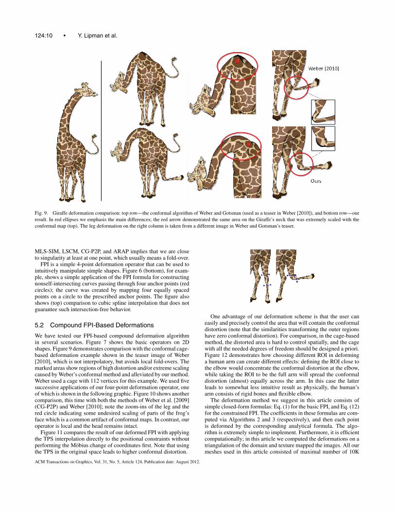
Fig. 9. Giraffe deformation comparison: top row—the conformal algorithm of Weber and Gotsman (used as a teaser in Weber [2010]), and bottom row—ourresult. In red ellipses we emphasis the main differences; the red arrow demonstrated the same area on the Giraffe’s neck that was extremely scaled with theconformal map (top). The leg deformation on the right column is taken from a different image in Weber and Gotsman’s teaser.

MLS-SIM, LSCM, CG-P2P, and ARAP implies that we are closeto singularity at least at one point, which usually means a fold-over.

FPI is a simple 4-point deformation operator that can be used tointuitively manipulate simple shapes. Figure 6 (bottom), for exam-ple, shows a simple application of the FPI formula for constructingnonself-intersecting curves passing through four anchor points (redcircles); the curve was created by mapping four equally spacedpoints on a circle to the prescribed anchor points. The figure alsoshows (top) comparison to cubic spline interpolation that does notguarantee such intersection-free behavior.

5.2 Compound FPI-Based Deformations

We have tested our FPI-based compound deformation algorithmin several scenarios. Figure 7 shows the basic operators on 2Dshapes. Figure 9 demonstrates comparison with the conformal cage-based deformation example shown in the teaser image of Weber[2010], which is not interpolatory, but avoids local fold-overs. Themarked areas show regions of high distortion and/or extreme scalingcaused by Weber’s conformal method and alleviated by our method.Weber used a cage with 112 vertices for this example. We used fivesuccessive applications of our four-point deformation operator, oneof which is shown in the following graphic. Figure 10 shows anothercomparison, this time with both the methods of Weber et al. [2009](CG-P2P) and Weber [2010]; note the zoom-ins of the leg and thered circle indicating some undesired scaling of parts of the frog’sface which is a common artifact of conformal maps. In contrast, ouroperator is local and the head remains intact.

Figure 11 compares the result of our deformed FPI with applyingthe TPS interpolation directly to the positional constraints withoutperforming the Mobius change of coordinates first. Note that usingthe TPS in the original space leads to higher conformal distortion.

One advantage of our deformation scheme is that the user caneasily and precisely control the area that will contain the conformaldistortion (note that the similarities transforming the outer regionshave zero conformal distortion). For comparison, in the cage-basedmethod, the distorted area is hard to control spatially, and the cagewith all the needed degrees of freedom should be designed a priori.Figure 12 demonstrates how choosing different ROI in deforminga human arm can create different effects: defining the ROI close tothe elbow would concentrate the conformal distortion at the elbow,while taking the ROI to be the full arm will spread the conformaldistortion (almost) equally across the arm. In this case the latterleads to somewhat less intuitive result as physically, the human’sarm consists of rigid bones and flexible elbow.

The deformation method we suggest in this article consists ofsimple closed-form formulas: Eq. (1) for the basic FPI, and Eq. (12)for the constrained FPI. The coefficients in these formulas are com-puted via Algorithms 2 and 3 (respectively), and then each pointis deformed by the corresponding analytical formula. The algo-rithm is extremely simple to implement. Furthermore, it is efficientcomputationally; in this article we computed the deformations on atriangulation of the domain and texture mapped the images. All ourmeshes used in this article consisted of maximal number of 10K



Fig. 10. Articulation of a frog. We compare to Weber10 [2010], andCG-P2P [Weber et al. 2009]. Note the zoom-ins of the frog’s right leg,and the red circle indicating undesired scaling in the two bottom examples.

Fig. 11. Comparison of deformation in a square ROI using the constrainedFPI (left column) versus TPS with the same edge constraints—Eq. (15)(right column).

Fig. 12. Controlling the locality of the deformation. Using different choicesof ROI the user can presciently determine where the conformal distortionin the deformation will be concentrated. We show an image of a human’shand (top-left), and two deformations (top-right, and bottom row). Note thatprescribing the FPI edges near the elbow concentrates the deformation’sdistortion in that area while taking edges farther from the elbow causes theconformal distortion to distribute along the entire arm.

vertices. The basic FPI scheme takes 0.001s to deform 1K verticeson 2.4 GHz processor. The constrained FPI requires additional TPScomputation over the basic FPI. In our implementation we used 40centers for the TPS and were required to solve a 40 × 40 linearsystem; for 1K vertices computing the deformation and applying ittakes 0.0016s on the same processor. Note that the overhead of theTPS is minor.

6. DISCUSSION, LIMITATIONSAND FUTURE WORK

We have presented a simple formula for 4-point planar warping thatspreads conformal distortion equally and has optimal worst-caseconformal distortion properties.

We have shown that the FPI can be used for building deformationoperators that are simple and can provide an alternative to previousplanar warping and interpolation methods. In particular the bene-fits over the more common cage-based techniques are: (1) the usercan define the deformed region on-the-fly, and does not need to



design an entire cage with enough degrees of freedom in a separatepreprocess stage, (2) the mapping comes with certain guarantees,(3) the algorithm is very simple, consisting of a formula that de-scribes the mapping, (4) the deformation is local; the user controlsprecisely the area to be deformed (this requirement is often raised byend-users), and (5) the FPI has 4 control points which we found veryintuitive to define deformations.

The method described in the article has some limitations. First, inour current implementation, the constrained deformation (Section 4)is described only for ROIs bounded by straight lines. However,generalizing this operator to consider ROIs bounded by any curveconnecting adjecent control points is trivial; there is nothing in ourconstruction that builds on the fact that the constrained edges arestraight. The second limitation is that the contrained deformationdoes not allow simultaneous control over adjacent edges of the ROI;the similarities defined on different edges of the ROI will not matchin general using our model, and therefore a more complicated modelshould be used to constrain the deformation outside the ROI whenedges being manipulated by the user share a point.

As for future work, we would be interested to find optimalquasiconformal mapping in different spaces than the periodicmappings. One interesting example is to consider the collectionof maps between the straight-edged quadrilateral that interpolatethe corners. Another example is the sphere. Also, finding provablyoptimal quasiconformal mapping with derivative constraints wouldbe interesting for our application; currently, we are using the FPIas our approximation for such an optimal map. Lastly, we wouldlike to develop a 4-point deformation application for touch screens(currently we have a standard PC implementation) as we believethat humans will find 4-points-based deformation intuitive anduseful (using two fingers out of each hand).

APPENDIX

Appendix A

In this appendix we provide the proof that the periodic map f ∈ Fthat bijectively takes one parallelogram P (η, ξ ) to another P (η, ξ )with lowest maximal conformal distortion is the affine map. Thisfact, although seeming natural, is not trivial to prove. The proofis contained within Ahlfors’ [2006] proof of a slightly differentproblem. We decided to adapt the proof to our setting for tworeasons: first, it has ideas that we believe can stimulate researchersto think about the type of problem discussed in this article in a moregeneral context, and second, the ideas are folded inside Ahlfors’arguments and are not easily accessible.

Since we can use the conformal map z → z/ξ to map (withoutintroducing conformal distortion) P (η, ξ ) to P (τ = η

ξ, 1), we will

only consider parallelograms of the form P (τ ) := P (τ, 1). Withoutloss of generality, we can assume Im (τ ) > 0. Given a differentiablemap between two periodic parallelograms (that interpolates the cor-ners) f : P (τ ) → P (τ ) we will measure its maximal conformaldistortion by Kf = maxz∈P (τ ) Df (z). We show that the map f ∈ Fthat minimizes Kf is the affine map taking τ → τ and fixing 1.

In Lemma A.1, we prove that any differentiable map f : P (τ ) →P (τ ) must satisfy

Kf ≥ Im (τ )

Im (τ ). (16)

Given this lemma we will show the result. We note that given any

a, b, c, d ∈ Z such that det(a bc d

) = 1 (unimodular matrix) the

periodic parallelogram P (aτ + b, cτ + d) is exactly equivalent toP (τ ) = P (τ, 1). It can be thought of as different parametrizationof the same object. Similarly, P (aτ + b, cτ + d) is equivalent toP (τ ). Note that f (aτ + b) = aτ + b, and f (cτ + d) = cτ + d ,and in general f satisfies f (z + k(aτ + b) + �(cτ + d)) = f (z) +k(aτ + b) + �(cτ + d).

Next, let us apply the (similarity) transform S1 : z → z/(cτ + d)to map P (aτ + b, cτ + d) to P ( aτ+b

cτ+d), and S2 : z → z/(cτ + d)

to map P (aτ + b, cτ + d) to P ( aτ+b

cτ+d). The map f = S2 ◦ f ◦ S−1

1

maps P ( aτ+b

cτ+d) to P ( aτ+b

cτ+d), and satisfies f (z + k aτ+b

cτ+d+ �) = f (z) +

k aτ+b

cτ+d+ �. Furthermore, DS2◦f ◦S−1

1(z) = Df (S−1

1 (z)) for all z ∈ C.Applying the lower bound (16) then implies

Kf = KS2◦f ◦S−11

≥ Im

(aτ + b

cτ + d

)/Im

(aτ + b

cτ + d

), (17)

for all a, b, c, d ∈ Z such that ad −bc = 1. To finish this argument,Ahlfors[2006] uses the following elegant geometrical observation:let m be a Mobius transformation taking the upper half-plane to theinterior of the unit disk such that m(τ ) = 0. Denote h(z) = az+b

cz+d,

where a, b, c, d ∈ Z, ad − bc = 1. From (17) we know that

Im (h(τ )) Kf ≥ Im (h(τ )) .

Denote the set C = {z | Im (z) > Im (h(τ )) Kf }. The precedingbound implies that m−1(τ ) is not inside the open circle m−1◦h−1(C).Furthermore, the shortest hyperbolic distance between h(τ ) and theclosure of C is dH (h(τ ), C) = dH (iIm (h(τ )) , iKf Im (h(τ ))) =log(Kf ). This is also the hyperbolic distance between the originand the circle m−1 ◦h−1(C) in the hyperbolic disk. The circle m−1 ◦h−1(C) is osculating to the boundary of the unit disk at the pointm−1 ◦ h−1(∞). Since we can always find unimodular h such thath−1(∞) is an arbitrary rational number, the circle C can osculateto a dense set of points on the boundary of the unit disk. Sincem−1(τ ) cannot be inside any of these circles the hyperbolic distanceof m−1(τ ) to the origin should be less or equal to the distance of anysuch circle to the origin which we already computed to be log(Kf ).We conclude that

dH (τ, τ ) ≤ log(Kf ).

Let us show that the affine map f : P (τ ) → P (τ ) defined by

f (z) = (τ − τ ) z + (τ − τ ) z

τ − τ

has Kf = edH (τ,τ ). Indeed,

Kf = Df = |fz| + |fz||fz| − |fz| = |τ − τ | + |τ − τ |

|τ − τ | − |τ − τ | = edH (τ ,τ ).

LEMMA A.1. Let f : P (τ ) → P (τ ) be a differentiable map.Then,

Kf ≥ Im (τ )

Im (τ ).

Although is possible to prove this lower bound with extremal lengthmethod, we will use a more direct technique due to Grotzch. Givena parallelogram P (τ ) we parameterize it over the unit square byz = sτ + t , 0 ≤ s, t ≤ 1. Then the change of variable formulaimplies∫∫

P (τ )φ(z)dx dy = Im (τ )

∫ 1

0

∫ 1

0φ(sτ + t)ds ts, (18)



for any integrable φ. Next, fix s and consider the curve γs(t) =sτ + t , 0 ≤ t ≤ 1. We have

1 ≤ length(f (γs)) =∫ 1

0|fz(γs(t)) + fz(γs(t)| dt ≤

∫ 1

0|fz|+ |fz| dt.

Integrating both sides with respect to to s ∈ [0, 1], multiplying bothsides by Im (τ ) and using (18) we get Im (τ ) ≤∫∫

P (τ )|fz| + |fz| dx dy =

∫∫P (τ )

|fz| + |fz|√|fz|2 − |fz|2

√Jf dx dy,

where in the last equality we multiplied and divided by the square-root of the jacobian Jf of f . Using Cauchy-Schwarz∫∫

P (τ )

|fz| + |fz|√|fz|2 − |fz|2

√Jf ≤

[∫∫P (τ )

|fz| + |fz||fz| − |fz|

] 12[∫∫

P (τ )Jf

] 12

,

squaring both sides and using previous inequality we get

Im (τ )2 ≤[∫∫

P (τ )Df

]Im (τ ) ≤ Kf Im (τ ) Im (τ )

and rearranging the terms proves the lemma.

ACKNOWLEDGMENTS

We would like to thank Ofir Weber for supplying the imagesof Figures 9,10, and Mirela Ben-Chen for the CG-P2P result inFigure 8.

REFERENCES

AHLFORS, L. 1966. Complex Analysis.AHLFORS, L. V. 2006. Lectures on Quasiconformal Mappings. University

Lecture Series, vol. 38.BOOKSTEIN, F. L. 1989. Principal warps: Thin-Plate splines and the decom-

position of deformations. IEEE Trans. Pattern Anal. Mach. Intell. 11,567–585.

DESBRUN, M., MEYER, M., AND ALLIEZ, P. 2002. Intrinsic parameterizationsof surface meshes. Comput. Graph. Forum 21.

FLETCHER, A. AND MARKOVIC, V. 2007. Quasiconformal Maps and Te-ichmuller Theory. Oxford Graduate Texts in Mathematics, OxfordUniversity Press.

FLOATER, M. S. 2003. Mean value coordinates. Comput. Aid. Geom. Des. 20,19–27.

IGARASHI, T., MOSCOVICH, T., AND HUGHES, F. J. 2005. As-Rigid-as-Possibleshape manipulation. ACM Trans. Graph 24, 1134–1141.

JU, T., SCHAEFER, S., AND WARREN, J. 2005. Mean value coordinates forclosed triangular meshes. ACM Trans. Graph. 24, 561–566.

LEVY, B., PETITJEAN, S., RAY, N., AND MAILLO T, J. 2002. Least squaresconformal maps for automatic texture atlas generation. In Proceedings ofACM SIGGRAPH Conference, ACM, New York.

LIPMAN, Y., LEVIN, D., AND COHEN-OR, D. 2008. Green coordinates. ACMTrans. Graph. 27, 3.

SCHAEFER, S., MCPHAIL, T., AND WARREN, J. 2006. Image deformation usingmoving least squares. ACM Trans. Graph. 25, 533–540.

SEDERBERG, T. AND PARRY, S. 1986. Free-Form deformation of solid geo-metric models. SIGGRAPH Comput. Graph. 20, 151–160.

WEBER, O., G. C. 2010. Controllable conformal maps for shape deformationand interpolation. ACM Trans. Graph. 29, 78:1–78:11.

WEBER, O., BEN-CHEN, M., AND GOTSMAN, C. 2009. Complex barycen-tric coordinates with applications to planar shape deformation. Comput.Graph. Forum 28.

WENDLAND, H. 2005. Scattered Data Approximation. Cambridge Mono-graphs on Applied and Computational Mathematics, No. 17.

ZENG, W. AND GU, X. D. 2011. Registration for 3d surfaces with largedeformations using quasi-conformal curvature flow. In Proceedings of theIEEE Conference on Computer Vision and Pattern Recognition (CVPR).2457–2464.

ZENG, W., LUO, F., YAU, S. T., AND GU, X. D. 2009. Surface quasi-conformalmapping by solving beltrami equations. In Proceedings of the 13th IMA In-ternational Conference on Mathematics of Surfaces XIII. Springer, Berlin.391–408.

ZENG, W., MARINO, J., CHAITANYA GURIJALA, K., GU, X., AND KAUFMAN,A. 2010. Supine and prone colon registration using quasi-conformalmapping. IEEE Trans. Vis. Comput. Graph. 16, 6, 1348–1357.

Received July 2011; revised October 2011, January 2012; accepted February 2012


simple formulas for quasiconformal plane deformations

Documents