simple and accurate algorithms
TRANSCRIPT
H. C. So Page 1 Semester A 2021/22
Perceptron
Chapter Intended Learning Outcomes: (i) Understand perceptron and its properties (ii) Study linear model for classification and its relation with
least squares, maximum likelihood estimation, and maximum a posteriori estimation
(iii) Study iterative methods and their properties as well as
application in classification
(iv) Understand least-mean-square algorithm and its relation with perceptron
H. C. So Page 2 Semester A 2021/22
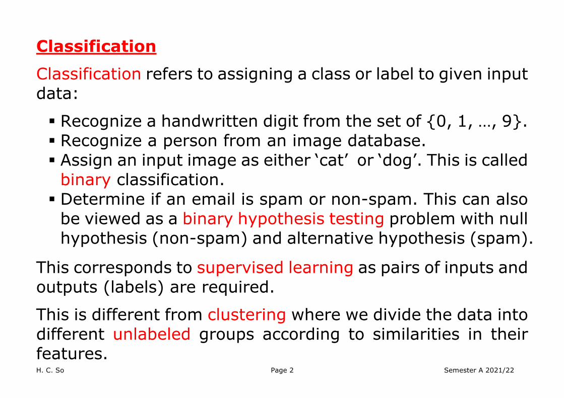
Classification
Classification refers to assigning a class or label to given input data:
Recognize a handwritten digit from the set of {0, 1, …, 9}. Recognize a person from an image database. Assign an input image as either ‘cat’ or ‘dog’. This is called
binary classification. Determine if an email is spam or non-spam. This can also
be viewed as a binary hypothesis testing problem with null hypothesis (non-spam) and alternative hypothesis (spam).
This corresponds to supervised learning as pairs of inputs and outputs (labels) are required.
This is different from clustering where we divide the data into different unlabeled groups according to similarities in their features.

H. C. So Page 3 Semester A 2021/22
Brief Historical Development of Perceptron
McCulloch and Pitts proposed the first artificial neuron in 1940s as computing machine, e.g.:
Input:
Output:

H. C. So Page 4 Semester A 2021/22
Rosenblatt’s perceptron generalized McCulloch-Pitts in 1950s which was the first supervised learning model.
Now the inputs are not restricted to be 0 or 1, but can be any real values, together with a bias term:
Perceptron which is a single artificial neuron, is able to perform the task of classifying 2 classes if they are linearly separable, i.e., they lie on the opposite sides of a hyperplane.

H. C. So Page 5 Semester A 2021/22
Properties and Algorithms for Perceptron
To perform classification, we need to determine and using a set of training data of input-output pairs.
Given an input vector to be classified, we first compute the linear combination:
(1)
then apply the activation function which is a sign function:
(2)
That is, if is positive, it corresponds to one class while it belongs to the other class if is negative.

H. C. So Page 6 Semester A 2021/22
Hence the hyperplane, which is a subspace of one dimension less than its ambient space, is the decision boundary:
(3)
For 2-D input point , hyperplane is a line:
Linearly separable Non-linearly separable

H. C. So Page 7 Semester A 2021/22
We can see that the bias provides a shift to the hyperplane, e.g., for 2-D case, moves the straight line up or down

H. C. So Page 8 Semester A 2021/22
Geometrically, is perpendicular to the hyperplane. If we consider , the hyperplane must pass through the origin as .
H. C. So Page 9 Semester A 2021/22
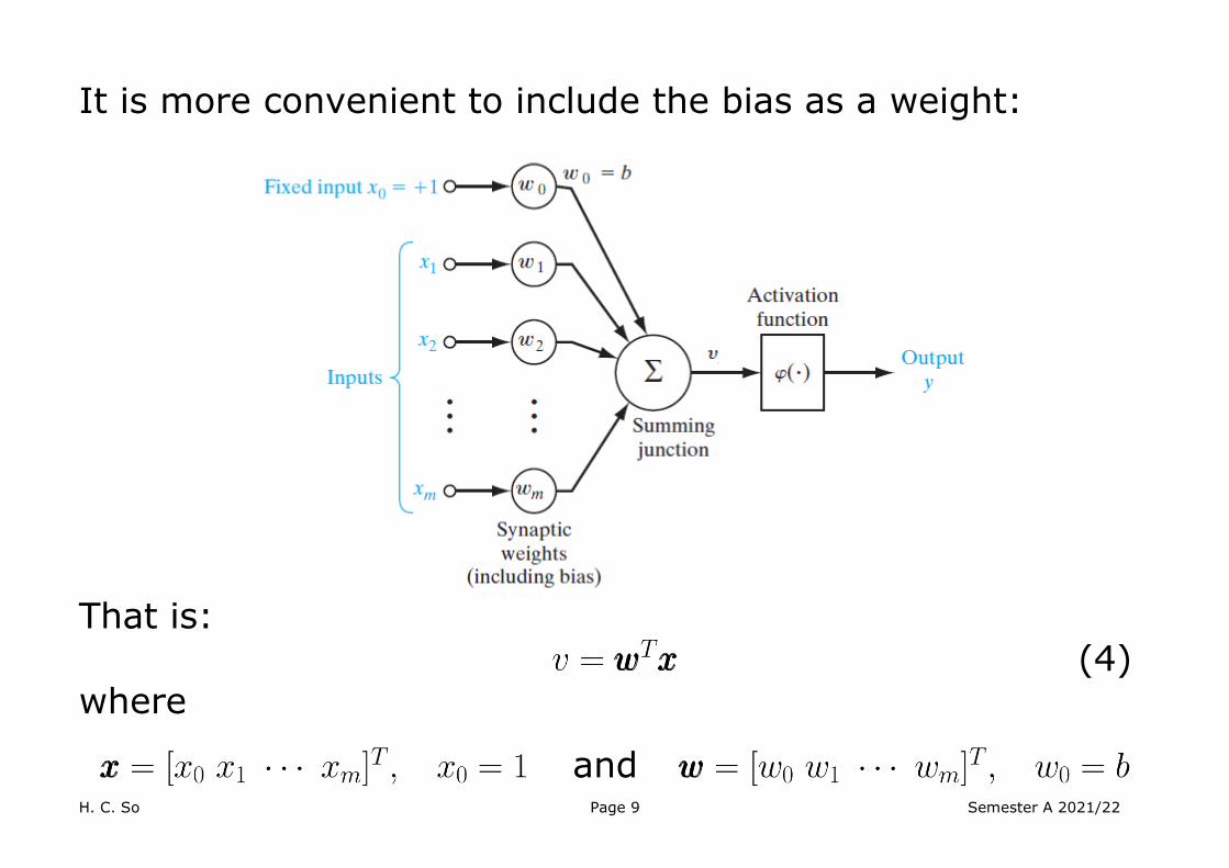
It is more convenient to include the bias as a weight:
That is:
(4) where
and

H. C. So Page 10 Semester A 2021/22
With the addition of extra dimension of , now the hyperplane must pass through the origin, e.g.,

H. C. So Page 11 Semester A 2021/22
Given a set of training vectors , , with known labels, say, Classes ( ) and ( ), the basic idea to update is:
If the th input is correctly classified by the weight vector at the th iteration , no update for in next iteration:
if and belongs to or if and belongs to .
Otherwise, we update in next iteration:
if and belongs to :
if and belongs to :
Here, is the learning rate parameter which controls the adjustment at each iteration, and can be function of .

H. C. So Page 12 Semester A 2021/22
Geometric intuition when an update is needed with :
Initializing , we use in a cyclic manner, i.e.,
to update until all training samples are correctly classified. When a complete set of goes through the algorithm, we refer it to as an epoch.
H. C. So Page 13 Semester A 2021/22
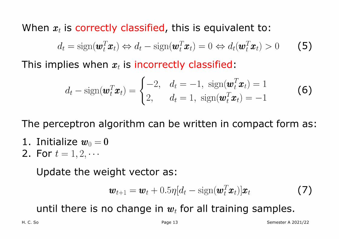
When is correctly classified, this is equivalent to:
(5)
This implies when is incorrectly classified:
(6)
The perceptron algorithm can be written in compact form as:
1. Initialize 2. For
Update the weight vector as:
(7)
until there is no change in for all training samples.

H. C. So Page 14 Semester A 2021/22
As long as the two classes are linearly separable, must converge after finite number of iterations.
Note that the algorithm can also be implemented in different forms, e.g., updating if .
Can perceptron realize OR function? How about AND function? And how about XOR function? Why? Is the hyperplane in perceptron unique?
H. C. So Page 15 Semester A 2021/22
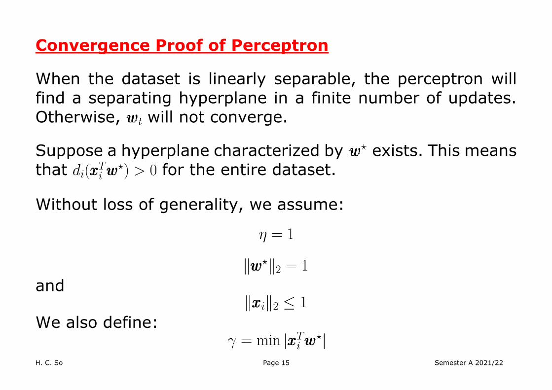
Convergence Proof of Perceptron When the dataset is linearly separable, the perceptron will find a separating hyperplane in a finite number of updates. Otherwise, will not converge. Suppose a hyperplane characterized by exists. This means that for the entire dataset. Without loss of generality, we assume:
and
We also define:

H. C. So Page 16 Semester A 2021/22
Under the above settings, the perceptron algorithm makes at most mistakes.

H. C. So Page 17 Semester A 2021/22
Proof:
To ease the presentation, all subscripts are removed.
Recall
When an update is needed, i.e., , we know .
Now we consider this effect on two terms: and .
For , the effect is:
because
This means that for each update, grows by at least .

H. C. So Page 18 Semester A 2021/22
For , the effect is:
because , ,
This means that for each update, grows by at most 1. Hence after certain number of updates, say, , the following two inequalities must hold:
(8)
(9) With the use of (8)-(9), we complete the proof as follows:
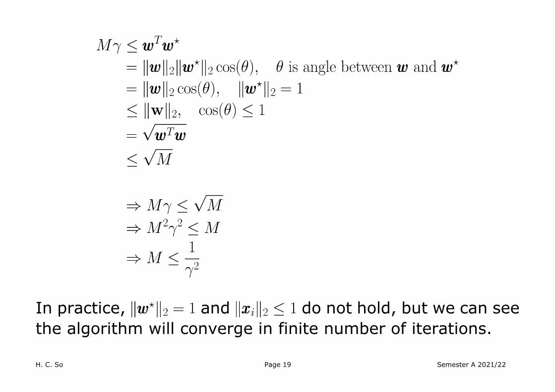
H. C. So Page 19 Semester A 2021/22
In practice, and do not hold, but we can see the algorithm will converge in finite number of iterations.

H. C. So Page 20 Semester A 2021/22
A Python code “perceptron” is provided and you can alter parameters including training sample number and learning rate, and choose visualizing per iteration or epoch:

H. C. So Page 21 Semester A 2021/22
Perceptron can perform AND operator. Training data are: X=np.array([[1,1],[1,-1],[-1,1],[-1, -1]]) y=np.array([1,-1,-1,-1])

H. C. So Page 22 Semester A 2021/22
Perceptron can classify flowers.
“Iris” a well-known dataset in the pattern recognition literature, which contains samples of 3 iris classes, Setosa, Versicolour and Virginica.
Source: IRIS Flower Prediction Using Machine Learning Algorithms (machinelearningsol.com) We just use two linearly separable classes Setosa and Versicolour, and two features, namely, sepal length and petal length, as input training data. UCI Machine Learning Repository: Iris Data Set
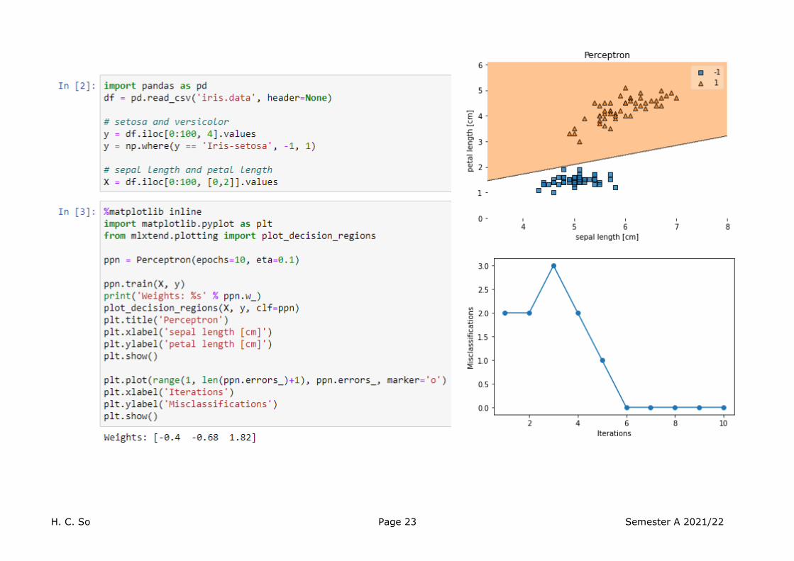
H. C. So Page 23 Semester A 2021/22

H. C. So Page 24 Semester A 2021/22
For XOR, weights cannot converge.
H. C. So Page 25 Semester A 2021/22
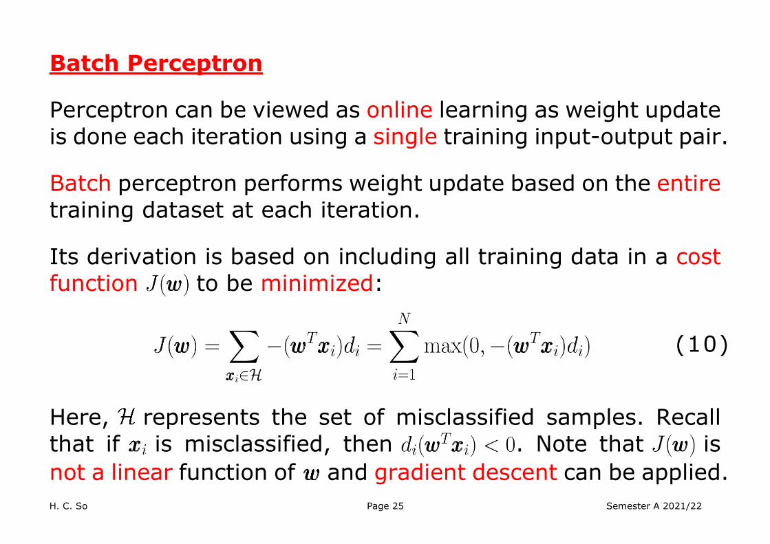
Batch Perceptron Perceptron can be viewed as online learning as weight update is done each iteration using a single training input-output pair. Batch perceptron performs weight update based on the entire training dataset at each iteration. Its derivation is based on including all training data in a cost function to be minimized:
(10)
Here, represents the set of misclassified samples. Recall that if is misclassified, then . Note that is not a linear function of and gradient descent can be applied.

H. C. So Page 26 Semester A 2021/22
What is the minimum value of ? The gradient is simply:
(11)
The gradient descent algorithm is then:
(12)
Note that the misclassified samples change during each iteration. Upon convergence, . Under what condition convergence is guaranteed?

H. C. So Page 27 Semester A 2021/22
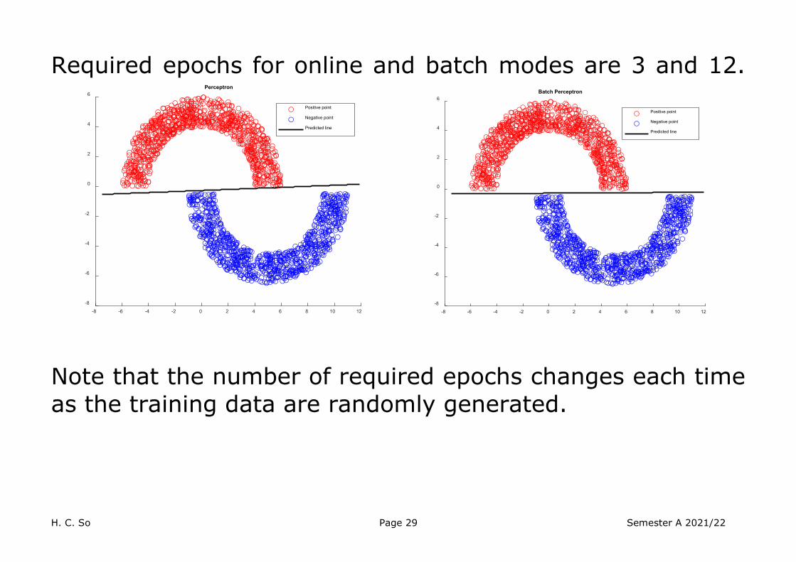
A MATLAB example for classifying data in 2 “moons” is also provided, where moon radius , moon width , separation between 2 moons , number of training data, can be adjusted.

H. C. So Page 28 Semester A 2021/22
Try Demo.m
H. C. So Page 29 Semester A 2021/22
Required epochs for online and batch modes are 3 and 12.
Note that the number of required epochs changes each time as the training data are randomly generated.
-8 -6 -4 -2 0 2 4 6 8 10 12
-8
-6
-4
-2
0
2
4
6Perceptron
Positive point
Negative point
Predicted line
-8 -6 -4 -2 0 2 4 6 8 10 12
-8
-6
-4
-2
0
2
4
6Batch Perceptron
Positive point
Negative point
Predicted line

H. C. So Page 30 Semester A 2021/22
Try N=100: Required epochs for online and batch modes are 6 and 5.
We see that both standard and batch perceptrons work properly although their decision boundaries are different. From the results, it is difficult to tell which scheme involves smaller number of iterations/epochs.
-8 -6 -4 -2 0 2 4 6 8 10 12
-8
-6
-4
-2
0
2
4
6Perceptron
Positive point
Negative point
Predicted line
-8 -6 -4 -2 0 2 4 6 8 10 12
-8
-6
-4
-2
0
2
4
6Batch Perceptron
Positive point
Negative point
Predicted line

H. C. So Page 31 Semester A 2021/22
When , the 2 classes are not linearly separable. The weights will not converge, and the boundary is changing.

H. C. So Page 32 Semester A 2021/22
Linear Model for Classification
This approach basically corresponds to a linear neuron, and there are no nonlinear operations in weight update.
From (5)-(7), error function is nonlinear:
Error function is linear:
Source: What is the difference between a Perceptron, Adaline, and neural network model? (sebastianraschka.com)
H. C. So Page 33 Semester A 2021/22
Following (4), we model the training input and output as:
(13) where
and This is also called linear regression model where is known as regressor, while is called parameter vector. As will not be exactly zero even for correct classification, accounts for this difference. We first apply the probability viewpoints based on Bayes’ rule to find . The basic setup is that (ignore the first element), and are considered as random variables, with , i.e., and are independent.
H. C. So Page 34 Semester A 2021/22
Batch Mode Solutions for Linear Model We first investigate the joint probability distribution function (PDF) of and conditional on , denoted by .
Applying Bayes’ rule and independence of and :
We get:
(14)
is called observation density or likelihood function. is called prior, i.e., it is our prior knowledge
about before observing . is called the posterior density is the conditional
PDF after observing . is called evidence.

H. C. So Page 35 Semester A 2021/22
The maximum likelihood (ML) estimate of is:
(15)
The maximum a posteriori (MAP) estimate of is:
(16)
We also see that:
(17) and is not required in the calculation. Suppose there are pairs of training samples :
(18)

H. C. So Page 36 Semester A 2021/22
A zero-mean Gaussian environment is considered with:
Assumption 1 Independence and identical distribution: The training data are independent and identically distributed (IID).
Assumption 2 Gaussianity: All are IID zero-mean Gaussian distributed with variance , i.e., , and the PDF is:
(19)
Assumption 3 Stationarity: Among this set of , is fixed. We further assume that all elements in are IID and zero-mean Gaussian distributed, i.e., :
(20)

H. C. So Page 37 Semester A 2021/22
For a given and fixed , is characterized by :
(21)
Together with the IID Assumption 1, we obtain:
(22)
Similarly, from Assumption 3:
(23)

H. C. So Page 38 Semester A 2021/22
To obtain the ML solution, we see that maximizing (22) is equivalent to minimizing the least squares (LS):
which can be compactly expressed as:
(24)
by defining
and
That is, the ML solution is the same as the LS solution:
(25)

H. C. So Page 39 Semester A 2021/22
Is the ML solution always equal to the LS solution?
According to (17), the MAP solution maximizes:
which is equivalent to minimizing regularized LS (RLS):
(26)
where is known as regularization parameter. Differentiating (26) w.r.t. and then setting the resultant expression to , we get:
(27)

H. C. So Page 40 Semester A 2021/22
Which solution is better? ML or MAP? Why? Consider a limiting case of such that , i.e., we have no prior information about . This results in which is the same as the ML or LS solution. On the other hand, the smaller the , the larger the , indicating that the second component increases its importance in the RLS cost function. Since we may not have the prior information of and even the probability distributions of the training data, only the performance of the LS solution is examined further.

H. C. So Page 41 Semester A 2021/22
Even 2 iris classes are not linearly separable, LS provides a reasonable boundary:

H. C. So Page 42 Semester A 2021/22
>>LM_w = LM(X,Y);
-8 -6 -4 -2 0 2 4 6 8 10 12
-8
-6
-4
-2
0
2
4
6LS
Positive point
Negative point
Predicted line

H. C. So Page 43 Semester A 2021/22
-15 -10 -5 0 5 10 15 20 25
-10
-5
0
5
10
15LS
Positive point
Negative point
Predicted line

H. C. So Page 44 Semester A 2021/22
Comparing the perceptron and LS solution, we may conclude: Both algorithms construct linear and distinct decision
boundaries. Even for the linearly separable scenario, the LS solution
cannot achieve classification error of 0 while the perceptron approach will provide perfect classification in this case.
The LS solution provides the solution in one step for both
linearly and non-linearly separable scenarios, and thus there is no convergence problem as in the perceptron applied in the non-linearly separable case.

H. C. So Page 45 Semester A 2021/22
Iterative Solutions for Linear Model
Minimization of the ML/LS cost function can also be achieved using iterative techniques such as Newton’s method and gradient descent:
(28) and
(29) The gradient vector of (24) is:
(30) Differentiating (30) once w.r.t. yields the Hessian matrix:
(31)
H. C. So Page 46 Semester A 2021/22
Using (30)-(31), the adjustment term in (28) is:
To obtain better insight and ease the convergence proof, we introduce a step size in (28):
or
(32)
…
H. C. So Page 47 Semester A 2021/22
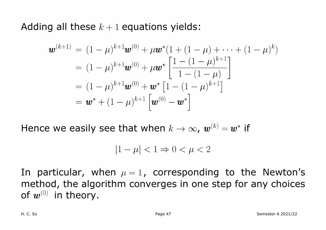
Adding all these equations yields:
Hence we easily see that when , if
In particular, when , corresponding to the Newton’s method, the algorithm converges in one step for any choices of in theory.

H. C. So Page 48 Semester A 2021/22
An example of the contour of using the Newton’s method with and 2 weights is illustrated below.
H. C. So Page 49 Semester A 2021/22
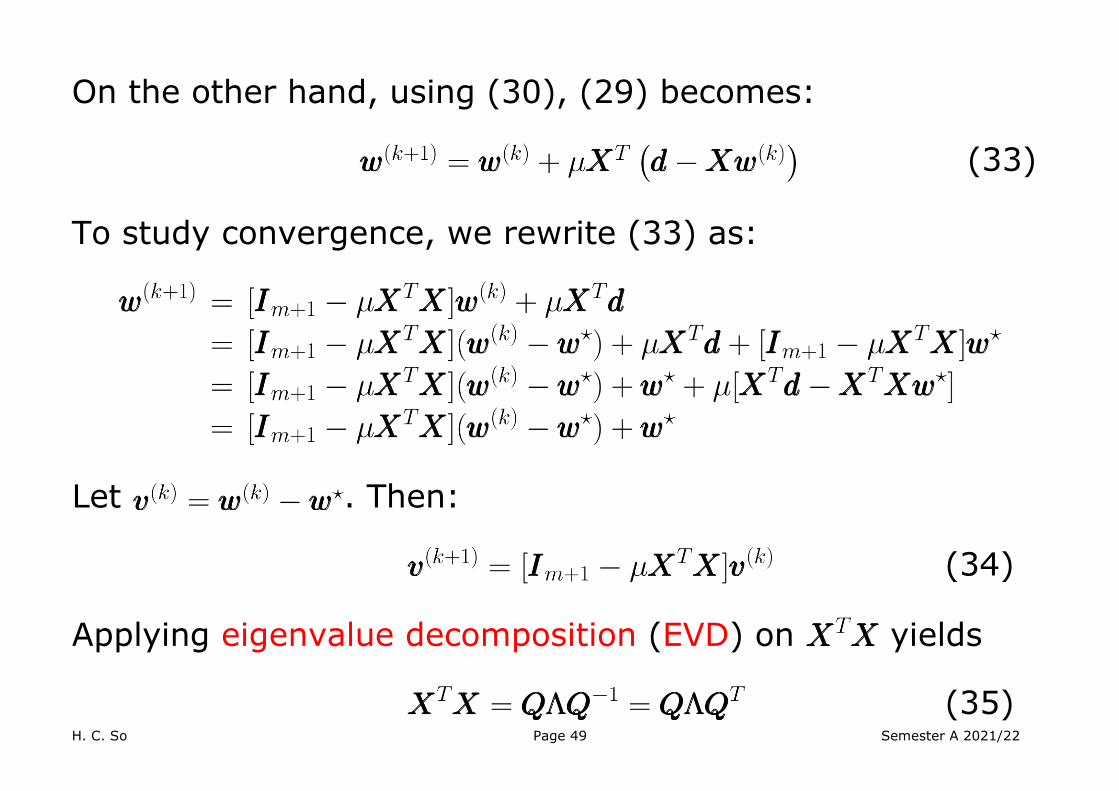
On the other hand, using (30), (29) becomes:
(33) To study convergence, we rewrite (33) as:
Let . Then:
(34) Applying eigenvalue decomposition (EVD) on yields
(35)
H. C. So Page 50 Semester A 2021/22
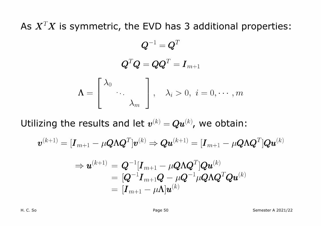
As is symmetric, the EVD has 3 additional properties:
Utilizing the results and let , we obtain:

H. C. So Page 51 Semester A 2021/22
The solution is:
We expect:
The convergence requirement is then:
or

H. C. So Page 52 Semester A 2021/22
Denote the maximum eigenvalue as , the algorithm converges if
That is, the convergence condition is governed by the largest eigenvalue of . Since may not be available, in practice a sufficiently small value of is chosen, and the steepest descent algorithm converges in multiple steps for any choices of . It is clear that for a larger , approaches 0 faster, indicating faster convergence. Nevertheless, the overall convergence is hindered by where denotes the minimum eigenvalue.

H. C. So Page 53 Semester A 2021/22
An example of the contour of using the steepest descent with 2 weights is illustrated below.

H. C. So Page 54 Semester A 2021/22
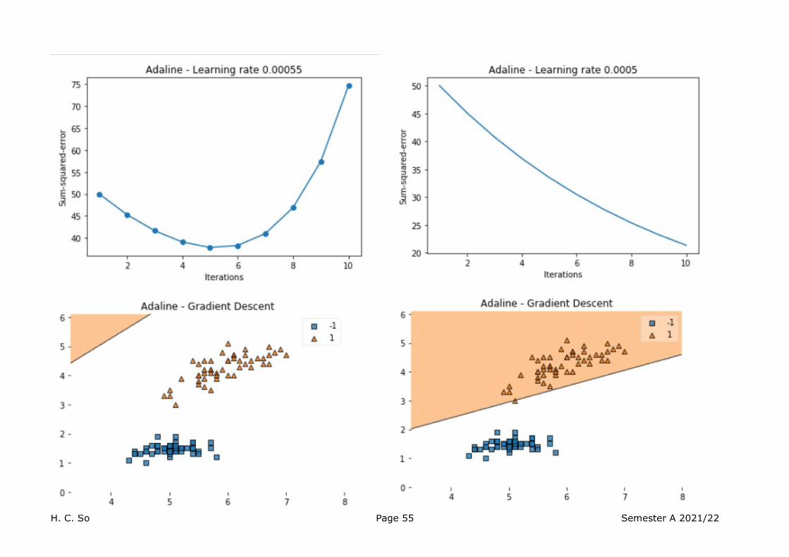
We examine the sum of squared error of (24) versus number of iterations for different values of .
H. C. So Page 55 Semester A 2021/22

H. C. So Page 56 Semester A 2021/22
Feature Standardization The convergence rate depends on the eigenvalue spread, defined as:
(36)
The fastest rate is attained when , or all eigenvalues are identical. In theory, we can transform to
such that , but it is a difficult task.
One simple way which can often increase the convergence rate is to shift and scale each feature:
(37)
where and are mean and standard deviation of the th feature. In doing so, all modified features have zero mean and unit variance.
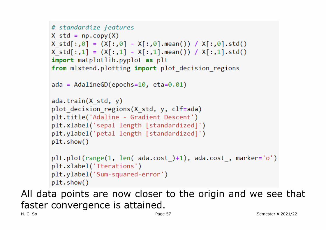
H. C. So Page 57 Semester A 2021/22
All data points are now closer to the origin and we see that faster convergence is attained.

H. C. So Page 58 Semester A 2021/22

H. C. So Page 59 Semester A 2021/22
Online Mode Solution for Linear Model
In the previously discussed iterative techniques, we minimize the LS cost function in each step:
(38)
Instead we can minimize only one of the squared terms in each step, and only one training sample pair is involved:
(39)
That is to say, it just removes the sign operator in the perceptron algorithm of (7):
(40)

H. C. So Page 60 Semester A 2021/22
Using the current notation, this online algorithm is summarized as:
1. Initialize 2. For ( )
Update the weight vector as:
(41)
until converges.
It can be proved that upon convergence, which is the LS solution.
This iterative rule which updates one sample at each iteration, is also referred to as ADALINE (adaptive linear, adaptive linear element, or adaptive linear neuron), Widrow-Hoff delta rule, and least-mean-square (LMS) algorithm.

H. C. So Page 61 Semester A 2021/22
-8 -6 -4 -2 0 2 4 6 8 10 12
-8
-6
-4
-2
0
2
4
6LMS
Positive point
Negative point
Predicted line

H. C. So Page 62 Semester A 2021/22
0 0.2 0.4 0.6 0.8 1 1.2 1.4 1.6 1.8 2
Epoch 10 4
0
0.5
1
1.5
2
2.5
3
3.5
Loss
H. C. So Page 63 Semester A 2021/22
0 0.2 0.4 0.6 0.8 1 1.2 1.4 1.6 1.8 2
Epoch 10 4
-0.6
-0.4
-0.2
0
0.2
0.4
0.6
0.8
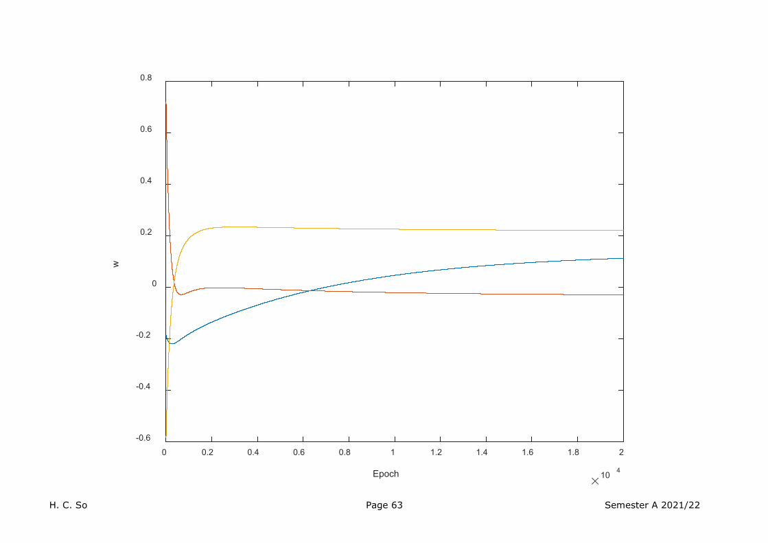
w

H. C. So Page 64 Semester A 2021/22
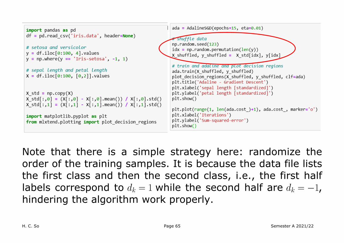
We also repeat the iris classification problem with feature standardization using the LMS algorithm.
H. C. So Page 65 Semester A 2021/22
Note that there is a simple strategy here: randomize the order of the training samples. It is because the data file lists the first class and then the second class, i.e., the first half labels correspond to while the second half are , hindering the algorithm work properly.

H. C. So Page 66 Semester A 2021/22
Least-Mean-Square Algorithm LMS algorithm was invented by Widrow and Hoff, and the corresponding work was published in 1960:
Widrow has been a professor at Standard University. His research focuses on adaptive signal processing, adaptive control systems, adaptive neural networks, human memory, and human-like memory for computers.
Hoff was Widrow’s Ph.D. student. Nevertheless, he is best known as the architect of the first microprocessor – Intel’s 4004 released in 1971.
To clearly present the LMS algorithm, we consider the setting of time-series training data , is the time index, and at time , no future data at , are available, while
is not restricted to be .

H. C. So Page 67 Semester A 2021/22
We use the probabilistic model as in (13):
(42) where
Here, , and are random while is the constant vector to be determined. Considering that is the error term, we can construct the mean square error (MSE) cost function :
(43)
Expanding (43) yields:
H. C. So Page 68 Semester A 2021/22
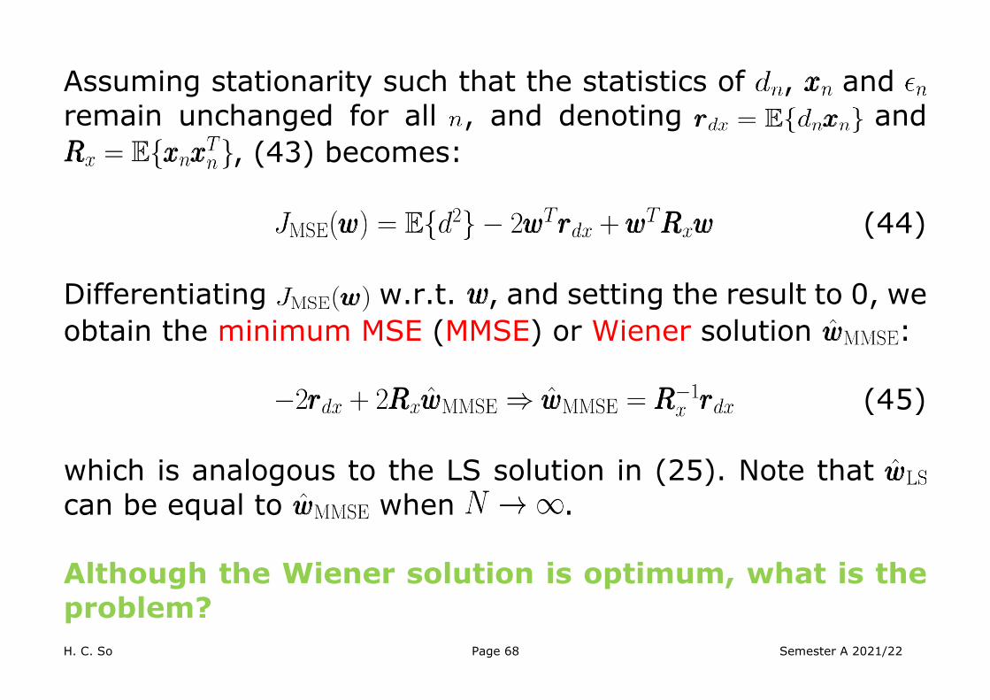
Assuming stationarity such that the statistics of , and remain unchanged for all , and denoting and
, (43) becomes:
(44) Differentiating w.r.t. , and setting the result to 0, we obtain the minimum MSE (MMSE) or Wiener solution :
(45) which is analogous to the LS solution in (25). Note that can be equal to when . Although the Wiener solution is optimum, what is the problem?
H. C. So Page 69 Semester A 2021/22
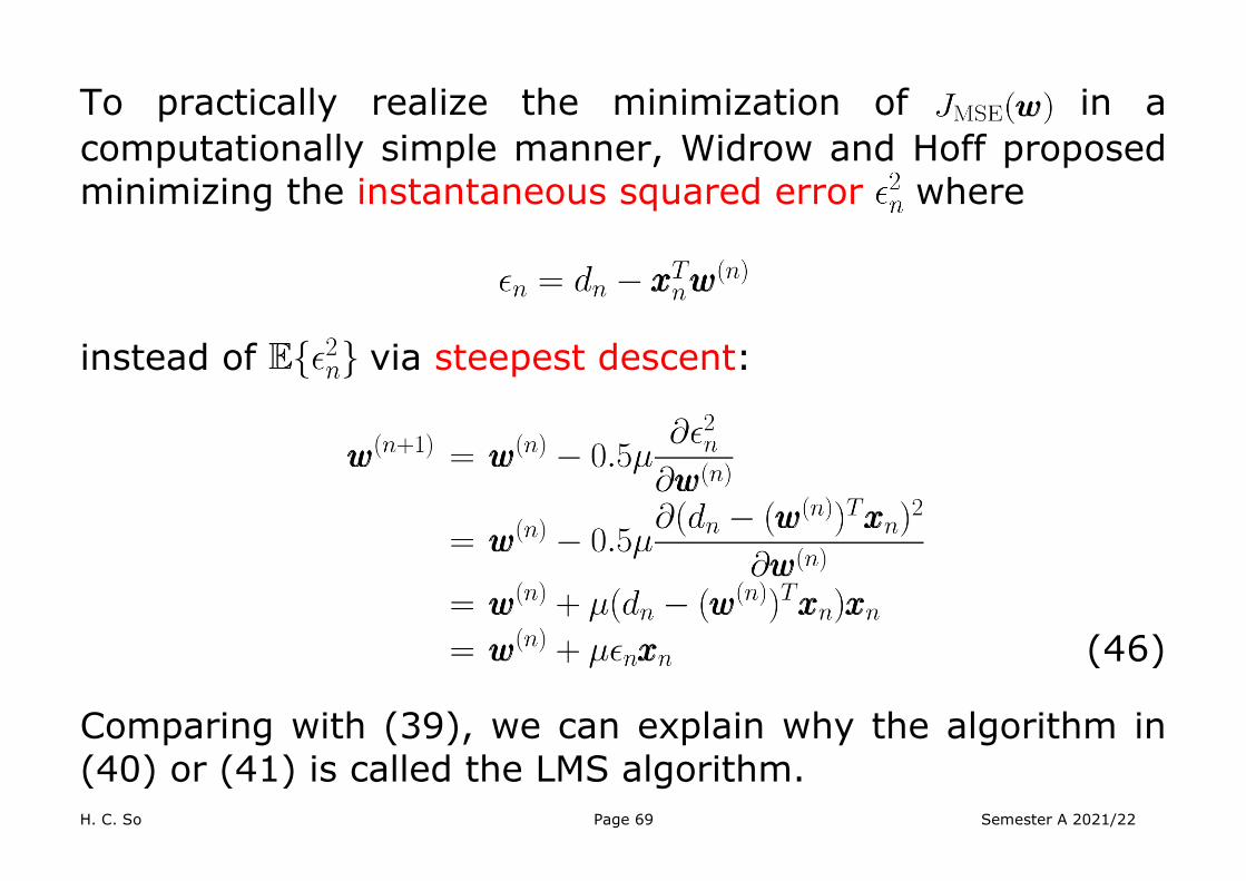
To practically realize the minimization of in a computationally simple manner, Widrow and Hoff proposed minimizing the instantaneous squared error where
instead of via steepest descent:
(46)
Comparing with (39), we can explain why the algorithm in (40) or (41) is called the LMS algorithm.

H. C. So Page 70 Semester A 2021/22
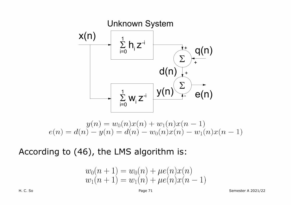
We use a system identification example to illustrate the applicability of (46).
Consider a linear time-invariant system with input and impulse response , the system output is:
where denotes the convolution operator. For a simple finite impulse response system, say, , then:
In the presence of noise , the output is modelled as:
Given the time sequences of and , we want to find using .
H. C. So Page 71 Semester A 2021/22
Σ h zi=0
1
i-i
Σ w zi=0
1
i-i
Σ
x(n)
d(n)
y(n) e(n)
+
-
Unknown System
Σq(n)+
+
According to (46), the LMS algorithm is:

H. C. So Page 72 Semester A 2021/22
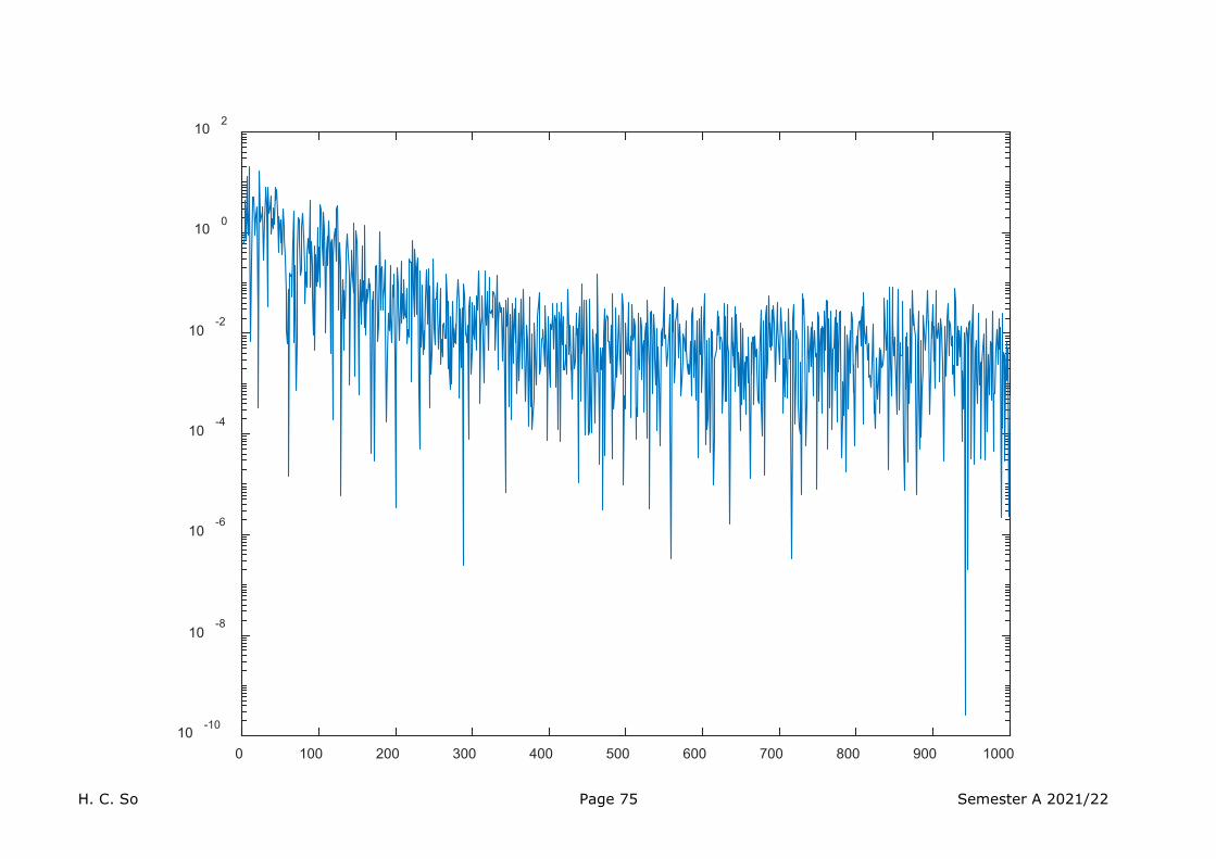
Here, we use zero-mean Gaussian IID and for data generation. Then we have:

H. C. So Page 73 Semester A 2021/22

H. C. So Page 74 Semester A 2021/22
100 200 300 400 500 600 700 800 900 10000
0.5
1
single run
expected
100 200 300 400 500 600 700 800 900 10000
0.5
1
1.5
2
single run
expected
H. C. So Page 75 Semester A 2021/22
0 100 200 300 400 500 600 700 800 900 100010 -10
10-8
10-6
10-4
10-2
10 0
10 2
H. C. So Page 76 Semester A 2021/22
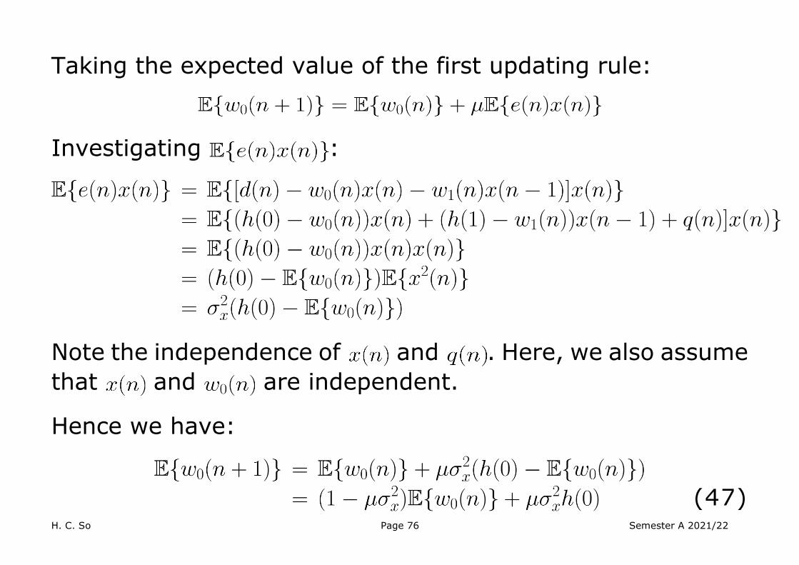
Taking the expected value of the first updating rule:
Investigating :
Note the independence of and . Here, we also assume that and are independent.
Hence we have:
(47)
H. C. So Page 77 Semester A 2021/22
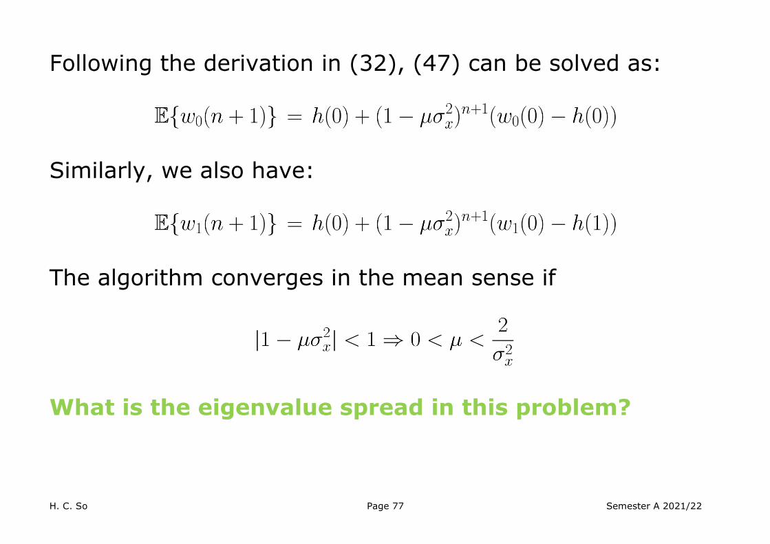
Following the derivation in (32), (47) can be solved as:
Similarly, we also have:
The algorithm converges in the mean sense if
What is the eigenvalue spread in this problem?

H. C. So Page 78 Semester A 2021/22
References:
1. S. Haykin, Neural Networks and Learning Machines, Prentice Hall, 2009
2. https://www.cs.sjsu.edu/~stamp/RUA/ann.pdf 3. https://www.cs.cornell.edu/courses/cs4780/2018fa/lec
tures/lecturenote03.html 4. B. Widrow and S. D. Stearns, Adaptive Signal Processing,
Prentice-Hall, 1985 5. B. Widrow and M. E. Hoff, “Adaptive switching circuits,”
Proceedings of IRE WESCON Convention Record, 1960, pp. 96-104.
6. https://engineering.stanford.edu/news/ted-hoff-birth-microprocessor-and-beyond