simple and fast algorithms for interactive machine

Journal of Machine Learning Research 22 (2021) 1-30 Submitted 5/19; Revised 10/20; Published 1/21

Simple and Fast Algorithms for Interactive MachineLearning with Random Counter-examples

Jagdeep Singh Bhatia [email protected]

Massachusetts Institute of Technology

Cambridge, MA 02139

Editor: Manfred Warmuth

Abstract

This work describes simple and efficient algorithms for interactively learning non-binaryconcepts in the learning from random counter-examples (LRC) model. Here, learning takesplace from random counter-examples that the learner receives in response to their properequivalence queries, and the learning time is the number of counter-examples needed bythe learner to identify the target concept. Such learning is particularly suited for onlineranking, classification, clustering, etc., where machine learning models must be used beforethey are fully trained.

We provide two simple LRC algorithms, deterministic and randomized, for exactlylearning concepts from any concept class H. We show that both these algorithms havean O(log |H|) asymptotically optimal average learning time. This solves an open problemon the existence of an efficient LRC randomized algorithm while also simplifying previousresults and improving their computational efficiency. We also show that the expected

learning time of any Arbitrary LRC algorithm can be upper bounded by O( 1ε log |H|

δ ),where ε and δ are the allowed learning error and failure probability respectively. Thisshows that LRC interactive learning is at least as efficient as non-interactive ProbablyApproximately Correct (PAC) learning. Our simulations also show that these algorithmsoutperform their theoretical bounds.

Keywords: interactive learning, active learning, online learning, PAC learning, algo-rithms, learning theory

1. Introduction

Machine learning has made great advances in fields such as image recognition and naturallanguage processing. However, it currently requires large sets of training data upfront.This is a problem because often the amount of data available is small or sometimes machinelearning models must be used before they are fully trained. In these cases, interactivelearning, which involves training machine learning models through interaction between alearner and a teacher can be very beneficial. For example, in personalized learning with one-on-one interaction, teachers are better able to assess their students’ strength and weaknessand provide individualized instruction. Companies such as Netflix and Amazon also usethese kinds of interactive algorithms to learn the preferences of their customers and providethem with engaging content.

There are numerous types of interactive learning frameworks, such as that of activelearning (Settles, 2012). Our work, however, uses the recently proposed framework of exact

c©2021 Jagdeep Singh Bhatia.

License: CC-BY 4.0, see https://creativecommons.org/licenses/by/4.0/. Attribution requirements are providedat http://jmlr.org/papers/v22/19-372.html.

https://creativecommons.org/licenses/by/4.0/

http://jmlr.org/papers/v22/19-372.html

Bhatia

learning through random counter-examples (LRC) presented by Angluin and Dohrn (An-gluin and Dohrn, 2017). In this environment, the learning process may be viewed as a gamebetween a teacher and a learner, where the goal of the learner is to identify a target conceptchosen by the teacher from a set of hypotheses H called a concept class. The learner learnsthrough proper equivalence queries (Angluin and Dohrn, 2017), which means that in everyround of the learning process, the learner queries the teacher by selecting a hypothesis fromtheir concept class. The teacher either indicates that the learner has identified the targetconcept or randomly reveals one of the mistakes the learner’s hypothesis makes, called acounter-example. This process continues until the learner correctly identifies the targetconcept. The learner’s goal is to minimize the number of rounds needed to do this.

In interactive learning, it is known that a learner can always identify the target conceptin O(log |H|) rounds even if counter-examples are adversarial (Littlestone, 1988). However,this is only true if the learning is improper, meaning that the learner’s queries may involvehypotheses from outside the concept class. By contrast, efficient proper learning withadversarial counter-examples is not possible (i.e. it may take up to |H| rounds) and isthe reason random counter-examples are crucial. In the Discussion Section (Section 6) weshow that for some concept classes, an adversarial teacher can choose counter examples ina way that requires a proper learner query almost every single hypothesis before correctlyidentifying the target concept.

While other interactive learning models assume adversarial teachers and do worst-caseanalysis (Angluin, 1988; Barzdin and Freivald, 1972; Emamjomeh-Zadeh and Kempe, 2017;Littlestone, 1988), the LRC framework proposes a more helpful teacher for which averagecase analysis can be done. This is more realistic because in most practical applications,the teacher is not trying to hinder the learning process. Additionally, learning in the LRCmodel is proper, meaning that the learner picks their hypotheses from their concept class.This is also more realistic because in applications such as personalized learning, learnerswith different concept classes can represent learners with different levels of skill and priorknowledge. With improper learning, however, learners cannot be distinguished in this way.

The main contribution of our work is the improved computational efficiency, simplifica-tion, and solution to an open problem from previous research in the LRC model (Angluinand Dohrn, 2017). We also provide a mathematical proof that interactive LRC learning is atleast as efficient as non-interactive Probably Approximately Correct (PAC) learning (Kearnsand Vazirani, 1994) regardless of the learning algorithm used by the interactive learner. Inparticular, our results are as follows:

• Majority learning algorithm: We provide a simple interactive learning algorithmbased on majority vote which learns in the asymptotically optimal O(log |H|) ex-pected number of rounds. This algorithm works by simply picking, in each round,a hypothesis in the concept class that has the highest “majority” score among thehypotheses that are consistent with, or do not contradict, the counter-examples seenso far. Thus, this algorithm can be seen as a generalization of the well known halv-ing algorithm based on majority voting (Angluin, 1988; Barzdin and Freivald, 1972;Littlestone, 1988) to the LRC setting. The Majority algorithm requires lower com-putation time and is a significant simplification over the previously known Max-Minalgorithm (Angluin and Dohrn, 2017) for learning binary hypotheses, which was alsoshown to be asymptotically optimal in the LRC setting, but is much more complex.

2

Simple Algorithms for Interactive Machine Learning

• Randomized learning algorithm: We solve the open problem posed by Angluinand Dohrn (Angluin and Dohrn, 2017) that asks if a randomized learning algorithmexists with the same asymptotically optimal O(log |H|) bound on expected numberof rounds, specifically when the teacher draws the target concept from a known prob-ability distribution over all hypothesis in H at the beginning of the learning process.We show that such an algorithm does exist, and that the bound is achieved whenthe learner also draws consistent hypotheses from the same probability distributionconditioned on the sequence of previous learner’s hypotheses and teacher’s counter-examples. This algorithm also requires lower computation time than the Max-Minalgorithm.

• Upper bound on the learning time of an Arbitrary learning algorithm: Weprove that with probability greater than 1−δ and with error less than ε, the expectednumber of rounds for an Arbitrary LRC algorithm is upper bounded by O(1ε log |H|δ ).This result holds for any arbitrary small ε and δ values. It also establishes that LRClearning, regardless of the learning algorithm, is at least as efficient as non-interactiveProbably Approximately Correct (PAC) learning (Kearns and Vazirani, 1994).

• Generalization to non-binary hypotheses: Our algorithms not only apply tobinary concept classes, but extend more generally to concept classes with arbitraryvalues.

• Performance evaluation: We show with simulations that, in practice, the Majorityand Arbitrary learning algorithms outperform their worst case bounds for one classof hypothesis spaces.

Our work mainly focuses on the number of rounds it takes for the learner to identify thetarget concept. However, another important consideration is the learner’s computationalcomplexity, or the time it takes for the learner to compute the next hypothesis to query. Inthe algorithms that we present, although the computational complexity is typically linearin |H|, it can still be exponential in the number of examples. As H is part of the input, thisis inevitable. However, in some scenarios better computational complexity may be possiblewhen H is, for instance, represented implicitly.

2. Related Work

Interactive learning is typically characterized by learning that takes place through query andresponse. One of the most common models of interactive learning is active learning (Settles,2012), where the learner queries the teacher for the labels of sample points. Active learningis commonly used in settings where labeling costs are high and therefore it is more cost-effective to selectively label the samples as opposed to labeling them all upfront.

Our work, however, pertains to the interactive learning setting of learning with randomcounter-examples (Angluin and Dohrn, 2017) using equivalence queries. In this setting, thelearner is not allowed to query the teacher directly for sample points. Instead, the teacherrandomly selects which sample points to label (i.e. gives random counter-examples) basedon where the learner’s hypothesis is incorrect. Interactive learning involving more general

3

Bhatia

membership, equivalence, and related queries was initially proposed in the seminal work ofAngluin (Angluin, 1988).

In a related setting, Littlestone (Littlestone, 1988) developed efficient learning algo-rithms for minimizing the number of mistakes when learning certain boolean functionsincluding k-DNF. Additionally, there has been significant work on interactive learning withequivalence queries involving specific geometric classes such as hyperplanes or axis-alignedboxes (Maass and Turan, 1994). The work of Maass and Turan (Maass and Turan, 1990,1992) is on the complexity of interactive learning including lower bounds on the number ofmembership and equivalence queries required for exact learning. Many complexity resultscan be found in the work of Angluin (Angluin, 2004).

Recent work in interactive learning with equivalence queries pertains to clustering, rank-ing, and classification (Emamjomeh-Zadeh and Kempe, 2017). For instance, one of the goalsis to quickly learn the preferred ranking of a list of items in an online setting (Joachims,2002; Emamjomeh-Zadeh and Kempe, 2017). This is motivated by applications in person-alized web search and information retrieval systems where the learning algorithms learntheir users’ preferences through online feedback in the form of click behavior. Another goal,involving interactive learning for clustering, is to learn a user’s preferred clustering of a setof objects in an online fashion (Awasthi et al., 2017; Balcan and Blum, 2008; Emamjomeh-Zadeh and Kempe, 2017). An application of this work includes identifying communities insocial networks.

Learning in the LRC framework (Angluin and Dohrn, 2017), on which our work is based,is proper since the learner’s equivalence queries are required to be from their concept classH. This makes LRC different from other recent work (Emamjomeh-Zadeh and Kempe,2017) because in other settings the learner’s hypotheses are not necessarily drawn from theconcept class H. This is also what makes our work different from the previous work onhalving algorithms based on majority vote (Littlestone, 1988; Barzdin and Freivald, 1972;Angluin, 1988). The LRC model (Angluin and Dohrn, 2017) that we use is also unique inthat the teacher’s counter-examples are not given arbitrarily, but are randomly drawn froma fixed probability distribution conditioned on the set of all possible counter-examples.

3. Learning Models

The primary learning model used in this work is that of learning through random counter-examples (LRC) (Angluin and Dohrn, 2017). As LRC is only defined for exact learning,we propose a new learning model called PAC-LRC for approximate learning in the LRCsetting.

In LRC, the learner’s concept class can be viewed as a n × m matrix H, whose rows(denoted by h) represent the set of learner’s hypotheses and whose columns (denoted byX) represent the set of examples (samples). The target concept is one of the rows of thematrix, h∗ ∈ H. Additionally, the entries of matrix H represent the values assigned by eachhypothesis h ∈ H to each example x ∈ X (denoted by function h(x)). In this framework, thelearner learns through proper equivalence queries (Angluin and Dohrn, 2017). This meansthat in every round of the learning process, the learner queries the teacher by selecting ahypothesis h ∈ H. The teacher either indicates that h is the target concept (and hencethe learning is complete), or reveals a counter-example on x for x ∈ X and the value of

4


h∗(x) on which the target concept differs with h, i.e. h(x) 6= h∗(x). Moreover, there is aknown probability distribution P over X. The teacher’s counter-example x is drawn fromthe probability distribution P(h, h∗), which is defined as P conditioned on the event h(x) 6=h∗(x). Upon receiving the counter-example, the learner selects another hypothesis h ∈ Hfor the next round until h = h∗. The learner’s goal is to minimize the number of roundsneeded for learning the target concept h∗. In this work, the LRC learning model is usedfor both the Majority and Randomized learning algorithms. However, for the Randomizedlearning algorithm it is additionally assumed that the target concept is randomly drawn bythe teacher at the beginning of the learning process using a known probability distribution.

We also define the PAC-LRC model, an extension of LRC, for approximate learning withrandom counter-examples. For this we introduce two additional parameters: ε, the allowederror, and δ, the allowed failure probability. In PAC-LRC, the goal is to approximately learnthe target concept with probability at least 1 − δ and with error no more than ε. We callhypotheses that differ with the target concept in a region with total probability at least ε,ε-bad hypotheses. As in LRC, learning in PAC-LRC proceeds in rounds. In each round thatthe learner presents a ε-bad hypothesis, a randomly drawn counter-example is returned tothe learner and the learning continues. Otherwise, the learner’s hypothesis is accepted andthe learning ends. Learning in PAC-LRC model may also end when all ε-bad hypothesesin concept class H have been eliminated with probability at least 1 − δ. The PAC-LRCmodel is inspired by the well known non-interactive Probably Approximately Correct orPAC learning model (Kearns and Vazirani, 1994), where generally δ, ε 1

2 . However,unlike in the LRC and PAC-LRC models, in the PAC model the probability distribution onexamples is unknown to the learner.

4. Algorithmic Results

In Section 4.1, some definitions used throughout the paper are explained. In Section 4.2,the Majority learning algorithm is presented and shown to be asymptotically optimal inthe LRC model. In Section 4.3, the Randomized learning algorithm is presented and is alsoshown to be asymptotically optimal in the LRC model. In Section 4.4, an upper bound isderived for the learning time of an Arbitrary learning algorithm in the PAC-LRC setting.

4.1 Preliminaries

Definition 1 The learner’s concept class H is a n×m matrix, for positive integers n andm, with no duplicated rows or columns. The entries of H are non-negative integers. H canalso be thought of as a set of hypotheses where |H| denotes the number of hypotheses in H.

Definition 2 X denotes the set of columns of matrix H.

Definition 3 h ∈ H denotes a hypothesis or row in matrix H. For x ∈ X, the functionh(x) denotes the value of row h at column x in H.

Definition 4 P denotes a probability distribution over X. For x ∈ X, P[x] denotes theprobability that x is drawn from P, or x ∼ P, and P[S] =

∑x∈S P[x]. P[x] > 0 for all

x ∈ X.

5

Bhatia

Definition 5 Define D(h1, h2) to be the set of all columns on which h1 ∈ H and h2 ∈ Hhave different values. More formally, D(h1, h2) = x ∈ X | h1(x) 6= h2(x).

Definition 6 For h1 6= h2, P(h1, h2) is defined as a probability distribution over D(h1, h2),and is the result of conditioning P on the event h1(x) 6= h2(x). P[x | h1(x) 6= h2(x)] isdefined as the individual probability of drawing element x ∈ D(h1, h2) from distributionP(h1, h2). For x /∈ D(h1, h2), P[x | h1(x) 6= h2(x)] = 0. Let P[S | h1(x) 6= h2(x)] =∑

x∈S P[x | h1(x) 6= h2(x)].

4.2 Majority Learning Algorithm

In this section, the Majority learning algorithm is proposed and mathematically analyzed.It is shown that the Majority learning algorithm has an expected learning time of O(log |H|)and is asymptotically optimal in the LRC learning model.

Definition 7 MAJH is a hypothesis constructed by setting the value in each of its columnsto the most frequent element in the corresponding column of matrix H. Ties are broken infavor of the smaller element. Note that it is possible that MAJH /∈ H.

Definition 8 The best majority hypothesis h of H is any hypothesis in H that maximizesP[h(x) = MAJH(x)]. Ties are broken in favor of the smallest h in a lexicographic sort bythe values of h(x). We consider h1 ∈ H lexicographically smaller than h2 ∈ H, if thereexists a column i such that h1(xi) < h2(xi) and h1(xj) = h2(xj) for all columns j < i.

while true do

Pick h to be a best majority hypothesis in H.Let x be the counter-example returned by the teacher for h.if there is no such counter-example then

Output h.endelse

Eliminate the set of hypotheses h ∈ H | h(x) 6= h∗(x) from H.end

endAlgorithm 1: Majority Learning Algorithm

The analysis for the Majority learning algorithm (Algorithm 1) is as follows. Lemma 9and Lemma 10 establish the performance of the algorithm for any particular round. In theselemmas, H denotes the set of consistent hypotheses (that do not contradict the counter-examples seen so far) and h denotes the learner’s choice of hypothesis for the round beingconsidered. Lemma 9 shows that the probability that the teacher’s counter-example x isa majority element in h, or h(x) = MAJH(x), is at least 1

2 . Lemma 10 shows that acounter-example drawn by the teacher will eliminate at least 1

4 of the remaining hypothesesin expectation. Through an example we show that 1

4 is the best possible per round fractionthat can be guaranteed for the Majority algorithm in general. Theorem 11 shows that the

6


Majority learning algorithm has an O(log |H|) expected learning time which is asymptoti-cally the best possible in the LRC model (Angluin and Dohrn, 2017). Finally, Theorem 14bounds the algorithm’s per round computation time.

Lemma 9 Let h be the best majority hypothesis selected by the Majority algorithm, theteacher’s hypothesis h∗ 6= h be any hypothesis in H, and A be the event the teacher returnscounter example x from the set x : h(x) 6= h∗(x) ∧ x ∈ X. Then, P[h∗(x) 6= MAJH(x) |A] ≥ 1

2 .

Proof Assume for sake of contradiction that the lemma is not true. Then,

P[h∗(x) 6= MAJH(x) | A] <1

2which implies P[h∗(x) = MAJH(x) | A] >

1

2.

By definition of A we have h(x) 6= h∗(x) for all x ∈ A. Thus given event A, for any x forwhich h∗(x) = MAJH(x), we must have h(x) 6= MAJH(x). Thus,

P[h(x) 6= MAJH(x) | A] ≥ P[h∗(x) = MAJH(x) | A] >1

2.

However,

P[h(x) 6= MAJH(x) | A] >1

2implies P[h(x) = MAJH(x) | A] <

1

2.

From P[h∗(x) = MAJH(x) | A] > 12 and P[h(x) = MAJH(x) | A] < 1

2 , it follows that

P[h∗(x) = MAJH(x) | A] > P[h(x) = MAJH(x) | A].

Since h(x) = h∗(x) for any x ∈ X not in A, we have

P[h∗(x) = MAJH(x)] > P[h(x) = MAJH(x)].

Since h∗ ∈ H, it follows that

maxh∈H

P[h(x) = MAJH(x)] > P[h(x) = MAJH(x)].

This contradicts the definition of h (Definition 8).

Lemma 10 Fix any hypothesis h∗ ∈ H, and let h be a best majority hypothesis selectedby the Majority algorithm. For counter-example x ∼ P(h, h∗), the expected number ofhypotheses h ∈ H with h(x) 6= h∗(x) is at least |H|/4. Thus, in expectation at least |H|/4hypotheses are eliminated by the counter-example.

Proof Consider counter-example x ∼ P(h, h∗) chosen in response to h. By definition ofMAJH (Definition 7) it follows that

|h | h(x) = MAJH(x)| ≥ |h | h(x) = h∗(x)|.

7

Bhatia

Consider a counter-example for which h∗(x) 6= MAJH(x). For such an x we have that

h | h(x) = MAJH(x) ⊆ h | h(x) 6= h∗(x)

and therefore

|h | h(x) 6= h∗(x)| ≥ |h | h(x) = MAJH(x)| ≥ |h | h(x) = h∗(x)|.

Since, H = h | h(x) 6= h∗(x)⋃h | h(x) = h∗(x) it follows that

|h | h(x) 6= h∗(x)| ≥ |H|2.

Note that h | h(x) 6= h∗(x) are exactly the hypotheses in H that get eliminated bycounter-example x. We conclude that a counter-example x for which h∗(x) 6= MAJH(x)eliminates |H|/2 of the hypotheses in H.

Let A be the event the teacher returns counter example x from the set x : h(x) 6=h∗(x) ∧ x ∈ X. By Lemma 9, P[h∗(x) 6= MAJH(x) | A] ≥ 1

2 . Thus, with probability

at least 1/2, the counter-example chosen in response to h satisfies h∗(x) 6= MAJH(x). Itfollows that, in expectation, at least 1/2 · |H|/2 = |H|/4 hypotheses are eliminated by acounter-example chosen in response to h.

Theorem 11 The Majority learning algorithm (Algorithm 1) only needs to see an expectedlog 4

3|H| or O(log |H|) counter-examples to learn h∗ in the general case.

Proof This proof by induction follows along the line of the proof of Theorem 21 in (Angluinand Dohrn, 2017). Define T (n) for the Majority algorithm to be the worst case expectednumber of queries required to learn any any concept class H with |H| = n hypotheses. Were-define predicate P (n) : T (n) ≤ log 4

3n. Note that the base case P (1) : T (1) ≤ 0 trivially

holds since no queries are needed when the learner’s concept class has only one hypothesis.Also, P (2) : T (2) ≤ log 4

32 since at most one query is needed when the learner’s concept class

has two hypotheses and therefore T (2) ≤ 1 < log 43

2. Assume P (r) is true for all positive

integers r ≤ n and for some n ≥ 2. Let H be any concept class with |H| = n+1 hypotheses.Let R be the number of remaining consistent hypotheses that do not get eliminated by theteacher’s counter-example in a round of the Majority algorithm applied to H. Then,

T (n+ 1) ≤ 1 +n∑r=1

(Pr(R = r) · T (r)) .

Applying the inductive hypothesis,

T (n+ 1) ≤ 1 +n∑r=1

(Pr(R = r) · log 4

3r).

Applying Jensen’s Inequality,

T (n+ 1) ≤ 1 + log 43E[R].

8


Here E[R] is the expected number of remaining hypotheses in H that are consistent with theteacher’s counter-example. By Lemma 10, the counter-example that is chosen eliminates atleast 1

4 of the hypotheses in expectation. Thus, E[R] ≤ 34(n+ 1). Thus,

T (n+ 1) ≤ 1 + log 43

3

4(n+ 1) = log 4

3(n+ 1),

concluding the inductive step. It follows that Majority learning algorithm can learn thetarget concept in log 4

3|H| = O(log |H|) expected rounds.

Theorem 11 establishes that the expected learning time of the Majority algorithm isasymptotically optimal. However its expected learning time is log 4

32 = 2.41 times more

than the log2 |H| expected learning time of the Max-Min algorithm (Angluin and Dohrn,2017). In addition there is a gap between the learning time of the Majority algorithm andthe log2 |H|−1 lower bound on the expected learning time for any LRC algorithm (Angluinand Dohrn, 2017). Whether the analysis in Theorem 11 for the Majority algorithm canbe improved remains an interesting open question. One key difficulty for answering thisquestion, as we show with Lemma 13, is that the bound in Lemma 10 is tight.

Theorem 12 Given a δ such that 0 < δ < 1, the Majority learning algorithm will terminatein O(log |H|δ ) rounds with probability at least 1− δ.

Proof We follow the same line of reasoning given in (Angluin and Dohrn, 2017). Let Ribe the number of consistent hypotheses remaining after i rounds of the Majority algorithm.

We first show by induction that E[Ri] ≤(34

)i · |H|. By Lemma 10, the counter-example ina round of the Majority algorithm eliminates at least 1

4 of the hypotheses in expectation.Thus E[R1] ≤ 3

4 · |H| and the base case holds. Applying the inductive step for i we get:

E[Ri+1] = E[E[Ri+1 | Ri]] ≤3

4· E[Ri] ≤

(3

4

)i+1

· |H|,

thus completing the induction. The inequality E[Ri+1 | Ri] ≤ 34 ·Ri used above follows from

Lemma 10.After the i-th round the identity of the target concept is still unknown iff there are

two or more remaining consistent hypotheses or Ri ≥ 2. As Ri is a non-negative randomvariable, we can apply Markov inequality to bound the probability of this event.

Pr(Ri ≥ 2) ≤ E[Ri]

2≤ 1

2·(

3

4

)i· |H|.

Thus, for i ≥ log 43

|H|δ we have Pr(Ri ≥ 2) < δ or Pr(Ri ≤ 1) ≥ 1− δ. Hence with proba-

bility ≥ 1− δ, by round log 43

|H|δ , there is at most one consistent hypotheses remaining and

the Majority algorithm, having identified the target concept, must terminate.

Lemma 13 The bound in Lemma 10 on the fraction of hypotheses eliminated by the teacher’scounter-example in one round of the Majority algorithm is tight.

9

Bhatia

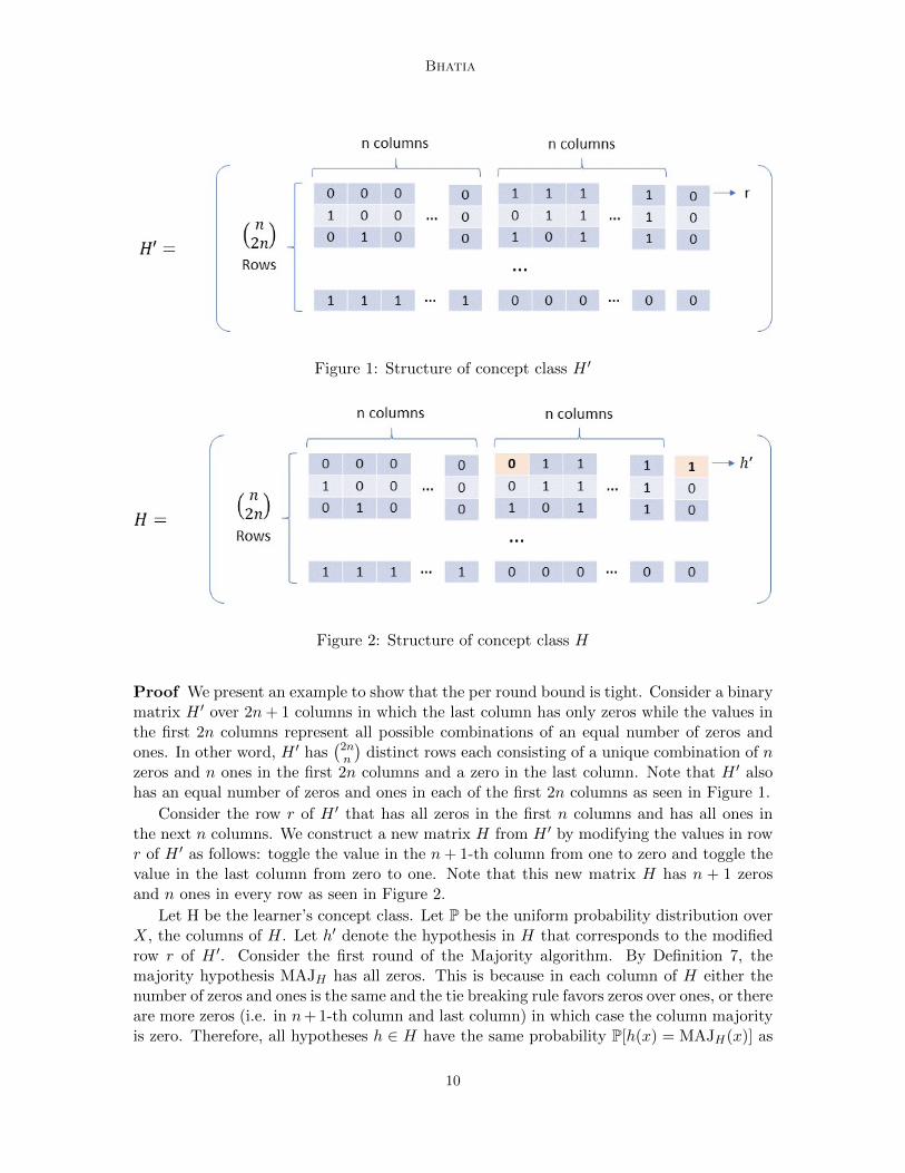
Figure 1: Structure of concept class H ′

Figure 2: Structure of concept class H

Proof We present an example to show that the per round bound is tight. Consider a binarymatrix H ′ over 2n+ 1 columns in which the last column has only zeros while the values inthe first 2n columns represent all possible combinations of an equal number of zeros andones. In other word, H ′ has

(2nn

)distinct rows each consisting of a unique combination of n

zeros and n ones in the first 2n columns and a zero in the last column. Note that H ′ alsohas an equal number of zeros and ones in each of the first 2n columns as seen in Figure 1.

Consider the row r of H ′ that has all zeros in the first n columns and has all ones inthe next n columns. We construct a new matrix H from H ′ by modifying the values in rowr of H ′ as follows: toggle the value in the n+ 1-th column from one to zero and toggle thevalue in the last column from zero to one. Note that this new matrix H has n + 1 zerosand n ones in every row as seen in Figure 2.

Let H be the learner’s concept class. Let P be the uniform probability distribution overX, the columns of H. Let h′ denote the hypothesis in H that corresponds to the modifiedrow r of H ′. Consider the first round of the Majority algorithm. By Definition 7, themajority hypothesis MAJH has all zeros. This is because in each column of H either thenumber of zeros and ones is the same and the tie breaking rule favors zeros over ones, or thereare more zeros (i.e. in n+ 1-th column and last column) in which case the column majorityis zero. Therefore, all hypotheses h ∈ H have the same probability P[h(x) = MAJH(x)] as

10


Figure 3: Majority, Learner’s, and Teacher’s Hypotheses

they all have n + 1 zeros. For this reason, by Definition 8, the majority hypothesis h ∈ His h′. This is because ties for the majority hypothesis are broken in favor of the smallestone in a lexicographic sort. h′ has all zeros in its first n + 1 columns while every otherhypothesis h ∈ H has at least one one in the first n + 1 columns. Therefore, h′ is smallerthan every other hypotheses in a lexicographic sort. Let the teacher’s hypothesis h∗ ∈ Hbe the hypothesis that differs from h = h′ in two columns: the first column (where it hasa one) and the last column (where it has a zero). Note that such h∗ is in H since H wasconstructed from all possible

(2nn

)combinations of equal number of ones and zeros.

Note that the teacher’s counter-example will either be returned on the first column orthe last column, each with probability 1/2. If it is the former, half the hypothesis in Hwill be eliminated, since there is an equal number of ones and zeros in the first column. Ifit is the latter, only one hypothesis will be eliminated—the learner’s hypothesis h. Thusthe expected fraction of hypotheses that get eliminated in the first round by the teacher’scounter-example is

1

|H|

(1

2· |H|

2+

1

2· 1)

=1

4+

1

2|H|,

which approaches 1/4 as |H| becomes large.

Theorem 14 Each round of the majority algorithm can be implemented in time O(|H||X|)

Proof By Definition 7, computation of MAJH(x) requires finding maximum values ineach column of matrix H, which can be done in time O(|H|) per column. Since there areO(|X|) columns in H, MAJH(x) can be computed in time O(|H||X|). The computationof P[h(x) = MAJH(x)] for any h ∈ H takes time O(|X|). Therefore, by Definition 8, thelearner’s hypothesis h can be computed in time O(|H||X|).

One of the primary advantages of the Majority algorithm (and also the Randomizedalgorithm described in the next section) over the Max-Min algorithm is the per roundrunning time for computing the next hypothesis. In the case of the Max-Min algorithm, thecomputation of the weights of all the edges in the elimination graph (Angluin and Dohrn,2017) entails a computation time of O(|H|2|X|). Compared to this, the O(|H||X|) perround computation time requirement of the Majority algorithm is a significant improvement,particularly when |H| is large.

11

Bhatia

4.3 Randomized Learning Algorithm

In this section, an open problem posed by Angluin and Dohrn (Angluin and Dohrn, 2017)regarding the existence of an efficient randomized algorithm is solved. In this version ofthe LRC model, the teacher’s target concept h∗ is drawn from the learner’s concept classH according to a known probability distribution Q. A Randomized learning algorithm ispresented and mathematically analyzed. It is shown that the Randomized learning algo-rithm has an expected learning time of O(log |H|) and is asymptotically optimal in the LRClearning model.

Definition 15 Q denotes a known teacher’s probability distribution of drawing the targetconcept h∗ from H.

This learning algorithm works as follows. In the first round of the Randomized learningalgorithm (Algorithm 2), the learner draws a hypothesis randomly from H according tothe distribution Q. When presented with a counter-example, the learner updates H byremoving the hypotheses that disagree with the counter-example. The learner also updatesthe teacher’s distribution Q to match the new H. The learner draws the hypothesis forthe next round from the updated H according to the updated distribution Q. This processcontinues until the learner correctly learns the target concept.

Definition 16 In the Randomized learning algorithm (Algorithm 2), the set of consistenthypotheses evolves over time by the sequence denoted by H1, H2, H3, . . .. Here H1 = H andH1 ⊃ H2 ⊃ H3 . . .. The corresponding evolution of the teacher’s probability distributionQ by the learner over this set is denoted by the sequence Q1,Q2,Q3, . . ., where Qi is adistribution on the hypothesis set Hi. Furthermore, the sequence of learner’s hypotheses isdenoted by h1, h2, h3, . . . and the corresponding sequence of counter-examples is denoted byx1, x2, x3, . . ..

Definition 17 For i ≥ 1, the pair (hi, xi) denotes that for the learner’s hypothesis hi,the counter-example xi is returned in round i of the Randomized algorithm. For i ≥ 1,Ri = (h1, x1), (h2, x2) . . . (hi, xi) denotes the sequence of these pairs in the first i roundsof the Randomized algorithm. R0 = denotes the empty sequence of pairs. For i ≥ 1, thenotation Ri = Ri−1 + (hi, xi) is used to indicate that in the sequence Ri is made up ofthe set of pairs in the sequence Ri−1 followed by the pair (hi, xi).

The probability distributions Qi are defined as follows. Q1 = Q is set to the known teacher’sdistribution over H. For i ≥ 1, Qi+1 is set to the teacher’s posterior distribution over Hi+1

given Ri. Specifically, for i ≥ 1, denote qij to be the probability the learner draws hj ∼ Qi.Then for hj ∈ Hi+1,

qi+1j = Pr(h∗ = hj | Ri).

We now show how these probabilities can be recursively computed.

Lemma 18 For i ≥ 1, the teacher’s posterior distribution over Hi+1 given Ri, or probabilitydistribution Qi+1, can be recursively computed as

qi+1j =

qij · P[xi | hj(x) 6= hi(x)]∑hk∈Hi+1

qik · P[xi | hk(x) 6= hi(x)]. (1)

12


Proof

Applying Bayes’ theorem:

qi+1j = Pr(h∗ = hj | Ri) =

Pr(Ri | h∗ = hj) · Pr(h∗ = hj)

Pr(Ri). (2)

Consider Pr(Ri | h∗ = hj) for i ≥ 1. This can be written as

Pr(Ri−1 + (hi, xi) | h∗ = hj) = Pr(Ri−1 | h∗ = hj) · Pr((hi, xi) | Ri−1 ∧ h∗ = hj). (3)

In other words it is the product of 1) the conditional probability that Ri−1 is the sequence ofpairs in the first i− 1 rounds of the Randomized algorithm given that teacher’s hypothesisis hj and 2) the conditional probability that for learner’s hypothesis hi in round i thecounter-example returned is xi given teacher’s hypothesis hj and the sequence of pairsRi−1 in the first i − 1 rounds of the Randomized algorithm. Applying Bayes’ theorem toPr(Ri−1 | h∗ = hj) we get

Pr(Ri−1 | h∗ = hj) =Pr(h∗ = hj | Ri−1) · Pr(Ri−1)

Pr(h∗ = hj)=qij · Pr(Ri−1)Pr(h∗ = hj)

.

The last equality follows from the definition of qij . By substituting in Equation (3) we get

Pr(Ri | h∗ = hj) =qij · Pr(Ri−1) · Pr((hi, xi) | Ri−1 ∧ h∗ = hj)

Pr(h∗ = hj). (4)

Substituting in Equation (2) we get:

qi+1j =

qij · Pr((hi, xi) | Ri−1 ∧ h∗ = hj) · Pr(Ri−1)Pr(Ri)

. (5)

Note that

Pr(Ri) =∑

hk∈Hi+1

Pr(Ri ∧ h∗ = hk) =∑

hk∈Hi+1

Pr(Ri | h∗ = hk) · Pr(h∗ = hk).

Substituting in Equation (5) and applying Equation (4) we get:

qi+1j =

qij · Pr((hi, xi) | Ri−1 ∧ h∗ = hj) · Pr(Ri−1)∑hk∈Hi+1

qik · Pr((hi, xi) | Ri−1 ∧ h∗ = hk) · Pr(Ri−1).

By simplifying we get

qi+1j =

qij · Pr((hi, xi) | Ri−1 ∧ h∗ = hj)∑hk∈Hi+1

qik · Pr((hi, xi) | Ri−1 ∧ h∗ = hk). (6)

Note that Pr((hi, xi) | Ri−1 ∧ h∗ = hk) is independent of Ri−1 as the probability ofgetting a counter-example xi in round i only depends on the learner’s hypothesis hi in round

13

Bhatia

i and the teacher’s hypothesis h∗ = hk. In particular these probabilities are distributed asP(hi, hk) (as defined in Definition 6). That is

Pr((hi, xi) | Ri−1 ∧ h∗ = hk) = P[xi | hk(x) 6= hi(x)].

Substituting in Equation (6), the result follows. Thus, the teacher’s posterior distri-bution over Hi+1 given Ri, which is also the probability distribution Qi+1 used by theRandomized algorithm, can be recursively computed from the prior probability distributionQi and the probability distributions P(hi, hk) for all hypotheses hk ∈ Hi+1.

r = 1, H1 = H, Q1 = Qwhile true do

Draw the learner’s hypothesis hr ∈ Hr randomly from Qr.Let xr be the counter-example returned by the teacher.if there is no such counter-example then

Output hr.endelse

Hr+1 = Hr − h ∈ Hr | h(xr) 6= h∗(xr).Calculate Qr+1 as described in Lemma 18.r = r + 1.

end

endAlgorithm 2: Randomized Learning Algorithm

The analysis for Algorithm 2 works as follows. A fact is proven in Lemma 22 usingwhich Lemma 23 proves that the expected fraction of hypotheses eliminated by the counter-example given in any round is at least 1

2 . In other words, E [|Hi+1|] ≤ |Hi|/2. Using thisresult, Theorem 24 proves that the expected learning time of Algorithm 2 is at most log2 |H|.The following analysis is for the i-th round of the algorithm and omits the index i whereverpossible.

Definition 19 For h ∈ Hi, define V (h, x) as the fraction of hypotheses in Hi that disagreewith h on example x. More formally,

V (h, x) =|h′ ∈ Hi | h′(x) 6= h(x)|

|Hi|.

Lemma 20 In any i-th round of the algorithm (i ≥ 1), for any two hypotheses h1, h2 ∈ Hi

where h1(x) 6= h2(x), V (h1, x) + V (h2, x) ≥ 1.

Proof Note that V (h1, x) =

|h′ ∈ Hi | h′(x) 6= h1(x)||Hi|

=

|h′ ∈ Hi | h′(x) 6= h1(x) ∧ h′(x) = h2(x)||Hi|

+|h′ ∈ Hi | h′(x) 6= h1(x) ∧ h′(x) 6= h2(x)|

|Hi|.

14


Likewise V (h2, x) =

|h′ ∈ Hi | h′(x) 6= h2(x) ∧ h′(x) = h1(x)||Hi|

+|h′ ∈ Hi | h′(x) 6= h2(x) ∧ h′(x) 6= h1(x)|

|Hi|.

Therefore V (h1, x) + V (h2, x) =

=|h′ ∈ Hi | h′(x) 6= h1(x) ∧ h′(x) = h2(x)|

|Hi|+|h′ ∈ Hi | h′(x) 6= h2(x) ∧ h′(x) = h1(x)|

|Hi|

+|h′ ∈ Hi | h′(x) 6= h1(x) ∧ h′(x) 6= h2(x)|

|Hi|+|h′ ∈ Hi | h′(x) 6= h1(x) ∧ h′(x) 6= h2(x)|

|Hi|.

Note that the numerator of the first three fractions adds up to exactly |Hi|. Hence we have

V (h1, x) + V (h2, x) =|Hi||Hi|

+|h′ ∈ Hi | h′(x) 6= h1(x) ∧ h′(x) 6= h2(x)|

|Hi|≥ 1.

Definition 21 Define E(h1, h2) to be the expected fraction of hypotheses that are eliminatedfrom Hi when the learner’s hypothesis is h1 ∈ Hi and the target concept is h2 ∈ Hi.

E(h1, h2) =∑

x∈D(h1,h2)

V (h2, x) · P[x | h1(x) 6= h2(x)].

Lemma 22 In any i-th round of the algorithm (i ≥ 1), for any two hypotheses h1, h2 ∈ Hi

where h1 6= h2, E(h1, h2) + E(h2, h1) ≥ 1.

Proof Recall from Definition 5 that D(h1, h2) = x ∈ X | h1(x) 6= h2(x). Therefore,D(h1, h2) = D(h2, h1). We can write

E(h1, h2) + E(h2, h1)

=∑

x∈D(h1,h2)

V (h2, x) · P[x | h1(x) 6= h2(x)] +∑

x∈D(h2,h1)

V (h1, x) · P[x | h2(x) 6= h1(x)]

=∑

x∈D(h1,h2)

(V (h2, x) · P[x | h1(x) 6= h2(x)] + V (h1, x) · P[x | h1(x) 6= h2(x)]). (7)

It follows from Lemma 20 that for any x ∈ D(h1, h2), since h1(x) 6= h2(x), V (h1, x) ≥1− V (h2, x). Substituting in Equation (7) we get

E(h1, h2) + E(h2, h1) ≥∑

x∈D(h1,h2)

(V (h2, x) + 1− V (h2, x)) · P[x | h1(x) 6= h2(x)]

=∑

x∈D(h1,h2)

P[x | h1(x) 6= h2(x)] = 1.

The last equality follows from D(h1, h2) = x ∈ X | h1(x) 6= h2(x).

15

Bhatia

Lemma 23 In any i-th round of the algorithm (i ≥ 1) the expected fraction of hypotheseseliminated by the counter-example given is at least 1

2 . In other words, E [|Hi+1|] ≤ |Hi|/2.

Proof Note that in round i of the Randomized algorithm the learner draws a hypothesish ∼ Qi, for i ≥ 1. Note that Qi is also the teacher’s posterior distribution over Hi in roundi of the Randomized algorithm (Lemma 18). Let n = |Hi|, and let qj denote the probabilitythat hj ∼ Qi (we drop the superscript i in qij for ease of exposition). Thus, for hypotheseshj , hk ∈ Hi, qj is the probability of learner drawing hypothesis hj and qk is the probabilityof hk being the teacher’s hypothesis in round i of the Randomized algorithm. Therefore,the expected fraction of hypotheses eliminated by the counter-example in round i of theRandomized algorithm is

n∑j=1

n∑k=1

qjqkE(hj , hk).

By Lemma 22, and using the fact that E(h, h) = 1 for any h ∈ Hi the expected fraction ofhypotheses eliminated by the counter-example in round i of the Randomized algorithm,

≥n∑j=1

qj2 +

n∑j=1

n∑k>j

qjqk = (q1 + q2 + q3 + ...+ qn)2 −n∑j=1

n∑k>j

qjqk

≥ (q1 + q2 + q3 + ...+ qn)2 − (q1 + q2 + q3 + ...+ qn)2

2= (1− 1

2) =

1

2.

Theorem 24 In the setting where the target concept is drawn from Q and the counter-examples are drawn from P, Algorithm 2 only needs to see an expected log2 |H| counter-examples to learn h∗.

Proof From Lemma 23 it follows that in any i-th round of the Randomized algorithm(i ≥ 1), at least 1

2 of the remaining hypotheses get eliminated in expectation. Thus, byTheorem 21 of Angluin and Dohrn (Angluin and Dohrn, 2017) it follows that the Random-ized algorithm (Algorithm 2) can learn the teacher’s hypothesis in log2 |H| expected rounds.

Theorem 25 Each round of the Randomized learning algorithm can be implemented intime O(|H||X|).

Proof The most expensive per-round operation in the Randomized learning algorithmis the computation of posterior distribution Qi+1. In round i + 1, for each of the |Hi+1|hypotheses hj , the quantity qi+1

j needs to be computed from Equation (1) in Lemma 18.The numerator of Equation (1) requires calculating the conditional probability of xi withrespect to hj(x) 6= hi(x), which takes time O(|X|). The denominator of Equation (1) issimply a normalization of the of qi+1

j values, which is achieved by dividing them by theirsum. Therefore, the overall per-round computation time of the Randomized learning algo-rithm is O(|H||X|).

16


4.4 Upper Bound on the Learning Time of Arbitrary Learning Algorithm

In this section, an Arbitrary learning algorithm (Algorithm 3) is analyzed in the PAC-LRC model where the learner is allowed to pick any consistent hypothesis in every round.Similar to LRC, in the PAC-LRC model, a randomly drawn counter-example is returned tothe learner in each round. However, the two differ in their termination conditions. Recallthat in the PAC-LRC model with parameters ε and δ, learning ends if all ε-bad hypotheses(hypothesis that differs with the target concept in a region with total probability at leastε) in H have been eliminated with probability at least 1 − δ. The only exception is if thelearner presents a hypothesis that is not ε-bad in any round, in which case the teacher doesnot return a counter-example and learning ends immediately.

The main result of this section is that with probability at least 1 − δ, the Arbitrarylearning algorithm terminates within O(1ε log |H|δ ) rounds. In other words, the learning time

of the Arbitrary learning algorithm is O(1ε log |H|δ ) with probability at least 1− δ.

i = 1.while true do

Pick hi to be any arbitrary hypothesis in H.Let xi be the counter-example returned by the teacher.if there is no such counter-example then

Output hi.endelse

Eliminate the set of hypotheses h ∈ H | h(xi) 6= h∗(xi) from H.endi = i+ 1.

endAlgorithm 3: Arbitrary Learning Algorithm

Definition 26 Let the target hypothesis be h∗. Let hi denote the learner’s hypotheses inround i. In other words, the sequence of learner’s hypotheses is written as h1, h2 . . .. Letthe sequence of counter-examples received by the learner be denoted by x1, x2 . . ..

Definition 27 Let the weight of a column x ∈ X at the start of any round i ≥ 1 be denotedas Wi(x), and let Wi(S) =

∑x∈SWi(x). For hypothesis h, Wi(h) = Wi(D(h, h∗)) denotes

the total weight on all the columns on which h differs from h∗ in round i. For all x ∈ X,define W1(x) = 0, and allow the weight of a column to be incremented in each round by theprobability that the column is chosen as a counter-example. More formally for n ≥ 2,

Wn(x) = Wn−1(x) + P[x | hn−1(x) 6= h∗(x)].

Or

Wn(x) =n−1∑i=1

P[x | hi(x) 6= h∗(x)].

17

Bhatia

Note that P[x | hi(x) 6= h∗(x)] = 0 if x /∈ D(hi, h∗).

Also note that in each round i ≥ 1, Wi+1(X) = Wi(X) + 1. This is because∑x∈X

P[x | hi(x) 6= h∗(x)] = 1

Definition 28 For i ≥ 1, let Ei(h) be the probability that on counter-example xi, hypothesish contradicts h∗. More formally,

Ei(h) = P[h(x) 6= h∗(x) | hi(x) 6= h∗(x)].

Note that for any h ∈ H and any round n ≥ 1, by Definition 27 and Definition 28,

n∑i=1

Ei(h) =

n∑i=1

P[h(x) 6= h∗(x) | hi(x) 6= h∗(x)]

=∑

x∈D(h,h∗)

n∑i=1

P[x | hi(x) 6= h∗(x)] = Wn+1(D(h, h∗)) = Wn+1(h).

Lemma 29 Let θ = ln( |H|δ ). At the beginning of any round n ≥ 1, consider a hypothesish ∈ H for which Wn(h) > θ. The probability that h has not already been eliminated, inother words it does not contradict any of the counter-examples x1, x2, . . . , xn−1, is at mostδ|H| .

Proof Note that for n = 1 the lemma holds trivially because W1(h) = 0 for all h ∈ H.Therefore, in the following we assume n > 1.

In each i-th round of the algorithm i ≥ 1, the counter-example xi is drawn with theprobability distribution P[x | hi(x) 6= h∗(x)]. The probability that on this counter-examplehypothesis h is inconsistent with h∗ is therefore P[h(x) 6= h∗(x) | hi(x) 6= h∗(x)], which byDefinition 28 equals Ei(h). Therefore, with probability 1 − Ei(h), hypothesis h is noteliminated in round i. Thus, the probability that hypothesis h ∈ H with Wn(h) > θ hasnot been eliminated in the first n− 1 rounds is:

n−1∏i=1

(1− Ei(h)) ≤n−1∏i=1

(1−∑n−1

i=1 Ei(h)

n− 1) =

n−1∏i=1

(1− Wn(h)

n− 1) ≤ e−Wn(h) < e− ln(

|H|δ

) =δ

|H|.

Definition 30 Let a threshold θ∗(x) = ln( |H|δ ) · 2P[x]ε be defined over every x ∈ X based onthe probability distribution P. A column is considered light at the start of any round i ifWi(x) ≤ θ∗(x) and heavy otherwise. Let Li ⊂ X denote the set of light columns and Bi ⊂ Xdenote the set of heavy (or bulky) columns at the start of round i.

18


Lemma 31 Let the learner’s hypothesis hi in round i ≥ 1 be ε-bad. That is, P[hi(x) 6=h∗(x)] ≥ ε. Let hi also satisfy that at the start of round i its total weight Wi(hi) ≤ ln( |H|δ ).Then, the weight of light columns Li should increase by at least half in round i. In otherwords

Wi+1(Li) ≥Wi(Li) +1

2.

Proof Assume for the sake of contradiction that

Wi+1(Li) < Wi(Li) +1

2.

Wi+1(X) = Wi(X) + 1 and Bi + Li = X together imply that

Wi+1(Bi) > Wi(Bi) +1

2. (8)

Note that only the weights of the columns in the set D(hi, h∗) change in this round as

the counter-example xi is drawn from the probability distribution P[x | hi(x) 6= h∗(x)].Additionally, all heavy columns whose weights change in this round therefore belong to theset D(hi, h

∗) ∩Bi. Applying Definition 27 we therefore have,

Wi+1(Bi)−Wi(Bi) =∑

x∈D(hi,h∗)∩Bi

P[x | hi(x) 6= h∗(x)]. (9)

From Equations (8) and (9) we get,∑x∈D(hi,h∗)∩Bi

P[x | hi(x) 6= h∗(x)] = P[D(hi, h∗) ∩Bi | hi(x) 6= h∗(x)] >

1

2. (10)

The total weight on hi at the beginning of round i satisfies

Wi(hi) = Wi(D(hi, h∗)) ≥Wi(D(hi, h

∗) ∩Bi).

Since the weights of all x ∈ Bi, at the beginning of round i, is at least θ∗(x) = ln( |H|δ ) · 2P[x]ε(Definition 30), the total weight on hi at the beginning of round i satisfies

Wi(hi) ≥Wi(D(hi, h∗) ∩Bi) > ln(

|H|δ

) · 2 · P[D(hi, h∗) ∩Bi]

ε. (11)

Since P[hi(x) 6= h∗(x)] ≥ ε, and since P[D(hi, h∗) ∩ Bi | hi(x) 6= h∗(x)] > 1

2 (Equation 10)we have

P[D(hi, h∗) ∩Bi)] >

ε

2.

Combining with Equation (11) we get, the total weight on hi at the beginning of round isatisfies

Wi(hi) > ln(|H|δ

) · 2 · P[D(hi, h∗) ∩Bi]

ε> ln(

|H|δ

) · 2 · εε · 2

= ln(|H|δ

).

This is a contradiction because we assumed Wi(hi) ≤ ln( |H|δ ).

19

Bhatia

Lemma 32 If for all i ≥ 1 the learner’s hypotheses hi satisfy Wi(hi) ≤ ln( |H|δ ), then within

O(1ε log |H|δ ) rounds either all x ∈ X become heavy, or the algorithm terminates because thelearner presents a hypothesis that is not ε-bad.

Proof Note that it is enough to bound the number of rounds it takes for all x ∈ X tobecome heavy under the assumption that in every round the learner’s hypothesis is ε-bad.Thus, in each round i we assume the learner’s hypothesis is ε-bad and has weight at mostln( |H|δ ). Therefore, by Lemma 31, the total weight of light columns increases by at least 1

2in each round i ≥ 1. We assume this in the proof below.

Additionally, we assume the number of rounds is at least 2, because otherwise the resulttrivially holds.

Note that in each round i ≥ 1, since hi is ε-bad, P[hi(x) 6= h∗(x)] ≥ ε and therefore

P[x | hi(x) 6= h∗(x)] ≤ P[x]ε . Thus, we can write

Wi+1(x)−Wi(x) ≤ P[x]

ε. (12)

We now provide some intuition motivating the rest of the proof. We know that each columnx ∈ X has threshold θ∗(x) = ln( |H|δ ) · 2P[x]ε . After acquiring θ∗(x) weight, x transitions fromlight to heavy. However, in the round j that x transitions from a light to a heavy column,its final weight Wj+1(x) exceeds threshold θ∗(x) by the amount s(x) = Wj+1(x) − θ∗(x).Call this difference s(x) spillover weight. Note that s(x) ≤ Wj+1(x) −Wj(x). Accountingfor spillover weight, the total weight that a column can accumulate while it is light is atmost θ∗(x) + s(x). At the same time, the weight of light columns increases by at least 1

2in each round. Therefore, during any arbitrary round i where light columns remain, wecan see that the total weight accumulated on the light columns, which is at least i

2 , cannotexceed the sum of θ∗(x) + s(x) over all columns x ∈ X. In other words,

i

2≤∑x∈X

[θ∗(x) + s(x)]

By Equation (12), it follows that s(x) ≤Wj+1(x)−Wj(x) ≤ P[x]ε . This in conjunction with

the definition of θ∗(x) yields

i

2≤∑x∈X

[ln(|H|δ

) · 2P[x]

ε+

P[x]

ε

]i

2≤ ln(

|H|δ

) · 2

ε+

1

ε

i ≤ O(log |H|δε

).

Thus the number of rounds i where light columns remain is bounded by O(log|H|δ

ε ). A formalargument follows below.

For any particular x ∈ X, and round i ≥ 1 we define values fi(x) as follows. Note thatall columns start out being light initially (since W1(x) = 0). Let j be the round in which

20


x turns from light to heavy. If, i > j, which happens when x ∈ Bi, then fi(x) = j + 1.Otherwise if i ≤ j, which happens when x ∈ Li, then fi(x) = i.

Let i ≥ 1 be any round in which the set Li is not empty. We claim that∑x∈X

Wfi(x)(x) ≥ i− 1

2.

We continue by induction on i. The base case, i = 1, holds because all columns are initiallylight. Therefore, for all x ∈ X, f1(x) = 1 and W1(x) = Wf1(x)(x) = 1−1

2 = 0. Assume (forthe sake of induction), the induction hypothesis that∑

x∈XWfk(x)(x) ≥ k − 1

2.

for some round k ≥ 1 where the set Lk is not empty. We want to prove that∑x∈X

Wfk+1(x)(x) ≥ k

2.

We know that for all x ∈ Lk, fk+1(x) = k + 1 and fk(x) = k. Therefore,∑x∈Lk

[Wk+1(x)−Wk(x)] =∑x∈Lk

[Wfk+1(x)(x)−Wfk(x)(x)

]. (13)

We also know by Lemma 31, that the total weight of light columns increases by at least 12

in round k. Thus, ∑x∈Lk

[Wk+1(x)−Wk(x)] ≥ 1

2. (14)

Combining Equations (13) and (14) we see that,∑x∈Lk

Wfk+1(x)(x) ≥∑x∈Lk

Wfk(x)(x) +1

2.

Also, because both Wk(x) and fk(x) are non-decreasing functions,∑x∈Bk

Wfk+1(x)(x) ≥∑x∈Bk

Wfk(x)(x).

Adding the last two inequalities we get∑x∈X

Wfk+1(x)(x) ≥∑x∈X

Wfk(x)(x) +1

2.

Using the induction hypothesis we arrive at∑x∈X

Wfk+1(x)(x) ≥ k − 1

2+

1

2≥ k

2.

21

Bhatia

This concludes the proof that ∑x∈X

Wfi(x)(x) ≥ i− 1

2. (15)

In any particular round i ≥ 2, let x ∈ Bi be a heavy column. By definition of fi(x),x ∈ Lfi(x)−1. In other words, x must have been a light column in round fi(x) − 1. By

definition 30, when a column x is light its weight is at most θ∗(x) = ln( |H|δ ) · 2P[x]ε . Thus,

Wfi(x)−1(x) ≤ ln(|H|δ

) · 2P[x]

ε.

Summing over all columns x ∈ Bi we get:∑x∈Bi

Wfi(x)−1(x) ≤∑x∈Bi

ln(|H|δ

) · 2P[x]

ε. (16)

From Equation (12), it follows that in any round i ≥ 2:

(Wfi(x)(x)−Wfi(x)−1(x)) ≤ P[x]

ε.

Considering all x ∈ Bi, it follows that in any round i ≥ 2,∑x∈Bi

(Wfi(x)(x)−Wfi(x)−1(x)) ≤∑x∈Bi

P[x]

ε≤∑x∈X

P[x]

ε=

1

ε. (17)

Therefore, ∑x∈Bi

Wfi(x)(x) ≤∑x∈Bi

Wfi(x)−1(x) +1

ε.

Combining with Equation (16) it follows:∑x∈Bi

Wfi(x)(x) ≤∑x∈Bi

ln(|H|δ

) · 2P[x]

ε+

1

ε. (18)

In round i ≥ 2, consider a light column x ∈ Li. By definition, fi(x) = i. Therefore,

Wfi(x)(x) ≤ ln(|H|δ

) · 2P[x]

ε.

Summing over all such light columns and combining with Equation (18) we get∑x∈X

Wfi(x)(x) =∑x∈Bi

Wfi(x)(x) +∑x∈Li

Wfi(x)(x) ≤∑x∈X

ln(|H|δ

) · 2P[x]

ε+

1

ε. (19)

Thus it follows that∑x∈X

Wfi(x)(x) ≤∑x∈X

ln(|H|δ

) · 2P[x]

ε+

1

ε≤ ln(

|H|δ

) · 2

ε+

1

ε. (20)

22


Combining with Equation (15) we get that

i− 1

2≤∑x∈X

Wfi(x)(x) ≤ ln(|H|δ

) · 2

ε+

1

ε. (21)

It follows that

i ≤4 · log |H|δ + 2

ε+ 1.

Thus, at the end of i rounds if all learner’s hypotheses hi are ε-bad and satisfy Wi(hi) ≤ln( |H|δ ), every column must be heavy. Here

i =4 · log |H|δ + 2

ε+ 1 = O(

1

εlog|H|δ

).

This establishes the Lemma.

Theorem 33 With probability at least 1− δ the Arbitrary learning algorithm terminates inO(1ε log |H|δ ) rounds.

Proof Let

N =4 · log |H|δ + 2

ε+ 1.

We first show that the Arbitrary algorithm cannot run for more than N + 1 roundsassuming that in every round i except the last, Wi(hi) ≤ ln( |H|δ ). We then show with

probability at least 1−δ that in every round i except the last, Wi(hi) ≤ ln( |H|δ ), completingthe proof.

Assume for the sake of contradiction that the algorithm runs for m+ 1 > N + 1 rounds,where in rounds 1 ≤ i ≤ m, Wi(hi) ≤ ln( |H|δ ). Note that in rounds 1 ≤ i ≤ m the learner’shypotheses hi are all ε-bad. Otherwise, the algorithm would have terminated before roundm+ 1. Consider the N + 1-th round (because N + 1 ≤ m). By our assumptions, Lemma 32applies and it follows that all the columns must be heavy both by the end of the N -th roundand in the beginning of round N + 1.

By Definition 27,

WN+1(hN+1) = WN+1(D(hN+1, h∗)).

Since every column in the beginning of round N + 1 is heavy, by Definition 30,

WN+1(D(hN+1, h∗)) > ln(

|H|δ

) · 2 · P[D(hN+1, h∗)]

ε.

Also, since hN+1 must be ε-bad, we have P[D(hN+1, h∗)] ≥ ε. Thus,

WN+1(hN+1) > ln(|H|δ

) · 2 · P[D(hN+1, h∗)]

ε≥ ln(

|H|δ

) · 2 · εε

> ln(|H|δ

).

23

Bhatia

This is a contradiction because WN+1(hN+1) ≤ ln( |H|δ ) (since N + 1 ≤ m). Thus, wemust have that the number of rounds, m + 1, cannot exceed N + 1 and the Arbitraryalgorithm must terminate in m+ 1 ≤ N + 1 = O(1ε log |H|δ ) rounds.

We now show with probability at least 1 − δ, our previous assumption holds. That is,in every round 1 ≤ i ≤ m, Wi(hi) ≤ ln( |H|δ ).

Each of the learner’s hypotheses h1, h2 . . . hm has to be ε-bad and is consistent in thebeginning of the i-th round in which it got selected by the algorithm. From Lemma 29 itfollows for any of these learner’s hypothesis hi:

Pr( [Wi(hi) > ln(|H|δ

)] ) <δ

|H|.

By applying the union bound we get:

Pr(

m∨i=1

[Wi(hi) > ln(|H|δ

)] ) < m · δ

|H|≤ δ.

Here we used the fact that m ≤ |H|, as any PAC-LRC learning algorithm must alwaysterminate within |H| rounds. Thus:

Pr(m∧i=1

[Wi(hi) ≤ ln(|H|δ

)] ) > 1− δ. (22)

Thus with probability at least 1−δ, each of the learner’s hypotheses hi satisfy Wi(hi) ≤ln( |H|δ ). This concludes the proof.

5. Simulation Results

In this section we present the results of testing the performance of our interactive LRCalgorithms on randomly generated learner’s concept classes H which are chosen to be binarymatrices.

We generate H with a particular structure—with g distinct groups of 100 rows each, forsome integer g—so that |H| = 100g. The groups are generated so that two hypotheses fromthe same group only differ in a few places. At the same time, hypotheses from differentgroups differ a lot. The process for generating |H| is described in detail below.

To generate H, we first generate g random rows, one for each group. From each of theseg rows we derive 99 additional random rows. H consists of these 99g rows plus the originalg rows for a total of 100g rows. Figure 4 illustrates this structure of the learner’s conceptclass.

The generation of the g rows in the first step is as follows. We construct a binary matrixH ′ with g rows and the same set of columns X as H. For each column xj of matrix H ′,1 ≤ j ≤ |X|, we draw a real number pj independently and uniformly from the interval[0, 1]. For each row hi ∈ H ′ and j-th column xj ∈ X, we independently set hi(xj) to 1 withprobability pj and 0 with probability 1− pj . Note that in H ′ the expected number of onesin column j is pj · g.

24


Figure 4: Structure of learner’s concept class H

Note that the probability that any two rows of H ′ differ on column j is 2pj(1 − pj).Since pj is uniformly distributed in the interval [0, 1], the expected value of 2pj(1 − pj) is1/3. This implies that any two rows of H ′ are likely to differ in |X|/3 columns. We use therows of H ′ as the g rows of H in the first step.

Let h ∈ H ′ be the row generated for a group in the first step. In the second step, theadditional 99 rows for this group are generated as follows. Let q1, q2, . . . q99 be 99 different,equally spaced, values that span the range [0.01, 0.04]. The i-th row hi for the group isgenerated by toggling each value in row h independently with probability qi. In otherwords, Pr(h(x) 6= hi(x)) = qi for all x ∈ X. Assuming a uniform distribution over thesamples X, in expectation, rows h and hi differ on qi|X| columns.

Some additional details regarding our implementation are as follows. The teacher’sconcept is randomly drawn from H. In each of our tests, the performance of a learningalgorithm is computed by taking an average over at least 100 randomly generated binarymatrices H of a given size. We also make some simplifications in our implementation.We assume a uniform distribution over the samples X. Thus P[x] is the same for allcolumns x ∈ X. Our implementation of the Arbitrary learning algorithm, called the Anti-majority learning algorithm, chooses in each round the hypothesis that has the lowestmajority score. Ideally we would want to implement an adversarial learning algorithm thatwould maximize the expected number of counterexamples needed for learning. However,as such an algorithm can be hard to design, we approximate it by following the oppositeof the Majority strategy as that can can be beneficial to the adversary. The Anti-majoritylearning algorithm terminates when there are no more ε-bad hypotheses left in H or whenthe learner proposes a hypothesis that is not ε-bad. In other words, we set δ = 0 for ease

25

Bhatia

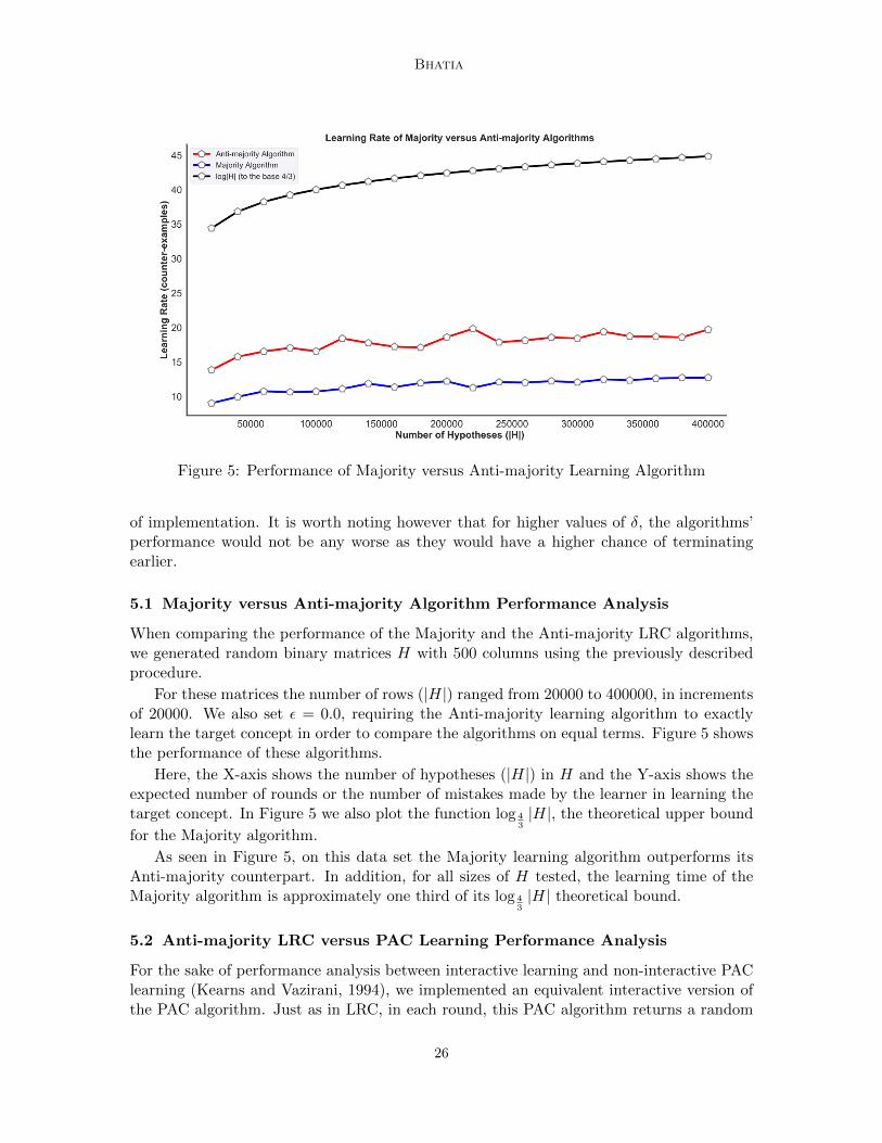
Figure 5: Performance of Majority versus Anti-majority Learning Algorithm

of implementation. It is worth noting however that for higher values of δ, the algorithms’performance would not be any worse as they would have a higher chance of terminatingearlier.

5.1 Majority versus Anti-majority Algorithm Performance Analysis

When comparing the performance of the Majority and the Anti-majority LRC algorithms,we generated random binary matrices H with 500 columns using the previously describedprocedure.

For these matrices the number of rows (|H|) ranged from 20000 to 400000, in incrementsof 20000. We also set ε = 0.0, requiring the Anti-majority learning algorithm to exactlylearn the target concept in order to compare the algorithms on equal terms. Figure 5 showsthe performance of these algorithms.

Here, the X-axis shows the number of hypotheses (|H|) in H and the Y-axis shows theexpected number of rounds or the number of mistakes made by the learner in learning thetarget concept. In Figure 5 we also plot the function log 4

3|H|, the theoretical upper bound

for the Majority algorithm.

As seen in Figure 5, on this data set the Majority learning algorithm outperforms itsAnti-majority counterpart. In addition, for all sizes of H tested, the learning time of theMajority algorithm is approximately one third of its log 4

3|H| theoretical bound.

5.2 Anti-majority LRC versus PAC Learning Performance Analysis

For the sake of performance analysis between interactive learning and non-interactive PAClearning (Kearns and Vazirani, 1994), we implemented an equivalent interactive version ofthe PAC algorithm. Just as in LRC, in each round, this PAC algorithm returns a random

26


Figure 6: Anti-majority Learning Algorithm versus PAC Learning

consistent hypothesis. However, instead of receiving a counter-example as is the case inLRC, the PAC algorithm receives any random example, which eliminates all hypotheses inH that disagree with it. The PAC algorithm terminates either when it returns a hypothesisthat is not ε-bad or when all the ε-bad hypotheses are eliminated from H. Note that just asin our implementation of the Arbitrary algorithm, the parameter δ does not play any rolein this PAC algorithm.

In Figure 6, we compare the performance of the Anti-majority interactive learning algo-rithm with the interactive PAC algorithm. For this evaluation, as shown on the X-axis, wevaried the error ε from 0.0 to 0.2 (0% to 20%). We used randomly generated binary conceptclasses H with 500 columns and of two different sizes: |H| = 20000 and |H| = 200000. TheY -axis plots the average number of rounds of interactions for these algorithms. As expected,both the Anti-majority and PAC algorithms require less counter-examples (or examples)when the error tolerance (ε) is increased. It can also be seen that the Anti-majority algo-rithm outperforms the PAC learner particularly when the error tolerance (ε) is small. This

contrasts with the fact that the4·log |H|

δ+2

ε + 1 theoretical bound on the learning time of

any arbitrary interactive learning algorithm is approximately 4 times that that of thelog|H|δ

εtheoretical bound of non-interactive PAC learning (Kearns and Vazirani, 1994). Note thatnon-interactive PAC learning has even higher learning time than interactive PAC learningused in our simulation.

5.3 Majority versus Max-Min Algorithm Performance Analysis

We also implemented the Max-Min algorithm (Angluin and Dohrn, 2017) and comparedits performance with the Majority algorithm. Figure 7 shows the results of comparingthe performance of the algorithms on randomly generated matrices H with 100 columnsand with rows (|H|) that ranged from 100 to 2000, in increments of 100. Since the per

27

Bhatia

Figure 7: Majority versus Max-Min Learning algorithm

round computation time of the Max-Min algorithm has a quadratic dependence on |H|,we were only able to run our tests on these smaller matrices. As can be seen, both thealgorithms perform equally well. This contrasts with the fact that the theoretical boundon the Majority algorithm’s expected learning time is log 4

3|H| which is 2.41 times more

than the log2 |H| expected learning time theoretical bound for the Max-Min algorithm. Itsuggests that the Majority algorithm’s theoretical upper bound may not be tight.

6. Discussion

These results demonstrate the potential benefits and limitations of using random counter-examples as a form of feedback in interactive learning. When learners are intelligent, anduse the Majority learning algorithm (Algorithm 1), they can learn by seeing an expectedO(log |H|) counter-examples. As was previously shown (Angluin and Dohrn, 2017), whencounter-examples are not chosen randomly, it is difficult for the learner to learn some conceptclasses. This happens, for instance, when H is simply the n × n identity matrix. In thiscase, for any target concept h∗ and consistent hypothesis h 6= h∗, the teacher will havea choice between exactly two counter-examples. One counter-example will eliminate allhypothesis but h∗, and the other bad counter-example will just eliminate h. An adversarialteacher could simply pick the bad counter-example every single round and thus it wouldtake Ω(|H|) time to learn h∗ without random counter-examples. While this problem ofneeding random counter-examples was previously solved by a well known halving algorithmbased on majority vote (Littlestone, 1988; Barzdin and Freivald, 1972; Angluin, 1988),that algorithm required that the learner be allowed to make improper queries. On theother hand, our work shows that a teacher who gives random counter-examples solves thisproblem without having to make any such sacrifices. The O(1ε log |H|δ ) upper bound onthe adversarial learner shows that the interactive LRC learner performs no worse than,

28


and achieves the same asymptotic bound as, the non-interactive PAC learner (Kearns andVazirani, 1994). This is somewhat surprising because intuitively, providing specific feedbackin the form of counter-examples would seem more valuable to the learner than providingrandomly sampled examples as is done in the PAC model (Kearns and Vazirani, 1994). Itseems that the reason that the bound was not improved was that the learner’s ability to beadversarial, or impede the learning process was much more pronounced in the LRC settingthan the PAC setting. The reason for this was that in the LRC setting, the learner couldchoose specific hypothesis on which the teacher’s random counter-example would generallymake little progress in eliminating ε-bad hypotheses.

7. Conclusion and Future Work

In this work we provided simple and efficient algorithms for interactively learning non-binary concepts in the recently proposed setting of exact learning from random counter-examples (LRC). One such algorithm is based on majority vote and the other works byrandomly selecting hypotheses from a probability distribution over target concepts that isevolved over time. Both these algorithms are shown to have the fastest possible O(log |H|)expected learning time and entail significantly lower computation time than previouslyknown algorithms. We also provided an analysis that shows that interactive LRC learning,regardless of the learning algorithm, is at least as efficient as non-interactive ProbablyApproximately Correct (PAC) learning.

Our future goal is to improve the efficiency of these algorithms on other cost measures.Throughout this paper, our focus has been on minimizing the learning complexity of thealgorithms, which is the number of counter-examples needed by the learner in order tocorrectly identify the target concept. However, calculating the majority hypothesis or up-dating the teacher’s distribution Q to match the new H, can require iterating over everyremaining consistent hypothesis in H, in every round. This can take time O(|H||X|), thusmaking it computationally expensive, especially since the number of hypothesis in H maygrow exponentially in the number of examples (the set of columns X of H). To address thehigh computational overhead of these tasks, we plan to explore alternative approaches forcarrying out these tasks such as by using sampling to trade accuracy for efficiency.

Acknowledgments

I would like to thank my mentor Professor Daniel Hsu who guided my research in the rightdirection by providing me with background material in the field of computational machinelearning, validating the correctness of my proofs, and assisting me in using mathematicalnotation when writing this paper. Professor Hsu also helped me formulate theoreticalmodels such as the PAC-LRC interactive learning model which served as the framework formy analysis of the upper bound of an Arbitrary LRC algorithm.

References

Dana Angluin. Queries and concept learning. Machine learning, 2(4):319–342, 1988.

29

Bhatia

Dana Angluin. Queries revisited. Theoretical Computer Science, 313(2):175–194, 2004.

Dana Angluin and Tyler Dohrn. The power of random counterexamples. In InternationalConference on Algorithmic Learning Theory, pages 452–465, 2017.

Pranjal Awasthi, Maria Florina Balcan, and Konstantin Voevodski. Local algorithms forinteractive clustering. J. Mach. Learn. Res., 18(1):75–109, January 2017. ISSN 1532-4435.

Maria-Florina Balcan and Avrim Blum. Clustering with interactive feedback. In Interna-tional Conference on Algorithmic Learning Theory, pages 316–328. Springer, 2008.

J. M. Barzdin and R. V. Freivald. On the prediction of general recursive functions. SovietMath. Doklady, 13:1224–1228, 1972.

Ehsan Emamjomeh-Zadeh and David Kempe. A general framework for robust interactivelearning. In Advances in Neural Information Processing Systems, pages 7082–7091, 2017.

Thorsten Joachims. Optimizing search engines using clickthrough data. In Proceedingsof the eighth ACM SIGKDD international conference on Knowledge discovery and datamining, pages 133–142. ACM, 2002.

Michael J Kearns and Umesh Vazirani. An introduction to computational learning theory.MIT press, 1994.

Nick Littlestone. Learning quickly when irrelevant attributes abound: A new linear-threshold algorithm. Machine learning, 2(4):285–318, 1988.

Wolfgang Maass and Gyorgy Turan. On the complexity of learning from counterexamplesand membership queries. In Foundations of Computer Science, 1990. Proceedings., 31stAnnual Symposium on, pages 203–210. IEEE, 1990.

Wolfgang Maass and Gyorgy Turan. Lower bound methods and separation results for on-linelearning models. Machine Learning, 9(2-3):107–145, 1992.

Wolfgang Maass and Gyorgy Turan. Algorithms and lower bounds for on-line learning ofgeometrical concepts. Machine Learning, 14(3):251–269, 1994.

Burr Settles. Active learning. Synthesis Lectures on Artificial Intelligence and MachineLearning, 6(1):1–114, 2012.

30

simple and fast algorithms for interactive machine

Documents