SimPEG DocumentationRelease 0.0.1

Rowan Cockett

June 22, 2016

Contents

1 Magnetics 31.1 Backgrounds . . . . . . . . . . . . . . . . . . . . . . . . . . . . . . . . . . . . . . . . . . . . . . . 31.2 Forward problem . . . . . . . . . . . . . . . . . . . . . . . . . . . . . . . . . . . . . . . . . . . . . 41.3 Inverse problem . . . . . . . . . . . . . . . . . . . . . . . . . . . . . . . . . . . . . . . . . . . . . 5

2 Mag Differential eq. approach 7

3 Mag Integral eq. approach 9

4 Mag analytic solutions 11

5 Testing SimPEG 13

6 Project Index & Search 15

Python Module Index 17

i

ii

SimPEG Documentation, Release 0.0.1

SimPEG (Simulation and Parameter Estimation in Geophysics) is a python package for simulation and gradient basedparameter estimation in the context of geoscience applications.

simpegPF uses SimPEG as the framework for the forward and inverse gravity and magnetics geophysical problems.

Contents 1

SimPEG Documentation, Release 0.0.1

2 Contents

CHAPTER 1

Magnetics

The geomagnetic field can be ranked as the longest studied of all the geophysical properties of the earth. In addition,magnetic survey, has been used broadly in diverse realm e.g., mining, oil and gas industry and environmental engi-neering. Although, this geophysical application is quite common in geoscience; however, we do not have modular,well-documented and well-tested open-source codes, which perform forward and inverse problems of magnetic sur-vey. Therefore, here we are going to build up magnetic forward and inverse modeling code based on two commonmethodologies for forward problem - differential equation and integral equation approaches.

First, we start with some backgrounds of magnetics, e.g., Maxwell’s equations. Based on that secondly, we usedifferential equation approach to solve forward problem with secondary field formulation. In order to discretzie oursystem here, we use finite volume approach with weak formulation. Third, we solve inverse problem through Gauss-Newton method.

1.1 Backgrounds

Maxwell’s equations for static case with out current source can be written as

∇𝑈 =1

𝜇�⃗�

∇ · �⃗� = 0

where \(\vec{B}\) is magnetic flux (\(T\)) and \(U\) is magnetic potential and \(\mu\) is permeability. Since we do nothave any source term in above equations, boundary condition is going to be the driving force of our system as givenbelow

(�⃗� · �⃗�)𝜕Ω = 𝐵𝐵𝐶

where \(\vec{n}\) means the unit normal vector on the boundary surface (\(\partial \Omega\)). By using seocondaryfield formulation we can rewrite above equations as

1

𝜇�⃗�𝑠 = (

1

𝜇 0

− 1

𝜇)�⃗�0 +∇𝜑𝑠

∇ · �⃗�𝑠 = 0

(�⃗�𝑠 · �⃗�)𝜕Ω = 𝐵𝑠𝐵𝐶

where \(\vec{B}_s\) is the secondary magnetic flux and \(\vec{B}_0\) is the background or primary magnetic flux. Inpractice, we consider our earth field, which we can get from International Geomagnetic Reference Field (IGRF) byspecifying the time and location, as \(\vec{B}_0\). And based on this background fields, we compute secondary fields

3

SimPEG Documentation, Release 0.0.1

(\(\vec{B}_s\)). Now we introduce the susceptibility as

𝜒 =𝜇

𝜇0− 1

𝜇 = 𝜇0(1 + 𝜒)

Since most materials in the earth have lower permeability than \(\mu_0\), usually \(\chi\) is greater than 0.

Note: Actually, this is an assumption, which means we are not sure exactly this is true, although we are sure, it isvery rare that we can encounter those materials. Anyway, practical range of the susceptibility is \(0 < \chi < 1 \).

Since we compute secondary field based on the earth field, which can be different from different locations in theworld, we can expect different anomalous responses in different locations in the earth. For instance, assume we havetwo susceptible spheres, which are exactly same. However, anomalous responses in Seoul and Vancouver are going tobe different.

Since we can measure total fields ( \(\vec{B}\)), and usually have reasonably accurate earth field (\(\vec{B}_0\)), wecan compute anomalous fields, \(\vec{B}_s\) from our observed data. If you want to download earth magnetic fieldsat specific location see this website (noaa).

1.1.1 What is our data?

In applied geophysics, which means in practice, it is common to refer to measurements as “the magnetic anomaly”and we can consider this as our observed data. For further descriptions in GPG materials for magnetic survey. Nowwe have the simple relation ship between “the magnetic anomaly” and the total field as

△�⃗� = |�̂�𝑜 − �⃗�𝑠| − |�̂�𝑜| ≈ |�⃗�𝑠|𝑐𝑜𝑠𝜃

where \(\theta\) is the angle between total and anomalous fields, \(\hat{B}_o\) is the unit vector for \(\vec{B}_o\).Equivalently, we can use the vector dot product to show that the anomalous field is approximately equal to the projec-tion of that field onto the direction of the inducing field. Using this approach we would write

△�⃗� = |�⃗�𝑠|𝑐𝑜𝑠𝜃 = |�̂�𝑜||�⃗�𝑠|𝑐𝑜𝑠𝜃 = �̂�𝑜 · �⃗�𝑠

This is important because, in practice we usually use a total field magnetometer (like a proton precession or opticallypumped sensor), which can measure only that part of the anomalous field which is in the direction of the earth’s mainfield.

1.1.2 Sphere in a whole space

1.2 Forward problem

1.2.1 Differential equation approach

Au = rhs

A = ()−1𝑇

rhs = ()−1M𝑓

𝜇−10

B0 −B0 + (𝑣)DP𝑇𝑜𝑢𝑡B𝑠𝐵𝐶

B𝑠 = ()−1M𝑓

𝜇−10

B0 −B0 − ()−1𝑇u

4 Chapter 1. Magnetics

SimPEG Documentation, Release 0.0.1

1.3 Inverse problem

1.3. Inverse problem 5

SimPEG Documentation, Release 0.0.1

6 Chapter 1. Magnetics

CHAPTER 2

Mag Differential eq. approach

7

SimPEG Documentation, Release 0.0.1

8 Chapter 2. Mag Differential eq. approach

CHAPTER 3

Mag Integral eq. approach

9

SimPEG Documentation, Release 0.0.1

10 Chapter 3. Mag Integral eq. approach

CHAPTER 4

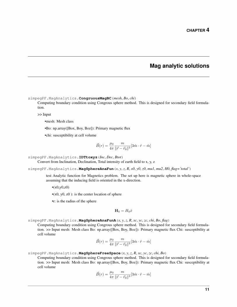
Mag analytic solutions

simpegPF.MagAnalytics.CongruousMagBC(mesh, Bo, chi)Computing boundary condition using Congrous sphere method. This is designed for secondary field formula-tion.

>> Input

•mesh: Mesh class

•Bo: np.array([Box, Boy, Boz]): Primary magnetic flux

•chi: susceptibility at cell volume

�⃗�(𝑟) =𝜇0

4𝜋

𝑚

‖�⃗� − �⃗�0‖3[3�̂� · 𝑟 − �̂�]

simpegPF.MagAnalytics.IDTtoxyz(Inc, Dec, Btot)Convert from Inclination, Declination, Total intensity of earth field to x, y, z

simpegPF.MagAnalytics.MagSphereAnaFun(x, y, z, R, x0, y0, z0, mu1, mu2, H0, flag=’total’)

test Analytic function for Magnetics problem. The set up here is magnetic sphere in whole-spaceassuming that the inducing field is oriented in the x-direction.

•(x0,y0,z0)

•(x0, y0, z0 ): is the center location of sphere

•r: is the radius of the sphere

H0 = 𝐻0�̂�

simpegPF.MagAnalytics.MagSphereAnaFunA(x, y, z, R, xc, yc, zc, chi, Bo, flag)Computing boundary condition using Congrous sphere method. This is designed for secondary field formula-tion. >> Input mesh: Mesh class Bo: np.array([Box, Boy, Boz]): Primary magnetic flux Chi: susceptibility atcell volume

�⃗�(𝑟) =𝜇0

4𝜋

𝑚

‖�⃗� − �⃗�0‖3[3�̂� · 𝑟 − �̂�]

simpegPF.MagAnalytics.MagSphereFreeSpace(x, y, z, R, xc, yc, zc, chi, Bo)Computing boundary condition using Congrous sphere method. This is designed for secondary field formula-tion. >> Input mesh: Mesh class Bo: np.array([Box, Boy, Boz]): Primary magnetic flux Chi: susceptibility atcell volume

�⃗�(𝑟) =𝜇0

4𝜋

𝑚

‖�⃗� − �⃗�0‖3[3�̂� · 𝑟 − �̂�]

11

SimPEG Documentation, Release 0.0.1

simpegPF.MagAnalytics.spheremodel(mesh, x0, y0, z0, r)Generate model indicies for sphere - (x0, y0, z0 ): is the center location of sphere - r: is the radius of the sphere- it returns logical indicies of cell-center model

12 Chapter 4. Mag analytic solutions

CHAPTER 5

Testing SimPEG

• Master Branch

13

SimPEG Documentation, Release 0.0.1

14 Chapter 5. Testing SimPEG

CHAPTER 6

Project Index & Search

• genindex

• modindex

• search

15

SimPEG Documentation, Release 0.0.1

16 Chapter 6. Project Index & Search

Python Module Index

ssimpegPF.MagAnalytics, 11

17

SimPEG Documentation, Release 0.0.1

18 Python Module Index

Index

CCongruousMagBC() (in module sim-

pegPF.MagAnalytics), 11

IIDTtoxyz() (in module simpegPF.MagAnalytics), 11

MMagSphereAnaFun() (in module sim-

pegPF.MagAnalytics), 11MagSphereAnaFunA() (in module sim-

pegPF.MagAnalytics), 11MagSphereFreeSpace() (in module sim-

pegPF.MagAnalytics), 11

SsimpegPF.MagAnalytics (module), 11spheremodel() (in module simpegPF.MagAnalytics), 12

19