1

Signaling vs. Human Capital:

Evidence from a reform in Colombia’s top University

Carolina Arteaga1 UCLA

April 2016

In this paper I test whether the returns to college education are due to increases in productivity

(human capital theory) or instead, to the fact that attending college signals higher ability to

employers. I exploit a reform at Universidad de Los Andes which in 2006 reduced the amount

of coursework required to earn a degree in economics and business. The size of the entering

class, their average high school exit test scores, and graduation rates were not affected by the

reform, indicating that the quantity and quality of students remained the same. Thus, the reform

decreased human capital students graduate with, while holding the value of the education signal

constant. Using administrative data on wages and college attendance, I find that wages fell by

approximately 16% in economics and 12% in business. These results suggest that human

capital plays an important role in the determination of wages, and reject a pure signaling model.

In addition, comparing this number to an OLS estimate that combines both human capital and

signaling effects, my results imply that human capital accounts for most of the return in

schooling. Surveying employers, I find that the decline in wages may have resulted from a

decline in performance in recruitment processes, which led to a smaller pool of jobs to choose

from. Using data from the recruitment process for economists at the Central Bank of Colombia,

I find that the reform reduced the probability of students from Los Andes being hired by 17pp.

JEL Classification: I20

Keywords: Education, human capital, signaling.

1 PhD student at the Department of Economics, UCLA (caroartc@ucla.edu). I would like to thank the Colombian Ministry of

Education, the Central Bank of Colombia and the Economics Department at Universidad de los Andes for providing the data

for this study. I’m extremely grateful to Adriana Lleras-Muney for her encouragement and suggestions. I also want to thank

David Atkin, Leah Boustan, Carlos Medina, Maurizio Mazzocco, Rodrigo Pinto, Sarah Reber, Juan E. Saavedra and Till von

Wachter for their comments and feedback. I am grateful to my colleagues Tiago Caruso, Richard Domurat, David Gelvez, Luis

O. Herrera, Vasily Korovkin, Keyoung Lee, Rustin Partow and Lucia Yanguas for insightful suggestions and discussions. I

thank seminar participants at UCLA, Universidad de Los Andes and the Central Bank of Colombia for valuable comments.

2

I Introduction

Education is one of the most important determinants of wages at the individual level. Returns to a year of

schooling are estimated to be positive and large in most countries, ranging from 2 to 20 percent around

the world (Montenegro and Patrinos, 2014). Moreover, the earnings premium associated with college has

risen substantially in the last decades (Oreopoulos and Petronijevic, 2013). In spite of this, there is much

debate about the mechanisms by which education leads to higher wages. The human capital theory argues

that education increases productivity, and rises wages as a result (Becker, 1964 and Mincer, 1974),

whereas the signaling theory states that it reflects the correlation between education and unobserved

ability. Spence (1973) provides a model in which higher ability individuals increase their education to

signal their ability to employers, and thus increase their wages, but where education is otherwise useless

in terms of productivity. If the signaling theory is important, it implies that the social returns to education

could be lower than the private returns, and thus can call into question the rationale for public investment.

Despite the importance of this debate, this remains an open question (Lange and Topel, 2006). The

fundamental difficulty in distinguishing these two theories arises because many of the empirical

implications are identical.2 In both models, the decision processes of firms and workers are the same.

Firms weigh the productivity of workers with different levels of education against their wages and select

the education level that maximizes profits. Workers weigh the increased wages against the cost of

education and choose the level of education that maximizes their utility. In both setting, higher ability

workers obtain higher levels of schooling and are paid more. Of course the two theories are not mutually

exclusive.

In this paper I identify the extent to which college education increases productivity and wages,

by exploiting a curriculum change at Los Andes, the top university in Colombia. In 2006 the time required

to earn a college degree in economics and business decreased from 4.5 to 4 years. This was accomplished

by dropping 12 required courses in economics and 6 in business, which was equivalent to a reduction in

credits of 20% and 14%, respectively.3 Crucial to my identification strategy, the reform did not alter the

quality of the entering class. At Los Andes, the admission process is constrained by a limited number of

slots and is solely based on the national standardized high school exit test. I show that the size of the

entering class did not grow, nor the average entrance test scores decreased, and dropout rates didn’t change

2 Lang and Kropp (1986) stated that ”Many members of the profession maintain (at least privately) that these

hypotheses cannot be tested against each other and that the debate must therefore by relegated to the realm of

ideology”. 3 In economics the change in curriculum not only reduced the number of semesters, but also the number of courses

per semester. Before the reform students were supposed to take six courses per term and this was changed to five.

In business the number of classes per term was unchanged at five.

3

with the reduction in the number of classes. All together the reform had no short run effect on the quality

of the affected entering class and thus, it decreased human capital exogenously, while at the same time

held the signaling value of the degree constant. The human capital model predicts a decline in wages as a

result of the reform, whereas the signaling model does not. This setting constitutes an ideal natural

experiment to learn about signaling vs. human capital.

To estimate the effect of the reform I use individual information on wages and educational

attainment, in a difference in difference framework. I compare wages in the formal sector before and after

the reform for economics and business students from Los Andes and other top 10 schools in Colombia.

This schools did not reform their degrees. I find that after the reform, wages for students from Los Andes

fell by approximately 16% in economics and 12% in business, and that the effects are statistically

significant. The result suggest that human capital plays an important role in the formation of wages and

reject a model in which signaling is the only role of college education. Although I allow for heterogeneity

in the effect of the reform using Athey and Imbens (2006) changes in changes estimator, I find a

homogenous effect along the wage distribution, in other words, wages declined proportionally for high

and low earners. Using data from the Survey of Quality of Life for 2008-2012, I estimate that the OLS

returns to one year of higher education is 17%. Interpreting the reduction of graduation requirements for

economics as a reduction of one year of schooling and in business as a reduction of one semester, my

results provide novel evidence, they suggest that human capital accounts for the largest share of the return

to college education.

I investigate the mechanisms that led to lower wages. Using data for economics graduates from

Los Andes, I find that the distribution of employers changed with the reform. Moreover, there is a

relationship between the classes dropped and the placement of graduates across employers. I interviewed

many of the top employers and found that most of them knew about the reform, they stated that they were

able to detect the change in human capital through tests performed in their recruitment process, and argued

that some knowledge made optional in the new curriculum is vital to some jobs. All of the above suggest

that under the new curriculum, the pool of jobs graduates can obtain is smaller because they performed

worse during recruitment, which subsequently decreased their wages. I find support for this hypothesis.

Using data from the recruitment process for economists at the Central Bank from 2008 to 2014, I find that

the probability of being hired for graduates from Los Andes fell by 17pp with the reform.

There are several potential issues with my approach. It is possible that the reform in curricula

changed the pool of applicants and entrants in dimensions, not captured by high school exit tests which

are relevant to the labor market. Specifically, given the decline in requirements to graduate, lower ability

4

individual should be induced into enrolling in these programs, which would lead to a decrease in the value

of the signal and in wages. In order to address this, I estimate an alternative specification, taking as the

treatment group only the students at Los Andes who were already enrolled at the time of the reform but

studied under the new curriculum. The result to this alternative treatment group are similar to the

benchmark specification. Also, one might be worried about the possibility that my estimates capture a

negative trend in the return to a degree from Los Andes. To test if this is the case I perform two exercises;

I replicate my baseline estimation using a placebo date for the reform, and also test my specification using

a major at Los Andes that didn’t undergo a reform in curriculum. The data suggest there is no change in

wages in the placebo date, or for the placebo group. My results are robust to several additional checks

explained in the robustness section. Finally, in order to interpret the reduction in wages as the causal effect

of human capital, the choices underlying labor force participation should be unaffected by the reform.

One of the motivations behind the curriculum change was to increase graduate school enrollment. If the

reform had this effect, and delayed working, my result could be confounding a change in the composition

of the new graduates in the labor market. I use LinkedIn data to check if the reform increased the share of

students attending graduate school, but find no evidence of an increase.

The primary contribution of this paper is to identify the role of signaling and human capital in a

college setting using a natural experiment. A number of papers in the literature have investigated this

issue for primary and secondary education and have found mixed results. Eble and Hu (2016), exploit the

introduction of one extra year in primary school in China in 1980, and find a small increase in wages,

which leads them to conclude that there is an important role for signaling in primary education. There was

however, no extra coursework introduced in that additional year. Lang and Kropp (1986) and Bedard

(2001) find secondary schooling decisions that are consistent with a signaling model, and that would reject

a pure human capital framework. Another strand of the literature attempts to measure directly if there is

a signaling value to education degrees. Tyler, Murnane, and Willett (2000) estimate the signaling value

of the GED to be between 12% and 20%, whereas, Martorell and Clark (2014), find little evidence of high

school diploma signaling effects.

To my knowledge this is the first paper to look at the signaling and human capital question at the

college level. This is particularly relevant because universal enrollment in primary education and school

leaving age laws, constrain schooling decisions in primary and secondary education, and as consequence

make college a good candidate to signal ability. In addition it is easier to argue that skills provided in

primary and secondary education are of use in the workplace, as opposed to those acquire in college, and

finally, there is greater debate about the role of public spending in financing college education. This is

also the first paper to look at the mechanisms that led to changes in wages, this is important because it

5

provides information about the tools employers use to learn about workers productivity.

The rest of the paper is structured as follows: Section 2 describes a simplified version of a

signaling and human capital model to derive testable implications in my context; Section 3 discusses the

curriculum reform at Los Andes; Section 4 describes the data, the empirical strategy, and the results;

Section 5 presents some robustness checks; Section 6 explores the channels that explain the results; and

the last section offers some concluding remarks.

II Signaling vs. Human Capital

In this section I lay out a simple model that allows me to derive a test of the signaling and human

capital theories, by exploiting a reduction in curricula in the best university, in a context of ability based

admissions and a binding number of slots.

Individuals have ability 𝜃𝑖 distributed with continuous support. There are J schools that offer

different levels of human capital accumulation 𝑓𝑗, where higher human capital requires higher effort, and

j indicates school ranking. The cost to attend school j for individual i increases in the level of human

capital and decreases in the level of ability (single crossing property), such that 𝑐(𝑓𝑗, 𝜃𝑖) > 𝑐(𝑓𝑘, 𝜃𝑖) for

every i when 𝑗 < 𝑘, meaning j offers higher human capital than k, and 𝑐(𝑓𝑗, 𝜃𝑖) < 𝑐(𝑓𝑗, 𝜃𝑚) when 𝜃𝑖 >

𝜃𝑚.

Firms’ value 𝜇(𝜃𝑖, 𝑓𝑗), which is a linear transformation of unobservable intrinsic ability 𝜃𝑖 and

human capital specific to each school 𝑓𝑗. In a separating equilibrium, agents signal their type, and firms

will predict ability based on the observed level of human capital, and offer wages accordingly.

𝑤𝑗 = 𝜇(𝐸[𝜃𝑖|𝑓𝑗], 𝑓𝑗) = 𝛼1 + 𝛼2�̅�𝑗 + 𝛼3𝑓𝑗 (1)

Students will choose school trying to maximize wages net of effort costs:

𝑤𝑗 − 𝑐(𝑓𝑗, 𝜃𝑖) = 𝜇(𝐸[𝜃𝑖|𝑓𝑗], 𝑓𝑗) − 𝑐(𝑓𝑗, 𝜃𝑖) (2)

Thus, a student chooses to attend the top school whenever:

𝑤1 − 𝑐(𝑓1, 𝜃𝑖) ≥ 𝑤2 − 𝑐(𝑓2, 𝜃𝑖) (3)

Because both sides are strictly increasing in 𝜃 (single crossing property), there exists a unique 𝜃1 such

that ∀𝜃 ≥ 𝜃1 (3) will hold. Subsequently, there is a threshold θ for each pair of schools that determines

school choice over the school ranking.

6

In this framework the question of signaling vs. human capital comes down to learning about the

values of 𝛼2 and 𝛼3 in (1). In order to identify the contribution of human capital to wages we need

variation in 𝑓 that holds 𝜃 constant. If school No.1 reduces the quantity of human capital produced (∆𝑓1 <

0), such that it is still higher than 𝑓2, this model would predict that since the effort required to attend

school No.1 went down, the level of ability that determines for whom it is profitable to attend the best

school would decrease, and thus �̅�1 would decrease, and the fall in wages will confound the effects of the

decline in the average ability of students and the decline in learning: ∆𝑤1 = 𝛼2∆�̅�1 + 𝛼3∆𝑓1. Note,

however, that in an environment where school No.1:

(i) Is constrained to admit a certain maximum number of students.

(ii) Uses a proxy of ability to determine admissions.

We will have that if the maximum number of students is binding before the curriculum change then:

The admissions criteria guarantees (selecting students based on test scores) that the quality

of the admitted class would not be affected with the reform, because the school was already

choosing a subset (the ones with highest ability) of the group of people who find it profitable

to attend school No.1.

And thus:

∆𝑤1 = 𝛼3∆𝑓1 (4)

In the next section of the paper I will go over the assumptions that lead to this result. Finally, to

account for trends in wages I will use as controls, students from other schools and estimate the following

difference in difference equation:

𝑤𝑖𝑡𝑗 = 𝑎0 + 𝑎1𝚰(post) + 𝑎2𝚰(𝑠𝑐ℎ𝑜𝑜𝑙1) + 𝑎3𝚰(𝑝𝑜𝑠𝑡 ∩ 𝑠𝑐ℎ𝑜𝑜𝑙1) + 𝜀𝑖𝑡𝑗

𝑎3 is the coefficient of interest and is my estimate of 𝛼3; if it’s zero, data support a pure signaling model,

if it’s negative and statistically significant, it suggests a role for human capital in the determination of

wages.

7

III Reform

In 2006, Los Andes a private university, unilaterally decided to reduce the coursework required

to earn a college degree in most of its majors.4,5 The reason behind this reform was to move towards

international standards of shorter college degrees, and to encourage graduate school enrollment. Each

department was autonomous in the implementation of the reform. In this paper I exploit the reform

implemented by the economics and business departments, because in other majors the change led to a

complete overhaul of the curricula, rather than a reduction of credits alone. For these two majors the

requirement went from 4.5 years of course work to 4 years. In economics, the reform consisted of a

reduction of 12 courses (20% of the total number of credits), which resulted in a curriculum of 4 years

instead of 4.5 and a median number of courses per term of five instead of six. Specifically the reform

consisted of: (i) turning six mandatory courses into electives (Monetary policy, Fiscal policy, Trade,

Marxist economics, Colombian economic policy and Social programs evaluation); (ii) reducing the

number of electives by four, for a reduction of ten courses; (iii) combining two courses of probability and

statistics into one; (iv) combining courses of accounting and measurement in economics into one; for a

final reduction of 12 courses. The reduction in business consisted of eliminating from the curriculum

Computer Programming, Simulations and Microeconomics I. In addition, in the old curriculum students

took six upper division electives and this requirement was reduced to three. The change in curricula

covered new students, and students who by the time of the reform were in the beginning of their second

year or less for economics, and in the beginning of their third year or less for business.

III a First stage: Empirical evidence of the reform for economics and business

In order to test the signaling and human capital models, I need an effective decline in the number

of terms studied and credits taken; and for my identification strategy to be valid, I require no change in

the quantity and quality of the pool of students graduating from Los Andes. This section features data on

aggregate statistics from the annual bulletins from Los Andes, and micro data on credits taken by

economics students to investigate these points.

4 Some institutional differences of the Colombian education system and labor market are in order. First, about the

education system, admission are twice a year, students apply directly to a major and the gross enrollment rate in

higher education is around 39%. On the labor market front,(i) recruitment of recent graduates are usually carried

all throughout the year, only a few multinational companies have an organized recruitment season, (2) recruitment

at this level usually consist of tests of specific knowledge, standard selection tests and interviews, and (3) 25% of

college graduates work in the informal sector. 5 Los Andes was the only school undergoing this practice.

8

Was the reform effective?

Figure 1 shows the effective average duration of the undergraduate programs for both economics

and business majors. We can see that there is actually a step down in these trends at the time of the reform

of about one semester, suggesting the reform was effective in decreasing the average length of the

program. For economics, the average duration went from 5 to 4.5 years, and for business the duration

declined from 5.5 to 5 years. Figure 2 shows the number of credits students graduated with in economics.

We can observe a sharp drop at the time of the reform of around 16%.

Did the reform affect the size and composition of the entering and graduating class?

To evaluate if the reform affected the selection of students entering and graduating from Los

Andes, I check the evolution of the size of the entering classes, their average High School exit exam, and

average graduation rates. Figure 3a shows the evolution of the entering class in economics and business.

I fit different trends before and after the reform. The graph shows that the number of entering students

was not affected by the reform.6 Panel b of Figure 3 shows the average High School exit test scores of

the entering class. The fitted regressions around the reform do not suggest a change in the quality of the

entering class. I also perform a difference in difference estimation, similar to the one I perform for my

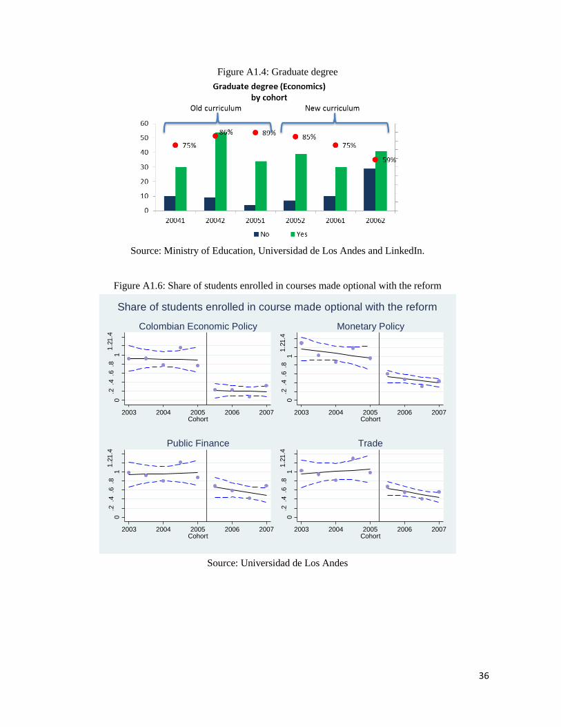
baseline analysis, to test if the reform decreased average High School exit score. Table A1.1 shows that

there is a small increase of approximately 0.2 to 0.3 standard deviations, which is not statistically

significant. On the other hand, if the change in curriculum alters the quantity of students graduating from

Los Andes, the value of the signal would change. This is plausible since the requirements to graduate

decreased with the reform. Panel c of Figure 3 shows the evolution of graduation rates, and suggests the

reform didn’t have an effect on the dropout rate. I also perform a difference in difference linear probability

model regression where I test if the reform changed the probability of graduating from economics and

business, and don’t find evidence that it did (Table-A1.1). Figure A1.1 in the appendix also shows that

the reform did not change the share of students that graduated with a minor.

The above should imply that the ranking of Los Andes was not affected by the reform, however,

to address this point directly I look at rankings and college exit scores. International rankings that include

6 Even though I don’t find a discontinuity in test scores, there is a change in trends around the time of the reform,

this can be problematic for my identification strategy if there is a different behavior in my control group. To check

for this possibility in appendix 1, Figure A1.2 shows high school exit scores for the entering cohorts at Rosario

University and find a similar pattern.

9

Latin American universities are only available since 2013, but from 2013 to 2016, Los Andes has been

ranked as the best school in the country.7 In Colombia, the Ministry of Education released its first ranking

on 2015 and Los Andes was also ranked first.8 Finally, Figure A1.3 shows the average college exit exam

for Los Andes and the next top 3 universities, according the data Los Andes has the highest score for most

cohorts, both before and after the reform.

To summarize, the reduction in curricula was translated into an effective cut of one semester from

the average degree duration in economics and business, which constitutes an exogenous reduction in

human capital. On the other hand, the number of new students, high school exit test scores and dropout

rates suggest that the quantity and quality of students was unaffected, thus the value of the signal remained

unchanged with the reform. This constitutes an ideal environment to test the role of signaling and human

capital in college education.

IV Effects of the Reform: human capital or signaling?

In this section I estimate the effect of the reduction of the curricula in business and economics on

wages, to test the prevalence of a pure signaling model versus a model where human capital matters. I

start by describing my data, continue with the identification strategy, and finally the results.

IV.a Data

My data consists of several databases from the Ministry of Education. My main database is OLE

(Observatorio Laboral de Educación), constructed to follow yearly earnings for college graduates in

Colombia in the formal sector.9 This information is recorded from social security payments from 2008 to

2012. OLE also contains education variables, such as university and program attended, graduation year,

and personal characteristics.

SPADIES (Sistema para la prevención de la deserción en la educación superior) is a database

built to track college dropout rates. Like OLE it, contains data on university attended, but additionally it

has information on the first semester of college, which is needed in this paper to identify the curriculum

for each student. This database also contains household socioeconomic variables. Finally, SABER 11 is

a database that contains individual data on the national standardized High School exit test scores, and also

7 https://www.timeshighereducation.com/world-university-rankings/2015/world-ranking#!/page/0/length/25

http://www.topuniversities.com/university-rankings/latin-american-university-

rankings/2014#sorting=rank+region=+country=+faculty=+stars=false+search=

Accessed February 10, 2016. 8 http://www.mineducacion.gov.co/cvn/1665/w3-article-351855.html Accessed February 10, 2016. 9 75% of workers with college education are employed in the formal sector (Fedesarrollo, 2013)

10

has socioeconomic variables. SABER 11 is a test taken at the end of high school, and it is a very important

input for college admissions. Specifically at Los Andes, it is the only factor taken into account in the

admission process. These databases contain generated ID numbers to trace individuals. Table 1 shows

summary statistics of some relevant variables in my data. We can see that the average individual in my

sample is 26 years old and has been working for almost three years10. On average, workers from Los

Andes earn 45% more than workers from the top 10 schools, have higher High School exit test scores,

and their parents have higher income.

IV.b Preliminary evidence and empirical strategy

Figure 4 shows a scatter plot of wages for graduates from Los Andes and Top 10 schools for

economics and business by cohort. Before the reform the evolution in wages seems fairly parallel, and the

slope in wages are statistically the same. There was a constant premium from attending Los Andes of 36%

for economics, and 50% for business. With the change in curricula this premium decreased immediately

for economics and gradually for business, for a final average reduction of 22 and 12pp, respectively.

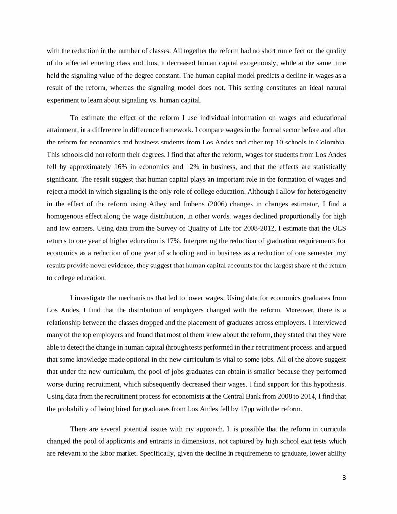
Figure 5 displays the wage densities for Los Andes and top 10 schools, both before and after the reform.

The graphs show that for the control group pre and post-reform wage densities overlap each other, whereas

for Los Andes, post-reform densities shifted to the left. Both Figure 5 and 6 show that the reform had a

stark negative effect on the wage distribution of graduates from Los Andes. To estimate the magnitude of

the role of human capital in wages, I estimate the following difference in difference regression:

ln 𝑤𝑎𝑔𝑒𝑖𝑡 = 𝛽0 + 𝛽1𝐴𝑛𝑑𝑒𝑠 ∗ 𝑃𝑜𝑠𝑡𝑖 + 𝛽2𝐴𝑛𝑑𝑒𝑠𝑖 + 𝛽3𝑃𝑜𝑠𝑡𝑖 + 𝛽4𝑒𝑥𝑝𝑒𝑟𝑖𝑒𝑛𝑐𝑒𝑖,𝑡 + 𝜀𝑖𝑡, (1)

where 𝑤𝑎𝑔𝑒𝑖,𝑡 is the average monthly earnings of individual i in year t, in 2010’s pesos. 𝐴𝑛𝑑𝑒𝑠 is a

dummy equal to 1 if the person 𝑖 went to college at Los Andes, and 0 if he went to another university in

the top 10 (my baseline control group). 𝑃𝑜𝑠𝑡 is a dummy that is 1 if the person started school after the

date of the reform implementation, and 0 otherwise, thus 𝐴𝑛𝑑𝑒𝑠 ∗ 𝑃𝑜𝑠𝑡𝑖 captures the diff-in-diff estimator

of the reform. 𝛽4 and 𝛽5 capture the effect of experience on wages, where experience is measured as the

difference between the current year in the data and the graduation year. I also control for gender, year and

cohort effects in other specifications. I perform this estimation by major, and cluster the standard errors

at the school level.

10 The fact that my data consists of wages from individuals in the beginning of their professional careers possess a

challenge to my specification since the wage profiles are very steep in terms of experience.

11

IV.c Results

Table 2 shows my baseline results, panel a displays the estimates for economics, and panel b for

business. In column 1, I estimate equation 1 and find a statistically significant decline in wages of 16%

for economics and 12% business. Column 2 adds controls for experience squared and gender, and columns

3 through 6 add year and cohort controls to these specifications. Throughout all such specifications there

is a negative and strong decline in wages as a result of the reform. These results reject a pure signaling

model, in which wages shouldn’t change; and given the magnitude of the decline, they evidence an

important role for human capital in the determination of wages. The coefficients on experience and gender

are similar to others found in the literature.

It is possible that the reform in curricula changed the pool of applicants and entrants in dimensions

not captured by high school exit tests, which are relevant to the labor market. Specifically, given the

decline in requirements to graduate, lower ability individuals should be induced into enrolling in these

programs, decreasing the value of the signal, and thus wages. In order to address this, I estimate an

alternative specification taking, as the treatment group only the students at Los Andes who were already

enrolled by the time of the reform, but studied under the new curriculum. Table 3 shows the results for

this alternative treatment group. According to the data there is a strong and negative effect on wages of

around 16% for economics and 10.5% for business, suggesting the pool of students wasn’t affected by the

reform.

Given that the years of wage observations by group (pre-reform vs. post-reform, and treated vs.

untreated), in Table 4 I include observations with at most three years of experience, to be sure that the

treatment coefficient is not capturing differences in the slope of the experience profile. Results in Table

4 suggest again strong declines in wages of the same magnitudes as the ones found before.

In order to make use of all the data available, and recognizing the potential of heterogeneous

effects, I now turn to a changes-in-changes (CIC) estimation following Athey and Imbens (2006). I

estimate CIC for the 10th through 90th percentiles after controlling for experience, gender and cohort

effects. The results are displayed in Figure 6, there is little evidence of heterogeneity in the effect of the

curriculum reduction on wages by percentiles and fields, suggesting that the assumptions of the traditional

diff in diff estimator hold.

To quantify the relative importance of signaling and human capital, we can take what we learned

in this paper one step forward. If we interpret the coefficient on the effect of the reform on wages as the

casual estimate of human capital, we can compare this estimate to an OLS return to education that besides

12

this effect, would include the value of the signal. Using data on the Survey of Quality of Life for 2008-

2012, I estimate an OLS return to a year of higher education of 16% (see appendix 2 for details).

Interpreting the reduction in economics as a reduction of one year of schooling and that in business as of

one semester, my results provide novel evidence; they suggest that human capital accounts for all of the

return to college education.

V. Robustness Checks & Caveats

In this section I perform several robustness checks that address possible confounding factors in

my estimation. Then I discuss some important caveats and limitations. In this section all standard errors

will be clustered at the individual level.

One might be worried about the possibility that my estimates capture a negative trend in the return

to a degree from Los Andes. To test if this is the case, I replicate my baseline estimation, but use a placebo

date for the reform. Specifically, I take only the cohorts that studied under the old curriculum, and set a

“fake” reform date in the middle of the period covered. If my results were driven by a decline in the return

to Los Andes, any post*Andes interaction will be negative and statistically significant. This is not the

case. According to the results in Table 5, all of the effects are statistically equal to zero and smaller than

0.7% in economics, and even positive for business.

An alternative placebo check to address this concern is to test what happens to law graduates (a

major without a reform in its curriculum) in the dates of the reform in economics and business. The results

in Table 6 show there is no effect on wages from graduates from Los Andes on the date of the reform in

economics or business. All of the above suggest the strong decline in wages I find is not the result of

trends or changes at Los Andes.

Table 7 features a series of robustness checks, the first two column show results for economics

and the last two for business, columns 1 and 3 estimate equation 1 with cohort controls, and columns 2

and 4 add experience squared and gender. A possible explanation for my results is that there is an age

penalty in the labor market. We can imagine that if two graduates have the same credentials, employers

can lean towards the older one, thinking that life experience is valuable for the job. In this case, having

cohorts that graduate half a year younger would result in lower wages, regardless of human capital or

signaling considerations. To check this possibility I include age as an independent variable in my baseline

estimation. The results in panel a of Table 7 suggest that there is a strong effect of the reform outside age

considerations. For economics the effect is the same (-16%) and for business is smaller (-9%).

13

One might also be worried about the fact that the reform generated two cohorts graduating at the

same time, and this could have distorted wages creating more competition. In panel b of Table 7 I remove

these two cohorts and perform my baseline estimation. The results show that the effects hold with this

exclusion.

An additional concern about the previous estimates is the validity of the control group. Even

though the pre trends in wages were similar, the control group may not be a good counter factual, if for

example the two groups face different labor markets, and these evolved in different ways after the reform.

To address this, I limit my control group to students graduating from top 3 schools. It is more likely for

students from these institutions to face the same labor market as the students from Los Andes. Panel c of

the Table 7 shows the results of the effect of the reform on wages under this alternative control group.

We can see that there is a negative effect of the reform on wages of similar magnitude to the one found

before.

An alternative way to go around this concern is to include in the control group only students who

had the ability to attend Los Andes. Specifically, I include in the control group students who attended top

10 schools, and had high school exit scores greater than the minimum per cohort observed at Los Andes,

in economics and business, respectively. This reduces the size of the control groups by around 30%. Panel

d of Table 7 shows the results of this alternative exercise: wages fall by a magnitude larger than in the

baseline estimation (18% for economics and 15% for business).

Panel e of Table 7 repeats the baseline estimation excluding cohort 2007-1, Figure 4 shows it

had particularly low wages for students from Los Andes. Again the results are very similar, suggesting

strong declines in wages. Finally, Panel f included as a covariate high school exit test scores. We can see

that, controlling for test scores, the results hold and increase a little in size.

It is evident that there are multiple choices of control group, and even though some are intuitive

there is no clear rule to discriminate among them. To address this issue, I follow Abadie and Gardeazabal

(2003), and perform a synthetic control exercise, where I look for the best combination of major/school

to match the pre-trend data of my treated groups. The comparison unit in the synthetic control method is

selected as the weighted average of all potential comparison units that best resembles the characteristics

of the case of interest. Table 8 shows the results of my baseline specification with respect to the optimally

chosen control group. This group features graduates from engineering, business and law degrees in Top

schools. Using this method, the results are similar to the ones found before: the effect of the reform in

economics ranges from - 7% to -13%, for business there is a larger dispersion, and the effects ranges from

-5% to -20%.

In the previous analysis I assumed that the reform didn’t have an effect on labor force

participation. Since one of the motives behind it was to increase graduate school enrollment, it’s important

14

to check for changes along this dimension. It can be the case that before the reform, only students in the

right tail of the ability distribution attended graduate school, but after the reform more students chose to

attend graduate school, and thus the estimated difference in wages resulted from comparing wages from

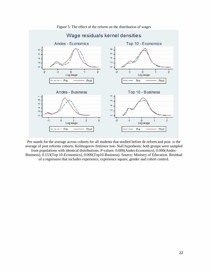
different segments of the ability distribution. To check if this is the case, I use LinkedIn and personal and

firm websites to obtain information on graduate school enrollment for the last three cohorts who studied

under the old curriculum, and the first three that studied under the new one. Figure A1.4 shows the

percentage of people found in LinkedIn. This number is around 60% and is similar before and after the

reform. Figure A1.5 also shows the share of graduates by cohort who enrolled in graduate school in the

first four years after graduation. According to these data there doesn’t seem to be an increase in this

number with the reform. All of the above suggest that selection doesn’t seem to be driving the decline in

wages, and thus we can interpret this decline as due to the causal return on human capital.

VI Discussion

The previous section laid out evidence on the importance of human capital in the determination

of wages. The next step is to think about the mechanisms that led recent graduates from Los Andes to

earn lower wages. When and how do employers find out about the lower human capital of these graduates?

Specifically, were they able to notice it in the recruitment process during tests or interviews? Or did they

notice it on the job? Unfortunately I don’t have information to fully answer these questions, but I have

data from Los Andes on the current employers of all graduates from economics by cohort; which I use to

investigate whether employers changed with the reform. Table A1.2 lists the main employers before and

after the reform and shows there are important differences. There seems to be a connection between the

change in curriculum and the change in employers. The Central Bank, the Ministry of Finance and the

National Planning Department are less common employers for economists who graduated under the new

curriculum, in which the classes Monetary Policy, Fiscal Policy and Colombian Economic Policy were

not mandatory, indeed Figure A1.6 shows that there was decline in the number of students enrolled in

these classes after the reform.

I also used this information to interview the most important employers to learn about their

experience hiring graduates from economics. From these interviews I learned that: (i) most of them knew

about the reform; (ii) they believe they can detect the change in human capital through tests they perform

in their recruitment process; (iii) they argue that for some jobs the content made optional in the new

curriculum is vital; (iv) taking fewer elective courses affects graduates’ labor prospects beyond the

recruitment process, because these professors are helpful with job offers and job referrals; and (v) wages

15

for recent graduates are fixed. All of the above suggest that under the new curriculum, the pool of jobs a

graduate can obtain is smaller, either because they can’t succeed in recruitment process that includes tests

on content they didn’t cover in school, or because they have less contact with professors who have

connections in the job market. It is clear that the first reason is entirely due to a decrease in human capital,

whereas this is not the case with the second one.

To evaluate if the reform had an impact on the ability of students to obtain a job, I perform a

difference-in-difference exercise with data from the recruitment process for recently graduated

economists at the Central Bank of Colombia. The process consists of a written exam or presentation,

which tests specific knowledge for the position; as well as human resources tests and interviews with both

human resources and department heads. Most processes are announced publicly through employment

websites and social networks, and are open to everyone. I have data on university and enrollment term on

all candidates to economist positions from 2008 to 2014, along with the final decision of the recruitment

process. For candidates that studied under the old curriculum the probability of being hired was 27%, this

number fell to 6% with the reform. Table 9 shows the results of the diff-in-diff exercise: according to the

data after the reform there is a reduction of 16.7pp on the probability of being hired in the Central Bank

for students from Los Andes versus students in other top ten schools. This suggests that one of the possible

mechanisms that led to the decline in wages is a decline in the performance of students in the recruitment

process, which was in turn generated by the reduction in courses.

VII Conclusions

In this paper I identify the effect of human capital on wages exploiting a curriculum change at

Universidad de Los Andes in Colombia. In 2006 the time required to earn a college degree in economics

and, business decreased from 4.5 to 4 years. This was accomplished by dropping 12 courses in economics

and 6 in business, which was equivalent to a reduction in credits of 20% and 14%, respectively. The

reform did not alter the quality of the graduating class from Los Andes or the ranking of the school.

Because wages should fall under the human capital model, but be constant under signaling, this constitutes

an ideal natural experiment to learn about signaling vs. human capital.

Using administrative data on wages and college attendance, I find that wages fall by around 16%

in economics and 10% in business. Given the statistically significant decline in wages, my estimates

suggest that human capital plays an important role in the formation of wages. The results also reject a

model in which signaling is the only function of college education. Even more, if we interpret the

16

coefficient on the effect of the reform on wages as the causal estimate of the effect of human capital on

wages, we can compare it to an OLS return to education that includes the human capital effect as well as

the value of the signal. Using data on the Survey of Quality, I estimate an OLS return to higher education

of 17%. Interpreting the reform as a reduction of one year of schooling in economics, and of one semester

in business, my results provide novel evidence, suggesting that human capital accounts for the largest

share of the return to college education.

I use data and interviews from employers of economics graduates to study the mechanisms that

led to the decline in wages. Employers argued that some of the content that was made optional in the new

curriculum was vital to the positions they offered, and if that was the case, they would have noticed that

students had less human capital in knowledge tests in the recruitment process. This suggests that under

the new curriculum, the pool of jobs a graduate can obtain is smaller, because they perform worse on

recruitment processes, which subsequently decreases their wages. Using data from the recruitment

processes at the Central Bank, I find support for this hypothesis and estimate that the reform reduced the

probability of being successful by 17pp.

17

References

Abadie, A. and Gardeazabal, J., 2003. The economic costs of conflict: A case study of the Basque

Country. American economic review, pp.113-132.

Athey, Susan, and Guido W. Imbens. 2006. "Identification and Inference in Nonlinear Difference‐in

Differences Models." Econometrica 74.2: 431-497.

Becker, Gary S. 1962. "Investment in Human Capital: A Theoretical Analysis." Journal of Political

Economy.70, no. 5, pt. 2 (October): 9-49

Bedard, Kelly. 2001. "Human capital versus signaling models: university access and high school

dropouts." Journal of Political Economy 109.4: 749-775.

Card, David. 1999. "The causal effect of education on earnings." Handbook of labor economics: 1801-

1863.

Clark, Damon, and Paco Martorell. 2014. "The signaling value of a high school diploma." Journal of

Political Economy 122.2: 282-318.

Eble, Alex, and Feng Hu. 2015 "Demand for Schooling, returns to schooling and the role of credentials."

Mimeo, Brown Univeristy.

Feng, Andy, and Georg Graetz. 2015. "A question of degree: the effects of degree class on labor market

outcomes." No. 8826. IZA Discussion Papers.

Jepsen, Christopher, Peter R. Mueser, and Kenneth R. Troske. 2012. "Labor-market returns to the GED

using regression discontinuity analysis." Working paper.

Lang, Kevin, and Kropp, David. 1986. "Human Capital versus Sorting: The Effects of Compulsory

Attendance Laws." Quarterly Journal of Economics. 101 (August): 609–24.

Lange, F., and R. Topel. 2006. "The Social Value of Education and Human Capital." In Handbook of

the Economics of Education, vol. 1, edited by E. Hanushek and F. Welch. Amsterdam: Elsevier

MacLeod, W. Bentley, Evan Riehl, Juan E. Saavedra, Miguel Urquiola. 2015. "The Big Sort: College

Reputation and Labor Market Outcomes". NBER Working Paper No. 21230.

Mincer, J.A., 1974. Schooling, Experience, and Earnings. NBER Books.

Melly, Blaise, and Giulia Santangelo. 2013. "The changes-in-changes model withcovariates." Vortrag

auf der Statistischen Woche.

Montenegro, C.E. and Patrinos, H.A., 2014. Comparable estimates of returns to schooling around the

world. World Bank policy research working paper, (7020).

Oreopoulos, P., & Petronijevic, U. 2013. Making college worth it: A review of research on the returns to

higher education (No. w19053). National Bureau of Economic Research.

Spence, A. Michael. 1973. "Job Market Signaling." Quarterly Journal of Economics. 87 (August): 355–

74.

18

Tyler, J., R. Murnane, and J. Willett. 2000. "Estimating the Labor Market Signaling Value of the GED".

Quarterly Journal of Economics, 115, 431—468.

Weiss, A. 1995. "Human Capital vs. Signalling Explanations of Wages." Journal of Economic

Perspectives, 9, 133—154.

19

List of Figures

Figure 1: Effect of the reform in degree duration

Source: Annual statistical bulletin – Universidad de los Andes. Scatter plots are mean degree duration

per cohort. The solid lines are the fitted values of a regression on time and the dashed lines the 95% CI

of the estimation. The vertical line represents the time of the reform.

Figure 2: Effect of the reform in credits studied

Source: Department of Economics – Universidad de los Andes. Scatter plots are credits studied by

cohort. The solid lines are the fitted values of a regression on time and the dashed lines the 95% CI of

the estimation. The vertical line represents the time of the reform.

20

21

Figure 4: Pre trends and the effect of the reform in wages

Source: Ministry of Education. Scatter plots are mean wages per cohort and school group. Lines are the

fitted values of a regression quadratic on time. The vertical line represents the time of the reform.

22

Figure 5: The effect of the reform on the distribution of wages

Pre stands for the average across cohorts for all students that studied before de reform and post is the

average of post reforms cohorts. Kolmogorov-Smirnov test- Null hypothesis: both groups were sampled

from populations with identical distributions. P-values: 0.000(Andes-Economics), 0.000(Andes-

Business), 0.153(Top 10-Economics), 0.000(Top10-Business). Source: Ministry of Education. Residual

of a regression that includes experience, experience square, gender and cohort control.

23

Figure 6: Changes in changes estimates

Source: Ministry of education. CIC estimates of an estimation that control for experience, gender and

cohort variables. Confidence intervals at the 90th percent level. 10.000 bootstrap repetitions.

Test - Economics: Constant effect: QTE(tau)=QTE(0.5) KS-statistic: 0.236. CMS-statistic: 0.227. Test -

Business: Constant effect: QTE(tau)=QTE(0.5) KS-statistic: 0.101. CMS-statistic: 0.062.

24

List of Tables

Table 1: Summary statistics

Andes Economics 3,017,001 2.6 25.8 0.46 58.1 5.93 1,736

1,776,674 1.9 2.2 0.50 5.5 1.44

Top 10 2,119,275 2.98 26.26 0.59 51.28 3.75 3,580

1,457,070 1.98 2.83 0.49 6.01 1.76

Andes Business 3,192,033 2.5 25.8 0.46 58.1 5.93 2,659

1,959,143 1.8 2.2 0.50 5.5 1.44

Top 10 2,141,599 2.90 26.24 0.59 51.33 3.82 22,505

1,522,623 2.01 2.79 0.49 6.03 1.76

2,482,154 2.66 25.8 0.55 57.6 5.87 6,069

1,695,091 1.99 2.2 0.50 5.4 1.53

Obs

Other majors at

Los Andes

Real wage Experience Age Female HS test Family income*

Note: Top rows show meand and the bottom rowd show standard deviation. * Based on a clasification over 9

categories of income. Data from cohorts that graduated after 2004. The top 10 universities were chosen using

SABER PRO scores for schools of at least 1000 students. Source: Ministry of Education, Colombia.

25

Table 2a: Baseline results. Effect of the reform on wages.

Economics

Dep var: Ln wage (1) (2) (3) (4) (5) (6)

Post*Andes -0.164*** -0.161*** -0.168*** -0.164*** -0.164*** -0.161***

[0.0359] [0.0356] [0.0385] [0.0384] [0.0362] [0.0360]

Post 0.0824* 0.0818* 0.0721* 0.0735* 0,0819 0,0863

[0.0326] [0.0325] [0.0306] [0.0300] [0.0423] [0.0414]

Andes 0.312*** 0.301*** 0.312*** 0.300*** 0.311*** 0.299***

[0.0450] [0.0451] [0.0443] [0.0445] [0.0452] [0.0454]

Experience 0.135*** 0.154*** 0.137*** 0.154*** 0.135*** 0.155***

[0.00822] [0.0251] [0.00760] [0.0249] [0.0158] [0.0278]

Experience sq -0,0042 -0,00389 -0,00422

[0.00548] [0.00579] [0.00511]

Female -0.0911** -0.0907** -0.0913**

[0.0272] [0.0274] [0.0287]

Constant 14.16*** 14.20*** 14.13*** 14.17*** 14.21*** 14.19***

[0.0416] [0.0461] [0.0756] [0.0733] [0.0449] [0.0639]

Cohort control N N Y Y N N

Year D N N N N Y Y

Clusters 11 11 11 11 11 11

Obs 3.621 3.621 3.621 3.621 3.621 3.621

R-sq 0,157 0,165 0,157 0,165 0,159 0,167

Standard errors clustered at the school level.

Control group: students from economics at top 10 schools.

Standard erros in brackets below the coefficients.

*p<0.1, **p<0.05, ***p<0.01

Source: Ministry of Education OLE and SPADIES.

Cohort control: Semiannual GDP growth. Cohort refer to the semester and year

the students started school. Year refers to the year of the wage observation.

Ln wage is the natural logarithm of the average monthly wage. Post is a dummy

equal to one after the reform, Andes is a dummy equal to one if the student

went to Los Andes. Experience is measured in years.

26

Table 2b: Baseline results. Effect of the reform on wages.

Business

Dep var: Ln wage (1) (2) (3) (4) (5) (6)

Post*Andes -0.121*** -0.121*** -0.126*** -0.126*** -0.121*** -0.121***

[0.0229] [0.0216] [0.0237] [0.0223] [0.0228] [0.0214]

Post 0.0846** 0.0840** 0.0480* 0.0484* 0.0904** 0.0928**

[0.0198] [0.0190] [0.0195] [0.0193] [0.0269] [0.0260]

Andes 0.425*** 0.419*** 0.428*** 0.422*** 0.425*** 0.418***

[0.0758] [0.0719] [0.0757] [0.0718] [0.0746] [0.0707]

Experience 0.127*** 0.140** 0.131*** 0.142*** 0.130*** 0.147***

[0.0102] [0.0328] [0.00942] [0.0319] [0.00923] [0.0288]

Experience sq -0,00299 -0,00257 -0,004

[0.00667] [0.00671] [0.00664]

Female -0.0990** -0.0984** -0.0994**

[0.0284] [0.0282] [0.0290]

Constant 14.06*** 14.11*** 13.96*** 14.01*** 14.18*** 14.10***

[0.0618] [0.0463] [0.0950] [0.0750] [0.106] [0.0610]

Cohort control N N Y Y N N

Year D N N N N Y Y

Clusters 12 12 12 12 12 12

N 10.970 10.970 10.970 10.970 10.970 10.970

R-sq 0,123 0,132 0,125 0,133 0,124 0,132

Standard errors clustered at the school level.

Control group: students from business at top 10 schools.

Standard erros in brackets below the coefficients.

*p<0.1, **p<0.05, ***p<0.01

Source: Ministry of Education OLE and SPADIES.

Cohort control: Semiannual GDP growth. Cohort refer to the semester and year

the students started school. Year refers to the year of the wage observation.

Ln wage is the natural logarithm of the average monthly wage. Post is a dummy

equal to one after the reform, Andes is a dummy equal to one if the student

went to Los Andes. Experience is measured in years.

27

Table 3: Effect of the reform on wages. Alternative treatment group: students already in school by the

time of the reform.

Panel A: Economics

Dep var: Ln wage (1) (2) (3) (4) (5) (6)

Post*Andes -0.165*** -0.162*** -0.169*** -0.165*** -0.164*** -0.162***

[0.0371] [0.0369] [0.0395] [0.0393] [0.0373] [0.0369]

Post 0.0774* 0,0762 0,0699 0,071 0,0756 0,0808

[0.0344] [0.0346] [0.0332] [0.0330] [0.0457] [0.0448]

Andes 0.313*** 0.300*** 0.312*** 0.300*** 0.312*** 0.299***

[0.0450] [0.0452] [0.0443] [0.0444] [0.0452] [0.0454]

Panel B: Business

Post*Andes -0.104*** -0.104*** -0.110*** -0.109*** -0.104*** -0.104***

[0.0209] [0.0198] [0.0215] [0.0203] [0.0210] [0.0199]

Post 0.0802** 0.0798** 0.0438* 0.0441* 0.0838** 0.0866**

[0.0191] [0.0183] [0.0189] [0.0188] [0.0266] [0.0257]

Andes 0.426*** 0.420*** 0.429*** 0.423*** 0.426*** 0.420***

[0.0758] [0.0719] [0.0755] [0.0717] [0.0746] [0.0707]

Standard errors clustered at the school level.

Standard erros in brackets below the coefficients.

*p<0.1, **p<0.05, ***p<0.01

Source: Ministry of Education.

Cohort control: Semiannual GDP growth. Cohort refer to the semester and year the

students started school. Year refers to the year of the wage observation.

Ln wage is the natural logarithm of the average monthly wage. Post is a dummy equal to

one if a person studied with the new curricul but was enrrolled beofre the change, Andes

is a dummy equal to one if the student went to Los Andes. Experience is measured in

years.

(1) experience. (2) experience, experience squared and gender. (3) experience and cohort

controls. (4) experience, experience squared, gender and cohort controls. (5) experience

and year dummies. (6) experience, experience squared, gender and year dummies.

28

Table 4: Cap at three years of experience

Panel A: Economics

Dep var: Ln wage (1) (2) (3) (4) (5) (6)

Post*Andes -0.167*** -0.164*** -0.170*** -0.168*** -0.166*** -0.164***

[0.0368] [0.0378] [0.0393] [0.0403] [0.0371] [0.0382]

Post 0.0849* 0.0837* 0.0748* 0.0748* 0,0831 0,0859

[0.0339] [0.0348] [0.0316] [0.0317] [0.0423] [0.0426]

Andes 0.314*** 0.305*** 0.313*** 0.304*** 0.313*** 0.304***

[0.0458] [0.0460] [0.0448] [0.0451] [0.0460] [0.0463]

Panel B: Business

Post*Andes -0.118*** -0.117*** -0.122*** -0.121*** -0.118*** -0.118***

[0.0210] [0.0196] [0.0219] [0.0204] [0.0207] [0.0192]

Post 0.0837** 0.0844*** 0.0515* 0.0534* 0.0916** 0.0962**

[0.0194] [0.0184] [0.0215] [0.0213] [0.0247] [0.0234]

Andes 0.421*** 0.415*** 0.424*** 0.418*** 0.421*** 0.414***

[0.0759] [0.0717] [0.0762] [0.0719] [0.0746] [0.0703]

Standard errors clustered at the school level.

Standard erros in brackets below the coefficients.

*p<0.1, **p<0.05, ***p<0.01

Source: Ministry of Education.

(1) experience. (2) experience, experience squared and gender. (3) experience and cohort

controls. (4) experience, experience squared, gender and cohort controls. (5) experience

and year dummies. (6) experience, experience squared, gender and year dummies.

Cohort control: Semiannual GDP growth. Cohort refer to the semester and year the

students started school. Year refers to the year of the wage observation.

Ln wage is the natural logarithm of the average monthly wage. Post is a dummy equal to

one if a person studied with the new curricul but was enrrolled beofre the change, Andes is

a dummy equal to one if the student went to Los Andes. Experience is measured in years.

29

Table 5: Placebo test 1- Alternative date of the reform

Panel A: Economics

Dep var: Ln wage (1) (2) (3) (4) (5) (6)

Fake post*Andes -0.004 -0.005 -0.007 -0.007 -0.002 -0.003

[0.0481] [0.0482] [0.0488] [0.0490] [0.0482] [0.0486]

Fake post 0.012 0.002 -0.017 -0.025 0.018 0.015

[0.0458] [0.0455] [0.0605] [0.0592] [0.0498] [0.0497]

Andes 0.313*** 0.300*** 0.315*** 0.301*** 0.309*** 0.294***

[0.0357] [0.0366] [0.0366] [0.0375] [0.0365] [0.0375]

Panel B: Business

Fake post*Andes 0.016 0.009 0.017 0.009 0.014 0.006

[0.0838] [0.0785] [0.0915] [0.0847] [0.0812] [0.0758]

Fake post 0.061 0.061 -0.057 -0.054 0.080 0.082

[0.0772] [0.0747] [0.184] [0.177] [0.0821] [0.0782]

Andes 0.420*** 0.417*** 0.423*** 0.420*** 0.420*** 0.416***

[0.0640] [0.0593] [0.0681] [0.0618] [0.0612] [0.0567]

Standard errors clustered at the school/cohort level.

Standard erros in brackets below the coefficients.

*p<0.1, **p<0.05, ***p<0.01

Source: Ministry of Education.

(1) experience. (2) experience, experience squared and gender. (3) experience and cohort

controls. (4) experience, experience squared, gender and cohort controls. (5) experience and

year dummies. (6) experience, experience squared, gender and year dummies.

I take only the students that studied under the old curriculum and set the reform date on the

midle of the period (2004-1 for econ and 2003-2 for business).

30

Table 6: Placebo test 2 – Reform evaluated using data from law graduates

Dep var: Ln wage (1) (2) (3) (4) (5) (6)

Date of economics reform

Post*Andes -0.00952 -0.00913 -0.00696 -0.00657 -0.00282 -0.00261

[0.0525] [0.0524] [0.0535] [0.0536] [0.0572] [0.0573]

Date of business reform

Post*Andes -0.0238 -0.023 -0.0224 -0.0216 -0.0103 -0.00964

[0.0341] [0.0342] [0.0347] [0.0348] [0.0379] [0.0380]

Obs 3,388 3,388 3,388 3,388 3,388 3,388

R-sq 0.12 0.12 0.12 0.12 0.13 0.13

St errors clustered at the school/cohort level.

Standard erros in brackets below the coefficients.

*p<0.1, **p<0.05, ***p<0.01

Source: Ministry of Education.

(1) experience. (2) experience, experience squared and gender. (3) experience and

cohort controls. (4) experience, experience squared, gender and cohort controls. (5)

experience and year dummies. (6) experience, experience squared, gender and year

dummies.

Cohort control: Semiannual GDP growth. Cohort refer to the semester and year the

students started school. Year refers to the year of the wage observation.

Ln wage is the natural logarithm of the average monthly wage. Post is a dummy equal

to one if a person studied with the new curricul but was enrrolled beofre the change,

Andes is a dummy equal to one if the student went to Los Andes. Experience is

measured in years.

31

Table 7: Robustness checks

Economics Economics Business Business

Dep variable: Ln wage (1) (2) (3) (4)

Panel a: Controlling for age

Treatment -0.162*** -0.158*** -0.0952** -0.0950**

[0.0510] [0.0510] [0.0410] [0.0412]

Panel b: Without cohorts that graduated at the same time

Treatment -0.159*** -0.154*** -0.118*** -0.118***

[0.0552] [0.0552] [0.0437] [0.0439]

Panel c: Taking graduates from Top 3 schools as control (1)

Treatment -0.115** -0.115** -0.145*** -0.145***

[0.0557] [0.0557] [0.0472] [0.0472]

Treatment -0.186*** -0.184*** -0.152** -0.151**

[0.0434] [0.0441] [0.0640] [0.0626]

Panel e: Without 2007-1 cohort

Treatment -0.152*** -0.146*** -0.117*** -0.118***

[0.0510] [0.0511] [0.0418] [0.0420]

Panel f: Controlling for HS exit scores

Treatment -0.185*** -0.180*** -0.161* -0.160**

[0.0469] [0.0472] [0.0624] [0.0611]

Experience Y Y Y Y

Experience squared N Y N Y

Gender N Y N Y

Cohort effects Y Y Y Y

Standard errors clustered by individual.

(1) Top 3 schools are Nacional, Javeriana and Rosario.

Standard erros in brackets below the coefficients.

*p<0.1, **p<0.05, ***p<0.01

Source: Ministry of Education.

Panel d: Including in the control group only students that could have

attended Los Andes

32

Table 8: Synthetic control

Dep variable: Ln wage (1) (2)

Treatment -0.133** -0.134**

[0.0632] [0.0635]

Treatment -0.0719 -0.07

[0.0695] [0.0695]

Treatment -0.11 -0.111

[0.0786] [0.0791]

Treatment -0.134** -0.133**

[0.0615] [0.0614]

Panel b: Business

Treatment -0.197*** -0.201***

[0.0539] [0.0539]

Treatment -0.101* -0.101*

[0.0578] [0.0578]

Treatment -0.0971* -0.0961*

[0.0551] [0.0549]

Treatment -0.0508 -0.0506

[0.0579] [0.0577]

Standard errors clustered by individual.

Standard erros in brackets below the coefficients.

The number in parenthesis is the optimal weight.

* p<0.1, ** p<0.05, *** p<0.01

Source: Ministry of Education.

Column 1 includes experience and cohort controls, column 2 adds experience square and

gender.

Control: Oil Engineering-Nacional (46%)

Control: Business - EAFIT (38.3%)

Panel a: Economics

Control: Industrial Engineering - Javeriana (70.8%)

Control: Industrial Engineering-Nacional (16.3%)

Control: Industrial Engineering- U Norte (6%)

Control: Oil Engineering-Nacional (7%)

Control: Industrial Engineering - Javeriana (14%)

Control: Law - Andes (1%)

33

Table 9: Effect of the reform in the recruitment process

Dependent variable: 1 if hired and 0 if not

Andes*Post -0.167**

0.073

Post -0.049

0.031

Andes 0.163***

0.058

Constant 0.112***

0.023

Obs 438

R squared 0.03

Standard errors below the coefficients

Source: Central Bank of Colombia.

* p<0.1, ** p<0.05, *** p<0.01

Data from the recruitment process for

economist position from 2008 to 2014

34

Appendix 1: Extra Figures and tables.

Figure A1.1

Source: Admissions Department – Universidad de los Andes

Figure A1.2

Source: Boletin Estadistico – Universidad del Rosario.

0.1

.2.3

.4.5

2002 2004 2006 2008Cohort

Share of students graduating with a minor

46

48

50

52

54

56

58

60

2000 2005 2010Cohort

Economics

46

48

50

52

54

56

58

60

2000 2005 2010Cohort

Business

High School exit test score - Rosario University

35

Figure A1.3: Effects of the reform on the ranking

Source: Ministry of Education.

Figure A1.4: LinkedIn profile

Source: Ministry of Education, Universidad de los Andes and LinkedIn.

36

Figure A1.4: Graduate degree

Source: Ministry of Education, Universidad de Los Andes and LinkedIn.

Figure A1.6: Share of students enrolled in courses made optional with the reform

Source: Universidad de Los Andes

0.2

.4.6

.81

1.2

1.4

2003 2004 2005 2006 2007Cohort

Colombian Economic Policy

0.2

.4.6

.81

1.2

1.4

2003 2004 2005 2006 2007Cohort

Monetary Policy

0.2

.4.6

.81

1.2

1.4

2003 2004 2005 2006 2007Cohort

Public Finance

0.2

.4.6

.81

1.2

1.4

2003 2004 2005 2006 2007Cohort

Trade

Share of students enrolled in course made optional with the reform

37

Table A1.1: Pre estimation tests

Source: Ministry of Education.

Table A1.2: Top Econ Employers

Economics Business Economics Business

Panel a: Panel b:

Dep variable - High school exit test score Dep variable - Graduation rates

Andes*Post 1.163 1.818*** Andes*Post 0.0283 -0.0016

[0.620] [0.446] [0.0545] [0.0505]

Post 1.632*** 1.181*** Post -0.0690* -0.0499

[0.389] [0.189] [0.0315] [0.0305]

Andes 5.104*** 5.799*** Andes 0.0412 0.0357

[0.390] [0.299] [0.0364] [0.0378]

Obs 3436 9844 Obs 1782 2274

Test mean 56.1 52.4

Test standard dev 5.7 5.2

Andes*Post in sd 0.2 0.3

*p<0.1, **p<0.05, ***p<0.01

Note: Panel a and b regressions include time controls, panel b regression also includes an individual

risk variable.

Universidad de los Andes 120

National Planning Dept 25 Universidad de los Andes 32 Universidad de los Andes 35

Central Bank 23 National Planning Dept 17 BANCO DE BOGOTA (Priv Bank) 9

BANCO DE BOGOTA (Priv Bank) 21 Central Bank 15 National Planning Dept 6

FEDESARROLLO (research center) 18 Ministry of Finance 9 Central Bank 5

Ministry of Finance 15 IADB 8 Ministry of Finance 5

DAVIVIENDA (Priv Bank) 14 BANCOLOMBIA (Priv Bank) 8 IADB 5

IADB 13 FEDESARROLLO (research center) 8 FEDESARROLLO (research center)5

CITI 12 Self employed 6 DAVIVIENDA (Priv Bank) 5

BANCOLOMBIA (Priv Bank) 11 DAVIVIENDA (Priv Bank) 5 LAN AIRLINES 5

ECOPETROL 8 BANCO DE BOGOTA (Priv Bank) 5 CITI (Priv Bank) 4

AVIANCA 7 BANCO DE CREDITO (Priv Bank) 5 World Bank 4

ANIF 7 CITI (Priv Bank) 5 CORFICOLOMBIANA 4

Ministry of Defense 7 ECOPETROL 5 OPORTUNIDAD ESTRATEGICA 4

Source: Department of Economics - Universidad de los Andes.

This accounts for 20% of the students

Top Employers cohorts 2003-1 to 2007-2 Top Employers

Pre Post

38

Appendix 2: Estimating the OLS return to a year of higher education

I use the Survey of Quality of Life for the years 2008, 2010, 2011 and 2012 to estimate the return to a

year of higher education for a group as similar as possible to the one in my estimation. I estimate mincer

type equations where I control for experience, experience squared, gender and my main dependent

variable is the number of years of higher education. To capture a group similar to the one in my estimation

I take samples that proxy workers in the formal sector from privileged backgrounds. Table A2 shows the

results from this estimation, according to the data an OLS return to a year of higher education ranges

between 15% and 17%.

Table A2: Return to higher education

(1) (2) (3)

Years of higher education 0.169*** 0.153*** 0.164***

0.0061 0.006684 0.011762

Experience 0.029*** 0.022*** 0.019***

0.0049 0.00553 0.009457

Experience squared -0.0003*** -0.0002***-0.0002***

0.0001 0.000113 0.000202

Gender 0.15*** 0.125*** 0.065***

0.0240 0.026364 0.045918

Constant 12.5*** 12.75*** 12.62***

0.0577 0.065413 0.103879

Obs 10,522 8,157 3,650

R Sq 0.0987 0.0859 0.0717

Group A B C

Survey D Y Y Y

A: Workers with a labor contract

B: Workers with a labor contract and professional risk insurance

Standard errors below the coefficients

* p<0.1, ** p<0.05, *** p<0.01

Source: Quality of life survey. Colombia

C: Workers with a labor contract and fathers education was higher

or equal than High School