signal processing for robust speech recognition motivated by

Signal Processing for Robust Speech Recognition Motivated by Auditory Processing

Chanwoo Kim

CMU-LTI-10-017

Language Technologies Institute

School of Computer Science Carnegie Mellon University

5000 Forbes Ave., Pittsburgh, PA 15213 www.lti.cs.cmu.edu

Thesis Committee:

Richard M. Stern, Chair Alex Rudnicky Bhiksha Raj

Hynek Hermansky, Johns Hopkins University

Submitted in partial fulfillment of the requirements for the degree of Doctor of Philosophy

In Language and Information Technologies

© 2010, Chanwoo Kim

SIGNAL PROCESSING FOR ROBUST SPEECH RECOGNITION

MOTIVATED BY AUDITORY PROCESSING

CHANWOO KIM

December 2010

This work was sponsored by the National Science Foundation Grants IIS-10916918 and IIS-0420866, by Samsung Electronics, by the Charles Stark Draper Laboratory URAD Program, and by the DARPA GALE project.

ABSTRACT

Although automatic speech recognition systems have dramatically improved in recent

decades, speech recognition accuracy still significantly degrades in noisy environments. While

many algorithms have been developed to deal with this problem, they tend to be more

effective in stationary noise such as white or pink noise than in the presence of more realistic

degradations such as background music, background speech, and reverberation. At the

same time, it is widely observed that the human auditory system retains relatively good

performance in the same environments. The goal of this thesis is to use mathematical

representations that are motivated by human auditory processing to improve the accuracy

of automatic speech recognition systems.

In our work we focus on five aspects of auditory processing. We first note that nonlin-

earities in the representation, and especially the nonlinear threshold effect, appear to play

an important role in speech recognition. The second aspect of our work is a reconsideration

of the impact of time-frequency resolution based on the observations that the best estimates

of attributes of noise are obtained using relatively long observation windows, and that fre-

quency smoothing provide significant improvements to robust recognition. Third, we note

that humans are largely insensitive to the slowly-varying changes in the signal components

that are most likely to arise from noise components of the input. We also consider the effects

of temporal masking and the precedence effect for the processing of speech in reverberant

environments and in the presence of a single interfering speaker. Finally, we exploit the

excellent performance provided by the human binaural system in providing spatial analysis

of incoming signals to develop signal separation systems using two microphones.

Throughout this work we propose a number of signal processing algorithms that are mo-

tivated by these observations and can be realized in a computationally efficient fashion using

real-time online processing. We demonstrate that these approaches are effective in improv-

ing speech recognition accuracy in the presence of various types of noisy and reverberant

environments.

i

CONTENTS

1. INTRODUCTION . . . . . . . . . . . . . . . . . . . . . . . . . . . . . . . . . . . . 1

2. REVIEW OF SELECTED PREVIOUS WORK . . . . . . . . . . . . . . . . . . . . 4

2.1 Frequency scales . . . . . . . . . . . . . . . . . . . . . . . . . . . . . . . . . . 4

2.2 Temporal integration times . . . . . . . . . . . . . . . . . . . . . . . . . . . . 5

2.3 Auditory nonlinearity . . . . . . . . . . . . . . . . . . . . . . . . . . . . . . . 6

2.4 Feature Extraction Systems . . . . . . . . . . . . . . . . . . . . . . . . . . . . 7

2.5 Noise Power Subtraction Algorithms . . . . . . . . . . . . . . . . . . . . . . . 10

2.5.1 Boll’s approach . . . . . . . . . . . . . . . . . . . . . . . . . . . . . . . 10

2.5.2 Hirsch’s approach . . . . . . . . . . . . . . . . . . . . . . . . . . . . . . 11

2.6 Algorithms Motivated by Modulation Frequency . . . . . . . . . . . . . . . . 11

2.7 Normalization Algorithms . . . . . . . . . . . . . . . . . . . . . . . . . . . . . 13

2.7.1 CMN, MVN, HN, and DCN . . . . . . . . . . . . . . . . . . . . . . . . 13

2.7.2 CDCN and VTS . . . . . . . . . . . . . . . . . . . . . . . . . . . . . . 15

2.8 ZCAE and related algorithms . . . . . . . . . . . . . . . . . . . . . . . . . . . 18

2.9 Discussion . . . . . . . . . . . . . . . . . . . . . . . . . . . . . . . . . . . . . . 18

3. TIME AND FREQUENCY RESOLUTION . . . . . . . . . . . . . . . . . . . . . . 29

3.1 Time-frequency resolution trade-offs in short-time Fourier analysis . . . . . . 30

3.2 Time Resolution for Robust Speech Recognition . . . . . . . . . . . . . . . . . 31

3.2.1 Medium-duration running average (MRA) method . . . . . . . . . . . 31

3.2.2 Medium duration window analysis and re-synthesis approach . . . . . 33

3.3 Channel Weighting . . . . . . . . . . . . . . . . . . . . . . . . . . . . . . . . . 35

3.3.1 Channel Weighting after Binary Masking . . . . . . . . . . . . . . . . 35

3.3.2 Averaging continuous weighting factors across channels . . . . . . . . 36

3.3.3 Comparison between the triangular and the gammatone filter bank . . 37

4. AUDITORY NONLINEARITY . . . . . . . . . . . . . . . . . . . . . . . . . . . . . 39

4.1 Introduction . . . . . . . . . . . . . . . . . . . . . . . . . . . . . . . . . . . . . 39

4.2 Physiological auditory nonlinearity . . . . . . . . . . . . . . . . . . . . . . . . 39

4.3 Speech recognition using different nonlinearities . . . . . . . . . . . . . . . . . 43

4.4 Recognition results using the hypothesized human auditory nonlinearity . . . 43

4.5 Shifted Log Function and the Power Function . . . . . . . . . . . . . . . . . . 44

4.6 Comparison of Speech Recognition Results using Several Different Nonlinearities 47

4.7 Summary . . . . . . . . . . . . . . . . . . . . . . . . . . . . . . . . . . . . . . 50

5. THE SMALL-POWER BOOSTING ALGORITHM . . . . . . . . . . . . . . . . . 51

5.1 Introduction . . . . . . . . . . . . . . . . . . . . . . . . . . . . . . . . . . . . . 51

5.2 The principle of small-power boosting . . . . . . . . . . . . . . . . . . . . . . 52

5.3 Small-power boosting with re-synthesized speech (SPB-R) . . . . . . . . . . . 55

5.4 Small-power boosting with direct feature generation (SPB-D) . . . . . . . . . 57

5.5 Log spectral mean subtraction . . . . . . . . . . . . . . . . . . . . . . . . . . 61

5.6 Experimental results . . . . . . . . . . . . . . . . . . . . . . . . . . . . . . . . 62

5.7 Conclusions . . . . . . . . . . . . . . . . . . . . . . . . . . . . . . . . . . . . . 65

6. ENVIRONMENTAL COMPENSATION USING POWER DISTRIBUTION NOR-

MALIZATION . . . . . . . . . . . . . . . . . . . . . . . . . . . . . . . . . . . . . . 66

6.1 Power function based power distribution normalization algorithm . . . . . . . 69

6.1.1 Structure of the system . . . . . . . . . . . . . . . . . . . . . . . . . . 69

6.1.2 Normalization based on the AM–GM ratio . . . . . . . . . . . . . . . 70

6.1.3 Medium-duration windowing . . . . . . . . . . . . . . . . . . . . . . . 74

6.2 Online implementation . . . . . . . . . . . . . . . . . . . . . . . . . . . . . . . 74

6.2.1 Power coefficient estimation . . . . . . . . . . . . . . . . . . . . . . . . 74

6.2.2 Online peak estimation using asymmetric filtering . . . . . . . . . . . 75

6.2.3 Power flooring and resynthesis . . . . . . . . . . . . . . . . . . . . . . 77

6.3 Simulation results using the online power equalization algorithm . . . . . . . 78

6.4 Conclusions . . . . . . . . . . . . . . . . . . . . . . . . . . . . . . . . . . . . . 80

iii

6.5 Open Source Software . . . . . . . . . . . . . . . . . . . . . . . . . . . . . . . 82

7. ONSET ENHANCEMENT . . . . . . . . . . . . . . . . . . . . . . . . . . . . . . . 83

7.1 Structure of the SSF algorithm . . . . . . . . . . . . . . . . . . . . . . . . . . 84

7.2 SSF Type-I and SSF Type-II Processing . . . . . . . . . . . . . . . . . . . . . 85

7.3 Spectral reshaping . . . . . . . . . . . . . . . . . . . . . . . . . . . . . . . . . 87


7.5 Conclusions . . . . . . . . . . . . . . . . . . . . . . . . . . . . . . . . . . . . . 89

7.6 Open source MATLAB code . . . . . . . . . . . . . . . . . . . . . . . . . . . . 90

8. POWER NORMALIZED CEPSTRAL COEFFICIENT . . . . . . . . . . . . . . . 91

8.1 Introduction . . . . . . . . . . . . . . . . . . . . . . . . . . . . . . . . . . . . . 91

8.1.1 Broader motivation for the PNCC algorithm . . . . . . . . . . . . . . 92

8.1.2 Structure of the PNCC algorithm . . . . . . . . . . . . . . . . . . . . . 94

8.2 Components of PNCC processing . . . . . . . . . . . . . . . . . . . . . . . . . 95

8.2.1 Initial processing . . . . . . . . . . . . . . . . . . . . . . . . . . . . . . 95

8.2.2 Temporal integration for environmental analysis . . . . . . . . . . . . 96

8.2.3 Asymmetric noise suppression . . . . . . . . . . . . . . . . . . . . . . . 97

8.2.4 Temporal masking . . . . . . . . . . . . . . . . . . . . . . . . . . . . . 103

8.2.5 Spectral weight smoothing . . . . . . . . . . . . . . . . . . . . . . . . . 106

8.2.6 Mean power normalization . . . . . . . . . . . . . . . . . . . . . . . . 107

8.2.7 Rate-level nonlinearity . . . . . . . . . . . . . . . . . . . . . . . . . . . 107


8.3.1 Experimental Configuration . . . . . . . . . . . . . . . . . . . . . . . . 111

8.3.2 General performance of PNCC in noise and reverberation . . . . . . . 112

8.3.3 Comparison with other algorithms . . . . . . . . . . . . . . . . . . . . 113

8.4 Experimental results under multi-style training condition . . . . . . . . . . . 113

8.5 Experimental results using MLLR . . . . . . . . . . . . . . . . . . . . . . . . 127

8.5.1 Clean training and multi-style MLLR adaptation set . . . . . . . . . . 128

8.5.2 Multi-style training and multi-style MLLR adaptation set . . . . . . . 130

8.5.3 Multi-style training and MLLR under the matched condition . . . . . 132

8.5.4 Multi-style training and unsupervised MLLR using the test set itself . 134

iv

8.6 Computational Complexity . . . . . . . . . . . . . . . . . . . . . . . . . . . . 134

8.7 Summary . . . . . . . . . . . . . . . . . . . . . . . . . . . . . . . . . . . . . . 135

9. COMPENSATION WITH 2 MICROPHONES . . . . . . . . . . . . . . . . . . . . 138

9.1 Introduction . . . . . . . . . . . . . . . . . . . . . . . . . . . . . . . . . . . . . 138

9.2 Structure of the PDCW-AUTO Algorithm . . . . . . . . . . . . . . . . . . . . 142

9.2.1 Source Separation Using ITDs . . . . . . . . . . . . . . . . . . . . . . 142

9.2.2 Obtaining the ITD from phase information . . . . . . . . . . . . . . . 144

9.2.3 Temporal resolution . . . . . . . . . . . . . . . . . . . . . . . . . . . . 146

9.2.4 Gammatone channel weighting and mask application . . . . . . . . . . 147

9.2.5 Spectral flooring . . . . . . . . . . . . . . . . . . . . . . . . . . . . . . 149

9.3 Optimal ITD threshold selection using complementary masks . . . . . . . . . 150

9.3.1 Dependence of speech recognition accuracy on the locations of the

target and interfering source . . . . . . . . . . . . . . . . . . . . . . . 150

9.3.2 The optimal ITD threshold algorithm . . . . . . . . . . . . . . . . . . 152


9.4.1 Experimental results using a single interfering speaker . . . . . . . . . 156

9.4.2 Experimental results using three randomly-positioned interfering speak-

ers . . . . . . . . . . . . . . . . . . . . . . . . . . . . . . . . . . . . . . 157

9.4.3 Experimental results using natural omnidirectional noise . . . . . . . . 158

9.5 Computational Complexity . . . . . . . . . . . . . . . . . . . . . . . . . . . . 158

9.6 Summary . . . . . . . . . . . . . . . . . . . . . . . . . . . . . . . . . . . . . . 158

9.7 Open Source Software . . . . . . . . . . . . . . . . . . . . . . . . . . . . . . . 159

10. COMBINATION OF SPATIAL AND TEMPORAL MASKS . . . . . . . . . . . . 171

10.1 Signal separation using spatial and temporal masks . . . . . . . . . . . . . . . 171

10.1.1 Structure of the STM system . . . . . . . . . . . . . . . . . . . . . . . 171

10.1.2 Spatial mask generation using normalized cross-correlation . . . . . . 172

10.1.3 Temporal mask generation using modified SSF processing . . . . . . . 174

10.1.4 Application of spatial and temporal masks . . . . . . . . . . . . . . . . 174

10.2 Experimental results and Conclusions . . . . . . . . . . . . . . . . . . . . . . 175

v

11. SUMMARY AND CONCLUSIONS . . . . . . . . . . . . . . . . . . . . . . . . . . . 179

11.1 Introduction . . . . . . . . . . . . . . . . . . . . . . . . . . . . . . . . . . . . . 179

11.2 Summary of Findings and Contributions of This Thesis . . . . . . . . . . . . 180

11.3 Suggestions for Further Research . . . . . . . . . . . . . . . . . . . . . . . . . 184

vi

LIST OF FIGURES

2.1 Comparison of the MEL, Bark, and ERB frequency scales. . . . . . . . . . . 5

2.2 The rate-intensity function of the human auditory system as predicted by the

model of Heinz et al. [1] for the auditory-nerve response to sound. . . . . . . 7

2.3 Comparison of the cube-root power law nonlinearity, the MMSE power-law

nonlinearity, and logarithmic nonlinearity. Plots are shown using two different

intensity scales: pressure expressed directly in Pa (upper panel) and pressure

after the log transformation in dB SPL (lower panel). . . . . . . . . . . . . . 8

2.4 Block diagrams of MFCC and PLP processing. . . . . . . . . . . . . . . . . . 9

2.5 Comparison of MFCC and PLP processing in different environments using

the RM1 test set: (a) additive white gaussian noise, (b) street noise, (c) back-

ground music, (c) interfering speaker, and (d) reverberation. . . . . . . . . . 21

2.6 Comparison of MFCC and PLP in different environments using the WSJ0 5k

test set: (a) additive white gaussian noise, (b) street noise, (c) background

music, (c) interfering speaker, and (d) reverberation. . . . . . . . . . . . . . 22

2.7 The frequency response of the high-pass filter proposed by Hirsch et al. [2] . 23

2.8 The frequency response of the band-pass filter proposed by Hermansky et al.

[3]. . . . . . . . . . . . . . . . . . . . . . . . . . . . . . . . . . . . . . . . . . . 23

2.9 Comparison of different normalization approaches in different environments

on the RM1 test set: (a) additive white gaussian noise, (b) street noise, (c)

background music, (c) interfering speaker, and (d) reverberation. . . . . . . . 24


on the WSJ0 5k test set: (a) additive white gaussian noise, (b) street noise,

(c) background music, (c) interfering speaker, and (d) reverberation. . . . . . 25

2.11 Recognition accuracy as a function of appended and prepended silence without

(left panel) and with (right panel) white Gaussian noise added at an SNR of

10 dB. . . . . . . . . . . . . . . . . . . . . . . . . . . . . . . . . . . . . . . . 26


using the RM1 test set: (a) additive white gaussian noise, (b) street noise, (c)

background music, (c) interfering speaker, and (d) reverberation. . . . . . . . 27


using the WSJ0 test set: (a) additive white gaussian noise, (b) street noise,

(c) background music, (c) interfering speaker , and (d) reverberation. . . . . 28

3.1 (a) Bock diagram of the Medium-duration-window Running Average (MRA)

Method. (b) Block diagram of the Medium-duration-window Analysis Synthesis

(MAS) Method. . . . . . . . . . . . . . . . . . . . . . . . . . . . . . . . . . . 32

3.2 Frequency response as a function of the medium-duration parameter M . . . . 34

3.3 Speech recognition accuracy as a function of the medium-duration parameter M . 34

3.4 (a) Spectrograms of clean speech with M = 0, (b) with M = 2, and (c) with M

= 4. (d) Spectrograms of speech corrupted by additive white noise at an SNR

of 5 dB with M = 0, (e) with M = 2, and (f) with M = 4. . . . . . . . . . . 35

3.5 (a) Gammatone Filterbank Frequency Response and (b) Normalized Gamma-

tone Filterbank Frequency Response . . . . . . . . . . . . . . . . . . . . . . . 37

3.6 Speech recognition accuracies when the gammatone and mel filter banks are

employed under different noisy conditions: (a) white noise, (b) musical noise,

and (c) street noise. . . . . . . . . . . . . . . . . . . . . . . . . . . . . . . . 38

4.1 Simulated relations between signal intensity and response rate for fibers of

the auditory nerve using the model developed by Heinz et al. [1] to describe

the auditory-nerve response of cats. (a) response as a function of frequency,

(b) response with parameters adjusted to describe putative human response,

(c) average of the curves in (b) across different frequency channels, and (d) is

the smoothed version of the curves of (c) using spline interpolation. . . . . . 40

viii

4.2 The comparison between the intensity and rate response in the human auditory

model [1] and the logarithmic curve used in MFCC. A linear transformation

is applied to fit the logarithmic curve to the rate-intensity curve. . . . . . . . 41

4.3 Block diagram of three feature extraction systems: (a) MFCC, (b) PLP, and

(c) a general nonlinearity system. . . . . . . . . . . . . . . . . . . . . . . . . 42

4.4 Speech recognition accuracy obtained in different environments using the hu-

man auditory rate-intensity nonlinearity: (a) additive white gaussian noise,

(b) street noise, (c) background music, and (d) reverberation. . . . . . . . . . 45

4.5 (a) Extended rate-intensity curve based on the shifted log function. (b) Power

function approximation to the extended rate-intensity curve in (a). . . . . . . 46

4.6 Speech recognition accuracy obtained in different environments using the shifted-

log nonlinearity: (a) additive white gaussian noise, (b) street noise, (c) back-

ground music, and (d) reverberation. . . . . . . . . . . . . . . . . . . . . . . 47

4.7 Comparison of speech recognition accuracy obtained in different environments

using the power function nonlinearity: (a) additive white gaussian noise, (b)

street noise, (c) background music, and (d) reverberation. . . . . . . . . . . . 48

4.8 Comparison of different nonlinearities (human rate-intensity curve, under dif-

ferent environments: (a) additive white gaussian noise, (b) street noise, (c)

background music, (d) Reverberation . . . . . . . . . . . . . . . . . . . . . . . 49

5.1 Comparison of the Probability Density Functions (PDFs) obtained in three

different environments : clean, 0-dB additive background music, and 0-dB

additive white noise. . . . . . . . . . . . . . . . . . . . . . . . . . . . . . . . . 52

5.2 The total nonlinearity consists of small-power boosting and the subsequent log-

arithmic nonlinearity in the SPB algorithm . . . . . . . . . . . . . . . . . . . 53

5.3 Small-power boosting algorithm which resynthesizes speech (SPB-R). Conven-

tional MFCC processing is followed after resynthesizing the speech. . . . . . . 56

5.4 Word error rates obtained using the SPB-R algorithm as a function of the value

of the SPB coefficient. The filled triangles along the vertical axis represent

baseline MFCC performance for clean speech (upper triangle) and for speech

in additive background music noise at 0 dB SNR (lower triangle). . . . . . 57

ix

5.5 Small-power boosting algorithm with direct feature generation (SPB-D). . . . 58

5.6 The effects of smoothing of the weights on recognition accuracy using the SPB-

D algorithm for clean speech and for speech corrupted by additive background

music at 0 dB. The filled triangles along the vertical axis represent baseline

MFCC performance for clean speech (upper triangle) and speech in additive

background music at an SNR of 0 dB (lower triangle). The SPB coefficient α

was 0.02. . . . . . . . . . . . . . . . . . . . . . . . . . . . . . . . . . . . . . . 59

5.7 Spectrograms obtained from a clean speech utterance using different types of

processing: (a) conventional MFCC processing, (b) SPB-R processing, (c)

SPB-D processing without any weight smoothing, and (d) SPB-D processing

with weight smoothing using M = 4, N = 1 in Eq. (5.9). A value of 0.02 was

used for the SPB coefficient α. . . . . . . . . . . . . . . . . . . . . . . . . . . 60

5.8 The impact of Log Spectral Subtraction on recognition accuracy as a function

of the length of the moving window for (a) background music and (b) white

noise. The filled triangles along the vertical axis represent baseline MFCC

performance. . . . . . . . . . . . . . . . . . . . . . . . . . . . . . . . . . . . . 63

5.9 Comparison of recognition accuracy between VTS, SPB-CW and MFCC pro-

cessing: (a) additive white noise, (b) background music. . . . . . . . . . . . . 64

6.1 The block diagram of the power-function-based power distribution normaliza-

tion system. . . . . . . . . . . . . . . . . . . . . . . . . . . . . . . . . . . . . . 68

6.2 The frequency response of a gammatone filterbank with each area of the

squared frequency response normalized to be unity. Characteristic frequencies

are uniformly spaced between 200 and 8000 Hz according to the Equivalent

Rectangular Bandwidth (ERB) scale [4]. . . . . . . . . . . . . . . . . . . . . . 70

6.3 The logarithm of the AM–GM ratio of spectral power of clean speech (upper

panel) and of speech corrupted by 10-dB white noise (lower panel). . . . . . 71

6.4 The assumption about the relationship between S[m, l] and P [m, l]. Note

that the slope of the curve relating P [m, l] to Q[m, l] is unity when P [m, l] =

cMM [m, l] . . . . . . . . . . . . . . . . . . . . . . . . . . . . . . . . . . . . . . 72

x

6.5 The relationship between T [m, l], the upper envelopeTup[m, l] = AF0.995,0.5[T [m, l]],

and the lower envelope Tlow[m, l] = AF0.5,0.995[T [m, l]]. In this example, the

channel index l is 10. . . . . . . . . . . . . . . . . . . . . . . . . . . . . . . . 77

6.6 Speech recognition accuracy as a function of window length for noise compen-

sation corrupted by white noise and background music. . . . . . . . . . . . . 78

6.7 Sample spectrograms illustrating the effects of online PPDN processing. (a)

original speech corrupted by 0-dB additive white noise, (b) processed speech

corrupted by 0-dB additive white noise (c) original speech corrupted by 10-dB

additive background music (d) processed speech corrupted by 10-dB additive

background (e) original speech corrupted by 5-dB street noise (f) processed

speech corrupted by 5-dB street noise . . . . . . . . . . . . . . . . . . . . . . 79

6.8 Comparison of recognition accuracy for the DARPA RM database corrupted

by (a) white noise, (b) street noise, and (c) music noise. . . . . . . . . . . . . 81

7.1 The block diagram of the SSF processing system . . . . . . . . . . . . . . . . 85

7.2 Power contour P [m, l], P1[m, l] (processed by SSF Type-I processing), and

P2[m, l] (processed by SSF Type-II processing) for the 10th channel in a clean

environment (a) and in a reverberant environment (b). . . . . . . . . . . . . . 86

7.3 The dependence of speech recognition accuracy on the forgetting factor λ and

the window length. In (a), (b), and (c), we used Eq. (7.4) for normalization.

In (d), (e), and (f), we used Eq. (7.5) for normalization. The filled triangles

along the vertical axis represent the baseline MFCC performance in the same

environment. . . . . . . . . . . . . . . . . . . . . . . . . . . . . . . . . . . . . 87

7.4 Comparison of speech recognition accuracy using the two types of SSF, VTS,

and baseline MFCC and PLP processing for (a) white noise, (b) musical noise,

and (c) reverberant environments. . . . . . . . . . . . . . . . . . . . . . . . . 90

xi

8.1 Comparison of the structure of the MFCC, PLP, and PNCC feature ex-

traction algorithms. The modules of PNCC that function on the basis of

“medium-time” analysis (with a temporal window of 65.6 ms) are plotted in

the rightmost column. If the shaded blocks of PNCC are omitted, the remain-

ing processing is referred to as simple power-normalized cepstral coefficients

(SPNCC). . . . . . . . . . . . . . . . . . . . . . . . . . . . . . . . . . . . . . 93





8.3 Functional block diagram of the modules for asymmetric noise suppression

(ANS) and temporal masking in PNCC processing. All processing is per-

formed on a channel-by-channel basis. Q[m, l] is the medium-time-averaged

input power as defined by Eq.(8.3), R[m, l] is the speech output of the ANS

module, , and S[m, l] is the output after temporal masking (which is applied

only to the speech frames). The block labelled Temporal Masking is depicted

in detail in Fig. 8.7 . . . . . . . . . . . . . . . . . . . . . . . . . . . . . . . . . 98

8.4 Sample inputs (solid curves) and outputs (dashed curves) of the asymmetric

nonlinear filter defined by Eq. (8.4) for conditions when (a) λa = λb (b)

λa < λb , and (c) λa > λb . In this example, the channel index l is 8. . . . . . 100

8.5 The corresponding dependence of speech recognition accuracy on the forget-

ting factors λa and λb. The filled triangle on the y-axis represents the baseline

MFF result for the same test set: (a) Clean, (b) 5-dB Gaussian white noise,

(c) 5-dB musical noise, and (d) reverberation with RT60 = 0.5 . . . . . . . . 102

8.6 The dependence of speech recognition accuracy on the speech/non-speech de-

cision coefficient c in (8.9) : (a) clean and (b) noisy environment . . . . . . . 103

8.7 Block diagram of the components that accomplish temporal masking in Fig. 8.3104

8.8 Demonstration of the effect of temporal masking in the ANS module for speech

in simulated reverberation with T60 = 0.5 s (upper panel) and clean speech

(lower panel). In this example, the channel index l is 18. . . . . . . . . . . . 105

xii

8.9 The dependence of speech recognition accuracy on the forgetting factor λt and

the suppression factor µt , which are used for temporal masking block. The

filled triangle on the y-axis represents the baseline MFCC result for the same

test set: (a) Clean, (b) 5-dB Gaussian white noise, (c) 5-dB musical noise,

and (d) reverberation with RT60 = 0.5 . . . . . . . . . . . . . . . . . . . . . . 115

8.10 Synapse output for a pure tone input with a carrier frequency of 500 Hz at 60

dB SPL. This synapse output is obtained using the auditory model by Heinz

et al. [1]. . . . . . . . . . . . . . . . . . . . . . . . . . . . . . . . . . . . . . . 116

8.11 Comparison of the onset rate (solid curve) and sustained rate (dashed curve)

obtained using the model proposed by Heinz et al. [1]. The curves were

obtained by averaging responses over seven frequencies. See text for details. . 116

8.12 Dependence on speech recognition accuracy on power coefficient in different

environments: (a) additive white gaussian noise, (b) street noise, (c) back-

ground music, and (d) reverberant environment. . . . . . . . . . . . . . . . . 117

8.13 Comparison between a human rate-intensity relation using the auditory model

developed by Heinz et al. [1], a cube root power-law approximation, an MMSE

power-law approximation, and a logarithmic function approximation. Upper

panel: Comparison using the pressure (Pa) as the x-axis. Lower panel: Com-

parison using the sound pressure level (SPL) in dB as the x-axis. . . . . . . 118

8.14 The effects of the asymmetric noise suppression, temporal masking, and the

rate-level nonlinearity used in PNCC processing. Shown are the outputs of

these stages of processing for clean speech and for speech corrupted by street

noise at an SNR of 5 dB when the logarithmic nonlinearity is used without

ANS processing or temporal masking (upper panel), and when the power-law

nonlinearity is used with ANS processing and temporal masking (lower panel).

In this example, the channel index l is 8. . . . . . . . . . . . . . . . . . . . . . 119

xiii

8.15 Recognition accuracy obtained using PNCC processing in various types of

additive noise and reverberation. Curves are plotted separately to indicate

the contributions of the power-law nonlinearity, asymmetric noise suppression,

and temporal masking. Results are described for the DARPA RM1 database

in the presence of (a) white noise, (b) street noise, (c) background music, (d)

interfering speech, and (e) artificial reverberation. . . . . . . . . . . . . . . . 120

8.16 Recognition accuracy obtained using PNCC processing in various types of

additive noise and reverberation. Curves are plotted separately to indicate

the contributions of the power-law nonlinearity, asymmetric noise suppression,

and temporal masking. Results are described for the DARPA WSJ0 database

in the presence of (a) white noise, (b) street noise, (c) background music, (d)

interfering speech, and (e) artificial reverberation. . . . . . . . . . . . . . . . 121

8.17 Comparison of recognition accuracy for PNCC with processing using MFCC

features, the ETSI AFE, MFCC with VTS, and RASTA-PLP features using

the DARPA RM1 corpus. Environmental conditions are (a) white noise, (b)

street noise, (c) background music, (d) interfering speech, and (e) reverbera-

tion. . . . . . . . . . . . . . . . . . . . . . . . . . . . . . . . . . . . . . . . . 122


features, ETSI AFE, MFCC with VTS, and RASTA-PLP features using the

DARPA RM1 corpus. Environmental conditions are (a) white noise, (b) street

noise, (c) background music, (d) interfering speech, and (e) reverberation. . 123


features using the DARPA RM1 corpus. Training database was corrupted by

street noise at 5 different levels plus clean. Environmental conditions are (a)

white noise, (b) street noise, (c) background music, (d) interfering speech, and

(e) reverberation. . . . . . . . . . . . . . . . . . . . . . . . . . . . . . . . . . 124


features using the DARPA RM-1 corpus. Training database was corrupted

by street noise at 5 different levels plus clean. Environmental conditions are

(a) white noise, (b) street noise, (c) background music, (d) interfering speech,

and (e) reverberation. . . . . . . . . . . . . . . . . . . . . . . . . . . . . . . . 125

xiv


features using the WSJ0 5k corpus. Training database was corrupted by street

noise at 5 different levels plus clean. Environmental conditions are (a) white

noise, (b) street noise, (c) background music, (d) interfering speech, and (e)

reverberation. . . . . . . . . . . . . . . . . . . . . . . . . . . . . . . . . . . . 126


features using the WSJ0 5k corpus. Training database was corrupted by street

noise at 5 different levels plus clean. Environmental conditions are (a) white

noise, (b) street noise, (c) background music, (d) interfering speech, and (e)

reverberation. . . . . . . . . . . . . . . . . . . . . . . . . . . . . . . . . . . . 127


features using the RM1 corpus. Clean training set was used, and MLLR was

directly performed spk-by-spk basis using the multi-style development set.

MLLR was performed in the unsupervised mode. Environmental conditions

are (a) white noise, (b) street noise, (c) background music, (d) interfering

speech, and (e) reverberation. . . . . . . . . . . . . . . . . . . . . . . . . . . 129


features using the RM1 corpus. Multi-style training set was used, and MLLR

was directly performed spk-by-spk basis using the multi-style development set.

MLLR was performed in the unsupervised mode. Environmental conditions

are (a) white noise, (b) street noise, (c) background music, (d) interfering

speech, and (e) reverberation. . . . . . . . . . . . . . . . . . . . . . . . . . . 131



was directly performed spk-by-spk basis under “the matched condition”. MLLR

was performed in the unsupervised mode. Environmental conditions are (a)


(e) reverberation. . . . . . . . . . . . . . . . . . . . . . . . . . . . . . . . . . 133

xv



was directly performed on “the test set itself” speaker-by-speaker basis. MLLR

was performed in the unsupervised mode. Environmental conditions are (a)


(e) reverberation. . . . . . . . . . . . . . . . . . . . . . . . . . . . . . . . . . 135

9.1 Selection region for the binaural sound source separation system: if the loca-

tion of a sound source is inside the shaded region, the sound source separation

system assumes that it is the target. If the location of a sound source is out-

side this shaded region, then it is assumed to be arising from a nose source

and is suppressed by the sound source separation system. . . . . . . . . . . . 141

9.2 Block diagram of a sound source separation system using the Phase Differ-

ence Channel Weighting (PDCW) algorithm and the automatic ITD threshold

selection algorithm. . . . . . . . . . . . . . . . . . . . . . . . . . . . . . . . . 143

9.3 The configuration for a single target (represented by T) and a single interfering

source (represented by I). . . . . . . . . . . . . . . . . . . . . . . . . . . . . . 147

9.4 The dependence of word recognition accuracy (100%-WER) on window length

under different conditions: (a) interfering source at angle θI = 45. SIR 10

dB. (b) omnidirectional natural noise. In both case PD-FIXED is used with

a threshold angle of θTH = 20. . . . . . . . . . . . . . . . . . . . . . . . . . . 148

9.5 Sample spectrograms illustrating the effects of PDCW processing. (a) original

clean speech, (b) noise-corrupted speech (0-dB omnidirectional natural noise),

(c) the time-frequency mask µ[m,k] in Eq. (9.9) with windows of 25-ms length,

(d) enhanced speech using µ[m,k] (PD), (e) the time-frequency mask obtained

with Eq. (9.9) using windows of 75-ms length, (f) enhanced speech using

µs[m,k] (PDCW). . . . . . . . . . . . . . . . . . . . . . . . . . . . . . . . . . 160





xvi

9.7 The dependence of word recognition accuracy on the threshold angle θTH and

the location of the interfering source θI using PD-FIXED, and (b) PDCW-

FIXED. The target is assumed to be located along the perpendicular bisector

of the line between two microphones (θT = 0). . . . . . . . . . . . . . . . . 161

9.8 The dependence of word recognition accuracy on the threshold angle θTH in

the presence of natural omnidirectional noise. The target is assumed to be

located along the perpendicular bisector of the line between the two micro-

phones (θT = 0). . . . . . . . . . . . . . . . . . . . . . . . . . . . . . . . . . 162

9.9 The dependence of word recognition accuracy on SNR in the presence of nat-

ural omnidirectional real-world noise, using different values of the threshold

angle θTH . Results were obtained using the PDCW-FIXED algorithm. . . . . 162

9.10 The dependence of word recognition accuracy on the threshold angle θTH and

the location of the target source θT using (a) the PD-FIXED, and (b) the

PDCW-FIXED algorithms. . . . . . . . . . . . . . . . . . . . . . . . . . . . . 163

9.11 Comparison of recognition accuracy using the DARPA RM database for speech

corrupted by an interfering speaker located at 30 degrees at different rever-

beration times: (a) 0 ms, (b) 100 ms, (c) 200 ms, and (d) 300 ms. . . . . . . 164

9.12 Speech recognition accuracy obtained using different algorithms in the pres-

ence of natural real-world noise. Noise was recorded in real environments

with real two-microphone hardware in locations such as a public market, a

food court, a city street, and a bus stop with background babble. This noise

was digitally added to the clean test set. . . . . . . . . . . . . . . . . . . . . 165


by an interfering speaker located at 30 degrees at different reverberation times:

(a) 0 ms, (b) 100 ms, (c) 200 ms, and (d) 300 ms. . . . . . . . . . . . . . . . 166


by an interfering speaker at different locations in a simulated room with dif-

ferent reverberation times: (a) 0 ms, (b) 100 ms, (c) 200 ms, and (d) 300 ms.

The signal-to-interference ratio (SIR) is fixed at 0 dB. . . . . . . . . . . . . . 167

xvii


by an interfering speaker located at 45 degrees (θI = 45) in an anechoic room.

The SIR is fixed at 0 dB. The target angle θT is varied from −30 to 30 . . 168

9.16 The experimental configuration using three interfering speakers. The target

speaker is represented by T, and the interfering speakers are represented by I1,

I2, and I3, respectively. The locations of the interfering speakers are random

for each utterance. . . . . . . . . . . . . . . . . . . . . . . . . . . . . . . . . . 168


by three interfering speakers that are randomly placed in a simulated room

with different reverberation times: (a) 0 ms, (b) 100 ms, (c) 200 ms, and (d)

300 ms. . . . . . . . . . . . . . . . . . . . . . . . . . . . . . . . . . . . . . . . 169

9.18 Speech recognition accuracy using different algorithms in the presence of nat-

ural real-world noise. Noise was recorded in real environments with real two-

microphone hardware in locations such as a public market, a food court, a

city street, and a bus stop with background babble. This noise was digitally

added to the clean test set. . . . . . . . . . . . . . . . . . . . . . . . . . . . . 170

10.1 The block diagram of the sound source separation system using spatial and

temporal masks (STM). . . . . . . . . . . . . . . . . . . . . . . . . . . . . . . 171

10.2 Selection region for a binaural sound source separation system: if the location

of the sound source is determined to be inside the shaded region, we assume

that the signal is from the target. . . . . . . . . . . . . . . . . . . . . . . . . . 173

10.3 Dependence of recognition accuracy on the type of mask used (spatial vs

temporal) for speech from the DARPA RM corpus corrupted by an interfering

speaker located at 30 degrees, using various simulated reverberation times: (a)

0 ms (b) 200 ms (c) 500 ms. . . . . . . . . . . . . . . . . . . . . . . . . . . . 177

10.4 Comparison of recognition accuracy using the STM, PDCW, and ZCAE al-

gorithms for the DARPA RM database corrupted by an interfering speaker

located at 30 degrees, using various simulated reverberation times: (a) 0 ms

(b) 200 ms (c) 500 ms. . . . . . . . . . . . . . . . . . . . . . . . . . . . . . . 178

0

1. INTRODUCTION

In recent decades, speech recognition systems have significantly improved. Nevertheless,

obtaining good performance in noisy environments still remains a very challenging task. The

problem is that recognition accuracy degrades significantly if training conditions are not

matched to the corresponding test conditions. These environmental differences might be due

to speaker differences, channel distortion, reverberation, additive noise, or other causes.

Many algorithms have been proposed over the past several decades to address this prob-

lem. The simplest form of environmental normalization is cepstral mean normalization

(CMN) [5, 6], which forces the mean of each element of the cepstral feature vector to be

zero for all utterances. CMN is known to be able to remove stationary linear filtering, if the

impulse response of the filter is short compared to the duration of the analysis frame, and it

also can be helpful additive noise as well. Mean-variance normalization (MVN) [6] [7] can be

considered to be an extension of CMN. In MVN, both the means and the variances of each

element of the feature vectors are normalized to zero and one, respectively, for all utterances.

In the more general case of histogram normalization it is assumed that the cumulative distri-

bution function (CDF) of all features are the same. Recently, it was found that performing

histogram normalization on delta cepstra as well as original cepstral coefficients can provide

further improvements to performance [8].

A second class of approaches is based on the estimation of the noise components for

different clusters and the subsequent use of this information to estimate the original clean

spectrum. Codeword-dependent cepstral normalization (CDCN) [9] and vector Taylor series

(VTS) [10] are examples of this approach. These algorithms may be considered to be gen-

eralizations of spectral subtraction [11], which subtracts the noise spectrum in the spectral

domain.

Even though a number of algorithms have shown improvements for stationary noise

(e.g.[12, 13]), improvement in non-stationary noise remains a difficult issue (e.g. [14]). In

these environments, approaches based on human auditory processing (e.g.[15]) and missing-

feature-based approaches (e.g.[16]) are promising. In [15], we observed that improved speech

recognition accuracy can be obtained by using a more faithful model of human auditory

processing at the level of the auditory nerve.

A third approach is signal separation based on analysis of differences in arrival time (e.g.

[17, 18, 19]). It is well documented that the human binaural system is remarkable in its ability

to separate speech arriving from different angles relative to the ears (e.g. [19]). Many models

have been developed that describe various binaural phenomena (e.g. [20, 21]), typically based

on interaural time difference (ITD), interaural phase difference (IPD), interaural intensity

difference (IID), or changes of interaural correlation. The zero crossing amplitude estimation

(ZCAE) algorithm was recently introduced by Park [18], which is similar in some respects

to work by Srinivasan et al. [17]. These algorithms (and similar ones by other researchers)

typically analyze incoming speech in bandpass channels and attempt to identify the subset

of time-frequency components for which the ITD is close to the nominal ITD of the desired

sound source (which is presumed to be known a priori). The signal to be recognized is

reconstructed from only the subset of “good” time-frequency components. This selection

of “good” components is frequently treated in the computational auditory scene analysis

(CASA) literature as a multiplication of all components by a binary mask that is nonzero

for only the desired signal components.

The goal of this thesis is to develop robust speech recognition algorithms that are moti-

vated by the human auditory system at the level of peripheral processing and simple binaural

analysis. These include time and frequency resolution analysis, auditory nonlinearity, power

normalization, and source separation using two microphones.

In time-frequency resolution analysis, we will discuss the duration of the optimal window

length for noise compensation. We will also discuss the potential benefits that can be obtained

by appropriate frequency weighting (which is sometimes referred to as channel weighting).

We will propose an efficient way of normalizing noise components based on these observations.

Next, we will focus on the role that auditory nonlinearity plays in robust speech recog-

nition. While the relationship between the intensity of a sound and its perceived loudness is

well known, there have not been many attempts to analyze the effects of rate-level nonlinear-

2

ity. In this thesis, we discuss several different nonlinearities derived from the rate-intensity

relation observed in physiological measurements of the human auditory nerve. We will show

that a power function nonlinearity is more robust than the logarithmic nonlinearity that is

currently being used in the standard baseline speech features, mel-frequency cepstral coeffi-

cients (MFCC) [22].

Another important theme of our work is the use of power normalization that is based on

the observation that noise power changes less rapidly than speech power. As a convenient

measure, we propose the use of the arithmetic mean-to-geometric mean ratio (the AM-to-

GM ratio). If a signal is highly non-stationary like speech, then the AM-to-GM ratio will

have larger values. However, if the signal changes more smoothly, this ratio will decrease.

We develop two algorithms that are based on the estimation of the ideal AM-to-GM ratio

from a training database of clean speech: power-function-based power equalization (PPE)

and power bias subtraction (PBS).

This thesis is organized as follows: Chapter 2 provides a brief review of background theo-

ries and several related algorithms. We will briefly discuss the key concepts and effectiveness

of each idea and algorithm. In Chapter 3, we will discuss time and frequency resolution and

its effect on speech recognition. We will see that the window length and frequency weight-

ing have significant impact on speech recognition accuracy. Chapter 4 deals with auditory

nonlinearity and how it affects the robustness of speech recognition systems. Auditory non-

linearity is the intrinsic relation between the intensity of the sound and representation in

auditory processing, and it plays an important role in speech recognition. In Chapter 8, we

introduce a new feature extraction algorithm called power-normalized cepstral coefficients

(PNCC). PNCC processing can be considered to be an application of some of principles of

time-frequency analysis as discussed in Chapter 3, the auditory nonlinearity discussed in

Chapter 4, and the power bias subtraction that is discussed in Chapter 6. In Chapter 9, we

discuss how to enhance speech recognition accuracy through the us of two microphones. This

discussion will focus on a new algorithm called phase-difference channel weighting (PDCW).

Finally, in Chapter 10 we describe results that are obtained when we combine spatial and

temporal masking. We summarize our findings in Chapter 11.

3

2. REVIEW OF SELECTED PREVIOUS WORK

As had been noted in the Introduction, there has been a great deal of work in robust speech

recognition over the decades. In this chapter, we will review the results of a small sample of

the previous research in this area that is particularly relevant to this thesis thesis.

2.1 Frequency scales

Frequency scales describe how the physical frequency of an incoming signal is related to the

representation of that frequency by the human auditory system. In general, the peripheral

auditory system can be modeled as a bank of bandpass filters, of approximately constant

bandwidth at low frequencies and of a bandwidth that increases in rough proportion to fre-

quency at higher frequencies. Because different psychoacoustical techniques provide some-

what different estimates of the bandwidth of the auditory filters, several different frequency

scales have been developed to fit the psychophysical data. Some of the widely used frequency

scales include the MEL scale [23], the BARK scale [24], and the ERB (Equivalent rectangular

bandwidth) scale [4]. The popular Mel Frequency Cepstral Coefficients (MFCCs) incorporate

the MEL scale, which is represented by the following equation:

Mel(f) = 2595 log(1 + f/700) (2.1)

The MEL scale that was proposed by Stevens et al. [23] describes how a listener judges the

distance between pitches. The reference point is obtained by defining a 1000 Hz tone 40 dB

above the listener’s threshold to be 1000 mels.

Another frequency scale, called the Bark scale, was proposed by Zwicker [24]:

Bark(f) = 13 arctan(0.00076f) + 3.5 arctan

(

f

7500

)2

(2.2)

In the Perceptual Linear Prediction (PLP) feature extraction approach [25], the Bark-

0 1000 2000 3000 4000 5000 60000

0.1

0.2

0.3

0.4

0.5

0.6

0.7

0.8

0.9

1

Frequency (Hz)

Rel

ativ

e P

erce

ived

Fre

quen

cy

Comparison of Three Different Frequency Scalings

Mel scaleBARK scaleERB scale

Fig. 2.1: Comparison of the MEL, Bark, and ERB frequency scales.

Frequency relation is based on a similar transformation given by Schroeder:

Ω(f) = 6 ln

(

f

600+

(

f

600

)0.5)

(2.3)

More recently, Moore and Glasberg [4] proposed the ERB (Equivalent Rectangular Band-

width) scale modifying Zwicker’s loudness model. The ERB scale is a measure that gives

an approximation to the bandwidth of filters in human hearing using rectangular bandpass

filters; several different approximations of the ERB scale exist. The following is one of such

approximations relating the ERB and the frequency f :

ERB(f) = 11.17 log

(

1 +46.065f

f + 14678.49

)

(2.4)

Fig. 2.1 compares the three different frequency scales in the range between 100 Hz and

8000 Hz. It can be seen that they describe very similar relationships between frequency and

its representation by the auditory system.

2.2 Temporal integration times

It is well known that there is a trade-off between time-resolution and frequency resolution

that depends on the window length (e.g. [26]). Longer windows provide better frequency

resolution, but worse time resolution. Usually in speech processing it is assumed that a

5

signal is quasi-stationary within an analysis window, so typical window durations for speech

recognition are on the order of 20 to 30 ms [27].

2.3 Auditory nonlinearity

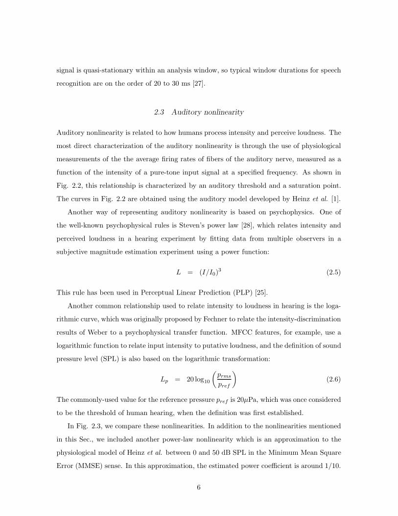
Auditory nonlinearity is related to how humans process intensity and perceive loudness. The

most direct characterization of the auditory nonlinearity is through the use of physiological

measurements of the the average firing rates of fibers of the auditory nerve, measured as a

function of the intensity of a pure-tone input signal at a specified frequency. As shown in

Fig. 2.2, this relationship is characterized by an auditory threshold and a saturation point.

The curves in Fig. 2.2 are obtained using the auditory model developed by Heinz et al. [1].

Another way of representing auditory nonlinearity is based on psychophysics. One of

the well-known psychophysical rules is Steven’s power law [28], which relates intensity and

perceived loudness in a hearing experiment by fitting data from multiple observers in a

subjective magnitude estimation experiment using a power function:

L = (I/I0)3 (2.5)

This rule has been used in Perceptual Linear Prediction (PLP) [25].

Another common relationship used to relate intensity to loudness in hearing is the loga-

rithmic curve, which was originally proposed by Fechner to relate the intensity-discrimination

results of Weber to a psychophysical transfer function. MFCC features, for example, use a

logarithmic function to relate input intensity to putative loudness, and the definition of sound

pressure level (SPL) is also based on the logarithmic transformation:

Lp = 20 log10

(

prms

pref

)

(2.6)

The commonly-used value for the reference pressure pref is 20µPa, which was once considered

to be the threshold of human hearing, when the definition was first established.

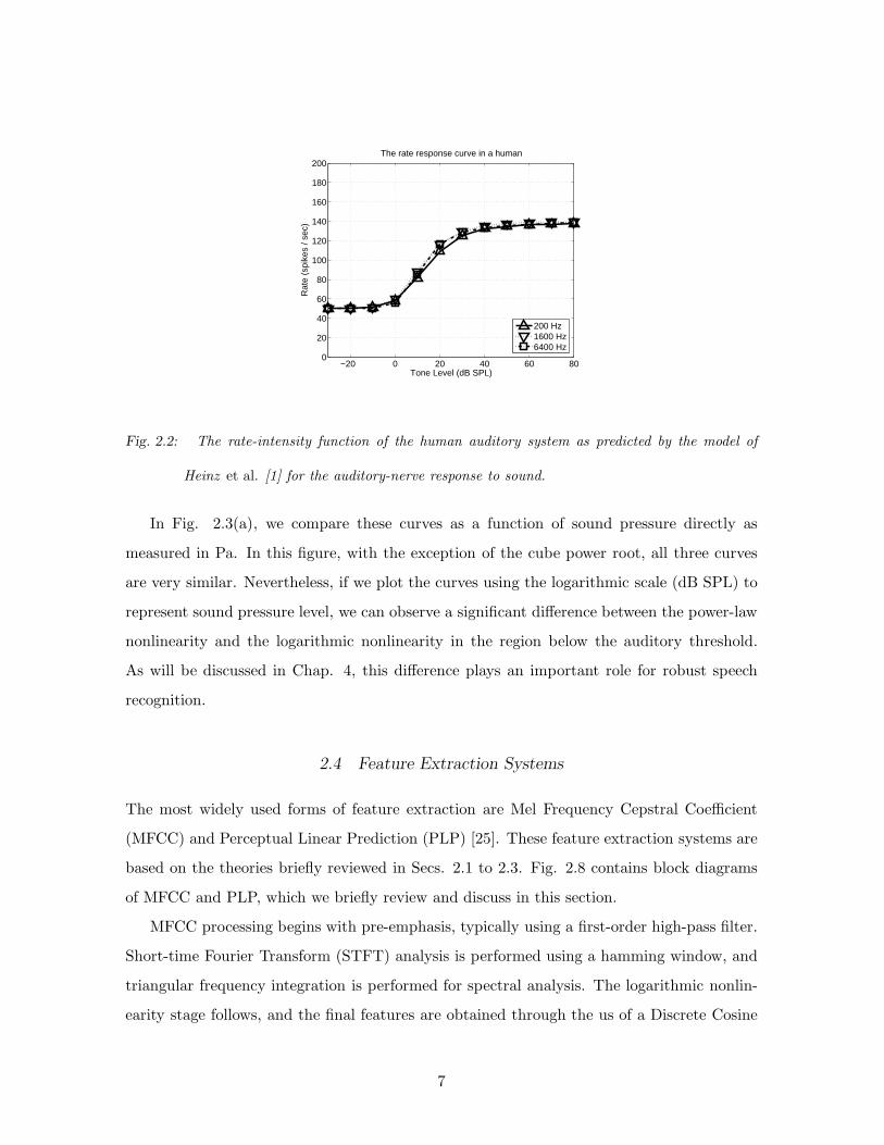
In Fig. 2.3, we compare these nonlinearities. In addition to the nonlinearities mentioned

in this Sec., we included another power-law nonlinearity which is an approximation to the

physiological model of Heinz et al. between 0 and 50 dB SPL in the Minimum Mean Square

Error (MMSE) sense. In this approximation, the estimated power coefficient is around 1/10.

6

−20 0 20 40 60 800

20

40

60

80

100

120

140

160

180

200

Tone Level (dB SPL)

Rat

e (s

pike

s / s

ec)

The rate response curve in a human

200 Hz1600 Hz6400 Hz

Fig. 2.2: The rate-intensity function of the human auditory system as predicted by the model of

Heinz et al. [1] for the auditory-nerve response to sound.

In Fig. 2.3(a), we compare these curves as a function of sound pressure directly as

measured in Pa. In this figure, with the exception of the cube power root, all three curves

are very similar. Nevertheless, if we plot the curves using the logarithmic scale (dB SPL) to

represent sound pressure level, we can observe a significant difference between the power-law

nonlinearity and the logarithmic nonlinearity in the region below the auditory threshold.

As will be discussed in Chap. 4, this difference plays an important role for robust speech

recognition.

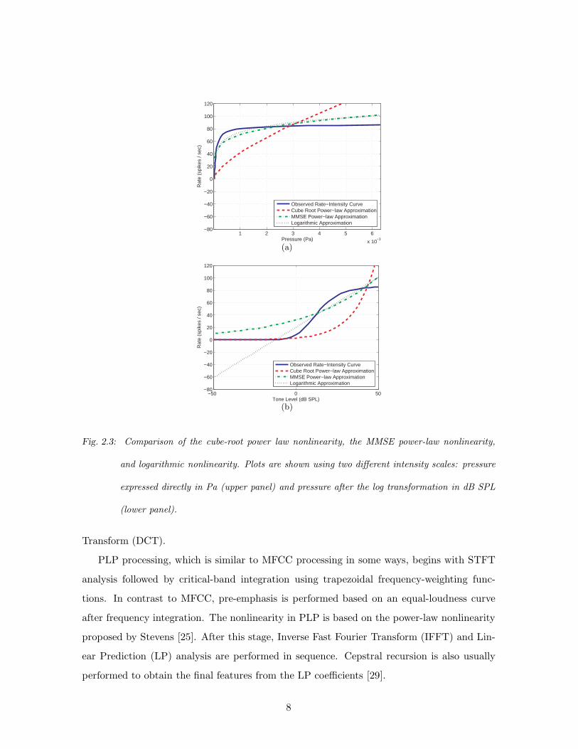
2.4 Feature Extraction Systems

The most widely used forms of feature extraction are Mel Frequency Cepstral Coefficient

(MFCC) and Perceptual Linear Prediction (PLP) [25]. These feature extraction systems are

based on the theories briefly reviewed in Secs. 2.1 to 2.3. Fig. 2.8 contains block diagrams

of MFCC and PLP, which we briefly review and discuss in this section.

MFCC processing begins with pre-emphasis, typically using a first-order high-pass filter.

Short-time Fourier Transform (STFT) analysis is performed using a hamming window, and

triangular frequency integration is performed for spectral analysis. The logarithmic nonlin-

earity stage follows, and the final features are obtained through the us of a Discrete Cosine

7

1 2 3 4 5 6

x 10−3

−80

−60

−40

−20

0

20

40

60

80

100

120

Pressure (Pa)

Rat

e (s

pike

s / s

ec)

Observed Rate−Intensity CurveCube Root Power−law ApproximationMMSE Power−law ApproximationLogarithmic Approximation

(a)

−50 0 50−80

−60

−40

−20

0

20

40

60

80

100

120

Tone Level (dB SPL)

Rat

e (s

pike

s / s

ec)

Observed Rate−Intensity CurveCube Root Power−law ApproximationMMSE Power−law ApproximationLogarithmic Approximation

(b)

Fig. 2.3: Comparison of the cube-root power law nonlinearity, the MMSE power-law nonlinearity,

and logarithmic nonlinearity. Plots are shown using two different intensity scales: pressure

expressed directly in Pa (upper panel) and pressure after the log transformation in dB SPL

(lower panel).

Transform (DCT).

PLP processing, which is similar to MFCC processing in some ways, begins with STFT

analysis followed by critical-band integration using trapezoidal frequency-weighting func-

tions. In contrast to MFCC, pre-emphasis is performed based on an equal-loudness curve

after frequency integration. The nonlinearity in PLP is based on the power-law nonlinearity

proposed by Stevens [25]. After this stage, Inverse Fast Fourier Transform (IFFT) and Lin-

ear Prediction (LP) analysis are performed in sequence. Cepstral recursion is also usually

performed to obtain the final features from the LP coefficients [29].

8

Fig. 2.4: Block diagrams of MFCC and PLP processing.

Fig. 2.5 compares the speech recognition accuracy obtained under various types of noisy

conditions. We used subsets of 1600 utterances for training and 600 utterances for testing

from the DARPA Resource Management 1 Corpus (RM1). In other experiments, which are

shown in Fig. 2.6, we used the DARPA Wall Street Journal WSJ0-si84 training set and

WSJ0 5k test set. For training the acoustical models we used SphinxTrain 1.0 and for

decoding, we used Sphinx 3.8.

9

For MFCC processing, we used sphinxe fe included in sphinxbase 0.4.1. For PLP

processing, we used both HTK 3.4 and the MATLAB package provided by Dan Ellis and

colleagues at Columbia University [30]. Both of the PLP packages show similar performance,

except for the for reverberation and interfering speaker environments, where the version of

PLP included in HTK provided better performance.

In all these experiments, we used 12th-order feature vectors including the zeroth coeffi-

cient, along with the corresponding delta and delta-delta cepstra. As shown in these figures,

MFCC and PLP show provide speech recognition accuracy. Nevertheless, in our experi-

ments we found that RASTA processing is not as helpful as conventional Cepstral Mean

Normalization (CMN).

2.5 Noise Power Subtraction Algorithms

In this section we discuss conventional ways of accomplishing noise power compensation,

focussing on the original spectral subtraction technique of Boll [11] and Hirsch [31]. The

biggest difference between the Boll’s and Hirsch’s approaches is how to estimate noise level.

In the Boll’s approach, voice activity detector (VAD) runs first, and noise level is estiamted

from the non-speech segment. In Hirsch’s approach, the noise level is conditionally updated

by comparing the current power level and the estimated noise level.

2.5.1 Boll’s approach

Boll proposed the first noise subtraction technique, of which dozens if not hundreds of variants

have been proposed since Boll’s original algorithm. The first step in Boll’s historic approach

is the use of a Voice Activity Detector (VAD) which determines whether or not the current

frame contains speech, and an estimate of the noise spectrum is obtained by averaging power

spectra from frames in which speech is absent. Frames in which speech is present are modified

by subtracting the noise in the following fashion:

|X [m, l]| = max(|X(m, l)| −N(m, l), δ|X(m, l)|) (2.7)

where N(m, l) is the noise spectrum, X(m, l) is the corrupt speech spectrum, and δ is a small

constant to prevent the subtracted spectrum from having a negative spectrum value. The

10

indices m and l denote the frame number and channel number, respectively.

2.5.2 Hirsch’s approach

Hirsch [31] proposed a noise-compensation method that was similar to that of Boll, but with

the fixed estimate of the power spectrum of the noise replaced by a running average estimate

using a simple difference equation:

|N(m, l)| = λ|N(m− 1, l)| + (1− λ)|X(m, l)| if|X(m, l)| < β|N(m, l)| (2.8)

where m is the frame index and l is the frequency index. We note that the above equation

is realizes in effect a first-order IIR lowpass filter. If the magnitude spectrum is larger

than βN(m, l), the estimate noise spectrum is not updated. Hirsch suggested using a value

between 1.5 and 2.5 for β.

2.6 Algorithms Motivated by Modulation Frequency

It has long been believed that modulation frequency plays an important role in human

listening. For example, it has been observed that the human auditory system is most sensitive

to modulation frequencies that are less than 20 Hz (e.g. [32] [33] [34]). On the other

hand, very slowly-changing components (e.g. less than 5 Hz) are usually related to noisy

sources (e.g. [35] [36] [37]). In some studies (e.g [2]) it has been argued that speaker-specific

information dominates for frequencies below 10Hz, while speaker-independent information

dominates higher frequencies. Based on these observations, many researchers have tried to

utilize modulation-frequency information to enhance speech recognition accuracy in noisy

environments. Typical approaches use high-pass or band-pass filtering in either the spectral,

log-spectral, or cepstral domains.

In [2], Hirsch et al. investigated the effects of high-pass filtering the spectral envelopes of

each subband after the initial bandpass filtering that is commonly used in signal processing

based on auditory processing. Unlike the RASTA processing proposed by Hermansky in [3],

Hirsch et al. conducted the high-pass filtering in the power domain (rather than in the log

power domain). They compared FIR filtering with IIR filtering, and concluded that the

latter approach is more effective. Their final system used the following first-order IIR filter:

11

H(z) =1− z−1

1− 0.7z−1(2.9)

where λ is a coefficient that adjusts the cut-off frequency. This is a simple high-pass filter

with a cut-off frequency at around 4.5 Hz.

It has been observed that online implementation of Log Spectral Mean Subtraction

(LSMS) is largely similar to RASTA processing. Mathematically, the online mean log-

spectral subtraction is equivalent to online CMN:

µL(m, l) = λµY (m− 1, l) + (1− λ)Y (m, l) (2.10)

where

Y (m, l) = P (m, l)− µP (m, l) (2.11)

This is also a high-pass filter like Hirsch’s approach, but the major difference is that Hirsch

conducted the high-pass filtering in the power domain, while in the LSMS, subtraction is done

after applying the log-nonlinearity. Theoretically speaking, filtering in the power domain

should be helpful in compensating for additive noise, while filtering in the log-spectral domain

should be better for ameliorating the effects of linear filtering including reverberation [6].

RASTA processing in [3] is similar to online cepstral mean subtraction and online LSMS.

While online cepstral mean subtraction is basically first-order high-pass filtering, RASTA

processing is actually bandpass processing motivated by the modulation-frequency concept.

This processing was based on the observation that the human auditory system is most

sensitive to modulation frequencies between 5 and 20 Hz (e.g. [33] [34]). Hence, signal

components outside this modulation frequency range are not likely to originate from speech.

In RASTA processing, Hermansky proposed the following fourth-order bandpass filtering:

H(z) = 0.1z42 + z−1 − z−3 − 2z−4

1− 0.98z−1(2.12)

As in the case of online CMN, RASTA processing is performed after the nonlinearity is

applied.

Hermansky [3] showed that band-pass filtering approach results in better performance

than high-pass filtering. In the original RASTA processing in Eq. (2.12), the pole location

12

was at z = 0.98; later, Hermansky suggested that z = 0.94 seems to be optimal [3]. Never-

theless, in some articles (e.g. [6]), it has been reported that online CMN (which is a form

of high-pass filtering) provides slightly better speech recognition accuracy than RASTA pro-

cessing (which is a form of band-pass filtering). As mentioned above, if we perform filtering

after applying the log-nonlinearity, then it would be more helpful for reverberation, but it

might not be very helpful for additive noise.

Hermansky and Morgan also proposed a variation of RASTA, called J-RASTA (or Lin-

Log RASTA) that uses the following function:

y = log(1 + Jx) (2.13)

This model has characteristics of both the linear model and the logarithmic nonlinearity and

in principle compensates for additive noise at low SNRs and for linear filtering at higher

SNRs.

2.7 Normalization Algorithms

In this section, we discuss some algorithms that are designed for enhancing robustness against

noise by matching the statistical characteristics of the training and testing environments.

Many of these algorithms operate in the feature domain including Cepstral Mean Normal-

ization (CMN), Mean Variance Normalization (MVN), Code-Dependent Cepstral Normaliza-

tion (CDCN), and Histogram Normalization (HN). The original form of VTS (Vector Taylor

Series) works in the log-spectral domain.

2.7.1 CMN, MVN, HN, and DCN

The simplest way of performing normalization is using CMN or MVN. Histogram normal-

ization (HN) is a generalization of these approaches. CMN is the most basic form of noise

compensation schemes, and it can remove the effects of linear filtering if the impulse response

of the filter is shorter then the window length [38]. By assuming that the mean of each ele-

ment of the feature vector from all utterances is the same, CMN is also helpful for additive

13

noise as well. CMN can be expressed mathematically as follows:

ci[j] = ci[j] − µci, 0 ≤ i ≤ I − 1, 0 ≤ j ≤ J − 1 (2.14)

where µci is the mean of the ith element of the cepstral vector. In the above equation, ci[j]

and ci[j] represent the original and normalized cepstral coefficients for the ith element of

the vector at the jth frame index. I denotes the dimensionality of the feature vector and J

denotes the number of frames in the utterance.

MVN is a natural extension of CMN and is defined by the following equation:

ci[j] =ci[j] − µci

σci, 0 ≤ i ≤ I − 1, 0 ≤ j ≤ J − 1 (2.15)

where µci and σci are the mean and standard deviation of the i-th element of the cepstral

vector.

As mentioned in Sec. 2.6, CMN can be implemented as an online algorithm (e.g. [7] [39]

[40]) where the mean of the cepstral vector is updated recursively.

µci [j] = λµci [j − 1] + (1− λ)ci[j], 0 ≤ i ≤ I − 1, 0 ≤ j ≤ J − 1 (2.16)

This online mean is subtracted from the current cepstral vector.

As in RASTA and online log-spectral mean subtraction, the initialization of the mean

value is very important in online CMN. Otherwise, the performance would be significantly

degraded (e.g. [6] [7]). It has been shown that using values obtained from the previous

utterances is a good means of initialization. Another method is to run a VAD to detect

the first non-speech-to-speech transition (e.g. [7]). If the center of the initialization window

coincides with the first non-speech-to-speech transition, then good performance is preserved,

but this method requires a small amount of processing delay.

In HN, it is assumed that the Cumulative Distribution Function (CDF) for an element

of a feature is the same for all utterances.

ci[j] = F−1ctri

(

Fctei(ci[j])

)

(2.17)

In the above equation, Fcteidenotes the CDF of the current test utterance and F−1

ctri

denotes

the inverse CDF from the entire training corpus. Using (2.17) we can make the distribution

14

of the element of the test utterance the same as that of the entire training corpus. We can

also perform HN in a slightly different way by assuming that every element of the feature

follows a Gaussian distribution with zero mean and unit variance. In this case, F−1ctri

is just

the inverse CDF of the Gaussian distribution with zero mean and unity variance. If we use

this approach, then the training database also needs to be normalized.

Recently, Obuchi [8] showed that if we do apply histogram normalization on the delta

cepstrum as well as on the original cepstrum, recognition accuracy is better than with the

original HN. This approach is called DCN (delta cepstrum normalization).

Fig. 2.9 shows speech recognition accuracy obtained using the RM1 database. First, we

observe that CMN provides significant benefit for noise robustness. MVN performs somewhat

better than CMN. Although HN is a very simple algorithm, it shows significant improvements

for the white noise and street noise environments. DCN provides the largest threshold shift

among all these algorithms. Fig. 2.10 shows the the results of similar experiments conducted

on the WSJ0 5k test set, using WSJ0-si84 dataset for training.

Although these approaches show improvements in noisy environments, they are also very

sensitive to the length of silence that precedes the speech, as shown in Fig. 2.11. This is

because in these approaches it is assumedd that all distributions are the same and if we

prepend or append silences this assumption no longer remains valid. As a consequence,

DCN provides better accuracy than Vector Taylor Series (VTS) in the RM white noise and

street noise environments, but the former is doing worse than the latter in the WSJ0 5k

experiment, which include more silences. Experimental results obtained using VTS will be

described in more detail in the next section.

2.7.2 CDCN and VTS

More advanced algorithms including CDCN (Code-Dependent Cepstral Normalization) and

VTS (Vector Taylor Series) attempt to simultaneously compensate for the effects of additive

noise and linear filtering. In this section we briefly review a selection of these techniques.

In CDCN and VTS the underlying assumption is that speech is corrupted by unknown

additive noise and linear filtering by an unknown channel [41]. This assumption can be

15

represented by the following equation:

Pz(ejwk) = Px(e

jwk)|H(ejwk)|2 + Pn(ejwk)

= Px(ejwk)|H(ejwk)|2

(

1 +Pn(e

jwk)

Px(ejwk)|H(ejwk)|2

)

(2.18)

Noise compensation can be performed either in the log spectral domain [10] or in the

cepstral domain [9]. In this subsection we describe compensation in the log spectral domain.

Let x, n, q, and z denote the logarithms of the powewr spectral densities Px(ejwk), Pn(e

jwk),

|H(ejwk)|2, and Pz(ejwk), respectively. For simplicity, we will remove the frequency index

wk in the following discussions. Then (2.18) can be expressed in the following form:

z = x+ q + log(1 + en−x−q) (2.19)

This equation can be rewritten in the form of

z = x+ q + r(x, n, q) = x+ f(x, n, q) (2.20)

where f(x, n, q) is called the “environment function” [41].

Thus, our objective is inverting the effect of the environment function f(x, n, q). This

inversion consists of two independent problems. The first problem is estimating the parame-

ters needed for the environment function. The second problem is finding the Minimum Mean

Square Error (MMSE) estimate of x given z in (2.20).

In the CDCN approach, it is assumed that x is represented by the following Gaussian

mixture and n and q are unknown constants:

f(x) =

M−1∑

k=0

ckN(µx,k,Σx,k) (2.21)

The vectors n and q are obtained by maximizing the following likelihood:

(n, q) = argmaxn,q

p(z|q, n) (2.22)

The maximization of the above equation is performed using the Expectation Maximiza-

tion (EM) algorithm. After obtaining n and q, x is obtained in the Minimum Mean Square

Error (MMSE) sense. In CDCN it is assumed that n and q are constants for that utterance,

so CDCN cannot efficiently handle non-stationary noise [42].

16

In the VTS approach, it is assumed that the probability density function (PDF) of the

log spectral density of clean utterance is represented by a GMM (Gaussian Mixture Model)

and that noise is represented by a single Gaussian component.

f(x) =

M−1∑

k=0

ckN(µx,k,Σx,k) (2.23)

f(n) = N(µn, |Σn) (2.24)

The VTS approach attempts to reverse the effect of the environment function in Eq.

(2.20). Because this function is nonlinear, it is not easy to find an environmental function

which maximizes the likelihood. This problem is made more tractable by using the first-order

Taylor series approximation. From (2.20), we consider the following first-order Taylor series

expansion of the environment function f(x, n, q):

µz = E [x+ f(n0, x0, q0)] + E

[

δ

δxf(x0, n0, q0)(x− x0))

]

E

[

δ

δnf(x0, n0, q0)(n− n0))

]

+ E

[

δ

δqf(x0, n0, q0)(q − q0))

]

(2.25)

The resulting distribution z is also Gaussian if x is Gaussian.

In a similar fashion, we also obtain the covariance matrix:

Σz =

(

I +d

dxf(n0, x0, q0)

)T

Σx

(

I +d

dxf(n0, x0, q0)

)

(

d

dxf(n0, x0, q0)

)T

Σn

(

d

dxf(n0, x0, q0)

)

(2.26)

Using the above approximations for the means and covariances of the Gaussian com-

ponents, q, µn, and hence µz and Σz are obtained using the EM method to maximize the

likelihood.

Finally, feature compensation is conducted in the MMSE sense as shown below.

xMMSE = E[X|z] (2.27)

=

∫

xp(x|z)dx (2.28)

[COMMENTS/DISCUSSION OF FIGS. 2.11 AND 2.12 SEEMS TO BE MISSING]

17

2.8 ZCAE and related algorithms

It has been long observed that human beings are remarkable in their ability to separate

sound sources. Many research results (e.g. [43, 44, 45]) have supported the contention that

binaural interaction plays an important role in sound source separation. For low frequencies,

the use of interaural time delay (ITD) is primarily used for sound source separation; for high

frequencies, interaural intensity difference (IID) plays an important role. This is because for

high frequencies, spatial aliasing occurs, which prevents the effective use of ITD information,

although ITDs of the low-frequency envelopes of high-frequency signals may be used in

localization.

In ITD-based sound source separation approaches (e.g. [46] [18]), we frequently use a

smaller distance between two microphones than the actual distance between two ears to avoid

spatial aliasing problems.

The conventional way of calculating the ITD (and the way the human binaural system is

believed to calculate ITDs) by computing the cross-correlation of the signals to the two mi-

crophones after they are passed through the bank of bandpass filters that is used to model the

frequency selectivity of the peripheral auditory system. In more recent work [18], it has been

shown that a zero-crossing approach is more effective than the cross-correlation approach for

accurately estimating the ITD, and resulting in better speech recognition accuracy, at least

in the absence of reverberation. This approach is called Zero Crossing Amplitude Estimation

(ZCAE).

However, one critical problem of ZCAE is that the zero crossing point is heavily affected

by in-phase noise and reverberation. Thus, as shown in [19] and [46], the ZCAE method

does not produce successful results in environments that include reverberation and/or omni-

directional noise.

2.9 Discussion

While it is generally agreed that a window length between 20 ms and 30 ms is appropriate for

speech analysis, as mentioned in Section 2.2, there is no guarantee that this window length

will remain optimal for the estimation of or the compensation for additive-noise components.

18

Since the noise characteristics are usually stationary compared to speech, it is expected that

longer windows might be more helpful for noise compensation purposes. In this thesis we

will consider what would be the optimal window length for noise compensation purposes.

We note that even though longer duration windows may be used for noise compensation, we

still need short duration windows for the actual speech recognition. We will discuss methods

for accomplishing this in Chapter 3 of this thesis.

In Section 2.3, we discussed several different rate-level nonlinearities based on different

data. Up until now, there has not been much discussion or analysis of the type of nonlinearity

that is best for feature extraction. For a nonlinearity to be appropriate, it should satisfy

some of the following characteristics:

• It should be robust with respect to the presence of additive noise and reverberation.

• It should discriminate each phone reasonably well.

• The nonlinearity should be independent of the absolute input sound pressure level, or

at worst, a simple normalization should be able to remove the effect of the input sound

pressure level.

Based on the above criteria, we will discuss in Chapter 4 of this thesis the nature of

appropriate nonlinearities to be used for feature extraction.

We discussed conventional spectral subtraction techniques in Section 2.5. The problem

with conventional spectral subtraction is that the structure is complicated and the perfor-

mance depends on the accuracy of the VAD. Instead of using this conventional approach,

since speech power changes faster than noise power, we can use the rate of power change as

a measure for power normalization.

Although algorithms like VTS are very successful for stationary noise, they have some

intrinsic problems. First, VTS is computationally costly, since it is based on a large number

of mixture components and an iterative EM algorithm, which is used for maximizing the

likelihood. Second, this model assumes that the noise component is modeled by a single

Gaussian component in the log spectral domain. This assumption is reasonable in many

cases, but it is not always true. A more serious problem is that the noise component is

assumed to be stationary, which is not quite true for non-stationary noise, like music noise.

19

Finally, since VTS requires maximizing the likelihood using the values in the current test

set, it is not straightforward to implement this algorithm for real-time applications.

In the work described in later chapters of this thesis, we will develop an algorithm that

is motivated by auditory observations, that imposes a smaller computational burden, and

that can be implemented as an online algorithm that operates in sub-real time with only a

very small delay. Instead of trying to estimate the environment function and maximizing the

likelihood, which is very computationally costly, we will simply use the rate of power change

or power distribution of the test utterance.

While the ZCAE algorithm described in Section 2.8 shows remarkable performance, it

does not provide much benefit in reverberant environments [19][46]. Another problem is

that this algorithm requires large computation[46], since it needs bandpass filtering. for

these reasons we consider various two-microphone approaches that provide greater robustness

with respect to reverberation in Chapters 9 and 10 of this thesis. We summarize our major

conclusions and provide suggestions for future work in Chapter 11.

20

0 5 10 15 20 Clean0

20

40

60

80

100

SNR (dB)

Acc

urac

y (1

00 −

WE

R)

RM1 (White Noise)

PLP with CMNPLP in HTK with CMNRASTA−PLP with CMNMFCC with CMN

(a)

0 5 10 15 20 Clean0

20

40

60

80

100

SNR (dB)

Acc

urac

y (1

00 −

WE

R)

RM1 (Street Noise)


(b)

0 5 10 15 20 Clean0

20

40

60

80

100

SNR (dB)

Acc

urac

y (1

00 −

WE

R)

RM1 (Music Noise)


(c)

0 5 10 15 20 Clean0

20

40

60

80

100

SIR (dB)

Acc

urac

y (1

00 −

WE

R)

RM1 (Interfering Speaker)


(d)

0 0.1 0.2 0.3 0.4 0.5 0.6 0.9 1.20

20

40

60

80

100

Reverberation Time (s)

Acc

urac

y (1

00 −

WE

R)

RM1 (Reverberation)


(e)

Fig. 2.5: Comparison of MFCC and PLP processing in different environments using the RM1 test

set: (a) additive white gaussian noise, (b) street noise, (c) background music, (c) interfering

speaker, and (d) reverberation.

21

0 5 10 15 20 Clean0

20

40

60

80

100

SNR (dB)

Acc

urac

y (1

00 −

WE

R)

WSJ0−5k (White Noise)


(a)

0 5 10 15 20 Clean0

20

40

60

80

100

SNR (dB)

Acc

urac

y (1

00 −

WE

R)

WSJ0−5k (Street Noise)


(b)

0 5 10 15 20 Clean0

20

40

60

80

100

SNR (dB)

Acc

urac

y (1

00 −

WE

R)

WSJ0−5k (Music Noise)


(c)

0 5 10 15 20 Clean0

20

40

60

80

100

SIR (dB)

Acc

urac

y (1

00 −

WE

R)

WSJ0−5k (Interfering Speaker)


(d)

0 0.1 0.2 0.3 0.4 0.5 0.6 0.9 1.20

20

40

60

80

100


Acc

urac

y (1

00 −

WE

R)

WSJ0−5k (Reverberation)


(e)

Fig. 2.6: Comparison of MFCC and PLP in different environments using the WSJ0 5k test set: (a)

additive white gaussian noise, (b) street noise, (c) background music, (c) interfering speaker,

and (d) reverberation.

22

0 10 20 30 40 50−30

−25

−20

−15

−10

−5

0

5

10

Mag

nitu

de R

espo

nse

(dB

)

Frequency (Hz)

Fig. 2.7: The frequency response of the high-pass filter proposed by Hirsch et al. [2]

0 10 20 30 40 50−30

−25

−20

−15

−10

−5

0

Mag

nitu

de R

espo

nse

(dB

)

Frequency (Hz)

Fig. 2.8: The frequency response of the band-pass filter proposed by Hermansky et al. [3].

23

0 5 10 15 20 Clean0

20

40

60

80

100

SNR (dB)

Acc

urac

y (1

00 −

WE

R)

RM1 (White Noise)

DCNHNMVNMFCC with CMNMFCC without CMN

(a)

0 5 10 15 20 Clean0

20

40

60

80

100

SNR (dB)

Acc

urac

y (1

00 −

WE

R)

RM1 (Street Noise)


(b)

0 5 10 15 20 Clean0

20

40

60

80

100

SNR (dB)

Acc

urac

y (1

00 −

WE

R)

RM1 (Music Noise)


(c)

0 5 10 15 20 Clean0

20

40

60

80

100

SIR (dB)

Acc

urac

y (1

00 −

WE

R)



(d)

0 0.1 0.2 0.3 0.4 0.5 0.6 0.9 1.20

20

40

60

80

100


Acc

urac

y (1

00 −

WE

R)

RM1 (Reverberation)


(e)

Fig. 2.9: Comparison of different normalization approaches in different environments on the RM1 test

set: (a) additive white gaussian noise, (b) street noise, (c) background music, (c) interfering

speaker, and (d) reverberation.

24

0 5 10 15 20 Clean0

20

40

60

80

100

SNR (dB)

Acc

urac

y (1

00 −

WE

R)



(a)

0 5 10 15 20 Clean0

20

40

60

80

100

SNR (dB)

Acc

urac

y (1

00 −

WE

R)



(b)

0 5 10 15 20 Clean0

20

40

60

80

100

SNR (dB)

Acc

urac

y (1

00 −

WE

R)



(c)

0 5 10 15 20 Clean0

20

40

60

80

100

SIR (dB)

Acc

urac

y (1

00 −

WE

R)



(d)

0 0.1 0.2 0.3 0.4 0.5 0.6 0.9 1.20

20

40

60

80

100


Acc

urac

y (1

00 −

WE

R)



(e)

Fig. 2.10: Comparison of different normalization approaches in different environments on the WSJ0

5k test set: (a) additive white gaussian noise, (b) street noise, (c) background music, (c)

interfering speaker, and (d) reverberation.

25

0 4 8 160

20

40

60

80

100

Total Silence Prepended and Appended (s)

Acc

urac

y (1

00 −

WE

R)

RM1 (Appended Silence (Clean))


(a)

0 4 8 160

20

40

60

80

100

Total Silence Prepended and Appended (s)

Acc

urac

y (1

00 −

WE

R)

RM1 (Appended Silence + White Noise 10−dB)


(b)

Fig. 2.11: Recognition accuracy as a function of appended and prepended silence without (left panel)

and with (right panel) white Gaussian noise added at an SNR of 10 dB.

26

0 5 10 15 20 Clean0

20

40

60

80

100

SNR (dB)

Acc

urac

y (1

00 −

WE

R)

RM1 (White Noise)

VTSBaseline MFCC with CMN

(a)

0 5 10 15 20 Clean0

20

40

60

80

100

SNR (dB)

Acc

urac

y (1

00 −

WE

R)

RM1 (Street Noise)


(b)

0 5 10 15 20 Clean0

20

40

60

80

100

SNR (dB)

Acc

urac

y (1

00 −

WE

R)

RM1 (Music Noise)


(c)

0 5 10 15 20 Clean0

20

40

60

80

100

SIR (dB)

Acc

urac

y (1

00 −

WE

R)



(d)

0 0.1 0.2 0.3 0.4 0.5 0.6 0.9 1.20

20

40

60

80

100


Acc

urac

y (1

00 −

WE

R)

RM1 (Reverberation)


(e)

Fig. 2.12: Comparison of different normalization approaches in different environments using the

RM1 test set: (a) additive white gaussian noise, (b) street noise, (c) background music, (c)

interfering speaker, and (d) reverberation.

27

0 5 10 15 20 Clean0

20

40

60

80

100

SNR (dB)

Acc

urac

y (1

00 −

WE

R)



(a)

0 5 10 15 20 Clean0

20

40

60

80

100

SNR (dB)

Acc

urac

y (1

00 −

WE

R)



(b)

0 5 10 15 20 Clean0

20

40

60

80

100

SNR (dB)

Acc

urac

y (1

00 −

WE

R)



(c)

0 5 10 15 20 Clean0

20

40

60

80

100

SIR (dB)

Acc

urac

y (1

00 −

WE

R)



(d)

0 0.1 0.2 0.3 0.4 0.5 0.6 0.9 1.20

20

40

60

80

100


Acc

urac

y (1

00 −

WE

R)



(e)

Fig. 2.13: Comparison of different normalization approaches in different environments using the

WSJ0 test set: (a) additive white gaussian noise, (b) street noise, (c) background music,

(c) interfering speaker , and (d) reverberation.

28

3. TIME AND FREQUENCY RESOLUTION

It is widely known that there is a trade-off between time resolution and frequency resolution

when we select an appropriate window length for frequency-domain analysis (e.g. [27]). If

we want to obtain better frequency-domain resolution, a longer window is more appropriate

since the Fourier transform of a longer window is closer to a delta function in the frequency

domain. However, a longer window is worse in terms of time resolution, and this is especially

true for highly non-stationary signals like speech. In speech analysis, we want the signal

within a single window to be stationary. As a compromise between these tradeoffs, a window

length between 20 ms and 30 ms has been widely used in speech processing (e.g. [27]).

Although a window of 20-30 ms is suitable for analyzing speech signals, if the statistical

characteristics of a certain signal do not change very quickly a longer window will be better.

If we use a longer window, we can analyze the noise spectrum in a better way. Also from large

sample theory, if we use more data in estimating statistics, then the variance of the estimate

will be reduced. Since noise power changes more slowly than speech signal power, longer

windows are expected to be better for estimating the noise power or noise characteristics.

Nevertheless, even if we use longer windows for noise compensation or normalization, we still

need to use short windows for feature extraction. In this section, we discuss two general

approaches to accomplish this goal, the Medium-duration-window Analysis and Synthesis

(MAS) method, and the Medium-duration-window Running Average (MRA) method.

We know from large sample theory that statistical parameter estimation provides esti-

mates with smaller variance as the amount of available data increases. While we previously

addressed this concept in terms of the duration of the analysis window used for speech

processing, we now consider integration along the frequency axis as well. In the analysis-

and-synthesis approach, we perform frequency analysis by directly estimating parameters

for each discrete-time frequency index. Nevertheless, we observe that the channel-weighting

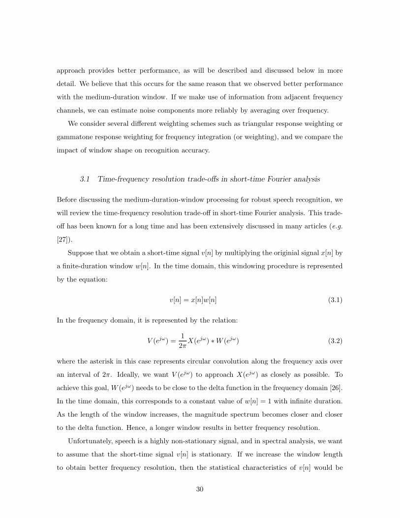
approach provides better performance, as will be described and discussed below in more

detail. We believe that this occurs for the same reason that we observed better performance

with the medium-duration window. If we make use of information from adjacent frequency

channels, we can estimate noise components more reliably by averaging over frequency.

We consider several different weighting schemes such as triangular response weighting or

gammatone response weighting for frequency integration (or weighting), and we compare the

impact of window shape on recognition accuracy.

3.1 Time-frequency resolution trade-offs in short-time Fourier analysis

Before discussing the medium-duration-window processing for robust speech recognition, we

will review the time-frequency resolution trade-off in short-time Fourier analysis. This trade-

off has been known for a long time and has been extensively discussed in many articles (e.g.

[27]).

Suppose that we obtain a short-time signal v[n] by multiplying the originial signal x[n] by

a finite-duration window w[n]. In the time domain, this windowing procedure is represented

by the equation:

v[n] = x[n]w[n] (3.1)

In the frequency domain, it is represented by the relation:

V (ejω) =1

2πX(ejω) ∗W (ejω) (3.2)

where the asterisk in this case represents circular convolution along the frequency axis over

an interval of 2π. Ideally, we want V (ejω) to approach X(ejω) as closely as possible. To

achieve this goal, W (ejω) needs to be close to the delta function in the frequency domain [26].

In the time domain, this corresponds to a constant value of w[n] = 1 with infinite duration.

As the length of the window increases, the magnitude spectrum becomes closer and closer

to the delta function. Hence, a longer window results in better frequency resolution.

Unfortunately, speech is a highly non-stationary signal, and in spectral analysis, we want

to assume that the short-time signal v[n] is stationary. If we increase the window length

to obtain better frequency resolution, then the statistical characteristics of v[n] would be

30

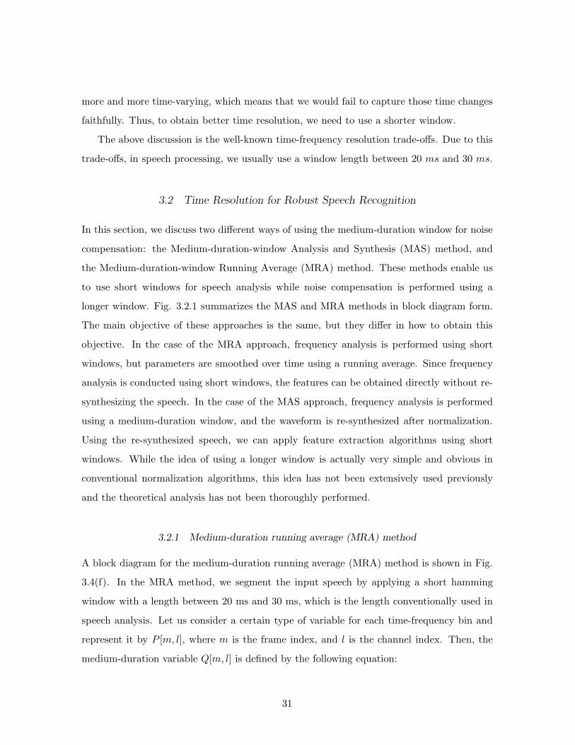
more and more time-varying, which means that we would fail to capture those time changes

faithfully. Thus, to obtain better time resolution, we need to use a shorter window.

The above discussion is the well-known time-frequency resolution trade-offs. Due to this

trade-offs, in speech processing, we usually use a window length between 20 ms and 30 ms.

3.2 Time Resolution for Robust Speech Recognition

In this section, we discuss two different ways of using the medium-duration window for noise

compensation: the Medium-duration-window Analysis and Synthesis (MAS) method, and

the Medium-duration-window Running Average (MRA) method. These methods enable us

to use short windows for speech analysis while noise compensation is performed using a

longer window. Fig. 3.2.1 summarizes the MAS and MRA methods in block diagram form.

The main objective of these approaches is the same, but they differ in how to obtain this

objective. In the case of the MRA approach, frequency analysis is performed using short

windows, but parameters are smoothed over time using a running average. Since frequency

analysis is conducted using short windows, the features can be obtained directly without re-

synthesizing the speech. In the case of the MAS approach, frequency analysis is performed

using a medium-duration window, and the waveform is re-synthesized after normalization.

Using the re-synthesized speech, we can apply feature extraction algorithms using short

windows. While the idea of using a longer window is actually very simple and obvious in

conventional normalization algorithms, this idea has not been extensively used previously

and the theoretical analysis has not been thoroughly performed.

3.2.1 Medium-duration running average (MRA) method

A block diagram for the medium-duration running average (MRA) method is shown in Fig.

3.4(f). In the MRA method, we segment the input speech by applying a short hamming

window with a length between 20 ms and 30 ms, which is the length conventionally used in

speech analysis. Let us consider a certain type of variable for each time-frequency bin and

represent it by P [m, l], where m is the frame index, and l is the channel index. Then, the

medium-duration variable Q[m, l] is defined by the following equation:

31

(a) (b)

Fig. 3.1: (a) Bock diagram of the Medium-duration-window Running Average (MRA) Method. (b)

Block diagram of the Medium-duration-window Analysis Synthesis (MAS) Method.

Q[m, l] =1

2M + 1

m+M∑

m′=m−M

P [m′, l] Averaging stage (3.3)

Averaging power across adjacent frames can be represented as a filtering operation with

32

the following transfer function:

H(z) =

M∑

n=−M

z−n (3.4)

This operation can be considered to be a low-pass filtering with the system’s frequency

response given by:

H(ejω) =sin((

2M+12

)

ω)

sin(

ω2

) , (3.5)

and these responses for different M values are shown in 3.2. However we observe that if we

directly perform low-pass filtering, then it has the effect of making the spectrogram quite

blurred, so in many cases, it induces the negative effects as shown in Fig. 3.3.

Thus, instead of performing normalization using the original power P [m, l], we perform

normalization on Q[m, l] as defined in Eq. (8.3). However, instead of using the normalized

medium-duration power Q[m, l] directly to obtain the features, the weighting coefficient is

multiplied by P [m, l] to obtain the normalized power P [m, l]. This procedure is represented

in the following equation:

P [m, l] =Q[m, l]

Q[m, l]P [m, l] (3.6)

An example of MRA is the Power Normalized Cepstral Coefficient (PNCC) algorithm,

which is explained in Subsection 8. In the case of PBS, when we used a 25.6-ms window

length with a 10-ms frame period, M = 2 ∼ 3 showed the best speech recognition accuracy

in noisy environments. So, this approximately corresponds to a window length of 75.6 ∼ 85.6

ms.

3.2.2 Medium duration window analysis and re-synthesis approach

As noted above, the other approach using a longer window for normalization is the MAS

method. This method is described in block diagram form in Fig. 3.4(e). In this method,

we directly apply a longer window to the speech signal to obtain a spectrum. From this

spectrum, we perform normalization. Since we need to use features obtained from short

windows, we cannot directly use the normalized spectrum from a longer window. Thus, a

33

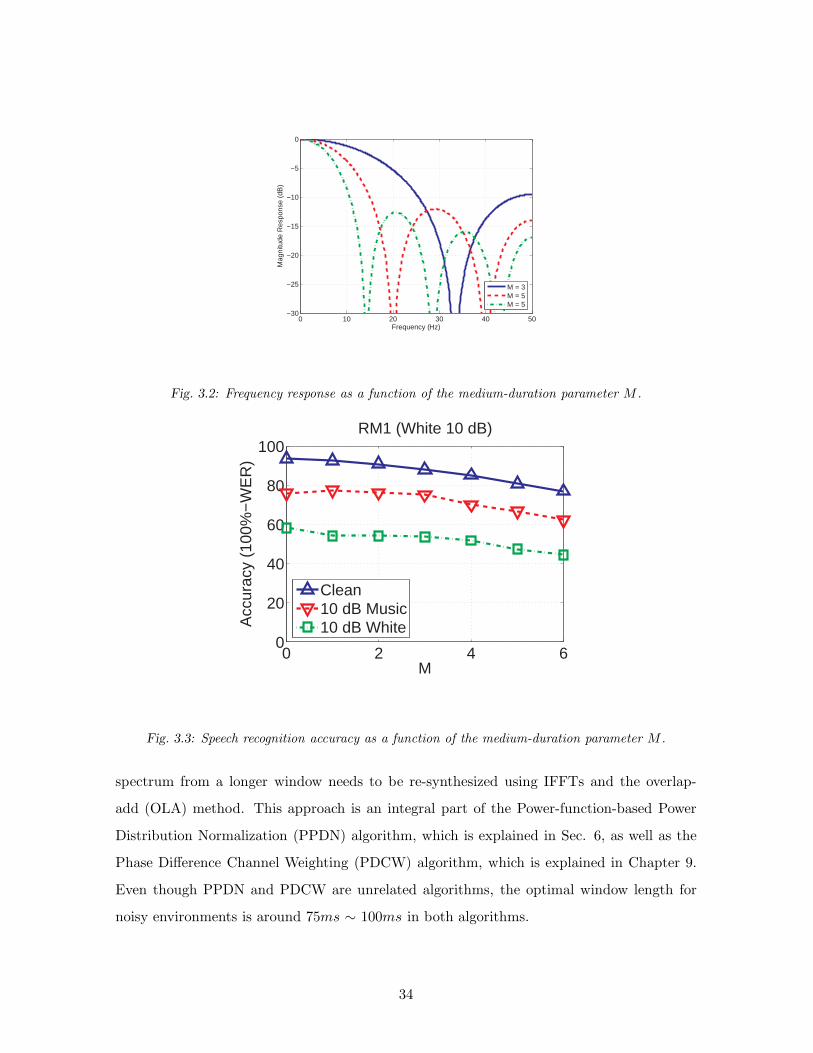
0 10 20 30 40 50−30

−25

−20

−15

−10

−5

0

Frequency (Hz)

Mag

nitu

de R

espo

nse

(dB

)M = 3M = 5M = 5

Fig. 3.2: Frequency response as a function of the medium-duration parameter M .

0 2 4 60

20

40

60

80

100

M

Acc

urac

y (1

00%

−W

ER

)

RM1 (White 10 dB)

Clean10 dB Music10 dB White

Fig. 3.3: Speech recognition accuracy as a function of the medium-duration parameter M .

spectrum from a longer window needs to be re-synthesized using IFFTs and the overlap-

add (OLA) method. This approach is an integral part of the Power-function-based Power

Distribution Normalization (PPDN) algorithm, which is explained in Sec. 6, as well as the

Phase Difference Channel Weighting (PDCW) algorithm, which is explained in Chapter 9.

Even though PPDN and PDCW are unrelated algorithms, the optimal window length for

noisy environments is around 75ms ∼ 100ms in both algorithms.

34

Time

Cha

nnel

Inde

x

0 1 2 3

10

20

30

40

(a)Time

Cha

nnel

Inde

x

0 1 2 3

10

20

30

40

(b)

Time

Cha

nnel

Inde

x

0 1 2 3

10

20

30

40

(c)Time

Cha

nnel

Inde

x0 1 2 3

10

20

30

40

(d)

Time

Cha

nnel

Inde

x

0 1 2 3

10

20

30

40

(e)Time

Cha

nnel

Inde

x

0 1 2 3

10

20

30

40

(f)

Fig. 3.4: (a) Spectrograms of clean speech with M = 0, (b) with M = 2, and (c) with M = 4. (d)

Spectrograms of speech corrupted by additive white noise at an SNR of 5 dB with M = 0,

(e) with M = 2, and (f) with M = 4.

3.3 Channel Weighting

3.3.1 Channel Weighting after Binary Masking

In many cases there are high correlations among adjacent frequencies, so performing channel

weighting is helpful in obtaining more reliable information about noise and for smoothing

purposes. This is especially true for environmental compensation algorithms in which a

binary mask is used to select a subset of time-frequency channels that are considered to

35

contain a valid representation of the speech signal. If we make a binary decision about

whether or not a particular time-frequency bin is corrupted by the effects of environmental

degradation, there are likely to be some errors in the mask values as a consequence of

the limitations of binary decision making. The use of a weighted average across adjacent

frequencies enables the system to make better decisions, which is expected to lead to better

system performance.

Suppose that ξ[m, l] is a component of a binary mask for the lth frequency index in the

mth frame.

w[m, l] =

∑

N−12

k=0 ξ[m,k] |X[m,k]Hl[k]|∑

N−12

k=0 |X[m, l]Hl[l]|(3.7)

where X[m, l] is the spectral component of the signal for this time-frequency bin and Hi[l]

is the frequency response of the ith channel. Usually, the number of channels is much less

than the FFT size. After obtaining the channel weighting coefficient w[m, l] using (9.11), we

obtain the smoothed weighting coefficient µg[m, l] using the following equation:

µg[m, l] =

∑I−1i=0 w[m, l] |Hi[l]|∑I−1

l=0 |Hi[l]|(3.8)

Finally, the reconstructed spectrum is given by:

X[m, l] = max (µg(m, l), η) X[m, l] (3.9)

where again η is a small constant used as a floor.

Using X[m, l], we can re-synthesize speech using the IFFT and OLA algorithms. This

approach has been used in Phase Difference Channel Weighting (PDCW), and experimental

results using PDCW may be found in Chapter 8 of this thesis.

3.3.2 Averaging continuous weighting factors across channels

In the previous section we discussed channel weighting for systems that use binary masks.

The same general approach can also be applied to systems that use continuous weighting

functions as well.

Suppose that we have the values for a noise-corrupted power coefficient P [m, l] and the

corresponding enhanced power P [m, l] for a particular time-frequency bin where as before m

represents the frame index and l represents the channel index.

36

0 1000 2000 3000 4000 5000 6000 7000 8000−100

−80

−60

−40

−20

0

20

Frequency (Hz)

Fre

quen

cy R

espo

nse

(dB

)

(a)

0 1000 2000 3000 4000 5000 6000 7000 8000−100

−80

−60

−40

−20

0

20

Frequency (Hz)

Fre

quen

cy R

espo

nse

(dB

)

(b)

Fig. 3.5: (a) Gammatone Filterbank Frequency Response and (b) Normalized Gammatone Filterbank

Frequency Response

Instead of directly using P [m, l] as the enhanced power, the weighting factor averaging

scheme works as follows:

P [m, l] =

1/(l2 − l1 + 1)

l2∑

l′=l1

P [m, l′]

P [m, l]

P [m, l] (3.10)

where l2 = min(l + N,Nch − 1) and l1 = max(l − N, 0). In the equation above, averaging

is performed using a rectangular window across frequency. Substitution of the rectangular

window by a Hamming or Bartlett windows did not appear to affect recognition error very

much in pilot

This approach has been used in Power Normalized Cesptral Coefficient (PNCC) and

Small Power Boosting (SPB), with experimental results to be found in Chapters 5 and 6.

3.3.3 Comparison between the triangular and the gammatone filter bank

In the previous subsection, we discussed obtaining performance improvement by using the

channel-weighting scheme. Usually, in conventional speech feature extraction such as MFCC

or PLP, frequency-domain integration has been already employed in the form of triangular

or trapezoidal frequency response integration. In this section, we compare the triangular fre-

quency integration and the gammatone frequency integration in terms of speech recognition

accuracy. The gammatone frequency response is shown in Fig 3.5. This figure was obtained

using Slaney’s auditory toolbox [47]. Figure 3.6 shows speech recognition accuracies obtained

37

0 5 10 15 20 250

10

20

30

40

50

60

70

80

90

100

SNR (dB)

Acc

urac

y (1

00%

− W

ER

)RM1 (Music Noise)

Gammatone weighting with MFCC (CMN)MFCC (CMN)

CLEAN

(a)

0 5 10 15 20 250

10

20

30

40

50

60

70

80

90

100

SNR (dB)

Acc

urac

y (1

00%

− W

ER

)

RM1 (Music Noise)


CLEAN

(b)

0 5 10 15 20 250

10

20

30

40

50

60

70

80

90

100

SNR (dB)

Acc

urac

y (1

00%

− W

ER

)

RM1 (Street Noise)


CLEAN

(c)

Fig. 3.6: Speech recognition accuracies when the gammatone and mel filter banks are employed under

different noisy conditions: (a) white noise, (b) musical noise, and (c) street noise.

using the gammatone and mel filter bank weightings are employed. As shown in this figure,

the difference in WER is somewhat small. In much of the work that is performed in this

thesis we will use gammatone weighting, because it is more faithful to the actual human

auditory response, even though the impact of the shapes of the filters in the filterbank on

the final results may be less than that of other model components.

38

4. AUDITORY NONLINEARITY

4.1 Introduction

In this chapter, we discuss auditory nonlinearities and their role in robust speech recognition.

The relation between sound pressure level and human perception has been studied for some

time (e.g. [48] [49]). Auditory nonlinearities have been an important part of many speech

feature extraction systems. Inarguably, the most widely used features extraction procedures

presently used in speech recognition and speaker identification are MFCC (Mel Frequency

Cepstral Coefficients) and PLP (Perceptual Linear Prediction coefficients). The MFCC

procedure uses a logarithmic nonlinearity motivated in part by the work of Fechner while

PLP includes a power-law nonlinearity that is motivated by Steven’s power law of hearing

[28]. In this chapter we will discuss the role of nonlinearity in feature extraction in terms of

phone discrimination ability, noise robustness, and speech recognition accuracy in different

noisy environments.

4.2 Physiological auditory nonlinearity

The putative nonlinear relationship between signal intensity and perceived loudness has been

investigated by many researchers. Due to the difficulty of conducting physiological experi-

ments on actual human nervous systems, researchers perform experiments on animals like

cats which have similar auditory systems [50], with results extrapolated to reflect presumed

human values e.g. [1]. Fig. 4.1 illustrates the results of simulations of the relation between

the average rate of response and the input SPL (Sound Pressure Level) for a pure sinu-

soidal signal using the auditory model proposed by Heinz et al. [1]. In Fig. 4.1(a) and Fig.

4.1(b), we can observe the rate-intensity relation at different frequencies obtained from the

cat’s nerve model and from a modification that is believed to describe the human auditory

−20 0 20 40 60 800

20

40

60

80

100

120

140

160

180

200

Tone Level (dB SPL)

Rat

e (s

pike

s / s

ec)

The rate response curve in a cat

200 Hz1600 Hz6400 Hz

(a)

−20 0 20 40 60 800

20

40

60

80

100

120

140

160

180

200

Tone Level (dB SPL)

Rat

e (s

pike

s / s

ec)

The rate response curve in a human

200 Hz1600 Hz6400 Hz

(b)

−20 0 20 40 60 800

20

40

60

80

100

120

140

160

180

200

Rat

e (s

pike

s / s

ec)

Tone Level (dB SPL)

The rate respone curve in a human averaged accross different frequency channels

(c)

−20 0 20 40 60 800

50

100

150

200R

ate

(spi

kes

/ sec

)

Tone Level (dB SPL)


(interpoloated using spline)

(d)

Fig. 4.1: Simulated relations between signal intensity and response rate for fibers of the auditory

nerve using the model developed by Heinz et al. [1] to describe the auditory-nerve response

of cats. (a) response as a function of frequency, (b) response with parameters adjusted to

describe putative human response, (c) average of the curves in (b) across different frequency

channels, and (d) is the smoothed version of the curves of (c) using spline interpolation.

physiology. In this figure, especially in the case of the putative human neural response, this

intensity-relation does not change significantly with respect to the frequency of the pure

tone. Fig. 4.1(c) illustrates the model human rate-level response averaged across frequency,

which is smoothed in Fig. 4.1(d) using spline interpolation. In the discussion that follows

we will use the curve of Fig. 4.1(c) for speech recognition experiments. As can be seen in

40

−20 0 20 40 60 800

50

100

150

200

Tone Level (dB SPL)

Rat

e (s

pike

s / s

ec)


compared to the logarithmic nonlineartiy

Human Rate−Intensity NonlinearityLogarithmic Nonlinearity

Threshold

Saturation

Fig. 4.2: The comparison between the intensity and rate response in the human auditory model

[1] and the logarithmic curve used in MFCC. A linear transformation is applied to fit the

logarithmic curve to the rate-intensity curve.

Fig. 4.1(c) and Fig. 4.2, this curve can be divided into three distinct regions. If the input

sound pressure level (SPL) is less than 0 dB, the rate is almost a constant referred to as the

spontaneous rate. In the region between 0 and 20 dB, the rate increases linearly with respect

to the input SPL. If the input SPL of the pure tone is more than 30 dB, then the rate curve

is largely constant. The distance between the threshold and the saturation points is around

25 dB SPL. As will be discussed later, this relative range in dB of this linear region causes

problems in applying the original human rate-intensity curve to speech recognition systems.

The MFCC procedure uses a logarithmic nonlinearity in each channel, which is given by

the following equation

g(m, l) = log10 (p(m, l)) (4.1)

where p(m, l) is the power for lth channel at time m and g(m, l) is the corresponding output

of the nonlinearity. Defining η(m, l) as

η(m, l) = 20 log10

(

p(m, l)

pref

)

(4.2)

Thus, if we represent g(m, l) in terms of η(m, l), it appears as:

g(m, l) = log10(pref ) +η(m, l)

20(4.3)

41

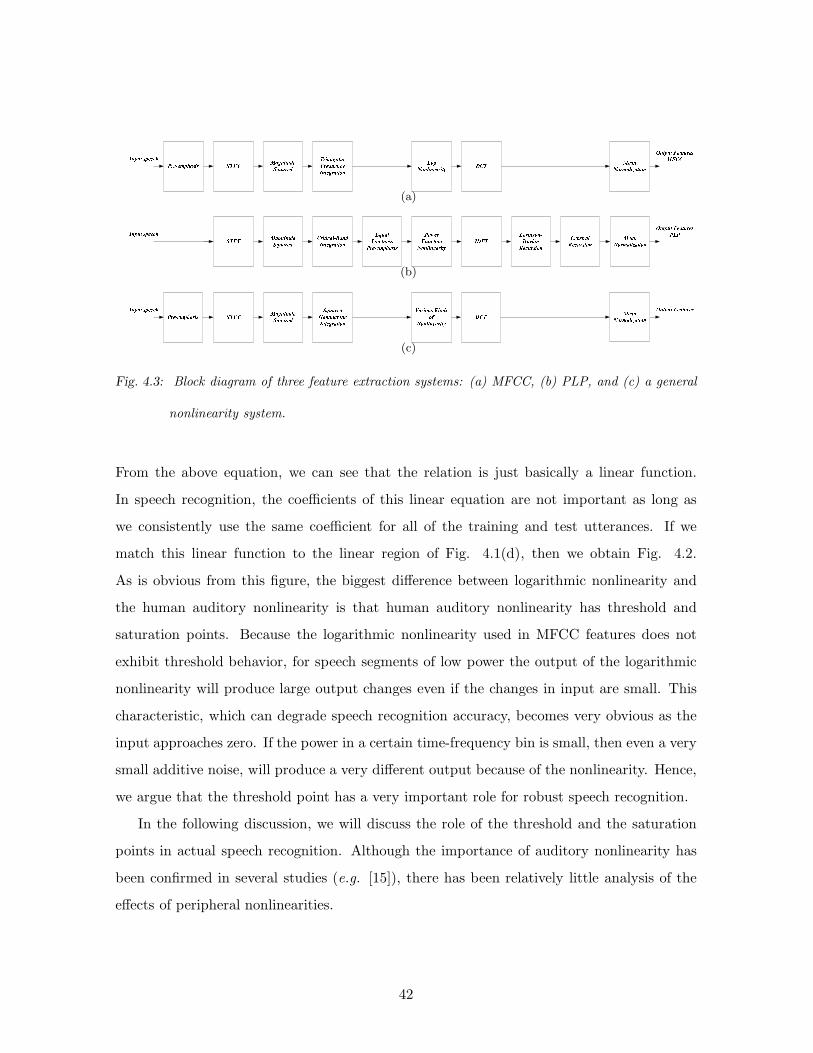
(a)

(b)

(c)

Fig. 4.3: Block diagram of three feature extraction systems: (a) MFCC, (b) PLP, and (c) a general

nonlinearity system.

From the above equation, we can see that the relation is just basically a linear function.

In speech recognition, the coefficients of this linear equation are not important as long as

we consistently use the same coefficient for all of the training and test utterances. If we

match this linear function to the linear region of Fig. 4.1(d), then we obtain Fig. 4.2.

As is obvious from this figure, the biggest difference between logarithmic nonlinearity and

the human auditory nonlinearity is that human auditory nonlinearity has threshold and

saturation points. Because the logarithmic nonlinearity used in MFCC features does not

exhibit threshold behavior, for speech segments of low power the output of the logarithmic

nonlinearity will produce large output changes even if the changes in input are small. This

characteristic, which can degrade speech recognition accuracy, becomes very obvious as the

input approaches zero. If the power in a certain time-frequency bin is small, then even a very

small additive noise, will produce a very different output because of the nonlinearity. Hence,

we argue that the threshold point has a very important role for robust speech recognition.

In the following discussion, we will discuss the role of the threshold and the saturation

points in actual speech recognition. Although the importance of auditory nonlinearity has

been confirmed in several studies (e.g. [15]), there has been relatively little analysis of the

effects of peripheral nonlinearities.

42

4.3 Speech recognition using different nonlinearities

In the following discussion, to test the effectiveness of different nonlinearities, we will use the

feature extraction system shown in Fig 4.3(c) using different nonlinearities. As a comparison,

we will also provide MFCC and PLP speech recognition results, which are shown in Fig.

4.8, respectively. Throughout this chapter, we will provide speech recognition results while

changing the nonlinearity in 4.3(c). We will use the traditional triangular frequency-domain

integration using MFCC processing, while for PLP processing we will make use of the critical

band integration used by Hermansky [51]. For the system in Fig 4.3(c), we use gammatone

frequency integration. In all of the following experiments, we used 40 channels. For the

MFCC processing in Fig. 4.3(a) and the general feature extraction system in Fig. 4.3(c),

a pre-emphasis filter of the form H(z) = 1 − 0.97z−1 is applied first. The STFT analysis

is performed using Hamming windows of duration 25.6 ms, with 10 ms between frames

for a sampling frequency of 16 kHz. Both the MFCC and PLP procedures include intrinsic

nonlinearities: PLP passes the amplitude-normalized short-time power of critical-band filters

through a cube-root nonlinearity to approximate the power law of hearing [51, 52]. In

contrast, the MFCC procedure passes its filter outputs through a logarithmic function.

4.4 Recognition results using the hypothesized human auditory nonlinearity

Using the structure shown in Fig. 4.3(c) and the nonlinearity shown in Fig. 4.2, we con-

ducted speech recognition experiments using the CMU Sphinx 3.8 system with Sphinxbase

0.4.1 and SphinxTrain 1.0 used to train the acoustic models. For comparison purposes,

we also obtained MFCC and PLP features using sphinx fe and HTK 3.4, respectively. All

experiments were conducted under the same conditions, and delta and delta-delta compo-

nents were appended to the original features. For training and testing, we used subsets of

1600 utterances and 600 utterances, respectively, from the DARPA Resource Management

(RM1) database. To evaluate the robustness of the feature extraction approaches, we digi-

tally added three different types of noise: white noise, street noise, and background music.

The background music was obtained from a musical segment of the DARPA Hub 4 Broad-

cast News database, while the street noise was recorded on a busy street. For reverberation

43

simulation, we used he Room Impulse Response (RIR) software [53]. We assumed a room of

dimensions 5× 4× 3 m with a distance of 2 m between the microphone and the speaker.

Since the rate-intensity curve is highly nonlinear, it is expected that the recognition accu-

racy that is obtained will be dependent on the speech power level. We conducted experiments

at several different input intensity levels to measure this effect. In Fig. 4.4, β dB represents

the intensity at which the average SPL falls slightly below the middle point of the linear

region of the rate-intensity curve. As can be seen in Fig. 4.4(a), for speech in the presence of

white noise, increasing the input intensity causes the recognition accuracy to degrade, which

is due to the fact that the benefit provided by limiting the response in the threshold region

affects a smaller percentage of the incoming speech frames. For street noise, the performance

improvement is small, and for music and reverberation, increasing the intensity reduces the

accuracy compared to the baseline condition.

Up until now, we discussed the characteristics of the human rate-intensity curve and

compared it with the log nonlinearity curve used in the MFCC. We observe both the ad-

vantages and disadvantages of the human rate-intensity curve. The biggest advantage of the

human rate-intensity curve compared to the log nonlinearity is that it uses the threshold

point, which provides a significant improvement in noise robustness in speech recognition ex-

periments. However, one clear disadvantage is that speech recognition performance depends

on the input sound pressure level. Thus, the optimal input sound pressure level needs to be

obtained empirically, and if we use a different input sound pressure level for training and

testing, recognition will degrade because of the environmental mismatch.

4.5 Shifted Log Function and the Power Function

In the previous section, we saw that the human auditory rate-intensity curve is more robust

against stationary additive noise. However, we also observed that performance depends

heavily on the input speech intensity, which is not desirable, and the input intensity must be

obtained empirically. Additionally, if there are mismatches between the input sound pressure

level between the training and testing utterances, performance will degrade significantly.

Another problem is that even though the feature extraction system with this human rate-

intensity curve shows improvement for stationary noisy environments, the performance is

44

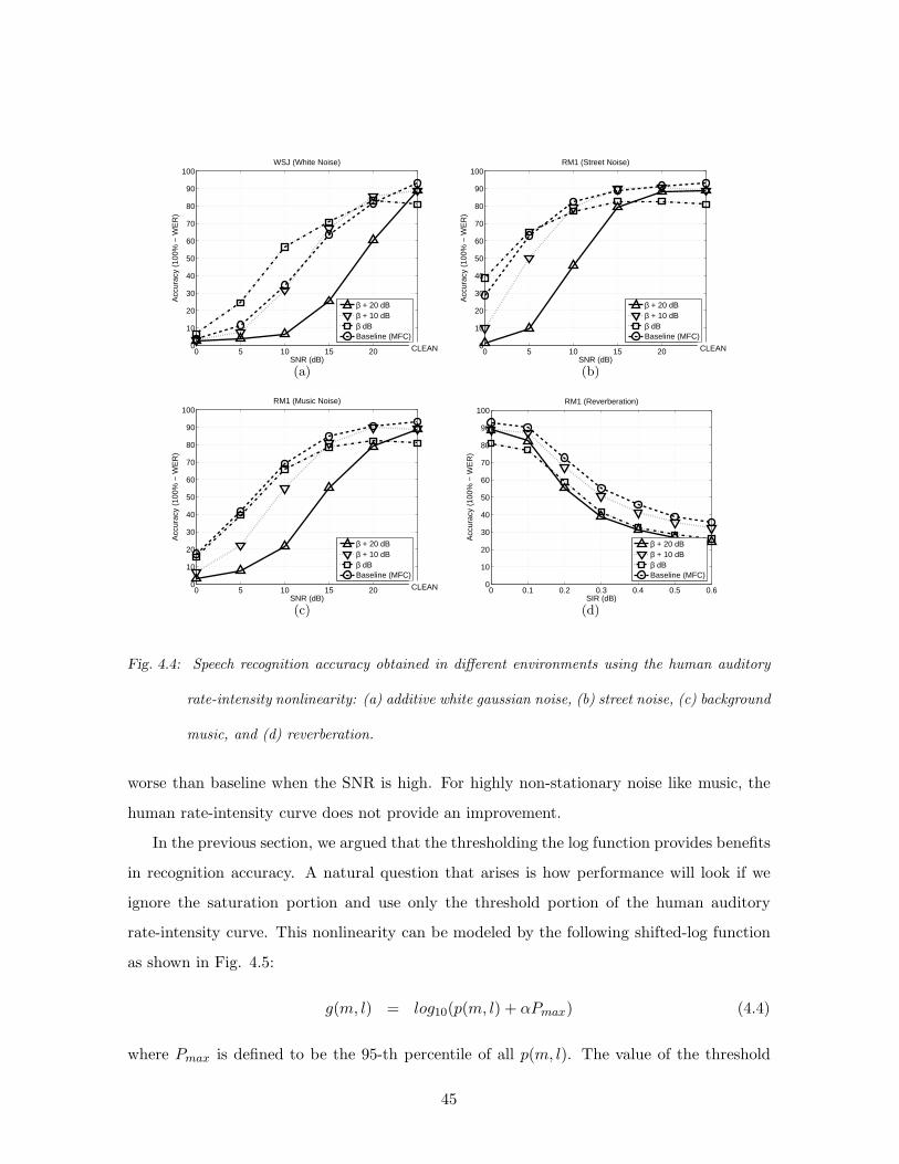
0 5 10 15 20 250

10

20

30

40

50

60

70

80

90

100

SNR (dB)

Acc

urac

y (1

00%

− W

ER

)

WSJ (White Noise)

β + 20 dBβ + 10 dBβ dBBaseline (MFC)

CLEAN

(a)

0 5 10 15 20 250

10

20

30

40

50

60

70

80

90

100

SNR (dB)

Acc

urac

y (1

00%

− W

ER

)

RM1 (Street Noise)


CLEAN

(b)

0 5 10 15 20 250

10

20

30

40

50

60

70

80

90

100

SNR (dB)

Acc

urac

y (1

00%

− W

ER

)

RM1 (Music Noise)


CLEAN

(c)

0 0.1 0.2 0.3 0.4 0.5 0.60

10

20

30

40

50

60

70

80

90

100

SIR (dB)

Acc

urac

y (1

00%

− W

ER

)

RM1 (Reverberation)


(d)

Fig. 4.4: Speech recognition accuracy obtained in different environments using the human auditory

rate-intensity nonlinearity: (a) additive white gaussian noise, (b) street noise, (c) background

music, and (d) reverberation.

worse than baseline when the SNR is high. For highly non-stationary noise like music, the

human rate-intensity curve does not provide an improvement.

In the previous section, we argued that the thresholding the log function provides benefits

in recognition accuracy. A natural question that arises is how performance will look if we

ignore the saturation portion and use only the threshold portion of the human auditory

rate-intensity curve. This nonlinearity can be modeled by the following shifted-log function

as shown in Fig. 4.5:

g(m, l) = log10(p(m, l) + αPmax) (4.4)

where Pmax is defined to be the 95-th percentile of all p(m, l). The value of the threshold

45

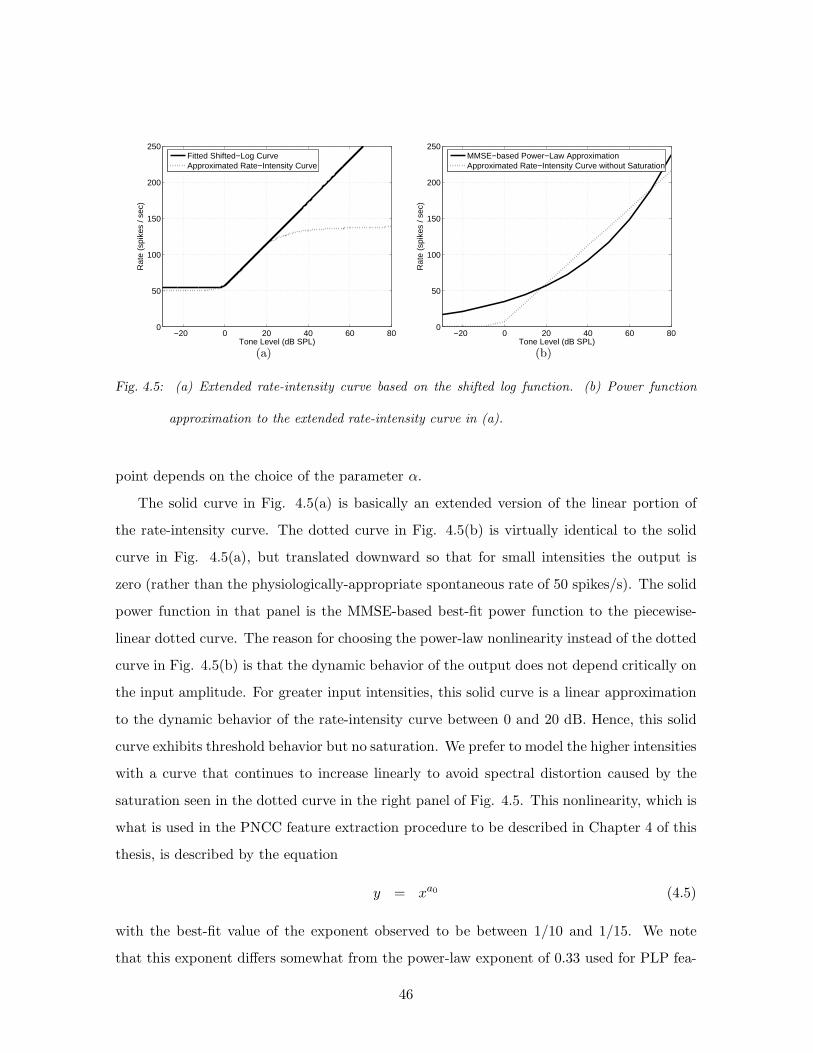
−20 0 20 40 60 800

50

100

150

200

250

Tone Level (dB SPL)

Rat

e (s

pike

s / s

ec)

Fitted Shifted−Log CurveApproximated Rate−Intensity Curve

(a)

−20 0 20 40 60 800

50

100

150

200

250

Tone Level (dB SPL)

Rat

e (s

pike

s / s

ec)

MMSE−based Power−Law ApproximationApproximated Rate−Intensity Curve without Saturation

(b)

Fig. 4.5: (a) Extended rate-intensity curve based on the shifted log function. (b) Power function

approximation to the extended rate-intensity curve in (a).

point depends on the choice of the parameter α.

The solid curve in Fig. 4.5(a) is basically an extended version of the linear portion of

the rate-intensity curve. The dotted curve in Fig. 4.5(b) is virtually identical to the solid

curve in Fig. 4.5(a), but translated downward so that for small intensities the output is

zero (rather than the physiologically-appropriate spontaneous rate of 50 spikes/s). The solid

power function in that panel is the MMSE-based best-fit power function to the piecewise-

linear dotted curve. The reason for choosing the power-law nonlinearity instead of the dotted

curve in Fig. 4.5(b) is that the dynamic behavior of the output does not depend critically on

the input amplitude. For greater input intensities, this solid curve is a linear approximation

to the dynamic behavior of the rate-intensity curve between 0 and 20 dB. Hence, this solid

curve exhibits threshold behavior but no saturation. We prefer to model the higher intensities

with a curve that continues to increase linearly to avoid spectral distortion caused by the

saturation seen in the dotted curve in the right panel of Fig. 4.5. This nonlinearity, which is

what is used in the PNCC feature extraction procedure to be described in Chapter 4 of this

thesis, is described by the equation

y = xa0 (4.5)

with the best-fit value of the exponent observed to be between 1/10 and 1/15. We note

that this exponent differs somewhat from the power-law exponent of 0.33 used for PLP fea-

46

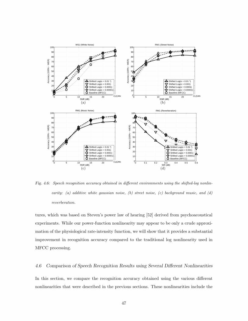
0 5 10 15 20 250

10

20

30

40

50

60

70

80

90

100

SNR (dB)

Acc

urac

y (1

00%

− W

ER

)

WSJ (White Noise)

Shifted Log(α = 0.01 *)Shifted Log(α = 0.001)Shifted Log(α = 0.0001)Shifted Log(α = 0.00001)Baseline (MFCC)

CLEAN

(a)

0 5 10 15 20 250

10

20

30

40

50

60

70

80

90

100

SNR (dB)

Acc

urac

y (1

00%

− W

ER

)

RM1 (Street Noise)


CLEAN

(b)

0 5 10 15 20 250

10

20

30

40

50

60

70

80

90

100

SNR (dB)

Acc

urac

y (1

00%

− W

ER

)

RM1 (Music Noise)


CLEAN

(c)

0 0.1 0.2 0.3 0.4 0.5 0.60

10

20

30

40

50

60

70

80

90

100

SIR (dB)

Acc

urac

y (1

00%

− W

ER

)

RM1 (Reverberation)


(d)

Fig. 4.6: Speech recognition accuracy obtained in different environments using the shifted-log nonlin-

earity: (a) additive white gaussian noise, (b) street noise, (c) background music, and (d)

reverberation.

tures, which was based on Steven’s power law of hearing [52] derived from psychoacoustical

experiments. While our power-function nonlinearity may appear to be only a crude approxi-

mation of the physiological rate-intensity function, we will show that it provides a substantial

improvement in recognition accuracy compared to the traditional log nonlinearity used in

MFCC processing.

4.6 Comparison of Speech Recognition Results using Several Different Nonlinearities

In this section, we compare the recognition accuracy obtained using the various different

nonlinearities that were described in the previous sections. These nonlinearities include the

47

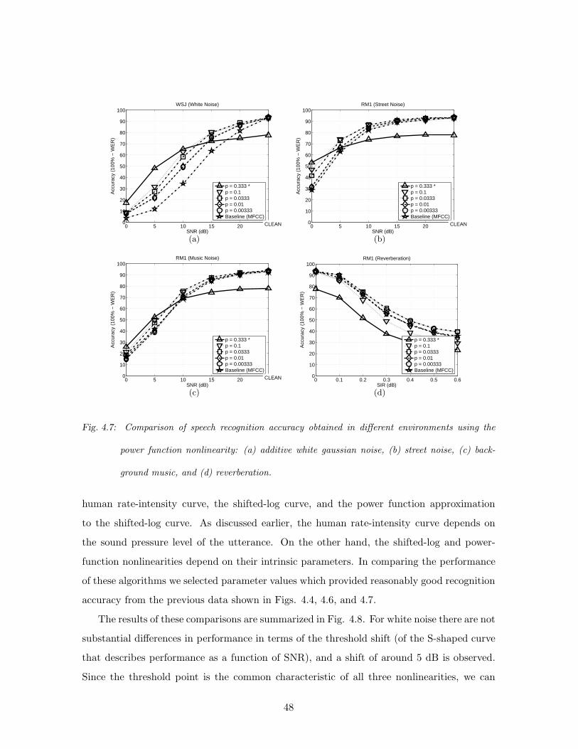
0 5 10 15 20 250

10

20

30

40

50

60

70

80

90

100

SNR (dB)

Acc

urac

y (1

00%

− W

ER

)

WSJ (White Noise)

p = 0.333 *p = 0.1p = 0.0333p = 0.01p = 0.00333Baseline (MFCC)

CLEAN

(a)

0 5 10 15 20 250

10

20

30

40

50

60

70

80

90

100

SNR (dB)

Acc

urac

y (1

00%

− W

ER

)

RM1 (Street Noise)


CLEAN

(b)

0 5 10 15 20 250

10

20

30

40

50

60

70

80

90

100

SNR (dB)

Acc

urac

y (1

00%

− W

ER

)

RM1 (Music Noise)


CLEAN

(c)

0 0.1 0.2 0.3 0.4 0.5 0.60

10

20

30

40

50

60

70

80

90

100

SIR (dB)

Acc

urac

y (1

00%

− W

ER

)

RM1 (Reverberation)


(d)

Fig. 4.7: Comparison of speech recognition accuracy obtained in different environments using the

power function nonlinearity: (a) additive white gaussian noise, (b) street noise, (c) back-

ground music, and (d) reverberation.

human rate-intensity curve, the shifted-log curve, and the power function approximation

to the shifted-log curve. As discussed earlier, the human rate-intensity curve depends on

the sound pressure level of the utterance. On the other hand, the shifted-log and power-

function nonlinearities depend on their intrinsic parameters. In comparing the performance

of these algorithms we selected parameter values which provided reasonably good recognition

accuracy from the previous data shown in Figs. 4.4, 4.6, and 4.7.

The results of these comparisons are summarized in Fig. 4.8. For white noise there are not

substantial differences in performance in terms of the threshold shift (of the S-shaped curve

that describes performance as a function of SNR), and a shift of around 5 dB is observed.

Since the threshold point is the common characteristic of all three nonlinearities, we can

48

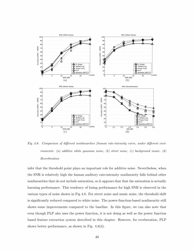
0 5 10 15 20 250

10

20

30

40

50

60

70

80

90

100

SNR (dB)

Acc

urac

y (1

00%

− W

ER

)

RM1 (White Noise)

S−shapeShifted LogPower FuncPLPBaseline (MFCC)

CLEAN

(a)

0 5 10 15 20 250

10

20

30

40

50

60

70

80

90

100

SNR (dB)

Acc

urac

y (1

00%

− W

ER

)

RM1 (Street Noise)


CLEAN

(b)

0 5 10 15 20 250

10

20

30

40

50

60

70

80

90

100

SNR (dB)

Acc

urac

y (1

00%

− W

ER

)

RM1 (Music Noise)


CLEAN

(c)

0 0.1 0.2 0.3 0.4 0.5 0.60

10

20

30

40

50

60

70

80

90

100

SIR (dB)

Acc

urac

y (1

00%

− W

ER

)

RM1 (Reverberation)


(d)

Fig. 4.8: Comparison of different nonlinearities (human rate-intensity curve, under different envi-

ronments: (a) additive white gaussian noise, (b) street noise, (c) background music, (d)

Reverberation

infer that the threshold point plays an important role for additive noise. Nevertheless, when

the SNR is relatively high the human auditory rate-intensity nonlinearity falls behind other

nonlinearities that do not include saturation, so it appears that that the saturation is actually

harming performance. This tendency of losing performance for high SNR is observed in the

various types of noise shown in Fig 4.8. For street noise and music noise, the threshold shift

is significantly reduced compared to white noise. The power-function-based nonlinearity still

shows some improvements compared to the baseline. In this figure, we can also note that

even though PLP also uses the power function, it is not doing as well as the power function

based feature extraction system described in this chapter. However, for reveberation, PLP

shows better performance, as shown in Fig. 4.8(d).

49

4.7 Summary

In this Chapter, we compared different nonlinearities and compared speech recognition ac-

curacies. We observe that the logarithmic nonlinearity is very vulnerable to additive noise,

since it ignores the auditory threshold which is an important characteristic in the human

rate-intensity relation. In a series of speech recognition experiments, we showed that hu-

man rate-intensity curve shows better robustness in the additive noise environments than

MFCC. However, there are two problems with this “S-shape” rate-intensity nonlinearity of

the human auditory system, which is characterized by the threshold and saturation points.

The first problem is that since the curve is highly nonlinear, if the input is scaled (different

SPL), then the output spectrum is also very different. This phenomena causes problems in

speech recognition. The second problem is, the saturation point does not give us any evident

benefits in speech recognition results. We compared “shifted-log” and “S-shape” nonlineari-

ties, and observed that both of them show similar robustness against additive noise, but the

“shifted-log” approach usually performs slightly better than “S-shape” curve for high SNR

regions. From the above discussion, we conclude that a good nolinearity for speech recogni-

tion systems need to have the following characteristics. First, it needs to have the auditory

threshold characteristic. It should not be affected by scaling effects, or at least, the effect of

scaling needs to be easily reversible. Based on these discussion and experimental results, we

conclude that a power function is a good choice for modelling the auditory nonlinearity. We

further discuss auditory nonlinearity in Chapter 5 and Chapter 8.

50

5. THE SMALL-POWER BOOSTING ALGORITHM

5.1 Introduction

Recent studies show that for non-stationary disturbances such as background music or back-

ground speech, algorithms based on missing features (e.g. [16, 54]) or auditory processing

are more promising than simple baseline approaches such as the CDCN algorithm or the

use of PLP coefficients (e.g [9, 15, 55, 56, 25]). Still, the improvement in non-stationary

noise remains less than the improvement that is observed in stationary noise. In previous

work [55] and in the previous section, we also observed that the “threshold point” of the

auditory nonlinearity plays an important role in improving performance in additive noise.

Let us imagine a specific time-frequency bin with small power. Even if a relatively small

distortion is applied to this time-frequency bin, due to the nature of compressive nonlinearity

the distortion can become quite large.

In this chapter we explain the structure of the small-power boosting (SPB) algorithm,

which reduces the variability introduced by the nonlinearity by applying a floor to the pos-

sible value that each time-frequency bin may take on. There are two different implemen-

tations of the SPB algorithm. In the first approach, we apply small-power boosting to

each time-frequency bin in the spectral domain, and then resynthesize speech (SPB-R). The

resynthesized speech is fed to the feature extraction system. This approach is conceptu-

ally straightforward but less computationally efficient (because of the number of FFTs and

IFFTs that must be performed). In the second approach, we use SPB to obtain feature

values directly (SPB-D). This approach does not require IFFT operations and the system is

consequently more compact. As we will discuss below, effective implementation of SPB-D

requires smoothing in the spectral domain.

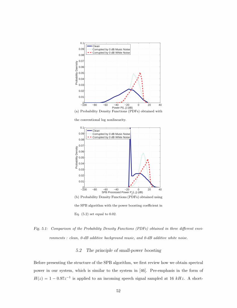
−100 −80 −60 −40 −20 0 20 400

0.01

0.02

0.03

0.04

0.05

0.06

0.07

0.08

0.09

0.1

Power P(i, j) (dB)

Pro

babi

lity

Dae

nstiy

CleanCorrupted by 0 dB Music NoiseCorrupted by 0 dB White Noise

(a) Probability Density Functions (PDFs) obtained with

the conventional log nonlinearity.

−100 −80 −60 −40 −20 0 20 400

0.01

0.02

0.03

0.04

0.05

0.06

0.07

0.08

0.09

0.1

SPB Processed Power Ps(i, j) (dB)

Pro

babi

lity

Den

stiy

CleanCorrupted by 0 dB Music NoiseCorrupted by 0 dB White Noise

(b) Probability Density Functions (PDFs) obtained using

the SPB algorithm with the power boosting coefficient in

Eq. (5.2) set equal to 0.02.

Fig. 5.1: Comparison of the Probability Density Functions (PDFs) obtained in three different envi-

ronments : clean, 0-dB additive background music, and 0-dB additive white noise.

5.2 The principle of small-power boosting

Before presenting the structure of the SPB algorithm, we first review how we obtain spectral

power in our system, which is similar to the system in [46]. Pre-emphasis in the form of

H(z) = 1 − 0.97z−1 is applied to an incoming speech signal sampled at 16 kHz. A short-

52

Fig. 5.2: The total nonlinearity consists of small-power boosting and the subsequent logarithmic non-

linearity in the SPB algorithm

time Fourier transform (STFT) is calculated using Hamming windows of a duration of 25.6

ms. Spectral power is obtained by integrating the magnitudes of the STFT coefficients over

a series of weighting functions [57]. This procedure is represented by the following equation:

P (i, j) =

N−1∑

k=0

|X(ejωk ; j)Hi(ejωk)|2 (5.1)

In the above equation i and j represent the channel and frame indices respectively, N is the

FFT size, and Hi(ejwk) is the frequency response of the i-th Gammatone channel. X(ejωk ; j)

is the STFT for the j-th frame. wk is defined by ωk = 2πkN , 0 ≤ k ≤ N − 1.

In Fig. 5.1(a), we observe the distributions of log(P (i, j)) for clean speech, speech in

0-dB music, and speech in 0-dB white noise. We used a subset of 50 utterances to obtain

these distributions from the training portion of the DARPA Resource Management 1 (RM1)

database. In plotting the distributions, we scaled each waveform to set the 95th percentile of

P (i, j) to be 0 dB. We note in Fig. 5.1(a) that higher values of P (i, j) are (unsurprisingly) less

affected by the additive noise, but the values that are small in power are severely distorted

by additive noise. While the conventional approach to this problem is spectral subtraction

(e.g. [11]), this goal can also be achieved by intentionally boosting power for all utterances,

thereby rendering the small-power regions less affected by the additive noise. We implement

53

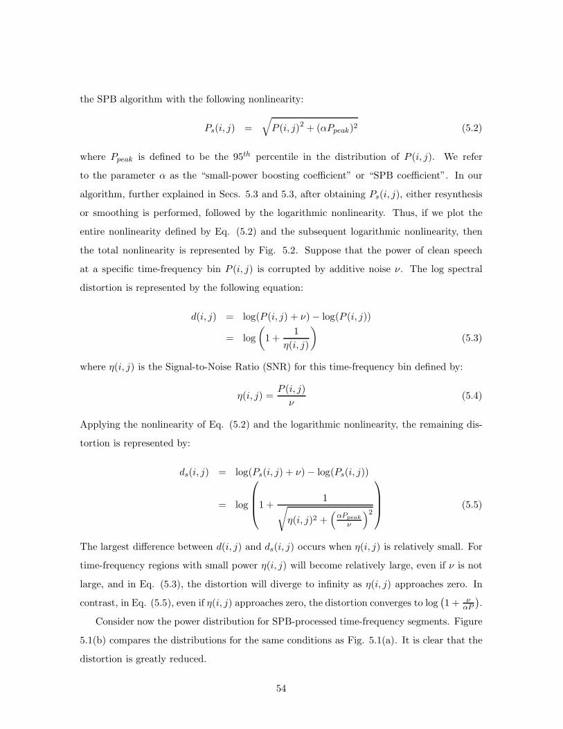
the SPB algorithm with the following nonlinearity:

Ps(i, j) =

√

P (i, j)2 + (αPpeak)2 (5.2)

where Ppeak is defined to be the 95th percentile in the distribution of P (i, j). We refer

to the parameter α as the “small-power boosting coefficient” or “SPB coefficient”. In our

algorithm, further explained in Secs. 5.3 and 5.3, after obtaining Ps(i, j), either resynthesis

or smoothing is performed, followed by the logarithmic nonlinearity. Thus, if we plot the

entire nonlinearity defined by Eq. (5.2) and the subsequent logarithmic nonlinearity, then

the total nonlinearity is represented by Fig. 5.2. Suppose that the power of clean speech

at a specific time-frequency bin P (i, j) is corrupted by additive noise ν. The log spectral

distortion is represented by the following equation:

d(i, j) = log(P (i, j) + ν)− log(P (i, j))

= log

(

1 +1

η(i, j)

)

(5.3)

where η(i, j) is the Signal-to-Noise Ratio (SNR) for this time-frequency bin defined by:

η(i, j) =P (i, j)

ν(5.4)

Applying the nonlinearity of Eq. (5.2) and the logarithmic nonlinearity, the remaining dis-

tortion is represented by:

ds(i, j) = log(Ps(i, j) + ν)− log(Ps(i, j))

= log

1 +1

√

η(i, j)2 +(

αPpeak

ν

)2

(5.5)

The largest difference between d(i, j) and ds(i, j) occurs when η(i, j) is relatively small. For

time-frequency regions with small power η(i, j) will become relatively large, even if ν is not

large, and in Eq. (5.3), the distortion will diverge to infinity as η(i, j) approaches zero. In

contrast, in Eq. (5.5), even if η(i, j) approaches zero, the distortion converges to log(

1 + ναP

)

.

Consider now the power distribution for SPB-processed time-frequency segments. Figure

5.1(b) compares the distributions for the same conditions as Fig. 5.1(a). It is clear that the

distortion is greatly reduced.

54

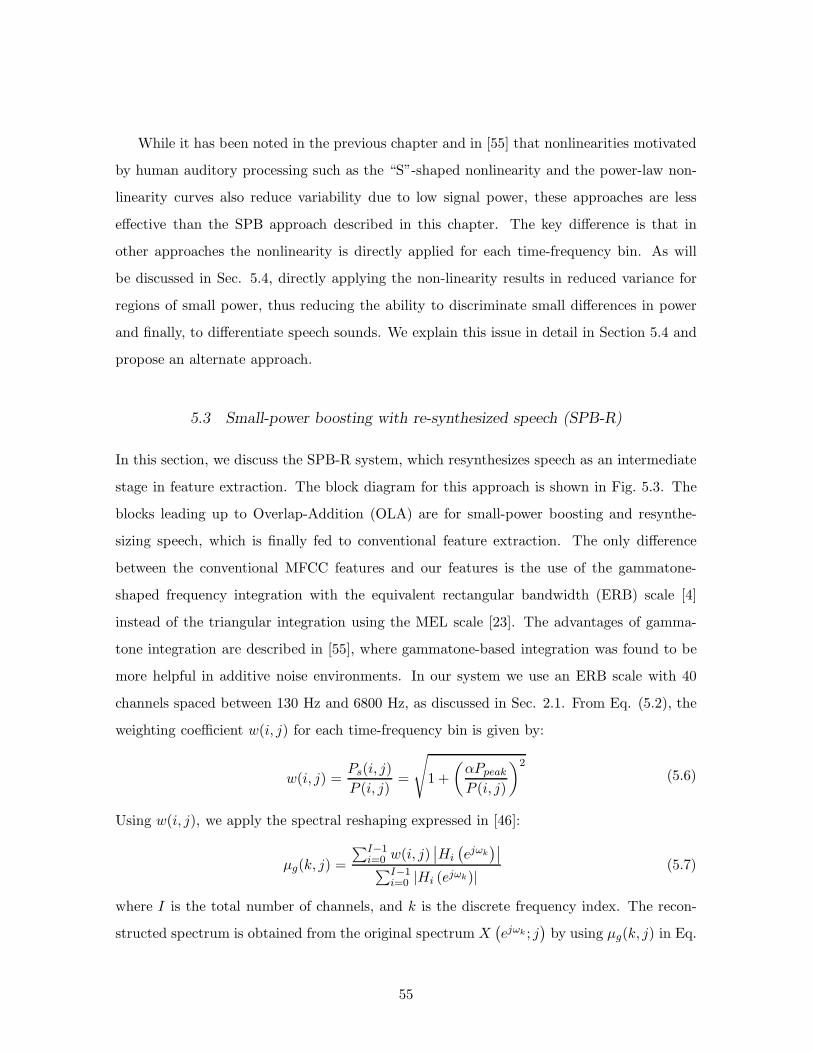
While it has been noted in the previous chapter and in [55] that nonlinearities motivated

by human auditory processing such as the “S”-shaped nonlinearity and the power-law non-

linearity curves also reduce variability due to low signal power, these approaches are less

effective than the SPB approach described in this chapter. The key difference is that in

other approaches the nonlinearity is directly applied for each time-frequency bin. As will

be discussed in Sec. 5.4, directly applying the non-linearity results in reduced variance for

regions of small power, thus reducing the ability to discriminate small differences in power

and finally, to differentiate speech sounds. We explain this issue in detail in Section 5.4 and

propose an alternate approach.

5.3 Small-power boosting with re-synthesized speech (SPB-R)

In this section, we discuss the SPB-R system, which resynthesizes speech as an intermediate

stage in feature extraction. The block diagram for this approach is shown in Fig. 5.3. The

blocks leading up to Overlap-Addition (OLA) are for small-power boosting and resynthe-

sizing speech, which is finally fed to conventional feature extraction. The only difference

between the conventional MFCC features and our features is the use of the gammatone-

shaped frequency integration with the equivalent rectangular bandwidth (ERB) scale [4]

instead of the triangular integration using the MEL scale [23]. The advantages of gamma-

tone integration are described in [55], where gammatone-based integration was found to be

more helpful in additive noise environments. In our system we use an ERB scale with 40

channels spaced between 130 Hz and 6800 Hz, as discussed in Sec. 2.1. From Eq. (5.2), the

weighting coefficient w(i, j) for each time-frequency bin is given by:

w(i, j) =Ps(i, j)

P (i, j)=

√

1 +

(

αPpeak

P (i, j)

)2

(5.6)

Using w(i, j), we apply the spectral reshaping expressed in [46]:

µg(k, j) =

∑I−1i=0 w(i, j)

∣

∣Hi

(

ejωk)∣

∣

∑I−1i=0 |Hi (ejωk)|

(5.7)

where I is the total number of channels, and k is the discrete frequency index. The recon-

structed spectrum is obtained from the original spectrum X(

ejωk ; j)

by using µg(k, j) in Eq.

55

Fig. 5.3: Small-power boosting algorithm which resynthesizes speech (SPB-R). Conventional MFCC

processing is followed after resynthesizing the speech.

56

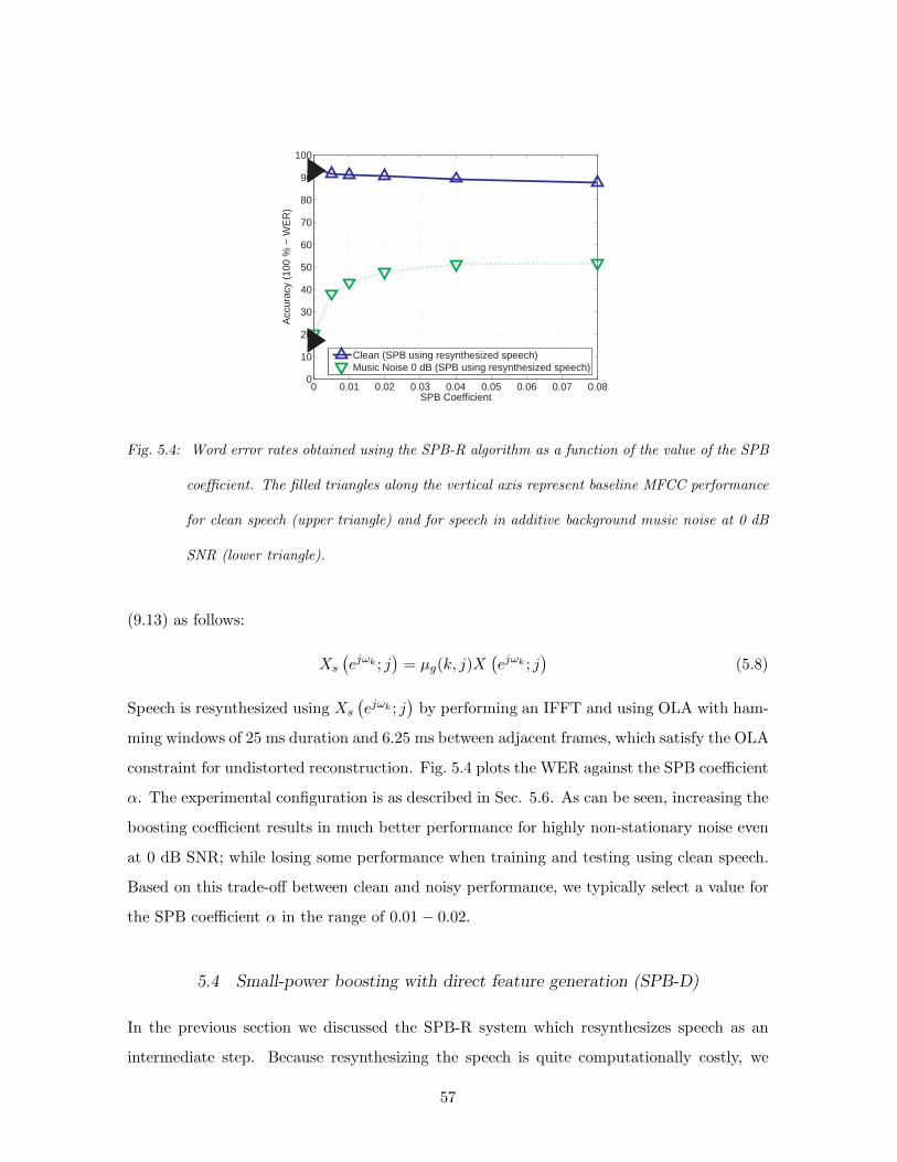
0 0.01 0.02 0.03 0.04 0.05 0.06 0.07 0.080

10

20

30

40

50

60

70

80

90

100

SPB Coefficient

Acc

urac

y (1

00 %

− W

ER

)

Clean (SPB using resynthesized speech)Music Noise 0 dB (SPB using resynthesized speech)

Fig. 5.4: Word error rates obtained using the SPB-R algorithm as a function of the value of the SPB

coefficient. The filled triangles along the vertical axis represent baseline MFCC performance

for clean speech (upper triangle) and for speech in additive background music noise at 0 dB

SNR (lower triangle).

(9.13) as follows:

Xs

(

ejωk ; j)

= µg(k, j)X(

ejωk ; j)

(5.8)

Speech is resynthesized using Xs

(

ejωk ; j)

by performing an IFFT and using OLA with ham-

ming windows of 25 ms duration and 6.25 ms between adjacent frames, which satisfy the OLA

constraint for undistorted reconstruction. Fig. 5.4 plots the WER against the SPB coefficient

α. The experimental configuration is as described in Sec. 5.6. As can be seen, increasing the

boosting coefficient results in much better performance for highly non-stationary noise even

at 0 dB SNR; while losing some performance when training and testing using clean speech.

Based on this trade-off between clean and noisy performance, we typically select a value for

the SPB coefficient α in the range of 0.01 − 0.02.

5.4 Small-power boosting with direct feature generation (SPB-D)

In the previous section we discussed the SPB-R system which resynthesizes speech as an

intermediate step. Because resynthesizing the speech is quite computationally costly, we

57

Fig. 5.5: Small-power boosting algorithm with direct feature generation (SPB-D).

58

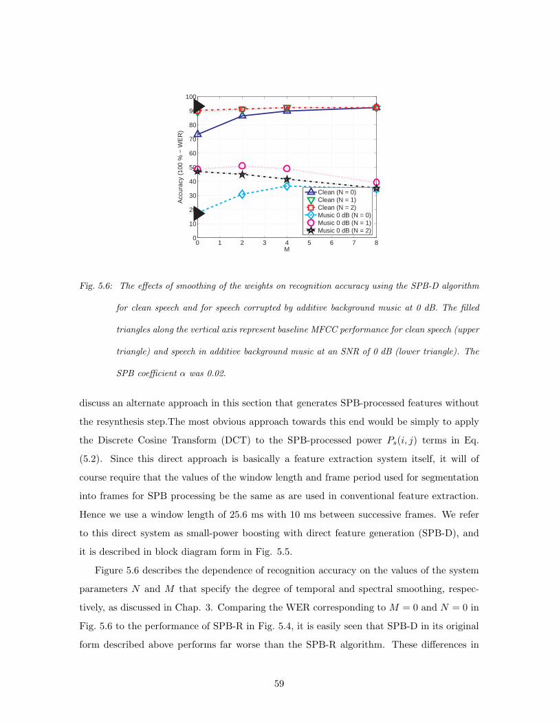
0 1 2 3 4 5 6 7 80

10

20

30

40

50

60

70

80

90

100

M

Acc

urac

y (1

00 %

− W

ER

)

Clean (N = 0)Clean (N = 1)Clean (N = 2)Music 0 dB (N = 0)Music 0 dB (N = 1)Music 0 dB (N = 2)

Fig. 5.6: The effects of smoothing of the weights on recognition accuracy using the SPB-D algorithm

for clean speech and for speech corrupted by additive background music at 0 dB. The filled

triangles along the vertical axis represent baseline MFCC performance for clean speech (upper

triangle) and speech in additive background music at an SNR of 0 dB (lower triangle). The

SPB coefficient α was 0.02.

discuss an alternate approach in this section that generates SPB-processed features without

the resynthesis step.The most obvious approach towards this end would be simply to apply

the Discrete Cosine Transform (DCT) to the SPB-processed power Ps(i, j) terms in Eq.

(5.2). Since this direct approach is basically a feature extraction system itself, it will of

course require that the values of the window length and frame period used for segmentation

into frames for SPB processing be the same as are used in conventional feature extraction.

Hence we use a window length of 25.6 ms with 10 ms between successive frames. We refer

to this direct system as small-power boosting with direct feature generation (SPB-D), and

it is described in block diagram form in Fig. 5.5.

Figure 5.6 describes the dependence of recognition accuracy on the values of the system

parameters N and M that specify the degree of temporal and spectral smoothing, respec-

tively, as discussed in Chap. 3. Comparing the WER corresponding to M = 0 and N = 0 in

Fig. 5.6 to the performance of SPB-R in Fig. 5.4, it is easily seen that SPB-D in its original

form described above performs far worse than the SPB-R algorithm. These differences in

59

Time (s)

Cha

nnel

Inde

x

0 0.5 1 1.5 2 2.5 3 3.50

10

20

30

40

(a)

Time (s)

Cha

nnel

Inde

x

0 0.5 1 1.5 2 2.5 3 3.50

10

20

30

40

(b)

Time (s)

Cha

nnel

Inde

x

0 0.5 1 1.5 2 2.5 3 3.50

10

20

30

40

(c)

Time (s)

Cha

nnel

Inde

x

0 0.5 1 1.5 2 2.5 3 3.50

10

20

30

40

(d)

Fig. 5.7: Spectrograms obtained from a clean speech utterance using different types of processing: (a)

conventional MFCC processing, (b) SPB-R processing, (c) SPB-D processing without any

weight smoothing, and (d) SPB-D processing with weight smoothing using M = 4, N = 1 in

Eq. (5.9). A value of 0.02 was used for the SPB coefficient α.

performance are reflected in the corresponding spectrograms, as can be seen by comparing

Fig. 5.7(c) to the SPB-R-derived spectrogram in Fig. 5.7(b)). In Fig. 5.7(c), the variance

in time-frequency regions of small power is very small [concentrated at αPpeak in Fig. 5.2

and Eq. (5.2)], thus losing the power to discriminate sounds which have small power. Small

variance is harmful in this context because the PDFs developed during the training process

are modeled by Gaussians with very narrow peaks. As a consequence, small perturbations

60

in the feature values from their means lead to large changes in log-likelihood scores. Hence

variances that are too small in magnitude should be avoided.

We also note that there exist large overlaps in the shape of gammatone-like frequency

responses, as well as an overlap between successive frames. Thus, the gain in one time-

frequency bin is correlated with that in an adjacent time-frequency bin. In the SPB-R

approach, similar smoothing was achieved implicitly by the spectral reshaping from Eq.

(9.13) and Eq. (5.8), and in the OLA process. With the SPB-D approach the spectral values

must be smoothed explicitly.

Smoothing of the weights can be done horizontally (along the time axis) as well as ver-

tically (along the frequency axis). The smoothed weights are obtained by:

w(i, j) = exp

(∑j+N

j′=j−N

∑i+Mi′=i−M log (w(i′, j′))

(2N + 1)(2M + 1)

)

(5.9)

where M and N respectively indicate smoothing along the time and frequency axes. The

averaging in Eq. (5.9) is performed in the logarithmic domain (equivalent to geometric

averaging) since the dynamic range of w(i, j) is very large. (If we had performed a normal

arithmetic averaging instead of geometric averaging in Eq. (5.9), the resulting averages would

be dominated inappropriately by the values of w(i, j) of greatest magnitude.)

Results of speech recognition experiments using different values of N and M are reported

in Fig. 5.6. The experimental configuration is the same as was used for the data shown

in Fig. 5.4. We note that the smoothing operation is quite helpful, and that with suitable

smoothing the SBP-D algorithm works as well as the SPB-R. In our subsequent experiments,

we used values of N = 1 and M = 4 in the SPB-D algorithm with 40 gammatone channels.

The corresponding spectrogram obtained with this smoothing is shown in Fig. 5.7(d), which

is similar to that obtained using SPB-R in Fig. 5.7(b).

5.5 Log spectral mean subtraction

In this section, we discuss log spectral mean subtraction (LSMS) and its potential use as

an optional pre-processing step in the SPB approach. We compare the performance of

LSMS computed for each frequency index with that of LSMS computed for each gammatone

channel. LSMS is a standard technique which has been commonly applied for robustness to

61

environmental mismatch, and this technique is mathematically equivalent to the well known

cepstral mean normalization (CMN) procedure. Log spectral mean subtraction is commonly

performed for log (P (i, j)) for each channel i as shown below.

P (i, j) =P (i, j)

exp( 12L+1

∑j+Lj′=j−L log (P (i, j′)))

(5.10)

Hence, this normalization is performed between the squared gammatone integration in each

band and the nonlinearity. It is also reasonable to apply LSMS for X(ejωk ; j) for each

frequency index k before performing the gammatone frequency integration. This can be

expressed as:

X(ejωk;j) =

∣

∣X(ejωk;j)∣

∣

exp( 12L+1

∑j+Lj′=j−L log (|X(ejωk;j′)|))

(5.11)

Fig. 5.8 depicts the results of speech recognition experiments using the two different

approaches to LSMS (without including SPB). In that figure, the moving average window

length indicates the length corresponding to 2L+ 1 in Eq. (5.10) and Eq. (5.11). We note

that the approach in Eq. (5.10) provides slightly better performance for white noise, but that

the performance difference diminishes as the window length increases. However, the LSMS

based on Eq. (5.11) shows consistently better performance in the presence of background

music, which is consistent across all window lengths. This may be explained due to the rich

discrete harmonic components in music, which makes frequency-index-based LSMS more

effective. In the next section we examine the performance obtained when LSMS as described

by Eq. (5.11) is used in combination with SPB.

5.6 Experimental results

In this section we present experimental results using the SPB-R algorithm described in Sec.

5.3 and the SPB-D algorithm described in Sec. 5.4. We also examine the performance of

SPB is combination with LSMS as described in Sec. 5.5. We conducted speech recogni-

tion experiments using the CMU Sphinx 3.8 system with Sphinxbase 0.4.1. For training

the acoustic model, we used SphinxTrain 1.0. For the baseline MFCC feature, we used

sphinx fe included in Sphinxbase 0.4.1. All experiments in this and previous sections

were conducted under identical conditions, with delta and delta-delta components appended

62

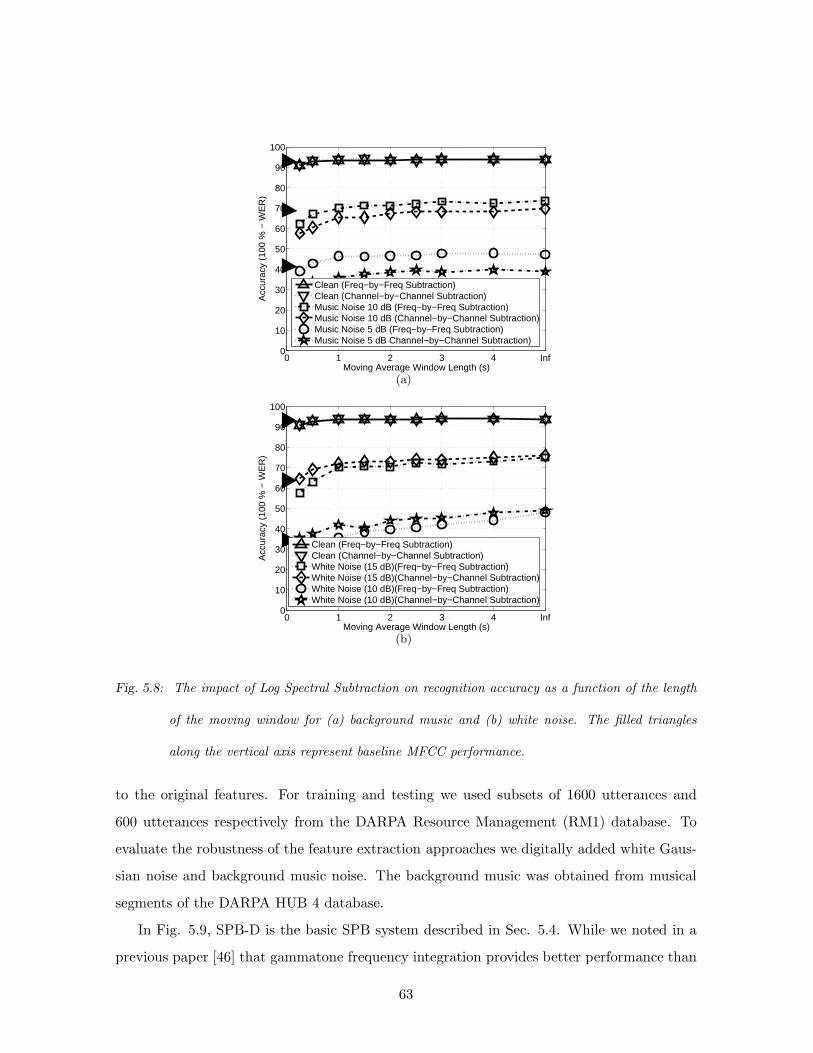
0 1 2 3 4 Inf0

10

20

30

40

50

60

70

80

90

100

Moving Average Window Length (s)

Acc

urac

y (1

00 %

− W

ER

)

Clean (Freq−by−Freq Subtraction)Clean (Channel−by−Channel Subtraction)Music Noise 10 dB (Freq−by−Freq Subtraction)Music Noise 10 dB (Channel−by−Channel Subtraction)Music Noise 5 dB (Freq−by−Freq Subtraction)Music Noise 5 dB Channel−by−Channel Subtraction)

(a)

0 1 2 3 4 Inf0

10

20

30

40

50

60

70

80

90

100

Moving Average Window Length (s)

Acc

urac

y (1

00 %

− W

ER

)

Clean (Freq−by−Freq Subtraction)Clean (Channel−by−Channel Subtraction)White Noise (15 dB)(Freq−by−Freq Subtraction)White Noise (15 dB)(Channel−by−Channel Subtraction)White Noise (10 dB)(Freq−by−Freq Subtraction)White Noise (10 dB)(Channel−by−Channel Subtraction)

(b)

Fig. 5.8: The impact of Log Spectral Subtraction on recognition accuracy as a function of the length

of the moving window for (a) background music and (b) white noise. The filled triangles

along the vertical axis represent baseline MFCC performance.

to the original features. For training and testing we used subsets of 1600 utterances and

600 utterances respectively from the DARPA Resource Management (RM1) database. To

evaluate the robustness of the feature extraction approaches we digitally added white Gaus-

sian noise and background music noise. The background music was obtained from musical

segments of the DARPA HUB 4 database.

In Fig. 5.9, SPB-D is the basic SPB system described in Sec. 5.4. While we noted in a

previous paper [46] that gammatone frequency integration provides better performance than

63

−5 0 5 10 15 20 Clean0

10

20

30

40

50

60

70

80

90

100

SNR (dB)

Acc

urac

y (1

00%

− W

ER

)

RM1 (White Noise)

VTSSPB−R−LSMS (50 ms window)SPB−D−LSMS (25.6 ms window)SPB−D (25.6 ms window)Baseline MFCC with CMN

(a)

−5 0 5 10 15 20 Clean0

10

20

30

40

50

60

70

80

90

100

SNR (dB)

Acc

urac

y (1

00%

− W

ER

)

RM1 (Music Noise)

VTSSPB−R−LSMS (50 ms window)SPB−D−LSMS (25.6 ms window)SPB−D (25.6 ms window)Baseline MFCC with CMN

(b)

Fig. 5.9: Comparison of recognition accuracy between VTS, SPB-CW and MFCC processing: (a)

additive white noise, (b) background music.

conventional triangular frequency integration, the effect is minor in these results. Thus, the

performance boost of SPB-D over the baseline MFCC is largely due to the SPB nonlinearity

in Eq. (5.2) and subsequent smoothing across time and frequency. SPB-D-LSMS refers to

the combination of the SPB-D and LSMS techniques. For both the SPB-D and SPB-D-

LSMS systems we used a window length of 25.6 ms with 10ms between adjacent frames.

Even though not explicitly plotted in this figure, SPB-R shows nearly the same performance

as SPB-D as mentioned in Sec. 5.4 and shown in Fig. 5.4.

We prefer to characterize the improvement in recognition accuracy by the amount of

64

lateral threshold shift provided by the processing. For white noise, SPB-D and SPB-D-

LSMS provides an improvement of about 7 dB to 8 dB compared to MFCC, as shown in Fig.

5.9. SPB-R-LSMS results in slightly smaller threshold shift. For comparison, we also conduct

experiments using the Vector Taylor Series (VTS) algorithm [10], as shown in Fig. 5.9. For

white noise, the performance of SPB family is slightly worse than that obtained using VTS.

Compensation for the effects of music noise, on the other hand, is considered to be

much more difficult (e.g. [42]). The SPB family of algorithms provides a very impressive

improvement in performance with background music. An implementation of SPB-R-LSMS

with window durations of 50 ms provides the greatest threshold shift (amounting to about

10 dB), and SPB-D provides a threshold shift of around 7 dB. VTS provides a performance

improvement of about 1 dB for the same data.

5.7 Conclusions

In this chapter we presented the robust speech recognition algorithm called Small-Power

Boosting (SPB), which is very helpful for difficult noise environments such as music noise.

The SPB algorithm works by intentionally boosting the representation of time-frequency

segments that are observed to have small power. We also noted that we should not boost

power in each time-frequency bin independently as adjacent time-frequency bins are highly

correlated. This correlation is achieved implicitly in SPB-R and by applying smoothing of

the weights in SPB-D over both time and frequency. We also observed that direct application

of the nonlinearity results in excessively small variance for time-frequency regions of small

power, which is harmful for robustness and speech sound discrimination. Finally, we also

note that for music noise the application of LSMS on a frequency-by-frequency basis is more

effective than the channel-by-channel implementation of the algorithm.

65

6. ENVIRONMENTAL COMPENSATION USING POWER DISTRIBUTION

NORMALIZATION

Even though many speech recognition systems have provided satisfactory results in clean

environments, one of the biggest problems in the field of speech recognition is that recog-

nition accuracy degrades significantly if the test environment is different from the train-

ing environment. These environmental differences might be due to additive noise, channel

distortion, acoustical differences between different speakers, etc. Many algorithms have

been developed to enhance the environmental robustness of speech recognition systems

(e.g.[58, 59, 10, 15, 16, 54, 41, 13, 12]). Cepstral mean normalization (CMN) [5] and mean-

variance Normalization (MVN) (e.g.[58]) are the simplest kinds of these techniques [6]. In

these approaches, it is assumed that the mean or the mean and variance of the cepstral vec-

tors should be the same for all utterances. These approaches are especially useful if the noise

is stationary and its effect can be approximated by a linear function in the cepstral domain.

Histogram Equalization (HEQ) (e.g. [59]) is a more powerful approach that assumes that the

cepstral vectors of all the utterances have the same probability density function. Histogram

normalization can be applied either in the waveform domain (e.g. [60]), the spectral domain

(e.g. [61]), or the cepstral domain (e.g.[62]). Recently it has been observed that applying

histogram normalization to delta cepstral vectors as well as the original cepstral vectors can

also be helpful for robust speech recognition [59].

Even though many of these simple normalization algorithms have been applied success-

fully in the feature (or cepstral) domain rather than in the time or spectral domains, nor-

malization in the power or spectral domain has some advantages. First, temporal or spectral

normalization can be easily used as a pre-processing stage for many kinds of feature extrac-

tion systems and can be used in combination with other normalization schemes. In addition,

these approaches can be also used as part of a speech enhancement scheme. In the present

study, we perform normalization in the spectral domain, resynthesizing the signal using the

inverse Fast Fourier Transform (IFFT) and combined with the overlap-add method (OLA).

One characteristic of speech signals is that their power level changes very rapidly while

the background noise power usually changes more slowly. In the case of stationary noise

such as white or pink noise, the variation of power approaches zero if the length of the

analysis window becomes sufficiently large, so the power distribution is centered at a specific

level. Even in the case of non-stationary noise like music noise, the noise power does not

change as fast as the speech power. Because of this, the distribution of the power can be

effectively used to determine the extent to which the current frame is affected by noise, and

this information can be used for equalization. One effective way of doing this is measuring

the ratio of arithmetic mean to geometric mean (e.g. [55]). This statistic is useful because

if power values do not change much, the arithmetic and geometric mean will have similar

values, but if there is a great deal of variation in power the arithmetic mean will be much

larger than the geometric mean. This ratio is directly related to the shaping parameter of

the gamma distribution, and it also has been used to estimate the signal-to-noise ratio (SNR)

[63].

In this paper we introduce a new normalization algorithm based on the distribution of

spectral power. We observe that the the ratio of the arithmetic mean to geometric mean of

power in a particular frequency band (which we subsequently refer to as the AM–GM ratio

in that band) depends on the amount of noise in the environment [55]. By using values

of the AM–GM ratio obtained from a database of clean speech, a nonlinear transformation

(specifically a power function) can be exploited to transform the output powers so that the

AM–GM ratio in each frequency band of the input matches the corresponding ratio observed

in the clean speech used for training the normalization system. In this fashion speech can re-

synthesized resulting in greatly improved sound quality as well as better recognition results

for noisy environments. In many applications such as voice communication or real-time

speech recognition, we want the normalization to work in online pipelined fashion, processing

speech in real time. In this paper we also introduce a method to find appropriate power

coefficients in real time.

As we have observed in previous work [55, 46], even though windows of duration between

20 and 30 ms are optimal for speech analysis and feature extraction, longer-duration windows

67

Fig. 6.1: The block diagram of the power-function-based power distribution normalization system.

between 50 ms and 100 ms tend to be better for noise compensation. We also explore the

effect of window length in power-distribution normalization and find the same tendency is

be observed for this algorithm as well.

The rest of the paper is organized as follows: Sec. 6.1 describes our power-function-based

power distribution normalization algorithm at a general level. We describe the online imple-

mentation of the normalization algorithm in Sec. 6.2. Experimental results are discussed in

Sec.6.3 and we summarize our work in Sec. 6.4.

68

6.1 Power function based power distribution normalization algorithm

6.1.1 Structure of the system

Figure 6.1 shows the structure of our power-distribution normalization algorithm. The input

speech signal is pre-emphasized and then multiplied by a medium duration (75-ms) Hamming

window. This signal is represented by xm[n] in Fig. 6.1 where m denotes the frame index.

We use a 75-ms window length and 10 ms between frames. The reason for using the longer

window will be discussed later. After windowing, the FFT is computed and integrated over

frequency using gammatone weighting functions to obtain the power P [m, l] in the mth frame

and lth frequency band as shown below:

P [m, l] =

K2−1∑

k=0

|X([m, ejωk)Hl(ejωk)|2 (6.1)

where k is a dummy variable representing the discrete frequency index, andK is the DFT size.

The discrete frequency ωk is defined by ωk = 2πkK . Since we are using a 75-ms window, for

16-kHz audio samples N is 2048. Hl(ejωk) is the frequency response of the gammatone filter

bank for the lth channel evaluated at frequency index k with center frequencies distributed

according to the Equivalent Rectangular Bandwidth (ERB) scale [4]. X[m, ejωk) is the short-

time spectrum of the speech signal for this mth frame. L in Fig. 6.1 denotes the total number

of gammatone channels, and we are using L = 40 for obtaining the spectral power.

The frequency response of the gammatone filterbank that we used is shown in Fig. 9.6.

In each channel the area under the squared transfer function is normalized to unity to satisfy

the equation as we did in [64]:∫ 8000

0|Hl(f)|

2df = 1 (6.2)

where Hl(f) is the frequency response of the lth gammatone channel. To reduce the amount

of computation, we modified the gammatone filter responses slightly by setting Hl(f) equal

to zero for all values of f for which the unmodified Hl(f) would be less than 0.5 percent

(corresponding to -46 dB) of its maximum value. Note that we are using exactly the same

gammatone weigthing as in [64].

After power equalization, which will be explained in the following subsections, we perform

spectral reshaping and compute the IFFT using OLA to obtain enhanced speech.

69

0 2000 4000 6000 80000

0.02

0.04

0.06

0.08

0.1

0.12

0.14

0.16

Frequency (Hz)

H(e

j ω)

Fig. 6.2: The frequency response of a gammatone filterbank with each area of the squared frequency

response normalized to be unity. Characteristic frequencies are uniformly spaced between

200 and 8000 Hz according to the Equivalent Rectangular Bandwidth (ERB) scale [4].

6.1.2 Normalization based on the AM–GM ratio

In this subsection, we examine how the frequency-dependent AM–GM ratio behaves. As

described previously, the AM–GM ratio of of P [m, l] for each channel is given by the following

equation:

g[l] =

1Nf

∑Nf−1m=0 P [m, l]

(

∏Nf−1m=0 P [m, l]

) 1Nf

(6.3)

where Nf represents the total number of frames. Since addition is easier to handle than

multiplication and exponentiation to 1/Nf , we will use the logarithm of the above ratio in

the following discussion.

G[l] = log

1

Nf

Nf−1∑

m=0

P [m, l]

−1

Nf

Nf−1∑

m=0

logP [m, l] (6.4)

Figure 6.3 illustrates G[l] for clean and noisy speech corrupted by 10-dB additive white noise.

To obtain statistics in Fig. 6.3, we used randomly selected 100 utterances from the WSJ

SI-84 training set. We calculated the AM–GM ratios from the speech segment of these 100

utterances using a Voice Activity Detector (VAD).

It can be seen that as noise is added the values of G[l] significantly decreases. We

define the function Gcl[l] to be the value of G[l] obtained from the speech segment of clean

70

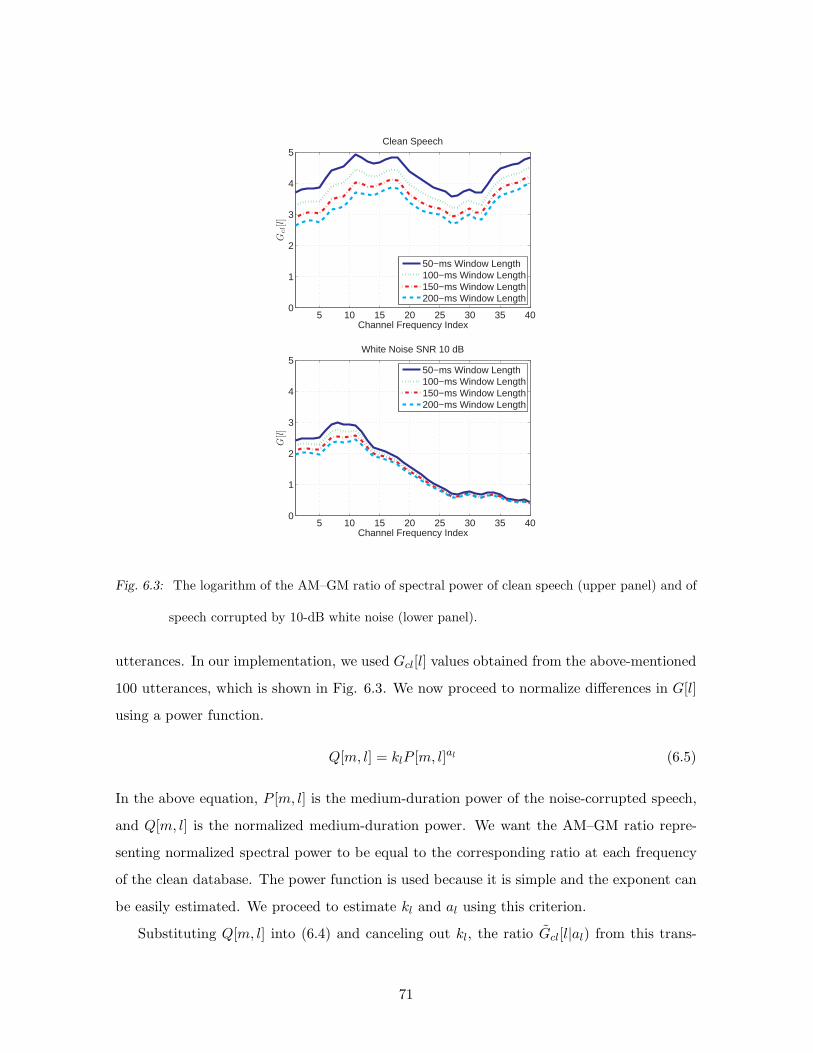
5 10 15 20 25 30 35 400

1

2

3

4

5

Channel Frequency Index

Gcl[l]

Clean Speech

50−ms Window Length100−ms Window Length150−ms Window Length200−ms Window Length

5 10 15 20 25 30 35 400

1

2

3

4

5

Channel Frequency Index

G[l]

White Noise SNR 10 dB

50−ms Window Length100−ms Window Length150−ms Window Length200−ms Window Length

Fig. 6.3: The logarithm of the AM–GM ratio of spectral power of clean speech (upper panel) and of

speech corrupted by 10-dB white noise (lower panel).

utterances. In our implementation, we used Gcl[l] values obtained from the above-mentioned

100 utterances, which is shown in Fig. 6.3. We now proceed to normalize differences in G[l]

using a power function.

Q[m, l] = klP [m, l]al (6.5)

In the above equation, P [m, l] is the medium-duration power of the noise-corrupted speech,

and Q[m, l] is the normalized medium-duration power. We want the AM–GM ratio repre-

senting normalized spectral power to be equal to the corresponding ratio at each frequency

of the clean database. The power function is used because it is simple and the exponent can

be easily estimated. We proceed to estimate kl and al using this criterion.

Substituting Q[m, l] into (6.4) and canceling out kl, the ratio Gcl[l|al) from this trans-

71

Q[m

,l]

P [m, l]

0c M

M[m

,l]

0 cMM[m, l]

a = 1a = 2a = 4

Fig. 6.4: The assumption about the relationship between S[m, l] and P [m, l]. Note that the slope of

the curve relating P [m, l] to Q[m, l] is unity when P [m, l] = cMM [m, l]

formed variable Q[m, l] can be represented by the following equation:

Gcl[l|al) = log

(

1

M

M−1∑

m=0

P [m, l]al

)

−1

M

M−1∑

m=0

logP [m, l]al (6.6)

For a specific channel l, we see that al is the only unknown variable in Gcl(j|al). From the

following equation:

Gcl[l|al) = Gcl[l] (6.7)

we can obtain a value for al using the Newton-Raphson method.

The parameter kl in Eq. (6.5) is obtained by assuming that the derivative of Q[m, l]

with respect to P [m, l] is the unity at maxiP [m, l] for this channel l, we set up the following

constraint:

dQ[m, l]

dP [m, l]

∣

∣

∣

∣

∣

maxmP [m,l]

= 1 (6.8)

The above constraint is illustrated in Fig 6.4. The meaning of the above equation is that

the slope of the nonlinearity is unity for the largest power of the lth channel. This constraint

72

might look arbitrary, but it makes sense for additive noise case, since the following equation

will hold:

P [m, l] = S[m, l] +N [m, l] (6.9)

where S[m, l] is the true clean speech power, andN [m, l] is the noise power. By differentiating

the above equation with respect to P [m, l] we obtain:

dS[m, l]

dP [m, l]= 1−

dN [m, l]

dP [m, l](6.10)

At the peak value of P [m, l] , the variation of N [m, l] will be much smaller for a given

variation of P [m, l], which means that the variation of P [m, l] around its largest value would

be mainly due to variations of the speech power rather than the noise power. In other words,

the second term on the right hand side of Eq. (6.10) would be very small, yielding Eq.(6.8).

By substituting (6.8) into (6.5), we obtain a value for kl:

kl =1

almaxm

P [m, l]1−al (6.11)

Using the above equation with (6.5), we obtain normalized power Q[m, l], which is given by:

Q[m, l] =1

almaxm

P [m, l]1−alP [m, l]al (6.12)

We apply a suitable flooring to Q[m, l]. This procedure is explained in Sec. 6.2.3. For each

time-frequency bin, the weight w[m, l] is given by the following equation.

w[m, l] =R[m, l]

P [m, l]

(6.13)

where R[m, l] is the floored power obtained from Q[m, l]. After obtaining the weight w[m, l]

for each gammatone channel, we reshape the original spectrumX[m, ejωk) using the following

equation for the mth frame:

Y [m, ejωk) =

∑L−1l=0

√

w[m, l]|Hl(ejωk)|

∑L−1l=0 |Hl(ejωk)|

X[m, ejωk) (6.14)

The above approach is similar to what we used in [46, 65]. In Fig. 6.1, the above procedure is

represented by the “spectral reshaping” block. As mentioned before, Hl(ejωk) is the spectrum

of the lth channel of the gammatone filter bank, and L is the total number of channels.

73

X[m, ejωk) is the resultant enhanced spectrum. After doing this, we compute the IFFT of

X[m, ejωk) to retrieve the time-domain signal and perform de-emphasis to compensate for

the effect of the previous pre-emphasis. The speech waveform is resynthesized using OLA.

6.1.3 Medium-duration windowing

Even though short-time windows of 20 to 30 ms duration are best for feature extraction for

speech signals, in many applications we observe that longer windows are better for normal-

ization purposes (e.g. [55] [46] [35] [66]). The reason for this is that noise power changes more

slowly than the rapidly-varying speech signal. Hence, while good performance is obtained

using short-duration windows for ASR, longer-duration windows are better for parameter

estimation for noise compensation. Figure describes recognition accuracy as a function of

window length. As can be seen in the figure a window of length between 75 ms and 100 ms

provides the best parameter estimation for noise compensation and normalization. We will

refer to a window of approximately this duration as a “medium-time window” as in [64].

6.2 Online implementation

In many applications the development of a real-time “online” algorithm for speech recognition

and speech enhancement is desired. In this case we cannot use (6.6) for obtaining the

coefficient al, since this equation requires the knowledge about the entire speech signal. In

this section we discuss how an online algorithm of the power equalization algorithm can be

implemented.

6.2.1 Power coefficient estimation

In this section, we discuss how to obtain a power coefficient al for each channel l, which

satisfies (6.7) using an “online” algorithm. We define two terms S1[m, l|al) and S2[m, l|al)

with a forgetting factor λ of 0.995 as follows.

S1[m, l|al) = λS1[m, l − 1) + (1− λ)Ql[m]al (6.15)

S2[m, l|al) = λS2[m, l − 1) + (1− λ) lnQl[m]al (6.16)

al = 1, 2, ..., 10

74

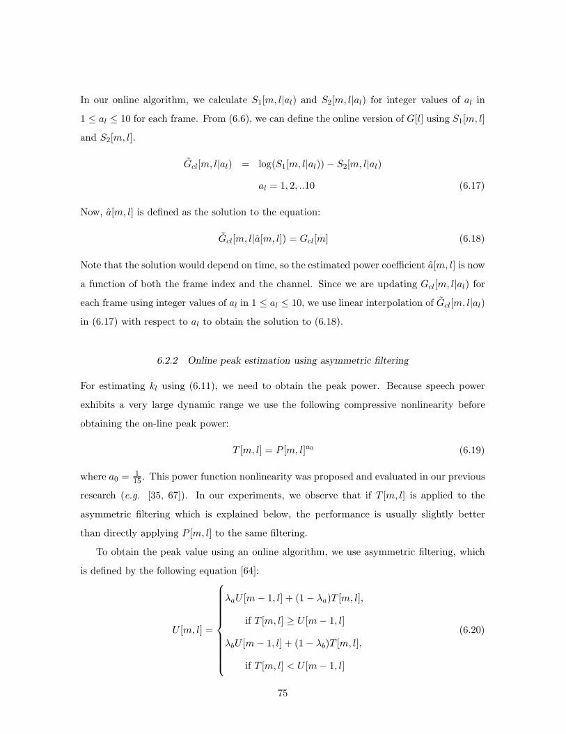
In our online algorithm, we calculate S1[m, l|al) and S2[m, l|al) for integer values of al in

1 ≤ al ≤ 10 for each frame. From (6.6), we can define the online version of G[l] using S1[m, l]

and S2[m, l].

Gcl[m, l|al) = log(S1[m, l|al))− S2[m, l|al)

al = 1, 2, ..10 (6.17)

Now, a[m, l] is defined as the solution to the equation:

Gcl[m, l|a[m, l]) = Gcl[m] (6.18)

Note that the solution would depend on time, so the estimated power coefficient a[m, l] is now

a function of both the frame index and the channel. Since we are updating Gcl[m, l|al) for

each frame using integer values of al in 1 ≤ al ≤ 10, we use linear interpolation of Gcl[m, l|al)

in (6.17) with respect to al to obtain the solution to (6.18).

6.2.2 Online peak estimation using asymmetric filtering

For estimating kl using (6.11), we need to obtain the peak power. Because speech power

exhibits a very large dynamic range we use the following compressive nonlinearity before

obtaining the on-line peak power:

T [m, l] = P [m, l]a0 (6.19)

where a0 =115 . This power function nonlinearity was proposed and evaluated in our previous

research (e.g. [35, 67]). In our experiments, we observe that if T [m, l] is applied to the

asymmetric filtering which is explained below, the performance is usually slightly better

than directly applying P [m, l] to the same filtering.

To obtain the peak value using an online algorithm, we use asymmetric filtering, which

is defined by the following equation [64]:

U [m, l] =

λaU [m− 1, l] + (1− λa)T [m, l],

if T [m, l] ≥ U [m− 1, l]

λbU [m− 1, l] + (1− λb)T [m, l],

if T [m, l] < U [m− 1, l]

(6.20)

75

where m is the frame index, l is the channel index as before, T [m, l] is the input to the filter,

and U [m, l] is the output of the filter. As shown in (8.4), the asymmetric filter resembles a

first-order IIR filter, but the filter coefficients are different depending on whether the current

input T [m, l] is equal to or larger than the previous filter U [m − 1, l]. More specifically, if

1 > λa > λb > 0, then as shown in Fig. 6.5, the nonlinear filter function as a conventional

upper envelope detector. In contrast, if 1 > λb > λa > 0, the filter output U [m, l] tends to

follow the lower envelope of T [m, l]. As in [64], we will use the following notation

U [m, l] = AFλa,λb[T [m, l]] (6.21)

to represent the nonlinear filter described by (8.4). In the examples in Fig. 6.5, Tup[m, l] =

AF0.995,0.5[T [m, l]] and Tlow[m, l] = AF0.5,0.995[T [m, l]]. From Tup[m, l], the moving peak

value V [m, l] is obtained using the following equation:

V [m, l] = Tup[m, l]1a0 (6.22)

where a0 = 115 as in (6.19). Thus, Eq. (6.22) decompresses the effect of the compressive

nonlinearity in Eq. (6.19).

For the actual peak level, we use the following value:

Vo[m, l] = c0V [m, l] (6.23)

where we use c0 of 1.5. We use this multiplicative factor, since the power T [m, l] can be

larger than Tup[m, l] for some peaks.

One problem with the above procedure is the initialization of the asymmetric filter in

(8.4). Usually, the first frames (when m = 0) belong to non-speech segments, so the peak

values in this part are likely to be be much smaller than those of the speech segments. We

observe that this characteristic has a negative effect on performance. In our implementation,

we resolve this issue by using the average values of Tup[m, l] for each channel l from the speech

segments of 100 utterances selected from WSJ0 SI-84, which was also used for obtaining AM–

GM ratio in Sec. 6.1.2. Let us denote these average values for each channel by µT [l]. The

initial value Tup[0, l] is obtained by the following equation:

Tup[0, l] = (µT [l]1a0 + P [0, l])a0 (6.24)

76

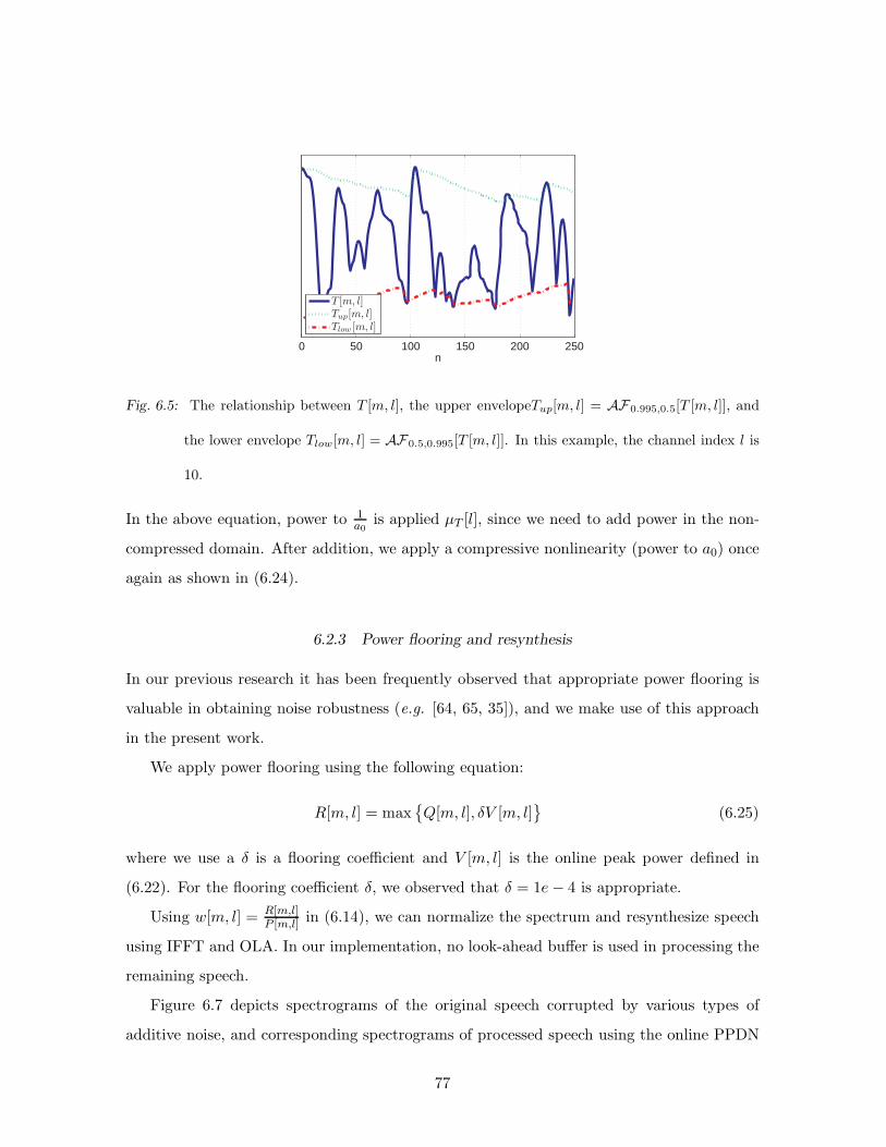
0 50 100 150 200 250n

T [m, l]Tup[m, l]Tlow [m, l]

Fig. 6.5: The relationship between T [m, l], the upper envelopeTup[m, l] = AF0.995,0.5[T [m, l]], and

the lower envelope Tlow[m, l] = AF0.5,0.995[T [m, l]]. In this example, the channel index l is

10.

In the above equation, power to 1a0

is applied µT [l], since we need to add power in the non-

compressed domain. After addition, we apply a compressive nonlinearity (power to a0) once

again as shown in (6.24).

6.2.3 Power flooring and resynthesis

In our previous research it has been frequently observed that appropriate power flooring is

valuable in obtaining noise robustness (e.g. [64, 65, 35]), and we make use of this approach

in the present work.

We apply power flooring using the following equation:

R[m, l] = max

Q[m, l], δV [m, l]

(6.25)

where we use a δ is a flooring coefficient and V [m, l] is the online peak power defined in

(6.22). For the flooring coefficient δ, we observed that δ = 1e− 4 is appropriate.

Using w[m, l] = R[m,l]P [m,l] in (6.14), we can normalize the spectrum and resynthesize speech

using IFFT and OLA. In our implementation, no look-ahead buffer is used in processing the

remaining speech.

Figure 6.7 depicts spectrograms of the original speech corrupted by various types of

additive noise, and corresponding spectrograms of processed speech using the online PPDN

77

0 50 100 150 2000

20

40

60

80

100

Window length (ms)

Acc

urac

y (1

00%

− W

ER

)

RM1 (White Noise)

CleanWhite 10 dBWhite 5 dBWhite 0 dB

(a)

0 50 100 150 2000

20

40

60

80

100

Window length (ms)

Acc

urac

y (1

00%

− W

ER

)

RM1 (Music Noise)

CleanMusic 10 dBMusic 5 dBMusic 0 dB

(b)

Fig. 6.6: Speech recognition accuracy as a function of window length for noise compensation cor-

rupted by white noise and background music.

explained in this section. As seen in 6.7(b), for additive Gaussian white noise, improvement

is observable even at 0-dB SNR. For the 10-dB music and 5-dB street noise samples, which

are more realistic, as shown in 6.7(d) and 6.7(f), we can clearly observe that processing

provides improvement. In the next section, we present speech recognition results using the

online PPDN algorithm.

6.3 Simulation results using the online power equalization algorithm

In this section we describe experimental results obtained on the DARPA Resource Man-

agement (RM) database using the online processing as described in Section 6.2. We first

observe that the online PPDN algorithm improves the subjective quality of speech, as can be

assessed by the reader by comparing processed and unprocessed speech in the demo package

at http://www.cs.cmu.edu/~robust/archive/algorithms/IEEETran_PPDN

78

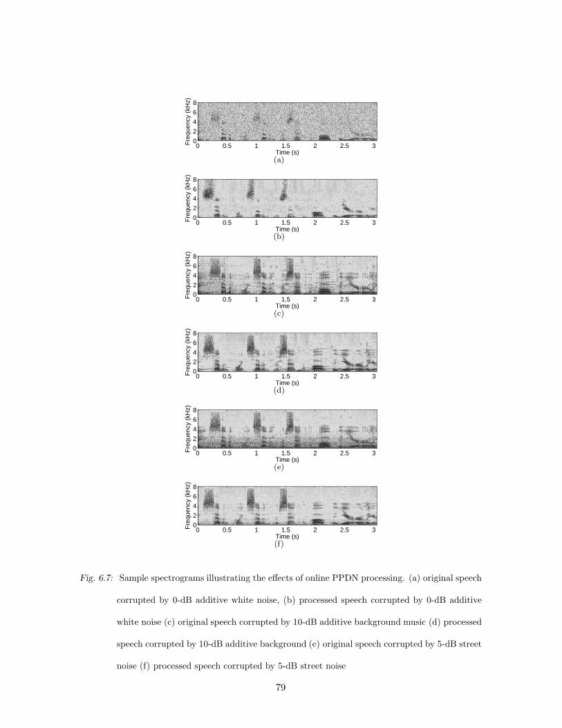
http://www.cs.cmu.edu/~robust/archive/algorithms/IEEETran_PPDN

Time (s)

Fre

quen

cy (

kHz)

0 0.5 1 1.5 2 2.5 30

2

4

6

8

(a)

Time (s)

Fre

quen

cy (

kHz)

0 0.5 1 1.5 2 2.5 30

2

4

6

8

(b)

Time (s)

Fre

quen

cy (

kHz)

0 0.5 1 1.5 2 2.5 30

2

4

6

8

(c)

Time (s)

Fre

quen

cy (

kHz)

0 0.5 1 1.5 2 2.5 30

2

4

6

8

(d)

Time (s)

Fre

quen

cy (

kHz)

0 0.5 1 1.5 2 2.5 30

2

4

6

8

(e)

Time (s)

Fre

quen

cy (

kHz)

0 0.5 1 1.5 2 2.5 30

2

4

6

8

(f)

Fig. 6.7: Sample spectrograms illustrating the effects of online PPDN processing. (a) original speech

corrupted by 0-dB additive white noise, (b) processed speech corrupted by 0-dB additive

white noise (c) original speech corrupted by 10-dB additive background music (d) processed

speech corrupted by 10-dB additive background (e) original speech corrupted by 5-dB street

noise (f) processed speech corrupted by 5-dB street noise

79

For quantitative evaluation of PPDN we used 1,600 utterances from the DARPA Re-

source Management (RM) database for training and 600 utterances for testing. We used

SphinxTrain 1.0 for training the acoustic models, and Sphinx 3.8 for decoding. For fea-

ture extraction we used sphinx fe which is included in sphinxbase 0.4.1. In Fig. 6.8(a),

we used test utterances corrupted by additive white Gaussian noise, and in Fig. 6.8(b), noise

recorded on a busy street was added to the test set. In Fig. 6.8(c) we used test utterances

corrupted by musical segments of the DARPA Hub 4 Broadcast News database.

We prefer to characterize the improvement in recognition accuracy as the amount by

which curves depicting WER as a function of SNR shift laterally when processing is applied.

We refer to this statistic as the “threshold shift”. As shown in these figures, PPDN provided

10-dB threshold shifts for white noise, 6.5-dB threshold shifts for street noise and 3.5-dB

shifts for background music. Note that obtaining improvements for background music is not

easy.

For comparison, we also obtained similar results using the state-of-the-art noise compen-

sation algorithm Vector Taylor series (VTS) [10]. For PPDN, further application of Mean

Variance Normalization (MVN) provided slightly better recognition accuracy than the appli-

cation of CMN. Nevertheless, for VTS, we could not observe any improvement in performance

by applying MVN in addition, so we compared the MVN version of PPDN and the CMN

version of VTS. For white noise, the PPDN algorithm outperforms VTS if the SNR is equal

to or less than 5 dB, and the threshold shift is also larger. If the SNR is greater than or

equal to 10 dB, VTS provides doing somewhat better recognition accuracy. In street noise,

PPDN and VTS exhibited similar performance. For background music, which is considered

to be more difficult, the PPDN algorithm produced threshold shifts of approximately 3.5 dB,

along with better accuracy than VTS for all SNRs.

6.4 Conclusions

We describe a new power equalization algorithm, PPDN, that is based on applying a power

function that normalizes the ratio of the arithmetic mean to the geometric mean of power

in each frequency band. PPDN is simple and easier to implement than many other normal-

ization algorithms. PPDN is quite effective in combatting the effects of additive noise and

80

0 5 10 15 20 Clean0

10

20

30

40

50

60

70

80

90

100

SNR (dB)

Acc

urac

y (1

00 −

WE

R)

RM1 (White Noise)

Baseline (CMN)Baseline (MVN)VTS (CMN)PPDN (MVN)

(a)

0 5 10 15 20 Clean0

10

20

30

40

50

60

70

80

90

100

SNR (dB)

Acc

urac

y (1

00 −

WE

R)

RM1 (Street Noise)


(b)

0 5 10 15 20 Clean0

10

20

30

40

50

60

70

80

90

100

SNR (dB)

Acc

urac

y (1

00 −

WE

R)

RM1 (Music Noise)


(c)

Fig. 6.8: Comparison of recognition accuracy for the DARPA RM database corrupted by (a) white

noise, (b) street noise, and (c) music noise.

it provides comparable or somewhat better recognition accuracy than the VTS algorithm.

Since PPDN resynthesizes the speech waveform, it can also be used for speech enhancement

or as a pre-processing stage in conjunction with other algorithms that work in the cepstral

domain. PPDN can also be implemented as an online algorithm without any look-ahead

81

buffer. This characteristic makes the algorithm potentially useful for applications such as

real-time speech recognition or real-time speech enhancement. We also noted above that

windows used to extract parametric information for noise compensation should be roughly

three times the duration of those that are used for feature extraction. We used a window

length of 100 ms for our normalization procedures.

6.5 Open Source Software

We provide the software used to implement PPDN in open source form at http://www.cs.

cmu.edu/~robust/archive/IEEETran_PPDN. [68]. The code in this directory was used for

obtaining the results described in this chapter.

82

http://www.cs.cmu.edu/~robust/archive/IEEETran_PPDN

http://www.cs.cmu.edu/~robust/archive/IEEETran_PPDN

7. ONSET ENHANCEMENT

In this chapter we introduce an onset enhancement algorithm which is referred to as Sup-

pression of Slowly-varying components and the Falling edge (SSF) of the power envelope. It

has long been believed that modulation frequency plays an important role in human hearing.

For example, it is observed that the human auditory system is more sensitive to modulation

frequencies less than 20 Hz (e.g. [33] [34]). On the other hand, very slowly changing com-

ponents (e.g. less than 5 Hz) are usually related to noisy sources (e.g.[35] [36] [37]). Based

on these observations, researchers have tried to utilize modulation frequency information to

enhance the speech recognition performance in noisy environments. Typical approaches use

highpass or bandpass filtering in either the spectral, log-spectral, or cepstral domains (e.g.

[32]). In [2], Hirsch et al. investigated the effects of highpass filtering of spectral envelopes

of each frequency subband. Hirsch conducted highpass filtering in the log spectral domain,

using the transfer function:

H(z) =1− z−1

1− 0.7z−1(7.1)

This first-order IIR filter can be implemented by subtracting an exponentially weighted

moving average from the current log spectral value. For robust speech recognition the other

common difficulty is reverberation. Many hearing scientists believe that human speech per-

ception in reverberation is enabled by the “precedence effect”, which refers to the emphasis

that appears to be given to the first-arriving wave-front of a complex signal in sound local-

ization and possibly speech perception (e.g. [69]). To detect the first wave-front, we can

either measure the envelope of the signal or energy in the frame (e.g. [70] [71]).

In this chapter we introduce an approach that we refer to as SSF processing, which

represents Suppression of Slowly-varying components and the Falling edge of the power

envelope. This processing mimics aspects of both the precedence effect and modulation

spectrum analysis. SSF processing operates on frequency weighted power coefficients as they

evolve over time, as described below. The DC-bias term is first removed in each frequency

band by subtracting an exponentially-weighted moving average. When the instantaneous

power in a given frequency channel is smaller than this average, the power is suppressed,

either by scaling by a small constant or by replacement by the scaled moving average. The

first approach results in better sound quality for non-reverberated speech, but the latter

results in better speech recognition accuracy in reverberant environments. SSF processing is

normally applied to both training and testing data in speech recognition applications.

In speech signal analysis, we normally use a short-duration window with duration between

20 and 30 ms. With the SSF algorithm, we observe that windows longer than this length are

more appropriate for estimating or compensating for noise components, which is consistent

with our observations in previous work (e.g. [55][46][35]). Nevertheless, even if we use

a longer-duration window for noise estimation, we must use a short-duration window for

speech feature extraction. After performing frequency-domain processing we use an IFFT

and the overlap-add method (OLA) to re-synthesize speech, as in [36]. Feature extraction

and subsequent speech recognition can be performed on the re-synthesized speech. We refer

to this general approach as the medium-duration analysis and synthesis approach (MAS).

7.1 Structure of the SSF algorithm

Figure 7.1 shows the structure of the SSF algorithm. The input speech signal is pre-

emphasized and then multiplied by a medium-duration Hamming window as in [36]. This

signal is represented by xm[n] in Fig. 7.1 where m denotes the frame index. We use a 50-ms

window and 10 ms between frames. After windowing, the FFT is computed and integrated

over frequency using gammatone weighting functions to obtain the power P [m, l] in the mth

frame and lth frequency band as shown below:

P [m, l] =

N−1∑

k=0

|X[m, ejωk)Hl(ejωk)|2, 0 ≤ l ≤ L− 1 (7.2)

where k is a dummy variable representing the discrete frequency index, and N is the FFT

size. The discrete frequency is ωk = 2πk/N . Since we are using a 50-ms window, for 16-kHz

audio samples N is 1024. Hl(ejωk) is the spectrum of the gammatone filter bank for the lth

channel evaluated at frequency index k, and X[m, ejωk) is the short-time spectrum of the

84

Pre-Emphasis

STFT

Magnitude Squared

|H0(ejωk )|2

Squared

Gammatone

Band Integration

|H1(ejωk )|2

Squared

Gammatone

Band Integration

|HL−1(ejωk )|2

Squared

Gammatone

Band Integration

SSF Processing SSF Processing SSF Processing

Spectral Reshaping

IFFT

Post-Deemphasis

x[n]

xm[n]

X[m, ejωk )

|X[m, ejωk)|2

P [m, 0] P [m, 1]P [m,L − 1]

w[m, 0] w[m, 1]w[m,L − 1]

X[m, ejωk )

xm[n]

x[n]

Fig. 7.1: The block diagram of the SSF processing system

speech signal for the mth frame, where L = 40 is the total number of gammatone channels.

After the SSF processing described below, we perform spectral reshaping and compute the

IFFT using OLA to obtain enhanced speech.

7.2 SSF Type-I and SSF Type-II Processing

In SSF processing, we first obtain the lowpassed power M [m, l] from each channel:

M [m, l] = λM [m− 1, l] + (1− λ)P [m, l] (7.3)

85

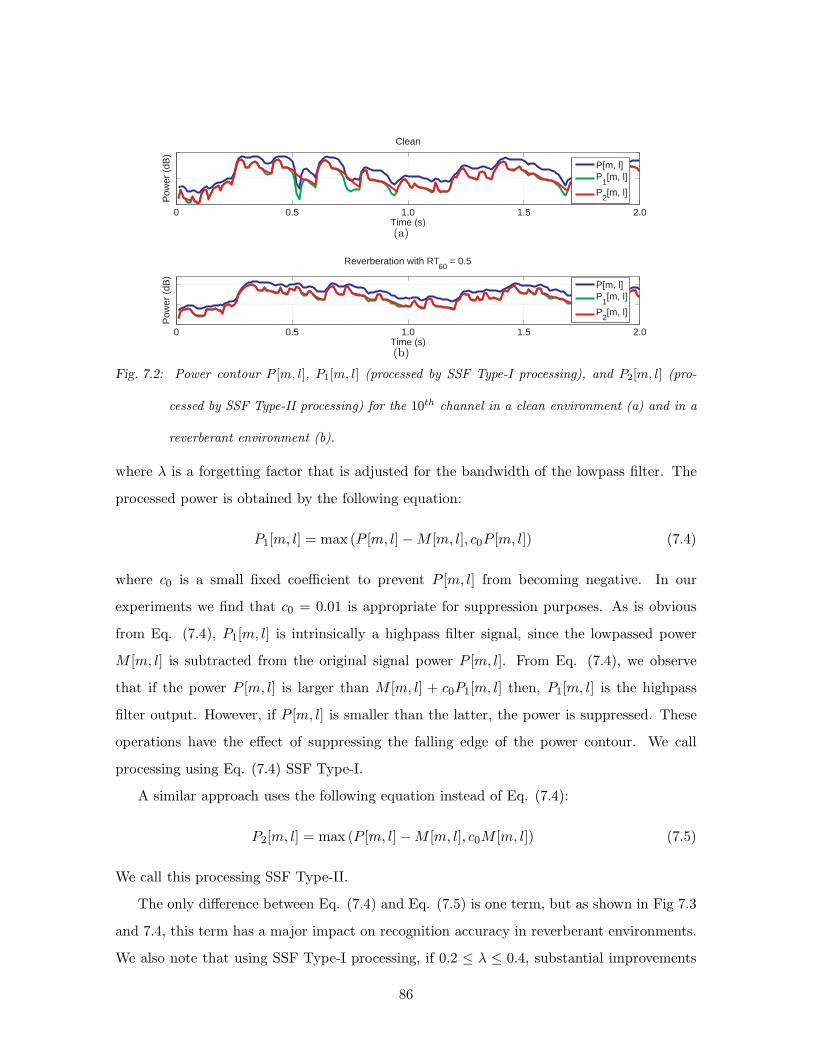
0 0.5 1.0 1.5 2.0Time (s)

Pow

er (

dB)

Clean

P[m, l]P

1[m, l]

P2[m, l]

(a)

0 0.5 1.0 1.5 2.0Time (s)

Pow

er (

dB)

Reverberation with RT60

= 0.5

P[m, l]P

1[m, l]

P2[m, l]

(b)

Fig. 7.2: Power contour P [m, l], P1[m, l] (processed by SSF Type-I processing), and P2[m, l] (pro-

cessed by SSF Type-II processing) for the 10th channel in a clean environment (a) and in a

reverberant environment (b).

where λ is a forgetting factor that is adjusted for the bandwidth of the lowpass filter. The

processed power is obtained by the following equation:

P1[m, l] = max (P [m, l]−M [m, l], c0P [m, l]) (7.4)

where c0 is a small fixed coefficient to prevent P [m, l] from becoming negative. In our

experiments we find that c0 = 0.01 is appropriate for suppression purposes. As is obvious

from Eq. (7.4), P1[m, l] is intrinsically a highpass filter signal, since the lowpassed power

M [m, l] is subtracted from the original signal power P [m, l]. From Eq. (7.4), we observe

that if the power P [m, l] is larger than M [m, l] + c0P1[m, l] then, P1[m, l] is the highpass

filter output. However, if P [m, l] is smaller than the latter, the power is suppressed. These

operations have the effect of suppressing the falling edge of the power contour. We call

processing using Eq. (7.4) SSF Type-I.

A similar approach uses the following equation instead of Eq. (7.4):

P2[m, l] = max (P [m, l]−M [m, l], c0M [m, l]) (7.5)

We call this processing SSF Type-II.

The only difference between Eq. (7.4) and Eq. (7.5) is one term, but as shown in Fig 7.3

and 7.4, this term has a major impact on recognition accuracy in reverberant environments.

We also note that using SSF Type-I processing, if 0.2 ≤ λ ≤ 0.4, substantial improvements

86

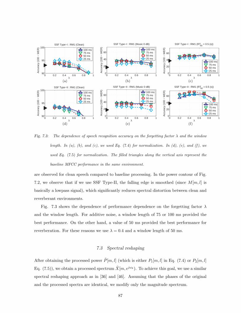
0 0.2 0.4 0.6 0.8 190

95

100

λ

Acc

urac

y (1

00 −

WE

R)

SSF Type−I : RM1 (Clean)

100 ms75 ms50 ms25 ms

(a)

0 0.2 0.4 0.6 0.8 10

20

40

60

λ

Acc

urac

y (1

00 −

WE

R)

SSF Type−I : RM1 (Music 0 dB)

100 ms75 ms50 ms25 ms

(b)

0 0.2 0.4 0.6 0.8 10

20

40

60

λ

Acc

urac

y (1

00 −

WE

R)

SSF Type−I : RM1 (RT60

= 0.5 (s))

100 ms75 ms50 ms25 ms

(c)

0 0.2 0.4 0.6 0.8 190

95

100

λ

Acc

urac

y (1

00 −

WE

R)

SSF Type−II : RM1 (Clean)

100 ms75 ms50 ms25 ms

(d)

0 0.2 0.4 0.6 0.8 10

20

40

60

λ

Acc

urac

y (1

00 −

WE

R)

SSF Type−II : RM1 (Music 0 dB)

100 ms75 ms50 ms25 ms

(e)

0 0.2 0.4 0.6 0.8 10

20

40

60

λ

Acc

urac

y (1

00 −

WE

R)

SSF Type−II : RM1 (RT60

= 0.5 (s))

100 ms75 ms50 ms25 ms

(f)

Fig. 7.3: The dependence of speech recognition accuracy on the forgetting factor λ and the window

length. In (a), (b), and (c), we used Eq. (7.4) for normalization. In (d), (e), and (f), we

used Eq. (7.5) for normalization. The filled triangles along the vertical axis represent the

baseline MFCC performance in the same environment.

are observed for clean speech compared to baseline processing. In the power contour of Fig.

7.2, we observe that if we use SSF Type-II, the falling edge is smoothed (since M [m, l] is

basically a lowpass signal), which significantly reduces spectral distortion between clean and

reverberant environments.

Fig. 7.3 shows the dependence of performance dependence on the forgetting factor λ

and the window length. For additive noise, a window length of 75 or 100 ms provided the

best performance. On the other hand, a value of 50 ms provided the best performance for

reverberation. For these reasons we use λ = 0.4 and a window length of 50 ms.

7.3 Spectral reshaping

After obtaining the processed power P [m, l] (which is either P1[m, l] in Eq. (7.4) or P2[m, l]

Eq. (7.5)), we obtain a processed spectrum X[m, ejωk). To achieve this goal, we use a similar

spectral reshaping approach as in [36] and [46]. Assuming that the phases of the original

and the processed spectra are identical, we modify only the magnitude spectrum.

87

First, for each time-frequency bin, we obtain the weighting coefficient w[m, l] as a ratio

of the processed power P [m, l] to P [m, l].

w[m, l] =P [m, l]

P [m, l], 0 ≤ l ≤ L− 1 (7.6)

Each of these channels is associated with Hl, the frequency response of one of a set of gam-

matone filters with center frequencies distributed according to the Equivalent Rectangular

Bandwidth (ERB) scale [4]. The final spectral weighting µ[m,k] is obtained using the above

weight w[m, l]

µ[m,k] =

∑L−1l=0 w[m, l]

∣

∣Hl

(

ejωk)∣

∣

∑L−1l=0 |Hl (ejωk)|

,

0 ≤ k ≤ N/2 − 1, 0 ≤ l ≤ L− 1 (7.7)

After obtaining µ[m,k] for the lower half of the frequencies (0 ≤ k ≤ N/2), we can obtain

the upper half by applying Hermitian symmetry:

µ[m,k] = µ[m,N − k], N/2 ≤ k ≤ N − 1 (7.8)

Using µ[m,k], the reconstructed spectrum is obtained by:

X [m, ejωk) = µ[m,k]X[m, ejωk), 0 ≤ k ≤ N − 1 (7.9)

The enhanced speech x[n] is re-synthesized using the IFFT and the overlap-add method as

in previous chapters.


In this section we describe experimental results obtained on the DARPA Resource Manage-

ment (RM) database using the SSF algorithm. For quantitative evaluation of SSF we used

1,600 utterances from the DARPA Resource Management (RM) database for training and

600 utterances for testing. We used SphinxTrain 1.0 for training the acoustic models, and

Sphinx 3.8 for decoding. For feature extraction we used sphinx fe which is included in

sphinxbase 0.4.1. Even though SSF was developed for reverberant environments, we also

conducted experiments in additive noise as well. In Fig. 7.4(a), we used test utterances

corrupted by additive white Gaussian noise, and in Fig. 7.4(b), we used test utterances

corrupted by musical segments of the DARPA Hub 4 Broadcast News database.

88

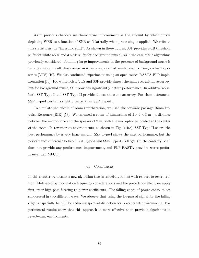
As in previous chapters we characterize improvement as the amount by which curves

depicting WER as a function of SNR shift laterally when processing is applied. We refer to

this statistic as the “threshold shift”. As shown in these figures, SSF provides 8-dB threshold

shifts for white noise and 3.5-dB shifts for background music. As in the case of the algorithms

previously considered, obtaining large improvements in the presence of background music is

usually quite difficult. For comparison, we also obtained similar results using vector Taylor

series (VTS) [10]. We also conducted experiments using an open source RASTA-PLP imple-

mentation [30]. For white noise, VTS and SSF provide almost the same recognition accuracy,

but for background music, SSF provides significantly better performance. In additive noise,

both SSF Type-I and SSF Type-II provide almost the same accuracy. For clean utterances,

SSF Type-I performs slightly better than SSF Type-II.

To simulate the effects of room reverberation, we used the software package Room Im-

pulse Response (RIR) [53]. We assumed a room of dimensions of 5 × 4 × 3 m , a distance

between the microphone and the speaker of 2 m, with the microphones located at the center

of the room. In reverberant environments, as shown in Fig. 7.4(c), SSF Type-II shows the

best performance by a very large margin. SSF Type-I shows the next performance, but the

performance difference between SSF Type-I and SSF-Type-II is large. On the contrary, VTS

does not provide any performance improvement, and PLP-RASTA provides worse perfor-

mance than MFCC.

7.5 Conclusions

In this chapter we present a new algorithm that is especially robust with respect to reverbera-

tion. Motivated by modulation frequency considerations and the precedence effect, we apply

first-order high-pass filtering to power coefficients. The falling edges of power contours are

suppressed in two different ways. We observe that using the lowpassed signal for the falling

edge is especially helpful for reducing spectral distortion for reverberant environments. Ex-

perimental results show that this approach is more effective than previous algorithms in

reverberant environments.

89

0 5 10 15 20 Clean0

20

40

60

80

100

Acc

urac

y (1

00 −

WE

R)

SNR (dB)

RM1 (White Noise)

(a)

0 5 10 15 20 Clean0

20

40

60

80

100

SNR (dB)

Acc

urac

y (1

00 −

WE

R)

RM1 (Music Noise)

SSF Type−IISSF Type−IMFCC with VTS and CMNBaseline MFCC with CMNRASTA−PLP with CMN

(b)

0 0.1 0.2 0.3 0.4 0.5 0.6 0.9 1.20

20

40

60

80

100

Acc

urac

y (1

00 −

WE

R)


RM1 (Reverberation)

(c)

Fig. 7.4: Comparison of speech recognition accuracy using the two types of SSF, VTS, and base-

line MFCC and PLP processing for (a) white noise, (b) musical noise, and (c) reverberant

environments.

7.6 Open source MATLAB code

MATLAB code for the SSF algorithm may be found at [URL here] . This code was used to

obtain the results in Section 7.4.

90

8. POWER NORMALIZED CEPSTRAL COEFFICIENT

In this chapter, we discuss our new feature PNCC processing. PNCC incorporates concepts

we discussed in Chap. 3, 4, and 7.

8.1 Introduction

In recent decades following the introduction of hidden Markov models (e.g. [72]) and sta-

tistical language models (e.g.[73]), the performance of speech recognition systems in benign

acoustical environments has dramatically improved. Nevertheless, most speech recognition

systems remain sensitive to the nature of the acoustical environments within which they are

deployed, and their performance deteriorates sharply in the presence of sources of degrada-

tion such as additive noise, linear channel distortion, and reverberation.

One of the most challenging contemporary problems is that recognition accuracy degrades

significantly if the test environment is different from the training environment and/or if

the acoustical environment includes disturbances such as additive noise, channel distortion,

speaker differences, reverberation, and so on. Over the years dozens if not hundreds of

algorithms have been introduced to address this problem. Many of these conventional noise

compensation algorithms have provided substantial improvement in accuracy for recognizing

speech in the presence of quasi-stationary noise (e.g. [9, 10, 7, 41, 12, 74]). Unfortunately

these same algorithms frequently do not provide significant improvements in more difficult

environments with transitory disturbances such as a single interfering speaker or background

music (e.g. [42]).

Virtually all of the current systems developed for automatic speech recognition, speaker

identification, and related tasks are based on variants of one of two types of features: mel

frequency cepstral coefficients (MFCC) [22] or perceptual linear prediction (PLP) coefficients

[25]. In this chapter we describe the development of a third type of feature set for speech

recognition which we refer to as power-normalized cepstral coefficients (PNCC). As we will

show, PNCC features provide superior recognition accuracy over a broad range of conditions

of noise and reverberation using features that are computable in real time using “online”

algorithms, and with a computational complexity that is comparable to that of traditional

MFCC and PLP features.

In the subsequent subsections of this Introduction we discuss the broader motivations

and overall structure of PNCC processing. We specify the key elements of the processing

in some detail in Sec. 8.2. In Sec. 8.3 we compare the recognition accuracy provided by

PNCC processing under a variety of conditions with that of other processing schemes, and

we consider the impact of various components of PNCC on these results. We compare the

computational complexity of the MFCC, PLP, and PNCC feature extraction algorithms in

Sec. 8.6 and we summarize our results in the final section.

8.1.1 Broader motivation for the PNCC algorithm

The development of PNCC feature extraction was motivated by a desire to obtain a set

of practical features for speech recognition that are more robust with respect to acousti-

cal variability in their native form, without loss of performance when the speech signal is

undistorted, and with a degree of computational complexity that is comparable to that of

MFCC and PLP coefficients. While many of the attributes of PNCC processing have been

strongly influenced by consideration of various attributes of human auditory processing, we

have favored approaches that provide pragmatic gains in robustness at small computational

cost over approaches that are more faithful to auditory physiology in developing the specific

processing that is performed.

Some of the innovations of the PNCC processing that we consider to be the most impor-

tant include:

• The replacement of the log nonlinearity in MFCC processing by a power-law nonlin-

earity that is carefully chosen to approximate the nonlinear relation between signal

intensity and auditory-nerve firing rate. We believe that this nonlinearity provides

superior robustness by suppressing small signals and their variability, as discussed in

Sec. 8.2.7.

92

Pre-Emphasis

STFT

Magnitude Squared

TriangularFrequency Integration

STFT

Magnitude Squared

Critical-BandFrequency Integration

NonlinearCompression

Pre-Emphasis

STFT

Magnitude Squared

GammatoneFrequency Integration

Medium-TimePower Calculation

Asymmetric NoiseSuppression with

Temporal Masking

Weight Smoothing

Time-FrequencyNormalization

Mean PowerNormalization

],[~

lmQ

],[~

lmR

Power FunctionNonlinearity

RASTA Filtering

NonlinearExpansion

Power FunctionNonlinearity

LogarithmicNonlinearity

DCT IDFT DCT

Mean NormalizationMean NormalizationMean Normalization

LPC-BasedCepstral Recursion

3/1)(• 15/1)(•

MFCCCoefficients

RASTA-PLPCoefficients

PNCCCoefficients

],[~

lmS

],[ lmP

],[ lmT

],[ lmU

],[ lmV

Input SpeechInput SpeechInput Speech

Short-TimeProcessing

Medium-Time

Processing

Init

ial P

ro

ce

ssin

gE

nviro

nm

en

ta

l Co

mp

en

satio

nF

ina

l Pro

ce

ssin

g

Fig. 8.1: Comparison of the structure of the MFCC, PLP, and PNCC feature extraction algorithms.

The modules of PNCC that function on the basis of “medium-time” analysis (with a tempo-

ral window of 65.6 ms) are plotted in the rightmost column. If the shaded blocks of PNCC

are omitted, the remaining processing is referred to as simple power-normalized cepstral

coefficients (SPNCC).

• The use of “medium-time” processing with a duration of 50-120 ms to analyze the

parameters characterizing environmental degradation, in combination with the tradi-

93

tional short-time Fourier analysis with frames of 20-30 ms used in conventional speech

recognition systems. We believe that this approach enables us to estimate environmen-

tal degradation more accurately while maintaining the ability to respond to rapidly-

changing speech signals, as discussed in Sec. 8.2.2.

• The use of a form of “asymmetric nonlinear filtering” to estimate the level of the

acoustical background noise for each time frame and frequency bin. We believe that

this approach enables us to remove slowly-varying components easily without needing

to deal with many of the artifacts associated with over-correction in techniques such

as spectral subtraction [11], as discussed in Sec. 8.2.3. As shown in Sec. 8.3.3, this

approach is more effective than RASTA processing [3].

• The development of computationally-efficient realizations of the algorithms above that

support “online” real-time processing.

8.1.2 Structure of the PNCC algorithm

Figure 8.1 compares the structure of conventional MFCC processing [22], PLP processing

[25, 3], and the new PNCC approach which we introduce in this chapter. As was noted above,

the major innovations of PNCC processing include the redesigned nonlinear rate-intensity,

along with the series of processing elements to suppress the effects of background acoustical

activity based on medium-time analysis.

As can be seen from Fig. 8.1, the initial processing stages of PNCC processing are quite

similar to the corresponding stages of MFCC and PLP analysis, except that the frequency

analysis is performed using gammatone filters [57]. This is followed by the series of nonlinear

time-varying operations that are performed using the longer-duration temporal analysis that

accomplish noise subtraction as well as a degree of robustness with respect to reverberation.

The final stages of processing are also similar to MFCC and PLP processing, with the

exception of the carefully-chosen power-law nonlinearity with exponent 1/15, which will be

discussed in Sec. 8.2.7 below.

94

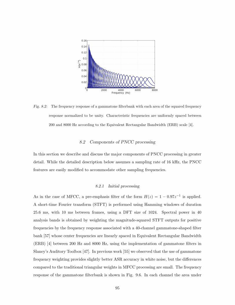
0 2000 4000 6000 80000

0.02

0.04

0.06

0.08

0.1

0.12

0.14

0.16

Frequency (Hz)

H(e

j ω)




8.2 Components of PNCC processing

In this section we describe and discuss the major components of PNCC processing in greater

detail. While the detailed description below assumes a sampling rate of 16 kHz, the PNCC

features are easily modified to accommodate other sampling frequencies.

8.2.1 Initial processing

As in the case of MFCC, a pre-emphasis filter of the form H(z) = 1 − 0.97z−1 is applied.

A short-time Fourier transform (STFT) is performed using Hamming windows of duration

25.6 ms, with 10 ms between frames, using a DFT size of 1024. Spectral power in 40

analysis bands is obtained by weighting the magnitude-squared STFT outputs for positive

frequencies by the frequency response associated with a 40-channel gammatone-shaped filter

bank [57] whose center frequencies are linearly spaced in Equivalent Rectangular Bandwidth

(ERB) [4] between 200 Hz and 8000 Hz, using the implementation of gammatone filters in

Slaney’s Auditory Toolbox [47]. In previous work [55] we observed that the use of gammatone

frequency weighting provides slightly better ASR accuracy in white noise, but the differences

compared to the traditional triangular weights in MFCC processing are small. The frequency

response of the gammatone filterbank is shown in Fig. 9.6. In each channel the area under

95

the squared transfer function is normalized to unity to satisfy the equation:

∫ 8000

0|Hl(f)|

2df = 1 (8.1)




(corresponding to -46 dB) of its maximum value.

We obtain the short-time spectral power P [m, l] using the squared gammatone summation

as below:

P [m, l] =

(K/2)−1∑

k=0

|X[m, ejωk)Hl(ejωk)|2 (8.2)

where K is the DFT size, m and l represent the frame and channel indices, respectively,

and ωk = 2πk/Fs, with Fs representing the sampling frequency. X[m, ejωk) is the short-time

spectrum of the mth frame of the signal.

8.2.2 Temporal integration for environmental analysis

Most speech recognition and speech coding systems use analysis frames of duration between

20 ms and 30 ms. Nevertheless, it is frequently observed that longer analysis windows provide

better performance for noise modeling and/or environmental normalization (e.g. [35, 36]),

because the power associated with most background noise conditions changes more slowly

than the instantaneous power associated with speech.

In PNCC processing we estimate a quantity we refer to as “medium-time power” Q[m, l]

by computing the running average of P [m, l], the power observed in a single analysis frame,

according to the equation:

Q[m, l] =1

2M + 1

m+M∑

m′=m−M

P [m′, l] (8.3)

where m represents the frame index and l is the channel index. We will apply the tilde

symbol to all power estimates that are performed using medium-time analysis.

We observed experimentally that the choice of the temporal integration factor M has a

substantial impact on performance in white noise (and presumably other types of broadband

96

background noise). This factor has less impact on the accuracy that is observed in more

dynamic interference or reverberation, although the longer temporal analysis window does

provide some benefit in these environments as well [75]. We chose the value of M = 2

(corresponding to five consecutive windows with a total net duration of 65.6 ms) on the basis

of these observations.

Since Q[m, l] is the moving average of P [m, l], Q[m, l] is a low-pass function of m. If

M = 2, the upper frequency is approximately 15 Hz. Nevertheless, if we were to use features

based on Q[m, l] directly for speech recognition, recognition accuracy would be degraded

because onsets and offsets of the frequency components would become blurred. Hence in

PNCC, we use Q[m, l] only for noise estimation and compensation, which are used to modify

the information based on the short-time power estimates P [m, l]. We also apply smoothing

over the various frequency channels, which will discussed in Sec. 8.2.5 below.

8.2.3 Asymmetric noise suppression

In this section, we discuss a new approach to noise compensation which we refer to as asym-

metric noise suppression (ANS). This procedure is motivated by the observation mentioned

above that the speech power in each channel usually changes more rapidly than the back-

ground noise power in the same channel. Alternately we might say that speech usually has

a higher-frequency modulation spectrum than noise. Motivated by this observation, many

algorithms have been developed using either high-pass filtering or band-pass filtering in the

modulation spectrum domain (e.g. [3, 32]). The simplest way to accomplish this objective is

to perform high-pass filtering in each channel (e.g. [31, 66]) which has the effect of removing

slowly-varying components.

One significant problem with the application of conventional linear high-pass filtering in

the power domain is that the filter output can become negative. Negative values for the

power coefficients are problematic in the formal mathematical sense (in that power itself is

positive). They also cause problems in the application of the compressive nonlinearity and in

speech resynthesis unless a suitable floor value is applied to the power coefficients (e.g. [66]).

Rather than filtering in the power domain, we could perform filtering after applying the

logarithmic nonlinearity, as is done with conventional cepstral mean normalization in MFCC

97

AsymmetricLowpass Filtering

HalfwaveRectification

AsymmetricLowpass Filtering

],[~

lmQ

Noise Removal

and Temporal

Masking

TemporalMasking

+

-

MAX

],[~

lmQle

],[~

lmQo

],[~

lmR

Floor Level

Estimation

Excitation Non-Excitation

],[~

lmQ f],[

~lmQtm

],[~

lmRsp

Fig. 8.3: Functional block diagram of the modules for asymmetric noise suppression (ANS) and

temporal masking in PNCC processing. All processing is performed on a channel-by-channel

basis. Q[m, l] is the medium-time-averaged input power as defined by Eq.(8.3), R[m, l] is the

speech output of the ANS module, , and S[m, l] is the output after temporal masking (which

is applied only to the speech frames). The block labelled Temporal Masking is depicted in

detail in Fig. 8.7

processing. Nevertheless, as will be seen in Sec. 8.3, this approach is not very helpful for

environments with additive noise. Spectral subtraction is another way to reduce the effects of

noise, whose power changes slowly (e.g. [11]). In spectral subtraction techniques, the noise

level is typically estimated from the power of non-speech segments (e.g. [11]) or through

98

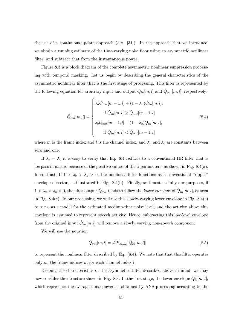
the use of a continuous-update approach (e.g. [31]). In the approach that we introduce,

we obtain a running estimate of the time-varying noise floor using an asymmetric nonlinear

filter, and subtract that from the instantaneous power.

Figure 8.3 is a block diagram of the complete asymmetric nonlinear suppression process-

ing with temporal masking. Let us begin by describing the general characteristics of the

asymmetric nonlinear filter that is the first stage of processing. This filter is represented by

the following equation for arbitrary input and output Qin[m, l] and Qout[m, l], respectively:

Qout[m, l] =

λaQout[m− 1, l] + (1− λa)Qin[m, l],

if Qin[m, l] ≥ Qout[m− 1, l]

λbQout[m− 1, l] + (1− λb)Qin[m, l],

if Qin[m, l] < Qout[m− 1, l]

(8.4)

where m is the frame index and l is the channel index, and λa and λb are constants between

zero and one.

If λa = λb it is easy to verify that Eq. 8.4 reduces to a conventional IIR filter that is

lowpass in nature because of the positive values of the λ parameters, as shown in Fig. 8.4(a).

In contrast, If 1 > λb > λa > 0, the nonlinear filter functions as a conventional “upper”

envelope detector, as illustrated in Fig. 8.4(b). Finally, and most usefully our purposes, if

1 > λa > λb > 0, the filter output Qout tends to follow the lower envelope of Qin[m, l], as seen

in Fig. 8.4(c). In our processing, we will use this slowly-varying lower envelope in Fig. 8.4(c)

to serve as a model for the estimated medium-time noise level, and the activity above this

envelope is assumed to represent speech activity. Hence, subtracting this low-level envelope

from the original input Qin[m, l] will remove a slowly varying non-speech component.

We will use the notation

Qout[m, l] = AFλa,λb[Qin[m, l]] (8.5)

to represent the nonlinear filter described by Eq. (8.4). We note that that this filter operates

only on the frame indices m for each channel index l.

Keeping the characteristics of the asymmetric filter described above in mind, we may

now consider the structure shown in Fig. 8.3. In the first stage, the lower envelope Qle[m, l],

which represents the average noise power, is obtained by ANS processing according to the

99

0 100 (1s) 200 (2s) 300 (3s)

Pow

er (

dB)

Frame Index m

Qin[m, l]Qout[m, l](λa = 0.9, λb = 0.9)

(a)

0 100 (1s) 200 (2s) 300 (3s)

Pow

er (

dB)

Frame Index m


(b)

0 100 (1s) 200 (2s) 300 (3s)

Pow

er (

dB)

Frame Index m


(c)

Fig. 8.4: Sample inputs (solid curves) and outputs (dashed curves) of the asymmetric nonlinear filter

defined by Eq. (8.4) for conditions when (a) λa = λb (b) λa < λb , and (c) λa > λb . In this

example, the channel index l is 8.

equation

Qle[m, l] = AF0.999,0.5[Q[m, l]] (8.6)

as depicted in Fig. 8.4(c). Qle[m, l] is subtracted from the input Q[m, l], effectively highpass

filtering the input, and that signal is passed through an ideal half-wave linear rectifier to

produce the rectified output Q0[m, l]. The impact of the specific values of the forgetting

factors λa and λb on speech recognition accuracy is discussed below.

The remaining elements of ANS processing in the right-hand side of Fig. 8.3 (other than

the temporal masking block) are included to cope with problems that develop when the

rectifier output Q0[m, l] remains zero for an interval, or when the local variance of Q0[m, l]

becomes excessively small. Our approach to this problem is motivated by our previous work

[35] in which it was noted that applying a well-motivated flooring level to power is very

100

important for noise robustness. In PNCC processing we apply the asymmetric nonlinear

filter for a second time to obtain the lower envelope of the rectifier output Qf [m, l], and

we use this envelope to establish this floor level. This envelope Qf [m, l] is obtained using

asymmetric filtering as before:

Qf [m, l] = AF0.999,0.5[Q0[m, l]] (8.7)

As shown in Fig. 8.3, we use the lower envelope of the rectified signal Qf [m, l] as a floor

level for the ANS processing output R[m, l] after temporal masking:

Rsp[m, l] = max (Qtm[m, l], Qf [m, l]) (8.8)

where Qtm[m, l] is the temporal masking output depicted in Fig. 8.3. Temporal masking for

speech segments is discussed in Sec. 8.2.4.

We have found that applying lowpass filtering to the non-excitation segments improves

recognition accuracy in noise by a small amount, and for that reason we use the lower

envelope of the rectified signal Rle[m, l] directly for these non-excitation segments. This

operation, which is effectively a further lowpass filtering, is not performed for the speech

segments because blurring the power coefficients for speech degrades recognition accuracy.

Excitation/non-excitation decisions for this purpose are obtained for each value of m and

l in a very simple fashion:

“excitation segment” if Q[m, l] ≥ cQle[m, l] (8.9a)

“non-excitation segment” if Q[m, l] < cQle[m, l] (8.9b)

where Qle[m, l] is the lower envelope of Q[m, l] as described above, and in and c is a fixed

constant. In other words, a particular value of Q[m, l] is not considered to be a sufficiently-

large excitation if it is less than a fixed multiple of its own lower envelope.

We observed experimentally that while a broad range of values of λb between 0.25 and

0.75 appear to provide reasonable recognition accuracy, the choice of λa = 0.9 appears to

be best under some circumstances as shown in Fig. 8.5. The parameter values used for the

current standard implementation are λa = 0.999 and λb = 0.5, which were chosen in part

to maximize the recognition accuracy in clean speech as well as performance in noise. We

101

0 0.25 0.5 0.75 180

85

90

95

100

Acc

urac

y (1

00 −

WE

R)

λb

WSJ0−5k (Clean)

(a)

0 0.25 0.5 0.75 10

20

40

60

Acc

urac

y (1

00 −

WE

R)

λb

WSJ0−5k (White Noise 5 dB)

(b)

0 0.25 0.5 0.75 10

20

40

60

Acc

urac

y (1

00 −

WE

R)

λb

WSJ0−5k (Music Noise 5 dB)

(c)

0 0.25 0.5 0.75 10

20

40

60

Acc

urac

y (1

00 −

WE

R)

λb

WSJ0−5k (Reverberation RT60

= 0.5 s))

λa = 1.0λa = 0.999λa = 0.99λa = 0.9

(d)

Fig. 8.5: The corresponding dependence of speech recognition accuracy on the forgetting factors λa

and λb. The filled triangle on the y-axis represents the baseline MFF result for the same test

set: (a) Clean, (b) 5-dB Gaussian white noise, (c) 5-dB musical noise, and (d) reverberation

with RT60 = 0.5

102

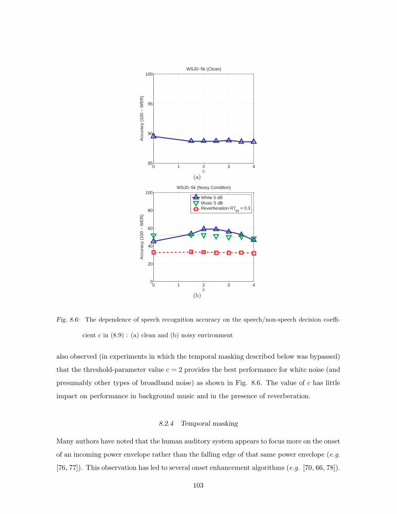
0 1 2 3 485

90

95

100

Acc

urac

y (1

00 −

WE

R)

c

WSJ0−5k (Clean)

(a)

0 1 2 3 40

20

40

60

80

100

c

Acc

urac

y (1

00 −

WE

R)

WSJ0−5k (Noisy Condition)

White 5 dBMusic 5 dBReverberation RT

60 = 0.3

(b)

Fig. 8.6: The dependence of speech recognition accuracy on the speech/non-speech decision coeffi-

cient c in (8.9) : (a) clean and (b) noisy environment

also observed (in experiments in which the temporal masking described below was bypassed)

that the threshold-parameter value c = 2 provides the best performance for white noise (and

presumably other types of broadband noise) as shown in Fig. 8.6. The value of c has little

impact on performance in background music and in the presence of reverberation.

8.2.4 Temporal masking

Many authors have noted that the human auditory system appears to focus more on the onset

of an incoming power envelope rather than the falling edge of that same power envelope (e.g.

[76, 77]). This observation has led to several onset enhancement algorithms (e.g. [70, 66, 78]).

103

MAX

],[~

lmQo

1−z

tλ

tµ

],[~

lmRsp

],[~

lmQp

],1[~

lmQp −

],1[~

],[~

0 lmQlmQ pt −< λ

],1[~

],[~

0 lmQlmQ pt −≥ λ

Fig. 8.7: Block diagram of the components that accomplish temporal masking in Fig. 8.3

In this section we describe a simple way to incorporate this effect in PNCC processing, by

obtaining a moving peak for each frequency channel l and suppressing the instantaneous

power if it falls below this envelope.

The processing invoked for temporal masking is depicted in block diagram form in Fig.

8.7. We first obtain the on-line peak power Qp[m, l] for each channel using the following

equation:

Qp[m, l] = max(

λtQp[m− 1, l], Q0[m, l])

(8.10)

where λt is the forgetting factor for obtaining the on-line peak. As before, m is the frame

index and l is the channel index. Temporal masking for speech segments is accomplished

using the following equation:

Rsp[m, l] =

Q0[m, l], Q0[m, l] ≥ λtQp[m− 1, l]

µtQp[m− 1, l], Q0[m, l] < λtQp[m− 1, l]

(8.11)

104

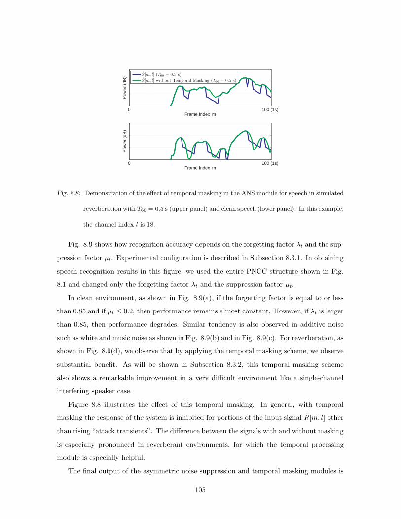
0 100 (1s)

Pow

er (

dB)

Frame Index m

S[m, l] (T60 = 0.5 s)

S[m, l] without Temporal Masking (T60 = 0.5 s)

0 100 (1s)

Pow

er (

dB)

Frame Index m

Fig. 8.8: Demonstration of the effect of temporal masking in the ANS module for speech in simulated

reverberation with T60 = 0.5 s (upper panel) and clean speech (lower panel). In this example,

the channel index l is 18.

Fig. 8.9 shows how recognition accuracy depends on the forgetting factor λt and the sup-

pression factor µt. Experimental configuration is described in Subsection 8.3.1. In obtaining

speech recognition results in this figure, we used the entire PNCC structure shown in Fig.

8.1 and changed only the forgetting factor λt and the suppression factor µt.

In clean environment, as shown in Fig. 8.9(a), if the forgetting factor is equal to or less

than 0.85 and if µt ≤ 0.2, then performance remains almost constant. However, if λt is larger

than 0.85, then performance degrades. Similar tendency is also observed in additive noise

such as white and music noise as shown in Fig. 8.9(b) and in Fig. 8.9(c). For reverberation, as

shown in Fig. 8.9(d), we observe that by applying the temporal masking scheme, we observe

substantial benefit. As will be shown in Subsection 8.3.2, this temporal masking scheme

also shows a remarkable improvement in a very difficult environment like a single-channel

interfering speaker case.

Figure 8.8 illustrates the effect of this temporal masking. In general, with temporal

masking the response of the system is inhibited for portions of the input signal R[m, l] other

than rising “attack transients”. The difference between the signals with and without masking

is especially pronounced in reverberant environments, for which the temporal processing

module is especially helpful.

The final output of the asymmetric noise suppression and temporal masking modules is

105

R[m.l] = Rsp[m, l] for the excitation segments and R[m, l] = Qf [m, l] for the non-excitation

segments.

8.2.5 Spectral weight smoothing

In our previous research on speech enhancement and noise compensation techniques (e.g.,

[55, 35, 36, 46, 37]) it has been frequently observed that smoothing the response across

channels is helpful. This is true especially in processing schemes such as PNCC where there

are nonlinearities and/or thresholds that vary in their effect from channel to channel, as well

as processing schemes that are based on inclusion of responses only from a subset of time

frames and frequency channels (e.g. [46]) or systems that rely on missing-feature approaches

(e.g. [16]).

From the discussion above, we can represent the combined effects of asymmetric noise

suppression and temporal masking for a specific time frame and frequency bin as the transfer

function R[m, l]/Q[m, l]. Smoothing the transfer function across frequency is accomplished

by computing the running average over the channel index l of the ratio R[m, l]/Q[m, l].

Hence, the frequency averaged weighting function T [m, l] (which had previously been sub-

jected to temporal averaging) is given by:

S[m, l] =

1

l2 − l1 + 1

l2∑

l′=l1

R[m, l′]

Q[m, l′]

(8.12)

where l2 = min(l +N,L) and l1 = max(l −N, 1), and L is the total number of channels.

The time-averaged frequency-averaged transfer function T [m, l] is used to modulate the

original short-time power P [m, l]:

T [m, l] = P [m, l]U [m, l] (8.13)

In the present implementation of PNCC, we use a value of N = 4, and a total number of

L = 40 gammatone channels, again based on empirical optimization from the results of pilot

studies [75]. We note that if we were to use a different number of channels L, the optimal

value of N would be also different.

106

8.2.6 Mean power normalization

In conventional MFCC processing, multiplication of the input signal by a constant scale fac-

tor produces only an additive shift of the C0 coefficient because a logarithmic nonlinearity is

included in the processing, and this shift is easily removed by cepstral mean normalization.

In PNCC processing, however, the replacement of the log nonlinearity by a power-law non-

linearity as discussed below, causes the response of the processing to be affected by changes

in absolute power, even though we have observed that this effect is usually small. In order

to further minimize the potential impact of amplitude scaling in PNCC we invoke a stage of

mean power normalization.

While the easiest way to normalize power would be to divide the instantaneous power

by the average power over the utterance, this is not feasible for real-time online processing

because of the “look ahead” that would be required. For this reason, we normalize input

power in the present online implementation of PNCC by dividing the incoming power by a

running average of the overall power. The mean power estimate µ[m] is computed from the

simple difference equation:

µ[m] = λµµ[m− 1] +(1− λµ)

L

L−1∑

l=0

T [m, l] (8.14)

where m and l are the frame and channel indices, as before, and L represents the number of

frequency channels. We use a value of 0.999 for the forgetting factor λµ.

The normalized power is obtained directly from the running power estimate µ[m]:

U [m, l] = kT [m, l]

µ[m](8.15)

where the value of the constant k is arbitrary. In pilot experiments we found that the

speech recognition accuracy obtained using the online power normalization described above

is comparable to the accuracy that would be obtained by normalizing according to a power

estimate that is computed over the entire estimate in offline fashion.

8.2.7 Rate-level nonlinearity

Several studies in our group (e.g. [55, 37]) have confirmed the critical importance of the

nonlinear function that describes the relationship between incoming signal amplitude in a

107

given frequency channel and the corresponding response of the processing model. This “rate-

level nonlinearity” is explicitly or implicitly a crucial part of every conceptual or physiological

model of auditory processing (e.g. [79, 80, 50]). In this section we summarize our approach

to the development of the rate-level nonlinearity used in PNCC processing.

It is well known that the nonlinear curve relating sound pressure level in decibels to the

auditory-nerve firing rate is compressive (e.g [1] [81]). It has also been observed that the

average auditory-nerve firing rate exhibits an overshoot at the onset of an input signal. As

an example, we compare in Fig. 8.11 the average onset firing rate versus the sustained rate

as predicted by the model of Heinz et al. [1]. The curves in this figure were obtained by av-

eraging the rate-intensity values obtained from sinusoidal tone bursts over seven frequencies,

100, 200, 400, 800, 1600, 3200, and 6400 Hz. For the onset-rate results we partitioned the

response into bins of length of 2.5 ms, and searched for the bin with maximum rate during

the initial 10 ms of the tone burst. To measure the sustained rate, we averaged the response

rate between 50 and 100 ms after the onset of the signals. The curves were generated under

the assumption that the spontaneous rate is 50 spikes/second. We observe in Fig. 8.11 that

the sustained firing rate (broken curve) is S-shaped with a threshold around 0 dB SPL and

a saturating segment that begins at around 30 dB SPL. The onset rate (solid curve), on the

other hand, increases continuously without apparent saturation over the conversational hear-

ing range of 0 to 80 dB SPL. We choose to model the onset rate-intensity curve for PNCC

processing because of the important role that it appears to play in auditory perception.

Figure 8.13 compares the onset rate-intensity curve depicted in Fig. 8.11 with various

analytical functions that approximate this function. The curves are plotted as a function of

dB SPL in the lower panel of the figure and as a function of absolute pressure in Pascals in the

upper panel, and the putative spontaneous firing rate of 50 spikes per second is subtracted

from the curves in both cases.

The most widely used current feature extraction algorithms are Mel Frequency Cepstral

Coefficients (MFCC) and Perceptual Linear Prediction (PLP) coefficients. Both the MFCC

and PLP procedures include an intrinsic nonlinearity, which is logarithmic in the case of

MFCC and a cube-root power function in the case of PLP analysis. We plot these curves

relating the power of the input pressure p to the response s in Fig. 8.13 using values of the

arbitrary scaling parameters that are chosen to provide the best fit to the curve of the Heinz

108

et al. model, resulting in the following equations:

scube = 4294.1p2/3 (8.16)

slog = 120.2 log(p) + 1319.3 (8.17)

We note that the exponent of the power function is doubled because we are plotting power

rather than pressure. Even though scaling and shifting by fixed constants in Eqs. (8.16) and

(8.17) do not have any significance in speech recognition systems, we included them in the

above equation to fit these curves to the rate-intensity curve in Fig. 8.13(a). The constants

in Eqs. (8.16) and (8.17) are obtained using an MMSE criterion for the sound pressure range

between 0 dB (20µPa) and 80 dB (0.2 Pa) from the linear rate-intensity curve in the upper

panel of Fig. 8.11.

As shown in Fig. 8.12, the power function coefficient obtained from the MMSE power-fit

gives us performance benefit compared to conventional logarithmic processing. If we use a

bigger coefficient such as 1/5, it gives us better performance for white noise, but it loses

performance in other environments as well as in clean environment. From this figure, we

observe that larger values of the pressure exponent such as 1/5 provide better performance

in white noise, but they degrade the recognition accuracy that is obtained for clean speech .

We consider the value 1/15 for the pressure exponent to represent a pragmatic compromise

that provides reasonable accuracy in white noise without sacrificing recognition accuracy for

clean speech, producing the power-law nonlinearity

V [m, l] = U [m, l]1/15 (8.18)

where again U [m, l] and V [m, l] have the dimensions of power. This curve is closely approx-

imated by the equation

spower = 1389.6p0.1264 (8.19)

which is also plotted in Fig. 8.13. The exponent of 0.1264 happens to be the best fit to the

Heinz et al. data as depicted in the upper panel of Fig. 8.11. As before, this estimate was

developed in the MMSE sense over the sound pressure range between 0 dB (20µPa) and 80

dB (0.2 Pa).

109

The power low function was chosen for PNCC processing for several reasons. First, it is

a relationship that is not affected in form by multiplying the input by a constant. Second,

it has the attractive property that its asymptotic response at very low intensities is zero

rather than negative infinity, which reduces variance in the response to low-level inputs such

as spectral valleys or silence segments. Finally, the power law has been demonstrated to

provide a good approximation to the “psychophysical transfer functions” that are observed

in experiments relating the physical intensity of sensation to the perceived intensity using

direct magnitude-estimation procedures (e.g. [52]).

Figure 8.14 is a final comparison of the effects of the asymmetric noise suppression, tempo-

ral masking, channel weighting, and power-law nonlinearity modules discussed in Secs. 8.2.3

through 8.2.7. The curves in both panels compare the response of the system in the channel

with center frequency 490 Hz to clean speech and speech in the presence of street noise at

an SNR of 5 dB. The curves in the upper panel were obtained using conventional MFCC

processing, including the logarithmic nonlinearity and without ANS processing or temporal

masking. The curves in the lower panel were obtained using PNCC processing, which in-

cludes the power-law transformation described in this section, as well as ANS processing and

temporal masking. We note that the difference between the two curves representing clean

and noisy speech is much greater with MFCC processing (upper panel), especially for times

during which the signal is at a low level.


In this section we present experimental results that are intended to demonstrate the su-

periority of PNCC processing over competing approaches in a wide variety of acoustical

environments. We begin in Sec. 8.3.1 with a review of the experimental procedures that

were used. We provide some general results for PNCC processing, we assess the contribu-

tions of its various components in PNCC in Sec. 8.3.2, and we compare PNCC to a small

number of other approaches in Sec. 8.3.3.

It should be noted that in general we selected an algorithm configuration and associated

parameter values that provide very good performance over a wide variety of conditions using

a single set of parameters and settings, without sacrificing word error rate in clean conditions

110

relative to MFCC processing. In previous work we had described slightly different feature

extraction algorithms that provide even better performance for speech recognition in the

presence of reverberation [35] and in background music [66], but these approaches do not

perform as well as MFCC processing in clean speech. We used five standard testing environ-

ments in our work: (1) digitally-added white noise, (2) digitally-added noise that had been

recorded live on urban streets, (3) digitally-added single-speaker interference, (4) digitally-

added background music, and (5) passage of the signal through simulated reverberation. The

street noise was recorded by us on streets with steady but moderate traffic. The masking

signal used for single-speaker-interference experiments consisted of other utterances drawn

from the TIMIT database, and background music was selected from music segments from

the original DARPA Hub 4 Broadcast News database. The reverberation simulations were

accomplished using the Room Impulse Response open source software package [53] based

on the image method [82]. The room size used was 3 × 4 × 5 meters, the microphone is

in the center of the room, the spacing between the target speaker and the microphone was

assumed to be 1.5 meters, and reverberation time was manipulated by changing the assumed

absorption coefficients in the room appropriately.

8.3.1 Experimental Configuration

The PNCC feature described in this chapter was evaluated by comparing the recognition

accuracy obtained with PNCC introduced in this chapter to that obtained using MFCC and

RASTA-PLP processing. We used the version of conventional MFCC processing implemented

as part of sphinx fe in sphinxbase 0.4.1 both from the CMU Sphinx open source codebase

[83]. We used the PLP-RASTA implementation that is available at [30]. In all cases decoding

was performed using the publicly-available CMU Sphinx 3.8 system [83] using training from

SphinxTrain 1.0. We also compared PNCC with the vector Taylor series (VTS) noise

compensation algorithm [10] and the ETSI advanced front end (AFE) which has several

noise suppression algorithms included [74]. In the case of the ETSI AFE, we excluded the

log energy element because this resulted in better results in our experiments. A bigram

language model was used in all experiments. In all experiments, we used feature vectors of

length of 39 including delta and delta-delta features. For experiments using the DARPA

111

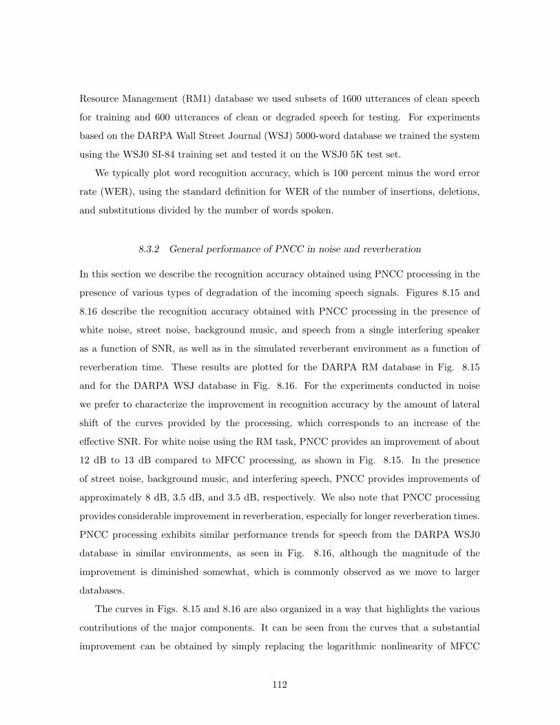
Resource Management (RM1) database we used subsets of 1600 utterances of clean speech

for training and 600 utterances of clean or degraded speech for testing. For experiments

based on the DARPA Wall Street Journal (WSJ) 5000-word database we trained the system

using the WSJ0 SI-84 training set and tested it on the WSJ0 5K test set.

We typically plot word recognition accuracy, which is 100 percent minus the word error

rate (WER), using the standard definition for WER of the number of insertions, deletions,

and substitutions divided by the number of words spoken.

8.3.2 General performance of PNCC in noise and reverberation

In this section we describe the recognition accuracy obtained using PNCC processing in the

presence of various types of degradation of the incoming speech signals. Figures 8.15 and

8.16 describe the recognition accuracy obtained with PNCC processing in the presence of

white noise, street noise, background music, and speech from a single interfering speaker

as a function of SNR, as well as in the simulated reverberant environment as a function of

reverberation time. These results are plotted for the DARPA RM database in Fig. 8.15

and for the DARPA WSJ database in Fig. 8.16. For the experiments conducted in noise

we prefer to characterize the improvement in recognition accuracy by the amount of lateral

shift of the curves provided by the processing, which corresponds to an increase of the

effective SNR. For white noise using the RM task, PNCC provides an improvement of about

12 dB to 13 dB compared to MFCC processing, as shown in Fig. 8.15. In the presence

of street noise, background music, and interfering speech, PNCC provides improvements of

approximately 8 dB, 3.5 dB, and 3.5 dB, respectively. We also note that PNCC processing

provides considerable improvement in reverberation, especially for longer reverberation times.

PNCC processing exhibits similar performance trends for speech from the DARPA WSJ0

database in similar environments, as seen in Fig. 8.16, although the magnitude of the

improvement is diminished somewhat, which is commonly observed as we move to larger

databases.

The curves in Figs. 8.15 and 8.16 are also organized in a way that highlights the various

contributions of the major components. It can be seen from the curves that a substantial

improvement can be obtained by simply replacing the logarithmic nonlinearity of MFCC

112

processing by the power-law rate-intensity function described in Sec. 8.2.7. The addition

of the ANS processing provides a substantial further improvement for recognition accuracy

in noise. Although it is not explicitly shown in Figs. 8.15 and 8.16, the temporal masking

is particularly helpful in improving accuracy for reverberated speech and for speech in the

presence of interfering speech.

8.3.3 Comparison with other algorithms

Figures 8.17 and 8.18 provide comparisons of PNCC processing to the baseline MFCC pro-

cessing with cepstral mean normalization, MFCC processing combined with the vector Taylor

series (VTS) algorithm for noise robustness [10], as well as RASTA-PLP feature extraction

[3]. The experimental conditions used were the same as those used to produce Figs. 8.15

and 8.16.

We note in Figs. 8.17 and 8.18 that PNCC provides substantially better recognition

accuracy than both MFCC and RASTA-PLP processing for all conditions examined. It

also provides recognition accuracy that is better than the combination of MFCC with VTS,

and at a substantially lower computational cost than the computation that is incurred in

implementing VTS. We also note that the VTS algorithm provides little or no improvement

over the baseline MFCC performance in difficult environments like background music noise,

single-channel interfering speaker or reverberation.

The ETSI AFE [74] generally provides slightly better recognition accuracy than VTS in

noisy environments, but accuracy that does not approach that obtained with PNCC pro-

cessing. Both the ETSI AFE and VTS do not improve recognition accuracy in reverberant

environments compared to MFCC features, while PNCC shows measuremable improvements

in reverberation and a closely related algorithm [66] provides even greater recognition accu-

racy in reverberation (at the expense of somewhat worse performance in clean speech).

8.4 Experimental results under multi-style training condition

In the above sections, we presented speech recognition results using clean training set. These

days, in many large-scale speech recognition systems, we use multi-style noisy training set.

So, we also evaluated the performance of PNCC for multi-style training set. In Fig. 8.19,

113

we used a training set corrupted by street noise at 5 different SNR levels (0, 5, 10, 15,

20) and clean. Each utterance in the training set was randomly corrupted to one of these 6

different SNR levels. As shown in Fig. 8.19, PNCC shows improvements in all kinds of cases.

Especially, we observe that for interfering speaker noise, MFCC using noisy training set is

doing even worse than MFCC using the clean training set. Another interesting observation

is that for the clean test set, PNCC shows significantly better performance than MFCC. The

reason is now clean test set is unmatched condition since we used noisy training set, and

PNCC does better than MFCC for unmatched conditions.

Experiments in Fig. 8.20 are similar to the experiments in Fig. 8.19. But we used 4

different types of noise (white, street, music, and interfering speaker noise) at 5 different

SNR levels (0, 5, 10, 15, 20 dB). So, in total, the utterances in the clean training set was

randomly selected to one of these 21 possible cases and was corrupted. In this experiment,

as shown in Fig. 8.20, PNCC is still doing better than MFCC even though the difference is

reduced compared to the clean training set.

Experiments in Fig. 8.21 is similar to experiments in Fig. 8.19, but we used WSJ0-si84

for acoustic model training and WSJ0-5k for decoding. Experiments in Fig.8.22 is the same

as experiments in Fig. 8.20, but we used WSJ0-si84 for acoustic model training and WSJ0-5k

for decoding.

114

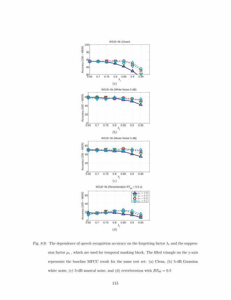
0.65 0.7 0.75 0.8 0.85 0.9 0.9580

85

90

95

100

Acc

urac

y (1

00 −

WE

R)

λt

WSJ0−5k (Clean)

(a)

0.65 0.7 0.75 0.8 0.85 0.9 0.950

20

40

60

Acc

urac

y (1

00 −

WE

R)

λt

WSJ0−5k (White Noise 5 dB)

(b)

0.65 0.7 0.75 0.8 0.85 0.9 0.950

20

40

60

Acc

urac

y (1

00 −

WE

R)

λt

WSJ0−5k (Music Noise 5 dB)

(c)

0.65 0.7 0.75 0.8 0.85 0.9 0.950

20

40

60

λt

Acc

urac

y (1

00 −

WE

R)

WSJ0−5k (Reverberation RT60

= 0.5 s)

µt = 1.0µt = 0.4µt = 0.2µt = 0.1

(d)

Fig. 8.9: The dependence of speech recognition accuracy on the forgetting factor λt and the suppres-

sion factor µt , which are used for temporal masking block. The filled triangle on the y-axis

represents the baseline MFCC result for the same test set: (a) Clean, (b) 5-dB Gaussian

white noise, (c) 5-dB musical noise, and (d) reverberation with RT60 = 0.5

115

0 20 40 60 80 100 120 1400

500

1000

1500

2000

2500

3000

3500

4000

Syn

apse

Out

put (

spik

es/s

ec)

Time (ms)

Fig. 8.10: Synapse output for a pure tone input with a carrier frequency of 500 Hz at 60 dB SPL.

This synapse output is obtained using the auditory model by Heinz et al. [1].

−40 −20 0 20 40 60 800

200

400

600

800

1000

Sound Pressure Level (dB)

Rat

e (s

pike

s/se

c)

Onset RateSustained Rate

Fig. 8.11: Comparison of the onset rate (solid curve) and sustained rate (dashed curve) obtained

using the model proposed by Heinz et al. [1]. The curves were obtained by averaging

responses over seven frequencies. See text for details.

116

0 5 10 15 20 Clean0

20

40

60

80

100

Acc

urac

y (1

00 −

WE

R)

SNR (dB)


(a)

0 5 10 15 20 Clean0

20

40

60

80

100

Acc

urac

y (1

00 −

WE

R)

SNR (dB)


(b)

0 5 10 15 20 Clean0

20

40

60

80

100

Acc

urac

y (1

00 −

WE

R)

SNR (dB)


(c)

0 0.1 0.2 0.3 0.4 0.5 0.6 0.9 1.20

20

40

60

80

100


Acc

urac

y (1

00 −

WE

R)


a0 = 1/5a0 = 1/15a0 = 1/50MFCC

(d)

Fig. 8.12: Dependence on speech recognition accuracy on power coefficient in different environments:

(a) additive white gaussian noise, (b) street noise, (c) background music, and (d) reverber-

ant environment.

117

0.05 0.1 0.15 0.2−200

0

200

400

600

800

1000

1200

1400

Pressure (Pa)

Rat

e (s

pike

s / s

ec)

Human Rate−Intensity ModelCube Root Power−Law ApproximationMMSE Power−Law ApproximationLogarithmic Approximation

(a)

−40 −20 0 20 40 60 80−1000

−500

0

500

1000

1500

Tone Level (dB SPL)

Rat

e (s

pike

s / s

ec)

Human Rate−Intensity ModelCube Root Power−Law ApproximationMMSE Power−Law ApproximationLogarithmic Approximation

(b)

Fig. 8.13: Comparison between a human rate-intensity relation using the auditory model developed

by Heinz et al. [1], a cube root power-law approximation, an MMSE power-law approx-

imation, and a logarithmic function approximation. Upper panel: Comparison using the

pressure (Pa) as the x-axis. Lower panel: Comparison using the sound pressure level (SPL)

in dB as the x-axis.

118

0 100 (1s) 200 (2s) 300 (3s)Frame Index m

logP

[m,l

]

Clean and Street 5 dB

Street 5 dBClean

0 100 (1s) 200 (2s) 300 (3s)Frame Index m

P[m

,l]1

/15

Clean and Street 5 dB

Street 5 dBClean

Fig. 8.14: The effects of the asymmetric noise suppression, temporal masking, and the rate-level

nonlinearity used in PNCC processing. Shown are the outputs of these stages of processing

for clean speech and for speech corrupted by street noise at an SNR of 5 dB when the log-

arithmic nonlinearity is used without ANS processing or temporal masking (upper panel),

and when the power-law nonlinearity is used with ANS processing and temporal masking

(lower panel). In this example, the channel index l is 8.

119

0 5 10 15 20 Clean0

20

40

60

80

100

Acc

urac

y (1

00 −

WE

R)

SNR (dB)

RM1 (White Noise)

(a)

0 5 10 15 20 Clean0

20

40

60

80

100

Acc

urac

y (1

00 −

WE

R)

SNR (dB)

RM1 (Street Noise)

(b)

0 5 10 15 20 Clean0

20

40

60

80

100

SNR (dB)

Acc

urac

y (1

00 −

WE

R)

RM1 (Music Noise)

PNCCPower−Law Nonlinearity with ANS processingPower−Law NonlinearityMFCC

(c)

0 5 10 15 20 Clean0

20

40

60

80

100A

ccur

acy

(100

− W

ER

)

SIR (dB)


(d)

0 0.1 0.2 0.3 0.4 0.5 0.6 0.9 1.20

20

40

60

80

100

Acc

urac

y (1

00 −

WE

R)


RM1 (Reverberation)

(e)

Fig. 8.15: Recognition accuracy obtained using PNCC processing in various types of additive noise

and reverberation. Curves are plotted separately to indicate the contributions of the power-

law nonlinearity, asymmetric noise suppression, and temporal masking. Results are de-

scribed for the DARPA RM1 database in the presence of (a) white noise, (b) street noise,

(c) background music, (d) interfering speech, and (e) artificial reverberation.

120

0 5 10 15 20 Clean0

20

40

60

80

100

Acc

urac

y (1

00 −

WE

R)

SNR (dB)


(a)

0 5 10 15 20 Clean0

20

40

60

80

100

Acc

urac

y (1

00 −

WE

R)

SNR (dB)


(b)

0 5 10 15 20 Clean0

20

40

60

80

100

Acc

urac

y (1

00 −

WE

R)

SNR (dB)


(c)

0 5 10 15 20 Clean0

20

40

60

80

100A

ccur

acy

(100

− W

ER

)

SIR (dB)


(d)

0 0.1 0.2 0.3 0.4 0.5 0.6 0.9 1.20

20

40

60

80

100


Acc

urac

y (1

00 −

WE

R)


PNCCPower−Law Nonlinearity with ANS processingPower−Law NonlinearityMFCC

(e)

Fig. 8.16: Recognition accuracy obtained using PNCC processing in various types of additive noise

and reverberation. Curves are plotted separately to indicate the contributions of the power-

law nonlinearity, asymmetric noise suppression, and temporal masking. Results are de-

scribed for the DARPA WSJ0 database in the presence of (a) white noise, (b) street noise,

(c) background music, (d) interfering speech, and (e) artificial reverberation.

121

0 5 10 15 20 Clean0

20

40

60

80

100

Acc

urac

y (1

00 −

WE

R)

SNR (dB)

RM1 (White Noise)

(a)

0 5 10 15 20 Clean0

20

40

60

80

100

Acc

urac

y (1

00 −

WE

R)

SNR (dB)

RM1 (Street Noise)

(b)

0 5 10 15 20 Clean0

20

40

60

80

100

Acc

urac

y (1

00 −

WE

R)

SNR (dB)

RM1 (Music Noise)

(c)

0 5 10 15 20 Clean0

20

40

60

80

100A

ccur

acy

(100

− W

ER

)

SIR (dB)


(d)

0 0.1 0.2 0.3 0.4 0.5 0.6 0.9 1.20

20

40

60

80

100


Acc

urac

y (1

00 −

WE

R)

RM1 (Reverberation)

PNCCETSI AFEMFCC with VTSMFCCRASTA−PLP

(e)

Fig. 8.17: Comparison of recognition accuracy for PNCC with processing using MFCC features, the

ETSI AFE, MFCC with VTS, and RASTA-PLP features using the DARPA RM1 corpus.

Environmental conditions are (a) white noise, (b) street noise, (c) background music, (d)

interfering speech, and (e) reverberation.

122

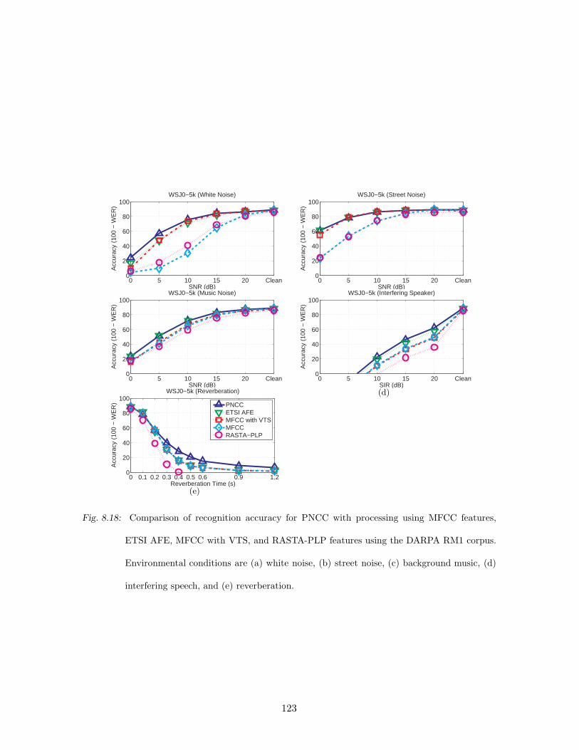
0 5 10 15 20 Clean0

20

40

60

80

100

Acc

urac

y (1

00 −

WE

R)

SNR (dB)


(a)

0 5 10 15 20 Clean0

20

40

60

80

100

Acc

urac

y (1

00 −

WE

R)

SNR (dB)


(b)

0 5 10 15 20 Clean0

20

40

60

80

100

Acc

urac

y (1

00 −

WE

R)

SNR (dB)


(c)

0 5 10 15 20 Clean0

20

40

60

80

100A

ccur

acy

(100

− W

ER

)

SIR (dB)


(d)

0 0.1 0.2 0.3 0.4 0.5 0.6 0.9 1.20

20

40

60

80

100


Acc

urac

y (1

00 −

WE

R)


PNCCETSI AFEMFCC with VTSMFCCRASTA−PLP

(e)

Fig. 8.18: Comparison of recognition accuracy for PNCC with processing using MFCC features,

ETSI AFE, MFCC with VTS, and RASTA-PLP features using the DARPA RM1 corpus.

Environmental conditions are (a) white noise, (b) street noise, (c) background music, (d)

interfering speech, and (e) reverberation.

123

−5 0 5 10 15 20 Clean0

20

40

60

80

100

Acc

urac

y (1

00 −

WE

R)

SNR (dB)

RM1 (White Noise)

(a)

−5 0 5 10 15 20 Clean0

20

40

60

80

100

Acc

urac

y (1

00 −

WE

R)

SNR (dB)

RM1 (Street Noise)

(b)

−5 0 5 10 15 20 Clean0

20

40

60

80

100

Acc

urac

y (1

00 −

WE

R)

SNR (dB)

RM1 (Music Noise)

(c)

−5 0 5 10 15 20 Clean0

20

40

60

80

100A

ccur

acy

(100

− W

ER

)

SNR (dB)


(d)

0 0.1 0.2 0.3 0.4 0.5 0.6 0.9 1.20

20

40

60

80

100


Acc

urac

y (1

00 −

WE

R)

RM1 (Reverberation)

PNCC (street noise training)MFCC (street noise training)PNCC (clean training)MFCC (clean training)

(e)

Fig. 8.19: Comparison of recognition accuracy for PNCC with processing using MFCC features

using the DARPA RM1 corpus. Training database was corrupted by street noise at 5

different levels plus clean. Environmental conditions are (a) white noise, (b) street noise,

(c) background music, (d) interfering speech, and (e) reverberation.

124

−5 0 5 10 15 20 Clean0

20

40

60

80

100

Acc

urac

y (1

00 −

WE

R)

SNR (dB)

RM1 (White Noise)

(a)

−5 0 5 10 15 20 Clean0

20

40

60

80

100

Acc

urac

y (1

00 −

WE

R)

SNR (dB)

RM1 (Street Noise)

(b)

−5 0 5 10 15 20 Clean0

20

40

60

80

100

Acc

urac

y (1

00 −

WE

R)

SNR (dB)

RM1 (Music Noise)

(c)

−5 0 5 10 15 20 Clean0

20

40

60

80

100A

ccur

acy

(100

− W

ER

)

SNR (dB)


(d)

0 0.1 0.2 0.3 0.4 0.5 0.6 0.9 1.20

20

40

60

80

100


Acc

urac

y (1

00 −

WE

R)

RM1 (Reverberation)

PNCC (multi−style training)MFCC (multi−style training)PNCC (clean training)MFCC (clean training)

(e)


using the DARPA RM-1 corpus. Training database was corrupted by street noise at 5

different levels plus clean. Environmental conditions are (a) white noise, (b) street noise,

(c) background music, (d) interfering speech, and (e) reverberation.

125

−5 0 5 10 15 20 Clean0

20

40

60

80

100

Acc

urac

y (1

00 −

WE

R)

SNR (dB)


(a)

−5 0 5 10 15 20 Clean0

20

40

60

80

100

Acc

urac

y (1

00 −

WE

R)

SNR (dB)


(b)

−5 0 5 10 15 20 Clean0

20

40

60

80

100

Acc

urac

y (1

00 −

WE

R)

SNR (dB)


(c)

−5 0 5 10 15 20 Clean0

20

40

60

80

100A

ccur

acy

(100

− W

ER

)

SNR (dB)


(d)

0 0.1 0.2 0.3 0.4 0.5 0.6 0.9 1.20

20

40

60

80

100


Acc

urac

y (1

00 −

WE

R)

RM1 (Reverberation)

PNCC (street noise training)MFCC (street noise training)PNCC (clean training)MFCC (clean training)

(e)

Fig. 8.21: Comparison of recognition accuracy for PNCC with processing using MFCC features using

the WSJ0 5k corpus. Training database was corrupted by street noise at 5 different levels

plus clean. Environmental conditions are (a) white noise, (b) street noise, (c) background

music, (d) interfering speech, and (e) reverberation.

126

−5 0 5 10 15 20 Clean0

20

40

60

80

100A

ccur

acy

(100

− W

ER

)

SNR (dB)


(a)

−5 0 5 10 15 20 Clean0

20

40

60

80

100

Acc

urac

y (1

00 −

WE

R)

SNR (dB)


(b)

−5 0 5 10 15 20 Clean0

20

40

60

80

100

Acc

urac

y (1

00 −

WE

R)

SNR (dB)


(c)

−5 0 5 10 15 20 Clean0

20

40

60

80

100

Acc

urac

y (1

00 −

WE

R)

SNR (dB)


(d)

0 0.1 0.2 0.3 0.4 0.5 0.6 0.9 1.20

20

40

60

80

100


Acc

urac

y (1

00 −

WE

R)

RM1 (Reverberation)

PNCC (multi−style training)MFCC (multi−style training)PNCC (clean training)MFCC (clean training)

(e)


the WSJ0 5k corpus. Training database was corrupted by street noise at 5 different levels

plus clean. Environmental conditions are (a) white noise, (b) street noise, (c) background

music, (d) interfering speech, and (e) reverberation.

8.5 Experimental results using MLLR

Maximum likelihood linear regression (MLLR) has become very popular in speech recogni-

tion. It has been observed that MLLR is a very powerful technique, in many cases, robustness

algorithm does not show substantial improvement compared to MFCC if MLLR is incorpo-

rated. To evaluate the performance of PNCC in combination of MLLR, we conducted speech

recognition experiments using four different types of MLLR configuration.

127

8.5.1 Clean training and multi-style MLLR adaptation set

Figure 8.23 shows speech recognition accuracies, when we used the clean training set, and

MLLR was performed on the noisy test set “speaker-by-speaker” basis. We used RM1 for

acoustic model training and decoding. We used 600 utterances for test and 600 utterances for

MLLR model adaptation (development set). In the test set, there are 40 different speakers,

and we adapted HMM model “speaker-by-speaker” basis using this adaptation set. As in the

previous section, for the MLLR adaptation set, multi-style noise was intentionally added to

the adaptation set. We used 4 different types of noise, white, street, music, and interfering

speaker noise at 5 different SNR levels (0, 5, 10, 15, 20 dB). Including the clean case, there are

21 possible cases, and for each utterance in the MLLR adaptation set, one of these conditions

are randomly selected to make multi-style MLLR adaptation set. In this experiment, MLLR

was performed under supervised mode. For each speaker, 15 utterances from the adaptation

set (corrupted by multi-style noise) was used for HMM model adaptation under supervised

mode (using the correct transcript for the adaptation set), and the adapted model was used

for decoding the test set. This process was performed each speaker.

As shown in Fig. 8.23, PNCC shows improvements under all types of noise except

reverberation. For the reverberation set, we later observed that if we use PNCC using “off-

line” peak normalization, then it still shows some small improvement. For white, street, and

interfering speaker noise, MFCC with MLLR processing is even worse than PNCC without

MLLR processing. Thus, we can observe that PNCC is still a very useful technique when it

is combined with MLLR.

128

−5 0 5 10 15 20 Clean0

20

40

60

80

100

Acc

urac

y (1

00 −

WE

R)

SNR (dB)

RM1 (White Noise)

(a)

−5 0 5 10 15 20 Clean0

20

40

60

80

100

Acc

urac

y (1

00 −

WE

R)

SNR (dB)

RM1 (Street Noise)

(b)

−5 0 5 10 15 20 Clean0

20

40

60

80

100

Acc

urac

y (1

00 −

WE

R)

SNR (dB)

RM1 (Music Noise)

(c)

−5 0 5 10 15 20 Clean0

20

40

60

80

100

Acc

urac

y (1

00 −

WE

R)

SNR (dB)


(d)

0 0.1 0.2 0.3 0.4 0.5 0.6 0.9 1.20

20

40

60

80

100

Acc

urac

y (1

00 −

WE

R)


RM1 (Reverberation)

PNCC (supervised MLLR on the noisy dev set)MFCC (supervised MLLR on the noisy dev set)PNCCMFCC

(e)


the RM1 corpus. Clean training set was used, and MLLR was directly performed spk-by-

spk basis using the multi-style development set. MLLR was performed in the unsupervised

mode. Environmental conditions are (a) white noise, (b) street noise, (c) background music,

(d) interfering speech, and (e) reverberation.

129

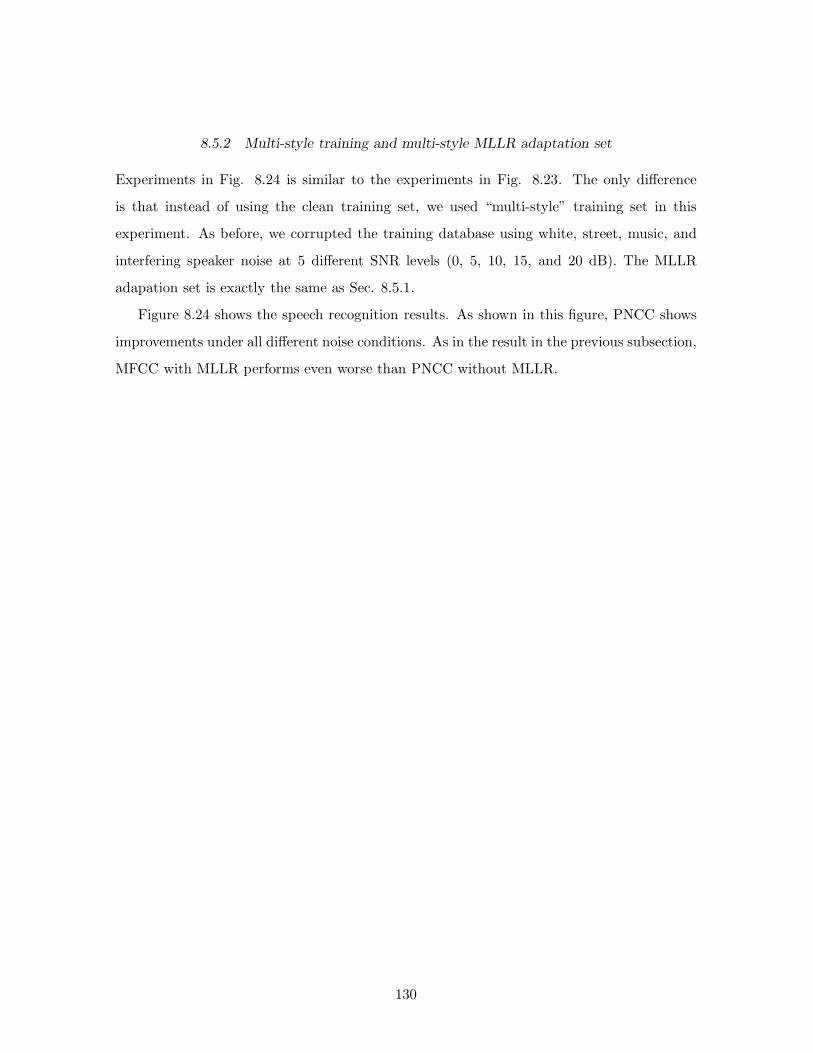
8.5.2 Multi-style training and multi-style MLLR adaptation set

Experiments in Fig. 8.24 is similar to the experiments in Fig. 8.23. The only difference

is that instead of using the clean training set, we used “multi-style” training set in this

experiment. As before, we corrupted the training database using white, street, music, and

interfering speaker noise at 5 different SNR levels (0, 5, 10, 15, and 20 dB). The MLLR

adapation set is exactly the same as Sec. 8.5.1.

Figure 8.24 shows the speech recognition results. As shown in this figure, PNCC shows

improvements under all different noise conditions. As in the result in the previous subsection,

MFCC with MLLR performs even worse than PNCC without MLLR.

130

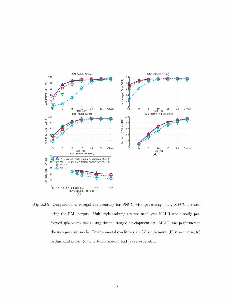
−5 0 5 10 15 20 Clean0

20

40

60

80

100

Acc

urac

y (1

00 −

WE

R)

SNR (dB)

RM1 (White Noise)

(a)

−5 0 5 10 15 20 Clean0

20

40

60

80

100

Acc

urac

y (1

00 −

WE

R)

SNR (dB)

RM1 (Street Noise)

(b)

−5 0 5 10 15 20 Clean0

20

40

60

80

100

Acc

urac

y (1

00 −

WE

R)

SNR (dB)

RM1 (Music Noise)

(c)

−5 0 5 10 15 20 Clean0

20

40

60

80

100

Acc

urac

y (1

00 −

WE

R)

SNR (dB)


(d)

0 0.1 0.2 0.3 0.4 0.5 0.6 0.9 1.20

20

40

60

80

100


Acc

urac

y (1

00 −

WE

R)

RM1 (Reverberation)

PNCC(multi−style trainig supervised MLLR)MFCC(multi−style trainig supervised MLLR)PNCCMFCC

(e)


using the RM1 corpus. Multi-style training set was used, and MLLR was directly per-

formed spk-by-spk basis using the multi-style development set. MLLR was performed in

the unsupervised mode. Environmental conditions are (a) white noise, (b) street noise, (c)

background music, (d) interfering speech, and (e) reverberation.

131

8.5.3 Multi-style training and MLLR under the matched condition

In this experiment, we use the same multi-style training set as Sec. 8.5.2, but MLLR is

performed under the matched condition. For example, if the test utterance is corrupted by

5-dB street noise, then the exactly same kind of noise type and level were used for MLLR

adaptation. As before, MLLR is performed “speaker-by-speaker” basis. Since MLLR is

performed under matched condition, recognition accuracies are very high even under very

noisy environment, so unlike previous figures, we used a different y-scale (70 % – 100 %) in

Fig. 8.25. As shown in Fig. 8.25, PNCC still shows improvements for all conditions even

though the difference between PNCC and MFCC is much reduced. We also note that for

clean environment, MFCC performs significantly poorer than PNCC, which is consistently

being observed if we use multi-style training set.

132

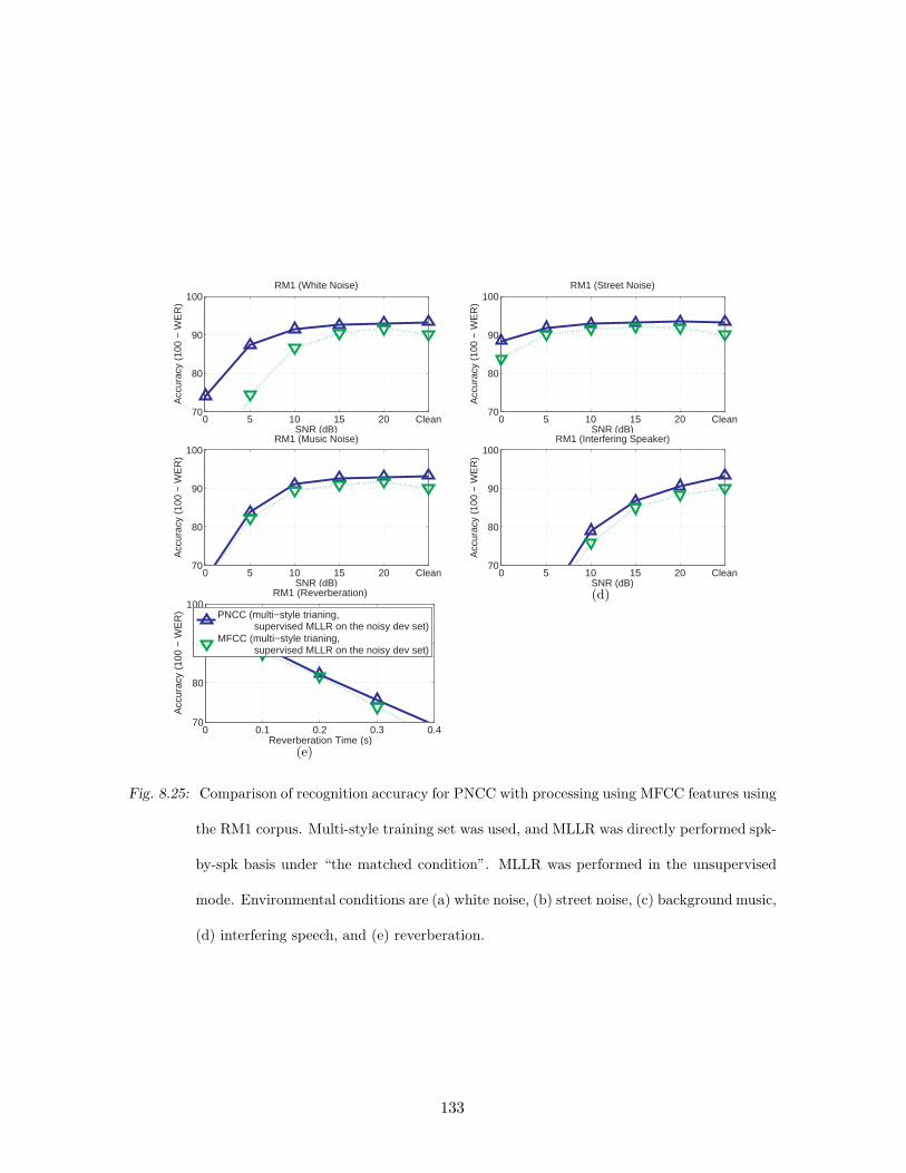
0 5 10 15 20 Clean70

80

90

100

Acc

urac

y (1

00 −

WE

R)

SNR (dB)

RM1 (White Noise)

(a)

0 5 10 15 20 Clean70

80

90

100

Acc

urac

y (1

00 −

WE

R)

SNR (dB)

RM1 (Street Noise)

(b)

0 5 10 15 20 Clean70

80

90

100

Acc

urac

y (1

00 −

WE

R)

SNR (dB)

RM1 (Music Noise)

(c)

0 5 10 15 20 Clean70

80

90

100

Acc

urac

y (1

00 −

WE

R)

SNR (dB)


(d)

0 0.1 0.2 0.3 0.470

80

90

100

Acc

urac

y (1

00 −

WE

R)


RM1 (Reverberation)

PNCC (multi−style trianing, supervised MLLR on the noisy dev set)MFCC (multi−style trianing, supervised MLLR on the noisy dev set)

(e)


the RM1 corpus. Multi-style training set was used, and MLLR was directly performed spk-

by-spk basis under “the matched condition”. MLLR was performed in the unsupervised



133

8.5.4 Multi-style training and unsupervised MLLR using the test set itself

In this experiment, we used “unsupervised MLLR” on the test set itself. Since we use the

test utterances themselves as the MLLR adaptation set, we can no longer use the supervised

MLLR. Thus, in the first path, the decoder runs and we obtained the hypothesis. Using this

hypothesis, we ran MLLR. Like the experiments in Sec. 8.5.3, MLLR is performed under

completely matched condition, but the difference is in the previous subsection, we used a

separate adaptation set, but in this experiment, we used the test itself as the adaptation

set. Experimental results are shown in Fig. 8.26. Again, PNCC shows improvements for all

kinds of conditions, even though the difference between MFCC and PNCC is now reduced.

8.6 Computational Complexity

Table 8.1 provides estimates of the computational demands MFCC, PLP, and PNCC feature

extraction. (The RASTA processing is not included in these tabulations.) As before we use

the standard open source Sphinx code in sphinx fe [83] for the implementation of MFCC,

and the implementation in [30] for PLP. We assume that the window length is 25.6 ms and

that the interval between successive windows is 10 ms. The sampling rate is assumed to be

16 kHz, and we use a 1024-pt FFT for each analysis frame.

It can be seen in Table 8.1 that because all three algorithms use 1024-point FFTs, the

greatest difference from algorithm to algorithm in the amount of computation required is

associated with the spectral integration component. Specifically, the triangular weighting

used in the MFCC calculation encompasses a narrower range of frequencies than the trape-

zoids used in PLP processing, which is in turn considerably narrower than the gammatone

filter shapes, and the amount of computation needed for spectral integration is directly pro-

portional to the effective bandwidth of the channels. For this reason, as mentioned in Sec.

8.2.1, we limited the gammatone filter computation to those frequencies for which the filter

transfer function is 0.5 percent or more of the maximum filter gain. In Table 8.1, for all

spectral integration types, we considered filter portion whose magnitude is 0.5 or more of

the maximum filter gain.

As can be seen in Table 8.1, PLP processing by this tabulation is about 32.9 percent more

costly than baseline MFCC processing. PNCC processing is approximately 34.6 percent more

134

0 5 10 15 20 Clean70

80

90

100A

ccur

acy

(100

− W

ER

)

SNR (dB)

RM1 (White Noise)

(a)

0 5 10 15 20 Clean70

80

90

100

Acc

urac

y (1

00 −

WE

R)

SNR (dB)

RM1 (Street Noise)

(b)

0 5 10 15 20 Clean70

80

90

100

Acc

urac

y (1

00 −

WE

R)

SNR (dB)

RM1 (Music Noise)

(c)

0 5 10 15 20 Clean70

80

90

100

Acc

urac

y (1

00 −

WE

R)

SNR (dB)


(d)

0 0.1 0.2 0.3 0.470

80

90

100


Acc

urac

y (1

00 −

WE

R)

RM1 (Reverberation)

PNCC (multi−style trianing, unsupervised MLLR on the test set)MFCC (multi−style trianing, unsupervised MLLR on the test set)

(e)


the RM1 corpus. Multi-style training set was used, and MLLR was directly performed on

“the test set itself” speaker-by-speaker basis. MLLR was performed in the unsupervised



costly than MFCC processing and 1.31 percent more costly than PLP processing.

8.7 Summary

In this chapter we introduce power-normalized cepstral coefficients (PNCC), which we char-

acterize as a feature set that provides better recognition accuracy than MFCC and RASTA-

PLP processing in the presence of common types of additive noise and reverberation. PNCC

processing is motivated by the desire to develop computationally efficient feature extrac-

135

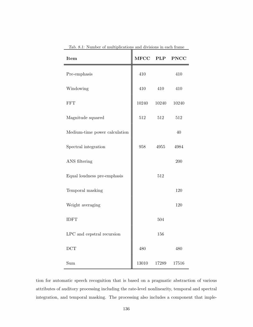
Tab. 8.1: Number of multiplications and divisions in each frame

Item MFCC PLP PNCC

Pre-emphasis 410 410

Windowing 410 410 410

FFT 10240 10240 10240

Magnitude squared 512 512 512

Medium-time power calculation 40

Spectral integration 958 4955 4984

ANS filtering 200

Equal loudness pre-emphasis 512

Temporal masking 120

Weight averaging 120

IDFT 504

LPC and cepstral recursion 156

DCT 480 480

Sum 13010 17289 17516

tion for automatic speech recognition that is based on a pragmatic abstraction of various

attributes of auditory processing including the rate-level nonlinearity, temporal and spectral

integration, and temporal masking. The processing also includes a component that imple-

136

ments suppression of various types of common additive noise. PNCC processing requires

only about 33 percent more computation compared to MFCC.

Open Source MATLAB code for PNCC may be found at http://www.cs.cmu.edu/

~robust/archive/algorithms/PNCC IEEETran. The code in this directory was used for obtain-

ing the results for this chapter.

137

9. COMPENSATION WITH 2 MICROPHONES

9.1 Introduction

Speech researchers have proposed many types of algorithms to enhance the noise robustness

of speech recognition systems, and many of these algorithms have shown provided improve-

ments in the presence of stationary noise (e.g. [12, 13, 9]). Nevertheless, improvement in

non-stationary noise remains a difficult issue (e.g. [14]). In these environments, auditory

processing (e.g. [37] [55]) and missing-feature-based approaches (e.g. [16]) are promising.

An alternative approach is signal separation based on analysis of differences in arrival time

(e.g. [17, 18, 19]). It is well documented that the human binaural system has a remarkable

ability to separate speech that arrives from different azimuths (e.g. [19] [84]). It has been

observed that various types of cues are used to segregate the target signal from interfering

sources. Motivated by these observations, many models and algorithms have been developed

using inter-microphone time differences (ITDs), inter-microphone intensity difference (IIDs),

inter-microphone phase differences (IPDs), and other cues (e.g. [17, 18, 85, 75]). IPD and

ITD have been extensively used in binaural processing because this information can be easily

obtained by spectral analysis (e.g. [85] [86] [46]). ITD can be estimated using either phase

differences (e.g. [46]), cross-correlation (e.g. [87], [78]), or zero-crossings (e.g. [18]).

In many of the algorithms above, either binary or continuous “masks” are developed

to indicate which time-frequency bins are dominated by the target source. Studies have

shown that continuous-mask techniques provide better performance than the binary masking

technique but they usually require that we know the exact location of the noise source (e.g.

[18]). Binary masking techniques (e.g. [55]) might be more realistic for situations when

multiple noise sources arise from all directions (“omnidirectional noise”) but we still need to

know which estimated source arrival anagle should serve as the threshold that determines

whether a particular time-frequency segment should be considered to be part of the desired

target speech or part of the unwanted noise source. Typically this is performed by sorting the

time-frequency bins according to ITD (either calculated directly or inferred from estimated

IPD). In either case, performance depends on how the threshold ITD for selection is selected,

and the optimal threshold depends on the configuration of the noise sources including their

locations and strength. If the optimal ITD from a particular environment is applied to a

somewhat different environment, the system performance will be degraded. In addition, the

characteristics of the environment typically vary with time.

The Zero Crossing Amplitude Estimation (ZCAE) algorithm recently introduced by Park

[18] is similar in some respects to earlier work by Srinivasan et al. [17]. These algorithms (and

similar ones by other researchers) typically analyze incoming speech in bandpass channels

and attempt to identify the subset of time-frequency components for which the ITD is close

to the nominal ITD of the desired sound source (which is presumed to be known a priori).

The signal to be recognized is reconstructed from only the subset of “good” time-frequency

components. This selection of “good” components is frequently treated in the computational

auditory scene analysis (CASA) literature as a multiplication of all components by a binary

mask that is nonzero for only the desired signal components. Although ZCAE provides

impressive performance even at low signal-to-noise ratios (SNRs), it is very computationally

intensive, which makes it unsuitable for hand-held devices.

Our own work on signal separation is motivated by human binaural processing. Sound

sources are localized and separated by the human binaural system primarily through the

use of ITD information at low frequencies and IID information at higher frequencies, with

the crossover point between these two mechanisms considered to be based on the physical

distance between the two ears and the need to avoid spatial aliasing (which would occur when

the ITD between two signals exceeds half a wavelength). In our work we focus on the use

of ITD cues and avoid spatial aliasing by placing the two microphones closer together than

occurs anatomically. When multiple sound sources are presented, it is generally assumed

that humans attend to the desired signal by attending only to information at the ITD

corresponding to the desired sound source.

The goals of the present paper are threefold. First, we would like to obtain improvements

in word error rate (WER) for speech recognition systems that operate in real world envi-

139

ronments that include noise (possibly multiple noisy sources) and reverberation. For this

purpose, we investigated into the effects of temporal resolution. We also perform channel

weighting to enhance speech recognition accuracy in real-world environments. In addition,

the performance of sound source separation system ITD heavily depends on the ITD thresh-

old. In this work, we investigate into an efficient way of finding an appropriate ITD threshold

blindly. Second, we also would like to develop a computationally efficient algorithm than

can run in real time in embedded systems. In the present ZCAE algorithm much of the

computation is taken up in the bandpass filtering operations. We found that computational

cost could be significantly reduced by estimating the ITD through examination of the phase

difference between the two sensors in the frequency domain. We describe in the sections

below how the binary mask is obtained using frequency information. We also discuss the

duration and shape of the analysis windows, which can contribute to further improvements

in WER. Third, and most important, we describe a method by which the threshold ITD that

separates time-frequency segments belonging to the target from the masker segments can be

obtained automatically and adaptively, without any a priori knowledge of the location of

the sound sources or the acoustics of the environment.

In many cases, we can assume knowledge of the location of the target source, but we don’t

have control of the number or locations of the noise sources. When target identification is

obtained by a binary masked based on an ITD threshold, the value of that threshold is

typically estimated from development test data. As noted above, the optimal ITD threshold

itself will depend on the number of noise sources and their locations, both of which may be

time-varying. If the azimuth of the noise source is very different from that of the target, a

threshold that ITD is relatively far from that of the target may be helpful. On the other

hand, if an interfering noise source is very close to the target and we use a similar ITD

threshold, the system will also classify many components of the interfering signal as part of

the target signal. If there is more than one noise source, or if the noise sources are moving,

the problem becomes even more complicated.

In our approach, which is summarized in Fig. 9.2, we construct two complementary masks

using a binary threshold. Using these two complementary masks, we obtain two different

spectra: one for the target and the other for everything except for the target. From these

spectra, we obtain the short-time power for the target and the interference. These power

140

θ

sin( )d θ

S

d

THθ

THθ

Fig. 9.1: Selection region for the binaural sound source separation system: if the location of a sound

source is inside the shaded region, the sound source separation system assumes that it is the

target. If the location of a sound source is outside this shaded region, then it is assumed to

be arising from a nose source and is suppressed by the sound source separation system.

sequences are passed through a compressive nonlinearity. We compute the cross-correlation

coefficient and normalized coefficient for the two resulting power sequences, and we obtain

the ITD threshold by minimizing these coefficients.

The rest of the paper is organized as follows: in Sec. 9.2, we explain the entire system

structure of the basic PDCW algorithm, including the estimation of the ITD from phase

difference information and further improvements in speech recognition accuracy that are

obtained through the use of a medium-time window and gammatone channel weighting. In

Sec. 9.3 we explain the method by which we obtain the optimal ITD threshold through the

construction of the complementary masks for speech and noise. We present experimental

results in Section 10.2.

141

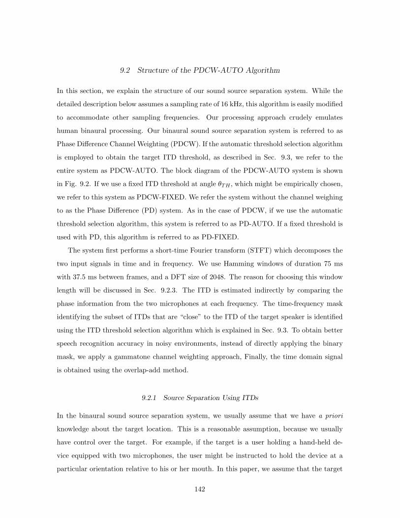
9.2 Structure of the PDCW-AUTO Algorithm

In this section, we explain the structure of our sound source separation system. While the

detailed description below assumes a sampling rate of 16 kHz, this algorithm is easily modified

to accommodate other sampling frequencies. Our processing approach crudely emulates

human binaural processing. Our binaural sound source separation system is referred to as

Phase Difference Channel Weighting (PDCW). If the automatic threshold selection algorithm

is employed to obtain the target ITD threshold, as described in Sec. 9.3, we refer to the

entire system as PDCW-AUTO. The block diagram of the PDCW-AUTO system is shown

in Fig. 9.2. If we use a fixed ITD threshold at angle θTH , which might be empirically chosen,

we refer to this system as PDCW-FIXED. We refer the system without the channel weighing

to as the Phase Difference (PD) system. As in the case of PDCW, if we use the automatic

threshold selection algorithm, this system is referred to as PD-AUTO. If a fixed threshold is

used with PD, this algorithm is referred to as PD-FIXED.

The system first performs a short-time Fourier transform (STFT) which decomposes the

two input signals in time and in frequency. We use Hamming windows of duration 75 ms

with 37.5 ms between frames, and a DFT size of 2048. The reason for choosing this window

length will be discussed in Sec. 9.2.3. The ITD is estimated indirectly by comparing the

phase information from the two microphones at each frequency. The time-frequency mask

identifying the subset of ITDs that are “close” to the ITD of the target speaker is identified

using the ITD threshold selection algorithm which is explained in Sec. 9.3. To obtain better

speech recognition accuracy in noisy environments, instead of directly applying the binary

mask, we apply a gammatone channel weighting approach, Finally, the time domain signal

is obtained using the overlap-add method.

9.2.1 Source Separation Using ITDs

In the binaural sound source separation system, we usually assume that we have a priori

knowledge about the target location. This is a reasonable assumption, because we usually

have control over the target. For example, if the target is a user holding a hand-held de-

vice equipped with two microphones, the user might be instructed to hold the device at a

particular orientation relative to his or her mouth. In this paper, we assume that the target

142

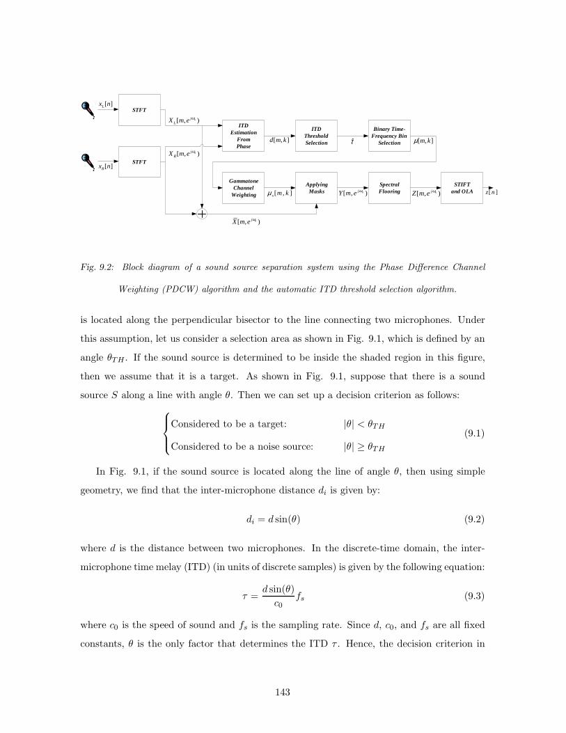
STFT

ITD Estimation

FromPhase

Binary Time-Frequency Bin

Selection

STIFTand OLA

ITDThresholdSelection

STFT

[ , )kjLX m e ω

[ , )kjRX m e ω

[ , ]d m k

[ ]Lx n

[ ]Rx n

[ , ]m kµ

GammatoneChannel

Weighting

ApplyingMasks

SpectralFlooring

[ , )kjX m e ω

),[ kjemY ω ),[ kjemZ ω ][ nz

τ

],[ kmsµ

Fig. 9.2: Block diagram of a sound source separation system using the Phase Difference Channel

Weighting (PDCW) algorithm and the automatic ITD threshold selection algorithm.

is located along the perpendicular bisector to the line connecting two microphones. Under

this assumption, let us consider a selection area as shown in Fig. 9.1, which is defined by an

angle θTH . If the sound source is determined to be inside the shaded region in this figure,

then we assume that it is a target. As shown in Fig. 9.1, suppose that there is a sound

source S along a line with angle θ. Then we can set up a decision criterion as follows:

Considered to be a target: |θ| < θTH

Considered to be a noise source: |θ| ≥ θTH

(9.1)

In Fig. 9.1, if the sound source is located along the line of angle θ, then using simple

geometry, we find that the inter-microphone distance di is given by:

di = d sin(θ) (9.2)

where d is the distance between two microphones. In the discrete-time domain, the inter-

microphone time melay (ITD) (in units of discrete samples) is given by the following equation:

τ =d sin(θ)

c0fs (9.3)

where c0 is the speed of sound and fs is the sampling rate. Since d, c0, and fs are all fixed

constants, θ is the only factor that determines the ITD τ . Hence, the decision criterion in

143

Eq. (9.1) can be expressed as follows:

considered to be a target: |τ | < τTH

considered to be a noise source: |τ | ≥ τTH

(9.4)

where τTH = d sin(θTH)c0

fs. Thus, if we obtain a suitable ITD threshold using Eq. (9.4), we

can make a binary decision to determine whether the source is in the shaded region in Fig.

9.1. In our sound source separation system the ITD is obtained for each-time frequency bin

using phase information according to Eq. (9.4) is made for each-time frequency bin. This

procedure will be explained in detail in Sec. 9.2.2.

9.2.2 Obtaining the ITD from phase information

In this subsection we review the procedure for obtaining the ITD from phase information (e.g.

[46]). Let xL[n] and xR[n] be the signals from the left and right microphones, respectively.

We assume that we know where the target source is located and, without loss of generality, we

assume that it is placed along the perpendicular bisector of the line between two microphones,

which means that its ITD is zero.

Suppose that the total number of interfering sources is S. Each source s, 1 ≤ s ≤ S has

an ITD of taus[m,k] where m is the frame index and k is the frequency index. Note that

both S and taus[m,k] are unknown. We assume that x0[n] represents the target signal and

that the notation xs[n], 1 ≤ s ≤ S, represents signals from each interfering source received

from the “left” microphone. In the case of signals from the “right” microphone, the target

signal is still x0[n], but the interfering signals are delayed by taus[m,k]. Note that for the

target signal x0[n], d0[m,k] = 0 for all m and k by the above assumptions.

To perform spectral analysis, we obtain the following short-time signals by multiplication

with a Hamming window w[n]:

xL[n;m] = xL[n−mLfp]w[n] (9.5a)

xR[n;m] = xR[n−mLfp]w[n] (9.5b)

for 0 ≤ n ≤ Lfl − 1

144

where m is the frame index, Lfp is the number of samples between frames, and Lfl is the

frame length. The window w[n] is a Hamming window with a length of Lfl. We use a

75-ms window length based on previous findings described in [46]. The short-time Fourier

transforms of Eq. (9.5) can be represented as

XL[m, ejωk) =

S∑

s=0

Xs[m, ejωk) (9.6a)

XR[m, ejωk) =S∑

s=0

e−jwkτs[m,k]Xs[m, ejωk) (9.6b)

where wk = 2πk/N and N is the FFT size. We represent the strongest sound source for a

specific time-frequency bin [m,k] as s∗[m,k]. This leads to the following approximation:

XL[m, ejωk) ≈ Xs∗[m,k][m, e−jwk) (9.7a)

XR[m, ejωk) ≈ e−jwkτs∗[m,k][m,k]

×Xs∗[m,k][m, e−jwk) (9.7b)

Note that s∗[m,k] may be either 0 (the target source) or 1 ≤ s ≤ S (any of the interfering

sources). From Eq. (9.7), The ITD for a particular time-frequency bin [m,k] is given by

|τs∗[m,k][m,k]| ≈1

|wk|minr

∣

∣

∣

6 XR[m, e−jwk)

− 6 XL[m, e−jwk)− 2πr∣

∣

∣0 ≤ k ≤

N

2(9.8)

Thus, by examining whether the obtained ITD from Eq. (9.8) is within a certain range

from the target ITD, we can make a simple binary decision concerning whether the time-

frequency bin [m,k] is likely to belong to the target speaker or not.

From here on we will use the notation τ [m,k] instead of τs∗[m,k][m,k] for simplicity. From

Eqs. (9.4) and (9.8), we obtain the mask for the target for τTH for 0 ≤ k ≤ N/2:

µ[m,k] =

1, if |τTH [m,k]| ≤ τTH

δ, otherwise

0 ≤ k ≤N

2(9.9)

145

In other words, we assume that time-frequency bins for which |τ(m,k)| < τTH are presumed

to belong to the target speaker, and that time-frequency bins for which|τ(m,k)| > τTH

belong to the noise source. We are presently using a value of 0.01 for the floor constant δ.

The mask µ[m,k] in Eq. (9.9) may be directly applied to X[m, ejωk), the averaged signal

spectrogram from the two microphones:

X[m, ejωk) =1

2

(

XL[m, ejωk) +XR[m, ejωk)

(9.10)

The mask is applied by multiplying X [m, ejωk) by the mask value in Eq. (9.9). As mentioned

before, if we directly apply µ[m,k] to the spectrum, this approach is referred to as the Phase

Difference (PD) approach. Even though the PD approach is able to separate sound sources,

in some cases, the mask in Eq. (9.9) is too noisy to be employed directly. In Sec. 9.2.4 we

discuss a channel weighting algorithm in detail that resolves this issue.

9.2.3 Temporal resolution

While the basic procedure described in Sec. 9.2.2 provides signals that are audibly separated,

the mask estimates are generally too noisy to provide useful speech recognition accuracy.

Figures 9.5(c) and 9.5(d) show the mask and the resynthesized speech that is obtained by

directly applying the mask µ[m,k]. As can be seen in these figures, there are a lot of artifacts

in the spectrum of resynthesized speech that occur as a consequence of discontinuities in the

mask. In this and the following subsection, we discuss the implementation of two methods

that smooth the estimates over frequency and time.

In conventional speech coding and speech recognition systems, we generally use a length

of approximately 20 to 30 ms for the Hamming window w[n] in order to capture effectively

the temporal fluctuations of speech signals. Nevertheless, longer observation durations are

usually better for estimating environmental parameters as shown in our previous works (e.g.

[36, 37, 35, 66, 55]). Using the configuration described in Sec. 10.2, we evaluated the effect

of window length on recognition accuracy using the PD-FIXED structure described in Sec.

9.2.2. While we defer a detailed description of our experimental procedures to Sec. 10.2,

we describe in Fig. 9.4(b) the results of a series of pilot experiments that describe the

dependence of recognition accuracy on window length, obtained using the DARPA RM1

database. These results indicate that best performance is achieved with window length of

146

TθIθ

I

T

d

Fig. 9.3: The configuration for a single target (represented by T) and a single interfering source

(represented by I).

about 75 ms. In the experiments described below we Hamming windows of duration 75 ms

with 37.5 ms between successive frames.

9.2.4 Gammatone channel weighting and mask application

As noted above, the estimates produced by Eq. (9.9) are generally noisy and must be

smoothed. To achieve smoothing along frequency, we use a gammatone weighting that

functions in a similar fashion to that of the familiar triangular weighting in MFCC feature

extraction. Specifically, we obtain the gammatone channel weighting coefficients w[m, l]

according to the following equation:

w[m, l] =

∑

N2k=0 µ[m,k]

∣

∣X [m; ejωk)Hl(ejωk)

∣

∣

∑

N2k=0

∣

∣X[m; ejωk)Hl(ejωk)∣

∣

(9.11)

where µ[m,k] is the original binary mask that is obtained using Eq. (9.9). With this weghting

we effectively map the ITD for each of the 256 original frequencies to an ITD for what we

refer to as one of L = 40 channels. Each of these channels is associated withHi, the frequency

response of one of a set of gammatone filters with center frequencies distributed according

to the Equivalent Rectangular Bandwidth (ERB) scale [4].

The frequency response of the gammatone filterbank is shown in Fig. 9.6. In each channel

147

0 20 40 60 80 100 12040

50

60

70

80

90

100

Acc

urac

y (1

00 −

WE

R)

Window Length ( ms)

RM1 (Interfering Speaker Noise at 10 dB)

T60 = 0msT60 = 100msT60 = 200ms

(a)

0 20 40 60 80 100 12020

40

60

80

100

Acc

urac

y (1

00 −

WE

R)

Window Length ( ms)

RM1 (Omni−Directional Noise)

Clean15 dB10 dB5 dB

(b)

Fig. 9.4: The dependence of word recognition accuracy (100%-WER) on window length under dif-

ferent conditions: (a) interfering source at angle θI = 45. SIR 10 dB. (b) omnidirectional

natural noise. In both case PD-FIXED is used with a threshold angle of θTH = 20.

the area under the squared transfer function is normalized to unity to satisfy the equation

∫ 8000

0|Hl(f)|

2df = 1 (9.12)




(corresponding to -46 dB) of its maximum value. Note that we are using exactly the same

gammatone weigthing as in [64].

The final spectrum weighting is obtained using the gammatone mask µs

µs[m,k] =

∑L−1l=0 w[m,k]

∣

∣Hl

(

ejωk)∣

∣

∑L−1l=0 |Hl (ejωk)|

0 ≤ k ≤N

2(9.13)

148

Examples of µ[m,k] in Eq. (9.9) and µs[m,k] in Eq. (9.13) are shown shown for a typical

spectrum in Figs. 9.5(c) and 9.5(e), respectively, with an SNR of 0 dB as before. The

reconstructed spectrum is given by:

Y [m, ejωk) = maxµs[m,k], η X [m, ejωk)

0 ≤ k ≤N

2(9.14)

where again we use η = 0.01 as in (9.9), and X[m, ejωk) is the averaged spectrum defined in

Eq. (9.10).

In the discussion up to now we have considered spectral components for frequency indicies

0 ≤ k ≤ N2 . For N

2 + 1 ≤ k ≤ N − 1, we obtain Y [m, ejωk) using the Hermition symmetry

property of Fourier transforms of real time functions:

Y [m, ejωk) = Y [m, ejω(N−k)) (9.15)

6 Y [m, ejωk) = − 6 Y [m, ejω(N−k)) (9.16)

9.2.5 Spectral flooring

In our previous work (e.g. [37] [35] ), it has been frequently observed that an appropriate

flooring helps in improving noise robustness. For this reason we also apply a flooring level

to the spectrum, that is described by the equation:

Yf = δf

√

√

√

√

1

NfN

Nf−1∑

m=0

N−1∑

k=0

|Y [m, ejωk)|2 (9.17)

where δf is the flooring coefficient, Nf is the number of frames in the utterance, N is the

FFT size, and Yf is the obtained threshold. We use a value of 0.01 for the flooring coefficient

δf .

Using the flooring level Yf , the floored spectrum Z[m, ejωk), 0 ≤ k ≤ N is obtained as

follows:

|Z[m, ejωk)| = max|Y [m, ejωk)|, Yf (9.18a)

6 Z[m, ejωk) = 6 Y [m, ejωk) (9.18b)

The above equations mean that the magnitude spectrum is floored by a minimum value of

Yf while the phase remains unchanged.

149

Using Z[m, ejωk), speech is resynthesized using IFFT and OverLap Addition (OLA).

In Sec. 9.3, we discuss how to obtain the optimal threshold without prior knowledge

about the noise sources.

9.3 Optimal ITD threshold selection using complementary masks

In the previous section we used a fixed ITD threshold to construct binary masks. Unfor-

tunately, in a real-world environment we typically do not have control over the locations of

the noise sources. It is reasonable to assume that the value of the ITD threshold will vary

depending on the types and locations of the noise sources. In this section we discuss how

to obtain an optimal threshold automatically without prior knowledge about the nature and

locations of the noise sources. Before explaining our algorithm in great detail we will discuss

the general dependence of speech recognition accuracy on the locations of the target and

interfering sources.

9.3.1 Dependence of speech recognition accuracy on the locations of the target and

interfering source

To examine the dependence of the optimal threshold on the interfering source location, let

us consider the simulation configuration shown in Fig. 9.3. To simplify the discussion, we

assume that there is a single single interfering source along the line of angle θI . As before, the

distance between two microphones is 4 cm. In the first set of experiments we assumed that

the target angle θT is zero. For the interfering source angle θI we used three different values

(30, 45, and 75). Signal-to-Interference Ratio (SIR) is assumed to be 0 dB and we assume

that the room is anechoic. For speech recognition experiments, we used the configuration

explained in Sec. 10.2.

Figure 9.7 describes the dependence of speech recognition accuracy on the threshold

angle θTH and the interfering source angle θI . We use the PD-FIXED and PDCW-FIXED

processing algorithms in Figs. 9.7(a) and 9.7(b), respectively. When the interfering source

angle is θI , we obtain best speech recognition accuracy when θTH is roughly equal to or

or slightly larger than θI/2. When θTH is larger than θI , the system fails to separate the

150

sound sources, which is is reflected in very poor speech recognition accuracy. In another

set of experiments we used natural omnidirectional stereo noises, but but maintaining the

target angle θT = 0 as before. Speech recognition results for this experiment are shown

in Fig. 9.7, fixing the SNR at 5 dB and measuring recognition accuracy as a function of

threshold angle θTH . In this experiment the best speech recognition accuracy is obtained at

a much smaller value of θT . Figure 9.9 describes the dependence of recognition accuracy on

SNR when the ITD threshold θTH is fixed at either 10 or 20. As can been in the figure,

the smaller threshold angle (θTH = 10) is more helpful than in the case of single-speaker

interference. As before, a greater difference in recognition accuracy provided by the PD-

FIXED and PDCW-FIXED algorithms is observed when the smaller threshold angle θTH is

10 is used.

In the previous discussion we observed that the optimal threshold angle θTH depends

heavily on the noise source location. In a real environment there is one more complication.

Up to now we have assumed that the target is placed at θT = 0. Even if we had control over

the target location there may still be some errors in estimating or controlling it. For example,

even if a user of a hand-held device is instructed to hold the device at a particular angle,

there is no way of ensuring that the user could accomplish this task perfectly. To understand

the impact of this issue we implemented an additional experiment using the configuration

shown in Fig. 9.7, but we changing the target angles to be one of the five values (−20,

−10, 0, 10, and 20) while holding the interfering angle fixed at θI = 45. Results of this

experiment are shown in Fig. 9.10(a). From the figure we observe that if we choose a very

small value for θTH , then the sound source separation system is not very robust with respect

to mis-estimation of the target angle.

In this section, we observed that the optimal ITD threshold depends on both the target

angle θT , the interfering source angle θI , and the noise type. If the ITD threshold is inap-

propriately selected, speech recognition accuracy becomes significantly degraded. From this

observation we conclude that we need to develop an automatic threshold selection algorithm

which obtains a suitable value for the ITD threshold without prior knowledge about the

noise sources, and that at the same time is robust with respect to error in the location of

the target angle θT .

151

9.3.2 The optimal ITD threshold algorithm

The algorithm we introduce in this section is based on two complementary binary masks,

one that identifies time-frequency components that are believed to belong to the target

signal and a second that identifies the components that belong to the interfering signals (i.e.

everything except the target signal). These masks are used to construct two different spectra

corresponding to the power sequences representing the target and the interfering sources. We

apply a compressive nonlinearity to these power sequences, and define the threshold to be

the separating ITD threshold that minimizes the cross-correlation between these two output

sequences (after the nonlinearity).

Computation is performed in discrete fashion, considering a set T of a finite number

of possible ITD threshold candidates. The set T is defined by the following minimum and

maximum values of the ITD threshold.

τmin =dsin(θTH,min)

cfs (9.19a)

τmax =dsin(θTH,max)

cfs (9.19b)

where d is the distance between two microphones, c is the speed of sound, and fs is the

sampling rate as in Eq. (9.3). θTH,min and θTH,max are the minimum and the maximum

values of the threshold angle. In the present implementation, we use values of θTH,min = 5

and θTH,max = 45. We use a set of candidate ITD thresholds T that consist of the 20

linearly-spaced values of θTH that lie between θTH,min and θTH,max.

We determine which element of this set is the most appropriate ITD threshold by per-

forming an exhaustive search over the set T . Let us consider one element of this set, τ0.

Using this procedure, we obtain the target spectrum XT [m, ejωk |τ0), 0 ≤ k ≤ N2 as shown

below:

XT [m, ejωk |τ0) = X [m, ejωk)µT [m, ejωk) (9.20)

In the above equation we explicitly include τ0 to show that the masked spectrum depends

on the ITD threshold. Using this spectrum XT [m, ejωk), we obtain the target power and the

power of the interfering sources. Since everything which is not the target is considered to

152

be an interfering source, the power associated with the target and interfering sources can be

obtained by the following equations:

PT [m|τ0) =N−1∑

k=0

∣

∣

∣XT [m, ejωk)

∣

∣

∣

2(9.21a)

PI [m|τ0) = Ptot[m]− PT [m|τ0) (9.21b)

where Ptot[m] is the total power at frame index m, given by:

Ptot[m] =

N−1∑

k=0

∣

∣

∣X [m, ejωk)∣

∣

∣

2. (9.22)

A compressive nonlinearity is invoked because the power signals in Eq. (9.21) have a very

large dynamic range. A compressive nonlinearity will reduce the dynamic range, and it may

be considered to represent a transformation that yields the perceived loudness of the sound.

While many nonlinearities have been proposed to characterize the relationship between signal

intensity and perceived loudness [88] we chose the following power-law nonlinearity motivated

by previous work (e.g. [55][35][64]):

RT [m|τ0) = PT [m|τ0)a0 (9.23a)

RI [m|τ0) = PI [m|τ0)a0 (9.23b)

where a0 = 1/15 is the power coefficient as in [35, 64].

In general, the optimal ITD threshold is determined by identifying the value of τ0 that

minimizes the cross-correlation between the signals RT [m|τ0) and RI [m|τ0) from Eq. (9.23),

but there are several plausible ways of computing this cross-correlation. The first method

considered, which was used in an earlier paper [67], is based on the cross-correlation coefficient

of the signals in Eq. (9.23):

ρT,I(τ0) =1N

∑Mm=1RT [m|τ0)RI [m|τ0)− µRT

µRI

σRTσRI

(9.24)

where µR1 and µR2 , and σRTand σRI

, are the means and standard deviations of RT [m|τ0)

and RI [m|τ0), respectively. (This statistic is also known as the Pearson product-moment

correlation or the normalized covariance.)

153

The optimal ITD threshold τ0 is selected to minimize the absolute value of the cross-

correlation coefficient:

τ1 = argminτ0

|ρT,I(τ0)| (9.25)

We refer to this approach as the “Type-I” statistic, and it has provided good speech recogni-

tion accuracy as shown in Fig. 9.11, especially at low SNRs such as 0 or 5 dB. Nevertheless, at

moderate SNRs such 10 or 15 dB, the speech recognition accuracies obtained using “Type-I”

processing are even worse than those obtained using the PDCW-FIXED algorithm. PDCW-

AUTO processing using the Type-I statistic also provides poor recognition accuracy in the

presence of omnidirectional natural noise, as shown in Fig. 9.12. We have also found in

pilot studies that the cross-correlation-based statistic in Eq. 9.24 is not a helpful measure in

situations where there is a single interfering source with power that is comparable to that of

the target, or where there are multiple interfering sources.

To address this problem, we consider a second related statistic, the normalized correlation:

rT,I(τ0) =1N

∑Mm=1 RT [m|τ0)RI [m|τ0)

σRTσRI

(9.26)

τ2 = argminτ0

|rT,I(τ0)| (9.27)

We refer to implementations of PD-AUTO or PDCW-AUTO using τ2 as “Type-II” systems.

The final ITD threshold τ3 is obtained easily by calculating the minimum of τ1 and τ2 as

shown below:

τ3 = min(τ1, τ2) (9.28)

We refer to implementations of PD-AUTO or PDCW-AUTO using τ3 as “Type-III” systems.

As can be seen in Figs. 9.11 and 9.12, systems using the “Type-III” stastistic consistently

provide recognition accuracy that is similar to or better than that obtained using either

the “Type-I” or “Type-II” approaches. For these reasons we adopt “Type-3” processing as

our default approach, and if the threshold type of a PD-AUTO or PD-AUTO system is not

mentioned explicitly, the reader should assume that a Type-III threshold statistic is used.

154


In this section we present experimental results using the PDCW-AUTO algorithm described

in this paper. To evaluate the effectiveness of the automatic ITD threshold selection al-

gorithm and the channel weighting, we compare the PDCW-AUTO system to the PDCW-

FIXED and PD-AUTO systems. We also compare our approach with an earlier state-of-

the-art technique, the ZCAE algorithm described above [18]. The ZCAE algorithm is im-

plemented with binary masking for the present comparisons because the better-performing

continuous-masking implementation requires that there should be only one interfering source

with a known location, which is an unrealistic requirement in many cases. As we have done

previously (e.g. [19] [89]), we convert the gammatone filters to a zero-phase form in order

to impose identical group delay on each channel. The impulse responses of these filters hl(t)

are obtained by the following equation:

hl(t) = hg,l(t) ∗ hg,l(−t) (9.29)

where l is the channel index and hg,l(t) is the original gammatone response. While this

approach compensates for the difference in group delay from channel to channel, it also

causes the magnitude response to become squared, which results in bandwidth reduction.

To compensate for this, we intentionally double the bandwidths of the original gammatone

filters at the outset.

In all speech recognition experiments described in this paper we perform feature extrac-

tion using the version of MFCC processing implemented in sphinx fe in sphinxbase 0.4.1.

For acoustic model training, we used SphinxTrain 1.0, and decoding was performed suing

the CMU Sphinx 3.8, all of which are readily available in Open Source form [83]. We used

subsets of 1600 utterances and 600 utterances, respectively, from the DARPA Resource Man-

agement (RM1) database for training and testing. A bigram language model was used in all

experiments. In all experiments, we used feature vectors of length of 39 including delta and

delta-delta features. We assumed that the distance between two microphones is 4 cm.

We conducted three different sets of experiments in this section. The first two sets of

experiments, described in Secs. 9.4.1 and 9.4.2, involve simulated reverberant environments

in which the target speaker is masked by a single interfering speaker (in Sec. 9.4.1) or by

three interfering speakers (in Sec. 9.4.2). The reverberation simulations were accomplished

155

using the Room Impulse Response open source software package [53] based on the image

method [82]. The third set of experiments, decscribed in Sec. 9.4.3, involve the use of

additive omnidirectional noise recorded in several natural environments.

9.4.1 Experimental results using a single interfering speaker

In the experiments in this section we assume a room of dimensions 5 x 4 x 3 m, with

microphones that are located at the center of the room, as in Fig. 9.3. Both the target and

interfering sources are 1.5 m away from the microphone. For the fixed-ITD threshold systems

such as PDCW-FIXED, we used the threshold angle θTH = 20 based on the experimental

results described in Sec. 9.3.1. We conducted three different kinds of experiments using this

scenario.

In the first set of experiments we assume that the target is located along the perpendicular

bisector of the line between two microphones, which means θT = 0. We assume that the

interfering source is located at θI = 30. We repeated the experiments by changing the

SIR and reverberation time. As shown in Fig. 9.13(a), in the absence of reverberation at

0-dB SIR, both the fixed ITD system and the automatic-ITD system provide comparable

performance. If reverberation is present, however, the automatic-ITD system PDCW-AUTO

provides substantially better performance than the PDCW-FIXED signal separation system.

In the second set of the experiments we changed the location of the interfering speaker

while maintaining the SIR at 0 dB. As shown in Fig. 9.14, even if the SIR is the same as

in the calibration environment, the performance of the fixed-ITD threshold system becomes

significantly degraded if the actual interfering speaker location is different from the location

used in the calibration environment. The PDCW-AUTO selection system provides recogni-

tion results that are much more robust with respect to the locations of the interfering sources.

In this figure we observe that as the interfering speaker moves toward the target, the fixed-

ITD threshold PD system provides increased word error rate. We repeated this experiment

with different reverberation times. As shown in Fig. 9.14, the automatic-threshold-selection

algorithm provides consistently better recognition accuracy than the fixed threshold system,

as expected.

In the third set of the experiments we conducted experiments in which the target angle

156

θT was varied from −30 to 30. In our previous work ([46, 78]), we assumed that the target

is located along the bisector of the line between two microphones, but this is not always the

case in a real environment, and θT may not be exactly zero. As shown in Fig. 9.15, if the

target angle |θT | becomes larger than 20 the PDCW-FIXED and ZCAE algoroithms fail to

separate the sound sources, resulting in poor performance. In contrast (and as expected),

both the PDCW-AUTO and PD-AUTO provide substantial robustness against deviation in

the target direction.

9.4.2 Experimental results using three randomly-positioned interfering speakers

In the second set of experiments we assumed the same room dimension (5 x 4 x 3 m) as the

experiments in Sec. 9.4.1. We also still assume that the distance between two microphones

is 4 cm, the target speaker is located along the perpendicular bisector to the line connecting

two microphones, and the distance between the target and microphones is 1.5 m. In this

experiment we assume that the target speech is masked by three interfering speakers, as

shown in Fig. 9.16. The location of each interfering speaker is uniformly distributed on the

plane at the same height as the microphones. Thus, in some cases, the interfering speaker

might be in a similar direction as the target. The locations of the interfering speakers is

changed for each utterance in the test set. Experimental results for this configuration are

shown in Fig. 9.17. The general tendencies of the experimental results is similar to those

in Fig. 9.13 where there is a single interfering speaker along the direction of θI = 30.

The greatest difference between the results in Figs. 9.17 and 9.13 is that the improvement in

performance observed when the automatic threshold ITD selection of the PDCW-AUTO and

PD-AUTO algorithms is invoked becomes much more profound with three randomly-placed

interfering speakers than with only a single interfering speaker.

We believe that if there are multiple noise sources, the mask pattern becomes more varied.

In this case, the use of a fixed narrow ITD threshold as in PD-FIXED introduces artifacts,

which harm speech recognition accuracy. As will be seen in Sec. 9.4.3, the same tendency is

observed in the presence of omnidirectional natural interfering sources as well.

157

9.4.3 Experimental results using natural omnidirectional noise

In the third set of experiments, we still assume that the distance between the two microphones

is the same as before (4 cm), but we added noise recorded with two microphones in real

environments such as a public market, a food court, a city street and a bus stop. These real

noise sources are at all locations around the two microphones, and the signals from these

recordings are digitally added to clean speech from the test set of the RM database. As

before, all fixed-ITD-threshold algorithms use a threshold value of θTH = 20. Fig. 9.18

shows speech recognition accuracy for this configuration. Again we observe that the PDCW-

AUTO algorithm provides the best performance by a significant margin, while the PDCW-

FIXED, PD-AUTO, and ZCAE show similar performance to each other. As previously seen

in Fig. 9.8, in the case of omnidirectional natural noise, an ITD threshold θTH smaller than

20 results in better speech recognition accuracy. If we use the automatic ITD threshold

algorithm, then it chooses a better ITD threshold than θTH = 20 that is used in the

PDCW-FIXED or PD-FIXED algorithms.

9.5 Computational Complexity

We profiled the run times of implementations in C of the PDCW-FIXED and ZCAE al-

gorithms on two machines. The PDCW-FIXED algorithms ran in only 9.03% of the time

required to run the ZCAE algorithm on an 8-CPU Xeon E5450 3-GHz system, and in only

9.68% of the time to run the ZCAE algorithm on an embedded system with an ARM11

667-Mhz processor using a vector floating point unit. The major reason for the speedup is

that in ZCAE the signal must be passed through a bank of 40 filters while PDCW-FIXED

requires only two FFTs and one IFFT for each feature frame. The PDCW-AUTO algorithm

requires more computation than the PDCW-FIXED algorithm, but it still requires much less

computation than ZCAE.

9.6 Summary

In this work, we present a speech separation algorithm, PDCW, based on inter-microphone

time delay that is inferred from phase information. The algorithm uses gammatone channel

158

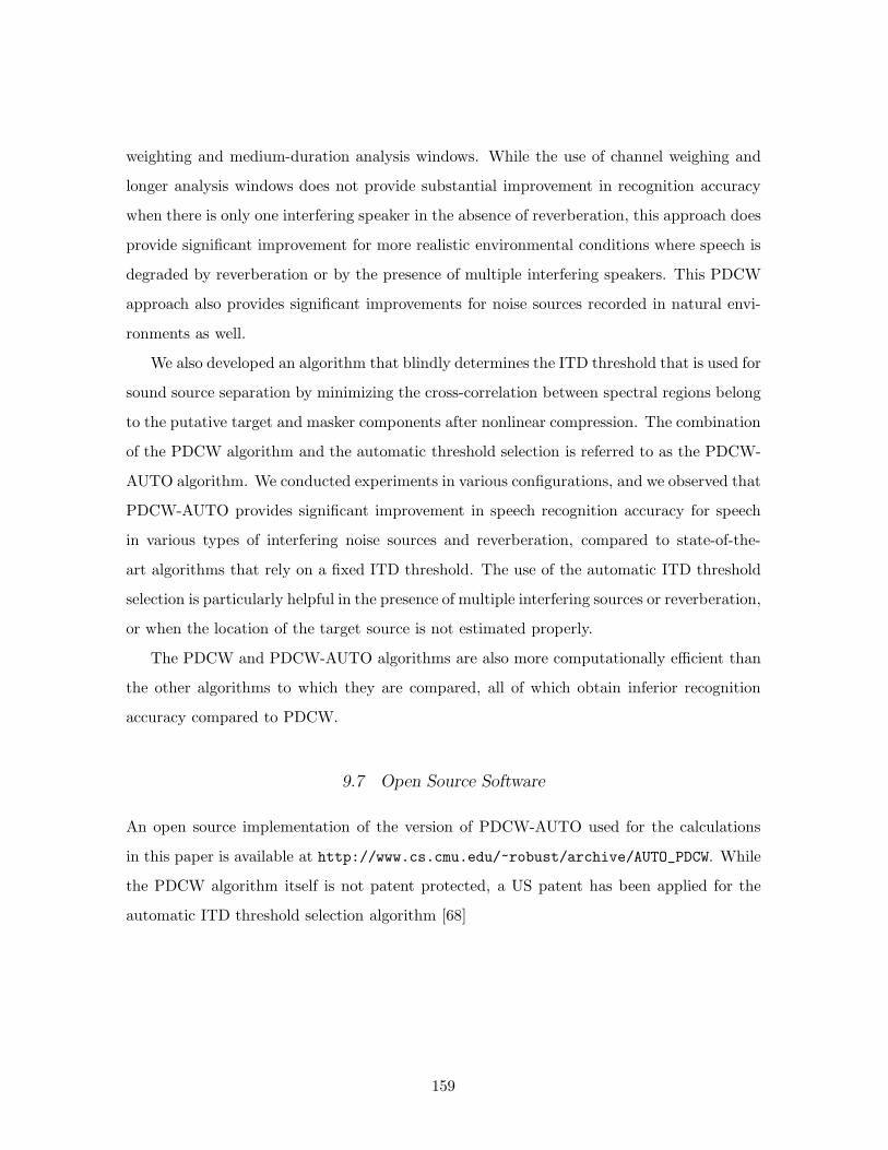
weighting and medium-duration analysis windows. While the use of channel weighing and

longer analysis windows does not provide substantial improvement in recognition accuracy

when there is only one interfering speaker in the absence of reverberation, this approach does

provide significant improvement for more realistic environmental conditions where speech is

degraded by reverberation or by the presence of multiple interfering speakers. This PDCW

approach also provides significant improvements for noise sources recorded in natural envi-

ronments as well.

We also developed an algorithm that blindly determines the ITD threshold that is used for

sound source separation by minimizing the cross-correlation between spectral regions belong

to the putative target and masker components after nonlinear compression. The combination

of the PDCW algorithm and the automatic threshold selection is referred to as the PDCW-

AUTO algorithm. We conducted experiments in various configurations, and we observed that

PDCW-AUTO provides significant improvement in speech recognition accuracy for speech

in various types of interfering noise sources and reverberation, compared to state-of-the-

art algorithms that rely on a fixed ITD threshold. The use of the automatic ITD threshold

selection is particularly helpful in the presence of multiple interfering sources or reverberation,

or when the location of the target source is not estimated properly.

The PDCW and PDCW-AUTO algorithms are also more computationally efficient than

the other algorithms to which they are compared, all of which obtain inferior recognition

accuracy compared to PDCW.

9.7 Open Source Software

An open source implementation of the version of PDCW-AUTO used for the calculations

in this paper is available at http://www.cs.cmu.edu/~robust/archive/AUTO_PDCW. While

the PDCW algorithm itself is not patent protected, a US patent has been applied for the

automatic ITD threshold selection algorithm [68]

159

http://www.cs.cmu.edu/~robust/archive/AUTO_PDCW

Time (s)

Fre

quen

cy (

kHz)

0.2 0.4 0.6 0.8 1 1.2 1.402468

(a)

Time (s)

Fre

quen

cy (

kHz)

0.2 0.4 0.6 0.8 1 1.2 1.402468

(b)

Time (s)

Fre

quen

cy (

kHz)

102468

(c)

Time (s)

Fre

quen

cy (

kHz)

0.2 0.4 0.6 0.8 1 1.2 1.402468

(d)

Time (s)

Fre

quen

cy (

kHz)

102468

(e)

Time (s)

Fre

quen

cy (

kHz)

0.2 0.4 0.6 0.8 1 1.2 1.402468

(f)

Fig. 9.5: Sample spectrograms illustrating the effects of PDCW processing. (a) original clean speech,

(b) noise-corrupted speech (0-dB omnidirectional natural noise), (c) the time-frequency mask

µ[m, k] in Eq. (9.9) with windows of 25-ms length, (d) enhanced speech using µ[m, k] (PD),

(e) the time-frequency mask obtained with Eq. (9.9) using windows of 75-ms length, (f)

enhanced speech using µs[m, k] (PDCW).

160

0 2000 4000 6000 80000

0.02

0.04

0.06

0.08

0.1

0.12

0.14

0.16

Frequency (Hz)

H(e

j ω)




0 20 40 60 800

20

40

60

80

100

Acc

urac

y (1

00 −

WE

R)

Threshold Angle θTH

RM1 (0 dB Interfering Speaker)

(a)

0 20 40 60 800

20

40

60

80

100

Acc

urac

y (1

00 −

WE

R)



θI = 15

θI = 45

θI = 75

(b)

Fig. 9.7: The dependence of word recognition accuracy on the threshold angle θTH and the location of

the interfering source θI using PD-FIXED, and (b) PDCW-FIXED. The target is assumed to

be located along the perpendicular bisector of the line between two microphones (θT = 0).

161

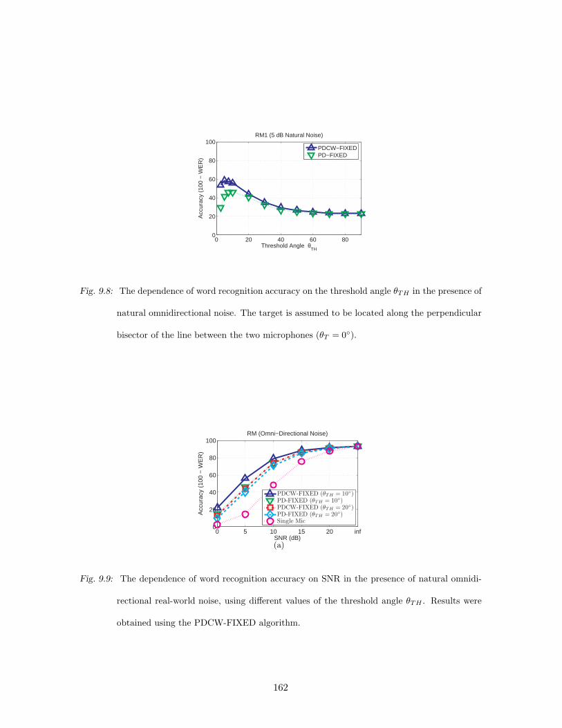
0 20 40 60 800

20

40

60

80

100

Acc

urac

y (1

00 −

WE

R)


RM1 (5 dB Natural Noise)

PDCW−FIXEDPD−FIXED

Fig. 9.8: The dependence of word recognition accuracy on the threshold angle θTH in the presence of

natural omnidirectional noise. The target is assumed to be located along the perpendicular

bisector of the line between the two microphones (θT = 0).

0 5 10 15 20 inf0

20

40

60

80

100

Acc

urac

y (1

00 −

WE

R)

SNR (dB)

RM (Omni−Directional Noise)

PDCW-FIXED (θTH = 10)PD-FIXED (θTH = 10)PDCW-FIXED (θTH = 20)PD-FIXED (θTH = 20)Single Mic

(a)

Fig. 9.9: The dependence of word recognition accuracy on SNR in the presence of natural omnidi-

rectional real-world noise, using different values of the threshold angle θTH . Results were

obtained using the PDCW-FIXED algorithm.

162

0 20 40 60 800

20

40

60

80

100

Acc

urac

y (1

00 −

WE

R)



(a)

0 20 40 60 800

20

40

60

80

100

Acc

urac

y (1

00 −

WE

R)



θT = 20

θT = 10

θT = 0

θT = −10

θT = −20

(b)

Fig. 9.10: The dependence of word recognition accuracy on the threshold angle θTH and the location

of the target source θT using (a) the PD-FIXED, and (b) the PDCW-FIXED algorithms.

163

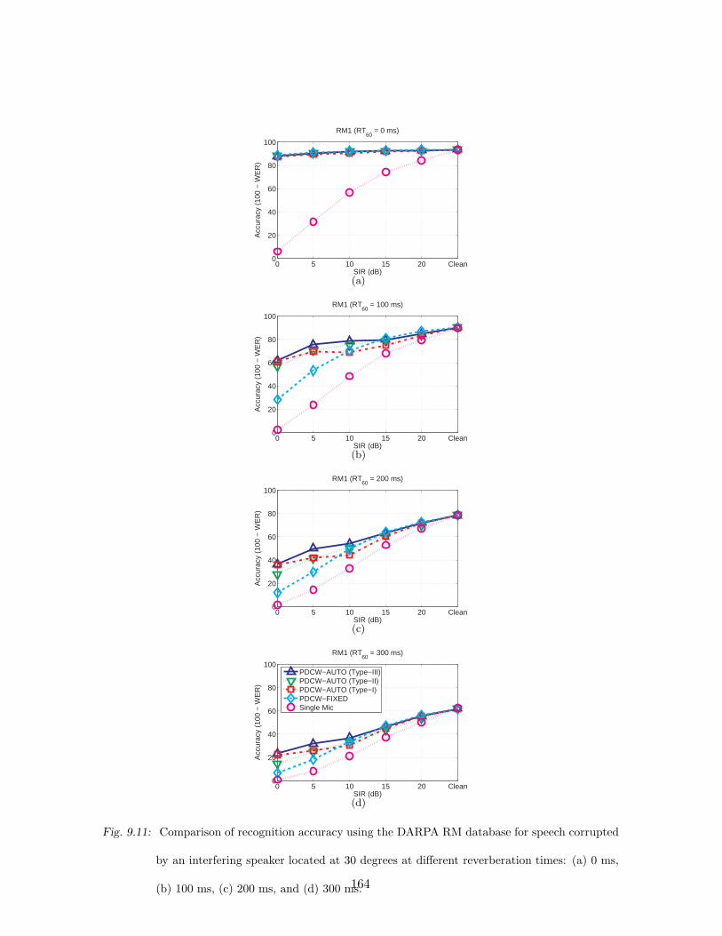
0 5 10 15 20 Clean0

20

40

60

80

100

Acc

urac

y (1

00 −

WE

R)

SIR (dB)

RM1 (RT60

= 0 ms)

(a)

0 5 10 15 20 Clean0

20

40

60

80

100

Acc

urac

y (1

00 −

WE

R)

SIR (dB)

RM1 (RT60

= 100 ms)

(b)

0 5 10 15 20 Clean0

20

40

60

80

100

Acc

urac

y (1

00 −

WE

R)

SIR (dB)

RM1 (RT60

= 200 ms)

(c)

0 5 10 15 20 Clean0

20

40

60

80

100

SIR (dB)

Acc

urac

y (1

00 −

WE

R)

RM1 (RT60

= 300 ms)

PDCW−AUTO (Type−III)PDCW−AUTO (Type−II)PDCW−AUTO (Type−I)PDCW−FIXEDSingle Mic

(d)

Fig. 9.11: Comparison of recognition accuracy using the DARPA RM database for speech corrupted

by an interfering speaker located at 30 degrees at different reverberation times: (a) 0 ms,

(b) 100 ms, (c) 200 ms, and (d) 300 ms.164

0 5 10 15 20 Clean0

20

40

60

80

100

SIR (dB)

Acc

urac

y (1

00 −

WE

R)

RM1 (RT60

= 300 ms)

PDCW−AUTO (Type−III)PDCW−AUTO (Type−II)PDCW−AUTO (Type−I)PDCW−FIXEDSingle Mic

Fig. 9.12: Speech recognition accuracy obtained using different algorithms in the presence of natural

real-world noise. Noise was recorded in real environments with real two-microphone hard-

ware in locations such as a public market, a food court, a city street, and a bus stop with

background babble. This noise was digitally added to the clean test set.

165

0 5 10 15 20 Clean0

20

40

60

80

100

Acc

urac

y (1

00 −

WE

R)

SIR (dB)

RM1 (RT60

= 0 ms)

(a)

0 5 10 15 20 Clean0

20

40

60

80

100

Acc

urac

y (1

00 −

WE

R)

SIR (dB)

RM1 (RT60

= 100 ms)

(b)

0 5 10 15 20 Clean0

20

40

60

80

100

Acc

urac

y (1

00 −

WE

R)

SIR (dB)

RM1 (RT60

= 200 ms)

(c)

0 5 10 15 20 Clean0

20

40

60

80

100

SIR (dB)

Acc

urac

y (1

00 −

WE

R)

RM1 (RT60

= 300 ms)

PDCW−AUTOPD−AUTOPDCW−FIXEDZCAESingle Mic

(d)

Fig. 9.13: Comparison of recognition accuracy for the DARPA RM database corrupted by an inter-

fering speaker located at 30 degrees at different reverberation times: (a) 0 ms, (b) 100 ms,

(c) 200 ms, and (d) 300 ms.

166

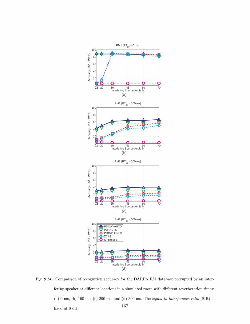
15 20 30 45 60 700

20

40

60

80

100

Acc

urac

y (1

00 −

WE

R)

Interfering Source Angle θI

RM1 (RT60

= 0 ms)

(a)

15 20 30 45 60 700

20

40

60

80

100

Acc

urac

y (1

00 −

WE

R)


RM1 (RT60

= 100 ms)

(b)

15 20 30 45 60 700

20

40

60

80

100

Acc

urac

y (1

00 −

WE

R)


RM1 (RT60

= 200 ms)

(c)

15 20 30 45 60 700

20

40

60

80

100


Acc

urac

y (1

00 −

WE

R)

RM1 (RT60

= 300 ms)


(d)


fering speaker at different locations in a simulated room with different reverberation times:

(a) 0 ms, (b) 100 ms, (c) 200 ms, and (d) 300 ms. The signal-to-interference ratio (SIR) is

fixed at 0 dB.167

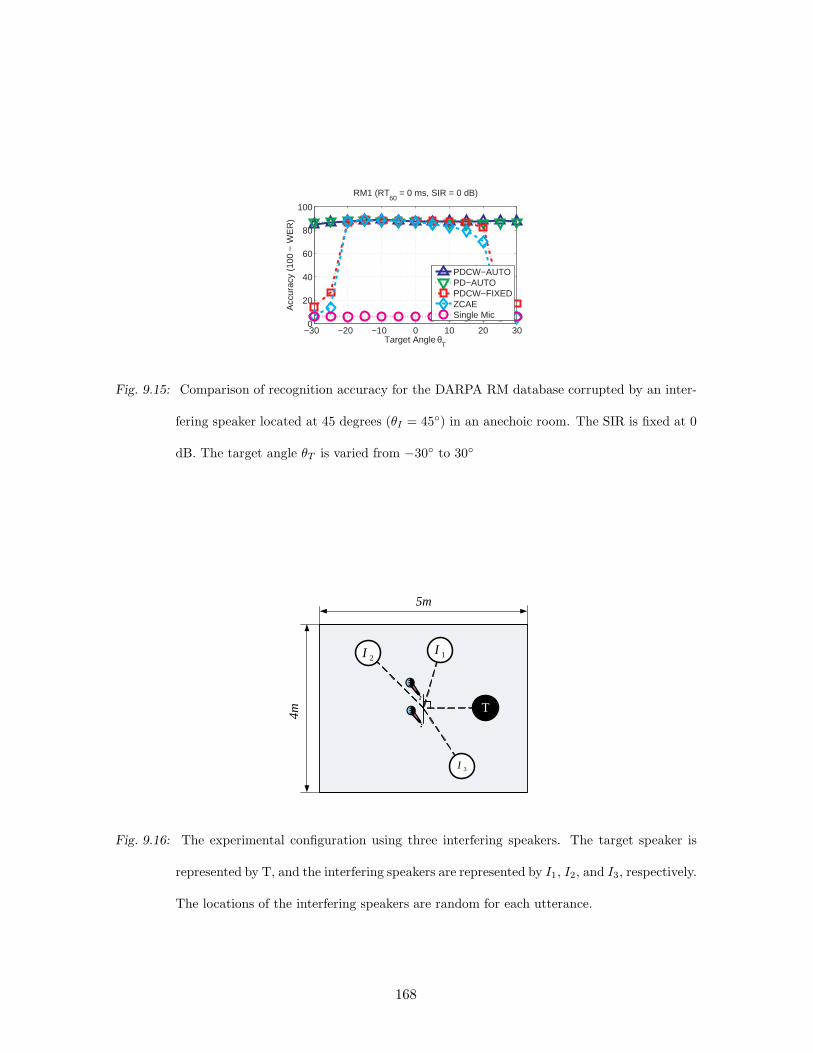
−30 −20 −10 0 10 20 300

20

40

60

80

100

Target Angle θT

Acc

urac

y (1

00 −

WE

R)

RM1 (RT60

= 0 ms, SIR = 0 dB)



fering speaker located at 45 degrees (θI = 45) in an anechoic room. The SIR is fixed at 0

dB. The target angle θT is varied from −30 to 30

T

1I2I

3I

5m

4m

Fig. 9.16: The experimental configuration using three interfering speakers. The target speaker is

represented by T, and the interfering speakers are represented by I1, I2, and I3, respectively.

The locations of the interfering speakers are random for each utterance.

168

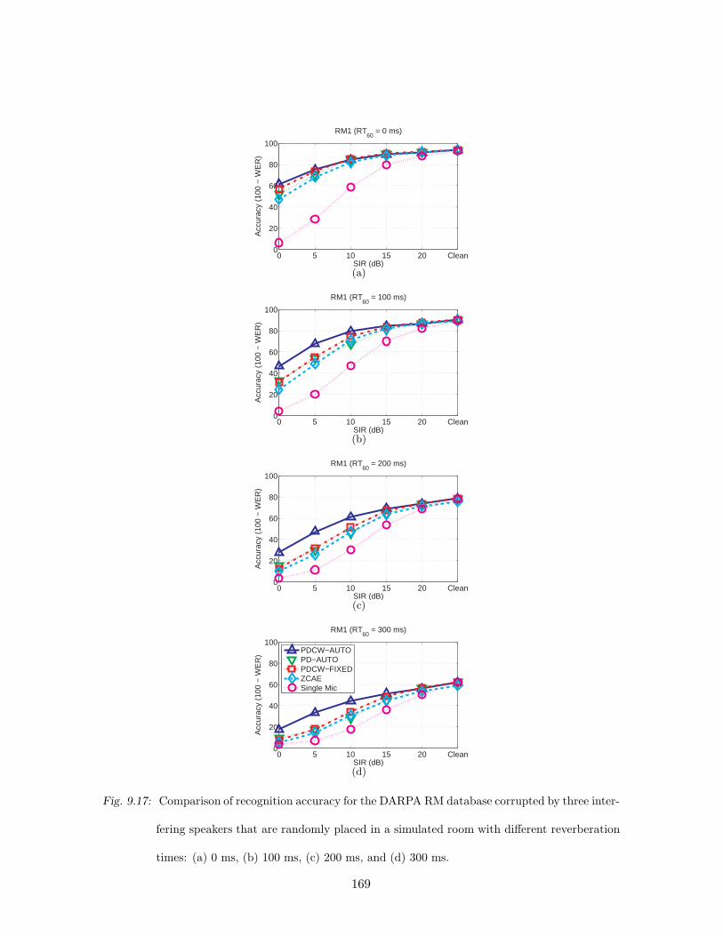
0 5 10 15 20 Clean0

20

40

60

80

100

Acc

urac

y (1

00 −

WE

R)

SIR (dB)

RM1 (RT60

= 0 ms)

(a)

0 5 10 15 20 Clean0

20

40

60

80

100

Acc

urac

y (1

00 −

WE

R)

SIR (dB)

RM1 (RT60

= 100 ms)

(b)

0 5 10 15 20 Clean0

20

40

60

80

100

Acc

urac

y (1

00 −

WE

R)

SIR (dB)

RM1 (RT60

= 200 ms)

(c)

0 5 10 15 20 Clean0

20

40

60

80

100

SIR (dB)

Acc

urac

y (1

00 −

WE

R)

RM1 (RT60

= 300 ms)


(d)

Fig. 9.17: Comparison of recognition accuracy for the DARPA RM database corrupted by three inter-

fering speakers that are randomly placed in a simulated room with different reverberation

times: (a) 0 ms, (b) 100 ms, (c) 200 ms, and (d) 300 ms.

169

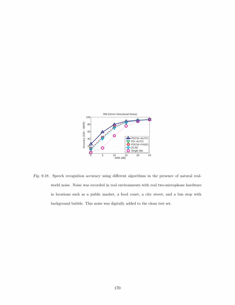
0 5 10 15 20 inf0

20

40

60

80

100

Acc

urac

y (1

00 −

WE

R)

SNR (dB)

RM (Omni−Directional Noise)


Fig. 9.18: Speech recognition accuracy using different algorithms in the presence of natural real-

world noise. Noise was recorded in real environments with real two-microphone hardware

in locations such as a public market, a food court, a city street, and a bus stop with

background babble. This noise was digitally added to the clean test set.

170

10. COMBINATION OF SPATIAL AND TEMPORAL MASKS

In this study we combine the use of a newly-developed form of single-microphone temporal

masking that has proved to be very effective in reverberant environments with a new type

of spatial masking that is both simple to implement and effective in noise. We evaluate

the effectiveness of this combination of spatial and temporal masking (STM) in a variety of

degraded acoustical environments.

10.1 Signal separation using spatial and temporal masks

10.1.1 Structure of the STM system

The structure of our sound source separation system, which crudely models some of the

processing in the peripheral auditory system and brainstem, is shown in Fig. 10.1. Signals

from the two microphones are processed by a bank of 40 modified gammatone filters [57]

with the center frequencies of the filters linearly spaced according to Equivalent Rectangular

Bandwidth (ERB) [4] between 100 Hz and 8000 Hz, using the implementation in Slaney’s

Filter Bank

Filter Bank( )Rx t

( )Lx t

ObtainSpatialMasks

ObtainTemporal

Masks

CombineChannels

ApplyCombined

Masks

, ( )R lx t

, ( )L lx t

( )ly t ( )y t

InterauralCross-

corelation

CalculateShort-term

Power)(txl

Fig. 10.1: The block diagram of the sound source separation system using spatial and temporal

masks (STM).

Auditory Toolbox [47]. As we have done previously (e.g. [19]), we convert the gammatone

filters to a zero-phase form in order to impose identical group delay on each channel. The

impulse responses of these filters hl(t) are obtained by computing the autocorrelation function

of the original filter response:

hl(t) = hg,l(t) ∗ hg,l(−t) (10.1)

where l is the channel index and hg,l(t) is the original gammatone response. While this

approach compensates for the difference in group delay from channel to channel, it also

causes the magnitude response to become squared, which results in bandwidth reduction. To

compensate for this, we intentionally double the bandwidths of the original gammatone filters

at the outset. We obtain binary spatial masks by calculating the normalized cross-correlation

coefficient and comparing its value to a pre-determined threshold value, as described in detail

in Sec. 10.1.2. Along with the spatial masks, we also generate binary temporal masks. This is

accomplished by calculating the short-time power for each time-frequency bin and comparing

this value to a short-time average value that had been obtained by IIR lowpass filtering, as

described in detail in Sec. 10.1.3. We obtain the final masks by combining these temporal

masks and spatial masks as described in Sec. 10.1.4. To resynthesize speech, we combine

the signals from each channel:

y(t) =L−1∑

l=0

yl(t) (10.2)

where L is the number of channels (40 at present), and yl(t) is the signal from in each channel

l after applying the masks. y(t) is the final output of the system.

10.1.2 Spatial mask generation using normalized cross-correlation

In this section, we describe the construction of the binary masks using normalized cross-

correlation. In our previous research (e.g. [46] [67]), which is also described in Chaps. 7 and

9 in this thesis, we have frequently observed that an analysis window that is longer than the

conventional window of about 25 ms typically used for speech recognition, is more effective

in noise-robustness algorithms. Hence, we use a window length of 50 ms with 10 ms between

analysis frames as in [66] for the present study. We define the normalized correlation ρ(t0, l)

172

θ

sin( )d θ

S

d

THθ

THθ

Fig. 10.2: Selection region for a binaural sound source separation system: if the location of the sound

source is determined to be inside the shaded region, we assume that the signal is from the

target.

for the time-frequency segment that begins at t = t0 and belongs to frequency bin l to be

ρ(t0, l) =1T0

∫

T0xR,l(t; t0)xL,l(t; t0)dt

√

1T0

∫

T0(xR,l(t; t0))2dt

√

1T0

∫

T0(xL,l(t; t0))2dt

(10.3)

where l is the channel index, xR,l(t; t0) and xL,l(t; t0) are the short-time signals from the left

and right microphones after Hamming windowing, and t0 refers to the time when each frame

begins. If xR,l(t; t0) = xL,l(t; t0), then ρ(t0, l) = 1 in Eq. (10.3). |ρ(t0, l)| is less than one

otherwise. We note that this statistic is widely used in models of binaural processing (e.g.

[87]), although typically for different reasons.

Let us consider the case where the sound source is located at an angle θ as shown in

Fig. 10.2. We assume that the desired signal is along the perpendicular bisector of the line

between the two mics. This leads to a decision criterion in which a component is accepted if

the putative location of the sound source for a particular time-frequency segment is within

the shaded region (i.e. |θ| < θTH), and rejected otherwise. If the bandwidth of a filter

is sufficiently narrow, then the signal after filtering can be approximated by the sinusoidal

function [18]:

xR,l(t; t0) = A sin(ω0t) (10.4a)

xL,l(t; t0) = A sin(ω0(t− τ)) (10.4b)

173

where ω0 is the center frequency of channel l. By inserting (10.4) into (10.3), we obtain the

following simple relation:

ρ(t0, l) = cos(ω0τ) = cos (ω0d sin(θ)) (10.5)

As long as the microphone distance is small enough to avoid spatial aliasing, Eq. (10.5)

implies that ρ(t0, l) decreases monotonically as |θ| increases. Thus, we can retain a given

time-frequency bin if ρ(t0, l) ≥ ρTH and reject it if ρ(t0, l) < ρTH , where for each channel

ρTH is given by ρTH = cos (ω0d sin(θTH)).

10.1.3 Temporal mask generation using modified SSF processing

Our temporal masking generation approach is based on a modification of the SSF approach

introduced in [55] and elaborated in Chap. 7 of this thesis. First, we obtain the short-time

power for each time-frequency bin:

Pl[m] =

∫ T0+Tf

T0

(xl(t; t0))2 dt (10.6)

where x(t; t0) is the short-time average of xL,l(t; t0) and xR,l(t; t0), which are the Hamming-

windowed signals at time t0 in Channel l from the two microphones. The index of the frame

that begins at t = t0 is m, and Tf is the window length. As in [55], we obtain a first-order

IIR lowpassed output:

Ql[m] = λQl[m− 1] + (1− λ)Pl[m] (10.7)

where λ is the forgetting factor which determines the bandwidth of the filter. Based on a

pilot study in [55], we use the value λ = 0.04. If the power in a specific time-frequency bin

is less than the lowpassed output developed in Eq. (10.7), we assume that it is masked by

temporal masking, so we accept a time-frequency segment if Pl[m] ≥ Ql[m] and reject it if

Pl[m] < Ql[m].

10.1.4 Application of spatial and temporal masks

If a specific time-frequency bin is accepted by both the spatial and temporal masking pro-

cesses described Secs. 10.1.2 and 10.1.3, then this time-frequency bin is selected; otherwise

174

it is rejected. Binary masking is applied according to the following equation:

yl(t, t0) = xl(t, t0) if selected

yl(t, t0) = µxl(t, t0) if rejected

(10.8)

where µ is a scaling factor that suppresses (but does not annihilate) the signal in the rejected

time-frequency bin. The signal yl(t, t0) is the short-time signal in each time-freqeuency bin

after applying the mask, and xl(t, t0) is the average of the left and right short-time signals

starting at time t0 in the lth channel.

In previous work (e.g. [35]) and in Chaps. 4 and 5 of this thesis we have observed

that power flooring (i.e. the imposition of a minimum power) is very important for robust

speech recognition. In this study as in others the choice of the power flooring coefficient µ is

important to prevent power from approaching zero too closely. In pilot work we have found

the following scaling factor to be useful:

µ =

√

√

√

√

√

δ(

1T

∫ T0 x2l (t)dt

)

1Tf

∫ Tf

0 x2l (t; t0)dt(10.9)

In the above equation, xl(t) is the average of the left and right signals for this lth channel

for this utterance, T is the length of the entire utterance, and Tf is the frame length (which

is 50 ms in our implementation). The above equation means that the input power of time-

frequency bins that are rejected is reduced to δ times the average power(

1T

∫ T0 x2l (t)dt

)

in

this channel. We have found that δ = 0.01 is a suitable coefficient.

10.2 Experimental results and Conclusions

In this section we present experimental results using the STM algorithm described in this

paper. We assume a room of dimensions 5 x 4 x 3 m, with two microphones located at the

center of the room. The distance between two microphones is 4 cm. The target is located

1.5 m away from the microphones along the perpendicular bisector of the line connecting

two microphones, and an interfering speaker is located at 30 degrees to one side and 1.5

m away from the microphones. The target and interfering signals are digitally added af-

ter simulating reverberation effects using the RIR software package. We used sphinx fe

175

included in sphinxbase 0.4.1 for speech feature extraction, SphinxTrain 1.0 for speech

recognition training, and Sphinx3.8 for decoding, all of which are readily available in Open

Source form. We used a subset of 1600 utterances from the DARPA Resource Management

(RM1) training data for acoustic modeling and a subset of 600 utterances from the RM test

data for evaluation.

Figure 10.3 describes the contributions of spatial masking and temporal masking in the

environments considered. We note that while temporal masking scheme must be applied

both to training and test data to avoid increased WER due to environmental mismatch,

the system performance is essential the same regardless of whether spatial masking is used

in training or no. This is not surprising, as spatial masking should routinely accept all

components of clean speech from the target location.

In the anechoic environment (Fig. 10.3(a)), we observe that improvement with the STM

algorithm is mostly provided by spatial masking, with temporal masking providing only

marginal improvement. If T60 is increased to 200 ms (Fig. 10.3(b)), or 500 ms (Fig. 10.3(c)),

however, we observe that the contribution of temporal masking becomes quite substantial.

When both noise and reverberation are present, the contributions of temporal and spatial

maskings are complementary and synergistic.

Figure 10.4 compares speech recognition accuracy for several algorithms including the

STM system described in this paper, PDCW [46], and ZCAE in [18], all using binary masking.

To compare the performance of these different systems in the same condition, we used a

threshold angle of 15 degrees with all algorithms to obtain binary masks. In the anechoic

condition (Fig. 10.4(a)), the STM approach provided slightly worse performance than the

PDCW and ZCAE algorithms. In reverberant environments , the STM system provides

the best results by a very large margin, and the PDCW results were slightly better than

the corresponding ZCAE results. In terms of computational cost, PDCW requires the least

amount of computation due to its efficient frequency-domain implementation, while STM

and ZCAE require much more computation because they involve time-domain filtering.

The MATLAB code for the STM algorithm can be found at http://www.cs.cmu.edu/

~robust/archive/algorithms/SMT_ICASSP2011/.

176

http://www.cs.cmu.edu/~robust/archive/algorithms/SMT_ICASSP2011/

http://www.cs.cmu.edu/~robust/archive/algorithms/SMT_ICASSP2011/

0 5 10 15 20 inf0

20

40

60

80

100

Acc

urac

y (1

00 −

WE

R)

SNR (dB)

RM1 (RT60

= 0 ms)

(a)

0 5 10 15 20 inf0

20

40

60

80

100

Acc

urac

y (1

00 −

WE

R)

SNR (dB)

RM1 (RT60

= 200 ms)

(b)

0 5 10 15 20 inf0

20

40

60

80

100

Acc

urac

y (1

00 −

WE

R)

SNR (dB)

RM1 (RT60

= 500 ms)

Spatial and Temporal MaskingSpatial MaskingTemporal MaskingSingle Mic

(c)

Fig. 10.3: Dependence of recognition accuracy on the type of mask used (spatial vs temporal) for

speech from the DARPA RM corpus corrupted by an interfering speaker located at 30

degrees, using various simulated reverberation times: (a) 0 ms (b) 200 ms (c) 500 ms.

177

0 5 10 15 20 inf0

20

40

60

80

100

Acc

urac

y (1

00 −

WE

R)

SNR (dB)

RM1 (RT60

= 0 ms)

(a)

0 5 10 15 20 inf0

20

40

60

80

100

Acc

urac

y (1

00 −

WE

R)

SNR (dB)

RM1 (RT60

= 200 ms)

(b)

0 5 10 15 20 inf0

20

40

60

80

100

Acc

urac

y (1

00 −

WE

R)

SNR (dB)

RM1 (RT60

= 500 ms)

STMPDCWZCAESingle Mic

(c)

Fig. 10.4: Comparison of recognition accuracy using the STM, PDCW, and ZCAE algorithms for

the DARPA RM database corrupted by an interfering speaker located at 30 degrees, using

various simulated reverberation times: (a) 0 ms (b) 200 ms (c) 500 ms.

178

11. SUMMARY AND CONCLUSIONS

11.1 Introduction

In this thesis we have sought to improve speech recognition accuracy in noisy environment us-

ing techniques motivated by auditory processing. Our goal in this thesis has been to enhance

robustness, especially in more difficult environments such as the presence of non-stationary

noise, reverberation, or interfering speakers using techniques motivated by auditory process-

ing.

After the introduction of Hidden Markov Models (HMMs), speech recognition accuracy

has significantly improved. However, if the test environment is different from the training en-

vironment, then speech recognition accuracy is seriously degraded. Conventional approaches

for enhancing robustness against environmental mismatch are usually based on statistical

feature normalization. For example, it is usually assumed that the mean of each element of

features is the same for all utterances. One can also make a similar assumption for variance

as well as mean. Cepstral Mean Normalization (CMN) and Mean Variance Normalization

(MVN) are based on these assumptions. Alternatively, one can assume that the histogram

is the same for all utterances. As mentioned in Chapter 2, these techniques are somewhat

sensitive to the lengths of silences that precede and follow each utterance, but if they are

combined with a reliable Voice Activity Detector (VAD), they usually proivide significant

performance improvement, especially for stationary noise. Another type of approaches is

based on the development of a statistical model (usually represented by a Gaussian Mixture

Model, GMM) of log spectra or features obtained from a clean training set. The effects

of noise and/or reverberation can be represented analytically by a nonlinear environmental

function. Using the statistical model obtained from training data, the environmental func-

tion is developed and then applied in inverse fashion to eliminate the effects of noise. These

kinds of approaches are typically successful for stationary noise, but they do not provide

substantial improvements in non-stationary noise or reverberation.

In this thesis we first attempt to understand why the human auditory system demon-

strates such a remarkable ability to understand speech, even in non-stationary noise or under

reverberation. We then apply our insights toward the development of signal processing that

improves speech recognition accuracy. We focus especially on the characteristics of nonlin-

earity, temporal masking, temporal resolution, and modulation filtering that are observed in

peripheral auditory processing, as well as the sound separation based on timing differences to

multiple sensors (or ears) and the precedence effect, both of which are essential components

of binaural hearing.

11.2 Summary of Findings and Contributions of This Thesis

We found that there are a number of auditory phenomena which have not been exploited

at all or which have been inefficiently exploited in conventional feature extraction and/or

noise compensation algorithms. Some examples include the rate-intensity nonlinearity, on-

set enhancement, and temporal masking. Our conclusion is that if we make use of a more

faithful model of human auditory processing, we can obtain improvements under unmatched

conditions (when the system is trained on clean speech and deployed in a degraded environ-

ment). Unfortunately, detailed modeling of the human auditory system is prohibitive, since

the models are too complicated and impractical for real-time applications. Thus, in our

work, we have attempted to make develop simple mathematical models that are motivated

by human auditory processing. Our objective is building simple models which can be useful

for real applications, so we also put emphasis on online processing and computational cost

as well. Our contributions are summarized in this Section.

First, we observe that the logarithmic nonlinearity employed in baseline MFCC processing

is not very robust in the presence of additive noise. The reason is that the logarithmic

nonlinearity does not include an auditory threshold as discussed in Chapter 4. If the short-

time power in a particular time-frequency bin is below the auditory threshold level for human

listeners, the signal effectively should be considered to represent a silence segment, regardless

of the actual power level. In contrast with a logarithmic nonlinearity, small power differences

180

in the inaudible range (power below the threshold level) can greatly affect the feature values.

This is especially true in situations in which the power in a certain time-frequency bin

approaches zero, as the logarithmic output approaches negative infinity. For these small-

power regions, even very small changes in the input power level will produce very large

changes in the output of the nonlinearity, which results in vulnerability to additive noise.

While the human auditory nonlinearity does not have this problem because it includes a

threshold, the rate-intensity function is highly nonlinear and not so suitable for automatic

speech recognition applications. Because of this we adopted a simplified nonlinearity that is

based on the power function. From an MMSE approximation to the human rate-intensity

curve, we obtained a power-function exponent between 1/10 and 1/15. As shown in experi-

mental results in Chapter 4, this range also shows good balance in terms of trade offs between

performance in clean speech and robustness in noise. In our proposed feature extraction pro-

cedure known as Power Normalized Cepstral Coefficients (PNCC), we use an exponent of

1/15. As shown in Chapter 8, PNCC processing provides recognition accuracy that is as

good as or better than that obtained with MFCC processing in clean speech, while obtaining

much better speech recognition accuracy than MFCC processing in noisy environments.

Small Power Boosting (SPB), discussed in Chapter 5, is another approach based on

this observation. As mentioned above, for these small power regions, even for a very small

change in the input power level, there is a very big change in the output of the nonlinearity.

Because this is the case, we can enhance robustness by systematically removing all small-

power regions. The SPB approach results in a slight degradation of speech recognition

accuracy for clean speech, but it provides superior performance especially in the case of

background music.

We discuss in Chapter 6 the PPDN algorithm, which reconstructs degraded speech sig-

nals based on an equalization of the probability distribution that characterizes the power

coefficients.

In addition, we also observe that in Chapter 7 onset enhancement plays an important

role in enhancing robustness especially in reverberant environments. Neurophysiological

measurements of the response of individual auditory-nerve fibers in mammals indicate that

the onset rate is much greater than the sustained rate, and it does not exhibit saturation.

In reverberant environments the effects of reverberation generally have more impact on the

181

trailing portion than the onset portion of the response to sound. Thus, we understand

that emphasizing the onset and suppressing the trailing portion is helpful in reverberant

environments, and this is the concept that is the basis for the SSF algorithm.

While temporal masking is in some sense similar to onset enhancement, they are not

exactly the same. In case of onset enhancement we provide a relative emphasis to the onset

portions (or a relative de-emphasis to the trailing portions). Temporal masking, in contrast,

refers to the diminished perception of smaller peaks of short-time power after a sufficiently

large peak in sound pressure. We also developed a simple mathematical model that captures

this phenomenon. The application of temporal masking also provided improvements of speech

recognition in reverberation and in the presence of interfering speakers.

We also observed that temporal resolution plays an important role in robust speech recog-

nition. For human listeners it is well known that we largely ignore slowly-varying spectral

components. If we try to remove such slowly-varying components, it is better to use a

longer-duration analysis window than then the shorter-duration window that has been typi-

cally been used in speech analysis. This poses a challenge in that a longer-duration window

is best for estimating the characteristics of the slowly-varying noise components, while a

shorter window is best for analyzing the speech itself, which varies more rapidly. We solved

this problem through the use of a novel two-stage window system, which was realized either

using the Medium-duration Analysis Synthesis (MAS) approach or the Medium-duration-

window Running Average (MRA) approach. This two-stage window length system has been

incorporated into many algorithms such as Power Normalized Cepstral Coefficients (PNCC),

Power-function-based Power Distribution Normalization (PPDN), Phase Difference Channel

Weighting (PDCW), etc.

As noted in the paragraph above, the human auditory systems pays less attention to

slowly-varying components. Motivated by this, researchers have developed various types of

approaches referred to as modulation spectrum analysis, based on filtering of the envelopes of

the signal that emerges from each of a bank of bandpass filters. We propose a new technique

along these lines that is based on nonlinear asymmetric filtering. The asymmetric filter has

the ability to track the lower-level envelope, which is especially useful in compensating for

slowly-varying noise components. The algorithm also uses medium-duration windows for

better temporal resolution, and applies the filtering before the nonlinearity to facilitate the

182

removal of additive noise.

All of the major fundamental insights that are developed in Chapters 3 to 6 are inte-

grated into a practical integrated feature extraction scheme called power-normalized cepstral

coefficients (PNCC) that are computationally efficient and that provide better recognition

accuracy than MFCC and PLP features, as well as several popular noise compensation al-

gorithms.

All of the approaches above are based on single-channel (or monaural) processing of

sound. It is also well known that the human auditory system makes use of differences

of timing information at low frequency to separate sound sources that arrive from different

azimuths. Motivated by binaural hearing phenomena, we developed an efficient sound source

separation algorithm called PDCW, which is described in Chapter 9. In this approach we

calculate the inter-microphone time delay (ITD) from phase difference information in the

frequency domain, and reconstruct an estimate of the target signal using only those time-

frequency segments that are believed to have ITDs that are consistent with the direction

of the target source. We make use of a smoothed frequency-weighting scheme based on the

gammatone frequency response that provides better recognition accuracy than the direct use

of binary masks for each frequency index.

An important parameter in the PDCW algorithm is the threshold ITD that is the basis

for decisions about which time-frequency components are considered to belong to the target

signal, and the optimal value of this threshold is a complex function of the locations of the

target and interfering sources, the SNR, and amount of reverberation in the environment.

We propose a novel and very successful algorithm to identify the optimal ITD threshold

blindly, by exploiting the cross correlation between the power from the target segments and

the other segments, passing both through a compressive nonlinearity. This approach, when

combined with PDCW, is called PDCW-AUTO and is discussed in detail in Chapter 9.

Finally, in Chapter 10 we discuss the advantages that can be obtained by combining

masks that are developed using temporal and spatial considerations.

183

11.3 Suggestions for Further Research

In this thesis we considered a number of aspects of human auditory processing, but still there

are other attributes that remain to be considered. For example, the only type of masking

considered was temporal masking. It is quite likely that appropriate consideration of other

types of masking such as two-tone suppression could provide additional improvements in

recognition accuracy.

In PDCW algorithm we calculated the ITD in the frequency domain for reasons motivated

by computational efficiency. This approach should be compared with the estimation of ITDs

using a correlation-based approach, which is closer to actual human binaural processing.

Finally, our work has all been based on the use of a fixed rate-level nonlinearity. It

may well be the case that a time-varying nonlinearity could provide superior performance.

In addition, it may be worthwhile to consider the incorporation of a time-varying filter

bandwidth (such as the one used in the auditory-nerve model of Zhang and Carney).

184

BIBLIOGRAPHY

[1] M. G. Heinz, X. Zhang, I. C. Bruce, and L. H. Carney, “Auditory-nerve model for predictingperformance limits of normal and impaired listeners,” Acoustics Research Letters Online, vol. 2,no. 3, pp. 91–96, July 2001.

[2] H. G. Hirsch, P. Meyer , and H. W. Ruehl, “Improved speech recognition using high-pass filteringof subband envelopes,” in EUROSPEECH ’91, Sept. 1991, pp. 413–416.

[3] H. Hermansky and N. Morgan, “RASTA processing of speech,” IEEE. Trans. Speech AudioProcess., vol. 2, no. 4, pp. 578–589, Oct. 1994.

[4] B. C. J. Moore and B. R. Glasberg, “A revision of Zwicker’s loudness model,” Acustica - ActaAcustica, vol. 82, pp. 335–345, 1996.

[5] B. Atal, “Effectiveness of linear prediction characteristics of the speech wave for automaticspeaker identification and verification,” Journal of the Acoustical Society of America, vol. 55,pp. 1304–1312, 1974.

[6] X. Huang, A. Acero, H-W Won, Spoken Language Processing: A Guide to Theory, Algorithm,and System Development. Upper Saddle River, NJ: Prentice Hall, 2001.

[7] P. Pujol, D. Macho, and C. Nadeu, “On real-time mean-and-variance normalization of speechrecognition features,” in IEEE Int. Conf. Acoust., Speech and Signal Processing, vol. 1, May2006, pp. 773–776.

[8] Y. Obuchi,N. Hataoka, and R. M. Stern, “Normalization of time-derivative parameters for robustspeech recognition in small devices,” IEICE Transactions on Information and Systems, vol. 87-D,no. 4, pp. 1004–1011, Apr. 2004.

[9] A. Acero and R. M. Stern, “Environmental Robustness in Automatic Speech Recognition,” inProc. IEEE Int. Conf. Acoust., Speech, Signal Processing (Albuquerque, NM), vol. 2, Apr. 1990,pp. 849–852.

[10] P. J. Moreno, B. Raj, and R. M. Stern, “A vector Taylor series approach for environment-independent speech recognition,” in IEEE Int. Conf. Acoust., Speech and Signal Processing,May. 1996, pp. 733–736.

[11] S. F. Boll, “Suppression of acoustic noise in speech using spectral subtraction,” IEEE Trans.Acoust., Speech and Signal Processing, vol. 27, no. 2, pp. 113–120, Apr. 1979.

[12] R. Singh, R. M. Stern, and B. Raj, “Signal and feature compensation methods for robust speechrecognition,” in Noise Reduction in Speech Applications, G. M. Davis, Ed. CRC Press, 2002,pp. 219–244.

[13] R. Singh, B. Raj, and R. M. Stern, “Model compensation and matched condition methods forrobust speech recognition,” in Noise Reduction in Speech Applications, G. M. Davis, Ed. CRCPress, 2002, pp. 245–275.

[14] B. Raj, V. N. Parikh, and R. M. Stern, “The effects of background music on speech recognitionaccuracy,” in IEEE Int. Conf. Acoust., Speech and Signal Processing, vol. 2, Apr. 1997, pp.851–854.

[15] C. Kim, Y.-H. Chiu, and R. M. Stern, “Physiologically-motivated synchrony-based processingfor robust automatic speech recognition,” in INTERSPEECH-2006, Sept. 2006, pp. 1975–1978.

[16] B. Raj and R. M. Stern, “Missing-Feature Methods for Robust Automatic Speech Recognition,”IEEE Signal Processing Magazine, vol. 22, no. 5, pp. 101–116, Sept. 2005.

[17] S. Srinivasan, M. Roman, and D. Wang, “Binary and ratio time-frequency masks for robustspeech recognition,” Speech Comm., vol. 48, pp. 1486–1501, 2006.

[18] H. Park, and R. M. Stern, “Spatial separation of speech signals using amplitude estimation basedon interaural comparisons of zero crossings,” Speech Communication, vol. 51, no. 1, pp. 15–25,Jan. 2009.

[19] R. M. Stern, E. Gouvea, C. Kim, K. Kumar, and H .Park, “Binaural and multiple-microphonesignal processing motivated by auditory perception,” in Hands-Free Speech Communication andMicrophone Arrys, 2008, May. 2008, pp. 98–103.

[20] R. M. Stern and C. Trahiotis, “Models of binaural interaction,” in Hearing, B. C. J. Moore, Ed.Academic Press, 2002, pp. 347–386.

[21] H. S. Colburn and A. Kulkarni, “Models of sound localization,” in Sound Source Localization,A. N. Popper and R. R. Fay, Eds. Springer-Verlag, 2005, pp. 272–316.

[22] S. B. Davis and P. Mermelstein, “Comparison of parametric representations for monosyllabicword recognition in continuously spoken sentences,” IEEE Trans. Acoust., Speech, and SignalProcessing, vol. 28, no. 4, pp. 357–366, Aug. 1980.

[23] J. Volkmann, S. S. Stevens, and E. B. Newman, “A scale for the measurement of the psychologicalmagnitude pitch (A),” J. Acoust. Soc. Am., vol. 8, no. 3, pp. 208–208, Jan 1937.

[24] E. Zwicker, “Subdivision of the audible frequency range into critical bands,” J. Acoust. Soc.Am., vol. 33, no. 2, pp. 248–248, Feb 1961.

[25] H. Hermansky, “Perceptual linear prediction analysis of speech,” J. Acoust. Soc. Am., vol. 87,no. 4, pp. 1738–1752, Apr. 1990.

[26] A. V. Oppenheim and R. W.Scafer, with .J. R. Buck, Discrete-time Signal Processing.Englewood-Cliffs, NJ: Prentice-Hall, 1999.

[27] L. R. Rabiner and R. W. Schafer, Digital Processing of Speech Signals. Englewood-Cliffs, NJ:Prentice-Hall, 1978.

[28] S. S. Stevens, “On the psychophysical law,” Psychological Review, vol. 64, no. 3, pp. 153–181,1957.

[29] B. G. Gold and N. Morgan, Speech and Audio Signal Processing:Processing and Perception ofSpeech and Music. New York: John Wiley & Sons, Inc., 2000.

[30] D. Ellis. (2006) PLP and RASTA (and MFCC, and inversion) in MATLAB using melfcc.m andinvmelfcc.m. [Online]. Available: http://labrosa.ee.columbia.edu/matlab/rastamat/

[31] H. G. Hirsch and C. Ehrlicher, “Noise estimation techniques or robust speech recognition,” inIEEE Int. Conf. on Acoustics, Speech, and Signal Processing, May 1995, pp. 153–156.

[32] B. E. D. Kingsbury, N. Morgan, and, S. Greenberg, “Robust speech recognition using the mod-ulation spectrogram,” Speech Communication, vol. 25, no. 1–3, pp. 117–132, Aug. 1998.

[33] R. Drullman, J. M. Festen and R. Plomp, “Effect of temporal envelope smearing on speechrecognition,” J. Acoust. Soc. Am., vol. 95, no. 2, pp. 1053–1064, Feb. 1994.

[34] ——, “Effect of reducing slow temporal modulations on speech recognition,” J. Acoust. Soc.Am., vol. 95, no. 5, pp. 2670–2680, May 1994.

186

http://labrosa.ee.columbia.edu/matlab/rastamat/

[35] C. Kim and R. M. Stern, “Feature extraction for robust speech recognition based on maximizingthe sharpness of the power distribution and on power flooring,” in IEEE Int. Conf. on Acoustics,Speech, and Signal Processing, March 2010, pp. 4574–4577.

[36] ——, “Power function-based power distribution normalization algorithm for robust speech recog-nition,” in IEEE Automatic Speech Recognition and Understanding Workshop, Dec. 2009, pp.188–193.

[37] C. Kim, K. Kumar and R. M. Stern, “Robust speech recognition using small power boostingalgorithm,” in IEEE Automatic Speech Recognition and Understanding Workshop, Dec. 2009,pp. 243–248.

[38] X. Huang, A. Acero, H-W Won, Spoken Language Processing: A Guide to Theory, Algorithm,and System Development. Upper Saddle River, NJ: Prentice Hall, 2001.

[39] O. Vikki, and K. Laurila, “Cepstral domain segmental feature vector normalization for noiserobust speech recognition,” Speech Communication, vol. 25, pp. 133–147, Aug. 1998.

[40] M. C. Benitez, L. Burget, B. Chen, S. Dupont, H. Garudadri, H. Hermansky , P. Jain, S.Kajarekar, N. Morgan, S. Sivadas, “Robust asr front-end using spectral-based and discriminantfeatures: experiments on the aurora tasks,” in EUROSPEECH-2001, Sept. 2001, pp. 429–432.

[41] R. M. Stern, B. Raj, and P. J. Moreno, “Compensation for environmental degradation in au-tomatic speech recognition,” in Proc. of the ESCA Tutorial and Research Workshop on RobustSpeech Recognition for Unknown Communication Channels, Apr. 1997, pp. 33–42.

[42] B. Raj, V. N. Parikh, and R. M. Stern, “The effects of background music on speech recognitionaccuracy,” in IEEE Int. Conf. Acoust., Speech and Signal Processing, vol. 2, Apr. 1997, pp.851–854.

[43] J. W. Strutt (Lord Rayleigh), “On our perception of sound direction,” Philosophical Magazine,vol. 13, pp. 214–232, 1907.

[44] R. H. Gilkey and T. R. Anderson, Eds., Binaural and Spatial Hearing in Real and VirtualEnvironments. Psychology Press (reprint), 1997.

[45] R. M. Stern, D. Wang, and G. J. Brown, “Binaural sound localization,” in Computational Audi-tory Scene Analysis: Principles, Algorithms and Applications, D. Wang and G. J. Brown, Eds.Wiley-IEEE Press, 2006.

[46] C. Kim, K. Kumar, B. Raj, and R. M. Stern, “Signal separation for robust speech recognitionbased on phase difference information obtained in the frequency domain,” in INTERSPEECH-2009, Sept. 2009, pp. 2495–2498.

[47] M. Slaney, “Auditory toolbox version 2,” Interval Research Corporation Technical Report,no. 10, 1998. [Online]. Available: http://cobweb.ecn.purdue.edu/∼malcolm/interval/1998-010/

[48] D. M. Green, An Introduction to Hearing, 6th edition. Hillsdale, NJ: Lawrence Erlbaum Asso-ciates, Inc., Publishers, 1976.

[49] B. G. Gold and N. Morgan, Speech and Audio Signal Processing:Processing and Perception ofSpeech and Music. New York: John Wiley & Sons, Inc., 2000.

[50] X. Zhang and M. G. Heinz and I. C. Bruce and L. H. Carney, “A phenomenological model forthe responses of auditory-nerve fibers: I. Nonlinear tuning with compression and suppression,”J. Acoust. Soc. Am., vol. 109, no. 2, pp. 648–670, Feb 2001.

[51] H. Hermansky, “Perceptual linear prediction analysis of speech,” J. Acoust. Soc. Am., vol. 87,no. 4, pp. 1738–1752, Apr. 1990.

187

http://cobweb.ecn.purdue.edu/~malcolm/interval/1998-010/

[52] S. S. Stevens, “On the psychophysical law,” Psychological Review, vol. 64, no. 3, pp. 153–181,1957.

[53] S. G. McGovern, “A model for room acoustics,” http://2pi.us/rir.html.

[54] B. Raj, M. L. Seltzer, and R. M. Stern, “Reconstruction of Missing Features for Robust SpeechRecognition,” Speech Communication, vol. 43, no. 4, pp. 275–296, Sept. 2004.

[55] C. Kim and R. M. Stern, “Feature extraction for robust speech recognition using a power-lawnonlinearity and power-bias subtraction,” in INTERSPEECH-2009, Sept. 2009, pp. 28–31.

[56] D. Kim, “Auditory processing of speech signals for robust speech recognition in real-world noisyenvironments,” IEEE Trans. Speech and Audio Processing, vol. 7, no. 1, pp. 55–69, Jan. 1999.

[57] P. D. Patterson, K. Robinson, J. Holdsworth, D. McKeown, C. Zhang, and M. H. Allerhand,“Complex sounds and auditory images,” in Auditory and Perception. Oxford, UK: Y. Cazals,L. Demany, and K. Horner, (Eds), Pergamon Press, 1992, pp. 429–446.

[58] P. Jain and H. Hermansky, “Improved mean and variance normalization for robust speech recog-nition,” in IEEE Int. Conf. Acoust., Speech and Signal Processing, May. 2001.

[59] Y. Obuchi,N. Hataoka, and R. M. Stern, “Normalization of time-derivative parameters for robustspeech recognition in small devices,” IEICE Transactions on Information and Systems, vol. 87-D,no. 4, pp. 1004–1011, Apr. 2004.

[60] R. Balchandran and R. Mammone, “Non-parametric estimation and correction of non-lineardistortion in speech system,” in IEEE Int. Conf. Acoust., Speech and Signal Processing, May.1998, pp. 749–752.

[61] S. Molau, M. Pitz, and H. Ney, “Histogram based normalization in the acoustic feature space,”in Proc. of Automatic Speech Recognition, Nov. 2001, pp. 21–24.

[62] S. Dharanipragada and M. Padmanabhan, “A nonlinear unsupervised adaptation technique forspeech recognition,” in Proc. Int Conf. Spoken Language Processing, Oct. 2001, pp. 556–559.

[63] C. Kim and R. M. Stern, “Robust signal-to-noise ratio estimation based on waveform amplitudedistribution analysis,” in INTERSPEECH-2008, Sept. 2008, pp. 2598–2601.

[64] C. Kim and R. M. Stern, “Power-normalized cepstral coefficients (pncc) for robust speech recog-nition,” IEEE Trans. Audio, Speech, Lang. Process., (in submission).

[65] ——, “Sound source separation algorithm using phase difference information and automatic se-lection of itd threshold (name needs to be revised),” IEEE Trans. Audio, Speech, Lang. Process.,(in submission).

[66] C. Kim and R. M. Stern, “Nonlinear enhancement of onset for robust speech recognition,” inINTERSPEECH-2010, Sept. 2010, pp. 2058–2061.

[67] J. L. C. Kim, K. Eom and R. M. Stern, “Automatic selection of thresholds for signal separationalgorithms based on interaural delay,” in INTERSPEECH-2010, Sept. 2010, pp. 729–732.

[68] C. Kim, R. M. Stern, K. Eom, and J. Lee, “Automatic Interaural Time Delay Threshold SelectionMethod for Sound Source Separation,” United States Patent (Filed), 2010.

[69] P. M. Zurek, The precedence effect. New York, NY: Springer-Verlag, 1987, ch. 4, pp. 85–105.

[70] K. D. Martin, “Echo suppression in a computational model of the precedence effect,” in IEEEASSP Workshop on Applications of Signal Processing to Audio and Acoustics, Oct. 1997.

[71] Y. Park and H. Park, “Non-stationary sound source localization based on zero crossings withthe detection of onset intervals,” IEICE Electronics Express, vol. 5, no. 24, pp. 1054–1060, 2008.

188

[72] L. R. Rabiner and B.-H. Juang, Fundamentals of Speech Recognition. Englewood Cliffs, NewJersey: PTR Prentice Hall, 1993.

[73] F. Jelinek, Statistical Methods for Speech Recognition (Language, Speech, and Communication).MIT Press, 1998.

[74] Speech Processing, Transmission and Quality Aspects (STQ); Distributed Speech Recognition;Advanced Front-end Feature Extraction Algorithm; Compression Algorithms, European Telecom-munications Standards Institute ES 202 050, Rev. 1.1.5, Jan. 2007.

[75] C. Kim, “Signal processing for robust speech recognition motivated by auditory processing,”Ph.D. dissertation, Carnegie Mellon University, Pittsburgh, PA USA, October 2010.

[76] C. Lemyre, M. Jelinek, and R. Lefebvre, “New approach to voiced onset detection in speech signaland its application for frame error concealment,” in IEEE Int. Conf. on Acoustics, Speech, andSignal Processing, May 2008, pp. 4757–4760.

[77] S. R. M. Prasanna and P. Krishnamoorthy, “Vowel onset point detection using source, spectralpeaks, and modulation spectrum energies,” IEEE Trans. Audio, Speech, and Lang. Process.,vol. 17, no. 4, pp. 556–565, May 2009.

[78] C. Kim, K. Kumar, and R. M. Stern, “Binaural sound source separation motivated by auditoryprocessing,” in IEEE Int. Conf. on Acoustics, Speech, and Signal Processing, 2011,(submitted).

[79] S. Seneff, “A joint synchrony/mean-rate model of auditory speech processing,” J. Phonetics,vol. 16, no. 1, pp. 55–76, Jan. 1988.

[80] J. Tchorz and B. Kolllmeier, “A model of auditory perception as front end for automatic speechrecognition,” J. Acoust. Soc. Am., vol. 106, no. 4, pp. 2040–2050, 1999.

[81] X. Zhang and M. G. Heinz and I. C. Bruce and L. H. Carney, “A phenomenological model forthe responses of auditory-nerve fibers: I. Nonlinear tuning with compression and suppression,”J. Acoust. Soc. Am., vol. 109, no. 2, pp. 648–670, Feb 2001.

[82] J. Allen and D. Berkley, “Image method for efficiently simulating small-room acoustics,” J.Acoust. Soc. Am., vol. 65, no. 4, pp. 943–950, April 1979.

[83] C. S. C. S. Consortium. CMU sphinx open source toolkit for speech recognition: Downloads.[Online]. Available: http://cmusphinx.sourceforge.net/wiki/download/

[84] W. Grantham, “Spatial hearing and related phenomena,” in Hearing, B. C. J. Moore, Ed. Aca-demic, 1995, pp. 297–345.

[85] P. Arabi and G. Shi, “Phase-based dual-microphone robust speech enhancement,” IEEE Tran.Systems, Man, and Cybernetics-Part B:, vol. 34, no. 4, pp. 1763–1773, Aug. 2004.

[86] D. Halupka, S. A. Rabi, P. Aarabi, and A. Sheikholeslami, “Real-time dual-microphone speechenhancement using field programmable gate arrays,” in IEEE Int. Conf. on Acoustics, Speech,and Signal Processing, March 2005, pp. v/149 – v/152.

[87] C. Trahiotis, L. Bernstein, R. M. Stern, and T. N. Buell, “Interaural correlation as the basis ofa working model of binaural processing,” in Sound Source Localization, ser. Springer Handbookof Auditory Research, R. Fay and T. Popper, Eds. Springer-Verlag, 2005, vol. 25, pp. 238–271.

[88] D. M. Green, An Introduction to Hearing, 6th edition. Hillsdale, NJ: Lawrence Erlbaum Asso-ciates, Inc., Publishers, 1976.

[89] C. Kim, Y-H. Chiu, and R. M. Stern, “A robust voice adtivity detection algorithm based on powernormalization and statistical hypothesis testing,” in IEEE Int. Conf. on Acoustics, Speech, andSignal Processing, 2011, (submitted).

189

http://cmusphinx.sourceforge.net/wiki/download/

signal processing for robust speech recognition motivated by

Documents