robust speech recognition richard stern

ROBUST SPEECH RECOGNITION

Richard SternRobust Speech Recognition Group

Carnegie Mellon University

Telephone: (412) 268-2535Fax: (412) 268-3890

[email protected]://www.cs.cmu.edu/~rms

Short Course at Universidad Carlos IIIJuly 12-15, 2005

CarnegieMellon Slide 2 CMU Robust Speech Group

Outline of discussion

Summary of the state-of-the-art in speech technology at Carnegie Mellon and elsewhere

Review of speech production and cepstral analysis

Introduction to robust speech recognition: classical techniques

Robust speech recognition using missing-feature techniques

Speech recognition using complementary feature sets

Use of multiple microphones for improved recognition accuracy

The future of robust recognition:

– Signal processing based on human auditory perception

– Computational auditory scene analysis


Speech in high noise (Navy F-18 flight line)

Speech in background music

Speech in background speech

Transient dropouts and noise

Spontaneous speech

Reverberated speech

Vocoded speech

Some of the hardest problems in speech recognition


Speech recognition accuracy degrades in noise

0

20

40

60

80

100

0 5 10 15 20 25SNR (dB)

CMN (baseline)

Complete retraining


Recognition accuracy also degrades in highly reverberant rooms

Comparison of single channel and delay-and-sum beamforming (WSJ data passed through measured impulse responses):

0

20

40

60

80

100

120

0 500 1000 1500

Reverb time (ms)

Single channel

Delay and sum


Challenges in robust recognition

“Classical” problems:

– Additive noise

– Linear filtering

“Modern” problems:

– Transient degradations

– Much lower SNR

“Difficult” problems:

– Highly spontaneous speech

– Speech masked by other speech

– Speech masked by music


Approach of Acero, Liu, Moreno, et al. …

Compensation achieved by estimating parameters of noise and filter and applying inverse operations

“Clean” speechx[m]

h[m]

n[m]

z[m]

Linear filtering

Degraded speech

Additive noise

“Classical” solutions to robust speech recognition based on a model of the environment


AVERAGED FREQUENCY RESPONSE FOR SPEECH AND NOISE

Close-talking microphone:

Desktop microphone:


Power spectra:

Effect of noise and filtering on cepstral or log spectral features:

or

where is referred to as the “environment function”

x[m] h[m]

n[m]

+ z[m]

z = x + q + log(1+ en−x−q )

PZ (ω ) = PX (ω ) H(ω) 2 + PN (ω )

z = x + q + r(x,n,q) = x + f(x,n,q)

f(x, n,q)

Representation of environmental effects in cepstral domain


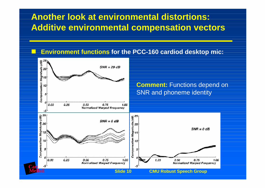
Another look at environmental distortions: Additive environmental compensation vectors

Environment functions for the PCC-160 cardiod desktop mic:

Comment: Functions depend on SNR and phoneme identity


Three types of compensation procedures

Compensation by high-pass filtering of feature vectors

Empirically-based compensation

Model-based compensation


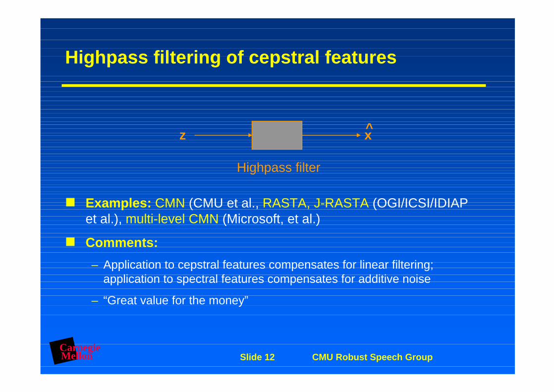
Highpass filtering of cepstral features

Examples: CMN (CMU et al., RASTA, J-RASTA (OGI/ICSI/IDIAP et al.), multi-level CMN (Microsoft, et al.)

Comments:

– Application to cepstral features compensates for linear filtering; application to spectral features compensates for additive noise

– “Great value for the money”

z x̂

Highpass filter


Two common cepstral highpass filters

CMN (Cepstral Mean Normalization):

RASTA (Relative Spectral Processing, 1994 version):

c ˆ x [m] = cz[m]− 1

Ncz[l]

l=1

N

∑

c ˆ x [m] = .1cz[m]+ .1cz[m −1]− .1cz[m − 3]− .2cz[m − 4]+ .98c ˆ x [m −1]


“Frequency response” of CMN and RASTA filters

Comment: Both RASTA and CMN have zero DC response


Principles of model-based environmental compensation

Attempt to estimate parameters characterizing unknown filter and noise that when applied in inverse fashion will maximize the likelihood of the observations

n[m]

x[m]z[m]h[m]



Estimate environment function from empirical frame-by-frame comparisons of features using “stereo” data:

Comment: indicates how frames are grouped:

– CDCN groups frames according to SNR

– MFCN groups frames according to SNR and VQ identity

x

Features fromdegraded speech

Features from“clean” speech

f(SNR, )^

z


Compensate by adding environmental correction to input:

Examples: SDCN, FCDCN, MFCDCN et al. (CMU); POF (SRI); adaptive labelling (IBM); others

Comments:

– primarily represents channel effects at low SNRs, and represents effects of noise at low SNR

– Very simple compensation method BUT requires “stereo” data


f(SNR, )^

z x^

ˆ f (SNR,θ)


Given speech in testing domain, estimate parameters of model of degradation:

Examples: CDCN, VTS (CMU), PMC (Cambridge)

Comments:

– Stereo data not needed

– Compensation can be accomplished with very little data BUT the model must be valid

Model-based compensation

n[m]^

z[m] x[m]^

h [m]^ -1


PDFs of log spectra of speech

Two one-dimensional examples:

Adding noise results in

– Increased means

– Decreased variances

– Non-Gaussian densities


Model-based compensation for noise and filtering: The VTS algorithm

The VTS algorithm (Moreno, Raj, Stern, 1996):

– Approximate f(x,n,q) by the first several terms of its Taylor series expansion, assuming that n and q are known

– The effects of f(x,n,q) on the statistics of the speech features then can be obtained analytically

– The EM algorithm is used to find the values of n and q that maximize the likelihood of the observations

– The statistics of the incoming cepstral vectors are re-estimated using MMSE techniques

z = x + q + log(1+ en−x−q ) = x + f(x, n,q)


Initial environmental compensation results

Performance on 5000-word ARPA WSJ dictation using “secondary” microphones:

Comments: Cepstral highpass filtering works, but better performance can be obtained with better modeling


“Classical” compensation improves accuracy in stationary environments

Threshold shifts by ~7 dB

Accuracy still poor for low SNRs

0

20

40

60

80

100

0 5 10 15 20 25SNR (dB)

CMN (baseline)

Complete retraining

VTS (1997)CDCN (1990)

–7 dB 13 dB Clean

Original

“Recovered”


Some general observations on classical compensation techniques

Recognition accuracy improves the most when

– Effects of noise and filtering are both modeled

– Richest possible description of the degradation is used, including the variance

– Greatest possible integration of compensation with recognition is sued

Improvement is greatest at lowest SNRs

Modification of internal statistical models is better than modification of input features

Model-based compensation is better than empirically-based compensation of model parameters are valid


The big problem: model-based compensation does not work in transient noise

Possible reasons: nonstationarity of background music and its speechlike nature

BBBBBB

J

JJ

J

JJ

0

10

20

30

40

50

0 5 10 15 20 25

Per

cen

t W

ER

Dec

.

SNR (dB)

H4 Music

White Noise


So ….. hard problems for speech recognition

Low SNRs

Transient disturbances

Co-channel speech and music

Reverberant environments

Spontaneous speech

Coded speech and telephone channels


So how do we hope to solve these problems?

Recognition using missing features

Combination of parallel information streams (incluing multiband analysis)

Microphone-array processing

Physiologically-motivated feature extraction

Processing based on auditory scene analysis

Time normalization

Modelling and recognition based on coded parameters


So what can we do about transient noises?

Two major approaches:

– Sub-band recognition (e.g. Bourlard, Morgan, Hermansky et al.)

– Missing-feature recognition (e.g. Cooke, Green, Lippmann et al.)

At CMU we’ve been working on a variant of the missing-feature approach


MULTI-BAND RECOGNITION

Basic approach:

– Decompose speech into several adjacent frequency bands

– Train separate recognizers to process each band

– Recombine information (somehow)

Comment:

– Motivated by observation of Fletcher (and Allen) that the auditory system processes speech in separate frequency bands

Some implementation decisions:

– How many bands?

– At what level to do the splits and merges?

– How to recombine and weight separate contributions?


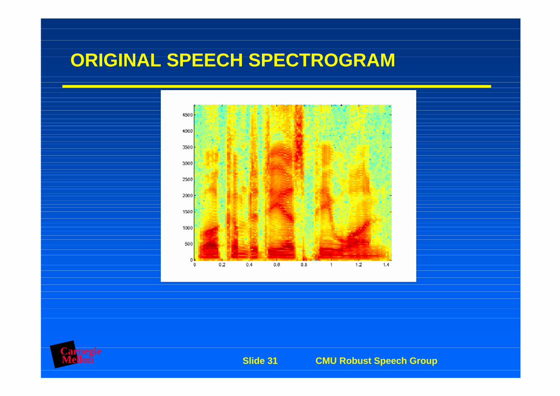
MISSING-FEATURE RECOGNITION

General approach:

– Determine which cells of a spectrogram-like display are unreliable (or “missing”)

– Ignore missing features or make best guess about their values based on data that are present


ORIGINAL SPEECH SPECTROGRAM


SPECTROGRAM CORRUPTED BY WHITE NOISE AT SNR 15 dB

Some regions are affected far more than others


IGNORING REGIONS IN THE SPECTROGRAM THAT ARE CORRUPTED BY NOISE

All regions with SNR less than 0 dB deemed missing (dark blue)

Recognition performed based on colored regions alone


F0

F1

Missing Feature Based Recognition:Simplified View


F0

F1



CURRENT MISSING DATA TECHNIQUES

Class Conditional Imputation

– Replace missing data by their class conditional estimate, [missing]class. Classify using P(Class | [present],[missing]class)

Marginalization

– Integrate out missing components. Classify using present components only as argmaxclassP(Class | [present]).


F0

F1

TECHNIQUE 1: Class Conditional Imputation


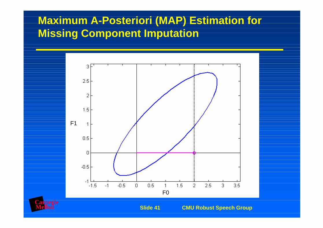
IMPUTING MISSING VALUES

MAP (Maximum A Posteriori): Find a “best guess” for F1 (in the statistical sense), given that we know F0

F1 = argmax f1 P(f1|F0)

ML (Maximum Likelihood): Find that value of F1 for which the statistical best guess of F0 would have been the observed F0

F1 = argmax f1 P(F0|f1)

MAP is simpler to visualize

– The rest of this talk assumes MAP estimation of missing points


Maximum A-Posteriori (MAP) Estimation for Missing Component Imputation

F0

F1


F0

F1

Maximum A-Posteriori (MAP) Estimation for Missing Component Imputation


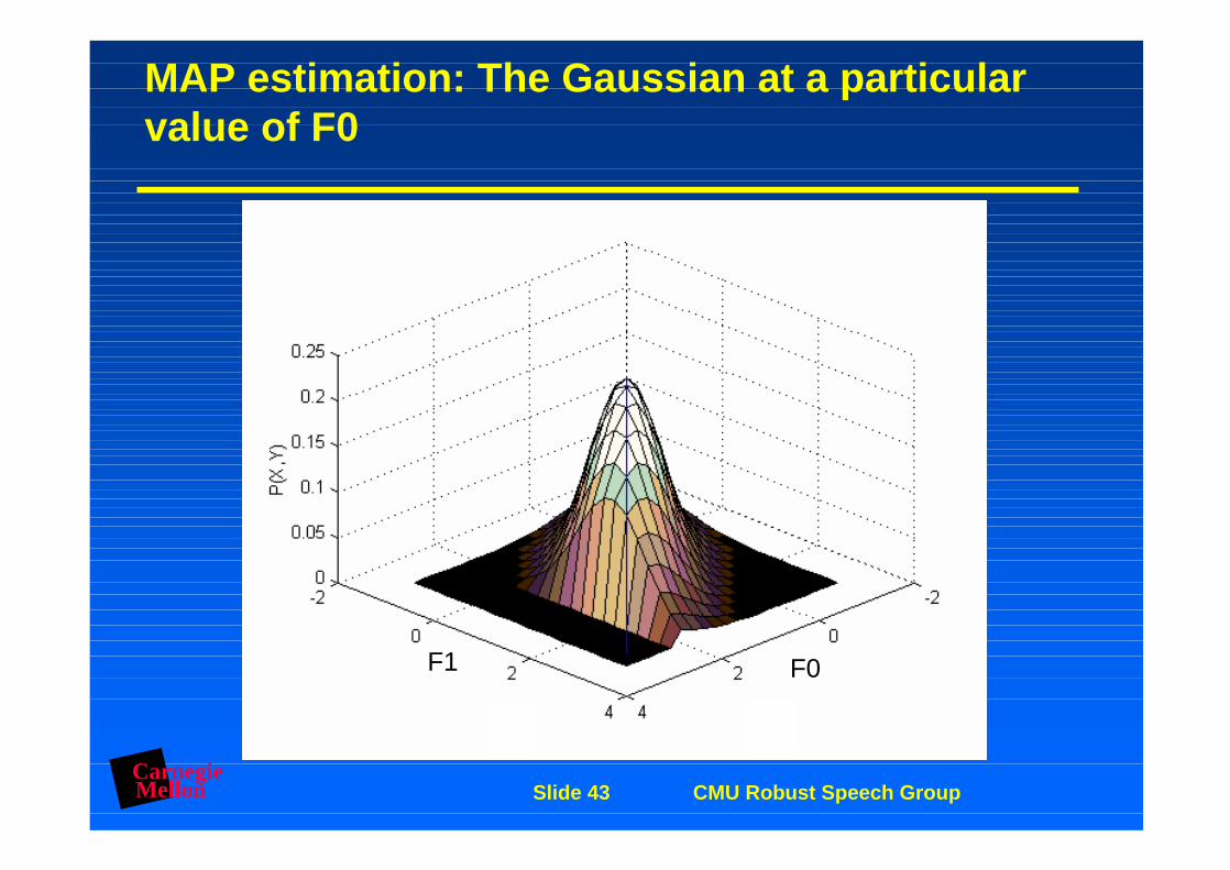
MAP estimation: Gaussian PDF

F1 F0


MAP estimation: The Gaussian at a particular value of F0

F0F1 F0


F0

F1

MAP Estimation for Missing Component Imputation F1 = argmaxf1 P(f1| F0)


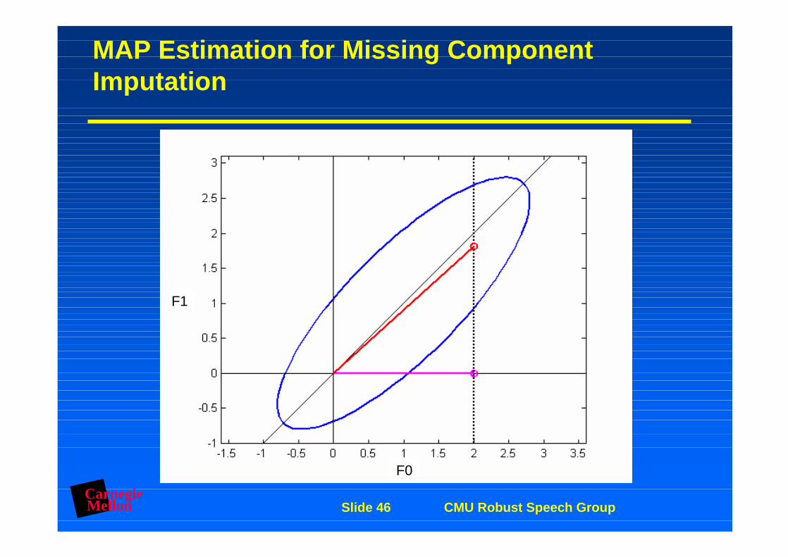
MAP Estimation for Missing Component Imputation

F0

F1

f1 = f1 + Cf1,f0Cf0,f0 (f0-f0)-1


MAP Estimation for Missing Component Imputation

F0

F1


TECHNIQUE 1: Class Conditional Imputation

F0

F1


F0

F1

Technique 2: Marginalization


F0

F1

Technique 2: Marginalization P(f0) = P(f0,f1)df1


F0

F1

Technique 2: Marginalization P(f0) = P(f0,f1)df1-


TECHNIQUE 2: Marginalization

F0


RECONSTRUCTION METHODS FOR INCOMING VECTORS

Cluster-based reconstruction

– Capture speech characteristics with a cluster based representation

Correlation-based reconstruction

– Capture speech characteristics as the correlation between element in the picture


METHOD 1: CLUSTER-BASED ESTIMATION

General procedure:

– Cluster incoming log spectra of clean speech

– Identify which cluster each incoming speech frame (with missing features) belongs to

– Use cluster statistics to obtain MAP estimates of missing data in vector given known values of data that are present


Cluster Based Estimation: Multiple Clusters


Cluster Identification using observed elementscluster = argmaxclst P(clst | F0)


Preliminary Estimation Based Cluster Identification


METHOD 2: COVARIANCE-BASED ESTIMATION

Comments:

– Uses covariances across both frequency and time

– Covariances assumed to be independent of position in picture

– In principle an attempt to reconstruct the entire picture all at once

General procedure:

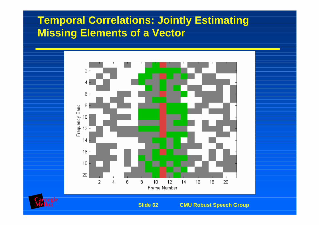
– Estimate covariances among elements of current frame and preceding and following 20 frames (200 ms) from a training corpus

– For each missing frequency component, identify neighbours with relative covariance > 0.5

– Use these neighbours to estimate values of missing features


Temporal Correlations: Estimating a Missing Point


Temporal Correlations: Estimating a Missing Element


Temporal Correlations: Jointly Estimating Missing Elements of a Vector


Recognition accuracy using compensated cepstra, speech corrupted by white noise

Large improvements in recognition accuracy can be obtained by reconstruction of corrupted regions of noisy speech spectrograms

Knowledge of locations of “missing” features needed

0 5 10 15 20 250

102030405060708090

SNR (dB)

Acc

ura

cy (

%)

Cluster Based Recon.

Temporal Correlations Spectral Subtraction

Baseline


0 5 10 15 20 250

102030405060708090

Recognition accuracy using compensatedcepstra, speech corrupted by music

Recognition accuracy goes up from 7% to 69% at 0 dB with cluster based reconstruction

SNR (dB)

Acc

ura

cy (

%)

Cluster Based Recon.

Temporal Correlations

Spectral Subtraction

Baseline


So how can we detect “missing” regions?

Current approach:

– Pitch detection to comb out harmonics in voiced segments

– Multivariate Bayesian classifiers using several features such as

» Ratio of power at harmonics relative to neighboring frequencies

» Extent of temporal synchrony to fundamental frequency

How well we’re doing now with blind identification:

– About half way between baseline results and results using perfect knowledge of which data are missing

– About 25% of possible improvement for background music


Recognition Accuracy vs. SNR

0102030405060708090

5 10 15 20 25

SNR (dB)

Oracle Masks

BayesianMasksEnergy-basedMasksBaseline

Practical recognition error: white noise (Seltzer)

Speech plus White Noise:



0102030405060708090

5 15 25

SNR (dB)

Oracle Masks

BayesianMasksEnergy-based MasksBaseline

Practical recognition error: factory noise

Speech plus Factory Noise:



0102030405060708090

5 10 15 20 25

SNR (dB)

Oracle Masks

BayesianMasksEnergy-based MasksBaseline

Practical recognition error: background music

Speech plus Music:


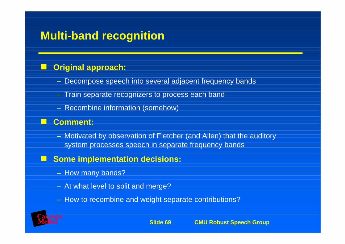
Multi-band recognition

Original approach:

– Decompose speech into several adjacent frequency bands

– Train separate recognizers to process each band

– Recombine information (somehow)

Comment:

– Motivated by observation of Fletcher (and Allen) that the auditory system processes speech in separate frequency bands

Some implementation decisions:

– How many bands?

– At what level to split and merge?

– How to recombine and weight separate contributions?


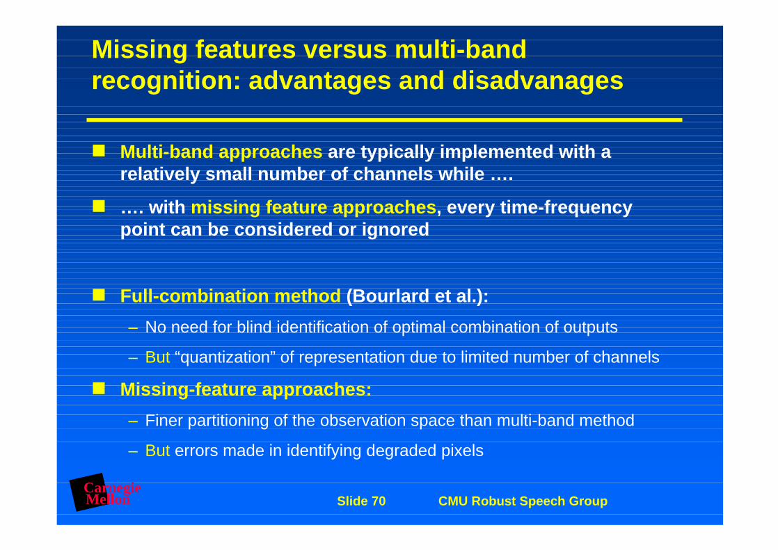
Missing features versus multi-band recognition: advantages and disadvanages

Multi-band approaches are typically implemented with a relatively small number of channels while ….

…. with missing feature approaches, every time-frequency point can be considered or ignored

Full-combination method (Bourlard et al.):

– No need for blind identification of optimal combination of outputs

– But “quantization” of representation due to limited number of channels

Missing-feature approaches:

– Finer partitioning of the observation space than multi-band method

– But errors made in identifying degraded pixels


Generalizations of multiband analysis:Information fusion

Partitions of information do need to be on a frequency-by-frequency basis

Combination of information can take place at various levels of a speech recognition system

Information fusion is presently a highly active area of research


Missing features versus multi-band recognition

Multi-band approaches are typically implemented with a relatively small number of channels while ….

…. with missing feature approaches, every time-frequency point can be considered or ignored

The full-combination method for multi-band recognition considers every possible combination of present or missing bands, eliminating the need for blind identification of optimal combination of inputs

Nevertheless, missing-feature approaches may provide superior recognition accuracy because they enable a finer partitioning of the observation space if we could solve the identification problem


Combination of information streams:Independent recognition


Combination of information streams:Feature combination


Combination of information streams:State combination


Combination of information streams:Output combination


The CMU SPINE system (Singh)

Three feature sets considered:

– Mel cepstra

– PLP cepstra

– Mel cepstra of lowpass filtered speech

Four compensation schemes:

– Codeword Dependent Codebook Normalization (CDCN)

– Vector Taylor Series (VTS)

– Singular Value Decomposition (SVD)

– Karhunen-Loeve Transform-based noise cancellation (KLT)

Additional features from ICSI/OGI:

– PLP cepstra subjected to MLP and KL transform for orthogonalization


Combination of hypotheses for SPINE eval

ConfirmedNorthwest </s><s> South0 4 16 46 76 79-1 -7 -9 -8 -4

SouthwestFire and go<s> </s>0 6 16 46 54 76 79-8 -3 -4 -5-2 -6

Likelihoods

Frame number of transition point

ConfirmedNorthwest</s>

<s> South04 16 46 76

-1 -7 -9 -8

SouthwestFire and go<s> 6 16 46 54 76

79

-8 -3 -4

-3.68

-2 -6

− = +− −3 68 5 4. log( )e e


Combination of hypotheses for SPINE eval

ConfirmedSouthwest </s><s> South0 4 16 46 76 79-1 -7 -9 -8 -4

SouthwestFire and go<s> </s>0 6 16 46 54 76 79-8 -3 -4 -5-2 -6

Likelihoods

Frame number of transition point

ConfirmedSouthwest </s>

<s> South04 16 46 76

-1 -7-7.68

-8

Fire and go<s> 6 16 46 54 76

79

-3 -4

-3.68

-2 -6

− = +− −7 68 9 8. log( )e e

CMU primary system for SPINE evaluation

Data

DecodeMFC

DecodePLP

DecodeBernoulli

WER = 35.1%

38.0

47.4

+

32.8

+26.5

AdaptMFC

AdaptPLP

AdaptBernoulli

32.9

34.7

38.7

RetrainMFC

RetrainPLP

RetrainBernoulli

30.6

31.6

35.4

AdaptMFC

AdaptPLP

AdaptBernoulli

29.9

32.1

35.0

+

30.3

+

28.4

+

27.3

AdaptPLP

AdaptMFC

AdaptBernoulli

40.1

33.3

34.8

Comments:

– Single class MLLR adaptation (all data from a single recording channel clustered together)

– Estimated score for MFCC alone is ~31-33%


Combining features improves error rates

Results from NRL SPINE 2000 task:

0

10

20

30

40

50

Wo

rd E

rro

r R

ate

(%)

Filtered MFCC PLP MFCC Combined


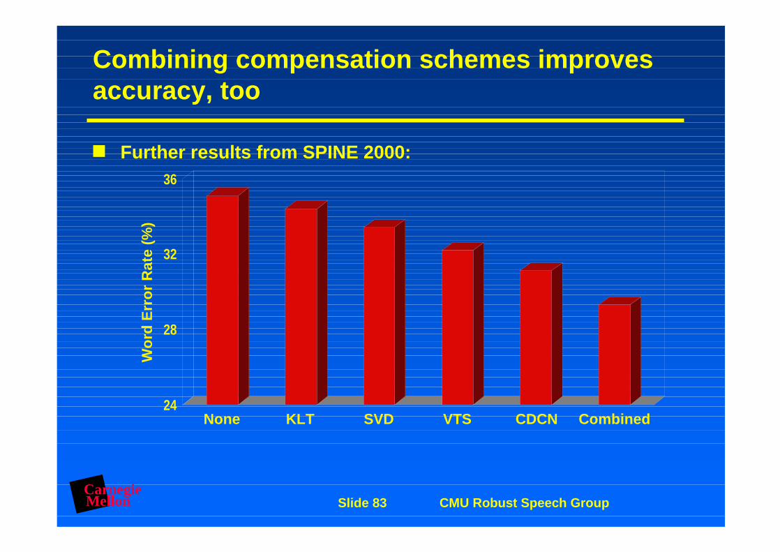
Combining compensation schemes improves accuracy, too

24

28

32

36

Wo

rd E

rro

r R

ate

(%)

None KLT SVD VTS CDCN Combined

Further results from SPINE 2000:


0

2

4

6

8

10

12

Comparison of different types of information fusion on Resource Management task (Li)

Baseline Output CombFeature Comb

NaturalFeaturesOptimizedFeatures


Two additional comments on output combination

Hypothesis combination is more powerful than the ROVER method because probability scores are used

There is a still more powerful output combination method known as lattice combination (Li et al., 2003):

– Merges lattice structures in a more complex fashion

– Provides better recognition accuracy but at greater computational cost


Combination of information streams:Feature combination


BLAH… BLAH….X(n)

Y(n) ( )nY

X

Possible dimensionality

Reduction here

Recognizer Hypothesis

Feature combination

Concatenate all features together to form a new feature vector, and perform recognition directly based on this new feature vector.


Types of common feature combination

Simple concatenation

Principal components analysis – reduces dimensionality by keeping dimensions with the most signal energy

Linear discrminative analysis (LDA) – reduces dimensionality while maintaining greatest signal separation


Example word error rates on Resource Management task

8.74 7.99 7.62 7.51

0

1

2

3

4

5

6

7

8

9

MFCC PCA LDA HLDA


Combination of information streams:State combination or probability combination


State combination or probability combination

We have found that state combination (also called probability combination) using optimal linear features is the most effective approach

Will discuss:

– Overview of state combination approach

– Development of best features through optimal linear transformation

– Development of combinations of best features through optimal linear transformation

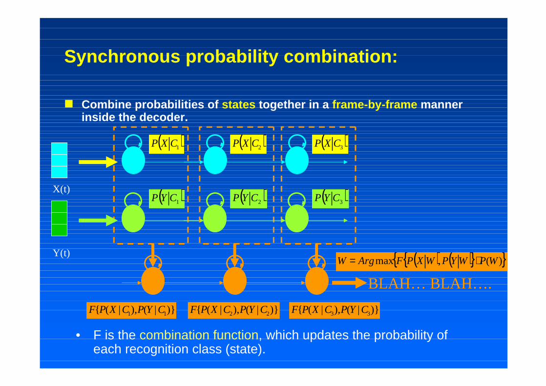
Synchronous probability combination:

Combine probabilities of states together in a frame-by-frame manner inside the decoder.

BLAH… BLAH….

( )1CXP

( )1CYP

)}|(),|({ 11 CYPCXPF

( )2CXP

( )2CYP

( )3CXP

( )3CYP

)}|(),|({ 22 CYPCXPF )}|(),|({ 33 CYPCXPF

( ) ( ){ }{ })(,max WPWYPWXPFArgW ⋅=

X(t)

Y(t)

• F is the combination function, which updates the probability of each recognition class (state).


Probability combination

Combine probabilities from multiple decoding lattices

Combination function is of critical importance

– Linear, weighted linear combination

– Non-linear combination

Probabilities can be combined at the state level (synchronous combination) or at the phoneme, syllable, or word levels (asynchronous combination)


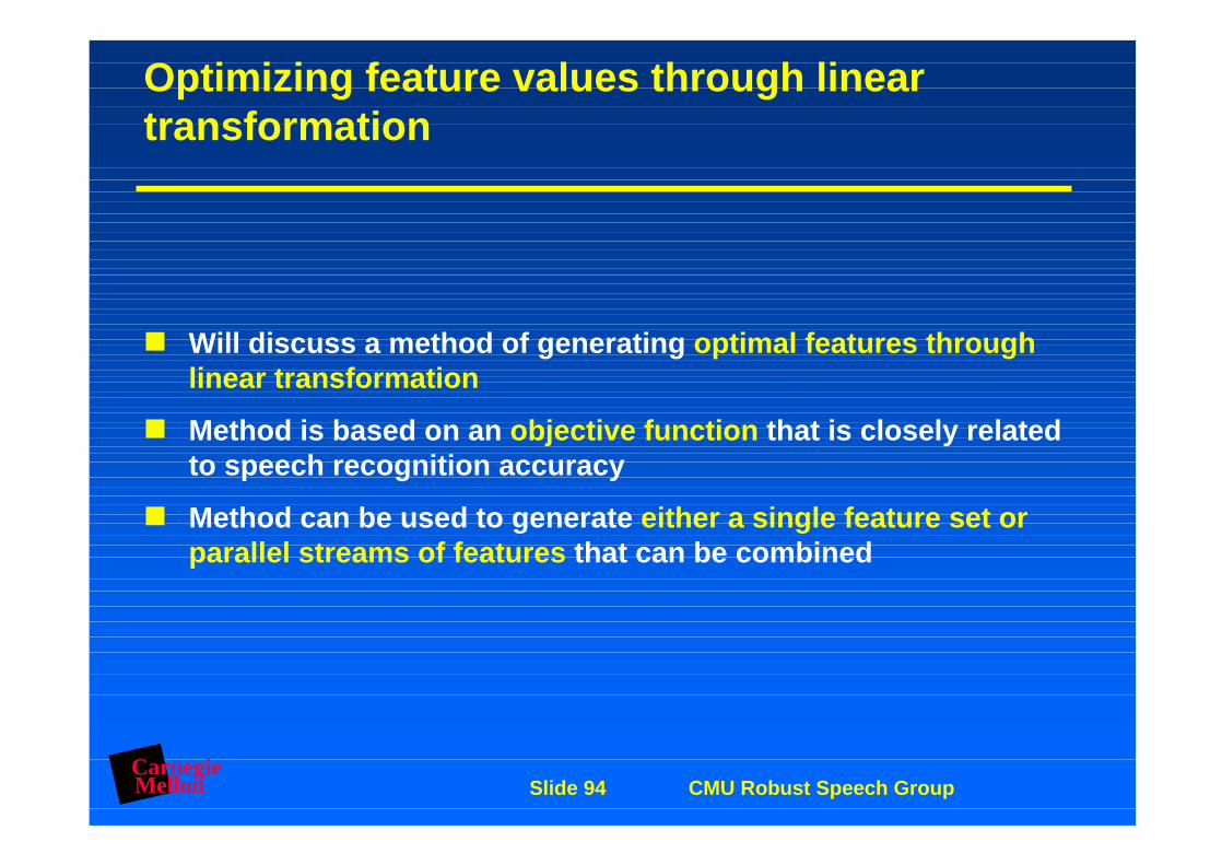
Optimizing feature values through linear transformation

Will discuss a method of generating optimal features through linear transformation

Method is based on an objective function that is closely related to speech recognition accuracy

Method can be used to generate either a single feature set or parallel streams of features that can be combined

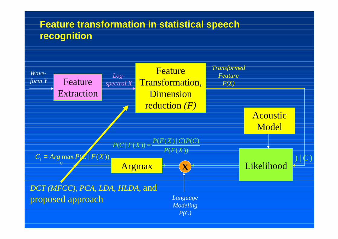
Feature transformation in statistical speech recognition

Wave-form Y Feature

Extraction

Log-spectral X

Acoustic Model

Language Modeling

P(C)

)|)(( CXFP))(|(max XFCPArgCC

t =))((

)()|)(())(|(

XFP

CPCXFPXFCP =

Argmax

Feature Transformation,

Dimension reduction (F)

Transformed Feature

F(X)

DCT (MFCC), PCA, LDA, HLDA, and proposed approach

X Likelihood


Feature transformation through linear combination

Traditionally used to reduce feature dimensions (e.g. from 40 to 13 in MFCC coefficients

Some classical examples:

– Linear transformation: DCT, PCA, LDA, HLDA, etc.

– Nonlinear transformation: PLP, MLP features, etc.

We will focus on linear feature transformation algorithms … finding a transformation matrix A that:

– Transforms feature vector X into AX.

– Feature likelihood is now P(AX|C).


Objectives in feature transformation method

The overall in speech recognition systems:

– Minimize the Word Error Rate (WER)

Objectives in conventional linear feature generation methods:

– DCT in MFCC: Find a smooth representation of the original log-spectral features

– PCA/KLT: Reduce dimensions in a way that best represents the original features in the least square sense

– LDA/HLDA: Maximally separate the data from different recognition classes in the new feature space

Can we generate a linear feature set that is based on the same objective as the speech recognizer?

We cannot directly minimize WER but we can …

– Focus on a posterior probability of true word sequence Wh :

– Consider only the acoustic modeling part (normalized likelihood term):

– Use Viterbi decoding and accumulate the normalized acoustic likelihood from each frame:

∑==

jjj

hhhhh WPWAXP

WPWAXP

AXP

WPWAXPAXWP

)()|(

)()|(

)(

)()|()|(

∑≈

jj

hh WAXP

WAXPAXWP

)|(

)|()|(

∏ ∑∏∏ ≈⋅≈i

jji

hiih

ihiihih SAXP

SAXPAXWPSAXPWSPWAXP

)|(

)|()|()|()|()|(

From WER to normalized acoustical likelihood


We generate our features based on accumulated normalized acoustic likelihood:

where Shi is the most likely state sequence corresponding to the word sequence Wh in frame i

The feature generation process is now transferred into an optimization process, whose objective function is:

or

)|(max)|(

)|(max

^

AXWPArgSAXP

SAXPArgA h

Aij

ji

hii

A≈= ∏ ∑

∏ ∑=

ij

ji

hiic SAXP

SAXPP

)|(

)|( ∑ ∑=i

jji

hiic SAXP

SAXPLogLogP

)|(

)|(

Feature based on the accumulated normalized acoustic likelihood


Goal: Find a single global feature transformation matrix A that maximizes our objective function in the transformed feature space:

How can we do that?

– Make our objective function LogPc a function of the matrix A

– Compute the derivative of LogPc with respect to matrix A

∑ ∑==i

jji

hii

Ac

A SAXP

SAXPLogArgLogPArgA

)|(

)|(maxmax

^

Generating single linear feature stream


LogPc as a function of the matrix A

Using mixtures of Gaussians as state observation probabilities …

If in the original feature space (X) we have

» Feature vector: X

» Mean: µ

» Covariance: Σ

Then in the transformed feature space (AX), we have:

» Feature vector: AX

» Mean: Aµ

» Covariance: AΣAT


Computing the derivative of LogPc with respect to the transformation matrix A

A closed-form expression of the derivative of LogPc is possible

But we don’t have a closed form solution to the value of A that sets the derivative to zero

Gradient ascent provides an iterative solution


Results on Resource Management task using optimal linear combination

8.74 7.99 7.62 7.51 6.87

0123456789

MFCC PCA LDA HLDA Our feat


WSJ0, Single feature stream, WERs (%)

8

8.5

9

9.5

10

10.5

MFCC PCA LDA HLDA Our feat10.43 9.90 9.32 9.35 9.13


Generating parallel feature streams

Goal: generate parallel global transformation matrices that maximize our objective function for the combined system in the transformed feature spaces

How can we do that?

The solution is very similar to the case of generating a singleoptimal feature stream except that:

– The likelihood term is now the combination of likelihoods from individual feature streams

– The objective function is now a function of the individual transformation matrix Ai.

Generating parallel feature streams

DataX(t)

Mean ,

Covariance

Compute LogPc, The normalized

acoustic likelihood

LogPc

Probability computation

P(A1X|S)

Probability computation

P(A2X|S)

F

Combined probabilityP(X’|S)

DerivativecA LogP1

∇

cA LogP2

∇

A2X(t)

A2 ,

A2 A2T

Transformation matrix A2

A1X(t)

A1 ,

A1 A1T

Transformation matrix A1


RM, Parallel feature streams, 4 Gaussians

0

1

2

3

4

5

6

7

8

WER (%)

LDA and PCA features Parallel featuresoptimized viamultiplication

Parallel featuresoptimized viasummation

Feat0

Feat1

Multiplicationcombination

Summationcombination


WSJ0, parallel feature streams, WERs (%)

0.00%

2.00%

4.00%

6.00%

8.00%

10.00%

12.00%

p(f1|s) p(f2|s) p(f1|s)*p(f2|s) p(f1|s)+p(f2|s)

LDA,PCA

Our parafeat(A1, A2)


Summary and conclusions

We reviewed three ways of combining features at various levels of the speech recognition process

– Hypothesis combination

– Feature combination

– State (or probability) combination

We described a new way of generating optimal features using linear transformation, using an objective that is closely related to WER

This algorithm can be applied to either single feature streams or linear combinations of features

The new features provide substantial improvement on the Resource Management database and a smaller (but still significant) improvement in the Wall Street Journal database


Global summary

“Classical” model-based robustness techniques work reasonably well in combating quasi-stationary degradations

“Modern” multiband and missing-feature techniques show great promise in coping with transient interference , etc.

Feature combination will be key component of future systems

robust speech recognition richard stern

Documents