settore concorsuale di a erenza: 01/a6 - ricerca operativa...
TRANSCRIPT

ALMA MATER STUDIORUM - UNIVERSITADI BOLOGNA
Consorzio Spinner
Dottorato di Ricerca inAutomatica e Ricerca Operativa
Settore Concorsuale di afferenza: 01/A6 - RICERCA OPERATIVA
Settore Scientifico disciplinare: Mat/09 - RICERCA OPERATIVA
Ciclo XXVII
Models and Algorithms for theOptimization of Real-World
Routing and Logistics Problems
Stefano Novellani
Coordinatore Dottorato SupervisoreProf. Daniele Vigo Prof. Manuel Iori
SupervisoreProf. Daniele Vigo
Esame finale anno 2015


Contents
Acknowledgments v
List of figures viii
List of tables x
Preface xi
I Introduction 1
1 Introduction to Routing Problems 3
1.1 The Vehicle Routing Problems . . . . . . . . . . . . . . . . . 3
1.1.1 The Network Characteristics . . . . . . . . . . . . . . 4
1.1.2 The Type of Transportation Requests . . . . . . . . . 4
1.1.3 Intra-route Constraints . . . . . . . . . . . . . . . . . 5
1.1.4 Fleet Characteristics . . . . . . . . . . . . . . . . . . . 6
1.1.5 Inter-route Constraints . . . . . . . . . . . . . . . . . . 6
1.1.6 The Objective Function . . . . . . . . . . . . . . . . . 6
1.2 Solution Methods for the VRPs . . . . . . . . . . . . . . . . . 6
1.2.1 Exact Algorithms . . . . . . . . . . . . . . . . . . . . . 7
1.2.2 Heuristic Algorithms . . . . . . . . . . . . . . . . . . . 8
1.2.3 Hybridization and Unified Methods . . . . . . . . . . . 9
1.3 Pickup and Delivery Problems . . . . . . . . . . . . . . . . . 9
1.3.1 Many-to-Many . . . . . . . . . . . . . . . . . . . . . . 9
1.3.2 One-to-Many-to-One . . . . . . . . . . . . . . . . . . . 10
1.3.3 One-to-One . . . . . . . . . . . . . . . . . . . . . . . . 10
1.4 Stochastic Vehicle Routing Problems . . . . . . . . . . . . . . 10
II Models and Algorithms for the Bike sharing Rebalanc-ing Problems 15
2 The Bike Sharing Rebalancing Problem 17
i

ii CONTENTS
2.1 Introduction . . . . . . . . . . . . . . . . . . . . . . . . . . . . 18
2.2 Data analysis of a real-world case . . . . . . . . . . . . . . . . 20
2.3 Problem description and previous work . . . . . . . . . . . . . 23
2.4 MILP formulations for the BRP . . . . . . . . . . . . . . . . . 26
2.4.1 Formulation F1 . . . . . . . . . . . . . . . . . . . . . . 26
2.4.2 Formulation F2 . . . . . . . . . . . . . . . . . . . . . . 28
2.4.3 Formulation F3 . . . . . . . . . . . . . . . . . . . . . . 28
2.4.4 Formulation F4 . . . . . . . . . . . . . . . . . . . . . . 29
2.5 Branch-and-Cut algorithm . . . . . . . . . . . . . . . . . . . . 31
2.5.1 Valid inequalities . . . . . . . . . . . . . . . . . . . . . 31
2.5.2 Separation procedures . . . . . . . . . . . . . . . . . . 33
2.6 Benchmark Instances . . . . . . . . . . . . . . . . . . . . . . . 34
2.7 Computational results . . . . . . . . . . . . . . . . . . . . . . 36
2.7.1 Randomly generated instances . . . . . . . . . . . . . 40
2.8 Conclusions . . . . . . . . . . . . . . . . . . . . . . . . . . . . 42
3 Destroy and Repair for the BRP 49
3.1 Introduction . . . . . . . . . . . . . . . . . . . . . . . . . . . . 50
3.2 Problem description . . . . . . . . . . . . . . . . . . . . . . . 51
3.2.1 Formulation for the BRP . . . . . . . . . . . . . . . . 51
3.2.2 A special case of the BRP: the 1-PDVRP . . . . . . . 53
3.2.3 Prior Work . . . . . . . . . . . . . . . . . . . . . . . . 53
3.3 Properties of feasible paths for the BRP . . . . . . . . . . . . 55
3.4 Algorithm Framework . . . . . . . . . . . . . . . . . . . . . . 60
3.4.1 Constructive algorithm . . . . . . . . . . . . . . . . . 60
3.4.2 Destroy Procedure . . . . . . . . . . . . . . . . . . . . 62
3.4.3 Repair Procedures . . . . . . . . . . . . . . . . . . . . 62
3.4.4 Local Search Procedures . . . . . . . . . . . . . . . . . 63
3.5 Adaptation to the 1-PDVRP . . . . . . . . . . . . . . . . . . 65
3.5.1 Metaheuristic algorithm for the 1-PDVRP . . . . . . . 65
3.5.2 Branch-and-Cut for the 1-PDVRP . . . . . . . . . . . 65
3.6 Computational Results . . . . . . . . . . . . . . . . . . . . . . 68
3.6.1 Small-size Instances . . . . . . . . . . . . . . . . . . . 69
3.6.2 Medium-size Instances . . . . . . . . . . . . . . . . . . 70
3.6.3 Large-size Instances . . . . . . . . . . . . . . . . . . . 71
3.6.4 Local Searches Evaluation . . . . . . . . . . . . . . . . 72
3.6.5 1-PDVRP Instances . . . . . . . . . . . . . . . . . . . 73
3.7 Conclusions . . . . . . . . . . . . . . . . . . . . . . . . . . . . 75
3.A Annex . . . . . . . . . . . . . . . . . . . . . . . . . . . . . . . 76
4 The Stochastic BRP 85
4.1 Introduction . . . . . . . . . . . . . . . . . . . . . . . . . . . . 85
4.2 Literature Review . . . . . . . . . . . . . . . . . . . . . . . . 86
4.3 Problems description . . . . . . . . . . . . . . . . . . . . . . . 87

CONTENTS iii
4.4 Formulations for the SBRP . . . . . . . . . . . . . . . . . . . 88
4.4.1 Deterministic Equivalent Program . . . . . . . . . . . 88
4.4.2 Two-stage Formulation . . . . . . . . . . . . . . . . . 90
4.4.3 Multi-cut Formulation . . . . . . . . . . . . . . . . . . 93
4.5 Formulation for the SBRPF . . . . . . . . . . . . . . . . . . . 95
4.6 Heuristic algorithm based on correlations . . . . . . . . . . . 96
4.6.1 Closest neighborhood with correlations . . . . . . . . . 97
4.6.2 Savings with correlations . . . . . . . . . . . . . . . . 98
4.7 Computational Results . . . . . . . . . . . . . . . . . . . . . . 99
4.7.1 Instances . . . . . . . . . . . . . . . . . . . . . . . . . 99
4.7.2 Results . . . . . . . . . . . . . . . . . . . . . . . . . . 100
4.8 Conclusions . . . . . . . . . . . . . . . . . . . . . . . . . . . . 104
III Models and Algorithms for Earthwork OptimizationProblems 107
5 Earthwork Optimization Models 109
5.1 Introduction . . . . . . . . . . . . . . . . . . . . . . . . . . . . 110
5.1.1 Main Contributions . . . . . . . . . . . . . . . . . . . 111
5.2 Problem Description . . . . . . . . . . . . . . . . . . . . . . . 113
5.3 Literature Review . . . . . . . . . . . . . . . . . . . . . . . . 115
5.4 Modeling Analysis and Notation . . . . . . . . . . . . . . . . 117
5.5 Aggregate Formulation . . . . . . . . . . . . . . . . . . . . . . 119
5.6 Disaggregate Models . . . . . . . . . . . . . . . . . . . . . . . 124
5.7 Computational Results . . . . . . . . . . . . . . . . . . . . . . 126
5.7.1 Realistic instances . . . . . . . . . . . . . . . . . . . . 126
5.7.2 Aggregate model results . . . . . . . . . . . . . . . . . 128
5.7.3 Disaggregate model results . . . . . . . . . . . . . . . 128
5.8 Conclusions . . . . . . . . . . . . . . . . . . . . . . . . . . . . 130
6 A DSS for Highway Construction 135
6.1 Introduction . . . . . . . . . . . . . . . . . . . . . . . . . . . . 136
6.2 The Autostrada Pedemontana LombardaProject . . . . . . . . . . . . . . . . . . . . . . . . . . . . . . 138
6.3 Strabag AG: a Leader in the construction industry . . . . . . 139
6.4 The Decision Support System . . . . . . . . . . . . . . . . . . 140
6.5 Computational Evaluation . . . . . . . . . . . . . . . . . . . . 146
6.6 Conclusions . . . . . . . . . . . . . . . . . . . . . . . . . . . . 148
6.A Mathematical Models . . . . . . . . . . . . . . . . . . . . . . 150
6.A.1 Disaggregate Formulation . . . . . . . . . . . . . . . . 154
iv CONTENTS
IV Models and Algorithms for 3D Printing Problems 159
7 Optimizing the 3D Printing Process 1617.1 Introduction . . . . . . . . . . . . . . . . . . . . . . . . . . . . 161
7.1.1 The 3DP Process . . . . . . . . . . . . . . . . . . . . . 1627.1.2 Advantages and disadvantages . . . . . . . . . . . . . 1627.1.3 Contribution of this Chapter . . . . . . . . . . . . . . 163
7.2 The Rural Postman Problems . . . . . . . . . . . . . . . . . . 1647.3 Problem Description . . . . . . . . . . . . . . . . . . . . . . . 1657.4 The 3D Printing Routing Problem . . . . . . . . . . . . . . . 1667.5 Heuristic Algorithms . . . . . . . . . . . . . . . . . . . . . . . 167
7.5.1 Closest 3DP . . . . . . . . . . . . . . . . . . . . . . . . 1687.5.2 Clustered 3DP . . . . . . . . . . . . . . . . . . . . . . 1687.5.3 Look Ahead 3DP . . . . . . . . . . . . . . . . . . . . . 1697.5.4 Shortest Path Based 3DP . . . . . . . . . . . . . . . . 169
7.6 Computational Results . . . . . . . . . . . . . . . . . . . . . . 1707.6.1 Instances . . . . . . . . . . . . . . . . . . . . . . . . . 1707.6.2 Results . . . . . . . . . . . . . . . . . . . . . . . . . . 170
7.7 Conclusions and Future Research Directions . . . . . . . . . . 177
Conclusions 185

Acknowledgments
Ringrazio le persone che hanno viaggiato al mio fianco in questa parte dipercorso. Ringrazio la famiglia, gli amici, i colleghi. In maggior parteper il sostegno, i sorrisi, le leggerezze, il filosofeggiare, la qualita dei dis-corsi. Ringrazio il mio supervisore Manuel Iori, per la disponibilita, iltempo, la pazienza. Ma soporattutto per i suggerimenti, le esortazioni, iproficui scambi d’idee, l’avermi insegnato -bene o male- a fare questo la-voro. Ringrazio Mauro Dell’Amico, Daniele Vigo, Eleni Hadjiconstantinou,Thomas Stutzle e Anand Subramanian per i consigli, le collaborazioni, leopportunita, tutte innumerevoli.
v

vi CONTENTS

List of Figures
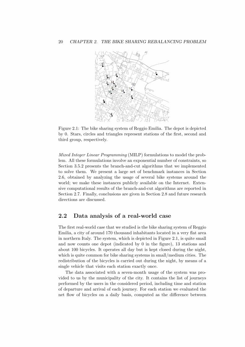
2.1 The bike sharing system of Reggio Emilia. The depot is de-picted by 0. Stars, circles and triangles represent stations ofthe first, second and third group, respectively. . . . . . . . . . 20
2.2 Net flow of bicycles per day, following (a) a normal-like distri-bution in station 4 and (b) a bimodal distribution in station5 (∆ = difference between arrivals and departures, Φ = fre-quence of occurrence). . . . . . . . . . . . . . . . . . . . . . 21
2.3 Typical arrivals and departures per hour in a station of (a)the first group, (b) the second group and (c) the third group(τ = hour of the day, ν = cumulative number of bikes arrivinginto or departing from a station within a seven-months period). 43
2.4 Optimal solutions for Reggio Emilia with (a)Q=10, (b)Q=20,and (c) Q=30. . . . . . . . . . . . . . . . . . . . . . . . . . . 44
4.1 Picture of the parameters of a station. . . . . . . . . . . . . 90
5.1 Activities flow chart. . . . . . . . . . . . . . . . . . . . . . . . 113
5.2 Network representation. . . . . . . . . . . . . . . . . . . . . . 117
5.3 The New Via Emilia layout: on the left the overall construc-tion site planned is depicted, while a highlight is given on theright. . . . . . . . . . . . . . . . . . . . . . . . . . . . . . . . . 127
5.4 Solution time of the disaggregate models with respect to thenumber of arcs. . . . . . . . . . . . . . . . . . . . . . . . . . . 129
6.1 Flow chart representing the main activities involved in theproject. . . . . . . . . . . . . . . . . . . . . . . . . . . . . . . 136
6.2 The Autostrada Pedemontana Lombarda project in NorthernItaly. . . . . . . . . . . . . . . . . . . . . . . . . . . . . . . . . 138
6.3 The characteristics of the main highway. . . . . . . . . . . . . 139
6.4 Operation Diagram of the developed Decision Support System.140
6.5 Network visualization of the basic instance , the highway sec-tion used for computational tests. . . . . . . . . . . . . . . . . 143
6.6 Flows in temporary depot TD2 during the construction timehorizon. . . . . . . . . . . . . . . . . . . . . . . . . . . . . . . 144
vii

viii LIST OF FIGURES
6.7 Graphical representations of the use of material during theconstruction time horizon. . . . . . . . . . . . . . . . . . . . . 144
6.8 Graphical representation of digging and filling activities in avertex. . . . . . . . . . . . . . . . . . . . . . . . . . . . . . . . 145
6.9 Graphical output of the disaggregate model. . . . . . . . . . . 146
7.1 Scheme of the 3DP process. . . . . . . . . . . . . . . . . . . 1627.2 An example of polygon with outer, inner, and filling parts. . . 168

List of Tables
2.1 BRP notation summary. . . . . . . . . . . . . . . . . . . . . . 24
2.2 Benchmark instances (notation explained in Table 2.1). . . . 35
2.3 Implementation of formulations F1−F4. . . . . . . . . . . . . 36
2.4 Computational results for formulations F1−F4 on all probleminstances. . . . . . . . . . . . . . . . . . . . . . . . . . . . . . 38
2.5 Root node – Comparison of various separation procedures onthe core formulation F3. . . . . . . . . . . . . . . . . . . . . . 39
2.6 Root node – Comparison of various separation procedures onthe full formulation F3. . . . . . . . . . . . . . . . . . . . . . 40
2.7 Tests on randomly generated instances . . . . . . . . . . . . . 41
3.1 New BRP instances. . . . . . . . . . . . . . . . . . . . . . . . 69
3.2 Parameters used for computational tests. . . . . . . . . . . . 69
3.3 Results on small-size instances . . . . . . . . . . . . . . . . . 70
3.4 Results on medium-size instances . . . . . . . . . . . . . . . . 71
3.5 Results on large-size instances . . . . . . . . . . . . . . . . . . 72
3.6 Evaluation of local search components. . . . . . . . . . . . . . 73
3.7 Comparison with the SZG algorithm with proportionate timelimits. . . . . . . . . . . . . . . . . . . . . . . . . . . . . . . . 74
3.8 Results on small-size instances for the 1-PDVRP. . . . . . . . 74
3.9 Results on medium-size and large-size instances for the 1-PDVRP. . . . . . . . . . . . . . . . . . . . . . . . . . . . . . . 75
4.1 Percentage gap between the solution of the closest with corre-lations and the best lower bound for all instances by changingthe parameter α. . . . . . . . . . . . . . . . . . . . . . . . . . 101
4.2 Percentage gap between the solution of the savings with corre-lations and the best lower bound for all instances by changingthe parameter α. . . . . . . . . . . . . . . . . . . . . . . . . . 101
4.3 Results obtained by running the DEP Formulation. . . . . . . 102
4.4 Results obtained by using the L-shaped method to solve theL-Shaped Formulation. . . . . . . . . . . . . . . . . . . . . . . 102
ix

x LIST OF TABLES
4.5 Results obtained by using the L-shaped multi-cut method tosolve the Multi-cut Formulation . . . . . . . . . . . . . . . . . 103
4.6 Results obtained by using the One-cut B&C algorithm withthe L-Shaped method derived cuts. . . . . . . . . . . . . . . . 103
4.7 Results obtained by using the Multi-cut B&C algorithm withthe L-Shaped multi-cut method derived cuts. . . . . . . . . . 103
4.8 Results for the SBRPF on the test instances obtained by run-ning the corresponding DEP Formulation. . . . . . . . . . . . 104
5.1 Characteristics of the 10 instances and computational timesobtained by running the aggregate model on Xpress 7.4 byusing Dual, Primal, and Barrier algorithms. . . . . . . . . . . 128
5.2 Characteristics of the 10 instances and computational timesobtained by running the aggregate model on Xpress 7.4 byusing Dual, Primal, and Barrier algorithms. . . . . . . . . . . 131
5.3 Evaluation of the multi-commodity and path-based disaggre-gate models. . . . . . . . . . . . . . . . . . . . . . . . . . . . . 131
6.1 Results obtained by solving the aggregate model with Dual,Primal, and Barrier algorithm . . . . . . . . . . . . . . . . . . 148
6.2 Sensitivity analysis on the quality of materials. . . . . . . . . 148
7.1 Instances Description . . . . . . . . . . . . . . . . . . . . . . . 1717.2 Results of the Closest algorithm on test instances. . . . . . . 1737.3 Results of the Clustered algorithm on test instances. . . . . . 1747.4 Results of the Look Ahead algorithm on test instances. . . . . 1757.5 Average results of the shortest path based algorithm on the
test instances. . . . . . . . . . . . . . . . . . . . . . . . . . . . 1767.6 Average results of the shortest path based algorithm on the
test instances. . . . . . . . . . . . . . . . . . . . . . . . . . . . 176

Preface
Logistics involves planning, managing, and organizing the flows of goodsfrom the point of origin to the point of destination in order to meet somerequirements. Logistics and transportation aspects are very important andrepresent a relevant costs for producing and shipping companies, but alsofor public administration and private citizens. The optimization of resourcesand the improvement in the organization of operations is crucial for allbranches of logistics, from the operation management to the transportation.As we will have the chance to see in this work, optimization techniques,models, and algorithms represent important methods to solve the alwaysnew and more complex problems arising in different segments of logistics.Many operation management and transportation problems are related tothe optimization class of problems called Vehicle Routing Problems (VRPs).In this work, we consider several real-world deterministic and stochasticproblems that are included in the wide class of the VRPs, and we solvethem by means of exact and heuristic methods. In Chapter 1 we brieflydescribe the VRPs, their characteristics, the most used solving techniques,and we highlight some subclasses of the VRPs related to our work. In thefollowing chapters we treat three classes of real-world routing and logisticsproblems. In Part II we deal with one of the most important tactical prob-lems that arises in the managing of the bike sharing systems, that is theBike sharing Rebalancing Problem (BRP). In Chapter 2 we formally de-fine the BRP, for which we supply a set of formulations and inequalitiesincluded in branch-and-cut algorithms. In Chapter 3 we tackle the BRPwith a destroy and repair algorithm including novel properties to reducethe complexity of the components of the algorithm. In the same chapter,we also solve the generalization of the BRP where maximum duration con-straints for the routes are considered, the so-called one-commodity Pickupand Delivery VRP (1-PDVRP), for which we propose new inequalities in-cluded in a branch-and-cut framework. We also show the adaptation of thedestroy and repair algorithm to solve the 1-PDVRP. In Chapter 4 we de-fine the stochastic BRP (SBRP), the version of the BRP with stochasticdemands. We provide different models for the SBRP and solve them withL-Shaped methods and branch-and-cut algorithms. Moreover, we presentheuristic algorithms for the SBRP that account for the negative and pos-
xi

xii LIST OF TABLES
itive correlations between the nodes in the solution construction. In PartIII we propose models and algorithms for real-world earthwork optimizationproblems. In Chapter 5 we present a novel two-phase earthwork optimiza-tion model for highway construction, considering many real-world featuresfor the first time. In Chapter 6 we present a Decision Support System (DSS)for highway construction developed for the Autostrada Pedemontana Lom-barda highway project in collaboration with one of the major constructioncompanies in Europe. The DSS includes easy-to-use graphical and opti-mization components and it can be applied to several highway constructionprojects. In Part IV we consider the optimization of the 3D Printing (3DP)process. In Chapter 7 we describe the 3DP process and we highlight severaloptimization issues in 3DP. Among those, we define the problem relatedto the tool path definition in the 3DP process, the 3D Routing Problem(3DRP), which is a generalization of the arc routing problem. We presentan ILP model and several heuristic algorithms to solve the 3DRP.

Part I
Introduction
1


Chapter 1
Introduction to RoutingProblems
We can say, without exaggeration, that one of the most studied class ofproblems in optimization and logistics is the class of the Vehicle RoutingProblems (VRPs). In this work, many facets of the VRPs are considered:we propose models and algorithms for real-world new routing and logisticsproblems. We thus report in this chapter a brief description of the mostclassic characteristics of the family of the VRPs, the most used solvingtechniques, and some highlights on the problem related to those tackled inthe following of this PhD thesis.
1.1 The Vehicle Routing Problems
The vehicle routing problem has been introduced for the first time by Dantzigand Ramsel [12] in 1959 for a real-world application for gasoline delivery togas stations and it was then called truck dispatching problem. By citingIrnish, Toth, and Vigo [26], the family of VRPs can be summarized as”determine a set of vehicle routes to perform all (or some) transportationrequests with the given vehicle fleet at minimum cost; in particular, decidewhich vehicle handles which request in which sequence so that all vehiclesroutes can be feasibly executed”.
The VRPs are normally defined on graphs that are made of nodes andarcs (and/or edges) that model the road network. Thus, the family of VRPscan be divided into problems where the requests are set on the nodes (thenode routing problems, that are the one normally referred as to VRPs) andproblems where the requests are set on the arcs (and/or edges), the so-calledArc Routing Problems (ARPs) (see, e.g., Dror [18], Wøhlk [50], and Corberanand Laporte [9]). In this thesis we tackle versions of both problems, inparticular we consider VRPs (node routing problems) in Chapters 2–6, anda generalization of the ARPs in Chapter 7. Also for this reason we discuss
3

4 CHAPTER 1. INTRODUCTION TO ROUTING PROBLEMS
now the most common version of the VRPs and the most used techniquesto solve them.
The relevance of the VRPs and the wide space they have in the inter-national academic and industrial community in all its facets and variants ismostly due to its practical and economical importance. Indeed, the algorith-mic results yielded in more than 50 years of academic and industrial researchon the VRPs allowed considerable cost and time savings, improvement inplanning and organizing activities, and, in practice, allowed to produce soft-ware tools, decision support systems, phone applications, etc. to respond toreal-world problems. In the following chapters we present many algorithmsand a decision support system made to respond to real-world problems ofpublic administrations, private citizens, and private companies.
To give an idea of the wideness of the family of VRPs, in the followingwe catalog the characteristics of the most important versions of the VRPstreated in the literature. We follow the classification delineated in Toth andVigo [48].
1.1.1 The Network Characteristics
When considering the characteristics of the network we can refer to prob-lems where the tasks to be performed are identified on nodes (node routingproblems), on arcs (or edges) (ARPs), or on both as in the general routingproblem (see, e.g., Orloff [34]). In the case of node routing problem we havetraveling costs or times on the links (arcs or edges), that can be symmetric(in case of edges) or asymmetric (in case of arcs). The traveling cost betweentwo nodes is considered, most of the times, as the shortest distance betweenthem, even if in real-world problems costs and times strongly depend on thehour of the day in which an arc (edge) is traveled. These types of data, suchas traveling times, can become known during the traveling operations andthis is the case of the dynamic VRP. If those data can be described by arandom variable with a given distribution probability, then it is the case ofthe stochastic VRP.
1.1.2 The Type of Transportation Requests
The type of requests can be very diverse, in the following are reported somecharacteristics of the requests.
• Delivery and collection: different type of demands representing deliver-ies and collections can be given, we can divide them into: distributionof goods from a depot to customers, which is the classic CapacitatedVehicle Routing Problem (CVRP) (see, e.g., Toth and Vigo [48]); col-lection of goods from customers to the depots (see, e.g., Sankaran andUgabe[43], Gouden et al. [24]); and pickup and delivery, where bothdistribution and collection are required (see, e.g., Berbeglia et al. [3]).

1.1. THE VEHICLE ROUTING PROBLEMS 5
• Visit and vehicle scheduling: in this case nor delivery or collection isconsider as the request, but simply the fact of visiting a customer ora location is required (see, e.g., Desrosier et al. [15]).
• Point-to-point transportation: we are considering here pickup and de-livery problems where the origin and destination of a customer arepaired (see, e.g., Parragh [35]).
• Repeated requests: sometimes it occurs that a certain set of requestscan be repeated in the time horizon, these are called repeated requests.This is the case of the periodic VRP (see, e.g., Cordeau et al [10]) andof the inventory routing problems (see, e.g., Bertazzi and Speranza[4]).
• Split and non-split services: if splitting services is allowed, requestscan be satisfied with more than one visit of one or more vehicle. Wethus have the split delivery VRP (see, e.g. Dror and Trudeau [19]).
• Combined shipment and multi-modal service: this is the case wherethe services can be performed by making use of consolidation centers,hubs, and cross-docking (see, e.g., Perboli et al. [36]).
• Routing with profits and service selection: in this case a completeservice to all the request is not possible due to the constraints, thuswe must decide a set of request to satisfy such that the maximumprofit is gained (see, e.g. Fillet et al. [20]).
• Dynamic and stochastic routing: it is the case where uncertainty is arelevant factor. In such a case the problem can be seen as dynamic,if part of the data are revealed during the operations, or stochastic, ifthe uncertain data are described with random variables and having aprobability distribution.
1.1.3 Intra-route Constraints
We refer here to constraints whose feasibility can be checked on single routes.These occur in the following cases:
• Loading constraints: loading constraints can depend on the maximumcapacity of the vehicle (as in the CVRP), but they can depend alsoon weight, space, and volume (see, e.g., Iori et al. [25]), the orderof loading (see, e.g., Cordeau et al. [11]), but also considering thecompatibility of different goods (see, e.g., Xu et al. [51]), and the useof several compartments on a vehicle (see, e.g., Derigis et al. [13]).
• Route length: route length constraint considers not to exceed a maxi-mum duration in time or distance for the routes (see, e.g., Christophideset al. [7]).

6 CHAPTER 1. INTRODUCTION TO ROUTING PROBLEMS
• Multiple use of vehicles: contemplating that vehicles can perform morethan one route over the planning horizon (see, e.g., Taillard et al. [46]).
• Time windows and scheduling aspects: constraints related to sched-ules are very important in many VRP variants, accounting for travel,service, and waiting times together with the time windows in whichservices must be performed (see, e.g., Dasaulniers et al. [14]).
1.1.4 Fleet Characteristics
We can consider the use of vehicles with different characteristics such asdimension, costs, speed, the possibility of loading just a set of goods, thepossibility of visiting just a set of customers, the possibility of using trans-shipment (see, e.g., Drexel [17]). The vehicles (homogeneous or not) canstart or end their journeys in different depots (see, e.g., Renard et al. [40]),and the routes can also be opened (vehicles can start or end their journeysin visiting nodes) (see, e.g., Li et al. [30]).
1.1.5 Inter-route Constraints
Inter-route constraints are constraints whose feasibility, and thus the fea-sibility of the solution, depend on how the routes are combined. In thisclass we have balancing constraints between the maximum and the mini-mum route duration (see, e.g., Bodin et al. [6]). Another constraint canbe related to the synchronization issues among the routes (see, e.g., Drexel[16]).
1.1.6 The Objective Function
The classic objective function for the VRPs is to minimize the travelingcosts expressed in distances or times of the routes, but other single or multi-objectives can be evaluated. For example the customer satisfaction, the min-max objective (minimizing the objective of the longest route), minimizingthe number of vehicles used, and using non-linear cost functions.
1.2 Solution Methods for the VRPs
Since the very first introduction in 1959, many solution methods have beenused and developed to solve and tackle the VRPs. These solving method-ologies can be divided into two classes of optimization algorithms: the exactalgorithms, that are proven to converge to the optimal solution, if it exist,and the heuristic algorithms, that can obtain very good solutions in shortcomputational times. In the following we report some classic methodologiesand algorithms used to solve VRPs, in accordance with the Toth and Vigo[48], in particular see, e.g, [44], [37], and [29]. The classification is far from

1.2. SOLUTION METHODS FOR THE VRPS 7
being exhaustive, for the interested reader we refer to Toth and Vigo [47]and [48].
1.2.1 Exact Algorithms
To give an idea of the exact algorithms for the VRPs, we report here someof the classic exact algorithms to solve the Capacitated VRP (CVRP).
• Branch-and-bound. Branch-and-Bound (B&B) algorithms are enu-merating algorithms that decompose the problem in subproblems eas-ier to solve creating a branching tree. The branching is performedon the variables and informations on bounds are used in order not toexplore the entire branching tree to obtain the optimal solution. TheB&B algorithms for the CVRP are based on the relaxation of someset of constraints of the classic 2-index formulation for the CVRP (see,e.g. Toth and Vigo [48]). These relaxations result in a AssignmentProblems or Shortest Spanning Tree problems on whose solutions isperformed the tree search. In addition, different branching techniquesand reduction strategies are applied, and the introduction of cuttingplanes can be attempted.
• Column Generation. The Column Generation (CG) methods are basedon the classic set partitioning and set covering formulations (see, e.g.,Balinski and Quandt [1]). THe CG method starts from a small subsetof routes, each one represented by a variables, and solves the linearrelaxation of the corresponding reduced model deriving the optimaldual variables associated with the constraints. Thanks to the dualinformation, the CG problem (called pricing) tries to find the route,not in the subset, that has the most negative reduced cost or provedthat no such a route exists. In this latter case the solution of thelinear relaxation on the subset of routes is the solution of the completemodel and the algorithm terminates. Otherwise the route with smallerreduced cost that the pricing algorithm found is added to the subsetof routes and a new iteration is performed. Recently, the CG methodshave been extended to branch-and-cut-and-price algorithms, which arehybrid methods between the CG and the branch-and-cut algorithms,that are presented in the following.
• Branch-and-cut. The Branch-and-Cut (B&C) algorithms involve run-ning a B&B algorithm and using cutting planes to tighten a relaxationof the problem considered. Given the solution of the relaxation, if thisis feasible for the relaxed constraints then the solution found is op-timal, otherwise we have to separate the obtained solution from theoptimal one by identifying violated inequalities. To do so, exact andheuristic separation algorithms can be used. We then include the gen-erated constraint to the relaxed model and reiterate (see, e.g., Laporte

8 CHAPTER 1. INTRODUCTION TO ROUTING PROBLEMS
et al. [28]). The branching strategies are normally applied on variableswith fractional values.
1.2.2 Heuristic Algorithms
As reported by Toth and Vigo [48], very sophisticated exact algorithmshave been developed, but only instances with around 100 customers can besolved to optimality and in high computing times. On the other hand, real-life problems and instances need good solutions in short times: this is thereason why, since the first appearance of the VRPs, heuristic algorithms havebeen designed and used to solve them. Without intending to furnish withan exhaustive classification of the heuristic algorithms, in the following wegive and overview on the constructive heuristics, the two-phase heuristics,the improvement heuristics, and the metaheuritics.
• Constructive Heuristics. Constructive heuristics are algorithms thatbuild step by step a solution, and are normally used to provide astarting solution for the improvement heuristics. The constructiveheuristics can be divided into sequential constructive heuristics andparallel constructive heuristics. In the first case the solution is builtone route at the time, while in the second case more routes are buildin parallel. The most known constructive heuristic for the VRP is thesavings algorithm (see, e.g., Clarke and Wright [8]), that builds routesmade of single vertices and then tries to merge them by using a savingscriterion. This algorithms can be used in both parallel and sequentialway.
• Two-phase Heuristics. The two-phase heuristics can be divided intoroute-first cluster-second algorithms and cluster-first route-second al-gorithms (see, e.g., Gillet and Miller [22]). In the first type one routeis built and then separated into several routes in order to obtain afeasible solution, in the second case the nodes are grouped in clustersand then the routes are formed with respect to the clusters.
• Improvement Algorithms. Improvement algorithms are algorithmsthat perform inter-route and intra-route moves on a solution to ob-tain better quality solutions. Some examples can be the swap betweentwo nodes on a solution, the k-opt exchange (see, e.g., Lin [31]), etc.These moves can also be seen as destroy and repair operators thatdestroy and repair the solution. In the adaptive large neighborhoodsearch (see, e.g., Ropke and Pisinger [42]) destroy and repair movesare selected randomly in a roulette wheel mechanism obtaining verygood results.
• Metaheuristic Algorithms. The metaheuristics for the VRPs can beclassified into local search methods and population based heuristics.

1.3. PICKUP AND DELIVERY PROBLEMS 9
– Local Search Methods. Local search methods explore the solutionspace by moving, at each iteration, from one solution to anotherin its neighborhood trying to escape from local optima. Just toname some metaheuritic algorithms based on local searches wehave: simmulated annealing (see, e.g., Kirckpatrick et al. [27]),tabu search (see, e.g., Glover [23]), iterated local search (see,e.g., Lourenco et al. [32]), variable neighborhood search (see,e.g., Mladenovic and Hansen [33]).
– Population Based Heuristics. Population based heuristics startsfrom a population of solutions that evolves during the iterationsof the algorithm, for example by combining the population so-lutions to obtain better ones. These algorithms normally takethe inspiration from natural concepts. Just to name some pop-ulation based algorithms, we have: ant colony optimization (see,e.g., Reiman et al. [39]), genetic algorithms (see, e.g., Prins [38]),scatter search, and path relinking (see, e.g., Glover [23] and Re-sende et al. [41]).
1.2.3 Hybridization and Unified Methods
In the last years, two research directions have emerged: a large use of hybridmethods and the research for unified algorithms. In the first case a hybridiza-tion of different techniques and paradigms such as local search, populationbased search, and exact algorithms has occurred (see, e.g., Subramanian etal. [45]). In the second case, the creation of unified methods attempts atassessing many different VRPs, moving from problem-specific methods tomore flexible approaches that could solve a wide range of problems (see,e.g., Vidal et al. [49]).
1.3 Pickup and Delivery Problems
In this thesis we widely treat Pickup and Delivery Problems (PDPs), inparticular we consider PDPs for good transportation. For this reason wegive a short recall to the PDPs and e brief classification following the onedelineated by Battarra et al. [2]. PDPs is a class of VRPs where commoditieshave to be transported from different origins to different destinations. Wecan have:
1.3.1 Many-to-Many
Many-to-Many (M-M) problems represent the class in which each commod-ity have multiple origins and destinations and in which any location can bethe origin and destination of multiple commodities. The problem of redis-

10 CHAPTER 1. INTRODUCTION TO ROUTING PROBLEMS
tributing bikes in a bike sharing system, that we also tackle in the following,lays in this class.
1.3.2 One-to-Many-to-One
One-to-Many-to-one (1-M-1) problems represent the class in which somecommodities must be delivered from a depot to the customers and someothers must be collected from customers and carried back to the depot.
1.3.3 One-to-One
The one-to-one (1-1) class of problems is the one where each commodity andrequest is given with an origin-destination pair.
1.4 Stochastic Vehicle Routing Problems
A particular class of problems, part of the wider class of VRPs, has receivedthe interest of many researcher recently: the class of Stochastic VehicleRouting Problems (SVRPs). In the SVRPs not all informations are deter-ministic, and hence some level of uncertainty has to be accounted for. Theuncertainty can derive from diverse events end on one or more set of data:we can thus have stochastic demands, stochastic customers, and stochastictraveling times/costs (see, e.g., Gendreau et al. [21]).
One of the most common way of modeling and solving stochastic prob-lems is Stochastic Programming (SP). In SP the stochastic parameters areformulated as random variables given with a probability distribution. TheSP models are obtained by determining the informational process. Based onthis process the SP models are defined in two or more stages depending towhen random variables become known. This problems are normally modeledin two-stage formulation with recourse, represented by a first stage decisionsto be made a priori, and the recourse decisions to be made after the realiza-tion of the stochastic variables, i.e. when the information is available. Therecourse decisions are related to the outcome of the stochastic parametersand can lead to an increase of the costs depending on the recourse function,that gives the average recourse cost after a first stage decision, or impose thefirst stage decisions to be changed. Both linear and integer SP models arenormally solved by using the L-Shaped method and the Integer L-Shapedmethod (see, e.g., Birge and Louveaux [5]).
Another method to model the stochastic problems is to include prob-abilistic constraints, which means that some constraints can be satisfiedwithin a certain probability. We refer the reader to Birge and Louveaux [5]for more details.

Bibliography
[1] M. L. Balinski and R. E. Quandt. On an integer program for a deliveryproblem. Operations Research, 12:300–304, 1964.
[2] M. Battarra, J.-F. Cordeau, and M. Iori. Vehicle Routing: Problems,Methods, and Applications, Chapter 6: Pickup-and-Delivery Problemsfor Goods Transportation. In [48], 2014.
[3] G. Berbeglia, J.-F. Cordeau, I. Gribkovskaia, and G. Laporte. Staticpickup and delivery problems: a classification scheme and survey. Top,15:1–31, 2007.
[4] L. Bertazzi and M. G. Speranza. Inventory routing problems: an intro-duction. EURO Journal on Transportation and Logistics, 1:307–326,2012.
[5] J. R. Birge and F. Louveaux. Introduction to stochastic programming.Springer Science & Business Media, 2011.
[6] L. Bodin, V. Maniezzo, and A. Mingozzi. Street routing and schedul-ing problems. In Handbook of Transportation Science, pages 395–432.Springer, 1999.
[7] N. Christofides, A. Mingozzi, P. Toth, and C. Sandi. The travellingsalesman problem, combinatorial optimisation, 1979.
[8] G. Clarke and J. W. Wright. Scheduling of vehicles from a central depotto a number of delivery points. Operations research, 12:568–581, 1964.
[9] A. Corberan and G. Laporte. (eds.) Arc Routing: Problems, Methods,and Applications. SIAM, 2014.
[10] J.-F. Cordeau, M. Gendreau, and G. Laporte. A tabu search heuristicfor periodic and multi-depot vehicle routing problems. Networks, 105–119, 1997.
[11] J.-F. Cordeau, M. Iori, G. Laporte, and J.-J. Salazar Gonzalez. Abranch-and-cut algorithm for the pickup and delivery traveling sales-man problem with lifo loading. Networks, 55:46–59, 2010.
11

12 BIBLIOGRAPHY
[12] G. B. Dantzig and J. H. Ramser. The truck dispatching problem. Man-agement science, 6:80–91, 1959.
[13] U. Derigs, J. Gottlieb, J. Kalkoff, M. Piesche, F. Rothlauf, and U. Vo-gel. Vehicle routing with compartments: applications, modelling andheuristics. OR spectrum, 33:885–914, 2011.
[14] G. Desaulniers, O. B- G. Madsen, and S. Ropke. Vehicle Routing:Problems, Methods, and Applications, Chapter 5: The Vehicle RoutingProblem with Time Windows. In [48], 2014.
[15] J. Desrosiers, Y. Dumas, M. M. Solomon, and F. Soumis. Time con-strained routing and scheduling. Handbooks in operations research andmanagement science, 8:35–139, 1995.
[16] M. Drexl. Synchronization in vehicle routing-a survey of vrps withmultiple synchronization constraints. Transportation Science, 46:297–316, 2012.
[17] M. Drexl. Applications of the vehicle routing problem with trailers andtransshipments. European Journal of Operational Research, 227:275–283, 2013.
[18] M. Dror. Arc routing: theory, solutions, and applications. SpringerScience & Business Media, 2000.
[19] M. Dror and P. Trudeau. Savings by split delivery routing. Transporta-tion Science, 141–145, 1989.
[20] D. Feillet, P. Dejax, and M. Gendreau. Traveling salesman problemswith profits. Transportation science, 39:188–205, 2005.
[21] M. Gendreau, O. Jabali, and W. Rei. Vehicle Routing: Problems, Meth-ods, and Applications, Chapter 8: Stochastic Vehicle Routing Problems.In [48], 2014.
[22] B. E. Gillett and L. R. Miller. A heuristic algorithm for the vehicle-dispatch problem. Operations research, 22:340–349, 1974.
[23] F. Glover. Heuristics for integer programming using surrogate con-straints. Decision Sciences, 8:156–166, 1977.
[24] B. L Golden, A. A. Assad, and E. A. Wasil. Routing vehicles in thereal world: applications in the solid waste, beverage, food, dairy, andnewspaper industries. In The vehicle routing problem, 245–286. SIAM,2001.

BIBLIOGRAPHY 13
[25] M. Iori, J.-J. Salazar-Gonzalez, and D. Vigo. An exact approach forthe vehicle routing problem with two-dimensional loading constraints.Transportation Science, 41:253–264, 2007.
[26] S. Irnich, P. Toth, and D. Vigo. Vehicle Routing: Problems, Methods,and Applications, Chapter 1: The Family of Vehicle Routing Problems.In [48], 2014.
[27] S. Kirkpatrick, C.D. Gelatt Jr, M.P. Vecchi, and A. McCoy. Optimiza-tion by simulated annealing. Science, 220:671–679, 1983.
[28] G. Laporte, Y. Nobert, and M. Desrochers. Optimal routing undercapacity and distance restrictions. Operations research, 33:1050–1073,1985.
[29] G. Laporte, S. Ropke, and T. Vidal. Vehicle Routing: Problems, Meth-ods, and Applications, Chapter 3: Heuristics for the Vehicle RoutingProblems. In [48], 2014.
[30] F. Li, B. Golden, and E. Wasil. The open vehicle routing problem: Al-gorithms, large-scale test problems, and computational results. Com-puters & Operations Research, 34:2918–2930, 2007.
[31] S. Lin. Computer solutions of the traveling salesman problem. BellSystem Technical Journal, The, 44:2245–2269, 1965.
[32] H. R. Lourenco, O. C. Martin, and T. Stutzle. Iterated local search.Springer, 2003.
[33] N. Mladenovic and P. Hansen. Variable neighborhood search. Comput-ers & Operations Research, 24:1097–1100, 1997.
[34] C. S. Orloff. Routing a fleet of m vehicles to/from a central facility.Networks, 4:147–162, 1974.
[35] S. N. Parragh, K. F. Doerner, and R. F. Hartl. A survey on pickup anddelivery problems. Journal fur Betriebswirtschaft, 58:21–51, 2008.
[36] G. Perboli, R. Tadei, and D. Vigo. The two-echelon capacitated vehiclerouting problem: Models and math-based heuristics. TransportationScience, 45:364–380, 2011.
[37] M. Poggi and E. Uchoa. Vehicle Routing: Problems, Methods, andApplications, Chapter 3: New Exact Algorithms for the CapacitatedVehicle Routing Problems. In [48], 2014.
[38] C. Prins. A simple and effective evolutionary algorithm for the vehiclerouting problem. Computers & Operations Research, 31:1985–2002,2004.

14 BIBLIOGRAPHY
[39] M. Reimann, K. Doerner, and R. F. Hartl. D-ants: Savings basedants divide and conquer the vehicle routing problem. Computers &Operations Research, 31:563–591, 2004.
[40] J. Renaud, G. Laporte, and F. F. Boctor. A tabu search heuristicfor the multi-depot vehicle routing problem. Computers & OperationsResearch, 23:229–235, 1996.
[41] M. G. C. Resende, C. C. Ribeiro, F. Glover, and R. Martı. Scattersearch and path-relinking: Fundamentals, advances, and applications.In Handbook of metaheuristics, 87–107. Springer, 2010.
[42] S. Ropke and D. Pisinger. An adaptive large neighborhood searchheuristic for the pickup and delivery problem with time windows. Trans-portation science, 40:455–472, 2006.
[43] J. K. Sankaran and R. R. Ubgade. Routing tankers for dairy milkpickup. Interfaces, 24:59–66, 1994.
[44] F. Semet, P. Toth, and D. Vigo. Vehicle Routing: Problems, Meth-ods, and Applications, Chapter 2: Classical Exact Algorithms for theCapacitated Vehicle Routing Problems. In [48], 2014.
[45] A. Subramanian, E. Uchoa, and L. S. Ochi. A hybrid algorithm for aclass of vehicle routing problems. Computers & Operations Research,40:2519–2531, 2013.
[46] E. D. Taillard, G. Laporte, and M. Gendreau. Vehicle routeing withmultiple use of vehicles. Journal of the Operational research society,1065–1070, 1996.
[47] P. Toth and D. Vigo. (eds.) The vehicle routing problem. SIAM, 2001.
[48] P. Toth and D. Vigo. (eds.) Vehicle Routing: Problems, Methods, andApplications. SIAM, 2014.
[49] T. Vidal, T. G. Crainic, M. Gendreau, and C. Prins. A unified solu-tion framework for multi-attribute vehicle routing problems. EuropeanJournal of Operational Research, 234:658–673, 2014.
[50] S. Wøhlk. A decade of capacitated arc routing. In The vehicle routingproblem: latest advances and new challenges, 29–48. Springer, 2008.
[51] H. Xu, Z.-L. Chen, S. Rajagopal, and S. Arunapuram. Solving a prac-tical pickup and delivery problem. Transportation science, 37:347–364,2003.

Part II
Models and Algorithms forthe Bike sharing Rebalancing
Problems
15


Chapter 2
The Bike SharingRebalancing Problem:Mathematical Formulationsand Benchmark Instances
1
Bike sharing systems offer a mobility service whereby public bicycles, lo-cated at different stations across an urban area, are available for shared use.These systems contribute towards obtaining a more sustainable mobility anddecreasing traffic and pollution caused by car transportation. Since the firstbike sharing system was installed in Amsterdam in 1965, the number of suchapplications has increased remarkably so that hundreds of systems are nowoperating all over the world.
In a bike sharing system, users can take a bicycle from a station, use itto perform a journey and then leave it at a station, not necessarily the sameone of departure. This behaviour typically leads to a situation in whichsome stations become full and others are empty. Hence, a balanced systemrequires the redistribution of bicycles among stations.
In this chapter, we address the Bike sharing Rebalancing Problem (BRP),in which a fleet of capacitated vehicles is employed in order to re-distributethe bikes with the objective of minimizing total cost. This can be viewedas a special one-commodity pickup-and-delivery capacitated vehicle routingproblem. We present four mixed integer linear programming formulationsof this problem. It is worth noting that the proposed formulations includean exponential number of constraints, hence, tailor-made branch-and-cutalgorithms are developed in order to solve them.
1The results of this chapter appear in: M. Dell’Amico, E. Hadjicostantinou, M. Iori,and S. Novellani. The bike sharing rebalancing problem: Mathematical formulations andbenchmark instances. Omega, 45:7–19, 2014.
17

18 CHAPTER 2. THE BIKE SHARING REBALANCING PROBLEM
The mathematical formulations of the BRP were first computationallytested using data obtained for the city of Reggio Emilia, Italy. Our compu-tational study was then extended to include bike sharing systems from otherparts of the world. The information derived from the study was used to builda set of benchmark instances for the BRP which we made publicly availableon the web. Extensive experimentation of the branch-and-cut algorithmspresented in this chapter was carried out and an interesting computationalcomparison of the proposed mathematical formulations is reported. Finally,several insights on the computational difficulty of the problem are high-lighted.
Keywords: Integer programming, Routing, Traveling salesman, Vehiclescheduling.
2.1 Introduction
Bike sharing systems offer a mobility service in which public bicycles areavailable for shared use. These bicycles are located at stations that aredisplayed across an urban area. The users of the system can take a bicyclefrom a station, use it for a journey, leave it into a station (not necessarilythe one of departure), and then pay according to the time of usage.
These systems are an important instrument used by public administra-tions to obtain a more sustainable mobility, decrease traffic and pollutioncaused by car transportation, and solve the so-called last mile problem re-lated to proximity travels. From the first bike sharing system installed inAmsterdam in 1965, their number increased in the following years to reach,in 2014, more than 700 systems only in Europe, see, e.g., DeMaio [10] andproject OBIS [23]. In North America the implementation of bike sharingsystems started only in 2008, see Pucher et al. [26], but as far as we knowit already counts more than 20 operating systems. In the rest of the worldthe number of systems is rising at a very high rate, as discussed, e.g., byShaheen et al. [28].
Stations are made of different slots, each of which hosts a single bicycle.In modern systems, stations are connected to the Internet and display inreal time the occupation status of each slot. In this way users can easilycheck where it is possible to pick up or drop a bicycle. The usage of thesystem is monitored continuously, and the collected information is used toimprove the level of service.
Operating bike sharing systems has a cost that may vary greatly (de-pending on the system itself, the population density, the service area andthe fleet size), with a consistent impact on the budget of the public admin-istration. The setup costs for installing the system include, among others,the cost of purchasing the bikes, the slots, and the stations, and the cost of

2.1. INTRODUCTION 19
the back-end system used to operate the equipment, see, e.g., DeMaio [10].The daily operating costs include maintenance, insurance, possibly websitehosting and electricity, and, most important, the cost due to the redistribu-tion of bikes among the stations. Indeed, at the end of a day some stationsare typically full and others are empty.
A commonly adopted rule for rebalancing is to keep each station onlypartly occupied, i.e., there should always be in a station some slots occupiedby bicycles, to allow users to pick them up, and some free slots, to allowusers to drop a bicycle at the end of their journey. Let us suppose that adesired level of occupation is present in the early morning in a given bikestation, then the number of bikes may change drastically during the dayfrom the desired level because of the users’ travel behavior. This happenstypically in cities characterized by a hilly territory, see, e.g., Kaltenbrunneret al. [18], where users take a bike from a station located at the top of ahill, leave it at the bottom and then take the journey back with differentmeans of transportation. It is also common for cities located in flat areas,where some stations have large inflows or outflows at different times of theday. In the next section we report the results of the analysis of the systemat the city of Reggio Emilia (Italy) used over a period of seven months.
Repositioning is usually done by means of capacitated vehicles basedat a central depot, that pick up bicycles from stations where the level ofoccupation is too high and deliver them to stations where the level is toolow. Usually a buffer of bicycles is kept at the depot, and used to allow amore flexible redistribution. The resulting optimization problem of decidinghow to route the vehicles so as to perform the redistribution at minimum costis known in the literature as the Bike sharing Rebalancing Problem (BRP),and has recently attracted the interest of many researchers and practitionersin the area. It can be modeled either as a dynamic or a static optimizationproblem. In the static version, a snapshot of the level of occupation at thestations is taken and then used to plan the redistribution. In the dynamicversion, the real-time usage of the system is taken into account, and theredistribution plan is possibly updated as soon as the information requiredto make decisions is revealed over time.
Usually, static rebalancing is associated with a redistribution processthat is performed during the night, when the system is kept closed or thedemand is very low, whereas dynamic rebalancing is associated to redistribu-tions operated during the day, when demand may be high. In the real-worldcase that we studied in detail the redistribution is performed during thenight, and hence we focus on the static version of the problem.
In this chapter we provide several contributions. In Section 2.2 we brieflypresent the real-world case study that we conducted at the city of ReggioEmilia, by analyzing the travel flows, the users behavior and the resultinglevels of occupation at the stations. In Section 4.3 we formally describethe BRP and discuss the related literature. In Section 4.4 we propose four
20 CHAPTER 2. THE BIKE SHARING REBALANCING PROBLEM
Figure 2.1: The bike sharing system of Reggio Emilia. The depot is depictedby 0. Stars, circles and triangles represent stations of the first, second andthird group, respectively.
Mixed Integer Linear Programming (MILP) formulations to model the prob-lem. All these formulations involve an exponential number of constraints, soSection 3.5.2 presents the branch-and-cut algorithms that we implementedto solve them. We present a large set of benchmark instances in Section2.6, obtained by analyzing the usage of several bike systems around theworld; we make these instances publicly available on the Internet. Exten-sive computational results of the branch-and-cut algorithms are reported inSection 2.7. Finally, conclusions are given in Section 2.8 and future researchdirections are discussed.
2.2 Data analysis of a real-world case
The first real-world case that we studied is the bike sharing system of ReggioEmilia, a city of around 170 thousand inhabitants located in a very flat areain northern Italy. The system, which is depicted in Figure 2.1, is quite smalland now counts one depot (indicated by 0 in the figure), 13 stations andabout 100 bicycles. It operates all day but is kept closed during the night,which is quite common for bike sharing systems in small/medium cities. Theredistribution of the bicycles is carried out during the night, by means of asingle vehicle that visits each station exactly once.
The data associated with a seven-month usage of the system was pro-vided to us by the municipality of the city. It contains the list of journeysperformed by the users in the considered period, including time and stationof departure and arrival of each journey. For each station we evaluated thenet flow of bicycles on a daily basis, computed as the difference between

2.2. DATA ANALYSIS OF A REAL-WORLD CASE 21
the inflow and the outflow. This gives the difference between the bicyclesavailable at the beginning of the day and those left at the end of the dayin each station. We then plotted the distribution of the net flow over theperiod, see the distribution graphs in Figure 2.2. The x-axis gives the differ-ence ∆ between arrivals and departures in a station per day, and the y-axisgives the percentage of times Φ (frequence of occurrence) this number ap-pears throughout the period that we studied. We mostly found normal-likedistributions, as the one depicted in Figure 2.2-(a) for station 4, but also abimodal one for station 5, see Figure 2.2-(b). In both cases, for the major-ity of the days over the observation the stations ended up with a numberof bikes different from that available at the beginning of the day, and thissupports the choice of performing rebalancing operations.
Furthermore, by analyzing the net flow per hour of all the stations wehave been able to determine the diverse variability in usage by the customers.We could consequently divide the stations into three groups, as shown in
0
10
20
30
40
50
60
-2 -1 0 1 2
Φ
Δ
(a)
0
5
10
15
20
25
30
35
-4 -3 -2 -1 0 1 2 3
Φ
Δ
(b)
Figure 2.2: Net flow of bicycles per day, following (a) a normal-like distribu-tion in station 4 and (b) a bimodal distribution in station 5 (∆ = differencebetween arrivals and departures, Φ = frequence of occurrence).

22 CHAPTER 2. THE BIKE SHARING REBALANCING PROBLEM
Figure 2.3. In this figure, the x-axis represents the hour τ of the day, andthe y-axis states the cumulative number ν of bikes arriving into or departingfrom the station within a seven-months period. More specifically:
1. The first group, see Figure 2.3-(a), has a peak of incoming bikes be-tween 7 and 9 am, and a smaller one between 1 and 3 pm. The peaksof outgoing bikes occur between 12 am and 2 pm and between 4 and6 pm. These stations are all situated in the city center, with the ex-ception of one that is located near the hospital (stations 1, 2, 3, 4, 5and 13). This usage fits well with the behavior of users that work inthe city center but live outside;
2. The second group is complementary to the first one, see Figure 2.3-(b).These stations (6, 7, 8, 9 and 12) are in the so-called park-and-rideareas, where users can leave their cars and continue their ride on apublic bike;
3. The third group, see Figure 2.3-(c), contains stations where arrivalsand departures follow a similar pattern during the day. These stations(10 and 11) are located close to places, such as the train station, thatare used all day long.
More enhanced studies on bike traveling habits are out of the scope ofthis chapter, so the interested reader is referred to the relevant literature.Vogel and Mattfeld [33] present a business model for bike sharing systems.They model the repositioning activities with the help of a system dynamicsapproach, that they solve with a simulation tool. They conclude that “moreeffort spent on repositioning leads to a better corporate performance interms of satisfied customers”. Kaltenbrunner et al. [18] provide an analysisof human mobility data in the urban area of Barcelona (Spain) using theamount of available bikes in the stations of the local bike sharing program.By using data sampled from the operator’s website, they detect temporaland geographic mobility patterns within the city. Lin and Yang [19] addressthe strategic planning of public bicycle sharing systems. These authorspropose a model that attempts to determine the number and locations ofbike stations, the users’ travel paths, and the network structure of bike tripsconnecting the stations.
The determination of the most suitable bike trips has been studied bySouffriau et al. [29], for a problem arising in East Flanders (Belgium),and motivated by the problem that a cyclist deals with when looking fora nice route of a certain length. They propose a mathematical model anda metaheuristic. The metaheuristic obtained good computational resultsand was then embedded into a web-based cycle route planner. We alsomention that a similar problem was faced in a different context by Boctoret al. [7], who studied the assignment of trips to vehicles in petrol stationsreplenishment problems.
2.3. PROBLEM DESCRIPTION AND PREVIOUS WORK 23
2.3 Problem description and previous work
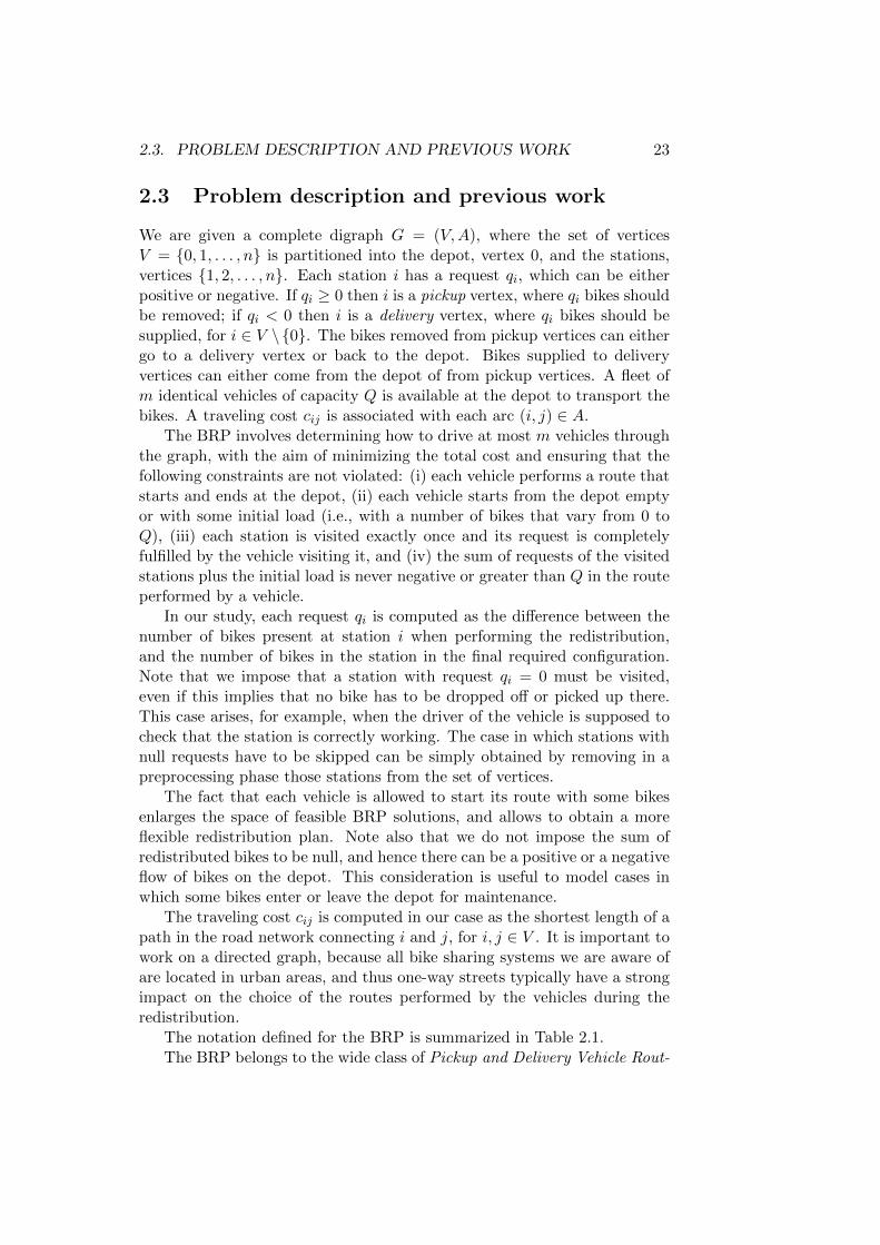
We are given a complete digraph G = (V,A), where the set of verticesV = 0, 1, . . . , n is partitioned into the depot, vertex 0, and the stations,vertices 1, 2, . . . , n. Each station i has a request qi, which can be eitherpositive or negative. If qi ≥ 0 then i is a pickup vertex, where qi bikes shouldbe removed; if qi < 0 then i is a delivery vertex, where qi bikes should besupplied, for i ∈ V \0. The bikes removed from pickup vertices can eithergo to a delivery vertex or back to the depot. Bikes supplied to deliveryvertices can either come from the depot of from pickup vertices. A fleet ofm identical vehicles of capacity Q is available at the depot to transport thebikes. A traveling cost cij is associated with each arc (i, j) ∈ A.
The BRP involves determining how to drive at most m vehicles throughthe graph, with the aim of minimizing the total cost and ensuring that thefollowing constraints are not violated: (i) each vehicle performs a route thatstarts and ends at the depot, (ii) each vehicle starts from the depot emptyor with some initial load (i.e., with a number of bikes that vary from 0 toQ), (iii) each station is visited exactly once and its request is completelyfulfilled by the vehicle visiting it, and (iv) the sum of requests of the visitedstations plus the initial load is never negative or greater than Q in the routeperformed by a vehicle.
In our study, each request qi is computed as the difference between thenumber of bikes present at station i when performing the redistribution,and the number of bikes in the station in the final required configuration.Note that we impose that a station with request qi = 0 must be visited,even if this implies that no bike has to be dropped off or picked up there.This case arises, for example, when the driver of the vehicle is supposed tocheck that the station is correctly working. The case in which stations withnull requests have to be skipped can be simply obtained by removing in apreprocessing phase those stations from the set of vertices.
The fact that each vehicle is allowed to start its route with some bikesenlarges the space of feasible BRP solutions, and allows to obtain a moreflexible redistribution plan. Note also that we do not impose the sum ofredistributed bikes to be null, and hence there can be a positive or a negativeflow of bikes on the depot. This consideration is useful to model cases inwhich some bikes enter or leave the depot for maintenance.
The traveling cost cij is computed in our case as the shortest length of apath in the road network connecting i and j, for i, j ∈ V . It is important towork on a directed graph, because all bike sharing systems we are aware ofare located in urban areas, and thus one-way streets typically have a strongimpact on the choice of the routes performed by the vehicles during theredistribution.
The notation defined for the BRP is summarized in Table 2.1.The BRP belongs to the wide class of Pickup and Delivery Vehicle Rout-

24 CHAPTER 2. THE BIKE SHARING REBALANCING PROBLEM
V set of verticesA set of arcsn number of stationsm number of vehiclesQ vehicle capacityqi demand at vertex icij cost of the arc (i, j)
Table 2.1: BRP notation summary.
ing Problems (PDVRPs), where a fleet of vehicles is used to transport re-quests from the depot and/or some vertices to the depot and/or other ver-tices in the network. In particular, some pickup customers require a certainamount of freight to be picked up by a vehicle and then transported else-where, whereas some delivery customers require a certain amount of freightto be delivered there. The BRP generalizes the well-known Capacitated Ve-hicle Routing Problem (CVRP), where customers are either all pickup ver-tices or all delivery vertices, but not both, and thus it is a strongly NP-hardproblem.
Detailed reviews and classifications of the PDVRPs have been proposedby Berbeglia et al. [6] and Parragh et al. [24, 25]. More recent surveys havebeen presented by Battarra et al. [3], for what concerns the transportationof freight, and Doerner and Salazar-Gonzalez [11], for the transportationof people. Following the notation introduced in Berbeglia et al. [6], theBRP can be classified as a Many-to-Many (M-M) vehicle routing problem,in which a request has multiple origins (in our case pickup stations) andmultiple destinations (in our case delivery stations).
The most basic problem in the class of M-M PDVRPs is probably theOne-commodity Pickup and Delivery Traveling Salesman Problem (1-PDTSP),which calls for routing a single capacitated vehicle to meet M-M requests.The 1-PDTSP was formally introduced by Hernandez-Perez and Salazar-Gonzalez [15], who presented mathematical formulations and branch-and-cut algorithms. The mathematical formulations were given for both thesymmetric and asymmetric version of the problem, and were based on theuse of a binary variable xij taking value one if the edge or arc (i, j) wasused, 0 otherwise, and a non-negative variable fij giving the flow of the sin-gle commodity on edge or arc (i, j). Computational results were providedonly for the symmetric formulation, that was solved by means of a branch-and-cut algorithm. The results of this approach were later improved byHernandez-Perez and Salazar-Gonzalez [17], with an enhanced branch-and-cut algorithm working again on the symmetric formulation but exploitingonly the binary variable xij . To address larger instances, Hernandez-Perezand Salazar-Gonzalez [16] proposed two simple heuristics, whereas a well-performing variable neighborhood descent metaheuristic was introduced byHernandez-Perez et al. [14]. All these works considered the case in which

2.3. PROBLEM DESCRIPTION AND PREVIOUS WORK 25
vehicles can leave the depot with some load, but the sum of all requests isequal to zero.
The 1-PDTSP has also attracted the interests of other researchers. Wanget al. [34] studied some variants of the 1-PDTSP that involve unit-load re-quests. They developed polynomial-time exact algorithms for the case ofdistribution on a path, and for the cases of distribution on a tree havingQ = 1 or Q = +∞. Martinovic et al. [20] presented a simulated anneal-ing approach, whereas Zhao et al. [35] developed a genetic algorithm. Theresults of these two metaheuristics were later improved by Hosny and Mum-ford [13] by means of a Variable Neighborhood Search (VNS), but at theexpense of very high computing times. A more recent VNS has been pro-posed by Mladenovic et al. [22], that used a binary tree to efficiently performfeasibility checks and obtained very good computational results.
The multiple-vehicle case, known as the One-commodity Pickup and De-livery Vehicle Routing Problem (1-PDVRP), was formally introduced by Shiet al. [30], who studied the case in which a maximum duration limit is im-posed on each route. They presented a genetic algorithm and a three-indexmathematical formulation making use of a binary variable xijk, taking value1 if vehicle k travels along edge or arc (i, j), 0 otherwise, and a non-negativevariable fij representing the flow of the single commodity on edge or arc(i, j). Computational experiments were performed only for the genetic al-gorithm, that was tested on a set of randomly generated instances withsymmetric costs.
The BRP is a generalization of the 1-PDTSP which involves more thanone vehicle. Indeed, in the next sections we use successful properties andalgorithmic ideas adapted for the BRP from [15] and [17]. Moreover, theBRP can be seen as a special case of the 1-PDVRP, because it does notconsider maximum route duration.
As previously mentioned, the issue of rebalancing a bike sharing systemhas attracted the interest of many researchers in recent years. Benchimol etal. [5] study the case in which the redistribution is performed by a singlecapacitated vehicle, split deliveries are allowed (i.e., a vertex may be visitedmore than once) and the sum of all requests is balanced to zero. Theypresent complexity results, lower bounding techniques, and approximationalgorithms, but do not provide computational results.
In a recent paper, Chemla et al. [8] focus again on the single vehiclecase, allowing split deliveries. Vertices with null demand are not forced to bevisited, but can be used by vehicles as temporary buffer when transportingbikes among other stations. In their paper, the authors obtain a lower boundby solving the relaxation of the problem in which a limit is imposed on themaximum number of times that a vertex can be visited. They also obtainan upper bound by using a tabu search algorithm and run their boundingprocedures on instances obtained by modifying those randomly created in[15].

26 CHAPTER 2. THE BIKE SHARING REBALANCING PROBLEM
In another recent paper, Raviv et al. [27] define the static bicycle reposi-tioning problem in which they do not only minimize total traveling costs ofa fleet of heterogeneous vehicles, but also users’ dissatisfaction that is linkedwith a convex function to the inventory level of each station. The authorspresent two MILP formulations, an arc-indexed and a time-indexed one,each of them represents a different version of the problem. They allow lim-ited or unlimited split delivery, limited or unlimited transshipment, dwellingwith a maximum duration of each route and with synchronized transship-ment. Exact and heuristics methods to speed up the computational timesfor solving the formulations are also presented in this paper.
Contardo et al. [9] present a formulation for the dynamic version of thebike rebalancing problem, allowing the use of more than one vehicle. Theirobjective function is the maximization of the serviced demand. An arc flowformulation working on a discretized time horizon is proposed and solvedwith with Dantzig-Wolfe and Benders decomposition. Extensive tests onseveral randomly created instances are presented.
2.4 MILP formulations for the BRP
In this section we present four Mixed Integer Linear Programming (MILP)formulations of the BRP. Computational evidence obtained from preliminaryexperiments suggested to us that it would be better to adopt two-indexformulations for the BRP.
2.4.1 Formulation F1
The starting point of the aforementioned two-index formulations is the well-known Multiple Traveling Salesman Problem (m-TSP), see, e.g., Bektas [4],in which at most m uncapacitated vehicles based at a central depot have tovisit a set of vertices, with the constraint that each vertex is visited exactlyonce. By defining a binary variable xij , taking value 1 if arc (i, j) is used bya vehicle, 0 otherwise, the m-TSP can be modeled as:
(m-TSP) min∑i∈V
∑j∈V
cijxij (2.1)
∑i∈V
xij = 1 j ∈ V \ 0 (2.2)∑i∈V
xji = 1 j ∈ V \ 0 (2.3)∑j∈V
x0j ≤ m (2.4)
∑j∈V \0
x0j =∑
j∈V \0
xj0 (2.5)

2.4. MILP FORMULATIONS FOR THE BRP 27
∑i∈S
∑j∈S
xij ≤ |S| − 1 S ⊆ V \ 0 , S 6= ∅ (2.6)
xij ∈ 0, 1 i, j ∈ V. (2.7)
Objective function (2.1) minimizes the traveling cost. Constraints (2.2)and (2.3) impose that every vertex but the depot is visited exactly once.Constraints (2.4) and (2.5) ensure, respectively, that at most m vehiclesleave the depot, and that all vehicles that are used return to the depot atthe end of their route. Constraints (2.6) are the classical subtour eliminationconstraints, see, e.g., Gutin and Punnen [12], that impose the connectivityof the solution. These constraints increase exponentially, so, as usual, weproceed in branch-and-cut fashion, by invoking a separation procedure toidentify the violated ones from the non-violated ones, and then adding tothe model only the violated constraints in an iterative way. The details willbe given in the next section.
To guarantee the feasibility of a solution with respect to the BRP, weneed to include additional constraints in the m-TSP formulation, so as toensure that demands are satisfied and vehicle capacities are not exceeded.This may be done in different ways.
The first option is to define an additional continuous variable θj , repre-senting the load of a vehicle after it visited vertex j, for j ∈ V . The loadshould be updated along the route by taking into consideration the fact that,if the vehicle travels along arc (i, j), then θj should be equal to θi + qj . Theaforementioned restriction can be imposed by the non-linear constraints:
θj ≥ (θi + qj)xij i ∈ V, j ∈ V \ 0 (2.8)
θi ≥ (θj − qj)xij i ∈ V \ 0 , j ∈ V (2.9)
max 0, qj ≤ θj ≤ min Q,Q+ qj j ∈ V. (2.10)
Constraints (2.8) and (2.9) impose that, if xij takes value 1, then θj =θi + qj , and hence model the flow conservation independently of the sign ofqj . Constraints (2.10) simply give lower and upper bounds on the loads.
These constraints generalize the Miller-Tucker-Zemlin subtour elimina-tion constraints for the TSP, see Miller et al. [21], to the case where verticeshave demands unrestricted in sign. They can be linearized with the standard“big M” method, obtaining:
θj ≥ θi + qj −M(1− xij) i ∈ V, j ∈ V \ 0 (2.11)
θi ≥ θj − qj −M(1− xij) i ∈ V \ 0 , j ∈ V. (2.12)
Constraints (2.8) and (2.9) are linearized to (2.11) and (2.12), respectively.In our implementation we set the “big M” equal to min Q,Q+ qj in (2.11),and equal to min Q,Q− qj in (2.12).

28 CHAPTER 2. THE BIKE SHARING REBALANCING PROBLEM
Our formulation F1 for the BRP is thus given by (2.1)–(2.7), (2.10)–(2.12). Note that subtour elimination constraints must be kept in the for-mulation, because (2.10)–(2.12) are not enough to ensure connectivity of thesolution when some demands are non-positive and some are non-negative.
2.4.2 Formulation F2
Our second formulation also builds upon the m-TSP, but makes use ofan additional variable fij giving the flow over arc (i, j), i.e., the load on thevehicle traveling along arc (i, j), if any, for (i, j) ∈ A. To impose feasibilitywith respect to the BRP, it is then enough to include in the m-TSP:∑
i∈Vfji −
∑i∈V
fij = qj j ∈ V \ 0 (2.13)
max0, qi,−qjxij ≤ fij ≤ minQ,Q+ qi, Q− qjxij (i, j) ∈ A. (2.14)
Constraints (2.13) model the balance of the flows on the arcs entering andleaving a given vertex. Constraints (2.14) impose lower and upper boundson the flows on each arc, and make these bounds as tight as possible byconsidering whether or not an arc is traveled by a vehicle. Indeed, for whatconcerns the lower bound, if arc (i, j) is used, then fij should be at leastgreater than qi if qi > 0 (because qi has just been collected) or greater than−qj if qj < 0 (because qj has to be supplied to the next vertex). Similarconsiderations apply to the upper bound.
Formulation F2 of the BRP is thus given by (2.1)–(2.7), (2.13)–(2.14).
2.4.3 Formulation F3
We use the approach proposed by Hernandez-Perez and Salazar-Gonzalez[15, 17] for the 1-PDTSP in order to develop another formulation of the BRP.We start again from the m-TSP, but ensure that solutions satisfy demands,without exceeding the vehicle capacity, by adding to the model the followingfamily of constraints:
∑i∈S
∑j∈S
xij ≤ |S| −max
1,
⌈∣∣∑i∈S qi
∣∣Q
⌉S ⊆ V \ 0 , S 6= ∅. (2.15)
Constraints (2.15) are similar to the generalized subtour elimination con-straints for the CVRP. They state that, for each subset S of vertices, thenumber of arcs with both tail and head in S should not exceed the car-dinality of S minus the minimum number of vehicles required to serve S.An estimation of the minimum number of vehicles is simply obtained bycomputing the absolute value of the sum of the demands, dividing it by thevehicle capacity and then rounding up the result. This value can be zerowhen the sum of the qj is null. In such a case the value 1 is used instead,

2.4. MILP FORMULATIONS FOR THE BRP 29
because at least one vehicle is needed (notice that S does not contain thedepot).
Our formulation F3 is thus given by (2.1)–(2.5), (2.7), and (2.15). Notethat constraints (2.15) are exponentially many, and hence, as already ob-served for (2.6), we need a separation procedure that identifies violated con-straints from non-violated ones. Also note that these constraints are validfor formulations F1 and F2, and may be used to improve their convergenceto the optimum.
2.4.4 Formulation F4
We propose a fourth formulation of the BRP that builds upon the two-commodity flow model originally presented by Baldacci et al. [2] for thesymmetric CVRP. This formulation first requires to modify the graph byadding a copy of the depot, defined in the following by a new vertex n+1. Wedefine V = V ∪n+ 1 the resulting set of vertices, and A = A∪(j, n+1) :j ∈ V ∪ (n + 1, j) : j ∈ V the resulting set of arcs. Let us also defineV0 = V \0, n+1 and Qtot =
∑j∈V0 qj . We set qn+1 = 0, cn+1,j = +∞, and
cj,n+1 = cj0 for j ∈ V , knowing that c0,n+1 = 0, and then we set cj0 = +∞for j ∈ V .
We use three sets of variables. The first two have already been usedin formulation F2: xij takes value 1 if arc (i, j) is used, 0 otherwise, for
(i, j) ∈ A, and fij gives the flow over arc (i, j), i.e., the load of the vehicle
passing over arc (i, j), if any, for (i, j) ∈ A. The third variable is anothercontinuous variable gji that gives the residual space of the vehicle traveling
along arc (i, j), if any, for (i, j) ∈ A.
In this formulation, vehicles leave the initial depot, vertex 0, visit cus-tomers, and then end their route in the final depot, vertex n + 1. Variablefij gives the load along the route performed by the vehicle, starting fromthe initial depot, vertex 0, following the vertices visited by the route andthen ending in the final depot, vertex n + 1. In opposite way, gji gives thefree space on the vehicle, starting from n+ 1, retracing back the route andthen ending 0. The resulting model is then:
(Formulation F4) min∑i∈V
∑j∈V
cijxij (2.16)
∑i∈V
xij = 1 j ∈ V0 (2.17)
∑i∈V
xji = 1 j ∈ V0 (2.18)
∑j∈V
x0j ≤ m (2.19)

30 CHAPTER 2. THE BIKE SHARING REBALANCING PROBLEM
∑j∈V0
x0j =∑j∈V0
xj,n+1 (2.20)
∑i∈S
∑j∈S
xij ≤ |S| − 1 S ⊆ V0, S 6= ∅ (2.21)
fij + gji = Qxij (i, j) ∈ A (2.22)∑i∈V
(fji − gij)−∑i∈V
(fij − gji) = 2qj j ∈ V0 (2.23)
∑j∈V0
f0j ≥ max 0,−Qtot (2.24)
∑j∈V0
fj,n+1 ≥ max 0, Qtot (2.25)
∑j∈V0
gj0 ≤ min mQ,mQ+Qtot (2.26)
max0, qi,−qjxij ≤ fijfij ≤ minQ,Q+ qi, Q− qjxij
(i, j) ∈ A (2.27)
(Q−minQ,Q+ qi, Q− qj)xij ≤ gjigji ≤ (Q−max0, qi,−qj)xij
(i, j) ∈ A (2.28)
xij ∈ 0, 1 i, j ∈ V . (2.29)
Constraints (2.17)–(2.20) and (2.29) are equivalent to the ones discussedfor formulation F1, but adapted to the new sets of vertices and arcs. Con-straints (2.22) state that, if a vehicle travels along arc (i, j), then the sum ofthe load and the residual space on that arc is equal to the vehicle capacity.Constraints (2.23) impose that the difference between loads and residualcapacities that enter and leave a vertex is double of the demand of thatvertex.
The total load leaving the initial depot should be in any case non-negative, and moreover, in case Qtot takes a negative value, it should benot lower than this value. This fact is imposed by constraints (2.24). Simi-larly, constraints (2.25) state that the total load entering the final depot isin any case non-negative, and not lower than the sum of all demands in casethis is positive. Inequalities (2.26) state that the free space on the vehiclesleaving the depot must be not greater than the minimum value between thetotal capacity of the m vehicles, and the total capacity plus Qtot. Finally,constraints (2.27) and (2.28) enforce lower and upper bounds on the contin-uous variables.

2.5. BRANCH-AND-CUT ALGORITHM 31
2.5 Branch-and-Cut algorithm
The models presented in the previous section include an exponential num-ber of constraints, hence we solve them with a Branch-and-Cut (B&C) al-gorithm. We use the B&C framework of CPLEX 12.2, that solves at everyvertex of an enumeration tree the linear relaxation of a MILP model, andthen invokes user-developed separation procedures for the possible additionof cuts.
At the root node of the B&C procedure we obtain an initial solution byusing a simple greedy heuristic. The greedy method builds routes one at atime, using the principle of the closest neighbor. It starts from the depotand then visits the closest, yet unserved, customer. It then extends the pathby moving to the next closest neighbor for which the sum of collected anddelivered demands is feasible (see Section 2.5.2 below for the algorithm usedto determine if a path is feasible), if any. When no extension is possible,the route is closed by going back to the depot, and possibly a new routeis initialized in an iterative fashion. The model is then initialized with thegeneralized subtour elimination constraints for sets of one or two vertices,hence xii = 0 for all i ∈ V and xij + xji ≤ 2 − max1, d|qi + qj |/Qe, forall (i, j) ∈ A. After testing a few branching strategies, we adopted theautomatic strong branching procedure by CPLEX, that provides the bestcomputational performance on our test bed.
In Section 2.5.1 we present some valid inequalities that we use to improvethe convergence of the algorithm to the optimum, whereas in Section 2.5.2 wediscuss the separation procedures that we implemented. Since inequalitiesand separation procedures are based only on the xij variables, they applydirectly to formulations 1, 2 and 3. The adaptation to formulation 4 istrivial, and is outlined in Section 2.5.2.
2.5.1 Valid inequalities
We first propose two new simple families of clique inequalities with threevertices. Consider a pair of vertices i and j, and let S(i, j) ⊂ V \ 0 be thesubset of vertices whose demand results in a total greater than Q or smallerthan −Q. Namely, S(i, j) = h ∈ V0, h 6= i, h 6= j : |qi+qj +qh| > Q. Thenthe following inequalities are valid for the BRP:
xij +∑
h∈S(i,j)
xjh ≤ 1 i, j ∈ V \ 0, h ∈ S(i, j) (2.30)
∑h∈S(i,j)
xhi + xij ≤ 1 i, j ∈ V \ 0, h ∈ S(i, j). (2.31)
We note that, in (2.30), at most one among the xjh variables may takethe value of 1 because of the degree constraint, and that all of them are

32 CHAPTER 2. THE BIKE SHARING REBALANCING PROBLEM
incompatible with xij because of the capacity constraint. Thus the sum ofall these variables is at most 1 in a feasible solution. A similar considerationapplies to (2.31).
For the next family of inequalities we need some further notation. Let Pdenote a path consisting of a sequence of vertices starting from the depot.Let also |P | denote the number of vertices in P , and P (i) denote the index ofthe i-th vertex of path P , for i = 0, 1, . . . , |P |−1, with P (0) = 0. Given P , we
compute qminP = min
|P |−1i=1
∑ij=1 qP (j) and qmax
P = max|P |−1i=1
∑ij=1 qP (j),
that denote, respectively, the minimum and maximum of the cumulativedemand along P .
As observed by Hernandez-Perez and Salazar-Gonzalez [15], a path P isinfeasible with respect to the capacity constraint if qmax
P −qminP > Q. Indeed,
if the vehicle leaves the depot with an empty load, then along the path itwill reach a maximum load equal to qmax
P , that clearly cannot exceed Q.Now notice that qmin
P may be negative even in a feasible solution, but in thiscase the vehicle has to start from the depot by carrying −qmin
P bikes. Hence,the maximum load becomes qmax
P − qminP , which also cannot exceed Q.
Let P be the family of all infeasible paths, the following infeasible pathconstraints are thus valid inequalities for the BRP:
|P |−2∑i=0
xP (i),P (i+1) ≤ |P | − 2 P ∈ P. (2.32)
Inequality (2.32) simply states that, if path P is infeasible then not allthe arcs connecting two consecutive vertices of P may belong to a feasiblesolution. A way to enforce them is to consider also the arcs connectingnon-consecutive vertices of P . Indeed, any arc (P (i), P (j)) with j 6= i + 1is incompatible with arcs (P (i), P (i+ 1)) and (P (j − 1), P (j)), because of,respectively, out-degree and in-degree constraints. Hence we can add thecorresponding variable, xP (i),P (j) to the left-hand side of (2.32), withoutaffecting the right-hand side value. This process can be repeated for all arcsconnecting two non-consecutive vertices in the path, with the exception ofthose arcs leaving the depot, because up to m of them may belong to afeasible solution. Hence, we obtain the following:
x0,P (1) +
|P |−2∑i=1
|P |−1∑j=i+1
xP (i),P (j) ≤ |P | − 2 P ∈ P. (2.33)
Inequalities (2.33) generalize, in the case of multiple vehicles, the tournamentconstraints, discussed by Ascheuer et al. [1] for the Traveling SalesmanProblem. Note that these constraints can be used in directed formulations(where a variable is associated to each directed arc), but cannot be appliedto undirected ones (where variables are associated to undirected edges).

2.5. BRANCH-AND-CUT ALGORITHM 33
2.5.2 Separation procedures
The aim of this section is to present the procedures that we use to determinewhether or not the valid inequalities we proposed in Section 2.5.1 are violatedby a given solution x (possibly fractional).
Separations S1 and S2. The inequalities of type (2.30) and (2.31)are separated exactly, by enumerating all possible pairs of vertices i and j,computing the set Sij , and then evaluating if the sum of the x involved inthe inequality exceeds one. In the following we will refer the separation of(2.30) and (2.31) as separation S1 and separation S2, respectively.
Separation S3. To separate constraints (2.6) and (2.15), we first builda supporting graph G = (V ,A), where V = V , A = (i, j) ∈ A : xij > 0,and a capacity xij is assigned to every arc (i, j) ∈ A. Constraints (2.6) maybe separated exactly as usually done for the TSP, by computing O(n) maxflows on G, using the depot as a source and any vertex i, in turn, as a sink.If the max flow value obtained is lower than one, then i is disconnectedfrom the depot, and hence the cut that corresponds to the set S induced bythe min cut may be added to the model. For the BRP, we obtain a simplealgorithmic improvement by checking, for any set S induced by a min cut,if the minimum number of vehicles required to serve S is lower than themax flow value obtained, and, in such a case, we add the corresponding(stronger) constraint (2.15). In this way the exact separation of (2.6) isused as a heuristic for separating (2.15). We refer to this procedure asseparation S3.
Separation S4. To separate constraint (2.15), we extend the proceduredeveloped in Hernandez-Perez and Salazar-Gonzalez [15] for the 1-PDTSPto the directed case. First of all we associate a demand q0 = Qtot to thedepot. Then we build a new supporting graph G
′, obtained by adding two
dummy nodes, n+ 1 and n+ 2, to G. We connect n+ 1 to any i ∈ V havingqi > 0 with an arc of capacity qi/Q, and then connect any i ∈ V havingqi < 0 to n + 2 with an arc of capacity −qi/Q (in this way, the capacitiesassociated with the arcs are always non-negative) . We then compute the
max flow on G′, using n+ 1 as a source and n+ 2 as a sink. The constraint
(2.15) corresponding to the set S induced by the min cut is then checked,and, if violated, it is added to the model. We refer to Hernandez-Perez andSalazar-Gonzalez [15] for further details.
Conforming to the fact that we are solving a problem on an asymmet-ric graph, we perform a second separation for (2.15). We build a second
modified supporting graph G′′, adding again two new dummy vertices, n+1
and n + 2, to G. In this case however we include in G′′
new arcs (n + 1, i)of capacity −qi/Q for all i ∈ V having qi < 0, and new arcs (i, n + 2) ofcapacity qi/Q for all i ∈ V having qi > 0. Once more, we use the maxflow procedure on the resulting supporting graph, from n+ 1 to n+ 2, andcheck the constraints (2.15) for the sets S induced by the min cuts. In the

34 CHAPTER 2. THE BIKE SHARING REBALANCING PROBLEM
following, these procedures are referred to as separation S4.
Separation S5. The tournament constraints (2.33) are separated ex-actly, by generating all possible paths starting from the depot and using adepth-first strategy. We initialize vector P with P (0) = 0, then select thefirst outgoing arc having a positive value of x, say, (0, i), and extend the pathto include the head of the selected arc by setting P (1) = i. The process isthen reiterated. Every time we add a vertex to the path, we check if it isinfeasible. If so, then we add the cut and backtrack to the previous vertex,otherwise we continue extending the path. The path extension continuesas long as the sum of the involved xij is large enough to possibly lead to aviolated cut, i.e., as long as it is strictly greater than |P | − 2. As soon asthe sum becomes smaller, we backtrack to the previous vertex. Anytime webacktrack, we continue the depth-first search by selecting the next arc withpositive value of x and then extend the path consequently.
Suppose a violated cut of type (2.33) has been found, then we know thatthe set S = P (1), P (2), . . . , P (|P |) is currently visited by a single vehicle(the one performing the path P ). Now we estimate the minimum numberof vehicles required to serve S using d|
∑i∈S qi|/Qe, and, if this is greater
than one, we add the violated generalized subtour elimination constraint(2.15) for this set S. Constraints (2.15) are usually stronger than (2.33),but do not dominate them (because the latter involves variable x0,P (1), notcontained in the former), and hence they are both profitable for the modelsolution. The current procedure is called separation S5.
The separation procedures (S1-S5) are invoked at every node of the enu-meration tree in the order in which we described them. With regards toformulation F4, there is only a slight modification to implement. Recallthat this formulation works on a modified graph V , where n+ 1 is a copy ofthe original depot 0. When creating the supporting graph G, we merge again0 and n+1 into a unique vertex 0 (this is done by simply setting xj,0 = xj,n+1
for all j ∈ V ), and then use the separation process just described for theprevious formulations. The resulting cut, if any, is then mapped back on V .On the basis of computational evidence resulting from detailed experimen-tation, the separation process for all formulations is terminated as soon asa violated cut is found.
2.6 Benchmark Instances
In our attempt to solve real-world instances, we collected real data fromthe web sites of twenty-two bike sharing systems characterized by diversesize. The cities included in our studies are: Bari, Brescia, Bergamo, LaSpezia, Parma, Rome, Torino, Treviso, and Reggio Emilia, in Italy; Dublinin Ireland; Boston, Denver, Madison, Miami, Minneapolis, and San Anto-
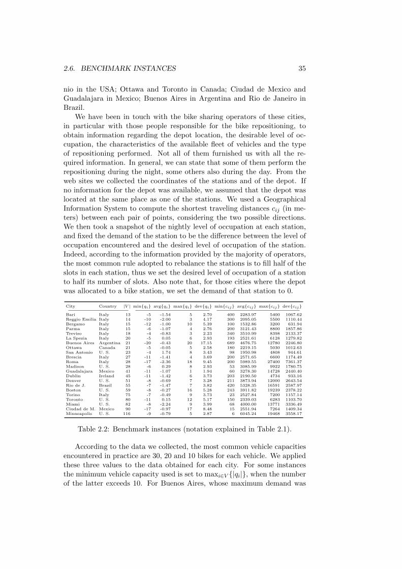
2.6. BENCHMARK INSTANCES 35
nio in the USA; Ottawa and Toronto in Canada; Ciudad de Mexico andGuadalajara in Mexico; Buenos Aires in Argentina and Rio de Janeiro inBrazil.
We have been in touch with the bike sharing operators of these cities,in particular with those people responsible for the bike repositioning, toobtain information regarding the depot location, the desirable level of oc-cupation, the characteristics of the available fleet of vehicles and the typeof repositioning performed. Not all of them furnished us with all the re-quired information. In general, we can state that some of them perform therepositioning during the night, some others also during the day. From theweb sites we collected the coordinates of the stations and of the depot. Ifno information for the depot was available, we assumed that the depot waslocated at the same place as one of the stations. We used a GeographicalInformation System to compute the shortest traveling distances cij (in me-ters) between each pair of points, considering the two possible directions.We then took a snapshot of the nightly level of occupation at each station,and fixed the demand of the station to be the difference between the level ofoccupation encountered and the desired level of occupation of the station.Indeed, according to the information provided by the majority of operators,the most common rule adopted to rebalance the stations is to fill half of theslots in each station, thus we set the desired level of occupation of a stationto half its number of slots. Also note that, for those cities where the depotwas allocated to a bike station, we set the demand of that station to 0.
City Country |V | minqi avgqi maxqi devqi mincij avgcij maxcij devcij
Bari Italy 13 -5 -1.54 5 2.70 400 2283.97 5400 1067.62Reggio Emilia Italy 14 -10 -2.00 3 4.17 300 2095.05 5500 1110.44Bergamo Italy 15 -12 -1.00 10 5.39 100 1532.86 3200 631.94Parma Italy 15 -6 -1.07 4 2.76 200 3121.43 8800 1857.86Treviso Italy 18 -4 -0.83 3 2.23 340 3510.99 8398 2133.37La Spezia Italy 20 -5 0.05 6 2.93 193 2521.61 6128 1279.82Buenos Aires Argentina 21 -20 -0.43 20 17.15 689 4676.75 12780 2246.80Ottawa Canada 21 -5 -0.05 5 2.58 180 2219.15 5030 1012.63San Antonio U. S. 23 -4 1.74 8 3.43 98 1950.98 4808 944.61Brescia Italy 27 -11 -1.41 4 3.69 200 2571.65 6600 1174.49Roma Italy 28 -17 -2.36 18 9.45 200 5989.55 27400 7361.37Madison U. S. 28 -6 0.29 8 2.93 53 3085.99 9922 1780.75Guadalajara Mexico 41 -11 -1.07 1 1.94 60 3278.30 14728 2440.40Dublin Ireland 45 -11 -1.42 6 3.73 203 2190.50 4734 933.16Denver U. S. 51 -8 -0.69 7 3.28 211 3873.94 12000 2643.54Rio de J. Brazil 55 -7 -1.47 7 3.82 420 5328.35 16591 2587.97Boston U. S. 59 -8 -0.27 16 5.28 243 3911.82 19239 2378.22Torino Italy 75 -7 -0.49 9 3.73 23 2527.84 7200 1157.14Toronto U. S. 80 -11 0.15 12 5.17 150 2339.03 6283 1103.70Miami U. S. 82 -8 -2.24 9 3.99 68 4000.00 13771 3336.49Ciudad de M. Mexico 90 -17 -0.97 17 8.48 15 2551.94 7264 1409.34Minneapolis U. S. 116 -9 -0.79 5 2.87 6 6045.24 19468 3558.17
Table 2.2: Benchmark instances (notation explained in Table 2.1).
According to the data we collected, the most common vehicle capacitiesencountered in practice are 30, 20 and 10 bikes for each vehicle. We appliedthese three values to the data obtained for each city. For some instancesthe minimum vehicle capacity used is set to maxi∈V |qi|, when the numberof the latter exceeds 10. For Buenos Aires, whose maximum demand was

36 CHAPTER 2. THE BIKE SHARING REBALANCING PROBLEM
20, we tested only 20 and 30. We generated 65 instances in total, thatare summarized in Table 2.2. The values minqi, avgqi, maxqi, anddevqi give, respectively, the minimum, average, and maximum demand,and the standard deviation. Similar information is provided for the distancescij . The number of vertices varies from 13 to 116 stations. All test instanceshave variability in the number of bikes leaving the depot (since avgqi isnot 0). All distances are given in meters. All instances are available onlineat http://www.or.unimore.it/resources.htm.
2.7 Computational results
All algorithms described in Sections 4.4 and 3.5.2 were coded in C/C++ andrun on an Intel Core i3-2100 CPU, 3.10 GHz, 4.00 GB. We used CPLEX12.2 as the MILP solver imposing the selection of a single processor. For-mulations F1−F4 were computationally tested on the problem instancesdescribed in Section 2.6. For clarity purposes, details of the computationalimplementation of the formulations we tested are given in Table 2.3, wherewe also include the additional separation procedures described in Section2.5.2.
variables core formulation additional separations
Formulation F1 xij , θj (2.1)–(2.7), (2.10)–(2.12), S3 S1, S2, S4, S5Formulation F2 xij , fij (2.1)–(2.7), (2.13)–(2.14), S3 S1, S2, S4, S5Formulation F3 xij (2.1)–(2.5), (2.7), (2.15), S3, S4 S1, S2, S5Formulation F4 xij , fij , gij (2.16)–(2.29), S3 S1, S2, S4, S5
Table 2.3: Implementation of formulations F1−F4.
In this section, we present the computational results of the B&C algo-rithm using formulations F1−F4. The B&C algorithm was terminated wheneither the optimal solution was found or a predetermined time-limit elapsed.The time-limit imposed was 3600 CPU seconds. Table 2.4 reports the com-putational results obtained for the complete set of 65 problem instances. Inthis table, the following information is provided for each problem instance:
• City (|V |, Q): City name associated with a given problem instancewhich is uniquely identified by the number of vertices |V | of the cor-responding digraph and the vehicle capacity Q used to transport thebikes at the specified city;
• UB: The value of the best feasible solution found by the B&C algo-rithm using formulations F1 to F4;
• Gap1−Gap4: Percentage deviation from UB of LB1−LB4, best lowerbounds obtained by the B&C algorithm using core formulations F1 toF4 including the set of additional separations for each formulation,

2.7. COMPUTATIONAL RESULTS 37
respectively, as shown in Table 3. Gapi = 100/(1 − LBi/UB), fori = 1, . . . , 4.
• Time: Computational time for running the B&C algorithm, in CPUseconds.
To compare the average performance of formulations F1−F4 over the com-plete set of problem instances, the following additional information is givenin Table 2.4:
• Opt: The total number of problem instances solved to optimality bythe B&C algorithm within 3600 seconds;
• #Nodes: Average number of nodes (over all instances) explored bythe B&C algorithm;
• #Cuts: Average number of cuts generated by the B&C algorithm.
As shown in Table 2.4, the first 25 problem instances and a large num-ber of other instances are easily solved by all formulations within a fewseconds. Formulation F1 gives the worst results in terms of average gap,computational time, and number of generated cuts, whereas, formulationsF2 and F4 demonstrate similar performance for all performance indicators.On the other hand, F3 performs best over all formulations with averageGap3 = 2.24% and it optimally solves all problem instances including up to50 vertices. Indeed, formulation F3 finds the optimal solution for 49 outof 65 instances within an average time of 15 minutes generating an averageof approximately 1200 B&C nodes. However, it is worth noting that, forsome of the larger instances, Gap3 is larger than Gap2, (e.g., Ciudad deMexico (90, 17)) or Gap4 (e.g., Miami (82, 10)). Further insight into thebest performing formulation F3 was gained by computationally evaluatingthe impact of each separation procedure on the resulting percentage gapscomputed at the root node of the B&C tree for the most difficult probleminstances.
In Table 2.5 we test the core formulation F3, see Table 2.3, and the onesobtained by including just one of the separation procedures at a time. Wedenote with Gapcore the percentage deviation from UB of the lower boundobtained with the core version, while we use Gap+(Sx) to denote the resultsof the core version plus separation Sx.
In Table 2.6 we present the results of the full version of formulation F3(i.e., core formulation plus all separation procedures) and those obtainedby removing from it one separation procedure at a time. We denote withGapfull the percentage deviation from UB of the lower bound obtainedwith the full version, while we use Gap−(Sx) to denote the results of thefull version minus separation Sx.

38 CHAPTER 2. THE BIKE SHARING REBALANCING PROBLEM
F1 F2 F3 F4
Inst. City (|V |, Q) UB Gap1 Time Gap2 Time Gap3 Time Gap4 Time
1 Bari (13, 30) 14600 0.00 0.06 0.00 0.11 0.00 0.02 0.00 0.272 Bari (13, 20) 15700 0.00 0.06 0.00 0.10 0.00 0.02 0.00 0.113 Bari (13, 10) 20600 0.00 0.16 0.00 0.39 0.00 0.03 0.00 0.324 Reggio Emilia (14, 30) 16900 0.00 0.03 0.00 0.03 0.00 0.02 0.00 0.065 Reggio Emilia (14, 20) 23200 0.00 0.09 0.00 0.52 0.00 0.03 0.00 0.336 Reggio Emilia (14, 10) 32500 0.00 5.59 0.00 0.67 0.00 0.05 0.00 0.227 Bergamo (15, 30) 12600 0.00 0.05 0.00 0.05 0.00 0.03 0.00 0.108 Bergamo (15, 20) 12700 0.00 0.06 0.00 0.26 0.00 0.00 0.00 0.219 Bergamo (15, 12) 13500 0.00 0.27 0.00 0.74 0.00 0.11 0.00 0.9510 Parma (15, 30) 29000 0.00 0.05 0.00 0.03 0.00 0.02 0.00 0.0611 Parma (15, 20) 29000 0.00 0.05 0.00 0.02 0.00 0.02 0.00 0.0612 Parma (15, 10) 32500 0.00 0.22 0.00 0.26 0.00 0.05 0.00 0.4513 Treviso (18, 30) 29259 0.00 0.12 0.00 0.14 0.00 0.05 0.00 0.6214 Treviso (18, 20) 29259 0.00 0.12 0.00 0.20 0.00 0.03 0.00 0.4515 Treviso (18, 10) 31443 0.00 0.27 0.00 0.75 0.00 0.09 0.00 0.7916 La Spezia (20, 30) 20746 0.00 0.09 0.00 0.16 0.00 0.03 0.00 0.3117 La Spezia (20, 20) 20746 0.00 0.09 0.00 0.10 0.00 0.03 0.00 0.2418 La Spezia (20, 10) 22811 0.00 0.16 0.00 1.45 0.00 0.09 0.00 1.3419 Buenos Aires (21, 30) 76999 0.00 1.36 0.00 3.54 0.00 0.37 0.00 12.4020 Buenos Aires (21, 20) 91619 0.00 23.26 0.00 3.58 0.00 16.80 0.00 7.3521 Ottawa (21, 30) 16202 0.00 0.06 0.00 0.05 0.00 0.02 0.00 0.0922 Ottawa (21, 20) 16202 0.00 0.06 0.00 0.06 0.00 0.02 0.00 0.0923 Ottawa (21, 10) 17576 0.00 0.30 0.00 1.90 0.00 0.11 0.00 1.2624 San Antonio (23, 30) 22982 0.00 0.19 0.00 2.74 0.00 0.08 0.00 4.3825 San Antonio (23, 20) 24007 0.00 3.63 0.00 1.36 0.00 0.09 0.00 7.5226 San Antonio (23, 10) 40149 5.36 3600.00 0.00 7.07 0.00 1.06 0.00 17.8627 Brescia (27, 30) 30300 0.00 0.70 0.00 0.77 0.00 0.06 0.00 2.2228 Brescia (27, 20) 31100 0.00 6.07 0.00 6.38 0.00 0.20 0.00 9.1129 Brescia (27, 11) 35200 0.00 24.46 0.00 10.83 0.00 1.37 0.00 9.3130 Roma (28, 30) 61900 0.00 4.27 0.00 5.48 0.00 0.84 0.00 8.4631 Roma (28, 20) 66600 0.00 22.04 0.00 7.61 0.00 1.72 0.00 33.3832 Roma (28, 18) 68300 0.00 16.15 0.00 3.26 0.00 0.58 0.00 4.9933 Madison (28, 30) 29246 0.00 0.09 0.00 0.10 0.00 0.02 0.00 0.2434 Madison (28, 20) 29839 0.00 0.31 0.00 0.44 0.00 0.05 0.00 0.8435 Madison (28, 10) 33848 0.00 6.02 0.00 16.56 0.00 0.53 0.00 6.3636 Guadalajara (41, 30) 57476 0.00 1.16 0.00 2.97 0.00 0.22 0.00 6.2237 Guadalajara (41, 20) 59493 0.00 2.29 0.00 8.18 0.00 0.34 0.00 7.2138 Guadalajara (41, 11) 64981 1.18 3600.00 0.00 39.15 0.00 1.79 0.00 17.9939 Dublin (45, 30) 33548 0.00 435.69 0.00 180.81 0.00 6.05 0.00 280.0540 Dublin (45, 20) 39786 2.43 3600.00 1.14 3600.00 0.00 76.72 0.00 3140.8941 Dublin (45, 11) 54392 7.70 3600.00 1.17 3600.00 0.00 610.80 0.00 3513.5542 Denver (51, 30) 51583 0.00 66.57 0.00 11.01 0.00 0.67 0.00 15.8843 Denver (51, 20) 53465 0.00 410.05 0.00 372.78 0.00 25.33 0.00 1096.9544 Denver (51, 10) 67459 1.47 3600.00 0.00 1535.62 0.00 231.52 0.00 3443.6845 Rio de J. (55, 30) 122547 4.16 3600.00 1.57 3600.00 0.00 65.57 1.97 3600.0046 Rio de J. (55, 20) 156140 8.57 3600.00 2.29 3600.00 0.44 3600.00 1.82 3600.0047 Rio de J. (55, 10) 259049 28.58 3600.00 2.07 3600.00 2.23 3600.00 2.23 3600.0048 Boston (59, 30) 65669 0.00 255.25 0.00 1136.46 0.00 28.14 0.00 975.9749 Boston (59, 20) 71879 0.00 1899.07 1.70 3600.00 0.00 473.84 1.63 3600.0050 Boston (59, 16) 75065 0.99 3600.00 2.59 3600.00 0.37 3600.00 2.94 3600.0051 Torino (75, 30) 47634 0.00 464.46 0.00 919.59 0.00 13.79 0.00 1703.4652 Torino (75, 20) 50204 2.38 3600.00 2.70 3600.00 0.00 859.69 3.50 3600.0053 Torino (75, 10) 64797 11.30 3600.00 9.66 3600.00 9.25 3600.00 9.23 3600.0054 Toronto (80, 30) 41549 3.54 3600.00 4.47 3600.00 1.82 3600.00 4.42 3600.0055 Toronto (80, 20) 47898 11.81 3600.00 11.02 3600.00 11.05 3600.00 11.39 3600.0056 Toronto (80, 12) 60763 13.15 3600.00 10.74 3600.00 11.84 3600.00 10.88 3600.0057 Miami (82, 30) 156104 23.68 3600.00 8.43 3600.00 2.48 3600.00 9.01 3600.0058 Miami (82, 20) 229237 38.43 3600.00 11.02 3600.00 8.66 3600.00 10.99 3600.0059 Miami (82, 10) 415762 38.14 3600.00 6.07 3600.00 6.49 3600.00 6.12 3600.0060 Ciudad de M. (90, 30) 88227 28.67 3600.00 23.28 3600.00 23.05 3600.00 23.74 3600.0061 Ciudad de M. (90, 20) 116418 29.95 3600.00 23.59 3600.00 23.61 3600.00 23.63 3600.0062 Ciudad de M. (90, 17) 109573 20.00 3600.00 9.00 3600.00 9.56 3600.00 10.73 3600.0063 Minneapolis (116, 30) 137843 4.58 3600.00 5.82 3600.00 1.23 3600.00 5.96 3600.0064 Minneapolis (116, 20) 186449 23.45 3600.00 18.61 3600.00 15.40 3600.00 18.41 3600.0065 Minneapolis (116, 10) 298886 37.08 3600.00 17.65 3600.00 17.96 3600.00 18.93 3600.00
Average Gaps and Times 5.33 1330.02 2.69 1228.99 2.24 923.37 2.73 1272.84Opt 42 44 49 46#Nodes 2134.32 1847.74 1240.91 1440.65#Cuts 2233.02 630.14 1908.28 578.09
Table 2.4: Computational results for formulations F1−F4 on all probleminstances.

2.7. COMPUTATIONAL RESULTS 39
City (|V |, Q) Gapcore Gap+(S1) Gap+(S2) Gap+(S5)
Dublin (45 ,30) 1.45 1.45 1.45 1.45Dublin (45 , 20) 4.56 4.31 3.68 4.56Dublin (45, 11) 5.52 5.61 4.69 4.86Denver (51, 30) 0.52 0.52 0.52 0.52Denver (51, 20) 2.58 2.58 2.58 2.56Denver (51, 10) 3.34 3.05 4.29 3.32Rio de Janeiro (55, 30) 2.05 2.05 2.05 2.05Rio de Janeiro (55, 20) 2.51 2.51 2.51 2.51Rio de Janeiro (55, 10) 4.12 3.99 3.35 4.12Boston (59, 30) 1.87 1.76 1.76 1.87Boston (59, 20) 3.31 3.45 3.11 3.28Boston (59, 16) 4.63 4.25 4.13 4.63Torino (75, 30) 1.35 1.35 1.35 1.35Torino (75, 20) 3.38 3.81 3.30 3.38Torino (75, 10) 11.73 11.44 11.50 11.73Toronto (80, 30) 5.55 5.55 5.55 5.55Toronto (80, 20) 15.19 13.48 14.10 15.19Toronto (80, 12) 14.40 14.87 14.97 14.40Miami (82, 30) 3.28 3.28 3.28 3.28Miami (82, 20) 8.91 9.17 9.29 8.91Miami (82, 10) 6.71 7.03 6.86 6.71Ciudad de Mexico (90, 30) 24.62 25.23 25.18 24.62Ciudad de Mexico (90, 20) 25.43 24.96 24.94 25.43Ciudad de Mexico (90, 17) 11.81 11.31 11.85 11.80Minneapolis (116, 30) 2.97 2.97 2.97 2.97Minneapolis (116, 20) 15.97 15.97 15.97 15.97Minneapolis (116, 10) 19.44 19.14 18.83 19.44
Average gaps (%) 7.67 7.60 7.56 7.65
Table 2.5: Root node – Comparison of various separation procedures on thecore formulation F3.
The results reported in Table 2.5 demonstrate that the average gap ofthe core formulation F3 is close to 7% but slightly greater than 25% inthe worst case – Ciudad De Mexico (90, 20). The average gap Gapcore isonly slightly improved by separately adding either separation S1, S2 or S5;however, it is worth noting that separations S1, S2 and S5 are computedvery fast. The importance of separations S3 and, more clearly, S4 is evidentfrom the results presented in Table 2.6, namely, removing S3 and S4 fromthe full formulation F3 leads to an increase of the percentage gap from anaverage value of Gapfull = 7.53% to Gap−(S3) = 8.18% and Gap−(S4) =14.56%, respectively. Notably, this gap increases from 18.52% to 36.39% forseparation S4 in the case of Minneapolis (116, 10).
Based on the overall computational results presented in this section, wenote that the computational difficulty of the instances grows not only withthe number of vertices, as it is expected, but also when the capacity ofthe vehicles decreases. This behaviour was also noted for the 1-PDTSPby Hernandez-Perez and Salazar-Gonzalez [15] and is due to the fact thatsmall capacity vehicles are forced to perform long and complicated routesfor pickups and deliveries. An illustrative example is given in Figure 2.4,which depicts the three optimal solutions obtained for the problem instance

40 CHAPTER 2. THE BIKE SHARING REBALANCING PROBLEM
City (|V |, Q) Gapfull Gap−(S1) Gap−(S2) Gap−(S3) Gap−(S4) Gap−(S5)
Dublin (45 ,30) 1.45 1.45 1.45 3.75 3.47 1.45Dublin (45 , 20) 3.68 3.68 4.31 6.38 12.08 3.68Dublin (45, 11) 5.16 4.43 5.61 5.26 13.95 5.16Denver (51, 30) 0.52 0.52 0.52 1.31 1.64 0.52Denver (51, 20) 2.56 2.56 2.56 2.60 3.33 2.58Denver (51, 10) 3.49 4.29 2.98 4.82 6.65 3.49Rio de J. (55, 30) 2.05 2.05 2.05 2.05 6.45 2.05Rio de J. (55, 20) 2.51 2.51 2.51 2.51 10.56 2.51Rio de J. (55, 10) 3.30 3.35 3.41 3.30 21.50 3.30Boston (59, 30) 1.76 1.76 1.76 2.75 1.68 1.76Boston (59, 20) 3.45 3.11 3.45 4.08 3.88 3.45Boston (59, 16) 3.87 4.13 4.25 4.48 4.33 3.87Torino (75, 30) 1.35 1.35 1.35 2.50 1.61 1.35Torino (75, 20) 3.81 3.30 3.81 4.68 4.41 3.81Torino (75, 10) 11.56 11.50 11.44 12.84 15.15 11.56Toronto (80, 30) 5.55 5.55 5.55 7.25 6.08 5.55Toronto (80, 20) 13.30 14.10 13.48 14.62 14.90 13.30Toronto (80, 12) 14.99 14.97 14.87 15.36 18.99 14.99Miami (82, 30) 3.28 3.28 3.28 3.36 20.32 3.28Miami (82, 20) 9.14 9.25 9.14 9.17 28.36 9.17Miami (82, 10) 7.00 6.86 7.03 7.01 35.36 7.00Ciudad de M. (90, 30) 25.46 25.18 25.23 25.51 32.58 25.46Ciudad de M. (90, 20) 25.04 24.94 24.96 25.04 34.97 25.04Ciudad de M. (90, 17) 11.48 11.48 11.31 11.50 24.47 11.55Minneapolis (116, 30) 2.97 2.97 2.97 3.59 6.73 2.97Minneapolis (116, 20) 15.97 15.97 15.97 16.50 23.42 15.97Minneapolis (116, 10) 18.52 18.83 19.14 18.72 36.39 18.83
Average gaps (%) 7.53 7.53 7.57 8.18 14.56 7.54
Table 2.6: Root node – Comparison of various separation procedures on thefull formulation F3.
arising in Reggio Emilia for the following cases:
(i) Q=10, three vehicle routes are needed. The first one visits stations 2, 6,13, 5, 8 and 7, the second vehicle visits stations 1, 3, 10, 4, 9, and 11but the third one visits only station 12. The total distance travelledis 32.5 km.
(ii) Q=20, two vehicle routes are needed. The first one visits stations 13,2, 10, 4, 6, 3, 1, 5, 8 and 7 while stations 9, 11, and 12 are visited bythe second vehicle. Total distance travelled is 23.2 km.
(iii) Q=30, a single vehicle route visits all stations (traveling for 16.9 km)in the following sequence: 7, 5, 8, 13, 2, 10, 4, 6, 3, 1, 11, 9, and 12.
2.7.1 Randomly generated instances
It is well known that TSP formulations perform differently on clustered andrandomized data set. To this end, we created a set of random instances,in addition to the real-world ones, to evaluate the quality of our algorithm.

2.7. COMPUTATIONAL RESULTS 41
F1 F2 F3 F4
Name |V | Q UB Gap1 Time Gap2 Time Gap3 Time Gap4 Time
R40 30 40 30 59429 1.45 3600.00 0.00 451.32 0.00 13.23 0.00 241.58R40 20 40 20 67789 1.92 3600.00 0.00 1171.56 0.00 115.25 0.00 845.35R40 10 40 10 102941 3.85 3600.00 0.00 890.31 0.00 217.83 0.00 842.11R45 30 45 30 52980 0.00 70.23 0.00 42.42 0.00 2.81 0.00 115.88R45 20 45 20 58204 0.00 825.68 0.00 1860.36 0.00 56.08 0.63 3600.00R45 10 45 10 75223 2.42 3600.00 2.84 3600.00 0.00 591.15 3.18 3600.00R50 30 50 30 60960 0.00 14.59 0.00 52.95 0.00 7.83 0.00 210.09R50 20 50 20 67212 0.00 2348.79 1.19 3600.00 0.00 41.82 0.95 3600.00R50 10 50 10 94465 4.55 3600.00 1.23 3600.00 0.00 248.73 0.28 3600.00R55 30 55 30 67491 0.00 872.29 0.00 403.45 0.00 11.83 0.00 1155.85R55 20 55 20 74429 0.00 2744.08 0.00 1143.11 0.00 33.71 0.00 1333.42R55 10 55 10 103117 12.37 3600.00 1.86 3600.00 1.07 3600.00 2.17 3600.00R60 30 60 30 76574 6.15 3600.00 3.08 3600.00 0.00 1025.23 3.52 3600.00R60 20 60 20 89762 9.96 3600.00 4.39 3600.00 0.88 3600.00 3.27 3600.00R60 10 60 10 133824 12.95 3600.00 1.90 3600.00 0.78 3600.00 1.78 3600.00
Average Gaps and Times 3.71 2618.38 1.10 2081.03 0.18 877.70 1.05 2236.28Opt 6 8 12 7#Nodes 7741.20 6479.47 4664.30 4958.07#Cuts 2822.73 903.27 1145.80 758.67
Table 2.7: Tests on randomly generated instances
We followed a classical random generation method adopted in the CVRPliterature, see e.g. Toth and Vigo [31]. We randomly generated instancesincluding 40, 45, 50, 55 and 60 vertices, because problems of this size arechallenging to solve for real-world cases. The coordinates of the verticesare randomly generated between 0 and 100, while the depot is set in (50,50). Distances between vertices are computed as the Euclidean ones, butperturbed by a factor δ, randomly chosen between −20% and 20% to induceasymmetry on the costs. In more detail, let bij be the Euclidean distancebetween the two vertices i and j, for i, j,∈ V, j > i. The cost matrix iscomputed by setting cij = bij(1 + δ), for i, j ∈ V , then the resulting cijvalues are multiplied by 100 and rounded up to the next integer value. Acheck on triangularity of distances is then performed to adjust non-triangulardistances. We considered 10, 20 and 30 as plausible values for Q. Thedemand of each vertex is randomly generated between −10 and 10 but otherthan zero, while the demand of the depot is set to zero.
In Table 2.7 we report the instance name, the number of vertices, thevehicle capacity, the best upper bound found and, for each formulation, thepercentage gap between the best upper bound and the best lower bound,and the solution time. The average gaps and computational times are alsoreported. The number of instances solved to optimality is indicated by Opt,while #Nodes and #Cuts illustrate the average number of visited nodes andadded cuts for each formulation. The time limit was set to 3600 seconds.
The results confirm the computational experience derived from solvingthe real-world instances. When increasing the number of vertices and thevehicle capacity the instances get harder to solve. The formulation havingbetter results is, once again, F3. As reported in Table 2.7, 12 instancesout of 15 are solved to optimality by F3, and the percentage gap betweenthe best upper bound and the best lower bound is, on average, lower than

42 CHAPTER 2. THE BIKE SHARING REBALANCING PROBLEM
0.20%. The average solution time is less than 15 minutes. Overall, tests onrandomly generated instances confirm the quality of the proposed algorithmsand formulations.
2.8 Conclusions
In this chapter we considered the Bike sharing Rebalancing Problem, whichcalls for the repositioning of public bikes of a bike sharing program at min-imum cost, using a fleet of capacitated vehicles. We modeled the problemproposing four different formulations, which take into account different typesof variables and constraints. All formulations involve an exponential numberof constraints, so we solved them by using a branch-and-cut algorithm.
By collecting data from several web sites, we produced an interesting testbed containing 65 instances. We made the test bed publicly available, andused it to computationally evaluate the branch-and-cut algorithm. Compu-tational evidence suggests that the best computational results are producedby formulation F3. This formulation efficiently solves instances with up to50 vertices, but may fail in solving some larger ones in one hour of compu-tational time on a standard PC.
Acknowledgments
We thank the Mobility Concilorship of Reggio Emilia, and Alessandro Meg-giato, Mobility Manager of the Municipality of Reggio Emilia, for the dataand information supplied. We also thank Scott Mullen (General Manager ofHubway, Boston bike sharing system), Matt Verlee (Customer Relations &Low Income Outreach Manager of Denver B-Cycle), Marco Verita (of BresciaMobilita, Brescia bike sharing system), Ben Kunde (Tech Manager, MadisonB-Cycle), Caleb Cohate (San Antonio B-Cycle), Sonia Fakiel (Mejor en Bici,Buenos Aires bike sharing system) and ATB Mobilita (La BiGi, Bergamobike sharing system) for the information they furnished us with.

2.8. CONCLUSIONS 43
(a)
(b)
(c)
Figure 2.3: Typical arrivals and departures per hour in a station of (a)the first group, (b) the second group and (c) the third group (τ = hour ofthe day, ν = cumulative number of bikes arriving into or departing from astation within a seven-months period).

44 CHAPTER 2. THE BIKE SHARING REBALANCING PROBLEM
(a)
(b)
(c)
Figure 2.4: Optimal solutions for Reggio Emilia with (a) Q=10, (b) Q=20,and (c) Q=30.

Bibliography
[1] N. Ascheuer, M. Fischetti, M. Grotschel. A polyhedral study of theasymmetric travelling salesman problem with time windows. Networks,36:69–79, 2000.
[2] R. Baldacci, E. Hadjiconstantinou, A. Mingozzi, An exact algorithmfor the capacitated vehicle routing problem based on a two-commoditynetwork flow formulation, Operations Research, 52:723–738, 2004.
[3] M. Battarra, J.-F. Cordeau, and M. Iori. Vehicle Routing: Problems,Methods, and Applications, Chapter 6: Pickup-and-Delivery Problemsfor Goods Transportation. In [32], 2014.
[4] T. Bektas, The multiple traveling salesman problem: an overview offormulations and solution procedures, Omega, 34:209 – 219, 2006.
[5] M. Benchimol, P. Benchimol, B. Chappert, A. De La Taille, F. Laroche,F. Meunier, L. Robinet, Balancing the stations of a self service ”BikeHire” system, RAIRO-Operations Reserach, 45:37–61, 2011.
[6] G. Berbeglia, J.-F. Cordeau, I. Gribkovskaia, G. Laporte, Static pickupand delivery problems: A classification scheme and survey, TOP, 15:1–31, 2007.
[7] F. Boctor, J. Renaud, F. Cornillier, Trip packing in petrol stationsreplenishment, Omega, 39:86 – 98, 2011.
[8] D. Chemla, F. Meunier, R. Wolfler Calvo, Bike sharing systems: Solv-ing the static rebalancing problem, Discrete Optimization, 10:120–146,2013.
[9] C. Contardo, C. Morency, L.-M. Rousseau, Balancing a Dynamic PublicBike-Sharing System, Technical Report CIRRELT-2012-09, CIRRELT,2012.
[10] P. DeMaio, Bike Sharing: History, Impacts, Model of Provision andFuture, Journal of Public Transportation, 10:41–56, 2009.
45

46 BIBLIOGRAPHY
[11] K. Doerner,J.-J. Salazar-Gonzalez Vehicle Routing: Problems, Meth-ods, and Applications, Chapter 7: Pickup-and-Delivery Problems forPeople Transportation. In [32], 2014.
[12] G. Gutin, A. Punnen (eds.), The Traveling Salesman and its Variations,Kluwer, Dordrecht, 2002.
[13] M. Hosny, C. Mumford, Solving the one-commodity pickup and deliveryproblem using an adaptive hybrid VNS/SA approach, in: R. Schaefer,C. Cotta, J. Kolodziej, G. Rudolph (eds.), Parallel Problem Solvingfrom Nature, PPSN XI, volume 6239 of Lecture Notes in ComputerScience, Springer, Berlin, 2010, pp. 189–198.
[14] H. Hernandez-Perez, I. Rodrıguez-Martın, J.-J. Salazar-Gonzalez, Ahybrid GRASP/VND heuristic for the one-commodity pickup-and-delivery traveling salesman problem, Computers & Operations Re-search, 36:1639–1645, 2009.
[15] H. Hernandez-Perez, J.-J. Salazar-Gonzalez, A branch-and-cut algo-rithm for a traveling salesman problem with pickup and delivery, Dis-crete Applied Mathematics, 145:126–139, 2009.
[16] H. Hernandez-Perez, J.-J. Salazar-Gonzalez, Heuristics for the one-commodity pickup-and-delivery traveling salesman problem, Trans-portation Science, 38:245–255, 2004.
[17] H. Hernandez-Perez, J.-J. Salazar-Gonzalez, The one-commoditypickup-and-delivery traveling salesman problem: Inequalities and al-gorithms, Networks, 50:258–272, 2007.
[18] A. Kaltenbrunner, R. Meza, J. Grivolla, J. Codina, R. Banchs, Ur-ban cycles and mobility patterns: Exploring and predicting trends in abicycle-based public transport system, Pervasive and Mobile Comput-ing, 6:455–466, 2010.
[19] J.-R. Lin, T. Yang, Strategic design of public bicycle sharing systemswith service level constraints, Transportation Research Part E 47:284–294, 2010.
[20] G. Martinovic, I. Aleksi, A. Baumgartner, Single-commodity vehiclerouting problem with pickup and delivery service, Mathematical Prob-lems in Engineering, Article ID 697981, 2008.
[21] C. Miller, A. Tucker, R. Zemlin, Integer programming formulations andtraveling salesman problems, em J. Association Comput. Machinery7:326–329, 1960.

BIBLIOGRAPHY 47
[22] N. Mladenovic, D. Urosevic, S. Hanafi, A. Ilic, A general variableneighborhood search for the one-commodity pickup-and-delivery trav-elling salesman problem, European Journal of Operational Research220:270–285, 1960.
[23] OBIS Project, Optimization Bike Sharing in European cities. A hand-book, 2011.
[24] S. N. Parragh, K. F. Doerner, R. F. Hartl, A survey on pickup anddelivery problems. Part I: Transportation between customers and depot,Journal fur Betriebswirtschaft, 58:21–51, 2008.
[25] S. N. Parragh, K. F. Doerner, l. R. F. Hart, A survey on pickup anddelivery problems. Part II: Transportation between pickup and deliverylocations, Journal fur Betriebswirtschaft 58:81–117, 2008.
[26] J. Pucher, R. Buehler, M. Seinen, Bicycling renaissance in North Amer-ica? An update and re-appraisal of cycling trends and policies, Trans-portation Research Part A, 45:451–475, 2011.
[27] T. Raviv, M. Tzur, I. Forma, Static repositioning in a bike-sharing sys-tem: models and solution approaches, EURO Journal of Transportationand Logistics,2:187–229,2013.
[28] S. Shaheen, S. Guzman, H. Zhang, Bikesharing in Europe, the Amer-icas, and Asia: Past, Present, and Future, Transportation ResearchRecord 2143:159–167, 2010.
[29] W. Souffriau, P. Vansteenwegen, G. Vanden Berghe, D. Van Oudheus-den, The planning of cycle trips in the province of East Flanders,Omega 39:209–213, 2011.
[30] X. Shi, F. Zhao, Y. Gong, Genetic algorithm for the one-commoditypickup-and-delivery vehicle routing problem, in: IEEE InternationalConference on Intelligent Computing and Intelligent Systems, volume 1:175–179, 2009.
[31] P. Toth and D. Vigo. (eds.) The Vehicle Routing Problem. SIAM,2002.
[32] P. Toth and D. Vigo. (eds.) Vehicle Routing: Problems, Methods, andApplications. SIAM, 2014.
[33] P. Vogel, D. Mattfeld, Modeling of repositioning activities in bike-sharing systems, in: 12th WCTR, Lisbon, Portugal, 1–13, 2010
[34] F. Wang, A. Lim, Z. Xu, The one-commodity pickup and deliverytravelling salesman problem on a path or a tree, Networks 48:24–35,2006.

48 BIBLIOGRAPHY
[35] F. Zhao, S. Li, J. Sun, D. Mei, Genetic algorithm for the one-commoditypickup-and-delivery traveling salesman problem, Computers & Indus-trial Engineering, 56:1642–1648, 2009.

Chapter 3
A Destroy and RepairAlgorithm for the Bikesharing Rebalancing Problem
In this chapter, we deal with the Bike sharing Rebalancing Problem (BRP),the problem of driving a fleet of capacitated vehicles to redistribute bicyclesamong the stations of a bike sharing system that we have already describedin Chapter 2. We tackle the BRP with a newly developed metaheuristicalgorithm that includes the use of an effective new constructive heuristicand of seven local search procedures for which we propose some techniquesto reduce the complexity of the neighborhood exploration. In addition, weadapted the algorithm for the BRP to solve the one-commodity Pickup andDelivery Vehicle Routing Problem (1-PDVRP), a problem similar to theBRP where a maximum duration is imposed for each route. Moreover, weadapted an available branch-and-cut algorithm for the BRP to solve the1-PDVRP and we show how to effectively handle the duration constraint ina two-index formulation for the general VRP. Our metaheuristic algorithmfor the BRP improved the best known solutions of instances from the litera-ture. We also tested our algorithm on newly collected, very large real-worldinstances obtaining good quality solutions. Morover, we solved literature1-PDVRP instances with our algorithm improving remarkably the qualityof the solutions and obtaining some new solution that were proved to beoptimal by the developed branch-and-cut algorithm.
Keywords: Bike sharing, Rebalancing, Metaheuristic, 1-PDVRP, Speed-up, Maximum duration, Branch-and-cut
49

50 CHAPTER 3. DESTROY AND REPAIR FOR THE BRP
3.1 Introduction
Bike sharing systems are public or private systems designed to increase theuse of bicycles and decrease congestion, to solve the last mile problem, and toprovide a mobility service to the users where other means of transportationare not available. These systems were born in the 1960s in Amsterdam(see, e.g., DeMaio [9]) and spread all over the world counting more than 700operating systems and more than 200 systems planned, under constructionor about to be implemented (see e.g., DeMaio and Meddin [10]).
Bike sharing systems are composed of several bike stations located in dif-ferent sites of the city and each station is composed of a number of bike slotswhere bicycles can be returned or collected. In a balanced situation, eachbike station must have a certain number of empty slots, to allow arrivals,and a certain number of full slots, to allow departures.
Let us define the level of occupation of a station as the number of bicyclesout of the number of slots present in that station, and the balanced level ofoccupation as the level of occupation that the system operator desires in astation in a balanced situation. After a certain amount of time, the userswill have moved the bicycles among the stations of the system and the levelof occupation will have gone far from the balanced one. For example, thestations on the top of a hill will be typically empty and the stations atthe bottom will typically be full. This situation creates inefficiency in thesystem such that users cannot collect or return bicycles when needed. Thesystem operators want the stations to be brought to their balanced levels ofoccupation to avoid the inefficiency created by full and/or empty stationsand they perform a redistribution of bicycles that is called rebalancing. Therebalancing is performed by vehicles and it is normally required every day atthe end of the day, when the system is closed or when the use of the systemcan be considered negligible. In this case, the rebalancing is called static.Some bike sharing operators may require that the rebalancing is performedwhen the system is open, that is a dynamic rebalancing. In this chapter westudy the static case.
The Bike sharing Rebalancing Problem (BRP) is a problem related tothe static rebalancing of a bike sharing system and, in particular, drives afleet of homogeneous and capacitated vehicles to rebalance the stations ofa bike sharing system at minimum cost. In this chapter, we present a newconstructive heuristic and a set of efficient local searches that are includedinto a metaheuristic algorithm for the BRP. This new algorithm providesshorter solving times for the easiest instances and better upper bounds forthe hardest instances when compared to the branch-and-cut algorithm devel-oped by Dell’Amico et al. [8] and good quality solutions for newly collected,large real-world instances. Moreover, we adapted the metaheuristic algo-rithm to the one-commodity Pickup and Delivery Vehicle Routing Problem(1-PDVRP), a variation of the BRP where a maximum duration constraint

3.2. PROBLEM DESCRIPTION 51
is imposed to each route. Instances of the 1-PDVRP from the literature havebeen solved and the best known solutions been strongly improved. Whensolving the 1-PDVRP, we adapted a previously available branch-and-cutalgorithm and we show how to efficaciously handle the maximum durationconstraint in a two-index formulation for general VRP problems. We believethis to be an additional interesting contribution in the field of capacitatedvehicle routing.
The chapter is structured as follows. In Section 4.3, we formally definethe BRP and its variation with maximum duration constraint, known asthe 1-PDVRP. A mathematical model is proposed for both problems and abrief literature review is reported. In Section 3.3, we describe some prop-erties of the BRP that allow us to speed up local searches. In Section 3.4,we present the framework of the proposed algorithm for the BRP and wedescribe its components. In Section 3.5, we describe the adaptation of thealgorithm to the 1-PDVRP and the adaptation of a branch-and-cut algo-rithm by Dell’Amico et al. [8] to solve the same problem. In Section 3.6,extensive computational results on newly collected real instances and onliterature instances are presented. We conclude in Section 7.7.
3.2 Problem description
The Bike sharing Rebalancing Problem (BRP) is modeled on a completedigraph G = (V,A), where V = 0, 1, . . . , n is the set of vertices includingthe n stations and the depot (vertex 0) and A is the set of arcs betweeneach pair of vertices. Let cij be the non-negative cost associated with thearc (i, j) ∈ A. For each vertex i ∈ V a request qi is given. Requests canbe positive or negative. If a station has a positive request, we call it pickupstation; if it has a negative request we call it delivery station. The quantitiespicked up at pickup stations can be used to respond to requests of deliverystations or go to the depot. Vehicles can leave the depot not necessarilyempty, if needed. The objective is to drive a fleet of m identical vehicles ofcapacity Q available at the depot to respond to requests and to minimizethe total cost. We impose that a station with request qi = 0 must be visited,even if this implies that no bike has to be dropped off or picked up there.The case in which stations with null request have to be skipped can besimply obtained by removing in a preprocessing phase those stations fromthe set of vertices.
3.2.1 Formulation for the BRP
In this section, we present a mixed integer linear programming (MILP)formulation to solve the BRP. The starting point is Formulation F3 byDell’Amico et al. [8] built on the multiple traveling salesman problem (m-TSP), in which at most m uncapacitated vehicles based at a central depot

52 CHAPTER 3. DESTROY AND REPAIR FOR THE BRP
have to visit a set of vertices, with the constraint that each vertex is vis-ited exactly once. By defining a binary variable xij , taking value 1 if arc(i, j) is traveled by a vehicle, and 0 otherwise, the BRP can be modeled as(3.1)–(3.6).
min z =∑i∈V
∑j∈V
cijxij (3.1)
∑i∈V
xij = 1 j ∈ V \ 0 (3.2)∑i∈V
xji = 1 j ∈ V \ 0 (3.3)∑j∈V
x0j ≤ m (3.4)
∑i∈S
∑j∈S
xij ≤ |S| −max
1,
⌈∣∣∑i∈S qi
∣∣Q
⌉S ⊆ V \ 0 , S 6= ∅.
(3.5)
xij ∈ 0, 1 i, j ∈ V. (3.6)
Objective function (3.1) minimizes the traveling costs. Constraints (3.2)and (3.3) impose that every node but the depot is visited once. Constraints(3.4) ensure that at most m vehicles leave the depot. To guarantee thefeasibility of a solution with respect to the BRP, we need to substitute thetypical subtour elimination constraints by the family of constraints (3.5)in the m-TSP formulation, so as to ensure that requests are satisfied andvehicles capacities are not exceeded. Constraints (3.5) are similar to thegeneralized subtour elimination constraints for the CVRP. They state that,for each subset S of vertices, the number of arcs with both tail and headin S should not exceed the cardinality of S minus the minimum numberof vehicles required to serve S. An estimation of the minimum number ofvehicles is simply obtained by computing the absolute value of the sum ofthe requests, dividing it by the vehicle capacity and then rounding up theresult. This value can be zero when the sum of the qi is null; in such acase, the value one is used instead, because at least one vehicle is needed(notice that S does not contain the depot) to impose the connectivity of thesolution. Constraints (3.5) are exponentially many, so the above formulationcan be solved in branch-and-cut fashion, by invoking a separation procedureto divide the violated ones from the non-violated ones, and then addingthe violated cuts to the model in an iterative way. For details we refer toDell’Amico et al. [8] and to Section 3.5.2 below.

3.2. PROBLEM DESCRIPTION 53
3.2.2 A special case of the BRP: the 1-PDVRP
The one-commodity Pickup and Delivery Vehicle Routing Problem (1-PDVRP)is a generalization of the BRP in which a maximum duration constraint isimposed for the routes. The problem was introduced by Shi et al. [32],where the authors impose a maximum distance MD to each route. In thischapter, we solve a more general version of the 1-PDVRP where the maxi-mum distance MD is considered as a maximum duration in time, T , wherea time tij of traveling the arc (i, j) ∈ A is introduced and it is proportionalto the cost between i and j such that cij = τtij . Moreover, we consider aservice time si in each station that depends on the quantity to be picked upor dropped, such that si = σ|qi|. The scalars τ and σ are non-negative. Wesolve the version of the 1-PDVRP that takes into account the traveling timetij , the service time si, and the maximum duration of a route T because itfits better with the BRP. The 1-PDVRP proposed by Shi et. al [32] is aparticular case of our version, where τ = 1, σ = 0, and T = MD.
When addressing the 1-PDVRP we need to express the maximum dura-tion constraints. To do so, we define the set P of routes that identify pathsstarting and ending at the depot. We guarantee that each route does notexceed the maximum duration limit considering the traveling times of thearcs of the path P and the service times of the visited stations as follows:∑
i∈P
∑j∈P
(tij + sj)xij ≤ T P ∈ P. (3.7)
Note that constraints (3.7) are exponentially many, and, hence, as al-ready observed for (3.5), we need a separation procedure that divides vio-lated constraints from non-violated ones.
3.2.3 Prior Work
The BRP and the 1-PDVRP belong to the class of Pickup and DeliveryVehicle Routing Problems (PDVRP), and generalize the Capacitated VehicleRouting Problem (CVRP). Thus, they are both strongly NP-hard problems.
According to the classification introduced by Berbeglia et al. [3] andfollowed by Battarra et al. [1] the BRP is a Many-to-Many (M-M) vehiclerouting problem, where M-M means that the origins and destinations of therequests are multiple. The simplest M-M PDVRP is the one-commodityPickup and Delivery Traveling Salesman Problem (1-PDTSP), which hasbeen introduced by Hernandez-Perez and Salazar-Gonzalez [18]. The 1-PDTSP aims at traveling a single capacitated vehicle to meet the multiplerequests of a single commodity and minimize the costs. Hernandez-Perezand Salazar-Gonzalez [16] presented asymmetric and symmetric formula-tions for the 1-PDTSP and solved the symmetric one by means of a branch-and-cut algorithm, which is then improved in Hernandez-Perez and Salazar-Gonzalez [19]. Hernandez-Perez et al. [17, 15] presented also two simple

54 CHAPTER 3. DESTROY AND REPAIR FOR THE BRP
heuristics and a variable neighborhood descent. Other metaheuristic algo-rithms for the 1-PDTSP have been proposed, lately, by Martinovic et al.[25] (iterated modified simulated annealing), Zhao et al. [35] (genetic al-gorithm), Hosny and Mumford [20] (hybrid variable neighborhood searchand simulated annealing approach), and Mladenovic et al. [26] (variableneighborhood search).
The BRP is a generalization of the 1-PDTSP to the case of multiplevehicles, and has been formally introduced by Dell’Amico et al. [8]. Theyproposed four formulations for the BRP and solved them by branch-and-cut.They evaluated the algorithms on 65 real-world instances and 15 randominstances solving to optimality all instances with up to 51 vertices.
The multiple vehicle case with a maximum duration limit imposed forevery route, i.e., the 1-PDVRP, has been formally introduced by Shi et al.[32]. They proposed a three-index formulation for which they did not reportany computational evaluation. They also presented a genetic algorithm andtested it on a set of randomly generated symmetric instances derived fromthose proposed by Hernandez-Perez and Salazar-Gonzalez [17].
Many other papers deal with the balancing of bike sharing systems con-sidering different aspects. We report a relevant collection of these papers bydividing them in static rebalancing with split delivery, rich static rebalanc-ing, and dynamic rebalancing. The static rebalancing with split delivery, thecase where customers can be visited more than once and their requests split,is examined in Benchimol et al. [2]. They present complexity results, lowerbounding techniques and approximation algorithms for the single vehiclecase where the sum of all requests is equal to zero. A computational evalu-ation of the techniques was not given. Chemla et al. [5] also considered thesingle vehicle case where split delivery is allowed, but they imposed a limiton the maximum number of times a vertex can be visited. Stations withnull requests can be used as buffers. The authors presented a formulationand a tabu search algorithm.
Several papers on rich static rebalancing problems have been presentedrecently. We refer to rich static rebalancing problems as those where thestatic rebalancing problem is considered and many features, such as trans-shipment, different objectives, multiple depots, and inventory policies, inaddition to split delivery, are accounted. Raviv et al. [28] defined the staticbicycle repositioning problem as the problem of minimizing the travelingcosts of a fleet of heterogeneous vehicles and the users’ dissatisfaction thatis linked to the inventory level of each station. They presented two MILPformulations allowing, respectively, limited and unlimited split delivery andtransshipment, and considering also a maximum duration for each route.They also developed exact and heuristic methods to solve the presented for-mulations. Rainer-Harbach et al. [27] solved another rich static problemdefined as the balancing bicycle sharing system problem, which intends tofind the routes of an heterogeneous fleet of vehicles to minimize the devia-

3.3. PROPERTIES OF FEASIBLE PATHS FOR THE BRP 55
tion from the target level of request of each station. They also considered,as secondary objectives, the duration of the routes and the number of load-ing actions performed. The problem allows split delivery and transshipmentand it is imposed that the vehicles return empty to the depot. The authorsproposed a greedy constructive heuristic and some metaheuristic algorithms.Di Gaspero et al. [12] solved a similar rich static rebalancing problem wheresplit delivery is allowed but intermediate storages are not. The problemconsiders multiple depots and multiple vehicles, and a maximum durationtime imposed on each vehicle. The aim is to find routes that operate pick-ups and deliveries to bring the level of occupation in each station as closeas possible to the balanced one and that minimize the total traveling time.The authors introduced two different constraint programming models andproposed two branching strategies. Then they included the constraint pro-gramming models in a large neighborhood search approach obtaining goodcomputational results. Schuijbroek et al. [34] combined the inventory policyand the routing optimization. The authors solved the problem of minimiz-ing the makespan of the routes respecting a lower and a upper bound on thenumber of bikes required in each station. The stations that do not need avisit can be used as a buffer, the routes can be open and a limited numberof transshipment is allowed. The authors proposed a MILP formulation, aconstraint programming approach and a cluster-first route-second heuristic.
A solution method for the dynamic rebalancing, where requests canchange during the rebalancing operations, has been presented by Contardoet al. [7]. The objective is to maximize the serviced requests by using a setof vehicles. The authors presented a formulation using discretized time andsolved it heuristically with Dantzig-Wolfe and Benders decompositions.
3.3 Properties of feasible paths for the BRP
In this section, we present some properties of feasible BRP paths that allowus to speed up the computation of several procedures that are at the basisof our metaheuristic algorithm. These procedures are formally defined inSection 3.4 and they are all based on the following set of operators:
• Remove a vertex i from its current position in the solution;
• Insert a vertex i in a position;
• Move a vertex i from its position to another one (composition of removeand insert);
• Swap two vertices i and j by moving i to the position of j and j tothe position of i (once again, composition of remove and insert);
• Merge two (partial) routes.

56 CHAPTER 3. DESTROY AND REPAIR FOR THE BRP
Our speed-up techniques build on the basic route feasibility propertypresented in [17], and that we recall here briefly. We recall that a path Pis an ordered sequence of vertices P (0), P (1), . . . , P (|P |), while a route is apath that starts and ends at the depot, i.e., P (0) = P (|P |) = 0. Let usfirst compute the cumulative request along a route by using the followingrecursion
lP (0)(P ) = 0, and lP (i)(P ) =i∑
k=0
qP (k) for i = 1, . . . , |P |. (3.8)
In other words lP (i)(P ) gives the value of the load on the vehicle after visitingvertex P (i) of path P , if the vehicle left the depot with no load. NegativelP (i)(P ) values may still lead to feasible routes, because the initial load ofthe vehicle is not restrained to be 0. In particular, a route is feasible if thefollowing inequality is satisfied
|P |−1maxi=0lP (i)(P ) −
|P |−1
mini=0lP (i)(P ) ≤ Q. (3.9)
In the following we make use of a parameter ∆P , that we call the amountof feasibility of P and set as
∆P = Q−|P |−1maxi=0lP (i)(P )+
|P |−1
mini=0lP (i)(P ). (3.10)
Intuitively, routes with a small ∆P value have a tight constraint on the choiceof the initial load. This parameter can be used to define some sufficientconditions, called ∆-checks in the following, for quick feasibility checks ofthe previously introduced neighborhood operators.
Property 1 If |qi| ≤ ∆P , then vertex i can be feasibly inserted in anyposition of route P .
Proof. Let P ′ be the route obtained after the insertion of vertex i in routeP . By applying (3.9), P ′ is feasible if
|P ′|−1maxk=0lP ′(k)(P
′) −|P ′|−1
mink=0lP ′(k)(P
′) ≤ Q. (3.11)
To prove that (3.11) holds if the hypothesis is satisfied, let us consider twocases:
-) qi ≥ 0. In this case, with respect to the route P , the insertion of vertexi may reduce or keep unchanged both the max and the min terms in(3.11). The maximum difference between the two emerges when themax increases by the maximum possible quantity, i.e., by qi, and themin does not change. We can thus bound this difference as

3.3. PROPERTIES OF FEASIBLE PATHS FOR THE BRP 57
|P ′|−1maxk=0lP ′(k)(P
′) −|P ′|−1
mink=0lP ′(k)(P
′) ≤(|P |−1maxk=0lP (k)(P )+ qi
)−|P |−1
mink=0lP (k)(P ) =
|P |−1maxk=0lP (k)(P )+ qi −
|P |−1
mink=0lP (k)(P ) ≤
|P |−1maxk=0lP (k)(P )+ ∆P −
|P |−1
mink=0lP (k)(P ) = Q,
where the last two steps follows, respectively, from the hypothesis andfrom (3.10).
-) qi < 0. In this case we consider instead that the maximum differ-ence between the two terms in (3.11) is obtained when the min termdecreases by qi and the max remains unchanged, thus we can statethat
|P ′|−1maxk=0lP ′(k)(P
′) −|P ′|−1
mink=0lP ′(k)(P
′) ≤
|P |−1maxk=0lP (k)(P ) −
(|P |−1
mink=0lP (k)(P )+ qi
)≤
|P |−1maxk=0lP (k)(P ) −
|P |−1
mink=0lP (k)(P ) − qi ≤
|P |−1maxk=0lP (k)(P ) −
|P |−1
mink=0lP (k)(P )+ ∆P = Q,
and the thesis is verified.
Similar proofs, reported in the Annex 3.A, lead to the following results.
Property 2 Given a feasible route P :
a) If i ∈ P and |qi| ≤ ∆P , then vertex i can be feasibly removed fromroute P ;
b) If i ∈ P and |qi| ≤ ∆P , then vertex i can be feasibly moved in anyposition along route P ;
c) If i, j ∈ P and |qi − qj | ≤ ∆P , then the swap of vertices i and j isfeasible;
Moreover, given a pair of feasible routes P and R:

58 CHAPTER 3. DESTROY AND REPAIR FOR THE BRP
d) If i ∈ P , j ∈ R, and |qi−qj | ≤ min∆P ,∆R, then the swap of verticesi and j is feasible.
Proof. See the Annex 3.A.
When the quick ∆-checks are not enough to certify feasibility of a move,an exact check must be performed. We consider more elaborated data struc-tures to reduce the computational complexity of the exact check. In thissense, our contribution follows a well established line of research on difficultcombinatorial problems such as the vehicle routing with time windows andscheduling with release and due dates (see, e.g., Ergun and Orlin [13], Liaoet al. [23], and Ibaraki et al. [21]).
We use the concept of load windows, that express the feasible intervalsof load that can be carried on the vehicle before or after visiting a vertexalong a given route, by extending the basic result in (3.9). In particular, weuse FP (i)(P ) = [f
P (i)(P ), fP (i)(P )] to define the forward load window along
route P , i.e., the feasible interval for the load on the vehicle after leavingvertex P (i), and supposing that P (i) is the last vertex of the route beforereturning to the depot. This can be obtained by
FP (i)(P ) =[fP (i)
(P ), fP (i)(P )]
=[lP (i)(P )−
iminj=0lP (j)(P ), lP (i)(P ) +Q− i
maxj=0lP (j)(P )
].
(3.12)
The computation of (3.12) can be performed in linear time by using a simplestructure that keeps track of the minimum and maximum values withoutrecalculating them from scratch. Note that the amount of feasibility of Pcan be quickly computed as ∆P = fP (|P |−1)(P )− f
P (|P |−1)(P ).
We similarly define the backward load window along route P , asBP (i)(P ) =
[bP (i)(P ), bP (i)(P )]. This load window gives the feasible interval for theload on the vehicle before it visits vertex P (i), and considering that P (i)is the first vertex in the route after the depot. This can be computedby first using a recursion that gives the cumulative load rP (i) in the re-verse route starting from the depot and visiting the vertices in the orderP (|P |), P (|P | − 1), . . . , P (i). Formally
rP (|P |)(P ) = 0, and rP (i)(P ) = −i∑
k=|P |
qP (k) for i = |P | − 1, . . . , 0. (3.13)
We thus compute, again in linear time, the backward load window as
BP (i)(P ) =[bP (i)(P ), bP (i)(P )
]=[
rP (i)(P )−|P |
minj=irP (j)(P ), rP (i)(P ) +Q−
|P |maxj=irP (j)(P )
].
(3.14)

3.3. PROPERTIES OF FEASIBLE PATHS FOR THE BRP 59
The forward and backward windows are used to construct the followingproperty.
Property 3 Two disjoint and feasible routes P and R can be merged in afeasible route P ⊕R, where the last vertex of P before returning to the depot,P (|P | − 1), is followed by the first vertex of R after the depot, R(1), if andonly if
FP (|P |−1)(P ) ∩BR(1)(R) 6= ∅.
Proof. See the Annex 3.A.
By applying similar reasonings, we obtain the following additional re-sults.
Property 4 Given a feasible BRP solution, the following moves lead toanother feasible solution.
a) Removing the first vertex after the depot or the last vertex before thedepot from a route is always feasible.
b) Removing a vertex P (i) from a route P is feasible if and only ifFP (i−1)(P ) ∩BP (i+1)(P ) 6= ∅
c) Let I be the single-vertex route formed by vertex i, i.e., (0, i, 0). Theinsertion of i into a route P after a node P (p) ∈ P is feasible if andonly if the two following conditions are satisfied. The first condition isthat i can be feasibly inserted after the first part of P , i.e., FP (p)(P )∩Bi(I) 6= ∅. If this is true, then let
Fi(P ) =[maxf
P (p)(P ), bi(I)+ li(I),minfP (p)(P ), bi(I)+ li(I)
],
and so obtain the second condition, that is Fi(P ) ∩BP (p+1)(P ) 6= ∅.
d) Let I = (0, i, 0) and J = (0, j, 0). The swap of a vertex i ∈ P (letP (h) = i) with another vertex j ∈ R is feasible if and only if thefollowing conditions are satisfied for route P and for route R. Thefirst condition for route P is FP (h−1)(P ) ∩Bj(J) 6= ∅. If this is valid,then let us compute
Fj(P ) =[maxf
P (h−1)(P ), bj(J)+ lj(J),minfP (h−1)(P ), bj(J)+ lj(J)
].
The second condition is then Fj(P )∩BP (h+1)(P ) 6= ∅. Similarly, beingR(k) = j, for route R we have the following condition FR(k−1)(R) ∩Bi(I) 6= ∅. If this is valid we can compute
Fi(R) =[maxf
R(k−1)(R), bi(I)+ li(I),minfR(k−1)(R), bi(I)+ li(I)
].

60 CHAPTER 3. DESTROY AND REPAIR FOR THE BRP
Then the last condition to be satisfied is Fi(R) ∩BR(k+1)(R) 6= ∅.
We conclude this section by discussing the update of the load windows.Let us consider, for example, that a merging of two routes P and R hasbeen performed in this order. Let us consider the intersection between theforward load window of the last node before the depot of route P , P (|P |−1),and the first node after the depot of route R, R(1), that is: FP (|P |−1)(P ) ∩BR(1)(R) =
[maxf
P (|P |−1)(P ), bR(1)(R),minfP (|P |−1)(P ), bR(1)(R)
]=[
φ, φ]. It is convenient to update the existing forward and backward load
windows, without recomputing them from scratch. To update the forwardload window for the vertices of route R we can compute: FR(i)(P ⊕ R) =[φ+ lR(i)(R), φ+ lR(i)(R)
], i = 1, . . . , |R|−1, while for the vertices of route
P the forward load window does not change. To update the backwardload windows for the vertices of route P we can compute: BP (j)(P ⊕ R) =[φ+ rP (j)(P ), φ+ rP (j)(P )
], j = 1, . . . , |P | − 1, while for the vertices of
route R the backward load window does not change.
3.4 Algorithm Framework
The overall framework of the algorithm that we use to solve the BRP isreported in Algorithm 1. It mainly consist of an iterated destroy and repairmechanism, enriched with local search procedures. The principle of usingsolution destruction with a subsequent solution re-construction or repairhas been proposed in a number of different algorithms using names such assimulated annealing (see, e.g., Jacobs and Brusco [22]), ruin-and-recreate(see, e.g., Schrimpf et al. [33]), large neighborhood search (see, e.g., Shaw[31]), iterated greedy (see, e.g., Ruiz and Stutzle [30]), iterative constructivesearch (see, e.g., Richmond and J. E. Beasley [29]), or iterative flattening(see, e.g., Cesta et al. [4]). We first construct a feasible initial solution byusing a greedy algorithm (Savings&Losses, described in Section 3.4.1) andwe refine it by using a set of local search procedures (explained in Section3.4.4). This solution is then iteratively destroyed and repaired by usingin order DestroyProcedure and RepairProcedure (presented in Sections 3.4.2and 3.4.3, respectively), and again improved by the local search procedures,until a StoppingCriterion is reached. Note that our algorithm works withroutes that are feasible with respect to the capacity constraint, but acceptssolutions in which the number of routes is larger than m. This number isimplicitly minimized by several of the adopted local search procedures.
3.4.1 Constructive algorithm
The constructive algorithm that we developed starts from the well-knownSavings algorithm by Clarke and Wright [6], but adapts it to the new prob-

3.4. ALGORITHM FRAMEWORK 61
Savings&Losses → (x∗, z∗)LocalSearches (x∗) → (xls, zls)if zls < z∗ thenz∗ ← zls and x∗ ← xls
end ifrepeat
DestroyProcedure (xls) → (x)RepairProcedure (x) → (x′)LocalSearches (x′) → (xls, zls)if zls < z∗ thenz∗ ← zls and x∗ ← xls
end ifuntil StoppingCriterionreturn x∗ and z∗
Algorithm 1: Algorithm DR BRP
lem at hand by introducing the concept of loss of flexibility. We start bybuilding n routes, each containing a single vertex. We then iteratively se-lect two routes and merge them into a single one, until no more merging ispossible.
To select the pair of routes to be merged, we take into account all possiblecombinations. When considering the merging of routes, say, P and R, weevaluate the feasibility of the resulting route P⊕R by making use of Property3. If feasible, then we evaluate the saving obtained in the cost function, ifany, as SP⊕R = cP (|P |−1),R(1) − c0,R(1) − cP (|P |−1),0. We also evaluate theloss of flexibility induced by the merging, as the difference between theamount of feasibility (as defined in Section 3.3) of the two original routes,∆P and ∆R, and that of the resulting route ∆P⊕R, computed as LP⊕R =∆P +∆R−2∆P⊕R. In practice, a high value of LP⊕R means that the size ofthe resulting load window would be consistently reduced with respect to thesizes of the original windows, and so the resulting route would be harder tobe feasibly merged with other routes in the successive iterations. We thenset an evaluation function that takes both terms into account, as
EP⊕R = αSP⊕R + (1− α)LP⊕R, (3.15)
where α is a parameter of the algorithm that takes values between 0 and 1. Afeasible merge of two routes leading to the lowest value according to (3.15),is then selected. The value taken by α in our computational experiments isdiscussed in Section 3.6.
We can note that only the backward load window of the first node afterthe depot of route P and the forward load window of the last node beforethe depot of route R are needed to determine the feasibility of merging the

62 CHAPTER 3. DESTROY AND REPAIR FOR THE BRP
two routes for Savings&Losses. Let us call FP (|P |−1)(P )∩BR(1)(R) =[φ, φ
],
then we can compute: FP⊕R(P ⊕ R) =[φ+ lR(|R|−1)(R), φ+ lR(|R|−1)(R)
]and BP⊕R(1) =
[φ+ rP (1)(P ), φ+ rP (1)(P )
].
Moreover rP (1)(P ) = −lR(|R|−1)(R) and lP⊕R(|P ⊕R| − 1)(P ⊕R) =lR(|R|−1)(R) + lP (|P |−1)(P ).
3.4.2 Destroy Procedure
To insert diversification into the metaheuristic algorithm, we make use of acomponent called DestroyProcedure. It randomly selects a number of ver-tices one at a time, independently one from the other and with uniformprobability, and removes them from the current solution. The number ofvertices to be removed is also selected randomly with a uniform proba-bility in an interval defined by the parameters π and δ; more precisely:[max3, π − δπ, π + δπ]. Each selected vertex is removed from its currentroute by applying the remove operator introduced in Section 3.3. If theselected vertex is the first one (right after the depot) or the last one (rightbefore the depot) of a route, its removal can be operated without causinginfeasibility on the remaining route because of Property 4-(a). In all othercases, we check the feasibility of the remaining route by checking Properties2-(a) and 4-(b). If the remaining route is feasible, we perform the removalof the selected vertex; if it is infeasible, we perform the removal and dividethe remaining route into the two separate routes defined by the removal(which are then feasible again because of Property 4-(b)). The values takenby the parameters π and δ were set after computational tests, as describedin Section 3.6. We found it computationally convenient to halve/double thenumber of vertices to destroy every ten iterations of the main algorithmloop.
3.4.3 Repair Procedures
After using DestroyProcedure, we have a partial solution where not everyvertex is allocated to a route, and some vertices that have not been assignedto any route. To restore feasibility, we apply two repair procedures thatuse the insert operator to include the non-assigned vertices into existing ornewly formed routes. In details:
1. RepairInsertion. We randomly select, with uniform probability, one ofthe non-assigned vertices. We evaluate the feasibility and the cost ofinserting this vertex in any position in any route, plus the option ofcreating a new route containing only this vertex. Among the feasibleoptions, we select the one having minimum cost, and then re-iteratewith the next non-assigned vertex until all of them are assigned. Tocheck the feasibility of the insertion we make use of Properties 1 and4-(c) of Section 3.3.

3.4. ALGORITHM FRAMEWORK 63
2. Savings&Losses. We use the constructive algorithm of Section 3.4.1,by considering the existing routes in the partial solution and eachnon-assigned vertex as if it were a single-vertex route. Merging of theroutes follows the previously described process.
According to preliminary computational tests, we set RepairProcedure toexecute at each iteration of the algorithm either RepairInsertion or Sav-ings&Losses, by alternating them.
3.4.4 Local Search Procedures
To improve the solution obtained by the constructive algorithm and/or aftera destroy and repair phase, we implemented several local search proceduresbased on the operators introduced in Section 3.3.
Apart from ∆-checks, load windows, and fast update techniques previ-ously described, we also make use of a simple but effective idea called Dont’look bit, that we describe here for the insert operator. If we determine thatthe insertion of a vertex into a route is infeasible, then we keep track of thisinfeasibility as long as the route is not modified by other procedures, so asto avoid useless feasibility reevaluations. A slight variation applies to theswap neighborhood. We now give the details of the local search proceduresthat we implemented.
1. MoveLS. Select a vertex, remove it from its current position and insertit into another position, either in the same route or in a different one.Feasibility is quickly checked by means of Properties 1, 2-(a), 2-(b),4-(b), and 4-(c). If the selected vertex is the only vertex in its route,then the route is deleted.
2. MoveConsecutiveLS. Select at most κ consecutive vertices in a route,remove them from their current position and insert them into anotherposition, either in the same route or in a different one. Let us callP the route from which we remove the κ vertices and R the one inwhich we insert them. The feasibility of the removal is checked bymerging the two remaining subroutes of P as discussed in Property 3.The feasibility of the insertion is instead performed in O(κ), by firstevaluating the κ forward and backward load windows of the removedvertices as if they were a single route, and then merging them withthe first part of R by using again Property 3. If this is feasible, weupdate the load windows and check the feasibility of merging this newsubroute with the second part of R. The value κ is a parameter ofthe algorithm to be defined after computational tests, as described inSection 3.6.
3. SwapLS. Select two vertices in the same route or in different routesand swap them. The feasibility is checked by applying Properties 2-(c),

64 CHAPTER 3. DESTROY AND REPAIR FOR THE BRP
2-(d), and 4-(d).
4. SwapCoupleLS. It extends the previous local search by selecting twopairs of consecutive vertices and swapping them, maintaining the sameorder of the vertices in each pair. The process for checking feasibilityis similar to the one described for MoveConsecutiveLS, but simplerbecause only pairs of vertices are moved in this case and no longerlists of κ vertices.
5. SwapThreeLS. Select three nodes, say, v1, v2, and v3, belonging toeither, one, two, or three routes, and swap them in the two possibleways (v1 with v2, v2 with v3, v3 with v1, or v1 with v3, v3 with v2, v2
with v1). Use Properties 2-(c), 2-(d), and 4-(d) for feasibility check.
6. CrossingLS. Select two routes, P and R, and two positions along theroutes. Cut each route right after the selected position, and merge thefirst part of P with the second part of R, and the first part of R withthe second part of P . Use Property 3 for feasibility check. Note thata particular case arises when a position is at the very beginning ofits route and the other position is at the very end of the other route,when CrossingLS consequently attempts a merging of the two routesinto a single one.
7. CrossingThreeLS. It extends the previous local search, by selectingthree routes, and attempting the two possible ways of cutting andmerging them.
The number of routes in the solution is possibly decreased by the pro-cedures MoveLS, MoveConsecutiveLS, CrossingLS, and CrossingThreeLS.Every procedure is run in first improvement fashion, which is computation-ally preferable to best improvement on our instances (as defined by theparameter ι). The procedures are inserted in a Variable Neighborhood De-scent (VND) type framework (see, e.g., Hansen and Mladenovic [14]), wherethey are invoked one after the other according to a given order. Our imple-mentation is a VND type framework because we do not come back to theprevious neighborhood if an improvement is found. In details, we continueinvoking local searches following the given order until the last one, then wecome back to the first local search procedure and repeat the order until noimprovement in the current solution is provided by all local search proce-dures. This method is similar to the piped VND (see, e.g., den Besten andStutzle [11]), where the procedure stops at the end of the last local searchprocedure. According to the preliminary computational tests, the order ofthe local searches was set to 1, 3, 5, 4, 6, 2, and 7.
In terms of complexity, we first note that a straightforward implementa-tion of MoveLS would require O(n3) time, because the number of possiblemoves is O(n2) (considering each vertex to be removed and each insertion

3.5. ADAPTATION TO THE 1-PDVRP 65
position), and evaluating each move would require O(n) for computing fea-sibility of the at most two routes involved by the move. With the use ofthe load windows we reduce this complexity to O(n2), because feasibilityis checked in O(1). Similar reasonings apply to the next local searches,leading to the following complexities: O(n2) for MoveConsecutiveLS con-sidering a fixed value of κ; O(n2) for SwapLS and SwapCoupleLS; O(n3) forSwapThreeLS; O(n2) for CrossingLS and O(n3) for CrossingThreeLS.
3.5 Adaptation to the 1-PDVRP
In this section, we describe how we adapted the algorithm presented inthe previous section and the branch-and-cut of Dell’Amico et al. [8], bothoriginally developed for the BRP, to include the maximum route durationconstraint and to solve the 1-PDVRP.
3.5.1 Metaheuristic algorithm for the 1-PDVRP
To solve the 1-PDVRP making use of the metaheuristic algorithm developedfor the BRP, we must perform additional tests when checking the feasibilityof a solution, as the feasibility for the BRP is a necessary but not sufficientcondition for the feasibility of the 1-PDVRP. Thus, after checking that asolution is feasible for the BRP, we evaluate that the sum of the travel andservice times of each route does not exceed the maximum duration.
The inclusion of this additional check can be performed without increas-ing the complexity when using the data structure as above. This inclusionis easy for every component of our algorithm so we do not describe it indetails. We mention here the fact that the remove operator is always fea-sible because of the triangular inequality that we assumed to be valid forthe cost matrix, and thus the time matrix, whilst the insert operator needsan additional check on the times of the routes. For local searches based onthe merge operator, it is convenient to keep track of the cumulative time(service and travel) from the depot to any node in a route. This is useful, forexample, when performing a move of CrossingLS that attempts to merge thefirst part of a route P with the second part of a route R. The total durationof the resulting route can be obtained by summing the total time of the firstpart of P , the time to travel along the connecting arc, and the total timeof the second part of R (obtained by subtracting the total time of the firstpart of R from the total time of R).
3.5.2 Branch-and-Cut for the 1-PDVRP
To solve to optimality model (3.1)-(3.7) for the 1-PDVRP, a branch-and-cutalgorithm is required since an exponential number of constraints is consid-ered. The branch-and-cut algorithm that we used is directly derived from

66 CHAPTER 3. DESTROY AND REPAIR FOR THE BRP
the one presented in Dell’Amico et al. [8]. We developed some new validinequalities for the different features of the problem and several separationprocedures have been added to the mentioned branch-and-cut algorithm.We use the branch-and-cut framework of CPLEX 12.2, that solves at everynode of an enumeration tree the linear relaxation of a MILP model, andthen invokes user-developed separation procedures to possibly add cuts.
We first present some valid inequalities that we use to strengthen con-straint (3.7), thus to improve the convergence of the algorithm to the opti-mum, and then we discuss the separation procedures that we implemented.
Valid inequalities
For the next family of inequalities we need some further notation. Let P be apath. We recall that P (i) denotes the index of the i-th vertex of path P , fori = 0, 1, . . . , |P |, with P (0) = 0. A path is called infeasible with respect to
the maximum duration if∑|P |−1
i=0 (tP (i)P (i+1) +sP (i+1)) > T . Adding tP (|P |),0to the left hand side the check can be improved.
Let P be the family of all infeasible paths, the following infeasible pathconstraints are thus valid inequalities for the BRP:
|P |−1∑i=0
xP (i),P (i+1) ≤ |P | − 2 P ∈ P. (3.16)
Inequality (3.16) simply states that, if path P is infeasible then not allthe arcs connecting two consecutive vertices of P may belong to a feasiblesolutions. A way to enforce them is to consider the related tournamentconstraints, by taking into account also the arcs connecting non-consecutivevertices of P . Indeed, any arc (P (i), P (j)) with j 6= i+1 is incompatible witharcs (P (i), P (i+1)) and (P (j−1), P (j)), because of, respectively, out-degreeand in-degree constraints. Hence, we can add the corresponding variable,xP (i),P (j) to the left-hand side of (3.16), without affecting the right-handside value. This process can be repeated for all arcs connecting two non-consecutive vertices in the path, with the exception of those arcs leaving thedepot, because up to m of them may belong to a feasible solution. We thusobtain the following:
x0,P (1) +
|P |−1∑i=1
|P |∑j=i+1
xP (i),P (j) ≤ |P | − 2 P ∈ P. (3.17)
Inequalities (3.16) and (3.17) enforce the maximum route duration con-straints, but are computationally very weak. To strengthen them in somefavored cases, we take advantage of a new type of constraint, similar to thewell-known capacity cut constraint, which we call time-packing constraint.

3.5. ADAPTATION TO THE 1-PDVRP 67
To express the time-packing constraint family of inequalities we need tointroduce a lower bound on the time needed to reach a node and serve it. Letus define lbi(V ) = minj∈V :|qj+qi|≤Qtji+ si, i ∈ V . If we compute the lowerbound in a subset S ⊆ V we have lbi(S) = minj∈S:|qj+qi|≤Qtji+ si, i ∈ V .Thus we can write the inequality (3.18), which computes a bound on thenumber of vehicles needed to serve the customers in S while respecting themaximum time constraint. Note that the equation also considers the timeneeded to return to the depot 0. If the summation of all the lower boundsis greater than the maximum time T then more routes are needed to servethe subset S.∑i∈S
∑j∈V \S
xij ≥⌈∑
i∈S lbi(V ) + lb0(S)
T
⌉S ⊆ V \ 0 , S 6= ∅, S ∩ 0 = ∅.
(3.18)
Separation procedures
The aim of this subsection is to present the procedures that we use to de-termine if the valid inequalities that we proposed are violated by a givenpossibly fractional solution x.
To separate constraints (3.18), we first build a supporting graph G =(V ,A), where the set of vertices is V = V ∪ n + 1, where n + 1 is adummy node, and the set of arcs is A = A′ ∪A′′. We have A′ = (i, j) ∈ A :xij > 0, and a capacity xij is assigned to every arc (i, j) ∈ A′; moreoverA′′ = (n+1, i) : i ∈ V0. To each arc (n+1, i) ∈ A′′ is associated a capacityequal to lbi(V )/T . We then compute the max flow on G, using n + 1 as asource and 0 as a sink. The constraint (3.18) corresponding to the set Sinduced by the min-cut is then checked, and, if violated, it is added to themodel.
The tournament constraints (3.17) are separated exactly, by generatingall possible paths starting from the depot and using a depth-first strategy.We initialize path P with P (0) = 0, then select the outgoing arc having thelargest value of x, and extend the path to include the head of the selectedarc. Every time we add a node to the path, we check if it is infeasible. Ifso, then we add the cut and backtrack to the previous node, otherwise wecontinue extending the path. The path extension continues as long as thesum of the involved xij is large enough to possibly lead to a violated cut,i.e., as long as it is strictly greater than |P | − 2. When it becomes smaller,we backtrack to the previous node. Anytime we backtrack, we continue thedepth-first search by selecting the next arc with positive value of x and thenextend the path consequently.
Suppose a violated cut of type (3.17) has been found, then we knowthat the set S = P (1), P (2), . . . , P (|P |) is currently visited by a singlevehicle (the one performing the path P ). This procedure can also be used

68 CHAPTER 3. DESTROY AND REPAIR FOR THE BRP
to separate the constraints (3.7). Indeed, when an infeasible path is foundwe can impose a constraint (3.7) where the route is the path found.
The separation procedures are invoked at every node of the enumerationtree in the order in which we described them. On the basis of computationalevidence on the instances we tested, we stop the separation process as soonas we find a violated cut, if any.
3.6 Computational Results
In this section, we present the computational results for the metaheuristicand the branch-and-cut algorithms that we implemented to solve the BRPand the 1-PDVRP. To evaluate the quality of the metaheuristic algorithmwhen solving the BRP, we used the instances by Dell’Amico et al. [8] and,according to their method, we collected some new larger instances in terms ofnumber of stations. The new instances use real data of bike sharing systemsof the following cities: Brisbane, Milano, Lille, Toulouse, Sevilla, Valencia,Bruxelles, Lyon, Barcelona and London. Some characteristics of the newinstances are reported in Table 3.1, where we depict the name of the cityand country in which the bike sharing system is located, and the number ofvertices of each instance. We then present the minimal, average, maximumvalue and the standard deviation of the request and of the transportationcosts. To evaluate the performance of our algorithm on the 1-PDVRP weused the instances proposed by Shi et al. [32].
According to the number of vertices |V |, we divided both the BRP andthe 1-PDVRP instances into three sets: for |V | ≤ 50, 50 < |V | < 100 and|V | ≥ 100. We will refer to the three sets as small-size instances, medium-size instances, and large-size instances, respectively.
We determined the parameter setting by tuning them with the iracePackage [24], which automatically configures optimization algorithms byfinding the most appropriate settings given a set of instances. We usedthe default irace Package setting which sets using a maximum number of1000 algorithms runs during the tuning. The stopping criterion for thealgorithm runs is set to ten, 600, and 3600 CPU seconds for small-size,medium-size, and large-size instances, respectively. We decided to tune ouralgorithm on a modified set of instances, derived by the medium-instances,the Dublin instances, and the Minneapolis instances. We generated themodified instances by perturbing the distances cij choosing randomly in[cij − 0.1 · cij , cij + 0.1 · cij ], (i, j) ∈ A and by perturbing the demand qi of10% of the nodes choosing randomly in [maxqi−2,−Q,minqi+2, Q], i ∈V \ 0. Both BRP and 1-PDVRP instances have been tested with theobtained set of parameters presented in Table 3.2. In the same table can befound the parameters used for testing the instances. We recall that α andδ can take real values in the interval [0, 1], π can take an integer value in

3.6. COMPUTATIONAL RESULTS 69
the interval [2, 15], ι can take value 0 for first improvement and 1 for bestimprovement, and κ can take an integer number in the interval [3, |V |]).All the tests reported in the following have been performed on a Intel Corei3-2100 with 3.10 GHZ by using randomly generated seed values.
City Country |V | minqi avgqi maxqi devqi mincij avgcij maxcij devcij
Brisbane Australia 150 -15 1.27 17 5.91 2 3769.07 13959 2129.98Milano Italy 184 -18 0.88 17 8.40 6 3313.63 8126 1422.46Lille France 200 -20 -0.42 16 6.72 163 7450.82 18877 4655.73Toulouse France 240 -13 -1.49 12 6.16 6 3943.35 12459 1904.32Sevilla Spain 258 -20 -1.56 10 6.89 2 4652.58 13510 2305.15Valencia Spain 276 -20 -1.50 14 7.64 134 4241.34 13413 1892.71Bruxelles Belgium 304 -13 -0.18 16 8.24 211 5844.93 19032 2726.70Lyon France 336 -20 -0.70 17 7.85 18 4817.44 47657 3571.38Barcelona Spain 410 -17 -2.56 19 9.84 2 4699.91 13671 2229.90London U. K. 564 -28 -0.58 29 9.91 2 5833.37 19412 3100.69
Table 3.1: New BRP instances.
Parameter Value
α 0.7335π 4δ 0.6582ι 1κ 35
Table 3.2: Parameters used for computational tests.
3.6.1 Small-size Instances
To evaluate the algorithm on the set of small-size instances we ran it for tenseconds taking note of the time when it found the best solution. Results arereported in Table 3.3, where the instances are depicted by the name of city,the number of vertices and the vehicle capacity. The table also reports thevalue of the optimal solution (opt) obtained by the branch-and-cut presentedin Dell’Amico et al. [8] and the time needed to get the optimal solution(tB&C). The last five columns refer to algorithm DR BRP and report theaverage solution value (avg) obtained by running the algorithm ten times fora ten seconds time limit, the percentage gap between the optimal and theaverage solution value (%gapavg = 100·(avg−opt)/opt), the minimal solutionvalue among the ten trials (min), the percentage gap between the minimalsolution value and the optimal one (%gapmin = 100 · (min− opt)/opt), andthe average time needed to obtain the best solution by the metaheuristicalgorithm(t b).
One can note that our metaheuristic algorithm DR BRP found the op-timal solution in all ten trials for 37 out of 41 instances in times that arecompetitive with the ones needed by the branch-and-cut algorithm and ob-tained the optimal solution at least once for the remaining four instances

70 CHAPTER 3. DESTROY AND REPAIR FOR THE BRP
of the set. The average gap of 0.04 % from the optimal solution within anaverage time of 0.66 seconds is extremely promising.
Instance B&C DR BRP (10 sec)
City |V | Q opt tB&C avg %gapavg min %gapmin t b
Bari 13 30 14600 0.02 14600.0 0.00 14600 0.00 0.00Bari 13 20 15700 0.02 15700.0 0.00 15700 0.00 0.00Bari 13 10 20600 0.03 20600.0 0.00 20600 0.00 0.00Reggio Emilia 14 30 16900 0.02 16900.0 0.00 16900 0.00 0.00Reggio Emilia 14 20 23200 0.03 23200.0 0.00 23200 0.00 0.00Reggio Emilia 14 10 32500 0.05 32500.0 0.00 32500 0.00 0.01Bergamo 15 30 12600 0.03 12600.0 0.00 12600 0.00 0.01Bergamo 15 20 12700 0.00 12700.0 0.00 12700 0.00 0.01Bergamo 15 12 13500 0.11 13500.0 0.00 13500 0.00 0.00Parma 15 30 29000 0.02 29000.0 0.00 29000 0.00 0.00Parma 15 20 29000 0.02 29000.0 0.00 29000 0.00 0.00Parma 15 10 32500 0.05 32500.0 0.00 32500 0.00 0.00Treviso 18 30 29259 0.05 29259.0 0.00 29259 0.00 0.04Treviso 18 20 29259 0.03 29259.0 0.00 29259 0.00 0.04Treviso 18 10 31443 0.09 31443.0 0.00 31443 0.00 0.08La Spezia 20 30 20746 0.03 20746.0 0.00 20746 0.00 0.03La Spezia 20 20 20746 0.03 20746.0 0.00 20746 0.00 0.03La Spezia 20 10 22811 0.09 22811.0 0.00 22811 0.00 0.12Buenos Aires 21 30 76999 0.37 76999.0 0.00 76999 0.00 0.03Buenos Aires 21 20 91619 3.58 91619.2 0.00 91619 0.00 4.20Ottawa 21 30 16202 0.02 16202.0 0.00 16202 0.00 0.00Ottawa 21 20 16202 0.02 16202.0 0.00 16202 0.00 0.00Ottawa 21 10 17576 0.11 17576.0 0.00 17576 0.00 0.02San Antonio 23 30 22982 0.08 22982.0 0.00 22982 0.00 0.00San Antonio 23 20 24007 0.09 24007.0 0.00 24007 0.00 0.05San Antonio 23 10 40149 1.06 40149.0 0.00 40149 0.00 0.37Brescia 27 30 30300 0.06 30300.0 0.00 30300 0.00 0.07Brescia 27 20 31100 0.20 31100.0 0.00 31100 0.00 0.09Brescia 27 11 35200 1.37 35200.0 0.00 35200 0.00 0.39Roma 28 30 61900 0.84 61900.0 0.00 61900 0.00 0.36Roma 28 20 66600 1.72 66670.0 0.11 66600 0.00 3.46Roma 28 18 68300 0.58 68300.0 0.00 68300 0.00 0.00Madison 28 30 29246 0.02 29246.0 0.00 29246 0.00 0.04Madison 28 20 29839 0.05 29839.0 0.00 29839 0.00 0.04Madison 28 10 33848 0.53 33848.0 0.00 33848 0.00 0.20Guadalajara 41 30 57476 0.22 57476.0 0.00 57476 0.00 2.14Guadalajara 41 20 59493 0.34 59493.0 0.00 59493 0.00 1.48Guadalajara 41 11 64981 1.79 64981.0 0.00 64981 0.00 2.41Dublin 45 30 33548 6.05 33595.4 0.14 33548 0.00 2.29Dublin 45 20 39786 76.72 39817.2 0.08 39786 0.00 3.73Dublin 45 11 54392 610.80 55000.6 1.12 54392 0.00 5.28
Avg. 17.25 0.04 0.00 0.66
Table 3.3: Results on small-size instances
3.6.2 Medium-size Instances
The computational results for the medium-size instances of the BRP arereported in Table 3.4. Some information on the branch-and-cut algorithmof Dell’Amico et al. [8] is reported, such as the best lower and upper bounds,the percentage gap between them (gap = 100 · (UB − LB)/UB), and thetime needed to get these values in a time limit set to one hour. Then wepresent zavg (under multicolumn Avg), the average solution obtained byrunning the algorithm ten times for ten minutes, and the percentage gapsbetween zavg and the lower and upper bounds from the branch-and-cut,%gapLB = 100 · (zavg − LB)/LB and %gapUB = 100 · (zavg − UB)/UB,respectively. In Table 3.4 are also presented the minimal values zmin (underMin) obtained by the algorithm on the ten trials and the gaps between

3.6. COMPUTATIONAL RESULTS 71
zmin and the bounds of the branch-and-cut computed in the same form asfor Avg. We also show the average time needed to obtain the best solutionwith a time limit set to 600 seconds in t b.
One can notice that the algorithm can procure the optimal solutionfor seven instances out of eight for which an optimal solution was given.To notice the improvement on the upper bound obtained for the instancesCiudad de Mexico (90,30) and Ciudad de Mexico (90,20), where we improvethe solution in average of 17.49 % and 18.72%, respectively, and in the bestcase of 18.08% and 18.98%, respectively.
We can see that on average the metaheuristic algorithm finds solutions2.68% above the lower bound obtained by the branch-and-cut and algorithmand improves the upper bound by 2.81%; the best solution cost is only 2.28%above the lower bound and improves the upper bound by 3.17%.
Instance B&C DR BRP (10 min)
Avg Min
City |V | Q LB UB %gap t zavg %gapLB %gapUB t b zmin %gapLB %gapUB
Denver 51 30 51583 51583 0.00 0.67 51583 0.00 0.00 0.48 51583 0.00 0.00Denver 51 20 53465 53465 0.00 25.33 53465 0.00 0.00 24.68 53465 0.00 0.00Denver 51 10 67459 67459 0.00 231.52 67459 0.00 0.00 102.99 67459 0.00 0.00Rio de J. 55 30 122547 122547 0.00 65.57 122582.1 0.03 0.03 198.66 122547 0.00 0.00Rio de J. 55 20 155446 156140 0.44 3600.00 155992.7 0.35 -0.09 304.13 155517 0.05 -0.40Rio de J. 55 10 253690 259049 2.07 3600.00 257412.5 1.47 -0.63 241.12 257147 1.36 -0.73Boston 59 30 65669 65669 0.00 28.14 65669 0.00 0.00 16.16 65669 0.00 0.00Boston 59 20 71879 71879 0.00 473.84 72057.2 0.25 0.25 178.16 71916 0.05 0.05Boston 59 16 74790 75065 0.37 3600.00 75318.8 0.71 0.34 280.50 75085 0.39 0.03Torino 75 30 47634 47634 0.00 13.79 47634 0.00 0.00 246.44 47634 0.00 0.00Torino 75 20 50204 50204 0.00 859.69 51026 1.64 1.64 251.83 50438 0.47 0.47Torino 75 10 58814 64797 9.23 3600.00 62031.6 5.47 -4.27 303.85 61717 4.94 -4.75Toronto 80 30 40794 41549 1.82 3600.00 41783.5 2.43 0.56 201.49 41390 1.46 -0.38Toronto 80 20 42621 47898 11.02 3600.00 46876.6 9.98 -2.13 269.37 46631 9.41 -2.65Toronto 80 12 54238 60763 10.74 3600.00 58878.7 8.56 -3.10 321.39 58539 7.93 -3.66Miami 82 30 152229 156104 2.48 3600.00 154344.7 1.39 -1.13 335.05 154038 1.19 -1.32Miami 82 20 209379 229237 8.66 3600.00 215167.1 2.76 -6.14 265.13 214250 2.33 -6.54Miami 82 10 390536 415762 6.07 3600.00 402746.8 3.13 -3.13 300.28 397921 1.89 -4.29C. de M. 90 30 67894 88227 23.05 3600.00 72797.5 7.22 -17.49 213.91 72279 6.46 -18.08C. de M. 90 20 88952 116418 23.59 3600.00 94621.6 6.37 -18.72 254.22 94319 6.03 -18.98C. de M. 90 17 99714 109573 9.00 3600.00 104213.7 4.51 -4.89 359.59 103658 3.96 -5.40
Avg. 5.17 2309.45 2.68 -2.81 222.35 2.28 -3.17
Table 3.4: Results on medium-size instances
3.6.3 Large-size Instances
In Table 3.5, we report the results for the large-size BRP instances. Thetests have been performed similarly to those for the medium-size instancesmaking use of the same parameter values, but with a time limit of 1800seconds. The columns depicted in Table 3.5 are the same used in Table 3.4,even if the column reporting the times of the branch-and-cut algorithm isnot necessary anymore since the time limit of one hour is always reached.
One can notice that the branch-and-cut algorithm is not giving goodbounds for the large-size instances, on the other hand we can comment thatin most of the cases we can get heuristic solutions with a value closer to the

72 CHAPTER 3. DESTROY AND REPAIR FOR THE BRP
lower bound than to the upper bound, which is improved by a 33.92%, inaverage.
Instance B&C (1 h)DR BRP (30 min)
Avg Min
City |V | Q LB UB %gap zavg %gapLB %gapUB t b zmin %gapLB %gapUB
Minneapolis 116 30 136148 137843 1.23 139874.3 2.74 1.47 745.28 138467 1.70 0.45Minneapolis 116 20 157736 186449 15.40 166797.0 5.74 -10.54 1003.72 166150 5.33 -10.89Minneapolis 116 10 246133 298886 17.65 264335.2 7.40 -11.56 946.37 262936 6.83 -12.03Brisbane 150 30 108275 158043 31.49 115949.2 7.09 -26.63 742.81 115120 6.32 -27.16Brisbane 150 20 132419 196739 32.69 146930.0 10.96 -25.32 957.83 146313 10.49 -25.63Brisbane 150 17 147236 234210 37.14 160385.6 8.93 -31.52 966.44 160015 8.68 -31.68Milano 184 30 145245 227983 36.29 168931.2 16.31 -25.90 871.18 167493 15.32 -26.53Milano 184 20 187175 295994 36.76 219558.6 17.30 -25.82 823.76 218249 16.60 -26.27Milano 184 18 203716 299630 32.01 236394.9 16.04 -21.10 1048.32 234423 15.07 -21.76Lille 200 30 164149 231244 29.01 178133.5 8.52 -22.97 666.67 176976 7.81 -23.47Lille 200 20 191630 440350 56.48 215007.8 12.20 -51.17 280.09 213090 11.20 -51.61Toulouse 240 30 166653 404792 58.83 190146.8 14.10 -53.03 1147.86 188995 13.41 -53.31Toulouse 240 20 190739 427959 55.43 231062.0 21.14 -46.01 1398.52 228674 19.89 -46.57Toulouse 240 13 256036 461125 44.48 308982.7 20.68 -32.99 868.98 307874 20.25 -33.23Sevilla 258 30 194805 461011 57.74 227911.7 16.99 -50.56 898.40 225076 15.54 -51.18Sevilla 258 20 240210 516734 53.51 281492.2 17.19 -45.52 1054.31 279990 16.56 -45.82Valencia 276 30 245979 673479 63.48 292262.6 18.82 -56.60 789.54 287854 17.02 -57.26Valencia 276 20 302368 698436 56.71 370057.4 22.39 -47.02 1064.40 367201 21.44 -47.43Bruxelles 304 30 255259 502920 49.24 315487.7 23.60 -37.27 851.97 311097 21.88 -38.14Bruxelles 304 20 301100 580594 48.14 379141.4 25.92 -34.70 835.66 376387 25.00 -35.17Bruxelles 304 16 348303 626721 44.42 426992.4 22.59 -31.87 1038.33 424432 21.86 -32.28Lyon 336 30 300950 580437 48.15 364083.4 20.98 -37.27 879.61 360009 19.62 -37.98Lyon 336 20 356787 668971 46.67 437588.1 22.65 -34.59 1136.03 433959 21.63 -35.13Barcelona 410 30 311774 983627 68.30 545633.1 75.01 -44.53 458.27 543929 74.46 -44.70Barcelona 410 20 449060 1088850 58.76 774818.4 72.54 -28.84 1538.57 771507 71.80 -29.14Barcelona 410 19 429327 1089070 60.58 805513.2 87.62 -26.04 1411.27 800622 86.48 -26.49London 564 30 385748 1304850 70.44 705232.0 82.82 -45.95 1572.97 699571 81.35 -46.39London 564 29 363299 1339890 72.89 725468.0 99.69 -45.86 1447.33 718026 97.64 -46.41
Avg. 45.85 27.78 -33.92 980.16 26.83 -34.40
Table 3.5: Results on large-size instances
3.6.4 Local Searches Evaluation
In this subsection we furnish with an insight on the contribution of the localsearch procedures with respect to the complete DR BRP algorithm. Weproduced seven versions of our algorithm, by removing one of the seven lo-cal search procedures. Each version was run ten times on the medium-sizeinstances, but disregarding the Denver instances because they are too easyand thus not interesting for this study. In Table 3.6 we report for eachevaluated instance the percentage gap, %gap(·), between the average solu-tion value obtained by the complete DR BRP algorithm and the averagesolution value reached without the local search procedure (·). The index ofthe local search procedure in Table 3.6 is the one already used in Section3.4.4 (e.g., %gap1 gives the percentage gap between DR BRP and DR BRPwithout MoveLS). By looking at the average values, reported in the lastline of the table, one can notice that all local search procedures that we im-plemented have a positive contribution to the behavior of DR BRP. Indeedeach removal leads to slightly worse solutions. In particular, MoveConsecu-tiveLS (index 2) and CrossingLS (index 6) have the largest impact on theoverall algorithm, as their removal worsens the average solution value by

3.6. COMPUTATIONAL RESULTS 73
0.74% and 0.18%, respectively.
City |V | Q %gap1 %gap2 %gap3 %gap4 %gap5 %gap6 %gap7
Rio de Janeiro 55 30 0.03 -0.36 -0.01 -0.02 -0.02 0.00 -0.01Rio de Janeiro 55 20 0.00 -0.15 0.02 -0.04 0.00 -0.10 0.00Rio de Janeiro 55 10 -0.03 -0.17 0.03 -0.07 -0.06 -0.04 -0.01Boston 59 30 0.00 -0.07 0.00 0.00 0.00 0.00 0.00Boston 59 20 -0.03 -0.07 -0.03 0.03 0.02 -0.03 0.00Boston 59 16 -0.08 -1.79 -0.04 -0.36 -0.20 -0.03 -0.13Torino 75 30 0.00 -0.42 -0.02 0.00 0.00 -0.01 -0.01Torino 75 20 -0.66 -1.01 -0.21 -0.13 0.24 -0.20 0.09Torino 75 10 -0.23 -0.59 -0.13 -0.09 0.09 -0.44 0.04Toronto 80 30 0.15 -1.32 0.07 -0.08 -0.14 -0.33 0.05Toronto 80 20 0.49 -1.89 0.39 0.17 0.41 -0.12 0.05Toronto 80 12 -0.33 -1.92 -0.50 -0.40 -0.15 -1.00 -0.43Miami 82 30 0.05 -0.09 0.00 0.04 -0.06 -0.14 0.05Miami 82 20 -0.11 -0.28 -0.17 -0.18 -0.40 -0.22 -0.18Miami 82 10 0.07 0.28 0.18 -0.09 -0.30 0.34 0.26Ciudad de Mexico 90 30 0.12 -1.59 -0.09 0.09 0.10 -0.32 0.06Ciudad de Mexico 90 20 0.06 -0.83 0.07 -0.05 -0.03 -0.24 -0.07Ciudad de Mexico 90 17 -0.20 -1.11 -0.16 -0.09 -0.09 -0.33 -0.01
Avg. -0.04 -0.74 -0.03 -0.07 -0.03 -0.18 -0.01
Table 3.6: Evaluation of local search components.
3.6.5 1-PDVRP Instances
The metaheuristic algorithm developed from the BRP has been slightly mod-ified to include the maximum duration constraint typical of the 1-PDVRPand we use it to solve the instances available in the literature for the 1-PDVRP (see, Shi et al. [32]).
To test the quality of our algorithm, we decided to solve the instances forthe 1-PDVRP setting as time limit the same times needed by the algorithmpresented by Shi et al. [32] to terminate. The PC on which we performedour tests is faster compared to the one used by Shi et al. [32]. In particular,our PC is equipped with a 3.10 GHz CPU while theirs with a 1.60 GHzCPU. Hence, to perform a fair set of tests we assumed as time limit for eachinstance the time needed by the algorithm of Shi et al. [32] divided by 3.10and multiplied by 1.60. In Table 3.7, we present the results of these tests.In details, we show the average solution obtained in the ten trials withinthe time limit computed as previously explained (zavg), and the averagetime needed to find the best solution (t b). Then we recall the best averagesolution of Shi et al. [32] (bestSZG) and the gap between zavg and bestSZG(%gapSZG = 100·(zavg−bestSZG)/zavg). Moreover we replicate the minimalsolution obtained by our algorithm (zmin) and the gap between zavg and zmin(%gapmin = 100 · (zavg − zmin)/zavg).
One can notice that DR BRP improves upon SZG algorithm by about10%. In two cases (n40q10A and n400q10A), our algorithm needs more timeto reach an improved solution. Our algorithm reaches solution values only3.66% above the best known ones, when using the SZG time limits.
In the following, we reproduce the experiments according to what we didfor the BRP instances. In Table 3.8, we present the results on the small-size

74 CHAPTER 3. DESTROY AND REPAIR FOR THE BRP
Inst. |V | Q zavg t b bestSZG %gapSZG zmin %gapmin
n20q10A 20 10 5001 0.10 5515.4 -10.29 5001 0.00n30q10A 30 10 6547.1 0.20 6906 -5.48 6503 0.67n40q10A 40 10 7619.3 0.32 7476.4 1.88 7407 2.79n50q10A 50 10 7478.9 0.54 9263.5 -23.86 7283 2.62n60q10A 60 10 9445.1 0.58 9931.6 -5.15 8939 5.36n100q10A 100 10 12946.6 0.37 14379.3 -11.07 12317 4.86n200q10A 200 10 20423.4 12.89 23331.7 -14.24 19341 5.30n300q10A 300 10 26069.2 43.60 29805.3 -14.33 24763 5.01n400q10A 400 10 35588 49.53 34574.4 2.85 33764 5.13n500q10A 500 10 34553.6 121.306 39872.5 -15.39 32890 4.81
Avg. 22.94 -9.51 3.66
Table 3.7: Comparison with the SZG algorithm with proportionate timelimits.
instances for the 1-PDVRP. We recall that we ran the algorithm ten timesfor ten seconds and set the parameters equally to the values used for theinstances of the BRP. In Table 3.8, we report the name of the instance, thenumber of the vertices, and the vehicle capacity. We then include the valueof the optimal solution (opt) obtained thanks to the newly developed branch-and-cut algorithm for the 1-PDVRP. In the columns underlying the DR BRPmulticolumn are shown the average and the minimum values of the ten trialsof our metaheuristic and their gaps with respect to the optimal solution. Inthe columns under the multicolumn SZG we report the best average solution(best) presented by Shi et al. [32] and the gaps relative to avg and min,specifically %gap = 100·(avg−best)/best and %gap = 100·(min−best)/best.In the last column we show the time needed by Shi et al. to get theirsolutions.
One can see that with our metaheuristic we can solve all the small-sizeinstances to optimality every time for n20q10A, and at least once for theother instances, within an average time of 3.01 seconds. Moreover, whencomparing our results to the algorithm presented by Shi et al. [32] it isclear that we can improve the solutions of more than 9% in average with anacceptable increase of computational times.
SZG DR BRP
Inst. |V | Q opt best %gap %gap t avg %gapavg min %gapmin t b
n20q10A 20 10 5001 5515.4 -9.33 -9.33 0.65 5001 0.00 5001 0.00 0.10n30q10A 30 10 6503 6906 -5.69 -5.84 0.92 6512.8 0.15 6503 0.00 1.91n40q10A 40 10 7407 7476.4 -0.02 -0.93 1.14 7474.8 0.92 7407 0.00 5.60n50q10A 50 10 7283 9263.5 -21.18 -21.38 1.52 7301.9 0.26 7283 0.00 4.43
Avg. -9.05 -9.37 1.06 0.33 0.00 3.01
Table 3.8: Results on small-size instances for the 1-PDVRP.
In Table 3.9, we depict the results of our algorithm on the medium-sizeand large-size instances of the 1-PDVRP. Since only one instance, n60q10A,could be considered as a medium-size instance we show its results with thosederived by the large-size instances. Instance n60q10A has been run for ten

3.7. CONCLUSIONS 75
minutes, while the other instances for 30 minutes. All instances have beenrun ten times by using the parameters used for the instances of the BRP.
Similarly to the previous tables, in Table 3.9 we show the name of theinstances, the number of vertices, and the vehicles capacity. We then presentthe average value of the solution computed on the ten trials (zavg), the bestvalue among them (zmin), and the average time needed to obtain the bestsolution (t b). In the remaining part of the Table we show the best averagesolution presented by Shi et al. [32], the gaps %gapSZG = 100 · (zavg −bestSZG)/bestSZG and %gapSZG = 100 · (zmin− bestSZG)/bestSZG, and theneeded computing times (tSZG).
One can notice that our algorithm is able to improve every solution, inparticular we improve the solution of 11.91%, in average, and of 12.85%considering the best solutions, within about 15 minutes, in average.
Inst. |V | Q zavg zmin t b bestSZG %gapSZG %gapSZG tSZG
n60q10A 60 10 8941.1 8939 140.87 9931.6 -9.97 -9.99 2.01n100q10A 100 10 12476.9 12317 855.75 14379.3 -13.23 -14.34 14.85n200q10A 200 10 19619.5 19341 1181.46 23331.7 -15.91 -17.10 47.00n300q10A 300 10 25092.3 24763 808.87 29805.3 -15.81 -16.92 100.25n400q10A 400 10 34209 33951 1237.71 34574.4 -1.06 -1.80 156.47n500q10A 500 10 33706.5 33108 1203.76 39872.5 -15.46 -16.97 240.06
Avg. 904.74 -11.91 -12.85 93.44
Table 3.9: Results on medium-size and large-size instances for the 1-PDVRP.
3.7 Conclusions
In this chapter, we solved the Bike sharing Rebalancing Problem propos-ing an effective metaheuristic algorithm in which are implemented a newconstructive heuristic and a set of local searches made more efficient bysome speed-up techniques. A related problem where a maximum durationconstraint is considered, the one-commodity Pickup and Delivery VehicleRouting Problem, has also been tackled by adapting the developed meta-heuristic and the branch-and-cut algorithm. The branch-and-cut algorithmused considers in an innovative and efficacious way the duration constraintincluding inequalities and separation procedures that can be applied to gen-eral VRP problems with maximum duration constraints. We evaluated ouralgorithms on newly collected real-world and literature instances for bothBRP and 1-PDVRP. We improved strongly the solutions reported in theliterature getting new optima and new best known solutions in effectivetimes.

76 CHAPTER 3. DESTROY AND REPAIR FOR THE BRP
3.A Annex
Proof of Property 2
a) Let P ′ be the route obtained by removing vertex i from P . Route P ′
is feasible if
|P ′|−1maxk=0lP ′(k)(P
′) −|P ′|−1
mink=0lP ′(k)(P
′) ≤ Q. (3.19)
To prove that this is always satisfied, let us consider two cases:
-) qi ≥ 0. With respect to the original route P , the removal ofthe vertex may either reduce or keep unchanged both the maxand min terms in (3.19). The maximum difference between thetwo terms arises when the max remains unchanged and the mindecreases by the largest possible quantity, i.e., by qi. We can thusstate that:
|P ′|−1maxk=0lP ′(k)(P
′) −|P ′|−1
mink=0lP ′(k)(P
′) ≤
|P |−1maxk=0lP (k)(P ) −
(|P |−1
mink=0lP (k)(P ) − qi
)=
|P |−1maxk=0lP (k)(P ) −
|P |−1
mink=0lP (k)(P )+ qi ≤
|P |−1maxk=0lP (k)(P ) −
|P |−1
mink=0lP (k)(P )+ ∆P = Q,
where the last two steps follow, respectively, from the hypothesisand from Equation (3.10).
-) qi < 0. In this case we consider instead that the largest differ-ence between the two terms in (3.19) is attained when the maxincreases by −qi and the min remains unchanged, thus:
|P ′|−1maxk=0lP ′(k)(P
′) −|P ′|−1
mink=0lP ′(k)(P
′) ≤(|P |−1maxk=0lP (k)(P ) − qi
)−|P |−1
mink=0lP (k)(P ) =
|P |−1maxk=0lP (k)(P ) −
|P |−1
mink=0lP (k)(P ) − qi ≤
|P |−1maxk=0lP (k)(P ) −
|P |−1
mink=0lP (k)(P )+ ∆P = Q.
b) Directly form Property 1 and Property 2.a.

3.A. ANNEX 77
c) Let P ′ be the route obtained by swapping vertices i and j in P . Firstsuppose that i precedes j in P . Then the proof follows the footstepsof that of point a), by considering two cases, qi ≥ qj and qi < qj , andshowing that (3.19) is always satisfied when the hypothesis holds. Thesame applies when j precedes i.
d) Let P ′ and R′ be the routes obtained from, respectively, P and R, afterthe swap of i with j. Suppose without loss of generality that ∆P ≤ ∆R,and let us concentrate on P . Similarly to the proof of point a), weconsider two cases, qi ≥ qj and qi < qj . Then one can check thatEquation (3.19) is satisfied on both cases, when the hypothesis holds,by applying a similar consideration to the one above on the largestdifference between the max and min values attained in the equation.Note that the fact that the swap is feasible does not imply that thesingle removal or insertion of a vertex is feasible, i.e., |qi| and/or |qj |could be greater than ∆P . The same reasoning applies to route R andthat concludes the proof.
Proof of Property 3We are given two disjoint and feasible routes P and R, to be merged in theorder (P ⊕ R). Recall that, by using (3.12), the last forward load windowof P can be expressed as
FP (|P |−1)(P ) = (3.20)[lP (|P |−1)(P )−min
|P |−1i=0 lP (i)(P ),
lP (|P |−1)(P ) +Q−max|P |−1i=0 lP (i)(P )
].
Now notice that the first backward load window of route R can be expressedas the difference between the last forward load window of the route and thecumulated demand along the route, that is
BR(1)(R) = FR(|R|−1)(R)− lR(|R|−1)(R). (3.21)
The extreme values of FR(|R|−1)(R) can be expressed again by using (3.12),obtaining
FR(|R|−1)(R) = (3.22)[lR(|R|−1)(R)−min
|R|−1i=0 lR(i)(R),
lR(|R|−1)(R) +Q−max|R|−1i=0 lR(i)(R)
].
Thus combining (3.21) and (3.23) we get
BR(1)(R) =
[−|R|−1
mini=0lR(i)(R), Q−
|R|−1maxi=0lR(i)(R)
]. (3.23)

78 CHAPTER 3. DESTROY AND REPAIR FOR THE BRP
Let us define, for the sake of simplicity, FP (|P |−1)(P ) = F =[f, f
]and
BR(1)(R) = B =[b, b]. Their intersection is given by
F ∩B =[maxf, b,minf, b
].
We first show the “if” part of the thesis, that is, if the intersection of the twoload windows is not empty, then the combined route is feasible. The twoload windows can be basically seen as two intervals, thus their intersectionis not empty if
maxf, b ≤ minf, b. (3.24)
There are four cases. If maxf, b = f and minf, b = f , then (3.24)is satisfied because P is feasible for hypothesis. The same holds when themax and min values are attained by b and b, respectively, because of thefeasibility of R. Let us now concentrate on the case where maxf, b = f
and minf, b = b.For this case (3.24) summarizes to f ≤ b, that using (3.21) and (3.23)
corresponds to
lP (|P |−1)(P )−|P |−1
mini=0lP (i)(P ) ≤ Q−
|R|−1maxi=0lR(i)(R),
which can be rewritten as
|R|−1maxi=0lR(i)(R) + lP (|P |−1)(P ) −
|P |−1
mini=0lP (i)(P ) ≤ Q. (3.25)
Route P ⊕R is feasible if the following condition is satisfied
|P⊕R|−1maxi=0
lP⊕R(i)(P ⊕R) −|P⊕R|−1
mini=0
lP⊕R(i)(P ⊕R) ≤ Q. (3.26)
To prove this, first notice that we can rewrite
max|P⊕R|−1i=0 lP⊕R(i)(P ⊕R) = (3.27)
maxmax|P |−1i=0 lP (i)(P ),max
|R|−1i=0 lR(i)(R) + lP (|P |−1)(P ),
min|P⊕R|−1i=0 lP⊕R(i)(P ⊕R) = (3.28)
minmin|P |−1i=0 lP (i)(P ),min
|R|−1i=0 lP (i)(R) + lP (|P |−1)(P ).
Because f ≥ b, we have that lP (|P |−1)(P ) + Q −max|P |−1i=0 lP (i)(P ) ≥ Q −
max|R|−1i=0 lR(i)(R), and thus
|R|−1maxi=0lR(i)(R) + lP (|P |−1)(P ) ≥
|P |−1maxi=0lP (i)(P ),

3.A. ANNEX 79
which combined with (3.28) gives
|P⊕R|−1maxi=0
lP⊕R(i)(P ⊕R) =|R|−1maxi=0lR(i)(R) + lP (|P |−1)(P ). (3.29)
Similarly, from f ≥ b, it follows
lP (|P |−1)(P )−|P |−1
mini=0lP (i)(P ) ≥ −
|R|−1
mini=0lR(i)(R),
and hence
|P |−1
mini=0lP (i)(P ) ≤
|R|−1
mini=0lR(i)(R) + lP (|P |−1)(P ),
which combined with (3.29) gives us that
|P⊕R|−1
mini=0
lP⊕R(i)(P ⊕R) =|P |−1
mini=0lP (i)(P ). (3.30)
By including (3.29) and (3.30) into (3.25) we can thus conclude that(3.26) is satisfied. The remaining case, maxf, b = b and minf, b = f , isspecular to the one just discussed, and this concludes the first part of theproof.
The “only if” part is proved similarly, noticing that F ∩ B = ∅ meansthat maxf, b > minf, b. Once again we have four cases, f > f and
b > b, which are impossible, and f > b and b > f , which are specular. We
concentrate on the case f > b, and use the consequent facts that f ≥ b andf ≥ b. By applying similar steps to the ones in the “if” part we can showthat
|P⊕R|−1maxi=0
lP⊕R(i)(P ⊕R) −|P⊕R|−1
mini=0
lP⊕R(i)(P ⊕R) > Q,
and thus P ⊕R is infeasible.

80 CHAPTER 3. DESTROY AND REPAIR FOR THE BRP

Bibliography
[1] M. Battarra, J.-F. Cordeau, and M. Iori. Vehicle Routing: Problems,Methods, and Applications, Chapter 6: Pickup-and-Delivery Problemsfor Goods Transportation. Vehicle Routing: Problems, Methods, andApplications, Toth P. and Vigo D. (eds.) SIAM, 2014.
[2] M. Benchimol, P. Benchimol, B. Chappert, A. De La Taille, F. Laroche,F. Meunier, and L. Robinet. Balancing the stations of a self service”Bike Hire” system. RAIRO-Operations Reserach, 45:37–61, 2011.
[3] G. Berbeglia, J.-F. Cordeau, I. Gribkovskaia, and G. Laporte, Staticpickup and delivery problems: A classification scheme and survey. TOP,15:1–31, 2007.
[4] A. Cesta, A. Oddi, and S. F. Smith. Iterative flattening: A scalablemethod for solving multi-capacity scheduling problems. Proceedings ofthe Seventeenth National Conference on Artificial Intelligence. AAAIPress / The MIT Press, 742–747, 2000.
[5] D. Chemla, F. Meunier, and R. Wolfler Calvo. Bike sharing systems:Solving the static rebalancing problem. Discrete Optimization, 10:120–146, 2013.
[6] G. Clarke and J. W. Wright. Scheduling of vehicles from a central depotto a number of delivery points. Operations research, 12:568–581, 1964.
[7] C. Contardo, C. Morency, and L.-M. Rousseau. Balancing a dynamicpublic bike-sharing system. Technical Report CIRRELT-2012-09, CIR-RELT, 2012.
[8] M. Dell’Amico, E. Hadjicostantinou, M. Iori, and S. Novellani, The bikesharing rebalancing problem: Mathematical formulations and bench-mark instances. Omega, 45:7–19, 2014.
[9] P. DeMaio, Bike Sharing: History, Impacts, Model of Provision andFuture. Journal of Public Transportation, 10:41–56, 2009.
[10] P. DeMaio and R. Meddin. Bike-sharing world map. [Online].Available: http://bike-sharing.blogspot.it/, 2014.
81

82 BIBLIOGRAPHY
[11] M. den Besten and T. Stutzle. Neighborhoods revisited: An experimen-tal investigation into the effectiveness of variable neighborhood descentfor scheduling. in Proceedings of the 4th Metaheuristics InternationalConference, Porto, Portugal, 2:545–550, 2001
[12] L. Di Gaspero, A. Rendl, and T. Urli. Balancing bike sharing systemswith constraint programming. Constraints, 2014 (submitted).
[13] O. Ergun and J. B. Orlin. Fast neighborhood search for the single ma-chine total weighted tardiness problem. Operations Research Letters,34:41–45, 2006.
[14] P. Hansen and N. Mladenovic. Variable neighborhood search: Principlesand applications. European Journal of Operational Research, 130:449–467, 2001.
[15] H. Hernandez-Perez, I. Rodrıguez-Martın, and J.-J. Salazar-Gonzalez.A hybrid GRASP/VND heuristic for the one-commodity pickup-and-delivery traveling salesman problem. Computers & Operations Re-search, 36:1639–1645, 2009.
[16] H. Hernandez-Perez and J.-J. Salazar-Gonzalez. A Branch-and-Cut Al-gorithm for a Traveling Salesman Problem with Pickup and Delivery.Discrete Applied Mathematics, 145:126–139, 2004.
[17] H. Hernandez-Perez and J.-J. Salazar-Gonzalez. Heuristics for the one-commodity pickup-and-delivery traveling salesman problem. Trans-portation Science, 38:245–255, 2004.
[18] H. Hernandez-Perez and J.-J. Salazar-Gonzalez. The One-CommodityPickup-and-Delivery Travelling Salesman Problem. Lecture Notes inComputer Science, 2570:89–104, 2003.
[19] H. Hernandez-Perez and J.-J. Salazar-Gonzalez. The one-commoditypickup-and-delivery traveling salesman problem: Inequalities and algo-rithms. Networks, 50:258–272, 2007.
[20] M. Hosny and C. Mumford. Solving the one-commodity pickup anddelivery problem using an adaptive hybrid VNS/SA approach. ParallelProblem Solving from Nature, PPSN XI, ser. Lecture Notes in Com-puter Science, R. Schaefer, C. Cotta, J. Kolodziej, and G. Rudolph,Eds. Springer, Berlin, 6239:189–198, 2010.
[21] T. Ibaraki, S. Imahori, M. Kubo, T. Masuda, T. Uno, and M. Yagiura.Effective local search algorithms for routing and scheduling problemswith general time-window constraints. Transportation Science, 39:206–232, 2005.

BIBLIOGRAPHY 83
[22] L. W. Jacobs and M. J. Brusco. A local search heuristic for large set-covering problems. Naval Research Logistics, 42:1129–1140, 1995.
[23] C.-J. Liao, H.-H. Tsou, and K.-L. Huang. Neighborhood search proce-dures for single machine tardiness scheduling with sequence-dependentsetups. Theoretical Computer Science, 434:45–52, 2012.
[24] M. Lopez-Ibanez, J. Dubois-Lacoste, T. Stutzle, and M. Birattari.The irace package, iterated race for automatic algorithm configuration.IRIDIA, Universite Libre de Bruxelles, Belgium, Tech. Rep.TR/IRIDIA/2011-004, 2011. [Online]. Available: http://iridia.ulb.ac.be/IridiaTrSeries/IridiaTr2011-004.pdf
[25] G. Martinovic, I. Aleksi, and A. Baumgartner. Single-Commodity Ve-hicle Routing Problem with Pickup and Delivery Service. MathematicalProblems in Engineering, 2008.
[26] N. Mladenovic, D. Urosevic, S. Hanafi, and A. Ilic. A general variableneighborhood search for the one-commodity pickup-and-delivery trav-elling salesman problem. European Journal of Operational Research,220:270–285, 2012.
[27] P. Papazek, G. Raidl, M. Rainer-Harbach, and B. Hu. A pi-lot/vnd/grasp hybrid for the static balancing of public bicycle shar-ing systems. Computer Aided Systems Theory-EUROCAST 2013.Springer, 372–379, 2013.
[28] T. Raviv, M. Tzur, and I. Forma. Static repositioning in a bike-sharingsystem: models and solution approaches. EURO Journal on Trans-portation and Logistics, 2:187–229, 2013.
[29] A. J. Richmond and J. E. Beasley. An iterative construction heuristicfor the ore selection problem. Journal of Heuristics, 10:153–167, 2004.
[30] R. Ruiz and T. Stutzle. A simple and effective iterated greedy algorithmfor the permutation flowshop scheduling problem. European Journal ofOperational Research, 177:2033–2049, 2007.
[31] P. Shaw. Using constraint programming and local search methods tosolve vehicle routing problems. Principles and Practice of ConstraintProgramming - CP98, ser. Lecture Notes in Computer Science, M. J.Maher and J.-F. Puget, (eds.), Springer, 1520:417–431, 1998.
[32] X. Shi, F. Zhao, and Y. Gong, Genetic algorithm for the one-commoditypickup-and-delivery vehicle routing problem. IEEE International Con-ference on Intelligent Computing and Intelligent Systems, 2009, 1:175–179, 2009.

84 BIBLIOGRAPHY
[33] G. Schrimpf, J. Schneider, H. Stamm-Wilbrandt, and G. Dueck. Recordbreaking optimization results using the ruin and recreate principle.Journal of Computational Physics, 159:139–171, 2000.
[34] J. Schuijbroek, R. Hampshire, and W.-J. van Hoeve. Inventory rebal-ancing and vehicle routing in bike sharing systems. 2013 (working pa-per).
[35] F. Zhao, S. Li, J. Sun, and D. Mei. Genetic algorithm for the one-commodity pickup-and-delivery traveling salesman problem. Computers& Industrial Engineering, 56:642–1648, 2009.

Chapter 4
The Bike sharingRebalancing Problem withStochastic Demands
In this chapter we deal with stochastic versions of the Bike sharing Rebal-ancing Problem (BRP), the problem of driving a fleet of vehicles to redis-tribute bicycles among stations of a bike sharing system. In the stochasticBRPs the demands of the stations are represented by random variables, eachone given with its probability distribution. We define two versions of theBRP with stochastic demands, considering different decisions to be madebefore the realization of the random variables. We modeled the problems asstochastic programming models and tackled them by using different solvingapproaches, including the L-Shaped method and branch-and-cut algorithms.Moreover, we developed constructive heuristic algorithms based on the noveluse of positive and negative correlations between the bike stations, basedon their stochastic demands. The algorithms have been tested on newlycollected real-world instances and an extensive comparison between the dif-ferent approaches is given.
Keywords: Stochastic Programming, Routing, Bike Sharing, Branch-and-cut, Correlations
4.1 Introduction
Bike sharing systems are public or private systems used to solve the last mileproblem and to provide an additional mean of transportation to the usersmoving across city centers. They appeared for the first time in Amsterdamin the 60s and they multiplied consistently in the last two decades in everycontinent. Bike sharing systems are made of several bike stations located indifferent places in a city, town, university campus, etc. Each station is made
85
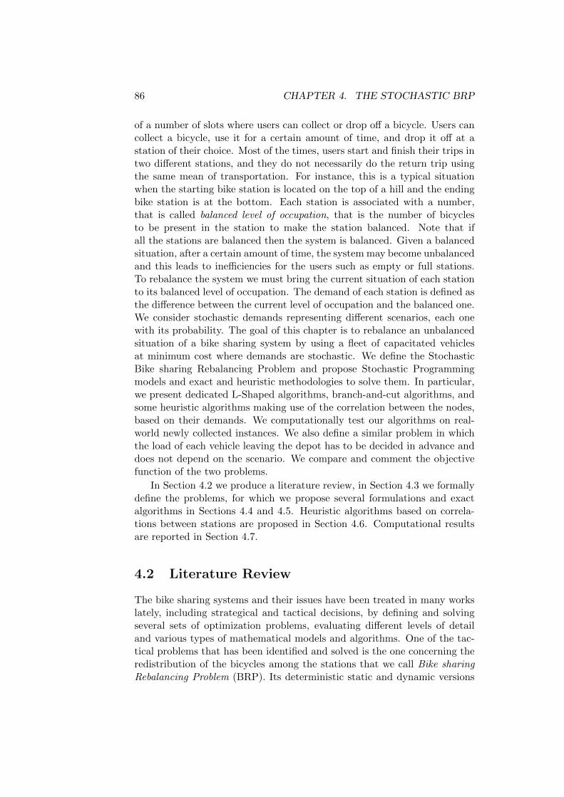
86 CHAPTER 4. THE STOCHASTIC BRP
of a number of slots where users can collect or drop off a bicycle. Users cancollect a bicycle, use it for a certain amount of time, and drop it off at astation of their choice. Most of the times, users start and finish their trips intwo different stations, and they do not necessarily do the return trip usingthe same mean of transportation. For instance, this is a typical situationwhen the starting bike station is located on the top of a hill and the endingbike station is at the bottom. Each station is associated with a number,that is called balanced level of occupation, that is the number of bicyclesto be present in the station to make the station balanced. Note that ifall the stations are balanced then the system is balanced. Given a balancedsituation, after a certain amount of time, the system may become unbalancedand this leads to inefficiencies for the users such as empty or full stations.To rebalance the system we must bring the current situation of each stationto its balanced level of occupation. The demand of each station is defined asthe difference between the current level of occupation and the balanced one.We consider stochastic demands representing different scenarios, each onewith its probability. The goal of this chapter is to rebalance an unbalancedsituation of a bike sharing system by using a fleet of capacitated vehiclesat minimum cost where demands are stochastic. We define the StochasticBike sharing Rebalancing Problem and propose Stochastic Programmingmodels and exact and heuristic methodologies to solve them. In particular,we present dedicated L-Shaped algorithms, branch-and-cut algorithms, andsome heuristic algorithms making use of the correlation between the nodes,based on their demands. We computationally test our algorithms on real-world newly collected instances. We also define a similar problem in whichthe load of each vehicle leaving the depot has to be decided in advance anddoes not depend on the scenario. We compare and comment the objectivefunction of the two problems.
In Section 4.2 we produce a literature review, in Section 4.3 we formallydefine the problems, for which we propose several formulations and exactalgorithms in Sections 4.4 and 4.5. Heuristic algorithms based on correla-tions between stations are proposed in Section 4.6. Computational resultsare reported in Section 4.7.
4.2 Literature Review
The bike sharing systems and their issues have been treated in many workslately, including strategical and tactical decisions, by defining and solvingseveral sets of optimization problems, evaluating different levels of detailand various types of mathematical models and algorithms. One of the tac-tical problems that has been identified and solved is the one concerning theredistribution of the bicycles among the stations that we call Bike sharingRebalancing Problem (BRP). Its deterministic static and dynamic versions

4.3. PROBLEMS DESCRIPTION 87
have been tackled. For a complete literature review on the static version werefer the reader to the previous chapters, where recent works on exact andmetaheuristic algorithms are described. A dynamic version of the problemis solved heuristically by Contardo et al. [4].
The deterministic versions of the problem have been studied and tackledin many recent works and some papers that we describe in the followingmade use of historical data. Instead, according to our knowledge, stochas-tic versions of the BRP have not been considered yet. Regue and Recker[11] also solved a dynamic problem, where the routing and the inventoryproblems are both accounted and the stochastic part is considered by us-ing historical data by means of a demand forecasting model. Saharidis et al.[12] define a mathematical formulation to design the bike sharing infrastruc-ture, deciding the location and the size of the bike stations, incorporatinga hourly demand estimation. Wang and Wang [15] provide an analysis onbike repositioning strategies proposing a simulation study where real timeand historical data are considered.
Stochastic optimization and in particular stochastic vehicle routing prob-lems have been studied in several works and with diverse methodologies inthe last years, we refer the interested reader to Birge and Louveaux [2] andto King and Wallace [5]. The stochastic vehicle routing problems wherethe stochastic variables are the demands (i.e., the vehicle routing problemswith stochastic demands) have been modeled and solved with a chance con-strained programming approach (see, e.g., Gouden and Stewart [13]), witha robust optimization approach (see, e.g, Bertsimas and Simchi-Levi [1]),and with stochastic programming with recourse (see, e.g., Laporte et al.[6]). The reader can have an idea of the heterogeneity of the works onthe stochastic vehicle routing problems in Gendreau et al [6]. Besides that,to our knowledge, problems with positive and negative stochastic demandsof the same product (i.e., one-commodity pickup and delivery VRPs/TSPswith stochastic demands) have been tackled only by Louveaux and Salazar-Gonzalez in [7] and [8], where they study the TSP version and a particularattention is payed to the vehicle capacity. In the following we define, modeland solve two versions of the family of one-commodity pickup and deliveryVRPs with stochastic demands.
4.3 Problems description
The Stochastic Bike sharing Rebalancing Problem (SBRP) is modeled on acomplete digraph G = (V,A), where V = 0, 1, . . . , n is the set of verticesincluding the n customers and the depot (vertex 0) and A is the set of arcsbetween each pair of vertices. For each vertex i ∈ V \0 a request qωi is givenfor every scenario ω ∈ Ω, where Ω is the set of all the possible scenarios andpω is the probability of the scenario ω, knowing that
∑ω∈Ω p
ω = 1. Requests

88 CHAPTER 4. THE STOCHASTIC BRP
can be positive or negative, we refer to as a pickup vertex and delivery vertexif the request is positive or negative, respectively. The quantities picked upat pickup vertices can be used to respond to demand of delivery verticesor go to the depot, so as to some quantities can come from the depot, ifneeded. We impose that a station with null request must be visited. In theSBRP the demands of different vertices and scenarios can be not respectedby paying a penalty ki for each unit of slack and surplus in vertices i ∈ V .These quantities of exceeding and lacking demands are limited by someconsiderations on the dimension Hi of each station and the balanced levelof occupation di of each station. The objective of the SBRP is to drive thefleet of m identical vehicles of capacity Q available at the depot to a set ofroutes in order to respond to the scenario demands, if possible, or by payingpenalties, and minimizing the sum of the traveling costs and the penaltycosts.
The Stochastic Bike sharing Rebalancing Problem with Fixed startingflows (SBRPF) is a similar problem, where the number of bikes to load oneach vehicle leaving the depot have to be determined before the realizationof the demands.
4.4 Formulations for the SBRP
In this section we present a set of formulations to solve the SBRP. Weadopted the terminology used in Birge and Louveaux [2].
4.4.1 Deterministic Equivalent Program
The first formulation we introduce in (4.1)-(4.12) is the Deterministic Equiv-alent Program (DEP). We define variables xij , (i, j) ∈ A, that can take value1 if arc (i, j) is used and 0 otherwise. The cost of traveling arc (i, j) is cij .Variable fωij represents the quantity flowing on the arc (i, j) ∈ A in scenarioω ∈ Ω. Variables sωj and yωj are the slack and surplus variables used to paya cost kj for each unit of slack and surplus when the flows do not respectthe demand at vertex j ∈ V \ 0 in scenario ω ∈ Ω.
(DEP) min∑i∈V
∑j∈V
cijxij +∑ω∈Ω
pω∑
j∈V \0
kj(yωj + sωj ) (4.1)
∑i∈V
xij = 1 j ∈ V \ 0 (4.2)∑i∈V
xji = 1 j ∈ V \ 0 (4.3)∑j∈V
x0j ≤ m (4.4)

4.4. FORMULATIONS FOR THE SBRP 89
∑i∈S
∑j∈S
xij ≤ |S| − 1 S ⊆ V \ 0 , S 6= ∅
(4.5)
fωij ≤ Qxij (i, j) ∈ A,ω ∈ Ω
(4.6)∑i∈V
fωji −∑i∈V
fωij = qωj + yωj − sωj j ∈ V \ 0 , ω ∈ Ω
(4.7)
yωj ≤ dj j ∈ V \ 0 , ω ∈ Ω
(4.8)
sωj ≤ Hj − dj j ∈ V \ 0 , ω ∈ Ω
(4.9)
yωj , sωj ≥ 0 j ∈ V \ 0 , ω ∈ Ω
(4.10)
fωij ≥ 0 (i, j) ∈ A,ω ∈ Ω
(4.11)
xij ∈ 0, 1 (i, j) ∈ A. (4.12)
The objective function (4.1) of the DEP considers two components, onethat aims at minimizing the traveling costs and a second component thatpays a penalty kj for every unit of demand that is not fulfilled, multiplied bythe probability of the related scenario. Constraints (4.2) and (4.3) imposethat one and only one arc can enter and exit every vertex but the depot.Constraint (4.4) set that the maximum number of arcs leaving the depotis not grater than the available vehicles. Subtours are avoided thanks toconstraints (4.5). In (4.6) we state that the flows can be at most the capacityof the vehicles if the corresponding arc is used, 0 otherwise. Constraints (4.7)assert that the difference between the exiting and entering flows in a vertexmust be equal to the demand of a certain vertex and scenario corrected bythe surplus and the slack variables. In constraints (4.8) and (4.9) a bound isset to the surplus and slack variables. In particular, we state that we cannotexceed the capacity of the station and that we cannot collect more bikes thanwhat we have in the station. To make easier to understand constraints (4.8)and (4.9), we report, in Figure 4.1, the possible balanced level of occupationdj with respect to a negative or non-negative demand, given that lj is thecurrent level of occupation of a station j ∈ V \ 0. One can correctlysay that the current level of occupation lj is the stochastic variable (moreproperly lωj ), although because the balanced level of occupation is fixedfor each station, the demand can be considered as the stochastic variablewithout loss of correctness, being
qωj = lωj − dj , j ∈ V \ 0, ω ∈ Ω. (4.13)

90 CHAPTER 4. THE STOCHASTIC BRP
We then impose the flow, slack and surplus variables to be positive in (4.10)and (4.11). In (4.12) the x variables are declared booleans.
Figure 4.1: Picture of the parameters of a station.
4.4.2 Two-stage Formulation
In this subsection we propose a two-stage Stochastic Linear Programming(SLP) model with simple recourse for the SBRP. As typical for the two-stageSLP models we can separate the DEP into two stages, the first one takesinto account the deterministic part of the problem, the decisions to takehere and now, whilst the second stage model represents a set of models,one for each scenario, that take as input the decisions made at the firststage and make them fit with the request of the various scenarios after therealization. To perform this fitting a cut is produced and inserted into thefirst stage model. Both models must be solved in an iterative way: when theinequalities produced by the second stage models do not cut the solution ofthe first stage then the optimal solution has been found.
(1-Stage) min∑i∈V
∑j∈V
cijxij + E(z(ω, y, s)) (4.14)
∑i∈V
xij = 1 j ∈ V \ 0 (4.15)∑i∈V
xji = 1 j ∈ V \ 0 (4.16)∑j∈V
x0j ≤ m (4.17)
∑i∈S
∑j∈S
xij ≤ |S| − 1 S ⊆ V \ 0 , S 6= ∅ (4.18)
xij ∈ 0, 1 (i, j) ∈ A. (4.19)

4.4. FORMULATIONS FOR THE SBRP 91
The objective function (4.14) of the first stage model contemplates thetraveling costs and the expected value of the solution of the second stage.This second component of (4.14) is the expected value of the solutions ofthe second stage models and substitutes the second component of (4.1), thatdefined the costs due to the penalties. Constraints (4.15)-(4.19) are similarto (4.2)-(4.5) and (4.12).
(2-Stage) min z(ω, y, s) =∑
j∈V \0
kj(yωj + sωj ) (4.20)
fωij ≤ Qxij (i, j) ∈ A (4.21)∑i∈V
fωji −∑i∈V
fωij = qωj + yωj − sωj j ∈ V \ 0 (4.22)
yωj ≤ dj j ∈ V \ 0 (4.23)
sωj ≤ Hj − dj j ∈ V \ 0 (4.24)
yωj , sωj ≥ 0 j ∈ V \ 0 (4.25)
fωij ≥ 0 (i, j) ∈ A (4.26)
The second stage formulation includes a model for each scenario ω ∈ Ω.Constraints (4.22) impose that the difference between the outgoing and theincoming flows coming from the first stage model respects the demands and,if not possible, doing it by using slack and surplus variables. Every unit ofslack and surplus is payed into the objective function (4.20) with a cost kj .The slack and surplus variables are bounded in (4.23) and (4.24). Then wehave the non-negativity constraints.
The most common way to solve a two-stage stochastic model is repre-sented by the L-Shaped method (see, e.g., Birge and Louveaux [2]), whichsolves the first stage LP, takes the linking variables between the two stages(xij) and uses them as fixed into all the second stage models. The dual prob-lem of the second stage problem is then solved for each ω ∈ Ω: if at leastone dual of the second stage problem is unbounded we need a feasibility cut,i.e., the first stage solution is not feasible for every scenario and we mustimpose its feasibility with a cut and solve again the first stage model.Whenall duals are feasible we could need to introduce an optimality cut, if it doesnot cut the solution then this is optimal, otherwise the cut that imposes thesolution vector to change or the penalty value (η, the variable that considersthe expected value of the second stage model) to increase. In this latter casewe must recompute the first stage model with the new cut.
Then the dual problem of the second stage problem can be written as in

92 CHAPTER 4. THE STOCHASTIC BRP
(4.27)-(4.38).
(2-Stage Dual) max zD(ω, y, s) = Q∑i∈V
∑j∈V
xijµωij+∑
j∈V \0
qωj φωj +
∑j∈V \0
djπωj +
∑j∈V \0
(Hj + dj)νωj
(4.27)
µωjj ≤ 0 j ∈ V (4.28)
µω0j − φωj ≤ 0 j ∈ V \ 0 (4.29)
µωj0 + φωj ≤ 0 j ∈ V \ 0 (4.30)
µωij + φωi − φωj ≤ 0 (i, j) ∈ A, i, j 6= 0, i 6= j
(4.31)
πω0 ≤ k0 (4.32)
πωj − φωj ≤ kj j ∈ V \ 0 (4.33)
νω0 ≤ k0 (4.34)
νωj + φωj ≤ kj j ∈ V \ 0 (4.35)
µωij ≥ 0 (i, j) ∈ A (4.36)
νωj , πωj ≥ 0 j ∈ V \ 0 (4.37)
φωj free j ∈ V \ 0. (4.38)
The overall formulation of the L-Shaped method, that we call L-ShapedFormulation, can be written as in (4.39)-(4.47), where η is the variable thattakes into account the penalties caused by the second stage models and thederived optimality cuts which are made explicit in (4.40). The feasibility cutsare shown in (4.41). |Topt| is the number of iterations providing optimalitycuts, while |Tfeas| is the number of iterations giving feasibility cuts, and|Topt| + |Tfeas| is the number of the iteration needed to obtain the optimalsolution.
(L-Shaped) min∑i∈V
∑j∈V
cijxij + η (4.39)

4.4. FORMULATIONS FOR THE SBRP 93
η ≥∑ω∈Ω
pω(−Q
∑(i,j)∈A
µω,tij xij−∑i∈V \0
φω,ti qωi −∑
i∈V \0
πω,ti di−
∑i∈V \0
νω,ti (Hi − di)) t ∈ Topt (4.40)
Q∑
(i,j)∈A
µω,tij xij ≥ −∑
i∈V \0
φω,ti qω,ti −∑i∈V \0
πω,ti di −∑
i∈V \0
νω,ti (Hi − di)t ∈ Tfeas (4.41)
∑i∈V
xij = 1 j ∈ V \ 0 (4.42)∑i∈V
xji = 1 j ∈ V \ 0 (4.43)∑j∈V
x0j ≤ m (4.44)
∑i∈S
∑j∈S
xij ≤ |S| − 1 S ⊆ V \ 0 , S 6= ∅ (4.45)
xij ∈ 0, 1 (i, j) ∈ A (4.46)
η ≥ 0. (4.47)
Branch-and-cut Implementation
We can solve the model described in (4.39)-(4.47) in a branch-and-cut fash-ion and we call this implementation One-cut B&C. In the DEP, the L-ShapedFormulation, and in the One-cut B&C we insert in the model the subtourelimination constraints (see, e.g., (4.45)) only when violated. To do so wefirstly use a heuristic procedure to detect a violated cut, this procedure iscalled max-back (see, e.g., Naddef and Thienel [9]). If no violated cut isfound we use the well known max-flow algorithm to find the most violatedone. After the seventh node of the branching tree we use only the max-flow procedure if the current solution is not integer. In the One-cut B&Calso the the constraints (4.40) and (4.41) are inserted in a branch-and-cutfashion when violated. This evaluation is performed at each branching nodeconsidering also fractional variables. In this case |Topt| + |Tfeas| representsthe number of inserted cuts derived by the scenarios.
4.4.3 Multi-cut Formulation
Another way of solving the two-stage problem is to insert more than oneoptimality cut for the entire set of scenarios, i.e., to insert one optimality

94 CHAPTER 4. THE STOCHASTIC BRP
cut for each scenario that needs its component of costs to increase at a par-ticular iteration. This method is called multi-cut L-shaped method, so weintroduce here the Multi-cut Formulation, defined in (4.48)–(4.56). We needa variable ηω for each scenario ω ∈ Ω. The summation of these new variablesis evaluated into the objective function (4.48) and the new optimality con-straints are represented in (4.49). |Topt| · |Ω|+ |Tfeas| represents the numberof iterations needed by the multi-cut L-Shaped algorithm to converge.
(Multi-cut) min∑i∈V
∑j∈V
cijxij +∑ω∈Ω
ηω (4.48)
ηω ≥ pω(−Q
∑(i,j)∈A
µω,tij xij −∑
i∈V \0
φω,ti qωi −∑i∈V \0
πω,ti di −∑
i∈V \0
νω,ti (Hi − di)) t ∈ Topt, ω ∈ Ω
(4.49)
Q∑
(i,j)∈A
µω,tij xij ≥ −∑
i∈V \0
φω,ti qω,ti −∑i∈V
πω,ti di −∑i∈V
νω,ti (Hi − di)t ∈ Tfeas
(4.50)∑i∈V
xij = 1 j ∈ V \ 0
(4.51)∑i∈V
xji = 1 j ∈ V \ 0
(4.52)∑j∈V
x0j ≤ m (4.53)
∑i∈S
∑j∈S
xij ≤ |S| − 1 S ⊆ V \ 0 , S 6= ∅
(4.54)
xij ∈ 0, 1 (i, j) ∈ A(4.55)
ηω ≥ 0 ω ∈ Ω.(4.56)
Branch-and-cut Implementation
Similarly to the L-Shaped Formulation, also the Multi-cut Formulation canbe solved in a branch-and-cut fashion: we call this Multi-cut B&C. For

4.5. FORMULATION FOR THE SBRPF 95
both the Multi-cut Formulation and for the Multi-cut B&C we separateconstraints (4.54) only when violated. As for the single cut case we use aheuristic procedure called max-back (see, e.g., Naddef and Thienel [9]) upto the seventh node of the branching tree or if the solution is integer. If noviolated cut is found we use max-flow algorithm to find the most violatedone. Moreover, in the Multi-cut B&C the constraints (4.49) and (4.50)are inserted in a branch-and-cut fashion when violated. This evaluation isperformed at each branching node considering also fractional variables. Inthis case |Topt| · |Ω|+ |Tfeas| represents the number of inserted cuts derivedby the scenarios.
4.5 Formulation for the SBRPF
In stochastic programming models we need to make some decision here andnow, in the SBRP this is the case of the route design, while some other deci-sion have to be made after the realization of the demand, in the SBRP theseare represented by the definition of the flows of bicycles and of the penal-ties for the demands we will not respond to. The SBRPF is the stochasticversion of the BRP where the flows leaving the depot on each vehicle arevariables that represent decisions to be made here and now. Having thisinformation, the bike sharing company will know the routing informationand the number of bikes to load on the vehicles leaving the depot. To solvethe SBRPF we just present the related deterministic equivalent program be-cause we are interested in comparing the objective function values obtainedwith respect to the SBRP ones. The formulation is reported in (4.57)–(4.70)
(SBRPF) min∑i∈V
∑j∈V
cijxij +∑ω∈Ω
pω∑
j∈V \0
kj(yωj + sωj ) (4.57)
∑i∈V
xij = 1 j ∈ V \ 0
(4.58)∑i∈V
xji = 1 j ∈ V \ 0
(4.59)∑j∈V
x0j ≤ m (4.60)
∑i∈S
∑j∈S
xij ≤ |S| − 1 S ⊆ V \ 0 , S 6= ∅
(4.61)
f0j ≤ Qx0j j ∈ V, ω ∈ Ω(4.62)

96 CHAPTER 4. THE STOCHASTIC BRP
fωij ≤ Qxij (i, j) ∈ A|i 6= 0, ω ∈ Ω
(4.63)∑i∈V
fωji −∑
i∈V \0
fωij − f0j = qωj + yωj − sωj j ∈ V \ 0 , ω ∈ Ω
(4.64)
yωj ≤ dj j ∈ V \ 0 , ω ∈ Ω
(4.65)
sωj ≤ Hj − dj j ∈ V \ 0 , ω ∈ Ω
(4.66)
yωj , sωj ≥ 0 j ∈ V \ 0 , ω ∈ Ω
(4.67)
f0j ≥ 0 j ∈ V(4.68)
fωij ≥ 0 (i, j) ∈ A|i 6= 0, ω ∈ Ω
(4.69)
xij ∈ 0, 1 (i, j) ∈ A.(4.70)
In the SBRPF Formulation, the objective function and the constraintsin (4.57)–(4.61), (4.65)–(4.67), and (4.70) are the same as (4.1)–(4.5), (4.8)–(4.10), and (4.12), while from (4.6), (4.7), and (4.11) we derived (4.62)–(4.64), (4.68), and (4.69). In constraint (4.62) we impose the vehicle leavingthe depot to have the same value for all the scenarios and we bound thisvalue at the capacity of the vehicles. All the other flows are bounded by thecapacity of the vehicles, but they are scenario dependent, as states constraint(4.63). Constraint (4.64) represents the flow conservation constraint for eachvertex but the depot, where the demand must be respected with flows orwith surplus and slack variables, and where the flow coming from the depotis the same for all the scenarios. In constraints (4.68) and (4.69) we imposethe non-negativity of the flow variables.
4.6 Heuristic algorithm based on correlations
One-commodity pickup and delivery problems, as the ones we are tack-ling in this chapter, consider positive demands of some vertices to be usedfor responding to negative demands of other vertices, without having anorigin-destination pair. If demands are stochastic, solution methods cantake advantage of the negative and positive correlations between vertices, ifany. For instance, it is common to have some vertices where the demand isnegative for a relevant number of scenarios, while some other vertices willmanifest positive demands for a relevant number of scenarios, thus the cor-

4.6. HEURISTIC ALGORITHM BASED ON CORRELATIONS 97
relation between one vertex of the first set and a vertex of the second setwill be negative. It is reasonable to look for the arcs of the optimal solu-tion among those connecting negatively correlated vertices because couplingthem can let the load of the vehicle far from the lower and upper bounds0 and Q, and hence more vertices can be served with the same vehicle. Ofcourse distances contribute relevantly to the objective function, and it alsoreasonable to seek the arcs of the optimal solution among those with a smalldistance cost. These considerations justify the simple heuristic algorithmswe propose that consider distances, penalties, and negative correlations inthe evaluating function. The two algorithms proposed are based on the wellknown closest neighbor algorithm (see, e.g., Toth and Vigo [14]) and savingsalgorithm (see, e.g, Clarke and Wright [3]).
4.6.1 Closest neighborhood with correlations
The first heuristic algorithm we propose to solve the SBRP is modeled onthe classical heuristic for solving vehicle routing problems known as closestneighborhood, in which at every iteration the unused closest vertex to thelast vertex of the current route is added at the end of the current route, if theinsertion is feasible. The version of the closest neighborhood we introduce,called Closest neighborhood with correlations, takes into account not onlythe distance between the two vertices added to the penalties needed to makethe insertion feasible for all the scenarios, but also the correlation betweenthe current route and the vertex we are evaluating for the insertion. Inparticular, the correlation is expressed as the Pearson-Bravais correlationcoefficient (see, e.g., Pearson [10]). Let us say that we have two pointsi, j ∈ V \ 0, i 6= j, then the correlation between them is computed asfollows:
ρij =σijσiσj
=
∑ω∈Ω(qωi − qi)(qωj − qj)√∑
ω∈Ω(qωi − qi)2√∑
ω∈Ω(qωj − qj)2
Where qi =∑
ω∈Ω qωi , i ∈ V \0 and being −1 ≤ ρij ≤ 1, where if ρij = −1
there is a perfect negative correlation between i and j, while i and j areperfectly positively correlated if ρij = 1. If two vertices are negativelycorrelated there is a good chance that in many scenarios an increase in thedemand of one vertex can correspond to a decrease in the demand of theother vertex, and this means that, if not to expensive, the arc (i, j) could bein the optimal solution. Otherwise, positive correlations suggest that twovertices have similar behaviors among the scenarios, and hence, probably,they will not be close in the optimal solution.
When we are building the solution with the closest neighborhood algo-rithm we have, on one hand, a vertex to be evaluated for the insertion and,on the other hand, a route being built. Thus, instead of considering a corre-

98 CHAPTER 4. THE STOCHASTIC BRP
lation between two vertices, we consider the correlation between the currentroute R and the vertex j /∈ R. The correlation is then computed as follows:
ρRj =σRjσRσj
=
∑ω∈Ω(
∑i∈R(qωi − qi))(qωj − qj)√∑
ω∈Ω(∑
i∈R(qωi − qR))2√∑
ω∈Ω(qωj − qj)2
Where qR =∑
ω∈Ω
∑i∈R q
ωi . Also in this case we have −1 ≤ ρRj ≤ 1,
where -1 corresponds to perfect negative correlation and 1 to perfect positivecorrelation.
When considering if appending vertex j at the end of the current routeR, j /∈ R, we then use the following evaluating function:
EC(R, j) = α
[cR(|R|),j
max(i,h)∈A cih+
∑ω∈Ω p
ωkj(yωj + sωj )
Q|V |
]+ (1− α)ρRj
(4.71)
Being R(|R|) the last vertex of the current route R, and where α is a rationalnumber between 0 and 1. In the component of the evaluating function mul-tiplied by α we consider a normalized distance cost and normalized penaltiesof the various scenarios. In the second component of the evaluating functionwe consider the correlation of the insertion as we computed in (4.71). Whenthe insertion of every vertex at the end of the current route is more expen-sive than opening a new route or when no more vertex is feasibly insertedthen a new route is open. The algorithm is terminated when all the verticesare assigned to a route.
4.6.2 Savings with correlations
The second heuristic algorithm we propose to solve the SBRP is based onthe well known savings algorithm, in which the iterative cheapest and fea-sible merging of two routes is applied. In the version of the algorithm wepropose, that we call Savings with correlations, we consider the iterativemerging of two routes if it is feasible for all scenarios (where the conceptof feasibility includes the payment of a penalty if non responding to somedemands of some vertices in a scenario). Besides that, we also take intoaccount the correlation between the two routes, let us say R and P , that weare considering for merging, which is computed as follows:
ρRP =σRPσRσP
=
∑ω∈Ω(
∑i∈R(qωi − qR))(
∑j∈P (qωj − qP ))√∑
ω∈Ω(∑
i∈R(qωi − qR))2√∑
ω∈Ω(∑
j∈P (qωj − qP ))2
Where qR =∑
ω∈Ω
∑i∈R q
ωi for route R. Thus the evaluating function
used when merging two routes results in:

4.7. COMPUTATIONAL RESULTS 99
ES(R,P ) = α(κ+ σ) + (1− α)ρRP (4.72)
Being:
κ =cR(|R|−1),P (1) − cR(|R|−1),0 − c0,P (1)
max(i,h)∈A cih
σ =
∑ω∈Ω p
ωkP (1)(yωP (1) + sωP (1))
Q|V |
Where α ∈ R is a number between 0 and 1, R(|R| − 1) is the last vertexof route R before the depot, and P (1) is the first vertex of route P afterthe depot. In the first part of the evaluating function in (4.72), we considerin κ the normalized savings of merging the two routes R and P in thisdirection and in σ the possible normalized penalties to pay if not respectingthe demand of P (1). The second part of (4.72) accounts for the correlationbetween R and P .
In both algorithms the solution does not necessarily respect the maxi-mum number of vehicles, and thus routes, available, even if the algorithmstry to minimize the number of routes.
4.7 Computational Results
In this section we present the computational tests on the different method-ologies used to solve the SBRP and the SBRPF. The algorithms were run onon Intel Core i3-2100 CPU, 3-10 GHz, 4.00 GB, and we used CPLEX 12.6 asthe MILP solver by imposing the selection of a single processor. The testshave been performed on instances derived by real-world data. We firstlydescribe how we collected those data.
4.7.1 Instances
To produce computational evaluation of the algorithms proposed to solvethe two problems here defined, the SBRP and the SBRPF, we collected aset of real-world instances. Firstly we considered a set of usage data of 7month concerning the bike sharing system of the city of Reggio Emilia, inNorthern Italy. These data has been given to us by the operator of thesystem. In addition to this, in order to have a larger number of testinginstances, we collected some data of Capital Bike, the bike sharing systeminstalled in Washington and Arlington, in the USA. The Capital Bike sitefurnishes with complete data on the usage of the system for many years. Wemade use of the usage data of the third quarter of 2014. We also collected thegeographic coordinates and the capacity of each station and used historical

100 CHAPTER 4. THE STOCHASTIC BRP
data to determine the demands of each scenario. To this extent, we clarifythat some correction on data has been necessary because the rebalancing isalready applied to the system and some demands appear to be too large withrespect to the station capacity. From these data we derived several instancesby selecting arbitrarily sets of stations counting from 20 to 66 stations each.We selected randomly a station among all to be used as the depot.
4.7.2 Results
We report here some results of tests performed on the collected instances.Firstly we tested the heuristic algorithms developed: in Table 4.1 we reportthe results obtained by testing the closest neighborhood with correlations.The first column shows the name of the instance, where RE stands for ReggioEmilia, while W stands for Washington; the numbers reports the numberof vertices (|V |) and the capacity of the vehicles (Q), respectively. Thebest lower bound obtained with the exact algorithms is reported (bold ifit is the optimal solution value) and the percentage gap between this valueand the solution value obtained thanks to the closest neighborhood withcorrelations is shown with respect to the different values of α used in theevaluating function. Similarly, the results for the savings with correlationsare reported in Table 4.2.
In Tables 4.1 and 4.2 the best gap obtained is highlighted. One cannotice that the heuristic algorithms do not present very good gaps withrespect to the best known lower bound. These gaps are large because thealgorithms move in the space of feasible solutions and it is not easy to buildcompetitive solutions that are feasible for all the scenarios (172, in the caseof Reggio Emilia, and 91 in the case of Washington). Besides that, one canobserve that the savings with correlations shows better results with respectto the closest neighborhood with correlations algorithm. Moreover, it canbe noticed that for some level of α the solution values are improved whileconsidering the correlations with respect to the classical heuristics, indeedvalues of α around to 0.9 for the closest neighborhood with correlations andaround 0.8 for the savings with correlations algorithm show the best results.
We now consider the results obtained thanks to the exact algorithms wedeveloped. In Table 4.3 we report the results on the collected test instanceswhile running the DEP Formulation. In particular, we report the name ofthe instance, the best lower bound (LB) and upper bound (UB), if any,and we compute and show the percentage gap between those two values.In the last column we report the time, in seconds, needed to terminate thealgorithm within a time limit set to one hour. Similarly, in Tables 4.4,4.5, 4.6, and 4.7 the results on the same instances given by the L-ShapedFormulation, the Multi-cut Formulation, the One-cut B&C implementation,and the Multi-cut B&C implementation are reported.
One can see that only the One-cut B&C and the Multi-cut B&C algo-

4.7. COMPUTATIONAL RESULTS 101
α
Inst. LB 0 0.1 0.2 0.3 0.4 0.5 0.6 0.7 0.8 0.9 1
RE(16,20) 16900.0000 39.43 43.67 31.58 31.58 38.55 35.00 30.45 21.76 21.03 19.91 25.55W(20,25) 81576.3736 77.56 55.57 55.57 53.28 52.95 50.40 50.11 49.41 49.41 49.21 49.16W(20,15) 77306.7802 80.92 80.93 77.28 77.28 80.83 80.98 81.15 81.15 80.97 77.33 80.91W(30,20) 101515.3967 75.53 66.51 65.38 63.27 59.76 58.63 60.42 54.53 67.17 67.42 67.48W(30,35) 120517.5714 75.92 68.60 66.33 64.33 62.82 60.92 60.51 58.35 55.62 54.12 50.86W(40,40) 101718.0349 83.69 77.05 79.14 79.14 79.14 79.47 78.77 75.32 74.59 77.53 77.65W(40,35) 103300.4636 87.86 85.62 85.63 85.63 85.63 85.50 85.63 86.68 86.53 86.51 86.62W(50,20) 121691.0000 87.91 85.83 85.80 83.32 83.07 85.40 85.40 87.46 83.80 84.79 84.91W(66,15) 131371.9231 89.33 79.20 64.28 57.04 54.39 49.98 49.60 47.72 43.19 38.80 34.85
Avg. 77.58 71.45 67.89 66.10 66.35 65.15 64.67 62.49 62.48 61.74 62.00
Table 4.1: Percentage gap between the solution of the closest with correla-tions and the best lower bound for all instances by changing the parameterα.
α
Inst. LB 0 0.1 0.2 0.3 0.4 0.5 0.6 0.7 0.8 0.9 1
RE(16,20) 16900 44.41 37.41 25.88 17.96 17.96 15.50 9.63 9.63 6.11 8.65 8.65W(20,25) 81576.3736 62.08 67.51 55.40 52.42 52.58 51.34 48.58 45.59 43.81 44.20 60.15W(20,15) 77306.7802 77.95 78.00 81.00 80.87 77.56 77.35 80.79 77.04 76.97 76.88 71.35W(30,20) 101515.3967 68.73 61.39 58.11 63.89 60.90 55.71 57.76 48.00 21.16 44.87 44.67W(30,35) 120517.5714 65.02 68.17 67.15 63.89 62.88 59.78 57.85 55.02 51.01 50.81 50.32W(40,40) 101718.0349 74.52 75.42 78.25 78.81 75.02 74.05 77.33 76.89 72.83 75.48 75.64W(40,35) 103300.4636 85.85 84.26 83.91 85.13 85.14 85.00 86.04 86.12 83.32 84.59 84.58W(50,20) 121691.0000 85.02 85.70 85.52 82.59 82.34 85.06 83.88 84.83 83.13 83.14 82.82W(66,15) 131371.9231 89.62 85.82 84.19 82.37 82.37 72.81 49.02 47.75 43.99 40.39 28.13
Avg. 72.58 71.52 68.82 67.55 66.31 64.07 61.21 58.98 53.59 56.56 56.26
Table 4.2: Percentage gap between the solution of the savings with correla-tions and the best lower bound for all instances by changing the parameterα.

102 CHAPTER 4. THE STOCHASTIC BRP
rithms can find a feasible solution for all the evaluated instances, in partic-ular the Multi-cut B&C is the algorithm, among all those presented, thatfound the smallest percentage gaps, that are 4.88% in average. On the otherhand the L-Shaped Formulation and the Multi-cut Formulation can get theoptimal values of six instances out of nine, while for W (40, 40), W (40, 35),and W (50, 20) they could not find a feasible solution. The DEP Formulationcould find a feasible solution only for the first five instances, but furnishedwith the best lower bound for W (40, 40) and W (40, 35), among all. Thebest upper bound for W (50, 20) is given by the Multi-cut Formulation. Thebest solving times are obtained by the Multi-cut B&C algorithm that needs1248.43 seconds to terminate, in average. Also the Multi-cut Formulation,which made use of a multi-cut L-Shaped algorithm, offers promising solvingtimes, that is in average 1252.45 seconds. To conclude, the Multi-cut B&Calgorithm seems the best performing one among the ones we tested on ourtest instances.
DEP
Inst. LB UB %gap t(sec)
RE(16,20) 16900.0000 16900.0000 0.00 9.88W(20,25) 81576.3736 81576.3736 0.00 424.29W(20,15) 77306.7802 77306.7802 0.00 31.79W(30,20) 101516.0000 101516.0000 0.00 412.12W(30,35) 120517.5714 120517.5714 0.00 1277.20W(40,40) 101718.0349 - - 3600.00W(40,35) 103300.4636 - - 3600.00W(50,20) 117067.0879 - - 3600.00W(66,15) 109426.9021 - - 3600.00
Avg. 1839.476
Table 4.3: Results obtained by running the DEP Formulation.
L-Shaped
Inst. LB UB %gap t(sec)
RE(16,20) 16900.0000 16900.0000 0.00 0.42W(20,25) 81576.3736 81576.3736 0.00 41.41W(20,15) 77306.7802 77306.7802 0.00 0.88W(30,20) 101516.2967 101516.2967 0.00 2.48W(30,35) 120517.5714 120517.5714 0.00 3.77W(40,40) 96715.0000 - - 3600.00W(40,35) 92828.0000 - - 3600.00W(50,20) 118714.0000 - - 3600.00W(66,15) 131313.6264 131313.6264 0.00 3258.75
Avg. 1567.52
Table 4.4: Results obtained by using the L-shaped method to solve theL-Shaped Formulation.
In Table 4.8 we report the results for the SBRPF we performed according

4.7. COMPUTATIONAL RESULTS 103
Lshaped Multi-cut
Inst. LB UB %gap t(sec)
RE(16,20) 16900.0000 16900.0000 0.00 1.06W(20,25) 81576.3736 81576.3736 0.00 16.13W(20,15) 77306.7802 77306.7802 0.00 2.95W(30,20) 101516.2967 101516.2967 0.00 9.95W(30,35) 120517.5714 120517.5714 0.00 7.83W(40,40) 96715.0000 - - 3600.00W(40,35) 92828.0000 - - 3600.00W(50,20) 121691.0000 - - 3600.00W(66,15) 131313.6264 131313.6264 0.00 434.12
Avg. 1252.45
Table 4.5: Results obtained by using the L-shaped multi-cut method to solvethe Multi-cut Formulation
One-cut B&C
Inst. LB UB %gap t(sec)
RE(16,20) 16900.0000 16900.0000 0.00 3.60W(20,25) 81576.3736 81576.3736 0.00 151.34W(20,15) 77306.7802 77306.7802 0.00 3.09W(30,20) 101516.2967 101516.2967 0.00 15.83W(30,35) 120517.5714 120517.5714 0.00 16.15W(40,40) 100158.2076 2502063.0000 96.00 3600.00W(40,35) 101506.7796 187114.7802 45.75 3600.00W(50,20) 121388.6227 3576619.0000 96.61 3600.00W(66,15) 131313.6264 131313.6264 0.00 2541.60
Avg. 26.48 1503.51
Table 4.6: Results obtained by using the One-cut B&C algorithm with theL-Shaped method derived cuts.
Multi-cut B&C
Inst. LB UB %gap t(sec)
RE(16,20) 16900.0000 16900.0000 0.00 2.23W(20,25) 81576.3736 81576.3736 0.00 26.90W(20,15) 77306.7802 77306.7802 0.00 3.25W(30,20) 101516.2967 101516.2967 0.00 10.30W(30,35) 120517.5714 120517.5714 0.00 14.23W(40,40) 100531.6473 133940.7802 24.94 3600.00W(40,35) 101984.7100 121856.5385 16.31 3600.00W(50,20) 121561.5534 124862.3956 2.64 3600.00W(66,15) 131313.6264 131313.6264 0.00 378.96
Avg. 4.88 1248.43
Table 4.7: Results obtained by using the Multi-cut B&C algorithm with theL-Shaped multi-cut method derived cuts.

104 CHAPTER 4. THE STOCHASTIC BRP
to what we did for the SBRP. One can notice that the instances that wereeasy to solve for the SBRP remain easy to solve also for the SBRPF and theinstances that were hard to solve for the SBRP remain hard to solve for theSBRPF. We can observe that the objective function value does not changeremarkably if compared to the SBRP one. This can lead to the conclusionthat the SBRP solution is robust even if a a priori decision on the load ofthe vehicles is not contemplated.
SBRPF DEP
Inst. LB UB %gap t (sec)
RE(16,20) 16922.5989 16922.5989 0.00 17.04W(20,25) 82054.3956 82054.3956 0.00 518.55W(20,15) 77389.1978 77389.1978 0.00 36.94W(30,20) 101928.4835 101928.4835 0.00 785.06W(30,35) 120742.8462 120742.8462 0.00 1051.97W(40,40) 101901.4091 - - 3600.00W(40,35) 103615.1235 - - 3600.00W(50,20) 117564.6711 - - 3600.00W(66,15) 110455.1959 - - 3600.00
Avg. 1867.73
Table 4.8: Results for the SBRPF on the test instances obtained by runningthe corresponding DEP Formulation.
4.8 Conclusions
In this chapter we defined and solved the SBRP, the stochastic version ofone a tactical problem that arises in bike sharing systems, that is the one ofredistributing bicycles among the bike stations of the system, the BRP. Tosolve the SBRP we proposed a deterministic equivalent program formulation,a two-stage stochastic linear programming model with simple recourse solvedby means of a L-Shaped algorithm, a multi-cut L-Shaped algorithm, andtwo branch-and-cut algorithms. To obtain upper bounds for the SBRP wedeveloped two heuristic algorithms that take advantage of the informationon the demands on different scenarios considering the negative and positivecorrelations between the vertices. We tested all the algorithms on newlycollected real-world instances proving the effectiveness of our methodologies,in particular, good results can be obtained with branch-and-cut algorithmswhere cuts are derived from the multi-cut L-Shaped method. Moreover, theproposed heuristic algorithms showed improved solutions when accountingfor correlations in the evaluating functions. Finally, we defined a stochasticversion of the BRP where the loads on vehicles leaving the depot must bedecided before the realization of the demands. We compare the values ofthe solutions of the two problems, and the objective functions differs of asmall amount of costs.

Bibliography
[1] D. J. Bertsimas and D. Simchi-Levi. A new generation of vehicle rout-ing research: robust algorithms, addressing uncertainty. OperationsResearch, 44:286–304, 1996.
[2] J. R. Birge and F. Louveaux. Introduction to stochastic programming.Springer Science & Business Media, 2011.
[3] G. Clarke and J. W. Wright. Scheduling of vehicles from a central depotto a number of delivery points. Operations research, 12:568–581, 1964.
[4] C. Contardo, C. Morency, and L.-M. Rousseau. Balancing a dynamicpublic bike-sharing system. Technical Report CIRRELT-2012-09, CIR-RELT, 2012.
[5] A. J. King and S. W. Wallace. Modeling with stochastic programming.Springer Science & Business Media, 2012.
[6] G. Laporte, F. Louveaux, and L. Van Hamme. An integer l-shapedalgorithm for the capacitated vehicle routing problem with stochasticdemands. Operations Research, 50:415–423, 2002.
[7] F. Louveaux and J.-J. Salazar-Gonzalez. On the one-commoditypickup-and-delivery traveling salesman problem with stochastic de-mands. Mathematical programming, 119:169–194, 2009.
[8] F. Louveaux and J.-J. Salazar-Gonzalez. Solving the single vehiclerouting problem with variable capacity. Transportation Science, 2014.
[9] D. Naddef and S. Thienel. Efficient separation routines for the sym-metric traveling salesman problem i: general tools and comb separation.Mathematical Programming, 92:237–255, 2002.
[10] K. Pearson. Notes on the history of correlation. Biometrika, 25–45,1920.
[11] R. Regue and W. Recker. Proactive vehicle routing with inferred de-mand to solve the bikesharing rebalancing problem. Transportation Re-search Part E: Logistics and Transportation Review, 72:192–209, 2014.
105

106 BIBLIOGRAPHY
[12] G. K. D. Saharidis, A. Fragkogios, and E. Zygouri. A multi-periodicoptimization modeling approach for the establishment of a bike sharingnetwork: a case study of the city of athens. In Proceedings of theInternational MultiConference of Engineers and Computer Scientists,2, 2014.
[13] W. R. Stewart and B. L. Golden. Stochastic vehicle routing: A compre-hensive approach. European Journal of Operational Research, 14:371–385, 1983.
[14] P. Toth and D. Vigo. Vehicle Routing: Problems, Methods, and Appli-cations, SIAM, 2014.
[15] I.-L. Wang and C.-W. Wang. Analyzing bike repositioning strategiesbased on simulations for public bike sharing systems: Simulating bikerepositioning strategies for bike sharing systems. In Advanced AppliedInformatics (IIAIAAI), 2013 IIAI International Conference on IEEE,306–311, 2013.

Part III
Models and Algorithms forEarthwork Optimization
Problems
107


Chapter 5
A Two-Phase EarthworkOptimization Model forHighway Construction
1
One of the main activities in highway construction is earthwork, that isa complex process involving excavation, transportation, and filling of largequantities of different earth material types. Earthwork operations are costly,and undergo several constraints due to their large environmental and socialimpacts. Using mathematical models to produce a minimum-cost earthworkplan that satisfies all constraints is thus of great significance for enhancingthe productivity of the overall construction project.
This chapter presents an earthwork optimization system based on theuse of linear programming that operates in a novel two-phase approach. Inthe first phase an aggregate model determines the feasibility of the overallproject, whereas in a second phase disaggregate models determine the actualflows of each material.
The developed quantitative method for earthwork optimization includesinteresting features derived from the everyday activity of one of the ma-jor European companies in construction. The new two-phase optimizationinvolves classical decisions on excavation, filling, quarries, dump sites, andtemporary depots, but it also accounts for several novelties. One innovationis the presence of time windows imposed by a tight production schedule thatlet the model decide when to conclude the tasks within the time windows.Another new feature is the installation of recycling facilities, which trans-form the excavated materials thanks to a separation and a mixing process so
1The results of this chapter appear in: C. Bogenberger, M. Dell’Amico, G. Fuellerer, G.Hoefinger, M. Iori, S. Novellani and B. Panicucci. A Two-Phase Earthwork OptimizationModel for Highway Construction. to appear on Journal of Construction Engineering andManagement, 2015.
109

110 CHAPTER 5. EARTHWORK OPTIMIZATION MODELS
to obtain several materials apt for filling. Our model includes also a varietyof materials for filling and to be processed in recycling plants. Moreover,the explicit integration of the project with the existing public road networkis considered so to account for local authority restrictions, and to considermultiple paths to link the construction site to the external facilities.
Extensive computational results are obtained by running the models ona set of realistic instances, and show the efficiency of the proposed approachin solving complex earthwork problems.
Keywords: Earthwork, Mathematical Models, Linear Programming, High-way Construction.
5.1 Introduction
A highway construction project involves many steps and may take years to becompleted. Before construction starts, an accurate topographic survey of thearea is developed and a layout of the future road is designed, specifying thealignment (i.e., the base line of the road) and the grades (i.e., the slopes ofthe longitudinal road line). Once the layout of the road has been completed,actual earthwork can begin. Earthwork is, in a few words, the process ofmoving earth from those areas that are too high with respect to the roadgrades to those areas that are too low, and is a crucial aspect of the overallconstruction problem.
More in details, once the road layout is given, one determines the cutareas, where some earth must be dug to accomplish with the required roadgrades, and the fill areas, where instead some earth must be placed, andeasily evaluate the cut and fill volumes for each area. The basic earthworkproblem consists then in digging earth from cut areas and moving it to fillareas, with the goal of minimizing operational costs.
This basic problem is known in the literature as the cut and fill problem,and has been described in classical textbooks (see, e.g., Ahuja et al. [1])as a typical application that can be solved by Minimum Cost Flow (MCF).Indeed, after associating the cut and fill areas to the nodes of a networkand assigning transportation costs to its arcs, the MCF allows to find theflows that move the required volumes at minimum cost, that is, an optimalearthwork solution.
This simple model has been successively expanded to include complica-tions arising in real-world construction problems, such as the presence ofdifferent types of earth, possible transport road constraints (e.g., accessi-bility and/or maximum flow restrictions), and the need of facilities such asdump sites or quarries to accommodate excess or lack of materials. Start-ing from Stark and Nicholls [17], Linear Programming (LP) became thena standard tool for solving optimization issues associated to the earthworkactivities, because it allowed to easily extend the original MCF model to

5.1. INTRODUCTION 111
include such additional constraints.
The aim of this chapter is to further advance the research on earthworkmodeling, by including novel features that derive from the everyday con-struction activities of one of the European leaders in civil engineering. Theactivity that they perform for highway construction is very complex, and hasbeen the motivation that has led us to the development of the models pre-sented in this chapter. Previously, the construction company (Strabag AG.)relied on tools, such Excel files and mass diagrams, integrated by the longterm experience of their practitioners. Thanks to the method presented inthis chpater Strabag, and other construction companies, can quickly eval-uate different configurations and obtain optimal solutions within secondsleaning on a fast and reliable support for decision making.
The optimal approach that we implemented to solve this challengingproblem is based on two phases that contemplate an aggregate model anda disaggregate one, both based on LP. The aggregate model associates avariable with each flow of a material that travels along an arc on a givenperiod, independently from its actual origin and destination. It is funda-mental to investigate the feasibility of the project, considering the giventime horizon, the available resources, and the strong capacity constraintson the arcs. Thanks to the quite small computing times that we managedto obtain for its solution, the aggregate model may be solved several times,under different network configurations, and is thus very helpful to find thebest way to ensure the feasibility of the problem.
To translate the resulting aggregate solution into practical actions involv-ing each material in each period, the disaggregate model is then invoked.This model computes precise flows by taking advantage of the fact that ve-hicles can transport just one material at a time. Indeed, we decompose theproblem in several models, one for each period and material, where decisionsmade at one model do not affect decisions made on the others. Each modeloutputs the optimal flow paths, together with the corresponding volumes,between each material origin and destination.
Aggregate and disaggregate models can be run many times, in a rollinghorizon perspective, to take into consideration the fact that the every dayactivity may diverge from the planned solution. Adjustments, as well asnew information on costs or availability of resources, are easily included inthe models by just modifying the input files. Our approach thus resulted ina powerful and effective decision support system. It is now being used bythe partner company in a highway construction process which is currentlyunder development in Northern Italy near the city of Milan.
5.1.1 Main Contributions
We advance the Body of Knowledge on quantitative methods for earthworkoptimization. We do this by proposing a new mathematical model based on

112 CHAPTER 5. EARTHWORK OPTIMIZATION MODELS
two phases: an aggregate and a disaggregate one. Within the method weinclude a set of properties that were not treated or only partially treatedin the literature and that are important not only for our case study. Wecomment them in the following:Multiple materials: in our model we do not consider only simple earth, asin the basic cut and fill problem, but we optimize the flows of ten differentmaterials. To our knowledge few papers accounts for multiple materials (see,e.g. Hare et al. [8] and Ammar et al. [2]), but in their works they considera multiple set only for digging materials, where some can be used for fillingand some others must be dumped, but they do not consider different typesof materials for filling or to be used for recycling process. In our work weconsider ten materials including three types of excavated earth, differenti-ated according to their quality, and four different filling materials such asasphalt, concrete and the two high quality materials coming from digging.Recycling of the excavated materials: many papers consider to reuseexcavated materials directly for filling, some of them also call it recycling(see, e.g. Ji et al. [10]). In our chapter we use two of the dug materialsfor filling without performing any other transformation, but we also con-sider a transformation process that we call recycling. The recycling activityincludes two transformations of materials to be performed in two plants.The first plant is called Separation plant where a refinement of the highquality excavated material is performed, separating the rocks from the soiland crushing it at the desired level. Some of the resulting material has tobe dumped, while the others two can be mixed with cement or bitumen inMixing plants to produce, respectively, asphalt and concrete, used for filling.To our knowledge this way of recycling materials has not been tackled yet inthe literature related to quantitative methods for earthwork optimization.Time windows: in our work the process is planned according to a spe-cific schedule, that, borrowing a terminology of production literature, wedefine Master Production Schedule (MPS). The MPS defines the activitiesto be performed in the overall period, the location where to dig and/or fillwhich material and the possible time windows in which they have to be com-pleted. Time windows imposed by the MPS have already been inserted incomplex construction projects, but we have not found any explicit referencein the existing Body of Knowledge in quantitative methods for earthworkoptimization. Thus the explicit insertion of time windows in our model is achallenging novelty.External network: quarries and dump sites are located outside with re-spect to the construction site, thus the company vehicles need to cross thepublic external network. Traffic restriction of heavy vehicles are normallyimposed or contracted with the local administrations. This is expressed inamount of cubic meters per day on a restricted set of roads. To deal withthat we consider capacity restriction on the arcs representing the externalnetwork, the availability of different paths on alternative roads, and the use

5.2. PROBLEM DESCRIPTION 113
of access points from the construction site to the external network. To ourknowledge just Burdett and Kozan [7] consider the problem of having anexternal network. To create a path from the construction site to an externalsite they use the Dijkstras algorithm to solve the shortest path, but thisalgorithm does not allow to have multiple paths from two locations: thusthey consider only one path otherwise they must fix some dummy nodes. Inboth disaggregate models we present this problem does not arise , indeedthe multi-commodity model can evaluate multiple arcs between two node,and the path-based model makes use of the labeling algorithm, that can findmore than one path between two nodes.
These innovations with respect to the Body of Knowledge are motivatedby the Strabag study case we considered. They appear in the model asconstraints but they can be easily inactivated one by one, so to let themodel to be very general and applied to many other cases.
5.2 Problem Description
Earthwork is a fundamental stage in highway construction process that in-volves several activities and requires careful planning and various evalua-tions, including environmental and structural assessments. The main earth-work activities that we identified are depicted in Figure 5.1. They includedigging, filling, recycling, material disposal in dump sites, temporary allo-cation of materials in depots, and material acquisition from quarries.
Figure 5.1: Activities flow chart.
The digging activities consist of cutting and moving a huge amount of

114 CHAPTER 5. EARTHWORK OPTIMIZATION MODELS
earth, typically in the order of (tens of) millions of cubic meters by means ofspecial plant machinery such as excavators and trucks. The filling activitiesconsist of carrying across the construction site a certain amount of a certainmaterial, to, e.g., fill earth cuts and trenches, or build bridges and artificialgalleries.
A fundamental step in the digging process is the on-site classification,that is, earth materials are classified depending on their geological charac-teristics and treated consequently. Indeed, materials excavated within thesite are often unacceptable for construction and must be recycled (througha recycling process to be described below) or disposed of. According tothe field activity , three types of dug earth materials can be distinguished,depending on whether they can be reused for purposes of filling, recycled,or else wasted on a dump site. In this chapter we denote them by rawI(high-quality soil and gravel), rawII (soil suitable for filling but not for recy-cling), and rawWaste (waste product without the possibility of further use).Reusing those materials, instead of throwing them directly in dump sites, isenvironmentally relevant and can significantly reduce the cost of earthwork.RawI and rawII materials can be used directly for filling or, if necessary,stored in temporary depots and used later on in the construction process.Temporary depots are flat areas that are rented close to the constructionsite, where dug materials can be stored until they are needed for filling.RawI material can also be reconstituted into other products appropriate forfilling, that is, asphalt and/or concrete, by means of a recycling process.
The inclusion of recycling activities in optimizing earthwork process is,as far as we know, a novelty of this chapter. Recycling is a two-stage process(see again Figure 5.1). In the first stage, separation, rawI material is trans-ported to the so-called separation plants, where it is broken and crushedinto two types of recycled aggregates: recI and recII. In this stage somewaste material, denoted by recWaste, is also produced. In the second stage,mixing, these recycled aggregates are carried to specialized plants wherethey are mixed with other materials to obtain asphalt or concrete. Moreprecisely, in asphalt mixing plants recI is mixed with bitumen to produce as-phalt, and in concrete mixing plants recII is mixed with cement to produceconcrete. The waste produced during separation, denoted by recWaste, aswell as rawWaste and possible surplus of rawI, rawII, recI, and recII aredumped into dump sites. If necessary, raw material for producing asphaltand concrete (i.e., recI and recII), as well as other materials required forfilling can be acquired from private quarries.
The earthwork process must take into account the fact that recyclingand mixing plants, quarries, dump sites, and temporary depots have phys-ical capacity limitations on the total quantity of materials that they canprocess. Moreover, it must be considered that the aforementioned activitiesare bounded in time by the time windows defined by the MPS. In particu-lar, the overall planning horizon is divided into periods (weeks in our study
5.3. LITERATURE REVIEW 115
cases) and each activity time window is represented by a starting and an end-ing period. The optimization of the earthwork process requires to considerthe transportation costs, as well as the costs incurred for storing materialsin temporary depots, acquiring materials from quarries, and disposing ofmaterials into dump sites.
To take into consideration all these issues, we modeled the earthworkactivities by using a directed graph, described in detail below. Briefly, thehighway building site is discretized in segments, and each segment is asso-ciated with a vertex of the graph. The graph is then extended by addingvertices that correspond to quarries, dump sites, temporary depots, andrecycling plants. For modeling purposes we also add a vertex for each dig-ging and filling activity to be performed. A set of arcs is then included torepresent the possible flows of materials from a vertex to another.
The arcs connecting the vertices are assigned a maximum flow capacity,that limits by above the sum of the material flows that can be carried overthe arc in a given period, and can vary during the time. With respect tothis point, we mention another interesting contribution of our approach,that is, the differentiation between private and public networks. The privatenetwork is in practice the highway being built, whereas the public networkis the existing neighbor road infrastructure, that is forcedly affected by theconstruction process. Indeed, some public roads external to the building sitemust also be included into the graph to take into account different paths thatcan be used to reach dump sites and quarries, that are typically located faraway from the site. These roads undergo the national transportation lawsof the country where the construction is taking place, and can have verysmall flow capacities, due to the fact that earth transportation is typicallyperformed by large and heavy trucks that have a large environmental andsocial impact on the surrounding areas.
In this framework, the goal of our optimization is to decide when and howmoving, storing, recycling, buying, or wasting materials, while responding todigging and filling requests in the imposed time windows, respecting capacityconditions on nodes and arcs, and minimizing total costs.
5.3 Literature Review
Apart from the basic MCF applications already discussed in the introduc-tion, see again Ahuja et al. [1], the first LP model to provide the earthworkallocation that minimizes the cost of the earthmoving activities, once aninitial layout is given, was suggested in Stark and Nicholls [17] and then de-veloped by Stark and Mayer [16]. The cited model solves the so-called earth-work allocation problem, that includes the presence of capacitated quarriesand dump sites, but does not assess the presence of multiple types of earthand assumes constant unit costs for the earthwork activities.

116 CHAPTER 5. EARTHWORK OPTIMIZATION MODELS
Easa [6] attempted to combine the design of roadway grades with thebasic earthwork allocation problem, limiting his study to a single type ofearth and using a trial and error approach. A combination of grade selectionwith the earthwork allocation problem in a single LP problem was laterdeveloped by Moreb [14]. To account for the different earth material typeswhich are usually encountered in construction practice, Mayer and Stark [13]incorporated the differing earth characteristics by creating different variablesand costs for dirt, gravel, and rock material. Successively, a model thataccommodates for multiple material types was also developed by Ammar etal. [2].
The basic model of Stark and Nicholls [17] has also been extended toinclude different cost functions. In particular, Easa [4, 5] proposed a MixedInteger Linear Programming (MILP) model to incorporate stepwise unitcosts, and a quadratic model to account for linear growth in movementcosts. In Karimi et al. [11] uncertainties in unit cost coefficients of earthworkactivities and facility capacities were considered by using a fuzzy LP model.Another extension of the basic earthwork allocation model, encompassingthe project duration and a dynamic selection of quarries and dump sites, wasintroduced by Jayawardane and Harris [9], and solved by employing MILP.Another MILP model was used in Hare et al. [8], to capture the presenceof natural obstacles that limit earth movements.
Marzouk and Moselhi [12], by using computer simulation and geneticalgorithms, considered a multi-objective framework for managing earthmov-ing operations so as to improve productivity, efficiency, and safety. Multi-objective simulation-optimization techniques were also used in Zhang [20],where earthmoving operations are modeled through simulation and a par-ticle swarm optimization method is used to avoid exhaustive simulationexperiments of all the alternatives. Xianja et al. [19] established a bilevelprogramming model, where the objective of the upper level is that of min-imizing the transportation cost, while the objective of the lower level is tobalance the supply and demand of earthwork in the digging and filling ac-tivities. The model is solved by combining particle swarm optimization withthe simplex algorithm.
To meet the need for tools that can assist project managers to plan andmanage construction projects more efficiently, some research efforts in earth-work planning, scheduling, and visualization of the infrastructure construc-tion projects have been conducted. Askew et al. [3] developed an approachto automate the earthwork planning process to create activity sets using aknowledge base and a simulation of earthwork processes. Tam et al. [18]proposed a method to automate the earthmoving planning by integrating apath-finding algorithm, a plant selection system, and a genetic algorithm.In Moselhi and Alshibani [15] genetic algorithms, LP, and geographic infor-mation systems were used to optimize the utilization of construction equip-ment involved in earthmoving operations. None of the cited contributions

5.4. MODELING ANALYSIS AND NOTATION 117
can, however, provide a comprehensive solution to all the aspects of theconstruction process that is faced by Strabag and that we describe in thenext sections.
5.4 Modeling Analysis and Notation
This section provides an overview of the network that we use for modelingthe highway construction project, as well as the main notation that weadopt in the remaining of the chapter. To account for the fact that theMPS bounds each activity of the project in time by a time window, weconsider an environment in which the overall horizon is discretized into aset of uniform periods (weeks in our study), T = 1, 2, . . . , Tmax. Thenetwork is represented by a graph G = (V,A) defined by a collection ofnodes V and arcs A, and is schematized in Figure 5.2.
Figure 5.2: Network representation.
Among all the nodes in V, we identify a set H of nodes representingmaterial locations, that is, cut and fill areas where different types of materialscan be dug or filled in (e.g., nodes 1, . . . , 12 in Figure 5.2. In other words,H represents the discretization of the highway being built. The materiallocations might need more than one digging/filling of one or more materialsto be completed in different time windows. We thus need to introduce anew set of nodes (in addition to the material location ones) to deal withthe digging and filling activities of the same material with overlapping timewindows to be performed on the material location. Thus, we consider a setI of nodes representing tasks, that is, digging or filling activities requiredfor a certain material in a given area. In particular, in I we identify Ifas the set of filling tasks (e.g., nodes 17, 19, 20, and 21) and Id as the setof digging tasks (e.g., nodes 13, 14, 15, 16, and 18), with If ∪ Id = Iand If ∩ Id = ∅. Each task i ∈ I is associated with a unique locationh(i) ∈ H and a unique material m(i) ∈ M, being M the set of all earthmaterials involved in the construction process. Moreover, each task i has itsown quantity di, that must be fully dug/filled in a time window [ts(i), te(i)]specified by its starting period ts(i) ∈ T and its ending period te(i) ∈ T .

118 CHAPTER 5. EARTHWORK OPTIMIZATION MODELS
The network also includes a set D of dump sites, representing locationswhere materials can be disposed of (e.g., nodes 31 and 32), and a set S ofquarries, representing sources where materials can be acquired to respond tofilling requests (e.g., nodes 28 and 29). Note that in our model it is allowedto dispose of some material in a dump site and acquire the same materialfrom a quarry if this leads to decreased costs. Dug materials can also bestored in temporary depots (e.g., nodes 25 and 26), whose set is denoted byL. Facilities which process materials for recycling are represented by a setof nodes F . We distinguish among separation plants (Fr), mixing plantsfor asphalt (Fa), and mixing plants for concrete (Fc). The union of all thedump sites, quarries, temporary depots and recycling facilities is denoted byN .
The highway being built is accessible from the outside through a setE of access points. Access points (pictured by diamond nodes in Figure5.2, see, e.g., nodes 24, 27, 30, and 33) represent the passage between theexisting public road network and the network that is still private. The publicnetwork is simply schematized by dashed lines in Figure 5.2, but it is, ingeneral, quite complex. It is composed by a subnetwork (represented bydashed lines in in Figure5.1) including a set of nodes, denoted by B, and aset of arcs connecting these nodes. This information is needed to representthe different capacitated paths that can be used to reach the set N of outsidefacilities.
Connections among the nodes are represented by the overall set A ofarcs. Note that in general there is not an arc for each pair of nodes. Indeed,movement of any material into a quarry is not permitted, therefore onlyleaving arcs from S exist and they are headed to the access points or tothe public network. Similarly, movement of materials out of a dump is notpermitted, thus only arcs entering in D exist and they come from the accesspoints or from the public network. Plants and temporary depots are alsoonly connected to access points and/or to the public network, but in this casethe arcs are in both directions. Access points are only connected to nodes inN , B, and H. All the arcs incident the access points are in both directionsbut those entering in D or leaving S. The nodes of the public network(set B) can only be connected to the nodes of E , N , and to each other.Each material location h ∈ H, is connected to other material locations byarcs in both directions. Material locations can also be connected to accesspoints with arcs in both directions and each material location is connectedto at least one filling and/or digging task. No other arcs are incident to thematerial locations. Each filling task i ∈ If is connected only to its materiallocation h(i) ∈ H by an entering arc, while each digging task i ∈ Id isconnected only to its material location h(i) ∈ H by a leaving arc. To eacharc (i, j) ∈ A we associate a maximum flow capacity U tij for each periodt ∈ T .
To model the recycling activity, we distinguish, in the set of all ma-

5.5. AGGREGATE FORMULATION 119
terials M, the subset Ms of materials that can be stored into temporarydepots, constituted by rawI and rawII, the subset Mr of materials exitingthe separation plants, constituted by recI, recII, and recWaste, the subsetMa of materials entering the asphalt mixing plants, constituted by recI andbitumen, and the subset Mc of materials entering concrete mixing plants,constituted by recII and cement. We denote by ϕmr the quantity of recy-cled aggregate m ∈ Mr that can be obtained from a unit quantity of rawImaterial at plant k ∈ Fr. Similarly, the quantity of m ∈ Ma necessary forproducing a unit quantity of asphalt at plant k ∈ Fa is denoted by ϕma , andthe quantity of m ∈Mc necessary for producing a unit quantity of concreteat plant k ∈ Fc is denoted by ϕmc .
To move the materials, different types of capacitated trucks can be used.We consider four types, that can load, respectively, bitumen, concrete, ce-ment, and all the other materials. We denote byW the set of types of truck,by M(w) the set of materials that a truck of type w ∈ W can load, and byVcap(w) the overall transportation capacity of the fleet of trucks of type w.
5.5 Aggregate Formulation
In the following we describe the overall aggregate LP model that we devel-oped to optimize the earthwork activities.
Variables.
The decision variables required to formulate the problem are denoted by xmtijand represent the flow (expressed in cubic meters) of material m ∈ M inperiod t ∈ T on arc (i, j) ∈ A, and fmtk , giving, respectively, the quantity ofmaterial m stored in a temporary depot k ∈ L, carried to a dump site k ∈ D,or bought from a quarry k ∈ S, at period t. Non-negativity constraints areimposed on both variables, that is:
xmtij ≥ 0 (i, j) ∈ A,m ∈M, t ∈ T , (5.1)
fmtk ≥ 0 k ∈ L ∪ D ∪ S,m ∈M, t ∈ T . (5.2)
Objective Function.
Our aim is to provide an optimal material distribution to complete theproject within the specified time, minimizing the overall costs. To each arc(i, j) ∈ A is associated a transportation cost cij . Moreover let cmk denotethe cost for storing, loading, or acquiring a unit of material m ∈ M into atemporary depot k ∈ L, into a dump site k ∈ D, or from a quarry k ∈ S,respectively. The objective function is then:
min zaggr =∑
(i,j)∈A
∑m∈M
∑t∈T
cijxmtij +
∑k∈L∪D∪S
∑m∈M
∑t∈T
cmk fmtk . (5.3)

120 CHAPTER 5. EARTHWORK OPTIMIZATION MODELS
Arc capacity constraints.
Every arc (i, j) ∈ A has a maximum capacity U tij (in cubic meters) that mayvary according to the period t ∈ T . This is enforced by:∑
m∈Mxmtij ≤ U tij (i, j) ∈ A, t ∈ T . (5.4)
To account for the fact that some nodes can be unaccessible during someperiods (e.g., because they can only be reached after the erection of an accessroad, or because some construction activities temporary block part of thenetwork) a capacity zero is associated to the arcs connecting those nodes inthose periods.
Vehicle capacity constraints.
Materials are moved by trucks, so the quantity of materials moved alongthe network is constrained by the quantity of trucks available. The fleet iscomposed by a set W of types of trucks, each of those may transport a setM(w) of materials and is assigned an aggregate estimation Vcap(w) of itstransportation capacity, expressed in km · m3. In practice, Vcap(w) givesthe total amount of material that this type of truck can move in a period,and is estimated on the basis of past activities performed by Strabag. Toeach arc (i, j) ∈ A is assigned a non-negative length `ij in km. The overalltransportation capacity is imposed by:∑
(i,j)∈A
∑m∈M(w)
`ijxmtij ≤ Vcap(w) t ∈ T , w ∈ W. (5.5)
Digging constraints.
Recall that each task i ∈ Id is assigned to a digging location h(i) andrequires a certain amount di of material m(i) to be dug in the time window[ts(i),te(i)]. Therefore it must be:
xmti,h(i) = 0 i ∈ Id,m ∈M : m 6= m(i), (5.6)
xm(i),ti,h(i) = 0 i ∈ Id, t ∈ T : t < ts(i) or t > te(i), (5.7)
te(i)∑t=ts(i)
xm(i),ti,h(i) = di i ∈ Id. (5.8)
Filling constraints.
As for digging, each task i ∈ If is assigned to location h(i)and has its ownamount di of material m(i) to be filled in during the time window [ts(i),te(i)],

5.5. AGGREGATE FORMULATION 121
therefore:
xmth(i),i = 0 i ∈ If ,m ∈M : m 6= m(i), (5.9)
xm(i),th(i),i = 0 i ∈ If , t ∈ T : t < ts(i) or t > te(i), (5.10)
te(i)∑t=ts(i)
xm(i),th(i),i = di i ∈ If . (5.11)
Flow conservation at material locations, access points, and exter-nal nodes.
To ensure the conservation flow for each material m and period t we need toimpose the following constraints for material locations, access points, andexternal nodes:∑
(i,j)∈A
xmtij =∑
(j,i)∈A
xmtji j ∈ H ∪ E ∪ B,m ∈M, t ∈ T . (5.12)
Temporary depots constraints.
Recall thatMs = rawI, rawII gives the set of materials that can be storedinto temporary depots during the construction process. Each depot k ∈ Lhas a maximum storing capacity Qk that must be respected at each period,thus: ∑
m∈Ms
fmtk ≤ Qk k ∈ L, t ∈ T . (5.13)
In a rolling horizon perspective, perhaps, we might consider just a set ofperiods of the entire construction process, thus having an initial level ofstorage imposed by the evolution of the construction activities and/or a finaldesired level of storage. Let therefore fm0
k be the initial stock of materialm ∈ Ms in depot k at the beginning of the first period (i.e., the initialavailable volume), and fm,Tmax+1
k the upper bound on the closing stock ofm in k at the end of the last period. We have the following material balanceconstraints:∑
(i,k)∈A
xmtik + fm,t−1k =
∑(k,i)∈A
xmtki + fmtk k ∈ L,m ∈Ms, t ∈ T . (5.14)
The final storage volumes are constrained by:
fm,Tmaxk ≤ fm,Tmax+1k k ∈ L,m ∈Ms. (5.15)
To assume, for example, that depots must be empty before and after thecompletion of the overall project, it is enough to set fm0
k and fm,Tmax+1k to
zero.

122 CHAPTER 5. EARTHWORK OPTIMIZATION MODELS
Dump sites constraints.
The amount of waste deposited in a dump site k ∈ D is limited by the totaldisposal capacity Ck, therefore:∑
(i,k)∈A
∑m∈M
∑t∈T
xmtik ≤ Ck k ∈ D. (5.16)
Moreover, in each period there is a maximum allowable quantity of materialm, say Qmk , that can be disposed of in the dump site, and hence:∑
(i,k)∈A
xmtik ≤ Qmk k ∈ D,m ∈M, t ∈ T . (5.17)
Quarries constraints.
As for the dump sites, each quarry k ∈ S has an overall capacity Ck and amaximum capacity Qmk for each material m in each period, therefore:∑
(k,i)∈A
∑m∈M
∑t∈T
xmtki ≤ Ck k ∈ S, (5.18)
∑(k,i)∈A
xmtki ≤ Qmk k ∈ S,m ∈M, t ∈ T . (5.19)
Separation plants constraints.
Recall only rawI material may be carried to the separation plants (seeFigure 5.1), and the exiting set of materials isMr = recI, recII, recWaste.It follows that the flows entering nodes k ∈ Fr for all materials m ∈ Mother than rawI, as well as the flows leaving the node for all materials otherthan Mr must be zero, that is:
xmtik = 0 (i, k) ∈ A : k ∈ Fr,m ∈M \ rawI, t ∈ T , (5.20)
xmtki = 0 (k, i) ∈ A : k ∈ Fr,m ∈M \Mr, t ∈ T . (5.21)
The capacity of any facility represents a physical limitation that must beconsidered. The accumulated material inflow should not exceed the max-imum allowable operating capacity Qk of each separation plant k ∈ Fr.Thus, we get: ∑
(i,k)∈A
xrawI,tik ≤ Qk k ∈ Fr, t ∈ T . (5.22)
Each separation plant has its own and specified recipe, that states the quan-tities of exiting materials obtained from a unit of rawI. Formally, recall ϕmrgives the quantity of exiting material m ∈ Mr that can be obtained from

5.5. AGGREGATE FORMULATION 123
a unit of rawI at plant k ∈ Fr, and note that, for feasibility, we must have∑m∈Mr
ϕmr = 1. The conservation flow at each separation plant is statedby: ∑
(k,i)∈A
xmtki = ϕmr∑
(i,k)∈A
xrawI,tik k ∈ Fr,m ∈Mr, t ∈ T . (5.23)
Asphalt mixing plants constraints.
Each asphalt mixing plant k ∈ Fa receives in input onlyMa = recI,bitumen,and gives in output only asphalt, thus:
xmtki = 0 (k, i) ∈ A : k ∈ Fa,m ∈M \ asphalt, t ∈ T , (5.24)
xmtik = 0 (i, k) ∈ A : k ∈ Fa,m ∈M \Ma, t ∈ T . (5.25)
The plant has a total production capacity Qk for each period. Its recipe isexpressed by the ϕma input, which gives the quantity of material m ∈ Ma
necessary for producing a unit quantity of asphalt at plant k ∈ Fa. Forfeasibility, the values of ϕma satisfy
∑m∈Ma
ϕma = 1. We thus get:∑(k,i)∈A
xasphalt,tki ≤ Qk k ∈ Fa, t ∈ T , (5.26)
∑(i,k)∈A
xmtik = ϕma∑
(k,i)∈A
xasphalt,tki k ∈ Fa,m ∈Ma, t ∈ T . (5.27)
Concrete mixing plants constraints.
These constraints are equivalent to the ones for the asphalt mixing plants.Each concrete mixing plant k ∈ Fc receives in input materials Mc =recII, cement, gives in output concrete, and has total processing capacityQk for each period. Its recipe is expressed by ϕmc , that gives the quantity ofmaterial m ∈ Mc necessary for producing a unit quantity of concrete, andis such that
∑m∈Mc
ϕmc = 1. We thus obtain:
xmtki = 0 (k, i) ∈ A : k ∈ Fc,m ∈M \ concrete, t ∈ T ,
(5.28)
xmtik = 0 (i, k) ∈ A : k ∈ Fc,m ∈M \Mc, t ∈ T ,(5.29)∑
(k,i)∈A
xconcrete,tki ≤ Qk k ∈ Fc, t ∈ T ,
(5.30)∑(i,k)∈A
xmtik = ϕmc∑
(k,i)∈A
xasphalt,tki k ∈ Fc,m ∈Mc, t ∈ T .
(5.31)

124 CHAPTER 5. EARTHWORK OPTIMIZATION MODELS
The resulting aggregate model is thus to minimize (6.3), subject to (6.1)–(6.2), (6.4)–(5.31).
5.6 Disaggregate Models
The aggregate model that we described in the previous section allows tostudy the behavior of the system in terms of volumes of materials, so as toinvestigate its feasibility. Since the model is computationally efficient, it canbe solved several times under different network configurations, enabling toovercome possible causes of infeasibilities. Once a feasible aggregate solutionhas been found, the aim is then to determine the actual flows of each materialin each period, i.e., the “disaggregate” flows. In the following, we proposetwo models, both based on LP, that allow to convert an aggregate solutionto disaggregate flows: a multi-commodity model, and a path-based model.
Note that, since vehicles may transport only one material at a timeand transport is performed in one period, the disaggregate flows can becomputed separately, without loosing the optimality of the solution, onefor each period and each material, independently from the flows of othermaterials and/or other periods. Therefore, let t and m, be, respectively, theperiod and the material for which we intend to compute the disaggregateflows. Let also xmthk and f mtk denote the solution of the aggregate model,representing, respectively, the quantity of material m hauled from h to k inperiod t, and the stock of material m at depot k ∈ L at the end of periodt. To ease notation, hereafter we suppress the explicit dependence on t andm, writing xhk for xmthk and fk for f mtk .
Given an aggregate solution, obtained by solving the aggregate model,we determine the subsets of vertices and arcs that are actually used by thematerial m in the period t. In particular we denote by O and D the subsets ofvertices having positive outgoing aggregate flow (origins) and having positiveincoming aggregate flow (destinations), respectively. The subset of verticescrossed by some aggregate flow (intermediate vertices) is denoted V, whilethe subset of arcs that are used by some aggregate flow (traversed arcs) isA.
A multi-commodity model.
The first disaggregation procedure that we developed is based on the solu-tion of a multi-commodity model. To formulate the problem, we introducecontinuous variables yhkij , which represent the quantity of material m taken
from origin i ∈ O, going to destination j ∈ D, and passing through arc(h, k) ∈ A, in period t. The disaggregate multi-commodity formulation is

5.6. DISAGGREGATE MODELS 125
then given by:
min∑i∈O
∑j∈D
∑(h,k)∈A
yhkij (5.32)
∑j∈D
∑(i,k)∈A
yikij =∑
(i,k)∈A
xik i ∈ O (5.33)
∑i∈O
∑(h,j)∈A
yhjij =∑
(h,j)∈A
xhj j ∈ D (5.34)
∑(h,v)∈A
yhvij =∑
(v,k)∈A
yvkij i ∈ O, j ∈ D, v ∈ V (5.35)
∑i∈O
∑j∈D
yhkij ≥ xhk (h, k) ∈ A (5.36)
yhkij ≥ 0 i ∈ O, j ∈ D, (h, k) ∈ A. (5.37)
The objective function (5.32) to be minimized is the total sum of thedisaggregate flows. Constraints (5.33) impose the sum of disaggregate flowsleaving an origin i to be equal to the sum of the aggregate flows leaving thatorigin. Constraints (5.34) are equivalent to (5.33), but refer to destinations.Constraints (5.35) impose flow conservation at intermediate nodes. Con-straints (5.36) force the sum of the disaggregate flows on each arc to be notlower than the aggregate flow on that arc. The “≥” inequality in (5.36) isused to avoid possible errors due to different precision measures and ensuresthat a disaggregate solution can always be found starting from an aggregateone.
A path-based model.
The second disaggregation procedure we developed is a path-based model.This formulation takes into account the various paths between a given originand a given destination that material m can use in period t. To this aim,we make use of a standard label setting algorithm for determining all thepaths from each origin i ∈ O to each destination j ∈ D going through thearcs (h, k) ∈ A. The label setting is an algorithm that builds paths from anorigin to a destination on a network and it allows to find all the possible pathsby setting a label on each node of the network that specifies its predecessors,that means which preceding node on which path. All possible paths arecreated, therefore the number of label on each node can be exponential.Thus, the algorithm produces the set P of all possible paths (for material min period t), and the set of arcs (h, k) ∈ A used by path p ∈ P, denoted A(p).To define the path-based model, we introduce new continuous variables yprepresenting the quantity of material m carried on path p ∈ P, in period t.
126 CHAPTER 5. EARTHWORK OPTIMIZATION MODELS
The resulting formulation is then:
min∑p∈P
yp (5.38)
∑p∈P:(h,k)∈A(p)
yp ≥ xhk (h, k) ∈ A (5.39)
yp ≥ 0 p ∈ P. (5.40)
This model allows to find the set of paths that minimizes the costs andrespects the requests derived by the aggregate solution. More precisely, theobjective function (6.28) is to minimize the quantities carried on the paths.Constraints (6.29) guarantee that the quantities carried on each path arenot lower than the original aggregate flows. Non-negativity of yp is statedin (6.30). The computational behavior of the two formulations is discussedin details in the next section.
5.7 Computational Results
The aggregate and disaggregate mathematical models have been imple-mented using the MOSEL language available with Xpress. Strabag is usingour models both for the planning and operative phases of the construction ofa highway in Northern Italy and is extremely satisfied with the potentialityof both aggregate and disaggregate models.
Furthermore, to clearly evaluate the quality of our algorithms and mod-els in a more general framework, we performed extensive numerical testson a new set of realistic instances. These new instances were obtained byapplying the real-world knowledge accumulated on a hypothetical highwayconstruction project, still based in an area located in Northern Italy. Somesimplifications were introduced in the project to limit its complexity. In thefollowing we first give some information of of the instances that we created,and then present the details of the computational results obtained by run-ning our models with different configurations. The instances are availablefrom the authors upon request. Our tests have been run on a PC with 3.1GHz Intel Core i3-2100 processor, by using one thread.
5.7.1 Realistic instances
The instances that we created are based on a hypothetical highway construc-tion among the provinces of Parma, Reggio Emilia, and Modena, in Italy,and is depicted in Figure 5.3. The highway we projected is located in par-allel to the Roman road Via Emilia and presents a length of approximately43.5 km. Henceforth, we will refer to it as New Via Emilia.
The New Via Emilia plan is set in an irregular territory, with altitudegaps and some rivers and streams. We discretized it in about 400 segments,

5.7. COMPUTATIONAL RESULTS 127
1
Figure 5.3: The New Via Emilia layout: on the left the overall constructionsite planned is depicted, while a highlight is given on the right.
each of about 100 meters length. For each segment a different amount andcomposition of materials to be dug and filled has been contemplated, consid-ering the presence of bridges, viaducts, galleries, embankments, and trenchesin the plan. An MPS has been drawn to engineer the various phases of theconstruction process. In particular, the New Via Emilia has been dividedinto 13 main parts, and six diverse construction phases have been estab-lished, one for digging and five for filling. The five filling phases are: 1)construction of concrete components of the skeletons of artificial and nat-ural galleries, bridges, and viaducts; 2) construction of banks for embank-ments, tranches, and artificial galleries; 3) juxtaposition of the first layerof the roadway; 4) termination of the structure of bridges and viaducts; 5)asphalt paving. Time windows were assigned to each task following realisticassumptions on transportation capacities and working hours.
We then created the sets of quarries, dump sites, mixing and separationplants, temporary depots, access points, and external nodes. With this aim,we looked for real plants in the area interested by the New Via Emilia anddetected 19 quarries and 19 dump sites. For simplicity, we considered eachquarry and dump site capable of selling and accepting all the materials,respectively. To connect the external sites to the construction site, we sit-uated several access points where the hypothetical building site meets theexisting public network. We then connected the access points to the exter-nal plants by building paths in the public network. The resulting paths arehighlighted, for a portion of the area involved by the project, in Figure 5.3.As discussed in the previous sections, several paths are typically available toreach a plant, because flow capacity on the least-cost path can be too smallto guarantee the entire materials transportation. The mixing and separationplants have then been located close to those access points where wide andnon-inhabited areas were available. The recipes of the separation and mix-ing plants were taken from real data. We also located 27 temporary depotsalong the building site. Capacities on arcs and nodes were again defined onthe basis of realistic assumptions.
We thus obtained a first instance made of 2954 nodes (2270 of whichrepresent tasks), 3694 arcs, and a building site characterized by 6 natu-

128 CHAPTER 5. EARTHWORK OPTIMIZATION MODELS
ral galleries, 4 bridges, one viaduct, and many kilometers in trenches. Weconsidered a two year project, that we discretized in weeks. Material andtransportation costs were estimated using real data. To have a more exhaus-tive test set of instances, we modified the basic New Via Emilia instance sofar described by perturbing some of its characteristics. This generated afinal collection of ten test instances, which is summarized in Table 5.2. Thetable gives the description of the modifications applied to the basic instance.
5.7.2 Aggregate model results
As previously mentioned, the aggregate model (6.3) – (5.31) has been solvedusing the LP solver Xpress 7.4. Different algorithms are available for solvingLPs. To find the best computational performance, we considered the DualSimplex, the Primal Simplex, and the Barrier algorithm.
Table 5.2 gives the results that we obtained on the 10 instances that wecreated. In particular, we report for each instance the computational time(in seconds) required by the given algorithms to reach the optimal solution.
The results of the comparison identify Barrier as the best algorithmwhen solving our set of instances. In average, it takes about 2 minutes withthe Xpress configuration to solve an instance. The second best algorithmis the Primal Simplex, which in average needs about 17 minutes. The DualSimplex is outperformed by the other algorithms, because its average solvingtime is barely three hours. The maximum values are quite small for theBarrier algorithm, but can be very high for the other two algorithms, aboutone hour and a half and more than 5 hours for the Primal and the Dualalgorithm, respectively. The minimum values of times are not particularlyhigh for the Primal and Barrier algorithms, while can be huge for the Dualalgorithm. To note that Xpress uses the Dual Simplex algorithm by default.
Table 5.1: Characteristics of the 10 instances and computational times ob-tained by running the aggregate model on Xpress 7.4 by using Dual, Primal,and Barrier algorithms.
5.7.3 Disaggregate model results
The disaggregate models have been tested on 7753 disaggregate subinstancesobtained by solving the 10 aggregate instances. The main characteristics ofthe disaggregate subinstances are reported in Table 5.3. In particular, thetable shows, for each aggregate instance (Inst.), the number of disaggregatesubinstances solved (#Subinst.), and the average numbers of origins, desti-nations, vertices, arcs, and paths touched by the flow (denoted, respectively,by O, D, V, A, and P). The last line gives average values over the entireset. The number 7753 comes from the fact that each aggregate instance

5.7. COMPUTATIONAL RESULTS 129
may generate up to |M|× Tmax = 1010 subinstances, thus leading to 10100subinstances in total, but not all materials have positive flows in all periodsand so not all disaggregate models need to be run.
In Table 5.3 we also present the results obtained by running the twomodels developed to solve the disaggregate problem. Values Tm and Tpdenote the times in seconds needed to solve the multi-commodity and thepath-based models, respectively, and indicate the time spent to compute allthe required sets (O, D, V, A, and, in addition for the path-based model, P)and to run the model. We then report ∆T = Tm − Tp. We can observethat, in average, the path-based model is about 20% faster than the multi-commodity one, even if an additional algorithmic component for detectingthe paths has to be included.
In Figure 5.4 we report the time needed to solve each one of the 7753models with respect to the number of the arcs considered. This shows howthe performances in time of the multi-commodity decrease when increasingthe number of arcs, while those of the path-based remain stable even whenthe number of arcs is relevant. To note that, for scaling problems, in thefigure we do not report the results of two subinstances that needed 29.07 and6.86 seconds to be solved to optimality using the multi-commodity model(and about 0.1 seconds with the path-based one).
Eventually we can conclude that the path-based model is faster than themulti-commodity model and that the path-based model is less affected by thenumber of arcs in the network to disaggregate, while the multi-commoditymodel is very sensible to the dimension of the network.
0
0.5
1
1.5
2
2.5
3
3.5
4
0 50 100 150 200 250 300 350
Sec
on
ds
Arcs
Muli-commodityPath-based
Figure 5.4: Solution time of the disaggregate models with respect to thenumber of arcs.

130 CHAPTER 5. EARTHWORK OPTIMIZATION MODELS
5.8 Conclusions
In this chapter we described our work of modeling and solving the earthworkoptimization problem that arises when building a highway, focusing on thereal-world activity performed by Strabag AG, one of the largest Europeancompanies operating in this sector. We modeled the earthwork problem byusing novel a two-phase approach. In the first phase we solve an aggregateproblem optimizing the overall flows of materials of the entire period of theproject described by the Master Production Schedule. In the second phasewe disaggregated the problem for each material and period and solved theobtained subproblems using two Linear Programming formulations. Ourquantitative method includes some novelties with respect to the Body ofKnowledge: we consider a set of multiple materials not only from excava-tions, we include a set of processes that can recycle dug material so to be usedas high quality material for filling and constructing, we accounts for timewindows for each activity derived from a Master Production Schedule, andwe evaluate the restriction given by an network external to the constructionsite and the possible alternative paths. Nevertheless all these new featurescan be deactivated one by one so to make our methodology general andfeasible to solve several types of earthwork optimization problems. To provethe quality of the proposed two-phase new algorithm we produced a set ofrealistic instances and solved the aggregate problem with Primal and Dualsimplex and Barrier algorithms, showing that the last one outperformed theothers. We also tested the disaggregate models concluding that the path-based model is more efficient than the multi-commodity one, especially whenthe number of arcs increases. Another reason why chosing the path-basedmodel is that is more general than the multi-commodity because it allowsthe use of different cost functions The resulting approach is currently in usein Strabag, and is a powerful, flexible, and easy to replicate tool for solvingreal-world earthwork optimization problems. We included our optimizationapproach in a Decision Support System, presented in the following chap-ter, that combines tha presente two-phase apporach with graphical tools tovisualize solutions and with a retroactive approach.

5.8. CONCLUSIONS 131
CPU Times
Inst. Description Dual Primal Barrier
1 basic instance 11 321.0 1 029.2 105.82 reduced number of quarries and dump sites 19 106.4 465.0 128.73 restricted materials in quarries and dump sites 11 532.5 390.0 115.04 optimistic digging (45% rawI, 45% rawII, and 10% rawWaste) 8 541.4 507.8 130.95 pessimistic digging (25% rawI, 25% rawII, and 50% rawWaste) 12 798.6 413.2 125.26 balanced filling (50% rawI and 50% rawII) 12 084.5 662.0 125.57 enlarged time windows for each task 7 282.2 802.6 168.58 restricted flow capacities on the arcs of the external network 11 556.3 1 105.3 121.79 increased capacities for recycling plants and temporary depots 4 583.5 281.6 118.310 decreased capacities for recycling plants and temporary depots 10 452.8 4 626.3 131.5
Min 4 583.5 281.6 105.8Avg 10 925.9 1 028.3 127.1Max 19 106.4 4 626.3 168.5
Table 5.2: Characteristics of the 10 instances and computational times ob-tained by running the aggregate model on Xpress 7.4 by using Dual, Primal,and Barrier algorithms.
Inst. #Subinst. |O| |D| |V| |A| |P| Tm Tp ∆T
1 777 3.40 4.07 53.14 57.64 4.53 143.59 122.29 21.302 782 3.34 3.79 58.71 63.19 4.49 138.11 116.24 21.873 778 3.34 4.04 56.62 61.09 4.50 141.02 115.38 25.644 767 3.23 3.99 53.34 57.71 4.38 138.23 112.95 25.285 783 3.34 3.97 52.56 57.00 4.48 140.25 115.80 24.456 781 3.31 3.95 51.48 55.86 4.41 139.82 115.73 24.097 740 3.05 3.60 43.26 47.60 4.43 171.19 109.38 61.818 798 3.88 4.48 59.02 64.10 5.17 154.76 117.27 37.499 774 3.31 3.97 52.63 57.05 4.44 137.86 114.13 23.73
10 773 3.36 3.99 59.06 63.62 4.64 146.49 114.05 32.44
avg 775.3 3.36 3.99 54.04 58.55 4.55 145.13 115.32 29.81
Table 5.3: Evaluation of the multi-commodity and path-based disaggregatemodels.

132 CHAPTER 5. EARTHWORK OPTIMIZATION MODELS
Bibliography
[1] R. K. Ahuja, T. L. Magnanti, and J. B. Orlin. Network Flows: Theory, Algo-rithms, and Applications. Prentice-Hall, Inc., Upper Saddle River, NJ, USA,1993.
[2] M. Ammar, A. I. Eldosouky, and F. A. Jarad. Optimization of earthworkallocation with multiple soil types. Alexandria Engineering Journal, 42:111–123, 2003.
[3] W. H. Askew, S. H. Al-Jibouri, M. J. Mawdesley, and D. E. Patterson. Plan-ning linear construction projects: automated method for the generation ofearthwork activities. Automation in construction, 11:643–653, 2002.
[4] S. M. Easa. Earthwork allocations with nonconstant unit costs. Journal ofConstruction Engineering and Management, 113:34–50, 1987.
[5] S. M. Easa. Earthwork allocations with linear unit costs. Journal of Construc-tion Engineering and Management, 114:641–655, 1988.
[6] S. M. Easa. Selection of roadway grades that minimize earthwork cost usinglinear programming. Transportation Research Part A: General, 22:121–136,1988.
[7] R. L. Burdett, and E. Kozan. An Integrated Approach for Earthwork Allo-cation, Sequencing and Routing. European Journal of Operational Research,238:741–759,2014.
[8] W. L. Hare, V. R. Koch, and Y. Lucet. Models and algorithms to improveearthwork operations in road design using mixed integer linear programming.European Journal of Operational Research, 215:470–480, 2011.
[9] A. K. W. Jayawardane and F.C. Harris. Further development of integer pro-gramming in earthwork optimization. Journal of Construction Engineeringand Management, 116:18–34, 1990.
[10] Y. Ji, A. Borrmann, E. Rank, J. Wimmer and W. Guenthner. An Integrated3D Simulation Framework for Earthwork Processes. Proceedings of the 26thCIB-W78 Conference on Managing IT in Construction, 2009.
[11] S. M. Karimi, S. J. Mousavi, A. Kaveh, and A. Afshar. Fuzzy optimizationmodel for earthwork allocations with imprecise parameters. Journal of con-struction engineering and management, 133:181–190, 2007.
[12] M. Marzouk and O. Moselhi. Multiobjective optimization of earthmoving op-erations. Journal of construction Engineering and Management, 130:105–113,2004.
133

134 BIBLIOGRAPHY
[13] R. H. Mayer and R. M. Stark. Earthmoving logistics. Journal of the Con-struction Division, 107:297–312, 1981.
[14] A. A. Moreb. Linear programming model for finding optimal roadway gradesthat minimize earthwork cost. European Journal of Operational Research,93:148–154, 1996.
[15] O. Moselhi and A. Alshibani. Optimization of earthmoving operations in heavycivil engineering projects. Journal of Construction Engineering and Manage-ment, 135:948–954, 2009.
[16] R. M. Stark and R. H. Mayer. Quantitative construction management: Usesof linear optimization. Wiley New York, 1983.
[17] R. M. Stark and R. L. Nicholls. Mathematical foundations for design: Civilengineering systems. McGraw-Hill New York, 1972.
[18] C. M. Tam, T. K. L. Tong, and B. W. L. Wong. An integrated system forearthmoving planning. Construction Management and Economics, 25:1127–1137, 2007.
[19] W. Xianjia, H. Yuan, and Z. Wuyue. The bilevel programming model ofearthwork allocation system. In Cutting-Edge Research Topics on MultipleCriteria Decision Making, 35:275–281. Springer Berlin Heidelberg, 2009.
[20] H. Zhang. Multi-objective simulation-optimization for earthmoving operations.Automation in Construction, 18:79–86, 2008.

Chapter 6
A Decision Support Systemfor Highway Constructionand its Application to theAutostrada PedemontanaLombarda
This chapter presents a new decision support system (DSS) to handle theactivities involved in construction logistics projects. The system has beendesigned through a collaboration with the construction company StrabagAG. The new DSS aids managers to schedule the construction activities,determining the amounts of materials that must be moved in a time period,and the corresponding paths to obtain minimum costs. Its application tothe highway construction project Autostrada Pedemontana Lombarda hasproduced significant results in terms of quickness in decision making andcost savings. Our system is based on the use of linear programming andoperates in two phases: firstly the feasibility of the project is determined byan aggregate mathematical model, then a disaggregate model is executed todetermine the actual flows for each material and period.
The efficiency of the proposed system is shown by means of computa-tional results run on a set of instances drawn from the Autostrada Pede-montana Lombarda project. Graphical tools are used to obtain a clearvisualization of the solutions of the models and to facilitate the decisionprocess.
The DSS, currently in use in the company, is a powerful, flexible, andeasy to replicate tool for solving real-world construction logistics problems.
Keywords: Decision support, Linear programming, Earthwork, Construc-tion logistics.
135

136 CHAPTER 6. A DSS FOR HIGHWAY CONSTRUCTION
6.1 Introduction
The construction of a highway includes various activities that have to bedone in different periods and take years to be completed. Earthwork op-erations account for about 25% (see Hare et al. [5]) of the constructioncosts and consist mainly of activities such as digging, filling, hauling, anddumping, that depend largely on heavy equipment.
The solution of complex projects that evolve over long time horizons canobtain substantial benefits from the use of modeling techniques. The collab-oration the supply chain optimization team of the construction company ledto the creation of an earthwork optimization system based on the use of lin-ear programming (LP) models. The use of the models produces a minimumcost earthwork plan and makes it possible to enhance the productivity ofthe overall construction project. The models are embedded into a decisionsupport system (DSS) that aids managers to schedule the highway construc-tion activities over a planning horizon. In particular, it helps in decidingwhen and how moving or storing the different materials to minimize costs.The main activities involved in the project are shown in Figure 6.1, wherethe arrows represent flows of materials of different kinds.
Figure 6.1: Flow chart representing the main activities involved in theproject.
The construction site is discretized into segments of different lengthcalled material locations, where several activities must take place. Diggingactivities, that is, the excavation of earth, must be done in different materiallocations. A fundamental step in digging activities is represented by on-siteseparation of the material according to its characteristics, obtaining the so-called rawH (high quality), rawM (medium quality), rawWaste (waste), andtopsoil (the outermost layer of soil). Materials such as rawH and rawM canbe used directly for filling. Moreover, rawH can be recycled and the wastesfrom digging and recycling must be discarded on dump sites, while topsoilis temporary stored and reused directly to recover the soil at the end ofthe construction. Filling activities consist in bringing towards highway con-struction locations a certain amount of material, for example to fill earthcuts and trenches, or build bridges and artificial galleries. In the recycling

6.1. INTRODUCTION 137
process, realized in recycling plants, rawH is recycled to obtain refined mate-rials which are then mixed with bitumen and cement to obtain concrete andasphalt, materials suitable for filling. If necessary or profitable, materialscan also be bought from private quarries. Construction materials can alsobe stored in temporary depots and used at a later stage. Quarries, dumpsites, temporary depots, and recycling plants have capacity restrictions. Tomove the materials, different types of capacitated vehicles are used.
The DSS consists of three phases: the input, the optimization, and theoutput phase. The input phase represents the integration with the MasterProduction Schedule (MPS) where all the activities and their time windowsare defined by the production department. In this phase data are collectedand preprocessed. The optimization phase aims at checking the MPS feasi-bility and optimize the execution of the activities. The output phase receivesthe output of the optimization and uses it to automatically create graphs,tables, and other interactive tool that are useful for the decision maker toimplement feedback actions.
In the optimization phase the highway building site is modeled as agraph composed by one part representing the building site and another partrepresenting a network of roads external to the building site, needed to reachthe dump sites and the quarries. The vertices of the network correspondto material locations, plants, dump sites, temporary depots, quarries, andjunctions of the road networks. The vertices are connected by arcs thatrepresent the private roads inside the building site and the public roads of theexternal network. To solve the problem we adopted a two-level approach, byusing first an aggregate and then a disaggregate formulation, both based onthe use of linear programming. The aggregate formulation aims at checkingthe feasibility of the project in the given time horizon, with the given limitedresources, while minimizing an estimation of the costs. It is possible torun the aggregate formulation several times and under different networkconfigurations to overcome possible infeasibility problems. The disaggregateformulation is executed, once a feasible solution to the aggregate formulationis on hand, to find precise minimum cost flows for each type of material andperiod.
Our formulations derive from those developed in Bogenberger et al. [2],but include some additional features that derive from our real-world casestudy and are discussed in the following. All the other components of theDSS, as well as the real-world case study, are presented in this chapter forthe first time
The modeling activity follows the footsteps of a well established line ofresearch on the so-called earthwork problems, that basically consist in find-ing the minimum cost flows of earth materials while satisfying operationalconstraints. The very basic earthwork optimization problem is known in theliterature as the cut and fill problem (see, e.g., Ahuja et al. [1]) and can besolved by the use of a minimum cost flow algorithm. This simple model has

138 CHAPTER 6. A DSS FOR HIGHWAY CONSTRUCTION
then been expanded to include constraints and complications arising in real-world construction problems and LP became in the time a standard tool forsolving these models (see, e.g. Stark and Nicholls [9] and Mayer and Stark[8]). Some variations are represented by the use of non-linear costs (see, e.g.,Easa [3, 4]), uncertainty in costs and facility capacities (see, e.g., Karimi etal. [6]), multi-objective frameworks and simulation (see, e.g., Marzouk andMoselhi [7] and Zhang [10]), just to cite some of the most relevant ones.
The reminder of the chapter is organized as follows. We introduce theAutostrada Pedemontana Lombarda project and we present the companyin two dedicated sections. The Decision Support System section shows theDSS in detail, specifying the tools and methods involved in each step of itsexecution. In Computational Evaluation of the Optimization Phase sectiona computational evaluation is presented. Conclusions are drawn in the lastsection.
6.2 The Autostrada Pedemontana LombardaProject
Autostrada Pedemontana Lombarda (www.pedemontana.com) is one of thelargest highway construction projects currently under development in Eu-rope. It covers the urban area of Milan, in Northern Italy (see Figure 6.2)and includes a large system of highways, access ramps, and local streets. Itwill be composed by 157 km of roads, 19% of which runs through naturaltunnels and 16% through artificial tunnels. There will be 87 km of highway(67 km of highway, 20 km of bypass) and 70 km of road links to ease localvehicular load.
Its construction is part of the activities planned for the forthcomingWorld Exposition Milano 2015 (Expo Milano 2015). It is an economicallyand socially strategic project, because the highway runs through a territorywith more than 220,000 companies (40% of the regional total) and four
Figure 6.2: The Autostrada Pedemontana Lombarda project in NorthernItaly.

6.3. STRABAGAG: A LEADER IN THE CONSTRUCTION INDUSTRY139
Figure 6.3: The characteristics of the main highway.
million inhabitants. The aim of this construction project is to redistributethe traffic of the existing road system, cover the lack of infrastructural offerin the northern area of Milan, link the three main airports of Lombardyand ease the traffic among the five provinces of Bergamo, Monza e Brianza,Milano, Como, and Varese.
To minimize the impact over the residential areas involved, nearly three-quarters of the 87 km of the highway will run in trench and artificial ornatural galleries. This implies the digging of a huge amount of earth, roughly30 millions m3. Figure 6.3 summarizes in a simple way the characteristicsof the highway. The building site extends for 12 km in natural galleries, 13km in artificial galleries, 36 km in trenches, 20 km in embankments, and 6km in bridges and viaducts.
The construction has been entrusted to a consortium, formed by the Ital-ian constructors Grandi Lavori Fincosit and Impresa Costruzioni GiuseppeMaltauro, and by the Austrian company Strabag AG, which holds 60% stakeof the project.
6.3 Strabag AG: a Leader in the construction in-dustry
Strabag AG Group, with headquarter in Vienna (Austria), has its originsin ILBAU, founded in 1835 in Austria, and in the namesake STRABAG,founded in 1895 in Germany. Over the years, the company has grown intoone of Europe largest construction companies, now operates in many Euro-pean markets, and also on individual cases in other continents. The companyoffers a wide range of services that span all areas of the Construction Indus-try: building construction and civil engineering, infrastructure constructionand tunneling, and facility management.
Zentrale Technik is an Engineer-center of excellence that develops thetechnical know-how of the Strabag AG Group and spreads it within thecompany. The Supply Chain Optimization (STRAsco) team of Strabag AG,composed of experts in operations research, network optimization, simula-

140 CHAPTER 6. A DSS FOR HIGHWAY CONSTRUCTION
tion, and logistics, treats topics along the whole supply chain and deliversa well founded basis to decision makers in the field of construction logistics.STRAsco operates in the Zentrale Technik of Vienna since January 2013.By making use of instruments such as mathematical optimization methodsand simulation, the STRAsco group manages design, planning, and ongoingoptimization of logistics in major projects.
6.4 The Decision Support System
Figure 6.4 schematically depicts the operating diagram of the DSS that wedeveloped, highlighting the tools and the methods used in each step formanaging the logistics of the highway construction project. The main stepsare the collection and management of input data, the optimization phasefor finding the best earthwork configuration, and, finally, the processing ofthe output, the graphical representation of the solutions found, and the useof these results as feedbacks in an iterative framework. In the next threesubsections we describe the details of these steps.
Figure 6.4: Operation Diagram of the developed Decision Support System.
Input Phase
The input is handled through a code in Visual Basic for Applications (VBA).In particular two input files are considered. The first one is the MPS, inthe form of an excel file (.xls), that is an output of the design phase of civilengineers that contains information about the tasks to be done in differentmaterial locations and their time windows. This file also contains useful

6.4. THE DECISION SUPPORT SYSTEM 141
information for the planning of activities such as the capacity of quarries,temporary storages, plants, and dump sites, the type and capacity of thevehicles involved, and the quality of materials.
The second input is a Keyhole Markup Language file (.kml), which col-lects information from Google Earth Pro. This information concerns thegeographic coordinates of the characteristic vertices of the project such asquarries, dump sites, plants, material locations, access points, and tempo-rary depots. Using Google Earth Pro, one can create and edit paths andadd other useful information. For example, it is possible to specify whethera particular path is subject to capacity restrictions and to include the char-acteristics of the roads (public roads, road to be constructed, etc.). Theinformation deriving from the .kml file and from the .xls files is collected bya specifically designed routine in VBA, and then translated into text files tomove to the optimization phase.
In the optimization phase, we use the FICO R©Xpress Optimization Suiteto solve the mathematical models. All information is passed to Xpress usinga few data files (.dat) that contain all the values of the parameters usedto describe the model. In this way the optimization models receive infor-mation about vertices, arcs, periods, materials, vehicles, digging and fillingdemands, capacities of plants, quarries, and dump sites, but also informa-tion about the coordinates of the vertices thanks to the details taken fromthe .kml file.
Optimization Phase
The optimization phase is based on LP models and is divided in two sub-phases represented by an aggregate formulation and a disaggregate formula-tion, respectively. Both formulations are defined and extensively explainedin the Annex 6.A. The aggregate formulation uses two sets of variables: thefirst one models the flows of materials in each period on the arcs of the net-work representing the building site. The second set of variables takes intoaccount the amount of material stored in depots, acquired from quarries, anddumped away in every period. The objective function minimizes the costof storing, dumping, acquiring, and hauling materials. A set of digging andfilling activities of several materials and their time windows are requirementsof the MPS: the aggregate formulation must respond to these requirementsminimizing the overall costs and respecting the imposed constraints. Theconstraints are many: the digging and filling must be accomplished respect-ing the time windows. When digging in a material location in differentperiods, the composition of materials is always the same, thus if some rawHis needed also a percentage of the others materials has to enter the network.On the other hand, a set of alternative materials can be used when filling.A number of facilities can be used during the construction of the highway:recycling plants to transform materials, quarries to buy materials, dump

142 CHAPTER 6. A DSS FOR HIGHWAY CONSTRUCTION
sites to discard some materials, and temporary depots to store materials.Some of these facilities are located outside of the building sites and a highlyconstrained external network must be considered. All facilities so as all arcsof the network and all vehicles have capacity constraints to be respected.The solution of the aggregate formulation, expressed in terms of flows, isstored in text files to be passed to the disaggregate formulation.
The disaggregate formulation is used to determine precise flows, one foreach material and each period, taking the solution of the aggregate formu-lation as input. It considers all origins and destinations for a given materialin a given period, and detects all paths connecting the origins with the des-tinations that respect the capacities derived from the aggregate solution.Each path is represented by a variable, whose cost is normally non-linearand depends on the length of the path itself. The disaggregate formulationdetermines the set of paths that allow to move the materials at minimumcost. Both formulations are an evolution of the modeling activity performedin Bogenberger et al. [2], and include some new features derived by the real-world application. The main changes affected digging and filling constraintsin the aggregate formulation and inclusion of costs in the disaggregate for-mulation. To solve the models we used the FICO R©Xpress OptimizationSuite software, and in particular we used the Xpress-Mosel language. Thesolutions are stored as plain text files that are then processed by the outputphase.
Output Phase
To make it easier to understand the results, characterized by values of mil-lions of variables, we make use of practical graphical tools. These tools canbe used to adapt diagrams and tables on customer request. More specifi-cally, we used the D3 JavaScript library to visualize the diagrams and tablesrepresenting the solution of the aggregate flows. To do this we necessitate,besides the file representing the solution obtained by Xpress, additional in-put files realized in the JavaScript Object Notation (.json) format, whichcontain the location classes, material classes, vertices definitions, relations,and routes. The D3.js library is useful to manipulate data files and createan interactive representation of data. Due to the security model of standardweb-browser implementations, it was necessary to implement a web serverin which one can see the graphs and tables filled with the information of theaggregate model.
In Figures 6.5, 6.6, 6.7, and 6.8 some of the graphical representations thatcan be obtained are shown. In particular, Figure 6.5 depicts the network ofthe basic instance (a segment of Autostrada Pedemontana Lombarda thatis used in the next section for the computational evaluation of our mod-els), formed by the construction site, several access points that link theconstruction site to external public roads, 13 dump sites, seven temporary

6.4. THE DECISION SUPPORT SYSTEM 143
Figure 6.5: Network visualization of the basic instance , the highway sectionused for computational tests.
depots, a quarry, and two concrete mixing plants. Such a representationhelps decision-maker to have a clear idea about the location of the points ofinterest and possible connections and obtain information on each point byclicking the interactive figure.
Figure 6.6 shows the inflow, storage, and outflow of material through thetemporary depot TD2 during the time horizon. In Figures 6.6, but also inFigures 6.7 and 6.8, different colors represent different materials. In Figures6.6-(a) and 6.6-(b) the inflows and outflows are depicted. In particular, thesmall bars represent the amount of entering and exiting materials, respec-tively, for each period, while in the background the overall inflows (for Figure6.6-(a)) and outflows (for Figure 6.6-(b)) are reported. In Figure 6.6-(c) theamount of materials stored in TD2 is shown. One can notice that at thebeginning of the construction process the inflows are more relevant becauseof the largest number of planned digging activities. Then the capacity of thedepot is reached and no additional inflows are registered. The last periodsof the time horizon are characterized by a larger number of filling activities,thus the temporary depot outflows increase.
In Figure 6.7-(a) one can observe the total handled material, expressedin m3, which refers to the total amount of material loaded on vehicles duringthe earthwork activities. The small bars represent the handled material foreach period. In Figure 6.7-(b) the hauling capacity, expressed in km ·m3,is depicted. Here the small bars show the hauling capacity used for everyperiod.
Figure 6.8 shows the amount of material treated in digging and fillingactivities in material location, period by period, material per material. Asone can see, the last periods are not interested by digging activities, whichis quite normal because these periods are interested by filling activities suchas paving.
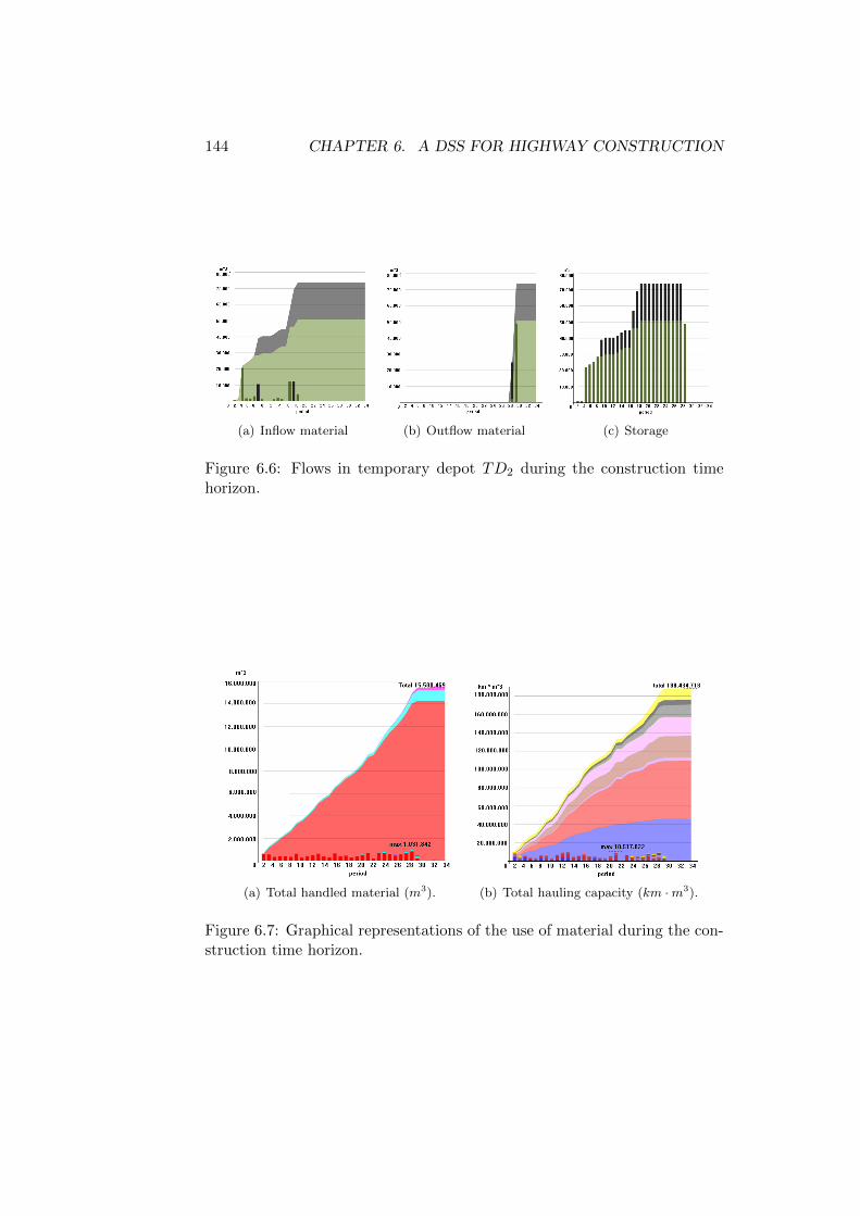
144 CHAPTER 6. A DSS FOR HIGHWAY CONSTRUCTION
(a) Inflow material (b) Outflow material (c) Storage
Figure 6.6: Flows in temporary depot TD2 during the construction timehorizon.
(a) Total handled material (m3). (b) Total hauling capacity (km ·m3).
Figure 6.7: Graphical representations of the use of material during the con-struction time horizon.

6.4. THE DECISION SUPPORT SYSTEM 145
(a) Excavated material (m3) (b) Filled material (m3)
Figure 6.8: Graphical representation of digging and filling activities in avertex.
The solution of the disaggregate model gives us detailed information onthe flow of a material in a certain period. It is a point to point solution, sinceby solving the model one understands exactly from which source to whichdestination the material travels over a certain period. For the graphicalrepresentation of the disaggregated flows we use a diagramming program,specifically the free yEd Graph Editor by yWorks. This editor directly readsthe solution provided by the model in the form of Excel file. The result is alarge diagram containing information about the flows of material that startfrom all sources and arrive on several destinations. Figure 6.9 is a partic-ular of an example of the graphical output (.graphlm) of the disaggregatemodel in which we consider the flows coming from a certain digging activ-ity, DIG123, and directed respectively to the temporary depots, TD6 andTD7, to the dump site DS10, and to the filling activity FIL145. This typeof representation highlights the distance in km from sources to destinationsand the amounts in m3 of materials involved, making a distinction betweenthe different types of materials. In particular, in DIG123 we represent withline mexc the total amount of excavated materials such as topsoil (italic)and the others materials (plane), while in line mcw we depict the amountof the excavated materials that are rawWaste. In TD6 and TD7 we depictthe total amount of materials stored, separated in topsoil (italic) and othermaterials (plane). The filling activity FIL145 shows the total amount re-quired in this period in line mcr and the amount derived by the block of thissubgraph in line mcri, both separated in topsoil (italic) and other materials(plane). The block representing the dump site DS10 shows the amount tobe carried to the dump site in this period in line mcr and the amount ofmaterials coming from the blocks of this graph in line mcri. On the arcs are

146 CHAPTER 6. A DSS FOR HIGHWAY CONSTRUCTION
depicted the amount of topsoil (italic) and of other materials (plane), andthe distance between the two sites.
Figure 6.9: Graphical output of the disaggregate model.
6.5 Computational Evaluation of the OptimizationPhase
The models, whose detailed mathematical formulation is given in Annex 6.A, were implemented using the Xpress-Mosel language available and solvedwith the LP solver FICO R©Xpress 7.6. The PC on which the tests wereperformed has the following characteristics: 2.21 GHz AMD Athlon(tm) 64Processor 3500+.
Real-world Instance
The instance used to conduct tests to validate the models corresponds to thereal-world highway segment of the project Autostrada Pedemontana Lom-barda between Cesano Maderno and Usmate Velate, that is what we callbasic instance (see Figure 6.2). The data refer to an intermediate stage ofthe project and therefore they do not exactly reflect the final configurationof the considered segment. The basic instance is one of the most problem-atic sections of the whole construction project from an environmental andurbanistic viewpoint, due to the need of construction in proximity of urbansettlements and areas of natural beauty. With a length of approximately16.5 km and three lanes in each direction, the basic instance extends forabout 6.5 km in artificial tunnels and for about 9.5 km in trenches, as wellas in embankments and in viaducts. The track intersects many waterways,the most important of which is the Lambro river, crossed by a bridge. Toconnect the highway with the local road network, some secondary trackswill be realized in addition to the main one.

6.5. COMPUTATIONAL EVALUATION 147
The section is discretized in segments of about 500 meters length. Foreach segment the amount and composition of materials to be dug has beenestimated by performing a core sampling. Similarly, the amount and compo-sition of materials to be used for filling has been determined by consideringthe presence of bridges, viaducts, galleries, embankments, and trenches inthe plan. On the basis of the MPS we determined the time windows of thevarious activities of the construction process. The overall planning horizonof the basic instance is about three years, that we discretized in months.
The area interested by the basic instance includes several facilities, suchas 13 dump sites, a quarry selling asphalt and cement, seven temporarydepots, and two concrete mixing plants. Several access points connect theexternal sites, i.e., the existing public network, to the construction sites.The access points are connected to the external plants by using the availablepaths in the public network. The resulting network is described in Figure6.5, that depicts the construction site (highlighted), and the paths throughaccess points and external plants (plain).
Computational Results
The instance described in the previous subsection has been modified byperturbing some of its characteristics with the purpose of obtaining an ex-haustive set of instances. We first created two instances by changing thediscretization of the segments, using segments of 250 meters and of 750 me-ters. Xpress offers different algorithms for solving LPs, among these theDual Simplex, the Primal Simplex, and the Barrier algorithm. To identifythe best method to solve our problem we tested the three algorithms on thebasic instance and on the other two perturbed instances.
Table 6.1 gives the results of the three algorithms on the instances thatwe created. For each instance we report the objective function value z andthe computational time required to reach the optimal solution. We alsoprovide the average of these computational times.
It should be noticed that the discretization in segments of 250 meterscosts slightly more than the real-world instance. Instead, the 750 discretiza-tion cost slightly less than the basic instance. We can conclude that theused discretization of 500 meters represents an appropriate level of detail.
As regards the computational times, the results of the comparison iden-tify the Barrier as the best algorithm when solving our set of instances. Inaverage, it takes about two minutes to solve an instance. The other two al-gorithms require in average a computational time about eight times higher.The maximum values are quite small for the Barrier algorithm, i.e., about3.5 minutes, but can be very high for the other two algorithms, reachingabout 50 minutes.
The problem we assessed is very complex, thus we performed a sensitiv-ity analysis, conducted by changing the percentages of excavated materials,

148 CHAPTER 6. A DSS FOR HIGHWAY CONSTRUCTION
Solution CPU seconds
Instance z Dual Primal Barrier
basic instance (0.500 km) 19206.1 386.8 901.3 95.80.250 km discretization 19298.9 923.2 2890.4 213.50.750 km discretization 19191.6 256.2 613.5 68.6
Avg 522.1 1468.4 126.3
Table 6.1: Results obtained by solving the aggregate model with Dual, Pri-mal, and Barrier algorithm
to better understand the behavior of the aggregate formulation. We recallthat rawH is the highest quality material obtained by digging. In the basicinstance rawH amounts to about 10% of the total excavated materials. Thisvalue derives from core sampling performed at material locations (roughly,a sampling every 500 m), so it is only an estimation of the real value. In-deed this percentage is a very critical parameter, this is why we present thefollowing analysis. We obtained three additional instances by increasing thepercentage of rawH by 5% and 10%, and decreasing it by 5%, respectively.
Instance z % gain CPU seconds
basic instance (10% rawH) 19206.1 95.8rawH +5% 16104.6 16.1 109.2rawH +10% 13485.1 29.8 120.3rawH -5% infeasible - 55.1
Table 6.2: Sensitivity analysis on the quality of materials.
As one can see in Table 6.2, in more optimistic situations the solutioncost decreases consistently with respect to that of the real-world instance.Instead, the more pessimistic situation gives an infeasible instance, becausesuch a situation creates too much waste and the capacity of the temporarydepots is not large enough to accommodate it.
6.6 Conclusions
In this chapter we described a new Decision Support System (DDS) de-veloped to furnish Strabag AG, one of the largest European constructioncompanies, with a tool that could assist the decision-makers in the processof construction of the Autostrada Pedemontana Lombarda. AutostradaPedemontana Lombarda is one of the largest highway project in progressnowadays in Europe and it is part of the activities planned for the WorldExposition Expo Milano 2015. Its construction requires to move roughly5·107 m3 of earth, for about 5·108 km ·m3 of flows.

6.6. CONCLUSIONS 149
The newly developed DDS is based on three phases: the input, the opti-mization, and the output phase. The input phase collects and preprocessesthe information to be passed to the optimization phase. The optimiza-tion is constituted of two sub-phases, a first one, where an aggregate modelsolves the earthwork optimization problem, and a second one that solves adisaggregate model which dispenses the actual flows for each material andeach period. The output phase uses the data procured by the optimizationphase and gives an useful, practical, and clever set of interactive outputs toimprove and simplify the decision making process.
To test the efficiency of the proposed DSS in solving complex earthworkoptimization problems, we produced a set of instances by perturbing somecharacteristics of the real-world instance corresponding to one of the ninesections of the Autostrada Pedemontana Lombarda project.
The DSS, currently in use at Strabag AG for the construction of Au-tostrada Pedemontana Lombarda, is an efficient, responsive, and adaptabletool suitable for solving different real-world construction logistics problemswith little changes. Its application to other construction projects is understudy by Stabag AG.

150 CHAPTER 6. A DSS FOR HIGHWAY CONSTRUCTION
6.A Mathematical Models
In this Appendix we report the mathematical models used in the optimiza-tion phase.
Aggregate Formulation
Let us first define the necessary sets of vertices: L is the set of temporarydepots, D of dump sites, S of quarries, H of the material locations (wheredigging and filling activities must be performed), B of vertices represent-ing the network outside the building site, including the access points to thebuilding site. Let A, M, and T be the sets of arcs, materials, and periods,respectively.
Variables. The variables xmtij represent the flow of material m ∈ M inperiod t ∈ T on arc (i, j) ∈ A, while fmtk represent, respectively, the quantityof material m stored in a temporary depot k ∈ L, carried to a dump sitek ∈ D, or acquired from a quarry k ∈ S, at period t. Variables must benon-negative, thus:
xmtij ≥ 0 (i, j) ∈ A,m ∈M, t ∈ T , (6.1)
fmtk ≥ 0 k ∈ L ∪ D ∪ S,m ∈M, t ∈ T . (6.2)
Objective Function. With each arc (i, j) ∈ A is associated an estimationof transportation cost cij proportional to the distance. The exact cost oftransportation can be computed only in the disaggregate formulation, sincethe transportation fare depend non-linearly from the length of the traveledpaths. Moreover let cmk denote the cost for storing, dumping, or buying aunit of material m ∈ M at location k ∈ L ∪ D ∪ S. The objective functionis then:
min z =∑
(i,j)∈A
∑m∈M
∑t∈T
cijxmtij +
∑k∈L∪D∪S
∑m∈M
∑t∈T
cmk fmtk . (6.3)
Arc capacity constraints. Every arc (i, j) ∈ A has a maximum capacityU tij (in cubic meters) for each period t ∈ T , so:∑
m∈Mxmtij ≤ U tij (i, j) ∈ A, t ∈ T . (6.4)
Vehicle capacity constraints. Materials are moved by trucks belonging toa setW of types, each of those may transport a setM(w) ⊆M of materials,has a maximum transportation capacity V (w), a maximum number of kmthat can be traveled in the time horizon K(w). The number of vehicles of

6.A. MATHEMATICAL MODELS 151
type w ∈ W is denoted by N(w). To each arc (i, j) ∈ A is assigned a non-negative length `ij in km. The overall transportation capacity is imposedby: ∑
(i,j)∈A
∑m∈M(w)
`ijxmtij ≤ N(w) · V (w) ·K(w) t ∈ T , w ∈ W. (6.5)
Filling constraints. Filling tasks represent the need of some amount ofmaterial in a location into a particular time window. If If is the set offilling tasks, each task i ∈ If is linked to its material location h(i) ∈ H,and has its own request di to be satisfied inside the time window, specifiedby its starting period ts(i) and its ending period te(i). Outside of this timewindow, the flow of a task must be zero. Let us define Mf (i) ⊆ M as theset of alternative materials that can be used to respond to the request ofa filling task i ∈ If . We must guarantee that the request is fulfilled, andmaterials not included in Mf (i) are not used. We obtain:
xmth(i),i = 0 i ∈ If ,m ∈M \Mf (i), t ∈ T ,
(6.6)
xmth(i),i = 0 i ∈ If ,m ∈M, t ∈ T : t < ts(i) or t > te(i),
(6.7)∑m∈M(i)
te(i)∑t=ts(i)
xmth(i),i = di i ∈ If .
(6.8)
Digging constraints. Digging tasks represent the excavation of someamount of materials in a certain location into a given time window. Letus define the set of digging tasks as Id, where each task i ∈ Id has a requestdi of a composition of materials defined by the setMd(i) ⊆M. Each mate-rial m ∈Md(i) has a coefficient that determines the composition of diggingtask i ∈ Id, ϕ
mi , where
∑m∈Md(i) ϕ
mi = 1. For each task i ∈ Id is set a
unique material location h(i) ∈ H and is defined a time window [ts(i), te(i)]to be respected.
We must impose zero flows for materials different fromM(i) and outsidethe time windows, while the demands of the tasks must be satisfied into thetime windows. We thus obtain:
xmti,h(j) = 0 i ∈ Id,m ∈M \Md(i), t ∈ T , (6.9)
xm,ti,h(j) = 0 i ∈ Id,m ∈Md(i), t ∈ T : t < ts(k) or t > te(k), (6.10)
∑m∈Md(i)
ϕmi
te(i)∑t=ts(i)
xm,ti,h(i) = di i ∈ Id (6.11)

152 CHAPTER 6. A DSS FOR HIGHWAY CONSTRUCTION
Flow conservation at material locations, and external vertices.Flow conservation among the material locations, the access points, and theexternal vertices is imposed by:∑
(i,j)∈A
xmtij =∑
(j,i)∈A
xmtji j ∈ H ∪ B,m ∈M, t ∈ T . (6.12)
Temporary depots constraints. Let us defineMs as the set of materialsthat can be stored into temporary depots and Qk as the maximum storingcapacity that must be respected at each period in k ∈ L. We have:∑
m∈Ms
fmtk ≤ Qk k ∈ L, t ∈ T . (6.13)
Let fm0k be the initial stock of material m ∈Ms in depot k at the beginning
of the first period, and fm,Tmax+1k the upper bound on the closing stock of
m in k at the end of the last period Tmax. We have the following materialbalance constraints:∑
(i,k)∈A
xmtik + fm,t−1k =
∑(k,i)∈A
xmtki + fmtk k ∈ L,m ∈Ms, t ∈ T , (6.14)
fm,Tmaxk ≤ fm,Tmax+1k k ∈ L,m ∈Ms. (6.15)
Dump sites constraints. Let Ck be the total capacity of a dump sitek ∈ D and Qmk the maximum capacity for each period and material. Then:∑
(i,k)∈A
∑t∈T
∑m∈M
xmtik ≤ Ck k ∈ D, (6.16)
∑(i,k)∈A
xmtik ≤ Qmk k ∈ D,m ∈M, t ∈ T . (6.17)
Quarries constraints. As for the dump sites, each quarry k ∈ S has anoverall capacity Ck and a maximum capacity Qmk for each material m ineach period, therefore:∑
(k,i)∈A
∑t∈T
∑m∈M
xmtki ≤ Ck k ∈ S, (6.18)
∑(k,i)∈A
xmtki ≤ Qmk k ∈ S,m ∈M, t ∈ T . (6.19)
Separation plants constraints. The recycling process is made of a firststep where material rawH (the highest quality material obtained by dig-ging) is separated into a set of materialsMs in separations plants, and of asecond part where some of these materials can be combined with bitumen

6.A. MATHEMATICAL MODELS 153
and cement to obtain asphalt and concrete in asphalt and concrete mixingplants. Let us define Fs,Fa, and Fc the sets of separation plants, asphaltmixing plants, and concrete mixing plants, respectively. The flows enteringa separation plant k ∈ Fs for all materials m ∈ M other than rawH, aswell as the flows leaving the vertex for all materials other thanMs must bezero, that is:
xmtik = 0 (i, k) ∈ A : k ∈ Fs,m ∈M \ rawH, t ∈ T , (6.20)
xmtki = 0 (k, i) ∈ A : k ∈ Fsm ∈M \Ms, t ∈ T . (6.21)
The accumulated material inflow should not exceed the maximum allowableoperating capacity Qk of each separation plant k ∈ Fs, thus:∑
(i,k)∈A
xrawH,tik ≤ Qk k ∈ Fs, t ∈ T . (6.22)
Each separation plant has its own and specified recipe, that states the quan-tities of exiting materials obtained from a unit of rawH. Formally, ϕms givesthe quantity of exiting material m ∈ Ms that can be obtained from a unitof rawH at plant k ∈ Fs, and note that, for feasibility, we must have∑
m∈Msϕms = 1. The conservation flow at each separation plant is stated
by: ∑(k,i)∈A
xmtki = ϕms∑
(i,k)∈A
xrawH,tik k ∈ Fs,m ∈Ms, t ∈ T . (6.23)
Asphalt mixing plants constraints. Each asphalt mixing plant k ∈ Famust receive as input the set of materialsMa, and gives in output asphalt,thus:
xmtki = 0 (k, i) ∈ A : k ∈ Fa,m ∈M \ asphalt, t ∈ T , (6.24)
xmtik = 0 (i, k) ∈ A : k ∈ Fa,m ∈M \Ma, t ∈ T . (6.25)
The plant has a total production capacity Qk for each period. Its recipe isexpressed by the ϕma input, which gives the quantity of material m ∈ Ma
necessary for producing a unit quantity of asphalt at plant k ∈ Fa. Forfeasibility, the values of ϕma satisfy
∑m∈Ma
ϕma = 1. We thus get:∑(k,i)∈A
xasphalt,tki ≤ Qk k ∈ Fa, t ∈ T , (6.26)
∑(i,k)∈A
xmtik = ϕma∑
(k,i)∈A
xasphalt,tki k ∈ Fa,m ∈Ma, t ∈ T . (6.27)
Concrete mixing plants constraints. Similarly as for the asphalt mixingplants, each concrete mixing plant k ∈ Fc receives as input materials Mc,

154 CHAPTER 6. A DSS FOR HIGHWAY CONSTRUCTION
gives in output concrete, and has total processing capacity Qk for eachperiod. Its recipe is expressed by ϕmc , that gives the quantity of materialm ∈ Mc necessary for producing a unit quantity of concrete, and is suchthat
∑m∈Mc
ϕmc = 1. Hence we impose constraints similar to (6.24)–(6.27)for the concrete mixing plants. The resulting aggregate model is thus tominimize (6.3), subject to (6.1)–(6.2), (6.4)–(6.27).
The main changes with respect to the aggregate formulation in [2] derivefrom the use of alternative materials for filling, which affects (6.6)–(6.8),and the use of fixed compositions of materials in digging tasks, which affects(6.9)–(6.11).
6.A.1 Disaggregate Formulation
The disaggregate formulation aims at determining the actual paths on thenetwork used by each material in each period by using a model one foreach material/period of the time horizon. To do so, we start from thesolution of the aggregate formulation, that provides all the possible originsand destinations. We enumerate the set of all possible paths P and arcsA(p) used by each path p ∈ P starting from all the possible origins andheading to all the possible destinations of a given material in a given period,by applying a standard label setting algorithm. We clarify that the typicalgraphs of the problem have a particular structure that is very sparse andthat follows the shape of the highway building site. This makes the numberof possible paths quite limited so it is not prohibitive to enumerate all ofthem.
We use a set covering model, where, for each path, we introduce a non-negative variable yp representing the quantity of material hauled on thatpath and the related cost cp. Note that, by using this model, the cost ofa path can also be given as a non-linear function, that we represent bycp. The flows provided by the aggregate solution are denoted by xhk onarc (h, k) ∈ A (where period and material are omitted because fixed) andrepresent a lower bound for the material hauled on paths on each arc asimposed on constraint (6.29).
We report here a generic disaggregate model for one material and oneperiod:
min∑p∈P
cpyp (6.28)
∑p∈P:(h,k)∈A(p)
yp ≥ xhk (h, k) ∈ A (6.29)
yp ≥ 0 p ∈ P. (6.30)
The objective function (6.28) aims at minimizing the costs, which canbe very flexible since they depend on each path. In our instances we calcu-

6.A. MATHEMATICAL MODELS 155
late the cost cp as a function that models the transport costs given by thecontracts in use at Strabag AG. These costs increase with a steep slope from0 to 5 km, and after that, the slope has a more gradual increase.

156 CHAPTER 6. A DSS FOR HIGHWAY CONSTRUCTION

Bibliography
[1] R. K. Ahuja, T. L. Magnanti, and J. B. Orlin. Network flows: theory,algorithms, and applications. Prentice-Hall, Inc., Upper Saddle River,NJ, USA, 1993.
[2] C. Bogenberger, M. Dell’Amico, G. Fuellerer, G. Hoefinger, M. Iori, S.Novellani, and B. Panicucci, B. A Two-Phase Earthwork OptimizationModel for Highway Construction. to appear on Journal of ConstructionEngineering and Management, 2014.
[3] S. M. Easa. Earthwork allocations with nonconstant unit costs. Journalof Construction Engineering and Management. 113:34-50, 1987.
[4] S. M. Easa. Earthwork allocations with linear unit costs. Journal ofConstruction Engineering and Management. 114:641-655, 1988.
[5] W. L. Hare, V. R. Koch, and Y. Lucet. Models and algorithms toimprove earthwork operations in road design using mixed integer linearprogramming. European Journal of Operational Research, 215:470-480,2011.
[6] S. M. Karimi, S. J. Mousavi, A. Kaveh, and A. Afshar. Fuzzy opti-mization model for earth-work allocations with imprecise parameters.Journal of Construction Engineering and Management, 133:181-190,2007.
[7] M. Marzouk and O. Moselhi. Multiobjective optimization of earthmov-ing operations. Journal of Construction Engineering and Management,130:105-113, 2004.
[8] R. M. Stark and R. H. Mayer. Quantitative construction management:Uses of linear optimization. Wiley, New York, 1983.
[9] R. M. Stark and R. L. Nicholls. Mathematical foundations for design:Civil engineering systems. McGraw-Hill, New York), 1972.
[10] H. Zhang. Multi-objective simulation-optimization for earthmoving op-erations. Automation in Construction 18:79-86, 2008.
157

158 BIBLIOGRAPHY

Part IV
Models and Algorithms for3D Printing Problems
159


Chapter 7
Optimizing the 3D PrintingProcess
In this chapter we treat the production technology known as 3D printing.We deal with the 3D printing process by describing it, its advantages anddisadvantages and by supplying an exhaustive classification of the manyfeatures to deal with in the 3D printing process optimization. Among themany operations related to the 3D printing process, we focus on the toolpath definition problem of a 3D printer, that we called 3D Routing Problem(3DRP). The 3DRP is a generalization of the rural postman problem, in thefamily of arc routing problems. We present an ILP formulation for the 3DRPand we developed four heuristic algorithms that can furnish with improvedsolutions with respect to the solutions obtained by one of the most usedsoftware for the tool path definition in 3D printing.
Keywords: 3D printing, Rural postman, Arc routing, Models, Heuristics.
7.1 Introduction
3D Printing (3DP), also known as Additive Manufacturing, is a productiontechnology that can construct three-dimesional objects of multiple shapes byadding one or more materials layer by layer. Since its rise in the 80s, differenttechniques for 3DP have been developed, including Stereolithography, thatmakes use of liquid polymers hardened by UV beams layer by layer, SelectiveLaser Sintering, where a laser melts the powder -layer by layer- in a selectiveway, and Fused Deposition Modeling (FDM), also known as Fused FilamentFabrication. FDM involves extruding thermoplastic material (such as ABSplastic or polycarbonate) through heated nozzles: the filament is pulled bya feed roller, it is heated to a temperature above the material’s meltingpoint, and then it is extruded by the nozzle. Once a layer is completed theplatform where the material has been deposited is lowered or the nozzles is
161

162 CHAPTER 7. OPTIMIZING THE 3D PRINTING PROCESS
raised to the next layer level and a new layer is added and fused with theprevious one. A supporting material can also be used in the process when itis needed for structural issues, especially in case of overhanging geometries(Campbell et al. [6], Akella [1]). From now on, when mentioning 3DP wewill refer to the FDM technique.
In this work we focus on the optimization of the 3DP process, in par-ticular we will concentrate on the optimization of the path that the nozzlehas to follow to produce the three-dimensional object, in terms of distances,given several sets of constraints. Before introducing models and heuristicalgorithms, we spend some words on the 3DP process.
7.1.1 The 3DP Process
The manufacturing process of a product through 3DP follows a typicalscheme as depicted in Figure 7.1. The process starts with the definitionof the 3D model which can be created by a computer-aided design (CAD)software or by scanning an object we want to reproduce. The second stepis to reproduce the three-dimensional object in a polygonal mesh, normallymade of triangles. The typical file used to report a polygonal mesh is in a.stl format. When the model is represented as a mesh, the corresponding.stl type file is passed to a slicing software that divides the mesh in layers.The following step is the most interesting to our work and it is to decidethe path to be followed by the tool for reproducing the three-dimensionalobject. The solution obtained is expressed in a sequence of commands in ag-code format that is passed to the printer in order to produce the final 3Dobject (Campbell et al. [6]).
Figure 7.1: Scheme of the 3DP process.
7.1.2 Advantages and disadvantages
The 3DP processes have some advantages such as the application to rapidprototyping, the attitude towards the tool-less production of finished goods,the mass production of customized parts and low volume ones, the free-dom in engineering design, the possibility of building complex geometriesimpossible to obtain with other techniques, and of delivering finished goodsfrom digital data cutting also the logistic costs and minimizing carbon foot-print. Some other advantages are incarnated by the limited use of chemicals

7.1. INTRODUCTION 163
such as etching and cleaning solutions, the possibility to use recycled mate-rial and the opportunity to use the same technique with diverse materials(Akella [1]). Some costs that can decrease thanks to 3DP technology areidentified in: waste generation as the one of subtractive machine is avoidedand thus disposal and recycling costs; inventory costs are minimized becauseproducts can be printed on demand and there is no need of semi-finishedproducts; labor time for designing and assembling multiple parts is avoided;less opportunity for human error since the production is driven by digitalinformation; lastly set-up costs are minimized since many products can beproduce without retooling (Bak, Beltrami and Bodin, Boding and Kursh,Campbell et al. [3, 6]).
However, 3DP is not free from limits. Indeed, 3DP does not seem appro-priate for the mass production since its main disadvantage is the requiredamount of production time. Another issue is the quality of the material,normally used materials are polymers that do not present the same goodcharacteristics of materials traditional of subtracting manufacturing andare typically weaker, moreover parts produced on different machines canguarantee particular properties with respect to quality and performances.Furthermore, the layer-by-layer building process makes the parts weaker inthe direction of the build (Campbell et al. [6]).
7.1.3 Contribution of this Chapter
In the 3DP process there are, mainly, two aspects that can be optimized.The first one is about the quality of the printed object and it is related to thequality of the surface. We will consider some features in order to improvethe quality of the surface, but to cover completely this point is not the aimof the chapter. The second aspect that can be optimized is related to thetime of the print that can be minimized and that is strictly connected to thetool path. In this chapter we will account for this second aspect by focusingin minimizing the distance traveled by the nozzle during the 3DP process,and, indirectly, minimizing the time of the print.
We will present a formal description of the problem derived from 3DP, arelated literature review, and a mathematical model to represent the basicproblem, which is a generalization of the well known Rural Postman Prob-lem. To solve the problem we introduce some heuristic algorithms and weproduce a collection of instances derived from three-dimensional objects onwhich we perform computational tests. Last but not least, we list a setof features and future research direction to be followed in the field thatrepresents the intersection between optimization and 3DP.
The chapter is organized as follows. In Section 7.2 we will define theclass of the Rural Postman Problems and produce an exhaustive literaturereview. In Section 7.3 we define the problem we are presenting, while inSection 7.4 we give a formulation for the problem. In Section 7.5 we present
164 CHAPTER 7. OPTIMIZING THE 3D PRINTING PROCESS
some heuristic algorithms to solve the problem and in Section 7.6 we showthe computational results of the presented algorithms on a set of newlycollected instances.
7.2 The Rural Postman Problems
The problem of defining the tool path in a 3DP process is a generalizationof the Rural Postman Problem (RPP), that is a particular version of themore general class of Arc Routing Problems (see, e.g., Corberan and Laporte[7]). The RPP is the problem of finding the minimum cost eulerian cyclethat visits a set of arcs at least once, by using also a second set of arcs, ifneeded, where each arc is associated with a non-negative cost. The RPPrepresents a generalization of the Chinese Postman Problem (CPP), thatis the problem of finding the minimum cost path that visits at least onceall the arcs. The CPP can be solved in polynomial time, while the RPP(directed or undirected) is an NP-hard problem if the set of required arcs isnot strongly connected (Laporte [27]).
The RRP arises in many real-world situations such as the snow plowing(see, e.g., Haslam and Wright [24]), the garbage collection (see, e.g., Beltramiand Bodin [4]), the mail delivery (see, e.g, Levy [29]), the school bus routing(see, e.g, Angel et al. [2]), the meter reading (see, e.g., Stern and Dror [32]),and the street sweeping (see, e.g., Bodin and Kursh [5]). The interestedreader can find other work related to these applications in Eiselt et al. [16].More recent application of the RRP are referred to the control of plottingand drilling machines (see, e.g. Groetschel [22]) and to the optimization oflaser-plotter beam movements (see, e.g. Ghiani and Improta [19]).
Many polyhedral studies and exact algorithms, mostly cutting plane andbranch-and-cut algorithm, have been proposed in the last years for the RRPand its generalizations. See, e.g., Corberan and Sanchis [12, 13], Laprte andGhiani [21] (where they use a formulation with just 1/0 variables), Reineltand Theis [31], and Fernandez et al. [17] (where they use a completely dif-ferent approach and formulation from the previous works). According tothe survey redacted by Corberan and Prins [11], the largest RPP instancesthat have been solved to optimality are characterized by up to 1000 vertices,3080 edges and 204 required components and are solved in about one hourin average on a standard PC by using the branch-and-cut described in Cor-beran et al. [10] for the Windy General Routing Problem (which containsthe RPP).
Probably, the most famous heuristic algorithm for the RPP is the oneproposed by Frederikson [18], which is built on the well known heuristic forthe TSP by Christofides, and, similarly, presents a worst case bound of 3/2.Hertz et al. [25] propose some improving techniques to be applied to theFrederickson algorithm and to a simply newly developed heuristic. Corberan

7.3. PROBLEM DESCRIPTION 165
et al. [9] present two heuristics approaches to solve the Mixed RPP where theproblem is defined on a graph with edges and arcs and required componentscan be both edges or arcs. Groves and Vuuren [23] present an effective localsearch framework for the URRP based on local searches for the TSP. Theysolve heuristically very large instances with up to about 5000 vertices and30000 edges. Ghiani et al. [20] propose a constructive heuristic for theUndirected RPP (URPP) with a local post-optimization. The procedureis competitive with the Frederickson one. Holmberg [26] proposes someheuristics for the RPP built on the Frederikson heuristic by changing theorder of the components. The author includes also two post-processingheuristics to improve the solution.
We report now a set of variants of the RPP that are interesting for 3DP.Dror and Langevin [15] introduced the Directed Clustered RPP and solvedit by transforming the problem into a Generalized TSP. They separate thearcs in clusters that must be finished before stepping to another cluster.Letchford and Eglese [28] present the RPP with deadline classes, a RPPwith time windows where the time windows have only a maximum time tobe respected. They propose a formulation and a cutting plane algorithm.Corberan et al. [8] consider the mixed RPP with turn penalties. Theyassociate a penalty to every turn and take into account also the existence offorbidden turns. The problem is to find the minimal tour avoiding forbiddentours and paying for turn penalties. The authors transform the problem intoan ATSP and solve it by using exact and heuristic algorithms for the ATSP.
Some relevant applications of the RPP are listed in the following. Ghi-ani and Improta [19] consider the problem of drawing and decorating metalsurfaces by means of a laser plotter, that works as a 2D printer, minimiz-ing the total length of the non-drawing moves. The so-called Laser-PlotterBeam Routing Problem is modeled as a RPP with additional constraintsand solved transforming it into a RPP. By using the branch-and-cut pre-sented in Ghiani and Laporte [21] istances with up to 225 vertices can besolved. Moreira et al. [30] describe the problem that arises when manufac-turing high-precision tools. They intend to determine the shortest path forthe cutting of given pieces. The problem is represented as a particular RPPwhere non-cutting movements are allowed only after the complete cut of apiece. Hence the problem is called Dynamic RPP and solved by means of aheuristic algorithm.
7.3 Problem Description
We call 3D printing Routing Problem (3DRP) the generalization of theURPP that is related to the tool path definition in a 3DP process. Inparticular, the nozzle must start from its starting position and return to thesame position when the print is terminated. In addition, the edges are set

166 CHAPTER 7. OPTIMIZING THE 3D PRINTING PROCESS
into clusters to be visited in a sequence, that are represented by the layersof the print. On each layer the set of compulsory edges represents the setof edges on which the nozzle is required to depose material (the first timethey are used), while the set of the optional edges represents the other edges.Because of the printed material, no layer can be started before terminatingthe previous one, and the nozzle cannot move back to previous layers. Thenone and only one optional edge can be used to move from one layer to thenext one and no edge between two non-subsequents layers is present. Lastly,only optional edges are present between two layers. We will formalize the3DRP in Section 7.4. The 3DRP represents the basic problem of optimizingthe tool path of a 3DP process. In the following we are focusing on thebasic problem, but some additional characteristics can arise across the 3DPprocess: we will list them in Section 7.7.
7.4 The 3D Printing Routing Problem
In this section we define the sets and parameters used to formulate the3DRP. The problem is defined on an undirected graph G = (V,E), whereV is the set of vertices and E is the set of edges. Moreover, it is defined asubset R ⊆ E of edges that must be visited at least once. In our case theseedges are the compulsory edges, where the material is extruded (printed)the first time they are used. On the other hand E \R represents the set ofoptional edges.
Let us define layer as a set of vertices characterized by the same altitude.We call L the set of all layers where a layer Lh ∈ L is one layer of print,
L = ∪|L|h=1Lh, and Lh ∩ Lk = ∅, h 6= k, Lh, Lk ∈ L. The graph G is clusteredin several subgraphs induced by the layers plus the starting and endingpoint of print, 0, and all the edges connecting these components. Thus,V = L ∪ 0.
Finally, let us define the variable xij that models the number of time theedge (i, j) ∈ E \R is traveled, and the number of times the edge (i, j) ∈ R istraveled in addition to the first time. We define cij as the shortest distancebetween the vertices i and j, (i, j) ∈ E. Hence, the 3DRP aims at minimizingthe path of the nozzle starting from vertex 0, traveling all the compulsoryedges at least once, respecting the order of the layers, and returning to thevertex 0. In the following we present the formulation for the basic problem:
min∑
(i,j)∈R
cij(1 + xij) +∑
(i,j)∈E\R
cijxij (7.1)
∑j∈R:j>i
(1 + xij) +∑
j∈R:j<i
(1 + xji)+

7.5. HEURISTIC ALGORITHMS 167
∑j∈V :j>i
xij +∑
j∈V :j<i
xji = 2z i ∈ V (7.2)
∑(i,j)∈R:i∈S,j∈S,j>i
(1 + xij) +∑
(i,j)∈R:i∈S,j∈S,j<i
(1 + xij)+
+∑
(i,j)∈E\R:i∈S,j∈S,j>i
xij +∑
(i,j)∈E\R:i∈S,j∈S,j>i
xij ≥ 1
(S ⊆ Lh,S = Lh+1 ∪ Lh \ S,
Lh ⊆ L \ L|L|)∨ (S ⊆ L|L|,
S = 0 ∪ L|L| \ S) (7.3)∑j∈L1
x0j = 1 (7.4)
∑j∈L|L|
xj0 = 1 (7.5)
∑(i,j):i∈Lh,j∈Lh+1
xij = 1 Lh ⊆ L \ L|L| (7.6)
xij ≥ 0 (i, j) ∈ E (7.7)
z ≥ 0 (7.8)
The objective function aims at minimizing the total costs, i.e. distances,counting also the compulsory edges. Constraint (7.2) states that the numberof edges incident a vertex are even or zero. In (7.3) we impose the connec-tivity of the solution. Constraints (7.4) and (7.5) state that one and onlyone edge must leave and return to the depot. Constraint (7.6) imposes thatone and only one edge can be used between one layer and the next one. Thenon-negativity of the variables is imposed in constraints (7.7) and (7.8).
7.5 Heuristic Algorithms
The 3DP process, when printing real objects, involves from thousands tomillions of edges to be printed and traveled by the nozzle. Thus, real 3DRPinstances result impossible to be solve exactly, because of the huge number ofvariables and constraints needed. For this reason we developed four heuristicalgorithms to solve the 3DRP. To do so, we organized the input in couplesof vertices that defines the edges to be traveled and printed on each layer(the set R), named as compulsory edges. The optional edges (E \ R) andthe compulsory edges used more than once are the non-printing edges, andare computed and inserted just when needed during the construction of thesolution. The input is obtained by analyzing the g-codes created by Cura

168 CHAPTER 7. OPTIMIZING THE 3D PRINTING PROCESS
[33], one of the most advanced 3DP software.
7.5.1 Closest 3DP
The first algorithm we present to solve the 3DRP is called Closest 3DPalgorithm. It starts from vertex 0 and moves from one edge to the closestunused compulsory edge (we enter in the edge by the closest vertex withrespect to the current one and then we travel the edge to arrive in its secondvertex, which will be the new current vertex). If the second vertex of thecurrent edge is also the first vertex of the next edge, we link them directly,otherwise we insert a non-printing edge. When the compulsory edges ofthe current layer have been used at least once, the algorithm moves to thenext layer by using the cheapest edge. We repeat this until the last layer iscompleted, then the last visited vertex is connected to vertex 0 to end thealgorithm.
7.5.2 Clustered 3DP
Before explaining the second algorithm presented, we specify that each layeris divided in different subpolygons and each subpolygon can be formed, atmost, by three clusters of compulsory edges: the outer part (the border ofthe subpolygon), the inner part (that follows the outer part internally, tostrengthen the structure), and the filling part (that represents the edgesused to fill the subpolygon), see e.g., Figure 7.2.
The second algorithm we present is called Clustered 3DP algorithm, fol-lows a similar idea with respect to the Closest algorithm, and makes useof the different clusters. The algorithm selects a cluster on a layer (choos-ing among outer, inner, and filling) and travels all the edges of the cluster,before going to another cluster. The algorithm starts from vertex 0 andselects the closest vertex of the compulsory edges on layer L1. This actionnot only defines the next edge, but also the first cluster among inner, outer,and filling to be completed before moving to the next one. When the cur-rent cluster is completed, the algorithm moves to the closest vertex, whichdefines the next edge and the next cluster. The algorithm continues untilall clusters of the current layer are completed and then the closest vertex ofthe next layer is chosen. When the last layer is completed we travel back to
Figure 7.2: An example of polygon with outer, inner, and filling parts.

7.5. HEURISTIC ALGORITHMS 169
vertex 0 and the algorithm terminates.
7.5.3 Look Ahead 3DP
The third algorithm we use to solve the 3DRP is called Look Ahead 3DP,whose name is inspired by the fact that it makes use of heuristic informationon the future possible decisions. The algorithm starts from vertex 0 and itthen selects the three closest vertices among those of the compulsory edgesof layer L1. A particular cost is then computed by running the Closest 3DPalgorithm from each of the three vertices till the end of the layer. The cost iscomputed as follows: we sum up the traveling cost of the non-printing edgesneeded to terminate the layer by the Closest 3DP, the vertex of the threeselected ones that furnishes with the cheapest cost is used. This process isiterated until all the compulsory edges of the current layer are used at leastonce. We then use the cheapest edge to move to the next layer and repeatthe procedure until the last layer. To conclude the algorithm we move backto the vertex 0.
7.5.4 Shortest Path Based 3DP
The forth algorithm that we are presenting is called Shortest Path Based3DP. This algorithm is divided into two phases, the first one builds a sup-porting graph to be used in the second phase. The second phase computesthe Dijkstra algorithm (see, e.g., Dijkstra [14]) on the newly built supportinggraph to obtain a solution for the 3DRP. In the following we will describethe two phases more precisely.
Phase one. In this phase we define the supporting graph G′ = (V ′, E′),where V ′ ⊆ V is the set of vertices called starting points and E′ the set ofedges that we describe in the following. For each layer we select a random setof vertices among those of the compulsory edges (R), called starting vertices,from which we can start the layer. Starting from the starting vertices weterminate the layer as if using the Closest 3DP algorithm. For each startingvertex we will end up in one and only one vertex that we call ending vertex.The distance between a starting vertex and its ending vertex is the costcomputed by the Closest 3DP algorithm. We now compute the distancebetween the ending vertices of one layer and the starting vertices of thenext layer. At this point we obtain an edge going from each starting vertexof one layer to each starting vertex of the next layer, that define E′. We callc′ij the cost of each edge of E′ as the sum of the costs derived by the Closest3DP algorithm and the distance between the corresponding ending vertexand the starting one of the next layer. The starting vertices of the first layerare linked to the vertex 0 and a cost c′0j , j ∈ L1 is associated to them. Theending vertices of the last layer are linked to the vertex 0’, that has the samecoordinates of vertex 0, and a cost c′j0, j ∈ L|L| is associated to them. The

170 CHAPTER 7. OPTIMIZING THE 3D PRINTING PROCESS
costs c′ij , (i, j) ∈ V ′ give the weight of the edges of the supporting graph G′.
Phase two. In the second phase, we compute the shortest path form 0to 0’ on the supporting graph G′. This leads to a feasible solution for the3DRP.
We tested the Shortest Path Based 3DP algorithm by selecting the num-ber of starting vertices in two ways, in the first one we decide a fixed numberbetween 10, 20, 30, 40, 50, 60, and 100 (or the cardinality if the layer, ifexceeded), while in the second case we use the maximum value between 1and a percentage of the vertices of each layer (1%, 2%, 5%, 10%, 15%, 20%,25%).
7.6 Computational Results
7.6.1 Instances
We collected 30 instances on the Internet from a design community for 3DPcalled thingiverse.com. In Table 7.1 we report the name of the instancein the first column. For each instance is specified |L|, the number of layers,|P|, the number of polygons, and the ratio between them. We then reportthe total distance of the compulsory edges (
∑(i,j)∈R cij) and the cardinality
of the set of compulsory edges (|R|).
7.6.2 Results
The collected instances have been processed with one of the most famoussoftware used for slicing polygonal meshes and for path definition, Cura [33].We used the collected instances as input for Cura that takes the polygonalmeshes of the instances, slice them, and defines a path of the nozzle in a codecalled gcode. The gcode represents, for each instance, a heuristic solutionfor the related 3DRP in a language that the 3D printer can understand.By processing the obtained gcode we can obtain the set of layers, the setof compulsory edges to be printed, the corresponding vertices and theircoordinates. These informations define the data that we used as instancesfor our algorithms.
Let us call Γ the cost of the non-printing edges used in a given solu-tion for the 3DRP. Let us call ∆Γ the difference between the cost of thenon-printing edges used by the solution defined by Cura and the cost ofthe non-printing edges used by the solution obtained thanks to one of ouralgorithms. Let %gapΓ be the percentage gap between them. In the fol-lowing tables presenting the results of the proposed algorithms we show thename of the instance, the corresponding ∆Γ and %gapΓ, the percentage gap(%gap) between the Cura solution value and the the solution value obtainedby our algorithm, and the time needed to our algorithm to terminate. Alltests have been performed on a on a Intel Core i3-2100 with 3.10 GHZ.

7.6. COMPUTATIONAL RESULTS 171
Instance |L| |P| |P|/|L|∑
(i,j)∈R cij |R|
30grams 219 222 1.01 91016.609 8693angel 153 663 4.33 1052191.750 353671block 4x4 37 112 3.03 32929.641 28694brickb 332 422 1.27 2851998.700 107355bunny 41 151 3.68 38896.449 21333chamfer 20 147 7.35 71653.297 12700Cityscape 342 1814 5.30 1907842.250 488409gear b 85 371 4.36 22001.822 19275geoboard 82 1642 20.02 291901.188 52244hilbert2 99 2203 22.25 55116.855 26703Hilton Chicago 73 73 1.00 22304.736 7179ingranaggio 39 51 1.31 64690.348 52569miwin1 132 396 3.00 610945.625 130267orso bis 52 52 1.00 73459.617 35772pesce bis 52 193 3.71 139978.297 65262polysoup 3 6 2.00 3186.609 3018portab 32 32 1.00 197571.750 47293portaingr 51 106 2.08 106148.930 69664RFin 188 248 1.32 54926.410 35898RostockBottom 44 208 4.73 117799.625 18120RostockTop 50 213 4.26 87387.406 21132Rpenta 369 1555 4.21 1039104.563 433954RShowerHead 274 580 2.12 513838.531 146602tardisflat2 170 170 1.00 100367.148 24695tetra 160 160 1.00 98250.273 20839trail 125 425 3.40 1304639.625 268372wbuilding 100 211 2.11 11281.513 3364wine fixed 39 59 1.51 93598.977 20276wine1 39 39 1.00 147826.547 19145WitchCastle 112 265 2.37 48852.797 56334
Table 7.1: Instances Description

172 CHAPTER 7. OPTIMIZING THE 3D PRINTING PROCESS
In Table 7.2 we report the results of the Closest 3DP algorithm compar-ing them with the results obtained by Cura. One can observe that we canimprove the solution value for 28 out of 30 instances improving of 5.60% thegaps in average. We can obtain an improvement of 27.79% in the bast case.If we focus on the Γ value we can see that the improvement is in average of22.91%. Also the average solving time is very promising being lower thanone second. In Table 7.3 the results for the Clustered 3DP algorithm areshown. In this case we can improve the solution value with respect to theCura one for 27 out of 30 instances. We can obtain an improvement of3.02% in average in solving times that are about half a second, in average.In Table 7.4 we show the results for the Look Ahead 3DP algorithm on thecollected set of instances. In this case the solution value is improved forevery instance with respect to the Cura solution value. In particular, wecan improve it of 8.06% in average. If we just consider the non-printingedges we can notice an improvement of 36.73%. To reach these results theLook Ahead 3DP algorithm needs to run for about 39 minutes, in average,which is a relevant solving time if compared with the previously proposedalgorithms. These very good solutions have a payback in solving times. InTable 7.5 and Table 7.6 the average results for the Shortest Path Based al-gorithms are shown. In particular, in Table 7.5 we report the results for theShortest Path Based 3DP algorithm, where the number of starting verticesfor each layer is fixed to 10, 20, 30, 50, 60, and 100. In Table 7.6 we presentthe results for the Shortest Path Based 3DP algorithm where the startingvertices are fixed with respect to a percentage of the vertices of each layer.The starting vertices are set to 1%, 2%, 5%, 10%, 15%, 20%, and 25% of thevertices of each layer. One can see that for both types of the Shortest PathBased 3DP algorithm the average gap between the solution value of our al-gorithm and the one obtained by Cura increases with the number of startingvertices explored. The gap is proportional also to the solving times. TheShortest Path Based 3DP algorithm with fixed numbers of starting verticescan reach a 6.40% gap in average in the best case, that is represented bythe starting vertices set to 100. This value is obtained in about 80 seconds.One can see that this version works similarly to the version with percentagestarting vertices when evaluating the average gaps, but need consistentlymore seconds to terminate.
The algorithm among the presented ones that shows the best results interms of improvement of the solution value, compared to the Cura solutionvalue, is the Look Ahead 3DP algorithm. On the other hand the LookAhead 3DP algorithm needs higher solving times with respect to the otherpresented algorithms. The Shortest Path Based 3DP algorithm furnishes, inits two versions, with good results in acceptable solving times. Similar gapvalues can be obtained by the Closest 3DP algorithm showing very smallcomputing times.

7.6. COMPUTATIONAL RESULTS 173
Closest
Inst. ∆Γ %gapΓ %gap t(sec)
30grams 661.348 5.66 0.64 0.001angel 14905.000 10.12 1.24 6.672block 4x4 6208.443 40.68 12.88 0.140brickb -1326.547 -1.00 -0.04 0.594bunny 1278.109 16.88 2.75 0.079chambler 373.906 3.17 0.45 0.094Cityscape 29226.813 9.95 1.33 7.438gear b 237.855 3.86 0.84 0.032geoboard 2005.250 3.93 0.59 0.281hilbert2 1749.555 11.71 2.50 0.031Hilton Chicago 1099.865 18.09 3.88 0.001ingranaggio 3669.916 22.22 4.52 0.422miwin1 12697.398 13.26 1.80 1.109orso bis 25021.842 60.24 21.76 0.157pesce bis 49553.654 64.16 22.81 0.531polysoup 1453.121 71.14 27.79 0.016portab 4651.479 13.53 2.01 0.437portaingr 1825.557 10.54 1.48 0.922Rfin 970.316 10.32 1.51 0.047RostockBottom 8677.307 31.54 5.97 0.125RostockTop 5156.719 23.36 4.71 0.172Rpenta 58169.266 28.52 4.68 3.125RShowerHead 34814.063 24.85 5.32 0.515tardisflat2 9363.699 39.63 7.55 0.031tetra -630.948 -4.81 -0.57 0.031trail 118281.531 48.29 7.63 4.188wbuilding 75.671 2.86 0.54 0.001wine fixed 11248.256 38.03 9.13 0.093wine1 11980.223 40.19 6.74 0.079WitchCastle 3353.075 26.33 5.44 0.219
Avg. 13891.725 22.91 5.60 0.919
Table 7.2: Results of the Closest algorithm on test instances.

174 CHAPTER 7. OPTIMIZING THE 3D PRINTING PROCESS
Clustered
Inst. ∆Γ %gapΓ %gap t(sec)
30grams 331.556 2.84 0.32 0.000angel 12535.188 8.51 1.05 3.563block 4x4 3031.178 19.86 6.29 0.094brickb -1362.438 -1.03 -0.05 0.469bunny 732.775 9.68 1.58 0.047chambler -368.381 -3.12 -0.44 0.063Cityscape 14744.344 5.02 0.67 3.641gear b 443.250 7.19 1.57 0.032geoboard 1475.285 2.89 0.43 0.235hilbert2 1749.555 11.71 2.50 0.078Hilton Chicago 868.675 14.28 3.06 0.000ingranaggio 716.305 4.34 0.88 0.328miwin1 860.414 0.90 0.12 0.578orso bis 15855.703 38.17 13.79 0.109pesce bis 24295.828 31.46 11.19 0.359polysoup 893.126 43.72 17.08 0.016portab 4127.695 12.01 1.78 0.453portaingr 1311.128 7.57 1.06 0.485Rfin 39.749 0.42 0.06 0.032RostockBottom 3831.223 13.92 2.64 0.141RostockTop 2383.146 10.80 2.18 0.125Rpenta 38163.313 18.71 3.07 2.047RShowerHead 24379.523 17.41 3.73 0.453tardisflat2 2159.188 9.14 1.74 0.031tetra -116.673 -0.89 -0.11 0.031trail 112033.766 45.74 7.23 2.765wbuilding 32.005 1.21 0.23 0.016wine fixed 3796.424 12.84 3.08 0.063wine1 474.381 1.59 0.27 0.063WitchCastle 2227.283 17.49 3.62 0.172
Avg. 9054.817 12.15 3.02 0.550
Table 7.3: Results of the Clustered algorithm on test instances.

7.6. COMPUTATIONAL RESULTS 175
Look Ahead
Inst. ∆Γ %gapΓ %gap t(sec)
30grams 2031.766 17.38 1.98 0.31angel 42756.773 29.02 3.56 22664.21block 4x4 7429.931 48.68 15.42 122.82brickb 16783.938 12.67 0.56 765.48bunny 2365.691 31.25 5.09 45.67chambler 1818.251 15.39 2.18 77.05Cityscape 89875.047 30.59 4.08 17105.26gear b 879.607 14.26 3.12 10.42geoboard 7729.773 15.14 2.25 303.95hilbert2 3211.244 21.50 4.58 13.39Hilton Chicago 1836.877 30.21 6.47 1.06ingranaggio 6060.851 36.70 7.46 758.60miwin1 30848.766 32.22 4.37 1645.93orso bis 30510.017 73.46 26.53 131.84pesce bis 54757.037 70.89 25.21 1012.54polysoup 1594.556 78.06 30.49 21.67portab 11027.746 32.08 4.75 1208.38portaingr 5104.657 29.48 4.13 3032.91Rfin 2859.243 30.41 4.45 17.16RostockBottom 12860.236 46.74 8.85 128.41RostockTop 8104.199 36.72 7.40 369.54Rpenta 94428.086 46.30 7.60 5144.17RShowerHead 56995.102 40.69 8.72 472.31tardisflat2 11276.629 47.73 9.10 6.00tetra 2179.606 16.62 1.96 6.94trail 145659.258 59.47 9.40 14259.08wbuilding 441.532 16.70 3.17 0.08wine fixed 14227.692 48.10 11.55 62.18wine1 15236.461 51.12 8.58 46.33WitchCastle 5396.093 42.37 8.76 187.03
Avg. 22876.222 36.73 8.06 2320.690
Table 7.4: Results of the Look Ahead algorithm on test instances.

176 CHAPTER 7. OPTIMIZING THE 3D PRINTING PROCESS
Shortest Path Based ∆Γ %gapΓ %gap t(sec)
10 14284.276 23.50 5.70 8.59320 15050.768 25.20 6.01 16.32030 15442.301 26.04 6.15 24.15740 15614.103 26.43 6.22 31.84650 15752.656 26.63 6.26 39.83160 15874.853 26.89 6.31 47.505100 16086.931 27.38 6.40 80.940
Table 7.5: Average results of the shortest path based algorithm on the testinstances.
Shortest Path Based ∆Γ %gapΓ %gap t(sec)
1% 13515.840 18.54 4.87 24.9582% 14628.480 21.10 5.31 48.7435% 15553.952 24.02 5.82 118.13110% 16012.425 25.70 6.11 181.53115% 16161.026 26.29 6.21 200.25020% 16253.602 26.59 6.27 208.47425% 16295.172 27.00 6.34 212.810
Table 7.6: Average results of the shortest path based algorithm on the testinstances.

7.7. CONCLUSIONS AND FUTURE RESEARCH DIRECTIONS 177
7.7 Conclusions and Future Research Directions
In this chapter we solved a generalization of the RPP related to the definitionof the tool path in a 3DP process, called 3DRP. We provided a collection ofinstances for the 3DRP that are solved with four different types of heuristicalgorithms we proposed and compared with one of the most famous soft-ware of path definition available, Cura [33]. We obtained very good resultsimproving the Cura solution values from about 3% to about 8% with ouralgorithms in very promising solving times.
The verision of the 3DRP we solved is what we called the basic problemof the 3DRP, but many other secondary features can be considered, startingfrom features to account for an improvement of the quality of the surface.In the following we report an overview of these features divided by topic.
Quality constraints. The 3DP process can produce some blemish on theexternal surface of the product we intend to print. Indeed, when travelingthe optional edges after ejecting material, the nozzle can eject some leftoversand ruin the quality of the external surface. To avoid it we could consideradditional constraints.
1. Second level of clusterization: Subpolygons. Several separated poly-gons, called subpolygons, can be present on the same layer. Subpoly-gons produces a second level of clusterization. To define a tool paththat follows the second level of clusterization is not strictly requiredas for the first level of clusterization (layers), but it can be consideredin order to improve the quality of the external surface. Indeed, mov-ing from one polygon to the other it can lead to some blemish on theexternal surface, because of the characteristics of the materials (nor-mally heated plastic). Then, we can impose to complete a polygonbefore stepping to the next one, by taking one and only one optionalarc between a subpolygon to another, on the same layer.
2. Corner. To preserve the quality of the surface from the blemishes,we can consider not only to leave the polygon just once, but also toimpose the nozzle to pass only through a vertex of the Outer part ofthe same subpolygon, called corner, in order to avoid the intersectionof the tool path and the surface when this has already been built.Doing this we will leave the majority of the blemishes on a corner andmake it easier to remove them after the print.
3. Temperature. The 3DP process includes the melting of the materialbefore extruding it from the nozzle. After being melt, the materialconserves a high temperature for a certain amount of time. This meansthat we cannot extrude some new material on the top of the previouslayer until the temperature of the material of the former layer is not

178 CHAPTER 7. OPTIMIZING THE 3D PRINTING PROCESS
under a certain value, otherwise some flaw or bending can be produced.Considering that layers are overlapped, some edges of a layer cannotbe completed before the underlying edge (of the previous layer) hadthe time to cool down. In order to cool down the temperature of someedges, the speed of the fan can also be considered as a variable.
4. First vertex of a layer. When moving from a non-printing edge toa printing one a small excess of material can be extruded. This canlead to an accumulation of unwilled material on the surface, especiallywhen the first vertex of a layer has the similar x-y coordinates withrespect to the first vertices of the previous layers. To avoid this, we canimpose that the first vertex of a layer must have different coordinatesif compared to the first vertex of the previous layer. Indeed, the sameline of reasoning can be used when starting overlappingsubpolygonson different layers, and not just the first vertex.
Costs. In the basic version of the 3DRP, we consider the cost of the edges asthe geometric distance between two vertices and the time to travel the edgeas directly linear to the distance. Considering a higher level of detail, we canobserve that the time of traveling an edge is not necessarily linear and thatit can depend on an acceleration at first, a constant speed in the middle, anda deceleration of the nozzle at the end when traveling the edge. Moreover,the deceleration can depend on the angle between the current edge and thefollowing one visited and the acceleration can depend on the angle betweenthe current edge and the previous one. This can lead to different options.Taking into account the acceleration and deceleration needed to obtain themaximum possible speed on a given edge, we can recompute the cost ofeach edge starting from the distance. If we considering the angles betweenthe previous and following edges, then the problem must be considered asa directed one. Other possibilities can include non-linear distances betweenthe vertices or considering the speed of the nozzle as a variable.
Other Features.
1. Layers with different thickness. Sometimes, to deal with structuralproblems or just to avoid to obtain a texture too subtle inside theprinted object, we can print some parts of the same layer with a dif-ferent thickness. Two different thicknesses must be related (one mustbe a multiple of the other).
2. Supporting material. Some 3D objects can have undercuts, thus asupporting material is needed when printing. In order to minimize thesupporting material, the positioning of the object can be a variable toaccount for.

7.7. CONCLUSIONS AND FUTURE RESEARCH DIRECTIONS 179
3. Filling. In this work we consider the filling part of a certain polygonas an input, but to decide the filling, in terms of distances betweenthe edges of the filling, their direction, and even a particular patterncan change the optimization of the print or be part of it.
4. Colors. Some printing objects can have different set of materialsand/or colors to be used. Indeed we can see the supporting mate-rial part of this case. When printing an object made of different colorsor materials we can decide to print first the polygons of one materialand then the others by deciding a sequence. Otherwise, we can decideto mix the use of colors to make the printing time shorter. Then thenumber of nozzles becomes relevant: if we have more materials thannozzle we must consider the time spent in changing material and goingback to the vertex 0 to clean the nozzle, otherwise we must considerthe distance between the nozzle of one color and the others.
All these features have a strong impact on the speed of the print and onthe quality of the surface, both very important characteristics in 3DP. Weare convinced that they will be the focus of many future research works.

180 CHAPTER 7. OPTIMIZING THE 3D PRINTING PROCESS

Bibliography
[1] S. Akella. Hot off the press: The technology behind 3d printing. Pro-fessor Scarlatos HON 301, 2012.
[2] R. D. Angel, W. L. Caudle, R. Noonan, and A. Whinston. Computer-assisted school bus scheduling. Management Science, 18:B279–B288,1972.
[3] D. Bak. Rapid prototyping or rapid production? 3d printing processesmove industry towards the latter. Assembly Automation, 23:340–345,2003.
[4] E. J. Beltrami and L. D. Bodin. Networks and vehicle routing formunicipal waste collection. Networks, 4:65–94, 1974.
[5] L. D. Bodin and S. J. Kursh. A computer-assisted system for the routingand scheduling of street sweepers. Operations Research, 26:525–537,1978.
[6] T. Campbell, C. Williams, O. Ivanova, and B. Garrett. Could 3d print-ing change the world? Technologies, Potential, and Implications ofAdditive Manufacturing. Washington, DC: Atlantic Council, 2011.
[7] A. Corberan and G. Laporte. Arc Routing: Problems, Methods, andApplications. SIAM, 2014.
[8] A. Corberan, R. Martı, E. Martınez, and D. Soler. The rural postmanproblem on mixed graphs with turn penalties. Computers & OperationsResearch, 29:887–903, 2002.
[9] A. Corberan, R. Martı, and A. Romero. Heuristics for the mixed ru-ral postman problem. Computers & Operations Research, 27:183–203,2000.
[10] A. Corberan, I. Plana, and J. M. Sanchis. A branch & cut algorithmfor the windy general routing problem and special cases. Networks,49:245–257, 2007.
181

182 BIBLIOGRAPHY
[11] A. Corberan and C. Prins. Recent results on arc routing problems: Anannotated bibliography. Networks, 56:50–69, 2010.
[12] A. Corberan and J. M. Sanchis. A polyhedral approach to the ruralpostman problem. European Journal of Operational Research, 79:95–114, 1994.
[13] A. Corberan and J. M. Sanchis. The general routing problem polyhe-dron: facets from the rpp and gtsp polyhedra. European Journal ofOperational Research, 108:538–550, 1998.
[14] E. W. Dijkstra. A note on two problems in connexion with graphs.Numerische mathematik, 1:269–271, 1959.
[15] M. Dror and A. Langevin. A generalized traveling salesman problemapproach to the directed clustered rural postman problem. Transporta-tion Science, 31:187–192, 1997.
[16] H. A. Eiselt, M. Gendreau, and G. Laporte. Arc routing problems, partii: The rural postman problem. Operations Research, 43:399–414, 1995.
[17] E. Fernandez, O. Meza, R. Garfinkel, and M. Ortega. On the undirectedrural postman problem: Tight bounds based on a new formulation.Operations Research, 51:281–291, 2003.
[18] G. N. Frederickson. Approximation algorithms for some postman prob-lems. Journal of the ACM (JACM), 26:538–554, 1979.
[19] G. Ghiani and G. Improta. The laser-plotter beam routing problem.Journal of the Operational Research Society, 52:945–951, 2001.
[20] G. Ghiani, D. Lagana, and R. Musmanno. A constructive heuristicfor the undirected rural postman problem. Computers & operationsresearch, 33:3450–3457, 2006.
[21] G. Ghiani and G. Laporte. A branch-and-cut algorithm for the undi-rected rural postman problem. Mathematical Programming, 87:467–481,2000.
[22] M. Grotschel, M. Junger, and G. Reinelt. Optimal control of plottingand drilling machines: a case study. Mathematical Methods of Opera-tions Research, 35:61–84, 1991.
[23] G. W. Groves and J. H. Van Vuuren. Efficient heuristics for the ruralpostman problem. ORiON: The Journal of ORSSA, 21:33–51, 2005.
[24] E. Haslam and J. R. Wright. Application of routing technologies to ruralsnow and ice control. Transportation Research Record, 1304, 1991.

BIBLIOGRAPHY 183
[25] A. Hertz, G. Laporte, and P. N. Hugo. Improvement procedures for theundirected rural postman problem. INFORMS Journal on Computing,11:53–62, 1999.
[26] K. Holmberg. Heuristics for the rural postman problem. Computers &Operations Research, 37:981–990, 2010.
[27] G. Laporte. Modeling and solving several classes of arc routing prob-lems as traveling salesman problems. Computers & operations research,24:1057–1061, 1997.
[28] A. N. Letchford and R. W. Eglese. The rural postman problem withdeadline classes. European Journal of Operational Research, 105:390–400, 1998.
[29] L. S. Levy. The walking line of travel problem: An application of arcrouting and partitioning. PhD thesis, University of Maryland, CollegePark, 1987.
[30] L. M. Moreira, J. F. Oliveira, A. M. Gomes, and J. S. Ferreira. Heuris-tics for a dynamic rural postman problem. Computers & operationsresearch, 34:3281–3294, 2007.
[31] G. Reinelt and D. O. Theis. A note on the undirected rural postmanproblem polytope. Mathematical programming, 106:447–452, 2006.
[32] H. I. Stern and M. Dror. Routing electric meter readers. Computers &Operations Research, 6:209–223, 1979.
[33] Ultimaker. “Cura Software”. https://ultimaker.com/en/products/software.

184 BIBLIOGRAPHY

Conclusions
In this PhD thesis we tackled severl real-world logistics and routing prob-lems. In Part II we considered a tactical problem that arises in bike sharingsystems, the Bike sharing Rebalancing Problem (BRP). The BRP is theproblem of driving a fleet of capacitated vehicles to redistribute bicycles inbike sharing systems at minimum costs. In Chapter 2 we defined the BRPand modeled it proposing four formulations and several inequalities to beembedded in branch-and-cut algorithms. We evaluated the formulations ona test bed of 60 newly collected real-world instances with up to 116 ver-tices. The best formulation could efficiently solve to optimality all instanceswith up to 50 vertices, and obtain small gaps for the larger instances inabout 20 minutes. In Chapter 3 we proposed a destroy and repair algo-rithm to solve the BRP, including a new constructive heuristic and a set oflocal searches made more efficient by dedicated speed-up techniques. We col-lected new real-world instances with up to more than 500 vertices. With ourmetaheuristic algorithm we could obtain all the optimal solutions obtainedthanks to the previously presented branch-and-cut in very short times andreach very good solutions for the large instances. In the same chapter we alsosolve the generalization of the BRP where a maximum duration constraintis imposed to each route, the so-called one-commodity Pickup and DeliveryVehicle Routing Problem (1-PDVRP). We adapted both the branch-and-cut, including new inequalities, and the metaheuristic algorithms developedfor the BRP to solve the 1-PDVRP. To test our algorithms for the 1-PDVRPwe used literature instances. For the smaller instances an optimal value hasbeen found for the first time with our branch-and-cut and the adaptation ofthe destroy and repair algorithm to solve the 1-PDVRP could improve thesolution values of about 12% in average with respect to literature results.In Chapter 4 we defined the BRP with stochastic demand. We proposedsome stochastic programming formulations and solved them by means ofL-Shaped and branch-and-cut algorithms. We compared the different for-mulations on real-world newly collected instances. All instances with up to30 vertices have been solved to optimality in short computing times. Wealso developed two heuristics algorithms to solve the SBRP. Those algo-rithms include a novel consideration on positive and negative correlationsbetween the vertices. In Part III we solved earthwork optimization problems
185

186 BIBLIOGRAPHY
considering some new features for the first time. In Chapter 5 we propose anovel two-phase approach to solve the earthwork optimization problem thatarises in highway construction. In particular we developed this new methodand the Decision Support System (DSS) presented in Chapter ch:II2 thanksto the collaboration with one of the major construction companies in Eu-rope (Strabag AG) for the construction of the Autostrada PedemontanaLombarda, a highway in Northern Italy. The DSS includes the optimizationpart and the graphical component to ease the decision making. The DSS iscurrently in use at Strabag AG, being an easy-to-use, efficient tool suitablefor solving several real-world construction logistics problems. In Part IV wesummarized the 3D printing process, its advantages and disadvantage. Wefocused on the problems that arise in the 3D printing process, giving a list ofpossible optimization issues and constraints. We then concentrated in solv-ing the generalization of the arc routing problem related to the definition ofthe tool path in 3D printing, that we called the 3D printing Routing Prob-lem (3DRP). We proposed an ILP model and four heuristic algorithms. Wetested the proposed algorithms on a set of 30 instances and compared theresults with respect to those obtained by one of the most famous availablesoftware for the tool path definition: Cura. We could improve the solutionvalues, in average, between about 3% to about 8%, in average, within goodcomputing times.