serdes high-speed i/o...
TRANSCRIPT

External Use
TM
SERDES High-Speed I/O
Implementation
FTF-NET-F0141
A R P . 2 0 1 4
Jon Burnett | Digital Networking Hardware
TM
External Use 1
Overview
• SerDes Background
− TX Equalization
− RX Equalization
− TX/RX Equalization optimization
• Printed Circuit Board and System Design Considerations
• Simulation Model – IBIS-AMI
• Channel simulations using IBIS-AMI model

TM
External Use 2
Agenda
• TX Equalization
• RX Equalization
• PCB and Systems Design Considerations
• IBIS-AMI Simulation Examples
• Summary
TM
External Use 3
High-Speed Serial Channel Analysis
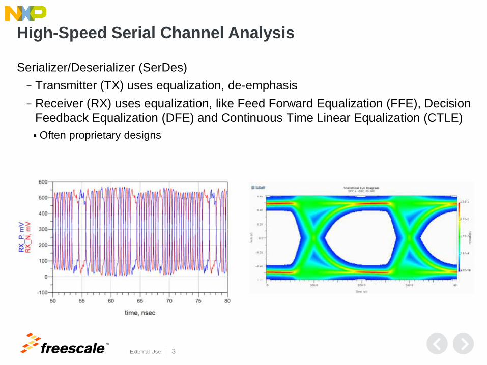
Serializer/Deserializer (SerDes)
− Transmitter (TX) uses equalization, de-emphasis
− Receiver (RX) uses equalization, like Feed Forward Equalization (FFE), Decision
Feedback Equalization (DFE) and Continuous Time Linear Equalization (CTLE)
Often proprietary designs

TM
External Use 4
Highlights
• Higher Speed SerDes busses operate with a closed eye at the pin of the Receiver in some cases
− RX EQ will help open the eye
− But RX EQ is producing a signal that is not seen at the pin
How to model what is happening inside the die to offset the losses in the channel and the closed eye that they produce?
• IBIS-AMI modeling finer details:
− TX EQ effects with RX EQ
− Lighter/less TX EQ may help with some RX settings
• PCB Design at 10Gbps
− Every detail matters on complex channels
− Simpler direct connect channels less of an issue
− Manage Return Loss

TM
External Use 5
SerDes: Differential Signaling
On occasion, there is confusion about the differential peak-to-peak voltage.
TM
External Use 6
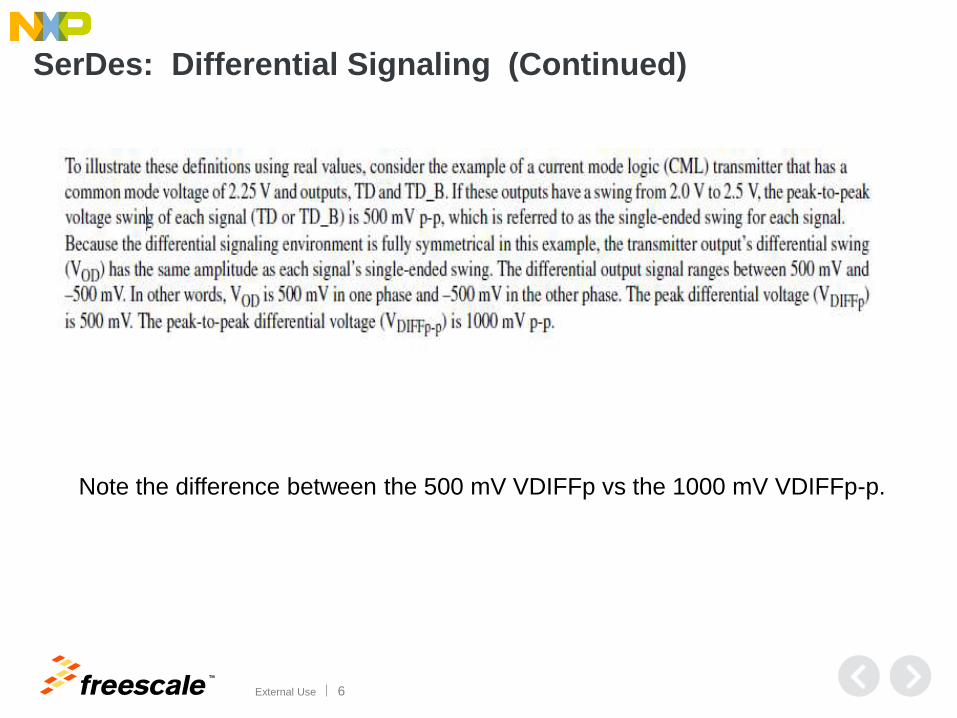
SerDes: Differential Signaling (Continued)
Note the difference between the 500 mV VDIFFp vs the 1000 mV VDIFFp-p.

TM
External Use 7
SerDes: Differential Signaling – Example
Amplitude for Blue and Green:
0 to 580 mV
Transition Bit:
Green – Blue =
0 – 580 = -580 mV
And
580 – 0 = 580 mV
Non-Transition Bit:
Green – Blue =
67 – 500 = -433 mV
And
500 – 67 = 433 mV
Vdiffp:
Transition Bit: 580 mV
Non-Transition Bit: 433 mV
Vdiffp-p:
Transition Bit: 2 x 580 = 1160 mV
Non-Transition Bit: 2 x 433= 866 mV
Red Signal: +/- 580, +/- 433 mV

TM
External Use 8
SerDes Transmitter and Receiver, Simplified
Generally, the SerDes TX and RX will be operating as 50 ohm single ended
drivers/receivers and 100 ohm differential drivers/receivers.

TM
External Use 9
SerDes TX: PCI Express Gen 2.0
HW Specs list the TX Amplitude (VTX-DIFFp-p) and the TX differential
impedance. In some protocols, the de-emphasis value is listed
TM
External Use 10
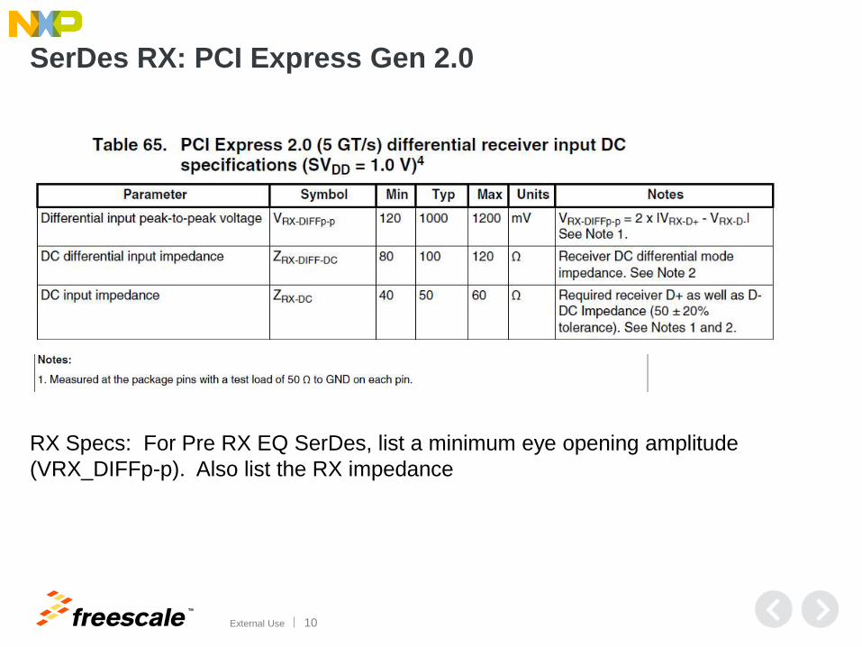
SerDes RX: PCI Express Gen 2.0
RX Specs: For Pre RX EQ SerDes, list a minimum eye opening amplitude
(VRX_DIFFp-p). Also list the RX impedance
TM
External Use 11
Equalization Related Parameters
in Freescale Documents

TM
External Use 12
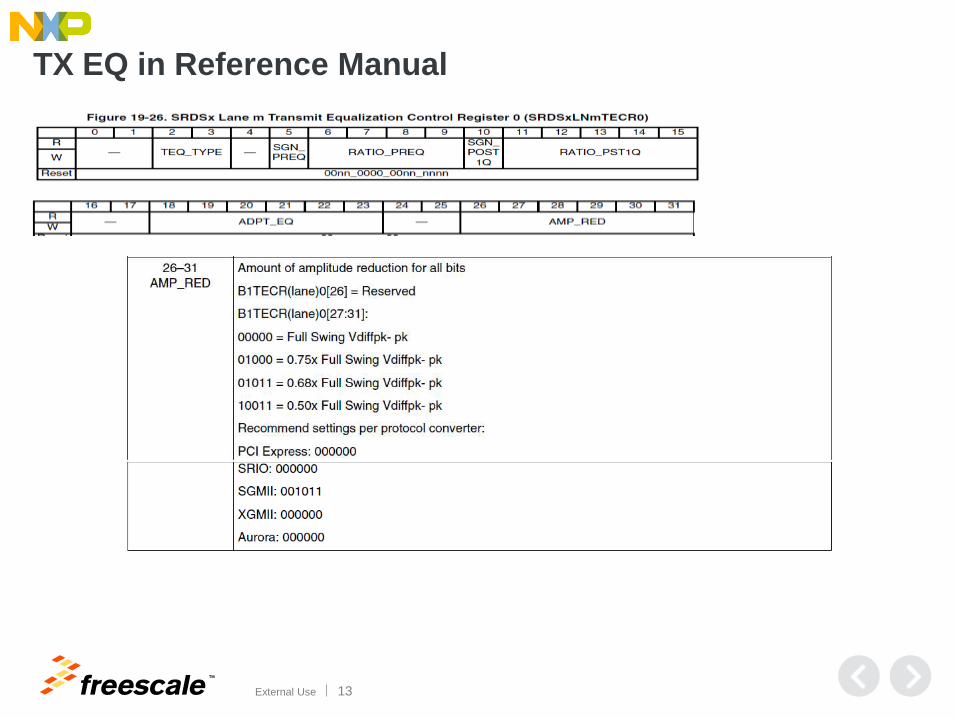
TX EQ Parameters Listed in Reference Manual
• Basic TX Controls:
− Amplitude of the TX (Differential peak to peak)
− What type of TX Equalization
Options for de-emphasis
De-emphasis levels
• TX EQ Controls:
− AMP_RED: Amplitude of the signal
− TEQ_TYPE: Number of bits of Equalization
− Emphasis
Pre-cursor: Values for Pre-cursor bit
Post-cursor: Value for Post-cursor bit
TM
External Use 13
TX EQ in Reference Manual

TM
External Use 14
TX EQ in Reference Manual

TM
External Use 15
Background on Electrical Data

TM
External Use 16
Data Eye, Bit Time and Unit Interval
• Note: GHz vs Gbps
• Clock: 4 GHz
− Rising Edge to Rising Edge: 250 ps
− Bit Time: 125 ps
− Data Rate: 1/Bit Time
− or 1/UI= 1/125ps or 8 GHz
• So Data Rate is 2x “Clock”
• But Nyquist frequency is “Clock” Rate or 4 GHz

TM
External Use 17
Example: De-emphasis, Transition, Non-Transition Bits

TM
External Use 18
Example: De-emphasis, Transition, Non-Transition Bits
Ratio log 10 * -20 (dB)
1.5 0.176 -3.522
2 0.301 -6.021
3 0.477 -9.542
Examine Transition (TX_DIFF_PP)
vs.
Non-Transition (TX_DE_EMPH_PP)

TM
External Use 19
Example De-Emphasis Requirements for TX Model
• 3-tap De-emphasis:
− Pre-cursor
− Post-cursor

TM
External Use 20
10G SerDes 3-Tap TX Equalization
TM
External Use 21
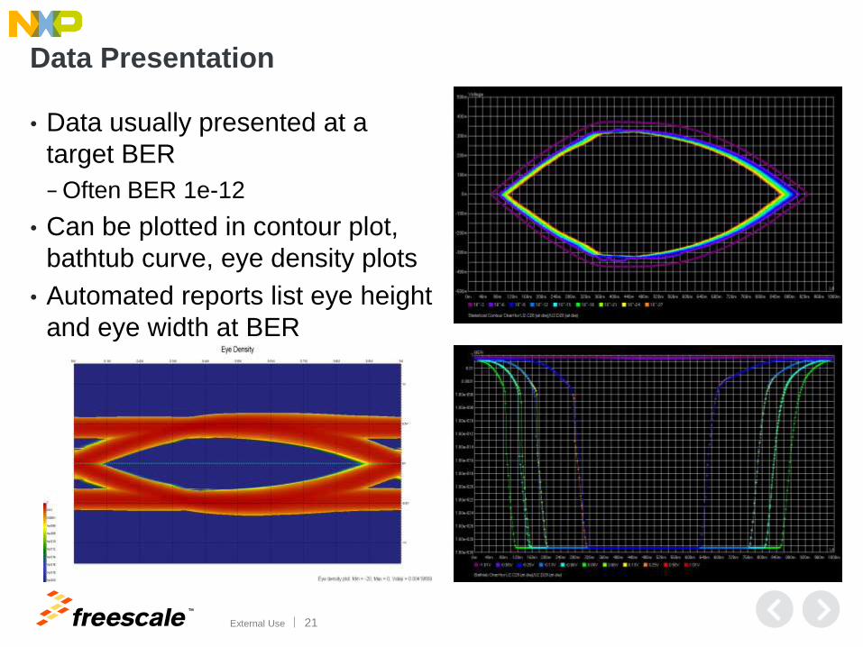
Data Presentation
• Data usually presented at a
target BER
− Often BER 1e-12
• Can be plotted in contour plot,
bathtub curve, eye density plots
• Automated reports list eye height
and eye width at BER

TM
External Use 22
Equalizer Frequency Response
• Channel Loss:
− “Boosted” by EQ
− EQ targets region where channel loss is critical

TM
External Use 23
IBIS AMI Background

TM
External Use 24
IBIS-AMI: How to Gain Post RX EQ Visibility in Simulations
TX EQ RX EQ
IO
Buffer
(IBIS)
IO
Buffer
(IBIS)
Standard IBIS for two
tap TX EQ or IBIS-AMI
or miscellaneous
models
IBIS-AMI or
miscellaneous models

TM
External Use 25
Pre- and Post-RX EQ Waveform Probing Locations
TX EQ RX EQ
IO
Buffer
(IBIS)
IO
Buffer
(IBIS)
Standard IBIS for
two tap TX EQ or
IBIS-AMI or misc
models
IBIS-AMI or
misc models
Probe Here for Post RX
EQ Waveform
Probe Here for Pre RX or
No RX AMI EQ Waveform

TM
External Use 26
IBIS 5.0 – IBIS-AMI Introduced
• IBIS-AMI
− IBIS 5.0 Release in 2008 added IBIS-AMI
− IBIS Algorithmic Modeling Interface (AMI)
− Expands IBIS Standard to include methods to model the algorithmic content in the SerDes TX and RX circuits
Used especially for RX EQ
• IBIS
− IO Buffer Interface Specification (IBIS)
− IBIS Specification 1.0: April 1993
Used extensively for PCI bus modeling
− Subsequent key versions:
2.1: December 1995
3.2: September 1999
5.0: August 2008
5.1 Being reviewed now; substantial addition of resolution documents
TM
External Use 27
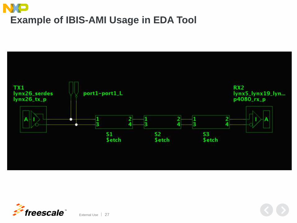
Example of IBIS-AMI Usage in EDA Tool
TM
External Use 28
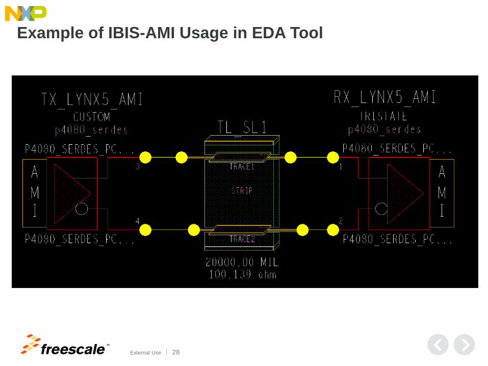
Example of IBIS-AMI Usage in EDA Tool

TM
External Use 29
IBIS-AMI Model Sections
• IBIS-AMI model
− Top Level is “.ibs” file, like standard IBIS
Has pin listing, signal to model name mapping, diff pair listing, etc.
Uses standard analog modeling for driver impedance, capacitive loading, edge
rates, etc.
− Parameter file – “.ami” file
Text file that is readable by user
Sets values to be used in DLL model file
− DLL
Where algorithms are modeled in AMI language
Compiled to protect the proprietary TX and RX model information
IBIS 5.0 compliant allows it to run in multiple tools

TM
External Use 30
IBIS-AMI Example Data
• View of “.ibs”, “.ami” and DLL/SO file listing
.ibs file header .ami file listing DLL/SO files

TM
External Use 31
Freescale TX IBIS-AMI
Model Background

TM
External Use 32
SerDes IBIS-AMI Model
• TX Model includes EQ (TEQ_TYPE)
− No Tap
− 2-Tap
− 3-Tap
− 4-Tap
• TX Model includes Amplitude Adjustment
− Matches to protocol
• TX Model: De-emphasis levels
− Ranges from: 0 to 2-3x
• RX Model: Includes Adaptive EQ
− May have ability to communicate with TX

TM
External Use 33
SerDes TX AMI Model Settings (1)
(TEQ_TYPE (List 0 1 2 3)(Usage In)(Type Integer)(Default 1)
(Labels "00: No TX Equalization"
"01: 2 level of TX Equalization"
"10: 3 levels of TX Equalization"
"11: Reserved")
(Description "Transmitter Equalization type selection"))
(AMP_RED (List 32 0 1 3 2 6 7 16 17 19 18 22 23 31)(Usage In)(Type Integer)(Default 0)
(Labels "10 0000 (d32): 1.100 X Full Swing" "00 0000 (d0): 1.000 X Full Swing"
"00 0001 (d1): 0.917 X Full Swing" "00 0011 (d3): 0.840 X Full Swing"
"00 0010 (d2): 0.752 X Full Swing" "00 0110 (d6): 0.667 X Full Swing"
"00 0111 (d7): 0.585 X Full Swing" "01 0000 (d16): 0.500 X Full Swing"
"01 0001 (d17): 0.458 X Full Swing" "01 0011 (d19): 0.420 X Full Swing"
"01 0010 (d18): 0.376 X Full Swing" "01 0110 (d22): 0.333 X Full Swing"
"01 0111 (d23): 0.292 X Full Swing" "01 1111 (d31): 0.170 X Full Swing")
(Description "Transmitter Output Amplitude Control"))

TM
External Use 34
SerDes TX AMI Model Settings (2)
(RATIO_PREQ (List 0 1 2 3 4 5 6 7 8 9 10 11 12)(Usage In)(Type Integer)(Default 0)
(Labels "0000 (d0): No equalization" "0001 (d1): 1.04 X relative amplitude"
"0010 (d2): 1.09 X relative amplitude" "0011 (d3): 1.14 X relative amplitude"
"0100 (d4): 1.20 X relative amplitude" "0101 (d5): 1.26 X relative amplitude"
"0110 (d6): 1.33 X relative amplitude" "0111 (d7): 1.40 X relative amplitude"
"1000 (d8): 1.50 X relative amplitude" "1001 (d9): 1.60 X relative amplitude"
"1010 (d10): 1.71 X relative amplitude" "1011 (d11): 1.84 X relative amplitude"
"1100 (d12): 2.00 X relative amplitude")
(Description "Transmitter Pre-Cursor Control"))
(SGN_PREQ (List 0 1)(Usage In)(Type Integer)(Default 1)
(Labels "0 = Negative"
"1 = Positive")
(Description "Transmitter Pre-Cursor Polarity"))

TM
External Use 35
SerDes TX AMI Model Settings (3)
(RATIO_PST1Q (List 0 1 2 3 4 5 6 7 8 9 10 11 12 13 14 15 16)(Usage In)(Type Integer)(Default 12)
(Labels "0 0000 (d0): No equalization" "0 0001 (d1): 1.04 X relative amplitude"
"0 0010 (d2): 1.09 X relative amplitude" "0 0011 (d3): 1.14 X relative amplitude"
"0 0100 (d4): 1.20 X relative amplitude" "0 0101 (d5): 1.26 X relative amplitude"
"0 0110 (d6): 1.33 X relative amplitude" "0 0111 (d7): 1.40 X relative amplitude"
"0 1000 (d8): 1.50 X relative amplitude" "0 1001 (d9): 1.60 X relative amplitude"
"0 1010 (d10): 1.71 X relative amplitude" "0 1011 (d11): 1.84 X relative amplitude"
"0 1100 (d12): 2.00 X relative amplitude" "0 1101 (d13): 2.18 X relative amplitude"
"0 1110 (d14): 2.40 X relative amplitude" "0 1111 (d15): 2.66 X relative amplitude"
"1 0000 (d16): 3.00 X relative amplitude")
(Description "Transmitter Post-Cursor Control"))
(SGN_POST1Q (List 0 1)(Usage In)(Type Integer)(Default 1)
(Labels "0 = Negative"
"1 = Positive")
(Description "Transmitter Post-Cursor Polarity"))

TM
External Use 36
TX EQ in Reference Manual

TM
External Use 37
TX EQ in Reference Manual
TM
External Use 38
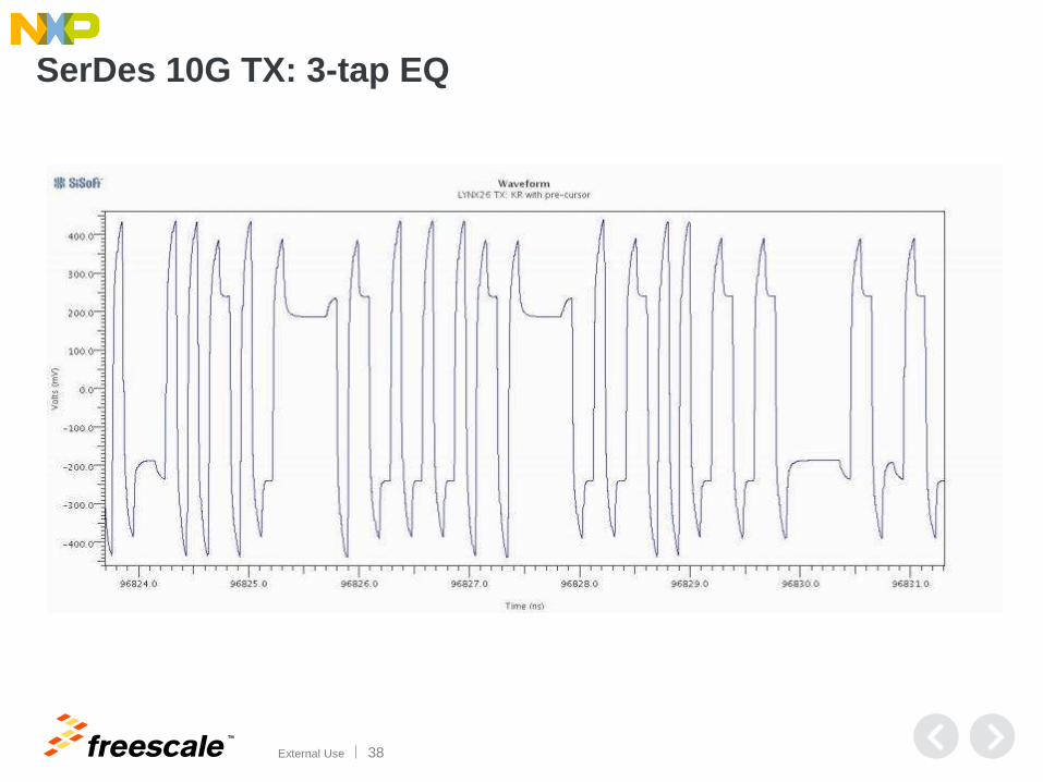
SerDes 10G TX: 3-tap EQ

TM
External Use 39
Freescale RX IBIS-AMI
Model Background

TM
External Use 40
Simulate to Optimize RX EQ
• RX EQ
− Simulation to provide visibility at Post RX EQ
− Typically where data eye recovery takes place
− EQ Types
FFE
DFE
CTLE
Freescale SerDes 10G is custom circuit
− Often Adaptive
May have over-rides
Freescale is adaptive (finds best values for its RX EQ parameters)
− Instructive to look at data eye before/after RX EQ in some cases

TM
External Use 41
Comment: 5G Post RX EQ ~65-80% UI
with +/- 320 to +/- 450 mV amplitude
100 200 300 400 500 6000 700
-0.5
0.0
0.5
-1.0
1.0
time, psec
De
nsity
measurement
Level1Level0HeightWidth
Summary
0.488-0.4870.857
2.976E-10

TM
External Use 42
IBIS-AMI Model Correlation
TM
External Use 43
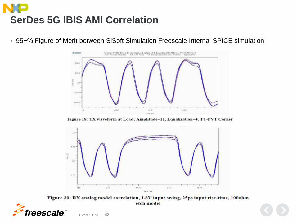
SerDes 5G IBIS AMI Correlation
• 95+% Figure of Merit between SiSoft Simulation Freescale Internal SPICE simulation
TM
External Use 44
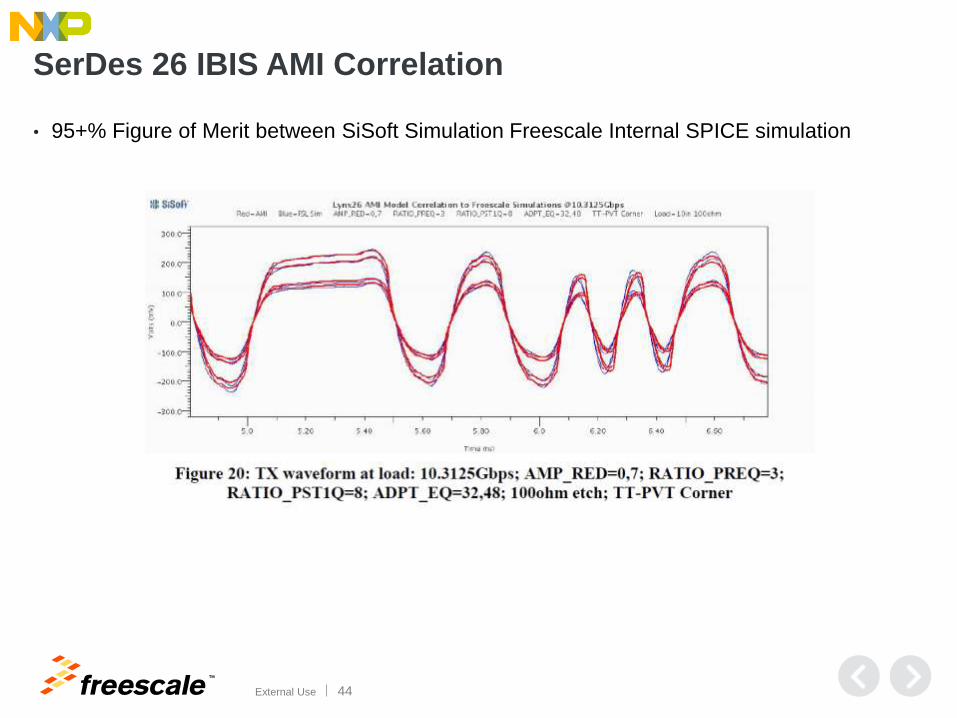
SerDes 26 IBIS AMI Correlation
• 95+% Figure of Merit between SiSoft Simulation Freescale Internal SPICE simulation

TM
External Use 45
TX EQ Simulations

TM
External Use 46
10G TX Driving 1x Etch Length @ 8G – TX AMI Only
• Compare Voltage vs. Time De-Emphasis Plots
– See how de-emphasis levels change non-transition bits

TM
External Use 47
SerDes 10G TX IBIS-AMI: Vary TX EQ Post1Q
TM
External Use 48
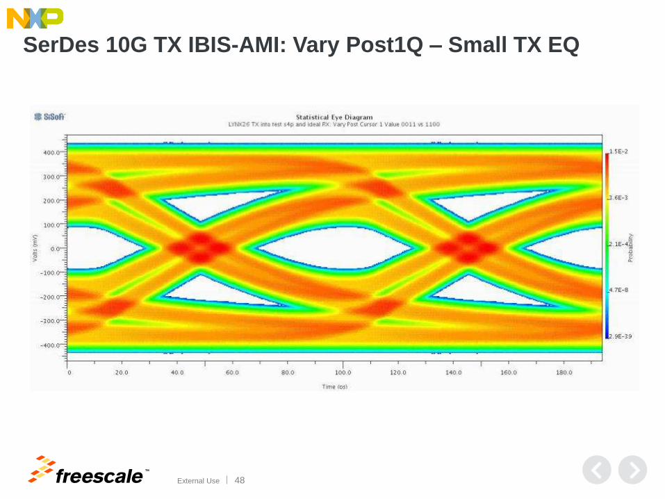
SerDes 10G TX IBIS-AMI: Vary Post1Q – Small TX EQ

TM
External Use 49
SerDes 10G TX IBIS-AMI: Vary Post1Q, Large TX EQ
- Note smaller outer eye; larger inner eye
TM
External Use 50
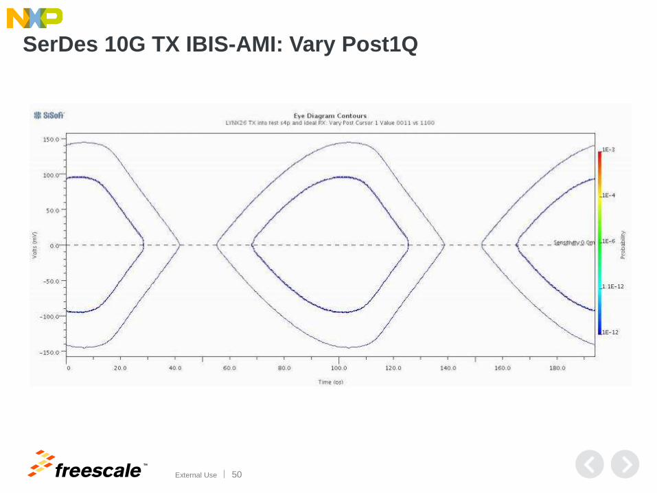
SerDes 10G TX IBIS-AMI: Vary Post1Q
TM
External Use 51
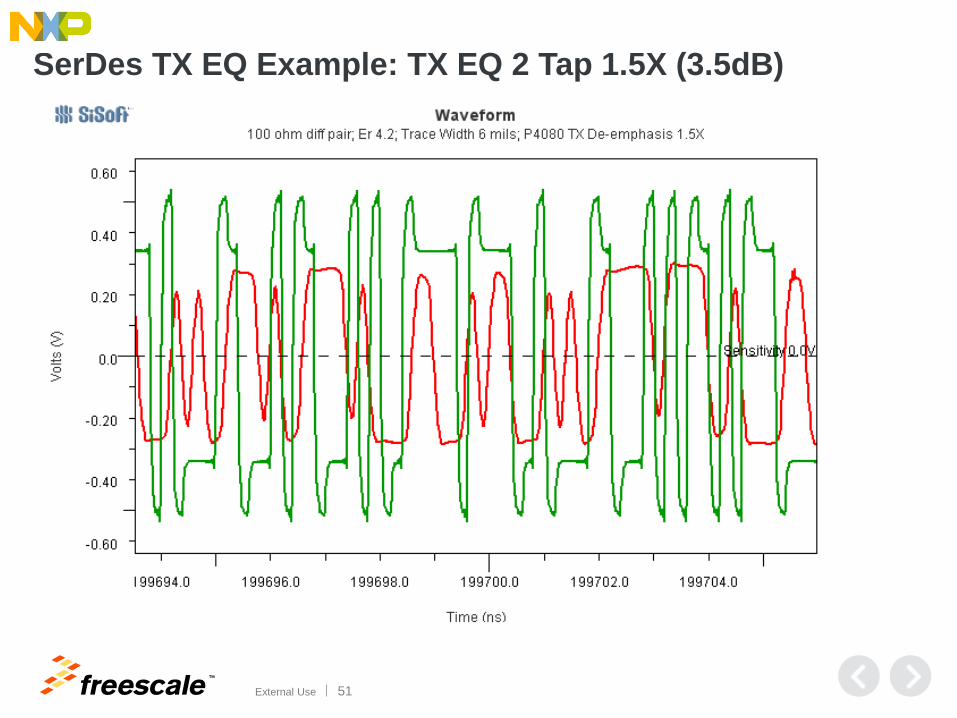
SerDes TX EQ Example: TX EQ 2 Tap 1.5X (3.5dB)

TM
External Use 52
SerDes TX EQ Example: TX EQ 2 Tap 1.5X (3.5dB)

TM
External Use 53
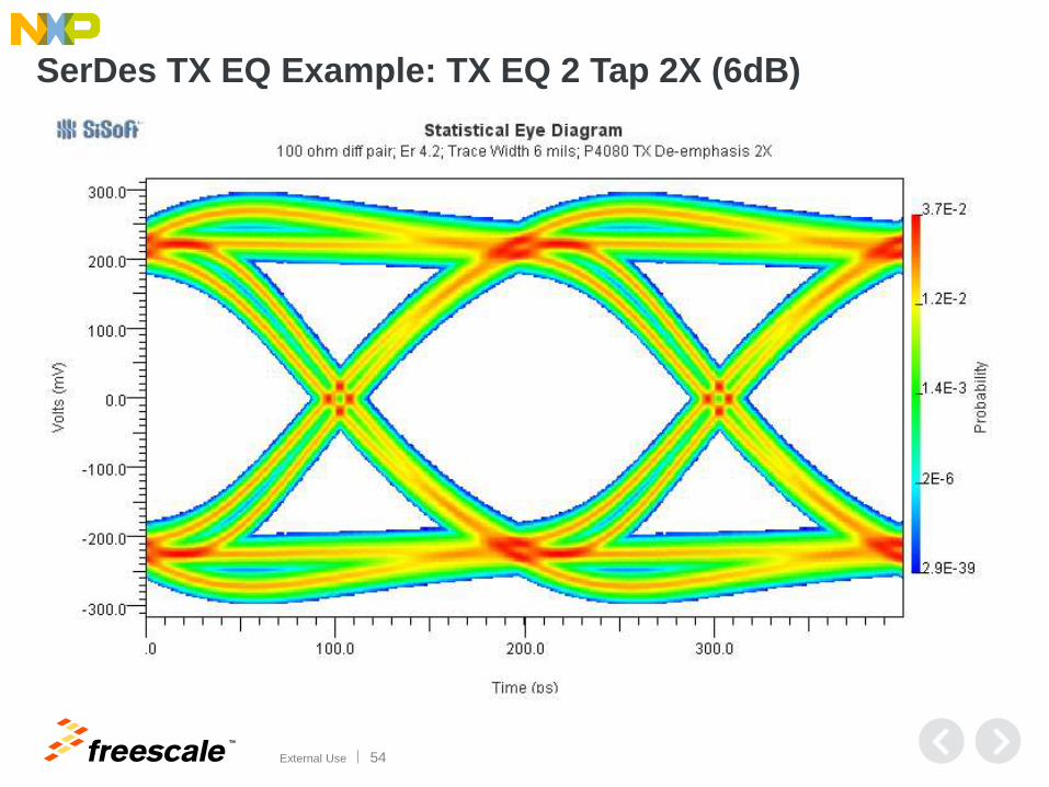
SerDes TX EQ Example: TX EQ 2 Tap 2X (6dB)
TM
External Use 54
SerDes TX EQ Example: TX EQ 2 Tap 2X (6dB)

TM
External Use 55
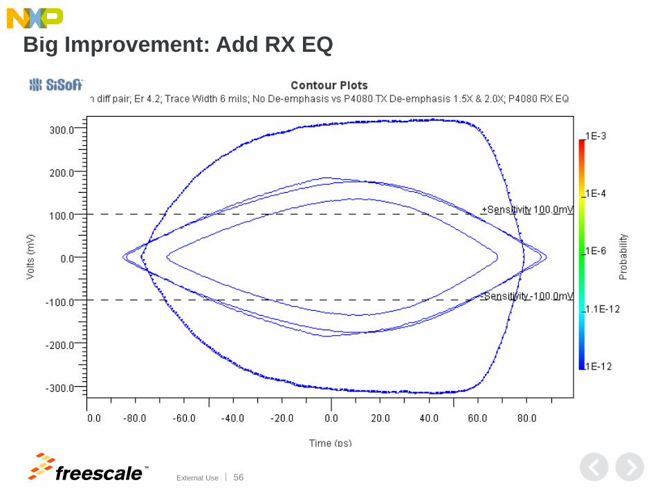
SerDes TX EQ Example: Compare Contours
TM
External Use 56
Big Improvement: Add RX EQ

TM
External Use 57
RX EQ Simulations

TM
External Use 58
Alter RXEQ @ 5G – Single Bit; Can See Some Change in
Single Bits

TM
External Use 59
Compare Eyes for RXEQ Difference @ 5G: Top 0,0;
Bottom 15,0

TM
External Use 60
Alter RXEQ @ 10G – Single Bit; Some Cases Don’t Work

TM
External Use 61
Compare Eyes for RXEQ Difference @ 10G: Top 8,0;
Bottom 15,0

TM
External Use 62
Alter RXEQ: Waveform Shifts
TM
External Use 63
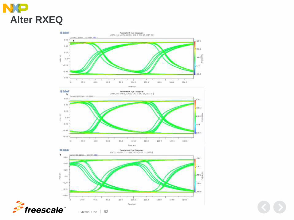
Alter RXEQ
TM
External Use 64
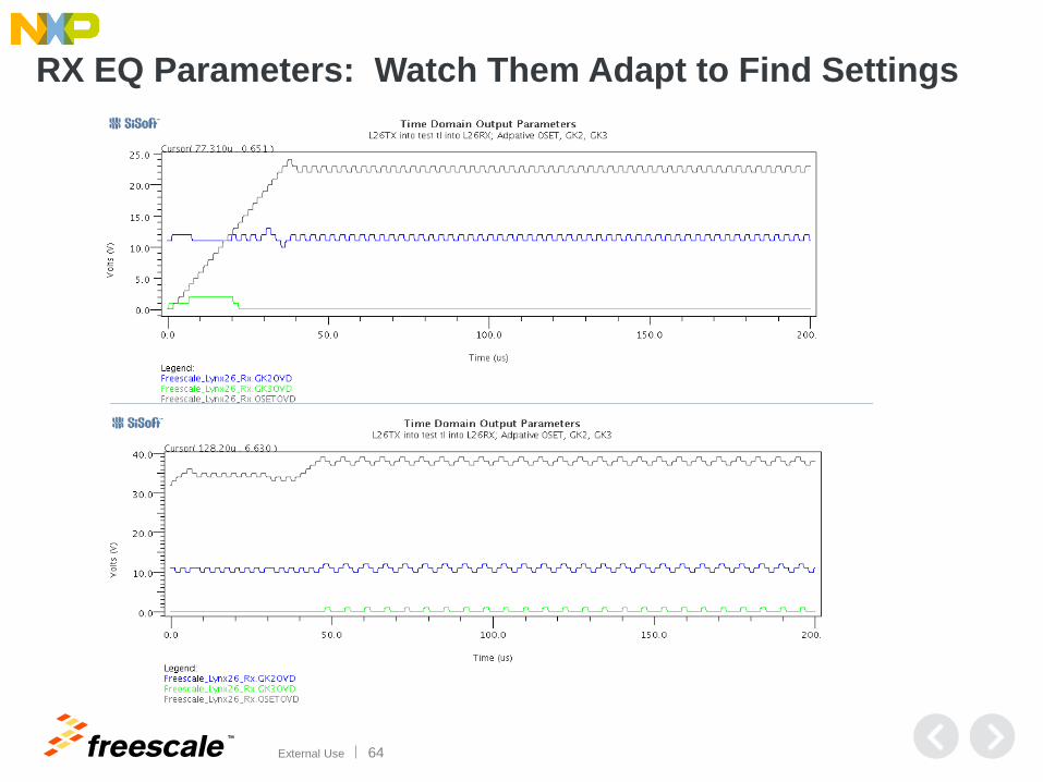
RX EQ Parameters: Watch Them Adapt to Find Settings

TM
External Use 65
RXEQ Settings: Helps in Some Cases
- Off for top
- On for middle
- On vs. off for
contour plot at bottom

TM
External Use 66
Comments on TX and RX EQ Parameters
• TX EQ Amplitude and De-emphasis map into typical usage
− Slower speeds, without RX EQ, then TX EQ helps
• RX EQ: Adaptive Design is very useful
− Very thankful we have that
− Runs automatically in silicon
Not needing to set RXEQ values

TM
External Use 67
How to Categorize a Channel

TM
External Use 68
PCB Trace Losses
• PCB Interconnect losses due to traces can be seen in S parameter data.
• Insertion Loss (S12, S21)
− The PCB dielectric materials and traces have losses that increase with the frequency of the signal. As the SerDes bus speeds increase, the PCB losses become a larger factor in signal degradation
• Return Loss (S11, S22)
− Signal losses are also caused by mismatches in impedance. Impedance mismatches occur in packages, PCB traces, vias, connectors, and sockets

TM
External Use 69
IEEE Spec Document: 10GBase-KR

TM
External Use 70
Channel Analysis and Printed
Circuit Board Considerations

TM
External Use 71
SerDes Channel: Device to Device, Same Board
• Device to Device:
− BGA Breakout
− BGA Vias: Stubs, Micro Vias
− PCB Trace
− BGA Breakout and Vias

TM
External Use 72
SerDes Channel: Board to Board
• Board to Board:
− BGA Breakout
− BGA Vias: Stubs, Micro Vias
− PCB Trace
− Connector Vias: Stubs
− Daughtercard Traces and Vias

TM
External Use 73
SerDes Channel: Board to Board with Cable
• Board to Board, to Cable, Board to Board:
− BGA Breakout
− BGA Vias: Stubs, Micro Vias
− PCB Trace
− Connector Vias: Stubs
− Daughtercard Traces and Vias
− Cable
− Motherboard – Daughtercard Path a second time

TM
External Use 74
Design Considerations
• BGA Breakout
− How many lanes? How many layers available?
− Pad size
− Via design
• PCB Stackup
− Trace width
− Material:
Lost Tangent, Dissipation Factor
Dielectric Constant
− Impedance
• PCB Routing
− Trace Length
− Trace Separation (Crosstalk)
• Connector
− Impedance
− Crosstalk

TM
External Use 75
PCB Cross Section/Materials

TM
External Use 76
PCB Trace Material
At higher speeds, have to consider surface roughness and plating
Surface Roughness Profiles
• Electrodeposited
• Reverse Treated
• Low Profile
• Rolled
Plating
• Nickel
• Silver
• Soldermask

TM
External Use 77
Foil Type and Surface Roughness (Rogers)

TM
External Use 78
BGA Breakout
• Breakout on which layer?
− Top Layer
− Bottom Layer
− Internal Layers
Stripline with short via stub
Stripline with micro via or back drilled via
− Trace Width Management
Neckdowns? Dog Bones?

TM
External Use 79
BGA Breakout
Note Dog Bone Break Out
Note Via Stub

TM
External Use 80
AC Capacitor Pad
• AC Capacitor Pads (or any pad)
− Consider cutting out plane under pad
• Shown here are AC cap pads on
PCB
− Pads are cut out to match pad width
• Also, Connector Pads are cut out

TM
External Use 81
PCB Vias
• PCB Vias (diff pair) generally
will be < 100 ohms
• Consider creating larger
antipad for planes in the
stackup to reduce
capacitance and raise
impedance
• Diff pair Vias from board with
antipad cutouts shown

TM
External Use 82
Other Forms of Impedance Discontinuities:
Mid Bus Probe, Test Points
• Test Point at Right
− 20 mils: would be 24 ohms (SE)
• Mid Bus Probe
− 60-70 ohm discontinuity

TM
External Use 83
Other Forms of Insertion Loss: Cables and MUX’s
• Multiplexer Devices
− Considerable loss for > 5 Gbps operation
8 dB loss at 5 GHz
Large (-40 dB) loss at 12-14 GHz
• Cable
− Considerable Loss
1-2 dB loss at 5 GHz
6-8 dB loss at 15 GHz

TM
External Use 84
BGA,
24 mil pad,
36 ohm
Dog bone
Mid Bus
Via Stub
AC Caps
and Vias
PCIe
Connector
Pads
Measured TDR (Top) vs. First Pass Simulated TDR (Bottom)

TM
External Use 85
PCB Losses: Conductor

TM
External Use 86
PCB Routing: Trace Width
• Trace Width affects the loss of the SerDes channel
• Narrower traces produce more loss due to skin effect
• Increases at Square Root of Frequency
a o f / tw
tw = trace width
(worse with narrow traces)
Frequency Dependent Skin Effect Loss
TM
External Use 87
PCB Trace Width Examples
• PCB Trace Widths to be examined:
− 4 mils
− 6 mils
− 8 mils
− 10 mils
− 12 mils
• Data eyes for narrower trace widths have a smaller amplitude and
smaller UI due to conductor loss

TM
External Use 88
Example Channel: Simulated at 5Gbps without EQ
PCB Trace: - 20 inches
- Dielectric Constant: 4.2
- Loss Tangent: 0.02
- Vary Trace Width: - 4, 6, 8, 10, 12 mils

TM
External Use 89
PCB Trace Width Examples: Insertion Loss - Up to a 3.2 dB change due to trace width

TM
External Use 90
Attenuation: Blue (total), Red (conductor), Green
(dielectric) 4 mil 6 mil
8 mil 10 mil

TM
External Use 91
PCB Trace Width Results: 4 Mils

TM
External Use 92
PCB Trace Width Results: 8 Mils

TM
External Use 93
PCB Trace Width Results No EQ: Compare

TM
External Use 94
PCB Trace Width Results No EQ: Compare Contour Plots
Trace Width (mils)
Eye Ht (mV)
Eye Width
(ps)
4 173.7 113.3
6 261.6 136.7
8 317.9 148.4
10 360.8 154.7
12 380.9 158.6

TM
External Use 95
PCB Losses: Dielectric
TM
External Use 96
PCB Routing: PCB Material
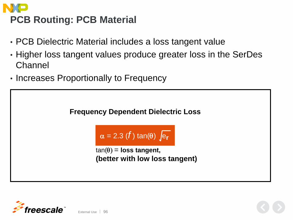
• PCB Dielectric Material includes a loss tangent value
• Higher loss tangent values produce greater loss in the SerDes
Channel
• Increases Proportionally to Frequency
a = 2.3 (f ) tan(q) er
tan(q) = loss tangent,
(better with low loss tangent)
Frequency Dependent Dielectric Loss

TM
External Use 97
Example Channel: Simulated at 5Gpbs No EQ
PCB Trace: - 20 inches
- Trace Width: 6 mils
- Vary PCB Materials
- Dielectric Constant and Loss Tangent - 4.2 and 0.0200
- 3.7 and 0.0090
- 3.5 and 0.0037
- 3.0 and 0.0013
TM
External Use 98
PCB Material Examples
• Common PCB materials to be examined: − Dielectric Constant (Er, Dk) = 4.2, Loss Tangent/Dissipation Factor (Df) = 0.02
− Dielectric Constant (Er, Dk) = 3.7, Loss Tangent/Dissipation Factor (Df) = 0.009
− Dielectric Constant (Er, Dk) = 3.5, Loss Tangent/Dissipation Factor (Df) = 0.0037
− Dielectric Constant (Er, Dk) = 3.0, Loss Tangent/Dissipation Factor (Df) = 0.0013
• Data eyes for higher loss tangent dielectrics generally have a
smaller amplitude and smaller UI due to dielectric loss
TM
External Use 99
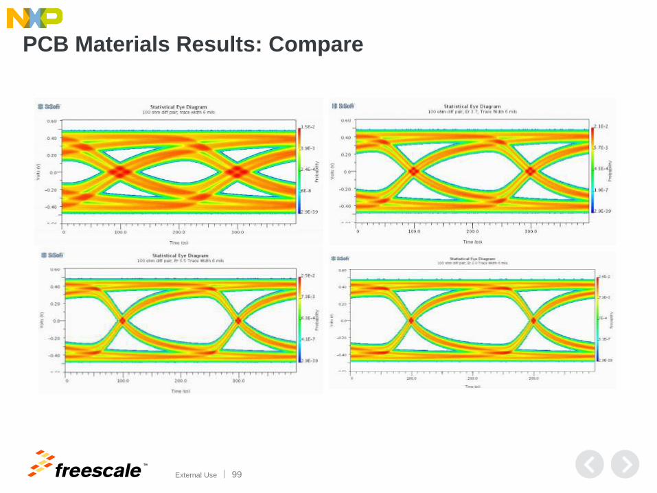
PCB Materials Results: Compare

TM
External Use 100
PCB Materials Results: Compare 1e-12 Contour Plot
Material Eye Ht
(mV)
Eye
Width
(ps)
Er 4.2, 0.02 261.6 136.7
Er 3.7, 0.009 414.7 170.3
Er 3.5,
0.0037 506.0 182.8
Er 3.0,
0.0013 536.9 185.9

TM
External Use 101
Summary Data on PCB Trace Width and Materials (1)
• Trace width: Use wider traces
(+) Improves skin-effect loss
(+) No increase in material cost
(-) Uses more routing area
(-) Increases PCB thickness to maintain impedance targets
Use of wider traces on internal layers may be limited due to board thickness
requirements

TM
External Use 102
Summary Data on PCB Trace Width and Materials (2)
• PCB materials: Use “high-speed” FR4
− (+) Lower loss tangent lowers dielectric loss
Loss tangent can be cut in half with modified FR4 materials
− Some boards using FR408HR, Megtron6
− Other boards using Rogers RO3003, Megtron6, Rogers RO4350
• Use “smooth” copper
− (+) Lower conductor loss
− (-) Caution! Peel strength is reduced
TM
External Use 103
Conductor Loss vs. Dielectric
Loss

TM
External Use 104
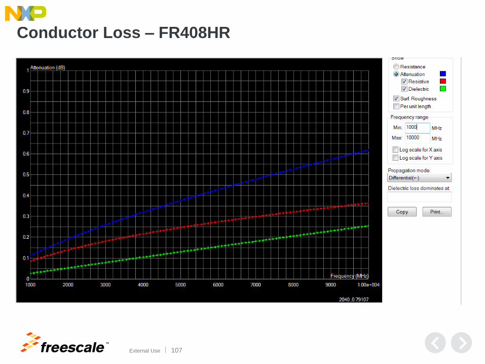
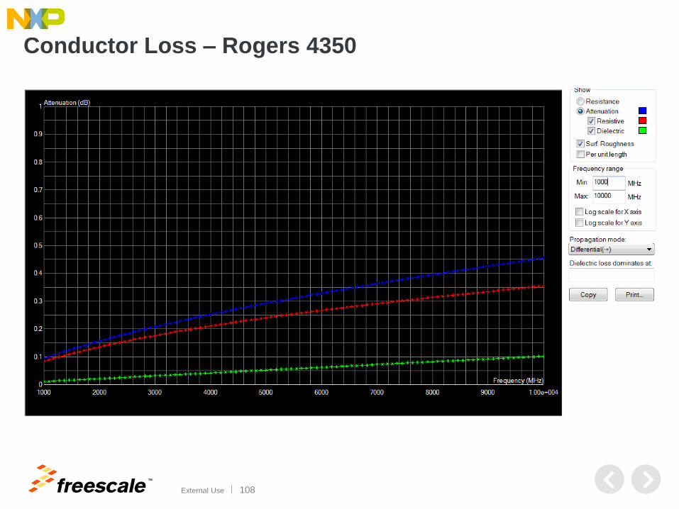
Conductor Loss vs. Dielectric Loss
• Plots from 2D models of PCB loss over frequency help to show conductor
vs. dielectric loss for different PCB materials
− Examine FR4, FR408HR, Rogers 4350, Rogers 3003

TM
External Use 105
Conductor Loss (red), Dielectric Loss (green), Total Loss (blue) (All plots for conductor loss are for 1 inch diff pair)
FR4 FR408HR
R4350 R3003

TM
External Use 106
Conductor Loss – FR4
TM
External Use 107
Conductor Loss – FR408HR
TM
External Use 108
Conductor Loss – Rogers 4350

TM
External Use 109
Conductor Loss – Rogers 3003
TM
External Use 110
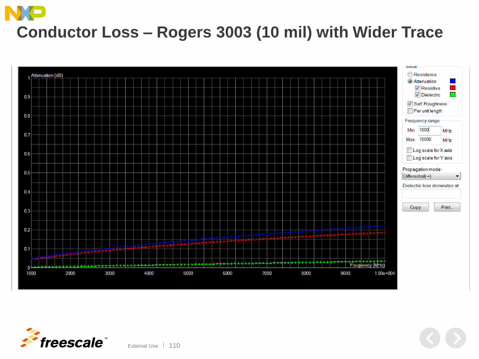
Conductor Loss – Rogers 3003 (10 mil) with Wider Trace

TM
External Use 111
Conductor Loss – Rogers 3003 (5 mil) to 100 GHz 1 dB total loss at ~57 GHz; FR4 1 dB total loss at ~10 GHz
TM
External Use 112
S21 vs. SDD21 Data
TM
External Use 113
SDD21 vs. S21 Data
• Consider external layer routing (Microstrip configuration)
• Simulations and measurements show that the amount of single-
ended insertion loss (S21) is more than the amount of the
differential insertion loss (SDD21) at the Nyquist Frequency of the
10Gbps signals
• A March 2013 blog by Eric Bogatin discusses this exact item
− One conclusion it brings forth is that a tightly coupled microstrip
differential pair should not be judged by its single-ended insertion loss
alone. Differential insertion loss may look good when the single-ended
insertion loss is questionable
− Key item is to track the deliberate far-end crosstalk (FEXT) in a
microstrip diff pair

TM
External Use 114
Measured Test Trace: SDD21 (in Green)
TM
External Use 115
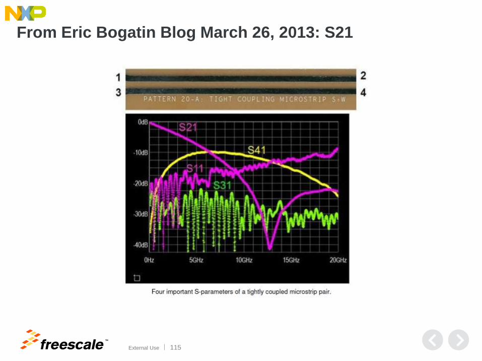
From Eric Bogatin Blog March 26, 2013: S21

TM
External Use 116
From Eric Bogatin Blog March 26, 2013: SDD21

TM
External Use 117
PCB Only SDD21 (Yellow) vs. S21 (Purple) and S41 (Red)
S41 FEXT rises
S21 insertion
loss dips

TM
External Use 118
Package SDD21 (Yellow) vs S21 (Purple) and S41 (Red)
S41 FEXT rises
S21 insertion
loss dips
S41 FEXT rises
S21 insertion
loss dips

TM
External Use 119
Connector SDD21 (Yellow) vs. S21 (Purple) and S41 (Red)
S41 FEXT rises
S21 insertion
loss dips
S41 FEXT rises
S21 insertion
loss dips
S41 FEXT rises
S21 insertion
loss dips

TM
External Use 120
Test Traces with Cables and Connectors:
S21 (Red) vs. SDD21 (Yellow) simulated to 20 GHz

TM
External Use 121
Compare Tightly/Loosely Coupled Diff Pairs SDD21 (Yellow), S21 (Purple), S41 (Red)
Trace Separation=0.5 *Trace Width Trace Separation= 1.0 * Trace Width
Trace Separation=2.0 *Trace Width Trace Separation= 5.0 * Trace Width
TM
External Use 122
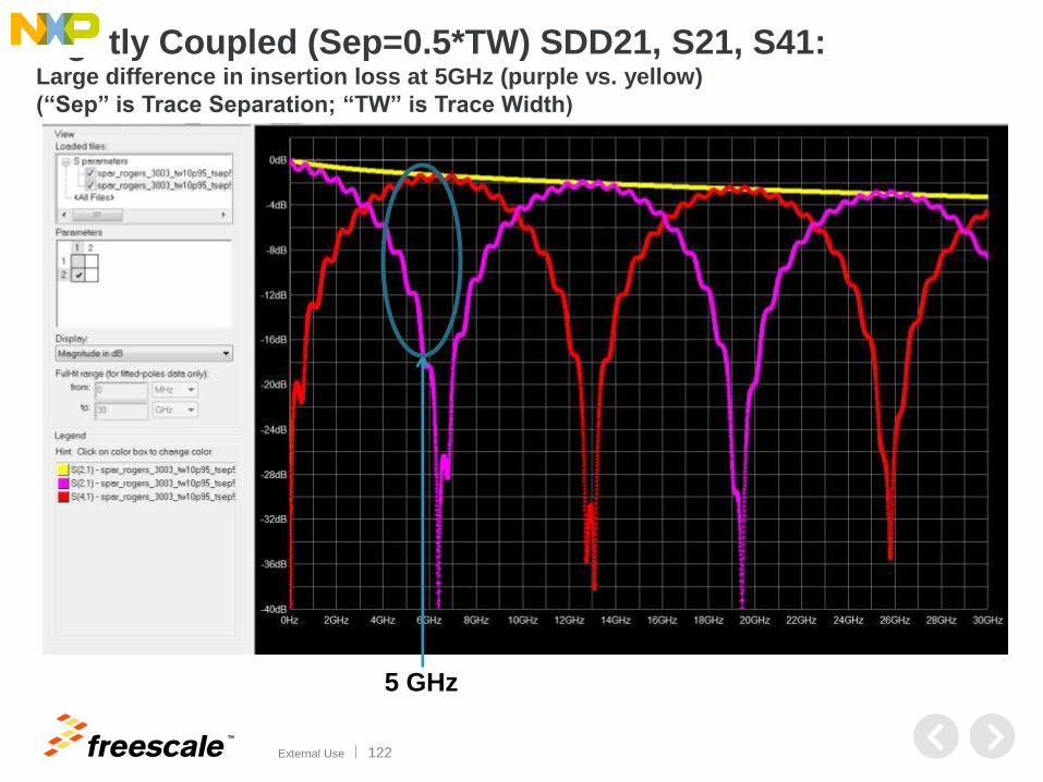
Tightly Coupled (Sep=0.5*TW) SDD21, S21, S41: Large difference in insertion loss at 5GHz (purple vs. yellow)
(“Sep” is Trace Separation; “TW” is Trace Width)
5 GHz

TM
External Use 123
Tightly Coupled (Sep=TW) SDD21, S21, S41
5 GHz

TM
External Use 124
Tightly-Loosely Coupled (Sep=2*TW) SDD21, S21, S41
5 GHz

TM
External Use 125
Loosely Coupled (Sep=3*TW) SDD21, S21, S41
5 GHz
TM
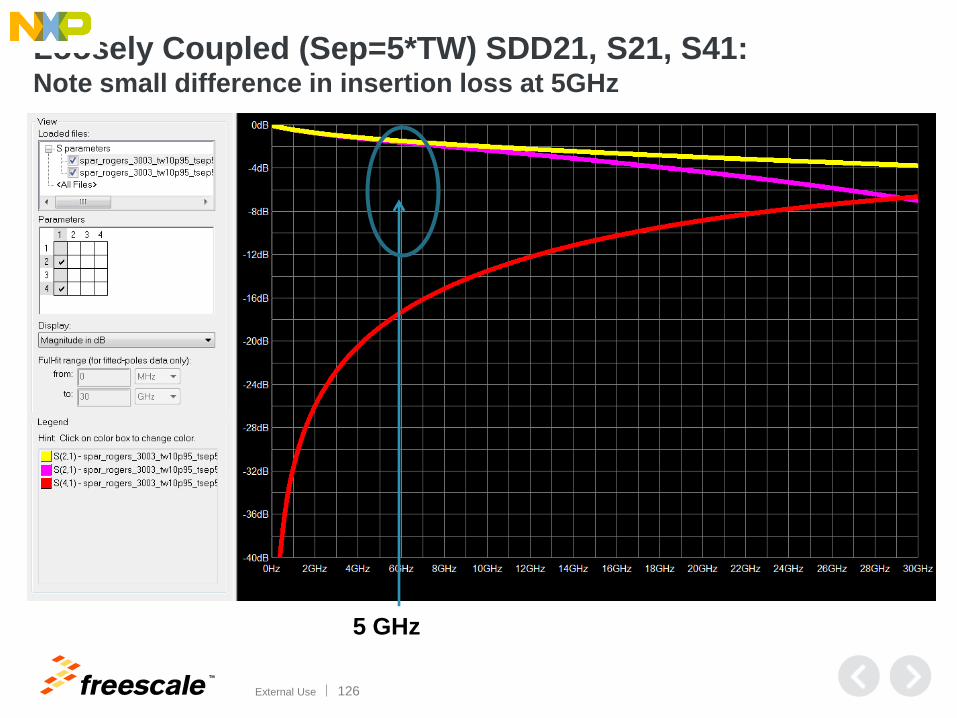
External Use 126
Loosely Coupled (Sep=5*TW) SDD21, S21, S41: Note small difference in insertion loss at 5GHz
5 GHz
TM
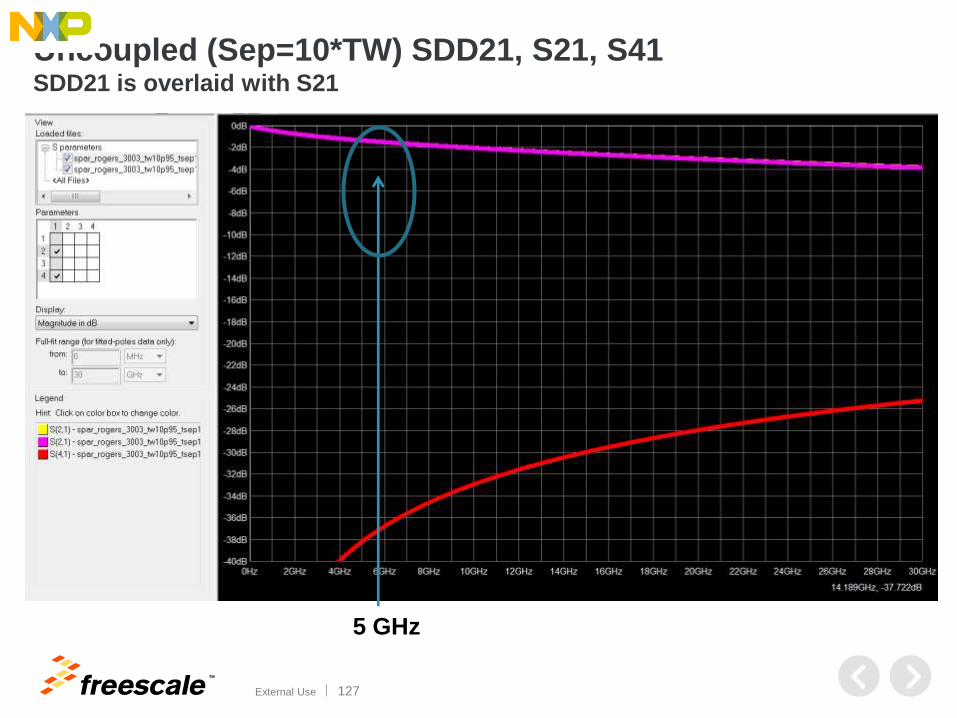
External Use 127
Uncoupled (Sep=10*TW) SDD21, S21, S41 SDD21 is overlaid with S21
5 GHz
TM
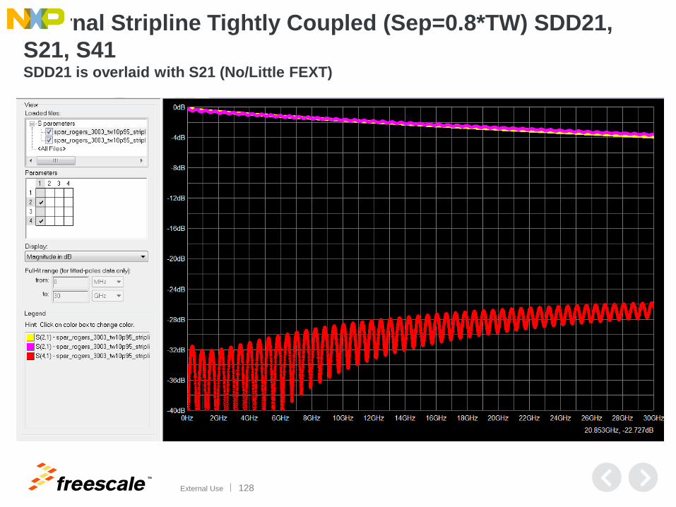
External Use 128
Internal Stripline Tightly Coupled (Sep=0.8*TW) SDD21,
S21, S41 SDD21 is overlaid with S21 (No/Little FEXT)

TM
External Use 129
Measured S21 vs. SDD21
test trace with vias – S21 test trace with vias – SDD21
TM
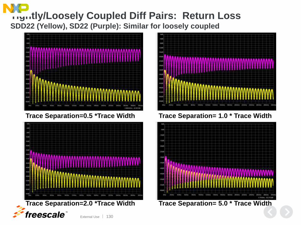
External Use 130
Tightly/Loosely Coupled Diff Pairs: Return Loss SDD22 (Yellow), SD22 (Purple): Similar for loosely coupled
Trace Separation=0.5 *Trace Width Trace Separation= 1.0 * Trace Width
Trace Separation=2.0 *Trace Width Trace Separation= 5.0 * Trace Width

TM
External Use 131
Channel Simulations with AMI
Models

TM
External Use 132
Multi-Board 8G: No TX EQ, No RX EQ – Closed

TM
External Use 133
Multi-Board 8G: TX EQ, No RX EQ – Almost Open

TM
External Use 134
Multi-Board 8G: TX No EQ, RX EQ – Open

TM
External Use 135
Multi-Board 8G: TX EQ, RX EQ – Open
TM
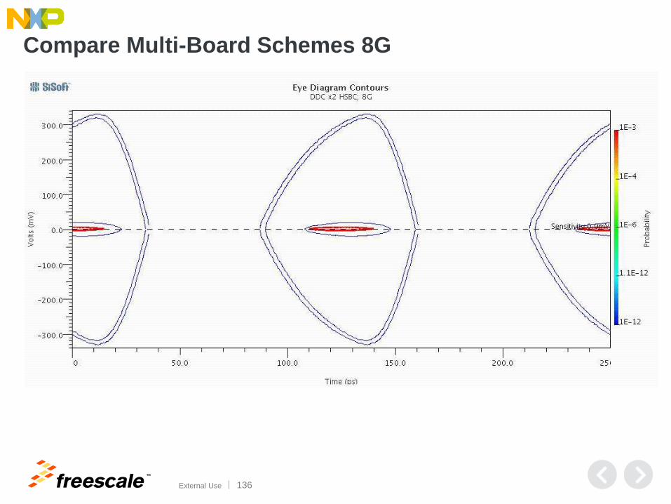
External Use 136
Compare Multi-Board Schemes 8G

TM
External Use 137
Sweep TX to Find Better Eye?

TM
External Use 138
10G TX Driving 1x Etch Length @ 8G – Insertion Loss

TM
External Use 139
10G TX Driving 1x Etch Length @ 8G – TX AMI Only:
• Compare Voltage vs. Time De-Emphasis Plots
– See how de-emphasis levels change non-transition bits

TM
External Use 140
10G TX Driving 1x Etch Length @ 8G – TX AMI Only;
1.0x – No TX EQ, Note Full Swing

TM
External Use 141
10G TX Driving 1x Etch Length @ 8G – TX AMI
Only; 1.2x – min TX EQ; Note Smaller Swing and
More Open Eye

TM
External Use 142
10G TX Driving 1x Etch Length @ 8G – TX AMI
Only; 1.5x – Moderate TX EQ; Swing Smaller;
Eye More Open

TM
External Use 143
10G TX Driving 1x Etch Length @ 8G – TX AMI Only;
2.0x – Strong TX EQ; Swing Smaller; Eye Open;
Too Much TX EQ?

TM
External Use 144
10G TX Driving 1x Etch Length @ 8G – TX AMI Only;
3.0x – Max TX EQ; Swing Smaller; Eye Open;
Too Much TX EQ
TM
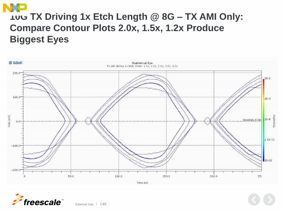
External Use 145
10G TX Driving 1x Etch Length @ 8G – TX AMI Only:
Compare Contour Plots 2.0x, 1.5x, 1.2x Produce
Biggest Eyes
TM
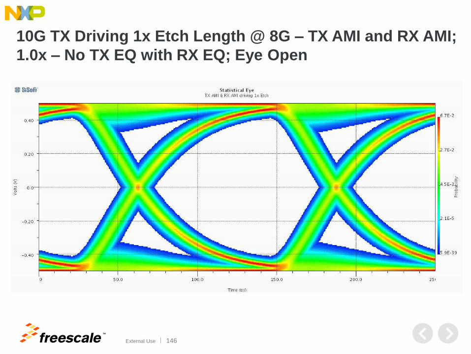
External Use 146
10G TX Driving 1x Etch Length @ 8G – TX AMI and RX AMI;
1.0x – No TX EQ with RX EQ; Eye Open
TM
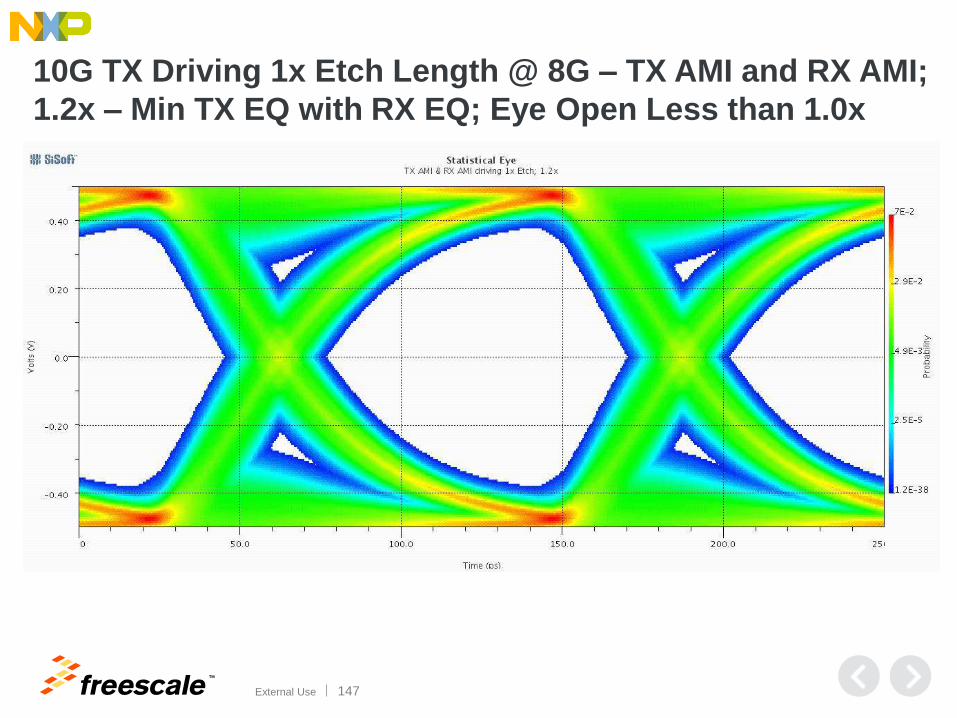
External Use 147
10G TX Driving 1x Etch Length @ 8G – TX AMI and RX AMI;
1.2x – Min TX EQ with RX EQ; Eye Open Less than 1.0x

TM
External Use 148
10G TX Driving 1x Etch Length @ 8G – TX AMI and RX AMI;
1.5x – Moderate TX EQ with RX EQ; Eye Open Less
than 1.2x

TM
External Use 149
10G TX Driving 1x Etch Length @ 8G – TX AMI and RX AMI;
2.0x – Strong TX EQ with RX EQ; Eye Open Less than 1.5x

TM
External Use 150
10G TX Driving 1x Etch Length @ 8G – TX AMI and RX AMI;
3.0x – Max TX EQ with RX EQ; Eye Open Less than 2.0x

TM
External Use 151
10G TX Driving 1x Etch Length @ 8G – TX AMI and RX AMI:
Compare Contour Plots: Best Settings Are Less TX EQ
TM
External Use 152
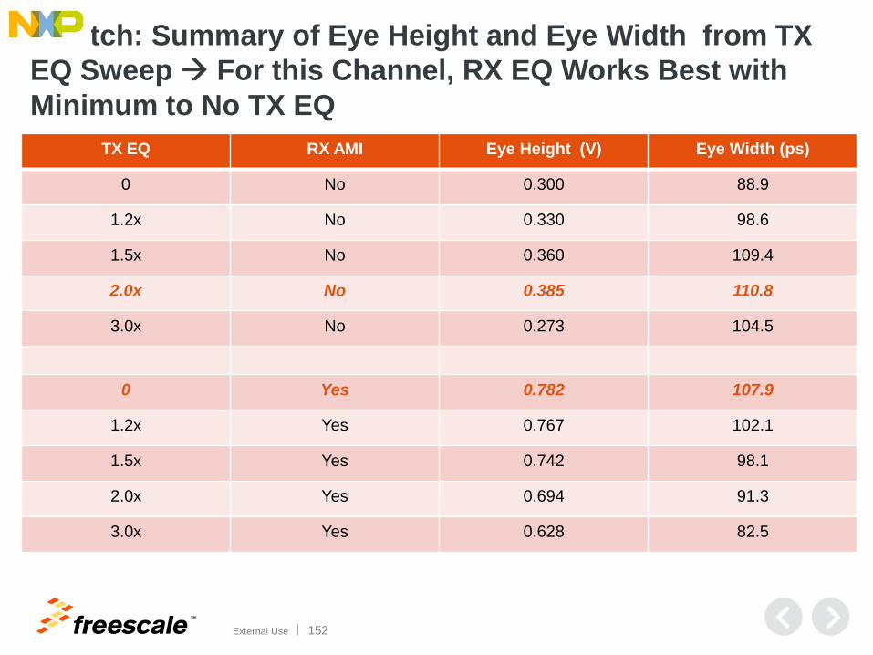
1x Etch: Summary of Eye Height and Eye Width from TX
EQ Sweep For this Channel, RX EQ Works Best with
Minimum to No TX EQ
TX EQ RX AMI Eye Height (V) Eye Width (ps)
0 No 0.300 88.9
1.2x No 0.330 98.6
1.5x No 0.360 109.4
2.0x No 0.385 110.8
3.0x No 0.273 104.5
0 Yes 0.782 107.9
1.2x Yes 0.767 102.1
1.5x Yes 0.742 98.1
2.0x Yes 0.694 91.3
3.0x Yes 0.628 82.5

TM
External Use 153
10G TX Driving 3x Etch Length @ 8G – Insertion Loss
(Compared to Prior Channel Insertion Loss ~3x More Loss)
TM
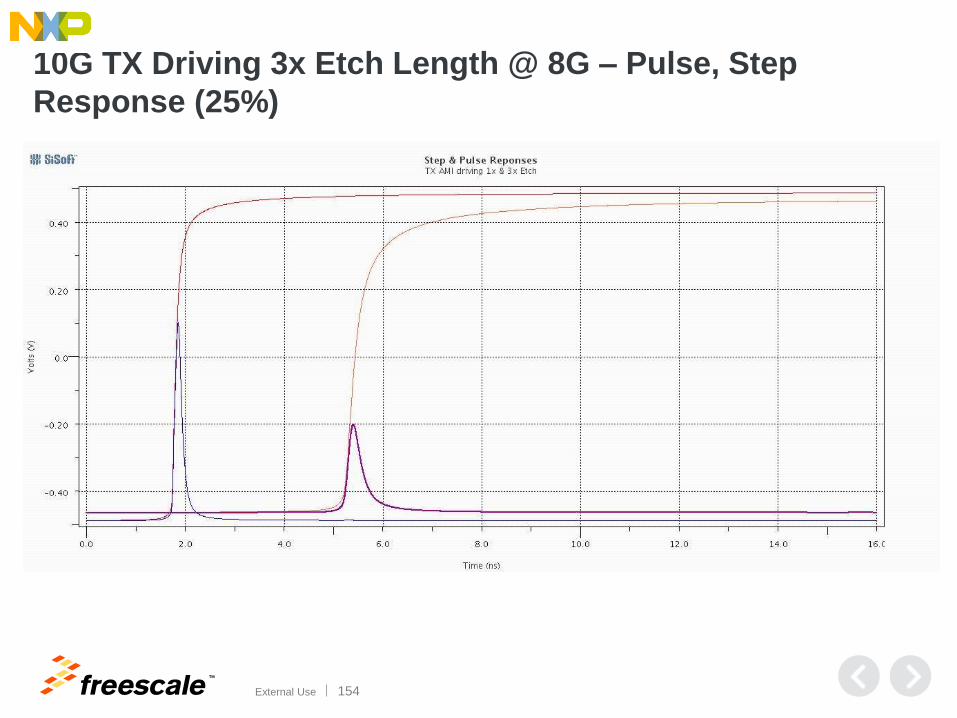
External Use 154
10G TX Driving 3x Etch Length @ 8G – Pulse, Step
Response (25%)

TM
External Use 155
10G TX Driving 3x Etch Length @ 8G – TX AMI Only; 1.0x

TM
External Use 156
10G TX Driving 3x Etch Length @ 8G – TX AMI Only; 1.2x
TM
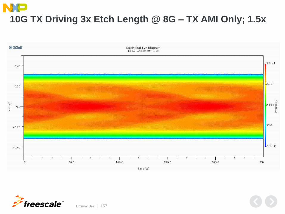
External Use 157
10G TX Driving 3x Etch Length @ 8G – TX AMI Only; 1.5x

TM
External Use 158
10G TX Driving 3x Etch Length @ 8G – TX AMI Only; 2.0x

TM
External Use 159
10G TX Driving 3x Etch Length @ 8G – TX AMI Only; 3.0x
- Almost opens the eye; notice how amplitude shrinks with stronger TX EQ

TM
External Use 160
10G TX Driving 3x Etch Length @ 8G – TX AMI Only:
Compare Contour Plots: Only TX EQ 3.0x Gives a Small
Open Contour
TM
External Use 161
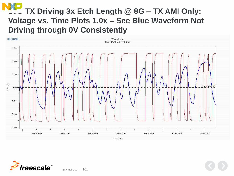
10G TX Driving 3x Etch Length @ 8G – TX AMI Only:
Voltage vs. Time Plots 1.0x – See Blue Waveform Not
Driving through 0V Consistently

TM
External Use 162
10G TX Driving 3x Etch Length @ 8G – TX AMI Only:
Voltage vs Time Plots 1.5x – See Blue Waveform Not
Driving through 0V Consistently Either

TM
External Use 163
10G TX Driving 3x Etch Length @ 8G – TX AMI Only:
Voltage vs. Time Plots 3.0x – See Blue Waveform Barely
Drives through 0V Consistently – Also Note that RX Signal Swing is Less Due to TX De-emphasis

TM
External Use 164
10G TX Driving 3x Etch Length @ 8G – TX AMI and RX AMI;
1.0x – No TX EQ; RX EQ Opens Eye

TM
External Use 165
10G TX Driving 3x Etch Length @ 8G – TX AMI and RX AMI;
1.2x – Min TX EQ; RX EQ Opens Eye

TM
External Use 166
10G TX Driving 3x Etch Length @ 8G – TX AMI and RX AMI;
1.5x – Moderate TX EQ; RX EQ Opens Eye Better with
this Setting

TM
External Use 167
10G TX Driving 3x Etch Length @ 8G – TX AMI and RX AMI;
2.0x – Strong TX EQ; RX EQ Opens Eye

TM
External Use 168
10G TX Driving 3x Etch Length @ 8G – TX AMI and RX AMI;
3.0x – Max TX EQ; RX EQ Opens Eye
TM
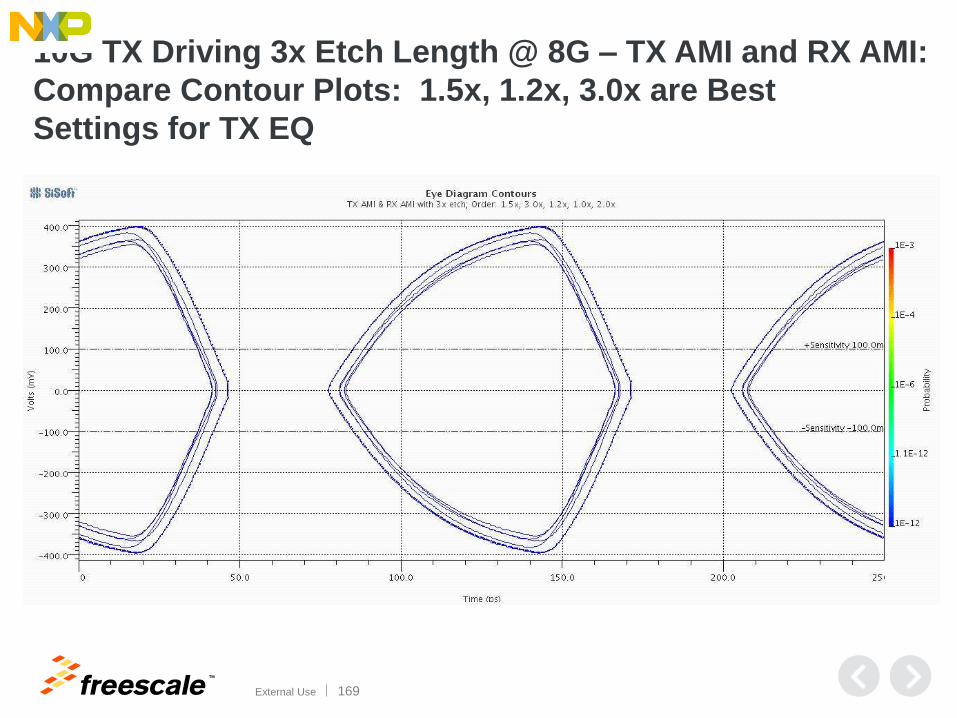
External Use 169
10G TX Driving 3x Etch Length @ 8G – TX AMI and RX AMI:
Compare Contour Plots: 1.5x, 1.2x, 3.0x are Best
Settings for TX EQ

TM
External Use 170
3x Etch: Summary of Eye Height and Eye Width from TX
EQ Sweep
TX EQ RX AMI Eye Height (V) Eye Width (ps)
0 No 0 0
1.2x No 0 0
1.5x No 0 0
2.0x No 0 0
3.0x No 0 0
0 Yes 0.658 84.5
1.2x Yes 0.661 87.9
1.5x Yes 0.721 94.7
2.0x Yes 0.640 84.9
3.0x Yes 0.699 87.4

TM
External Use 171
Summary of IBIS-AMI Benefits
• TX EQ modeling
− 2 tap, 3 tap, 4 tap TX EQ
• RX EQ modeling
− Multiple types of RX EQ
− Proprietary Circuits can be modeled
− AMI Model can be tailored specifically for a device’s design
• IBIS-AMI based simulation tools permit effective sweeping of TX and RX parameters to determine optimal settings
• EDA tools are building in GUI-based means to sweep parameters easily
• Good for tool usage that is not running models adaptively
• TX EQ and RX EQ can be significant tools for improving SerDes channel response
− May permit design using lower cost materials and narrower traces Translates to << $$ and << board space

TM
External Use 172
Questions and Answers Thanks!

TM
External Use 173
References
• Ambiguous Influences Affecting Insertion Loss of Microwave
Printed Circuit Boards, Rogers Corp.
• Eric Bogatin Blog March 26, 2013.

TM
External Use 174
Introducing The
QorIQ LS2 Family
Breakthrough,
software-defined
approach to advance
the world’s new
virtualized networks
New, high-performance architecture built with ease-of-use in mind Groundbreaking, flexible architecture that abstracts hardware complexity and
enables customers to focus their resources on innovation at the application level
Optimized for software-defined networking applications Balanced integration of CPU performance with network I/O and C-programmable
datapath acceleration that is right-sized (power/performance/cost) to deliver
advanced SoC technology for the SDN era
Extending the industry’s broadest portfolio of 64-bit multicore SoCs Built on the ARM® Cortex®-A57 architecture with integrated L2 switch enabling
interconnect and peripherals to provide a complete system-on-chip solution

TM
External Use 175
QorIQ LS2 Family Key Features
Unprecedented performance and
ease of use for smarter, more
capable networks
High performance cores with leading
interconnect and memory bandwidth
• 8x ARM Cortex-A57 cores, 2.0GHz, 4MB L2
cache, w Neon SIMD
• 1MB L3 platform cache w/ECC
• 2x 64b DDR4 up to 2.4GT/s
A high performance datapath designed
with software developers in mind
• New datapath hardware and abstracted
acceleration that is called via standard Linux
objects
• 40 Gbps Packet processing performance with
20Gbps acceleration (crypto, Pattern
Match/RegEx, Data Compression)
• Management complex provides all
init/setup/teardown tasks
Leading network I/O integration
• 8x1/10GbE + 8x1G, MACSec on up to 4x 1/10GbE
• Integrated L2 switching capability for cost savings
• 4 PCIe Gen3 controllers, 1 with SR-IOV support
• 2 x SATA 3.0, 2 x USB 3.0 with PHY
SDN/NFV
Switching
Data
Center
Wireless
Access
TM
External Use 176
See the LS2 Family First in the Tech Lab!
4 new demos built on QorIQ LS2 processors:
Performance Analysis Made Easy
Leave the Packet Processing To Us
Combining Ease of Use with Performance
Tools for Every Step of Your Design

TM
© 2014 Freescale Semiconductor, Inc. | External Use
www.Freescale.com