september 2016 - university of sheffield

EVALUATE THE ABILITY OF MOLECULAR DESCRIPTORS FOR PREDICTING

BIOACTIVITY PROFILES OF COMPOUNDS WITH MACHINE LEARNING METHOD

A study submitted in partial fulfilment

of the requirements for the degree of

Master of Science in Data Science

at

THE UNIVERSITY OF SHEFFIELD

by

JINGYAN SUI

September 2016

Abstract

Research context

Drug discovery is a complex process for finding new drug candidates, and it is time-

consuming and high cost (Taylor, 2015). With the rapid development of human

genome technology and pharmacology, huge amounts of potential targets and

biological activity data are producing. With the accumulation of data redundancy

and complexity, simple analysis methods have been unable to meet the demand of

large data analysis. In this situation, as a kind of fast and low cost way,

computational methods in chemoinformatics has great significance in early drug

discovery process. Computer-aided drug discovery or design methods can be used

to improve the efficiency of drug discovery (Sliwoski, Kothiwale, Meiler, & Lowe,

2014).

Bioactivity profiles for compounds are generated from their bioactivity data. Insight

of mode of actions for compounds can be got from comparison of bioactivity

profiles, beside, compounds bioactivities are strongly correlated with their chemical

structures (Cheng, Wang, &Bryant, 2010).

Aim

The aim of this dissertation is to evaluate the effectiveness of different molecular

descriptors on their ability to predict the bioactivity profiles of compounds extracted

from the open ChEMBL database.

Methodology

Bioactivity data for compounds and targets were extracted from ChEMBL database,

and transformed into bioactivity profiles for compounds by EXCEL and Rstudio.

Two kinds of 2D fingerprints (Morgan, MACCS) and physiochemical properties of

compounds were calculated by KNIME and RDkit.

One of machine learning method named clustering was used in this dissertation. One

of clustering algorithms named k-means was implemented in WEKA to cluster

compounds into subgroups based on their bioactivity profiles, 2D fingerprints

(Morgan, MACCS) ,and physiochemical properties respectively.

4

Cluster purity was applied to evaluate the ability of molecular descriptors for

predicting bioactivity profiles of compounds.

Results

Bioactivity profiles, 2D fingerprints, and physiochemical properties of compounds

was extracted or calculated from data of ChEMBL. Compounds and targets were

analysed based on bioactivity profiles extracted from ChEMBL. For most

compounds in dataset, they were tested and bound with sporadic targets. For a very

few compounds, they were tested and bound with many targets. For targets, the

situation was similar. Clustering results were got by k-means algorithm and

evaluated by cluster purity.

Conclusion

Comparison of clustering results showed that both 2D fingerprints and

Physiochemical properties could predict bioactivity profiles of compounds to some

extent. In some cases, prediction of 2D fingerprints was better than that of

Physiochemical properties, sometimes the contrary. In order to find out which

method is better, more rigorous researches need to be done.

5

Acknowledgements

First and foremost, I would like to express my sincere thanks to my supervisor

Professor Valerie J. Gillet, for her excellent support and guidance throughout this

project.

I would like to thank Dr Christina Maria Founti for helping me to calculate

molecular descriptors, and Dr Gerard JP van Westen for contributing his data for

my dissertation.

I would like to express deep gratitude to my parents and my brother, for their

continuous love and support all the time.

I would also give a special thanks to my boyfriend Pengfei Yue, for his unremitting

encouragement throughout my study in the United Kingdom.

List of Figures

Figure 1 Partial presentation of downloaded dataset…………………………….. 22

Figure 2 Confidence score………………………………………………………..25

Figure 3 Number of target that each compound tested………………….………...44

Figure 4 Percent of compounds tested with targets……………………………….45

Figure 5 Number of Target that top 100 compound tested………………………45

Figure 6 Number of target that each compound hit………………………………46

Figure 7 Percent of compounds hit targets……………………………………….47

Figure 8 Number of target that top 100 compound hit……………………………47

Figure 9 Number of compounds that each target tested………………………….48

Figure 10 Percent of targets tested with compounds……………………………..49

Figure 11 Number of Compound that top 50 targets tested………………………49

Figure 12 Number of compounds that each target hit……………………………50

Figure 13 Percent of targets hit compounds………………………………………50

Figure 14 Number of compounds that each target hit…………………………….51

Figure 15 Selectivity of compounds……………………………………………...53

Figure 16 Selectivity of targets…………………………………………………...54

Figure 17 Distribution of targets…………………………………………………57

Figure 18 Cluster dendrogram for 6μM matrix…………………………………..58

Figure 19 Clustering result for 6μM matrix (Number= 4)……………………….59

Figure 20 Clustering result for 6μM matrix (Number= 8)………………………..59

Figure 21 Cluster dendrogram for 10μM matrix…………………………………60

Figure 22 Clustering result for 10μM matrix (Number= 4)………………………60

Figure 23 Clustering result for 10μM matrix (Number=8)………………………61

Figure 24 Cluster dendrogram for van Westen matrix……………………………61

Figure 25 Clustering result for van Westen matrix (Number=4)…………………62

Figure 26 Clustering result for van Westen matrix (Number=8)…………………62

Figure 27 Purity comparison for 6μM matrix……………………………………70

Figure 28 Purity comparison for 10μM matrix…………………………………..71

Figure 29 Purity comparison for van Westen matrix…………………………….73

Figure 30 Trend of ‘1’rate………………………………………………………..74

Figure 31 Purity comparison for four matrices…………………………………..76

Figure 32 Purity comparison for four matrices…………………………………...79

7

List of Tables

Table 1 Two bioactivity profiles & near complete bioactivity profiles…………...33

Table 2 Three bioactivity profiles & near complete bioactivity profiles…………35

Table 3 Example for calculating cluster purity…………………………………..40

Table 4 Summary of three bioactivity profiles……………………………….…..42

Table 5 Summary of three complete bioactivity profiles…………………….…..51

Table 6 Compounds in three complete matrices…………………………………55

Table 7 Targets in three complete matrices………………………………………57

Table 8 Clustering results for 6μM matrix by molecular descriptors (N= 4)…… 65

Table 9 Clustering results for 6μM matrix by molecular descriptors (N= 8)…….65

Table 10 Clustering results for 10μM matrix by molecular descriptors (N= 4).......66

Table 11 Clustering results for 10μM matrix by molecular descriptors (N= 8)…….67

Table 12 Clustering results for van Westen matrix by molecular descriptors (N= 4)

.…………………………………………………………………………………..…..68

Table 13 Clustering results for van Westen matrix by molecular descriptors (N= 8)

……………………………………………………………………………………….69

Table 14 Cluster purity summary for 6μM matrix (N=4)….....................................70

Table 15 Cluster purity summary for 6μM matrix (N=8)………..……….….…….70

Table 16 Cluster purity summary for 10μM matrix (N=4)……………….………..71

Table 17 Cluster purity summary for 10μM matrix (N=8)……………….………..71

Table 18 Cluster purity summary for van Westen matrix (N=4)……………….….72

Table 19 Cluster purity summary for van Westen matrix (N=8)……….……….…72

Table 20 Summary for four matrices.………………………………….….…….…74

Table 21 Clustering results for four matrices………………………….….…….….76

Table 22 Cluster purity for four matrices……………………………….…….……76

Table 23 Clustering results for four new matrices……………….……….……..…78

Table of Contents Abstract ........................................................................................................................ 3

Acknowledgements ...................................................................................................... 5

List of Figures .............................................................................................................. 6

List of Tables................................................................................................................ 7

Chapter 1 Introduction ............................................................................................... 11

1.1 Research context .......................................................................................... 11

1.2 Aim and objectives ....................................................................................... 13

1.3 Structure of dissertation ............................................................................... 13

Chapter 2 Literature Review ...................................................................................... 14

2.1 Drug discovery ............................................................................................. 14

2.2 Data-driven medicinal chemistry ................................................................. 14

2.3 Structure-activity relationship ...................................................................... 15

2.4 Bioactivity profile ........................................................................................ 16

2.5 Molecular descriptors ................................................................................... 18

2.6 Machine learning algorithms ....................................................................... 18

2.7 Conclusion ................................................................................................... 19

Chapter 3 Methodology and implementation ............................................................. 20

3.1 Data collection ............................................................................................. 20

3.1.1 Experimental parameters and thresholds .......................................... 20

3.1.2 Data acquisition from ChEMBL ....................................................... 21

3.1.3 Data pre-processing ........................................................................... 23

3.1.3.1 Data filtering .......................................................................... 26

3.1.3.2 Data transformation ................................................................ 27

3.1.3.3 Extracting a complete bioactivity matrix ............................... 29

3.1.3.4 A bioactivity matrix generated from van Westen’s dataset. .. 34

3.2 Calculation of molecular descriptors ........................................................... 35

3.2.1 2D fingerprint .................................................................................... 35

3.2.2 Physiochemical properties ................................................................ 36

3.3 Machine learning method ............................................................................. 36

3.3.1 Concept and principle ....................................................................... 36

3.3.2 Choosing appropriate number of clusters ......................................... 37

9

3.4 Evaluation method ....................................................................................... 38

3.5 Limitations/Constraints with methodology .................................................. 40

3.6 Ethical statement .......................................................................................... 41

Chapter 4 Results and discussion ............................................................................... 42

4.1 Bioactivity profiles ....................................................................................... 42

4.1.1 Results and descriptive analysis of bioactivity profiles .................... 42

4.1.1.1 Result and analysis for compounds ........................................ 43

4.1.1.2 Result and analysis for targets................................................ 47

4.1.2 Results and comparison of complete bioactivity profiles ................. 51

4.1.3 Analysis for selectivity of compounds and targets in complete matrices

.................................................................................................................... 52

4.1.3.1 Selectivity of compounds ....................................................... 52

4.1.3.2 Selectivity of targets ............................................................... 54

4.1.4 Analysis for compounds and targets in complete matrices ............... 55

4.1.4.1 Analysis for compounds in complete matrices ...................... 55

4.1.4.2 Analysis for targets in complete matrices .............................. 56

4.2 Clustering results by bioactivity profiles ..................................................... 58

4.2.1 Clustering results for compounds in 6μM matrix by bioactivity profiles

.................................................................................................................... 58

4.2.2 Clustering results for compounds in 10μM matrix by bioactivity

profiles........................................................................................................ 60

4.2.3 Clustering results for compounds in van Westen matrix by bioactivity

profiles........................................................................................................ 61

4.3 Molecular descriptors ................................................................................... 63

4.3.1 2D fingerprints .................................................................................. 63

4.3.1.1 Morgan fingerprints ............................................................... 63

4.3.1.2 MACCS fingerprints .............................................................. 63

4.3.2 Physiochemical properties ................................................................ 63

4.4 Clustering results by molecular descriptors ................................................. 64

4.4.1 Clustering results for compounds in 6μM matrix by molecular

descriptors .................................................................................................. 64

4.4.1.1 Cluster number = 4 ................................................................. 64

4.4.1.2 Cluster number = 8 ................................................................. 65

10


descriptors .................................................................................................. 66

4.4.2.1 Cluster number = 4 ................................................................. 66

4.4.2.2 Cluster number = 8 ................................................................. 67

4.4.3 Clustering results for compounds in van Westen matrix by molecular

descriptors .................................................................................................. 67

4.4.3.1 Cluster number = 4 ................................................................. 68

4.4.3.2 Cluster number = 8 ................................................................. 68

4.5 Comparison for different clustering results.................................................. 69

4.5.1 For compounds in 6μM matrix ......................................................... 69

4.5.2 For compounds in 10μM matrix ....................................................... 71

4.5.3 For compounds in van Westen matrix .............................................. 72

4.5.4 Further research for one group of compounds .................................. 74

4.5.4.1 Comparison for clustering results of three new matrices and van

Westen matrix .................................................................................... 74

4.5.4.2 Comparison for clustering results of adjusted matrices ......... 77

Chapter 5 Conclusion ................................................................................................. 80

References .................................................................................................................. 83

Appendix .................................................................................................................... 88

R code for iteration............................................................................................. 88

11

Chapter 1 Introduction

1.1 Research context

In the field of medicine, drug discovery is the process of finding new drug candidates,

which is not an easy process. Although it is just the beginning of the work of drug

research and development, it is time-consuming and high cost (Taylor, 2015). In

history of drug discovery, researchers found new drugs by the identification of

traditional drugs or by accidental discovery of active ingredients. In modern times, to

develop new drugs, researchers start from the confirmation of drug targets. Based on

confirming the targets, the follow-up research has the basis to continue. The following

step after confirming targets is to synthesize new compounds or to optimize the

structure of existing compounds. All the synthetic need to be tested experimentally to

find out their activity. Through these experiments, some compounds can be selected

to be candidates, which are called lead compounds. The activity data obtained from

the experiments combined with the structure of compounds can be used to make a

preliminary analysis for structure activity relationship. Structure activity relationship

can effectively guide the structure optimization of the following compounds. The

process of screening and optimization is often repeated many times until get rational

compounds with sufficient activity. However, a large number of compounds will be

excluded during the process of experimental testing. The whole process is expensive,

time consuming, and inefficient. Computer-aided drug discovery or design methods

can be used to predict lead compounds, reduce the number of compounds into the

experiments, and improve the efficiency of drug discovery (Sliwoski, Kothiwale,

Meiler, & Lowe, 2014).

With the rapid development of human genome technology and pharmacology, huge

amounts of potential targets and biological activity data are producing. With the

accumulation of data redundancy and complexity, simple analysis methods have been

unable to meet the demand of large data analysis. The growth of chemoinformatics can

meet the urgent need to solve the data processing and data analysis. The main research

of chemical information is how to properly select diverse subsets of compound, how

to characterize the drug molecular characteristics, how to identify molecular structure

and biological properties, and how to develop the corresponding computer software

and hardware (Fang, Liu, & Du, 2014).

12

Bioactivity profiles of compounds can be used to indicate bioactivity of compounds

about binding with different targets. If a compound can interact with a target, it means

the compound is active to the target. An increasing number of evidences that many

compounds can interact with a set of targets are changing drug discovery methods from

a single target to multi-target paradigm (Medina-Franco et al., 2013). Meanwhile,

Chemoinformatics techniques are being developed to predict compounds that relevant

to multi-target, although they were initially design to identify compounds matched a

single target.

Generally, experimental methods is difficult to widely carry out because of the

accuracy and cost constraints. In this situation, as a kind of fast and low cost way,

computational methods in chemoinformatics has great significance in early drug

discovery process. Chemoinformatics method in the post genome era is an important

application for predicting small molecule compounds and potential targets,

accelerating the drug development process.

Machine learning methods use advanced search techniques and algorithms to identify

effective and potential patterns from data sets (Lavecchia, 2015). It can find useful

information from a large number of data, improving the utilization of information.

Several machine learning methods have been used in drug discovery process

(Lavecchia, 2015). Machine learning methods can produce models with training set to

predict biological attributes, such as efficacy or absorption, distribution, metabolism,

and excretion (ADMET) properties. Researchers can use models to predict and analyse

properties of new compounds, to sort them for the following research, and to explore

their structure–activity relations (SARs) (Lavecchia, 2015). Machine learning

approaches can also be used in high-throughput screening to predict potential

compound and target pairs. Based on the generally valid assumption that “structurally

similar molecules exhibit similar biological activity compared dissimilar or less

similar molecules” (Lavecchia, 2015), machine learning methods can also be applied

to analyse chemical structural properties of compounds to predict their bioactivity.

Machine learning techniques can improve the collection, acquisition and use of

information that submerged in a large number of data, and extract insights from

13

information to help drug researchers to make more effective decision. Machine

learning methods can also improve the level of drug discovery and accelerate the speed

of drug development.

1.2 Aim and objectives

The aim of this dissertation is to compare the effectiveness of different molecular

descriptors on their ability to predict the bioactivity profiles of compounds extracted

from the ChEMBL database. The ChEMBL database is an open large bioactivity

database of molecules for drug discovery (Gaulton et al., 2012). It is useful to find out

effectiveness of different molecular descriptors. Because, in some cases, researchers

may be interested in finding compounds that are active against multiple targets as this

will increase the chance of a compound affecting multiple pathways in the body,

alternatively they may be interested in find compounds that hit some but not other

targets as this will make the compounds more selective.

Objective 1: collect useful data from ChEMBL to generate bioactivity profiles.

Objective 2: use machine learning method to divide compounds into clusters based on

their similarity of bioactivity.

Objective 3: calculate molecular descriptors by different methods.

Objective 4: use machine learning method to divide compounds into clusters based on

molecular descriptors, getting one clustering result for each molecular descriptor.

Objective 5: compare these clustering results to evaluate the ability of molecular

descriptors for predicting bioactivity of compounds, and get the information about

which calculate method is most useful.

1.3 Structure of dissertation

This dissertation is structured as follows:

Chapter 2 discusses the theoretical basis of this dissertation, and reviews the literature

of the application of chemoinformatics and machine learning in drug discovery field.

14

Chapter 3 describes the methodology and implementation of research, such as how to

extract data from ChEMBL, which thresholds or criteria applied in extraction, how to

implement clustering, how to calculate molecular descriptors with different software,

the criterion for evaluation of clusters, and how to implement evaluation. In addition,

this chapter talks about research limitations.

Chapter 4 presents and analyses extraction results, clustering results, and evaluation

results.

Chapter 5 presents conclusion, research limitation and possible suggestion in future

research.

Chapter 2 Literature Review

2.1 Drug discovery

The development of drug discovery goes through three main periods. The first period

was nineteenth century when medicinal chemists found out drug by chance. The

second period was from early twentieth Century to late stage. During this period, new

drug structures was found and many new techniques was development, such as

molecular modelling, combinatorial chemistry, automated high-throughput screening.

Based on these new discoveries, drug discovery was developed rapidly in the late

twentieth Century. The third period is the twenty-first century. In this period, new

technologies expanded and more biopharmaceutical drugs was approved for

therapeutic use (Pina, Hussain, & Roque, 2009).

Drug discovery pipeline usually contains target identification and selection, assay

development, generation of lead compound, optimisation of lead compound, and

clinical development (Hughes, Rees, Kalindjian, & Philpott, 2011).

2.2 Data-driven medicinal chemistry

15

With the development of computer and network technology, big data era has begun.

In big data era, the way medicinal chemists undertake research, is changing (Lusher et

al., 2014). The huge amount of data is providing many new opportunities for data-

driven research and change of current practices. Besides, big data brings some

challenges in medicinal chemistry. Modern research projects are becoming more

complexity than before and researchers need to work together with scientist from

different disciplines. Furthermore, team members maybe are from different sites or

different continents. How to share, manage, and use information from different

members is a challenge. Modern research needs to access and manage huge amounts

of data, which require all researchers to have the ability as data scientists. Researcher

need to collect relevant data, use machine learning tools to extract meaningful

information, and analyse results and patterns. With the use of modern technologies,

researcher can make better decisions based on the data.

At present, several open database in chemical field are available for researchers, such

as ChEMBL and PubChem. The huge data of compounds, targets, and their

interactions could be used by researchers for investigating associations between small

molecules and targets (Cheng, Wang, & Bryant, 2010).

2.3 Structure-activity relationship

Structure-activity relationship refers to the relationship between the chemical structure

of the drug or other physiological active substance and its physiological activity, and

it is one of the main research contents of the drug chemistry. The earliest researches

about structure-activity relationship use intuitive qualitative way to speculate the

relationship between physiologically active substance structure and its activity, and

then infer the target structure and structure of the active substance.

At present, computers are used for both qualitative and quantitative structure-activity

relationship modelling. Qualitative methods are usually classification methods, for

example, predict active or inactive; whereas quantitative methods predict quantitative

values such as IC50.

16

Furthermore, quantitative structure-activity relationship that uses computer as an

auxiliary tool has become the main direction of this field. Accordingly, quantitative

structure-activity relationship has become one of the important methods for rational

drug design.

The relationship between molecular structure and biological activity across multiple

targets is important in hit selection and hit-to-lead projects (Wawer et al., 2010). Hit

selection is the process of selecting hits, and a hit is a compound with some desired

effects in a high throughput screening. Selecting compounds with desired effects is

one of the major goals for high throughput screening. After limited optimization, some

hits are identify as lead compounds. This process is called hit-to-lead process (Deprez-

Poulain & Deprez, 2004).

Cheng, Wang, &Bryant (2010) and Petrone et al. (2012) respectively compared

compounds based on their bioactivity and found that compounds with similar

bioactivity tend to hit similar targets.

2.4 Bioactivity profile

Selectivity trends have extensive implications in various field of drug discovery, such

as target selection, compound development prioritization, patient tailoring, mechanism

of action, and toxicity (Sutherland et al., 2013). Selectivity trends means the selectivity

pattern of compounds against targets, for example, what kind of compound are more

selective than other kinds or which compounds have similar selectivity. Many research

have been conducted to explore and analyse compound selectivity trends.

Davis et al. (2011) tested the interaction of 72 kinase inhibitors with 442 kinases and

the results showed interaction patterns and selectivity characteristics. From the

interaction patterns, a class of group-selective inhibitors showed similar selectivity

against a single subfamily of kinases, but dissimilar selectivity against kinases outside

the subfamily. The research also illustrated that, generally, type I inhibitors are less

selective than type II inhibitors. In this research, most type II inhibitors prefer a "DFG-

out" conformation of activation loop, while type I inhibitors do not require a "DFG-

https://en.wikipedia.org/wiki/High-throughput_screening

https://en.wikipedia.org/wiki/High-throughput_screening

17

out". The reason why some inhibitors show similar selectivity may be explained by

the structure-activity relationship. That is, compounds with similar chemical structure

show similar bioactivity.

Selectivity trend could be represented by bioactivity profiles for compounds and

targets. Bioactivity profiles could be represented by matrix of binary (active, inactive)

values or other values, which is used in this dissertaion. Besides, there are other kind

of bioactivity profiles. Backman & Girke (2016) introduced a ternary representation:

0 for missing or untested values, 1 for inactive values, and 2 for active values. Helal et

al. (2016) designed and evaluated a kind of bioactivity profiles in Z-score matrix. In

terms of how to generate bioactivity profiles from bioactivity values, different

researchers applied different threshold based on their need. For many research, it is

sensible default for threshold IC50 = 6μM, but it is appropriate to adjust the threshold

according to the quantity of active compounds, that is, a higher threshold is suitable

when large number of compounds would be identified as active, and a lower threshold

is suitable when small number of compounds would be identified as active (Clark &

Ekins, 2015). Paolini et al. (2006) used 10μM as activity threshold in their research,

and Bender et al. (2007) also used 10μM for IC50 or Ki in research. Martı´nez-Jime nez

et al. (2015) used 10μM for IC50, Ki or EC50 to extract bioactivity data form ChEMBL.

Insight of mode of actions for molecules could be got from comparison of bioactivity

profiles (Cheng, Wang, &Bryant, 2010). Cheng, Wang, &Bryant (2010) investigated

“correlations among chemical structures, bioactivity profiles and molecular targets of

small molecules”. They did hierarchical clustering of compounds according to their

bioactivity profiles and found that compounds were divided into clusters with similar

bioactivity. They also found that compounds bioactivities were strongly correlated

with chemical structures.

From bioactivity profiles, some properties of compounds and targets can be

statistically analysed. For example, selectivity of compounds and targets can be

analysed. Karaman et al. (2008) introduced a concept of selectivity score to do it.

Selectivity score represents the ability of a compound binding with a group of targets.

Similarly, it represents the ability of targets binding with a group of targets.

18

From bioactivity profiles, compounds with similar bioactivity can be approximately

clustered into same group by machine learning methods. Cheng, Wang, &Bryant (2010)

used hierarchical clustering to cluster compounds into groups with similar mode of

actions.

2.5 Molecular descriptors

Molecular descriptors are numerical values that represent molecules properties. They

can be used to analyse chemical structural information of molecules. Many different

molecular descriptors have been created and they can be calculated for different

purposes. There are two main descriptors: descriptors calculated from the 2D structure

and descriptors based on 3D representations. In this dissertation, two kinds of

descriptors calculated form 2D structure will be used to predict compounds selectivity,

which are physicochemical properties and 2D fingerprints. There are many kinds of

physicochemical properties such as hydrophobicity, lipophilicity, and so on.

Hydrophobicity (logP) is commonly used descriptor in drug discovery. It is an

important physicochemical property for representing the activity and transport of

compounds, which is commonly used for relatively large data sets. 2D fingerprints are

also frequently used descriptors, which are a kind of binary fragment descriptors. They

are "concerned with the chemical bonding between atoms rather than their 3D

structures", and there are two different kinds of 2D fingerprints: one kind "based on

the use of a fragment dictionary", and the other kind "based on hashed methods"

(Leach & Gillet, 2003). The good ability of 2D fingerprints for similarity searching

have been proved (Leach & Gillet, 2003).

2.6 Machine learning algorithms

Machine learning usually contains two kind of tasks: supervised leaning and

unsupervised learning. For supervised learning, training data (the input and desired

results) is usually given to build model, while for unsupervised learning, the model is

built without knowing correct labels, and it is used to divide the input data into clusters

according to their statistical properties. Classification, regression, and causal

modelling are typically supervised learning, while clustering, co-occurrence grouping,

19

and behaviour profiling are typically unsupervised learning, in addition, similarity

matching and link prediction are supervised or unsupervised learning (Provost &

Fawcett, 2013).

Lavecchia (2015) compared five kind of machine learning algorithms and their

applications in drug discovery: support vector machines, decision tree, naïve bayesian

classifier, k-nearest neighbours, and artificial neural networks. These methods are

widely used in chemoinformatics and in drug discovery. The relative software are

easily accessible and simple to implement, therefore these tools have become popular.

It is important for researchers to know how to use these methods properly to generate

useful models.

Besides, another machine learning approach - cluster method plays a wide role in many

fields such as medicine, social sciences, engineering and astronomy (Leach & Gillet,

2003). There are a large number of algorithms in this method such as hierarchical

algorithm and k-means algorithm (Witten, Frank & Hall, 2011). Most clustering

algorithm are non-overlapping, while some clustering algorithms are overlapping, that

is, one object belongs to more than one cluster (Witten, Frank & Hall, 2011). Cheng,

Wang, &Bryant (2010) applied hierarchical clustering to investigate “correlations

among chemical structures, bioactivity profiles and molecular targets of small

molecules”.

2.7 Conclusion

The continual growth of data in amount and complexity bring opportunities to drug

discovery, at the meantime, it also bring many challenges in collecting, managing, and

using big data. Chemoinformatics and machine learning methods can help to meet the

need to solve the data processing and information extraction tasks. Structure-activity

relationship is useful in hit selection and hit-to-lead projects. Based on the theory that

structurally similar molecules are likely to exhibits similar biological activity, proper

molecular descriptors that representing molecules structure properties can be used to

analyse the similarity of compounds and predict their biological activity.

20

Chapter 3 Methodology and implementation

3.1 Data collection

Experimental data and chemical structural information used in this dissertation are

collected from ChEMBL database, which is developed by European Bioinformatics

Institute. There are 11,019 targets, 1,928,903 compound records and 1,592,191 distinct

compounds in the database as well as relative bioactivity data and chemical structural

information.

ChEMBL database is an open large database of “bioactive drug-like small molecules”

(ChEMBL FAQ, 2014). There are “2-D structures”, “calculated properties” and

“abstracted bioactivities”, such as “binding constants”, “pharmacology and ADMET

data” about molecules, and these data are manually extracted from primary scientific

literature (ChEMBL FAQ, 2014). Usually, it is updated every three or four months

(ChEMBL FAQ, 2014). At present, ChEMBL database has been updated to the

ChEMBLdb21.

ChEMBL database can be used to deal with a wide range of drug discovery problems.

Data can be applied to identify “suitable chemical tools for a target”, investigate

“selectivity and off-targets effects of drugs”, and mine large-scale data （Bento et al.,

2014). Researchers can download data or software from ChEMBL to do their

research.

ChEMBL also provides users with the function of filtering data, therefore bioactivity

data and structural information used in this dissertation are filtered by ChEMBL and

downloaded in EXCEL format.

3.1.1 Experimental parameters and thresholds

There are various types of activity information in ChEMBL database, such as IC50, Ki,

EC50, and so on, with total 13,967,816 activity records. IC50 means half maximal

21

inhibitory concentration, which represents the concentration of a compound that is

needed for 50% inhibition in experiments, and EC50 means the concentration giving

half maximal effective response of a compound (Beck et al., 2012). Ki is inhibition

constant, which can be calculated from IC50 (Burlingham & Widlanski, 2003). Both of

them are measures of the effectiveness of compound.

Throughout the process of collecting data, experimental parameters and thresholds

used in this dissertation were adjusted several times, based on literatures and obtained

results of bioactivity profiles. In the beginning of collecting bioactivity data from

ChEMBL, three types of experimental parameters are considered to generate

bioactivity profiles, which are IC50, Ki, and EC50. However, in the later attempt, IC50

became the only filter parameter. The reason why changed experimental parameters is

explained in details in section of data pre-procession.

For many research, it is sensible default for threshold IC50 = 6μM, but it is appropriate

to adjust the threshold according to the quantity of active compounds, that is, a higher

threshold is suitable when large number of compounds would be identified as active,

and a lower threshold is suitable when small number of compounds would be identified

as active (Clark & Ekins, 2015). Paolini et al. (2006) used 10μM as activity threshold

in their research, and Bender et al. (2007) also used 10μM for IC50 or Ki in research.

Martı´nez-Jime´nez et al. (2015) used 10μM for IC50, Ki or EC50 to extract bioactivity

data form ChEMBL.

In this dissertation, three values (1μM, 6μM, and 10μM) of threshold were tried to

identify activity. Eventually, 6μM and 10μM were selected to filter IC50 data in order

to create several different bioactivity profiles for the later clustering and comparison.

3.1.2 Data acquisition from ChEMBL

On the home page of ChEMBL, there is a button named “browse targets” under search

box. When click this button, a new page can open and present a target tree, which show

names and quantity of various targets. When click protein kinases, another new page

can open and show search result, which contains 628 protein kinases and a summary

22

of their relative information. In order to get bioactivity data of these protein kinases,

users can choose required data by the function of “filter bioactivities”. When filter

bioactivities by IC50, Ki, and EC50, a dataset that contained interaction records of

compounds and protein kinases were created by ChEMBL. This dataset can be

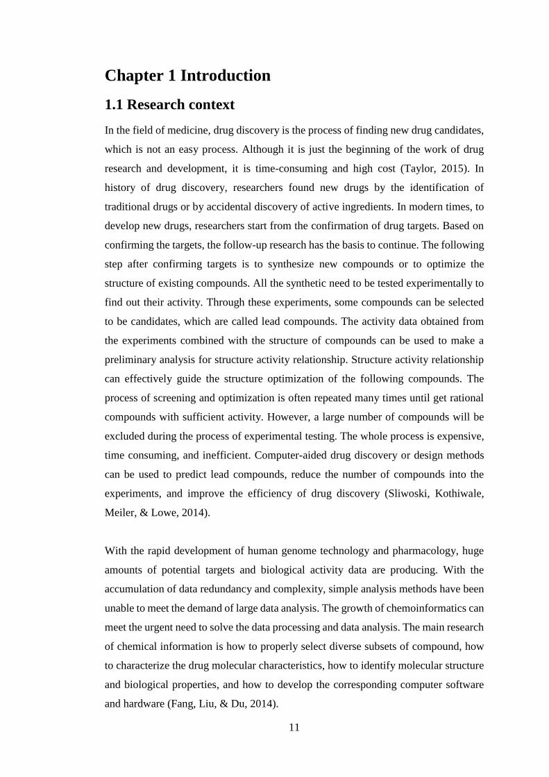
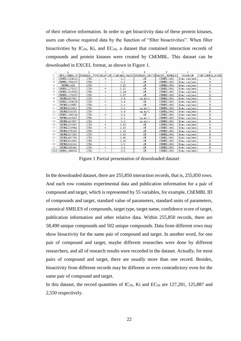
downloaded in EXCEL format, as shown in Figure 1.

Figure 1 Partial presentation of downloaded dataset

In the downloaded dataset, there are 255,850 interaction records, that is, 255,850 rows.

And each row contains experimental data and publication information for a pair of

compound and target, which is represented by 55 variables, for example, ChEMBL ID

of compounds and target, standard value of parameters, standard units of parameters,

canonical SMILES of compounds, target type, target name, confidence score of target,

publication information and other relative data. Within 255,850 records, there are

58,490 unique compounds and 502 unique compounds. Data from different rows may

show bioactivity for the same pair of compound and target. In another word, for one

pair of compound and target, maybe different researches were done by different

researchers, and all of research results were recorded in the dataset. Actually, for most

pairs of compound and target, there are usually more than one record. Besides,

bioactivity from different records may be different or even contradictory even for the

same pair of compound and target.

In this dataset, the record quantities of IC50, Ki and EC50 are 127,281, 125,887 and

2,550 respectively.

23

It should be note that these 628 protein kinases in this dataset come from 17 different

species, such as Homo sapiens, bacillus subtilis, eimeria tenella, and so on. This

dissertation focuses on protein kinases of Homo sapiens, therefore, further filtering

work need to be carried out in data pre-processing. For Homo sapiens, quantities of

IC50, Ki and EC50 in this dataset are 122,285, 124,535 and 2,438 respectively. In

another word, most records in the dataset are about Homo sapiens

3.1.3 Data pre-processing

As mentioned above, there are 255,850 interaction records in the dataset downloaded

from ChEMBL, with 55 variables. Most variables in this dataset are not needed for

creating bioactivity profiles. Therefore, delete other variables, except

CMPD_CHEMBLID, STANDARD_TYPE, RELATION, STANDARD_VALUE,

STANDARD_UNITS, TARGET_CHEMBLID, ORGANISM, and

CONFIDENCE_SCORE.

In the early stage of data pre-processing, confidence score was not considered.

Meanwhile, three experimental parameters (IC50, Ki and EC50) were used to filter

interaction records. Initially, the threshold of compound activity was set to 1μM.

When value of experimental parameters in a record was less than 1μM, the

compound recorded in this record was considered to be active to the target in the

same record. Otherwise, when the value was equal to or more than 1μM (1000nM),

the compound was considered to be inactive. On this basis, the original dataset was

transform to bioactivity matrix, the rows of which contained ChEMBL IDs of

targets and the columns of which contained ChEMBL IDs of compounds. When a

compound was considered to be active to a target, the value in the corresponding

position of the matrix was set to 1. Accordingly, when a compound was considered

to be inactive to a target, the value was set to 0.

Actually, there were usually more than one records for a pair of compound and

target, and some records are duplicate and contradictory for experiment result in the

original dataset that downloaded from ChEMBL. So a more complicated method

was used to assign values to a matrix. Taking threshold < 1000nM as an example,

24

value 1 was assigned to records whose IC50/Ki/EC50 < 1000nM, and assigned 0 to

records whose IC50/Ki/EC50 ≥ 1000nM, then the mean value of all records for the

same pair of compound and target is used as the bioactivity value of this pair of

compound and target. That is, when all records of a pair of compound and target

have value=1, their mean value is 1, then this compound is identified as active to

this target. Similarly, when all records of a pair of compound and target have

value=0, their mean value is 0, then this compound is identified as inactive to this

target. When some records for a pair of compound and target have value=1 and

some records for the same pair of compound and target have value=0, their mean

value is decimal. Therefore, there are three kind of values (1, 0, and decimals) in the

bioactivity profiles during extraction process. Then decimals were deleted from

bioactivity profiles, getting binary tables. Actually, deleting decimals does not mean

deleting compounds, but it means deleting decimal values in the matrix. In the

obtained matrix, the ratio of decimal to integer (0 and 1) is around 0.01, that is, the

ratio of deleted values is very small. In summary, filtering criteria in this dissertation

were more stringent. A compound was identified as active to a target when all

records about it show a consistent result. Contradictory results was treated as

missing value for a pair of compounds and target.

When threshold <1μM， a bioactivity matrix was created through the above method,

which has 54,397 unique compounds and 398 unique targets, with binary values 1

and 0. The reason why quantities of compounds and targets were less than original

dataset is that some were deleted during filtering process, which is described in

detail in section of data filtering. In the obtained matrix, there are a large number of

missing values. Because, for most pairs of compound and target, no experiments

had been done to provide their activity information. Then, by using a mathematical

idea and Rstudio described later, a complete bioactivity matrix was finally extracted

from this 54,397*398 matrix. In the complete matrix, there are 256 compounds and

99 targets.

However, there were two problems in this stage of processing. One problem was to

set the same threshold value for the three parameters. The other was not to consider

confidence score. From Cheng-Prusoff relationship (Burlingham & Widlanski,

25

2003), relationship between IC50 and Ki is described as IC50=Ki (1+[S]/Km) for

competitive inhibitors and IC50=Ki (1+Km/[S]) for uncompetitive inhibitors. This

means IC50 is normally bigger than Ki, unless the following situations: IC50≈Ki for

competitive inhibitors when [S]≈0, and IC50≈Ki for uncompetitive

inhibitors when [S]≈+∞ (Burlingham & Widlanski, 2003). Based on this theory, it

is not appreciate to set a same threshold value for both IC50 and Ki. In order to get

a consistent standard for IC50 and Ki, concentration of substrate and Km for each

assay are needed to transform Ki data into IC50 data, but this work is not easy to

achieve. Besides, for most compounds, they had both IC50 and Ki values. In order

to ensure the strict filtering, only using one of them is feasible. Therefore, IC50

was used to identify activity for compounds in the following work, instead of using

both IC50 and Ki at the same time. In addition, the quantity of EC50 in original

dataset is a very small number, with only 2,550 records, accounting for 2% of the

number of IC50 records. Based on the above reasons, only IC50 was used in the

following work.

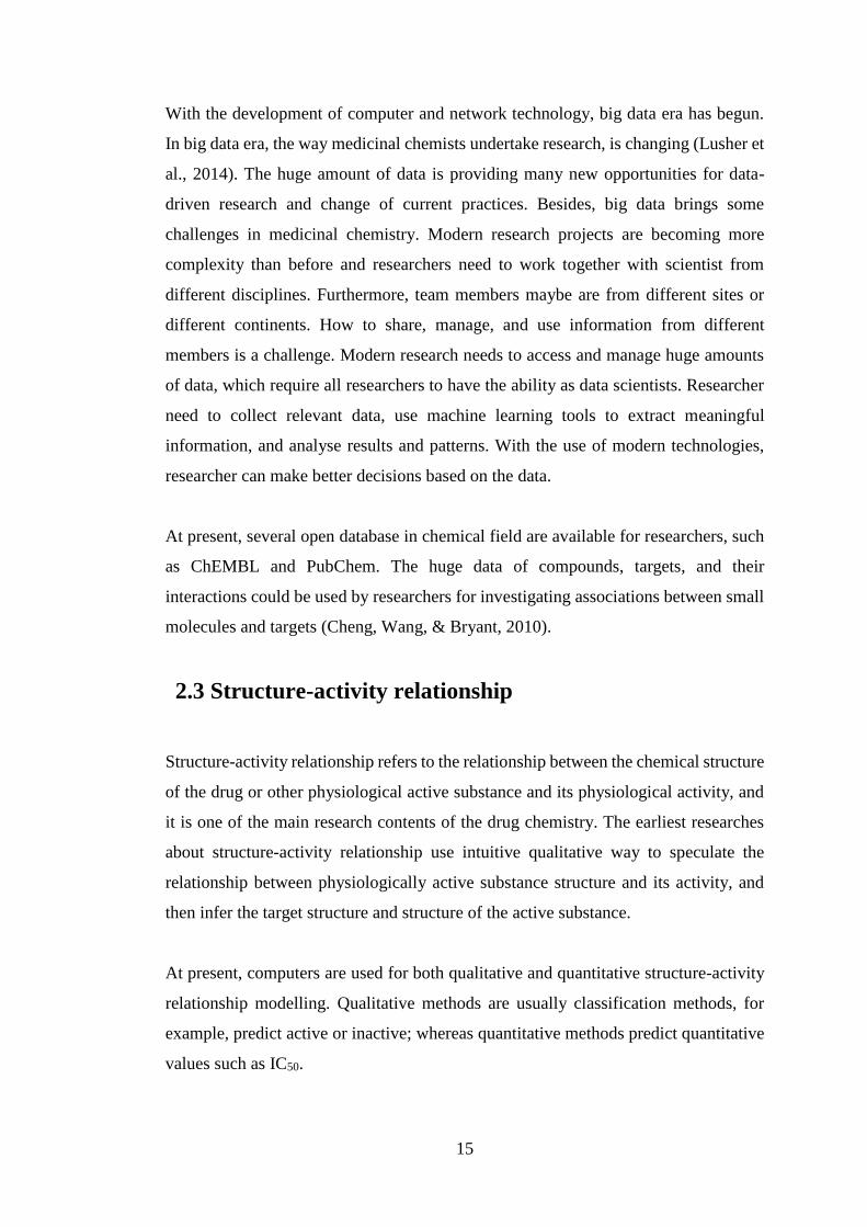
Confidence score was assigned to the assay-to-target relationships by ChEMBL. It

represented “both the type of target assigned to a particular assay and the confidence

that the target assigned is the correct target for that assay”, and details about

confidence score was displayed in Figure 2 (ChEMBL FAQ, 2014).

Figure 2 Confidence score (ChEMBL FAQ, 2014)

In the second stage of data pre-processing, only IC50 was used as the parameter for

distinguishing activity. Meanwhile, confidence score was used to filter interaction

records. When adding confidence score=9 as a filter limitation, a new bioactivity

26

matrix was produced, which contained 25,194 unique compounds and 289 unique

targets, with binary values and missing values. Then a complete bioactivity matrix

was extracted from the 25,194*289 matrix, with 17 unique compounds and 11

unique targets. However, there were some rows with all “0” values, which meant

some compounds were inactive to each targets in the final matrix. Such rows in

complete matrix were not helpful for the following clustering part. After deleting

these rows, the size of the complete matrix became less, which was not big enough

for the following work.

Then, both confidence score 8 and 9 were considered to be filter limitations in the

next attempt. In this attempt, a bioactivity matrix with 44,254 unique compounds

and 330 unique targets was produced. Then a complete bioactivity matrix was

extracted from the 44,254*330 matrix, which consisted of 20 unique compounds

and 16 unique targets. But after deleting rows with all “0” values, its size reduced

to 12*16. Besides, the number of “1” value in the matrix was too small, which meant

the quantity of pairs of compound and target that could be defined as active was too

few. In another word, the threshold of IC50 needs to be larger, so that to increase the

number of pairs of active compound and target.

In the third stage of data pre-processing, two bigger values of threshold were used

to generate bioactivity matrix. They were 6μM and 10μM. At the same time,

confidence score 8 and 9 were considered to filter data. Next, taking 6μM as an

example, the method of data pre-process is explained in details. In the ChEMBL

dataset, 6μM is expressed in 6000nM.

3.1.3.1 Data filtering

On the basis of the downloaded dataset with 255,850 interaction records, filtering steps

are as following:

a. Delete other variables, except “CMPD_CHEMBLID”,

“STANDARD_TYPE”, “RELATION”, “STANDARD_VALUE”,

27

“STANDARD_UNITS”, “TARGET_CHEMBLID”, “ORGANISM”, and

“CONFIDENCE_SCORE”.

b. Filter data about “IC50”, “nM”, “Homo sapiens”, and “confidence score=9

and 8” in columns of STANDARD_TYPE, STANDARD_UNITS,

ORGANISM, and CONFIDENCE_SCORE respectively. After filtering, the

quantity of interaction records reduced to 94,600. Actually, data in ChEMBL

were manually extracted from different literatures, therefore many different

types of units are contained in dataset, such as nM, ug.mL-1, %, ucm, uM-1,

umol/dm3. The number of nM accounted for more than 90% in the

downloaded dataset.

c. There were six relations in the column “RELATION”, including “<”, “≤”,

“=”, “>”, “≥”, and “>>”. In next step, different relations were filtered

according to different thresholds. Meanwhile, uncertain records were deleted.

For example, when threshold IC50 = 6μM (6000nM), a record that IC50 > 5000

was confused to identify the corresponding compound as active or inactive

to its target, because this IC50 may be 5500 or 7000, that is, it was hard to

identified as less or more than threshold. In this case, the record need to be

deleted. The method of how to delete such records are described in the

following section.

3.1.3.2 Data transformation

a. During data preparation, each record was set a value of 1 or 0 according to

their IC50 less or more than threshold. There are two advantages to do so. One

advantage was to help to delete uncertain records, which was described in step

c. The other advantage was to help to identify and delete contradictory records,

which was described in step f. On the basis of the dataset after filtering, sort

dataset from small to large according to the value of “STANDARD_VALUE”.

b. In the column of “STANDARD_VALUE”, replace values of less than 6000

with “1”, and replace values of equal to or more than 6000 with “0”.

28

c. Filter “1” values in the column “STANDARD_VALUE”. At the same time,

filter “<”, “≤” and “=” in the column of “RELATION”, excluding “>” and “≥”.

Then get 67,294 interaction records, which are considered “active” records for

compounds. In some records, IC50 > 4000nM, which meant IC50 might be

5000nM or 7000nM. In this situation, it was hard to say the compound was

active or not. Through this step, such uncertain records were excluded.

Filter “0” values in the column “STANDARD_VALUE”. At the same time,

filter “=”, “>”, “≥” and “>>” in the column of “RELATION”, excluding “<”

and “≤”. Then get 24,801 interaction records, which are considered “inactive”

records for compounds. Similarly, in some records, IC50 < 8000nM, which

meant IC50 might be 5000nM or 7000nM. In this situation, it was also hard to

say the compound was inactive or not. Through this step, such uncertain

records were excluded.

d. Combine “active” records and “inactive” records in one sheet of EXCEL,

getting a dataset with 92,095 interaction records.，After step c, uncertain

records were deleted, then remaining records were less than records got from

section of data filtering. Through step c and d, for different threshold, different

records could be excluded. That is, remaining compounds and targets might

be different for different thresholds. Therefore, obtained bioactivity profiles

with threshold < 6μM and threshold < 10μM might be different in size,

compounds and targets.

e. With the function of pivot table in EXCEL, assign “CMPD_CHEMBLID” to

“column” and “TARGET_CHEMBLID” to “row”, getting a bioactivity matrix

with 43,866 compounds in the first column and 329 targets in the first row.

f. In order to calculate values for the bioactivity matrix, assign “mean value” to

“value” in the pivot table, getting a matrix with values of “0”, “1”, and some

decimals. “1” value in a cell meant the corresponding compound was active to

the corresponding target. “0” value in a cell meant the corresponding

compound was inactive to the corresponding target. The reason why some

29

decimals were generated in the pivot table was that some pairs of compound

and target have contradictory records as described in the early stage of data

pre-process. Decimals were helpful to identified contradictory records for

these pairs of compounds and targets that showed contradictory activity in

different experiments. The ratio of decimal to integer (0 and 1) is 0.013.

Decimal were deleted in this dissertation with IF function in EXCEL. Then a

binary bioactivity profiles were generated.

3.1.3.3 Extracting a complete bioactivity matrix

Through the above steps, a bioactivity matrix was generated, with 43,866

compounds and 329 targets (Supplementary Table 1). Actually, there are many

missing values in this table, because many pairs of compound and target were not

verified by experiment. The proportion of cells with values in the table was

represented by density rate. Density rate of this matrix was 0.528%. The

proportion of cells with value 1 in the table was represented by “1” rate. It meant

percentage of compounds binding with targets. “1” rate of this matrix was 0.372%.

Then complete bioactivity matrix could be extracted from this matrix. However,

different complete bioactivity matrices in different size could be extracted with

different methods. Even in the same way, different attempts generated different

complete matrices.

A mathematical idea was used to extract a complete bioactivity matrix from

bioactivity profiles in this dissertation. The methodology of this idea is based on the

optimization theory in mathematics. Mathematical optimization is the theory of

choosing a best solution from some available alternatives according to some criteria

(Boyd & Vandenberghe, 2004). In each iteration, rows and columns were

respectively sorted according their number of values from high to low, and some

rows and columns with least quantity of values are deleted from the inputted

matrix. That is, the complete matrix outputted from iterations is the best one for

current inputted matrix. The method is shown as following:

30

a. Sort the entire matrix by the number of values in per row and per column in

order from large to small. Then the most dense part of values appeared in the

top left of the matrix.

b. Delete some rows and columns that contained the least amount of values,

getting a new matrix with less size.

c. Resort the obtained matrix by the number of values in per row and per column,

which meant repeat the first step.

d. Repeat the second step.

e. Repeat the sorting and deleting work for many times, until get a complete

matrix.

The above iteration could be done by writing and running several functions in

Rstudio or by manually. However, the size of obtained complete matrix was not big

enough. Then, the iteration was stopped at some level before the complete matrix

was obtained, in order to retain enough compounds and targets in the final matrix to

do further analysis. This meant there were some blank space, ie missing values, in

the final matrix. With Rstudio, the density rate of each matrix that generated during

the iteration was calculated, helping users to decide which level is the appropriate

time to stop the iterative process. This could ensure the balance between the size of

final matrix and density rate of values in final matrix.

In this dissertation, an extra row named “count1” and an extra column named

“count2” were added at the end of the 43,866*329 matrix. Count1 and count2 were

used to calculate and sort the number of values in each columns and each rows.

Then, manual method and Rstudio were combined to do the iteration. Due to the

size of the matrix before iteration was relatively large, only using the manual method

was ineffective and time consuming. Meanwhile, for most compounds and targets,

only a few of them could react with each other, in another word, most of cells in the

lower right part of matrix were blank. It was more efficient for Rstudio to do

iteration after deleting these rows and columns with large range of blank cells.

The manual part follow these steps:

a. Sort the entire matrix by count1 and count2 from large to small, thus the most

dense part of values appeared in the top left of the matrix,

31

b. Delete compounds whose count2 value ≤ 3, thus the number of compound

reduced from 43,866 to 3,101, then resort matrix by count1,

c. Delete targets whose count1 value ≤ 3, then the number of targets reduced

from 329 to 244,resort matrix by count2,

d. Delete compounds whose count2 value ≤ 5, then the number of compound

reduced to 1363, resort matrix by count1,

e. Delete targets whose count1 value ≤ 5, then the number of targets reduced to

201,resort matrix by count2,

f. Delete compounds whose count2 value ≤ 6,then the number of compound


g. Delete targets whose count1 value ≤ 6, then the number of targets reduced to

180, resort matrix by count2.

After the manually iterative process, the size of bioactivity matrix reduced to

1001*180, which meant there were 1001 compounds and 180 targets in the matrix.

Then the matrix was inputted into Rstudio to do iterations. R code is placed in the

appendix. There are two FOR functions in the code, whose iterative parameters need

to try many times to find a best option. For example, set iterative parameters to

2:13, and run FOR functions repeatedly, after many times iterations, a 39*32 matrix

could be generated, with density rate of 74.6%. Then run more iterations, smaller

matrices could be got. The meaning of iterative parameters 2:13 is that 2 columns

and 13 rows were deleted per time.

There are some rows with all “0” values in the obtained matrix. After deleting these

rows, the size of the final matrix reduced to 28*32, with density rate of 72.54% and

“1” rate of 20.60%. “1” rate equals the number of “1” values/the number of all cells

in the matrix.

In the view of activity values were rarer than inactivity values, missing values in the

final matrix were replaced by “0”. Backman and Girke (2016) handled missing

activity values by assigning inactivity values to them, that was to say, setting them

“0” values. They also introduced another method to deal with missing values, which

was to use three values: 0 for missing or untested values, 1 for inactive values, and

2 for active values (Backman & Girke, 2016). Both methods were reasonable. The

32

first method made bioactivity profiles more clear, so it was adopted in this

dissertation.

After all the steps above, a complete bioactivity profiles was generated, which

contained 28 compounds and 32 targets, with binary values. This matrix was

obtained based on the threshold that IC50 < 6μM. In the later part, this matrix was

called “6μM matrix” (Supplementary Table 4). It’s density rate and “1” rate were

72.54% and 20.6% respectively.

Similarly, a complete bioactivity profiles could be generated based on a threshold

IC50 < 10μM. When threshold < 10μM, after data filtering, data transformation, data

cleaning, a 43856*329 matrix (Supplementary Table 2) was obtained from original

records. It’s density rate and “1” rate were 0.527% and 0.39% respectively. During

data transformation, the ratio of decimal to integer (0 and 1) is 0.01.

A question may be asked why size of matrix decreased from 43866*329 to 43856*329

with threshold increased from 6μM to 10μM. Because there were some records with

IC50 > X, where X ∈（6μM, 10μM）. When filter records with threshold < 6μM,

compounds in these records were identified as inactive, while when filter records with

threshold < 10μM, these records were identified as confused records and should be

deleted, as described in step c of section data transformation. This led to less records

remaining in the second matrix, thereby the second matrix had less size.

Next, extract complete matrix from the second matrix. Delete some rows and columns

manually, following these steps using the same process as above however the number

of compounds remaining after each step is different:

a. Sort the entire matrix by count1 and count2 from large to small, thus the most

dense part of values appeared in the top left of the matrix,

b. Delete compounds whose count2 value ≤ 3, thus the number of compound

reduced from 43,856 to 3100, then resort matrix by count1,

c. Delete targets whose count1 value ≤ 3, then the number of targets reduced

from 329 to 245,resort matrix by count2,

33

d. Delete compounds whose count2 value ≤ 5, then the number of compound


e. Delete targets whose count1 value ≤ 5, then the number of targets reduced to

201,resort matrix by count2,

f. Delete compounds whose count2 value ≤ 6,then the number of compound


g. Delete targets whose count1 value ≤ 6, then the number of targets reduced to

180, resort matrix by count2.

During iteration with Rstudio, iterative parameter was set to 2:13, which meant 2

columns and 13 rows were deleted per time. After iteration, a 35*32 matrix was

generated. After deleting rows with all 0 values and dealing with missing values, a

complete 27*32matrix was obtained, with binary values. In the later study, this matrix

was called “10μM matrix” (Supplementary Table 5). It’s density rate and “1” rate were

74.77% and 22.22% respectively.

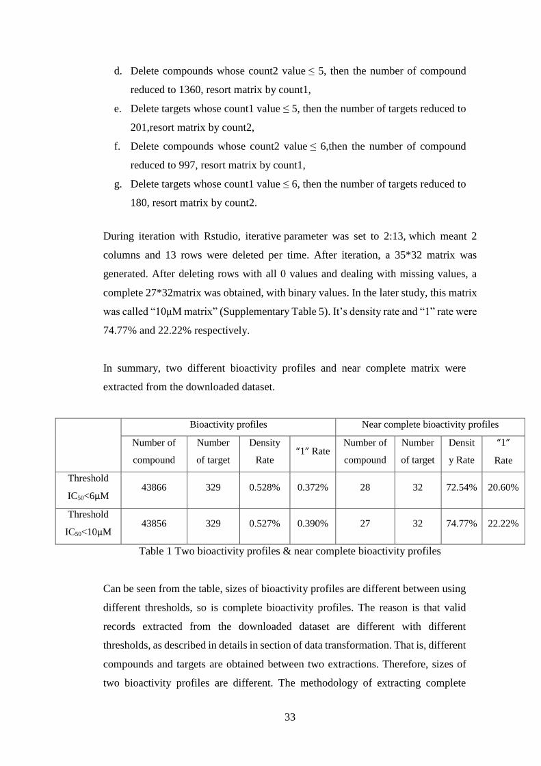
In summary, two different bioactivity profiles and near complete matrix were

extracted from the downloaded dataset.

Bioactivity profiles Near complete bioactivity profiles

Number of

compound

Number

of target

Density

Rate “1” Rate

Number of

compound

Number

of target

Densit

y Rate

“1”

Rate

Threshold

IC50<6μM 43866 329 0.528% 0.372% 28 32 72.54% 20.60%

Threshold

IC50<10μM 43856 329 0.527% 0.390% 27 32 74.77% 22.22%

Table 1 Two bioactivity profiles & near complete bioactivity profiles

Can be seen from the table, sizes of bioactivity profiles are different between using

different thresholds, so is complete bioactivity profiles. The reason is that valid

records extracted from the downloaded dataset are different with different

thresholds, as described in details in section of data transformation. That is, different

compounds and targets are obtained between two extractions. Therefore, sizes of

two bioactivity profiles are different. The methodology of extracting complete

34

matrix from bioactivity profiles is based on the idea of optimization in mathematics.

In each iteration, rows and columns with least quantity of data are deleted from the

inputted matrix. That is, the complete matrix outputted from iteration is the best one

for current inputted matrix. Therefore, the two complete matrices are the best to

their original matrices respectively. They do not necessarily have the same

compounds and targets, because the original matrices are different. Besides, it may

be good for clustering repeatedly with different datasets. This may lead to a more

objective result. Of course, another method can be used to extract complete matrix

for different thresholds. It is choosing the same compounds and targets for 10μM

matrix as that in 6μM matrix. This method is easy to implement. However, too single

sample may bias experiment result. Therefore, in this dissertation, different samples

are used to avoid bias result. Actually, the two complete matrices are not significant

different because of the similar thresholds. However, if thresholds are significant

different, there may be much difference between complete matrices.

3.1.3.4 A bioactivity matrix generated from van Westen’s dataset.

A researcher named van Westen (Personal communication, July 2016) also

extracted interaction records from ChEMBL for some compounds and targets. In

order to do more comparison and analysis for different bioactivity profiles, an extra

bioactivity matrix was extracted from his dataset. His dataset was in SD format, and

an Open Source data mining Platform named KNIME was used to read and rewrite

the SD file into EXCEL format (Mazanetz, Marmon, Reisser, & Morao, 2012).

In this dataset, there were 237,081 interaction records and more than one type of targets,

including protein kinases of Homo sapiens. van Westen applied 6.5 log units (~300

nM) as his threshold to identify compounds as active or inactive. After screening

protein kinases of Homo sapiens from the dataset, 30,335 records were obtained. Then

these interaction records were transformed into bioactivity matrix for corresponding

20188 compounds and 181 targets with the function pivot table in EXCEL

(Supplementary Table 3). It’s density rate and “1” rate were 0.83% and 0.476%

respectively.

35

An extra row named “count1” and an extra column named “count2” were added at

the end of the 20188*181 matrix. Count1 and count2 were used to calculate the number

of values in each columns and each rows. Then the 20188*181 matrix was sorted by

count1 and count2 from large to small, thus the most dense part of values appeared in

the top left of the matrix. After deleting compounds whose count2 value ≤ 8, the

number of compound reduced to 105, then resorted matrix by count1. After deleting

targets whose count1 value ≤ 11, the number of targets reduced to 108. During iteration

with Rstudio, iterative parameter was set to 1:1, which meant 1 columns and 1 rows

were deleted per time. After iteration, a 27*30 matrix was generated. After deleting

rows with all 0 values and dealing with missing values, a complete 26*30 matrix was

obtained, with binary values. In the later part, this matrix was called “van Westen

matrix” (Supplementary Table 6). It’s density rate and “1” rate were 75% and 35.9%

respectively.

In summary, three near complete matrices were generated at last.

Bioactivity profiles Near complete bioactivity profiles

Number of

compound

Number

of target

Density

Rate “1” Rate

Number of

compound

Number

of target

Density

Rate “1” Rate

Threshold

IC50<6μM 43866 329 0.528% 0.372% 28 32 72.54% 20.60%

Threshold

IC50<10μM 43856 329 0.527% 0.390% 27 32 74.77% 22.22%

van Westen’s

data

IC50<300nM

20189 181 0.830% 0.476% 26 30 75.00% 35.90%

Table 2 Three bioactivity profiles & near complete bioactivity profiles

3.2 Calculation of molecular descriptors

3.2.1 2D fingerprint

There are many different types of fingerprints for compounds, for example ECPF,

36

Morgan, and MACCS. ECFP algorithm was originated from a variant of Morgan

algorithm, and it made some changes to Morgan (Rogers & Hahn, 2010). Rogers

and Hahn (2010) described that “an iterative process assigned numeric identifiers to

each atom” from which a 2D fingerprint is generated. MACCS algorithm generated

MACCS keys for a molecule, and the result is a 167-bit vector. The Morgan

fingerprint, which is very similar to ECFP, and MACCS fingerprints were used as

calculated molecular descriptors in this dissertation.

RDKit is integrated into KNIME and was used to calculate 2D descriptors from

SMILES strings for compounds. 2D fingerprints calculated by Morgan and MACCS

algorithms for compounds were presented in the form of string values, which need

to be split into single digits like 0 and 1, generating a matrix with binary values. An

easy method for the transformation was to copy and paste these string values into a

word file, then add commas behind each character and save the word file as notepad

format. After that, opened a new EXCEL file, and imported data through the

function “DATA” & “FROM NOTEPAD”, splitting string value into single digit.

Eventually, a binary matrix was generated in EXCEL format.

3.2.2 Physiochemical properties

Five kinds of physiochemical properties were contained in matrix, which were

SlogP, SMR, LabuteASA, TPSA, and ExactMW. Actually, this is a small number

of physiochemical properties. This is because of the limitation of software. RDKit

was integrated into KNIME to calculate physiochemical properties from SMILES

for compounds. The obtained matrix was standardized with the formula Z=(x-

mean(x))/STD(x) (Larsen & Marx, 1986). The standardization was done in EXCEL

with the formulas AVERAGE and STDEV.S.

3.3 Machine learning method

3.3.1 Concept and principle

37

In this dissertation, k-means algorithm in WEKA was used more than once to divide

compounds into clusters based on their bioactivity profiles or molecular descriptors.

K-means method is a typical clustering algorithm based on Euclidean distance, using

Euclidean distance as the similarity evaluation index, that is, when the Euclidean

distance between two objects is less, their similarity is greater. The principle of k-

means method is following this:

Firstly, choose K objects from data set as the initial cluster centres, and the remaining

other objects are assigned to its nearest clusters respectively according to Euclidean

distance (cluster similarity) between each object and each cluster centre.

Secondly, calculate each new cluster centre for the received clusters, then objects are

assigned to a nearest clusters based on each new cluster centre.

Thirdly, keep repeating the process of calculating and assigning, until no change

occurs.

The compounds within the same cluster have similar properties, while compounds

from different clusters have dissimilar properties.

3.3.2 Choosing appropriate number of clusters

Leskovec, Rajaraman & Ullman (2014) described a method to decide the appropriate

number of clusters in their book. They suggested to start clustering dataset with N=2.

N represented the number of clusters in this dissertation. When average diameter of

clusters did not change significantly with the increase of N, this value of N was the

appropriate number. Here, the diameter of a cluster was the maximum distance

between any two points of the cluster.

In clustering result of WEKA, a parameter named “within cluster sum of squared errors”

showed the discrete degree of points within cluster. When this value is greater, distance

between points is greater, which means the diameter of a cluster is greater. Thereby,

this parameter can also reflect the diameter of a cluster.

38

In the clustering process, value of this parameter continued to become smaller as N

increased. This means there is no suitable K for datasets in this dissertation. The reason

for this situation may be the size of dataset in this dissertation is not big enough, so

that distances between points are relatively large. In this case, the appropriate N can

be set according to the need of research.

3.4 Evaluation method

In this dissertation, clusters generated using 2D fingerprints and physiochemical

properties were compared with clusters based on the bioactivity profiles

respectively. In another word, clustering result of bioactivity profiles was treated as

standard class information to evaluate cluster quality of molecular descriptors,

which was evaluating the ability of molecular descriptors for predicting bioactivity

profiles. In this case, several methods can be used to evaluate the quality of clusters,

such as measuring cluster purity, running classification algorithms, and measuring

precision, recall or F-measure.

In this dissertation, cluster purity was used to do evaluation. Manning, Raghavan,

& Schutze (2008) described a formula to calculate cluster purity as following:

Purity(Ω, C) = 1

𝑁∑ max

𝑗|𝜔𝑘

𝑘

∩ 𝑐𝑗|

In this formula, Ω is clusters, C is classes, and N is the number of all objects. Based

on the formula, Objects in cluster k were compared with each class, then each object

in cluster k was labelled by class number, that is, after comparison, it can be got that

how many objects in cluster k belonged class1, class2, class 3…, for example, the

corresponding quantity was k1, k2, k3…, then chose the biggest one of these numbers.

With the same steps, objects in each cluster were compared with each class, then the

biggest number for each cluster was got. At last, these biggest numbers for each

cluster were added up to get a total number, and the total number was divided by N

to get a result, which was purity (Ω, C).

39

In this dissertation, cluster of bioactivity profiles was standard class for compounds,

and clusters of molecular descriptors were evaluated to see how similar they were

to the standard cluster. When the purity was higher, the similarity was higher.

The calculation for purity could be done in EXCEL. For example, as shown in Table

3, a group of compounds (28) were clustered into 4 subgroups by bioactivity profiles

and Morgan fingerprints respectively. The results for these two methods were shown

in columns “Experimental cluster” and “Morgan cluster” respectively. Experimental

cluster was treated as standard class. And Morgan cluster was compared with

standard class to get the conclusion that how similarity between these two clusters.

For easy of counting, compounds in different Morgan clusters were distinguished

by colours. In the right part of the following table, the “YES” in the first yellow

row means that CHEMBL1094408 was in both Morgan cluster1 and Class0.

Similarly, position of each compound was shown in the table. “YES” could be

calculated by IF function in EXCEL, for example, IF(COUNTIF($A$2:$A$10,

C2)>0, "YES", "").

Apparently, among four classes, compounds in Class0 appeared most frequently in

Morgan cluster0, and other cluster also could got the class that compounds appeared

most frequently. Then count the quantity of compounds in the obtained pairs of

cluster and class.

Purity (Morgan, Class)

= 1

28 (Morgan0∩Class0+ Morgan1∩Class1+ Morgan2∩Class2+ Morgan3∩Class3)

= 1

28 (4+1+11+1)

= 0.68

On a special note, in the obtained results, the same serial number of each cluster and

class in this example was just a coincidence.

CMPD_CHEMBLID Experimental

cluster CMPD_CHEMBLID

Morgan

cluster Class0 Class1 Class2 Class3

CHEMBL103667 0 CHEMBL1094408 0 YES

40




























Table 3 Example for calculating cluster purity

3.5 Limitations/Constraints with methodology

a. In this dissertation, only IC50 was used to identify activity for compounds,

which did not make full use of various activity data in ChEMBL, hoping that

a better way could be found to identify bioactivity for compounds.

41

b. A small number of physicochemical properties was used for this descriptor,

because of the limitation of software. Actually, there are many others that

could have been used.

c. When a dataset is huge, it is inefficiency and time consuming to pre-process

the dataset in EXCEL.

d. In the process of extracting complete bioactivity profiles, the written code for

iteration was not the best. The final matrix got after iteration was just one of

many possibilities, and may not be the best one. This was actually a waste of

data resources.

e. Because of the theory described by Leskovec, Rajaraman & Ullman (2014)

for choosing the number of clusters was not suitable for datasets in this

dissertation, different values of N were tried for the following study. Actually,

this tentative approach of determination for N was not rigorous.

f. The efficiency for calculating cluster purity in EXCEL was not high, hoping

to find a better way to do calculations.

g. Clustering was done by a single way with WEKA and K-means algorithm,

which may be not enough to eliminate the errors caused by software and

algorithms themselves. A comprehensive comparison may be necessary to

apply a variety of soft wares and algorithms in future research.

h. In this research, not all the compounds and target data contained in ChEMBL

could be used to study the selectivity for compounds. Activity data for

selected sets of compounds and targets were required to be verified by

previous experiments. However, a considerable portion of compounds and

targets did not have corresponding experimental data. Based on this limitation,

the data collected from ChEMBL was not sufficient for the research, which

led to the analysis results was not perfect as predicted.

3.6 Ethical statement

This dissertation has no risk. The topic of this dissertation is a normal question in

drug discovery field, not a sensitive topic. There is no need for this dissertation to

choose participants for interviews or surveys, so there is no ethical issues for

considering sample or privacy.

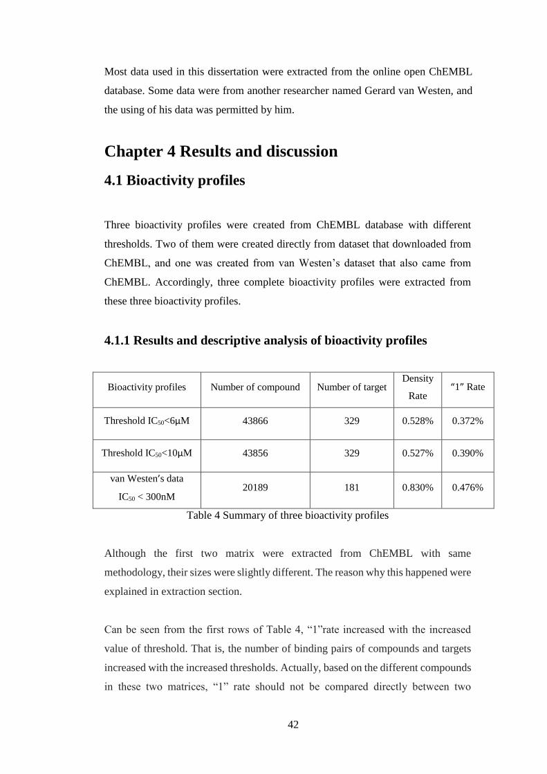
42

Most data used in this dissertation were extracted from the online open ChEMBL

database. Some data were from another researcher named Gerard van Westen, and

the using of his data was permitted by him.

Chapter 4 Results and discussion

4.1 Bioactivity profiles

Three bioactivity profiles were created from ChEMBL database with different

thresholds. Two of them were created directly from dataset that downloaded from

ChEMBL, and one was created from van Westen’s dataset that also came from

ChEMBL. Accordingly, three complete bioactivity profiles were extracted from

these three bioactivity profiles.

4.1.1 Results and descriptive analysis of bioactivity profiles

Bioactivity profiles Number of compound Number of target Density

Rate “1” Rate

Threshold IC50<6μM 43866 329 0.528% 0.372%

Threshold IC50<10μM 43856 329 0.527% 0.390%

van Westen’s data

IC50 < 300nM 20189 181 0.830% 0.476%

Table 4 Summary of three bioactivity profiles

Although the first two matrix were extracted from ChEMBL with same

methodology, their sizes were slightly different. The reason why this happened were

explained in extraction section.

Can be seen from the first rows of Table 4, “1”rate increased with the increased

value of threshold. That is, the number of binding pairs of compounds and targets

increased with the increased thresholds. Actually, based on the different compounds

in these two matrices, “1” rate should not be compared directly between two

43

matrices. It is reasonable to compare “1” rate between two matrices with same

compounds and targets. Therefore, different compounds in that two matrices were

deleted, getting two new matrices with same compounds. Meanwhile, targets in two

matrices were same, then no need to change them. Size of new matrices was

43856*329, and their “1” rate were 0.3716% (6μM) and 0.3896% (10μM).

Obviously, it was true that “1” rate was increased with threshold increasing.

It is interesting that the third matrix in Table 4 had the highest “1” rate, while it

applied the lowest threshold. After researching values of IC50 for some pairs of

compounds and targets, one reason for this might be the difference between criteria

applied in different extraction. For example, for compound CHEMBL535 and target

CHEMBL279, there are 40 interaction records of IC50 in ChEMBL. Some values

are less than 300nM, while some values are far greater than 300nM. In this situation,

compound CHEMBL535 was identified as active to target CHEMBL279 by van

Westen, but, based on extraction criteria in this dissertation, compound

CHEMBL535 could not be identified as active to target CHEMBL279, because their

records did not show a consistent result. In this dissertation, the value in the

corresponding cell associated with the compound and target was assigned to a

missing value. However, the number of such missing values was not so much as to

cause obvious gap as shown in the table. Therefore, there might be other reasons.

4.1.1.1 Result and analysis for compounds

In this part, the first bioactivity profiles is analysed in details as an example. There

were 43866 compounds and 329 targets in the result.

a. Test situation

Compounds in the matrix were sorted from large to small by the number of targets

that each compound tested with. From the left part of Figure 1, difference in the

quantity of tested targets was significant for small portion of compounds. For these

compounds, the number of targets tested with them was relatively large. Form the

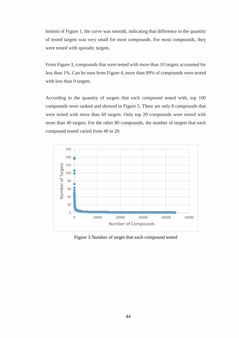
44

bottom of Figure 1, the curve was smooth, indicating that difference in the quantity

of tested targets was very small for most compounds. For most compounds, they

were tested with sporadic targets.

From Figure 3, compounds that were tested with more than 10 targets accounted for

less than 1%. Can be seen from Figure 4, more than 99% of compounds were tested

with less than 9 targets.

According to the quantity of targets that each compound tested with, top 100

compounds were ranked and showed in Figure 5. There are only 8 compounds that

were tested with more than 60 targets. Only top 20 compounds were tested with

more than 40 targets. For the other 80 compounds, the number of targets that each

compound tested varied from 40 to 20.

Figure 3 Number of target that each compound tested

0

20

40

60

80

100

120

140

160

0 10000 20000 30000 40000 50000

Nu

mb

er o

f Ta

rget

s

Number of Compounds

45

Figure 4 Percent of compounds tested with targets

Figure 5 Number of Target that top 100 compound tested

b. Hit situation

Compounds in the first matrix were sorted from large to small by the number of

targets that each compound hit. From the left part of Figure 6, difference in the

quantity of targets that each compound hit was significant for small portion of

compounds. For these compounds, the number of targets that they hit was relatively

large. Form the bottom of Figure 6, the curve was smooth, indicating that difference

99.046%

0.678%

0.165%

0.052%

0.032%

0.009%

0.002%

0.005%

0.000%

0.002%

0.009%0.000%

10.000%

20.000%

30.000%

40.000%

50.000%

60.000%

70.000%

80.000%

90.000%

100.000%

0-9 10-19 20-29 30-39 40-49 50-59 60-69 70-79 80-89 90-99 100and

more

Perc

ent

of

com

po

un

ds

Number of targets that tested with compounds

0

20

40

60

80

100

120

140

160

0 20 40 60 80 100

Nu

mb

er o

f ta

rget

s

Number of compounds

46

in the quantity of hit targets was very small for most compounds. For most

compounds, they were active to sporadic targets.

From Figure 7, compounds that were active to more than 10 targets accounted for

less than 0.3%. More than 99.7% of compounds were active to less than 9 targets.

According to the quantity of targets that each compound hit, top 100 compounds

were ranked and showed in Figure 8. There are only 2 compounds that were active

to more than 40 targets. Only top 20 compounds are active to more than 19 targets.

For the other 80 compounds, the number of targets that each compound hit varied

from 19 to 10.

Figure 6 Number of target that each compound hit

0

10

20

30

40

50

60

70

80

90

100

0 10000 20000 30000 40000 50000

Nu

mb

er o

f Ta

rget

s

Number of Compounds

47

Figure 7 Percent of compounds hit targets

Figure 8 Number of target that top 100 compound hit

4.1.1.2 Result and analysis for targets

In this part, the first bioactivity profiles was analysed in details as an example too.

a. Test situation

Targets in the matrix were sorted from large to small by the number of compounds that

each target tested with. From the left part of Figure 9, difference in the quantity of

99.761%

0.196%

0.036%

0.002%

0.002%

0.000%

0.000%

0.000%

0.000%

0.002%

0.000%

10.000%

20.000%

30.000%

40.000%

50.000%

60.000%

70.000%

80.000%

90.000%

100.000%

0-9 10-19 20-29 30-39 40-49 50-59 60-69 70-79 80-89 90-99

Perc

ent

of

com

po

un

ds

Number of targets that hit compounds

0

10

20

30

40

50

60

70

80

90

100

0 20 40 60 80 100

Nu

mb

er o

f Ta

rget

s

Number of Compounds

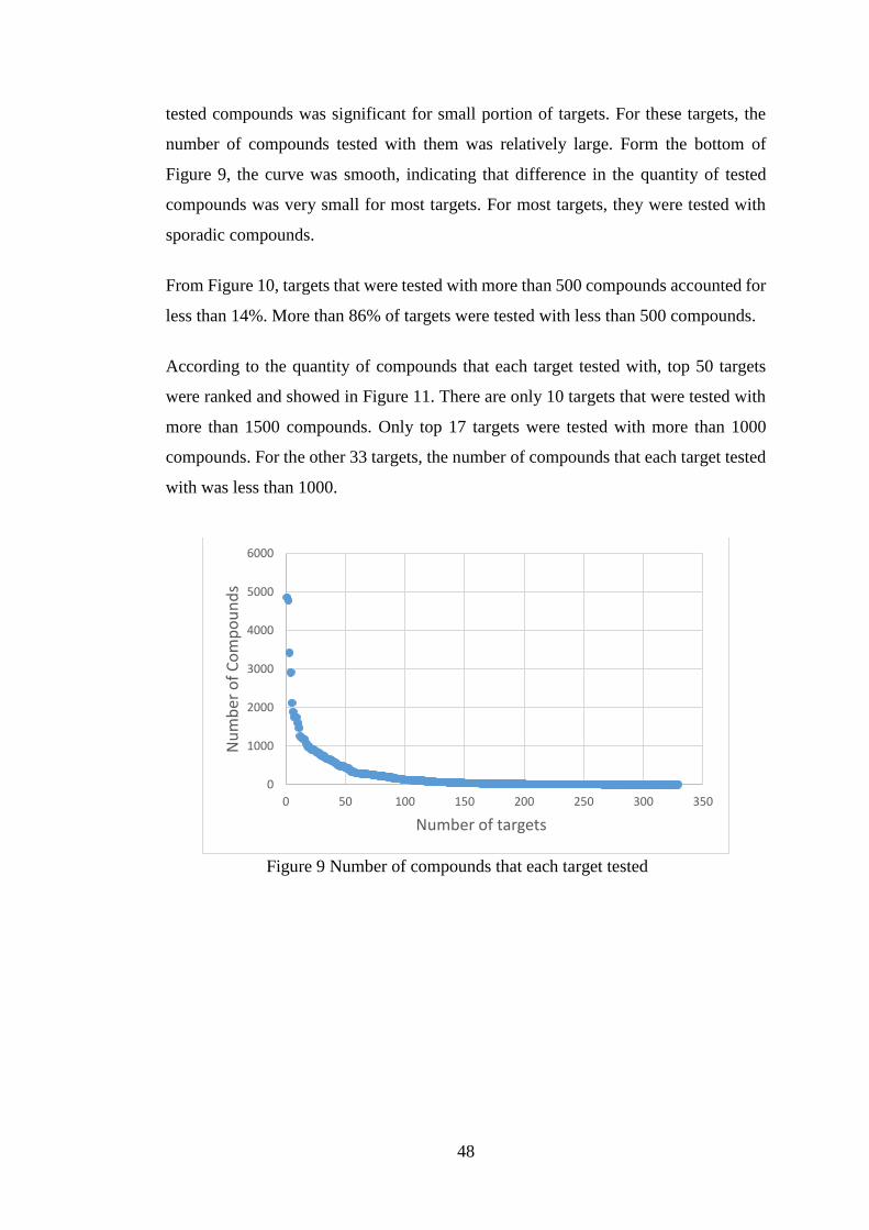
48

tested compounds was significant for small portion of targets. For these targets, the

number of compounds tested with them was relatively large. Form the bottom of

Figure 9, the curve was smooth, indicating that difference in the quantity of tested

compounds was very small for most targets. For most targets, they were tested with

sporadic compounds.

From Figure 10, targets that were tested with more than 500 compounds accounted for

less than 14%. More than 86% of targets were tested with less than 500 compounds.

According to the quantity of compounds that each target tested with, top 50 targets

were ranked and showed in Figure 11. There are only 10 targets that were tested with

more than 1500 compounds. Only top 17 targets were tested with more than 1000

compounds. For the other 33 targets, the number of compounds that each target tested

with was less than 1000.

Figure 9 Number of compounds that each target tested

0

1000

2000

3000

4000

5000

6000

0 50 100 150 200 250 300 350

Nu

mb

er o

f C

om

po

un

ds

Number of targets

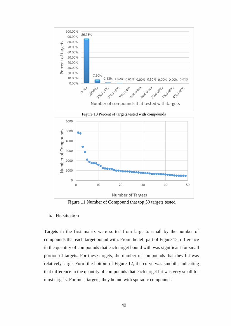
49

Figure 10 Percent of targets tested with compounds

Figure 11 Number of Compound that top 50 targets tested

b. Hit situation

Targets in the first matrix were sorted from large to small by the number of

compounds that each target bound with. From the left part of Figure 12, difference

in the quantity of compounds that each target bound with was significant for small

portion of targets. For these targets, the number of compounds that they hit was

relatively large. Form the bottom of Figure 12, the curve was smooth, indicating

that difference in the quantity of compounds that each target hit was very small for

most targets. For most targets, they bound with sporadic compounds.

86.93%

7.90%2.13% 1.52% 0.61% 0.00% 0.30% 0.00% 0.00% 0.61%

0.00%

10.00%

20.00%

30.00%

40.00%

50.00%

60.00%

70.00%

80.00%

90.00%

100.00%

Perc

ent

of

targ

ets

Number of compounds that tested with targets

0

1000

2000

3000

4000

5000

6000

0 10 20 30 40 50

Nu

mb

er o

f C

om

po

un

ds

Number of Targets

50

From Figure 13, targets that bound with more than 500 compounds accounted for

less than 11%. More than 89% of targets bound with less than 500 compounds.

According to the quantity of compounds that each target hit, top 50 targets were

ranked and showed in Figure 14. Only top 11 targets bound with more than 1000

compounds. For the other 39 targets, the number of compounds that each target

bound with less than 1000.

Figure 12 Number of compounds that each target hit

Figure 13 Percent of targets hit compounds

0

500

1000

1500

2000

2500

3000

3500

4000

0 50 100 150 200 250 300 350

Nu

mb

er o

f C

om

po

un

ds

Number of targets

89.36%

7.29%1.82% 0.61% 0.00% 0.61% 0.00% 0.30%

0.00%

10.00%

20.00%

30.00%

40.00%

50.00%

60.00%

70.00%

80.00%

90.00%

100.00%

Perc

ent

of

targ

ets

Number of compounds that hit targets

51

Figure 14 Number of compounds that each target hit

For compounds and targets in the other two bioactivity profiles, their tested trend

and hit trend were similar to that of the first matrix. That is, for small portion of

compounds, they were tested/bound with relatively large quantity of targets, while

vast majority of compounds were tested/bound with sporadic targets. For targets, it

was similar trend.

4.1.2 Results and comparison of complete bioactivity profiles

According to methods of extraction and dealing with missing value described in the

Chapter3, three complete bioactivity profiles were generated from those three

bioactivity profiles described above. Comparison for their size and “1” rate are in

Table 5.

Complete bioactivity profiles Number of

compound

Number of

target “1” Rate

6μM matrix 28 32 20.60%

10μM matrix 27 32 22.22%

van Westen matrix 26 30 35.90%

Table 5 Summary of three complete bioactivity profiles

“1” rate = (number of “1”) / (number of all cells in a matrix)

0

500

1000

1500

2000

2500

3000

3500

4000

0 10 20 30 40 50

Nu

mb

er o

f C

om

po

un

ds

Number of targets

52

Can be seen from Table 5, “1” rate of 10μM matrix was a little higher than that of

6μM matrix, while “1” rate of van Westen matrix was significantly higher than

others. This meant binding rate of compound and target in van Westen matrix are

apparently higher than that in other matrices.

Theoretically, binding rate should increase with increasing value of threshold.

Binding rate in 10μM matrix was higher than that of 6μM matrix. However, binding

rate of van Westen matrix should be lower than that of other matrices, because it

used a lower threshold 300nM.

4.1.3 Analysis for selectivity of compounds and targets in complete

matrices

There are three groups of compounds/targets in three matrix of Table 5. Analysis

and comparison for selectivity of compounds/targets were displayed in this part.

Karaman et al. (2008) introduced the concept of selectivity score to analyse kinases

and compounds.

Selectivity score of a compound

= (the number of targets that the compound hit)

(the number of all targets)

Selectivity score of a target

= (the number of compounds that the target hit)

(the number of all compounds)

4.1.3.1 Selectivity of compounds

Can be seen from Figure 15, the difference of Selectivity score among different

groups of compounds was significant.

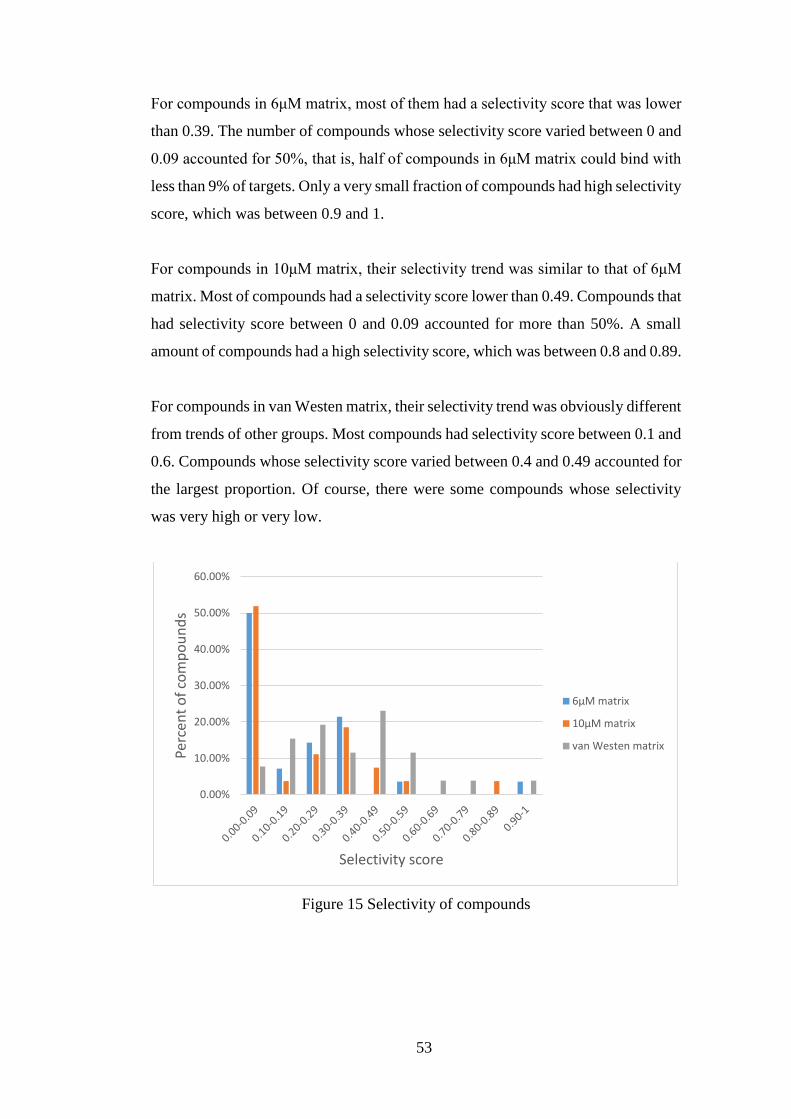
53

For compounds in 6μM matrix, most of them had a selectivity score that was lower

than 0.39. The number of compounds whose selectivity score varied between 0 and

0.09 accounted for 50%, that is, half of compounds in 6μM matrix could bind with

less than 9% of targets. Only a very small fraction of compounds had high selectivity

score, which was between 0.9 and 1.

For compounds in 10μM matrix, their selectivity trend was similar to that of 6μM

matrix. Most of compounds had a selectivity score lower than 0.49. Compounds that

had selectivity score between 0 and 0.09 accounted for more than 50%. A small

amount of compounds had a high selectivity score, which was between 0.8 and 0.89.

For compounds in van Westen matrix, their selectivity trend was obviously different

from trends of other groups. Most compounds had selectivity score between 0.1 and

0.6. Compounds whose selectivity score varied between 0.4 and 0.49 accounted for

the largest proportion. Of course, there were some compounds whose selectivity

was very high or very low.

Figure 15 Selectivity of compounds

0.00%

10.00%

20.00%

30.00%

40.00%

50.00%

60.00%

Perc

ent

of

com

po

un

ds

Selectivity score

6μM matrix

10μM matrix

van Westen matrix

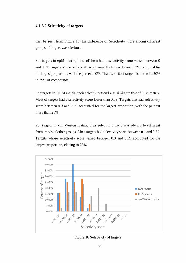
54

4.1.3.2 Selectivity of targets

Can be seen from Figure 16, the difference of Selectivity score among different

groups of targets was obvious.

For targets in 6μM matrix, most of them had a selectivity score varied between 0

and 0.39. Targets whose selectivity score varied between 0.2 and 0.29 accounted for

the largest proportion, with the percent 40%. That is, 40% of targets bound with 20%

to 29% of compounds.

For targets in 10μM matrix, their selectivity trend was similar to that of 6μM matrix.

Most of targets had a selectivity score lower than 0.39. Targets that had selectivity

score between 0.3 and 0.39 accounted for the largest proportion, with the percent

more than 25%.

For targets in van Westen matrix, their selectivity trend was obviously different

from trends of other groups. Most targets had selectivity score between 0.1 and 0.69.

Targets whose selectivity score varied between 0.3 and 0.39 accounted for the

largest proportion, closing to 25%.

Figure 16 Selectivity of targets

0.00%

5.00%

10.00%

15.00%

20.00%

25.00%

30.00%

35.00%

40.00%

45.00%

Perc

ent

of

targ

ets

Selectivity score

6μM matrix

10μM matrix

van Westen matrix

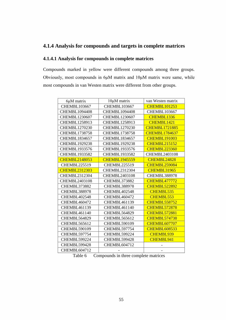
55

4.1.4 Analysis for compounds and targets in complete matrices

4.1.4.1 Analysis for compounds in complete matrices

Compounds marked in yellow were different compounds among three groups.

Obviously, most compounds in 6μM matrix and 10μM matrix were same, while

most compounds in van Westen matrix were different from other groups.

6μM matrix 10μM matrix van Westen matrix

CHEMBL103667 CHEMBL103667 CHEMBL101253


























CHEMBL599428 CHEMBL604712 -

CHEMBL604712 - -

Table 6 Compounds in three complete matrices

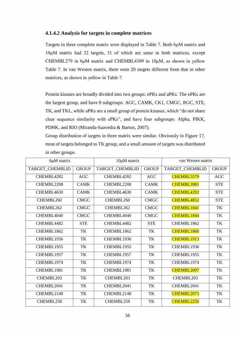
56

4.1.4.2 Analysis for targets in complete matrices

Targets in three complete matrix were displayed in Table 7. Both 6μM matrix and

10μM matrix had 32 targets, 31 of which are same in both matrices, except

CHEMBL279 in 6μM matrix and CHEMBL4309 in 10μM, as shown in yellow

Table 7. In van Westen matrix, there were 20 targets different from that in other

matrices, as shown in yellow in Table 7.

Protein kinases are broadly divided into two groups: ePKs and aPKs. The ePKs are

the largest group, and have 8 subgroups: AGC, CAMK, CK1, CMGC, RGC, STE,

TK, and TKL, while aPKs are a small group of protein kinases, which “do not share

clear sequence similarity with ePKs”, and have four subgroups: Alpha, PIKK,

PDHK, and RIO (Miranda-Saavedra & Barton, 2007).

Group distribution of targets in three matrix were similar. Obviously in Figure 17,

most of targets belonged to TK group, and a small amount of targets was distributed

in other groups.

6μM matrix 10μM matrix van Westen matrix

TARGET_CHEMBLID GROUP TARGET_CHEMBLID GROUP TARGET_CHEMBLID GROUP

CHEMBL4282 AGC CHEMBL4282 AGC CHEMBL5579 AGC

CHEMBL2208 CAMK CHEMBL2208 CAMK CHEMBL3981 STE

CHEMBL4630 CAMK CHEMBL4630 CAMK CHEMBL4202 STE

CHEMBL260 CMGC CHEMBL260 CMGC CHEMBL4852 STE

CHEMBL262 CMGC CHEMBL262 CMGC CHEMBL1841 TK

CHEMBL4040 CMGC CHEMBL4040 CMGC CHEMBL1844 TK

CHEMBL4482 STE CHEMBL4482 STE CHEMBL1862 TK

CHEMBL1862 TK CHEMBL1862 TK CHEMBL1868 TK










http://www.compbio.dundee.ac.uk/kinomer/families/AGC.html

http://www.compbio.dundee.ac.uk/kinomer/families/CAMK.html

http://www.compbio.dundee.ac.uk/kinomer/families/CK1.html

http://www.compbio.dundee.ac.uk/kinomer/families/CMGC.html

http://www.compbio.dundee.ac.uk/kinomer/families/RGC.html

http://www.compbio.dundee.ac.uk/kinomer/families/STE.html

http://www.compbio.dundee.ac.uk/kinomer/families/TK.html

http://www.compbio.dundee.ac.uk/kinomer/families/TKL.html

http://www.compbio.dundee.ac.uk/kinomer/families/Alpha.html

http://www.compbio.dundee.ac.uk/kinomer/families/PIKK.html

http://www.compbio.dundee.ac.uk/kinomer/families/PDHK.html

http://www.compbio.dundee.ac.uk/kinomer/families/RIO.html

57










CHEMBL3905 TK CHEMBL4247 TKL CHEMBL5274 TK

CHEMBL4247 TKL CHEMBL1991 Other CHEMBL5319 TK

CHEMBL1991 Other CHEMBL2185 Other CHEMBL3935 Other

CHEMBL2185 Other CHEMBL3024 Other CHEMBL4355 Other

CHEMBL3024 Other CHEMBL4309 Other - -

CHEMBL4722 Other CHEMBL4722 Other - -

Table 7 Targets in three complete matrices

Figure 17 Distribution of targets

0.00%

10.00%

20.00%

30.00%

40.00%

50.00%

60.00%

70.00%

80.00%

90.00%

AGC CAMK CMGC STE TK TKL Other

Perc

ent

of

each

gru

op

Protein kinases groups

6μM matrix

10μM matrix

van Westen matrix

58

4.2 Clustering results by bioactivity profiles

All datasets of bioactivity profiles in EXCEL format need to be changed into csv

format for clustering in WEKA. The value of seed for each clustering operation used

the default value 10.

As explained in methodology section, there is no appropriate value for the number

of clusters in this project. Then the number of clusters can be determined according

to research need.

4.2.1 Clustering results for compounds in 6μM matrix by bioactivity

profiles

The cluster dendrogram in Figure 18 was draw in Rstudio. It was used to directly

show distance between different compounds in 6μM matrix.

Based on the cluster dendrogram, two levels were chosen to implement clustering

by K-means algorithm, which were number of clusters equalled to 4 and 8

respectively. Then compounds were clustered into 4 and 8 clusters respectively in

WEKA. Clustering results were shown in Figure 19 and 20.

59

Figure 18 Cluster dendrogram for 6μM matrix

Figure 19 Clustering result for 6μM matrix (Number= 4)

60


4.2.2 Clustering results for compounds in 10μM matrix by

bioactivity profiles

Similarly, cluster dendrogram and clustering results for compounds in 10μM matrix

were shown in the following three figures.

Figure 21 Cluster dendrogram for 10μM matrix

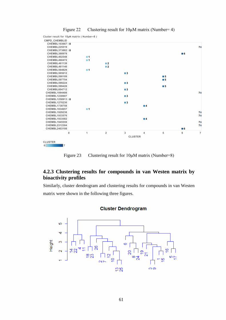
61


Figure 23 Clustering result for 10μM matrix (Number=8)

4.2.3 Clustering results for compounds in van Westen matrix by

bioactivity profiles

Similarly, cluster dendrogram and clustering results for compounds in van Westen

matrix were shown in the following three figures.

62

Figure 24 Cluster dendrogram for van Westen matrix

Figure 25 Clustering result for van Westen matrix (Number=4)

Figure 26 Clustering result for van Westen matrix (Number=8)

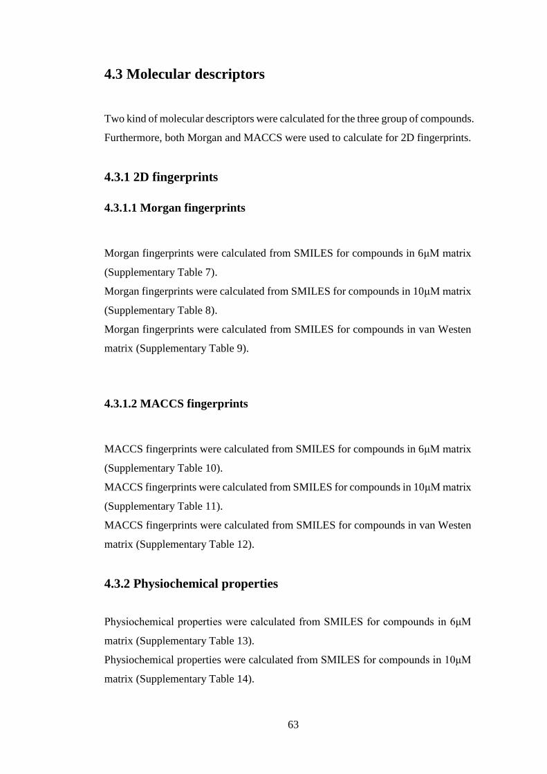
63

4.3 Molecular descriptors

Two kind of molecular descriptors were calculated for the three group of compounds.

Furthermore, both Morgan and MACCS were used to calculate for 2D fingerprints.

4.3.1 2D fingerprints

4.3.1.1 Morgan fingerprints

Morgan fingerprints were calculated from SMILES for compounds in 6μM matrix

(Supplementary Table 7).

Morgan fingerprints were calculated from SMILES for compounds in 10μM matrix


Morgan fingerprints were calculated from SMILES for compounds in van Westen

matrix (Supplementary Table 9).

4.3.1.2 MACCS fingerprints

MACCS fingerprints were calculated from SMILES for compounds in 6μM matrix


MACCS fingerprints were calculated from SMILES for compounds in 10μM matrix


MACCS fingerprints were calculated from SMILES for compounds in van Westen


4.3.2 Physiochemical properties

Physiochemical properties were calculated from SMILES for compounds in 6μM


Physiochemical properties were calculated from SMILES for compounds in 10μM


64

Physiochemical properties were calculated from SMILES for compounds in van

Westen matrix (Supplementary Table 15).

4.4 Clustering results by molecular descriptors

Similar to the clustering results by bioactivity profiles, the three group of

compounds were clustered respectively by their 2D fingerprints and physiochemical

properties. Besides, each group were clustered two times based on two options for

the number of clusters (4 and 8).


descriptors

There are 28 compounds in 6μM matrix. According to their 2D fingerprints and

physiochemical properties, they were clustered into different results respectively, as

shown in Table 8 and Table 9.

4.4.1.1 Cluster number = 4

CMPD_CHEMBLID Morgan

CLUSTER

MACCS

CLUSTER

PCP

CLUSTER

CHEMBL103667 2 0 3

CHEMBL1094408 0 0 0

CHEMBL1230607 2 0 0

CHEMBL1258913 2 2 3

CHEMBL1270230 2 2 2

CHEMBL1738758 0 0 0

CHEMBL1834657 1 1 1

CHEMBL1929238 2 3 3

CHEMBL1933576 0 0 0

CHEMBL1933582 0 0 0

CHEMBL2148053 1 1 1

CHEMBL225519 2 2 2

CHEMBL2312303 2 0 3

CHEMBL2312304 2 0 3

CHEMBL2403108 2 3 3

CHEMBL373882 3 3 3

CHEMBL388978 2 0 3

CHEMBL402548 2 0 0

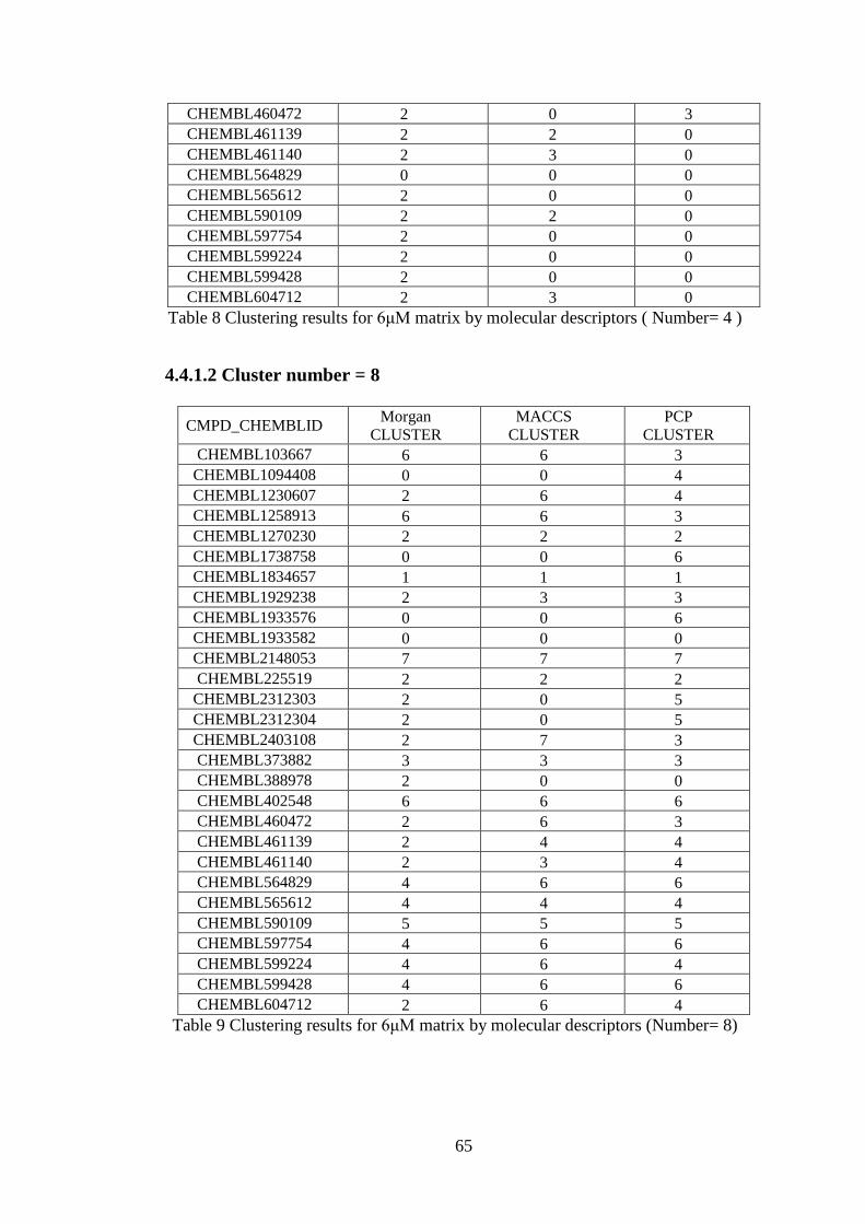
65

CHEMBL460472 2 0 3

CHEMBL461139 2 2 0

CHEMBL461140 2 3 0

CHEMBL564829 0 0 0

CHEMBL565612 2 0 0

CHEMBL590109 2 2 0

CHEMBL597754 2 0 0

CHEMBL599224 2 0 0

CHEMBL599428 2 0 0

CHEMBL604712 2 3 0

Table 8 Clustering results for 6μM matrix by molecular descriptors ( Number= 4 )



CLUSTER

MACCS

CLUSTER

PCP

CLUSTER

CHEMBL103667 6 6 3

CHEMBL1094408 0 0 4

CHEMBL1230607 2 6 4

CHEMBL1258913 6 6 3

CHEMBL1270230 2 2 2

CHEMBL1738758 0 0 6

CHEMBL1834657 1 1 1

CHEMBL1929238 2 3 3

CHEMBL1933576 0 0 6

CHEMBL1933582 0 0 0

CHEMBL2148053 7 7 7

CHEMBL225519 2 2 2

CHEMBL2312303 2 0 5

CHEMBL2312304 2 0 5

CHEMBL2403108 2 7 3

CHEMBL373882 3 3 3

CHEMBL388978 2 0 0

CHEMBL402548 6 6 6

CHEMBL460472 2 6 3

CHEMBL461139 2 4 4

CHEMBL461140 2 3 4

CHEMBL564829 4 6 6

CHEMBL565612 4 4 4

CHEMBL590109 5 5 5

CHEMBL597754 4 6 6

CHEMBL599224 4 6 4

CHEMBL599428 4 6 6

CHEMBL604712 2 6 4

Table 9 Clustering results for 6μM matrix by molecular descriptors (Number= 8)

66

4.4.2 Clustering results for compounds in 10μM matrix by

molecular descriptors

There are 27 compounds in 10μM matrix. According to their 2D fingerprints and

physiochemical properties, they were clustered into different results respectively, as

shown in Table 10 and Table 11.



CLUSTER

MACCS

CLUSER PCP CLUSTER

CHEMBL103667 0 0 0

CHEMBL1094408 3 3 2

CHEMBL1230607 3 3 3

CHEMBL1258913 0 2 0

CHEMBL1270230 3 3 3

CHEMBL1738758 3 0 2

CHEMBL1834657 1 1 1

CHEMBL1929238 0 0 0

CHEMBL1933576 3 3 2

CHEMBL1933582 3 3 2

CHEMBL1945559 3 3 3

CHEMBL225519 2 2 3

CHEMBL2312304 3 2 2

CHEMBL2403108 3 1 0

CHEMBL373882 1 1 0

CHEMBL388978 3 0 2

CHEMBL402548 1 3 2

CHEMBL460472 0 0 0

CHEMBL461139 2 2 2

CHEMBL461140 2 2 2

CHEMBL564829 3 3 2

CHEMBL565612 3 3 2

CHEMBL590109 3 3 2

CHEMBL597754 3 3 2

CHEMBL599224 3 3 3

CHEMBL599428 3 3 2

CHEMBL604712 3 3 3

Table 10 Clustering results for 10μM matrix by molecular descriptors

(Number= 4)

67


CMPD_CHEMBLI

D

Morgan

CLUSTER

MACCS

CLUSER PCP CLUSTER

CHEMBL103667 0 0 0

CHEMBL1094408 3 4 7

CHEMBL1230607 3 3 2

CHEMBL1258913 0 2 0

CHEMBL1270230 7 7 3

CHEMBL1738758 7 4 5

CHEMBL1834657 1 1 1

CHEMBL1929238 0 7 0

CHEMBL1933576 7 7 7

CHEMBL1933582 4 4 4

CHEMBL1945559 3 4 2

CHEMBL225519 2 2 3

CHEMBL2312304 3 2 4

CHEMBL2403108 6 6 6

CHEMBL373882 7 7 6

CHEMBL388978 3 4 4

CHEMBL402548 7 3 4

CHEMBL460472 0 0 6

CHEMBL461139 2 2 2

CHEMBL461140 2 2 2

CHEMBL564829 3 3 4

CHEMBL565612 3 7 7

CHEMBL590109 3 3 4

CHEMBL597754 5 5 5

CHEMBL599224 3 3 3

CHEMBL599428 3 3 7

CHEMBL604712 3 3 2

Table 11 Clustering results for 10μM matrix by molecular descriptors

(Number= 8)

4.4.3 Clustering results for compounds in van Westen matrix by

molecular descriptors

There are 26 compounds in van Westen matrix. According to their 2D fingerprints

and physiochemical properties, they were clustered into different results

respectively, as shown in Table 12 and Table 13.

68


CMPD_CHEMBLI

D

Morgan

CLUSTER

MACCS

CLUSER PCP CLUSTER

CHEMBL101253 3 0 0

CHEMBL103667 3 2 2

CHEMBL1336 2 2 3

CHEMBL1421 1 1 3

CHEMBL1721885 3 3 0

CHEMBL1784637 1 1 1

CHEMBL191003 0 0 0

CHEMBL215152 2 3 2

CHEMBL223360 0 0 0

CHEMBL2403108 0 2 2

CHEMBL24828 3 3 3

CHEMBL259084 0 0 3

CHEMBL31965 3 3 3

CHEMBL388978 0 1 3

CHEMBL477772 0 0 0

CHEMBL522892 0 0 0

CHEMBL535 0 3 0

CHEMBL553 3 3 0

CHEMBL558752 2 0 3

CHEMBL572878 0 0 3

CHEMBL572881 1 0 0

CHEMBL574738 2 2 2

CHEMBL607707 3 3 3

CHEMBL608533 0 1 2

CHEMBL939 3 3 3

CHEMBL941 1 0 2

Table 12 Clustering results for van Westen matrix by molecular descriptors

(Number= 4)



CLUSTER MACCS CLUSER PCP CLUSTER

CHEMBL101253 7 4 7

CHEMBL103667 3 2 2

CHEMBL1336 2 4 3

CHEMBL1421 1 1 3

CHEMBL1721885 7 3 0

CHEMBL1784637 1 1 1

CHEMBL191003 0 4 0

CHEMBL215152 6 3 3

69

CHEMBL223360 0 4 7

CHEMBL2403108 6 2 2

CHEMBL24828 6 6 5

CHEMBL259084 6 4 4

CHEMBL31965 3 3 3

CHEMBL388978 5 5 5

CHEMBL477772 4 4 0

CHEMBL522892 0 0 6

CHEMBL535 7 0 6

CHEMBL553 6 6 6

CHEMBL558752 4 4 4

CHEMBL572878 0 0 3

CHEMBL572881 7 7 7

CHEMBL574738 2 2 2

CHEMBL607707 3 3 3

CHEMBL608533 5 5 2

CHEMBL939 3 3 5

CHEMBL941 1 0 2

Table 13 Clustering results for van Westen matrix by molecular descriptors

(Number= 8)

4.5 Comparison for different clustering results

4.5.1 For compounds in 6μM matrix

In this dissertation, clusters of bioactivity profiles were standard classes for

compounds, and clusters of molecular descriptors were compared with standard

classes to see how similar they were to the standard classes. When cluster purity

was higher, the similarity was higher.

As shown in Table 14, when N = 4, cluster purity of Morgan algorithm is the higher

than physiochemical properties method, which means clustering result of Morgan

algorithm is closer to experimental result than that of physiochemical properties

method. If only from this view, it can be said that 2D fingerprints are better than

physiochemical properties in predicting activity of compounds. However, at the

same time, cluster purity of MACCS algorithm is less than that of physiochemical

properties method. That is to say, from MACCS perspective, 2D fingerprints are

worse than physiochemical properties in predicting activity of compounds.

70

From Table 15, when N = 8, cluster purities of both Morgan and MACCS algorithm

are higher than that of physiochemical properties method. In this case, it is clear that

clustering result of 2D fingerprints is closer to experimental result. In another word,

this moment, 2D fingerprints are better than physiochemical properties in predicting

activity of compounds.

Cluster number = 4 Cluster purity

Bioactivity profiles & Morgan fingerprints 0.61

Bioactivity profiles & MACCS fingerprints 0.50

Bioactivity profiles & Physiochemical properties 0.57

Table 14 Cluster purity summary for 6μM matrix (N=4)






Besides, no matter to Morgan or MACCS algorithm, cluster purity is increased with

the increase of N, as shown in Figure 27. This means, the number of clusters might

affect evaluation result. In another word, for a group of compounds and a kind of

fingerprints, when choosing different number of clusters to implement clustering,

maybe getting different evaluation result. However, cluster purity of

physiochemical properties method did not change with the increase of cluster

numbers.

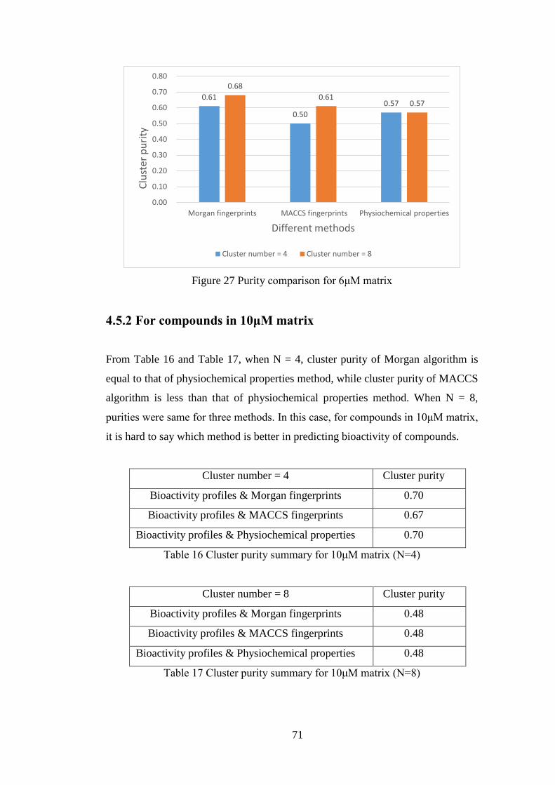
71

Figure 27 Purity comparison for 6μM matrix

4.5.2 For compounds in 10μM matrix

From Table 16 and Table 17, when N = 4, cluster purity of Morgan algorithm is

equal to that of physiochemical properties method, while cluster purity of MACCS

algorithm is less than that of physiochemical properties method. When N = 8,

purities were same for three methods. In this case, for compounds in 10μM matrix,

it is hard to say which method is better in predicting bioactivity of compounds.











0.61

0.50

0.57

0.68

0.61 0.57

0.00

0.10

0.20

0.30

0.40

0.50

0.60

0.70

0.80

Morgan fingerprints MACCS fingerprints Physiochemical properties

Clu

ster

pu

rity

Different methods

Cluster number = 4 Cluster number = 8

72

Figure 28 Purity comparison for 10μM matrix

Besides, cluster purity of each method is decreased with the increase of cluster

number, as shown in Figure 28. That is, evaluation result was affected by number

of clusters.

4.5.3 For compounds in van Westen matrix

Contrary to the results of the other matrices, from Table 18 and Table 19, cluster

purity of both Morgan and MACCS algorithm is lower than that of physiochemical

properties method. That is, in this case, clustering result of physiochemical

properties method is closer to experimental result than that of 2D fingerprints. In

another word, for compounds in this matrix, 2D fingerprints are worse than

physiochemical properties in predicting activity of compounds.





Table 18 Cluster purity summary for van Westen matrix (N=4)



0.70 0.67

0.70

0.48 0.48 0.48

0.00

0.10

0.20

0.30

0.40

0.50

0.60

0.70

0.80


Clu

ster

pu

rity

Different methods


73



Table 19 Cluster purity summary for van Westen matrix (N=8)

Besides, cluster purity of Morgan algorithm does not change with the increase of

cluster number, as shown in Figure 29, while cluster purity of MACCS algorithm is

increased. In addition, cluster purity of physiochemical properties method is

decreased with the increase of cluster number.

Figure 29 Purity comparison for van Westen matrix

In summary, for different groups of compounds with different thresholds, both 2D

fingerprints and Physiochemical properties can predict bioactivity of compounds to

some extent. However, results of three groups did not show a consistent result about

which method had the highest ability of prediction. One set of data in three sets

shows that 2D fingerprints are better than physiochemical properties in predicting

bioactivity of compounds. One showed an opposite result that physiochemical

properties are better than 2D fingerprints in predicting bioactivity of compounds.

The other shows there is no significant difference in prediction ability between 2D

fingerprints and physiochemical properties.

Then further research was done on one group of compounds with different threshold.

0.46 0.46

0.58

0.46 0.50

0.54

0.00

0.10

0.20

0.30

0.40

0.50

0.60

0.70

0.80


Clu

ster

pu

rity

Different methods


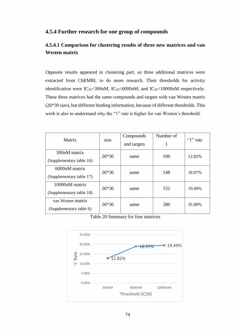
74

4.5.4 Further research for one group of compounds

4.5.4.1 Comparison for clustering results of three new matrices and van

Westen matrix

Opposite results appeared in clustering part, so three additional matrices were

extracted from ChEMBL to do more research. Their thresholds for activity

identification were IC50<300nM, IC50<6000nM, and IC50<10000nM respectively.

These three matrices had the same compounds and targets with van Westen matrix

(26*30 size), but different binding information, because of different thresholds. This

work is also to understand why the “1” rate is higher for van Westen’s threshold.

Matrix size Compounds

and targets

Number of

1 “1” rate

300nM matrix

(Supplementary table 16) 26*30 same 100 12.82%

6000nM matrix


10000nM matrix


van Westen matrix


Table 20 Summary for four matrices

12.82%

18.97% 19.49%

0.00%

5.00%

10.00%

15.00%

20.00%

25.00%

300nM 6000nM 10000nM

'1' R

ate

Threshold (IC50)

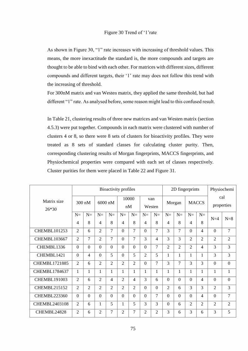
75

Figure 30 Trend of ‘1’rate

As shown in Figure 30, “1” rate increases with increasing of threshold values. This

means, the more inexactitude the standard is, the more compounds and targets are

thought to be able to bind with each other. For matrices with different sizes, different

compounds and different targets, their ‘1’ rate may does not follow this trend with

the increasing of threshold.

For 300nM matrix and van Westen matrix, they applied the same threshold, but had

different “1” rate. As analysed before, some reason might lead to this confused result.

In Table 21, clustering results of three new matrices and van Westen matrix (section

4.5.3) were put together. Compounds in each matrix were clustered with number of

clusters 4 or 8, so there were 8 sets of clusters for bioactivity profiles. They were

treated as 8 sets of standard classes for calculating cluster purity. Then,

corresponding clustering results of Morgan fingerprints, MACCS fingerprints, and

Physiochemical properties were compared with each set of classes respectively.

Cluster purities for them were placed in Table 22 and Figure 31.

Matrix size

26*30

Bioactivity profiles 2D fingerprints Physiochemi

cal

properties 300 nM 6000 nM

10000

nM

van

Westen Morgan MACCS

N=

4

N=

8

N=

4

N=

8

N=

4

N=

8

N=

4

N=

8

N=

4

N=

8

N=

4

N=

8 N=4 N=8

CHEMBL101253 2 6 2 7 0 7 0 7 3 7 0 4 0 7

CHEMBL103667 2 7 2 7 0 7 3 4 3 3 2 2 2 2

CHEMBL1336 0 0 0 0 0 0 0 7 2 2 2 4 3 3

CHEMBL1421 0 4 0 5 0 5 2 5 1 1 1 1 3 3

CHEMBL1721885 2 6 2 2 2 2 0 7 3 7 3 3 0 0

CHEMBL1784637 1 1 1 1 1 1 1 1 1 1 1 1 1 1

CHEMBL191003 2 6 2 4 2 4 3 6 0 0 0 4 0 0

CHEMBL215152 2 2 2 2 2 2 0 0 2 6 3 3 2 3

CHEMBL223360 0 0 0 0 0 0 0 7 0 0 0 4 0 7

CHEMBL2403108 2 6 1 5 1 5 3 3 0 6 2 2 2 2

CHEMBL24828 2 6 2 7 2 7 2 2 3 6 3 6 3 5

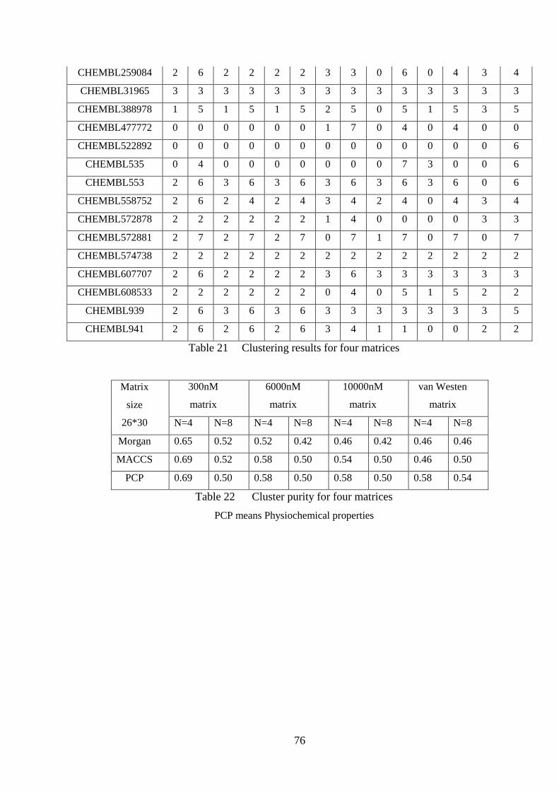
76

CHEMBL259084 2 6 2 2 2 2 3 3 0 6 0 4 3 4

CHEMBL31965 3 3 3 3 3 3 3 3 3 3 3 3 3 3

CHEMBL388978 1 5 1 5 1 5 2 5 0 5 1 5 3 5

CHEMBL477772 0 0 0 0 0 0 1 7 0 4 0 4 0 0

CHEMBL522892 0 0 0 0 0 0 0 0 0 0 0 0 0 6

CHEMBL535 0 4 0 0 0 0 0 0 0 7 3 0 0 6

CHEMBL553 2 6 3 6 3 6 3 6 3 6 3 6 0 6

CHEMBL558752 2 6 2 4 2 4 3 4 2 4 0 4 3 4

CHEMBL572878 2 2 2 2 2 2 1 4 0 0 0 0 3 3

CHEMBL572881 2 7 2 7 2 7 0 7 1 7 0 7 0 7

CHEMBL574738 2 2 2 2 2 2 2 2 2 2 2 2 2 2

CHEMBL607707 2 6 2 2 2 2 3 6 3 3 3 3 3 3

CHEMBL608533 2 2 2 2 2 2 0 4 0 5 1 5 2 2

CHEMBL939 2 6 3 6 3 6 3 3 3 3 3 3 3 5

CHEMBL941 2 6 2 6 2 6 3 4 1 1 0 0 2 2

Table 21 Clustering results for four matrices

Matrix

size

26*30

300nM

matrix

6000nM

matrix

10000nM

matrix

van Westen

matrix

N=4 N=8 N=4 N=8 N=4 N=8 N=4 N=8

Morgan 0.65 0.52 0.52 0.42 0.46 0.42 0.46 0.46

MACCS 0.69 0.52 0.58 0.50 0.54 0.50 0.46 0.50

PCP 0.69 0.50 0.58 0.50 0.58 0.50 0.58 0.54

Table 22 Cluster purity for four matrices

PCP means Physiochemical properties

77

Figure 31 Purity comparison for four matrices


Can be seen from Figure 31, for van Westen classes, purities of physiochemical

properties method were higher than Morgan and MACCS algorithms, no matter

number of clusters is 4 or 8. That is, in this situation, physiochemical properties

method was better than 2D fingerprints in predicting bioactivity of compounds.

However, for other classes, sometimes prediction of 2D fingerprints was better than

that of physiochemical properties, sometimes the contrary.

4.5.4.2 Comparison for clustering results of adjusted matrices

In last section, clustering results of three new matrices were compared with that of

van Westen matrix. Actually, there were some rows with all “0” values in these

three new matrices. The reason why these rows were not deleted is that to ensure

these matrices had same compounds and targets with van Westen matrix, and ensure

fairness of comparison. However, these rows might affect the accuracy of clustering,

so they were deleted in the following analysis and comparison.

In 300nM matrix, the number of rows with all”0”value was the most. Five

compounds of this matrix were active to none of targets, and only one or two of

these compounds in other matrices were active to none of targets. So these five

0.00

0.10

0.20

0.30

0.40

0.50

0.60

0.70

0.80

N=4 N=8 N=4 N=8 N=4 N=8 N=4 N=8

300nM 6000nM 10000nM Gerard

Cu

ster

Pu

rity

Diffrent sets of classes

Morgan MACCS PCP

78

compounds were deleted from the four matrices: 300nM matrix, 6000nM matrix,

10000nM matrix, and van Westen matrix, in order to ensure no rows with all “0”

values in matrices, so as to ensure accuracy of clustering. Then, four new matrices

were generated. In this section, they were named 300nM_new matrix (Supplementary

table 19), 6000nM_new matrix (Supplementary table 20), 10000nM_new matrix

(Supplementary table 21), and van Westen_new matrix (Supplementary table 22)

respectively.

The size of each matrix was 21*30, with same compounds and targets in each matrix.

Morgan fingerprints (Supplementary table 23), MACCS fingerprints (Supplementary

table 24), and Physiochemical properties (Supplementary table 25) of this group

compounds were calculated respectively.

Clustering results were placed in Table 23. Similarly, after calculation, cluster

purities of each methods were shown in Table 24 and Figure 32.

Matrix size

21*30

Bioactivity profiles 2D fingerprints Physiochem

ical

properties

300nM_n

ew

6000nM_

new

10000nM

_new

van

Westen_

new

Morgan MACCS

N=

4

N=

8

N=

4

N=

8

N=

4

N=

8

N=

4

N=

8

N=

4

N=

8

N=

4

N=

8 N=4 N=8

CHEMBL101253 1 1 1 1 1 1 1 1 1 0 1 1 1 1

CHEMBL103667 1 7 0 7 1 7 3 3 3 1 3 5 2 5

CHEMBL1336 2 6 2 6 2 6 1 6 1 3 3 6 3 3

CHEMBL1421 0 0 3 3 3 3 0 0 1 1 3 5 0 4

CHEMBL1784637 2 2 2 2 2 2 1 1 1 4 3 5 2 5

CHEMBL191003 1 1 0 4 0 4 3 3 1 7 1 6 3 6

CHEMBL215152 1 4 1 4 0 4 1 4 3 1 3 5 2 4

CHEMBL223360 1 6 1 6 1 6 1 6 1 3 1 6 3 7

CHEMBL2403108 1 1 2 2 2 2 3 3 1 6 3 3 2 5

CHEMBL24828 0 0 0 0 0 0 0 0 0 1 0 0 0 0

CHEMBL31965 1 5 3 5 0 5 3 5 3 5 3 5 0 2

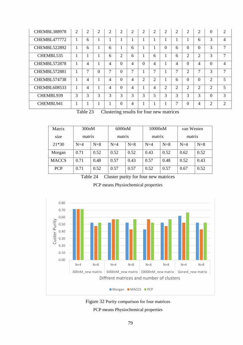
79

CHEMBL388978 2 2 2 2 2 2 2 2 2 2 2 2 0 2

CHEMBL477772 1 6 1 1 1 1 1 1 1 1 1 6 3 4

CHEMBL522892 1 6 1 6 1 6 1 1 0 6 0 0 3 7

CHEMBL535 1 1 1 6 2 6 1 6 1 6 2 2 3 7

CHEMBL572878 1 4 1 4 0 4 0 4 1 4 0 4 0 4

CHEMBL572881 1 7 0 7 0 7 1 7 1 7 2 7 3 7

CHEMBL574738 1 4 1 4 0 4 2 2 1 6 0 0 2 5

CHEMBL608533 1 4 1 4 0 4 1 4 2 2 2 2 2 5

CHEMBL939 3 3 3 3 3 3 3 5 3 3 3 3 0 3

CHEMBL941 1 1 1 1 0 4 1 1 1 7 0 4 2 2

Table 23 Clustering results for four new matrices

Matrix

size

21*30

300nM

matrix

6000nM

matrix

10000nM

matrix

van Westen

matrix

N=4 N=8 N=4 N=8 N=4 N=8 N=4 N=8

Morgan 0.71 0.52 0.52 0.52 0.43 0.52 0.62 0.52

MACCS 0.71 0.48 0.57 0.43 0.57 0.48 0.52 0.43

PCP 0.71 0.52 0.57 0.57 0.52 0.57 0.67 0.52

Table 24 Cluster purity for four new matrices


Figure 32 Purity comparison for four matrices


0.00

0.10

0.20

0.30

0.40

0.50

0.60

0.70

0.80

N=4 N=8 N=4 N=8 N=4 N=8 N=4 N=8

300nM_new matrix 6000nM_new matrix 10000nM_new matrix Gerard_new matrix

Cu

ster

Pu

rity

Diffrent matrices and number of clusters

Morgan MACCS PCP

80

Can be seen from Figure 32, for van Westen classes, only when N=4, purity of

physiochemical properties method was higher than Morgan and MACCS algorithms.

When n=8, purity of Morgan algorithm was as same as that of physiochemical

properties method. That is, for van Westen_new matrix, physiochemical properties

method was not always better than 2D fingerprints in predicting bioactivity of

compounds. Besides, for other classes, sometimes prediction of 2D fingerprints was

better than that of Physiochemical properties, sometimes the contrary.

In summary, no matter for different groups or the same group of compounds, both 2D

fingerprints and Physiochemical properties could predict bioactivity of compounds to

some extent, while which method was definitely better than the other one, more

rigorous researches need to be done. Actually, many factors may affect results. For

example, criteria for data extraction, size of complete matrix, cluster algorithms and

software, number of clusters, or other factors. In this dissertation, contrary records

were deleted at the step of data extraction, while if remain these records and identify

corresponding compounds as active or inactive according to the number of active

records or inactive records, result may be affected. Besides, if expand size of complete

matrix, result may be affected too.

Chapter 5 Conclusion

In this dissertation, bioactivity data and SMILES strings of compounds were extracted

from ChEMBL database respectively with different bioactivity thresholds (6μM,

10μM), then bioactivity data were transformed into two bioactivity profiles with

different compounds, and bioactivity profiles in this dissertation were represented by

binary values (1 meant active, 0 meant in active). “1” rate in dataset were increased

with threshold value increasing.

By using a mathematical idea and Rstudio, two complete bioactivity profiles were

extracted from obtained bioactivity profiles respectively. The methodology of

extracting complete matrix from bioactivity profiles is based on the idea of

optimization in mathematics. In each iteration, rows and columns were respectively

81

sorted according their number of values from high to low, and some rows and columns

with least quantity of values are deleted from the inputted matrix. That is, the complete

matrix outputted by iterations is the best one for current inputted matrix. Therefore,

the two complete matrices are the best to their original matrices respectively. Based

on their original inputted matrices were different, two outputted matrices did not

necessarily have same compounds and targets. Actually, compounds, targets and size

were different for two complete matrices. It was good for clustering repeatedly with

different matrices. Because this led to a more objective result, with less bias.

Besides, a complete bioactivity profiles was extracted from dataset of a researcher

named van Westen. This complete matrix also had different compounds and target

from other two complete matrices.

Bioactivity profiles were analysed from different angles. For most compounds in

dataset, they were tested and bound with sporadic targets. For a very few compounds,

they were tested and bound with many targets. For targets, the situation was similar.

For most compounds and targets in complete matrices, their selectivity score were

lower than 0.49.

Molecular descriptors such as 2D fingerprints and physiochemical properties for

compounds were calculated from their SMILES strings by KNIME and RDkit, and

two kinds of fingerprints were calculated by Morgan and MACCS algorithm

respectively.

One of machine learning methods named k-means was applied in WEKA to cluster

each group of compounds into subgroups, based on their bioactivity profiles, 2D

fingerprints, and physiochemical properties respectively.

Eventually, this dissertation compared and evaluated the ability of each molecular

descriptor for predicting bioactivity profiles of compounds. Evaluation of clusters was

achieved by using cluster purity. Clustering result of bioactivity profiles was treated

as standard class information to evaluate cluster quality of molecular descriptors.

Clusters of 2D fingerprints and physiochemical properties were compared with

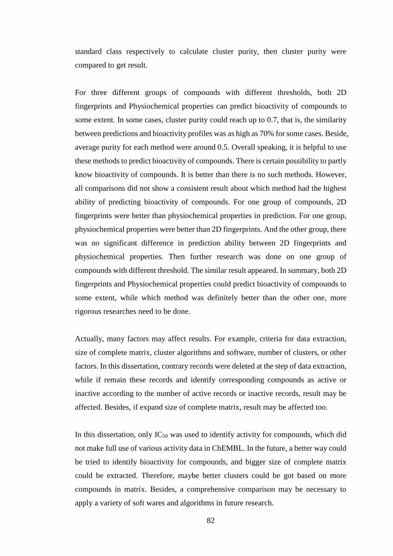
82

standard class respectively to calculate cluster purity, then cluster purity were

compared to get result.

For three different groups of compounds with different thresholds, both 2D

fingerprints and Physiochemical properties can predict bioactivity of compounds to

some extent. In some cases, cluster purity could reach up to 0.7, that is, the similarity

between predictions and bioactivity profiles was as high as 70% for some cases. Beside,

average purity for each method were around 0.5. Overall speaking, it is helpful to use

these methods to predict bioactivity of compounds. There is certain possibility to partly

know bioactivity of compounds. It is better than there is no such methods. However,

all comparisons did not show a consistent result about which method had the highest

ability of predicting bioactivity of compounds. For one group of compounds, 2D

fingerprints were better than physiochemical properties in prediction. For one group,

physiochemical properties were better than 2D fingerprints. And the other group, there

was no significant difference in prediction ability between 2D fingerprints and

physiochemical properties. Then further research was done on one group of

compounds with different threshold. The similar result appeared. In summary, both 2D

fingerprints and Physiochemical properties could predict bioactivity of compounds to

some extent, while which method was definitely better than the other one, more

rigorous researches need to be done.

Actually, many factors may affect results. For example, criteria for data extraction,

size of complete matrix, cluster algorithms and software, number of clusters, or other

factors. In this dissertation, contrary records were deleted at the step of data extraction,

while if remain these records and identify corresponding compounds as active or

inactive according to the number of active records or inactive records, result may be

affected. Besides, if expand size of complete matrix, result may be affected too.

In this dissertation, only IC50 was used to identify activity for compounds, which did

not make full use of various activity data in ChEMBL. In the future, a better way could

be tried to identify bioactivity for compounds, and bigger size of complete matrix

could be extracted. Therefore, maybe better clusters could be got based on more

compounds in matrix. Besides, a comprehensive comparison may be necessary to

apply a variety of soft wares and algorithms in future research.

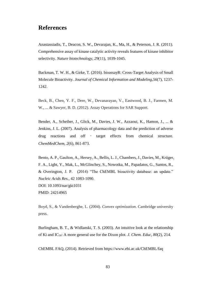
83

References

Anastassiadis, T., Deacon, S. W., Devarajan, K., Ma, H., & Peterson, J. R. (2011).

Comprehensive assay of kinase catalytic activity reveals features of kinase inhibitor

selectivity. Nature biotechnology, 29(11), 1039-1045.

Backman, T. W. H., & Girke, T. (2016). bioassayR: Cross-Target Analysis of Small

Molecule Bioactivity. Journal of Chemical Information and Modeling,56(7), 1237-

1242.

Beck, B., Chen, Y. F., Dere, W., Devanarayan, V., Eastwood, B. J., Farmen, M.

W., ... & Sawyer, B. D. (2012). Assay Operations for SAR Support.

Bender, A., Scheiber, J., Glick, M., Davies, J. W., Azzaoui, K., Hamon, J., ... &

Jenkins, J. L. (2007). Analysis of pharmacology data and the prediction of adverse

drug reactions and off ‐ target effects from chemical structure.

ChemMedChem, 2(6), 861-873.

Bento, A. P., Gaulton, A., Hersey, A., Bellis, L. J., Chambers, J., Davies, M., Krüger,

F. A., Light, Y., Mak, L., McGlinchey, S., Nowotka, M., Papadatos, G., Santos, R.,

& Overington, J. P. (2014) “The ChEMBL bioactivity database: an update.”

Nucleic Acids Res., 42 1083-1090.

DOI: 10.1093/nar/gkt1031

PMID: 24214965

Boyd, S., & Vandenberghe, L. (2004). Convex optimization. Cambridge university

press.

Burlingham, B. T., & Widlanski, T. S. (2003). An intuitive look at the relationship

of Ki and IC50: A more general use for the Dixon plot. J. Chem. Educ, 80(2), 214.

ChEMBL FAQ, (2014). Retrieved from https://www.ebi.ac.uk/ChEMBL/faq

http://dx.doi.org/%2010.1093/nar/gkt1031

http://europepmc.org/abstract/MED/24214965

https://www.ebi.ac.uk/ChEMBL/faq

84

Cheng, T., Wang, Y., & Bryant, S. H. (2010). Investigating the correlations among

the chemical structures, bioactivity profiles and molecular targets of small

molecules. Bioinformatics, 26(22), 2881-2888.

Davis, M. I., Hunt, J. P., Herrgard, S., Ciceri, P., Wodicka, L. M., Pallares, G., ... &

Zarrinkar, P. P. (2011). Comprehensive analysis of kinase inhibitor


Deprez-Poulain, R., & Deprez, B. (2004). Facts, figures and trends in lead

generation. Current topics in medicinal chemistry, 4(6), 569-580.

Fang, J. S., Liu, A. L., & Du, G. H. (2014). Research advance in the drug target

prediction based on chemoinformatics. Acta pharmaceutica Sinica, 49(10), 1357-

1364.

Gaulton, A., Bellis, L. J., Bento, A. P., Chambers, J., Davies, M., Hersey, A., ... &

Overington, J. P. (2012). ChEMBL: a large-scale bioactivity database for drug

discovery. Nucleic acids research, 40(D1), D1100-D1107.

Helal, K. Y., Maciejewski, M., Gregori-Puigjane, E., Glick, M., & Wassermann, A.

M. (2016). Public domain HTS fingerprints: design and evaluation of compound

bioactivity profiles from PubChem”s bioassay repository. Journal of chemical

information and modeling, 56(2), 390-398.

Hughes, J. P., Rees, S., Kalindjian, S. B., & Philpott, K. L. (2011). Principles of

early drug discovery. British journal of pharmacology, 162(6), 1239-1249.

Karaman, M. W., Herrgard, S., Treiber, D. K., Gallant, P., Atteridge, C. E.,

Campbell, B. T., ... & Faraoni, R. (2008). A quantitative analysis of kinase inhibitor


Larsen, R. J., & Marx, M. L. (1986). An introduction to mathematical statistics and

its applications.

85

Lavecchia, A. (2015). Machine-learning approaches in drug discovery: methods and

applications. Drug discovery today, 20(3), 318-331.

Leach, A. R., & Gillet, V. J. (2003). An introduction to chemoinformatics. Kluwer

Academic Publishers.

Leskovec, J., Rajaraman, A., & Ullman, J. D. (2014). Mining of massive datasets.

Cambridge University Press

Lusher, S. J., McGuire, R., van Schaik, R. C., Nicholson, C. D., & de Vlieg, J. (2014).

Data-driven medicinal chemistry in the era of big data. Drug discovery today, 19(7),

859-868.

Manning, C. D., Raghavan, P., & Schutze, H. (2008) Introduction to Information

Retrieval. Cambridge University Press

Martínez-Jiménez, F., Papadatos, G., Yang, L., Wallace, I. M., Kumar, V., Pieper,

U., ... & Marti-Renom, M. A. (2013). Target prediction for an open access set of

compounds active against Mycobacterium tuberculosis. PLoS Comput Biol, 9(10),

e1003253.

Mazanetz, M. P., Marmon R. J., Reisser, C. BT., & Morao, I. (2012). Drug discovery

applications for KNIME: an open source data mining platform.Current topics in

medicinal chemistry, 12(18), 1965-1979.

Medina-Franco, J. L., Giulianotti, M. A., Welmaker, G. S., & Houghten, R. A.

(2013). Shifting from the single to the multitarget paradigm in drug discovery. Drug

discovery today, 18(9), 495-501.

Miranda-Saavedra, D., & Barton, G.J. (2007) Classification and functional

annotation of eukaryotic protein kinases. Proteins 68, 893-914.

86

Paolini, G. V., Shapland, R. H., van Hoorn, W. P., Mason, J. S., & Hopkins, A. L.

(2006). Global mapping of pharmacological space. Nature biotechnology, 24(7),

805-815.

Petrone, P. M., Simms, B., Nigsch, F., Lounkine, E., Kutchukian, P., Cornett, A., ...

& Glick, M. (2012). Rethinking molecular similarity: comparing compounds on the

basis of biological activity. ACS chemical biology, 7(8), 1399-1409.

Personal communication, (July, 2016). van Westen, G.

Pina, A. S., Hussain, A., & Roque, A. C. A. (2010). An historical overview of drug

discovery. Ligand-Macromolecular Interactions in Drug Discovery: Methods and

Protocols, 3-12.

Provost, F., & Fawcett, T. (2013). Data Science for Business: What you need to

know about data mining and data-analytic thinking. "O'Reilly Media, Inc.".

Rogers, D., & Hahn, M. (2010). Extended-connectivity fingerprints. Journal of

chemical information and modeling, 50(5), 742-754.

Sliwoski, G., Kothiwale, S., Meiler, J., & Lowe, E. W. (2014). Computational

methods in drug discovery. Pharmacological reviews, 66(1), 334-395.

Sutherland, J. J., Gao, C., Cahya, S., & Vieth, M. (2013). What general conclusions

can we draw from kinase profiling data sets?. Biochimica et Biophysica Acta (BBA)-

Proteins and Proteomics, 1834(7), 1425-1433.

Taylor, D. (2015). The Pharmaceutical Industry and the Future of Drug

Development, Pharmaceuticals in the Environment, pp. 1-33

Wawer, M., Lounkine, E., Wassermann, A. M., & Bajorath, J. (2010). Data

structures and computational tools for the extraction of SAR information from large

compound sets. Drug discovery today, 15(15), 630-639.

87

Witten, I. H., Frank, E., & Hall, M. A. (2011). Data Mining: Practical machine

learning tools and techniques (3rd edition.). Morgan Kaufmann Publishers

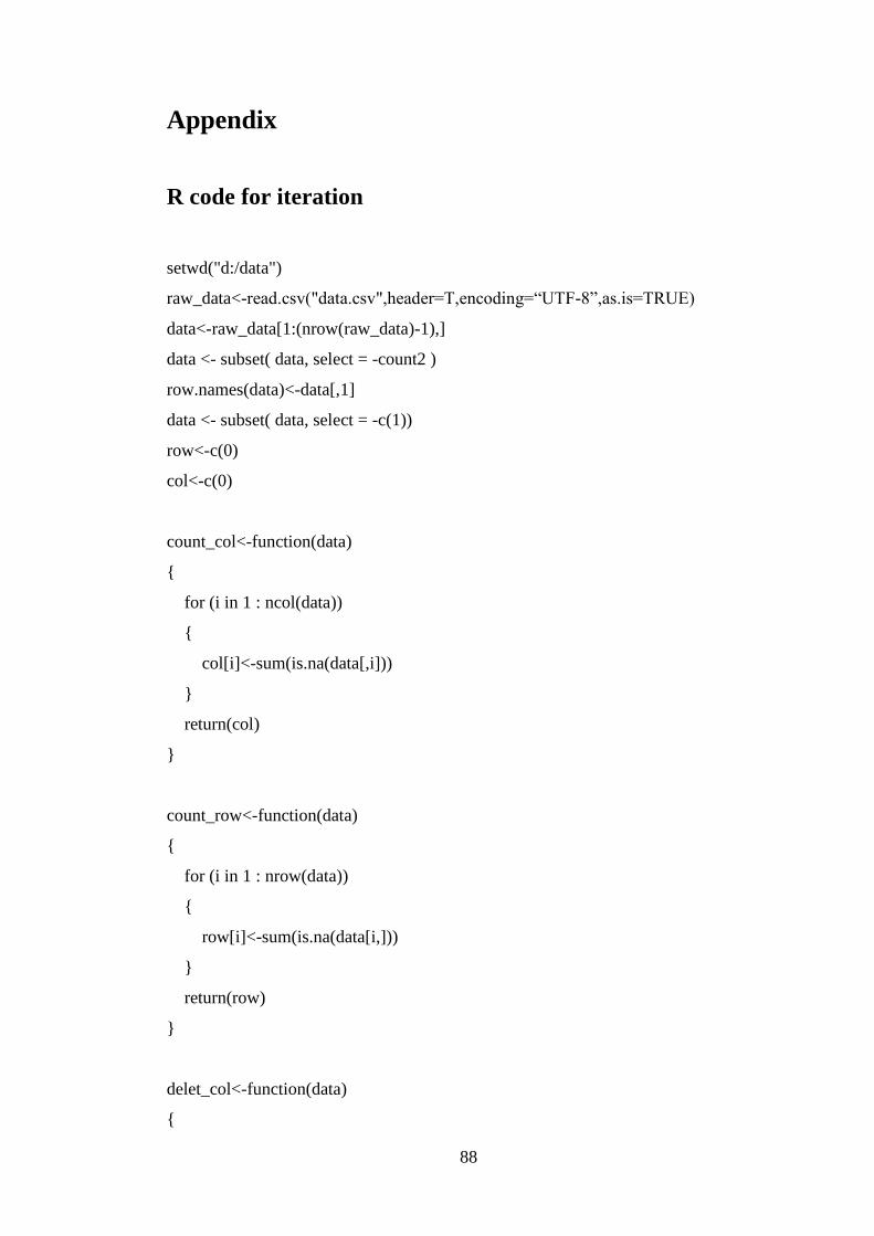
88

Appendix

R code for iteration

setwd("d:/data")

raw_data<-read.csv("data.csv",header=T,encoding=“UTF-8”,as.is=TRUE)

data<-raw_data[1:(nrow(raw_data)-1),]

data <- subset( data, select = -count2 )

row.names(data)<-data[,1]

data <- subset( data, select = -c(1))

row<-c(0)

col<-c(0)

count_col<-function(data)

{

for (i in 1 : ncol(data))

{

col[i]<-sum(is.na(data[,i]))

}

return(col)

}

count_row<-function(data)

{

for (i in 1 : nrow(data))

{

row[i]<-sum(is.na(data[i,]))

}

return(row)

}

delet_col<-function(data)

{

89

j<-which.max(col)

data <- subset( data, select = -c(j))

return(data)

}

delet_row<-function(data)

{

j<-which.max(row)

data<-data[-j,]

return(data)

}

result<-function(data)

{

num_na<-0

for(i in 1:nrow(data))

num_na<-num_na+sum(is.na(data[i,]))

return(1-num_na/(nrow(data)*ncol(data)))

}

for(i in 1:2)

{

col<-c(0)

col<-count_col(data)

data<-delet_col(data)

}

result(data)

for(i in 1:13)

{

row<-c(0)

row<-count_row(data)

data<-delet_row(data)

print(i)

90

}

result(data)

write.csv(data, file="result.csv",row.names=T,quote=F)

Access to Dissertation

A Dissertation submitted to the University may be held by the Department (or School) within which the Dissertation was

undertaken and made available for borrowing or consultation in accordance with University Regulations.

Requests for the loan of dissertations may be received from libraries in the UK and overseas. The Department may also receive

requests from other organisations, as well as individuals. The conservation of the original dissertation is better assured if the

Department and/or Library can fulfill such requests by sending a copy. The Department may also make your dissertation

available via its web pages.

In certain cases where confidentiality of information is concerned, if either the author or the supervisor so requests, the

Department will withhold the dissertation from loan or consultation for the period specified below. Where no such

restriction is in force, the Department may also deposit the Dissertation in the University of Sheffield Library.

To be completed by the Author – Select (a) or (b) by placing a tick in the appropriate box

If you are willing to give permission for the Information School to make your dissertation available in these ways, please

complete the following:

(a) Subject to the General Regulation on Intellectual Property, I, the author, agree to this dissertation being made

immediately available through the Department and/or University Library for consultation, and for the Department

and/or Library to reproduce this dissertation in whole or part in order to supply single copies for the purpose of

research or private study

(b) Subject to the General Regulation on Intellectual Property, I, the author, request that this dissertation be withheld

from loan, consultation or reproduction for a period of [ ] years from the date of its submission. Subsequent to

this period, I agree to this dissertation being made available through the Department and/or University Library for

consultation, and for the Department and/or Library to reproduce this dissertation in whole or part in order to supply

single copies for the purpose of research or private study

Name Jingyan Sui

Department Information School

Signed Jingyan Sui Date September 1, 2016

To be completed by the Supervisor – Select (a) or (b) by placing a tick in the appropriate box

(a) I, the supervisor, agree to this dissertation being made immediately available through the Department and/or

University Library for loan or consultation, subject to any special restrictions (*) agreed with external organisations

as part of a collaborative project.

*Special

restrictions

(b) I, the supervisor, request that this dissertation be withheld from loan, consultation or reproduction for a period of

[ ] years from the date of its submission. Subsequent to this period, I, agree to this dissertation being made

available through the Department and/or University Library for loan or consultation, subject to any special

restrictions (*) agreed with external organisations as part of a collaborative project

Name

Department

Signed Date

THIS SHEET MUST BE SUBMITTED WITH DISSERTATIONS BY DEPARTMENTAL REQUIREMENTS.

september 2016 - university of sheffield

Documents