sensor-based robot motion planning - a tabu search approach

IEEE Robotics & Automation Magazine48 1070-9932/08/$25.00ª2008 IEEE JUNE 2008

Sensor-Based RobotMotion Planning

A Tabu Search Approach

Planning robot motions in unknown environments hasbeen an attractive research theme for many roboticistsduring the past two decades. The class of motion plan-ners dealing with this kind of problem isknown as online, sensor-based, local, a pos-

teriori, real-time, or reactive motion planners.Among the first works on online motion

planning is Lumelsky’s Bug algorithmpresented for a point robot to movefrom a source point to a destinationpoint, using touch sensing in a planarterrain populated with arbitrarilyshaped obstacles [1]. Cox and Yapdeveloped algorithms to navigatea rod to a destination position inplanar polygonal terrains [2]. Asurvey on early online path plan-ning works is provided in [3].Another noteworthy approachfor real-time planning is Khatib’spotential fields (PFs) method, inwhich a point robot is directedby the forces in a field of poten-tials exerted by repulsive obstaclesand the attractive goal [4].

Aiming to take advantage ofthe properties of roadmaps con-structed usually in the offline mode,some researchers have tried to utilizethe distance transform approach to buildthem incrementally. In [5], an algorithm isproposed for the navigation of a circularrobot in unknown terrains by iteratively visit-ing the vertices of the Voronoi diagram. Chosetdeveloped an incremental method to construct the hierarchicalgeneralized Voronoi graph (HGVG) [6], which exploits somebridge edges (called GVG2) to maintain the connectivity of theGVG in high dimensions. Also, another method is proposed in

[7] for online motion planning through incremental construc-tion of medial axis.

Other works such as [8] have tried to guide the motions ofthe robot along the edges of the visibility graph of aworkspace of convex polygons in online mode. In

[9], an algorithm is presented in which thevisibility graph of the workspace is incre-

mentally constructed by integrating theinformation of the paths traversed so

far, and then, a globally optimal pathis planned after the graph comple-tion, as in offline mode.

In addition to the classic motion-planning approaches, other optimi-zation methods generally knownas heuristics have been increas-ingly employed for planning andoptimizing robot motions. Heu-ristic algorithms do not guaranteeto find a solution, but if they do,they are likely to do so muchfaster than the competing com-plete methods.

Some well-known metaheur-istics such as genetic algorithms

(GAs) and simulated annealing(SA) have found applications in

robot motion planning. In [10], thepath planning problem is expressed as

an optimization problem and solved witha GA. It is done by building a path planner

for a planar arm with 2 degrees of freedom, andthen for a holonomic mobile robot. In [11], the

path planning for vehicles is formulated as an optimiza-tion problem; the goal is to choose a path connecting initial andfinal points that crosses the least number of obstacles (with theeventual goal of zero crossings) in configuration space. A GA isdevised in which the population is a set of paths. The SAapproach is widely used in combination with the artificialpotential field approach to escape from local minima, as in [12].Digital Object Identifier 10.1109/MRA.2008.921543

BY ELLIPS MASEHIAN AND MOHAMMAD REZA AMIN-NASERI

The Tabu SearchThe tabu search (TS) method is another well-known metaheuris-tic technique first introduced by Fred Glover in 1989 [13]. TS is apowerful algorithmic approach that has been applied with greatsuccess to a large variety of difficult combinatorial optimizationproblem areas, such as assignment, scheduling, routing, TSP, etc.

TS has three phases: preliminary search, intensification, anddiversification. During the first of these three steps, TS is similarto some other optimization methods in that whatever point xin the input space the robot is currently at, it evaluates the crite-rion function f ðxÞ at all the neighbors N of x and finds the newpoint x0 that is best in N . Repeating this idea creates the possi-bility of endlessly cycling back and forth between x and x0 (a localminimum). To avoid this, TS differs from many other methodsin that the robot moves to x0 even if it is worse than x.

TS keeps track of performed moves and labels the recentmoves as tabu moves, meaning that the search shall not revisitthese points. The set of tabu moves is called tabu list (which isactually a push-down stack of s elements managed in a first-in/first-out manner), and its size is called tabu size. So that, forinstance, once the move x! x0 has been made, the reversemove x0 ! x is forbidden for at least the next s moves. Ofcourse, when a tabu move has a cost lower than an aspirationlevel, it can be selected regardless of its tabuness. In addition tothis tabu list, which is a recency-based short-term memory, wemight introduce a frequency-based memory that operates on amuch longer horizon (e.g., the last 50 iterations) and penalizethe most frequently visited moves.

In the second (intensification) part of the search, it 1) startswith the best solution found so far (which is always storedthroughout the entire algorithm), 2) clears the tabu list, and 3)proceeds as in the preliminary search for a specified number ofmoves. Finally, in the diversification phase, the tabu list iscleared again, and the s most frequent moves of the run so farare set to be tabu. Then, it chooses a random x to move to andproceeds as in the preliminary search phase for a specifiednumber of iterations. The intensification phase focuses on thepromising regions discovered during preliminary search,whereas the diversification phase forces exploration of com-pletely new regions [14].

In this article, we introduce a TS-based robot motion-planning algorithm, which is in fact the first of its kind, as wedid not find any prior instance in the literature. One reasonmight be that a straightforward way for defining tabu and non-tabu moves is via discretizing the C-space, for which someapproaches like PFs have been introduced long ago. Neverthe-less, because of our different approach in defining neighbor-hoods, employing TS has been possible and effective.

The Motion Planner’s ComponentsThe new online motion planner presented in this article incor-porates the robot’s sensory data into the intelligence inducedfrom the TS technique.

Before dealing with the major components of the motionplanner, we define a move: a move is a motion from the cur-rent point x to another point inside the free C-space (Cfree)with a step size equal to the radius of the current point’s locally

maximal disc (LMD)—which is the largest disc centeredaround x and completely contained in Cfree—and a directionalong one of its radial sensors (Figure 1).

The outline of the algorithm is as follows. Beginning fromthe start point, the robot performs a visibility scan to find visi-ble obstacle vertices and decides to move toward an obstaclevertex it finds most promising according to a cost criterion.Upon making the move, backward directions are labeled astabu and excluded from the set of next promising directions.The visibility scan and its ensuing operations are repeated forthe new location, and the robot continues to navigate the envi-ronment until it sees the goal point. If at any stage the robot istrapped in a local minimum, it takes a random and relativelylarge step toward unexplored areas of the search space and con-tinues its search in that area. The algorithm’s main componentsare described later.

Perception ComponentThe perception component is responsible for acquiring infor-mation from the environment and processing those data todetermine the appropriate moves for the robot at each itera-tion. This is done by 1) performing a visibility scan and2) detecting the visible obstacle vertices.

Upon arriving at a new point in the workspace, the robot firstdetermines its distance to the surrounding obstacles by means ofits radial range-finder sensor readings, which yields a list of candi-date moves. Suppose that a circular mobile robot with radiusRrob and S range-sensors situated equidistantly on its perimeteris centered at point c. Each sensor projects a ray ri (i ¼ 1, . . . , S,counterclockwise) to find out its distance qi from the nearestvisible obstacle point xi along the i-th direction (Figure 1).

Taking the metric D(xi, xc) for the Euclidean distance ofpoints xi and xc , we have qi ¼ D(xc , xiÞ � Rrob, where xc isthe coordinate of the robot center’s current position in theworkspace. A representation of qi ’s versus ray angles is depictedin Figure 2(a).

0 5 10 15

2

4

6

8

10

12

14

g

c

LMD(c)

Figure 1. The visibility scan of the environment from therobot’s location at point c.

IEEE Robotics & Automation MagazineJUNE 2008 49

In order for the robot to avoid getting trapped in obstacles’concave regions and bypass any blocking obstacle, it shouldmove toward the tangent rays of the obstacle’s boundaries. Aray ri is tangent to an obstacle if in a neighborhood U of xi theinterior of the obstacle lies entirely on a single side of the line ri.Otherwise, the robot’s motion toward the middle of the obsta-cle will lead to collision. This strategy stipulates the robot todistinguish the obstacle’s outermost vertices, or in a broadersense (if the obstacles are not polygons), the regions adjacent totangent rays, as viewed from the robot’s vantage point.

For determining the tangent rays, a difference function isapplied for successive adjacent rays to calculate the ray differ-ence variables, as

q̂i ¼ qiþ1 � qi: (1)

Figure 2(b) shows the difference variables of the Figure 2(a).The sharp peaks (both positive and negative) imply abrupt andlarge differences in successive ray magnitudes, and so indicatethe points where sweeping rays leave or meet a convex con-tour on the obstacle boundary. These peaks are detected byapplying a notch filter to the plot. If no peaks are found, thenthe algorithm shifts to the diversification mode in which a ran-dom step is taken by the robot.

Cost Evaluation ComponentAfter determining visible obstacles’ extreme vertices, the costevaluation component associates a value to each tangent ray asa measure for the cost of reaching the goal via the direction ofthat ray. The criterion by which the cost is specified is a com-pound function. It incorporates two basic functions related toeach ray: 1) distance function and 2) neighborhood function.

The distance function fD(ri) aims to estimate the length ofthe path connecting the robot center’s current configurationto the goal configuration and is defined by

fD(ri) ¼ k1 �D(xc , xi)þ k2 �D(xi, xg): (2)

The first part of (2) is deterministic and is calculated in theperception component. The second term is a heuristic esti-mation for the length of the free path connecting the ri’sendpoint xi and the goal point xg. The weighted linear com-bination of these two terms (with k1 and k2 as weights) pro-vides a heuristic criterion widely used in the A* searchtechnique. The thick dotted lines in Figure 1 show the dis-tances involved in building the cost function: the lines origi-nated from the robot’s configuration show the tangent rays,i.e., the perceived obstacle vertices, and the lines to the pointg present rough estimations for the distance of the vertices tothe goal point, as in the A* search.

The neighborhood function fN (ri) measures the degree ofchange in the magnitudes of neighboring rays occurring at riand is expressed as

fN (ri) ¼ a �maxfq̂i, q̂i�1g, (3)

where a is a tuning parameter. A large value of fN (ri) impliesthat the obstacle (vertex) adjacent to ri has a relatively large freespace behind it and will possibly lead the robot to a key posi-tion in the configuration space, hence offering a better maneu-verability for it. Small amounts of fN (ri) indicate crampedareas, narrow passages, or obstacle borders, which generallyhave lesser priority for navigation.

The overall cost evaluation criterion C(ri) is minimizinga blend of the distance and neighborhood functions accord-ing to

C(ri) ¼ Pi � fD(ri)b � fN (ri)

�c, (4)

in which b and c are scalars and Pi is defined as

Pi ¼e if ri has the direction of the last move

v if ri points to a visited vertex

t if ri is a tabu direction.

8<:

(5)

Through its reducing effect, the parameter e < 1 encouragesthe robot to continue its navigation along a direction selectedin the past few iterations and to be not diverted frequently byevery new vertex that appears in its scope. The parameter vincreases the cost of a ray pointing to a previously visited ver-tex, whereas the parameter t imposes a penalty for directionsthat are designated as tabu ones. The suggested values for theseparameters are shown in Table 3.

0 30 60 90 120 150 180 210 240 270 300 330 360

0 30 60 90 120 150 180

(a)

(b)

210 240 270 300 330 3600

2

4

6

8

10

12

14

–6

–4

–2

0

2

4

6

Figure 2. (a) The magnitudes of rays emitted from the robot’sposition in Figure 1, which was acquired by range sensors.(b) By applying a difference function, obstacle vertices areidentified by sharp peaks. Insignificant peaks are omitted byusing a notch filter (dashed horizontal lines at 60.9).

IEEE Robotics & Automation Magazine50 JUNE 2008

After evaluating all rays, the motion planner is able to selectthe most promising goal-oriented direction to move along,which corresponds to the ray associated with the lowest cost.

Note that since the neighborhood function fN (ri) has anegative exponent in (4), its large values (corresponding totangent rays) reduce the overall cost dramatically. It followsthat the probability of selecting obstacle vertices as next prom-ising destinations is much higher than that of the ordinary rays(which point to obstacle borders), and, therefore, the robot isnaturally being attracted to vertices. On the other hand, thedistance function fD(ri) in (4) increases the probability of select-ing near-to-goal destinations through its positive exponent. Inother words, the designed cost evaluation function leads tolocally optimal (i.e., shortest) navigations, just as the visibilitygraph does in offline mode, and, thus, the robot’s performanceimproves significantly.

Aspiration and Desperation LevelsThe aspiration level is a level set to accept a very good move, evenif it is tabu. This is an established concept in TS, proposed byGlover. Now, we make the TS metaheuristic more flexible andpowerful by introducing a new concept called desperation level.

The desperation level is a level (of cost) beyond which a non-tabu move having higher cost values (for minimization problems)or lower cost values (for maximization problems) is rejected andincluded in the tabu list. It is somehow a counterpart and comple-mentary concept for the aspiration level. The relation of theselevels with regard to the tabu or nontabu moves is depicted inFigure 3. The gray sections of the diagram (i.e., II and IV) repre-sent unacceptable moves, since they are either tabu—with costsnot better than the aspiration level—or nontabu, but with costshigher than the desperation level.

In our planning context, it frequently happens that thereare no nearby nontabu obstacle vertices. Instead, there aresome remote vertices with high costs beyond the desperationlevel. Excluding such vertices from the moves list will makethe list empty and limit the search space, which in turn willactivate the diversification component and will cause the robotto take a random step toward unexplored areas of the space.

The Short-Term Tabu ListThe notion of a tabu list is critical and fundamental to thisapproach. The attribute by which we set up tabu lists is thedirection of the rays emanated from the robot.

In each iteration, tabu moves are identified based on therobot’s direction. A tabu envelope (TE) variable is specified toset the range of tabu directions. It is laid out symmetricallyaround the reverse of the robot’s direction, covering all rayswithin a 6TE/2 deviation. For instance, in Figure 4, therobot’s initial direction is 50�. By setting TE ¼ 90�, all thedirections included in the area (pþ 50�) 6 45� (i.e., 185–275�)are characterized as tabu moves (the gray sector).

For setting up the short-term tabu list, if its size (STLS) isset to k, then the tabu directions of the last k iterations areappended to form the total set of tabu moves. We found k ¼ 2to be the best size, although k ¼ 1 is also possible, but it leadsto more fluctuations in the robot’s motion.

The Long-Term Tabu ListAside from the short-term tabu list discussed earlier, we set along-term tabu list by keeping a record of the already visited(i.e., almost touched) vertices. If the robot happens to head fora visited vertex, then since it has been at that location duringearlier iterations, it should avoid the point and concentrate onother vertices in view. This is done by a simple checking of thelong-term tabu list, with a size of LTLS. The long-term tabulist may also contain a set of nonvertex points that are provento be ineffective and misleading in directing the robot towardthe goal.

Diversification ComponentThis component is evoked when there are no admissible non-tabu directions. This situation occurs when 1) all the vertices inscope have been previously visited and marked as tabu (i.e., arein tabu list), 2) all nontabu moves have a cost value higher thanthe desperation level, or 3) the robot is entrapped in a dead end.

The robot will then take a large step with a random direc-tion selected from among rays with big magnitudes (comparewith the concept of the diversification phase discussed earlier).The short-term tabu list is cleared after this step, but the long-term tabu list is retained. This action will most likely guide the

Figure 4. A short list of tabu moves is constructed byappending the tabu envelopes of the last two iterations.

Cost Value

DesperationLevel

AspirationLevel

Tabu Nontabu

I

IV

III

II

Moves

Figure 3. The aspiration and desperation levels for aminimization problem. Region IV represents moves consideredunacceptable, although nontabu.


robot toward new and unexplored areas of the searching space.Consequently, all the elements of the short-term tabu list, aswell as some older elements of the long-term tabu list, will beeliminated.

In fact, the diversification component provides the plan-ner’s probabilistic-completeness property. That is, given suffi-cient time, the algorithm will eventually reach the goal if thereis a valid path. The random steps guarantee that the robot willexplore all areas of the workspace.

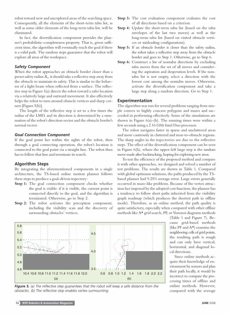
Safety ComponentWhen the robot approaches an obstacle border closer than apreset safety radius Rs, it should take a reflective step away fromthe obstacle to maintain its safety. This is similar to the behav-ior of a light beam when reflected from a surface. The reflec-tive step in Figure 5(a) directs the robot toward a safer locationvia a relatively large and outward movement. It also effectivelyhelps the robot to turn around obstacle vertices and sharp cor-ners [Figure 5(b)].

The length of the reflective step is set to a few times theradius of the LMD, and its direction is determined by a sum-mation of the robot’s direction vector and the obstacle border’snormal vector.

Goal Connection ComponentIf the goal point lies within the sights of the robot, thenthrough a goal connecting operation, the robot’s location isconnected to the goal point via a straight line. The robot thenhas to follow that line and terminate its search.

Algorithm StepsBy integrating the aforementioned components in a singlearchitecture, the TS-based online motion planner followsthese steps to produce a goal-driven trajectory:Step 1: The goal connection component checks whether

the goal is visible: if it is visible, the current point isconnected directly to the goal, and the algorithm isterminated. Otherwise, go to Step 2.

Step 2: The robot activates the perception component,including the visibility scan and the discovery ofsurrounding obstacles’ vertices.

Step 3: The cost evaluation component evaluates the costof all directions based on a criterion.

Step 4: Update the short-term tabu list (based on the tabuenvelopes of the last two moves) as well as thelong-term tabu list (based on visited obstacle verti-ces or misleading configurations).

Step 5: If an obstacle border is closer than the safety radius,the robot takes a reflective step away from the obstacleborder and goes to Step 1. Otherwise, go to Step 6.

Step 6: Construct a list of nontabu directions by excludingtabu moves from the set of all moves and consider-ing the aspiration and desperation levels. If the non-tabu list is not empty, select a direction with thelowest cost among the nontabu moves. Otherwise,activate the diversification component and take alarge step along a random direction. Go to Step 1.

ExperimentationThe algorithm was run for several problems ranging from sim-ple convex to highly concave polygons and mazes and suc-ceeded in performing effectively. Some of the simulations areshown in Figure 6(a)–(h). The running times were within afew seconds using a 2.16 GHz Intel Duo processor.

The robot navigates faster in sparse and uncluttered areasand more cautiously in cluttered and near-to-obstacle regions.The sharp angles in the trajectories are due to the reflectivesteps. The effect of the diversification component can be seenin Figure 6(h), where the upper-left large step is the randommove made after backtracking, hoping for exploring new areas.

To test the efficiency of the proposed method and compareit with other approaches, we designed and solved a number oftest problems. The results are shown in Table 1. Comparedwith global optimum solutions, the paths produced by the TS-based planner had 9.25% average error. Large errors generallyoccurred in maze-like problems. Because of the vertex attrac-tion fact imposed by the adopted cost function, the planner hasa tendency to follow short paths inherited from the visibilitygraph roadmap (which produces the shortest path in offlinemode). Therefore, as an online method, the path quality isquite satisfactory, especially when compared with other offlinemethods like A* grid search, PF, or Voronoi diagrams methods

(Table 1 and Figure 7). Be-cause grid-based methods(like PF and A*) examine theneighboring cells of grid points,the resulting path is roughand can only have vertical,horizontal, and diagonal lo-cal directions.

Since online methods ac-quire their knowledge of en-vironment by sensors and plantheir path locally, it would beincorrect to compare the pro-cessing times of offline andonline methods. However,compared with the average

5.8

5.6

5.4

5.2

5.0

4.8

4.6

4.5

4.0

3.510.4 10.6 10.8 11.0 11.2 11.4 11.6 11.8 12.0 0.6 0.8 1.0 1.2 1.4

(a) (b)

1.6 1.8 2.0 2.2

Figure 5. (a) The reflective step guarantees that the robot will keep a safe distance from theobstacles. (b) The reflective step enables vertex surmounting.


processing time of 7.46 s for the A* search and 3.08 s for thePF method (calculated for the 15 problems), the TS-basedalgorithm performed convincingly well.

We also compared the performance of the proposed newplanner with that of an online distance transform method, theincremental construction of generalized Voronoi diagram(GVD). This method builds the GVD incrementally using theinformation acquired by its sensors [6], [7]. Overall, the pathlengths of the TS-based method are shorter (about 25% less inour experiments) than that of the GVD method. This is due tothe nature of the Voronoi diagram that keeps the maximumclearance from the obstacles, whereas the TS-based planner is

attracted to obstacle vertices and thus emulates the visibilitygraph, which provides the shortest path. Problem 13 in Table 1was solved by the GVD online method in 24.3 s through 243iterations and with 24 sensors and a path length of 75.06

G

G G

S

S S

G

S

(a) (b) (c)

G

S

(e)

G

S

(f)

GS

(g)

GS

(h)

(d)

Figure 6. Some experiments: (a)–(d) convex and concave obstacles, (e)–(g) maze-like obstacles, (h) a random move is madefollowing the activation of the diversification component.

The robot navigates faster in sparse

and uncluttered areas and more

cautiously in cluttered and

near-to-obstacle regions.


[Figure 7(c)]. The TS-based algorithm’s solution is shown inTable 1 and Figure 6(e). Other problems were also comparedand gave more or less the same results.

To evaluate the performance of the TS-based planneragainst one more online motion planner, we selected thesensor-based rapidly exploring random tree (SRT) method[15], which is an online version of LaValle’s rapidly exploring

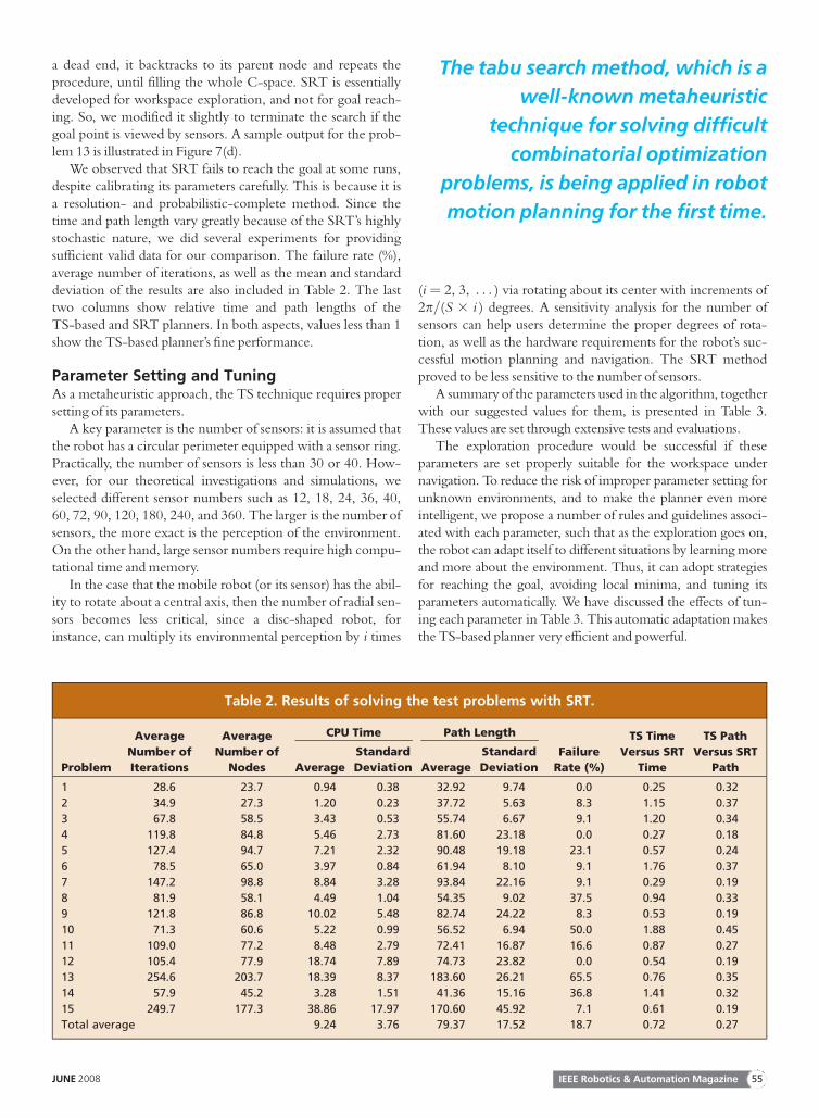
random tree (RRT) method [16]. The SRT-Star method wasrun for the 15 benchmark problems, and the results are sum-marized in Table 2.

As its name implies, the SRT method builds a rooted treefrom the start point, and at each iteration, by generating neigh-boring nodes, it extends its branches randomly but toward pre-viously unexplored areas of the C-space. When encountering

Table 1. A comparison of the path lengths generated by different methods.

Problem

Number

of Convex

Obstacles

Work-

Space

Size

TS-Based Online Planner Path Lengths by Offline MethodsTS-Based

Path

Length

Error %

Number

of Sensors

Number of

Iterations

CPU

Time (s)

Path

Length

A*

Searchab

Potential

Fieldsac

Voronoi

Diagramd

Visibility

Graphe

1 1 [10 3 10] 24 7 0.24 10.42 10.61 13.31 14.07 10.33 0.87

2 2 [10 3 10] 24 31 1.37 14.08 14.18 21.74 19.90 13.72 2.62

3 4 [10 3 10] 36 60 4.11 18.85 21.53 24.67 27.71 18.01 4.66

4 5 [15 3 10] 16 36 1.65 14.94 18.27 20.85 21.92 13.92 7.33

5 5 [15 3 10] 16 47 4.09 21.49 22.26 28.77 33.01 19.12 12.39

6 6 [10 3 10] 18 79 7.00 22.64 23.21 27.22 26.82 18.96 19.41

7 7 [15 3 10] 24 40 2.54 17.77 19.53 23.79 26.66 16.95 4.84

8 8 [10 3 10] 24 41 4.20 18.09 18.06 18.81 20.37 15.38 17.62

9 8 [15 3 10] 36 46 5.31 15.74 17.75 21.95 20.47 15.18 3.69

10 7 [10 3 10] 36 83 9.79 25.54 26.25 34.51 31.84 23.73 7.63

11 11 [15 3 10] 20 53 7.36 19.24 18.48 21.94 24.35 16.36 17.60

12 16 [15 3 10] 36 29 10.10 14.07 13.55 18.58 17.40 13.93 1.01

13 11 [13 3 24] 20 183 14.06 64.67 54.50 64.90 74.61 53.60 20.65

14 12 [9 3 10] 24 52 4.62 13.04 19.11 18.46 16.31 12.26 6.36

15 16 [13 3 24] 40 97 23.86 32.43 31.71 36.31 39.46 28.90 12.20

Average 59 6.68 21.53 21.93 26.39 27.66 19.36 9.25

aAfter graduating the workspace with 1/10 of the unit length.bWith a best-first search strategy and Euclidean distance heuristic.cWith filling-up local minima.dSearched by the Dijkstra’s method.eOptimal solution.

(a) (b) (c) (d)

Figure 7. The problem 13 in Table 1 is solved by (a) PF approach in 3.1 s, (b) A* search in 41.5 s, (c) online distance transform(GVD) builder in 24.3 s, and (d) sensor-based RRT planner in 14.4 s.


a dead end, it backtracks to its parent node and repeats theprocedure, until filling the whole C-space. SRT is essentiallydeveloped for workspace exploration, and not for goal reach-ing. So, we modified it slightly to terminate the search if thegoal point is viewed by sensors. A sample output for the prob-lem 13 is illustrated in Figure 7(d).

We observed that SRT fails to reach the goal at some runs,despite calibrating its parameters carefully. This is because it isa resolution- and probabilistic-complete method. Since thetime and path length vary greatly because of the SRT’s highlystochastic nature, we did several experiments for providingsufficient valid data for our comparison. The failure rate (%),average number of iterations, as well as the mean and standarddeviation of the results are also included in Table 2. The lasttwo columns show relative time and path lengths of theTS-based and SRT planners. In both aspects, values less than 1show the TS-based planner’s fine performance.

Parameter Setting and TuningAs a metaheuristic approach, the TS technique requires propersetting of its parameters.

A key parameter is the number of sensors: it is assumed thatthe robot has a circular perimeter equipped with a sensor ring.Practically, the number of sensors is less than 30 or 40. How-ever, for our theoretical investigations and simulations, weselected different sensor numbers such as 12, 18, 24, 36, 40,60, 72, 90, 120, 180, 240, and 360. The larger is the number ofsensors, the more exact is the perception of the environment.On the other hand, large sensor numbers require high compu-tational time and memory.

In the case that the mobile robot (or its sensor) has the abil-ity to rotate about a central axis, then the number of radial sen-sors becomes less critical, since a disc-shaped robot, forinstance, can multiply its environmental perception by i times

(i ¼ 2, 3, . . . ) via rotating about its center with increments of2p=(S 3 i ) degrees. A sensitivity analysis for the number ofsensors can help users determine the proper degrees of rota-tion, as well as the hardware requirements for the robot’s suc-cessful motion planning and navigation. The SRT methodproved to be less sensitive to the number of sensors.

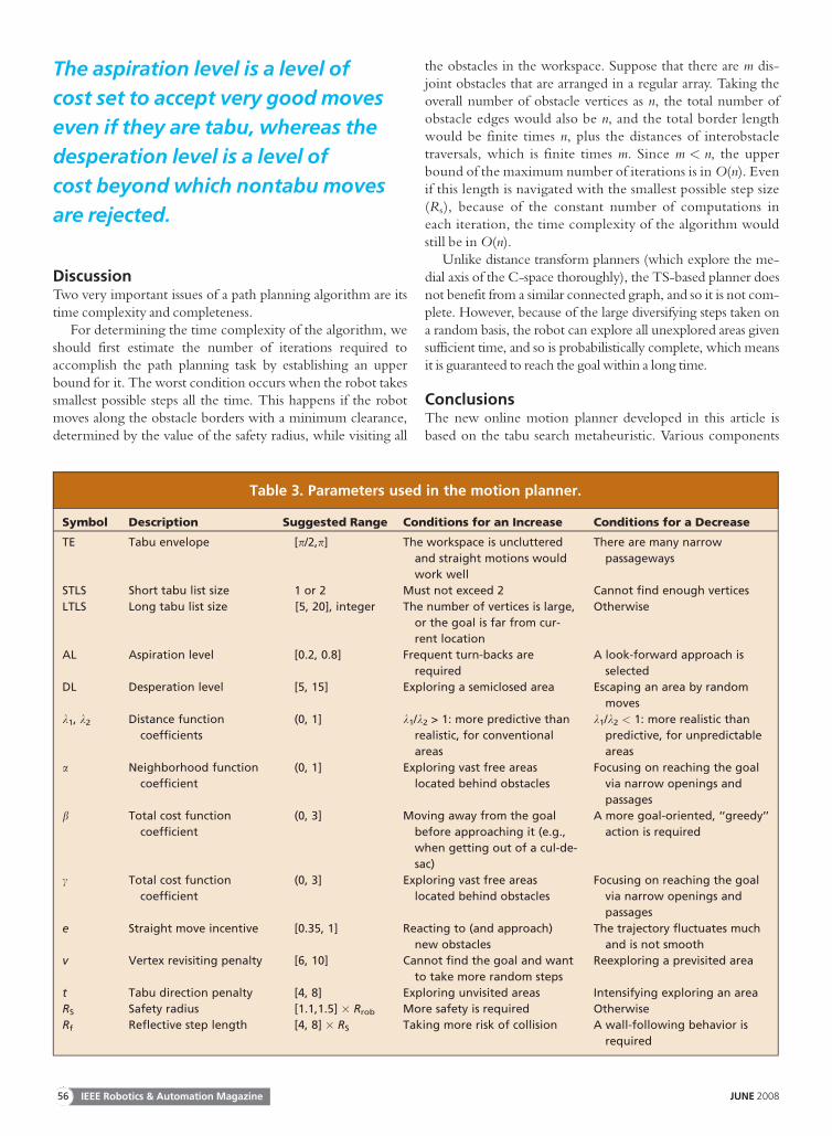
A summary of the parameters used in the algorithm, togetherwith our suggested values for them, is presented in Table 3.These values are set through extensive tests and evaluations.

The exploration procedure would be successful if theseparameters are set properly suitable for the workspace undernavigation. To reduce the risk of improper parameter setting forunknown environments, and to make the planner even moreintelligent, we propose a number of rules and guidelines associ-ated with each parameter, such that as the exploration goes on,the robot can adapt itself to different situations by learning moreand more about the environment. Thus, it can adopt strategiesfor reaching the goal, avoiding local minima, and tuning itsparameters automatically. We have discussed the effects of tun-ing each parameter in Table 3. This automatic adaptation makesthe TS-based planner very efficient and powerful.

Table 2. Results of solving the test problems with SRT.

Problem

Average

Number of

Iterations

Average

Number of

Nodes

CPU Time Path Length

Failure

Rate (%)

TS Time

Versus SRT

Time

TS Path

Versus SRT

PathAverage

Standard

Deviation Average

Standard

Deviation

1 28.6 23.7 0.94 0.38 32.92 9.74 0.0 0.25 0.32

2 34.9 27.3 1.20 0.23 37.72 5.63 8.3 1.15 0.37

3 67.8 58.5 3.43 0.53 55.74 6.67 9.1 1.20 0.34

4 119.8 84.8 5.46 2.73 81.60 23.18 0.0 0.27 0.18

5 127.4 94.7 7.21 2.32 90.48 19.18 23.1 0.57 0.24

6 78.5 65.0 3.97 0.84 61.94 8.10 9.1 1.76 0.37

7 147.2 98.8 8.84 3.28 93.84 22.16 9.1 0.29 0.19

8 81.9 58.1 4.49 1.04 54.35 9.02 37.5 0.94 0.33

9 121.8 86.8 10.02 5.48 82.74 24.22 8.3 0.53 0.19

10 71.3 60.6 5.22 0.99 56.52 6.94 50.0 1.88 0.45

11 109.0 77.2 8.48 2.79 72.41 16.87 16.6 0.87 0.27

12 105.4 77.9 18.74 7.89 74.73 23.82 0.0 0.54 0.19

13 254.6 203.7 18.39 8.37 183.60 26.21 65.5 0.76 0.35

14 57.9 45.2 3.28 1.51 41.36 15.16 36.8 1.41 0.32

15 249.7 177.3 38.86 17.97 170.60 45.92 7.1 0.61 0.19

Total average 9.24 3.76 79.37 17.52 18.7 0.72 0.27

The tabu search method, which is a

well-known metaheuristic

technique for solving difficult

combinatorial optimization

problems, is being applied in robot

motion planning for the first time.


DiscussionTwo very important issues of a path planning algorithm are itstime complexity and completeness.

For determining the time complexity of the algorithm, weshould first estimate the number of iterations required toaccomplish the path planning task by establishing an upperbound for it. The worst condition occurs when the robot takessmallest possible steps all the time. This happens if the robotmoves along the obstacle borders with a minimum clearance,determined by the value of the safety radius, while visiting all

the obstacles in the workspace. Suppose that there are m dis-joint obstacles that are arranged in a regular array. Taking theoverall number of obstacle vertices as n, the total number ofobstacle edges would also be n, and the total border lengthwould be finite times n, plus the distances of interobstacletraversals, which is finite times m. Since m < n, the upperbound of the maximum number of iterations is in O(n). Evenif this length is navigated with the smallest possible step size(Rs), because of the constant number of computations ineach iteration, the time complexity of the algorithm wouldstill be in O(n).

Unlike distance transform planners (which explore the me-dial axis of the C-space thoroughly), the TS-based planner doesnot benefit from a similar connected graph, and so it is not com-plete. However, because of the large diversifying steps taken ona random basis, the robot can explore all unexplored areas givensufficient time, and so is probabilistically complete, which meansit is guaranteed to reach the goal within a long time.

ConclusionsThe new online motion planner developed in this article isbased on the tabu search metaheuristic. Various components

Table 3. Parameters used in the motion planner.

Symbol Description Suggested Range Conditions for an Increase Conditions for a Decrease

TE Tabu envelope [p/2,p] The workspace is uncluttered

and straight motions would

work well

There are many narrow

passageways

STLS Short tabu list size 1 or 2 Must not exceed 2 Cannot find enough vertices

LTLS Long tabu list size [5, 20], integer The number of vertices is large,

or the goal is far from cur-

rent location

Otherwise

AL Aspiration level [0.2, 0.8] Frequent turn-backs are

required

A look-forward approach is

selected

DL Desperation level [5, 15] Exploring a semiclosed area Escaping an area by random

moves

k1, k2 Distance function

coefficients

(0, 1] k1/k2 > 1: more predictive than

realistic, for conventional

areas

k1/k2 < 1: more realistic than

predictive, for unpredictable

areas

a Neighborhood function

coefficient

(0, 1] Exploring vast free areas

located behind obstacles

Focusing on reaching the goal

via narrow openings and

passages

b Total cost function

coefficient

(0, 3] Moving away from the goal

before approaching it (e.g.,

when getting out of a cul-de-

sac)

A more goal-oriented, ‘‘greedy’’

action is required

c Total cost function

coefficient

(0, 3] Exploring vast free areas

located behind obstacles

Focusing on reaching the goal

via narrow openings and

passages

e Straight move incentive [0.35, 1] Reacting to (and approach)

new obstacles

The trajectory fluctuates much

and is not smooth

v Vertex revisiting penalty [6, 10] Cannot find the goal and want

to take more random steps

Reexploring a previsited area

t Tabu direction penalty [4, 8] Exploring unvisited areas Intensifying exploring an area

RS Safety radius [1.1,1.5] 3 Rrob More safety is required Otherwise

Rf Reflective step length [4, 8] 3 RS Taking more risk of collision A wall-following behavior is

required

The aspiration level is a level of

cost set to accept very good moves

even if they are tabu, whereas the

desperation level is a level of

cost beyond which nontabu moves

are rejected.


of the classic TS have been remodeled and integrated in a sin-gle algorithm to craft a motion planner capable of solving vari-eties of exploration and goal-finding problems. By employingdifferent combinations of a number of parameters, the plannercan react intelligently and promptly to the new situations itfaces during the robotic navigation. The presented explana-tions on the parameters’ definitions and attributes can helpresearchers in applying this algorithm to their real-worldexperiments and applications.

The newly defined concept of desperation level also enrichesthe still-evolving TS discipline, and together with the aspirationlevel and the diversification step, it enables the robot particularlyto escape from local minima. Numerous experiments andcomparisons with offline and online methods showed the algo-rithm’s success and efficiency in coping with different problems,from simple polygons to highly concave obstacles.

Considering the online and sensor-based nature of thepresented model, it is believed that it can be applied todynamic environments (with moving obstacles) as well. In thatcase, the neighborhood and distance functions must be modi-fied to accommodate some predictive information about thevelocity vectors of each obstacle.

Keywords

Robot motion planning, sensor-based navigation, tabu searchmetaheuristic.

References[1] V. J. Lumelsky and A. A. Stepanov, ‘‘Dynamic path planning for a

mobile automation with limited information on the environment,’’IEEE Trans. Automat. Contr., vol. 31, no. 11, pp. 1058–1063, 1986.

[2] J. Cox and C. K. Yap, ‘‘On-line motion planning: moving a planar armby probing an unknown environment,’’ Courant Institute of Mathemati-cal Sciences, New York Univ., New York, Tech. Rep., July 1988.

[3] N. S. V. Rao, S. Kareti, W. Shi, and S. S. Iyenagar, ‘‘Robot navigationin unknown terrains: Introductory survey of non-heuristic algorithms,’’Oakridge National Lab., Tech. Rep. ORNL/TM-12410, 1993.

[4] O. Khatib, ‘‘Real-time obstacle avoidance for manipulators and mobilerobots,’’ Int. J. Robot. Res., vol. 5, no. 1, pp. 90–98, 1986.

[5] N. S. V. Rao, N. Stolzfus, and S. S. Iyengar, ‘‘A ‘retraction’ method forlearned navigation in unknown terrains for a circular robot,’’ IEEETrans. Robot. Automat., vol. 7, no. 5, pp. 699–707, 1991.

[6] H. Choset, S. Walker, K. Eiamsa-Ard, and J. Burdick, ‘‘Sensor-basedexploration: Incremental construction of the hierarchical generalizedVoronoi graph,’’ Int. J. Robot. Res., vol. 19, no. 2, pp. 126–148, 2000.

[7] E. Masehian, M. R. Amin-Naseri, and S. Esmaeilzadeh Khadem,‘‘Online motion planning using incremental construction of medialaxis,’’ in Proc. IEEE Int. Conf. Robotics and Automation, Sept. 2003, vol. 3,pp. 2928–2933.

[8] V. Krishnaswamy and W. S. Newman, ‘‘Online motion planning usingcritical point graphs in two-dimensional configuration space,’’ in Proc. IEEEInt. Conf. Robotics and Automation, May 1992, vol. 3, pp. 2334–2339.

[9] J. B. Oommen, S. S. Iyengar, N. S. V. Rao, and R. L. Kashyap, ‘‘Robotnavigation in unknown terrains using visibility graphs—Part I: The dis-joint convex obstacle case,’’ IEEE J. Robot. Automat., vol. 3, pp. 672–

681, Dec. 1987.

[10] J. M. Ahuactzin, T. El-Ghazali, P. Bessiere, and E. Mazer, ‘‘Usinggenetic algorithms for robot motion planning,’’ in Proc. Workshop ofGeometric Reasoning for Perception and Action, Sept. 16–17, 1991,pp. 84–93.

[11] C. Eldershaw and S. Cameron, ‘‘Real-world applications: Motionplanning using GAs,’’ in Proc. Genetic & Evolutionary Computation Conf.,Orlando, FL, July 1999, p. 1776.

[12] F. Janabi-Sharifi and D. Vinke, ‘‘Integration of the artificial potentialfield approach with simulated annealing for robot path planning,’’ inProc. IEEE Int. Symp. Intell. Contr., Aug. 1993, pp. 536–541.

[13] F. Glover, ‘‘Tabu search—Part I,’’ ORSA J. Comp., vol. 1, no. 3,pp. 190–206, 1989.

[14] F. Glover and M. Laguna, Tabu Search. Norwell, MA: Kluwer Aca-demic, 1997.

[15] G. Oriolo, M. Vendittelli, L. Freda, and G. Troso, ‘‘The SRT method:Randomized strategies for exploration,’’ in Proc. IEEE Int. Conf. Roboticsand Automation, New Orleans, LA, Apr. 2004, pp. 4688–4694.

[16] S. M. LaValle, ‘‘Rapidly-exploring random trees; a new tool for pathplanning,’’ Comp. Sci. Dept., Iowa State Univ., Tech. Rep. TR 98-11,Oct. 1998.

Ellips Masehian is an assistant professor at the Faculty ofEngineering, Tarbiat Modares University, Tehran, Iran. Hereceived the B.S. and M.S. degrees in industrial engineering,both from Iran University of Science and Technology, Teh-ran, with honors, and a Ph.D. degree from Tarbiat ModaresUniversity. His research is focused on the application of heu-ristic and intelligent methods to single and multiple robotmotion planning problems.

Mohammad Reza Amin-Naseri is currently an associateprofessor of the industrial engineering department at TarbiatModares University, Tehran, Iran. He received his B.S.degree in chemical and petrochemical engineering fromAmir-Kabir University of Technology (Tehran Polytechnic),an M.S. degree in operations research from Western Michi-gan University, and a Ph.D. degree in industrial and systemsengineering from West Virginia University. His researchinterests include computational intelligence, artificial neuralnetworks, metaheuristics, and their applications to variousoptimization problems.

Address for Correspondence: Ellips Masehian, Faculty of Engi-neering, Tarbiat Modares University, Jalale-ale-Ahmad Highway,Tehran, 14115-317, Iran. E-mail: [email protected].

Considering the online and sensor-

based nature of the presented

model, it can be applied to dynamic

environments as well.


sensor-based robot motion planning - a tabu search approach

Documents