sensitivity analysis of imperfect systems using …...d. antić et al. sensitivity analysis of...

Acta Polytechnica Hungarica Vol. 8, No. 6, 2011

– 79 –

Sensitivity Analysis of Imperfect Systems Using

Almost Orthogonal Filters

Dragan Antić, Saša Nikolić, Marko Milojković, Nikola

Danković, Zoran Jovanović, Staniša Perić

Department of Control Systems

Faculty of Electronic Engineering

University of Niš, Serbia

Email: [email protected], [email protected],

[email protected], [email protected],

[email protected], [email protected]

Abstract: This paper considers the application of the almost orthogonal filters in the

sensitivity analysis of imperfect systems. First, we explain the concepts of dynamical

systems sensitivity. Then we design almost orthogonal filters based on almost orthogonal

polynomials. These filters are a generalization of the classical orthogonal filters commonly

used in circuit theory, control system theory, signal processing, signal approximation and

process identification. The advantage of the almost orthogonal filters is that they can be

used for the modeling and analysis of systems with imperfections, i.e. imperfect technical

systems. In this paper, we use a designed filter to obtain a model of an imperfect system,

where the model’s parameters have been determined with the help of genetic algorithm. A

new approach for determining the sensitivity of imperfect systems is also given and an

example of an imperfect system in the form of a hydraulic multitank system is considered.

Keywords: sensitivity analysis; imperfect systems; almost orthogonal polynomials; almost

orthogonal filters; multitank system

1 Introduction

Sensitivity analysis considers the impact of parameter or disturbance changes on

the change of the systems’ state coordinates. In this paper, our focus is on the

parametric sensitivity of the imperfect systems. Analysis of the parametric

sensitivity is usually performed as a series of tests in which the operator sets

different parameter values to see if and how these changes impact the system

dynamic behaviour. By showing how the model behaviour responds to changes in

the parameter values, sensitivity analysis is a useful tool in model design as well

as in model evaluation.

D. Antić et al. Sensitivity Analysis of Imperfect Systems Using Almost Orthogonal Filters

– 80 –

Uncertainty in engineering analysis usually pertains to stochastic uncertainty, i.e.,

variance in product or process parameters [1-3] characterized by probability.

Methods for calculating sensitivity under stochastic uncertainty are well

documented. Imprecision, or the concept of uncertainty in choice, is one such

form. Recently, systems with imperfections have been intensively studied [4-8].

The components, used for designing any real system, are not perfect and their

parameters values are in the range of allowed (or not) tolerance. The reasons can

be various: imperfect manufacturing, systems exploitation conditions

(environment temperature, pressure, moisture, electromagnetic fields, variations in

voltage, etc.). With respect to that fact, every real system in analogue technique is

in some way imperfect. Digital systems, on the other hand, are considered to be

perfect. Imperfections of their components do not impact system accuracy as a

whole.

Therefore, because of the imperfections, parameters are not completely defined,

i.e. they can vary in a certain range. In the case of systems modeling by some

classical method, we use fixed parameters values, although it is not the case in

reality. For the purpose of modeling these systems, it is possible to use orthogonal

functions, i.e. orthogonal polynomials [9, 10]. Orthogonal polynomials are already

used in approximation theory and numerical integration, and also in other

scientific disciplines, e.g. in solving series of limitary problems in mathematics

and physics and in solving some quantum mechanics problems. A very important

application of orthogonal polynomials is the designing of orthogonal filters [11-

15]. These filters are useful for orthogonal signal generators, least square

approximations, and the practical realizations of optimal and adaptive systems.

However, since the components of these systems cannot be manufactured exactly,

filters made with these components are not quite orthogonal, but rather almost

orthogonal. The signals obtained by these filters are almost orthogonal as well.

The measure of nearness between the obtained and the regular orthogonal signals

depends on the exactness of the component manufacturing. Thus, almost

orthogonal filters are imperfect filters. Therefore, for designing these filters we

cannot use the classical orthogonal polynomials, but rather we must use almost

orthogonal [16-18]. In this paper, almost orthogonal filters have been used for the

sensitivity analysis of imperfect systems. Theoretical results have been verified

with performed experiments on laboratory setup, consisting of a multitank

hydraulic system, and compared with similar method for sensitivity analysis.


– 81 –

2 Sensitivity of Dynamical Systems

Consider the linear system described by the transfer function in general form:

1

1 1 0

1

1 1 0

m m

m m

n n

n n

b s b s b s bW s

a s a s a s a

(1)

with the output:

y s W s x s (2)

where x(s) represents the input of the system.

Equation (1) has (n+m+2) parameters ai (i=0,1,…,n), bj (j=0,1,…,m) [19]. So it is

possible to define (n+m+2) sensitivity functions in s-domain as follows:

0,1,...,

0,1,...,

i

i

a

i

b

i

y su s i n

a

y su s i m

b

(3)

In accordance we have:

1

1 1 0

1 1

1 1 0 1 1 0

i

m m i

m m

a n n n n

n n n n

b s b s b s b su s x s

a s a s a s a a s a s a s a

(4)

For parameters bi, sensitivity functions can be also obtained:

1

1 1 0

i

i

b n n

n n

su s x s

a s a s a s a

(5)

In the case of the system sensitivity in steady state, we can use [20-24]:

0

limi ss

y sW s x s

(6)

i

i

i

a

i

i

b

i

yu

a

yu

b

(7)


– 82 –

3 Almost Orthogonal Filters

To analyze the sensitivity of the imperfect systems, we need to have the best

possible model of the given system. For that purpose we will use almost

orthogonal Legendre type polynomials [1, 4]. It has already been demonstrated

how relation (1) can be turned into an orthogonal filter [12-14]. Then this filter

can be used for systems modeling. This modeling method achieves greater

accuracy with a lesser number of variable parameters used [11, 12].

The filter generates almost orthogonal functions k t

[1, 8], which can be used

for designing the imperfect systems models and for the least square

approximation, using the following relation:

0

n

M k k

k

y t c t

(8)

An adjustable model of imperfect system is given in Fig. 1. Labels in the figure

have the following meanings: δ(t) is the Dirac impulse function, h(t) is the

Heaviside step function, functions i t are inverse Laplace transforms of the

functions i t , and n t

represent Legendre type almost orthogonal

functions. This is the sequence of almost orthogonal exponential functions over

interval (0, ∞) with weight function tw t e .

Figure 1

Adjustable model of imperfect system


– 83 –

The transfer function of the system model, described by almost orthogonal filter

(see Fig. 1), has the following form [1]:

1

1 1 0

1

1 1 0

,

m m

m m

n n n

n n

b s b s b s bW s m n

a s a s a s a

(9)

Coefficients mb have complex dependence on parameter , and we can write

this in the following way: m n n nb c k r , where nr is coefficient defined

in [1]. The coupled transfer function of this system is:

0

0 0

mj

j

j

s n mi j

i j

i j

b s

W s

a s b s

(10)

Now, sensitivity functions related to parameters ai and bi are the following:

0

2

0 0

i

mj

j

j i

an m

i j

i j

i j

b s

u s s x s

a s b s

(11)

0

2

0 0

i

ni

iii

bn m

i j

i j

i j

a s

u s s x s

a s b s

(12)

4 Case Study – Description

For the purpose of sensitivity analysis of imperfect systems model, we will use a

multitank system shown in Fig. 2. The multitank system [25] (Fig. 2) comprises a

number of separate tanks fitted with drain valves. The separate tank mounted in

the base of the set-up acts as a water reservoir for the system. Some of the tanks

have a constant cross section, while others are spherical or conical, and so have a

variable cross section. This creates the main nonlinearities of the system. A

variable speed pump is used to fill the upper tank. The liquid flows out of the

tanks due to gravity. The tank valves act as flow resistors. The area ratio of the

valves is controlled and can be used to vary the outflow characteristic. Each tank

is equipped with a level sensor based on hydraulic pressure measurement.


– 84 –

Figure 2

The multitank system by Inteco

The multitank system relates to liquid level control problems commonly occurring

in industrial storage tanks. For example, steel producing companies around the

world have repeatedly confirmed that substantial benefits are gained from accurate

mould level control in continuous bloom casting. Mould level oscillations tend to

stir foreign particles and flux powder into molten metal, resulting in surface

defects in the final product. The multitank system has been designed to operate

with an external, PC-based digital controller. The control computer communicates

with the level sensors, valves and pump by a dedicated I/O board and the power

interface. The I/O board is controlled by the real-time software which operates in

MATLAB®/Simulink RTW/RTWT® rapid prototyping environment.

The multitank system given in Fig. 2 can be described using the well-known

“mass balance” equations:

1

1 2

32

1

1 1

1 1 1 1

2

1 1 2 2

2 2 2 2

3

2 2 3 3

3 3 3 3

1 1

1 1

1 1

dHq C H

dt H H

dHC H C H

dt H H

dHC H C H

dt H H

(13)

where q represents the inflow to the upper tank, Hi is the fluid level in the i-th tank

(i=1, 2, 3), Ci is the resistance of the output orifice of i-th tank, αi represents the


– 85 –

flow coefficient for the i-th tank. 1 1H represents the cross sectional area of i-

th tank at the level Hi. These values for the single tanks are the following:

i iH aw is the constant cross sectional area of the upper tank;

2

2 2

2max

HH cw bw

H is the variable cross sectional area for the middle tank,

and 22

3 3 3H R R Hw is the variable cross sectional area of the lower

tank.

The specified parameter values are the following:

0.25 , 0.345 , 0.1 , 0.035 , 0.364a m b m c m w m R m ,

and 1max 2max 3max 0.35H H H m .

Rewrite the right sides of (13) in the form F(x, q)=[F1, F2, F3], where:

1

1 2

32

1 1 1 1

1 1 1 1

2 1 2 1 1 2 2

2 2 2 2

3 2 3 2 2 3 3

3 3 3 3

1 1,

1 1,

1 1,

F q H q C HH H

F H H C H C HH H

F H H C H C HH H

(14)

For the model (13), for fixed q=q0 we can define an equilibrium state (steady-state

points) given by 31 2

0 1 10 2 20 3 30q C H C H C H

.

The linearized model is obtained by the Taylor expansion of (14) around the

assumed equilibrium state:

H q

dhJ h J u

dt (15)

where: h=H-H0 is the modified state vector (deviation from the equilibrium state

H0), u=q-q0 is deviation of the control, relative to q0, Jp and Jq are Jacobians of the

function (14):

0 0 0 0, ,

, ,, H q

H H q q H H q q

F H q F H qJ J

H q

i.e.:


– 86 –

1

1 2

2 3

1 1

1

10 1 10

1 1 2 2

1 1

10 2 20 20 2 20

3 32 2

1 1

20 3 30 30 3 30

1 10

0 0

0 ,

0

1

0

0

H

q

C

H H

C CJ

H H H H

CC

H H H H

H

J

(16)

This linear model (16) can be used for the sensitivity analysis, for the stability

analysis, and for the design of local controllers of the pump-controlled system.

5 Case Study – Almost Orthogonal Modeling

The multitank (imperfect system) model can be obtained in two ways [1]. The first

method is to use (8) with direct appliance of genetic algorithm [26, 27] to the

adjustment of the parameters ci with respect to the minimization of the mean

squared error:

2

0

1T

S MJ y y dtT

(17)

where yS is the output of unknown system and yM is the model output. Genetic

algorithm is an optimization technique based on the simulation of the phenomena

taking place in the evolution of the species and adapting it to an optimization

problem. They have demonstrated very good performances as global optimizers in

many types of applications [1, 12, 28-30].

After obtaining the optimal parameters, Laplace transform is applied to the output

signal. The model of the imperfect system can be directly obtained by dividing the

output Y(s) with the input X(s).

The second method is to assume the form of the transfer function and then to

adjust the function parameters in order to minimize the criteria function. In the

case of imperfect systems, these coefficients will be dependent on ε. To obtain the

model of the multitank system, we will use the almost orthogonal filter in Fig. 1,


– 87 –

which has three sections. The only known data about the system is the measured

output - tank liquid level H2 (t) for a given step input, shown in Fig. 3.

Figure 3

Step response of unknown hydraulic system

The transfer function of unknown imperfect system (the multitank system) can be

obtained by applying inverse Laplace transform:

3 2

3 2 1 0

3 3 26 11 6

b s b s b s bW s

s s s

(18)

with the parameters ib , which directly depends on ε i.e., i ib f c ,

i=0,1,2,3 [1]. ic are coefficients from (8).

The transfer function directly depends on ε. Parameter ε is an uncertain quantity

which describes the imperfection of the system. Variations of ε contain cumulative

impacts of all imperfect elements, model uncertainties, and measurement noise on

the system output. The range of variations can be determined by conducting

several experiments. Hence, it is expected that the responses obtained from

different experiments are mutually different. The responses are within certain

boundaries, which depend on parameter ε i.e., on the real system components

quality. So, 3W s

represents the model of imperfect system, obtained by the

almost orthogonal polynomials. This general model describes all the possible

models whose parameters are in the range relative to the idealized system

model. In our case, the experimental value obtained for ε is equal to 0.01.

The optimal values of the adjustable parameters c0, c1, c2 and c3, needed for the

best model of the unknown imperfect system, are determined by using genetic

algorithm. Genetic algorithm used in simulation has the following parameters: an


– 88 –

initial population of 150, a number of generations 300, a stochastic uniform

selection, reproduction with 12 elite individuals, and Gaussian mutation with

shrinking and scattered crossover. The chromosome has a structure which consists

of four parameters encoded as real numbers: c0, c1, c2, c3. The goal of the

simulation was to make a mean squared error as small as possible for a chosen

input, i.e., to obtain the best model of the unknown system in the sense of mean

squared error. So, relation (17) was used as the fitness function for the genetic

algorithm. The experiment time was 300 seconds.

6 Case Study – Sensitivity Analysis

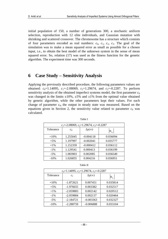
Applying the previously described procedure, the following parameters values are

obtained: c0=1.14095, c1=-2.08069, c2=1.29674, and c3=-0.2287. To perform

sensitivity analysis of the obtained imperfect systems model, the first parameter c0

was changed in the limits ±10%, ±5% and ±1% from the optimal value obtained

by genetic algorithm, while the other parameters kept their values. For each

change of parameter c0, the output in steady state was measured. Based on the

equations given in Section 2, the sensitivity value related to parameter c0 was

calculated.

Table I

c1=-2.08069, c2=1.29674, c3=-0.2287

Tolerance c0 Δy(∞) 0cu

+10% 1.255045 -0.004118 0.036094

+5% 1.197997 -0.002041 0.035777

+1% 1.152359 -0.000412 0.036112

-1% 1.129541 0.000413 0.036199

-5% 1.083903 0.002085 0.036549

-10% 1.026855 0.004216 0.036951

Table II

c0=1.14095, c2=1.29674, c3=-0.2287


+10% -1.872621 0.007451 0.035814

+5% -1.976655 0.003382 0.032517

+1% -2.059883 0.002142 0.020512

-1% -2.059884 0.002137 0.020464

-5% -2.184721 -0.003363 0.032327

-10% -2.288759 -0.006888 0.033104


– 89 –

Table III

c0=1.14095, c1=-2.08069, c3=-0.2287


+10% 1.426414 -0.003801 0.029312

+5% 1.361577 -0.001772 0.027331

+1% 1.309707 -0.000221 0.017099

-1% 1.283773 0.000202 0.015601

-5% 1.231903 0.001705 0.026309

-10% 1.167066 0.003678 0.028366

Table IV

c0=1.14095, c1=-2.08069, c2=1.29674


+10% -0.205831 0.000315 0.027585

+5% -0.217261 0.000285 0.024962

+1% -0.226413 0.000026 0.011368

-1% -0.230987 0.000031 0.013229

-5% -0.240135 0.000263 0.023025

-10% -0.251572 0.000683 0.029864

The results are given in Table I, where Δy(∞) represents a deviation of the

response in steady state and 0cu represents system sensitivity in steady state

related to parameter c0. We repeat this procedure for the other parameters c1, c2

and c3 and the results are given in Tables II, III and IV respectively. The results

demonstrated that the imperfect systems model is most sensitive to parameter c0,

and least sensitive to parameter c3 (see Fig. 4). This result can be used in reality,

when it is necessary to parametrically adjust the desired output value. In our case

it is the best to use adjustable parameter c0, because the output is the most

sensitive to this parameter. If it is not possible to adjust the steady state output

with only one parameter, it is necessary to make adjustments with two parameters

c0 and c1, and so on. This also means that the model is most sensitive to parameter

b0, and the least sensitive to parameter b3 with the highest index.

The results obtained by the developed method for sensitivity analysis using the

almost orthogonal filter have been compared with those obtained by the nominal

range sensitivity method [31], a known method for sensitivity analysis. Nominal

range sensitivity analysis evaluates the effect on model outputs exerted by

individual inputs, varying only one of the model inputs across its entire range of

plausible values, while holding all other inputs at their nominal or base-case

values.


– 90 –

Figure 4

Graphic dependence ic iu f c

The results are given in Table V and Fig. 5. We can see that the results are similar

to those shown in Fig. 4, with dependencies moved to the lower sensitivity values.

The drawback of this method is that it does not include the effect of interactions or

correlated inputs. The method is also time-consuming and demands a nominal

range for each input.

Table V

Tolerance 0cu

1cu 2cu

3cu

+10% 0.033678 0.032718 0.028477 0.026577

+5% 0.031261 0.030171 0.026964 0.022911

+1% 0.030147 0.027221 0.014335 0.011377

-1% 0.028883 0.026508 0.013844 0.012561

-5% 0.031455 0.030054 0.026022 0.024163

-10% 0.032149 0.030115 0.028401 0.027476


– 91 –

Figure 5

Graphic dependence ic iu f c

Conclusions

In this paper, the concept of the almost orthogonal polynomials is applied in the

sensitivity analysis of imperfect systems. First, we designed almost orthogonal

filters as generators of almost orthogonal functions. These filters can be used for

the modeling, identification, simulation, and analysis of different dynamical

systems as well as for the designing of adaptive systems. In this paper, an almost

orthogonal filter has been used to obtain a model of an imperfect system, where

the models parameters have been determined using genetic algorithm. The

necessary mathematical relations for the proposed approach for determining

sensitivity of imperfect systems are also given. Experiments with a multitank

hydraulic system were performed to validate the theoretical results and to

demonstrate that the method described in the paper is suitable for the sensitivity

analysis of imperfect systems. The results have been compared with another

known method for sensitivity analysis.

Acknowledgement

This paper was realized as a part of the projects “Studying climate change and its

influence on the environment: impacts, adaptation and mitigation” (III 43007),

“Development of new information and communication technologies, based on

advanced mathematical methods, with applications in medicine,

telecommunications, power systems, protection of national heritage and

education” (III 44006) and “Research and Development of New Generation Wind

Turbines of High-energy Efficiency” (TR 35005), financed by the Ministry of

Education and Science of the Republic of Serbia within the framework of

integrated and interdisciplinary research.


– 92 –

References

[1] M. Milojković, S. Nikolić, B. Danković, D. Antić, Z. Jovanović: Modelling

of Dynamical Systems Based on Almost Orthogonal Polynomials,

Mathematical and Computer Modelling of Dynamical Systems, Vol. 16,

No. 2, pp. 133-144, 2010

[2] B. Danković, P. Rajković, S. Marinković: On a Class of Almost Orthogonal

Polynomials, in Lecture Notes in Computer Science 5434, S. Margenov, L.

G. Vulkov, and J. Wasniewski, Eds., Springer-Verlag, Berlin, 2009, pp.

241-248

[3] Y. C. Schorling, T. Most, C. Bucher: Stability Analysis for Imperfect

Systems with Random Loading, Proceedings of the 8th

International

Conference on Structural Safety and Reliability, Newport Beach,

California, USA, June 17.-22, 2001, pp. 1-9

[4] B. Danković, S. Nikolić, M. Milojković, Z. Jovanović: A Class of Almost

Orthogonal Filters, Journal of Circuits, Systems, and Computers, Vol. 18,

No. 5, pp. 923-931, 2009

[5] T. Most, C. Bucher, Y. C. Schorling: Dynamic Stability Analysis of

Nonlinear Structures with Geometrical Imperfections under Random

Loading, Journal of Sound and Vibration, Vol. 276, pp. 381-400, 2004

[6] H. Chen, L. Li: Semisupervised Multicategory Classification with

Imperfect Model, IEEE Transactions Neural Networks, Vol. 20, No. 10, pp.

1594-1603, 2009

[7] G. M. Coghill, A. Srinivasan, R. D. King: Qualitative System Identification

from Imperfect Data, Journal of Artificial Intelligence Research, Vol. 32,

pp. 825-877, 2008

[8] B. Danković, Z. Jovanović, S. Nikolić, D. Mitić: Modelling of Imperfect

System Based on Almost Orthogonal Polynomials, Proceedings of the 9th

International Conference on Telecommunications in Modern Satellite,

Cable and Broadcasting Services, TELSIKS 2009, Niš, Serbia, October 7-9,

2009, Vol. 2, pp. 514-517

[9] G. Szegö: Orthogonal Polynomials, American Mathematical Society,

Colloquium Publications, 23, Providence, 1975

[10] Ya. L. Geronimus: Polynomials Orthogonal on a Circle and Interval. Fiz.

Mat. Lit., Moscow, 1958

[11] D. Antić, B. Danković, M. Milojković, S. Nikolić: Dynamical Systems

Modeling Based on Legendre Orthogonal Function, TEHNIKA-

Elektrotehnika, Vol. 58, No. 5, pp. 1-6, 2009

[12] B. Danković, D. Antić, Z. Jovanović, S. Nikolić, M. Milojković: Systems

Modeling Based on Rational Functions, Scientific Bulletin of UPT,


– 93 –

Transactions on Automatic Control and Computer Science, Vol. 54(68),

No. 4, pp. 149-154, 2009

[13] P. Heuberger, P. Van den Hof, B. Wahlberg: Modelling and Identification

with Rational Orthogonal Basis Functions. Springer-Verlag, London, 2005

[14] S. Nikolić, D. Antić, B. Danković, M. Milojković, Z. Jovanović, S. Perić:

Orthogonal Functions Applied in Antenna Positioning, Advances in

Electrical and Computer Engineering, Vol. 10, No. 4, pp. 35-42, 2010

[15] P. C. McCarthy, J. E. Sayre, B. L. R. Shawyer: Generalized Legendre

Polynomials, Journal of Mathematical Analysis and Applications, Vol. 177,

pp. 530-537, 1993

[16] A. Beny, R. H. Torres: Almost Orthogonality and a Class of Bounded

Bilinear Pseudodifferential Operator, Mathematical Research Letters, Vol.

11, pp. 1-11, 2004

[17] I. Ben-Yaacov, F. Wagner: On Almost Orthogonality in Simple Theories,

Journal of Symbolic Logic, Vol. 69, pp. 398-408, 2004

[18] B. Danković, P. Rajković: On a Class of Almost Orthogonal Polynomials,

Proceedings of the 4th

International Conference on Numerical Analysis and

Application, Lozenetz, Bulgaria, 2008, pp. 241-248

[19] B. Danković, D. Antić, Z. Jovanović, D. Mitić: On a Correlation between

Sensitivity and Identificability of Dynamical Systems, Proceedings of the

IEEE International Joint Conferences on Computational Cybernetics and

Technical Informatics, ICCC-CONTI 2010, Timisoara, Romania, May 27-

29, 2010, pp. 361-366

[20] L. Breierova, M. Choudhari: An Introduction to Sensitivity Analysis. MIT

System Dynamics in Education Project, 1996

[21] R. Tomović: Sensitivity Analysis of Dynamic Systems. McGraw-Hill, New

York, 1983

[22] R. Gumovski: Sensitivity of the Control Systems. Nauka, Moscow, 1993,

(in Russian)

[23] R. Pintelon, J. Schoukens: System Identification. IEEE Press, New York,

2001

[24] R. E. Precup, S. Preitl: Stability and Sensitivity Analysis of Fuzzy Control

Systems. Mechatronics Applications, Acta Polytechnica Hungarica, Vol. 3,

No. 1, pp. 61-76, 2006

[25] Inteco, Modular Servo System-User’s Manual (2008) Available at

www.inteco.com.pl

[26] J. H. Holland: Adaptation in Natural and Artificial Systems. University of

Michigan Press, Ann Arbor, 1975

http://www.inteco.com.pl/


– 94 –

[27] M. Mitchel: An Introduction to Genetic Algorithms. MIT Press,

Cambridge, 1996

[28] D. Mitić, D. Antić, S. Nikolić, M. Milojković: Identification of the

Multitank System Using Genetic Algorithm, Proceedings of the XLV

International Scientific Conference on Information, Communication and

Energy Systems and Technologies, ICEST 2010, Ohrid, Macedonia, June

23-26, 2010, Vol. 1, pp. 453-456

[29] F. Durovsky, L. Zboray, Ž. Ferkova: Computation of Rolling Stand

Parameters by Genetic Algorithm, Acta Polytechnica Hungarica, Vol. 5,

No. 2, pp. 59-70, 2008

[30] B. Danković, D. Antić, Z. Jovanović, S. Nikolić, M. Milojković: Systems

Modeling Based on Legendre Polynomials, Proceedings of the 5th

International Symposium on Applied Computational Intelligence and

Informatics, SACI 2009, Timisoara, Romania, May 28.-29, 2009, pp. 241-

246

[31] A. C. Cullen, H. C. Frey: Probabilistic Techniques in Exposure

Assessment. Plenum Press, New York, 1999

sensitivity analysis of imperfect systems using …...d. antić et al. sensitivity analysis of...

Documents