senior design project - washington university in st. louis · 2008-12-16 · senior design project...

Tischler-Nguyen 12/16/2008

Senior Design Project

Strain Imaging

Josh Tischler and Ken Nguyen

JEE 4980, Fall 2008

UMSL/Washington University Joint Undergraduate Engineering Program

December 16, 2008

1 Introduction

The purpose of this project is to develop algorithms that take electrical signals from an ultrasound device and output a strain image. We will be using MATLAB to create and edit functions that will accomplish specific, coordinated tasks. Creating a strain image

from an ultrasound device is significant because allows non�invasive detection of concealed anomalies. In the large scope of marketable medical technology, ultrasound saves lives.

1.1 Problem Statement

To develop a strain image (output) using raw electrical signals from an ultrasound device (input).

Previous groups have accomplished this to a certain degree, but the results are unfinished and can use improvement. By focusing on several different options to advance existing code, we hope to create a better end result. Making improvements to the existing code has the potential to give one or several of the following results:

• Make the code faster.

• Automate the code further.

• Develop clearer, more error free results.


1.2 Background Information

Medical technology has been an integral part of the advancement of humanity. Medical sonography, or ultrasound, has been used for several decades for many different purposes. Most people are familiar with the ultrasound images of fetuses during pregnancy. Ultrasound allows for noninvasive examination of objects that are otherwise concealed from view. Developing a method to take raw data and output recognizable images is an invaluable function for today’s medical world.

Elastography

Using ultrasound technology, we can introduce time and compression to the mix to develop strain images. Elasticity, which is what a strain image measures, can determine whether a detected abnormality is malignant or benign. This can inform a doctor and patient whether or not further action is required in cases such as possible breast cancer.

For this project, we will focus on unidirectional displacement rather than bidirectional (or an added lateral) displacement.

1.3 Initial Project Objectives

The first objective of this semester was to examine the code from last semester, learn it, and utilize it. We chose to focus on OSH code from last semester, primarily because their code appeared to give the best results. After having an idea of the scope of the project and how to improve upon it, we started with several possible (and more specific) OSH code improvement options:

• Eliminate for-loops

• Reduce operations within for-loops

• Implement a function to determine upsampling rate

According to the list above, all proposed improvements at the beginning of the semester pertained to the usability of the code, and not the quality. At the time, the concept of the existing code was too intimidating to set lofty goals. We knew the code was not optimized for speed, and our first objective was to do so.


2 Preliminary Studies

This preliminary studies section encompasses all the investigative research we did on OSH code from weeks 1-8 leading up to the proposal. This period was primarily focused on gaining insight on key concepts relating to the operation of the code. Make note that all images are generated with a preliminary version of the code.

2.1 Summary of Terms

The following subsections give a summary of terms as we learned to understand them during our preliminary studies.

2.1.1 Window Sizes

The window size is the amount of the signal used to determine displacement by correlating. A window size that is too large can find displacement of a point other than the point we are interested in. A window size that is too small can miss the shift amount altogether. In OSH code, the large window size is hard-coded at 50% larger than the small window size.

Window Size = 20 Window Size = 30

2.1.2 Upsampling

One of the first things that must be understood in order to succeed in this project is the resample function. The resample function essentially creates data points using a polyphase filter implementation. It is necessary to resample the original data in order to smooth results. Resampling the data increases the length of the resampled vector by a factor of the upsampling variable. For instance, resampling at twice the rate creates twice as many data points and therefore twice the vector length. Figures showing this basic principle are given at the beginning of the next page.


100 samples of raw data Raw data resampled at twice the sample

rate. Note smoother curves, particularly at the peaks

2.1.3 Blips

Blips are best described as inaccuracies in a resulting displacement image. They can be caused or fixed by the code used to find displacement, however (as we found out later in the semester) the most common cause of blips is a noisy signal.

1-D signal without blips 1-D signal with blips


For blip correction, the OSH code checks the previous row and previous column for the displacement, and uses that as a base for the current calculation. The problem with that is that sometimes the previous row and/or column are not a good indicator of what the next value should be. Because of this, some errors tend to propagate down through the displacement image like in the one shown below:

We can tell that the anomaly is likely due to the previous row and column estimation simply because of the fact that the anomaly propagates down a 1:1

column�row slope. One way to improve the code in future semesters could be to find a solution to this blip propagation, or eliminate the need for previous row/column estimation altogether. This problem can also be avoided altogether by choosing input frames that are closer together.

2.1.4 Shift and 1-D Signal Alignment

The foundation of developing a good strain image is successful manipulation of

one�dimensional signals and finding displacement. The best way to show that compressed signals have the correct amount of shifts associated with them is to find the shift of a window size, shift the compressed signal to its original position, and plot the original signal with the shifted signal to check for a match. By examining MW code and applying it to OHS code, we are able to demonstrate this in the following figures.


1. Original Signal (Small Window) 2. Displaced Signal (Large Window)

3. Original Signal with Displaced Signal 4. Original Signal and Displaced Signal Shifted to Match

2.2 Preliminary Advancement Failures

The following subsections summarize the attempts we made at improving the code. The one thing all the following attempts have in common is that they resulted in failure or no significant results. We are including this section so that future students do not waste time attempting to implement these ideas as we did, unless they are approached from a different angle.

2.2.1 Automating the Upsampling Rate

During our preliminary studies, we developed a prototype function that determines an appropriate upsampling rate based on an input signal. The following steps show how our code worked:


Step 1: Input a 1�D Signal Step 2: Resample the Signal

Step 3: Differentiate Both Signals

Original Signal Differentiated Resampled Signal Differentiated

Step 4: Resize the Resampled Signal to

Match the Original Signal

Step 5: Compare the Signals

Repeat Steps 2�5 Until the Difference Becomes Small


Theoretically, an idea like the upsample rate finder could work with some heavy tuning, but experimentation has shown that the best method is still trial and error (even more so now that the run time of the code has been significantly decreased as explained in later sections).

2.2.2 Finding Displacement from Local Maximums

One approach that we tried is to find displacement from the local maximums in the signals (zeros and local minimums are also worth looking at). Theoretically, in each pair of frames there is the same number of local maximums. Each local maximum has its matching pair in the subsequent frame. By tracking where these maximums occur, we could be able to determine how far each maximum has shifted from its pair, therefore finding displacement. The primary hurdle for this method (and ultimate downfall) is when a pair of maximums do not match each other. This is often caused by artificial local maximums created by the upsampling process or signal noise.

This plot shows the position of each

maximum. Theoretically, there should be more divergence between the positions of maximums near the end of the signal.

This plot shows the difference of the two signals in plot 1. It appears that the

displacement is increasing, but the plot is not smooth at all.

2.3 Preliminary Advancement Successes

In the preliminary weeks of the project, we were able to significantly decrease the run time of the code by moving the upsampling function outside the for-loops. In this way, the code only has to resample once instead of several thousand times. We realized a decrease in run time of 70-80% with this change.


3 Cognizant Studies – Final Report

This cognizant studies section encompasses all the research and evaluation we performed from the midterm proposal to completion period. During this period we were primarily focused on implementing changes to improve the quality of the final result and evaluating it qualitatively and quantitatively. All images in this section are generated with the final version of the code.

After our midterm proposal, Dr. Trobaugh gave a lecture during which he presented us with code that gives actual displacement and strain from controlled young’s modulus input parameters. Using this code, we were able to request our own input signal so that we could test our code against an ideal output. Thus, the more we could make our strain image appear like the ideal image, the more accurate we could consider our own strain image code.

To create our sim data, we had to give Dr. Trobaugh the specifications for the regions of interest. We chose to use Gaussian data, which is a smooth increase in Young’s Modulus rather than an instant increase. We did this because we guessed that Gaussian data would more closely match realistic data. The specifications for the regions of interest are Young’s Modulus and FWHM (full width half maximum). FWHM is a Gaussian specification only. We chose to create 10 regions of interest on our simulation data. The specifications for each area of interest are shown below.


Ideal Displacement Result from Simulation

Ideal Strain Result from Simulation

As can be seen from the ideal strain image above, we wanted to test our code to determine sensitivity to FWHM (full width half max, or the size of the region of interest) and sensitivity to the difference in elasticity of a region. The difference in elasticity test data can be seen in row 1 and the FWHM test data is in row 2 of the ideal strain image. It is important to note that random noise was also added to the ideal strain image to simulate a more realistic input.

3.1 Methodology

With this new information, we were able to piece together the fact that smoothing the 1-D signal (and in effect, the entire image) is the key to obtaining a quality strain image. We determined that the OSH wiener2 filter was not doing an acceptable job.

Example of Unfiltered Result Desired Result

3.1.1 Moving Average Filter

In order to get a filtered result that looks more like the desired result, the first observation that can be made is that the slope of our unfiltered curve is roughly


accurate. One simple way to smooth a curve and maintain the rough characteristics of that curve is to apply a moving average (as in the analysis of stock market trends). The more data points used to establish a moving average, the smoother the curve becomes. However, using more data points can skew or stretch the overall pattern of that curve, as the following figure demonstrates.

Red = Unfiltered Displacement Signal (dirty signal, no shift)

Green = 16 Point Moving Average Filter (better smoothing, small shift)

Blue = 30 Point Moving Average Filter (smoothest, most shift)

Strain Image with 16 point moving average. Strain Image with 30 point moving average. Notice that the signal is clearer, but the shapes begin to stretch in the vertical direction due to the moving

average shift (most evident on shape at (120,120).)


Strain Image using weiner2 filter from last semester’s code. Not a good result.

By using the moving average filter, it seems we can get a much better output than by using the weiner2 filter. The negative of using this filter, however, is that it can tend to stretch the data rather than properly representing it. For this reason, we designed a butterworth filter to see if this would give better results.

3.1.2 Butterworth Low-Pass Filter

The easiest way to create a butterworth filter for our data is by finding the cutoff frequency by trial and error. The butterworth function creates filter vectors that can be used in the filtfilt function and has two input parameters: the first is the order of filter desired, and the second is the cutoff frequency. Through trial and error, we determined that for the simulation data, the best result is achieved by using a normalized cutoff value of .05 with an order of at least 2. Our initial BW filter results relative to the ideal results are shown below.

We found through some quick quantitative analysis (and obvious qualitative results) that our butterworth filter design performs much better than both the weiner2 filter and the moving average filter. Hence, the butterworth low-pass filter was our final successful addition to the code for this semester.


Strain Image using butterworth filter Ideal result


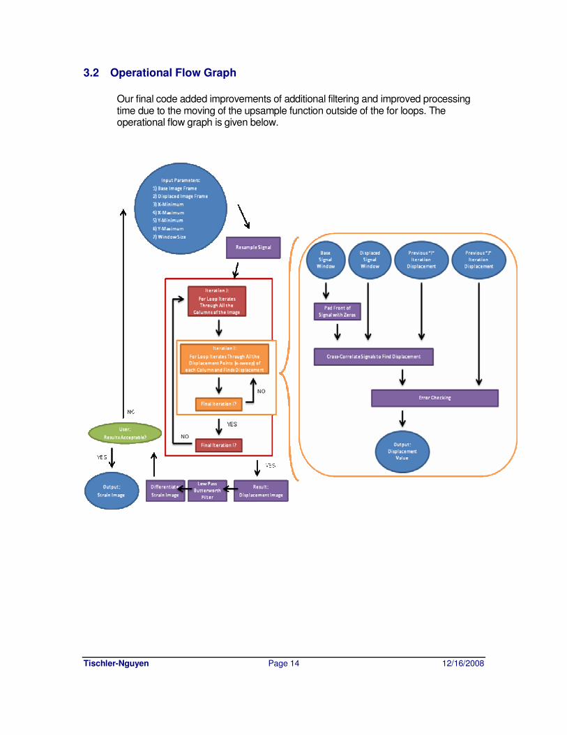
3.2 Operational Flow Graph

Our final code added improvements of additional filtering and improved processing time due to the moving of the upsample function outside of the for loops. The operational flow graph is given below.


3.3 Results

3.3.1 Evaluation Methods

To evaluate our final results, we iterated through our flow graph process until we achieved the best possible strain images using our final code. Each set of data required its own parameters. We then evaluated contrast (difference in strain between the point of interest and surroundings) of our image and compared it to the appropriate comparable data.

Contrast

To quantitatively compare our results with other strain image comparisons, we take the root mean squared, the mean, and the standard deviation of both the area of interest and an outside region and compare these values to previous code and an ideal result if available.

3.3.2 Evaluation Comparison Table

Data OSH Code Ideal Result SimNT X X Tfu2 X Tfu1 X

For the SimNT data supplied by the instructor, we compared it to both the ideal result and the OSH code. Since an ideal result does not exist for the Tfu data, we only compared it to the old OSH code.


3.3.3 Qualitative Results

3.3.3.1 SimNT

OSH Code NT Code

Ideal Result


3.3.3.2 Tfu1

OSH Code NT Code

3.3.3.3 Tfu2

OSH Code NT Code

3.3.4 Quantitative Results

Data Code Region 1 Region 2 Ratio Difference Region 1 Region 2 Ratio Difference Region 1 Region 2

OSH 7.671E-05 0.000178 0.43168 0.000101 0.0261 0.0342 0.763158 0.0081 0.0261 0.0342

NT 0.2871 0.8155 0.35205 0.5284 0.3035 0.8437 0.359725 0.5402 0.0984 0.2166

StDevMean RMS

Tfu1

Data Code Region 1 Region 2 Ratio Difference Region 1 Region 2 Ratio Difference Region 1 Region 2

OSH 0.0153 0.0058 2.63793 0.0095 0.0308 0.0295 1.044068 0.0013 0.0267 0.029

NT 0.4694 0.1113 4.21743 0.3581 0.475 0.1366 3.477306 0.3384 0.0726 0.0792

Mean RMS StDev

Tfu2


Outer Region Code Region 1 Ratio Region 2 Ratio Region 3 Ratio Region 4 Ratio Region 5 Ratio

0.6068 NT 0.5264 0.867501648 0.473 0.779499011 0.4358 0.718193804 0.393 0.647659855 0.3659 0.602999

0.02 Ideal 0.0167 0.835 0.0144 0.72 0.0126 0.63 0.0112 0.56 0.0101 0.505

0.6068 NT 0.5264 0.867501648 0.473 0.779499011 0.4358 0.718193804 0.393 0.647659855 0.3659 0.602999

0.02 Ideal 0.0167 0.835 0.0144 0.72 0.0126 0.63 0.0112 0.56 0.0101 0.505

0.001 NT 0.0013 0.0020 0.0037 0.0032 0.0030

0 Ideal* 0.0012 0.0017 0.0020 0.0021 0.0021

Outer Region Code Region 6 Ratio Region 7 Ratio Region 8 Ratio Region 9 Ratio Region 10 Ratio

0.6068 NT 0.5895 0.971489782 0.5553 0.915128543 0.475 0.78279499 0.3988 0.657218194 0.3586 0.590969

0.02 Ideal 0.0153 0.765 0.0117 0.585 0.0104 0.52 0.0102 0.51 0.0101 0.505

0.6068 NT 0.5895 0.971489782 0.5553 0.915128543 0.475 0.78279499 0.3988 0.657218194 0.3586 0.590969

0.02 Ideal 0.0155 0.775 0.0117 0.585 0.0104 0.52 0.0102 0.51 0.0101 0.505

0.001 NT 0.0010 0.0008 0.0032 0.0035 0.0034

0 Ideal* 0.0819 0.0334 0.0084 0.0037 0.0021

NT Sim

Data Row

2

Mean

RMS

StDev

Mean

RMS

StDev

NT Sim

Data Row

1

Region Contrast Accuracy

1 104%

2 108%

3 114%

4 116%

5 119%

6 127%

7 156%

8 151%

9 129%

10 117%

3.4 Conclusion

We believe that we succeeded in improving upon the code from last semester. The visual quality of the strain image was improved, the processing time was drastically reduced, and the quantitative analysis was a good evaluation of the final results.


3.5 Recommendations

There is plenty of room for improvement on this project for perhaps one more semester of students. At the end of this semester, almost all of the groups in our class went different directions and improved the code in their own ways. The easiest and quickest way to make an excellent final product would be to take each of the strengths from all the groups and compile it into one function. The speed of the Sivewright-Chesnut code (5 second strain image generation time) combined with our superior filtering to create better image quality and contrast would create an excellent final product. Perhaps another group corrected the anomaly problem (page 5 of this report) in their code. If not, this could be another issue to resolve.

One other way to attempt to improve the code is to try different filters. Since the semester was quickly approaching, the only filter we tried was the butterworth. There are other low-pass filter designs with different characteristics that may give better results.

An entirely different challenge may be to try and re-write the code completely and implement everything that can be learned from work done in the past. One group did that this semester, and I believe they were able to produce a decent quality strain image.

4 Appendix

4.1 Code

4.1.1 Test_CodeOfStrain

%Robert Ochs, John Harte and Mike Swanson %Editted by Josh Tischler, Ken Nguyen %JEE4980 Senior Design Project %Wave Displacement Analysis Program %This function generates a displacement image based on the cross %correlation between two functions. %Variables xmin, xmax, ymin and ymax are based around the output image %axis for ease of understanding. Variable func1 is the base function and %func2 is the comparison function. Variable wsize is the sample size of %the base signal used for comparison. function MDisp = Test_CodeOfStrain(func1, func2, xmin, xmax, ymin, ymax, wsize, filt) tic [rows cols] = size(func1); %Determines size of input base function.


BaseS = func1; DispS = func2; UpSamF = 30; %Upsampling ratio factor. BaseS = resample(BaseS, UpSamF, 1); DispS = resample(DispS, UpSamF, 1); BaseS = BaseS'; DispS = DispS'; MDisp(1:(ymax-ymin),1:ceil((xmax*UpSamF-xmin*UpSamF)/wsize)) = 0; %Creates a displacement matrix WSpan1 = ceil(wsize / 2); %Sizing for window around center point. WSpan2 = ceil(1.5 * WSpan1); %Sizing of comparison window size. line = 0; Offset = 1; %Previous pointer comparison offset. Pointers(1:(xmax*UpSamF-xmin*UpSamF),1:(ymax-ymin)) = 0; SamCount = ceil((xmax*UpSamF-xmin*UpSamF)/5) + 1; PrevCol(1,1:(SamCount)) = 0; %This loop performs cross correlation of func1 and func2 for wsize samples. %This loop also has previous data comparison to prevent spikes in %displacement imaging. for ysweep = ymin:ymax sample = 0; line = line + 1; Ref1 = PrevCol(1,1); %Reference for first row displacement values. for xsweep = xmin*UpSamF:(5*UpSamF):xmax*UpSamF sample = sample + 1; BaseR = [zeros(1,WSpan2) BaseS(ysweep,(xsweep-WSpan1):(xsweep+WSpan1))]; DispR = DispS(ysweep,(xsweep-WSpan2):(xsweep+WSpan2)); [Corr, Lag] = xcorr(BaseR, DispR); [row, col] = size(Corr); %The following is the algorithm for spike prevention in the %displacement calculations. if line == 1 if sample == 1 %For only previous point vertial comparison. [MCorr, MLag] = max(Corr); elseif Prev <= Offset %Prevents out of range low comparisons. [MCorr, MLag] = max(Corr(1,1:Prev+Offset)); elseif Prev > (col - Offset) %Prevents out of range high. [MCorr, TLag] = max(Corr(1,Prev-Offset:(col-1))); MLag = TLag + (Prev-Offset-1); else %Normal previous point comparison. [MCorr, TLag] = max(Corr(1,Prev-Offset:Prev+Offset)); MLag = TLag + (Prev-Offset-1); end


Prev = MLag; else %For both previous point vertical and horizontal comparison. Prev = ceil((MLag + PrevCol(1,sample)) / 2); if sample == 1 [MCorr, TLag] = max(Corr(1,Ref1-Offset:Ref1+Offset)); MLag = TLag + (Ref1-Offset-1); elseif Prev <= Offset [MCorr, MLag] = max(Corr(1,1:Prev+Offset)); elseif Prev > (col - Offset) [MCorr, TLag] = max(Corr(1,Prev-Offset:(col-1))); MLag = TLag + (Prev-Offset-1); else [MCorr, TLag] = max(Corr(1,Prev-Offset:Prev+Offset)); MLag = TLag + (Prev-Offset-1); end end PrevCol(1,sample) = MLag; %Generates values for horizontal comp. MDisp(line,sample) = Lag(1,MLag); %Generates displacement matrix. end end %MDisp = (filter(ones(1,(filt/2))/(filt/2),1,MDisp)); %filters the rows with a moving average %MDisp = (filter(ones(1,filt)/filt,1,MDisp')); %filters the columns with a moving average [num den] = butter(2,.05); % For sim input % [num den] = butter(3,.1); % For real input MDisp = filtfilt(num, den, MDisp); MDisp = MDisp'; MDisp = filtfilt(num, den, MDisp); %MDisp = MDisp'; %For column filtering, the image was transposed. [rows cols] = size(MDisp); MDisp = MDisp(10:rows-20,:); %removes the manufactured data used for filtering toc figure imagesc(MDisp); colorbar figure imagesc((diff(MDisp)));


colorbar

4.1.2 findRMS

%Calculates RMS for an image. This was primarily used for evaluating our %final results. function RMS = findRMS(inputImg) [rows cols] = size(inputImg); input2 = inputImg.*inputImg; input2 = sum(sum(input2))/(rows*cols); RMS = input2^(.5);

4.1.3 Concept

%%% This code is an unsuccessful attempt to create a displacement image by %%% locating local maximums. img1 = resample(b_data030,10,1); img2 = resample(b_data050,10,1); sig1 = img1(1:15500,100); sig2 = img2(1:15500,100); relmax1 = zeros(1,1); relmax2 = zeros(1,1); counter = 1; for i = 2:15500 if (img1(i,1) > img1(i-1,1)) & (img1(i,1) > img1(i+1,1)) relmax1(counter,1) = img1(i,1); %magnitude of local maximum relmax1(counter,2) = i; %location of local maximum counter = counter + 1; end end counter = 1; for i = 2:15500 if (img2(i,1) > img2(i-1,1)) & (img2(i,1) > img2(i+1,1)) relmax2(counter,1) = img2(i,1); relmax2(counter,2) = i; counter = counter + 1; end end plot(relmax1(:,2)) %development code hold all %


plot(relmax2(:,2)) % shift = zeros(1,1); for i = 1:356 if (relmax1(i,1) < 100 + relmax2(i,1)) & (relmax1(i,1) > relmax2(i,1) - 100) shift(i,1) = relmax2(i,2) - relmax1(i,2); shift(i,2) = relmax1(i,2); else shift(i,1) = relmax2(i-1,2) - relmax1(i-1,2); shift(i,2) = relmax2(i-1,2); end end figure plot(shift(:,1))

4.1.4 bestSampleRate

%This function determines the appropriate sample rate for a 1D signal. function[bestSampleRate]=findUpsample(inputSignal) i = 2; checker = 11000; sumDiff = zeros(1,20); %sample1 = inputSignal(1,:,50); sample1 = inputSignal(:,200); signal1 = sample1(1:50); %signal1 = sample1; %demo step1 plot(signal1) title('Original 1-D Signal') pause clf %demo step1 end while checker > 700 signal2 = resample(signal1,i,1); %demo step 2 plot(signal2) title('1-D Signal Resampled') pause clf %demo step 2 end diff1 = diff(signal1); diff2 = diff(signal2);


%demo step 3 plot(diff1) hold all plot(diff2) title('Differentiated Signals') pause clf %demo step 3 end diff2Resize = diff2(1:i:i*50-i); %demo step 4 and 5 figure plot(diff1) hold all plot(diff2Resize) title('Signals to Compare (Resized)') pause clf %demo step 4 and 5 diff12 = diff1-diff2Resize; sumDiff(1,i) = sum(abs(diff12)); checker = sumDiff(1,i)-sumDiff(1,i-1); i = i + 1; end bestSampleRate = i

4.2 References

4.2.1 By Examination of Code

• Group WM, Spring 2009 (Mary Watts, George Michaels)

• Group BRW, Spring 2009 (Nick Baer, Christine Robinson, Curt Wibbenmeyer)

• Group BGS, Spring 2009 (Eric Burkey, Matt Schneiders, Danny Graves)

4.2.2 By Use of Code

• Group OSH, Spring 2009 (Rob Ochs, Mike Swanson, John Harte) • Patrick Vogelaar and Amir Lilienthal, Students, Class of Fall 2009


4.2.3 By Conversation

• Mary Watts, Student, Class of Spring 2009

• John Powers, Co-Worker, Emerson Electric

• Patrick Vogelaar and Amir Lilienthal, Students, Class of Fall 2009 • Steven Sivewright and Phillip Chesnut, Students, Class of Fall 2009

4.2.4 Formal Lecture/Presentations

• Jason Trobaugh, Instructor

• Steven Sivewright and Phillip Chesnut, Students, Class of Fall 2009

senior design project - washington university in st. louis · 2008-12-16 · senior design project...

Documents