Semi-analytical formulas for theHertzsprung-Russell Diagram

L. ZaninettiDipartimento di Fisica Generale,

Via Pietro Giuria 110125 Torino, Italy

November 27, 2008

The absolute visual magnitude as function of the observed color (B-V) , alsonamed Hertzsprung-Russell diagram can be described through five equations;that in presence of calibrated stars means eight constants. The developedframework allows to deduce the remaining physical parameters that are mass, radius and luminosity. This new technique is applied to the first 10 PC ,the first 50 pc , the Hyades and to the determination of the distance ofa cluster. The case of the white dwarfs is analyzed assuming the absenceof calibrated data: our equation produces a smaller χ2 in respect to thestandard color-magnitude calibration when applied to the Villanova Catalogof Spectroscopically Identified White Dwarfs. The theoretical basis of theformulas for the colors and the bolometric correction of the stars are clarifiedthrough a Taylor expansion in the temperature of the Planck distribution.keywordsstars: formation ; stars: statistics ; methods: data analysis ; techniques:photometric

1

arX

iv:0

811.

4524

v1 [

astr

o-ph

] 2

7 N

ov 2

008

1 Introduction

The diagrams in absolute visual magnitude versus spectral type for the starsstarted with Hertzsprung (1905); Rosenberg (1911); Hertzsprung (1911) .The original Russell version can be found in Russell (1914b,a,c), in the follow-ing H-R diagram. The common explanation is through the stellar evolution,see for example chapter VII in Chandrasekhar (1967). Actually the presenceof uncertainties in the stellar evolution makes the comparison between theoryand observations an open field of research , see Maeder & Renzini (1984);Madore (1985); Renzini & Fusi Pecci (1988); Chiosi et al. (1992); Beddinget al. (1998). Modern application of the H-R diagram can be found in deBruijne et al. (2001) applied to the Hyades when the parallaxes are pro-vided by Hipparcos, and in Al-Wardat (2007) applied to the binary systemsCOU1289 and COU1291.

The Vogt theorem , see Vogt (1926), states thatTheorem 1 The structure of a star is determined by it’s mass and it’s

chemical composition.Another approach is the parametrization of physical quantities such as

absolute magnitude, mass , luminosity and radius as a function of the tem-perature , see for example Cox (2000) for Morgan and Keenan classification, in the following MK, see Morgan & Keenan (1973). The temperature is notan observable quantity and therefore the parametrization of the observableand not observable quantities of the stars as a function of the observablecolor is an open problem in astronomy.

Conjecture 1 The absolute visual magnitude MV is a function, F , ofthe selected color

MV = F (c1, ....., c8, (B − V )) .

The eight constants are different for each MK class.In order to give an analytical expression to Conjecture 1 we first analyze

the case in which we are in presence of calibrated physical parameters forstars of the various MK spectral types , see Section 2 and then the case ofabsence of calibration tables, see Section 3 . Different astrophysical envi-ronments such as the first 10 pc and 50 pc , the open clusters and distancedetermination of the open clusters are presented in Section 4. The theoreti-cal dependence by the temperature for colors and bolometric corrections areanalyzed in Section 5.

2

2 Presence of calibrated physical parameters

The MV ,visual magnitude, against (B − V ) can be found starting from fiveequations , four of them were already described in Zaninetti (2005). When thenumerical value of the symbols is omitted the interested reader is demandedto Zaninetti (2005). The luminosity of the star is

log10(L

L�) = 0.4(Mbol,� −Mbol) , (1)

where Mbol,� is the bolometric luminosity of the sun that according to Cox(2000) is 4.74. The equation that regulates the total luminosity of a starwith it’s mass is

log10(L

L�) = aLM + bLM log10(

MM�

) , (2)

here L is the total luminosity of a star , L� the sun’s luminosity,M the star’smass , M� the sun’s mass , aLM and bLM two coefficients that are reportedin Table 1 for MAIN V , GIANTS III and SUPERGIANTS I ; more detailscan be found in Zaninetti (2005). We remember that the tables of calibration

Table 1: Table of coefficients derived from the calibrated data (see Table 15.7in Cox (2000)) through the least square method

MAIN, V GIANTS, III, SUPERGIANTS IKBV -0.641 ± 0.01 -0.792 ± 0.06 -0.749 ± 0.01TBV[K] 7360 ± 66 8527± 257 8261 ± 67KBC 42.74 ± 0.01 44.11 ± 0.06 42.87 ± 0.01TBC[K] 31556 ± 66 36856 ± 257 31573 ± 67aLM 0.062 ± 0.04 0.32 ± 0.14 1.29 ± 0.32bLM 3.43 ± 0.06 2.79 ± 0.23 2.43 ± 0.26

of MK spectral types unify SUPERGIANTS Ia and SUPERGIANTS Ib intoSUPERGIANTS I, see Table 15.7 in Cox (2000) and Table 3.1 in Bowers& Deeming (1984). From the theoretical side Padmanabhan (2001) quotes3 < bLM < 5 ; the fit on the calibrated values gives 2.43 < bLM < 3.43 , seeTable 1.

3

From a visual inspection of formula (2) is possible to conclude that alogarithmic expression for the mass as function of the temperature will allowsus to continue with formulas easy to deal with. The following form of themass-temperature relationship is therefore chosen

log10(MM�

) = aMT + bMT log10(T

T�) , (3)

where T is the star’s temperature, T� the sun’s temperature , aMT and bMT

two coefficients that are reported in Table 2 when the masses as function ofthe temperature ( e.g. Table 3.1 in Bowers & Deeming (1984)) are processed.According to Cox (2000) T� = 5777 K. Due to the fact that the masses of

Table 2: Table of aMT and bMT with masses given by Table 3.1 in Bowers &Deeming (1984).

main,V giants,III supergiants,I(B-V)> 0.76 (B-V) < 0.76

aMT -7.6569 5.8958 -3.0497 4.1993bMT 2.0102 -1.4563 -0.8491 1.0599χ2 28.67 3.41 20739 18.45

the SUPERGIANTS present a minimum at (B−V ) ≈ 0.7 or T≈ 5700 K wehave divided the analysis in two. Another useful formula is the bolometriccorrection BC

BC = Mbol −MV = −TBC

T− 10 log10 T +KBC , (4)

where Mbol is the absolute bolometric magnitude, MV is the absolute visualmagnitude, TBC and KBC are two parameters that are derived in Table 1 .The bolometric correction is always negative but in Allen (1973) the analyt-ical formula was erroneously reported as always positive.

The fifth equation connects the physical variable T with the observedcolor (B − V ) , see for example Allen (1973),

(B − V ) = KBV +TBV

T, (5)

where KBV and TBV are two parameters that are derived in Table 1 fromthe least square fitting procedure. Conversely in Section 5 we will explore

4

a series development for (B − V ) as given by a Taylor series in the variable1/T . Inserting formulas (4) and (3) in (2) we obtain

MV = −2.5 aLM − 2.5 bLM aMT −2.5 bLM bMT log10 T

−KBC + 10 log10 T +TBC

T+Mbol,� . (6)

Inserting equation (5) in (6) the following relationship that regulates MV and(B − V ) in the H-R diagram is obtained

MV = −2.5 aLM − 2.5 bLM aMT −

2.5 bLM bMT log10 (TBV

(B − V )−KBV

)

−KBC + 10 log10 (TBV

(B − V )−KBV

) +

TBC

TBV

[(B − V )−KBV] +Mbol,� . (7)

Up to now the parameters aMT and bMT are deduced from Table 3.1in Bowers & Deeming (1984) and Table 2 reports the merit function χ2

computed as

χ2 =n∑j=1

(MV −M calV )2 , (8)

where M calV represents the calibration value for the three MK classes as given

by Table 15.7 in Cox (2000). From a visual inspection of the χ2 reportedin Table 2 we deduced that different coefficients of the mass-temperaturerelationship (3) may give better results. We therefore found by a numericalanalysis the values aMT and bMT that minimizes equation (8) when (B − V )and MV are given by the calibrated values of Table 15.7 in Cox (2000).This method to evaluate aMT and bMT is new and allows to compute themin absence of other ways to deduce the mass of a star. The absolute visualmagnitude with the data of Table 3 is

MV = 31.34−3.365 ln

(7361.0 ((B − V ) + 0.6412)−1

)+

4.287 (B − V ) (9)

5

Table 3: Table of aMT and bMT when M calV is given by calibrated data.

main,V giants, III, supergiants, I(B-V)>0.76 (B-V)<0.76

aMT -7.76 3.41 3.73 0.20bMT 2.06 -2.68 -0.64 0.24χ2 11.86 0.152 0.068 0.567

MAIN SEQUENCE , V when

− 0.33 < (B − V ) < 1.64,

MV = −109.6 +

12.51 ln(8528.0 ((B − V ) + 0.7920)−1

)+4.322 (B − V ) (10)

GIANTS , III 0.86 < (B − V ) < 1.33 ,

MV = −39.74 +

3.565 ln(8261.0 ((B − V ) + 0.7491)−1

)+

3.822 (B − V ) (11)

SUPERGIANTS, I when

− 0.27 < (B − V ) < 0.76 ,

MV = −61.26 +

6.050 ln(8261.0 ((B − V ) + 0.7491)−1

)+

3.822 (B − V ) (12)

SUPERGIANTS , I when

0.76 < (B − V ) < 1.80 .

Is now possible to build the calibrated and theoretical H-R diagram , seeFigure 1.

6

Figure 1: MV against (B − V ) for calibrated MK stars (triangles) and theo-retical relationship with aMT and bMT as given by Table 3.

7

2.1 The mass (B-V) relationship

Is now possible to deduce the numerical relationship that connects the massof the star ,M, with the variable (B − V ) and the constants aMT and bMT

log10(MM�

) = aMT +

bMT ln

(TBV

(B − V )−KBV

)(ln (10))−1 . (13)

When aMT and bMT are given by Table 3 and the other coefficients are asreported in Table 1 the following expression for the mass is obtained:

log10(MM�

) = 7.769 +

+0.8972 ln(7360.9 ((B − V ) + 0.6411)−1

)(14)

MAIN SEQUENCE , V when

−0.33 < (B − V ) < 1.64 ,

log10(MM�

) = 10.41 +

−1.167 ln(8527.5 ((B − V ) + 0.792)−1

)(15)

GIANTS , III 0.86 < (B − V ) < 1.33 ,

log10(MM�

) = 0.2 +

+0.1276 ln(8261 ((B − V ) + 0.7491)−1

)(16)

SUPERGIANTS , I when

−0.27 < (B − V ) < 0.76 ,

log10(MM�

) = 3.73 +

−0.2801 ln(8261 ((B − V ) + 0.7491)−1

)(17)

SUPERGIANTS , I when

0.76 < (B − V ) < 1.80 .

8

Figure 2: log10(MM�

) against (B − V ) for calibrated MK stars : MAIN SE-

QUENCE , V (triangles) , GIANTS , III (empty stars) and SUPER-GIANTS , I (empty circles). The theoretical relationship as given by for-mulas (14-17) is reported as a full line.

Figure 2 reports the logarithm of the mass as function of (B−V ) for the threeclasses here considered (points) as well the theoretical relationships given byequations (14-17) (full lines).

2.2 The radius (B − V ) relationship

The radius of a star can be found from the Stefan-Boltzmann law, see forexample formula (5.123) in Lang (1999) . In our framework the radius is

log10(R

R�) =

1/2 aLM + 1/2 bLM aMT + 2ln(T�

)ln (10)

+

9

+1/2 bLM bMT ln

(TBV

(B − V )−KBV

)(ln (10))−1

−2 ln

(TBV

(B − V )−KBV

)(ln (10))−1 . (18)

When the coefficients are given by Table 3 and Table 1 the radius is

log10(R

R�) = −5.793 +

0.6729 ln(7360 ((B − V ) + 0.6411)−1

)(19)

MAIN SEQUENCE , V when

−0.33 < (B − V ) < 1.64 ,

log10(R

R�) = 22.25

−2.502 ln(8527 ((B − V ) + 0.7920)−1

)(20)

GIANTS , III when

0.86 < (B − V ) < 1.33 ,

log10(R

R�) = 8.417−

0.7129 ln(8261 ((B − V ) + 0.7491)−1

)(21)

SUPERGIANTS , I when

−0.27 < (B − V ) < 0.76 ,

log10(R

R�) = 12.71

−1.21 ln(8261 ((B − V ) + 0.7491)−1

)(22)

SUPERGIANTS , I when

0.76 < (B − V ) < 1.80 .

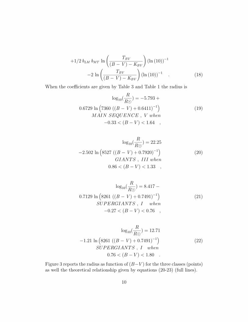
Figure 3 reports the radius as function of (B−V ) for the three classes (points)as well the theoretical relationship given by equations (20-23) (full lines).

10

Figure 3: log10(RR�)) against (B − V ) for calibrated MK stars : MAIN SE-

QUENCE , V (triangles) , GIANTS , III (empty stars) and SUPER-GIANTS , I (empty circles). The theoretical relationships as given by for-mulas (20-23) are reported as a full line.

11

2.3 The luminosity (B − V ) relationship

The luminosity of a star can be parametrized as

log10(L

L�) = aLM + bLM aMT

+bLM

(bMT ln

(TBV

(B − V )−KBV

)1

ln (10)

). (23)

When the coefficients are given by Table 3 and Table 1 the luminosity is

log10(L

L�) = −26.63 +

+3.083 ln(7360.9 ((B − V ) + 0.6411)−1

)(24)

MAIN SEQUENCE , V when

−0.33 < (B − V ) < 1.64 ,

log10(L

L�) = 29.469 +

−3.2676 ln(8527.59 ((B − V ) + 0.7920)−1

)(25)

GIANTS , III 0.86 < (B − V ) < 1.33 ,

log10(L

L�) = 1.7881 +

+0.3112 ln(8261.19 ((B − V ) + 0.7491)−1

)(26)

SUPERGIANTS , I when

−0.27 < (B − V ) < 0.76 ,

log10(L

L�) = 10.392 +

−0.682 ln(8261.19 ((B − V ) + 0.749)−1

)SUPERGIANTS , I when

0.76 < (B − V ) < 1.80 . (27)

12

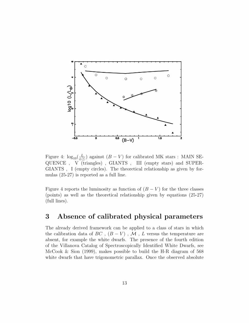
Figure 4: log10(LL�) against (B − V ) for calibrated MK stars : MAIN SE-

QUENCE , V (triangles) , GIANTS , III (empty stars) and SUPER-GIANTS , I (empty circles). The theoretical relationship as given by for-mulas (25-27) is reported as a full line.

Figure 4 reports the luminosity as function of (B − V ) for the three classes(points) as well as the theoretical relationship given by equations (25-27)(full lines).

3 Absence of calibrated physical parameters

The already derived framework can be applied to a class of stars in whichthe calibration data of BC , (B − V ) , M , L versus the temperature areabsent, for example the white dwarfs. The presence of the fourth editionof the Villanova Catalog of Spectroscopically Identified White Dwarfs, seeMcCook & Sion (1999), makes possible to build the H-R diagram of 568white dwarfs that have trigonometric parallax. Once the observed absolute

13

magnitude is derived the merit function χ2 is computed as

χ2 =n∑j=1

(MV −M obsV )2 , (28)

where M obsV represents the observed value of the absolute magnitude and the

theoretical absolute magnitude, MV , is given by equation (7). The fourparameters KBV , TBV , TBC and KBC are supplied by theoretical arguments,i.e. numerical integration of the fluxes as given by the Planck distribution,see Planck (1901). The remaining four unknown parameters aMT , bMT ,aLM and bLM are supplied by the minimization of equation (28). Table 4reports the eight parameters that allow to build the H-R diagram.

Table 4: Table of the adopted coefficients for white dwarfs.Coefficient value methodKBV -0.4693058 from the Planck lawTBV[K] 6466.229 from the Planck lawKBC 42.61225 from the Planck lawTBC[K] 29154.75 from the Planck lawaLM 0.28 minimum χ2 on real databLM 2.29 minimum χ2 on real dataaMT -7.80 minimum χ2 on real databMT 1.61 minimum χ2 on real data

The numerical expressions for the absolute magnitude (equation (7)) ,radius (equation (18)) , mass (equation (13)) and luminosity (equation (23))are:

MV = 8.199

+0.3399 ln(6466.0 ((B − V ) + 0.4693)−1

)+

4.509 (B − V ) (29)

white dwarf, −0.25 < (B − V ) < 1.88 ,

log10(R

R�) = −1.267

−0.0679 ln(6466 ((B − V ) + 0.4693)−1

)(30)

white dwarf, −0.25 < (B − V ) < 1.88 ,

14

Figure 5: MV against (B−V ) (H-R diagram) of the fourth edition of the Vil-lanova Catalog of Spectroscopically Identified White Dwarfs. The observedstars are represented through small points, the theoretical relationship ofwhite dwarfs through big full points and the reference relationship given byformula (33) is represented as a little square points.

15

log10(MM�

) = −7.799

+0.6992 ln(6466 ((B − V ) + 0.4693)−1

)(31)

white dwarf, −0.25 < (B − V ) < 1.88 ,

log10(L

L�) = −17.58 +

1.601 ln(6466 ((B − V ) + 0.4693)−1

)(32)

white dwarf, −0.25 < (B − V ) < 1.88 .

Figure 5 reports the observed absolute visual magnitude of the whitedwarfs as well as the fitting curve; Table 5 reports the minimum , the averageand the maximum of the three derived physical quantities.

Table 5: Table of derived physical parameters of the Villanova Catalog ofSpectroscopically Identified White Dwarfsparameter min average maximumM/M� 5.28 10−3 4.23 10−2 0.24R/R� 1.07 10−2 1.31 10−2 1.56 10−2

L/L� 1.16 10−5 2.6 10−3 7.88 10−2

Our results can be compared with the color-magnitude relation as sug-gested by McCook & Sion (1999), where the color-magnitude calibration dueto Dahn et al. (1982) is adopted ,

MV = 11.916 ((B − V ) + 1)0.44 − 0.011

when(B − V ) < 0.4

(33)

MV = 11.43 + 7.25 (B − V )− 3.42 (B − V )2

when 0.4 < (B − V )

The previous formula (33) is reported in Figure 5 as a line made by littlesquares and Table 6 reports the χ2 computed as in formula (28) for our

16

formula (30) and for the reference formula (33). From a visual inspection ofTable 6 is possible to conclude that our relationship represents a better fitof the data in respect to the reference formula.

Table 6: Table of χ2 when the observed data are those of the fourth editionof the Villanova Catalog of Spectroscopically Identified White Dwarfs.equation χ2

our formula (30) 710reference formula (33) 745

The three classic white dwarfs that are Procyon B, Sirius B, and 40Eridani-B can also be analyzed when (B−V ) is given by Wikipedia (http://www.wikipedia.org/).The results are reported in Table 7, 8 and 9 where is also possible to visualizethe data suggested by Wikipedia.

Table 7: Table of derived physical parameters of 40 Eridani-B where (B −V )=0.04parameter here suggested in WikipediaMV 11.59 11.01M/M� 6.41 10−2 0.5R/R� 1.23 10−2 2 10−2

L/L� 3.53 10−3 3.3 10−3

Table 8: Table of derived physical parameters of Procyon B where (B −V )=0.0parameter here suggested in WikipediaMV 11.43 13.04M/M� 7.31 10−2 0.6R/R� 1.21 10−2 2 10−2

L/L� 4.77 10−3 5.5 10−4

17

Table 9: Table of derived physical parameters of Sirius B where (B − V )=-0.03parameter here suggested in WikipediaMV 11.32 11.35M/M� 8.13 10−2 0.98R/R� 1.21 10−2 0.8 10−2

L/L� 6.08 10−3 2.4 10−3

4 Application to the astronomical environ-

ment

The stars in the first 10 pc , as observed by Hipparcos (ESA (1997)) , belongto the MAIN V and Figure 6 reports the observed stars, the calibration starsand the theoretical relationship given by equation (10) as a continuous line.

Different is the situation in the first 50 pc where both the MAIN V andthe GIANTS III are present , see Figure 7 where the theoretical relationshipfor GIANTS III is given by equation (11).

Another astrophysical environment is that of the Hyades cluster, with(B − V ) and mv as given in Stern et al. (1995) and available on the VizieROnline Data Catalog. The H-R diagram is build in absolute magnitudeadopting a distance of 45 pc for the Hyades, see Figure 8 , where also thetheoretical relationship of MAIN V is reported.

Another interesting open cluster is that of the Pleiades with the data ofMicela et al. (1999) and available on the VizieR Online Data Catalog.

Concerning the distance of the Pleiades we adopted 135 pc , accordingto Bouy et al. (2006) ; other authors suggest 116 pc as deduced from theHipparcos data , see Mermilliod et al. (1997). The H-R diagram of thePleiades is reported in Figure 9.

4.1 Distance determination

The distance of an open cluster can be found through the following algorithm:

1. The absolute magnitude is computed introducing a guess value of thedistance.

18

Figure 6: MV against (B−V ) (H-R diagram) in the first 10 pc. The observedstars are represented through points, the calibrated data of MAIN V withgreat triangles and the theoretical relationship of MAIN V with a full line.

19

Figure 7: MV against (B−V ) (H-R diagram) in the first 50 pc. The observedstars are represented through points, the calibrated data of MAIN V andGIANTS III with great triangles , the theoretical relationship of MAIN Vand GIANTS III with a full line.

20

Figure 8: MV against (B−V ) (H-R diagram) for the Hyades . The observedstars are represented through points, the theoretical relationship of MAIN Vwith a full line.

21

Figure 9: MV against (B−V ) (H-R diagram) for the Pleiades. The observedstars are represented through points, the theoretical relationship of MAIN Vwith a full line.

22

2. Only the stars belonging to MAIN V are selected.

3. The χ2 between observed an theoretical absolute magnitude ( see for-mula (10)) is computed for different distances.

4. The distance of the open cluster is that connected with the value thatminimize the χ2.

In the case of the Hyades this method gives a distance of 37.6 pc with anaccuracy of 16% in respect to the guess value or 19% in respect to 46.3 pc ofWallerstein (2000).

5 Theoretical relationships

In order to confirm or not the physical basis of formulas (4) and (5) we per-formed a Taylor-series expansion to the second order of the exact equationsas given by the the Planck distribution for the colors , see Section 5.1 , andfor the bolometric correction , see Section 5.2. A careful analysis on thenumerical results applied to the Sun is reported in Section 5.3.

5.1 Colors versus Temperature

The brightness of the radiation from a blackbody is

Bλ(T ) =

(2hc2

λ5

)1

exp( hcλkT

)− 1, (34)

where c is the light velocity , k the Boltzmann constant , T the equivalentbrightness temperature and λ the considered wavelength , see formula (13)in Planck (1901),or formula (275) in Planck (1959), or formula (1.52) inRybicki & Lightman (1985) , or formula (3.52) in Kraus (1986).

The color-difference , (C1 - C2) , can be expressed as

(C1 − C2) = m1 −m2 = K − 2.5 log10

∫S1Iλdλ∫S2Iλdλ

, (35)

where Sλ is the sensitivity function in the region specified by the index λ ,K is a constant and Iλ is the energy flux reaching the earth. We now definea sensitivity function for a pseudo-monochromatic system

Sλ = δ(λ− λi) i = U,B, V,R, I , (36)

23

where δ denotes the Dirac delta function. In this pseudo-monochromaticcolor system the color-difference is

(C1 − C2) = K − 2.5 log10

λ52

λ51

(exp( hcλ2kT

)− 1)

(exp( hcλ1kT

)− 1). (37)

Table 10: Johnson system

symbol wavelength (A)U 3600B 4400V 5500R 7100I 9700

The previous expression for the color can be expanded through a Taylorseries about the point T =∞ or making the change of variable x = 1

T, about

the point x = 0 . When the expansion order is 2 we have

(C1 − C2)app = −5

2ln

(λ2

4

λ14

)1

ln(10)

−5

4

hc (λ1 − λ2 )

λ2 λ1 k ln (10)T− 5

48

h2c2(λ1

2 − λ22)

λ22λ1

2k2 ln (10)T 2, (38)

where the index app means approximated. We now continue inserting thevalue of the physical constants as given by CODATA Mohr & Taylor (2005)and wavelength of the color as given by Table 15.6 in Cox (2000) and visible inTable 10. The wavelength of U,B and V are exactly the same of the multicolorphotometric system defined by Johnson (1966), conversely R(7000 A) andI(9000 A) as given by Johnson (1966) are slightly different from the valueshere used. We now continue parameterizing the color as

(C1 − C2)app = a+b

T+

d

T 2. (39)

Another important step is the calibration of the color on the maximumtemperature Tcal of the reference tables. For example for MAIN SEQUENCE

24

V at Tcal = 42000 , see Table 15.7 in Cox (2000) , (B − V ) = −0.3 andtherefore a constant should be added to formula (38) in order to obtain sucha value. With these recipes we obtain , for example

(B − V ) = −0.4243 +3543

T+

17480000

T 2(40)

MAIN SEQUENCE, V when − 0.33 < (B − V ) < 1.64.

The basic parameters b and d for the four colors here considered are re-ported in Table 10. The parameter a when WHITE DWARF , MAIN SE-QUENCE, V, GIANTS, III and SUPERGIANTS, I are considered is reportedin Table 11 , conversely the Table 12 reports the coefficient b and d that arein common to the classes of stars here considered. The WHITE DWARF

Table 11: Coefficient a(B-V) (U-B) (V-R) (R-I)

WHITE DWARF , Tcal[K]=25200 - 0.1981 - 1.234MAIN SEQUENCE, V , Tcal[K]=42000 - 0.4243 - 1.297 - 0.233 - 0.395

GIANTS III , Tcal[K]=5050 - 0.5271 - 1.156 - 0.4294 - 0.4417SUPERGIANTS I , Tcal[K]=32000 - 0.3978 - 1.276 - 0.2621 - 0.420

calibration is made on the values of (U − B) and (B − V ) for Sirius B, seeWikipedia (http://www.wikipedia.org/).

Table 12: Coefficients b and d

(B-V) (U-B) (V-R) (R-I)b 3543 3936 3201 2944d 17480000 23880000 12380000 8636000

The Taylor expansion agrees very well with the original function andFigure 10 reports the difference between the exact function as given by theratio of two exponential and the Taylor expansion in the (B − V ) case.

In order to establish a range of reliability of the polynomial expansion wesolve the nonlinear equation

(C1 − C2)− (C1 − C2)app = f(T ) = −0.4 , (41)

25

Figure 10: Difference between (B − V ) , the exact value from the Planckdistribution , and (B−V )app , approximate value as deduced from the Taylorexpansion for MAIN SEQUENCE, V

26

Table 13: Range of existence of the Taylor expansion for MAIN SE-QUENCE, V

(B-V) (U-B) (V-R) (R-I)Tmin [K] 4137 4927 3413 2755Tmax [K] 42000 42000 42000 42000

for T . The solutions of the nonlinear equation are reported in Table 13 forthe four colors here considered. For the critical difference we have chosen thevalue −0.4 that approximately corresponds to 1/10 of range of existence in(B−V ) . Figure 11 reports the exact and the approximate value of (B−V )as well as the calibrated data.

5.2 Bolometric Correction versus Temperature

The bolometric correction BC , defined as always negative, is

BC = Mbol −MV , (42)

where Mbol is the absolute bolometric magnitude and MV is the absolutevisual magnitude. It can be expressed as

BC =5

2

ln(

15( hckTπ

)4( 1λV

)5 1exp( hc

kTλV)−1

)ln(10)

+KBC , (43)

where λV is the visual wavelength and KBC a constant. We now expand witha Taylor series about the point T =∞

BCapp =

−15

2

ln (T )

ln (10)− 5

4

hc

kλV ln (10)T− 5

48

h2c2

k2λV2 ln (10)T 2

+KBC . (44)

The constant KBC can be found with the following procedure. The maximumof BCapp is at Tmax , where the index max stands for maximum

Tmax =1

6

(√5

2+ 1

2

)ch

kλV

. (45)

27

Figure 11: Exact (B − V ) as deduced from the Planck distribution , orequation (37), traced with a full line. Approximate (B − V ) as deducedfrom the Taylor expansion, or equation (38), traced with a dashed line. Thecalibrated data for MAIN SEQUENCE V are extracted from Table 15.7in Cox (2000) and are represented through empty stars.

28

Figure 12: Exact BC as deduced from the Planck distribution , or equa-tion (43), traced with a full line. Approximate BC as deduced from the Tay-lor expansion, or equation (46), traced with a dashed line. The calibrateddata for MAIN SEQUENCE V are extracted from Table 15.7 in Cox (2000)and are represented through empty stars.

Given the fact that the observed maximum in the BC is -0.09 at 7300 K inthe case of MAIN SEQUENCE V we easily compute KBC and the followingapproximate result is obtained

BCapp = 31.41− 3.257 ln (T )− 14200

T− 3.096 107

T 2. (46)

Figure 12 reports the exact and the approximate value of BC as well as thecalibrated data.

The Taylor expansion agrees very well with the original function and Fig-ure 13 reports the difference between exact function as given by equation (43)and the Taylor expansion as given by equation (46).

In order to establish a range of reliability of the polynomial expansion wesolve the nonlinear equation for T

BC −BCapp = −0.4 . (47)

29

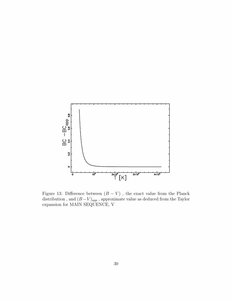
Figure 13: Difference between (B − V ) , the exact value from the Planckdistribution , and (B−V )app , approximate value as deduced from the Taylorexpansion for MAIN SEQUENCE, V

30

Table 14: (B-V) of the Sun , T=5777 K

meaning (B-V)

calibration, Cox (2000) 0.65

here, Taylor expansion 0.711here , Planck formula 0.57least square method, Zaninetti (2005) 0.633Allen (1973) 0.66Sekiguchi & Fukugita (2000) 0.627Johnson (1966) 0.63

Table 15: (R-I) of the Sun , T=5777 K

meaning (R-I)

calibration, Cox (2000) 0.34

here, Taylor expansion 0.37here , Planck formula 0.34

The solution of the previous nonlinear equation allows to state that thebolometric correction as derived from a Taylor expansion for MAIN SE-QUENCE, V is reliable in the range 4074 K < T < 42000 K.

5.3 The Sun as a blackbody radiator

The framework previously derived allows to compare our formulas with onespecific star of spectral type G2V with T=5777 K named Sun. In orderto make such a comparison we reported in Table 14 the various value of(B − V ) as reported by different methods as well as in Table 15 the valueof the infrared color (R-I). From a careful examination of the two tables weconclude that our model works more properly in the far-infrared window inrespect to the optical one.

31

6 Conclusions

New formulas A new analytical approach based on five basic equationsallows to connect the color (B − V ) of the stars with the absolute visualmagnitude, the mass, the radius and the luminosity.The suggested method isbased on eight parameters that can be precisely derived from the calibrationtables; this is the case of MAIN V , GIANTS III and SUPERGIANTS I. Inabsence of calibration tables the eight parameters can be derived mixing fourtheoretical parameters extracted from Planck distribution with four parame-ters that can be found minimizing the χ2 connected with the observed visualmagnitude ; this is the case of white dwarfs. In the case of white dwarfs themass-luminosity relationship , see Table 4, is

log10(L

L�) = 0.28 + 2.29 log10(

MM�

) , (48)

white dwarf, 0.005M� <M < ′.∈4M� .

Applications The applications of the new formulas to the open clusterssuch as Hyades and Pleiades allows to speak of universal laws for the star’smain parameters. In absence of accurate methods to deduce the distance ofan open cluster an approximate evaluation can be done.

Theoretical bases The reliability of an expansion at the second orderof the colors and bolometric correction for stars as derived from the Planckdistribution is carefully explored and the range of existence in temperatureof the expansion is determined.

Inverse function In this paper we have chosen a simple hyperbolicbehavior for (B−V ) as function of the temperature as given by formula (5).This function can be easily inverted in order to obtain T as function of (B−V )(MAIN SEQUENCE, V)

T =7360

(B − V ) + 0 .641K (49)

MAIN SEQUENCE, V when 4137 < T [K] < 42000

or when − 0.33 < (B − V ) < 1.45 .

When conversely a more complex behavior is chosen , for example a twodegree polynomial expansion in 1

Tas given by formula (38) , the inverse

32

formula that gives T as function of (B−V ) (MAIN SEQUENCE, V) is morecomplicated than formula (49),

T =

50000.355 108 +

√4.217× 1015 + 6.966× 1015 (B − V )

108 (B − V ) + 0.4244 108K (50)

MAIN SEQUENCE, V when 4137 < T [K] < 42000

or when − 0.33 < (B − V ) < 1.45 .

The mathematical treatment that allows to deduce the coefficients of theseries reversion can be found in Morse & Feshbach (1953); Dwight (1961);Abramowitz & Stegun (1965).

References

Abramowitz, M. & Stegun, I. A. : 1965, Handbook of mathematical functionswith formulas, graphs, and mathematical tables (New York: Dover)

Al-Wardat, M. A. : 2007, Astronomische Nachrichten, 328, 63

Allen, C. W. : 1973, Astrophysical quantities (London: University of London,Athlone Press, — 3rd ed.)

Bedding, T. R., Booth, A. J., & Davis, J., eds. 1998, Proceedings of IAUSymposium 189 on Fundamental Stellar Properties: The Interaction be-tween Observation and Theory

Bouy, H., Moraux, E., Bouvier, J., et al. : 2006, ApJ , 637, 1056

Bowers, R. L. & Deeming, T. : 1984, Astrophysics. I and II (Boston: Jonesand Bartlett )

Chandrasekhar, S. : 1967, An introduction to the study of stellar structure(New York: Dover, 1967)

Chiosi, C., Bertelli, G., & Bressan, A. : 1992, ARA&A, 30, 235

Cox, A. N. : 2000, Allen’s astrophysical quantities (New York: Springer)

33

Dahn, C. C., Harrington, R. S., Riepe, B. Y., et al. : 1982, AJ, 87, 419

de Bruijne, J. H. J., Hoogerwerf, R., & de Zeeuw, P. T. : 2001, A&A , 367,111

Dwight, H. B. : 1961, Mathematical tables of elementary and some highermathematical functions (New York: Dover)

ESA. : 1997, VizieR Online Data Catalog, 1239, 0

Hertzsprung, E. : 1905, Zeitschrift fr Wissenschaftliche Photographie, 3, 442

Hertzsprung, E. : 1911, Publikationen des Astrophysikalischen Observatori-ums zu Potsdam, 63

Johnson, H. L. : 1966, ARA&A, 4, 193

Kraus, J. D. : 1986, Radio astronomy (Powell, Ohio: Cygnus-Quasar Books,1986)

Lang, K. R. : 1999, Astrophysical formulae. (Third Edition) (New York:Springer)

Madore, B. F., ed. 1985, Cepheids: Theory and observations; Proceedings ofthe Colloquium, Toronto, Canada, May 29-June 1, 1984

Maeder, A. & Renzini, A., eds. 1984, Observational tests of the stellar evolu-tion theory; Proceedings of the Symposium, Geneva, Switzerland, Septem-ber 12-16, 1983

McCook, G. P. & Sion, E. M. : 1999, ApJS, 121, 1

Mermilliod, J.-C., Turon, C., Robichon, N., Arenou, F., & Lebreton, Y. 1997,in ESA SP-402: Hipparcos - Venice ’97, 643–650

Micela, G., Sciortino, S., Harnden, Jr., F. R., et al. : 1999, A&A , 341, 751

Mohr, P. J. & Taylor, B. N. : 2005, Reviews of Modern Physics, 77, 1

Morgan, W. W. & Keenan, P. C. : 1973, ARA&A, 11, 29

34

Morse, P. H. & Feshbach, H. : 1953, Methods of Theoretical Physics (NewYork: Mc Graw-Hill Book Company)

Padmanabhan, P. : 2001, Theoretical astrophysics. Vol. II: Stars and StellarSystems (Cambridge, MA: Cambridge University Press)

Planck , M. : 1901, Annalen der Physik, 309, 553

Planck , M. : 1959, The theory of heat radiation (New York: Dover Publi-cations)

Renzini, A. & Fusi Pecci, F. : 1988, ARA&A, 26, 199

Rosenberg, H. : 1911, Astronomische Nachrichten, 186, 71

Russell, H. N. : 1914a, Nature , 93, 252

Russell, H. N. : 1914b, The Observatory, 37, 165

Russell, H. N. : 1914c, Popular Astronomy, 22, 331

Rybicki, G. & Lightman, A. : 1985, Radiative Processes in Astrophysics(New-York: Wiley-Interscience)

Stern, R. A., Schmitt, J. H. M. M., & Kahabka, P. T. : 1995, ApJ , 448, 683

Vogt, H. : 1926, Astronomische Nachrichten, 226, 301

Wallerstein, G. 2000, in Bulletin of the American Astronomical Society, 102–+

Zaninetti, L. : 2005, Astronomische Nachrichten, 326, 754

35