self balanced bare electrodynamic tethers. space debris ... · la investigación en el ámbito de...
TRANSCRIPT

See discussions, stats, and author profiles for this publication at: https://www.researchgate.net/publication/27623815
Self Balanced Bare Electrodynamic Tethers. Space Debris Mitigation and other
Applications
Article · September 2009
Source: OAI
CITATIONS
10READS
48
1 author:
Some of the authors of this publication are also working on these related projects:
Horizonte ISDEFE View project
Horizonte ISDEFE View project
Manuel Sanjurjo Rivo
University Carlos III de Madrid
30 PUBLICATIONS 102 CITATIONS
SEE PROFILE
All content following this page was uploaded by Manuel Sanjurjo Rivo on 12 August 2014.
The user has requested enhancement of the downloaded file.

DEPARTAMENTO DE FÍSICA APLICADA A LA
INGENIERÍA AERONÁUTICA
ESCUELA TÉCNICA SUPERIOR DE INGENIEROS
AERONÁUTICOS
Self Balanced Bare Electrodynamic
Tethers. Space Debris Mitigation and
other Applications
TESIS DOCTORAL
Por:
Manuel Sanjurjo Rivo
Ingeniero Aeronáutico
Dirigida por:
Jesús Peláez Álvarez
Doctor Ingeniero Aeronáutico
2009


Resumen
La investigación en el ámbito de las amarras electrodinámicas ha sido un
campo fructífero desde la década de los setenta. Esta tecnología se ha desa-
rrollado gracias tanto a análisis teóricos como a misiones de demostración. En
este período, se han identificado y superado diversos retos tecnológicos. Entre
ellos, existen dos que conllevarían una merma importante en las capacidades
operacionales de estos dispositivos. En primer lugar, la colección eficiente de
electrones en el seno de un plasma rarificado y, en segundo lugar, la inestabili-
dad dinámica que presentan las amarras electrodinámicas en óbitas inclinadas.
Cada uno de estos problemas ha sido tratado en trabajos anteriores. El con-
cepto de amarra desnuda permite salvar la escasez de corriente en plasmas de
baja densidad electrónica. Este método de interacción con la ionosfera promete
aumentar considerablemente la intensidad a lo largo del cable. Por su parte,
la inestabilidad dinámica puede ser evitada gracias al equilibrado de la ama-
rra. Este fenómeno ha dado lugar al concepto de amarras electrodinámicas
autoequilibradas (SBET en sus siglas en inglés). El propósito de esta tesis es
demostrar la adecuación de la utilización conjunta de ambos conceptos en dis-
tintas aplicaciones espaciales: desde la mitigación de basura espacial hasta la
captura de un sistema de satélites ligados en una órbita joviana.
Por lo tanto, esta tesis se ocupa del análisis detallado de ambas propuestas.
El cálculo de la colección de corriente en una amarra desnuda se trata en primer
lugar. El método semi-analítico desarrollado en este trabajo permite calcular
de manera eficiente y precisa la intensidad que circula a lo largo de una ama-
rra que trabaja en el régimen OML (orbit-motion-limited). Posteriormente, se
llevará a cabo un estudio energético, donde la amarra electrodinámica es ana-
lizada como un conversor de energía. Esta aproximación proporciona un hilo
conductor entre los diferentes aspectos del problema, tanto desde el punto de
vista eléctrico como dinámico. Todas las consideraciones anteriores conducirán
a la introducción de leyes de control basadas en el autoequilibrado de las ama-
rras, mejorando sus capacidades operativas. Dichos análisis serán probados en
dos escenarios particulares de interés.
La mitigación de basura espacial se ha convertido en un problema de primer
nivel para todas las instituciones relacionadas con operaciones espaciales. En
este contexto, las amarras electrodinámicas han sido reconocidas como una
tecnología adecuada y económica para la de-orbitación de vehículos espaciales
al final de su vida útil. A lo largo de esta tesis, distintas simulaciones numéricas
i

de misiones de de-orbitado haciendo uso de amarras electrodinámicas permi-
tirán resaltar sus principales características así como identificar los diferentes
parámetros que intervienen. Las simulaciones evaluarán la pertinencia de uti-
lizar amarras electrodinámicas para llevar a cabo este tipo de misiones.
Por otra parte, uno de los objetivos más destacados dentro de la explo-
ración del Sistema Solar es el planeta Júpiter y sus lunas. Debido a la pre-
sencia de campo magnético y ambiente plasmático, este escenario resulta ser
especialmente apropiado para la utilización de amarras electrodinámicas. Estos
dispositivos serían capaces de generar potencia y empuje sin la utilización de
propulsante. Permiten, por consiguiente, realizar maniobras orbitales así como
generar potencia de manera permanente. En este trabajo se estudia la posibi-
lidad de utilizar amarras electrodinámicas autoequilibradas para la realización
de la captura en órbita joviana. Adicionalmente, dentro de esta investigación,
el análisis de la dinámica de una amarra en las proximidades de un punto de
Lagrange resulta ser interesante dado que modela el movimiento del vehícu-
lo espacial en las proximidades de una luna joviana. Esto permitiría estudiar
el establecimiento de un observatorio permanente de observación científica en
órbita joviana. El análisis del problema restringido de tres cuerpos es llevado
a cabo sin considerar las fuerzas electrodinámicas, dejando su inclusión para
futuras investigaciones. Finalmente, dentro del marco de esta tesis, se ha in-
cluido un análisis adicional. Éste está relacionado con el posible papel de las
amarras electrodinámicas en misiones geodéticas. El trabajo aquí recogido des-
cribe un análisis inicial de la capacidad de los sistemas de satélites ligados para
la recuperación de señales gravitatorias midiendo la tensión en el cable.
ii

Abstract
The research on electrodynamic tethers (EDT) has been a fruitful field since
the 70’s. This technology has been developed thanks to both theoretical studies
and demonstration missions. During this period, several technical issues were
identified and overcome. Among those problems, two of them would entail an
important reduction in the operational capabilities of these devices. First, the
efficient collection of electrons in rarefied plasma and, second, the dynamic
instability of EDTs in inclined orbits. The bare tether concept represents the
surmounting of the current scarcity in low density plasma. This method of
interaction with the ionosphere promises to considerably increase the intensity
along the tether. In turn, the dynamic instability could be avoided by balanc-
ing the EDT, as it has been proposed with the Self Balanced Electrodynamic
Tether (SBET) concept. The purpose of this thesis is to prove the suitability of
both concepts working together in several space applications: from mitigation
of the space debris to capture in a Jovian orbit.
The computation of the electron collection by a bare tether is faced in first
place. The semi-analytical method derived in this work allows to calculate ac-
curately and efficiently the intensity which flows along a tether working on the
OML (orbit-motion-limited) regime. Then, an energy study is derived, where
the EDT is analyzed as an energy converter. This approach provides a link
among the different aspects of the problem, from both electrical and dynamical
points of view. All the previous considerations will lead to the introduction
of control laws based on the SBET concept, enhancing its capabilities. These
analysis will be tested in a couple of particular scenarios of interest.
Mitigation of space debris has become an issue of first concern for all the
institutions involved in space operations. In this context, EDTs have been
pointed out as a suitable and economical technology to de-orbit spacecrafts at
the end of their operational life. Throughout this dissertation the numerical
simulation of different de-orbiting missions by means of EDTs will allow to
highlight its main characteristics and recognize the different parameters which
are involved. The simulations will assess the suitability of electrodynamic
tethers to perform these kind of mission.
On the other hand, one of the foremost objectives within Solar System
exploration is Jupiter, its moons and their surroundings. Due to the pres-
ence of magnetic field and plasma environment, this scenario turns out to be
particularly appropriate for the utilization of EDTs. These devices would be
iii

capable to generate power and thrust without propellant consumption. Or-
bital maneuvers and power generation will be therefore ensured. In this work,
the possibility of using self balanced bare electrodynamic tethers to perform
a capture in Jovian orbit is analyzed. In addition, within this research, the
analysis of the dynamics of a tether in the neighborhoods of a Lagrangian
point results to be interesting since it models the motion of a space system
near a Jupiter’s moon. That would allow to study the establishment of a per-
manent observatory for scientific observation in Jovian orbit. The analysis of
the restricted three body problem is developed without taking into account the
electrodynamic perturbation, leaving the inclusion of this feature for further
research. Finally, within the frame of this dissertation, an additional analysis
is presented. The study is related to the possible role of EDT in geodetic mis-
sions. The work gathered here describes an initial analysis of the capabilities
of a tethered system to recover gravitational signals by means of measuring its
tension.
iv

Contents
Index of Tables ix
Index of Figures xvi
1 INTRODUCTION 1
1.1 Space Tethers in Context . . . . . . . . . . . . . . . . . . . . . . 1
1.2 Electrodynamic Tethers . . . . . . . . . . . . . . . . . . . . . . 4
1.3 Plasma Contactors . . . . . . . . . . . . . . . . . . . . . . . . . 5
1.4 Dynamical Studies . . . . . . . . . . . . . . . . . . . . . . . . . 6
1.5 Research Scope . . . . . . . . . . . . . . . . . . . . . . . . . . . 7
1.6 Dissertation Outline . . . . . . . . . . . . . . . . . . . . . . . . 9
2 LITERATURE REVIEW 11
2.1 Current Collection. OML regime . . . . . . . . . . . . . . . . . 11
2.1.1 Electric Potentials . . . . . . . . . . . . . . . . . . . . . 13
2.1.2 Electrical Devices . . . . . . . . . . . . . . . . . . . . . . 15
2.1.3 Dimensional Equations . . . . . . . . . . . . . . . . . . . 18
2.1.4 Previous Solutions . . . . . . . . . . . . . . . . . . . . . 19
2.2 Dynamics . . . . . . . . . . . . . . . . . . . . . . . . . . . . . . 20
2.2.1 Model Description . . . . . . . . . . . . . . . . . . . . . 20
2.2.1.1 Motion Description . . . . . . . . . . . . . . . . 21
2.2.1.2 Mass Geometry . . . . . . . . . . . . . . . . . . 21
2.2.1.3 Kinematics . . . . . . . . . . . . . . . . . . . . 24
2.2.2 Equations of Motion . . . . . . . . . . . . . . . . . . . . 24
2.2.2.1 Newton-Euler Approach . . . . . . . . . . . . . 24
2.2.2.2 Relative Motion . . . . . . . . . . . . . . . . . 28
2.2.3 Force Analysis . . . . . . . . . . . . . . . . . . . . . . . . 31
2.2.3.1 Gravitational Force . . . . . . . . . . . . . . . . 31
2.2.3.2 Gravitational Torque . . . . . . . . . . . . . . . 35
2.2.3.3 Electrodynamic Force and Torque . . . . . . . . 35
v

CONTENTS
2.2.4 Tension . . . . . . . . . . . . . . . . . . . . . . . . . . . 37
2.2.4.1 Massless Tether . . . . . . . . . . . . . . . . . . 38
2.2.4.2 Tether with mass . . . . . . . . . . . . . . . . . 39
3 ANALYSIS OF BARE EDTs 43
3.1 Computation of Current Collection . . . . . . . . . . . . . . . . 43
3.1.1 Non Dimensional Approach . . . . . . . . . . . . . . . . 43
3.1.1.1 Passive Tether . . . . . . . . . . . . . . . . . . 44
3.1.1.2 Active Tether . . . . . . . . . . . . . . . . . . . 46
3.1.2 Semi-analytical Solution . . . . . . . . . . . . . . . . . . 49
3.1.2.1 Passive Tether . . . . . . . . . . . . . . . . . . 49
3.1.2.2 Active Tether . . . . . . . . . . . . . . . . . . . 57
3.1.3 Validation and Comparison . . . . . . . . . . . . . . . . 63
3.1.4 Corrections . . . . . . . . . . . . . . . . . . . . . . . . . 65
3.1.4.1 Corrections on Rotating Tethers . . . . . . . . 65
3.1.4.2 Corrections due to temperature . . . . . . . . . 71
3.2 Energy Analysis . . . . . . . . . . . . . . . . . . . . . . . . . . . 72
3.2.1 Mechanical Energy . . . . . . . . . . . . . . . . . . . . . 72
3.2.2 Power of the Electrodynamic Forces . . . . . . . . . . . . 74
3.2.3 Energy Bricks . . . . . . . . . . . . . . . . . . . . . . . . 78
3.2.3.1 Ionospheric Impedance . . . . . . . . . . . . . . 79
3.2.3.2 Cathodic Contactor . . . . . . . . . . . . . . . 79
3.2.3.3 Ohmic Losses in the Tether . . . . . . . . . . . 80
3.2.3.4 Ohmic Losses in the Interposed Load . . . . . . 80
3.2.3.5 Power Generator . . . . . . . . . . . . . . . . . 81
3.2.3.6 Co-rotational Electric Field . . . . . . . . . . . 81
3.2.4 Power Balance . . . . . . . . . . . . . . . . . . . . . . . 83
3.3 Control . . . . . . . . . . . . . . . . . . . . . . . . . . . . . . . 83
3.3.1 SBET Concept . . . . . . . . . . . . . . . . . . . . . . . 86
3.3.1.1 Self Balanced Condition . . . . . . . . . . . . . 87
3.3.2 Control Laws . . . . . . . . . . . . . . . . . . . . . . . . 88
3.3.2.1 Effectiveness of the Control Methods . . . . . . 88
3.3.2.2 Continuous SBET . . . . . . . . . . . . . . . . 90
3.3.2.3 Indirect Continuous SBET . . . . . . . . . . . . 91
3.3.2.4 Using Intensity Measures for Continuous Control 93
3.3.2.5 Extended Continuous SBET . . . . . . . . . . . 95
vi

CONTENTS
4 APPLICATIONS 97
4.1 Space Debris . . . . . . . . . . . . . . . . . . . . . . . . . . . . . 97
4.1.1 De-orbiting a Satellite . . . . . . . . . . . . . . . . . . . 98
4.1.2 Energy Analysis . . . . . . . . . . . . . . . . . . . . . . . 100
4.1.3 Performance of Proposed Control Laws . . . . . . . . . . 106
4.1.3.1 Continuous SBET . . . . . . . . . . . . . . . . 106
4.1.3.2 Indirect continuous SBET . . . . . . . . . . . . 110
4.1.3.3 Extended continuous SBET . . . . . . . . . . . 111
4.2 Jovian Capture of a Spacecraft with a Bare EDT . . . . . . . . 116
4.2.1 Description of the Tethered Manoeuvre . . . . . . . . . . 117
4.2.2 Motion of the Center of Mass . . . . . . . . . . . . . . . 119
4.2.2.1 Dynamics . . . . . . . . . . . . . . . . . . . . . 121
4.2.2.2 Non Dimensional Formulation . . . . . . . . . . 123
4.2.2.3 Electrodynamic Work . . . . . . . . . . . . . . 124
4.2.3 Attitude Dynamics . . . . . . . . . . . . . . . . . . . . . 125
4.2.3.1 Non Rotating Tethers . . . . . . . . . . . . . . 126
4.2.3.2 Rotating Tethers . . . . . . . . . . . . . . . . . 128
4.2.4 Control on Non Rotating Tethers . . . . . . . . . . . . . 130
4.2.4.1 Assessment of Control Authority . . . . . . . . 130
4.2.4.2 Needed Torque . . . . . . . . . . . . . . . . . . 130
4.2.4.3 Electrodynamic Torque . . . . . . . . . . . . . 131
4.2.4.4 Comparison . . . . . . . . . . . . . . . . . . . . 132
4.2.4.5 Control Solution . . . . . . . . . . . . . . . . . 133
4.2.5 Thermal Analysis . . . . . . . . . . . . . . . . . . . . . . 135
4.2.5.1 Operational Limits . . . . . . . . . . . . . . . . 138
4.3 TSS at Lagrangian Points . . . . . . . . . . . . . . . . . . . . . 139
4.3.1 Introduction . . . . . . . . . . . . . . . . . . . . . . . . . 139
4.3.2 Previous Analysis . . . . . . . . . . . . . . . . . . . . . . 141
4.3.3 Equations of Motion. Extended Dumbbell Model . . . . 142
4.3.3.1 Tension . . . . . . . . . . . . . . . . . . . . . . 145
4.3.4 Constant Length . . . . . . . . . . . . . . . . . . . . . . 148
4.3.4.1 Equilibrium Positions . . . . . . . . . . . . . . 148
4.3.4.2 Stability Analysis . . . . . . . . . . . . . . . . . 157
4.3.5 Variable Length . . . . . . . . . . . . . . . . . . . . . . . 157
4.3.5.1 Linear Approximation. λ≪ 1 . . . . . . . . . . 158
4.3.5.2 Full Problem. Proportional control . . . . . . . 164
4.3.6 Control Drawbacks . . . . . . . . . . . . . . . . . . . . . 166
4.3.6.1 Length Variations . . . . . . . . . . . . . . . . 166
vii

CONTENTS
4.3.7 Tension . . . . . . . . . . . . . . . . . . . . . . . . . . . 170
4.4 Gravity Gradient Measurements with TS . . . . . . . . . . . . . 171
4.4.1 Semi-Analytical Approach . . . . . . . . . . . . . . . . . 173
4.4.1.1 Lumped Coefficients Approach . . . . . . . . . 173
4.4.1.2 Nominal Orbit . . . . . . . . . . . . . . . . . . 174
4.4.1.3 Linear Observational Model . . . . . . . . . . . 176
4.4.1.4 Introductory Analysis . . . . . . . . . . . . . . 178
4.4.2 Application and Results . . . . . . . . . . . . . . . . . . 180
4.4.2.1 Preliminary Considerations . . . . . . . . . . . 180
4.4.2.2 Sensitivity Analysis . . . . . . . . . . . . . . . . 187
4.4.3 Stochastic Model . . . . . . . . . . . . . . . . . . . . . . 194
4.4.3.1 Covariance Analysis . . . . . . . . . . . . . . . 194
5 CONCLUSIONS 199
5.1 Research Conclusions . . . . . . . . . . . . . . . . . . . . . . . . 199
5.2 Summary of Findings . . . . . . . . . . . . . . . . . . . . . . . . 200
5.3 Questions for Further Research . . . . . . . . . . . . . . . . . . 204
viii

List of Tables
2.1 Operational modes of the electrodynamic tether according to
the classification: active/ passive and thrust/power generation. . 16
4.1 Tether characteristics . . . . . . . . . . . . . . . . . . . . . . . . 98
4.2 Shared input of the numerical simulations . . . . . . . . . . . . 100
4.3 Characteristics of three different tether configurations . . . . . . 101
4.4 Reference case for numerical simulations. . . . . . . . . . . . . . 131
4.5 Possible equilibrium positions in the coordinate plane O ξ η . . . 150
4.6 Orbit and tether characteristics used in the numerical simulation 184
ix

LIST OF TABLES
x

List of Figures
2.1 Passive tether configuration (a), and active tether configuration
(b) in prograde Earth orbit. . . . . . . . . . . . . . . . . . . . . 17
2.2 Current and potential profiles in a passive tether. . . . . . . . . 17
2.3 Current and potential profiles in an active tether. . . . . . . . . 18
3.1 Solutions in the state plane. . . . . . . . . . . . . . . . . . . . . 45
3.2 Orbits on the state plane . . . . . . . . . . . . . . . . . . . . . . 47
3.3 Solutions in the plane ϕ-i. Ideal case . . . . . . . . . . . . . . . 49
3.4 Non dimensional length limits as a function of Vcc for different
values of Ω . . . . . . . . . . . . . . . . . . . . . . . . . . . . . 54
3.5 Graphic solution for the values of the parameters: ℓt = 6; Ω =
0.1; Vcc = 0.01 . . . . . . . . . . . . . . . . . . . . . . . . . . . . 55
3.6 Influence of the parameters on the operation point. . . . . . . . 56
3.7 State plane where constant curves of de-orbiting efficiency ηd
and integral of intensity U1 are plotted. . . . . . . . . . . . . . . 57
3.8 Non dimensional length limits as a function of ε−Vcc for different
values of ℓB/ℓt . . . . . . . . . . . . . . . . . . . . . . . . . . . 61
3.9 Graphic resolution for the following values of the parameters:
ℓB = 20; ℓB/ℓt = 0.5; ε = 1.5; Vcc = 0.01 . . . . . . . . . . . . . 62
3.10 Influence of the parameters on tether operation. . . . . . . . . . 62
3.11 State plane where constant curves of thrust efficiency ηi and
integral of intensity U1 are plotted. . . . . . . . . . . . . . . . . 64
3.12 Computational time in seconds vs. number of calls for each
method. . . . . . . . . . . . . . . . . . . . . . . . . . . . . . . . 65
3.13 χ in equatorial circular Earth orbits as a function of its altitude. 68
3.14 χ in equatorial circular Jovian orbits as a function of orbital
radius . . . . . . . . . . . . . . . . . . . . . . . . . . . . . . . . 69
xi

LIST OF FIGURES
3.15 Variations of the integral of non dimensional intensity profile,
U1, as a function of χ for different values of ℓt and Ω. The
nominal case from which the variations are carried out is: ℓt = 4,
Ω = 0.5, Vcc = 0.01 and φ = 45o. . . . . . . . . . . . . . . . . . . 69
3.16 Variations of the integral of the non dimensional intensity pro-
file, U1, as a function of φ for different values of χ and Ω. The
nominal case from which the variations are carried out is: ℓt = 4,
Ω = 0.5 and Vcc = 0.01. . . . . . . . . . . . . . . . . . . . . . . . 70
3.17 Variations of the integral of the non dimensional current profile,
U1, as a function of χ for different values of ℓt and ℓB. The
nominal case from which the variations are carried out is: ℓt = 8,
ℓB = 4, ǫ = 2 and Vcc = 0.01. . . . . . . . . . . . . . . . . . . . . 70
3.18 Variations of the integral of the non dimensional intensity, U1,
as a function of χ for different values of ǫ and as a function of
φ for different values of χ. The nominal case from which the
variations are carried out is: ℓt = 8, ℓB = 4, ǫ = 2 and Vcc = 0.01. 71
3.19 Some elements of tether dynamics . . . . . . . . . . . . . . . . . 75
3.20 Level curves of˙W IL in the plane (ℓt,Ω) for Vcc = 0.1. For
different values of Vcc the qualitative behavior is similar. Note
the maximum close to Ω ≈ 1; ℓt ≈ 10 . . . . . . . . . . . . . . . 81
3.21 χ as a function of orbit altitude h in (km) . . . . . . . . . . . . 82
3.22 Schematic outline of the proposed control laws . . . . . . . . . . 85
3.23 Limits of the function ΩSBET = Ω(ℓt, Vcc, φ) for Vcc = 0.01 and
µ = 1/172 (left). Limits of the function ǫSBET = ǫ(ℓt, ℓB, Vcc, φ∗)
for the same values of µ y Vcc and for ℓB = ℓt/2 (right). . . . . . 91
3.24 Variation of f as function of χ for different values of ℓt, φ. Left
figure: φ = 43o; right figure: ℓt = 3 . . . . . . . . . . . . . . . . 93
3.25 Performances of the algorithm of Em estimation. Relative error
in % and number of iterations in each function calling . . . . . . 94
4.1 Perigee height, H, vs. time (left). In-plane libration angle(right) 99
4.2 Out-of-plane libration angle (left). Average tether current(right) 100
4.3 Perigee altitude, H, vs. time of descent . . . . . . . . . . . . . . 101
4.4 Energy dissipated in each one of the sinks described in the text
vs. the interposed load ZT (in ohms). It is expressed as a
percentage of the total energy dissipated in the orbital transfer. 102
4.5 E5 as a function of orbit altitude h in (km) . . . . . . . . . . . 102
4.6 De-orbiting time in days vs. ZT in ohms . . . . . . . . . . . . . 103
xii

LIST OF FIGURES
4.7 Average power, in watts, vs. ZT , in ohms (upper axis corre-
sponds to non-dimensional values) . . . . . . . . . . . . . . . . . 104
4.8 In rows, the percentage of the total orbital energy dissipated by
each sink, and the average power for each configuration (SBET
(a) in the first row, SBET (b) in the second and non SBET in
the third). . . . . . . . . . . . . . . . . . . . . . . . . . . . . . . 105
4.9 Time of descent in days vs. dissipated power Wtot for different
configurations . . . . . . . . . . . . . . . . . . . . . . . . . . . . 106
4.10 tm and tdes (days) as functions of E0 for different initial condi-
tions. Continuous SBET strategy . . . . . . . . . . . . . . . . . 107
4.11 Comparison of the dynamic evolution of the system for different
initial conditions given in the orbital plane. . . . . . . . . . . . . 108
4.12 Comparison of dynamic evolution of the system for different
initial conditions given out of the orbital plane. . . . . . . . . . 108
4.13 Evolution in the phase space θ, ϕ in the case θ0 6= 0 (left) and
φ0 6= 0 (right) . . . . . . . . . . . . . . . . . . . . . . . . . . . . 109
4.14 tm and tdes (days) as function of E0 for different initial condi-
tions. Indirect continuous SBET strategy . . . . . . . . . . . . . 110
4.15 ε in the descent process, with in-plane initial conditions (left)
and out-of-plane initial conditions (right) . . . . . . . . . . . . . 111
4.16 Evolution of the non dimensional rotational energy as a function
of descent time (days). In-plane initial conditions . . . . . . . . 112
4.17 In-plane libration angle in the first day of descent. In-plane
initial conditions. . . . . . . . . . . . . . . . . . . . . . . . . . . 113
4.18 Ω in the first 12 hours of descent. In-plane initial conditions . . 113
4.19 Descent trajectory and libration angles during its course. In-
plane initial conditions. (t in days) . . . . . . . . . . . . . . . . 114
4.20 Evolution of the non dimensional rotational energy as a function
of time (days). Out-of-plane initial conditions. . . . . . . . . . . 114
4.21 In-plane libration angle the first day of descent. Out-of-plane
initial conditions . . . . . . . . . . . . . . . . . . . . . . . . . . 115
4.22 Ω during the first twelve hours of descent (left). Comparative
of the descent trajectory for extended and continuous SBET
control (right). Out-of-plane initial conditions. . . . . . . . . . . 115
4.23 Angles and vectors considered in the jovian capture . . . . . . . 120
4.24 Needed values of im1 as a function of ℓt during the capture (blue
crosses) and the control limits of im1 (black lines). Control law:
φ ≡ 0 . . . . . . . . . . . . . . . . . . . . . . . . . . . . . . . . . 132
xiii

LIST OF FIGURES
4.25 Comparison of the different evolution of the angular variables
regarding the initial condition in ψ. The nominal solution (blue
line) is obtained with ψnominal0 = −57.2o, while the red line is ob-
tained with ψ0 = 1.01ψnominal0 and the black one ψ0 = 0.99ψnominal
0 .134
4.26 Comparison of the different evolution of the angular variables
regarding whether the electrodynamic forces are present (red
curve) or not (blue line). . . . . . . . . . . . . . . . . . . . . . . 134
4.27 Maximum temperature as a function of the periapsis of the ini-
tial hyperbolic trajectory. . . . . . . . . . . . . . . . . . . . . . 138
4.28 Operational limits of a tethered system performing a capture
at Jupiter. The red line is the upper limit due to the maxi-
mum temperature the tether can reach (in this case, it has been
considered the 80 % of the melting temperature). The black
line corresponds to the lower limit needed to perform a capture,
while the blue and cyan lines correspond to the length needed to
obtain a final elliptical orbit with a period of 100 and 50 days,
respectively. . . . . . . . . . . . . . . . . . . . . . . . . . . . . . 139
4.29 Reference Frames . . . . . . . . . . . . . . . . . . . . . . . . . . 143
4.30 Dumbbell Model . . . . . . . . . . . . . . . . . . . . . . . . . . 144
4.31 On the left: location of the family of solutions 5 of Table 4.5 in
the coordinate plane O ξ η. Bars show tether orientation. On
the right: distance ρ as a function of the non dimensional length
λ . . . . . . . . . . . . . . . . . . . . . . . . . . . . . . . . . . . 152
4.32 Ratio of tether length to distance of the center of mass from
the small primary as a function of λ. a2 = 1/4. Equilibrium
position 3 . . . . . . . . . . . . . . . . . . . . . . . . . . . . . . 154
4.33 Relative error in the potential computation as a function of the
parameter λ. . . . . . . . . . . . . . . . . . . . . . . . . . . . . . 155
4.34 Relative error in the potential computation. On the left, ∆(rel)
as a function of the parameter λ for different values of α. On
the right, the variation of the relative error with α for a given
value of λ. . . . . . . . . . . . . . . . . . . . . . . . . . . . . . . 156
4.35 Comparison between the relative error due to the approximation
used for ψ ≪ 1 and that due to the hypothesis of spherical body.
Λ = 0.1, φ = 45o, α = 0. . . . . . . . . . . . . . . . . . . . . . . 157
4.36 Unstable eigenvalue as a function of λ . . . . . . . . . . . . . . . 158
xiv

LIST OF FIGURES
4.37 One dimensional control scheme. Massless tether with two equal
masses (500 kg) at both ends in the Earth-Moon system. The
selected parameters are β = 0.5, Ω = 1.5, for the initial con-
ditions u0 = 0.15 and u0 = 0. The nominal tether length is
considered to be L = 1000 km . . . . . . . . . . . . . . . . . . . 160
4.38 Bidimensional control scheme. Massless tether with two equal
masses (500 kg) at both ends in the Earth-Moon system. The
selected parameters are β = 0.5, Ω = 1.5, for the initial con-
ditions u0 = 0.15 and u0 = 0. The nominal tether length is
considered to be L = 1000 km . . . . . . . . . . . . . . . . . . . 162
4.39 Evolution of the attitude angle θ when the bi-dimensional con-
trol scheme is used. Variation of θ vs. time. . . . . . . . . . . . 163
4.40 Sufficient condition for Kξ to stabilize the system as a function
of λ. Values over the curve provide stability. . . . . . . . . . . . 165
4.41 Ratio between the variation of length needed and the deviations
of the center of mass of the system as a function of the parameter
λ. Comparison of linear and general expressions. . . . . . . . . . 167
4.42 Ratio between the variation of length needed and the devia-
tions of the center of mass of the system as a function of the
dimensional tether length (km). . . . . . . . . . . . . . . . . . . 168
4.43 On the left, ∆ξ|max for both limits: ∆ξ|C1max (blue line) and
∆ξ|C2max (red line). On the right, ratio between maximum allow-
able perturbations for each of the above-mentioned constraints . 169
4.44 Maximum perturbation allowed for each value of L, consider-
ing the constraint of stabilization which is more requiring than
keeping TSS on the right side of the libration point. . . . . . . . 170
4.45 Maximum and minimum tether tension as a function of the
initial perturbation ∆ξ for a given equilibrium position: λe =
10−2. . . . . . . . . . . . . . . . . . . . . . . . . . . . . . . . . . 171
4.46 ∆ξ which provides zero tension as a function of the equilib-
rium position described by the parameter λe (blue line). ∆ξ
which provide zero tether length when the minimum value of
Kξ needed to stabilize the system is considered (red line). . . . . 172
4.47 Non dimensional value of the mean tension: τ(ε, φ) . . . . . . . 178
4.48 ∆T |lT0
vs. l for different values of rG (in terms of the altitude h
in km) . . . . . . . . . . . . . . . . . . . . . . . . . . . . . . . . 179
4.49 Comparison between simulated (T1, T2) and predicted (Tp) val-
ues of tension. Only the central geopotential field is considered. 185
xv

LIST OF FIGURES
4.50 Metric keplerian elements as functions of the orbital period, Torb.
J2 perturbation is considered in the motion of the center of mass 186
4.51 Comparison between simulated (T1, T2) and predicted (Tp) val-
ues of tension including J2 perturbations. . . . . . . . . . . . . . 187
4.52 Tension variations in case of in-plane libration motion. T1 is
showed on the right while T2 is represented on the left . . . . . . 187
4.53 Tension variations in case of out-of-plane libration motion. T1
is showed on the right while T2 is represented on the left . . . . 188
4.54 RMS orbit perturbation per order on the inter-satellite veloc-
ity for two co-orbiting spacecraft at 250 km and separated by
200 km. Results obtained with in-house software (right) and
comparison with those in [7] . . . . . . . . . . . . . . . . . . . . 191
4.55 RMS orbit perturbation per order on the inter-satellite veloc-
ity for two co-orbiting spacecraft at 250 km and separated by
200 km considering three spherical harmonic coefficients: main,
maximun and minimum (3 σ criterion) . . . . . . . . . . . . . . 192
4.56 Different performances for the diverse methods used in sensitiv-
ity analysis in the example case of a low-low satellite mission.
On the left, one dimensional oriented methods. On the right,
the two dimensional representation of the required sensitivity slm193
4.57 Sensitivity analysis for the tension on the tether. On the left,
the RMS value of the tension as a function of the order. On the
right, mapping of an upper bound of the tension in the spherical
harmonics domain . . . . . . . . . . . . . . . . . . . . . . . . . . 194
4.58 Performances of a low-low SST mission in terms of the standard
deviation of the harmonic coefficients . . . . . . . . . . . . . . . 195
4.59 Performances of a tethered mission in terms of the standard
deviation of the harmonic coefficients for different values of the
RMS of the instrument. . . . . . . . . . . . . . . . . . . . . . . 196
xvi

Chapter 1
INTRODUCTION
1.1 Space Tethers in Context
It is almost inevitable to start a discussion about tethers mentioning the figure
of Tsiolkovskii. Even if it has become a common place, it is worth weighting
the merit of this Russian space pioneer. According to Beletskii and Levin
[9], this visionary conceived the usefulness of tethers in space environment
more than sixty years before the beginning of the space era. In Tsiolkovskii’s
work ‘Day-Dreams of Earth and Heaven’ [100], it is sketched the study of
several possible applications of space tethers. The most remarkable one may
be the conception of using tethered satellites to create artificial gravity. It
is astonishing how this personage was able to figure out the necessities and
limitations of space exploration well before its birth or even its conception.
Nevertheless, the idea which is mentioned more often from that book is the
‘space tower’: a floating tapered planet-to-orbit self-equilibrated tower as it
is defined by Beletskii and Levin [9], although its purpose is more specific,
ambitious and long-term than space tethers. Maybe this shared origin of both
ideas has tied them together and nowadays tethers are popularly related to
extremely big space structures or simply to science fiction technologies.
During the first half of the past century, and mainly in the West, these ideas
remained hidden. In this period there is only one figure which has his place
among the explorers of this concept. According to the historical approach of
Beletskii and Levin, a Russian engineer named Tsander devised another titanic
structure to link Moon and Earth [99].
The birth of the space era marks a turning point on the development of the
space tether idea. While the notions of the pioneers are revisited in Russia by
Artsutanov [4, 5], the West rediscovers some of those ambitious concepts and
1

1.1. SPACE TETHERS IN CONTEXT
the ‘Skyhook’ as it was called by the authors [44] came out in 1966. In addition,
deeper analysis begin to appear dealing with the dynamics of these systems.
Chobotov in 1963 [14] describes in detail the motion of a tethered satellite in
orbit pointing out the important role of the gravity gradient on its dynamics.
Three years later, within the framework of the Gemini Program, a couple of
experiments were carried on, proving the feasibility of tethers in space less
than ten years after the launch of the Sputnik 1. During the Gemini-XI flight,
the Gemini vehicle was tied to a Agena rocket stage with a 30 m tether. The
next flight went one step further setting up the system into librational motion
[54]. The successful demonstration of tethering spacecrafts would foster further
studies in tether technology.
The baton is passed in the seventies and two Italian scientist of the Smith-
sonian Astrophysical Observatory took it: Mario D. Grossi and Giuseppe
Colombo. In 1973, Mario D. Grossi presented his concept for a conducting
tether as an orbiting antenna [38] within the studies of the AMPS(NASA’s
Atmospheres, Magnetospheres, and Plasmas in Space study group)[8]. The
possibilities of using tethers as privileged measurement devices was analyzed
thoroughly in the frame of this group from 1973-1976. Simultaneously, in 1974,
Giuseppe Colombo published his work about the intention of using it as a probe
for atmospheric research [21, 22]. This last work encouraged the interest of
NASA on the implementation of scientific missions within the frame of the
space shuttle program, giving birth to the NASA-sponsored Tethered Satellite
Facilities Requirements Definition Team (FRDT). This team produced by the
end of the decade a paper on intended uses of tethers, establishing objectives
for tethered satellites. Although this decade witnesses also the birth of new
concepts for space tether applications, its importance lies in the technological
maturing which takes place in those years.
In the eighties, the activity in this field blossomed. Several International
Tethers in Space conferences are held and multiple suborbital and orbital flight
programs are developed. The mood of the tether community is captured in
these words of Dr. Ivan Bekey in The New York Times January 7th, 1986:
“Tethers are going to be commonplace in the 21st century”. By the end of
the decade, over fifty tether applications had been identified [26] and from
this point on, several lines of research are followed to exploit the promising
characteristic of space tethers. Among them, electrodynamic tethers (EDTs)
were especially mentioned for further study due to their complexity and en-
couraging possibilities: power generation, transportation, measurement instru-
ments... Next paragraph is devoted to describe EDTs in a more extensive way.
2

CHAPTER 1. INTRODUCTION
Apart form this specific utilization of space tethers, a variety of potentialities
were identified: momentum exchange, artificial gravity, ... Nonetheless, this
introduction is not intended to provide an extended review of all the branches
of this field, and therefore we will refer to review papers and books for further
information.
During the nineties, several missions were lunched providing insight on
tether technology as well as scientific data acquisition. The realization of these
achievements encouraged an optimistic perspective of space tethers: “Space
tether technology has the near-term potential to meet a broad range of sci-
ence and technological demands. The unique capabilities of tether technology
enable acquisition of science data otherwise not achievable and can provide
cost-effective demonstrations of innovative concepts.”(Michael A. Greenfield,
Ph.D., Committee Chairman, Tether Applications Review, June 1993, [12]).
In the following paragraph the flights involving tethers are reviewed.
Despite the accomplishment of the tethered systems experiments, there was
a halt on space tethers missions. There were more flights of tethered systems
during the last ten years, but not as much as during the nineties. By the time
of the change of millennium, a more calm plan emerges and several road maps
appeared indicating the direction space tethers may follow [46, 37].
Tether Flight Experiments
The first flight of a tethered system has been already mentioned. The Gemini-
Agena flight constitutes a milestone on space tether history. Another mile-
stone in this history is the TSS-1 mission. It represents the first orbital flight
of an electrodynamic tethered satellite system [28]. This achievement was the
outcome of a collaboration between NASA and ASI (Italian National Space
Agency). The project was defined by 1983, after the recognition from the space
community of the scientific and technological opportunities offered by electro-
dynamic tethers [8]. The Tethered Satellite System was partially deployed on
August 4, 1992, from the Shuttle Orbiter. After unreeling 257 m of the tether,
the deployment was blocked by a bolt interfering with the reel mechanism [56].
Despite the short length of the deployed tether, the tethered system proved
to be stable and fully controllable and was able to measure voltage-current
characteristics [24, 102].
Before the TSS-1 mission, there were suborbital experiments which had
used tether technology. Among them, it is worth mentioning the mission
Charge-2B which was capable of deploying a 500 m tether on March 29, 1992,
3

1.2. ELECTRODYNAMIC TETHERS
in a suborbital trajectory with an apogee of 267 km.
After the TSS-1 mission, the flights of tethered systems became regular
during the nineteens. We present here just an enumeration of them: SEDS-1,
PMG, SEDS-2, OEDIPUS-C, TSS-1R, TiPS, YES and ATEx.
The present decade started with a planned mission to demonstrate the
electrodynamic capabilities of bare tethers, conductive wires which will be
treated in detail afterwards. Unfortunately, the Propulsive Small Expendable
Deployer System (ProSEDs) was about to be lunched after several delays, but
was eventually canceled in 2003 [58, 46]. The system included 5 km of a bare
wire and 7 km of a non-conductive tether to be deployed from a Delta-II stage.
Recently, there has been a renewed interest on tethered system missions.
The YES2 experiment was lunched in September 2007 deploying the largest
structure on space so far: a 30 km tether [80]. The main achievement of this
mission consist on the analysis of a highly complex and accurate deployment
manoeuvre [52]. There are also increasing concern on utilization of tethers on
board of micro-satellites as the report [45] shows.
1.2 Electrodynamic Tethers
The development of the electrodynamic tether concept followed a parallel path
to space tethers in general. In the sixties, the decade of the pioneering concepts,
the envision of using Alfven waves to provide thrust appeared for the first time
in [29]. Since this original work the twofold character of electrodynamic teth-
ers was revealed, as scientific instruments to investigate the ionosphere as well
as devices capable to generate power or provide propulsion. This last aspect
of the electrodynamic tethers was fostered by Alfven thanks to his article [3].
Nonetheless, the promotion of this technology was due to Grossi and Colombo
again. Suborbital flights were performed in the eighties. And workshops and
conferences were also held. A turning point in the consideration of electro-
dynamic tethers was the article by Martinez-Sanchez et al. [60] assessing the
feasibility of these devices from a multi-disciplinary perspective. Eventually,
this technology was successfully tested in TSS-1R mission.
From then on, the appealing of these devices has lied in the possibility of
getting power or producing thrust with little propellant consumption. The
research carried out in this field is huge and summarizing it is out of the scope
of this work. Nevertheless, it is worth mentioning two recent articles. The first
one [89] gathers the knowledge in this field, specially concerning the current
collection model. It also outlines interesting possible applications given an
4

CHAPTER 1. INTRODUCTION
insight in their main aspects. The second one [97] analyzes the feasibility of
electrodynamic tethers in space stressing the drawbacks or challenges they have
to face. According to the author, the main technological aspects that EDTs
have to solve are: long-term dynamic stability, survivability, plasma contact
and deployment analysis.
As it was indicated in the abstract, this work is devoted to tackle dynamic
instability. Since the intensity profile plays an important role on this issue,
both aspects should be addressed together. In the following sections, a brief
review of the literature concerning these two points is presented.
1.3 Plasma Contactors
The ionosphere is in charge of closing the electric circuit of the EDT. The
current loop, so-called “phantom loop” in several studies, is then established
through the ionosphere and the tether. Therefore, plasma contactors are
needed to interact with the plasma environment. By the time of the pub-
lication of the first edition of [26], the proposed devices to perform such con-
tact were basically three: 1) large conductive structure (like a balloon); 2)
electron gun; and 3) plasma generating hollow cathode. The second can only
work on the cathode while the other two can, in principle, work at both ends.
Large conductive structures are not efficient because they cause a phenomenon
known as screening, which prevents electrons far away from the probe to be at-
tracted by these structures. This fact can be also seen as a greater ionospheric
impedance. Nevertheless, this technology was successfully tested in TSS-1 and
TSS-1R missions. Furthermore, the intensity measurements exceeded the fore-
cast, based on the Parker-Murphy law, in almost a factor of two. Concerning
electron guns, they provide a more efficient contact at the cathodic tip of the
tether but they need an important power supply. On the other hand, hollow
cathodes were recognized early as a good solution for plasma contact. They
need power supply but less than electron guns and gas supply which is not
significative. They provide flexible configurations where the direction of the
intensity was easily reversed. The possibilities of this technology were proved
in PGM (Power Generator Mission) which was launched in 1996.
Despite the research on this field and the success of the above mention
missions, plasma contactors were identified as a bottleneck for EDTs to reach
higher performances. The reason for this lies in the several drawbacks the
different technologies presented and, among them, the large contact impedance
and collection processes strongly dependant on electron plasma density. In
5

1.4. DYNAMICAL STUDIES
1993, in the article [83], a different way of collecting electrons was proposed
to surmount the problems associated to the previous configurations. The idea
can be outlined easily: using a conductive tether without insulation, a segment
of it would collect electrons from the plasma. The two main advantages of this
system are simplicity and robustness. The former is easily understandable
since the EDT does not need anodic contactor any more. The latter is less
straightforward. In the literature we can find descriptions of the self adjusting
mechanism of bare tethers which allows them to devote a larger segment to
collect electrons when their density is lower. In this manner, this configuration
is more robust against large ionospheric plasma density fluctuations. The
prediction of its performances was based on the hypothesis that the bare tether
behaves as a cylindrical probe in a collisionless, Maxwellian plasma at rest
working on the so-called Orbital Motion Limit (OML) regime. There are
classical theories which can then be applied to estimate the current collected
by the electrodynamic tether [53]. Accordingly, the first part of chapter 2
is devoted to review the main features of the OML regime. The promising
capabilities of these devices have fostered the design of demonstration missions:
ProSEDS, which was eventually canceled as it was said before and a recent
suborbital flight proposed by the Japanese Space Agency (JAXA).
Furthermore, there have been a great number of research works dealing
with the improvement of tether current model. They have tried to relax the
constraints imposed to develop the theory, namely, flowing and magnetized
plasma as well as possible instabilities. Nevertheless, the analytical results of
the OML theory seems to match recent numerical studies [87].
1.4 Dynamical Studies
Tethers present a small or negligible rigidity since they are long and thin
cables. On the other hand, they are subject to a distribution of lateral forces,
given that the electrodynamic forces are perpendicular to the tether line. Both
factors give rise to complex lateral dynamics which have been matter of study
for a number of previous works. One of the conclusions of these studies is
that such dynamics are inherently unstable, causing phenomena of increasing
of libration amplitude, or transversal oscillations or excitation of vibrational
modes of high order (“skipe-rope”, e.g.).
The analysis of the dynamical behavior of electrodynamic tethers goes back
to the eighties. In 1987, Levin [57] studies the stability of the stationary mo-
tions of EDT in orbit. In this article, the tether is considered to be flexible,
6

CHAPTER 1. INTRODUCTION
to orbit in the equatorial plane with a non-tilted dipole model of the mag-
netic field and with constant current. One unexpected result was that the
equilibrium positions can be unstable.
Colombo [18], using a dipole model aligned with the Earth’s rotation axis
for the magnetic field, shows that the dynamics of the in plane motion of the
system presents an oscillatory character, while for the out of plane motion
the oscillations grow in an unstable way. In 2000, linked to the analysis of
ProSEDS mission, a new kind of dynamic stability was described in [69]. In
this article, it is showed that there exists a coupling between in and out of
plane motion in inclined orbits, giving rise to instabilities in the librational
oscillations of the electrodynamic tether. The origin of this instability is found
in the Lorentz torque in the center of mass of the system. Such a torque
excites the attitude motion periodically, in such a way that an energy transfer
to the relative motion respect to the center of mass happens and it eventually
destabilizes the electrodynamic tether. Therefore, this behavior is independent
on the model considered for the tether (both rigid and flexible).
The first concern for us will be to avoid the latter instability since it is
more fundamental in the sense that it affects both rigid and flexible tethers
and it is always present in any inclined orbit despite the magnitude of the
intensity and the characteristics of the material. Besides, as the longitudinal
and in-plane coupling, it has to do with the first librational mode of the tether
and, therefore, constitutes an fundamental problem for tether operation.
In 2005, a concept named Self-Balanced Electrodynamic Tether (SBET)
was presented in [65]. This paper describes the proposal to overcome the
above mentioned instability. The basics of the concept are simple. Since the
instability has its roots in a pumping mechanism excited by the torque of the
electrodynamic forces, that problem would disappear if the moment of the
Lorentz force is canceled. It shows that both current profile and geometry of
mass play a decisive role in the development of such instability.
Nevertheless, and due mainly to the variation of environmental parameters,
the SBET concept is not able to provide long term stability in particular cases.
For these situations a control scheme is needed to surmount this inconvenience.
This context is where this work is framed.
1.5 Research Scope
The objective of this work is the assessment of bare EDTs as a viable technology
from the point of view of the dynamical stability. Particularly, the concern
7

1.5. RESEARCH SCOPE
will be focused on the instability of the first librational mode in inclined orbits
defined and described in [69]. As it has been stated before, both aspects,
plasma contact and long term stability, constitute two of the main matters
of research nowadays along with deployment and survivability. In order to
analyze the feasibility of these devices, it is necessary to consider together all
the different elements which participate in system dynamics. These aspects
are briefly summarized in this section.
First of all, it is necessary to model the current along the tether since the
profile of electrodynamic forces acting on the cable is linked directly to it.
The current collection on an EDT is analyzed within the OML regime. Based
on the previous solutions found in the literature, an original semi-analytical
method is proposed to compute current and bias profiles along the tether. In
addition, the field of solutions is explored varying the parameters involved in
the current collection process.
Then, an energy analysis is presented to provide a global frame to under-
stand the EDT operation. From this point of view, EDT will be characterized
as energy converters, exchanging mechanical and electrical energy. This ap-
proach helps to understand the different regimes of operation as well as the
role of the electrical and dynamical parameters which are involved. In partic-
ular, the mechanism of instabilization is investigated under this perspective,
connecting the conclusions which can be drawn with those of previous studies.
The SBET concept, introduced in the previous paragraph, allows to provide
stability in a large amount of circumstances. Nevertheless, as it will be shown,
in some situations it is not enough to ensure long term stability of the system.
To overcome these situations, a set of simple control laws will be proposed.
The aim of these set of control laws is to provide a flexible tool for EDT mission
design. Furthermore, it establishes a relation between stabilization capabilities
of the different control schemes and their complexity.
The last step consists on testing the feasibility of EDT missions in realistic
scenarios. Due to their interest, two applications have been selected for this
purpose: de-orbiting of space debris and Jupiter capture. The former is an
issue of growing interest during the last years, and electrodynamic tethers has
been pointed out as trade-off solutions to de-orbit spacecrafts in high LEO
orbit at their end of life [88]. One of the aspects that is remarkable here is the
potential of EDTs to recover part of the mechanical energy involved on the
descent process. The latter application is interesting due to the high interest
and potential relevance of these devices in the Jovian world [82, 74]. The corre-
sponding section tries to extend the philosophy of the above mentioned simple
8

CHAPTER 1. INTRODUCTION
control laws to a more demanding situation as a capture manoeuvre. Related
to the article [74], an analysis has been carried out about tethered systems
operating in the vicinity of Lagragian points. The rationale for this study was
the possibility of establishing a permanent observatory in the Jovian world
close to a Jovian moonlet. In this dissertation a preliminary investigation is
presented, without including electrodynamic forces. This first step, though, is
interesting by itself and allow to explore the options of operating tethers in
the neighborhood of collinear libration points. In particular, the capabilities
of this devices to provide station keeping stability. Finally, another field is
explored: the utilization of space tethers for gradiometry missions. The possi-
bilities of space tethers for this purpose are multiple. It can be used to place a
probe at a lower altitude improving the sensitivity of the measurements. More-
over, the tension which comes out in the tether can provide with information
about the gravity field. This particular issue is analyzed in chapter 4. There
is one more aspect which is worth investigating but it has been left for future
research: using electrodynamic forces to compensate aerodynamic drag. The
main advantage of this concept is that both forces, drag and thrust, depend on
physical magnitudes with similar behavior: atmospheric density and electronic
density of ionospheric plama.
1.6 Dissertation Outline
Following closely the scope of this work, the dissertation is laid in five chapters:
1) Introduction, 2) Literature Review, 3) Analysis of Bare Electrodynamic
Tethers, 4) Applications, and 5) Conclusions.
• Chapter 1 introduced the motivation and scope of the research and pro-
vides an outlook of tether technology development.
• Chapter 2 is devoted to present the main relevant concepts from the
literature that are important to follow the rest of the dissertation.
• Chapter 3 deals with the methodology used in this work, presenting the
study of the computation of the current collection, the energy analysis
and the control needed to stabilize the system.
• Chapter 4 tackles the application of the previous results to realistic sce-
narios: de-orbiting mission of space debris and Jovian capture.
• Chapter 5 gathers the conclusions of this work and suggest possibilities
for future research.
9

1.6. DISSERTATION OUTLINE
10

Chapter 2
LITERATURE REVIEW
The model and computation of the electrodynamic forces play an important
role on the dynamic study of electrodynamic tethers. From the equation of
Lorentz, it is possible to deduce all the elements that are involved in such a
computation. The form of the force which act upon a tether element is:
~F dsed = I(s) ~u× ~B (2.1)
Both the orientation of the tether represented by the unitary vector ~u and the
value of the magnetic field depend on the system dynamics. In the second
section of this chapter the dynamical model will be described and some con-
sideration will be sketched about the model of the magnetic field. In turn,
the computation of the intensity along the cable I(s) is another fundamental
aspect to deal with. The first section of this chapter is devoted to this specific
issue.
2.1 Current Collection. OML regime
The advantages of bare electrodynamic tethers lie in the hypothesis that the
current collection process takes place in the optimal regime of cylindrical
probes: orbital-motion-limited (OML). Given the disparity between tether lon-
gitudinal and transversal dimensions, every point of the tether would collect
electrons as if it belongs to an uniformly polarized cylinder [83]. In the OML
regime, the collection of electrons per unit length of the cable, for high and
positive potential bias between conductor and plasma is [16, 83]:
d I(s)
d s= eNe
ptπ
√2 eΦ
me
(2.2)
where e is the electron charge, Ne is the electronic density of the ionospheric
plasma, pt is the perimeter of the cable, Φ is the potential bias between con-
11

2.1. CURRENT COLLECTION. OML REGIME
ductor and plasma and me is the electron mass. On the other hand, in the
region where the potential bias Φ is negative, the variation of the intensity due
to ion collection will be [61]:
d I(s)
d s= −eNe
ptπ
√2 e (−Φ)
mi
(2.3)
where mi is the ionic mass and, therefore, it depends on the considered species.
In the present study, the intensity variation due to secondary emission of elec-
trons in the cathodic region is not considered, on the contrary that in previous
studies [86]. The consideration of the above-mentioned effect implies a small
correction with respect to (2.3) and disregarding it, it will be possible to obtain
the semi analytical solution presented in the following chapter.
The range of application of the regime OML is defined in a parametric
domain that has been analyzed in previous studies [81]. It is out of the scope
of this work to carry out an exhaustive review of the different studies related
to plasma physics and focus on that specific issue. However, some aspects of
current collection along electrodynamic bare tethers will be summarized in the
following lines.
Firstly, since the ratio of the intensity variation within the anodic and
cathodic regions is proportional to the square root of the relation between the
electronic and ionic mass µ =√me/mi, and this value is usually small, the
decrease in the intensity along the cathodic region will be considerably smaller
than the increase in the anodic area per unit length.
Secondly, the result provided by the previous equation (2.2) has been ob-
tained considering high potential differences as compared with the plasma
temperature, so that eΦ ≫ k Te, k Ti [81], where k is the Boltzmann constant.
Likewise, the study is confined to plasmas without colllisions, no magnetized
and following a Maxwellian distribution function. Henceforth it is discussed
the validity conditions of application of the regime OML considering the pre-
vious premises.
Thirdly, for a cylindrical tether with radius Rt, the OML law is valid for
rt lower than the upper limit rmaxt , which, for one plasma temperature and
fulfilling the assumption of the high potential bias, is [81, 2]:
rmaxt ∼ λD
where λD is the length of Debye. Slightly above of the OML regime, the
decrease in the collected current in comparison with the OML is small, around
5 % for rt = 2rmaxt [30]. An important property of the collection on the OML
12

CHAPTER 2. LITERATURE REVIEW
regime is that, in general, it is applicable to convex sections [53]; for the case
of a thin tape of width dt and thickness ht, with the thickness much lower than
the width (ht ≪ dt) the OML law is valid for [81]:
dt < 4rmxt
On other hand, in a magnetized plasma, the OML law is valid, at least, for
[81, 1]:
λD ≪ le
where le is the thermal electron gyroradius, that is, the radius of rotation of
an electron in a plane normal to the magnetic field.
It has been confirmed experimentally [79, 36] that the OML law is satisfied
(with a 10 % margin) in motional plasmas whereas the relative velocity was
lower than the thermal velocity of the electrons:
T∞mi
≪ v2s
2≪ T∞
me
where vs is the tether orbital velocity. The ionic distribution and, as a conse-
quence, the structure of the electric potential will be highly anisotropic, but
the OML law depends only on the electric distribution, that remains basi-
cally maxwellian [2]. Besides, numerical studies have been carried out about
motional electrodynamic tethers [63] that predict electrical currents slightly
greater than those established in the OML regime. Recent analysis [87] shows
the agreement between analytical [81, 30] and numerical results [15, 33]
In this chapter it is assumed that the tether parameters are within the
limits of application of the OML regime and, as a consequence, the variation
of the intensity along the cable follows the equations (2.2-2.3).
2.1.1 Electric Potentials
As it was seen in the previous section, the current collected in a cable element
is proportional to the square root of the potential bias between tether and
plasma. Therefore, it is necessary to establish how both electric potentials
vary along the cable.
The plasma electric potential is related to the induced electric field. The
origin of this field lies in that for an observer attached to a frame which is
moving with the electrodynamic tether, its movement and the magnetic field~B generates an electric field ~E given by:
~E = (~vds − ~vpl) × ~B
13

2.1. CURRENT COLLECTION. OML REGIME
where ~vds is the velocity of a cable element and ~vpl is the local velocity of the
plasma. The celestial body and the plasma around it are considered to behave
as a rigid body [84]. In the former expression, it is highlighted that the electric
field depends on the tether velocity at the considered point. Consequently,
within the range of validity of the Dumbbell model (see 2.2), the velocity in a
point of the cable is given by the velocity field of a solid:
~vds = ~vG + (s− sG)~ω × ~u
where sG is the arch length corresponding to the center of mass of the system.
Therefore, the induced electric field presents the following form:
~E = (~vG + (s− sG)~ω × ~u− ~vpl) × ~B (2.4)
Nevertheless, in usual working conditions of an electrodynamic tether, the
contribution of the term due to the angular velocity is negligible in relation to
the velocity of the center of mass. Hence, the electric field is written as
~E = (~vG − ~vpl) × ~B
Any charged particle will be subjected to the field strength ~E. Since the
variations of the magnetic field and the plasma velocity along the cable are
ignored, the field is constant and derives from a potential given as
Vpl = − ~E · ~x+ c (2.5)
where c is a constant with an irrelevant value. Therefore, the plasma particles
around the tether are subjected to the field ~E and the potential Vpl.
Within the Dumbbell model approach, the vicinity of the tether can be
described by means of an arc variable, s, thus ~x = ∓s · ~u. The change in
the sign is due to the definition of ~u, since this unity vector goes from the
anodic end to the cathodic end, and the configuration varies according to the
operational regime, the positive sign corresponds to active tethers, while the
negative sign corresponds to passive tethers. Hence:
Vpl = − ~E · ~x = ±Em · s
where the upper sign is applied to passive tethers and the lower one to active
tethers, In the previous expression it has been implicitly defined the component
of the field ~E along the tether direction, Em, which depends on the attitude
and it is one of the basic parameters of the current collection process, Its value
is
Em = ~E · ~u = ~u ·((~v − ~vpl) × ~B
)= [~u,~v − ~vpl, ~B]
14

CHAPTER 2. LITERATURE REVIEW
Finally, the potential variation of the plasma in the vicinity of the cable will
be:dVplds
= ±Em (2.6)
On the other hand, when the intensity flows through the electrodynamic
tether, there will be potential drops in the opposite direction of the current
circulation, which value is provided by the Ohm law. In the way that the unity
vector ~u and the associated arc length have been defined, the intensity direction
is always opposite to the direction of ~u since I goes from the cathodic to the
anodic end. Hence, the potential variation due to the intensity will always
have positive sign:dVtds
=I
σAt(2.7)
where σ is the cable conductivity and At its conductive transversal area. That
is to say, positive intensities will cause potential drops in the direction of
decreasing s.
This section establishes the principles which governs the evolution not only
of the potential bias Φ = Vt − Vp between tether and plasma but also of the
intensity I flowing through it. In order to close this approach, it is necessary
to specify the boundary conditions that play a decisive role in the solution of
the problem.
2.1.2 Electrical Devices
To determine the boundary conditions it is necessary to carry out a brief
description of the electrical devices and operational modes of different config-
urations. Since these devices would be placed in the external masses of the
tether, it will be assumed that those are located only at the ends of the cable.
Three types will be taken into account: cathodic contactors, necessary to close
the circuit within the ionosphere (phantom loop); interposed loads, that can
be used to feed useful electric charges; and power generators.
The cathodic contactors considered in this work are the hollow contactors
(hollow cathodes). These devices are able to emit high currents at low power.
In the most efficient operational mode, the spot mode [1], the curve voltage-
intensity Φ = Φ(I) is nearly horizontal. This fact justifies the characterization
of the cathodic contactor with a constant value of potential bias, Vcc, indepen-
dently of the intensity along the tether. The potential drops between plasma
and contactor are within the range 15-30 V [2]. On the other hand, the expelled
mass used for its operation will be neglected.
15

2.1. CURRENT COLLECTION. OML REGIME
The electrical resistance will usually model in an easy way those devices
intended to take advantage of the electric intensity flowing through the cable.
The resistance is in series in the circuit and the symbol ZT will stand for it.
Regarding power generators, they will be represented by the Greek letter
ǫ and will be modeled assuming that they provide a constant potential bias
independently of the intensity flowing through the cable.
Depending on the direction of the intensity it is possible to distinguish two
operational regimes: passive tethers, in which the intensity flows in opposite
direction to the induced electric field, and active tethers, in which the intensity
follows along the same direction of the induced electric field. In order to
obtain the latter, it is necessary to have a power generator that allows to
reverse the current direction. In a prograde Earth orbit, each of these regimes
corresponds to the two basic objectives that it is possible to pursue with the
use of an electrodynamic cable: power generation and thrust. However, other
situations are possible in which passive tethers do not provide orbit decay and
vice versa. Table 2.1 shows all the possible configurations that the above-
mentioned classifications give rise to: direct (−Em) or inverse (Em) direction
of the intensity, and electrodynamic force in the direction of the velocity of the
center of mass of the system (~F · ~vG > 0) or the opposite (~F · ~vG < 0). The
possible operational modes in an Earth orbit correspond to the cell of the first
row, second column and the second row, first column.
dVpl/ds
+Em −Em
~F · ~vG
>0
Thrust Thrust
Passive Active
<0
Power Generation Power Generation
Passive Active
Table 2.1: Operational modes of the electrodynamic tether according to the
classification: active/ passive and thrust/power generation.
The configurations under study leading to the different regimes in prograde
Earth orbit are presented in Figure 2.1.2, where it is assumed that the tether
is aligned with the local vertical. In In this figure, cathodic contactors are
16

CHAPTER 2. LITERATURE REVIEW
illustrated as triangles at the tether ends. Likewise, the intensity directions for
the cables orbiting with inclination angles lower than 90 oare plotted (assuming
prograde orbits)
a) b) A
A
B
B
C
C
II
ǫ
ZTTo
Earth
Figure 2.1: Passive tether configuration (a), and active tether configuration
(b) in prograde Earth orbit.
Hence, the intensity profiles and the potential bias through the cable are
shown in Figures 2.2 and 2.3, where the intensity has been considered positive
in both configurations:
IB
s
s
EmLVt
Vp
A B C
LB L− LB
I
V
IC
IZT + Vcc
EmLB
Figure 2.2: Current and potential profiles in a passive tether.
The boundary conditions are determined by the electrical devices at the
tether ends. It is necessary that the intensities and potential bias along the
17

2.1. CURRENT COLLECTION. OML REGIME
s
s
EmL
Vt
Vp
A B CD D
LB L− LB
I
V
ǫ− Vcc
IC
Figure 2.3: Current and potential profiles in an active tether.
cable satisfy the tether circuit equation. Thus, a link is established between
the variables of the system. For each regime, the circuit equation presents the
following form:
• Passive tether
Vcc + ZT Ic = Em(L− LB) −∫ L
LB
I(s)
σAtds (2.8)
• Active tether
ǫ− Vcc = Em(L− LD) + ICL− LBσAt
+
∫ LB
L eD
I(s)
σAtds+
∫ L eD
LD
I(s)
σAtds (2.9)
In the active tether, it has been assumed that there exists an insulated
segment of the cable whose length is L − LB in which the current is
not collected. Likewise, it is highlighted that with this formulation, I(s)
keeps it sign (in the integral between LD and L eD the intensity has a
negative sign)
2.1.3 Dimensional Equations
Taking into account all the information provided in the previous sections it is
possible to deduce the dimensional equations which this model gives rise to.
It constitutes a system of ordinary differential equations with its associated
boundary conditions. It is a bi-dimensional (Φ; I) and autonomous system. In
this approach the influence of the operational and functional tether character-
istics is decisive. Among these, the main parameters are the orientation and
18

CHAPTER 2. LITERATURE REVIEW
the electrical devices which determine the boundary conditions and allow to
establish the different operating regimes of the tether.
All in all, the dimensional equations take the following form in each of the
considered segments and regimes.
• Passive tether
– Segment AB (anodic). Φ > 0.
dI
ds= 2ReN∞
√2e
me
Φ
dΦ
ds=
I
σAt− Em(2.10)
s = 0 ; I = 0 (2.11)
s = sB ; Φ = 0 (2.12)
– Segment BC (cathodic). Φ <
0.
dI
ds= −2ReN∞µ
√2e
me
|Φ|
dΦ
ds=
I
σAt− Em (2.13)
s = sB ; Φ = 0 (2.14)
– Boundary conditions
Vcc + ZT Ic = Em(L− sB) −∫ L
sB
I(x)
σAtdx (2.15)
• Active tether
– Segment DA (cathodic). Φ <
0.
dI
ds= −2ReN∞µ
√2e
me
|Φ|
dΦ
ds=
I
σAt+ Em (2.16)
s = 0 ; I = 0 (2.17)
s = sD ; Φ = 0 (2.18)
– Segment BD (anodic). Φ > 0.
dI
ds= 2ReN∞
√2e
me
Φ
dΦ
dh=
I
σAt+ Em (2.19)
s = sD ; Φ = 0 (2.20)
s = sB ; I = IC ; Φ = ΦC
– Boundary conditions
ǫ− Vcc = Em(L− sD) + ICL− sBσAt
+
∫ sB
sD
I(x)
σAtdx (2.21)
2.1.4 Previous Solutions
The formulation of this problem was posed for the first time in [83]. In this and
subsequent articles [2, 86] a handful of analytical approximations and exact
solutions were proposed for different operational conditions and functions of
electrodynamic tethers. Nevertheless, the problem of providing a general ap-
proach to solve numerically the system of differential equations for an arbitrary
set of boundary conditions were not addressed.
19

2.2. DYNAMICS
It was in [55] where this problem is tackled first. Although the boundary
conditions considered in such paper were different from those exposed here, the
fundamentals for the resolution of the boundary value problem are common.
The system of differential equations with boundary conditions is turned into a
set of non linear equations. This transformation can be carried out thanks to a
relation which links the length along the tether and the variables: intensity and
bias. In this manner, functions I and Φ can be described in terms of a single
parameter. The above mentioned relation between length and the variables of
the problem entails the use of hypergeometric functions. Due to this, hitherto,
this approach will be called hypergeometric solution or formulation.
2.2 Dynamics
The dumbbell model was introduced in the previous chapter. It considers the
tether as a rigid body. Despite ignoring the elastic phenomena, it allows to
carry on preliminary studies where the behavior of the system can be analyzed.
Besides, its simplicity allows to perform analytical approaches which are of
great use to dynamic analysis.
The motivation to use this model was also presented in the first chapter.
Since the study is devoted to analyze an instability which appears in all kind
of situations, this model will allow to isolate this instability, eliminating those
related to tether flexibility.
In this section, the features of the dumbbell model are described as well as
the parameters which define it and the dynamics which it gives rise to
2.2.1 Model Description
The tether will be considered as a rigid rod, conductive, homogeneous, with
massmT and length L, at whose ends two masses are attachedm1 andm2. The
dynamics of the system will be analyzed assuming it follows an orbit around
a celestial body with atmosphere and magnetic field.
For such dynamical analysis, two orthogonal reference frames are intro-
duced:
• 1) Inertial planetocentric reference frame Ex1y1z1. Its origin, E, is the
center of mass of the celestial body (usually, the Earth). Its axis Ex1
points to the first point of Aries, and its axis Ez1 is aligned with the
rotation axis of the planet.
20

CHAPTER 2. LITERATURE REVIEW
• 2) Orbital reference frame Oxyz. Its origin is coincident with the center
of mass of the system. It will be described in detail in section 2.2.2.1.2.
In order to determine the orientation of the tether, both systems will be
used. On the one hand, in a reference frame with its center in O and parallel
to the inertial geocentric the position of the tether is defined by two angles:
α, within a plane parallel to the inertial x1y1, and β within a perpendicular
plane respect to the previous one. In turn, using the orbital reference frame,
the mentioned orientation is defined by the angles θ and ϕ. θ is within the
orbital plane (and it is called in-plane angle) while ϕ is within a perpendicular
plane and it is known as out-of-plane angle.
2.2.1.1 Motion Description
This paragraph is intended to present the elements which participate in the
description of the system dynamics respect to the inertial geocentric reference
frame Ex1y1z1. This system is formed by the tether and its two end masses.
Let ~r1 and ~r2 be the two position vectors of the two end masses with
origin in E. It is assumed that m1 is the lower mass and m2 is the higher.
The system has five degrees of freedom since the transversal dimension of the
tether is neglected.
Since the system has five degrees of freedom, a functional alternative con-
sists of using five independent generalized coordinates. An appropriate set
would be :
• the coordinates (ξ, η, ζ) of the system center of mass G, which are gath-
ered together in the vector ~rG, and
• a couple of angles (α, β) which determines an unitary vector ~u pointing
from the lower mass m1 to the higher m2 and which fixes the orientation
of the tether.
As it has been mentioned before, other set of angles will be used to establish
the vector ~u, θ and φ. It will be necessary, therefore, to perform appropri-
ate changes of the reference frames. This issue will be dealt with in section
2.2.2.2.1.
2.2.1.2 Mass Geometry
Simultaneously, along with the generalized coordinates, non dimensional pa-
rameters will be introduced to simplify the description of the mass geometry
of the system.
21

2.2. DYNAMICS
There are three masses in the system : m1, m2 and mT , being the latter
the mass of the tether. Instead of working with these three data, other three
values will be used m, Λ and φ. Their definitions are gathered in the following
lines:
• a)m = m1 +m2 +mT is the total mass of the system.
• b) Λ =mT
mis the tether mass expressed as a fraction of the total mass
m. Obviously, it will always be Λ < 1. Besides, usually the mass of the
tether will fulfil Λ ≪ 1 because they are light, in general.
• c) in order to define the angle φ, the reduced masses ν1 and ν2 are
introduced. They are defined as:
m · ν1 = m1 +1
2mT (2.22)
m · ν2 = m2 +1
2mT (2.23)
and since ν1 + ν2 = 1 is always verified, both values can be described by
a single parameter, the angle φ given by the relations:
ν1 = cos2 φ, ν2 = sin2 φ (2.24)
All in all, in order to describe the system masses, the non dimensional values
Λ and φ, as well as m will be used. The expressions which link the dimensional
masses m1, m2 and mT with the mentioned parameters m, Λ, and φ are:
m1 = m
(cos2 φ− 1
2Λ
)(2.25)
m2 = m
(sin2 φ− 1
2Λ
)(2.26)
mT = mΛ (2.27)
In turn, vectors ~r1 and ~r2 are given by the following relations as functions of
the chosen generalized coordinates.
~r1 = ~rG − L sin2 φ~u (2.28)
~r2 = ~rG + L cos2 φ~u (2.29)
When the angle φ is used to describe the end masses, it should be taken into
account that the minimum and maximum values of this angle are obtained
when m2 = 0 and m1 = 0, respectively. Therefore, φ will take values within
22

CHAPTER 2. LITERATURE REVIEW
the interval [φmin, φmax], whose limits are given by:
m2 = 0 ⇒ φmin = arcsin(
√Λ
2), (2.30)
m1 = 0 ⇒ φmax = arccos(
√Λ
2), (2.31)
and depend only on Λ. Note that, when Λ = 0, φmin = 0 and φmax = π/2.
If the values of Λ and m are fixed, when φ covers the interval [φmin, φmax]
from φmin to φmax, the mass is being moved form the lower end (m1) to the
higher (m2), without modifying m, the total mass of the system. When the
end masses are equal (and the tether homogeneous), then φ = π/4.
2.2.1.2.1 Inertia tensor In a three-orthogonal system of axis, attached
to the tether and whose first vector is ~u, the inertial tensor of the system, ¯IG,
has an associated matrix
¯IG =
0 0 0
0 Is 0
0 0 Is
where Is is the moment of inertia of the system respect to a line which contains
the point G and is perpendicular to the tether.
The obtention of the moment of inertia Is can be split into two parts. First,
the contribution of the point masses, which can be easily obtained multiplying
the mass by the square of the distance to the center of mass G. Second, the
contribution of the tether. Since G is not coincident, in general, with the center
of mass of the tether itself, the Steiner’s theorem is used. That is,
Is = Im1 + Im2 + ITether (2.32)
where each term turns out to be
Im1 = m1L2 sin4 φ
Im2 = m2L2 cos4 φ
ITether =1
12mTL
2 +mT (L
2− L sin2 φ)2
Using the equations (2.25), (2.26) and (2.27) to express m1, m2 and mT as
functions of m, φ and Λ, the moment of inertia is finally expressed as
Is =1
12mL2(3 sin2 2φ− 2Λ) (2.33)
23

2.2. DYNAMICS
2.2.1.3 Kinematics
Let ~ω be the angular velocity of the tether in its relative motion respect to the
center of mass of the system 1. Since the vector ~u is attached to the tether,
the relationd~u
dt= ~ω × ~u
is satisfied. Starting from this expression and performing the cross product by
~u, it is derived that ~ω turns into:
~ω = ~u× ~u + σ~u (2.34)
Here, the value of sigma σ is irrelevant because the moment of inertia of the
system in the direction of ~u is zero.
Since ~u × ~u is orthogonal to ~u, ~u × ~u is always a principal direction of
inertia. This is because all the directions within a plane normal to the tether
through G are principal directions. As a consequence, the following relations
are satisfied:
¯IG ~u = ~0, ¯
IG ~u = Is ~u¯IG (~u× ~u ) = Is(~u× ~u )
2.2.2 Equations of Motion
This section tries to analyze the motion of the system constituted of the tether
and the two end masses respect to the planetocentric inertial reference frame
Ex1y1z1.
In general, it will be admitted that the motion of the system respect to the
inertial geocentric reference frame Ex1y1z1 is governed by two forces: gravita-
tional and electrodynamic. That is, the effect of several classical perturbations
are usually neglected, as it will be the effect of aerodynamic forces, which are
present when the tether is moving in the bosom of an atmosphere.
2.2.2.1 Newton-Euler Approach
Since the tethered system is considered as a rigid body, the analysis corre-
sponds to its motion respect to the inertial planetocentric reference frame
Ex1y1z1. It is useful, in consequence, to split the study into two: the analysis
of the motion of the center of mass (momentum equation) and the motion
relative to it (angular momentum equation).
1It is coincident with the angular velocity relative to the inertial geocentric reference
frame Ex1y1z1
24

CHAPTER 2. LITERATURE REVIEW
2.2.2.1.1 Motion of the center of mass Let ~x = ~x(t) be the position
vector of the center of mass of the system G in the planetocentric reference
frame Ex1y1z1 whose origin is the center of mass E of the planet (in general,
the Earth). To determine the evolution of ~x = ~x(t) is a problem of order six.
The equations which govern the movement are:
m~x = −mµ|~x|3~x+ ~Fp (2.35)
where ~Fp is the perturbation force, which is defined as the resultant of all the
external forces acting upon the system but the main term of the gravitational
potential evaluated on its center of mass. The considerations about the treat-
ment of the gravitational potential are summarized in section 2.2.3.1. In the
problem as it has been defined here, the perturbation force includes two terms:
~Fp = ~FpG+ ~Fpe
The second, ~Fpe , is the resultant of the electrodynamic forces acting on the
system. The first term, ~FpG, is the gravitational perturbation. Note that the
latter is due to two different causes: a) the harmonics of the gravitational
potential, and b) the size of the system, that is, the gravitational effect due
to the fact that the system is not a particle and it has extension. Later,
expressions will be given for these two perturbation sources: ~FpGand ~Fpe . The
former is gathered in equation 2.53. The latter, in the expression (2.59).
To perform a numerical integration of the system (2.35), the natural vari-
ables would be, in principle, ξ, η, ζ, ξ, η and ζ. That is, the coordinates of
G in the planetocentric reference frame and their temporal derivatives. As a
whole, they define the dynamical state of G. The solution of the system of
equations takes the form:
~x = ~x(t; ~x0, ~x0)
Without loosing generality, the position ~x0 and velocity ~x0 of G in t0 (initial
time) are taken as constants of integration.
However, other set of variables has been chosen in order to use all the
available information of the system in a suitable manner to obtain a simpler
formulation of the integration problem. In the following paragraphs such for-
mulation is derived in detail.
2.2.2.1.2 Orbital frame The orbital frame R = O;~i,~j, ~k can be asso-
ciated to the motion of a particle. Its origin O is coincident with the particle
G itself and whose unitary vectors (~i,~j, ~k) are defined as follows:
25

2.2. DYNAMICS
• ~i, with the direction of the position vector ~x
• ~k, is contained in a plane determined by E, ~x and the velocity ~v = ~x of
the particle. Its direction is such that ~k · ~v ≥ 0
• ~j, is chosen so that the frame is right-hand oriented.
Accordingly, if the evolution of the particle is known, the evolution of the
orbital frame is also known. Such evolution is given by these relations:
~i =~x
|~x| =~x
R, ~j =
~v × ~x
|~v × ~x| = −~h
h, ~k = ~i × ~j (2.36)
where the distance R = |~x| has been called R(t), and ~h = ~x× ~v is the specific
angular momentum of the particle.
Unlike the particle, the evolution of a free solid S in a given reference
is, in general, a problem of order 12, since it is necessary to determine the
evolution of one of its points (six unknowns) and, besides, the evolution of its
attitude (six more unknowns). Nevertheless, the time evolution of the orbital
frame R is defined by a system of order six, equivalent to system (2.35) which
provides the time evolution of the particle G. This is the basic argument of
some numerical integration methods based on Orbital Dynamics.
In effect, let
~ωR = p~i + q~j + r~k
be the angular velocity of the orbital frame R, and (ψ1, θ1, ϕ1), the Euler angles
which fix its attitude respect to the inertial planetocentric reference frame
Ex1y1z1. To determine the time evolution of R involves the determination
of the time evolution of R, (p, q, r) and (ψ1, θ1, ϕ1). Apparently, the problem
is of order seven but it is actually of order six, since the component r of the
angular velocity ~ωR is always zero, due to the definition of the orbital frame.
This fundamental property can be deduced using the time derivatives of the
versors (~i,~j). These time derivatives can be expressed in two different ways.
The first one can be obtained from the time derivation of equations (2.36),
and the second one from the elementary properties of the angular velocity of
a solid.
d~i
dt=~v
R− 1
R2R ~x
d~j
dt=
h
h2~h− 1
h
d~h
dt
≡
d~i
dt= ~ωR ×~i = r~j − q~k,
d~j
dt= ~ωR × ~j = −r~i + p~k
26

CHAPTER 2. LITERATURE REVIEW
Identifying the values corresponding to both expressions, the component of the
angular velocity of the reference R can be deduced:
p = −1
h(~k · d
~h
dt), q = − 1
R(~v · ~k), r =
1
R(~v · ~j) = 0
In turn, considering the equations of the angular momentum
d~h
dt=
1
m~x× ~Fp
which can be derived easily from (2.35), the components of ~ωR take the form
p = − R
mh(~Fp · ~j), q = − h
R2, r = 0
We arrive to the property stated before. The component r is zero, indepen-
dently of the perturbation force acting on the particle.
This result has been obtained by other authors in a different way. Thus,
Beletskii and Levin [9] obtain the following value of the angular velocity of the
orbital frame
~ωR =~x× ~v
R2+
~x
|~x× ~v |
(~γ · ~x× ~v
|~x× ~v |
)
where ~γ = ~x is the acceleration of the origin G of the orbital frame. If equation
(2.35) is taken into account, this yields
~ωR =~x× ~v
R2+
~x
|~x× ~v |
(~Fpm
· ~x× ~v
|~x× ~v |
)
This result is coincident with the above-mentioned.
If the perturbation ~Fp is neglected in a first approximation, the orbit fol-
lowed by the center of mass is a keplerian ellipse, completely determined by the
initial conditions. Besides, such orbit remains fixed in space, i.e., it is a fixed
curve of the reference Ex1y1z1. As a consequence, the orbital plane remains
fixed and it is coincident with the plane Gxz of the orbital reference frame.
In such a case, the motion of the orbital reference frame is planar, with the
plane Gxz gliding over the orbital plane. The angular velocity of the orbital
reference frame is normal to the orbital plane and turns out to be
~ωR = −ν~j = − h
R2~j
The angular acceleration of the orbital frame is also normal to the orbital plane
and takes the value:
~αR = −ν~j
When the effect of the perturbation ~Fp is considered, the orbital plane is no
longer constant and the angular velocity changes. Terms proportional to the
27

2.2. DYNAMICS
perturbation are added in the directions of~i and ~j (along the local vertical and
normal to the orbital plane, respectively) to the previous result, correspondent
to the unperturbed problem.
The development presented in these lines follows closely the work [67] and
it will be the used approach for the numerical simulation of electrodynamic
tethers.
2.2.2.2 Relative Motion
Note, firstly, that the motion relative to the center of mass G is, by definition,
the motion of the system respect to a frame Gx1y1z1 with origin in G and axis
parallel to those of the inertial frame Ex1y1z1. Therefore, it is not the relative
motion respect to the orbital frame. For that reason it is convenient to use
as generalized coordinates the angles α and β, since they provide the tether
orientation respect to the inertial frame.
The equation of the angular momentum turns out to be
d
dt( ~HG) = ~Mp (2.37)
being ~HG the angular momentum of the system in the motion relative to the
center of mass. The vector ~Mp is the moment of all the external torques acting
upon the system respect to the center of mass G.
The angular momentum ~HG which appears in (2.37) is given by:
~HG = ¯IG ~ω
In this expression ¯IG stands for the inertial tensor of the system in the center
of mass G, and ~ω is the tether angular velocity respect to the frame Gx1y1z1 (it
is coincident with its angular velocity respect to the inertial frame Ex1y1z1).
Such angular velocity is given by (2.34).
Observe that
¯IG ~ω = ¯
IG (~u× ~u ) + ¯IG (σ~u) = Is(~u× ~u )
since the direction of (~u × ~u ) is principal of inertial in G. Equation (2.37)
turns into
~u× ~u =1
Is( ~Mp) (2.38)
where the derivative ~u is done in the inertial frame (where the versors (~i1,~j1, ~k1)
are fixed).
28

CHAPTER 2. LITERATURE REVIEW
In order to develop equation (2.38) in a proper form, the angles α and β
are introduced. The vector ~u is given by the following relation:
~u = cosα cos β~i1 + sinα cos β ~j1 + sin β ~k1
The vectorial equation (2.37) can be decomposed in three scalar equations
from which there are only two independent. Accordingly, projecting along
the directions ~k1 and (sinα~i1 − cosα~j1), the following scalar equations are
obtained:
cos2 βα− α β sin 2β =1
IsMz (2.39)
β + cos β sin β α2 =1
Is(Mx sinα−My cosα) (2.40)
Where M = (Mx,My,Mz) is a generic moment respect to the center of
mass of the system.
As a result, it is possible to complete the formulation which provides the
tether dynamic evolution adding the following equations to the system which
describes the motion of the center of mass:
dα
dt=α = u1;
dβ
dt=β = u2;
du1
dt=2u1 u2 tan β +
Mz
Is cos2 β;
du2
dt=Mx sinα−My cosα
Is− cos β sin β u2
1;
This approach is equivalent to other formulations found in the literature
[69, 66], where the vector ~u is expressed as a function of θ and ϕ.
2.2.2.2.1 Change of reference frame In the development performed so
far, the equations which allow to get α and β and their time derivatives,
α and β have been obtained. However, since the angles are referred to a
frame whose axis remained parallel to those of the inertial frame, they do not
provide information about the orbital frame. The angles which determine the
latter are θ (in-plane-angle) and ϕ (out-of-plane-angle). This representation
of the tether orientation is much more useful for qualitative analysis of tether
dynamics. Therefore, it is convenient to perform the transformation from α,
β to θ, ϕ (as well as α, β to θ, ϕ), once the evolution of the formers is known.
29

2.2. DYNAMICS
It is possible to establish such relation, starting from the representation of
~u in both frames:
~u = cosβ cosα~i1 + cos β sinα~j1 + sin β~k1 = [~i1,~j1, ~k1]
cos β cosα
cos β sinα
sin β
(2.41)
~u = cos θ cosϕ~i − sinϕ~j + sin θ cosϕ~k = [~i,~j, ~k]
cos θ cosϕ
− sinϕ
cosϕ sin θ
(2.42)
The change of coordinates is governed by the expression:
[~i,~j, ~k] = [~i1,~j1,~k1]Q
As a consequence, the columns of the matrix Q are the components of the
versors ~i, ~j, ~k respect to the inertial frame, respectively. Identifying, 2.41 and
2.42 yield:
cos θ cosϕ
− sinϕ
cosϕ sin θ
= QT
cos β cosα
cos β sinα
sin β
(2.43)
If ~b stands for the vector (cos β cosα, cos β sinα, sin β) and the versors of the
orbital frame are represented by ~i ~j ~k, the resultant relations for β and ϕ can
be written as:
θ = arctan(~k ·~b~i ·~b
), θ ⊂ [−π, π]
ϕ = arcsin(−~j ·~b), ϕ ⊂ [−π2,π
2]
The time variation of θ and ϕ can be also expressed as a function of them-
selves, α, β, α, β and the perturbation forces. Deriving 2.43, the following
relation is obtained:
− sin θ cosϕ − cos θ sinϕ
0 − cosϕ
cosϕ cos θ − sin θ sinϕ
(θ
ϕ
)=
QT
− cos β sinα − sin β cosα
cos β cosα − sin β sinα
0 cos β
(α
β
)+ +QT
cos β cosα
cos β sinα
sin β
(2.44)
Here, the kinematic relation:
Ω = QT Q, where Ω =
0 −r q
r 0 −p−q p 0
30

CHAPTER 2. LITERATURE REVIEW
is used to rewrite 2.44 as follows:(θ
ϕ
)=
(− sin θ/ cosϕ 0 cos θ/ cosϕ
− cos θ sinϕ − cosϕ − sin θ sinϕ
)
[QT
− cos β sinα − sin β cosα
cos β cosα − sin β sinα
0 cos β
(α
β
)+ ΩTQT
cos β cosα
cos β sinα
sin β
]
2.2.3 Force Analysis
The proposed model only considers gravitational and electrodynamic forces.
In the following lines, the models used to describe both forces are exposed.
2.2.3.1 Gravitational Force
In order to analyze the effect of the body extension on the computation of the
gravitational force which acts upon it, it is supposed that the potential model
of the gravity is spherical. That is, higher harmonics of the gravitational po-
tential are neglected. Since this force is conservative, firstly, the gravitational
potential energy of the system, V , is computed as a function of the generalized
coordinates used to describe the motion. Note that the tether length is much
smaller than the position vector of the center of mass of the system (L≪ rG),
and thus, it can be deduced an approximative expression in which terms of the
order equal to or higher than (L/rG)3 are neglected.
The potential V can be subdivided into the contribution of each mass and
the tether:
V = Vm1 + Vm2 + VTether
where each term is given by
Vm1 = −m1µ
r1, Vm2 = −m2µ
r2, VTether = −
∫
Tether
µ dm
r
In these expressions the position vectors of both masses are involved, as well
as the position vector of an element of mass of the tether. Subsequently, it is
shown how to express them in a more convenient form for the computation of
the potential V .
From (2.28), it is obtained for position r1 of the mass m1
r21 = r2
G+L2 sin4 φ−2L sin2 φ ~rG·~u = r2G
(1 − 2
L
r Gsin2 φ
(~rGrG
· ~u)
+L2 sin4 φ
r2G
)
Plugging this value into the expression of the potential Vm1 , it yields
Vm1 = −m1µ
r1= − m1µ
rG
√1 − 2
L
rGsin2 φ
(~rGrG
· ~u)
+L2 sin4 φ
r2G
31

2.2. DYNAMICS
In this relation, the square root of the denominator is a particular form
of a more generic expression which can be developed in series of Legendre
polynomials:
1√1 − 2γ cosϑ+ γ2
=∞∑
n=0
γnPn(cosϑ) (2.45)
where Pn(cosϑ) is the Legendre polynomial of order n. Actually, it is enough
to take for γ and ϑ the values
γ =L sin2 φ
rG, cosϑ =
~rGrG
· ~u
in such a case ϑ is the angle formed by the tether end the position vector of
the center of mass.
The Legendre polynomials are known functions already computed and tab-
ulated. The first five polynomial are gathered here:
P0(x) = 1
P1(x) = x
P2(x) =3x2 − 1
2(2.46)
P3(x) =5x3 − 3x
2
P4(x) =35x4 − 30x2 + 3
8
Accordingly, the gravitational potential form1 can be written as a Legendre
polynomial series development:
Vm1 = −m1µ
rG·
∞∑
n=0
(L sin2 φ
rG
)nPn(cosϑ) (2.47)
An analogous development for the mass m2, with the same ϑ and where γ
would take the value
γ = −L cos2 φ
rG
yields the following expression of the potential Vm2
Vm2 = −m2µ
rG·
∞∑
n=0
(−1)n(L cos2 φ
rG
)nPn(cosϑ) (2.48)
For the tether, the position vector of an element of mass can be expressed
as:
~r = ~rG + sL~u (2.49)
32

CHAPTER 2. LITERATURE REVIEW
where s is a non dimensional length which varies along the tether, within the
interval [− sin2 φ, cos2 φ]. As a function of ds, dm can be written as: dm =
mTds. The relation is, then, reached:
r2 = r2G + (Ls)2 + 2Ls ~rG · ~u = r2
G
(1 − 2
L
rGs
(~rGrG
· ~u)
+
(L
rGs
)2)
Plugging the last expression into VTether, it allows to rewrite it as:
VTether = −µmT
rG
∫ cos2 φ
− sin2 φ
ds√1 + 2L
rGs(~u · ~rG
rG
)+(LrGs)2
The potential of the tether can also be developed in terms of Legendre
polynomial series. To do that, the value of ϑ is kept and γ takes now the form:
γ = − L
rGs
Consequently, the gravitational potential of the tether is:
VTether = −µmT
rG
∫ cos2 φ
− sin2 φ
∞∑
j=0
(−1)j(L
rG
)jsjPj(cosϑ)ds = −µmT
rG·
∞∑
n=0
(L
rG
)n· (−1)n
n+ 1
((cos2 φ)n+1 − (− sin2 φ)n+1
)Pn(cosϑ) (2.50)
Once the contributions of each part of the system is obtained, the gravita-
tional potential of the whole system V is the sum of every contribution. Thus,
the result is a Legendre polynomial series which takes the form, if the relations
(2.25), (2.26) and (2.27) are taken into account:
V = −µmrG
∑∞n=0
[(cos2 φ− Λ
2)(sin2 φ
)n+ (sin2 φ− Λ
2) (− cos2 φ)
n+
+ Λ · (−1)n
n+1
((cos2 φ)n+1 − (− sin2 φ)n+1
)] (LrG
)nPn(cosϑ) (2.51)
Therefore, the potential V can be computed with the desired accuracy, taking
as many terms of the series as it was necessary.
If only the first four (n = 3) are considered:
V ≈ −mµrG
1 + (
L
rG)2(
1
4sin2 2φ− Λ
6)P2(cosϑ) − (
L
rG)3 1
4cos 2φ(sin2 2φ− Λ)P3(cosϑ) + . . .
In general, and until indicated otherwise, only the terms till third order
will be taken (n = 2). Considering
1. cosϑ = 1rG
· a (ξ, η, ζ, α, β) where,
2. a(ξ, η, ζ, α, β) = ξ cos β cosα+ η cos β sinα+ ζ sinα
33

2.2. DYNAMICS
and substituting the known expressions of the Legendre polynomials and the
position vector of the center of mass, the potential energy is given by:
V = −µmrG
1 +
(L
rG
)2
P2(cosϑ)
(sin2 φ cos2 φ− Λ
6
)
= −µmrG
1 +
L2Cm2 r4
G
(3 a2 (ξ, η, ζ, α, β) − r2
G
)(2.52)
Note that the form of the potential V can be expressed as
V = −µmrG
1 +
(L
rG
)2
g(ξ, η, ζ, α, β,Λ, φ)
where
g =Cm
2 · r2G
(3 a2 − r2
G
)
is of the order of the unity. Therefore, and despite the spherical gravitational
filed, the extension of the system, i.e, the fact that the system is not a particle,
gives rise to a modification of the gravitational potential of a particle, which
can be understood as a perturbation of such potential.
The resultant of the gravitational forces acting on the center of mass G of
the system can be computed as
~FG = −∇~xV
Here ∇~x represents the gradient vector, computing the derivatives of the posi-
tion vector ~x of the center of mass G respect to its coordinates (ξ, η, ζ). Taken
into account
∇~x(1
rnG) = −n~x/rn+2
G , ∇~x(1
rG) = −~x/r3
G, ∇~x(1
r3G
) = −3~x/r5G
and
∇~xg = −3 aCmr2G
(a
r2G
~x− ~u
)
~FG takes the value:
~FG = − mµ
r3G
[1 +
Cm2
(L
rG
)2(6a2
r2G
− 1
)]~x −
(L
rG
)2
Cma~u
This means that the gravitational perturbation introduced in the motion of
the center of mass will be:
~FpG= −mµCm
2 r3G
(L
rG
)2 (6a2
r2G
− 1
)~x − 2 a~u
(2.53)
34

CHAPTER 2. LITERATURE REVIEW
2.2.3.2 Gravitational Torque
The gravitational forces which act upon the system cause a moment in its
center of mass G. It is usually know as gravitational torque and its value is
given by the integral:
~MpG= −
∫
Ω0
(~r − ~x) × µ
r3(~r)dm = ~x×
(∫
Ω0
µ
r3(~r)dm
)
which has to be extended to the volume Ω0 occupied by the mass of the system.
In this expression ~r is the position vector of a generic mass element whose origin
is the center of mass E of the inertial frame. Introducing the decomposition:
~r = ~x+ ~s
and taking into account that |~s | ≪ |~x |, it is possible to obtain an approxima-
tive expression for the torque ~MpG:
~MpG≈ 3µ
R3~i × (¯IG ~i)
since ~x is in the direction of the unitary vector ~i. To obtain this expression,
terms of the order of L/R have been neglected against terms of order unity.
The identity ~i = (~i · ~u)~u+ ~u× (~i × ~u), allows to write
¯IG ~i = Is~u× (~i × ~u) = Is~i − ~u(~i · ~u)
and the gravitational torque turns into:
~MpG≈ 3µ
R3Is(~u×~i)(~u ·~i) (2.54)
2.2.3.3 Electrodynamic Force and Torque
In order to determine the electrodynamic forces which are acting upon the
tether it is required to model the magnetic field. The following paragraph
is devoted to that purpose. Once the magnetic field is modeled, it will be
projected onto the inertial frameEx1y1z1 to use within the equations of motion.
2.2.3.3.1 Magnetic field In general, for analytical developments, the mag-
netic field is modeled as a fixed dipole respect to Earth (or other planet, where
appropriate), whose axis is defined by a unitary vector ~um. If ~r = r~ur is the
position vector of a given point P , then the magnetic field ~B in P can be
written as:~B(~r) =
µmr3
(~um − 3(~um · ~ur)~ur) (2.55)
35

2.2. DYNAMICS
where µm is the strength of the dipole.
For the geomagnetic field, the direction of the vector ~um can be expressed
in a reference frame attached to Earth ExTyT zT and whose plane xT zT is
coincident with the prime meridian. In such a frame, vector ~um takes the
form: ~um = sin βm cosαm~iT +sin βm sinαm~jT +cos βm~kT . The following step
consists on project this vector on the inertial geocentric frame:
~um = sin βm cos (αm + θs(t))~i1 + sin βm sin (αm + θs(t))~j1 + cos βm~k1 (2.56)
where θs(t) is the Greenwich Sidereal Time (GST). In 1994, the following
mean values were measured αm ≃ 256 and βm ≃ 11.7. Plugging again the
decomposition: ~r = ~x+ ~s we obtain:
~B (~x+ ~s) = ~B (~x)−3µm|~x|3
(~um · ~x|~x| ~s+
~s · ~x|~x|2 ~um +
(~um · ~s|~x|2 − ~um · ~x
|~x|2 · ~s · ~x|~x|2)~x
)+0
( |~s||~x|
)2
Considering that |~s| ≪ |~x|, the magnetic field in any point of the tether
can be approximated by its value in its center of mass, neglecting terms of the
order(
|~s||~x|
):
~B (~x+ ~s) ≈ ~B (~x)
Therefore, the components of the magnetic field in the inertial frame Ex1y1z1
have the form:
Bx1 = ~B ·~i1 = −µmr3G
(sin βm cos (αm + θs(t)) −
3 b
r2G
ξ
)
By1 = ~B · ~j1 = −µmr3G
(sin βm sinαm − 3 b
r2G
η
)
Bz1 = ~B · ~k1 = −µmr3G
(cos βm − 3 b
r2G
ζ
)(2.57)
where b (ξ, η, ζ) = ξ sin βm cosαm + η sin βm sinαm + ζ cos βm.
Nevertheless, for numerical simulations, more sophisticated models of the
magnetic filed will be used. In particular, for Earth orbits, the model IGRF
[43] will be utilized.
2.2.3.3.2 Expressions of electrodynamic force and torque. The present
analysis can be applied to any configuration of the current collection devices.
That is, it can be applied to tethers with a collector at one end or to bare
tethers, as well.
Let ds be a differential element of tether length, placed at a distance s from
the center of mass of the system G. The electrodynamic force which acts upon
36

CHAPTER 2. LITERATURE REVIEW
this element is given by:
~fe ds = I(s)ds~u × ~B (2.58)
The distributed forces acting upon a rigid tether are equivalent to a re-
sultant force and a moment applied in the center of mass G. They have this
form:~Fe = ImL~u × ~B , ~Me = feImL
2~u× (~u× ~B) (2.59)
where Im is the averaged intensity along the cable, and the non dimensional
factor fe allows to write ~Me as a convenient manner for a generic current
distribution along the tether. Their mathematical expressions are:
Im =1
L
∫ L cos2 φ
−L sin2 φ
I(s)ds, feImL2 =
∫ L cos2 φ
−L sin2 φ
sI(s)ds (2.60)
For uniform intensity fe = 12cos 2φ.
2.2.4 Tension
In this paragraph the computation of the tension acting on the tether is de-
veloped. In order to do that, the motion of the system is analyzed relative to
the inertial frame.
Two hypothesis are considered: the tether is flexible and inextensible and
the tether length LT is small compared to the other characteristic lengths of
the problem.
The motion of the tether relative to Ex1y1z1 can be described by the fol-
lowing set of partial differential equations:
∂
∂ s
(T (s, t)~t(s, t)
)+ ~F = ρL
∂2 ~x
∂ t2(s, t) (2.61)
~t =∂ ~x
∂ s,
∣∣∣∣∂ ~x
∂ s
∣∣∣∣ = 1 (2.62)
where T (s, t) is tension, ~F is the force acting upon the mass element of the
tether and s is the arc length of the tether, whose origin is in the center of
mass of the tethered system 2. These equations must be integrated with the
appropriate initial conditions and the following boundary conditions:
in s = s1 : m1~r1 = +T1~t(s1, t) +m1~γ(~r1, ~r1) (2.63)
in s = s2 : m2~r2 = −T2~t(s2, t) +m2~γ(~r2, ~ρ2) (2.64)
2if the tether is not straight, the center of mass can be outside the cable. In such a case,
the previous definition can be extended, using as origin of the arc length the point of the
cable which is the closest to G
37

2.2. DYNAMICS
where T1 y T2 are the tension values at the tether end, and ~γ stands for the
acceleration which must fulfill the system dynamics.
2.2.4.1 Massless Tether
Here, it will be assumed that all the forces acting upon the tether, ~F , are
masic and therefore they are affected by the linear density ρL. The limit
ρL → 0 equation (2.61) takes the form
∂
∂s(T (s, t)~t(s, t)) = ~0
and developing it:∂T
∂s~t+ T
∂~t
∂s= ~0
Since the two vectors are linearly independent, the relations:
∂T
∂s= 0 ⇒ T = T0(t) (2.65)
∂~t
∂s= ~0 ⇒ ~t = ~u(t) (2.66)
can be deduced, where ~u(t) is unitary by virtue of (2.62). A further integration
provides:
~x(s, t) = ~u(t)s+ ~a(t)
~a(t) is here a integration constant and it is only function of time. Therefore,
the tether is the line connecting the positions of m1 and m2. Note that ~x is the
position vector of a tether element in the reference frame Ex1y1z1, according to
the statement of the problem (2.61-2.62). Since the tether adopts a rectilinear
shape, it must cross the center of mass of the system. Taking the origin of the
arc length in G, the constant ~a(t) turns out to be ~xG. The solution is then
~x(s, t) = ~xG + ~u(t)s (2.67)
where the unitary vector ~u points to the mass m23. Therefore, a massless
tether is adequately modeled by the dumbbell model.
In order to study the tension along the cable, it is convenient to linearize
the expressions around the system center of mass. Accordingly, it will be
considered that: ~x = ~xG + δ~x. Identifying the previous expression and (2.67),
it is reached: δ~x = s ~u.
3This description corresponds to passive tethers. For active tethers the results are valid
changing only the sign of ~u → −~u
38

CHAPTER 2. LITERATURE REVIEW
The boundary conditions that equation (2.67) must fulfill are:
in s = s1 : m1~x1 = +T1~u+m1~γ(~x1, ~x1) (2.68)
in s = s2 : m2~x2 = −T2~u+m2~γ(~x2, ~x2) (2.69)
Taking into account the linearization presented above:
m1 ~xG +m1 δ~x1 = T1 ~u+m1 ~γG +m1 δ~γ1
m2 ~xG +m2 δ~x2 = T2 ~u+m2 ~γG +m2 δ~γ2
And using the relations mi ~xG = mi ~γG, δ~xi = si~u and δ~γi = si ~Υ(~u, ~u), the
boundary conditions take the final form:
~u − ~Υ(~u, ~u) = +T0
m1s1
~u
~u − ~Υ(~u, ~u) = − T0
m2s2
~u
The cross product of any of these expressions with ~u yield the vector equation
~u× [~u − ~Υ(~u, ~u)] = ~0 (2.70)
which governs the tether motion relative to the center of mass. This relation
is completely equivalent to (2.38).
By means of a dot product with ~u, the value of the tension is obtained:
T0 = m1s1~u · [~u − ~Υ(~u, ~u)] (2.71)
Note that m1s1 = −m2s2 since the center of mass G is in s = 0. The values of
s1 and s2 are
s1 = − m2
m1 +m2
L, s2 =m1
m1 +m2
L
2.2.4.2 Tether with mass
An intended solution similar to the one of the massless tether:
~x(s, t) = ~xG + s~u(t)
fulfills equation (2.62) since ~u(t) is unitary. In order to verify also equation
(2.61) the relation:∂T
∂s~u = ρL s[~u − ~Υ(~u, ~u)] (2.72)
must be satisfied. Where it has been used that ρL ~γG = ρL ~xG. Again, the cross
product of (2.72) with ~u, provides the relation (2.70), which governs the time
39

2.2. DYNAMICS
evolution of the unitary vector ~u. As a consequence, the mass of the tether
does not alter the dynamical equations obtained for the massless tether.
If the following notation is introduced:
b(t) = [~u − ~Υ(~u, ~u)] · ~u
the relation∂T
∂s= ρL s b(t)
is obtained. Note that the maximum tension is reached in s = 0, i.e., in the
center of mass G. A new integration drives to
T (s, t) =1
2ρL s
2b(t) + Tmax(t) (2.73)
where Tmax(t) is an unknown integration constant which is coincident with the
maximum tension along the tether and is only a function of time. In turn, b(t)
is a known function once the time evolution of the unitary vector ~u.
The boundary conditions (2.68-2.69) take the form
~u − ~Υ(~u, ~u) = +T1
m1s1
~u
~u − ~Υ(~u, ~u) = − T2
m2s2
~u
and from them it can be deduced that
T1 = m1s1b(t), T2 = −m2s2b(t)
Since the tension at both ends is given by
T1 =1
2ρL s
21b(t) + Tmax(t)
T2 =1
2ρL s
22b(t) + Tmax(t)
the value of the unknown constant Tmax(t) is derived from them:
Tmax(t) = −b(t)[−m1s1 +1
2ρLs
21]
Tmax(t) = −b(t)[+m2s2 +1
2ρLs
22]
The two values are identical since the center of mass G is in s = 0 and therefore
the equation
−m1s1 +1
2ρLs
21 = m2s2 +
1
2ρLs
22
is verified. If the total mass of the system m and the masic angle φ are
introduced, the maximum tension adopts the form
Tmax = −1
4mL sin2 2φ · b(t)
40

CHAPTER 2. LITERATURE REVIEW
and it will be positive whenever b(t) is negative.
As it has been shown, the rectilinear solution found for the limit ρL → 0
is also solution when ρL 6= 0, within the linear approximation presented here.
Moreover, the presence of mass changes the tension distribution along the
tether. For a massless tether tension is uniform, while for a tether with mass
tension has a parabolic profile with a maximum in the center of mass of the
system G.
41

2.2. DYNAMICS
42

Chapter 3
ANALYSIS OF BARE
ELECTRODYNAMIC TETHERS
3.1 Computation of Current Collection
The problem which is addressed in this section is the one described in 2.1. We
start stating the problem in non dimensional form. Then, the semi analytical
approach proposed in this work is described in detail. After that, we compare
the performances of this method to the previous in term of the computational
time. Finally, an estimation of the errors committed due to the hypothesis
used in this formulation is carried out.
3.1.1 Non Dimensional Approach
The utilization of non dimensional variables will be useful to state the prob-
lem in a more straightforward form. The non dimensional description most
profusely used was already derived in the seminal paper [83]. Lately, a new
approach has been proposed using different characteristic magnitudes. Never-
theless, this work has been carried on using the former.
The characteristic magnitudes are gathered in the following lines for the
sake of compactness. First of all, a characteristic length is introduced L∗
dependant on the tether parameters (σ, ht), physical constants (e,me) and on
the environmental conditions through Em and the electron plasma density, Ne:
L∗ =(meEm)1/3
e 27/3(3π
σhtNe
)2/3, ht =2Atpt
= R (3.1)
This value gauges the ohmic effects on the EDT [83]. All the lengths appearing
on the problem will be scaled with this length. In this way, we will have:
ξ =s
L∗∈ [0, ℓt], being ℓt =
L
L∗(3.2)
43

3.1. COMPUTATION OF CURRENT COLLECTION
The characteristic current is the short circuit current, i.e., Isc = σEmAt. Con-
versely, it is used a characteristic voltage drop equal to the bias due to the
induced electric field along the characteristic length: Em L∗. Finally, the de-
pendent non dimensional variables i and ϕ are defined as:
i(ξ) = I/Isc ϕ = Φ/(Em L∗) (3.3)
The non dimensional form of the parameters related to the electric devices is
as follows:
Ω =ZTRT
, being RT ≡ L
σ At(3.4)
ǫ =ǫ
Em L, Vcc =
VccEm L
(3.5)
Regarding the nomenclature, it has been chosen to use the capital letter corre-
sponding to the point where the variables ϕ and i are specified as its subindex.
(see figures 2.2, 2.3).
3.1.1.1 Passive Tether
The non dimensional form of the system of differential equations and boundary
conditions for a passive tether is presented here:
ϕ > 0 ϕ < 0
di
dξ=
3
4
√ϕ
di
dξ= −3
4µ√|ϕ|
dϕ
dξ= i− 1
dϕ
dξ= i− 1
ξ = 0 : i = 0 ξ = ℓt : Vcc ℓt + iC Ω ℓt + ϕC = 0
Since it is an autonomous system, it is relatively simple to provide an
interpretation of this problem in the phase plane (ϕ, i). The field vector in
the above mentioned phase plane has the form:
ϕ > 0 :di
dϕ=
−34
√ϕ
1 − i< 0 (3.6)
ϕ < 0 :di
dϕ=
34µ√|ϕ|
1 − i> 0 (3.7)
The analysis of the previous expressions would lead to the statement of the
following clarifications:
• The vector field is symmetric with a scale factor of µ respect to the ϕ = 0
axis where it vanishes. In this axis the function is continuous but not
differentiable.
44

CHAPTER 3. ANALYSIS OF BARE EDTS
• In i = 1 : di/dϕ→ ±∞.
• The pair (0,1) is a singular point.
• The vector field is small in the cathodic semi-plane.
From the previous comments, it is derived that the evolution of the system
in the cathodic semi-plane is the same as in the anodic semi-plane, but with
opposite sign and µ times slower.
It is feasible to represent the family of solutions of the differential equations
3.6 and 3.7. Moreover, it is also possible to depict the boundary conditions
and the operational physic limits, as it is shown in figure 3.1. These orbits can
be expressed analytically as follows:
ϕ(i; iB) = (iB − i)2/3(2 − iB − i)2/3 ϕ > 0 (3.8)
ϕ(i; iB) =−1
µ2/3(iB − i)2/3(2 − iB − i)2/3 ϕ < 0 (3.9)
-2 -1.5 -1 -0.5 0 0.5 1-0.2
0
0.2
0.4
0.6
0.8
1
i
ϕ
1Ωℓt
iA(ϕA)
(ϕC , iC)
eVccΩ
Figure 3.1: Solutions in the state plane.
We can note from the figure the characteristics of the system. The more
interesting of them are summarized here:
1. Given that di/dϕ → ∞ when i = 1, the solutions which reach the line
i = 1 in the phase plane would cross to the area i > 1.
2. There exists an operational limit of the passive tether represented in
the figure by a black line. This limit operation takes place when the
short circuit current is reached (in the transition from the anodic to the
cathodic segment).
3. The orbits of the solutions are mirrored with a scale factor of µ2/3.
45

3.1. COMPUTATION OF CURRENT COLLECTION
4. ϕ = 0 is reached with zero slope, except for the singular point.
5. In this figure, the meaning of ℓt is the path along the orbit in the phase
space. It is worth noting that the relation between the non dimensional
length and the arc parameter along the curve is not straightforward.
6. Regarding the boundary conditions, the following appreciations can be
made:
• The boundary condition at the anodic end (point A) imposes that
the orbit starts from the x axis. In figure 3.1, it is shown the effect
of a device at the anodic end A when it is characterized by the
relation iA = iA(ϕA). In such a case, the start point will belong to
this curve.
• The circuit equation is referred to the conditions at the cathodic
end C. This equation can be represented in the phase plane by
means of a straight line with a slope equal to −1/(ℓt Ω) and a cut
with the x axis at −Vcc/Ω.
i = − ϕ
Ωℓt− Vcc
Ω(3.10)
The integration of the orbit must be done till the straight line repre-
senting the boundary conditions. From these relations, the behavior
of the system when the parameters vary can be inferred, as it will
be exposed in next section.
3.1.1.2 Active Tether
The analysis of the active tether is similar to the passive one and the same
steps will be pursued. The equations which govern the current collection in
this case are:
ϕ > 0 ϕ < 0
di
dξ=
3
4
√ϕ
di
dξ= −3
4µ√|ϕ|
dϕ
dξ= 1 − i
dϕ
dξ= 1 − i
ξ = 0 : i = 0 ξ = ℓB : ǫ ℓt − Vcc ℓt = (1 + iB)(ℓt − ℓB) + ϕB
where ℓt − ℓB is the length of the insulated segment of the tether. Again,
this system gives rise to an autonomous problem. Therefore, the interpretation
46

CHAPTER 3. ANALYSIS OF BARE EDTS
of the solution in the state space (ϕ, i) will be useful. The field vector on the
above mentioned state plane presents the following form:
ϕ > 0 :di
dϕ=
34
√ϕ
1 + i> 0 (3.11)
ϕ < 0 :di
dϕ=
−34µ√|ϕ|
1 + i> 0 (3.12)
The characteristics of this system, as it has been posed, are similar to the
passive tether problem. Consequently, its analysis will drive to resembling
results.
• The vector field presents symmetric with a scale factor of µ respect to the
ϕ = 0 axis, where it vanishes. In this axis the vector field is continuous
but not differentiable.
• In i = −1 : di/dϕ→ ±∞.
• The pair (0,-1) is a singular point.
• The vector field is small in the cathodic semi-plane.
In this case, it is also deduced that the evolution of the system in the cathodic
length is the same but with opposite sign and µ times slower than the anodic
length.
It is possible to represent on the state plane the solutions of the system
(3.11-3.12) and draw the boundary conditions on it as it is shown in figure 3.2.
This orbits can be expressed analytically in this way:
ϕ(i) = (i− iD)2/3(2 + iD + i)2/3 ϕ > 0 (3.13)
ϕ(i) =−1
µ2/3(i− iD)2/3(2 + iD + i)2/3 ϕ < 0 (3.14)
-2 -1.5 -1 -0.5 0 0.5 1 1.5 2
-0.5
0
0.5
1
ϕ
i
1ℓt−ℓB
iC = iC(ϕC , ǫ)
Figure 3.2: Orbits on the state plane
47

3.1. COMPUTATION OF CURRENT COLLECTION
In the previous figure the properties of the system can be seen graphically.
However, they are summarized here:
1. Since di/dϕ→ −∞ the orbits on the plane state that reach i = −1 will
pass to the region i < −1.
2. Orbits are mirrored respect to the i axis with a scale factor of µ2/3.
However, due to the boundary conditions, in ϕ < 0 the values of i are
smaller than 0, while that is not the case for ϕ > 0.
3. ϕ = 0 is reached with zero slope, except for the singular point.
4. The meaning in this figure of ℓB is the path along the trajectory on
the state plane. It is necessary to note that the relation between the
physical length of the cable (bare segment) and the arc parameter is not
straightforward.
5. Regarding the boundary conditions, we can observe:
• In point A, the boundary condition imposes that the solution starts
in the ϕ-axis. In figure 3.2 it has been represented the effect of
including a device at the anodic end A, when it is characterized by
the relation iA = iA(ϕA). In such a case, the start point will belong
to this curve.
• In the circuit equation, the variables ϕ, i at the point B are involved.
This equation can be represented by a straight line of slope equal to
−1/(ℓt− ℓB) and cut with the ϕ axis in −1 + (ε− Vcc)/(1− ℓB/ℓt),
as it can be seen in figure 3.2.
i = − ϕ
ℓt − ℓB− 1 +
ǫ− Vcc1 − ℓB/ℓt
(3.15)
The integration of the system has to be made till this straight line
representing the boundary condition. These relationships allow to
deduce the behavior of the system when the parameters involved in
it (ε , ℓt , ℓB , Vcc) vary.
Finally, it can be noticed that the behavior of the system corresponds to
a floating tether in the region comprised between the lower end and the point
where the intensity is zero. In this region, the ion collection gives rise to a
negligible current in opposite direction to the desired one. While along the
rest of the tether, the intensity has the adequate direction to provide thrust in
this regime.
48

CHAPTER 3. ANALYSIS OF BARE EDTS
3.1.2 Semi-analytical Solution
3.1.2.1 Passive Tether
As it has been posed the problem, its solution consist on finding the orbit
among the possible trajectories in the state plane which fulfills that in the
intersection with the straight line of the boundary conditions the variable ξ
was equal to ℓt (ξ can be assimilated to a arc parameter of the curve described
in the state plane)
Two cases will be taken into account: an ideal case, in the limit where Vcc
and ZT vanishes; and a general case without any restriction.
This different treatment is due to two causes. Firstly, the ideal case has
been tackled in previous works [1], [2] and we will use their methodology here.
Secondly, the qualitative behavior of the system is slightly different.
Ideal Case The solutions on the state plane for the ideal case are pre-
sented in figure 3.3.
-0.1 0 0.1 0.2 0.3 0.4 0.5 0.6 0.7 0.8 0.9-0.2
0
0.2
0.4
0.6
0.8
1
i
ϕ
Figure 3.3: Solutions in the plane ϕ-i. Ideal case
The main feature of these solutions is that they are only on the anodic
half plane. That is due to the fact that the straight line of the boundary
conditions is coincident with the axis ϕ = 0. This happens when Ω = 0 and
Vcc = 0 (see equation (3.10)). On the other hand, as it can be looked up in
the above mentioned articles, the boundary condition can be fulfilled in two
different ways:
• Short tether regime. With values of iB < 1, this condition is reached
for a given non dimensional length (ℓt < 4). This case is handled in the
same manner as the general case, considering only an anodic stretch.
49

3.1. COMPUTATION OF CURRENT COLLECTION
• Long tether regime. In this case the singular point is reached (ϕ = 0, i =
1) and the trajectory in the state space ‘disappears ’. The state variables
do not evolve with (ξ) and, therefore, any value of the non dimensional
length is valid above a critic value (ltcr = 4). This case will have an ‘ad
hoc’treatment.
General Case A natural way to face the posed problem is to find a vari-
able which describes the length arc of the solution in the state space and related
to the non dimensional length of the electrodynamic tether. This approach is
gathered in these lines.
In order to do so, the state variables will be expressed in terms of an arc
length, represented by the letter v. A change of variables is used to reduce the
problem to quadratures. The approach on the cathodic and anodic segments
are slightly different and both are described next.
• Anodic segment. ϕ > 0.
di
dξ=
3
4
√ϕ ξ = 0 : i = 0, ϕ = ϕA
dϕ
dξ= i− 1 ξ = ξB : i = iB, ϕ = 0
The value of ϕA in an unknown while ξB and iB are defined as the non
dimensional length and intensity corresponding to the point where the
potential bias is zero and thus, they are also unknowns. Starting from
the expression (3.8), and introducing it in the first of the differential
equations, it is possible to obtain parametric expressions for both ξ and
i which fulfil the above mentioned conditions:
ϕ(i) =(iB − i)23 (2 − iB − i)
23
i(v) =1 − (1 − iB) cosh(v)
ξ(v) =4
3(1 − iB)
13 [f(v0) − f(v)]
where v ∈ [0, v0], v0 = cosh−1( 11−iB ) y f(x) =
∫ x0
sinh13 (ζ)dζ. This
description is valid for iB 6= 1. When iB ≡ 1 the previous relations take
the following aspect:
ϕ(i) =(1 − i)43
ξ(v) =4[1 − (1 − i)1/3
]
con i ∈[ 0, 1 ]
50

CHAPTER 3. ANALYSIS OF BARE EDTS
• Cathodic segment. ϕ < 0.
di
dξ= −3
4µ√
(−ϕ) ξ = ξB : i = iB, ϕ = 0
dϕ
dξ= i− 1 ξ = ℓt : i = iC , ϕ = ϕC
Proceeding in an analogous manner, the result is similar to the anodic
segment:
ϕ(i) = − 1
µ2/3(iB − i)
23 (2 − iB − i)
23
i(v) =1 − (1 − iB) cosh(v)
ξ(v) =4
3(1 − iB)
13
[f(v0) +
f(v)
µ2/3
]
where v ∈ [0, vT ], being vT the value of the arc length correspondent to
ξ(vT ) = ℓt, and, therefore, an unknown of the problem. If iB ≡ 1 the
parametric expressions of the cathodic segment are:
ϕ(i) = − 1
µ2/3(1 − i)4/3
ξ(i) =4
(1 +
(1 − i)1/3
µ2/3
)
con i ∈[ iC , 1 ]
3.1.2.1.1 Computational Algorithm As it was posed the problem, there
exist two unknowns in the parametric representation of the solution: iB and
vT . On the other hand, the solution should fulfil the constraints:
ξ(vT ) = ℓt (3.16)
Ω ℓt iC + Vccℓt + ϕC = 0 (3.17)
In this way, the formulation of the problem is close and, in general, it will be
well posed.
However, its numerical resolution can be carried out using diverse compu-
tational algorithms. Here, two strategies are briefly described. The difference
between them is mainly due to the order followed to imposed the constraints
(3.16) and (3.17).
1. Supposed a tentative non dimensional intensity iB ∈ [0, 1] the arc length
vT corresponding to ξ = ℓt is solved in first place. Then, the boundary
condition at the cathodic end (C) is examined, checking if it is satisfied.
51

3.1. COMPUTATION OF CURRENT COLLECTION
That is, given a tentative iB, vT is computed a way that it satisfies:
ℓt =4
3(1 − iB)
13
[f(v0) +
f(vT )
µ2/3
]
Subsequently, since the arc length v fixes the system state, computing
i(v) and ϕ(v) using vT , the values iC and ϕC are obtained. The value of
iB is changed in order to fulfil (3.17).
2. Supposed a tentative non dimensional intensity iB ∈ [0, 1], in first place,
the boundary condition in terms of the intensity is solved and checked, af-
ter that, if the solution corresponds to the given non dimensional length.
In order to do that, an intensity iC is used as unknown, instead of vT .
In fact, for a more compact formulation of this computational strategy,
a change of variable is used: iC = iB− ε. A sistem of two equations with
two unknows (ε, iB) is obtained where there is a number of parameters:
µ, ℓt,Ω y Vcc.
µ2/3 (ΩℓtiB + Vccℓt) = µ2/3 Ωℓtε+ ε2/3(2(1 − iB) + ε)2/3
µ2/3ℓt =4
3(1 − iB)1/3
[µ2/3f(v0) + f(vT )
]
with vT = cosh−1(1 + ε1−iB ). That is, the boundary condition on the
state space is enforced firstly, considering there is a degree of freedom (iB)
which comes from the parametrization of the solution, and checking after
that if the corresponding arc length provides ξ = ℓt.This formulation
presents two advantages respect to the former scheme. Firstly, taking
into account that the fall of intensity along the cathodic segment is small
for common tether lengths and electric loads, the approximation iC =
iB − ε (with ε ≪ 1) is adequate; and it can be used as guess in the
iterative process 1:
ε0 ≈µ[ΩℓtiB + Vccℓt
]3/2
2(1 − iB)
Secondly, the equation in ε (with iB as parameter) is simplerthan the
correspondent integral equation for vT (3.16). In this case, more effi-
cient methods for searching roots can be used, as the Newton-Raphson
method.
1This approximation is not valid if iB ≡ 1. In such a case, ε ≈ µ1/2[
ℓt (Ω + Vcc)] 3
4
52

CHAPTER 3. ANALYSIS OF BARE EDTS
3.1.2.1.2 Non Dimensional Length Limits Till this point, the compu-
tational method has been derived and described without considering any limit
on the parameters which are involved: ℓt,Ω, Vcc. Nevertheless, as it will be
shown, those limits appear naturaally and it is required to establish them in
order to confer stability to the algorithm.
First of all, there is a limit associated to the condition iB = 1. It is a
boundary related to the derivation of this method and it can be avoided easily.
The expression of this limit in the parametric field is:
(Ω + Vcc
)ℓt − µ2
(ℓt4− 1
)3 [ℓt
(Ω +
1
4
)− 1
]= 0
The red curves in Figure 3.4 represent this limit for different values of Ω. When
the corresponding point to the specific value of the parameters ℓt,Ω, Vcc is over
the red line, other method to compute the solution will be used.
Since the solution ϕ = 0, i = 1 is valid for an arbitrary segment length,
it can help to connect the anodic and cathodic solutions in a way such that
the total non dimensional length is equal to the sum of the three segments. In
mathematical terms, if ℓt > ℓcrt then iB = 1 and therefore ξanodic = 4. On the
other hand, the length of the cathodic segment can be computed as
ξcathodic = 4(1 − iC)1/3
µ2/3
The value of ic must satisfy the boundary conditions, i.e.: Ω iC (ξanodic +
ξcathodic) + Vcc (ξanodic + ξcathodic) − 1µ2/3 (1 − iC)4/3 = 0. Once the value of
iC is calculated, the last unknown which remains is the length of the segment,
ξS, where ϕ = 0 and i = 1. Its computation is straightforward because it can
be obtained as the difference: ξS = ℓt − ξanodic − ξcathodic.
On the other hand, there is a limit related to tether operation. This limit
is reached when the intensity at the cathodic end is zero. In other and plain
words, all the electrons collected along the anodic segment are captured by
the ions collected along the cathodic segment. This regime is called floating
tether. All the potential drop is due to the cathodic contactor, since the
intensity which flows along the electric load is canceled. The equations which
corresponds to this limit are:
ℓt =4
3(1 − iB)1/3f(v0)
(1 +
1
µ2/3
)
Vcc ℓt =1
µ2/3i2/3B (2 − iB)2/3
53

3.1. COMPUTATION OF CURRENT COLLECTION
This system of equations provides the non dimensional length ℓFTt and the
parameter iFTB which give rise to the floating tether operation for each value
of Vcc. In Figure 3.4, the blue line represents this limit.
Besides the limit on the method exposed and the operational limit pre-
sented so far, there is an intrinsic boundary of the system of equations. In
effect, if the intensity condition at the anodic end is fixed and equal to zero,
there is an area of the phase plane not allowed for the solution of the system.
Although it corresponds to a degenerated operation of the passive tether (the
direction of the intensity is inverted), it deserves our attention. The boundary
of the possible solutions corresponds to the value of the parameter iB = 0. In
such a case, the parametric representation of the variables takes the form:
ℓt =4
3µ2/3f(vT ) iC = 1 − cosh(vT ) ϕC = − 1
µ2/3i2/3C (2 − iC)2/3
The particular value of vT for a given set ℓt,Ω, Vcc can be obtained imposing
the boundary condition: Ω ℓt iC + Vccℓt + ϕC = 0. The black curve in Figure
3.4 establishes the area where the existence of solution is not guaranteed. This
curve has been obtained for Ω = 0. Note that Vcc must be greater than 1 for
the non existence of solution. That means, Vcc > Em L, and this condition
should not correspond to the normal operation of the electrodynamic tether.
0 0.2 0.4 0.6 0.8 1 1.2 1.4 1.60
50
100
150
200
ℓt
Vcc
iB = 1 along ξSΩ
∃ solution ∀ΩiC < 0
Figure 3.4: Non dimensional length limits as a function of Vcc for different
values of Ω
3.1.2.1.3 Graphic Solution The utilization of the state plane allows to
perform an interpretation of the method of solution exposed in these lines. It
is also possible to take out qualitative information about the behavior of the
system.
54

CHAPTER 3. ANALYSIS OF BARE EDTS
Regarding the solution, it is about finding the trajectory on the state plane
which satisfies the boundary conditions as well as fulfils the constraint on the
non dimensional length by means of graphic methods. In order to do so, the
curves ℓt = constant should be represented. Analitically, the relation which
provides them is:
ℓt =4
3(1 − iB)1/3
[f(v0) +
f(v)
µ2/3
]= constant
-2 -1.5 -1 -0.5 0 0.5 1-0.5
0
0.5
1
1.5
ℓt = 6Operation point
b.c.
Figure 3.5: Graphic solution for the values of the parameters: ℓt = 6; Ω =
0.1; Vcc = 0.01
In this way, the intersection between the curve ℓt = constant with the
line of boundary conditions corresponding to the particular values of Ω, Vcc, ℓt
provides the “operating point” of the system and the solution orbit in the state
plane. The operational point is given in the state plane by a pair (ϕC , iC)
since in this manner all the electrodynamic characteristics of the tether are
determined (assuming there is no device at the anodic end A which varies the
boundary conditions).
This graphic representation allows also to study the influence of each of
the parameters involved Ω, Vcc, ℓt in the tether operation. In order to see that
influence, each of these parameters has been modified keeping fixed the other
two. In figure 3.6, it can be noted that the variation of the non dimensional
length ℓt has two effects: it changes the slope of the line of boundary conditions
keeping fixed the intersection with the abscissa, and the curve ℓt constant.
The two consequences have opposite results regarding the non dimensional
intensity: while the change on the curve ℓt would increase iC , the modification
of the line of boundary conditions would diminish its value. In the case of the
figure, the increase of ℓt gives rise to a greater value of iC , but this result is
not general since it depends on the relative weight of each mentioned effect.
Concerning ϕC , it will be more negative with increasing values of ℓt. Moreover,
55

3.1. COMPUTATION OF CURRENT COLLECTION
-2 -1.5 -1 -0.5 0 0.5 1-0.5
0
0.5
1
1.5
ℓt
∆ℓt
-2 -1.5 -1 -0.5 0 0.5 1-0.5
0
0.5
1
1.5
Ω
∆Ω
-2 -1.5 -1 -0.5 0 0.5 1-0.5
0
0.5
1
1.5
Vcc
∆Vcc
Figure 3.6: Influence of the parameters on the operation point.
the increase of Ω modifies the slope of the boundary conditions line keeping
constant the intersection with the i axis, in a way that both iC and ϕC decrease.
The same result is obtained when Vcc increases, because the line of boundary
conditions moves towards the left in the state space keeping the slope fixed.
3.1.2.1.4 Plane of Design This paragraph deals with the inverse problem
we have tackled so far. Instead of computing the operational characteristics
for given parameters Ω, Vcc, ℓt, the aim now is focused on obtaining the needed
parameters for a settled operational characteristics. In general, this is the
formulation of a design problem.
Among others, there are two performances which should be considered for
passive tethers:
• Tether de-orbiting efficiency, ηd. It has been defined in [1] as:
ηd = 1 − ϕA − ϕCℓt
The ratio between the electrodynamic force produced by the tether and
its mass is proportional to this non dimensional value. In a way that ηd
gauges the efficiency of the cable to provide electrodynamic drag regard-
ing its mass.
• The integral of the non dimensional current profile, U1.
U1 = ℓt − ϕA + ϕC = ℓtηd
This value, U1, is proportional to the produced electrodynamic force. On
a whole, large values of this parameter are interesting (either to de-orbit
or to feed electric loads).
Both characteristics depends only on the “operating point” of the tether. This
point is defined as the pair (ϕC , iC) in the state space. For a specific oper-
ating point in the state plane, ℓt = ℓt(ϕC , iC) while Ω and Vcc are not fixed,
56

CHAPTER 3. ANALYSIS OF BARE EDTS
although they are not independent since they have to satisfy (3.10). Thus,
once the operating conditions are determined, it is possible to establish the
nominal operating point and the needed values of ℓt,Ω, due to Vcc is usually a
given value that depends on the cathodic contactor characteristics. From the
nominal values of the non dimensional parameters and nominal environmental
conditions, the tether features can be induced. Finally, this state plane allows
to analyze the influence of the environmental conditions Em and Ne along the
mission through the variations in ℓt and Vcc.
−30 −25 −20 −15 −10 −5 00
0.1
0.2
0.3
0.4
0.5
0.6
0.7
0.8
0.9
1
ϕC
iC
ηd = 0.1ηd = 0.4ηd = 0.6ηd = 0.8ηd = 0.9
−30 −25 −20 −15 −10 −5 00
0.1
0.2
0.3
0.4
0.5
0.6
0.7
0.8
0.9
1
ϕC
iC
U1 = 1.0U1 = 5.0U1 = 10.U1 = 15.U1 = 17.
Figure 3.7: State plane where constant curves of de-orbiting efficiency ηd and
integral of intensity U1 are plotted.
Form Figure 3.11, it can be deduced that it is convenient in de-orbiting
missions to work around non dimensional intensities iC close to 1 and non
dimensional bias ϕC close to 0. This can be obtained with values of ℓt >
4 being Ω and Vcc close to zero. In this state, both de-orbiting efficiency
and U1 are large. Nevertheless, it is worth noting that the tether operational
characteristics are highly sensitive to variations of the boundary conditions in
the vicinity of ϕC = 0.
3.1.2.2 Active Tether
The formulation considered for the resolution of this problem is analogous
to the one exposed for passive tethers. Firstly, it is necessary to perform
the appropriate development which allow to express the system variables as a
function of the arc length v.
• cathodic segment. ϕ > 0.
di
dξ= −3
4µ√|ϕ| ξ = 0 : i = 0, ϕ = ϕA
dϕ
dξ= 1 + i ξ = ξD : i = iD, ϕ = 0
57

3.1. COMPUTATION OF CURRENT COLLECTION
The value of ϕA is an unknown of the problem, while ξD e iD are defined
as the non dimensional length and intensity correspondent to the point
where the potential bias is zero. They are, therefore, unknown, too.
Considering (3.13), it is possible to state the parametric equations of the
system variable in the following manner:
ϕ(i) = − 1
µ2/3(i− iD)2/3(2 + i+ iD)2/3
i(v) = −1 + (1 + iD) cosh (v)
ξ(v) = − 4
3µ2/3(1 + iD)1/3 [f(v) − f(v0)]
where v ∈ [0, v0] with v0 = cosh−1(
11+iD
). These expressions are valid if
iD 6= −1. In this situation, the final relations are as follows:
ϕ(i) = − 1
µ2/3(1 + i)4/3
ξ(i) =4
µ2/3
(1 − (1 + i)1/3
)
con i ∈ [−1, 0]
• Anodic segment. ϕ < 0.di
dξ=
3
4
√|ϕ| ξ = ξD : i = iD, ϕ = 0
dϕ
dξ= 1 + i ξ = ℓB : i = iB, ϕ = ϕB
The values iB y ϕB are unknowns of the problem which must fulfill the
boundary conditions. Using 3.13 and the same method as before a similar
result is obtained:
ϕ(i) = (i− iD)2/3(2 + i+ iD)2/3
i(v) = −1 + (1 + iD) cosh(v)
ξ(v) =4
3(1 + iD)1/3
(f(v0)
µ2/3+ f(v)
)
Again, when iD ≡ −1 the expressions take simpler forms:
ϕ(i) = (1 + i)4/3
ξ(i) = 4
(1
µ2/3+ (1 + i)1/3
)
con i ∈ [−1, 1 ]
3.1.2.2.1 Computational Algorithm Once it is stated in this manner,
the problem consist on finding the two unknowns of the parametric represen-
tation iD, vT of the solution which satisfy the constraints:
ξ(vT ) = ℓB (3.18)
ǫ ℓt − Vcc ℓt = (1 + iB)(ℓt − ℓB) + ϕB (3.19)
58

CHAPTER 3. ANALYSIS OF BARE EDTS
Depending on the order the constraints are imposed, it gives rise to two dif-
ferent computation strategies:
1. Supposed a value of iD, it is possible to compute the arc length vT for
which the condition ξ = ℓB is fulfilled, her
ξ(vT ) = ℓB =4
3(1 + iD)1/3
(f(v0)
µ2/3+ f(vT )
)
t With the value of vT , it is necessary to check if the pair iD, vT satisfies
the boundary condition:
ǫ ℓt − Vcc ℓt = (1 + iB)(ℓt − ℓB) + ϕB
2. For a tentative iD, the boundary condition is solved for i (where it is
taken into account that iB ≡ iC) providing as a result the arc length vT .
ǫ ℓt − Vcc ℓt = (1 + iC)(ℓt − ℓB) + (iC − iD)2/3(2 + iC + iD)2/3
vT = cosh−1
(1 + iC1 + iD
)
In this case, the couple of values iD, vT must fulfill the constraint ξ(vT ) =
ℓB.
ξ(vT ) = ℓB =4
3(1 + iD)1/3f(vT )
Once the solution is obtained, the values of the electric variables at the end C
can be computed considering the evolution equations in the insulated segment:
di
dξ=0
dϕ
dξ=1 + i
i =iB
ϕ− ϕB =(1 + iB)(ξ − ℓB)
3.1.2.2.2 Non Dimensional Electromotive Force Limits The active
tether presents limits on its operation in a similar way as it has been shown for
passive tethers. In fact there exists a correlation between the limits for both
kind of tethers. The first limit is the associated to the condition iD = −1. As
it was said for passive tethers, this boundary is related to the derivation of the
method and it can be avoided easily. In the parametric field, the expression of
this limit is as follows:(ǫ− Vcc
)ℓt − (1 + i)4/3 −
(ℓt − 4
(1
µ2/3+ (1 + i)1/3
))= 0
The red curves in Figure 3.4 represent this limit for different values of ℓB/ℓt.
If the parameters of the active tether ℓt, ℓB, ǫ, Vcc are within the region over
the red line, other method to compute the solution will be used.
59

3.1. COMPUTATION OF CURRENT COLLECTION
The same argument as for passive tethers will be followed to derive the
method in this case. Considering the solution ϕ = 0, i = −1 is valid for an
arbitrary segment length, the total non dimensional length of the tether is no
longer a constraint, and it will only take part to determine the length of the
arbitrary segment where ϕ = 0, i = −1. That is, if ℓB > ℓcrB then iD = −1
and therefore ξcathodic = 4/µ2/3. On the other hand, the length of the anodic
segment can be computed as
ξanodic = 4(1 − iB)1/3
The value of iB must satisfy the boundary conditions, i.e.:
(ǫ− Vcc
)(ℓt − ℓB + 4
(1
µ2/3+ (1 + iB)1/3
))− (1 + iB)4/3 − (ℓt − ℓB) = 0
Once the value of iB is calculated, the last unknown which remains is the length
of the segment, ξS, where ϕ = 0 and i = −1. Its computation is straightforward
because it can be obtained as the difference: ξS = ℓB − ξanodic − ξcathodic.
On the other hand, there is a limit related to tether operation. As it has
pointed out in the previous lines, there is a cathodic segment at one of the ends
of the tether. It is possible, then, that the electron collection can not provide
with “positive” values of the intensity at the anodic end. Along the tether
a marginal intensity flows which comes from ion collection. In plain words,
all the electrons collected along the anodic segment are captured by the ions
collected along the cathodic segment. Again, this is the floating tether regime.
The equations which corresponds to this limit are:
ℓB =4
3(1 − iD)1/3f(v0)
(1 +
1
µ2/3
)
(ǫ− Vcc
)ℓt = (−iD)2/3(2 + iD)2/3 + ℓt − ℓB
This system of equations provides the non dimensional length ℓFTB and the
parameter iFTD which give rise to the floating tether operation for each value
of ǫ, Vcc, ℓt. In Figure 3.8, the blue line represents this limit.
For active tethers there is also an intrinsic boundary of the system of equa-
tions. That is due to the fact that there is an area of the phase plane not
allowed for the solution of the system when the intensity condition at the ca-
thodic end is fixed and equal to zero. Since it is the desired operation of the
active tether (electrons are collected along all the tether), it deserves a detailed
analysis. The mathematical expression of this boundary is simply: iD = 0. In
60

CHAPTER 3. ANALYSIS OF BARE EDTS
such a case, the parametric representation of the variables takes the form:
ℓB =4
3 f(vT )iB = −1 + cosh(vT ) ϕB = i
2/3B (2 + iB)2/3
The particular value of vT for a given set ℓt, ℓB, ǫ, Vcc can be obtained imposing
the boundary condition:(ǫ− Vcc
)ℓt−ϕB− (ℓt − ℓB) = 0. The black curve in
Figure 3.8 establishes the area where the existence of solution is not guaran-
teed. This curve has been obtained for different values of ℓt. Nevertheless, the
influence of this parameter is slight. Similarly as for passive tethers, ǫ − Vcc
must be greater than 1 for the non existence of solution.
0 0.2 0.4 0.6 0.8 1 1.2 1.4 1.6 1.8 20
50
100
150
ℓB
ε− Vcc
iD = −1 along ξSℓB/ℓtℓcrt
∃ solution ∀ ℓB/ℓt
iB > 0
Figure 3.8: Non dimensional length limits as a function of ε− Vcc for different
values of ℓB/ℓt
3.1.2.2.3 Graphic Resolution Using the same tool which have been uti-
lized for passive tethers, we can draw several conclusions about the behavior
of the system.
The solution of a two point boundary value problem is tranlated into the
location of an orbit on the state plane which fulfils that the non dimensional
length corresponding to the intersection with the line of boundary conditions
was equal to ℓB. Consequently, it is necessary to represent the curves ℓB =
constant in this plane. This curves are given by the expression:
ℓB =4
3(1 + iD)1/3
[f(v0)
µ2/3+ f(v)
]= constant
In this way, the intersection with the curve ℓB = constant with the line
of boundary conditions correspondent to the particular values of ε, Vcc, ℓt, ℓB
61

3.1. COMPUTATION OF CURRENT COLLECTION
−2 0 2 4 6 8−0.5
0
0.5
1
1.5
2
2.5
3
3.5
4
ℓB = 20
Operational point
c.c.
ϕ
i
Figure 3.9: Graphic resolution for the following values of the parameters: ℓB =
20; ℓB/ℓt = 0.5; ε = 1.5; Vcc = 0.01
provides the “operation point” of the system and the orbit of the solution in
the state plane. The operational point of the state plane is given by the pair
(ϕB, iB). Because in this way all the electrodynamic characteristics of the
tether operation, assuming there is no device at the anodic end A which would
modify the boundary conditions in that point. It is important to notice that
the value of non dimensional intensity iB is kept constant along the insulated
segment BC. The graphic representation allows also to see the influence of the
parameters ε, Vcc, ℓt, ℓBon the tether operation. To illustrate that influence,
each of these parameters have been modified from nominal conditions and
keeping constant the other three.
-2 0 2 4 6 8-0.5
0
0.5
1
1.5
2
2.5
3
3.5
4
ℓB
∆ℓB
-2 0 2 4 6 8-0.5
0
0.5
1
1.5
2
2.5
3
3.5
4
ℓB/ℓt
∆(ℓB/ℓt)
-2 0 2 4 6 8-0.5
0
0.5
1
1.5
2
2.5
3
3.5
4
ε
∆ε
Figure 3.10: Influence of the parameters on tether operation.
As it can be seen in figure 3.10, the variations of ℓB have two effects, on the
one hand the curve ℓB = constant changes providing quasi parallel curves in the
operational region, and on the other hand, they modify the line of boundary
conditions increasing its slope for larger values of ℓB. In this way, an increase of
the non dimensional length of the bare tether gives rise to increases in both iB
and ϕB. Moreover, the effect of the parameters ℓB/ℓt and ǫ is similar because
the influence on the bundary conditions is analogous. The increase of these
62

CHAPTER 3. ANALYSIS OF BARE EDTS
parameters provides a vertical displacement of the line of boundary conditions
and, therefore, an increase on the values of iB and ϕB.
3.1.2.2.4 Plane of Design In the same way it has been devised for pas-
sive tethers, it is also possible to define a plane of design for active tethers.
The parameters which determine the interesting performances depend only
on the “operating point” specified in the state plane by a pair (ϕB, iB). The
representation on this plane of the curves of constant value of the parameters
which characterize the performances of the tether are useful to determine the
nominal operating point for a particular mission. Among the performances of
an active electrodynamic tether, there are two which deserve consideration:
• ηi, tether thrust efficiency.
ηi =ℓBℓt
[ϕB − ϕA
ℓB+ 1 + iB
]− 1
This parameter is proportional to the ratio between the electrodynamic
force produced by the tether and its mass. Unlike the de-orbiting effi-
ciency, this parameter can take values greater than unity.
• U1, integral of the non dimensional intensity profile.
U1 = ϕB − ϕA − (ℓt − ℓB) + iB ℓB = ℓtηp
Like for passive tethers, this value is proportional to the electrodynamic
force. In general, high values are of interest.
In this manner, given predetermined mission characteristics, it is feasible
to define in its phase of design which will be the nominal operating point and
to study the influence on the performances due to the variations which the
parameters ε, Vcc, ℓt, ℓB will undergo.
From Figure 3.11 we can infer the convenience of working in the vicinity of
the point (0, 0) and the line iB = 0 where the efficiencies are higher. However,
to get greater values of U1, larger values of ϕB are needed and this fact is
directly related to the increase on the length ℓB.
3.1.3 Validation and Comparison
The semi analytical method presented in the previous lines has been tested and
compared to the preceding solutions found in the literature. As it has been
exposed in section 2.1.4, two different ways of computing the exact solution of
63

3.1. COMPUTATION OF CURRENT COLLECTION
0 1 2 3 40
0.2
0.4
0.6
0.8
1
1.2
1.4
1.6
1.8
2
ϕB
iB
ηp = 1.0ηp = 2.0ηp = 3.0ηp = 5.0ηp = 6.5
0 1 2 3 40
0.2
0.4
0.6
0.8
1
1.2
1.4
1.6
1.8
2
ϕB
iB
U1 = 1.0U1 = 5.0U1 = 10.U1 = 15.U1 = 20.
Figure 3.11: State plane where constant curves of thrust efficiency ηi and
integral of intensity U1 are plotted.
the current collection problem have been formerly described. The conventional
shooting method will be used as the reference method. The computation has
been carried out using a shooting algorithm developed by Claudio Bombardelli.
Moreover, a method based on the utilization of hypergeometric functions as it
is described in [55] has been derived. The interest of this comparison lies in
two features: the relative error of the method and its computational time.
For the first aspect, the shooting algorithm has been taken as reference,
as it was said. Regarding the relative error, a batch of computations has
been carried out for passive tethers and random values of the parameters:
ℓt,Ω, Vcc. To perform the comparison, the integral of the intensity along the
tether,∫ ℓt0i(ξ)dξ, has been considered. The result show that almost all the
cases are below a relative error of 10−3. Those which are above that threshold
correspond to either values of ℓt ≪ 1 or the region of the parameter space
where iB = 1 along ξS. In the first situation, the integral of the intensity is too
small, and therefore, the relative errors increase. Nevertheless, the absolute
error remains bounded. In the second case, the problem lies in the difficulty
of the shooting method to reproduce numerically the singular solution i = 1,
ϕ = 0 along a segment.
In Figure 3.12, the comparison of the three methods is made in terms of
the computational time. As it can be observed, the semi analytical method
presented here is about an order of magnitude faster than the method based
on hypergeometric functions, and a couple of orders of magnitude more rapid
than the conventional shooting method.
64

CHAPTER 3. ANALYSIS OF BARE EDTS
101
102
103
104
100
101
102
103
ShootingHypergeometricProposed Method
Number of calls
Time (s)
Figure 3.12: Computational time in seconds vs. number of calls for each
method.
3.1.4 Corrections
3.1.4.1 Corrections on Rotating Tethers
As it has been shown in section 2.1.1, the angular velocity of the tether mo-
tion relative to its center of mass has influence on the induced electric field.
In normal operation of non rotating tethers, however, its contribution is negli-
gible. In this paragraph we will assess in which conditions the contribution of
the angular velocity to the induced electric field ~E must be considered. The
velocity of a tether element is, assuming the velocity field of a rigid body,
~vds = ~v + (s− sG) ~u× ~ω. This yields:
~E = (~v + (s− sG) ~u× ~ω − ~vpl) × ~B (3.20)
where sG is the distance from the origin of the arc length to the position of the
center of mass of the system. The electromotive force Em presents, then,the
following form:
Em = ~E · ~u =[(~v − ~vpl) × ~B
]· ~u+ (s− sG)
[(~ω × ~u) × ~B
]· ~u (3.21)
Calling Em0 =[(~v − ~vpl) × ~B
]· ~u and taking into account that
[(~ω × ~u) × ~B
]· ~u = −
(~ω · ~B
)~u+ (~ω · ~u) ~B
65

3.1. COMPUTATION OF CURRENT COLLECTION
the final expression of the induced electric field will be:
Em = Em0 − (s− sG)(~ω · ~B
)(3.22)
where it has been supposed that (~u · ~ω) ≈ 0, neglecting the angular velocity in
the direction of the tether line respect to its perpendicular component. Thus,
the potential of the plasma along the cable takes the form:
∇~xVpl = − ~E ⇒ dVplds
= − ~E · ~u = −Em0 + (s− sG)(~ω · ~B
)(3.23)
The dimensional equation which governs the evolution of the potential bias be-
tween plasma and tether presents an additional term regarding the expressions
(2.10) and (2.16) of passive:
dΦ
d s=
I
σ At− Em0 + (s− sG)
(~ω · ~B
)(3.24)
and active tethers:
dΦ
d s=
I
σ At+ Em0 − (s− sG)
(~ω · ~B
)(3.25)
The boundary conditions of the problem are also affected. For passive tethers,
the constraint in s = L is rewritten as:
Vcc + ZT Ic = Em0(L− sB) −∫ L
sB
I(x)
σAtdx−
(~ω · ~B
)∫ L
sB
(x− sG)dx (3.26)
assuming the magnetic field ~B remains constant along the tether. In turn, for
active tethers, the boundary condition is as follows:
ǫ−Vcc = Em0(L−sD)+ICL− sBσAt
+
∫ sB
sD
I(x)
σAtdx−
(~ω · ~B
)∫ L
sD
(x−sG)dx (3.27)
The non dimensional analysis is made using the same approach as before.
Nevertheless, Em0 is used as characteristic magnitude yielding:
Φ = ϕEm0 L∗ I = Em0 σ At i Vcc = VccEm0 L∗ (3.28)
The characteristic length is now defined as:
L∗ =(meEm0)
1/3
e 27/3(3π
σhtNe
)2/3
In this manner, the definition of the non dimensional variables is not affected.
In addition, there is a new parameter related to the correction term of the
electromotive force defined as:
χ =~ω · ~BEm0
L∗ (3.29)
This parameter is, therefore, proportional to ∝ E−2/3m0 N
−2/3e and it does not
depend on Lt. In the following paragraphs, the variations on the intensity and
bias profiles are analyzed when the value of χ is not negligible.
66

CHAPTER 3. ANALYSIS OF BARE EDTS
3.1.4.1.1 Passive Tether Using the above-mentioned non dimensional
variables, the problem of the computation of non dimensional intensity and
bias is posed as:
ϕ > 0 ϕ < 0
di
dξ=
3
4
√ϕ
di
dξ= −3
4µ√−ϕ
dϕ
dξ= i− 1 + χ
(ξ − ℓt cos2 φ
) dϕ
dξ= i− 1 + χ
(ξ − ℓt cos2 φ
)
with the following boundary conditions:
ξ = 0 : i = 0
ξ = ℓt : Vcc + Ω iC ℓt + ϕC = 0
3.1.4.1.2 Active Tether The non dimensional problem for active tethers
is posed similarly:
ϕ > 0 ϕ < 0
di
dξ=
3
4
√ϕ
di
dξ= −3
4µ√−ϕ
dϕ
dξ= 1 + i− χ
(ξ − ℓt sin
2 φ) dϕ
dξ= 1 + i− χ
(ξ − ℓt sin
2 φ)
while the boundary conditions:
ξ = 0 : i = 0
ξ = ℓB : ǫ ℓt − Vcc ℓt = (ℓt − ℓB)(1 + iC + χ ℓt sin2 φ
)− χ
2
(ℓ2t − ℓ2B
)+ ϕB
3.1.4.1.3 Results First of all, an analysis of the values the parameter χ
can take is presented for two different scenarios: circular equatorial Earth and
Jovian orbits. It is supposed that the rotation of the tether take place on the
orbital plane. In these conditions, and assuming the magnetic fields of Earth
and Jupiter do not present deviation from the rotational axis of the planet,
~ω · ~B = ±ωB. Since the value of Em0 depends on the orientation of the cable,
we will consider that the tether is aligned with the local vertical. This attitude
provides the greatest possible magnitude of the induced electric field. From
equation (3.29) it can be deduced that the bigger the electron plasma density
and electromotive force are, the bigger χ will be. In the case of the Earth,
orbits whose altitude is comprised between 200 km and 2000 km are studied.
The latter altitude is usually considered as the upper limit of operation of
tether in the ionosphere. To estimate the value of χ the magnetic field has
67

3.1. COMPUTATION OF CURRENT COLLECTION
200 400 600 800 1000 1200 1400 1600 1800 20000
0.1
0.2
0.3
0.4
0.5
0.6
0.7
0.8
0.9
1
h (km)
χ
Trot = 10 minTrot = 50 minTrot = 100 min
Figure 3.13: χ in equatorial circular Earth orbits as a function of its altitude.
been assumed as dipolar and an exponential variation of the electronic plasma
density.
Figure 3.13 shows how the value of χ grows rapidly when the electronic
plasma density and the intensity of the magnetic field decrease. However, for
tethers whose rotational period is not too small (Trot = 100 min), the value of
χ does not exceed 10 %, except for the highest orbits.
In turn, for the Jovian case, it is worth noting that there is a circular orbit
for which ~v−~vpl = 0 and therefore, Em0 = 0. This stationary orbit constitutes
a boundary in a way that the electromotive force is positive below it and
negative above. Keeping the hypothesis formulated in chapter 2 about the
motion of the plasma as a rigid body with the same spin rate as Jupiter, the
radius of such orbit is r ≈ 2.24RX (being RX the equatorial Jovian radius).
Since χ is proportional to ∝ E−2/3m0 it will present an asymptote χ→ ∞ for this
stationary radius, as it can be seen in Figure 3.14. Moreover, the change of
sign of Em0 affects also the sign of χ (if the spin direction of the electrodynamic
tether does not vary), in such a way that for spin directions ~ω · ~B > 0, the
values of χ would be negative in orbit whose radius r > 2.24RJ .
Figure 3.14 shows that the Jovian environmental conditions makes the
corrections due to rotation more noteworthy. The values of χ are greater than
0.1 in any case and they are above 1 in some regions, even for the tether with
a greater period of rotation.
As a consequence, it seems justified to investigate the effects of this phe-
nomenon in the computation of the intensity along the electrodynamic tether.
Since it is about a problem of ordinary differential equations with boundary
68

CHAPTER 3. ANALYSIS OF BARE EDTS
1 1.5 2 2.5 3 3.5 4 4.5 50
0.2
0.4
0.6
0.8
1
1.2
1.4
1.6
1.8
2
r/RJ
|χ|
Trot = 10 minTrot = 50 minTrot = 100 min
Figure 3.14: χ in equatorial circular Jovian orbits as a function of orbital
radius
conditions, a shooting method will be used to solve a particular case with
given values of: ℓt,Ω, Vcc for passive tethers and ℓt, ℓB, ǫ, Vcc for active tethers,
varying the parameters χ y φ.
In the following figures the results are presented as a function of the integral
of the non dimensional intensity profile, U1. The reference case for passive
tethers is: ℓt = 4, Ω = 0.5, Vcc = 0.01, φ = 45o.
0 0.5 1 1.5 20
0.5
1
1.5
2
2.5
3
3.5
χ
U1
ℓt = 1ℓt = 2ℓt = 4ℓt = 6
0 0.5 1 1.5 20.5
1
1.5
2
2.5
3
χ
U1
Ω = 0.0Ω = 0.5Ω = 2.0Ω = 5.0
Figure 3.15: Variations of the integral of non dimensional intensity profile, U1,
as a function of χ for different values of ℓt and Ω. The nominal case from which
the variations are carried out is: ℓt = 4, Ω = 0.5, Vcc = 0.01 and φ = 45o.
Figure 3.15 shows that rotation makes intensity fall significantly. This effect
is more pronounced when the integral of non dimensional intensity profile is
bigger for χ = 0, that is, the bigger ℓt is and the smaller Ω is. In the worst
case, the decrease of U1 when we go from χ = 0 to χ = 1 is about 50 % (case:
ℓt = 4, Ω = 0, Vcc = 0.01, φ = 45o).
69

3.1. COMPUTATION OF CURRENT COLLECTION
25 30 35 40 45 50 55 60 65−0.5
0
0.5
1
1.5
2
2.5
3
3.5
4
χ = 0
χ = 1
U1
φ(o)
Figure 3.16: Variations of the integral of the non dimensional intensity profile,
U1, as a function of φ for different values of χ and Ω. The nominal case from
which the variations are carried out is: ℓt = 4, Ω = 0.5 and Vcc = 0.01.
The influence of the parameter φ on the variation of χ is shown in Figure
3.16. In it, it can be observed that integral of the non dimensional intensity
when the value of φ is below a threshold of about ∼ 40o, and it decreases in the
opposite case. The results of the graphics in Figure 3.15 should be interpreted
in the light of this fact, that is, for a different value of φ < 40o (instead of the
one we have used - φ = 45o -) we will observe an increase on the integral of the
non dimensional intensity. However, since the rotating tethers are designed to
work as passive tethers during the whole revolution, they have a masic angle φ
in half of the revolution and its complementary π/2− φ during the other half,
the non dimensional intensity will decrease when the whole turn of the tether
is considered.
In turn, for active tethers, the following values have been used for the
nominal case ℓt = 8, ℓB = 4, ǫ = 2, Vcc = 0.01 and φ = 45o.
0 0.5 1 1.5 20
20
40
60
80
100
120
140
χ
U1
ℓB/ℓt = 0.3ℓB/ℓt = 0.5ℓB/ℓt = 0.7
0 0.5 1 1.5 20
10
20
30
40
50
60
70
80
90
100
χ
U1
ℓt − ℓB = 3ℓt − ℓB = 4ℓt − ℓB = 5
Figure 3.17: Variations of the integral of the non dimensional current profile,
U1, as a function of χ for different values of ℓt and ℓB. The nominal case from
which the variations are carried out is: ℓt = 8, ℓB = 4, ǫ = 2 and Vcc = 0.01.
70

CHAPTER 3. ANALYSIS OF BARE EDTS
In Figure 3.17 it can be observed that the integral of non dimensional
current presents a minimum varying either ℓB or ℓB/ℓt. In this case, however,
the increase is more pronounced when the value of ℓB and ℓB/ℓt are larger.
In the same way, in Figure 3.18, it can be seen that the integral of the non
dimensional current presents a minimum as a function of χ for any value of ǫ.
The behavior of U1 does not differ significantly for several values of ǫ. Since
the results have been obtained for a masic angle of 45o, to increase the angular
velocity of the electrodynamic tether can increase, in theory, the intensity along
the cable.
0 0.5 1 1.5 20
10
20
30
40
50
60
70
U1
χ
ǫ = 1ǫ = 2ǫ = 3
30 40 50 605
10
15
20
25
30
φ
U1
χ = 0χ = 1
Figure 3.18: Variations of the integral of the non dimensional intensity, U1,
as a function of χ for different values of ǫ and as a function of φ for different
values of χ. The nominal case from which the variations are carried out is:
ℓt = 8, ℓB = 4, ǫ = 2 and Vcc = 0.01.
Finally, Figure 3.18 shows the influence of the masic angle φ on the variation
of U1. Like for passive tethers, small masic angles φ <∼ 55o give rise to increase
the intensity, while bigger values φ >∼ 55o produce decrease. It is worth noting
that, as before, if the tether is designed to operate on the whole revolution, the
masic angle will take the values φ and π/2− φ in each half turn. Accordingly,
in order to profit from the increase on the intensity along the whole revolution,
the masic angle must be included in φ ∈ [35o , 55o].
3.1.4.2 Corrections due to temperature
One of the advantages of the non dimensional approach lies in the possibility of
analyzing and evaluating the influence of the temperature in a easy way. The
variation of the temperature in the cable modifies its electric conductivity, in
such a way that
σ =σ0
(1 + α (T0 − T ))
71

3.2. ENERGY ANALYSIS
Nevertheless, this change on the conductivity does not affect the non dimen-
sional problem, since it only takes part on the definition of the characteristic
intensity: the shortcut intensity defined as Isc = Em σ At. Here σ is the con-
ductivity of the material at the operating temperature T . That is, the relation
between the intensity in one point of the cable when it is at different temper-
atures (keeping the rest of conditions fixed) is given by:
I(T1, s)
I(T2, s)=Em(s)σ(T1)At i(s)
Em(s)σ(T2)At i(s)=
1 + α (T0 − T2)
1 + α (T0 − T1)(3.30)
In particular, if we choose T1 as the reference temperature:
I(T0, s)
I(T2, s)= 1 + α (T0 − T2)
That is, lower temperatures provide larger intensities and viceversa (whenever
α is positive).
3.2 Energy Analysis
In this section, tether operation is presented from a new perspective. The elec-
trodynamic tether is analyzed as an energy exchange device between mechani-
cal and electrical energy. Works devoted to study of electrodynamic tethers are
usually focused on only one aspect of their operation. This fact is due to the
different and complex subjects that are involved in their analysis, from plasma
physics to dynamical systems or control theory. In this context, the energy
analysis represents a comprehensive approach where the above mentioned dif-
ferent outlooks can be put together. Moreover, as it will be shown later, this
vision will link several important aspects of the electrodynamic tether perfor-
mance. It will be shown that the approach presented here permits to connect
the factors which participate in the dynamic instability and those which take
part in the orbital transfer. Likewise, the energy study of the tether provide
information about the power which can be recovered in a descent trajectory
or the needed power to required to perform any other orbital transfer.
In the next paragraph, a brief analysis of the power developed by the
electrodynamic forces is posed. Within this section, the sources and sinks of
that power are enumerated and described in terms of meaningful parameters,
some of them previously defined in the literature.
3.2.1 Mechanical Energy
In order to clarify the operation of the tether as an energy exchange device,
it is convenient to write down some initial considerations about the energy of
72

CHAPTER 3. ANALYSIS OF BARE EDTS
the orbital system. To simplify the analysis, we use the dumbbell model, as it
has been done throughout this work.
The total energy of the system is made up of kinetic energy and potential
energy. In turn, the kinetic energy can be split into the energy of the center
of mass and the rotational energy respect to it:
E =1
2mv2
G + Vgrav +1
2~ω · ¯IG · ~ω
Here ~vG is the inertial velocity of the center of mass G, ~ω is the angular velocity
of the tether relative to the inertial frame, ¯IG, the central inertia tensor and
Vgrav is the gravitational potential energy. The interest lies in establishing the
mechanisms which determine the evolution of these terms. Consequently, in
this section the derivation of the energy evolution equation is carried out.
Let ~F grav be the resultant of the gravitational forces acting on the system.
The linear momentum equation provides the variation of the mechanical energy
of the center of mass
md~vGd t
= ~F grav + ~F p
where ~F p is the resultant of all the perturbation forces. Taking the dot product
with ~vG, it yields
d
d t
(1
2mv2
G
)= ~F grav · ~vG + ~F p · ~vG (3.31)
Let ~M grav be the gravitational torque in the center of mass G. The angular
momentum equation provides the variation of the rotational energy
d
d t
(~HG
)= ~M grav + ~M p
where ~M p is the torque of the perturbation forces in the center of mass G.
Taking the dot product with(~u × ~u
), it provides
d
d t
(1
2~ω · ¯IG · ~ω
)= ~M grav ·
(~u × ~u
)+ ~M p ·
(~u × ~u
)(3.32)
In the next section, it would be possible to discuss in detail the terms which are
in the right hand side of the equations (3.31-3.32). Finally, it should be notice
that a linear combination of the equations (3.31-3.32) provides the equation
for the total energy of the system
d
dt
(1
2mv2
G + Vgrav +1
2~ω · ¯IG · ~ω
)= ~F p · ~vG + ~M p ·
(~u × ~u
)(3.33)
where the relation
dVgravdt
= −~F grav · ~vG − ~M grav ·(~u × ~u
)
73

3.2. ENERGY ANALYSIS
has been taken into account. Note that if the main perturbation is due to
the electrodynamic forces, the right hand side of the equation (3.33) can be
positive or negative depending on the operating regime.
3.2.2 Power of the Electrodynamic Forces
Let ~B be the electromagnetic field in the center of mass G of the system (we
neglect the variation of ~B along the tether). The power dissipated by the
electrodynamic forces in a tether element is
W dsfe = ~vds ·
(~u × ~B
)Ie(s) ds
where s is the distance along the tether measured from the center of mass G.
Assuming the tether is a rigid body, the expression of the velocity field will be
~vds = ~vG + ~ω × ~r
where ~ω is the angular velocity of the tether with respect to the inertial geo-
centric frame, and ~r is the position vector of the mass element in the orbital
frame. These magnitudes can be expressed as follows:
~ω = ~u × ~u + α~u
~r = s~u, s ∈ [−L(1 − G(φ)), LG(φ)]
In the expression of the angular velocity, α is an arbitrary value. Besides, G(φ)
is equal to cos2 φ for passive tethers and sin2 φ for active tethers. Therefore,
the velocity of the tether element is
~vds = ~vG + s~u
It is worth noting that the direction of the unit vector ~u always corresponds
to the direction of the tether form the anode to the cathode. Consequently,
the direction of the vector ~u of a tether working as an active tether will be
the opposite as the direction of the same tether working as passive. Then, the
power developed by the electrodynamic forces becomes
W dsfe = ~vG ·
(~u × ~B
)Ie(s)ds+ ~u ·
(~u × ~B
)s Ie(s)ds
Thus, the overall power on the cable will be
Wfe = ~vG ·(~u × ~B
)∫ LG(φ)
−L(1−G(φ))
Ie(s)ds+ ~u ·(~u × ~B
)∫ LG(φ)
−L(1−G(φ))
s Ie(s)ds
(3.34)
74

CHAPTER 3. ANALYSIS OF BARE EDTS
~u
O
G
~vds
Figure 3.19: Some elements of tether dynamics
Since the electrodynamic force and the torque which act over the cable are:
~F p =
∫ L
0
(~u × ~B
)Ie(s) ds
~M p =
∫ L
0
(~u × ~B
)s Ie(s) ds
the power could be expressed as follows:
Wfe = ~F p · ~vG + ~M p · ~ω
As a result, it will be possible to establish a relation between the terms of the
electrodynamic power and their influence on the energy of the system through
(3.31) and (3.32).
For a further insight, it is convenient to express the term ~vG ·(~u × ~B
)in
a different manner:
~vG ·(~u × ~B
)= (~vG − ~vpl) ·
(~u × ~B
)+ ~vpl ·
(~u × ~B
)= −Em − [~u, ~vpl, ~B]
being ~vpl the inertial velocity of the ionospheric plasma and where the relation
Em = [~u, (~vG − ~vpl), ~B] (3.35)
has been used. In the previous chapter, this parameter, the induced electric
field Em, has appeared as a determinant element of the electron collection
process. By definition, it will be positive for the passive tether and negative
for the active one.
The integrals which come out in (3.34) can be rewritten as∫ LG(φ)
−L(1−G(φ))
Ie(s)ds = IscL∗
∫ ℓt
0
i(ζ)dζ = IscL∗U1
∫ LG(φ)
−L(1−G(φ))
s Ie(s)ds = IscL∗
∫ ℓt
0
(ℓtG(φ) − ζ)i(ζ)dζ = IscL∗ ℓ2t f
75

3.2. ENERGY ANALYSIS
In these expressions the following non dimensional parameters have been uti-
lized
U1 =
∫ ℓt
0
i(ζ) dζ
U2 =
∫ ℓt
0
ζ i(ζ) dζ
f =U1
ℓtG(φ) − U2
ℓ2t
Therefore, the power developed by the electrodynamic forces can be expressed
in a compact relation :
Wfe = −Em L∗ Isc U1 − L∗ Isc U1 [~u, ~vpl, ~B] − L2∗ Isc ℓ
2t f [~u, ~u, ~B] (3.36)
On the right hand side of (3.36), it is possible to distinguish three terms. The
first one is the main term and it has to do with the power generated thanks
to the intensity which flows along the cable. Because of the sign of Em, for
passive tethers this term will be negative and positive for active tethers. The
second one, is due to the non zero inertial velocity of the plasma and represents
its kinetic energy. Again, the sign depends on the relative configuration of the
vectors ~u, ~vpl and ~B. The last term is related to the motion relative to the
center of mass, G. That is:
Wfe|m = − Em L∗ Isc U1
Wfe|c = − L∗ Isc U1 [~u, ~vpl, ~B]
Wfe|r = − L2∗ Isc ℓ
2t f [~u, ~u, ~B]
In order to obtain non dimensional expressions of these powers, the variables
|Em|, L, Isc are introduced:
˙W fe|p =
Wfe|p|Em|L Isc
= ∓U1
ℓt(3.37)
˙W fe|c =
Wfe|c|Em|L Isc
= −U1
ℓt
[~u, ~vpl, ~B]
|Em|(3.38)
˙Wfe|r =
Wfe|rEm L Isc
= −f L [~u, ~u, ~B]
|Em|(3.39)
The negative sign in (3.37) corresponds to passive tethers and the positive sign
to active tethers. These dimensionless expressions of the three terms of the
generated electrodynamic power have the profit of establishing the influence of
the main parameters. Note that the first and second term are proportional to
U1/ℓt = ηt which is defined as the de-orbiting efficiency [1] and it depends only
76

CHAPTER 3. ANALYSIS OF BARE EDTS
on the current collection. The third term is proportional to f , a parameter that
appears in the stability studies of the relative motion and it is proportional to
the Lorentz torque with respect to the center of mass of the system. It should
be noted that, for a SBET, from its own definition, f = 0, and the third term
vanishes for the nominal environmental conditions.
Moreover, it is possible to establish the relation between these terms and
the energy of the system. From (3.34), it is easy to derive that Wfe|p+Wfe|c =
~F p · ~vG, and Wfe|r = ~M p ·(~u × ~u
). Therefore, the first and second terms
are responsible for the variation of the orbital energy of the center of mass
G of the system, while the third term provides the variation of the rotational
energy respect to the center of mass.
Despite the convenience of these non dimensional expressions, they don’t
provide results which can be comparable quantitatively. Due to Em (and there-
fore Is) variations with the orbital and attitude conditions of the cable, it is
better to use an alternative and constant quantity as characteristic magnitude,
Erefm , whose value is determined and known. It has been chosen as Eref
m , the
mean value of Em obtained in an hypothetical equatorial orbit whose constant
radius is equal to the equatorial terrestrial radius has been chosen. In that
case Erefm = 260 V/km. From a practical point of view, this is the maximum
value that can be obtained in a circular orbit around the Earth and, as a conse-
quence, the factor Erefm L Irefsc has a clear physical meaning: it is the maximum
electrodynamic power which can be achieved with a certain cable following an
Earth’s circular orbit. Moreover, this parameter can play an important role
in the design of the system since it permits to compare actual performances
of the tether. In particular, this formulation allows to establish the tether
specific power, a relation between the maximum power and the mass of the
cable. That is:
Wmaxfe = Eref
m L Irefsc =(Erefm
)2σ LAtc
Mt = ρc LAtc + ρnc LAtnc
where ρc and ρnc are the densities of the conductive material and the non
conductive material, respectively. Likewise, Atc and Atnc are the transversal
area of the conductive material and non conductive material, respectively.
When there is no insulation (Atnc = 0 m2), the relation depends only on the
chosen material:
Wmaxfe
Mt
=
(Erefm
)2σ LAtc
ρc LAtc=(Erefm
)2 σρ
77

3.2. ENERGY ANALYSIS
For aluminium, for example:
Wmaxfe
Mt
= 937.2Wkg
(3.40)
Its inverse, the inverse specific power, would be: ∼ 1.1 kg/kW and it is co-
herent with previous estimations of this value. Using the last characteristic
magnitude, the terms contained on the expression of the electrodynamic power
take the form:
Wfe|pErefm L Irefsc
= −(Em
Erefm
)2
ηt
Wfe|cErefm L Irefsc
= − Em
Erefm
[~u, ~vpl, ~B]
Erefm
ηt
Wfe|rErefm L Irefsc
= − Em
Erefm
L[~u, ~u, ~B]
Erefm
f
In these relations, the involved parameters have the following dependencies:
ηt = ηt(ℓt,Ω, Vcc)
f = f(ℓt,Ω, Vcc;φ)
Em
Erefm
=Em
Erefm
(a, e, i,Ωan, ω, ν;ϕ, θ)
[~u, ~vpl, ~B]
Erefm
=[~u, ~vpl, ~B]
Erefm
(a, e, i,Ωan, ω, ν;ϕ, θ)
[~u, ~u, ~B]
Erefm
=[~u, ~u, ~B]
Erefm
(a, e, i,Ωan, ω, ν;ϕ, θ, ϕ, θ)
where a, e, i,Ωan, ω, ν are the classical orbital parameters and the libration
angles θ, φ describes the attitude of the tether in the orbital frame. As a
consequence, it is observed that tether design and electric variables influence
the electrodynamic power through two parameters ηt and f , related to the
variation of the orbital energy and the rotational energy, respectively. The
actual values of the power are affected by terms which depend on orbit and
attitude variables.
3.2.3 Energy Bricks
In the previous section an analysis of the whole system has been presented.
Therefore, we have seen the effect of the electrodynamic forces on the tethered
system. In short, a tether working in the passive regime reduces the mechanical
energy of the system and, viceversa, the active regime increases the mechanical
energy (even though the co-rotating plasma can play an important role and
78

CHAPTER 3. ANALYSIS OF BARE EDTS
invert this behavior). There is also an impact on the attitude dynamics of the
tether which is proportional to the factor f .
Nevertheless, there is another point of view to address this analysis: the
study of the different sinks and sources of energy which are present in the
operation of the tether. Those will receive the name of energy bricks, since
they allow to “build” the power of the electrodynamic forces. This formulation
helps to understand the tether as an energy exchange device.
The sinks and/or sources of electrodynamic power are: ionosphere impedance,
cathodic contactor, ohmic losses, interposed load, power generator and co-
rotational electric field. In what follows we analyze briefly each one of these
energy bricks.
3.2.3.1 Ionospheric Impedance
In the process of electron collection, the ionosphere presents an impedance.
That is, a fraction of the power is invested in attracting that electric charges
from the infinite. The power can be computed as:
WII = −∫
ΦdI = −Em L⋆ Isc∫ϕdi = −Em L Isc
1
ℓt
∫ϕdi
The integral which appears in the expression is a linear integral defined in the
phase plane (ϕ, i) by the curve ϕ(i), solution of the boundary value problem
of the tether current profile. In non dimensional variables it can be written as
˙W II =
WII
|Em|L Isc= − 1
ℓt
∫ϕdi = − 1
ℓt
[ϕi
∣∣∣∣C
A
−∫ ϕC
ϕA
i(ϕ)dϕ
]=
=|ϕC |iCℓt
− 1
ℓt
∫ ϕA
ϕC
i(ϕ)dϕ
for the passive regime, while for the active regime we will have
˙W II =
WII
|Em|L Isc=
1
ℓt
∫ϕdi = − 1
ℓt
[∫ ϕB
ϕA
i(ϕ)dϕ− ϕi
∣∣∣∣B
A
]=
=ϕB iBℓt
− 1
ℓt
∫ ϕB
ϕA
i(ϕ)dϕ
since it is assumed that there is an insulated segment where the current col-
lection is not taken place.
3.2.3.2 Cathodic Contactor
The power dissipated in the cathodic contactor is given by:
WCC = −IC Vcc = −IscEm L iC Vcc
79

3.2. ENERGY ANALYSIS
And, in non dimensional variables, it will be
˙WCC = ∓iC Vcc (3.41)
Where the positive value corresponds to the active regime.
3.2.3.3 Ohmic Losses in the Tether
The dissipated power in the conductive cable can be calculated as:
WOL = −∫ RT
0
I2 dR = −∫ L
0
I2 1
σ Atdh
where dR = dh/(σ At). In non dimensional terms:
WOL = −IscEm σ At1
L⋆
∫ ℓt
0
i2(ξ)dξ = −IscEm L1
ℓt
∫ ℓt
0
i2(ξ)dξ
For passive tether, it is considered that i = dϕ/dξ + 1, and replacing it in the
integral
˙WOL = − 1
lt
[∫ ℓt
0
i(ξ)dξ +
∫ ϕC
ϕA
i(ϕ)dϕ
]= −U1(ℓt,Ω)
ℓt+
1
ℓt
∫ ϕA
ϕC
i(ϕ)dϕ
(3.42)
In turn, in passive regime, the relation i = dϕ/dξ−1 holds on the bare segment
and i = iB on the insulated stretch, and the expression of the non dimensional
ohmic losses is computed as:
˙WOL = − 1
lt
[∫ ℓB
0
i(ξ)dξ −∫ ϕB
ϕA
i(ϕ)dϕ− i2B (ℓt − ℓB)
]=
= −U1(ℓt,Ω)
ℓt+
1
ℓt
∫ ϕB
ϕA
i(ϕ)dϕ+ℓt − ℓBℓt
iB (1 + iB)
3.2.3.4 Ohmic Losses in the Interposed Load
For passive tethers, the dissipated power in the interposed load is given by:
WIL = −I2C ZT = −I2
scRT i2C Ω = −IscEm σ At
L
σ Ati2C Ω = −IscEm L i2C Ω
Using the circuit equation, in non dimensional variables, it takes the form
˙W IL = iC
(Vcc −
|ϕC |ℓt
)(3.43)
This power can be used in on board equipments or batteries and for that reason
it should be considered as useful power. The non dimensional variable˙W IL is
a function of the electric non dimensional parameters: Ω, ℓt, Vcc and, therefore,
it is possible to represent the values of it as it is shown in figure 3.20. Note
that there is a maximum around the values Ω ≈ 1; ℓt ≈ 10. This should be
the design point when the main objective is recovering part of the mechanical
energy of the system.
80

CHAPTER 3. ANALYSIS OF BARE EDTS
0 0 0
0.020.02
0.02
0.02 0.02
0.040.04
0.04 0.04 0.04
0.060.06
0.06 0.06 0.06
0.08
0.08
0.08
0.08 0.08
0.1
0.1
0.1
0.1 0.1
0.12
0.12
0.120.12 0.12
0.14
0.14
0.140.14
0.14
0.14
0.16
0.16
5 10 15 200
0.2
0.4
0.6
0.8
1
1.2
1.4
1.6
1.8
2
ℓt
Ω
˙W 4
Figure 3.20: Level curves of˙W IL in the plane (ℓt,Ω) for Vcc = 0.1. For different
values of Vcc the qualitative behavior is similar. Note the maximum close to
Ω ≈ 1; ℓt ≈ 10
3.2.3.5 Power Generator
In the active regime, it is necessary to provide the voltage to invert the natural
direction of the intensity. This power supply can be computed as:
WPG = −IC · ǫ = −Em Isc L iC ǫ
In non dimensional variables, and using the circuit equation:
˙W PG =
(iBVcc + iB (1 + iB)
ℓt − ℓBℓt
+ϕBℓtiB
)(3.44)
3.2.3.6 Co-rotational Electric Field
There is a co-rotational electric field due to the movement of the surrounding
plasma in the bosom of the geomagnetic field. Its value can be calculated as:
~E = −(~ωe × ~r) × ~B
where ~ωe is the angular velocity of the Earth.
This electric field can be responsible for the dissipation of part of the energy
of the system or, on the contrary, can supply with additional power. The power
developed by such an electric field is given by:
~F = e ~E = −e(~ωe × ~r) × ~B
W dsCF = ~F · ~ve = −~ve ·
(e(~ωe × ~r) × ~B
)= I ~u · ((~ωe × ~r) × ~B)
81

3.2. ENERGY ANALYSIS
0.055
0.06
0.065
0.07
0.075
0.08
0.085
0.09
0.095
0.1
0.105
0 500 1000 1500 2000 2500 3000
χ
h
Figure 3.21: χ as a function of orbit altitude h in (km)
where e is the electronic charge, ~ve is the velocity of the electrons in the cable
and the expression −e~ve = I~u has been used. It is assumed that plasma is
moving with the angular velocity of the Earth [84]. That is ~vpl = ~ωe×~r. Take
into account the last consideration, the total power will be
WCF =
∫ L
0
I(s)ds ~u · (~vpl × ~B) = Isc L∗ U1 [~u, ~vpl, ~B]
and in non dimensional terms:
˙WCF =
U1
lt· χ where χ =
[~u, ~vpl, ~B]
|Em|
The parameter χ is a function of the orbital elements and the attitude of
the tether. Depending on its sign, the co-rotational plasma can substract or
supply energy from or to the system. For Earth orbits, where the geostationary
orbit is highly above the limit of the ionosphere, it is not possible to obtain
energy from the co-rotational electric field for a passive tether in a circular
orbit. However, that is feasible in a jovian orbit, for example. For further
discussion about this issue it is recommended to look up reference [82].
This term corresponds to˙W fe
∣∣∣c, shown in the previous analysis where it
comes up naturally. In order to show the behavior of the parameter χ in near
Earth circular orbits when the altitude varies, the graphic 3.21 is introduced.
To obtain this graphic, some assumptions have been considered. First, it
is supposed the tether is in an equatorial circular orbit, therefore ~vG and ~vpl
are collinear. Moreover, it has been assumed that the tether is aligned with
the direction of the vector ~vG × ~B(local vertical).
As it is noticeable in figure 3.21, the value of this parameter increases quasi
linearly with the altitude of the orbit.
82

CHAPTER 3. ANALYSIS OF BARE EDTS
3.2.4 Power Balance
All the mechanisms which have been reviewed in this section must fulfil that
the sum of the energy interchanges matches the computations made for the
whole system.
We distinguish between active and passive tethers. For the latters, the sum
of the power dissipated in every sink studied in the previous paragraph results
˙W II +
˙WCC +
˙WOL +
˙W IL =
=|ϕC |iC
ℓt− 1
ℓt
∫ ϕA
ϕC
i(ϕ)dϕ − iC Vcc −U1(ℓt, Ω)
ℓt+
1
ℓt
∫ ϕA
ϕC
i(ϕ)dϕ + iC
(Vcc − |ϕC |
ℓt
)=
= −U1(ℓt, Ω)
ℓt
and it is equal to the term˙W fe|p of the dissipated power by the electrodynamic
forces as it was seen in the previous section (3.37).
Concerning active tethers, the equation is slightly different. In this case,
the power supplied by the generator is partially dissipated but provides also
mechanical energy. In terms of the previous terms, the power balance is ex-
pressed as:
˙W II +
˙WCC +
˙WOL +
˙W fe
∣∣∣p
=
=ϕB iBℓt
+1
ℓt
∫ ϕB
ϕA
i dϕ+ iC Vcc −U1
ℓt+
1
ℓt
∫ ϕB
ϕA
i dϕ+ℓt − ℓBℓt
iB (1 + iB) +U1
ℓt=
=ϕB iBℓt
+ iC Vcc +ℓt − ℓBℓt
iB (1 + iB) =˙W PG
3.3 Control
As it has been explained in chapter 2, in this work we will use the dumbbell
model for simulating the dynamics of electrodynamic tethers. In this way,
since the cable is considered as a rigid body, it is not possible to study the
instabilities connected to the vibrational modes of the flexible tether. However,
as it has been pointed out in the introduction, it has been proved that, even for
this simple case, the librational motion shows an unstable behavior due to the
effect of the electrodynamic torque on the attitude dynamics of the system.
Since this instability is not desirable to be present during tether operation,
there has been a lot of research aimed to face the control of electrodynamic
tethers. In the literature two different approaches can be distinguish, in gen-
eral. On the one hand, those works where a switching control function is
proposed [25], [106], [98]. In the former article, there is an analysis of the
83

3.3. CONTROL
instability evolution. From that starting point, it is established as Liapunov
function of the system the difference between the whole hamiltonian and the
correspondent to the unperturbed motion. Using a geometric constraint to
impose the non rotation of the system, a criterion to switch the intensity on
the cable is given. In such a way that the Liapunov function will be always
within the allowed region. In [98] some modifications are made in the Liapunov
function in order to apply this formulation in elliptic orbits.
On the other hand, there are the works based on the concept of self bal-
anced electrodynamic tethers (SBET) [65]. The SBET concept is not based
on switching the current on and off but it reconciles keeping high intensities
with negligible electrodynamic torques without exerting active control on the
system. Consequently, it allows to profit from the performances of the electro-
dynamic tethers keeping the stability of the non electrodynamic cables, since
this configuration gets rid of the electrodynamic torque on the center of mass of
the system. Although their effectiveness is not linked to the utilization of bare
tethers, these devices present better characteristic to implement this control
scheme. The reason for this lies in the fact that the intensity profile (and its
momentum) in bare tethers can vary depending on tether and environmental
parameters as it has been shown in a previous section. This feature makes
bare tethers appealing for the implementation of the SBET control concept.
The main drawback of the SBET concept is due to the fact that the bal-
ance condition is obtained for nominal values of electron plasma density n∞
and induced electric field, Em. Nevertheless, these conditions vary along the
orbit and through time and it not possible, then, to cancel the electrodynamic
perturbation torque all the time without control. That is, the system is not
completely stabilized in a realistic scenario but the time invested in the insta-
bility process is longer (usually longer than descent time in typical de-orbiting
missions). There exist, however, situations in which the instability grows faster
(for example, when the end masses are small) or in which the residence time is
greater (for example, in missions devoted to power generation). To avoid this
problem, several control solutions based on the SBET concept will be proposed
in this section.
The aim of this work is to design simple useful control strategies. In order
to gauge both qualities, simplicity and usefulness, it is necessary to establish
a criterion. Regarding the effectiveness on the control of the instability, a
paragraph will be devoted to study the above-mentioned objective method to
establish a quality factor of the control laws. This task is not easy to accom-
plish since the evolution of the instability is linked to the dynamical evolution
84

CHAPTER 3. ANALYSIS OF BARE EDTS
of the system. In turn, the complexity of the implementation will be consid-
ered to be related to the magnitudes needed to provide the feedback of each
control scheme. As it can be seen in Figure 3.22, the proposed control strate-
gies can be represented schematically in a frame gathering the two qualities,
effectiveness on the control of the instability and complexity of its implemen-
tation. Figure 3.22 constitutes a summary of the contents of this section and
allows to make a couple of “a priori” statements. It can be noted that, on a
whole, more complexity provides better effectiveness on the control of the in-
stability. Besides, the SBET is the one with easier implementation since there
is no required feedback.
PERFORMANCE
IMPLEMENTATION
EXTENDED
SBET
CONTINUOUS
SBET
SBET
INTENSITY
MESUREMENTS
INDIRECT
SBET
SBET
Figure 3.22: Schematic outline of the proposed control laws
Following the ascending diagonal, the next control strategy is called indi-
rect continuous self balanced control. The basics of this method lies on the
assumption that the tether is continuously aligned with the local vertical. This
way, it is possible to estimate the induced electric field without knowing the
dynamical state of the system. In the corresponding section, the principles on
which this method is based are exposed as well as the analysis of the differences
with the other methods.
In the following step, we find two diverse methods of continuous control
(continuous SBET). The continuous self balanced control allows to provide the
necessary value of the control magnitude to keep the tether balanced continu-
ously for a given mass configuration. The difference between the two strategies
lies in the required measures to establish the feedback. The conventional con-
tinuous self balanced control (“Continuous SBET”) needs the magnitudes of the
environmental parameters: electron plasma density and induced electric field
85

3.3. CONTROL
2. In turn, the continuous self balanced control with intensity measurement, as
its name suggests, uses an intensity measurement along with a measure of the
electron plasma density to estimate the induced electric field using the OML
current collection model.
To complete the perspective of the implementable control strategies, an
analysis of a control that uses the electrodynamic torque to reduce the rota-
tional energy of the system is included. The difference respect to the continuous
SBET has its root on the following fact: while the continuous SBET tries to
cancel the Lorentz torque, the extended continuous SBET tries to use it in a
profitable manner. To do that, it is required to get the same information as
the continuous self balanced control as well as the temporal derivatives θ, ϕ. In
next chapter, the performances of these control strategies will be shown based
on numerical simulations and referring the data to those of the previous cases.
3.3.1 SBET Concept
The concept of the self balanced electrodynamic tether came up as a solution
to the instability problem of electrodynamic tethers described in [69]. As it has
been explained, this instability affects tethers’ first librational mode when they
are in inclined orbits. This concept was proposed originally in the article [65],
extending the analysis subsequently in consecutive works, [64, 70]. In these
articles, it is established that the parameter which determines the evolution of
the dynamical instability is:
ε =J1
Is
µmµE
(3.45)
This parameter gauges the relation between electrodynamic and gravity torques.
In the previous expression, µE is the Earth’s gravitational constant, µm is the
strength of the magnetic dipole which describes the geomagnetic field, Is is the
moment of inertia relative to a line perpendicular to the tether by G and J1 is
the integral expression which appears in the definition of the Lorentz torque.
The Lorentz torque around G provided by the current profile Ie(h) can be
defined in such a way that the parameter J1 appears explicitly:
~ME = ~u × (~u × ~B) J1 where J1 =
∫ L
0
(hG − h)Ie(h)dh (3.46)
Here L is the tether length, ~B is the magnetic field, assumed to be constant
along the cable and equal to its value in G. The details about the model of
the magnetic field can be found in [69, 68]. In equation (3.46) the definition
2To compute the induced electric field, some dynamical variables are involved.
86

CHAPTER 3. ANALYSIS OF BARE EDTS
of h depends on the tether operating regime because of the determination of
the unitary vector ~u 3. When the electrodynamic tether is passive, h is the
distance from the upper mass of the system and hG = L cos2 φ is the position
of its center of mass G; while when the tether is active, h is the distance from
the lower mass of the system and hG = L sin2 φ is the position of its center of
mass G. When the parameter J1 is canceled, the instability disappears. This
is the final rationale of the self balanced electrodynamic tether.
The basic idea of the concept is simple. Since the source of the instability
is the moment of the electrodynamic forces, the instability can be erased can-
celing the above mentioned Lorentz torque. As long as they are distributed
forces along the cable, there exist a point in which this moment vanishes. If
the point is located inside the cable and the center of mass of the system is
coincident with that point, the electrodynamic torque does not take part on
the tether attitude dynamics.
In this way, the control problem is stated as a design problem of the mass
configuration of the system, making coincident the center of mass and the
application point of the electrodynamic forces 4.
The electrodynamic tether would be, thus, free from the instability de-
scribed in [69] when the design of the tether and end masses is suitable. In the
following lines the condition which must be fulfilled to be balanced is gathered
in terms of the electric and masic variables.
3.3.1.1 Self Balanced Condition
Introducing non dimensional variables, the integral J1 defined in (3.46) be-
comesJ1
σEmAtL2∗
=
∫ ℓt
0
(ℓtG(φ) − ξ) ie(ξ) dξ (3.47)
where G(φ) = cos2 φ for passive tethers and G(φ) = sin2 φ for active tethers.
The parameter ε can be written as
ε = ε0 · f (3.48)
where
ε0 =EmL
12Λt
(3 sin2 2φ− 2Λt)· µmµE
σ
ρvf =
∫ ℓt
0
(G(φ) − ξ
ℓt) ie(ξ)
dξ
ℓt(3.49)
3The direction of ~u is always from cathode to anode4The application point is defined as the point where the distributed forces do not provide
torque.
87

3.3. CONTROL
Accordingly, ε has been split into two factors: ε0 and f . The factor ε0
depends on the tether material (σ/ρv) (ρv is the material density), the mass
distribution (through φ and Λt), the relation Em/L and the ratio (µm/µE).
This factor will take values of the order of the unity except for φ close to the
interval ends I = [φmin, φmax] (see chapter 2).
The Lorentz torque as well as the parameter ε depend on the electron
plasma density n∞. This dependance comes through the parameter f =
f(φ, ie(ξ)). This parameter depends on the intensity profile along the tether,
ie(ξ), which has to be computed numerically. Using the non dimensional vari-
ables presented in a previous paragraph, this parameter f can be rewritten
f = G(φ)U1(Σ)
ℓt− U2(Σ)
ℓ2t
where U1(Σ) and U2(Σ) are defined by the following integrals
U1(Σ) =
∫ ℓt
0
ie(ξ)dξ, U2(Σ) =
∫ ℓt
0
ξ ie(ξ)dξ (3.50)
Σ represents the parameters that the intensity profile depends on, i.e., for the
passive tether: Σ =ℓt,Ω, Vcc
and for the active one: Σ =
ℓt, ℓB, ǫ, Vcc
.
Therefore, f is a function of f = f(φ,Σ) which has to be determined for the
different regimes of the problem.
The balance condition can be expressed in a simple manner by means of
the equation f = 0. This yields the following masic angle which ensures that
the Lorentz torque vanishes:
cosφ∗ =
√U2(ℓt,Ω, Vcc)
ℓt U1(ℓt,Ω, Vcc)passive tether
sinφ∗ =
√U2(ℓt, ℓB, ǫ, Vcc)
ℓt U1(ℓt, ℓB, ǫ, Vcc)active tether
In these expressions we can note that when Em and n∞ vary the masic angle
needed to balanced the tether will vary because of the dependance of Σ on
those parameters. This is the reason why it is not possible to balance a tether
continuously along its mission for a given fixed mass configuration.
3.3.2 Control Laws
3.3.2.1 Effectiveness of the Control Methods
The purpose of this paragraph lies in providing a measure of the effectiveness of
the control methods to avoid the development of the dynamical instability. We
88

CHAPTER 3. ANALYSIS OF BARE EDTS
deal with balanced electrodynamic tethers for a nominal operating condition
determined by a pair: Enomm , nnom
∞ . In this case, ε, even being small, takes non
zero values during the evolution of the system. To analyze this situation, it is
convenient to establish an index related to the instability. It is also desirable
the existence of a constraint on that index which indicates the change on the
dynamical state of the system, from libration to rotation. In this way, it will be
possible to evaluate the effect of the different control methods on this index. In
order to explore the definition of such an index, the energy analysis presented
in [69] is extended.
The model used here is the same as the one used in [69]. The single variation
consists in the mass distribution, since the center of mass is not considered to
be at one end but allowing flexible configurations characterized by the masic
angle φ. As a result, the kinetic energy of the system presents the form:
K =1
2mωL2
(sin2(2φ)
(1 − Λ
3
)− Λ
3
)T
where T =1
2
(ϕ2 + cos2 ϕθ2
)
The generalized potential G of the gravity and inertial forces have the
following aspect:
G =1
2mωL2
(sin2(2φ)
(1 − Λ
3
)− Λ
3
)(V0 + V1)
where
V0 = 1
2(4 − cos2 ϕ(1 + 3 cos2 θ))
V1 = θ cos2 ϕ
The ordinary potential V0 has been normalized in such a way that V0(0, 0) = 0.
Therefore, the total energy of the system relative to the orbital frame in non
dimensional form is:
E = T + V0 (3.51)
This expression is the same as the one derived in [69]. From the conclusions
of this work we gather here one that is referred to the state of the system as a
function of its energy: “when the total energy reaches the critical value E = 32,
which corresponds to a unstable saddle point (θ = ±π2, ϕ = 0) [...] the in plane
libration becomes in plane rotation and the angle θ increases monotonously”.
The criterion of stability is then established as: E < 32.
It is worth noting that the Liapunov function used in [25] is twice the
non dimensional total energy of the system relative to the orbital reference
frame. Coherently, the constraint which marks the transition from libration to
rotation is equivalent, that is, the value of the Liapunov function equal to 3.
89

3.3. CONTROL
In consequence, to study the instability, it is interesting to know the evo-
lution of the total energy of the system. The equation which governs such
evolution presents the form:dE
dt= ε sin i
(− cos2 ϕf(ν, θ, ϕ)θ + g(ν, θ)ϕ
)(3.52)
f(ν, θ, ϕ) = tanϕ (2 sin ν cos θ − cos ν sin θ) + cot i (3.53)
g(ν, θ) = 2 sin ν sin θ + cos ν cos θ (3.54)
The influence of the parameter ε and the inclination appears clearly. This
expression is coincident with the relation gathered in [73] which was referred
to the power of the electrodynamic forces in the motion relative to the center
of mass.
Accordingly, two aspects will be considered to analyze the instability: the
initial energy of the system which depends only on the initial conditions and
its evolution determined by (3.52). This expression depends on the variation
of the parameter ε and on the system dynamics. However, it is not possible to
obtain an analytical relation of this evolution, even for a simple model of ε (ε =
constant). Therefore, we will try to obtain information about the behavior of
the total energy of the system relative to the orbital frame from numerical
simulations. The suitability of the different control laws will be determined by
their capability to avoid the increase of the rotational energy.
3.3.2.2 Continuous SBET
In Figure 3.22, the continuous self balanced control (“continuous SBET”) is
the one with the best performance after the extended SBET. This is due to
the fact that it allows to keep the electrodynamic perturbation torque equal
to zero continuously, as its name suggests. Moreover, it represents the natural
evolution of the SBET concept and it constitutes a basis for the development
of the rest of control methods. For this reason, it is presented in first place.
This control scheme was already defined in [70] and it allows to obtain stabi-
lization for mass configurations with small moment of inertia or for long times
of residence. As it will be seen in the results shown in next chapter, a close
loop control like this one, gives rise to smooth dynamics of the relative motion
even for adverse cases. The inconvenience of this strategy lies in the required
data for its implementation, since it is needed to know the electron plasma
density, n∞ and the electromotive force Em. In order to know the latter, it is
necessary to determine the value of the angles θ, ϕ.
The basic idea of the continuous SBET is the utilization of a free electric
parameter, electric load for passive tethers and electromotive force for active
90

CHAPTER 3. ANALYSIS OF BARE EDTS
tethers, as a control variable in such a way that the electrodynamic torque
is erased for the given masic configuration. If the relations (3.51-3.51) are
expressed as: φ∗ = φ(Σ), the control would be in charge of inverting that
relation in a way that:
ΩSBET = Ω(ℓt, Vcc, φ∗) ǫSBET = ǫ(ℓt, ℓB, Vcc, φ
∗)
where φ∗ is the angle fixed by a given geometry of mass.
Again, in this expression it is evident the necessity of knowing the values
of the environmental parameters Em and n∞, which determine the non di-
mensional values ℓt and Vcc, in order to evaluate the self balanced condition.
Nevertheless, this method presents operational limits. For passive tethers, the
electric load must be positive. For active tethers, the electromotive force must
be comprised between the limits established in section 3.1. In Figure 3.23,
the flexibility of mass configuration which is allowed by this control method is
shown for both passive and active tethers.
36
38
40
42
44
46
48
50
52
54
0 20 40 60 80 100 120
φ(o)
ℓt
ΩminΩmax
0 50 100 15030
35
40
45
50
55
60
φ(o)
ℓt
ǫmin
ǫmax
Figure 3.23: Limits of the function ΩSBET = Ω(ℓt, Vcc, φ) for Vcc = 0.01 and
µ = 1/172 (left). Limits of the function ǫSBET = ǫ(ℓt, ℓB, Vcc, φ∗) for the same
values of µ y Vcc and for ℓB = ℓt/2 (right).
3.3.2.3 Indirect Continuous SBET
One of the challenges involved in the implementation of the control exposed in
the previous paragraph is to provide the correct measures of the environmental
and dynamical variables, n∞ and Em. In particular, it is not possible to
measure directly the second one. In addition, to calculate this value, it is
necessary to know the dynamical state of the system, which represents an
inconvenient. The control strategy considered in this section is similar to the
continuous SBET but using an estimation of the value of Em. Accordingly,
it makes unnecessary the complete knowledge of the dynamic state of the
system. It will be only necessary the measure of n∞. In order to carry out the
91

3.3. CONTROL
estimation of the value of the induced electric field, the assumption that the
cable is aligned with the local vertical is done. In this manner, a control law
with an easier implementation is obtained, as it has been sketched in Figure
3.22.
In the following paragraph, an investigation of the effect of this estimation
is provided. This will allow to forecast the evolution of the system instability.
Subsequently, in next chapter, those considerations will be confronted to the
results obtained by means of dynamic simulation, showing the repercussion of
this approximation in the control performances.
3.3.2.3.1 Behavior of non dimensional electrical variables The in-
duced electric field is defined in the following expression:
Em = ~u ·(~vG × ~B
)(3.55)
where the orbit velocity of the tether has been considered greater than the
inertial velocity of the environmental plasma, ~vpl, i.e., (~vG − ~vpl) ≈ ~vG.
The difference between the actual value, Eacm , and the approximative value,
Eesm , of the induced electric field is due to the unitary vectors which defined
the tether direction in each case:
~ues =~i ~uac = cos θ cosϕ~i− sinϕ~j + sin θ cosϕ~k
Calling χ the relation between the real value and the estimated one of the
induced electric field, in circular orbits we have
χ =Eacm
Eesm
= cos θ cosϕ+Bx
By
sinϕ
Now, taking into account a dipolar model for the geomagnetic field, whose axis
is aligned with the terrestrial rotational axis, the expression of χ is:
χ = cos θ cosϕ+ 2 tan i sin ν sinϕ
where i is the orbit inclination and ν the true anomaly. Therefore, an
in-plane libration motion with ϕ = 0 continuously, would drive to values of
χ always smaller than the unity, while an out-of-plane libration motion could
provide values greater or smaller than 1.
The relations between the actual and estimated non dimensional electric
variables can be expressed as functions of χ.
92

CHAPTER 3. ANALYSIS OF BARE EDTS
ℓestℓact
=Lac∗Les∗
=
(Eacm
Eesm
)1/3
= χ1/3 ℓesBℓacB
= χ1/3 V escc
V accc
=Eacm
Eesm
= χ
Consequently, the value of the non dimensional interposed load, Ω, for
passive tethers or the non dimensional electromotive force, ǫ, for active tethers,
are computed from the estimated values to cancel the electrodynamic torque
(ε = 0) in the center of mass. That is:
ΩesSBET = Ω∗(φ, ℓest , V
escc ) = Ω∗(φ, χ1/3ℓact , χ V
accc )
ǫesSBET = ǫ∗(φ, ℓest , ℓesB , V
escc ) = ǫ∗(φ, χ1/3ℓact , χ
1/3ℓacB , χ Vaccc )
Nevertheless, the values of Ω or ǫ which actually cancel the torque are
ΩacSBET = Ω∗(φ, ℓact , V
accc ) and ǫac = ǫ∗(φ, ℓact , ℓ
acB , V
accc ), respectively. Thus, only
if χ = 1 a zero value of ε can be obtained. To analyze the behavior of ε in this
control method, the variation of the parameter f as function of χ, for different
values of ℓt, φ, Vcc is evaluated. In Figure 3.24, that variations are shown for a
passive tether.
-0.14
-0.12
-0.1
-0.08
-0.06
-0.04
-0.02
0
0.02
0.04
0.06
0.6 0.8 1 1.2 1.4
f
χ
ℓt = 0.10ℓt = 2.57ℓt = 5.05ℓt = 7.52ℓt = 10.
-0.12
-0.1
-0.08
-0.06
-0.04
-0.02
0
0.02
0.04
0.6 0.8 1 1.2 1.4
f
χ
φ = 39.oφ = 40.87oφ = 42.75oφ = 44.63oφ = 46.5o
Figure 3.24: Variation of f as function of χ for different values of ℓt, φ. Left
figure: φ = 43o; right figure: ℓt = 3
As it could be appreciated in the figure, values of χ below 1 provides
negatives f and vice versa. It is only possible to cancel the electrodynamic
perturbation if χ = 1.
3.3.2.4 Using Intensity Measures for Continuous Control
In the previous section the problem of the measurement of Em is eluded, mak-
ing it unnecessary. In this paragraph, however, we tried to use the information
contained on easier measures to estimate the induced electric field.
93

3.3. CONTROL
The scheme of the search is simple. Given the geometrical and mass tether
parameters and using the current collection model, it is possible to calculate
the corresponding current intensity in the cathodic end, IC , and the voltage
in that point, ΦC , from the values of the induced electric field, Em, and the
plasma electronic density, n∞. Supposing, then, the measure of n∞ is known,
there exist a relation which links the induced electric field and the intensity
in the cathodic end. Providing a trial value, E∗m, the corresponding current
intensity is obtained, I∗C . The objective lies in finding the trial value which
cancels the difference ξ = I∗C − IC . Furthermore, it is about to establish an
iteration algorithm which converges to the desired solution.
In such algorithm, it is necessary to provide a seed in the beginning of
the search. Since the induced electric field is related to a tether attitude,
we can obtain one supposing the tether is aligned with the local vertical, as
in the previous section. Hence, the given initial condition for the algorithm
corresponds to the estimation of the indirect continuous SBET control.
From a practical point of view, this strategy constitutes an important im-
provement regarding to the indirect continuous SBET control, since, instead
of the estimation of Em, its effective calculation is provided, within the va-
lidity of the current collection model used to obtain the intensity in a bare
tether. In order to check the performance of the searching algorithm, the cur-
rent intensity values coming from numerical simulations are used to obtain
from them the estimated induced electric field. The description of the oper-
ation of the algorithm in terms of solution accuracy and computational cost
has been tested. In the following graphics the performances of the algorithm
are shown regarding the difference between simulated and computed values of
the induced electric field and the number of iterations carried out to reach the
solution in each case.
-0.05
-0.04
-0.03
-0.02
-0.01
0
0.01
0.02
0.03
0.04
0 20 40 60 80 100 120 140 160 180 200
Ecalm −Eac
m
Eacm
(%)
3
3.5
4
4.5
5
5.5
6
6.5
7
0 20 40 60 80 100 120 140 160 180 200
No iter
Figure 3.25: Performances of the algorithm of Em estimation. Relative error
in % and number of iterations in each function calling
94

CHAPTER 3. ANALYSIS OF BARE EDTS
The computation of the electric field from the intensity measurements al-
lows to obtain Em with a relative error of order 10−4 in a number of itera-
tions which varies between three and seven. Furthermore, this kind of control
presents the same performance as the continuous SBET control but changing
the control variable Em for a measure easier to carry out, IC . This modifica-
tion involves an increase in the computational cost which results, in principle,
assumable.
3.3.2.5 Extended Continuous SBET
In previous works [73, 68] and in section 3.2, the effects of the electrodynamic
forces in the dynamics relative to the center of mass have been studied in detail.
There, the relation which links the evolution of the total energy relative to the
orbital frame with the parameter ε has been exposed. Up to now, the objective
of the control strategies are based on cancel the perturbation torque. In this
section the goal is searching for a control that, instead of the previous ones,
uses the Lorentz torque conveniently in such a way the rotational energy of
the system decreases.
The approach to that scheme is simple. It is necessary to impose a negative
value to dE/dt, i.e., from (3.52):
ε sin i(− cos2 ϕf(ν, θ, ϕ)θ + g(ν, θ)ϕ
)< 0 (3.56)
An equivalent formulation of this control strategy consist on making neg-
ative the power developed by the electrodynamic forces in the motion relative
to the center of mass. This condition can be expressed as follows [73] :
−L2∗Iscℓ
2t f(~u ·(~u× ~B
))< 0 (3.57)
where f ∝ ε. Both formulations are equivalent and would be expressed in
the same way if we take into account the same hypothesis to describe the
geomagnetic field which was used to reach (3.52).
In most cases when it is possible to equilibrate the tether (f = 0 with
Ω = ΩSBET (ǫSBET )5)), it will be feasible to provide a f with the appropriate
sign by means of a value of Ω (ǫ) greater or smaller than ΩSBET (ǫSBET )(in
fact, whenever ΩSBET 6= 0 (ǫSBET 6= ǫmax, ǫmin))). In this manner, this control
uses the electrodynamic perturbation in order to avoid the instability and to
take the system to the stable equilibrium position of the inert tether.
5In brackets, the conditions correspondent to active tethers
95

3.3. CONTROL
Furthermore, the extended continuous SBET control provides the segment
where the control variable, Ω, renders a safe operation from de point of view
of the instability. Ensuring that Ω is comprised, either in (0,ΩSBET ), or
(ΩSBET ,∞) (ǫ ∈ [ǫmin, ǫSBET ] ó ǫ ∈ [ǫSBET , ǫmin]) as function of the sign of the
second member of (3.52), we ensure the system will not only tend to increase
the amplitude of its libration but it will also tend to decrease it. The fact that
the existence of a rank of possible values to place the control variable allows
to take into account other considerations regarding the whole mission as, e.i.,
the de-orbiting efficiency for passive tethers. Despite that, in the results pre-
sented in the next chapter, the value of Ω which maximize the decreasing ratio
of the non dimensional rotational energy has been chosen. Accordingly, the
possible performances of this method will be assessed in terms of stabilization
capabilities.
At last, it is necessary to point out that this control scheme is the most
complex of the presented in this papers form the point of view of its imple-
mentation. This is due to the requirement of knowing the complete system
dynamics, i.e. θ, θ, ϕ, ϕ, to establish the appropriate segment for the value of
Ω or ǫ. It is worth noting, however, that its complexity is the same as all the
methods which use the rotational energy as observable.
96

Chapter 4
APPLICATIONS
4.1 Space Debris
The accumulation of man made objects in orbit around the Earth which no
longer serve a useful purpose poses increasing risks in space operations. The
hazard that comes from the growth of this space debris lies in the increase
of the collision probability. Because of the high orbital velocities, collisions
with even small pieces of debris can release considerable energy and therefore
pose a significant danger to spacecraft and astronauts. In order to limit the
increase of space debris, there exist an international effort focused on develop-
ing countermeasures. Two remarkable activities in this field are the disposal
of spacecrafts at the end of its useful life and the removal of inert objects like
spent upper stages of rockets. The last one is particularly appropriate to avoid
the dangerous fragmentation which characterize the time evolution of most
space debris.
In these activities, electrodynamic tethers can play an important role in
the near future due to they has been revealed as a highly effective technology
to be used as de-orbiting devices [41, 42, 2]. Moreover, their capability to work
in different modes allows them to be used not only for orbit decay but also as
an orbit transfer [103] or power generation systems [60].
In debris mitigation scenario, at first sight the most effective tether regime
is the de-orbiting mode since it provides the minimum de-orbiting time; in this
regime the electrodynamic tether uses no load in order to maximize the current
[2] and also the braking force. Nevertheless, there exist missions involving
debris de-orbiting which could present other requirements like slower descents
enlarging the operational life of spacecrafts or reusable vehicle design to debris
removal [50]. In that cases, a mixture of power generation and orbit transfer
97

4.1. SPACE DEBRIS
is needed.
4.1.1 De-orbiting a Satellite
The objective of this section is to present the differences on the operation of
two tether configurations: SBET and non-SBET. The selected target for this
purpose is a de-orbiting mission, in which a 1063 kg satellite in a circular orbit
with an altitude of about 1000 km and an inclination 35 is de-orbited by
using the tether described in Table 1 (the natural lifetime of such a satellite is
measured in centuries).
Self-balanced Not balanced
Diameter 1.5 mm 1.5 mm
Length 5 km 5 km
Mass m1 647.8 kg 1000 kg
Mass m2 392.2 kg 40 kg
Initial height 1000 km 1000 km
Material Aluminum Aluminum
VCC 10 V 10 V
Interposed load 0 Ω 0 Ω
Orbit Circular Circular
Date 15/6/2000 15/6/2000
Table 4.1: Tether characteristics
The characteristics of numerical simulations are summarized in the follow-
ing lines. The dumbbell model has been considered, the Earth’s magnetic field
is modeled with the IGRF 2000 while ionospheric properties are those of the IRI
2000 model. The effect of the J2 harmonic of the Earth’s gravity is included,
because the regression of the ascending node in the inertial frame affects the
ionospheric plasma density during the orbit. However, aerodynamic drag is
excluded to avoid interferences of other perturbation forces in the comparison.
It should be noted that the simulations were performed under the following
conditions conceived to maximize the dynamic instabilities: the natural damp-
ing and the variations of the electrical resistance of a real tether (due to the
temperature variations) were ignored, since these help to produce smoother
dynamics; and the simulation was performed in an epoch of high solar ac-
tivity, which assures the highest values of ionospheric plasma density and,
consequently, maximum tether current.
98

CHAPTER 4. APPLICATIONS
Figure 4.1 shows the time history of the perigee height for both tethers.
The SBET shows a very smooth dynamics leading to de-orbiting the satellite
in ∼8 weeks. In contrast, the non balanced tether experiences complex and
violent dynamics with, after ∼5 weeks, a transition from libration to rotation
taking place. In the figure, this transition gives rise to an decrease on the slope
of the perigee height curve.
0
100
200
300
400
500
600
700
800
900
1000
0 10 20 30 40 50 60
Not balanced
Self-balanced
Time (days)
H (km)
-200
-150
-100
-50
0
50
100
150
200
0 10 20 30 40 50 60
Not balanced
Self-balanced
θ
Time (days)
Figure 4.1: Perigee height, H, vs. time (left). In-plane libration angle(right)
The transition appears clearly in the left graph of Fig. 4.1, which plots
the time history of the in-plane libration angle (θ) for the two types of teth-
ers. After 3 weeks the tethered system reaches layers of the ionosphere with
increasing plasma density. For the non balanced tether an instability in the
attitude dynamics begins to develop, with the transition from libration to ro-
tation taking place approximately 2 weeks later. In a real tether this transition
would be preceded by violent dynamics that must be avoided. In contrast, the
in-plane angle θ takes values lower than 1 degree for the self-balanced tether,
during the entire descent.
Figure 4.2 shows the time history of the out-of-plane libration angle (ϕ)
for both cases. Notice that, for the non balanced tether the angle ϕ reaches
almost 90 degrees just before the transition instant. In contrast, the out-of-
plane angle remains in the range [−3, 3] for the self-balanced tether during
the entire descent. The dynamics of SBET are quite smooth even when the
system is traversing the F layer of the ionosphere where the plasma density
reaches its maximum values.
Figure 4.2 shows the average current collected by the tether during the
descent in the two considered cases. Note that for the SBET the current
reaches peak values of 8–9 A. This figure helps to explain the key point of the
SBET concept—the combination of a high tether current with very smooth
dynamics.
It should be noted that the performed simulations did not include the
99

4.1. SPACE DEBRIS
-100
-80
-60
-40
-20
0
20
40
60
80
100
0 10 20 30 40 50 60
Not balanced
Self-balanced
ϕ
Time (days)
0
1
2
3
4
5
6
7
8
9
0 10 20 30 40 50 60
Im
Not balanced
Self-balanced
Time (days)
Figure 4.2: Out-of-plane libration angle (left). Average tether current(right)
Input data
Initial semi-major axis 7378.1 km
Initial eccentricity 0
Initial inclination 35o
Initial date 15/6/2000
Final semi-major axis 6578.1
Table 4.2: Shared input of the numerical simulations
lateral dynamics or the vibrational motion of the tether. This particular and
other aspects of tether dynamics should be clarified in the future.
4.1.2 Energy Analysis
In the context of de-orbiting missions, the power developed by the electro-
dynamic forces as well as the sinks of mechanical energy are analyzed. The
objective is to determine the influence of tether mass configuration and elec-
tric variables in the above-mentioned aspects and in the descent trajectory.
Therefore, a batch of numerical simulations has been carried out. The shared
characteristics for all the simulations are gathered in Table 4.2. The nominal
mission entails an orbit. The dynamic initial conditions are fixed. Initially, the
inclination is 35 and the orbit is circular. The initial date has been chosen in
order to tally approximately with a maximum of the solar cycle.
Regarding the mass configuration, three options have been considered.
Tether characteristics of the three are gathered in Table 4.3. Their total mass,
length and diameter are equal in the three cases. The variation lie in the mass
distribution. The self-balanced (a) configuration is a SBET with a high mo-
ment of inertia since the whole mass is found at both ends. The self-balanced
(b) is also a SBET but with almost all the mass concentrated in the center of
100

CHAPTER 4. APPLICATIONS
Self-balanced (a) Self-balanced (b) Not balanced
Total mass 1063 kg 1063 kg 1063 kg
Mass m1 647.8 kg 27.67 kg 1000 kg
Mass m2 392.2 kg 12.33 kg 40 kg
Mass mc 0 kg 1000 kg 0 kg
Length 5 km 5 km 5 km
Diameter 1.5 mm 1.5 mm 1.5 mm
Material Aluminium Aluminium Aluminium
VCC 10 V 10 V 10 V
Table 4.3: Characteristics of three different tether configurations
mass and, therefore, with a small moment of inertia. Finally, the third tether
is non balanced because almost all the mass is at one tether end. Concerning
the electric parameters, an interposed load is used as a control variable and
different values of it will be contemplated.
200
300
400
500
600
700
800
900
1000
0 20 40 60 80 100 120 140 160
Hper (km)
t (days)
SBET (a)
SBET (b)
Non SBET
Figure 4.3: Perigee altitude, H, vs. time of descent
The reference case to compare the results of all the simulations will be a
self-balanced tether, mass configuration (a) with an interposed load of 100 Ω.
In Figure 4.3, the history of the perigee altitude during the descent trajectory
for the three mentioned configurations are shown.
The detailed exposition of all the obtained data can be consulted in [71].
Here, some of that results are reproduced varying the interposed load from 0
Ω to 1000 Ω for the same SBET configuration.
Let ∆EM =∫ tfti
(Wef |p + Wef |c
)dt be the total energy dissipated during
the simulated orbital transfer. Figure 4.4, shows the ratio Eα = 100·Eα/∆EM ,
α = II (ionospheric impedance), CC (cathodic contactor), OL (ohmic looses),
101

4.1. SPACE DEBRIS
0
10
20
30
40
50
60
70
0 200 400 600 800 1000
E1
E2
E3
E4
E5
E(%)
ZT (Ω)
Figure 4.4: Energy dissipated in each one of the sinks described in the text vs.
the interposed load ZT (in ohms). It is expressed as a percentage of the total
energy dissipated in the orbital transfer.
5.5
6
6.5
7
7.5
8
8.5
9
9.5
0 500 1000 1500 2000 2500 3000
ECF (%)
h
Figure 4.5: E5 as a function of orbit altitude h in (km)
IL (interposed load), CF (corrotational field), as a function of the interposed
load ZT . In the ordinate axis we represent the percentage of the total energy
lost in the descent, dissipated in each one of the considered mechanisms. It
is clear that the useful energy, EIL, raises with ZT . The other contributions
Eα, α = II, CC,OL decrease but ECF is kept approximately constant, because˙WCF does not depend on the electrical parameters.
In fact, it is possible to show the variation of ECF with the altitude of
the orbit, taking into account the assumptions which have been made in the
previous chapter.
ECF =ECF∆EM
=
∫ tfti
(Em L Isc
˙WCF
)dt
∫ tfti
(Wfe|p + Wfe|c
)dt
102

CHAPTER 4. APPLICATIONS
We consider the mean values of the variables as a rough approximation of the
integral. As a result, it is possible to derive the value of ECF as a function
of the mean value of the parameter χ in the descent trajectory. Since χ is a
function of h, ECF is also a function of h (see figure 4.5).
ECF ≈ < χ >
1+ < χ >
Nevertheless, the distribution of mechanical energy in each energy brick is
not a suitable parameter to measure the performances of the tether. Note that
the time of descent is another significant issue which has been not considered.
In fact, the time of descent, Td, increases with ZT , as it is shown in figure 4.6.
40
60
80
100
120
140
160
0 200 400 600 800 1000
Td
ZT
Figure 4.6: De-orbiting time in days vs. ZT in ohms
Thus, it is more appropriate to consider the average power dissipated by
each sink, since it also takes into account the time of descent and it is closely
related to operational issues of the tether. The average power is defined as W =
Eα/Td, α = II, CC,OL, IL,CF . These average powers have the behavior
which could be observed in figure 4.7. The average useful power, WIL, presents
a maximum which lies, approximately, between 350 and 500 Ω. It should be
noted that in the neighborhoods of its maximum, the curve WIL = WIL(ZT ) is
very flat. This fact allows to work near the maximum value of the useful power
for a large interval of ZT . Since the interposed load plays also a role in other
aspects of the tether operation, the existence of this large interval ZT which
gives rise to near optimum useful power makes easier the required trade-off.
The total dissipated power varies between 700 W and 250 W. If we con-
sider the mass of the cable, 23 kg, that provide a specific power between 30.4
W/kg and 10.9 W/kg; and represent the 3.24% and 1.15%, respectively, of the
maximum ratio for an aluminium tether (3.40).
103

4.1. SPACE DEBRIS
0
100
200
300
400
500
600
700
800
0 200 400 600 800 1000
0 2 4 6 8 10 12
W1
W2
W3
W4
W5
WtotW
ZT
Ω
Figure 4.7: Average power, in watts, vs. ZT , in ohms (upper axis corresponds
to non-dimensional values)
When the mass configuration changes, the most relevant variation occurs
in the descent trajectory. When the tether is not balanced, and due to the non
zero value of f , it starts to rotate at some point. Obviously, from a practical
point of view, this behavior is not acceptable. However, we also present the
results of those simulations for comparison. Figure 4.8 presents the mean
energy as a function of the interposed load for each configuration (SBET (a),
SBET (b) and non-SBET).
Basically, these results show that Ei do not depend on the mass configura-
tion of the system. Note that for these simulations the initial and final orbits
are fixed; therefore, the total mechanical energy loss is the same (the terminal
condition has been imposed in terms of the semi-major axis). The time history
of each one of the energy sinks depends on environmental conditions, through
the non dimensional variables Ω, Vcc, ℓt and the parameter χ. Therefore, when
descent trajectories are similar, the respective percentage of energy of every
sink are also similar; this is the case of the SBET (a) and (b) configurations.
However, the simulations show same results also for the non-SBET case, de-
spite of having quite different descent trajectories (see figure 4.3). This fact
suggest that environmental conditions do not have an important weight on the
energy distribution.
Nonetheless, the global average power is deeply affected by the change on
the mass configuration, as it can be observed on the right column of Figure
4.8 (note the different scales in the ordinate axis). This substantial decrease
of power is due to the increase of the descent time Td, since the value of
the energy remains the same. This time of descent becomes a meaningful
104

CHAPTER 4. APPLICATIONS
0
10
20
30
40
50
60
70
0 20 40 60 80 100
E1
E2
E3
E4
E5
E(%)
ZT (Ω)
0
100
200
300
400
500
600
700
800
0 20 40 60 80 100
W1
W2
W3
W4
W5
WtotW (W )
ZT (Ω)
0
10
20
30
40
50
60
70
0 20 40 60 80 100
E1
E2
E3
E4
E5
E(%)
ZT (Ω)
0
100
200
300
400
500
600
700
800
0 20 40 60 80 100
W1
W2
W3
W4
W5
WtotW (W )
ZT (Ω)
0
10
20
30
40
50
60
70
0 20 40 60 80 100
E1
E2
E3
E4
E5
E(%)
ZT (Ω)
0
50
100
150
200
250
300
350
400
450
0 20 40 60 80 100
W1
W2
W3
W4
W5
WtotW (W )
ZT (Ω)
Figure 4.8: In rows, the percentage of the total orbital energy dissipated by
each sink, and the average power for each configuration (SBET (a) in the first
row, SBET (b) in the second and non SBET in the third).
parameter. Actually, it measures two important performances: descent time
itself and power in a single parameter.
Indeed, for each energy sink , the average power fulfills this relation
Wi =EiTd
⇔ WiTd = Ei (4.1)
As a consequence, the influence of the mass configuration in the global aver-
age power Wtot and Td should be balanced, since the total energy lost ∆E is
constant. Thus, the previous expression leads to an hyperbola.
Figure 4.9 describes this interesting property. In such figure the time of
descent, in days, is plotted versus the global average power Wtot dissipated
along the descent process.
The three mass configurations considered in the simulations have been in-
cluded in the figure. Note that all the points from the simulations can be
105

4.1. SPACE DEBRIS
40
60
80
100
120
140
160
180
200 300 400 500 600 700 800
Wtot
SBET(a)
SBET(b)
Not SBET
Td
Figure 4.9: Time of descent in days vs. dissipated power Wtot for different
configurations
included in a hypothetical hyperbola. Nevertheless, not all the hyperbola is
accessible for any mass configuration, being SBET (a) the one which provides
the highest flexibility. Moreover, this figure shows the requirement of the
trade-off between time of descent and useful power, since the useful power of
the fastest descent is zero.
4.1.3 Performance of Proposed Control Laws
4.1.3.1 Continuous SBET
In previous works [72] , the operational principles and results obtained using
the self balanced continuous control were shown. Nevertheless, the present
purpose consists on comparing the different control strategies.
In order to carry out that task properly, a reference mission is established.
The descent from an initial circular orbit 1000 km height and 35o inclination.
In fact, Table 4.2 gathers the characteristics of the simulation correspondent
to this section as well. However, the tether will be a tape made of aluminium
with 12 mm width and 0.1 mm thickness with a length of 5 km. The lower
mass is 22.97 kg (nearer to the Earth in normal operation) and upper mass
17.03 kg. In the center of mass of the system there is another mass with 1000
kg weight. In this mission, due to the low moment of inertial and the high
collected current, the self balanced electrodynamic tether itself is not able to
stabilize the attitude motion.
As it was pointed out, it is convenient to establish a variable linked to the
instability evolution of the system in the analysis of the control performance.
106

CHAPTER 4. APPLICATIONS
Furthermore, it is desirable that this variable allows to establish a criterion
to determine the loss of stability, that is, the change of the attitude motion
from libration to rotation in the orbital plane. The non dimensional rotational
energy, E , fulfils such conditions as it was stated previously and the stability
criterion reads E < 3/2 [69].
Therefore, it is reasonable to suppose that the initial value of the rota-
tional energy, E0, is an important parameter for the system behavior. The
constraint which determines the change from libration to rotation can be ex-
pressed as E0 + ∆E < 3/2. Nevertheless, since ∆E (θ, θ, ϕ, ϕ; t0, t) (3.52), it is
not straightforward to establish a direct relation between the time needed to
lose the stability and E0.
Other aspect of the behavior of EDTs to be evaluated is their de-orbiting
efficiency. Therefore, as a measure of this performance of the control strategies
the descent time, tm, will be used. This time is defined as the invested to
complete the mission. Nevertheless, in those cases in which the loss of stability
happens, the descent time will not be well defined and another time will be
used, the destabilization time, tdes. Both indexes can be expressed in terms of
E0, using numerical simulations for this purpose. Since E0 = E0(θ0, θ0, ϕ0, ϕ0),
it is possible to obtain the same non dimensional value for different sets of
initial conditions. The later evolution of the non dimensional energy, however,
depends strongly on the initial conditions. Thus, four extreme cases of initial
conditions will be considered. In each case, one of the dynamical variables
remains different from zero, while the other three are canceled. It is intended,
in this way, to provide a global idea of the system performances.
The results obtained in the simulations are gathered in Figure 4.10.
40
42
44
46
48
50
52
54
56
58
60
62
0 0.2 0.4 0.6 0.8 1 1.2
E0
tm
θ0 = ϕ0 = ϕ0 = 0θ0 = ϕ0 = ϕ0 = 0θ0 = θ0 = ϕ0 = 0θ0 = θ0 = ϕ0 = 0
0
10
20
30
40
50
60
1.25 1.3 1.35 1.4 1.45 1.5
E0
tdes
θ0 = ϕ0 = ϕ0 = 0θ0 = ϕ0 = ϕ0 = 0θ0 = θ0 = ϕ0 = 0θ0 = θ0 = ϕ0 = 0
Figure 4.10: tm and tdes (days) as functions of E0 for different initial conditions.
Continuous SBET strategy
107

4.1. SPACE DEBRIS
Firstly, we can observe that the tether presents a similar behavior with
initial conditions θ0 6= 0 and θ0 6= 0, the same way as with ϕ0 6= 0 and
ϕ0 6= 0. In the first case, the results show a divergency of, at the most,
approx. 1%. This value is obtained in the simulation with a largest time of
descent. The differences in the second case are a bit larger, around 10 % in the
most unfavorable case, which takes place for the greater evolution time. The
explanation of this behavior is the similar evolution of both cases in dynamics
and energy relative to the orbital frame. That similar behavior of the state
variables and the energy E for the initial conditions θ0 6= 0 and θ0 6= 0 is shown
in Figure 4.11.
-60
-40
-20
0
20
40
60
49.5 49.6 49.7 49.8 49.9 50
θ0 = ϕ0 = ϕ0 = 0θ0 = ϕ0 = ϕ0 = 0
t(days)
θ(o)
-1
-0.5
0
0.5
1
49.5 49.6 49.7 49.8 49.9 50
θ0 = ϕ0 = ϕ0 = 0θ0 = ϕ0 = ϕ0 = 0
t(days)
ϕ(o)
0.8
0.85
0.9
0.95
1
1.05
1.1
1.15
1.2
49.5 49.6 49.7 49.8 49.9 50
θ0 = ϕ0 = ϕ0 = 0θ0 = ϕ0 = ϕ0 = 0
t(days)
E
Figure 4.11: Comparison of the dynamic evolution of the system for different
initial conditions given in the orbital plane.
In Figure 4.11 we can see that, after 50 days of operation, the dynamics
relative to the orbital frame is the same for θ0 6= 0 and θ0 6= 0 (with E0 = 1).
There exist little differences in the phase of ϕ which produces a difference in
the phase of the energy E , as well. The same thing happens for the initial
conditions ϕ0 6= 0 and ϕ0 6= 0. However the divergences are greater in this
case.
-30
-20
-10
0
10
20
30
40 40.1 40.2 40.3 40.4 40.5
θ0 = θ0 = ϕ0 = 0θ0 = ϕ = ϕ0 = 0
t(days)
θ(o)
-60
-40
-20
0
20
40
60
40 40.1 40.2 40.3 40.4 40.5
θ0 = θ0 = ϕ0 = 0θ0 = ϕ = ϕ0 = 0
t(days)
ϕ(o)
0.8
0.9
1
1.1
1.2
1.3
1.4
40 40.1 40.2 40.3 40.4 40.5
θ0 = θ0 = ϕ0 = 0θ0 = ϕ = ϕ0 = 0
t(days)
E
Figure 4.12: Comparison of dynamic evolution of the system for different initial
conditions given out of the orbital plane.
The physical interpretation of these results points out that, when the tether
is self balanced, the initial energy relative to the orbital frame can be split into
two, one part related to the in plane movement and the other to the out of
108

CHAPTER 4. APPLICATIONS
plane movement. This way, the same value of energy E0 in each movement
would give rise to the same subsequent evolution.
On the other hand, it could be observed that an increase in the initial
in-plane energy produce a greater loss of de-orbiting efficiency than the same
increase in the out-of-plane energy. This can be due to the fact that the same
energy level provides with larger oscillation amplitudes for the in-plane case.
Nevertheless, to explain completely the reasons of that behavior, it is necessary
to know more deeply the processes of the instability evolution.
Another interesting point is related to the different behavior observed when
the initial conditions provide the threshold energy of instability. It is seen that,
while for the in-plane case the instability appears immediately, in the out-of-
plane case the transition takes place when the descent process is advanced. In
fact, the values of the non dimensional energy relative to the reference frame
are greater than 1.5.
-0.4
-0.2
0
0.2
0.4
-150 -100 -50 0 50 100 150
θ
ϕ
-80
-60
-40
-20
0
20
40
60
80
-150 -100 -50 0 50 100 150
θ
ϕ
Figure 4.13: Evolution in the phase space θ, ϕ in the case θ0 6= 0 (left) and
φ0 6= 0 (right)
Note that the trajectory in the phase space remains enclosed during the
greater part of the descent process in the case ϕ 6= 0. On the contrary, when
the initial condition is θ 6= 0, the transition from libration to rotation happens
immediately for the same value of the initial energy. This is because of the limit
E ≤ 3/2 represents a necessary but not sufficient condition for the transition.
In particular, when the initial energy is due to the in-plane motion, it can be
ascertained that the simulation starts in an unstable saddle-point and for that
reason the transition is immediate. However, this doesn’t happen when the
energy is related to the out-of-plane motion.
Finally, from a practical point of view, we can point out that this control
strategy allows to stabilize systems which tend to instability even for unfavor-
able initial conditions. We have seen that, even for errors in the deployment
109

4.1. SPACE DEBRIS
process of the order of 50o in in-plane angle, θ, or out-of-plane angle ϕ with
respect to the local vertical, it is possible to complete the de-orbiting mis-
sion with the system stabilized. Moreover, we can see that the de-orbiting
efficiency, measured in descent time, is more sensitive to in-plane errors.
4.1.3.2 Indirect continuous SBET
The considerations made in 3.3.2.3 allow us to know the behavior of the pa-
rameter ε. Despite that knowledge, the analysis of the development of the
instability in an actual trajectory is not straightforward. The objective of
the simulations is to establish the scenarios where this control strategy is com-
pletely effective. Likewise, they are aimed to compare the system performances
when this control is used in front of the situation where there is no control or
other strategies are utilized. Figure 4.14 shows the obtained results of descent
time and destabilization time as a function of the initial energy E0.
40
42
44
46
48
50
52
54
56
58
0 0.1 0.2 0.3 0.4 0.5 0.6 0.7
E0
tm
θ0 = ϕ0 = ϕ0 = 0θ0 = ϕ0 = ϕ0 = 0θ0 = θ0 = ϕ0 = 0θ0 = θ0 = ϕ0 = 0
0
10
20
30
40
50
60
0.4 0.6 0.8 1 1.2 1.4
E0
tdes
θ0 = ϕ0 = ϕ0 = 0θ0 = ϕ0 = ϕ0 = 0θ0 = θ0 = ϕ0 = 0θ0 = θ0 = ϕ0 = 0
Figure 4.14: tm and tdes (days) as function of E0 for different initial conditions.
Indirect continuous SBET strategy
Comparing the graphics of figure 4.14 with the corresponding to continu-
ous SBET control, we observed that the performances of this kind of control
are slightly worse when the motion takes place in the orbital plane. The de-
scent time rises around 5%, and the instability occurs for smaller values of the
initial energy (E0 = 1). However, when the motion takes place out of the or-
bital plane, the performances are significantly lower than the continuous SBET
case. In this situation, for E0 ≥ 0.25, the transition form libration to rotation
happens before the end of the descent process. An additional characteristic is
that this destabilization time presents little dependance on the initial energy
relative to the orbital frame.
The simulations with an initial out-of-plane energy exhibits a greater ten-
110

CHAPTER 4. APPLICATIONS
dency to destabilization. This tendency can be explained taken into account
the considerations about the parameter ε which has been exposed in the pre-
vious paragraph. For the out of plane motion, the parameter takes positive
and negative values, and this would increase the energy variation ratio, making
worse the destabilizing time. The differences in ε for the cases θ 6= 0 and ϕ 6= 0
are showing in Figure 4.15.
-0.05
-0.04
-0.03
-0.02
-0.01
0
0.01
0.02
10 11 12 13 14 15
ε
tdes
-0.05
-0.04
-0.03
-0.02
-0.01
0
0.01
0.02
10 11 12 13 14 15
ε
tdes
Figure 4.15: ε in the descent process, with in-plane initial conditions (left) and
out-of-plane initial conditions (right)
This fact would also explain the independency with the initial energy, since
the most important contribution to destabilization would come from the energy
evolution produced by the given ε.
We can derived from these results that it would be convenient to utilize an
estimation of the tether attitude, ~ues = α~i+ β~j + γ~k with constant α, β, γ, in
such a way that the absolute value of χ will be always smaller than 1 (as with
in-plane motion) for any combination of the variables i, ν, θ, ϕ. Mathematically
it could be expressed as follows:
2 sin i sin ν[sin2 ψ − sinϕ
]< cos i
[cos2 ψ + cos θ cosϕ
]
2 sin i sin ν[sin2 ψ + sinϕ
]< cos i
[cos2 ψ − cos θ cosϕ
]α = cos2 ψ ; β = sin2 ψ
The chosen option, tether aligned with the local vertical (ψ = 0), provides
the maximum for the right term and the minimum for the left term. Therefore,
it is the most convenient attitude from this perspective.
4.1.3.3 Extended continuous SBET
In order to compare the results of this kind of control, two reference missions
have been chosen. Both of them use continuous SBET control and the system
undergoes the transition from libration to rotation at the end of the descent
111

4.1. SPACE DEBRIS
process. One starts in the plane of motion and the other has out-of-plane
initial conditions.
0
0.5
1
1.5
2
2.5
0 10 20 30 40 50
E
t
ExtendedContinuous
0.4
0.5
0.6
0.7
0.8
0.9
1
1.1
1.2
1.3
1.4
0 0.1 0.2 0.3 0.4 0.5
E
t
ExtendedContinuous
Figure 4.16: Evolution of the non dimensional rotational energy as a function
of descent time (days). In-plane initial conditions
4.1.3.3.1 In-plane initial conditions. Firstly, we consider the simula-
tion with the in-plane initial conditions. In this case, the continuous self bal-
anced control is able to keep the rotational energy approximately constant
and equal to the initial value. This is the expected result since the objective
of the continuous self balanced control is to remove the effect of the electrody-
namic torque, and the system without that electrodynamic interaction remains
conservative. On the contrary, when the applied control is the extended self
balanced one, the initial energy decreases rapidly till it reaches an approx-
imative value of E ≈ 0.4, around which it oscillates. The right graphic of
Figure 4.16 shows that the fall of energy is very marked in the beginning of
the simulation, till it reaches a low value corresponding to periodic orbits with
amplitudes substantially smaller than those of the continuous control.
The fast initial reduction of the non dimensional energy results in an also
quick decrease of the oscillation amplitudes. This contraction in the amplitude
of the oscillations is clear in the beginning of the simulation. The first day of
operation of the electrodynamic tether, the amplitude of the oscillation in θ
is reduced in more than a half, as Figure 4.17 shows. This control method
allows to attenuate the libration motion and correct possible errors in the
initial conditions due to the deployment.
This convenient behavior is achieved with a law of non dimensional inter-
posed load completely feasible. In Figure 4.18, it should be noted that the
maximum value of the interposed load, ZT , is not greater than 50RT (that is,
fifty times the resistance of the cable) and the values of Ω oscillate over and
112

CHAPTER 4. APPLICATIONS
-80
-60
-40
-20
0
20
40
60
80
0 0.2 0.4 0.6 0.8 1
t
θ(o)
Extended
Continuous
Figure 4.17: In-plane libration angle in the first day of descent. In-plane initial
conditions.
0
10
20
30
40
50
0 0.1 0.2 0.3 0.4 0.5
t
Ω
ExtendedContinuous
Figure 4.18: Ω in the first 12 hours of descent. In-plane initial conditions
below ΩSBET , without reaching 5ΩSBET . Note that the mean value of Ω in the
extended self balanced control is remarkably higher than the corresponding
continuous one.
The use of higher resistances results in a loss of de-orbiting efficiency. That
means a slower descent with a greater mission period. Nevertheless, despite its
longer duration, when the de-orbiting process finishes the tether is stabilized
thanks to the extended SBET control. In Figure 4.19 the complete descent
trajectory and the libration angles θ and ϕ are shown.
4.1.3.3.2 Out-of-plane initial conditions. In this situation we observe
that the qualitative behavior of the non dimensional rotational energy is similar
to the previous analysis. However, there exist some quantitative interesting
differences. Firstly, the periodic orbit which is followed in the most part of
the simulations presents a lower energy level than the in-plane case. And
113

4.1. SPACE DEBRIS
200
300
400
500
600
700
800
900
1000
0 20 40 60 80 100
t
h
-80
-60
-40
-20
0
20
40
60
80
0 20 40 60 80 100
t
(o)
θϕ
Figure 4.19: Descent trajectory and libration angles during its course. In-plane
initial conditions. (t in days)
0
0.2
0.4
0.6
0.8
1
1.2
1.4
1.6
0 5 10 15 20 25 30 35 40
E
t
ExtendedContinuous
0.85
0.9
0.95
1
1.05
1.1
1.15
1.2
1.25
1.3
1.35
1.4
0 0.1 0.2 0.3 0.4 0.5
E
t
ExtendedContinuous
Figure 4.20: Evolution of the non dimensional rotational energy as a function
of time (days). Out-of-plane initial conditions.
secondly, the decreasing ratio of the energy is slower as it can be seen on the
right graphic of Figure 4.20. In other words, more time is consumed in reaching
a lower energy periodic orbit.
In Figure 4.21 it could be noticed that the attenuation of the out-of-plane
oscillations is less marked than the corresponding to θ oscillations in Figure
4.17. This behavior indicates a smaller efficiency in the extraction of rotation
energy when the motion takes place out of the orbital plane. Nevertheless, it
is more effective taking the system to lower energy levels.
To complete the analysis, the comparative graphics between the continuous
and extended control are incorporated. These figures show the evolution of Ω
in the first day of mission, and the descent trajectory in both cases. The
behavior is similar to the in-plane case, and a loss of de-orbiting efficiency
can be noticed. However, as in the former case, the system reaches the final
altitude with a stable attitude.
114

CHAPTER 4. APPLICATIONS
-60
-40
-20
0
20
40
60
0 0.5 1 1.5 2
t
ϕ(o)
Extended
Continuous
Figure 4.21: In-plane libration angle the first day of descent. Out-of-plane
initial conditions
0
10
20
30
40
50
0 0.1 0.2 0.3 0.4 0.5
t
Ω
ExtendedContinuous
400
500
600
700
800
900
1000
0 5 10 15 20 25 30 35 40
t
h
ExtendedContinuous
Figure 4.22: Ω during the first twelve hours of descent (left). Comparative
of the descent trajectory for extended and continuous SBET control (right).
Out-of-plane initial conditions.
4.1.3.3.3 Outline of the obtained results Three aspects of this kind of
control should be pointed out. Firstly, the decreasing ratio of non dimensional
rotational energy is higher at the beginning of the simulation, e.g. when the
energy is higher. Secondly, a periodic orbit is reached as it happens with
the self balanced continuous control. Lastly, in the presented simulations the
required values of Ω are, in general, higher than ΩSBET , and this influences
the de-orbiting efficiency of the system in a negative way.
As a corollary of this section, it could be said that this control scheme,
which imposes the maximum decrease in the energy derivative, is especially
suitable at the beginning of the mission in order to correct possible errors in
the deployment process. However, the utilization of this control during the
whole descent takes its toll in terms of de-orbiting efficiency. Furthermore, it
115

4.2. JOVIAN CAPTURE OF A SPACECRAFT WITH A BARE EDT
seems more appropriate a more flexible control law searching for reconciling
stability and high de-orbiting efficiencies. In particular, it should be suggested
an initial control law which maximizes the decreasing of the non dimensional
energy and after that, a modified control law which provides a value of Ω
varying between 0 and ΩSBET as a function of the sign of the left member of
(3.52). This kind of control maximize the de orbiting efficiency keeping the
restriction dEdt
≤ 0.
4.2 Jovian Capture of a Spacecraft with a Bare
EDT
Missions to the outer planets have to face two important limitations which
constrain their operability and their scientific payload. On the one hand, the
necessary propellant mass for the capture and, on the other hand, the scarcity
of power generation. Both of these have had an important impact on the de-
sign of previous missions to Jupiter. The search for solutions to avoid these
handicaps led to the proposal of the Jupiter Icy Moons Orbiter mission which
enhanced as compared to the performance of former missions. JIMO would
have used a small nuclear reactor to overcome the weak electrical power gen-
eration and to power ion electric thrusters, improving mission manoeuvering.
The cancelation of this mission means the problem is still open and fosters the
proposal of alternative new concepts.
In this scenario, the consideration of electrodynamic tethers appear to be a
suitable solution since they can target both limitations simultaneously. Firstly,
in [75, 76] , a new strategy to provide power in a permanent manner using
electrodynamic tethers is fully described and analyzed for a jovian orbit. Fur-
thermore, the utilization of electrodynamic tethers to perform the capture
manoeuvre has been studied in several articles. Gallagher et al. [34] presents
a numerical computation of spacecraft trajectories assuming a given attitude
for the tether and an “ad hoc” model of the current collection. Besides, they
consider retrograde captures and provide a study of the possible thermal side
effects on the cable. In turn, Sanmartin and Lorenzini [82] give a fully an-
alytical estimation of an electrodynamic tether’s performance and the main
parameters involved in a prograde capture with an accurate model of the cur-
rent collection as well as some simplifications concerning the geometry of the
trajectory and the attitude of the tether. In this work the concept of the drag
sphere was presented, inside of which the tether produces drag while outside of
116

CHAPTER 4. APPLICATIONS
which it can generate thrust. In [101] a complete study of the electrodynamic
force capabilities of electrodynamic tethers in the jovian environment is devel-
oped. The attitude is considered here in detail, though the results are applied
only to circular orbits. Finally, Sanmartin et al. [85] is an essential report
gathering almost all the important concepts regarding the capture manoeuvre
at Jupiter. Nevertheless, it is focused only on rapidly rotating tethers, and
therefore obviates the attitude dynamics.
In this paper, the feasibility of using electrodynamic tethers to overwhelm
the constraint imposed by the capture manoeuver is analyzed from a broader
point of view. In order to achieve that goal, a comprehensive model is derived,
gathering the relevance of the attitude dynamics in the jovian capture as well
as keeping the accuracy of the environmental models. Some formerly proposed
strategies are reviewed in the light of this model and a new capture method is
studied based on the SBET (Self Balanced Electrodynamic Tether) concept.
The next section is devoted to describing the manoeuvre and the tethered
system, comparing the models used with those applied in previous studies.
The following sections are aimed to define in detail the complete dynamical
model which is used in the analysis of the jovian capture. According to the
attitude strategy chosen to perform the capture manoeuvre, the study will be
split into rotating and non rotating tethers. For the particular case of rapidly
rotating tethers, a specific formulation is proposed. Then, the control options
of non rotating tethers are explored in detail, arriving to the establishment of
a control strategy. Lastly, a thermal analysis of the cable has been performed.
The high currents the tether would provide produce the heating of the cable
due mainly to ohmic effects. This element can be a limiting factor of the
allowable current which can be borne. Considering this fact, the operational
limits for both rotating and non rotating tethers are established.
4.2.1 Description of the Tethered Manoeuvre
The electrodynamic tether generates drag only in a fraction of an arc of the
whole trajectory. Due to this, the tethered system will follow a hyperbolic
trajectory during the first part of the manoeuvre, within the validity of the
patched conic approximation. This initial hyperbolic orbit can be defined com-
pletely by means of the arrival velocity, v∞, the radius of the periapsis, rp, and
the orbital plane 1. All the foregoing studies, as well as the present, have con-
sidered an equatorial plane for the capture manoeuvre since it represents the
1By definition of the jovian reference frame, ω + Ωo = 0
117

4.2. JOVIAN CAPTURE OF A SPACECRAFT WITH A BARE EDT
most effective solution in terms of the electrodynamic work which can be pro-
vided. Additionally, the initial relative velocities which have been considered
vary from 5.64 km/s of the minimum-energy transfer from the Earth (ignoring
the inclination of Jupiter’s orbit with respect to the ecliptic) in [85] to 6 km/s
in [82] and to 6.854 km/s of a previous concept space mission in [34]. In this
article we will consider arrival velocities of 1.0 and 1.2 times the velocity of
the Hohmann transfer.
On the other hand, the considered radius of periapsis varies from 1.01 RJ
(from a proposed mission Radio Science Observer) in [34] to 1.5 RJ in [82].
In retrograde capture orbits, there are no constraints on this parameter, but
in prograde orbit it is necessary that the perijove is inside the drag sphere
(generally speaking, since for hyperbolic orbits the stationary radius is not
defined). From the results of these articles, it can be deduced that the radius of
periapsis is a decisive parameter in the design of Jovian capture trajectories. In
the current work we will explore the results obtained for the radius of periapsis
between 1.0 RX and 2.0 RX.
Concerning the computation of the current profile along the cable, it will
be supposed that the tether is bare and it works within the validity of the
OML regime. Therefore, all the computational tools described in chapter 3
will be used.
Regarding the environment of Jupiter, the magnetic field is generally con-
sidered as a no-tilt dipole [85, 101] whose characteristics are described in [27]
. Nevertheless, in [34] , a more complex model [51] is followed. On the other
hand, to determine the charge population the work of Divine and Garret [27]
is generally used. Still in [34] a simplified version of a more extended model
[6] has been considered. For a deep discussion about the jovian environmental
conditions related to the operation of electrodynamic tethers see [85](chapter
3).
With respect to the tether model, the Dumbbell model will be used to
describe the tethered system. Accordingly, all the relations derived in chapter
2 can be used. It is worth mentioning that the more restrictive assumption
of the Dumbbell model for the case of study is the hypothesis that the tether
remains straight, since important lateral forces are acting during the capture
trajectory.
118

CHAPTER 4. APPLICATIONS
4.2.2 Motion of the Center of Mass
In this section a description of the dynamics of the center of mass is derived in
terms of the osculating orbital elements of the trajectory. This characterization
allows us to provide further insight on the manoeuvre as well as develop an
easy numerical implementation.
Before exposing the detailed derivation of the dynamical equations, it is
necessary to present the model used for the electrodynamic force acting upon
the tether. Although there is a description of the electrodynamic force in
chapter 2, it is gathered here the derivation of the model used in this work,
stressing its particular features. The electrodynamic force which appears on a
tether element, F dsed , can be computed as:
~Fds
ed = I(s,~r, ~v, ~q, ~q) ~u(~q) × ~B(s,~r)
where I(s,~r, ~v, ~q, ~q) is the current along the tether, ~B(s,~r) is the magnetic
field at the tether element, ~u(~q) represents the unit vector in the direction from
the cathode to the anode, s is the variable along the tether and ~r, ~v, ~q, ~q is the
state of the system 2. In order to simplify that expression, some hypothesis
are made:
• Both the magnetic field and the velocity do not vary along the tether:~B(s,~r) ≈ ~B(~r), ~v(s,~r) ≈ ~v(~r).
• The trajectory takes place in the equatorial plane and the tether motion
is contained in this plane. Therefore, ~u is a function only of an angle: φ.
Expressed in cylindrical coordinates: ~u = cosφ ~ur + sinφ ~uθ. A scheme
of the angles involved in the analysis can be seen in Figure 4.23.
• The intensity along the tether is computed as the average in a given
instant: Lt Iav(~r, ~v, φ) =∫ sf
s0I(ξ,~r, ~v, φ) d ξ.
• The magnetic field is a non titled dipole: ~B(~r) = B(r)~uz3
Hence, the Lorentz force is written as:
~F ed = LtB(r) Iav(~r, ~v, φ) · (− cosφ ~uθ + sinφ ~ur)
2~q and ~q stand for the variables used to represent the attitude of the tether.3The value of B(r) in Jupiter will be negative, due to the dipole orientation. Nevertheless,
as it will be showed later, the electrodynamic force is proportional to B(r)2 and its sign only
changes the direction of the intensity along the tether.
119

4.2. JOVIAN CAPTURE OF A SPACECRAFT WITH A BARE EDT
x
y
~u1
~u2
~ur~uθ
α
θ
Figure 4.23: Angles and vectors considered in the jovian capture
The averaged intensity along the tether can be modeled as a function of the
state of the system using the OML regime model as it is presented in Sanmartin
et al. [85] . According to this model,
Iav(~r, ~v, φ) = σcEm(~r, ~v, φ) dt ht iav(ℓt(~r, ~v, φ),Ω)
where σc is the conductivity of the tether material, dt and ht are the width and
the thickness of the tape, respectively and iav is a function of ℓt and Ω which
are the non dimensional values defined in chapter 3. The latter parameter
is free and can be used as a control variable. In turn, the value of Em, the
motional electrical field projected on the tether direction, is:
Em(~r, ~v, φ) = ~u · [(~v−~vpl)× ~B] = ~u · [~vrel× ~B] = B(r) (vrelθ cosφ− vrelr sinφ)
Imposing the dipole moment description of the magnetic field: B(r) = −µm(RX/r
)3
the final result for the electrodynamic force as a function of the position, ve-
locity and the angle φ (mt = dt ht Lt/ρv, tether mass) is:
~F ed(~r, ~v, φ) =σcmt
ρvµ2mR
6
X· iavr6
· (vrelθ cosφ− vrelr sinφ) · (− cosφ ~uθ + sinφ ~ur)
Nevertheless, we are interested in expressing the dynamics in terms of the
osculating orbital elements. Moreover, the description must be valid for all the
conics since the initial trajectory is a hyperbola and the final target trajectory
is an ellipse. The radial and longitudinal velocity as well as the radius of
all conics can be described as a function of the osculating orbit elements as
follows:
~v =e µ
hsin θ ~ur +
µ
h(1 + e cos θ) ~uθ r =
h2
µ(1 + e cos θ)(4.2)
120

CHAPTER 4. APPLICATIONS
where e is the eccentricity, θ the true anomaly and h the specific angular
momentum. For convenience, the specific angular momentum will be consid-
ered instead of the semi-major axis hereafter. Furthermore, if we take into
account that the velocity of the plasma is ~vpl = rΩX ~uθ4, where ΩX is the
angular velocity of the sideral rotation of Jupiter. The final expression for the
electrodynamic force acting on the tether is:
~F ed = Λ iavP1 (1 + e cos θ)6
h13(− cosφ ~uθ + sinφ ~ur) (4.3)
where
Λ =mt µ
7
Xσc
ρvµ2mR
6
Xand P1(θ, h, φ, e) = cosφ+e cos (θ + φ)− ΩX h3 cosφ
µ2
X(1 + e cos θ)
4.2.2.1 Dynamics
The tether is considered to be rigid, therefore we should analyze the motion of
a rigid body respect to a inertial frame Jx1y1z1. Let ~r = ~r(t) be the position
vector of the center of mass of the tether in the inertial reference frame Jx1y1z1.
Hence, the equations of motion can be expressed as:
MS/C ~r = −MS/C µX
|~r|3 ~r + ~F p (4.4)
where ~F p is the perturbation force, defined as the resultant of all the external
forces acting in the system except for the main term of the gravitational poten-
tial. We will consider only the electrodynamic force as the perturbation force~F p = ~F ed. Under the assumptions enumerated in the previous paragraph, the
Lorentz force is gathered in (4.3). This constitutes a system of fourth order 5.
The numerical integration of this system would provide us with the evolution
of ~r(t) given the functions Λ and φ(t) and certain initial conditions. It can be
noted that the attitude of the tether and the motion of the center of mass are
not independent.
The goal of this section is to derive a complete set of equations of motion
in terms of the osculating values of h, e, θ and α, being α the longitude of the
periapsis. In order to do that, we start by rewriting the acceleration of the
center of mass of the tether:
d~v
d t=
(−µX
r2+
Λ iavMSC
P1 (1 + e cos θ)6
h13sinφ
)~ur−
Λ iavMSC
P1 (1 + e cos θ)6
h13cosφ ~uθ
4For prograde trajectories.5Assuming ~r · ~k = 0 and ~r · ~k = 0
121

4.2. JOVIAN CAPTURE OF A SPACECRAFT WITH A BARE EDT
The time variation of the specific angular momentum can be obtained from its
definition ~h = ~r × ~v.
d ~h
d t= ~r × d~v
d t= −rΛ iav
MSC
P1 (1 + e cos θ)6
h13cosφ ~uz
Substituting r = h2/(µ(1 + e cos θ)), the final expression for the modulus of
the derivative of the specific angular momentum is:
dh
dt= − Λ iav
µXMSC
P1 (1 + e cos θ)5
h11cosφ
On the other hand, considering the definition of the eccentricity ~e = −~r/r −(~h × ~v)/µ, and taking its derivative with respect to time, we obtain:
d~e
d t= − Λ iav
µXMSC
P1 (1 + e cos θ)6
h12cosφ [2 ~ur+
+
(tanφ− e sin θ
1 + e cos θ
)~uθ
] (4.5)
In the perifocal reference frame, the expression of the eccentricity is ~e = e ~u1,
being:
~ur = cos θ ~u1 + sin θ ~u2 (4.6)
~uθ = − sin θ ~u1 + cos θ ~u2 (4.7)
Differentiating the previous expression leads to:
d~e
d t=d e
d t~u1 + e
d ~u1
d t(4.8)
Identifying the equations (4.5) and (4.8), the result turns out to be:
d e
d t= − Λ iav
µXMSC
(1 + e cos θ)6
h12P1 P2 cosφ (4.9)
dα
d t= − Λ iav
µXMSC
(1 + e cos θ)6
h12P1 P3 cosφ sin θ (4.10)
where it has been considered that:
~u1 = cosα~i + sinα~j (4.11)
~u2 = − sinα~i + cosα~j (4.12)d ~u1
d t= α ~u2 ;
d ~u1
d t= −α ~u1 (4.13)
while the functions P2 and P3 have been defined as:
P2(θ, φ, e) =
[2 cos θ +
e sin2 θ
1 + e cos θ− tanφ sin θ
](4.14)
P3(θ, φ, e) =
[2
e+
tanφ
e tan θ− cos θ
1 + e cos θ
](4.15)
122

CHAPTER 4. APPLICATIONS
At last, it is necessary to establish the relation between true anomaly and
time. Differentiating the expression of the velocity in cylindrical coordinates,
we reach the formula for the variation of the true anomaly with time:
d θ
d t=µ2
X(1 + e cos θ)2
h3− Λ iav (1 + e cos θ)6
µXMS/C h12P1 P4 (4.16)
where the function P4 is defined as follows:
P4(θ, φ, e) =
[sinφ+ cosφ tan θ
(2 + e cos θ
1 + e cos θ− (e+ cos θ)
(2
e+
tanφ
e tan θ− cos θ
))]
Gathering the results in a system of equations, we have a new system of
fourth order:
dh
dt= − Λ iav
µXMSC
P1 (1 + e cos θ)5
h11cosφ (4.17)
d e
d t= − Λ iav
µXMSC
(1 + e cos θ)6
h12P1 P2 cosφ (4.18)
dα
d t= − Λ iav
µXMSC
(1 + e cos θ)6
h12P1 P3 cosφ sin θ (4.19)
d θ
d t=
µ2
X(1 + e cos θ)2
h3− Λ iav (1 + e cos θ)6
µXMS/C h12P1 P4 (4.20)
4.2.2.2 Non Dimensional Formulation
The utilization of non dimensional equations instead of the dimensional ones
is desirable since it allows to defined the main parameters involved in the
capture process. We will use hc = h0, the initial value of the specific angular
momentum, as its characteristic value. Regarding the characteristic time, there
are two possible choices, in one hand, the angular velocity of the sideral rotation
of Jupiter, ΩX, and on the other hand, the time related to the orbital motion,
τc = h30/µ
2
X. We will use τc as the characteristic time calling γ the relation
between both times: γ = ΩX τc. Using that variables, the non dimensional
equations of motion can be expressed as follows:
dh
dτ= −Λ iav
(1 + e cos θ)5
h11P1 cosφ (4.21)
de
dτ= −Λ iav
(1 + e cos θ)6
h12P1 P2 cosφ (4.22)
dα
dτ= −Λ iav
(1 + e cos θ)6
h12P1 P3 cosφ sin θ (4.23)
dθ
dτ=
(1 + e cos θ)2
h3− Λ iav
(1 + e cos θ)6
h12P1 P4 (4.24)
where
Λ =mt
MSC
σcρv
µ2mR
6
X
τ 2c h
30
123

4.2. JOVIAN CAPTURE OF A SPACECRAFT WITH A BARE EDT
is a non dimensional value. If we consider there is no drag force during the
flyby orbit, i.e. Λ = 0, we recover the relation between time and true anomaly
for Keplerian orbits.
dθ
(1 + e cos θ)2= dτ ⇒ p2
0 dθ
h0 (1 + e cos θ)2= d t (4.25)
where p0 is the semi-latus rectum of the initial hyperbolic orbit, p0 = h20/µX.
The initial conditions needed to integrate the system (4.21-4.24) are:
h(0) = 1; e(0) = e0; α(0) = 0
And the initial true anomaly fulfilling the constraint (from Em = 0):
P1 = 0 ⇒ (cosφ+ e0 cos (θ0 + φ)) (1 + e0 cos θ0) = γ cosφ
In some situations, it can be useful to express the system as a function
of the true anomaly instead of the non dimensional time, since that allows to
restrict the integration to the drag arc. As τ does not appear explicitly in the
dynamic equations, the true anomaly will be used as the independent variable,
provided dθ/d τ is not canceled. This situation is extreme, undesirable and
unlikely to happen. Eventually, the final expression for the dynamic equations
is found to be:
dh
dθ= −Λ iav
h (1 + e cos θ)3 P1 cosφ
h9 − Λ iav (1 + e cos θ)4 P1 P4
(4.26)
de
dθ= −Λ iav
(1 + e cos θ)4 P1 P2 cosφ
h9 − Λ iav (1 + e cos θ)4 P1 P4
(4.27)
dα
dθ= −Λ iav
(1 + e cos θ)4 P1 P3 cosφ sin θ
h9 − Λ iav (1 + e cos θ)4 P1 P4
(4.28)
With the initial conditions:
h(θ0) = 1 ; e(θ0) = e0 ; α(θ0) = 0 (4.29)
4.2.2.3 Electrodynamic Work
Some of the previous works facing the capture of a tethered system in Jupiter
by means of electrodynamic forces have used the electrodynamic work as the
main variable to characterize the manoeuvre. The aim of this paragraph is to
present such variable in terms of the osculating elements h, e, α and θ, as it
has been done hitherto for the dynamics.
Assuming the velocity does not vary along the tether and introducing the
expression (4.3) in the formula of the work exerted by the electrodynamic
124

CHAPTER 4. APPLICATIONS
forces, the following expression is obtained:
Wed =
∫ tf
t0
~F ed · ~v dt =
∫ tf
t0
Λ iavP1 (1 + e cos θ)6
h13(− cosφ ~uθ + sinφ ~ur) · ~v dt
Using the former relations for the velocity in cylindrical coordinates (4.2), the
result is:
Wed = −∫ tf
t0
µX Λ iavP1 (1 + e cos θ)6
h14(P1 + T1) dt
where T1 =Ωh3 cosφ
µ2
X(1 + e cos θ)
(4.30)
In the equation (4.30), Wed is a function of the orbital parameters (variables in
our study): h, e and the true anomaly and time: θ, t. Besides, it depends also
on the attitude, and the angle φ appears everywhere explicitly in the integrand
(except for the influence of the attitude in iav(ℓt(φ)) which appears implicitly).
The non dimensional expression of the work can be derived according to the
definition of the characteristic values seeing in the previous paragraph. Using
as the characteristic work the total initial energy MSC v2∞/2 of the orbital
motion, the former expression (4.30) takes the form:
− 2Wed
MSC v2∞
=2
e20 − 1
∫ τf
τ0
Λ iav(1 + e cos θ)6
h14P1 (P1 + T1) dτ (4.31)
where e0 is the initial magnitude of the eccentricity of the hyperbolic arrival
orbit.
Therefore, the final statement of the work exerted by the electrodynamic
forces is as follows:
− 2Wed
MSC v2∞
=2
e20 − 1
∫ θf
θ0
Λ iav(1 + e cos θ)4 P1 (P1 + T1)
h2(h9 − Λ iav (1 + e cos θ)4 P1 P4
) d θ (4.32)
where the initial and final value of the anomaly are constrained to:
(cosφ+ e0 cos (θ0 + φ)) (1 + e0 cos θ0) = γ cosφ (4.33)
(cosφ+ e(θf ) cos θf + φ) (1 + e(θf ) cos θf ) = −γ h3(θf ) cosφ (4.34)
4.2.3 Attitude Dynamics
From the expressions obtained in the previous section, it can be noted that
the attitude plays an important role in the motion of the center of mass. It is,
therefore, compulsory to study the attitude behavior of the tethered systems.
This paragraph is intended to present the attitude dynamics in a comprehen-
sive way considering two possible situations: non rotating and rotating tethers.
125

4.2. JOVIAN CAPTURE OF A SPACECRAFT WITH A BARE EDT
4.2.3.1 Non Rotating Tethers
The equation which governs the attitude dynamics is the equation of the an-
gular momentumd ~LG
d t= ~M
where the angular momentum can be expressed as a function of the angular
velocity and the inertia tensor: ~LG = ¯IG ~ω. In turn, the angular velocity is
related to the unitary vector ~u in the tether direction, assuming the tether is
a rigid body and remains straight: ~ω = ~u × ~u + (~ω · ~u) ~u
The equation of the angular momentum can then be rewritten as:
~u × ~u =1
Is~M
The torques considered in this work will be the gravity gradient and the
electrodynamic torque. The momentum due to the gravity forces is analyzed
in first place. It can be established as:
~M gg = −∫
Ξ
(~r − ~rG) × µX
r3~r dm = ~rG ×
∫
Ξ
µX
r3~r dm
where ~r and ~rG are the position vector of each mass element and the center
of mass of the tether, respectively, and Ξ is the volume of the whole system.
Considering ~r = ~rG+~s with |~s| ≪ |~rG|, the first approximation of the gravity
gradient is as follows:
~M gg = ~rG ×∫
Ξ
µX
|~rG + ~s|3~s dm ≈ 3µX
r5G
~rG ×(¯IG ~rG
)
Expressing the vector ~u in the inertial reference frame: ~u = cosψ~i+sinψ~j,
the vector product ~u × ~u is a function of the angle ψ:
~u × ~u = ψ ~k =1
Is~M
On the other hand, naming ~rG = rG ~ur, the identity ~ur = (~ur · ~u) ~u + ~u ×(~ur × ~u) allows to write:
¯IG ~ur = Is ~u × (~ur × ~u) = Is ~ur − ~u (~ur · ~u)
The gravity torque can be, therefore, expressed as:
~M gg =3µX
r3G
Is (~u × ~ur) (~ur · ~u)
Taking into account that ~ur = cos(α+ θ)~i + sin(α+ θ)~j, the final expression
for the equation of the angular momentum is stated as:
ψ =3µX
r3G
sin (θ + α− ψ) cos (θ + α− ψ) (4.35)
126

CHAPTER 4. APPLICATIONS
On the other hand, the electrodynamic torque due to the Lorentz force
acting over the tether can be computed as:
~M ed =
∫
Ξ
(s ~u × ~F
ds
ed
)ds
Considering the previous definition of the electrodynamic force (4.3) and as-
suming the same hypothesis used to simplified its expression in the previous
analysis, we obtain:
~M ed = ~u ×(~u × ~B
) ∫
Ξ
s I ds
With respect to the derivation of the force, there is a slight difference regarding
the intensity, since the value of the integral is no longer the average value but
the first momentum of the current profile. In this situation we have:
• Momentum of first order of the intensity:
L2t Im1 =
∫
Ξ
sIds
• Non dimensional form:
Im1 = σcEm dt ht im1
That yields the following relation:
~M ed = −B(r)2 σcmt Ltρv
im1 (vrelθ cosφ− vrelr sinφ) ~uz
The value of the moment of inertia as a function of the parameters of the
center of mass is gathered in 2.33. Introducing this expression and the term of
the electrodynamic torque in the attitude equation, we can obtain the relation
for the evolution of the angular velocity. Besides, as it was made for the motion
of the center of mass, the equation of the attitude dynamics can be expressed in
non dimensional form. Using the same characteristic magnitudes, the results
are gathered in the following lines. Describing the attitude by means of the
inertial angle ψ:
d2 ψ
d τ 2= −3
2
(1 + e cos θ)3
h6sin (2(ψ − θ − α))−
− κ im1(3 sin2 (2χ) − 2 Γ
) (1 + e cos θ)6
h13P1
(4.36)
or in terms of the angle φ:
d2 φ
d τ 2= −d
2 θ
d τ 2− d2 α
d τ 2− 3
2
(1 + e cos θ)3
h6sin (2φ)−
− κ im1(3 sin2 (2χ) − 2 Γ
) (1 + e cos θ)6
h13P1
(4.37)
127

4.2. JOVIAN CAPTURE OF A SPACECRAFT WITH A BARE EDT
where
κ =12µ2
mR6
Xσc µ
3
X
Lt h70 ρv
4.2.3.2 Rotating Tethers
The attitude equations which govern the motion of the rotating tethers are
the same as we have already seen in the previous paragraph for non rotating
tethers. Nevertheless, it is possible to perform a qualitative analysis of their
behavior as a function of its period of rotation Trot, which constitutes another
dynamical characteristic time. Depending on the ratio τc/Trot, the possible
cases are between two extremes: slowly rotating tethers τc ≪ Trot and rapidly
rotating tethers τc ≫ Trot. The former can be handled assuming the tether is
non rotating and using the relations gathered in the previous paragraph. In
the latter, some considerations can be made about the nature of the attitude
motion.
The constraint that must be fulfilled to apply the fast rotating tether ap-
proximation, τc ≪ Trot, is equivalent to assume that the angular velocity in
non dimensional variables is dψ/d τ ≫ 2π, since
Trotdψ
d t= 2π ⇒ τc
Trot=
1
2π
dψ
d τ
On the other hand, due to the orders of magnitude of the derivatives of
the state variables, the relation among the derivatives respect to time of these
variables responds to:
d h
d τ,d e
d τ,d α
d τ∼ Λ ;
d θ
d τ∼ O(1) ⇒ dψ
d τ≫ d h
d τ,d e
d τ,d α
d τ,d θ
d τ(4.38)
In this situation we can assume that dψd τ
= d(θ+α+φ)d τ
≈ d φd τ
and d φ/d τ is
nearly constant in the interval of time ∆τ = π/ (dφ/dτ). Hence, an average in
the tether orientation angle will equal the time average [85] in the interval ∆τ
and the state variables are approximately constant during that interval. All
these considerations yield to the formulation of the averaged attitude equations
for fast rotating tethers.
<d2 ψ
d τ 2>= − κ
3 sin2 (2χ) − 2 Γ
(1 + e cos θ)6
h13
1
∆ψ
∫ ψf
ψ0
P1(ϕ)im1(ϕ) dϕ
where <> stands for the average value in a revolution, while the initial, ψ0, and
final, ψf , values of the integrals correspond to the angles where the value of Em
vanishes, which is equivalent to the solutions of the non linear equation P1 ≡ 0.
Besides, the value of ∆ψ is equal to ψf−ψ0, and providing P1(ψ, h, e, α, θ; γ) =
0 ⇒ P1(ψ + π, h, e, α, θ; γ) = 0 we will have ∆ψ = π.
128

CHAPTER 4. APPLICATIONS
Therefore, the variation in the angular velocity of fast rotating tethers
depends only on the electrodynamic torque, i.e., the geometry of mass of
the system as well as the tether current profile. In [85] , a similar result is
achieved, drawing an interesting conclusion for a tether with equal end masses
and no electric load: the Lorentz torque is continually antiparallel to the spin
of Jupiter, and, consequently, the tether should enter the drag arc with a neg-
ative spin respect to the Jupiter angular velocity since, otherwise, the Lorentz
torque could brake the tether spin preventing the tether to have the suitable
attitude to perform the capture.
4.2.3.2.1 Averaged Equations For fast rotating tethers, the integration
of the system of equations (4.21-4.24) along with (4.36) leads to a stiff problem
with two extremely different characteristic times. In order to deal with this
situation, the averaged equations of the motion of the center of mass can be
derived in the same way as the attitude equations for this kind of systems,
providing the conditions (4.38) are fulfilled.
<d h
d τ> = −Λ (1 + e cos θ)5
π h11Q1
<d e
d τ> = −Λ (1 + e cos θ)6
π h12
[(2 cos θ +
e sin2 θ
1 + e cos θ
)Q1 − sin θQ2
]
<dα
d τ> = −Λ (1 + e cos θ)6
π h12
[sin θ
(2
e− cos θ
1 + e cos θ
)Q1 +
cos θ
eQ2
]
<d θ
d τ> =
(1 + e cos θ)2
h3− Λ (1 + e cos θ)6
π h12[cos θ
(2 + e cos θ
1 + e cos θ− (e+ cos θ)
(2
e− cos θ
))Q1 −
cos θ
eQ2
]
Where the following notation have been used:
Q1 = I1
(1 − γ h3
1 + e cos θ
)+ e I2 Q2 = I3
(1 − γ h3
1 + e cos θ
)+ e I4
I1 =
∫ ψf
ψ0
iav cos2 (ϕ− θ − α) dϕ I2 =
∫ ψf
ψ0
iav cos (ϕ− α) cos (ϕ− θ − α) dϕ
I3 =
∫ ψf
ψ0
iav cos (ϕ− θ − α) sin (ϕ− θ − α) dϕ I4 =
∫ ψf
ψ0
iav cos (ϕ− α) sin (ϕ− θ − α) dϕ
To compute their value it is necessary to solve the non linear equation P1(h, e, θ;φ) ≡0 in each position determined by (h, e, θ). The condition ∆ψ = ψf − ψ0 = π
has been taken into account as well.
129

4.2. JOVIAN CAPTURE OF A SPACECRAFT WITH A BARE EDT
4.2.4 Control on Non Rotating Tethers
While for rotating tethers attitude is not an important issues, as it has been
seen before, for non rotating tethers constitutes a matter of the first relevance.
That is due to the fact that having the right orientation is compulsory to
complete the capture manoeuvre successfully. In this section, the feasibility of
obtaining the desired attitude without using external means is explored.
4.2.4.1 Assessment of Control Authority
The first question addressed is whether or not the electrodynamic torque is
able to keep controlled the attitude of the tether. Therefore, the required
control torque and the operational limits of the electrodynamic torque will be
analyzed to eventually compare the both of them.
4.2.4.2 Needed Torque
The attitude dynamics is governed by the equation (4.37) in terms of the angle
φ. To evaluate the torque needed to maintain a prefigured attitude profile, we
will consider the function:
G(τ) = −(d2 φ
d τ 2+d2 θ
d τ 2+d2 α
d τ 2+
3
2
(1 + e cos θ)3
h6sin (2φ)
)Lt ρv h
70
12µ2mR
6
Xσc µ3
X
·
· h13(τ)
(1 + e(τ) cos θ(τ))6 P1(h(τ), e(τ), θ(τ))
According to the equation (4.37) the needed torque can be written as:
ineedm1 =
(3 sin2(2χ) − 2 Γ
)G(τ) (4.39)
The function G(τ) can be obtained as a result of the integration of the equa-
tions of motion for a given attitude profile φ(τ). It should be noted that this
expression is only valid for P1 ≥ 0, i.e., only along the arc where it is possible
to generate drag. On the other hand, χ and Γ are functions of the geometry of
mass of the system. And consequently, the function FIs =(3 sin2(2χ) − 2 Γ
)
is easily computed given the values of the end masses m1 and m2 and the
tether mass mt. The values corresponding the self-balance configurations (with
χ ∈∼ [40o, 50o]) vary between 1 and 3. Accordingly, the influence of this factor
is not expected to be determinant in the controllability.
On the other hand, the function G(τ) must be computed as a result of the
integration of the equations of motion. A reference case is chosen to perform
the above-mentioned integration, characterized by the parameters gathered in
130

CHAPTER 4. APPLICATIONS
Periapsis radius (initial hyperbolic trajectory) 1.42 RX
Initial velocity 5.64 km/s
Tether length 100 km
Tether thickness 0.05 mm
Tether mass 405 kg
Spacecraft mass 905 kg
Tether material Aluminium
Table 4.4: Reference case for numerical simulations.
4.4. Additionally, a control law should be established. We will consider three
cases regarding the suitability from the point of view of the electrodynamic
forces which can be generated.
• φ = 0. The tether is pointing continuously toward Jupiter.
• ψ = 0. The tether keeps a fix inertial orientation.
• ~u ·~vrel = 0. The tether is forced to be perpendicular to both the relative
velocity to the plasma and the magnetic field.
The results obtained are shown in the last paragraph of this section.
4.2.4.3 Electrodynamic Torque
In the equation (4.39), the left term depends on the intensity profile along the
tether. In fact, im1 is the non dimensional first order moment of the intensity
respect to the center of mass, i.e.:
im1 =
∫ ℓt
0
(ξG − ξ) i(ξ) dξ = ℓt cos2 (χ)U1(ℓt,Ω) − U2(ℓt,Ω) (4.40)
where: U1(ℓt,Ω) =∫ ℓt0i(ξ) dξ and U2(ℓt,Ω) =
∫ ℓt0ξ i(ξ) dξ. To compute the
values of U1 and U2, it is necessary to solve the two boundary value problem
for the intensity i(ξ) as it is exposed in chapter 3. With that formulation which
can be consulted, U1 and U2 are:
U1(ℓt,Ω) = ℓt + ϕC − ϕA
U2(ℓt,Ω) = ϕC ℓt +ℓ2t2− 4
3(1 − iB)5/3
[∫ v0
0
sinh5/3(ζ) dζ − 1
µ4/3
∫ vT
0
sinh5/3(ζ) dζ
]
131

4.2. JOVIAN CAPTURE OF A SPACECRAFT WITH A BARE EDT
We are interested on the operational limits of the control, being Ω = 0 and
Ω → ∞. In the first case, Ω = 0, we have ϕC = 0, ℓt = ξB and therefore:
U1(ℓt, 0) = ℓt − ϕA
U2(ℓt, 0) =ℓ2t2− 4
3(1 − iB)5/3
∫ v0
0
sinh5/3(ζ) dζ
In the second case, we have iC = 0 and vT = v0, and then:
U1(ℓt,→ ∞) = ℓt + ϕC − ϕA
U2(ℓt,→ ∞) =ℓ2t2
+ ϕC ℓt −4
3(1 − iB)5/3
∫ v0
0
sinh5/3(ζ) dζ
(1 − 1
µ4/3
)
In the next paragraph the limits im1(Ω = 0) and im1(Ω → ∞) are plotted in
the same graphs as the needed values ineedm1 as functions of ℓt and τ .
4.2.4.4 Comparison
In Figure 4.24, we compare the needed values of the electrodynamic torque
and its limits of operation for the first of the attitude profiles proposed, i.e.,
the tether pointing continuously toward Jupiter. The needed values are repre-
sented by blue crosses while the limits of operation appear as black lines.
0.6 0.8 1 1.2−1
−0.8
−0.6
−0.4
−0.2
0
0.2
0.4
0.6
0.8
1
im1
ℓt−0.4 −0.2 0 0.2 0.4
−1
−0.8
−0.6
−0.4
−0.2
0
0.2
0.4
0.6
0.8
1
im1
τ
Figure 4.24: Needed values of im1 as a function of ℓt during the capture (blue
crosses) and the control limits of im1 (black lines). Control law: φ ≡ 0
The results obtained for the other two attitude profiles are similar to those
shown in Figure 4.24. Therefore, we can conclude that none of the control
laws can provide the needed torque to keep the prefigured attitude while the
electrodynamic tether is operative. Furthermore, the electrodynamic torque
is only available during the drag arc, and therefore there is no compensating
torque outside the drag sphere.
132

CHAPTER 4. APPLICATIONS
4.2.4.5 Control Solution
From the results exposed in [91] and [90], the change in angular momentum
during an equatorial flyby will only have a component along the z-axis pro-
portional to sin 2(ω + Ωo). We can cancel this term by means of making the
x-axis of the tether fixed reference frame at the periapsis point towards the
center of mass of the planet, where the x-axis in the body fixed reference frame
is defined to lie along the axis of minimum momentum of inertia. That is, the
tether should be aligned with the local vertical in the periapsis passage.
As a first step we will analyze the motion of the tethered system when
the electrodynamic forces are not present. Our objective will be to obtain a
solution which fulfill the condition of keeping the tether without spin at the
end of the flyby. The non dimensional form of the equation which governs the
attitude in terms of a inertial angle, ψ is (4.36). To get the necessary initial
condition in the angle ψ to keep the tether non rotating, the equation (4.36)
should be solved with these boundary conditions:
ψ(θ0) = 0 (4.41)
ψ(θ = 0) = 0 (4.42)
One relevant issue in this approach is where the initial condition is consid-
ered to be. Since the angle which defines the asymptote of the hyperbola is
θa = arccos(−1/e), where e is its eccentricity, the initial angle θ0 must be a
fraction of θa. The solution can vary slightly when different values of θ0 are
considered. When we take θ0 = 0.99 θa, the initial angle ψ0 which provides no
change of the angular momentum is: ψ0 ≈ −57.2o. In Figure 4.25, the blue
line represents the solution along the whole trajectory in terms of the inertial
angle and the non dimensional angular velocity.
The result shows the profile of the inertial angle is antisymmetric respect
to θ = 0. Furthermore, the value of ψ is close to 0 in the neighborhood of the
periapsis (being exactly zero in the periapsis) which represents a convenient
profile in terms of the generation of electrodynamic force. In turn, the desired
final value of the angular velocity has been obtained. Nevertheless, it expe-
riences a large excursion reaching its minimum at the periapsis and being its
profile symmetric respect to θ = 0.
Other aspects that should be assessed include the sensitivity of the solution
which has been obtained. In Figure 4.25 the evolution of the inertial angle and
the non dimensional angular velocity is presented when the initial condition
in ψ is modified by 1% and compared to the nominal solution. From the
133

4.2. JOVIAN CAPTURE OF A SPACECRAFT WITH A BARE EDT
−2 −1 0 1 2
−150
−100
−50
0
50
100
150
ψ
θ−2 −1 0 1 2
−2
−1.5
−1
−0.5
0
0.5
1
dψd τ
θ
Figure 4.25: Comparison of the different evolution of the angular variables re-
garding the initial condition in ψ. The nominal solution (blue line) is obtained
with ψnominal0 = −57.2o, while the red line is obtained with ψ0 = 1.01ψnominal
0
and the black one ψ0 = 0.99ψnominal0 .
results of Figure 4.25, we can conclude that slight initial deviations from the
nominal value in the initial angle yields an important difference in the final
non dimensional angular velocity.
Finally we should explore the situation when electrodynamic forces are
considered. A comparison between the nominal solution and the capture tra-
jectory is presented in Figure 4.26. The initial angle ψ0 is the same in both
cases. The control variable Ω has been set to zero during the whole drag arc.
−2 −1 0 1 2
−150
−100
−50
0
50
100
150
dψd τ
θ −2 −1 0 1 2−2
−1.5
−1
−0.5
0
0.5
dψd τ
θ
Figure 4.26: Comparison of the different evolution of the angular variables
regarding whether the electrodynamic forces are present (red curve) or not
(blue line).
As it can be noted in Figure 4.26, the effect of the electrodynamic torque
during the drag arc has an effect of the same order as the small perturbations
in the initial value of the inertial angle ψ.
The electrodynamic torque can be controlled using the free parameter Ωt as
a control variable. In particular, we can cancel the value of the electrodynamic
torque adjusting the value of Ωt to ΩSBET , the value of the non dimensional
134

CHAPTER 4. APPLICATIONS
load for a self balanced electrodynamic tether (SBET)[65, 76, 75] . In fact,
since the electrodynamic perturbation torque no longer affects the attitude
dynamics, this control strategy will lead to an inertial angle profile identical
to that showed in Figure 4.25 when the appropriate initial condition is chosen.
Additionally, small variations of Ωt around ΩSBET can be performed to correct
the attitude when the actual inertial angle differs from the nominal one.
4.2.5 Thermal Analysis
In previous studies [34], overheating of the tether turned out to be one of the
limiting factors for Jupiter capture. That is the reason why we will carry out
a thermal analysis to estimate the effect of the heating problem on the tether.
The energy equation determining the temperature T (s) of an element of
tether length δs is
dt ht δs× ρt ct∂T
∂t= Qth δs+ QX δs+ Q δs+ QA δs−
− 2 dt δs× ǫt σB T4 + dt ht δs×Kt
∂2T
∂s2
(4.43)
where dt and ht are the width and thickness of the tether tape; ρt, ct, ǫt and
Kt are the tether density, specific heat, emissivity and thermal conductivity;
σB is the Stefan-Boltzmann constant (σB = 5.68 · 10−8 W/(m2 K4)); and the
contributions to the thermal energy are:
• Internal heating power, Qth δs. It is made of two contributions [85], one
due to the ohmic dissipation and other due to the impact of collected
electrons:
Qth δs =I(s)2
σc dt htδs+ Φ(s)
d I(s)
d sδs (4.44)
where σc is the resistivity of the tether, I(s) is the intensity and Φ(s) is
the bias between plasma and tether. Using the non dimensional variables
defined in the study of the intensity along the tether I(s) = Em σc dt ht i,
Φ(s) = ϕEm L⋆ and s = ξ L⋆, the result is:
Qth δs = E2m σc dt ht
[i2 + ϕ
di
dξ
]δs (4.45)
• Jupiter infrared radiation, QX. The form of this contribution is [26]:
QX δs = 2 dt δs× F o σB T4
Xǫt (4.46)
where F o is the view factor of the tether for Jupiter, and TX is the black
body temperature of Jupiter.
135

4.2. JOVIAN CAPTURE OF A SPACECRAFT WITH A BARE EDT
• Sun radiation, Q. The expression for the Sun radiation can be written
as [26]:
Q δs = dt δs× σa Ψ Φ (4.47)
where σa is the tether absorption coefficient, Ψ is the shining factor and
Φ is the solar flux.
• Jupiter albedo radiation QA. Its intensity is given by [26]:
QA δs = 2 dt ht δs× F oτA Φ σa cos ς (4.48)
where τA denotes the Jupiter albedo and ς represents the Sun-zenith
angle, i.e., the reflection angle of Sun rays on Jupiter.
To evaluate the importance of each contribution, we will substitute (4.45)-
(4.48) in (4.43), using the non dimensional variables η = s/Lt and τ = t/τc
where τc = h30/µ
2
X. The latter is the characteristic time of the hyperbolic
initial trajectory. That yields
∂T (η, τ)
∂τ=E2m σc τcρt ct
[i2(ξ) + ϕ(ξ)
di(ξ)
dξ
]− ǫt σB τcht ρt ct
[T 4(η, τ) − 2F o T 4
X
]+
+Φ σa τc
ht ρt ct[Ψ + 2F o τA cos ς] +
Kt τcL2t ρt ct
∂2T (η, τ)
∂η2
(4.49)
The relation between both non dimensional lengths is ξ = ℓt η. Using the values
of the aluminum: density, ρt = 2700 kg/m3; specific-heat, ct ≈ 900 J/(kg K);
thermal conductivity, Kt ≈ 2.37 J/(m s K); resistance, σc = 3.7668 · 107 1/(Ω
m) and considering that τc is in the interval τc ∈ [5.4 · 103 , 14. · 103] s, the
order of magnitude of the conductivity term in (4.49) is
Kt τcL2t ρt ct
∂2T (η, τ)
∂η2∼ Kt τcL2t ρt ct
∼ 10−12
Hence, we don’t take into account this term hereafter. We are interested,
in first place, in knowing the steady temperature before the capture manoeu-
vre. In that situation, the left term of the equation vanishes (by assumption
the temperature does not vary) and there is no internal heating because the
electrodynamic tether is switched off. Therefore, the stationary temperature
T0:
T 40 = 2F o T 4
X+σa Φ
ǫt σB[Ψ + 2F o τA cos ς]
The Jupiter’s black body temperature is about TX ≈ 110 K [47] and the solar
flux at Jupiter is about Φ ≈ 50.5 W/m2 [47]. The values of other parameters
136

CHAPTER 4. APPLICATIONS
which are involved are more difficult to specify. We will take approximations
for all of them. The view factor F o can vary between 0 and 1; we will take
F o ≈ 0.5 since it is a conservative limit for vertical tethers [26]. Besides,
we neglect variations on the Jupiter albedo and we will consider an average
value τA ≈ 0.34 [47]. The emissivity and the absorption coefficients of the
aluminium are in the ranges: ǫt ∈ [0.02 , 0.45] and σa ∈ [0.1 , 0.9] [26]. We then
choose values ǫt ≈ 0.4, σa ≈ 0.5. Finally, we will consider the shining factor
Ψ ≈ 0.5 and the Sun-zenith angle such that cos ς ≈ 0.5. In these conditions,
the value of the stationary temperature before the capture manoeuvre is: T0 ≈172 K Further, we can neglect the variations of all these parameters during
the capture so that we can rewrite the equation (4.49) as follows:
∂T (η, τ)
∂τ=E2m σc τcρt ct T0
[i2(ξ) + ϕ(ξ)
di(ξ)
dξ
]− ǫt σB τc T
30
ht ρt ct
[T 4(η, τ) − 1
]
where T (η, τ) = T (η, τ)/T0.
Even though we are interesting in the maximum temperature, we will av-
erage the energy equation along the cable to obtain the average temperature
of the tether. That is, we are assuming that T (η, τ) ≡ T (τ). Therefore, there
will be points at a higher temperature within the tether. However, safety
margins on the design should account for that. Thus, considering that:
∫ ℓt
0
(i2(ξ) + ϕ(ξ)
d i
d ξ
)dξ =
∫ ℓt
0
i2d ξ + ϕ i|ℓt0 −∫ ℓt
0
(i2 − 1) dξ = ϕC iC + U1
the final form of the energy equation will be:
d T (τ)
d τ=E2m σc τcρt ct T0
(ϕC iC + U1)
ℓt− ǫt σB τc T
30
ht ρt ct
[T 4 − 1
](4.50)
Because of the definition of the non dimensional temperature T , the initial
condition at the beginning of the capture manoeuvre T (0) = 1. One of the
results which can be obtained from the equation (4.50) is an estimation of
the maximum value of the temperature during the capture. Imposing the
condition: dT /dτ = 0 yields:
T 4max = 1 +
σc htǫt σB T 4
0
[E2m
(ϕC iC + U1)
ℓt
]
max
(4.51)
In Figure 4.27 the value of Tmax = Tmax T0 is shown as a function of the
periapsis radius of the initial hyperbolic trajectory, when we suppose the ideal
case in the current collection problem: ϕC = 0 and we consider the attitude is
controlled in such a way that φ ≡ 0. The tether is made of aluminium and its
length is 100 km, being the total mass of the system 3075.5 kg.
137

4.2. JOVIAN CAPTURE OF A SPACECRAFT WITH A BARE EDT
1.2 1.4 1.6 1.8 2200
300
400
500
600
700
800
900
1000
1100
1200
Tmax (K)
rp/RX
Figure 4.27: Maximum temperature as a function of the periapsis of the initial
hyperbolic trajectory.
Taking into account that the melting temperature or the aluminium is
about 930 K, the periapsis of the initial hyperbolic trajectory should be greater
than say 1.4 RX for this particular tether. The measures we can implant to
reduce the maximum temperature as well as the intensity are: increasing the
value of rp, reduce the value of Lt or ht. Since the intensity is lower along
with the maximum temperature, it is more difficult to perform the capture.
Additionally, there are other measures which can be taken affecting only the
thermal analysis like: increasing the value of ǫt, decreasing the value of σa or
performing the capture in such a way that the periapsis of the trajectory was
shadowed by Jupiter (in such a case Ψ = 0 and ς = π/2). Even though these
changes would have a minor effect.
4.2.5.1 Operational Limits
According to what has been said, it is possible to establish the operational
limits of a specific tethered system concerning the maximum allowed temper-
ature of the cable material. That constraint imposes an upper limit on the
length of the tether, once the other parameters of the system are fixed. On
the other hand, in order to perform a capture a minimum value of the tether
length will be needed. Both restrictions allow to draw the parametric field
where the capture can be carried out without reaching too high temperatures.
In Figure 4.28, the operational limits for a specific non rotating tether are
shown. The characteristics of the tether are: the cable is made of aluminium,
its width is 3 cm and its thickness is 0.05 mm. The total mass of the sys-
tem is the tether mass plus 500 kg. Moreover, a hypothesis has been made
concerning the attitude dynamics, assuming the tether follows the nominal
138

CHAPTER 4. APPLICATIONS
attitude defined in Figure 4.25 during the capture. Regarding the constraints,
the maximum allowable temperature has been considered to be 80 % of the
melting temperature of the aluminium, and besides the limit of the capture,
curves showing the length needed to achieve final elliptical orbits with a period
of 100 and 50 days has been represented as well.
1 1.2 1.4 1.6 1.8 20
50
100
150
Lt (km)
rp/RJ
Figure 4.28: Operational limits of a tethered system performing a capture at
Jupiter. The red line is the upper limit due to the maximum temperature the
tether can reach (in this case, it has been considered the 80 % of the melting
temperature). The black line corresponds to the lower limit needed to perform
a capture, while the blue and cyan lines correspond to the length needed to
obtain a final elliptical orbit with a period of 100 and 50 days, respectively.
As it can be observed, the margin of operation vanishes when the radius of
periapsis is close to the radius of Jupiter and it is broader for larger values of
that parameter. Nevertheless, as the radius of periapsis increases, the necessary
lengths are also larger.
4.3 Tethered Satellite Systems at Lagragian Points
4.3.1 Introduction
In the last decades an increase of the interest in the librational points of the
restricted circular three body problem has been witnessed. The reason which
motivates it is the attracting opportunities the regions near that points offer for
space exploration. An increasing number of missions exploits the advantages
of maintaining a fixed relative position in the system constituted by the two
primaries.
139

4.3. TSS AT LAGRANGIAN POINTS
The utilization of tethers at Lagrangian points, or its vicinities, has been
considered in many occasions as a suitable solution for providing or improving
the orbital keeping of satellites in regions near the librational points. On
the one hand, in constellations operating in the vicinity of Lagrangian points,
the utilization of cables connecting the satellites would search for improving
the accuracy in the relative position (fundamental feature for interferometric
missions, e.g.). On the other hand, space tethers would allow to overcome the
inherent instability of the collinear Lagrangian points. The idea which lies in
the basis of this possibility is settled in the follow argument. If a mass is moved
toward the right from an unstable librational point L1, e.g., it will move away
from that point toward the right. In a similar way, if the mass is perturbed
towards the left, it will continue moving in that direction. If both masses are
connected by means of a cable, the unstable effects would be canceled.
Several papers [17], [32], [31], [62] have been published devoted to the
exploration of that possibility offered by tethers. The methodology used is
common in all of them: the linearization around Earth-Moon collinear points
in order to obtain both the qualitative behavior and some quantitative results
for certain specific cases. Particularly, in [32] a control law for the tether
length is obtained in the one-dimensional motion along the line which links
the primaries which permits the stabilization of the satellite tethered system.
In turn, in [62], a study of the motion in the orbital plane of the primaries is
presented, providing numerical results where the benefits of the utilization of
tethers in these kind of missions is shown.
In this work, a different approach has been used in order to provide a
global image of the dynamical behavior of the tethered system. By means of
the Hill approach in the study of the system motion in the vicinity of the second
primary, it is possible to get a general method. This method is convenient to
study the restricted circular three body problem when the third of them is a
tethered system. In practicable configurations of satellites and two primaries
in the Solar System, the validity field of the Hill approximation is very broad.
Within this approach, and starting from the Lagrangian points, the equilibrium
positions will be located. Moreover, the results will be compared to the those
of the previous works exposed in the literature. Subsequently, the stability
of the above mentioned equilibrium positions will be studied as function of
a single parameter related to the tether length. At last, the utilization of
the length as a control variable as well as rotating tethers will be explored as
possible solutions which would be able to stabilize the whole system.
Accordingly, a global analysis of the tether dynamics in this scenario and
140

CHAPTER 4. APPLICATIONS
those control options which represent practical solutions for future space mis-
sions are provided.
4.3.2 Previous Analysis
In these lines, those previous works devoted to the study of tethered satellite
systems in the vicinity of Lagrangian points are reviewed [31, 62, 104]. Firstly,
we consider the article of Farquhar [31]. The equations of motion are obtained
considering the following conditions: 1) the variables are the cartesian coordi-
nates of the end masses and, therefore, the length is considered as a constraint;
2) the tether has no mass and the end masses are equal; 3) the equations of
motion are linearized around the librational point, neglecting terms higher
than second order; and 4) the system constituted of the two primaries and the
tethered device is isolated (the distance between primaries as well as the angu-
lar rate of the synodic frame are constant) In this study unstable equilibrium
positions are found in the neighborhood of Lagrangian points, dependant on
the tether length. Firstly, a one dimensional analysis is developed neglecting
the coupling terms. Subsequently, a three dimensional study is performed as
regards the equilibrium solution obtained in the one dimensional analysis. Be-
sides, a control law is introduced adding tether orientation. The out of plane
motion turns out to be not controllable with this law, while a detailed analysis
is performed about the gains which ensure stability.
The approach gathered in the article [62] is devoted to the same purpose,
applying its results to the Earth-Moon system. Nevertheless, there are many
particular characteristics of this paper which differentiate it from the previous
works. Some of them are listed here: 1) the paper only considers the in-plane
motion and it takes as generalized coordinates the cartesian coordinates of the
system center of mass and the tether in-plane libration angle, 2) a massless
tether is considered, but the end masses can be different.
In a first analysis, the position of the center of mass of the TSS is assumed
to be fixed. Therefore, the libration of the tether is studied without considering
the coupling of the motion of the center of mass. The results achieved show that
there is one stable and one unstable equilibrium positions for each Lagrangian
point. The frequency of the libration is obtained for the stable case.
In the second part of the article, the system of equations is linearized
considering x, y ≪ 1 (small deviations from the position of the center of mass
respect to the location of L2 - or L1 -) and assuming the libration is negligible.
Accordingly, a control law is provided showing its stabilizing efficacy for specific
141

4.3. TSS AT LAGRANGIAN POINTS
values of the control gains. Moreover, the possibility of stabilize the dynamics
of a tethered system by means of its rotation is presented for a particular case.
More complex analysis have been carried out by Wong and Misra in pa-
pers [104, 105], where the three-dimensional controlled dynamics of a spinning
tether connected three–spacecraft system near the second libration point of
the Sun-Earth system is examined. The center of mass follows a predefined
trajectory (Lyapunov orbit, Lissajous trajectory or halo orbit); in order for
this spinning formation to be useful as an interferometer, the tether libration
must be controlled in a way such that the observation axis of the system can
be pointed in a specified direction, while the center of mass follows one of these
trajectories.
4.3.3 Equations of Motion. Extended Dumbbell Model
In these lines, a new approach facing the general treatment of a two point
tethered system moving in the neighborhood of a collinear libration point is
presented. The previous analysis are extended thanks to: 1) a three dimen-
sional analysis allowing different mass configurations and considering the effect
of the tether mass, 2) a more solid linearization process which avoid, in some
extension, the problems associated with several small magnitudes, 3) a re-
duced number of parameters describing the motion of the system, and 4) a
more tractable set of equations which makes easy the understanding of the
main features of the dynamics.
Our approach is based on Hill approximation; this formulation uses a spa-
tial scale in the neighborhood of the small primary where the gravity gradient
of the main primary, the inertia Coriolis force and the gravitational attraction
of the small primary are of the same order of magnitude. Such an approach
allows to analyze the dynamics of the system at Lagragian points with the
suitable accuracy for the majority of the binary systems of the Solar System.
Additionally, it permits to present the equations of motion in an understand-
able way even when a general case is considered. Moreover, there is no need
of carrying out a linearization to achieve the set of equations since the sim-
plification of the original equations is due to an asymptotic expansion in the
parameter ν, i.e., the reduced mass of the small primary which is quite small
in a great number of cases. At last but not least, this formulation provides a
closed model involving only one non-dimensional parameter which sheds light
into the importance and organization of each and every element involved in
the dynamics.
142

CHAPTER 4. APPLICATIONS
A pair of primaries moving in circular orbits around its common center of
mass is assumed. Here, the main results of the CRTBP (circular restricted
three body problem) are summarized. The masses of the main primary (mP1)
and the small primary (mP2) are known. Any non rotating frame with origin
at GP , the center of mass of the primaries, is an inertial frame. The relative
motion of primaries takes place in a constant plane. Let GPx1y1 be an inertial
frame embedded in this plane.
m
~1
~GP
ℓ
mP1
mP2
x
y
zω
~i
~j
~k
O
ℓ2 = (1 − ν)ℓ
νℓ
Figure 4.29: Reference Frames
Since we are interested in the motion of the S/C in the neighborhood of
the small primary (mP2) the synodic frame Oxyz is taken with origin at the
center of mass of mP2 as well as the plane Oxy in the orbital plane of both
primaries (see Fig. 4.29). This frame coincides with the orbital frame of the
small primary in its trajectory around the main primary and it is rotating
around the direction Oz with the angular velocity:
ω =
√G(mP1 +mP2)
ℓ3(4.52)
The primaries are at rest in this frame at positions mP2(0, 0, 0),mP1(−ℓ, 0, 0).
The Hill approximation is introduced by means of the following change of
variables:
x = ℓ ν1/3 ξ, y = ℓ ν1/3 η, z = ℓ ν1/3 ζ
and an extended Dumbbell Model is used. This model gathers influence of thetether mass in the analysis. In such a case, and taking the non-dimensionaltime τ = ω t as independent variable, the equations of motion of the tethered
143

4.3. TSS AT LAGRANGIAN POINTS
system are expressed —in non-dimensional form— as follows:
ξ − 2 η − ξ
„
3 −
1
ρ3
«
=λ
ρ5
3 N cos θ cos ϕ − ξ S2
„
N
ρ
«ff
(4.53)
η + 2 ξ +η
ρ3=
λ
ρ5
3 N sin θ cos ϕ − η S2
„
N
ρ
«ff
(4.54)
ζ + ζ
„
1 +1
ρ3
«
=λ
ρ5
3 N sin ϕ − ξ S2
„
N
ρ
«ff
(4.55)
θ +“
1 + θ”
»
Is
Is− 2 ϕ tan ϕ
–
+ 3 sin θ cos θ =3 N
ρ5
(η cos θ − ξ sin θ)
cos ϕ(4.56)
ϕ + sin ϕ cos ϕ
»
“
1 + θ”2
+ 3 cos2 θ
–
+Is
Isϕ =
3 N
ρ5(−ξ sin ϕ cos θ−
−η sin ϕ sin θ + ζ cos ϕ) (4.57)
where ρ =√ξ2 + η2 + ζ2 and the quantity N and the function S2(x) are given
by
N = ξ cosϕ cos θ + η cosϕ sin θ + ζ sinϕ S2(x) = (3/2)(5x2 − 1)
O
m1
m2
G~r2
x
x
yy
z
z
θ
ϕ
~u
Figure 4.30: Dumbbell Model
Here, (θ, ϕ) are the classical tether libration angles (see Fig. 4.30). In these
equations the new parameter that captures the influence of the tether length
is
λ =
(Ldℓ
)2
· a2
ν2/3, a2 =
IsmL2
d
(4.58)
where, m = m1 + m2 + mT is the total mass of the system and Is is themoment of inertia about a line normal to the tether by the center of mass Gof the system. The non-dimensional parameter a2 is of order of the unity andtakes its maximum value a2 = 1/4 for a massless tether with equal end masses(m1 = m2). For a tether of variable length, the parameter λ is a functionof time since the deployed tether mass md(t) and the deployed tether length
144

CHAPTER 4. APPLICATIONS
Ld(t) change. Moreover, some terms of these governing equations involve theratio:
Is
Is= 2
Ld
LdJg , Jg = 1 − Λd (1 + 3 cos 2 φ)(
3 sin2 2φ − 2Λd
) , Λd =md
m, cos2 φ =
m1
m− Λd
2(4.59)
This formulation includes the mass of the tether through the parameter Λd and
the mass angle φ. In order to neglect the tether mass, we only have to introduce
the condition Λd = 0 in the above expressions. For a tether of constant length,
the parameter λ is also constant and the ratio Is/Is vanishes, i.e., Is/Is = 0.
For the sake of simplicity a massless tether will be assumed in what follows
but the equations (4.53-4.57) can be used to simulate the dynamics of massive
tethers in a simple way.
4.3.3.1 Tension
In this paragraph, the results described in 2.2.4 are particularized to this spe-
cific case. As it has been seen, the motion of the tethered system is analyzed
relative to the synodic reference frame with origin in the center of mass of
the small primary. In addition, there exist three characteristic distances in
the dynamics of these systems: distance ℓ between primaries, distance to the
origin O and tether length, L. The hypothesis made in 2.2.4 about the size of
L compared to the other characteristic length of the problem is adequate in
this case.
4.3.3.1.1 Involved Forces In the circular restricted three body problem,
using the synodic reference frame, the forces per mass unit (accelerations)
which act upon a particle are:
• Gravitational attraction of the big primary: ~f g1 = −µ1 ~ 1/31
• Gravitational attraction of the small primary: ~f g2 = −µ ~ /3
• Dragging force: ~f IA = ω2((1 − ν) ℓ~i − ~k × (~k × ~ )
)
• Coriolis force: ~f IC = −2ω ~k × ~
Therefore, a mass particle dm undergoes an acceleration which is the sum of
all the previous contributions: ~fdm
= ~f g1+~f g2+~f IA+~f IC . It is convenient to
express the force per mass unit in non dimensional variables. Thus, the charac-
teristic magnitudes which will be used are: ℓ, the distance between primaries,
and ω, the angular velocity of the synodic reference frame respect to the iner-
tial. Accordingly, the total non dimensional acceleration ~γ = ~fdm/(ω2 ℓ) can
145

4.3. TSS AT LAGRANGIAN POINTS
be expressed as:
~γ = −(1 − ν) ~ρ1
ρ31
− ν ~ρ
ρ3+ (1 − ν)~i − ~k × (~k × ~ρ) − 2 ~k × ~ρ (4.60)
where ~ρ = ℓ ~ and ~ρ1 = ℓ ~ 1.
In the same way as it was exposed in 2.2.4, a linearization is carried out to
study the tension along the tether. Here, it is consider that ~ρ = ~ρG + δ~ρ and
~ρ1 = ~ρ1G + δ~ρ. In this way, the undergone acceleration by a tether element is
expressed as the sum of the acceleration of the center of mass,
~γG = −(1 − ν) ~ρ1G
ρ31G
− ν ~ρGρ3G
+ (1 − ν)~i − ~k × (~k × ~ρG) − 2 ~k × ~ρ
plus a contribution which depends on the position of the element:
δ~γ = −[1 − ν
ρ31G
+ν
ρ3G
]δ~ρ +
3 (1 − ν)~ρ1G
ρ51G
(~ρ1G · δ~ρ)+
+3 ν~ρGρ5G
(~ρG · δ~ρ) − ~k × (~k × δ~ρ) − 2 ~k × δ~ρ
(4.61)
4.3.3.1.2 Massless Tether This paragraph is intended again to particu-
larize the results obtained in 2.2.4 for the problem we are dealing with. In this
case, the linearized expression of the acceleration is:
~Υ(~u, ~u) = −[1 − ν
ρ31G
+ν
ρ3G
]~u +
3 (1 − ν)~ρ1G
ρ51G
(~ρ1G · ~u)+
+3 ν~ρGρ5G
(~ρG · ~u) − ~k × (~k × ~u) − 2 ~k × ~u
Moreover, if the libration angles θ and ϕ are introduced to describe the
unitary vector ~u in the synodic reference frame:
~u = cosϕ cos θ~i + cosϕ sin θ~j + sinϕ~k
from equation (2.70), two independent relations can be obtained. Performing
the dot product with ~k and ~uθ, being ~uθ the unitary vector ~uθ = − sin θ~i +
cos θ~j, we arrive to
[~u − ~Υ(~u, ~u), ~u,~j] = 0
[~u − ~Υ(~u, ~u), ~u, ~uθ] = 0
The development of the previous relations gives rise to
θ cos ϕ − 2 (1 + θ)ϕ sin ϕ = 31 − ν
ρ51
(~ρ1 · ~u)(~ρ1 · ~uθ) + 3ν
ρ5(~ρ · ~u)(~ρ · ~uθ) (4.62)
ϕ + sin ϕ cos ϕ(1 + θ)2 = 31 − ν
ρ51
(~ρ1 · ~u)(~ρ1 · ~u3) + 3ν
ρ5(~ρ · ~u)(~ρ · ~u3) (4.63)
146
CHAPTER 4. APPLICATIONS
which govern the evolution of the libration angles and are coincident with
the correspondent to the Hill approximation (4.56-4.57). In these expression
the definition ~u3 = − sinϕ cos θ~i − sinϕ sin θ~j + cosϕ~k has been used. In
the previous differential equations, the differentiation is respect to the non
dimensional time τ = ωt.
If the equation (2.71) is developed, the value of the tension is obtained in
terms of the system variables:
T0 =m1m2
m1 +m2
ω2L
[ϕ2 + cos2 ϕ(1 + θ)2 −
(1 − ν
ρ31G
+ν
ρ3G
)+
+3
(1 − ν
ρ51G
(~ρ1G · ~u)2 +ν
ρ5G
(~ρG · ~u)2
)] (4.64)
where L is the dimensional tether length. Again, the time derivatives which
appear in the right hand side of (4.64) are derivatives with respect to the non
dimensional time τ .
4.3.3.1.3 Tether with Mass The particularization of the results obtained
in a previous chapter 2.2.4 for tethers with mass is gathered in the following
lines. In terms of the libration angles, the factor b(t) is written as:
b(t) = −[ϕ2 + cos2 ϕ(1 + θ)2 −
(1 − ν
ρ31G
+ν
ρ3G
)+ 3
(1 − ν
ρ51G
(~ρ1G · ~u)2 +ν
ρ5G
(~ρG · ~u)2
)]
In short, the tension along the tethers is:
T (s, t) = −ω2 b(t) · [14mL sin2 2φ− 1
2ρLs
2]
Tension must be positive in a cable since it does not withstand compression;
therefore, this solution is only valid while b(t) was negative. When b(t) is
positive, the tether is slack and the solution is no longer valid.
Introducing the non dimensional value Λ, the final expression for the tension
along the tether is
T (s, τ) =1
4mω2L
[sin2 2φ− 2Λ
( sL
)2]·[ϕ2 + cos2 ϕ(1 + θ)2−
−(
1 − ν
ρ31G
+ν
ρ3G
)+ 3
(1 − ν
ρ51G
(~ρ1G · ~u)2 +ν
ρ5G
(~ρG · ~u)2
)] (4.65)
Again, the derivatives are with respect to the non dimensional time τ .
After this analysis, the value of the tension which will be considered in this
chapter is:
T0 ≈m1m2
m1 +m2
ω2 Ld
[ϕ2 + cos2 ϕ
((1 + θ
)2
+ 3 cos2 θ
)− 1+
+1
ρ3
3
(N
ρ
)2
− 1
− Ld
Ld
(4.66)
147

4.3. TSS AT LAGRANGIAN POINTS
This relation has been obtained under the follow hypothesis: 1) the tether is
massless and 2) the Hill approximation has been taken into account. Obviously,
in any equilibrium position tension must be positive since it does not undergo
compression. In any equilibrium position, the previous expression takes the
form:
T0 ≈ Tc
cos2 ϕ
(1 + 3 cos2 θ
)− 1 +
1
ρ3
3
(N
ρ
)2
− 1
Tc =m1m2
m1 +m2
ω2 Ld
(4.67)
The relation (4.67) will be used to check the tether tension in the stationary
solutions of equations (4.53)-(4.57); if the tension is positive, the equilibrium
position will be viable, otherwise, there will not exist equilibrium position.
4.3.4 Constant Length
As a first step the simplest case is analyzed: non rotating tethers with constant
length for which Is = 0. The system of equations (4.53)-(4.57) has several
families of equilibrium positions depending on λ. In this section, the existence
and stability of such stationary solutions is investigated.
4.3.4.1 Equilibrium Positions
The equilibrium positions can be computed canceling the derivatives on the
equations of motion. Thus, the following system of non linear algebraic equa-
tions is obtained:
−ξ(
3 − 1
ρ3
)=
δ
ρ5
3 N cos θ cosϕ− ξ S2
(N
ρ
)(4.68)
η
ρ3=
δ
ρ5
3 N sin θ cosϕ− η S2
(N
ρ
)(4.69)
ζ
(1 +
1
ρ3
)=
δ
ρ5
3 N cos θ cosϕ− ξ S2
(N
ρ
)(4.70)
3 ρ5 sin θ cos θ cosϕ = 3 N (η cos θ − ξ sin θ) (4.71)
sinϕ cosϕ[1 + 3 cos2 θ
]=
3 N
ρ5(−ξ sinϕ cos θ−
−η sinϕ sin θ + ζ cosϕ) (4.72)
In the following paragraph, the search for equilibrium positions in the co-
ordinate plane O ξ η is described in detail.
148

CHAPTER 4. APPLICATIONS
4.3.4.1.1 Equilibrium position in O ξ η When the center of mass is
within the plane ζ = 0, the equation (4.70) turns into:
N sinϕ = 0 (4.73)
Therefore, there exist only two cases: 1) N = 0 and 2) sinϕ = 0. If it is
assumed N = 0, the system of equations (4.68-4.72) with the definition of N
yields:
ξ
(−3 +
1
ρ3− 3
2
λ
ρ5
)= 0 (4.74)
η
(1
ρ3− 3
2
λ
ρ5
)= 0 (4.75)
sin θ cos θ cosϕ = 0 (4.76)
sinϕ cosϕ[1 + 3 cos2 θ
]= 0 (4.77)
cosϕ (ξ cos θ + η sin θ) = 0 (4.78)
Considering the solution cosϕ = 0 through the expression (4.67) will drive to
negative tensions, it is assumed that cosϕ 6= 0. In this case, equation (4.77)
yields the solution sinϕ = 0 ⇒ ϕ = 0. Therefore, sinϕ = 0 is obtained in any
situation. Two cases can be distinguish depending on the value of N .
• Case N = 0. The system of equations (4.68-4.72) turns into:
ξ
(−3 +
1
ρ3− 3
2
λ
ρ5
)= 0 (4.79)
η
(1
ρ3− 3
2
λ
ρ5
)= 0 (4.80)
sin θ cos θ = 0 (4.81)
ξ cos θ + η sin θ = 0 (4.82)
These equations provide two possible equilibrium positions parameterized with
ρ and gathered in Table 4.5 (positions 1 and 2).
• Case N 6= 0. When N 6= 0 the system of equations (4.68-4.72) takes the
form:
−ξ
(3 − 1
ρ3
)=
δ
ρ5
3 N cos θ − ξ S2
(N
ρ
)(4.83)
η
ρ3=
δ
ρ5
3 N sin θ − η S2
(N
ρ
)(4.84)
ρ5 sin θ cos θ = sin θ cos θ(−ξ2 + η2
)+ ξ η
(cos2 θ − sin2 θ
)(4.85)
149

4.3. TSS AT LAGRANGIAN POINTS
E.P. ξ η ζ θ ϕ λ Tension T Existence
1 0 ±ρ 0 0,π 0 23ρ2 Tc
(3 − 1
ρ3
)3 ρ3 > 1
2 ±ρ 0 0 ±π2
0 23ρ5(
1ρ3−1
)−Tc
(1ρ3
)Never
3 ±ρ 0 0 0,π 0 ρ5
3
(3 − 1
ρ3
)Tc
(3 + 2
ρ3
)3 ρ3 > 1
4 0 ±ρ 0 ±π 0 −13ρ2 Tc
(2ρ3
)Never
5 (4.96) (4.97) 0 (4.93) 0 (4.95) (4.98) 3 ρ3 > 1
Table 4.5: Possible equilibrium positions in the coordinate plane O ξ η
Eliminating the term S2 between equation (4.83) and (4.84):
ξ η =λ
ρ5(ξ cos θ + η sin θ) (ξ sin θ − η cos θ) =
λ
ρ5
[(ξ2 − η2
)cos θ sin θ + ξ η
(sin2 θ − cos2 θ
)] (4.86)
and considering the equation (4.85), this expression turns into:
ξ η = −λ sin θ cos θ (4.87)
Introducing the relation (4.87) in (4.85) we get:
sin θ cos θ(ρ5 + ξ2 − η2 + λ cos 2θ
)= 0 (4.88)
Summing up, we reach the following system of equations:
−ξ
(3 − 1
ρ3
)=
δ
ρ5
3 N cos θ − ξ S2
(N
ρ
)(4.89)
η
ρ3=
δ
ρ5
3 N sin θ − η S2
(N
ρ
)(4.90)
ξ η = −λ sin θ cos θ (4.91)
sin θ cos θ(ρ5 + ξ2 − η2 + λ cos 2θ
)= 0 (4.92)
Only three of them are linearly independent, since the forth can be obtained
as a linear combination of the other three. Equation (4.92) provides, in turn,
three subcases:
150

CHAPTER 4. APPLICATIONS
1. sin θ = 0. In this subcase, equation (4.91) shows that ξ = 0 or η = 0.
However, the first case (ξ = 0) is coincident with the case gathered in
Table 4.5 as solution 1 and it is already known. Therefore, there is only
a new solution when η = 0, and it is gathered as 3 in Table 4.5.
2. cos θ = 0. In this subcase, equation (4.91) shows again that ξ = 0 or
η = 0. However, η = 0 drives to solution 2 of Table 4.5, and it is not
an equilibrium solution due to tether tension. In turn, η = 0 drives to
solution 4 gathered in Table 4.5. This is not an equilibrium solution
since λ can not take negative values.
3. ρ5 + ξ2 − η2 + λ cos 2θ = 0. In this subcase, equations can be grouped
in the following way:
ξ2 =1
2
(ρ2 − ρ5 − λ cos (2 θ)
)
η2 =1
2
(ρ2 + ρ5 + λ cos (2 θ)
)
Combining both equations, we arrive to:
4 ξ2 η2 = ρ4 − (ρ5 + λ cos (2θ))2
Taking into account (4.91), this relationship turns into:
λ2 sin2 (2 θ) = ρ4 − (ρ5 + λ cos (2θ))2 ⇒
⇒ cos (2 θ) =ρ4 − ρ10 − λ2
2 ρ5 λ
(4.93)
and that allows to write (ξ2, η2) in the form:
ξ2 =λ2 − ρ10 + 2 ρ7 − ρ4
4 ρ5
η2 =−λ2 + ρ10 + 2 ρ7 + ρ4
4 ρ5
Using these expressions, the variables (ξ, θ) can be eliminated from equa-
tion (4.90), which turns into:
η(15 ρ10 − 12 ρ7 + 5 ρ4 + 6 ρ2 λ− 15λ2
)= 0 (4.94)
Assuming η 6= 0, the single positive root of this equation turns out to
be:
λ =
(1
5+
√84 + 225 ρ6 − 180 ρ3
15
)ρ2 (4.95)
151

4.3. TSS AT LAGRANGIAN POINTS
Plugging this value into the previous expressions (4.94) and (4.94), the
pair (ξ, η) can be obtained. The solutions are the pairs (±ξ0, ±η0) where
(ξ0, η0) are given by:
ξ0 =
√45 ρ3 − 22 +
√84 + 225 ρ6 − 180 ρ3
150 ρ(4.96)
η0 =
√105 ρ3 + 22 −
√84 + 225 ρ6 − 180 ρ3
150 ρ(4.97)
For each solution the value of θ can be obtained using (4.91) and (4.93).
Finally, the tension for each equilibrium position is written as:
T
Tc=
15 ρ3 + 2 −√
84 + 225 ρ6 − 180 ρ3
10 ρ3(4.98)
As a consequence, we arrive to a parametric description of the equilib-
rium position gathered in Table 4.5 as solution 5, taking ρ as parameter.
Figure 4.31 shows the family of solutions in the coordinate plane O ξ η
obtained varying the parameter ρ. The minimum value of ρ is (1/3)1/3
and for it two symmetric positions in axis O η are obtained. These posi-
tions are the closest to the small primary. In this position the value of
θ is zero. The bars in the figure indicate the tether orientation in each
equilibrium position.
−1 −0.8 −0.6 −0.4 −0.2 0 0.2 0.4 0.6 0.8 1−2
−1.5
−1
−0.5
0
0.5
1
1.5
2
ξ
η
0 0.5 1 1.5 2 2.5 3 3.5 40.6
0.7
0.8
0.9
1
1.1
1.2
1.3
1.4
1.5
λ
ρ
Figure 4.31: On the left: location of the family of solutions 5 of Table 4.5
in the coordinate plane O ξ η. Bars show tether orientation. On the right:
distance ρ as a function of the non dimensional length λ
Among the possible equilibrium solutions gathered in the table, only solu-
tion 3 is coherent with this approach, as it is argued in the following paragraph.
Likewise, the search in the other coordinate planes is not gathered here be-
cause the found solutions have the same problem described in the following
152

CHAPTER 4. APPLICATIONS
lines. Accordingly, only solution 3 will be considered as a valid equilibrium
point and the rest of the section is devoted to analyze it.
4.3.4.1.2 Validity range of the gravitational model First of all, it
is necessary to analyze the approximation made regarding the gravitational
field to obtain equations (4.53-4.57). The gravitational potential of the small
primary has been expanded in powers of L/r2, where r2 is the distance r2 =
| ~OG| (see Fig. 4.30), and terms of order 3 and greater have been neglected.
This approximation works properly when L/r2 ≪ 1. As a function of the non
dimensional variables this condition can be written as
L
r2=
1
ρ
√λ
a2
≪ 1 ⇒ λ≪ ρ2 a2
Since a2 is equal to 1/4 for a massless cable, the previous condition implies that
the value of λ must be small campared to the square of ρ, at least. In Table
4.5, it can be checked that λ is of the order of ρ2 in the equilibrium positions
1 and 5, and therefore they constitute spurious solutions. The same thing
happens for other equilibrium solutions found in the other coordinate planes.
Thus, the single equilibrium position coherent with the derived approach is
solution 3 gathered in Table 4.5.
In those equilibrium positions, given the relation between ρ and λ, the
previous condition can be expressed in terms of the non dimensional distance
to the small primary alone:
L
r2=
√3 ρ3 − 1
3 a2
≪ 1
Reciprocally, since λ = λ(ρ) in the equilibrium positions, it is possible to
express such condition implicitly as a function of λ. Figure 4.32 shows that
relation for a massless tether(a2 = 1/4). From the figure it can be concluded
that the approximation is adequate when λ is smaller than 10−1, but it fails
when λ is of the order of the unity.
In a more general manner, it is possible to study the validity range of the
gravitational model comparing the exact value of the potential, V (exact), to
the considered approximation. The exact computation of the gravitational
potential, assumed spherical, is derived considering the following relations:
Vg = − µ
rG
∫
S2
dm√1 + 2 υ cosα+ υ2
where υ = s/rG, ~x = ~xG + s~u and cosα = ~u · ~uG. Where ~u and ~uG are unitary
vectors in the direction of the tether and the vector radius, respectively. In
turn, S2 is the volume of the whole tethered satellite system.
153

4.3. TSS AT LAGRANGIAN POINTS
10−4
10−3
10−2
10−1
100
10−1
100
λ
Lr2
Figure 4.32: Ratio of tether length to distance of the center of mass from the
small primary as a function of λ. a2 = 1/4. Equilibrium position 3
Initially, the tether is supposed to be aligned with the local vertical. That
is, ~u = ~uG and α = 0. In this case, the exact gravitational potential can be
expressed in terms of the ratio ψ = L/rG as follows:
V (exact)g = −µm
rG
[cos2 φ− ΛT/2
1 − ψ sin2 φ+
sin2 φ− ΛT/2
1 + ψ cos2 φ+
ΛT
ψln
(1 + ψ cos2 φ
1 − ψ sin2 φ
)]
while the mentioned approximation considers only the first correction term
and can be written as:
V (approx)g = −µm
rG
[1 +
3 sin2 2φ− 2 ΛT
12ψ2
]
In the subsequent Figure 4.33 the relative error is shown, computed as:
∆(rel) =‖V (exact)
g − V(approx)g ‖
‖V (exact)g ‖
as a function of λ. Therefore, both the potential and its approximation are
functions of the mass parameters m,φ,Λ for a given λ. However, the relative
error ∆(approx) depends only on φ,Λ. In the following graphics the influence
of both parameters in the relative error is shown. The nominal configuration
which has been used is φ = 45o; Λ = 0.1.
In Figure 4.33, it can be noted that, in general, lower errors are committed
for light tethers (Λ ≪ 1) with the center of mass near to the geometric center
of the cable (φ ∼ 45o). However, φ is the parameter which establishes the
greater differences. Besides, it can be observed that for a particular value
of λ, there exists a optimum configuration Λ, φ which provide a very small
relative error. On the right figure, it can be seen that for λ ∼ 6.5 · 10−1 the
combination Λ = 0.1, φ = 40.42o provide relative errors smaller than 10−5.
154

CHAPTER 4. APPLICATIONS
10−3
10−2
10−1
100
10−5
10−4
10−3
10−2
10−1
100
Λ =0.0
Λ =0.1
Λ =0.2
Λ =0.3
Λ =0.4
Λ =0.6
Λ =0.7
Λ =0.8
Λ =0.9
Λ =1.0
λ
∆(rel)
10−3
10−2
10−1
10−5
10−4
10−3
10−2
10−1
100
φ =07.48
φ =15.82
φ =24.16
φ =32.49
φ =40.83
φ =49.17
φ =57.51
φ =65.84
φ =74.18
φ =82.52
λ
∆(rel)
Figure 4.33: Relative error in the potential computation as a function of the
parameter λ.
Moreover the variation of relative errors does not present a linear relation to
ψ. The reason which explains this behavior is that for small values of φ the
potential approximation represents a underestimation while for greater values
of φ it corresponds to a overestimation. That is also the reason why the slope
of the lines under and over ∼ 45o are different. Therefore, for values of φ ∼ 45o,
the change from under to overestimation happens varying λ, in a way that it
is possible to find a value of λ for which the approximation coincides with the
exact value of the spherical gravitational potential.
Till the moment the tether is supposed to be aligned with the local vertical,
i.e., α = 0. When the value of α is considered to be different from zero, the
gravitational potential has this form:
V (exact)g = −µm
rG
[cos2 φ− ΛT/2√
1 − 2ψ sin2 φ cosα+ ψ2 sin4 φ+
sin2 φ− ΛT/2√1 + 2ψ cos2 φ cosα+ ψ2 cos4 φ
+
+ΛT
ψln
(cosα+ ψ cos2 φ+
√1 + 2 cos2 φ cosα+ ψ2 cos4 φ
cosα− ψ sin2 φ+√
1 − 2 sin2 φ cosα+ ψ2 sin4 φ
)]
In Figure 4.34 the influence of the variation of this angle in the relative error
is shown for the nominal configuration.
It can be note in that figure that the most unfavorable attitude is the
considered so far, α = 0. There exist two angles (α1 and π/2 − α1), which
depend on the values of Λ, φ, for which the relative error tends to zero, in the
same way as it has seen for φ.
Finally, an estimation of the relative importance of the committed error due
to the approximation (ψ ≪ 1) and that due to the spherical potential model
is studied. In order to provide that comparison, the difference between the
155

4.3. TSS AT LAGRANGIAN POINTS
10−3
10−2
10−1
10−5
10−4
10−3
10−2
10−1
100
α =00.00
α =22.50
α =45.00
α =67.50
α =90.00
λ
∆(rel)
0 20 40 60 8010
−4
10−3
10−2
∆(rel)
α(o)
Figure 4.34: Relative error in the potential computation. On the left, ∆(rel)
as a function of the parameter λ for different values of α. On the right, the
variation of the relative error with α for a given value of λ.
spherical gravitational potential and the one computed assuming the existence
of a term due to the flattened of the attractive body is investigated. The
expression of the oblate potential can be computed as:
V (oblate)g = −
∫
S2
µdm
r
[1 +
J2a2
2r2
]
where a is the diameter of the body in the direction of the smaller moment of
inertia. It has been assumed that the movement takes place in the equatorial
plane of the body, leading ~r · ~k = 0. Additionally, the case α = 0 is analyzed,
in such a way that the gravitational potential including the J2 term can be
written as:
V J2g = −µm
rG
[cos2 φ− ΛT/2
1 − ψ sin2 φ+
sin2 φ− ΛT/2
1 + ψ cos2 φ+
ΛT
ψ
(ln
(1 + ψ cos2 φ
1 − ψ sin2 φ
)+
+J2β
2
4
(1
1 − ψ sin2 φ− 1
1 − ψ cos2 φ
))]
where β = a/rG. In Figure 4.35 the relative error of the approximation ψ ≪ 1
is presented, as well as the relative difference
∆(sph) =‖V (spherical)
g − V(oblate)g ‖
‖V (exact)g ‖
As it can be seen, for high values of J2 β2, the error due to the approximation
is smaller than the spherical potential model. That is, for attractive bodies
highly non spherical, the error committed in the potential computation will be
due to the hypothesis of spherical body.
156
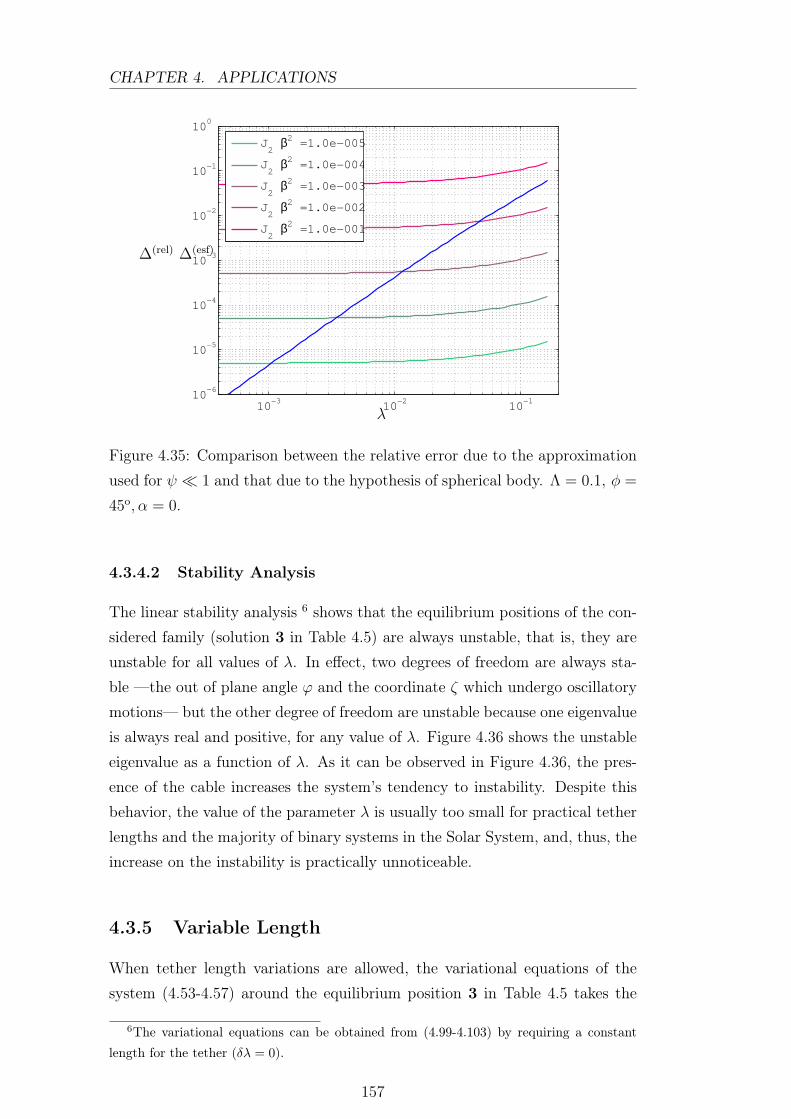
CHAPTER 4. APPLICATIONS
10−3
10−2
10−1
10−6
10−5
10−4
10−3
10−2
10−1
100
J2 β2 =1.0e−005
J2 β2 =1.0e−004
J2 β2 =1.0e−003
J2 β2 =1.0e−002
J2 β2 =1.0e−001
λ
∆(rel) ∆(esf)
Figure 4.35: Comparison between the relative error due to the approximation
used for ψ ≪ 1 and that due to the hypothesis of spherical body. Λ = 0.1, φ =
45o, α = 0.
4.3.4.2 Stability Analysis
The linear stability analysis 6 shows that the equilibrium positions of the con-
sidered family (solution 3 in Table 4.5) are always unstable, that is, they are
unstable for all values of λ. In effect, two degrees of freedom are always sta-
ble —the out of plane angle ϕ and the coordinate ζ which undergo oscillatory
motions— but the other degree of freedom are unstable because one eigenvalue
is always real and positive, for any value of λ. Figure 4.36 shows the unstable
eigenvalue as a function of λ. As it can be observed in Figure 4.36, the pres-
ence of the cable increases the system’s tendency to instability. Despite this
behavior, the value of the parameter λ is usually too small for practical tether
lengths and the majority of binary systems in the Solar System, and, thus, the
increase on the instability is practically unnoticeable.
4.3.5 Variable Length
When tether length variations are allowed, the variational equations of the
system (4.53-4.57) around the equilibrium position 3 in Table 4.5 takes the
6The variational equations can be obtained from (4.99-4.103) by requiring a constant
length for the tether (δλ = 0).
157

4.3. TSS AT LAGRANGIAN POINTS
10−6
10−4
10−2
2.5
2.55
2.6
2.65
2.7
2.75
2.8
2.85
R(s5)
λ
Figure 4.36: Unstable eigenvalue as a function of λ
form:
δξ =
(15 ∓ 2
ξ3E
)δξ + 2 δη − 3 δλ
ξ4E
(4.99)
δη =
(6 ± 1
ξ3E
)δη +
(3 ξ3E ∓ 1)
ξ2E
δθ − 2 δξ (4.100)
δζ = −(
7 ∓ 1
ξ3E
)δζ +
(3 ξ3E ∓ 1)
ξ2E
δϕ (4.101)
δθ = ± 3
ξ4E
δη − 3
(1 ± 1
ξ3E
)δθ − 3 Jg δλ
λE(4.102)
δϕ = ± 3
ξ4E
δζ −(
4 ± 3
ξ3E
)δϕ (4.103)
where λ stands for the variations of λ from its equilibrium value λE and Jg ≤ 1
is a function of the tether mass configuration (for massless tethers Jg = 1;
see eq. (4.59)). These equations show that the coordinates (ζ, ϕ) associated
to the out-of-plane motion are decoupled from the other coordinates. That
is, the oscillations of the out of plane motion can not be corrected by the
variation of the tether length as it has been pointed out in previous works [31].
Fortunately, the out-of-plane motion is stable (oscillatory). From now on, we
focus the analysis on the in-plane motion which is the source of the instability
exhibited by the system.
4.3.5.1 Linear Approximation. λ≪ 1
In the previous paragraph, it was stated that the validity field of the approach
covers small values of λ. As a consequence, the linear study can provide a
first and valuable approximation. In this section, we will suppose that the
deviations of the position of the center of mass from the equilibrium position
is small and of the order of λ. In this way, the linear analysis with λ ≪ 1
158

CHAPTER 4. APPLICATIONS
have the advantage of simplicity keeping a wide validity range. Applying the
following change of variables:
ξ = ξL + 31/3 λ0(1 + u(τ)) , η = 31/3 λ0 v(τ) , λ = λ0(1 + s(τ)) (4.104)
the Hill equations linearized in λ0 yield this system of equations:
d2 u
d τ2− 2
d v
d τ− 9 u(τ) +
9
2
`
3 cos2 θ cos2 ϕ − 1´
s(τ) +27
2
`
cos2 θ cos2 ϕ − 1´
= 0 (4.105)
d2 v
d τ2+ 2
d u
d τ+ 3 v(τ) − 9 cos2 ϕ cos θ sin θ (1 + s(τ)) = 0 (4.106)
d2 w
d τ2+ 4 w(τ) − 9 cos ϕ cos θ sin ϕ (1 + s(τ)) = 0 (4.107)
(1 + s(τ))d2 θ
d τ2+
d s
d τ(1 +
d θ
d τ) − 2 tan ϕ
d ϕ
d τ
„
1 +d θ
d τ
« „
1 +d s
d τ
«
+
+12 cos θ sin θ (1 + s(τ)) = 0 (4.108)
(1 + s(τ))d2 ϕ
d τ2+
d s
d τ
d ϕ
d τ+ (1 + s(τ)) sin ϕ cos ϕ
"
„
1 +d θ
d τ
«2
+ 12 cos2 θ
#
= 0 (4.109)
4.3.5.1.1 “Ad hoc” control. In this paragraph, the solution of the above
system of equations is forced to be bounded, avoiding the instability. Firstly,
the one dimensional problem is considered and then we will tackle the in-plane
analysis.
One dimensional. In the one dimensional case the variables v(τ), w(τ),
θ(τ), ϕ(τ) are canceled permanently. This way, the equation which establishes
the evolution of the system is:
d2 u
d τ 2− 9u(τ) + 9 s(τ) = 0 (4.110)
The solution of this second order ordinary differential equation can be explicitly
written as
u(τ) = C e−3 τ +D e3 τ + up(τ)
for all function s(τ). This control function is chosen fulfilling the follow re-
quirements:
1. It should fit to the general form
s(τ) = eβ τ (A cos Ωτ +B sin Ωτ)
being (A,B, β,Ω) parameters which satisfy the remaining conditions.
2. The particular solution must cancel the contribution of D e3 τ .
3. Initially the tether length is that of the equilibrium corresponding to the
position around we are linealizing.
159

4.3. TSS AT LAGRANGIAN POINTS
The conditions which are obtained for the parameters making them compatible
with the previous restrictions are:
A = 0 B =Ω2 + (β + 3)2
9 Ω· (3u0 + u0)
In Figure 4.37, the response of the system for a couple of arbitrary values of
Ω = 1.5 and β = 0.5 is gathered. The initial conditions are u0 = 0.15 and
u0 = 0.
3.6
3.8
4
4.2
4.4
4.6
4.8
5
5.2
0 200 400 600 800 1000
t (hours)
x(km)
940
960
980
1000
1020
1040
1060
1080
1100
1120
1140
1160
0 200 400 600 800 1000
t (hours)
L(km)
-0.6
-0.4
-0.2
0
0.2
0.4
0.6
0.8
1
1.2
1.4
0 200 400 600 800 1000
t (hours)
L(m/s)
0.0145
0.015
0.0155
0.016
0.0165
0.017
0.0175
0.018
0.0185
0.019
0 200 400 600 800 1000
t (hours)
T (N)
Figure 4.37: One dimensional control scheme. Massless tether with two equal
masses (500 kg) at both ends in the Earth-Moon system. The selected param-
eters are β = 0.5, Ω = 1.5, for the initial conditions u0 = 0.15 and u0 = 0.
The nominal tether length is considered to be L = 1000 km
As it can be observed in Figure 4.37, the system tends asymptotically to
the equilibrium position keeping the corresponding equilibrium tether length.
The maximum length is of the order of a 10 % of the final one. To carry on
the control manoeuvre, small deployment and retrieval tether velocities are
needed, although the involved tensions are also small, of the order of 10 mN.
Bi-dimensional. In this paragraph we deal with the in plane problem
ξ, η, since the instability is linked to the motion within it. Furthermore, it has
been shown that the tether length can not stabilize the out of plane motion
160

CHAPTER 4. APPLICATIONS
(which is naturally bounded, anyway) as it is exposed at the beginning of
this section. Additionally, a new hypothesis is made presuming the system
attitude variations would be small, i.e., θ ≪ 1 and θ ≪ 1. Hence, the system
of equations (4.105)-(4.109) yields:
d2 u
d τ 2− 2
d v
d τ− 9u(τ) + 9 s(τ) = 0 (4.111)
d2 v
d τ 2+ 2
d u
d τ+ 3 v(τ) − 9 θ = 0 (4.112)
d2 θ
d τ 2+d s
d τ+ 12 θ = 0 (4.113)
In this case, the general solution of the second order system of differential
equations can be expressed as:
u(τ) = C1 sin(
√−1 + 2
√7τ) + C2 e
√1+2
√7τ +
+C3 cos(
√−1 + 2
√7τ) + C4 e
−√
1+2√
7τ +
C512
47
√3 cos(2
√3τ) − C6
12
47
√3 sin(2
√3τ) + up(τ)
v(τ) = C1
√7 + 4√
−1 + 2√
7cos
√−1 + 2
√7τ + C2
√3(2 −
√7)√
−1 + 2√
7e√
1+2√
7τ −
−C3
√7 + 4√
−1 + 2√
7sin
√−1 + 2
√7τ − C4
√3(2 −
√7)√
−1 + 2√
7e−
√1+2
√7τ −
−C563
47sin 2
√3τ − C6
63
47cos 2
√3τ + vp(τ)
θ(τ) = C5 sin 2√
3τ + C6 cos 2√
3τ
In the same way as in the previous paragraph, we search for a control strategy
represented by the function s(τ) which complies with the follow requirements:
1. Its general form should be
s(τ) = eβ τ (A cos Ωτ +B sin Ωτ)
being (A,B, β,Ω) parameters which are chosen to fulfil the rest of the
conditions.
2. The particular solution of u(τ), v(τ), θ(τ) must cancel the contribution
of C2 e√
1+2√
7τ .
3. Initially the tether length is that of the equilibrium corresponding to the
position around we are linearizing.
161

4.3. TSS AT LAGRANGIAN POINTS
With this requirements, we obtain, on one hand A = 0, and, on the other hand
a relation B = B(β,Ω) which links all the parameters involved in the control
definitions. In Figure 4.38, the in plane extension of the previous paragraph
case is presented. That is, the response of the system for an arbitrary couple of
values Ω = 1.5 and β = 0.5, with the initial conditions u0 = 0.15 and u0 = 0,
as in the previous situation.
3
3.2
3.4
3.6
3.8
4
4.2
4.4
4.6
4.8
5
5.2
0 100 200 300 400 500 600 700 800 900 1000
t (hours)
x(km)
940
960
980
1000
1020
1040
1060
1080
1100
1120
1140
0 100 200 300 400 500 600 700 800 900 1000
t (hours)
L(km)
-0.4
-0.2
0
0.2
0.4
0.6
0.8
1
0 100 200 300 400 500 600 700 800 900 1000
t (hours)
L(m/s)
0.007
0.0075
0.008
0.0085
0.009
0.0095
0.01
0 100 200 300 400 500 600 700 800 900 1000
t (hours)
T (N)
Figure 4.38: Bidimensional control scheme. Massless tether with two equal
masses (500 kg) at both ends in the Earth-Moon system. The selected param-
eters are β = 0.5, Ω = 1.5, for the initial conditions u0 = 0.15 and u0 = 0.
The nominal tether length is considered to be L = 1000 km
Obviously, the tether length and its variation are similar to the previous
case. The differences occur in the position of the center of mass and in the
tension. These are due to the impossibility of canceling the contribution of
the unstable term and, simultaneously, the oscillatory terms. The remaining
oscillation in position, attitude and tension is, therefore, due to those terms.
Moreover, the solution of the angle θ which can be seen in Figure 4.39 shows
that its variations are small, consistently with the hypothesis which has been
made.
4.3.5.1.2 Proportional control. Keeping the linear approximation, it is
possible to set out other control strategies, also linear, which follow the general
162

CHAPTER 4. APPLICATIONS
-4
-3
-2
-1
0
1
2
3
4
5
6
0 100 200 300 400 500 600 700 800 900 1000
t (hours)
θ(o)
Figure 4.39: Evolution of the attitude angle θ when the bi-dimensional control
scheme is used. Variation of θ vs. time.
form s(τ) =∑Ki xi, where Ki are the gains and xi the state variables of the
system. A simple analysis can provide indications about the options that this
kind of control (the proportional control) can render. It would be useful to
make hypothesis related again to the attitude of the system, supposing that
θ, ϕ and its derivatives are small (≪ 1). Consequently, the system can be
expressed as:
d2 u
d τ 2− 2
d v
d τ− 9u(τ) + 9 s(τ) = 0 (4.114)
d2 v
d τ 2+ 2
d u
d τ+ 3 v(τ) − 9 θ(τ) = 0 (4.115)
d2w
d τ 2+ 4w(τ) − 9ϕ(τ) = 0 (4.116)
d2 θ
d τ 2+ 12 θ(τ) +
d s(τ)
d τ= 0 (4.117)
d2 ϕ
d τ 2+ 13ϕ(τ) = 0 (4.118)
Substituting the control function for the proportional scheme, the system of
ordinary differential equations yields the follow linear system.
d ~y
d t= A ~y (4.119)
163

4.3. TSS AT LAGRANGIAN POINTS
where ~y =u, v, w, θ, ϕ, u, v, w, θ, ϕ
Tand the matrix
AT =
0 0 0 0 0 9 − 9Ku 0 0 −9Ku(1−Ku)1+Kθ
0
0 0 0 0 0 −9Kv −3 0 9KuKv+3Kv
1+Kθ0
0 0 0 0 0 −9Kw 0 −4 9KuKw+4Kw
1+Kθ0
0 0 0 0 0 −9Kθ 0 0 9KuKθ−121+Kθ
0
0 0 0 0 0 −9Kϕ 0 99KuKϕ−9Kw+13Kϕ
1+Kθ−13
1 0 0 0 0 −9Ku −2 09K2
u−Ku+2Kv
1+Kθ0
0 1 0 0 0 2 − 9Kv 0 0 −Kv+Ku(2−9Kv)1+Kθ
0
0 0 1 0 0 −9Kw 0 0 9KuKw−Kw
1+Kθ0
0 0 0 1 0 −9Kθ 0 09KuKθ−Kθ
1+Kθ0
0 0 0 0 1 −9Kϕ 0 09KuKϕ−Kϕ
1+Kθ0
In first place, the stabilization possibilities which provide this kind of con-
trol with only one gain different from zero, i.e., s(τ) = Ki xi is explored. The
eigenvalue analysis shows that the only control of this particular type which
can produce stabilization is s(τ) = Ku u(τ) with Ku > 1. In this situation all
the eigenvalues are pure imaginary and the system would oscillate around the
equilibrium position.
In a second step, we include a second variable with a gain different from
zero searching for the system dynamics to be asymptotically stable in the in
plane motion. Hence, the control schemes which correspond to this general
expression s(τ) = Ku u(τ) + Ki xi are studied. The eigenvalue analysis can
proof that there is not any combination that drives us to the desirable result.
Since, even the most favorable case (s(τ) = Ku u(τ) + Ku u(τ) with Ku >
1 , Ku > 0) yields a system with two complex conjugate imaginary eigenvalues
associated to the in plane motion.
4.3.5.2 Full Problem. Proportional control
In this paragraph, the full problem is faced, stated by the system of equations
(4.99,4.100, 4.102). Furthermore, the length variation will be supposed to be
governed by a proportional control law on λ. In this way, we search for the
gains needed to stabilize the system when the behavior of λ is described, in a
general manner, by the expression: λ = λE +∑Ki (xi − xE,i) where Ki are
gains and xi stands for the variables ξ, η, θ. When this control law is included
in the system of variational equations, it becomes a linear system of differential
164

CHAPTER 4. APPLICATIONS
equations which can be written in vectorial form:
d ~y
d t= M ~y (4.120)
here ~yT =ξ, η, θ, ˙ξ, ˙η, ˙θ
.
The detailed stability analysis of the system (4.120) can be cumbersome.
Nevertheless, taking into account the results of the linear analysis, we firstly
consider the simpler case only with a gain different from zero, Kξ. In that
situation, the characteristic polynomial takes the form:
s3 +
[3Kξ
ξ4e
−(
2 − 4
ξ3e
)]s2 +
[(6 Jg + 27
ξ4e
+6
ξ7e
)Kξ −
(105 − 6
ξ3e
+4
ξ6e
)]s+
+6
[(9
ξ4e
− 3
ξ7e
)Kξ −
(45 +
9
ξ3e
− 2
ξ6e
)]= 0
And applying the rule of the signs of Descartes, we reach the sufficient con-
ditions required to Kξ in order to stabilize the system as a function of the
equilibrium position and the parameter Jg. That condition is drawn in Figure
4.40 for a massless tether (Jg = 1).
10−6
10−4
10−2
2
2.5
3
3.5
4
4.5
5
K∗ξ
λe
Figure 4.40: Sufficient condition for Kξ to stabilize the system as a function
of λ. Values over the curve provide stability.
According to this approximation, we are able to provide stability but not
asymptotic stability. In order to do that, it is advisable to include gains which
affect the velocity variables. Following the analysis with λ ≪ 1, it should had
been advisable to try with two control gains: Kξ and Kξ, even if they are not
able to stabilize the system in the linear approximation. For the full problem
situation, the Routh-Hurwitz stability criterion [35] has been used in order to
establish whether that pair of gains can provide stability. The result shows
that they must fulfil these incompatible conditions:
Kξ > 0, (11+2Jg)ξ4e−2ξe−3Kξ < 0,
12((J2g + 10Jg − 6)ξ3
e + 1)
ξ3e ((11 + 2Jg)ξ4
e − 2ξe − 3Kξ)Kξ > 0
165

4.3. TSS AT LAGRANGIAN POINTS
since in last condition the numerator is positive for all values of ξe (and for
a massless tether). Therefore we can conclude that the system can not be
stabilized using values of Kξ and Kξ different from zero at the same time.
4.3.6 Control Drawbacks
4.3.6.1 Length Variations
This paragraph analyzes the length variations associated to the control laws
required to stabilize the system.
On one hand, we can address the philosophy which lies in the control
strategies. In the simplest case, the one dimensional linearized for λ ≪ 1, it
is clearly observed that the basis of the control method is found in modifying
the tether length in a manner that the given position would be always the
equilibrium one. In such a case the question of which is the length variation
associated to a fixed deviation of the position of the center of mass can be
answered. In dimensional values, the equation which link both variations are:
∆L
∆xe=
1
2 313
√a2 λ
(4.121)
In the general case, this ratio can be expressed as a function of the non dimen-
sional equilibrium position:
dL
d re=
15 ρ3e − 2
2√
3 a2
√3 ρ3
e − 1(4.122)
The aspect of both relations is shown in Figure 4.41.
In Figure 4.41 it can be observed that the linear approximations fits well
till values of λ of the order of ∼ 10−2. Moreover, for small values of λ (λ <
10−6) the variations of the tether length are extremely high (deployment (or
retrieval) of 1000 km for deviations of 1 km in the center of mass position).
The presence of a minimum suggest that it would be worth working near that
point where dL/d re is approximately ∼ 4.5. That implies searching for values
of λ ∼ 1.3 ·10−1. Nevertheless, we should note that, taking into account Figure
4.41, the values of λ which allow to be coherent with the hypothesis made in
this approach are smaller than λ < 10−1. As a result, we should try to search
for λ of the order of 10−2 in order to be coherent with our approximation and
also to provide a feasible tether length variation.
Figure 4.42 shows the ration dLdxe
as a function of tether length (km) for the
equilibrium position in different binary systems of interest. The part of the
curve on the right of the minimum should not be considered since it corresponds
166

CHAPTER 4. APPLICATIONS
10−6
10−4
10−2
100
100
101
102
103
λ
dLt
d re
GeneralLineal
Figure 4.41: Ratio between the variation of length needed and the deviations of
the center of mass of the system as a function of the parameter λ. Comparison
of linear and general expressions.
to values of λ out of its validity range. This figure allows to establish which
systems of primaries would be more suitable for control length strategies. On
the right hand side of the picture the tether length needed to work in the
vicinity of the minimum of dLt/d re is extremely high. However, with more
reasonable values of the tether length in the systems of the left of the picture,
the ratio dLt/d re is near its minimum. Hence, this analysis help us to evaluate
“ a priori ” the suitability of the tether length control in each of the binary
systems of the Solar System.
On the other hand, other troubles in the proportional control regarding the
tether length can be noticed. Firstly, there exists a limit associated to the fact
that the equilibrium positions are on only one side of the Lagrangian point (on
the right for L2, on the left for L1) and not on both. Therefore, it is necessary
to ensure that the tether is in the right side. This condition can be expressed
in dimensional and non dimensional values for the L2 case as follows
‖x− xE‖ = ∆x < ‖xE − xL2‖ ‖ξ − ξE‖ = ∆ξ < ‖ξ − 3−1/3‖ (4.123)
Secondly, the constraint about the tether length: L > 0 yields a restriction on
the control strategy. The dimensional value of the cable length is proportional
to√λ. This non dimensional variable varies according to the control law. In
a general situation of proportional control, λ can be expressed as a function of
the variations ∆~y with respect to the equilibrium position:
λ = λE + ~K · ∆~y
167

4.3. TSS AT LAGRANGIAN POINTS
10−2
100
102
104
102
104
106
Sun-Earth
Earth-Moon
Mars-Phobos
Jupiter-Amaltea
Jupiter-Io
Saturn-Enceladus
L (km)
d Ld xe
Figure 4.42: Ratio between the variation of length needed and the deviations
of the center of mass of the system as a function of the dimensional tether
length (km).
Hence, the constraint can be written as: λE+ ~K ·∆~y > 0. In a general manner,
λ can be bounded taking into account the triangular inequality:
λE + ~K · ∆~y > λE − | ~K| |∆~y|max > 0 (4.124)
It is not easy to establish the maximum value of |∆~y|max in a general man-
ner, since it depends on the dynamical evolution of the system. However, it is
reasonable to suppose that, in a stabilized system, the maximum perturbation
is the initial one as the control is in charge of bringing the system closer to
the unstable equilibrium point. As a consequence, in a majority of situations
|∆~y|max = |∆~y|0.For the particular case of the control law exposed in the previous section:
λ = λE + Kξ (ξ − ξE), the previous constraint (4.124) can be expressed as:
Kξ < λE/(ξ − ξE)max. Supposing that maximum is produced in the initial
instant and for the same ∆ρst(0) 7, the one that produce a greater (ξ − ξE) is
when ∆xi = ∆ξ. In this manner, the condition in Kξ is as follows:
Kξ <λe
ξ0 − ξEnon dimensional Kξ <
√λe a2
‖x0 − xe‖dimensional (4.125)
In summary, there are two limiting constraints: 1) keeping the center of mass of
the system on the correct side of the Lagrangian point and 2) the length of the
cable must have positive values. The follow lines are devoted to reveal which is
more limitative. Both restrictions can be measured in terms of the maximum
7∆ρst(t) =√
(ξ(t) − ξE)2 + (η(t) − ηE)2 + ξ(t)2 + η(t)2
168

CHAPTER 4. APPLICATIONS
allowable perturbation in each case, making possible the comparison between
them. This maximum allowable perturbation is defined as the maximum initial
perturbation which allows to keep the system stable fulfilling the required
requisite (constraint 1) or 2)).
For the first constraint, once the equilibrium position is established, it is
necessary to ensure that the initial position is within an interval centered in ξE,
being the length of the interval equal to 2∣∣ξE − 3−1/3
∣∣. Hence, the maximum
allowable perturbation is the half-interval ∆ξ|(C1)max =
∣∣ξE − 3−1/3∣∣ and this value
is fixed for each equilibrium position.
For the second constraint, we can obtain the maximum allowable pertur-
bation from the relation (4.125).
∆ξ|C2max =
λEKξ
Since the value of ∆ξ|C2max depends not only on λE but also on the control gain,
Kξ will be chosen in order to provide a real maximum of the perturbation, that
is, it will be used the minimum value of Kξ which guarantees the stability of
the system (the geometry place of the curve represented in 4.40). Accordingly,
the value of the maximum allowable perturbation for each constraint can be
drawn as a function of the equilibrium position as it is shown in Figure 4.43,
on the left.
10−6
10−5
10−4
10−3
10−2
10−8
10−6
10−4
10−2
100
λ
∆ξ
10−6
10−5
10−4
10−3
10−2
0.258
0.259
0.26
0.261
0.262
0.263
0.264
0.265
λ
∆ξ|C1max
∆ξ|C2max
Figure 4.43: On the left, ∆ξ|max for both limits: ∆ξ|C1max (blue line) and ∆ξ|C2
max
(red line). On the right, ratio between maximum allowable perturbations for
each of the above-mentioned constraints
The fulfillment of the condition L > 0 requires smaller perturbations than
the necessity of placing the center of mass on the correct side of the Lagrangian
point. It is clear, then, that the limitation on the control law constitutes a
more important requirement than the constraint related to keeping the TSS
on the right side of the libration point. Taking those non dimensional results,
169

4.3. TSS AT LAGRANGIAN POINTS
Figure 4.44 gathers the maximum perturbation in the position of the center of
mass of the system allowed for a given configuration and a particular binary
system.
10−2
100
102
104
10−5
100
Sun-EarthEarth-MoonMars-PhobosJupiter-AmalteaJupiter-IoSaturn-Enceladus
L (km)
∆x|max (km)
Figure 4.44: Maximum perturbation allowed for each value of L, considering
the constraint of stabilization which is more requiring than keeping TSS on
the right side of the libration point.
4.3.7 Tension
Tethers require positive tension since a cable can not withstand compression.
As a consequence there exists a natural limit for tether operation which will
be explored in this paragraph. The expression of the tension in a massless
cable within the Hill approximation is collected in equation (4.67). Hence, the
tension will depend on the tether control law through the last term: (Ld/Ld).
We analyze the stabilizing proportional control studied in the previous
section (λ = λe+Kξ(ξ−ξe)) in order to determine the influence of the different
elements involved in the control law: initial perturbation, equilibrium position
and mass configuration. Figure 4.46 shows the maximum and the minimum
tensions for a massless tether as a function of the initial perturbation, for a
given equilibrium position (in this case the corresponding to λe = 10−2).
As it can be seen, there exists a maximum acceptable initial perturbation
over which the tension becomes negative. Moreover, the maximum value of the
initial perturbation in the figure has been chosen as the maximum ∆ξ which
can be controlled with the minimum gain Kξ of this equilibrium position.
That means that the positive tension constraint is more restrictive than the
requirement L > 0 exposed in the previous paragraph.
170

CHAPTER 4. APPLICATIONS
10−5
10−4
10−3
−5
0
5
10
15
20
TTc
∆ξ
Figure 4.45: Maximum and minimum tether tension as a function of the initial
perturbation ∆ξ for a given equilibrium position: λe = 10−2.
This way, it is possible to associate a critical value of ∆ξ to each equi-
librium position. Figure 4.46 summarizes such a critical value as a function
of λe. Along the blue line, the zero tether tension condition is reached; as a
consequence, the acceptable values of ∆ξ must be below this line. Here the
red line represents the requirement L > 0. In turn, the blue line represents the
zero tension condition. It is clear, from the Figure, that the last requirement
is the most restrictive for all values of λe. Therefore, the blue line in Figure
4.46 constitutes the maximum perturbation allowed which can be controlled
with feasible tether length variations maintaining the tether tight.
4.4 Gravity Gradient Measurements with Teth-
ered Satellites
In recent years an important effort has been made in order to improve the
knowledge of the gravity field and the geoid. This endeavor could be noticed
in the missions planed and also in the development of newer methods of analysis
and data processing.
Since the early 1970’s, tethers has been considered as suitable devices to
investigate gravity anomalies, not only on the Earth but on the Moon and
planets as well [19]. The role of this kind of devices in Geodesy field is twofold.
On the one hand, they can be used as a tool to carry out gradiometry measure-
ments at low altitudes during long periods [19, 39, 40, 59]. On the other hand,
the tether can represent an instrument which measures the gravity anomalies
171

4.4. GRAVITY GRADIENT MEASUREMENTS WITH TS
10−4
10−3
10−6
10−5
10−4
λe
∆ξ
Figure 4.46: ∆ξ which provides zero tension as a function of the equilibrium
position described by the parameter λe (blue line). ∆ξ which provide zero
tether length when the minimum value of Kξ needed to stabilize the system is
considered (red line).
by means of the tether tension [19, 48, 20]. Tension on the wire is related to
the gravity difference of the end masses the tether connects. Therefore, ten-
sion contains information of the gravity gradient [13] and the tethered satellite
system could be seen as a large base gradiometer. Having this in mind, tether
tension is related to radial gravity gradient and its values should present the
same behavior, i.e., it should be expected that the upward continuation in de-
gree would be attenuated by a counteract term, quadratic in the degree. That
is the rationale for satellite gravity gardiometric [95] and, therefore, for tether
utilization in gravity field missions.
In this document we present a study of the feasibility of tethers as gravity
recovery devices. In order to carry out that task, we will use the semi-analytical
method described in [94]. In 4.4.1, that method is discussed, presenting its fun-
damentals. Basically, it allows to derive analytically the relationship between
the known observable and the unknown spherical harmonics. In our case, the
observable is the tension on the cable and it is necessary to develop a linear
observation model for it. In subsection 4.4.1.3 that model is described in de-
tail. From the observable only we can derive some important information, as
it will be seen in 4.4.2. Nevertheless, the actual information of the tension will
be an stochastic variable. How the realistic scenario affects the recovery of the
gravity coefficients is tackled in section 4.4.3. In summary, this chapter assess
the utilization of tethered satellites in geodetic missions using the tension as
172

CHAPTER 4. APPLICATIONS
the observable. Moreover, this analysis can be easily extended to estimate the
gravity recovery capabilities of tethered devices for planetary missions.
4.4.1 Semi-Analytical Approach
In this section the considerations taken into account to perform the analysis
of a tethered system as a gravity gradient measure device are exposed. The
first paragraph represents a review of the method which is used in the present
study. Then the necessary elements to develop that procedure are presented.
4.4.1.1 Lumped Coefficients Approach
In the PhD Thesis [94] a semi analytical method for gravity field analysis is
exposed in a systematic way. The technique is specially suitable for pre mission
analysis since it can provide the performance of the mission in terms of sen-
sitivity, stability and recoverability of the corresponding potential coefficients
without a great amount of computing time.
The main concepts which support this method are roughly three: the defi-
nition of a nominal orbit, the utilization of the lumped coefficient approach and
the consideration of least squares method in the treatment of the stochastic
model. The objective of this approach is to obtain an easy-to-compute method
to estimate the performance of each observable. In order to achieve this, some
simplifications are made in the definition of the nominal orbit which allows an
analytical treatment of the observational model. Then, the prescribed accu-
racy can be acquired by means of iteration. From this point of view, this work
prioritize simple treatment instead of model complexity.
The nominal orbit is defined as the ideal orbit where the measurements
of the observational would be made. It constitutes an element of design and,
for convenience, it is usually characterized as a circular orbit, with constant
inclination and secular precessing due to the flattening term (J2). That implies
this nominal orbit does not coincide with the real one.
In turn, lumped coefficients are defined as linear combinations of poten-
tial coefficients over the degree. They allow to recast the potential in a 2-D
Fourier expression. Then the problem is posed in terms of a transformation
from spherical representation of the harmonics to a 2-D Fourier expression.
Moreover, this formulation leads to a non coupled linear system where each
order can be solved independently.
At last, the least squares method is a well known optimal estimator used in
a broaden kind of problems. In this work, the methods which are considered
173

4.4. GRAVITY GRADIENT MEASUREMENTS WITH TS
are the weighted least squares and the weighted least squares with a priori
information. In both cases the weight matrix is the inverse of the noise co-
variance matrix of the vector of observations. That matrix, together with the
model characteristics gives rise to the normal matrix which gathered the main
information of the recover capabilities of the considered observations.
Accordingly to the former appreciations, a separate linear system is ob-
tained for each spherical order m. Such set of linear equation are numerically
affordable even for relative simple computer equipment. The solution of that
linear system provides valuable information about pre-mission error analysis
of gravity field missions.
4.4.1.2 Nominal Orbit
Establishing a linear observational model in a similar way as the semi-analytical
approach does [94] is the objective of this paragraph. In that approach one
prerequisite is the introduction of a nominal orbit of constant radius, con-
stant inclination and precessed due to the flattering term J2. In this manner,
the lumped coefficients becomes time-independent. Regarding this concept, it
must be remarked that the real and the nominal orbits do not coincide and
the last should be considered as a set of points where the observational model
is evaluated [23, 11].
In the situation discussed here the dynamics are a bit more complicated
than in the motion of a particle in a gravitational field. Therefore, the defi-
nition of the nominal orbit for the tethered system is more cumbersome. The
rough consideration of this problem, i.e. a rigid body in a gravitational field,
should drive to a non integrable problem, which involves not only the path of
the center of mass but the attitude dynamics as well.
To define the nominal orbit, we will use an Earth-fixed coordinate system.
The tethered system will be represented by the simple model present through-
out this work, the dumbbell. Moreover, the cable is supposed to be massless,
i.e., a rigid massless cable attaching two point masses. The values of that
masses will be m1 and m2, and the length of the cable, L. For the sake of com-
pactness, the full gravitational model will be considered in its representation
on a sphere by means of spherical harmonics with complex-valued factors [94]:
V (r, θ, λ) =µ
Re
∞∑
l=0
l∑
m=−l
(Re
r
)l+1
KlmYlm(θ, λ) (4.126)
In this expression, r, θ, λ are the spherical coordinates (radius, co-latitude
and longitude respectively), Re is the equatorial radius of the Earth, µ is the
174

CHAPTER 4. APPLICATIONS
Earth’s gravitational constant, Ylm(θ, λ) is the normalized spherical harmonic
of degree l and order m, and Klm is the spherical harmonic coefficient of degree
l and orderm. The perturbation force could be derived from the last expression
in this way:
~FG = −m[∂V (r, θ, λ)
∂r~ur +
1
r cos(λ)
∂V (r, θ, λ)
∂θ~uθ +
1
r
∂V (r, θ, λ)
∂λ~uλ
](4.127)
Nevertheless, some additional assumptions are made in order to provide an
analytical solution for the linear observation model. First, the distance from
the origin of the reference frame to the point masses, r1 and r2, are supposed
to be constant. Second, the cable which connects that masses is aligned with
the local vertical. It should be noted that these hypothesis do not mean that
the masses evolve in a keplerian orbit.
In such a case, the equilibrium equations are
~FG(~r1) · (−~ur) − T = m1 Ω20 r1 (4.128)
~FG(~r2) · (−~ur) + T = m2 Ω20 r2 (4.129)
If we use the expression (4.127) in the former equations, we can obtain the
angular velocity of the whole system:
Ω20 =
µ
r3G
∞∑
l=0
l∑
m=−l
(cos2(φ)
(1 − ǫ sin2(φ))l+2+
sin2(φ)
(1 + ǫ cos2(φ))l+2
)·
·(l + 1)
(Re
rG
)lKlmYlm(θ, λ)
(4.130)
where the m and φ have been introduced in chapter 2, while the distance
of the center of mass rG is defined as mrG = m1 r1 +m2 r2.
Furthermore, a non dimensional parameter ǫ gauges the system extension
ǫ =L
rG
It is worth remarking the fact that the center of mass describes a circular
trajectory but not a keplerian orbit, since the angular velocity varies with
time. In fact it is possible to establish which point of the system follows a
“true” keplerian orbit. That point should fulfills:
r0 Ω20 =
µ
r20
(4.131)
whose movement corresponds to a circular keplerian orbit. Its radius, r0, is
related to the center of mass, rG, in this way:(rGr0
)3
=∞∑
l=0
l∑
m=−lfl(ε, φ)(l + 1)
(Re
rG
)lKlmYlm(θ, λ) (4.132)
175

4.4. GRAVITY GRADIENT MEASUREMENTS WITH TS
where the follow notation was used:
fl(ε, φ) =cos2(φ)
(1 − ǫ sin2(φ))l+2+
sin2(φ)
(1 + ǫ cos2(φ))l+2(4.133)
As a result, and due to the body “extension”, the distance r0 does not match
with the distance of the center of mass, rG, even if a central field was considered.
In that case the point of the tether whose distance was r0 = rG/3√f0 describes a
“true” circular keplerian orbit. Eventually, a last hypothesis is made concerning
the nominal orbit. It is supposed that the motion of the material point r0
corresponds to that of a particle in the Earth gravity field retaining only the
secular effects of the oblateness of the Earth. Hence, the orbit will be circular
with radius r0, with constant inclination and the three angular Kepler elements
(Ω, ω,M) varying due to J2 secular perturbations. From [49]:
Ω = −3
2nJ2
(Re
r0
)2
cos I (4.134)
ω = −3
4nJ2
(Re
r0
)2
[5 cos2 I − 1] (4.135)
M = n+3
4nJ2
(Re
r0
)2
[3 cos2 I − 1] (4.136)
Such orbit will be considered as the nominal orbit in the sequel.
Some remarks should be taken into account regarding the nominal orbit.
As it has pointed out the real motion and the nominal orbit do not coincide.
Even more, the effects of the flattering term of the potential in the motion has
been “assumed”, and therefore, it represents only an unrefined approximation.
To assess the difference between the nominal an the actual orbit, an estimation
has been made using numerical simulations. Nevertheless, the inconsistency
of the real and nominal orbit can be solved by means of applying corrections
to the data or iteration [94].
4.4.1.3 Linear Observational Model
Once the nominal orbit is defined, we search for the relationship which links
the new observable with the unknown coefficients of the gravity field. Using
the expressions (4.128)-(4.129) and (4.130), and after some computations we
can obtain the tension T as a function of the spherical coordinates of the center
of mass and the parameters of the system:
176

CHAPTER 4. APPLICATIONS
T (rG, θ, λ; ε, φ) =mµ
r2G
χ(ε, φ)∞∑
l=0
l∑
m=−lgl(ε, φ)(l + 1)
(Re
rG
)lKlmYlm(θ, λ)
(4.137)
where the following notation is introduced:
χ(ε, φ) =cos2(φ) sin2(φ)
(1 − ǫ sin2(φ))2(1 + ǫ cos2(φ))2(4.138)
gl(ε, φ) = (1 + ǫ cos2(φ))l+3 − (1 − ǫ sin2(φ))l+3 (4.139)
These variables are functions only of the mass configuration of the tethered
system, therefore they are fixed for a given tether.
To perform the spectral analysis of this observable and obtain a lumped
coefficient representation it is necessary to express the former relationship in
terms of the orbital elements. In order to achieve that we can perform a
rotation of the spherical harmonics. After some computations the expression
for the tension takes the form:
T (a, e, I,Ω, ω,M ; ε, φ) =mµ
a2
χ(ǫ, φ)
f2/30 (ε, φ)
∞∑
l=0
(l + 1)gl(ε, φ)
fl/30 (ε, φ)
(Re
a
)l
l∑
m=−l
l∑
k=−lKlmFlmp(I) exp i(k u+mΛ)
being u = ω +M the argument of latitude and Λ = Ω − θG the longitude
of the ascending node in an Earth-fixed system (θG, Greenwich sidereal time).
The inclination functions are complex-valued and they are defined in [94].
Note that the parameter ε depends on rG instead of r0. Nevertheless, the ratio
between this parameter and a new one based on the radius of the circular orbit
ε = L/r0 is of the order O(ε2).
Then, the lumped coefficients could be written as:
ATmk =∞∑
l=max (|m|,|k|)HTlmkKlm (4.140)
with
HTlmk =
mµ
a2
χ(ε, φ) gl(ε, φ)
f(l+2)/30 (ε, φ)
(l + 1)
(Re
a
)lFlmk(I) (4.141)
Using this expressions, the tension expression reduces to:
T (u,Λ; ε, φ) =m=∞∑
m=−∞
k=∞∑
k=−∞ATmke
iψmk (4.142)
ψmk = ku+mΛ
177

4.4. GRAVITY GRADIENT MEASUREMENTS WITH TS
4.4.1.4 Introductory Analysis
Before the rigorous study of the tether capabilities for gravity recovery, it is
possible to estimate and analyze them a priori. From the expression of the
tension in terms of the gravity harmonics 4.137 we can derive some conclu-
sions. First of all, the parameter gl is greater as l increases, ǫ is greater or φ
tends to zero. From a practical point of view, this fact allows to enlarge the
amplitude of the tension for increasing l. Despite the fact this term cannot
compensate completely the effect of (Re/rG)l for reasonable values of ǫ, it could
help to maintain that amplitude between measurable quantities. In fact, the
asymptotic behavior of that parameter with a realistic value of ǫ (ǫ≪ 1) is
gl ≈ (l + 3)ǫ+ O(ǫ2)
Accordingly, for this observable a characteristic expression would be (l+1)(l+
3) which amplifies the signal with increasing degree.
On the other hand, the mean value of the tension will be:
T0 =mµ
r2G
cos2(φ) sin2(φ)
(1 − ǫ sin2(φ))2(1 + ǫ cos2(φ))2g0 (4.143)
Therefore, the value of the tension due to the main term of the gravity field
could be split into two: a term which gather the gravity force as if the sys-
tem would be a point mass orbiting the Earth at the altitude of its center
of mass; and a term which takes into account the actual mass distribution
and depends only on the parameters ε, φ. We can express this fact as follows,
T0 = mµr2Gτ(ε, φ). The values of τ are plotted to show the order of magnitude
of that function.
0.0010.001
0.001 0.001
0.00
10.
0010.002
0.002
0.002
0.00
2
0.00
2
0.003
0.003
0.00
3
0.00
3
0.004
0.004
0.00
4
0.005
0.005
0.006
0.00
6
0.007
0 10 20 30 40 50 60 70 80 900
0.001
0.002
0.003
0.004
0.005
0.006
0.007
0.008
0.009
0.01
φ
ε
τ
Figure 4.47: Non dimensional value of the mean tension: τ(ε, φ)
To provide with an estimation of the tether tension, we consider the follow-
ing quantities for a typical mission: m ∼ 1000 kg., rG ∼ 6671.22 km., φ ∼ 40o
178

CHAPTER 4. APPLICATIONS
and ǫ ∼ 1.5 · 10−3. In such a case, the value of the average tension is:
T0 = 9.77 N (4.144)
Furthermore, the effect of the harmonics of order l could be measure by
means of differential tension :
∆T |l =mµ
r2G
cos2(φ) sin2(φ)
(1 − ǫ sin2(φ))2(1 + ǫ cos2(φ))2(l+1)
(Re
rG
)lgl(ε, φ)
l∑
m=−lKlmYlm(θ, λ)
(4.145)
And , the relative differential tension can be written
∆T |lT0
= (l + 1)
(Re
rG
)lglg0
l∑
m=−lKlmYlm(θ, λ)
The order of magnitude of this relative differential tension could be obtained
considering ǫ≪ 1:
gl ∼ (l + 3)ǫ+ (3 +5
2l +
1
2l2)ǫ2 cos(2φ) (4.146)
and Kaula’s ‘rule of thumb’:
Clm ∼ 10−5
l2Slm ∼ 10−5
l2(4.147)
The final expression of the ratio between the relative differential tension and
its mean value reads
∆T |lT0
∼ 1
3
(1 +
4
l+
3
l2
)(Re
rG
)l10−5 (4.148)
1e-016
1e-014
1e-012
1e-010
1e-008
1e-006
0.0001
50 100 150 200 250 300
h = 100 kmh = 200 kmh = 300 kmh = 400 kmh = 500 km
l
∆T |lT0
Figure 4.48: ∆T |lT0
vs. l for different values of rG (in terms of the altitude h in
km)
In Figure 4.48 this relationship is plotted for different values of rG, showing
that the variation of the tension is more than about four orders of magnitude
smaller than the mean term.
179

4.4. GRAVITY GRADIENT MEASUREMENTS WITH TS
4.4.2 Application and Results
4.4.2.1 Preliminary Considerations
The following and subsequent paragraphs will be devoted to the analysis of
the observable as it has been defined previously. However, some considerations
should be taken into account regarding the feasibility and discussing the hy-
pothesis which are made up to this point. In the aim of providing a realistic
view of a geodesy tether mission scenario, this section tackles three significant
aspects: former proposed solutions for the instrument and its features, the
suitability of the nominal orbit approximation and a brief exposition of the
impact of the different dynamical models in the tension signal, and, lastly,
some observations about the noise sources and their aftermaths.
4.4.2.1.1 Measurement Device In the literature we can find two main
sources which deal with the design of a tension measurement device in tethered
satellite systems. Chronologically, the first proposal has been exposed in [19]
by a Smithsonian team. In that study a description of the working principles
of such instrument is provided in a minute detail. In [48] an outline with a
review of its main characteristics can be looked up. Shortly, we reproduce here
some of the main features of the device.
The proposed instrument is intended to measure the bending moment
which appears in a beam due to the tether tension applied on it. That consti-
tutes a relatively simple device that employs some mechanical amplification in
combination with electrical-resistance strain gauges to provide a tension sig-
nal. A noise analysis is also furnished concerning the thermal and shot noise
in the electrical circuitry, arriving the estimation that these noise sources are
of non concern for the a priori requirements. These requirements impose the
beam to survive a 100 N load and be capable of an absolute sensitivity of 10−4
N tension change in an environment consisting both of an unsteady tension
component (10−2 N) and a steady component (10 N). Nevertheless, one of the
conclusions gathered in the former study states that the concept is not lim-
ited by any fundamental or physical reason, and the ability to achieve better
precisions will be hampered only by practical considerations, such as manu-
facturing, calibration, or testing. In fact, in the second article a sensitivity of
10−5 N is considered for an improved version.
On the other hand, there exist another proposal for a high accurate instru-
ment based on a tether system linked to a very required task in terms of sen-
sibility: gravitational-wave detection [13]. In the Skyhook gravitational-wave
180

CHAPTER 4. APPLICATIONS
detector concept, a spring would be in charge of measure the tether tension
variations. The engineering aspects of this design are not discussed in detail
as it happened for the previous case. However, the advantage of an instrument
based on a spring-like device lies in the fact that the signal is directly a relative
measurement and, with the appropriate calibration, it would not be necessary
to measure the steady component of the tension.
4.4.2.1.2 Actual Tether Dynamics In the previous section the concept
of nominal orbit and its definition for the tether case was described. As it was
exposed there, the nominal orbit does not coincide with the actual one and
constitutes an useful tool which allows to obtain a straightforward formula-
tion for geopotential coefficient treatment and calculation. Nonetheless, since
the tether dynamics are quite more complicated than the particle motion, it
is worth investigating the true comportment of the observable in a realistic
scenario. Furthermore, we will discuss the hypothesis which are assumed in
the nominal orbit description.
Tether Tension Firstly, we deal with the assumption of the massless
tether. When an actual cable is taken into account, a tension distribution is
obtained even for a central gravity field instead of the unique corresponding
value in the ideal tether defined for the nominal orbit.
Following the exposition of 2.2.4, a more accurate computation of tether
tension can be carried out. The formulation of the tension problem for a
differential element of the cable drive us to the following equation:
d
ds(T~u) + ~fs = ρ~rs (4.149)
where T is the tether tension, ~u is the unitary vector which provides the
tether orientation, s is the arc lenght, ~fs is the force per unit lenght which acts
in the element and ρ is the linear density of the cable. This equation should
be integreted with initial and the following boundary conditions.
~F1 + T1~u = m1~r1 (4.150)
~F2 − T2~u = m2~r2 (4.151)
Taking into account the considerations listed below:
1. d~u/ds = 0. The tether is not bending, is completely tight.
181

4.4. GRAVITY GRADIENT MEASUREMENTS WITH TS
2. ~fs = −ρµ~rs/r3s + ρ~γs. The force acting in the element is composed
of a principal term due to the central Earth gravity potential and a
perturbation expressed in terms of acceleration.
3. ~rs = ~rG + s~u. The element position can be expressed as a sum of the
position vector of the center of mass, the arc length and the unitary
vector ~u. And the relationship of its derivatives is straightforward.
4. rs = rGD(s, rG), where D(s, rG) =√
1 + 2s/rG((~rG · ~u)/rG) + (s/rG)2.
In the same way, the element position can be expressed as a function of
the distance of the center of mass and the arc length.
5. ~rG = −µ~rG/r3G+~γG. The acceleration of the center of mass is assumed to
be equal to the gravitational central field acceleration plus a perturbation
term (in this term we could consider also the terms derived from the
tether extension)
equation (4.149) becomes:
dT
ds~u = ρ
(µ
r3GD3(s)
(~rG + s~u) − ~γs − µ~rGr3G
+ ~γG + s~u
)
The corresponding non dimensional equations can be obtained using the
initial distance of the center of mass rG, the initial angular velocity ω0 and the
linear density ρ of the tether
ζ =s
rG0
τ =T
ρr2G0ω
20
ω0 =µ
r3G0
χ =rG0
rG
Finally, projecting in the tether tangent direction, a single scalar differential
equation describes the tension along the cable
dτ
dζ= −χ3
[cosϑ− 1
D3(ζ, χ)(cosϑ+ ζ)
]+ ζ
~u · ~uω2
0
+(~γG − ~γs) · ~u
rG0ω20
(4.152)
The notation which has been used here is:
~i =~rGrG
cosϑ =~i · ~u D(ζ, χ) =√
1 + 2χζ + (χζ)2 (4.153)
In turn, the boundary conditions expressed in the dimensionless variables
182

CHAPTER 4. APPLICATIONS
have the following form:
τ1 = ε
(cos2 φ
Λ− 1
2
)[−χ2 cosϑ
(1 − 1
D3(−ε sin2 φ, χ)
)−
−ε sin2 φ
(~u · ~uω2
0
+χ3
D3(−ε sin2 φ, χ)
)+
(~γG − ~γ1) · ~urG0ω2
0
]
τ2 = ε
(sin2 φ
Λ− Λ
2
)[χ2 cosϑ
(1 − 1
D3(ε cos2 φ, χ)
)−
−ε cos2 φ
(~u · ~uω2
0
+χ3
D3(ε cos2 φ, χ)
)− (~γG − ~γ2) · ~u
rG0ω20
]
where the parameter ε = L/rG0 has been defined. Note that the description
is exact (depending on the definition of the perturbation terms) so far. However
for its effective computation it is necessary to have a model to describe the
perturbation accelerations at one’s disposal, so that the evaluation of that
quantities was discrete.
In the effective computation inside the tether dynamics simulator, the algo-
rithm which implements such computation is summarized here in the following
steps:
1. Election of the number of discretization points where the perturbation
accelerations would be computed n.
2. Computation of the escalar function (~γG − ~γs) · ~u in the n points.
3. Obtention of the values τ1, τ2.
4. Asymptotic expansion of 1/D3 =∑n
i=0 aiζi till order n.
5. Polynomical interpolation of order n − 1 of the escalar function (~γG −~γs) · ~u =
∑nj=0 bjζ
j. The tension function can be written as follows.
τ = K−χ3 cosϑ ζ+(a0 + b0) ζ+~u · ~uω2
0
ζ2
2+
n∑
i=1
(ai + bi + ai−1)ζ i+1
i+ 1+an
ζ i+1
i+ 1
(4.154)
6. Obtention of the constant K, using the value of ζ = −ε sin2 φ in the
former expression and replacing τ = τ1.
7. Accordingly, we obtain the tension distribution as a function of the ex-
pansion and interpolation parameters.
183

4.4. GRAVITY GRADIENT MEASUREMENTS WITH TS
Numerical Simulations In order to compare the tension distribution
with the predicted value, a simulation was carried out. In that simulation a
tether with mass is placed in the Earth central gravity field, hence only the
massless hypothesis is relaxed to see its influence solely. The parameters which
are chosen for the numerical simulation are showed in the table 4.6.
Magnitude Value Unit
Semi-major axis 6671.22 km
Inclination 98 o
Eccentricity 0
End Masses 500 (each) kg
Tether Length 6671.22 m
Tether Material Aluminium
Mission Duration 1 day
Table 4.6: Orbit and tether characteristics used in the numerical simulation
The orbit has been selected since the tether performances will be compared
to those of other gravity recovery methods in the frame of the same environ-
mental conditions. The mission duration, in this case, does not represents an
important parameter because tension remains constant and, consequently, the
extension of the mission duration does not provide further information. The
results showing the tether tension in both ends of the cable and the predicted
one are presented in figure 4.49.
In this graphic we can observe that the predicted value using the massless
dumbbell model present a divergence regarding the values of the tension in
the end masses (T1 stands for the tension in the lower mass and T2 for the
tension in the higher one) which is of the order of 0.1 % and that extreme
values remain constant along the time (an orbital period is represented in the
figure). Indeed, since the tension in the cable is a continuous function which
takes values between T1 and T2 (reaching a maximum in a point near the center
of mass), we can affirm that there is a point in the tether where the tension
is exactly the predicted one. These values of the tether tension in the end
masses are obtained keeping the assumption of a circular orbit with constant
inclination. In order to reproduce numerically that dynamical behavior, only
the effects of the geopotential central field has been considered. Considering
that, if we take into account the J2 perturbation the orbital elements we get
184

CHAPTER 4. APPLICATIONS
6.808
6.81
6.812
6.814
6.816
6.818
6.82
6.822
6.824
0 1000 2000 3000 4000 5000
t(s)
(N)
T1
T2
Tp
Figure 4.49: Comparison between simulated (T1, T2) and predicted (Tp) values
of tension. Only the central geopotential field is considered.
are not constant any more as it is shown in figure 4.50.
The frequency of these oscillations is the orbital frequency for the eccen-
tricity and twice that value for the inclination and the semi-major axis. This
is the reason why these changes are not gathered in the linear perturbations
exposed by Kaula in [49]. The equations
da
dt= 0
de
dt= 0
di
dt= 0
are obtained after averaging with respect the mean anomaly in the aim of
retain long period terms. Due to that, the results of the numerical simulation
and the evolution equations for the orbital elements which were showed are
not contradictory. These observation is also valid in a general case, not only
for tethered satellite systems. Nevertheless, these short period terms have
influence in the observable, as it can be noticed in figure 4.51.
On the other hand, regarding the tether attitude, other assumption states
that the tether is aligned with the local vertical all along its path. Even
though that cable orientation represents an equilibrium position in the attitude
dynamics, small deviations in the tether deployment would drive to an initial
non alignment and a subsequent libration motion. Due to that, it is worth
exploring the variations of the tether tension when the initial conditions in
relative motion are not exactly zero. Once again, a simulation was performed
in order to establish the effect when that constraint is relaxed. All the tether
and orbital parameters are the same as in the previous numerical simulation.
We only vary the initial libration angles considering two cases, non-alignment
185

4.4. GRAVITY GRADIENT MEASUREMENTS WITH TS
6600
6602
6604
6606
6608
6610
6612
6614
6616
6618
6620
6622
0 0.5 1 1.5 2
Torb
a(km)
0
0.0005
0.001
0.0015
0.002
0.0025
0 0.5 1 1.5 2
Torb
e
97.998
98
98.002
98.004
98.006
98.008
98.01
98.012
0 0.5 1 1.5 2
Torb
i(o)
Figure 4.50: Metric keplerian elements as functions of the orbital period, Torb.
J2 perturbation is considered in the motion of the center of mass
in the orbital plane (non zero initial value of θ) and out of it (non zero initial
value of ϕ). Firstly, we consider the in-plane case. In such situation the
tension variation reach large values (about 11% for 5o deviation) as it can
be observed in figure 4.52. Nevertheless, that variations oscillates around the
value corresponding to the aligned case. Moreover, that oscillations present
the same frequency as the in-plane oscillations, i.e.√
3ω (being ω the orbital
frequency), and the behavior of the tension in both ends shows a difference
in phase of Π. These characteristics could be very useful in order to avoid
the noise coming from the libration motion, since the observable signal will
be affected in a concrete frequency and measuring the inverse effect on the
tether ends could allow to eliminate this kind of noise in a similar way the
phenomenon “common-mode rejection” does for gradiometers [40].
Secondly, we investigate the significance of the out-of-plane libration in the
observable comportment. In Figure 4.53, the tension on both tether ends is
represented. Note that the differences are not as high as in the previous case,
about 0.2% for 5o deviation. However, the interpretation of the effects in terms
of frequency are not straightforward. In fact, the out-of-plane deviation seems
to produce a global descent in tether tension, generating a kind of dynamical
noise. From this point of view the deployment requirements regarding out-
186

CHAPTER 4. APPLICATIONS
6.805
6.81
6.815
6.82
6.825
6.83
6.835
6.84
6.845
6.85
6.855
0 1000 2000 3000 4000 5000
T1
T2
Tp
t(s)
(N)
Figure 4.51: Comparison between simulated (T1, T2) and predicted (Tp) values
of tension including J2 perturbations.
6
6.2
6.4
6.6
6.8
7
7.2
7.4
7.6
0 1000 2000 3000 4000 5000
(N)
t(s)
AlignedNon-Aligned
6
6.2
6.4
6.6
6.8
7
7.2
7.4
0 1000 2000 3000 4000 5000
(N)
t(s)
AlignedNon-Aligned
Figure 4.52: Tension variations in case of in-plane libration motion. T1 is
showed on the right while T2 is represented on the left
of-plane misalignments could be more restrictive than those corresponding
in-plane ones.
4.4.2.2 Sensitivity Analysis
Generally speaking, sensitivity analysis is used to determine how “sensitive”
a model is to changes in the value of the parameters of the model and to
changes in the structures of the model. By showing how the model behavior
responds to changes in parameter values, sensitivity analysis is a useful tool in
model building as well as in model evaluation [10]. This issue constitutes an
important field of development as the amount of related bibliography reveals
(e.g. [96, 78]).
In our concerned area, our interest does not lie in model building but in its
evaluation. In particular, the aim of this analysis is to provide a qualitative be-
havior of the observable without the computation of the dynamics of the whole
187

4.4. GRAVITY GRADIENT MEASUREMENTS WITH TS
6.66
6.68
6.7
6.72
6.74
6.76
6.78
6.8
6.82
6.84
6.86
0 1000 2000 3000 4000 5000
(N)
t(s)
AlignedNon-Aligned
6.64
6.66
6.68
6.7
6.72
6.74
6.76
6.78
6.8
6.82
6.84
0 1000 2000 3000 4000 5000
(N)
t(s)
AlignedNon-Aligned
Figure 4.53: Tension variations in case of out-of-plane libration motion. T1 is
showed on the right while T2 is represented on the left
mission. Regarding the aforementioned, the lumped coefficient approach al-
lows to establish the contribution of the transfer coefficients to the magnitude
of the observable. Moreover, that contribution can be split into the compo-
nents related to each order and degree. Furthermore, this analysis provides
with the expected observable as a function of the coefficients of the gravity
field. Nevertheless, the obtention of such relation is not straightforward and
several methods can be conceived. On one hand, some authors tackled with
establishing an upper bound for the contribution of the transfer coefficients in
the observable. To accomplish this kind of analysis, some appreciations should
be made. From (4.142) and (4.140), it is possible to define the observable f as
a sum of the elements:
f =∑
lmk
flmk where flmk = HflmkKlme
iψkm ∈ C (4.155)
The norm of that element, as it is defined for complex numbers, can be
expressed as follows
‖flmk‖ =
√(Hf
lmkKlmeiψkm)(HflmkKlmeiψkm)∗ = ‖Hf
lmk‖‖Klm‖ (4.156)
where the symbol (∗) indicates the complex conjugate and the identity
‖eiψkm‖ =√eiψkm (eiψkm)∗ = 1 (4.157)
has been used. Nevertheless, the collection of the quantities ‖flmk‖ provides
an amount of information that is not usable. Instead of the modulus of the
observable for each frequency l,m, k, we are interested on the projection of
the observable on the spherical harmonics, in such a way that the observable
188

CHAPTER 4. APPLICATIONS
can be split into the contribution of each frequency corresponding to a degree
l and a order m. Consequently, the interest lies in the quantities:
‖flm‖ = ‖∑
k
flmk‖ (4.158)
Contrary to the former values, ‖flm‖ can not be evaluated without a precise
description of the mission in terms of the time law of the angles u,Λ. In order
to avoid this objection, in [94] an upper bound for this sensibility measure is
provided
‖flm‖ ≤ slm‖Klm‖ where slm =
√∑
k
|Hflmk|2
In [77] the same concept is applied to orbit perturbation and it is called maxi-
mum orbit perturbation. In this study we define an upper bound for ‖flm‖ in a
slightly different way. Taken into account the triangle inequality, we can state
the follow relationship:
‖flm‖ = ‖∑
k
flmk‖ ≤∑
k
‖flmk‖ = ‖Klm‖∑
k
‖Hflmk‖ = ‖Klm‖slm (4.159)
where slm =∑
k ‖Hflmk‖ represents the required sensitivity.
On the other hand, other sensitivity estimations can be made profiting
from the lumped coefficients approach. Despite the fact that this method does
not allow to project the observable in the spherical harmonics, its utilization
can afford a better estimation in the way we expose in what follows. Since the
lumped coefficients Afmk represent the Fourier coefficients of the series in the
coordinates u,Λ, its norm constitutes the contribution of the observable for
the values m, k in that space. However, due to k is not related to the spherical
harmonics, this representation is not too useful. It is worth expressing the
observable in terms of its contribution for each order m of the geopotential
harmonic series. In such a case it is possible to establish the following upper
bound
‖fm‖ = ‖∑
k
fmk‖ ≤∑
k
‖fmk‖ =∑
k
‖Afmk‖ (4.160)
The reason why this approximation would be more accurate than the pre-
vious lies in the fact that lumped coefficients show “phase” aspects linked to
the complex nature of the coefficients which are lost in the modulus repre-
sentation. Indeed, instead of the product of the norms as in (4.156), lumped
189

4.4. GRAVITY GRADIENT MEASUREMENTS WITH TS
coefficients stand for the actual multiplication (4.140), where the interaction
between transfer and spherical harmonic coefficients takes into account “phase”
considerations. The upper bound of the observable contribution for each order
m can be estimated from (4.156) according to:
‖fm‖ = ‖∑
l
flm‖ ≤∑
l
‖flm‖ ≤∑
l
‖Klm‖slm (4.161)
Lastly, there are some authors who consider an estimation of the observable
contribution which does not represent an upper bound but a real approxima-
tion. That is the case in [7], where the root mean square is used in order to
provide that estimation. In that case, the value obtained gauges the “mean”
(more precisely, the RMS as it is said) contribution of a specific spherical har-
monic to the observable. It is not an accumulate measure of sensitivity, but
the mean response of the observable to a concrete spherical harmonic char-
acterized by a pair (l ,m). The definition, however, is not unique. As in the
definition of the upper bound in the previous case, the RMS of the observable
for a given order m can be expressed in two different ways:
RMSfm =
∑k fmk
2Lmax + 1=
∑k A
fmk
2Lmax + 1(4.162)
RMSfm =
∑l flm
Lmax − |m| ≤∑
l slm‖Klm‖Lmax − |m| (4.163)
providing different results. In that relationships, we have implicity assumed
that our spherical harmonic domain is triangular, i.e. m ∈ [−Lmax, Lmax] ; l ∈[|m|, Lmax], being Lmax the maximum degree value considered. The first ex-
pression provides an actual estimation while the second one is only an upper
bound of the statistical measure. When the RMS is calculated for a degree l,
the number of elements which contributes to a single value of fl is naturally
delimited, so the value of the arbitrary maximum degree does not appear.
Notwithstanding the RMS would seem a more refined tool to provide a
measure of the contribution of each spherical harmonic to the complete signal
of the observational, that is not always the case. In fact, while slm provides
with an actual 2D mapping in the spherical harmonics domain even though
only an upper bound, the RMS is only valuable when the observable presents
an ‘order-oriented’ behavior (or ‘degree-oriented’) in the spherical harmonics
domain. The same conclusion can be attained for other summation quantities
(4.160-4.161) either in order or in degree. Otherwise an important part of the
information could be lost in this kind of treatment.
190

CHAPTER 4. APPLICATIONS
As it is pointed out in [94] the sensitivity analysis represents a projection
of the unknowns in the observable and does not supply information on the
recoverability of the corresponding potential coefficients, that represents the
main goal of gravity field analysis. Nevertheless, since the expected qualitative
behavior of the new observable is shown by the sensitivity analysis, this will
be performed for a reference case in the next paragraph.
4.4.2.2.1 Reference case In order to obtain numerical values a reference
mission must be defined. The chosen nominal orbit is sun synchronous with
an altitude of 250 km. These elements are the same as those for the missions
ARISTOTELES and GAMES [7].
We perform a sensitivity analysis using the a priori information, in partic-
ular the coefficients of the EGM96 gravity field model have been considered.
Firstly, we apply this study to a different observable in order to compare
the obtained results with those of the literature. Furthermore, we investigate
the distance as the observable in a low-low SST mission, as it is done in [7].
Likewise, the different magnitudes which have been defined in the previous
paragraph will be presented. Firstly, the RMS orbit perturbation regarding its
order (RMSfm in the sense of (4.163)) will be provided and compared to the
result exposed in [7]. Here we reproduce the result we have obtained for that
case of study.
0 10 20 30 40 50 60 70 80 9010
−6
10−5
10−4
10−3
10−2
m
(m/s)
Figure 4.54: RMS orbit perturbation per order on the inter-satellite velocity
for two co-orbiting spacecraft at 250 km and separated by 200 km. Results
obtained with in-house software (right) and comparison with those in [7]
The graphic presented here reproduces accurately the figure which is showed
in [7]. Nevertheless, some comments should been made concerning this figure.
Firstly, it should be noted that in 4.54 the point corresponding to order zero
has not been represented. That is the reason for the different scales in each
191

4.4. GRAVITY GRADIENT MEASUREMENTS WITH TS
graphic. Otherwise, the values of the function in the peaks and the rough ten-
dency in the valleys are the same in both representations. Small divergences
can be explained regarding the statistical definition of the spherical harmonic
coefficients used in the calculations. In order to remark this fact the figure
4.55 is depicted where three spherical harmonic coefficients have been used,
the main value and the maximum and minimum ones using the 3 σ criterion.
The values of the standard deviations are also provided by the EGM96 gravity
model.
0 10 20 30 40 50 60 70 80 9010
−6
10−5
10−4
10−3
10−2
10−1
100
m
(m/s)
Figure 4.55: RMS orbit perturbation per order on the inter-satellite velocity for
two co-orbiting spacecraft at 250 km and separated by 200 km considering three
spherical harmonic coefficients: main, maximun and minimum (3 σ criterion)
This example can help also to show the differences among the different
methods presented in the previous paragraph. The purpose of Figure 4.56 is
to show on the whole all the methods presented. The graphic on the left is
devoted to one dimensional representation, both upper bound representation
(black line for the upper bound based on the required sensitivity slm and the
blue one for the method based on the lumped coefficients) and RMS calculation
(the red curve corresponds to the RMS of the orbital perturbation in the
sense of (4.163)). As it can be observed, the three representations retain the
main performances of the observable even though for different values of the
amplitude. That discrepancy is smaller as the order increases since the in the
number of terms which participate in the summation decreases with the order
and the RMS value tends to the upper bound.
Apart from that, the graphic on the right shows the two dimensional behav-
ior of the slm coefficients, which provide an actual projection of the observable
in the spherical harmonics domain. In the figure the horizontal parallel lines
appear clearly corresponding to the peaks in the one dimension representation.
192

CHAPTER 4. APPLICATIONS
0 10 20 30 40 50 60 70 80 9010
−6
10−5
10−4
10−3
10−2
10−1
100
m
(m/s)
10 20 30 40 50 60 70 80−80
−60
−40
−20
0
20
40
60
80
−7 −6 −5 −4 −3 −2
l
m
(m/s)
Figure 4.56: Different performances for the diverse methods used in sensitivity
analysis in the example case of a low-low satellite mission. On the left, one di-
mensional oriented methods. On the right, the two dimensional representation
of the required sensitivity slm
On the other hand, some observations can be pointed out respecting the
results in terms of root mean square values of the orbital perturbation. Pri-
marily, the most striking feature is the existence of amplitude peaks. These
are due to the resonant harmonics with orders m ≈ j · n (revolutions/day), in
this case m ≈ 16. This fact allows to make the RMS representation meaningful
since it is able to gather all the resonant terms in the same magnitude. Never-
theless, this will not be the case for any other resonant phenomenon where the
largest values are attained not only regarding the order but also the degree of
the observable signal. That perturbation would be represented in terms of slm
in a non horizontal line, which, projected on the order, would not retain the
information about the resonance.
Finally, it should be noted that the amplitude of the perturbations is larger
than 10 µm/s even for orders (and degrees) larger than 70.
4.4.2.2.2 Tension Analysis Once we have tested the performance of our
analysis tool, we use it for the new observable. That allows us to predict the
behavior of the tension in an actual scenario.
Some remarks should be made regarding this results. Firstly, in this case
there are not any resonance effect which produce a smooth descendent profile
of the RMS curve. Secondly, that descendent rate, which reflects the effect of
the upward continuation for larger degrees l, is smaller than in the reference
case. From order m = 2 to m = 70 the difference of the RMS amplitude is
slightly higher than an order of magnitude. That comportment is related to the
193

4.4. GRAVITY GRADIENT MEASUREMENTS WITH TS
0 10 20 30 40 50 60 70 80 9010
−6
10−5
10−4
10−3
m
(N)
10 20 30 40 50 60 70 80−80
−60
−40
−20
0
20
40
60
80
−7 −6 −5 −4 −3
l
m
(N)
Figure 4.57: Sensitivity analysis for the tension on the tether. On the left, the
RMS value of the tension as a function of the order. On the right, mapping of
an upper bound of the tension in the spherical harmonics domain
factor which takes part in (4.137) and counteracts the upward continuation.
The two dimensional representation of slm shows that slight dependance on
the degree l while non clear dependance can be established as function of the
order m. Finally, the magnitude varies between 102 and 10 µ N. Due to the
considerations regarding the instrument which have been exposed, this values
are within the rank of the detectable signals 8. Nevertheless, they would be
near the minimum resolution and it should be advisable the utilization of a
more accurate instrument.
4.4.3 Stochastic Model
4.4.3.1 Covariance Analysis
The most important feature in gravity field satellite missions is the capabil-
ity to improve the Earth’s gravitational model. This performance is usually
gauged in terms of the predicted error of potential coefficients. Furthermore, an
essential tool in pre-mission analysis is the error analysis whose goal is to quan-
tify the expected accuracy of recovered potential coefficients [92]. A relatively
simple manner to provide such kind of pre-mission assessment can be carried
out thanks to least-squares error simulations. Given preliminary measurement
characteristics and mission parameters (and occasionally a priori information
about the gravitational field) at one’s disposal, the error simulations provide
with a predicted level of precision for that particular case [93]. Consequently,
8The instrument described in [48] is capable of measurements of 10−5 N (minimum de-
tectable signal)
194

CHAPTER 4. APPLICATIONS
the analysis of the expected standard deviations on the spherical harmonic
coefficients constitutes an unavoidable step to estimate the gravity recovery
capabilities of the satellite geodetic missions.
Since the goal of this report is to shed light on the possibility of using a new
technology in that kind of missions, the error analysis is completely necessary
for the novel observable. Nevertheless, our approach should be slightly different
from the usual scheme exposed in the previous lines. In our case the knowledge
regarding the instrument for measuring the tether tension is poor and tentative,
and therefore, a variable in our study rather than an a priori information.
Furthermore, the interest here lies on establishing the requirements for tether
tension measurements to obtain an expected performance in terms of accuracy
of the recovered potential coefficients which can give directions for further
studies in this field.
As it was done in the previous paragraph, we proceed in two steps. Firstly,
we utilize a validation case to compare the results using our own software and
those found in literature. In particular, we carry on with Balmino’s exam-
ple regarding the satellite to satellite ARISTOTELES mission [7]. Next, we
perform the analysis for the tether tension case using the same numerical tools.
Regarding the graphic exploitation of the results obtained, we will use the
both one dimensional and two dimensional representation in degree and order,
trying to profit from them to clarify the behavior of the standard deviation of
the harmonic coefficients. The fundamentals for that spectral error represen-
tation which are used in this analysis are gathered in [94].
0 20 40 60 80
10−10
10−9
10−8
10−7
10−6
10−5
l
RMS
low-low SSTTheoreticalEGM96
20 40 60 80
−50
0
50
−9.5 −9 −8.5 −8
l
m
Figure 4.58: Performances of a low-low SST mission in terms of the standard
deviation of the harmonic coefficients
In Figure 4.58, the results of the standard deviation of the harmonic coeffi-
cients is presented in a two dimensional frame in terms of degree and order as
195

4.4. GRAVITY GRADIENT MEASUREMENTS WITH TS
well as the mean RMS harmonic coefficient error as a function of the degree.
To obtain such figure, a white noise has been considered, as well as a constant
r.m.s. error in the measures of the observable. In the one dimensional case,
the solution is shown together with the theoretical spectrum (Kaula’s rule of
thumb) and with the error spectrum of the EGM96 model for clarity. The
peaks which appear for low values of the degree in the one dimensional repre-
sentation as well as on the boundaries of the 2-D graphic are due to numerical
instabilities which are related to the performance of the inverse of the nor-
mal matrix. This results are similar to those of ARISTOTELES as they are
gathered in [7]. Nevertheless, since the model of the error considered in this
work is quite simple, it was not possible to reproduce all the features of the
above-mentioned mission.
0 20 40 60 8010
−12
10−10
10−8
10−6
10−4
l
RMS
σI = 10−5 NσI = 10−7 NTheoreticalEGM96
20 40 60 80
−50
0
50
−8.8 −8.6 −8.4 −8.2 −8 −7.8
l
m
Figure 4.59: Performances of a tethered mission in terms of the standard
deviation of the harmonic coefficients for different values of the RMS of the
instrument.
Figure 4.59 gathers the results of the standard deviation of the harmonic
coefficients for two different values of the instrument noise. Again, the solution
is shown together with the theoretical spectrum (Kaula’s rule of thumb) and
with the error spectrum of the EGM96 model for clarity. The two dimensional
representation, however, corresponds only to an instrument noise equal to
σI = 10−7 N. In addition, a white noise has been taken into account. As it
can be seen from the plot on the left of Figure 4.59, an instrument noise of
σI = 10−5 N do not provide information for degrees higher than ∼ 20. Besides,
it would be unable to improve the current model of the gravity coefficients. In
turn, an improvement in two orders of magnitude of the instrument accuracy
would lead to a performance well below the RMS error of the EGM96 model.
In fact, the performances of the mission with such instrument would be similar
196

CHAPTER 4. APPLICATIONS
to those predicted for the low-low SST ARISTOTELES mission.
197

4.4. GRAVITY GRADIENT MEASUREMENTS WITH TS
198

Chapter 5
CONCLUSIONS
5.1 Research Conclusions
This research developed (1) a new method to compute current and bias profile
of an electrodynamic tether operating in the OML regime, (2) a global energy
analysis of EDT, and (3) simple control laws to ensure long term stability
of these devices. From these studies it is possible to drawn the following
conclusions.
Regarding the first point, it was shown that the method described in sec-
tion 3.1 is able to provide solutions of the boundary value problem with ac-
curacy and rapidity. The comparison with a shooting method and another
semi-analytical method proves that the solution given by this new approach
is accurate and is computed a couple of order of magnitudes faster than the
other methods. These favorable features make it especially suitable for exten-
sive computation. That is the case of simulations which involve the calculation
of electrodynamic forces along the cable.
Concerning the energy analysis, the role of EDTs as energy converters has
been highlighted. The study of the different sources and sinks of electrical and
mechanical energy provides insight into the tether operation. In particular,
power generation, thrust generation and librational motion can be understood
in a global context. Moreover, these performances for both passive and active
tethers can be investigated and the dependence on the design and environmen-
tal parameters can be elucidated.
Finally, in this work a set of simple control laws is proposed to solve the
stability problem of the electrodynamic tethers in non equatorial orbits. All
of them are based on the self balanced electrodynamic tether (SBET) concept
and all of them provide high intensities with smooth dynamics. The differences
199

5.2. SUMMARY OF FINDINGS
among the control methods can be expressed in terms of two performances:
the efficacy on the stabilization and the complexity of its implementation.
This classification permits to frame the proposed control laws according to
two complementary points of view: system engineering and dynamic analysis.
According to the outcomes of these control laws in a de-orbiting mission which
is presented in chapter 4, the exposed control methods are not mutually ex-
clusive and in a whole they constitute a useful tool which allows to offer the
more appropriate solution for each mission.
5.2 Summary of Findings
Within the frame of this research, a simulation software has been developed.
This tool has allowed to perform numerical computations in the scenario pre-
sented before: a space debris mitigation mission.
Three aspects of the tether performance have to be considered in missions
which involve the descent of space debris:
• the velocity of the descent, measured by the orbital decay or the descent
time, Td.
• the dynamic stability of the tethered system during the descent process.
• in those cases implying the retrieve of energy, how much energy is possible
to be recovered.
In section 4.1.2, it is shown that the three facets are linked and can be
analyzed from the energy point of view.
The first variable, the descent time (or the global dissipated power since
they are related), is the most important measure of the de-orbiting efficiency
of the transfer orbit manoeuvre. It depends on the electrical parameters, the
environmental conditions and also on the attitude dynamics. In the literature
it is stated that the best strategy in a de-orbiting mission was linked to the
maximization of the de-orbiting parameter ηt. This means there is no inter-
posed load to maximize the current along the cable. Taking into account the
simulations it can be said that the last statement is true when the attitude
dynamics are not considered. In fact, when the librational motion of the tether
is taken into account, the obtained results show that having a good attitude
control could be more efficient than working with a high de-orbiting param-
eter, although the control implies giving up part of the efficiency ηt. As a
200

CHAPTER 5. CONCLUSIONS
consequence, the relevance of providing control strategies is stressed and it is
clear the importance of having a good control of the attitude dynamics.
The dynamic stability of a rigid tether is directly related to a single pa-
rameter f and, through it, to the amount of electrodynamic power which is
invested in the rotational energy of the system. f depends strongly on the
geometry of mass of the system, but also on the environmental conditions and
on its attitude state. The idea of balancing the tether, the so-called SBET
concept, is based on tuning the mass distribution of the system to obtain a
Lorentz torque whose averaged value along the orbit is zero. This makes zero,
or near zero, the parameter f . That is an efficient control with a fair per-
formance as it was shown in previous works. Self Balanced Electrodynamic
Tethers combine high current and smooth dynamics. Unfortunately, they are
not able to stabilize all the possible mass distributions of the system over large
periods of residence in orbit. That is the reason why different control laws
were proposed to cover those contingencies.
Chronologically, the first proposed control law was the so-called Continu-
ous SBET control. It is based on using a small interposed load which is able
to exactly cancel the Lorentz torque for a wide range of environmental condi-
tions. This is achieved at the expense of de-orbiting efficiency, ηd. Therefore,
some trade-off between the dynamic stability and the de-orbiting efficiency is
required for each mission in order to optimize the procedure. Concerning its
implementation, the control procedure is outlined here. The variation of the
interposed load can be carried on by adding a potentiometer to the tether
circuit. In turn, in order to obtain the required variables to determine the
value of the interposed load, it would be needed to (i) measure the ionospheric
plasma density (e.g., with a cylindrical Langmuir probe) and to (ii) estimate
the induced electric field from the dynamical state of the system and the IGRF
model.
The easier scheme of control from the point of view of its implementation is
the indirect continuous control, since it only requires the measurement of the
electronic plasma density, n∞. Its performances are a little lower than those
of continuous SBET control. Nevertheless, it is especially suitable for systems
which do not present a strong tendency to instability or when it is possible to
assure that the out-of-plane motion is well bounded.
The utilization of the measurement of the intensity in the cathodic end
to estimate the induced electric field increases the complexity and allows to
improve the performances, making them similar to the corresponding of con-
tinuous control. This method allows to carry out a descent mission even for
201

5.2. SUMMARY OF FINDINGS
systems with a strong tendency to instability and with unfavorable initial con-
ditions.
The last control strategy, the extended continuous control allows theoreti-
cally to stabilize any kind of electrodynamic tether in every condition. How-
ever, to obtain such achievement, an accurate knowledge of the system rotation
dynamics is needed.
Finally, regarding the third feature of the tether performance, the power
generation, it was observed that there exists a value of the interposed load
ZT which maximizes the useful power which can be obtained. Note that this
maximum is very flat and allows to work in its neighborhood for a broad
interval of interposed loads. This fact is convenient since the interposed load
influences also the dynamics and the descent time and it would be necessary
to make trade off among all these aspects.
In addition to a de-orbiting mission, there are three more cases which have
been investigated: (1) a Jovian capture by means of a bare EDT, (2) tether
stabilization at Lagragian points, and (3) tethers for gradiometry measure-
ments.
In the first case, a derivation of a method to compute accurately the effect
of the electrodynamic forces in a flyby on Jupiter has been carried out. This
method accounts for both center of mass and attitude motion and it can be
applied to other scenarios where low thrust is involved by simply changing the
force model, e.g., aerodynamic drag. Nevertheless, it is especially well suited
for the case of study due to the great coupling between the attitude and center
of mass dynamics. Using the above-mentioned method, numerical simulations
of the behavior of the tethered system can be performed easily and precisely.
The results have been compared to those found in the literature and the pos-
sibility of complete a capture manoeuvre by means of only a electrodynamic
tether has been corroborated. Furthermore, a new strategy is proposed to per-
form the capture. Accordingly, there are two main options to face the design
of the tether manoeuvre from the point of view of its attitude profile: on one
hand, rapidly rotating tethers with a spin pointing in the direction of the mag-
netic field at the equator and, on the other hand, a self-balanced non rotating
electrodynamic tether with an attitude profile similar to the one showed in
Figure 4.25. Both procedures present advantages and disadvantages which are
summarized in what follows. The rotating tether concept does not need control
to keep its operability and the tension required to maintain the cable straight
is provided naturally by the centrifugal force. Nevertheless, it also presents
drawbacks since the spin should be obtained by means of thrusters and the
202

CHAPTER 5. CONCLUSIONS
implementation necessary to change the direction of the current each half revo-
lution is complex. In turn, the non rotating scheme has a better efficiency and
less complexity from the point of view of the hardware. However, the control
is compulsory and the needed tension to keep the tether tight considering the
lateral forces that act on the cable requires further study. Finally, the oper-
ational limits for these strategies have been provided considering the thermal
constraints and the characteristics of the capture. The results show that it
is feasible to perform a capture with tethers of reasonable characteristics in
broad areas of the field of parameters (mainly, v∞ and rp).
As regards the second case, several significative conclusions can be drawn
from the analysis presented in the previous chapter. First of all, a robust
formulation has been deduced including the Hill approach which gives rise to
simpler expressions keeping the accuracy of the results. With this new formu-
lation a single non dimensional parameter is obtained. This parameter gathers
the influence of the tether length and plays a fundamental role on the system
dynamics. Equilibrium positions are also found near the collinear Lagrangian
points where a tethered system can be placed profiting for the characteristics
of these locations. Since the equilibrium positions are unstable, several con-
trol laws have been obtained to allow the operation of tethered system in the
vicinity of Lagrangian points. This stabilization techniques allow to use the
tethers for different purposes of space exploration and astrodynamics.
In general, the utilization of tethers is more convenient in binary systems
with a small second primary. This is due to the tether length required in
the equilibrium positions. In the previous chapter some of the difficulties
associated to the stabilization techniques were pointed out. In particular, the
proposed stabilization can only be used at one side of the Lagrangian point,
because there is no equilibrium positions on the other side. Therefore, it is not
allowed to cross the collinear point. It has been also shown the great sensitivity
of the tether length to deviations from the initial equilibrium position, as
well as the limitation imposed by the requirement of keeping positive tension
along the cable. Form this point of vies, it has seen that the most restrictive
requirement is the later. In addition, it is possible to establish the maximum
allowed initial deviation for each control law, as it is gathered for a particular
case in Figure 4.46.
Finally, regarding the utilization of tethers for gravity field determination,
the analysis developed in this work allows to estimate the capabilities of these
devices in such a task. The sensitivity analysis shows that tether tension can
be an interesting observable with high performances. Nevertheless, the final
203

5.3. QUESTIONS FOR FURTHER RESEARCH
capacity of tethers to provide gravity information is conditioned by instrument
precision as it has been seen in the covariance analysis. Likewise, the influence
of the dynamical noise on the tether tension needs to be assessed and it can be
a subject of further research. All these considerations lead to the conclusion
that tethers can provide with information about the gravity field, although it
can be difficult to obtain the same accuracy of specifically dedicated missions
to recover the Earth’s gravitational potential. Nonetheless, tethers with their
twofold character of structural and measurement devices can be considered as
economical solutions for missions to other celestial bodies.
5.3 Questions for Further Research
Electrodynamic tethers are promising devices which can become usual in space
due to its competitive performances. Nevertheless, there are open issues which
need to be assessed concerning this technology. Among them maybe the more
cited are: 1) tether long term survivability; 2) stability; 3) deployer devel-
opment and 4) plasma contact analysis. The amount of research already ad-
dressed to improve our knowledge in these fields is prominently. However, it
seems also necessary to test this technology in space demonstration missions.
This dissertation tries to contribute to the above mentioned research facing
a dynamic stability problem and its coupling with tether current. Something
that can be called as dynamic-electrodynamic stability. In this work, apart
form the results achieved, several additional questions have risen. In the fol-
lowing lines several no-close problems are enumerated:
1. Whether is it possible to improve the computational features of the semi-
analytical method using other approaches?
2. Which could be the effect on the instability of including flexibility and
considering the tether as a continuous body?
3. How and how much the improvement of the dynamical and environmental
models would modify the results presented here in a de-orbiting misison?
4. Regarding the analysis of tethered systems near Lagragian points, which
is the role electrodynamic forces can play?
Providing these and other open issues will be close satisfactorily, the po-
tential of electrodynamic tethers will drive the spreading of these devices in
space missions.
204

Bibliography
[1] Ahedo, E., and Sanmartín, J. R. Analysis of electrodynamic tethers
as deorbiting systems. Paper AIAA 2000-3263 36th Joint Propulsion
Conference (July 16-19 2000). Hunstville, AL.
[2] Ahedo, E., and Sanmartín, J. R. Analysis of bare-tether systems for
deorbiting low-earth-orbit satellites. Journal of Spacecraft and Rockets
39 (Mar. 2002), 198–205.
[3] Alfven, H. Spacecraft propulsion: New methods. Science 176, 4031
(1972), 167–168.
[4] Artsutanov, Y. N. To space by a locomotive. Komsomolskaya Pravda
(1960). in Russian.
[5] Artsutanov, Y. N. To space without rockets. Znaniye-Zila 7, 7 (1969),
5. En ruso, citado por Carroll, Beletsky y Levin, y Clarke.
[6] Bagenal, F. Empirical Model of the Io Plasma Torus: Voyager Mea-
surements. Journal of Geophysical Research 99 (1994), 11043–11062.
[7] Balmino, G., and Perosanz, F. Comparison of geopotential recov-
ery capabilities of some future satellite missions. In Gravity and Geoid
(September 1994), M. I. Sünkel H, Ed., vol. 113 of Joint Symposium
of the International Gravity Commission and the International Geoid
Commission, pp. 403–412.
[8] Banks, P. M. Review of electrodynamic tethers for space plasma sci-
ence. Journal of Spacecraft and Rockets 26 (July 1989), 234–+.
[9] Beletskii, V. V., and Levin, E. M. Dynamics of the space tether
system. Advances in the Astronautical Sciences 83 (1993).
[10] Bereiova, L., and Choudhari, M. An introduction to sensitivity
analysis. http://sysdyn.clexchange.org/sdep/Roadmaps/RM8/D-4526-
2.pdf, 2001.
205

BIBLIOGRAPHY
[11] Betti, B., and Sansò, F. The integrated approach to satellite geodesy.
In Theory of Satellite Geodesy and Gravity Field Determination, S. F and
R. R, Eds., vol. 25 of Lectures Notes in Earth Sciences. Springer-Verlag,
Berlin, 1989.
[12] Bilen, S. Space-borne tethers. Potentials, IEEE 13, 3 (Aug/Sep 1994),
47–50.
[13] Braginsky, V. B. Skyhook gravitational-wave detector. Nature 316
(august 1985), 610 – 611.
[14] Chobotov, V. A. Gravity gradient excitation of a rotating cable-
counterweight space station in orbit. Journal of Applied Mechanics 30,
4 (Dec. 1963), 547–554.
[15] Choiniere, R., and Gilchrist, B. E. Self-Consistent 2-D Ki-
netic Simulations of High-Voltage Plasma Sheaths Surrounding Ion-
Attracting Conductive Cylinders in Flowing Plasmas. IEEE Transac-
tions on Plasma Science 35 (Feb. 2007), 7–22.
[16] Chung, P. M., Talbot, L., and Touryan, K. J. Electrical Probes
in Stationary and Flowing Plasmas. Springer-Verlang. New York, 1975.
[17] Colombo, G. The Stabilization of an Artificial Satellite at the Infe-
rior Conjunction Point of Earth-Moon System. Tech. Rep. Smithsonian
Astrophysical Observatory Special Report Number 80, 1961.
[18] Colombo, G. Study of certain tether safety issues and the use of tethers
for payload orbital transfer. Continuation of investigation of electrody-
namic stabilization and control of long orbiting tethers. Tech. rep., Aug.
1981.
[19] Colombo, G., Arnold, D. A., Binsack, J. H., Gay, R. H.,
Grossi, M. D., Lautman, D. A., and Orringer, O. Dumbbell-
gravity gradient sensor: A new application of orbiting long tethers. Re-
ports in Geoastronomy 2, Smithsonian Astrophysical Observatory, Cam-
bridge, Massachusetts 02138, June 1976.
[20] Colombo, G., Arnold, D. A., Lanham, N., and Nystrom, G.
System noise analysis of the dumbbell tethered satelite for gravity-
gradient measurements. NASA Grant NSG 8063, Smithsonian Astro-
physical Observatory, Cambridge, Massachusetts 02138, October 1979.
206

BIBLIOGRAPHY
[21] Colombo, G., et al. Shuttle-borne ‘skyhook’: A new tool for low
orbital altitude research. Reports in Geoastronomy N. 1, Smithsonian
Astrophysical Observatory, Cambridge, MA, 1974.
[22] Colombo, G., Gaposchkin, E. M., Grossi, M. D., and Weiff-
enbach, G. C. The ‘skyhook’: A shuttle-borne tool for low orbital
altitude research. Meccanica 10, 1 (Mar. 1975).
[23] Colombo, O. L. Notes on the mapping of gravity field using satellite
data. In Mathematical and Numerical Techniques in Physical Geodesy,
S. H, Ed., vol. 7 of Lectures Notes in Earth Sciences. Springer-Verlag,
Berlin, 1986.
[24] Cooke, D. L., and Katz, I. Tss-1r electron currents: Magnetic lim-
ited collection from a heated presheath. Geophysical Research Letters25
(1998), 753–756.
[25] Corsi, J., and Iess, L. Stability and control of electrodynamic tethers
for de-orbiting applications. Acta Astronautica 48 (Mar. 2001), 491–501.
[26] Cosmo, M., and Lorenzini, E. Tethers in space handbook. Special
Report under Grant NAG8-1160 Third Edition, NASA Marshall Space
Flight Center, Dec. 1997.
[27] Divine, N., and Garret, H. Charged particle distributions in
jupiter’s magnetosphere. Journal of Geophysical Research 88, A9 (1983),
6889–6903.
[28] Dobrowolny, M., and Stone, N. H. A technical overview of tss-1:
The first tethered-satellite system mission. Nuovo Cimento C Geophysics
Space Physics C 17 (Jan. 1994), 1–12.
[29] Drell, S. D., Foley, H. M., and Ruderman, M. A. Drag and
propulsion of large satellites in the ionosphere; an alfvén propulsion en-
gine in space. Phys. Rev. Lett. 14, 6 (Feb 1965), 171–175.
[30] Estes, R. D., and Sanmartín, J. R. Cylindrical Langmuir probes
beyond the orbital-motion-limited regime. Physics of Plasmas 7 (Oct.
2000), 4320–4325.
[31] Farquar, R. Tether stabilization at a collinear libration point. Journal
of the Astronautical Sciences 49, 1 (2001).
207

BIBLIOGRAPHY
[32] Farquhar, R. The control and use of libration-point satellites. Tech.
Rep. NASA TR T-346, NASA, 1970.
[33] Ferry, J.-B., and Martinez-Sanchez, M. Electron collection
by a tether at high potential in a magnetized plasma. In 39th
AIAA/ASME/SAE/ASEE Joint Propulsion Conference and Exhibit,
Huntsville, Alabama (July 2003), no. AIAA-2003-4948.
[34] Gallagher, D., Johnson, L.and Moore, J., and Bagenal, F.
Electrodynamic tether propulsion and power generation at jupiter. 7
NASA/TP-1998-208475, NASA.
[35] Gantmacher, F. Applications of the Theory of Matrices. Mineola,
New York : Dover, 2005.
[36] Gilchrist, B. E., Bilén, S. G., Choinière, É., Gallimore, A. D.,
and Herman, D. A. Laboratory experiments of current collection to
long conductors with geometries relevant to bare electrodynamic tethers.
In Space Technology and Applications International Forum (Jan. 2002),
M. S. El-Genk, Ed., vol. 608 of American Institute of Physics Conference
Series, pp. 517–525.
[37] Gilchrist, B. E., Johnson, L., and Lorenzini, E. Electrody-
namic Tethers as Propulsion Systems: System Considerations and Future
Plans. In 6th Spacecraft Charging Technology (Nov. 1998), pp. 147–151.
[38] Grossi, M. D. A ulf dipole antenna on a spaceborne platform of the
ppepl class. Report for Contract NAS8-28203, NASA, May 1973.
[39] Gullahorn, G. E. Investigation of dynamic noise affecting geody-
namics information in a tethered subsatellite. NASA Grant NAG5-
458, Smithsonian Astrophysical Observatory, Cambridge, Massachusetts
02138, July 1985.
[40] Gullahorn, G. E., Fuligni, F., and Grossi, M. D. Gravity gra-
diometry from the tethered satellite system. IEEE Transactions on Geo-
science and Remote Sensing GE-23, 4 (July 1985), 531–540.
[41] Iess, L., Bruno, C., Ulivieri, C., Ponzi, U., Parisse, M., Lan-
eve, G., Vannaroni, G., Dobrowolny, M., De Venuto, F.,
Bertotti, B., and Anselmo, L. Satellite de-orbiting by means of
electrodynamic tethers Part I: general concepts and requirements. Acta
Astronautica 50 (Apr. 2002), 399–406.
208

BIBLIOGRAPHY
[42] Iess, L., Bruno, C., Ulivieri, C., and Vannoroni, G. Satellite
De-Orbiting by Means of Electrodynamic Tethers Part II: System Con-
figuration and Performance. Acta Astronautica 50 (Apr. 2002), 407–416.
[43] IGRF model. http://www.ngdc.noaa.gov/IAGA/vmod/igrf.html, Au-
gust 2009.
[44] Isaacs, J. D., Vine, A. C., Bradner, H., and Bachus, G. E.
Satellite Elongation into a True "Sky-Hook". Science 151, 3711 (1966),
682–683.
[45] Jablonski, A. Deorbiting of microsatellites in low earth orbit (leo):
An introduction. Tech. Rep. DRDC-OTTAWA-TM-2008-097, Defence
R&D Canada - Ottawa, Ottawa ONT (CAN), June 2008.
[46] Johnson, L., and Ballance, J. Propulsive Small Expendable De-
ployer System (ProSEDS) space demonstration. In Space Technology
and Applications (Jan. 1998), M. S. El-Genk, Ed., vol. 420 of American
Institute of Physics Conference Series, pp. 354–358.
[47] Jupiter Fact Sheet. http://nssdc.gsfc.nasa.gov/planetary/factsheet/jupiterfact.html,
January 2009.
[48] Kalaghan, P. M., and Colombo, G. Gravity gradient determina-
tion with tethered systems. In UAH/NASA Workshop on the Uses of a
Tethered Satellite System (Hunstville, Alabama, May 1978).
[49] Kaula, W. M. Theory of Satellite Geodesy. Blaisell Publishing Com-
pany, Waltham Massachusetts, 1966.
[50] Kawamoto, S., Makida, T., Sasaki, F., Okawa, Y., and Nishida,
S. Precise numerical simulations of electrodynamic tethers for an active
removal system. Acta Astronautica 59 (2006), 139–148.
[51] Khurana, K. Euler potential models of jupiter’s magnetospheric filed.
Journal of Geophysical Research 102 (1997), 11295–11306.
[52] Kruijff, M., and van der Heide, E. J. Qualification and in-flight
demonstration of a European tether deployment system on YES2. Acta
Astronautica 64 (May 2009), 882–905.
[53] Laframboise, J. G., and Parker, L. W. Probe design for orbit-
limited current collection. Physics of Fluids 16 (May 1973), 629–636.
209
BIBLIOGRAPHY
[54] Lang, D., and Nolting, R. Operations with tethered space vehicles.
In Proceedings of the Gemini Summary Conference (1967), no. SP-138,
NASA, pp. 55–64.
[55] Leamy, M., Noor, A., and Wasfy, T. Sensitivity analysis of bare-
wire space tether systems. Computer Methods in Applied Mechanics and
Engineering 190 (3 August 2001), 5495–5503(9).
[56] Levin, E. Dynamic Analisys of Space Tether Missions. American As-
tronautical Society, 2007.
[57] Levin, E. M. Stability of the stationary motions of a tethered system
of two bodies in orbit under the effect of gravitational and aerodynamic
forces. Kosmicheskie Issledovaniia 22 (September 1984), 675–682.
[58] Lorenzini, E. C., Estes, R. D., Cosmo, M. L., Sanmartin, J.,
Pelaez, J., and Ruiz, M. The propulsive small expendable deployer
system (proseds). Tech. rep., Dec. 2003.
[59] Lorenzini, E. C., Gullahorn, E., and Fuligni, F. Recent devel-
opments in gravity gradiometry from the space-shuttle-borne tethered
satellite system. Journal of Applied Physics 63, 1 (January 1988), 216–
223.
[60] Martínez-Sánchez, M., and Hastings, D. E. A systems study of
a 100 kw electrodynamic tether. Journal of the Astronautical Sciences
35, 1 (1987), 75–96.
[61] Martínez-Sanchez, M., and Sanmartín, J. R. Artificial auroral
effects from a bare conducting tether. Journal of Geophysical Research
102 (Dec. 1997), 27257–27264.
[62] Misra, A., Bellerose, J., and Modi, V. Dynamics of a tethered
system near the earth-moon lagrangian points. Advances in the Astro-
nautical Sciences 109, III (2001), 415–435.
[63] Onishi, T., and Martinez-Sanchez, M. Computation of current to
a moving bare tether. In 6th Spacecraft Charging Tecnology Conference
(September 2000), no. AFRL-VS-TR-20001578.
[64] Peláez , J., Sanjurjo, M., and Fontdecaba, J. Satellite Deor-
biting using Self Balanced Electrodynamic Bare Tethers. In The 55th
210

BIBLIOGRAPHY
International Astronautical Congress (Vancouver, Canada, oct 2004).
Paper IAC–04–A.5.08.
[65] Peláez, J. Self balanced electrodynamic tethers. In Proceedings of
The 2004 AAS/AIAA Astrodynamics Specialist Conference and Exhibit,
Providence, Rhode Island (2004), no. Paper AIAA 2004-5309.
[66] Peláez, J., and Andrés, Y. N. Dynamic stability of electrodynamic
tethers in inclined elliptical orbits. Journal of Guidance, Control and
Dynamics 28 (4) (2005), 611–622. (Submitted).
[67] Peláez, J., Hedo, J. M., and de Andrés, P. R. A special pertur-
bation method in orbital dynamics. Celestial Mechanics and Dynamical
Astronomy 97 (Feb. 2007), 131–150.
[68] Peláez, J., Lorenzini, E. C., López-Rebollal, O., and Ruiz,
M. A New Kind of Dynamic Instability in Electrodynamic Tethers.
The Journal of the Astronautical Sciences (2000). Submitted February
2000.
[69] Peláez, J., Lorenzini, E. C., López-Rebollal, O., and Ruiz, M.
A new kind of dynamic instability in electrodynamic tethers. Advances
in the Astronautical Sciences 105 (2000), 1367–1386.
[70] Peláez, J., and Sanjurjo, M. Generator regime of self balanced
electrodynamic tethers. Journal of Spacecraft and Rockets 43, 6 (novdec
2006), 1359–1369.
[71] Peláez, J., and Sanjurjo, M. Self-Balanced Tethers for Space Debris
Mitigation. In The 57th International Astronautical Congress, Valencia,
Spain (2006), no. Paper IAC-06-B6.4.05.
[72] Peláez, J., and Sanjurjo-Rivo, M. Debris mitigation with self
balanced electrodynamic tethers. In The 25th International Symposium
on Space Technology and Science (Kanazawa, Japan, oct 2006). Paper
ISTS 2006–r–2–17.
[73] Peláez, J., and Sanjurjo-Rivo, M. Power generation using self-
balanced electrodynamic tethers in debris mitigation scenarios. In Pro-
ceedings of the 17 th AAS/AIAA Space Flight Mechanics Meeting (2007).
211

BIBLIOGRAPHY
[74] Peláez, J., and Scheeres, D. On the Control of a Permanent Teth-
ered Observatory at Jupiter . Advances in the Astronautical Sciences
129 (2) (2008), 1835–1858.
[75] Peláez, J., and Scheeres, D. J. On the control of a permanent
tethered observatory at jupiter. In 2007 AAS/AIAA Astrodynamics
Specialist Conference, Mackinac Island, Michigan (August 19-23 2007),
no. Paper AAS07-369.
[76] Peláez, J., and Scheeres, D. J. A permanent tethered observatory
at jupiter. dynamical analysis. Advances in the Astronautical Sciences
127 (2007), 1307–1330.
[77] Reigberg, C. Gravity field recovery from satellite tracking data. In
Theory of Satellite Geodesy and Gravity Field Determination, S. F and
R. R, Eds., vol. 25 of Lectures Notes in Earth Sciences. Springer-Verlag,
Berlin, 1989.
[78] Saltelli, A., Chan, K., and Scott, M., Eds. Sensitivity Analysis.
J.Wiley, London, 2000.
[79] Samantha Roy, R. I., Hastings, D. E., and Ahedo, E. Systems
analysis of electrodynamic tethers. Journal of Spacecraft and Rockets 29
(June 1992), 415–424.
[80] Sanderson, K. Dropping a line from space. Nature449 (September
2007), 387–+.
[81] Sanmartín, J., and Estes, R. The orbital-motion-limited regime of
cylindrical langmuir probes. Physics of Plasmas 6, 1 (jan 1999), 395–405.
[82] Sanmartín, J., and Lorenzini, E. Exploration of the outer planets
using tethers for power and propulsion. Journal of Propulsion and Power
21, 3 (may-june 2005), 573–576.
[83] Sanmartín, J., Martínez-Sánchez, M., and Ahedo, E. Bare Wire
Anodes for Electrodynamic Tethers. Journal of Propulsion and Power
9, 3 (MayJune 1993), 353–360.
[84] Sanmartin, J. R. Macroscopic motion and gravitation in thermody-
namics. European Journal of Physics 16 (Jan. 1995), 8–13.
212

BIBLIOGRAPHY
[85] Sanmartin, J. R., Charro, M., Bramanti, C., and Bom-
bardelli, C. Electrodynamic tether microsats at the giant planets.
Ariadna Ariadna Study/05/3203, ESA.
[86] Sanmartin, J. R., Charro, M., Pelaez, J., Tinao, I., Elaskar,
S., Hilgers, A., and Martinez-Sanchez, M. Floating bare tether
as upper atmosphere probe. Journal of Geophysical Research (Space
Physics) 111 (Nov. 2006), 11310–+.
[87] Sanmartin, J. R., Choiniere, E., Gilchrist, B. E., Ferry, J.-
B., and Martinez-Sanchez, M. Bare-Tether Sheath and Current:
Comparison of Asymptotic Theory and Kinetic Simulations in Stationary
Plasma. IEEE Transactions on Plasma Science 36 (Oct. 2008), 2851–
2858.
[88] Sanmartin, J. R., Estes, R. D., and Lorenzini, E. C. Efficiency of
different types of ED-tether thrusters. In American Institute of Physics
Conference Series (Feb. 2001), M. S. El-Genk, Ed., vol. 552 of American
Institute of Physics Conference Series, pp. 479–487.
[89] Sanmartin, J. R. and Lorenzini, E.C. and Martinez-Sanchez,
M. A Review of Electrodynamic Tethers for Space Applications. In Pro-
ceedings 44th AIAA/ASME/SAE/ASEE Joint Propulsion Conference &
Exhibit (July 2008), no. AIAA 2008-4595.
[90] Scheeres, D. J. Changes in Rotational Angular Momentum due to
Gravitational Interactions between Two Finite Bodies. Celestial Me-
chanics and Dynamical Astronomy 81 (2001), 39–44.
[91] Scheeres, D. J., Ostro, S. J., Werner, R. A., Asphaug, E., and
Hudson, R. S. Effects of Gravitational Interactions on Asteroid Spin
States. Icarus 147 (September 2000), 106–118.
[92] Schrama, E. J. O. Gravity field error analysis: Applications of gps
receivers and gradiometers on low orbiting platforms. Journal of Geo-
physical Research 96, B12 (1991), 20041–20051.
[93] Sneeuw, N. Global gravity field error simulations for step-geodesy.
Report 1994 of the step geodesy working group, GFZ Postdam, Postdam,
Germany, November 1994.
213

BIBLIOGRAPHY
[94] Sneeuw, N. A Semi-Analytical Approach to Gravity Field Analysis from
Satellite Observations. PhD thesis, Technischen Universität München,
2000.
[95] Sneeuw, N., Gerlach, C., Müller, J., Oberndorfer, H., and
Rummel, R. Fundamentals and applications of the gravity field mission
GOCE. In Towards an Integrated Global Geodetic Observing System
(IGGOS) (2000), vol. 120 of IAG Symposium, pp. 205–208.
[96] Sobol, I. M. Sensitivity estimates for nonlinear mathematical models
(english translation). Mathematical Modeling and Computational Exper-
iment 1, 4 (1993), 407–414.
[97] Stone, N. Why not Space Tethers? 2nd Spacecraft Propul-
sion Joint Subcommittee, 14-17 May 2007, Denver, CO, United
States NNM06AC61D, Nasa. Marshall Space Flight Center, May 2007.
20070031863.
[98] Takeichi, N. Practical Operation Strategy for Deorbit of an Electro-
dynamic Tethered System. Journal of Spacecraft and Rockets 43 (Nov.
2006), 1283–1288.
[99] Tsander, F. Selected Papers. Ed. Zinatne, Riga, 1978. Reimpreso en
ruso.
[100] Tsiolkovsky, K. A way to stars. Izdateltsvo AN SSSR, Moscú, 1961.
En ruso; reimpresión de una obra de 1895.
[101] van Dijk, A., Kruijff, M., van der Heide, E., and Lebreton,
J. LeBRETON - A lightweight bare rotating tether system for Jovian
atmospheric entry. In 54th International Astronautical Congress of the
International Astronautical Federation (IAF) (Sep. 29 - Oct. 3 2003),
A. I. of Aeronautics and I. Astronautics, Eds.
[102] Vannaroni, G., Dobrowolny, M., Lebreton, J. P., Melchioni,
E., De Venuto, F., Harvey, C. C., Iess, L., Guidoni, U., Boni-
fazi, C., and Mariani, F. Current-voltage characteristic of the TSS-
1R satellite: Comparison with isotropic and anisotropic models. Geo-
physical Research Letters25 (1998), 749–752.
[103] Williams, P. Optimal Orbital Maneuvers using Electrodynamic Teth-
ers. Advances in the Astronautical Sciences 120(2) (2005), 1671–1690.
214

BIBLIOGRAPHY
[104] Wong, B., and Misra, A. Dynamics of multitethered system near
the sun-earth lagrangian points. In Proceedings of the 13th Space Flight
Mecanics Meeting, Ponce, Puerto Rico (February 2003), no. Paper No
AAS-03-218.
[105] Wong, B., and Misra, A. Dynamics of libration point multi-tethered
system. In Proceedings of 2004 International Astronautical Congress
(2004), no. Paper No. IAC-04-A.05.09.
[106] Yamaigiwa, Y., Hiragi, E., and Kishimoto, T. Dynamic behavior
of electrodynamic tether deorbit system on elliptical orbit and its control
by Lorentz force. Aerospace Science and Technology 9, 4 (2005), 366–373.
215View publication statsView publication stats