INTEG, GEOPIC, ONGC, Dehradun,

Email Id: ajeetgpbhu@gmail.com

10th Biennial International Conference & Exposition

P408

SEISMIC VELOCITY MODEL BUILDING: AN AID FOR BETTER

UNDERSTANDING OF SUBSURFACE- A CASE STUDY FROM

CAMBAY BASIN, INDIA

Ajeet Kr.Pandey*, Ravendra Kumar, Manish Shukla, Anil Negi, A. K. Tandon

Summary

A seismic velocity model is necessary to map depth and thickness of subsurface layers interpreted from seismic reflection

images. Depth conversion is a way to remove the structural ambiguity inherent in time and verify structure. A good approach

to depth conversion, especially in a complex geological environment, is first to perform a depth migration with a velocity

model optimized for structural imaging, second to render the resulting laterally positioned depth image to time using the initial

velocities, and finally to convert the depth-migrated seismic data (now in the time domain) to true depth using a true vertical

velocity model. Velocity modeling is a step forward beyond direct conversion because velocity information adds two features

to the conversion to depth. First, the velocity model can be evaluated numerically, visually, and intuitively for reasonableness

(i.e., tested independently of its ability to predict depth, thus increasing its reliability), something that cannot be done with a

global time-depth correlation. Second, velocity modeling enables the use of velocity information from both seismic and wells,

providing a much broader data set for critical review and quality control.

Key words: TD relationship, raw depth grid, velocity transformations, slope relationship, mis-tie analysis, error correction.

Introduction

Present study deals with velocity modeling of Kalol field

with the help of VelPAK module of Kingdom Suite by

average velocity method derived by stacking and interval

velocities of the area. More particularly it describes an

integrated methodology of velocity modeling by using TD

relationship and time surfaces to have a better understating

of sub-surface which is most useful for further G & G

activities.

Kalol Field:

Kalol field, located 20 km NW of Ahmedabad is on

production since 1968 and produces oil and gas from nine

main pay zones The field has an aerial extent of 300 sq km.

The field is broad and is flanked by two important intra-

basinal depressions, namely Wamaj Low in the West and

Nardipur low towards east. The field has a prominent high

oriented NNW-SSE located towards the central and

western portions which appears to be a resultant of

transpressional tectonism. As per the figures of 1.4.2012

the field has In Place (PD) reserves of 149.86 MMt of oil

and 7989 MMm3 of free gas with an Ultimate (PDD)

component of 22.55 MMt oil and 6465.5 MMm3 free gas

component. Pay Zone II, III and IV are both oil and gas

bearing while Pay zones V, VI+VII, IX+X, XI and XII are

oil bearing.

Tectonically, Cambay basin is divided by a series of NE-

SW trending faults into five prominent tectonic blocks /

sub-basins which are bounded by transverse basement

faults, namely Sanchor - Patan, Mehsana - Ahmedabad,

Tarapur -Cambay, Bharuch - Jambusar and Narmada –

Tapti blocks from north to south. The area of the current

study falls in the Ahmedabad sub block. The NE-SW

trending transverse faults are basement faults and were

reactivated in the Middle Eocene-Oligocene and Late

Miocene ages. Strike slip along the faults resulted in

segmentation of the basin, localized uplift and erosion and

development of the main structural hydrocarbon traps

(Biswas, 1987; Zutshi et al., 1997). The Ahmedabad

tectonic block has an important doubly plunging anticlinal

2

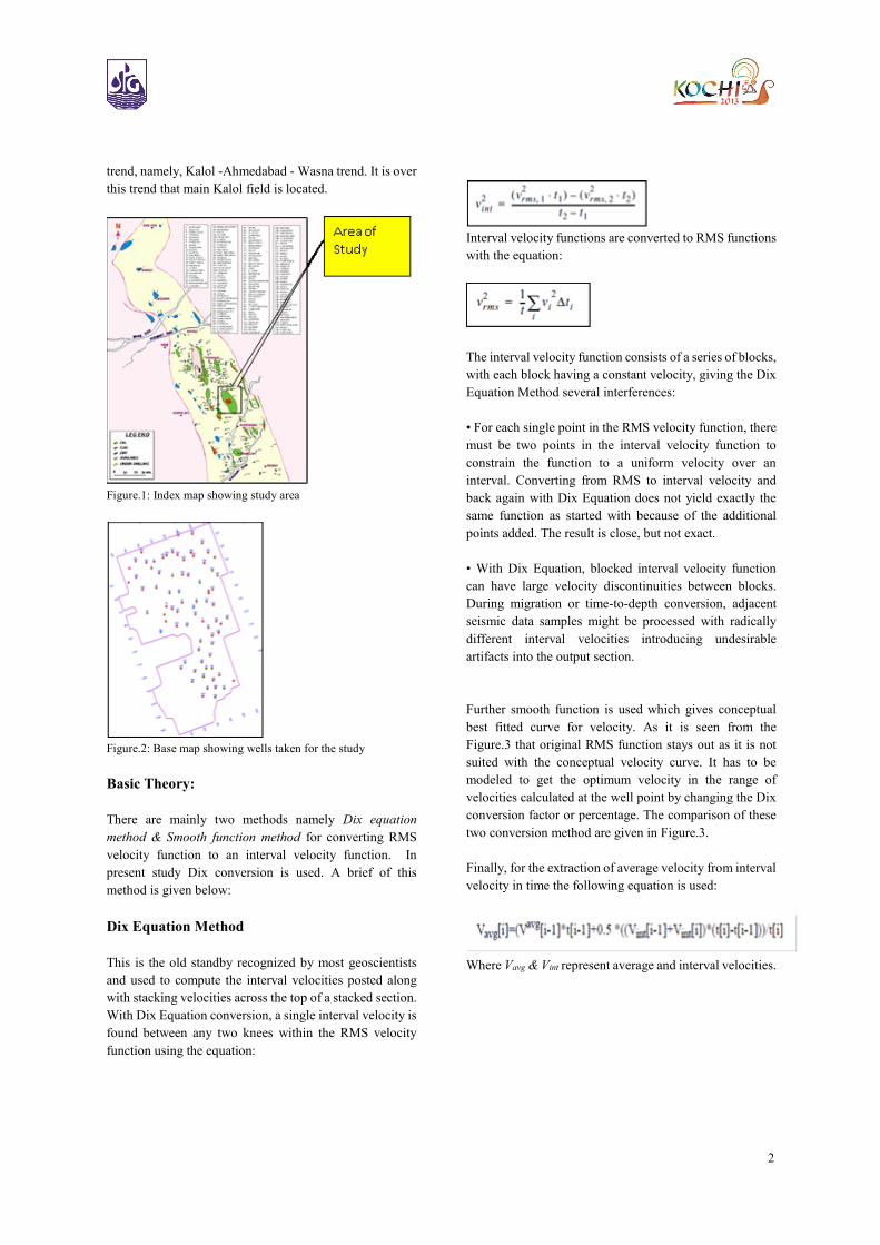
trend, namely, Kalol -Ahmedabad - Wasna trend. It is over

this trend that main Kalol field is located.

Figure.1: Index map showing study area

Figure.2: Base map showing wells taken for the study

Basic Theory:

There are mainly two methods namely Dix equation

method & Smooth function method for converting RMS

velocity function to an interval velocity function. In

present study Dix conversion is used. A brief of this

method is given below:

Dix Equation Method

This is the old standby recognized by most geoscientists

and used to compute the interval velocities posted along

with stacking velocities across the top of a stacked section.

With Dix Equation conversion, a single interval velocity is

found between any two knees within the RMS velocity

function using the equation:

Interval velocity functions are converted to RMS functions

with the equation:

The interval velocity function consists of a series of blocks,

with each block having a constant velocity, giving the Dix

Equation Method several interferences:

• For each single point in the RMS velocity function, there

must be two points in the interval velocity function to

constrain the function to a uniform velocity over an

interval. Converting from RMS to interval velocity and

back again with Dix Equation does not yield exactly the

same function as started with because of the additional

points added. The result is close, but not exact.

• With Dix Equation, blocked interval velocity function

can have large velocity discontinuities between blocks.

During migration or time-to-depth conversion, adjacent

seismic data samples might be processed with radically

different interval velocities introducing undesirable

artifacts into the output section.

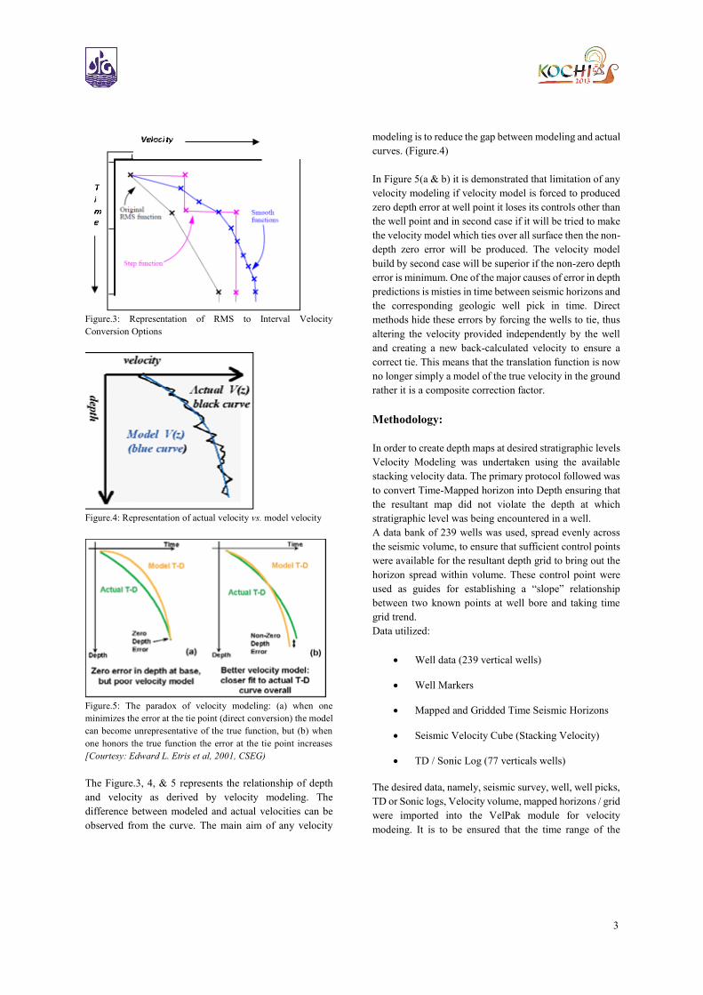
Further smooth function is used which gives conceptual

best fitted curve for velocity. As it is seen from the

Figure.3 that original RMS function stays out as it is not

suited with the conceptual velocity curve. It has to be

modeled to get the optimum velocity in the range of

velocities calculated at the well point by changing the Dix

conversion factor or percentage. The comparison of these

two conversion method are given in Figure.3.

Finally, for the extraction of average velocity from interval

velocity in time the following equation is used:

Where Vavg & Vint represent average and interval velocities.

3

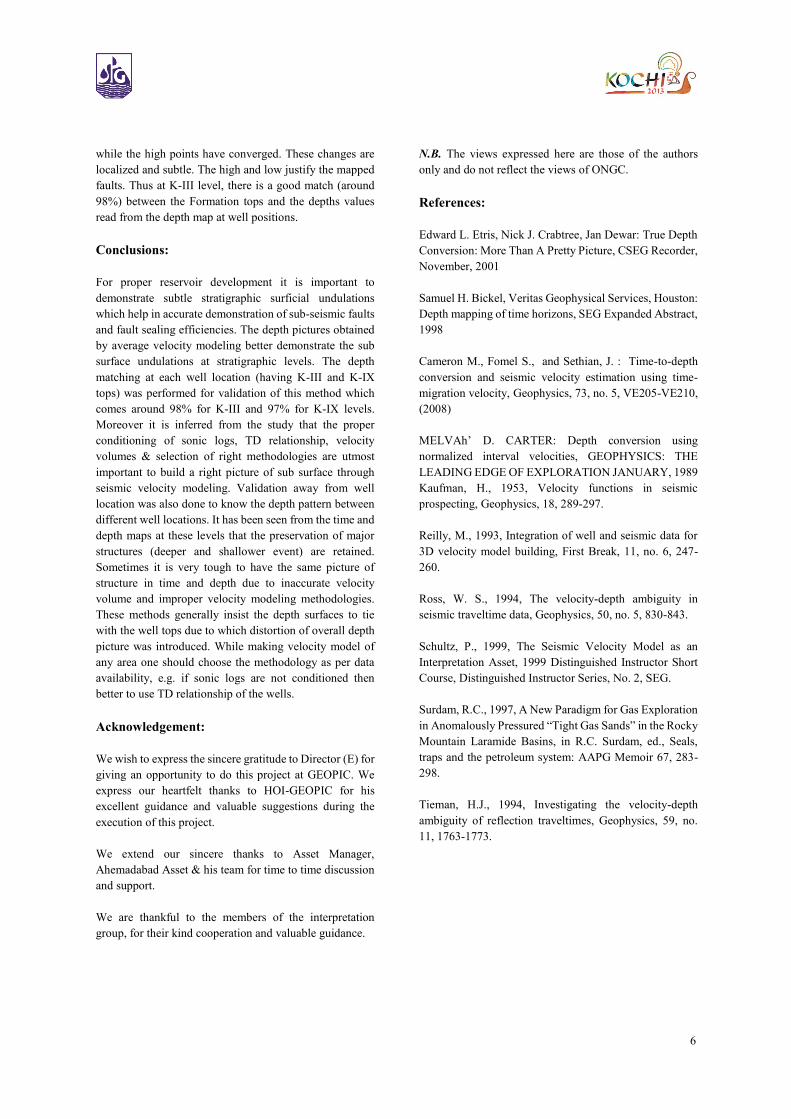
Figure.3: Representation of RMS to Interval Velocity

Conversion Options

Figure.4: Representation of actual velocity vs. model velocity

Figure.5: The paradox of velocity modeling: (a) when one

minimizes the error at the tie point (direct conversion) the model

can become unrepresentative of the true function, but (b) when

one honors the true function the error at the tie point increases

[Courtesy: Edward L. Etris et al, 2001, CSEG)

The Figure.3, 4, & 5 represents the relationship of depth

and velocity as derived by velocity modeling. The

difference between modeled and actual velocities can be

observed from the curve. The main aim of any velocity

modeling is to reduce the gap between modeling and actual

curves. (Figure.4)

In Figure 5(a & b) it is demonstrated that limitation of any

velocity modeling if velocity model is forced to produced

zero depth error at well point it loses its controls other than

the well point and in second case if it will be tried to make

the velocity model which ties over all surface then the non-

depth zero error will be produced. The velocity model

build by second case will be superior if the non-zero depth

error is minimum. One of the major causes of error in depth

predictions is misties in time between seismic horizons and

the corresponding geologic well pick in time. Direct

methods hide these errors by forcing the wells to tie, thus

altering the velocity provided independently by the well

and creating a new back-calculated velocity to ensure a

correct tie. This means that the translation function is now

no longer simply a model of the true velocity in the ground

rather it is a composite correction factor.

Methodology:

In order to create depth maps at desired stratigraphic levels

Velocity Modeling was undertaken using the available

stacking velocity data. The primary protocol followed was

to convert Time-Mapped horizon into Depth ensuring that

the resultant map did not violate the depth at which

stratigraphic level was being encountered in a well.

A data bank of 239 wells was used, spread evenly across

the seismic volume, to ensure that sufficient control points

were available for the resultant depth grid to bring out the

horizon spread within volume. These control point were

used as guides for establishing a “slope” relationship

between two known points at well bore and taking time

grid trend.

Data utilized:

Well data (239 vertical wells)

Well Markers

Mapped and Gridded Time Seismic Horizons

Seismic Velocity Cube (Stacking Velocity)

TD / Sonic Log (77 verticals wells)

The desired data, namely, seismic survey, well, well picks,

TD or Sonic logs, Velocity volume, mapped horizons / grid

were imported into the VelPak module for velocity

modeing. It is to be ensured that the time range of the

4

imported grid in VelPak matches with those in actual

interpretation. Later, Velocity Module is used for

displaying the staking velocities with respect to activated

grid. After this the staking velocities are converted to

interval velocities using the Dix Conversion. The resultant

Interval Velocity volume is used to extract average

velocity corresponding to active time grid in X,Y and Z

format where Z is the average velocity while X, Y are the

co-ordinates of Inline and Cross Line cross overs in the

active time grid. Validation of these average velocities at

well positions is shown in Fig.7.

These X, Y and Z values are gridded using available

gridding algorithms (Collocated co-kriging or global

method), during this procedure the corresponding Time

Grid is used as a Parent Grid which provides control trend

for the velocity gridding (Fig.13). This grid is further

validated at well point to have a better control for depth

conversion. Example of this validation is given at well

location ‘A’ in Fig.7. Later the depth conversion is done

using Simple Average Velocity method where above

gridded average velocities (Fig. 13) are used. This output

is used to produce Raw Depth Grid.

It is important to define the stratigraphic levels at which

the depth needs to be created. These layered definitions are

propagated at each of the chosen well to ensure uniformity

in establishing a time depth relationship (Fig. 8).

Figure.6: Process flow of velocity modeling considered for the

study

Prior to advancing in depth creation it is imperative to

establish a “Tie” between well picks / formation top and

Raw Depth Grid which will quantify the ‘mistie’ or the

‘error value’ at each well position (Fig. 8& 9). These error

values are further grided to generate error grid. This “error

grid”, linked to a particular stratigraphic level (Parent

Grid) is used to create Final Depth Grid by compensating

these error factor/ values in the Raw Depth Grid extracted

earlier (Fig.10).The Final Depth Grid, thus generated, is

exported to use for map generation purpose.

It is also advisable to export, independently, the error and

average velocity grid so that these too can be mapped for

the purpose of quality check.

Figure.7: Validation of gridded average velocity values

(extracted vs. actual)

Figure.8: Defining layers for calibration and tie processes

Figure.9: Calibration process with respect to K-III top

5

Figure.9: Tie process with respect to K-III top

Figure.10: Error grid generation and analysis

Figure.11: Time & Depth structure map at K-IX Top

Results & Discussions:

This is a case study and gives the practical approach for

velocity modeling which can be further utilized for time to

depth conversion.

Figure.12: Time & Depth structure map at K-III Top

The depth map of K-IX level has been created using well

tie with 184 wells of Kalol and Wadu fields (Fig.11).The

position of prominent high and lows remains intact but

there are places where the axis of the lows appears to have

slightly changed. The axis of low, located towards the

north eastern portion of the area, changes from E-W to

NNW-SSE. Within the large flat area occurring towards

central east portion of the map, few lows appear which

were not so clear in the time domain map. The high and

low justify the mapped faults. At K-IX level, there is a

good match (around 97%) between the Formation tops and

the depths values read from the depth map at well

positions. Thus the overall slope picture created on depth

matches with that observed in time.

Figure.13: Average velocity map at K-IX & K-III level

The depth map at K-III level has been created using 185

wells of Kalol and Wadu field which were falling within

the area (Fig.11). The time and depth map appear to be

quite similar and most of the geomorphic features

identified in time remain preserved in depth also. The axial

trends of features have maintained their azimuthal

relationship in time and depth. However at local levels

there are small pockets in which the lows have widened

6

while the high points have converged. These changes are

localized and subtle. The high and low justify the mapped

faults. Thus at K-III level, there is a good match (around

98%) between the Formation tops and the depths values

read from the depth map at well positions.

Conclusions:

For proper reservoir development it is important to

demonstrate subtle stratigraphic surficial undulations

which help in accurate demonstration of sub-seismic faults

and fault sealing efficiencies. The depth pictures obtained

by average velocity modeling better demonstrate the sub

surface undulations at stratigraphic levels. The depth

matching at each well location (having K-III and K-IX

tops) was performed for validation of this method which

comes around 98% for K-III and 97% for K-IX levels.

Moreover it is inferred from the study that the proper

conditioning of sonic logs, TD relationship, velocity

volumes & selection of right methodologies are utmost

important to build a right picture of sub surface through

seismic velocity modeling. Validation away from well

location was also done to know the depth pattern between

different well locations. It has been seen from the time and

depth maps at these levels that the preservation of major

structures (deeper and shallower event) are retained.

Sometimes it is very tough to have the same picture of

structure in time and depth due to inaccurate velocity

volume and improper velocity modeling methodologies.

These methods generally insist the depth surfaces to tie

with the well tops due to which distortion of overall depth

picture was introduced. While making velocity model of

any area one should choose the methodology as per data

availability, e.g. if sonic logs are not conditioned then

better to use TD relationship of the wells.

Acknowledgement:

We wish to express the sincere gratitude to Director (E) for

giving an opportunity to do this project at GEOPIC. We

express our heartfelt thanks to HOI-GEOPIC for his

excellent guidance and valuable suggestions during the

execution of this project.

We extend our sincere thanks to Asset Manager,

Ahemadabad Asset & his team for time to time discussion

and support.

We are thankful to the members of the interpretation

group, for their kind cooperation and valuable guidance.

N.B. The views expressed here are those of the authors

only and do not reflect the views of ONGC.

References:

Edward L. Etris, Nick J. Crabtree, Jan Dewar: True Depth

Conversion: More Than A Pretty Picture, CSEG Recorder,

November, 2001

Samuel H. Bickel, Veritas Geophysical Services, Houston:

Depth mapping of time horizons, SEG Expanded Abstract,

1998

Cameron M., Fomel S., and Sethian, J. : Time-to-depth

conversion and seismic velocity estimation using time-

migration velocity, Geophysics, 73, no. 5, VE205-VE210,

(2008)

MELVAh’ D. CARTER: Depth conversion using

normalized interval velocities, GEOPHYSICS: THE

LEADING EDGE OF EXPLORATION JANUARY, 1989

Kaufman, H., 1953, Velocity functions in seismic

prospecting, Geophysics, 18, 289-297.

Reilly, M., 1993, Integration of well and seismic data for

3D velocity model building, First Break, 11, no. 6, 247-

260.

Ross, W. S., 1994, The velocity-depth ambiguity in

seismic traveltime data, Geophysics, 50, no. 5, 830-843.

Schultz, P., 1999, The Seismic Velocity Model as an

Interpretation Asset, 1999 Distinguished Instructor Short

Course, Distinguished Instructor Series, No. 2, SEG.

Surdam, R.C., 1997, A New Paradigm for Gas Exploration

in Anomalously Pressured “Tight Gas Sands” in the Rocky

Mountain Laramide Basins, in R.C. Surdam, ed., Seals,

traps and the petroleum system: AAPG Memoir 67, 283-

298.

Tieman, H.J., 1994, Investigating the velocity-depth

ambiguity of reflection traveltimes, Geophysics, 59, no.

11, 1763-1773.