63

Q U A L I T É

GÉOPHYSIQUE APPLIQUÉE3Seismic tomography 5

M. Mendes

According to Wikipedia, “tomography is imaging by sections or sectioning, through the use of any kind of penetrating wave”. The apparatus applied in tomography is called a tomograph, while the image revealing the internal structure of an unknown property of the object under study is a tomogram.

Tomography was originally developed in medical research to produce images of tissue density (Hounsfield, 1973). In this type of tomography, the object (the patient) is moved through a large donut-shaped machine, where an X-ray beam and a set of electronic X-ray detectors are located opposite each other. The source and detectors are rotated around the target region, collecting the amount of radiation being absorbed throughout the patient’s body at many different angles (Goldman, 2007) (Figure 3.1).

This chapter of Seismic Imaging: a practical approach is published under Open Source Creative Commons License CC-BY-NC-ND allowing non-commercial use, distribution, reproduction of the text, via any medium, provided the source is cited.© EDP Sciences, 2019DOI: 10.1051/978-2-7598-2351-2.c005

64

Seismic Imaging

Figure 3.1 Geometry of a computed tomography scanner apparatus (third-generation). The emission of a large X-ray beam encompasses the entire patient’s width and the array of detectors measures the amount of radiation being absorbed throughout the patient’s body. X-ray tube and detectors were rigidly linked and underwent single rotational motion. Adapted from Goldman (2007).

The method has been successfully employed in many other scientific fields, such as biology, astrophysics, materials science and geophysics. In geophysics, seismic tomography is an effective technique for 2D, 3D and 4D reconstructions of the Earth’s subsurface, exploiting the properties of seismic wave energy after it has travelled through the ground. Such properties include travel time, ray paths and amplitude, which are an important key to reveal information about seismic veloc-ity, density, and absorption or the Q-factor attenuation of geological formations (Padina et al., 2006; Brzostowski and McMechan, 1992; Spakman et al., 1993; Witten et al., 1992).

Currently, seismic tomography is widely applied on a variety of scales and geometries:

• On regional and global scales, tomography inverts the seismic records generated by passive sources, such as natural or induced earthquakes, and those received by the seismograph network located around the world. Historically, seismic tomog-raphy was first applied to global scale data to study crustal velocity anomalies (Aki and Lee, 1976). The irregularity in time and space distribution presented by this type of source, along with the incomplete coverage of recording stations, leads to significant gaps in the data and limits the spatial resolution of global tomography to 100 - 200 Km.

• On the local scale, tomography is convenient for environmental or civil engi-neering investigations, economic exploration and archaeological research. The versatility of applying this technique to surface, vertical seismic profile (VSP) or cross-hole data makes it very popular, gaining widespread acceptance as a viable

65

3. Seismic tomography

tool to generate detailed geophysical models of the subsurface. However, higher spatial resolution requires greater computational effort, therefore, tomograms with high spatial resolution are limited to smaller scale data acquisitions, such as VSP and cross-hole, where the spatial resolution may reach less than 1 m.

Classically, depending on the input data, seismic tomographies fall into three main categories:

• transmission tomography using P or S first arrivals, i.e., direct, diving and refracted waves;

• reflection tomography using P or S reflection waves;• diffraction tomography using P or S scattered waves (e.g., diffractions, reflec-

tions, and converted transmissions).

In the following sections, we present some field study examples of each tomography category to show the adaptability of the technique to provide subsurface images in different applications. The intention here is not to describe the field cases in detail, but to provide some background information and the main model features identi-fied from the tomography.

The authors emphasize that although a different type of acquisition geometry was chosen for almost every tomography category described below, this by no means implies that these geometries are restricted only to these acquisition types.

3.1 Transmission tomography example: surface seismic field data

Transmission tomography is an appropriate technique to define:

• horizontal layering structures;• regions exhibiting low complexity velocity distributions.

This section shows:

• how to obtain a P-wave velocity model from first arrival times;• how to evaluate the spatial (horizontal and vertical) resolution for the tomo-

grams.

A transmission tomographic technique was used to invert a 3D seismic data set, part of a more comprehensive geophysical survey conducted in a karstified dolos-tone region, to provide information about the upper epikarst structure. The selected field example comes from Galibert et al. (2014).

66

Seismic Imaging

3.1.1 Geophysical survey

The acquisition procedures were optimized to obtain the best results with a high acquisition speed and a high resolution. For a seismic survey this involves high folds and wide azimuthal coverage.

A three-member crew was required, working for two and a half days, to acquire:

• 3D surface seismic survey, extended for about 120 × 100 m;• 2D surface seismic line, 235 m long;• Walkaway VSP, 50 m depth;• GPS surveying.

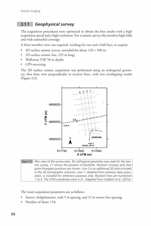
The 3D surface seismic acquisition was performed using an orthogonal geome-try, shot lines were perpendicular to receiver lines, with two overlapping swaths (Figure 3.2).

Figure 3.2 Plan view of the survey area. 3D orthogonal geometry was used for the seis-mic survey, C1 shows the position of borehole. Receiver (crosses) and shot point (triangles) positions are shown. Line 3 is an additional 2D shot included in the 3D tomographic inversion. Line 1, obtained from previous data acqui-sition, is included for reference purposes only. Receiver lines are numbered 1 to 4. The UTM coordinate zone is 31. Adapted from Galibert et al. (2014).

The main acquisition parameters are as follows:

• Source: sledgehammer, with 5 m spacing, and 15 m source line spacing;• Number of shots: 154;

67

3. Seismic tomography

• Receiver: vertical geophone, Oyo GS-14 Hz, with 5 m spacing, and 10 m receiver line spacing;

• Number of receiver lines: 3;• Seismograph: 96 channels;• Record length: 1 second;• Swaths: 1 using receiver lines 1-3; 2 using receiver lines 2-4.

3.1.2 Tomographic methodology

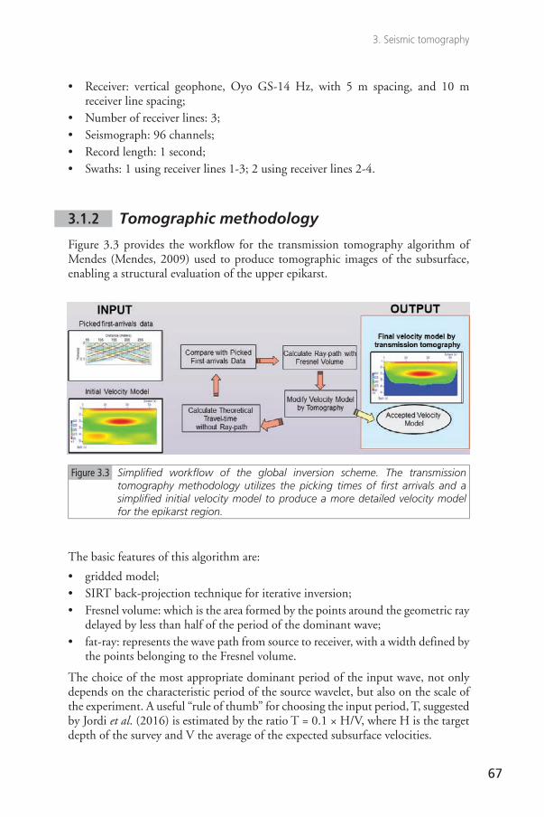
Figure 3.3 provides the workflow for the transmission tomography algorithm of Mendes (Mendes, 2009) used to produce tomographic images of the subsurface, enabling a structural evaluation of the upper epikarst.

Figure 3.3 Simplified workflow of the global inversion scheme. The transmission tomography methodology utilizes the picking times of first arrivals and a simplified initial velocity model to produce a more detailed velocity model for the epikarst region.

The basic features of this algorithm are:

• gridded model;• SIRT back-projection technique for iterative inversion;• Fresnel volume: which is the area formed by the points around the geometric ray

delayed by less than half of the period of the dominant wave;• fat-ray: represents the wave path from source to receiver, with a width defined by

the points belonging to the Fresnel volume.

The choice of the most appropriate dominant period of the input wave, not only depends on the characteristic period of the source wavelet, but also on the scale of the experiment. A useful “rule of thumb” for choosing the input period, T, suggested by Jordi et al. (2016) is estimated by the ratio T = 0.1 × H/V, where H is the target depth of the survey and V the average of the expected subsurface velocities.

68

Seismic Imaging

3.1.3 Data pre-processing

Typical shot-gathers and first arrival picking is shown in Figure 3.4.

Figure 3.4 Example of two parallel shot-gathers. The picked first arrivals at receiver line 2 are marked with a dashed line, and at receiver line 4 with a solid line.

The first-break times were picked manually, and their reliability was carefully analyzed for plausibility and erroneous travel times.

Figure 3.5 Travel time azimuthal variations. Estimated refractor velocity at the base of the epikarst from surface receivers; the solid line is the fitted azimuthal model. Adapted from Galibert et al. (2014).

69

3. Seismic tomography

The picked travel times were used to compute the refractor velocity at the base of the epikarst. It was noted that the values change between 2,000 m/s and 3,200 m/s, with a clear azimuthal variation, being the strike of the fast axis around 175°N (Figure 3.5).

Despite the azimuthal variation of velocity, for simplicity, an initial 1D velocity model, with linear velocity gradients, was considered adequate for the tomographic inversion.

Then, the input data were:

• 7,813 first-break times;• 1D model with 2 linear vertical velocity gradients;• 100 Hz central signal frequency.

3.1.4 Results and discussion

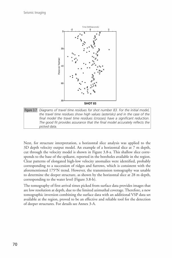
The processing of seismic data led to a 3D velocity block. The inversion scheme was stopped after 10 iterations, when the misfit function reached 1.69 ms for the root-mean-squared (rms) error, i.e., the squared difference between measured and calculated travel times. An example describing the quality control of the inversion results is specified for shot number 83. Figure 3.6 shows three travel time sets: a) the picked times of field data; b) computed times for the initial model; and the times for the best model provided by the tomographic inversion. The evolution of travel time residues, during velocity model building, is illustrated in Figure 3.7. Note the significant reduction of travel time differences, showing a good tie between the picked and best model data. This provides assurance that the final model accurately reflects the field data.

Figure 3.6 Diagrams of travel times for shot number 83. The picked times of field data (black triangles), travel times for initial model (asterisks) and travel times for a model provided by iteration 10 (crosses).

70

Seismic Imaging

Figure 3.7 Diagrams of travel time residues for shot number 83. For the initial model, the travel time residues show high values (asterisks) and in the case of the final model the travel time residues (crosses) have a significant reduction. The good fit provides assurance that the final model accurately reflects the picked data.

Next, for structure interpretation, a horizontal slice analysis was applied to the 3D depth velocity output model. An example of a horizontal slice at 7 m depth, cut through the velocity model is shown in Figure 3.8-a. This shallow slice corre-sponds to the base of the epikarst, reported in the boreholes available in the region. Clear patterns of elongated high-low velocity anomalies were identified, probably corresponding to a succession of ridges and furrows, which is consistent with the aforementioned 175°N trend. However, the transmission tomography was unable to determine the deeper structure, as shown by the horizontal slice at 28 m depth, corresponding to the water level (Figure 3.8-b).

The tomography of first arrival times picked from surface data provides images that are low resolution at depth, due to the limited azimuthal coverage. Therefore, a new tomographic inversion combining the surface data with an additional VSP data set available at the region, proved to be an effective and reliable tool for the detection of deeper structures. For details see Annex 3-A.

Time (Milliseconds)

71

3. Seismic tomography

a)

Figure 3.8 Constant-depth velocity slices from 3D tomography output, presenting notice-able differences: (a) The depth-slice at 7 m, corresponding to the base of the epikarst, exhibits high-low elongated patterns in 175°N; (b) The depth-slice at 28 m, contrasting with the shallow complexity, is characterized by a very poor resolution (high and homogeneous velocity). Adapted from Galibert et al. (2014).

3.1.5 Conclusions

This example showed the successful application of a transmission tomography algo-rithm to uncover the shallow complex structures at a karst region. A set of elongated furrows incised at the base of the epikarst, along a strike of 175°, were revealed. The limited azimuthal coverage obtained from the surface acquisition data limited the depth of the investigation. To increase the depth of the analysis, a combination of borehole acquisitions is suggested.

In general, transmission tomography enables the velocity of subsurface structures to be obtained, containing smooth information on a large scale, which is an essential component for pre or post-stack seismic migrations or inversion techniques.

Annex 3-A

The limits of spatial resolution can be estimated according to the formula suggested by Sheng and Schuster (2003)

∆xki

f xip( ) ≈ ( )

πηmax ,

, (3.1)

with k s p p rxi xi xi= ∇ ( ) + ∇ ( )[ ]ω τ τ, , , (3.2)

where Δxi (p) indicates the resolution limit for the direction i, kxi denotes the hori-zontal wavenumber at maximum frequency f, ∇xi τ (r1, r2) is the horizontal gradient

Slice at depth 7 m (base of epikarst)

Slice at depth 28 m, abc

72

Seismic Imaging

of travel time from point r1 to point r2, and η stands for the set of suitable rays selected from all available shots.

In the example presented here, only the horizontal resolution is considered and discussed.

Our first step was the analysis of the Fresnel zone for a frequency of 120 Hz, with a surface acquisition and velocity gradient model characteristic of the karst region (Figure 3.A.1-a).

We noted that:

• in the shallow area - wave paths are nearly vertical and provide large horizontal wavenumbers, by combining neighbouring shots, leading to small Δx values => high horizontal resolution (≈ 1.5 m);

• in the deeper area - wave paths are nearly horizontal and provide small hori-zontal wavenumbers for all shots, leading to large Δx values => low horizontal resolution (≈ 10 m).

Figure 3.A.1 Horizontal resolution Δx of band limited travel time tomography: (a) for surface acquisition, (b) for borehole acquisition. The contours represent the background velocity gradient. Inside the Fresnel volume, there is no resolution at all along the geometrical ray (white area), according to wave path theory. Resolution increases toward the fringes (dark area). Adapted from Galibert et al. (2014).

These very different limits of spatial resolution demonstrate the capacity of the technique, as shown by the surface acquisition data, for investigating the upper epikarst; but its unsuitability for the underlying low-permeability region.

To overcome this issue, an additional VSP acquisition was suggested to increase the azimuthal coverage with depth. Under such acquisition conditions, the analysis of the Fresnel zone (Figure 3.A.1- b) illustrates how the wave path is nearly vertical and the horizontal cross width of the low-sensitivity region becomes narrow. Therefore, in situations where it is possible to combine surface and borehole acquisitions, the tomographic resolution should be substantially improved.

73

3. Seismic tomography

For this reason, we repeated the tomographic inversion using both surface and VSP data. The result presented in Figure 3.A.2 revealed some significant veloc-ity anomalies, which can be compared with the homogenous velocity presented in Figure 3.8-b.

Figure 3.A.2 A horizontal slice at 28 m depth taken at the 3D velocity cube produced by tomography when combining seismic surface and VSP data. Now, the model is characterized by velocity anomalies contrasting with the high homogeneous velocity and very poor resolution produced by the tomo-graphic inversion of the surface data (Figure 3.8-b). Adapted from Galibert et al. (2014).

3.2 Reflection tomography example: cross-hole field data

It has been demonstrated that reflection tomography is an appropriate technique for building a good velocity model of subsurface structures based on multichannel seismic data.

This section describes the use of a reflection tomography procedure to image a limestone reservoir at a depth of about 1,850 m, utilizing the information present in the travel time of reflected S-waves. These data were recorded during a cross-hole seismic experiment, carried out in the Paris basin. The data processing sequence is detailed in Becquey et al. (1992).

74

Seismic Imaging

3.2.1 Seismic survey

In general, a typical cross-hole seismic profile has sources situated in one borehole and receivers in another, with the source and receiver boreholes being separated by a distance of up to 1 km.

For this study, the seismic source was wall-clamped in a vertical borehole and the receivers in a deviated borehole. The distance between the two boreholes increased from 30 m at the surface to 380 m at the reservoir level, located at a depth of 1,850 m. Both boreholes were cased with a 7-inch casing.

The total recording time was 40 hours and the whole operation, which involved more than 3,000 shots and the removal and resetting of the tubing, took one week.

The principal parameters of this data acquisition were:

• Source: S-wave weight-drop, releasing ≈ 2,000 joules/shot, 4 m spacing between 1,314 - 1,916 m in vertical depth;

• 8 shots/position;• 400 shot positions;• Receiver: Multilock™ tool with 4 levels and triaxial geophones, 4 m spacing

between 1,620 - 1,916 m in logging depth.

For promoting the S-wave conversions two conditions were combined:

• source directivity pattern diagram with a strong S lobe perpendicular to the borehole;

• acquisition geometry designed to explore the wide angles of incidence.

Figure 3.9 shows the multicomponent raw data with complex arrivals.

Figure 3.9 Raw data. PZ component along the borehole axis. H1 and H2 perpendicular to the borehole axis. Adapted from Becquey et al. (1992).

75

3. Seismic tomography

3.2.2 Data processing

Only two preprocessing steps were applied to the multicomponent data set, namely:

• a bandpass filter (20-120 Hz);• a re-orientation following the projection along the source-receiver direction R,

its normal in the source-receiver plane N and the binormal B, orthogonal to the source-receiver plane.

We noted that the component R (Figure 3.10) contains clear direct down-going P-waves, followed by up-going S-wave reflections. The component N has obvious down-going S waves, appearing as a train of quasi-parallel events spread over about 150 ms.

Figure 3.10 Filtered and reoriented data. R component along the source-receiver direc-tion; N component perpendicular to R, in the source-receiver plane; B com-ponent, orthogonal to R and N, so normal to the source-receiver plane. Adapted from Becquey et al. (1992).

The imaging from the cross-hole data set was inspired from a traditional offset VSP. Therefore, based on other previous VSP data acquisitions of P and S-waves at the vertical borehole, a velocity-depth model was built and used by the VSP-CDP time technique to transform the S-S reflected data (Figure 3.11). More details on the VSP-CDP time technique are available in chapter 2 of “Well seismic surveying and acoustic logging” (J.-L. Mari and C. Vergniault, 2018).

76

Seismic Imaging

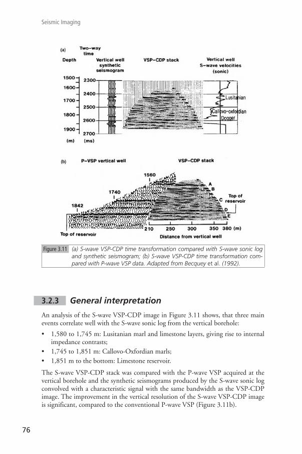
Figure 3.11 (a) S-wave VSP-CDP time transformation compared with S-wave sonic log and synthetic seismogram; (b) S-wave VSP-CDP time transformation com-pared with P-wave VSP data. Adapted from Becquey et al. (1992).

3.2.3 General interpretation

An analysis of the S-wave VSP-CDP image in Figure 3.11 shows, that three main events correlate well with the S-wave sonic log from the vertical borehole:

• 1,580 to 1,745 m: Lusitanian marl and limestone layers, giving rise to internal impedance contrasts;

• 1,745 to 1,851 m: Callovo-Oxfordian marls;• 1,851 m to the bottom: Limestone reservoir.

The S-wave VSP-CDP stack was compared with the P-wave VSP acquired at the vertical borehole and the synthetic seismograms produced by the S-wave sonic log convolved with a characteristic signal with the same bandwidth as the VSP-CDP image. The improvement in the vertical resolution of the S-wave VSP-CDP image is significant, compared to the conventional P-wave VSP (Figure 3.11b).

77

3. Seismic tomography

3.2.4 Conclusions

A good agreement was obtained between the S-wave image and the S-wave sonic log, furthermore the enhanced S-wave reflection image revealed high vertical resolu-tion, approximately 5 m, and allowed imaging of the region between two boreholes, nearly 400 m away from the borehole.

This field experiment also demonstrated that the conventional borehole seismic receiver tools and the low-energy sources are well suited to obtain high-resolution lithological structure delineation.

3.3 Diffraction tomography example: Borehole field data

Exploiting amplitude information in addition to arrival times, the diffraction tomography schemes are the most suitable to interpret the propagation of recorded seismic data through complex velocity structures.

Diffraction tomography algorithms are available:

• in the spatial domain and based on the Born approximation, most suited for the primary reflected or diffracted part of the wave field;

• in the wavenumber domain and based on the Rytov approximation, most suited for the transmitted wave field.

This section shows:

• how to obtain elastic depth images (P and S-wave velocities and density) from P-P or S-S and P-S or S-P reflected and diffracted waves;

• how to evaluate the elastic image confidence.

We adopted the diffraction tomography algorithm developed by Beydoun and Mendes (1989) for the following depth imaging examples. This imaging technique, based on the Born approximation, uses a one-step conditioned gradient technique for optimization and is equivalent to an elastic pre-stack migration.

The procedure requires the following input data:

• gridded model defined for 3 elastic parameters (P and S-wave velocities and density), close to the actual medium;

• elastic ray-Born approximation;• multi-component field data, with scattered waves (diffracted and reflected body

waves).

And the provided output data are:

• quantitative elastic depth images.

78

Seismic Imaging

3.3.1 Vertical seismic profile (VSP) field data

This example describes the processing of a multicomponent offset VSP dataset, collected in the North Sea. The purpose of this survey was to detect fault blocks at the deep Brent reservoir formation, thicker than 150 m. The reservoir is located in the Middle Jurassic Brent formation, positioned under the Cimmerian unconform-ity (3,558 m) at the boundary between the base of the Lower Cretaceous and the top of the Upper Jurassic. An analysis of the VSP tomograms enabled the deline-ation of the reservoir and the identification of at least two faults. Beydoun et al. (1990), provide details of this application.

3.3.1.1 Seismic data acquisition

Surface seismic data acquisition carried out previously in this area had failed to provide good quality imaging of the Brent reservoir. In particular, the strong multi-ples generated at the Cimmerian unconformity masked the weak primary reflections from the reservoir. To improve the quality of the seismic results and considering the surface data information, a multi-component offset VSP set up was performed with the following characteristics:

Source:

• 2 x 200 in2 Bolt air guns (on a supply boat);• depth 7 m;• offset: 1,200 m;• 6 shots per level (i.e., at each receiver location).

Receiver:

• 3 component Geolock H3 hydraulic tool (from CGG);• Geophones:15 Hz;• sampled rate: 2 ms;• station interval: 25 m;• depth range: 600 – 4,140 m;• number of depth levels: 129.

A zero offset VSP was simultaneously acquired, shooting alternatively from the supply boat and from the rig, which had a 550 in2 Bolt air gun attached.

The VSP survey recording time was 27 hours, while rig down time was 28 hours.

3.3.1.2 Data Processing

The main focus of data preprocessing was to preserve the seismic wave amplitude. For such preprocessing, it was sufficient to only apply a few steps, which were:

• the reorientation of the three-component data along Z the vertical axis, X the axis in the plane of propagation, and Y the transverse (out of plane) horizontal axis;

79

3. Seismic tomography

• the separation of up-going and down-going P-waves and S-waves;• the recombination of P-P and P-S up-going waves for the X and Z-components.

The following points were noted after the analysis of the processed data (Figure 3.12):

• Y-component data present very weak energy compared with that of X and Z-components. For simplicity, this component was disregarded in further pro-cessing;

• weak up-going S-P and S-S waves;• strong reflected P-P and P-S waves;• some hyperbolic-shaped arrivals, probably due to fault diffractions (see at

4,000 m; 1,700 ms).

Figure 3.12 Two-component (X, Z) VSP field data input to diffraction tomography. The Y-component was disregarded due to its weak energy. Adapted from Beydoun et al. (1990).

3.3.1.3 Diffraction tomography processing

In this example, the imaging technique deals with the processed X and Z-components of the data, mainly consisting of up-going P-P and P-S waves. The 1D initial elastic model (P and S-wave velocities and density) was created by the combination of geological and geophysical information available for the region.

The target zone, covering the reservoir area, is a rectangle extending from 50 m to 550 m east of the borehole with depths from 3,400 m to 4,400 m, discretized by a uniform square grid of 10 x 10 m.

The selected field data were 86 VSP levels, ranging from depths of 2,000 – 4,150 m within a time window of 1,400 – 3,400 ms.

80

Seismic Imaging

3.3.1.4 Depth elastic images and general discussion

The diffraction tomography provided an estimation of the elastic parameters, P and S-wave velocities, and density, as illustrated in Figure 3.13. These results enabled the identification of several interesting features that were interpreted as:

• the top of the Brent reservoir, which can be delineated and described continu-ously away from the borehole;

• tilted panels under the Cretaceous base discordance - Cimmerian unconformity, at depth of 3,558 m.

• a reverse fault at 250 m east of the borehole, with an apparent throw < 30 m, unclear whether it reaches the reservoir;

• a normal fault about 450 m east of the borehole with an apparent throw ≈ 60 m, intersects the reservoir at about 350 m offset;

• an event at depth ≈ 3,850 m, slightly dipping to the west, which was interpreted to be the Heather sandy claystone formation.

Figure 3.13 Elastic depth images (P and S-wave velocities and density) of VSP field data of Figure 3.12. The initial input model is at the left of each image. The Brent reservoir and two fault locations were successfully interpreted. Adapted from Beydoun et al. (1990).

The quality control of the elastic depth images is given by the goodness of fit between synthetic and field data sets. Therefore, Figure 3.14 illustrates the synthetic

81

3. Seismic tomography

seismograms computed with the elastic images provided by the tomography, and in Figure 3.15 the residual data, i.e. the difference between field and computed seismograms. There is observable evidence of some major P-P and P-S events in the field data also present in the synthetic seismograms. The underlined P upgo-ing arrival (on the Z-component) and S upgoing arrival (on the X-component) are particularly recognizable, see Figures 3.12 and 3.15.

Figure 3.14 Two-component (X, Z) synthetic VSP using P-P and P-S scattered waves from elastic images in Figure 3.13. Adapted from Beydoun et al. (1990).

Figure 3.15 Residual data (i.e., the difference between the data in Figures 3.12 and 3.14). The box represents the part of the data covered by the rectan-gular area under study. The comparison between the black underlined P upgoing arrival (on the Z-component) along with the S upgoing arrival (on the X-component) in Figure 3.12, with those of this figure confirms the high quality of the tomography. Adapted from Beydoun et al. (1990).

82

Seismic Imaging

3.3.1.5 Conclusions

This diffraction tomography approach produced high-resolution 2D depth elastic models from offset VSP data, collected in the North Sea. The images reveal several geological and geomorphological features that had previously been undetected or poorly mapped by other surface seismic acquisitions.

The study has shown that the diffraction tomography technique is practical, effi-cient and particularly suitable for depth imaging of complex geological systems.

3.3.2 Cross-hole field data

The second diffraction tomography example is aimed at handling acoustic and multicomponent borehole data collected at two different boreholes, located in the Paris basin. High-resolution tomograms were produced, allowing the identification of three near-surface hydrocarbon reservoirs with thicknesses of between 2–5 m. The reservoirs are separated by a set of north-south faults with east dips and throws in the order of 30-40 m, consisting of three sand levels imbedded in shales, and depths of between 575-600 m.

Beydoun provides a more detailed processing and interpretation of these data (Beydoun et al., 1989).

3.3.2.1 Field parameters

An oil field test site was constructed in the Paris basin, an area in which the geology is well known from previous well logs and seismic studies.

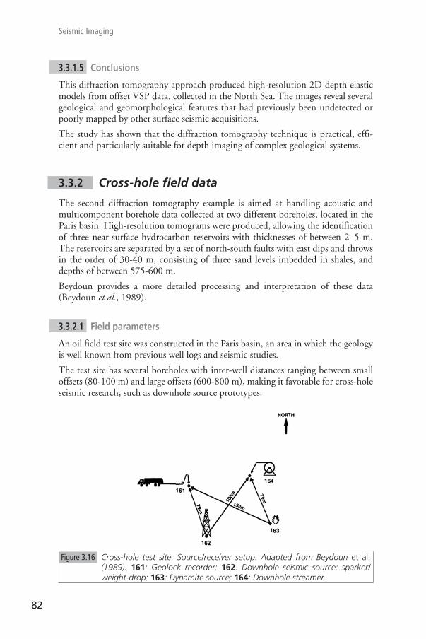
The test site has several boreholes with inter-well distances ranging between small offsets (80-100 m) and large offsets (600-800 m), making it favorable for cross-hole seismic research, such as downhole source prototypes.

Figure 3.16 Cross-hole test site. Source/receiver setup. Adapted from Beydoun et al. (1989). 161: Geolock recorder; 162: Downhole seismic source: sparker/weight-drop; 163: Dynamite source; 164: Downhole streamer.

83

3. Seismic tomography

For the purposes of this study, four cased 7-inch diameter boreholes were available (Figure 3.16) and a prototype weight drop downhole source was tested, designed at the Institut Français du Pétrole (IFP). A diagram showing the principle and mechanism of this downhole weight-drop source, which generates P and S-waves, is shown in Figure 3.17.

Figure 3.17 Principle and mechanism of the downhole weight-drop source developed at the Institut Français du Pétrole (IFP). Adapted from Beydoun et al. (1989).

The seismic source was deployed with drill strings in borehole 162 and wall-clamped at depth 455 m, the firing position, with a packer (Brown 7 inches, type MI) which locked and unlocked to the hole through the tool’s rotation. The loading of the source (lifting of the mass) is carried out with the drill strings, the weight is then dropped automatically, hitting an anvil bound to the packer.

The seismic data were recorded simultaneously in borehole 164 with a vertical hydrophone streamer and in borehole 161 with a three-component geophone tool.

The basic acquisition tools were as follows:

– Source in borehole 162:• weight-drop, generating mainly S-waves perpendicular to the borehole;• 3,000 joules/shot;• 2 shots/minute capability;• depth = 455 m;

– Receivers in borehole 164:• vertical hydrophone streamer not anchored, thus highly sensitive to tube waves;• band range 10-5,000 Hz;

84

Seismic Imaging

• 48 channels;• 1 m spacing.

– Receivers in borehole 161:• triaxial geophone tool (Geolock H, CGG VSP tool) anchored, thus less sen-

sitive to tube waves;• band range 10-150 Hz.

3.3.2.2 Seismic data

It should be noted that the hydrophones recorded the pressure disturbance in the borehole fluid and the geophones the vector wave field at the borehole wall, since the shot was simultaneously recorded by two receiver tools with sensitivity to differ-ent physical quantities.

Figure 3.18 (a) shows the hydrophone data, dominated by down-going S waves, S-S and S-P reflections; while P-P and P-S reflections are absent.

Figure 3.18 Hydrophone data. (a) Showing the different seismic arrivals in the raw data after tube-wave filtering. Note the absence of P-P and P-S reflections and the presence of strong down-going S-wave arrivals. (b) Subset data used as input data for the tomography. Adapted from Beydoun et al. (1989).

85

3. Seismic tomography

This is due to:

• the pattern radiation of the source having a strong S lobe perpendicular to the borehole;

• the acquisition geometry with large angles of incidence, favouring the shear-wave conversions.

The acquired data were processed with tube-wave filter removal, down-wave field separation and band-pass filters (40-60-300-450) Hz. Figure 3.18 (b) shows a subset of processed data.

Figure 3.19 shows the raw geophone data after rotation from (H1, H2) directions to (X, Y) directions, where X is the horizontal axis in the acquisition plane and Y is the transverse (out-of-plane) direction.

(a) (b)

Figure 3.19 Geophone data: Z-component (upper) and X-component (lower). (a) Raw data after reorientation (X, Y). (b) After down-wave field separation and used as input data for the tomography. Adapted from Beydoun et al. (1989).

Given that seismic wave amplitude and travel time information are both used in the inversion algorithm, for a successful solution it is fundamental that careful data pre-processing is carried out to preserve both amplitude and travel time parameters.

The pre-processing steps for both datasets were similar:

• least-squares approach in the frequency and depth domains to estimate simul-taneously the up and down-going tube waves by minimizing the separation residual;

• residual waves were filtered by similar processing to eliminate only down-going P and S-waves;

• only upgoing S-S and S-P reflected events are used for the tomography;

86

Seismic Imaging

• band-pass filtered; hydrophone data (40-60-300-450) Hz; geophone data (6-12-150-200) Hz;

• no deconvolution;• 3D to 2D amplitude correction, i.e., √t multiplicative amplitude correction to

compensate for the transverse (out of plane) spreading.

3.3.2.3 Initial model

The starting model for the tomographic inversion was defined by integrating cross-hole data with log information from the three holes, and VSP information on P and S-waves in borehole 161. Unfortunately, a shear-wave sonic log was not available, because S-waves, being slower than Stoneley waves, were masked. The density infor-mation was obtained from a compensated formation density (FDC) log in bore-hole 164. An elastic 1D velocity-depth model was used as background (Figure 3.20) with the P/S-wave velocity ratio constant (equal to 1.9) at the reservoir area.

Figure 3.20 Initial elastic 1D model. Adapted from Beydoun et al. (1989).

3.3.2.4 Depth elastic images: comparison with density log

In this field example, given that P-P scattered waves are not visible in the data and only up-going S-S and S-P scattered waves have enough energy, then P-wave imag-ing is not possible and only two images, S-wave velocity and density images, could be generated.

87

3. Seismic tomography

The diffraction tomography applied to the single-shot geophone data has a target zone, which encloses the reservoir area near the receiver borehole (161), and is defined as follows:

• from 40 to 75 m away from the emitter borehole (162) to the receiver bore-hole (161);

• depth interval 475-625 m.

Since the tomography technique produces reliable estimates of changes in elastic parameters only when the source and receiver coverage is satisfactory, then the upper part of the elastic images (above 560 m) should not be interpreted due to insufficient coverage (Figure 3.21). In the lower right portion of the images (below 560 m), source and receiver coverage is very good (maximum coverage), so a confi-dence region can be defined here in the target zone.

The target zone for the single-shot hydrophone data, which encloses the reservoir area near the receiver borehole (164), is defined as follows:

• from 50 and 86 m away from the emitter borehole (162) to the receiver bore-hole (164);

• depth interval 500-650 m.

In spite of the different nature of both geophone and hydrophone data (parti-cle velocity and pressure), in coupling with the formation (clamped geophone versus hydrophone string), and spatially (holes 161 and 164), a good correlation between the images is observed. Furthermore, the three reservoir levels, R3=575 m, R2=583 m, and R1=600 m, can be identified.

In both boreholes, the density tomograms were assessed in a practical manner, by carrying out a comparison between the density images with a pseudo-density log. The density logs were convolved with a characteristic signal matching the frequency bandwidth of the density tomogram. Therefore, the results could be compared directly to identify similarities and differences to aid in interpretation.

In borehole 164, an FDC log was used, which verifies a good correlation between the two independent sets of density information.

In borehole 161, a density log was generated from a combination of gamma-ray, neutron-porosity, and the sonic logs from this borehole, and the density log of borehole 164.

The tomography of hydrophone data produced a better and cleaner density tomo-gram than the geophone data image. Comparison of the images from both data sets revealed a vertical resolution of the geophone data image that is lower than that of the hydrophone data. This also fits with differences in signal bandwidth, 150 Hz versus 350 Hz. However, the fit at the Lower Hauterivian level, around R1= 600 m, seems reasonable.

Since the thicknesses of these reservoirs are of the order ≈ 3 m, the very limit of seismic resolution, it is difficult and delicate to attempt any detailed interpretation within each reservoir level, especially with only one-shot record.

88

Seismic Imaging

Figure 3.21 Density logs, band-pass filtered density logs, and elastic depth migration images (density) of geophone and hydrophone data. Note the strong and different image artifacts on the upper portion of both images (above 560 m) due to insufficient source and receiver coverage of this region. Within the reservoir area, the density image from the hydrophone data corresponds closely to the filtered log from borehole 164. Adapted from Beydoun et al. (1989).

3.3.2.5 Conclusions

The diffraction tomography approach, even using only a one-shot cross-hole acous-tic (hydrophone) dataset, or a multicomponent (geophone) field dataset, proved successful in producing high-resolution (≈ 3-5 m) density tomograms for the inter-well region. These tomograms are in close agreement with regional geology and density borehole logs.

89

3. Seismic tomography

3.4 General conclusion

This chapter, supported by several seismic field data examples, demonstrates the possibility of imaging the subsurface structures with seismic tomography.

Seismic tomography is able:

• to handle acquisitions of various scales and geometries;• to handle single or multi-component data;• to handle direct, reflected or diffracted P or S-body waves;• to produce high-resolution depth or time images;• to provide confidence criteria for the resulting tomogram.

The main requirements for seismic tomography to build reliable images are:

• high fold coverage;• large azimuthal coverage;• data that preserves travel times and amplitudes;• an initial model (P and/or S-wave velocity and density) that adequately repre-

sents the main subsurface features.• low or moderate computational effort.

These tomograms may provide useful input data for further processing as pre or post-stack seismic migrations or for full waveform inversion techniques.

References

Aki K., Lee W.H.K., 1976, Determination of the three-dimensional velocity anom-alies under a seismic array using first P arrival times from local earthquakes 1. A homogeneous initial model, J. Geophys. Res. 81, 4381-4399.

Becquey M., Bernet-Rollande J.O., Laurent J., Noual G., 1992, Imaging reser-voirs - a crosswell seismic experiment, First Break, 10 (9), 337.

Beydoun W.B., Mendes M., Blanco J., Tarantola A., 1990, North Sea reservoir description: Benefits of an elastic migration/inversion applied to multicompo-nent vertical seismic profile data, Geophysics, 55 (2), 209-217.

Beydoun W.B., Mendes M., 1989, Elastic ray-Born K2-migration/inversion, Geophys. J. 97, 151-160.

Beydoun W.B., Delvaux J., Mendes M., Noual G., Tarantola A., 1989, Practical aspects of an elastic migration/inversion of crosshole data for reservoir charac-terization: A Paris basin example, Geophysics, 54 (12), 1587-1595.

Brzostowski, M.A. and McMechan G. A., 1992, 3-D tomographic imaging of near-surface seismic velocity and attenuation, Geophysics, 57 (3), 396-403, https://doi.org/10.1190/1.1443254.

90

Seismic Imaging

Galibert P.-Y., Valois R., Mendes M., Guérin R., 2014, Seismic study of the low-permeability volume in southern France karst systems, Geophysics, 79 (1), EN1-EN13, http://dx.doi.org/10.1190/geo2013-0120.1.

Goldman L.W., 2007, J. Nucl. Med. Technol., 35 (3), 115-128, DOI: 10.2967/jnmt.107.042978 http://tech.snmjournals.org/content/35/3/115.full.

Hounsfield G.N., 1973, Computerized transverse axial scanning (tomography): Part 1. Description of system. The British Institute of Radiology Central Research Laboratories of EMI Limited, Hayes, Middlesex, 1973, https://doi.org/10.1259/0007-1285-46-552-1016.

Jordi C., Schmelzbach C., Greenhalgh S., 2016, Frequency-dependent travel-time tomography using fat rays: application to near-surface seismic imaging, Journal of Applied Geophysics 131, 202-213, http://dx.doi.org/10.1016/j.jap-pgeo.2016.06.002.

Mari J.L., Vergniault C., 2018, Well seismic surveying and acoustic logging, EDP Sciences, DOI: 10.10051/978-2-7598-2263-8, ISBN (ebook): 978-2-7598-2263-8. https://www.edp-open.org/well-seismic-surveying-and-acoustic-logging

Mendes, M., 2009, A hybrid fast algorithm for first arrivals tomography, Geophysical Prospecting, 57, 803–809, doi: 10.1111/j.1365-2478.2008.00755.x.

Padina S., Churchill D., Bording R.P., 2006, Travel time inversion in seismic tomog-raphy. Available from http://webdocs.cs.ualberta.ca/~cdavid/pdf/HPCSPaper.pdf

Sheng J., Schuster G.T., 2003, Finite-frequency resolution limits of wave path travel-time tomography for smoothly varying velocity models, Geophysical Journal International, 152, 669–676, doi: 10.1046/j.1365-246X.2003.01878.x.

Spakman W., Van der Lee S., Van der Hilst R., 1993, Travel-time tomography of the European-Mediterranean mantle down to 1400 km, Physics of the Earth and Planetary Interiors, 79 (1–2), 3-74.

Witten A., Gillette A. A., Sypniewski J., King W.C., 1992, Geophysical Diffraction Tomography at a Dinosaur site, Geophysics, 57, 187-195.