seismic performance of self-centering frames …
TRANSCRIPT

SEISMIC PERFORMANCE OF SELF-CENTERING FRAMES COMPOSED OF PRECAST
POST-TENSIONED CONCRETE ENCASED IN FRP TUBES
By
AHMAD ABDULKAREEM SAKER SHA’LAN
A thesis submitted in partial fulfillment of the requirements for the degree of
MASTER OF SCIENCE IN CIVIL ENGINEERING
WASHINGTON STATE UNIVERSITY Department of Civil Engineering
DECEMBER 2009

ii
To the Faculty of Washington State University:
The members of the Committee appointed to examine the dissertation/thesis of AHMAD
ABDULKAREEM SAKER SHA’LAN find it satisfactory and recommend that it be accepted.
___________________________________ Mohamed ElGawady, Ph.D., Chair
___________________________________
David McLean, Ph.D.
___________________________________ David Pollock, Ph.D.
___________________________________
William Cofer, Ph. D.

iii
ACKNOWLEDGEMENT
I could not have finished this project without the support and contribution of many
people to whom I am deeply thankful.
Initially and most importantly, I would like to thank my parents, Abdulkareem and
Wafa’, for their unconditional support at all times. You have always been there for me, and I
would not have made it without your love, advice, patience, and financial support. Thank you for
being the wonderful parents you are and I hope I will make you proud.
Also I would like to thank my brother Mohamed and my sisters Mona, Doa’ and Wala’
for their love and for continuously trying to call me and setting up internet calls with the family,
which made it easier for me to stay all this long time away from you guys.
I would like to thank my committee, Dr. Mohamed ElGawady, Dr. David McLean, Dr.
David Pollock, and Dr. William Cofer for providing me with an opportunity to come and learn at
Washington State University and for their academic support throughout the time I spent working
on this project; Dr. ElGawady for constantly pushing me to the best I could be, Dr. Pollock for
being a great source of advice and practical solutions, Dr. Cofer for the important theoretical
suggestions, and Dr. McLean for helping me making this project a better and a more professional
one.
I would also like to thank the SEED Grant, Washington State University for providing
support for this research.
I would like to thank the staff at the Civil Engineering department: Vicki Ruddick,
Maureen Clausen, Glenda Rogers, Lola Gillespie, and Tom Weber for their help and support
with various aspects throughout my work here at WSU. Also I would like to thank Robert

iv
Duncan and Scott Lewis at the Wood Materials and Engineering Laboratory for helping and
guiding me during my work at the lab, which was vital for this project.
I would like to thank the staff of the Graduate School at WSU for all their support.
Special thanks to Dr. Debra Sellon who helped me through hard times and provided me with
great support and advice. Your thoughts and wisdom made me see the bigger picture, and I
deeply respect you.
I would like to thank my professors at the University of Jordan who helped me both
academically and professionally and for believing in me: Dr. Abdullah Assaad, Dr. Raed Samra,
Dr. Ghaleb Sweis, and Abdelqader Najmi. Special thanks to Dr. Abdulla Assaad for being the
great mentor, teacher, and advisor whom I deeply respect. Thank you for your time both at
Pullman and Amman, I really enjoyed the time we spent together.
I would like also to thank Robbie Giles at Owen Science and Engineering Library for all
the help and for giving me a chance to help support myself financially by working at Fischer
Agricultural Sciences Library which I adore working at. Also, I would like to thank Rhonda
Gaylord for being a great person and for listening and offering advice throughout my time at
AgSci Library. I would like also to thank Katherine Lovrich for giving me the chance to
participate in the Peer-Tutoring program where I learned how to be a better teacher, to
communicate better, and to have an extra source of financial support.
Last but not least, I would like to thank my Jordanian friends here at Pullman, the great
students and workers who continue to prove to me that nothing is impossible. Dr. Hamza Qadiri,
I started to like the area after you showed us around. Dr. Hala Abu Taleb, thank you for inviting
us to your wonderful home and for the soup during Ramadan. Hamza Bardaweel for being my
first friend here in Pullman, I hope you get your PhD very soon. Amer Al Halig for the great

v
friend you are. Amer Hamdan, you are a brother to me. Thank you for coming every time I
needed you at the lab and for the wonderful time we spent here, and I hope your experiments
succeed and you get your PhD very soon. Leen Kawas, thank you for being the great friend and
neighbor, I consider you part of my family. Thank you for all your support; at the university, the
lab, work, home, and all the great time we spent. I hope you succeed in your research and your
academic career. I’m positive that you will make us all proud, and I’m looking forward to
hearing about your success in your PhD research.

vi
SEISMIC PERFORMANCE OF SELF-CENTERING FRAMES COMPOSED OF PRECAST
POST-TENSIONED CONCRETE ENCASED IN FRP TUBES
Abstract
By Ahmad Adulkareem Saker Sha’lan, M.S. Washington State University
December 2009
Chair: Mohamed ElGawady This research studied the performance of continuous and segmented precast post-
tensioned concrete columns confined by fiber reinforced polymer (FRP) tubes used to construct
moment resisting frames that were 60 in. high and 82 in. wide. Four unbonded post-tensioned
frames constructed using precast members were designed to re-center in the direction of the
original position after lateral loading. The columns were 8 in. in diameter and 45 in. in clear
height. The FRP columns were composed of either continuous 45 in. long segments or by
stacking three 15 in. long segments on top of each other. A monolithic reinforced concrete
moment resisting frame with similar dimensions of the FRP specimens designed according to the
provisions of the American Concrete Institute Building Code Requirements for Structural
Concrete was constructed as a control specimen. Key parameters were analyzed and compared
such as hysteresis, damage, drift, and energy dissipation. SAP2000 was used to construct
pushover models of the reinforced concrete specimen and one FRP specimen to predict load-drift
response, which were about 95% accurate.
Three FRP specimens were constructed from segmented columns while one was
constructed from continuous columns. Neoprene layers were added to the column-beam and

vii
column-base interfaces of one segmented FRP specimen to dissipate energy, reduce damage to
the structural members, and to lengthen the period of the frame. External sacrificial energy
dissipating devices in the form of modified steel angles were attached to another segmented FRP
specimen to dissipate energy when deforming plastically while allowing them to be replaced
after testing.
The reinforced concrete specimen was the most damaged in the form of plastic hinge
formation, cover spalling, core crushing, as well as rebar fracture. The FRP specimens suffered
minor damage with the specimen with neoprene layers the least damaged. The FRP specimen
with sacrificial energy dissipaters had the highest amount of energy dissipated followed by the
reinforced concrete specimen. The FRP specimen with segmented columns dissipated more
energy than the one with continuous columns, while the specimen with neoprene layers
dissipated the least amount of energy. Post-tensioning bar yielding only occurred in the specimen
with sacrificial energy dissipaters.

viii
TABLE OF CONTENTS
Page
Chapter 1: Introduction ....................................................................................................................1
1.1: Introduction and background ........................................................................................1
1.2: Research objectives.......................................................................................................3
Chapter 2: Literature review ............................................................................................................5
2.1: Precast concrete components ........................................................................................5
2.2 Ductile design ................................................................................................................5
2.3 Re-centering system and damage control ......................................................................6
2.4 Segmental columns ........................................................................................................8
2.5 Steel jacketing ................................................................................................................9
2.6 FRP tubes ....................................................................................................................10
Chapter 3: Experimental testing Program ......................................................................................12
3.1 Test specimens and parameters ....................................................................................12
3.2 Test setup and procedures ............................................................................................27
Chapter 4: Analytical Procedures ..................................................................................................34
4.1 Moment-curvature analysis ..........................................................................................34
4.1.1 Moment-curvature analysis for the reinforced concrete column ..................34
4.1.2 Moment-curvature analysis for post-tensioned column ................................35
4.2 Material constitutive behavior .....................................................................................42
Chapter 5: Experimental Results ...................................................................................................47
5.1 Introduction ..................................................................................................................47
5.2 Test observations and hysteresis figures ......................................................................47

ix
5.2.1 Specimen F-RC .............................................................................................48
5.2.2 Specimen F-FRP1 .........................................................................................54
5.2.3 Specimen F-FRP3 .........................................................................................58
5.2.4 Specimen F-FRP3-R .....................................................................................65
5.2.5 Specimen F-FRP3-S .....................................................................................69
5.3 Backbone Curves .........................................................................................................80
5.4 Stiffness........................................................................................................................82
5.5 Energy dissipation ........................................................................................................85
5.6 Equivalent viscous damping ........................................................................................91
5.7 Post-tensioning steel-bars strain ..................................................................................93
5.7.1 Bar stress while post-tensioning ..................................................................93
5.7.2 Bar stress while testing .................................................................................95
5.8 FRP tubes strains..........................................................................................................99
5.9 Section rotations.........................................................................................................104
5.10 Curvature..................................................................................................................113
Chapter 6: Pushover Analysis ......................................................................................................120
6.1 Introduction ................................................................................................................120
6.2 Pushover of specimen F-RC ......................................................................................120
6.3 Pushover of specimen F-FRP1...................................................................................123
6.4 Interpretation of analyses ...........................................................................................125
Chapter 7: Summary and conclusions..........................................................................................127
7.1 Summary ....................................................................................................................127
7.2 Conclusions ................................................................................................................128

x
7.2.1 Lateral Load resistance ...............................................................................128
7.2.2 Damage and residual drift ...........................................................................130
7.2.3 Energy dissipation .......................................................................................131
7.3 Overall performance ..................................................................................................132
7.4 Recommendations for future studies .........................................................................133
References ........................................................................................................................134
Appendix A: XTRACT Analysis results .........................................................................136
Appendix B: FRP strain ...................................................................................................137
Appendix C: Moment-Curvature Analysis of FRP Column ............................................150
Appendix D: MATLAB M-Files for Analyses ................................................................157

xi
LIST OF TABLES
Table 3.1.1 Summary of test specimens ………………………………………......................... 12
Table 3.1.2 GFRP tube material properties …………………………………………………… 18
Table 4.1.1 Specimen F-RC material properties used in XTRACT ………………………… 35
Table 5.5.1 Comparison of total energy dissipated of specimens and average drop of energy dissipated in 2nd and 3rd loading cycles
91
Table 5.6.1 Maximum, minimum (excluding initial value), and final EVD values with corresponding drift
93
Table 5.7.1 Summary of post-tensioning bars strain values …………………………………... 97

xii
LIST OF FIGURES
Figure 3.1.1 Beam cross sections .......................................................................................13
Figure 3.1.2 Schematic drawing of the footings of specimen F-RC .................................14
Figure 3.1.3 Schematic drawing of the footing for the FRP specimens ............................15
Figure 3.1.4 Reinforcement of specimen F-RC ................................................................16
Figure 3.1.5 Specimen F-RC prior to testing ....................................................................17
Figure 3.1.6 Specimen F-FRP1 ..........................................................................................19
Figure 3.1.7 Specimen F-FRP3 ..........................................................................................20
Figure 3.1.8 Southern column of specimen F-FRP3 prior to testing .................................20
Figure 3.1.9 Figure 3.1.9 Rubber layers in specimen F-FRP3-R .......................................21
Figure 3.1.10 Specimen F-FRP3-R prior to testing..............................................................22
Figure 3.1.11 Southern column of specimen F-FRP3-R ......................................................22
Figure 3.1.12 Sacrificial steel angle used in specimen F-FRP3-S .......................................24
Figure 3.1.13 Layout of sacrificial steel angles in specimen F-FRP3-S ..............................25
Figure 3.1.14 Specimen F-FRP3-S prior to testing ..............................................................26
Figure 3.1.15 Energy dissipating device attached to southern column of specimen
F-FRP3 ...........................................................................................................26
Figure 3.1.16 Energy dissipating device attached to northern column of specimen
F-FRP3-S .......................................................................................................26
Figure 3.2.1 Test Setup.......................................................................................................27
Figure 3.2.2 Layout of string potentiometers for specimen F-RC .....................................29
Figure 3.2.3 Layout of string potentiometers for FRP specimens......................................29

xiii
Figure 3.2.4 Layout of circumferential and longitudinal strain gages of
FRP specimens ...............................................................................................32
Figure 3.1.5 Post-tensioning specimen F-FRP3 .................................................................33
Figure 3.1.6 Post-tensioning hydraulic jack .......................................................................33
Figure 4.1.1 Post-tensioned column at key stages of response ..........................................36
Figure 4.2.1 Parameters of bilinear confinement model ....................................................43
Figure 4.2.2 Dilation curves of FRP confined concrete vs. Axial strain of FRP confined
concrete ..........................................................................................................46
Figure 5.2.1 Specimen F-RC after testing ..........................................................................48
Figure 5.2.2 Specimen F-RC Load-Displacement Hysteresis Curve .................................49
Figure 5.2.3 Horizontal cracks at the top of Column N at 0.40 in. displacement ..............50
Figure 5.2.4 Cracks extending to the beam at 1.40 in displacement ..................................50
Figure 5.2.5 Concrete spalling at 2.7 in. displacement ......................................................51
Figure 5.2.6 Core concrete crushing at 3.6 in. displacement .............................................51
Figure 5.2.7 Plastic Hinge at the top of the southern column ............................................52
Figure 5.2.8 Plastic hinge at the bottom of the northern column .......................................52
Figure 5.2.9 Joints of specimen F-RC after the end of the test ..........................................53
Figure 5.2.10 Specimen F-FRP1 at the end of the test .........................................................54
Figure 5.2.11 Specimen F-FRP1 Load-Displacement Hysteresis Curve .............................55
Figure 5.2.12 Specimen F-FRP1 at maximum displacement ...............................................56
Figure 5.2.13 Northern column of specimen F-FRP1 undergoing rocking mechanism ......56
Figure 5.2.14 Gaps due to rocking of specimen F-FRP1 .....................................................57
Figure 5.2.15 Specimen F-FRP3 after testing ......................................................................59

xiv
Figure 5.2.16 Specimen F-FRP3 Load-Displacement Hysteresis Curve .............................60
Figure 5.2.17 Specimen F-FRP3 at maximum displacement ...............................................61
Figure 5.2.18 Rocking of the columns of specimens F-FRP3 at
maximum displacement .................................................................................62
Figure 5.2.19 Gaps due to rocking of specimen F-FRP3 .....................................................63
Figure 5.2.20 Damage to FRP tube of specimen F-FRP3 ....................................................64
Figure 5.2.21 Specimen F-FRP3-R at the end of the test .....................................................66
Figure 5.2.22 Specimen F-FRP3-R Load-Displacement Hysteresis Curve .........................67
Figure 5.2.23 Specimen F-FRP3-R at 4.25 in. displacement ...............................................68
Figure 5.2.24 Upper column segment of the northern column of specimen F-FRP3-R at
maximum displacement .................................................................................68
Figure 5.2.25 Specimen F-FRP3-S after testing...................................................................70
Figure 5.2.26 Specimen F-FRP3-S Load-Displacement Hysteresis Curve..........................71
Figure 5.2.27 Cracks developing at the corners of the beam of specimen F-FRP3-S after
the first cycle of the 2.12 in. displacement level............................................72
Figure 5.2.28 Concrete began to spall at the northern corner of the beam of specimen
F-FRP3-S after the 3rd cycle of the 2.12 in. displacement level ...................73
Figure 5.2.29 Pull-out of concrete surrounding the bolts fixing the northern modified
steel angle to the beam at the 3.40 in. displacement cycle ............................74
Figure 5.2.30 Crack appeared at FRP tube as bolts fixing the steel angle to the
column-segments of specimen F-FRP3-S were pulled out of position
after 3.80 in. displacement level ....................................................................75

xv
Figure 5.2.31 Bolts fixing angles to lower column-segment of northern column of
specimen F-FRP3-S pulled out of position after 3.80 in.
displacement level ..........................................................................................76
Figure 5.2.32 Specimen F-FRP3-S undergoing rocking mechanism at maximum
displacement ..................................................................................................77
Figure 5.2.33 Gaps at interfaces of specimen F-FRP3-S while rocking at maximum
displacement ..................................................................................................78
Figure 5.2.34 Gap opening between steel angle and beam bottom surface at the north
corner of the beam during maximum displacement .......................................79
Figure 5.3.1 Backbone curves showing drift vs. load ........................................................80
Figure 5.4.1 Secant stiffness curves ...................................................................................83
Figure 5.4.2 Drift vs. Normalized secant stiffness .............................................................85
Figure 5.5.1 Drift vs. cumulative energy dissipated in the 1st cycle .................................86
Figure 5.5.2 Energy Dissipation of specimen F-RC ..........................................................88
Figure 5.5.3 Energy Dissipation of specimen F-FRP1 .......................................................88
Figure 5.5.4 Energy Dissipation of specimen F-FRP3 .......................................................89
Figure 5.5.5 Energy Dissipation of specimen F-FRP3-R ...................................................89
Figure 5.5.6 Energy Dissipation of specimen F-FRP3-S ...................................................90
Figure 5.6.1 Drift vs, equivalent viscous damping.............................................................92
Figure 5.7.1 Post-tensioning specimen F-FRP1 .................................................................94
Figure 5.7.2 Post-tensioning specimen F-FRP3 .................................................................94
Figure 5.7.3 Post-tensioning specimen F-FRP3-R .............................................................94
Figure 5.7.4 Post-tensioning specimen F-FRP3-S .............................................................94

xvi
Figure 5.7.5 Specimen F-FRP1 displacement vs. steel bar strain ......................................96
Figure 5.7.6 Specimen F-FRP3 displacement vs. steel bar strain ......................................96
Figure 5.7.7 Specimen F-FRP3-S displacement vs. steel bar strain...................................97
Figure 5.8.1 Specimen F-FRP1 FRP strain for North and South columns ........................100
Figure 5.8.2 Specimen F-FRP3 FRP strain for North and South columns ........................101
Figure 5.8.3 Specimen F-FRP3-R FRP strain for North and South columns ....................102
Figure 5.8.4 Specimen F-FRP3-S FRP strain.....................................................................103
Figure 5.9.1 Time vs. rotation of specimen F-RC at different column heights ..................106
Figure 5.9.2 Time vs. rotation of specimen F-FRP1 at different column heights ..............108
Figure 5.9.3 Time vs. rotation of specimen F-FRP3 at different column heights ..............110
Figure 5.9.4 Time vs. rotation of specimen F-FRP3-R at different column heights ..........111
Figure 5.9.5 Time vs. rotation of specimen F-FRP3-S at different column heights ..........112
Figure 5.10.1 Displacement vs. curvature of specimen F-RC..............................................114
Figure 5.10.2 Displacement vs. curvature of specimen F-FRP1 ..........................................115
Figure 5.10.3 Displacement vs. curvature of specimen F-FRP3 ..........................................116
Figure 5.10.4 Displacement vs. curvature of specimen F-FRP3-R ......................................117
Figure 5.10.5 Displacement vs. curvature of specimen F-FRP3-S ......................................118
Figure 6.2.1 Moment-curvature relationship of the RC column-section
from XTRACT ...............................................................................................121
Figure 6.2.2 Specimen F-RC SAP2000 pushover model comparison ...............................122
Figure 6.3.1 Stress-strain model of FRP column-section ...................................................123
Figure 6.3.2 Moment-curvature relationship of FRP column-section................................124
Figure 6.3.3 Specimen F-FRP1 SAP2000 pushover model comparison ...........................125

xvii
Figure B.1 North column of Specimen F-FRP1 circumferential strain ...........................137
Figure B.2 North column of Specimen F-FRP1 longitudinal strain ................................138
Figure B.3 South column of Specimen F-FRP1 circumferential strain ...........................139
Figure B.4 South column of Specimen F-FRP1 longitudinal strain ................................140
Figure B.5 North column of Specimen F-FRP3 circumferential strain ...........................141
Figure B.6 North column of Specimen F-FRP3 longitudinal strain ................................142
Figure B.7 South column of Specimen F-FRP3 circumferential strain ...........................143
Figure B.8 South column of Specimen F-FRP3 longitudinal strain ................................144
Figure B.9 North column of Specimen F-FRP3-R circumferential strain .......................145
Figure B.10 North column of Specimen F-FRP3-R longitudinal strain ............................146
Figure B.11 South column of Specimen F-FRP3-R circumferential strain .......................147
Figure B.12 South column of Specimen F-FRP3-R longitudinal strain ............................147
Figure B.13 North column of Specimen F-FRP3-S circumferential strain........................148
Figure B.14 North column of Specimen F-FRP3-S longitudinal strain .............................148
Figure B.15 South column of Specimen F-FRP3-S circumferential strain........................149
Figure B.16 South column of Specimen F-FRP3-S longitudinal strain .............................149

1
Chapter 1
Introduction
1.1 Introduction and background
Due to increasing traffic flows and the high demand on bridges in transportation systems,
methods have been developed to increase the speed of their construction. Construction of bridges
with conventional cast-in-place reinforced concrete systems has several disadvantages. It
requires a relatively long time for construction. Such time delays lead to traffic congestions.
Also, it is highly susceptible to major structural damage after undergoing large seismic loads.
Repairing the major structural elements of the bridge after seismic events is usually difficult if
not impossible. In addition to that, conventional cast-in-place concrete construction poses
negative environmental impacts on local surroundings of the bridge during construction
especially for bridges spanning waterways.
As an alternative to the conventional cast-in-place concrete bridge system, a precast system may
be used and has several advantages. Using precast components in bridges provides a faster
method of construction. It is also favorable since it provides increased work-zone safety and
reduces the environmental impacts of constructing bridges. Another advantage is the higher
quality structural components of a precast system since they are manufactured in quality
controlled plants.

2
Most applications of precast systems have been in areas of relatively low seismic potential. The
behavior of such systems under seismic loading thus needs to be studied further. To improve
their behavior under lateral loads, the strength capabilities of post-tensioned concrete columns
comprising precast moment resisting frames may be enhanced by confining the columns with
external jackets composed of various options of different materials. In this research, tubes
composed of fiber reinforced polymers (FRP) were used to confine concrete columns that are
parts of precast post-tensioned frames. This thesis presents the experimental results of a study of
concrete moment resisting frames. Five 20% (1:5) scale frames consisting of circular columns
and beams were tested. All frames had the same dimensions. One frame was designed according
to the specifications of ACI 318-05 for special moment resisting frames as a control specimen
for comparison with the other four frames.
The second frame consisted of precast concrete components. The columns included central
unbonded post-tensioning strands. The third frame consisted of segmented precast column
components. The fourth frame is similar to the third frame except it included additional steel
angles fixed at corners of the bottom segments of the columns with the footings. The fifth frame
included rubber padding between the interfaces of the segmental columns. Except for the frame
designed according to ACI 318-05 provisions, no columns included any reinforcement, but were
cast inside carbon fiber reinforced polymer (CFRP) composite tubes for shear strengthening and
concrete confinement.

3
All specimens were subjected to pseudo-static, reverse-cyclic loading. The performance of the
tested specimens was evaluated based on failure mode, measured displacement ductility, and
hysteretic behavior.
1.2 Research objectives
This research was conducted to investigate the performance of bridge frames with post-tensioned
concrete columns confined with FRP tubes while undergoing lateral loads and to compare their
behavior to the conventional cast-in-place monolithic reinforced concrete bridge frames. The key
objectives of this research are:
• Studying the structural characteristics and designing post-tensioned concrete
columns confined with FRP tubes with improved strength capabilities when
compared to similar sized conventional monolithic concrete columns.
• Evaluating the performance of frame systems with FRP confined columns
undergoing lateral loading and comparing several key characteristics with those
of a conventional monolithic reinforced concrete frame of similar dimensions.
• Investigating the effect of using multiple FRP-confined column-segments on the
behavior of the post-tensioned frame system.
• Investigating the effect of adding energy dissipating mechanisms to the post-
tensioned frame system with FRP confined columns and comparing its
performance with that of the conventional monolithic reinforced concrete frame.
Two methods of energy dissipation were investigated:
i. Sacrificial modified steel angles attached to the columns.
ii. Rubber sheets placed at column-beam and column-base interfaces.

4
• Investigate the control of damage of the structural members of several post-
tensioned frame systems with FRP-confined columns undergoing lateral loading
and comparing that with the conventional monolithic reinforced concrete frame
and also offering the possibility of easy replacement of sacrificial members.

5
Chapter 2
Literature Review
2.1 Precast concrete components
Constructing bridges with cast-in-place concrete leads to several problems that include:
• Slow rate of construction which obstructs the flow of traffic.
• Relatively lower work-zone safety.
• The environmental impacts where bridges span waterways.
Precast concrete systems, which consist of components fabricated off-site and then connected
on-site, offer a convenient method for rapid construction of bridges and hence are favorable over
the traditional cast-in-place ones. In addition to that, the concrete components are fabricated in
plants where better control environments are established, resulting in higher quality members.
Most applications of precast systems have been in areas of relatively low seismic potential. The
behavior of such systems under seismic loading thus needs to be studied further. Several types of
precast concrete systems for rapid construction of bridges were used in Washington State. Hieber
et al. (2005) summarized the common ones used in non-seismic regions.
2.2 Ductile design
Seismic forces can cause structures to displace beyond their elastic range. Therefore, structural
members need to possess adequate ductility to sustain an earthquake event as well as to prevent

6
brittle failures. According to the provisions of ACI318-05, ductility of reinforced concrete
achieved by:
• Appropriate detailing of beam-column joints resulting in ductile connections.
• Applying sufficient transverse reinforcements to prevent shear failure (with the concept
of strong shear and weak flexural strength), premature buckling of rebar under
compression, or crushing of concrete under compression.
• Maintaining a weak beam – strong column flexural strength ratio preventing the
relatively more brittle column failure as well as simultaneous formation of plastic hinges
at the top and bottom of a column.
The structure is also required to dissipate seismic energy in order to be able to resist the lateral
loading efficiently. Loading beyond the elastic range provides a means to dissipate energy as the
members deform. However, such permanent deformations are considered disadvantages since
they often require costly methods for repair.
2.3 Re-centering system and damage control
Residual drifts are also a matter of concern, and therefore methods have been developed to
minimize that. An idea is to provide a re-centering force to the drifting column. Hieber et al.
(2005) introduced a hybrid system; where unbonded prestressing strands, placed at the center of
the column cross section, provide a re-centering force. The weight of the structure also works
with the re-centering force. Using un-bonded steel strands distributes the additional stress
induced by the lateral load over the whole length of the reinforcement, and hence prevents local

7
yielding. Mild steel reinforcement is provided at the joints of the hybrid column. Their main
function is to dissipate energy as the steel yields.
Mander and Cheng (1997) proposed the concept of the control and repairability of damage
(CARD) seismic paradigm. In this study, purposely weakened hinge zones are achieved by using
machined-down longitudinal reinforcing steel effectively forming a so-called “fuse bar”. In this
manner, all damage is focused within the sacrificial repairable hinge zone while all other
portions of the structure remain elastic at all times.
Large deformations of the bridge pier must be prevented in order to stay functional after a
seismic event. Under this philosophy, using steel reinforcement (as longitudinal bar
reinforcement) is not favorable, since they are expected to yield and, hence, deform permanently.
As an alternative to the traditional ductile design philosophy, Mander and Cheng (1997)
introduced a design approach of bridge piers based on damage avoidance design. In this design
approach, energy is generally dissipated through mechanical dissipating devices such as lead
cores within lead-rubber bearings, via friction in sliding bearings, or with special supplemental
mechanical energy dissipating devices such as steel, viscous or visco-elastic dampers. In the
design of bridge piers, the longitudinal column steel is made discontinuous at the beam-column
interface, allowing column rocking. Energy is dissipated through radiation damping. Rocking
piers dissipate considerable energy when each leg of the pier slams onto the foundation.

8
Sakai et al (2006) studied and compared the behavior of conventionally detailed columns with
similar columns having various prestressing with the use of unbounded mild bars in some
specimens. The results showed that the residual displacements of the proposed columns were
about 10% of those of conventionally detailed columns, while the peak responses were almost
identical.
Another idea can be implemented by using external steel members fixed at the base of the
columns to the footings. The steel members are expected to dissipate seismic energy as they
deform after yielding, decreasing the demand on the main structure. The steel members can then
be replaced without obstructing the traffic flow. Chou and Chen (2006) applied the use of such a
steel member as an energy dissipating device. The result was a higher equivalent viscous
damping and hence, higher energy dissipation.
2.4 Segmented Columns
The idea of rocking is developed further to increase the rocking interfaces. This can be done by
dividing the columns into segments. Hewes and Priestly (2002) investigated the performance of
unbonded post-tensioned precast concrete segmental bridge columns under lateral earthquake
loading. Different aspect ratios, initial tendon stress, and thickness of steel jackets (wrapping the
bottom segments of the columns) were tested. Low residual drifts resulted from the high total
vertical force (prestress force and applied dead load). Inelastic straining of the tendons did not
occur. Hysteretic energy dissipation was low. For the design of precast segmental columns; they
recommended an initial prestressing steel stress such that an initial load ratio of 0.20 is achieved,

9
and that the maximum axial load ratio during a seismic event should be less than or equal to
0.30.
Chou and Chen (2006) investigated the behavior of circular precast concrete-filled tube (CFT)
segmental bridge columns to evaluate their seismic performance. The segments did not include
any transverse or longitudinal reinforcements. The test results showed that the columns rotated
about the base and the top interface of the bottom segment.
Chen Ou et al. (2005) investigated the behavior of segmental bridge columns to evaluate their
seismic performance. Analytical results were compared with those obtained from three-
dimensional (3D) finite element method (FEM). Columns with mild steel reinforcements across
the segment joints were compared with ones without reinforcement. They concluded that a
limitation on the reinforcement ratio must be applied to enable the prestressing force to re-center
the column. They also found that increasing the reinforcement ratio increases the equivalent
damping ratio as well as the residual displacements.
2.5 Steel jacketing
Since no reinforcement is to be used, and while the bottom segments of the columns may still
need additional shear strength and lateral confinement, a substitute to lateral ties had to be
introduced. The idea is to confine the concrete with an external jacket of a stronger material, i.e
retrofitting.
Hewes and Priestly (2002) used steel jackets to confine the bottom segments of their column
specimens. They concluded that the regions where jacketing is required should be equal to the

10
section dimension for axial load ratios of 0.30 or less; where the axial load ratio is the ratio of the
axial stress to the compressive strength of the cross section. If the axial load ratio is greater than
0.30, then those values are increased by 50%.
Chou and Chen (2006) encased all of their column segments with A36 steel tubes, with higher
wall thicknesses for the bottom segments. The steel tube did not extend the height of the segment
so that contact between the steel tubes or the footing is prevented. The use of the steel tubes
minimized concrete spalling.
Sakai et al (2006) studied the effect of applying steel jackets at expected plastic hinge zones of
their column specimens. Applying the steel jackets decreased the peak displacement as well as
the residual displacement which was less than a quarter of that measured for a similar specimen
but without steel jacketing.
2.6 FRP tubes
Fiber reinforced polymers have undergone a lot of development and they have gained attention
from researchers as an alternative retrofitting material. Carbon-fiber-reinforced-polymers
(CFRP) can have a high modulus of elasticity, exceeding that of steel, high tensile strength, low
density (114 lb/ft3), and high chemical inertness.
Carbon-fiber-reinforced-polymer (CFRP) layers can be used to laminate the exterior face of the
bottom column segments (as jackets), satisfying shear and confinement requirements. Compared
to steel and concrete jacketing, FRP has the advantage of lower weight to strength ratios, which

11
results in less seismic forces induced at the structure. It has higher elastic moduli, leading to
higher strength under elastic loading. It is more durable because of its resistance to corrosion.
ACCT-95/08 guidelines for CFRP retrofitting were applied in this study.
Ye et al. (2003) tested the performance of reinforced concrete columns with wrapped CFRP
sheets. The tests also compared the effect of applying the CFRP sheets before and after loading.
They concluded that using CFRP sheets improves the ductility of RC columns substantially,
when the shear to flexural strength ratio is greater than 1. They also suggested an equivalent
transverse reinforcement index to be used for calculating the amount of CFRP needed for seismic
strengthening.

12
Chapter 3
Experimental Testing Program
3.1 Test specimens and parameters
This study involved studying the behavior of five moment resisting frames under cyclic lateral
loading. The specimens had 20% (1:5) scale modeling the dimensions as well as reinforcement
detailing. All the columns were designed with sufficient shear capacity so that flexural failure is
considered in this study. Test objectives include evaluating and comparing the performance of
special moment resisting frames under ACI 318-05 recommendations with the other four
proposed frame systems. Table 3.1.1 provides a summary of the test specimens.
Specimen
Name
Key test parameters
Column Diameter
(in)
Number of
segments per column
Height of segment
(in)
Segment aspect ratio
F-RC
Control
8 1 45 5.625
F-FRP1
Post-tensioned FRP confined columns of single segment
8 1 45 5.625
F-FRP3
- Segmented columns - Segment aspect ratio
8 3 15 1.875
F-FRP3-R
Rubber sheets at column-beam and column-base interfaces
8 3 15 1.875
F-FRP3-S
Energy dissipation devices: modified steel angles
8 3 15 1.875
Table 3.1.1: Summary of test specimens

13
All the specimens were composed of frames of identical dimensions: 52.5 in. high (to the center
of the beam height) and 74 in. (columns center to center) in bay width. All the columns had a
clear height of 45 in. In each of the 5 specimens, a beam with a cross section of 8 in. in width
and 15 in. in height was used to connect the upper ends of the two columns comprising the
frame. Figure 3.1.1 shows the cross sections of the beams used in the specimens. All the
specimens are fixed to identical footings 26 in. long, 16 in. wide, and 24 in. deep. The footings
were designed to withstand all flexural and shear forces including the ones resulting from the
post-tensioning force for specimens F-FRP1, F-FRP3, F-FRP3-R, and F-FRP3-S. Figures 3.1.2
and 3.1.3 show schematic drawings of the footing of specimen F-RC and FRP specimens
respectively, along with the reinforcement used.
Figure 3.1.1: Beam cross sections: (a) Specimen F-RC. (b) FRP specimens

14
Figure 3.1.2: Schematic drawing of the footings of specimen F-RC

15
Figure 3.1.3: Schematic drawing of the footing for the FRP specimens
Specimen F-RC was the control specimen, designed according to ACI318-05 recommendations,
and was composed of monolithic beam-column connections. Spiral reinforcement was used as
shear reinforcement. Figure 3.1.4 shows a drawing of the frame used in specimen F-RC along
with its reinforcement.

16
Figure 3.1.4: Reinforcement of specimen F-RC
The longitudinal steel was Grade 60 (with a tested tensile strength of 63 ksi). All reinforcement
used in the footings was Grade 60. The spiral reinforcement for the columns in specimen F-RC
as well as the stirrups used in all the beams was No.2 Grade 40 (with a tested tensile strength of
54 ksi).
Figure 3.1.5 shows a photo of specimen F-RC prior to testing.

17
Figure 3.1.5: Specimen F-RC prior to testing
For all FRP specimens, 8 in. diameter GFRP tubes of 0.125 in. thickness were used in the
columns. The tubes were “CLEAR FUBERGLASS TUBING” provided by Amalga Composites.
Table 3.2.1 shows a summary of the material of the FRP tubes, which were used in the design
calculations.

18
Material Property Value
Flexural Modulus Longitudinal, 1300 ksi
Flexural Modulus Circumferential 3600 ksi
Tensile Strength Longitudinal 16 ksi
Tensile Strength Circumferential 40 ksi
Compressive Strength Longitudinal 27 ksi
Compressive Strength Circumferential 37 ksi
Shear Modulus 800 ksi
Shear Strength 8 ksi
CTE Circumferential 4.6 in/in/oF x 10-6
CTE Longitudinal 8.8 in/in/oF x 10-6
Poisson's ratio 0.35
Density 0.072 lb/in3
Table 3.1.2: GFRP tube material properties
The concrete and FRP material properties were tested. The measured concrete compressive
strength was found to be 2 ksi. Also, the modulus of elasticity of the concrete used was measured
and was found to be 1975 ksi. The measured FRP tensile modulus of elasticity was found to be
2008 ksi while the tensile strength was 9.2 ksi. For the FRP tubes, the tests were conducted
according to the provisions of ASTM D3039M-08 (ASTM 2008b). The concrete cylinders and
FRP tubes were prepared by the author and testing was performed in collaboration with another
graduate student (Dawood, Haitham).
Specimens F-FRP1 and F-FRP3 were constructed using the same concrete used for constructing
specimen F-RC, and therefore have the same concrete material properties stated above.

19
Specimens F-FRP3-R and F-FRP3-S were constructed of concrete with an average compressive
strength of 3 ksi and a measured modulus of elasticity of 2167 ksi.
Each column of specimen F-FRP1 was composed of 1 segment 45 in. long. Figure 3.1.5 shows a
photo of specimen F-FRP1 Each column of specimens F-FRP3, F-FRP3-R and F-FRP3-S were
composed of 3 segments 15 in. stacked on top of each other to construct a segmented column 45
in. long. Figures 3.1.6 and 3.1.7 show specimens F-FRP1 and F-FRP3, respectively, prior to
testing. Figure 3.1.8 shows a closer focus on the southern column.
Figure 3.1.6: Specimen F-FRP1

20
Figure 3.1.7: Specimen F-FRP3
Figure 3.1.8: Southern column of specimen F-FRP3 prior to testing
Specimen F-FRP3-R had a layer of rubber pads placed at the column-base interface as well as
the column-beam interface. Each layer was composed of two sheets of rubber pads, each 0.5 in.

21
thick. Figure 3.1.9 shows the layout of the rubber pads in specimen F-FRP3-R. Figure 3.1.10
shows specimen F-FRP3-R prior to testing. Figure 3.1.11 shows a closer focus on the southern
column of specimen F-FRP3-R.
Figure 3.1.9: Rubber layers in specimen F-FRP3-R

22
Figure 3.1.10: Specimen F-FRP3-R prior to testing
Figure 3.1.11: Southern column of specimen F-FRP3-R

23
Specimen F-FRP3-S had external sacrificial modified steel angles attached at four alternating
corners of the frame. Each angle was constructed by welding a 0.25 in. thick plate to connect the
two legs of a 4 in. long A36 steel angle. The thin plate was wider at the ends and
narrower at the middle to concentrate the tensile stresses at the center of the plate and prevent
weld failure. The cross-sectional area of the thin plate was designed so that it yields at a force
resulting from a moment 10% of the maximum moment that occurs at the joints. The maximum
moment values were determined from the maximum lateral load applied to specimen F-FRP3
since it is similar to specimen F-FRP3-S in everything but the attachment of the sacrificial
angles. Figure 3.1.12 shows a drawing of the modified steel angle.

24
Figure 3.1.12: Sacrificial steel angle used in specimen F-FRP3-S
The sacrificial steel angle was designed with the criterion of dissipating energy by yielding of a
thin plate that connects the two legs of the angle. This was implemented by attaching the
modified steel angles, i.e. the energy dissipating devices to specimen F-FRP3-S at four
alternating corners, as shown in Figure 3.1.13. With that layout, and when the specimen is
displaced in the negative direction (south), the energy dissipation devices attached to the

25
northern column are in tension and therefore dissipate energy by yielding; while the energy
dissipating devices attached to the southern column will be under compression, and could
therefore buckle. The opposite phenomenon occurs when displacing the specimen in the positive
direction (north). Since steel yielding by tension dissipates relatively a larger amount of energy
than buckling, the northern column dissipates more energy when the specimen is loaded in the
negative direction (south), while the southern column dissipates more energy when the specimen
is displaced in the positive direction (north). Figure 3.1.14 shows specimen F-FRP3-S prior to
testing. Figures 3.1.15 and 3.1.16 show the modified steel angles attached to the top of the
southern column and to the bottom of the northern column, respectively.
Figure 3.1.13: Layout of sacrificial steel angles in specimen F-FRP3-S

26
Figure 3.1.14: Specimen F-FRP3-S prior to testing
Figure 3.1.15: Energy dissipating device attached to
southern column of specimen F-FRP3-S
Figure 3.1.16: Energy dissipating device attached to
northern column of specimen F-FRP3-S

27
3.2 Test setup and procedures
Figure 3.2.1 shows the overall test setup. The specimens were subjected to reverse cyclic lateral
loading with increasing levels of lateral displacements under no applied external axial load. The
lateral load was applied using a horizontally-aligned 50-kip hydraulic actuator.
The lateral loading was applied in a quasi-static manner. Horizontal loads were applied under
displacement control. Progressively increasing displacements based on a horizontal displacement
causing first yield (Δy) were the basis of the displacement control. Failure was defined as 20%
drop in peak lateral load for each specimen. Δy was theoretically determined from moment
curvature analyses.
Figure 3.2.1: Test Setup
String potentiometers were used to measure rotations at different sections of each column of
every specimen. The section heights were selected based on the theoretical plastic hinge length,

28
(Equation 4.1.12 for RC columns and 4.1.15 for post-tensioned columns). To measure
rotations, horizontal dowels were fixed to the columns using adhesives at heights of and ;
and since all of the columns were under double bending, rotations were measured at and
from the bottom of each column as well as from the top. The equations used for calculating
are discussed in Chapter 4. For the columns of specimen F-RC, was found to be 5.3 in. while
for columns of all of the FRP specimens, was found to be 4 in.
Two string potentiometers are attached at the ends of each horizontal dowel. To calculate at each
section, Equation 3.2.1 was used.
(Equation 3.2.1)
where:
displacement at first string potentiometer
displacement at second string potentiometer
horizontal separation between the two string potentiometers
For each column of every specimen, eight string potentiometers were used as described above.
Figure 3.2.2 shows the layout of the string potentiometers (SP1 to SP8) on one of the columns of
specimen F-RC. Figure 3.2.3 shows the layout of the string potentiometers (SP1 to SP8) on one
of the columns of the FRP specimens.

29
Figure 3.2.2: Layout of string potentiometers for specimen F-RC
Figure 3.2.3: Layout of string potentiometers for FRP specimens

30
Curvature was calculated at all the sections at which rotations were measured using equation
3.2.2.
(Equation 3.2.2)
where:
curvature of a column section
difference in rotation between the upper and lower interfaces of the column section
height of the column section
The rotation of the footing and beam interfaces are assumed to be zero since they are relatively
much stiffer to rotation than the columns. Therefore, for the sections directly above the footings
or directly below the beam, is the measured rotation from Equation 3.2.1 minus zero. For the
other sections, is the rotation of that section minus the rotation of the section closer to the
base in lower joints and the section closer to the beam for the upper joints. When the rotations of
two successive sections are equal, the curvature between them is zero. Increasing the number of
sections at which rotations are measured while simultaneously decreasing the vertical distance
between them provides more accurate curvature measurements and distribution along the
column.
Strain gages were used to monitor the strains in the column longitudinal bars for specimen F-RC,
the strain in the post-tensioning steel bars in the FRP specimens, and strain of the FRP tubes in
the circumferential and longitudinal directions.
For each post-tensioning bar, four strain gages were attached at heights coinciding with the
locations of the center of the theoretical plastic hinge (Equation 4.1.15) and , that is at 2

31
in. and 4 in. above the column-base interface and at 2 in. and 4 in. below the column-beam
interface of each column of every FRP specimen. Bar strain readings were collected during the
post-tensioning stage of each FRP specimen as well during testing.
Circumferential and longitudinal strain at the FRP tubes was also measured. For each column of
every FRP specimen, 6 circumferential and 2 longitudinal strain gages were attached.
For each column of specimens F-FRP1, F-FRP3, F-FRP3-R, and F-FRP3-S; the gages measuring
circumferential strain were divided into two groups: one measuring circumferential strain at the
north face of the column while the other group was at the south face. The circumferential strain
gages were set at three heights: 2 in., 41 in., and 43 in. At each height, two strain gages were
used: one at the north face of the column while the other was at the south face of the column.
The gages measuring longitudinal strain of every column of specimens F-FRP1, F-FRP3, F-
FRP3-R, and F-FRP3-S; were set at the west face of the column and at two heights: 4 in. and 41
in. Figure 3.2.4 shows the layout of the circumferential strain gages (gages C1 to C12) and the
longitudinal strain gages (gages L1 to L4) used in the FRP specimens.

32
Figure 3.2.4: Layout of circumferential and longitudinal strain gages of FRP specimens
Using the procedure described in Chapter 4, the initial post-tensioning stress was determined,
and knowing the post-tensioning bar modulus of elasticity (29700 ksi), the initial post-tensioning
bar strain was calculated to be 935 micro-strain. Post-tensioning of the FRP specimens was
conducted using hydraulic jacks which were installed at the top of the beam. The nuts were
manually tightened after the bar strain reach the target initial strain. Immediate losses occurred as
soon as the hydraulic jack was turned off, so the procedure was repeated until the target initial
post-tensioning strain is achieved. Figures 3.2.5 and 3.2.6 show the post-tensioning hydraulic
jack during the procedure of post-tensioning.

33
Figure 3.1.5: Post-tensioning specimen F-FRP3
Figure 3.1.6: Post-tensioning hydraulic jack

34
Chapter 4
Analytical Procedures
4.1 Moment-curvature analysis
Moment curvature analysis was used for determining the deformation response to loads applied
on reinforced concrete sections using nonlinear stress-strain relationships, particularly at critical
sections of columns where moment is greatest. Moment-curvature analyses were used in this
study to generate pushover curves for the specimens.
4.1.1 Moment-curvature analysis for the reinforced concrete column
For the reinforced concrete frame, the cross-section parameters and the material properties were
input to XTRACT (XTRACT v3.0.8) to obtain a moment-curvature relationship. XTRACT
release notes indicate using Mander’s confined reinforced concrete stress strain model (Mander
et. al, 1988). The built in steel rebar stress-strain model was used, but with updating the yield
strength (fy) as given below.
The reinforced concrete column cross-section properties were as per table 4.1.1.

35
Property
Value
Concrete cover
0.5 in.
Unconfined concrete compressive strength
2 ksi
Ec
1975 ksi
Type of lateral reinforcement
Spiral
Spacing of lateral reinforcement
3.5 in.
Yield strength of lateral reinforcement
54 ksi
Longitudinal reinforcement
6#3 Grade 60
Yield strength of longitudinal reinforcement
63 ksi
Table 4.1.1: Specimen F-RC material properties used in XTRACT
The analysis report of XTRACT is available in the Appendix.
4.1.2 Moment-curvature analysis for post-tensioned column
The moment-curvature behavior of the post-tensioned column differs from the reinforced
concrete column. The reason is that the post-tensioning tendon stretches at certain stages of
lateral loading, leading to a varying axial load. A method for obtaining the moment-curvature
curve was proposed by Hewes and Priestly (2002), and it is adopted in this study.
The structural deformations of an unbounded post-tensioned column are due to the rigid rotation
of the column (or column segment) about its base. The base of the column exhibits a rocking

36
effect where it lifts off the ground once the moment due to downward vertical forces is
overcome. These vertical forces include the weight of the structure plus the post-tensioning force
which is the main moment resistance against overturning.
There are three stages of response under lateral loading of the post-tensioned column, as shown
in Figure 4.1.1 (after Hewes and Priestley, 2002).
Figure 4.1.1: Post-tensioned column at key stages of response (Hewes and Priestley, 2002)
Initially, the column is stressed with the post-tensioning force (after losses) “Fsi” and the dead
load “P”. As the lateral load “E” is increased, compression stresses under the column base will

37
vary linearly increasing at one side while decreasing at the other until it drops to zero at one side
of column base. This defines the first significant point of the column response, first cracking.
The behavior is still elastic during this stage. The total vertical force acting on the column is
known and equilibrium is achieved by the resultant concrete compression force “C”. By trial and
error, values for the concrete compression strain “εc” are assumed, iteration is conducted to find
the neutral axis depth “c” so that equilibrium of the vertical forces is satisfied on the section:
(Equation 4.1.1)
where:
resultant concrete compressive force (Equation 4.1.2)
dead load
initial post-tensioning force after losses
The resultant concrete compression force is found by in integrating the stress over the neutral
axis depth:
(Equation 4.1.2)
where:
compressive stress function with respect to strain distribution
diameter of the column
The section moment capacity is then calculated using equation 4.1.3.

38
(Equation 4.1.3)
where:
moment capacity of section
centroid of integral area over which the compression function is integrated
Following this stage, and as the lateral load “E” increases, a crack will develop at the column
base and will keep propagating until it reaches half the depth of the cross section. This situation
defines the second key point of the column response. Elastic behavior is retained up to this point.
The beginning of nonlinearity in response begins beyond this stage. The neutral axis depth “c” is
at the mid-depth of the column cross section, and the post-tensioning stress is not significantly
changed up to this point. The curvature at this point is denoted as “Φe” and is calculated using
the assumed the value εc that causes the 4.1.1 be satisfied when “c” is at mid-depth.
(Equation 4.1.4)
where:
neutral axis at stage 2 =
The third and final stage of column response follows as the lateral load “E” increases while the
neutral axis depth passes the mid-depth causing stretching of the post-tensioning tendon,
increasing the steel stress by “Δfs”. The increase in bar strain “Δεs” is given by:
(Equation 4.1.5)
where:
increase in post-tensioning bar strain

39
increase in post-tensioning bar length
unbonded tendon lengths
plastic rotation (Equation 4.1.9)
The post-tensioning stress increase is calculated using equation 4.1.6.
(Equation 4.1.6)
To complete the calculations for the moment-curvature response, these calculations are
performed.
(Equation 4.1.7)
(Equation 4.1.8)
(Equation 4.1.9)
(Equation 4.1.10)
where:
total curvature (elastic and inelastic)
plastic curvature
plastic hinge length (Equations 4.1.12 and 4.1.15)
increase in post-tensioning bar force
area of post-tensioning bar
post-tensioning bar modulus of elasticity
Equilibrium of vertical forces on the section should be checked by finding the resultant
compressive force on the section “C” using equation 4.1.2 and then checking if “C” is equal to

40
the sum of the dead load “P” and the increased post-tensioning force “Fs” by satisfying equation
4.1.11.
(Equation 4.1.2)
(Equation 4.1.11)
If equilibrium is not satisfied, the assumed neutral axis depth “c” is changed and the calculations
repeated until equilibrium is achieved. The moment capacity of the section is calculated using
equation 4.1.3.
(Equation 4.1.3)
The above procedure is implemented for values of εc ranging up to the ultimate concrete
compression strain “εcu” which depends on the material constitutive behavior discussed in
section 4.2.
The post-tensioning stress of the post-tensioning bar at the ultimate stage can be calculated using
the above procedure. Therefore, the value of the initial post-tensioning stress should be selected
so that the bar stress stays in the elastic region until the column fails. This criterion ensures that
the central tendon will provide a re-centering force for the column since the post-tensioning bar
will not yield. However, the initial post-tensioning stress should satisfy the required clamping
force between the column segments so that shear is transferred across the column segments.
Equation 4.1.12 (Priestley et al., 2007) was used to calculate the plastic hinge length for the
columns of specimen F-RC.

41
(Equation 4.1.12)
where:
plastic hinge length
factor related to the ratio of ultimate to yield strength of longitudinal
reinforcement (Equation 4.1.13)
distance from critical section to point of contraflexure
strain penetration length (Equation 4.1.14)
(Equation 4.1.13)
where:
ultimate tensile strength of longitudinal reinforcement
yield strength of longitudinal reinforcement
(Equation 4.1.14)
where:
diameter of the longitudinal reinforcement
Equation 4.1.15 was used to calculate the plastic hinge length of the post-tensioned columns of
the FRP specimens.
(Equation 4.1.15)
where:
core diameter of column

42
4.2 Material constitutive behavior
Confinement significantly enhances the strength and ductility of concrete, and therefore must be
accounted for in stress-strain calculations. The stress-strain relationship of confined concrete is
required for moment-curvature as well as pushover analysis (Chapter 6). Confined concrete
stress-strain relationships vary depending on the method of confinement such as confinement
with lateral reinforcement (ties or spiral) or external jackets or tubes made of different types of
materials.
Several models for the stress-strain relationships of confined columns are available. Those
relationships depend on the parameters of the encasing tubes and the column cross section, such
as: area and material property of the FRP tubes, geometry of the cross section, and the radius of
circular sections. As discussed in Section 4.1, XTRACT uses Mander’s model for confined
reinforced concrete with spiral reinforcement (Mander et al., 1988). In this study, the model
presented by Samaan et al. (1998) is used in the calculations for the FRP specimens.
In summary, the concrete stress “fc” as a function of the concrete compressive strain “εc” is
modeled as a bilinear relation with the general shape shown in Figure 4.2.1 (Samaan et. al.,
1998). The model is computed using Equation 4.2.1.

43
Figure 4.2.1: Parameters of bilinear confinement model (Samaan et al., 1998)
Confined concrete shows two stages of response while undergoing increasing compressive
stresses. Initially, as the compressive stresses increase from zero, the behavior of the FRP
confined concrete is similar to the behavior of unconfined concrete and has a similar slope (Ec).
As the compressive stresses increase, and due to Poisson’s effect, the circular column dilates
radially, increasing the hoop stress on the FRP tube confining the concrete column. As the
compressive stresses in the concrete core approaches f’c , microcracks propagate to a level where
Poisson’s ratio does not describe the relation between axial and lateral strains. At this point, the
FRP tube is activated and begins to affect the response. The second slope of the model (E2)
depends on the unconfined compressive strength of concrete, the modulus of elasticity of the
FRP tube in the hoop direction (Ej), the thickness of the FRP tube (tj), and the core diameter (D),
as shown in Equation 4.2.2.
(Equation 4.2.1)

44
where:
first slope of the stress-strain bilinear confinement model = modulus of
elasticity of concrete (ksi)
concrete unconfined compressive strength (ksi)
second slope of the stress-strain bilinear confinement model (Equation 4.2.2)
the intercept stress of the stress-strain function at which the slop changes
(Equation 4.2.3)
constant equal to 1.5
(Equation 4.2.2)
where:
modulus of elasticity of FRP tube in the circumferential direction (ksi)
thickness of FRP tube (in.)
core diameter (in.)
(Equation 4.2.3)
where:
confinement pressure (Equation 4.2.4)

45
(Equation 4.2.4)
where:
hoop strength of the tube (ksi)
Other important parameters that are calculated from this relation are ultimate confined stress
(f’cu) and the ultimate confined strain (εcu) using equations 4.2.5 and 4.2.6, respectively.
(Equation 4.2.5)
(Equation 4.2.6)
For modeling the FRP confined columns, the resulting Poisson’s ratio also needs to be
calculated. Mirmiran and Shahawy (1997) presented a model for describing the Poisson’s ratio of
the FRP confined concrete columns under increasing axial strains.
For unconfined concrete, the dilation rate (change in radial strain divided by change in axial
strain) which is characterized by Poisson’s ratio increases as the axial strain increases, reaching a
maximum as the micro-cracks propagate leading to failure. For FRP confined concrete, the
dilation rate increases with increasing axial strains reaching a maximum (μmax) when the FRP
gets activated. At that point, the FRP contains the dilation rate of the concrete core and reduces it
to a constant value (μu), as shown in Figure 4.2.2 (Samaan et al., 1998). Equations 4.2.7 and
4.2.8 (Mirmiran and Shahawy, 1997) were used to find μmax and μu.

46
Figure 4.2.2: Dilation curves of FRP confined concrete vs. Axial strain of FRP confined concrete (Samaan et al., 1998)
(Equation 4.2.7)
(Equation 4.2.8)

47
Chapter 5
Experimental Results
5.1 Introduction
In this chapter, the results of the experimental tests performed on the five specimens are
presented. They include:
- Test observations and load-displacement hysteresis figures.
- Backbone curves.
- Secant stiffness curves.
- Energy dissipation curves.
- Equivalent viscous damping curves.
- Post-tensioning bar strain curves.
- FRP strain curves.
- Rotation figures.
- Curvature curves
5.2 Test observations and hysteresis figures
This section presents the experimental tests observations and the load-displacement hysteresis
curves for the five specimens. The figures show differences in the behavior of the specimens in
regard to the peak loads and permanent deformation after successive loading cycles.

48
5.2.1 Specimen F-RC
Specimen F-RC was the control specimen and was designed according to the provisions of ACI
318-05 for special moment resisting frames. This specimen is the control specimen with which
the other four proposed specimens are to be compared. Figure 5.2.1 shows specimen F-RC while
testing.
Figure 5.2.1: Specimen F-RC after testing
Figure 5.2.2 shows the load-displacement hysteresis curve for specimen F-RC. Positive
displacements indicate displacement to the “North” direction of the specimen.

49
Figure 5.2.2: Specimen F-RC Load-Displacement Hysteresis Curve
The maximum load applied on specimen F-RC in the positive direction was 11840 lb and it
occurred at a displacement level of 2.71 in. The maximum load in the negative direction was
11894 lb and occurred at displacement level of -2.69 in. The difference in magnitude of the
maximum loads in the two directions is 0.45% which is relatively insignificant.
Minor horizontal cracks in the columns began to appear at a displacement level of 0.40 in.,
Figure 5.2.3. Cracks, which were at the upper joints, extended to the beam at a lateral
displacement level of 1.40 in., as shown in Figure 5.2.4. Significant concrete spalling began to
occur at the joints after the 2.70 in. cycle, Figure 5.2.5. Plastic Hinges began to form at all four
joints with lengths ranging from 4 in to 7 in. Excessive concrete spalling occurred, the concrete
cover was lost and the spiral reinforcement began to appear. Crushing of confined concrete at the
joints began to appear at 3.6 in. lateral displacement, Figure 5.2.6. The spiral reinforcement of
the northern column fractured at a lateral displacement level of 3.8 in. and a load of 7300 lb.

50
Figure 5.2.3: Horizontal cracks at the top of Column N at 0.40 in. displacement
Figure 5.2.4: Cracks extending to the beam at 1.40 in displacement

51
Figure 5.2.5: Concrete spalling at 2.7 in.
displacement
Figure 5.2.6: Core concrete crushing at 3.6 in.
displacement
All four plastic hinges suffered excessive damage by the final loading cycle leading to excessive
loss of stiffness where the peak load decreased to 4370 lb (63% lower than maximum load) in
the positive direction and 5140 lb (57% lower than the maximum load) in the negative direction.
The permanent deformation at the final loading cycle was 3.29 in. Figure 5.2.7 and figure 5.2.8
show plastic hinges at the end of the test. Figure 5.2.9 shows photos of the 4 joints of the frame
after the end of the test.

52
Figure 5.2.7: Plastic Hinge at the top of the southern column
Figure 5.2.8: Plastic hinge at the bottom of the northern column

53
(a): Bottom of Column N
(b): Top of Column N
(c): Top of Column S
(d): Bottom of Column S
Figure 5.2.9: Joints of specimen F-RC after the end of the test

54
5.2.2 Specimen F-FRP1
As described in Chapter 3, specimen F-FRP1 had two post-tensioned columns which were 45 in.
long and 8 in. diameter FRP tubes filled with concrete, with the target strain for the initial post-
tensioning of 0.000935. Figure 5.2.10 shows specimen F-FRP1 during testing.
Figure 5.2.10: Specimen F-FRP1 at the end of the test
Figure 5.2.11 shows the load-displacement hysteresis curve for specimen F-FRP1. Positive
displacements indicate displacement to the “North” direction of the specimen.

55
Figure 5.2.11: Specimen F-FRP1 Load-Displacement Hysteresis Curve
The maximum load in the positive direction was 23025 lb and it occurred at a displacement of
4.90 in. The maximum load in the negative direction was 22817 lb and it occurred at a
displacement of 4.90 in. The difference in the maximum loads is 0.9% which is insignificant.
Compared to specimen F-RC, the average of the maximum loads in the two directions is 93%
higher. It should be noted that testing specimen F-FRP1 was limited by the length capacity of
jack of the hydraulic actuator (10 in.) and not by a drop in the frame’s stiffness.
The two columns developed rocking mechanisms while testing. Figure 5.2.12 shows specimen F-
FRP1 at maximum lateral displacement where the rocking mechanism is demonstrated. Figure
5.2.13 shows a closer focus at the northern column undergoing rocking mechanism.

56
Figure 5.2.12: Specimen F-FRP1 at maximum displacement
Figure 5.2.13: Northern column of specimen F-FRP1 undergoing rocking mechanism

57
Gaps opened at the column-base interface as well as the column-beam interface. Figure 5.2.14
shows gaps that developed at the column-beam interface and column-base interface of the north
and south columns, respectively, during the 3.8 in. displacement cycle.
(a) Gap at column-beam interface of northern column
(b) Gap at column-beam interface of southern column
(c) Gap at column-base interface of northern column
(d) Gap at column-base interface of southern column
Figure 5.2.14: Gaps due to rocking of specimen F-FRP1

58
The surface of the base was covered with approximately 0.25 in. of mortar to create a flat
surface. This layer suffered some cracks by the end of the test, as shown in figure 5.2.14 (c) and
(d). As for the columns, neither cracks nor concrete crushing occurred. Due to the presence of
the 0.125 in. uncovered extension at the tips of the columns, the FRP tube did not bear against
the base or the beam surface during testing, preventing any damage to them. No FRP matrix
damage was observed. The permanent deformation at the final loading cycle was 0.56 in. which
is 83% less than permanent deformation of specimen F-RC at the final loading cycle. Overall,
specimen F-FRP1 showed significantly less damage and permanent deformation than specimen
F-RC.
5.2.3 Specimen F-FRP3
Specimen F-FRP3 was similar to specimen F-FRP1 except that each column was formed of three
15 in. long column segments, post-tensioned to the same target initial post-tensioning stress of
specimen (steel bar strain = 0.000935). Figure 5.2.15 shows specimen F-FRP3 after testing.

59
Figure 5.2.15: Specimen F-FRP3 after testing
Figure 5.2.16 shows the load-displacement hysteresis curve for specimen F-FRP3. Positive
displacements indicate displacement to the “North” direction of the specimen.

60
Figure 5.2.16: Specimen F-FRP3 Load-Displacement Hysteresis Curve
The maximum load in the positive direction was 23931 lb and occurred at a displacement level
of 4.95 in. The maximum load in the negative direction was 23932 lb and occurred at a
displacement level of 4.66 in. The average of the maximum loads of specimen F-FRP3 was
higher than that of specimen F-RC by 101%. Compared to specimen F-FRP1, the average of the
maximum loads in the two directions for specimen F-FRP3 is 4% higher. Although the peak
loads in the positive directions continued to rise at successive displacement levels, the peak loads
in the negative direction slightly dropped after the 4.66 in displacement level; reaching 22985 lb
at the first loading cycle of the final displacement level, a drop of 4%. It should be noted that as
with specimen F-FRP1, testing specimen F-FRP3 was limited by the stroke length of the jack of
the hydraulic actuator (±5 in.).
The rocking mechanism occurred at the column-base interfaces as well as at the column-beam
interfaces, but not at the column segment-segment interface. Figure 5.2.17 shows specimen F-
FRP3 at the maximum lateral displacement where gaps opened at the base and top of the

61
columns due to rocking mechanism. Figure 5.2.18 shows a more focused view at the northern
and southern columns undergoing the rocking mechanism at maximum displacement.
Figure 5.2.17: Specimen F-FRP3 at maximum displacement

62
(a) Northern column
(b) Southern column
Figure 5.2.18: Rocking of the columns of specimens F-FRP3 at maximum displacement

63
Figure 5.2.19 shows gaps that developed as a result of rocking at the column-beam and column-
base interfaces of the north and south columns during the 3.8 in. displacement cycle. The gaps at
the column-beam interface opened to a length up to 7/8 in., where as the gaps at the column-base
interface opened to a length of 5/8 in.
(a) Gap at column-beam interface of northern column
(b) Gap at column-beam interface of southern column
(c) Gap at column-base interface of northern column
(d) Gap at column-base interface of northern column
Figure 5.2.19: Gaps due to rocking of specimen F-FRP3

64
The grout layer above the foundation suffered some cracks by the end of the test, as shown in
figure 5.2.19 (c) and (d). Due to the absence of the 0.125 in. uncovered extension at the tips of
the columns, the FRP tube was locally damaged at the location of contact with the beam surface
during testing. A crack about 2 in. long appeared at the FRP tube of the top segment as shown in
Figure 5.2.20 (a). Figure 5.2.20 (b) shows damage to the FRP tube at the column-beam interface
of the northern column. The permanent deformation at the final loading cycle was 0.72 in. which
compared to specimen F-RC is 78% less, and compared to specimen F-FRP1 is 29% higher. For
all the columns’ segments, no concrete crushing occurred at any point of the test. Overall,
specimen F-FRP1 showed significantly less damage and permanent deformation than specimen
F-RC, which was similar to the behavior of specimen F-FRP1.
Figure 5.2.20 (a): Damage to FRP tube of specimen F-FRP3 (including crack) at column beam-interface of southern
column during the 4.25 in. displacement cycle

65
Figure 5.2.20 (b): Damage to FRP tube of specimen F-FRP3 at column beam-interface of northern column
5.2.4 Specimen F-FRP3-R
Specimen F-FRP3-R was similar to specimen F-FRP3, but with rubber pads installed at the
column-beam interfaces as well as at the column-base interfaces. Each rubber pad was 0.5 in.
thick, and two pads were used at each of the interfaces. The target post-tensioning stress for
specimen F-FRP3-R was the same as that of specimen F-FRP1 and F-FRP3 (steel bar strain =
0.000935). Figure 5.2.21 shows specimen F-FRP3-R at the end of the test.

66
Figure 5.2.21: Specimen F-FRP3-R at the end of the test
Figure 5.2.22 shows the load-displacement hysteresis curve for specimen F-FRP3-R. Positive
displacements indicate displacement to the “North” direction of the specimen.

67
Figure 5.2.22: Specimen F-FRP3-R Load-Displacement Hysteresis Curve
The maximum load in the positive direction was 6813 lb and occurred at a displacement level of
4.67 in. The maximum load in the negative direction was 7939 lb and occurred at a displacement
level of 4.67 in. The average of the maximum loads of specimen F-FRP3-R was lower than that
of specimen F-RC by 38%. Compared to specimen F-FRP1, the average of the maximum loads
in the two directions for specimen F-FRP3 is 69% lower. The peak load at the final loading cycle
dropped 10% below the maximum load.
The rocking mechanism did not occur at any column segment-segment interface. The two
columns rotated as a whole at the column-beam interface as well as at the column-base interface
by compressing the rubber pads present at those interfaces. No gap openings appeared. Figure
5.2.23 shows specimen F-FRP3-R at 4.25 in. displacement where the rocking mechanism is
demonstrated. Figure 5.2.24 shows a closer view at the upper column segment of the northern
column of specimen F-FRP3-R undergoing rocking mechanism at maximum displacement.

68
Figure 5.2.23: Specimen F-FRP3-R at 4.25 in. displacement
Figure 5.2.24: Upper column segment of the northern column of specimen F-FRP3-R at maximum displacement

69
Due to the presence of the rubber pads at the column-base interface, no damage occurred to the
grout layer above the foundation.
The column segments of specimen F-FRP3-R were not covered completely with FRP tubes. As
with specimen F-FRP1, the column segments of specimen F-FRP3-R had 0.125 in. uncovered
extension at the tips of the columns. Due to the presence of those extensions, the FRP tubes
suffered no damage.
The permanent deformation at the final loading cycle was 0.92 in. which compared to specimen
F-RC is 72% less, compared to specimen F-FRP1 is 64% higher, and compared to specimen F-
FRP3 is 28% higher. For all the column segments, no concrete crushing occurred at any point of
the test. Some minor rupture occurred to some of the rubber pads; however, this may have
happened during the post-tensioning process. Overall, specimen F-FRP1 showed significantly
less damage and permanent deformation compared to specimen F-RC, which was similar to the
behavior of specimen F-FRP1 and specimen F-FRP3.
5.2.5 Specimen F-FRP3-S
Specimen F-FRP3-S had external energy dissipaters in the form of four steel angles that were
modified and attached at alternating corners as described in Chapter 3. With that layout, and
when the specimen is displaced in the negative direction (south), the energy dissipation devices
attached to the northern column are in tension and therefore dissipate energy by yielding; while
the energy dissipating devices attached to the southern column will be under compression, and
could therefore buckle. The opposite phenomenon occurs when displacing the specimen in the

70
positive direction (north). Steel yielding by tension dissipates a relatively larger amount of
energy than buckling. Therefore, the northern column dissipates more energy when the specimen
is loaded in the negative direction (south), while the southern column dissipates more energy
when the specimen is displaced in the positive direction (north).
The target post-tensioning stress for specimen F-FRP3-R was the same as that of specimen F-
FRP1, F-FRP3, and F-FRP3-R (steel bar strain = 0.000935). Figure 5.2.25 shows specimen F-
FRP3-S after testing.
Figure 5.2.25: Specimen F-FRP3-S after testing

71
Figure 5.2.26 shows the load-displacement hysteresis curve for specimen F-FRP3-S. Positive
displacements indicate displacement to the “North” direction of the specimen.
Figure 5.2.26: Specimen F-FRP3-S Load-Displacement Hysteresis Curve
The maximum load in the positive direction was 25205 lb and occurred at a displacement level
of 3.34 in. The maximum load in the negative direction was 26647 lb and occurred at a
displacement level of 4.66 in. The average of the maximum loads of specimen F-FRP3-R was
higher than that of all the other four specimens: specimen F-RC by 118%, specimen F-FRP1 by
13%, specimen F-FRP3 by 8%, and specimen F-FRP3-R by 251%.
Each modified steel angle was fixed into position using five bolts: two planted in the column and
three planted into the beam or the base depending on the location of the angle (as explained in
chapter 3). However, the angle at the northern corner of the beam was fixed into position with 2
bolts in the beam instead of 3. The reason was the presence of a stirrup that was disoriented
while pouring concrete blocking the location of the third bolt.

72
Cracks (45 degrees) began to appear at the bottom surface of the beam near the anchor bolts
while specimen F-FRP3-S was being loaded at the first loading cycle during the 2.12 in.
displacement level. Figure 5.2.27 shows the cracks that developed at the northern and southern
corners by the end of the first cycle of the 2.12 in. displacement level.
(a) Northern corner
(b) Southern corner
Figure 5.2.27: Cracks developing at the corners of the beam of specimen F-FRP3-S
after the first cycle of the 2.12 in. displacement level.
By the end of the third cycle of the 2.12 in. displacement level, the cracks at the northern corner
of the beam increased in length and thickness, and the concrete cover appeared to begin spalling,
as shown in figure 5.2.28, which later developed to pull-out failure.

73
Figure 5.2.28: Concrete began to spall at the northern corner of the beam of specimen F-FRP3-S
after the 3rd cycle of the 2.12 in. displacement level
By the end of the 3.40 in. displacement level, the volume of concrete in the beam holding the
two bolts fixing the angle at the northern corner of the beam spalled, the two bolts were pulled
out of position, and the longitudinal reinforcement of the beam became visible as shown in figure
5.2.29. Due to the spalling of concrete at the location of the angle fixed to the northern corner of
the beam of specimen F-FRP3-S, the stiffness of the frame when displaced in the positive
direction (north) suddenly dropped 9% as seen in figure 5.2.26. The peak load at the 3.40 in.
displacement level was 25205 lb, while the peak load at the 3.82 in. displacement level was
22952 lb.

74
Figure 5.2.29: Pull-out of concrete surrounding the bolts fixing the northern modified steel angle
to the beam at the 3.40 in. displacement cycle
By the end of the 3.80 in. displacement level, bolts fixing the sacrificial steel angles to the
column segments began to get pulled out of position. A crack appeared in the FRP tube of the
upper as well as the lower column-segment of the southern column of specimen F-FRP3-S at the
location of the bolt holes as they were being pulled out during the second cycle of the 3.80 in.
displacement level; as shown in figure 5.2.30. Figure 5.2.31 shows the bolts fixing the angle to
the lower column-segment of the northern column of specimen F-FRP3-S as they were pulled
out of position after the 3.80 in. displacement level.

75
Figure 5.2.30 (a): Crack appeared at FRP tube as bolts fixing the steel angle to the upper column-segment of
southern column of specimen F-FRP3-S were pulled out of position after 3.80 in. displacement level
Figure 5.2.30 (b): Crack appeared at FRP tube as bolts fixing the steel angle to the lower column-segment of
southern column of specimen F-FRP3-S were pulled out of position after 3.80 in. displacement level
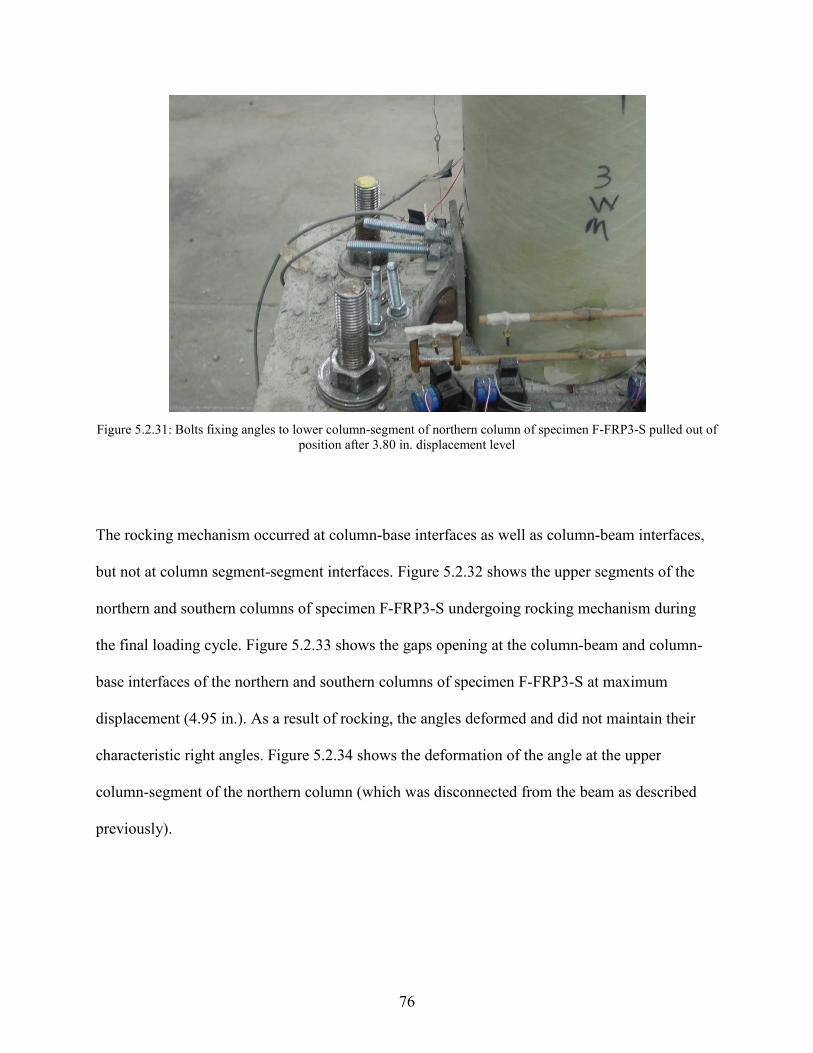
76
Figure 5.2.31: Bolts fixing angles to lower column-segment of northern column of specimen F-FRP3-S pulled out of
position after 3.80 in. displacement level
The rocking mechanism occurred at column-base interfaces as well as column-beam interfaces,
but not at column segment-segment interfaces. Figure 5.2.32 shows the upper segments of the
northern and southern columns of specimen F-FRP3-S undergoing rocking mechanism during
the final loading cycle. Figure 5.2.33 shows the gaps opening at the column-beam and column-
base interfaces of the northern and southern columns of specimen F-FRP3-S at maximum
displacement (4.95 in.). As a result of rocking, the angles deformed and did not maintain their
characteristic right angles. Figure 5.2.34 shows the deformation of the angle at the upper
column-segment of the northern column (which was disconnected from the beam as described
previously).

77
(a): Upper column-segment of northern column
(b) Upper column-segment of southern
Figure 5.2.32: Specimen F-FRP3-S undergoing rocking mechanism
at maximum displacement (4.95 in.)

78
(a) Column-beam interface of northern column
(b) Column-base interface of northern column
(c) Column-beam interface of southern
column
(d) Column-base interface of southern column
Figure 5.2.33: Gaps at interfaces of specimen F-FRP3-S while rocking at maximum displacement

79
Figure 5.2.34: Gap opening between steel angle and beam bottom surface at the north
corner of the beam during maximum displacement
The peak load at the final loading cycle dropped 18% below the maximum load. The permanent
deformation at the final loading cycle was 0.99 in, which is higher than the permanent
deformation of all the other FRP specimens. Compared to specimen F-RC, the permanent
deformation of specimen F-FRP3-S at the final loading cycle is 70% lower; compared to
specimen F-FRP1 is 77% higher, compared to specimen F-FRP3 is 38% higher, and compared to
specimen F-FRP3-R is 8% higher. It should be noted that, as with specimens F-FRP1 and F-

80
FRP3, testing specimen F-FRP3-S was limited by the length capacity of jack of the hydraulic
actuator (10 in.).
5.3 Backbone Curves
The backbone curves of the five specimens were constructed by graphing the peak load in each
displacement level (ordinate) against the corresponding drift value (abscissa). Figure 5.3.1 shows
the backbone curves of the five specimens.
Figure 5.3.1: Backbone curves showing drift vs. load
0
5
10
15
20
25
30
0 2 4 6 8 10
Load
(kip
)
Drift (%)
F-RC
F-FRP1
F-FRP3
F-FRP3-R
F-FRP3-S

81
The initial response of specimens F-RC, F-FRP1, and F-FRP3 was similar up to a drift of about
1.1%. Specimen F-RC yielded at a load of 10 kips and a drift ratio of 1.8% and began to fail after
reaching a load of 11.9 kips at a drift of 5%.
Specimen F-FRP1 was losing stiffness from the beginning of the test until reaching a load of 7.2
kips at a drift of 1.2% where the behavior began to follow a linear fashion reaching a maximum
load of 22.9 kips at a drift ratio of 9.3% which was the stroke length of the hydraulic actuator.
The response of specimen F-FRP3 was similar to the response of specimen F-FRP1, but with
5% higher loads at similar drift ratios. The specimen was losing stiffness from the beginning of
the test until reaching a load of 7.6 kips at a drift ratio of 1.2%. The response followed a linear
behavior following that, reaching a maximum load of 23.9 kips at a drift ratio of 8.9%, where the
load dropped as a result of the loss of stiffness, reaching a load of 23.5 kips at a drift ratio of
9.3%.
Specimen F-FRP3-R followed a linear response from the beginning of the test until reaching a
maximum load of 7.4 kips at a drift ratio of 8.9%. Following that point, the stiffness dropped and
the load decreased 4% reaching 7.1 kips at a drift of 9.3%.
Specimen F-FRP3-S was losing stiffness throughout the test, leading to a response of a
logarithmic form. The failure of the steel angle at the north corner of the beam after the 3.4 in
displacement level (described with more details in section 5.2.5) led to a sudden drop of 3.7% in
the frame resistance from the maximum load of 25.3 kips at a drift of 6.5% to a load of 24.4 kips
at a drift of 7.3%. After that stage, the loads continued to rise as the drift increased, reaching a

82
load of 24.8 kips (an increase of 1.5%) at a drift of 8.9%. The load dropped again at the final
displacement level, decreasing 3.7% from the previous displacement level, reaching a value of
23.9 kips at a drift of 9.3%.
The loss of stiffness can be explained by the decrease in the post-tensioning stress which is a
result of losses due to micro-cracks in concrete, shortening of the columns due to permanent
expansion in the radial direction as a result of Poisson’s effect, and possibly by the permanent
elongation of the post-tensioning due to yielding which occurred in specimen F-FRP3-S.
5.4 Stiffness
As mentioned is the previous section, all of the specimens were losing stiffness as the
displacement level was increasing. To observe this phenomenon in a more detailed manner,
secant stiffness curves were constructed for the five specimens. Figure 5.4.1 shows the secant
stiffness curves.

83
Figure 5.4.1: Secant stiffness curves
Initial stiffness values of specimens F-RC, F-FRP1, and F-FRP3 were relatively close in
magnitude. The initial stiffness of specimen F-RC was 15.4 kip/in, of specimen F-FRP1 was 18.3
kip/in, and of specimen F-FRP3 was 16.7 kip/in. Specimen F-FRP3-S had the highest initial
stiffness, 35.1 kip/in, whereas specimen F-FRP3-R had the lowest initial stiffness, 2.4 kip/in.
Comparing the initial stiffness values to that of specimen F-RC; specimen F-FRP1 was 1.6%
higher, specimen F-FRP3 was 7.1% lower, specimen F-FRP3-R was 86.5% lower, and specimen
F-FRP3-S was 95% higher.
The stiffness values of specimens F-RC, F-FRP1, F-FRP3, and F-FRP3-S dropped significantly
by the end of the test, whereas the stiffness values of specimen F-FRP3-R had an almost constant
stiffness throughout the test. The values of the final stiffness of specimens F-FRP1, F-FRP3, and
F-FRP3-S were relatively close in magnitude, while the final stiffness of specimen F-RC
0
5
10
15
20
25
30
35
40
0 2 4 6 8 10
Seca
nt s
tiff
ness
(kip
/in)
Drift (%)
F-RC
F-FRP1
F-FRP3
F-FRP3-R
F-FRP3-S

84
dropped to a value relatively close to that of specimen F-FRP3-R, which is significantly lower
than the final stiffness values of the other three specimens. The final stiffness of specimen F-RC
was 1.9 kip/in, that of specimen F-FRP1 was 4.7 kip/in, that of specimen F-FRP3 was 4.8 kip/in,
that of specimen F-FRP3-R was 1.5 kip/in, and that of specimen F-FRP3-S was 4.9 kip/in.
Compared to specimen F-RC, the final stiffness of specimen F-FRP1 was 150% higher, that of
specimen F-FRP3 was 158% higher, that of specimen F-FRP3-R was 22% lower, and that of
specimen F-FRP3-S was 163% higher.
To have a more representative comparison of the drop in stiffness of the five specimens
throughout the test when compared to the initial stiffness of each specimen on its own, the
normalized secant stiffness was calculated, and a graph of drift vs. the normalized secant
stiffness of the five specimens was constructed and is shown in figure 5.4.2. The normalized
secant stiffness was computed by calculating the ratio of the current secant stiffness to the initial
secant stiffness of each specimen.

85
Figure 5.4.2: Drift vs. Normalized secant stiffness
Specimen F-RC had the greatest drop of stiffness, 89.6%. The drop in stiffness of specimens F-
FRP1, F-FRP3, F-FRP3-R, and F-FRP3-S were 74.4%, 71.2%, 40.2%, and 85.9%, respectively.
Specimen F-FRP3-R had the lowest drop in stiffness.
5.5 Energy dissipation
Comparison of energy dissipation among the five specimens was one of the significant
objectives of this study. To quantify energy dissipation, the area inside each loop of the load-
displacement hysteresis curves was calculated, which reflects the energy dissipated at that
specific loading cycle. To better compare the response of the five specimens, the cumulative
0
0.2
0.4
0.6
0.8
1
1.2
0 2 4 6 8 10
Nor
mal
ized
Sec
ant s
tiff
ness
Drift (%)
F-RC
F-FRP1
F-FRP3
F-FRP3-R
F-FRP3-S

86
energy dissipated had to be computed. This was calculated by summing up the areas of all the
loops in the load-displacement hysteresis curve. Figure 5.5.1 shows drift against cumulative
energy dissipated in the first cycle of each drift level.
Figure 5.5.1: Drift vs. cumulative energy dissipated in the 1st cycle
All of the five specimens dissipated energy. Specimen F-FRP3-S dissipated the highest total
amount of energy, due to permanent deformation in the form of yielding of the sacrificial
external steel angles, which is the objective of creating this specimen. As expected, Specimen F-
RC had the next highest total energy dissipated, followed by specimen F-FRP3, F-FRP1, and F-
FRP3-R. Specimen F-RC dissipated energy due to concrete cover spalling, concrete crushing,
0
20,000
40,000
60,000
80,000
100,000
120,000
0 2 4 6 8 10
Cum
ulat
ive
Ener
gy (l
b.in
)
Dift (%)
F-RC
F-FRP1
F-FRP3
F-FRP3-R
F-FRP3-S

87
and rebar yielding. Specimens F-FRP1 and F-FRP3 dissipated energy by rocking, micro-
cracking and creep of concrete. Specimen F-FRP3 dissipated more energy than specimen F-
FRP1 due to the higher number of segments which created more rocking interfaces. Specimen F-
FRP3-R was the least to dissipate energy due to the lack of damage or rocking occurance due to
the presence of the rubber layers at the interfaces stated previously.
The total amount of energy dissipated by specimen F-RC was 211.1 kip.in., that by specimen F-
FRP1 was 119.8 kip.in., that by specimen F-FRP3 was 198.5 kip.in., that by specimen F-FRP3-R
was 79.1 kip.in., and that by specimen F-FRP3-S was 299.0 kip.in. Compared to specimen F-RC,
the cumulative energy dissipated by specimen F-FRP1 was 43.3% lower, specimen F-FRP3 was
5.9% lower, specimen F-FRP3-R was 62.5% lower, and specimen F-FRP3-S was 41.7% higher.
The amount of energy dissipated for each specimen depended primarily on two factors: the drift
level and the cycle number of each drift level. Generally, as the drift level increases, the amount
of energy dissipated also increases. Given that for each drift level of loading there are three
loading cycles; the first cycle of loading dissipates the most amount of energy, followed by the
second and third cycle, respectively. However, specimen F-FRP3-R had almost equal
magnitudes of energy dissipated in the three loading cycles, as shown in figure 5.5.5. Figures
5.5.2 to 5.5.6 show a comparison of the amount of energy dissipated in each loading cycle for
each of the five specimens: F-RC, F-FRP1, F-FRP3, F-FRP3-R, and F-FRP3-S, respectively.

88
Figure 5.5.2: Energy Dissipation of specimen F-RC
Figure 5.5.3: Energy Dissipation of specimen F-FRP1
0
5000
10000
15000
20000
25000
0 2 4 6 8 10
Ener
gy D
issi
pate
d (lb
.in)
Drift (%)
First cycle
Second cycle
Third cycle
0
2000
4000
6000
8000
10000
12000
0 2 4 6 8 10
Ener
gy D
issi
pate
d (lb
.in)
Drift (%)
First cycle
Second cycle
Third cycle

89
Figure 5.5.4: Energy Dissipation of specimen F-FRP3
Figure 5.5.5: Energy Dissipation of specimen F-FRP3-R
0
2000
4000
6000
8000
10000
12000
14000
16000
0 2 4 6 8 10
Ener
gy D
issi
pate
d (lb
.in)
Drift (%)
First cycle
Second cycle
Third cycle
0
1000
2000
3000
4000
5000
6000
0 2 4 6 8 10
Ener
gy D
issi
pate
d (lb
.in)
Drift (%)
First cycle
Second cycle
Third cycle

90
Figure 5.5.6: Energy Dissipation of specimen F-FRP3-S
Using the values of energy dissipated at the first loading cycle; the maximum amount of energy
dissipated by specimen F-RC occurred at a drift of 6.8%, by specimen F-FRP1 at a drift of 9.3%
(maximum drift capacity of the actuator), by specimen F-FRP3 at a drift of 8.9%, by specimen F-
FRP3-R at a drift of 9.3% (maximum drift capacity of the actuator), and by specimen F-FRP3-S
at a drift of 7.3%.
The average drop in energy dissipated in the second and third loading cycles, respectively,
compared to the first loading cycle of specimen F-RC were 20.8% and 31.0%, by specimen F-
FRP1 were 22.3% and 29.2%, by specimen F-FRP3 were 21.3% and 27.9%, by specimen F-
FRP3-R were 2.7% and 4.0%, and by specimen F-FRP3-S were 18.2% and 24.6%.
Table 5.5.1 shows a summary of the results presented in this section. Table 5.5.2 compares the
total amount of energy dissipation in the first, second, and third loading cycles of each of the five
specimens. Table 5.5.3 compares the maximum amounts of energy dissipation in the first,
0
2000
4000
6000
8000
10000
12000
14000
0 2 4 6 8 10
Ener
gy D
issi
pate
d (lb
.in)
Drift (%)
First cycle
Second cycle
Third cycle

91
second, and third loading cycles of the five specimens along with their corresponding drift
values.
Specimen
Total energy
dissipated in 1st cycle
(kip.in)
% Difference in total energy dissipated
compared to F-RC
Average drop in
energy dissipation of 2nd cycle
compared to 1st cycle (%)
Average drop in energy dissipation
of 3rd cycle compared to 1st
cycle (%)
F-RC 82.6 N/A 20.8 31.0 F-FRP1 57.2 - 43.3 22.3 29.2 F-FRP3 78.0 - 5.9 21.7 27.9
F-FRP3-R 26.8 - 62.5 2.7 4.0 F-FRP3-S 110.9 + 41.7 18.2 24.6
Table 5.5.1: Comparison of total energy dissipated of specimens and average drop of energy dissipated in 2nd and 3rd loading cycles
5.6 Equivalent viscous damping
The ability of a specimen to dissipate energy can be reflected by calculating the equivalent
viscous damping, which was calculated for each specimen at all displacement levels. The
equivalent viscous damping was calculated by equation 5.6.1 (Blandon & Priestley, 2005):
(Equation 5.6.1)
where:
- ζeq : equivalent viscous damping
- Ahyst : area enclosed one load-displacement hysteresis loop
- F0 : average peak force during the specific cycle
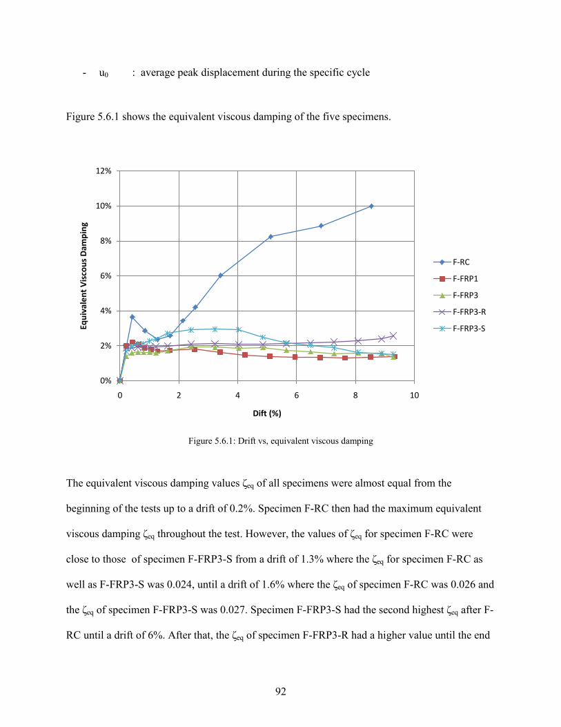
92
- u0 : average peak displacement during the specific cycle
Figure 5.6.1 shows the equivalent viscous damping of the five specimens.
Figure 5.6.1: Drift vs, equivalent viscous damping
The equivalent viscous damping values ζeq of all specimens were almost equal from the
beginning of the tests up to a drift of 0.2%. Specimen F-RC then had the maximum equivalent
viscous damping ζeq throughout the test. However, the values of ζeq for specimen F-RC were
close to those of specimen F-FRP3-S from a drift of 1.3% where the ζeq for specimen F-RC as
well as F-FRP3-S was 0.024, until a drift of 1.6% where the ζeq of specimen F-RC was 0.026 and
the ζeq of specimen F-FRP3-S was 0.027. Specimen F-FRP3-S had the second highest ζeq after F-
RC until a drift of 6%. After that, the ζeq of specimen F-FRP3-R had a higher value until the end
0%
2%
4%
6%
8%
10%
12%
0 2 4 6 8 10
Equi
vale
nt V
isco
us D
ampi
ng
Dift (%)
F-RC
F-FRP1
F-FRP3
F-FRP3-R
F-FRP3-S

93
of the test. Specimens F-FRP1, F-FRP3, and F-FRP3-R had relatively close values of ζeq
throughout the test, with specimen F-FRP3-R having the second highest ζeq among the five
specimens at the end of the test: 0.0256 at a drift of 9.3%. Table 5.6.1 summarizes the ζeq results
of the five specimens, showing the maximum, minimum (excluding initial value), and final
equivalent viscous damping values along with their corresponding drift values.
Specimen
Maximum Equivalent Viscous Damping
Minimum Equivalent
Viscous Damping (excluding initial value)
Equivalent Viscous Damping at final drift
level
Drift (%)
ζeq Drift (%) ζeq Drift
(%) ζeq
F-RC 8.5 0.0998 1.3 0.0236 8.5 0.0998 F-FRP1 0.4 0.0222 7.6 0.0131 9.3 0.0139 F-FRP3 2.4 0.0194 9.3 0.0136 9.3 0.0136
F-FRP3-R 9.3 0.0256 0.2 0.0187 9.3 0.0256 F-FRP3-S 3.2 0.0295 9.3 0.0151 9,3 0.0151
Table 5.6.1: Maximum, minimum (excluding initial value), and final EVD values with corresponding drift
5.7 Post-tensioning steel-bar strain
The steel bars in specimens F-FRP1, F-FRP3, F-FRP3-R, and F-FRP3-S underwent two stages
of loading. The first stage was post-tensioning and the second stage was testing of the specimen.
The following sub-sections describe results of the two stages with more details.
5.7.1 Bar stress while post-tensioning
As discussed in chapter 4, the initial post-tensioning value determines the yielding moment of
the post-tensioned column. Each bar was equipped with strain gages to monitor the bar stress

94
while post-tensioning. The theoretical initial post-tensioning strain was determined using the
procedure described in chapter 4, and was calculated to be 935 micro-strain. Figures 5.7.1 to
5.7.4 show the steel-bar strain values of specimens F-FRP1, F-FRP3, F-FRP3-R, and F-FRP3-S
respectively, during the process of post-tensioning.
Figure 5.7.1: Post-tensioning specimen F-FRP1
Figure 5.7.2: Post-tensioning specimen F-FRP3
Figure 5.7.3: Post-tensioning specimen F-FRP3-R
Figure 5.7.4: Post-tensioning specimen F-FRP3-S

95
As described in chapter 3, the procedure of post-tensioning the two columns of each of the four
specimens involved several steps, starting with post-tensioning the first column to the target
strain using the hydraulic ram. Immediate losses in post-tensioning stress appeared following
turning off the hydraulic ram after tightening the top nut, which was performed manually.
Tightening the ram manually is highly variable and the losses that follow that step were also
widely variable depending on the degree of tightening performed by the operator. One reason for
such losses is that the nut will slip into the anchorage plate as soon as the hydraulic ram stops
supporting it when it is turned off, leading to losses, which are inversely proportional to the
degree of tightening the nut performed by the operator. For example, the initial attempt in
specimen F-RC suffered immediate losses of 47%. By trial and error, the steel bar was then post-
tensioned to a higher strain, the top nut tightened, and the hydraulic ram turned off to observe the
final strain value. The procedure was repeated until both columns reached the target strain.
5.7.2 Bar stress while testing
The rocking mechanism was observed during testing specimens of F-FRP1, F-FRP3, F-FRP3-R,
and F-FRP3-S. Gap openings formed at interfaces were described in section 5.2. These gaps led
to elongation of the steel-bar, resulting in stressing the steel bars beyond the initial post-tension.
Figures 5.7.3 to 5.7.5 show displacement graphed against the steel bar strain values during
testing of specimens F-FRP1, F-FRP3, and F-FRP3-S. Negative displacements indicate
displacement to the south direction. The strain gages attached to the north column of specimen F-
FRP1 failed after displacement values of 3.57 in. and -3.43 in. and therefore only the strain
readings prior to reaching the displacement levels of 3.57 in and -3.43 were included in the

96
figure. The strain gages attached to the steel bars of specimen F-FRP3-R failed early during
testing and their results were therefore omitted.
(a): North Column
(b): South Column
Figure 5.7.5: Specimen F-FRP1 displacement vs. steel bar strain
(a): North Column
(b): South Column
Figure 5.7.6: Specimen F-FRP3 displacement vs. steel bar strain

97
(a): North Column
(b): South Column
Figure 5.7.7: Specimen F-FRP3-S displacement vs. steel bar strain
Table 5.7.1 shows a summary of the maximum and minimum bar strains and the displacements
at which they occurred for the above specimens. It also shows the percentage that the maximum
bar stresses reached compared to the nominal strength of the bars (150 ksi).
Specimen
North Column
South Column
Lateral disp. at
min. strain (in)
Min. strain
(micro-strain)
Lateral disp. at max. strain
Max. strain
(micro-strain)
% max. bar stress of
nominal bar strength
Lateral disp. at
min. strain (in)
Min. strain
(micro-strain)
Lateral disp. at max. strain
Max. strain
(micro-strain)
% max. bar stress of
nominal bar strength
F-FRP1
-0.36 455 3.12 2473 49 -0.53 11 4.90 2426 48
F-FRP3
-0.11 269 -4.80 2893 57 -0.06 91 4.95 3089 61
F-FRP-S
0.16 20 -4.80 3329 66 0.37 703 -4.80 4443 88
Table 5.7.1: Summary of post-tensioning bars strain values

98
As mentioned in chapter 3, the ultimate strength of the post-tensioning steel bar is 150 ksi
corresponding to a force of 187.5 kips. Also, the post-tensioning steel bar complies with ASTM
A722 which states that the minimum yield strength of the steel bar must exceed at least 80% of
the ultimate strength. Comparing the maximum strain values, specimen F-FRP3-S had the
highest strain of 3329 at the north column corresponding to a force of 124 kips which is 66% of
the ultimate strength of the post-tensioning steel bar and is therefore less than the yielding
strength of the bar; and 4443 micro-strain at the south column corresponding to a force of 165
kips which is 88% of the ultimate strength of the post-tensioning steel bar, i.e. exceeded the yield
strength of the steel bar (120 ksi or 150 kips). Given that, none of the bars reached the yielding
stress (which was one of the design provisions) except for the bar at the south column of
specimen F-FRP3-S, which exceeded the yielding force by 5.9%, mostly due to the unexpected
failure in the steel angle at the northern corner of the beam.
The columns of all specimens lost various amount of post-tension. One reason is loosening of the
anchor nut of the post-tensioning bar during the test. Other reasons are related to permanent
deformation to the columns due to creep and permanent shortening due to radial expansion as a
result of high axial loads (Poisson’s effect). For specimen F-FRP1, the north column lost 51.9%
of its initial post-tensioning stress before the strain gages attached to the bar failed after the 3.40
in. displacement level as mentioned previously in this section; while the south column lost 98.8%
of its initial post-tensioning stress. For specimen F-FRP3, the north column lost 69.3% while the
south column lost 90.0% of its initial post-tension. For specimen F-FRP3-S, the north column
lost 97.7% while the south column lost 32.8% of its initial post-tension.

99
5.8 FRP tube strains
The FRP circumferential strains in north and south faces of each column of each FRP frame was
measured at heights of 2, 4, 41, and 43 in.
The gages measuring longitudinal strain of every column of specimens F-FRP1, F-FRP3, F-
FRP3-R, and F-FRP3-S were set at the west face of the column and at two heights: 4 in. and 41
in. More details are shown in Chapter 3.
Figures 5.8.1 to 5.8.4 show the FRP circumferential and longitudinal strains for North and south
columns of each FRP specimen plotted against displacement. All the graphs of the FRP strain
gages of each specimen are available in the appendix.

100
(a): Circumferential north gage at 43 in
Column N
(b): Circumferential north gage at 43 in.
Column S
(c): Longitudinal strain at 41 in.
Column N
(d): Longitudinal strain gage at 41 in
Column S
Figure 5.8.1: Specimen F-FRP1 FRP strain for North and South columns

101
(a): Circumferential south gage at 43 in.
Column N
(b): Circumferential north gage at 43 in.
Column S
(c): Longitudinal strain gage at 41 in.
Column N
(d): Longitudinal strain at 4 in. height
Column S
Figure 5.8.2: Specimen F-FRP3 FRP strain for North and South columns

102
(a): Circumferential south gage at 43 in.
Column N
(b): Circumferential north gage at 2 in.
Column S
(c): Longitudinal strain gage at 4 in.
Column N
(d): Longitudinal strain gage at 4 in.
Column S
Figure 5.8.3: Specimen F-FRP3-R FRP strain for North and South columns

103
(a): Circumferential north gage at 43 in.
(b): Circumferential north gage at 2 in.
(c): Longitudinal strain gage at 4 in.
(d): Longitudinal strain gage at 4 in.
Figure 5.8.4: Specimen F-FRP3-S FRP strain
For circumferential FRP strain, it can be seen from the figures that the values reach higher
magnitudes in one direction of displacement but not the other. This is explained by the rocking
mechanism. Each of the circumferential strain gages was attached at either the north face or the
south of the column. When the frame is laterally displaced, the columns undergo rocking. This
leads to a gap opening at one side of the column while the other undergoes increasing
compression due to the rotation of the interface which is blocked by the support interface (i.e. the
beam if at the top interface or the footing at the bottom interface). The strain readings reach
maximum values depending on whether the circumferential strain gage is at the north or south
face of the column and on the direction of lateral loading.

104
The circumferential FRP strain depends mainly on the axial stress applied in the column, hence,
the post-tensioning force influences the strain readings. Initial post-tension as well as losses in
post-tension therefore affect FRP strain readings.
All the above explanations assume flat interfaces of the columns that are perpendicular to
column longitudinal axis. The column segments interfaces were not perfectly flat or
perpendicular to the column segment longitudinal axis due to errors in the cut of the FRP tube
and to errors that occurred while casting which include minor tilting of the column segments and
sagging of the wooden supports holding the column segments. Wheel grinding of the interfaces
was conducted to create flat and smooth surfaces, but that did not assure interfaces that are
perpendicular to the column’s longitudinal axis. As a result of such imperfections, the stresses
were not evenly distributed on the column interface which is another reason of differences in
circumferential FRP strain values.
Specimen F-FRP3-R had the lowest circumferential strain due to the presence of the rubber
layers. These layers acted as buffer layers preventing high compression in the columns as they
were expanding radially.
5.9 Section rotations
For each of the five specimens, sixteen string potentiometers were installed for measuring
rotations, as described in Chapter 3. Rotations were measured for each column of the five
specimens at four sections. Readings from each string potentiometer was multiplied by
correction factors which were found by calibration.

105
For specimen F-RC, the test was completed over two separate time periods. No rotations
readings were taken at the top joints of the North or South columns. Also, the rods attached to
the columns (with adhesives) were detached when the concrete cover was compromised during
testing and therefore the rotation readings were stopped when that occurred. Figure 5.9.1 shows
graphs of time against rotations measured at different heights of the North and South columns of
specimen F-RC.

106
(a): North Column top joint
(b): South Column top joint
(c): North Column bottom joint
(d): South Column bottom joint
Figure 5.9.1: Time vs. rotation of specimen F-RC at different column heights
The applied lateral load applied to the specimen increased as time increased, which explains why
rotations increased with time. Also, each displacement level was repeated for three cycles, which
explains why rotations were close every three cycles. However, since the resistance of the
specimen to the applied lateral load decreases slightly when the cycle is repeated for the same

107
displacement level (due to damage of the specimen after each loading cycle), the magnitudes of
the rotations at the same displacement level are not exactly equal in magnitude.
Rotations at the top joints of both columns are higher than those at the bottom joints. This can be
explained by the fact the footing is relatively much stiffer to rotations than the beam, and since
the columns joints are fixed, larger magnitude of rotation occurred at the top joints.
Figure 5.9.2 shows graphs of time against rotations measured at different heights of the North
and South columns of specimen F-FRP1.

108
(a): North Column top joint
(b): South Column top joint
(c): North Column bottom joint
(d): South Column bottom joint
Figure 5.9.2: Time vs. rotation of specimen F-FRP1 at different column heights
Compared to specimen F-RC, rotation values of specimen F-FRP1 are higher in magnitude. This
can be explained by the occurrence of rocking mechanism in specimen F-FRP1, which lead to
the joints of the columns acting as pins rather than being fixed as in specimen F-RC. The joints

109
with specimen F-FRP1 have lower rotational stiffness than those of specimen F-RC, and
therefore rotated to higher magnitudes.
Comparing the rotations of the top joints of specimen F-FRP1 to the bottom joints, the top joints
have lower rotation magnitudes. This can be explained by the fact that the beam is more flexible
to rotation than the footing, which led to the upper joints undergoing less rocking with smaller
gaps opening, leading to the top joints acting less as pins than the lower joints.
Figure 5.9.3 shows graphs of time against rotations measured at different heights of the North
and South columns of specimen F-FRP3.

110
(a): North Column top joint
(b): South Column top joint
(c): North Column bottom joint
(d): South Column bottom joint
Figure 5.9.3: Time vs. rotation of specimen F-FRP3 at different column heights
Compared to specimen F-FRP1, the rotation values of specimen F-FRP3 are lower. This can be
explained by the fact that the columns of specimen F-FRP3 are segmented. This leads to less
rotation of the upper and lower segments since rocking and gap opening may occur at the middle
segment. Although such gaps were not visible due to their small magnitudes as well as the fact

111
that the surfaces of the column segments were not perfectly flat and perpendicular to the
longitudinal axes of column segments stacked on top of each other.
(a): North Column top joint
(b): South Column top joint
(c): North Column bottom joint
(d): South Column bottom joint
Figure 5.9.4: Time vs. rotation of specimen F-FRP3-R at different column heights

112
Rotations values for specimen F-FRP3-R were close in magnitude to those of specimen F-FRP3,
which means that the rubber layer does not appear to affect rotation values at the same lateral
displacements.
(a): North Column top joint
(b): South Column top joint
(c): North Column bottom joint
(d): South Column bottom joint
Figure 5.9.5: Time vs. rotation of specimen F-FRP3-S at different column heights

113
Rotation values of specimen F-FRP3-S were close in magnitude to the other segmented FRP
frames. With specimen F-FRP3-S, the top and bottom segments were more restricted to rocking
due to the attached sacrificial steel angles at the corners. The values of rotations of the other
segmented specimens were close in magnitude to those of specimen F-FRP3-S, which means that
the top and bottom segments of those other segmented specimens (i.e. specimen F-FRP3 and F-
FRP3-R) also did not rotate as each of the single segmented columns of specimen F-FRP1 did.
A general observation related to all the FRP specimens is that the columns rotated more in a
rigid way with joints resembling pins rather than undergoing double curvature as the monolithic
columns of specimen F-RC did. This can be seen by the almost equal rotation angles measured at
different points of the top joint of a column or the rotation angles measured at different points at
the bottom joint of a column.
5.10 Curvature
Curvature was computed for each section at which rotations were calculated in the
previous section as discussed in Chapter 3. Curvature was calculated at the first peak
displacement value of each displacement level. Figure 5.10.1 shows graphs of displacement
against curvature at different sections of the north and south columns of specimen F-RC.

114
(a): North Column top joint
(b): South Column top joint
(c): North Column bottom joint
(d): South Column bottom joint
Figure 5.10.1: Displacement vs. curvature of specimen F-RC
Figure 5.10.2 shows graphs of displacement against curvature at different sections of the north
and south columns of specimen F-FRP1
.

115
(a): North Column top joint
(b): South Column top joint
(c): North Column bottom joint
(d): South Column bottom joint
Figure 5.10.2: Displacement vs. curvature of specimen F-FRP1
Figure 5.10.3 shows graphs of displacement against curvature at different sections of the north
and south columns of specimen F-FRP3.

116
(a): North Column top joint
(b): South Column top joint
(c): North Column bottom joint
(d): South Column bottom joint
Figure 5.10.3: Displacement vs. curvature of specimen F-FRP3
Figure 5.10.4 shows graphs of displacement against curvature at different sections of the north
and south columns of specimen F-FRP3-R.

117
(a): North Column top joint
(b): South Column top joint
(c): North Column bottom joint
(d): South Column bottom joint
Figure 5.10.4: Displacement vs. curvature of specimen F-FRP3-R
Figure 5.10.5 show graphs of displacement against curvature at different sections of the north
and south columns of specimen F-FRP3-S.

118
(a): North Column top joint
(b): South Column top joint
(c): North Column bottom joint
(d): South Column bottom joint
Figure 5.10.5: Displacement vs. curvature of specimen F-FRP3-S
The curvature data depended on the rotation data. In concept, if two sections rotate with similar
angles then no curvature has occurred between them. However, in this case, the curvature at each

119
section was calculated without reference to the rotation of the previous section. Therefore, the
height of the section by which the value of rotation was divided becomes the key factor. The
rotation of the FRP columns was discussed in the previous section and can be described as rigid
rotation. Therefore, it can be seen here that the curvature values calculated for the sections at
height of 43 in. are lower in magnitude than those at height of 41 in. The same applies for the
lower joints. The reason is that curvature is inversely proportional to the height of the section.

120
Chapter 6
Pushover Analysis
6.1 Introduction
Pushover models were constructed to anticipate the performance of specimens. In this chapter,
the backbone curves measured during testing of specimens F-RC and F-FRP1 are compared to
the force-displacement response predicted using pushover models.
6.2 Pushover of specimen F-RC
SAP2000 was used to construct a pushover model to simulate the performance of the monolithic
reinforced concrete frame (specimen F-RC). The model required several key variables to define
its properties. These include material properties, geometric properties, boundary conditions, and
moment-curvature relationships.
Initially, moment curvature relationships were computed using the software package XTRACT.
Concrete strength and reinforcement details mentioned in Chapter 3 were input in XTRACT.
Moments and curvature at initial yield as well as at ultimate capacity, then the effective yield
moment and curvature values were determined using the idealized bilinear moment-curvature
envelope obtained from XTRACT. Figure 6.2.1 shows the idealized bilinear moment-curvature
envelope obtained from XTRACT for the as-built monolithic RC frame.

121
Figure 6.2.1: Moment-curvature relationship of the RC column-section from XTRACT
SAP2000 is then used to conduct pushover analysis of the monolithic frame. Columns and beam
cross sections were modeled with the same values as those in Chapter 3. The height of the
columns was input as the height from the surface of the footing to the beam center, which is 52.5
in. Effective EI (obtained from XTRACT) was input into SAP2000.
SAP2000 uses the material properties mentioned above during the elastic stage of pushover
analysis. To model the frame in the nonlinear inelastic stage, plastic hinges were defined and
assigned to the frame. The type of plastic hinge selected was M2 which is a plastic hinge rotating
about axis 2 and is non-interacting to axial load. Using an interactive plastic hinge would be
more accurate, but due to relatively low changes in axial stresses, using this type of hinge is
adequate. The plastic hinge was defined using ductility factors obtained from XTRACT. The

122
analysis report from XTRACT is available in the Appendix. The plastic hinge length was
calculated as discussed in Chapter 4 (Equation 4.1.12). Plastic hinges were assigned at the top
and bottom of each column since the columns underwent double bending. Each plastic hinge
location was assigned with its center a distance above the surface of the base for lower joints
and below the bottom surface of the beam for upper joints. The reason for this assumption is that
the base and the beam were much stiffer to rotation than the columns due to their geometric
properties, and therefore the plastic hinges form in the column’s clear height.
Figure 6.2.2 shows the load-drift response of the monolithic RC frame model in SAP2000
(specimen F-RC) compared with actual backbone curves obtained from experiments.
Figure 6.2.2: Specimen F-RC SAP2000 pushover model comparison
0
2
4
6
8
10
12
14
0 2 4 6 8 10
Load
(kip
)
Drift (%)
Experimental
Sap2000 pushover analysis

123
6.3 Pushover of specimen F-FRP1
SAP2000 was used to construct a pushover model to simulate the performance of the FRP frame
(specimen F-FRP1). The model required several key variables to define its properties. These
include material properties, geometric properties, boundary conditions, and moment-curvature
relationships.
Initially, a stress-strain model is required to obtain a moment-curvature relationship. The model
developed by Samaan et al. (1998) was selected, and the material properties (concrete
compressive strength , concrete modulus of elasticity, FRP tensile strength, and FRP modulus of
elasticity) presented in Chapter 3 were used to define the stress-strain function. Figure 6.3.1
shows the stress strain model of the FRP column-section.
Figure 6.3.1: Stress-strain model of FRP column-section
0
0.5
1
1.5
2
2.5
3
3.5
0 0.001 0.002 0.003 0.004 0.005 0.006 0.007
Stre
ss (k
si)
Strain

124
The stress-strain function is then used to develop the moment-curvature relationship as described
in Chapter 4 after Hewes and Priestley (2002). Figure 6.3.2 shows the resulting moment-
curvature envelopes for FRP column.
Figure 6.3.2: Moment-curvature relationship of FRP column-section
Pushover analysis is then conducted using the same procedure stated in the previous section. The
same type of plastic hinge was selected (M2). The plastic hinge length was calculated as
discussed in Chapter 4 and assigned. Figure 6.3.3 shows the results of the pushover analysis of
the FRP frame compared with the experimental results.
0
10
20
30
40
50
60
70
80
90
100
0 0.0005 0.001 0.0015 0.002 0.0025
Mom
ent (
kip-
in)
Curvature (1/in)

125
Figure 6.3.3: Specimen F-FRP1 SAP2000 pushover model comparison
6.4 Interpretation of analyses
The pushover models results using SAP2000 predicted a close approximation to the actual
experimental response. It should be noted that the concrete compressive strength, concrete
modulus of elasticity, FRP tensile strength, and FRP modulus of elasticity values were vital in
predicting the results. They affect both the elastic portion and the inelastic portion of the
response. One observation is that the equation for calculating Ec in section 8.5.1 of ACI318-05
overestimates the modulus of elasticity of concrete. The actual values were 75% of the values
calculated using the ACI318-05 equation. Also, SAP2000 does not take into account the cracked
section moment of inertia, and therefore effective values must be input into the material
properties to account for that.
The SAP2000 pushover model of specimen F-RC overestimated the ultimate force by 4.6%,
which is relatively a good approximation. The drift at which the ultimate load occurred for
specimen F-RC was 5.1% in the actual tests compared to 5.3% from the pushover model, which
0
5
10
15
20
25
0 5 10 15
Load
(kip
)
Drift (%)
Experimental
Sap2000 pushover analysis

126
was also over estimated by 4.2% of the actual drift. One reason for that is that the pushover
model does not into account the cyclic nature of the tests. Successive cycles weaken the frames
stiffness due to damage such as micro-crack in concrete, cover spalling, and possibly rebar
yielding.
The SAP2000 pushover model depended primarily on the stress-strain model that was selected.
This model affects almost all the parameters of response of the model including: effective section
modulus, moment and curvature at yield, moment and curvature at the ultimate loading stage.
The pushover model slightly underestimated the ultimate load by 5.7% although that anticipated
load was calculated at a drift 8.4% higher than the experimental ultimate drift. It should be noted
that the experimental test did not lead to failure of specimen F-FRP1 which suggests that the
actual behavior might differ at higher drifts, and therefore failure should be investigated to have
a better understanding of the behavior the FRP frames, and to compare the results with the actual
model. It should be noted that in this pushover model, the pushover load case was defined to be
displacement controlled and the ultimate lateral displacement was set to be the same as the
ultimate lateral drift with which the experimental tests were limited.

127
Chapter 7
Summary and Conclusions
7.1 Summary
Bridge construction using conventional reinforced concrete poses several disadvantages
including the long period of time for construction, high susceptibility to damage during seismic
events, the difficulty of repair after seismic events, and the harmful effects on local surroundings
in close proximity to bridge construction projects. This research was conducted with objectives
aimed to resolve the above issues along with other improvements.
In this research, the precast system was used to offer solutions to some of the above problems.
Construction using the precast system is much faster than conventional reinforced concrete
construction. The effect on local surroundings is much lower when the precast system is utilized
since mostly the members are only to be assembled on site and no building formwork or concrete
pouring occurs at the construction site. Using the precast system also offers additional
advantages in terms of higher efficiency and quality control of the production of structural
members due to production at specialized plants.
The concept of confinement of concrete was then applied to improve strength (compressive and
shear) capabilities of bridge columns. Tubes fabricated from fiber reinforced polymers were used
because they proved to offer better confinement than steel jackets due to their higher strength

128
properties, with the advantages of lower density (which is important for decreasing seismic force
attraction to the structure) as well as not being susceptible to corrosion as steel is.
Post-tensioning was utilized in this research to provide a solution to the high residual
displacements of bridges after seismic events. Unbonded post-tensioning resolved the problem of
local yielding of post-tensioning steel bars and maintained them in their elastic phase of
response.
Energy dissipation mechanisms were also added to the proposed systems to improve energy
dissipation while maintaining damage in easily replaceable parts of the structure to facilitate the
ease of repair. Different energy dissipation mechanisms were applied and evaluated.
7.2 Conclusions
Several key points can be concluded from the results of this study, these include:
• Lateral load resistance
• Damage and residual drift
• Energy dissipation
7.2.1 Lateral Load resistance
Although the conventional monolithic reinforced concrete specimen (specimen F-RC) shared the
same geometric properties as that of other four proposed specimens (where the same dimensions
of the footings, columns, and beam of each specimen were used for all the other specimens), the
specified unconfined concrete strength was constant for all the columns, and the columns were

129
all designed with the same theoretical yielding moment, the monolithic frame (specimen F-RC)
showed significantly lower lateral load resistance than all the other specimens. The maximum
lateral load resisted by specimen F-RC was about 50% of the maximum lateral load of specimens
F-FRP1, F-FRP3, and F-FRP-S. Specimen F-FRP3-R, however, showed poor response; where
the lateral load resistance was significantly lower than that of all the other specimens due to the
presence of rubber pads which softened the column interfaces leading to a reduction in rotational
stiffness. Previous studies showed that using rubber pads at frame joints reduced the period of
vibration. Due to the quasistatic nature of the cyclic testing in this study, the effect of using
rubber at joints on the period of the structure was not investigated. However, more detailed
results regarding this issue may be deduced by applying a ground motion to the specimens using
a shaking table. Overall, the proposed systems (excluding specimen F-FRP3-R) have the
advantage of higher lateral load resistance, i.e. higher strength. One downside that was observed
is the loss of initial post-tension after the end of the test. For specimen F-FRP3-S, post-
tensioning bar yielding was partially attributed to the loss of the initial-post-tensioning stress.
However, that was not that case for the other three specimens (F-FRP1, F-FRP3, and F-FRP-R),
since the bar stresses did not overcome their yielding strength, according to strain gage readings.
Two reasons are suggested: Permanent axial plastic deformation of concrete as a result of lateral
dilation due to high axial stresses that the columns undergo during the test which can go up to
more than double the initial post-tensioning axial compressive stress. Another reason could have
been the loosening of the nut that was initially tightened to the anchorage plate after successive
loading cycles. The cyclic nature of the test has several effects on the system which are
suggested to be further investigated.

130
Also, the results of the pushover analysis for the control specimen (F-RC) and specimen F-FRP1
provided close values to the experimental load-drift results. This indicates that the response of
the FRP specimens may be anticipated using the parameters discussed in Chapter 6.
7.2.2 Damage and residual drift
The conventional monolithic reinforced concrete frame (specimen F-RC) suffered the highest
overall damage which was concentrated in its major structural members (the columns and the
beam). Plastic hinges formed, as expected, at the four corners of the frame, and damage was
highest at those locations. One steel reinforcement rebar fractured at later stages of the test. The
high degree of damage suggests the high difficulty or even impossibility of repair of the
structural member, which can be disastrous in actual bridges.
All the other specimens, which were mainly based on the proposed system of unbonded post-
tensioned precast structural members, suffered much lower damage and residual drift when
compared to the monolithic specimen (specimen F-RC). The re-centering mechanism proved to
be effective in the proposed systems. Damage was limited to local FRP tube locations due to
interlocking while rotating, which does not affect the performance of the confined concrete
column segment. This problem can be simply resolved by using FRP tubes that are little shorter
than the column segments to prevent any interaction of two adjacent tubes while the column-
segments are rotating.
Except for specimen F-FRP3-S, none of the post-tensioning steel bars yielded due to the
carefully selected initial post-tensioning stress. The maximum post-tensioning steel bar stress

131
was close to the predicted values, which were designed not to exceed 60% of the ultimate
strength of the bar. The attachment of the modified steel angles to specimen F-FRP-S led to
higher lateral stiffness of the frame and caused the post-tensioning bar to undergo higher stresses
than in the other specimens at similar drifts. Therefore, the effect of attaching energy dissipating
devices must be accounted for while analyzing the frame to better predict the maximum stresses
at the steel bars and other locations. Specimen F-FRP3-R was almost free from any kind of
damage due to the presence of rubber pads which prevented the FRP tubes from interacting at
interlocking interfaces while rotating, and also provided a buffer zone preventing significant
increase in bar stresses.
7.2.3 Energy dissipation
Conventional monolithic reinforced concrete frames dissipate most of the input seismic energy
applied to them via permanent damage and deformation in the form of reinforcement yielding as
well as concrete crushing, leading to the formation of plastic hinges. As expected, the monolithic
frame (specimen F-RC) exhibited higher energy dissipation than the post-tensioned system
whether the columns of the frame were of a single segment (as with specimen F-FRP) or with
multiple specimens (F-FRP3). To overcome this challenge, energy dissipation mechanisms were
developed. The main criterion was to attach additional parts to the frame that can dissipate more
energy through permanent deformation while being easily replaced after damage. This was
implemented by attaching modified steel angles. Previous research showed that adding such
angles to the frame can absorb some energy, but cease to perform efficiently after certain drifts
due to the relatively small part of the angle undergoing permanent deformation (i.e. local
yielding at the corner of the steel angle). The steel angle was therefore modified to improve its

132
energy dissipation. As expected, the specimen with the modified steel angles (specimen F-FRP-
S) dissipated more energy than all the other proposed post-tensioned specimens and overcame
the magnitude of energy dissipation of the conventional monolithic frame (specimen F-RC) as
well, which is one important goal of this study.
Specimen F-FRP3-R showed the lowest energy dissipation, proving that the use of rubber pads
does not offer a good energy dissipation alternative.
7.3 Overall performance
The goal of this research was achieved: a better proposed system sharing similar geometric,
dimensional, and concrete properties with a conventional monolithic bridge moment resisting
frame was created. The proposed system has the advantages of:
- higher strength in terms of lateral load resistance
- lower damage post lateral loading
- easier repair post lateral loading
- faster, easier, and cleaner construction
The proposed system offers a feasible and efficient alternative to the conventional reinforced
concrete system. The loss of post-tension however still poses a significant problem that has to be
addressed, since it can affect a key property of the proposed system - re-centering - and hinder its
effect. One improvement to that would be bonding the nut which is tightened to the anchorage
plate with the post-tensioning bar (such as by the use of adhesives or by welding). Further
research is recommended regarding this issue.

133
7.4 Recommendations for future studies
The stress-strain model used for the FRP confined concrete in this study did not account for the
cyclic nature of the test. Future research may include models that include unloading pathways of
stress-strain relationships of FRP confined concrete columns. These can then be incorporated to
find better predictions of the moment-curvature relationships, which are key values to finding the
design initial post-tension. Accurately predicting the initial post-tension is important also so that
design values can prevent the post-tensioning bars/tendons from yielding and hence, preventing
permanent damage as well as re-centering the bridges more efficiently.
The sources of loss of post-tension may be further investigated since loss of post tension poses a
serious threat to the performance of the bridge columns after a seismic event, and could be
cumbersome to resolve. Loss of post-tension may prevent re-centering, which is one of the key
goals of using the proposed system.
Also, designing more efficient energy dissipation devices can be an advantageous topic for future
research. The modified steel angles used in this study as energy dissipation mechanisms were
based on simple design criteria: a tension member was added to the steel angle with a “fuse”
section where damage can be directed to and concentrated while having better efficiency than
unmodified steel angles. Incorporating both modified steel angles and rubber pads can also be
studied since rubber pads offer buffer zones and may therefore better control the specimen’s
overall stresses as well as limit the degree of local damage at locations where the steel angles are
anchored.

134
References
M.J.N. Priestley, G.M. Calvi, M.J. Kowalsky, “Displacement-based seismic design of structures:, IUSS Press, Pavia, Italy, 2007 Chung-Che Chou, Yu-Chih Chen, "Cyclic tests of post-tensioned precast CFT segmental bridge columns with unbonded strands", Earthquake Engineering and Structural Dynamics, 35:159–175, 2006. Junichi Sakai, Hyungil Jeong, Stephen A. Mahin, “Reinforced concrete bridge columns that re-center following earthquakes”, Proceedings of the 8th U.S. National Conference on Earthquake Engineering April 18-22, 2006, San Francisco, California, USA, Paper No. 1421 Building Code Requirements for Structural Concrete (ACI 318-05) and Commentary, American Concrete Institute, 2005. Carlos Andres Blandon, M. J. N. Priestley, “Equivalent viscous damping equations for direct displacement based design”, Journal of Earthquake Engineering Vol. 9, Special Issue 2 (2005) 257–278 David G. Hieber, Jonathan M. Wacker, Marc O. Eberhard, John F. Stanton. "State-of-the-Art Report on Precast Concrete Systems for Rapid Construction of Bridges", Washington State Transportation Center (TRAC), University of Washington, 2005. David G. Hieber, Jonathan M. Wacker, Marc O. Eberhard, John F. Stanton, " Precast Concrete Pier Systems for Rapid Construction of Bridges in Seismic Regions", Washington State Transportation Center (TRAC) ,University of Washington, 2005. Yu-Chen Ou, Methee Chiewanichakorn, Il-Sang Ahn, Amjad J. Aref, Stuart S. Chen, Andre Filiatrault, George C. Lee, "Cyclic Performance of Precast Concrete Segmental Bridge Columns", University at Buffalo, State University of New York, 2005. L.P Ye, K. Zhang, S.H. Zhao, P.Feng. “Experimental study on seismic strengthening of RC columns with wrapped CFRP sheets”. Elsevier, Construction and Building Materials 17 (2003) 499-506. Joshua T. Hewes, M.J. Nigel Priestly, "Seismic Dsesign and Performance of Precast Concrete Segmental Bridge Columns", University of California, San Diego, 2002. NIST Workshop on Standards Development for the Use of Fiber Reinforced Polymers for the Rehabilitation of Concrete and Masonry Structures, January 7-8, 1998, Tucson, Arizona. Michel Samaan, Amir Mirmiran, Mohsen Shahawy. “Model of Concrete confined by fiber composites”. Journal of Structural Engineering / September 1998, p. 1025-1031.

135
John B. Mander, Chin-Tung Cheng. "Seismic Resistance of Bridge Piers Based on Damage Avoidance Design", NCEER-97-0014, 1997. M. J. N. Priestley, g. M. Calvi, "Seismic design and retrofit of bridges", John Wiley & Sons, Inc., 1996. Mander, M. J., Priestley, M. J. & Park, R. (1988, August). Theoretical Stress-Strain Model for Confined Concrete. Journal of Structural Engineering , 114 (8). Note: Some material tests (discussed in Chapter 3) were performed in collaboration with Dawood, Haitham who was preparing a thesis with a preliminary title of “Numerical modeling of self-centering concrete bridge piers and bents under seismic loads”, but was not complete at the time of completing this thesis.

136
Appendix A
XTRACT Analysis Results

137
Appendix B
FRP Strain
(a): Gage C1
(b): Gage C2
(c): Gage C3
(d): Gage C4
(e): Gage C5
(f): Gage C6
Figure B.1: North column of Specimen F-FRP1 circumferential strain

138
(a): Gage L1
(b): Gage L2
Figure B.2: North column of Specimen F-FRP1 longitudinal strain

139
(a): Gage C8
(b): Gage C9
(c): Gage C10
(d): Gage C11
Figure B.3: South column of Specimen F-FRP1 circumferential strain

140
(a): Gage L3
(b): Gage L4
Figure B.4: South column of Specimen F-FRP1 longitudinal strain

141
(a): Gage C1
(b): Gage C2
(c): Gage C3
(d): Gage C4
(e): Gage C5
(f): Gage C6
Figure B.5: North column of Specimen F-FRP3 circumferential strain

142
(a): Gage L1
(b): Gage L2
Figure B.6: North column of Specimen F-FRP3 longitudinal strain

143
(a): Gage C7
(b): Gage C8
(c): Gage C9
(d): Gage C10
(e): Gage C11
(f): Gage C12
Figure B.7: South column of Specimen F-FRP3 circumferential strain

144
(a): Gage L3
(b): Gage L4
Figure B.8: South column of Specimen F-FRP3 longitudinal strain

145
(a): Gage C1
(b): Gage C2
(c): Gage C3
(d): Gage C5
(e): Gage C6
Figure B.9: North column of Specimen F-FRP3-R circumferential strain

146
(a): Gage L1
(b): Gage L2
Figure B.10: North column of Specimen F-FRP3-R longitudinal strain

147
(a): Gage C9
(b): Gage C10
(c): Gage C11
(d): Gage C12
Figure B.11: South column of Specimen F-FRP3-R circumferential strain
(a): Gage L3
(b): Gage L4
Figure B.12: South column of Specimen F-FRP3-R longitudinal strain

148
(a): Gage C1
(b): Gage C5
(c): Gage C6
Figure B.13: North column of Specimen F-FRP3-S circumferential strain
(a): Gage L1
(b): Gage L2
Figure B.14: North column of Specimen F-FRP3-S longitudinal strain

149
(a): Gage C10
(b): Gage C11
(c): Gage C12
Figure B.15: South column of Specimen F-FRP3-S circumferential strain
(a): Gage L3
(b): Gage L4
Figure B.16: South column of Specimen F-FRP3-S longitudinal strain

fc 13.79:=tj 1
8
25.4⋅ 3.175=:=D 203.2:=Ej 2008 6.895⋅ 1.385 104×=:=n 1.5:=fj 9.2 6.895⋅ 63.434=:=fr 2 fj⋅ tj
D⋅:=f0 0.872 fc⋅ 0.371 fr⋅+ 6.258+:=E1 1975 6.895⋅:=E2 245.61 fc0.2⋅ 1.3456 Ej⋅ tj
D⋅+:=
fc1 εc( ) E1 E2−( ) εc⋅
1 E1 E2−( ) εcf0⋅n
+
1n
E2 εc⋅+:=
fcu fc 6 fr0.7⋅+:=
εcu fcu f0−E2:=
μmax 0.977− ln 2 Ej⋅ tj⋅fc D⋅
⋅ 3.938+ 0.571=:=
μu 0.187− ln 2 Ej⋅ tj⋅fc D⋅
⋅ .881+ 0.237=:=
150

D 203.2:=
fc 2 6.89475728⋅ 13.79=:=
fu 150 6.895⋅ 1.034 103×=:=
As 806.45:=
Esteel 29700 6.89475728⋅:=initial post-tensioning strain:
pt0n 945.367 10 6−⋅:= pt0s 918.6583 10 6−⋅:=
α
pt0n pt0s+2 Esteel⋅fu 0.185=:=
Ps α fu⋅ As⋅:=
Ac π
4
D2⋅:=
R 0:= kN
151

Stage 1:
x 0D10:=
ε2 .000779:=
ε1 y( )ε2 D
2
x− y+⋅
D x−:=
ε1 D−2 x+
0=
CD2
x−
−
D2
yfc1 ε1 y( )( ) 2⋅ D24
y2−⋅
⌠⌡d:=
ybarD2
x−
−
D2
yfc1 ε1 y( )( ) y x− D2+⋅ 2⋅ D2
4
y2−⋅⌠⌡
d
D2
x−
−
D2
yfc1 ε1 y( )( ) 2⋅ D24
y2−⋅
⌠⌡d
:=
C 1.539 105×= Ps R 1000⋅+ 1.539 105×=
ybar x+ D2− 23.198221=
Cfu As⋅ 0.1846=
152

M1 C ybar x+ D2−⋅:= M1 3.570889 106×= N mm−
fc1 ε1 D2
8.647= MPa
ε1 D2
7.79 10 4−×=
ϕ1ε1 D
2
D x−:= ϕ1 3.833661 10 6−×= mm 1−
Stage 2:
x 5D10:=
ε2 .00245:=
ε1 y( )ε2 D
2
x− y+⋅
D x−:=
ε1 D−2 x+
0=
CD2
x−
−
D2
yfc1 ε1 y( )( ) 2⋅ D24
y2−⋅
⌠⌡d:=
153

ybarD2
x−
−
D2
yfc1 ε1 y( )( ) y x− D2+⋅ 2⋅ D2
4
y2−⋅⌠⌡
d
D2
x−
−
D2
yfc1 ε1 y( )( ) 2⋅ D24
y2−⋅
⌠⌡d
:=
C 1.539 105×= Ps R 1000⋅+ 1.539 105×=
Cfu As⋅ 0.1845=
ybar x+ D2− 55.654958=
M2 C ybar x+ D2−⋅:= M2 8.565 106×= N mm−
ε1 D2
2.45 10 3−×= fc1 ε1 D
2
16.466= MPa
ϕeε1 D
2
D x−:= ϕe 2.411417 10 5−×= mm 1−
Stage 3:
Es 29700 6.89475728⋅:=Ps2 Ps:=Lp D
2:=
Lt 2133.6:=
154

x 6.247 D⋅10:=
c D x−:=
ε2 εcu 6.313 10 3−×=:=
ε1 y( )ε2 D
2
x− y+⋅
D x−:=
ε1 D−2 x+
0=
ϕtε1 D
2
c:= ϕt 8.278 10 5−×=
ϕp ϕt ϕe−:= ϕp 5.867 10 5−×=
θp ϕp Lp⋅:=
∆εs θpD2
c−Lt⋅:= ∆εs 7.079 10 5−×=
∆fs ∆εs Es⋅:= ∆fs 14.496=
∆Ps ∆fs As⋅:= ∆Ps 1.169 104×=Ps Ps2 ∆Ps+:= Ps 1.656 105×=
CD2
x−
−
D2
yfc1 ε1 y( )( ) 2⋅ D24
y2−⋅
⌠⌡d:=
155

ybarD2
x−
−
D2
yfc1 ε1 y( )( ) y D2
+ x−
⋅ 2⋅ D24
y2−⋅
⌠⌡d
D2
x−
−
D2
yfc1 ε1 y( )( ) 2⋅ D24
y2−⋅
⌠⌡d
:=
C 1.656 105×= Ps R 1000⋅+ 1.656 105×=
Psfu As⋅ 0.199=
ybar 38.787=
ybar x+ D2− 64.126=
M1 C ybar x+ D2−⋅:= M1 1.062 107×=
ε1 D2
6.313 10 3−×= fc1 ε1 D
2
22.17=
ϕ
ε1 D2
D x−:= ϕ 8.278242 10 5−×=
156

157
Appendix D
MATLAB M-Files for Analyses
M-File 1: Hysteresis, Energy and Viscous Damping Calculations clear all clc a=xlsread('demo data.xls'); b=size(a(:,1)); c=0; d=0; e=0; % loop for finding the max disp and loads of each load cycle. for i=1:b-2 if a(i,2) < 0 % i.e. if under x axis if a(i+1,1) == a(i,1) && a(i,1)< a(i-1,1) % in case there are redundant displacements f=i; while a(f,1)== a(i,1) if f+1<b(1) f=f+1; end if f+1==b(1) f=b(1); break end end if a(f,1)>a(i,1) c=c+1; neg(c)=i; end end if a(i+1,1) < a(i,1) if a(i+2,1) > a(i+1,1) c=c+1; neg(c)=i; end end end if a(i,2) > 0 % i.e. if above x axis if a(i+1,1) == a(i,1) && a(i,1)> a(i-1,1) f=i; while a(f,1)== a(i,1) f=f+1;

158
end if a(f,1) < a(i,1) d=d+1; pos(d)=i; end end if a(i+1,1) > a(i,1) if a(i+2,1) < a(i+1,1) d=d+1; pos(d)=i; end end end end %% loop for finding the begining of each load cycle for i=1:b-1 if a(i+1,1).*a(i,1) <= 0 && a(i+1,1)<a(i,1) && a(i+1)<0 e=e+1; g(e)=i; end end %loop for finding locations of given zero-diplacemnts j=1; for i=1:b(1) if a(i,1)==0 zerodisp(j)=i; j=j+1; end end % interploating zeroload displacements h=1; for i=1:b(1)-1 if a(i,2).*a(i+1,2)>=0 aa(h,1)=a(i,1); aa(h,2)=a(i,2); h=h+1; end if a(i,2).*a(i+1,2)<0 aa(h,1)=a(i,1); aa(h,2)=a(i,2); q=a(i,2).*(a(i+1,1)-a(i,1))./(a(i+1,2)-a(i,2)); aa(h+1,1)=a(i,1)-q; aa(h+1,2)=0; h=h+2; end end

159
%%loop for calculating absorbed energy for each load cycle (i.e area under %%graph) % first, find when load is zero (depending on actual and/or interpolated % zero-load values r=1; for i=1:b(1) if aa(i,2)==0 zeroload(r)=i; r=r+1; end end % to find energy abosrbed, calculate area under graph between the elements of "zeroload" s=size(zeroload); for i=1:s(2)-1 area1(i)=0; for j=zeroload(i):zeroload(i+1) area2(j)=0.5.*(aa(j,2)+aa(j+1,2)).*(aa(j+1,1)-aa(j,1)); area1(i)=area1(i)+area2(j); end end %%loops for preparing the x and y values for a plot of energy vs drift (first cycle of each disp level) % loop for disp-level (cycle 1 of each 3) % The following loops are for "negative displacements" then "positive % displacements" respectively. counter1=1; for i=1:3:c displevelneg1(counter1)=a(neg(i)+1,1); peakloadneg1(counter1)=a(neg(i)+1,2); %these values will be used in EVD calculations counter1=counter1+1; end counter1pos=1; for i=1:3:d displevelpos1(counter1pos)=a(pos(i)+1,1);

160
peakloadpos1(counter1pos)=a(pos(i)+1,2); counter1pos=counter1pos+1; end %} % loop for energy absorbed corresponding to each of displevel1 s2=size(area1); counter2=1; for i=1:6:s2(2) energyneg1(counter2)=area1(i); counter2=counter2+1; end % counter2pos=1; for i=2:6:s2(2) energypos1(counter2pos)=area1(i); counter2pos=counter2pos+1; end %} %Now we can calculate Equivalent Viscous Damping (EVD) for each disp level1 for i=1:counter1-1 EVD1(i)=energyneg1(i)./(2.*pi.*peakloadneg1(i).*displevelneg1(i)); EVDpos1(i)=energypos1(i)./(2.*pi.*peakloadpos1(i).*displevelpos1(i)); end % loop for calculating cumulative energy for energy in negative then % positive direction respectively % cycle one of each three s3=size(energyneg1); cumenergyneg1(1)=energyneg1(1); for i=1:s3(2)-1 cumenergyneg1(i+1)=cumenergyneg1(i)+energyneg1(i+1); end % s3pos=size(energypos1); cumenergypos1(1)=energypos1(1); for i=1:s3pos(2)-1 cumenergypos1(i+1)=cumenergypos1(i)+energypos1(i+1); end %}

161
% loop for disp-level (cycle 2 of each 3) counter3=1; for i=2:3:c displevelneg2(counter3)=a(neg(i)+1,1); peakloadneg2(counter3)=a(neg(i)+1,2); counter3=counter3+1; end % counter3pos=1; for i=2:3:d displevelpos2(counter3pos)=a(pos(i)+1,1); peakloadpos2(counter3pos)=a(pos(i)+1,2); counter3pos=counter3pos+1; end %} % loop for energy absorbed corresponding to each displevelneg2 counter4=1; % the area undergraph i.e. energy abosrbed correspomding to the 2nd cycle % in negative disp. level is area 3 then 9,...,etc for i=3:6:s2(2) energyneg2(counter4)=area1(i); counter4=counter4+1; end % loop for energy absorbed corresponding to each displevelpos2 counter4pos=1; for i=4:6:s2(2) energypos2(counter4pos)=area1(i); counter4pos=counter4pos+1; end %loop for calculating EVD2 for i=1:counter3-1 EVD2(i)=energyneg2(i)./(2.*pi.*peakloadneg2(i).*displevelneg2(i)); end %loop for EVDpos2 for i=1:counter3pos-1 EVDpos2(i)=energypos2(i)./(2.*pi.*peakloadpos2(i).*displevelpos2(i)); end

162
% loop for calculating cumulative energy for energy in negative and pos % direction respectivley, cycle two of each three s3=size(energyneg2); cumenergyneg2(1)=energyneg2(1); for i=1:s3(2)-1 cumenergyneg2(i+1)=cumenergyneg2(i)+energyneg2(i+1); end s3pos=size(energypos2); cumenergypos2(1)=energypos2(1); for i=1:s3pos(2)-1 cumenergypos2(i+1)=cumenergypos2(i)+energypos2(i+1); end % loop for disp-level 3 (cycle 3 of each 3) counter5=1; for i=3:3:c displevelneg3(counter5)=a(neg(i)+1,1); peakloadneg3(counter5)=a(neg(i)+1,2); counter5=counter5+1; end counter5pos=1; for i=3:3:d displevelpos3(counter5pos)=a(pos(i)+1,1); peakloadpos3(counter5pos)=a(pos(i)+1,2); counter5pos=counter5pos+1; end % loop for energy absorbed corresponding to each displevel2 (neg then pos) % the area undergraph i.e. energy abosrbed correspomding to the 3rd cycle % in negative disp. level is area 5 then 11,...,etc counter6=1; for i=5:6:s2(2) energyneg3(counter6)=area1(i); counter6=counter6+1; end counter6pos=1; for i=6:6:s2(2) energypos3(counter6pos)=area1(i); counter6pos=counter6pos+1; end %loop for calculating EVD3 for i=1:counter5-1 EVD3(i)=energyneg3(i)./(2.*pi.*peakloadneg3(i).*displevelneg3(i)); end

163
for i=1:counter5pos-2 %(because last loop is not complete - does not return to zero) EVDpos3(i)=energypos3(i)./(2.*pi.*peakloadpos3(i).*displevelpos3(i)); end % loop for calculating cumulative energy for energy in negative direction % cycle three of each three s3=size(energyneg3); cumenergyneg3(1)=energyneg3(1); for i=1:s3(2)-1 cumenergyneg3(i+1)=cumenergyneg3(i)+energyneg3(i+1); end s3=size(energypos3); cumenergypos3(1)=energypos3(1); for i=1:s3(2)-1 cumenergypos3(i+1)=cumenergypos3(i)+energypos3(i+1); end figure(1) plot(abs(displevelneg1)./0.525,energyneg1,'b--') hold on plot(abs(displevelneg2)./0.525,energyneg2,'r--') plot(abs(displevelneg3)./0.525,energyneg3,'g--') plot(displevelpos1./0.525,energypos1,'b') plot(displevelpos2./0.525,energypos2,'r') plot(displevelpos3(1:16)./0.525,energypos3,'g') legend('energyneg1','energyneg2','energyneg3','energypos1','energypos2','energypos3') xlabel('Drift (%)') ylabel('Abosrbed Energy (lb.in)') title('Lateral drift vs. Absorbed energy') figure(2) plot(abs(displevelneg1)./0.525,cumenergyneg1,'--b') hold on plot(abs(displevelneg2)./0.525,cumenergyneg2,'--r') plot(abs(displevelneg3)./0.525,cumenergyneg3,'--g') plot(displevelpos1./0.525,cumenergypos1,'b') plot(displevelpos2./0.525,cumenergypos2,'r') plot(displevelpos3(1:16)./0.525,cumenergypos3,'g') legend('cumenergyneg1','cumenergyneg2','cumenergyneg3','cumenergypos1','cumenergypos2','cumenergypos3') xlabel('Drift (%)') ylabel('Cumulative absorbed energy (lb.in)') title('Lateral drift vs. cumulative absorbed energy')

164
figure(3) plot(abs(displevelneg1)./0.525,EVD1,'--b') hold on plot(abs(displevelneg2)./0.525,EVD2,'--r') plot(abs(displevelneg3)./0.525,EVD3,'--g') plot(displevelpos1./0.525,EVDpos1,'b') plot(displevelpos2./0.525,EVDpos2,'r') plot(displevelpos3(1:16)./0.525,EVDpos3,'g') legend('EVDneg1','EVDneg2','EVDneg3','EVDpos1','EVDpos2','EVDpos3') xlabel('Drift (%)') ylabel('EVD') title('Lateral drift vs. EVD') energypos3(1,17)=nan; cumenergypos3(1,17)=nan; EVDpos3(1,17)=nan; energyspreadsheet=[abs(displevelneg1'),energyneg1',cumenergyneg1',EVD1',displevelpos1',energypos1',cumenergypos1',EVDpos1',abs(displevelneg2'),energyneg2',cumenergyneg1',EVD2',displevelpos2',energypos2',cumenergypos2',EVDpos2' ,abs(displevelneg3'),energyneg3',cumenergyneg3',EVD3',displevelpos3',energypos3',cumenergypos3',EVDpos3'];

165
M-File 2: Curvature Calculations – Part 1 clear all clc a=xlsread('rotationsdemodatanew.xls'); s1=size(a); c1=0; h=2; for i=1:s1(1) c1=c1+1; curv(c1)=a(i,2)./h; end c1=0; for i=1:s1(1) c1=c1+1; disp0(c1)=a(i,1); end c2=2; i1=35; i2=i1+1; sign(1)=i1; for i=i2:s1(1)-1 if disp0(i+1).*disp0(i)<=0 && disp0(i).*disp0(i+2)<0 sign(c2)=i; c2=c2+1; end end sign(c2)=s1(1); c3=1; c3neg=1; s2=size(sign); interval=disp0(sign(1):sign(2)); [localmax,lml]=max(interval); if localmax>0.0003 localmax1(c3,1)=lml+sign(1)-1; localmax1(c3,2)=localmax; c3=c3+1; end for i=2:s2(2)-1 intervalb4=disp0(sign(i-1):sign(i)); [localmaxb4,lmlb4]=max(intervalb4); [localminb4,lminlb4]=min(intervalb4); interval=disp0(sign(i):sign(i+1)); [localmax,lml]=max(interval); if localmax>0.0003 && localmax>localmaxb4 localmax1(c3,1)=lml+sign(i)-1; localmax1(c3,2)=localmax; c3=c3+1; end [localmin,lminl]=min(interval); if localmin<-.0003 && localmin<localminb4 localmin1(c3neg,1)=lminl+sign(i)-1; localmin1(c3neg,2)=localmin;
166
c3neg=c3neg+1; end end s3=size(localmax1); c4=1; for i=1:1:s3(1) localmax2(c4,1)=localmax1(i,1); localmax2(c4,2)=localmax1(i,2); c4=c4+1; end s3neg=size(localmin1); c4neg=1; for i=1:1:s3neg(1) localmin2(c4neg,1)=localmin1(i,1); localmin2(c4neg,2)=localmin1(i,2); c4neg=c4neg+1; end s4=size(localmax2); c5=1; for i=1:s4(1) disp(c5)=disp0(localmax2(i,1)); curv1(c5)=curv(localmax2(i,1)); c5=c5+1; end s4neg=size(localmin2); c5neg=1; for i=1:s4neg(1) dispneg(c5neg)=a(localmin2(i,1),1); curv1neg(c5neg)=curv(localmin2(i,1)); c5neg=c5neg+1; end M=[disp',curv1']; Mneg=[dispneg',curv1neg']; % xlswrite('curvature frame x joint x pos',M) % xlswrite('curvature frame x joint x neg',Mneg)

167
M-File 3: Curvature Calculations – Part 2 aa=xlsread('curvdemodata.xls'); s5=size(aa); c6=1; for i=1:3:s5(1) curv2(c6,1)=(aa(i,1)+aa(i+1,1)+aa(i+2,1))./3; curv2(c6,2)=(aa(i,2)+aa(i+1,2)+aa(i+2,2))./3; c6=c6+1; end % xlswrite('curvature frame x joint x refined',curv2)