seismic performance, capacity and reliability of...
TRANSCRIPT

SEISMIC PERFORMANCE, CAPACITY AND RELIABILITY OFSTRUCTURES AS SEEN THROUGH INCREMENTAL DYNAMIC
ANALYSIS
A DISSERTATION
SUBMITTED TO THE DEPARTMENT OF CIVIL AND ENVIRONMENTAL ENGINEERING
AND THE COMMITTEE ON GRADUATE STUDIES
OF STANFORD UNIVERSITY
IN PARTIAL FULFILLMENT OF THE REQUIREMENTS
FOR THE DEGREE OF
DOCTOR OF PHILOSOPHY
Dimitrios VamvatsikosJuly 2002

© Copyright by Dimitrios Vamvatsikos 2002All Rights Reserved
ii

I certify that I have read this dissertation and that in my opinionit is fully adequate, in scope and quality, as a dissertation for thedegree of Doctor of Philosophy.
C. Allin Cornell(Principal Adviser)
I certify that I have read this dissertation and that in my opinionit is fully adequate, in scope and quality, as a dissertation for thedegree of Doctor of Philosophy.
Gregory G. Deierlein
I certify that I have read this dissertation and that in my opinionit is fully adequate, in scope and quality, as a dissertation for thedegree of Doctor of Philosophy.
Eduardo Miranda
Approved for the University Committee on Graduate Studies:
iii
Abstract
Incremental Dynamic Analysis (IDA) is an emerging structural analysis method that offers thor-ough seismic demand and limit-state capacity prediction capability by using a series of nonlineardynamic analyses under a suite of multiply scaled ground motion records. Realization of its op-portunities is enhanced by several innovations, such as choosing suitable ground motion intensitymeasures and representative structural demand measures. In addition, proper interpolation andsummarization techniques for multiple records need to be employed, providing the means forestimating the probability distribution of the structural demand given the seismic intensity. Limit-states, such as the dynamic global system instability, can be naturally defined in the context ofIDA. The associated capacities are thus calculated such that, when properly combined with Prob-abilistic Seismic Hazard Analysis, they allow the estimation of the mean annual frequencies oflimit-state exceedance.
IDA is resource-intensive. Thus the use of simpler approaches becomes attractive. The IDAcan be related to the computationally simpler Static Pushover (SPO), enabling a fast and accurateapproximation to be established for single-degree-of-freedom systems. By investigating oscilla-tors with quadrilinear backbones and summarizing the results into a few empirical equations, a newsoftware tool, SPO2IDA, is produced here that allows direct estimation of the summarized IDAresults. Interesting observations are made regarding the influence of the period and the backboneshape on the seismic performance of oscillators. Taking advantage of SPO2IDA, existing method-ologies for predicting the seismic performance of first-mode-dominated, multi-degree-of-freedomsystems can be upgraded to provide accurate estimation well beyond the peak of the SPO.
The IDA results may display quite large record-to-record variability. By incorporating elasticspectrum information, efficient intensity measures can be created that reduce such dispersions, re-sulting in significant computational savings. By employing either a single optimal spectral value, avector of two or a scalar combination of several spectral values, significant efficiency is achieved.As the structure becomes damaged, the evolution of such optimally selected spectral values isobserved, providing intuition about the role of spectral shape in the seismic performance of struc-tures.
iv

Acknowledgements
Ah, at last, the single unedited part of my thesis. It may appear in the first pages, but it was actuallythe last to be written. It is meant to acknowledge all these wonderful people who made it possiblefor me to come to Stanford and made my life here richer.
So where do I start? There is a long line of teachers, professors and mentors that apparentlyconspired to put me here, at the end of my PhD. There were at least a couple of teachers in myearly years that tried to make me overcome my low self-esteem and make me believe in myself. Iremember Mr. Leventis, who pushed me hard to read, write and understand literature, skills thatcame very handy later. And Mr. Danasis, my tutor in English, who drilled me hard and taughtme this language. He will probably be very unhappy if any syntax error has crept into my thesis.Probably one of the most memorable is the late Mr. Koutoulakis, my math teacher for two yearsin high school. He taught me well and he actively encouraged me to participate in the nationalmathematical competitions. I never believed I could do it, but he did! Then came Mr. Fanourakisand for three years he taught me mathematics, logic and how to construct proofs. You can still seehis insistence for precision and clarity when I am using symbols like∈ or ∞ in my formulas. Thisguy practically got me through the entrance exams for civil engineering college. I was convincedat the time that I would become a practicing engineer and I still remember when he told my motherthat I had better turn into research. I did not believe it then, but maybe he was right after all.
Then came the college years and my meeting with Prof. Vardoulakis. What a great guy.Research flowed around him, ideas were popping in and out of his office and I can surely say thathe steered me towards research when he asked me if I knew what a middle-age crisis is. He wenton to say that this is what would happen to me if I submitted to the “background noise” in mysurroundings that was convincing me to go against my true heart’s desire. He said that he justknew I was meant for a PhD, and I had better get it early rather than when I became forty. Underhis and Prof. Georgiadis’s tutoring I got my first glimpse of research, and I have to admit I likedit. A lot.
Well, maybe it was all these guys that seemed to know me better than I knew myself. Maybeit was just my lusting for California through the scenes in Top Gun. Maybe it was destiny that Icould not escape, nor delay, that just made me want to come here. And when I met Danai, she didnot believe that I was serious about it. Almost a year after meeting her and a few months beforeleaving college, I got this letter from Prof. Borja, incorrectly addressed to Alec Zimmer (wholater became a great buddy during my masters year), opening the gateway for an MS at Stanford.And so I left, leaving behind friends, family and girlfriend to pursue a degree that was supposedlygoing to last only a year. How clueless I was, even then.
Upon arriving at Stanford, I decided I did not want anything to do with all these silly probabil-ity classes and tried to convince Steve Winsterstein that I had no use for the (required) class he wasteaching. He got me to come to the first lecture and I have to admit he was the one that seduced meto the other side. Have you noticed how probability flows around us and binds all things together?Well, something like that, but then it got better. I got to meet master Yoda. At that welcome BBQ
v

of the department I first said “hi” to Allin, (aka Prof. Cornell). After a few more months, I waslooking for a way to stay longer at Stanford (or Berkeley). It was when talking to Prof. ArmenDer Kiureghian at Berkeley and he asked me whether I had worked with Allin that I somehow gotthe idea that I had better do it. The rest is history.
If I start talking about Allin, my thesis will get too thick, and I will probably make him un-comfortable when he reads this. It suffices to say that I will never be able to pay him back forall he did for me, and I will surely miss those weekly meetings and the resulting indecipherablenotes. His enthusiasm for research is contagious, simply too difficult to resist.
Many thanks for Professor Eduardo Miranda and Greg Deierlein who spend time to revise thisdocument, and make it look even better. It is just great having your signatures on the front pages!
And all along these characters have been many many friends and colleagues, probably toomany to be listed here without fear of leaving someone out. So, many thanks to the RMS team, theBlume gang, and of course all my friends at Stanford who took the time to listen to my researchproblems and propose ideas and venues that I had never thought of before.
Hi mom, hi dad, thanks for being patient with me. Lot’s of hugs to you Danai, it took a whilebut I made it, and you have waited for me all these years. And yes, I do love you so it is in inknow, ok? Ahhh, girls...
Lot’s of thanks to you, Stanford Greeks (nothing to do with fraternities), for keeping me in theHellenic Association board for 4 years and not letting me give up having parties even when I reallyneeded to work. I am going to miss those extended lunch hours at the greek corner of Tressider.Not to mention the ski trips, the nights out, the weekend soccer games, the dinners or so manyother happy occasions.
So what now? The future is not set. I can only leave hoping that I will stay in touch witheveryone, remain true to the principles that I have been taught and I will do even more and betterresearch. But I will settle for what I have now, and just hope that my upcoming military duty willnot rust my brain.
So I guess it is time to turn off my trustedNausika(that is my computer of course) and bid youall goodbye. For now. The time has come to raise the sails and see what lies beyond the horizon.
Yours,
Dimitrios Vamvatsikos,Stanford, Thursday, July 18th, 2002.
vi

Contents
Abstract iv
Acknowledgements v
1 Introduction 11.1 Motivation. . . . . . . . . . . . . . . . . . . . . . . . . . . . . . . . . . . . . . 11.2 Objectives and scope. . . . . . . . . . . . . . . . . . . . . . . . . . . . . . . . 21.3 Organization and outline. . . . . . . . . . . . . . . . . . . . . . . . . . . . . . 2
2 Incremental Dynamic Analysis 52.1 Abstract . . . . . . . . . . . . . . . . . . . . . . . . . . . . . . . . . . . . . . . 52.2 Introduction. . . . . . . . . . . . . . . . . . . . . . . . . . . . . . . . . . . . . 52.3 Fundamentals of single-record IDAs. . . . . . . . . . . . . . . . . . . . . . . . 72.4 Looking at an IDA curve: Some general properties. . . . . . . . . . . . . . . . 92.5 Capacity and limit-states on single IDA curves. . . . . . . . . . . . . . . . . . . 132.6 Multi-record IDAs and their summary. . . . . . . . . . . . . . . . . . . . . . . 152.7 The IDA in a PBEE framework. . . . . . . . . . . . . . . . . . . . . . . . . . . 182.8 Scaling legitimacy andIM selection . . . . . . . . . . . . . . . . . . . . . . . . 182.9 The IDA versus theR-factor . . . . . . . . . . . . . . . . . . . . . . . . . . . . 202.10 The IDA versus the Nonlinear Static Pushover. . . . . . . . . . . . . . . . . . . 212.11 IDA Algorithms . . . . . . . . . . . . . . . . . . . . . . . . . . . . . . . . . . . 232.12 Conclusions. . . . . . . . . . . . . . . . . . . . . . . . . . . . . . . . . . . . . 24
3 Applied Incremental Dynamic Analysis 263.1 Abstract . . . . . . . . . . . . . . . . . . . . . . . . . . . . . . . . . . . . . . . 263.2 Introduction. . . . . . . . . . . . . . . . . . . . . . . . . . . . . . . . . . . . . 263.3 Model and ground motion records. . . . . . . . . . . . . . . . . . . . . . . . . 273.4 Performing the Analysis. . . . . . . . . . . . . . . . . . . . . . . . . . . . . . 283.5 Postprocessing. . . . . . . . . . . . . . . . . . . . . . . . . . . . . . . . . . . 29
3.5.1 Generating the IDA curves by Interpolation. . . . . . . . . . . . . . . . 303.5.2 Defining Limit-States on an IDA curve. . . . . . . . . . . . . . . . . . 323.5.3 Summarizing the IDAs. . . . . . . . . . . . . . . . . . . . . . . . . . . 333.5.4 PBEE calculations. . . . . . . . . . . . . . . . . . . . . . . . . . . . . 353.5.5 Taking advantage of the data: SPO versus IDA. . . . . . . . . . . . . . 37
3.6 Discussion of choices and their influence on IDA. . . . . . . . . . . . . . . . . 403.6.1 Numerical convergence. . . . . . . . . . . . . . . . . . . . . . . . . . . 403.6.2 Choice of Tracing Algorithm. . . . . . . . . . . . . . . . . . . . . . . . 413.6.3 Interpolation issues. . . . . . . . . . . . . . . . . . . . . . . . . . . . . 42
vii

3.6.4 Sensitivity of the limit-state capacities to their definition. . . . . . . . . 443.6.5 Summarization givenIM or DM . . . . . . . . . . . . . . . . . . . . . . 463.6.6 Sensitivity to the record suite size. . . . . . . . . . . . . . . . . . . . . 48
3.7 Conclusions. . . . . . . . . . . . . . . . . . . . . . . . . . . . . . . . . . . . . 493.8 Acknowledgements. . . . . . . . . . . . . . . . . . . . . . . . . . . . . . . . . 50
4 SPO2IDA for SDOF systems 514.1 Abstract . . . . . . . . . . . . . . . . . . . . . . . . . . . . . . . . . . . . . . . 514.2 Introduction. . . . . . . . . . . . . . . . . . . . . . . . . . . . . . . . . . . . . 514.3 Methodology . . . . . . . . . . . . . . . . . . . . . . . . . . . . . . . . . . . . 524.4 Moderate period pinching model. . . . . . . . . . . . . . . . . . . . . . . . . . 55
4.4.1 Fitting the hardening branch of the IDA. . . . . . . . . . . . . . . . . . 554.4.2 Fitting the negative branch of the IDA. . . . . . . . . . . . . . . . . . . 564.4.3 Fitting the residual part of the IDA. . . . . . . . . . . . . . . . . . . . . 574.4.4 Joining the pieces: The SPO2IDA tool. . . . . . . . . . . . . . . . . . . 584.4.5 Illustrative Results and Observations. . . . . . . . . . . . . . . . . . . . 604.4.6 SPO2IDA error estimates for moderate periods. . . . . . . . . . . . . . 60
4.5 Extension to all-periods pinching model. . . . . . . . . . . . . . . . . . . . . . 624.5.1 Fitting the hardening branch of the IDA. . . . . . . . . . . . . . . . . . 624.5.2 Fitting the negative branch of the IDA. . . . . . . . . . . . . . . . . . . 634.5.3 Fitting the residual part of the IDA. . . . . . . . . . . . . . . . . . . . . 644.5.4 Illustrative Results and Observations. . . . . . . . . . . . . . . . . . . . 644.5.5 SPO2IDA error estimates for all periods. . . . . . . . . . . . . . . . . . 65
4.6 From the IDA to the inelastic displacement ratios. . . . . . . . . . . . . . . . . 664.7 Influence of other SDOF parameters. . . . . . . . . . . . . . . . . . . . . . . . 674.8 Conclusions. . . . . . . . . . . . . . . . . . . . . . . . . . . . . . . . . . . . . 694.9 Acknowledgments . . . . . . . . . . . . . . . . . . . . . . . . . . . . . . . . . 694.10 Appendix: The SPO2IDA algorithm. . . . . . . . . . . . . . . . . . . . . . . . 70
5 SPO2IDA for MDOF systems 725.1 Abstract . . . . . . . . . . . . . . . . . . . . . . . . . . . . . . . . . . . . . . . 725.2 Introduction. . . . . . . . . . . . . . . . . . . . . . . . . . . . . . . . . . . . . 725.3 IDA fundamentals. . . . . . . . . . . . . . . . . . . . . . . . . . . . . . . . . . 735.4 SPO2IDA for SDOF systems. . . . . . . . . . . . . . . . . . . . . . . . . . . . 745.5 SPO2IDA for MDOF Systems. . . . . . . . . . . . . . . . . . . . . . . . . . . 74
5.5.1 Defining the SPO. . . . . . . . . . . . . . . . . . . . . . . . . . . . . . 755.5.2 Estimating the IDA elastic stiffness. . . . . . . . . . . . . . . . . . . . 775.5.3 Putting it all together. . . . . . . . . . . . . . . . . . . . . . . . . . . . 77
5.6 Application to a 5-story braced frame. . . . . . . . . . . . . . . . . . . . . . . 795.7 Application to a 20-story moment frame. . . . . . . . . . . . . . . . . . . . . . 795.8 Limit-state capacity estimation using the MDOF SPO2IDA. . . . . . . . . . . . 835.9 Sensitivity to user choices. . . . . . . . . . . . . . . . . . . . . . . . . . . . . . 845.10 Conclusions. . . . . . . . . . . . . . . . . . . . . . . . . . . . . . . . . . . . . 855.11 Acknowledgements. . . . . . . . . . . . . . . . . . . . . . . . . . . . . . . . . 86
6 Elastic spectral shape for capacities 876.1 Introduction. . . . . . . . . . . . . . . . . . . . . . . . . . . . . . . . . . . . . 876.2 Methodology . . . . . . . . . . . . . . . . . . . . . . . . . . . . . . . . . . . . 896.3 Using a single spectral value. . . . . . . . . . . . . . . . . . . . . . . . . . . . 916.4 Using a vector of two spectral values. . . . . . . . . . . . . . . . . . . . . . . . 95
6.4.1 Postprocessing IDAs with vectorIM s . . . . . . . . . . . . . . . . . . . 95
viii

6.4.2 Collapsing a vector to a scalar. . . . . . . . . . . . . . . . . . . . . . . 1016.4.3 Investigating the vector of two spectral values. . . . . . . . . . . . . . . 101
6.5 Using a power-law form with two or three spectral values. . . . . . . . . . . . . 1036.6 Using all spectral values. . . . . . . . . . . . . . . . . . . . . . . . . . . . . . 1116.7 Conclusions. . . . . . . . . . . . . . . . . . . . . . . . . . . . . . . . . . . . .115
7 Conclusions 1177.1 Summary . . . . . . . . . . . . . . . . . . . . . . . . . . . . . . . . . . . . . .1177.2 Limitations and Future Work. . . . . . . . . . . . . . . . . . . . . . . . . . . . 1197.3 Overall Conclusions. . . . . . . . . . . . . . . . . . . . . . . . . . . . . . . . .120
Bibliography 121
ix

List of Tables
3.1 The set of twenty ground motion records used.. . . . . . . . . . . . . . . . . . . 273.2 Sequence of runs generated by the hunt & fill tracing algorithm for record #14.. 283.3 Summarized capacities for each limit-state.. . . . . . . . . . . . . . . . . . . . 333.4 MAFs of exceedance for each limit-state, calculated both numerically from Equa-
tion (3.11) and with the approximate analytical form (3.12), using either a globalor a local fit to theIM -hazard curve.. . . . . . . . . . . . . . . . . . . . . . . . 37
3.5 Comparing the sensitivity to parameters of the stepping versus the hunt & fillalgorithm. . . . . . . . . . . . . . . . . . . . . . . . . . . . . . . . . . . . . . . 41
3.6 MedianIM andDM capacities for each limit-state, shown versus the bootstrappedstandard error and the 90% confidence interval on the median estimate.. . . . . . 48
3.7 MAFs for each limit-state, calculated both numerically and with the approximateanalytical form (global or local fit). The bootstrapped standard error and 90%confidence interval on the MAF estimate are also presented. Additionally, we testthe hypothesis that the approximateλLS is equal to the exact at the 95% confidencelevel. . . . . . . . . . . . . . . . . . . . . . . . . . . . . . . . . . . . . . . . . . 49
4.1 The suite of thirty ground motion records used.. . . . . . . . . . . . . . . . . . 534.2 Coefficients and functions needed for the IDA hardening part in Equation (4.1). . 564.3 Coefficients and functions needed for the flatline of the IDA softening part in
Equation (4.2). . . . . . . . . . . . . . . . . . . . . . . . . . . . . . . . . . . . 574.4 Coefficients and functions needed for fitting the IDA residual part in Equation (4.4). 584.5 Average fractile-demand and fractile-capacity errors for moderate periods and a
variety of backbone shapes, as caused by the fitting in SPO2IDA and by the record-to-record variability in IDA. . . . . . . . . . . . . . . . . . . . . . . . . . . . . 61
4.6 Coefficients needed for the IDA hardening part in Equation (4.7). . . . . . . . . 634.7 Coefficients needed for the flatline of the IDA softening part in Equation (4.8). . 634.8 Coefficients needed for fitting the IDA residual part in Equation (4.9). . . . . . . 644.9 Average fractile-demand and fractile-capacity errors for short, moderate and long
periods and a variety of backbone shapes, as caused by the fitting in SPO2IDA andby the record-to-record variability in IDA.. . . . . . . . . . . . . . . . . . . . . 65
5.1 Comparing the real and estimated 16%, 50% and 84%Sca(T1,5%) capacities over
three limit-states for each of the studied structures. Note that the 5-story reachesglobal collapse quite early, so the GI and CP limit-states coincide.. . . . . . . . 83
5.2 Comparing the real and estimated 16%, 50% and 84%θmax-value of capacity forthe CP limit-state for each of the studied structures.. . . . . . . . . . . . . . . . 83
5.3 Comparing the median IDA elasticθroof andθmax stiffnesses, as estimated by sev-eral different methods for the three structures.. . . . . . . . . . . . . . . . . . . 85
x

List of Figures
2.1 An example of information extracted from a single-record IDA study of aT1 = 4sec, 20-story steel moment-resisting frame with ductile members and connections,including global geometric nonlinearities (P-∆) subjected to the El Centro, 1940record (fault parallel component).. . . . . . . . . . . . . . . . . . . . . . . . . 6
2.2 IDA curves of aT1 = 1.8 sec, 5-story steel braced frame subjected to 4 differentrecords. . . . . . . . . . . . . . . . . . . . . . . . . . . . . . . . . . . . . . . . 9
2.3 IDA curves of peak interstory drifts for each floor of aT1 = 1.8 sec 5-story steelbraced frame. Notice the complex “weaving” interaction where extreme softeningof floor 2 acts as a fuse to relieve those above (3,4,5).. . . . . . . . . . . . . . . 10
2.4 Ductility response of aT = 1 sec, elasto-plastic oscillator at multiple levels ofshaking. Earlier yielding in the stronger ground motion leads to a lower absolutepeak response.. . . . . . . . . . . . . . . . . . . . . . . . . . . . . . . . . . . . 11
2.5 Structural resurrection on the IDA curve of aT1 = 1.3 sec, 3-story steel moment-resisting frame with fracturing connections.. . . . . . . . . . . . . . . . . . . . 12
2.6 Two different rules producing multiple capacity points for aT1 = 1.3 sec, 3-storysteel moment-resisting frame with fracturing connections. TheDM rule, wheretheDM is θmax, is set atCDM = 0.08and theIM rule uses the20%slope criterion. 14
2.7 An IDA study for thirty records on aT1 = 1.8 sec, 5-story steel braced frame,showing (a) the thirty individual curves and (b) their summary (16%, 50% and84%) fractile curves (in log-log scale). . . . . . . . . . . . . . . . . . . . . . . 17
2.8 Roof ductility response of aT1 = 1 sec, MDOF steel frame subjected to 20 records,scaled to 5 levels ofSa(T1,5%). The unscaled record response and the power-lawfit are also shown for comparison (fromBazzurro et al., 1998). . . . . . . . . . . 19
2.9 IDA curves for aT1 = 2.2sec, 9-story steel moment-resisting frame with fracturingconnections plotted against (a)PGA and (b)Sa(T1,5%). . . . . . . . . . . . . . 19
2.10 The median IDA versus the Static Pushover curve for (a) aT1 = 4 sec, 20-storysteel moment-resisting frame with ductile connections and (b) aT1 = 1.8 sec, 5-story steel braced frame.. . . . . . . . . . . . . . . . . . . . . . . . . . . . . . 22
3.1 The numerically-converging dynamic analysis points for record #14, Table3.2,are interpolated, using both a spline and a piecewise linear approximation.. . . . 31
3.2 The limit-states, as defined on the IDA curve of record #14.. . . . . . . . . . . . 313.3 All twenty IDA curves and the associated limit-state capacities. The IO limit is at
the intersection of each IDA with theθmax = 2% line, the CP limit is representedby the dots, while GI occurs at the flatlines.. . . . . . . . . . . . . . . . . . . . 34
3.4 The summary of the IDA curves and corresponding limit-state capacities into their16%, 50% and 84% fractiles.. . . . . . . . . . . . . . . . . . . . . . . . . . . . 34
3.5 Hazard curve for the Van Nuys Los Angeles site, forSa(2.37s,5%). . . . . . . . 35
xi
3.6 The median peak interstory drift ratios for all stories at several specifiedSa(T1,5%)levels. . . . . . . . . . . . . . . . . . . . . . . . . . . . . . . . . . . . . . . . . 38
3.7 The IDA curves of the odd stories for record #1.. . . . . . . . . . . . . . . . . 383.8 The SPO curve generated from an inverse-triangle (maximum force at roof) load
pattern versus the median IDA.. . . . . . . . . . . . . . . . . . . . . . . . . . . 393.9 Linearly interpolated IDA curve for record #14, traced with a different total num-
ber of converging runs.. . . . . . . . . . . . . . . . . . . . . . . . . . . . . . . 433.10 Spline-interpolated IDA curve for record #14, traced with a different total number
of converging runs.. . . . . . . . . . . . . . . . . . . . . . . . . . . . . . . . . 433.11 The sensitivity of the fractile (16%, 50% and 84%)Sa(T1,5%) andθmax capacities
for the CP limit-state to the elastic stiffness fraction used (20% is the standard byFEMA, 2000a). The results are less sensitive if theθmax = 10%limit is used. . . 45(a) ResultingSa(T1,5%) andθmax capacities when theθmax = 10%limit is not
imposed. . . . . . . . . . . . . . . . . . . . . . . . . . . . . . . . . . . . 45(b) ResultingSa(T1,5%) andθmax capacities when theθmax = 10%limit is im-
posed.. . . . . . . . . . . . . . . . . . . . . . . . . . . . . . . . . . . . . 453.12 Summarization into fractiles ofIM givenDM versus fractiles ofDM givenIM . . 463.13 Two stripes, one givenDM and one givenIM , converging on the same median
(the star). The records are No.18,5,19,6,9,10,13 from the highest to the lowestIMat θmax = 4%. . . . . . . . . . . . . . . . . . . . . . . . . . . . . . . . . . . . . 47
4.1 The backbone to be investigated and its five controlling parameters.. . . . . . . 524.2 Generating the fractile IDA curves and capacities from dynamic analyses versus
estimating them by SPO2IDA for an SPO withah = 0.3, µc = 2, ac =−2, r = 0.5,µ f = 5. . . . . . . . . . . . . . . . . . . . . . . . . . . . . . . . . . . . . . . . 54(a) Thirty IDA curves and flatline capacities. . . . . . . . . . . . . . . . . . 54(b) Summarization into fractile IDAs, givenRor µ . . . . . . . . . . . . . . . 54(c) The fractile IDAs from (b) versus the SPO curve. . . . . . . . . . . . . . 54(d) The fractile IDAs, as estimated by SPO2IDA. . . . . . . . . . . . . . . . 54
4.3 An elastic-hardening-negative backbone and the two extremes of its “equivalent”set.. . . . . . . . . . . . . . . . . . . . . . . . . . . . . . . . . . . . . . . . . . 56
4.4 Demonstrating SPO2IDA: the median demand and collapse capacity as the SPOchanges.. . . . . . . . . . . . . . . . . . . . . . . . . . . . . . . . . . . . . . . 59(a) Increasingµc helps performance. . . . . . . . . . . . . . . . . . . . . . . 59(b) Increasingah has negligible effects if sameµeq . . . . . . . . . . . . . . . 59(c) The milder the negative slope,ac, the better. . . . . . . . . . . . . . . . . 59(d) ac is changing, but constantreq anchors capacity. . . . . . . . . . . . . . 59(e) Higher plateaur benefits demand and capacity. . . . . . . . . . . . . . . 59(f) Increasing the fracturing ductilityµ f helps . . . . . . . . . . . . . . . . . 59
4.5 Median IDAs for a backbone withah = 0.2, µc = 2, ac = −0.5, r = 0.5, µ f = 6but varying periods.. . . . . . . . . . . . . . . . . . . . . . . . . . . . . . . . . 65
4.6 Comparing estimates of meanCµ ratios generated by SPO2IDA for the specialelastic-perfectly-plastic case versus the real data and results fromMiranda(2000)for µ = 1.5,2,3,4,5,6. . . . . . . . . . . . . . . . . . . . . . . . . . . . . . . . 66(a) Results from IDA versus SPO2IDA. . . . . . . . . . . . . . . . . . . . . 66(b) Results fromMiranda(2000) . . . . . . . . . . . . . . . . . . . . . . . . . 66
4.7 Viscous damping has negligible influence, as shown for moderate periods for abackbone withah = 0.3, µc = 2, ac =−2, r = 0.5, µ f = 5. . . . . . . . . . . . . 67
4.8 The different effect of the hysteresis model on oscillators with elastic-perfectly-plastic and elastic-negative backbones.. . . . . . . . . . . . . . . . . . . . . . . 68(a) Three hysteresis models for elastic-perfectly-plastic system,ah = 0, T = 1s. 68
xii

(b) Three hysteresis models for elastic-negative,ac =−0.2, T = 1s. . . . . . . 68(c) Kinematic hysteresis for elastic-negative system,ac = −0.2, T = 1s for
record #29 at intensityR= 2.4. . . . . . . . . . . . . . . . . . . . . . . . 68(d) Pinching hysteresis for elastic-negative system,ac =−0.2, T = 1sfor record
#29 at intensityR= 2.4). . . . . . . . . . . . . . . . . . . . . . . . . . . . 68
5.1 The 16%, 50%, 84% fractile IDAs and limit-state capacities.. . . . . . . . . . . 735.2 The median IDA compared against the SPO generated by an inverted-triangle load
pattern. . . . . . . . . . . . . . . . . . . . . . . . . . . . . . . . . . . . . . . . 735.3 Fourθroof SPOs produced by different load patterns.. . . . . . . . . . . . . . . . 755.4 The most-damaging of the four SPO curves, shown in bothθroof andθmax terms.. 755.5 Approximating the most-damaging of the fourθroof SPO with a trilinear model.. 755.6 The fractile IDA curves for the SDOF with the trilinear backbone, as estimated by
SPO2IDA. . . . . . . . . . . . . . . . . . . . . . . . . . . . . . . . . . . . . . . 755.7 Generating the fractile IDAs from nonlinear dynamic analyses versus the MDOF
SPO2IDA approximation for the 9-story building.. . . . . . . . . . . . . . . . . 78(a) Full IDA θroof fractile curves. . . . . . . . . . . . . . . . . . . . . . . . . 78(b) SPO2IDA estimatedθroof fractile curves. . . . . . . . . . . . . . . . . . . 78(c) Full IDA θmax fractile curves. . . . . . . . . . . . . . . . . . . . . . . . . 78(d) SPO2IDA estimatedθmax fractile curves. . . . . . . . . . . . . . . . . . . 78
5.8 The most-damaging SPO curve for the 5-story building, shown in bothθroof andθmax terms. . . . . . . . . . . . . . . . . . . . . . . . . . . . . . . . . . . . . . 80
5.9 Approximating the 5-storyθroof SPO with a trilinear model.. . . . . . . . . . . . 805.10 Generating the fractile IDAs from nonlinear dynamic analyses versus the MDOF
SPO2IDA approximation for the 5-story building.. . . . . . . . . . . . . . . . . 80(a) Full IDA θroof fractile curves. . . . . . . . . . . . . . . . . . . . . . . . . 80(b) SPO2IDA estimatedθroof fractile curves. . . . . . . . . . . . . . . . . . . 80(c) Full IDA θmax fractile curves. . . . . . . . . . . . . . . . . . . . . . . . . 80(d) SPO2IDA estimatedθmax fractile curves. . . . . . . . . . . . . . . . . . . 80
5.11 The most-damaging SPO curve for the 20-story building, shown in bothθroof andθmax terms. . . . . . . . . . . . . . . . . . . . . . . . . . . . . . . . . . . . . . 81
5.12 Approximating the 20-storyθroof SPO with a trilinear model.. . . . . . . . . . . 815.13 Generating the fractile IDAs from nonlinear dynamic analyses versus the MDOF
SPO2IDA approximation for the 20-story building.. . . . . . . . . . . . . . . . 82(a) Full IDA θroof fractile curves. . . . . . . . . . . . . . . . . . . . . . . . . 82(b) SPO2IDA estimatedθroof fractile curves. . . . . . . . . . . . . . . . . . . 82(c) Full IDA θmax fractile curves. . . . . . . . . . . . . . . . . . . . . . . . . 82(d) SPO2IDA estimatedθmax fractile curves. . . . . . . . . . . . . . . . . . . 82
6.1 The 5%-damped elastic acceleration spectra for thirty records, normalized to thefirst-mode period of the 20-story building.. . . . . . . . . . . . . . . . . . . . . 88
6.2 Dispersion of theSca(τ,5%)-values versus periodτ for four different limit-states
for the 5-story building.. . . . . . . . . . . . . . . . . . . . . . . . . . . . . . . 90(a) Elastic region. . . . . . . . . . . . . . . . . . . . . . . . . . . . . . . . . 90(b) θmax = 0.007 . . . . . . . . . . . . . . . . . . . . . . . . . . . . . . . . . 90(c) θmax = 0.01 . . . . . . . . . . . . . . . . . . . . . . . . . . . . . . . . . . 90(d) Global Instability. . . . . . . . . . . . . . . . . . . . . . . . . . . . . . . 90
6.3 The fractile IDA curves and capacities for four limit-states (Figure6.2) of the5-story building.. . . . . . . . . . . . . . . . . . . . . . . . . . . . . . . . . . . 90
6.4 The optimal periodτ as it evolves withθmax for the 5-story building.. . . . . . . 92
xiii

6.5 The dispersion for the optimalSa(τ,5%) compared toSa(T1,5%) and PGA, versusthe limit-state definition,θmax, for the 5-story building. . . . . . . . . . . . . . . 92
6.6 Dispersion of theSca(τ,5%) values versus periodτ for four different limit-states
for the 9-story building.. . . . . . . . . . . . . . . . . . . . . . . . . . . . . . . 93(a) Elastic region. . . . . . . . . . . . . . . . . . . . . . . . . . . . . . . . . 93(b) θmax = 0.05 . . . . . . . . . . . . . . . . . . . . . . . . . . . . . . . . . . 93(c) θmax = 0.1 . . . . . . . . . . . . . . . . . . . . . . . . . . . . . . . . . . 93(d) Global Instability. . . . . . . . . . . . . . . . . . . . . . . . . . . . . . . 93
6.7 The fractile IDA curves and capacities for four limit-states (Figure6.6) of the9-story building.. . . . . . . . . . . . . . . . . . . . . . . . . . . . . . . . . . . 93
6.8 The optimal periodτ as it evolves withθmax for the 9-story building.. . . . . . . 946.9 The dispersion for the optimalSa(τ,5%) compared toSa(T1,5%) and PGA, versus
the limit-state definition,θmax, for the 9-story building. . . . . . . . . . . . . . . 946.10 Dispersion of theSc
a(τ,5%)-values versus periodτ for four limit-states of the 20-story building.. . . . . . . . . . . . . . . . . . . . . . . . . . . . . . . . . . . . 96(a) Elastic region. . . . . . . . . . . . . . . . . . . . . . . . . . . . . . . . . 96(b) θmax = 0.02 . . . . . . . . . . . . . . . . . . . . . . . . . . . . . . . . . . 96(c) θmax = 0.1 . . . . . . . . . . . . . . . . . . . . . . . . . . . . . . . . . . 96(d) Global Instability. . . . . . . . . . . . . . . . . . . . . . . . . . . . . . . 96
6.11 The fractile IDA curves and capacities for four limit-states (Figure6.10) of the20-story building. . . . . . . . . . . . . . . . . . . . . . . . . . . . . . . . . . . 96
6.12 The optimal periodτ as it evolves withθmax for the 20-story building. . . . . . . 976.13 The dispersion for the optimalSa(τ,5%) compared toSa(T1,5%) and PGA, versus
the limit-state definition,θmax, for the 20-story building. . . . . . . . . . . . . . 976.14 The thirty IDA curves for the 5-story building inSa(T1,5%) andRsa(1.5,T1) coor-
dinates. . . . . . . . . . . . . . . . . . . . . . . . . . . . . . . . . . . . . . . . 986.15 The median IDA surface for the 5-story building inSa(T1,5%) andRsa(1.5,T1)
coordinates.. . . . . . . . . . . . . . . . . . . . . . . . . . . . . . . . . . . . . 986.16 Median contours for thirty IDA curves for the 5-story building inSa(T1,5%) and
Rsa(1.5,T1) coordinates. Their color indicates the level ofθmax as shown in thecolor bar. . . . . . . . . . . . . . . . . . . . . . . . . . . . . . . . . . . . . . .100
6.17 The 16%, 50% and 84% capacity lines at the limit-state ofθmax = 0.016 for the5-story building.. . . . . . . . . . . . . . . . . . . . . . . . . . . . . . . . . . .100
6.18 Median contours for the 9-story building inSa(T1,5%) andRsa(1.5,T1) coordi-nates. Little has been gained by using a vector.. . . . . . . . . . . . . . . . . . 102
6.19 Median contours for the 20-story building inSa(T1,5%) andRsa(1.5,T1) coordi-nates. They are colored by the value ofθmax. In this case, the use of a vector hasonly a small influence. . . . . . . . . . . . . . . . . . . . . . . . . . . . . . . .102
6.20 Median contours for the 20-story building inSa(T1,5%) andRsa(0.5,T1) coordi-nates. They are colored by the value ofθmax. Some variability is explained but thecontours are not simple.. . . . . . . . . . . . . . . . . . . . . . . . . . . . . . .103
6.21 Median contours for the 9-story building inSa(T1,5%) andRsa(0.7,T1) coordi-nates. They are colored by the value ofθmax. The use of a vector is beneficial, andthe contours have power-law shape.. . . . . . . . . . . . . . . . . . . . . . . . 104
6.22 Median contours for the 20-story building inSa(T1,5%) andRsa(0.3,T1) coordi-nates. They are colored by the value ofθmax. The use of a vector is beneficial, andthe contours have power-law shape.. . . . . . . . . . . . . . . . . . . . . . . . 104
6.23 The two optimal periodsτa, τb as they evolve withθmax for the 5-story building.. 1056.24 The dispersions for optimalSa(τa,5%)1−β Sa(τb,5%)β versusSa(T1,5%) and PGA
for the 5-story building.. . . . . . . . . . . . . . . . . . . . . . . . . . . . . . .105
xiv

6.25 The three optimal periodsτa, τb, τc as they evolve withθmax for the 5-story building.1066.26 The dispersions for optimalSa(τa,5%)1−β−γ Sa(τb,5%)β Sa(τc,5%)γ versus the
dispersions for PGA andSa(T1,5%) for the 5-story building. . . . . . . . . . . . 1066.27 The 84% fractile of the suboptimal dispersion when using a single spectral value
versus a power-law combination of two or three periods for the 5-story build-ing. For comparison, the dispersion achieved bySa(T1,5%) and the optimal three-periods power-law is also shown.. . . . . . . . . . . . . . . . . . . . . . . . . . 107
6.28 The two optimal periodsτa, τb as they evolve withθmax for the 9-story building.. 1096.29 The dispersions for optimalSa(τa,5%)1−β Sa(τb,5%)β versusSa(T1,5%) and PGA
for the 9-story building.. . . . . . . . . . . . . . . . . . . . . . . . . . . . . . .1096.30 The three optimal periodsτa, τb, τc as they evolve withθmax for the 9-story building.1106.31 The dispersions for optimalSa(τa,5%)1−β−γ Sa(τb,5%)β Sa(τc,5%)γ versus the
dispersions for PGA andSa(T1,5%) for the 9-story building. . . . . . . . . . . . 1106.32 The 84% fractile of the suboptimal dispersion when using a single spectral value
versus a power-law combination of two or three periods for the 9-story build-ing. For comparison, the dispersion achieved bySa(T1,5%) and the optimal three-periods power-law is also shown.. . . . . . . . . . . . . . . . . . . . . . . . . . 111
6.33 The two optimal periodsτa, τb as they evolve withθmax for the 20-story building. 1126.34 The dispersions for optimalSa(τa,5%)1−β Sa(τb,5%)β versusSa(T1,5%) and PGA
for the 20-story building.. . . . . . . . . . . . . . . . . . . . . . . . . . . . . . 1126.35 The three optimal periodsτa, τb, τc as they evolve withθmax for the 20-story building.1136.36 The dispersions for optimalSa(τa,5%)1−β−γ Sa(τb,5%)β Sa(τc,5%)γ versus the
dispersions for PGA andSa(T1,5%) for the 20-story building.. . . . . . . . . . . 1136.37 The 84% fractile of the suboptimal dispersion when using a single spectral value
versus a power-law combination of two or three periods for the 20-story build-ing. For comparison, the dispersion achieved bySa(T1,5%) and the optimal three-periods power-law is also shown.. . . . . . . . . . . . . . . . . . . . . . . . . . 114
6.38 The regression coefficient functionβ (τ) at global dynamic instability for the 20-story building.. . . . . . . . . . . . . . . . . . . . . . . . . . . . . . . . . . . .115
xv

Chapter 1Introduction
1.1 Motivation
Earthquake engineering has come a long way since its birth, and it still seems to grow rapidly as wegain experience. Each time an earthquake happens, we learn something new and the professiongrows to accommodate it. Such is the case in the aftermath of the 1989 Loma Prieta and 1994Northridge earthquakes, where we learned that sometimes a life-safe building is just not enough.
Both research and practice used to be mostly concerned with the design of structures thatwould be safe, in the sense of surviving a seismic event with a minimum number of casualties.Still, many building owners have realized the staggering costs incurred by a life-safe yet heavilydamaged and non-operational building. Replacing or rehabilitating it, means stopping its oper-ation, relocating the people and functions that it houses and finally dealing with an expensiveconstruction market overwhelmed with competing projects after a major earthquake. Comparethat to the slightly increased cost of having had a structure designed to higher standards, chosen tomeet the specific needs of the (demanding) owner, and thus able to remain functional after a smallbut relatively frequent event, while still being safe if a rare destructive earthquake hits.
Thus was Performance-Based Earthquake Engineering (PBEE) born, a relatively new but rap-idly growing idea that seems to be present in all guidelines that were recently published: Vision2000 (SEAOC, 1995), ATC-40 (ATC, 1996), FEMA-273 (FEMA, 1997), and SAC/FEMA-350(FEMA, 2000a). In loose terms, it requires that a building be designed to meet specific perfor-mance objectives under the action of the frequent or the rarer seismic events that it may experiencein its lifetime. So, a building with a lifetime of 50 years may be required to sustain no damages un-der a frequent, “50% in 50 years” event, e.g., one that has a probability of 50% of being exceededin the next 50 years. At the same time it should be able to remain repairable, despite sustainingsome damage, during a “10% in 50 years” event and remain stable and life-safe for rare events of“2% in 50 years”, although, subsequently, it may have to be demolished. Obviously such perfor-mance objectives can be better tailored to a building’s function, e.g., being stricter for a hospitalthat needs to remain operational even after severe events, while being more relaxed for less criticalfacilities, flexible and able to suit each building owner’s needs (respecting a minimum of safety ofcourse).
PBEE is quite a complicated subject and has created many new challenges that need to beovercome. We need methods to quantify structural damage (e.g., beams, columns, foundations)and non-structural damage (e.g., partitions, glass panels), ways to estimate the number of casu-alties, the loss of building contents, the building downtime, rehabilitation costs, even estimatesof the price inflation after a major earthquake. But before we even get there, we have to startat the basis; we need a powerful analysis method that will accurately analyze structural modelsand estimate the (distribution of) demands that any level of shaking (frequent of not) may impose
1
2 CHAPTER 1. INTRODUCTION
and, specifically, determine the level of shaking that will cause a structure to exceed a specifiedlimit-state, thus failing a given performance objective. In more accurate terms, we need a methodthat will allow us to predict the mean annual frequency of violating the prescribed limit-states.
Several methodologies have been proposed to fulfill this role, but arguably the most promisingone is Incremental Dynamic Analysis (IDA). It takes the old concept of scaling ground motionrecords and develops it into a way to accurately describe the full range of structural behavior, fromelasticity to collapse. Specifically, IDA involves subjecting a structural model to one (or more)ground motion record(s), each scaled to multiple levels of intensity, thus producing one (or more)curve(s) of response parameterized versus intensity level. By suitably summarizing such IDAcurves, defining limit-states and combining the results with standard Probabilistic Seismic HazardAnalysis (PSHA), we can easily reach the goals we have set. But why stop there? IDA has greatpotential and can extend far beyond being just a solution for PBEE, to provide valuable intuitionand help both researchers and professional engineers better understand the seismic behavior ofstructures.
1.2 Objectives and scope
The goal of this study is to unify the concept of Incremental Dynamic Analysis and place it in aconcrete context of unambiguous definitions. Given that, this work aims to uncover the strengthsof the methodology and show how it can be applied in a practical way to deal with the issuesof PBEE. Furthermore, IDA is expanded and extended to cover larger ground. We will show itsconnection with old and established seismic analysis methods, like the response modificationR-factor, or the Static Pushover Analysis (also known as the Nonlinear Static Procedure,FEMA,1997). Additionally, we will use it as a tool to investigate the influence of elastic spectral shape inthe seismic behavior of structures. The ultimate goal is to establish the use of nonlinear dynamicanalyses under multiple ground motion records as the state of the art and try to encourage practicetowards that direction, away from the current use of one to three accelerograms or just the StaticPushover.
1.3 Organization and outline
All chapters are designed to be autonomous, each being a self-contained, single paper that haseither appeared in a professional journal or is being planned as a future publication. Still, it issuggested that one becomes acquainted with the concepts introduced by the next chapter beforeskipping ahead to other material that may be of interest:
Chapter 2 establishes and defines the basic principles of Incremental Dynamic Analysis (IDA).Despite being an altogether novel method, bits and pieces of it have appeared in the literaturein several different forms. The goal is to establish a common frame of reference and unifiedterminology. First, the concept of the Intensity Measure (IM ) is introduced to better describethe scaling of a ground motion record, while the Damage Measure (DM ) is used to measurethe structural response. Combined together they define the IDA curve that describes theresponse of a structure at several levels of intensity for a given ground motion record: fromelasticity to nonlinearity and ultimately global dynamic instability. Suitable algorithms arepresented to select the dynamic analyses and form the IDA curves, while properties of theIDA curve are looked into for both single-degree-of-freedom (SDOF) and multi-degree-of-freedom (MDOF) structures. In addition, we discuss methods for defining limit-states onthe IDA curves and estimating their capacities. Appropriate summarization techniques formulti-record IDA studies and the association of the IDA study with the conventional StaticPushover (SPO) Analysis and the yield reductionR-factor are also discussed. Finally in

1.3. ORGANIZATION AND OUTLINE 3
the framework of Performance-Based Earthquake Engineering (PBEE), the assessment ofdemand and capacity is viewed through the lens of an IDA study.
Were this a car-dealership brochure, you would be looking at the shiny new Ferrari. Thismythical beast has been around for a while, you may have heard about it or seen it inpictures, but may have felt intimidated. Now we are doing everything we can to describe itat length, give you complete understanding of the inner workings and offer it at a greatlyreduced cost (of analysis).
Chapter 3 describes the practical use of IDA. Taking a realistic 9-story building as an exampleand using the theory and observations of the previous chapter, we will generate a completeapplication for PBEE assessment. We are going to take you through a step-by-step tuto-rial of performing IDA in this representative case-study: choosing suitable ground motionIntensity Measures (IM s) and representative Damage Measures (DM s), employing inter-polation to generate continuous IDA curves, defining appropriate limit-states, estimatingthe corresponding capacities and summarizing the IDA demands and capacities. Finally,by combining such summarized results with PSHA in an appropriate probabilistic frame-work, the mean annual frequencies of exceeding each limit-state are calculated. At first, thereader is walked through the direct and efficient route to the final product. Then the acquiredknowledge of the process is used to contemplate the choices that we have made along theway, highlighting the shortcuts we took and the pitfalls we have skillfully avoided.
This is practically where we take you out, sitting at the wheel of the Ferrari, for a test-drive.See the beast, play with it and experience the thrill it delivers. Is there anything it cannotdo?
Chapter 4 investigates the connection of the IDA with the Static Pushover (SPO) for SDOF sys-tems. An established method for analyzing structures, the SPO is clearly superseded by theIDA, but still has a lot to offer in understanding the more complex analysis. Starting withthe simplest of all systems, the SDOF, but allowing it to have a complex force-deformationbackbone, we map the influence of the SPO, or the backbone, to the IDA. There is largetradition in the profession to provide equations for the mean peak displacement response ofsimple nonlinear oscillators, usually sporting the simplest (elastic-perfectly-plastic) back-bones (SPOs). Here we tap into the power of IDA to take this concept one step further,in the hope of upgrading the SPO to become a light, inexpensive alternative to the IDA.The final product is SPO2IDA, an accurate, spreadsheet-level tool for Performance-BasedEarthquake Engineering that is available on the internet. It offers effectively instantaneousestimation of nonlinear dynamic displacement demands and limit-state capacities, in addi-tion to conventional strength reductionR-factors and inelastic displacement ratios, for anySDOF system whose Static Pushover curve can be approximated by a quadrilinear back-bone.
Even at a discount, not everybody can afford a Ferrari. So, how about using a good oldreliable Toyota, but with a brand new Ferrari-like engine? We are only going to develop theengine now, creating a free, efficient and mass-producible replica called SPO2IDA, then letyou see how it compares with the real thing.
Chapter 5 extends the connection between SPO and IDA to MDOF structures. Taking advan-tage of the tools generated in the previous chapter, we venture forth to apply them suit-ably to MDOF systems, in a manner similar to existing methodologies (e.g.,FEMA, 1997).SPO2IDA allows the use of an SDOF system whose backbone closely matches the SPO ofthe MDOF structure even beyond its peak. The result is a fast and accurate method to esti-mate the seismic demand and capacity of first-mode-dominated MDOF systems. The sum-marized IDA curves of complex structures are effortlessly generated, enabling an engineer-

4 CHAPTER 1. INTRODUCTION
user to obtain accurate estimates of seismic demands and capacities for structural limit-statessuch as immediate occupancy or global dynamic instability. Testing the method against thefull IDA for three MDOF systems shows the accuracy it can achieve, but also highlights itslimitations.
That is where we take our rejuvenated Toyota (SPO2IDA for MDOF systems) out to threedifferent race tracks (buildings) and have a try-out versus the Ferrari (IDA). Conclusion:The Toyota cannot really win, but can hold its own, and performs much better that the orig-inal car we started with. We even come up with suggestions to the “Toyota manufacturers”(engineers who perform SPOs) on how to build their cars to better take advantage of ournew engine.
Chapter 6 discusses the influence of the elastic spectral shape to the observed dispersion in thelimit-state capacities extracted from IDA. Their record-to-record variability can be signif-icant, but can be reduced with the introduction of efficientIM s that incorporate spectralinformation. While the use of inelastic spectral values can be advantageous, they needcustom-made attenuation laws to be used in a PBEE framework. Thus we focus on elasticspectra, choosing to investigate an optimal single elastic spectral value, a vector of two, ora scalar combination of several optimal values. The resulting dispersions are calculated foreach limit-state individually thus allowing us to observe the evolution of such optimal spec-tral values as the structural damage increases. Most importantly, we measure the sensitivityof suchIM s to the suboptimal selection of the spectral values, shedding some light into thepossibility ofa priori selection of an efficientIM .
That’s where we make some additions to our Ferrari only to realize we can make it moreefficient (almost twice the miles per gallon) and turn it into a Batmobil. Still experimental,fresh off the works, but when we open up the throttle and unleash its power, it can take us toseismic outer-space!
Chapter 7 summarizes the virtues but also the limitations of our methods, describing directionsfor future work and improvements needed. Finally, it provides the overall conclusions andthe summary of the thesis.
Here, we praise the abilities and also put some dents to our Ferrari, Toyota and Batmobil.We acknowledge their weaknesses and suggest how to resolve them in the future.

Chapter 2Incremental Dynamic Analysis
Vamvatsikos, D. and Cornell, C. A. (2002a).Earthquake Engineering and Structural Dynam-ics, 31(3): 491–514.© John Wiley & Sons Limited. Reproduced with permission.
2.1 Abstract
Incremental Dynamic Analysis (IDA) is a parametric analysis method that has recently emerged inseveral different forms to estimate more thoroughly structural performance under seismic loads.It involves subjecting a structural model to one (or more) ground motion record(s), each scaledto multiple levels of intensity, thus producing one (or more) curve(s) of response parameterizedversus intensity level. To establish a common frame of reference, the fundamental concepts areanalyzed, a unified terminology is proposed, suitable algorithms are presented, and properties ofthe IDA curve are looked into for both single-degree-of-freedom (SDOF) and multi-degree-of-freedom (MDOF) structures. In addition, summarization techniques for multi-record IDA studiesand the association of the IDA study with the conventional Static Pushover Analysis and the yieldreductionR-factor are discussed. Finally in the framework of Performance-Based EarthquakeEngineering (PBEE), the assessment of demand and capacity is viewed through the lens of an IDAstudy.
2.2 Introduction
The growth in computer processing power has made possible a continuous drive towards increas-ingly accurate but at the same time more complex analysis methods. Thus the state of the art hasprogressively moved from elastic static analysis to dynamic elastic, nonlinear static and finallynonlinear dynamic analysis. In the last case the convention has been to run one to several differentrecords, each once, producing one to several “single-point” analyses, mostly used for checkingthe designed structure. On the other hand methods like the nonlinear static pushover (SPO) (ATC,1996) or the capacity spectrum method (ATC, 1996) offer, by suitable scaling of the static forcepattern, a “continuous” picture as the complete range of structural behavior is investigated, fromelasticity to yielding and finally collapse, thus greatly facilitating our understanding.
By analogy with passing from a single static analysis to the incremental static pushover, onearrives at the extension of a single time-history analysis into an incremental one, where the seismic“loading” is scaled. The concept has been mentioned as early as 1977 byBertero(1977), and hasbeen cast in several forms in the work of many researchers, includingLuco and Cornell(1998,2000), Bazzurro and Cornell(1994a,b), Yun et al.(2002), Mehanny and Deierlein(2000), Dubinaet al. (2000), De Matteis et al.(2000), Nassar and Krawinkler(1991, pg.62–155) andPsychariset al. (2000). Recently, it has also been adopted by the U.S. Federal Emergency Management
5
6 CHAPTER 2. INCREMENTAL DYNAMIC ANALYSIS
0 0.05 0.1 0.15 0.2 0.250
0.05
0.1
0.15
0.2
0.25
maximum interstory drift ratio, θ max
"firs
t−m
ode"
spe
ctra
l acc
eler
atio
n S
a(T
1, 5
%)
(g)
(a) Single IDA curve versus Static Pushover
Sa = 0.2g
Sa = 0.1g
Sa = 0.01g
Static Pushover Curve
IDA curve
0 0.01 0.02 0.03 0.04 0.05 0.060
2
4
6
8
10
12
14
16
18
20 (b) Peak interstorey drift ratio versus storey level
peak interstorey drift ratio θi
stor
ey le
vel
Sa = 0.01g
Sa = 0.2g
Sa = 0.1g
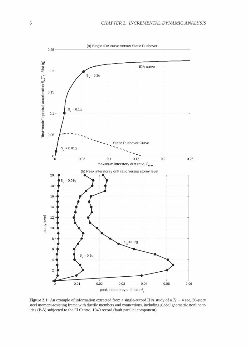
Figure 2.1: An example of information extracted from a single-record IDA study of aT1 = 4 sec, 20-storysteel moment-resisting frame with ductile members and connections, including global geometric nonlinear-ities (P-∆) subjected to the El Centro, 1940 record (fault parallel component).

2.3. FUNDAMENTALS OF SINGLE-RECORD IDAS 7
Agency (FEMA) guidelines (FEMA, 2000a,b) as the Incremental Dynamic Analysis (IDA) andestablished as the state-of-the-art method to determine global collapse capacity. The IDA studyis now a multi-purpose and widely applicable method and its objectives, only some of which areevident in Figure2.1(a,b), include
1. thorough understanding of the range of response or “demands” versus the range of potentiallevels of a ground motion record,
2. better understanding of the structural implications of rarer / more severe ground motionlevels,
3. better understanding of the changes in the nature of the structural response as the intensityof ground motion increases (e.g., changes in peak deformation patterns with height, onsetof stiffness and strength degradation and their patterns and magnitudes),
4. producing estimates of the dynamic capacity of the global structural system and
5. finally, given a multi-record IDA study, how stable (or variable) all these items are from oneground motion record to another.
Our goal is to provide a basis and terminology to unify the existing formats of the IDA studyand set up the essential background to achieve the above-mentioned objectives.
2.3 Fundamentals of single-record IDAs
As a first step, let us clearly define all the terms that we need, and start building our methodologyusing as a fundamental block the concept of scaling an acceleration time history.
Assume we are given a single acceleration time-history, selected from a ground motion data-base, which will be referred to as the base, “as-recorded” (although it may have been pre-processedby seismologists, e.g., baseline corrected, filtered and rotated), unscaled accelerograma1, a vectorwith elementsa1(ti), ti = 0, t1, . . . , tn−1. To account for more severe or milder ground motions, asimple transformation is introduced by uniformly scaling up or down the amplitudes by a scalarλ ∈ [0,+∞): aλ = λ ·a1. Such an operation can also be conveniently thought of as scaling theelastic acceleration spectrum byλ or equivalently, in the Fourier domain, as scaling byλ theamplitudes across all frequencies while keeping phase information intact.
Definition 1. TheSCALE FACTOR (SF) of a scaled accelerogram,aλ , is the non-negative scalarλ ∈ [0,+∞) that producesaλ when multiplicatively applied to the unscaled (natural) accelerationtime-historya1.
Note how theSF constitutes a one-to-one mapping from the original accelerogram to all itsscaled images. A value ofλ = 1 signifies the natural accelerogram,λ < 1 is a scaled-downaccelerogram, whileλ > 1 corresponds to a scaled-up one.
Although theSF is the simplest way to characterize the scaled images of an accelerogram it isby no means convenient for engineering purposes as it offers no information of the real “power” ofthe scaled record and its effect on a given structure. Of more practical use would be a measure thatwould map to theSF one-to-one, yet would be more informative, in the sense of better relating toits damaging potential.
Definition 2. A MONOTONIC SCALABLE GROUND MOTION INTENSITY MEASURE (or sim-ply intensity measure,IM ) of a scaled accelerogram,aλ , is a non-negative scalarIM ∈ [0,+∞)that constitutes a function,IM = fa1(λ ), that depends on the unscaled accelerogram,a1, and ismonotonicallyincreasing with the scale factor,λ .

8 CHAPTER 2. INCREMENTAL DYNAMIC ANALYSIS
While many quantities have been proposed to characterize the “intensity” of a ground motionrecord, it may not always be apparent how to scale them, e.g., Moment Magnitude, Duration,or Modified Mercalli Intensity; they must be designated as non-scalable. Common examplesof scalableIM s are the Peak Ground Acceleration (PGA), Peak Ground Velocity, theξ = 5%damped Spectral Acceleration at the structure’s first-mode period (Sa(T1,5%)), and the normalizedfactor R = λ/λyield (whereλyield signifies, for a given record and structural model, the lowestscaling needed to cause yielding) which is numerically equivalent to the yield reductionR-factor(e.g., Chopra, 1995) for, for example, bilinear SDOF systems (see later section). TheseIM salso have the property of being proportional to theSF as they satisfy the relationIMprop = λ ·fa1. On the other hand the quantitySam(T1,ξ ,b,c,d) = [Sa(T1,ξ )]b · [Sa(cT1,ξ )]d proposed byShome and Cornell(1999) andMehanny and Deierlein(2000) is scalable and monotonic but non-proportional, unlessb+d = 1. Some non-monotonicIM s have been proposed, such as the inelasticdisplacement of a nonlinear oscillator byLuco and Cornell(2004), but will not be focused upon,soIM will implicitly mean monotonic and scalable hereafter unless otherwise stated.
Now that we have the desired input to subject a structure to, we also need some way to monitorits state, its response to the seismic load.
Definition 3. DAMAGE MEASURE (DM) or STRUCTURAL STATE VARIABLE is a non-negativescalarDM ∈ [0,+∞] that characterizes the additional response of the structural model due to aprescribed seismic loading.
In other words aDM is an observable quantity that is part of, or can be deduced from, theoutput of the corresponding nonlinear dynamic analysis. Possible choices could be maximumbase shear, node rotations, peak story ductilities, various proposed damage indices (e.g., a globalcumulative hysteretic energy, a global Park–Ang index (Ang and De Leon, 1997) or the stabilityindex proposed byMehanny and Deierlein, 2000), peak roof driftθroof, the floor peak interstorydrift anglesθ1, . . . ,θn of an n-story structure, or their maximum, the maximum peak interstorydrift angleθmax = max(θ1, . . . ,θn). Selecting a suitableDM depends on the application and thestructure itself; it may be desirable to use two or moreDM s (all resulting from the same nonlinearanalyses) to assess different response characteristics, limit-states or modes of failure of interestin a PBEE assessment. If the damage to non-structural contents in a multi-story frame needs tobe assessed, the peak floor accelerations are the obvious choice. On the other hand, for structuraldamage of frame buildings,θmax relates well to joint rotations and both global and local storycollapse, thus becoming a strongDM candidate. The latter, expressed in terms of the total drift,instead of the effective drift which would take into account the building tilt, (seePrakhash et al.,1992, pg.88) will be our choice ofDM for most illustrative cases here, where foundation rotationand column shortening are not severe.
The structural response is often a signed scalar; usually, either the absolute value is used orthe magnitudes of the negative and the positive parts are separately considered. Now we are ableto define the IDA.
Definition 4. A SINGLE-RECORD IDA STUDY is a dynamic analysis study of a given structuralmodel parameterized by the scale factor of the given ground motion time history.
Also known simply as Incremental Dynamic Analysis (IDA) or Dynamic Pushover (DPO), itinvolves a series of dynamic nonlinear runs performed under scaled images of an accelerogram,whoseIM s are, ideally, selected to cover the whole range from elastic to nonlinear and finally tocollapse of the structure. The purpose is to recordDM s of the structural model at each levelIMof the scaled ground motion, the resulting response values often being plotted versus the intensitylevel as continuous curves.
Definition 5. An IDA CURVE is a plot of a state variable (DM) recorded in an IDA study versusone or moreIMs that characterize the applied scaled accelerogram.

2.4. LOOKING AT AN IDA CURVE: SOME GENERAL PROPERTIES 9
0 0.01 0.02 0.030
0.5
1
1.5
(a) A softening case
0 0.01 0.02 0.030
0.5
1
1.5
(b) A bit of hardening
0 0.01 0.02 0.030
0.5
1
1.5
(c) Severe hardening
maximum interstory drift ratio, θ max
"firs
t−m
ode"
spe
ctra
l acc
eler
atio
n S
a(T1, 5
%)
(g)
0 0.01 0.02 0.030
0.5
1
1.5
(d) Weaving behavior
Figure 2.2: IDA curves of aT1 = 1.8 sec, 5-story steel braced frame subjected to 4 different records.
An IDA curve can be realized in two or more dimensions depending on the number of theIM s. Obviously at least one must be scalable and it is such anIM that is used in the conventionaltwo-dimensional (2D) plots that we will focus on hereafter. As per standard engineering practicesuch plots often appear “upside-down” as the independent variable is theIM which is consideredanalogous to “force” and plotted on the vertical axis (Figure2.1(a)) as in stress-strain, force-deformation or SPO graphs. As is evident, the results of an IDA study can be presented in amultitude of different IDA curves, depending on the choices ofIM s andDM .
To illustrate the IDA concept we will use several MDOF and SDOF models as examples in thefollowing sections. In particular the MDOFs used are aT1 = 4 sec 20-story steel-moment resistingframe (Luco and Cornell, 2000) with ductile members and connections, including a first-ordertreatment of global geometric nonlinearities (P-∆ effects), aT1 = 2.2 sec 9-story and aT1 = 1.3 sec3-story steel-moment resisting frame (Luco and Cornell, 2000) with ductile members, fracturingconnections and P-∆ effects, and aT1 = 1.8 sec 5-story steel chevron-braced frame with ductilemembers and connections and realistically buckling braces including P-∆ effects (Bazzurro andCornell, 1994b).
2.4 Looking at an IDA curve: Some general properties
The IDA study isaccelerogramandstructural modelspecific; when subjected to different groundmotions a model will often produce quite dissimilar responses that are difficult to predict a priori.Notice, for example, Figure2.2(a–d) where a 5-story braced frame exhibits responses ranging froma gradual degradation towards collapse to a rapid, non-monotonic, back-and-forth twisting behav-ior. Each graph illustrates thedemandsimposed upon the structure by each ground motion recordat different intensities, and they are quite intriguing in both their similarities and dissimilarities.

10 CHAPTER 2. INCREMENTAL DYNAMIC ANALYSIS
0 0.005 0.01 0.015 0.02 0.025 0.03
0.2
0.4
0.6
0.8
1
1.2
1.4
storey 1 storey 2 storey 3
storey 4
storey 5
maximum interstory drift ratio, θ max
"firs
t−m
ode"
spe
ctra
l acc
eler
atio
n S
a(T
1, 5
%)
(g)
Figure 2.3: IDA curves of peak interstory drifts for each floor of aT1 = 1.8 sec 5-story steel braced frame.Notice the complex “weaving” interaction where extreme softening of floor 2 acts as a fuse to relieve thoseabove (3,4,5).
All curves exhibit a distinct elastic linear region that ends atSyielda (T1,5%)≈ 0.2g andθ yield
max ≈0.2% when the first brace-buckling occurs. Actually, any structural model with initially linearlyelastic elements will display such a behavior, which terminates when the first nonlinearity comesinto play, i.e., when any element reaches the end of its elasticity. The slopeIM/DM of this segmenton each IDA curve will be called its elastic “stiffness” for the givenDM , IM . It typically variesto some degree from record to record but it will be the same across records for SDOF systemsand even for MDOF systems if theIM takes into account the higher mode effects (i.e.,Luco andCornell, 2004).
Focusing on the other end of the curves in Figure2.2, notice how they terminate at differentlevels ofIM . Curve (a) sharply “softens” after the initial buckling and accelerates towards largedrifts and eventual collapse. On the other hand, curves (c) and (d) seem to weave around the elasticslope; they follow closely the familiarequal displacementrule, i.e., the empirical observation thatfor moderate period structures, inelastic global displacements are generally approximately equalto the displacements of the corresponding elastic model (e.g.,Veletsos and Newmark, 1960). Thetwisting patterns that curves (c) and (d) display in doing so are successive segments of “softening”and “hardening”, regions where the local slope or “stiffness” decreases with higherIM and otherswhere it increases. In engineering terms this means that at times the structure experiences acceler-ation of the rate ofDM accumulation and at other times a deceleration occurs that can be powerfulenough to momentarily stop theDM accumulation or even reverse it, thus locally pulling the IDAcurve to relatively lowerDM s and making it a non-monotonic function of theIM (Figure2.2(d)).Eventually, assuming the model allows for some collapse mechanism and theDM used can trackit, a final softening segment occurs when the structure accumulatesDM at increasingly higherrates, signaling the onset ofdynamic instability. This is defined analogously to static instability,as the point where deformations increase in an unlimited manner for vanishingly small incrementsin the IM . The curve then flattens out in a plateau of the maximum value inIM as it reaches the

2.4. LOOKING AT AN IDA CURVE: SOME GENERAL PROPERTIES 11
0 0.5 1 1.5 2 2.5 3 3.5 40
0.5
1
1.5
2
2.5
3
3.5
"firs
t−m
ode"
spe
ctra
l acc
eler
atio
n S
a(T1, 5
%)
(g)
(a) IDA curve
Sa = 2.8g
ductility, µ
Sa = 2.2g
0 5 10 15 20 25 30 35 40
−0.1
−0.05
0
0.05
0.1
Acc
eler
atio
n (g
)
(b) Loma Prieta, Halls Valley (090 component)
0 5 10 15 20 25 30 35 40
−2
0
2
(c) Response at Sa = 2.2g
duct
ility
, µ
0 5 10 15 20 25 30 35 40
−2
0
2
(d) Response at Sa = 2.8g
duct
ility
, µ
time (sec)
maximum
maximum
first yield
first yield
Figure 2.4: Ductility response of aT = 1 sec, elasto-plastic oscillator at multiple levels of shaking. Earlieryielding in the stronger ground motion leads to a lower absolute peak response.

12 CHAPTER 2. INCREMENTAL DYNAMIC ANALYSIS
0 0.05 0.1 0.150
0.2
0.4
0.6
0.8
1
1.2
1.4
1.6
1.8
maximum interstory drift ratio, θ max
"firs
t−m
ode"
spe
ctra
l acc
eler
atio
n S
a(T1, 5
%)
(g)
structural resurrection
intermediate collapse area
Figure 2.5: Structural resurrection on the IDA curve of aT1 = 1.3 sec, 3-story steel moment-resisting framewith fracturing connections.
flatline andDM moves towards “infinity” (Figure2.2(a,b)). Although the examples shown arebased onSa(T1,5%) andθmax, these modes of behavior are observable for a wide choice ofDM sandIM s.
Hardening in IDA curves is not a novel observation, having been reported before even for sim-ple bilinear elastic-perfectly-plastic systems, e.g., byChopra(1995, pg.257-259). Still it remainscounter-intuitive that a system that showed high response at a given intensity level, may exhibit thesame or even lower response when subjected to higher seismic intensities due to excessive harden-ing. But it is thepatternand thetiming rather than just the intensity that make the difference. Asthe accelerogram is scaled up, weak response cycles in the early part of the response time-historybecome strong enough to inflict damage (yielding) thus altering the properties of the structure forthe subsequent, stronger cycles. For multi-story buildings, a stronger ground motion may lead toearlier yielding of one floor which in turn acts as a fuse to relieve another (usually higher) one,as in Figure2.3. Even simple oscillators when caused to yield in an earlier cycle, may be provenless responsive in later cycles that had previously caused higherDM values (Figure2.4), perhapsdue to “period elongation”. The same phenomena account for thestructural resurrection, an ex-treme case of hardening, where a system is pushed all the way to global collapse (i.e., the analysiscode cannot converge, producing “numerically infinite”DM s) at someIM , only to reappear asnon-collapsing at a higher intensity level, displaying high response but still standing (e.g., Figure2.5).
As the complexity of even the 2D IDA curve becomes apparent, it is only natural to examinethe properties of the curve as a mathematical entity. Assuming a monotonicIM the IDA curvebecomes afunction([0,+∞)→ [0,+∞]), i.e., any value ofIM produces a single valueDM , whilefor any givenDM value there is at least one or more (in non-monotonic IDA curves)IM s thatgenerate it, since the mapping is not necessarily one-to-one. Also, the IDA curve is not necessar-

2.5. CAPACITY AND LIMIT-STATES ON SINGLE IDA CURVES 13
ily smooth as theDM is often defined as a maximum or contains absolute values of responses,making it non-differentiable by definition. Even more, it may contain a (hopefully finite) numberof discontinuities, due to multiple excursions to collapse and subsequent resurrections.
2.5 Capacity and limit-states on single IDA curves
Performance levels or limit-states are important ingredients of Performance Based EarthquakeEngineering (PBEE), and the IDA curve contains the necessary information to assess them. Butwe need to define them in a less abstract way that makes sense on an IDA curve, i.e., by a statementor a rule that when satisfied, signals reaching a limit-state. For example, Immediate Occupancy(FEMA, 2000a,b) is a structural performance level that has been associated with reaching a givenDM value, usually inθmax terms, while (in FEMA 350,FEMA, 2000a, at least) Global Collapseis related to theIM or DM value where dynamic instability is observed. A relevant issue that thenappears is what to do when multiple points (Figure2.6(a,b)) satisfy such a rule? Which one is tobe selected?
The cause of multiple points that can satisfy a limit-state rule is mainly the hardening issueand, in its extreme form, structural resurrection. In general, one would want to be conservative andconsider the lowest, inIM terms, point that will signal the limit-state. Generalizing this concept tothe whole IDA curve means that we will discard its portion “above” the first (inIM terms) flatlineand just consider only points up to this first sign of dynamic instability.
Note also that for most of the discussion we will be equating dynamic instability to numeri-cal instability in the prediction of collapse. Clearly the non-convergence of the time-integrationscheme is perhaps the safest and maybe the only numerical equivalent of the actual phenomenonof dynamic collapse. But, as in all models, this one can suffer from the quality of the numericalcode, the stepping of the integration and even the round-off error. Therefore, we will assume thatsuch matters are taken care of as well as possible to allow for accurate enough predictions. Thatbeing said, let us set forth the most basic rules used to define a limit-state.
First comes theDM-based rule, which is generated from a statement of the format: “IfDM≥CDM then the limit-state is exceeded” (Figure2.6(a)). The underlying concept is usually thatDM is a damage indicator, hence, when it increases beyond a certain value the structural model isassumed to be in the limit-state. Such values ofCDM can be obtained through experiments, theoryor engineering experience, and they may not be deterministic but have a probability distribution.An example is theθmax= 2%limit that signifies the Immediate Occupancy structural performancelevel for steel moment-resisting frames (SMRFs) with type-1 connections in the FEMA guidelines(FEMA, 2000b). Also the approach used byMehanny and Deierlein(2000) is another case wherea structure-specific damage index is used asDM and when its reciprocal is greater than unity, col-lapse is presumed to have occurred. Such limits may have randomness incorporated, for example,FEMA 350 (FEMA, 2000a) defines a local collapse limit-state by the value ofθmax that induces aconnection rotation sufficient to destroy the gravity load carrying capacity of the connection. Thisis defined as a random variable based on tests, analysis and judgment for each connection type.Even a uniqueCDM value may imply multiple limit-state points on an IDA curve (e.g., Figure2.6(a)). This ambiguity can be handled by an ad hoc, specified procedure (e.g., by conservativelydefining the limit-state point as the lowestIM ), or by explicitly recognizing the multiple regionsconforming and non-conforming with the performance level. TheDM -based rules have the ad-vantage of simplicity and ease of implementation, especially for performance levels other thancollapse. In the case of collapse capacity though, they may actually be a sign of model deficiency.If the model is realistic enough it ought to explicitly contain such information, i.e., show a collapseby non-convergence instead of by a finiteDM output. Still, one has to recognize that such modelscan be quite complicated and resource-intensive, while numerics can often be unstable. HenceDM -based collapse limit-state rules can be quite useful. They also have the advantage of being

14 CHAPTER 2. INCREMENTAL DYNAMIC ANALYSIS
0 0.05 0.1 0.15 0.2 0.250
0.2
0.4
0.6
0.8
1
1.2
1.4
1.6
1.8
maximum interstory drift ratio, θ max
"firs
t−m
ode"
spe
ctra
l acc
eler
atio
n S
a(T1, 5
%)
(g)
(a) DM−based rule
collapse
CDM
= 0.08
capacity point
0 0.05 0.1 0.15 0.2 0.250
0.2
0.4
0.6
0.8
1
1.2
1.4
1.6
1.8
maximum interstory drift ratio, θ max
"firs
t−m
ode"
spe
ctra
l acc
eler
atio
n S
a(T1, 5
%)
(g)
(b) IM−based rule
collapse
CIM
= 1.61g capacity point
rejected point
Figure 2.6: Two different rules producing multiple capacity points for aT1 = 1.3 sec, 3-story steel moment-resisting frame with fracturing connections. TheDM rule, where theDM is θmax, is set atCDM = 0.08andtheIM rule uses the20%slope criterion.

2.6. MULTI-RECORD IDAS AND THEIR SUMMARY 15
consistent with other less severe limit-states which are more naturally identified inDM terms, e.g.,θmax.
The alternativeIM-based rule, is primarily generated from the need to better assess collapsecapacity, by having a single point on the IDA curve that clearly divides it to two regions, oneof non-collapse (lowerIM ) and one of collapse (higherIM ). For monotonicIM s, such a ruleis generated by a statement of the form: “IfIM ≥CIM then the limit-state is exceeded” (Figure2.6(b)). A major difference with the previous category is the difficulty in prescribing aCIM valuethat signals collapse for all IDA curves, so it has to be done individually, curve by curve. Still, theadvantage is that it clearly generates a single collapse region, and the disadvantage is the difficultyof defining such a point for each curve in a consistent fashion. In general, such a rule results inboth IM andDM descriptions of capacity. A special (extreme) case is taking the “final” point ofthe curve as the capacity, i.e., by using the (lowest) flatline to define capacity (inIM terms), whereall of the IDA curve up to the first appearance of dynamic instability is considered as non-collapse.
TheFEMA (2000a) 20% tangent slope approach is, in effect, anIM -based rule; thelast pointon the curve with a tangent slope equal to 20% of the elastic slope is defined to be the capacitypoint. The idea is that the flattening of the curve is an indicator of dynamic instability (i.e., theDM increasing at ever higher rates and accelerating towards “infinity”). Since “infinity” is not apossible numerical result, we content ourselves with pulling back to a rate ofθmax increase equalto five times the initial or elastic rate, as the place where we mark the capacity point. Care needsto be exercised, as the possible “weaving” behavior of an IDA curve can provide several suchpoints where the structure seems to head towards collapse, only to recover at a somewhat higherIM level, as in Figure2.6(b); in principle, these lower points should thus be discarded as capacitycandidates. Also the non-smoothness of the actual curve may prove to be a problem. As mentionedabove, the IDA curve is at best piecewise smooth, but even so, approximate tangent slopes can beassigned to every point along it by employing a smooth interpolation. For sceptics this may also bethought of as a discrete derivative on a grid of points that is a good “engineering” approximationto the “rate-of-change”.
The above mentioned simple rules are the building blocks to construct composite rules, i.e.,composite logical clauses of the above types, most often joined by logical OR operators. Forexample, when a structure has several collapse modes, not detectable by a singleDM , it is ad-vantageous to detect global collapse with an OR clause for each individual mode. An example isoffshore platforms where pile or soil failure modes are evident in deck drift while failures of bracesare more evident in maximum peak inter-tier drift. The first — inIM terms — event that occurs isthe one that governs collapse capacity. Another case is Global Collapse capacity, which as definedby FEMA in FEMA (2000a,b) is in fact an OR conjunction of the 20% slopeIM -based rule and aCDM = 10%DM -based rule, whereSa(T1,5%) andθmax are theIM andDM of choice. If either ofthe two rules obtains, it defines capacity. This means that the 20% stiffness detects impending col-lapse, while the 10% cap guards against excessive values ofθmax, indicative of regions where themodel may not be trustworthy. As aDM description of capacity is proposed, this definition maysuffer from inaccuracies, since close to the flatline a wide range ofDM values may correspond toonly a small range ofIM s, thus making the actual value ofDM selected sensitive to the quality ofIDA curve tracing and to the (ad hoc) 20% value. If, on the other hand, anIM description is used,the rule becomes more robust. This is a general observation for collapse capacity; it appears thatit can be best expressed inIM terms.
2.6 Multi-record IDAs and their summary
As should be evident by now, a single-record IDA study cannot fully capture the behavior a build-ing may display in a future event. The IDA can be highly dependent on the record chosen, so asufficient number of records will be needed to cover the full range of responses. Hence, we have

16 CHAPTER 2. INCREMENTAL DYNAMIC ANALYSIS
to resort to subjecting the structural model to a suite of ground motion records.
Definition 6. A MULTI -RECORD IDA STUDY is a collection of single-record IDA studies of thesame structural model, under different accelerograms.
Such a study, correspondingly produces sets of IDA curves, which by sharing a commonselection ofIM s and the sameDM , can be plotted on the same graph, as in Figure2.7(a) for a5-story steel braced frame.
Definition 7. An IDA CURVE SET is a collection of IDA curves of the same structural modelunder different accelerograms, that are all parameterized on the sameIMs andDM.
While each curve, given the structural model and the ground motion record, is a completelydefined deterministic entity, if we wish to take into account the inherent randomness with respectto what record the building might experience, we have to bring a probabilistic characterizationinto play. The IDA given the structural model and a statistical population of records is no longerdeterministic; it is arandom line, or a random functionDM = f (IM ) (for a single, monotonicIM ). Then, just as we are able to summarize a suite of records by having, for example, mean,median, and 16%, 84% response spectra, so we can define mean, median and 16%, 84% IDAcurves (e.g., Figure2.7(b)) to (marginally) summarize an IDA curve set. We, therefore, needmethods for estimating statistics of a sample of 2D random lines (assuming a singleIM ), a topicof Functional Data Analysis (Ramsay and Silverman, 1996). They conveniently fall in two maincategories.
First are the parametric methods. In this case a parametric model of theDM given theIM isassumed, each line is separately fit, providing a sample of parameter values, and then statistics ofthe parameters are obtained. Alternatively a parametric model of the medianDM given theIMcan be fit to all the lines simultaneously. As an example, consider the 2-parameter, power-lawmodelθmax = α · [Sa(T1,5%)]β introduced byShome and Cornell(1999), which under the well-documented assumption of lognormality of the conditional distribution ofθmax givenSa(T1,5%),often provides a simple yet powerful description of the curves, allowing some important analyticresults to be obtained (Jalayer and Cornell, 2002; Cornell et al., 2002). This is a general propertyof parametric methods; while they lack the flexibility to accurately capture each curve, they makeup by allowing simple descriptions to be extracted.
On the other end of the spectrum are the non-parametric methods, which mainly involve theuse of “scatterplot smoothers” like the running mean, running median,LOESSor the smoothingspline (Hastie and Tibshirani, 1990). Perhaps the simplest of them all, the running mean witha zero-length window (or cross-sectional mean), involves simply calculating values of theDMat each level ofIM and then finding the average and standard deviation ofDM given theIMlevel. This works well up to the point where the first IDA curve reaches capacity, whenDMbecomes infinite, and so does the mean IDA curve. Unfortunately most smoothers suffer fromthe same problem, but the cross-sectional median, or cross-sectional fractile is, in general, morerobust. Instead of calculating means at eachIM level, we now calculate sample medians, 16%and 84% fractiles, which become infinite only when collapse occurs in 50%, 84% and 16% of therecords respectively. Another advantage is that under suitable assumptions (e.g., continuity andmonotonicity of the curves), the line connecting thex% fractiles ofDM given IM is the same asthe one connecting the(100−x)% fractiles ofIM givenDM . Furthermore, this scheme fits nicelywith the well-supported assumption of lognormal distribution ofθmax givenSa(T1,5%), where themedian is the natural “central value” and the 16%, 84% fractiles correspond to the median timese∓dispersion, where “dispersion” is the standard deviation of the logarithms of the values (Jalayerand Cornell, 2002).
Finally, a variant for treating collapses is proposed byShome and Cornell(2000), where theconventional moments are used to characterize non-collapses, thus removing the problem of in-

2.6. MULTI-RECORD IDAS AND THEIR SUMMARY 17
0 0.005 0.01 0.015 0.02 0.0250
0.5
1
1.5
2
maximum interstory drift ratio, θ max
"firs
t−m
ode"
spe
ctra
l acc
eler
atio
n S
a(T1, 5
%)
(g)
(a) Thirty IDA curves
10−3
10−2
10−1
100
maximum interstory drift ratio, θ max
"firs
t−m
ode"
spe
ctra
l acc
eler
atio
n S
a(T1, 5
%)
(g)
• 50%
• 16%
• 84 %
(b) 16%, 50% and 84% fractiles
Figure 2.7: An IDA study for thirty records on aT1 = 1.8 sec, 5-story steel braced frame, showing (a) thethirty individual curves and (b) their summary (16%, 50% and 84%) fractile curves (in log-log scale).

18 CHAPTER 2. INCREMENTAL DYNAMIC ANALYSIS
finities, while the probability of collapse given theIM is summarized separately by a logisticregression.
A simpler, yet important problem is the summarizing of the capacities of a sample ofN curves,expressed either inDM (e.g.,{C i
θmax}, i = 1. . .N ) or IM (e.g.,{C i
Sa(T1,5%)}, i = 1. . .N ) terms.Since there are neither random lines nor infinities involved, the problem reduces to conventionalsample statistics, so we can get means, standard deviations or fractiles as usual. Still, the observedlognormality in the capacity data, often suggests the use of the median (e.g.,CSa(T1,5%) or Cθmax),estimated either as the 50% fractile or as the antilog of the mean of the logarithms, and the stan-dard deviation of the logarithms as dispersion. Finally, when considering limit-state probabilitycomputations (see section below), one needs to address potential dependence (e.g., correlation)between capacity and demand. Limited investigation to date has revealed little if any systematiccorrelation betweenDM capacity andDM demand (givenIM ).
2.7 The IDA in a PBEE framework
The power of the IDA as an analysis method is put to use well in a probabilistic framework, wherewe are concerned with the estimation of the annual likelihood of the event that the demand exceedsthe limit-state or capacityC. This is the likelihood of exceeding a certain limit-state, or of failinga performance level (e.g., Immediate Occupancy or Collapse Prevention inFEMA, 2000a), withina given period of time. The calculation can be summarized in the framing equation adopted by thePacific Earthquake Engineering Center (Cornell and Krawinkler, 2000)
λ (DV ) =∫∫
G(DV |DM ) |dG(DM |IM )| |dλ (IM )| (2.1)
in which IM , DM andDV are vectors of intensity measures, damage measures and “decisionvariables” respectively. In this paper we have generally used scalarIM (e.g., Sa(T1,5%)) andDM (e.g.,θmax) for the limit-state case of interest. The decision variable here is simply a scalar“indicator variable”: DV = 1 if the limit-state is exceeded (and zero otherwise).λ (IM) is theconventional hazard curve, i.e., the mean annual frequency ofIM exceeding, say,x. The quantity|dλ (x)|= |dλ (x)/dx| dx is its differential (i.e.,|dλ (x)/dx| is the mean rate density).|dG(DM |IM)|is the differential of the (conditional) complementary cumulative distribution function (CCDF)of DM given IM , or fDM |IM (y|x)dy. In the previous sections we discussed the statistical char-acterization of the random IDA lines. These distributions are precisely this characterization of|dG(DM |IM)|. Finally in the limit-state case, when on the left-hand side of Equation (2.1) weseekλ (DV=1) = λ (0), G(0|DM) becomes simply the probability that the capacityC is less thansome level of theDM , say,y; so G(0|DM) = FC(y), whereFC(y) is the cumulative distributionfunction ofC, i.e., the statistical characterization of capacity, also discussed at the end of the pre-vious section. In the global collapse case, capacity estimates also come from IDA analyses. Inshort, save for the seismicity characterization,λ (IM), given an intelligent selection ofIM , DMand structural model, the IDA produces, in arguably the most comprehensive way, precisely theinformation needed both for PBEE demand characterization and for global collapse capacity char-acterization.
2.8 Scaling legitimacy andIM selection
As discussed above, we believe there is useful engineering insight to be gained by conductingindividual and sets of IDA studies. However, concern is often expressed about the “validity” ofDM results obtained from records that have been scaled (up or down), an operation that is notuncommon both in research and in practice. While not always well expressed, the concern usuallyhas something to do with “weaker” records not being “representative” of “stronger” ones. The

2.8. SCALING LEGITIMACY AND IM SELECTION 19
0
0.1
0.2
0.3
0.6
Sa,T=0.42
Sa,2=0.51
Sa,yldg
0.75
0 1 2 3 4 5 6 7 8 9 10
Sa(
f,ξ)
(g)
µ=δMDOF/δyldg
(δMDOFNL,1)T/δyldg
(δMDOFNL,2)T/δyldg
Scaled recordsUnscaled records
Figure 2.8: Roof ductility response of aT1 = 1 sec, MDOF steel frame subjected to 20 records, scaled to5 levels ofSa(T1,5%). The unscaled record response and the power-law fit are also shown for comparison(from Bazzurro et al., 1998).
0 0.05 0.1 0.150
1
2
3
4
5
6
maximum interstory drift ratio, θ max
peak
gro
und
acce
lera
tion
PG
A (
g)
(a) Twenty IDA curves versus Peak Ground Acceleration
0 0.05 0.1 0.150
0.5
1
1.5
2
2.5
3
maximum interstory drift ratio, θ max
"firs
t−m
ode"
spe
ctra
l acc
eler
atio
n S
a(T
1, 5
%)
(g)
(b) Twenty IDA curves versus Sa(T1, 5%)
Figure 2.9: IDA curves for aT1 = 2.2sec, 9-story steel moment-resisting frame with fracturing connectionsplotted against (a)PGA and (b)Sa(T1,5%).

20 CHAPTER 2. INCREMENTAL DYNAMIC ANALYSIS
issue can be more precisely stated in the context of the last two sections as: will the median (or anyother statistic of)DM obtained from records that have been scaled to some level ofIM estimateaccurately the medianDM of a population of unscaled records all with that same level ofIM .Because of current record catalog limitations, where few records of any single givenIM level canbe found, and because we have interest usually in a range ofIM levels (e.g., in integrations suchas Equation (2.1)), it is both more practical and more complete to ask: will the (regression-like)function medianDM versusIM obtained from scaled records (whether via IDAs or otherwise)estimate well that same function obtained from unscaled records? There is a growing body ofliterature related to such questions that is too long to summarize here (e.g.,Shome and Cornell,1998, 1999). An example of such a comparison is given in Figure2.8from Bazzurro et al.(1998),where the two regressions are so close to one another that only one was plotted by the authors.Suffice it to say that, in general, the answer to the question depends on the structure, theDM ,the IM and the population in mind. For example, the answer is “yes” for the case pictured inFigure2.8, i.e., for a moderate period (1 sec) steel frame, for whichDM is maximum interstorydrift and IM is first-mode-period spectral acceleration, and for a fairly general class of records(moderate to large magnitudes,M, all but directivity-influenced distances,R, etc.). On the otherhand, for all else equal exceptIM defined now asPGA, the answer would be “no” for this samecase. Why? Because such a (first-mode dominated) structure is sensitive to the strength of thefrequency content near its first-mode frequency, which is well characterized by theSa(1 sec,5%)but not byPGA, and as magnitude changes, spectral shape changes implying that the averageratio of Sa(1 sec,5%) to PGA changes with magnitude. Therefore the scaled-record median driftversusPGA curve will depend on the fractions of magnitudes of different sizes present in thesample, and may or may not represent well such a curve for any (other) specified population ofmagnitudes. On the other hand, theIM first-mode spectral acceleration will no longer work wellfor a tall, long-period building that is sensitive to shorter periods, again because of spectral shapedependence on magnitude.
There are a variety of questions of efficiency, accuracy and practicality associated with the wisechoice of theIM for any particular application (e.g.,Luco and Cornell, 2004), but it can generallybe said here that if theIM has been chosen such that the regression ofDM jointly on IM , M andR is found to be effectively independent ofM andR (in the range of interest), then, yes, scaling ofrecords will provide good estimates of the distribution ofDM given IM . Hence we can concludethat scaling is indeed (in this sense) “legitimate”, and finally that IDAs provide accurate estimatesof DM given IM statistics (as required, for example, for PBEE use; seeBazzurro et al.(1998),Shome and Cornell(1999).
IDA studies may also bring a fresh perspective to the larger question of the effectiveIMchoice. For example, smaller dispersion ofDM givenIM implies that a smaller sample of recordsand fewer nonlinear runs are necessary to estimate medianDM versusIM . Therefore, a desir-able property of a candidateIM is small dispersion. Figure2.9 shows IDAs from a 9-story steelmoment-resisting frame in which theDM is θmax and theIM is either (a)PGA or (b)Sa(T1,5%).The latter produces a lower dispersion over the full range ofDM values, as the IDA-based resultsclearly display. Furthermore, the IDA can be used to study how well (with what dispersion) partic-ular IM s predict collapse capacity; againSa(T1,5%) appears preferable toPGA for this structureas the dispersion ofIM values associated with the “flatlines” is less in the former case.
2.9 The IDA versus theR-factor
A popular form of incremental seismic analysis, especially for SDOF oscillators, has been thatleading to the yield reductionR-factor (e.g.,Chopra, 1995). In this case the record is left un-scaled, avoiding record scaling concerns; instead, the yield force (or yield deformation, or, inthe multi-member MDOF case, the yield stress) of the model is scaled down from that level that

2.10. THE IDA VERSUS THE NONLINEAR STATIC PUSHOVER 21
coincides with the onset of inelastic behavior. If both are similarly normalized (e.g., ductility =deformation/yield-deformation andR= Sa(T1,5%)/Syield
a (T1,5%)), the results of this scaling andthose of an IDA will be identical for those classes of systems for which such simple structuralscaling is appropriate, e.g., most SDOF models, and certain MDOF models without axial-force–moment interaction, without second-or-higher-order geometric nonlinearities, etc. One mightargue that these cases of common results are another justification for the legitimacy of scalingrecords in the IDA. It can be said that the difference between theR-factor and IDA perspectivesis one of design versus assessment. For design one has an allowable ductility in mind and seeksthe design yield force that will achieve this; for assessment one has a fixed design (or existingstructure) in hand and seeks to understand its behavior under a range of potential future groundmotion intensities.
2.10 The IDA versus the Nonlinear Static Pushover
The common incremental loading nature of the IDA study and the SPO suggests an investigationof the connection between their results. As they are both intended to describe the same structure,we should expect some correlation between the SPO curve and any IDA curve of the building(Figure2.1), and even more so between the SPO and the summarized (median) IDA curve, as thelatter is less variable and less record dependent. Still, to plot both on the same graph, we shouldpreferably express the SPO in theIM , DM coordinates chosen for the summarized IDA. WhilesomeDM s (e.g.,θmax) can easily be obtained from both the static and the dynamic analysis, itmay not be so natural to convert theIM s, e.g., base shear toSa(T1,5%). The proposed approachis to adjust the “elastic stiffness” of the SPO to be the same as that of the IDA, i.e., by matchingtheir elastic segments. This can be achieved in the aforementioned example by dividing the baseshear by the building mass, which is all that is needed for SDOF systems, times an appropriatefactor for MDOF systems.
The results of such a procedure are shown in Figures2.10(a,b) where we plot the SPO curve,obtained using a first-mode force pattern, versus the median IDA for a 20-story steel moment-resisting frame with ductile connections and for a 5-story steel braced frame usingSa(T1,5%) andθmax coordinates. Clearly both the IDA and the SPO curves display similar ranges ofDM values.The IDA always rises much higher than the SPO inIM terms, however. While a quantitativerelation between the two curves may be difficult, deserving further study (e.g.,Seneviratna andKrawinkler, 1997), qualitatively we can make some, apparently, quite general observations thatpermit inference of the approximateshapeof the median IDA simply by looking at the SPO.
1. By construction, the elastic region of the SPO matches well the IDA, including the first signof nonlinearity appearing at the same values ofIM andDM for both.
2. A subsequent reduced, but still non-negative stiffness region of the SPO correlates on theIDA with the approximate “equal-displacement” rule (for moderate-period structures) (Ve-letsos and Newmark, 1960), i.e., a near continuation of the elastic regime slope; in factthis near-elastic part of the IDA is often preceded by ahardeningportion (Figure2.10(a)).Shorter-period structures will instead display some softening.
3. A negative slope on the SPO translates to a (softening) region of the IDA, which can lead tocollapse, i.e., IDA flat-lining (Figure2.10(a)), unless it is arrested by a non-negative segmentof the SPO before it reaches zero inIM terms (Figure2.10(b)).
4. A non-negative region of the SPO that follows after a negative slope that has caused a signifi-cantIM drop, apparently presents itself in the IDA as a new, modified “equal-displacement”rule (i.e., an near-linear segment that lies on a secant) that has lower “stiffness” than the elas-tic (Figure2.10(b)).

22 CHAPTER 2. INCREMENTAL DYNAMIC ANALYSIS
0 0.02 0.04 0.06 0.08 0.1 0.12 0.14 0.160
0.05
0.1
0.15
0.2
0.25
0.3
0.35
0.4
maximum interstory drift ratio, θ max
"firs
t−m
ode"
spe
ctra
l acc
eler
atio
n S
a(T
1, 5
%)
(g)
(a) IDA versus Static Pushover for a 20−storey steel moment resisting frame
median IDA curve Static Pushover curve
equal displacement
hardening
softening towards flatline
elastic
non−negative segment
negative slope dropping to zero IM
0 0.002 0.004 0.006 0.008 0.01 0.012 0.014 0.016 0.018 0.020
0.1
0.2
0.3
0.4
0.5
0.6
0.7
0.8
0.9
1
maximum interstory drift ratio, θ max
"firs
t−m
ode"
spe
ctra
l acc
eler
atio
n S
a(T
1, 5
%)
(g)
(b) IDA versus Static Pushover for a 5−storey steel braced frame
median IDA curve Static Pushover curve
equal displacement
"new" equal displacement
"mostly non−negative" segment
elastic negative segment
softening
Figure 2.10: The median IDA versus the Static Pushover curve for (a) aT1 = 4 sec, 20-story steel moment-resisting frame with ductile connections and (b) aT1 = 1.8 sec, 5-story steel braced frame.

2.11. IDA ALGORITHMS 23
2.11 IDA Algorithms
Despite the theoretical simplicity of an IDA study, actually performing one can potentially beresource intensive. Although we would like to have an almost continuous representation of IDAcurves, for most structural models the sheer cost of each dynamic nonlinear run forces us to thinkof algorithms designed to select an optimal grid of discreteIM values that will provide the desiredcoverage. The density of a grid on the curve is best quantified in terms of theIM values used,the objectives being: a highdemand resolution, achieved by evenlyspreadingthe points and thushaving no gap in ourIM values larger than some tolerance, and a highcapacity resolution, whichcalls for aconcentrationof points around the flatline to bracket it appropriately, e.g., by having adistance between the highest (in terms ofIM ) “non-collapsing” run and the lowest “collapsing”run less than some tolerance. Here, by collapsing run we mean a dynamic analysis performed atsomeIM level that is determined to have caused collapse, either by satisfying some collapse-rule(IM or DM based, or more complex) or simply by failing to converge to a solution. Obviously, ifwe allow only a fixed number of runs for a given record, these two objectives compete with oneanother.
In a multi-record IDA study, there are some advantages to be gained by using information fromthe results of one record to adapt the grid of points to be used on the next. Even without exploitingthese opportunities, we can still design efficient methods to tackle each record separately that aresimpler and more amenable to parallelization on multiple processors. Therefore we will focus onthetracingof single IDA curves.
Probably the simplest solution is asteppingalgorithm, where theIM is increased by a constantstep from zero to collapse, a version of which is also described inYun et al.(2002). The end resultis a uniformly-spaced (inIM ) grid of points on the curve. The algorithm needs only a pre-definedstep value and a rule to determine when to stop, i.e., when a run is collapsing.
repeatincreaseIM by the stepscale record, run analysis and extractDM (s)
until collapse is reached
Although it is an easily programmable routine it may not be cost-efficient as its quality islargely dependent on the choice of theIM step. Even if information from previously processedground motion records is used, the step size may easily be too large or too small for this record.Even then, the variability in the “height” (inIM terms) of the flatline, which is both accelerogramandIM dependent, tends to unbalance the distribution of runs; IDA curves that reach the flatlineat a lowIM level receive fewer runs, while those that collapse at higherIM levels get more points.The effect can be reduced by selecting a goodIM , e.g.,Sa(T1,5%) instead ofPGA, asIM s withhigher DM variability tend to produce more widely dispersed flatlines (Figure2.9). Anotherdisadvantage is the implicit coupling of the capacity and demand estimation, as the demand andthe capacity resolutions are effectively the same and equal to the step size.
Trying to improve upon the basis of the stepping algorithm, one can use the ideas on searchingtechniques available in the literature (e.g.,Press et al., 1986). A simple enhancement that increasesthe speed of convergence to the flatline is to allow the steps to increase, for example by a factor,resulting in a geometric series ofIM s, or by a constant, which produces a quadratic series. This isthehunting phaseof the code where the flatline is bracketed without expending more than a fewruns.
repeatincreaseIM by the stepscale record, run analysis and extractDM (s)

24 CHAPTER 2. INCREMENTAL DYNAMIC ANALYSIS
increase the stepuntil collapse is reached
Furthermore, to improve upon the capacity resolution, a simple enhancement is to add a step-reducing routine, for example bisection, when collapse (e.g., non-convergence) is detected, so asto tighten the bracketing of the flatline. This will enable a prescribed accuracy for the capacity tobe reached regardless of the demand resolution.
repeatselect anIM in the gap between the highest non-collapsing and lowest non-collapsingIM sscale record, run analysis and extractDM (s)
until highest collapsing and lowest non-collapsingIM -gap< tolerance
Even up to this point, this method is a logical replacement for the algorithm proposed inYunet al.(2002) and in the FEMA guidelines (FEMA, 2000a) as this algorithm is focused on optimallylocating the capacity, which is the only use made of the IDA in those two references. If we alsowish to use the algorithm for demand estimation, coming back to fill in the gaps created by theenlarged steps is desirable to improve upon the demand resolution there.
repeatselect anIM that halves the largest gap between theIM levels runscale record, run analysis and extractDM (s)
until largest non-collapsingIM -gap< tolerance
When all three pieces are run sequentially, they make for a more efficient procedure, ahunt& fill tracing algorithm, described in detail byVamvatsikos and Cornell(2002b), that performsincreasingly larger leaps, attempting to bound theIM parameter space, and then fills in the gaps,both capacity and demand-wise. It needs an initial step and a stopping rule, just like the steppingalgorithm, plus a step increasing function, a capacity and a demand resolution. The latter two canbe selected so that a prescribed number of runs is performed on each record, thus tracing eachcurve with the same load of resources.
A subtle issue here is the summarization of the IDA curves produced by the algorithm. Obvi-ously, if the same step is used for all records and if there is no need to use anotherIM , the steppingalgorithm immediately provides us with stripes ofDM at given values ofIM (e.g., Figure2.8).So a “cross-sectional median” scheme could be implemented immediately on the output, withoutany post-processing. On the other hand, a hunt & fill algorithm would produceDM values atnon-matching levels ofIM across the set of records, which necessitates the interpolation of theresulting IDA curve to calculate intermediate values. Naturally, the same idea can be applied tothe output of any IDA tracing algorithm, even a stepping one, to increase the density of discretepoints without the need for additional dynamic analyses. Ideally, a flexible, highly non-parametricscheme should be used. Coordinate-transformed natural splines, as presented inVamvatsikos andCornell (2002b), are a good candidate. Actually all the IDA curves in the figures of the paper areresults of such an interpolation of discrete points. However, before implementing any interpola-tion scheme, one should provide a dense enough grid ofIM values to obtain a high confidence ofdetecting any structural resurrections that might occur before the final flatline.
2.12 Conclusions
The results of Incremental Dynamic Analyses of structures suggest that the method can becomea valuable additional tool of seismic engineering. IDA addresses both demand and capacity ofstructures. This paper has presented a number of examples of such analyses (from simple oscil-lators to 20-story frames), and it has used these examples to call attention to various interesting

2.12. CONCLUSIONS 25
properties of individual IDAs and sets of IDAs. In addition to the peculiarities of non-monotonicbehavior, discontinuities, “flatlining” and even “resurrection” behavior within individual IDAs,one predominate impression left is that of the extraordinary variability from record to record ofthe forms and amplitudes of the IDA curves for a single building (e.g., Figure2.7(a)). The (de-terministic) vagaries of a nonlinear structural system under irregular input present a challenge toresearchers to understand, categorize and possibly predict. This variability also leads to the needfor statistical treatment of multi-record IDA output in order to summarize the results and in orderto use them effectively in a predictive mode, as for example in a PBEE context. The paper hasproposed some definitions and examples of a variety of issues such as these IDA properties, thescaling variables (IM s), limit-state forms, and collapse definitions. Further we have addressedthe question of “legitimacy” of scaling records and the relationships between IDAs andR-factorsas well as between IDAs and the Static Pushover Analysis. Finally, while the computational re-sources necessary to conduct IDAs may appear to limit them currently to the research domain,computation is an ever-cheaper resource, the operations lend themselves naturally to parallel com-putation, IDAs have already been used to develop information for practical guidelines (FEMA,2000a,b), and algorithms presented here can reduce the number of nonlinear runs per record toa handful, especially when the results of interest are not the curious details of an individual IDAcurve, but smooth statistical summaries of demands and capacities.

Chapter 3Applied Incremental Dynamic Analysis
Vamvatsikos, D. and Cornell, C. A. (2003a).Earthquake Spectra, (in preparation).
3.1 Abstract
Presenting a practical and detailed example of how to perform Incremental Dynamic Analysis(IDA), interpret the results and apply them to Performance-Based Earthquake Engineering. IDAis an emerging analysis method that offers thorough seismic demand and capacity prediction ca-pability by using a series of nonlinear dynamic analyses under a multiply scaled suite of groundmotion records. Realization of its opportunities requires several steps and the use of innovativetechniques at each one of them. Using a 9-story steel moment-resisting frame with fracturing con-nections as a testbed, the reader is guided through each step of IDA: (1) Choosing suitable groundmotion Intensity Measures and representative Damage Measures, (2) using appropriate algorithmsto select the record scaling, (3) employing proper interpolation and (4) summarization techniquesfor multiple records to estimate the probability distribution of the structural demand given theseismic intensity and (5) defining limit-states, such as the dynamic global system instability, tocalculate the corresponding capacities. Finally, (6) the results can be used to gain intuition forthe structural behavior, highlighting the connection between the Static Pushover (SPO) and thedynamic response, or (7) they can be integrated with conventional Probabilistic Seismic HazardAnalysis (PSHA) to estimate mean annual frequencies of limit-state exceedance. Building uponthis detailed example based on the 9-story, a complete commentary is provided, discussing thechoices that are available to the user, and showing their implications for each step of the IDA.
3.2 Introduction
An important issue in Performance-Based Earthquake Engineering (PBEE) is the estimation ofstructural performance under seismic loads, in particular the estimation of the mean annual fre-quency (MAF) of exceeding a specified level of structural demand (e.g., the maximum, over allstories, peak interstory drift ratioθmax) or a certain limit-state capacity (e.g., global dynamic in-stability). A promising method that has recently risen to meet these needs is Incremental DynamicAnalysis (IDA), which involves performing nonlinear dynamic analyses of the structural modelunder a suite of ground motion records, each scaled to several intensity levels designed to forcethe structure all the way from elasticity to final global dynamic instability (Vamvatsikos and Cor-nell, 2002a).
Applying IDA to determine the performance of a structure requires several steps. First, aproper nonlinear structural model needs to be formed, and a suite of records must be compiled.Then, for each record, the scaling levels must be selected, the dynamic analyses run and the
26
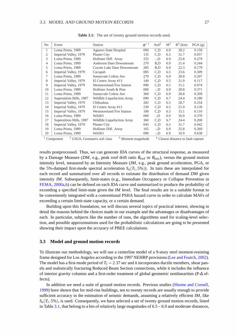
3.3. MODEL AND GROUND MOTION RECORDS 27
Table 3.1: The set of twenty ground motion records used.
No Event Station φ◦ 1 Soil2 M3 R4 (km) PGA (g)
1 Loma Prieta, 1989 Agnews State Hospital 090 C,D 6.9 28.2 0.1592 Imperial Valley, 1979 Plaster City 135 C,D 6.5 31.7 0.0573 Loma Prieta, 1989 Hollister Diff. Array 255 –,D 6.9 25.8 0.2794 Loma Prieta, 1989 Anderson Dam Downstream 270 B,D 6.9 21.4 0.2445 Loma Prieta, 1989 Coyote Lake Dam Downstream 285 B,D 6.9 22.3 0.1796 Imperial Valley, 1979 Cucapah 085 C,D 6.5 23.6 0.3097 Loma Prieta, 1989 Sunnyvale Colton Ave 270 C,D 6.9 28.8 0.2078 Imperial Valley, 1979 El Centro Array #13 140 C,D 6.5 21.9 0.1179 Imperial Valley, 1979 Westmoreland Fire Station 090 C,D 6.5 15.1 0.07410 Loma Prieta, 1989 Hollister South & Pine 000 –,D 6.9 28.8 0.37111 Loma Prieta, 1989 Sunnyvale Colton Ave 360 C,D 6.9 28.8 0.20912 Superstition Hills, 1987 Wildlife Liquefaction Array 090 C,D 6.7 24.4 0.18013 Imperial Valley, 1979 Chihuahua 282 C,D 6.5 28.7 0.25414 Imperial Valley, 1979 El Centro Array #13 230 C,D 6.5 21.9 0.13915 Imperial Valley, 1979 Westmoreland Fire Station 180 C,D 6.5 15.1 0.11016 Loma Prieta, 1989 WAHO 000 -,D 6.9 16.9 0.37017 Superstition Hills, 1987 Wildlife Liquefaction Array 360 C,D 6.7 24.4 0.20018 Imperial Valley, 1979 Plaster City 045 C,D 6.5 31.7 0.04219 Loma Prieta, 1989 Hollister Diff. Array 165 –,D 6.9 25.8 0.26920 Loma Prieta, 1989 WAHO 090 –,D 6.9 16.9 0.638
1 Component 2 USGS, Geomatrix soil class 3 Moment magnitude 4 Closest distance to fault rupture
results postprocessed. Thus, we can generate IDA curves of the structural response, as measuredby a Damage Measure (DM , e.g., peak roof drift ratioθroof or θmax), versus the ground motionintensity level, measured by an Intensity Measure (IM , e.g., peak ground acceleration, PGA, orthe 5%-damped first-mode spectral accelerationSa(T1,5%)). In turn these are interpolated foreach record and summarized over all records to estimate the distribution of demandDM givenintensity IM . Subsequently, limit-states (e.g., Immediate Occupancy or Collapse Prevention inFEMA, 2000a,b) can be defined on each IDA curve and summarized to produce the probability ofexceeding a specified limit-state given theIM level. The final results are in a suitable format tobe conveniently integrated with a conventional PSHA hazard curve in order to calculate MAFs ofexceeding a certain limit-state capacity, or a certain demand.
Building upon this foundation, we will discuss several topics of practical interest, showing indetail the reasons behind the choices made in our example and the advantages or disadvantages ofeach. In particular, subjects like the number of runs, the algorithms used for scaling-level selec-tion, and possible approximations used for the probabilistic calculations are going to be presentedshowing their impact upon the accuracy of PBEE calculations.
3.3 Model and ground motion records
To illustrate our methodology, we will use a centerline model of a 9-story steel moment-resistingframe designed for Los Angeles according to the 1997 NEHRP provisions (Lee and Foutch, 2002).The model has a first-mode period ofT1 = 2.37sec and it incorporates ductile members, shear pan-els and realistically fracturing Reduced Beam Section connections, while it includes the influenceof interior gravity columns and a first-order treatment of global geometric nonlinearities (P-∆ ef-fects).
In addition we need a suite of ground motion records. Previous studies (Shome and Cornell,1999) have shown that for mid-rise buildings, ten to twenty records are usually enough to providesufficient accuracy in the estimation of seismic demands, assuming a relatively efficientIM , likeSa(T1,5%), is used. Consequently, we have selected a set of twenty ground motion records, listedin Table3.1, that belong to a bin of relatively large magnitudes of 6.5 – 6.9 and moderate distances,

28 CHAPTER 3. APPLIED INCREMENTAL DYNAMIC ANALYSIS
all recorded on firm soil and bearing no marks of directivity; effectively they represent a scenarioearthquake.
3.4 Performing the Analysis
Once the model has been formed and the ground motion records have been selected, we need afast and automated way to perform the actual dynamic analyses required for IDA. This entailsappropriately scaling each record to cover the entire range of structural response, from elasticity,to yielding, and finally global dynamic instability. Our task is made significantly easier by usingan advanced algorithm, likehunt & fill (Vamvatsikos and Cornell, 2002a). This ensures that therecord scaling levels are appropriately selected to minimize the number of required runs: Analysesare performed at rapidly increasing levels ofIM until numerical non-convergence is encountered(signaling global dynamic instability), while additional analyses are run at intermediateIM -levelsto sufficiently bracket the global collapse and increase the accuracy at lowerIM s. The user onlyneeds to specify the desired accuracy for demand and capacity, select the maximum tolerable num-ber of dynamic analyses, and then wait for a few hours to get the results. Since the algorithm hasbeen implemented in software (Vamvatsikos and Cornell, 2002b) able to wrap around most exist-ing analysis programs (e.g., DRAIN-2DX,Prakhash et al., 1992) it renders IDA almost effortless,needing no human supervision.
As an example, we will show in detail the computations resulting to theIM -levels selectedby hunt & fill when tracing record #14 from Table3.1. To express the scaling level we need aninitial, temporary choice ofIM , and we have chosenSa(T1,5%), a decision that need not restrictus in any way: scaling can be re-expressed in any other scalableIM (Vamvatsikos and Cornell,2002a) that we wish after the runs are performed. Hence, inSa(T1,5%) terms, the algorithm wasconfigured to use an initial step of 0.1g, a step increment of 0.05g and a designated first elastic runat 0.005g, while a maximum of 12 runs was allowed for each record. Additionally, we specified aresolution of 10% on the global collapse capacity, i.e., we expect the model to develop numericalnon-convergence and show practically infiniteθmax at some high intensity level, and we wishthis level to be known within 10% of itsIM -value. Finally, we allowed the demand resolution,i.e., the maximum difference between successiveIM -values, to run to its best attainable value byexpending all the 12 runs. Alternatively we could have designated some minimum satisfactoryIM -gap below which we do not wish to proceed, thus saving some runs.
Table 3.2: Sequence of runs generated by the hunt & fill tracing algorithm for record #14.
No. calculations Sa(T1,5%) (g) θmax
1 0.005 0.05%2 0.005+0.10 0.105 0.79%3 0.105+0.10+1×0.05 0.255 2.02%4 0.255+0.10+2×0.05 0.455 3.01%5 0.455+0.10+3×0.05 0.705 5.85%6 0.705+0.10+4×0.05 1.005 +∞7 0.705+(1.005−0.705)/3 0.805 18.83%8 0.805+(1.005−0.805)/3 0.872 +∞9 (0.805+0.705)/2 0.755 9.18%10 (0.705+0.455)/2 0.580 3.27%11 (0.455+0.255)/2 0.355 2.96%12 (0.255+0.105)/2 0.180 1.34%
Using the above settings we get the sequence of runs shown in Table3.2. The first run ismeant to be in the elastic region. In the subsequent five runs, 2–6, we are hunting upwards till

3.5. POSTPROCESSING 29
the first numerical non-convergence appears in the form of “infinite”θmax. Then, the dynamicanalysis algorithm does not converge thus either failing to complete the dynamic run (as happenedfor this record) or producing extreme values ofθmax, say 200%. The next two runs, 7–8, areused to better bracket the first appearance of non-convergence, closing within 10% of itsIM -value((0.872−0.805)/0.805= 8.32%< 10%) so that the gap between highest converging and lowestnon-converging run is less that 10% of the former. Notice, that instead of placing each new runin the middle of the gap, the algorithm places it closer to the converging run, only one third ofthe way to the non-converging one. This ensures that the search will be somewhat biased towardsconverging runs, which are more informative than non-converging ones (which are essentiallydiscarded). The rest of the runs, up to the maximum of 12, are used to fill in the IDA at lowerlevels, being sequentially placed in the middle of the largestIM -gaps. Thus, the large gaps left bythe initial increasing steps to the flatline (runs 2–6), are filled in; this step increases the demandresolution and, given enough runs, it ensures that the algorithm has not missed an earlier collapse.Although it is a rare phenomenon in multi-degree-of-freedom structural models, certain recordsmay cause them to collapse for a range ofIM -values, but not for some higherIM , an event wecall structural resurrection(Vamvatsikos and Cornell, 2002a). By reducing theIM -gaps with runs9–12, we are making sure that we have not missed such an earlier (inIM terms) global collapseand the flatline we have found is the first one to occur.
Notice that the maximumIM -gap, i.e., the demand resolution, is about 0.13g (but less than halfon average), while theIM -difference between the highest converging and lowest non-convergingrun (the capacity resolution) is much less than 10% of the highest convergingIM , about 0.06g.Naturally, if we knew a priori the approximateIM -height of the flatline, we could use a steppingalgorithm with 12 runs and constant step of 0.1g to achieve similar results with a homogeneousdistribution of the accuracy, but this scheme would fail with the next records, producing either toofew or too many runs, due to the large record-to-record variability.
Assuming that the computational cost for each run is the same, then, the more the analysesper record, the longer for IDA to complete but the better the accuracy. Still, with the use of suchan advanced algorithm no runs are wasted, thus 12 runs per record will suffice to strike a goodcompromise between speed and accuracy. Nevertheless, it may be pointed out that performing240 dynamic runs for a model with thousands of degrees-of-freedom is a daunting task. Yet,even for such a complicated model, it took less than 12 hours on two 1999-era Pentium-classprocessors running independently. The process is completely automated and so easily performedovernight that actually setting up the structural model can now be expected to take substantiallymore (human) time than doing the analysis, while computer time is becoming an ever-cheapercommodity.
3.5 Postprocessing
Equally important to the analysis is the postprocessing of the resulting data and perhaps the mostimportant issue is selecting a suitableIM andDM . There are several issues of efficiency and suf-ficiency associated with theIM selection (Luco and Cornell, 2004). Since there are no directivity-influenced records in our suite and the building is of medium height (hence first-mode-dominated),the 5%-damped first-mode spectral accelerationSa(T1,5%) will be our choice; it has been provento be both efficient, by minimizing the scatter in the results, requiring only a few ground motionrecords to provide good demand and capacity estimates, and sufficient, as it provides a completecharacterization of the response without the need for magnitude or source-to-site distance infor-mation (Shome and Cornell, 1999). Similarly, selecting aDM can be application-specific; forexample, the peak floor accelerations are correlated with contents’ damage and many types of non-structural elements’ damage, while the maximum peak interstory drift ratioθmax (the maximumover time and over all stories of the interstory drift ratios recorded during the timehistory analysis)

30 CHAPTER 3. APPLIED INCREMENTAL DYNAMIC ANALYSIS
is known to relate well (FEMA, 2000a) to global dynamic instability and several structural perfor-mance limit-states upon which we intend to focus. Therefore,θmax will be our DM -choice. Still,it must be emphasized that theseIM andDM choices are by no means limiting. Assuming thatadditionalDM s have been recorded from the analyses, they can be substituted instead ofθmax,and by employing the postprocessing techniques presented, the IDA data can be expressed in adifferent scalableIM , without any need to rerun the dynamic analyses.
Having selected ourIM andDM , we are still faced with an abundance of IDA-generated datathat need to be sorted out and presented in meaningful ways. It is a time-consuming and challeng-ing task that we are going to step our way through, but it can be rendered totally effortless with theproper software. Actually, most of what follows is a direct description of the inner workings ofan automated postprocessing program (Vamvatsikos and Cornell, 2002b), whose graphical outputappears in the accompanying figures.
3.5.1 Generating the IDA curves by Interpolation
Once the desiredIM andDM values (in our caseSa(T1,5%) andθmax) are extracted from eachof the dynamic analyses, we are left with a set of discrete points for each record that reside inthe IM -DM plane and lie on its IDA curve, as in Figure3.1. By interpolating them, the entireIDA curve can be approximated without performing additional analyses. To do so, we may use abasic piecewise linear approximation, or the superior spline interpolation. Based on the concept ofnatural, coordinate-transformed, parametric splines with a centripetal scheme for knot-selection(Lee, 1989; Farin, 1990), a realistic interpolation can be generated that accurately represents thereal IDA curve, as shown in Figure3.1 for our example of record #14 in Table3.2. Having thecomplete curve available, it is now possible to calculateDM values at arbitrary levels ofIM ,allowing the extraction of more(IM ,DM ) points with a minimum of computation.
The spline comes inn cubic polynomial pieces and is parameterized on a single non-negativeparameter,t ∈ [0, t1]
⋃. . .
⋃[tn−1, tn] , wheren is the number of convergent runs/points including
the default (0,0) point, i.e.,n = 10+ 1 = 11 for record #14, Table3.2. For each value of theparametert, and depending on the interval[ti−1, ti ] where it lies, we get two polynomials, one fortheIM (thex-variable) and one for theDM (they-variable):
{xi(t) = axi t
3 +bxi t2 +cxi t +dxi
yi(t) = ayi t3 +byi t
2 +cyi t +dyit ∈ [ti−1, ti ] , i = 1, . . . ,n (3.1)
With the help of Equation (3.1) we can approximate theDM -value at arbitrary levels ofIMand vice versa. All we need is to solve the appropriatexi(t) polynomial piece given the value ofx to get the parametert and then replace at the correspondingyi(t) piece to get the appropriatey-value (DM ), i.e.,
DM = y(x−1(IM )
), (3.2)
IM = x(y−1(DM )
), (3.3)
where the -1 superscript denotes the inverse of a function. All these operations only involvepolynomials, hence they are trivial to perform, especially if properly coded in a program.
The smooth IDA curve provided by the interpolation scheme offers much to observe. Evenfor the single record depicted in Figure3.1 the IDA curve is not at all simple. It starts as astraight line in the elastic range but then shows the effect of yielding and slightly “softens” at0.3g by displaying a tangent slope less than the elastic. Subsequently, it “hardens”, having a localslope higher that the elastic, and the building apparently responds with almost the sameθmax≈3% for Sa(T1,5%) in the range of 0.35g – 0.55g. Finally, the IDA curve starts softening again,showing ever decreasing slopes, i.e., greater rates ofDM accumulation asIM increases, reaching

3.5. POSTPROCESSING 31
0 0.02 0.04 0.06 0.08 0.1 0.12 0.14 0.16 0.18 0.20
0.1
0.2
0.3
0.4
0.5
0.6
0.7
0.8
0.9
maximum interstory drift ratio, θ max
"firs
t−m
ode"
spe
ctra
l acc
eler
atio
n S
a(T1,5
%)
(g)
spline interpolation points from analyses piecewise linear interpolation
Figure 3.1: The numerically-converging dynamic analysis points for record #14, Table3.2, are interpo-lated, using both a spline and a piecewise linear approximation.
0 0.02 0.04 0.06 0.08 0.1 0.12 0.14 0.16 0.18 0.20
0.1
0.2
0.3
0.4
0.5
0.6
0.7
0.8
0.9
maximum interstory drift ratio, θ max
"firs
t−m
ode"
spe
ctra
l acc
eler
atio
n S
a(T1,5
%)
(g)
IDA curve Immediate OccupancyCollapse Prevention
flatline
elastic slope
20% of elastic slope
Figure 3.2: The limit-states, as defined on the IDA curve of record #14.
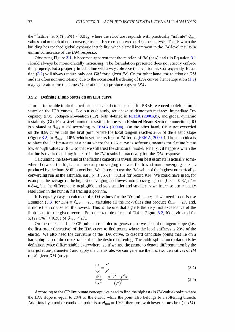
32 CHAPTER 3. APPLIED INCREMENTAL DYNAMIC ANALYSIS
the “flatline” atSa(T1,5%) ≈ 0.81g, where the structure responds with practically “infinite”θmax
values and numerical non-convergence has been encountered during the analysis. That is when thebuilding has reached global dynamic instability, when a small increment in theIM -level results inunlimited increase of theDM -response.
Observing Figure3.1, it becomes apparent that the relation ofIM (or x) andt in Equation3.1should always be monotonically increasing. The formulation presented does not strictly enforcethis property, but a properly fitted spline will always observe this restriction. Consequently, Equa-tion (3.2) will always return only oneDM for a givenIM . On the other hand, the relation ofDMandt is often non-monotonic, due to the occasional hardening of IDA curves, hence Equation (3.3)may generate more than oneIM solutions that produce a givenDM .
3.5.2 Defining Limit-States on an IDA curve
In order to be able to do the performance calculations needed for PBEE, we need to define limit-states on the IDA curves. For our case study, we chose to demonstrate three: Immediate Oc-cupancy (IO), Collapse Prevention (CP), both defined inFEMA (2000a,b), and global dynamicinstability (GI). For a steel moment-resisting frame with Reduced Beam Section connections, IOis violated atθmax = 2% according toFEMA (2000a). On the other hand, CP is not exceededon the IDA curve until the final point where the local tangent reaches 20% of the elastic slope(Figure3.2) or θmax = 10%, whichever occurs first inIM terms (FEMA, 2000a). The main idea isto place the CP limit-state at a point where the IDA curve is softening towards the flatline but atlow enough values ofθmax so that we still trust the structural model. Finally, GI happens when theflatline is reached and any increase in theIM results in practically infiniteDM response.
Calculating theIM -value of the flatline capacity is trivial, as our best estimate is actually some-where between the highest numerically-converging run and the lowest non-converging one, asproduced by the hunt & fill algorithm. We choose to use theIM -value of the highest numerically-converging run as the estimate, e.g.,Sa(T1,5%) = 0.81g for record #14. We could have used, forexample, the average of the highest converging and lowest non-converging run,(0.81+0.87)/2=0.84g, but the difference is negligible and gets smaller and smaller as we increase our capacityresolution in the hunt & fill tracing algorithm.
It is equally easy to calculate theIM -values for the IO limit-state; all we need to do is useEquation (3.3) for DM ≡ θmax = 2%, calculate all theIM -values that produceθmax = 2% and,if more than one, select the lowest. This is the one that signals the very first exceedance of thelimit-state for the given record. For our example of record #14 in Figure3.2, IO is violated forSa(T1,5%)≥ 0.26g or θmax≥ 2%.
On the other hand, the CP points are harder to generate, as we need the tangent slope (i.e.,the first-order derivative) of the IDA curve to find points where the local stiffness is 20% of theelastic. We also need the curvature of the IDA curve, to discard candidate points that lie on ahardening part of the curve, rather than the desired softening. The cubic spline interpolation is bydefinition twice differentiable everywhere, so if we use the prime to denote differentiation by theinterpolation-parametert and apply the chain-rule, we can generate the first two derivatives ofIM(or x) givenDM (or y):
dxdy
=x ′
y ′(3.4)
d2xdy2 =
x ′′y ′−y ′′x ′
(y ′)3 (3.5)
According to the CP limit-state concept, we need to find the highest (inIM -value) point wherethe IDA slope is equal to 20% of the elastic while the point also belongs to a softening branch.Additionally, another candidate point is atθmax = 10%; therefore whichever comes first (inIM ),

3.5. POSTPROCESSING 33
the slope or theθmax limit, decides capacity. Hence, we specify:
dxdy
∣∣∣∣t= 0.20
dxdy
∣∣∣∣t=0
(3.6)
d2xdy2
∣∣∣∣t< 0 (3.7)
t = y−1(10%), (3.8)
All we need to do is solve for allt satisfying Equation (3.6) and select the maximum sucht (cor-responding to the maximumIM ) that still satisfies Equation (3.7). Then, we compare againstthe minimumt that satisfies (3.8). Whichever is the smallest is thet that defines the CP point.Following this procedure with record #14 we get:Sa(T1,5%) = 0.72g, θmax = 6.4% from Equa-tions (3.6)–(3.7), andSa(T1,5%) = 0.76g, θmax = 10%from (3.8). By choosing the smallestt, orequivalently the smallestIM , we end up with the first of the two points, i.e., in this case the slopelimit defines CP (Figure3.2).
3.5.3 Summarizing the IDAs
By generating the IDA curve for each record and subsequently defining the limit-state capacities,a large amount of data can be gathered, only part of which is seen in Figure3.3. There, the IDAcurves display a wide range of behavior, showing large record-to-record variability, thus makingit essential to summarize such data and quantify the randomness introduced by the records. Weneed to employ appropriate summarization techniques that will reduce this data to the distributionof DM givenIM and to the probability of exceeding any specific limit-state given theIM level.
The limit-state capacities can be easily summarized into some central value (e.g., the mean orthe median) and a measure of dispersion (e.g., the standard deviation, or the difference betweentwo fractiles). Consequently, we have chosen to calculate the 16%, 50% and 84% fractile values ofDM (DM c
16%, DM c50% andDM c
84% respectively) andIM (IM c16%, IM c
50% andIM c84% respectively)
for each limit-state, as shown in Table3.3, and also graphically depicted in Figure3.4. For ex-ample, reading off Table3.3, at Sa(T1,5%) = 0.83g or equivalently atθmax = 0.10, 50% of theground motion records have forced the 9-story structure to violate CP.
Table 3.3: Summarized capacities for each limit-state.
Sa(T1,5%) (g) θmax
IM c16% IM c
50% IM c84% DM c
16% DM c50% DM c
84%
IO 0.18 0.27 0.33 0.02 0.02 0.02CP 0.57 0.83 1.29 0.07 0.10 0.10GI 0.74 0.91 1.35 +∞ +∞ +∞
There are several methods to summarize the IDA curves, but the cross-sectional fractiles arearguably the most flexible and robust with respect to the infiniteDM s introduced by the flatlines(Vamvatsikos and Cornell, 2002a). Using the spline interpolation we can generate stripes ofDM -values at arbitrary levels of theIM ; each stripe contains twentyDM -values, one for each record,that may be finite or even infinite when a record has already reached its flatline at a lowerIM -level.By summarizing theDM -values for each stripe into their 16%, 50% and 84% percentiles, we getfractile values ofDM given IM that are in turn interpolated for each fractile to generate the 16%,50% and 84% fractile IDA curves, shown in Figure3.4. For example, givenSa(T1,5%) = 0.4g,16% of the records produceθmax≤ 2.3%, 50% of the recordsθmax≤ 2.5%and 84%θmax≤ 6.5%.Under suitable assumptions of continuity and monotonicity of the IDA curves (as shown at alater section), the fractiles can also be used in the inverse way, e.g., in order to generate demand

34 CHAPTER 3. APPLIED INCREMENTAL DYNAMIC ANALYSIS
0 0.02 0.04 0.06 0.08 0.1 0.12 0.14 0.16 0.18 0.20
0.5
1
1.5
2
2.5"f
irst−
mod
e" s
pect
ral a
ccel
erat
ion
Sa(T
1,5%
) (g
)
maximum interstory drift ratio, θ max
flatlines
Collapse Prevention
ImmediateOccupancy
Figure 3.3: All twenty IDA curves and the associated limit-state capacities. The IO limit is at the intersec-tion of each IDA with theθmax = 2% line, the CP limit is represented by the dots, while GI occurs at theflatlines.
0 0.02 0.04 0.06 0.08 0.1 0.12 0.14 0.16 0.18 0.20
0.5
1
1.5
2
2.5
maximum interstory drift ratio, θ max
"firs
t−m
ode"
spe
ctra
l acc
eler
atio
n S
a(T1,5
%)
(g)
16% IDA
50% IDA
84% IDA
Immediate Occupancy
Collapse Prevention 84% flatline
50% flatline
16% flatline
84%
50%
16%
16%
50%
84%
Figure 3.4: The summary of the IDA curves and corresponding limit-state capacities into their 16%, 50%and 84% fractiles.

3.5. POSTPROCESSING 35
θmax= 4%, 84% of the records need to be scaled at levelsSa(T1,5%)≥ 0.31g, 50% of the recordsat Sa(T1,5%)≥ 0.52g and 16% atSa(T1,5%)≥ 0.76g. Consequently, the 16%, 50% and 84% IOpoints and GI flatlines actually reside on the 84%, 50% and 16% IDA curves respectively, a directresult of the definition of these limit-states. On the other hand, no such general property exists forthe CP points, but experience has shown that they usually lie quite close and often on top of theircorresponding fractile IDAs, just like the other limit-state points.
10−1
100
10−7
10−6
10−5
10−4
10−3
10−2
10−1
"first−mode" spectral acceleration Sa(T
1,5%) (g)
mea
n an
nual
freq
uenc
y of
exc
eeda
nce
T1=2.37s
Figure 3.5: Hazard curve for the Van Nuys Los Angeles site, forSa(2.37s,5%).
3.5.4 PBEE calculations
One of the goals of PBEE is producing MAFs of exceedance for the limit-states. This can beeasily accomplished with the summarized results that have been calculated so far, especially if oneconsiders the formats proposed by SAC/FEMA (FEMA, 2000a,b) or by the Pacific EarthquakeEngineering Research Center (Cornell and Krawinkler, 2000). The process invariably involvescalculating the MAF of exceeding values of the chosenIM , readily available forSa(T1,5%) fromconventional PSHA, and appropriately integrating with the conditional probabilities of exceed-ing each limit-state (given theIM or DM level) to produce the desired MAFs of limit-state ex-ceedance. It is a relatively straightforward method that has been described in extent, for example,by Cornell et al.(2002).
Here we will perform such calculations using a form of the framing equation adopted by thePacific Earthquake Engineering Research Center (Cornell and Krawinkler, 2000; Vamvatsikos andCornell, 2002a),
λ (DV ) =∫∫
G(DV |DM ) |dG(DM |IM )| |dλ (IM )| (3.9)
To simplify the above equation and the ones to follow, we will loosely useλ (X), F(X) andG(X)to denote the MAF function, cumulative distribution function (CDF) and the complementary CDF

36 CHAPTER 3. APPLIED INCREMENTAL DYNAMIC ANALYSIS
(CCDF), respectively, of their arguments. For example,λ (X) actually meansλX(x) and is a dif-ferent function fromλ (Y)≡ λY(y).
In this paper we have generally usedSa(T1,5%) for theIM andθmax asDM for the limit-statesof interest. The decision variable,DV , here is simply a scalar “indicator variable”:DV = 1 if thelimit-state is exceeded (and zero otherwise).λ (IM ) ≡ λIM (x) is the conventional hazard curve,i.e., the MAF ofIM exceeding, say,x. |dG(DM |IM )| is the differential of the (conditional) CCDFof DM given IM , or fDM |IM (y|x)dy, i.e., it is the probabilistic characterization of the distributionof DM givenIM , offered by the fractile IDAs. Finally in the limit-state (LS) case, when on the left-hand side of Equation (3.9) we seek the MAF of exceeding the limit-state,λ (DV=1) = λ (0) = λLS
andG(0|DM) becomes simply the probability that the capacityDM c is less than some level of theDM ; so G(0|DM ) = F(DM c|DM), whereF(DM c|DM) is the CDF ofDM c, i.e., the statisticalcharacterization of theDM -value of capacity, as offered, e.g., by the fractiles ofDM -capacity.
Thus, for our purposes, we can modify Equation (3.9) to become:
λLS =∫∫
G(0|DM ) |dG(DM |IM )| |dλ (IM )|
=∫ DM=+∞
DM=0F(DM c|DM )
{∫ IM=+∞
IM=0
∣∣∣∣dG(DM |IM )
dDM
∣∣∣∣∣∣∣∣dλ (IM )
dIM
∣∣∣∣ dIM}
dDM
=∫ DM=+∞
DM=0F(DM c|DM )
∣∣∣∣dλ (DM )
dDM
∣∣∣∣ dDM (3.10)
where the integration overIM in the braces needs to be carried out either numerically or by anappropriate analytic approximation (Cornell et al., 2002) to produce the absolute value of theDMhazard gradient|dλ (DM)/dDM |. Then we can proceed to integrate overDM and estimateλLS.If, on the other hand, we first integrate-out theDM , then we can rewrite the above equation to usetheIM -value of capacity:
λLS =∫
G(0|IM ) |dλ (IM )|
=∫ IM=+∞
IM=0F(IM c|IM )
∣∣∣∣dλ (IM )
dIM
∣∣∣∣ dIM (3.11)
where the quantity in the absolute value is theIM hazard gradient andF(IM c|IM ) is the CDF ofthe IM -value of limit-state capacity. In this case, all quantities in Equation (3.11) are known, andonly one integration is needed to calculateλLS.
We can proceed to the MAF calculations using either theDM -form (Equation3.10) or thepureIM -form (Equation3.11). There are several issues of compatibility with current guidelines(e.g.,FEMA, 2000a) that may dictate the use of theDM -approach, otherwise theIM -form is moreattractive, as it needs only one integration rather than two; hence, it will be our method of choice.Still, it must be emphasized that either of the two approaches should provide the exact sameresults if the integrations are performed with sufficient accuracy (see alsoJalayer and Cornell,2002). These are just two ways to the same goal, and the choice lies with the user.
The MAF calculations for any of the two approaches can be carried out either numerically orwith an analytical approximation. If a high degree of accuracy is desired, a trapezoidal rule canbe employed to directly integrate Equation (3.11). All we need to do is assign1/20 probabilityto each of the 20 records, then derive the empirical CDF of theIM -value of capacity and numeri-cally integrate with values of the hazard curve slope, calculated either by differentiating a smoothinterpolation or by simply reading them off Figure3.5. On the other hand, if we make some rea-sonable approximations, Equation (3.11) can be analytically integrated (Shome and Cornell, 1999;Cornell et al., 2002). We only need to assume that theIM -values of capacity are lognormally dis-tributed and then approximate theIM -hazard curve by fitting a straight line in the log-log space,

3.5. POSTPROCESSING 37
λ (IM ) = k0IM −k, either by a global regression, same for all limit-states, or by a local fit at themedianIM -capacity for each limit-state. Then we arrive at the equation
λLS = λ (IM c50%) ·exp
(12(k ·Sln IM c)2
)(3.12)
whereSln IM c =(ln IM c
50%− ln IM c16%
)is (approximately) the standard deviation of the natural
logarithm of theIM -capacity.
Table 3.4: MAFs of exceedance for each limit-state, calculated both numerically from Equation (3.11) andwith the approximate analytical form (3.12), using either a global or a local fit to theIM -hazard curve.
IO CP GI
numerical 0.019 0.0004 0.00010analytical (global fit) 0.017 0.0002 0.00003analytical (local fit) 0.008 0.0005 0.00040
As an example, the MAFs of exceeding each of the three limit-states (IO, CP and GI) werecalculated using both the approximate analytic approach (with either the global or the local fitto the hazard curve) and the “exact” numerical integration (Table3.4). In general, it seems thatby approximating the hazard curve with a global fit, the MAFs are consistently underestimated.On the other hand, the local fit seems to cause overestimation for all limit-states but IO. Theapproximations may sometimes miss the MAFs by a factor of three or get as close as 10%. Still, thelarge record-to-record variability coupled with the limited size of our suite of twenty records maygenerate considerable standard errors around these estimates, possibly making the approximateresults statistically indistinguishable from the exact MAF for some limit-states. This is an issuethat is going to be investigated in a later section.
3.5.5 Taking advantage of the data: SPO versus IDA
Beyond the essential calculations needed for PBEE, there is much more information that we couldeasily glean out of the IDA by taking a closer look at the results and plotting them in new ways.For example, Figure3.6displays a story-to-story profile of the median peak interstory drift ratiosat severalSa(T1,5%)-levels. As the intensity increases, then, in a median sense across all records,the fifth floor seems to accumulate most of the deformation. On the other hand, in Figure3.7 theindividual story drift IDA curves are plotted for record #1, showing a record-specific picture ofthe odd-numbered stories. Most interesting for this record is the sudden change of behavior thatoccurs aroundSa(T1,5%) = 0.82g, when the top floors suddenly start accumulating more and moredeformation asIM increases, while the previously leading lower floors are held back, displayingalmost constant peak interstory drifts.
It is also very informative to visually compare on the same figure the Static Pushover (SPO)curve (also known as the Nonlinear Static Procedure curve, e.g.,FEMA, 1997) versus the median(50%-fractile) IDA. Since the SPO curve usually comes in base shear versusθroof (peak roof driftratio) coordinates, it needs to be transformed intoIM andDM axes. In our case, theθmax responsecan be easily extracted from the SPO analysis results, while the base shear can be converted toacceleration units by dividing with the building mass times some (ad hoc) factor chosen to makethe curves match in their elastic range. This can be achieved for our structure by dividing the baseshear with 85% of the total building mass (which is very close to the ratio of the first modal overthe total mass). By thus plotting the two curves together, as pictured in Figure3.8, we see thatthey correspond to each other. The elastic region of the IDA matches the SPO by construction,and the post-yield non-negative SPO segment corresponds to a continuation of the elastic regionin the IDA, where the IDA is following the familiar “equal displacement” rule for moderate period

38 CHAPTER 3. APPLIED INCREMENTAL DYNAMIC ANALYSIS
0 0.02 0.04 0.06 0.08 0.1 0.12 0.14 0.16 0.18 0.21
2
3
4
5
6
7
8
9
peak interstory drift ratio
stor
y le
vel
Sa(T
1,5%)
= 0.54g
Sa(T
1,5%)
= 0.81g
Sa(T
1,5%) = 0.89g
Sa(T
1,5%) = 0.91g
Figure 3.6: The median peak interstory drift ratios for all stories at several specifiedSa(T1,5%) levels.
0 0.02 0.04 0.06 0.08 0.1 0.12 0.14 0.16 0.18 0.20
0.2
0.4
0.6
0.8
1
1.2
1.4
1 3 5
7
9
maximum interstory drift ratio, θ max
"firs
t−m
ode"
spe
ctra
l acc
eler
atio
n S
a(T1,5
%)
(g)
1st story 3rd story 5th story 7th story 9th story
Figure 3.7: The IDA curves of the odd stories for record #1.

3.5. POSTPROCESSING 39
0 0.05 0.1 0.15 0.2 0.25 0.3 0.35 0.40
0.1
0.2
0.3
0.4
0.5
0.6
0.7
0.8
0.9
1
maximum interstory drift ratio, θmax
"firs
t−m
ode"
spe
ctra
l acc
eler
atio
n S
a(T1,5
%)
(g)
Static Pushover curve50% IDA curve
flatline
negative slope
non−negative slope
equal displacement
softening
elastic
Figure 3.8: The SPO curve generated from an inverse-triangle (maximum force at roof) load pattern versusthe median IDA.
structures (Veletsos and Newmark, 1960). When the SPO turns into a negative slope, the IDAsoftens and acquires a local slope less than the initial elastic, that gradually decreases till the IDAbecomes flat. Essentially, the ending of the SPO at zero strength signals the end of the IDA by theflatline.
The question then arises as to why this relationship exists. Some light can be shed on thisissue if we simplify the problem and think in terms of a single-degree-of-freedom system witha force-deformation backbone that has the shape of the building’s SPO curve. Then we need torealize that in terms of dynamics, where the IDA is concerned, an ascending part of the “back-bone” generally means a “dynamically stable” part while a descending branch corresponds to a“dynamically unstable” part (e.g.,Macrae and Kawashima, 1997). For each dynamic run theθmax
value serves as an indicator of whether the building has remained completely in the ascendingparts (approximatelyθmax < 5% in Figure3.8) or it has ventured into the descending branch aswell. So, for lowerIM s, approximatelySa(T1,5%) < 0.6 g in Figure3.8, the building (in a me-dian sense, i.e., for at least 50% of the records) oscillates along the ascending part of its “SPObackbone” thus the increase inθmax is controlled and stable in the median. But for higherIM sthe building (in a median sense again) also sustains more and more cycles in the descending partof the “SPO backbone”, thus the medianθmax increases uncontrollably towards infinity. This canhelp us understand why the behavior of the median IDA changes so drastically when the medianθmax is higher than 5%, as it shifts from an ascending to a descending branch. On the contrary,the median IDA remains virtually indifferent when this moderate period structure passes from theelastic part to the non-negative post-yield segment of the SPO, since both are ascending branches.
Observing these facts, one could stipulate that some more direct, perhaps quantitative rulesmay be devised to connect the two curves. Actually, one such attempt has been tried out both forsingle (Vamvatsikos and Cornell, 2004c) and multi-degree-of-freedom systems (Vamvatsikos andCornell, 2004b) with encouraging results.

40 CHAPTER 3. APPLIED INCREMENTAL DYNAMIC ANALYSIS
3.6 Discussion of choices and their influence on IDA
We took the reader through a direct, hands-on example of how to perform IDA and apply it for thepurposes of PBEE. At each step we had to make some choices, e.g., how to set up the dynamicanalysis algorithm, what tracing algorithm and interpolation scheme to use, how to summarize theIDAs (using stripes given theIM instead of stripes given theDM ) or how many records and howmany runs per record to allow. Still, we chose not to focus on such details; instead we proceeded bymaking seemingly ad hoc choices. Now, armed with the knowledge of the complete IDA process,we can discuss such choices, explain the reasons behind them and understand their influence tothe final results.
3.6.1 Numerical convergence
The details of the analysis and the structural model play an important role in generating accu-rate IDA curves. Especially in the region of global dynamic instability, the very existence of theflatline and the associated numerical non-convergence may often generate several accuracy prob-lems. Ideally, the structural model would be composed of (numerically) robust and well-testedelements, while the dynamic analysis algorithm should be able to accurately track the structuralresponse through, e.g., yielding events, sharp strength drops, load redistribution and geometricnonlinearities; it would fail to converge only when the structure has exhausted its reserves to be-come dynamically unstable, thus correctly matching global dynamic instability with numericalnon-convergence. Unfortunately, most algorithms and element models have not really been de-signed or tested to operate in such extreme ranges of behavior. As a result, some records maycause a premature non-convergence, creating a characteristic halting of the IDA curve which doesnot resemble a flatline.
All the flatlines in our model normally occur beyondθmax = 12%(Figure3.3), meaning thatthe model can remain stable at least up to suchθmax-values. Still, in our initial attempt to trace theIDA curves, two of the twenty records failed prematurely, atθmax≈ 2%, barely past the end-of-elasticity value ofθmax≈ 1%. The main reason is the use of a large, complex model with manydegrees of freedom, plus the adoption of the fracturing connection model (Shi and Foutch, 1997)with sharp strength drops that probably tend to destabilize the solution algorithm of DRAIN-2DX(Prakhash et al., 1992). Further confirmation is provided by the SPO-to-IDA connection, asθmax
values in the order of 2% are still on the ascending branch of the SPO in Figure3.8, thus deemedunable to cause collapse. Actually, each IDA curve should be able to behave stably at least up tothe start of the SPO’s negative slope, at aboutθmax = 7%. Still, this comparison should not becarried too far; while the SPO ends atθmax = 37%, the post-peak part of the SPO is often veryload-pattern dependent, and an arbitrary load pattern may result in very optimisticθmax values thatdo not reflect the dynamic behavior (Vamvatsikos and Cornell, 2004b).
Such illegitimate and premature collapses are thus relatively easily identified, either by lookingat the SPO or at the IDAs of other records, but how are they to be fixed? Of course, if the model orthe elements or the algorithm are deficient in the first place, the situation is hopeless. Experiencehas shown that this is not the case with the well-tested DRAIN-2DX; it is more a problem ofcorrectly setting up the analysis parameters, rather than anything else. The best strategy is totweak the analysis knobs, e.g., reduce the integration time-step, adopt a variable-step solutionor experiment with the parameters of the event-to-event solver. In our case-study, the dynamicanalyses of the two problematic records had to be repeated at a reduced time-step, one-fourthinstead of one-half of the acceleration timehistory time-step, thus easily resolving convergenceissues. Note that after such false, premature collapses are dealt with, then further (reasonable)changes in the parameters of the solution algorithm will make only small arbitrary changes to theIDA results. For example, it has been found empirically that changing the integration time-stepcan incur arbitrary changes of up to 10% to the flatline heights, where, surprisingly, smaller steps

3.6. DISCUSSION OF CHOICES AND THEIR INFLUENCE ON IDA 41
do not necessarily mean more stability (i.e., higher flatline heights). This is simply the effect ofsmall errors piling up on each step of the time-integration that may affect convergence when thestructure is close to the flatline, sometimes causing it to collapse a bit earlier and sometimes not.This is the reason why when tracing each record we specified a capacity resolution of only 10%;a better accuracy does not have much meaning in the presence of these analysis uncertainties.
Such inaccuracies remain relatively insignificant when good analysis software is used. Ac-tually, we cannot stress enough the need for reliable, bug-free algorithms and well-tested, robustelement models. Such tools are exactly what makes the difference in such analyses, especially forthe limit-states close to global dynamic instability, and when available, with only a little attentionto the analysis details allow us to easily obtain accurate IDA curves.
3.6.2 Choice of Tracing Algorithm
When tracing the IDA curve for each record, the choice of theIM -level for each run is a decisionleft to the automated tracing algorithm that we use. We have theoretically argued about the superi-ority of the hunt & fill algorithm versus the use of a constantIM -step (i.e., the stepping algorithm)in Vamvatsikos and Cornell(2002a), so it is time to see in detail what the true differences reallyare when both are applied to the 9-story structure.
Before we proceed, keep in mind that given the same structural model, analysis program andcomputing platform, still not all runs are equal in computational cost. In general, the closer the runis to the flatline (either at a lower or a higherIM ) the longer it takes to complete the analysis. Onthe other hand, both converging and non-converging runs that are far away from the flatline willbe significantly faster, as convergence or non-convergence will be achieved within a minimum ofiterations. Still, when comparing the tracing algorithms, we will assume that the intent is to tracethe whole IDA curve and a similar amount of runs will be spent both high and low in the curve(in IM terms). Thus, looking at each record as a whole, the total amount of runs (converging andnon-converging alike) spent for it provide a very accurate idea of the computational time needed,while the number of converging runs accurately describes the accuracy achieved.
Table 3.5: Comparing the sensitivity to parameters of the stepping versus the hunt & fill algorithm.
Algorithm Parameter (g) Total C+NC1 min C 2 max C2 average C2
stepping 0.05 475 11 45 22.8(step-size sensitivity) 0.075 318 7 30 14.9
0.1 244 5 22 11.20.2 128 2 11 5.40.3 87 1 7 3.4
hunt & fill 0.05 280 12 13 12.2(initial-step sensitivity) 0.1 280 12 13 12.2
0.2 280 11 13 12.00.3 280 11 12 11.8
hunt & fill 0.025 280 11 13 12.4(step-increment sensitivity) 0.05 280 12 13 12.2
0.1 280 11 13 12.00.2 280 11 13 11.9
1 Converging and non-converging runs for all records 2 Converging runs per record
The most important task that a user faces when applying either of the two algorithms is settingup their parameters correctly. For the stepping algorithm, the only parameter is the step size, whilefor the hunt & fill the most important ones are the initial step, the step increment and the allowednumber of runs per record. Both algorithms were used to trace the IDAs of the 9-story structure forthe suite of 20 records, using various settings for their parameters, the results shown in Table3.5.

42 CHAPTER 3. APPLIED INCREMENTAL DYNAMIC ANALYSIS
Obviously, changing the step size of the stepping algorithm generates huge differences in the totalnumber of runs. Still, if we let the minimum number of converging runs generated for any of the20 records be our standard for accuracy, we need at least a step size of 0.05g, or 475 runs to get atleast 11 runs per record and reach the standards of hunt & fill. Also, if we do not set the steppingsize correctly, we either get too few or too many runs, the resolution easily dropping to 1 or 2runs in the worst case, if we happen to set a step size of 0.2g or 0.3g. On the other hand, we canchange the initial step or the step increment for the hunt & fill within a wide range, increasingthem or reducing them by 2 or 4 times, and the hunting algorithm remains practically unchanged,constantly providing at least 11 converging runs per record. In essence, it has the right knobs tobe tuned to the tolerance limits that we wish and allows us to do the runs the way we want, not theway nature decides through the records.
Still, one may notice that if we over-increase the initial step or the step increment, then theaccuracy starts to slowly drop, as the algorithm overshoots the flatline by a lot and spends manynon-converging runs to find its way down. But still the effect is minor, not overwhelming. Noticealso that keeping both parameters relatively small seems to improve accuracy both on average andin the minimum. Still, we should not decrease them too much because as the steps become smallerwe are risking expending all the allotted runs before reaching the flatline.
Coming back to our example, in Table3.2, we usedSa(T1,5%) to measure theIM -value forour runs. Why not anotherIM ? We could have used pretty much any monotonic and scalableIM (Vamvatsikos and Cornell, 2002a) that we might want, but the less efficient it is, the furtherdispersed the IDA flatlines would be, and we would start having some resolution discrepancieswithin tracing, i.e., a greater difference between the observed number of minimum and maximumconvergent runs per record in our suite. By using at leastSa(T1,5%), we are assured that our algo-rithm, be it hunt & fill or stepping, will be efficient for a wide range of conditions. If another, moreefficient IM appears that can drastically reduce the record-to-record flatline variability, then thehunt & fill would only marginally benefit, but the stepping algorithm would significantly improve.In conclusion, the hunt & fill procedure desensitizes IDA from theIM selection and the setting ofthe algorithm’s parameters, easily achieving the desired resolution, in contrast to the very sensitivestepping algorithm. Additionally, it fixes the number of total runs performed, so we can plan aheadand assign enough computers to run in parallel so the IDA is computed in time.
3.6.3 Interpolation issues
By interpolating the discrete points to generate each record’s IDA curve we are gaining one enor-mous advantage: we do not need to have our runs in stripes of the sameIM -level. The conse-quences are very important. First, this allows us to use the hunt & fill algorithm instead of thestepping one, thus gaining in all the aspects described previously. Second, it allows us to expressthe IDA results in anyIM . All we need is to calculate the newIM for each run, re-plot the IDAcurves and re-interpolate versus the newIM . In this way, IDA becomes truly independent of theIM used for tracing, allowing us to reuse the same data again and again, without needing to runany more analyses.
But why use complex spline schemes instead of the simpler linear interpolation? In Figures3.9and3.10, we present a comparison of the linear and the spline interpolation scheme, pitted againsteach other for a given number of converging runs. We have tweaked the hunt & fill tracing so thatin all cases the flatline is accurately reached with the same number of runs, and then the algorithmis allowed to fill in the gaps using up to a total of 4, 6, 8 or 18 runs. Unless we are only interestedin the flatline, 4 converging runs are just too few to capture the IDA adequately, regardless of theinterpolation scheme used. Clever postprocessing cannot make up for gross data gaps. On theother hand, if we allow only 2 more runs, for a total of 6, the results are markedly better, but onlyif we are using a spline scheme. Had we used 6 linearly interpolated runs we would be grosslyunderestimating the CP limit-state capacity, finding a capacity point at onlySa(T1,5%) = 0.63g,

3.6. DISCUSSION OF CHOICES AND THEIR INFLUENCE ON IDA 43
0 0.02 0.04 0.06 0.08 0.1 0.12 0.14 0.16 0.18 0.20
0.1
0.2
0.3
0.4
0.5
0.6
0.7
0.8
0.9
maximum interstory drift ratio, θ max
"firs
t−m
ode"
spe
ctra
l acc
eler
atio
n S
a(T1,5
%)
(g)
4 conv. runs 6 conv. runs 8 conv. runs 18 conv. runs
Figure 3.9: Linearly interpolated IDA curve for record #14, traced with a different total number of con-verging runs.
0 0.02 0.04 0.06 0.08 0.1 0.12 0.14 0.16 0.18 0.20
0.1
0.2
0.3
0.4
0.5
0.6
0.7
0.8
0.9
maximum interstory drift ratio, θ max
"firs
t−m
ode"
spe
ctra
l acc
eler
atio
n S
a(T1,5
%)
(g)
4 conv. runs 6 conv. runs 8 conv. runs 18 conv. runs
Figure 3.10: Spline-interpolated IDA curve for record #14, traced with a different total number of converg-ing runs.

44 CHAPTER 3. APPLIED INCREMENTAL DYNAMIC ANALYSIS
θmax = 4% instead of the correct 0.72g and 6.4%. At 8 and 18 runs, the spline interpolations arepractically indistinguishable, while the linear ones are close enough but still can be told apart. Inconclusion, if we allow enough runs, the interpolation scheme doesn’t really matter, both schemeswill provide good results. On the other hand, if we use too few runs, it doesn’t really matter againbecause both schemes are going to give us bad results. But there is a gray area in between, whereusing a better and smarter interpolation can make the difference to increase the accuracy in ourfinal IDA curve. In retrospect, this is precisely what gives us confidence to reduce the allottednumber of runs and save on computational resources.
3.6.4 Sensitivity of the limit-state capacities to their definition
Several limit-states were defined on the IDA curves, often through the use of ad hoc rules. Forexample, the IO limit-state was defined atθmax = 2%, while the CP limit-state was based onthe arbitrary 20% fraction of the elastic slope (or stiffness) and the additionalθmax = 10% limit(FEMA, 2000a). On the other hand, the GI limit-state was unambiguously defined to be on theflatline of the IDA, being subject to no such arbitrary rules. Therefore, it is of interest to investigatethe sensitivity of the summarizedIM , DM capacities to these choices, both for the IO and the CPlimit-state.
For the IO limit-state, the simplicity of the definition makes it easy to understand what ishappening. If we look at Figure3.4, it is obvious that IO is occurring in the “equal displacement”region of the fractile IDAs, i.e., the fractiles are almost straight lines resembling a continuation ofthe elastic segment. In turn, this means that moderate changes to the defining value for IO, i.e.,from θmax = 2%to 1% or 3% will proportionately increase or decrease theIM andDM values ofcapacity.
On the other hand, the definition of the CP limit-state is quite more complicated. The elas-tic stiffness fraction controls how much the IDA has to soften, i.e., how close to the flatline itcan come, before CP is reached. Hence, increasing this fraction will force the CP points (e.g.,Figure 3.3) to move to lowerIM s andDM s. The influence of theθmax = 10% limit is morestraightforward. It enforces a rigid limit on the capacity points, restricting theθmax value theycan reach, i.e., it is another way to restrict the CP points from coming close to the flatline. Ac-tually, in our case of the 9-story building, Figure3.3, it becomes obvious that by changing theθmax = 10%limit to, say, 8% or 12%, theIM -value of capacity will only slightly change, but theDM -value will be highly influenced, the 50% and 84%θmax capacities actually becoming 8% or12% respectively.
To show the combined influence of the two rules on the CP limit-state, the fraction of theelastic stiffness has been varied from 10% to 60% and the resulting fractileSa(T1,5%), θmax ca-pacities have been plotted, both when theθmax = 10%rule is imposed (Figure3.11(b)) and whenit is not (Figure3.11(a)). In the latter case, theIM capacity becomes relatively sensitive, almostlinearly, to the elastic stiffness fraction. TheDM capacity is even more sensitive, decreasing ina geometric fashion as the fraction increases. This makes absolute sense given the shape of theIDAs (Figure3.3); close to global collapse, each IDA softens towards the flatline, hence, as theslope-fraction decreases, the CPIM capacity approaches the flatlineIM -height. On the otherhand, theDM capacity is destabilized by the same flattening, since by definition, in the vicinity ofthe flatline, small changes in the elastic stiffness fraction result to large changes of theDM -value.
If we include theθmax = 10% limit, as in Figure3.11(b), both theIM and especially theDM capacity are stabilized, as this hard upper limit simply cuts off all higher values. Further-more, this limit seems to drastically reduce theDM -capacity dispersion, at all levels of the elasticstiffness fraction. Obviously, several records now have the same CP limit-stateDM capacity,namelyθmax = 10%. Therefore, the 10% limit makes the CP capacity more stable, but no lessarbitrary, as theθmax = 10% limit is often the governing rule. Actually, looking at the tables inFEMA (2000a,b) it becomes obvious that 10% is often the quoted medianθmax-capacity for all

3.6. DISCUSSION OF CHOICES AND THEIR INFLUENCE ON IDA 45
0 0.1 0.2 0.3 0.4 0.5 0.60
0.5
1
1.5
2
capa
city
in S
a(T1,5
%)
(g)
Elastic stiffness fraction
0 0.1 0.2 0.3 0.4 0.5 0.60
0.05
0.1
0.15
0.2
0.25
0.3
capa
city
in θ
max
Elastic stiffness fraction
84%50%16%
(a) ResultingSa(T1,5%) andθmax capacities when theθmax = 10%limit is not imposed.
0 0.1 0.2 0.3 0.4 0.5 0.60
0.5
1
1.5
2
capa
city
in S
a(T1,5
%)
(g)
Elastic stiffness fraction
0 0.1 0.2 0.3 0.4 0.5 0.60
0.05
0.1
0.15
0.2
0.25
0.3
capa
city
in θ
max
Elastic stiffness fraction
84%50%16%
(b) ResultingSa(T1,5%) andθmax capacities when theθmax = 10%limit is imposed.
Figure 3.11: The sensitivity of the fractile (16%, 50% and 84%)Sa(T1,5%) andθmax capacities for the CPlimit-state to the elastic stiffness fraction used (20% is the standard byFEMA, 2000a). The results are lesssensitive if theθmax = 10%limit is used.

46 CHAPTER 3. APPLIED INCREMENTAL DYNAMIC ANALYSIS
but the tallest buildings. Is, then, this arbitrarily imposedθmax = 10%a problem? From an MAF-sensitivity point-of-view, the answer is negative. In Equation3.11 it becomes apparent that it isonly theIM -value of capacity that truly matters. As we have observed, at least for this structure,the IM -value of CP-capacity is only mildly sensitive to the definition of the rules, thus yieldingsimilarly mildly sensitive MAFs. Even if the calculation is done using theDM -form in Equa-tion (3.10), assuming that the integrations are accurately performed, the conclusions will still bethe same.
There are also several other details and corresponding sensitivity issues in the implementationof the CP limit-state definition, that may or may not make a difference. For example, inYun et al.(2002) the 20% fraction is applied to the median elastic stiffness of all records and the resultingreduced stiffness is used for the capacity point estimation. On the other hand, we have used the20% fraction on the elastic stiffness of each individual record to define its CP capacity. In this case,the summarized capacities show negligible difference between the two approaches. On the otherhand, inYun et al.(2002) CP is defined to occur at the first point where the IDA curve softensto 20% of the (median) elastic slope, while we use the last point where it reaches the reducedstiffness. This may make a large difference for some records that alternatively harden and softenbefore global collapse, and may be interpreted as another sign of sensitivity to the CP definition.Still, for reasons explained inVamvatsikos and Cornell(2002a), we believe it is more consistentwith the CP limit-state concept to use the last rather than the first such point, thus resolving thisproblem.
0 0.02 0.04 0.06 0.08 0.1 0.12 0.14 0.16 0.18 0.20
0.2
0.4
0.6
0.8
1
1.2
1.4
1.6
1.8
2
maximum interstory drift ratio, θ max
"firs
t−m
ode"
spe
ctra
l acc
eler
atio
n S
a(T1,5
%)
(g) fractiles of θ given Sa
fractiles of Sa given θ
50% IDA of θ | Sa vs 50% of Sa | θ
16% IDA of θ | Sa vs 84% of Sa | θ
84% IDA of θ | Sa vs 16% of Sa | θ
Figure 3.12: Summarization into fractiles ofIM givenDM versus fractiles ofDM givenIM .
3.6.5 Summarization givenIM or DM
When summarizing the IDA curves, we decided to use stripes ofDM given levels ofIM , insteadof stripes ofIM given DM . It often becomes an issue in the literature (e.g.,Miranda, 2001),whether one should summarize givenIM or DM . The first approach can be thought of providing
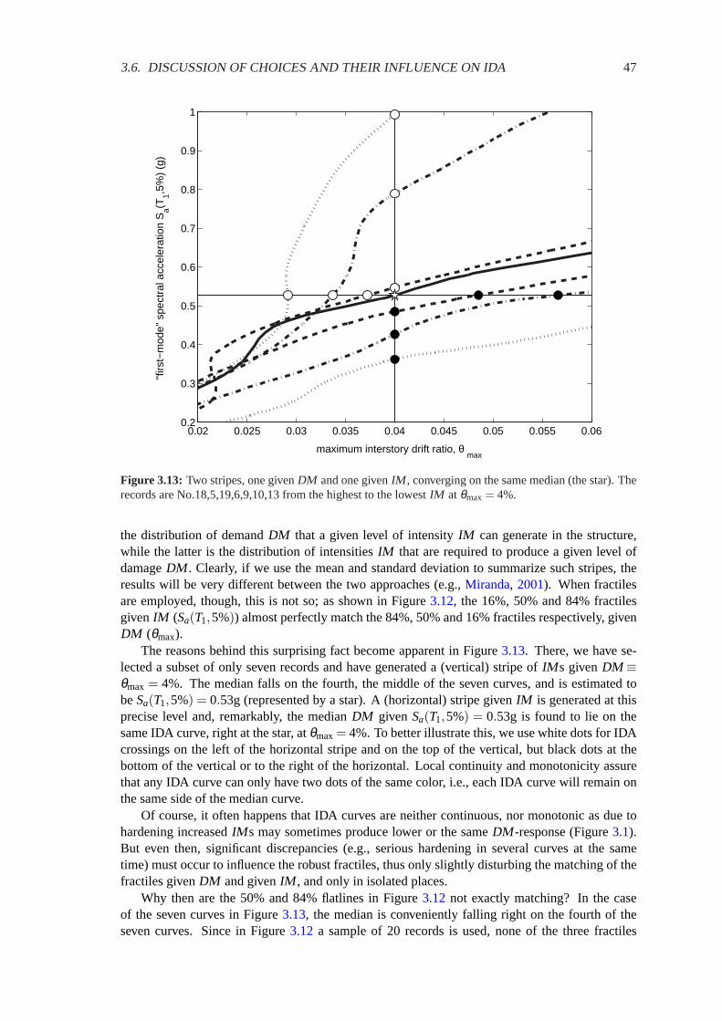
3.6. DISCUSSION OF CHOICES AND THEIR INFLUENCE ON IDA 47
0.02 0.025 0.03 0.035 0.04 0.045 0.05 0.055 0.060.2
0.3
0.4
0.5
0.6
0.7
0.8
0.9
1
maximum interstory drift ratio, θ max
"firs
t−m
ode"
spe
ctra
l acc
eler
atio
n S
a(T1,5
%)
(g)
Figure 3.13: Two stripes, one givenDM and one givenIM , converging on the same median (the star). Therecords are No.18,5,19,6,9,10,13 from the highest to the lowestIM at θmax = 4%.
the distribution of demandDM that a given level of intensityIM can generate in the structure,while the latter is the distribution of intensitiesIM that are required to produce a given level ofdamageDM . Clearly, if we use the mean and standard deviation to summarize such stripes, theresults will be very different between the two approaches (e.g.,Miranda, 2001). When fractilesare employed, though, this is not so; as shown in Figure3.12, the 16%, 50% and 84% fractilesgivenIM (Sa(T1,5%)) almost perfectly match the 84%, 50% and 16% fractiles respectively, givenDM (θmax).
The reasons behind this surprising fact become apparent in Figure3.13. There, we have se-lected a subset of only seven records and have generated a (vertical) stripe ofIM s givenDM ≡θmax = 4%. The median falls on the fourth, the middle of the seven curves, and is estimated tobeSa(T1,5%) = 0.53g (represented by a star). A (horizontal) stripe givenIM is generated at thisprecise level and, remarkably, the medianDM given Sa(T1,5%) = 0.53g is found to lie on thesame IDA curve, right at the star, atθmax= 4%. To better illustrate this, we use white dots for IDAcrossings on the left of the horizontal stripe and on the top of the vertical, but black dots at thebottom of the vertical or to the right of the horizontal. Local continuity and monotonicity assurethat any IDA curve can only have two dots of the same color, i.e., each IDA curve will remain onthe same side of the median curve.
Of course, it often happens that IDA curves are neither continuous, nor monotonic as due tohardening increasedIM s may sometimes produce lower or the sameDM -response (Figure3.1).But even then, significant discrepancies (e.g., serious hardening in several curves at the sametime) must occur to influence the robust fractiles, thus only slightly disturbing the matching of thefractiles givenDM and givenIM , and only in isolated places.
Why then are the 50% and 84% flatlines in Figure3.12 not exactly matching? In the caseof the seven curves in Figure3.13, the median is conveniently falling right on the fourth of theseven curves. Since in Figure3.12 a sample of 20 records is used, none of the three fractiles
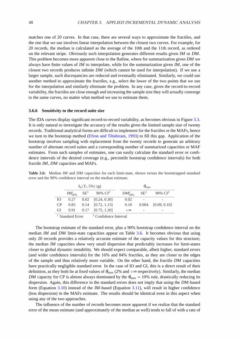
48 CHAPTER 3. APPLIED INCREMENTAL DYNAMIC ANALYSIS
matches one of 20 curves. In that case, there are several ways to approximate the fractiles, andthe one that we use involves linear interpolation between the closest two curves. For example, for20 records, the median is calculated as the average of the 10th and the 11th record, as orderedon the relevant stripe. Obviously such interpolation generates different results givenIM or DM .This problem becomes more apparent close to the flatline, where for summarization givenDM wealways have finite values ofIM to interpolate, while for the summarization givenIM , one of theclosest two records produces infiniteDM (which cannot be used for interpolation). If we use alarger sample, such discrepancies are reduced and eventually eliminated. Similarly, we could useanother method to approximate the fractiles, e.g., select the lower of the two points that we usefor the interpolation and similarly eliminate the problem. In any case, given the record-to-recordvariability, the fractiles are close enough and increasing the sample size they will actually convergeto the same curves, no matter what method we use to estimate them.
3.6.6 Sensitivity to the record suite size
The IDA curves display significant record-to-record variability, as becomes obvious in Figure3.3.It is only natural to investigate the accuracy of the results given the limited sample size of twentyrecords. Traditional analytical forms are difficult to implement for the fractiles or the MAFs, hencewe turn to the bootstrap method (Efron and Tibshirani, 1993) to fill this gap. Application of thebootstrap involves sampling with replacement from the twenty records to generate an arbitrarynumber of alternate record suites and a corresponding number of summarized capacities or MAFestimates. From such samples of estimates, one can easily calculate the standard error or confi-dence intervals of the desired coverage (e.g., percentile bootstrap confidence intervals) for bothfractile IM , DM capacities and MAFs.
Table 3.6: Median IM andDM capacities for each limit-state, shown versus the bootstrapped standarderror and the 90% confidence interval on the median estimate.
Sa(T1,5%) (g) θmax
IM c50% SE1 90% CI2 DM c
50% SE1 90% CI2
IO 0.27 0.02 [0.24, 0.30] 0.02 - -CP 0.83 0.14 [0.72, 1.13] 0.10 0.004 [0.09, 0.10]GI 0.91 0.17 [0.75, 1.20] +∞ - -1 Standard Error 2 Confidence Interval
The bootstrap estimate of the standard error, plus a 90% bootstrap confidence interval on themedianIM andDM limit-state capacities appear on Table3.6. It becomes obvious that usingonly 20 records provides a relatively accurate estimate of the capacity values for this structure;the medianIM capacities show very small dispersion that predictably increases for limit-statescloser to global dynamic instability. We should expect comparable, albeit higher, standard errors(and wider confidence intervals) for the 16% and 84% fractiles, as they are closer to the edgesof the sample and thus relatively more variable. On the other hand, the fractileDM capacitieshave practically negligible standard error. In the case of IO and GI, this is a direct result of theirdefinition, as they both lie at fixed values ofθmax (2% and+∞ respectively). Similarly, the medianDM capacity for CP is almost always dominated by theθmax = 10%rule, drastically reducing itsdispersion. Again, this difference in the standard errors does not imply that using theDM -basedform (Equation3.10) instead of theIM -based (Equation3.11), will result in higher confidence(less dispersion) in the MAFs estimate. The results should be identical even in this aspect whenusing any of the two approaches.
The influence of the number of records becomes more apparent if we realize that the standarderror of the mean estimate (and approximately of the median as well) tends to fall of with a rate of

3.7. CONCLUSIONS 49
Table 3.7: MAFs for each limit-state, calculated both numerically and with the approximate analytical form(global or local fit). The bootstrapped standard error and 90% confidence interval on the MAF estimate arealso presented. Additionally, we test the hypothesis that the approximateλLS is equal to the exact at the95% confidence level.
limit-state method λLS SE1 90% CI2 “equal” to exact?
IO exact 0.019 0.011 [0.007, 0.04]global 0.017 > 1000 [0.005, 0.33] yeslocal 0.008 2.5 [0.004, 0.04] yes
CP exact 0.0004 0.0002 [0.0002, 0.0009]global 0.0002 0.0008 [0.0001, 0.0004] yeslocal 0.0005 > 1000 [0.0001, 0.7] yes
GI exact 0.0001 0.00007 [0.0001, 0.0003]global 0.00003 0.00006 [0.00001, 0.00002] yeslocal 0.0004 > 1000 [0.00003, 160] yes
1 Standard Error 2 Confidence Interval
1/√
n wheren is the number of records (e.g.,Benjamin and Cornell, 1970). Hence, quadruplingthe number of records to use a total ofn= 80, results in only half the dispersion, while decreasingit by a factor of four, to use onlyn = 5, will (approximately) double the dispersion.
How do the standard errors in the fractile capacities translate to the estimates of the MAFs?By applying the bootstrap to both the “exact” numerical (Equation3.11) and the approximateanalytic form (Equation3.12) with either a local or a global fit to the hazard curve, we get theresults shown in Table3.7. As seen from the “exact” results, the limited sample of 20 recordscauses standard errors in the order of 50% in the estimates of theλLS for all limit-states. Onthe other hand, the approximation through Equation (3.12) considerably increases the standarderror; in some cases it is in the order of 200% but sometimes the approximation totally fails andconsiderably overestimates the MAF. For the IO limit-state, it is the approximation with a globalfit that may be destabilized, while at the CP and GI limit-state, it is the local fit that may becomehighly inaccurate. What happens is that individual bootstrap samples violate the assumptionsneeded to derive Equation (3.12); in some cases theIM -capacities are not nearly lognormallydistributed and in other cases either the global or the local fit fail to capture the shape of the hazardcurve.
The bootstrap also offers us a way to investigate the accuracy of the approximate versus the“exact” calculation of the MAFs, given that we have only used 20 records. By bootstrappingthe difference of the “exact” minus the approximate MAFs, a 95% confidence interval can begenerated for each limit-state. If the interval contains zero, then, at the 95% confidence level,we cannot reject the hypothesis that the analytical and the numerical method produce the sameresults. As seen in Table3.7, given the record-to-record variability and the limited sample size,the approximate results cannot be distinguished from the exact ones for any limit-state. In general,as long as we take care not to violate the stated assumptions, Equation (3.12) will provide goodestimates.
3.7 Conclusions
The step-by-step practical application of Incremental Dynamic Analysis has been demonstratedfor a 9-story steel moment-resisting frame. By using publicly available software it has becomealmost trivial to perform the analysis, interpolate the IDA curves, estimate limit-state capacitiesand summarize the results into a format that can be easily integrated with modern PBEE frame-works. IDA offers a complete methodology to handle the abundant data from numerous analysesand extract useful conclusions. Still, the attention to detail is important: How many records, how

50 CHAPTER 3. APPLIED INCREMENTAL DYNAMIC ANALYSIS
many runs per record, how well interpolated, the use of approximations, are just some of the is-sues that can make a difference in the accuracy of the final IDA results. The methods that havebeen presented are designed to strike a favorable compromise between speed and accuracy andthus resolve such issues. Perhaps, the single most important thing to remember is the wealth ofinformation that can be found in IDA if only we take advantage of ever-cheaper computing powerand automated methods to investigate the structure’s behavior.
3.8 Acknowledgements
Financial support for this research was provided by the sponsors of the Reliability of MarineStructures Affiliates Program of Stanford University.

Chapter 4Direct Estimation of the Seismic Demandand Capacity of Oscillators withMulti-Linear Static Pushovers throughIncremental Dynamic Analysis
Vamvatsikos, D. and Cornell, C. A. (2003b).Earthquake Engineering and Structural Dynam-ics, (in preparation).
4.1 Abstract
SPO2IDA is introduced, a new software tool that is capable of practically instantaneously recreat-ing the seismic behavior of oscillators with complex multi-linear backbones at almost any period.Essentially, it provides a direct connection between the Static Pushover (SPO) curve and the resultsof Incremental Dynamic Analysis (IDA), a computer-intensive procedure that offers thorough (de-mand and capacity) prediction capability by using a series of nonlinear dynamic analyses under asuitably scaled suite of ground motion records. To achieve this, the seismic behavior of numer-ous single-degree-of-freedom (SDOF) systems is investigated through IDA. The oscillators areof moderate period with pinching hysteresis and feature backbones ranging from simple bilinearto complex quadrilinear with an elastic, a hardening and a negative-stiffness segment plus a finalresidual plateau that terminates with a drop to zero strength. The results of the analysis are sum-marized into their 16%, 50% and 84% fractile IDA curves. By appropriately reducing the fractileIDAs down to a few parameters and finding the simplest backbones that can mimic the seismicperformance of more complex ones, we introduce a unique and efficient way to treat the backboneshape. The vast economies that are realized in the number of backbones to be investigated allowus an easy extension to the all-periods pinching model, opening the way to similar extensionsdesigned to cover other aspects of SDOF systems. The final product is SPO2IDA, an accurate,spreadsheet-level tool for Performance-Based Earthquake Engineering that is freely available onthe internet. It offers effectively instantaneous estimation of demands and limit-state capacities,in addition to conventional strength reductionR-factors and inelastic displacement ratios, for anySDOF system whose SPO curve can be approximated by such a quadrilinear backbone.
4.2 Introduction
Of great interest in Performance-Based Earthquake Engineering (PBEE) is the accurate estimationof the seismic demand and capacity of structures. To accomplish the task several important meth-
51

52 CHAPTER 4. SPO2IDA FOR SDOF SYSTEMS
ods have emerged, a promising one being Incremental Dynamic Analysis (IDA), a parametric anal-ysis method that estimates seismic demand and capacity by subjecting the structural model to sev-eral ground motion records, each scaled to multiple levels of intensity (Vamvatsikos and Cornell,2002a). Still, the need for simplified methods for professional practice remains, and the rationalchoice has often been the use of results stemming from the dynamic analysis of single-degree-of-freedom (SDOF) approximations to the multi-degree-of-freedom (MDOF) structural model. Suchmethods often use an oscillator with a backbone curve that mimics the Static Pushover (SPO, alsoknown as Nonlinear Static Procedure) curve of the MDOF structure (e.g.,FEMA, 1997). However,most systematic demand research efforts have not progressed further than using an oscillator witha bilinear backbone, allowing only for either positive (Nassar and Krawinkler, 1991; Lee et al.,1999) or negative (Al-Sulaimani and Roessett, 1985) post-yield stiffness or, still more simply,elastic perfectly-plastic behavior (Riddell and Newmark, 1979; Newmark and Hall, 1982; Vidicet al., 1994; Miranda, 2000), while few, if any, attempts have been made to quantify its dynamic,global-instability collapse capacity (e.g.,FEMA, 2000a). As an extension to existing procedures,it is only natural to apply the IDA method to SDOF systems featuring a variety of backbones andto attempt to quantify the resulting demands and capacities in a handful of comparatively simpleempirical equations.
0 10
1
ductility, µ = δ / δ yield
stre
ngth
red
uctio
n fa
ctor
, R =
F /
F yie
ld
µc
µf
aca
h
r
non−negative(hardening) negative
residual plateau
fracture elastic
Figure 4.1: The backbone to be investigated and its five controlling parameters.
4.3 Methodology
To study the influence of the SPO curve on the dynamic behavior, we have chosen a piecewiselinear backbone that is composed of up to four segments (Figure4.1). A full quadrilinear backbonestarts elastically, yields at ductilityµ = 1 and hardens at a slopeah ∈ [0,1), then at ductilityµc ∈(1,+∞) turns negative at a slopeac ∈ [−∞,0), but is revived atµr = µc+(1− r +(µc−1)ah)/|ac|by a residual plateau of heightr ∈ [0,1], only to fracture and drop to zero strength atµ f ∈ [1,+∞).By suitably varying the five parameters,ah, µc, ac, r and µ f , almost any (bilinear, trilinear orquadrilinear) shape of the SPO curve may easily be matched.
To fully investigate the dynamic behavior of a single SDOF model, we will use IDA for asuite of thirty ground motion records (Table4.1) that have been selected to represent a scenarioearthquake; the moment magnitude is within the range of 6.5 – 6.9, they have all been recorded onfirm soil (USGS type C or B) and show no directivity effects. IDA involves performing a seriesof nonlinear dynamic analyses for each record by scaling it to several levels of intensity that aresuitably selected to uncover the full range of the model’s behavior: elastic, yielding, non-linear

4.3. METHODOLOGY 53
Table 4.1: The suite of thirty ground motion records used.
No Event Station φ◦ 1 Soil2 M3 R4 (km) PGA (g)
1 Loma Prieta, 1989 Agnews State Hospital 090 C,D 6.9 28.2 0.1592 Northridge, 1994 LA, Baldwin Hills 090 B,B 6.7 31.3 0.2393 Imperial Valley, 1979 Compuertas 285 C,D 6.5 32.6 0.1474 Imperial Valley, 1979 Plaster City 135 C,D 6.5 31.7 0.0575 Loma Prieta, 1989 Hollister Diff. Array 255 –,D 6.9 25.8 0.2796 San Fernando, 1971 LA, Hollywood Stor. Lot 180 C,D 6.6 21.2 0.1747 Loma Prieta, 1989 Anderson Dam Downstream 270 B,D 6.9 21.4 0.2448 Loma Prieta, 1989 Coyote Lake Dam Downstream 285 B,D 6.9 22.3 0.1799 Imperial Valley, 1979 El Centro Array #12 140 C,D 6.5 18.2 0.14310 Imperial Valley, 1979 Cucapah 085 C,D 6.5 23.6 0.30911 Northridge, 1994 LA, Hollywood Storage FF 360 C,D 6.7 25.5 0.35812 Loma Prieta, 1989 Sunnyvale Colton Ave 270 C,D 6.9 28.8 0.20713 Loma Prieta, 1989 Anderson Dam Downstream 360 B,D 6.9 21.4 0.2414 Imperial Valley, 1979 Chihuahua 012 C,D 6.5 28.7 0.2715 Imperial Valley, 1979 El Centro Array #13 140 C,D 6.5 21.9 0.11716 Imperial Valley, 1979 Westmoreland Fire Station 090 C,D 6.5 15.1 0.07417 Loma Prieta, 1989 Hollister South & Pine 000 –,D 6.9 28.8 0.37118 Loma Prieta, 1989 Sunnyvale Colton Ave 360 C,D 6.9 28.8 0.20919 Superstition Hills, 1987 Wildlife Liquefaction Array 090 C,D 6.7 24.4 0.1820 Imperial Valley, 1979 Chihuahua 282 C,D 6.5 28.7 0.25421 Imperial Valley, 1979 El Centro Array #13 230 C,D 6.5 21.9 0.13922 Imperial Valley, 1979 Westmoreland Fire Station 180 C,D 6.5 15.1 0.1123 Loma Prieta, 1989 Halls Valley 090 C,C 6.9 31.6 0.10324 Loma Prieta, 1989 WAHO 000 -,D 6.9 16.9 0.3725 Superstition Hills, 1987 Wildlife Liquefaction Array 360 C,D 6.7 24.4 0.226 Imperial Valley, 1979 Compuertas 015 C,D 6.5 32.6 0.18627 Imperial Valley, 1979 Plaster City 045 C,D 6.5 31.7 0.04228 Loma Prieta, 1989 Hollister Diff. Array 165 –,D 6.9 25.8 0.26929 San Fernando, 1971 LA, Hollywood Stor. Lot 090 C,D 6.6 21.2 0.2130 Loma Prieta, 1989 WAHO 090 –,D 6.9 16.9 0.638
1 Component 2 USGS, Geomatrix soil class 3 moment magnitude 4closest distance to fault rupture
inelastic and finally global dynamic instability. Each dynamic analysis can be represented by atleast two scalars, an Intensity Measure (IM ), which corresponds to the scaling factor of the record(e.g., the strength reduction factorR= Sa(T1,5%)/Sy
a(T1,5%), which is equal to the 5%-dampedfirst-mode spectral accelerationSa(T1,5%) normalized by its value that causes first yield) and aDamage Measure (DM ), which monitors the structural response of the model (e.g., peak ductilityµ).
By suitably interpolating between the runs that were performed for a given record, we can ploton theDM -IM axes an IDA curve for each record, e.g., Figure4.2(a). Each curve ends with acharacteristic “flatline” which indicates that theDM rapidly increases towards “infinite” valuesfor small changes in theIM , thus signalling global dynamic instability and defining the global-collapse capacity at theIM where the IDA curve effectively becomes flat. Such “capacity points”are visible as black dots in Figure4.2(a). A set of IDA curves can be summarized into 16%, 50%and 84% cross-sectional fractile IDAs of responseµ given the intensityRor Rgivenµ, dependingon how the cross-sections of the curves are taken, e.g., at specified levels ofR or µ (Vamvatsikosand Cornell, 2002a). Fortunately, under suitable assumptions of continuity and monotonicity, thex%-fractile IDA µx%(R) (x∈ {16,50,84}) of µ givenR, will be identical (or nearly identical if theassumptions are slightly violated,Vamvatsikos and Cornell, 2004a) to the(100−x%)-fractile IDAR(100−x%)(µ) of Rgivenµ as shown in Figure4.2(b). As a direct result, if we similarly summarizethe capacity points, the(100−x%) global-instability collapse capacity will always appear on theflatline of thex%-fractile IDA of µ givenR (Figure4.2(c)).
By thus summarizing the fractile IDA curves, we get both a characterization of the distri-

54 CHAPTER 4. SPO2IDA FOR SDOF SYSTEMS
0 1 2 3 4 5 60
1
2
3
4
5
6
7
8
9
10
ductility, µ = δ / δ yield
stre
ngth
red
uctio
n fa
ctor
, R =
Sa /
Sayi
eld
IDA curves flatline capacities
(a) Thirty IDA curves and flatline capacities
0 1 2 3 4 5 60
1
2
3
4
5
6
7
8
9
10
ductility, µ = δ / δ yield
stre
ngth
red
uctio
n fa
ctor
, R =
Sa /
Sayi
eld
fractiles of µ given Rfractiles of R given µfractiles of capacities
16% IDA of µ|Ror 84% of R|µ
50% IDA of µ|Ror R|µ
84% IDA of µ|Ror 16% of R|µ
84% capacity
50% capacity
16% capacity
(b) Summarization into fractile IDAs, givenR or µ
0 1 2 3 4 5 60
1
2
3
4
5
6
84% capacity
−200%
50%
stre
ngth
red
uctio
n fa
ctor
, R =
Sa /
Sayi
eld
ductility, µ = δ / δ yield
30%
16% IDA
50% IDA
84% IDA
50% capacity
16% capacity
(c) The fractile IDAs from (b) versus the SPO curve
0 1 2 3 4 5 60
1
2
3
4
5
6
84% capacity
−200%
50%
stre
ngth
red
uctio
n fa
ctor
, R =
Sa /
Sayi
eld
ductility, µ = δ / δ yield
30%
16% IDA
50% IDA
84% IDA
50% capacity
16% capacity
(d) The fractile IDAs, as estimated by SPO2IDA
Figure 4.2: Generating the fractile IDA curves and capacities from dynamic analyses versus estimatingthem by SPO2IDA for an SPO withah = 0.3, µc = 2, ac =−2, r = 0.5, µ f = 5.
bution of R given µ and µ given R. While the individual IDAs are highly variable and oftennon-monotonic, i.e., higher values ofRdo not necessarily correspond to higher values ofµ (Vam-vatsikos and Cornell, 2002a), the fractiles are much smoother and empirically are found to bealmost always monotonic. They are thus suitable to be modeled with relatively simple functions.
If we choose to plot the SPO of the SDOF system onµ versusR= F/Fy axes (whereF is thetotal base shear andFy its value that causes first yield) we can make it appear versus the summa-rized IDA curves on the same graph (Vamvatsikos and Cornell, 2002a), as in Figure4.2(c). Sucha comparison shows that the SPO and the fractiles are composed of the same number of corre-sponding and distinguishable segments. Moreover, each segment has its own nature. The elasticsegment of the SPO naturally coincides with the elastic IDA region for all three fractiles, whilethe yielding and hardening of the SPO forces the 16%, 84% IDAs to branch uniformly around themedian which approximately follows the familiar “equal displacement” rule (µ ≈ R) for moder-ate (and long) periods (Veletsos and Newmark, 1960). The SPO’s negative stiffness appears as acharacteristic flattening of all three IDAs that stops when the residual plateau is activated, causing

4.4. MODERATE PERIOD PINCHING MODEL 55
the “revival” of the IDA curves towards higherR-values. Ultimately, all IDA curves submit tothe SPO fracturing, thus signaling collapse by producing a flatline (and the corresponding fractilecapacity point).
This consistent behavior makes it is possible to approximate each separate segment of the IDAby its prominent features, e.g., the height of the flatline or the slope and intercept of a fitted line.By examining a large enough population of SDOF systems with different shapes of the backbone,we can track the evolution of the features of each segment, and subsequently model them as afunction of the SPO parameters. Thus, we are able to generate almost the same fractile IDAsand capacities (within some acceptable tolerance) without needing to repeat the multiple dynamicanalyses. This set of rules and equations will be collectively called the SPO2IDA tool, a typicalexample of its accuracy visible in Figure4.2(d).
However, the complexity of the backbone has forced us to initially limit the scope of ourinvestigation by choosing SDOF systems that share an identical moderately pinching hysteresismodel with no cyclic deterioration (Nassar and Krawinkler, 1991), having viscous damping ofξ = 5% and a moderate period ofT1 = 0.92sec. The results will thus be a good approximationfor the moderate period range, and will provide a good basis for an extension to shorter andlonger periods. Still, the full investigation of a five-dimensional space of parameters requiresa staggering amount of dynamic analyses, especially since the parameters do not influence theIDAs independently of each other. Nevertheless, there are several facts that allow us to reducethe size of the problem. First, since we are measuring thepeakductility, at any given value ofµ the IDA will only be influenced by the segments of the SPO backbone that appear at lesser orequal ductilities. This would not be true if we were monitoring, say, permanent deformation. So,in fitting the hardening branch, the negative stiffness is of no consequence, while in fitting thenegative branch, the plateau plays no part. Therefore, we can cut the problem into smaller pieces,as we only need to investigate a bilinear elastic-hardening, a trilinear elastic-hardening-negativebut still, a full quadrilinear for the plateau. Even then, we may not have to go all the way, evenfor the plateau. The idea is that some of the SPO parameters may be redundant, so their influencecan be summarized in only one or two new parameters which combine them. In effect this meansthat (for the same damping and period) we are going to search for “equivalent backbones”, in thesense that such oscillators would share very similar dynamic behavior in the region of interest, asmanifested by their displaying the same fractile IDAs.
When modeling the IDA features we will use least-squares fits of polynomials, either in thelinear or in the log-domain. To simplify the expressions to follow, we will represent linear com-binations of functionsp(y1, . . . ,yk) of given variablesy1, . . . ,yk, as a sum∑i bx%,i pi (y1, . . . ,yk),where the appropriate functionspi and coefficientsbx%,i (corresponding to thex%-fractile) will beprovided in tables.
As a general principle, note that the relatively small number of records, the record-to-recordvariability and the fitting error, combine to introduce some noise which tends to become largeras the ductility response itself increases. So we will generally fit elaborate models but only ascomplex as the noise in the IDA results allows. Still, as we try to interpolate as closely as possiblegiven the noise, we are risking eliciting criticism for “overfitting” (in the sense that a simplermodel would do only a little worse). The idea is to provide as a complete and objective model asthe record-to-record noise allows, and in retrospect observe it and simplify it enough to satisfy thearithmo-phobic users.
4.4 Moderate period pinching model
4.4.1 Fitting the hardening branch of the IDA
Fitting the hardening part is the easiest task, and actually several attempts have been done inthe past (Nassar and Krawinkler, 1991; Lee et al., 1999; Miranda, 2000), sometimes for a wider
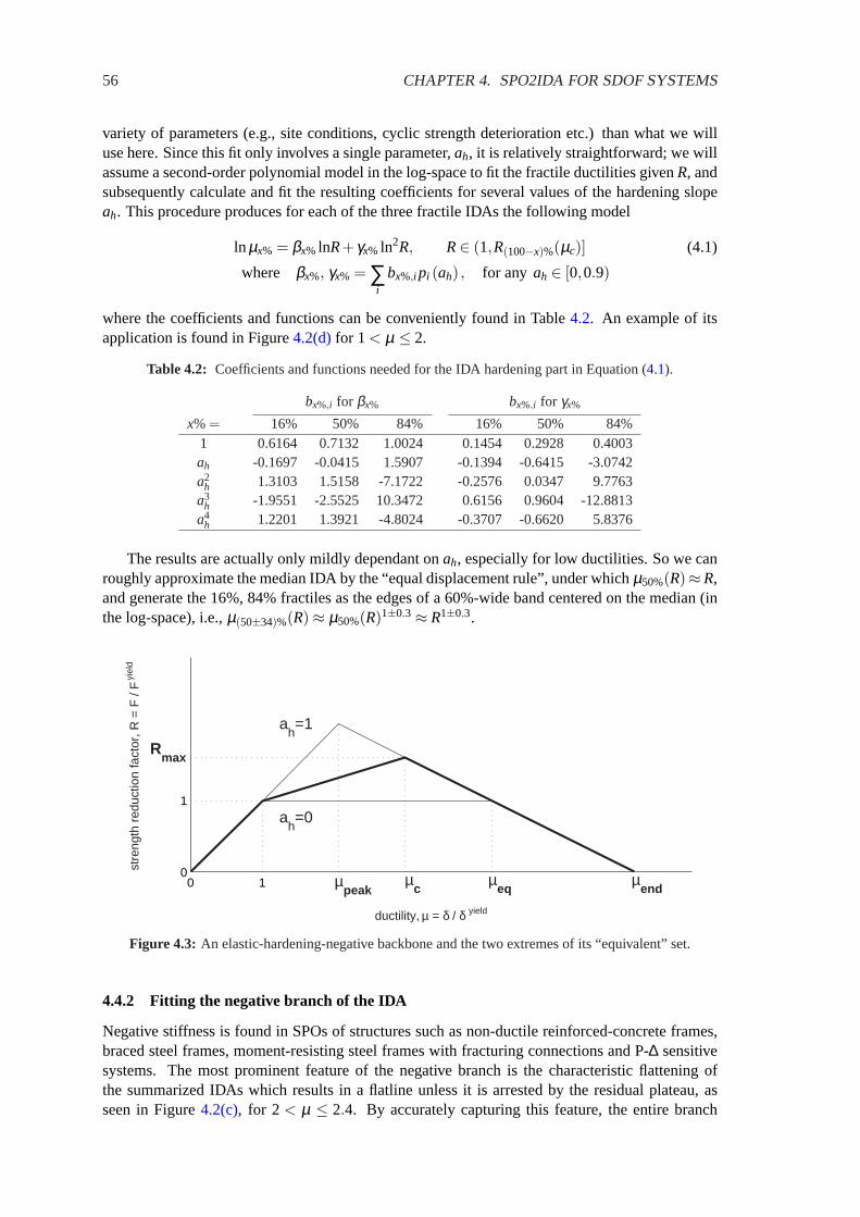
56 CHAPTER 4. SPO2IDA FOR SDOF SYSTEMS
variety of parameters (e.g., site conditions, cyclic strength deterioration etc.) than what we willuse here. Since this fit only involves a single parameter,ah, it is relatively straightforward; we willassume a second-order polynomial model in the log-space to fit the fractile ductilities givenR, andsubsequently calculate and fit the resulting coefficients for several values of the hardening slopeah. This procedure produces for each of the three fractile IDAs the following model
ln µx% = βx% lnR+ γx% ln2R, R∈ (1,R(100−x)%(µc)] (4.1)
where βx%, γx% = ∑i
bx%,i pi (ah) , for any ah ∈ [0,0.9)
where the coefficients and functions can be conveniently found in Table4.2. An example of itsapplication is found in Figure4.2(d)for 1 < µ ≤ 2.
Table 4.2: Coefficients and functions needed for the IDA hardening part in Equation (4.1).
bx%,i for βx% bx%,i for γx%
x% = 16% 50% 84% 16% 50% 84%1 0.6164 0.7132 1.0024 0.1454 0.2928 0.4003ah -0.1697 -0.0415 1.5907 -0.1394 -0.6415 -3.0742a2
h 1.3103 1.5158 -7.1722 -0.2576 0.0347 9.7763a3
h -1.9551 -2.5525 10.3472 0.6156 0.9604 -12.8813a4
h 1.2201 1.3921 -4.8024 -0.3707 -0.6620 5.8376
The results are actually only mildly dependant onah, especially for low ductilities. So we canroughly approximate the median IDA by the “equal displacement rule”, under whichµ50%(R)≈R,and generate the 16%, 84% fractiles as the edges of a 60%-wide band centered on the median (inthe log-space), i.e.,µ(50±34)%(R)≈ µ50%(R)1±0.3 ≈ R1±0.3.
0 10
1
ductility, µ = δ / δ yield
stre
ngth
red
uctio
n fa
ctor
, R =
F /
F yie
ld
µpeak
µeq
µend
Rmax
µc
ah=0
ah=1
Figure 4.3: An elastic-hardening-negative backbone and the two extremes of its “equivalent” set.
4.4.2 Fitting the negative branch of the IDA
Negative stiffness is found in SPOs of structures such as non-ductile reinforced-concrete frames,braced steel frames, moment-resisting steel frames with fracturing connections and P-∆ sensitivesystems. The most prominent feature of the negative branch is the characteristic flattening ofthe summarized IDAs which results in a flatline unless it is arrested by the residual plateau, asseen in Figure4.2(c), for 2 < µ ≤ 2.4. By accurately capturing this feature, the entire branch
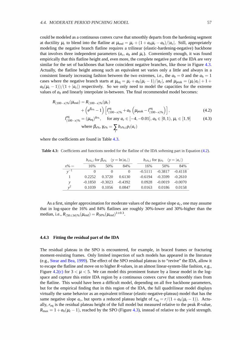
4.4. MODERATE PERIOD PINCHING MODEL 57
could be modeled as a continuous convex curve that smoothly departs from the hardening segmentat ductility µc to blend into the flatline atµend = µc + (1+ ahµc− ah)/|ac|. Still, appropriatelymodeling the negative branch flatline requires a trilinear (elastic-hardening-negative) backbonethat involves three independent parameters (ac, ah andµc). Conveniently enough, it was foundempirically that this flatline height and, even more, the complete negative part of the IDA are verysimilar for the set of backbones that have coincident negative branches, like those in Figure4.3.Actually, the flatline height among such an equivalent set varies only a little and always in aconsistent linearly increasing fashion between the two extremes, i.e., theah = 0 and theah = 1cases where the negative branch starts atµeq = µc + ah(µc− 1)/|ac|, andµpeak= (µc|ac|+ 1+ah(µc− 1))/(1+ |ac|) respectively. So we only need to model the capacities for the extremevalues ofah and linearly interpolate in-between. The final recommended model becomes:
R(100−x)%(µend) = R(100−x)%(µc)
+(
eβx%−1)[
leq(100−x)% +ah
(µpeak− leq
(100−x)%
)], (4.2)
leq(100−x)% = (µeq)γx%, for anyac ∈ [−4,−0.01], ah ∈ [0,1), µc ∈ [1,9] (4.3)
whereβx%,γx% = ∑i
bx%,i pi(ac)
where the coefficients are found in Table4.3.
Table 4.3: Coefficients and functions needed for the flatline of the IDA softening part in Equation (4.2).
bx%,i for βx% (y = ln |ac|) bx%,i for γx% (y = |ac|)x% = 16% 50% 84% 16% 50% 84%y−1 0 0 0 -0.5111 -0.3817 -0.41181 0.2252 0.3720 0.6130 -0.6194 -0.3599 -0.2610y -0.1850 -0.3023 -0.4392 0.0928 -0.0019 -0.0070y2 0.1039 0.1056 0.0847 0.0163 0.0186 0.0158
As a first, simpler approximation for moderate values of the negative slopeac, one may assumethat in log-space the 16% and 84% flatlines are roughly 30%-lower and 30%-higher than themedian, i.e.,R(50±34)%(µend) = R50%(µend)1±0.3.
4.4.3 Fitting the residual part of the IDA
The residual plateau in the SPO is encountered, for example, in braced frames or fracturingmoment-resisting frames. Only limited inspection of such models has appeared in the literature(e.g.,Stear and Bea, 1999). The effect of the SPO residual plateau is to “revive” the IDA, allow itto escape the flatline and move on to higherR-values, in an almost linear-system-like fashion, e.g.,Figure4.2(c) for 3 < µ < 5. We can model this prominent feature by a linear model in the log-space and capture this entire IDA region by a continuous convex curve that smoothly rises fromthe flatline. This would have been a difficult model, depending on all five backbone parameters,but for the empirical finding that in this region of the IDA, the full quadrilinear model displaysvirtually the same behavior as an equivalent trilinear (elastic-negative-plateau) model that has thesame negative slopeac, but sports a reduced plateau height ofreq = r/(1+ ah(µc− 1)). Actu-ally, req is the residual plateau height of the full model but measured relative to the peakR-value,Rmax = 1+ah(µc−1), reached by the SPO (Figure4.3), instead of relative to the yield strength.

58 CHAPTER 4. SPO2IDA FOR SDOF SYSTEMS
This revelation leaves us with only two influential parameters,ac andreq, resulting in the model:
ln µx% = βx% + γx% lnR, R∈ (R(100−x)%(µr),R(100−x)%(µ f )
](4.4)
where βx%, γx% = ∑i
bx%,i pi(ac, req
),
for any ac ∈ [−4,−0.01], req∈ [0.05,0.90]
where the coefficients can be found in Table4.4. An example of this model’s application can beseen in Figure4.2(d)for 3 < µ ≤ 5.
Table 4.4: Coefficients and functions needed for fitting the IDA residual part in Equation (4.4).
bx%,i for βx% bx%,i for γx%
x% = 16% 50% 84% 16% 50% 84%1 -0.3615 0.2391 0.9557 1.1022 1.0846 1.0176
ln |ac| -0.0729 -0.0297 -0.0696 0.0180 0.0081 0.0203ln req -0.4557 -0.4907 -0.4759 0.1111 0.1218 0.1086
ln req· ln |ac| -0.0372 -0.0272 -0.0308 0.0136 0.0086 0.0061
By observing the results, one can derive that the median IDA does behave much like a secantlinear segment that takes on smaller slopes asreq decreases, eventually becoming one with theflatline induced by the negative branch of the SPO. So, by restricting ourselves to (quite practical)ductilities of 10 or less, the modeling could be further simplified if one decides to model theresidual branch of the median IDA as a secant by assumingγ50% = 1, while generating the 16%,84% fractiles as a 100%-wide band centered on the median (in the log-space), i.e.,µ(50±34)%(R)≈µ50%(R)1±0.5 ≈ β50% ·R1±0.5. The existing table ofβ50% coefficients, although not optimal, canstill be used for this approximation, since the difference is negligible.
4.4.4 Joining the pieces: The SPO2IDA tool
We have separately modeled the three segments but we have chosen to keep track of only theflattening caused by the negative SPO and the “secant” caused by the residual. To join them intosmooth and continuous curves that accurately resemble the fractile IDAs we need two “filletingcurves” that will connect the negative branch flatline to the hardening and the “secant”. We canchoose to neglect such details and linearly extend all three pieces to a point of mutual interception,which is usually accurate enough. Alternatively, we can generate splines through a knot-insertionalgorithm (Farin, 1990), which provides a smooth transition from segment to segment, while atthe same time offering computational simplicity and robustness, as it preserves convexity and canbe made to be monotonic (as the fractile IDAs are empirically known to be). Once this step hasbeen completed, we have an almost complete description of the IDA for any ductility, modeledas an invertible one-to-one function of eitherµ or R, a choice left to the user as an advantage ofthe equivalency of the fractiles givenR or µ. We are only missing the final flatline, caused by theSPO’s ending at ductilityµ f . This can be accurately and easily modeled in the IDAs by addinga flatline at heightR(100−x)%(µ f ), simultaneously producing the(100− x)%-fractile of global-collapse capacity. By implementing in software the modeling and joining of the IDA segments wehave generated the SPO2IDA tool, available in a spreadsheet or as an online internet application(Vamvatsikos, 2001), and it does a remarkable job of reproducing the real behavior of oscillators,as demonstrated in Figure4.2(d).

4.4. MODERATE PERIOD PINCHING MODEL 59
0 1 2 3 4 5 6 7 80
0.5
1
1.5
2
2.5
3
3.5
4
4.5
µc= 1
20%
−50%
stre
ngth
red
uctio
n fa
ctor
, R =
Sa /
Sayi
eld
ductility, µ = δ / δ yield
µc= 2
µc= 3
µc= 1 (50% IDA)
µc= 2 (50% IDA)
µc= 3 (50% IDA)
(a) Increasingµc helps performance
0 1 2 3 4 5 6 7 80
0.5
1
1.5
2
2.5
3
3.5
4
4.5
ac= 10%
−200%
stre
ngth
red
uctio
n fa
ctor
, R =
Sa /
Sayi
eld
ductility, µ = δ / δ yield
ac= 25%
ac= 50%
ac= 75%
ac= 10% (50% IDA)
ac= 25%, 50%, 75% (50% IDAs)
(b) Increasingah has negligible effects if sameµeq
0 1 2 3 4 5 6 7 80
0.5
1
1.5
2
2.5
3
3.5
4
4.5
ac= −25%
20%
stre
ngth
red
uctio
n fa
ctor
, R =
Sa /
Sayi
eld
ductility, µ = δ / δ yield
ac= −50% a
c= −200%
ac= −25% (50% IDA)
ac= −50% (50% IDA)
ac= −200% (50% IDA)
(c) The milder the negative slope,ac, the better
0 1 2 3 4 5 6 7 80
0.5
1
1.5
2
2.5
3
3.5
4
4.5
ac= −25%
50%
20%
stre
ngth
red
uctio
n fa
ctor
, R =
Sa /
Sayi
eld
ductility, µ = δ / δ yield
ac= −50% a
c= −200%
ac= −25% (50% IDA)
ac= −50% (50% IDA)
ac= −200% (50% IDA)
(d) ac is changing, but constantreq anchors capacity
0 1 2 3 4 5 6 7 80
0.5
1
1.5
2
2.5
3
3.5
4
4.5
r = 20%
ductility, µ = δ / δ yield
stre
ngth
red
uctio
n fa
ctor
, R =
Sa /
Sayi
eld
20%
r = 50%
−50% r = 80%
r = 20% (50% IDA)
r = 80% (50% IDA)
r = 50% (50% IDA)
(e) Higher plateaur benefits demand and capacity
0 1 2 3 4 5 6 7 80
0.5
1
1.5
2
2.5
3
3.5
4
4.5
20%
50%
ductility, µ = δ / δ yield
stre
ngth
red
uctio
n fa
ctor
, R =
Sa /
Sayi
eld
−50%
µf= 4 µ
f= 5 µ
f= 6 µ
f= 7
µf= 4 (50% IDA)
µf= 7 (50% IDA)
µf= 6 (50% IDA)
µf= 5 (50% IDA)
(f) Increasing the fracturing ductilityµ f helps
Figure 4.4: Demonstrating SPO2IDA: the median demand and collapse capacity as the SPO changes.

60 CHAPTER 4. SPO2IDA FOR SDOF SYSTEMS
4.4.5 Illustrative Results and Observations
The ease of computation provided by such a tool, plus the unique perspective offered by the IDA-versus-SPO picture, can offer remarkable intuition into the seismic behavior of systems. As ademonstration of the SPO2IDA tool, we present Figure4.4, an array of cases to briefly study theinfluence of the backbone on the seismic demand and capacity. In each figure we select a basicbackbone, vary one or two of its parameters and then generate the median IDA responses and thecorresponding global instability collapse-capacities for each case. Figure4.4(a)shows the benefitof delaying the negative branch of the SPO and allowing hardening to reach higher ductilities.Each increase inµc allows the median to stay on “equal displacement” longer, proportionally in-creasing the capacity. On the other hand, in Figure4.4(b), radically changing the hardening slopeah but keeping an identical negative branch generates an equivalent set of trilinear SPOs, whosecapacities only slightly increase withah. Actually, the difference in the capacity is small enough tobe within the noise in the fitted data, so the resulting capacities are not strictly increasing withah.Decreasing the negative slopeac in Figure4.4(c)has a beneficial effect when no residual plateauis present, as the milder slopes allow higher capacities. Still, if we include an extensive enoughresidual plateau (Figure4.4(d)), the benefits of the milder slope are restricted to the somewhatlower µ-demands that may influence some earlier limit-states; the global instability collapse ca-pacity is almost the same for all cases, as the backbones have the samereq, therefore the milderac’sare providing only a small advantage. Figure4.4(e)shows the benefits of increasing the residualplateau that consequently increases the slope of the “secant” that the IDA follows, thus improvingcapacities and decreasing the demands. And finally, Figure4.4(f) shows the obvious advantage ofallowing higher fracturing ductilitiesµ f . The value ofµ f literally decides where to terminate theIDA, at times fully negating the effect of the plateau if it becomes too small; atµ f = 4 the IDAhardly receives any benefit from the plateau. As intuitive or surprising as some of the pictures inFigure4.4may be, they are only a glimpse of what our new tool can really do.
4.4.6 SPO2IDA error estimates for moderate periods
Since the SPO2IDA tool is based on fitting over only a small subset of the SDOF backbones itcan simulate, just showing the fitting error over the sample of oscillators that we have used wouldgreatly underestimate the true prediction error. In order to be objective we have generated a largeseparate test sample of randomly chosen bilinear, trilinear and quadrilinear backbones, that wereanalyzed both through full IDA and SPO2IDA. Thus, for each backbone and each of the threex%-fractiles we are presented with two IDA curves, the “real” curveR(100−x)%(µ) and the approximateR(100−x)%(µ), or equivalently expressed inµ givenRcoordinates,µx%(R) versusµx%(R).
We are interested in knowing the error in two different settings: error in estimating a demandµ given a certain level on intensityR and error in estimating a capacityR given a certain levelof demandµ. In both cases, theabsolutedifference between exact and approximate results tendsto increase rapidly when we progress further into the nonlinear range, making this measure un-suitable. We choose instead to quantify the errors by integrating therelative absolutedifferenceof each approximatex%-fractile IDA curve versus the real one over their length, either inµ or Rcoordinates accordingly, a concept similar to the one used byLee et al.(1999):
(εR)x% =∫ µ f
0
∣∣R(100−x)%(µ)− R(100−x)%(µ)∣∣
R(100−x)%(µ)dµ (4.5)
(εµ)x% =∫ Rf
0
|µx%(R)− µx%(R)|µx%(R)
dR (4.6)
In each case, the fractile-capacity error(εR)x% is calculated over the full demand spectrum fromzero toµ f , and the fractile-demand error(εµ)x% is similarly calculated up toRf , where either of

4.4. MODERATE PERIOD PINCHING MODEL 61
the two curves compared flatlines first.
Table 4.5: Average fractile-demand and fractile-capacity errors for moderate periods and a variety ofbackbone shapes, as caused by the fitting in SPO2IDA and by the record-to-record variability in IDA.
SPO2IDA 10 records 30 records
x% = 16% 50% 84% 16% 50% 84% 16% 50% 84%
elastic-hardeningεR 0.02 0.01 0.02 0.11 0.07 0.07 0.06 0.04 0.04εµ 0.01 0.01 0.02 0.06 0.06 0.09 0.04 0.03 0.05
elastic-hardening-negativeεR 0.02 0.03 0.03 0.09 0.06 0.06 0.05 0.03 0.03εµ 0.02 0.03 0.03 0.07 0.05 0.06 0.04 0.03 0.04
elastic-hardening-negative-plateauεR 0.16 0.14 0.18 0.20 0.12 0.13 0.12 0.08 0.07εµ 0.09 0.11 0.18 0.20 0.18 0.23 0.11 0.11 0.14
What is more important to the user than just an error measure is an assessment of how large isSPO2IDA’s estimation error, caused by imperfect fitting, as compared to the full IDA estimationerror caused by the record-to-record variability when using a limited sample of records. To providesuch a standard for comparison, we will use the bootstrap method (Efron and Tibshirani, 1993) toestimate the equivalent(εR)x% and(εµ)x% error that one would expect to encounter when usingonly 10 or 30 randomly chosen records from the same scenario earthquake. According to thebootstrap principle, the original 30 records are sampled with replacement to generate numerousalternate samples of 10 and 30 records, which are then applied to each of the randomly-chosenbackbones, thus resulting to a large number of alternate estimates of the fractile IDAs for each test-case. Then, using the original 30-record suite results as “exact”, the average (over all bootstrapsamples)(εR)x% and(εµ)x% are calculated, as shown in Table4.5.
Before we interpret these results, it is important to understand that SPO2IDA was based on the30-record IDA, thus its error, as calculated in the table, comesin addition to the error induced byrecord-variability in the 30-record fractile IDAs, i.e., SPO2IDA cannot be more accurate than a 30-record IDA. Still, if the additional (fitting induced) error it incurs is small enough, it will disappear(as when taking the square root of sum of squares of the two errors) under the considerable (record-variability induced) error in estimating the fractiles with a 30-record IDA. Thus, by comparingthe (εR)x% and (εµ)x% of SPO2IDA versus the average such errors due to the record-to-recordvariability, we observe that SPO2IDA can estimate the fractile demands or capacities with an errorcomparable to the record-to-record noise around the 10-record full IDA results. This means thatstatistically, the difference between the full IDA and SPO2IDA results is on average insignificantwhen only 10 records are used. If 30 records are employed for IDA, SPO2IDA again performsvery well for all backbones except the complex quadrilinears where it has, on average, an errorsomewhat more significant, but still comparable to the record-to-record induced noise. All in all,SPO2IDA is proven to be remarkably accurate, able to outperform the 10-record full IDA and inmany cases match the 30-record IDA.
Naturally, the values in Table4.5do not tell the whole story, as they describe the performanceof SPO2IDA averaged over numerous backbone shapes and over the length (either inRor µ terms)of the fractile curves. Some individual backbone shapes may be captured better than others andwithin the curves themselves some segments may be more accurately matched. As evident fromTable4.5, the error tends to increase for more complex backbones. This is caused by the cascadingof the models, i.e., as more segments are added to the backbone, each additional segment relieson the accuracy achieved in the previous ones. Thus, the more complex our backbone, the more

62 CHAPTER 4. SPO2IDA FOR SDOF SYSTEMS
error we should expect in the later segments (e.g., the residual plateau). But even within the samesegment of the curve, the distribution of the error is not homogeneous, neither for the full IDA,nor for the SPO2IDA. In the IDA results, as the ductility increases beyond yielding, the record-to-record variability and the error it induces increase as well. This, in turn, introduces higher noise inthe fitted data, thus making the fitted equations less accurate at higher ductilities. So, in general,one should expect errors lower than average at low ductilities and higher than average at highductilities for both methods. Finally, since we have relied on regression to fit the IDA curves, justlike all fits these equations will perform better in the middle of the fitted dataset and worse at theedges (Weisberg, 1985). So, one should generally expect higher errors closer to the edges wheresome fits are least accurate, e.g., atac = −0.01 for Equation4.2 or at req = 0.9 andac = −0.01in Equation4.4. All such observations taken into consideration, there are some combinations ofbackbone parameters that may cause SPO2IDA to produce a mediocre estimate for some segmentof the IDA, but in our experience even these cases are rare.
4.5 Extension to all-periods pinching model
Up to now we have described a procedure used to obtain the fractile IDA curves of a fairly limitedmodel. Still, this can be easily extended to other periods, dampings, or hysteretic models. Whatwe have really introduced above is a methodology that permits the accurate modeling of the SDOFfractile IDA curves for complex backbones by investigating only a small number of them. If onewishes to capture the behavior of a different SDOF system, or use a different suite of groundmotion records, all that is needed is repeating the above three fits for the hardening, negative andresidual part to include the new parameters. As an example, we are going to extend SPO2IDA toboth short and long periods, still using the same suite of 30 records, moderately pinching hysteresisand viscous damping ofξ = 5%. The overall concept will be precisely the same as for the moderateperiods, simply the necessary coefficients will be given by more complicated equations that, inaddition to the backbone parameters, will now include the oscillator periodT.
Unfortunately, the oscillator period influences each of the backbone regions in a complex,coupled way, that makes it impossible to assume independence. So, where we had mostly oneor two dimensional fits, now we will have two and three dimensional ones. This fact increasesthe number of oscillators that we have to investigate by an order of magnitude, and unfortunatelyno fancy methods can help us further reduce the dimensionality of the problem. Still, the samefundamental results that we employed previously to reduce the number of backbones investigatedare not period dependent, i.e., the equivalency of the backbones is found to be valid for the shortand long periods as well.
4.5.1 Fitting the hardening branch of the IDA
Several researchers have provided similar fits for wide period ranges but most have focused on justthe elastic-perfectly-plastic model (Newmark and Hall, 1982; Miranda, 2000), while even thosewho have gone beyond that have only a limited coverage of the hardening slopeah (Nassar andKrawinkler, 1991), or consider the effect ofah to be independent of periodT (Lee et al., 1999).On the other hand, we will make no such simplifications. Using Equation (4.1), which accuratelycaptures the shape of the hardening part of the IDA, all we need to do is provide fits for thecoefficientsβx% andγx% that depend both onT andah.
lnβx% = ∑i
bx%,i px%,i(ah,T), ln(γx% +1) = max
(∑
i
bx%,i pi(ah,T) , 0
), (4.7)
for any ah ∈ [0,0.9],T ∈ [0.2s,4s]

4.5. EXTENSION TO ALL-PERIODS PINCHING MODEL 63
where the coefficientsbx%,i and corresponding functions can be conveniently found in Table4.6.
Table 4.6: Coefficients needed for the IDA hardening part in Equation (4.7).
bx%,i for βx% bx%,i for γx%
x% = 16% 50% 84% 16% 50% 84%ln−1(T +1) -0.1520 -0.1985 -0.6344 0.1925 0.3689 0.9434
1 -0.5027 -0.0955 0.2649 0.1246 0.0480 0.0277lnT -0.0542 -0.0316 0.0818 -0.1045 -0.1747 -0.4226ln2T 0.0181 0.0291 -0.1250 0.0605 0.1364 0.3241
ah ln−1(T +1) -0.1520 -0.1985 -0.6344 0.1925 0.3689 0.9434ah 0.8058 0.3737 -0.0954 -0.1989 -0.2105 -0.0297
ah lnT 0.2037 0.2334 0.5720 -0.0822 -0.1916 -0.5081ah ln2T -0.2572 -0.3683 -0.5508 0.1711 0.3816 0.5662
a0.5h ln−1(T +1) -0.1520 -0.1985 -0.6344 0.1925 0.3689 0.9434
a0.5h -0.3675 -0.3041 -0.1600 0.0713 0.1533 -0.0010
a0.5h lnT -0.1520 -0.1985 -0.6344 0.1925 0.3689 0.9434
a0.5h ln2T 0.2258 0.3128 0.6418 -0.2237 -0.4964 -0.8851
As expected, the results are similar in the moderate and long period range, the median follow-ing the “equal displacement” rule, but the situation is much different in the short period domain.In that region there is significant dependance on bothah andT, making any simplifications of theabove equations quite difficult.
4.5.2 Fitting the negative branch of the IDA
Again, using Equations (4.2) and (4.3) we only need to fit and redefine the coefficientsβx% andγx% so that they depend both onT andac:
βx% = ∑i
bx%,i pi(ac,T), γx% = min
(∑
i
bx%,i pi(ac,T),1
)(4.8)
for anyac ∈ [−4,−0.02], T ∈ [0.2s,4s]
where the coefficients and relevant functions are found in Table4.7.
Table 4.7: Coefficients needed for the flatline of the IDA softening part in Equation (4.8).
bx%,i for βx% bx%,i for γx%
x% = 16% 50% 84% 16% 50% 84%1 0.2391 0.3846 0.5834 1 -0.2508 -0.2762 -0.2928
lnT 0.0517 0.0887 0.1351 |ac| -0.5517 -0.1992 -0.4394ln |ac| -1.2399 -1.3531 -1.4585 a2
c 0.0941 -0.0031 0.0683ln |ac| lnT -0.0976 -0.1158 -0.1317 |ac|−1 0.0059 0.0101 0.0131
ln2 |ac| 0.0971 0.1124 0.1100 lnT 0.1681 0.2451 0.1850ln2 |ac| lnT 0.0641 0.0501 0.0422 |ac| lnT 0.1357 -0.0199 0.1783
ln3 |ac| -0.0009 0.0041 0.0056 a2c lnT -0.0127 0.0091 -0.0305
ln3 |ac| lnT 0.0072 0.0067 0.0074 |ac|−1 lnT 0.0010 -0.0075 -0.0066ln2T -0.1579 -0.0135 0.0027
|ac| ln2T 0.2551 -0.0841 0.0447a2
c ln2T -0.0602 0.0222 -0.0151|ac|−1 ln2T 0.0087 -0.0003 -0.0025

64 CHAPTER 4. SPO2IDA FOR SDOF SYSTEMS
4.5.3 Fitting the residual part of the IDA
Similarly, by using the equivalent residual concept, only three influential parameters exist,ac, req
andT, resulting in the same model as in Equation (4.4), only now we will define new coefficients:
βx%, γx% = ∑i
bx%,i pi(ac, req,T), (4.9)
for any ac ∈ [−4,−0.05], req∈ [0.05,0.90], T ∈ [0.2s,4s]
where the coefficients can be found in Table4.8.
Table 4.8: Coefficients needed for fitting the IDA residual part in Equation (4.9).
bx%,i for βx% bx%,i for γx%
x% = 16% 50% 84% 16% 50% 84%1 -0.2226 0.1401 0.7604 1.0595 1.0635 1.0005
ln |ac| -0.0992 -0.0817 -0.1035 0.0236 0.0177 0.0283ln req -0.4537 -0.5091 -0.5235 0.1237 0.1466 0.1607
ln req· ln |ac| -0.0398 -0.0236 -0.0287 0.0111 0.0048 -0.0004ln r−1
eq 0.0829 -0.0364 -0.0174 -0.0023 0.0102 0.0021ln r−1
eq · ln |ac| 0.0193 -0.0126 -0.0118 0.0008 0.0019 0.0035lnT -0.1831 -0.2732 -0.5651 -0.0881 -0.1044 -0.1276
lnT · ln |ac| -0.0319 0.0015 0.0437 -0.0077 -0.0137 -0.0413lnT · ln req 0.1461 0.1101 0.0841 -0.0239 -0.0090 -0.0085
lnT · ln req· ln |ac| -0.0227 -0.0045 0.0159 0.0025 -0.0014 -0.0198lnT · ln r−1
eq -0.0108 0.0333 0.0033 0.0082 -0.0003 0.0037lnT · ln r−1
eq · ln |ac| -0.0081 -0.0000 0.0033 0.0007 -0.0013 -0.0043ln2T 0.1660 0.1967 0.0929 0.0317 0.0038 0.0673
ln2T · ln |ac| -0.0124 -0.0304 0.0130 0.0006 0.0065 0.0074ln2T · ln req 0.0273 0.0396 0.0580 -0.0173 -0.0484 -0.0737
ln2T · ln req· ln |ac| -0.0167 -0.0209 -0.0144 0.0056 0.0068 0.0255ln2T · ln r−1
eq -0.0182 0.0311 0.0221 0.0007 -0.0112 -0.0073ln2T · ln r−1
eq · ln |ac| -0.0097 -0.0047 0.0007 0.0004 0.0008 0.0005
4.5.4 Illustrative Results and Observations
Using splines to connect the above presented three fits and to integrate them into SPO2IDA, wehave generated a tool that can accurately capture the behavior of a complex quadrilinear backbonefor a wide range of periods, from 0.2s to 4s (Vamvatsikos, 2002). An example of its application ispresented in Figure4.5. Therein the median IDA curve of an elastic-hardening-negative-plateaubackbone is recreated for several oscillator periods. Starting from at a moderate period ofT = 1s,the flatline happens atR≈ 4.1, but if we decrease the period down toT = 0.3s, we observe thatthe IDA becomes more aggressive; softening commences at very low values ofRand the flatline isreached very quickly, atR≈ 2.7 for T = 0.3s. On the other end, when the period is increased, themedian IDA is “milder”, it rises and straightens out, staying longer on the “equal displacement”rule, i.e., on theµ = R line. Thus, the flatline is greatly delayed, occurring atR≈ 5.5 at T = 4s.Obviously, the oscillator period has a significant effect on the flatline but also on all the features ofthe fractile IDAs. The only exception appears for moderate and long periods in the region wherethe backbone is still hardening. There the median IDA follows the equal displacement rule andthus becomes insensitive to the (moderate or long) period. As observed at least for the median inFigure4.5, SPO2IDA is now able to capture all such period-dependent effects.
4.5. EXTENSION TO ALL-PERIODS PINCHING MODEL 65
0 1 2 3 4 5 6 7 80
1
2
3
4
5
6
20%
−50% 50%
ductility, µ = δ / δ yield
stre
ngth
red
uctio
n fa
ctor
, R =
Sa /
Sayi
eld
T=4s (50% IDA)
T=2s (50% IDA)
T=1s (50% IDA)
T=0.5s (50% IDA)
T=0.3s (50% IDA)
Figure 4.5: Median IDAs for a backbone withah = 0.2, µc = 2, ac = −0.5, r = 0.5, µ f = 6 but varyingperiods.
4.5.5 SPO2IDA error estimates for all periods
Similarly to the moderate period model, we have generated a separate test-sample of various os-cillators with randomly generated backbones and periods. Then we performed a calculation ofthe fractile demand and capacity errors(εµ)x% and(εR)x% according to Equations (4.5)–(4.6) bothshown in Table4.9. Therein we have also included the bootstrapped(εµ)x% and(εR)x% values fora full IDA with 10 and 30 records.
Once again, the SPO2IDA error is, practically speaking, comparable to the error induced by therecord-to-record variability in a full 30-record IDA for all cases, except the last, the quadrilinearone. Again, the most complex of the backbones is harder to capture, but still, the SPO2IDA errorremains within reasonable limits.
Table 4.9: Average fractile-demand and fractile-capacity errors for short, moderate and long periods and avariety of backbone shapes, as caused by the fitting in SPO2IDA and by the record-to-record variability inIDA.
SPO2IDA 10 records 30 records
x% = 16% 50% 84% 16% 50% 84% 16% 50% 84%
elastic-hardeningεR 0.04 0.04 0.05 0.09 0.07 0.09 0.06 0.04 0.05εµ 0.02 0.03 0.04 0.06 0.06 0.09 0.04 0.04 0.06
elastic-hardening-negativeεR 0.05 0.04 0.05 0.08 0.06 0.09 0.05 0.04 0.04εµ 0.05 0.03 0.04 0.07 0.07 0.10 0.04 0.04 0.04
elastic-hardening-negative-plateauεR 0.20 0.18 0.20 0.21 0.16 0.18 0.14 0.10 0.12εµ 0.19 0.24 0.26 0.20 0.17 0.24 0.12 0.12 0.15
The same observations apply here as in the moderate period range; the errors in Table4.9areaveraged over numerous backbones, periods and along each individual fractile curve. Therefore,individual cases may perform better or worse than the posted values. The only difference from themoderate period case is the additional consideration of period. Generally, in the short period range,the record-to-record variability is higher thus degrading the accuracy of both IDA and SPO2IDA.Still, barring some isolated below-average-accuracy estimates, the results are very reliable.

66 CHAPTER 4. SPO2IDA FOR SDOF SYSTEMS
10−1
100
0.5
1
1.5
2
2.5
3
3.5
period (s)
inel
astic
dis
p. r
atio
, Cµ
spo2ida real data
µ = 6
µ = 1.5
(a) Results from IDA versus SPO2IDA
10−1
100
0.5
1
1.5
2
2.5
3
3.5
period (s)
inel
astic
dis
p. r
atio
, Cµ
µ = 6
µ = 1.5
(b) Results fromMiranda(2000)
Figure 4.6: Comparing estimates of meanCµ ratios generated by SPO2IDA for the special elastic-perfectly-plastic case versus the real data and results fromMiranda(2000) for µ = 1.5,2,3,4,5,6.
4.6 From the IDA to the inelastic displacement ratios
On a more practical aspect, SPO2IDA can directly produceR-factors and inelastic displacementratios, often used in seismic guidelines (e.g.,FEMA, 1997). The direct mapping of theµ-given-Rto theR-given-µ fractiles effortlessly provides fractileR-factors. Similarly, one can easily generate(Cµ)x%, the x%-fractile of inelastic to elastic displacement ratio givenµ, and(CR)x%, the x%-fractile of inelastic to elastic displacement ratio givenR, as defined inMiranda(2001). Actuallythe fractiles of the two ratios are equivalent as(Cµ)x% = (CR)x% = µx%(R)/R= µ/R(100−x)%(µ).By modeling the fractiles in SPO2IDA we can use the same fits to generate theR-factors and boththe inelastic displacement ratios; had we chosen to model the mean response, we would need aseparate fit for each of the three quantities (Miranda, 2001).
On the other hand, instead of the fractiles, the meanR-factors or mean inelastic displacementratios may be of interest. IfE[·] is the expectation operator, then we want to estimateE[R], E[Cµ ] =µE[1/R] for a given value ofµ andE[CR] = E[µ]/R for a given value ofR. Actually, for valuesof R higher than any of the flatlines,E[µ] and correspondinglyE[CR] become infinite. At lowerR-values the distribution ofµ givenR is approximately lognormal (Shome and Cornell, 1999) andso is the distribution ofR given µ for any µ-value. In those ranges we can use the properties ofthe lognormal distribution (e.g.,Benjamin and Cornell, 1970) to show that
E[R] = R50%(µ) ·exp
(12
σ2lnR
), σlnR =
12
(lnR84%(µ)− lnR16%(µ)) (4.10)
E[CR] =E[µ]
R=
µ50%(R)R
·exp
(12
σ2ln µ
), σln µ =
12
(ln µ84%(R)− ln µ16%(R)) (4.11)
E[Cµ ] = µE
[1R
]=
µR50%(µ)
·exp
(12
σ2− lnR
), σ− lnR = σlnR (4.12)
In Figure4.6(a)we have used Equation (4.12) to calculate averageCµ ratios using SPO2IDAfor an elastic-perfectly-plastic system over a range of periods from 0.1s to 3s using SPO2IDA. Onthe same figure we also plot the averageCµ calculated directly from the 30 record suite throughIDA, without the use of any approximation or fit. Clearly, the SPO2IDA results closely matchthe exact ones, except perhaps for the shortest of periods. As a further comparison, we haverecreated in Figure4.6(b)theCµ results from the proposed equation inMiranda(2000), generatedfor an elastic-perfectly-plastic model with kinematic hardening, using over 200 records that have

4.7. INFLUENCE OF OTHER SDOF PARAMETERS 67
a wide magnitude and source-to-site distance range, and that were all recorded on firm soil. Asexpected, the results are comparable everywhere but in the short period range, where the record-to-record variability is maximum. Of course, such a specialized fit should be expected to outperformSPO2IDA, having much less error, especially in the short periods. Still, our tool is proven tobe suited to many applications, even beyond estimating the fractile IDAs that it was originallydesigned for.
0 2 4 6 8 100
1
2
3
4
5
6
30% −200%
50%
ductility, µ = δ / δ yield
stre
ngth
red
uctio
n fa
ctor
, R =
Sa /
Sayi
eld
SPO 50% IDA (8% damped)50% IDA (5% damped)50% IDA (2% damped)
Figure 4.7: Viscous damping has negligible influence, as shown for moderate periods for a backbone withah = 0.3, µc = 2, ac =−2, r = 0.5, µ f = 5.
4.7 Influence of other SDOF parameters
By mostly focusing on the oscillator backbone we have restricted our modeling effort in severalother aspects; ground motion records were selected from a narrow magnitude and distance binand correspond to firm soil only, while hysteresis-wise, we have only considered a 5% damped,moderately pinching model. Do these choices seriously restrict SPO2IDA, or can the results beapplied in cases beyond what we have considered?
Regarding the selection of the records, the issue of magnitude, source-to-site distance and soilsite appear. It has been well documented in the literature that the elastic-perfectly-plastic and theelastic-hardening system results (meanR-factor,Cµ andCR) are not significantly influenced bymagnitude, except maybe in the shortest of periods (Ruiz-Garcia and Miranda, 2003), or distance,unless near-fault directivity is an issue (e.g.,Miranda, 2000; Nassar and Krawinkler, 1991). Actu-ally, several researchers have found evidence of significant difference between forward-directivityand non-directivity influenced records (Cuesta and Aschheim, 2001; Baez and Miranda, 2000),while a recent study byChopra and Chintanapakdee(2001), proposes modifyingR-µ-T relation-ships to account for such effects. In that case, SPO2IDA needs to be upgraded before being appliedwhen directivity matters. On the other hand, regarding soil-site issuesMiranda(2000) has foundlittle dependance within different firm soil sites. ButMiranda(1993) andRahnama and Krawin-kler (1993) confirm that soft soil sites can be significantly different and their effect needs to betaken into account when applicable. Obviously, this effect has not been taken into considerationfor SPO2IDA.
As for the details of the oscillator itself, at least viscous damping does not seem to be animportant issue. As shown in Figure4.7, at least for moderate and long periods, there is, practicallyspeaking, little or no difference in the actual normalized responseR, µ of systems that have thesame backbone, but damping ratios as low as 2% or as high as 8%.
The oscillator hysteresis is another problem, and we have only used a moderately pinchingmodel; we have not considered the influence of the degree of pinching nor the use of other modelsthat otherwise account for pinching, e.g., modified Clough, or models that totally dismiss pinching

68 CHAPTER 4. SPO2IDA FOR SDOF SYSTEMS
0 2 4 6 8 100
1
2
3
4
5
6
7
8
0%
ductility, µ = δ / δ yield
stre
ngth
red
uctio
n fa
ctor
, R =
Sa /
Sayi
eld
SPO 50% IDA (pinching) 50% IDA (M.Clough) 50% IDA (kinematic)
(a) Three hysteresis models for elastic-perfectly-plasticsystem,ah = 0, T = 1s.
0 1 2 3 4 5 60
0.5
1
1.5
2
2.5
3
3.5
4
−20%
ductility, µ = δ / δ yield
stre
ngth
red
uctio
n fa
ctor
, R =
Sa /
Sayi
eld
SPO 50% IDA (pinching) 50% IDA (M.Clough) 50% IDA (kinematic)
(b) Three hysteresis models for elastic-negative,ac =−0.2, T = 1s.
−2 −1 0 1 2 3 4 5 6−1.5
−1
−0.5
0
0.5
1
1.5
ductility, µ = δ / δ yield
stre
ngth
red
uctio
n fa
ctor
, R =
Sa /
Sayi
eld
(c) Kinematic hysteresis for elastic-negative system,ac =−0.2, T = 1s for record #29 at intensityR= 2.4.
−2 −1 0 1 2 3 4 5 6−1.5
−1
−0.5
0
0.5
1
1.5
ductility, µ = δ / δ yield
stre
ngth
red
uctio
n fa
ctor
, R =
Sa /
Sayi
eld
(d) Pinching hysteresis for elastic-negative system,ac =−0.2, T = 1s for record #29 at intensityR= 2.4).
Figure 4.8: The different effect of the hysteresis model on oscillators with elastic-perfectly-plastic andelastic-negative backbones.
and stiffness degradation, e.g., the kinematic model used with the standard elastic-perfectly-plasticsystem (for the details of the models see, e.g.,Rahnama and Krawinkler, 1993). For an elastic-perfectly-plastic backbone (Figure4.8(a)) the effect is practically negligible, as the three modelsgenerate the same median (and similarly all fractile) IDA curves. This is not the case for theelastic-negative backbone, as seen in Figure4.8(b). The median IDA (and actually any individualIDA curve) of the kinematic shows consistently higherµ-demands and lowerR-capacities ver-sus the two peak-oriented models, which are almost the same. The reason is that the kinematicmodel cannot maintain full loops when on the descending branch of the backbone, as seen inFigure4.8(c); when the oscillator unloads and subsequently reloads it remains on the same elas-tic slope that leads it quickly back to the negative backbone, not allowing any hysteretic energyabsorption, an effect also observed byMahin and Lin(1983), Rahnama and Krawinkler(1993),Krawinkler and Seneviratna(1998). On the other hand, the pinching model is able to display themore realistic full loops of Figure4.8(d), a behavior that is similarly matched by the modifiedClough model, thus both having quite similar median (and also all fractile) IDAs in Figure4.8(b).

4.8. CONCLUSIONS 69
In general, once we go past the peak of the backbone, the hysteretic model may indeed becomean important parameter, and previous sensitivity studies on just elastic-perfectly-plastic backboneswill not be adequate.
Another issue that may influence SPO2IDA is that the hysteretic model used has no cyclicdeterioration features, i.e., if subjected to cycles of the same deformation amplitude the hystereticloops will not change or deteriorate in any way. InRahnama and Krawinkler(1993) there appearssome evidence that cyclic deterioration may play a significant role, i.e., severe cyclic strengthdeterioration seems to be increasing the demands. On the other hand, (Gupta and Kunnath, 1998)have qualitatively investigated such effects and found them to be more pronounced at the lowerperiods (less that 0.5s), where the numerous high frequency cycles can emphasize the details ofthe hysteretic model, causing enough large loading-unloading cycles to induce significant strengthdeterioration.
In conclusion, the degree of pinching, the cyclic deterioration and other such hysteretic detailsmay or may not be important but they are mostly confined to the level of the SDOF system. Whenthe ultimate goal of a tool like SPO2IDA is actually approximating the response of a first-mode-dominated MDOF building (Vamvatsikos and Cornell, 2004b), in a manner similar toFEMA(1997), then it becomes questionable whether focusing on such details makes sense. While the os-cillator backbone can be modeled after the MDOF SPO curve, it is hard to capture other hystereticcharacteristics of the MDOF in the equivalent SDOF. And even when a methodology is devisedthat allows such assessments, a study byFoutch and Shi(1998) has found small effect of suchdetails of the hysteretic modeling of connections in steel moment resisting frames to the responseof MDOF systems. In our opinion, it seems a greater priority to investigate directivity and softsoils rather than focus on the smaller details of hysteresis.
4.8 Conclusions
A complete methodology has been presented that accurately accounts for the effect of the back-bone on the seismic behavior of an oscillator with arbitrary period. The investigated backboneshapes range from simple bilinear to complex quadrilinear with an elastic, a hardening and anegative-stiffness segment plus a final residual plateau that terminates with a drop to zero strength.Long hardening segments are found to significantly improve performance, while their slope hasonly a small effect. On the other hand, the steeper the slope of the negative-stiffness segment, thehigher the demands and the lower the capacities past the peak of the backbone. Residual plateausthat are higher in terms of strength or longer in terms of ductility, both benefit the post-peak per-formance. Finally, the oscillator period significantly influences the effect of all segments exceptthe hardening one in the moderate or long period ranges. Several different backbone shapes werefound to produce similar dynamic behavior. Thus, the required number of backbone shapes tobe investigated is drastically reduced, allowing the effect of a complete quadrilinear backbone tobe captured with only a handful of regressions. In accordance, a number of equations have beenproposed, defining a flexible, publicly available, software tool for performing fast assessments ofthe (median and dispersion of) demand and capacity of virtually any oscillator. Thus, an engineer-user is able to effortlessly get an accurate, spreadsheet-level estimate of the performance of theoscillator without having to perform the costly analyses, providing ready insights into the relativeadvantages and disadvantages of possible design or retrofit alternatives.
4.9 Acknowledgments
Financial support for this research was provided by the sponsors of the Reliability of MarineStructures Affiliates Program of Stanford University. We would also like to thank L. Ibarra andProfessors H. Krawinkler, A. Ayoub for providing the SDOF analysis program.

70 CHAPTER 4. SPO2IDA FOR SDOF SYSTEMS
4.10 Appendix: The SPO2IDA algorithm
Here we provide the exact details of the algorithm that actually constructs the fractile curvesin SPO2IDA from the three fitted segments. The only user input is the five parameters of thebackboneah, µc, ac, r, µ f and the periodT (if applicable). Before we start, we need to determinewhich of the three parts (hardening, negative, residual) are going to be needed for the backbone.For example, ifµ f is equal toµc then no negative or residual part need to be plotted, similarly, ifr = 0 the residual does not exist. Once that is decided we can proceed to generate each individualpart.
First, we generate the elastic part for each line. This is really straightforward and actually thesame for all fractiles. Then, we append the hardening part. The only twist to this is calculatingtheR-value where the hardening stops, but this can be easily done by solving for each fractile thesecond-order Equation (4.1) for R, givenµ = µc, to get
lnR(100−x)%(µc) =
−βx% +√
β 2x% +4γx% ln µc
2γx%if γx% 6= 0
ln µc
βx%if γx% = 0
(4.13)
Then it is trivial to calculate the hardening part directly from Equation (4.1). Additionally, tofacilitate the smooth fit with the negative part, it is also useful to calculate the slope of the IDA (inthe log-log domain) at the end of the hardening,sx%(µc) = βx% + γx% lnR(100−x)%(µc).
for eachx%-fractile IDAgenerate the elastic part as a straight line(µ,R) = (0,0) . . .(1,1)get theβx%, γx% coefficients for the hardening branchcalculatelnR(100−x)%(µc)selectN equidistant pointsRi ∈ (1,R(100−x)%(µc)], i = 1. . .Ncalculate the correspondingµi = exp(βx% lnRi + γx% ln2Ri), i = 1. . .Ncalculate slope-at-endsx%(µc)
end
To generate the negative part we need some way for a smooth transition from the hardeningto the flatline that will be induced by the negative if the residual does not exist. True to ourcascading-models principle, we will note that indeed, up to ductilityµr the IDA will behave as ifthe residual did not exist, so it makes sense to ignore it in this part. As discussed previously wewill use the repeated-midpoint insertion spline for this purpose (Farin, 1990). All we need is tosupply acontrol polygonand the algorithm will generate a smooth curve that tangentially touchesthe midpoint of each segment of the polygon. So if we let
ln µ intx% =
[lnR(100−x)%(µend)− lnR(100−x)%(µc)
]sx%(µc)+ ln µc, (4.14)
then the points
(µ,R) =
2lnµc− ln µ intx% 2lnR(100−x)%(µc)− lnR(100−x)%(µend)
ln µ intx% lnR(100−x)%(µend)
2lnµend− ln µ intx% lnR(100−x)%(µend)
(4.15)
define the appropriate control polygon. All we need is to fit the spline to this polygon and it willblend the hardening segment nicely into the flatline atµend. Since we may have a residual segmentfollowing, we would want to truncate this spline atµr and also calculate the slope at that point(e.g., through finite differences) to fit the next segment.

4.10. APPENDIX: THE SPO2IDA ALGORITHM 71
for eachx%-fractile IDAestimateR(100−x)%(µend) from Equation (4.2)define the control polygonfit a spline to the polygon in the log-log domaincalculateN points(ln µ, lnR) on the fitted spline, spanning the range fromµc to µr
transform them to the linear domaincalculate the slope-at-end of the segmentsx%(µr)
end
Finally we are left with the residual plateau part. The fits provide us only with the linearbehavior (in log-log) at ductilities beyondµr , so we need again a smooth transition from therelatively flat segment caused by the negative part. If we calculate theβx%, γx% coefficients fromEquation (4.4), then we can calculate the ductility at the intersection of the tangent at the end ofthe negative-branch with the residual-plateau “secant” line:
lnRmid(100−x)% =
ln µr −sx%(µr) lnR(100−x)%(µr)−βx%
γx%−sx%(µr)(4.16)
ln µmidx% = βx% + γx% lnRmid
(100−x)% (4.17)
Then the tangent and the secant provide the following control polygon that allows a smooth splinefit in the log-log domain:
(µ,R) =
2lnµr − ln µmidx% 2lnR(100−x)%(µr)− lnRmid
(100−x)%ln µ int
x% lnRmid(100−x)%
3lnµmidx% 3lnµmid
x% −βx%)/γx%
(4.18)
All we need to do is calculate this transition part with the spline and then add as many pointsas we need along the linear (in log-log) segment provided by the residual-plateau fit to reach thefracturing at ductilityµ f . The final touch is adding a flatline atµ f :
for eachx%-fractile IDAestimateβx%, γx% from Equation (4.4) or Equation (4.9)define the control polygonfit a spline to the polygon in the log-log domaincalculateN points(ln µ, lnR) on the fitted spline, spanning the range fromµr to µ f
transform them to the linear domainappend a flatline, as a linear segment(µ,R) = (µ f ,R(100−x)%(µ f )) . . .(+∞,R(100−x)%(µ f ))
end
If we plot the points that we have calculated, we will get graphs of the fractile IDAs, just likethe figures presented earlier.

Chapter 5Direct estimation of the seismic demandand capacity of MDOF systems throughIncremental Dynamic Analysis of anSDOF approximation
Vamvatsikos, D. and Cornell, C. A. (2003c).ASCE Journal of Structural Engineering, (inpreparation).
5.1 Abstract
Introducing a fast and accurate method to estimate the seismic demand and capacity of first-mode-dominated multi-degree-of-freedom systems in regions ranging from near-elastic to global col-lapse. This is made possible by exploiting the connection between the Static Pushover (SPO) andthe Incremental Dynamic Analysis (IDA). While the computer-intensive IDA would require sev-eral nonlinear dynamic analyses under multiple suitably-scaled ground motion records, the sim-pler SPO helps approximate the multi-degree-of-freedom system with a single-degree-of-freedomoscillator whose backbone matches the structure’s SPO curve far beyond its peak. Similar method-ologies exist but they usually employ oscillators with a bilinear backbone. In contrast, the empir-ical equations implemented in the SPO2IDA software allow the use of a complex quadrilinearbackbone shape. Thus, the entire summarized IDA curves of the resulting system are effortlesslygenerated, enabling an engineer-user to obtain accurate estimates of seismic demands and ca-pacities for limit-states such as immediate occupancy or global dynamic instability. Using threemulti-story buildings as case studies, the methodology is favorably compared to the full IDA.
5.2 Introduction
At the core of Performance-Based Earthquake Engineering (PBEE) lies the accurate estimationof the seismic demand and capacity of structures, a task that several methods are being pro-posed to tackle. One of the promising candidates is IDA (Vamvatsikos and Cornell, 2002a), acomputer-intensive procedure that has been incorporated in modern seismic codes (e.g.,FEMA,2000a) and offers thorough demand and capacity prediction capability, in regions ranging fromelasticity to global dynamic instability, by using a series of nonlinear dynamic analyses under suit-ably multiply-scaled ground motion records. Still, professional practice favors simplified meth-ods, mostly using single-degree-of-freedom (SDOF) models that approximate the multi-degree-of-freedom (MDOF) system’s behavior by matching its SPO curve, coupled with empirical equations
72
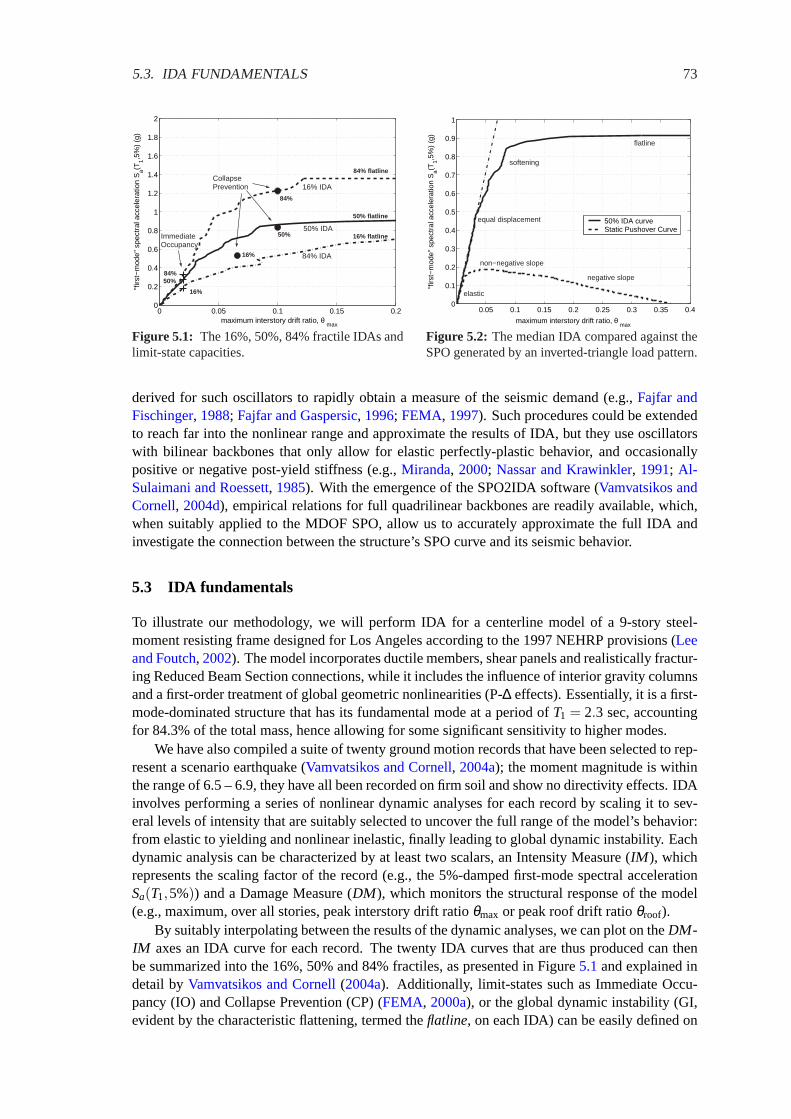
5.3. IDA FUNDAMENTALS 73
0 0.05 0.1 0.15 0.20
0.2
0.4
0.6
0.8
1
1.2
1.4
1.6
1.8
2
maximum interstory drift ratio, θ max
"firs
t−m
ode"
spe
ctra
l acc
eler
atio
n S
a(T1,5
%)
(g)
16% IDA
50% IDA
84% IDA
Immediate Occupancy
Collapse Prevention
84% flatline
50% flatline
16% flatline
84%
50%
16%
16%
50% 84%
Figure 5.1: The 16%, 50%, 84% fractile IDAs andlimit-state capacities.
0.05 0.1 0.15 0.2 0.25 0.3 0.35 0.40
0.1
0.2
0.3
0.4
0.5
0.6
0.7
0.8
0.9
1
maximum interstory drift ratio, θ max
"firs
t−m
ode"
spe
ctra
l acc
eler
atio
n S
a(T1,5
%)
(g)
50% IDA curve Static Pushover Curve
flatline
negative slope
non−negative slope
elastic
equal displacement
softening
Figure 5.2: The median IDA compared against theSPO generated by an inverted-triangle load pattern.
derived for such oscillators to rapidly obtain a measure of the seismic demand (e.g.,Fajfar andFischinger, 1988; Fajfar and Gaspersic, 1996; FEMA, 1997). Such procedures could be extendedto reach far into the nonlinear range and approximate the results of IDA, but they use oscillatorswith bilinear backbones that only allow for elastic perfectly-plastic behavior, and occasionallypositive or negative post-yield stiffness (e.g.,Miranda, 2000; Nassar and Krawinkler, 1991; Al-Sulaimani and Roessett, 1985). With the emergence of the SPO2IDA software (Vamvatsikos andCornell, 2004d), empirical relations for full quadrilinear backbones are readily available, which,when suitably applied to the MDOF SPO, allow us to accurately approximate the full IDA andinvestigate the connection between the structure’s SPO curve and its seismic behavior.
5.3 IDA fundamentals
To illustrate our methodology, we will perform IDA for a centerline model of a 9-story steel-moment resisting frame designed for Los Angeles according to the 1997 NEHRP provisions (Leeand Foutch, 2002). The model incorporates ductile members, shear panels and realistically fractur-ing Reduced Beam Section connections, while it includes the influence of interior gravity columnsand a first-order treatment of global geometric nonlinearities (P-∆ effects). Essentially, it is a first-mode-dominated structure that has its fundamental mode at a period ofT1 = 2.3 sec, accountingfor 84.3% of the total mass, hence allowing for some significant sensitivity to higher modes.
We have also compiled a suite of twenty ground motion records that have been selected to rep-resent a scenario earthquake (Vamvatsikos and Cornell, 2004a); the moment magnitude is withinthe range of 6.5 – 6.9, they have all been recorded on firm soil and show no directivity effects. IDAinvolves performing a series of nonlinear dynamic analyses for each record by scaling it to sev-eral levels of intensity that are suitably selected to uncover the full range of the model’s behavior:from elastic to yielding and nonlinear inelastic, finally leading to global dynamic instability. Eachdynamic analysis can be characterized by at least two scalars, an Intensity Measure (IM ), whichrepresents the scaling factor of the record (e.g., the 5%-damped first-mode spectral accelerationSa(T1,5%)) and a Damage Measure (DM ), which monitors the structural response of the model(e.g., maximum, over all stories, peak interstory drift ratioθmax or peak roof drift ratioθroof).
By suitably interpolating between the results of the dynamic analyses, we can plot on theDM -IM axes an IDA curve for each record. The twenty IDA curves that are thus produced can thenbe summarized into the 16%, 50% and 84% fractiles, as presented in Figure5.1and explained indetail byVamvatsikos and Cornell(2004a). Additionally, limit-states such as Immediate Occu-pancy (IO) and Collapse Prevention (CP) (FEMA, 2000a), or the global dynamic instability (GI,evident by the characteristic flattening, termed theflatline, on each IDA) can be easily defined on
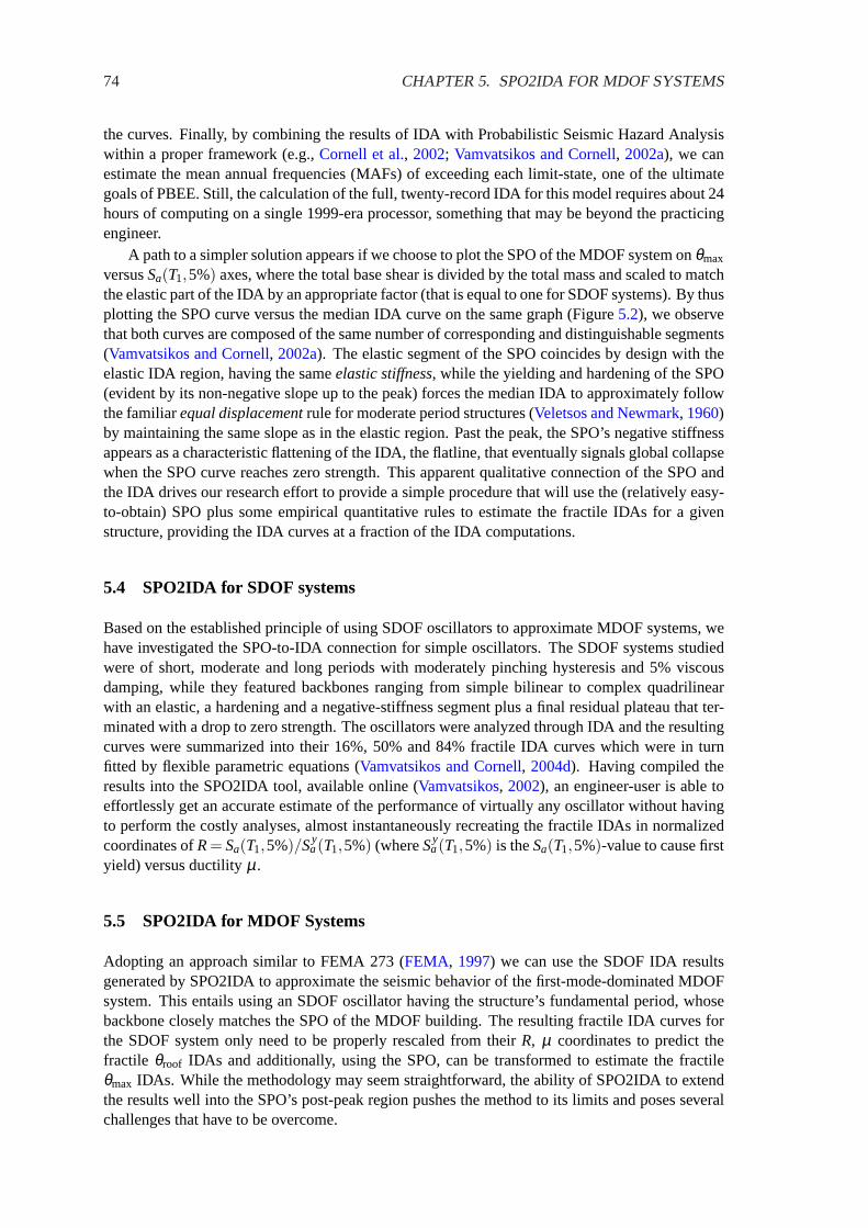
74 CHAPTER 5. SPO2IDA FOR MDOF SYSTEMS
the curves. Finally, by combining the results of IDA with Probabilistic Seismic Hazard Analysiswithin a proper framework (e.g.,Cornell et al., 2002; Vamvatsikos and Cornell, 2002a), we canestimate the mean annual frequencies (MAFs) of exceeding each limit-state, one of the ultimategoals of PBEE. Still, the calculation of the full, twenty-record IDA for this model requires about 24hours of computing on a single 1999-era processor, something that may be beyond the practicingengineer.
A path to a simpler solution appears if we choose to plot the SPO of the MDOF system onθmax
versusSa(T1,5%) axes, where the total base shear is divided by the total mass and scaled to matchthe elastic part of the IDA by an appropriate factor (that is equal to one for SDOF systems). By thusplotting the SPO curve versus the median IDA curve on the same graph (Figure5.2), we observethat both curves are composed of the same number of corresponding and distinguishable segments(Vamvatsikos and Cornell, 2002a). The elastic segment of the SPO coincides by design with theelastic IDA region, having the sameelastic stiffness, while the yielding and hardening of the SPO(evident by its non-negative slope up to the peak) forces the median IDA to approximately followthe familiarequal displacementrule for moderate period structures (Veletsos and Newmark, 1960)by maintaining the same slope as in the elastic region. Past the peak, the SPO’s negative stiffnessappears as a characteristic flattening of the IDA, the flatline, that eventually signals global collapsewhen the SPO curve reaches zero strength. This apparent qualitative connection of the SPO andthe IDA drives our research effort to provide a simple procedure that will use the (relatively easy-to-obtain) SPO plus some empirical quantitative rules to estimate the fractile IDAs for a givenstructure, providing the IDA curves at a fraction of the IDA computations.
5.4 SPO2IDA for SDOF systems
Based on the established principle of using SDOF oscillators to approximate MDOF systems, wehave investigated the SPO-to-IDA connection for simple oscillators. The SDOF systems studiedwere of short, moderate and long periods with moderately pinching hysteresis and 5% viscousdamping, while they featured backbones ranging from simple bilinear to complex quadrilinearwith an elastic, a hardening and a negative-stiffness segment plus a final residual plateau that ter-minated with a drop to zero strength. The oscillators were analyzed through IDA and the resultingcurves were summarized into their 16%, 50% and 84% fractile IDA curves which were in turnfitted by flexible parametric equations (Vamvatsikos and Cornell, 2004d). Having compiled theresults into the SPO2IDA tool, available online (Vamvatsikos, 2002), an engineer-user is able toeffortlessly get an accurate estimate of the performance of virtually any oscillator without havingto perform the costly analyses, almost instantaneously recreating the fractile IDAs in normalizedcoordinates ofR= Sa(T1,5%)/Sy
a(T1,5%) (whereSya(T1,5%) is theSa(T1,5%)-value to cause first
yield) versus ductilityµ.
5.5 SPO2IDA for MDOF Systems
Adopting an approach similar to FEMA 273 (FEMA, 1997) we can use the SDOF IDA resultsgenerated by SPO2IDA to approximate the seismic behavior of the first-mode-dominated MDOFsystem. This entails using an SDOF oscillator having the structure’s fundamental period, whosebackbone closely matches the SPO of the MDOF building. The resulting fractile IDA curves forthe SDOF system only need to be properly rescaled from theirR, µ coordinates to predict thefractile θroof IDAs and additionally, using the SPO, can be transformed to estimate the fractileθmax IDAs. While the methodology may seem straightforward, the ability of SPO2IDA to extendthe results well into the SPO’s post-peak region pushes the method to its limits and poses severalchallenges that have to be overcome.
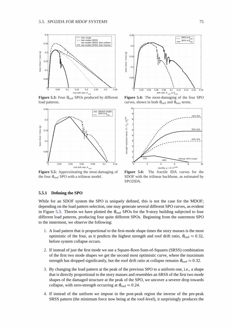
5.5. SPO2IDA FOR MDOF SYSTEMS 75
0 0.05 0.1 0.15 0.2 0.25 0.3 0.350
0.05
0.1
0.15
0.2
0.25
0.3
roof drift ratio, θ roof
base
she
ar /
mas
s (g
)first−mode two modes SRSS two modes SRSS, then uniformtwo modes SRSS, then inverse
Figure 5.3: Fourθroof SPOs produced by differentload patterns.
0 0.02 0.04 0.06 0.08 0.1 0.12 0.14 0.16 0.180
0.05
0.1
0.15
0.2
0.25
drift ratio, θ roof
or θmax
base
she
ar /
mas
s (g
)
SPO in θroof
SPO in θmax
Figure 5.4: The most-damaging of the four SPOcurves, shown in bothθroof andθmax terms.
0 0.02 0.04 0.06 0.08 0.1 0.120
0.05
0.1
0.15
0.2
0.25
roof drift ratio, θ roof
base
she
ar /
mas
s (g
)
trilinear model SPO in θ
roof
Figure 5.5: Approximating the most-damaging ofthe fourθroof SPO with a trilinear model.
0 2 4 6 8 100
1
2
3
4
5
6
7
8
9
10
11% −24%
ductility, µ = δ / δ yield
stre
ngth
red
uctio
n fa
ctor
, R =
Sa /
Sayi
eld
16% IDA
50% IDA
84% IDA
trilinear SPO model
Figure 5.6: The fractile IDA curves for theSDOF with the trilinear backbone, as estimated bySPO2IDA.
5.5.1 Defining the SPO
While for an SDOF system the SPO is uniquely defined, this is not the case for the MDOF;depending on the load pattern selection, one may generate several different SPO curves, as evidentin Figure5.3. Therein we have plotted theθroof SPOs for the 9-story building subjected to fourdifferent load patterns, producing four quite different SPOs. Beginning from the outermost SPOto the innermost, we observe the following:
1. A load pattern that is proportional to the first-mode shape times the story masses is the mostoptimistic of the four, as it predicts the highest strength and roof drift ratio,θroof ≈ 0.32,before system collapse occurs.
2. If instead of just the first mode we use a Square-Root-Sum-of-Squares (SRSS) combinationof the first two mode shapes we get the second most optimistic curve, where the maximumstrength has dropped significantly, but the roof drift ratio at collapse remainsθroof≈ 0.32.
3. By changing the load pattern at the peak of the previous SPO to a uniform one, i.e., a shapethat is directly proportional to the story masses and resembles an SRSS of the first two modeshapes of the damaged structure at the peak of the SPO, we uncover a severer drop towardscollapse, with zero-strength occurring atθroof≈ 0.24.
4. If instead of the uniform we impose in the post-peak region the inverse of the pre-peakSRSS pattern (the minimum force now being at the roof-level), it surprisingly produces the

76 CHAPTER 5. SPO2IDA FOR MDOF SYSTEMS
severest SPO of all, with global collapse happening atθroof ≈ 0.11, almost one third of theprediction generated by the pure first-mode load pattern.
In essence, the choice of the load pattern has a significant effect on the calculated SPO curvefor large levels of deformation and, evidently, each of the four possible realizations pictured inFigure5.3will produce a different estimate for the seismic demands and capacities. As shown forsimple oscillators byVamvatsikos and Cornell(2004d), if we progress from the outermost SPO tothe innermost one, the estimates ofDM -demands past the SPO peak will monotonically increase,and correspondingly the estimatedIM -capacity for any limit-state that lies beyond the peak willdecrease.
So, how is one to choose among the four SPOs? Since we have the full IDA results, we cancompare the deformed shapes of the structure produced by the various SPOs versus the IDA. Whilethe median IDA deformed shape shows that in the post-peak region most of the deformations areconcentrated on the upper floors, only the innermost (most-damaging) of the four SPOs managesto produce a similar deformation pattern. The other three load patterns seem to concentrate defor-mations mostly at the lower floors, thus not forcing the structure through the same path to collapseas the dynamic analysis does. We should expect that this most-damaging, worst-case SPO willprovide a good approximation to the behavior of the 9-story structure during a nonlinear dynamicanalysis.
Such a conclusion can be generalized to structures other than the particular 9-story; it makessense to assume that a structure under seismic excitation will collapse following the weakest-link,most-damaging, least-energy path. On the other hand, the use of a rigid load pattern will, ingeneral, constrain the deformed shape of the structure, allowing it to withstand higher lateral loadsand carry them to higher ductilities. Hence, we suggest that the SDOF oscillator whose backbonemimics the worst-case SPO will most accurately approximate the dynamic behavior of the trueMDOF model. Specifically, we should expect that in the post-peak region, the further an SPO liesfrom the worst-case one, the more unconservative results it will produce; i.e., SPOs that envelopthe worst-case one, when they are used as basis for the calculations of our method, they willgenerate upper-bound estimates of limit-state capacities and lower-bound estimates of demands.Hence, we choose to focus on the most-damaging of the four SPOs for all the calculations thatfollow.
Unfortunately, there is no obvious recipe to help us arrive at the worst-case SPO. It is hardto predict in advance what load pattern will be the most appropriate, especially if one does nothave a priori the dynamic analysis results to confirm that the dynamic and static deformed shapesmatch. Fully adaptive schemes may prove to be able to find the least-energy path to collapse,several candidates having been proposed at least byKrawinkler and Seneviratna(1998), Gupta andKunnath(2000) andAntoniou et al.(2002), but none of the proposed schemes has been sufficientlytested and verified in the post-peak region, where good accuracy matters the most for all limit-states that lie close to global dynamic instability (e.g., CP and GI). A simpler, viable solution forregular structures involves using a pattern proportional to the SRSS of several mode shapes timesthe story masses or a code-supplied pattern, at most up to the peak of the SPO (i.e.,θroof ≈ 0.02or θmax≈ 0.04 in Figure5.4), and consequently testing at least three configurations in the post-peak region: Continuing the pre-peak pattern (i.e., maximum force is at the roof), changing toa uniform or using the inverse of the pre-peak pattern (maximum force at the first story). Byperforming these three basic pushovers we get sufficiently broad coverage and can pick a loadpattern that will provide a good enough approximation to the overall most damaging, worst-caseSPO.
Once we have an acceptable estimate of the worst-caseθroof SPO, it is a simple matter toapproximate it with a piecewise-linear backbone, in this case a trilinear elastic-hardening-negativemodel (Figure5.5), and process it through SPO2IDA. Instantaneously we will get estimates ofthe fractile IDAs (normalized toR andµ) for the SDOF with the matching trilinear backbone, as

5.5. SPO2IDA FOR MDOF SYSTEMS 77
shown in Figure5.6.
5.5.2 Estimating the IDA elastic stiffness
SPO2IDA will provide us with accurate estimates of the SDOF system fractile IDAs, but the resultswill be in dimensionlessR versusµ coordinates and need to be properly scaled toSa(T1,5%)versusθroof or θmax axes. Therefore, we need to determine for eachx%-fractile,x∈ {16,50,84},the values ofSa(T1,5%), θroof andθmax that correspond to its yield point, namelySy
a,x%(T1,5%),θ y
roof,x% andθ ymax,x%. Obviously, for an SDOF system, this task is trivial; the backbone directly
provides the yield displacement (same for all fractiles), while it also offers the yield base shear,which when divided by the total mass will result to the value ofSy
a(T1,5%) (again, common for allfractiles). This is much harder for an MDOF system, mainly due to the effect of the higher modes;some records will force the structure to yield earlier and some later, at varying levels ofIM andDM . The problem can be simplified if we assume that the SPO accurately captures at least themedian valueθ y
roof,50% and that all fractiles IDAs yield at about the same value ofSya,x%(T1,5%).
This assumption is not strictly true for MDOF systems and it becomes highly accurate only if thefirst mode is dominant but, in general, it is more than enough for our purposes. In this case, weonly need to estimate the elastic stiffness (IM /DM ) of the medianθroof andθmax IDA, or, evenbetter, the elastic stiffness of all three fractileθroof andθmax IDAs, kroof,x% andkmax,x% respectively.
Since such a task involves dynamic linear elastic analysis, it can be easily performed with aminimum of computations. The direct way is to select a suitable suite of records and performelastic response spectrum or timehistory analysis for each record to determine theθroof andθmax
response. Then, we can estimate the 16%, 50% and 84% fractiles of the sample of elastic stiff-nesses,Sa(T1,5%)/θroof andSa(T1,5%)/θmax, calculated for each ground motion.
A simpler method appears if we approximate the medianθroof andθmax elastic stiffness bydividing any elastic SPO level of base shear by the total building mass times the correspondingelasticθroof or θmax value respectively. This is the same operation one would perform for an SDOFsystem, hence we cannot recover information about the variability in the elastic stiffnesses. There-fore, we are forced to assume thatkroof,x% = kroof,50%andkmax,x% = kmax,50%, which is accurate onlywhen higher modes are negligible. This is the same assumption adopted for the standard NonlinearStatic Procedure, e.g.,Fajfar and Fischinger(1988), Fajfar and Gaspersic(1996), FEMA (1997),although, in that case, normalization is done by the first mode mass rather than the total, somethingthat usually makes very little difference.
Obviously, only the first method is an exact calculation of the elastic IDA stiffnesses, andhence is the method of choice for the calculations to follow. The simpler method reduces thecomputational load, but in a manner similar toFEMA (1997), it neglects the variability in theelastic stiffness. This reduces its accuracy and restricts its usefulness to shorter buildings withinsignificant higher mode effects. Ultimately, the selection of the estimating procedure is a trade-off between speed and accuracy, and depends solely on each user’s needs.
5.5.3 Putting it all together
Having determined the appropriate elastic stiffnesses for the fractile IDAs, all that remains isto properly de-normalize and scale the SPO2IDA results, fromR versusµ coordinates, intoSa(T1,5%) versusθroof and θmax axes. Since the SPO has been approximated with a trilinearelastic-hardening-negative model (Figure5.5), its yield-point values of base shear,θroof andθmax,namelyFy, θ y
roof,spo andθ ymax,spo, are readily available. As explained previously, we will assume
that eachx%-fractile IDA, x∈ {16,50,84}, yields at the same value ofSya,x%(T1,5%), but at dif-

78 CHAPTER 5. SPO2IDA FOR MDOF SYSTEMS
0 0.05 0.1 0.150
0.2
0.4
0.6
0.8
1
1.2
1.4
1.6
16% IDA
peak roof drift ratio, θ roof
50% IDA
84% IDA
"firs
t−m
ode"
spe
ctra
l acc
eler
atio
n S
a(T1,5
%)
(g)
(a) Full IDA θroof fractile curves
0 0.05 0.1 0.150
0.2
0.4
0.6
0.8
1
1.2
1.4
1.6
peak roof drift ratio, θ roof
"firs
t−m
ode"
spe
ctra
l acc
eler
atio
n S
a(T1,5
%)
(g)
16% IDA
50% IDA
84% IDA
(b) SPO2IDA estimatedθroof fractile curves
0 0.05 0.1 0.15 0.2 0.250
0.2
0.4
0.6
0.8
1
1.2
1.4
1.6
16%IDA
maximum interstory drift ratio, θ max
"firs
t−m
ode"
spe
ctra
l acc
eler
atio
n S
a(T1,5
%)
(g)
50%IDA
84%IDA
(c) Full IDA θmax fractile curves
0 0.05 0.1 0.15 0.2 0.250
0.2
0.4
0.6
0.8
1
1.2
1.4
1.6
maximum interstory drift ratio, θ max
"firs
t−m
ode"
spe
ctra
l acc
eler
atio
n S
a(T1,5
%)
(g)
16% IDA
50% IDA
84% IDA
(d) SPO2IDA estimatedθmax fractile curves
Figure 5.7: Generating the fractile IDAs from nonlinear dynamic analyses versus the MDOF SPO2IDAapproximation for the 9-story building.
ferentθ yroof,x% andθ y
max,x%, hence, for allx∈ {16,50,84} we get:
Sya,x%(T1,5%) = θ y
roof,spo·kroof,50%, (5.1)
θ yroof,x% = Sy
a,x%(T1,5%)/kroof,x% (5.2)
θ ymax,x% = Sy
a,x%(T1,5%)/kmax,x% (5.3)
Using Equations (5.1–5.3), we can easily rescale the results of SPO2IDA and bring them intoproperSa(T1,5%) versusθroof axes to generate theθroof fractile IDAs, as seen in Figure5.7(b),which clearly compare very well against the real IDAs in Figure5.7(a).
If all that we want is an estimate of theIM -capacity for global dynamic instability of the struc-ture, we need not proceed further. On the other hand, to estimate other limit-state capacities (e.g.,IO or CP), we need the IDAs expressed in otherDM s, usuallyθmax. The SPO curve actually pro-vides the means for such a transformation thanks to the directθroof-to-θmax mapping it establisheswhen expressed inθroof andθmax coordinates (Figure5.4), a concept that has been used at leastin FEMA 273 (FEMA, 1997). The variation that we propose involves shifting theDM axes ofthe SPO for eachx%-fractile, scaling the elasticθroof values of the SPO byθ y
roof,x%/θ yroof,spo and
shifting the inelasticθroof values byθ yroof,x%− θ y
roof,spo. By performing the equivalent operationto theθmax SPO values, i.e., scaling the elasticθmax by θ y
max,x%/θ ymax,spoand shifting the inelastic

5.6. APPLICATION TO A 5-STORY BRACED FRAME 79
values byθ ymax,x%−θ y
max,spo, we provide a customθroof-to-θmax mapping that will correctly trans-form demands for each fractile, recognizing the variability in elastic stiffness. Of course, were itpossible to get the equivalent of a “fractile SPO”, by tracing in some way the force-deformationpath that the structure would follow for 16%, 50% and 84% of the ground motion records, suchtransformations would not be needed. In the absence of such data, we use this method to roughlyapproximate such fractile SPOs, at least in the elastic range.
The results are visible in Figure5.7(d)and compare favorably with the real IDA estimates inFigure5.7(c). Indeed, the estimated IDAs seem to slightly overestimate capacities and underesti-mate demands, mostly an effect of higher modes plus having just an approximation rather than thereal worst-case SPO. For example, the post-peak load pattern cannot take advantage of the sharpdrops due to connection fracturing that clearly appear (Figure5.4), but instead allows the structureto recover. A more adaptive pattern would probably do better. Still, even this rough approximationis good enough considering the roughly±20%standard error (estimated by bootstrapping,Efronand Tibshirani, 1993) that exists in estimating the fractiles from the twenty-record full IDA.
On the other hand, regarding ease-of-computation, if we assume that a single 1999-era pro-cessor is used, the analysis time is reduced from 24 hours for the MDOF IDA, to only severalminutes for the SPO and the elastic response spectrum analyses, not to mention the practicallyinstantaneous SPO2IDA procedure. Thus, we have achieved a fast and inexpensive estimate of theMDOF dynamic behavior at only a small cost in accuracy, the results, at least for this structure, ly-ing within the statistical error (caused by the record-to-record variability) of estimating the fractileIDAs from MDOF nonlinear dynamic analyses with twenty ground motion records.
5.6 Application to a 5-story braced frame
Let us now test the proposed procedure on a different structure, using a centerline model of aT1 =1.8 sec 5-story steel chevron-braced frame with ductile members and connections but realisticallybuckling braces including P-∆ effects (Bazzurro and Cornell, 1994b). For this building, the highermodes are practically insignificant, thus there is little or no ambiguity about the shape of thebackbone. It suffices to use a load pattern that is proportional to the first mode shape times thestory masses, thus getting the SPO curve shown in Figure5.8 in θroof andθmax coordinates.
Taking advantage of the SPO2IDA tool, theθroof SPO curve is closely matched with a trilinearelastic-negative-plateau model (Figure5.9). Finally, by combining the results from SPO2IDA withthe fractile elastic stiffnesses, we generate the approximateθroof andθmax fractile IDAs. Using thesame suite of records as for the 9-story, the IDA curves are calculated and summarized in their16%, 50% and 84% fractiles. By comparing the trueθroof fractile IDAs in Figure5.10(a)versusthe approximate results in Figure5.10(b), it becomes apparent that they are in excellent agreement.Similarly, theθmax fractile IDAs in Figure5.10(c)are accurately captured by the approximateresults, shown in Figure5.10(d). Clearly, as we should expect for such a building with insignificanthigher modes, the proposed procedure is a very cost-effective way to approximate the IDA results.But what happens at the other end, for a tall structure with significant higher mode effects?
5.7 Application to a 20-story moment frame
In order to test the limits of our method, we decided to use it on a tall structure, heavily influencedby higher modes. Our choice was a centerline model of a 20-story steel moment-resisting frame(Luco and Cornell, 2000) with ductile members and connections that includes the influence ofthe interior gravity columns plus a first-order treatment of global geometric nonlinearities (P-∆effects). Its first mode has a period ofT1 = 4 sec and accounts for 80.2% of the total mass, placingthis structure beyond the realm of first-mode-dominated buildings. Once more, the structure is

80 CHAPTER 5. SPO2IDA FOR MDOF SYSTEMS
0 0.01 0.02 0.03 0.04 0.05 0.060
0.05
0.1
0.15
0.2
0.25
0.3
drift ratio, θ roof
or θmax
base
she
ar /
mas
s (g
)
SPO in θroof
SPO in θmax
Figure 5.8: The most-damaging SPO curve forthe 5-story building, shown in bothθroof andθmax
terms.
0 0.005 0.01 0.015 0.02 0.025 0.030
0.05
0.1
0.15
0.2
0.25
0.3
roof drift ratio, θ roof
base
she
ar /
mas
s (g
)
trilnear model SPO in θ
roof
Figure 5.9: Approximating the 5-storyθroof SPOwith a trilinear model.
0 0.005 0.01 0.015 0.02 0.025 0.030
0.5
1
1.5
2
2.5
3
3.5
4
4.5
5
peak roof drift ratio, θroof
"firs
t−m
ode"
spe
ctra
l acc
eler
atio
n S
a(T1,5
%)
(g)
16% IDA
50% IDA
84% IDA
(a) Full IDA θroof fractile curves
0 0.005 0.01 0.015 0.02 0.025 0.030
0.5
1
1.5
2
2.5
3
3.5
4
4.5
5
peak roof drift ratio, θ roof
"firs
t−m
ode"
spe
ctra
l acc
eler
atio
n S
a(T1,5
%)
(g)
16% IDA
50% IDA
84% IDA
(b) SPO2IDA estimatedθroof fractile curves
0 0.01 0.02 0.03 0.04 0.05 0.060
0.5
1
1.5
2
2.5
3
3.5
4
4.5
5
"firs
t−m
ode"
spe
ctra
l acc
eler
atio
n S
a(T1,5
%)
(g)
maximum interstory drift ratio, θ max
16% IDA
50% IDA
84% IDA
(c) Full IDA θmax fractile curves
0 0.01 0.02 0.03 0.04 0.05 0.060
0.5
1
1.5
2
2.5
3
3.5
4
4.5
5
maximum interstory drift ratio, θ max
"firs
t−m
ode"
spe
ctra
l acc
eler
atio
n S
a(T1,5
%)
(g)
16% IDA
50% IDA
84% IDA
(d) SPO2IDA estimatedθmax fractile curves
Figure 5.10: Generating the fractile IDAs from nonlinear dynamic analyses versus the MDOF SPO2IDAapproximation for the 5-story building.

5.7. APPLICATION TO A 20-STORY MOMENT FRAME 81
0 0.02 0.04 0.06 0.08 0.1 0.12 0.14 0.16 0.180
0.01
0.02
0.03
0.04
0.05
0.06
0.07
0.08
drift ratio, θ roof
or θmax
base
she
ar /
mas
s (g
)
SPO in θroof
SPO in θmax
Figure 5.11: The most-damaging SPO curve forthe 20-story building, shown in bothθroof andθmax
terms.
0 0.01 0.02 0.03 0.04 0.050
0.01
0.02
0.03
0.04
0.05
0.06
0.07
0.08
roof drift ratio, θ roof
base
she
ar /
mas
s (g
)
trilinear model SPO in θ
roof
Figure 5.12: Approximating the 20-storyθroof SPOwith a trilinear model.
analyzed through IDA for the same suite of records used previously, the resulting fractile IDAcurves to be used as the standard for comparison.
First of all, the worst-case SPO needs to be determined. Surprisingly, this is an easy task,compared with the previously examined 9-story building. Because of the height of the structure,the massive P-∆ effects are dominating and quickly push the structure towards global collapse.There is only one path to collapse, and almost all reasonable load patterns will force the structureto take it. Hence, a simple load pattern proportional to the first modal shape times the storymasses is adequate to capture the worst-case SPO, even beyond its peak, the resulting curve shownin Figure5.11 in θroof andθmax coordinates. Comparing versus the IDA, we can confirm againthat the worst-case SPO and the IDA produce similar deformation patterns, concentrating mostdeformation at the lower stories of this building.
Using a trilinear elastic-hardening-negative backbone, we can accurately capture theθroof SPO(Figure5.12), then use SPO2IDA and the fractile elastic stiffnesses to reach the results shown inFigures5.13(b) and 5.13(d). By comparing them versus the real fractile IDA curves, in Fig-ures5.13(a)and5.13(c), one notices several striking differences and similarities. Theθroof IDAsare relatively well estimated. There is some overestimation ofθroof demands in the near-elasticregion, as the MDOF system is capable of high hardening that the SDOF system cannot reproduce,still, in the region near collapse, theθroof IDAs are almost perfectly matched. On the other hand,the proposed method largely overestimates theθmax IDA demands and correspondingly underes-timates theSa(T1,5%)-values of capacities, especially for limit-states in the near-elastic domain,but maintains good accuracy close to global collapse. It seems that the higher modes are influenc-ing the accuracy of the approximation, reducing it in the near-elastic range but not close to globalcollapse.
It is well known that it is very difficult to capture the higher mode effects with just the SPO(Krawinkler and Seneviratna, 1998). Theθroof response is somewhat insensitive to them becauseof its global nature, but local damage measures, likeθmax, are not, thus making it very difficultto capture the correctθroof-to-θmax mapping with just the SPO. For example, even in the elasticrange, the ratio of the elastic stiffnesses of the medianθroof to the medianθmax IDA is about 1.5.This means that at any level ofSa(T1,5%), the medianθmax is about 50% higher than the medianθroof, i.e., a high degree of deformation localization exists even in the elastic region. On the otherhand, the equivalent ratio for the SPO produced with the first-mode load pattern is only 1.3; muchless localization is predicted by the static analysis than the dynamic. Even more so, this ratio forthe 84%θroof andθmax IDAs is almost 2, which explains why the estimation seems to suffer awayfrom the median in the near-elastic region. Such differences are a direct manifestation of higher
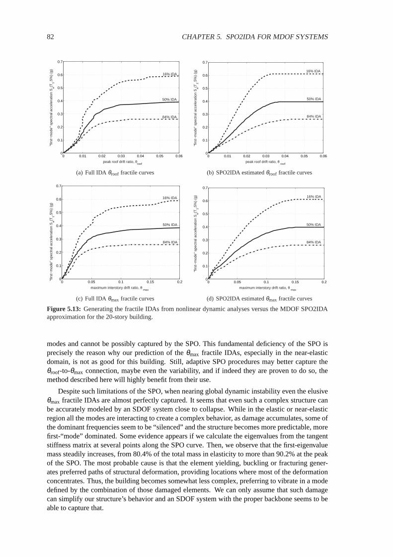
82 CHAPTER 5. SPO2IDA FOR MDOF SYSTEMS
0 0.01 0.02 0.03 0.04 0.05 0.060
0.1
0.2
0.3
0.4
0.5
0.6
0.7
peak roof drift ratio, θroof
"firs
t−m
ode"
spe
ctra
l acc
eler
atio
n S
a(T1,5
%)
(g)
16% IDA
50% IDA
84% IDA
(a) Full IDA θroof fractile curves
0 0.01 0.02 0.03 0.04 0.05 0.060
0.1
0.2
0.3
0.4
0.5
0.6
0.7
peak roof drift ratio, θ roof
"firs
t−m
ode"
spe
ctra
l acc
eler
atio
n S
a(T1,5
%)
(g) 16% IDA
50% IDA
84% IDA
(b) SPO2IDA estimatedθroof fractile curves
0 0.05 0.1 0.15 0.20
0.1
0.2
0.3
0.4
0.5
0.6
0.7
maximum interstory drift ratio, θ max
50% IDA
84% IDA
16% IDA
"firs
t−m
ode"
spe
ctra
l acc
eler
atio
n S
a(T1,5
%)
(g)
(c) Full IDA θmax fractile curves
0 0.05 0.1 0.15 0.20
0.1
0.2
0.3
0.4
0.5
0.6
0.7
maximum interstory drift ratio, θ max
"firs
t−m
ode"
spe
ctra
l acc
eler
atio
n S
a(T1,5
%)
(g) 16% IDA
50% IDA
84% IDA
(d) SPO2IDA estimatedθmax fractile curves
Figure 5.13: Generating the fractile IDAs from nonlinear dynamic analyses versus the MDOF SPO2IDAapproximation for the 20-story building.
modes and cannot be possibly captured by the SPO. This fundamental deficiency of the SPO isprecisely the reason why our prediction of theθmax fractile IDAs, especially in the near-elasticdomain, is not as good for this building. Still, adaptive SPO procedures may better capture theθroof-to-θmax connection, maybe even the variability, and if indeed they are proven to do so, themethod described here will highly benefit from their use.
Despite such limitations of the SPO, when nearing global dynamic instability even the elusiveθmax fractile IDAs are almost perfectly captured. It seems that even such a complex structure canbe accurately modeled by an SDOF system close to collapse. While in the elastic or near-elasticregion all the modes are interacting to create a complex behavior, as damage accumulates, some ofthe dominant frequencies seem to be “silenced” and the structure becomes more predictable, morefirst-“mode” dominated. Some evidence appears if we calculate the eigenvalues from the tangentstiffness matrix at several points along the SPO curve. Then, we observe that the first-eigenvaluemass steadily increases, from 80.4% of the total mass in elasticity to more than 90.2% at the peakof the SPO. The most probable cause is that the element yielding, buckling or fracturing gener-ates preferred paths of structural deformation, providing locations where most of the deformationconcentrates. Thus, the building becomes somewhat less complex, preferring to vibrate in a modedefined by the combination of those damaged elements. We can only assume that such damagecan simplify our structure’s behavior and an SDOF system with the proper backbone seems to beable to capture that.

5.8. LIMIT-STATE CAPACITY ESTIMATION USING THE MDOF SPO2IDA 83
5.8 Limit-state capacity estimation using the MDOF SPO2IDA
Apparently, the SPO2IDA approximation provides reasonable estimates, within the limitations ofthe SPO, for the fractile IDA curves of all three buildings that we have examined. Having theseresults at our disposal we can follow the same steps as we did for the full IDA to perform PBEEcalculations; the only difference is that we have to calculate the summarizedIM -capacities forthe defined limit-states (IO, CP and GI) directly on the fractile IDAs instead of estimating themindividually on each record’s IDA curve and then summarize them (Vamvatsikos and Cornell,2004a).
This is straightforward for the IO and GI limit-states (Vamvatsikos and Cornell, 2004a); theirfractile capacities reside on the fractile IDAs (e.g., Figure5.1), so we only need to calculate thevalues ofSc
a,x%(T1,5%) where eachx%-fractile IDA, x ∈ {16,50,84}, reachesθmax = 0.02 toviolate the IO limit-state, or reaches the flatline for GI. On the other hand, the CP limit-statepoints do not necessarily lie on the fractile IDAs, e.g., Figure5.1, but, in most cases, they arequite close (Vamvatsikos and Cornell, 2004a). Therefore, we propose to apply the SAC/FEMAdefinition of the CP limit-state point (FEMA, 2000a) directly to the fractile IDAs and thus estimatethe fractile CP capacity points. The final results are shown for all three buildings on Table5.1.
Table 5.1: Comparing the real and estimated 16%, 50% and 84%Sca(T1,5%) capacities over three limit-
states for each of the studied structures. Note that the 5-story reaches global collapse quite early, so the GIand CP limit-states coincide.
16% (g) 50% (g) 84% (g)
Real Est Real Est Real EstIO 0.61 0.75 1.02 1.05 1.43 1.55
5-story CP&GI 1.43 1.84 2.23 2.72 4.04 4.26IO 0.18 0.14 0.27 0.20 0.33 0.24
9-story CP 0.57 0.58 0.83 0.88 1.29 1.31GI 0.74 0.64 0.91 0.95 1.35 1.37IO 0.12 0.08 0.16 0.10 0.21 0.15
20-story CP 0.23 0.22 0.34 0.35 0.53 0.57GI 0.26 0.26 0.39 0.40 0.63 0.61
Table 5.2: Comparing the real and estimated 16%, 50% and 84%θmax-value of capacity for the CP limit-state for each of the studied structures.
16% 50% 84%
Real Est Real Est Real Est5-story CP 0.05 0.05 0.05 0.05 0.05 0.059-story CP 0.07 0.10 0.10 0.10 0.10 0.1020-story CP 0.05 0.10 0.06 0.10 0.07 0.10
By comparing the full IDA versus the approximate results in Table5.1, it becomes obviousthat the proposed method manages to perform very well for a variety of buildings and for each ofthe three limit-states. Even for the 20-story building, only the IO limit-state is seriously hamperedby the approximation, simply an effect of IO happening at the near-elastic region of the IDA wherethe structure is toughest to predict, as explained earlier. As presented inVamvatsikos and Cornell(2004a), theseIM -values are actually all that we need, coupled with conventional ProbabilisticSeismic Hazard Analysis, to get estimates for the MAF of limit-state exceedance. Hence, fromthe results of Table5.1, we should expect that the MDOF SPO2IDA method can provide quiteaccurate MAF predictions.
If we want to use an alternative format similar to FEMA 350 (FEMA, 2000a), we need instead

84 CHAPTER 5. SPO2IDA FOR MDOF SYSTEMS
the DM -values of the capacity points. For IO the appropriateDM -value is 0.02, by definition,while for GI it is +∞. For the CP limit-state the results are listed in Table5.2, where it becomesobvious that the SPO2IDA estimates are quite accurate, except perhaps for the 20-story build-ing. Still, the actual estimate of the MAF of the CP limit-state exceedance will not be as bad asindicated by these results; assuming that the appropriateDM -based integrations are accuratelycarried through, they should provide the same result with theIM -based ones (Jalayer and Cornell,2002; Vamvatsikos and Cornell, 2004a). These somewhat higher estimates ofDM capacity for the20-story are tempered by equally high estimates ofDM demand, in the end producing accurateestimates of MAFs. Using eitherDM or IM -based frameworks, the MDOF SPO2IDA procedurecan be used to easily calculate the MAF of exceeding a limit-state, even for higher mode influencedbuildings in the case that we restrict ourselves to the near-collapse region.
5.9 Sensitivity to user choices
The SPO2IDA method for MDOF structures has proven to be quite accurate. Still, several ques-tions may be raised, regarding the sensitivity of the capacities displayed in Tables5.1 and5.2 tothe average user’s choices when applying the proposed methodology.
Obviously, the largest effect comes from finding or missing the right SPO. When the structurefails due to a global failure mode, e.g., due to P-∆ like the 20-story building, or it has insignificanthigher mode effects, e.g., like the 5-story building, then the right SPO should be easy to calculate.Almost any reasonable load pattern, e.g., one proportional to the first mode shape times the storymasses, will suffice. If, on the other hand, there are significant higher mode effects and the struc-ture fails mainly due to a succession of local events, e.g., connections fractured or braces buckling,then it is much tougher to find the worst-case SPO. One needs only use the SPO2IDA tool to un-derstand the large influence of the backbone on the IDA (Vamvatsikos and Cornell, 2004d), andrealize that no estimation beyond the SPO peak will be accurate without the right SPO. In suchcases, it is important to use several, preferably adaptive, load patterns and, in the absence of aproven automated method, use trial and error to select the best of the tried patterns.
Assuming we have found the rightθroof, θmax SPO, like in our examples, we now have to fitthe first with a multilinear model. Obviously, there are many trilinear models that we could useinstead of the ones in Figures5.4, 5.8 and5.11. Would using them change the final results? Itis recommended that one becomes familiar with the SPO2IDA tool and understand the influenceof the backbone to the SDOF fractile IDAs (Vamvatsikos and Cornell, 2004d). This greatly helpsrealize the implications of how to best fit theθroof SPO. For example, the backbone’s hardeningslope is not as important, while the negative slope greatly influences global collapse. Therefore,care should be exercised to always fit theθroof SPO closer where it matters most to achieve the mostaccurate results. Even so, the quadrilinear model offered by SPO2IDA allows much flexibility, andas was the case with all our examples, the shape of theθroof SPO can be reasonably captured. Inthat case, no major differences should be expected in the final results.
Another important issue is the estimation of the elastic stiffness. Up to now we have reliedon the direct estimation from elastic timehistory analysis for each record. How much accuracywill one sacrifice by using a simpler method, and what are the implications for the estimates ofcapacities?
Since the normalized SPO2IDA results for the SDOF fractiles are scaled exclusively by themedian elasticθroof stiffness,kroof,50%, its value directly influences theIM -estimates of capacityfor all limit-states. As a direct effect of Equations (5.1)-(5.3), if all the otherkroof,x%, kmax,x%
were accurately predicted butkroof,50% was overestimated or underestimated byα%, we will seea proportionalα% overestimation or underestimation of all limit-state capacities. Intuitively, thiscan be understood if we realize that the value ofkroof,50% determines the scaling of the verticalIM -axis for the fractile IDAs. Similarly, the five other elastic stiffnesses control the scaling of the
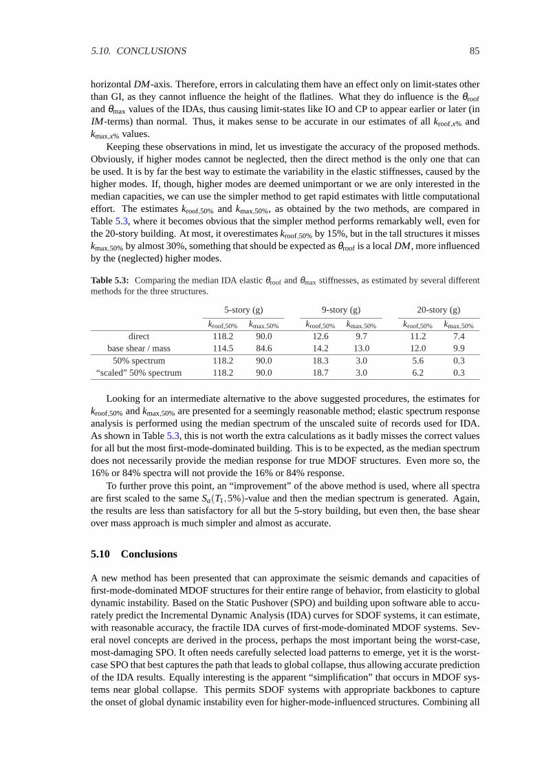
5.10. CONCLUSIONS 85
horizontalDM -axis. Therefore, errors in calculating them have an effect only on limit-states otherthan GI, as they cannot influence the height of the flatlines. What they do influence is theθroof
andθmax values of the IDAs, thus causing limit-states like IO and CP to appear earlier or later (inIM -terms) than normal. Thus, it makes sense to be accurate in our estimates of allkroof,x% andkmax,x% values.
Keeping these observations in mind, let us investigate the accuracy of the proposed methods.Obviously, if higher modes cannot be neglected, then the direct method is the only one that canbe used. It is by far the best way to estimate the variability in the elastic stiffnesses, caused by thehigher modes. If, though, higher modes are deemed unimportant or we are only interested in themedian capacities, we can use the simpler method to get rapid estimates with little computationaleffort. The estimateskroof,50% and kmax,50%, as obtained by the two methods, are compared inTable5.3, where it becomes obvious that the simpler method performs remarkably well, even forthe 20-story building. At most, it overestimateskroof,50% by 15%, but in the tall structures it misseskmax,50% by almost 30%, something that should be expected asθroof is a localDM , more influencedby the (neglected) higher modes.
Table 5.3: Comparing the median IDA elasticθroof andθmax stiffnesses, as estimated by several differentmethods for the three structures.
5-story (g) 9-story (g) 20-story (g)
kroof,50% kmax,50% kroof,50% kmax,50% kroof,50% kmax,50%
direct 118.2 90.0 12.6 9.7 11.2 7.4base shear / mass 114.5 84.6 14.2 13.0 12.0 9.9
50% spectrum 118.2 90.0 18.3 3.0 5.6 0.3“scaled” 50% spectrum 118.2 90.0 18.7 3.0 6.2 0.3
Looking for an intermediate alternative to the above suggested procedures, the estimates forkroof,50% andkmax,50% are presented for a seemingly reasonable method; elastic spectrum responseanalysis is performed using the median spectrum of the unscaled suite of records used for IDA.As shown in Table5.3, this is not worth the extra calculations as it badly misses the correct valuesfor all but the most first-mode-dominated building. This is to be expected, as the median spectrumdoes not necessarily provide the median response for true MDOF structures. Even more so, the16% or 84% spectra will not provide the 16% or 84% response.
To further prove this point, an “improvement” of the above method is used, where all spectraare first scaled to the sameSa(T1,5%)-value and then the median spectrum is generated. Again,the results are less than satisfactory for all but the 5-story building, but even then, the base shearover mass approach is much simpler and almost as accurate.
5.10 Conclusions
A new method has been presented that can approximate the seismic demands and capacities offirst-mode-dominated MDOF structures for their entire range of behavior, from elasticity to globaldynamic instability. Based on the Static Pushover (SPO) and building upon software able to accu-rately predict the Incremental Dynamic Analysis (IDA) curves for SDOF systems, it can estimate,with reasonable accuracy, the fractile IDA curves of first-mode-dominated MDOF systems. Sev-eral novel concepts are derived in the process, perhaps the most important being the worst-case,most-damaging SPO. It often needs carefully selected load patterns to emerge, yet it is the worst-case SPO that best captures the path that leads to global collapse, thus allowing accurate predictionof the IDA results. Equally interesting is the apparent “simplification” that occurs in MDOF sys-tems near global collapse. This permits SDOF systems with appropriate backbones to capturethe onset of global dynamic instability even for higher-mode-influenced structures. Combining all

86 CHAPTER 5. SPO2IDA FOR MDOF SYSTEMS
these observations, we can conclude that simply by using the appropriate SPO curve plus, perhaps,a few elastic response spectrum analyses, the engineer-user is able to generate accurate predictionsof the seismic behavior of complex MDOF structures within a fraction of the time needed for afull IDA.
5.11 Acknowledgements
Financial support for this research was provided by the sponsors of the Reliability of MarineStructures Affiliates Program of Stanford University.
Chapter 6Investigating the influence of elasticspectral shape on limit-state capacitiesthrough IDA
6.1 Introduction
The IDA curves and, correspondingly, the limit-state capacities display large record-to-recordvariability, even for the simplest of structures, as evident in the previous chapters. This observeddispersion is closely connected to theIM used; someIM s are moreefficientthan others, bettercapturing and explaining the differences from record to record, thus bringing the results from allrecords closer together. Compare, for example, Figures2.9(a) and2.9(b) (Chapter2), where PGAis proven to be deficient relative toSa(T1,5%) in expressing limit-state capacities, as it increasestheir dispersion, practically everywhere on the IDAs. On the other hand, even the improvementachieved bySa(T1,5%) still leaves something to be desired, as dispersions are in the order of 30%or more.
Why should we search for such a betterIM ? There is a clear computational advantage if wecan select ita priori, before the IDA is performed. By reducing the variability in the IDA curves,we need fewer records to achieve a given level of confidence in estimating the fractileIM -valuesof limit-state capacities. Typically, a reduction to theIM -capacity dispersion by a factor of twomeans that we need four times fewer records to achieve the same confidence in the results, asexplained in Chapter3. Obviously, the computational savings can be enormous.
Additionally, it is speculated that increasing the efficiency of theIM , may also lead to im-provedsufficiencyas well. A sufficientIM produces the same distribution of demands and capac-ities independently of the record selection, e.g., there is no bias in the fractileIM -capacities if weselect records with low rather than high magnitudes or if the records do or do not contain direc-tivity pulses (Luco and Cornell, 2004). The goals of efficiency and sufficiency are not necessarilytied together as the former aims at reducing the variability in the IDA results while the latter atreducing (or eliminating) their dependance on record characteristics other than theIM . Still, usinga more efficientIM will bring the results from all records closer, and similarly bring close the IDAcurves of records coming from different magnitudes or containing different directivity pulses, thusreducing the importance of any magnitude or directivity dependance.
While Sa(T1,5%) is found to be sufficient for first-mode-dominated, moderate period struc-tures when directivity is not present (Shome and Cornell, 1999), it is not necessarily so for othercases (Luco and Cornell, 2004). Therefore, it is important to try and improve ourIM s beyondthe capabilities ofSa(T1,5%). Figure6.1 may provide some clues; therein we have plotted the5%-damped acceleration spectra of the 30 records in Table4.1, normalized bySa(3.98s,5%), i.e.,
87

88 CHAPTER 6. ELASTIC SPECTRAL SHAPE FOR CAPACITIES
0.5 1 1.5 2 2.5 3 3.5 4 4.5 5 5.5 6
−1
0
1
2
3
4
period, T (s)
log
Sa(T
,5%
)
Figure 6.1: The 5%-damped elastic acceleration spectra for thirty records, normalized to the first-modeperiod of the 20-story building.
the value ofSa(T1,5%) at the first period of the 20-story building used in Chapter5. There isobviously much variability in the individual spectra that cannot be captured by justSa(T1,5%). Astructure is not always dominated by a single frequency, and even then, when the structure sus-tains damage its properties change. Thus, spectral regions away from the elastic first-mode period,T1, may become more influential. By taking the differences in the individual spectral shapes intoaccount, we may be able to reduce the variability in the IDA curves and come up with an overallbetterIM .
Such information may be incorporated into theIM by using appropriate inelastic spectralvalues (Luco and Cornell, 2004). This seems to be a promising method, as it directly incorporatesthe influence of the record on an oscillator that can yield and experience damage in a way similarto the structure. Still, in the context of PBEE, the use of inelastic spectral values requires new,custom-made attenuation relationships. On the other hand, using the elastic spectral values allowsthe use of the attenuation laws available in the literature. Therefore, there is still much to be gainedfrom the use ofIM s based on elastic spectra.
Actually, studies byShome and Cornell(1999), Carballo and Cornell(2000), Mehanny andDeierlein (2000) andCordova et al.(2000) have shown that the elastic spectral shape can be auseful tool in determining an improvedIM . Shome and Cornell(1999) found that the inclusionof spectral values at the second-mode period (T2) and at the third-mode (T3), namelySa(T2,5%)andSa(T3,5%), significantly improved the efficiency ofSa(T1,5%) for tall buildings. Carballoand Cornell(2000) observed greatly reduced variability in theDM demands when spectral shapeinformation was included by compatibilizing a suite of records to their median elastic spectrum.In addition,Mehanny and Deierlein(2000) andCordova et al.(2000) observed an improvementin the efficiency ofSa(T1,5%) when an extra period, longer than the first-mode was included byemploying anIM of the formSa(T1,5%)1−β Sa(c·T1,5%)β (with suggested valuesβ = 0.5, c= 2).Additionally, they presented some evidence suggesting that sufficiency may be improved as well,
6.2. METHODOLOGY 89
since the newIM made the IDA curves of several near-fault records practically indistinguishable,regardless of the directivity-pulse period. Motivated by such encouraging results, we are going touse the methodology and tools developed in Chapters2 and3 to better investigate the potential ofincorporating elastic spectral shape information toIM s to reduce the dispersion in IDA results.
6.2 Methodology
We will employ three different structures for our investigation into the potential use of the elasticacceleration spectrum. These will be theT1 = 1.8s 5-story steel braced-frame, theT1 = 2.4s 9-storysteel moment-resisting frame and theT1 = 4s 20-story steel moment-resisting frame, all introducedin Chapter5. For each one we will use the suite of 30 records introduced in Chapter4, Table4.1to perform IDA and we will proceed to define numerous limit-states, each at a givenθmax value,to represent the capacity of the structure at successive damaged states. Finally, the appropriateSc
a(T1,5%)-values will be calculated, i.e., the values ofSa(T1,5%)-capacity for each record andeach limit-state. The ultimate goal is to minimize the dispersion in theIM -capacities for eachlimit-state individually by selecting appropriate spectral values or functions of spectral values tobe theIM . As a measure of the dispersion we will use the standard deviation of the logarithm of theIM -capacities, which is a natural choice for values that are approximately lognormally distributed(e.g.,Shome and Cornell, 1999).
Fortunately, no further dynamic analyses are needed to perform this dispersion-minimization;all we need to do is to transform each limit-state’sSc
a(T1,5%)-values in the coordinates of the trialIM s and calculate their new dispersion. For example, if we want the dispersion of the capacitiesin PGA terms, then for each unscaled record (or at a scale factor of one) we know both the PGAandSa(T1,5%)-values and the former can be appropriately scaled by the same factor that the valueof Sc
a(T1,5%) implies; e.g., for the 20-story building, the unscaled record #1 of Table4.1 hasSa(T1,5%) = 0.044g and PGA= 0.159g, while global instability occurs atSc
a(T1,5%) = 0.40g,representing a scale factor of0.40/0.044≈ 9.1. Hence, theIM -capacity at the global instabilitylimit-state in PGA terms is PGAc = 9.1 ·0.159= 1.45g. Similarly we can accomplish such trans-formations for anyIM based on elastic spectral values. Thus, we are taking full advantage of theobservations in Chapter3, by appropriately postprocessing the existing dynamic runs instead ofperforming new ones.
The adopted approach in evaluating the candidateIM s is very different from the one usedby Shome and Cornell(1999), Mehanny and Deierlein(2000), Cordova et al.(2000) andLucoand Cornell(2004). There, the focus is on demands, i.e.,DM -values, all four studies looking for asingle “broad-range”IM that will improve efficiency for all damage levels of a given structure. Onthe other hand, our search will be more focused, zeroing on each limit-state separately to developa “narrow-range”IM that will better explain the given limit-state rather than all of them. Thus,we are able to follow the evolution of suchIM s as damage increases in the structure, hopefullygaining valuable intuition in the process. Still, since we use onlyθmax to define the structurallimit-states, our observations may or may not be applicable when limit-states are defined on otherstructural response measures (e.g., peak floor accelerations).
Regarding the choice ofIM s to use, we will start by investigating single spectral coordinates.This does not constitute an investigation of spectralshapeper se as it focuses on the use of just onevalue at one period. Still, it will provide a useful basis as we expand our trialIM s to include vectorsand scalar combinations of several spectral values. In all cases the focus will be on the efficiencygained by incorporating elastic spectrum information in each of the above ways. Another issue ofinterest is the robustness offered by eachIM , i.e., how much efficiency it retains when the userselects spectral values other than those chosen by the dispersion-minimization process. This is animportant question when trying to identifya priori an appropriateIM in order to take advantage ofits efficiency and use fewer records in the analysis. We are not aiming to provide the final answer

90 CHAPTER 6. ELASTIC SPECTRAL SHAPE FOR CAPACITIES
1 2 3 4 5 60
0.1
0.2
0.3
0.4
0.5
0.6
0.7
0.8
T1
θmax
= 0.0001
disp
ersi
on o
f IM
cap
aciti
es
period, τ (s)
(a) Elastic region
1 2 3 4 5 60
0.1
0.2
0.3
0.4
0.5
0.6
0.7
0.8
T1
θmax
= 0.007
period, τ (s)
disp
ersi
on o
f IM
cap
aciti
es(b) θmax = 0.007
1 2 3 4 5 60
0.1
0.2
0.3
0.4
0.5
0.6
0.7
0.8
T1
θmax
= 0.01
period, τ (s)
disp
ersi
on o
f IM
cap
aciti
es
(c) θmax = 0.01
1 2 3 4 5 60
0.1
0.2
0.3
0.4
0.5
0.6
0.7
0.8
T1
θmax
= Inf
period, τ (s)
disp
ersi
on o
f IM
cap
aciti
es
(d) Global Instability
Figure 6.2: Dispersion of theSca(τ,5%)-values versus periodτ for four different limit-states for the 5-story
building.
0 0.01 0.02 0.03 0.04 0.05 0.060
0.5
1
1.5
2
2.5
3
3.5
4
4.5
5
"firs
t−m
ode"
spe
ctra
l acc
eler
atio
n S
a(T1,5
%)
(g)
maximum interstory drift ratio, θ max
16% IDA
50% IDA
84% IDA
(a)
(b)
(c)
(d)
Figure 6.3: The fractile IDA curves and capacities for four limit-states (Figure6.2) of the 5-story building.

6.3. USING A SINGLE SPECTRAL VALUE 91
for the besta priori IM , but rather to investigate the efficiency and the potential for practicalimplementation offered by several promising candidates.
6.3 Using a single spectral value
The use of a single spectral value, usually at the first-mode of the structure, i.e.,Sa(T1,5%), hasseen widespread use for IDAs, having being incorporated into theFEMA (2000a,b) guidelines andused throughout most of our research. Obviously, it is an accurate measure for SDOF systems orfirst-mode-dominated structures in the elastic range. But when higher modes are important or thestructure deforms into the nonlinear range, it may not be optimal. There seems to be a consensusthat when structures are damaged and move into the nonlinear region, period lengthening willoccur (e.g.,Cordova et al., 2000). In that sense, there may be some merit in looking for elasticspectral values at longer, or in general different, periods than the first-mode. Therefore we willconduct a search, across all periods in the spectrum, to determine the one that most reduces thevariability in theIM -values of limit-state capacities.
Some representative results are shown in Figure6.2for the 5-story building, for limit-states atfour levels ofθmax (Figure6.3), namely 0.01% (elastic), 0.7% (early inelastic), 1% (highly non-linear) and+∞ (global instability). The structure has obviously insignificant higher modes, sinceSa(T1,5%) produces practically zero dispersion for the capacities in the elastic region. As thestructure becomes progressively more damaged, the optimal period moves away fromT1, length-ening to higher values as expected. Initially, only a narrow band of periods around the optimalτ display low dispersions. When close to global collapse, this band around the optimal periodincreases so that any period from 2s to 4s will achieve low dispersion, at most 30% compared toabout 40% when usingSa(T1,5%). A summary of the results is shown in Figure6.4, where theoptimal period is shown versus theθmax-value of all the limit-states considered, while the bestachieved dispersion is presented in Figure6.5, compared against the dispersion when using PGAandSa(T1,5%). As observed before, the optimal period increases after yielding, fromτ = T1 toτ = 2.4s. Similarly, the dispersion increases for all threeIM s in Figure6.5, but with the use of theoptimal period, the efficiency is improved, at least by 40% compared toSa(T1,5%).
Similar results for the 9-story building are presented in Figure6.6, for the limit-states appear-ing in Figure6.7atθmax equal to 0.5% (elastic), 5% (inelastic), 10% (close to global collapse) and+∞ (global instability). The building has significant higher modes, as evident in Figure6.6(a),since the first mode is not optimal even in the elastic region. While all three modes,T1, T2 andT3,seem to locally produce some dispersion reduction, the overall best single period is somewherebetween theT1 andT2, at τ ≈ 1.2s. As damage increases, the optimal period lengthens to highervalues, to finally settle close toT1 when global instability occurs. In Figure6.8, the results aresummarized for all limit-states, showing the gradual lengthening of the optimal period. Similarly,in Figure6.9the optimal dispersion thus achieved is compared versus the results when using PGAandSa(T1,5%). Remarkably, only in the elastic and near-elastic region does this single optimalspectral value provide some improvement, in the order of 10%. Close to global collapse, no gainsare realized overSa(T1,5%).
For the 20-story structure, the results for four limit-states are shown in Figure6.10, for θmax
equal to 0.5% (elastic), 2% (near-elastic), 10% (close to global collapse) and+∞ (global instabil-ity); each limit-state is shown versus the fractile IDAs in Figure6.11. This is a building wherehigher modes are even more important, and by looking at Figure6.10(a), it seems that, at leastinitially, the second-mode period,T2, manages to explain more thanT1 in the dispersion of theIMcapacity values. The limit-states are defined onθmax, the maximum of the story drifts, which oftenappears in the upper stories at low ductilities and is thus quite sensitive to the higher frequencies.As damage increases, the optimal period moves away fromT2 and at global collapse reaches avalue somewhere in the middle ofT1 andT2, at aboutτ ≈ 2.5s. In Figure6.12the summarized

92 CHAPTER 6. ELASTIC SPECTRAL SHAPE FOR CAPACITIES
0 0.01 0.02 0.03 0.04 0.05 0.060
1
2
3
4
5
6
T1
maximum interstory drift ratio, θ max
perio
d, τ
(s)
Figure 6.4: The optimal periodτ as it evolves withθmax for the 5-story building.
0 0.01 0.02 0.03 0.04 0.05 0.060
0.1
0.2
0.3
0.4
0.5
0.6
0.7
0.8
maximum interstory drift ratio, θ max
disp
ersi
on o
f IM
cap
aciti
es
PGA S
a(T
1,5%)
optimal Sa(τ,5%)
Figure 6.5: The dispersion for the optimalSa(τ,5%) compared toSa(T1,5%) and PGA, versus the limit-state definition,θmax, for the 5-story building.
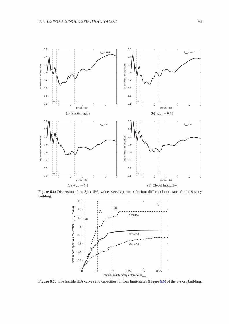
6.3. USING A SINGLE SPECTRAL VALUE 93
1 2 3 4 5 60.1
0.2
0.3
0.4
0.5
0.6
0.7
0.8
T1 T2 T3
θmax
= 0.005
period, τ (s)
disp
ersi
on o
f IM
cap
aciti
es
(a) Elastic region
1 2 3 4 5 60.1
0.2
0.3
0.4
0.5
0.6
0.7
0.8
T1 T2 T3
θmax
= 0.05
period, τ (s)
disp
ersi
on o
f IM
cap
aciti
es
(b) θmax = 0.05
1 2 3 4 5 60.1
0.2
0.3
0.4
0.5
0.6
0.7
0.8
T1 T2 T3
θmax
= 0.1
period, τ (s)
disp
ersi
on o
f IM
cap
aciti
es
(c) θmax = 0.1
1 2 3 4 5 60.1
0.2
0.3
0.4
0.5
0.6
0.7
0.8
T1 T2 T3
θmax
= Inf
period, τ (s)
disp
ersi
on o
f IM
cap
aciti
es
(d) Global Instability
Figure 6.6: Dispersion of theSca(τ,5%) values versus periodτ for four different limit-states for the 9-story
building.
0 0.05 0.1 0.15 0.2 0.250
0.2
0.4
0.6
0.8
1
1.2
1.4
1.6
16%IDA
maximum interstory drift ratio, θ max
"firs
t−m
ode"
spe
ctra
l acc
eler
atio
n S
a(T1,5
%)
(g)
50%IDA
84%IDA
(a)
(b) (c)
(d)
Figure 6.7: The fractile IDA curves and capacities for four limit-states (Figure6.6) of the 9-story building.

94 CHAPTER 6. ELASTIC SPECTRAL SHAPE FOR CAPACITIES
0 0.05 0.1 0.15 0.20
1
2
3
4
5
6
T1
T2
T3
maximum interstory drift ratio, θ max
perio
d, τ
(s)
Figure 6.8: The optimal periodτ as it evolves withθmax for the 9-story building.
0 0.05 0.1 0.15 0.20
0.1
0.2
0.3
0.4
0.5
0.6
0.7
0.8
maximum interstory drift ratio, θ max
disp
ersi
on o
f IM
cap
aciti
es
PGA S
a(T
1,5%)
optimal Sa(τ,5%)
Figure 6.9: The dispersion for the optimalSa(τ,5%) compared toSa(T1,5%) and PGA, versus the limit-state definition,θmax, for the 9-story building.

6.4. USING A VECTOR OF TWO SPECTRAL VALUES 95
results confirm the above observations for the limit-states defined on all values ofθmax and, sim-ilarly to the 9-story, only small reductions in dispersion are realized with the use of one spectralcoordinate, as seen in Figure6.13. At least, in this case, using a single optimal period seems toachieve somewhat better performance thanSa(T1,5%) close to global collapse.
Summarizing our observations, the use of a single spectral value seems to offer some benefits,but mostly to structures with insignificant higher modes. For such structures, it seems relativelyeasy to identify the optimal period, as it is invariably an appropriately lengthened value of thefirst-mode periodT1. One could almost say that practically any (reasonably) lengthened first-modeperiod will work well. On the other hand, when higher modes are present, one spectral value isprobably not enough. There do exist specific periods that one can use to reduce the variability, butthey appear in a very narrow range and are difficult to pinpoint as damage increases. It would bedifficult to pick a priori a single period for such structures as a slight miss will probably penalizethe dispersion considerably.
Most probably, the reason behind this apparent difficulty is that even into the nonlinear rangethe structure is sensitive to more than one frequency. Thus, our attempt to capture this effectwith just one period results in the selection of some arbitrary spectral coordinate that happensto provide the right “mix” of spectral values at the significant frequencies. Looking at all theprevious figures, it becomes obvious that missing by a little bit will again, in most cases, pumpup the dispersion significantly. Obviously, this one period is not a viable solution for any but thestructures dominated by the first-mode. On the other hand, the introduction of another spectralvalue, to form a vector or an appropriate scalar combination of two periods, might prove better.
6.4 Using a vector of two spectral values
The use of more than one discrete spectral value necessitates the development of a frameworkfor the use of vectorIM s. While the definitions set forth inVamvatsikos and Cornell(2002a)(Chapter2) do provide for a vectorIM , up to now, there has been no formal framework developedon how to postprocess and summarize such IDAs. So, before we proceed with our spectral shapeinvestigation, we will propose a methodology to deal with vectorIM s.
6.4.1 Postprocessing IDAs with vectorIM s
The most important thing that we must keep in mind is that the IDA per se remains unchanged,and no need exists to rerun the results that we have acquired; this is all about postprocessing,as explained in Chapter3. On the other hand, there are some conceptual differences between ascalar and a vector ofIM s. Since theIM must in both cases represent the scaling of the groundmotion record, the scalarIM had to be scalable, i.e., be a function of the scale factor of the record(Vamvatsikos and Cornell, 2002a, Chapter2). However, for a vector ofIM s it would be redundantand often confusing if more than one of the elements were scalable. Hence, we will focus onvectors where only one of the elements can be scaled, while the others are scaling-independent.That is not to say, for example, that when we haveSa(T1,5%) in a vector, other spectral values arenot acceptable. Rather, we will replace such extra spectral values by their ratio overSa(T1,5%)(and similarly normalize any other scalableIM ); thus, we convey only the additional informationthat the new elements in the vector bring in with respect to our primary scalable (scalar)IM . Inthis case it is quite precise to speak of this additional information (one or more additional spectralratios) as reflecting the influence of spectral shape (rather than the amplitude of the record).
Following a similar procedure as for a single scalableIM , we will use splines to interpolatethe discrete IDA runs for each record versus the scalableIM from the vector (Vamvatsikos andCornell, 2002a, Chapter2). Then, we can plot the IDA curves for all records versus the elements ofthe vector, as in Figure6.14for the 5-story braced frame and a vector ofSa(T1,5%) (scalable) andthe spectral ratioRsa(1.5,T1) = Sa(1.5T1,5%)/Sa(T1,5%) (non-scalable). Contrary to the usual
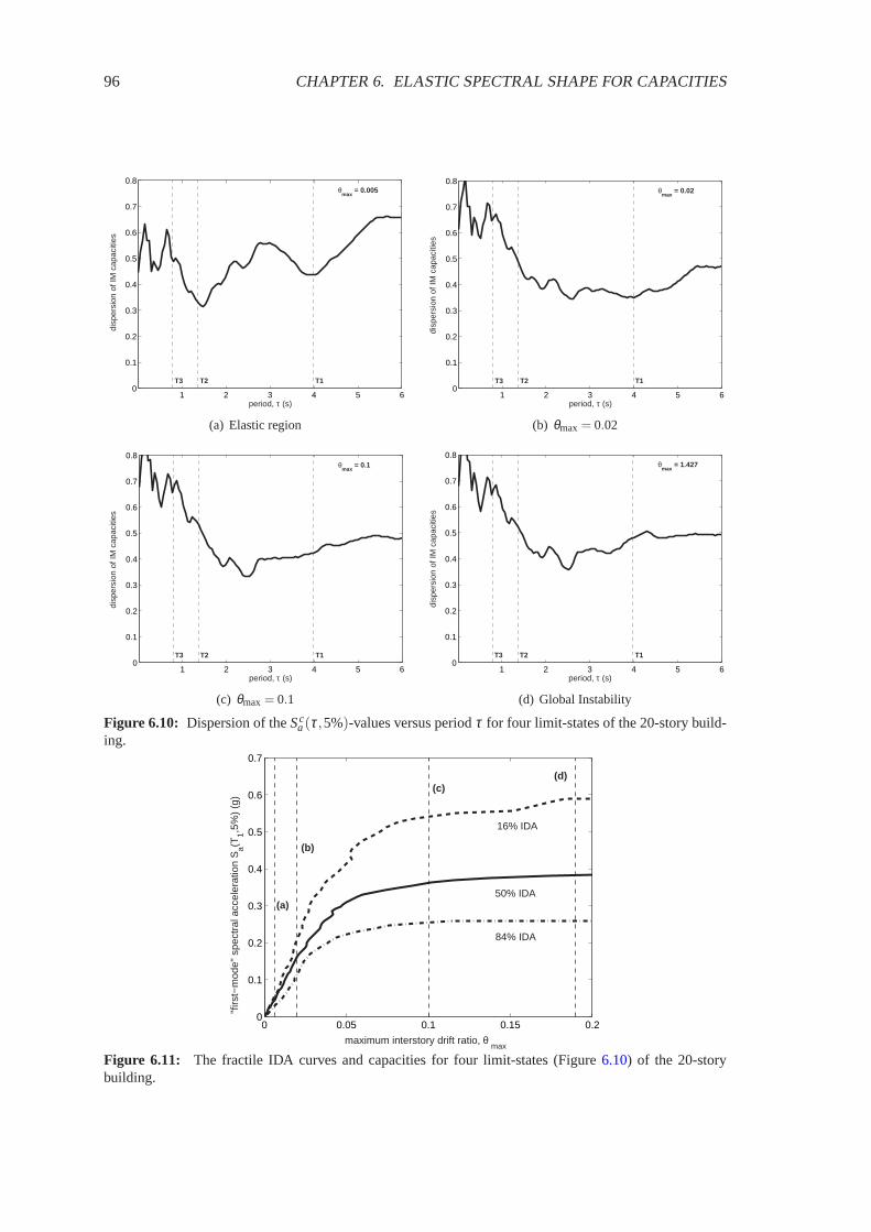
96 CHAPTER 6. ELASTIC SPECTRAL SHAPE FOR CAPACITIES
1 2 3 4 5 60
0.1
0.2
0.3
0.4
0.5
0.6
0.7
0.8
T1 T2 T3
θmax
= 0.005
period, τ (s)
disp
ersi
on o
f IM
cap
aciti
es
(a) Elastic region
1 2 3 4 5 60
0.1
0.2
0.3
0.4
0.5
0.6
0.7
0.8
T1 T2 T3
θmax
= 0.02
period, τ (s)
disp
ersi
on o
f IM
cap
aciti
es(b) θmax = 0.02
1 2 3 4 5 60
0.1
0.2
0.3
0.4
0.5
0.6
0.7
0.8
T1 T2 T3
θmax
= 0.1
period, τ (s)
disp
ersi
on o
f IM
cap
aciti
es
(c) θmax = 0.1
1 2 3 4 5 60
0.1
0.2
0.3
0.4
0.5
0.6
0.7
0.8
T1 T2 T3
θmax
= 1.427
period, τ (s)
disp
ersi
on o
f IM
cap
aciti
es
(d) Global Instability
Figure 6.10: Dispersion of theSca(τ,5%)-values versus periodτ for four limit-states of the 20-story build-
ing.
0 0.05 0.1 0.15 0.20
0.1
0.2
0.3
0.4
0.5
0.6
0.7
maximum interstory drift ratio, θ max
50% IDA
84% IDA
16% IDA
(a)
(b)
(c) (d)
"firs
t−m
ode"
spe
ctra
l acc
eler
atio
n S
a(T1,5
%)
(g)
Figure 6.11: The fractile IDA curves and capacities for four limit-states (Figure6.10) of the 20-storybuilding.

6.4. USING A VECTOR OF TWO SPECTRAL VALUES 97
0 0.05 0.1 0.15 0.20
1
2
3
4
5
6
T1
T2
T3
maximum interstory drift ratio, θ max
perio
d, τ
(s)
Figure 6.12: The optimal periodτ as it evolves withθmax for the 20-story building.
0 0.05 0.1 0.15 0.20
0.1
0.2
0.3
0.4
0.5
0.6
0.7
0.8
maximum interstory drift ratio, θ max
disp
ersi
on o
f IM
cap
aciti
es
PGA S
a(T
1,5%)
optimal Sa(τ,5%)
Figure 6.13: The dispersion for the optimalSa(τ,5%) compared toSa(T1,5%) and PGA, versus the limit-state definition,θmax, for the 20-story building.

98 CHAPTER 6. ELASTIC SPECTRAL SHAPE FOR CAPACITIES
00.5
11.5
22.5
0
0.5
1
1.5
20
0.01
0.02
0.03
0.04
Sa(T
1,5%) (g)S
a(1.5 T
1,5%) / S
a(T
1,5%)
max
imum
inte
rsto
ry d
rift r
atio
, θ m
ax
Figure 6.14: The thirty IDA curves for the 5-story building inSa(T1,5%) andRsa(1.5,T1) coordinates.
00.5
11.5
22.5
0
0.5
1
1.5
20
0.01
0.02
0.03
0.04
Sa(T
1,5%) (g)S
a(1.5 T
1,5%) / S
a(T
1,5%)
max
imum
inte
rsto
ry d
rift r
atio
, θ m
ax
Figure 6.15: The median IDA surface for the 5-story building inSa(T1,5%) andRsa(1.5,T1) coordinates.
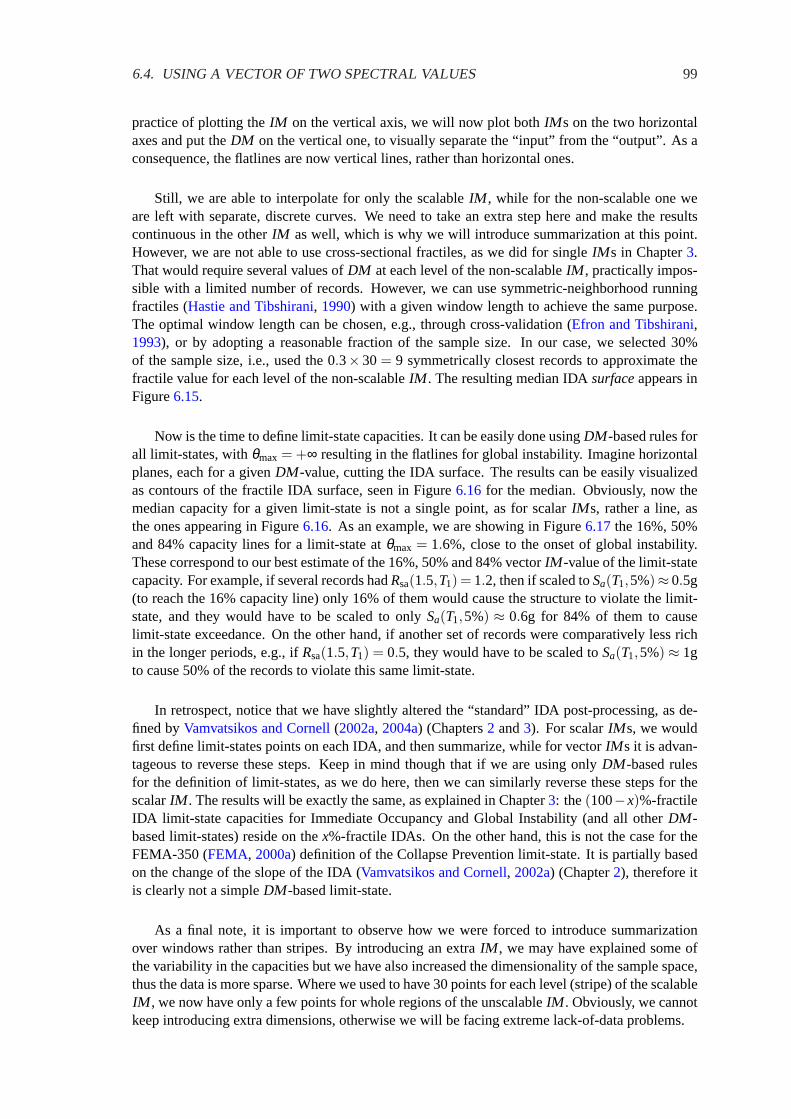
6.4. USING A VECTOR OF TWO SPECTRAL VALUES 99
practice of plotting theIM on the vertical axis, we will now plot bothIM s on the two horizontalaxes and put theDM on the vertical one, to visually separate the “input” from the “output”. As aconsequence, the flatlines are now vertical lines, rather than horizontal ones.
Still, we are able to interpolate for only the scalableIM , while for the non-scalable one weare left with separate, discrete curves. We need to take an extra step here and make the resultscontinuous in the otherIM as well, which is why we will introduce summarization at this point.However, we are not able to use cross-sectional fractiles, as we did for singleIM s in Chapter3.That would require several values ofDM at each level of the non-scalableIM , practically impos-sible with a limited number of records. However, we can use symmetric-neighborhood runningfractiles (Hastie and Tibshirani, 1990) with a given window length to achieve the same purpose.The optimal window length can be chosen, e.g., through cross-validation (Efron and Tibshirani,1993), or by adopting a reasonable fraction of the sample size. In our case, we selected 30%of the sample size, i.e., used the0.3×30= 9 symmetrically closest records to approximate thefractile value for each level of the non-scalableIM . The resulting median IDAsurfaceappears inFigure6.15.
Now is the time to define limit-state capacities. It can be easily done usingDM -based rules forall limit-states, withθmax = +∞ resulting in the flatlines for global instability. Imagine horizontalplanes, each for a givenDM -value, cutting the IDA surface. The results can be easily visualizedas contours of the fractile IDA surface, seen in Figure6.16for the median. Obviously, now themedian capacity for a given limit-state is not a single point, as for scalarIM s, rather a line, asthe ones appearing in Figure6.16. As an example, we are showing in Figure6.17the 16%, 50%and 84% capacity lines for a limit-state atθmax = 1.6%, close to the onset of global instability.These correspond to our best estimate of the 16%, 50% and 84% vectorIM -value of the limit-statecapacity. For example, if several records hadRsa(1.5,T1) = 1.2, then if scaled toSa(T1,5%)≈ 0.5g(to reach the 16% capacity line) only 16% of them would cause the structure to violate the limit-state, and they would have to be scaled to onlySa(T1,5%) ≈ 0.6g for 84% of them to causelimit-state exceedance. On the other hand, if another set of records were comparatively less richin the longer periods, e.g., ifRsa(1.5,T1) = 0.5, they would have to be scaled toSa(T1,5%) ≈ 1gto cause 50% of the records to violate this same limit-state.
In retrospect, notice that we have slightly altered the “standard” IDA post-processing, as de-fined byVamvatsikos and Cornell(2002a, 2004a) (Chapters2 and3). For scalarIM s, we wouldfirst define limit-states points on each IDA, and then summarize, while for vectorIM s it is advan-tageous to reverse these steps. Keep in mind though that if we are using onlyDM -based rulesfor the definition of limit-states, as we do here, then we can similarly reverse these steps for thescalarIM . The results will be exactly the same, as explained in Chapter3: the(100−x)%-fractileIDA limit-state capacities for Immediate Occupancy and Global Instability (and all otherDM -based limit-states) reside on thex%-fractile IDAs. On the other hand, this is not the case for theFEMA-350 (FEMA, 2000a) definition of the Collapse Prevention limit-state. It is partially basedon the change of the slope of the IDA (Vamvatsikos and Cornell, 2002a) (Chapter2), therefore itis clearly not a simpleDM -based limit-state.
As a final note, it is important to observe how we were forced to introduce summarizationover windows rather than stripes. By introducing an extraIM , we may have explained some ofthe variability in the capacities but we have also increased the dimensionality of the sample space,thus the data is more sparse. Where we used to have 30 points for each level (stripe) of the scalableIM , we now have only a few points for whole regions of the unscalableIM . Obviously, we cannotkeep introducing extra dimensions, otherwise we will be facing extreme lack-of-data problems.

100 CHAPTER 6. ELASTIC SPECTRAL SHAPE FOR CAPACITIES
0.005
0.01
0.015
0.02
0.025
0.03
0 0.5 1 1.5 2 2.5
0.4
0.6
0.8
1
1.2
1.4
1.6
1.8
Sa(T
1,5%) (g)
Sa(1
.5 T
1,5%
) /
Sa(T
1,5%
)
Figure 6.16: Median contours for thirty IDA curves for the 5-story building inSa(T1,5%) andRsa(1.5,T1)coordinates. Their color indicates the level ofθmax as shown in the color bar.
0 0.5 1 1.5 2 2.5
0.4
0.6
0.8
1
1.2
1.4
1.6
1.8
Sa(T
1,5%) (g)
Sa(1
.5 T
1,5%
) /
Sa(T
1,5%
)
84% IM|DM
16% IM|DM
50% IM|DM
Figure 6.17: The 16%, 50% and 84% capacity lines at the limit-state ofθmax = 0.016 for the 5-storybuilding.
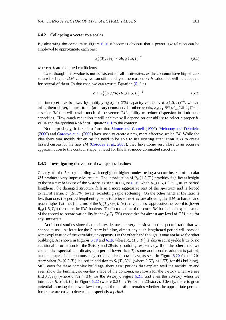
6.4. USING A VECTOR OF TWO SPECTRAL VALUES 101
6.4.2 Collapsing a vector to a scalar
By observing the contours in Figure6.16 it becomes obvious that a power law relation can beemployed to approximate each one:
Sca(T1,5%)≈ aRsa(1.5,T1)b (6.1)
wherea, b are the fitted coefficients.Even though theb-value is not consistent for all limit-states, as the contours have higher cur-
vature for higherDM -values, we can still specify some reasonableb-value that will be adequatefor several of them. In that case, we can rewrite Equation (6.1) as
a≈ Sca(T1,5%) ·Rsa(1.5,T1)−b (6.2)
and interpret it as follows: by multiplyingSca(T1,5%) capacity values byRsa(1.5,T1)−b, we can
bring them closer, almost to an (arbitrary) constant. In other words,Sa(T1,5%)Rsa(1.5,T1)−b isa scalarIM that will retain much of the vectorIM ’s ability to reduce dispersion in limit-statecapacities. How much reduction it will achieve will depend on our ability to select a properb-value and the goodness-of-fit of Equation6.1to the contour.
Not surprisingly, it is such a form thatShome and Cornell(1999), Mehanny and Deierlein(2000) andCordova et al.(2000) have used to create a new, more effective scalarIM . While theidea there was mostly driven by the need to be able to use existing attenuation laws to createhazard curves for the newIM (Cordova et al., 2000), they have come very close to an accurateapproximation to the contour shape, at least for this first-mode-dominated structure.
6.4.3 Investigating the vector of two spectral values
Clearly, for the 5-story building with negligible higher modes, using a vector instead of a scalarIM produces very impressive results. The introduction ofRsa(1.5,T1) provides significant insightto the seismic behavior of the 5-story, as seen in Figure6.16; whenRsa(1.5,T1) > 1, as its periodlengthens, the damaged structure falls in a more aggressive part of the spectrum and is forcedto fail at earlierSa(T1,5%) levels, exhibiting rapid softening. On the other hand, if the ratio isless than one, the period lengthening helps to relieve the structure allowing the IDA to harden andreach higher flatlines (in terms of theSa(T1,5%)). Actually, the less aggressive the record is (lowerRsa(1.5,T1)) the more the IDA hardens. The introduction of the extraIM has helped explain someof the record-to-record variability in theSa(T1,5%) capacities for almost any level ofDM , i.e., forany limit-state.
Additional studies show that such results are not very sensitive to the spectral ratio that wechoose to use. At least for the 5-story building, almost any such lengthened period will providesome explanation of the variability in capacity. On the other hand though, it may not be so for otherbuildings. As shown in Figures6.18and6.19, whereRsa(1.5,T1) is also used, it yields little or noadditional information for the 9-story and 20-story building respectively. If on the other hand, weuse another spectral coordinate, at a period lower thanT1, some additional resolution is gained,but the shape of the contours may no longer be a power-law, as seen in Figure6.20 for the 20-story whenRsa(0.5,T1) is used in addition toSa(T1,5%) (where0.5T1 ≈ 1.5T2 for this building).Still, even for these complex buildings, there exist periods that explain well the variability andeven show the familiar, power-law shape of the contours, as shown for the 9-story when we useRsa(0.7,T1) (where0.7T1 ≈ 2T2 for the 9-story), Figure6.21, and even the 20-story when weintroduceRsa(0.3,T1) in Figure6.22(where0.3T1 ≈ T2 for the 20-story). Clearly, there is greatpotential in using the power-law form, but the question remains whether the appropriate periodsfor its use are easy to determine, especiallya priori.
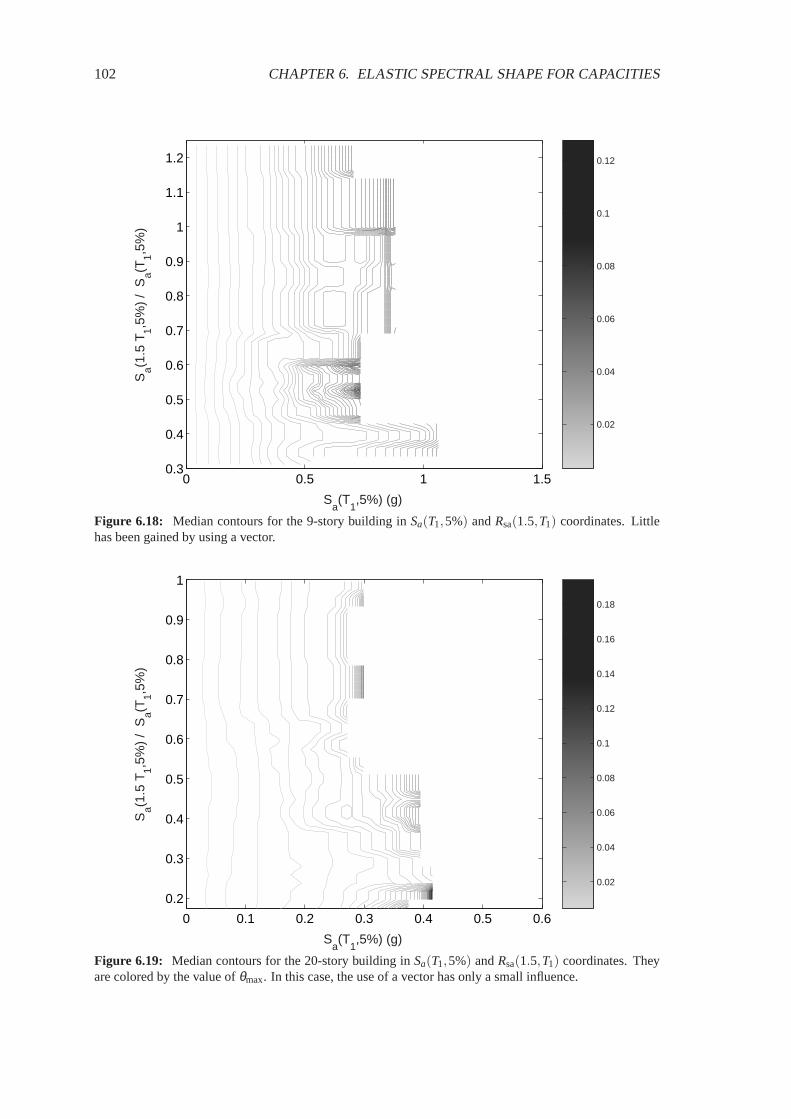
102 CHAPTER 6. ELASTIC SPECTRAL SHAPE FOR CAPACITIES
0.02
0.04
0.06
0.08
0.1
0.12
0 0.5 1 1.50.3
0.4
0.5
0.6
0.7
0.8
0.9
1
1.1
1.2
Sa(T
1,5%) (g)
Sa(1
.5 T
1,5%
) /
Sa(T
1,5%
)
Figure 6.18: Median contours for the 9-story building inSa(T1,5%) andRsa(1.5,T1) coordinates. Littlehas been gained by using a vector.
0.02
0.04
0.06
0.08
0.1
0.12
0.14
0.16
0.18
0 0.1 0.2 0.3 0.4 0.5 0.6
0.2
0.3
0.4
0.5
0.6
0.7
0.8
0.9
1
Sa(T
1,5%) (g)
Sa(1
.5 T
1,5%
) /
Sa(T
1,5%
)
Figure 6.19: Median contours for the 20-story building inSa(T1,5%) andRsa(1.5,T1) coordinates. Theyare colored by the value ofθmax. In this case, the use of a vector has only a small influence.
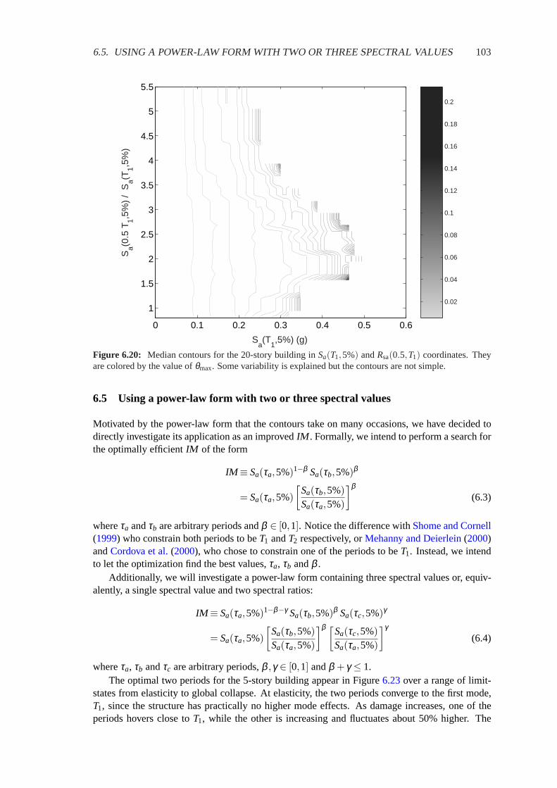
6.5. USING A POWER-LAW FORM WITH TWO OR THREE SPECTRAL VALUES 103
0.02
0.04
0.06
0.08
0.1
0.12
0.14
0.16
0.18
0.2
0 0.1 0.2 0.3 0.4 0.5 0.6
1
1.5
2
2.5
3
3.5
4
4.5
5
5.5
Sa(T
1,5%) (g)
Sa(0
.5 T
1,5%
) /
Sa(T
1,5%
)
Figure 6.20: Median contours for the 20-story building inSa(T1,5%) andRsa(0.5,T1) coordinates. Theyare colored by the value ofθmax. Some variability is explained but the contours are not simple.
6.5 Using a power-law form with two or three spectral values
Motivated by the power-law form that the contours take on many occasions, we have decided todirectly investigate its application as an improvedIM . Formally, we intend to perform a search forthe optimally efficientIM of the form
IM ≡ Sa(τa,5%)1−β Sa(τb,5%)β
= Sa(τa,5%)[
Sa(τb,5%)Sa(τa,5%)
]β(6.3)
whereτa andτb are arbitrary periods andβ ∈ [0,1]. Notice the difference withShome and Cornell(1999) who constrain both periods to beT1 andT2 respectively, orMehanny and Deierlein(2000)andCordova et al.(2000), who chose to constrain one of the periods to beT1. Instead, we intendto let the optimization find the best values,τa, τb andβ .
Additionally, we will investigate a power-law form containing three spectral values or, equiv-alently, a single spectral value and two spectral ratios:
IM ≡ Sa(τa,5%)1−β−γ Sa(τb,5%)β Sa(τc,5%)γ
= Sa(τa,5%)[
Sa(τb,5%)Sa(τa,5%)
]β [Sa(τc,5%)Sa(τa,5%)
]γ(6.4)
whereτa, τb andτc are arbitrary periods,β ,γ ∈ [0,1] andβ + γ ≤ 1.The optimal two periods for the 5-story building appear in Figure6.23over a range of limit-
states from elasticity to global collapse. At elasticity, the two periods converge to the first mode,T1, since the structure has practically no higher mode effects. As damage increases, one of theperiods hovers close toT1, while the other is increasing and fluctuates about 50% higher. The
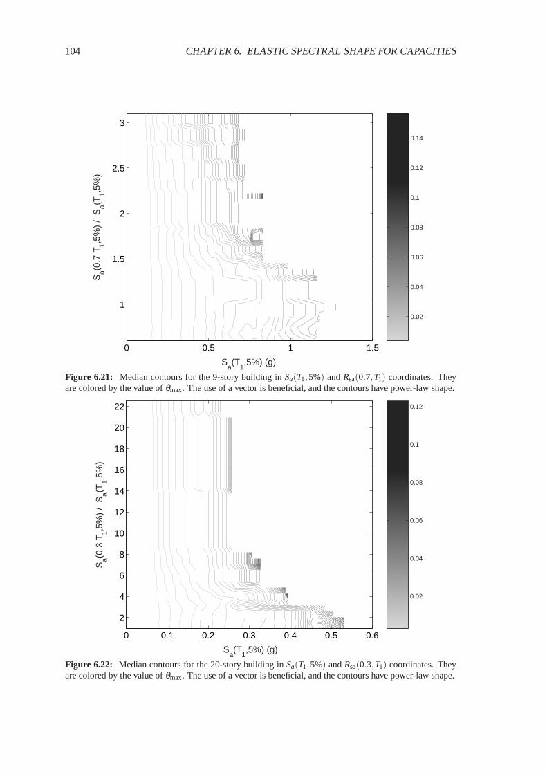
104 CHAPTER 6. ELASTIC SPECTRAL SHAPE FOR CAPACITIES
0.02
0.04
0.06
0.08
0.1
0.12
0.14
0 0.5 1 1.5
1
1.5
2
2.5
3
Sa(T
1,5%) (g)
Sa(0
.7 T
1,5%
) /
Sa(T
1,5%
)
Figure 6.21: Median contours for the 9-story building inSa(T1,5%) andRsa(0.7,T1) coordinates. Theyare colored by the value ofθmax. The use of a vector is beneficial, and the contours have power-law shape.
0.02
0.04
0.06
0.08
0.1
0.12
0 0.1 0.2 0.3 0.4 0.5 0.6
2
4
6
8
10
12
14
16
18
20
22
Sa(T
1,5%) (g)
Sa(0
.3 T
1,5%
) /
Sa(T
1,5%
)
Figure 6.22: Median contours for the 20-story building inSa(T1,5%) andRsa(0.3,T1) coordinates. Theyare colored by the value ofθmax. The use of a vector is beneficial, and the contours have power-law shape.

6.5. USING A POWER-LAW FORM WITH TWO OR THREE SPECTRAL VALUES 105
0 0.01 0.02 0.03 0.04 0.05 0.060
1
2
3
4
5
6
T1
maximum interstory drift ratio, θ max
perio
d, τ
(s)
Figure 6.23: The two optimal periodsτa, τb as they evolve withθmax for the 5-story building.
0 0.01 0.02 0.03 0.04 0.05 0.060
0.1
0.2
0.3
0.4
0.5
0.6
0.7
0.8
maximum interstory drift ratio, θ max
disp
ersi
on o
f IM
cap
aciti
es
PGA S
a(T
1,5%)
best 2 periods
Figure 6.24: The dispersions for optimalSa(τa,5%)1−β Sa(τb,5%)β versusSa(T1,5%) and PGA for the5-story building.

106 CHAPTER 6. ELASTIC SPECTRAL SHAPE FOR CAPACITIES
0 0.01 0.02 0.03 0.04 0.05 0.060
1
2
3
4
5
6
T1
maximum interstory drift ratio, θ max
perio
d, τ
(s)
Figure 6.25: The three optimal periodsτa, τb, τc as they evolve withθmax for the 5-story building.
0 0.01 0.02 0.03 0.04 0.05 0.060
0.1
0.2
0.3
0.4
0.5
0.6
0.7
0.8
maximum interstory drift ratio, θ max
disp
ersi
on o
f IM
cap
aciti
es
PGA S
a(T
1,5%)
best 3 periods
Figure 6.26: The dispersions for optimalSa(τa,5%)1−β−γ Sa(τb,5%)β Sa(τc,5%)γ versus the dispersionsfor PGA andSa(T1,5%) for the 5-story building.
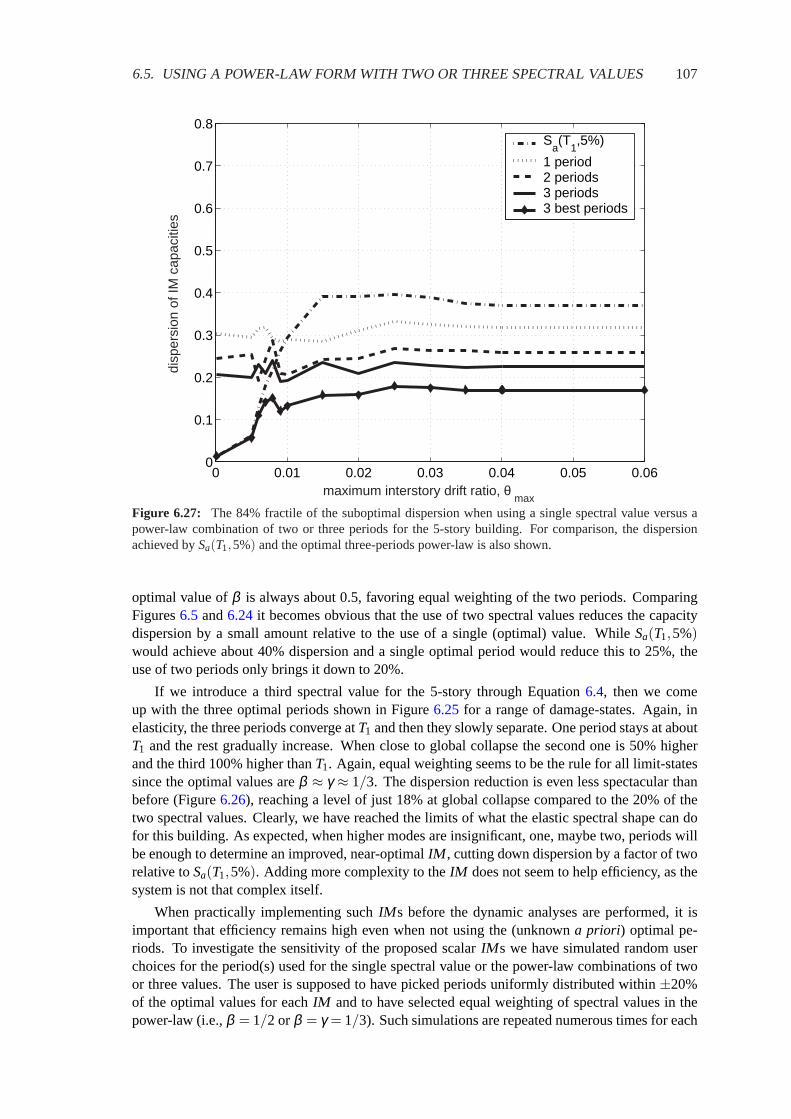
6.5. USING A POWER-LAW FORM WITH TWO OR THREE SPECTRAL VALUES 107
0 0.01 0.02 0.03 0.04 0.05 0.060
0.1
0.2
0.3
0.4
0.5
0.6
0.7
0.8
maximum interstory drift ratio, θ max
disp
ersi
on o
f IM
cap
aciti
es
Sa(T
1,5%)
1 period 2 periods 3 periods 3 best periods
Figure 6.27: The 84% fractile of the suboptimal dispersion when using a single spectral value versus apower-law combination of two or three periods for the 5-story building. For comparison, the dispersionachieved bySa(T1,5%) and the optimal three-periods power-law is also shown.
optimal value ofβ is always about 0.5, favoring equal weighting of the two periods. ComparingFigures6.5 and6.24it becomes obvious that the use of two spectral values reduces the capacitydispersion by a small amount relative to the use of a single (optimal) value. WhileSa(T1,5%)would achieve about 40% dispersion and a single optimal period would reduce this to 25%, theuse of two periods only brings it down to 20%.
If we introduce a third spectral value for the 5-story through Equation6.4, then we comeup with the three optimal periods shown in Figure6.25for a range of damage-states. Again, inelasticity, the three periods converge atT1 and then they slowly separate. One period stays at aboutT1 and the rest gradually increase. When close to global collapse the second one is 50% higherand the third 100% higher thanT1. Again, equal weighting seems to be the rule for all limit-statessince the optimal values areβ ≈ γ ≈ 1/3. The dispersion reduction is even less spectacular thanbefore (Figure6.26), reaching a level of just 18% at global collapse compared to the 20% of thetwo spectral values. Clearly, we have reached the limits of what the elastic spectral shape can dofor this building. As expected, when higher modes are insignificant, one, maybe two, periods willbe enough to determine an improved, near-optimalIM , cutting down dispersion by a factor of tworelative toSa(T1,5%). Adding more complexity to theIM does not seem to help efficiency, as thesystem is not that complex itself.
When practically implementing suchIM s before the dynamic analyses are performed, it isimportant that efficiency remains high even when not using the (unknowna priori) optimal pe-riods. To investigate the sensitivity of the proposed scalarIM s we have simulated random userchoices for the period(s) used for the single spectral value or the power-law combinations of twoor three values. The user is supposed to have picked periods uniformly distributed within±20%of the optimal values for eachIM and to have selected equal weighting of spectral values in thepower-law (i.e.,β = 1/2 or β = γ = 1/3). Such simulations are repeated numerous times for each
108 CHAPTER 6. ELASTIC SPECTRAL SHAPE FOR CAPACITIES
limit-state (i.e., value ofθmax) and the achieved suboptimal dispersion is calculated for eachIM .In Figure6.27we are plotting the 84%-fractile of the suboptimal dispersion for the single periodand the two power-law combinations versus theθmax definition of each limit-state; i.e., we are fo-cusing on a worse-than-average scenario. For comparison, the dispersion when usingSa(T1,5%)and when using the optimal three periods power-law is also shown. Obviously, the largest effectfor the 5-story is in the elastic region, where not usingT1 is a very bad choice in all cases. In thenonlinear range, missing the optimal period seriously degrades the performance of a singleIM ,bringing its dispersion to about 30%, a fact also observed in Figure6.2. On the other hand, thetwo and three period combinations perform relatively well, managing to keep a dispersion of about25% and 20%. Again, just as when using a vector of two spectral values, the power-law form isquite stable, even more so than using a single spectral value, hence relatively large changes awayfrom the optimal periods do not significantly influence the dispersion reduction of the power-lawIM . Practically, in the post-yield region, using the first mode plus e.g., a 50% increased period,with β = 0.5 (i.e., equal weight on both spectral values) will in general produce good results.Actually these conclusions are quite in agreement withCordova et al.(2000).
In the case of the 9-story building, the two optimal periods appear in Figure6.28and the threebest in Figure6.30. In the first case, the smaller period seems to stay atT2 while the higher onestarts fromT1 and increases to some higher value, only to return back toT1 again. For the threeperiods, the results seem to favor one period atT1, another atT2 and a third at about twiceT1.Similarly to the 5-story, equal weighting is the optimal strategy for bothIM s and almost all limit-states. With either two or three periods, as seen in Figures6.29and6.31, the dispersion reductionis about the same. Actually, the dispersion drops from 40% for one optimal period (or even forjustSa(T1,5%)), to less than 25–30% when two or more periods are used. Again, it seems that twospectral values are enough for this first-mode-dominated building and clearly better than just one.
What is of more value though is that the efficiency of the two or three-elementIM is very stablerelative to the choices of the periods and theβ , γ weights. In Figure6.32we plot the results ofthe previously described sensitivity analysis for the 9-story. Clearly, using only one (suboptimal)period is often worse or at most as good as when usingSa(T1,5%), as observed in Figure6.6 aswell. On the other hand, with two or three periods, equally weighted in a power-law form, theIMis considerably more robust and relatively reasonable efficiency is maintained. If we follow ourobservations and set one value aroundT1, another at aboutT2 and maybe a third 50% or 100%higher thanT1, then weigh them equally (β = 1/2 or β = γ = 1/3), a dispersion of about 30% iseasily achieved in contrast to the elusive single optimal period.
Figure6.33shows the best two periods for the 20-story building. One seems to stay somewherein the middle ofT2 andT3 while the other is a lengthened version of the first mode, perhaps by30–50%. The picture is clearer for the three best periods in Figure6.35, where each seems to bea (roughly) 50% lengthened version of one of the three elastic modes,T1, T2 andT3. The optimalweights are roughly equal for all two or three periods. The dispersion reduction is significantin both cases, reaching down to 25% versus the 35% achieved by a single optimal period or the40% of Sa(T1,5%) (Figure6.34, 6.36). While the use of three periods rather than two seems tooffer little benefit, actually it makes theIM quite easier to define. Additionally the results ofthe sensitivity analysis in Figure6.37suggest that efficiency remains relatively high when threesuboptimal periods are employed, versus two or one. Simply by increasing all three elastic periodsby some reasonable percentage and employing equal weights (β = γ = 1/3) works fine for alllimit-states, achieving dispersions in the order of 30%.
In conclusion, it seems that the use of the power-law form with two or three spectral valueshelps even when the higher modes are significant. Actually, the more significant they are, the moreperiods we might want to include. The benefit is not so much in the reduction of dispersion, ratherin the robustness of theIM and the ability to identify ita priori. Further investigation of morestructures is needed before some concrete proposals are made, but the concept looks promising.

6.5. USING A POWER-LAW FORM WITH TWO OR THREE SPECTRAL VALUES 109
0 0.05 0.1 0.15 0.20
1
2
3
4
5
6
T1
T2
T3
perio
d, τ
(s)
maximum interstory drift ratio, θ max
Figure 6.28: The two optimal periodsτa, τb as they evolve withθmax for the 9-story building.
0 0.05 0.1 0.15 0.20
0.1
0.2
0.3
0.4
0.5
0.6
0.7
0.8
maximum interstory drift ratio, θ max
disp
ersi
on o
f IM
cap
aciti
es
PGA S
a(T
1,5%)
best 2 periods
Figure 6.29: The dispersions for optimalSa(τa,5%)1−β Sa(τb,5%)β versusSa(T1,5%) and PGA for the9-story building.

110 CHAPTER 6. ELASTIC SPECTRAL SHAPE FOR CAPACITIES
0 0.05 0.1 0.15 0.20
1
2
3
4
5
6
T1
T2
T3
maximum interstory drift ratio, θ max
perio
d, τ
(s)
Figure 6.30: The three optimal periodsτa, τb, τc as they evolve withθmax for the 9-story building.
0 0.05 0.1 0.15 0.20
0.1
0.2
0.3
0.4
0.5
0.6
0.7
0.8
maximum interstory drift ratio, θ max
disp
ersi
on o
f IM
cap
aciti
es
PGA S
a(T
1,5%)
best 3 periods
Figure 6.31: The dispersions for optimalSa(τa,5%)1−β−γ Sa(τb,5%)β Sa(τc,5%)γ versus the dispersionsfor PGA andSa(T1,5%) for the 9-story building.

6.6. USING ALL SPECTRAL VALUES 111
0 0.05 0.1 0.15 0.20
0.1
0.2
0.3
0.4
0.5
0.6
0.7
0.8
maximum interstory drift ratio, θ max
disp
ersi
on o
f IM
cap
aciti
es
Sa(T
1,5%)
1 period 2 periods 3 periods 3 best periods
Figure 6.32: The 84% fractile of the suboptimal dispersion when using a single spectral value versus apower-law combination of two or three periods for the 9-story building. For comparison, the dispersionachieved bySa(T1,5%) and the optimal three-periods power-law is also shown.
6.6 Using all spectral values
The problems encountered with all previous attempts to use the spectral shape mainly stem fromthe fact that we were looking for distinct “perfect” periods. This in part made the problem quitemore difficult, as we were trying to describe the full spectral shape with only one or two values.We might want to use more information from the spectral shape than just two discrete values, andthis hopefully will open up some easier paths. Still, visualizing such a vector would be hard, and itwould be equally difficult to have enough data to fill the extra dimensions. On the other hand, thecollapsed form of the vector to a scalar suggests an easier way to approach this problem. Includingmore spectral coordinates in Equation (6.1) is relatively straightforward, while finding the rightβ , γ-coefficients may be handled by standard linear regression methods, penalized to reflect thesample size limitations.
Taking one step further, there exist methods in statistics that can treat each record’s spectrum asa single, functional predictor, thus taking into consideration the shape of the full spectrum and useit as a predictor for limit-state capacity. In formal terms we are proposing the use of a functionallinear model (Ramsay and Silverman, 1996) that will use each record’s spectrum to predict a scalarresponse, i.e., its limit-stateSc,i
a (T1,5%)-capacity derived from the IDA curve of thati-th record.In essence, we are proposing the use of the linear functional model
lnSc,ia (T1,5%) = α +
∫ te
tsβ (τ) ln
[Sa(τ ,5%)Sa(T1,5%)
]dτ + εi (6.5)
whereα is the regression intercept,β (τ) is the regression coefficient function,ts andte are thestarting and ending periods that bound the spectral region of interest and, finally,εi are the inde-pendent and normally distributed errors (with a mean of zero).

112 CHAPTER 6. ELASTIC SPECTRAL SHAPE FOR CAPACITIES
0 0.05 0.1 0.15 0.20
1
2
3
4
5
6
T1
T2
T3
maximum interstory drift ratio, θ max
perio
d, τ
(s)
Figure 6.33: The two optimal periodsτa, τb as they evolve withθmax for the 20-story building.
0 0.05 0.1 0.15 0.20
0.1
0.2
0.3
0.4
0.5
0.6
0.7
0.8
maximum interstory drift ratio, θ max
disp
ersi
on o
f IM
cap
aciti
es
PGA S
a(T
1,5%)
3 best periods
Figure 6.34: The dispersions for optimalSa(τa,5%)1−β Sa(τb,5%)β versusSa(T1,5%) and PGA for the20-story building.
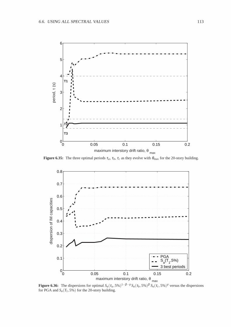
6.6. USING ALL SPECTRAL VALUES 113
0 0.05 0.1 0.15 0.20
1
2
3
4
5
6
T1
T2
T3
maximum interstory drift ratio, θ max
perio
d, τ
(s)
Figure 6.35: The three optimal periodsτa, τb, τc as they evolve withθmax for the 20-story building.
0 0.05 0.1 0.15 0.20
0.1
0.2
0.3
0.4
0.5
0.6
0.7
0.8
maximum interstory drift ratio, θ max
disp
ersi
on o
f IM
cap
aciti
es
PGA S
a(T
1,5%)
3 best periods
Figure 6.36: The dispersions for optimalSa(τa,5%)1−β−γ Sa(τb,5%)β Sa(τc,5%)γ versus the dispersionsfor PGA andSa(T1,5%) for the 20-story building.

114 CHAPTER 6. ELASTIC SPECTRAL SHAPE FOR CAPACITIES
0 0.05 0.1 0.15 0.20
0.1
0.2
0.3
0.4
0.5
0.6
0.7
0.8
maximum interstory drift ratio, θ max
disp
ersi
on o
f IM
cap
aciti
es
Sa(T
1,5%)
1 period 2 periods 3 periods 3 best periods
Figure 6.37: The 84% fractile of the suboptimal dispersion when using a single spectral value versus apower-law combination of two or three periods for the 20-story building. For comparison, the dispersionachieved bySa(T1,5%) and the optimal three-periods power-law is also shown.
This can be thought as a conventional multivariate linear regression model, only we can havean infinite number of predictors, or degrees of freedom, in our fitting. Of course, having infiniteparameters and only a finite number of responses, allows such a model to actually interpolate theresponses, if we choose so. This would not provide a meaningful estimator, but can be reme-died by sufficiently smoothing the coefficient functionβ (τ) at a level easily found through cross-validation. We end up with a model to predict limit-state capacities, that can be easily imagined tobe of the same power-law form as the one we have introduced to collapse the vector of twoIM sinto a scalar in Equation (6.1). If we use a trapezoidal rule to perform the integration, then we canwrite Equation (6.5) as:
lnSc,ia (T1,5%)≈ α +
n
∑j=1
β (τi) ln
[Sa(τi ,5%)Sa(T1,5%)
]∆τ ⇔
Sc,ia (T1,5%)≈ eα
n
∏j=1
[Sa(τi ,5%)Sa(T1,5%)
]β (τi)∆τ⇔
eα ≈ Sc,ia (T1,5%)
n
∏j=1
[Sa(τi ,5%)Sa(T1,5%)
]−β (τi)∆τ(6.6)
Equation (6.6) allows us to define a newIM , of similar form to Equation (6.2), that now usespractically the whole spectrum to explain (and reduce) the record-to-record variability. Similarlyto the collapsed vector form, as described inCordova et al.(2000), it is expected that hazard curvescan be easily determined for such anIM without the need of new attenuation relationships.
But why expand to such a complicatedIM ? We have performed such a functional linear fit forthe global instability capacities of the 20-story building, for the spectral coordinates withints =

6.7. CONCLUSIONS 115
0.5 1 1.5 2 2.5 3 3.5 4 4.5 5 5.5 6
−0.28
−0.26
−0.24
−0.22
−0.2
−0.18
−0.16
Period, T (s)
Reg
. Coe
ffici
ent
T1 T2 T3
Figure 6.38: The regression coefficient functionβ (τ) at global dynamic instability for the 20-story build-ing.
0.1s andte = 6s, and have plotted the coefficient functionβ (τ) in Figure6.38; it precisely explainsthe influence of every spectral coordinate on the flatline capacity. We can think ofβ (τ) as aweight function, where its absolute value at each period provides us with the degree of the period’ssignificance to capacity. As it appears, the importance of spectral coordinates is highest for periodslonger than the first mode (high|β (τ)|-values), while it decreases rapidly for periods lower thanthe second mode (low|β (τ)|-values). The simplicity of the shape suggests that we can probablyprovide some generala priori suggestions for the coefficient function that will provide relativelyefficient IM s. Note, that we need not match the actual values of the coefficient function, only itsshape, as we are not interested in capacity-prediction, only in capacity dispersion reduction.
Again, the realized gains may not lie as much with dispersion reduction as with robustness.The IM suggested by the fit reduces all capacity dispersions for all limit-states by approximately50% relative toSa(T1,5%), almost to similar amounts as the power-law form with three periods.Only further investigations can prove whether this functional model will prove more useful orrobust than the simpler power-law form. Still, it may help us identify spectral regions of interestand characterize structures in a very simple way.
6.7 Conclusions
Providing more efficient Intensity Measures (IM s) is a useful exercise, both in reducing the num-ber of records needed for PBEE calculations but also in improving our understanding of the seismicbehavior of structures. The observed record-to-record dispersion in the limit-stateIM -capacitiescan be practically halved by taking advantage of elastic spectrum information. Several methods ex-ist to incorporate elastic spectral values inIM s. One could use a single optimally selected spectralvalue, a vector of two or a power-law combination of several spectral values. While all candi-dates seem to achieve similar degrees of efficiency, not all of them are suitable for usea priori;

116 CHAPTER 6. ELASTIC SPECTRAL SHAPE FOR CAPACITIES
it may be quite difficult to select the appropriate periods (or spectral values) before we completeour dynamic analyses. Using a single optimal spectral value is practical only for buildings withinsignificant higher modes. On the other hand, when the influence of higher modes is significant,spectralshapebecomes important. Then, using two or even three spectral values seems to helpboth the efficiency and the robustness of theIM to the suboptimal selection of periods. Still,before suchIM s are adopted, significant work remains to be done; we need to investigate morestructures and more ground motion records, probably ones with important local spectral features,e.g., soft soil or directivity influence. Thus we will be able to better select the appropriateIM thatwill be both efficient and sufficient for a given structure and site.

Chapter 7Conclusions
7.1 Summary
In the preceding chapters we have defined Incremental Dynamic Analysis (IDA) and used it toinvestigate various aspects of the seismic performance of structures.
Chapter2 provides a concrete theoretical basis for IDA, fully describing the process of per-forming multiple nonlinear dynamic analyses under a suite of multiply-scaled ground motionrecords. The Intensity Measure (IM ) was introduced to quantify the scaling of a ground mo-tion record and the Damage Measure (DM ) was used to record its response, generating an IDAcurve for each record in theIM , DM plane. Observing such curves revealed large record-to-recordvariability but also several interesting aspects of structural behavior. The equal displacement rulewas found to be applicable for moderate and long period structures in the near elastic region.Additionally the phenomena of non-monotonic behavior, discontinuities, hardening, softening,flatlining and even resurrection behavior were observed in individual curves. On each IDA curvelimit-states were defined using a variety of methods or rules. Using cross-sectional fractiles theIDA curves where summarized into the 16%, 50% and 84% IDA curves, and the capacities weresummarized into their 16%, 50% and 84%DM or IM values. Further we have addressed thequestion of “legitimacy” of scaling records and the relationships between IDAs andR-factors aswell as between IDAs and the Static Pushover (SPO) Analysis. A significant connection appearedbetween the IDA and the SPO; individual segments of the SPO (e.g., elastic, positive-stiffness,negative-stiffness, residual plateau) correspond to unique segments of the IDA (e.g., elastic, equaldisplacement, softening, secant at reduced stiffness). Finally, algorithms were presented that cansignificantly reduce the number of nonlinear runs per record. All in all, IDA was shown to provideuseful intuition into the seismic behavior of structures.
In Chapter3we looked into the practical application of IDA to a 9-story steel moment-resistingframe, using the methods presented in the previous chapter to produce a complete example andcommentary for applying IDA to PBEE. Publicly available software is used to perform the anal-ysis, interpolate the IDA curves, estimate limit-state capacities and summarize the results into aformat that can be easily integrated with modern PBEE frameworks. The final goal is estimatingthe mean annual frequency of exceeding certain limit-states. We pay special attention to the detailsof the practical implementation: how many records, how many runs per record, how the curvesare interpolated, the use of approximations in the probabilistic calculations. These are just someof the subjects that we investigate, and they are all found to influence the accuracy of the finalIDA results. The methods that have been presented are designed to strike a favorable compromisebetween speed and accuracy and thus resolve such issues. Perhaps, the single most important thingto remember is the wealth of information that can be found in IDA if only we take advantage ofever-cheaper computing power and automated methods to investigate the structure’s behavior.
117

118 CHAPTER 7. CONCLUSIONS
In Chapter4 the SPO2IDA tool was developed to provide rapid estimation of the seismicperformance of oscillators with complex backbones and arbitrary periods. The investigated back-bone shapes range from simple bilinear to complex quadrilinear with an elastic, a hardening and anegative-stiffness segment plus a final residual plateau that terminates with a drop to zero strength.Using a suite of thirty ground motion records, IDA was performed for numerous such backboneshapes and the summarized IDA curves were extracted for each individual case, yielding inter-esting observations. Long hardening segments are found to significantly improve performance,while their slope has only a small effect. On the other hand, the steeper the slope of the negative-stiffness segment, the higher the demands and the lower the capacities past the peak of the back-bone. Residual plateaus that are higher in terms of strength or longer in terms of ductility, bothbenefit the post-peak performance. Finally, the oscillator period significantly influences the effectof all segments except the hardening one in the moderate or long period ranges. Several differentbackbone shapes were found to produce similar dynamic behavior. Thus, the required numberof backbone shapes to be investigated is drastically reduced, allowing the effect of a completequadrilinear backbone to be captured with only a handful of regressions. In accordance, a numberof equations have been proposed, defining a flexible, publicly available, software tool (SPO2IDA)for performing fast assessments of the (median and dispersion of) demand and capacity of virtu-ally any oscillator. Using SPO2IDA we can effortlessly get accurate estimates of the performanceof the oscillator without having to perform the costly analyses, providing ready insights into therelative advantages and disadvantages of possible design or retrofit alternatives.
In Chapter5 we employed SPO2IDA in conjunction with the SPO for direct approximationof the MDOF seismic behavior. This method can estimate the seismic demands and capacitiesof first-mode-dominated MDOF structures for their entire range of behavior, from elasticity toglobal dynamic instability. Based on the SPO and building upon software able to accurately pre-dict the Incremental Dynamic Analysis (IDA) curves for SDOF systems, it can estimate, withreasonable accuracy, the fractile IDA curves of first-mode-dominated MDOF systems. Similarexisting methodologies usually employ bilinear oscillators. The use of SPO2IDA enables us toextend them well beyond the peak of the SPO. Several novel concepts are derived in the process,perhaps the most important being the worst-case, most-damaging SPO. Sometimes, carefully se-lected load patterns are needed to estimate it, but the worst-case SPO best captures the path thatleads to global collapse. Thus it allows accurate prediction of the IDA results. Equally interestingis the apparent “simplification” that occurs in MDOF systems near global collapse. This permitsSDOF systems with appropriate backbones to capture the onset of global dynamic instability evenfor higher-mode-influenced structures. Combining all these observations, we can conclude thatsimply by using the appropriate SPO curve plus, perhaps, a few elastic response spectrum analy-ses, the engineer-user is able to generate accurate predictions of the seismic behavior of complexMDOF structures within a fraction of the time needed for a full IDA.
Finally, in Chapter6, the limit-state capacities estimated by IDA were used as a tool to re-search the effect of the elastic spectrum on structural performance and its ability to improveIM -efficiency. Providing more efficient Intensity Measures (IM s) is a useful exercise, both in reducingthe number of records needed for PBEE calculations but also in improving our understanding ofthe seismic behavior of structures. The observed record-to-record dispersion in the limit-stateIM -capacities can be practically halved by taking advantage of elastic spectrum information. Severalmethods exist to incorporate elastic spectral values inIM s. We chose to use a single optimallyselected spectral value, a vector of two or a power-law combination of several spectral values.While all candidates seem to achieve similar degrees of efficiency, not all of them are suitablefor usea priori; it may be quite difficult to select the appropriate periods (or spectral values) be-fore we complete our dynamic analyses. Using a single optimal spectral value is practical onlyfor buildings with insignificant higher modes. On the other hand, when the influence of highermodes is significant, spectralshapebecomes important. Then, using two or even three spectral

7.2. LIMITATIONS AND FUTURE WORK 119
values seems to help both the efficiency and the robustness of theIM to the suboptimal selectionof periods. Still, before suchIM s are adopted, significant work remains to be done; we need toinvestigate more structures and more ground motion records, probably ones with important localspectral features, e.g., soft soil or directivity influence. Thus we will be able to better select theappropriateIM that will be both efficient and sufficient for a given structure and site.
7.2 Limitations and Future Work
All the work presented revolves around IDA and is limited in all the ways that IDA is. Thus,the single most important issue is the concept of ground motion record scaling. There certainlyexist structures for which scaling is “legitimate”, e.g., moderate period buildings in sites withno directivity whenSa(T1,5%) is the IM (Shome and Cornell, 1999). Still the issue is far fromresolved. Structures that have short or long fundamental period, have significant higher modesor exist in sites influenced by near-fault directivity, are candidates for causing problems. That isnot to say that in these case the results coming from IDA over a given suite of records will notbe legitimate, rather that care should be taken to remove the dependence on record characteristicsother than theIM used.
The obvious way to do so is to properly select the ground motion records a priori, before per-forming IDA. Another, easier-to-implement method would be the introduction of a sufficientIM ,as attempted byLuco and Cornell(2004) andCordova et al.(2000). A sufficient IM would beable to remove the possible bias, bringing together the results from records with different charac-teristics, like magnitude or forward-directivity. Or, one could try to properly weigh each recordaccording to its contribution to the total hazard, as found by disaggregation; thus, record-selectioncan be exercised a posteriori. Obviously, there are several candidate methods and more work needsto be directed to this area before the scaling issue is resolved.
IDA is also limited by the very structural model, analysis algorithms and element modelsthat it uses and all the assumptions incorporated therein. Therefore, it has the unique advantageof growing as the power of our modeling and our computational abilities evolve, but it is alsohampered by their limits. For example, in many of the results shown herein, there exist damagedbut still stable structures at roof drifts in excess of 5%. This is a conclusion that many professionalsand researchers may seriously question. It is important to understand that this is exactly whatcurrent models can predict. Only the comparison with better models, observations in the fieldand lab experiments will prove or refute them. But the point is that we are focusing only on themethod, and we anticipate that it will remain unchanged as the models improve.
Thus, we await with great anticipation structural models that will include all the importantfactors that we have left out: the introduction of soil-structure interaction, the expansion of modelsto three-dimensional structures simultaneously subjected to more than one component of groundmotion and the inclusion of more structural elements (e.g., stairwell and partitions) or improvedelement models that can show e.g., axial failure of columns and shear failure of beams. Until then,IDA will be limited to what has been incorporated to structural models so far.
The approximation of IDA by SPO2IDA is hampered by several additional problems. At theSDOF-level, it is the consideration of directivity, soft soil and the characteristics of the hystereticmodel that limit its application, as explained in detail in Chapter4. In the MDOF case, we havealso inherited the limitations of the SPO, especially its inability to capture the influence of highermodes. These further constrain the accuracy we can achieve with SPO2IDA in the near elasticand nonlinear region, although, remarkably, not in the global collapse domain. Also, furtherwork is needed to test and maybe modify the methodology for buildings with stiffness or strengthirregularities along their height or within a story. One could easily assume that it may becomequite challenging to find the worst-case SPO, or some equivalent SPO that would give the bestprediction.

120 CHAPTER 7. CONCLUSIONS
Finally, the use of the elastic spectral shape to reduce the dispersion of capacities in the non-linear range carries all the problems of using elastic information to predict inelastic results. Theinelastic spectral shape will probably be a better bet in the long-term, but the cost comes in theface of the building-specific attenuation laws needed.
7.3 Overall Conclusions
IDA has proved a useful tool, and can be part of both the short and long-term future of PBEE.It helps quantify the seismic performance of structures, and in the form of the summarized IDAcurves and theIM -capacities it provides a remarkably useful foundation to develop importantintuition and create new approaches to PBEE. Built upon this very foundation, the SPO2IDA toolhas proven both accurate and useful for understanding how a structural design may help or hinderthe seismic performance both for SDOF but also for MDOF structures. In a similar way we havedeveloped the investigation of the elastic spectral shape. Its potential to explain the record-to-record variability in capacity is promising and can help resolve many problems. Naturally, thesemethods have limitations but they are not insurmountable and we anticipate that future researchwill address them appropriately.

Bibliography
Al-Sulaimani, G. J. and Roessett, J. M. (1985). Design spectra for degrading systems,ASCE Journal ofStructural Engineering, 111(12): 127–136.
Ang, A. H. S. and De Leon, D. (1997). Determination of optimal target reliabilities for design and upgradingof structures,Structural Safety, 19(1): 19–103.
Antoniou, S., Pinho, R., and Rovithakis, A. (2002). Development and verification of a fully adaptivepushover procedure,Proceedings of the 12th European Conference on Earthquake Engineering, PaperNo. 822, London, UK, 1–10.
ATC (1996). Seismic evaluation and retrofit of concrete buildings,Report No. ATC–40, Applied TechnologyCouncil, Redwood City, CA.
Baez, J. I. and Miranda, E. (2000). Amplification factors to estimate inelastic displacement demands forthe design of structures in the near field,Proceedings of the 12th World Conference on EarthquakeEngineering, Paper No. 1561, New Zealand, 1–8.
Bazzurro, P. and Cornell, C. A. (1994a). Seismic hazard analysis for non-linear structures. I: Methodology,ASCE Journal of Structural Engineering, 120(11): 3320–3344.
Bazzurro, P. and Cornell, C. A. (1994b). Seismic hazard analysis for non-linear structures. II: Applications,ASCE Journal of Structural Engineering, 120(11): 3345–3365.
Bazzurro, P., Cornell, C. A., Shome, N., and Carballo, J. E. (1998). Three proposals for characterizingMDOF nonlinear seismic response,ASCE Journal of Structural Engineering, 124: 1281–1289.
Benjamin, J. R. and Cornell, C. A. (1970).Probability, Statistics, and Decision for Civil Engineers,McGraw-Hill, New York.
Bertero, V. V. (1977). Strength and deformation capacities of buildings under extreme environments,Struc-tural Engineering and Structural Mechanics, K. S. Pister, ed., Prentice Hall, Englewood Cliffs, NJ,211–215.
Carballo, J. E. and Cornell, C. A. (2000). Probabilistic seismic demand analysis: Spectrum matching anddesign,Report No. RMS-41, RMS Program, Stanford University, Stanford, CA, [Feb 12th, 2004].URL http://www.stanford.edu/group/rms/Reports/RMS41.pdf
Chopra, A. K. (1995).Dynamics of Structures: Theory and Applications to Earthquake Engineering, Pren-tice Hall, Englewood Cliffs, NJ.
Chopra, A. K. and Chintanapakdee, C. (2001). Comparing response of SDF systems to near-fault andfar-fault earthquake motions in the context of spectral regions,Earthquake Engineering and StructuralDynamics, 30(12): 1769–1789.
121

122 BIBLIOGRAPHY
Cordova, P. P., Deierlein, G. G., Mehanny, S. S., and Cornell, C. A. (2000). Development of a two-parameterseismic intensity measure and probabilistic assessment procedure,Proceedings of the 2nd U.S.-JapanWorkshop on Performance-Based Earthquake Engineering Methodology for Reinforced Concrete Build-ing Structures, Sapporo, Hokkaido, 187–206.
Cornell, C. A., Jalayer, F., Hamburger, R. O., and Foutch, D. A. (2002). The probabilistic basis for the 2000SAC/FEMA steel moment frame guidelines,ASCE Journal of Structural Engineering, 128(4): 526–533.
Cornell, C. A. and Krawinkler, H. (2000). Progress and challenges in seismic performance assessment,PEER Center News, 3(2), (accessed: June 18th, 2002).URL http://peer.berkeley.edu/news/2000spring/index.html
Cuesta, I. and Aschheim, M. A. (2001). Inelastic response spectra using conventional and pulse R-factors,ASCE Journal of Structural Engineering, 127(9): 1013–1020.
De Matteis, G., Landolfo, R., Dubina, D., and Stratan, A. (2000). Influence of the structural typology on theseismic performance of steel framed buildings,Moment resistant connections of steel frames in seismicareas, F. M. Mazzolani, ed., E & FN Spon, New York, 513–538.
Dubina, D., Ciutina, A., Stratan, A., and Dinu, F. (2000). Ductility demand for semi-rigid joint frames,Moment resistant connections of steel frames in seismic areas, F. M. Mazzolani, ed., E & FN Spon, NewYork, 371–408.
Efron, B. and Tibshirani, R. J. (1993).An Introduction to the Bootstrap, Chapman & Hall/CRC, New York.
Fajfar, P. and Fischinger, M. (1988). N2 — a method for non-linear seismic analysis of regular structures,Proceedings of the 9th World Conference on Earthquake Engineering, Tokyo-Kyoto, Japan, 111–116.
Fajfar, P. and Gaspersic, P. (1996). The N2 method for the seismic damage analysis for RC buildings,Earthquake Engineering and Structural Dynamics, 25(1): 23–67.
Farin, G. (1990).Curves and Surfaces for Computer Aided Geometric Design: A Practical Guide, 2nd edn.,Academic Press, San Diego, CA.
FEMA (1997). NEHRP guidelines for the seismic rehabilitation of buildings,Report No. FEMA-273, Fed-eral Emergency Management Agency, Washington DC.
FEMA (2000a). Recommended seismic design criteria for new steel moment-frame buildings,Report No.FEMA-350, SAC Joint Venture, Federal Emergency Management Agency, Washington DC.
FEMA (2000b). Recommended seismic evaluation and upgrade criteria for existing welded steel moment-frame buildings,Report No. FEMA-351, SAC Joint Venture, Federal Emergency Management Agency,Washington DC.
Foutch, D. A. and Shi, S. (1998). Effects of hysteresis type on the seismic response of buildings,Proceed-ings of the 6th U.S. National Conference on Earthquake Engineering, Paper No. 409, EERI, El Cerrito,CA, Seattle, WA, 1–12.
Gupta, B. and Kunnath, S. K. (1998). Effects of hysteretic model parameters on inelastic seismic demands,Proceedings of the 6th U.S. National Conference on Earthquake Engineering, Paper No. 358, EERI, ElCerrito, CA, Seattle, WA, 1–12.
Gupta, B. and Kunnath, S. K. (2000). Adaptive spectra-based pushover procedure for seismic evaluation ofstructures,Earthquake Spectra, 16(2): 367–391.
Hastie, T. J. and Tibshirani, R. J. (1990).Generalized Additive Models, Chapman & Hall, New York.
Jalayer, F. and Cornell, C. A. (2002). A technical framework for probability-based demand and capacityfactor (DCFD) seismic formats,Report No. RMS-43, RMS Program, Stanford University, Stanford, CA.
Krawinkler, H. and Seneviratna, G. D. P. K. (1998). Pros and cons of a pushover analysis of seismic perfor-mance evalation,Engineering Structures, 20(4-6): 452–464.

BIBLIOGRAPHY 123
Lee, E. (1989). Choosing nodes in parametric curve interpolation,Computer Aided Design, 21(6): 363–370.
Lee, K. and Foutch, D. A. (2002). Performance evaluation of new steel frame buildings for seismic loads,Earthquake Engineering and Structural Dynamics, 31(3): 653–670.
Lee, L. H., Han, S. W., and Oh, Y. H. (1999). Determination of ductility factor considering different hys-teretic models,Earthquake Engineering and Structural Dynamics, 28(9): 957–977.
Luco, N. and Cornell, C. A. (1998). Effects of random connection fractures on demands and reliability for a3-story pre-Northridge SMRF structure,Proceedings of the 6th U.S. National Conference on EarthquakeEngineering, Paper No. 244, EERI, El Cerrito, CA, Seattle, WA, 1–12.
Luco, N. and Cornell, C. A. (2000). Effects of connection fractures on SMRF seismic drift demands,ASCEJournal of Structural Engineering, 126: 127–136.
Luco, N. and Cornell, C. A. (2004). Structure-specific, scalar intensity measures for near-source and ordi-nary earthquake ground motions,Earthquake Spectra, in review.
Macrae, G. A. and Kawashima, K. (1997). Post-earthquake residual displacements of bilinear oscillators,Earthquake Engineering and Structural Dynamics, 26(7): 701–716.
Mahin, S. A. and Lin, J. (1983). Construction of inelastic response spectra for single-degree-of-freedomsystems: computer program and applications,Report UCB/EERC-83/17, Earthquake Engineering Re-search Center, University of California, Berkeley, CA.
Mehanny, S. S. and Deierlein, G. G. (2000). Modeling and assessment of seismic performance of com-posite frames with reinforced concrete columns and steel beams,Report No. 136, The John A.BlumeEarthquake Engineering Center, Stanford University, Stanford, CA.
Miranda, E. (1993). Evaluation of site-dependent inelastic seismic design spectra,ASCE Journal of Struc-tural Engineering, 119(5): 1319–1338.
Miranda, E. (2000). Inelastic displacement ratios for structures on firm sites,ASCE Journal of StructuralEngineering, 126(10): 1150–1159.
Miranda, E. (2001). Estimation of inelastic deformation demands of SDOF systems,ASCE Journal ofStructural Engineering, 127(9): 1005–1012.
Nassar, A. A. and Krawinkler, H. (1991). Seismic demands for SDOF and MDOF systems,Report No. 95,The John A.Blume Earthquake Engineering Center, Stanford University, Stanford, CA.
Newmark, N. M. and Hall, W. J. (1982).Earthquake Spectra and Design, Earthquake Engineering ResearchInstitute, Berkeley, CA.
Prakhash, V., Powell, G. H., and Filippou, F. C. (1992). DRAIN-2DX: Base program user guide,ReportNo. UCB/SEMM-92/29, Department of Civil Engineering, University of California, Berkeley, CA.
Press, W. H., Flannery, B. P., Teukolsky, S. A., and Vetterling, W. T. (1986).Numerical Recipes, CambridgeUniversity Press, Cambridge.
Psycharis, I. N., Papastamatiou, D. Y., and Alexandris, A. P. (2000). Parametric investigation of the sta-bility of classical comlumns under harmonic and earthquake excitations,Earthquake Engineering andStructural Dynamics, 29: 1093–1109.
Rahnama, M. and Krawinkler, H. (1993). Effects of soft soils and hysteresis model on seismic demands,Report No. 108, The John A.Blume Earthquake Engineering Center, Stanford University, Stanford, CA.
Ramsay, J. O. and Silverman, B. W. (1996).Functional Data Analysis, Springer, New York.
Riddell, R. and Newmark, N. M. (1979). Statistical analysis of the response of nonlinear systems subjectedto earthquakes,Structural Research Series No. 468, University of Illinois at Urbana-Champaign, Urbana,IL.

124 BIBLIOGRAPHY
Ruiz-Garcia, J. and Miranda, E. (2003). Inelastic displacement ratios for evaluation of existing structures,Earthquake Engineering and Structural Dynamics, 32(8): 1237–1258.
SEAOC (1995).Vision 2000: A Framework for Performance Based Design, vol. I–III, Structural EngineersAssociation of California, Sacramento, CA.
Seneviratna, G. D. P. K. and Krawinkler, H. (1997). Evaluation of inelastic MDOF effects for sesmic design,Report No. 120, The John A.Blume Earthquake Engineering Center, Stanford University, Stanford, CA.
Shi, S. and Foutch, D. A. (1997). Connection element (type 10) for DRAIN-2DX,Technical Report No.468, Department of Civil and Environmental Engineering, University of Illinois at Urbana-Champaign,Urbana, IL.
Shome, N. and Cornell, C. A. (1998). Normalization and scaling accelerograms for nonlinear structuralanalysis,Proceedings of the 6th U.S. National Conference on Earthquake Engineering, Paper No. 243,EERI, El Cerrito, CA, Seattle, WA, 1–12.
Shome, N. and Cornell, C. A. (1999). Probabilistic seismic demand analysis of nonlinear structures,ReportNo. RMS-35, RMS Program, Stanford University, Stanford, CA, [Feb 12th, 2004].URL http://www.stanford.edu/group/rms/Thesis/NileshShome.pdf
Shome, N. and Cornell, C. A. (2000). Structural seismic demand analysis: Consideration of collapse,Pro-ceedings of the 8th ASCE Specialty Conference on Probabilistic Mechanics and Structural Reliability,Paper No. 119, Notre Dame, 1–6.
Stear, J. D. and Bea, R. G. (1999). A simplified structural analysis method for jacket–type platforms inseismically–active regions,Report to Joint Industry Project sponsors, Marine Technology and Manage-ment Group, Department of Civil and Environmental Engineering, University of California, Berkeley,CA.
Vamvatsikos, D. (2001). SPO2IDA software for moderate periods, [Feb 12th, 2004].URL http://tremble.stanford.edu/cgi-bin/spo2ida-mt.pl
Vamvatsikos, D. (2002). SPO2IDA software for short, moderate and long periods, [Feb 12th, 2004].URL http://tremble.stanford.edu/nausika/software/spo2ida-allt.xls
Vamvatsikos, D. and Cornell, C. A. (2002a). Incremental dynamic analysis,Earthquake Engineering andStructural Dynamics, 31(3): 491–514.
Vamvatsikos, D. and Cornell, C. A. (2002b). Tracing and post-processing of IDA curves: Theory andsoftware implementation,Report No. RMS-44, RMS Program, Stanford University, Stanford, CA.
Vamvatsikos, D. and Cornell, C. A. (2004a). Applied incremental dynamic analysis,Earthquake Spectra,20(2): 523–553.
Vamvatsikos, D. and Cornell, C. A. (2004b). Direct estimation of the seismic demand and capacity ofMDOF systems through incremental dynamic analysis of an SDOF approximation,ASCE Journal ofStructural Engineering, in review.
Vamvatsikos, D. and Cornell, C. A. (2004c). Direct estimation of the seismic demand and capacity of oscil-lators with multi-linear static pushovers through incremental dynamic analysis,Earthquake Engineeringand Structural Dynamics, in review.
Vamvatsikos, D. and Cornell, C. A. (2004d). Direct estimation of the seismic demand and capacity of oscil-lators with multi-linear static pushovers through incremental dynamic analysis,Earthquake Engineeringand Structural Dynamics, in review.
Veletsos, A. S. and Newmark, N. M. (1960). Effect of inelastic behavior on the response of simple systemsto earthquake motions,Proceedings of the 2nd World Conference on Earthquake Engineering, Tokyo,Japan, 895–912.

BIBLIOGRAPHY 125
Vidic, T., Fajfar, P., and Fischinger, M. (1994). Consistent inelastic design spectra: Strength and displace-ment,Earthquake Engineering and Structural Dynamics, 23(5): 507–521.
Weisberg, S. (1985).Applied Linear Regression, 2nd edn., John Wiley & Sons, New York.
Yun, S. Y., Hamburger, R. O., Cornell, C. A., and Foutch, D. A. (2002). Seismic performance evaluationfor steel moment frames,ASCE Journal of Structural Engineering, 128(4): 534–545.