Chapter 3

Seismic instrumentation

In this chapter we discuss the different instrumentation components as used for gatheringseismic data. It discusses briefly these components as typically used in seismic exploration:the seismic sources (airgun at sea and dynamite and the so-called vibroseis source onland), the seismic sensors (hydrophones at sea and geophones on land) and the seismicacquisition system. The effects of these components can usually be directly observed in theseismic records, and the aim of this chapter is that the reader should become aware of thecontribution of these components. (For the readers with a background in signal analysis,the effects are quantified in terms of signals and Fourier spectra.)

3.1 Seismic data acquisition

The object of exploration seismics is obtaining structural subsurface information fromseismic data, i.e., data obtained by recording elastic wave motion of the ground. Themain reason for doing this is the exploration for oil or gas fields (hydro-carbonates). Inexploration seismics this wave motion is excitated by an active source, the seismic source,e.g. for land seismics (onshore) dynamite. From the source elastic energy is radiated intothe earth, and the earth reacts to this signal. The energy that is returned to the earth’ssurface, is then studied in order to infer the structure of the subsurface. Conventionally,three stages are discerned in obtaining the information of the subsurface, namely dataacquisition, processing and interpretation.

In seismic data acquisition, we concern ourselves only with the data gathering in thefield, and making sure the data is of sufficient quality. In seismic acquisition, an elasticwavefield is emitted by a seismic source at a certain location at the surface. The reflectedwavefield is measured by receivers that are located along lines (2D seismics) or on a grid(3D seismics). After each such a shot record experiment, the source is moved to anotherlocation and the measurement is repeated. Figure 3.1 gives an illustration of seismicacquisition in a land (onshore) survey. At sea (in a marine or offshore survey) the sourceand receivers are towed behind a vessel. In order to gather the data, many choices have

29

t t t t t t t t tt t t t t t t t t

Figure 3.1: Seismic acquisition on land using a dynamite source and a cable of geop hones.

to be made which are related to the physics of the problem, the local situation and, ofcourse, to economical considerations. For instance, a choice must made about the seismicsource being used: on land, one usually has the choice between dynamite and vibroseis;at sea, air guns are deployed. Also on the sensor side, choices have to be made, mainlywith respect to their frequency characteristics. With respect to the recording equipment,one usually does not have a choice for each survey but one must be able to exploit itscapabilities as much as possible.

Various supporting field activities are required for good seismic data acquisition. Forexample, seismic exploration for oil and gas is a complex interaction of activities requiringgood management. Important aspects are:

• General administration/exploration concession and permit work (”land and legal”);topographic surveying and mapping, which is quite different for land- or marinework.

• More specific seismic aspects: placing and checking the seismic source, which on landis either an explosive (for example dynamite) or Vibroseis and at sea mostly an arrayof airguns; positioning and checking the detectors, geophones on land, hydrophonesat sea; operating the seismic recording system.

The organisation of a seismic land crew, often faced with difficult logistics, terrain-and access road conditions is quite different from that of marine seismic crew on board ofan exploration vessel, where a compact streamlined combination of seismic and topo op-erations is concentrated on the decks of one boat; different circumstances require different

30

strategies and different technological solutions.

This chapter deals with seismic instrumentation, i.e., all the necessary hardware tomake seismic measurements in the field.

First of all, we have to generate sound waves, with sufficient power and adequatefrequency content in order to cause detectable reflections. This will be discussed in thesection on sources. Then, when the waves have travelled through the subsurface, we wantto detect the sound, and convert the motion to an electrical signal. This will be discussedin section on geophones and hydrophones. Then, the electrical signal is transported viacables to the recording instrument where it will be converted such that it can be stored,usually on tape, and can be read again at a later time. This is necessary when we wantto process the data to obtain a seismic image of the subsurface. Recording systems arediscussed in the section of recording systems.

The general model which is assumed behind the whole seismic system, is that all thecomponents are linear time-invariant (LTI) systems. This means that the digital output weobtain after a seismic experiment in the field is a convolution of the different components,i.e.,:

x(t) = s(t) ∗ g(t) ∗ r(t) ∗ a(t) (3.1)

in which

x(t) = the seismogram (digitally) on tape or disk

s(t) = the source pulse or signature

g(t) = the impulse response (or Green’s function) of the earth

r(t) = the receiver impulse response

a(t) = the seismograph impulse response (mostly A/D conversion)

As may be obvious, in each of the following sections, we will discuss each of these impulseresponses, apart that from the earth, since that is the function we would like to know atthe end. That will be part of the chapter on processing.

31

3.2 Seismic sources

This section deals with the seismic source. The source generates the (dynamical) me-chanical disturbance that cause a seismic wave motion with a characteristic signal shape(”signature”) to travel through the subsurface from source to receivers. The seismic sourcehas a dominant influence on the signal response resulting from the total acquisition sys-tem, i.e. the response due to source, receiver(s) and seismic recording system. In thischapter the seismic sources as routinely used by the oil industry in the exploration for oiland gas will be treated: airguns as used in marine operations, Vibroseis and dynamite asused for seismic operations on land. For each type of source the most important aspects ofthe mechanical principles of operation will be treated and then the characteristic seismicsignal produced by the source (the source’s ”signature”).

3.2.1 Airguns

Many oil and gasfields are found in water-covered areas, such as the Gulf of Mexico andthe North Sea. Ever since the 1960’s companies were not allowed to use dynamite anymore as seismic source because of fish dying massively due to the sharp and destructivestrong shockwave from the dynamite. Exploration companies had to look for alternatives.Many sources were developed since then, such as airguns, waterguns and even a marineequivalent of the Vibroseis. Airguns became the most popular marine source in the oilindustry because of their renowned reliability and signature repeatability. The signatureof one airgun has an inconveniently long and oscillatory character, the reason why airgunsare used in specifically designed arrays, consisting of airguns with different volumes.

The mechanics of the airgun

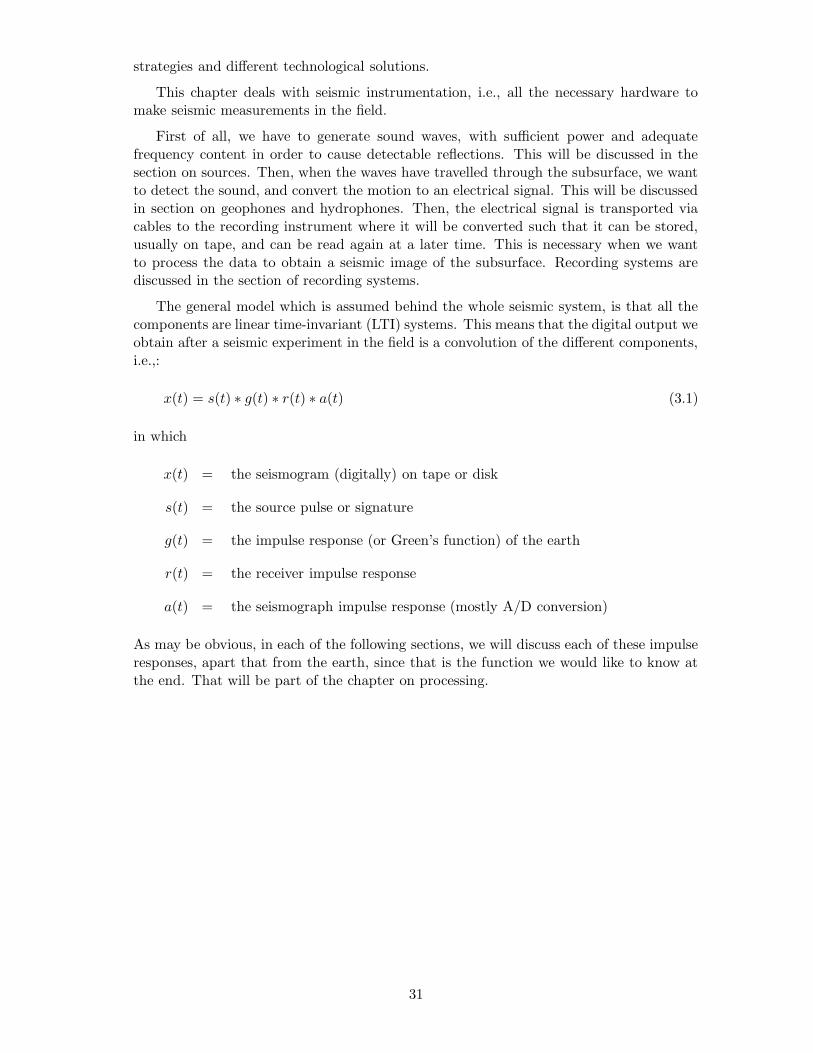
As is obvious from the name, the driving mechanism of the airgun is supplied by(compressed) air. In Figure (3.2) we have given a schematic view of an airgun. Air underpressure is pumped into a chamber. Using the piston, the air is suddenly released and theair leaves the chamber and starts to create a bubble in the surrounding water. Inside thebubble we have the air but there is a turbulent region which consists of many little bubbles,the non-linear zone. This is schematically given in figure (3.3) (a). The mechanism behindthe behaviour of the airgun is depicted in figure (3.3) (b) and (c). The bubble increases inthe beginning but after a while the pressure from outside, the hydrostatic pressure, is largerthan the pressure from inside of the bubble and the expansion slows down. The expansioncomes to an end and the bubble reaches its maximum radius when the kinetic energy ofthe outward moving water is fully converted into potential energy related to bubble radius,hydrostatic pressure and some heat losses. From there on, the bubble starts to collapsesince the hydrostatic pressure from outside is larger than the pressure inside. The collapseslows down when we have again passed the equilibrium position (where the pressure insidethe bubble is equal to the hydrostatic pressure) until we have reached a minimum radiuswhere it will start to expand again, and so on.

The collapses and expansions will not go on forever because of the heat dissipation

32

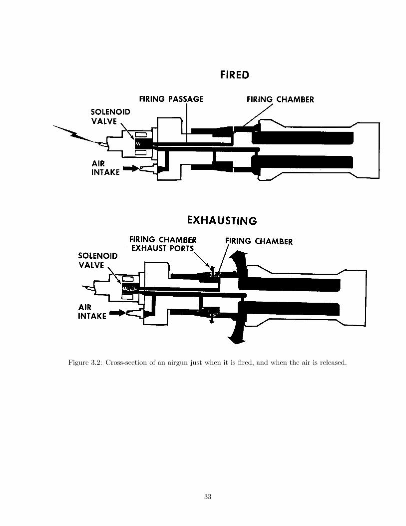
Figure 3.2: Cross-section of an airgun just when it is fired, and when the air is released.

33

NONLINEARZONE

BUBBLE

LINEAR ZONE

PH

R(t)

Radi

us

time time

Pres

sure

0

T

(a)

(b) (c)

implosionsexplosion

Figure 3.3: (a) Schematic section of the released air bubble; the radius (b) and the pressure(c) as a function of time for the air bubble of an airgun.

34

into the water. The result from this behaviour is a damped oscillatory pressure signal,somewhat similar to a damped sine curve. The behaviour is depicted in the figure (3.3)(b) and (c), where both bubble radius and the pressure have been plotted as a function oftime.

The signal from an airgun

The signal from a single airgun has a length of some 200 ms. Of course, this dependson the type of airgun and the pressure of the air supplied to the airgun. The larger thesize, i.e. airgun airchamber volume, or the higher the pressure the longer the period in theoscillations (or, the lower the frequency content). Common pressures are 2000 and 3000psi. The gun sizes are specified airchamber volume. Common values are 10, 20, 30 upto 100 cubic inches. Much used by many contractors these are the so-called sleeve guns.With the sleeve gun, as the name suggests, the air escapes via a complete ringed opening.

The signature resulting from one airgun is an oscillatory signal which does not resemblethe ultimate goal: creating a short seismic signature, preferably a delta pulse. This is themain reason why arrays are used. Airguns of different sizes and at different distancesfrom each other are used such that the first pressure peaks coincide but the other peakscancel, i.e., destructive interference for the other peaks. Usually with the design of airgunarrays, the largest gun is chosen to give the desired frequency content needed for a survey.Then smaller guns are used to cancel out the second, third, etc. peaks from this largegun. This is done in the frequency domain rather than in the time domain: a delta pulsein time corresponds to a flat amplitude spectrum in frequency. This has resulted in afew configurations of airgun arrays of which the so-called Shell array is the mostly usedone. This array has seven guns in one array. The quality of an array is measured viathe so-called primary-to-bubble ratio, that means the ratio between the first peak and thesecond-largest peak. An example of such a signature is given in Figure (3.4). These daysP/B ratios of 16 can be achieved.

35

Figure 3.4: Far-field wavelet of tuned air-gun array.

3.2.2 Vibroseis

In seismic exploration, the use of a vibrator as a seismic source has become widespread eversince its introduction as a commercial technique in 1961. In the following the principles ofthe Vibroseis1 method are treated and the mechanism which allows the seismic vibratorto exert a pressure on the earth is explained. The basic features of the force generatedby the seismic vibrator is discussed: the non-impulsive signal generated by a seismicvibrator having a duration of several seconds. Finally, the advantages and disadvantagesof Vibroseis over most impulsive sources are discussed.

The vibrator is a surface source, and emits seismic waves by forcing vibrations of thevibrator baseplate which is kept in tight contact with the earth through a pulldown weight.The driving force applied to the plate is supplied either by a hydraulic system, which isthe most common system in use, or an electrodynamic system, or by magnetic levitation.The direction in which the plate vibrates can also vary: P wave vibrators (where themotion of the plate is in the vertical direction) as well as S wave vibrators (vibrating inthe horizontal direction) are used. Finally, a marine version of the seismic vibrator hasbeen developed, however not in frequent use. For all these vibrator types, the generalprinciple which governs the generation of the driving force applied to the plate (usuallyreferred to as the baseplate) can be described by the configuration shown in Figure (3.5).A force F is generated by a hydraulic, electrodynamic or magnetic-levitation system. Areaction mass supplies the system with the reaction force necessary to apply a force on theground. The means by which this force is actually generated is illustrated in Figure (3.6),

1Registered trademark of Conoco Inc.

36

BASEPLATE

REACTION MASS

F

F

earth surface

Figure 3.5: The force-generating mechanism of the seismic vibrator source.

in which the principle of the hydraulic drive method is shown. By pumping oil alternatelyinto the lower and upper chamber of the piston, the baseplate is moved up and down.The fluid flow is controlled by a servo valve. The driving force acting on the baseplate isequal and opposite to the force acting on the reaction mass, as can easily be inferred fromFigure (3.6). In general, the peak force is such that the accelerations are in the order ofseveral g’s, so that an additional weight has to be applied to keep the baseplate in contactwith the ground. For the hydraulic and electrodynamic vibrators, the weight of the truckis used for this purpose. This weight, commonly referred to as the holddown mass, isvibrationally isolated from the system shown in Figure (3.6) by an air spring system witha low spring stiffness (shown in figure (3.7)), and its influence on the actual output of thesystem is usually neglected. The resonance frequency of the holddown mass is in the orderof 2 Hz, the lowest frequency of operation in Vibroseis seismic surveys for explorationpurposes being usually not less than 5 Hz.

The force exerted on the baseplate

The mechanism by which the seismic vibrator applies a force to the baseplate is verycomplicated, and differs for different vibrators. In this section, the applied force is de-scribed using a simplified mechanical model for a hydraulic P wave vibrator.

A model of a compressional wave vibrator is introduced here which describes thedifferent components of the vibrator in terms of masses, springs and dashpots (i.e. shockabsorbers). The model, shown in Figure (3.8), contains three masses. These are theholddown mass, which represents the weight of the truck and is used to keep the baseplatein contact with the ground; the reaction mass, which allows the vibrator to exert a force

37

BASEPLATE

PISTON

REACTIONMASS

FLUID PRESSUREFROMSERVO VALVE

Figure 3.6: Schematic view of the generation of the driving force for a hydraulic vibrator.

Figure 3.7: (a) schematic view of the Vibroseis truck with the air springs, the baseplateand the vibrator actuator (reaction mass), and (b) detailed view of the middle part of thetruck.

38

BASEPLATE

REACTIONMASS

HOLDDOWNMASS

K

f3

f3

s2

f2

f2

s1

f1

f1

i

f

f

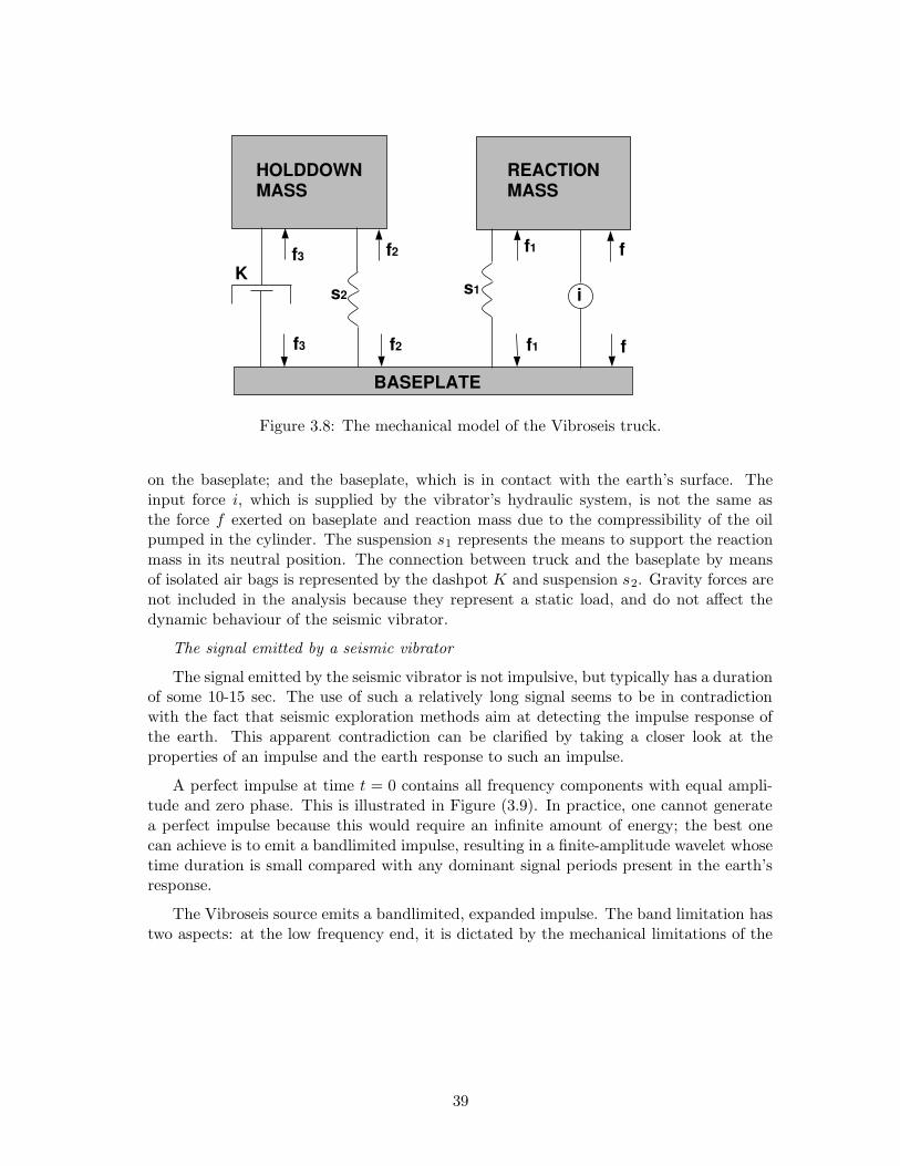
Figure 3.8: The mechanical model of the Vibroseis truck.

on the baseplate; and the baseplate, which is in contact with the earth’s surface. Theinput force i, which is supplied by the vibrator’s hydraulic system, is not the same asthe force f exerted on baseplate and reaction mass due to the compressibility of the oilpumped in the cylinder. The suspension s1 represents the means to support the reactionmass in its neutral position. The connection between truck and the baseplate by meansof isolated air bags is represented by the dashpot K and suspension s2. Gravity forces arenot included in the analysis because they represent a static load, and do not affect thedynamic behaviour of the seismic vibrator.

The signal emitted by a seismic vibrator

The signal emitted by the seismic vibrator is not impulsive, but typically has a durationof some 10-15 sec. The use of such a relatively long signal seems to be in contradictionwith the fact that seismic exploration methods aim at detecting the impulse response ofthe earth. This apparent contradiction can be clarified by taking a closer look at theproperties of an impulse and the earth response to such an impulse.

A perfect impulse at time t = 0 contains all frequency components with equal ampli-tude and zero phase. This is illustrated in Figure (3.9). In practice, one cannot generatea perfect impulse because this would require an infinite amount of energy; the best onecan achieve is to emit a bandlimited impulse, resulting in a finite-amplitude wavelet whosetime duration is small compared with any dominant signal periods present in the earth’sresponse.

The Vibroseis source emits a bandlimited, expanded impulse. The band limitation hastwo aspects: at the low frequency end, it is dictated by the mechanical limitations of the

39

δ(t)

ampl

itude

ampl

itude

frequency

1

frequency

phas

e

. . . .0time

. .. .

(a) (b) (c)

Figure 3.9: The notion of a perfect impulse, (a) in the time domain, and (b),(c) itscorresponding frequency domain version.

system and the size of the baseplate. The high frequency limit is determined by the massand stiffness of the baseplate, the compliance of the trapped oil volume in the drivingsystem for a hydraulic vibrator and mechanical limitations of the drive system.

The notion of an ”expanded ” impulse can be explained in terms of the amount ofenergy per unit time, known as energy density. In an impulsive signal, all energy is concen-trated in a very short time period, leading to a very high energy density. In the Vibroseismethod, a comparable amount of energy is transmitted over a longer time (i.e., smearedout over a longer time), so that the energy density of the signal is reduced considerably.This reduction in energy density is achieved by delaying each frequency component with adifferent time delay, while keeping the total energy contained in the signal constant. Thus,instead of emitting a signal with a flat amplitude spectrum and a zero phase spectrum, asignal is created which has the same flat amplitude spectrum in the frequency band of in-terest, however having a non-zero phase spectrum. The frequency-dependent phase shiftscause time delays which enlarge the duration of the signal. However, the total energyof the signal is determined only by its amplitude spectrum (Parseval’s theorem!). Theeffect of the increased time duration of the emission on the recorded seismogram has tobe eliminated. This is achieved by having full control of the phase function of the emittedsignal. Then, the signal received at the geophone can be corrected for the non-zero phasespectrum of the source wavelet by performing a cross-correlation process of the receivedseismogram and the outgoing signal (source signal). To clarify this point, let the sourcewavelet be denoted by s(t). If the convolutional model is adopted to describe the response

40

at the geophone, x(t), the following expression is obtained in the absence of noise:

x(t) = s(t) ∗ g(t) (3.2)

where g(t) denotes the impulse response of the earth, i.e., the layered geology, and ∗denotes a convolution. Transforming equation (3.2) to the frequency domain yields

X(ω) = S(ω)G(ω) (3.3)

If the received signal x(t) is cross-correlated with the source signal s(t), the signal c(t) isobtained which, in the frequency domain, is given by

C(ω) = X(ω)S∗(ω) = |S(ω)|2G(ω) (3.4)

since cross-correlation of x(t) with s(t) in the time domain corresponds to a multiplicationin the frequency domain of X(ω) with the complex conjugate of S(ω). In this equation,the complex conjugate is denoted by the superscript ∗. This cross-correlation is merely aspecial deconvolution process, in which we exploit the feature that we send out a signalwhose amplitude spectrum is constant. This can be seen by looking at the deconvolutionas discussed in the chapter on Fourier theory. Applying the deconvolution filter withstabilisation constant amounts to:

F (ω)X(ω) =X(ω)S∗(ω)

S(ω)S∗(ω) + ε2. (3.5)

It can be seen here that the numerator is equal to equation (3.4), so the cross-correlationis a partial deconvolution. The main achievement of the cross-correlation is that it undoesthe phase of the signal. The denominator has the term S(ω)S∗(ω). This is a purelyreal number and therefore only affects the amplitude. In the case that the amplitude isflat, the amplitude does not depend on frequency any more and becomes a simple scalingfactor in the deconvolution process. So when the amplitude spectrum of S(ω) is flat overthe frequency band of interest , and zero outside this frequency band, it follows that bycross-correlating the measured seismogram x(t) with the source function s(t), the (scaled)bandlimited impulse response g(t) of the earth is obtained.

In Figure (3.10) the concepts are illustrated for the example of an upsweep, a signalwhich ends with a larger frequency than it started off with. An 8 sec, 10-100 Hz linearupsweep is used with a taper length of 250 msec. Figure (3.10) (a) shows the sweep.Because the oscillations in the sweep are too rapid to yield a clear picture, the frequencylimits for this figure are 1-5 Hz. Figures (3.10) (b) and (3.10) (c) show the amplitudeand phase, respectively. It can be observed from these figures that the phase indeed is aquadratic function of frequency, and that the amplitude spectrum of the sweep is constantover the bandwidth. Finally, Figure (3.10) (d) shows the autocorrelation of the sweep.

41

Figure 3.10: An 8 sec, 10-100 Hz upsweep with a taper length of 250 msec. (a) the sweepin the time domain; the frequency range for this Figure is 1-5 Hz for display purposes, (b)the amplitude spectrum of the sweep, (c) the phase spectrum of the sweep, in degrees,and (d) the autocorrelation of the sweep.

42

3.2.3 Dynamite

Until the arrival of the Vibroseis technique, dynamite was the mostly used seismic sourceon land. Dynamite itself is very cheap, the costs involved are mainly the costs of drillingthe shotholes to place the dynamite. These costs may run up so high as to make theVibroseis a good competitor of the dynamite source. Dynamite is usually used in non-urban areas for obvious reasons. A nice characteristic of dynamite is that it is resemblinga (bandlimited) form of the delta pulse, something we would ideally like to have, since weare interested in the impulse response of the earth. In this section some features of thedynamite source and the signature resulting from it will be discussed.

The chemical working of dynamite and its mechanical impact

Dynamite is a chemical composition which burns extremely fast when detonating.Typically, 1 kilogram of dynamite burns in about 20 microseconds. In this very short timeit vaporizes and generates very high pressures and temperatures. The dynamite is usuallyignited with a detonator which is a small-size charge of dynamite as well, but enough toignite the larger charge. The detonator must get a large current through it in order to beset off. For safety reasons, the detonator is designed such that a large current has to beapplied. A typical current strength is some 5 Amp.

Explosives can be classified by their chemical composition. Dynamite itself consistsof a combination of the explosives glyceroltrinitrate and glycoldinitrate. Since the com-bination of these two give a fluid, they are mixed with celluloid-nitrate and then give agelatinous material. Additives of certain (secret) components result in different types ofdynamite. Because all of these dynamites contain glyceroltrinitrate, contact with the skinor inhalation, causing head aches, must be avoided.

Since the burning of the dynamite takes place in a very short time generating suddenhigh pressures and temperatures, it is obvious that in the ground, immediately aroundthe explosive a non-linear zone is created, that means the rock or soil will have undergonesome permanent change by the explosion. Three processes are at work there: deformationof the material, conversion of work into heat and geometrical spreading. There will be adistance from the source where there will be no deformation any more; this is given infigure (3.11). The behaviour of the dynamite as a function of time is given in the lowerof figure (3.11). In time, we first have an intense shock wave with a complete shatteringof the rock or soil. Then, at a certain time, we get two effects, namely a cavity expansionand anelastic rock deformation, until we reach finally a time where we left a cavity whichstays there, and an elastic wave originating from this area. So there will always be a cavityleft when using dynamite. This cavity is not the same as the radius where the anelasticwave becomes an elastic wave. There has actually been some people who have dug outthese cavities in order to see how the cavity changed with a different charge of dynamite.It turned out that the cavity radius was proportional to the cube root of the charge mass.

The dynamite signature

Let us now look at the pressure resulting from a dynamite explosion. It will not be

43

a

ELASTIC RADIUS r

LINEARZONE

NONLINEARZONE

intenseshockwave

anelasticrockdeformation

cavity expansion

anelastic stress wave

elastic wave

a

RADI

US (r

)

(a)

(b)TIME (t)0

Figure 3.11: The behaviour of dynamite: (a) the characteristic zones in space, and (b) theradius as a function of time with its characteristic zones.

44

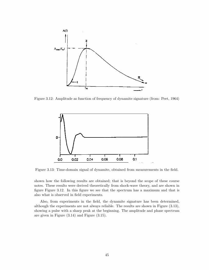
Figure 3.12: Amplitude as function of frequency of dynamite signature (from: Peet, 1964)

Figure 3.13: Time-domain signal of dynamite, obtained from measurements in the field.

shown how the following results are obtained; that is beyond the scope of these coursenotes. These results were derived theoretically from shock-wave theory, and are shown infigure Figure 3.12. In this figure we see that the spectrum has a maximum and that isalso what is observed in field experiments.

Also, from experiments in the field, the dynamite signature has been determined,although the experiments are not always reliable. The results are shown in Figure (3.13),showing a pulse with a sharp peak at the beginning. The amplitude and phase spectrumare given in Figure (3.14) and Figure (3.15).

45

Figure 3.14: Amplitude spectrum of dynamite signature.

Figure 3.15: Phase spectrum of dynamite signature.

46

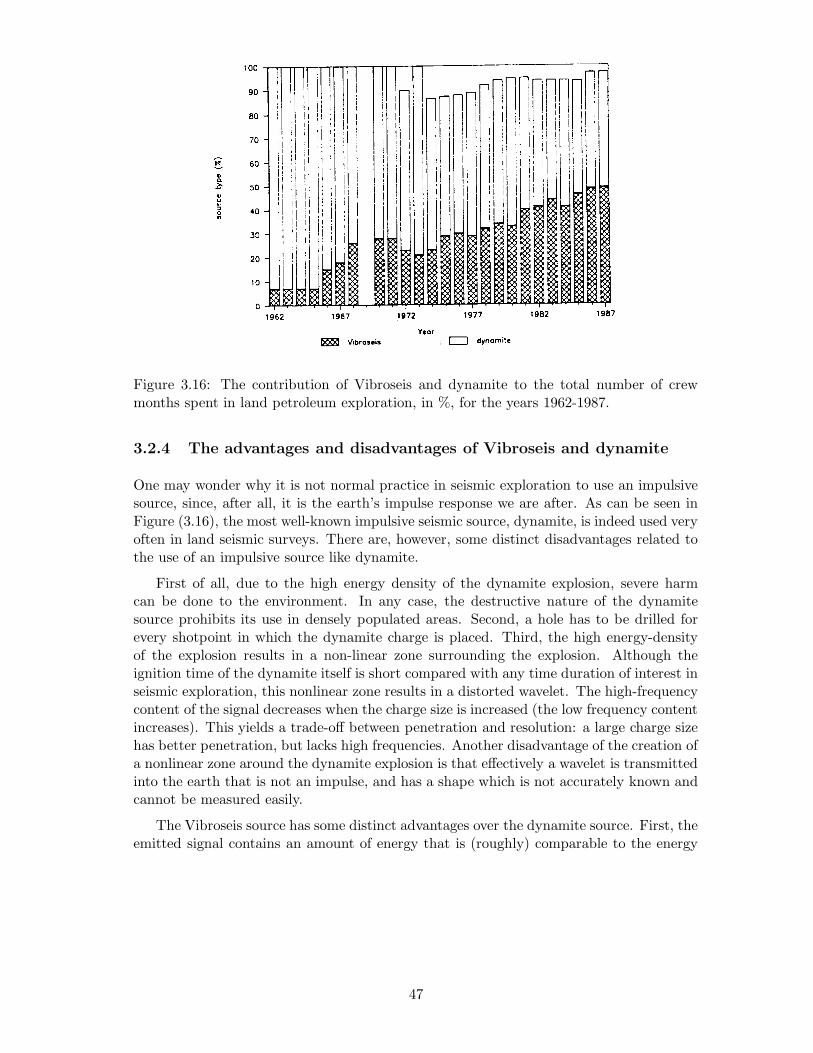
Figure 3.16: The contribution of Vibroseis and dynamite to the total number of crewmonths spent in land petroleum exploration, in %, for the years 1962-1987.

3.2.4 The advantages and disadvantages of Vibroseis and dynamite

One may wonder why it is not normal practice in seismic exploration to use an impulsivesource, since, after all, it is the earth’s impulse response we are after. As can be seen inFigure (3.16), the most well-known impulsive seismic source, dynamite, is indeed used veryoften in land seismic surveys. There are, however, some distinct disadvantages related tothe use of an impulsive source like dynamite.

First of all, due to the high energy density of the dynamite explosion, severe harmcan be done to the environment. In any case, the destructive nature of the dynamitesource prohibits its use in densely populated areas. Second, a hole has to be drilled forevery shotpoint in which the dynamite charge is placed. Third, the high energy-densityof the explosion results in a non-linear zone surrounding the explosion. Although theignition time of the dynamite itself is short compared with any time duration of interest inseismic exploration, this nonlinear zone results in a distorted wavelet. The high-frequencycontent of the signal decreases when the charge size is increased (the low frequency contentincreases). This yields a trade-off between penetration and resolution: a large charge sizehas better penetration, but lacks high frequencies. Another disadvantage of the creation ofa nonlinear zone around the dynamite explosion is that effectively a wavelet is transmittedinto the earth that is not an impulse, and has a shape which is not accurately known andcannot be measured easily.

The Vibroseis source has some distinct advantages over the dynamite source. First, theemitted signal contains an amount of energy that is (roughly) comparable to the energy

47

contained in a dynamite signal. Because of the use of an expanded impulse, the energydensity of the source wavelet in the Vibroseis technique is much less than the energy densityof the dynamite wavelet. Therefore, destructive effects are much less severe. Secondly,Vibroseis provides us with a direct means to measure and control the outgoing wavelet.Thirdly, there is no need to drill holes when using Vibroseis.

There are, however, also some disadvantages connected with the use of Vibroseis asa source. Firstly, a single vibrator in general does not deliver a sufficient amount ofenergy required for seismic exploration purposes, so that arrays of vibrators have to beused. Typically, 4 vibrators vibrate at each vibration location simultaneously. Second,as vibrators are surface sources, large amounts of Rayleigh waves are generated. Thegeneration of Rayleigh waves can be suppressed in a dynamite survey by placing the chargeat or below the bottom of the weathered layer. In Vibroseis surveys, the Rayleigh waveshave a very high amplitude and are an undesired feature on the seismogram. Thirdly,the Vibroseis method can be employed only in areas which are accessible to the seismicvibrator trucks, whose weight may exceed 20 tons. Fourth, correlation noise (i.e. the noisegenerated by the correlation process that converts the Vibroseis signal into a pulse) limitsthe ratio between the largest and smallest detectable reflections.

In spite of many disadvantages, the Vibroseis method is now a standard method inthe seismic exploration for hydrocarbons. In 1987, Vibroseis was used more often inland seismics than dynamite (the contribution of Vibroseis to the total number of crewmonths spent in land seismic petroleum exploration was 49 %, whereas the contributionof dynamite was 48.3 %). The operational advantages of the Vibroseis method over theconventional dynamite survey result in an average cost per kilometre of Vibroseis whichis only two-thirds of the cost per kilometre for a dynamite survey (figures for 1987). Also,the average number of kilometres that can be covered per crew month is 30 % higher forVibroseis surveys than it is for dynamite surveys (figures for 1987). This cost-effectivenessand efficiency, together with the increasing importance of signal control in the search forhigher resolution of seismic data and the non-destructive character of the method explainsthe increasing popularity of Vibroseis. In table (3.1) the advantages and the disadvantagesof the Vibroseis and dynamite are tabulated.

48

Advantages Disadvantages

Vibroseis 1. Less destructive than dynamite : 1. One truck does not deliver enoughcan operate in urban areas energy : arrays, so directivity2. Not labour-intensive : cheap in 2. Surface source : many Rayleigh wavesoperation 3. Can only operate in areas which can3. Some control over outgoing signal support 20 tons

4. Correlation imperfect : correlation noise

Dynamite 1. Buried source : much less surface 1. Destructive : cannot operate in urbanwaves generated than Vibroseis areas2. Signal close to δ-pulse 2. Labour intensive for making shotholes :

expensive in operation

Table 3.1: Advantages and disadvantages of Vibroseis and dynamite

49

3.3 Seismic detectors

The source generates a mechanical disturbance which propagates in the ground, is re-flected, refracted or diffracted, and returns to the surface. When the disturbance prop-agates in a fluid such as water a temporary variation of pressure is created. Elasticdeformation results in movements of the surface and at some point of the surface theacceleration, the velocity or the displacement of a point can be measured. In any case,whether a movement or a variation of pressure is observed, we have to represent it bysome other physical quantity which can be easily stored and manipulated. Consideringthe development of electronic technology, a representation by an electrical voltage is evi-dently a good solution. The first field component of a seismic data acquisition system isthe detector group. The detectors convert the seismic disturbance into a voltage of whichthe variations represent faithfully the variations of the mechanical disturbance detected,a voltage which is the analog of the seismic disturbance.

The detectors used for seismic exploration work are called geophones since they areused to ”hear” echoes from the earth underneath. Sometimes, they are called seismometersbut this term is more often applied to long period seismographs used for recording naturalearthquakes. The term ”detector” applies to all types of seismic-to-electrical transducers.From what has been said before, it will be clear that they can be classified into two maingroups: motion-sensitive, mainly for land operations, and pressure-sensitive for operationsin water (or fluids), be it for marine seismic work or in the mud column of a borehole, forwell-shooting or a VSP. Pressure-sensitive geophones are also called hydrophones.

The types of detectors commonly used in practice, are electromagnetic and piezoelectrictransducers and we shall omit all others. Piezoelectric transducers which are pressure-sensitive are used as hydrophones and electromagnetic transducers are used on land. In themoving coil geophone of the electromagnetic type, a voltage is generated by the movementof a conductor in a strong permanent magnetic field. These types are used nowadays.

Geophones are the parts of the system which undergo the roughest treatment. Theyare planted and picked up many times, they are flung down, run over by the trucks,stamped into the ground by the line men. And yet, they are expected to generate anaccurate, noise-free reproduction of the earth movements. They are built to withstandrough handling but a minimum of care on the part of the line men can help in obtaininggood quality data.

50

coil

case

NS S

Figure 3.17: Schematic cross-section of a moving-coil geophone.

3.3.1 Geophones

A moving coil geophone (Figure 3.17) operates according to the principle of a microphoneor a loudspeaker: the coil consisting of copper wire wound on a thin non-conductingcylinder (”former”) moves in the ring-shaped gap of a magnet. Figure 3.17 is the crosssection of a cylindrical structure. The annular magnet and polar pieces N and S in softiron create a radial field in the gap. The only movement allowed for the coil, suspendedfrom springs not shown in the picture, is a translation along the direction of the axis andin the gap. As the coil moves, its windings cut magnetic lines of force and an electromotiveforce is generated. The output voltage is proportional to the rate at which the coil cutsthe lines of magnetic force, that is to say, proportional to the velocity at which it moves.Therefore this type of detector is known as ”velocity geophone”.

The main parts of the geophone are:

• the moving mass, made up by the coil and the ”former” on which it is wound;

• the coil suspension, usually two flat springs, one at the top and one at the bottom,to avoid lateral displacement of the coil;

• the case, with the magnet and polar pieces inside a cylindrical container whichprotects the other elements against dust and humidity.

The case is placed on the ground and is supposed to follow the ground movementexactly (Figure 3.18). The output voltage is proportional to the velocity of the massrelative to the case and what we are interested in is this relative movement as a functionof the movement of the case.

A complete description of geophones must take into account many phenomena beyondthe scope of these lecture notes. The final design of a geophone is usually a compromise

51

M

ground

spring

Figure 3.18: The geophone on the ground.

between conflicting requirements. For a geophysicist it is often sufficient to know the basicoperating principle of the geophone in order to understand the behaviour of this componentas part of the whole data acquisition network. Consequently, the considerations whichfollow are restricted to the response of an ideal geophone.

Assuming the vertical component of the velocity is:

vz =dz

dt, (3.6)

and the output voltage is given by V , the conversion of the motion to the electric signaltakes place via the transfer function:

R(ω) =Voltage

Particle Velocity=

V (ω)

vz(ω)=

ω2K

ω2 − 2ihωω0 − ω20

(3.7)

where ω0 is the resonance frequency of the spring, and K and h are some constants depend-ing on mechanical and electrical components; K represents a sensitivity (proportionalityconstant) and h a damping factor. Consider now three situations:

ω → 0 : R(ω) → −ω2

ω20

K =ω2

ω20

K exp(πi)

ω = ω0 : R(ω) → K

−2ih=

K

2hexp(πi/2) (3.8)

ω → ∞ : R(ω) → K

52

Figure 3.19: Amplitude response of geophone at constant velocity drive (From: Pieuchot,1984)

These are depicted in Figure 3.19 and Figure 3.20. The received voltage is proportionalto the velocity of the ground only at frequencies well above the resonance frequency ofthe geophone. At these frequencies the constant K is the sensitivity of the geophone, withunits of, for example, volts/mm/s.

53

Figure 3.20: Phase response of geophone at constant velocity drive (From: Pieuchot, 1984)

3.3.2 Hydrophones

As has been shown in the foregoing section, the geophone exhibits a flat pass-band char-acteristic from a few Hertz above the resonance frequency to the spurious frequency. Inthat pass-band the output voltage VGeop is proportional to the particle velocity v:

VGeop = constant · vz (3.9)

We will show in the next paragraph that in the pass band of the hydrophone, the outputvoltage VHydr is proportional to the acoustic pressure p, i.e.,:

VHydr = constant · p (3.10)

Hydrophones are thus pressure-sensitive detectors and they are used for operations inwater-covered areas.

At present often hydrophones with ceramic pressure sensitive elements are used. Theyoperate on the principle of piezoelectricity. A piezoelectric material is one which producesan electrical potential when it is submitted to a physical deformation. The phenomenonis observable in some crystalline structures such as quartz and tourmaline and is used inrecord player pick-ups. It can also be produced by in artificially-made poly-crystallineceramics after they have been submitted to a high-intensity electric field (several tens ofthousands volts per centimeter). The most commonly used material in seismic applica-tions, is lead zirconate titanate (PZT).

54

−

(a)

+ +

(b)

−

poling axis

+

−

(c)− +

0 0+ −

compressive force

a

tensile forceb

compressiveforce

d

tensile forcec

Figure 3.21: Piezoelectric voltages from applied force. (a) Output voltage of same polarityas poled element; (b) output voltage of opposite polarity as poled element.

When compressive and tensile forces are applied to the ceramic element, it generatesa voltage. Refer to Figure 3.21. A voltage with the same polarity as the poling voltageresults from a compressive force (a) applied parallel to the poling axis, or from a tensileforce (b) applied perpendicular to the poling axis. A voltage with the opposite polarityresults from a tensile force (c) applied parallel to the poling axis, or from a compressiveforce (d) applied perpendicular to the poling axis. The magnitude of piezoelectric forces,actions, and voltage is relatively small. For example, the maximum relative dimensionalchanges of a single element are in the order of 10−8. Amplification is often required andaccomplished by other components in the system, such as electronic circuits. In some cases,the design of the ceramic element itself provides the required mechanical amplification.The use of ceramic elements as seismic (pressure) detectors / hydrophones is based onthese principles.

Figure 3.22 represents the cross section of a typical piezo-electric hydrophone. Itconsists of a plate of the piezo-electric ceramic placed on an elastic electrode. The activeelement is deformed by pressure variations in the surrounding water and it produces avoltage collected between the electrode and a terminal bonded to the other face. Theelectrode rests on a metallic base which supports its ends and also limits the maximumdeformation so as to avoid breaking the ceramic, even if the hydrophone is accidentallysubmitted to high pressures (when the streamer is broken and drops to the bottom forinstance).

With its mass, the active element produces a voltage not only under a variation ofpressure but also when it is subjected to acceleration. In offshore operations, with the

55

Figure 3.22: Schematic cross-section of a piezoelectric hydrophone (From: Pieuchot, 1984)

E VRC

Figure 3.23: Simplified circuit for deriving the hydrophone response.

boat movements and the waves, the hydrophones are continually subjected to accelerationsand this would create a high level of noise in the absence of any compensation. Theprotection against acceleration is obtained by assembling two elements as shown in thefigure. The voltage produced by an acceleration cancel each other whereas those producedby a pressure wave add.

As with the geophones in land operations, the hydrophones are always assembled inmultiple arrays at each trace. They are often assembled so as to increase the capacitance(more hydrophones in parallel than in series) and decrease the low-frequency cut-off. Thenetwork model for the hydrophone is given in Figure 3.23.

56

V/E is the transfer function since E represents the variations of pressure in the water.From the circuit given in Figure 3.23, the transfer function R(ω) can be derived:

R(ω) =Voltage

Pressure=

V

E=

R

R + 1iωC

=iωCR

1 + iωCR(3.11)

Consider now three situations:

ω → 0 :V (ω)

E→ iωCR = ωCR exp(πi/2)

ω = 1/CR :V (ω)

E→ i

1 + i=

1

2

√2 exp(πi/4) (3.12)

ω → ∞ :V (ω)

E→ 1

The amplitude and phase response are given in Figure 3.24.

It is now interesting to compare this response to the one from the geophone. At lowfrequencies the responses are out of phase by π/2, decreasing to π/4 at higher frequenciesand in phase at high frequencies. This can be important when comparing two seismicsections, one shot on land and the other one shot at sea.

57

-2 0 2

0

log VE

log ω/ω0

-1

-2 0 2

π /2

π /4arg(V/E)

log ω/ω0

Figure 3.24: Amplitude and phase response of a hydrophone.

58

3.4 Seismic recording systems

The modern seismic data recording system is a compound of electric subsystems (am-plifiers, filters, etc.). The (glasfibre) cable system may often be considered integral partof it. It has as input analog electrical signals from the seismic detectors (see section ongeophones and hydrophones) and puts digital data out on magnetic tape. Nearly all sys-tems offer the facility of instant data verification through the creation of output on paperrecord, the so-called ”monitor recording”.

In a very general sense, a recorder consists of several parts, namely amplifiers, filtersand an A/D converter, before it is stored on (magnetic) tape. The analog signal comesfrom the geophones into the system, where it is first amplified. The data can be filtered,the most important one being the anti-alias (high-cut) filter. Then the data is convertedto a digital signal using the A/D converter, giving digital data which can be stored ondisc or computer tape.

3.4.1 (Analog) filters

An important setting of a data recording system is that of different filters. The filters areanalog filters. Some of these filters may be predetermined but others must be left at thediscretion of the user and must be adjustable in the field. These filters can be categorisedinto two groups, namely passive and active filters. Passive filters are built from passiveelectrical elements: resistors, capacitors and coils. Active filters have an amplifier as anintegral part of the filter. Usually there are three types of filters available to the user inthe field: low-pass (high-cut), notch and high-pass (low-cut) filters.

In the following the principles of passive filters will be dealt with. Let us look at ageneral scheme of a filter by considering figure (3.25). When a potential difference E is putover a series connection of two passive elements with impedances Y and Z, and when wemeasure the potential difference V over the Y component, the ratio of the two potentialsis given by:

V

E=

Y

Z + Y(3.13)

The components Y and Z can be any components as tabulated in appendix C.

For a resistance, the impedance is R, for an inductance iωL, and for a capacitance1/iωC. So, when the component Y is an capacitance and Z a resistance, the measuredpotential difference is a ”high-cut” (or ”low-pass”) version of the input voltage E. Thiscan be seen by substituting the values in the above equation:

V

E=

1iωC

1iωC + R

=1

1 + iωCR(3.14)

59

E

Z

Y V

Figure 3.25: A passive filter.

which is a ratio, dependent on the frequency ω. When we write this in polar coordinates,we get:

V

E=

1

1 + iωCR

1 − iωCR

1 − iωCR=

1

1 + ω2C2R2+i

−ωCR

1 + ω2C2R2=

1

(1 + ω2C2R2)1/2exp(iφ)(3.15)

where φ is the phase angle. When ω is small, then ωCR can be neglected compared to 1in the amplitude factor and thus, V/E behaves like 1 (amplitudewise). When ω is largethen 1 can be neglected compared to ωCR, and the numerator approaches ωCR so V/Ewill behave like 1/ω. This is thus a high-cut filter.

In the same way we can derive that when Y is a resistor, the filter acts as a low-cut orhigh-pass filter. It is customary to specify a filter by its so-called corner frequency, i.e., thefrequency where ωLCR = 1. With a high-cut filter as above, the signal will be significantlydamped above this frequency, with a low-cut filter the signal will be significantly dampedbelow this frequency. The foregoing filter was an example of a passive filter, i.e., a filterbuilt-up of passive elements (R, L, C).

Why do we need these filters in our geophysical measurements? Let us discuss themseparately, first the low-cut filter. As the name says, low-frequency waves can be sup-pressed with these filters. On land, filtering is sometimes applied to suppress the surfacewaves or ground roll, although there is a preference for keeping surface waves in the seis-mogram and remove them later during processing. At sea, a low-cut filter is needed tosuppress the waves at the surface of the sea itself.

A most important filter is the anti-alias filter, needed for proper sampling in time ofthe seismic signal. Aliasing of the seismic signal should be avoided when we sample it intime. This means that the highest frequency in the signal should at least be sampled with 2samples per full period. But we do not know the frequency content of our signal beforehandand therefore we make sure, using a high-cut filter, that above a certain frequency, the

60

Figure 3.26: The time-domain aspect of aliasing.

signal is suppressed below a certain level. The high-cut filter must reduce the signalabove the Nyquist frequency below the noise level. The Nyquist frequency is given by:fN = 1/2∆t. The effect of aliasing in the time domain is illustrated in figure (3.26). Oncethe frequency content of the signal is suppressed sufficiently above the Nyquist frequency,digitizing the data makes real sense. Because of this application, this filter is also called ananti-alias filter or just alias filter. This filter must always be set according to the samplingrate.

Another type of filter which is usually present in a seismic recording system, is thenotch filter. Once in a while, it can happen that 50 or 60 Hz interference from powercables is disturbing the seismic measurement (Europe 50 Hz, America 60 Hz). Wheninput balancing circuits, cable screening fails to cure this problem, it is possible to use anactive steep-flank so-called ”notch filter” to cut the signal at these frequencies. It shouldbe noted however that by cutting the signal before recording, we may also cut valuableinformation from our data and we may never be able to retrieve it later on.

61

V

E

E/2

E/2+

E/4

E/2+

E/8

E/2+

E/8+

E/16

1 0 1 00

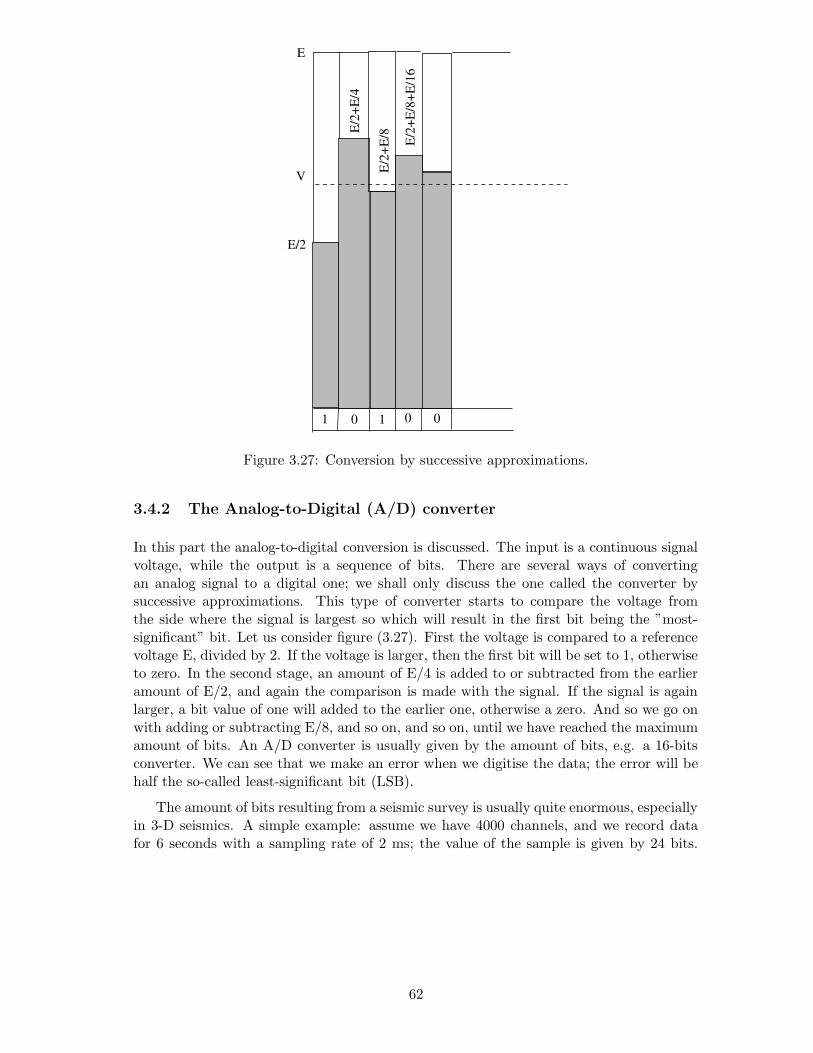
Figure 3.27: Conversion by successive approximations.

3.4.2 The Analog-to-Digital (A/D) converter

In this part the analog-to-digital conversion is discussed. The input is a continuous signalvoltage, while the output is a sequence of bits. There are several ways of convertingan analog signal to a digital one; we shall only discuss the one called the converter bysuccessive approximations. This type of converter starts to compare the voltage fromthe side where the signal is largest so which will result in the first bit being the ”most-significant” bit. Let us consider figure (3.27). First the voltage is compared to a referencevoltage E, divided by 2. If the voltage is larger, then the first bit will be set to 1, otherwiseto zero. In the second stage, an amount of E/4 is added to or subtracted from the earlieramount of E/2, and again the comparison is made with the signal. If the signal is againlarger, a bit value of one will added to the earlier one, otherwise a zero. And so we go onwith adding or subtracting E/8, and so on, and so on, until we have reached the maximumamount of bits. An A/D converter is usually given by the amount of bits, e.g. a 16-bitsconverter. We can see that we make an error when we digitise the data; the error will behalf the so-called least-significant bit (LSB).

The amount of bits resulting from a seismic survey is usually quite enormous, especiallyin 3-D seismics. A simple example: assume we have 4000 channels, and we record datafor 6 seconds with a sampling rate of 2 ms; the value of the sample is given by 24 bits.

62

Then the total amount of samples per shot would be : 4000 x 6 x 500 x 24 = 288 · 106

bits = 288 Megabits per record (shot). This is quite an amount of data, realizing thatthis is recorded for each shot and offshore, where shots are fired roughly every 10 seconds,thousands of shots are fired.

63

3.5 Total responses of instrumentation

In the beginning of this chapter, we defined a general model that was assumed behind thewhole seismic system, namely a convolution of the different responses, i.e.,

X(t) = S(t) ∗ G(t) ∗ R(t) ∗ A(t) (3.16)

where the responses were defined in the introduction (eq. (3.1)). A convolution in time isequivalent to a multiplication in the Fourier domain, see the chapter on Fourier analysis.Therefore the seismogram can be written in terms of frequencies as:

X(ω) = S(ω)G(ω)R(ω)A(ω) (3.17)

We see that the seismogram consists of (complex) multiplications of the individual transferfunctions. Since the multiplications are complex, it can be written as a multiplication ofamplitudes and adding of phases, i.e,:

X(ω) = |S(ω)||G(ω)||R(ω)||A(ω)| exp(iφS) exp(iφG) exp(iφR) exp(iφA)

= |S(ω)||G(ω)||R(ω)||A(ω)| exp{i(φS + φG + φR + φA)} (3.18)

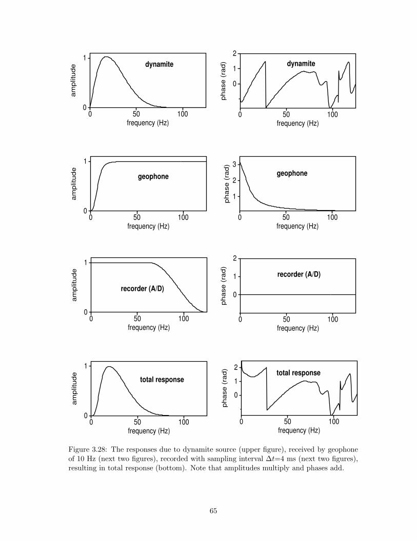
where the symbols φi denote the phase of the component i. In figure 3.28, we have givenan example of such a system. In the figure we have taken the example of a recording thatis made with dynamite, detected with a geophone and recorded with a certain samplinginterval (with then the Nyquist frequency following as 1/2∆t). From this example, we cansee that the source is mostly determining the total response. The geophone mostly affectsthe low frequencies.

64

0 50 100frequency (Hz)

0

1

ampl

itude

0 50 100frequency (Hz)

0

1

2

phas

e (r

ad)

0 50 100frequency (Hz)

1

2

3

phas

e (r

ad)

0 50 100frequency (Hz)

0

1

2

phas

e (r

ad)

0 50 100frequency (Hz)

012

phas

e (r

ad)

0 50 100frequency (Hz)

0

1

ampl

itude

0 50 100frequency (Hz)

0

1

ampl

itude

0 50 100frequency (Hz)

0

1

ampl

itude

dynamite dynamite

geophone geophone

recorder (A/D)

recorder (A/D)

total responsetotal response

Figure 3.28: The responses due to dynamite source (upper figure), received by geophoneof 10 Hz (next two figures), recorded with sampling interval ∆t=4 ms (next two figures),resulting in total response (bottom). Note that amplitudes multiply and phases add.

65