seismic design of deep bridge pier foundations in...

Seismic Design of Deep Bridge Pier Foundations in Seasonally Frozen Ground

FINAL REPORT

Prepared for

Alaska University Transportation Center

Alaska Department of Transportation and Public Facilities

Aaron Shelman Jared Levings Sri Sritharan

Iowa State University

Department of Civil, Construction and Environmental Engineering

Ames, IA 50011

Report # UAF08-0033

December 2010

1

ii

ABSTRACT

In the field of bridge engineering, columns supported on cast-in-drilled-hole (CIDH) shafts

are common due to the elimination of a column-foundation connection, simplicity of

construction and reduced construction costs. Due to these benefits, this combination of column

and foundation is frequently used in high seismic regions. However, the modeling of lateral load

behavior of the column-shaft system is a complex matter due to the effects of soil-foundation-

structure-interaction (SFSI) and temperature effects. The research presented within this project

report identifies numerous challenges associated with the current state of practice of accounting

for SFSI in cohesive soils, develops a new method that accounts for SFSI in cohesive soils,

examines the current state of cohesionless soil models, examines temperature effects on

construction material behavior and provides a design methodology for columns supported by

CIDH shafts.

The project undertook an extensive literature review as well as an examination of codes and

guidelines to identify the challenges within current practice. Within this task, it was concluded

that existing methods are able to capture the behavior of column/shaft systems in cohesionless

soils. However, the process also found that although many models exist to simplify the use of

the Winkler soil spring concept, none of the simplified models are able to capture both the elastic

and inelastic lateral load response of an integrated column/foundation system in cohesive soils.

The challenges arose for the following reasons:

1. some models are only applicable in the elastic range;

2. models recommended for use in cohesive soils and cohesionless soils were only verified

against experimental data obtained in cohesionless soils;

3. nonlinearity of materials (i.e., soil, concrete and steel reinforcement) was not accounted

for in the development of the models; and

4. plastic action within the different methods is generally lower than what actually will be

found using a detailed analysis method such as that based on fully implementing the

Winkler spring concept.

In addition to the aforementioned shortcomings, the existing methods ignore the effects of

seasonal freezing in their development, even though it significantly alters the lateral load

response of CIDH shafts. However, it was found this approach is not appropriate, as two-thirds

3

of the bridges in the United States are affected by seasonal freezing. This problem is only further

exacerbated by the fact that half of the bridges in high seismic regions are also affected by

seasonal freezing. After identifying these issues, a new method was developed that more

accurately predicts the lateral load response of columns supported on CIDH shafts in cohesive

soils.

The new approach presented within this report uses a set of three springs to determine a

bilinear force-displacement response of the column/foundation system using minimal input

parameters about the structure and surrounding soil. The model was developed as a cantilever

supported on a flexible base located at the expected maximum moment location. First, a

rotational spring and a translational spring were placed at the maximum moment location to

capture the behavior of the foundation shaft at and below the location. The final translational

spring was located halfway between the maximum moment location and the ground surface to

capture the resistance of the soil above the maximum moment location. By basing the system on

the maximum moment location, the point at which the most damage will occur is defined. The

global response of the system, as well as the local response of the CIDH shaft over the entire

lateral loading range, is also captured.

Comparing the alternative method to results from experimental testing performed at Iowa

State University and LPILE analyses of several different systems, the new model was found to

simulate well the response of the column/foundation system in cohesive soils. The developed

method was able to predict the secant stiffness to the first yield location within 10%. Yield and

ultimate limit states were within 10% of the detailed analyses performed in LPILE (Reese et al.,

2004) and correlated well with the full-scale experimental testing performed by Suleiman et al.

(2006). The overall comparisons included multiple displacement and rotation factors, as well as

local curvatures developed near the maximum moment location. These aforementioned local

comparisons of the CIDH shaft, along with a global comparison of the entire system, were

performed to minimize any errors that occurred during model development.

The remaining parts of the project consisted of performing controlled material tests on

concrete, steel and soil specimens to examine the effects of seasonal freezing on their behavior.

These tests were performed in a laboratory environment in which the temperature during testing

was maintained and the results would provide a realistic model. In each case it was determined

4

that the material properties would experience significant changes when subjected to freezing

conditions.

The materials testing on concrete provided evidence such that an increase in strength and

modulus of elasticity occurs when subjected to seasonal freezing. However, the cracking

strain of unconfined concrete decreased. The confined concrete specimens experienced

an increase in strength, modulus and strain at peak confined compressive stress. This is

of key importance to ensure an accurate moment-curvature response of the column and

foundation shafts is obtained for design purposes.

In the steel testing it was discovered that as the specimens undergo freezing, a quadratic

increase in the yield and ultimate strengths of the material will occur while experiencing

no change in the modulus of elasticity and ultimate strain. This portion of the project

provided additional evidence to suggest that strain rate and bar diameter will affect the

overall strength gain. All of these results should be accounted for in the design process to

ensure that an accurate moment-curvature response of the column and foundation shafts

is captured.

The results of soil testing found that a significant increase in strength could be expected

at -1 °C (30.2 °F) and -20 °C (-4 °F). In these cases, it was found the warm weather value

could be multiplied by a factor of 10 and 100 to represent the soil unconfined

compressive strength at the respective temperatures. This is of great importance as these

values will greatly modify the stiffness of the system during times of seasonal freezing,

causing an upward shift in the maximum moment location and requiring a larger shear

demand to be accounted for in the column/foundation shafts.

The final portion of the project provided a series of flowcharts that should be used during the

design of columns supported on CIDH shafts. These charts were constructed such that a detailed

computer-based methodology as well as simplified methodologies can be used to account for all

seasons of the year during the design process. Therefore, these charts ensure that all possible

failure modes are examined and prevented during the seismic design of columns supported on

CIDH shafts.

5

ACKNOWLEDGEMENTS

The study reported herein was made possible through funding provided by the Alaska

University Transportation Center (AUTC) along with the Alaska Department of Transportation

and Public Facilities (ADOT&PF). Special thanks are due to Billy Connor, AUTC Director; J.

Leroy Hulsey, UAF AUTC Associate Director; Kathy Petersen, Grants Manager at AUTC; and

Elmer Marx, project manager through the ADOT&PF; Angela Parsons, research project manager

at ADOT&PF; Clint Adler, Engineer at ADOT&PF; David Stanley, Chief Engineering Geologist

for ADOT&PF.

Additional thanks are required for members of Mueser Rutledge Consulting Engineers

(MRCE), who provided their expertise and services in testing frozen soil samples in New York,

New York. These persons are Sissy Nikolaou, Associate and Director of Geoseismic

Department; James Tantalla, Lab Manager and Engineer; Yesid Ordonez, Lab Technician.

Douglas Wood, structural engineering laboratory manager at Iowa State University, provided

a great deal of help with the controlled materials testing of steel and concrete.

In addition, the authors would like to thank the following organizations for donating

materials to the project: IPC, Inc. in Iowa Falls, Iowa, for providing a high strength concrete mix

for testing; Manatt’s in Ames, Iowa, for providing two normal strength concrete mixes typically

used for bridge construction.

6

TABLE OF CONTENTS

ABSTRACT.................................................................................................................................... ii

ACKNOWLEDGEMENTS ............................................................................................................ v

TABLE OF CONTENTS............................................................................................................... vi

TABLE OF FIGURES .................................................................................................................... x

TABLE OF TABLES .................................................................................................................. xix

NOMENCLATURE .................................................................................................................... xxi

CHAPTER 1: INTRODUCTION ................................................................................................... 1

1.1 Historical Background .......................................................................................................... 1

1.2 Seismic Engineering Practices .............................................................................................. 1

1.2.1 Seismic Loading ............................................................................................................. 3

1.2.2 Capacity Design Philosophy .......................................................................................... 4

1.2.3 Behavior of Plastic Hinges ............................................................................................ 4

1.2.4 Temperature Concerns................................................................................................... 7

1.3 Types of Foundations............................................................................................................ 8

1.3.1 Shallow Foundations ..................................................................................................... 9

1.3.2 Deep Foundations ........................................................................................................ 10

1.4 Soil-Foundation-Structure-Interaction ................................................................................ 11

1.4.1 State of Practice ........................................................................................................... 12

1.4.2 Alternative Approach ................................................................................................... 15

1.5 Scope of Research............................................................................................................... 17

1.6 Report Layout ..................................................................................................................... 17

CHAPTER 2: LITERATURE REVIEW ...................................................................................... 19

2.1 Introduction......................................................................................................................... 19

2.2 Analytical Investigation ...................................................................................................... 20

2.2.1 Reese and Welch (1975)............................................................................................... 20

2.2.2 Crowther (1990)........................................................................................................... 23

2.2.3 Priestley et al. (1996)................................................................................................... 24

2.2.4 Chai (2002) .................................................................................................................. 25

2.2.5 Priestley et al. (2007)................................................................................................... 32

2.2.6 AASHTO Specifications ............................................................................................... 36

2.3 Impact of Seasonal Freezing ............................................................................................... 38

2.3.1 Effects of Seasonal Freezing ........................................................................................ 39

2.4 Broad Impacts ..................................................................................................................... 46

2.5 Material Behavior ............................................................................................................... 50

2.5.1 Concrete ....................................................................................................................... 50

2.5.2 Steel .............................................................................................................................. 53

2.5.3 Soil ............................................................................................................................... 54

2.6 Sectional Analysis Tool ...................................................................................................... 62

2.7 Pushover Analysis Tool ...................................................................................................... 64

vii

CHAPTER 3: EXAMINATION OF EXISTING METHODS ..................................................... 66

3.1 Introduction......................................................................................................................... 66

3.1.1 Example Problem ......................................................................................................... 66

3.1.2 Moment – Curvature Analysis...................................................................................... 66

3.2 Detailed Analysis ................................................................................................................ 68

3.3 Chai (2002) ......................................................................................................................... 76

3.3.1 Clay .............................................................................................................................. 76

3.3.2 Sand.............................................................................................................................. 83

3.3.3 Seasonal Freezing Capability ...................................................................................... 87

3.4 Priestley et al. (2007) .......................................................................................................... 89

3.5 ATC 32 (1996) .................................................................................................................... 94

3.6 AASHTO (2009)................................................................................................................. 95

3.7 Summary of Examination ................................................................................................... 99

CHAPTER 4: DEVELOPMENT OF A NEW SIMPLIFIED MODEL FOR CLAY SOILS .... 104

4.1 Objective ........................................................................................................................... 104

4.2 Background on Model Development ................................................................................ 105

4.2.1 Description of New Model ......................................................................................... 105

4.2.2 Process of Development............................................................................................. 107

4.3 LPILE Analyses ................................................................................................................ 107

4.3.1 Analysis Parameters .................................................................................................. 108

4.3.2 Moment – Curvature Analyses ................................................................................... 109

4.3.3 Soil Material Models.................................................................................................. 110

4.4 Simplified Model for Quantifying Lateral Response ....................................................... 110

4.4.1 Maximum Moment Location ...................................................................................... 111

4.4.2 Plastic Hinge Length and Zero Moment Location..................................................... 116

4.4.3 Rotational Spring at Maximum Moment Location..................................................... 122

4.4.4 Translational Spring .................................................................................................. 126

4.4.5 Translational Spring Representing the SFSI Effects below Maximum Moment

Location ....................................................................................................................... 129

4.4.6 Global Bilinear Force-Displacement Response ........................................................ 136

4.5 Model Verification............................................................................................................ 140

4.5.1 Experimental Verification .......................................................................................... 140

4.5.2 LPILE Analytical Verification of Concrete Drilled Shafts ........................................ 145

CHAPTER 5: CONCRETE BEHAVIOR AT FROZEN TEMPERATURES ........................... 149

5.1 Introduction....................................................................................................................... 149

5.2 Test Matrix........................................................................................................................ 150

5.2.1 Concrete Selection ..................................................................................................... 150

5.2.2 Testing Plan ............................................................................................................... 151

5.3 Testing Procedures............................................................................................................ 153

5.3.1 Specimen Construction .............................................................................................. 153

5.3.2 Load Frame Setup and Instrumentation .................................................................... 156

5.3.3 Loading Protocols...................................................................................................... 159

5.4 Results............................................................................................................................... 160

5.4.1 Monotonic Testing of Unconfined Concrete .............................................................. 160

8

5.4.2 Monotonic Testing of Confined Concrete .................................................................. 169

5.5 Conclusions....................................................................................................................... 186

CHAPTER 6: STEEL BEHAVIOR AT FROZEN TEMPERATURES .................................... 189

6.1 Introduction....................................................................................................................... 189

6.1.1 Background ................................................................................................................ 189

6.1.2 Previous Research ..................................................................................................... 190

6.2 Experimental Study........................................................................................................... 192

6.2.1 Sample Preparation ................................................................................................... 193

6.2.2 Test Setup ................................................................................................................... 194

6.2.3 Loading Protocol ....................................................................................................... 196

6.2.4 Test Matrix ................................................................................................................. 197

6.3 Results and Discussion of Study....................................................................................... 199

6.3.1 Temperature Effects ................................................................................................... 199

6.3.2 Effects of Bar Size ...................................................................................................... 203

6.3.3 Strain Rate Effects...................................................................................................... 204

6.3.4 Comparison with Previous Recommendations .......................................................... 208

6.3.5 Effects of Cyclic Loading ........................................................................................... 209

6.3.6 Analysis Model ........................................................................................................... 212

6.4 Recommendations and Conclusions ................................................................................. 213

CHAPTER 7: SOIL BEHAVIOR AT FROZEN TEMPERATURES ....................................... 216

7.1 Introduction....................................................................................................................... 216

7.2 Testing Matrix................................................................................................................... 216

7.2.1 Soil Selection.............................................................................................................. 216

7.2.2 Testing Plan ............................................................................................................... 217

7.3 Testing Procedures............................................................................................................ 220

7.3.1 Specimen Preparation................................................................................................ 220

7.3.2 Specimen Setup in Chamber ...................................................................................... 221

7.3.3 Testing Process .......................................................................................................... 223

7.4 Results............................................................................................................................... 224

7.4.1 Typical Results of Experimental Testing.................................................................... 224

7.4.2 Summary of Monotonic Testing ................................................................................. 226

7.4.3 Cyclic Testing............................................................................................................. 236

7.5 Conclusions....................................................................................................................... 238

CHAPTER 8: SUMMARY, CONCLUSIONS AND RECOMMENDATIONS ....................... 241

8.1 Introduction....................................................................................................................... 241

8.2 Summary ........................................................................................................................... 241

8.3 Conclusions....................................................................................................................... 243

8.4 Design Guidelines and Recommendations ....................................................................... 251

8.4.1 Design Guidelines ...................................................................................................... 251

8.4.2 Recommendations for Future Research ..................................................................... 260

9

REFERENCES ........................................................................................................................... 262

APPENDIX A: ADDITIONAL INFORMATION FOR PROPOSED NEW MODEL ............. 268

APPENDIX B: ADDITIONAL CONCRETE TESTING INFORMATION ............................. 288

APPENDIX C: ADDITIONAL A706 MILD STEEL REINFORCING BAR TEST Data ........ 290

APPENDIX D: ADDITIONAL FROZEN SOIL TESTING INFORMATION ......................... 295

10

TABLE OF FIGURES

Figure 1-1: Arched pedestrian bridge over I-235 in Des Moines, Iowa (Iowa DOT, 2009) .......... 1

Figure 1-2: Observed earthquake damage: San Fernando (left); Loma Prieta (top right);

Northridge (bottom right) [photos accessed through USGS website (2009)] ......................... 2

Figure 1-3: 1971 San Fernando earthquake damage, (a) Confinement failure (b) Shear failure

within a plastic hinge (Priestley et al., 1996)........................................................................... 5

Figure 1-4: Flexural design method based on the equivalent stress block (ACI, 2008) ................. 6

Figure 1-5: Cyclic load testing results (Suleiman et al., 2006)....................................................... 8

Figure 1-6: Typical configuration of a spread footing .................................................................... 9

Figure 1-7: Different deep foundation systems ............................................................................ 10

Figure 1-8: Typical bridge bent with a continuous column to cast-in-drilled-hole (CIDH) shaft

cross-section down longitudinal axis..................................................................................... 11

Figure 1-9: Typical lateral load response of a column supported on a CIDH shaft ..................... 13

Figure 1-10: Fixed base cantilever with moment and deflection profiles .................................... 13

Figure 1-11: Comparison of equivalent cantilevers with expected response ............................... 14

Figure 1-12: Alternative approach to accounting for SFSI........................................................... 16

Figure 2-1: Winkler foundation model ......................................................................................... 21

Figure 2-2: Beam-column element used in differential equation derivation ................................ 22

Figure 2-3: (a) Plastic hinge length; (b) depth to plastic hinge location [Reproduced from

Budek et al., 2000] ................................................................................................................. 24

Figure 2-4: Equivalent fixed-base cantilever (after Chai 2002) ................................................... 25

Figure 2-5: Subgrade coefficient and effective friction angle of cohesionless soils (ATC-32,

1996) ...................................................................................................................................... 28

Figure 2-6: Assumed perfectly plastic response between yield and ultimate conditions ............. 30

Figure 2-7: Assumed equivalent plastic hinge length of concrete CIDH shafts (after Chai,

2002) ...................................................................................................................................... 31

Figure 2-8: Moments in pile/column system (after Priestley et al., 2007) ................................... 33

Figure 2-9: Basic strain wedge theory model in a uniform soil (Ashour et al., 1998) ................. 37

Figure 2-10: Cross-section details of column-shafts (after Sritharan et al., 2007); (1 in. = 25.4

mm = 2.54 x 10-2

m) .............................................................................................................. 40

Figure 2-11: Measured force-displacement response (after Sritharan et al., 2007)...................... 41

Figure 2-12: Frost depth, maximum moment location and plastic hinge length at ultimate

condition for column-foundation shafts with dimensions of SS1 and SS2 (Sritharan et al.,

2007) ...................................................................................................................................... 44

11

Figure 2-13: Global force-displacement response as temperatures decrease for a column-

foundation shaft system with SS1 and SS2 dimensions (Sritharan et al., 2007) ................... 44

Figure 2-14: Comparison of the force-displacement characteristics at the column top for the

monotonic and cyclic Ruaumoko models (a) SS1; (b) SS2................................................... 45

Figure 2-15: Cyclic force-displacement responses for (a) SS1 column top; (b) SS2 column

top; (c) SS1 column base; (d) SS2 column base. ................................................................... 46

Figure 2-16: Frozen soil depth contours produced for a two-year return period by DeGaetano

and Wilks (2001) ................................................................................................................... 47

Figure 2-17: Average winter temperatures for Japan’s larger cities (Japanese Meteorological

Agency, 2009)........................................................................................................................ 47

Figure 2-18: Statewide distribution of bridges in the United States (Bureau of Transportation

Statistics, 2007)...................................................................................................................... 48

Figure 2-19: USGS seismic hazard map (2002) overlaid with frost depth contours shown in

Figure 2-16............................................................................................................................. 49

Figure 2-20: Seismic activity of Japan near Hokkaido Island circa year 2000 ............................ 50

Figure 2-21: Percentage increase of concrete strength with reduction in temperature (after

Sehnal et al., 1983) ................................................................................................................ 51

Figure 2-22: Yield and ultimate strength increase generated from the works of Sloan (2005) .... 54

Figure 2-23: Typical curves of unfrozen water content against temperature (after Williams,

1988) [Harris, 1995] .............................................................................................................. 57

Figure 2-24: Temperature dependence of unconfined compressive strength for several frozen

soils and ice (after Sayles, 1966) [Andersland and Anderson, 1978].................................... 58

Figure 2-25: Ultimate compressive strength of frozen soils as a function of their total moisture

content: (1) sand; (2) sandy loams; (3) clay (51% content of 0.005 mm fractions); (4) silty

clay (63% content of fraction < 0.005 mm). [Tsytovich, 1975] ............................................ 60

Figure 2-26: Stress-strain curves for uniaxial compression of a remoulded silt (after Zhu and

Carbee, 1984) [Harris, 1995] ................................................................................................. 61

Figure 2-27: Modulus of normal elasticity E, kg/cm2, of frozen ground at constant pressure

= 2 kg/cm2. (1) Frozen sand; (2) frozen silty soil; (3) frozen clay. (Tsytovich, 1975).......... 62

Figure 2-28: Comparison of the measured and calculated force-displacement response

envelopes of the column-foundation systems at different temperatures (Sritharan et al.

2007) ...................................................................................................................................... 65

Figure 3-1: Details of experimental test units SS1 and SS2 (after Sritharan et al., 2007); (1 in.

= 25.4 mm = 2.54 x 10-2

m) ................................................................................................... 67

Figure 3-2: Moment-curvature response of SS1 cross-sections without soil confinement .......... 68

Figure 3-3: Soil profile with depth (a) CPT tip resistance (after Sritharan et al., 2007); (b)

Undrained shear strength (GWT = Ground Water Table) ..................................................... 70

xii

Figure 3-4: Laboratory testing for development of soil springs at Spangler test site from

Sritharan et al. (2007) ............................................................................................................ 71

Figure 3-5: Moment-curvature analyses revised after adjusting the effects of soil confinement

for the foundation cross-section A-A .................................................................................... 73

Figure 3-6: Global lateral load response of LPILE analyses compared to experimental results

of Suleiman et al. (2006) ....................................................................................................... 74

Figure 3-7: Idealized moment-curvature analysis for Chai's method ........................................... 78

Figure 3-8: Global response based on Chai’s method to those from experimental testing and

detailed models containing nonlinear soil springs ................................................................. 79

Figure 3-9: Moment-curvature comparison for non-cohesive soil example................................. 84

Figure 3-10: Global response comparison of experimental data with other modeling

approaches ............................................................................................................................. 86

Figure 3-11: Global response comparison of seasonally frozen system in cohesionless soil....... 88

Figure 3-12: Bilinear idealized moment-curvature response ........................................................ 91

Figure 3-13: LPILE detailed analysis results (a) moment profile; (b) shear profile..................... 96

Figure 4-1: Proposed new simplified model ............................................................................... 105

Figure 4-2: Definition of critical parameters used in the proposed simplified model ................ 106

Figure 4-3: Structural behavior of the column and foundation shafts used in model

development......................................................................................................................... 110

Figure 4-4: Location of the maximum moment at the first yield and ultimate limit states at 5%

ALR ..................................................................................................................................... 113

Figure 4-5: Location of the maximum moment with second order polynomial trendlines ........ 114

Figure 4-6: Soil coefficient relationships used to locate the point of maximum moment (1 psi

= 6.895 kPa)......................................................................................................................... 115

Figure 4-7: Comparison of maximum moment location using the developed equation and

detailed analysis results ....................................................................................................... 116

Figure 4-8: Analytical plastic hinge length in terms of Lmb for all aboveground column heights

at the ultimate limit state as a function of cu ........................................................................ 118

Figure 4-9: Normalized zero moment location as a function of undrained shear strength at the

ultimate limit state for a column shaft system with a 5% axial load ratio ........................... 119

Figure 4-10: Normalized zero moment location with the established power series trend lines at

the ultimate limit state ......................................................................................................... 120

Figure 4-11: Coefficient and exponent relationships used for locating the first zero moment

location below the maximum moment location................................................................... 121

Figure 4-12: Comparison of normalized zero moment location using Equation 4-5 and

detailed analyses .................................................................................................................. 122

13

Figure 4-13: Comparison of normalized plastic hinge lengths where the solid filled bars are

Lpb/D and the colorless bars are Lpa/D ................................................................................. 124

Figure 4-14: Data and trends obtained for the elastic rotation at the maximum moment

location due to the elastic curvature below the maximum moment location occurring ...... 125

Figure 4-15: Description of bilinear moment rotation spring located at the point of maximum

moment ................................................................................................................................ 126

Figure 4-16: Description of soil spring located halfway between the maximum moment

location and ground surface ................................................................................................. 128

Figure 4-17: Average first yield to ultimate subgrade reaction comparison including data

points and best fit trend line................................................................................................. 129

Figure 4-18: Normalized translation at first yield and ultimate limit states versus normalized

length Lmb/D ........................................................................................................................ 131

Figure 4-19: Linear trend lines associated with the yield and ultimate limit state translation at

the point of maximum moment............................................................................................ 132

Figure 4-20: Soft soil correction information for coefficient to account for deviation from

the linear trend specified in Equation 4-16 (Note: = Adjustment factor) ........................ 134

Figure 4-21: Soft soil adjustment factor data and a linear fit curve............................................ 134

Figure 4-22: Graphical verification of proposed translation equations at the maximum

moment location with = 1.0 ............................................................................................. 135

Figure 4-23: Description of the bilinear translational spring located at the point of maximum

moment ................................................................................................................................ 136

Figure 4-24: Spangler soil profile with depth in the unfrozen and frozen state (GWT = Ground

Water Table) ........................................................................................................................ 141

Figure 4-25: Moment-curvature section analyses of test units SS1 and SS2 of Suleiman et al.

(2006) for foundation section A-A (see Figure 2-10).......................................................... 142

Figure 4-26: Global response comparison obtained from the new model with the experimental

response and that established from a detailed LPILE analysis of SS1 at 23 °C (73.4 °F) ... 143

Figure 4-27: Global response comparison obtained from the new model with the experimental

response and that established from a detailed LPILE analysis of SS2 at -10 °C (14 °F)..... 143

Figure 4-28: Global response comparison obtained from the new model with that established

from a detailed LPILE analysis at cu = 48.3 kPa (7 psi) and Lcol/D = 0 .............................. 146

Figure 5-1: Idealized stress-strain behavior of confined and unconfined concrete subjected to

an axial loading.................................................................................................................... 149

Figure 5-2: Experimental testing of a confined concrete specimen with s = 0.7% subjected to

monotonic and cyclic loading (after Thiemann 2009)......................................................... 152

Figure 5-3: Details of specimens used for testing of confined and unconfined concrete ........... 154

Figure 5-4: Constructed concrete cylinder molds prior to placement of concrete...................... 154

14

Figure 5-5: Loading frame setup for testing of cylindrical concrete specimens: (a) front

schematic view; (b) actual view of testing apparatus .......................................................... 157

Figure 5-6: Axial and bending failure of confined concrete cylinder when upper head rotated

after damage to the confined specimen ............................................................................... 157

Figure 5-7: Clamping system for concrete cylinder tests ........................................................... 158

Figure 5-8: Concrete experimental instrumentation setup: (a) original; (b) modified................ 159

Figure 5-9: Comparison of SGF obtained from experimental testing for Man AB concrete

mix, a linear best fit curve and trendlines established in past studies ................................. 161

Figure 5-10: Average value comparison of experimental concrete study and past research ...... 163

Figure 5-11: Recommended strength increase curve for unconfined concrete with average test

data....................................................................................................................................... 163

Figure 5-12: Change in co of Man AB mix as temperature decreases ....................................... 164

Figure 5-13: Comparison of recommended co and experimental results of Man AB mix ........ 165

Figure 5-14: Comparison of the recommended curve with experimental results for strain at

peak compressive stress of the Man C and IF concrete mixes ............................................ 166

Figure 5-15: Comparison of experimental modulus of Man AB mix with trends established

from previous unconfined concrete research ....................................................................... 167

Figure 5-16: Comparison of RV for experimental modulus of Man AB concrete mix to

recommended equations ...................................................................................................... 169

Figure 5-17: Comparison of strength RV of Man AB confined cylinders with the ISU

unconfined recommendation and Mander et al. (1988) ....................................................... 171

Figure 5-18: Effect of cold temperature on Poisson’s ratio of concrete [reproduced from Lee

et al. (1988b)]....................................................................................................................... 172

Figure 5-19: Comparison of Mander et al. (1988) and experimental f′cc/f′c,avg20 data at 20 °C

(68 °F) for the ManAB concrete mix ................................................................................... 173

Figure 5-20: Effect of reinforcement ratio on f′cc/f′cc,avg20 .......................................................... 174

Figure 5-21: Confined concrete strength ratio deviation with temperature ................................ 175

Figure 5-22: Comparison of the proposed equation for the increase in confined compressive

strength against the test data for the Man AB confined concrete specimens ...................... 177

Figure 5-23: cc values obtained from experimental testing of Man AB confined specimens ... 179

Figure 5-24: Comparison of theoretical cc from Mander's et al. (1988a) with average

experimental results at 20 °C (68 °F) for the Man AB concrete mix................................... 180

Figure 5-25: Experimental results of cc plotted against s at freezing temperatures ................. 181

Figure 5-26: Verification of equations for strain at peak confined concrete stress .................... 182

Figure 5-27: Ultimate confined strain capacity of the Man AB mix test specimens .................. 183

15

Figure 5-28: Modulus of elasticity experimental data points for confined and unconfined

concrete at the four testing temperatures ............................................................................. 185

Figure 5-29: Experimental concrete stress-strain curves of the Man AB concrete mix tested at

20 °C (68 °F) ........................................................................................................................ 186

Figure 6-1: Yield and ultimate tensile strength increases reported for A706 steel by Sloan

(2005)................................................................................................................................... 191

Figure 6-2: Aluminum sleeves used to ensure uniform grip at bar ends .................................... 194

Figure 6-3: Milled specimen for cyclic loading.......................................................................... 194

Figure 6-4: Setup used for testing A706 specimens within an environmental chamber ............ 196

Figure 6-5: Idealized stress-strain curve for A706 mild steel reinforcement ............................. 200

Figure 6-6: Effects of cold temperature on the yield strength of A706 mild steel reinforcement

established from monotonic testing ..................................................................................... 201

Figure 6-7: Effects of cold temperature on the ultimate tensile strength of A706 mild steel

reinforcement established from monotonic testing.............................................................. 202

Figure 6-8: Comparison between yield and ultimate tensile strength increases obtained for tow

bar sizes subjected to monotonic loading ............................................................................ 204

Figure 6-9: Modulus of elasticity vs. strain rate at -1°C (30.2°F) and -20°C (-4°F) .................. 205

Figure 6-10: Effects of strain rate on the yield strength of A706 mild steel reinforcement at -

1°C (30.2°F) and -20°C (-4°F) ............................................................................................ 205

Figure 6-11: Effects of strain rate on the yield plateau length of A706 mild steel

reinforcement at -1°C (30.2°F) and -20°C (-4°F)................................................................ 206

Figure 6-12: Dissipation of yield plateau length due to strain rate of a milled #8 A706 mild

steel reinforcing bar at -20°C (-4°F) .................................................................................... 207

Figure 6-13: Effects of strain rate on the ultimate strength of A706 mild steel

reinforcement at -1°C (30.2°F) and -20°C (-4°F)................................................................ 208

Figure 6-14: Comparison of proposed A706 temperature effects to those found in the

literature for A572, CSA G30.16, and A706 ....................................................................... 209

Figure 6-15: Initial cyclic buckling problem for A706 mild steel reinforcement....................... 210

Figure 6-16: Comparison of planned and actual loading path used for cyclic testing................ 211

Figure 6-17: Effects of cyclic loading on stress-strain behavior of A706 mild steel

reinforcement at -1°C (30.2°F) and at 0.03 /min. ................................................................ 211


reinforcement at -20°C (-4°F) and at 0.03 /min................................................................... 212

Figure 6-19: Validation of proposed temperature effect strength increase equations for

A706 mild steel reinforcement ............................................................................................ 213

Figure 7-1: Sample compaction process: (a) loosely placing soil in mold; (b) using a plunger

to compact soil; (c) placing compacted soil and molds in storage freezer .......................... 221

16

Figure 7-2: Final soil sample preparation: (a) extrusion of sample from mold; (b) fully

prepped sample ready to be tested ....................................................................................... 222

Figure 7-3: Modified triaxial chamber setup for testing of frozen soils at MRCE ..................... 222

Figure 7-4: Experimental stress-strain curve for a Type I soil at -20 C (-4 F) and a 15%

moisture content................................................................................................................... 223

Figure 7-5: Stress-strain response of a Type I soil subjected to monotonic loading and

temperatures between 20 °C (68 °F) and -22.8 °C (-9 °F) ................................................... 224

Figure 7-6: Experimental cyclcic stress-strain response of a Type I soil ................................... 225

Figure 7-7: Failure strengths of analyzed soils at 20 °C (68 °F) [Note: 1 tsf = 95.8 kPa; 1 pcf =

0.157 kN/m3]........................................................................................................................ 226

Figure 7-8: Increase in the ultimate compressive strength of a Type I soil with respect to

warm temperature at 20 °C (68 °F) ...................................................................................... 227

Figure 7-9: Increase in ultimate compressive strength of the five soil types specified in Table

7-2 tested at -1 °C (30.2 °F) with respect to the ultimate compressive strength at 20 °C (68

°F) ........................................................................................................................................ 228

Figure 7-10: Increase in ultimate compressive strength of the five soil types specified in Table

7-2 tested at -20 °C (-4 °F) with respect to the ultimate compressive strength at 20 °C (68

°F) ........................................................................................................................................ 229

Figure 7-11: Effects of temperature on the strain at the ultimate compressive strength of a

Type I: Alluvial soil ............................................................................................................. 230

Figure 7-12: Effects of temperature on the soil modulus of elasticity under monotonic loading231

Figure 7-13: Effects of density on undrained shear strength of a CH soil at -20 °C (-4 °F) ....... 232

Figure 7-14: Effects of moisture content on the undrained shear strength of a CH soil at -20

°C (-4 °F).............................................................................................................................. 233

Figure 7-15: Effect of strain rate on the ultimate compressive strength of a Type I soil tested

at -20 °C (-4 °F) ................................................................................................................... 234

Figure 7-16: Effect of strain rate on the strain at the ultimate compressive strength of a Type I

soil tested at -20 °C (-4 °F) .................................................................................................. 235

Figure 7-17: Effect of strain rate on the secant modulus of elasticity to the undrained shear

strength of a Type I soil tested at -20 °C (-4 °F) .................................................................. 235

Figure 7-18: Experimental cyclic stress-strain results of a Type I soil subjected to subzero

temperatures and a loading rate of 1% strain per minute .................................................... 236

Figure 7-19: Experimental strain rate effects on the cyclic stress-strain response of a Type I

soil tested at -20 °C (-4 °F) .................................................................................................. 237

Figure 8-1: Initial design flow chart for the seismic design of CIDH shafts .............................. 252

Figure 8-2: Sophisticated design method flowchart in all soil types .......................................... 253

Figure 8-3: Simplified method design flowchart in cohesive soils............................................. 254

xvii

Figure 8-4: Description of the terminology used within the simplified method for cohesive

soils provided in Figure 8-3 ................................................................................................. 255

Figure 8-5: Final bilinear force-displacement response attained using the simplified method

for cohesive soils ................................................................................................................. 257

Figure 8-6: Simplified method design flowchart in cohesionless soil ........................................ 258

Figure 8-7: Flowchart for defining concrete, steel and soil material properties at cold

temperatures......................................................................................................................... 259

Figure A-1: Global response comparison of new methodology with additional analytical

verification #1 ...................................................................................................................... 273


verification #2 ...................................................................................................................... 275


verification #3 ...................................................................................................................... 277


verification #4 ...................................................................................................................... 279


verification #5 ...................................................................................................................... 281


verification #6 ...................................................................................................................... 283


verification #7 ...................................................................................................................... 285


verification #8 ...................................................................................................................... 287

Figure B-1: Comparison of SGF obtained from experimental testing of Man C concrete mix

and past studies .................................................................................................................... 288

Figure B-2: Comparison of SGF obtained from experimental testing of IF concrete mix and

past studies ........................................................................................................................... 289

Figure C-1: Modulus of elasticity vs. temperature obtained at a strain rate of 0.001896 /min. 290

Figure C-2: Yield plateau length vs. temperature obtained at a strain rate of 0.001897 /min.

for all tested bar sizes .......................................................................................................... 291

Figure C-3: Ultimate strain vs. temperature at a strain rate of 0.275 /min. .............................. 291

Figure C-4: Ultimate strain vs. strain rate at various temperatures ............................................ 292

Figure C-5: Strain-hardening strength increase equation 6-5 validation at 20 °C (68 °F) .......... 292

Figure C-6: Strain-hardening strength increase equation 6-5 validation at 5 °C (41 °F) ............ 293

Figure C-7: Strain-hardening strength increase equation 6-5 validation at -1 °C (30.2 °F) ....... 293

Figure C-8: Strain-hardening strength increase equation 6-5 validation at -20 °C (-4 °F) ......... 294

18

Figure C-9: Strain-hardening strength increase equation 6-5 validation at -40 °C (-40 °F) ....... 294

Figure D-1: Refernce value comparison for failure strength on a Type II soil........................... 295

Figure D-2: Reference value comparison for failure strain on a Type II soil ............................. 295

Figure D-3: Reference value comparison for failure strength on Type III soil .......................... 296

Figure D-4: Reference value comparison for failure strain on Type III Soil.............................. 296

Figure D-5: Reference value comparison for failure strength on Type IV soil .......................... 297

Figure D-6: Reference value comparison for failure strain on Type IV soil .............................. 297

Figure D-7: Reference value comparison for failure strength on Type V soil ........................... 298

Figure D-8: Reference value comparison for failure strain on Type V soil ............................... 298

19

TABLE OF TABLES

Table 2-1: Studies on lateral loading of drilled shafts .................................................................. 19

Table 2-2: Ultimate strength of frozen soils in uniaxial compression (after Tsytovich, 1975) .... 59

Table 2-3: Instantaneous and ultimate long-term tensile strengths of frozen soils (after

Tsytovich, 1975) .................................................................................................................... 59

Table 2-4: Values of Poisson’s coefficient for frozen soils (after Tsytovich, 1975) .................... 62

Table 3-1: Loading and material properties used for moment-curvature analyses of SS1 cross-

sections (see Figure 3-1) ........................................................................................................ 67

Table 3-2: Primary soil profile chosen for soil springs in LPILE analysis ................................... 70

Table 3-3: Secondary soil profile chosen for soil springs in LPILE analysis based on

laboratory testing modifications ............................................................................................ 71

Table 3-4: Lateral load response of SS1 at the critical conditions ............................................... 74

Table 3-5: Localized responses of final models at the ultimate condition ................................... 75

Table 3-6: Local response comparison between Chai's method and the nonlinear soil spring

methods.................................................................................................................................. 80

Table 3-7: Sensitivity of Chai’s (2002) plastic rotation on the ultimate displacement capacity

of SS1..................................................................................................................................... 82

Table 3-8: Detailed comparison of experimental values with Chai’s analytical model ............... 87

Table 3-9: Comparison of detailed analysis method with Chai’s methodology (2002) in

seasonally frozen ground ....................................................................................................... 88

Table 3-10: Results of detailed analysis of modified SFSI system using LPILE ......................... 90

Table 3-11: Global comparison between LPILE and Priestley models ........................................ 92

Table 3-12: Localized comparison between LPILE and Priestley models ................................... 92

Table 4-1: Mathematical verification of the proposed translation equations at the maximum

moment location for cu = 48.3 kPa (7 psi) ........................................................................... 136

Table 4-2: Bilinear idealization obtained for shafts from moment-curvature analyses .............. 142

Table 4-3: Comparison of critical parameters of SS1 at the ultimate limit state ........................ 144

Table 4-4: Comparison of critical parameters of SS2 at the ultimate limit state ........................ 144

Table 4-5: Comparison of critical parameters at the ultimate limit state obtained from the new

model with that established from a detailed LPILE analysis at cu = 48.3 kPa (7 psi) and

Lcol/D = 0 ............................................................................................................................. 147

Table 5-1: Concrete strength, reinforcement type and horizontal reinforcement ratios of

cylindrical test specimens .................................................................................................... 151

Table 5-2: Test Matrix used for Cylindrical Concrete Specimens ............................................. 152

Table 5-3: A summary of concrete batch testing results............................................................. 155

20

Table 6-1: Cyclic test target strains for A706 mild steel reinforcement ..................................... 197

Table 6-2: Monotonic test matrix used to study the effects of temperature, bar size and strain

rate on A706 mild steel reinforcement ................................................................................ 198

Table 6-3: Cyclic test matrix used to study the effects of temperature on A706 mild steel

reinforcement ....................................................................................................................... 199

Table 6-4: Adjusted parameters to define the stress-strain behavior of A706 mild steel

reinforcement at warm temperatures ................................................................................... 213

Table 7-1: Five main soils types and expected temperature and moisture content ranges ......... 217

Table 7-2: Summary of Completed Soil Tests............................................................................ 218

Table 7-3: Target strains for cyclic loading of Type I: Alluvial Soil at strain rates of 1% per

minute and 10% per minute ................................................................................................. 219

Table 7-4: Numerical results of the Type I soil stress-strain curves depicted in Figure 7-5 ...... 225

Table A-1: Input parameters for additional analytical verification #1 ....................................... 272

Table A-2: Comparison of critical parameters at the ultimate limit state for additional

analytical verification #1 ..................................................................................................... 272













Table A-11: Input parameters for additional analytical verification #6 ..................................... 282









21

NOMENCLATURE

Abbreviations

AASHTO = American Association of State and Highway Transportation Officials

ALR = P/f′cAg = axial load ratio

ASTM = American Society for Testing and Materials ATC = Applied Technology Council

CIDH = cast-in-drilled-hole

CPT = cone penetration test

CRSI = Concrete Reinforcing Steel Institute

PTC = Parametric Technology Corporation

SFSI = soil-foundation-structure-interaction

UHPC = ultra-high performance concrete

USCS = Unified Soil Classification System

USGS = United States Geological Service

VSAT = Versatile Section Analysis Tool

ult = ultimate limit state

yld = first yield limit state Symbols

C1 = coefficient dependent on end fixity condition (Priestley et al., 2007)

C3 = coefficient for changing moment pattern (Priestley et al., 2007)

D = column or pile shaft diameter

D′ = effective core diameter for a circular concrete shaft

D*

= reference pile diameter = 1.83 m (6 ft) (Priestley et al., 1996)

Ep = pile modulus of elasticity

Es = soil modulus of elasticity Es = Young’s modulus of elasticity for mild steel reinforcement (Chapter 6) EI = flexural stiffness of foundation (Reese et al., 1975) EIeff = effective flexural stiffness term

H = height of column above ground

Hcp = height to contraflexure point from top of column

HIG = distance to in-ground plastic hinge from top of column Ie = effective moment of inertia for pile cross-section Ip = soil plasticity index Iw = weak axis moment of inertia for foundation shaft K = soil subgrade modulus in units of force per length cubed

Ksp = stiffness of soil-pile system when subjected to lateral loading

Kc = stiffness of a cantilever column when subjected to lateral loading L = overall length of column-pile shaft

La = above ground column height

La*

= normalized above ground column height Lcant = equivalent cantilever length from column top to effective fixity location Lf = depth to effective fixity from ground surface Lf = length of foundation shaft

max

Lm = depth to the maximum moment location from ground surface *

Lm = normalized depth to maximum moment location from the ground surface Lcol = height of column above ground surface Lma = distance to point of maximum moment from top of column Lmb = distance below maximum moment to first point of zero moment Lm0 = distance to first point of zero moment from top of column Lsp = idealized strain penetration length Lp = analytical plastic hinge length Lpa = analytical length of plastic hinge above the maximum moment location Lpb = analytical length of plastic hinge below the maximum moment location Lp,actual = actual length of plastic hinge from detailed analysis Lp,IG = analytical plastic hinge length due to in-ground hinging M = moment

M *

= normalized flexural strength of foundation shaft

M′y = first yield moment capacity of shaft cross-section corresponding with ′y

My = yield moment capacity of shaft cross-section corresponding with y

Mu = ultimate moment capacity of shaft cross-section corresponding with u

Nk = bearing capacity factor used in a CPT test P = axial load applied to column-pile shaft system

Rc = characteristic length of column-pile shaft = ( ⁄ ) T = temperature of material V = lateral force applied at top of column-pile shaft

Vs = soil shear force at location of soil spring

Vsy = soil shear force at the yield limit state Vsu = soil shear force at the ultimate limit state Vt = corrected lateral load at the top of the column Vt1 = uncorrected lateral load at the top of the column Vy = first yield lateral load at top of column Vu = ultimate lateral load at top of column

Vu*

= normalized lateral strength of soil-pile system (Chai, 2002) b = width of foundation in Reese et al. (1975) b = exponent in p-y curve development using Reese et al. (1975) suggestions

c = neutral axis depth in concrete shaft for a given curvature

cu = undrained shear strength of soil

db = nominal diameter of deformed reinforcing bar dbl = diameter of longitudinal reinforcing bar f′c = specified ultimate concrete compressive stress f′ce = expected ultimate concrete compressive stress

f′c,avg20 = average ultimate concrete compressive stress at 20 °C (68 °F) f′c,exp = experimental ultimate concrete compressive stress

f′t = concrete tensile stress

fy = specification yield steel stress of reinforcing bars fy = yield strength of longitudinal mild steel reinforcement (Chapter 6) fye = expected yield steel stress of reinforcing bars fsu = ultimate tensile strength of longitudinal mild steel reinforcement fu = ultimate steel stress of reinforcing bars

xxii

23

g = acceleration due to gravity

hs = height of soil between the maximum and zero moment locations

k = coefficient in Lp equation for a fixed head condition (Priestley et al., 2007) k = initial p-y modulus used in LPILE analyses in units of force per length cubed

kh = constant modulus of subgrade reaction in units of force per length squared

p = soil subgrade reaction per unit length of pile

pu = ultimate soil subgrade reaction per unit length of pile

qu = unconfined compression strength of soil

su = maximum unconfined compressive strength of soil

w/c = water to cement ratio

x = depth from ground surface to location of soil spring in Reese et al. (1975) x = distance from bottom of pile to a point along length of column-pile shaft

y = displacement of soil/pile according to Reese et al. (1975) at depth z

y50 = displacement of soil/pile at one-half the ultimate soil subgrade reaction

z = depth below ground surface

= displacement of column-shaft system at top of column

D = design displacement of column-shaft system at top of column

e = elastic displacement of column-shaft system at top of column

ea = corrected elastic displacement of system at top of column from cantilever action

above the maximum moment location

ea = uncorrected elastic displacement of system at top of column from cantilever

action above the maximum moment location

eb = elastic displacement of system at top of column from elastic rotation below the

maximum moment location

g = displacement of column-CIDH shaft at ground level

La = above ground cantilever lateral displacement at column tip

p = plastic displacement of column-shaft system at top of column

pu = plastic displacement of column-shaft system at top of column for the ultimate

limit state

p,IG = plastic displacement of column-shaft system at top of column due to in-ground

hinging

sp = lateral displacement of soil-pile system at column tip

t = translation of foundation shaft at the maximum moment location

trans = displacement of the system at the maximum moment location

ty = translation at the maximum moment location for the first yield limit state

t = translation at the maximum moment location for the ultimate limit state

y = yield displacement of system at top of column

y,F = yield displacement of system at top of column due to fixed head condition

y,IG = yield displacement of system at top of column due to in-ground hinging

u = ultimate displacement of system at top of column

fy(%) = percent increase in yield strength with respect to 20 °C (68 °F)

fsu(%) = percent increase in ultimate tensile strength with respect to 20 °C (68 °F)

f0.03(%) = percent increase in strength at 0.03 strain with respect to 20 °C (68 °F)

ma = coefficient for computing the maximum moment location

m0 = coefficient for computing the first zero moment location

24


m0 = coefficient for computing the first zero moment location


= soil strain from laboratory testing

c = concrete strain

co = concrete cracking strain

cu = ultimate strain of concrete

dc,c = damage control strain for concrete

dc,s = damage control strain for steel reinforcing bars

sh = strain in mild steel reinforcement at the onset of the strain hardening

su = ultimate strain of mild steel reinforcement corresponding to fsu

y = yield strain of mild steel reinforcement corresponding to fy

50 = soil strain at fifty percent of maximum principal stress

= curvature of shaft cross-section

e = elastic curvature of shaft cross-section

ls = limit state curvature of shaft cross-section

ls,c = damage control limit state curvature of shaft cross-section for concrete failure

ls,s = damage control limit state curvature of shaft cross-section for steel failure

′y = first yielding curvature of shaft cross-section

y = idealized elasto-plastic yield curvature of cross-section used in Chai (2002)

y = yield curvature of shaft cross-section

p = plastic curvature of shaft cross-section

u = ultimate curvature of shaft cross-section

= effective unit weight of soil

m = effective moist unit weight of soil

= coefficient to modify the ultimate soil shear force to a yield condition

p = normalized analytical plastic hinge length

= displacement ductility of system

= curvature ductility of foundation shaft

eb = elastic rotation from effects below the maximum moment location

eby = elastic rotation from effects below the maximum moment location at first yield

ebu = elastic rotation from effects below the maximum moment location at ultimate

g = rotation of column-pile shaft at ground level

p = plastic rotation of column-pile shaft

pa = plastic rotation above point of maximum moment

pb = plastic rotation below point of maximum moment

y = yield rotation of column-pile shaft at the maximum moment location

u = ultimate rotation of column-pile shaft at the maximum moment location

l = longitudinal reinforcement ratio

s = transverse (spiral) reinforcement ratio

± = percent increase standard deviation from fy(%)

± = percent increase standard deviation from fsu(%)

a = coefficient for locating the above ground height (Chai, 2002)

f = coefficient for locating the equivalent depth to fixity (Chai, 2002)

25

= soft soil modification factor in translation computations for new method

~ = approximately Units

cm = centimeter (1 cm = 0.01 m)

ft = feet

in. = inch

kN = kilonewton (1 kN = 1000 N)

kip = 1000 pound-force

kPa = kilopascal (1 kPa = 1000 Pa)

ksi = kip per square inch (1 ksi = 1000 psi)

ksf = kip per square foot (1 ksf = 1000 psf)

lb = pound-force

m = meter

mm = millimeter (1 mm = 0.001 m)

MN = meganewton (1 MN = 1E+06 N)

MPa = megapascal (1 MPa = 1E+06 Pa)

Pa = pascal (1 Pa = 1 N/m2)

psi = pound-force per square inch

psf = pound-force per square foot

°C = degrees Centigrade °F = degrees Fahrenheit

1

CHAPTER 1: INTRODUCTION

1.1 Historical Background

A bridge, by definition, is a time, place, or means of connection or transition (Merriam-

Webster, 2008). In ancient times, this may have been as easy as a log that had fallen across a

river or as complicated as a Roman arch bridge. As the years passed, the design of bridges

became more complicated due to the desire to provide functionality along with an artistic

appearance, such as the pedestrian bridges located in Des Moines, Iowa (Figure 1-1). With the

ever changing demands on designers, significant advancements of knowledge within structural

behavior and construction materials have been made to further advance the innovation in bridge

design.

Figure 1-1: Arched pedestrian bridge over I-235 in Des Moines, Iowa (Iowa DOT, 2009)

1.2 Seismic Engineering Practices

Structural engineering is an expanding field based on knowledge ascertained over the

decades. In the specialized field of seismic engineering, the design of structures has been

constantly evolving as knowledge about earthquakes and their effects on structural response

progresses. The earliest records of earthquakes go back as far as 1831 BC, in the Shandong

province of China (USGS, 2009). However, China is not the only location in the world to have

recorded early earthquakes. In the United States, European settlers experienced earthquakes as

2

early as 1663 AD (USGS, 2009). From this point in time, earthquakes within the United States

have been steadily recorded in time histories.

One of the more significant sets of earthquakes in the history of the United States is the New

Madrid Series of 1811 – 1812. This series contained three earthquakes with a magnitude of at

least 8 and had devastating effects on structures in the central United States due to the efficiency

of the geological features to propagate seismic energy (USGS 2009). As time progressed, more

information was gained about dynamics and structural behavior, as well as characteristics of

earthquakes from when a full earthquake ground acceleration record was collected during the

1940 Imperial Valley earthquake. This information allowed structures to be designed to target

ground accelerations using a force-based approach that related to the ground accelerations

measured during past earthquakes. However, it was not until the 1980s when engineers began to

realize that a force-based approach combined with an allowable stress method would not be a

sound approach for the seismic design of structures (Priestley et al., 2007). The problem with a

force-based approach without emphasizing adequate displacement capacities became prevalent

with damage caused by the 1971 San Fernando earthquake, the 1989 Loma Prieta earthquake and

the 1994 Northridge earthquake to name a few (see Figure 1-2). Today, an approach that relies

on the final performance of structures when subjected to different intensities of earthquakes is

slowly taking over. This method ensures an appropriate design is created such that the desired

performance of the structure is met over the lifespan of the structure.

Figure 1-2: Observed earthquake damage: San Fernando (left); Loma Prieta (top right);

Northridge (bottom right) [photos accessed through USGS website (2009)]

3

1.2.1 Seismic Loading

Since the first full record of ground accelerations were first captured during the 1940

Imperial Valley earthquake, the understanding of seismic loading has been constantly evolving.

This evolution in seismic loading has generally come from two different sources. The first

source of evolution is the improvement of data acquisition systems over the years, which has led

to more data collections with enhanced accuracy in capturing seismic accelerations across the

entire world. The increased amount of data collected has led to maps and time history data files

able to provide more localized accelerations based on previously recorded events as well as the

geology of the areas. The second major point of evolution is the continuously learned

knowledge of structural behavior and its effects on the seismic design process. A key component

of this evolution is the understanding of material behavior and how the nonlinearity in the

material properties can be used to ensure a structure that performs as desired when subjected to

earthquake excitation. By using the nonlinearity of material properties, structures are now

designed to form a hinge point and essentially deform in a ductile manner while losing minimal

capacity. This evolution of design also led to a better understanding of hysteretic damping and

how it may be used to dissipate the seismic energy applied to a structure.

Although a great deal of evolution has occurred with data collection and understanding of

structural behavior, the analysis methods used for determining the final seismic loading have

been relatively unchanged. The analysis methods are generally classified into two areas—a full

dynamic analysis and a simplified analysis. The full dynamic analysis will use a previously

recorded or artificially generated earthquake time history in a numerical integration method that

will generate the full response of the structure, forces and displacements, due to the energy

imparted by an earthquake ground motion. The simplified method uses an approximation based

on the period of the structure to establish a design base shear force that is then distributed to the

different levels of the structure using the appropriate modal shapes of the structure. These

distributed shear values are then used to determine the design forces for individual members of

the structure. No matter what method is chosen for determining the seismic loading, the

response of the structure should be understood in the design process to ensure an adequate

response during a seismic event.

4

1.2.2 Capacity Design Philosophy

In high seismic regions of the United States, such as California, Alaska and South Carolina,

structures are now designed to ensure an adequate response to seismic loading. To maintain a

satisfactory performance, structures are designed in accordance with standards as specified by

the owning agency. The standards within the high seismic regions generally follow a design

philosophy that uses capacity design principles (Priestley et al., 1996). These principles as stated

by Priestley et al. (1996) are summarized as follows:

the structure is allowed to respond inelastically through flexural yielding and formation

of plastic hinges under design-level earthquakes;

plastic hinge locations are pre-determined and carefully detailed to ensure that ductile

response of the structure can occur; and

undesirable mechanisms (e.g., shear failure) are prevented throughout the structure by the

provision of a suitable strength margin.

Currently, the capacity design principles are not widely used around the United States

(Priestley et al., 2007) even though the principles can be used within a force-based design. The

future of earthquake engineering, however, is steadily progressing toward the principles of

capacity design as the performance-based method of design takes over by ensuring all possible

scenarios, including seismic events, are accounted over the lifespan of the structure. Designs

will be further improved, as well, since the capacity design principles will ensure other modes of

lateral loading shall not collapse the structure.

1.2.3 Behavior of Plastic Hinges

The predetermined placement of plastic hinges is vital in seismic design. Plastic hinges are

designed and detailed to dissipate energy by responding inelastically during a seismic event

without experiencing significant strength degradation (Priestley et al., 1996). The locations are

determined by identifying the critical section of the flexural members. These plastic hinges can

be positioned in a structure to allow for a bridge superstructure to perform elastically or to

provide redundancy in buildings to protect human life during a seismic event. If designed

properly, the catastrophic failures depicted in Figure 1-3 and the collapse of the entire structure

can be prevented.

5

(a) (b)

Figure 1-3: 1971 San Fernando earthquake damage, (a) Confinement failure (b) Shear

failure within a plastic hinge (Priestley et al., 1996)

In addition, flexural members containing the plastic hinges must be designed in such a way

that they meet the displacement or displacement ductility requirements at the ultimate limit state

as specified in the code of practice (e.g., ACI, AASHTO, etc.). To attain this displacement

ductility, the preselected hinges undergo inelastic deformation during the design seismic event.

The flexural members should also be designed so undesirable failure modes, such as shear and

buckling, do not dictate the member’s performance during the structure’s design life.

The current procedure to design for the ultimate limit state for seismic condition is presented

by the AASHTO LRFD Bridge Design Specifications with interim revisions and/or the ACI-08

code (ACI, 2008; AASHTO, 2007). Both sources, ACI-08 Chapter 21 and AASHTO Section

5.7.2.2, use the equivalent stress block method to determine the flexural capacity of a flexural

member and provide provisions on transverse reinforcement near the ends of these members to

incorporate ductility. The equivalent stress block method, as shown in Figure 1-4, recreated

from ACI-08 Section 10.2, assumes the non-uniform concrete compressive stress contour

provides a total force that can be represented as a stress block with dimensions 0.85* by B1*c,

where B1 is the factor relating depth of compressive block to neutral axis depth, c is the neutral

axis depth and f′c is the concrete compressive stress. All mild steel within the section is assumed

to be at yield, fy, or at the nominal flexural capacity, fps, in prestressed sections (ACI-08 Section

18.7.1 and AASHTO Section 5.7.3.1). From these assumptions, one can determine the ultimate

flexural capacity of the section. The AASHTO code allows for the 0.85* concrete strength to

6

B1*c

be modified for sections if experimentation can prove the new value accurate and dependable

(AASHTO, 2007).

εcu = 0.003 in/in 0.85*f’c

c

d Equivalent

Stress Block

εy

(a) Cross-Section (b) Strain Profile (c) Stress Profile

Asfy

Figure 1-4: Flexural design method based on the equivalent stress block (ACI, 2008)

The equivalent stress block method has limitations and disadvantages. This method tends to

be conservative (Priestley et al., 1996), leading to more costly sections. The underestimation of

flexural strength may lead to additional funds spent on retrofitting of existing structures where a

more precise method of analysis may deem the section adequate. The equivalent stress block

method cannot accurately depict the true flexural capacity of the section because the resultant

compressive force location varies based on the assumed material behavior of the cross-section.

This includes the concrete compressive strength which changes based on confined or unconfined

concrete behavior. An inaccuracy in the section’s flexural resistance may cause undesirable

failures, such as shear failure, to occur because the demand is too high. Finally, the designer has

no control over the ductility of the system because it cannot be determined with the information

provided.

In Section 8.4 of the newest AASHTO Design guide, AASHTO Guide Specifications for

LRFD Seismic Bridge Design, a moment-curvature approach for designing sections is provided

(AASHTO, 2009). This approach is more consistent with the Capacity Design Philosophy and

also contains information on material models that can be used in lieu of material test data. This

design guide was created in response to the vulnerability of columns with inadequate transverse

reinforcement and anchorage of longitudinal reinforcement evidenced in the 1989 Loma Prieta

and 1998 Northridge earthquakes (AASHTO, 2009). The material models provided in this

7

document allow mild steel reinforcement, concrete and prestress steel responses to be captured.

However, utilizing this material information may lead to errors in the moment-curvature

response if the data used in the field is not adequately represented by the models (e.g., the strain

hardening region not being fully captured).

Upon the completion of designing for the ultimate limit state, the service limit state should be

checked. After an event, no remedial action should be required at this state as no crushing of

concrete, extensive cracks that require injection grouting, or spalling of the concrete should form

under service and/or minor earthquake loading. Currently, this is satisfied in codes and

guidelines by extra provisions, such as crack control reinforcement spacing or deflection check

requirements.

To better estimate the actual behavior and capacity of flexural members for ultimate and

service limit states while maintaining the most cost effective section, a moment-curvature

approach can be used. The stress quantifications are refined to more accurately predict moment

capacities and an idealized force-displacement response can be found. However, the LRFD

method indirectly specifies the maximum displacement possible for a section, as the ductility is

empirically integrated into the equations for most structures, while other standards require a

pushover analysis (Caltrans, 2006).

1.2.4 Temperature Concerns

The capacity design principles, as stated above, heavily rely on allowing flexural yielding

and preventing undesirable effects in the structure; however, little research has been performed

on the effects of seasonal cold temperatures on ductile behavior of structures when subjected to a

seismic event. This is a major deficiency in the field of earthquake engineering, as some of the

largest earthquakes (e.g., 1811-1812 New Madrid Series and the 1964 Great Alaska earthquake)

actually occurred in the earthquake affected regions of the United States during winter months

that cause ground freezing. It has been shown in an exploratory research program by Sritharan et

al. (2007) that the seasonally frozen effects can cause brittle failure of bridges designed to

respond in a ductile manner unless their effects are accounted for in seismic design. The effects

of cold temperature are further exacerbated by the unknown effects caused to the moment-

curvature response of a critical member section, an important element in determining flexural

yielding. The significance of these two issues are made even more critical as they are in direct

violation of the capacity design principles. These principles state the designer should allow

8

La

tera

l F

orc

e (k

N)

La

tera

l F

orc

e (k

ips)

La

tera

l F

orc

e (k

N)

La

tera

l F

orc

e (k

ips)

flexural yielding while preventing an undesirable failure mode, such as a brittle failure. In the

exploratory research that examined the performance of continuous columns supported on drilled

shaft foundations, Suleiman et al. (2006) drew the following conclusions regarding the lateral

load response of a full-scale test in wintry conditions with respect to the response of an identical

system in warm conditions:

effective elastic stiffness increased by 170%,

lateral load resistance increased by 44%,

maximum moment location shifted upwards by 0.84 m (33 in.),

plastic region length reduced by 64% in the foundation shaft, and

gap opening at the base of the column reduced by 60%.

Results for the cyclic responses of the two column-shaft systems are presented in Figure 1-5.

The results demonstrate the drastic difference between seasonal wintry conditions and summer

conditions where one can see a significant difference in the lateral force at a comparable

displacement between the two experiments. Due to the large variation in the lateral response of

the system, any new development in the seismic design process of an integrated column-

foundation shaft should give consideration to this issue.

Displacement (inches)

-15.75 -7.88 0.00 7.87 15.75

300


-15.75 -7.87 0.00 7.87 15.75

300

200

100

0

-100

-200

-300

-400

-40 -20 0 20 40

Displacement (cm)

45.0

22.5

0.0

-22.5

-45.0

-67.4

-89.9

200

100

0

-100

-200

-300

-400

-40 -20 0 20 40

Displacement (cm)

45.0

22.5

0.0

-22.5

-45.0

-67.4

-89.9

(a) SS1 at 23 °C (b) SS2 at -10 °C

Figure 1-5: Cyclic load testing results (Suleiman et al., 2006)

1.3 Types of Foundations

Over the years bridge superstructures have undergone many changes in seismic regions for

both artistic and structural reasons. However, bridge substructures have essentially remained

unchanged and can be classified into two main groups: those utilizing shallow foundations and

those utilizing deep foundations. Shallow foundations are foundations located on competent

9

soils that are able to support the structure directly through bearing for vertical loads. Shallow

foundations require a large enough base to prevent overturning and sliding to handle lateral

seismic loading. When the soil is not competent enough to support the structure or a shallow

foundation is not cost effective, deep foundation systems are used.

1.3.1 Shallow Foundations

Shallow foundations are typically referred to as spread footings and consist of a rectangular

pad of concrete that bears directly on the soil as depicted in Figure 1-6. This method of

foundation construction generally requires less excavation and no specialized equipment, making

this a cost-effective foundation on competent soils. Although a spread footing is easy to

construct and can lessen building costs, the cross-section of the spread footing may be inefficient

because the footing must be extremely large to prevent a failure due to bearing capacity,

overturning or sliding, especially under seismic loading. Inefficiency also appears within the

spread footing because of how seismic loads are handled. When dealing with seismic loads, the

typical method of design for a shallow foundation is to allow inelastic action to occur within the

bridge column for ease of inspection, repair and design. By allowing the inelastic action to occur

in the column, conversely, extensive amounts of reinforcement are generally required to keep the

response of the footing elastic due to large shear demands at the interface between the column

and footing in both the vertical and horizontal directions. Therefore, this type is not commonly

used in seismic bridge design practice. Another disadvantage to the spread footing is that the

footing must be placed on a competent soil that will not cause significant settlement. Spread

footings cannot be used in most bridge locations due to site constraints and the availability of

competent soils to support the structure.

Bridge Column Ground

Surface

Spread Footing

Figure 1-6: Typical configuration of a spread footing

10

1.3.2 Deep Foundations

When spread footings are not a suitable substructure support, deep foundations are used.

Deep foundations use piles or shafts to transmit vertical and horizontal loads to the soil,

respectively, through the development of skin as well as tip resistance and passive lateral earth

pressure. Deep foundation systems come in many different forms and materials, as depicted in

Figure 1-7, with specific advantages and disadvantages to each. For example, pile supported

spread footings are generally assumed to maintain elastic behavior below the ground surface

unlike a continuous column-foundation shaft, known as drilled or cast-in-drilled-hole (CIDH)

shafts, which are typically designed to form inelastic plastic hinges below the ground surface.

Differences between types of piles also occur within the placing methods (i.e., driven versus

cast-in-place). Unlike driven piles, cast-in-place concrete piles are able to develop an extremely

high axial load, as the piles are designed for the ultimate condition. The steel non-displacement

driven pile disturbs less soil area during placement, allowing for a better characterization of soil

properties and a more economical design. In general, both driven and cast-in-place piles are very

advantageous in areas where:

environmental concerns prohibit excavation,

weak soils cause excessive settlement,

spread footings are not cost effective, and

bridge locations, where deemed appropriate.

Typical cross-sections (a) (H-pile, circular, rectangular, octagonal)

(b) Pile supported spread

footing

(c) Continuous column –

foundation (d) Continuous column with

oversized foundation

Figure 1-7: Different deep foundation systems

11

Currently, columns that extend into the ground as cast-in-drilled-hole (CIDH) shafts, as

depicted in Figure 1-8, are a common column and foundation system due to the simplicity of

construction, elimination of a column to foundation connection and reduced construction costs.

The aforementioned benefits continue to make the continuous column-foundation system more

desirable to engineers in the bridge design community. Since the nature of the research

performed during this project focuses on columns supported by drilled shafts, this foundation

type will be the focus for the remainder of the report.

Bridge Superstructure

Concrete Bridge

Column Ground Surface

CIDH Pile

Figure 1-8: Typical bridge bent with a continuous column to cast-in-drilled-hole (CIDH)

shaft cross-section down longitudinal axis

1.4 Soil-Foundation-Structure-Interaction

When performing seismic design, accounting for the effects of lateral loading is a critical

portion of the design process and must be examined correctly. During the design process of

integrated column-foundation systems, such as the one depicted in Figure 1-8, the effects of soil-

foundation-structure-interaction (SFSI) further complicate the lateral loading analysis and thus

the design methodology. SFSI complicates the process for multiple reasons, but all hinges on

one issue—how to correctly model the effects of the soil onto the structural design. A

satisfactory approach to capture these effects is by a numerical analysis method that models the

soils using nonlinear springs and determines the force-displacement response of piles subjected

to lateral loading in soil as well as the overall structural response.

In addition to the complexity of this analysis, soil properties involved in SFSI, especially

those near the ground surface, greatly influence the response of a CIDH shaft and the column

that it is supporting. Soil located near the ground surface has the greatest influence on the

12

response of the system, as this is where the soil is providing the largest amount of resistance to

lateral movement. The amount of resistance provided within this critical region is the largest

area of variability due to the depositional nature of soil, the type of soil present, the stiffness of

the soil and the environmental surroundings (e.g., temperature). In addition to providing

resistance to lateral movement, soil stiffness along the foundation depth dictates the global and

local displacements of the system, the local curvature demand and much more.

The influence of SFSI on the design of continuous column-foundation systems subjected to

lateral loading has been researched by numerous people [e.g., Reese et al. (1975), Priestley et al.

(1996), Budek et al. (2000), Chai (2002) and Priestley et al. (2007)]. In these studies, researchers

were typically looking for a way to better define the response of these systems subjected to a

monotonic lateral loading. For example, Reese et al. (1975) improved on the definition of soil

springs in cohesive soils; whereas, Chai (2002) expanded the definition of the flexural strength

and ductility of an extended pile shaft. No matter what research was undertaken, the end goal

was to obtain an accurate representation of the expected lateral response of the column-

foundation-soil system. A typical column-pile shaft with its expected displacement, expected

moment profile and critical locations is presented in Figure 1-9. The critical locations identified

are (1) the maximum moment location, the surrounding area needs the most confinement in

seismic design, and (2) the typical fixity point, current models assume the foundation shaft is

fully fixed against all deformation at this point.

1.4.1 State of Practice

Today’s practice suggests simple and complex methods to account for the effects of SFSI.

Although the complex methods involving nonlinear material models and analyses are generally

able to capture the realistic lateral load response, they take a considerable amount of time to

complete and require a great deal of information about the structure and soil surrounding the

foundation shaft. In this approach, it is especially important to accurately represent the soil, as

this dictates the response on local and global levels. To reduce the amount of information and

time required to account for SFSI, simplified methods [e.g., Chai (2002), Priestley et al. (2007),

etc.] are suggested for use in current guidelines and specifications (AASHTO, 2007 and 2009).

These simplified methods generally establish an equivalent fixed base cantilever loaded laterally

at the column tip without the presence of soil between the fixity location and ground surface.

Even though this approach to modeling allows for simple calculations that can be performed in

13

significantly less time than a more complex approach, these simplified methods do not capture

the realistic response depicted in Figure 1-9 and described in Chapter 3.

P P

Vt Vt

Column Shaft

Foundation Shaft

Compressed Soil

Ground Surface

Maximum Moment lm

Typical Fixity Point ls

(a) Typical Column-Pile

Shaft

(b) Expected Displaced

Shape (c) Expected Moment Profile

Figure 1-9: Typical lateral load response of a column supported on a CIDH shaft

The first reason why a realistic response is not captured is due to the fact that the base is

assumed to be completely fixed against deformation (Figure 1-10). The fully fixed base implies

the maximum moment location occurs at this point, and no forces or displacements will occur

below this point along the length of the foundation shaft. These implications, however, are not

an accurate representation of the system, as forces and displacements are expected to occur at

and below this location and must be accounted for correctly (see Figure 1-9 and Figure 1-11).

V

Mmax

Cantilever Column Moment Profile

lm

Deflected Shape Assumed (left); Actual (Right) ls

Figure 1-10: Fixed base cantilever with moment and deflection profiles

14

(a) Integrated Shaft (b) Deflection Profile (c) Moment Profile (d) Shear Profile

Figure 1-11: Comparison of equivalent cantilevers with expected response

Besides the challenges associated with capturing the displacement and forces along the

length of the column and foundation shafts correctly (see Figure 1-11), a number of other

challenges arise in the development and use of models in existence today. The first one stems

from the way in which the different models were developed and verified for use in different soil

types. The major issue that arises within the verification area is that although the models were

developed for both cohesive and cohesionless soils, they were only verified against cohesionless

soil experiments. Verifications were performed in this manner due to the ability of a researcher

to better control the high variability of soil material properties. Even though the different

methods were verified in this manner, they were still suggested for use in cohesive soils although

they do not capture the lateral response of integrated systems tested in clay soils (more details in

Chapter 3). In addition, verifications were performed in a column of uniform soil which is not a

realistic assumption in actual field conditions.

A second challenge associated with the models appears in the defining of the lateral response

of a CIDH shaft. The model presented by Chai (2002) suggests that a perfectly plastic response

between the yield and ultimate limit states will provide a good estimation of lateral response.

This, however, is not accurate as seen in Figure 1-5, where an increase between the yield and

ultimate limit states occurs. The increase comes from the combined effects of material

nonlinearity in soil, concrete and steel when the column is pushed past the first yield state. In the

method suggested by Priestley et al. (2007), the lateral shear forces applied at the top of the

15

column are not easily determined, since a significant amount of information is needed about

damping and the design level earthquake. The last point made within this area is that some of

the methods (e.g., AASHTO 2009) are only applicable when all of the materials behave within

an elastic manner.

A third concern associated with the development of the existing models is that none of the

researchers gave consideration to the effects of seasonal freezing in the construction of their

approaches. Although ignored in the development, it is clear that wintry conditions significantly

alter the effects of SFSI and they cannot be easily accounted for in the existing models. The

effects were previously mentioned with the quick overview of the research performed by

Suleiman et al. (2006) and Sritharan et al. (2007) at Iowa State University. These challenges, as

well as others, are expanded on in the report that follows in the literature review provided in

Chapter 2 and the examination of common methods used in practice provided in Chapter 3.

1.4.2 Alternative Approach

When performing a design or analysis in engineering, a free-body diagram (FBD) is typically

used to represent a system and simplify the force and displacement calculations based on known

constraints in the system. Using this approach, a FBD was constructed for a column supported

on a CIDH shaft (see Figure 1-12a). In this diagram, the effective height of the system, Lma, was

taken to be the distance from the column tip to the maximum moment location. This point was

chosen for the following reasons:

1. the maximum moment will occur here and this point must be defined for analysis and

design purposes,

2. the most confinement will be placed in the area immediately surrounding this point to

allow plastic action to form once the foundation shaft exceeds the yielding capacity, and

3. the point is the simplest location to cut the system without having to define multiple

locations to account for plastic action and soil stiffness.

16

Cen

terl

ine

und

efle

cted

pil

e

P P

Vt Vt

Lma

t

V

M

P

Soil resistance spring Translational spring at

maximum moment location Rotational spring at

maximum moment location

(a) Free-Body-Diagram (b) Proposed Model

Figure 1-12: Alternative approach to accounting for SFSI

By constructing a FBD for this system, one can see that a flexible foundation system and the

inclusion of a soil spring, as shown in Figure 1-12b, is more applicable to account for the effects

of SFSI. In this approach, the rotational spring located at the maximum moment location would

account for the elastic rotations occurring below this point as well as all of the plastic rotations,

above and below this point, within the system. The translational spring, as part of the flexible

foundation, accounts for the fact that the column-pile shaft system does not experience zero

lateral displacement at the maximum moment location. By including this spring, the

displacement that forms due to the curvature of the pile below the maximum moment is included

in addition to the possibility of a variable shear force along the shaft. The second translational

spring accounts for the resistance of the soil to lateral movement above the maximum moment

location, providing a more realistic representation. Although one soil spring is depicted, this

could be replaced by multiple springs to better define soil properties in this critical region more

accurately. Through the inclusion of springs into the proposed model, the effects of soil stiffness

are included into their definitions. In the springs at the flexible foundation, for example, the

rotation and the lateral displacement will decrease when compared with an equivalent system

pushed to the same force at the column tip in a softer soil. In addition, the soil spring would

create a larger resistance to lateral movement, causing the global displacement to decrease.

17

1.5 Scope of Research

In the current state of practice of designing bridges subjected to lateral loading, numerous

deficiencies were identified (more details provided in Chapters 2 and 3) at Iowa State University

(ISU), especially in the cohesive soil models. The literature review within the current study has

found that deficiencies in practice are located in the range of applicable soils, the model

verifications, the handling of seasonal temperature effects and the lateral response over the full

elastic and inelastic range. Based on the deficiencies noted within today’s practices, the current

project was undertaken with the overall scope being the development of a simplified model

suitable for determining the lateral load response of deep bridge pier foundations in clay that is

also able to account for seasonal temperature effects. In order to develop the simplified model,

the project focuses on the following objectives:

1. A detailed examination of the current SFSI practice through a literature review.

2. A verification of existing models presented in current codes and the literature review.

3. The development of a simplified equation-based model to capture local and global

responses of a continuous column-foundation system in clay with the inclusion of

seasonal temperature effects.

4. Modification to existing sand models to account for temperature effects.

5. Ensure that shafts encompassed by steel shells may be adequately handled in the design

process.

6. A systematic study on the effects to temperature to the behavior of material properties.

This includes an examination of concrete, ASTM A706 steel and soil typical to the state

of Alaska.

7. To formulate design and analysis recommendations suitable for continuous column-

foundation systems in all soil types while ensuring the ability to handle seasonal

temperatures.

1.6 Report Layout

The remainder of the report discusses in detail the aforementioned project. The discussion

began with the introduction to the project in this chapter by providing background information

and the scope of the research undertaken in this study. The second chapter presents a detailed

literature review of the current state of practice for the design and analysis of drilled shafts

18

subjected to lateral loading during all seasons of the year. Using the information provided within

the second chapter, the third chapter provides a comparison of the different methods through

example column-foundation systems. The fourth chapter of the report presents a new simplified

methodology for the seismic design of drilled shafts in clay soils along with its verification.

Chapters five through seven present experimental materials testing performed on concrete, steel

and soil in freezing conditions. The eighth chapter provides the design guidelines suggested for

use in the design of drilled shafts subjected to a design-level or greater seismic event in

seasonally frozen ground. The ninth and final chapter of this report provides the conclusions and

recommendations determined upon completion of the project.

19

CHAPTER 2: LITERATURE REVIEW

2.1 Introduction

In the seismic design and analysis of columns supported on CIDH shafts, SFSI is a

component that must be included in any modeling technique. Over the years, researchers are

constantly improving the methods of accounting for SFSI through experimental and analytical

studies, Table 2-1. The goal of each study normally falls within two categories—improvement

or simplification of the soil spring concept (described in Section 2.2.1) used in today’s practice.

Table 2-1: Studies on lateral loading of drilled shafts

Researcher

Year Type of

Study

Study Overview

Reese and

Welch

1975

Experimental

Development of soil subgrade reaction- displacement curves (p-y curves) in clay soils for

use in the Winkler soil spring concept

Crowther

1990

Experimental Modification of curves by Reese and Welch for use

in frozen clay soils

Priestley et al.

1996

Analytical Determination of inelastic rotation and ductility of a

column/foundation shaft in cohesionless soils

Budek et al.

2000

Analytical

Parametric study on the inelastic seismic response of reinforced concrete bridge column/pile shafts in

non-cohesive soils to simplify Winkler model.

Verified against experimental and in-situ testing.

Chai

2002

Analytical

Analytical model for the flexural strength and ductility of drilled shafts subjected to lateral loads

in cohesive and non-cohesive soils

Chai and

Hutchinson

2002

Experimental

Experimental testing on full scale drilled shafts in cohesionless soils. Used to verify the analytical

model proposed by Chai (2002)

Suleiman et

al.

2006

Experimental

Experimental testing on full scale integrated column/foundation systems in cohesive soil to

examine the effects of seasonal freezing on the

lateral response.

Suarez and

Kowalsky

2007

Analytical

Parametric study on cohesive and non-cohesive soils for the displacement-based seismic design of

drilled shafts. Verified against experimentation by

Chai and Hutchinson (2002)

Sritharan et al.

2007

Analytical Parametric study to examine the effects of seasonal

freezing in clay soils.

20

Although multiple studies have been performed, a lack of accurate simplified lateral loading

models in cohesive soils exists, even though these are typical soils around deep foundations in

many parts of the United States, including some regions of Alaska. Concerns with today’s

methods are due to the way cohesive soil models were verified, their inability to capture seasonal

freezing effects, omission of nonlinear material properties after yielding, and the inability to

capture the global and local lateral response of CIDH shafts over the elastic and inelastic regions

expected at design-level and greater seismic events. The verifications, for example, have been

performed using experimentation in cohesionless soils due to the ability of the researcher to

better control material properties, although the models are still recommended for cohesive soils.

Besides the verification concern, seasonal freezing is a major issue as continuous bridge

column/foundation shafts may experience cold temperatures as low as -40 °C (-40 °F) and still

need to perform as stipulated by the capacity design principles during a seismic event. Based on

the nature of this project and challenges associated with current methods of accounting for SFSI,

this chapter will examine today’s state of design, analysis and overall behavior of continuous

column-foundation systems in a soil medium subjected to seismic loads during all seasons of the

year.

2.2 Analytical Investigation

During the examination of the current state of practice, an investigation into the multiple

methods available for determining design displacements and the lateral response of bridge

columns supported by CIDH shafts was performed. The investigation found that these methods

range from simple to complex in both the amount of information needed and the number of steps

needed to execute the methods. The remainder of this analytical investigation section will

examine in detail some of the more common methods [e.g., Reese et al. (1975), Crowther (1990),

Priestley et al. (1996), Applied Technology Council (ATC, 1996), Budek et al. (2000), Chai

(2002), Priestley et al. (2007) and American Association of State and Highway Transportation

Officials (AASHTO, 2007 and 2009)] used for determining the lateral response of continuous

column/foundation systems.

2.2.1 Reese and Welch (1975)

The Winkler foundation method is a very common detailed method in foundation

engineering that uses a series of soil springs placed along the shaft length, as depicted in Figure

21

Mo

men

t

2-1, to determine the lateral response of drilled shafts. This method breaks down the

column/foundation shaft into a series of equal length beam-column elements. Each element is

then characterized by specifying the moment resistance and corresponding flexural stiffness,

EcIeff, where Ec is the concrete modulus of elasticity and Ieff is the effective moment of inertia of

the section. The resistance of the soil surrounding the foundation shaft is then modeled as a

series of nonlinear compression-only springs located at the mid-height of each beam-column

element. The springs are characterized by a p-y curve in which p defines a soil subgrade reaction

(force/length) for a given displacement, y, of the soil. After defining these parameters along with

the loading conditions, a finite difference or direct stiffness method is typically followed to

complete the numerical calculations. The methods use a numerical iteration process to handle

the nonlinear material properties and ensure that equilibrium is obtained between the lateral soil

springs, foundation element displacements and foundation element forces. A key component

within these methods is to accurately define the resistance of the soil surrounding the foundation

shaft through the use of p-y curves. Although soil is highly variable in nature, many researchers

have attempted to quantify the lateral resistance of different soils. In clay soils for example, an

accepted method to represent the lateral behavior of soil was provided by Reese and Welch

(1975).

V p

y

Curvature Compression only soil

spring

Concrete Section Behavior

Figure 2-1: Winkler foundation model

In 1975, Reese and Welch performed experimental testing on full scale drilled shafts in a stiff

to very stiff red clay (Beaumont clay). The goal of the project was to determine a soil modulus

value that could be used in the well known differential equation (Hetenyi 1946), Equation 2-1,

22

which relates the soil and structure for use in the Winkler foundation system when a deep

foundation is loaded laterally. The differential equation is based off of structural equilibrium in

the beam-column element shown in Figure 2-2, where M is the applied moment and Vv is the

horizontal shear force.

(2-1)

where, EI = flexural stiffness of foundation;

y = lateral deflection of beam-column element and soil;

x = length along foundation;

P = axial load on column/foundation shaft

Es = soil modulus; and

p = soil subgrade reaction.

y

x y P

M VV

dx p

VV + dVv

y + dy M + dM

P

x Note: dVv/dx = p d

2M/dx

2 = EI(d

4y/dx

4)

p = -Esy

Figure 2-2: Beam-column element used in differential equation derivation

In order to obtain a relationship for the soil modulus, experimental testing was performed

ensuring the moment profile along the length of the shaft could be determined. Using the

computed moment value, a lateral deflection of the soil and foundation shaft could be determined

with a soil reaction at differing depths using standard beam theory from mechanics and

numerical iteration processes. After completing analysis of the data, Reese and Welch (1975)

found that a power series with the soil reaction, p, normalized with respect to the ultimate soil

reaction, pu, and the soil deflection, y, normalized against the deflection at one-half the ultimate

23

soil reaction, y50, would provide a good representation of the horizontal soil resistance. Using

this relationship, the following procedures were suggested to determine the short-term static p-y

curves in clay soils:

1. Obtain the best estimate of variation of undrained shear strength, cu or su, effective unit

weight, , and strain corresponding to one-half the maximum principal stress difference,

50, along the length of shaft. If 50 is unavailable, use a value of 0.005 or 0.010 with the

larger value being more conservative.

2. Compute the ultimate soil resistance per unit length using the smaller of Equations 2-2

and 2-3.

( ) (2-2)

where, x = depth from ground surface to point of spring

b = width or diameter of foundation

(2-3)

3. Compute the deflection at one-half the ultimate soil subgrade reaction using Equation 2-4

(2-4)

4. Compute the points describing the p-y curve using Equation 2-5. (Note: p = pu for all

values of y beyond y = 16y50)

( ) (2-5)

A second method was also presented in conjunction with the above procedure, if laboratory

testing was performed on soil samples taken from the site. The idea being that the p-y curve can

be derived on the basis that it will follow the same shape as the soil stress-strain curve. Using

this concept, the p-y curve could be constructed using the relationship shown in Equation 2-6 to

find the lateral deflection of the soil, where the exponent z is taken to be one-quarter and

Equation 2-5 to find the corresponding soil subgrade reaction.

( ) ( ) (2-6)

2.2.2 Crowther (1990)

A key part in constructing the p-y curves for soils is to ensure that an appropriate exponent is

used on the deflection criteria in the model produced by Reese and Welch (1975). Crowther

24

2.00

1.80

1.60

1.40

H = 10D 1.20

H = 6D

H = 4D 0.80

Pla

stic

Hin

ge L

eng

th / P

ile

Dia

met

er

Dep

th o

f P

last

ic H

ing

e / P

ile

Dia

met

er

(1990) examined the prediction of lateral displacements in frozen layered soils. The

investigation included the use of data obtained from testing performed by Weaver and

Morgenstern (1981) as well as Sayles and Haines (1974). During the study, Crowther

demonstrated that by modifying the exponent, z, in Equation 2-6, to a value of 0.33, a

satisfactory performance could be obtained in frozen clays. This modification is important to

this project as the new methodology must be able to handle seasonally cold temperatures.

2.2.3 Priestley et al. (1996)

Priestley et al. (1996) suggested the plastic hinge length and depth of plastic hinge follow a

hyperbolic trend related to a normalized value based on the flexural stiffness, EIeff, of the

foundation shaft and a soil subgrade modulus, K. The graphs, Figure 2-3, presented in this

reference were an initial portion of the work that would be later published by Budek et al.

(2000). Although the trends were initially suggested for soils, in general, the research published

later states that the trends were developed and verified only for cohesionless soils. The

aforementioned graphs, therefore, are not recommended for use in the modeling of a cohesive

soil. Additionally, the text in which these graphs were presented does not suggest a method on

their use in the design of continuous column/foundation systems. The only suggestion provided

for handling a bridge column that extends into the ground as a CIDH shaft was to perform an

elastic analysis and shift the location of the maximum moment towards the ground surface. The

upwards shift was stated to be 30% of the total depth predicted by an elastic analysis.

2.20

2.00

1.80

1.60

1.20

1.00

0.80

0.60

H = 2D

0 20 40 60 80 100 120 140 160

1000 x KD6 / D*EIeff

0.60

0.40

0.20

H = 2D

H = 6D

H = 10D

0 20 40 60 80 100 120 140 160

1000 x KD6 / D*EIeff

Figure 2-3: (a) Plastic hinge length; (b) depth to plastic hinge location [Reproduced from

Budek et al., 2000]

25

2.2.4 Chai (2002)

Chai proposed a model to determine the lateral response of extended pile shafts while

accounting for the effects of soil. The model relies on the use of two points, fixity and maximum

moment, along the length of the system in order to determine the systems flexural strength and

ductility. A visual representation of the model and the two points defining the fixity and the

maximum moment locations used to determine the lateral loading and displacements of the

column/foundation system in a uniform layer of soil, cohesive or non-cohesive, are shown in

Figure 2-4.

Figure 2-4: Equivalent fixed-base cantilever (after Chai 2002)

Chai began the development of the model by determining the point of fixity over the elastic

and inelastic regions, which would relate the stiffness of a soil-pile system, Ksp, to the stiffness

of an equivalent fixed-base cantilever, Kc. The stiffness of the cantilever is defined as the shear

force, V, applied at the top of the column divided by the lateral displacement at the top of the

cantilever, . The stiffness expression was further expanded into Equation 2-7 using principles

of mechanics.

( )

where, EIe = effective flexural rigidity of the cantilever; Lf = equivalent depth-to-fixity; and La = above ground height of the column.

(2-7)

26

Cohesive Soil

In order to relate the equivalent cantilever system to the soil-pile system in a cohesive soil the

closed form solution to ground movement (see Equations 2-8 and 2-9) of a long pile subjected to

lateral loading produced by Poulos and Davis (1980) was used.

( √ ) (2-8)

where, √ ; and

(√ ) (2-9)

The closed form solution was added to the above ground cantilever displacement, La, to

develop Equation 2-10, which defines the total displacement of the soil-pile system, sp, within

the elastic region.

(2-10)

where, ; and

Ie = effective moment of inertia of the foundation shaft.

After obtaining the total displacement of the soil-pile system, its lateral stiffness can be

determined. At this point, Kc and Ksp are set equal to one another, thus locating the equivalent

point of fixity. In order to efficiently equate the two stiffness terms, the above ground height and

depth to fixity were defined in terms of the characteristic length of the pile (i.e., La = aRc and Lf

= fRc, where a and f are coefficients for the above ground height and equivalent depth-to-

fixity, respectively). The soil-pile system stiffness can be written as shown in Equation 2-11

with the coefficient for the equivalent depth-to-fixity being computed through Equation 2-12.

(2-11)

√ √

√ (2-12)

Once the point of fixity is located, the maximum moment location is also needed in order to

determine the ductility capacity of the system. Using a modified version of Broms (1964a) soil

pressure distribution acting on the pile (see Equation 2-13), shear and moment relationships are

27

developed based off of static equilibrium of horizontal forces and bending moments. The shear

and moment relationships are presented in Equation 2-14 and Equation 2-15, respectively.

( ) { [ - ( ) ]

(2-13)

where, z = depth below the ground surface; and

D = pile diameter

(2-14)

where ; and

;

( ) ( ) (2-15)

where, ; and

The normalized depth to maximum moment and ultimate lateral strength of the system can

now be determined using an idealized elasto-plastic moment-curvature response established for

the cross-section of the foundation shaft.

Cohesionless Soil

Similar to the cohesive soil model, Chai produced a cohesionless soil model using the work

of Poulos and Davis (1980) in non-cohesive soils to relate the stiffness of the soil to that of an

equivalent cantilever system. This was done through the closed form solution proposed in

Poulos and Davis (1980) that relates ground movement and ground rotation to lateral load (see

Equations 2-16 and 2-17)

[ ] (2-16)

where, √ ; and

[ ] (2-17)

28

Using the process described in the cohesive soil section, the soil-pile system stiffness and the

coefficient for the equivalent depth to fixity are defined in Equations 2-18 and 2-19.

(2-18) [ ]

√ (2-19)

where, Lf = fRn and La = aRn

In order to complete these computations the rate of change of the horizontal modulus of

subgrade reaction must be known. Chai (2002) suggested the use of a chart presented in ATC-32

(1996), provided herein as Figure 2-5. This figure establishes the coefficient as a function of the

relative density, Dr, and the friction angle, bar, of cohesionless soil. Based on the assumption

this value should be determined at the working load, the chart value was suggested to be divided

by a value of four for larger seismic considerations.

Figure 2-5: Subgrade coefficient and effective friction angle of cohesionless soils (ATC-32,

1996)

Once the effective point of fixity has been established, the maximum moment location is

defined to establish the ductility capacity of the system. This process was undertaken by using

the soil pressure distribution along the length of the pile suggested by Broms (1964b) (see

Equation 2-20) and the principles of static equilibrium. The principle of horizontal equilibrium

and zero shear force at the maximum moment location defines Equation 2-21; while the principle

of bending moment equilibrium defines Equation 2-22. By solving these two equations

29

simultaneously, the normalized depth to maximum moment and lateral strength are obtained (see

Equations 2-23 and 2-24)

( ) ( ) (2-20)

where, C = coefficient suggested by Broms (1964b) = 3

Kp = Rankine lateral earth pressure coefficient =

′v = vertical effective overburden stress = ′*z

′ = effective unit weight of the soil

( ) - ( )

z = depth to point of examination below ground surface

√ (2-21)

where, Lm = depth to maximum moment Vu = lateral strength of pile-shaft system D = foundation shaft diameter

√ (2-22)

where, Mmax = maximum flexural strength of foundation shaft

( ) * + (2-23)

where, = normalized depth-to-maximum moment = Lm/D

= normalized aboveground height = La/D

√ ( ) √ ( ( ) )

⁄

( ) (2-24)

where, ⁄

Kinematic Model

After defining the critical locations and ultimate lateral strength of the soil-pile system, the

kinematic model was developed. In this model, Chai (2002) proposed that a perfectly plastic

response between the yield and ultimate conditions be assumed for the force-displacement

response of the equivalent fixed-base cantilever as shown in Figure 2-6. Using the

aforementioned assumptions, the displacement ductility, , of the system and curvature

ductility, , of the foundation shaft are related, allowing the curvature demand for the

30

foundation shaft to be determined based off of the desired displacement ductility of the system.

To determine the yield displacement, y, for use in finding the ductility, two relationships for the

ultimate lateral force, Vu, were equated and rearranged to find the lateral yield displacement.

They are presented below as Equations 2-25 and 2-26.

Vy = Vu

1st

Yield, V′y

Note: uy

y u

Figure 2-6: Assumed perfectly plastic response between yield and ultimate conditions

{( )

(2-25)

( )

(2-26)

where, y = equivalent elasto-plastic yield curvature.

The plastic displacement, p, of the system is the final portion needed to determine the

ultimate displacement, u, and therefore the displacement ductility of the system. The plastic

action is found by assuming that all of the plastic rotation, p, is concentrated at the maximum

moment location and equal to the plastic curvature, p, multiplied by the length of the plastic

hinge, Lp. The plastic curvature is defined as a curvature, , beyond the yield point minus the

idealized yield curvature. Chai then normalized the plastic displacement equation with respect to

the column diameter leading to the final relationship depicted in Equation 2-18.

( ) ( ) (2-27)

where, p = ( – y)Lp = pLp; and

p = normalized plastic hinge length = Lp/D

Using the yield and plastic displacements, the displacement ductility of the system was

related to the demand curvature ductility. The final relationship for the displacement ductility

suggested by Chai (2002) is presented in Equation 2-19.

31

No

rma

lize

d p

last

ic h

ing

e le

ng

th,

Lp/D

( ) ( ) (2-28)

( )

The normalized plastic hinge length in the model is a key component within the analysis,

since this plays a significant role in determining the ultimate displacement of the soil-pile

system. As stated in Section 2.2.3, previous research found the plastic hinge length varies with

the lateral stiffness of the soil surrounding the foundation shaft; however, this was shown to be

inaccurate in a companion paper to the analytical model presented by Chai (2002). This

companion paper by Chai and Hutchinson (2002) found that the plastic hinge length was

insensitive to the lateral stiffness of the soil through an experimental investigation. The

experimental investigation was performed on four full-scale columns to drilled shaft systems in

cohesionless soils of different densities and as shown later in Chapter 4. During the analysis of

the data, the plastic hinge length was found to primarily depend on the aboveground height of the

column. Using the results of this experimentation, Chai suggests that a plastic hinge length

varying from 1.0D at ground level to 1.6D at an aboveground column height of La = 6D. After

this point, the plastic hinge length is assumed to be constant for all other aboveground column

heights. The suggested relationship for both cohesive and cohesionless soils is shown as a

function of the normalized aboveground height in Equation 2-29 and graphically in Figure 2-7.

{ (2-29)

2.00

1.75

1.50

1.25

1.00

0.75

0.50

0 2 4 6 8 10

Normalized above-ground height, La/D

Figure 2-7: Assumed equivalent plastic hinge length of concrete CIDH shafts (after Chai,

2002)

32

Although Chai’s model was verified experimentally by Chai and Hutchinson (2002), some

limitations are noted for this model and its verifications. The first limitation with the model is

the verification was performed only within a uniform layer of experimentally constructed

cohesionless soils, although recommended for both cohesive and non-cohesive soils. This would

ensure the model accurately represents a cohesionless soil, but it does not verify the validity of

the cohesive soil model. The making of the soil properties in the testing chamber is a point of

concern, as this does not represent a realistic field application. The second challenge associated

with the model is that a perfectly plastic response between the yield and ultimate conditions was

assumed for the lateral response of the system. The perfectly plastic response is an inaccurate

representation of actual conditions because it does not account for the strength gains accrued due

to the combined effects of soil and material nonlinearity in the plastic region of lateral loading.

The third limitation noted is that multiple locations, apparent fixity and maximum moment, are

needed to define the global response of the system. By needing multiple points to define the

system, the model cannot be easily input into a structural analysis program and used as part of

the full analysis of the structure when dealing with the formation of nonlinear components during

a seismic event. If the model is input into structural analysis software, the maximum moment

will form at the fixity location and cause the plastic displacements components to be located

from this point. This, however, is an inaccurate representation and is the reason two points were

used to define the overall response of the system. Further examination of this model is presented

in Chapter 3 to identify other challenges associated with the use of this model.

2.2.5 Priestley et al. (2007)

In 2007, Priestley et al. published a textbook on displacement-based seismic design of

structures. The book covers multiple types of structures, steel to concrete and buildings to

bridges, including the topic of bridge columns that extend into the ground as CIDH shafts.

During the presentation of the aforementioned topic area, a model was introduced by Priestley et

al. (2007) to determine the design displacement of a column/foundation system, including the

effects of SFSI, which is discussed in detail in the remainder of this section. A visual depiction

of the terminology used within this method is presented in Figure 2-8, where Hcp = 0 when a

pinned connection to the superstructure exists.

The method introduced in Figure 2-8 for handling soil-structure-interaction is a variation of

the displacement-based design model suggested by the authors for use in a bridge column

33

supported on an isolated footing. For a shaft supported bridge column, the design displacement

is determined by adding the yield displacement to the plastic displacement. The yield

displacement for a shaft supported column is presented in Equation 2-30, where C1 is a constant

dependent on end-fixity; H is the effective height of the column; and Lsp is a length used to

account for the effects of strain penetration when appropriate.

( ) (2-30)

HCP

H

top

hinge

HIG contraflexure point

in-ground hinge

moment D

Figure 2-8: Moments in pile/column system (after Priestley et al., 2007)

Priestley et al. (2007) suggested the yield displacement is modified such that strain

penetration is conservatively neglected and the effective column height is taken as the distance

from the in-ground plastic hinge to the top of the column in a pinned connection to the

superstructure, Equation 2-31.

(2-31)

If a fixed connection is present at the level of the superstructure, the top hinge will dictate the

design displacement and modifications must be made to Equation 2-30. These modifications

include changing the coefficient for end fixity conditions to account for the superstructure

flexibility of a fixed superstructure, replacing the effective height of the system with the depth to

the point of in-ground hinging, and using strain penetration effects. The new relationship is

presented below as Equation 2-32.

( ) (2-32)

34

The modifications to the pier supported system were proposed based off of an analytical

parametric study performed by Suarez and Kowalsky (2007) on the effects of SFSI on drilled

shafts. For cohesive soils, two different undrained shear strengths, cu = 20 kPa and 40 kPa (420

psf and 840 psf), were examined. An analysis of the data led to Equation 2-33, for locating the

in-ground hinge, as well as Equation 2-34, for modifying the coefficient that accounts for end-

fixity conditions, based off of the undrained shear strength parameter and head fixity. In

addition to the cohesive soil, two types of cohesionless soils were investigated. These analyses

were performed in soils with an effective friction angle of = 30° and = 37°. By examining

the results, the authors developed Equation 2-35 for locating the in-ground hinge and Equation 2-

36 for modifying the coefficient that accounts for end-fixity conditions based on the effective

friction angle.

( ) { (2-33) ( )

( ) ( )

( ) ( )

{ ( )

(2-34)

{ (2-35)

( )

( )

{ ( )

(2-36)

After determining the modifications as presented above, the design displacements are

computed for the column/foundation system using the following procedures:

1. Locate the in-ground plastic hinge using Equation 2-33 or Equation 2-35.

2. Determine the yield and ultimate limit state curvatures of the foundation shaft, y and u,

using equations presented by Priestley et al. (2007) for the yield limit state and damage-

control limit strains of concrete and steel to find the appropriate ultimate limit state

curvature, ls.

35

3. Find the analytical plastic hinge length, Lp, based off the head fixity conditions. For a

pinned condition, use the plastic hinge length presented in Section 2.2.4 as suggested by

Chai (2002). For a fixed head condition, use Equation 2-37.

(2-37)

where, ( ) ;

{ ;

fu = ultimate stress of flexural reinforcement; fy = yield stress of flexural reinforcement; fye = expected yield stress of CIDH shaft longitudinal reinforcement; and dbl = diameter of CIDH shaft longitudinal reinforcing bars.

4. Determine the end-fixity coefficient, C1, using Equation 2-34 or Equation 2-36.

5. Find the yield displacement using Equations 2-31 and 2-32 depending on head fixity

conditions.

6. Find the design displacement, D, using Equation 2-38 for the pinned head condition or

Equation 2-39 for the fixed head condition.

( ) (2-38)

( ) (2-39)

where, C3 = coefficient to account for changing moment pattern = 1.54

The method presented within this section appears to have limitations. The first limitation of

this model for cohesive soils is that it is only applicable to soils in a limited range of undrained

cohesive strengths, cu = 20 kPa (420 psf) and 40 kPa (840 psf). The limited range is a concern as

stiff cohesive soils could reach undrained shear strengths as high as 400 kPa (8350 psf). In

addition, the cohesionless soil model is only applicable to the two effective friction angles of =

30° and = 37°. Although these are typical extremes, no information is presented as how to

handle soils with effective friction angles between these two extremes. The next challenge

associated with this method is the verification of the model was performed by Suarez and

Kowalsky (2007) only for cohesionless soils by using the experimental data produced by Chai

and Hutchinson (2002), which used a uniform Nevada sand as the soil media with a friction

angle of 38°. The third limitation arises because the lateral shear demands at the top of the

36

column are not easily produced by the model, unless information regarding the viscous damping

of the soil is known. The lack of this information means that a bilinear force-deflection curve

cannot be easily established.

2.2.6 AASHTO Specifications

In the United States of America, bridge design is generally governed by the current

specifications and interim revisions published by the American Association of State and

Highway Transportation Officials (AASHTO). The code being used in this report, based on the

start time of this project, was published in 2007 with interim revisions updated yearly to maintain

changes while the next code is being developed. Within the AASHTO specifications (2007), two

methods are deemed appropriate to ensure an adequate displacement capacity is provided for

laterally loaded foundation shafts. Both methods require an extensive knowledge about the

subsurface surroundings as well as an iterative process that is not easy to perform using hand

calculations.

The first of the two methods is to perform an analysis using the Winkler foundation method

previously presented in Section 2.2.1. The second method suggested for use is the strain wedge

model. This model uses an iterative process to relate the one-dimensional beam on an elastic

foundation to that of an envisioned three-dimensional passive wedge of soil that will form on the

front of a pile (see Figure 2-9) when pushed laterally (Ashour et al., 1998). Although both

methods have been shown to accurately represent the behavior of laterally loaded CIDH shafts,

the models require knowledge about the pile and surrounding soil (e.g., moist unit weight,

friction angle, material strengths, pile dimensions, etc.) to complete numerous iterations to within

the inelastic displacement range.

In an attempt to update the specifications used for the LRFD seismic design of bridges,

AASHTO recently published guidelines (AASHTO, 2009) that may be used in conjunction with

the previously discussed specifications. The new guidelines present multiple methods, from

simple to complex, for determining the lateral response of pile foundations based on site

location, bridge design and site importance. Many of the models suggested in the main

guidelines and commentary have already been discussed. Within the main commentary, the

detailed method suggested for use is the Winkler foundation system presented in Section 2.2.1.

The simple methods presented within the commentary were those proposed by Chai (2002) and

Priestley et al. (2007), and they were previously discussed in Sections 2.2.4 and 2.2.5,

37

respectively. Despite the limitations and shortcomings of these methods, each method was

suggested for use in both cohesive and non-cohesive soils as specified by the authors.

Figure 2-9: Basic strain wedge theory model in a uniform soil (Ashour et al., 1998)

The final method presented within the new guidelines is to determine the effective point-of-

fixity for the soil-shaft system to establish an elastic system void of any soil above the fixity

location. This method is suggested within the main guidelines and uses an empirical equation to

locate the effective point-of-fixity which can then be related to an equivalent cantilever system

modeled without any surrounding soil and the base being fully constrained from deformation

similar to Chai (2002). The top of the equivalent cantilever system is modeled based on the

constraints imposed by the bridge superstructure. In order to locate the equivalent point of fixity,

Equation 2-40 was proposed for use in a uniform layer of cohesive soil. A second approach is

suggested for a uniform layer of cohesionless soil, but is not presented here. The empirical

equation was found based on the research performed by Davisson and Robinson (1965).

( ) (2-40)

where, Ep = modulus of elasticity of pile (ksi); Es = soil modulus for clays = 0.465cu (ksi);

Iw = weak axis moment of inertia for pile shaft (ft4); and

cu = undrained shear strength of clays (ksf).

38

The main limitation associated with the effective fixity model is the maximum moment will

develop at the point of fixity and is only applicable within the elastic range of loading. However,

the maximum moment will not occur at the point of fixity but rather between this point and the

ground surface. The location of the maximum moment is critical, as this will determine the

region at which the most damage will occur within the system and where confinement

reinforcement is required to maintain an adequate response of the concrete foundation shaft due

to seismic loading. Furthermore, the moment profile of the point of fixity models will not be the

same as that expected for the soil-foundation-structure system, leading to erroneous information

about lateral displacements. When compared with Chai (2002) and Priestley et al. (2007), this

method is much simpler to perform, but it is only applicable in the elastic region of loading

experienced by the column/foundation system (i.e., when displacement demands are being

determined).

2.3 Impact of Seasonal Freezing

As noted previously, some of the largest earthquakes recorded in the history of the United

States and the world have taken place during winter months. Examples include the New Madrid

earthquake sequence of 1811-1812, the Great Alaska earthquake of 1964 (ML = 9.2), the

Nisqually earthquake of 2001 (ML = 6.9) in Washington, and several large magnitude Hokkaido

earthquakes in Japan. Although the occurrence of major future earthquakes cannot be predicted,

seasonal temperature variations across the United States are well known. In areas expected to

seasonally freeze, the following temperature variations are expected:

Alaska: from -40 °C to 20 °C (variation of 110 °F),

Midwest: from -20 °C to 20 °C (variation of ~75 °F),

Eastern seismic region: from -20 °C to 20 °C (variation of ~75 °F), and

Western seismic region: from -20 °C to 15 °C (variation of ~60 °F).

Despite these drastic temperature changes, they are not accounted for in routine design although

SFSI and to a certain extent structural behavior will be greatly influenced. Understanding the

influences of cold temperatures on the response of SFSI systems are critical within the field of

seismic engineering to prevent undesirable failure modes in accordance with the capacity design

philosophy.

39

2.3.1 Effects of Seasonal Freezing

In order to understand the effects of seasonal freezing on deep bridge pier foundations,

Sritharan et al. (2007) undertook an exploratory research program into the lateral response of

integrated bridge column/foundation systems with a CIDH shaft subjected to seasonal freezing.

The exploratory research program consisted of analytical and experimental components.

Following completion of the experimental investigation (Suleiman et al., 2006), analytical

studies were performed by Sritharan et al. (2007) and Wotherspoon et al. (2010 a&b)

The experimental investigation was performed on three full-scale integrated bridge column-

foundation systems located on the grounds of Iowa State University in Ames, Iowa. Using

multiple cone penetration tests (CPTs), the soil present at the site was further classified as low

plasticity clay according to the Unified Soil Classification System (USCS). As part of the

experimental investigation performed on this site, two of three specimens were identical and

were constructed as continuous bridge columns that extended into the ground as drilled shaft

foundations to examine the effects of seasonal freezing in a lateral loading situation. The third

specimen, which will not be discussed within this report, consisted of a bridge column supported

on an oversized drilled shaft foundation.

The two identical systems, SS1 and SS2, had 0.61 m (24 in.) diameter sections for the

column and foundation shafts with column heights of 2.69 m (106 in.) and shaft lengths of 10.36

m (410 in.). The systems were reinforced longitudinally with a two percent longitudinal

reinforcement ratio, l, along the entire column length, as this represents an average steel ratio

for columns in high seismic regions (Priestley et al., 1996) and bridge columns in the Midwest,

which are generally not designed for seismic events. The aforementioned steel ratio was

obtained by using twenty number six bars [db = 19 mm (0.75 in.), db = diameter of bar] as the

longitudinal reinforcement. The transverse reinforcement ratio, s, was designed in accordance

with codes for seismic regions and found to be eight tenths of a percent in the critical plastic

hinge region. In order to obtain this transverse steel ratio, number three bar [db = 9.5 mm (0.375

in.)] in a spiral reinforcement pattern with a spacing of 63 mm (2.5 in.) was used along the entire

column length and top two-thirds of the foundation shaft. The remaining portion of the

foundation shaft, a non-critical region, contained a number three bar spiral with spacing of 152

mm (6 in.). The cross-section details are presented graphically in Figure 2-10 below.

40

4.2

6m

6.1

0m

2.6

9m

As a part of this investigation, material testing was performed to identify changes caused by

seasonal freezing. Material testing consisted of unconfined compressive strength tests for the

concrete, unconfined compression stress-strain test on soil and cone penetration tests in the field

near the test specimens [additional information available in Sritharan et al. (2007) and Chapter

3]. The differences noted from the cone penetration testing were that the tip resistance differed

markedly near the ground surface from an unfrozen state to a frozen state. In addition to the

differences in tip resistance near the ground surface, a frozen soil layer of 0.75 m (~30 in.) was

identified from temperature readings taken in the soil surrounding the foundation shafts. The

unconfined compressive strength testing found that the concrete strength increased during the

frozen state as opposed to the unfrozen state. To ensure that the correct deviation in material

properties was determined, the aforementioned testing was performed at the same ambient

temperatures as the testing of SS1 and SS2, 23 °C and -10 °C (73.4 °F and 14 °F) respectively.

Column

Clear cover 48 mm

9.5 mm dia.

spiral @ 63 mm

A A

Ground Surface

20, 19 mm

diameter bars

A A Clear cover

48 mm

Section A - A spiral @ 152 mm

20, 19 mm

diameter bars

B B

Section B - B

0.61m

Figure 2-10: Cross-section details of column-shafts (after Sritharan et al., 2007); (1 in. =

25.4 mm = 2.54 x 10-2

m)

The lateral loading of the columns consisted of repeated fully reverse cyclic motions with

respect to a reaction column in a quasi-static manner. One load cycle was used until the

theoretical displacement for first yielding was reached. After this point, three loading cycles per

target displacement were used. This method of loading was performed to effectively capture the

effects of degradation that will occur after the initial loading to a specified target displacement.

41

SS2 at -10^C

SS1 at 23^C

La

tera

l F

orc

e (k

N)

Dis

pla

cem

ent

(kip

s)

The testing continued in this manner until the limitations of the actuator were obtained, which

was about 280 mm (11 in.) in the push direction and 290 mm (11.5 in.) in the pull direction. The

final force-displacement response of the two systems is depicted in Figure 2-11, in which the

solid line is SS1 and the dashed line is SS2.

Based on the experimental data, a number of conclusions were drawn on the effects of

seasonal freezing to the lateral loading of integrated column/foundation systems. The following

conclusions were reported in Suleiman et al. (2006):

1. As expected, the continuous shaft increased the flexibility of the system due to the

maximum moment forming below the ground surface.

2. With respect to SS1, SS2 experienced the following changes in the lateral load response:

increased effective elastic stiffness by 170%,

increased lateral load resistance by 44%,

upward shift of the maximum moment location by 0.84 m (~33 in.),

reduced plastic region length by 64% in the foundation shaft, and

reduced the gap opening at the base of the column by 60%.

3. Seasonal wintry conditions must be accounted for in the seismic design of continuous

column to drilled shaft foundations because of the drastic changes seen in the lateral

response of these systems.


-15.75 -7.87 0.00 7.87 15.75

300

200 45.0

100 22.5

0 0.0

-100 -22.5

-200

-300

-400

SS2 at -10 °C

SS1 at 23 °C

-40 -20 0 20 40

Displacement (cm)

-45.0

-67.4

-89.9

Figure 2-11: Measured force-displacement response (after Sritharan et al., 2007)

42

The analytical investigation undertaken by Sritharan et al. (2007) examined the generalized

effects of freezing temperatures and associated design implications on integrated

column/foundation systems. LPILE (2004), which uses the finite difference method and the

Winkler soil spring concept, was used to complete the analytical portion. To account for the

effects of seasonally wintry conditions, material properties were modified as needed.

The response of the soil springs was of significant importance, as this response will greatly

dictate the lateral loading behavior of the column-shaft system. To modify the soil springs,

unconfined compression stress-strain data were generated through laboratory experiments on

glacial till specimens at -1 °C (30.2 °F), -7 °C (19.4 °F), -10 °C (14 °F) and -20 °C (-4 °F). Using

these data sets, the p-y curves were generated using the procedure suggested by Reese and Welch

(1975). The aforementioned method was modified based off of the work performed by Crowther

(1990) with an exponent of 0.43 and experimental data to ensure the model accurately captured

the frozen soil response. The depth of frozen soil for the analyses at -1 °C (30.2 °F), -7 °C (19.4

°F), -10 °C (14 °F)and -20 °C (-4 °F) were found to be 0.076 m (3 in.), 0.46 m (18 in.), 0.76 m

(30 in.) and 1.2 m (47 in.), respectively For a direct comparison with the experimental testing,

the soil profile produced by the cone penetration test (CPT) was used to generate the p-y curves

at 23 °C (73 °F) and -10 °C (14 °F). To do this, the unconfined compressive strength of the soil

was found using the recommendations of Robertson and Campanella (1983) with a bearing

capacity factor, Nk, of fifteen. The final portions needed for the computer program, a soil

subgrade modulus and strain at fifty percent of the soil strength, were found for the laboratory

and CPT curves based on the recommendations of Reese et al. (2000).

The final modifications for the analysis were made to the concrete and steel properties.

Concrete compressive strength properties were modified based on the research performed by Lee

et al. (1988), in which it was found that the concrete strength and elastic modulus would increase

by 22% and 10%, respectively, at -20 °C (-4 °F) when compared to the properties at 0 °C (32 °F).

Reinforcing steel properties for the wintry conditions were modified following the research

performed by Filiatrault and Holleran (2001). This research found that the strength of steel

would increase by 4.5% at -20 °C (-4 °F) when compared to the strength at 23 °C (73.4 °F).

Using these modifications, the moment-curvature analyses were performed to accurately

represent the flexural stiffness of the shaft as a function of temperature.

43

Using the above modifications, the analyses were run and compared to the experimental

results as appropriate. These comparisons concluded that the modeling would accurately capture

the effects of seasonally frozen conditions, allowing the remaining analyses at different

temperatures to be legitimized. A number of conclusions were drawn from this study, which are

as follows:

1. A 2-D model that uses beam-column elements to represent the column and foundation

shafts and compression only springs satisfactorily captured the measured response of the

column/foundation system in warm and freezing conditions. This correlates well with the

design recommendations presented in AASHTO (2007 and 2009) in which a method

involving soil springs is the primary recommendation.

2. With respect to warm weather conditions, the response of a column to drilled shaft

system at -1 °C (30.2 °F) to -20 °C (-4 °F) will change the lateral response as follows:

increase the effective lateral stiffness by 40% - 188%,

reduce the lateral displacement capacity by 17% - 63%,

increase the lateral load resistance and shear demand in the column by 25% - 30%,

increase the shear demand in the foundation shaft by 25% - 80%,

shift the maximum moment location upwards by 0.54 m - 0.82 m, and

reduce the length of plastic action in the foundation shaft by 19% - 68%.

3. The change in soil stiffness plays a more significant role in dictating the lateral response

of column/foundations systems than the change in concrete and steel properties.

4. The depth of frozen soil and axial load do not greatly alter the response of the system in

the frozen state (see Figure 2-12).

5. Seasonal freezing will significantly alter the seismic response of integrated bridge

column-foundations systems. Therefore, unless these effects are accounted for in design,

they will have serious implications in areas where seasonal freezing occurs around the

world (see Figure 2-13).

44

Figure 2-12: Frost depth, maximum moment location and plastic hinge length at ultimate

condition for column-foundation shafts with dimensions of SS1 and SS2

(Sritharan et al., 2007)

Figure 2-13: Global force-displacement response as temperatures decrease for a column-

foundation shaft system with SS1 and SS2 dimensions (Sritharan et al., 2007)

In addition to the monotonic analytical modeling performed by Sritharan et al. (2007),

analytical investigations were conducted by Wotherspoon et al. (2010 a&b) to construct a full

cyclic model of the lateral force-displacement response of the two systems examined by

Suleiman et al. (2006). The research was conducted using Ruaumoko (Carr 2005) and the

Winkler soil spring concept. The springs in this method were established as a series of

detachable springs so the gap opening and reattachment occurs during the cyclic loading would

be accurately captured. Each soil spring response was uniquely defined using the methodology

45

of Reese and Welch (1975), since CPT and experimental soils testing data was provided in

Sritharan et al. (2007). The structural behavior of the reinforced concrete column and foundation

shafts were modeled using experimental material properties through the use of moment-

curvature responses constructed using a fiber based approach available in OpenSees. Cyclic

loading was applied to the top of the column based on the experimental testing by applying

increasing target displacements with no less than three cycles at each target displacement.

Wotherspoon et al. (2010a) concluded that through the use of elements available in

Ruaumoko, the full-scale cyclic response of a column/foundation shaft could successfully

capture the outdoor testing in both summer and winter conditions. This was accomplished by

modeling structural nonlinearity, gap development and soil nonlinearity in compression. Each

model was verified using multiple output parameters on the global and local level to ensure

accuracy of the model. Global force-displacement comparisons used in the model validation are

provided herein as Figure 2-14 and Figure 2-15. The modeling in Ruaumoko further validated

the findings of Sritharan et al. (2007) in which the range of temperatures experienced by the

system must be included in the design process to ensure adequate response during a seismic

event.

Figure 2-14: Comparison of the force-displacement characteristics at the column top for

the monotonic and cyclic Ruaumoko models (a) SS1; (b) SS2

46

Figure 2-15: Cyclic force-displacement responses for (a) SS1 column top; (b) SS2 column

top; (c) SS1 column base; (d) SS2 column base.

2.4 Broad Impacts

To better understand the broad impacts of seasonal freezing, an investigation was undertaken

to examine the potential of seismic events and seasonal freezing to occur simultaneously within

the United States and Japan (Sritharan and Shelman, 2008). In the United States, one commonly

assumes that a significant freezing condition would only occur within the Central and Eastern

United States and Alaska, but this is not an accurate assumption. In fact, a depth as small as 10

cm (4 in.) can alter the lateral loading response of integrated bridge column/foundation systems

according to Sritharan et al. (2007). DeGaetano and Wilks (2001) suggested a depth of this

nature can be expected in the seismic region of the western United States including the

northeastern part of California (see Figure 2-16). In Japan, the northern portion of Honshu

Island and the Island of Hokkaido should experience seasonal freezing and high seismic activity

as well (see Figure 2-17).

47

Figure 2-16: Frozen soil depth contours produced for a two-year return period by

DeGaetano and Wilks (2001)

Figure 2-17: Average winter temperatures for Japan’s larger cities (Japanese

Meteorological Agency, 2009)

Despite the presence of frozen ground in winter months, all seismic regions of the United

States, Japan and other countries around the world ignore the effects of seasonally frozen

conditions on SFSI and the seismic response of bridges. To better understand the significance of

48

soil freezing and the seismic response of bridges, an impact study was performed for the United

States and Japan.

For the United States, the number of bridges within each state was determined and then

compared to the frost depth contour map in Figure 2-16 and a seismic hazard map. Due to a lack

of information, it was assumed the number of bridges shown in Figure 2-18 were uniformly

distributed within each state. The chosen seismic map for this study was the 0.2-second spectral

acceleration map with a 10% probability of exceedance in 50 years as published by the United

States Geological Survey (2002). With a limiting criterion that the bridges should experience at

least 0.2g spectral acceleration at a period of 0.2-second, 66,000 bridges were estimated to be in

the seismic region. To examine how many of these bridges would be affected by seasonally

frozen conditions, the frost contours were overlaid on the seismic hazard map, as shown in

Figure 2-19, and the number of bridges that may experience both a minimum of 10 cm (~ 4 in.)

of frost depth and 0.2g spectral acceleration was estimated. This combination showed that

seismic response of approximately 50% of the 66,000 bridges in active seismic regions would be

affected by seasonal freezing, which is a significant finding. When only the minimum frost

depth condition was used (i.e., the bridge site should experience a frost depth greater than or

equal to10 cm [~ 4 in.]), over 400,000 bridges or two-thirds of all bridges in the U.S. were found

to be affected by seasonally frozen conditions, yet this issue is seldom addressed in routine

design methods.

Alaska – 1,289

Hawaii – 1,105

Total Bridges as of August 2007: 597,876

Figure 2-18: Statewide distribution of bridges in the United States (Bureau of

Transportation Statistics, 2007)

49

Notes:

1. Hawaii omitted because of no frost concerns.

2. Entire State of Alaska would experience greater than 10cm

frost depth

Figure 2-19: USGS seismic hazard map (2002) overlaid with frost depth contours shown in

Figure 2-16

The broad impact study of Japan consisted of examining the average winter temperatures and

comparing the locations of possible frozen soils to seismic hazards and population distribution.

Figure 2-17 demonstrated the locations for possible frozen soils were Hokkaido Island and the

northern part of Honshu Island. Within this region, seismic hazards were found, using the

National Earthquake Information Center’s historical and present data, and compared with the

frozen soils area. With this information, the population distribution was examined to provide a

qualitative risk estimate, as bridge locations were unavailable. It was noted that some major

cities were located within this region, such as Sapporo. A final map correlating with Figure 2-17

was produced that shows the population distribution and seismic events in the area in Figure

2-20. It appears that bridges in four major cities and the south-eastern part of the island may be

affected by both earthquakes and seasonally frozen conditions.

50

Key:

1. Small black circles are magnitude 5.5 or greater earthquakes

2. Open circles are population centers of 35,000 to 1.8 million persons

Figure 2-20: Seismic activity of Japan near Hokkaido Island circa year 2000

2.5 Material Behavior

When examining the lateral response of columns supported on CIDH shafts, the material

behavior must be defined for concrete, soil and steel. These definitions are even more critical

during times of seasonal freezing in which material properties are markedly different from warm

weather conditions. The section below provides information on the studies performed in

freezing conditions. These studies are critical to understand the local response of a confined

concrete member so the moment-curvature response is correctly captured. By accounting for the

freezing effects in the moment-curvature response and the soil parameters, the development of

the new methodology presented in Chapter 4 will provide consideration to all seasons of the

year.

2.5.1 Concrete

Sritharan et al. (2007) demonstrated in an exploratory research program that concrete

material properties will change as temperature decreases. Although they state that these changes

51

Per

cen

tag

e S

tren

gth

In

cre

ase

(%

)

in the material properties do not cause as significant an impact as the change in soil properties,

they must be accounted for to correctly handle the effects of seasonal freezing in design.

Currently, a limited amount of research is present to show the influence of cold temperatures, as

warm weather conditions are generally used for the design process. The following section will

discuss prior research that has been completed on the effects of cold temperatures to concrete

material properties.

Sehnal et al. (1983)

Prior research in material testing of concrete has shown that as temperature decreases the

compressive strength, elastic modulus and bond strength of concrete increases. Sehnal et al.

(1983) demonstrated that as temperature decreased, concrete compressive strength increased

according to a polynomial curve in normal strength concrete. The curve produced by this study,

reproduced in Figure 2-21, showed that between 20 °C (68 °F) and -25 °C (-13 °F) an increase of

25% in compressive strength could be expected. Although experimentation was performed on

41.4 MPa (6 ksi) concrete, it was assumed that this was applicable over varying strengths as the

testing was performed on plain Type II Portland cement concrete for a w/c ratio of 0.6 which is

high for typical bridge designs throughout Alaska and the United States. They also provided

evidence, based on statistical modeling, that the rate at which concrete test specimens were

cooled to testing temperature was independent of the compressive strength (1983).

250

200

Practical Maximum

for Most Bridge

Design

150

100

50 ~35%

0

20 0

-20

-40

-60

-80

-100

-120

-140

-160

Temperature (deg. C)

Figure 2-21: Percentage increase of concrete strength with reduction in temperature (after

Sehnal et al., 1983)

52

Lee et al. (1988)

The information provided by Sehnal et al. (1983) was furthered in 1988 by Lee et al. (1988a).

This research demonstrated the compressive strength increased in a polynomial manner as

suggested by Sehnal et al. (1983). Lee et al. (1988a) further concluded the modulus of elasticity

and bond strength would increase at lower temperatures. These researchers noted that the

increase in modulus of elasticity occurred at a slower rate than the rate of increase of concrete

compressive strength (e.g., at -70 °C [-94 °F] the compressive strength increased by 151.3%

compared with the elastic modulus increase of 114.7%). This rate of decrease is as expected, as

most codes suggest Ec is a function of the square root of the unconfined compressive strength.

The bond strength in confined concrete was also noted to increase with lower temperatures, since

bond strength is correlated with the unconfined compressive strength of concrete. In the study it

was found that at -70 °C [-94 °F] the bond strength would increase by 145.1% compared with the

128.6% increase of the concrete compressive strength. The data also demonstrate a non-uniform

increase of bond strength was experienced as temperature decreased from ambient room

temperature.

In a follow-up paper published by Lee et al. (1988b), the effects of high strength concrete at

low temperatures provided conclusions in terms of compressive strength, modulus of elasticity

and bond strength. The main conclusions drawn were that the respective properties increased at a

similar rate to that of normal strength concrete; however, the percent of increase tended to be

lower than those of normal strength concrete at similar temperatures. This difference may be due

to the variation in water to cement ratio between the normal strength, w/c = 0.48, and high

strength, w/c = 0.35, tests; however, the authors do not provide any reasons for the differences

experienced between the two types of concrete.

In the two papers published by Lee et al. in 1988 (a & b), the researchers expanded the

information available on Poisson’s ratio. They reported that the past studies conclude Poisson’s

ratio should be taken to be approximately 0.20 regardless of compressive strength and that

Poisson’s ratio will decrease as the compressive strength of the concrete increases. This suggests

that no matter the temperature of concrete a constant value of 0.20 should be used for Poisson’s

ratio in concrete. However, Lee et al. (1988a, 1988b) has shown in both normal strength

concrete and high strength concrete that as temperature decreases and unconfined compressive

strength increases, the Poisson’s ratio will increase. The researchers provide data that suggest

53

that at a temperature as low as -70 °C [-94 °F], Poisson’s ratio will increase by approximately

50% in normal strength concrete and 25% in high strength concrete with interpolation required to

attain increases at other subzero temperatures.

2.5.2 Steel

Understanding the behavior of steel at low temperatures is the other key component needed

to perform a moment-curvature analysis to account for the effects of seasonal freezing on the

section response. Although a key component, very little research has been performed in this

area. This section presents a brief overview of previous studies on the effects of steel reinforcing

behavior at cold temperatures. Additional information may be found in Chapter 6.

Filiatrault and Holleran (2001) completed experiments on CSA 30.16 reinforcing steel and

found the yield and ultimate tensile strengths would increase by 20% and 10%, respectively, at -

40 °C (-40 °F) when compared to 20 °C (68 °F). In addition, the research concluded that

Young’s modulus and the ultimate tensile strain were unaffected by temperature. Another study

performed by Bruneau et al. (1997) on American Society for Testing and Materials (ASTM)

A572 Grade 50 steel found the yield and ultimate tensile strengths increased by 9% and 5%,

respectively, at -40 °C (-40 °F) when compared to 20 °C (68 °F). Bruneau et al. (1997) also

noted the ultimate tensile strain and Young’s modulus would not be affected when temperature

decreases. These results, although comparable, were not performed on steel reinforcing bars that

are now commonly used in high seismic regions (i.e., ASTM A706 Grade 60 steel).

Sloan (2005) conducted testing on A706 mild steel reinforcement at temperatures of 22 °C

(71.6 °F) and approximately -20 °C (-4 °F), the temperature after cooling the samples with dry

ice, as supplemental research on the examination of the performance of reinforced concrete

members subjected to low temperatures. The specimens were placed in a cooler with dry ice

until they were ready to test, quickly removed, placed into the grips of the Materials Testing

Systems (MTS) fatigue machine, and tested. The results of the testing were compiled into

graphical form by the authors of this report in Figure 2-22 and noted that a large scatter in the

data existed with the trend appearing to be an increase in both the yield and ultimate steel

stresses as temperature decreased.

54

Str

eng

th I

ncr

ease

, %

60 40

16

14

12

10

8

6

4

2

0

-2

-4

20 10

Temperature, ⁰F

20

0 -10

Temperature, ⁰C

0

-20

-20

-30

-40

-40

Yield Strength Ultimate Strength

Figure 2-22: Yield and ultimate strength increase generated from the works of Sloan (2005)

Some of the challenges associated with this testing program arose due to the use of dry ice to

cool the test samples rather than placing the sample in a controlled environment. The first of

these challenges was that a thermocouple was attached to the exterior of each sample during

cooling with the sample being tested upon reaching the desired temperature (Sloan, 2005). It is

believed this method may have caused the temperature inside the sample to be different than the

reported value. Second, the samples were removed from the dry ice for testing (Sloan, 2005).

Sloan (2005) stated the warming of the samples made it difficult to correctly quantify the cold

temperature stresses during testing. Finally, failure of the deformed bar specimens were

experienced near the grips due to rapid warming, likely due to heat transfer (Sloan, 2005).

Milled samples were only used toward the end of testing to resolve this phenomenon.

2.5.3 Soil

Frozen soil can be both an advantage and disadvantage when designing or constructing a

structure in civil engineering projects. This is the case, as the inherent impervious nature of ice

within the frozen soil construct allows for weak and soft soils to be bridged temporarily for

stabilizing slips, underpinning structures, sampling weak or non-cohesive soils, temporary roads,

55

protecting sensitive equipment and many other advantages (Harris, 1995). All of these benefits

rely on the stiffening of soil which is a concern for the seismic design of columns supported on

CIDH shafts as previously shown in Section 2.3. Thus, the mechanical properties of the soil

must be adequately established.

To define engineering properties correctly, the effects of moisture content and ice on the

unconfined compressive strength of concrete must be understood. According to Tsytovich

(1975), the range in which water experiences a significant phase transformation, the factors

determining the strength of frozen soils, both seasonally and permanently, are the overall

amounts of ice and unfrozen water and how they vary with temperature. The range discussed in

Tystovich (1975) was suggested as 0 °C to -0.5 °C (32 °F to 31.1 °F) for sandy soils and 0 °C to -

5 °C (32 °F to 23 °F) for clayey soils. The variation of unfrozen water content with temperature

for different soils was examined during a project undertaken by Williams (1988). The data

attained during this investigation, Figure 2-23, demonstrate that between 0 °C to -5 °C (32 °F to

23 °F) the amount of unfrozen water in a soil specimen will change rapidly as the water

undergoes a phase change from a liquid to a solid. In addition, the information provided

suggests the rate of change in the unfrozen water content is a function of the soil type which is

most likely due to the variation in the molecular structures.

After understanding the formation of ice in soil, the next step is to examine how the overall

freezing of the soil affects engineering properties (e.g., compressive strength and modulus of

elasticity). In 1978, Andersland and Anderson provided a summary of the work conducted by

Sayles (1966 and 1968) on the effects of temperature on the unconfined compressive strength of

soils. This summary was provided graphically and is provided here as Figure 2-24. Figure 2-24

shows that as temperature decreases from 0 °C (32 °F) to approximately -150 °C (-238 °F) an

overall increase in the unconfined compressive strength of the soil occurs. In addition to the soil

curves, three curves representing the increase in compressive strength of ice were provided to

demonstrate the hardening that takes place with temperature. The combination of soil and ice

curves demonstrates the influence of ice forming within the pores of the soil contributes to the

overall unconfined compressive strength gain. However, the figure also provides evidence

suggesting that as temperatures decreases, the influence of ice reduces and the contact between

the microscopic particles has a direct impact on the unconfined compressive strength of soil.

56

••

57

Figure 2-23: Typical curves of unfrozen water content against temperature (after Williams,

1988) [Harris, 1995]

58

-so ' I

GO

50

._ j_ ,

0 I

-100

Tenpua?.:re, ..C

I -ISO

Figure 2-24:Ten>perature depende :eofUD:onfined con>pressite stren,<>ihfor several frozen soik and ice (after S.ylos,1966) [Andersbnd and Anderson, 1978[

59

Besides the work performed by Sayles (1966), Tsytovich (1975) provided a table, Table 2-2,

on past investigations that noted the increase in ultimate compression strength of soil when

subjected to freezing temperatures. Additional information was provided by Tsytovich (1975) on

the temperature effects on the strength of permafrost, but the data sets have not been included

due to the focus of the report being on seasonally frozen ground.

Table 2-2: Ultimate strength of frozen soils in uniaxial compression (after Tsytovich, 1975)

Designation of Soil

Total Moisture Temperature Strength

Investigator Wd, % °C (°F) ul, MPa (tsf)

Quartz sand (100%

content of 1 – 0.05

mm fraction

14.7

14.3

14.0

14.1

14.9

14.3

-1.8 (28.8)

-3.0 (26.6)

-6.0 (21.2)

-9.0 (15.8)

-12.0 (10.4)

-20.0 (-4)

6.08 (63.5)

7.65 (79.9)

9.71 (101.4)

11.57 (120.8)

13.14 (137.2)

14.91(155.7)

N. A. Tystovich (1930)

Silty sandy loam

(61.2% of 0.05 –

0.005 mm fraction;

3.2% < 0.005 mm)

21.6

23.1

22.1

21.3

-0.5 (31.1)

-1.8 (28.8)

-5.1 (22.8)

-10.3 (13.5)

0.88 (9.2)

3.53 (36.9)

7.65 (79.9)

12.55 (131.1)

N. A. Tystovich (1940)

Clay (50% content

of < 0.005 mm

fraction)

34.6

36.3

35.0

35.3

-0.5 (31.1)

-1.6 (29.1)

-3.4 (25.9)

-8.2 (17.2)

0.88 (9.2)

1.27 (13.3)

2.26 (23.6)

4.41 (46.1)

N.A. Tystovich (1940)

Quartz sand (100%

content of 1 – 0.05

mm fraction

16.7

-20.0 (-4)

14.71 (153.6)

N. K. Pekarskaya (1966)

Cover Clay (44.3 content of < 0.005

mm fraction)

32.0

-20.0 (-4)

8.92 (93.2)

N. K. Pekarskaya (1966)

Tsytovich (1975) furthered the information on frozen soils through an examination of the

tensile strength of soil, both instantaneously and long term. This data set, Table 2-3, suggests

that as temperature decreases the tensile strengths of soil will increase. Therefore, when a

system is subjected to a lateral load during a time of seasonal freezing, larger tensile cracks will

form, decreasing the soil confinement on the foundation shaft.

Table 2-3: Instantaneous and ultimate long-term tensile strengths of frozen soils (after

Tsytovich, 1975)

Designation of Soil Total Moisture Temperature Strength, inst Strength, lt

Investigator Wd, % °C (°F) MPa (tsf) MPa (tsf)

Clay (45% content of

fraction < 0.005 mm)

19.4

19.4

19.4

-1.2 (29.8)

-2.5 (27.5)

-4.0 (24.8)

0.96 (10.0)

1.65 (17.2)

2.12 (22.1)

--

--

--

N. A. Tsytovich

(1952)

Cover Clay 32.0 -2.0 (28.4) 1.13 (11.8) -- N. K. Pekarskaya

60

32.0

32.0

-5.0 (23.0)

-10.0 (14.0)

1.35 (14.1)

2.60 (27.1)

--

--

(1966)

Heavy loam (22.5% content of fraction <

0.005 mm)

31.8

-3.0 (26.6)

1.18 (12.3)

0.25 (2.7)

S.E. Grechishchlev

(1963)

Heavy sandy loam

34.0

-4.0 (24.8)

1.67 (17.4)

0.20 (2.0) N. A. Tsytovich

(1952)

Quartz Sand

17.0

17.0

17.0

-2.2 (28.0)

-5.0 (23.0)

-10.0 (14.0)

0.62 (6.5)

0.77 (8.1)

1.57 (16.4)

--

--

--

N. K. Pekarskaya

(1966)

In addition to the temperature being a significant contributor to the ultimate compressive

strength of the soil, the total moisture content of the soil will influence the strength. Tsytovich

(1975) found that as the moisture content increases the ultimate compressive strength of the soil

will increase until just short of complete water saturation and decrease thereafter, similar to

unfrozen soil. Tsytovich’s figure is provided within this report as Figure 2-25.

Figure 2-25: Ultimate compressive strength of frozen soils as a function of their total

moisture content: (1) sand; (2) sandy loams; (3) clay (51% content of 0.005

mm fractions); (4) silty clay (63% content of fraction < 0.005 mm). [Tsytovich,

1975]

Harris (1995) further expanded on the strength of frozen soil by providing information on the

work of Zhu and Carbee (1984) performed on frozen silt (Plasticity Index, Ip = 4). The work

concluded that as the strain rate applied to the specimens increased the strength of the soil

increased, as shown in Figure 2-26. Additionally, Figure 2-26 shows the failure mode of the silt

switched from a ductile failure at slower rates of loading to a more brittle failure at the higher

rates of loading. A closer examination of the data provided evidence to suggest that the sharp

61

bend in the stress-strain curves at less than 1% strain is most likely due to the cracking of the ice

matrix.

The elastic modulus of soil is a major component when determining the deformation of the

soil, as this property dictates the initial portion of a p-y curve. Tsytovich (1975) examined the

effects of negative temperatures on the modulus of elasticity of soil. This investigation found

that as temperature decreased the elastic modulus would increase as expected, since the soil

modulus of elasticity is proportional to soil strength. Tsytovich found that the modulus could be

predicted by a power series or a third order polynomial function, as depicted by the data shown

in Figure 2-27. However, if the temperature of the specimen is not within the phase changing

range of water a linear approximation can be used with coefficients determined using

experimental means. It was also noted that the applied external pressure will influence the

coefficients used to determine modulus of elasticity through the suggested relationships.

Figure 2-26: Stress-strain curves for uniaxial compression of a remoulded silt (after Zhu

and Carbee, 1984) [Harris, 1995]

62

Figure 2-27: Modulus of normal elasticity E, kg/cm2, of frozen ground at constant pressure

= 2 kg/cm2. (1) Frozen sand; (2) frozen silty soil; (3) frozen clay. (Tsytovich,

1975)

Another deformation component examined by Tsytovich (1975) was Poisson’s coefficient to

examine the effects of temperature on the lateral elastic deformation of soil. This examination

was performed using direct measurements of experimental test specimens. Data retrieved from

this testing, Table 2-4, show that as temperature decreases Poissson’s ratio will substantially

reduce. In addition, the data demonstrate that as the temperature approaches 0 °C (32 °F) the

coefficient approached 0.5, similar to an ideal plastic body at lower temperatures.

Table 2-4: Values of Poisson’s coefficient for frozen soils (after Tsytovich, 1975)

Designation of Soil Total Moisture Temperature Axial Stress, t Poisson’s

Coefficient Wd, % °C (°F) MPa (tsf)

Frozen Sand 19.0

19.0

-0.2 (31.6)

-0.8 (30.6)

0.20 (2.0)

0.59 (6.1)

0.41

0.13

Frozen Silty

Loam

28.0

28.0

25.3

28.7

-0.3 (31.5)

-0.8 (30.6)

-1.5 (29.3)

-4.0 (24.8)

0.15 (1.5)

0.20 (2.0)

0.20 (2.0)

0.59 (6.1)

0.35

0.18

0.14

0.13

Frozen Clay

50.1

53.4

54.8

-0.5 (31.1)

-1.7 (28.9)

-5.0 (23.0)

0.20 (2.0)

0.39 (4.1)

1.18 (12.3)

0.45

0.35

0.26

2.6 Sectional Analysis Tool

In an attempt to handle the multiple issues associated with determining the moment-

curvature behavior of a confined concrete section, such as the column and foundation shafts, a

63

section analysis tool was developed at ISU by Levings (2009). The program, Versatile Section

Analysis Tool (VSAT), was designed to include the following features: 1) permitting different

cross-sections; 2) allowing both normal strength and ultra-high performance concrete (UHPC)

material behavior; 3) enabling mild steel and prestress reinforcing steel; 4) allowing the

confining effects of soil pressure; 5) including a steel shell circular section; and 6) accounting for

low temperature effects on concrete and steel behavior. Upon selecting the appropriate features,

VSAT would define the moment-curvature the chosen section.

The geometry of the cross-section is a major contributor to the moment-curvature response;

therefore, VSAT was designed to handle different sections. Typical cross-sections, such as

circular and rectangular sections, used in the seismic design of reinforced concrete as well as

well as some unusual sections, including circular concrete filled steel shells and H-shaped ultra

high performance pile sections, are available. Each of these sections can be subjected to a

compressive or tensile external axial load and/or prestress forces during the analysis.

Simplified normal strength concrete and UHPC models exist in VSAT to allow the user to

accurately define the behavior of concrete with a minimal number of variables. Both the tensile

and compressive concrete stress-strain profiles can be modeled in VSAT to allow for a more

accurate depiction of how concrete contributes to the section’s performance. A more complex

normal concrete model, as discussed in Levings (2009), is also available to account for the

varying confinement as the transverse reinforcing steel behaves in an elastic, plastic and strain

hardening manner.

In addition to the concrete models, the stress-strain behavior of mild steel and prestress

reinforcing, along with their ASTM diameters and areas, can be defined within VSAT. This

lessens the input required by the user during the analysis definition stage. The user may,

however, opt to enter their own for bar sizes with areas calculated assuming a circular cross-

section.

The inclusion of soil pressure and/or an exterior steel shell alter(s) the section’s performance

during loading. VSAT models these effects as a secondary confining pressure that confines all

concrete within the section and inhibits the section from spalling cover concrete during loading.

The effects of low temperatures on steel and concrete have also been included in VSAT.

The user may enter both an analysis temperature and a temperature at which the material

properties are known to eliminate further experimentation that would otherwise be required.

64

Steel temperature effects are determined based off of the conclusions of this report, as presented

in Chapter 6; whereas, the concrete temperature effects are handled based off of data found

through a literature review in Levings (2009) which presented data consistent with the

experimental study completed in Chapter 5.

2.7 Pushover Analysis Tool

To conduct the numerous pushover analyses within this project, the fifth version of a

computer software package entitled LPILE (Reese et al. 2004) was selected. The program takes

the specified pile/shaft system and creates a series of beam-column elements as shown in Figure

2-1 to solve Equation 2-1 using the finite difference method. In order to discretize the system

into its elements, the user specifies the number of elements along with the material properties

and applied loadings. The software then takes the applied loadings and uses the finite difference

method to iterate until equilibrium within the displacements, slope, moments and shears of the

system are attained. LPILE allows the user to perform a full nonlinear analysis, since the user is

able to specifically input a moment-curvature response of the structural shaft and full p-y curves

for the soil. This allows the plastic deformation of the system to be captured as the program is

iterating using the input moment-curvature response generated in a separate package, such as the

tool discussed in Section 2.6. Additionally, the program takes into account the pile/shaft systems

boundary conditions (i.e., fixed head or pinned head) during the iteration process to find

equilibrium. It is noted, however, that these constraints do not take into consideration the effects

of strain penetration.

As part of the study performed by Sritharan et al. (2007) at ISU, LPILE was used to expand

the experimental results of Suleiman et al. (2006) to a broader temperature range as discussed in

Section 2.3. Prior to using the program for this purpose, a verification of its capabilities was

performed using the experimental test results of Suleiman et al. (2006) and the known properties

of both the shaft and the surrounding site based on field and laboratory measurements. These

properties were then input into LPILE and the system was analyzed to provide a comparison

between the field results and the software package. The analysis found the localized critical

locations were adequately captured (details in Chapter 3). Additionally, the global response

compared well between the field test and computer simulation results as shown in Figure 2-28.

65

Figure 2-28: Comparison of the measured and calculated force-displacement response

envelopes of the column-foundation systems at different temperatures

(Sritharan et al. 2007)

66

CHAPTER 3: EXAMINATION OF EXISTING METHODS

3.1 Introduction

In today’s engineering practice, many models are available for use in the design and analysis

of drilled shafts subjected to lateral loading. Several of the models currently recommended for

seismic design and analysis were introduced in Chapter 2: Literature Review. This chapter

illustrates in detail that each of these methods uses different procedures and techniques to

account for the effects of SFSI. To better understand the models and the underlying rationale,

this section further examines the different methods presented within the literature review through

an example problem of a continuous bridge column supported by a CIDH shaft.

3.1.1 Example Problem

In order to compare the different methods to an experimental baseline, the identical full-scale

systems (i.e., SS1 and SS2) used in the exploratory research program by Suleiman et al. (2006)

and Sritharan et al. (2007) were chosen as the integrated column-shaft system. The column and

foundation shafts, depicted in Figure 3-1, were originally designed taking into consideration the

average column and foundation reinforcement details used in the Midwest and high seismic

regions, as well as the seismic design recommendations included in the Applied Technology

Council (ATC) 32 guidelines (1996) and AASHTO (1998). Due to the limitations of the

different models, soil profiles were varied based on the method being examined and are

presented in the respective sections below.

3.1.2 Moment – Curvature Analysis

To create an accurate analytical model that can characterize the nonlinearity in the system,

moment-curvature analyses must be performed for the different cross-sections depicted in Figure

3-1. To perform these analyses, VSAT (Levings, 2009) was used with the loadings and material

properties provided in Table 3-1. The material properties and loadings were taken from the

analytical study performed by Sritharan et al. (2007) for the warm weather integrated column-

shaft system, SS1. The results of the moment-curvature analyses are provided in Figure 3-2 and

idealized later, depending on the requirements of the specific model being examined. The longer

lines within Figure 3-2 are for the two foundation cross-sections and are nearly identical.

Although soil confinement pressure alters the moment-curvature response, it is ignored in the

67

4.2

6m

6.1

0m

2.6

9m

initial detailed analyses and therefore ignored in this section. The effects of soil confinement and

how they were included in the analysis, however, are described in the sections that follow to help

develop a more accurate analytical model.

Column Clear cover

48 mm

9.5 mm dia.

spiral @ 63 mm

A A

Ground

Surface

20, 19 mm

diameter bars

A A Clear cover

48 mm

Section A - A

9.5 mm dia.

spiral @ 152 mm

20, 19 mm

diameter bars

B B

Section B - B

0.61m

Figure 3-1: Details of experimental test units SS1 and SS2 (after Sritharan et al., 2007); (1

in. = 25.4 mm = 2.54 x 10-2

m)

Table 3-1: Loading and material properties used for moment-curvature analyses of SS1

cross-sections (see Figure 3-1)

Location (Cross-Section)

Material Property Column

(A-A)

Foundation

(A-A)

Foundation

(B-B)

Axial load, P [kN (kip)] 0 (0) 0 (0) 0 (0)

Concrete compressive strength, f′c [MPa (ksi)] 57.9 (8.4) 56.5 (8.2) 56.5 (8.2)

Concrete cracking strain, co 0.002 0.002 0.002

Ultimate concrete strain, cu 0.01367 0.01386 0.0086

Concrete tensile strength, f′t 7.5(f′t)0.5

Steel yield stress, fy [MPa (ksi)] 471.5 (68.4)

Steel ultimate stress, fu [MPa (ksi)] 748.4 (113.8)

Ultimate steel strain, su 0.12

68

Mo

men

t (k

iN-m

)

Mo

men

t (k

ip-i

n)

800

Curvature, (1/in)

0 0.001 0.002 0.003

700 6196

600 5310

500 4425

400

300

200

Column (A-A)

Foundation (A-A)

Foundation (B-B)

3540

2655

1770

100 885

0 0

0 0.04 0.08 0.12

Curvature, (1/m)

Figure 3-2: Moment-curvature response of SS1 cross-sections without soil confinement

3.2 Detailed Analysis

The current bridge design specifications in use today, AASHTO (2007 and 2009), suggest

that a detailed analysis involving soil springs is a more appropriate means to correctly model the

lateral load response of drilled shafts in soil. To use this method, a computer program, such as

LPILE (Reese et al., 2004) or FB-Pier (UF, 2009), is needed to perform a numerical analysis that

will find the structural equilibrium at a given loading condition, force or displacement. These

computer programs require a significant amount of information about the site to complete the

analysis and have limitations when examining nonlinear shaft/pile response. This section will

further discuss the needs of such a detailed method by examining the use of LPILE (2004) in

determining the lateral response of the example column/foundation system presented in Section

3.1. As a basis of comparison, analysis results obtained for a model of SS1 in LPILE will be

compared with the experimental results of this system as reported by Suleiman et al. (2006).

To use a computer program such as LPILE, the first step in determining the lateral behavior

of a drilled shaft foundation is to define the type of analysis needed for the project. For the

example problem, a full nonlinear static analysis was chosen to represent the inelastic action

expected within the foundation shaft due to the lateral loading. After defining the type of

analysis to be used by the program, the integrated column/foundation system and surrounding

69

soil properties must be defined. The first step in this process was to define the structural

parameters of the shafts (e.g., cross-sectional area, moment of inertia and stiffness).

A key component in defining the structural parameters was the modeling of the shaft

stiffness. In LPILE, the full moment-curvature results of the column and shaft section are used

to accurately represent the stiffness of the SFSI system when performing a full nonlinear

analysis. The inputs needed for this are the flexural rigidities and moments of the different

cross-sections along the length of the shaft. The values taken for this step were initially specified

within Section 3.1.2. After manually inserting these data sets generated from other software, the

next step is to define the soil parameters at the site.

Since the basis of comparison for this analysis was with the experimental research completed

by Suleiman et al. (2006), the soil profile obtained for the field test location at the Spangler

testing facility on the ISU campus was directly used in the analysis; however, the soil profile was

later modified to meet the capabilities of the approach being examined. Accordingly, the site

contained a glacial till composed mostly of low plasticity clay with a permanent water table at

8.2 m (26.9 ft) below the ground surface. To better define the entire soil profile along the length

of the shaft, the CPT data established in this research project are reproduced in Figure 3-3a. The

undrained shear strength, cu, of the soil was then computed by using the method presented by

Robertson and Campanella (1983) with a soil unit weight of 21.2 kN/m3

(0.078 lb/in3), Figure

3-3b. To input the soil profile into LPILE, the graphs were broken into piecewise linear portions

and the resulting data were used to define the soil parameters needed for the selected soil models.

The soil model chosen for this analysis was Reese’s stiff clay model with and without free water

as needed by the ground conditions. The soil parameters used by this method included the soil’s

effective unit weight, , undrained shear strength, strain at fifty percent of the maximum

compressive stress and a p-y modulus, k, as needed. The p-y modulus and fifty percent strain

value were chosen based on recommendations by Reese et al. (2004). The final points and

parameters chosen for the analysis are provided in Table 3-2.

70

Dep

th B

elo

w G

rou

nd

(m

)

Dep

th B

elo

w G

rou

nd

(in

)

Dep

th B

elo

w G

rou

nd

(m

)

Dep

th B

elo

w G

rou

nd

(in

)

Tip Resistance (MPa)

0 3 6 9 12 15 18

0

2

4

6

8

10

0 100 200 300 400

Undrained Shear Strength, cu (kPa)

0 400 800 1200

0 0

2 100

4

200

6

8 300

10 400

12

14

16

0 0.5 1 1.5 2 2.5

500 600

12 14 16

0 40 80 120 160

500 600

Tip Resistance (ksi) Undrained Shear Strength, cu (psi)

Spangler Warm Conditions

Bottom of Pile

GWT

End Cross Section A-A

Warm Conditions

Bottom of Pile

GWT


(a) (b)

Figure 3-3: Soil profile with depth (a) CPT tip resistance (after Sritharan et al., 2007); (b)

Undrained shear strength (GWT = Ground Water Table)

Table 3-2: Primary soil profile chosen for soil springs in LPILE analysis

Depth Below Ground

Surface

Water

Present

cu

50

k

m (in.) 3

kN/m (lb/in

3)

kPa

(lb/in2)

in/in MN/m

3

(lb/in3)

0 (0) No 21.2 (0.078) 253 (36.7) 0.0045 N/A

0.61 (24) No 21.2 (0.078) 193 (28) 0.005 N/A

1.22 (48) No 21.2 (0.078) 96.5 (14) 0.007 N/A

1.40 (55) No 21.2 (0.078) 115 (16.7) 0.005 N/A

5.33 (210) No 21.2 (0.078) 186 (27) 0.005 N/A

8.23 (324) Start GWT 21.2 (0.078) 152 (22) 0.005 271.5 (1000)

8.79 (346) Yes 21.2 (0.078) 100 (14.5) 0.007 135.7 (500)

10.41 (410) Yes 21.2 (0.078) 345 (50) 0.004 542.9 (2000)

Note: GWT = Ground Water Table

71

As part of the comparison, a secondary soil profile was created based off of the laboratory

soils testing completed for this field experiment. In Sritharan et al. (2007), stress-strain curves

obtained from unconfined compression tests on soil samples were provided for the Spangler test

site (see Figure 3-4a) as a function of temperature. Using this information along with the CPT,

p-y curves were generated (see Figure 3-4b) using Reese and Welch’s methodology (1975) for

approximately the first two pile diameters below the ground surface, since the soils closest to the

ground surface play a significant role in the lateral response of an integrated column-shaft

system. The second soil profile is shown in Table 3-3.

(a) Unconfined compression stress-strain curves (b) p-y curves

Figure 3-4: Laboratory testing for development of soil springs at Spangler test site from

Sritharan et al. (2007)

Table 3-3: Secondary soil profile chosen for soil springs in LPILE analysis based on

laboratory testing modifications

Depth Below Ground

Surface

Water

Present

cu

50

k

m (in.) 3

kN/m (lb/in

3)

kPa

(lb/in2)

in/in MN/m

3

(lb/in3)

0 (0) No p-y curve

0.61 (24) No p-y curve



5.33 (210) No 21.2 (0.078) 186 (27) 0.005 N/A

8.23 (324) Start GWT 21.2 (0.078) 152 (22) 0.005 271.5 (1000)

8.79 (346) Yes 21.2 (0.078) 100 (14.5) 0.007 135.7 (500)

10.41 (410) Yes 21.2 (0.078) 345 (50) 0.004 542.9 (2000)

Note: GWT = Ground Water Table

72

The final major step prior to completing the analysis of the integrated column-shaft system in

warm weather conditions, SS1, was to define the boundary conditions enforced at the top of the

column. Depending on the analysis program selected, these conditions may be defined in a

manner of different ways (e.g., shear and moment, shear and rotation, displacement and moment,

pinned, fixed, etc.). The main boundary condition specified for the example problem was that a

pinned connection was present between the superstructure and bridge column. With this as the

basis, a pushover analysis was performed using the following criteria:

the pushover analysis should be run incrementally by increasing the boundary conditions

at the top of the column whether through force or preferably displacement means;

first occurrence of the extreme compression fiber in the concrete reaching a strain, c, of

0.002. This value is important in the soil confinement process as this is where the

unconfined and confined concrete curves begin to deviate from one another; and

ultimate lateral displacement occurs when the ultimate curvature, u, of a cross-section is

reached (typically within foundation shaft). This curvature assumes that a flexural failure

in the system occurs at the in-ground hinge when a pinned superstructure is present in the

analysis.

After running an initial analysis on the drilled shaft system, an iterative process that included

changing the target pile head displacements was used to locate the second and third points listed

in the above criteria. These points were critical to the analysis in that they are used to define the

amount of soil pressure acting as confinement to the foundation shaft based on the study

performed by Sritharan et al. (2007), and should be included in the moment-curvature analysis.

Using the procedure suggested by these authors, the average soil pressure experienced by the

foundation shaft was found to be 372.3 kPa (54 psi) and 296.5 kPa (43 psi) for the primary and

secondary soil profiles, respectively. These pressures were applied along the length of the

foundation shaft in which the concrete strain exceeded 0.002 at the ultimate condition, since this

is where the response of the shaft would be altered. This point typically occurred before the

change in reinforcement properties and was therefore only applied to the foundation shaft of

cross-section A-A. Although a non-uniform soil pressure more accurately represents the soil

confinement, a uniform pressure was specified for the different soil profiles based on the

limitations of VSAT. Using these soil pressures, the moment-curvature analysis was repeated

and the results indicated an increase in the ultimate moment and ultimate curvature for the

73

Mo

men

t (k

N-m

)

Mo

men

t (k

ip-i

n)

foundation shaft. The ultimate moment and curvature of the foundation section increased by

3.7% and 7.5% in the primary soil profile analysis; whereas, an increase of 2.9% and 5.9% was

experienced in the secondary soil profile analysis. The results of the moment-curvature analysis

for the foundation shaft with cross-section A-A are shown in Figure 3-5.

Curvature, (1/in)

0.0000 0.0008 0.0015 0.0023 0.0030 0.0038

900

800 7081

700 6196

600 5310

500 4425

400 3540

300 2655

200

100

0

Foundation (A-A)

Foundation (A-A) - soil confined primary

Foundation (A-A) - soil confined secondary

1770

885

0

0 0.03 0.06 0.09 0.12 0.15

Curvature, (1/m)

Figure 3-5: Moment-curvature analyses revised after adjusting the effects of soil

confinement for the foundation cross-section A-A

Upon completion of the second moment-curvature analyses, LPILE was reconfigured with

the new structural parameters and run again using an iterative process to determine the lateral

force-displacement response of the system. The results of two critical conditions, the point of

first yielding and the ultimate point, are presented within Table 3-4 for the different soil profile

models. The overall global lateral force-displacement responses of the final models are

compared to the experimental data from Suleiman et al. (2006) in Figure 3-6.

Figure 3-6 includes the global results of a third analysis, for use in later comparisons, in

which the soil profile was created to be a uniform soil along the length of the foundation shaft.

The parameters of the uniform soil were found by using a weighted average of the unconfined

compressive strength of the soil within the first six pile diameters below the ground surface.

74

SS1 at 23^C

Example Problem: average cu over 6D

La

tera

l F

orc

e (k

N)

La

tera

l F

orc

e (k

ips)

Table 3-4: Lateral load response of SS1 at the critical conditions

Soil Profile

Critical Value Experimental Primary (CPT) Secondary (Lab)

First yielding lateral load

137.75 kN (30.97 kip)

147.4 kN (33.14 kip)

138.15 kN (31.1 kip)

First yielding column head displacement

6.25 cm (2.45 in.)

5.54 cm (2.18 in.)

6.65 cm (2.617 in.)

Ultimate lateral load Not pushed to failure 270.5 kN (60.80 kip) 252.6 kN (56.78 kip)

Ultimate displacement Not pushed to failure 64.62 cm (25.44 in.) 78.87 cm (31.05 in.)

Max. moment location from top of column

3.69 m (145.28 in.)

3.32 m (130.72 in.)

3.67 m (144.48 in.)

300


0.0 11.8 23.6 35.4

67.4

250 56.2

200 45.0

150 33.7

100 22.5

SS1 at 23 °C

50 Example Problem: Primary (CPT)

Example Problem: Secondary (Lab)

Example Problem: Average cu over 6D

0

0 30 60 90

Displacement (cm)

11.2 0.0

Figure 3-6: Global lateral load response of LPILE analyses compared to experimental

results of Suleiman et al. (2006)

Besides the global responses mentioned above, a computer program using the Winkler soil

spring method also provides information regarding the localized responses. This is possible as

the method employed internally by LPILE uses a numerical process (i.e., the finite difference

method) to find structural equilibrium along the length of the column-foundation shaft. Some of

the more critical localized responses are provided in Table 3-5 for the primary and secondary soil

profiles.

75

Table 3-5: Localized responses of final models at the ultimate condition

Soil Profile

Local Response Values Primary (CPT) Secondary (Lab)

Elastic Curvature, e 0.0098/m

(0.0002486/in.) 0.011/m

(0.0002749/in.)

Plastic Curvature, p 0.13/m (0.003294/in.) 0.127/m (0.00322/in.)

Elastic Rotation below Max Moment, eb 0.01783 rad 0.01987 rad

Plastic Rotation below Max Moment, pb 0.08220 rad 0.08942 rad

Total Plastic Rotation, p 0.15737 rad 0.17386 rad

Translation at Max Moment Location, trans 5.42 cm (2.132 in.) 6.07 cm (2.39 in.)

Length to First Zero Moment after Max, Lm0 6.84 m (269.35 in.) 7.19 m (283.13 in.)

Analytical Plastic Hinge Length, Lp 1.21 m (47.78 in.) 1.37 m (53.99 in.)

Actual Plastic Hinge Length, Lp,actual 3.77 m (148.48 in.) 3.85 m (151.37 in.)

The method discussed above, although it provides more detailed results with good accuracy,

has several challenges associated with its use in design practice, as follows:

1. A significant amount of information is required about the structure and surrounding soil

to create an accurate model that represents real world conditions. This information

includes the drilled shaft and column dimensions, reinforcing details along the length of

the entire system, axial and lateral loading conditions, and boundary conditions at the

column superstructure interface. The main issue, however, is detailed information about

the surrounding soil (e.g., CPT and laboratory testing) is needed to accurately capture the

lateral load response. In most cases, a designer may only be able to blindly predict the

behavior of the system within about 15%.

2. The selected soil profile, especially near the ground surface, alters the overall response of

the system significantly. This is prevalent within Figure 3-6, where the soil profile based

off of laboratory testing near the ground surface provided a more realistic soil response

and, therefore, a more accurate lateral load behavior. This can be further emphasized by

examining the global lateral displacement from the different curves generated for the

system for a given lateral force, especially in the 200 kN (45 kip) to 250 kN (56 kip)

range. Taking for example an inertial force of 200 kN (45 kip), the lateral displacement

demand shows a variation of approximately 60%, which can cause an undesirable failure

mechanism depending on the method chosen, leading to a potential violation of the

assumption made within the capacity design principles. This variation is significant in

76

seismic design, where the displacements experienced by a system are extremely

important to ensure an adequate performance is maintained over the lifespan of the

structure. Therefore, one may conclude that the model will only be as good as the

information used during its creation.

3. The number of iterations needed to ensure the equilibrium of the SFSI system at a given

loading condition for these methods typically requires an expertise in software, such as

LPILE (2004) or FB-Pier (2009), since the computations are not easily performed by

hand.

4. Every time a structural or soil parameter is modified, a new model must be constructed in

the appropriate computer software. This leads to numerous models being constructed, so

an accurate representation of the lateral load response of a column supported on a CIDH

shaft is obtained. New models must be created to ensure the new system will effectively

maintain the desired performance and adhere to the capacity design principles stated in

Chapter 1.

5. The design process using this method will require a significant amount of time to

complete. More time is required than with other methods due to the creation of multiple

models because of the inherent iterative process between the foundation engineering and

structural design.

6. The effects of wintry conditions were not considered in this section or the AASHTO

specifications used for this project, but Sritharan et al. (2007) addressed this concern. In

the study, the researchers found that seasonal freezing could be modeled using LPILE

when soil and structural parameters were modified for these conditions.

3.3 Chai (2002)

3.3.1 Clay

Since the method of designing and analyzing drilled shafts proposed by Chai (2002) was

suggested for use in the AASHTO guidelines for seismic design (2009), an attempt was made to

compare the model Chai provided to that of the more detailed soil spring model verified in

Section 3.2 as well as the experimental data from Suleiman et al. (2006). Two modifications to

the soil and structural parameters were necessary to undertake Chai’s method for use in the

verification process. The first modification was that the soil needs to be represented as a single

77

uniform layer, and the second modification was the moment-curvature analysis needs to be

idealized to provide an elasto-plastic response. The remainder of this section discusses how

these modifications were made and compares the results with the experimental data found from

Suleiman et al. (2006) and the detailed soil spring model shown in Section 3.2 to the response of

the model suggested by Chai (2002).

To provide a realistic verification, the CPT data shown in Figure 3-3 were used to determine

the properties of the uniform soil layer using properties within the first six pile diameters of the

ground surface due to the models development (Chai 2002). Although the CPT data did not

provide the closest lateral response in Section 3.1, these data were considered the best option for

computing average soil properties. By using this information, the soil profile was the same as

the primary profile presented in Table 3-2. The uniform soil layer was then constructed by

finding a weighted average of the undrained shear strength of the soil within the first six

diameters of the ground surface. This length was chosen in the range for which Chai’s method

would be applicable. The final soil profile was found to be a soil with a unit weight of 21.2

kN/m3

(0.078 lb/in3) and an undrained shear strength, cu, of 150.2 kPa (21.79 psi).

The structural parameters used for the model were modified by relating the area under the

moment-curvature response with soil confinement effects for the primary condition depicted in

Figure 3-5 to that of an idealized elasto-plastic response. Similar to the detailed analysis, only

the foundation with cross-section A-A was examined, as this section develops the plastic action

and, therefore, will dictate the inelastic response of the total system. The area under the curve

was determined by generating a cubic function in Mathcad 14 (PTC 2007) that represents the

moment-curvature response. This function was then integrated over the entire curvature

spectrum to find an area that may be related to the elastoplastic response. Using this area, an

elastoplastic response was found, in which the yield moment, My, was 739.9 kN-m (6549 kip-in),

the corresponding yield curvature, y, equals 0.00985/m (0.000255/in.) and the ultimate

curvature, u, equals 0.1396/m (0.003546/in.) at an ultimate moment equivalent to My. The

idealized elasto-plastic response is compared to the more accurate response shown in Figure 3-7,

where it is noted that the idealized curve goes through the first yield point.

Upon determining the aforementioned modifications, Chai’s model was completed following

the procedures described in Section 2.2.4. The results found using this method are as follows:

modulus of horizontal subgrade reaction, kh = 10.06 MPa (1459.7 lb/in2);

78

f M

om

ent

(kN

-m)

Mo

men

t (k

ip-i

n)

shaft characteristic length, Rc = 164.54 cm (64.78 in.);

coefficient for aboveground height and depth to fixity, a and f = 1.636 and 1.464;

depth to point of fixity, Lf = 240.84 cm (94.82 in.);

normalized aboveground height and depth to fixity, La*

and L *

*

= 4.42 and 3.95;

normalized maximum moment, Mmax = 21.744;

*

normalized depth to maximum moment location, Lm = 1.160;

depth to maximum moment from the ground surface, Lm = 70.72 cm (27.84 in.);

normalized ultimate shear at top of column, Vu*

= 4.28;

ultimate shear at top of column, Vu = 238.84 kN (53.693 kip);

yield displacement, y = 14.33 cm (5.64 in.);

normalized plastic hinge length, p = 1.442;

plastic hinge length, Lp = 87.88 cm (34.6 in.);

plastic curvature, p = 0.13/m (0.003291/in.);

plastic rotation at ultimate condition, p = 0.1139 radians;

plastic displacement at ultimate, p = 38.71 cm (15.24 in.); and

total lateral displacement at column top, u = 53.03 cm (20.88 in.).

Curvature, (1/in.)

0.0000 0.0008 0.0015 0.0023 0.0030 0.0038

900

800 7081

700 6196

600 5310

500 4425

400 3540

300 2655

200

100

Foundation (A-A) - soil confined from CPT

First Yield Point

Idealized Elastoplastic Response

1770 885

0 0

0 0.03 0.06 0.09 0.12 0.15

Curvature, (1/m)

Figure 3-7: Idealized moment-curvature analysis for Chai's method

79

La

tera

l F

orc

e (k

N)

La

tera

l F

orc

e (k

ips)

Based on the analysis results presented above, the local and global responses of the example

problem were compared. Chai’s method provides an initial secant stiffness to the first yield

point as 1667.2 kN/m (9.52 kip/in) compared with experimental results of 2213.6 kN/m (12.64

kip/in) a difference of 24.7%. If yielding for the experimental data is approximated at a

displacement of 10 cm (3.94 in.) and a lateral force of 177.93 kN (40 kip) for a bilinear

idealization, Chai’s model over predicts the displacement and force at yield by 43.3% and

34.2%, respectively. At the ultimate condition, Chai’s model under predicts the displacement and

force by 32.8% and 5.4% when compared to the detailed analysis using the secondary soil profile.

The global response comparison is presented in Figure 3-8. When compared to a soil spring

method or experimental data the model over predicts the yield point, but the ultimate condition

appears to be within about 15% of the experimental data. The results of the local responses of the

detailed analyses and Chai’s model are compared in Table 3-6, in which the data demonstrate the

inelastic range of the lateral loading is not accurately predicted. The maximum moment location,

a localized parameter that can be compared with the experimental data, was under predicted by

29.3%; thus, stating that the point at which the most damage will occur is

closer to the ground surface than where it actually occurred.

300


0.0 11.8 23.6 35.4

67.4

250 56.2

200 45.0

150 33.7

100

50

SS1 at 23^C

Example Problem: Primary

Example Problem: Secondary

Chai's Model

22.5 11.2

0

0 30 60 90

Displacement (cm)

0.0

Figure 3-8: Global response based on Chai’s method to those from experimental testing

and detailed models containing nonlinear soil springs

80

Table 3-6: Local response comparison between Chai's method and the nonlinear soil spring

methods

Soil Spring Method Chai Method

% Difference

Local Values Primary

(CPT)

Secondary

(Lab)

Primary

(CPT)

Secondary

(Lab)

e 0.0098/m

(0.0002486/in.) 0.0108/m

(0.0002749/in.) 0.0098/m

(0.00025/in.)

0.56%

9.06%

p 0.1297/m

(0.003294/in.) 0.1268/m

(0.00322/in.) 0.1296/m

(0.003291/in.)

0.09%

2.20%

Lm 0.628 m

(24.72 in.) 0.977 m

(38.48 in.) 0.707 m

(27.84 in.)

12.62%

27.65%

p 0.15737 rad 0.17386 rad 0.1139 rad 27.62% 34.49%

trans 5.42 cm

(2.132 in.) 6.07 cm (2.39 in.)

Cannot Compute

Cannot Compute

Lp 1.21 m

(47.78 in.) 1.37 m

(53.99 in.) 0.879 m (34.6 in.)

27.58%

35.91%

Lp,actual 3.77 m

(148.48 in.) 3.84 m

(151.37 in.)

Cannot Compute

Cannot Compute

Chai’s method demonstrated that a fairly good representation of a bilinear response of the

SFSI system can be attained. Although the ultimate condition appears to be more accurately

captured, the yield location is of great importance for both force and displacement responses,

since this dictates when the plastic hinge in the foundation shaft starts to form. In this model the

yield force and displacement are over predicted by approximately 40%. The verification of

Chai’s model has demonstrated some shortcomings associated with the use of this approach

when applied to CIDH shafts in cohesive soils. The challenges associated with the method are

believed to be mostly due to the fact that the model was verified against data from full-scale

testing in cohesionless soils. The concerns associated with this method of predicting the local

and global responses of CIDH shafts in cohesive soils are as follows:

1. The use of an elasto-plastic moment curvature response assumption introduces larger

errors, as it ignores the nonlinear behavior of reinforcing steel and to a larger extent that

of soil, leading to a perfectly plastic force-displacement response between the yield and

ultimate limit states. The perfectly plastic response, however, does not seem to capture

the experimental response of SS1 in which a second slope occurs between the yield and

ultimate limit states.

81

2. The maximum moment location is over predicted by 12.6% when compared directly to

the detailed analysis performed in LPILE using just the CPT data. The location was also

under predicted by 27.7% when compared with the detailed analysis using the soil profile

with p-y curves generated from laboratory testing. In addition, the maximum moment

location was found to be under predicted by 29.3% when compared with the experimental

data produced by Suleiman et al. (2006). These differences in the maximum moment

location alter the total displacement, although not as significantly as the other parameters,

of the system as the plastic rotation is assumed to be concentrated at this location.

3. When compared to the primary and secondary soil profile analyses in LPILE, the plastic

rotation in the system was under predicted by 24% and 31%, respectively. Although

conservative in a design process, this approach may lead to a higher cost of construction

due to the increase in materials needed to obtain the appropriate lateral response of the

system. Additionally, variation in the plastic rotation value in this manner under predicts

the plastic displacement of the system and the displacement capacity, which is of primary

interest in the design of these SFSI systems.

4. The analytical plastic hinge length was also largely under predicted by 24.5% and 32.5%.

This value dictates the amount of plastic rotation concentrated at the maximum moment

location and, therefore, the lateral plastic displacement of the system at the top of the

column. The difference in plastic rotation caused the final displacements to differ by

13.4% and 27.8% when compared to the primary and secondary soil profiles,

respectively. In this case, the ultimate displacement can be a little further from actual

response, since this type of SFSI system will typically never reach the ultimate

displacement of over 20 cm (7.9 in.) without causing other components in the structure to

experience damage.

As part of the comparison between Chai’s model and the detailed analyses, the sensitivity

of the plastic rotation variation was examined. This was accomplished by assuming the

detailed methods would provide a more realistic value of plastic rotation and, therefore,

the values presented in Table 3-6 for the primary and secondary soil profiles were

assumed to be the correct amount of plastic rotation experienced by the system. By using

plastic rotations from the detailed analyses and decreasing them by a randomly selected

percentage, a new plastic displacement for Chai’s model was computed, assuming no

82

variation in the maximum moment location. This new plastic displacement was then

added to the original yield displacement found through Chai’s methodology to find an

ultimate displacement of the column supported on a CIDH shaft. The new ultimate

displacement value was then compared to the ultimate displacement of the detailed

analyses based on the assumption that these were the values expected at the top of the

column for a flexural failure at the maximum moment location. The results of this

sensitivity analysis are provided in Table 3-7, in which the displacement comparison

shows that with minor changes in Chai’s plastic rotation, the lateral displacement at the

ultimate limit state is altered. This is as expected based on the fact the plastic

displacement is simply the amount of rotation multiplied by the distance from the

maximum moment location to column tip. An example of the plastic rotation variation is

if the rotation was equivalent to that of the detailed analyses, the ultimate displacement in

Chai’s model would be 105% of the ultimate displacement found in the primary soil

profile analysis and 93.14% of the ultimate displacement found in the secondary soil

profile analysis. Overall, the trend is approximately linear and was expected based on the

equation of plastic displacement.

Table 3-7: Sensitivity of Chai’s (2002) plastic rotation on the ultimate displacement

capacity of SS1

Error in Plastic Rotation Percentage of Ultimate Displacement

Primary Soil Profile Secondary Soil Profile

0% 105.0 93.14

2% 103.3 91.64

4% 101.7 90.14

6% 99.99 88.64

8% 98.34 87.14

10% 96.68 85.64

15% 92.54 81.89

20% 88.40 78.14

25% 84.26 74.39

30% 80.12 70.65

35% 75.98 66.90

5. Another challenge associated with Chai’s model is experimental verification and

determination of plastic hinge length were specified using data from testing in uniform

cohesionless soils (Chai and Hutchinson, 2002). By testing in this soil type and

83

condition, the plastic hinge length, although recommended for use in all soil types and

profiles, has effectively been under predicted in cohesive soils of uniform properties.

This arises because cohesive soils are generally less stiff and, therefore, develop a larger

plastic zone and plastic rotation in the foundation shaft. In addition, the model suggested

by Chai (2002) was never verified in cohesive soils; therefore, most likely leading to the

inaccuracies within locating the maximum moment location.

6. The final shortcoming associated with this method is the effects of temperature variation

are not considered within the model development as presented in Section 3.2 nor can the

model be easily extended to address this issue. This is an issue as a temperature variation

as large as 60 °C (110 °F) commonly occurs across the United States, as the weather and

seasons change. The changes in material properties, however, should be given

consideration; since, Sritharan et al. (2007) demonstrated that the overall lateral response

of the system will be significantly altered.

3.3.2 Sand

In order to demonstrate the reliability of the non-cohesive model suggested for use by Chai

(2002), the four full-scale test setups in Chai and Hutchinson (2002) were examined in more

detail. This was achieved by comparing the experimental force-displacement response with that

of the analytical model suggested by Chai along with a detailed analysis in LPILE v 5.0 (Reese

et al., 2004). Additional full-scale tests do exist in non-cohesive soils, but this was the setup

used in the Suarez and Kowalsky (2007) work discussed in Section 3.4 of this report. Other full-

scale test data is available (e.g., Kumar and Lalvani, 2004 and Anderson et al., 2003) and may be

used for comparisons, but are not presented within this report. Therefore, the comparison

presented in this section begins by defining a new moment-curvature response based on the

cross-sections and material properties used in the full-scale experimentation in Chai and

Hutchinson (2002).

The four column-foundation systems examined consisted of a 406 mm (15.98 in.) diameter

shaft with a clear cover of 50 mm (1.96 in.) to the longitudinal reinforcement and an applied

axial load of 445 kN (100 kip). Within each test pile, seven Grade A706 22.2 mm (0.874 in.)

diameter bars with a well defined yield stress of 421 MPa (61.1 ksi) were used as longitudinal

reinforcement. This amount of reinforcement correlates to a longitudinal reinforcement ratio, l,

of 2.1%. Lateral reinforcement was MW25 [5.4 mm (0.21 in.)] or MW45 [7.3 mm (0.29 in.)]

84

Mo

men

t (k

N-m

)

Mo

men

t (k

ip-i

n)

smooth wire with an equivalent yield stress of 710 MPa (103 ksi) and 605 MPa (87.7 ksi),

respectively. The MW25 reinforcement was used with test piles 1 and 2 which had an

aboveground column height of 2D; whereas, the MW45 reinforcement was used with test piles 3

and 4 which had an aboveground column height of 6D. Since the piles were placed in pairs, each

set had a similar concrete compressive strength. For test piles 1 and 2, a compressive strength of

41 MPa (5.95 ksi) was obtained; whereas, test piles 3 and 4 had a compressive strength of 47.5

MPa (6.89 ksi). The final dimension needed for the different analyses was that each system was

embedded into the sand a depth of 13.5D or 5.48 m (~18 ft).

With the information provided in the previous paragraph, two moment-curvature analyses

were obtained in VSAT (Levings, 2009) for the four different test piles. Upon completion, each

analysis was idealized into an elasto-plastic response for use in the analytical model. A

comparison of the different curves produced throughout this process, both actual and idealized, is

provided in Figure 3-9.

Curvature, (1/in)

0.0000 0.0013 0.0025 0.0038 0.0051

250

2213

200 1770

150 1328

100 885

2D above ground height

Idealized 2D

50 6D above ground height

Idealized 6D

443

0 0

0 0.05 0.1 0.15 0.2

Curvature, (1/m)

Figure 3-9: Moment-curvature comparison for non-cohesive soil example

Using the idealized and actual responses depicted in Figure 3-9, Chai’s methodology (2002)

in cohesionless soils and the full nonlinear analysis in LPILE were completed. The multiple

analyses were undertaken following the procedures outlined in Sections 2.2.4 and 3.1 without the

presence of soil confinement within the comparison. The global responses obtained from the

85

experiments as well as simplified analytical and detailed approaches were then compared to

examine the validity of the simplified approach. Figure 3-10 shows that from a global standpoint,

Chai’s model can adequately capture the lateral loading response of a bridge column supported

on a CIDH shaft in cohesionless soils. This is evident, especially within the 2D above ground

height systems, where the analytical model proposed by Chai (2002) closely follows the

experimental data. These comparisons further demonstrate a detailed analysis involving the use

of soil springs along the entire length of the shaft will provide the most accurate means of

determining the lateral loading behavior, since it can account for crushing and spalling of

concrete and the variable nature of soil, when experiencing a nonlinear response during a design

level or greater seismic event. The deviation between the experimental and methods in the 6D

column systems is due to the applied axial load causing excess deformation to occur due to P-

effects. Chai’s model does not take this phenomenon into account, but could probably be

modified to handle the axial conditions, since it greatly impacts the ultimate displacement of the

SFSI system.

After examining the global response, a more detailed comparison into some critical locations

and values was undertaken between the experimental data and the analytical model produced by

Chai. This included an examination of the maximum moment location, the secant stiffness to

first yield, and the analytical plastic hinge length. The results of this comparison are provided in

Table 3-8, which shows that Chai’s analytical approach generally matches well with the full-

scale experimental testing of Chai and Hutchinson (2002) as expected. The data provided in

Table 3-8, however, suggest the analytical model proposed by Chai has some errors within the

definition of the maximum moment location and the secant stiffness to the yield limit state.

These errors most likely arise due to the cohesionless soil model selected when development of

the maximum moment location was undertaken by Chai (2002), since this parameter greatly

influences the lateral load behavior of the SFSI system.

86

La

tera

l F

orce

(k

N)

La

tera

l F

orce

(k

N)

La

tera

l F

orce

(k

ip)

La

tera

l F

orce

(k

ip)

La

tera

l F

orce

(k

N)

La

tera

l F

orce

(k

N)

La

tera

l F

orce

(k

ip)

La

tera

l F

orce

(k

ip)

Lateral Displacement (in) Lateral Displacement (in) -15.75 -7.87 0.00 7.87 15.75 -15.75 -7.87 0.00 7.87 15.75

200 45.0 200 45.0

150 33.7 150 33.7

100 22.5 100 22.5

50 11.2 50 11.2

0 0.0 0 0.0

-50 -11.2 -50 -11.2

-100

-150

-200

Chai Experiment

Chai Method

LPILE

-22.5

-33.7

-45.0

-100

-150

-200

Chai Experiment

Chai Method

LPILE

-22.5

-33.7

-45.0

-400 -200 0 200 400

Lateral Displacement (mm)

-400 -200 0 200 400


(a) Test Pile #1 – 2D Dense (b) Test Pile #2 – 2D Loose

Lateral Displacement (in)

-31.5 -15.7 0.0 15.7 31.5

Lateral Displacement (in)

-31.5 -15.7 0.0 15.7 31.5 150 33.7 150 33.7

100 22.5 100 22.5

50 11.2 50 11.2

0 0.0 0 0.0

-50 -11.2 -50 -11.2

-100 Chai Experiment

Chai Method

-22.5

-100

Chai Experiment

Chai Method

-22.5

-150

LPILE -33.7

-150

LPILE -33.7

-800 -400 0 400 800


-800 -400 0 400 800


(c) Test Pile #3 – 6D Dense (d) Test Pile #4 – 6D Loose Figure 3-10: Global response comparison of experimental data with other modeling

approaches

87

Table 3-8: Detailed comparison of experimental values with Chai’s analytical model

Test Pile #1 Test Pile #2

Value Exp. Ana. Error Exp. Ana. Error

Lm 2.5D 3.39D 35.6% 3.3D 3.94D 19.4%

Lp 1.11D 1.2D -7.5% 1.2D 1.2D 0.0%

Ksec 1715 kN/m (9.79 kip/in)

2008 kN/m (11.47 kip/in)

17.1% 1112 kN/m (6.35 kip/in)

1417 kN/m (8.09 kip/in)

27.4%

Test Pile #3 Test Pile #4

Value Exp. Ana. Error Exp. Ana. Error

Lm 2.0D 2.68D 34.0% 2.31D 3.00D 29.9%

Lp 1.53D 1.6D 4.58% 1.65D 1.6D -3.03%

Ksec 483.3 kN/m (2.76 kip/in)

591.7 kN/m (3.38 kip/in)

22.43% 335.3 kN/m (1.91 kip/in)

374.5 kN/m (2.14 kip/in)

11.7%

3.3.3 Seasonal Freezing Capability

Section 3.3.2 found the cohesionless soil proposed by Chai (2002) would be able to

adequately capture the behavior of a SFSI column-foundation system subjected to lateral

loading. Since this was the case, the report authors undertook an investigation into the capability

of the method to handle the effects of seasonal freezing within the soil strata. This analysis was

completed by modifying the soil parameter in Chai’s model to account for freezing. The results

of this method were then compared with a more detailed analysis of the SFSI system within

LPILE.

In both of the aforementioned models, a modification was made to the soil profile used in test

pile 2 of Chai and Hutchinson (2002) to include the effects of seasonal freezing (see Section

3.3.2). The change made to the soil profile consisted of including the presence of a 0.914 cm (36

in.) layer of frozen ground starting at the ground surface. This layer was constructed by

arbitrarily increasing the strength properties of the cohesionless soil by 15%, making the soil

have an effective friction angle of 42.6° and a rate of modulus increase of 5184.2 kN/m3

(19.1

lb/in3). This value was chosen to ensure the method could handle an increase in strength near the

ground surface and still capture the lateral response. Once the soil properties were modified, the

analysis was run again using a full nonlinear analysis in LPILE and then compared to the method

proposed by Chai (2002). To provide a comparable soil for the method suggested by Chai, a

weighted average of the soil properties were taken along the length of the foundation shaft and

found to be 37.9° and 4620 kN/m3

(17.0 lb/in3), respectively.

88

La

tera

l F

orc

e (k

N)

La

tera

l F

orc

e (k

ip)

Results of this comparison are provided graphically in Figure 3-11 and numerically in Table

3-9. In each instance, the data demonstrate the model would be able to adequately capture the

effects of seasonal freezing on the lateral load response of a continuous column supported on a

CIDH shaft. The deviation between the curves provided in Figure 3-11 is expected to increase as

the displacement increases; however, the capabilities of LPILE did not allow this to be

demonstrated. The differences can be accounted for based on the inclusion of P- effects

increasing the moment at the maximum moment location and causing a drop in the stiffness of

the system at a more rapid rate.

Lateral Displacement (in.)

-15.75 -11.81 -7.87 -3.94 0.00 3.94 7.87 11.81 15.75

200

150 33.72

100 22.48

50 11.24

0 0.00

-50 -11.24

-100 -22.48

-150 Sophisticated Model (LPILE - Reese)

Chai Kinematic Model

-33.72

-200

-400 -300 -200 -100 0 100 200 300 400


-44.96

Figure 3-11: Global response comparison of seasonally frozen system in cohesionless soil

Table 3-9: Comparison of detailed analysis method with Chai’s methodology (2002) in

seasonally frozen ground

Value Chai LPILE Error

Lma 3.88D 2.96D 31.1%

Lp 1.2D 0.57D 110%

Ksec 1432.7 kN/m (8.18 kip/in)

2017.7 kN/m (11.52 kip/in)

-29.0%

Although the numerical results in Table 3-9 do not seem to correlate well, this is a matter of

how the yield point and soil layers are defined between the two models. In the simpler approach,

89

the yield is actually defined as the idealized yield location of an elasto-plastic response; however,

in the more detailed approach using LPILE, the yield limit state was defined at the first

occurrence of yielding in the steel reinforcement. In addition to the definition of the yield limit

state, the soil layering used in the two methods makes a difference. In Chai’s approach, a single

uniform layer of non-cohesive soil is used to estimate the lateral response of an SFSI system in a

multi-layered cohesionless soil, leading to inaccuracies.

The 110% error within the analytical plastic hinge length between the two methods is most

likely due to the fact that the plastic hinge length will decrease as temperature decreases, as

noted in Section 2.3.1. The decrease in the plastic hinge length will directly influence the

ultimate displacement of the system and brings the ending points of the two curves, provided in

Figure 3-11, closer together and producing less error. The error itself arises from the fact that the

analytical plastic hinge length was determined based on the experimental testing of Chai and

Hutchinson (2002) performed during warm weather conditions. Even though errors occur

between the two approaches, the global response and maximum moment location are captured

adequately. Therefore, this method can be used when accounting for the effects of seasonal

freezing.

If the ground water table was at the ground surface or not at the ground surface the increase

in soil strength properties would have to take into consideration the strength gain surrounding the

pile/shaft system due to formation of ice and particle interaction. The specific increases will

vary depending on the amount of water present within the system, since the strength of the soil is

a function of soil particle contact and quality of ice formation as discussed in Chapter 2.

Additional information on how to adequately design for the frozen limit state is provided in

Chapter 7 based on experimental testing.

3.4 Priestley et al. (2007)

Another common approach to handling soil-foundation-structure-interaction in cohesive soils

is to use the method suggested by Priestley et al. (2007). The method is recommended for a

limited range of cohesive soils; therefore, a new soil profile was needed for a basis of

comparison, since the previous profile falls outside this range. The selected profile was chosen

by the authors of the report to be a uniform layer of soil to a depth of 10.4 m (410 in.) below

ground with an undrained shear strength of 40 kPa (5.8 psi) and an effective unit weight of 18.85

kN/m3

(0.069 lb/in3) because of the upper limit bound on the capabilities of this approach. Using

90

this new soil profile, the suggested method was compared against an LPILE analysis using a

modified version of the procedure discussed in Section 3.2, which accounts for the nonlinear

behavior of soil, concrete and steel.

To minimize the amount of time required to perform an LPILE analysis, the moment-

curvature response from column tip to bottom of foundation was assumed constant. In addition,

simplification was further included by maintaining consistent material and using a soil

confinement value of 372.3 kPa (54 psi) found in the detailed analysis using the primary soil

profile (see Section 3.2). This modification was done as the effects of soil confinement would

not significantly alter the moment-curvature response of the column-foundation shaft using this

system (see Figure 3-5). The main difference, however, was that an axial load of 400 kN (90

kips) was applied to the cross-section. The remaining soil parameters, k and 50, for Reese’s stiff

clay model were determined as necessary based off of recommendations by Reese et al. (2004).

The results of the detailed analysis performed in LPILE are presented below in Table 3-10 and

were used as the basis for comparison.

Table 3-10: Results of detailed analysis of modified SFSI system using LPILE

Global Response

First Yielding / Ultimate Lateral Load 127 kN (28.6 kip) / 137.4 kN (30.9 kip)

First Yielding / Ultimate Column Head Displacement 12.7 cm (4.98 in.) / 112.1 cm (44.1in.)

Local Response at the Ultimate Limit State

Maximum Moment Location from Column Tip, HIG 4.54 m (178.88 in.)

Elastic Curvature at ultimate, e 0.011 1/m (0.0002701 1/in.)

Plastic Curvature at ultimate, p 0.114 1/m (0.002902 1/in.)

Total Plastic Rotation, p 0.1938 radians

Translation at Max Moment Location, trans 9.1 cm (3.58 in.)

Analytical Plastic Hinge Length, Lp 169.6 cm (66.78 in.)

Actual Plastic Hinge Length, Lp,actual 4.77 m (187.94 in.)

To further establish a basis for comparison, the idealized yield and ultimate locations for the

moment-curvature analysis were found through a bilinear idealization of the response. Using

this method of idealization, the yield moment was found to be 747.3 kN-m (6614 kip-in) at a

curvature of 0.00909 1/m (0.0002309 1/in.) and the ultimate moment was found to be 875.1 kN-

m (7745 kip-in) at a curvature of 0.125 1/m (0.003172 1/in.). These values were based on the

91

Mo

men

t (k

N-m

)

Mo

men

t (k

ip-i

n)

foundation shaft response obtained with soil confinement. The actual curve produced by VSAT

for the shaft is compared with the bilinear idealization in Figure 3-12.

Curvature (1/in.)

0.0000 0.0010 0.0020 0.0030 0.0041

900

800

700

600

500

400

300

200

Foundation (A-A) - soil confined from CPT

7966

7081

6196

5310

4425

3540

2655

1770

100 Idealized Bilinear Response

0

885

0

0 0.04 0.08 0.12 0.16

Curvature, (1/m)

Figure 3-12: Bilinear idealized moment-curvature response

At this point, all of the information needed to perform the suggested method has been

obtained and the comparison with the LPILE analysis can be conducted. Following the

procedures suggested in Priestley et al. (2007) and Section 2.2.5, the lateral response of the

system was determined. This included the computation of limit state strains and curvatures

based on suggestions of Priestley et al. (2007), so the method was fully examined for possible

limitations. The results of the proposed method are as follows:

location of in ground hinging from column tip, HIG = 4.94 m (194.3 in.);

damage control strain limit in concrete and steel, dc,c = 0.01382 and dc,s = 0.07;

estimated neutral axis depth, c = 13.15 cm (5.14 in.);

concrete curvature limit state, ls,c = 0.105/m (0.00267/in.) [Controlling limit state since

this is the maximum curvature obtainable before section failure according to equations

provided in Priestley et al. (2007)];

steel curvature limit state, ls,s = 0.166/m (0.00423/in.);

plastic hinge length, Lp,IG = 87.88 cm (34.6 in.);

idealized yield curvature, y = 0.0087/m (0.000221/in.);

coefficient needed to account for fixity conditions, C1 = 1.232;

idealized yield displacement based off of in ground hinging, y,IG = 26.12 cm (10.28 in.);

92

plastic curvature, p = 0.0963/m (0.00245/in.) at damage control strain;

plastic rotation, p = 0.0846 rad;

plastic displacement, p,IG = 41.77 cm (16.44 in.); and

total design displacement, D,IG = 67.88 cm (26.73 in.).

The results of the method suggested by Priestley et al. (2007) to determine the design

displacement were then compared with the results of the LPILE analysis (Table 3-10) and

bilinear idealization of the moment-curvature response (Figure 3-12), since the model equations

are not based on the moment-curvature limits states to find the design displacement. The global

information is compared numerically in Table 3-11 while the localized information is compared

in Table 3-12. In this method, the lateral loads at the yield and ultimate limit states were not

computed, since this requires the use of a spectral chart to determine a period of the system based

on an estimate of the viscous damping including soil effects. Additionally, an estimate using the

moments associated with the appropriate limit state curvatures was not performed, since

knowledge on the effective moment of inertia of the section varies greatly and the exact steel

layout is typically not known during the design process.

Table 3-11: Global comparison between LPILE and Priestley models

Value LPILE Priestley et al. (2007) Error

Idealized Yield Displacement 18.56 cm (7.31 in.) 26.12 cm (10.28 in.) 40.63%

Idealized Yield Lateral Load 187.3 kN (42.1 kip) Not Computed N/A

Ultimate Displacement 112.1 cm (44.1 in.) 67.88 cm (26.73 in.) 39.45%

Ultimate Lateral Load 137.4 kN (30.9 kip) Not Computed N/A

Table 3-12: Localized comparison between LPILE and Priestley models

Value LPILE Priestley et al. Error Maximum Moment Location from Column

Tip, HIG

4.54 m (178.88 in.)

4.94 m (194.3 in.)

8.62%

Yield Curvature, y 0.00909/m

(0.0002309/in.) 0.0087/m

(0.000221/in.)

4.29%

Elastic Curvature at Ultimate, e 0.011/m

(0.0002701/in.)

0.0087/m (0.000221/in.)

18.18%

Plastic Curvature, p 0.114/m

(0.002902/in.)

0.0963/m

(0.00245/in.)

15.58%

Total Plastic Rotation, p 0.1938 radians 0.0846 radians 56.35%

Translation at Max. Moment Location, t 9.1 cm (3.58 in.) N/A N/A

Analytical Plastic Hinge Length, Lp 169.6 cm (66.78 in.) 87.88 cm (34.6 in.) 48.2%

Actual Plastic Hinge Length, Lp,actual 4.77 m (187.94 in.) N/A N/A

93

The following conclusions were drawn about the method suggested by Priestley et al. (2007)

to determine the lateral response of a continuous bridge column supported by a drilled shaft

foundation in cohesive soils:

1. The controlling curvature limit state in concrete was underestimated by 16% when

compared to the bilinear idealization of the moment-curvature analysis. This value was

based on the ultimate strain limit of the confined concrete in the plastic hinge region.

This under prediction causes the plastic curvature to be lower, causing the plastic

displacement to be lower than what will actually occur within the system. Although not

the main contributor to the error in the plastic displacement, it will cause additional

deviation from the more detailed analysis performed in LPILE.

2. The yield curvature was 4.3% lower than the idealized response and does not have a

significant impact on the final design displacement or idealized yield displacement. In

this case, the two displacement values would increase by half an inch which correlates to

a 4% increase in the idealized yield displacement and 2% increase in the total design

displacement.

3. The analytical plastic hinge length is approximately 50% less than the length determined

using the more detailed methodology which employs the moment-curvature analysis in

Figure 3-12. Due to this error, the plastic rotation and plastic displacement will be

significantly under predicted. The issue with the plastic hinge length arises due to the

fact it was determined in accordance with Chai’s methodology, shown to have limitations

for use in cohesive soils in Section 3.3.

4. The overall design displacement of the system was found to be 39.5% lower than that

found using the detailed methodology. Most of the missing displacement is likely due to

the under estimation of plastic action within the inelastic range of the lateral displacement

because of a difference in the ultimate limit state curvatures and the plastic hinge length

method employed in the computations.

5. A global force-displacement curve was not computed for this method, since the design

spectrum, which relates the design displacement and effective damping with the period of

the system, was not known. Additionally, a designer would have to estimate the effective

moment of inertia of the system or the steel layout in order to determine a moment for the

limit state curvatures to get a quick estimate on the lateral forces.

94

6. The last challenge, besides those discussed within the literature review, associated with

this method is that seasonal temperature variation was once again not considered in the

development of the model. This is a concern, as the lateral loading response is

significantly altered in sub-freezing temperatures.

3.5 ATC 32 (1996)

In the guidelines of ATC 32 (1996), it is suggested that an alternative method, equivalent

cantilever length, can be used to design a pile shaft foundation instead of the detailed method

using soil springs. This approach works on the concept of defining a fixed-base cantilever

system that does not include soil in the model, but is equivalent to a more detailed model which

includes soil resistance. To use this method, the designer is redirected toward bridge design aids

published by the California Department of Transportation (Caltrans) [Caltrans, 1990], which use

an estimated depth to fixity found through a simplified or rigorous process to determine the

lateral response.

The bridge design aids use one of two nomographs, based on soil type (i.e., clay or sand), to

define a depth below ground to the fixity location. These graphs, however, are limited by the

following parameters:

pile diameter must fall within 1.22 m (4 ft) to 3.05 m (10 ft);

above ground column height shall fall between 6.1 m (20ft) and 30.5 m (100 ft);

modulus of elasticity of the concrete should be approximately 22,400 MPa (468,000 ksf);

and

the stiffness of the soil (i.e., shear strength or blow count) should be known.

The simplified design process starts by defining the structural and geotechnical parameters

(e.g., shaft diameter and soil stiffness) to be used for the design. The next step in the process

would be to use the nomographs to estimate the number of diameters to effective fixity based off

of the soil stiffness parameter and appropriate column diameter. After defining the effective

fixity location, the designer would use programs available through Caltrans to determine the

appropriate loading and finalize the design of the system.

The more rigorous method of design follows the same procedures as outlined above, but

determines the effective fixity location using a more detailed method. The more detailed method

consists of running a program similar to LPILE, available through Caltrans, to define the top

95

lateral deflection of the column and rotation at the top of the column at service loads. These

deflection and rotation values are then placed in equations related to the shear and moment

applied to the system to determine the point of effective fixity for the system. No matter what

method is used, ATC 32 further recommends that the effective cantilever length conservatively

be taken to be no deeper than two pile diameters below the ground surface when determining the

design shear force at column tip. If a concrete sidewalk is present, it was further stated that the

shear load should be determined using a cantilever that does not penetrate into the ground.

The example problem presented in Section 3.1 does not meet the criteria specified in the

above list and this method was therefore not used as a basis of comparison within this report.

Instead, an elastic analysis was performed by the authors in LPILE to determine the efficiency in

locating the effective point of fixity. This consisted of creating a system in LPILE with a 1.83 m

(6 ft), 6.1 m (20 ft) column height, a foundation length of twenty pile diameters below ground

and a uniform layer of cohesive soil with a strength of 95.76 kPa (13.89 psi) and unit weight of

18.85 kN/m3

(0.0694 lb/in3). The analysis consisted of pushing the top of the column to a

displacement of 76.2 mm (3 in.) while maintaining a pinned head condition, so the SFSI system

would remain in an elastic state.

The results concluded that the maximum moment would form at a depth of approximately

2.0 pile diameters in LPILE compared with the simplified method which predicts a fixity

location at 2.4 pile diameters below the ground. This is a 20% error between the detailed

analysis and simplified approach. The other challenge associated with this method is a constant

shear is stipulated along the entire length of the shaft. This assumption ignores the resistance of

the soil which causes a variable shear to occur along the length of the shaft once the shaft enters

the ground level to act as the pile foundation. The shear and moment profile of the detailed

analysis performed in LPILE (see Figure 3-13) demonstrate the shortcomings in the model.

3.6 AASHTO (2009)

In the guidelines available in AASHTO (2009), it is suggested that alternative methods to

soil springs may be used to determine the lateral response of the integrated bridge column to

foundation shaft. Within the guidelines, multiple alternative methods are presented [Chai

(2002), Priestley et al. (2007) and AASHTO (2007) –fixity] for determining the lateral behavior

of a column/foundation shaft, all of which have already been examined. Therefore, the

remainder of this section focuses on the common practice approach of estimating a depth to

96

Dep

th b

elo

w p

ile

tip

(m

)

Dep

th b

elo

w p

ile

tip

(in

.)

Dep

th b

elo

w p

ile

tip

(m

)

Dep

th b

elo

w p

ile

tip

(in

.)

fixity for the system. The AASHTO (2009) guidelines state that the estimated depth to fixity

may be used in lieu of a more detailed method, such as the soil spring method, and is determined

by means of a simplified equation previously presented in Section 2.2.6. These equations,

however, are only applicable as long as the system and all of its components follow a linear

elastic behavior.

Moment (kN-m)

-600 4400 9400

Shear (kN)

-2000 -1250 -500 250 1000

0

5

10 Ground Surface

15

20

25

30

35

Bottom of

40 Pile

45

0

200

400

600

800

1000

1200

1400

1600

0 Ground

5 Surface

10

15

20

25

30

35 Bottom of

Pile 40

45

0

200

400

600

800

1000

1200

1400

1600

-5,310 19,690 44,690 69,690

Moment (kip-in)

-500 0 500

Shear (kip)

Moment Profile

Pile Line

Shear Profile

Pile Line

Figure 3-13: LPILE detailed analysis results (a) moment profile; (b) shear profile

For this method, the soil profile used in verifying Chai’s methodology was selected, since

this is an average value of the soil’s undrained shear strength within the top six pile diameters

and was the area where the largest influence on the lateral response would occur. Therefore, the

selected soil was a cohesive low plasticity clay with cu = 150.2 kPa (21.79 psi) and a unit weight

of 21.2 kN/m3

(0.078 lb/in3). Using the structural parameters depicted in Figure 3-1 with elastic

material properties and the equation produced by Davisson and Robinson (1965) in Section

2.2.6, the following results were obtained:

97

soil modulus for clays, Es = 10.06 MPa (1.46 ksi);

concrete modulus of elasticity, Ec = 35.59 GPa (5161.6 ksi);

gross moment of inertia for weak axis (circular column), Iw = 0.00678 m4

(0.785 ft4);

effective depth to fixity, Lf = 3.10 m (121.97 in.); and

effective cantilever length, Lcant = 5.79 m (227.97 in.).

After determining the effective cantilever length, an estimate may be obtained for the lateral

load resistance and displacement capacities using structural analysis software or standard

cantilever equations derived from mechanics. For this verification, the standard cantilever

equations developed through mechanics were used to compute lateral resistance and

displacement values. To determine these values, the model was originally defined to be fully

elastic and gross section properties and the concrete modulus of elasticity could be used. To

ensure the system was fully elastic, the maximum moment was assumed to occur before any

yielding of the longitudinal reinforcement occurs. This meant that a moment of 435.76 kN-m

(3856.8 kip-in) was attainable, according to the moment-curvature analysis presented in Section

3.2. Based off of standard cantilever equations, this correlates to a maximum lateral load of

75.26 kN (16.92 kip) at a displacement of 2.02 cm (0.80 in.).

If the designer were to assume a linear elastic behavior was attainable up to the yield point

from a bilinear idealization of the moment-curvature analysis, the method suggested by Davisson

and Robinson could be performed again with different results. The idealized yield moment in

this situation would be 801.6 kN-m (7094.76 kip-in) and an effective moment of inertia of

0.0027 m4

(0.240 ft4). Using these aforementioned values, the following results were obtained

for the effective point of fixity method suggested by AASHTO:

effective depth to fixity, Lf = 2.30 m (90.67 in.);

effective cantilever length, Lcant = 5.00 m (196.67 in.);

yield lateral load, Vy = 160.47 kN (36.07 kip); and

yield displacement, y = 9.04 cm (3.56 in.).

Although this method is very simple to use and will provide a result for design purposes,

there are many shortcomings and limitations associated with its use, as summarized below:

1. A key component with this method is the model accounts for the effects of SFSI by

creating a cantilever without soil in which the base is fixed against all deformation and

the top is modeled based on the boundary conditions at the superstructure level. By

98

modeling the system in this manner, the shear along the shaft length is constant maintain

the static equilibrium. This assumption, however, is not valid once the shaft is below the

ground surface where shear demands will vary with depth (see Figure 3-13b). In addition

to variable shear demands, the shear experienced in the foundation shaft may increase, as

seen in Figure 3-13b, after the maximum moment has occurred. Should a designer ignore

this increase in shear, a brittle failure from shear may occur during the formation of

plastic action within the foundation shaft, which is against the principles of capacity

design.

2. When the two different approaches to defining linear elastic behavior were compared

with the experimental data produced by Suleiman et al. (2006), the following results were

drawn:

lateral force at the point of first yielding was under predicted by 45.37%;

displacement at the point of first yielding was under predicted by 67.35%;

lateral force at idealized yielding was under predicted by 9.83%; and

displacement at idealized yielding was under predicted by 10.67%.

3. When moving from a purely elastic system in which the reinforcement does not yield to

an idealized yield point, the effective point to fixity decreases by 25.7%. Although the

method is used to define the equivalent stiffness of the soil column system, the maximum

moment would occur at this point in a computer software package, unless the moment

was specifically specified to form at a separate location not dictated in the code.

Therefore, it is important to ensure this point in space is adequately defined to prevent a

devastating failure in the design process due to the formation of any possible inelastic

action that may occur under design level or greater earthquakes.

4. Another limitation associated with this method of relating the stiffness of the column to

an equivalent cantilever is that the maximum moment location generally occurs at a point

in the ground between the effective point of fixity and the ground surface. The

experimental data from Suleiman et al. (2006) and the detailed analyses, completed by

the authors of this report, performed using LPILE found the maximum moment location

would form at approximately 1.02 m (40 in.) below the ground surface which is

significantly less than either elastic method presented above. The method using the first

yielding approach over predicts the location by 209.8%; whereas, the method using the

99

idealized yield location over predicts the location by 130.3%. As previously stated, the

shaft design may violate the capacity design principles as the shaft confinement

reinforcement will not be located in the correct places or designed for the correct

response.

5. Another limitation of this approach is that inelastic action is not considered in

determining the lateral displacement of the system. However, most of the lateral

displacements for an integrated column/foundation system develop due to inelastic action

that is expected with a large seismic event. By not including the effects of inelastic

action, the plastic action developed due to in ground hinging at the maximum moment

location is not included and the lateral response at the ultimate limit state cannot be

defined.

6. This effective fixity model does not take into account the effects of seasonal temperature

variations, which was expected as the current codes typically ignore the effects of cold

temperatures in bridge design practice.

3.7 Summary of Examination

The examination undertaken within this chapter provided more information regarding the

limitations of the existing methods for determining the lateral load response of columns

supported on CIDH shafts in cohesive soils. Both simple and complex methods were presented,

but each method had limitations associated with its use.

A summary of the findings within the confines of this examination are provided below:

No matter the method selected for determining the lateral load response of a CIDH shaft

subjected to a design level or greater earthquake, a designer may only be able to blindly

predict the response within about 15% of the actual response. It was noted, however, that

it is important to capture the point of yielding, whether idealized or first occurrence, as

accurately as possible, since this is when inelastic action begins to form. Additionally,

the ultimate displacement may exceed this value as these pile/shaft systems will typically

not be allowed to deform to these high values in excess of 20 cm (~8 in.)

The detailed method suggested by AASHTO (2007), although able to accurately capture

the lateral load response of a column-shaft system both globally and locally, had a

number of shortcomings associated with its use and are as follows:

100

o This method of analysis requires a significant amount of information about the

structure and surrounding soil to accurately capture the response. The defining of

properties for the soil surrounding the foundation shaft was found to be the area in

which the most amount of information was needed. It was concluded that the lateral

response of the system would experience significant differences in displacements for

a given inertial loading based on the accuracy of the soil model used within the

method. These differences in displacements are critical in a seismic based design

where a designer must ensure other components of the structure are not damaged

from excessive lateral deflection.

o Hand calculations are not easily performed for the detailed method. This means that

expertise in computer programs, such as LPILE, is needed to perform the analysis.

o The design procedure using this method takes more time due to the inherent iterative

process between foundation engineering and structural design. The iterations arise

from the need to construct multiple models in LPILE as the structural design changes

and more information is gathered on the surrounding soil.

o The effects of seasonal, wintry conditions on the lateral load response of columns

supported on CIDH shafts in cohesive soils were not discussed in the specifications

for bridge design. Although not discussed, Sritharan et al. (2007) demonstrated this

method was capable of handling wintry conditions and the associated freezing when

material properties (i.e., soil, concrete and steel) are adjusted correctly.

The method proposed by Chai (2002) for determining the lateral load response of an

integrated column/foundation system was found to have a number of challenges

associated with its use in cohesive soil. These challenges are summarized below:

o The assumption of an elasto-plastic response between the yield and ultimate

conditions based on the response of SS1 in the experiment performed by Suleiman et

al. (2006). This response does not compare well with experimental results because,

unlike reinforced concrete members, the combined nonlinearity response of soil, steel

and concrete create a secondary slope over the inelastic loading range.

o The method was verified against a full-scale test in cohesionless soils although

recommended for use in cohesive soils.

101

o The plastic action within the system was significantly under predicted. Most of the

error in this location was found to occur within the analytical plastic hinge length that

dictates the plastic rotation and plastic displacement. The plastic hinge length was

found to be the largest error source, since it was defined based off of the full-scale

testing of a column/foundation shaft performed by Chai and Hutchinson (2002) in a

cohesionless soil. By basing the plastic hinge length on testing in cohesionless soils,

it was under predicted analytically due to the differences in stiffness common

between a cohesive and non-cohesive soil.

o Temperature effects were not given consideration in the development of the model,

even though they will alter the lateral load response of a column supported on a

CIDH shaft.

Although the model suggested for use by Chai (2002) in cohesive soils has a number of

challenges associated with its use, the model provided for cohesionless soils adequately

captures the lateral loading response of a column supported by a CIDH shaft. In addition

to being able to capture the desired response in the unfrozen state, it was shown that if the

model is adjusted correctly the effects of seasonal freezing may be adequately

determined.

Priestley et al. (2007) suggested a method for handling the effects of SFSI in the

determination of the design displacement for the lateral loading of column-pile shafts in

cohesive soils. A summary of the shortcomings and limitations associated with the use of

this method are presented below:

o The model was found applicable over a limited range of geotechnical properties. This

method should only be performed for cohesive soils with undrained shear strength of

20 kPa (420 psf) or 40 kPa (840 psf) based on the information provided. The range

could be expanded to handle soils that fall between these bounds, but no information

was provided on how to handle this situation.

o Plastic action within the model was under predicted when determining the design

displacement at the ultimate condition. This was found to be correlated with the way

in which the plastic hinge length was determined for the suggested method. The

authors recommended the use of the plastic hinge length developed by Chai (2002),

based on cohesionless soil testing.

102

o Lateral forces were not computed, as an appropriate spectral graph relating the design

displacement to the effective damping of the system and period was not known. A

quick estimate was not provided, since the idealized yield moment and ultimate

moment relating to the appropriate curvatures was unknown.

o Seasonal freezing was once again ignored in the development of the model that

determines the lateral design displacement of a column-pile shaft in cohesive soils.

The final two methods, ATC 32 and AASHTO, presented in the this chapter examine the

effective point of fixity method. The shortcomings and limitations associated with the

use of these models are summarized below:

o Both methods produced a constant shear profile along the length of the column and

foundation shafts. This profile, however, ignores the variable shear profile that may

cause the shear demand to increase, depending on the location examined within the

system. This can lead to a brittle failure of the structure when subjected to a design

level or greater earthquake, thus violating the capacity design principles.

o The maximum moment location was found to occur between the point of fixity and

the ground surface, even though these models suggest it occurs at the effective point

of fixity. By incorrectly defining the maximum moment location, insufficient

confinement reinforcement may be provided at the actual location where the

maximum moment develops and may cause a failure in the foundation shaft. This

would violate the capacity design principles in which the designer wishes flexural

yielding and plastic hinges to develop without failure.

o Neither method discusses how the inelastic action expected from a design level or

greater earthquake will be handled. This limits the range of the models to the elastic

loading range, even though the most displacement occurs after yielding in the

inelastic range.

o The effects of seasonal freezing on the lateral response of an integrated

column/foundation system were not included in the development of either method,

limiting their use to warm weather conditions.

o The ATC 32 model requires the use of computer software available at Caltrans to

determine the forces used in the design of the column. In addition, this model is only

103

applicable over a limited range of structural parameters as described in Section 3.5

above.

o The AASHTO method is only applicable when the response of the system and

materials fall within the linear elastic range. Although stated as an elastic analysis, no

recommendations were made as to the range over which this occurs and the designer

must ensure this will be the case when using this method. In addition, no validation

of the method was provided within the specifications and guidelines provided by

AASHTO.

104

CHAPTER 4: DEVELOPMENT OF A NEW SIMPLIFIED MODEL FOR

CLAY SOILS

4.1 Objective

The current state of practice, as described in Chapters 2 and 3, are unable to satisfactorily

capture the lateral load response of a bridge column supported on a drilled shaft founded in clay.

The major issues associated with the existing simplified models are as follows:

plastic action within the inelastic range of the system is generally underestimated as the

analytical plastic hinge length in some models is based on experimentation in

cohesionless soils;

although recommended for use in cohesive soils, most of the current models were only

verified against experimental testing performed in cohesionless soils as the engineering

properties are easier to control;

none of the current models considered the effects of seasonal temperature variation on

material properties during their development;

the maximum moment location is generally found to not coincide with that of a detailed

analysis in cohesive soils; and

localized effects (e.g., curvature and translation) at the point of the maximum moment are

not accurately captured in most of the models although this is where the most damage

will occur in an integrated column/foundation system subjected to design level or greater

seismic events.

Due to these deficiencies within the current state of practice, a new simplified model for

determining the lateral load response of drilled shafts in cohesive soils was deemed necessary.

Taking the aforementioned issues into consideration, a model was created that would be able to

effectively capture both the elastic and inelastic ranges of the lateral load response of bridge

columns that extend into the ground as CIDH shafts. The new simplified model was also created

such that effects of seasonally cold temperature conditions could be captured to address the

impacts of seasonally frozen clay on the seismic design of these systems (Sritharan et al., 2007).

By giving consideration to the effects of wintry conditions in the model development, the new

model will be applicable for design in all seasons of the year.

105

4.2 Background on Model Development

This section discusses in more detail the background information used in regards to the

development of the model. This includes a general description of the new model as well as an

introduction to the procedures that determined the critical parameters and their values. The

general description provides background as to why the selected model was chosen and brief

information about the critical parameters and three springs used within the new methodology.

The developmental process, on the other hand, presents a brief introduction on the procedures

used to create the data necessary for determining critical parameters for use in the model.

4.2.1 Description of New Model

Model development began with the selection of the type of system to be used for determining

the lateral loading response of a bridge column continued into the ground to act as a drilled shaft

foundation. The premise used for the model was that it must be easy to use and generate a

bilinear force displacement curve with sufficient accuracy while ensuring the model would lead

to conservative outcomes from design perspectives. In addition to these two main requirements,

the new model had to be easily input into a structural analysis computer program. With these

constraints in mind, the model, as depicted in Figure 4-1, was conceived for further development

based on the FBD of Figure 1-12(a) that locates critical regions and the reasons proposed in

Section 4.1 about the missing capabilities of existing methods.

Top Lateral

Loading

Lcol

Axial Load Lma

Lf

Typical Column/Pile

Simplified Cohesive

Model

Soil sp ring (SS) to be used in all conditions

Translational spring (TS)

at maximum moment

Rotational spring (RS)

at maximum moment

Figure 4-1: Proposed new simplified model

106

The model depicted in Figure 4-1 was chosen as the springs would allow the model to be

easily input into a structural analysis program, while still able to locate critical locations and

produce a force-displacement response as desired. The parameters used within the final model

are presented in Figure 4-2 and their development is discussed further in Section 4.4. The most

critical point within the model, the maximum moment location, defines the effective height of

the system, but with a flexible base as opposed to a fixed base used in current practices [Chai,

2002; AASHTO, 2007; AASHTO, 2009]. This location was important since two springs, a

rotational and a translational, were placed here. This point was given significant consideration,

as this section in the drilled shaft is where the most damage would occur when the column-shaft

system is subjected to lateral seismic loading and all plastic action is assumed to act solely in this

vicinity when determining the ultimate displacement capacity. The flexible base was chosen so

the translation and rotation, which occur at this point due to the CIDH shaft below this point

being subjected to flexural action, could be accurately represented in the final model. The

second translational spring was added to the model to represent the resistance to displacement

provided by the soil above the maximum moment location as well as the variation in shear along

the length of the shaft below the ground surface (see Section 1.4.1). The model was developed

based on a free head condition with modifications for other boundary conditions made later.

Figure 4-2: Definition of critical parameters used in the proposed simplified model

107

4.2.2 Process of Development

The development of critical locations and values associated with the new simplified model

consisted of running a series of detailed analyses using LPILE plus 5.0 (Reese et al., 2004) and

then examining the results of the different trials to rationally identify appropriate trends within

the data. The first step of the examination was to determine the overall local curvatures, ,

experienced within the system by dividing the moment with the flexural rigidity at each node

produced by the analysis along the length of the shaft. At this point, the overall curvatures

developed at a given section were broken into elastic and plastic components, e and p,

respectively, to better identify the contributions of each component to the overall lateral response

of the system. To break down the curvatures into elastic and plastic components, the elastic

curvature, Equation 4-1, was subtracted from the total curvature to determine the amount of

plastic curvature experienced at any given section. After obtaining these components,

integrations were performed along the length of the column and foundation shaft from bottom to

top to determine the elastic and plastic rotation and displacement values at each node. Once this

step was completed, the data sets were compiled and normalized with respect to multiple

parameters (e.g., column diameter and effective height) to help examine possible trends

occurring within different data sets.

(4-1)

where, M = moment at a given point along the shaft;

M′y = moment at first yield of the concrete section; and

′y = curvature of the concrete section at the first yield moment.

4.3 LPILE Analyses

For the numerous detailed analyses run during the development of the new methodology for

determining the seismic response of drilled shafts in clay soils, certain information was needed to

perform the fully inelastic analysis with a displacement convergence tolerance of 2.54E-05 cm

(1E-05 in.). This section discusses the parameters varied during the model development as well

as the different tools used to represent the material properties within the system.

108

4.3.1 Analysis Parameters

To perform the detailed analyses, a series of carefully chosen structural and geotechnical

parameters were needed to provide a significant amount of data for the development of the new

methodology. Selections of the parameters needed to complete these analyses were based off of

commonly occurring cases in practice. The structural and geotechnical parameters were varied

in the analyses as detailed below:

1. Structural Parameters

Axial load ratio, ALR, varied from 0% to 10% for cu = 168.6 kPa (24.45 psi) and was

equal to 5% in all other cases.

Top of the column was taken to experience pinned head conditions with an intention

of including a procedure to deal with other boundary conditions.

Column diameter, D, was kept constant at 0.61 m (24 in.) as the critical parameters

were nondimensionalized with respect to D.

Above ground column height, Lcol, varied from 0D to 10D.

Length of foundation shaft, Lf, per Figure 4-2 was chosen to be long enough to ensure

a portion of the shaft would not experience any lateral movement in all trials. This

length was kept constant at 10.41 m (410 in.) or Lf = 17D based on results of the

analyses.

Longitudinal reinforcement ratio, l, was maintained at 2%.

Horizontal reinforcement ratio, s, was constant at 0.9% based off of a 5.03 cm (1.98

in.) cover to the main longitudinal bars. This satisfies the recommendations made in

ATC-32 (1996) and AASHTO (2007).

Expected concrete compressive strength, f′ce, was kept constant at 27.6 MPa (4000

psi), since this is common practice in foundation engineering.

Steel reinforcement was taken as ASTM A706 Grade 60.

2. Geotechnical Parameters

Uniform layer of clay soil with no groundwater present.

Effective moist unit weight of soil, m, was constant at 21.2 kN/m3

(135 lb/ft3), since

this property does not greatly influence the soil spring properties and is an average

value for cohesive soils.

109

Mo

men

t (k

N-m

)

Mo

men

t (k

ip-i

n)

Undrained shear strength of soil, cu, varied from 48.3 kPa to 380 kPa (7 psi to 55 psi)

to represent clay soil from soft to stiff.

Strain at fifty percent of maximum stress, 50, was selected based on the undrained

shear strength of the soil as suggested by Reese et al. (2004).

4.3.2 Moment – Curvature Analyses

A key component in defining the parameters for a full inelastic analysis is to define the

structural behavior of the individual elements within LPILE. To define this, a moment-curvature

analysis was undertaken in VSAT (Levings, 2009) using the aforementioned structural

parameters. The moments and corresponding flexural rigidities obtained from these analyses

were then input into LPILE to represent the structural behavior. Within LPILE, the moment-

curvature response of any section was assumed constant from column tip to bottom of the drilled

shaft to reduce the number of variables modified with each analysis. The constant moment-

curvature response was used for simplicity and should not greatly influence the behavior of the

system outside the plastic hinge region, as this section remains elastic and the deformation is

then based on the effective section properties of the concrete depending on the presence of

cracking. However, these sections would not necessarily be constant along the entire length if

designed to meet the appropriate bridge design standards (e.g., AASHTO, 2007). The three

moment curvature responses and the corresponding input information for LPILE are provided in

Figure 4-3.

Curvature , (1/in.)

0.0000 0.0010 0.0020 0.0030 0.0041

800

700

600

500

400

300

200

0% Axial Load Ratio

5% Axial Load Ratio

6196

5310

4425

3540

2655

1770

100 10% Axial Load Ratio

0

885

0

0 0.04 0.08 0.12 0.16

Curvature, (1/m)

(a) Moment-curvature response of the column-foundation

shaft using VSAT (Levings 2009)

110

Eff

ecti

ve

Sti

ffn

ess,

EI

(MN

-m2)

Eff

ecti

ve

Sti

ffn

ess,

EI

(kip

-in

2)

200

160

120

Moment (kip-in)

0 1770 3540 5310

0% Axial Load Ratio

5% Axial Load Ratio

10% Axial Load Ratio

7.0E+07

5.6E+07

4.2E+07

80 2.8E+07

40 1.4E+07

0

0 200 400 600 800

Moment (kN-m)

0.0E+00

(b) Input parameters used in LPILE (Reese et al., 2004)

for the column-foundation shaft

Figure 4-3: Structural behavior of the column and foundation shafts used in model

development

4.3.3 Soil Material Models

Each soil model used theoretically generated p-y curves to define the nonlinear behavior. To

develop these curves, the selected soil model in LPILE was that of Reese for Stiff Clay (Reese et

al., 2004) which requires input of the soil’s undrained shear strength, effective unit weight and

strain at fifty percent of the maximum stress with depth. Since the foundation soil was assumed

to be a uniform layer, the height of the soil layer was taken to be equal to the length of the

foundation below the ground surface by varying the necessary soil parameters as stated in

Section 4.3.1. After specifying the parameters, LPILE internally generated the p-y curves for

each node along the length of the shaft using the method suggested by Reese and Welch (1975).

Although this material model is stated by Reese et al. (2004) to be for stiff clay, the original

work by Reese and Welch (1975) does not specifically imply this is the only area where the soil

material model is applicable. Therefore, this soil model was used for the multiple undrained

shear strength parameters selected in the analyses used for trend establishment.

4.4 Simplified Model for Quantifying Lateral Response

While performing different lateral load analyses, the results were compiled in Microsoft

Excel and different trends were examined to identify the suitable parameters for use in the new

111

methodology. Each trial was individually examined and broken into elastic and plastic

components using the method described in Section 4.2.2. The remainder of this section presents

the process undertaken to identify the critical locations as well as the final equations developed

for use in the new model for quantifying the lateral response of drilled shafts subjected to design

level or greater earthquakes.

4.4.1 Maximum Moment Location

The most critical portion of the model development was to define the effective height by

locating the point of maximum moment. The process started by taking the different systems

created in the detailed analyses and pushing them all to a pre-determined deflection of 24.2 cm

(9.5 in.), less than the ultimate displacement and greater than the yield displacement, to locate

the point of maximum moment. The displacement was selected by examining the analytical

models produced by Sritharan et al. (2007) and finding a value approximately halfway between

the ultimate limit state and the yield limit state. This method was chosen initially to remove the

variability associated with having multiple displacement values to examine at the ultimate and

yield limit states. Although this appeared to be a benefit when examining the data, no consistent

trends could be developed for anything other than the maximum moment location, where data

consistently varied with above ground column height as expected based on previous research. In

addition, the method was not accurately predicting the maximum moment location when the pre-

determined deflection was exceeded as the maximum moment location typically shifts towards

the ground surface, albeit minimally, as a larger displacement is induced at the top of the pinned

head column.

Due to these issues arising with the first attempt, an adjustment was made to the limit state at

which the equations would be developed. The new limit state chosen was that of the ultimate

condition defined by a flexural failure of the shaft when the ultimate moment capacity, Mu, and

therefore ultimate curvature of the concrete cross-section, u, were obtained anywhere along the

length of the column and foundation shaft. Flexural failure was taken to be the ultimate limit

state as this approach is consistent with the capacity design principles. By basing the decision on

the capacity design principles, it was assumed that any other failure modes, such as a shear

failure, would not occur prior to reaching the flexural failure of the system. After developing the

equations at this limit state, the equations would then be verified against the yield limit state to

see if the equations would still be valid for predicting the needed force-displacement point to

112

construct a bilinear response for the entire system. The yield limit state was defined as the first

occurrence of the yield strain being reached in any one of the longitudinal tension reinforcing

bars of the shaft. Since this limit state is different than the idealized yield limit state used in

practice (Priestley et al., 1996), this particular state is referred to as the first yield limit state in

the remainder of this report. It will be shown later that the first yield limit state was found to be

more appropriate for defining the bilinear response of the column-shaft system, as the response

of this system is affected by both soil nonlinearity and that of the section response. From the

aforementioned first attempts at defining the system behavior, it was concluded that the axial

load ratio would not significantly change the maximum moment location and that the 5% ratio

provided the average effective cantilever height. This was noted as there was only a minimal

variation of plus or minus 5% in the data for the different ALR examined at cu = 168.6 kPa

(24.45 psi).

Using the ultimate limit state and the 5% axial load ratio, a trend was found to be present

within the data when the aboveground height, Lcol, and the maximum moment location, Lma,

were normalized with respect to the diameter of the continuous column-shaft system. The

diameter was chosen as the value for normalization, as this is a common approach between the

different methods presented in Chapter 2 and avoids investigating the new method for different

values of D. The data points for both the ultimate limit state and the first yield limit state found

through this examination are shown in Figure 4-4. The trend that can be noted in this figure is

that as the aboveground height of the column increases, the depth to the maximum moment

location will increase in a nonlinear manner. The observed trend further demonstrates the

location of the maximum moment will be a function of the undrained shear strength for the soil,

as the lower this value gets at a similar above ground column height the maximum moment

location will be deeper. This is expected as a less stiff soil will disperse the lateral loading over a

longer shaft length, causing the maximum moment location to occur at a greater depth. The final

trend depicted in Figure 4-4 is the maximum moment location does not vary significantly when

examining the yield or ultimate limit state of the integrated column-foundation system.

113

Ultimate cu = 7

Ultimate cu = 55

Ultimate cu = 15.7

Ultimate cu = 24.455

Ultimate cu = 34.64

First Yield cu = 7

First Yield cu = 15.7



First Yield cu = 55

Lm

a/D

12

10

8

6 cu = 48.3 kPa (7 psi) [ult]

cu = 108.2 kPa (15.7 psi) [ult]

cu = 168.6 kPa (24.5 psi) [ult]

4 cu = 238.8 kPa (34.6 psi) [ult]

cu = 379.2 kPa (55 psi) [ult]

cu = 48.3 kPa (7 psi) [yld]

2 cu = 108.2 kPa (15.7 psi) [yld]

cu = 168.6 kPa (24.5 psi) [yld]

cu = 238.8 kPa (34.6 psi) [yld]

cu = 379.2 kPa (55 psi) [yld]

0

0 1 2 3 4 5 6 7 8 9 10

Lcol/D

Figure 4-4: Location of the maximum moment at the first yield and ultimate limit states at

5% ALR

Based on the trends noted in Figure 4-4, equations were developed that would locate the

point of maximum moment for a given design problem by creating a series of best fit lines for

the different ultimate limit state data sets and then ensuring that all factors noted to influence the

location were included. A linear trend was tried initially to represent the differing data sets, but

was found to under predict the maximum moment location at the extremes while over predicting

the moment location in soil with medium cu values. Due to these issues, a series of second order

equations were created that fit the data as shown in Figure 4-5. These equations were found to

well represent the data and used to create a final equation that takes the form of

y(x) = max2+max+ma, where x is defined as the normalized above ground height of the

column, Lcol/D; y is defined as the normalized depth to maximum moment taken from the top of

the column, Lma/D; and ma, ma and ma are coefficients that account for the soil parameters

based on the soils undrained shear strengths and the established trend lines.

114

Ultimate cu = 7 Ultimate cu = 55 Ultimate cu = 15.7 Ultimate cu = 24.455 Ultimate cu = 34.64

Lm

a/D

12

10

8

6

4

2

cu = 48.3 kPa (7 psi) [ult]

0

cu = 108.2 kPa (15.7 psi) [ult]

cu = 168.6 kPa (24.45 psi) [ult]

cu = 238.8 kPa (34.64 psi) [ult]

cu = 379.2 kPa (55 psi) [ult]

0 1 2 3 4 5 6 7 8 9 10

Lcol/D

Figure 4-5: Location of the maximum moment with second order polynomial trendlines

The final step in the equation development was to define the coefficients needed to complete

the second order polynomial equation. This was accomplished by taking individual coefficients

for each of the lines shown in Figure 4-5 and graphing them against the undrained shear strength,

so the effect of differing soil properties could be handled within a single equation. The effective

unit weight and fifty percent strain values of the cohesive soil were not included as the first of

these variables remained constant in all analyses, while the second variable was chosen based off

of the undrained shear strength following the recommendations of Reese et al. (2004). After

plotting the data, trends were then created that would allow for the coefficients (ma, ma and

ma) used to locate the maximum moment location to be computed based on the undrained shear

strength of the soil. These coefficients ensure the correct polynomial line is used. The data

points and the trends for the different coefficient relationships are provided in Figure 4-6.

Although data suggest that a constant of ma = 0.0315 may be appropriate, this causes the

relationships to cross over one another at the higher undrained shear strengths used in the model

115

u

m

a

m

a

m

a

development. Therefore, the quadratic relationship shown is still recommended for use in the

final equation.

0.034 0.6 5

0.033

0.032

0.031

0.030

0.029

ma = -5E-06c 2 +

0.5

0.4

0.3

ma = 0.0038cu +

0.3247

4 3 2 1

ma

= -1.28ln(cu) +

0.028

0.0003cu + 0.028

0 20 40 60

cu (psi)

0.2

0 20 40 60

cu (psi)

7.1307

0

0 20 40 60

cu (psi)

(a) ma coefficient (b) ma coefficient (c) ma coefficient

Figure 4-6: Soil coefficient relationships used to locate the point of maximum moment (1

psi = 6.895 kPa)

At this point, the final equation for locating the point of maximum moment and, therefore,

the effective height of the system was completed. The developed second order equation is

provided here as Equation 4-2 with the left and right hand sides of the normalized equation

multiplied by D to provide a solution with a length dimension. The final equation was then used

and compared with the ultimate limit state data to ensure that the equation would accurately

locate the point of maximum moment. This comparison is provided in Figure 4-7, where it can

be seen that the new equation correlates well with the maximum moment locations found

through the detailed analyses.

[ ( ) ( ) ] (4-2)

where, ; ;

[ ( )] ;

[ ( )] ;

a = 0.021 for cu in kPa and 1.0 for cu in psi; and b = 0.145 for cu in kPa and 1.0 for cu in psi.

116

Ultimate cu = 7 psi

Ultimate cu = 55 psi

Ultimate cu = 15.7 psi



Equation cu = 24.455 psi

Equation with cu = 7 psi

Equation with cu = 34.64 psi

Equation with cu = 15.7 psi

Equation with cu = 55 psi

Lm

a/D

12

10

8

6 cu = 48.3 kPa (7 psi) [ult]

cu = 108.2 kPa (15.7 psi) [ult]

cu = 168.6 kPa (24.5 psi) [ult] 4 cu = 238.8 kPa (34.6 psi) [ult]

cu = 379.2 kPa (55 psi) [ult]

Eq. 4-2 [cu = 48.3 kPa (7 psi)]

2 Eq. 4-2 [cu = 108.2 kPa (15.7 psi)]

Eq. 4-2 [cu = 168.6 kPa (24.5 psi)]

Eq. 4-2 [cu = 238.8 kPa (34.6 psi)]

Eq. 4-2 [cu = 379.2 kPa (55 psi)] 0

0 1 2 3 4 5 6 7 8 9 10

Lcol/D

Figure 4-7: Comparison of maximum moment location using the developed equation and

detailed analysis results

4.4.2 Plastic Hinge Length and Zero Moment Location

After establishing the maximum moment location, the next critical step in the development of

the new model was to define the analytical plastic hinge length above and below the maximum

moment location, Lpa and Lpb, respectively. This step was deemed to be the next crucial step, as

this will define the amount of plastic rotation and plastic displacement experienced within the

inelastic range of the system’s behavior. The analytical plastic hinge length, however, should

not be used to determine the area over which confinement reinforcement should be provided,

since it is strictly to find an equivalent length that will estimate the plastic rotation when

multiplied by the plastic curvature, p, at the maximum moment location. The plastic hinge

lengths above and below the maximum moment location were treated separately in this manner

in case it was necessary to define two different trends based on the data, and the original plan

was for the rotational spring to only model the system deformation below the maximum moment

location.

The plastic rotation below the maximum moment location, pb, was first obtained by

performing an integration of the plastic curvatures along the length of the shaft to the maximum

117

moment location. Since a function is not directly obtained through the data, the integration was

performed using the trapezoidal rule and averaging the plastic curvature at the point being

considered with the plastic curvature at the previous point. The analytical plastic hinge length

was determined by dividing the plastic rotation with the plastic curvature obtained at the ultimate

limit state and the maximum moment location. This is presented algebraically in Equation 4-3,

where x is the length along the shaft.

∫ ( )

(4-3)

After establishing the analytical plastic hinge length used for comparison purposes, trends

were examined to establish an equation or graph that would easily provide a numerical value for

the analytical plastic hinge length. During the iterative process, a number of comparisons were

examined. The comparisons were undertaken using normalized data and trends that other

researchers have previously established. The approaches, as presented in the following list, did

not provide consistent trends when plotted and separated by differences in the analyses. In the

following list, kh is a horizontal subgrade modulus taken in units of force per length cubed based

on Vesic’s equations reproduced in Bowles (1988) and L is the total length of the system.

Lpb/D versus khD5/EIe;

Lpb/D versus 1000[khD6/D′(EIe)] (Priestley 1996);

Lpb/D versus Lcol/D (Chai 2002);

Lpb/D versus (L-Lma)/D;

Lpb/D versus cuD2/m;

Lpb/D versus cu;

[3.7D-0.2(L-Lma)]/(L-Lma) versus cu, where 3.7D-0.2(L-Lma) was a conservative lower

limit on Lpb that does not capture the full plastic action; and

[3.7D-0.2(L-Lma)]/[D(L-Lma)] versus cu.

At this point, a new approach was undertaken in which the analytical plastic hinge length

below the maximum moment location was compared to a length within the system that might be

determined through an equation-based approach. Using this method as a basis it was found that

the analytical plastic hinge length ranged from 0.16 to 0.20 times the distance between the first

point of zero moment, Lm0, after the maximum moment is obtained and this variable is defined

118

Lp

b/L

mb

as, Lmb (see Figure 4-2). This is clarified in the bar graph shown in Figure 4-8, where the

analytical plastic hinge length was divided by Lmb and then compared for all of the ultimate limit

state trials. Recognizing the column-shaft displacement capacity will be rarely reached in

seismic loading due to the influence of soil flexibility, the analytical plastic hinge length below

the maximum moment location was conservatively specified at the lower limit of this ratio. The

final equation developed for Lpb is provided below as Equation 4-4. This approach is based on

the long shaft behavior of the system and occurs when Lf ≥ 1.5Lm0 based on the LPILE analyses.

(4-4)

The first point of zero moment below the maximum moment location was chosen, since this

is where the moment profile reverses sign and the remaining flexural action does not

significantly contribute to the displacement of the column tip. This is the case, since the analyses

typically demonstrate that deflections at this point are essentially negligible at about 0.25 mm (~

0.1 in.). The minimal deformation at this point is typically less than 3% of the yield limit state

column tip displacement and 1% of the ultimate limit state column tip displacement.

0.25

0.20 maximum = 0.1986

0.15

minimum = 0.16

0.10

0.05

0.00 cu = 48.3 kPa

(7 psi)

cu = 108.25 kPa

(15.7 psi)

cu = 168.61 kPa

(24.455 psi)

cu = 238.83 kPa

(34.64 psi)

cu = 379.21 kPa

(55 psi)

Undrained Shear Strength

Figure 4-8: Analytical plastic hinge length in terms of Lmb for all aboveground column

heights at the ultimate limit state as a function of cu

119

Lcol/D = 0 Lcol/D = 1 Lcol/D = 2 Lcol/D = 3

Lcol/D = 4 Lcol/D = 4.42 Lcol/D = 6 Lcol/D = 8

Lcol/D = 10 Y Lcol/D = 0 Y Lcol/D = 1

Lm

0/D

Using the results from the detailed LPILE analyses at the ultimate limit state, the zero

moment location was defined for each case by a linear interpolation between the positive and

negative moments on either side of the zero point. The value was then normalized with respect

to the shaft diameter and plotted against the normalized above ground height and the undrained

shear strength of the soil. The plot against the undrained shear strength provided a better

correlation when the trends were examined in detail (see Figure 4-9). The values at the first

yield were included for the first two series to demonstrate that only the ultimate limit state

needed to be analyzed, since data are nearly identical and this was the case with all the other

series not provided in this report. Similar to the maximum moment location, the effects of the

ALR were examined at an undrained shear strength of 168.6 kPa (24.455 psi). This comparison

found that the ALR did not significantly alter the zero moment location and an average value for

the ALR of 5% was used in the remainder of the analyses. The two main trends demonstrated in

the figure are: (1) as the undrained shear strength increases the zero moment location decreases,

and (2) as the normalized above ground column height increases the zero moment location

increases.

cu (psi)

0.00 7.25 14.50 21.76 29.01 36.26 43.51 50.76

20

18

16

14

12

10

8

6

4 Lcol/D = 0 [ult] Lcol/D = 1 [ult] Lcol/D = 2 [ult] Lcol/D = 3 [ult]

2 Lcol/D = 4 [ult] Lcol/D = 4.42 [ult] Lcol/D = 6 [ult] Lcol/D = 8 [ult]

Lcol/D = 10 [ult] Lcol/D = 0 [1st yld] Lcol/D = 1 [1st yld]

0

0 50 100 150 200 250 300 350 400

cu (kPa)

Figure 4-9: Normalized zero moment location as a function of undrained shear strength at

the ultimate limit state for a column shaft system with a 5% axial load ratio

120

Lcol/D = 0 Lcol/D = 1 Lcol/D = 2 Lcol/D = 3 Lcol/D = 4

Lcol/D = 4.42 Lcol/D = 6 Lcol/D = 8 Lcol/D = 10

Lcol/D = 0 [ult] Lcol/D = 1 [ult] Lcol/D = 2 [ult] Lcol/D = 3 [ult] Lcol/D = 4 [ult]

Lcol/D = 4.42 [ult]

Lcol/D = 6 [ult]

Lcol/D = 8 [ult]

Lcol/D = 10 [ult]

Lm

0/D

After establishing the desired plot for locating the first point of zero moment below the

maximum moment, the results were examined for logical trends including functions following

linear, second order polynomial and power series behaviors. During this process, it was found

that a power series function would best capture the trend depicted by the data in Figure 4-10 for

the ultimate limit state. This was the case, as the linear and second order polynomial functions

could not accurately capture the curvilinear behavior of the data. A higher order function was

not chosen to maintain simplicity and, thus, the final equation assumed the form of y(x) =

m0xm0

, where y is the normalized length to the first zero moment location; x is the undrained

shear strength of the soil; m0 is a coefficient determined based on the normalized above ground

height and m0 is an exponent based on the normalized above ground height.

cu (psi)

0.00 7.25 14.50 21.76 29.01 36.26 43.51 50.76

20

18

16

14

12

10

8

6

4

2

0

0 50 100 150 200 250 300 350 400

cu (kPa)

Figure 4-10: Normalized zero moment location with the established power series trend lines

at the ultimate limit state

Similar to the maximum moment location, the final step in determining the first zero moment

location equation was to find a means to incorporate the influence of soil and determine the

coefficient value, m0, and the exponent value, m0, to be used in the proposed equation. To

121

m

0

m

0

define these variables, the coefficients for each trend were taken and plotted against the

normalized aboveground height, as this was the main factor missing in the equation development

and the soil effects are already accounted for in the overall equation. By accounting for the

column height in this manner, the coefficients effectively establish the required power series in

the equation for the curves shown in Figure 4-10. The data and relationships chosen for each

coefficient are provided in Figure 4-11. The linear trend for the m0 coefficient was selected

since the data generally increase as the above ground column height increases. Although a

parabolic curve as that shown by the dashed line in Figure 4-11(a) fits the data points more

consistently, the equation for this approach is more complicated and does not capture the Lm0

location as accurately as when the linear trend is used. Therefore, m0 was specified to follow a

linearly increasing trend that follows the equation presented in the chart.

25.0

24.5

m0 = 0.1113(Lcol/D) + 22.32

-0.10

-0.15

24.0

23.5

23.0

22.5

22.0

21.5

-0.20

-0.25

-0.30

-0.35

-0.40

m0

= 0.021(L

col

/D) - 0.3306

0 4 8 12 Lcol/D

0 4 8 12

Lcol/D

(a) m0 coefficient (b) m0 coefficient

Figure 4-11: Coefficient and exponent relationships used for locating the first zero moment

location below the maximum moment location

Following establishment of the two relationships as included in Figure 4-11, the final

equation was fully developed for defining the point at which the first occurrence of zero moment

is reached below the maximum moment location. The developed equation is presented within

the text as Equation 4-5 with some reorganization by moving the variable D to the right hand

side of the equation and manipulation of significant figures to provide a final value that has units

of length. The equation was then used to determine the zero moment location and the results

122

Lcol/D = 0 Lcol/D = 1 Lcol/D = 2

Lcol/D = 3 Lcol/D = 4 Lcol/D = 4.42

Lcol/D = 6 Lcol/D = 8 Lcol/D = 10

Eqn. Lcol/D = 0

Eqn. Lcol/D = 3

Eqn. Lcol/D = 6

Eqn. Lcol/D = 1 Eqn. Lcol/D = 4

Eqn. Lcol/D = 8

Eqn. Lcol/D = 2

Eqn. Lcol/D = 4.42

Eqn. Lcol/D = 10

Lm

0/D

were plotted against the detailed analyses at the ultimate condition. This comparison is provided

in Figure 4-12 where it can be seen that equation 4-5 correlates well with the actual data obtained

from detailed LPILE analyses at the ultimate limit state. At this point, the analytical plastic

hinge length below the maximum moment location was fully developed, as Lmb is defined as Lm0

minus Lma.

[ ( )] or (4-5)

[ ( )]

where, ( ) ; and

( ) .

cu (psi)

0.00 7.25 14.50 21.76 29.01 36.26 43.51 50.76

20

18

16

14

12

10

8

6

Lcol/D = 0 [ult] Lcol/D = 1 [ult] Lcol/D = 2 [ult]

4 Lcol/D = 3 [ult] Lcol/D = 4 [ult] Lcol/D = 4.42 [ult]

Lcol/D = 6 [ult] Lcol/D = 8 [ult] Lcol/D = 10 [ult]

2 Eq. 4-5 (Lcol/D = 0)

Eq. 4-5 (Lcol/D = 3)

Eq. 4-5 (Lcol/D = 6) 0

Eq. 4-5 (Lcol/D = 1)

Eq. 4-5 (Lcol/D = 4)

Eq. 4-5 (Lcol/D = 8)

Eq. 4-5 (Lcol/D = 2)

Eq. 4-5 (Lcol/D = 4.42) Eq. 4-5 (Lcol/D = 10)

0 50 100 150 200 250 300 350 400

cu (kPa)

Figure 4-12: Comparison of normalized zero moment location using Equation 4-5 and

detailed analyses

4.4.3 Rotational Spring at Maximum Moment Location

The next step in the development of the model was to define the spring properties at

maximum moment location. This process began by establishing the bilinear rotational spring

123

that would be located at this point. A bilinear representation was selected for the moment-

rotation response as this will provide a means to account for the strength gained due to the

nonlinear behavior of soil and steel reinforcement between the first yield and ultimate limit

states. The remainder of this section will discuss the development of the properties needed to

define the bilinear moment-rotation behavior of the rotational spring at the maximum moment

location.

The rotational spring was originally specified to model the elastic and plastic rotations

occurring in the shaft below the effective height of the cantilever, but was later modified to

further simplify hand calculations. This simplification was accomplished by including the effects

of plastic rotation that will take place in the shaft and possibly column above the maximum

moment location. This facilitates all plastic action to be concentrated solely at this point,

allowing the plastic displacement, p, of the system to be determined by multiplying the effective

height of the cantilever with the total plastic rotation, p, as shown in Equation 4-6.

(4-6)

To establish the plastic displacement in this manner, it was necessary to define the analytical

plastic hinge length for the region above the maximum moment so that an analytical plastic

hinge length for all of the plastic action could be established as Lp = Lpa + Lpb. The analytical

plastic hinge length above the maximum moment location was found through the integration

method detailed in Section 4.4.2, thus, establishing the plastic rotation to be specified as shown

in Equation 4-7 with p being determined from Equation 4-8.

(4-7)

(4-8)

where, is the curvature at a given moment past the first yield point; and

e is found using Equation 4-1.

At this point it was necessary to define the analytical plastic hinge length above the

maximum moment location as a numerical value. To define the length above the maximum

moment location, the results of the analytical plastic hinge lengths above and below the

maximum moment location were compared using a bar graph. The bar graph used for this

comparison, as presented in Figure 4-13, showed the two normalized values are approximately

the same. Figure 4-13 also showed that as cu increased Lp would decrease as expected due to the

124

Lpa/D

Lpb/D

Lp

(a o

r b

)/D

change in stiffness of the soil and will be accounted for by the inclusion of Lmb in the equations.

Additionally, as the aboveground column height increased, Lp increased as expected because of

the longer clear distance between supporting locations. Based on this, the analytical plastic

hinge length above the maximum moment location was defined as being equivalent to the

analytical plastic hinge length below the maximum moment location. By defining the length in

this manner, the overall analytical plastic hinge length could simply be determined by doubling

the equation developed for the plastic hinge length below the maximum moment location,

Equation 4-9, and thus defined the plastic displacement of the system.

1.60

1.40

1.20

Lpb/D

Lpa/D

1.00

0.80

0.60

0.40

0.20

0.00 cu = 48.3 kPa

(7 psi)

cu = 108.25 kPa

(15.7 psi)

cu = 168.61 kPa

(24.455 psi)

cu = 238.83 kPa

(34.64 psi)

cu = 379.21 kPa

(55 psi)

Undrained Shear Strength

Figure 4-13: Comparison of normalized plastic hinge lengths where the solid filled bars are

Lpb/D and the colorless bars are Lpa/D

( ) (4-9)

The other two rotations needed for defining the rotational spring were the elastic rotations

below the maximum moment location at the first yield and ultimate limit states, defined as eby

and ebu, respectively. The elastic rotation above the maximum moment location was not

included in the rotational spring, as it is subsequently accounted for when determining the elastic

125

eb

(R

ad

ian

s)

displacement above the flexible base. The limit states for the rotational spring were previously

defined as the first occurrence of the yield strain in the extreme tension bar and the flexural

failure of the system, respectively. To determine the elastic rotation, the elastic curvature

components of the detailed analyses were used to perform a first integration along the length of

the pile shaft from the bottom tip to the maximum moment location. This integration was

performed using the trapezoidal rule to compute the area under the curve from the bottom tip to

the maximum moment location. Using these data sets, the elastic rotations were examined for

trends.

The main trend examined for this process was a comparison of the elastic rotation with the

normalized length, Lmb/D. This trend was primarily examined, since no other locations would

have to be defined to determine the amount of elastic rotation below this point. The data in

Figure 4-14 demonstrated two different linear trends could be developed for the first yield and

ultimate limit states. The linear equations that follow the trends are provided below as Equations

4-10 and 4-11.

0.030

0.025

0.020

0.015

0.010

0.005

0.000

LPILE Data at Ultimate

LPILE Data at First Yield 3 4 5 6 7 8 9

Lmb/D

Figure 4-14: Data and trends obtained for the elastic rotation at the maximum moment

location due to the elastic curvature below the maximum moment location

occurring

( ) ( ) (4-10)

126

( ) ( ) (4-11)

The bilinear moment-rotation spring can now be fully defined as all of the components have

been defined, with the exception of the moments which are to be taken based on a moment-

curvature analysis. The three points that will define the rotational spring are the initial point, the

first yielding point and the ultimate point. These points are defined graphically in Figure 4-15

and verbally as follows:

The initial point is defined by the point of zero radians and zero moment.

The first yielding point is defined by the yield rotation, y, and the first yielding moment,

M′y, from the moment-curvature analysis. The yield rotation is defined as the elastic

rotation below the maximum moment location at first yield, eby.

The ultimate point is defined by the ultimate rotation, u, and the ultimate moment, Mu,

obtained from the moment-curvature analysis. The ultimate rotation is defined as ebu

plus p.

M

Mu

M′y

0 y = eby

u = ebu + p

Figure 4-15: Description of bilinear moment rotation spring located at the point of

maximum moment

4.4.4 Translational Spring

The translational spring above the maximum moment location used to represent the soil

above the maximum moment location (see spring SS in Figure 4-1) was originally to be included

in the model when dealing with the effects of seasonal freezing with the intent of capturing the

necessary changes needed to relocate the point of maximum moment. However, it was quickly

realized this would not be the only case in which the soil spring was needed. The need for the

spring became evident when attempting to compute the top lateral force resistance using static

127

equilibrium of the proposed new model. Due to the large differences experienced in the top

lateral force without this spring, it was specified for use in all temperature conditions that an

integrated column/foundation system can be accurately modeled for design purposes.

A single spring is used to represent the resistance of the soil to lateral movement over the

height of the soil, hs, between the ground surface and the maximum moment location. Since this

spring represents the average stiffness of the soil over this height, it is placed halfway between

the ground surface and the maximum moment location, hs/2. By locating the spring in the system

in this manner, the influence of seasonal freezing on the soil properties are accounted for, and the

modified behavior of the system can be captured. Even though seasonal temperature variation

affects the behavior of construction material properties, their influence is relatively small on the

overall response of the integrated system (Sritharan et al., 2007). However, the inclusion of

construction material properties at freezing temperature is recommended; these changes are

accounted for by modifying the moment-curvature response used in the analysis. If desired, the

designer may replace this single spring with multiple springs to represent the soil stiffness above

the maximum moment location, which can increase the accuracy of the analysis, especially when

the temperature gradient is significant or expected to be irregular in this region. Each spring

used would still be developed in a similar manner to that presented below, with the main

difference being the length over which the passive soil pressure is activated for each spring.

The properties of the translational spring are determined following the methodology

presented by Reese and Welch (1975) as discussed in Chapter 2, with modifications that create a

force-displacement curve as opposed to the p-y curve presented in the research by modifying the

developed curve through the multiplication of the soil subgrade reaction value, p, by the length

over which the soil spring is being activated when subjected to a lateral load. For the model, this

length is equal to the distance between the ground surface and the maximum moment location,

hs. When using multiple springs, the distance in the multiplication would be equal to the depth

of the soil layer that each spring is supposed to represent. By performing this multiplication, a

force value, Vs, for each spring can be determined at a given lateral displacement for the soil for

representing the average soil resistance above the maximum moment location. Once this

multiplication is completed, the force-displacement curve is fully developed for use in a

computer program as provided in Figure 4-16.

128

Vs = ps*hs

Vsu

Vsy

0

Note: is computed using Equation 2-5 and

designer would specify ultimate displacement

Figure 4-16: Description of soil spring located halfway between the maximum moment

location and ground surface

Although the force-displacement response of the soil spring was previously defined, a simpler

method for determining the soil force, Vs, was needed for the hand calculations at the ultimate

and first yield limit states. For the ultimate limit state, the soil was assumed to be fully activated

and, therefore, the ultimate soil subgrade reaction, pu, found using the Reese and Welch

methodology (1975) would be expected in the passive loading of the soil. With this assumption

in mind, the ultimate soil shear force, Vsu, would be equal to the ultimate soil subgrade reaction

multiplied by the height of the soil above the maximum moment location as presented in

Equation 4-12. In the model proposed by Reese and Welch (1975), this value is obtained and the

soil proceeds to deform in a perfectly plastic manner with no ultimate displacement reached for

the translational spring. A designer must make an appropriate decision on the final displacement

of the soil in the region above the maximum moment location.

(4-12)

where, pu = ultimate soil subgrade reaction, smaller of Equations 2-2 and 2-3; and

hs = height of soil between the maximum moment location and ground surface when only one SS spring is used.

To determine the resistance of the soil at the first yield condition, the ultimate soil subgrade

reaction was compared with the soil reaction found at the first yield limit state, py, in the detailed

analyses. The averages for each limit state were found by averaging the subgrade reaction at

individual points along the length of the foundation shaft from the ground surface to the

maximum moment location. This was considered appropriate, since the subgrade reaction was

129

Av

era

ge

(py/p

u)

essentially constant in this region. In order to compare the two limit states, the average value of

the first yield to ultimate soil subgrade reaction was compared to the undrained shear strength of

the soil. This comparison, as presented in Figure 4-17, found that as the undrained shear strength

of the soil increased the ratio of the first yield to ultimate soil subgrade reaction would decrease

in a logarithmic manner. Since the comparison is made based on a ratio of the first yield to

ultimate limit state, a coefficient, could be developed that would relate the yield soil shear

force, Vsy, to the ultimate soil shear force, as given in Equation 4-13. The value of is then

determined through Equation 4-14, which was developed based off of the best fit trend line

shown in Figure 4-17.

cu (psi)

0.00 14.50 29.01 43.51

0.71

0.70

0.69

0.68

0.67

0.66

0.65

0.64

0.63

0 100 200 300 400

cu (kPa)

Figure 4-17: Average first yield to ultimate subgrade reaction comparison including data

points and best fit trend line

(4-13)

[ ( )] or (4-14)

[ ( )]

4.4.5 Translational Spring Representing the SFSI Effects below Maximum Moment Location

The last major component in the development of the new model was to specify the properties

of the translational spring (TS) located at the point of maximum moment. This translational

spring is a bilinear representation of force and displacement that is taking place at the maximum

moment location due to the behavior of the soil and foundation shaft as well as the associated

130

interaction below this point. The properties of this bilinear spring were specified so the changes

between the first yield and ultimate limit states due to material nonlinearity, soil and structural,

and the interaction effects are more realistically captured. In addition to the effects of material

nonlinearity, the bilinear system was chosen since this requires definition of only three points.

The remainder of this section discusses the development of the translational spring located at the

point of maximum moment.

The initial development of the displacement components of the bilinear force-displacement

spring were determined based off of the common moment profile for an integrated system

subjected to lateral loading (see Figure 4-2). By using the moment profile in the development,

the idea was to create an equation that would be solely based off of the structural parameters of

the foundation shaft. For this method, the soil parameters were included in the definition of the

critical locations (i.e., maximum moment and zero moment locations). To determine a

displacement value in this manner, a quick integration using virtual work methods was employed

over the length of shaft between the first zero moment and maximum moment location (i.e.,

Lmb). The aforementioned length was chosen as the displacement at the zero moment location is

typically negligible, as found in the results of the detailed analyses, thus suggesting the lateral

displacement at the maximum moment location would be mostly due to the induced moment

above the zero moment location and the curvature change along Lmb. The integration was

performed by using different geometric profiles, such as parabolic and triangular, and relating

them to the typical moment profile of an integrated column/foundation system (see Figure 4-2) to

determine the translational displacement. Although equations were developed using this method,

they proved to be unreliable at both the first yield and ultimate limit states, when compared to the

detailed analysis results.

To correct the issues associated with this method, empirical equations were developed by

normalizing the translation at the maximum moment location with the foundation shaft diameter

(i.e., t/D) and relating it to the normalized length between the maximum moment location and

zero moment location (i.e., Lmb/D). The relationship was determined by plotting the normalized

translation against the normalized length value for the first yield and ultimate limit states. These

relationships are presented in Figure 4-18 and a linear trend for both the first yield and ultimate

limit states was found to exist. The linear trend prevalent in the graph shows that as the length

Lmb increases, the translation at the maximum moment location would also increase. This is

131

t/D

expected because the increase in the translation occurs with softer soil, where the length between

the maximum moment location and the zero moment location will increase based on the

relationships developed in Section 4.4.2. It is also noted the softer soils deviate further from the

apparent linear trend than the stiffer soils, especially at the ultimate limit state.

0.16

0.14


LPILE Data at First Yield

cu = 48.3 kPa

(7 psi)

0.12

0.10

cu = 108.3 kPa

(15.7 psi)

0.08

0.06

0.04

0.02

0.00 3 4 5 6 7 8

Lmb/D

Figure 4-18: Normalized translation at first yield and ultimate limit states versus

normalized length Lmb/D

The next step in developing the displacement components of the translational spring was to

determine a set of equations that defines the translation at both the first yield and ultimate limit

states. To determine equations that would represent the displacement for these limit states, best

fit linear trend lines were individually created that would represent the entire data sets including

the soft soil range. The trends are shown in Figure 4-19 with the developed linear equations

provided herein as Equations 4-15 and 4-16, where ty and tu are the translations at the

maximum moment at the first yield and ultimate limit states, respectively.

* ( ) + (4-15)

* ( ) + (4-16)

132

t/D

0.16

0.14

0.12



Linear (LPILE Data at Ultimate)

Linear (LPILE Data at First Yield)

0.10

0.08

0.06

0.04

0.02

0.00 3 4 5 6 7 8

Lmb/D

Figure 4-19: Linear trend lines associated with the yield and ultimate limit state translation

at the point of maximum moment

Although two equations that represent the average displacement of the system at the point of

maximum moment were found, modifications were made to better capture the effects of the soft

soil and to further simplify hand calculations. The first modification undertaken was the

simplification of the two equations by relating the first yield translation to the ultimate

translation. By dividing tu with ty, it was found the slope would differ approximately by a

factor of 4.40 and the intercept of Equation 4-15 and 4-16 would differ by a factor of 4.35. Since

these values are relatively the same, they were averaged and resulted in a value of 4.372. The

first yield translation in the model was, therefore, specified as the translation at the ultimate

condition, as previously defined, divided by the constant 4.37, Equation 4-17.

(4-17)

Upon completion of this simplification, the modification for a soft soil was examined. The

goal of the examination was to determine a coefficient, , which could be included in the

133

ultimate translation equation so that the relationship defined in Equation 4-17 would still be

valid. To do this, it was determined that the normalized length between the zero moment and the

maximum moment locations should be adapted such that the coefficients already developed in

Equation 4-16 for the linear trend at the ultimate limit state would remain unchanged. The new

relationship would then take the form shown in Equation 4-18. The coefficient, , was also

specified to be used only if the soil had an undrained shear strength less than or equal to 70 kPa

(10 psi) based off of the better fit of the linear trend to the detailed analyses at higher shear

strengths as presented in Figure 4-19. This specific location was chosen as Figure 4-18 shows

the variation does not become prevalent until after an undrained shear strength of 108.3 kPa

(15.7 psi) and the value of 70 kPa (10 psi) is approximately the middle location between the data

sets used in the model development and correlates with an Lmb/D value between 6.25 and 6.9,

depending on the aboveground column height.

* ( ) + (4-18)

To determine a value in this manner, the actual data points were compared to the linear trend

line and the relative percentage of the normalized length was computed at each data point as

demonstrated in Figure 4-20. By examining the data and possible trends presented within this

figure, a secondary graph of the relative percentages of the normalized length was then plotted

against the normalized above ground column height. The secondary plot, Figure 4-21, depicts a

linear trend in which the relative percentage of the normalized length increases as the above

ground column height increases. This response allowed the coefficient, , to be determined as a

linear function of the above ground height and is presented in Equation 4-19.

( ) for cu ≤ 70 kPa (10 psi) (4-19)

134

t/D

Ad

just

men

t F

act

or,

0.16

0.15

0.14


Comparison Lines

Linear (LPILE Data at Ultimate)

Lcol/D = 10; = 1.0739

Lcol/D = 8; = 1.0596

Lcol/D = 6; = 1.0401

0.13

0.12

0.11

0.10

Lcol/D = 4.42; = 1.045

Lcol/D = 4; = 0.9817

Lcol/D = 3; = 0.9672

Lcol/D = 2; = 0.9711

Lcol/D = 1; = 0.953

Lcol/D = 0; = 0.9177

6.50 6.70 6.90 7.10 7.30 7.50 7.70 7.90 8.10 8.30 8.50

Lmb/D

Figure 4-20: Soft soil correction information for coefficient to account for deviation from

the linear trend specified in Equation 4-16 (Note: = Adjustment factor)

1.10

1.05

1.00

0.95

0.90

0 2 4 6 8 10 12

Lcol/D

Figure 4-21: Soft soil adjustment factor data and a linear fit curve

135

t/D

Equations 4-18 and 4-17 were verified graphically in Figure 4-22 and mathematically in

Table 4-1 to ensure that they would provide satisfactory results over the range of the soil shear

strengths. A graphical and mathematical representation were both needed to ensure that the

modification factor, , would capture the correct data if the soil had a shear strength less than 70

kPa (10 psi). The graphical verification is only provided using equal to 1.0, since this term is

dependent on the aboveground column height, and the exact values of Lmb/D for the soft soils are

only known for an undrained shear strength of 48.3 kPa (7 psi). Therefore, a mathematical

verification was performed by using the normalized length Lmb/D obtained from the detailed

analyses at an undrained shear strength of 48.3 kPa (7 psi) and determining the translation

through Equations 4-18 and 4-17, depending on the limit state. This provided a direct

comparison of the equations with detailed analyses and showed that an adequate value could be

attained using the aforementioned equations. Although a higher percentage of error,

approximately 10%, exists at the yield limit state, this is most likely due to the modifying

coefficient being developed at the ultimate limit state. Both the graphical and mathematical

comparisons agree well with the detailed analyses.

0.16

0.14

0.12

0.10



Ultimate Prediction

First Yield Prediction

10% Error

- 10% Error

0.08

0.06

0.04

0.02

0.00 3 4 5 6 7 8 9

Lmb/D

Figure 4-22: Graphical verification of proposed translation equations at the maximum

moment location with = 1.0

136

Table 4-1: Mathematical verification of the proposed translation equations at the

maximum moment location for cu = 48.3 kPa (7 psi)

tu/D ty/D

Lcol/D Lmb/D LPILE Eqn. Error LPILE Eqn. Error

0 7.1707 0.934 0.1026 0.1056 2.96% 0.0230 0.0242 4.94%

1 7.2090 0.950 0.1100 0.10942 0.53% 0.0247 0.0250 1.30%

2 7.2763 0.966 0.1147 0.1140 0.61% 0.0263 0.0261 0.67%

3 7.3135 0.981 0.1148 0.1178 2.66% 0.0272 0.0269 0.89%

4 7.3869 0.997 0.1195 0.1226 2.56% 0.0267 0.0281 4.92%

4.42 7.5489 1.004 0.1360 0.1280 5.90% 0.0269 0.0293 9.04%

6 7.6070 1.028 0.1369 0.1343 1.89% 0.0280 0.0307 9.74%

8 7.7153 1.060 0.1437 0.1433 0.25% 0.0299 0.0327 9.74%

10 7.8246 1.091 0.1499 0.1525 1.74% 0.0316 0.0349 10.58%

The final step to define the properties for the bilinear spring is to specify the forces at which

the first yield and ultimate translations will occur. These forces are specified by ensuring

structural equilibrium is maintained at each limit state. Therefore, the horizontal shear forces

used in specifying the bilinear spring behavior can be found by ensuring the summation of the

horizontal forces are equal to zero at each respective limit state. The final definition of the

translational spring is shown in Figure 4-23.

V

Vu

V′y

0 ty

tu

t

Note: Vu = Vtu - Vsu and V′y = Vty - Vsy

Figure 4-23: Description of the bilinear translational spring located at the point of

maximum moment

4.4.6 Global Bilinear Force-Displacement Response

The necessary individual components have now been fully developed and this section

establishes the global bilinear force-displacement response for a column supported by a CIDH

shaft in clay. This process combines the elastic, plastic and translation components of the

137

displacement (i.e., e, p and t, respectively) to determine the total displacement, , at the top of

the column at the first yield and ultimate limit states (see Equation 4-20). An idealized yield

location was not specified as the equations presented for the elastic rotations below the

maximum moment location and the translation at the maximum moment location were specified

at the first yield location. Thus, to define an idealized yield location, these components must be

modified by the ratio Myi/My prior to determining the tip lateral forces and displacements to

maintain structural equilibrium within the system. This is the case, as the changes in these

values do not proportionally modify the tip lateral force and displacement using the same ratio.

This is primarily due to the nonlinear behavior of the soil.

(4-20)

In defining the tip lateral displacement, a minor iteration on the elastic displacement of the

system is used to more accurately capture additional displacements and forces developed due to

the applied axial load at the top of the column. In addition to computing the ultimate

displacement of the system, the lateral load applied at the top of the column will be determined,

thus finalizing the global force-displacement response of the integrated column/foundation

system.

The plastic displacement shall be specified first, as this component of the total displacement

requires no iterations at the first yield or ultimate limit states. When examining the first yield

limit state, the system is expected to behave in a fully elastic manner which means no plastic

displacement occurs at this limit state. Therefore, the plastic displacement at first yield, py, is

equal to zero and the total displacement is just that of the elastic displacement in the system. At

the ultimate limit state, the model was created such that the plastic displacement, pu, was simply

equal to the plastic rotation multiplied by the effective height of the system as in Equation 4-21.

The plastic rotation can be found using Equation 4-7 with the analytical plastic hinge length

taken from Equation 4-9. The effective height of the system is the distance from the column tip

to the maximum moment location as specified in Equation 4-2.

(4-21)

The second component to be specified in the final displacement equation is the translational

component, t. This component is used to specify the amount of translation that takes place at

the maximum moment location due to lateral movement that occurs to the shaft below this point.

138

Therefore, this value is simply taken as the displacement of the translational spring at the

maximum moment location for the correct limit state. At the ultimate limit state, this

displacement is equal to tu taken from Equation 4-18, thus allowing the first yield displacement,

ty, to be determined using Equation 4-17.

The third and final component to be specified for the total displacement is the elastic

displacement of the system. This component is defined as the summation of the elastic

displacement occurring above the maximum moment location, et, and the elastic displacement

caused by the elastic rotation below the maximum moment location, eb. The elastic component

of translation at the flexible base is not included here, since it was already accounted for as ty in

the previous paragraph. The displacement caused by the elastic rotation does not require an

iterative process and is equal to the elastic rotation below the maximum moment, eb, at the

appropriate limit state multiplied by the effective height of the system as in Equation 4-22. The

elastic rotation for the appropriate limit state is found through Equation 4-10 or Equation 4-11.

(4-22)

where, eb = elastic rotation at the appropriate limit state using Equation 4-10 or 4-11

To determine the component of elastic displacement above the maximum moment location,

ea, at the ultimate limit state, an iterative process must be used due to the large displacements

expected within the SFSI system. To define this deflection, the top lateral force must be

approximated based on structural equilibrium including P- effects. This initial estimate can be

found through the use of Equation 4-23, where P is the applied axial load to the system, Mmax is

the ultimate moment capacity of the shaft at a given limit state, and Vt1 is the uncorrected lateral

load at the top of the column. Once this lateral force is obtained, an estimate on the elastic

displacement may be made by using the deflection of a free end of a fixed cantilever ignoring the

resisting force from the soil, Equation 4-24 (first term only), as the soil resistance typically

causes a variation in the displacement of less than 10% and is therefore considered negligible by

the authors. A more accurate analysis can be performed with the inclusion of this force (second

term of Equation 4-24) and a fixed base cantilever, but the second term is small in comparison to

the first and may be neglected when performing this step.

( ) ( ⁄ )

(4-23)

139

( ) (4-24)

where, EIe is the effective flexural rigidity of the system and is taken as M′y/′y

Although these values are a good approximation of the global lateral load and elastic

displacement above the maximum moment location, these values should be corrected again due

to the large displacement of the column tip at the ultimate limit state. The correction ensures the

moment caused by the P- effects is adequately captured. To find a more appropriate

displacement and the top lateral load, Equation 4-23 is modified to include the elastic

displacement above the maximum moment location and the new lateral load input into Equation

4-24 to determine the elastic displacement above the maximum moment location, eac. The

corrected lateral, Vt, is found through the use of Equation 4-25. By accounting for the elastic

displacement in this manner, the rotation of the foundation shaft above the maximum moment

location has also been accurately accounted for.

( ) ( ⁄ )

(4-25)

The final step in specifying the global force-displacement response of an integrated

column/foundation shaft is to combine the information presented above into a graphical form.

The bilinear approximation for the system uses the following three points to define the response:

The initial point of the curve is taken as the origin of a Cartesian coordinate system. This

point is used because it is assumed that at no lateral load there will be no lateral

displacement and vice versa.

The second point is defined as the first yield location. The model presented above

defines this point as the location at which the extreme tension bar in the foundation shaft

first experiences a yielding strain. This point would use M′y in Equation 4-25 to

determine the lateral load at the top of the column and the displacement is obtained from

Equation 4-20 and does not include any plastic displacement component.

The third and final point defines the ultimate limit state. In the model, the ultimate limit

state is defined as the full development of the flexural capacity in the foundation shaft at

the maximum moment location. Therefore, the point would be defined using the ultimate

capacity and curvature of the foundation shaft based off of a moment-curvature analysis.

140

The lateral force is defined using Equation 4-25 and the lateral displacement is defined

using Equation 4-20 with the inclusion of plastic action.

4.5 Model Verification

The new model established for determining the seismic response of drilled shafts in clays has

been developed and the effectiveness of the approach must be verified. Therefore, verification

against the detailed analyses used in developing the model as well as the experimental data

reported by Suleiman et al. (2006) was performed. In each case, two different investigations

were conducted to ensure both local and global responses of the system would be satisfactorily

captured by the proposed model. In addition to these responses, the comparison with the

experimental data will demonstrate the ability of the model to handle both the frozen and the

unfrozen state, when dealing with seasonal freezing as well as its effectiveness in a real life

situation. The remainder of this section will discuss in detail the results of the analytical and

experimental verifications performed for the proposed methodology.

4.5.1 Experimental Verification

The first key step in performing the experimental verification was to specify an equivalent

soil profile to be used in the new method based on the information provided in Section 2.3.1.

This was achieved by taking the soil profile at the Spangler site on the Iowa State University

campus in the frozen and unfrozen state, as illustrated in Figure 4-24, and determining an

average undrained shear strength, moist unit weight and strain at fifty percent of maximum stress

for the cohesive soil within the first six pile diameters below the ground surface. This depth was

chosen based on the assumption that the maximum moment location occurs within the specified

length and this zone has the greatest influence on the lateral load behavior. In addition to this,

the height of the soil between the ground surface and the maximum moment location was not

used, since this would require multiple iterations to define the response of the overall system.

This length is also common within previous research (e.g., Chai, 2002 and Das, 2004) into the

lateral load response of an integrated column/foundation system.

The average undrained shear strength was found by using a weighted average method based

on the length of the pile between two consecutive points. The undrained shear strengths for the

system were thus found to be 150.2 kPa (21.79 psi) and 440.5 kPa (63.98 psi) for the unfrozen

and frozen states respectively. The fifty percent strain value was based off of recommendations

141

Dep

th B

elo

w G

rou

nd

(m

)

Dep

th B

elo

w G

rou

nd

(in

.)

Dep

th B

elo

w G

rou

nd

(m

)

Dep

th B

elo

w G

rou

nd

(in

.)

by Reese et al. (2004) and found that the corresponding values would be 0.005 and 0.004 for the

unfrozen and frozen states, respectively. The last parameter, moist unit weight, was taken as

21.2 kN/m3

(0.078 lb/in3) based off of the laboratory testing performed by Suleiman et al. (2006)

for all layers examined.

Tip Resistance (MPa)

0 3 6 9 12 15 18

0

2

4

6

8

10

0 100 200 300 400

Undrained Shear Strength, cu (kPa)

0 300 600 900 1200

0 0

2 100

4

200

6

8 300

10 400

12

14

16

0 0.5 1 1.5 2 2.5

500 600

12 14 16

0 40 80 120 160

500 600

Tip Resistance (ksi)

Undrained Shear Strength, cu (psi) Spangler Warm Conditions

Bottom of Pile


GWT

Spangler Frozen Conditions

Spangler Warm Conditions

Bottom of Pile


GWT

Spangler Frozen Conditions

(a) CPT tip resistance (b) undrained shear strength

Figure 4-24: Spangler soil profile with depth in the unfrozen and frozen state (GWT =

Ground Water Table)

The remaining information needed to perform the analysis using the simplified model is a

definition of the structural response of the foundation shaft. This was performed by using VSAT

(Levings, 2009) to determine the moment-curvature response of the column and shaft sections.

The cross-section and material properties used within this analysis were modeled following the

data presented in Sritharan et al. (2007) for the foundation shaft and then corrected based on the

142

Mo

men

t (k

N-m

)

Mo

men

t (k

ip-i

n)

information provided in Chapters 5 and 6 of this report for the effects of temperature. In

addition, a soil confining pressure of 344.75 kPa (50 psi) was specified based on the work done

in Chapter 3 and a water percentage by weight for the concrete was assumed to be 3% to account

for the effects of frozen temperatures in VSAT. The input parameters used in VSAT were

previously provided in Table 3-1 as the Foundation (A-A) cross-section. To handle the

temperature effects, VSAT internally computed the modified values based on the work

performed by Levings (2009) for an analysis temperature of -10 °C (14 °F) and testing

temperatures of 20 °C (68 °F).

The results of the section analyses were then idealized using a bilinear representation, since

this will provide enough information to use the new method. The results of the bilinear

idealization are provided in Table 4-2. This is compared to the actual moment-curvature

response in Figure 4-25.

Table 4-2: Bilinear idealization obtained for shafts from moment-curvature analyses

Value SS1 at 23 °C (73.4 °F) SS2 at -10 °C (14 °F)

First Yield Moment 435.30 kN-m (3852.72 kip-in) 451.18 kN-m (3993.24 kip-in)

First Yield Curvature 0.00591 1/m (1.50E-04 1/in.) 0.006171 1/m (1.57E-04 1/in.)

Yield Moment 678.14 kN-m (6002.01 kip-in) 705.78 kN-m (6246.70 kip-in)

Yield Curvature 0.009201 1/m (2.34E-04 1/in.) 0.009654 1/m (2.45E-04 1/in.)

Ultimate Moment 801.60 kN-m (7094.76 kip-in) 810.13 kN-m (7170.24 kip-in)

Ultimate Curvature 0.138865 1/m (3.53E-03 1/in.) 0.125594 1/m (3.19E-03 1/in.)

Curvature, (1/in.)

0.0000 0.0008 0.0015 0.0023 0.0030 0.0038

900

800

700

600

500

400

300

200

100

0

SS1 Calculated Response

SS1 Bilinear Idealization

SS2 Actual Data

SS2 Bilinear Idealization

7081

6196

5310

4425

3540

2655

1770

885

0

0 0.03 0.06 0.09 0.12 0.15

Curvature, (1/m)

Figure 4-25: Moment-curvature section analyses of test units SS1 and SS2 of Suleiman et

al. (2006) for foundation section A-A (see Figure 2-10)

143

SS1 at 23^C

New Model cu = 21.79 psi

SS2 at -10^C

New Model - cu = 63.982

La

tera

l F

orc

e (k

N)

La

tera

l F

orc

e (k

N)

La

tera

l F

orc

e (k

ips)

La

tera

l F

orc

e (k

ips)

Following the development of the two different models for frozen and unfrozen conditions,

based on the information provided in Table 4-2, the results of the simplified model analyses were

then compared to the experimental data of SS1 in Figure 4-26 and SS2 in Figure 4-27, to

examine the global lateral force-displacement trend in both the warm weather and cold weather

conditions. The full model development of the warm weather condition is provided in Appendix

A as an example using actual numbers.

Displacement (kips)

0.00 7.87 15.75 23.62

300

67.4

250 56.2

200

150

100

50

0

SS1 at 23 °C (73.4

Experimental First Yield

Detailed LPILE Analysis

Proposed Model cu = 150.2 kPa (21.79 psi)

0 20 40 60 80

Displacement (cm)

45.0

33.7

22.5

11.2

0.0

Figure 4-26: Global response comparison obtained from the new model with the

experimental response and that established from a detailed LPILE analysis of

SS1 at 23 °C (73.4 °F)


0.00 3.94 7.87 11.81 15.75

300 67.4

250 56.2

200 45.0

150

100

50

0

SS2 at -10 °C (14 °F)

Experimental First Yield

Detailed LPILE Analysis

Proposed Model cu = 440.5

kPa (63.98 psi)

0 10 20 30 40

Displacement (cm)

33.7

22.5

11.2

0.0

Figure 4-27: Global response comparison obtained from the new model with the

experimental response and that established from a detailed LPILE analysis of

SS2 at -10 °C (14 °F)

144

In addition, the proposed new model was compared with the detailed analyses completed for

SS1 and SS2 to demonstrate the accuracy of the other parameters involved in the model

development. These comparisons are provided below in Table 4-3 and Table 4-4 for SS1 and

SS2, respectively.

Table 4-3: Comparison of critical parameters of SS1 at the ultimate limit state

Detailed Analysis Proposed New Model

Parameter SI Unit English Unit SI Unit English Unit Error Lma 3.67 m 144.5 in 3.42 m 134.7 in -6.81%

Lm0 7.19 m 283.1 in 6.69 m 263.3 in -6.95%

Lmb 3.52 m 138.7 in 3.27 m 128.5 in -7.10%

pu 249.5 kN/m 1424.9 lb/in 306.4 kN/m 1749.8 lb/in -18.6%

Vs 243.9 kN 54.8 kip 223.6 kN 50.3 kip -8.32%

t 6.07 cm 2.39 in 4.35 cm 1.71 in -28.3%

eb 0.01987 rad 0.017 rad -14.4%

eb 7.29 cm 2.87 in 5.89 cm 2.32 in -19.3%

Lpb 0.71 m 27.8 in 0.52 m 20.56 in -26.8%

pb 0.0894 rad 0.067 rad -25.1%

p 0.1739 rad 0.1337 rad -23.1%

p 0.64 m 25.3 in 0.46 m 18.01 in -28.1%

ea 5.33 cm 2.10 in 4.68 cm 1.84 in -12.20%

Vt 252.6 kN 56.8 in 258.1 kN 58.0 kip 2.18%

u 0.79 m 31.1 in 0.61 m 23.9 in -22.8%

Table 4-4: Comparison of critical parameters of SS2 at the ultimate limit state


Parameter SI Unite English Unit SI Unit English Unit Error Lma 2.80 m 110.08 in. 2.95 m 116.1 in. 5.36%

Lm0 4.94 m 194.39 in. 5.18 m 203.9 in. 4.86%

Lmb 2.14 m 84.31 in. 2.23 m 87.8 in. 4.21%


Vs 208.6 kN 46.9 kip 215.1 kN 48.3 kip 3.12%

t 1.24 cm 0.49 in 1.71 cm 0.67 in. 37.9%

eb 0.0105 rad 0.012 rad 14.29%

eb 2.95 cm 1.16 in. 3.52 cm 1.39 in. 19.32%

Lpb 0.31 m 12.21 in. 0.36 m 14.05 in. 16.13%

pb 0.0355 rad 0.041 rad 15.49%

p 0.0839 rad 0.0817 rad -2.62%

p 0.23 m 9.02 in. 0.24 m 9.49 in. 4.35%

ea 2.84 cm 1.12 in. 3.32cm 1.31 in. 16.90%

Vt 295.8 kN 66.5 kip 284.1 kN 63.9 kip -3.95%

u 0.29 m 11.5 in. 0.33 m 12.9 in. 13.79%

145

The global comparison provided in Figure 4-26 and Figure 4-27 shows the new model is able

to capture the full range of elastic and inelastic action with slopes that correspond well with the

experimental data produced by Suleiman et al. (2006). Therefore, the comparison is showing

that the effects of nonlinearity within the system are accurately captured as desired in both

seasonal temperatures. In the more direct comparison of the two methods, it may appear at first

glance that the data sets do not well correlate in the inelastic range. However, this is not true

based on the assumptions made within the model development. An examination of the plastic

displacement and its components is the particular area within the model where the most error

appears to occur. However, this was expected, since the plastic hinge length was conservatively

chosen based on the information in Figure 4-8 for the entire range of data analyzed. A closer

look at the experimental data in Figure 4-8 for cu = 150.24 kPa (21.79 psi), which is close to the

value of cu = 168.61 kPa (24.45 psi) shown in the figure, would suggest a longer analytical

plastic hinge length, resulting in a conservative plastic displacement. This conservatism in the

displacement at the ultimate limit state was deliberately chosen, which would help to guarantee

that an undesirable failure mechanism would not occur. The top lateral load, however, is not a

conservative value, so the shear force is adequately captured and allows for the horizontal shear

reinforcement to be correctly included. By maintaining conservatism in this manner, the

proposed model better adheres to the capacity design principles by allowing flexural action to

occur while preventing an undesirable failure mechanism. The more detailed method also

demonstrates that the critical locations within the integrated column foundation system are

accurately captured with an error of less than 10%. In addition to the critical parameters, the

effects of seasonal freezing were effectively captured during the modeling of SS2 even though cu

= 441.1 kPa (63.98 psi) exceeds the range [i.e., cu = 48.3 kPa (7 psi) – 379.2 kPa (55 psi)] used

for the detailed LPILE analyses in the model development. Therefore, it can be said that the new

method is effectively capturing the lateral loading behavior of an integrated column/foundation

system during the different seasons of the year.

4.5.2 LPILE Analytical Verification of Concrete Drilled Shafts

To further expand on the verification process, the simplified model was also compared

against more detailed analyses used to create the model in the first place. This verification is

provided here as the two models above only provide information in the mid and upper ranges [cu

= 150.2 kPa (21.79 psi) to 441.1 kPa (63.98 psi)] of the soil undrained shear strengths for which

146

La

tera

l F

orc

e (k

N)

La

tera

l F

orc

e (k

ips)

the model was developed. Although numerous comparisons were made (see Appendix A), this

section discusses a model on the lower end of the proposed model [cu = 48.3 kPa (7 psi)], since

the experimental verification establishes validity for the mid and upper range of cu. The

remainder of this section presents the model verification for a column continued into the ground

as a drilled shaft foundation with the same cross-sectional dimensions and reinforcement as SS1,

but with no column shaft above ground. The drilled shaft was assumed to have a five percent

axial load ratio and is to be constructed in a soft cohesive soil of uniform strength with cu = 48.3

kPa (7 psi).

Similar to the previous section, a global comparison and a more direct comparison of the

simplified model with the detailed LPILE analysis was performed to examine the accuracy of the

new model. The global comparison is provided using force-displacement responses obtained

from a detailed LPILE analysis (Reese et al., 2004) and that from the simplified method in

Figure 4-28. The direct comparison at the ultimate limit state, presented in Table 4-5, examines

the critical locations and values of the detailed LPILE analysis and the simplified model to

further validate the model.

Displacement (in.)

0.00 7.87 15.75 23.62

400

89.9

350 78.7

300 67.4

250 56.2

200

150

100

50

LPILE Results

ISU Model

First Yield Location

45.0 33.7 22.5

11.2

0

0 20 40 60

Displacement (cm)

0.0

Figure 4-28: Global response comparison obtained from the new model with that

established from a detailed LPILE analysis at cu = 48.3 kPa (7 psi) and Lcol/D

= 0

147

Table 4-5: Comparison of critical parameters at the ultimate limit state obtained from the

new model with that established from a detailed LPILE analysis at cu = 48.3

kPa (7 psi) and Lcol/D = 0


Parameter SI Unit English Unit SI Unit English Unit Error

Lma 2.92 m 114.8 in. 2.83 m 111.4 in. -3.08%

Lm0 7.29 m 286.9 in. 7.15 m 281.6 in. -1.92%

Lmb 4.37 m 172.1 in. 4.32 m 170.2 in. -1.16%


Vs 399.6 kN 89.8 kip 361.3 kN 81.2 kip -9.58%

t 6.25 cm 2.46 in. 6.33 cm 2.49 in. 1.28%

eb 0.0222 rad 0.023 rad 3.60%

eb 6.47 cm 2.55 in. 6.39 cm 2.52 in. -1.24%

Lpb 0.70 m 27.61 in. 0.69 m 27.24 in. -1.43%

pb 0.0891 rad 0.088 rad -1.23%

p 0.179 rad 0.176 rad -1.68%

p 0.52 m 20.59 in. 0.50 m 19.58 in. -3.85%

ea 3.68 cm 1.45 in. 3.89 cm 1.53 in. -5.52%

Vt 351.8 kN 79.1 kips 355.5 kN 79.9 kips 1.06%

u 0.65 m 25.53 in. 0.66 m 26.12 in. 1.54%

The two comparisons provided within this section further validate the accuracy of the

simplified model when determining the lateral response of a drilled shaft in clay soils as the

results of the direct comparison are typically within 10% between the simplified model and the

detailed LPILE analysis. The graphical comparison shows the yield and ultimate limit locations

closely match the detailed analysis results produced using LPILE. This is seen as the first yield

limit state point is almost exactly on the line obtained for the detailed analysis. In addition to

this, the representation shows that the ultimate limit state is captured accurately and the effects of

nonlinearity between the yield and ultimate limit states occur. For this case, conservatism in the

ultimate displacement has disappeared because this is the trial in Figure 4-8, for which the

minimum value in the analytical plastic hinge length, Lmb, was obtained, producing the most

accurate estimate for the plastic displacement.

The additional verification information provided in Appendix A further demonstrates the

validity of the model. Each case presented in this section provides a detailed comparison of the

simplified model with a detailed LPILE analysis at the ultimate limit state and a global lateral

force-displacement response comparison. For all cases in the additional comparisons provided in

148

Appendix A, the first yield limit state was typically captured within 5% of the expected force and

10% of the expected displacement based on the detailed analyses in LPILE. At the ultimate limit

state, the displacements obtained through the proposed simplified model are a conservative

estimate and are justifiable, since an integrated column/foundation system should not be

permitted to experience lateral displacements as high as 100 cm (39.4 in.) when subjected to a

design level or greater seismic event. The top lateral load, on the other hand, was not a

conservative value and typically overestimated the top lateral load at the ultimate condition.

Obtaining an overestimation in this manner is more appropriate in the capacity design principles

to prevent any undesirable failure mode developing when the system is pushed past the point of

first yielding in a seismic event.

149

Ax

ial

Str

ess

CHAPTER 5: CONCRETE BEHAVIOR AT FROZEN TEMPERATURES

5.1 Introduction

A critical component of seismic design is being able to effectively define material properties

for all possible loading conditions. This is especially true when defining the behavior of

confined concrete within the plastic hinge region of column or foundation shaft. Defining the

behavior of confined and unconfined concrete requires a definition of the stress-strain behavior

of the specimens. A typical idealized representation of the stress-strain behavior of concrete is

shown in Figure 5-1.

f′cc

Confined

Concrete

f′c Unconfined

Concrete

Ec

Terminology:

co cc sp cu

Axial Strain

f′c = peak unconfined compressive stress; Ec = concrete modulus of elasticity; co = strain at

peak unconfined concrete stress; co = peak unconfined compressive strain; f′cc = peak confined

compressive stress; cc = strain at peak confined concrete stress; cu = ultimate confined

compressive strain;

Figure 5-1: Idealized stress-strain behavior of confined and unconfined concrete subjected

to an axial loading

To better understand the effects of seasonally frozen temperatures on confined and

unconfined concrete, an experimental study was undertaken as part of this project. Testing was

needed as it was found that no research has ever really been performed on the effects of confined

concrete when it is subjected to frozen conditions. This chapter discusses in detail the

investigation completed at ISU that examined multiple concrete strengths, multiple horizontal

150

reinforcement ratios and multiple temperatures in an attempt to define changes in the concrete’s

compressive behavior, ultimate strength, elastic modulus and Poisson’s ratio as a function of

temperature.

5.2 Test Matrix

Before any testing could be performed on concrete, it was important to define horizontal

reinforcement ratios, concrete strengths and temperatures experienced in the State of Alaska and

other seismic regions so that representative samples could be constructed. To complete this task,

reinforcement ratios and concrete strengths typical of design in columns and foundations for

Alaska were examined along with expected seasonal temperatures (see Section 5.2.1). After

defining the type of concrete and testing temperatures to be used in the experimental

investigation, a test plan was created to capture the desired results (see Section 5.2.2) so the

appropriate amount of samples would be constructed.

5.2.1 Concrete Selection

Throughout Alaska and the United States, it was determined that typical concrete

compressive strengths should be in the range between 27.6 MPa (4 ksi) and 55.2 MPa (8 ksi),

horizontal reinforcement ratios should vary between 0.006 and 0.012, confinement reinforcement

should include horizontal spirals and steel shell external reinforcement, and a minimum

temperature of -40 °C (-40 °F) would be appropriate, as they encompass the full variation of

seasonal temperatures

The concrete strengths and reinforcement ratios were selected as these are common in high

seismic regions, including Alaska and many parts of the United States. The minimum

temperature for testing purposes was determined based on discussions with the personnel of the

ADOT&PF and AUTC organizations. During these discussions, it was also concluded that the

mix designs to be used for the concrete could be representative of the local batch plant, as this

would adequately represent the mix available in Alaska. Since it was known that the specimens

would be too small to handle deformed bar reinforcement, the horizontal reinforcement would be

designed such that the reinforcement ratio would provide an equivalent confining stress to the

selected ratio when Grade 60 reinforcing bar was used in the specimens. With these values in

mind, Table 5-1 was created to define the ratios and concrete strengths needed for experimental

testing.

151

Table 5-1: Concrete strength, reinforcement type and horizontal reinforcement ratios

of cylindrical test specimens

Reinforcement Type Reinforcement

Yield Stress

Grade 60

Reinforcement Ratios

Concrete Strengths

(material) MPa (ksi) (s) MPa (ksi)

None None Unconfined 27.6 (4), 41.4 (6), 55.2 (8)

1/8 inch wire 344.7 (50) 0.006, 0.009, 0.012 27.6 (4)

1/8 inch wire 344.7 (50) 0.009 41.4 (6)

1/8 inch wire 344.7 (50) 0.009 55.2 (8)

Steel Shell 248.2 (36) 0.013 27.6 (4), 41.4 (6), 55.2 (8)

5.2.2 Testing Plan

The next step in the process was to effectively decide upon a testing plan so that all of the

required samples could be constructed and tested as needed. By using the information in Table

5-1, a testing sequence was setup such that a significant amount of data on material properties for

use in the design of CIDH shafts would be obtained. The concrete samples were tested at four

temperature levels, 20 °C (68 F), -1 °C (30.2 °F), -20 °C (-4 °F), and -40 °C (-40 °F), to represent

the changes in ground and ambient air temperatures experienced in cold weather conditions.

Using the above information and the confined concrete properties in Table 5-1, the test matrix

provided in Table 5-2 was established to allow sample construction.

The information provided in Table 5-2 shows that the tests specified will be conducted under

a monotonic loading at a table displacement of 1.27 mm/min (0.05 in/min) or an approximate

strain rate of 0.5%/min. The main loading rate specified for testing was selected based on

ASTM C 39/C 39M (2003), where the test apparatus head should travel at a rate of

approximately 1 mm/min (0.05 in/min). The other key component demonstrated in the test plan

is the largest amount of testing will be performed on 27.6 MPa (4 ksi) concrete, since this mix

represents the most commonly specified concrete strength used in foundation design throughout

the United States including Alaska.

152

Ax

ial

Str

ess

(MP

a)

Ax

ial

Str

ess

(psi

)

Table 5-2: Test Matrix used for Cylindrical Concrete Specimens

Concrete Strength

Cyclic or Monotonic

Reinforcement Ratio

Number of Samples

Temperature °C

Loading Rate

27.6 MPa

(4 ksi)

Monotonic

Unconfined 12 20, -1, -20, -40 LR1

0.006 12 20, -1, -20, -40 LR1

0.009 12 20, -1, -20, -40 LR1

0.012 12 20, -1, -20, -40 LR1

Steel Shell 12 20, -1, -20, -40 LR1

41.4 MPa

(6 ksi)

Monotonic

Unconfined 6 -1, -20 LR1

0.009 6 -1, -20 LR1

Steel Shell 6 -1, -20 LR1

55.2 MPa

(8 ksi)

Monotonic

Unconfined 6 -1, -20 LR1

0.009 6 -1, -20 LR1

Steel Shell 6 -1, -20 LR1

Total 96

The majority of the testing was performed under monotonic loading because a previous

study at ISU demonstrated the peak values on the cyclic stress-strain curve adequately agreed

with the monotonic stress-strain curve as shown in Figure 5-2 (Thiemann, 2009). This allowed

the experimental study to be performed at a quicker rate instead of having to account for the

degradation of the samples to be considered through loading to a given strain point three times

before moving to the next strain limit.

35 5076.3

30 Mander's Model

Monotonic Test

25 Cyclic Test

4351.1

3625.9

20 2900.8

15 2175.6

10 1450.4

5 725.2

0

0.00 0.02 0.04 0.06

Vertical Strain ()

0.0

Figure 5-2: Experimental testing of a confined concrete specimen with s = 0.7% subjected

to monotonic and cyclic loading (after Thiemann 2009)

153

5.3 Testing Procedures

Prior to performing any tests, a number of steps were followed to prepare the samples and

available test space. These steps included creating the samples, modifying the load frame setup

to maintain a controlled environment, installing the appropriate instrumentation and defining the

loading protocols used during the testing. The processes undertaken to complete this portion of

the experiment are provided within the following sections.

5.3.1 Specimen Construction

Using the information in Table 5-1 and Table 5-2, the confined and unconfined concrete

samples were constructed to create the desired testing specimen as provided in Figure 5-3. This

process began by creating the necessary amount of forms needed during the placement of the

concrete mixes. For the spirally reinforced and unreinforced concrete specimens, the forms were

made of plastic cylinder molds of 101.6 mm by 203.2 mm (4 in. by 8 in.) for the 27.6 MPa (4

ksi) and 41.4 MPa (6 ksi) concrete mixes. In addition, 76.2 mm by 152.4 mm (3 in. by 6 in.)

cylinder molds were used for the 55.2 MPa (8 ksi) unconfined and spirally reinforced concrete

samples. Each mold then had spiral reinforcement, formed by wrapping the reinforcement wire

around a steel pipe, as specified in the aforementioned tables placed inside. The spacing of the

reinforcement was determined such that the amount of horizontal reinforcement ratio would be

the equivalent of a concrete cylinder confined by Grade 60 deformed reinforcing bar. After

placement of the spiral reinforcement, two horizontal bars were placed through the mold so that

gauges could be placed for measuring vertical strain over the middle third of the specimen to

capture the stress-strain behavior. These bars were wrapped in tape to create an unbonded state

within the cylinder except for a single nut placed at the center of the bar to prevent its rotation by

creating localized anchoring to the concrete. Additionally, a thermocouple was placed within the

center of each specimen to ensure the entire sample was at the desired testing temperature. A

picture of the samples prior to placement of the concrete is provided in Figure 5-4.

154

Debonded Threaded

Steel Rods to Attach

Displacement Gauges

Gauge Length

(Middle Third)

Confined /

Unconfined

Concrete

Specimen

Varies between

152.4 mm (6 in.) and

203.2 mm (8 in.)

Notes:

Varies between

76.2 mm (3 in.) &

101.6 mm (4 in.)

- Spiral reinforcement shown as the dashed line was not present in all specimens.

- High strength sulfur caps were used to ensure cylinder levelness on top and bottom.

- Instrumentation is not depicted within the figure.

Figure 5-3: Details of specimens used for testing of confined and unconfined concrete

Figure 5-4: Constructed concrete cylinder molds prior to placement of concrete

In addition to the plastic molds, a number of steel shell cylinder molds were constructed for

testing purposes. This was performed by machinists on the ISU campus by creating cylinders

with dimensions of 74.2 mm by 146 mm (2.92 in. by 5.75 in.) and 99.6 mm by 196.8 mm (3.92

in. by 7.75 in.) using 0.38 mm (0.015 in.) steel shim stock with holes on the side for the

horizontal rods. To ensure the shell would act as lateral confinement only, the shell height was

155

intentionally cut 6.3 mm (0.25 in.) short in total to allow for compression of the concrete

cylinder without applying direct load to the steel shell. The diameter was fabricated smaller by 2

mm (0.08 in.), so the expansion of the metal due to welding would permit the outside of the

specimen to fit exactly within a typical plastic cylinder mold. The cylinders were made to the

correct size by first cutting an appropriate sized rectangle for the desired cylinder size. This was

then wrapped around a milled circular template and the ends were welded together along the

entire height of the specimen. The next step was to create the remainder of the mold by

removing the top and bottom of a plastic cylinder and attaching them to the shell such that the

appropriate height of concrete was obtained for testing. The final step in the process was to

insert the horizontal rods and thermocouples needed for measurements during testing.

Upon completion of the mold construction, the specimens were taken as necessary to local

concrete batch plants, where materials were donated to the project by the owning organizations.

Each mix was tested in accordance with ACI field testing procedures to determine temperature,

air content, slump and strength. The results of this testing are provided herein as

Table 5-3.

Table 5-3: A summary of concrete batch testing results

Mix ID Man AB Man C IF

Specified 28-Day Strength 27.6 MPa (4 ksi) 41.4 MPa (6 ksi) 55.2 MPa (8 ksi)

Mix Temperature 21.1 °C (69.9 °F) 20.7 °C (69.3 °F) 21.7 °C (71 °F)

Slump 3.8 cm (1.5 in.) 17.8 cm (7 in.) 20.3 cm (8 in.)

Air Content 3.50% 1.60% 4.40%

Measured 28-Day Strength 37.1 MPa (5.38 ksi) 46.6 MPa (6.76 ksi) 54.5 MPa (7.91 ksi)

w/c ratio 0.26 0.33 0.31

After testing the concrete mixes, they were placed within the molds using three lifts per mold

and consolidation through rodding and tapping procedures dictated in the appropriate field

testing guidelines. The specimens were then covered and allowed to cure for one day prior to

transporting the specimens back to the structures laboratory at ISU. Once at the lab, the

specimens were field cured by leaving them in the molds for 28 days and covering them with a

thin layer of water and plastic wrap to lock in the moisture at the top of the concrete specimens.

After the full cure time of 28 days had elapsed, the specimens were removed from the molds and

stored in the lab until testing.

156

5.3.2 Load Frame Setup and Instrumentation

Once the specimens were cured and stripped of the plastic molds, they were taken to the

testing apparatus at the time of testing. If they were cold temperature samples, they were pre-

frozen in a separate freezer chamber to decrease testing time. After removal from the freezer in

the next room or the plastic molds, the specimens were instrumented and placed within the test

apparatus as quickly as possible. The loading frame consisted of an MTS uniaxial testing frame

as depicted in Figure 5-5. Within the confines of the frame, an environmental chamber was

centered so the specimens would be kept at the desired temperature throughout the duration of

the test. The environmental chamber, purchased through MTS, uses pressurized liquid nitrogen

to cool the interior of the chamber to the testing temperature specified for the cylinder. To test a

specimen within this chamber, two extensions were designed and milled at ISU to extend from

the wedge grips into the center of the chamber and safely obtain the maximum compressive

capacity of the loading frame of 489.3 kN (110 kips).

The final component of the loading system was the compression platens located at the ends

of the extension rods. These platens consisted of a fixed head at the bottom of the specimen and

a rotating head at the top of the specimen. The rotating head was used to ensure that the

compression forces were evenly distributed across the contact surface of the specimen. Although

this method works fairly well for unconfined concrete, this movable head caused unequal loading

in confined concrete. This was noted early in the experimental program when a specimen was

noted to experience bending instead of pure compression as shown in Figure 5-6. The authors

believe the additional rotation of the movable head came from the failure process of confined

concrete in which one side of the specimen experiences damage before another, causing a non-

uniform pressure which the head adjusted by rotating to apply even pressure.

To correct this problem, a simple clamping system was devised as shown in Figure 5-7. This

system allows the rotating head to be used initially so the desired testing position can be obtained

through a small initial pressure [e.g., ~0.14 MPa (20 psi)] and then locked into place, preventing

additional rotation. Therefore, a uniaxial compressive force was obtained during the testing of

the remaining confined and unconfined cylinders.

157

Stationary

Mount

Wedge Grip

Extension Rod

Compression

Platen

Environmental

Chamber

Concrete

Specimen

Compression

Platen

Extension

Rod

Wedge Grip

Hydraulic

Piston

(a) (b)

Figure 5-5: Loading frame setup for testing of cylindrical concrete specimens: (a) front

schematic view; (b) actual view of testing apparatus

Figure 5-6: Axial and bending failure of confined concrete cylinder when upper head

rotated after damage to the confined specimen

158

(a) Front View

(b) Side View (c) Actual Clamp at the Top of Picture

Figure 5-7: Clamping system for concrete cylinder tests

The remaining component needed for testing purposes was the instrumentation setup for each

cylinder as shown in Figure 5-8(a). This originally consisted of a displacement gauge on either

side of the cylinder, attached to the top bar of horizontal thread rods, to measure the change in

length experienced in the center of the specimen due to compression loading, determining a

vertical strain for the concrete specimen to go along with the frames load cell measuring the

applied compressive force. A thermocouple was placed at the center of the specimen prior to

placement of the concrete to provide confidence that the entire specimen had reached the desired

testing temperature. The laterally confined specimens using spiral reinforcement or external

steel shells had two strain gauges placed on opposite sides of the cylinder to measure the hoop

strain developed from the steel resisting the dilation of the concrete. Additionally, these gauges

were placed where they could be used to make a comparison between the concrete dilation and

vertical strain being applied to the system. This instrumentation was modified, Figure 5-8(b), to

include two additional displacement gauges placed along the plane perpendicular to that of the

thread rods. These gauges were used to measure vertical strain over the entire height of the

159

specimen as it was noted during testing that the original rods would rotate significantly in the

softening region and not adequately capturing the full stress-strain behavior.

Pivoting Head

Platen

Platen Clamp

Original Displacement

Gauge

Additional

Displacement Gauge

Thermocouple

Strain Gauge

Fixed Head

Platen

(a) (b)

Figure 5-8: Concrete experimental instrumentation setup: (a) original; (b) modified

5.3.3 Loading Protocols

The last step prior to any testing of the specimens was to establish the loading protocols

needed for the monotonic testing. This was a crucial step to make sure that all of the specimens

were tested in the exact same way to eliminate as much error as possible due to variable loading.

To accomplish this task, the testing software provided with the loading frame was used to define

a program that would perform the same loading tasks each time it was started.

Monotonic testing

Monotonic testing started by loading to an initial force value of 1.3 kN (0.3 kip) to ensure the

specimen was seated correctly within the testing apparatus. After this stage, the machine

automatically applied compressive force to the specimen with a table rate of movement equal to

0.5 mm/min (0.02 in./min). This rate was followed until the table had displaced approximately

0.63 mm (0.025 in.), so that a better seating would take place as the multiple components of the

testing apparatus became fully seated. Once this limit was reached, the computer increased the

rate of table movement to 1.27 mm/min (0.05 in/min) in accordance with Table 5-2. This rate

was then used until the end of the test, defined as the ultimate capacity of the testing apparatus

160

[490 kN (110 kip)], complete failure of the unconfined specimen, failure of the lateral

reinforcement or an additional head displacement of 12.7 mm (0.5 in.) was reached without

failure. The last value was selected, as this would correspond to an approximate strain of 0.06

which exceeds strains typically used in the design process. In addition, the axial stress being

maintained at this level is typically below 40% of the maximum stress experienced by the

specimen at the peak load. At this point, the specimen was unloaded and removed from the

environmental chamber so that another specimen could be instrumented and tested.

5.4 Results

After completing the experimental testing program described in Sections 5.1 through 5.3, the

data obtained from the tests were analyzed and examined for trends and comparisons with

previous research. The trends noted within the testing were examined first for the unconfined

concrete specimens, since this could be compared against other research [i.e., Sehnal et al.

(1983) and Lee et al. (1988 a & b)]. Then the trends in the confined concrete specimens were

examined so the differentiation in the responses could be better defined. The following sections

will provide the results obtained from the examination of the data obtained from the

experimental testing performed on confined and unconfined concrete subjected to varying

temperatures

5.4.1 Monotonic Testing of Unconfined Concrete

The following section presents the results found from the testing of the unconfined concrete

cylinders subjected to monotonic loading. This includes results regarding the ultimate concrete

compressive stress (f′c), concrete modulus (Ec) and strain at the ultimate concrete compressive

stress (co) of the cylinder.

Ultimate Concrete Compressive Strength, f′c

The examination of the ultimate concrete compressive strength of cylinders began by

establishing a normalized strength gain factor (SGF) so the multiple concrete mixes could be

easily compared. This was done by normalizing the ultimate concrete compressive strength at

the desired temperature, f′c,exp, against the average ultimate concrete compressive strength at 20

°C (68 °F), f′c,avg20. The SGF is arithmetically described in Equation 5-1.

(5-1)

161

C

o

20 at . g v /A

Co

ld

alu

e: V ce

feren

Re

SG

F =

f′ c

at

Co

ld T

emp

/f′ c

av

g a

t 2

0 °

C

After defining the normalized value to be used in comparing the three different specified

concrete strengths, individual figures were plotted to examine the trends that formed within the

data sets and to compare the information with past studies. An example of this is provided in

Figure 5-9 with the remainder of the individual graphs provided in Appendix B.

1.8

1.6

1.4

Cylinder 1

Cylinder 2

Cylinder 3

Lee et al. (1988) Normal Strength

Lee et al. (1988) High Strength


Linear Trend of Average Values

1.2

1.0

0.8

30 20 10

0 -10

-20

-30

-40

-50

Temperature (oC)

Figure 5-9: Comparison of SGF obtained from experimental testing for Man AB concrete

mix, a linear best fit curve and trendlines established in past studies

In all figures, the data obtained experimentally are shown as a series of bars centered on the

temperature at which the specimens were tested for that concrete mix. In addition, the graphs

provide information from past studies as a series of lines with data points at the testing

temperatures performed by previous research groups. In the case of the Man AB and IF mixes,

the experimental values correlate well with the past studies of Lee et al. (1988b) and Sehnal et al.

(1983) thus providing additional validation to the experimental study. The third mix tested, Man

C, did not follow the expected trend from previous research and the trends noted within the other

concrete mixes. This mix, in particular, experienced a decreasing trend in the SGF from a value

162

of 1.0 at 20 °C (68 °F) to approximately 0.9 at -20 °C (-4 °F). It is not known why the material

behaved in this manner, since the concrete strengths and w/c ratios were similar to past research

and test specimens used within this study. Further testing on the peak unconfined compressive

strength would be needed to determine the direct cause of the decreasing trend. Therefore, the

data obtained from this data series were omitted when establishing trends for the change in the

ultimate unconfined concrete compressive stress when subjected to temperatures varying from

20 °C (68 °F) to -40 °C (-40 °F).

After establishing individual comparisons for the different concrete mixes, the data were

combined into a single figure that included the Man AB and IF mixes along with previous

research data of Lee et al. (1988b) and Sehnal et al. (1983), Figure 5-10. The low strength mix

data from Lee et al. (1988a) was not included, since these values were approximately 20% higher

than those of the other data sets that had a similar starting unconfined compressive strength.

Figure 5-10 demonstrates the water to cement ratio (w/c) does not appear to affect the overall

strength increase when unconfined concrete is subjected to freezing temperatures. Also, the data

set of Lee et al. (1988b) seems to closely match the experimental data and will therefore be

included as a third data set during the establishment of the strength trend of unconfined concrete.

Although the curvilinear data of Sehnal et al. (1983) adequately captures the upper bound of the

increase in concrete strength as temperature decreases, a linear trend is also apparent within the

temperature range focused herein and will be easier to use in design practice.

Using the information presented in Figure 5-10, a secondary graph of average values, Figure

5-11, was created and a linear trend was established. The linear trend, as presented in Equation

5-2, was found using a best fit line of the data and then modified to ensure that at 20 °C (68 °F)

the SGF would be equivalent to a value of one. The line shown in the graph demonstrates the

equations will adequately capture the strength increase of concrete as temperature decreases from

20 °C (68 °F) to -40 °C (-40 °F). Therefore, the equations are recommended for use in

accounting for variations in concrete strength when subjected to seasonal freezing.

[ ( )] (5-2a)

[ ( )] (5-2b)

163

C s

ee r

de

g

20 .t.

w.r

RV) ( e lu

Va

ence er

Re

f

C

ees r g de 0 2

w.r

.t.

RV

) (

lue

Va ce en er

Re

f

Data Set f'c,avg20 w/c Ratio

Sehnal et al. (1983) 40.7 MPa (5.9 ksi) 0.6

Lee et al. (1988b) 65.8 MPa (9.55 ksi) 0.35

Man AB 37.1 MPa (5.38 ksi) 0.26

IF 54.5 Mpa (7.91 ksi) 0.31

SG

F =

f′ c

at

Co

ld T

emp

/f′ c

avg a

t 2

0 °

C

SG

F =

f′ c

at

Co

ld T

emp

/f′ c

avg a

t 2

0 °

C

1.8

1.6

1.4

1.2

1.0

0.8

30 20 10

0 -10

-20

-30

-40

-50

Temperature (degrees C)

Average Values Man AB

Average Values IF

Average Values Lee et al. (1988b)


Figure 5-10: Average value comparison of experimental concrete study and past research

1.6

1.4

Average Values Man AB

Average Values IF

Average Values Lee et al. (1988b)

Recommended Trend Line

1.2

1.0

0.8

30 20 10

0 -10

-20

-30

-40

-50

Temperature (degrees C)

Figure 5-11: Recommended strength increase curve for unconfined concrete with average

test data

164

Str

ain

(in

/in

or

m/m

)

Strain at Peak Compressive Stress, co

The next critical step to define the changes of unconfined concrete subjected to decreasing

temperature is to define the strain at the peak of the concrete stress-strain curve. The

establishment of this strain value with decreasing temperature was performed by examining the

actual strain values attained at the peak of the stress-strain curves for the Man AB mix and

plotting them as a series of bars centered on the testing temperature, Figure 5-12. The Man AB

mix was used to establish trends based on the testing matrix specifications and the remaining

mixes were used to verify the trends previously defined. In addition, if a given data point drifted

by more than 20% from the median value at the testing temperature, it was removed from the

data set. This was not performed at the testing temperature of -40 °C (-40 °F), since the data

points were approximately equidistant from the median value and provided a more accurate

behavior in the establishment of a trend. Additionally, no published information was found for

co.

0.0035

0.0030

0.0025

Cylinder 1

Cylinder 2

Cylinder 3

Linear Trend of Average Strain Values

0.0020

0.0015

0.0010

0.0005

0.0000

30 20 10

0 -10

-20

-30

-40

-50

Temperature (oC)

Figure 5-12: Change in co of Man AB mix as temperature decreases

The data provided in Figure 5-12 suggest an approximate decrease of 23% in the strain of

unreinforced concrete at peak compressive stress is expected as temperature falls from 20 °C (68

°F) to -40 °C (-40 °F). This suggests the unconfined concrete becomes more brittle as the

strength of the concrete increases while the strain at the peak stress decreases. This suggests that

165

Str

ain (

in/i

n o

r m

/m)

additional confinement may be required in the seismic design of structures at freezing

temperatures to ensure adequate ductility of the system is obtained; however, further testing

should be conducted to verify the decreasing strain at peak compressive stress. Another key

point found in Figure 5-12 is the assumed strain of 0.002, used commonly in practice (e.g.,

Priestley et al., 1996), correlates well with the linear trendline established from the experimental

testing. Based on this, the value of 0.002 is recommended for use at 20 °C (68 °F) and, therefore,

was used in the establishment of the strain relationship at the peak compressive strength as

temperature decreases.

Using the information provided in Figure 5-12, a relationship was established for the strain of

concrete at peak compressive strength. The arithmetic relationship provided in Equation 5-3 was

found by connecting the recommended strain value of 0.002 at 20 °C (68 °F) with a linear curve

to the strain value of 0.00159 found at -40 °C (-40 °F) using the linear trendline presented in

Figure 5-12. The relationship was then graphed over the experimental data, Figure 5-13, and

found to adequately capture the decrease in strain as temperature varies from 20 °C (68 °F) to -40

C (-40 °F).

[ ( )] (5-3a)

[ ( )] (5-3b)

0.0035

0.0030

0.0025

Cylinder 1

Cylinder 2

Cylinder 3

ISU Recommendation

0.0020

0.0015

0.0010

0.0005

0.0000

30 20 10

0 -10

-20

-30

-40

-50

Temperature (oC)

Figure 5-13: Comparison of recommended co and experimental results of Man AB mix

166

Str

ain

(in

/in

or

m/m

)

After establishing the relationship for the variation in strain at the peak unconfined

compressive stress with temperature for the Man AB mix, the curve was compared to the data

obtained for the two remaining mixes. This was performed by plotting the recommended line

over the experimental results and provided in Figure 5-14. Similar to the Man AB mix, data

were removed if a drift from the median value by more than 20% existed. The ISU relationship

was once again found to adequately capture the experimental data and is recommended for

defining the strain at the unconfined compressive strength as temperature decreases.

0.0035

0.0030

0.0025

Man C Cylinder 1

Man C Cylinder 2

IF Cylinder 1

IF Cylinder 2

ISU Recommendation

0.0020

0.0015

0.0010

0.0005

0.0000

30 20 10

0 -10

-20

-30

-40

-50

Temperature (oC)

Figure 5-14: Comparison of the recommended curve with experimental results for strain at

peak compressive stress of the Man C and IF concrete mixes

Modulus of Elasticity

The final parameter of the unconfined concrete examined was the modulus of elasticity of

concrete, Ec. This examination started by comparing the previous research results of Lee et al.

(1988 a&b) and Sehnal et al. (1983) with experimental data for the ISU tests. To perform this

comparison, the experimental moduli, Ec,exp, were all normalized against the average value of the

moduli obtained at 20 °C (68 °C), Ec,avg20, for a given concrete mix, establishing a Reference

Value (RV), Equation 5-4, appropriate for comparison between different strength concrete. The

experimental moduli were found using a chord method to a second point on the data set that

started from the point suggested in ACI 318-05 (ACI, 2005). The origin could not be used in all

167

Ref

eren

ce V

alu

e: C

old

/Av

g.

at 2

0 o

C

cases as the initialization of the stress-strain curve was curvilinear and caused the slope formed

by the modulus value to not be parallel with the elastic range of the data set. Although Sehnal et

al. (1983) did not provide any information on the cold temperature effects on modulus, it was

assumed for comparison purposes in this study that the RV for the modulus would be

proportional to the square root of the ratio of compressive strength at a given temperature to the

compressive strength at 20 °C (68 °F). This relationship is provided in Equation 5-5 and was

deemed appropriate, since industry (e.g., ACI 318) assumes that the modulus is a function of the

square root of the unconfined compressive strength of the concrete. After compiling the data sets

and removing experimental data that drifted from the median value by more than 20%, the

remaining information was plotted for further examination, as shown in Figure 5-15.

(5-4)

√ (5-5)

1.6

1.4

1.2

1.0

0.8

0.6

30 20 10

0 -10

-20

-30

-40

-50

Temperature (oC)

Cylinder 1

Cylinder 2

Lee et al. (1988a) - ACI Modulus

Lee et al. (1988b) - ACI Modulus

Sehnal Modulus (Approximated)

Figure 5-15: Comparison of experimental modulus of Man AB mix with trends established

from previous unconfined concrete research

168

The experimental data for the elastic modulus of the Man AB concrete mix shown in Figure

5-15 generally follows a linear increasing trend as temperature decreases. Also, the increase in

elastic modulus is in agreement with previous studies by Lee et al. (1988b) and Sehnal et al.

(1983) as they appear to provide a good upper bound location for the increase in modulus as

temperatures decrease, except at -20 °C (-4 °F). Although, Lee et al. (1988a) supports the idea

that as temperature decreases the modulus will increase, these data do not correlate well with the

experimental research or other studies that have similar increases; suggesting that this data set

should not be used in any trend establishment. The final factor to note was although the data

have large scatter between -1 °C (30.2 °F) and -20 °C (-4 °F), the linear trendline for the data will

fall directly between these two locations. That is, the upper and lower values are approximately

equidistant from the median range. Thus, the data will help to more accurately predict the

increase of modulus expected as temperature decreases.

Using the data presented in Figure 5-15, an arithmetic means of capturing the increase in

modulus was determined. This was achieved by relating the unconfined concrete compressive

strength to the modulus of elasticity in a similar manner to that of Equation 5-5. By relating the

modulus in this manner, no additional equations would need definition for the unconfined

concrete data set, since this ratio was established in Equation 5-2. Therefore, the relationship

established for the RV for the modulus of elasticity is that shown in Equations 5-6. The

equations were then plotted against the experimental data set of the Man AB mix, Figure 5-16, to

examine the validity of the approach.

√ √ [ ( )] (5-6a)

√ √ [ ( )] (5-6b)

The linear curve shown in this figure correlates well with the experimental data included in

the figure. In addition to the Man AB mix, the information obtained from IF mix testing was

used as a basis of comparison for the relationships established for the modulus of elasticity. In

this comparison, the IF mix moduli at the different temperatures were established using the

equation-based recommendations of ACI 318-05 (ACI, 2005), as these test specimens only had

two instruments on the concrete specimens, in which the modulus is equivalent to 57,000 times

the square root of the unconfined compressive stress of the concrete in pounds per square inch.

169

Ref

eren

ce V

alu

e: C

old

/Avg

. at

20

oC

Using this method, the RV obtained at -1 °C (30.2 °F) and -20 °C (-4 °F) were 1.01 and 1.02,

respectively. These values match well with the equation values of 1.05 and 1.09 which are

within 10% of one another. The Man C values were not examined, since the data in the

experiment does not adequately reflect the behavior of concrete subjected to freezing conditions.

Therefore, Equation 5-6 is suggested for use in estimating the effects of freezing on the modulus

of elasticity in unconfined concrete.

1.6

1.4

Cylinder 1

Cylinder 2

ISU Recommendation for Modulus

1.2

1.0

0.8

0.6

30 20 10

0 -10

-20

-30

-40

-50

Temperature (oC)

Figure 5-16: Comparison of RV for experimental modulus of Man AB concrete mix to

recommended equations 5.4.2 Monotonic Testing of Confined Concrete

In seismic design, confinement is used to increase the strain capacity and overall strength of

unreinforced concrete, so that plastic hinges can be formed with sufficient ductility allowing a

structure to sustain large lateral deformation but not fail when subjected to high intensity ground

motions. To accomplish a satisfactory performance-based design, the designer must ultimately

know the seismic behavior of the system at all times of the year. A key component in

understanding this behavior is to know the changes occurring to the confined concrete stress-

strain curve, since this will dictate the moment-curvature response of the section and its

deformation and moment capacities. In all seasons of the year, the confinement, provided

typically by transverse reinforcement, causes an increase in the compressive strength and

ductility of the system as demonstrated in Figure 5-1. However, these increases are highly

dependent on the strength, size and spacing of the reinforcement as well as the initial unconfined

compressive strength of the concrete. Although the effects of these parameters are adequately

170

known in the unfrozen condition, minimal research exists on the effects of confinement on

concrete when subjected to temperatures at or below the freezing limit. The following sections

present the results of the experimental study that investigated the behavior of confined concrete

subjected to monotonic loading at temperatures ranging from 20 °C (68 °F) to -40 °C (-40 °F)

based on the test matrix of Table 5-2.

Ultimate Confined Concrete Compressive Strength, f′cc

The confined concrete compressive strength at the peak of the stress-strain curve was the first

parameter examined during the analysis of test data. This was performed through the use of the

Man AB mix data and then later compared to the remaining concrete mixes to determine the

effectiveness of the established relationship for other concrete strengths. The examination into

the effects of temperature on f′cc began by normalizing the maximum concrete stress obtained for

each confined cylinder against the average value of f′c obtained experimentally at 20 °C (68 °F).

By normalizing the data set in this manner, a direct comparison was possible between the

unconfined and confined concrete specimens. If the effects of confinement are assumed to

remain unchanged with temperature, a constant increase in strength that follows the slope of the

linear relationship previously established for unconfined concrete (see Equation 5-2 and Figure

5-11) should be maintained as temperature decreases. In order to determine whether or not this

was the case, the normalized data were plotted in Figure 5-17 along with the unconfined

relationship established in Section 5.4.1. In addition, the model proposed by Mander et al.

(1988) was included in the plot by modifying material properties for temperature effects through

the relationships defined in Section 5.4.1 for unconfined concrete and Chapter 6 for A706

reinforcing steel.

The multiple graphs provided in Figure 5-17 allow numerous observations on the effects of

cold temperature on the behavior of confined concrete. The first noticeable effect is that as

temperature decreases from 20 °C (68 °F) to -40 °C (-40 °F), the strength of confined concrete

increases but not as significantly as it was observed for unconfined concrete. In other words,

strength gains due to the presence of confinement diminish as temperature reduces. This is

demonstrated by the dash-dot-dot average trend line curves of the experimental data sets in

Figure 5-17b and Figure 5-17c and the dashed line of the recommended unconfined concrete

strength increase in which a larger separation between the two curves exists at the warmer

temperatures than at the colder temperatures. For example, Figure 5-17c demonstrates an

171

C) C)

C) C)

Ref

eren

ce V

alu

e: f

' cc,e

xp/f

' c,a

vg

20

Ref

eren

ce V

alu

e: f

' cc,e

xp/f

' c,a

vg

20

approximate 20% separation exists between the unconfined curve and average experimental

trend line curve at 20 °C (68 °F) compared to the 3% difference at -40 °C (-40 °F). Figure 5-17a

does not demonstrate this trend; however, it is believed this was most likely due to the large

spacing of the horizontal reinforcing wire used on the cylinders to obtain the desired volumetric

reinforcement ratio. Thus, the behavior of these specimens was closer to the unconfined

concrete than confined concrete specimens as reflected by the concrete strength gain. The same

trend is also expected to occur in Figure 5-17d, but no conclusions could be drawn due to the

load capacity of the testing apparatus being reached before test completion at -20 °C (-4 °F) and -

40 °C (-40 °F).

1.8

(a) 0.61% Lateral Confinement 1.8

(b) 1.01% Lateral Confinement

1.6 1.6

1.4 1.4

1.2 1.2

1.0 1.0

0.8

30

20 10

0 -10

-20

-30

-40

-50

0.8

30 20 10

0 -10

-20

-30

-40

-50

Temperature (o

0.61% Cylinder 1

0.61% Cylinder 2

0.61% Cylinder 3

ISU Unconfined Recommendation

Linear Trendline of Average Values

Mander's Approach

Temperature (o

1.01% Cylinder 1

1.01% Cylinder 2

1.01% Cylinder 3


Linear Trendline of Average Values

Mander's Approach

1.8

1.6

(c) 1.22% Lateral Confinement 2.0

1.8

(d) Shell Lateral Confinement

Note: Testing apparatus capacity was reached

at -20 oC and -40

oC so the corresponding

points do not reflect the full confinement

effects at these temperatures.

1.4

1.6

1.4

1.2

1.2

1.0 1.0

0.8

30 20 10

0 -10

-20

-30

-40

-50

0.8

30 20 10 0 -10

-20

-30

-40

-50

Temperature (o

1.22% Cylinder 1

1.22% Cylinder 2

1.22% Cylinder 3

ISU Unconfined Recommendation Linear

Trendline of Average Values

Temperature vs 1.22% f'cc/f'c20 Mander

Temperature (o

Shell Cylinder 1

Shell Cylinder 2

Shell Cylinder 3


Figure 5-17: Comparison of strength RV of Man AB confined cylinders with the ISU

unconfined recommendation and Mander et al. (1988)

172

Po

isso

n's

Ra

tio

Va

ria

tio

n (

%)

The decrease in the confinement effects with cold temperatures is believed to be due to the

increase of Poisson’s ratio as temperature decreases shown in Figure 5-18, based on data

reported by Lee et al. (1988 a&b). When Poisson’s ratio increases, the concrete begins to dilate

faster causing the horizontal reinforcement to expand quicker, thus reducing its efficiency. As a

result, the steel confinement reinforcement is unable to provide the resistance needed to gain the

same amount of additional strength experienced at 20 °C (68 °F). However, to understand the

true impact of the reduced confinement effects at cold temperatures, the entire system should be

analyzed at the lower temperatures, as the demands and capacities of the concrete foundation and

column section can significantly change as discussed in Section 2.3.1. The expected changes,

typically associated with an increase in force demand and decrease in displacement capacity,

suggest the amount of horizontal reinforcement in the system may need to be altered so the

required performance of the system is met.

50

Lee et al. (1988a)

40 Lee et al. (1988b)

30

20

10

0

20 0

-20

-40

-60

-80

Temperature (°C)

Figure 5-18: Effect of cold temperature on Poisson’s ratio of concrete [reproduced from

Lee et al. (1988b)]

Another observation noted in Figure 5-17 is the model suggested by Mander et al. (1988) for

use in the establishment of the confined concrete strength consistently produced higher values

than those found from the experimental tests. This observation is consistent with the data

presented above with regards to the change in Poisson’s ratio. To further examine this trend, a

graph was created to compare the effects of confinement at 20 °C (68 °F) with the ratio of

173

f'cc/f

' c,a

vg2

0

f′cc/f′c,avg20 obtained through experimental means and the theoretical curve of Mander et al.

(1988). This graph is provided in Figure 5-19.

1.4

1.3

Mander's Theory

Experimental Data

1.2

1.1

1.0

0.9

0% 0.61% 1.01% 1.22%

Horizontal Reinforcement Ratio, s

Figure 5-19: Comparison of Mander et al. (1988) and experimental f′cc/f′c,avg20 data at 20 °C

(68 °F) for the ManAB concrete mix

As expected, the experimental data provided in Figure 5-19 demonstrate that as the amount

of lateral reinforcement increases the effect on the overall confined strength of the cylinder also

increases. This concurs with the theoretical model suggested by Mander et al. (1988a).

Although the effect of confinement is not apparent for 0.61% for the reason discussed above, the

increase in confined compressive strength with a decrease in temperature exists and was left in

the data sets when determining a relationship for the confined concrete strength. To ensure the

data from the multiple reinforcement ratios increased as expected at all temperatures, Figure 5-20

was created to compare the different confinement ratios with the ratio of f′cc/f′cc,avg20 for the Man

AB concrete mix and the remaining temperatures not examined in Figure 5-19. The data

provided in the figure concur with the theory, except again for the 0.61% s data, which means

that as lateral reinforcement increases the confined strength of the cylinder increases similar to

the warm weather comparison in Figure 5-19.

174

C

f'cc

/f' c,

avg20

1.4

1.3

Experimental Data @ -1

o

Experimental Data @ -20 oC

Experimental Data @ -40 oC

1.2

1.1

1.0

0.9

0% 0.61% 1.01% 1.22%


Figure 5-20: Effect of reinforcement ratio on f′cc/f′cc,avg20

Even though the experimental data increase as expected in Figure 5-19, the resulting increase

is lower than the theoretical Mander et al. curve (1988a) by a minimum of 11% at s of 1.22%

and a maximum of 20.5% at s of 0.61%. The difference noted between the two curves may be

due to the fact the experimental testing performed at ISU did not include longitudinal bars in the

specimen, although the testing performed by Mander et al. (1988b) used varying amounts of

longitudinal reinforcement. These vertical bars increase the efficiency of the confinement.

Although not included in the comparison model constructed using Mander et al. (1988) in

comparing to the confined concrete strengths, the efficiency factor could still be significantly

different than predicted by the model. A second difference in the experimental testing and

theoretical model verification of Mander et al. (1988b) is that 500 mm (~20 in) diameter

specimens were used which are nearly full-scale models compared to the small specimens tested

at ISU. Although these are important differences in the experiments, the variation in strength

suggests the designer of the system should first establish an appropriate means for determining

the confined concrete strength at the warm weather condition prior to establishing any effects

that take place due to variation in temperature from 20 °C (68 °F) to a lower freezing

temperature.

At this point, a method for establishing the effects of temperature on the confined strength of

concrete was established. Since it was previously concluded that the experimental data and

theoretical model would not satisfactorily agree, a new method for determining the confined

175

f'cc/f

' cc,a

vg20

compressive strength of concrete as a function of temperature was established similar to the

approach used for the unconfined concrete. This was completed by first normalizing the

confined concrete strength of the cylinders, f′cc, with the average value of the confined concrete

strength for the corresponding horizontal reinforcement ratio obtained at 20 °C (68 °F), f′cc,avg20.

After normalization, the data were examined and linear trends appropriate for capturing

temperature effects were determined for the average normalized data sets of the different

horizontal reinforcement ratios. The linear trend lines were then plotted, Figure 5-21, and it was

noticed that the increase in the f′cc/f′cc,avg20 ratio, RVconf, did not follow the expected pattern of the

lower reinforcement ratios being below the higher reinforcement ratios. This is noted by the fact

that as s increases the 1.01% curve is higher than the remaining horizontal curves.

1.20

1.15

Average of Linear Trend

0.61% Linear Trend

1.01% Linear Trend

1.22% Linear Trend

1.10

1.05

1.00

0.95

20 10

0 -10

Temperature (oC)

-20

-30

-40

Figure 5-21: Confined concrete strength ratio deviation with temperature

Once it was determined that the amount of horizontal reinforcement did not directly influence

the strength gain of the confined concrete samples due to temperature, the data sets were

averaged together. The average values as provided within Figure 5-21 were within 10% of the

maximum and minimum points obtained using the linear trend data at any given temperature. In

addition, an approximate value of 1.0 occurred at 20 °C (68 °F). Therefore, the average data set

was used to establish the ISU recommendation for the increase in the RVconf term. To

accomplish this task, the slope of the linear curve was established first by using the average

value obtained at -40 °C (-40 °F) and a value of 1.0 at 20 °C (68 °F) based on the appearance of

176

the average data set. The intercept of the line could then be determined using either data point to

complete the linear curve. This relationship is provided arithmetically in Equation 5-7.

[ ( )] (5-7a)

[ ( )] (5-7b)

After defining the trend for the average data set shown in

Figure 5-21, a verification of the RVconf term was performed by graphing the proposed curve of

Equation 5-7 with the experimental data obtained from the confined cylinder specimens of the

Man AB concrete mix. The multiple charts provided in Figure 5-22 demonstrate the proposed

curves adequately capture the behavior of the confined concrete strength as temperature varies

from 20 °C (68 °F) to -40 °C (-40 °F) in the spirally reinforced specimens. In addition, the steel

shell experimental data appear to initially follow this trend between 20 °C (68 °F) and -1 °C (30.2

°F) as provided in Figure 5-22d, suggesting the proposed curve may be used for this type of

reinforcement. The experimental data for the steel shell specimens at -20 °C (-4 °F) and -40 °C (-

40 °F) were not included in this figure, since the testing apparatus capacity was reached and the

maximum compressive strength of the specimens were not attained during testing. Since the

proposed curves adequately capture the behavior of the confined strength, they are recommended

for use when establishing the peak point of the confined concrete stress-strain curve for seasonal

temperature variations between summer and winter months.

177

>.<.

c

>.<.

c

0.9

-·

1.4

0 N 1.3

!!::.:..

(a) 0.61% Lateral Confinement

1.4

1.3


<i

li-" Ill

1.2 1.2

:::s 1.1 "(;

> Ill (J

1.0

!!! .e! fi. 0.9

-----·- 1.1

1.0

0.9

-·-

0.8

30 20

10 0 -10 -20 -30 -40 -50

Temperature (°C)

0.61% Cy1inder 1

0.61% Cy1inder 2

0.61% Cy1inder 3

0.8 30 20

10 0 -10 -20 -30 -40 -50

Temperature (0

C)

1.01% Cy1inder 1

1.01% Cy1inder 2

1.01% Cy1inder 3

-·-·-· ISU Confined Recommendation -·-·-· ISU Confined Recommendation

(c) 1.22% Lateral Confinement 1.4 --,---'----------------,

0 N 1.3

!!::.:..

(d) Shell Lateral Confinement 1.4 --,-----------------,

Note: Testing apparatus capacity was reached

at -20 °C and -40 °C thus the data is not

1.3 included.

<i

li-" Ill

1.2 1.2

-· 1.1

-----·- ---

:::s 1.1 "(;

> Ill (J

1.0

!!! .e! Ill

0:::

-

1.0 .- 0.9

0.8

30 20

10 0 -10 -20 -30 -40 -50

Temperature (°C)

1.22% Cylinder 1

1.22% Cylinder 2

1.22% Cylinder 3

ISU Confined Recommendation

0.8 +--- T-L .----- r- ----,---,----.,--

1

30 20 10 0 -10 -20 -30 -40 -50

Temperature (0

C)

Shell Cy1inder 1 Shell Cy1inder 2

Shell Cy1inder 3

ISU Confined Recommendation

Figure 5-22: Comparison of the proposed equation for the increase in confmed compressive

strength against the test data for the Man AB confmed concrete specimens

178

Confined Concrete Strain at Peak Compressive Strength, cc

The strain at the peak of the confined concrete stress-strain curve is another key component

to be defined. This strain defines the point at which the transition occurs from strengthening and

softening compressive behavior of confined concrete. To establish this point, an examination of

the actual strain values obtained at f′cc for the confined cylinder specimens of the Man AB

concrete mix was undertaken by plotting them as a series of vertical bars centered on the testing

temperature, Figure 5-23. In addition to the experimental data, a linear trend of the average data

for each confinement ratio and a theoretical trend predicted by Mander et al. (1988a) were

included. The theoretical model of Mander et al. (1988a) was constructed by modifying the

concrete material properties based on the experimental testing (i.e., Ec, f′c and co) and the steel

material properties based on the information provided in Chapter 6 (i.e., fy). Erroneous data

were removed from the multiple sets if a given data point drifted from the median value by more

than 20% or if the peak stress was not attained due to the maximum capacity of the testing

apparatus being reached.

The linear trends depicted in Figure 5-23 have an overall increase in cc between 0% to 40%

as temperature decreases from 20 °C (68 °F) to -40 °C (-40 °F). The overall increase in strain

contrasts with the theoretical curve of Mander et al. (1988a), which shows a decrease in cc is

expected as temperature decreases. This major variation in the experimental testing and

theoretical model demonstrates the confinement model commonly used in practice cannot be

adjusted to adequately capture the experimental results.

To define changes in cc as a function of temperature, the process began by creating a curve

that would capture the response of the strain at the peak confined concrete stress. In order to

establish this curve, the average experimental strain at -40 °C (-40 °F) was divided by the

average experimental strain at 20 °C (68 °F) for the three confinement ratios of spiral

reinforcement provided in Figure 5-23. These ratios were found to be 1.237, 0.983 and 1.396 for

the horizontal reinforcement ratios of 0.61%, 1.01% and 1.22% respectively. Since a distinct

order of increasing or decreasing with reinforcement ratio existed and the values were within

plus or minus 20% of the median value, an average number of 1.205 was computed for the

increase in the ratio of cc/cc,20 at -40 °C (-40 °F). Thus, a single curve could be established by

179

assuming the increase of the aforementioned ratio would be equal to a value of 1.0 at 20 oc (68

oF). The curve produced using this method is provided arithmetically in Equation 5-8.

(a) 0.61% Lateral Confinement 0.012 -.---------------------,

0.010

0.012

0.010


0')

0.008

0.006

0.004

0.002

---

-----

0.008

0.006

0.004

0.002

--- --- --

--- -

0.000 +---'-r--L._-,--+----.----'-r'-----,----'l j

30 20 10 0 -10 -20 -30 -40 -50

Temperature (0

C)

0.61% Cylinder 1

0.61% Cylinder 2

0.61% Cylinder 3

Linear Trend of Average Data

Mander's Approach

0.000 30 20 10 0 -10 -20 -30 -40 -50

Temperature (0C)

1.01% Cylinder 1

1.01% Cylinder 2

1.01% Cylinder 3


Mander's Approach

0.012 (c) 1.22% Lateral Confinement

0.012 (d) Shell Lateral Confinement

u u

0')

0.010

0.008

0.006

0.004

0.002

----

--- -- -

0.010

0.008

0.006

0.004

0.002

Note: Testing apparatus

capacity was

reached at -20 °C

and -40 °C thus

data is not

included.

0.000

30 20 10 0 -10 -20 -30 -40 -50

Temperature (0

C)

1.22% Cylinder 1

1.22% Cylinder 2

1.22% Cylinder 3


Mander's Approach

0.000 30 20 10 0 -10 -20 -30 -40 -50

Temperature (0C)

-Shell Cylinder 1

c:=::::J Shell Cylinder 2

-Shell Cylinder 3

Figure 5-23: Bee values obtained from experimental testing of Man AB confined specimens

180

Str

ain

(in

/in

)

[ (

)]

(5-8a)

[ ( )]

(5-8b)

The final component in the strain at peak confined compressive strength is to define the

initial strain value to be used within the design process. The authors first started this process by

taking a closer look at the average experimental and theoretical cc strain values obtained at 20

°C (68 °F). This examination is provided in Figure 5-24, where the two data sets are plotted as a

function of the confinement reinforcement ratio. As expected, both data sets depict an increasing

trend as the amount of lateral confinement rises from 0% to 1.22% with the difference between

the theoretical and experimental curves ranging from 19% at no reinforcement to 42% at

approximately one percent reinforcement. The differences in the theoretical and experimental

data may be due to the lack of vertical bars in the specimen as well as the possibility of the small

specimen size tested at ISU, but further investigation is required for this matter.

0.008

0.007 Mander's Theory

Experimental Data

0.006

0.005

0.004

0.003

0.002

0.001

0% 0.61% 1.01% 1.22%


Figure 5-24: Comparison of theoretical cc from Mander's et al. (1988a) with average

experimental results at 20 °C (68 °F) for the Man AB concrete mix

In addition to the comparison of the theoretical and experimental curves provided in Figure

5-24, an additional graph was created to examine the effects of confinement at cold temperatures.

The experimental strain data at the remaining three testing temperatures were plotted against the

horizontal reinforcement ratio in Figure 5-25. Each curve provided in the figure follows an

increasing trend in strain at the peak of the confined concrete stress-strain curve as the horizontal

181

Str

ain

(in

/in

)

reinforcement varies from 0% to 1.22%. Thus, at frozen temperatures, the more spiral

reinforcement present within the system will increase the effectiveness of the confinement. This

concurs with the theory of confined concrete during warm weather conditions.

0.012

0.010

-1

oC Curve

-20 o

C Curve

-40 oC Curve

0.008

0.006

0.004

0.002

0.000 0% 0.61% 1.01% 1.22%


Figure 5-25: Experimental results of cc plotted against s at freezing temperatures

The experimental strain values are consistently higher than the theoretical values suggested

by Mander et al. (1988a) as depicted in Figure 5-24; therefore, the theoretical model was

considered conservative by the authors as the lower strain values at the peak will lead to a lower

strength gain and, therefore, moment behavior in the confined region of a concrete column or

foundation. Due to the conservatism in the method, the designer should select an appropriate

starting point for defining the strain at peak confined stress. For the purposes of verifying

Equation 5-8, the approach suggested by Mander et al. (1988a) was deemed adequate for

defining the initial strain value at 20 °C (68 °F). After establishing the starting point for each

horizontal reinforcement ratio, the reference values were computed and graphed in Figure 5-26

against the experimental data to examine the efficiency of the approach.

The information provided within the aforementioned figure demonstrates that Equation 5-8 is

able to adequately capture the increase in cc as temperature decreases from 20 °C (68 °F) to -40

°C (-40 °F). Although the data are consistently lower than the experimental values, the overall

trend is well captured. This provides a conservative estimate on the strain at peak confining

stress. The conservatism suggests that a higher ductility of the system will be attained during a

182

-·-·-

"

seismic event during all seasons ofthe year. Additional verification information on the confined

concrete peak strain can be found in Appendix B of the IF and Man C concrete mixes.

(a) 0.61% Lateral Confinement (b) 1.01% Lateral Confinement

0.012 0.012

0.010 0.010

0.008 0.008

" 0.006 0.006 .-- M

-·-·-· 1-·-·-

0.004 --·-· 0.004

0.002 0.002

0.000 +----.,.-----,---+---"-.- l-r----,--------

',-

30 20 10 0 -10 -20 -30 -40 -50

Temperature (0

C)

0.61% Cylinder 1

0.61% Cylinder 2

0.61% Cylinder 3

-·-·-· ISU Recommendation

0.000 +--c.,.----.--+-'--.- --,- . ,_----

',-

30 20 10 0 -10 -20 -30 -40 -50

Temperature (°C)

1.01% Cylinder 1

1.01% Cylinder 2

1.01% Cylinder 3


0.012

0.010

0.008

0.006 M

0.004

0.002

(c) 1.22% Lateral Confinement

--·

0.012

0.010

0.008

0.006

0.004

0.002

(d) Shell Lateral Confinement


capacity was

reached at -20 °C

and -40 °C thus

data is not

included.

0.000 +- j.,.. ,_--,-<----,--- --"-r-----r- ..,._---1

30 20 10 0 -10 -20 -30 -40 -50

Temperature (°C)

1.22% Cylinder 1

1.22% Cylinder 2

1.22% Cylinder 3


0.000

30 20 10 0 -10 -20 -30 -40 -50

Temperature (°C) -Shell Cylinder 1

c=J Shell Cylinder 2

-Shell Cylinder 3

Figure 5-26: Verification of equations for strain at peak confmed concrete stress

183

cc

cc

Ultimate Confined Compressive Strain, cu

Another major factor in the definition of the confined concrete stress-strain curve is the

establishment of the ultimate confined compressive strain. This strain is a major component in

any design, as this defines the ultimate displacement that a section can attain when subjected to

any form of loading. This arises as the concrete strain establishes one of the ultimate limit state

curvatures that would be used in any model to effectively define the plastic behavior of the

specific cross-section used in any design. Therefore, the ultimate confined compressive strain

was plotted as a function of temperature in Figure 5-27 to determine if any trends existed in the

results of the test specimens. The data presented show the ultimate strain capacity is not affected

by decreasing temperature. Thus, it is recommended that the ultimate strain be taken the same as

a designer defines in the warm weather condition.

0.06

(a) 0.61% Lateral Confinement 0.06


0.05 0.05

0.04 0.04

0.03 0.03

0.02 0.02

0.01 0.01

0.00

30

20 10

0 -10

-20

-30

-40

-50

0.00

30 20 10

0 -10

-20

-30

-40

-50

Temperature (o

C)

0.61% Cylinder 1

0.61% Cylinder 2

0.61% Cylinder 3

Temperature (o

C) 1.01% Cylinder 1

1.01% Cylinder 2

1.01% Cylinder 3

0.06 (c) 1.22% Lateral Confinement

0.06 (d) Shell Lateral Confinement

0.05 0.05

0.04 0.04

0.03

0.02

0.01

0.03

0.02

0.01


capacity was

reached at -20 oC

and -40 oC thus

data is not included.

0.00

30 20 10

0 -10

-20

-30

-40

-50

0.00

30 20 10

0 -10

-20

-30

-40

-50

Temperature (o

C)

1.22% Cylinder 1

1.22% Cylinder 2

1.22% Cylinder 3

Temperature (o

C) Shell Cylinder 1

Shell Cylinder 2

Shell Cylinder 3

Figure 5-27: Ultimate confined strain capacity of the Man AB mix test specimens

184

Confined Concrete Modulus of Elasticity, Ecc

The last key component in adjustments made to the stress-strain curve of confined concrete at

frozen temperatures is to establish an appropriate modulus of elasticity of the concrete

specimens. This process was undertaken by using a secant chord on the linear portion of the

experimental stress-strain curves for the multiple Man AB specimens tested between 20 °C (68

°F) and -40 °C (-40 °F). The experimental results, after removing invalid data points, of these

chord values are provided graphically in Figure 5-28. Experimental data points were removed if

they were an order of magnitude greater than the expected response based on other results. In

addition, data points were removed if a given value at a specific temperature and horizontal

confinement ratio exceeded the median value by more than 20%.

At each temperature, the graphs provided in Figure 5-28 show that the unconfined specimens

consistently maintained a higher modulus of elasticity than the confined concrete specimens

tested between 20 °C (68 °F) and -40 °C (-40 °F). This is in contrast with the idea of confined

concrete in which the modulus of elasticity remains constant between the unconfined state and

the confined state. Although these differences are prevalent within the data sets, the confined

modulus of elasticity is still believed to remain the same as the unconfined concrete specimens.

The authors believe this is the case, upon further inspection of the actual concrete stress-strain

curves attained from the experimental testing. This comparison, provided herein as Figure 5-29,

shows the slope of the elastic portion of the curves are nearly identical, even though the values of

the unreinforced concrete modulus of elasticity were consistently 25% to 80% higher than the

confined concrete values. The discrepancy between the experimental results is most likely due

to the selection of data points when determining Ec or Ecc. This is shown in the inset portion of

Figure 5-29, where the instantaneous values for the modulus of elasticity of the unreinforced

concrete sample vary based on the stress level selected for the computation.

Since the remaining temperatures tested for the confined concrete samples experienced

similar trends upon closer inspection of the data sets, it is recommended that the confined

modulus of elasticity remain the same as the unconfined modulus of elasticity. This is consistent

with current methods for the establishment of confined concrete stress-strain curves. Therefore,

Ecc is equal to Ec and is affected by temperature in accordance with Equation 5-6.

185

C C

C C

Mod

ulu

s of

Ela

stic

ity (

ksi

) M

od

ulu

s of

Ela

stic

ity (

ksi

)

0%

- 1

0%

- 2

0

% -

3

0.6

1%

- 1

0

.61%

- 2

0

.61%

- 3

1

.01%

- 1

1

.01%

- 2

1

.01%

- 3

1

.22%

- 1

1

.22%

- 2

1

.22%

- 3

S

hel

l 1

Shel

l 2

Shel

l 3

0%

- 1

0

% -

2

0%

- 3

0

.61%

- 1

0

.61%

- 2

0

.61%

- 3

1

.01%

- 1

1

.01%

- 2

1

.01%

- 3

1

.22%

- 1

1

.22%

- 2

1

.22%

- 3

S

hel

l 1

Shel

l 2

Shel

l 3

Mod

ulu

s of

Ela

stic

ity (

ksi

) M

od

ulu

s of

Ela

stic

ity (

ksi

)

0%

- 1

0%

- 2

0

% -

3

0.6

1%

- 1

0

.61%

- 2

0

.61%

- 3

1

.01%

- 1

1

.01%

- 2

1

.01%

- 3

1

.22%

- 1

1

.22%

- 2

1

.22%

- 3

S

hel

l 1

Shel

l 2

Shel

l 3

0%

- 1

0

% -

2

0%

- 3

0

.61%

- 1

0

.61%

- 2

0

.61%

- 3

1

.01%

- 1

1

.01%

- 2

1

.01%

- 3

1

.22%

- 1

1

.22%

- 2

1

.22%

- 3

S

hel

l 1

Shel

l 2

Shel

l 3

(a) Moduli at 20 o (b) Moduli at -1

o

5000

4000

Modulus @ 20 oC

5000 4000

Modulus @ -1 oC

3000 3000

2000 2000

1000 1000

0 0

R/F Ratio and Cylinder Number R/F Ratio and Cylinder Number

(c) Moduli at -20 o (d) Moduli at -40

o

5000

4000

Modulus @ -20 oC

5000 4000

Modulus @ -40 oC

3000 3000

2000 2000

1000 1000

0 0

R/F Ratio and Cylinder Number R/F Ratio and Cylinder Number

Figure 5-28: Modulus of elasticity experimental data points for confined and unconfined

concrete at the four testing temperatures

186

Figure 5-29: Experimental concrete stress-strain curves of the Man AB concrete mix tested

at 20 °C (68 °F)

5.5 Conclusions

The preceding chapter undertook an investigation of the effects of seasonal freezing on the

behavior of confined and unconfined concrete through an experimental testing program on small

scale specimens. The testing program provided the necessary data for making modifications to a

confined or unconfined concrete stress-strain curve subjected to seasonal freezing. These

modifications were determined through the establishment of trends related to temperature and a

property specific to concrete such as compressive stress, strain at peak compressive stress and

modulus of elasticity. Below is a list summarizing the results presented within this chapter,

along with recommendations for future research on concrete materials testing at cold

temperatures.

187

The unconfined concrete compressive stress (f′c) of concrete increased an average of 28%

when temperature decreased from 20 °C (68 °F) to -40 °C (-40 °F). The recommended

equation for defining the linear increase is presented as Equation 5-2.

The concrete strain at the peak of the unconfined concrete curve (co) was found to be

approximately 0.002 at 20 °C (68 °F). This value will decrease in a linear manner by

approximately 23% as the temperature decreases to -40 °C (-40 °F). The equations for

defining the concrete strain at peak compressive stress for a given temperature is

presented in Equation 5-3.

The modulus of elasticity for unconfined concrete (Ec) was found to increase by 13% as

temperature decreased to -40 C (-40 F) from 20 C (68 F). The increase in Ec was found

to follow a power series trend related to the unconfined compressive strength of the

concrete and an exponent of 0.5. This relationship correlates well with current practice in

which the modulus of elasticity is related to the square root of the unconfined

compressive strength of the concrete. The equation for defining the increase is presented

in Equation 5-6.

Similar to the unconfined compressive stress, the confined concrete compressive stress

(f′cc) was found to increase as temperature decreased from 20 C (68 F) to -40 C (-40 F).

This meant the confinement behaves differently than at warm weather conditions and

separate recommendations were made for the increase in confined concrete compressive

stress. The recommended equation for the increase is presented as Equation 5-7.

The rate of increase in f′cc was determined to be affected by the increase in Poisson’s

ratio of the concrete specimen as temperature decreases. The changing Poisson’s ratio

decreased the effectiveness of the confinement thus reducing the overall strength gain

possible. However, additional steel added to the specimen will increase the ductility of

the confined region as it does during a warm weather condition.

In contrast to the unconfined concrete, the strain at the peak confined compressive stress

(cc) increased between 0% and 40%, depending on the amount of horizontal

reinforcement present in the specimen, as temperature went from 20 °C (68 °F) to -40 °C

(-40 °F). The increase, however, was able to be setup as a single trend with a variable

188

starting location based on the amount of horizontal reinforcement. The recommended

equation is presented in Equation 5-8.

The modification of material properties alone in Mander’s model will not adequately

capture the behavior of confined concrete subjected to seasonal freezing as shown in

Figure 5-23.

The ultimate confined compressive strain (cu) was found to not be affected by decreasing

temperature. Therefore, it is recommended the value be equal to that which a designer

establishes in the warm weather condition.

The unconfined concrete modulus was consistently higher than the confined concrete

modulus; however, this was most likely due to a localized value being selected for

determining the modulus of elasticity. Therefore, it is recommended that the modulus for

confined concrete be equal to the value attained for unconfined concrete. The

recommended equation is presented in Equation 5-6.

Additional specimens should be constructed and tested so that a larger data set can be

obtained to further verify the equations presented within this chapter.

Larger specimens should be constructed and tested with the inclusion of longitudinal

reinforcement to verify the approach with this reinforcement. This will also calibrate the

equations for any possible size effect issues.

189

CHAPTER 6: STEEL BEHAVIOR AT FROZEN TEMPERATURES

6.1 Introduction

ASTM A706 Grade 60 reinforcing steel is being increasingly used in seismic applications,

but a systematic study on the behavioral changes of this reinforcement at low temperatures does

not exist. To fulfill this need, a study to determine the cold temperature effects on the stress-

strain behavior of A706 reinforcement was undertaken. Several reinforcement samples were

tested in a controlled environment utilizing monotonic quasi-static loading and varying

temperatures between 20°C (68°F) to -40°C (-40°F).

Based on the measured data, this chapter presents the effects of cold temperature on the

yield strength, yield strain, modulus of elasticity, strain at the onset of strain hardening, ultimate

tensile strength, and ultimate tensile strain of ASTM A706 Grade 60 mild steel reinforcement.

Two bar sizes tested at five different temperatures, three different strain rates at two

temperatures, and utilizing a cyclic loading path were also examined in this study. This chapter

presents a historical background of ASTM A706 reinforcing steel as well as relevant past

research, laboratory testing, experimental findings, and material modeling recommendations.

6.1.1 Background

The most commonly used reinforcing steel in the US is ASTM A615, originally

standardized in 1968 but included no specific regard for seismic or welding applications (ASTM

Standard A615, 2009). The first version of ASTM A706 was published by ASTM International

in 1974. This reinforcement standard was created in response to the engineering requirements

for deformed reinforcing bars to a) have a controlled tensile strength for improving earthquake-

resistant design of structures, b) enable weldability of reinforcement(Gustafson, 2007), and c)

increased elongation for improved plastic deformation capacity. In 1990, the Concrete

Reinforcing Steel Institute (CRSI) published Report No. 34, "ASTM A706 Reinforcing Bars-

Technical Information with Commentary on Usage and Availability" to respond to questions

regarding A706 mild steel reinforcement from engineers, architects, and contractors(Concrete

Reinforcing Steel Institute, 1990).

It was the California Department of Transportation (Caltrans) that first required the use of

A706 reinforcement in virtually all concrete bridge structures(Gustafson, 2007). From 1995 to

the present time, several Departments of Transportation (DOT’s) have followed in the footsteps

190

of Caltrans in utilizing A706 as the standard reinforcement type. These DOT’s, which are also

active seismic states in the US, include: the Alaska DOT & Public Facilities, Illinois DOT, and

Washington DOT. Today, Section 21.1.5.2 of the ACI 318-08 code states that all “Deformed

reinforcement resisting earthquake-induced flexural and axial forces…shall comply with ASTM

A706” (American Concrete Institute (ACI), 2008), making A706 steel required for all buildings

designed in seismic regions.

6.1.2 Previous Research

Previous studies reported by Bruneau et al. (1997), Filiatrault and Holleran (2001, 2002),

and Sloan (2005) examined the effects of low temperature on various steel types under

monotonic loading. Although most of these studies were not performed on A706 reinforcing

steel, they are discussed herein as they offered insight into possible strength increases that could

be expected for A706 steel at low temperatures. The previous information was used to create a

test matrix and define specimen preparation methods in the present study. The material

properties of ASTM A706 reinforcing steel will be compared to the observations of the previous

research in a subsequent section.

Bruneau et al. (1997) summarized the results of cold temperature testing conducted by the

Bethlehem Steel Corporation on ASTM A572 Grade 50 steel. The yield and ultimate strengths

of A572 were found to increase in a polynomial fashion by 9 percent and 5 percent, respectively,

when the specimen temperature was decreased from 20°C (68°F) to -40°C (-40°F). It was also

reported that the modulus and ultimate strain were unaffected by cold temperatures. No

information regarding the sample shape, size, test temperatures and temperature control method

was available in this reference.

The studies by Filiatrault and Holleran (2001, 2002) examined the effects of cold

temperature on CSA G30.16 reinforcing steel with a nominal yield strength of 400 MPa (58 ksi)

at 20°C (68°F), -20°C (-4°F), and -40°C (-40°F) and the following loading strain rates:

(80 x 10-6

) /s, 0.005 /s, 0.02 /s, and 0.1 /s. The stress-strain response of the milled 15 mm (0.591

in.) diameter deformed bar samples were all from a single bar. A temperature chamber was

installed around the samples to maintain a constant temperature during each test. The

researchers concluded that the elastic modulus and the ultimate tensile strain of CSA G30.16

reinforcing appeared to be unaffected by cold temperature. In contrast, the yield strength and

ultimate tensile strength increased linearly by 20 percent and 10 percent, respectively, when

191

Str

ength

In

crea

se, %

temperatures were decreased from 20°C (68°F) to -40°C (-40°F). Their data suggests that the

yield strength and ultimate tensile strength changes associated with altering the strain rate are

affected by temperature. Increasing the strain rate caused higher increases for cold specimens

than warm specimens.

Sloan (2005) conducted testing on A706 mild steel reinforcement at temperatures of

approximately 22°C (71.6°F) and -20°C (-4°F). This cold temperature was achieved by placing

the specimens in an insulated box with dry ice. When the samples were ready to test, they were

reported to have been quickly removed, placed into the grips of the Materials Testing Systems

(MTS) fatigue machine and tested. The data presented in Figure 6-1 was compiled from the

information reported by Sloan (2005).

Temperature, °F

60 40 20

16

Yield Strength 14

0 -20 -40

Ultimate Strength 12

10

8

6

4

2

0

-2

-4

20 10

0 -10

Temperature, °C

-20

-30

-40

Figure 6-1: Yield and ultimate tensile strength increases reported for A706 steel by Sloan

(2005)

192

The data collected by Sloan (2005) demonstrated an increase of approximately 8 percent in

yield strength and 10 percent in ultimate tensile strength when temperatures decreased from

20°C (68°F) to -20°C (-4°F). As noted by Sloan (2005), some concerns arose due to using dry

ice to cool the test samples rather than placing a controlled environment. The first concern was

that a thermocouple was attached to the exterior of each sample during cooling with the sample

being tested upon reaching the desired temperature. It was suspected that the test method may

have caused the temperature inside the specimen to be different than the target value. The

second concern was related to maintaining the target temperature of the specimen after removing

it from the dry ice for testing. A similar approach was explored in the study reported herein, but

it was found that the samples had increased by 10 to 20°C before testing could be completed.

Sloan (2005) stated that the warming of the samples made it difficult to correctly quantify the

cold temperature stresses. The final concern was that specimen failure occurred near the grips

due to rapid warming(Sloan, 2005). This may be attributed to heat transfer between the

specimen and testing apparatus. Milled samples were utilized in an attempt to resolve this

concern.

From this previous research, the experimental study presented in this chapter was modified

to include additional, yet beneficial, data. The effects of temperature on strain hardening were

included in this study as it has not been previously examined for A706 reinforcement. A smaller

incremental temperature difference was used in order to capture the effects around 0°C (32°F)

and to allow for a dependable data curve fit to be established. Furthermore, a reliable cooling

method was utilized to determine if the previous research provided is applicable to the ASTM

A706 Grade 60 reinforcing steel used in the U.S.

6.2 Experimental Study

Details of the experimental study undertaken to quantify the stress-strain response of A706

reinforcing steel at low temperatures are presented in this section. The testing performed

followed ASTM E8 guidelines as much as possible (ASTM Standard E8, 2004 (2006)). Like the

previous research, some challenges were encountered during this study. They were successfully

overcome as discussed below.

193

6.2.1 Sample Preparation

Monotonic

Deformed bars provided from a national steel manufacturing company with a nominal

diameter of 19 mm (0.750 in.) and 25 mm (1.0 in.) were used in this study to ensure that the

material composition and performance be reflective of that used in the field. Specimens were cut

from these bars into roughly 0.9144 m (3 ft) lengths. These long specimen lengths were

necessary to accommodate the environmental chamber that was positioned between the grips of

the MTS machine as the grips could not fit inside the chamber. Each bar was separated, labeled,

and tested at each predetermined temperature to avoid introducing the influence of other

variables into the data. Comparisons between temperature variations would then only be made

between samples of the same manufacturer’s heat number. All specimens were milled to a

cylindrical cross-section at their center for a specified gauge. This approach enabled the exact

cross-sectional area of the specimen, utilized in calculating stress, to be accurately determined.

This also forced the failure to occur within the monitored milled region and away from the grips.

It was found that deformed reinforcing bars cannot be gripped directly due to the bar

deformations (ribs) on the bar. Gripping directly to the reinforcing bars was initially utilized but

led to the failure of the testing apparatus grips during early stages of testing. This problem was

resolved by using one of two methods. In the first method, four aluminum half-pipe sleeves, as

shown in Figure 6-2a, were placed on the ends of the bar at the point of gripping. Upon

gripping, the sleeves formed to the outer surface of the bar (see Figure 6-2b), which allowed for a

constant transverse stress distribution to be attained around the bar during each test. For the

second method, the ends of each bar were milled to a cylindrical cross-section to avoid any stress

concentration. The first of these methods were used for testing the 19 mm (0.75 in.) bars while

the latter for the 25 mm (1.0 in.) bars due to the size constraints of the MTS apparatus.

194

(a) Before Testing (b) After Testing

Figure 6-2: Aluminum sleeves used to ensure uniform grip at bar ends

Cylcic

Deformed bars with a nominal diameter of 36 mm (1.41 in.) were used instead of 25 mm (1.0

in.) bars for this portion of the study. Similar to the monotonic testing, specimens were cut into

roughly 0.9144 m (3 ft) lengths with each specimen reduced at its center to the size of a milled

25 mm (1.0 in.) bar. In addition, as shown in Figure 6-3, the ends of each specimen were milled

down to fit the size constraints of the MTS machine while maintaining a cross-sectional area 15

percent larger than the 25 mm (1.0 in.) diameter milling. This specimen configuration was

necessary for accurate data collection and preventing failure of the specimens outside the

monitored region while maintaining the expected force resistance of a 25 mm (1.0 in.) deformed

bar.

Figure 6-3: Milled specimen for cyclic loading

6.2.2 Test Setup

All specimens were tested in an environmental chamber that was designed to fit a 489 kN

(110 kip) capacity uniaxial MTS fatigue machine as shown in Figure 6-4. The environmental

195

chamber ensured that the specimens would be subjected to the intended temperatures during

testing via electronic temperature readouts. To confirm that each specimen had reached the

desired temperature, a “dummy” bar housing a thermocouple within a hole drilled at its

centerline was inserted from the side of the chamber as shown in Figure 6-4. Another

thermocouple was placed in the chamber to verify that the environmental temperature readout

was accurate during testing.

When conducting a trial test, it was found that it could take an excess of 2-3 hours for the

sample to cool to the desired testing temperature. To lessen this time burden, the chamber was

initially set at a temperature 10-15°C colder than desired. This reduced the time necessary for a

sample to reach the target temperature to about 30 minutes. Upon reaching the desired stable

temperature, the testing of each specimen was initiated. During each test, the temperature was

monitored to ensure no significant change, ± 0.1°C, in temperature occurred that would

compromise the rest results.

A low-temperature rated extensometer was used to record the elongations and thus the strains

induced in the specimens. The extensometer was placed on the milled section of the specimen

by direct contact to capture strains for the milled area instead of the nominal bar area (See Figure

6-4). The tensile stresses induced on the specimen were determined by a load cell that measured

the applied axial load. These values were then divided by the reduced cross-sectional area of the

specimen. Data recorded from each test was used to develop a stress-strain curve as a function

of temperature similar to that found in Figure 6-5. Data for each test was gathered at least 300

times a minute to better define the stress-strain curve.

196

Stationary

Mount

Wedge Grip

Environmental

Chamber

Aluminum

Sleeve

Wedge Grip

Hydraulic

Piston

Insulation

Reduced

Bar Section

Extensometer

(a) Environmental Chamber

and MTS Setup

Mild Steel

Specimen

Dummy Bar

(b) Sample Setup

Figure 6-4: Setup used for testing A706 specimens within an environmental chamber

6.2.3 Loading Protocol

Monotonic

The monotonic testing, with the setup shown in Figure 6-4, utilized two different constant

strain rates per test. Both strain rates corresponded to the mid ranges of the acceptable values

specified by ASTM E8. The first strain rate of 0.001896 /min., which determined the yield

strength of the sample, was used up to a strain of 1 percent. This strain approximately

corresponded to the onset of the strain hardening region of the stress-strain curve. Upon

reaching 1 percent strain, a faster rate of 0.275 /min. was used until the test was terminated at 18

percent strain, by which point the ultimate strength of the specimen had been recorded.

197

Additional testing was conducted at constant strain rates of 0.003, 0.03, and 0.3 /min., gathering

data 300 times a minute, at two temperatures to determine if strain rate would affect the stress-

strain behavior of the material.

Cyclic

The cyclic testing, with the same setup as shown in Figure 6-4, utilized a constant strain rate

of 0.03 /min. per test which was determined from the completed monotonic tests. The cyclic

loading path chosen for the tests, consisting of increasing tension and compression strains, can be

found in Table 6-1. The specimens were to be loaded to the targeted tension strain and then

unloaded to the targeted compressive strain. At each strain set, a minimum of three cycles were

planned before continuing onto the next set of targeted strains. All compressive strains shown in

Table 6-1 are 1/3 of the tensile strains for each strain set in order to achieve a compressive strain

between 0.02 and 0.03 during the final cycle set.

Table 6-1: Cyclic test target strains for A706 mild steel reinforcement

Cycle Set

Target Tensile

Strains

Target

Compressive

Strains

1 -0.00060 0.00020

2 -0.00119 0.00040

3 -0.00179 0.00060

4 -0.00238 0.00079

5 -0.00500 0.00167

6 -0.01000 0.00333

7 -0.01500 0.00500

8 -0.02000 0.00667

9 -0.04000 0.01333

10 -0.06000 0.01667

11 -0.08000 0.02667

6.2.4 Test Matrix

A summary of all the tests performed on ASTM A706 Grade 60 is presented in Table 6-2.

As seen in Table 6-2, the first portion of the study utilized two different size bars subjected to

monotonic testing at five temperatures: 20°C (68°F), 5°C (41°F), -1°C (30.2°F), -20°C (-4°F),

and -40°C (-40°F). These bar sizes were chosen because their expected ultimate load capacity

was below that of the MTS fatigue test machine. Eight tests, with three samples per test yielding

198

a total of 24 samples, were used to determine the combined effects of low temperatures and the

effects of bar size.

The second portion of the study consisted of testing 25 mm (1.0 in.) diameter bars, tested at

two temperatures: -1°C (30.2°F) and -20°C (-4°F). Six tests, with a minimum of two samples

per test yielding a total of 12 samples, were used to examine the effects of strain rate on the

stress-strain behavior of A706 reinforcing steel.

Table 6-2: Monotonic test matrix used to study the effects of temperature, bar size and

strain rate on A706 mild steel reinforcement

Purpose

Temperature

in °C (°F)

Nominal Bar

Diameter

mm (in.)

Loading Rates

Strain/min

Number of

Test Samples

Determine the

Effects of

Temperature

-40 (-40.0)

-20 (-4.0)

-1 (30.2)

5 (41.0)

20 (68.0)

25 (1.0)

25 (1.0)

25 (1.0)

25 (1.0)

25 (1.0)

0.001896/0.2750

0.001896/0.2750

0.001896/0.2750

0.001896/0.2750

0.001896/0.2750

3

3

3

3

3

Determine the

Effects of

Temperature and

Bar Diameter

-40 (-40.0)

-20 (-4.0)

-1 (30.2)

5 (41.0)

20 (68.0)

19 (0.75)

19 (0.75)

19 (0.75)

19 (0.75)

19 (0.75)

0.001896/0.2750

0.001896/0.2750

0.001896/0.2750

0.001896/0.2750

0.001896/0.2750

3

3

3

3

3

Determine the

Effects of Strain

Rate

-20 (-4.0) 25 (1.0) 0.003 2

-1 (30.2) 25 (1.0) 0.003 2

-20 (-4.0) 25 (1.0) 0.03 2

-1 (30.2) 25 (1.0) 0.03 2

-20 (-4.0) 25 (1.0) 0.3 2

-1 (30.2) 25 (1.0) 0.3 2

199

The final portion of the study, as depicted in Table 6-3, consisted of testing milled 36 mm

(1.41 in.) diameter bars at two temperatures: -1°C (30.2°F) and -20°C (-4°F). Two tests, with a

minimum of two samples per test yielding a total of 4 samples, were used to examine the

behavioral differences between monotonic and cyclic loading. Monotonic test matrix used to

study the effects of temperature, bar size, and strain rate on A706 mild steel reinforcement.

Table 6-3: Cyclic test matrix used to study the effects of temperature on A706 mild steel

reinforcement

Purpose

Temperature

in °C (°F)

Milled Bar

Diameter

mm (in.)

Loading Rate

strain/min

Number of

Test Samples

Determine the

Effects of

Cyclic Loading

-20 (-4.0)

-1 (30.2)

25 (1.000)

25 (1.000)

0.03

0.03

2

2

6.3 Results and Discussion of Study

This section is devoted to the key experimental results. Although all stress calculations

were based on the measured cross-sectional bar area, it is believed that all data is applicable to

the behavior of deformed bars as well. A summary of the temperature effects on the modulus of

elasticity, Es; yield strength, fy; yield strain, εy; strain at the onset of hardening, εsh; ultimate

tensile strength, fsu; and ultimate tensile strain corresponding to fsu, εsu, of A706 mild steel is

discussed first, followed by a discussion on the effects of strain rate and bar size. Figure 6-5

provides an idealized stress-strain graph for mild steel reinforcement with these critical

parameters.

6.3.1 Temperature Effects

Elastic Modulus

The modulus of elasticity, Es, was found using the best fit slope between (0, 0) and (εy, fy).

From the moduli established at different temperatures, it was observed that varying the

temperature between 20°C (68°F) to -40°C (-40°F) caused no significant change in the elastic

modulus of the material. This observation is consistent with the observations made in past

research.

200

Str

ess

(εsh , fy )

(εy , fy )

(εx , fx )

(εsu , fsu )

Fracture

Es

Strain

Figure 6-5: Idealized stress-strain curve for A706 mild steel reinforcement

Yield Strength

The yield strength, fy, was attained by applying a best fit horizontal line to a minimum of

500 data points within the yield plateau region of the recorded stress-strain curve. The value of

fy varied in a quadratic fashion with temperature, as depicted in Figure 6-6. Also included in this

figure is Eq. (6-1), which corresponds to the best fit trendline established for the increase in the

yield strength based on the test data. A standard deviation equation, ±σ, has been provided in

Eq. (6-2).

( ) ( ) ( ) (6-1a)

where, T is in °C

( ) [ ( ) ] (6-2a)

( ) ( ) ( ) (6-1b)

where, T is in °F

( ) [ ( ) ] (6-2b)

201

Str

eng

th I

ncr

ease

, %

60 40

10

9

8

7

6

Temperature, ⁰F

20 0

-20

-40

5

4

3

2

1

0

20 10

0 -10

Equation (6-1)

+σ

−σ

-20

-30

-40

Temperature, ⁰C

Figure 6-6: Effects of cold temperature on the yield strength of A706 mild steel

reinforcement established from monotonic testing

As shown in Figure 6-6, the test specimens experienced a 5.1 percent increase in yield

strength as the temperature decreased from 20°C (68°F) to -40°C (-40°F) with strength increases

apparent before reaching 0°C (32°F). This polynomial data variation is similar in trend to A572

reported by Bruneau et al. (1997), but does not support the linear variation reported for CSA

G30.16 steel by Filiatrault and Holleran (2001, 2002). In addition, the magnitude by which the

yield strength of A706 is affected for the temperature range examined is less than that observed

for both A572 and CSA G30.16 steel reinforcement. The yield strength increase experienced at

-20°C (-4°F) is about 3 percent, which is considerably less than that indicated by the data

produced by Sloan (2005). The scatter of the data is also considerably less than that reported by

Sloan, confirming the higher quality of data resulting from testing the steel coupons in a well-

controlled environmental chamber.

Yield Strain and Onset of Strain Hardening

The yield strain, εy, was calculated by dividing the yield strength by the elastic modulus for

each specimen (i.e., εy = fy / Es) because the modulus remained constant between tests.

Consequently, the calculated yield strain increased proportionally to the yield strength. The

onset of strain hardening, εsh, was defined as the strain at which the specimen began to steadily

202

Str

ength

In

crea

se, %

increase in strength after yielding (see Figure 6-5). The yield plateau length was then be defined

as the difference between the onset of strain hardening and the calculated yield strain (i.e., εsh –

εy). It was observed that no considerable change occurred in the yield plateau length when

varying the temperature from 20°C (68°F) to -40°C (-40°F).

Ultimate Tensile Strength

The ultimate tensile strength, fsu, was defined as the maximum stress recorded during a test

(see Figure 6-5). The test data showed a polynomial trend, as depicted in Figure 6-7. Also

included in this figure is Eq. (6-3), which corresponds to the best fit trendline established for the

increase in strength on the test data. A standard deviation equation, ±σ, has been provided in Eq.

(6-4).

( ) ( ) ( ) (6-3a)

where, T is in °C

( ) [ ( ) ] (6-4a)

( ) ( ) ( ) (6-3b)

where, T is in °F

( ) [ ( ) ] (6-4b)

60 40

10

9

8

Temperature, ⁰F

20 0

-20

-40

7

6

5

4

3 +σ

2

1 −σ

0

Equation (6-3)

20 10 0 -10

Temperature, ⁰C

-20 -30 -40

Figure 6-7: Effects of cold temperature on the ultimate tensile strength of A706 mild steel

reinforcement established from monotonic testing

203

As shown in Figure 6-7, the A706 steel specimens experienced a 6.3 percent increase in

ultimate tensile strength as the temperature decreased from 20°C (68°F) to -40°C (-40°F) with

strength increases apparent before reaching 0°C (32°F). This polynomial data variation is

similar in trend to A572 reported by Bruneau et al. (1997), but again does not support the linear

variation reported for CSA G30.16 steel by Filiatrault and Holleran (2001, 2002). In addition,

the magnitude by which the ultimate tensile strength of A706 is affected for the temperature

range examined is more than that observed for A572, but less than that reported for CSA G30.16

steel reinforcement. Lastly, the ultimate tensile strength increase experienced at -20°C (-4°F) is

about 3.5 percent, which is considerably less than that indicated by Sloan (2005). Similar to the

yield strength, the data scatter was considerably less than reported by Sloan (2005).

Ultimate Tensile Strain

The ultimate tensile strain, εsu, was defined as the strain corresponding to the ultimate

strength, fsu, as shown in Figure 6-5. The average value of εu obtained from data at all

temperatures was 0.116. For the temperature range of 20°C (68°F) to -40°C (-40°F), the scatter

of the data revealed no considerable change to the ultimate tensile strain as the temperature

decreased. The observation of cold temperatures having no impact on the ultimate tensile strain

was also observed by the data presented by Bruneau (1997) and Filiatrault and Holleran (2001,

2002) on A572 and CSA G30.16, respectively.

6.3.2 Effects of Bar Size

The increases in yield and ultimate strength presented in the previous section ignored the

effects of bar size and included the data from both 19 mm (0.750 in.) and 25 mm (1.0 in.)

diameter milled bars. Figure 6-8 provides a comparison between the yield and ultimate strength

increases associated with lowering the temperature from 20°C (68°F) to -40°C (-40°F).

The data in the figure shows that, in general, the temperature-induced strength increases

for the 25 mm (1.0 in) diameter bar are higher than the 19 mm (0.75 in.) diameter bar as

indicated by the best fit trendlines. From the presented data, it appears that the increases in yield

and ultimate tensile strengths are somewhat affected by specimen size, but there is insufficient

data to fully establish this hypothesis at this stage.

204

Str

eng

th I

ncr

ease

, %

Temperature, °F

60 40 20

9

8 25 mm (1.0 in.) Yield

0 -20 -40

7 19 mm (0.75 in.) Yield

6 25 mm (1.0 in.) Ultimate

5 19 mm (0.75 in.) Ultimate

4

3

2

1

0

20 10 0 -10 -20 -30 -40

Temperature, ⁰C

Figure 6-8: Comparison between yield and ultimate tensile strength increases obtained for

tow bar sizes subjected to monotonic loading

6.3.3 Strain Rate Effects

Elastic Modulus

From the testing performed on 25mm (1.0 in.) reinforcing bars, it was observed that varying the

strain rate from 0.003 to 0.3 /min. caused no significant change in the modulus at both -1°C

(30.2°F) and -20°C (-4°F). This is apparent in the graphical representation of data presented in a

logarithmic scale in Figure 6-9, where the scatter is relatively small and without an apparent

trend due to strain rate. This finding is consistent with the observations of Filiatrault and

Holleran (2001, 2002) for CSA G30.16 steel.

Yield Strength

As depicted in Figure 6-10, increasing the strain rate from 0.003 to 0.3 /min. caused an

increase of about 3 percent (13.79 MPa or 2 ksi) in the yield strength of the milled 25 mm (1.0

in.) rebar specimens at temperatures of -1°C (30.2°F) and -20°C (-4°F) with minimal scatter.

The best fit trendlines corresponding to the yield strength increases of this data set are

logarithmic functions and are included in the figure for the two tested temperatures.

205

Yie

ld S

tren

gth

, M

Pa

E,

MP

a

E,

ksi

Yie

ld S

tren

gth

, k

si

300000

250000

200000

150000

100000

50000

-1°C (30.2°F)

-20 °C (-4°F)

40000 35000 30000 25000 20000 15000 10000 5000

0 0

0.001 0.01 0.1 1

Strain Rate, strain/min

Figure 6-9: Modulus of elasticity vs. strain rate at -1°C (30.2°F) and -20°C (-4°F)

-560

-540

-520

-500

-480

-460

-440

-420

-400

-1 °C (30.2 °F)

-20 °C (-4 °F)

y = -0.467ln(x) - 74.620

y = -0.456ln(x) - 73.949

-81.2

-79.2

-77.2

-75.2

-73.2

-71.2

-69.2

-67.2

-65.2

-63.2

-61.2

-59.2

0.003 0.03 0.3


Figure 6-10: Effects of strain rate on the yield strength of A706 mild steel reinforcement at

-1°C (30.2°F) and -20°C (-4°F)

206

Yie

ld P

late

au

Len

gth

= (

ε sh

- ε

y)

From the presented data, it appears that the yield strength increases are a function of strain

rate and temperature as shown by the slight variation in trendline slope, a 2.5% increase from -

1°C (30.2°F) to -20°C (-4°F). This observation is consistent with that of Filiatrault and Holleran

(2001, 2002) for CSA G30.16 steel where a larger range of temperature was examined.

Onset of Strain Hardening

The effects of strain rate upon the onset of strain hardening were also examined and are

expressed in Figure 6-11. Under the strain rate and temperature conditions previously mentioned,

the yield plateau length (as previously defined) dissipated at an average of 0.00084 strain (or by

34.7 percent) as the strain rate was increased from 0.003 to 0.3 /min at both -1°C (30.2°F) and -

20°C (-4°F). The scatter for this portion of the study was relatively high due to the high yield

plateau length dissipation (see Figure 6-12), making the yield plateau length parameter harder to

quantify.

-0.003

-0.0025

-0.002

-0.0015

-0.001

-0.0005

0

-1 °C (30.2 °F)

-20 °C (-4 °F)

0.001 0.01 0.1 1


Figure 6-11: Effects of strain rate on the yield plateau length of A706 mild steel

reinforcement at -1°C (30.2°F) and -20°C (-4°F)

At the highest strain rate of 0.3 /min., it was necessary to define εsh as the minimum stress

following the first peak above 500 MPa (72.5 ksi). In this case, the yield plateau length appears

to be completely dissipated.

207

Str

ess,

MP

a

Str

ess,

ksi

-600

-500

-400

-87.0

-77.0

-67.0

-57.0

-300

-200

-100

0

0.003 /min

0.03 /min

0.3 /min

-47.0

-37.0

-27.0

-17.0

-7.0

0.000 -0.005

Strain

-0.010

Figure 6-12: Dissipation of yield plateau length due to strain rate of a milled #8 A706 mild

steel reinforcing bar at -20°C (-4°F)

Ultimate Tensile Strength

As depicted in Figure 6-13, increasing the strain rate from 0.003 to 0.3 /min. caused an

increase of around 1.67 percent (13.79 MPa or 2 ksi) in the ultimate tensile strength of the milled

25 mm (1.0 in.) rebar specimens at temperatures of -1°C (30.2°F) and -20°C (-4°F) with minimal

scatter. The best fit trendlines corresponding to the ultimate tensile strength increases of this

data set were logarithmic as indicated in the figure for the two tested temperatures.

From the presented data, it appears that the ultimate tensile strength increases with increasing

strain rate and temperature as shown by the variation in trendline slope, a 17% increase from -

1°C (30.2°F) to -20°C (-4°F). This observation is consistent with CSA G30.16 steel where a

larger temperature range was examined (Filiatrault and Holleran 2001, 2002).

Ultimate Tensile Strain

Varying the strain rate caused no significant change in the ultimate strain when varying the

strain rate from 0.003 to 0.3 /min. at -1°C (30.2°F) and -20°C (-4°F). For all practical purposes,

208

Ult

imate

Str

eng

th, M

Pa

Ult

ima

te S

tren

gth

, k

si

the ultimate strain may be considered independent of cold temperature and strain rate within the

limits of this study.

-820

-800

-780

-760

-740

-720

-700

-1 °C (30.2 °F)

-20 °C (-4 °F)

y = -0.467ln(x) - 114.22

y = -0.399ln(x) - 112.34

-118.9

-113.9

-108.9

-103.9

-680

0.003 0.03 0.3


-98.9

Figure 6-13: Effects of strain rate on the ultimate strength of A706 mild steel reinforcement

at -1°C (30.2°F) and -20°C (-4°F)

6.3.4 Comparison with Previous Recommendations

Figure 6-14 illustrates the mean yield and ultimate tensile strength increases established for

A706 mild steel as a function of cold temperature in the current study with the previously

recommended trends. Although Sloan (2005) presented no trendlines, Montejo et al. (2008) at

North Carolina State University (NCSU) presented a recommendation for yield and ultimate

tensile strength variations using the data of both Filiatrault and Holleran (2001, 2002) and Sloan

(2005), which is included in this comparison.

As previously stated and as shown in the Figure 6-14, when the temperature was reduced,

both the yield and ultimate strengths were found to increase in a polynomial fashion for the A706

mild steel specimens in this study. This is similar to the trends reported for A572 steel by

Bruneau et al. (1997), but dissimilar from the linear trends observed for CSA G30.16 steel by

Filiatrault and Holleran (2001, 2002) and the recommendation by Montejo et al. (2008).

209

Str

ength

In

crea

se, %

Temperature, °F

60 40 20

20

18

16

14

12

0 -20

CSA G30.16 Ult.

CSA G30.16 Yld.

-40

10

8

6 A572 Yld.

4

A572 Ult.

A706 Montejo et al.

2 A706 Ult.

0

A706 Yld.

20 10 0 -10

Temperature, °C

-20 -30 -40

Figure 6-14: Comparison of proposed A706 temperature effects to those found in the

literature for A572, CSA G30.16, and A706

The increase in magnitude of the yield and ultimate tensile strengths due to decreasing

temperature observed for this study are generally less than previous recommendations with the

exception of the ultimate strength that was reported for A572 steel by Bruneau et al. (1997). The

impact of lowering the temperature from 20°C (68°F) to -40°C (-40°F) had a greater impact on

the ultimate strength of A706 mild steel than the yield strength. This is opposite to the trend

reported by Bruneau et al. (1997), Filiatrault and Holleran (2001, 2002), Sloan (2005) and

Montejo et al. (2008). Finally, an increase in the yield and ultimate tensile strength for A706

was observed before reaching 0°C (32°F). This observation is consistent with previous research

except that recommended by Montejo et al. (2008).

6.3.5 Effects of Cyclic Loading

The initial cyclic tests, coinciding with the path previously provided in Table 6-1,

experienced two challenges that needed to be addressed. First, a “noise” phenomenon occurred

in the extensometer causing recorded strains to oscillate. Changing the parameters of the

extensometer that controlled the data accuracy and the rate of data collection alleviated this

challenge. Second, global buckling occurred before reaching the target compressive strains of

210

Str

ess,

MP

a

Str

ess,

ksi

around 2 percent. In an attempt to avoid this problem, all target compressive strains were

modified to 0 percent strain. As shown in Figure 6-15, global buckling still occurred at a

compressive stress of around 398.5 MPa (57.8 ksi). The buckling observed was likely due to the

length, 0.9144 m (3 ft), and diameter to length ratio, 1/36, that was required for each specimen to

be tested with the MTS grips positioned outside of the environmental chamber (see Figure 6-4).

-850

-750

-650

-550

-450

-350

-250

-150

-50

50

150

250

350

450

E

Cyclic Part 1

Cyclic Part 2

Incipient of Buckling

-123.3

-103.3

-83.3

-63.3

-43.3

-23.3

-3.3

16.7

36.7

56.7

0.01 -0.01 -0.03 Strain

-0.05 -0.07 -0.09

Figure 6-15: Initial cyclic buckling problem for A706 mild steel reinforcement

Because the specimens could not be loaded to 0 percent strain, it was decided to unload the

specimens from the target tensile strains to low compressive stresses. To aid in determining the

strains corresponding to these low compressive stresses, the buckled sample was straightened

and further tested as shown in Figure 6-15. The modulus was estimated from the unloading

portion of each test cycle via a best fit trendline in order to extrapolate the strains that would

attain a 0 MPa (0 ksi) compressive stress. The modified loading path is compared with the

planned loading path in Figure 6-16.

211

Str

ess,

S

tra

in

Str

ess,

ksi

-0.20

-0.16

-0.12

-0.08

-0.04

0.00

0.04

Planned

Actual

0 10 20 30 40

Cycle

Figure 6-16: Comparison of planned and actual loading path used for cyclic testing

Figure 6-17 and Figure 6-18 show that the possible cyclic loading path, given the MTS and specimen length constraints, resulted in similar findings to monotonic testing for both -1⁰C (30.2⁰F) and -20⁰C (-4⁰F). For any given strain, similar stresses were attained except within the yield plateau region. No clearly defined onset of strain hardening was observed for the steel

coupons subjected to cyclic loading. Furthermore, the ultimate tensile strain was unaffected by

the performed cyclic loading when compared to the monotonic specimens.

-850

-750

-650

-550

-450

-350

-250

-150

-50

50

150

-0.02

Cyclic Sample 1

Cyclic Sample 2 Monotonic Sample 1 Monotonic Sample 2

-0.07 Strain

-123.3

-103.3

-83.3

-63.3

-43.3

-23.3

-3.3

16.7

-0.12


reinforcement at -1°C (30.2°F) and at 0.03 /min.

212

Str

ess,

Str

ess,

ksi

-850

-750

-650

-550

-450

-350

-250

-150

-50

50

150

-0.02

Cyclic Sample 1

Cyclic Sample 2

Monotonic Sample 1

Monotonic Sample 2

-0.07 Strain

-123.3

-103.3

-83.3

-63.3

-43.3

-23.3

-3.3

16.7

-0.12


reinforcement at -20°C (-4°F) and at 0.03 /min.

6.3.6 Analysis Model

Dodd and Restrepo-Posada (1995) have presented a typical model for adequately defining the

stress-strain curve of mild steel, which includes an elastic, perfectly plastic, and strain-hardening

behavior of the material as in Figure 6-5. To correctly define the strain-hardening region for a

given cold temperature, a representative point along the strain hardening curve, (fx, εx), is

required in addition to Eqs. (6-1) and (6-3). The intermediate strain chosen for A706 mild steel

was 3 percent. For simplicity, a linear combination of the yield and ultimate strength increase

equations (i.e., Eq. (6-1) and Eq. (6-3) were used in conjunction with the Dodd and Restrepo-

Posada model (1995) to create the following equation:

( ) [ ( ) ( )] (6-5)

Eq. (6-5) represents the best linear combination of Eq. (6-1) and Eq. (6-3) for the recorded data

and is valid between the tested temperature range of 20°C (68°F) to -40°C (-40°F). The

comparison of the theoretical and measured stress-strain curve is presented in Figure 6-19, where

the proposed yield, 0.03 strain, and ultimate strength increase equations were used. It is seen that

the proposed equations make the Dodd and Restrepo-Posada material model correlate well with

the measured data obtained for the 19 mm (0.750 in.) milled samples. A more detailed

213

Str

ess,

MP

a

Str

ess,

ksi

comparison between the theoretical and measured stress-strain curves for each temperature

observed in this study can be found in the appendix.

-850 -800 -750 -700 -650 -600 -550 -500 -450 -400 -350 -300 -250 -200 -150 -100

-50 0

20 °C (68 °F)

-20 °C (-4 °F)

-40 °C (-40 °F)

Equation

-123.3 -103.3 -83.3 -63.3 -43.3 -23.3 -3.3

0.00 -0.02 -0.04 -0.06

Strain

-0.08 -0.10 -0.12

Figure 6-19: Validation of proposed temperature effect strength increase equations for

A706 mild steel reinforcement

In lieu of test data, Table 6-4 may be used to assist in identifying the stress-strain behavior of

A706 Grade 60 mild steel reinforcement at warm temperatures. This table was created from the

previously mentioned monotonic testing of this section by scaling all stresses proportionally to

achieve a yield stress of 60ksi (i.e., fy = 60ksi).

Table 6-4: Adjusted parameters to define the stress-strain behavior of A706 mild steel

reinforcement at warm temperatures

Parameter Value

fy [MPa (ksi)] 413.69 (60.00)

Es [MPa (ksi)] 205,905 (29,864)

εsh 0.007115

f0.03 [MPa (ksi)] 535.41 (77.65)

fsu [MPa (ksi)] 621.81 (90.19)

εsu 0.12

6.4 Recommendations and Conclusions

This chapter has presented an investigation on the effects of cold temperature, bar size, strain

rate, and cyclic loading on the behavioral changes of ASTM A706 Grade 60 mild steel

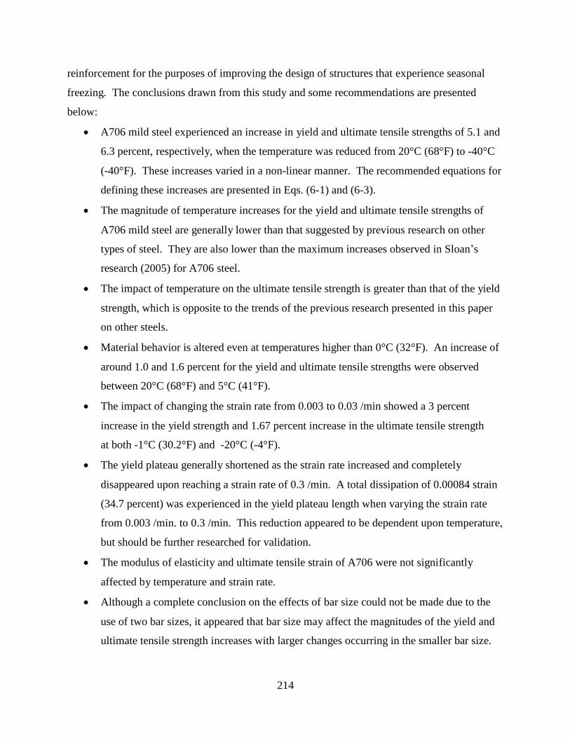
214

reinforcement for the purposes of improving the design of structures that experience seasonal

freezing. The conclusions drawn from this study and some recommendations are presented

below:

A706 mild steel experienced an increase in yield and ultimate tensile strengths of 5.1 and

6.3 percent, respectively, when the temperature was reduced from 20°C (68°F) to -40°C

(-40°F). These increases varied in a non-linear manner. The recommended equations for

defining these increases are presented in Eqs. (6-1) and (6-3).

The magnitude of temperature increases for the yield and ultimate tensile strengths of

A706 mild steel are generally lower than that suggested by previous research on other

types of steel. They are also lower than the maximum increases observed in Sloan’s

research (2005) for A706 steel.

The impact of temperature on the ultimate tensile strength is greater than that of the yield

strength, which is opposite to the trends of the previous research presented in this paper

on other steels.

Material behavior is altered even at temperatures higher than 0°C (32°F). An increase of

around 1.0 and 1.6 percent for the yield and ultimate tensile strengths were observed

between 20°C (68°F) and 5°C (41°F).

The impact of changing the strain rate from 0.003 to 0.03 /min showed a 3 percent

increase in the yield strength and 1.67 percent increase in the ultimate tensile strength

at both -1°C (30.2°F) and -20°C (-4°F).

The yield plateau generally shortened as the strain rate increased and completely

disappeared upon reaching a strain rate of 0.3 /min. A total dissipation of 0.00084 strain

(34.7 percent) was experienced in the yield plateau length when varying the strain rate

from 0.003 /min. to 0.3 /min. This reduction appeared to be dependent upon temperature,

but should be further researched for validation.

The modulus of elasticity and ultimate tensile strain of A706 were not significantly

affected by temperature and strain rate.

Although a complete conclusion on the effects of bar size could not be made due to the

use of two bar sizes, it appeared that bar size may affect the magnitudes of the yield and

ultimate tensile strength increases with larger changes occurring in the smaller bar size.

215

Although a complete conclusion on the combined effects of strain rate and temperature

could not be made due to the scope limits of this study, strength increases associated with

strain rate changes may be dependent upon the testing temperature used. It appeared that

a slightly greater strength increase occurred for specimens at a lower temperature when

varying the strain rate from 0.003 /min to 0.3 /min.

The cyclic loading, consisting mainly of inelastic tensile strains and zero compressive

strains, led to no change in the cold temperature effects of parameters from that

established from the monotonic testing except for the exclusion of the onset of strain

hardening. It is recommended that the initially proposed cyclic loading path, involving

both inelastic compression and tensile strains, be performed on a higher diameter/length

ratio so that buckling does not occur and more useful data can be collected.

216

CHAPTER 7: SOIL BEHAVIOR AT FROZEN TEMPERATURES

7.1 Introduction

During the design process of columns supported on CIDH shafts, defining the properties of

soil surrounding the foundation shaft is of extreme importance. The response of the soil

becomes even more important in the frozen state as it will alter the lateral response of the system

significantly. This is due to the frozen state causing a significant increase in the stiffness of the

soil thus potentially making the structural components of the system to resist additional load

while displacing less (see Section 2.3). In order to better understand the changes in soil stiffness,

an experimental study was conducted on five types of soil common to the State of Alaska to

examine the effects of frozen temperatures. The following sections present details of the

experimental testing completed at Mueser Rutledge Consulting Engineers (MRCE) in New York

and the obtained key test results.

7.2 Testing Matrix

Prior to any experimental testing being performed on soil, the types of soil to be tested were

defined and representative samples were obtained from within the State of Alaska. The

completion of this task, required an examination of the types of soil common to the state and the

soil properties that they may have in the in-situ condition (see Section 7.2.1). After defining the

five most common types of soil present within the state at bridge sites, a testing matrix was

constructed so that the effects of multiple variables could be examined (see Section 7.2.2) and an

appropriate amount of soil samples for testing were obtained.

7.2.1 Soil Selection

For the purposes of the study, five soil types were selected by examining population and

bridge distributions within the state. Population trends revealed that approximately sixty percent

of Alaskan residents live within the south-central portion of the state, around Anchorage (State

of Alaska 2006). An additional twenty percent of the population resides near or in the city of

Fairbanks and the city of Juneau (State of Alaska 2006). Comparing bridge and population

distributions led to the conclusion that a majority of the critical bridges were located within the

aforementioned areas (i.e., Anchorage, Fairbanks and Juneau). The five main soils selected for

the project were obtained from the areas where population and bridge distributions coincided.

217

By examining the Major Land Resource Areas (MLRA) as determined by the United States

Department of Agriculture (USDA) in conjunction with the Natural Resources Conservation

Service (NRCS), the soils, annual temperature range and moisture range were determined using

the Agriculture Handbook No. 296 (USDA, NRCS 2006). Furthermore, the temperature ranges

were expanded using information available from the ENSR group at the University of Alaska at

Fairbanks (2002) to identify the full range of temperatures that the soils experience seasonally.

Upon discussing the initial soil selections with the Chief Engineering Geologist for the State of

Alaska, the soil selections were modified using the paper entitled “Physiographic Divisions of

Alaska” (Wahrhaftig, 1965) and the technical knowledge of the geologist. Although this study

provides information regarding the saturated moisture content of the soils, it is noted that not all

samples may be saturated depending on the location and time of year sampled. An average range

of the different soil dry densities was provided to better improve the soil description prior to

sampling. The final results of the soil selection, expected seasonal temperature range, saturated

moisture content and dry soil density are shown in Table 7-1.

Table 7-1: Five main soils types and expected temperature and moisture content ranges

Soil Type

Soil Description

Temperature

in °C (°F)

Saturated Moisture

Content

Dry Soil

Density in

kN/m3

(lb/ft3)

Alluvial

Deposits

Well graded to well

sorted, fine to coarse-

grained (fan deposit or

flood plain deposit)

35 to -30

(95 to -22)

10% - 50%

10 to 30

(63.7 to 191.0)

Glacial Till /

Ice Contact

Deposits

Well graded; very

dense

35 to -30

(95 to -22)

10% - 50%

10 to 30

(63.7 to 191.0)

Estuarine /

Lacustrine

silty/clayey/organic(?)

; soft/loose

35 to -30

(95 to -22)

15% - 30% / 90% - 150%

(Silty,Clayey/Organic)

8 to 20

(50.9 to 127.3)

Glacial

Outwash

coarse-grained; loose

to dense

35 to -30

(95 to -22)

10% - 50% 10 to 30

(63.7 to 191.0)

Loess

Silty 35 to -30

(95 to -22)

15% - 30% 10 to 17

(63.7 to 108.2)

7.2.2 Testing Plan

Using the information provided in Table 7-1 it was decided that a set of soil samples from

Alaska should be tested at the following four different soil temperatures to understand the impact

of temperature on soils: 20°C, -1°C, -10°C, -20°C. Frozen soil tests were performed using an

218

apparatus specifically designed for this purpose to determine initial, secant and unload/reload

moduli, shear strength, and Poisson’s ratio. To determine these properties, twenty tests with three

samples per test (i.e., a total of sixty samples) were completed. In addition to the testing for

material properties with variable temperature, additional testing was performed at 20°C and -1°C

under repeated loading and unloading with three different loading rates. The additional testing

used a minimum of six tests with two samples per test (i.e., a total of twelve samples) to examine

strain rate effects and cyclic loading on frozen soil. Table 7-2 summarizes the soils testing

performed as part of this investigation.

Table 7-2: Summary of Completed Soil Tests

Soil Type

Samples

Tested

Temperature

in °C (°F)

Moisture

Content,

%

Moist Unit Weight 3 3

in kN/m (lb/ft )

Loading

Rate

I: Alluvial Deposits –

well graded to well

sorted, fine to coarse-

grained (fan deposit or

flood plain deposit)

3 -22.8 (-9) 30 20 (127.3) LR1

3 -10 (14) 30 20 (127.3) LR1

3 -1 (30.2) 30 20 (127.3) LR1

3 20 (68) 30 20 (127.3) LR1

3 -20 (-4) 30 10 (63.7) LR1

3 -20 (-4) 30 30 (191.0) LR1

3 -20 (-4) 15 20 (127.3) LR1

3 -20 (-4) 45 20 (127.3) LR1

II: Glacial Till/Ice

Contact Deposits – well

graded, very dense

3 -20 (-4) 30 20 (127.3) LR1

3 -1 (30.2) 30 20 (127.3) LR1

3 20 (68) 30 20 (127.3) LR1

III: Estuarine/Lacustrine

– silty/clayey/organic(?),

soft/loose

3 -20 (-4) 22 14 (89.1) LR1

3 -1 (30.2) 22 14 (89.1) LR1

3 20 (68) 22 14 (89.1) LR1

IV: Glacial Outwash –

coarse-grained – loose to

dense

3 -20 (-4) 30 20 (127.3) LR1

3 -1 (30.2) 30 20 (127.3) LR1

3 20 (68) 30 20 (127.3) LR1

V: Loess - silty

3 -20 (-4) 25 14 (89.1) LR1

3 -1 (30.2) 25 14 (89.1) LR1

3 20 (68) 25 14 (89.1) LR1

Total Tests 60 Additional Testing – Repeated Loading and Unloading under Variable Loading Rates

I: Alluvial Deposits

2 -1 (30.2) 30 20 (127.3) LR2

2 -20 (-4) 30 20 (127.3) LR2

2 -20 (-4) 30 20 (127.3) LR3

2 -1 (30.2) 30 20 (127.3) LS1

2 -20 (-4) 30 20 (127.3) LS1

2 -20 (-4) 30 20 (127.3) LS2

Total Tests 12

LR1 = 1% per min LR2 = 0.1% per min LR3 = 10% per min LS1 and LS2 = Cyclic loading

219

Table 7-2 demonstrates that most of the testing was performed in a monotonic manner at a

rate of 1% strain per minute. As can be seen, the test matrix included a plan to examine the

effects of density as well as moisture content on the behavior of frozen soil. In addition to being

able to account for these variables, the effect of loading rate was taken into consideration within

the additional testing section by performing monotonic testing at 0.1% strain per minute and

10% strain per minute. This information allowed for a better prediction of the soil strength

during different types of loading in the frozen state. The final portion of the test matrix showed

that cyclic loading of the specimens was used to determine an unloading/reloading secant

modulus for comparison with the initial modulus found for the soil.

The cyclic loading process was performed at two different loading rates, 1% and 10% strain

per minute, to examine the effects of loading rate. The overall testing pattern of the cyclic test

consisted of loading to the set target strain and then fully unloading the specimen prior to

proceeding to the next target strain. Once a strain of 1% was reached for the first time in the

loading pattern, the effects of reloading to a certain strain level were examined by reloading to

that strain point three times prior to proceeding to the next target strain. The pattern selected for

the cyclic testing was based on observations made of the stress-strain curves obtained from the

monotonic triaxial testing on the alluvial soil specified in Table 7-2. The final pattern selected

for the testing is provided in as Table 7-3.

Table 7-3: Target strains for cyclic loading of Type I: Alluvial Soil at strain rates of 1% per

minute and 10% per minute

Target Strain (%) Loading Cycles (#)

0.25 1

0.5 1

0.75 1

1.0 3

1.5 3

2.0 3

3.0 3

4.0 3

6.0 3

8.0 3

10.0 3

12.5 3

15.0 3

220

7.3 Testing Procedures

Using the information provided in Table 7-1 and Table 7-2, a number of samples were

collected both disturbed and undisturbed from the State of Alaska courtesy of the AUTC and the

ADOT&PF. These samples were then shipped to New York for testing purposes at MRCE

where the appropriate test setup was already in place for handling frozen soils. Although ASTM

D7300 – 06 states that the soils should not be artificially prepared in a laboratory setting due to

the variation in ice content and strength (ASTM Standard D7300, 2006), this was not possible to

perform for our testing. The disturbed sampling, however, was not expected to be an issue with

the laboratory results as the authors believe this process would be more representative of

multiple freeze thaw cycles changing the soil structure. In addition, this approach made it easier

for samples to be collected from actual bridge sites since the collecting organizations typically

perform construction in summer months when the ground is in an unfrozen state. The following

sections describe in detail the process used for preparing the specimens, the testing apparatus

setup and the loading protocols used in monotonic and cyclic testing.

7.3.1 Specimen Preparation

Once the disturbed samples arrived at MRCE, the soils were separated into the main

groupings proposed in Table 7-1 and then kept in plastic containers to maintain consistent

moisture contents until samples for testing purposes were made. The next step in preparing the

multiple samples was to create the specimen that would be placed into a modified triaxial

chamber as presented in Section 7.3.2. These specimens were cylindrical in nature and were

created by loosely placing the soil which passed a #4 sieve into a mold supported on a hard

surface and a consistent effort was used to compact the soil (see Figure 7-1). The effort

consisted of striking a metal plunger on top of the soil a set number of times with a hammer as

shown in Figure 7-1b. For each specimen, the process of compaction was done in three lifts with

the same amount of blows per lift to ensure that the soil shaft would have a constant density over

the length of the shaft. Upon completion the specimens and molds were placed inside a freezer

to immediately begin the freezing process if needed. Unfrozen test specimens were tested

immediately as no freezing was required and final preparations prior to testing were done in a

similar fashion to the frozen specimens as described in the next paragraph.

221

Figure 7-1: Sample compaction process: (a) loosely placing soil in mold; (b) using a plunger

to compact soil; (c) placing compacted soil and molds in storage freezer

Immediately prior to placing the specimen in the triaxial chamber, the sample was removed

from the storage freezer for final preparation. These final preparations took place inside the

testing room that was maintained at subzero temperatures to help keep the sample from warming

prior to testing. The process began by extruding the frozen sample from the mold using standard

practices, Figure 7-2a. After extrusion, the sample was reduced to the correct diameter of 50.8

mm (2 in.) using a split ring mold and trimmed with a saw as needed to get a consistent specimen

with level ends. A 50.8 mm (2 in.) diameter specimen was needed so that the testing apparatus

could typically reach an axial stress level of 27.6 MPa (4,000 psi). Once all trimming was

completed, the specimen was measured and placed between the upper and lower loading plates

and then covered with a neoprene membrane to protect the sample from contamination inside the

testing chamber. At this point, the sample is ready for testing, Figure 7-2b, and the testing

apparatus may be constructed around the specimen.

7.3.2 Specimen Setup in Chamber

In order to capture the changes in soil properties at subzero temperatures, a specially

designed triaxial chamber was used. The chamber allowed for a liquid capable of maintaining

frozen temperatures (i.e., antifreeze or salt water) to be circulated around the soil specimen thus

creating an ideal temperature controlled environment for testing. This section discusses the

testing apparatus shown in Figure 7-3 that was designed and used for testing of frozen soils at

MRCE in New York City.

222

Extruded

Top Loading

Plate

Sample Rubber O-ring to

Seal Membrane

Specimen and

Neoprene Membrane

Bottom Loading

Plate

Figure 7-2: Final soil sample preparation: (a) extrusion of sample from mold; (b) fully

prepped sample ready to be tested

Load Cell

Copper tube

circulating

antifreeze

Pin allowing

axial loading

Top Plate

Copper Tube

Static

Antifreeze

Bottom Plate Actuator for

Vertical Load

Figure 7-3: Modified triaxial chamber setup for testing of frozen soils at MRCE

The chamber, placed within a walk-in freezer, consists of a top and a bottom plate separated

by a large diameter clear tube capable of sustaining a horizontal pressure. All interfaces were

sealed using o-rings and vacuum seal grease such that any fluid within the chamber would be

unable to leak out of the chamber when pressurized. The bottom plate was a rigid plate that

created a surface for supporting the specimen as well as ports to put the static antifreeze into the

223

Str

ess

(kP

a)

stra

in a

t m

axim

um

co

mpre

ssiv

e st

ress

Str

ess

(tsf

)

chamber. The top plate, on the other hand was designed such that an axial load could be applied

to the specimen by lifting the entire chamber upwards without compressing the clear tube. In

addition, the top plate was further modified to allow copper coils to be placed around the

specimen that would constantly circulate cold antifreeze with a pump to maintain the

temperature. The overall loading frame was a Sigma-1 automated load test machine capable of

applying a 44.5 kN (10 kip) axial load to the sample.

7.3.3 Testing Process

After placing the specimen within the chamber depicted in Figure 7-3, sufficient time was

permitted for the specimen to stabilize at the testing temperature within the chamber. The

temperature of the specimen was monitored using a steel probe thermocouple that was placed

directly in the center of the chamber and connected to a data acquisition system to continuously

monitor the temperature. Upon reaching the desired temperature, the test system was activated

through an external computer that would apply a consistent loading rate to the soil sample as

specified in Table 7-2 and Table 7-3. Throughout testing the sample was in an unconsolidated,

undrained state. During testing, the data acquisition system recorded the applied force and

deformation to the sample. These values were then used to create a stress-strain curve similar to

that shown in Figure 7-4 so that the critical parameters could be determined.

5000

4000

unconfined compr.

strength, qu

52.2 41.8

3000

cu

31.3

2000 20.9

1000

Esoil 10.4

0 0.0

0.00 2.00 4.00 6.00 8.00 10.00 12.00 14.00 16.00

Strain (%)

Figure 7-4: Experimental stress-strain curve for a Type I soil at -20 C (-4 F) and a 15%

moisture content

224

Com

pre

ssiv

e S

tres

s (M

Pa)

Com

pre

ssiv

e S

tres

s (t

sf)

7.4 Results

Upon completion of the experimental testing, the data was analyzed to examine trends within

the data. The trends examined were on both a localized value to the different soil types as well

as a side by side comparison of the different soil types in some instances for a better definition of

the soil properties. The results of the different comparisons are provided in the following

sections and are separated between the monotonic testing and cyclic testing.

7.4.1 Typical Results of Experimental Testing

Monotonic Testing

Figure 7-5 shows the typical stress-strain response of the Type I soil specified in Table 7-2

when subjected to a monotonic loading rate of 1% strain per minute and temperatures ranging

from 20 °C (68 °F) to -22.8 °C (-9 °F). The results demonstrate that between the extreme testing

temperatures the elastic modulus of the soil increased by a factor of 300, the ultimate

compressive strength increased by a factor of 80 and the ultimate strain capacity decreased by

5%. The secant modulus to the undrained shear strength, the ultimate compressive strength and

the ultimate strain capacity of the data in Figure 7-5 is listed in Table 7-4 to provide a numerical

evaluation of the effects of temperature on the behavior of a Type I soil. Although the

information provided in this section is for a Type I soil, these results are typical of the other soil

types examined in this investigation. Additional information on the other data sets is provided in

the following sections and Appendix D.

12

-22.8 °C (-9 °F)

10

-20 °C (-4 °F)

125

104

8 84

-10 °C (14 °F)

6 63

-1 °C (30.2 °F) 4 42

20 °C (68 °F)

2 21

0 0

0 5 10 15 20

Axial Strain (%)

Figure 7-5: Stress-strain response of a Type I soil subjected to monotonic loading and

temperatures between 20 °C (68 °F) and -22.8 °C (-9 °F)

225

Co

mp

ress

ive

Str

ess

(MP

a)

Co

mp

ress

ive

Str

ess

(tsf

) C

om

pre

ssiv

e S

tres

s (M

Pa

)

Co

mp

ress

ive

Str

ess

(tsf

)

Table 7-4: Numerical results of the Type I soil stress-strain curves depicted in Figure 7-5

Testing

Temperature

Esoil

qu

Strain at cu

Strain at qu Strain at

End of Test

°C (°F) MPa (tsf) MPa (tsf) % % %

20 (68) 1.13 (11.82) 0.14 (1.47) 6.29 19.83 20.01

-1 (30.2) 36.01 (376.0) 1.63 (16.97) 2.24 10.82 20.01

-10 (14) 133.8 (1397.5) 5.35 (55.89) 1.97 13.11 14.79

-20 (-4) 190.1 (1985.6) 9.46 (98.83) 2.51 15.49 15.49

-22.8 (-9) 357.4 (3731.9) 11.15 (116.5) 1.58 15.49 15.49

Cyclic Testing

Figure 7-6 shows the typical response of the Type I soil tested under cyclic loading according

to the sequence presented in Table 7-3 at a strain rate of 1% per minute in and temperatures of -1

C (30.2 F) and -20 C (-4 F). The results, similar to the monotonic testing, demonstrate that the

modulus of elasticity increased by a factor of 8 and soil strength increase by more than a factor

of 10 as the testing temperature decreased from -1 °C (30.2 °F) to -20 °C (-4 °F). Additionally,

Figure 7-6 indicates that the unloading and reloading moduli were approximately the same as the

initial loading modulus. The -1 °C (30.2 °F) test specimens, therefore, had a residual strain

equivalent to 93% of the maximum strain reached during a given cycle, and the -20 °C (-4 °F)

cyclic tests had a residual strain of 84% of the maximum. The results demonstrate an 80%

degradation in compression strength upon repeated loading to a given strain level.

0.5 10

0.4 4.2 8 84

0.3 3.1 6 63

0.2 2.1 4 42

0.1 1.0 2 21

0

0 2 4 6 8 10

Axial Strain (%)

0.0 0 0

0 2 4 6 8 10

Axial Strain (%)

(a) -1 °C (30.2 °F) (b) -20° C (-9 °F)

Figure 7-6: Experimental cyclcic stress-strain response of a Type I soil

226

Ult

ima

te C

om

pre

ssiv

e S

tren

gth

(k

Pa

)

Ult

ima

te C

om

pre

ssiv

e S

tren

gth

(ts

f)

7.4.2 Summary of Monotonic Testing

Ultimate Compressive Strength

As a baseline of comparison, the ultimate compressive strength of the different soil

specimens at the warm condition [i.e., 20 °C (68 °F)] was established first by taking the peak

point of the typical stress-strain curves depicted in Figure 7-4 and averaging the results. These

values are provided below in Figure 7-7, where it can be seen that the data varies depending on

the type of soil being examined. The ultimate compressive strengths in the soils range from

14.25 kPa (0.15 tsf) to 145.5 kPa (1.52 tsf) with average density and moisture content as stated in

Table 7-1.

150 1.57

120 1.25

90 0.94

m = 19.5 kN/m3

(124.08 pcf)

60 m.c. = 25.33%

30

m = 18.68 kN/m3

(118.90 pcf) m.c. = 29.97%

m = 22.9 kN/m3

(145.79 pcf) m.c. = 10.77%

m = 19.18 kN/m3

(122.08 pcf) m.c. = 31.47%

m = 19.07 kN/m3

(121.39 pcf) m.c. = 39.40%

0.63

0.31

0

Type I (CH) Type V (ML) Type IV (SP-SM) Type III (SM) Type II (SP -

SM)

0.00

Soil Type Analyzed

Figure 7-7: Failure strengths of analyzed soils at 20 °C (68 °F) [Note: 1 tsf = 95.8 kPa; 1 pcf

= 0.157 kN/m3]

Once the baseline values were established at the warm weather condition, a series of

comparisons were made to examine the effects of cold temperatures on the ultimate compressive

strength of the soil as this is an indirect measure of the undrained shear strength. The

comparison was performed by defining a reference value based on the average ultimate

compressive strength established at a cold temperature divided by the average ultimate

227

Ref

eren

ce V

alu

e =

qu

,co

ld /

qu

,wa

rm

compressive strength at the warm temperature tests of 20 °C (68 °F). Using this reference value

a series of charts were produced to examine the overall trends present within each type of soil.

Figure 7-8 provided below shows the individual chart produced for the alluvial soil specified as

Type I in the testing matrix. The other individual charts are provided in Appendix D of this

report.

80

70

60

50

40

30

20

10

0

0 -5

-10

-15

-20

-25

Temperature (°C) Avg. -1 deg. C Avg. -10 deg. C Avg. -20 deg. C Avg. -22.8 deg. C

Figure 7-8: Increase in the ultimate compressive strength of a Type I soil with respect to

warm temperature at 20 °C (68 °F)

Figure 7-8 demonstrates that as temperature decreases, the strength of the soil is going to

increase in a linear manner in which the rate and magnitude of increase for each soil type varied

depending on the type of soil examined. The importance of the temperature effects, however,

stems from the fact that as the soil strength and stiffness increases (see Figure 7-5) the

foundation and column shafts must begin to resist more of the lateral load being applied to the

system. Also, the increased stiffness will cause an upward shift of the maximum moment

location while decreasing the overall ductility of the SFSI system.

In addition to the individual graphs two additional figures were created for a side by side

comparison of the data. These charts were done at -1 °C (30.2 °F) and -20 °C (-4 °F) for the

multiple soil types since this is where the majority of the testing was performed. These charts

228

Ref

ere

nce

Valu

e: q

u,c

old

/ q

u,w

arm

are provided here as Figure 7-9 and Figure 7-10. In Figure 7-9 the ultimate compressive strength

of the Type IV soil was not provided as only a limited amount of material was obtained for this

soil type.

140

120

100

80

60

40

20

0

Type I (CH) Type V (ML) Type IV (SP-SM) Type III (SM) Type II (SP - SM)

Soil Type Analyzed

Figure 7-9: Increase in ultimate compressive strength of the five soil types specified in

Table 7-2 tested at -1 °C (30.2 °F) with respect to the ultimate compressive

strength at 20 °C (68 °F)

The data provided in the figures suggest that even a temperature near the freezing point of

water significantly alters the ultimate compressive strength of the soil and continues to increase

as temperature decreases. Although it appears that the relative increase in strength varies greatly

between soil types, a closer examination of the data reveals that the ultimate compressive

strength of the soils has a consistent increase as a function of temperature. That is to say, the

magnitudes of strength in the frozen states are very similar to one another and can most likely be

attributed to the presence of ice crystals forming in the soil voids and their influence on strength.

However, the main conclusion that can be drawn is that the increase in soil strength must be

accounted for in the design of foundation shafts subjected to seasonally frozen conditions.

229

Refe

ren

ce V

alu

e: q

u,c

old

/ q

u,w

arm

800

700

600

500

400

300

200

100

0

Type I (CH) Type V (ML) Type IV (SP-SM) Type III (SM) Type II (SP - SM)

Soil Type Analyzed

Figure 7-10: Increase in ultimate compressive strength of the five soil types specified in

Table 7-2 tested at -20 °C (-4 °F) with respect to the ultimate compressive

strength at 20 °C (68 °F)

Strain at Ultimate Compressive Strength

After comparing the strength at failure, the strain achieved at the ultimate compressive

strength was also examined. Although multiple data sets were examined, no definitive

conclusions were drawn about the effects of freezing temperature on the strain at the peak stress

of the soil specimens as the data did not have any consistent trends. This is evident in Figure

7-11 where the data corresponding to the CH alluvial deposit is shown. Although a clear trend is

not seen in this figure, the indication is that strain at failure decreases with reducing temperature.

This is expected based on the soil stress-strain curves presented in Figure 7-4. Therefore, it is

believed that the ultimate compressive strain of the soil decreases with freezing conditions but no

trend can adequately be established. Additional charts representing this conclusion are provided

in Appendix D.

230

Str

ain

(%

)

67 57

25

47 37

Temperature (°F)

27 17 7

-3 -13

20

15

10

5

0

20 15 10 5

0 -5

-10

-15

-20

-25

Temperature (°C)

Figure 7-11: Effects of temperature on the strain at the ultimate compressive strength of a

Type I: Alluvial soil

Modulus of Elasticity

The effect of temperature on the soil modulus of elasticity was the next soil property

investigated. The examination consisted of computing the secant modulus of elasticity from the

point of qu/2 to the origin and then dividing the cold temperature value with the average soil

modulus of elasticity at 20 °C (68 °F). Figure 7-12 shows the results of this process for the five

soil types that were tested. The figure shows that as the temperature decreases, the soil modulus

of elasticity increases in a curvilinear manner as a function of soil type. This relationship

follows an exponential or second order polynomial as shown by the equations within the figure.

The results being a function of soil type is depicted in the figure by the fact that the more

cohesive soils tested (e.g., Type I) increase at a slower rate than the non-cohesive soils (e.g.,

Type II). Although trends exist, an adequate approach for accounting for the increase cannot be

established due to the large scatter in the data points and variability in soil types. It is noted

however that the modulus of elasticity is significantly altered as temperature decreases as

evidenced by the large reference equal to 1400 for the Type II soil.

231

Ref

eren

ce V

alu

e: E

soil

,co

ld /

Eso

il,w

arm

Temperature (°F)

67

2000

57 47 37 27 17 7 -3 -13

1800

1600

1400

1200

1000

800

600

Type I Soil

Type II Soil

Type III Soil

Type IV Soil

Type V Soil

y = 0.9649x2 - 32.512x + 265.27

y = 16.61e-0.126x

y = 272.22e-0.082x

400

200

0

20 15 10 5

0 -5

-10

-15

-20

-25

Temperature (°C)

Figure 7-12: Effects of temperature on the soil modulus of elasticity under monotonic

loading

Density Effects

The process of examining the effects of moist soil density on the undrained shear strength of

the soil at a subzero temperature was undertaken for the Type I: Alluvial soil that was classified

using the USCS classification system as a CH soil. This variable was tested by varying the

compaction of the soil in the samples while maintaining consistent moisture content in the

multiple specimens. At each set of densities, three samples were produced and tested at -20 °C (-

4 °F) to examine the effects of the frozen state on the undrained shear strength. The results of the

strength testing are provided in Figure 7-13. As seen in this figure, when the density of the

specimen was increased, there appears to be a linear increase in the undrained shear strength of

the soil. This is similar to the behavior of soil in a warm condition where the compacting causes

the internal soil matrix to become closer together thus increasing the amount of friction between

the soil particles and in turn the undrained shear strength of the soil.

232

Un

dra

ined

Sh

ear

Str

eng

th, c

u (

kP

a)

Un

dra

ined

Sh

ear

Str

eng

th (

tsf)

Moist Unit Weight (pcf)

89.12 95.49 101.85 108.22 114.59 120.95 127.32

7000 73.10

6000 62.66

5000 52.21

4000 41.77

3000 31.33

2000

1000

Average MC for Specimens:

m.c. = 28% m = 15.7 kN/m3 (100 pcf)

m.c. = 28.1% m = 18.6 kN/m3 (118.4 pcf)

m.c. = 24% m = 19.0 kN/m3 (120.92 pcf)

20.89

10.44

0

14 15 16 17 18 19 20

Moist Unit Weight (kN/m3)

0.00

Figure 7-13: Effects of density on undrained shear strength of a CH soil at -20 °C (-4 °F)

Moisture Content Effects

The next variable that was examined was the presence of different amounts of moisture

content within the soil. This was once again examined in the alluvial soil classified as a CH

according to USCS. In order to complete this testing sequence, the samples were constructed

such that a uniform density would be maintained as much as possible while varying the moisture

content. The samples were then tested at -20 °C (-4 °F) and the effects of moisture content on the

undrained shear strength of the soil were examined as shown in Figure 7-14.

In Figure 7-14 it can be seen that originally the variation in moisture content caused an

increase in the density of the soil even though a standard compaction effort was used in all

specimens. This is believed to have occurred due to the parabolic curve that typically appears

when a standard proctor test is performed. This was the case as the laboratory process used for

determining the proctor curve is similar to the process used in the experiment. Despite this

anomaly, the data was corrected as noted by the square data point based on the results of the

density effects chart previously presented. The data taken from the linear trend was found to

have an undrained shear strength of 3514 kPa (36.7 tsf) at a moisture content of 28.1% and an

233

Un

dra

ined

Sh

ear

Str

eng

th, c

u (

kP

a)

Un

dra

ined

Sh

ear

Str

eng

th (

tsf)

approximate density of 17.0 kN/m3

(108 pcf). When this point is included into the data set, it

can be seen that a linear increase in the undrained shear strength is generally seen with an

increase in the moisture content at a comparable density. This was once again expected due to

the fact that an increase in moisture content will cause an increase in the amount of ice

formation, thus enhancing the overall strength of the sample.

5000 52.21

4500 46.99

4000 41.77

3500 36.55

3000 31.33

2500

2000

Densities for Specimens:

m.c. = 17% m = 17.4 kN/m3 (110.75 pcf)

m.c. = 28.1% m = 18.6 kN/m3 (118.43 pcf)

m.c. = 40% m = 16.8 kN/m3 (106.75 pcf)

26.11 20.89

1500 10 15 20 25 30 35 40 45 50

Moisture Content (%)

15.66

Figure 7-14: Effects of moisture content on the undrained shear strength of a CH soil at -20

°C (-4 °F)

Effect of Strain Rate

As part of the experimental investigation at MRCE, a number of samples were prepared at a

similar moisture content and density for testing under variable loading rates as shown in Table

7-2. These tests were used to examine the effects of different rates of loading on the ultimate

compressive strength of the soil, the strain at the ultimate compressive strength and the secant

modulus of elasticity to the undrained shear strength of the soil at a temperature of -20 °C (-4 °F).

The strain rate effects were only examined for the CH soil listed as Type I in the five main soil

types of Alaska.

The first variable examined for strain rate effects was the ultimate compressive strength of

the Type I soil by comparing the applied loading rate with the ultimate compressive strength of

234

Ult

ima

te C

om

pre

ssiv

e S

tren

gth

(M

Pa

)

Ult

ima

te C

om

pre

ssiv

e S

tren

gth

(ts

f)

the soil as shown in Figure 7-15. The figure shows that as the loading rate increases for a 0.1%

strain per minute to 10% strain per minute a linear increase of 33% in the ultimate compressive

strength of the soil occurred. The results were expected as the rapid loading does not allow the

soil to respond as quickly thus decreasing the deformation at a given point while increasing the

ultimate compressive strength. This result concurs with the previous study of Zhu and Carbee

(1984) as depicted in Figure 2-26 where the strength of the remolded silt depended on the rate of

loading applied to the test specimens.

14 146

13 136

12 125

11 115

10 104

9 94

8 84

0 2 4 6 8 10

Applied Strain Rate %/minute

Figure 7-15: Effect of strain rate on the ultimate compressive strength of a Type I soil

tested at -20 °C (-4 °F)

The strain at the ultimate compressive strength of the soil was the next parameter studied for

the effects of strain rate. This was performed by plotting the strain attained at qu with the

applied strain rate to the specimen as shown in Figure 7-16. Similar to the ultimate compressive

strength, the strain increased linearly by approximately 25% as the rate of loading increased from

0.1% strain per minute to 10% strain per minute. The increase in strain at the peak stress was

expected based on the previous studies of Zhu and Carbee (1984) presented in Figure 2-26 where

it can be seen that the strain at the peak is shifting to the right as rates of applied strain increased.

235

So

il M

od

ulu

s o

f E

last

icit

y (

MP

a)

Str

ain

(%

)

So

il M

od

ulu

s o

f E

last

icit

y (

tsf)

20

18

16

14

12

10

0 2 4 6 8 10


Figure 7-16: Effect of strain rate on the strain at the ultimate compressive strength of a

Type I soil tested at -20 °C (-4 °F)

The final parameter investigated for the effects of strain rate was the secant modulus of

elasticity to the undrained shear strength point of the Type I soil as presented in Figure 7-17.

The data sets presented in this figure show a large scatter in the secant modulus of elasticity at

each applied strain rate making a definitive trend hard to establish. Although a clear trend is not

seen in this figure, the data indicates that as the applied rate of loading increased an increase of

25% in the secant modulus of elasticity occurred. This increase, however, is essentially

negligible as the secant moduli of materials are known to vary by as much as 20%. Therefore,

the authors of this report concluded that the secant modulus of elasticity was unaffected by the

strain rate applied to the specimen.

400

350

300

250

200

150

100

50

0

0 2 4 6 8 10


4177

3655

3133

2611

2089

1566

1044

522

0

Figure 7-17: Effect of strain rate on the secant modulus of elasticity to the undrained shear

strength of a Type I soil tested at -20 °C (-4 °F)

236

Co

mp

ress

ive

Str

ess

(kP

a)

Co

mp

ress

ive S

tress

(ts

f)

Co

mp

ress

ive

Str

ess

(MP

a)

Co

mp

ress

ive

Str

ess

(tsf

)

7.4.3 Cyclic Testing

Cyclic testing was performed on the Type I soil specified in Table 7-1 to examine the effects

of temperature on the behavior of soil subjected to cyclic loading. The results of this

experimentation is provided here as Figure 7-18. In this figure, it can be seen that as the

temperature decreased from -1 °C (30.2 F°) to -20 °C (-4 °F) the ultimate compressive strength of

the soil increased by 22 times the warmer temperature tested. This concurs with the monotonic

testing where an increase in the ultimate compressive strength of the Type I soil was a function

of temperature as noted in Sections 7.4.1 and 7.4.2. Additionally, the data presented in the figure

shows that the modulus of elasticity increased as temperature decreased which is in accordance

with the monotonic testing. The figure further demonstrates that the unloading and reloading

moduli were approximately equal to the initial soil modulus of elasticity found for the

temperature at which the samples were tested.

500 10 I -20 20 1% AC

450 I -1 20 1% BC 4.7 I -20 20 1% BC

400

350

300

250

200

150

100

50

0

0 2 4 6 8 10

Axial Strain (%)

4.2

3.7

3.1

2.6

2.1

1.6

1.0

0.5

0.0

8 84

6 63

4 42

2 21

0 0

0 2 4 6 8 10

Axial Strain (%)

(a) -1 C (30.2 F) (b) -20 C (-4 F)

Figure 7-18: Experimental cyclic stress-strain results of a Type I soil subjected to subzero

temperatures and a loading rate of 1% strain per minute

A prevalent trend in the cyclic testing depicted in Figure 7-18 is that residual deformation of

the soil specimens occurred after each loading cycle. This residual deformation was found to be

a function of temperature and the peak strain applied during a given cycle as the amount of

residual displacement was 93% of the peak strain at -1 °C (30.2 °F) and 84% of the peak strain at

237

Co

mp

ress

ive

Str

ess

(MP

a)

Co

mp

ress

ive S

tress

(ts

f)

Co

mp

ress

ive

Str

ess

(MP

a)

Co

mp

ress

ive

Str

ess

(tsf

)

-20 °C (-4 °F). The variation in residual strain was not surprising as the stiffening of the soil

caused the samples to behave in an elastic manner for higher strain values as seen in Figure 7-5.

Additionally, the second and third cycles of loading demonstrated an 80% drop in the peak stress

attained during the first loading cycle at a given strain limit.

Effect of Strain Rate

In order to better understand the cyclic behavior of soil at subzero temperatures, Type I soil

specimens were subjected to the cyclic load pattern of Table 7-3 at -20 °C (-4 °F) and an applied

loading rate of 10% strain per minute as this is comparable to an actual seismic event. The

results of the variable loading rate testing performed at MRCE are provided in Figure 7-19. The

data was split into the “A” and “B” samples for each cyclic pattern for ease of comparison in the

figures. In each instance the solid line represents the applied loading rate of 1% strain per

minute while the dashed line represents the applied loading of 10% strain per minute.

14 1% strain/min

10% strain/min 12

125

14 1% strain/min

12 10% strain/min

125

10 104 10 104

8 84 8 84

6 63 6 63

4 42 4 42

2 21 2 21

0 0

0 2 4 6 8 10

Axial Strain (%)

0 0

0 2 4 6 8 10

Axial Strain (%)

(a) “A” Samples (b) “B” Samples

Figure 7-19: Experimental strain rate effects on the cyclic stress-strain response of a Type I

soil tested at -20 °C (-4 °F)

As the applied rate of loading increased, Figure 7-19 shows that the compressive strength of

the soil increased by 30% which is comparable to the effects of strain rate noted for the

monotonic loading of the soil specimens. This figure further demonstrates that the secant

modulus of elasticity was unaffected by a variable loading rate as described in Section 7.4.2 of

238

this report (especially prevalent in Figure 7-19b). Additionally, the unloading/reloading moduli

and the residual deformation of the soil specimens were unaffected by the change in the rate of

applied loading. This was demonstrated by the fact that the unloading and reloading cycles to a

given strain limit at the 10% strain per minute closely follows the path established by the curves

established for a 1% strain per minute loading. The strain at the ultimate compressive strength

was not examined for the cyclic testing since the test was performed using a specified strain

limit.

7.5 Conclusions

This chapter of the report has presented the results of an investigation conducted at MRCE

into the effects of seasonal freezing on the response of soil through an examination of the failure

strength, density effects and moisture content effects of the five soil types (see Table 7-1) tested

from the State of Alaska. The following section provides the conclusions drawn in regards to the

response of soil subjected to seasonal freezing conditions.

The failure strength of the five soil types significantly increased when subjected to

freezing temperatures. At -1 °C (30.2 °F), the increase was typically by a magnitude of

ten whereas at -20 °C (-4 °F) the soil samples typically experienced a magnitude of one

hundred increase. It is suggested that the relative increase in strength of magnitude 10

and 100 be used to account for seasonal freezing at -1 °C (30.2 °F) and -20 °C (-4 °F) if

actual testing of specimens in the frozen state is not possible. These relationships are

shown in the equations below.

( ) ( ) (7-1)

( ) ( ) (7-2)

To more accurately define the p-y curves additional testing is needed on sandy soils to

examine the effect of cold temperatures on the effective friction angle. This data would

be used to define the modulus of horizontal subgrade reaction. It is believed that the

friction angle increases at temperatures decreases and an estimate on the friction angle.

Therefore, the designer can estimate a friction angle such the ultimate strengths of the p-y

curves agree with the relationships in Equations (7-1) and (7-2).

239

Although a correlation for the strain at the ultimate compressive stress of the soil could

not be established, the data suggests that a decrease in strain is experienced as

temperatures decrease from 20 °C (68 °F) to -23 °C (-9.4 °F).

The modulus of elasticity increased according to a polynomial or exponential curve as

temperature of the tested soil specimens decreased from 20 °C (68 °F) to -23 °C (-9.4 °F).

A direct correlation was not established due to the scatter in the test data because of the

multiple soil types tested in this investigation. The cold temperature modulus of

elasticity increased by 200 times for the Type I soil and 1400 times for the Type II soil.

As the density of the specimen increased the undrained shear strength of an alluvial

deposit of CH soil increased in a linear manner in a frozen state when the moisture

content was held constant. The increase in undrained shear strength experienced at -20

°C (-4 °F) was a factor of 2.75 from a density of 15.7 kN/m3

(100 pcf) to 19.0 kN/m3

(121

pcf)

The effects of moisture content on the undrained shear strength of an alluvial deposit of

CH soil at -20 °C (-4 °F) was found to increase in a linear manner when the density of the

specimens were maintained at a constant level. The increase in strength was a factor of 2

from a moisture content of 17% to a moisture content of 40%.

The effects of strain rate on the monotonic testing of soils was found to agree with

previous studies and have an impact on the stress-strain behavior of a Type I (CH) soil

tested at -20 °C (-4 °F). The ultimate compressive strength of the soil was found to

increase linearly increase by 33% between an applied loading rate of 0.1% and 10%

strain per minute. The strain at the ultimate compressive strength of the soil was found to

linearly increase by 26% between an applied loading rate of 0.1% and 10% strain per

minute. Although slight increase in the secant modulus of elasticity was noted, the

difference was found to be negligible thus suggesting that modulus of elasticity was

unaffected by a change in the applied rate of loading during testing.

The effects of temperature on cyclic testing on a Type I soil produced similar results to

the monotonic testing. The strength of the specimens tested at -20 °C (-4 °F) increased by

22 times the strength of the specimens tested at -1 °C (30.2 °F). The modulus of elasticity

was also noted to increase as the temperature decreased.

240

The cyclic testing found that the unloading and reloading moduli of the soil at the frozen

state were equivalent to the initial modulus of loading (see Figure 7-18).

Residual strains of 93% and 84% of the peak strain during a given cycle were present

during the cyclic testing of a Type I soil at -1 °C (30.2 °F) and -20 °C (-4 °F).

Additionally, the second and third cycles at a given strain experienced an 80% drop in

strength from the first loading cycle applied to the soil specimens.

The effects of strain rate on the cyclic testing were found to agree with the results found

for the monotonic testing. The compressive strength increased and the modulus of

elasticity remained unchanged. Also, the unload and reload moduli were not affected by

the variable loading rates of 1% strain per minute and 10% strain per minute.

It is recommended that future testing should be performed to provide a larger data set of

results so that the effects of density and moisture content can be better examined for all

soil types.

More testing should also be performed on all soil types in order to provide a more

statistically sound equation for determining the increase of failure strength with a

decrease in temperature.

241

CHAPTER 8: SUMMARY, CONCLUSIONS AND RECOMMENDATIONS

8.1 Introduction

The research on the seismic design of drilled shaft foundations in clay soils was motivated on

the basis of the challenges associated with models in practice today and the experimental testing

performed by Suleiman et al. (2006) especially in high seismic regions such as Alaska where

seasonal freezing is a major concern. Therefore, the objective of this research was to develop a

simplified method for use in the seismic design of drilled shafts in clay that would provide a

good representation of the critical locations and lateral loading response of an integrated

column/foundation system. The proposed model had to capture the lateral loading response in

all seasons of the year without the use of a detailed approach as this has not been handled in

current approaches even though numerous models exist in practice today. The sections presented

below provide a summary of the completed work, conclusions drawn from the project and

recommendations developed throughout the process.

8.2 Summary

The research presented in the report started with a brief historical background on bridges and

their evolvement with time. Seismic engineering practices were then examined with specific

details about seismic loading, the design philosophy used in practice and concerns associated

with seasonal temperature variation. Multiple foundation types were then presented along with

the seismic design approaches used for each foundation. Specific emphasis was given to deep

foundations, specifically drilled shafts, based on the topic of the project. The effects of soil-

foundation-structure-interaction on drilled shafts were then described prior to defining the scope

of research.

An extensive literature review was completed with the goal of obtaining knowledge on the

lateral response of drilled shafts when subjected to design level or greater earthquakes in all

seasonal conditions. Several analytical methods for determining the lateral response in design

and analysis were investigated based off of current code and guideline recommendations. A

seasonal freezing investigation that included analytical and experimental case studies was

provided along with a broad impact study on infrastructure within the United States and Japan.

During this investigation it was noted that seasonal freezing would significantly alter the lateral

load response of an integrated column/foundation system by:

242

Increasing the effective elastic stiffness of the system;

Increasing the shear demand experienced by the column and foundation shafts;

Shifting the maximum moment location toward the ground surface;

Reducing the lateral displacement capacity when compared to the warm weather

condition; and

Reducing the plastic hinge length.

In addition to the lateral response, it was found that material properties are effected during times

of seasonal freezing with the typical trend being an increase in overall strength, thus causing a

larger zone of elastic behavior. Finally, the capabilities of the sectional analysis tool to be used

within the research were discussed.

An examination of the existing methods was completed, identifying the associated

challenges. This process involved comparisons between detailed analyses and the common

simplified methods presented within the literature review. Thus providing justification as to why

a new method of determining the lateral response of integrated column/foundation systems in

clay soils was needed.

A simplified method for determining the lateral response of drilled shafts in clay soils was

developed for the pinned head condition. The new method was modeled as a cantilever with an

effective height from the top of the bridge column to the point of maximum moment within the

foundation shaft. Properties of the flexible base and spring representing soil resistance were

established thus defining critical locations for an integrated column/foundation system including

the maximum moment location and point of first zero moment after the maximum moment. A

bilinear force-displacement curve representing the lateral load response of the system using the

origin of a Cartesian coordinate system, the first yield limit state and the ultimate limit state was

constructed based off of the information presented in Section 4.4. The accuracy of the method

was then verified against experimental data from Suleiman et al. (2006) and detailed analyses

performed in LPILE in Section 4.5. To adjust for different boundary conditions at the tip of the

column, it is expected that the model can be adjusted similarly to a column supported on a spread

footing by adjusting the effective height of the cantilever to the inflection point and computing

deflections from this location while the force will not change at the column tip. This is currently

under investigation by the researchers.

243

8.3 Conclusions

Based on the completed study presented within this report, the following conclusions were

drawn:

Approximately two-thirds of about 600,000 bridges in the United States are effected by

seasonal freezing alone. In addition, it was found that half of the approximately 70,000

bridges located in high seismic regions would be affected by seasonal freezing, which

includes areas such as the north eastern part of California, the eastern half of Washington,

Alaska and Missouri. It was also concluded that freezing and high seismicity would

occur in the northern regions of Japan, especially on Hokkaido Island. Although all these

bridges are effected across the world, it appears that the effects of seasonal freezing are

not routinely addressed in current seismic design practice around the world.

The detailed method used to determine the lateral load response suggested by AASHTO

(2007), although accurate if correctly modeled, requires a significant amount of

information about the structure and surrounding soil in order to complete the analysis.

The method suggested for the lateral design of drilled shafts by Chai (2002) has

challenges associated with its use that include the following based off of the information

examined in Chapter 3:

o Although the model was created for cohesive and cohesionless soils, it was only

verified experimentally against cohesionless soils thus invalidating its use in cohesive

soils;

o The maximum moment location was found to be improperly located by 12.5% to

27.7% when compared to the detailed analyses performed in LPILE which was

shown in Chapter 2 to be able to capture the behavior of the system accurately;

o The analytical plastic hinge length was specified based off of experimental testing in

cohesionless soils and is therefore not applicable to cohesive soils. This was

demonstrated in Chapter 3 when it was shown that the analytical plastic hinge length

was off by 27.6% and 35.9% when compared to the detailed LPILE analyses for the

primary and secondary soil profiles, respectively;

o Seasonal freezing was not included in the development of the model and therefore

should only be used in warm weather conditions; and

244

o The method also uses an idealized elastic perfectly-plastic force-displacement

response between the yield and ultimate conditions which is not capturing the

nonlinear effects of the material properties (soil, steel and concrete). This idealization

also significantly over predicts the behavior of the integrated column/foundation

system tested by Suleiman et al. (2006) in both frozen and unfrozen conditions.

The use of the method suggested by Priestley et al. (2007) had its own challenges and the

conclusions drawn from this are as follows:

o Although the method was developed for both cohesive and cohesionless soils, it was

once again only verified against experimental data performed in cohesionless soils

thus providing no validation for the cohesive soil model;

o The model is only applicable for a limited range of soft cohesive soils and should

technically only be used for the two undrained shear strengths of 20 kPa (420 psf) and

40 kPa (840 psf);

o Lateral forces were not computed as an appropriate spectral graph relating the design

displacement to the effective damping of the system and period was not known. A

quick estimate was not provided since the idealized yield moment and ultimate

moment relating to the appropriate curvatures was unknown;

o The analytical plastic hinge length used in the model is based off of the suggestions

made by Chai (2002) which was previously shown to be invalid for use in cohesive

soils. This challenge along with the underestimation of the controlling limit state

curvature by 16% led to the underestimation of the final design displacement by 40%;

and

o The method was not created with the thought of seasonal freezing effects in mind thus

limiting the model to use in warm conditions only.

Simplified methods suggested by ATC 32 (1996) and AASHTO (2009) were also found

to have the following challenges associated with their use:

o The equivalent fixed based cantilever method is only applicable within the elastic

range of loading and will not capture the inelastic action where the most significant

displacement will occur in the system;

o When compared to a detailed analysis in LPILE based on the discussion in Chapter 2,

the effective fixity location where the maximum moment would occur was found to

245

be over predicted by approximately 100%. This is a major concern as this point is

where the most damage to the system will occur when subjected to a design level or

greater earthquake;

o The shear is assumed to be constant along the length of the shaft, which is incorrect

once the soil begins to resist the lateral movement. This is a concern as an increase in

shear typically occurs in the shaft below the ground surface; and

o No consideration was given to the effects of seasonal freezing in the development of

the model thus limiting it use to warm weather conditions.

A new method was developed for the lateral loading response of drilled shafts that can

capture both the elastic and inelastic range during all seasons of the year. The new model

can be run using a structural analysis program or through the use of hand calculations as

desired. In addition, the model is applicable in clay soils that range from soft to very

stiff.

The new method is able to effectively provide a bilinear force-displacement curve for the

lateral load response of an integrated column/foundation system. The new method does

this through the location of the first onset of yield strains and ultimate flexural capacity

using minimal input parameters about the shaft and surrounding soil;

Verification using the experimental data by Suleiman et al. (2006) demonstrated that the

model is able to effectively capture the critical locations within the system (e.g., the

maximum moment location), the global-force displacement response and localized effects

in the system (e.g., translation and rotation at the maximum moment location). The

following conclusion were drawn from the verification:

o the ultimate lateral force in both warm and freezing conditions was within 10% of a

detailed analysis;

o the ultimate displacement for the SS1 was found to be 23% less than the

experimental data by Sritharan et al. (2007) which is a conservative estimate due to

the assumption purposely made for the analytical plastic hinge length;

o The maximum moment and zero moment location were located accurately with less

than 8% error when compared to the experimental findings from the test in warm

conditions. When compared to the test in cold conditions, these locations were

located accurately with less than 6% error;

246

o The proposed model predicts the secant stiffness to the first yield location within 5%

of the experimental value;

o The second slope in the warm test comparison under predicts the lateral shear force

for an equivalent displacement between yield and ultimate by an average of 10%; and

o The effects of seasonal freezing were effectively handled by varying material

properties for the soil, steel and concrete as seen in the SS2 global comparison.

The analytical verification of the proposed new model provided the following

conclusions:

o The secant stiffness to the first yield location is within 10% of the detailed analysis

performed in LPILE;

o The yield and ultimate shear forces at the top of the column were predicted within an

error of approximately 1%;

o The yield displacement was found within approximately 10% and the ultimate

displacement was within 2.3% of the LPILE analysis; and

o The second slope under predicts the lateral shear force by an average of 13%.

Within the material testing of confined and unconfined concrete a number of conclusions

were drawn about the behavior when subjected to seasonal freezing conditions. Based on

the information presented in Chapter 5, these conclusions are provided below:

o The unconfined concrete compressive stress of concrete increased an average of 28%

when temperature decreased from 20 °C (68 °F) to -40 °C (-40 °F). The

recommended equation for defining the linear increase is presented as Equation 5-2.

o The concrete strain of unconfined concrete at peak compressive strength was found to

be approximately 0.002 at 20 °C (68 °F). This value will decrease in a linear manner

by approximately 23% as the temperature decreases to -40 °C (-40 °F). The equation

for defining the strain at peak compressive strength for a given temperature is

presented in Equation 5-3.

o The modulus of elasticity for unconfined concrete was found to increase by 13% as

temperature decreased to -40 C (-40 F) from 20 C (68 F). The increase in Ec was

found to follow a power series trend related to the unconfined compressive strength

of the concrete and an exponent of 0.5. This relationship correlates well with current

practice in which the modulus of elasticity is related to the square root of the

247

unconfined compressive strength of the concrete. The equation for defining the

increase is presented in Equation 5-6.

o Similar to the unconfined compressive stress, the confined concrete compressive

stress (f′cc) was found to increase as temperature decreased from 20 °C (68 °F) to -40

°C (-40 °F). This meant that the confinement behaves differently than at warm

weather conditions and separate recommendations were made for the increase in

confined concrete compressive stress. The recommended equation for the increase is

presented as Equation 5-7.

o The rate of increase in f′cc was determined to be affected by the increase in Poisson’s

ratio of the concrete specimen as temperature decreases. The changing Poisson’s

ratio decreased the effectiveness of the confinement thus reducing the overall strength

gain possible. However, additional steel added to the specimen will increase the

ductility of the confined region as it does during a warm weather condition.

o In contrast to the unconfined concrete, the strain at the peak confined compressive

stress (cc) increased between 0% and 40%, depending on the amount of horizontal

reinforcement present in the specimen, as temperature went from 20 °C (68 °F) to -40

°C (-40 °F). The increase, however, was able to be setup as a single trend with a

varying starting location based on the amount of horizontal reinforcement. The


o The modification of material properties alone in the Mander’s model will not

adequately capture the behavior of confined concrete subjected to seasonal freezing

as shown in Figure 5-23. However, it is noted that the change in f′cc does not greatly

impact the overall moment-curvature response of the system.

o The ultimate confined compressive strain (cu) was found to not be affected by

decreasing temperature. Therefore, it is recommended that the value be equal to that

which a designer establishes in the warm weather condition.

o The unconfined concrete modulus was consistently higher than the confined concrete

modulus; however, this was most likely due to a localized value being selected for

determining the modulus of elasticity. Therefore, it is recommended that the modulus

for confined concrete be equal to the value attained for unconfined concrete. The


248

Within the material testing of A706 steel a number of conclusions were drawn about the

behavior when subjected to seasonal freezing conditions. Based on the information

presented in Chapter 6, these conclusions are provided below:

o A706 mild steel experienced an increase in yield and ultimate tensile strengths of 5.1

and 6.3 percent, respectively, when the temperature was reduced from 20°C (68°F) to

-40°C (-40°F). These increases varied in a non-linear manner. The recommended

equations for defining these increases are presented in Eqs. (6-1) and (6-3).

o The magnitude of temperature increases for the yield and ultimate tensile strengths of

A706 mild steel are generally lower than that suggested by previous research on other

types of steel. They are also lower than the maximum increases observed in Sloan’s

research (2005) for A706 steel.

o The impact of temperature on the ultimate tensile strength is greater than that of the

yield strength, which is opposite to the trends of the previous research presented in

this paper on other steels.

o Material behavior is altered even at temperatures higher than 0°C (32°F). An

increase of around 1.0 and 1.6 percent for the yield and ultimate tensile strengths

were observed between 20°C (68°F) and 5°C (41°F).

o The impact of changing the strain rate from 0.003 to 0.03 /min showed a 3 percent

increase in the yield strength and 1.67 percent increase in the ultimate tensile strength

at both -1°C (30.2°F) and -20°C (-4°F).

o The yield plateau generally shortened as the strain rate increased and completely

disappeared upon reaching a strain rate of 0.3 /min. A total dissipation of 0.00084

strain (34.7 percent) was experienced in the yield plateau length when varying the

strain rate from 0.003 /min. to 0.3 /min. This reduction appeared to be dependent

upon temperature, but should be further researched for validation.

o The modulus of elasticity and ultimate tensile strain of A706 were not significantly

affected by temperature and strain rate.

o Although a complete conclusion on the effects of bar size could not be made due to

the use of two bar sizes, it appeared that bar size may affect the magnitudes of the

yield and ultimate tensile strength increases with larger changes occurring in the

smaller bar size.

249

o Although a complete conclusion on the combined effects of strain rate and

temperature could not be made due to the scope limits of this study, strength increases

associated with strain rate changes may be dependent upon the testing temperature

used. It appeared that a slightly greater strength increase occurred for specimens at a

lower temperature when varying the strain rate from 0.003 /min to 0.3 /min.

o The cyclic loading, consisting mainly of inelastic tensile strains and zero compressive

strains, led to no change in the cold temperature effects of parameters from that

established from the monotonic testing except for the exclusion of the onset of strain

hardening. It is recommended that the initially proposed cyclic loading path,

involving both inelastic compression and tensile strains, be performed on a higher

diameter/length ratio so that buckling does not occur and more useful data can be

collected.

A number of conclusions were drawn from the soil testing performed on soils typical of

the State of Alaska by MRCE in New York. Based on the information presented in

Chapter 7, the results from the investigation are as follows:

o The failure strength of the five soil types significantly increased when subjected to

freezing temperatures. At -1 °C (30.2 °F), the increase was typically by a magnitude

of ten whereas at -20 °C (-4 °F) the soil samples typically experienced a magnitude of

one hundred increase. It is suggested that the relative increase in strength of

magnitude 10 and 100 be used to account for seasonal freezing at -1 °C (30.2 °F) and

-20 °C (-4 °F) if actual testing of specimens in the frozen state is not possible. These

relationships are shown in the equations below.

( ) ( ) (8-1)

( ) ( ) (8-2)

o To more accurately define the p-y curves additional testing is needed on sandy soils

to examine the effect of cold temperatures on the effective friction angle. This data

would be used to define the modulus of horizontal subgrade reaction. It is believed

that the friction angle increases at temperatures decreases and an estimate on the

friction angle. Therefore, the designer can estimate a friction angle such the ultimate

strengths of the p-y curves agree with the relationships in Equations (7-1) and (7-2).

250

o Although a correlation for the strain at the ultimate compressive stress of the soil

could not be established, the data suggests that a decrease in strain is experienced as

temperatures decrease from 20 °C (68 °F) to -23 °C (-9.4 °F).

o The modulus of elasticity increased according to a polynomial or exponential curve as

temperature of the tested soil specimens decreased from 20 °C (68 °F) to -23 °C (-9.4

°F). A direct correlation was not established due to the scatter in the test data because

of the multiple soil types tested in this investigation. The cold temperature modulus

of elasticity increased by 200 times for the Type I soil and 1400 times for the Type II

soil.

o As the density of the specimen increased the undrained shear strength of an alluvial

deposit of CH soil increased in a linear manner in a frozen state when the moisture

content was held constant. The increase in undrained shear strength experienced at -

20 °C (-4 °F) was a factor of 2.75 from a density of 15.7 kN/m3

(100 pcf) to 19.0

kN/m3

(121 pcf)

o The effects of moisture content on the undrained shear strength of an alluvial deposit

of CH soil at -20 °C (-4 °F) was found to increase in a linear manner when the density

of the specimens were maintained at a constant level. The increase in strength was a

factor of 2 from a moisture content of 17% to a moisture content of 40%.

o The effects of strain rate on the monotonic testing of soils was found to agree with

previous studies and have an impact on the stress-strain behavior of a Type I (CH)

soil tested at -20 °C (-4 °F). The ultimate compressive strength of the soil was found

to increase linearly increase by 33% between an applied loading rate of 0.1% and

10% strain per minute. The strain at the ultimate compressive strength of the soil was

found to linearly increase by 26% between an applied loading rate of 0.1% and 10%

strain per minute. Although slight increase in the secant modulus of elasticity was

noted, the difference was found to be negligible thus suggesting that modulus of

elasticity was unaffected by a change in the applied rate of loading during testing.

o The effects of temperature on cyclic testing on a Type I soil produced similar results

to the monotonic testing. The strength of the specimens tested at -20 °C (-4 °F)

increased by 22 times the strength of the specimens tested at -1 °C (30.2 °F). The

modulus of elasticity was also noted to increase as the temperature decreased.

251

o The cyclic testing found that the unloading and reloading moduli of the soil at the

frozen state were equivalent to the initial modulus of loading (see Figure 7-18).

o Residual strains of 93% and 84% of the peak strain during a given cycle were present

during the cyclic testing of a Type I soil at -1 °C (30.2 °F) and -20 °C (-4 °F).

Additionally, the second and third cycles at a given strain experienced an 80% drop in

strength from the first loading cycle applied to the soil specimens.

o The effects of strain rate on the cyclic testing were found to agree with the results

found for the monotonic testing. The compressive strength increased and the

modulus of elasticity remained unchanged. Also, the unload and reload moduli were

not affected by the variable loading rates of 1% strain per minute and 10% strain per

minute.

8.4 Design Guidelines and Recommendations

Throughout the duration of the project, a number of challenges were identified within codes

and guidelines when determining the seismic response of deep bridge bridge pier foundations in

seasonally frozen ground. These challenges led the author to develop a simplified model that

would determine a bilinear force-displacement response for a bridge column supported by a

CIDH shaft in cohesive soils using minimal input parameters thus reducing the need for a

detailed computer based analysis. This proposed model was verified against available

experimental data and analytical techniques in LPILE (Reese et al., 2004). In addition to the

model development, material testing at cold temperatures was performed on confined/unconfined

concrete, A706 mild steel reinforcement and soils typical of the state of Alaska. Using the

results of this project, design guidelines were constructed for using the new simplified model

along with a number of recommendations for future research.

8.4.1 Design Guidelines

To meet the scope of research requirements specified in Chapter 1, a series of guidelines

were created to allow for the seismic design of CIDH shafts in both a simplified and

sophisticated method. This process was completed by creating a series of flowcharts dependent

on the type of soil present at the site and the design method desired. The process starts in Figure

8-1 where the input parameters are defined and the analysis method is selected. After going

252

T T

through this flowchart, the designer is referred to the appropriate flowchart for completion of the

design process. These series of charts are presented herein as Figure 8-2 through Figure 8-6.

Start the Design of CIDH

Shafts for Seismic Loading

Define Define

CIDH Geometry Temperature Range

Material Properties

at Twarm

Boundary Conditions

and Loading

X-Section

Details

Overall

Dimensions warm cold

Soil Steel Concrete

Axial

Load

D if

known

Pinned

or

Fixed

Perform Moment – Curvature

for Shaft at Twarm

Establish M vs EI

Curve Establish M vs

Curve

Computer Based Which Approach

Type is Desired?

Equation Based

Start Sophisticated Method

Figure 8-2

Start Simplified Method

Figure 8-3 or Figure 8-6

Figure 8-1: Initial design flow chart for the seismic design of CIDH shafts

253

Sophisticated Method (All Soil Types)

Start Sophisticated Method

LPILE or other applicable programs

Identify Analysis Program

Iterations per

Loading Step

Convergence

Tolerance

Define Nonlinear Analysis

Parameters

Define Inputs at Twarm

1

Structural Behavior CIDH Geometry Soil Profile Boundary Conditions

and Loading

M vs EI

Curve

X-Section

Details

No. of

Increments

Overall

Dimensions

Soil

Parameters

Depth to

Layers

Column

Head BC

Axial

Load

Lateral

Loads

2 Modify M v EI curve

Run Lateral Load

Analysis

Perform M- Analysis with

Avg. Soil Pressure

Define Inputs at Tcold

Iterate F – Response until Defined Limit

State is Reached

Are Soil Confinement

Effects Adequately Accounted For?

Average Soil Pressure that

Occurs at Each Stage (See

Figure Below)

Locate point of c = 0.002

at Ultimate Limit State

No Locate point of 1

st

occurrence of c = 0.002

Modify M v EI

Perform M-

Analysis at Tcold

Yes

Ensure Sufficient Displacement

and Displacement Ductility

Exists

Define Material No

Properties at Tcold

(see Figure 8-7)

Are the Effects of Cold Temperatures

Adequately Captured?

From Sritharan et al. (2007)

Yes

Change s and /or No

geometry and establish M vs EI

Is u > dem for

warm and cold conditions?

Yes Design Complete

Figure 8-2: Sophisticated design method flowchart in all soil types

254

Simplified Method for Drilled Shafts in Cohesive Soils


for Cohesive Soils


3

CIDH

Geometry Bilinear M –

Curve

Loading

Soil

Column

Diameter Overall

Dimensio (M′y , ′y); (My

, ); (M , )

Axial c

Load u m 50

y u u

Define Model Parameters Using

Equation Design Set 1

Define Soil Resistance Above

Max. Moment Location Using


Define Rotations from Movement

Below the Max. Moment Using


Determine Component

Displacements and Top Lateral

Force Using Equation Design Set 4

Is the lateral force at

column tip adequately

corrected?

Iterate with ea

Included No

Yes

Define Spring Properties

Rotational Soil Translational

(M′y , eby) (My , u) Reese p-y

Curve (Vy , ty) (Vu , tu)


Modify M v

Determine F – Response

Computer Bilinear Curve

Spring

Change s and/or

geometry and establish

M vs

Properties (Vtcy , y) (Vtcu , u)

No

Perform M-

Analysis at Tcold

Define Material Properties No

at Tcold (see Figure 8-7)

Ensure Sufficient Displacement and

Displacement Ductility Exists

Are the Effects of Cold

Temperatures


Yes

Is u > dem for warm

and cold conditions?

Yes

Design Complete

Figure 8-3: Simplified method design flowchart in cohesive soils

255

2

2

D

Lcol

Lma

hs

Lp Mmax

Lm0

Lmb

Lf

Note:

1. Recommend that Lf ≥ 1.5*Lm0

2. Lcol taken between 0D and 10D where D is the diameter of the pile/shaft

Figure 8-4: Description of the terminology used within the simplified method for cohesive

soils provided in Figure 8-3

Equation Design Set #1

L col

L col

L ma Dα ma D βma D

χ ma

α ma 0.000005ac u 0.0003bc u 0.028

β ma 0.0038bc u 0.3247

χ ma 1.28lnc u kPa 9.6021

χ ma 1.28lnc u psi 7.1307

a = 0.021 for cu in kPa and 1.0 for cu in psi

b = 0.145 for cu in kPa and 1.0 for cu in psi

L m0 Dα m0 c u psiβm0 , or

L m0 Dα m0 0.145c u kPaβm0

α 0.11 Lcol

22.3

m0 D

β 0.021 Lcol

0.33

m0

Lmb Lm0 Lma

256

b

M

c

Lpb 0.16L mb

Lp 20.16L mb 0.32L mb


p 3 γx

0.5 x c b

u u

u

pu 9c u b = unit weight of soil

x = depth from ground surface to point of spring

b = width or diameter of foundation

Vsu pu hs

pu = ultimate soil subgrade reaction, minimum of above equations

hs = height of soil being effected for the soil spring

Vsy ηVsu

= modification factor to determine a yield soil reaction

η 0.03lnc u psi 0.7536

η 0.03lnc u kPa 0.8115

If using one soil spring only,

hs Lma Lcol


L

θ 0.002 mb 0.00001

eby

D L θ 0.0031 mb

0.0006

ebu

D θp L pp L p e

= curvature at a given point past the first yield point

e = elastic curvature component

M

'

e ' y

y

M = moment at a given point past the first yield point M′y = moment at first-yield for concrete cross-section

257

′y = curvature of concrete cross-section at first-yield moment

258


L Δ D 0.0255ψ mb

0.0652

tu

L

D

ψ 0.0157 col

0.9342 For c 70 kP a (10 psi). Else ψ 1

Δ ty

D u

Δ tu

4.37

Δeby θeby L ma

Δebu θebu L ma

Δp θpLma

M max PΔ p Δ eb Vs h s 2Vt1

L ma

3 Δ ea V L

t1 ma 3EI e

The above value needs to be corrected for P- effects using the following:

Vt

M max PΔ p Δ eb Δ ea Vs h s 2L ma

3 Δ ea

V L

t ma 3EI e

V

Vtu

V′ty

0 y u

Note: 1. V′ty and Vtu correspond to values in design set 4

2. u = ea + ebu + p + tu

3. y = ea + eby + ty

Figure 8-5: Final bilinear force-displacement response attained using the simplified method

for cohesive soils

259

Simplified Method for Drilled Shafts in Cohesionless Soils (Equations in Section 2.2.4)


for Cohesionless Soils


4

CIDH

Geometr

Elastoplastic

M – Curve

Loading

Soil

Column

Diameter

Overall

Dimensio

(Mn , y);

(M , )

Desired

Displacement

e Dr

ff m ns

n u

Ductility

Define rate of increase of

modulus of horizontal

subgrade reaction, nh

Find Equivalent Depth to

Fixity and Depth to

Maximum Moment

Establish Idealized Top

Lateral Force


Modify M - curve

Perform M-

Analysis at Tcold

Define Plastic Hinge Length

and Yield Displacement

Determine Curvature

Demand Ductility

Ensure Sufficient Displacement

and Curvature Ductility

Define Material Properties No

at Tcold (see Figure 8-7)

Are the Effects of Cold

Temperatures


Yes

Is u > dem for warm

and cold conditions? No

Change s and/or

geometry and establish a

new M vs

Yes

Design Complete

Figure 8-6: Simplified method design flowchart in cohesionless soil

260

Define Confined Concrete

Properties using desired model

[e.g., Mander et al. (1988)]

Definition of Cold Temperature Material Properties

Start Materials Definition

at Cold Temperature

Define Tcold

Define Properties at Twarm

Concrete A706

Steel Soil

f′c co c sp

fy fsu

su sh s

Clay

5

Clay or

Sand?

Sand

6

f′cc cc cc su

Define Properties of Steel at Tcold

using Equation (6-1) and Equation (6-3)*

cu m 50

m eff

Define properties of unconfined Concrete at Tcold using Equations

(5-2), (5-3) and (5-6)**

Define properties of confined

concrete at Tcold using Equations

(5-6), (5-7) and (5-8)§

Input results into desired model to

fit parameters to a stress-strain

curve [e.g., Mander et al. (1988)]

Define f0.03(%) using

Equation (6-5)

Input f0.03(%) into Dodd and

Restrepo-Posada Model (1995) to get the steel stress-strain curve at

Tcold

Adjust cu using

Equation (7-1) or (7-2)

Estimate 50 based

on cu,cold

Input results into

desired p-y curve

model [e.g., Reese

and Welch (1975)]

Estimate %

increase in eff

Estimate k

based on eff,cold

Input results into

desired p-y curve

model [e.g., Reese

(2004)]

Input result into selected section

analysis tool for defining moment-

curvature [e.g., VSAT (Levings

2009)]

Yes

Does peak

stress agree

with Equation

(7-1) or (7-2)?

Start Design of CIDH

Shaft Figure 8-1 No

6 Adjust eff,cold

Notes:

* The other steel properties remain unchanged or can be computed based on these two equations

** Test data was not available for sp therefore assume remains unchanged

§ Ultimate compressive strain does not change

Figure 8-7: Flowchart for defining concrete, steel and soil material properties at cold

temperatures

261

8.4.2 Recommendations for Future Research

During the development of the proposed simplified model, the following recommendations

were established:

the use of a tri-linear curve in determining the lateral response could be investigated to

more accurately capture the shear demands experienced by the system;

further full-scale experimental testing should be performed in cohesive soils to verify the

effectiveness of the model and the design guidelines suggested in Section 8.4.1;

additional analyses should be run with differing structural parameters to better define the

sensitivity of the simplified model; and

an examination into cohesionless soils should be performed in the future to determine

whether or not the same model may be used with this soil type thus creating a more

coherent method for all soil types.

During the experimental investigations into the effects of seasonal freezing on the response

of material properties a number of recommendations arose for future research into the material

properties area. The recommendations are as follows:

additional confined/unconfined concrete specimens should be constructed and tested so

that a larger data set can be obtained to further verify the equations presented within this

report that account for cold temperatures;

larger specimens should be constructed and tested with the inclusion of longitudinal

reinforcement to verify the approach with this reinforcement. This will also calibrate the

equations for any possible size effect issue;

additional testing should be performed on multiple bar sizes as it appears to effect the

magnitude of increase of the yield and ultimate strengths of A706 mild steel reinforcing

bar. In order to provide a better result a larger data set is required including more than

two bar sizes;

it is recommended that the initially proposed cyclic loading path be performed on a

higher diameter/length ratio so that buckling does not occur and more useful data can be

collected for mild steel reinforcement;

it is recommended that future testing should be performed to provide a larger data set of

results so that the effects of density and moisture content can be better examined for all

soil types; and,

262

• testing should be performed on all soil types in order to provide equations for each

specific soil to determine the ultimate compressive strength, strain at ultimate

compressive strength and modulus of elasticity as a function of temperature.

263

REFERENCES

American Association of State and Highway Transportation Officials (AASHTO). (1998). LRFD

bridge design specifications, 2nd

edition. Washington D.C.: AASHTO.

AASHTO. (2007). LRFD bridge design specifications with 2008 interim revisions, customary

U.S. units, 4th

edition. Washington D.C.: AASHTO.

AASHTO. (2009). Guide specifications for LRFD seismic bridge design. Washington D.C.:

AASHTO.

American Concrete Institute (ACI). (2008). Building code requirements for structural concrete

(ACI 318-08) and commentary (ACI 318R-08). Farmington Hills, MI: ACI.

Andersland, O. B. and Anderson, D. M. (1978). Geotechnical engineering for cold regions.

U.S.A.: McGraw-Hill Inc.

Anderson, J. B., Townsend, F. C. and Grajales, B. (2003). “Case history evaluation of laterally

loaded piles.” Journal of geotechnical and geoenvironmental engineering 129(3): 187-196.

Applied Technology Council (ATC). (1996). Improved seismic design criteria for California

bridges: provisional recommendations. Redwood City, California: Applied Technology

Council.

Ashour, M., Norris, G. and Pilling, P. (1998). “Lateral loading of a pile in layered soil using the

strain wedge model.” Journal of geotechnical and geoenvironmental engineering 124(4):

303-315.

ASTM Standard A615. (2009). “Standard specification for deformed and plain carbon-steel bars

for concrete reinforcement.” West Conshohocken, PA: ASTM International.

ASTM Standard D7300. (2006). “Standard test method for laboratory determination of strength

properties of frozen soil at a constant rate of strain.” West Conshohocken, PA: ASTM

International.

ASTM Standard E8. [2004 (2006)]. “Standard test methods for tension testing of metallic

materials.” West Conshohocken, PA: ASTM International.

Bowles, J. E. (1988). Foundation analysis and design, 4th

edition. United States of America:

McGraw-Hill Book Company.

Broms, B. B. (1964a). “Lateral resistance of piles in cohesive soils.” Journal of soil mechanics

foundation division, American Society of Civil Engineers 90(SM2), 27-63.

264

Broms, B. B. (1964b). “Lateral resistance of piles in cohesionless soils.” Journal of soil

mechanics foundation division, American Society of Civil Engineers 90(SM3), 123-156.

Bruneau, M., Uang, C-M. and Whittaker, A. (1997). Ductile design of steel structures. New

York: Mc-Graw Hill.

Budek, A. M., Priestley, M. J. N. and Benzoni, G. (2000). “Inelastic seismic response of bridge

drilled-shaft rc pile/columns.” Journal of structural engineering 126(4): 510-517.

Bureau of Transportation Statistics. (Accessed Online: 2007). “Conditions of U.S. Highway

Bridges By State.” Washington D.C.: United States Department of Transportation.

http://www.bts.gov/current_topics/2007_08_02_bridge_data/html/bridges_by_state.html

Butkovich, T. R. (1954). “Ultimate strength of ice.” Report No. 11. U.S. Army Res.

California Department of Transportation (Caltrans). (1990). Bridge design aids: pile shaft

design: 12-30 to 12-49. (Accessed online: 2009 through http://www.dot.ca.gov).

Caltrans (2006). Seismic design criteria version 1.4. Sacramento, CA: Caltrans

Carr, A. J. (2005) 3D Ruaumoko: inelastic three-dimensional analysis program. Christchurch,

NZ: University of Canterbury – Department of Civil Engineering.

Chai, Y. H. (2002). “Flexural strength and ductility of extended pile-shafts I: Analytical model.”

Journal of structural engineering 128(5): 586-594.

Chai, Y. H. and Hutchinson, T. C. (2002). “Flexural strength and ductility of extended pile-shafts

II: Experimental study.” Journal of structural engineering 128(5): 595-602.

Concrete Reinforcing Steel Institute (CRSI). (1990). ASTM A706 reinforcing - bars technical

information with commentary on usage and availability. Schaumburg, IL: CRSI

Crowther, G. S. (1990). “Analysis of laterally loaded piles embedded in layered frozen soil.”

Journal of geotechnical engineering 116(7): 1137-1152.

Das, B. M. (2004). Principles of Foundation Engineering, 5th

Edition. United States of America:

Thomson, Brooks/Cole.

Davisson, M. T. and Robinson, K. E. (1965). “Bending and buckling of partially embedded

piles.” Proceedings of the sixth international conference S. M. and F. E. Montreal, Canada:

University of Toronto Press. pp. 243-246.

DeGaetano, A. T., and Wilks, D. S. (2001). “Development of Frost Depth Maps for the United

States.” Research report. Upper Marlboro, Maryland: National Association for Home

Builders (NAHB) Research Center, Inc.

http://www.bts.gov/current_topics/2007_08_02_bridge_data/html/bridges_by_state.html

http://www.dot.ca.gov/

265

Dodd, L. L. and Restrepo-Posada, J. I. (1995). “Model for predicting cyclic behavior of

reinforcing steel.” Journal of structural engineering 121(3): 433-445.

ENSR (2002). “ Fort Wainwright hydrological data network.” Alaska: University of Fairbanks.

(Accessed Online November 2007). http://www.uaf.edu/water/projects/ftww/gwdata/gwdata.html.

Filiatrault, A. and Holleran, M. (2001a). “Stress-strain behavior of reinforcing steel and concrete

under seismic strain rates and low temperatures.” Materials and structures 34: 235-239.

Filiatrault, A. and Holleran, M. (2001b). “Characteristics of reinforced concrete bridge

components under seismic strain rates and low temperatures.” Proceedings of the 18th

US-

Japan bridge engineering workshop, St. Louis. FHWA: 49-63.

Gustafson, D. (2007). Revisiting Low-Alloy Steel Reinforcing Bars. (Accessed online: May 5,

2009 through BNET at:

http://findarticles.com/p/articles/mi_qa5363/is_200701/ai_n21290713/?tag=content;col1)

Harris, J. S. (1995). Ground freezing in practice. London, England: Thomas Telford Services

Ltd.

Hetenyi, M. (1946). Beams on elastic foundation. Ann Arbor, Michigan: University of Michigan

Press.

Hose, Y., Brestel, D., Seible, F. and Dowell, R. (2001). Assessment of hoop strains in the

flexural plastic hinge region of typical bridge columns. San Diego, CA: University of

California

Iowa Department of Transportation (Accessed Online: September 2009).

http://www.i235.com/ped_bridge_2.htm

Japanese Meteorological Agency. (Accessed Online: August 2008).

http://www.jma.go.jp/jma/indexe.html

Kumar, S. and Lalvani, L. (2004). “Lateral load-deflection response of drilled shafts in sand.”

Journal of the institution of engineers (India): civil engineering division 84(4): 282-286.

Lee, G. C., Shih, T. S. and Chang, K. C. (1988a). “Mechanical properties of concrete at low

temperature.” Journal of cold regions engineering 2(1): 13-24.

Lee, G. C., Shih, T. S. and Chang, K. C. (1988b). “Mechanical properties of high-strength

concrete at low temperature.” Journal of cold regions engineering 2(4): 169-178.

Levings, J. C. (2009). “Development of a versatile section analysis tool for use in seismic

design.” Master’s Thesis. Ames, Iowa: Iowa State University.

http://www.uaf.edu/water/projects/ftww/gwdata/gwdata.html

http://findarticles.com/p/articles/mi_qa5363/is_200701/ai_n21290713/?tag=content%3Bcol1

http://www.i235.com/ped_bridge_2.htm

http://www.jma.go.jp/jma/indexe.html

266

Levings, J. C. and Sritharan, S. (2010: In Progress). “Stress-strain characteristics of ASTM A706

mild steel reinforcement at low temperatures.” To be submitted to: Journal of materials in

civil engineering.

Mander, J. B., Priestley, M. J. N. and Park, R. (1988a). “Theoretical stress-strain model for

confined concrete.” Journal of structural engineering 114(8): 1804-1826.

Mander, J. B., Priestley, M. J. N. and Park, R. (1988b). “Observed stress-strain behavior of

confined concrete.” Journal of structural engineering 114(8): 1827-1849.

Merriam-Webster. (Accessed Online: October 22, 2008). Bridge definition.

http://www.merriam-webster.com/dictionary.

Montejo, A., Kowalsky, M. and Hassan, T. (2008). Seismic behavior of reinforced concrete

bridge columns at sub-freezing temperatures. Springfield, Illinois: North Carolina State

University, FHWA.

Parametric Technology Corporation (PTC). (2007). Mathcad, version 14.0.0.163. Needham:

PTC.

Poulos, H. G. and Davis, E. H. (1980). Pile foundation analysis and design. New York: Wiley.

Priestley, M. J. N., Seible, F. and Calvi, G. M. (1996). Seismic design and retrofit of bridges.

New York: John Wiley & Sons, Inc.

Priestley, M. J. N., Calvi, G. M. and Kowalsky, M. J. (2007). Displacement-based seismic design

of structures. Pavia, Italy: IUSS Press

Reese, L. C. and Welch, R. C. (1975). “Lateral loading of deep foundations in stiff clay.”

Journal of geotechnical engineering division 101(GT7): 633-649.

Reese, L. C., Wang, S. T., Isenhower, W. M. and Arrellaga, J. A. (2000). LPILE plus 4.0,

technical manual. Austin: Ensoft, Inc.

Reese, L. C., Wang, S. T., Isenhower, W. M., Arrellaga, J. A. and Hendrix, J. (2004). LPILE plus

5.0, user’s manual. Austin: Ensoft, Inc.

Reese, L. C., Wang, S. T.. Isenhower, W. M. and Arrellaga, J. A. (2004). LPILE plus 5.0,

technical manual. Austin: Ensoft, Inc.

Robertson, P. K. and Campanella, R. G. (1983). “Interpretation of cone penetration tests. Part II:

Clay.” Canadian geotechnical journal 20(4): 734-745.

Sayles, F. H. (1966). “Low temperature soil mechanics.” Technical note. Hanover, N.H.: Cold

regions research and engineering laboratory.

http://www.merriam-webster.com/dictionary

267

Sayles, F. H. (1968). “Creep of frozen sands.” Technical Report 190. Hanover, N.H.: Cold

regions research and engineering laboratory.

Sehnal, Z. A., Kronen, H. and Marshall, A. L. (1983). “Factors influencing the low temperature

strength of concrete.” Proceedings 2nd

international conference on cryogenic concrete,

Amsterdam. London: Concrete Society of UK. pp. 1-11.

Sloan, J. E. (2005). “The seismic behavior of reinforced concrete members at low temperatures.”

Master’s Thesis. Raleigh, NC: North Carolina State University.

Sritharan, S., Suleiman, M. T. and White, D. J. (2007). “Effects of seasonal freezing on bridge

column-foundation-soil interaction and their implications.” Earthquake spectra 23(1): 199-

222.

Sritharan, S. and Shelman, A. (2008). “An assessment of broad impact of seasonally frozen soil

on seismic response of bridges in the U.S. and Japan.” Proceedings of the 24th

US-Japan

bridge engineering workshop, Minneapolis. FHWA: 429-440.

State of Alaska (2006). “Department of Transportation/Department of Labor” (Accessed online

October 2007 from http://www.state.ak.us/).

Suarez, V. and Kowalsky, M. J. (2007). “Displacement-based seismic design of drilled shaft

bents with soil-structure interaction.” Journal of earthquake engineering 11: 1010-1030.

Suleiman, M. T., Sritharan, S. and White, D. J. (2006). “Cyclic lateral load response of bridge

column-foundation-soil systems in freezing conditions.” Journal of structural engineering

132(11): 1745-1754.

Thiemann, Z. J. (2009). “Pretest three-dimensional finite element analysis of the girder-to-cap-

beam connection of an inverted-tee cap beam designed for seismic loadings.” Master’s

Thesis. Ames, Iowa: Iowa State University.

Tsytovich, N. A. (1975). The mechanics of frozen ground. U.S.A.: Scripta Book Company

United States Department of Agriculture, Natural Resources Conservation Service (2006). “Land

resource regions and major land resource areas of the United States, Caribbean, and the

Pacific Basin.” U.S. Department of Agriculture Handbook 296.

United States Geological Survey (USGS). (Accessed Online: 2009) http://www.usgs.gov.

United States Geological Survey (USGS). (Accessed Online: July 6, 2009) About earthquakes:

earthquake facts. Earthquake hazards program web site.

http://earthquake.usgs.gov/learning/facts.php.

http://www.state.ak.us/

http://www.usgs.gov/

http://earthquake.usgs.gov/learning/facts.php

268

United States Geological Service. (2002). (Accessed Online: August 2008). “0.2 second spectral

acceleration with a 10 percent probability of exceedance in 50 years seismic hazard map.”

USGS. http://earthquake.usgs.gov/research/hazmaps/products_data/2002/maps/.

University of Florida (UF). (2009). FB-Pier v 3.2.1. Florida: University of Florida.

Wahrhaftig, C. (1965). “Physiographic Divisions of Alaska.” Geological Survey Professional

Paper 482. Washington D.C.: U.S. Government Printing Office.

Weaver, J. S. and Morgenstern, N. R. (1981). “Pile design in permafrost.” Canadian

geotechnical journal 18: 357-370.

Williams, P. J. (1988). “Thermodynamic and mechanical conditions within frozen soils and their

effects.” Proceedings of the 5th

International Conference on Permafrost, Trondheim.

International Permafrost Association: 493-498

Wotherspoon, L. M., Sritharan, S. and Pender, M. J. (2010a). “Modeling the response of

cyclically loaded bridge columns embedded in warm and seasonally frozen soils.”

Engineering structures journal 32:933-943.

Wotherspoon, L. M., Sritharan, S., Pender, M. J. and Carr, A. J. (2010b). “Investigation on the

impact of seasonally frozen soil on the seismic response of bridge columns.” Journal of

bridge engineering 15(5):473-481.

Zhu, Y. and Carbee, L. (1984). “Uniaxial compressive strength of frozen silt under constant

deformation rates.” Cold regions science and technology. 9:3-15

http://earthquake.usgs.gov/research/hazmaps/products_data/2002/maps/

269

APPENDIX A: ADDITIONAL INFORMATION FOR PROPOSED NEW

MODEL

Example Calculations for SS1

Input Parameters

Soil Input Variables:

Undrained Cohesive Strength, cu = 21.79 psi

Soil Moist Unit Weight, m = 0.078 lb/in3

Strain at 1/2 max princ stress dif., 50 = 0.005 in/in

Pile Input Variables:

Column Diameter, D = 24 in

Aboveground Column Height, Lcol = 106 in

Length of Foundation, Lf = 410 in

Axial Load to Column, P = 0 lb

Inputs from Moment Curvature Analysis:

Moment at First Yield, M'y = 3852720 lb-in

Curvature at First Yield, 'y = 0.00015002 1/in

Idealized Moment at Yield, My = 6002005 lb-in

Idealized Curvature at Yield, y = 0.00023371 1/in

Moment at Ultimate, Mu = 7094760 lb-in

Curvature at Ultimate, u = 0.003527164 1/in

Effective Flexural Rigidity, EIe = 25681375817 lb-in2

Output Parameters

Ultimate Limit State Calculations

Maximum Moment Location using Equation (4-2):

Coef. for Max Moment Location, ma = 0.032



Maximum Moment Location, Lma = 134.727 in

270

First Zero Moment Location using Equation (4-5):

Coef. for Zero Moment Location, m0 = 22.786

Coef. for Zero Moment Location, m0 =

First Zero Moment Location, Lm0 =

-0.237

263.254

in

Length Between Maximum Moment and Zero Moment Location:

Dist. btwn Max M and Zero M Location, Lmb = 128.526 in

Soil Resistance Outputs at Ultimate Condition using Equation (4-12):

Height of Soil Above Max Moment, hs = 28.727 in

Soil Resistance at Ultimate, pu = 1749.786 lb/in

Soil Shear Force Resistance, Vs = 50.267 kip

Translation at Maximum Moment Location (Ultimate) using Equation (4-18):

Soft Soil Correction Factor, =

Translation at Max M Location, TRANS =

N/A

1.713

in

Displacement due to Elastic Rotation Below Max M (Ultimate) using

Equations (4-11) and (4-22):

Elastic Rotation Below Max Moment, ebu = 0.017 rad

Displacement due to ebu, ebu = 2.317 in

Plastic Displacement of the System at Ultimate Condition using Equations (4-7), (4-9) and (4-21):

Analytical Plastic Hinge Length, Lpb = 20.564 in

Elastic Curvature at Ultimate, e = 0.000276 1/in

Plastic Curvature at Ultimate, p = 0.00325 1/in

Plastic Rotation below Max M, pb = 0.067 rad

Plastic Displacement at Ultimate, p = 18.014 in

Determine Lateral Displacement due to Cantilever Action using Equations (4-23) thru (4-25):

Initial Lateral Force at Column, Vt1 = 58.019 kip

Cantilever Displacement, ea = 1.842 in

Corrected Lateral Force at Column, Vt = 58.019 kip

Corrected Cantilever Displacement, eac = 1.842 in

271

Determine Ultimate Displacement and Force at top of Column using Equations (4-20) and (4-25):

Lateral Force at Top of Column, Vt = 58019.205 lb

Ultimate Displacement, u = 23.885 in

Yield Calculations

Translation at Maximum Moment Location (Yield) using Equation (4-17):

Translation at Max M Location, TRANSy = 0.392 in

Displacement due to Elastic Rotation Below Max M (Yield) using

Equations (4-10) and (4-22):

Elastic Rotation Below Max Moment, eby = 0.011 rad

Displacement due to eby, eby = 1.444 in

Determine Lateral Displacement due to Cantilever Action using

Equations (4-13), (4-14) and (4-23) thru (4-25):

Correction Factor for Soil Resistance, = 0.661

Initial Lateral Force at Column, Vt1y = 32.140 kip

Cantilever Displacement, eay = 1.020 in

Corrected Lateral Force at Column, Vty = 32.140 kip

Corrected Cantilever Displacement, eacy = 1.020 in

Determine Yield Displacement and Force at top of Column using Equations (4-20) and (4-25):

Lateral Force at Top of Column, Vty = 32139.612 lb

Ultimate Displacement, y = 2.856 in

Initial Values for Force Displacement Curve

Lateral Force at Top of Column, Vti = 0.000 lb

Ultimate Displacement, i = 0.000 in

272

y

in

p

lb/in

Vs

kip

0.00

0.1

0.2

0.3

0.4

0.5

1

1.5

2

2.5

3

3.5

4

4.5

4.75

4.8

5

5.5

0.35

664.7748

790.555

874.8929

940.1336

994.0702

1182.155

1308.27

1405.828

1486.482

1555.804

1616.931

1671.82

1721.78

1745.211

1749.786

1749.786

1749.786

0.010042

19.0973

22.71064

25.13346

27.00766

28.55712

33.96033

37.58328

40.38587

42.70286

44.69431

46.45034

48.02716

49.46238

50.1355

50.26691

50.26691

50.26691

Forc

e (k

ips)

Spring Properties

Rotational Spring Properties:

Initial Rotation, i = 0.00000 rad

Initial Moment, Mi = 0.00000 kip-in

Yield Rotation, eby = 0.01072 rad

Yield Moment, My = 3852.72000 kip-in

Ultimate Rotation, eb + p = 0.15091 rad

Ultimate Moment, Mu = 7094.76000 kip-in

Translational Spring Properties:

Initial Displacement, ti = 0.00000 in

Initial Force, Vti = 0.00000 kip

Yield Displacement, ty = 0.39190 in

Yield Force, Vty =

Ultimate Displacement, tu =

-1.09468

1.71262

kip

in

Ultimate Force, Vtu = 7.75229 kip

Soil Spring Properties:

Disp. at 50 Value, y50 = 0.30000 in

Ultimate Soil Resistance, pu = 1749.78577 lb/in

Soil Spring Values using Equation (2-5)

Soil Spring Chart 60

40

20

0

-10 -5 0 5 10 -20

-40

-60


273

Additional Analytical Verification #1

Table A-1: Input parameters for additional analytical verification #1

Soil Properties

cu 48.3 kPa 7 psi

m 21.2 kN/m3

0.078 lb/in3

50 0.007

Structural Properties

D 0.61 m 24 in.

Lcol 2.69 m 106 in.

Lf 10.4 m 410 in.

ALR 5 %

M-Response See Section 4.3.2


analytical verification #1


Property SI English SI English Error

Lma 4.11 m 161.7 in. 4.13 m 162.6 in. 0.49%

Lm0 8.71 m 342.9 in. 8.75 m 344.6 in. 0.49%

Lmb 4.60 m 181.2 in. 4.63 m 182.1 in. 0.65%


Vs 155.7 35.0 kip 155.7 kN 35.0 kip 0%

t 8.28 cm 3.26 in. 9.96 cm 3.92 in. 20.29%

eb 0.0244 rad 0.024 rad -1.64%

eb 10.01 cm 3.94 in. 9.96 cm 3.92 in. -0.50%

Lpb 0.83 m 32.87 in. 0.74 m 29.13 in. -10.84%

pb 0.106 rad 0.094 rad -11.32%

p 0.199 rad 0.188 rad -5.53%

p 0.83 m 32.59 in. 0.78 m 30.57 in. -6.02%

ea 6.68 cm 2.63 in. 4.09 cm 1.61 in. -38.77%

Vt 113.4 kN 25.5 kip 116.1 kN 26.1 kip 2.35%

u 1.03 m 40.37 in. 0.99 m 39.14 in. -3.05%

274

La

tera

l F

orc

e (k

N)

La

tera

l F

orc

e (k

ips)

160


0 10 20 30 40

35

140

120

100

80

60

40

20

30

25

20

15

LPILE Results

ISU Model 10


5

0 0

0 20 40 60 80 100

Displacement (cm)


verification #1

275



Soil Properties

cu 48.3 kPa 7 psi

m 21.2 kN/m3

0.078 lb/in3

50 0.007


D 0.61 m 24 in.

Lcol 6.10 m 240 in.

Lf 10.4 m 410 in.

ALR 5 %






Lma 6.71 m 264.3 in. 6.79 m 267.3 in. 1.19%

Lm0 11.48 m 452.1 in. 11.29 m 444.6 in. -1.66%

Lmb 4.77 m 187.8 in. 4.50 m 177.3 in. -5.66%

pu 94.2 kN/m 537.9 lb/in 97.95 kN/m 559.3 lb/in 3.98%

Vs 58.3 kN 13.1 kip 68.1 kN 15.3 kip 16.81%

t 9.14 cm 3.60 in. 8.56 cm 3.37 in. -6.35%

eb 0.0256 rad 0.024 rad -6.25%

eb 17.20 cm 6.77 in. 15.95 cm 6.28 in. -7.27%

Lpb 0.87 m 34.37 in. 0.72 m 28.37 in. -17.24%

pb 0.111 rad 0.092 rad -17.12%

p 0.221 rad 0.183 rad -17.19%

p 1.48 m 58.3 in. 1.24 m 48.95 in. -16.22%

ea 16.76 cm 6.60 in. 4.01 cm 1.58 in. -76.1%

Vt 6.81 kN 1.53 kip 26.4 kN 5.94 kip 288%

u 1.86 m 73.08 in. 1.53 m 60.18 in. -17.65%

276

La

tera

l F

orc

e (k

N)

La

tera

l F

orc

e (k

ips)


0 10 20 30 40 50 60 70

70

14 60

12

50

10

40

8

30

6

20

4

LPILE Results

10 ISU Model 2 First Yield Location

0 0

0 50 100 150 200

Displacement (cm)


verification #2

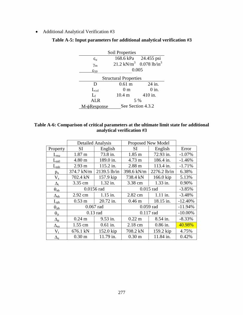
277



Soil Properties

cu 168.6 kPa 24.455 psi

m 21.2 kN/m3

0.078 lb/in3

50 0.005


D 0.61 m 24 in.

Lcol 0 m 0 in.

Lf 10.4 m 410 in.

ALR 5 %






Lma 1.87 m 73.8 in. 1.85 m 72.93 in. -1.07%

Lm0 4.80 m 189.0 in. 4.73 m 186.4 in. -1.46%

Lmb 2.93 m 115.2 in. 2.88 m 113.4 in. -1.71%


Vs 702.4 kN 157.9 kip 738.4 kN 166.0 kip 5.13%

t 3.35 cm 1.32 in. 3.38 cm 1.33 in. 0.90%

eb 0.0156 rad 0.015 rad -3.85%

eb 2.92 cm 1.15 in. 2.82 cm 1.11 in. -3.48%

Lpb 0.53 m 20.72 in. 0.46 m 18.15 in. -12.40%

pb 0.067 rad 0.059 rad -11.94%

p 0.13 rad 0.117 rad -10.00%

p 0.24 m 9.53 in. 0.22 m 8.54 in. -8.33%

ea 1.55 cm 0.61 in. 2.18 cm 0.86 in. 40.98%

Vt 676.1 kN 152.0 kip 708.2 kN 159.2 kip 4.75%

u 0.30 m 11.79 in. 0.30 m 11.84 in. 0.42%

278

La

tera

l F

orc

e (k

N)

La

tera

l F

orc

e (k

ips)

800


0 2 4 6 8 10 12 14

700 160

600 140

500

400

300

200

LPILE Results

ISU Model


120

100

80

60

40

100 20

0 0

0 5 10 15 20 25 30 35 40

Displacement (cm)


verification #3

279



Soil Properties

cu 168.6 kPa 24.455 psi

m 21.2 kN/m3

0.078 lb/in3

50 0.005


D 0.61 m 24 in.

Lcol 2.69 m 106 in.

Lf 10.4 m 410 in.

ALR 5 %






Lma 3.32 m 130.7 in. 3.36 m 132.3 in. 1.20%

Lm0 6.50 m 256.0 in. 6.50 m 256.1 in. 0.04%

Lmb 3.18 m 125.3 in. 3.14 m 123.8 in. -1.26%


Vs 189.5 kN 42.6 kip 228.2 kN 51.3 kip 20.42%

t 4.34 cm 1.71 in. 4.04 cm 1.59 in. -6.91%

eb 0.0174 rad 0.017 rad -2.30%

eb 5.77 cm 2.27 in. 5.59 cm 2.20 in. -3.12%

Lpb 0.61 m 24.15 in. 0.50 m 19.81 in. -18.03%

pb 0.078 rad 0.064 rad -17.95%

p 0.14 rad 0.128 rad -8.57%

p 0.48 m 18.8 in. 0.43 m 16.92 in. -10.42%

ea 4.19 cm 1.65 in. 3.30 cm 1.30 in. -21.24%

Vt 174.8 kN 39.3 kip 179.7 kN 40.4 kip 2.80%

u 0.59 m 23.36 in. 0.56 m 22.01 in. -5.08%

280

La

tera

l F

orc

e (k

N)

La

tera

l F

orc

e (k

ips)

250


0 5 10 15 20 25

50

200

40

150

30

100 LPILE Results

ISU Model 20


50 10

0 0

0 10 20 30 40 50 60 70

Displacement (cm)


verification #4

281



Soil Properties

cu 168.6 kPa 24.455 psi

m 21.2 kN/m3

0.078 lb/in3

50 0.005


D 0.61 m 24 in.

Lcol 6.10 m 240 in.

Lf 10.4 m 410 in.

ALR 5 %






Lma 6.38 m 251.3 in. 6.37 m 250.8 in. -0.16%

Lm0 9.61 m 378.4 in. 9.72 m 382.7 in. 1.14%

Lmb 3.23 m 127.1 in. 3.35 m 131.9 in. 3.72%

pu 263.8 kN/m 1506.6 lb/in 321.7 kN 1837.0 lb/in 21.95%

Vs 75.6 kN 17.0 kip 88.1 kN 19.8 kip 16.53%

t 4.19 cm 1.65 in. 4.57 cm 1.80 in. 9.07%

eb 0.0174 rad 0.018 rad 3.45%

eb 11.10 cm 4.37 in. 11.23 cm 4.42 in. 1.17%

Lpb 0.59 m 23.33 in. 0.54 m 21.1 in. -8.47%

pb 0.075 rad 0.068 rad -9.33%

p 0.17 rad 0.136 rad -20.00%

p 1.06 m 41.6 in. 0.87 m 34.16 in. -17.92%

ea 15.01 cm 5.91 in. 6.43 cm 2.53 in. -57.12%

Vt 35.7 kN 8.03 kip 51.6 kN 11.6 kip 44.54%

u 1.33 m 52.5 in. 1.09 m 42.9 in. -18.05%

282

La

tera

l F

orc

e (k

N)

La

tera

l F

orc

e (k

ips)


0 10 20 30 40 50

80

70 16

14

60

12 50

10

40

8

30 6

20 LPILE Results

ISU Model 4

First Yield Location 10 2

0 0

0 20 40 60 80 100 120 140

Displacement (cm)


verification #5

283



Soil Properties

cu 379.2 kPa 55 psi

m 21.2 kN/m3

0.078 lb/in3

50 0.004


D 0.61 m 24 in.

Lcol 0 m 0 in.

Lf 10.4 m 410 in.

ALR 5 %






Lma 1.39 m 54.67 in. 1.22 m 48.03 in. -12.15%

Lm0 3.60 m 141.8 in. 3.62 m 142.6 in. 0.56%

Lmb 2.21 m 87.14 in. 2.40 m 94.59 in. 8.55%

pu 748.8 kN/m 4276 lb/in 827.2 kN/m 4723.5 lb/in 10.47%

Vs 1040.0 233.8 kip 1009.3 kN 226.9 kip -2.95%

t 1.85 cm 0.73 in. 2.16 cm 0.85 in. 16.44%

eb 0.0117 rad 0.013 rad 11.11%

eb 1.63 cm 0.64 in. 1.57 cm 0.62 in. -3.68%

Lpb 0.38 m 15.13 in. 0.38 m 15.14 in. 0.07%

pb 0.0488 rad 0.049 rad 0.41%

p 0.10 rad 0.0977 rad -2.30%

p 0.14 m 5.32 in. 0.12 m 4.69 in. -11.84%

ea 0.86 cm 0.34 in. 0.97 cm 0.38 in. 11.76%

Vt 1014.2 kN 228.0 kip 1060.0 kN 238.3 kip 4.52%

u 0.17 m 6.57 in. 0.17 m 6.52 in. -0.76%

284

La

tera

l F

orc

e (k

N)

La

tera

l F

orc

e (k

ips)


0 1 2 3 4 5 6 7

1000

200

800

600

150

400

200

LPILE Results

ISU Model


100 50

0 0

0 5 10 15 20

Displacement (cm)


verification #6

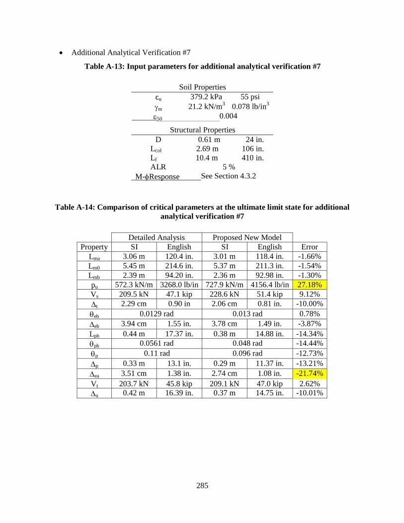
285



Soil Properties

cu 379.2 kPa 55 psi

m 21.2 kN/m3

0.078 lb/in3

50 0.004


D 0.61 m 24 in.

Lcol 2.69 m 106 in.

Lf 10.4 m 410 in.

ALR 5 %






Lma 3.06 m 120.4 in. 3.01 m 118.4 in. -1.66%

Lm0 5.45 m 214.6 in. 5.37 m 211.3 in. -1.54%

Lmb 2.39 m 94.20 in. 2.36 m 92.98 in. -1.30%


Vs 209.5 kN 47.1 kip 228.6 kN 51.4 kip 9.12%

t 2.29 cm 0.90 in 2.06 cm 0.81 in. -10.00%

eb 0.0129 rad 0.013 rad 0.78%

eb 3.94 cm 1.55 in. 3.78 cm 1.49 in. -3.87%

Lpb 0.44 m 17.37 in. 0.38 m 14.88 in. -14.34%

pb 0.0561 rad 0.048 rad -14.44%

p 0.11 rad 0.096 rad -12.73%

p 0.33 m 13.1 in. 0.29 m 11.37 in. -13.21%

ea 3.51 cm 1.38 in. 2.74 cm 1.08 in. -21.74%

Vt 203.7 kN 45.8 kip 209.1 kN 47.0 kip 2.62%

u 0.42 m 16.39 in. 0.37 m 14.75 in. -10.01%

286

La

tera

l F

orc

e (k

N)

La

tera

l F

orc

e (k

ips)

250


0 5 10 15

50

200

40

150

30

100

50

LPILE Results 20

ISU Model


10

0 0

0 10 20 30 40 50

Displacement (cm)


verification #7

287



Soil Properties

cu 379.2 kPa 55 psi

m 21.2 kN/m3

0.078 lb/in3

50 0.004


D 0.61 m 24 in.

Lcol 6.10 m 240 in.

Lf 10.4 m 410 in.

ALR 5 %






Lma 6.27 m 247.0 in. 6.26 m 246.6 in. -0.16%

Lm0 8.68 m 341.9 in. 8.82 m 347.2 in. 1.55%

Lmb 2.41 m 94.87 in. 2.36 m 100.6 in. 6.04%


Vs 91.6 kN 20.6 kip 119.7 kN 26.9 kip 30.58%

t 2.21 cm 0.87 in. 2.54 cm 1.00 in. 14.94%

eb 0.0129 0.014 rad 8.53%

eb 8.10 cm 3.19 in. 8.51 cm 3.35 in. 5.02%

Lpb 0.43 m 16.94 in. 0.41 m 16.09 in. -5.02%

pb 0.0547 rad 0.052 rad -4.94%

p 0.14 rad 0.104 rad -25.71%

p 0.86 m 33.9 in. 0.65 m 25.62 in. -24.42%

ea 14.33 cm 5.64 in. 7.90 cm 3.11 in. -44.86%

Vt 49.8 kN 11.2 kip 66.3 kN 14.9 kip 33.04%

u 1.09 m 43.08 in. 0.84 m 33.08 in. -23.21%

288

La

tera

l F

orc

e (k

N)

La

tera

l F

orc

e (k

ips)

100


0 10 20 30 40

90 20

80

70

15

60

50

10

40 LPILE Results

ISU Model 30 First Yield Location

20 5

10

0 0

0 20 40 60 80 100 120

Displacement (cm)


verification #8

289

Ref

eren

ce V

alu

e: C

old

/Av

g.

at 2

0 o

C

APPENDIX B: ADDITIONAL CONCRETE TESTING INFORMATION

1.8

1.6

Cylinder 1

Cylinder 2

Cylinder 3





1.4

1.2

1.0

0.8

30 20 10

0 -10

Temperature (oC)

-20

-30

-40

-50

Figure B-1: Comparison of SGF obtained from experimental testing of Man C concrete

mix and past studies

Notes:

1. Data is not indicative of strength increases associated with past studies and other data

within this experiment. Therefore, the data will not be used in the establishment of

trends.

290

Ref

eren

ce V

alue:

Cold

/Avg

. at

20

oC

1.8

1.6

1.4

Cylinder 1

Cylinder 2

Cylinder 3





1.2

1.0

0.8

30 20 10

0 -10

Temperature oC

-20

-30

-40

-50

Figure B-2: Comparison of SGF obtained from experimental testing of IF concrete mix and

past studies

Notes:

1. High strength data by Lee et al. (1988b) and data from Sehnal (1983) adequately capture

the increase in strength found in the experimental testing at ISU as an upper bound.

2. The normal strength concrete data suggested by Lee et al. (1988a) does not sufficiently

capture the behavior of the experimental data and will not be included in the average

value charts.

3. The average values of the experimental data set follow a linear trend better than that of a

curvilinear trend and will be used in determining a recommendation for strength increase.

291

Ela

stic

Mod

ulu

s, M

Pa

Ela

stic

Mod

ulu

s, k

si

APPENDIX C: ADDITIONAL A706 MILD STEEL REINFORCING BAR

TEST DATA

The following section provides additional results from the testing of A706 mild steel

reinforcement. The results depict the effects of temperature on the elastic modulus, yield plateau

length, and ultimate strain, along with the effects of strain rate on the elastic modulus and

ultimate strain. The last portion of this section provides a comparison between the recommended

and recorded stress-strain curves to show how closely the Equations capture the measured

response.

60

300000

Temperature, ⁰F

40 20 0

-20

-40

250000

25 mm (1.000 in.)

19 mm (0.750 in.)

40,000

35,000

200000 30,000

150000

25,000

20,000

100000 15,000

50000

10,000

5,000

0

20 10

0 -10

Temperature, ⁰C

-20

-30

0

-40

Figure C-1: Modulus of elasticity vs. temperature obtained at a strain rate of 0.001896

/min.

292

Ult

ima

te S

tra

in

Yie

ld P

late

au

Len

gth

60

0.009

Temperature, ⁰F

40 20 0

-20

-40

0.008

0.007

0.006

0.005

0.004

0.003

0.002

0.001

0

20 10

0 -10

-20

-30

-40

Temperature, ⁰C

Figure C-2: Yield plateau length vs. temperature obtained at a strain rate of 0.001897 /min. for all tested bar sizes

60

-0.13

Temperature, ⁰F

40 20 0

-20

-40

-0.125

-0.12

-0.115

-0.11

-0.105

25 mm (1.000 in.)

19 mm (0.750 in.)

-0.1

20 10

0 -10

-20

-30

-40

Temperature, ⁰C

Figure C-3: Ultimate strain vs. temperature at a strain rate of 0.275 /min.

293

Ult

ima

te S

tra

in

Str

ess,

MP

a

Str

ess,

ksi

-0.13

-0.125

-0.12

-0.115

-0.11

-0.105

-0.1

-1 Deg C B4

-20 Deg C B4

-1 Deg C B5

-20 Deg C B5

0.003 0.03 0.3

Strain rate, /min

Figure C-4: Ultimate strain vs. strain rate at various temperatures

-850

-800

-750

-700

-650

-600

-550

-500

-450

-400

-350

-300

-250

-200

-150

-100

-50

0

25 mm (1.00 in.)

19 mm (0.75 in.)

25 mm (1.00 in.) Equation


-118.9

-98.9

-78.9

-58.9

-38.9

-18.9

0.00 -0.02 -0.04 -0.06

Strain

-0.08 -0.10 -0.12

Figure C-5: Strain-hardening strength increase equation 6-5 validation at 20 °C (68 °F)

294

Str

ess,

MP

a

Str

ess,

MP

a

Str

ess,

ksi

S

tres

s, k

si

-850

-800

-750

-700

-650

-600

-550

-500

-450

-400

-350

-300

-250

-200

-150

-100

-50

0

25 mm (1.00 in.)

25 mm (1.00) Equation

-118.9

-98.9

-78.9

-58.9

-38.9

-18.9

0 -0.02 -0.04 -0.06

Strain

-0.08 -0.1 -0.12

Figure C-6: Strain-hardening strength increase equation 6-5 validation at 5 °C (41 °F)

-850

-800

-750

-700

-650

-600

-550

-500

-450

-400

-350

-300

-250

-200

-150

-100

-50

0

25 mm (1.00 in.)

19 mm (0.75 in.)



-118.9

-98.9

-78.9

-58.9

-38.9

-18.9

0 -0.02 -0.04 -0.06

Strain

-0.08 -0.1 -0.12

Figure C-7: Strain-hardening strength increase equation 6-5 validation at -1 °C (30.2 °F)

295

Str

ess,

MP

a

Str

ess,

MP

a

Str

ess,

ksi

S

tres

s, k

si

-850

-800

-750

-700

-650

-600

-550

-500

-450

-400

-350

-300

-250

-200

-150

-100

-50

0

25 mm (1.00 in.)

19 mm (0.75 in.)



-118.9

-98.9

-78.9

-58.9

-38.9

-18.9

0 -0.02 -0.04 -0.06

Strain

-0.08 -0.1 -0.12

Figure C-8: Strain-hardening strength increase equation 6-5 validation at -20 °C (-4 °F)

-850

-800

-750

-700

-650

-600

-550

-500

-450

-400

-350

-300

-250

-200

-150

-100

-50

0

25 mm (1.00 in.)

19 mm (0.75 in.)



-118.9

-98.9

-78.9

-58.9

-38.9

-18.9

0.00 -0.02 -0.04 -0.06

Strain

-0.08 -0.10 -0.12

Figure C-9: Strain-hardening strength increase equation 6-5 validation at -40 °C (-40 °F)

296

Ref

eren

ce V

alu

e

Ref

eren

ce V

alu

e

APPENDIX D: ADDITIONAL FROZEN SOIL TESTING INFORMATION

The following section provides additional information from the frozen soil investigation.

Included within this section are the individual figures constructed for the failure strength

reference values as well as the individual failure strain comparisons.

Additional Type II Soil Information

800

700

600

500

400

300

200

100

Avg. -1 deg. C

Avg. -20 deg. C

0

0 -5

-10

-15

-20

-25

Temperature (°C)

Figure D-1: Refernce value comparison for failure strength on a Type II soil

1.6

1.4

1.2

1

0.8

0.6

Experimental Data

Avg. -1 deg C

Avg -20 deg C

0.4

0.2

0

20 10

0 -10

-20

-30

Temperature (°C)

Figure D-2: Reference value comparison for failure strain on a Type II soil

297

Refe

ren

ce V

alu

e

Ref

eren

ce V

alu

e

Additional Type III Soil Information

100

90

80

70

60

50

40

30

Avg. -1 deg. C

20 Avg. -20 deg. C

10

0

0 -5

-10

-15

-20

-25

Temperature (°C)

Figure D-3: Reference value comparison for failure strength on Type III soil

1.2

1

0.8

0.6

0.4

0.2

Experimental Data

Avg. -1 deg C

Avg -20 deg C

0

20 10

0 -10

-20

-30

Temperature (°C)

Figure D-4: Reference value comparison for failure strain on Type III Soil

298

Refe

ren

ce V

alu

e

Ref

eren

ce V

alu

e

Additional Type IV Soil Information

160

140

120

100

80

60

40

20

0

0 -5

-10

-15

-20

-25

Temperature (°C)

Figure D-5: Reference value comparison for failure strength on Type IV soil

1.4

1.2

1

0.8

0.6

0.4

0.2 Experimental Data

Avg -20 deg C

0

20 10

0 -10

-20

-30

Temperature (°C)

Figure D-6: Reference value comparison for failure strain on Type IV soil

299

Ref

ere

nce

Va

lue

Ref

eren

ce V

alu

e

Additional Type V Soil Information

140

120

100

80

60

40

20

0

0 -5

-10

-15

-20

-25

Temperature (°C)

Figure D-7: Reference value comparison for failure strength on Type V soil

1.2

1

0.8

0.6

0.4

0.2

Experimental Data

Avg. -1 deg C

Avg -20 deg C

0

20 10

0 -10

-20

-30

Temperature (°C)

Figure D-8: Reference value comparison for failure strain on Type V soil

seismic design of deep bridge pier foundations in...

Documents