seismic and electrical signatures of the lithosphere
TRANSCRIPT

EA45CH06-Kawakatsu ARI 14 August 2017 12:51
Annual Review of Earth and Planetary Sciences
Seismic and ElectricalSignatures of theLithosphere–AsthenosphereSystem of the Normal OceanicMantleHitoshi Kawakatsu and Hisashi UtadaEarthquake Research Institute, The University of Tokyo, Tokyo 113-0032, Japan;email: [email protected]
Annu. Rev. Earth Planet. Sci. 2017. 45:139–67
The Annual Review of Earth and Planetary Sciences isonline at earth.annualreviews.org
https://doi.org/10.1146/annurev-earth-063016-020319
Copyright c© 2017 by Annual Reviews.All rights reserved
Keywords
lithosphere, asthenosphere, Lid, low-velocity zone, G-discontinuity, platetectonics, anisotropy, electrical conductivity
Abstract
Although plate tectonics started as a theory of the ocean basins nearly 50 yearsago, the mechanical details of how it works are still poorly known. Ourunderstanding of these details has been hampered partly by our inabilityto characterize the physical nature of the lithosphere–asthenosphere system(LAS) beneath the ocean. We review the existing observational constraintson the seismic and electrical properties of the LAS, particularly for normaloceanic regions away from mid-oceanic ridges, hot spots, and subductionzones, where plate tectonics is expected to present its simplest form. Whereasa growing volume of seismic data on land has provided remarkable advancesin large-scale pictures, seafloor observations have been shedding new lighton essential details. By combing through these observational constraints,researchers are unveiling the nature of the enigmatic LAS. Future directionsfor large-scale seafloor observations are also discussed.
139
Click here to view this article's online features:
• Download figures as PPT slides• Navigate linked references• Download citations• Explore related articles• Search keywords
ANNUAL REVIEWS Further
Ann
u. R
ev. E
arth
Pla
net.
Sci.
2017
.45:
139-
167.
Dow
nloa
ded
from
ww
w.a
nnua
lrev
iew
s.or
g A
cces
s pr
ovid
ed b
y U
nive
rsity
of
Tok
yo -
Lib
rary
Ear
thqu
ake
Res
earc
h In
stitu
te o
n 09
/08/
17. F
or p
erso
nal u
se o
nly.

EA45CH06-Kawakatsu ARI 14 August 2017 12:51
LAS: lithosphere–asthenospheresystem
LAB: lithosphere–asthenosphereboundary
LVZ: low-velocityzone
LCL:low-conductivity layer
HCL:high-conductivitylayer
EM: electromagnetic
1. INTRODUCTION: LITHOSPHERE–ASTHENOSPHERESYSTEM IN THE OCEAN
Plate tectonics, a phenomenological framework describing the motions of the solid Earth, is basedon the concept that a small number of rigid shells that cover Earth’s surface move horizontallyrelative to each other, making earthquakes and volcanoes at and around their boundaries. Tofacilitate such motions, the rigid surface part of Earth comprising its plates, the lithosphere, isbelieved to sit on top of a weak layer, the asthenosphere, and thus elucidation of the lithosphereand asthenosphere as a whole is essential for understanding how our planet works. Consideringthat the lithosphere is created from the mantle, i.e., asthenosphere, at ridges beneath the oceanand that it thermally thickens (ages) as it moves away from these ridges, the lithosphere and theasthenosphere need to be understood together as an evolving system. Thus, elucidation of thelithosphere–asthenosphere system (LAS) has been the focus of recent observational geophysics.
Although advances in seismic tomography and numerical simulations of mantle convection overthe past 30 years or so have greatly improved our understanding of how plate tectonics might berelated to processes occurring in the deep interior of Earth, the physical conditions that distinguishthe lithosphere and asthenosphere are under debate. The complicated history of the evolution ofthe continents makes it difficult to resolve this fundamental question using observations under thecontinents. In contrast, plate tectonics is expected to show its simplest representation of the LASunder the oceans. Thus, better observational constraints are expected from the oceanic crust andmantle, although great challenges exist from the observational point of view. This article reviewsrecent progress in this direction. We concentrate on properties of the normal oceanic mantle,staying away from popular science targets, such as mid-oceanic ridges, hot spots (seamounts), andsubduction zones (and also the crustal structure).
1.1. Mechanical Layering
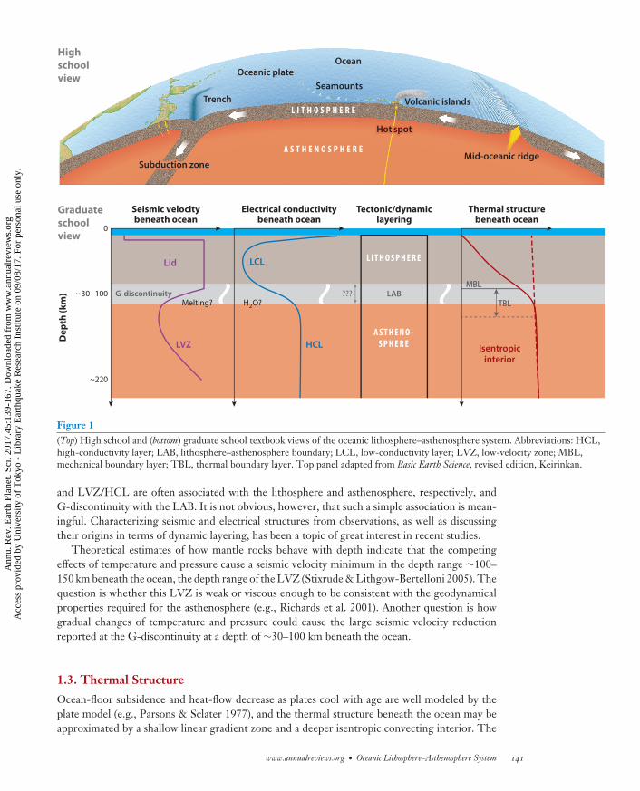
Figure 1 illustrates two schematic views of the LAS in the ocean that may be seen in textbooks.The terms “lithosphere” and “asthenosphere” refer to tectonic/dynamic layering in the suboceanicmantle on the basis of mechanical strength. The lithosphere is Earth’s rigid outermost shell andconsists of the crust and the uppermost part of the upper mantle; it is considered equivalent withthe term “plate” in the context of plate tectonics. The asthenosphere, named after the Greek wordmeaning “weak,” is a soft layer of the mantle, just below the lithosphere, that facilitates horizontalmovements of plates. The word existed even in the early 1900s, before the birth of plate tectonics,to explain the long-term ground deformation associated with the removal of Pleistocene glaciers.Recent literature discusses what defines the lithosphere–asthenosphere boundary (LAB), and someresearchers argue that the boundary could be transitional rather than sharp.
1.2. Seismic and Electrical Layering
Seismic velocity layering typically indicates a thin (∼6-km) oceanic crust (White et al. 1992) un-derlaid by a nearly constant high-velocity layer (Lid) and a low-velocity zone (LVZ) (Gutenberg1959). The sharp velocity decrease from Lid to LVZ is called the G-discontinuity after BenoGutenberg (Revenaugh & Jordan 1991). Some recent seismological literature refers to such dis-continuous structures as the LAB, which may be somewhat misleading, as from seismology alonethere is no simple way to tell whether a structure is the true LAB. Similarly, electrical conductivitylayering shows a low-conductivity layer (LCL) underlaid by a high-conductivity layer (HCL). Asthe transition thickness from LCL to HCL is difficult to constrain from electromagnetic (EM)data, no boundary structure is usually reported for the electrical conductivity. The Lid/LCL
140 Kawakatsu · Utada
Ann
u. R
ev. E
arth
Pla
net.
Sci.
2017
.45:
139-
167.
Dow
nloa
ded
from
ww
w.a
nnua
lrev
iew
s.or
g A
cces
s pr
ovid
ed b
y U
nive
rsity
of
Tok
yo -
Lib
rary
Ear
thqu
ake
Res
earc
h In
stitu
te o
n 09
/08/
17. F
or p
erso
nal u
se o
nly.
EA45CH06-Kawakatsu ARI 14 August 2017 12:51
Trench
Ocean
Volcanic islands
Mid-oceanic ridge
Oceanic plate
Highschoolview
Graduateschoolview
Subduction zoneSubduction zone
Hot spotHot spot
Lid
LVZ
~ 30–100 LABG-discontinuity
Seismic velocitybeneath ocean
Dep
th (k
m)
Tectonic/dynamiclayering
~220
0
Melting? H2O?
Electrical conductivitybeneath ocean
LCL
HCL
???MBLMBL
Isentropicinterior
Thermal structurebeneath ocean
Seamounts
TBLTBL
L I T H O S P H E R E
L I T H O S P H E R E
A S T H E N O -S P H E R E
A S T H E N O S P H E R E
Figure 1(Top) High school and (bottom) graduate school textbook views of the oceanic lithosphere–asthenosphere system. Abbreviations: HCL,high-conductivity layer; LAB, lithosphere–asthenosphere boundary; LCL, low-conductivity layer; LVZ, low-velocity zone; MBL,mechanical boundary layer; TBL, thermal boundary layer. Top panel adapted from Basic Earth Science, revised edition, Keirinkan.
and LVZ/HCL are often associated with the lithosphere and asthenosphere, respectively, andG-discontinuity with the LAB. It is not obvious, however, that such a simple association is mean-ingful. Characterizing seismic and electrical structures from observations, as well as discussingtheir origins in terms of dynamic layering, has been a topic of great interest in recent studies.
Theoretical estimates of how mantle rocks behave with depth indicate that the competingeffects of temperature and pressure cause a seismic velocity minimum in the depth range ∼100–150 km beneath the ocean, the depth range of the LVZ (Stixrude & Lithgow-Bertelloni 2005). Thequestion is whether this LVZ is weak or viscous enough to be consistent with the geodynamicalproperties required for the asthenosphere (e.g., Richards et al. 2001). Another question is howgradual changes of temperature and pressure could cause the large seismic velocity reductionreported at the G-discontinuity at a depth of ∼30–100 km beneath the ocean.
1.3. Thermal Structure
Ocean-floor subsidence and heat-flow decrease as plates cool with age are well modeled by theplate model (e.g., Parsons & Sclater 1977), and the thermal structure beneath the ocean may beapproximated by a shallow linear gradient zone and a deeper isentropic convecting interior. The
www.annualreviews.org • Oceanic Lithosphere–Asthenosphere System 141
Ann
u. R
ev. E
arth
Pla
net.
Sci.
2017
.45:
139-
167.
Dow
nloa
ded
from
ww
w.a
nnua
lrev
iew
s.or
g A
cces
s pr
ovid
ed b
y U
nive
rsity
of
Tok
yo -
Lib
rary
Ear
thqu
ake
Res
earc
h In
stitu
te o
n 09
/08/
17. F
or p
erso
nal u
se o
nly.
EA45CH06-Kawakatsu ARI 14 August 2017 12:51
TBL: thermalboundary layer
MBL: mechanicalboundary layer
transition between these layers is called the thermal boundary layer (TBL) by Parsons & McKenzie(1978), where small-scale convection might be taking place to transport heat from below. Abovethe TBL, there is a mechanical boundary layer (MBL) that may be equated with the lithosphere.Incorporating gravity data, Crosby et al. (2006) estimated the cross point of the two linear thermalgradients at a depth of 90 km for old Pacific Ocean, which might give a deepest possible depth ofthe lithosphere (i.e., lower boundary of the MBL).
1.4. Melts and Volatiles
The presence of partial melt has a strong influence on the physical properties of mantle rocks.Seismic velocity of mantle rocks decreases and electrical conductivity increases where melts exist.Therefore, the presence of partial melt was suggested to account for the origin of the LVZ andthe HCL in the upper mantle (Anderson & Sammis 1970, Shankland & Waff 1977). However, theconnection between physical properties of the melt phase and of the bulk partially molten rock isnot simple. The geometry of melt phases (or aqueous fluids) has significant effects on the velocitychange that might be inferred from seismic observations (Takei 2002). The connectivity of themelt phase has a significant influence on electrical properties (Toramaru & Fujii 1986). However,once a well-connected melt network is formed in a partially molten system, the bulk electricalconductivity does not depend much on the texture of the network but is simply proportional tothe fraction and connectivity of melt (Utada & Baba 2014).
A certain quantity of volatiles is expected in the mantle, and H2O and CO2 in particular are con-sidered to play important roles in controlling the physical properties of that region. Geochemicalstudies suggest the water content to be about 100 ppm H2O and the mass ratio H/C to be about0.75 in the typical suboceanic mantle (Hirschmann & Dasgupta 2009). Deformation experimentsshowed that even a small amount (only a few ppm by weight) of water will enhance the creeprate of olivine by orders of magnitude (Mei & Kohlstedt 2000a,b). However, a recent study castdoubt on this result, reporting a rather weak effect of water on upper-mantle rheology (Fei et al.2013). Water (hydrogen) dissolved in mantle minerals is also considered to reduce seismic velocityand to enhance electrical conductivity, but the significance of these effects is not well resolved.The water effect on electrical conductivity is especially controversial, and significant inconsistencyamong experimental results obtained by different groups has prevented conclusive, quantitativeinterpretation of the geophysical data (Gardes et al. 2014).
In addition, volatiles (H2O or CO2) in the upper mantle, even in small amounts, significantlyreduce the solidus temperature, which is effective in producing partial melting in the upper man-tle. In the presence of volatiles at likely concentration, most of the oceanic LVZ and HCL iseither close to or above the solidus temperature of hydrated or carbonated peridotite. Stabilitycalculations of partial melt (Hirschmann 2010) indicate large spatial variations of partial melts,with different H2O and CO2 concentrations depending on different degrees of melting. At a lowdegree of melting, melt contains high concentrations of CO2 and is called carbonatite melt. Recentexperimental studies report that carbonatite melt has extremely high electrical conductivity (e.g.,Gaillard et al. 2008, Yoshino & Katsura 2013).
2. GLOBAL AND LAND-BASED STUDIES
Extensive seismological investigation of the oceanic LAS has been conducted by employingsurface-wave dispersion measurements from land-based seismic stations. Surface waves propa-gate effectively in the oceanic region, and at long periods (say, longer than ∼30 s) they dominatethe wavefield, making for easy observation. The surface-wave dispersion curve, that is, the period
142 Kawakatsu · Utada
Ann
u. R
ev. E
arth
Pla
net.
Sci.
2017
.45:
139-
167.
Dow
nloa
ded
from
ww
w.a
nnua
lrev
iew
s.or
g A
cces
s pr
ovid
ed b
y U
nive
rsity
of
Tok
yo -
Lib
rary
Ear
thqu
ake
Res
earc
h In
stitu
te o
n 09
/08/
17. F
or p
erso
nal u
se o
nly.
EA45CH06-Kawakatsu ARI 14 August 2017 12:51
dependence of the wave velocity, can be converted to a one-dimensional (1-D) velocity [(shearwave (S-wave)] structure. Earlier work (e.g., Takeuchi et al. 1959, Dorman et al. 1960) demon-strated the general Lid/LVZ pattern in the ocean. The lateral variation of the oceanic LAS wasalso studied in the 1970s, and it was shown that the Lid thickens with age (e.g., Leeds et al. 1974,Forsyth 1975, Yoshii et al. 1976). Recent tomographic studies further confirm this plate evolutionscenario (e.g., Ritzwoller et al. 2004, Maggi et al. 2006b).
The EM field is mostly sensitive to the structure just beneath the station, and station distributionis quite sparse in oceanic regions (Kelbert et al. 2014). Thus, global EM imaging can resolve onlylarge and deep structures, but the upper mantle is imaged as a nearly uniform resistive layer withconductivity of about 0.01 S/m, which increases in the transition zone by about one order ofmagnitude. More detailed electrical signatures of the oceanic LAS will need to be explored byseafloor in-situ measurements.
2.1. One-Dimensional Structure
One-dimensional average properties of the oceanic LAS have been studied using various seismo-logical approaches. These studies characterize representative structures of the LAS in the ocean.
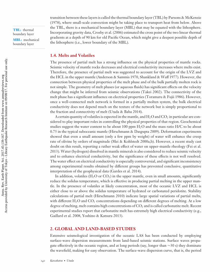
2.1.1. Surface-wave studies. Figure 2a,b shows averaged S-wave velocity structures in thePacific Ocean in the absence of abnormal topography based on two recent tomographic models asa function of plate age (Priestley & McKenzie 2013). The Lid/LVZ pattern and the general increaseof S-wave velocity with plate age are evident (although the absolute values do not agree). Priestley& McKenzie (2006, 2013) used this type of information to estimate S-wave velocity as a functionof temperature and pressure for given depths, reporting that S-wave velocity decreases nonlinearlywhen approaching the melting temperature. It is worth noting that the peak (velocity minimum)depth of the LVZ stays shallower than ∼150 km. It should also be noted that Figure 2 starts froma depth of 50 km, above which long-period surface waves cannot constrain the structure, and thatsurface waves have a limited sensitivity to the sharpness of velocity changes with depth: A gradualvelocity decrease over ∼50 km and a sharp one at the center of transition cannot be distinguished.
–100
–200
–300
–400
Dep
th (k
m)
β V (k
m/s
)
a PM_v2_2012 SV
–100
5.0
4.8
4.6
4.4
4.2
4.0
3.8
–200
–300
–40025 50
4.0 4.2 4.4 4.6 4.8 5.0
75 100 125 150 175 400 600 800 1,000 1,200 1,400 1,600Age (Ma) Temperature, T (°C)
Shear wave speed (km/s)
Nodule geotherms
b
c
S362ANI SV
ObservationDepth50 km
Depth75 km
βV (T )used in fitting
Calculation
100–200 km≥200 km
Isentrope
Oceanic geotherms
Figure 2Shear wave (S-wave) velocity (βV) profiles from tomographic models of the Pacific Ocean, stacked as functions of age. [Models are from(a) Priestley & McKenzie (2013), (b) Kustowski et al. (2008).] (c) βV as a function of temperature estimated from panel a. The solid grayline shows the velocities at a depth of 50 km and the solid red line those at 75 km. All panels adapted from Priestley & McKenzie (2013)with permission.
www.annualreviews.org • Oceanic Lithosphere–Asthenosphere System 143
Ann
u. R
ev. E
arth
Pla
net.
Sci.
2017
.45:
139-
167.
Dow
nloa
ded
from
ww
w.a
nnua
lrev
iew
s.or
g A
cces
s pr
ovid
ed b
y U
nive
rsity
of
Tok
yo -
Lib
rary
Ear
thqu
ake
Res
earc
h In
stitu
te o
n 09
/08/
17. F
or p
erso
nal u
se o
nly.

EA45CH06-Kawakatsu ARI 14 August 2017 12:51
2.1.2. Body-wave studies. To discuss the details of the LAS, information obtained by surfacewaves that traverse the LAS horizontally needs to be supplemented by results for body waves thattraverse the LAS near-vertically.
2.1.2.1. ScS reverberation analysis. The ScS reverberation technique developed by Revenaugh& Jordan (1991) utilizes ScS-waves, which are emitted downward from earthquake sources andreflected at the core–mantle boundary. For large earthquakes, multiply reflected ScS-waves arewell observed at a period longer than ∼30 s and give tight constraints on the average structure ofthe mantle. When seismic discontinuities, such as the 410-km or the 660-km discontinuity, arepresent, reflections from these discontinuities are also well observed between multiple ScS phases,giving a unique constraint on the depth and size of the impedance contrast across the boundaries.Using this technique, Revenaugh & Jordan (1991) reported the presence of a sharp (�40-km)velocity reduction around a depth interval of 50–100 km in the oceanic region and named itthe G-discontinuity, which separates the Lid and LVZ. Although this technique provides uniqueand tight constraints on the nature of the LAS, a recent report from the same group (Bagley &Revenaugh 2008) substantially revised the original depth estimates for some of the paths (Bagley& Revenaugh 2008, Bagley et al. 2009, Fischer 2015).
2.1.2.2. Multiple S-wave transect. Besides ScS, multiply reflected S-waves, such as SS, SSS, SSSS,etc., pass through the LAS with slightly different incidence angles and can be used to constrainthe LAS structure, as well as the velocity structure of the entire upper mantle. Tan & Helmberger(2007) analyzed waveforms of Tonga–Fiji events recorded in southern California to develop a path-averaged upper-mantle shear velocity model across the Pacific Ocean (Figure 3), obtaining a modelthat contains a fast Lid (VSH = 4.78 km/s, VSV = 4.58 km/s) with a thickness of 60 km. It shouldbe noted that in this type of analysis, there is a trade-off between Lid thickness and average Lidvelocity, and that the same data can be equally fitted with a 40-km-thick (or 80-km-thick) Lid withfaster (or slower) velocity (see inset of Figure 3a). Similar earlier attempts (e.g., by Gaherty et al.1999) presumably suffer from the trade-off, as the imposed constraint on G-discontinuity by theScS reverberation is now reported to be ill-constrained (Bagley & Revenaugh 2008, Fischer 2015).Constraining the depth (and the degree of velocity reduction) of the G-discontinuity is importantin characterizing the LAS, as we discuss later. In the model of Tan & Helmberger (2007), the un-derlying LVZ is prominent, with the lowest velocities, VSH = 4.34 km/s and VSV = 4.22 km/s, oc-curring at a depth of 160 km, which is similar to the aforementioned surface-wave results. This typeof data can also constrain deeper structure, such as the positive gradient below the LVZ peak, whichmay be useful to compare with theoretical predictions (e.g., Stixrude & Lithgow-Bertelloni 2005).
2.1.2.3. SS-precursor analysis. Teleseismic SS phases are often preceded by small-amplitudephases that correspond to their underside reflections at mantle discontinuities, which are calledSS precursors. Because of their small amplitude, it is common to stack a large number of waveformsreflected from a given area in order to observe the phase. These precursors are useful in measuringthe depth of discontinuity and the strength of velocity change there (e.g., Gu et al. 2001, Deuss& Woodhouse 2002), but if a reflector is too close to the surface, the time separation betweenSS and its precursor becomes too small to be easily detected. To avoid this difficulty, Rychert &Shearer (2011) directly modeled long-period (>10-s) SS waveforms, including both the parentSS phase and its precursor, for detecting a velocity reduction with depth in the LAS (possibly theG-discontinuity) beneath the Pacific Ocean; they reported detection of a discontinuity (sharperthan ∼30 km) in some places (not in the whole Pacific Ocean) whose depth varies from 25 to 130 km
144 Kawakatsu · Utada
Ann
u. R
ev. E
arth
Pla
net.
Sci.
2017
.45:
139-
167.
Dow
nloa
ded
from
ww
w.a
nnua
lrev
iew
s.or
g A
cces
s pr
ovid
ed b
y U
nive
rsity
of
Tok
yo -
Lib
rary
Ear
thqu
ake
Res
earc
h In
stitu
te o
n 09
/08/
17. F
or p
erso
nal u
se o
nly.

EA45CH06-Kawakatsu ARI 14 August 2017 12:51
6,0005,000
4,000
400660
CMB
Depth
(km)
100°
80°
S O U R C ERECE IVER
40°60°20°
0°
1,000 2,000
bbr Δ 77.12
pas Δ 76.19
fig
Seisimic station:
Δ 75.27
3,0004.0
0
0
100
200
300
400
100
200
300
VSH PAC06
Other models
VSV
Tectonic North America (TNA)Old Atlantic (ATL)Shield North America (SNA)
40 kmLid
60 km80 km
400
500
600
700
8004.5
4.0 4.5 5.0
5.0 5.5 6.0 6.5
Observed waveformModel waveform
Time (s) Velocity, Vs (km/s)
Dep
th (k
m)
S
S
SSSS
SSSSScS2
ScS3 ScS4
SSS
SSS
SS
SS
4,000
Distance
Am
plit
ude
Radius
(km
)
a b
c
Figure 3(a) Model PAC06 constructed from various S multiples—S, SS, SSS, SSSS—whose ray paths are shown in panel b. VSH and VSV usedhere should be taken as S-wave velocities of SH- and SV-waves, which traverse the mantle with intermediate incidence angles (i.e.,these quantities are distinct from βH and βV). For further details on notation, see Section 2.2.1. (Inset) Trade-off between Lid thicknessand velocity. Three models, with 40-km-, 60-km-, and 80-km-thick Lids, give a similar fit to observations. (c) Comparison of observedand model waveforms at three stations, whose station codes and epicentral distances are indicated. Abbreviation: CMB, core–mantleboundary. Figure adapted from Tan & Helmberger (2007) with permission.
LPO:lattice-preferredorientation
(25 to 93 km for normal oceanic areas). A clear dependence on crustal age is evident, especially fornormal oceanic areas. Schmerr (2012), using a similar dataset but differentiating seismograms intime to enhance higher-frequency content sensitive to subtle changes, directly identified phasesoriginating from discontinuities in a depth range of 40–75 km. As the detection was limited inregions associated with recent surface volcanism and mantle melt production, Schmerr (2012)suggested that his observation is consistent with an intermittent layer of asthenospheric partialmelt residing at the lithospheric base. His observation shows a very weak age dependence, and atyounger ages (<20 Ma) depths are mostly deeper than 50 km, which may be due to the difficultyof separating precursors from the parent SS phase. Reported velocity reductions range from ∼7%to 12%. Tonegawa & Helffrich (2012) reported detection of precursors of the sS phase (notthe SS phase) originating from deep earthquakes, moving upward, and being reflected at theG-discontinuity beneath the Philippine Sea Plate (20–40 Ma). They conclude that there is aminimum S-wave contrast of −5.8% and a depth range of 50–70 km.
2.2. Seismic Anisotropy
Seismic anisotropy plays an essential role in the elucidation of the LAS. This is because platemotion–related shear motion in the asthenosphere is expected to introduce lattice-preferred ori-entation (LPO) of olivine, which is highly anisotropic and the most abundant mineral in the man-tle (e.g., Mainprice 2015), resulting in macroscopic seismic anisotropy observable by long-period
www.annualreviews.org • Oceanic Lithosphere–Asthenosphere System 145
Ann
u. R
ev. E
arth
Pla
net.
Sci.
2017
.45:
139-
167.
Dow
nloa
ded
from
ww
w.a
nnua
lrev
iew
s.or
g A
cces
s pr
ovid
ed b
y U
nive
rsity
of
Tok
yo -
Lib
rary
Ear
thqu
ake
Res
earc
h In
stitu
te o
n 09
/08/
17. F
or p
erso
nal u
se o
nly.

EA45CH06-Kawakatsu ARI 14 August 2017 12:51
seismic waves. Although the most general form of seismic anisotropy can be described by 21 elasticconstants, as opposed to two elastic constants for the isotropic case, it is common and practical toreduce the number to make the problem more tractable. The most common method is to assumeaxial (i.e., hexagonal) symmetry. Hexagonal symmetry requires five elastic constants in addition tothe direction of the symmetry axis, and it is also called transverse isotropy (TI). When the symme-try axis is vertical (radial), such anisotropy is called radial anisotropy or TI with a vertical symmetryaxis (VTI), and the standard Earth model PREM (Dziewonski & Anderson 1981) has a layer ofradial anisotropy between depths of 24.4 km and 220 km. When the symmetry axis is in the hor-izontal plane, azimuthally varying wave propagation velocity is realized as azimuthal anisotropy.
2.2.1. Radial Anisotropy. The presence of radial anisotropy in the upper mantle is inferredfrom observed phase velocities of Love and Rayleigh waves that cannot be explained by a single1-D isotropic model (Love–Rayleigh wave discrepancy). A Love wave is mainly sensitive to βH =√
N /ρ, the phase velocity of a horizontally polarized horizontally propagating S-wave, whereas aRayleigh wave is sensitive to βV = √
L/ρ, the phase velocity of a vertically polarized horizontallypropagating S-wave, where L, N , and ρ are Love’s representative elastic shear moduli and thedensity.1 In a radially anisotropic system, a vertically traveling S-wave has a phase velocity βV. Inthe oceanic regions, βH > βV is generally observed in the upper mantle (Forsyth 1975, Schlue &Knopoff 1977, Leveque & Cara 1985, Nishimura & Forsyth 1989). Recent tomographic modelsof radial anisotropy indicate strong and laterally varying radial anisotropy in the LVZ (Ekstrom &Dziewonski 1998, Nettles & Dziewonski 2008, Kustowski et al. 2008). Strong and puzzling radialanisotropy (larger than 5%) is observed in the central Pacific Ocean in the LVZ. Figure 4 shows
–1 0 1 2 3 4 5 0 1 2 3 4 5 6 7 8
100
200
300 Young oceans
Radial anisotropy Azimuthal anisotropy
a b
Mid-age oceansOld oceans
400
(βH – βV)/βVoigt Plate velocity (cm/year)
Dep
th (k
m)
3.0
2.0
1.0
0
2.5
1.5
0.5
–0.5
Stre
ngth
of a
niso
trop
y (%
) 100km V
150200250350
APM
Figure 4Strength of radial and azimuthal anisotropy. (a) Average radial anisotropy profiles for the oceanic regions. Panel a adapted from Nettles& Dziewonski (2008) with permission. (b) The peak-to-peak strength of azimuthal anisotropy at various depths as a function of platevelocity (dotted lines) and its projection onto the absolute plate motion direction (APM) (solid lines). Panel b adapted from Debayle &Ricard (2013) with permission. Note that the peak strength of anisotropy is ∼4% (radial) and ∼2.5% (azimuthal) for these models.
1The notation of S-wave velocity in a radially anisotropic system can be confusingly unclear if one fails to consider theincidence-angle dependence of body-wave velocities (Kawakatsu 2016). Here we distinguish between βH/βV and VSH/V SV;the former are as defined above, whereas the latter are wave velocities of SH/SV-waves, defined by the conventions ofseismology (e.g., Aki & Richards 2002), that traverse media with arbitrary incidence angles. (The polarization of an SH-waveis horizontal, and that of an SV-wave is perpendicular to SH).
146 Kawakatsu · Utada
Ann
u. R
ev. E
arth
Pla
net.
Sci.
2017
.45:
139-
167.
Dow
nloa
ded
from
ww
w.a
nnua
lrev
iew
s.or
g A
cces
s pr
ovid
ed b
y U
nive
rsity
of
Tok
yo -
Lib
rary
Ear
thqu
ake
Res
earc
h In
stitu
te o
n 09
/08/
17. F
or p
erso
nal u
se o
nly.
EA45CH06-Kawakatsu ARI 14 August 2017 12:51
average depth profiles for oceanic areas. It is interesting to note that the peak of radial anisotropyis generally above 150 km, a depth that is comparable to the peak depth of the LVZ, and thus itseems that the strong radial anisotropy is mainly due to the strong low velocity of βV.
2.2.2. Azimuthal anisotropy. The presence of azimuthal anisotropy in the ocean was establishedvia refraction surveys of Pn-waves in very early studies of P-waves (e.g., Raitt et al. 1969), andalso via regionalized surface-wave studies for the deeper mantle for S-waves (e.g., Forsyth 1975,Montagner 1985, Nishimura & Forsyth 1989). Tanimoto & Anderson (1984) first presented theglobal tomography model that inferred the connection with large-scale flow in the mantle. Thegrowing volume of digital waveform data in the past few decades has made it possible to constructdetailed tomographic models of the upper mantle (e.g., Smith et al. 2004, Ritzwoller et al. 2004,Maggi et al. 2006a, Debayle & Ricard 2013, Schaeffer & Lebedev 2013, Burgos et al. 2014), andcomparison with parameters related to plate tectonics has become possible. For example, Debayle& Ricard (2013) showed that beneath fast-moving (>5 cm/year) plates (i.e., the Indian, Cocos,Nazca, Australian, Philippine Sea, and Pacific plates), between depths of 100–200 km, fast az-imuthal directions generally coincide with present-day plate motion (Figure 4). However, forthe shallow lithosphere, a better correlation is obtained with fossil accretion directions, indicatingfrozen-in anisotropy for the origin of lithospheric azimuthal anisotropy. From a similar compar-ison, Becker et al. (2014) conclude that LPO inferred from mantle flow computations produces abetter fit than simple plate motion directions. In both results, it is interesting to note that the bestcorrelation is obtained for a depth range of 150–200 km, generally deeper than the peak depth ofradial anisotropy.
2.2.2.1. Limitations of surface-wave tomography. Although surface-wave tomography offers apowerful way to constrain the structure of the uppermost mantle, it is important to recognize thatthere are certain limitations, especially for the elucidation of the oceanic LAS. First, the difficultyof measuring short-period surface-wave dispersions (which is caused by multipathing that resultsfrom shallow lateral heterogeneities) makes the structure above ∼50 km undetermined, and thusit is common to assume some structure, including sediment and crustal structures. It is knownthat there is a trade-off between the shallow structure and the deeper structure, especially in radialanisotropy at depths of ∼100 km (Bozdag & Trampert 2008, Ferreira et al. 2010). Second, therelative strength of radial and azimuthal anisotropy, which gives an essential constraint on theorigin of anisotropy, is difficult to constrain because of the nonuniqueness of damping parametersinherent in inversion methods (e.g., Smith et al. 2004). Third, the depth resolution is limited to∼50 km and therefore prevents detailed investigations of the origins of peculiar structures, such asthe G-discontinuity. In light of these limitations, the usage of depth derivatives of various tomo-graphic models should be treated carefully unless high-resolution regional modeling is conducted(e.g., Yoshizawa 2014).
2.2.2.2. Subslab anisotropy. Change of the dip of the LAS at a subduction zone provides aunique way to investigate the anisotropy of the LAS. Radial anisotropy in the LAS under theoceanic environment is difficult to observe using shear-wave splitting, as nearly vertically incidentS-waves, such as SKS-waves, are not sensitive to radial anisotropy. Song & Kawakatsu (2012)have demonstrated that strong radial anisotropy of the suboceanic LAS observed by surface-wavetomography (e.g., Kustowski et al. 2008) (Figure 4) can have a significant effect on the observedSKS-wave splitting when the system is dipping, as in subduction zones, and that this might wellexplain the so-called subslab trench-parallel fast directions at the majority of subduction zones(Long & Silver 2008) without invoking any unrealistic trench-parallel flow in the mantle. When
www.annualreviews.org • Oceanic Lithosphere–Asthenosphere System 147
Ann
u. R
ev. E
arth
Pla
net.
Sci.
2017
.45:
139-
167.
Dow
nloa
ded
from
ww
w.a
nnua
lrev
iew
s.or
g A
cces
s pr
ovid
ed b
y U
nive
rsity
of
Tok
yo -
Lib
rary
Ear
thqu
ake
Res
earc
h In
stitu
te o
n 09
/08/
17. F
or p
erso
nal u
se o
nly.

EA45CH06-Kawakatsu ARI 14 August 2017 12:51
BBOBS: broadbandocean-bottomseismometer
azimuthal anisotropy present in the suboceanic LAS is incorporated in the modeling, they furthershowed that trench-normal fast directions at shallowly dipping subduction zones, such as theCascadia subduction zone and the central South American subduction zone, can also be explainedby a single model of orthorhombic anisotropy; if this model represents the general property ofsuboceanic anisotropy, radial anisotropy is stronger (∼3–4%) than azimuthal anisotropy (∼2%)(Figure 4); thus, it may require modification of the commonly accepted view that the A-typeolivine fabric ( Jung et al. 2006) is the dominant one in LAS, implying rather that the AG-typefabric (Mainprice 2015) is dominant (Song & Kawakatsu 2013).
3. CONSTRAINT FROM SEAFLOOR OBSERVATIONS
3.1. Active Source (Pn)
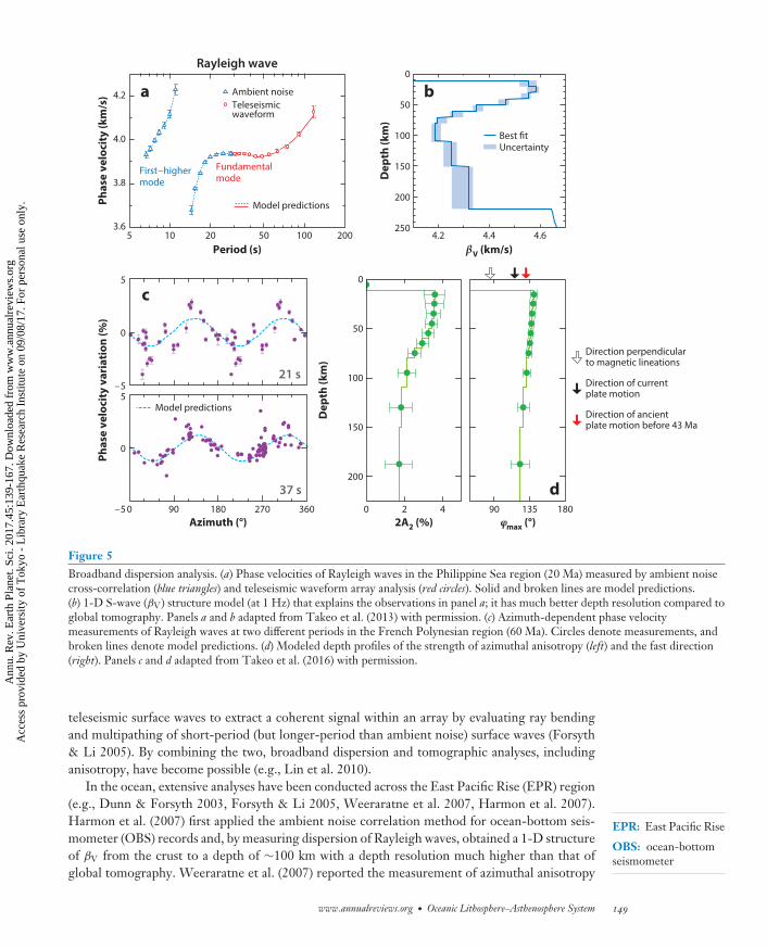
The crustal structure and the uppermost mantle just below the Mohorovicic discontinuity (Moho)have been extensively studied by active-source seismic surveys in the ocean (e.g., Raitt et al. 1969,White et al. 1992, Shinohara et al. 2008). A recent, interesting finding is that the strength of Pnazimuthal anisotropy can be expressed as a linear function of the ancient spreading rate at the ridge(Song & Kim 2011), indicating that the origin of the anisotropy is directly related to the spreadingprocess. The direction of the fast axis is generally believed to be perpendicular to the spreadingaxis, but Toomey et al. (2007) reported a 10◦ rotation from the plate-spreading direction andGaherty et al. (2004) also reported such a possibility. Takeo et al. (2016) also reported a rotationangle of more than 50◦ for the S-wave fast direction (Figure 5d).
Studies beyond the sub-Moho depth range in the oceanic lithosphere (Lid) are quite limited.The Lid structure is often assumed to be nearly constant with depth (e.g., Gaherty et al. 1999, Tan& Helmberger 2007, Shinohara et al. 2008), but the structure has never been seriously examined.The refraction survey by Lizarralde et al. (2004) reported that the P-wave velocity structurebeneath the mid-ocean-ridge region in the northern Atlantic Ocean increases with depth at thetop of the mantle, an observation that is contrary to the theoretical prediction for the pyrolyticcomposition, with temperature and pressure effects that predict a steep decrease of velocity withdepth. Recent direct measurements using broadband ocean-bottom seismometer (BBOBS) dataalso support such a Lid-like velocity structure in the Philippine Sea (Takeo et al. 2013; see alsoFigure 5b). Regarding azimuthal anisotropy, Shimamura et al. (1983) reported the presence ofextremely large (∼13%) values in the deeper part of the Lid in the northwestern Pacific Ocean,but recent BBOBS observations so far do not confirm such a strong azimuthal S-wave anisotropyin the deeper part of the oceanic Lid (e.g., Takeo et al. 2016). The deeply penetrating P-waveobservation of Shimamura et al. (1983) (due to the long-distance traveling of P-waves) shouldprobably be understood in terms of the scattered wavefield that will be discussed later, but theenigma of the strong anisotropy is yet to be resolved.
3.2. Broadband Dispersion Analysis
Advances in array-based analysis techniques in seismology, together with advances in broadbandocean-bottom seismometry (Suetsugu & Shiobara 2014), have brought great opportunities forresolving the structure of the LAS in the ocean. Array methods for surface-wave analysis consistof two components: ambient noise cross-correlation and teleseismic event analysis. The formerutilizes continuous recordings of the ambient noise seismic wavefield to extract waves travelingbetween pairs of stations at ∼10-s periods, and has become a powerful way to resolve the shallowsubsurface structure on land (Aki 1957, Shapiro et al. 2005, Nishida et al. 2008). The latter analyzes
148 Kawakatsu · Utada
Ann
u. R
ev. E
arth
Pla
net.
Sci.
2017
.45:
139-
167.
Dow
nloa
ded
from
ww
w.a
nnua
lrev
iew
s.or
g A
cces
s pr
ovid
ed b
y U
nive
rsity
of
Tok
yo -
Lib
rary
Ear
thqu
ake
Res
earc
h In
stitu
te o
n 09
/08/
17. F
or p
erso
nal u
se o
nly.
EA45CH06-Kawakatsu ARI 14 August 2017 12:51
3.6
3.8
4.0
4.2Ph
ase
velo
city
(km
/s)
Phas
e ve
loci
ty v
aria
tion
(%)
5 200100502010Period (s) βV (km/s)
Rayleigh wave
Fundamentalmode
First−highermode
0
50
100
150
200
250
Dep
th (k
m)
4.2 4.4 4.6
37 s
–5
0
5
–5
0
Azimuth (°) φmax (°)
21 s
0
50
100
150
200
Dep
th (k
m)
2A2 (%)180 270 3600 0 2 4 90 135 18090
5
a
c
d
b
Best fitUncertainty
Ambient noise
Model predictions
Teleseismicwaveform
Direction perpendicularto magnetic lineations
Direction of currentplate motion
Direction of ancientplate motion before 43 Ma
Model predictions
Figure 5Broadband dispersion analysis. (a) Phase velocities of Rayleigh waves in the Philippine Sea region (20 Ma) measured by ambient noisecross-correlation (blue triangles) and teleseismic waveform array analysis (red circles). Solid and broken lines are model predictions.(b) 1-D S-wave (βV) structure model (at 1 Hz) that explains the observations in panel a; it has much better depth resolution compared toglobal tomography. Panels a and b adapted from Takeo et al. (2013) with permission. (c) Azimuth-dependent phase velocitymeasurements of Rayleigh waves at two different periods in the French Polynesian region (60 Ma). Circles denote measurements, andbroken lines denote model predictions. (d) Modeled depth profiles of the strength of azimuthal anisotropy (left) and the fast direction(right). Panels c and d adapted from Takeo et al. (2016) with permission.
EPR: East Pacific Rise
OBS: ocean-bottomseismometer
teleseismic surface waves to extract a coherent signal within an array by evaluating ray bendingand multipathing of short-period (but longer-period than ambient noise) surface waves (Forsyth& Li 2005). By combining the two, broadband dispersion and tomographic analyses, includinganisotropy, have become possible (e.g., Lin et al. 2010).
In the ocean, extensive analyses have been conducted across the East Pacific Rise (EPR) region(e.g., Dunn & Forsyth 2003, Forsyth & Li 2005, Weeraratne et al. 2007, Harmon et al. 2007).Harmon et al. (2007) first applied the ambient noise correlation method for ocean-bottom seis-mometer (OBS) records and, by measuring dispersion of Rayleigh waves, obtained a 1-D structureof βV from the crust to a depth of ∼100 km with a depth resolution much higher than that ofglobal tomography. Weeraratne et al. (2007) reported the measurement of azimuthal anisotropy
www.annualreviews.org • Oceanic Lithosphere–Asthenosphere System 149
Ann
u. R
ev. E
arth
Pla
net.
Sci.
2017
.45:
139-
167.
Dow
nloa
ded
from
ww
w.a
nnua
lrev
iew
s.or
g A
cces
s pr
ovid
ed b
y U
nive
rsity
of
Tok
yo -
Lib
rary
Ear
thqu
ake
Res
earc
h In
stitu
te o
n 09
/08/
17. F
or p
erso
nal u
se o
nly.

EA45CH06-Kawakatsu ARI 14 August 2017 12:51
RF: receiver function
of fundamental-mode Rayleigh waves. By analyzing records of BBOBSs previously deployed inthe Philippine Sea region, Takeo et al. (2013) reported the broadband dispersion measurementof both Rayleigh and Love waves from a period range of 3–100 s and constructed an average 1-Dradially anisotropic structure from the crust to the asthenosphere depth range for the ShikokuBasin, whose crustal age is ∼20 Ma (Figure 5). Takeo et al. (2016) conducted a similar broad-band dispersion analysis (5–200 s) for the BBOBS array deployed in the French Polynesian region(∼60 Ma) and measured the dispersion of fundamental-mode and first higher-mode Rayleighwaves, including azimuthal anisotropy; the model thus obtained shows a peak-to-peak intensity ofazimuthal anisotropy of 2–4% that decreases with depth, with the fastest azimuth in the NW-SEdirection (rotated more than 50◦ from the perpendicular direction of the magnetic lineations) inboth the lithosphere and the asthenosphere, suggesting that the ancient flow frozen in the litho-sphere is not perpendicular to the strike of the ancient mid-ocean ridge but is roughly parallel tothe ancient plate motion.
Note that it is challenging to measure Love wave dispersion in the ocean. Depending on thenature of the Lid-LVZ structure, the Love wave fundamental mode and higher modes possesssimilar group velocities and interfere with each other, making dispersion measurement extremelydifficult in a period range of ∼10–50 s. This is especially true in the ocean, as has been knownfor some time (e.g., Nettles & Dziewonski 2011), and may severely affect small-aperture-arrayobservations of Love wave dispersion (and thus radial anisotropy estimation) (Foster et al. 2014,Takeo et al. 2016).
3.3. Receiver Function Analysis
The receiver function (RF) analysis method utilizes P-to-S or S-to-P conversion phases to char-acterize a sharp S-wave velocity change beneath a seismic station. Whereas application of thismethod to expore discontinuities in the continental mantle has been very common (e.g., Fischer2015), its use for the oceanic LAS has been limited. This is because OBSs generally have largenoise in the horizontal components, which RF analysis requires; also, strong reverberation phasesin the water layer (appearing in the vertical component) and sediment layer (in the horizontalcomponent) make modeling and interpretation of RFs for subsurface structure extremely difficult(e.g., Audet 2016). To reduce these difficulties, Japanese researchers constructed seafloor boreholeseismic stations in the Philippine Sea and northwestern Pacific Ocean; broadband seismic sensorswere deployed in two deep boreholes below the sediment layer, enabling high-quality observationfor a limited time period (Shinohara et al. 2008). Employing both P-RF and S-RF methods fordata from these stations, Kawakatsu et al. (2009) and Kumar et al. (2011) reported observation ofsharp discontinuities (i.e., G-discontinuities) in the mantle, which they interpreted as signaturescharacterizing the LAB. Kawakatsu et al. (2009) also suggested that the observed S-velocity reduc-tion (7–8%) might be explained by the presence of shear-induced banded melt zones (Holtzmanet al. 2003) in the asthenosphere—named the millefeuille asthenosphere2—that should contributeto the reported radial anisotropy there (e.g., Ekstrom & Dziewonski 1998, Nettles & Dziewonski2008). RF analysis using conventional pop-up type (BB)OBSs to resolve shallow mantle structureremains highly challenging, but there are some recent developments that may become useful (e.g.,Audet 2016, Akuhara et al. 2016).
2The millefeuille model is often misunderstood, as it requires a melt fraction of 0.25–1.25% (e.g., Hirschmann 2010), butmathematically speaking the melt fraction can be much lower.
150 Kawakatsu · Utada
Ann
u. R
ev. E
arth
Pla
net.
Sci.
2017
.45:
139-
167.
Dow
nloa
ded
from
ww
w.a
nnua
lrev
iew
s.or
g A
cces
s pr
ovid
ed b
y U
nive
rsity
of
Tok
yo -
Lib
rary
Ear
thqu
ake
Res
earc
h In
stitu
te o
n 09
/08/
17. F
or p
erso
nal u
se o
nly.
EA45CH06-Kawakatsu ARI 14 August 2017 12:51
3.4. Seismic Scatterers/Small-Scale Heterogeneities
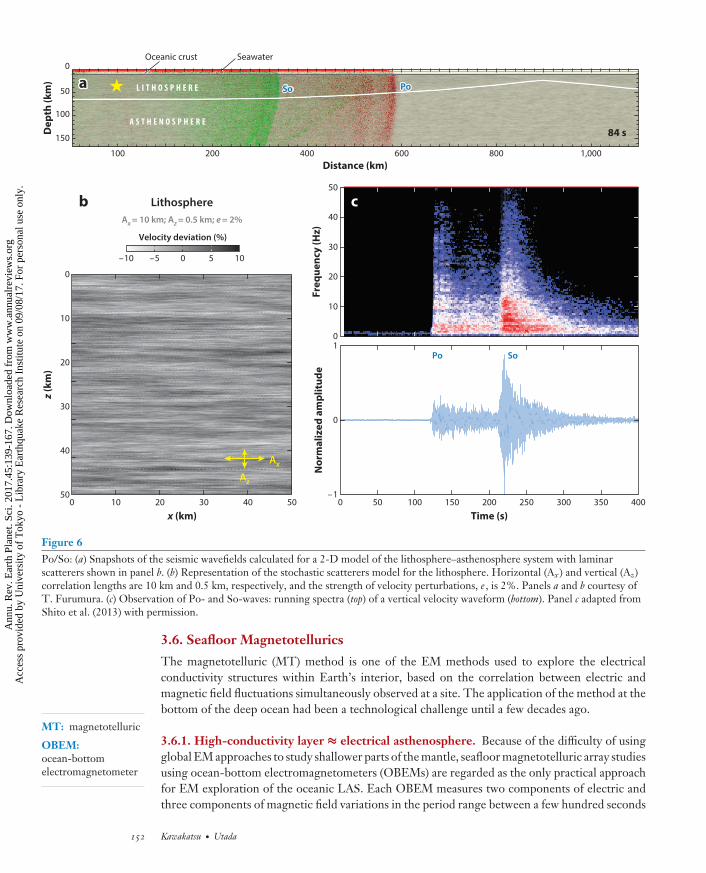
Although the detailed velocity structure of the oceanic lithosphere (Lid) is not well constrained,recent analyses of BBOBS data indicate clear evidence for a peculiar scattering property of theoceanic lithosphere that sheds new light on the origin and formation mechanism of the litho-sphere. By analyzing BBOBS recordings of deep-focus earthquakes occurring in the subductingslab beneath Japan, Shito et al. (2013) reported the presence of large-amplitude, high-frequency,long-duration coda waves for both P- and S-waves that were previously known as Po- and So-waves (or sometimes just called Pn/Sn) (e.g., Walker 1977). Combining this observation of Po- andSo-waves with finite-difference wave propagation simulation analysis (Furumura & Kennett 2005),Shito et al. (2013) demonstrated that Po/So-waves are generated by scattering due to laterallyelongated heterogeneities in both the subducting and horizontal parts of the oceanic lithosphere(Figure 6). Subsequent analyses (Shito et al. 2015, Kennett & Furumura 2013, Kennett et al. 2014)indicated that such scatterers exist in parts of the lithosphere as young as ∼15 Ma, but Po/So-wavespropagate much more efficiently in the older lithosphere, suggesting that the creation of thosescatterers may be directly linked to the generation and/or growth of the oceanic lithosphere.
The seismological observations so far are all compatible with quasi-laminate features with ahorizontal correlation length of 10–50 km and a vertical correlation length of 0.5 km, with auniform level of about ∼2% variation through the full thickness of the lithosphere. Kennett &Furumura (2015), however, suggest that models with stronger heterogeneity near the base ofthe lithosphere, or even in the asthenosphere, might equally explain the observations, althoughthere remains a need for some quasi-laminate structure throughout the mantle component of theoceanic lithosphere. They suggest that these models are more compatible with petrological models(e.g., Hirschmann 2010, Tommasi & Ishikawa 2014), which might favor stronger heterogeneityat the base of the lithosphere associated with underplating from frozen melts. Recent active-source surveys also report observations of scatterers in the deeper part of the lithosphere (e.g.,Kaneda et al. 2010), and the stochastic nature of Po/So-wave observations might be investigateddeterministically via ocean-bottom observations in the future.
3.5. Seismic Attenuation
Seismic attenuation is the least constrained physical parameter, both from the observational andfrom the theoretical/experimental point of view. From the former, it is quite challenging to sepa-rate intrinsic (anelastic) and extrinsic (scattering, heterogeneity) attenuation effects from waveformdata, resulting in very different views for the cause of attenuation (intrinsic is thermally activated,whereas extrinsic is a structural effect); from the latter, the physical conditions of laboratory exper-iments are limited, and interpolations and extrapolations are required for making inferences forthe mantle conditions (e.g., Jackson et al. 2014, Takei et al. 2014). Nevertheless, we summarize therelevant observations. Dalton et al. (2009) performed a global tomographic study of upper mantleattenuation and showed general strong (anti)correlation between attenuation and velocity (strongattenuation correlates well with low velocity). From local observations in oceanic areas, employingthe array technique of Forsyth & Li (2005), Yang et al. (2007) studied seismic attenuation near theEPR region (2-Ma and 6-Ma areas) and suggested, with empirically determined scaling betweenattenuation and velocity, the presence of a melt beneath or near the ridge between a depth rangeof 25–40 km and ∼100 km. Recent observation of the old seafloor of the western Pacific Ocean(150–160 Ma) exhibits attenuation in the depth range of the LVZ as strong as that observed atthe EPR (Figure 7), suggesting the presence of small fractions of melt in the asthenosphere ofthe oldest part of the Pacific Ocean; note that the observational constraint for attenuation is thecombined effects of intrinsic and extrinsic attenuation (Booth et al. 2014).
www.annualreviews.org • Oceanic Lithosphere–Asthenosphere System 151
Ann
u. R
ev. E
arth
Pla
net.
Sci.
2017
.45:
139-
167.
Dow
nloa
ded
from
ww
w.a
nnua
lrev
iew
s.or
g A
cces
s pr
ovid
ed b
y U
nive
rsity
of
Tok
yo -
Lib
rary
Ear
thqu
ake
Res
earc
h In
stitu
te o
n 09
/08/
17. F
or p
erso
nal u
se o
nly.
EA45CH06-Kawakatsu ARI 14 August 2017 12:51
100 200 400 600 800 1,000Distance (km)
0
50
100
150
PoSoL I T H O S P H E R E
A S T H E N O S P H E R E
SeawaterOceanic crust
10
20
30
40
50
x (km)
z (k
m)
0
0 10 20 30 40 50
1050–5–10
Velocity deviation (%)
Lithosphere
Ax
Ax = 10 km; Az = 0.5 km; e = 2%
Az
84 s
0
10
20
30
40
50
Freq
uenc
y (H
z)
–1
0
1
Nor
mal
ized
am
plit
ude
0 50 100 150 200 250 300 350 400
Time (s)
Po So
Dep
th (k
m) aa
bb c
Figure 6Po/So: (a) Snapshots of the seismic wavefields calculated for a 2-D model of the lithosphere–asthenosphere system with laminarscatterers shown in panel b. (b) Representation of the stochastic scatterers model for the lithosphere. Horizontal (Ax ) and vertical (Az)correlation lengths are 10 km and 0.5 km, respectively, and the strength of velocity perturbations, e , is 2%. Panels a and b courtesy ofT. Furumura. (c) Observation of Po- and So-waves: running spectra (top) of a vertical velocity waveform (bottom). Panel c adapted fromShito et al. (2013) with permission.
MT: magnetotelluric
OBEM:ocean-bottomelectromagnetometer
3.6. Seafloor Magnetotellurics
The magnetotelluric (MT) method is one of the EM methods used to explore the electricalconductivity structures within Earth’s interior, based on the correlation between electric andmagnetic field fluctuations simultaneously observed at a site. The application of the method at thebottom of the deep ocean had been a technological challenge until a few decades ago.
3.6.1. High-conductivity layer ≈ electrical asthenosphere. Because of the difficulty of usingglobal EM approaches to study shallower parts of the mantle, seafloor magnetotelluric array studiesusing ocean-bottom electromagnetometers (OBEMs) are regarded as the only practical approachfor EM exploration of the oceanic LAS. Each OBEM measures two components of electric andthree components of magnetic field variations in the period range between a few hundred seconds
152 Kawakatsu · Utada
Ann
u. R
ev. E
arth
Pla
net.
Sci.
2017
.45:
139-
167.
Dow
nloa
ded
from
ww
w.a
nnua
lrev
iew
s.or
g A
cces
s pr
ovid
ed b
y U
nive
rsity
of
Tok
yo -
Lib
rary
Ear
thqu
ake
Res
earc
h In
stitu
te o
n 09
/08/
17. F
or p
erso
nal u
se o
nly.

EA45CH06-Kawakatsu ARI 14 August 2017 12:51
0
50
100
150
200
250
300
350
400
450
5000 100 200 300 400 500
Dep
th (k
m)
Shear attenuation, Qµ
25
20
15
10
5
04.2 4.4 4.6 4.8
Shea
r att
enua
tion
× 1
0–3
(1/Q
)
Velocity (km/s)
ba
Young ocean (0 –25 Ma)Dalton et al. 2008
Mid-age ocean (25 –100 Ma)Dalton et al. 2008
Old ocean (>100 Ma)Dalton et al. 2008
East Pacific Rise (2 –10 Ma)Yang et al. 2007
Tonga Back ArcRoth et al. 1999
Booth et al. 2014 (150 –160 Ma)
DataYoung oceansMid-age oceansOld oceansOrogenic/magmaticsOld continents
Figure 7Seismic attenuation: (a) Scatter plot showing the shear velocity and shear attenuation values at a depth of 100 km. Panel a adapted fromDalton et al. (2009) with permission. (b) Shear attenuation model beneath old western Pacific seafloor (solid gray line; uncertainty rangesare denoted by broken gray lines) compared with other oceanic shear attenuation models. Panel b adapted from Booth et al. (2014) withpermission.
and one day (Utada 2015). The depth resolution of the MT method relies on the EM skin effect:The longer the variation period is, the deeper the EM signals of external sources penetrate intothe conductive Earth. As a result, seafloor MT data, especially those gathered at deep-ocean sites,are usually insensitive to the conductivity in the crust and shallower part of the upper mantlebecause of the strong attenuation of short-period signals through conductive seawater. However,a few controlled-source EM experiments (Cox et al. 1986, MacGregor et al. 2001, Key et al. 2012)provide solid evidence that the shallowest part of the oceanic crust is highly conductive becauseof the presence of sediments with saline water but that the deeper part of the oceanic lithosphereis very resistive (Figure 8a). A high-frequency MT result at relatively shallow water around theEPR (Key et al. 2013) also constrains the presence of the LCL corresponding to the lithosphere.
In the case of seafloor MT data from deep-ocean sites, a model of conductivity is estimatedwith a priori constraints on the conductivity of the LCL (e.g., Baba et al. 2010). The EM methodis more sensitive to conductive structures in general, and in fact the main structural feature ofthe HCL depends little on assumptions about the LCL’s conductivity, as shown in Figure 8b.Conductivity changes smoothly with depth from the LCL to the HCL and then becomes almostconstant throughout the HCL. Here, the depth at which there is maximum curvature in thistransition is used as a proxy for the depth of the HCL.
In Figure 9a, HCL depths estimated from recent seafloor MT results are presented as afunction of plate age. These HCL depths do not show a simple age dependence, which mightbe expected from a model of plate cooling. It is most likely that a simple age dependence ofnormal oceanic mantle is being masked by structural variation from other causes. For example, theyoungest result shown in Figure 9a, from the MELT (Mantle Electromagnetic and Tomography)experiment (Evans et al. 1999), shows a greater HCL depth than two results from 20–30-Maseafloor. The two oldest (140–150-Ma) results, from the northwestern Pacific subduction zone
www.annualreviews.org • Oceanic Lithosphere–Asthenosphere System 153
Ann
u. R
ev. E
arth
Pla
net.
Sci.
2017
.45:
139-
167.
Dow
nloa
ded
from
ww
w.a
nnua
lrev
iew
s.or
g A
cces
s pr
ovid
ed b
y U
nive
rsity
of
Tok
yo -
Lib
rary
Ear
thqu
ake
Res
earc
h In
stitu
te o
n 09
/08/
17. F
or p
erso
nal u
se o
nly.

EA45CH06-Kawakatsu ARI 14 August 2017 12:51
0
50
100
150
200
250
300
350
400
450
500101100100 10 –110 –1 10 –210 –2 10 –310 –3 10 –410 –5
Marginslope
0
1
2
3
4
5
6
7
Abyssal plain
Dep
th (k
m)
Dep
th (k
m)
Top of HCL
Conductivity (S/m)Conductivity (S/m)
SedimentsSediments
MohoMoho
Layer 2Layer 2
Layer 3Layer 3
Model L1Model L2Model L3Model L4
ba
Abyssal plain
Trench outer rise
PEGASUS
Northeast Pacific; 40 Ma
Northeast Pacific; 40 Ma
Figure 8(a) 1-D conductivity profiles obtained by controlled source electromagnetic survey at abyssal plain (blue), trench outer rise (red), andmargin slope (light gray) in the Middle America Trench offshore from Nicaragua, and from the PEGASUS experiment (dark gray) inthe northeast Pacific. Horizontal lines show crustal layering observed by active-source seismics. Panel a adapted from Key et al. (2012)with permission. (b) 1-D profiles obtained by inversion of seafloor magnetotelluric data in the Philippine Sea with different constraintson the shallow structures. Panel b adapted from Baba et al. (2010) with permission. Abbreviation: HCL, high-conductivity layer.
(Baba et al. 2010), show a very deep HCL (thick LCL) of >150 km, which we discuss in Section 4.If we remove these three results, which might reflect anomalous features near plate boundaries,the dependence of the HCL depth on age appears more consistent with a plate-cooling model.
The conductivity of the HCL is another robust parameter obtained from MT data. Figure 9bshows the age dependence of the maximum conductivity values in the HCL. We notice that theconductivity of the HCL does not exhibit much age dependence, taking similar values of about−1.4 on a log scale (about 0.04 S/m). The only apparent exception is from the 23-Ma Cocos Plateoff Nicaragua (Naif et al. 2013). This extremely high conductivity may be ascribed to strong shearin the asthenosphere arising from the high convergence rate (85 mm/yr) of the Cocos Plate.
3.6.2. Electrical anisotropy. MT response, usually called impedance, is a second-order complex-valued tensor usually defined in the frequency domain, relating vectors of horizontal electricand magnetic field variations. Impedance tensors determined from observations generally showanisotropic features, but this does not mean that subsurface materials are electrically anisotropic.Lateral heterogeneity of underground structure also causes apparently anisotropic impedance. Forseafloor MT, bathymetric variations and coastline geometry are also possible sources of apparentanisotropy. In fact, it is generally difficult to distinguish the effects of intrinsic anisotropy fromthose of lateral heterogeneity.
154 Kawakatsu · Utada
Ann
u. R
ev. E
arth
Pla
net.
Sci.
2017
.45:
139-
167.
Dow
nloa
ded
from
ww
w.a
nnua
lrev
iew
s.or
g A
cces
s pr
ovid
ed b
y U
nive
rsity
of
Tok
yo -
Lib
rary
Ear
thqu
ake
Res
earc
h In
stitu
te o
n 09
/08/
17. F
or p
erso
nal u
se o
nly.

EA45CH06-Kawakatsu ARI 14 August 2017 12:51
log
(σH
CL)
Age (Ma)
–0.5
–1.0
–1.5
–2.00 25 50 75 100 125 150 175
Age (Ma)
Dep
th (k
m)
200
180
160
140
120
100
80
60
40
20
0
0 25 50 75
600°C
1,000°C
1,300°C
IsotropicInversion results
Anisotropic
100 125 150 175
ba
Figure 9(a) Depth to the HCL (high-conductivity layer) versus seafloor age with temperature profiles by plate cooling (the constant thermalconductivity model of McKenzie et al. 2005) and (b) the maximum conductivity value of the HCL versus seafloor age. Red and purplesymbols denote isotropic and anisotropic inversion results, respectively, and the red vertical bar indicates a range of variation.
Nevertheless, there have been a few examples of attempting anisotropic inversion for seafloorMT data. Initial results were reported from the MELT experiment conducted around the EPR(Evans et al. 2005, Baba et al. 2006). A 2-D anisotropic inversion revealed azimuthal electricalanisotropy in the HCL below the Nazca Plate with higher conductivity by nearly one order ofmagnitude in the direction of plate spreading, as shown in Figure 10. This anisotropic featurewas interpreted in terms of crystallographic orientation of hydrous olivine crystals (Evans et al.2005), which, as well as the relatively deep HCL for the plate age, is regarded as strong evidencefor compositional (hydrogen content) control over the electrical conductivity of the oceanic plate.
A second example, from Naif et al. (2013), can be seen offshore from Nicaragua, where theCocos Plate (mean seafloor age 23 Ma) is subducting below Central America. The azimuthalanisotropy was estimated, by 2-D anisotropic inversion, for both the LCL and the HCL, with theresulting contrast between high- and low-conductivity directions shown in Figure 10, althoughthe anisotropy of the LCL is not well constrained by the data. The inferred contrast of a factorof about 3 is slightly weaker than the MELT result. The anisotropy in the HCL was ascribedexclusively to the presence of partially molten layers with shear deformation, because the average(isotropic) conductivity is too high to be accounted for by the effects of hydration (Naif et al. 2013,Pommier et al. 2015). Dai & Karato (2014) suggested, on the basis of their new laboratory results,that the high conductivity and anisotropy are both consistent with a hydrous asthenosphere model.According to their laboratory data, the anisotropy estimated from the MELT experiment may beslightly too intense to be accounted for by the effect of hydrogen. On the other hand, this partialmelt model needs an additional mechanism to explain the anisotropy in the LCL, if it is significant.
A third example is a result from the Mariana subduction zone, where the 140–150-Ma PacificPlate is subducting below the Philippine Sea plate (Matsuno et al. 2010). A 2-D inversion suggeststhe presence of the HCL at a depth of 70–100 km beneath the Pacific Plate, showing azimuthalanisotropy with a contrast of a factor of 3 between conductive (trench-normal) and resistive
www.annualreviews.org • Oceanic Lithosphere–Asthenosphere System 155
Ann
u. R
ev. E
arth
Pla
net.
Sci.
2017
.45:
139-
167.
Dow
nloa
ded
from
ww
w.a
nnua
lrev
iew
s.or
g A
cces
s pr
ovid
ed b
y U
nive
rsity
of
Tok
yo -
Lib
rary
Ear
thqu
ake
Res
earc
h In
stitu
te o
n 09
/08/
17. F
or p
erso
nal u
se o
nly.

EA45CH06-Kawakatsu ARI 14 August 2017 12:51
100
0 –0.5 –1.0 –1.0 –.08 –0.6 –0.4 –0.2 0 0.2 0.4–1.5 –2.0 –2.5 –3.0 –3.5 –4.0
150
0
50
100
150
2000
50
100
150
200200 250
Distance from ridge axis (km)
log (σy/σx)
ρxx
ρyy
log conductivity (S/m)
300 350
0
40
80
120
160
200
LAB, Cocos
LAB, off East Pacific Rise
Off East Pacific Rise
Cocos plate
LAB, Pacific Ocean basin
Off Mariana Trench(Pacific Ocean basin)240
280
Dep
th (k
m)
Dep
th (k
m)
ba
Figure 10(a) Electrical anisotropy obtained from the MELT experiment (Evans et al. 2005) showing estimated conductivity values in the (top) ridgeparallel and (bottom) perpendicular directions. (b) Anisotropic conductivity models obtained from electromagnetic data from three differentregions [the Cocos Plate in blue, off the EPR (the MELT experiment) in red, and off the Mariana Trench in gray]. The ratio of conductivityvalues in conductive and resistive directions in the HCL is presented as a function of depth. Panel b adapted from Pommier et al. (2015)with permission. Abbreviations: EPR, East Pacific Rise; HCL, high-conductivity layer; LAB, lithosphere–asthenosphere boundary.
(trench-parallel) directions. On the back arc side, the HCL is found at shallower depths andshows a slightly weaker anisotropy of a factor of 2. These smaller values of anisotropy comparedwith the MELT result were ascribed to a slower flow velocity in the asthenosphere than the flowvelocity below the fast-spreading ridges in the previous two cases. However, the relative motionof the Nazca Plate is about 45 mm/yr in the hot-spot coordinate frame, which is about a half of theconvergence rate of the Cocos Plate and similar to the convergence rate of the old Pacific Platein the Mariana subduction zone.
For further discussion, improvement of the data analysis method, allowing separation of theeffects of lateral heterogeneity and intrinsic anisotropy in observed MT impedances, will be in-dispensable. To achieve this, one needs a dataset that is sensitive to both intrinsic anisotropy andlateral heterogeneity. Unfortunately, an array along a line is not sensitive to lateral variation of thestructure perpendicular to the line. Observation has to be done in a 2-D array. Although there area few seafloor EM studies with a 2-D array, separation of intrinsic anisotropy from other effectshas not yet been successful (Utada 2015).
3.6.3. Bottom of asthenosphere. We have seen that the signature of the top of the astheno-sphere (LAB) can be studied by seismic and EM observations. However, its bottom is not wellcharacterized by these observations, although the thickness of the asthenosphere has a significantimpact on distinguishing between flow patterns predicted by different models of the astheno-sphere (e.g., Phipps-Morgan et al. 1995, French et al. 2013). It is difficult, especially for the EMmethod, to characterize such great depths. Recently, Matsuno et al. (2017) estimated the depth
156 Kawakatsu · Utada
Ann
u. R
ev. E
arth
Pla
net.
Sci.
2017
.45:
139-
167.
Dow
nloa
ded
from
ww
w.a
nnua
lrev
iew
s.or
g A
cces
s pr
ovid
ed b
y U
nive
rsity
of
Tok
yo -
Lib
rary
Ear
thqu
ake
Res
earc
h In
stitu
te o
n 09
/08/
17. F
or p
erso
nal u
se o
nly.

EA45CH06-Kawakatsu ARI 14 August 2017 12:51
of the bottom of the HCL beneath the northwestern Pacific Basin by long-period MT. It wasinferred from the result that EM observations are compatible with the bottom of the HCL beingin the depth range of 200–300 km. Although it is a preliminary result, this might indicate thatthe asthenosphere has a bottom within the upper mantle. The depth range inferred by this studyincludes that of the Lehmann discontinuity, at about 220 km, which defines the bottom of theanisotropic layer in PREM (e.g., Dziewonski & Anderson 1981). Although PREM has this struc-ture built in it, the presence of the Lehmann discontinuity in the ocean is not widely accepted.Earlier SS-precursor studies suggested the absence or intermittent/weak presence of such a struc-ture beneath the oceans, whereas it is better observed in the continental regions (Gu et al. 2001,Deuss & Woodhouse 2002).
4. OBSERVATIONS AT AND NEAR SUBDUCTION ZONES
Subduction zones offer a unique environment for studying the oceanic LAS, as land-based high-density network data may be directly used to map slab and subslab structures that correspondto the LAS in the oceanic environment. Using dense Japanese Hi-net data, Kawakatsu et al.(2009) obtained a clear RF image of a sharp surface of S-wave velocity reduction and suggested aconnection between this and the observation of the G-discontinuity at a depth of ∼80 km beneaththe seafloor (Figure 11). S-RF imaging by Kumar & Kawakatsu (2011) used records of onshorebroadband stations located along the northern Pacific Rim, and the authors reported that the
0 100 200 300 400Distance (km)
50
100
150
200
250
50
0
100
150
200
250
LAB
??
10010–110–210–310–4
Dep
th (k
m) D
epth (km)
Conductivity (S/m)P-RF
XX YY
S-RF
SSP-C
NOMan-A
WP2
NOMan-ASSP-CO C E A N I C M O H OO C E A N I C M O H O
A S T H E N O S P H E R E
E U R A S I A N P L A T E
P A C I F I C P L A T E
Figure 11Lithosphere–asthenosphere system at a subduction zone: Shown are a P-RF image using dense land seismic data of Hi-net from Japanand a P-RF and S-RF image for the seafloor borehole station WP2, adapted from Kawakatsu et al. (2009). Also shown are the regionalelectrical conductivity profiles in two areas, NOMan-A and SSP-C; these data are from Baba et al. (2013). Abbreviations: LAB,lithosphere–asthenosphere boundary; NOMan, Normal Oceanic Mantle Project; P-RF, P-receiver function; S-RF, S-receiver function;SSP, Stagnant Slab Project.
www.annualreviews.org • Oceanic Lithosphere–Asthenosphere System 157
Ann
u. R
ev. E
arth
Pla
net.
Sci.
2017
.45:
139-
167.
Dow
nloa
ded
from
ww
w.a
nnua
lrev
iew
s.or
g A
cces
s pr
ovid
ed b
y U
nive
rsity
of
Tok
yo -
Lib
rary
Ear
thqu
ake
Res
earc
h In
stitu
te o
n 09
/08/
17. F
or p
erso
nal u
se o
nly.
EA45CH06-Kawakatsu ARI 14 August 2017 12:51
estimated thickness of oceanic plate increased with plate age, although the data points are quitescattered.
At the Hikurangi subduction zone (120 Ma) in New Zealand, Stern et al. (2015) observedhigh-frequency P-wave reflectors (at thicknesses of 73 km and 83 km from the slab surface)and interpreted this 10-km-thick low-velocity (P-wave velocity reduction of 8%) layer as a low-viscosity channel at the LAB that decouples plates from the underlying mantle flow. At the MiddleAmerica Trench offshore from Nicaragua (23 Ma), Naif et al. (2013) showed that underneath theLCL, the HCL is confined to depths of 45–70 km, which they interpreted as a partially moltenlayer capped by an impermeable frozen lid that is the base of the lithosphere. Although these newobservations appear to be finding structures near the base of the subducting lithosphere, it shouldbe realized that a thin (∼10 km) low-velocity channel is not consistent with the G-discontinuity-like structure (e.g., large velocity reduction) inferred by teleseismic body-wave analyses (e.g.,Bagley & Revenaugh 2008, Kawakatsu et al. 2009, Rychert & Shearer 2011).
Figure 11 shows regional electrical conductivity profiles that indicate large lateral variation ofelectrical conductivity (thickening of LCL near the trench in a short distance) in the old part ofthe Pacific Plate (Baba et al. 2013) (Figure 9). According to regional 3-D inversion results (Tadaet al. 2014), this extremely thick LCL does not extend further to the south, where the older (about160 Ma) Pacific Plate is subducting beneath the Mariana arc, suggesting that the thickening of theLCL near the trench is likely to be a regional feature along the Japan–Izu–Ogasawara subductionzone. Considering that petit-spot volcanism, a recent volcanism that might be associated with thedeformation of the oceanic plate before subduction (Hirano et al. 2006), is also observed in thesame region, there might be a close connection between the two phenomena.
5. VIEWS OF LITHOSPHERE–ASTHENOSPHERE SYSTEMOF NORMAL OCEANIC MANTLE
For the elucidation of the LAS in the ocean, we first list the most robust observations that, wethink, any modeling attempt should be able to explain. They are
1. the thermal evolution of the LAS as depicted by surface-wave tomography,2. the presence of seismic anisotropy in the LAS,3. the presence of the G-discontinuity,4. the presence of lithospheric laminar heterogeneities, and5. the presence of the LCL and HCL.
5.1. Nature of Lid/LVZ and LCL/HCL Transitions
Investigation of the LAB has been a focus of recent global geophysics/geodynamics studies (e.g.,Fischer et al. 2010, Fischer 2015). Figure 12 shows a compilation of recent seismological estimatesof the depth of the G-discontinuity (or seismic LAB) or the lithosphere thickness beneath theocean. The data points are scattered, and if we take it that all observations are related to the sameG-discontinuity (a velocity reduction from Lid to LVZ), no simple view emerges. As Rychert et al.(2012) noted, there appears to be some inconsistency among the various observations. Althoughthese seeming inconsistencies might be caused by the stochastic nature of the LAS, as warned byKennett & Yoshizawa (2016), here we attempt to synthesize the observations. Generally speaking,longer-period seismic data reflect larger-scale structures, such as the Lid/LVZ transition, andshorter-period data are sensitive to local properties, such as elongated flat scatterers (e.g., Shitoet al. 2013, Kennett et al. 2014). If we assume that the longer-period SS-precursor observations(Rychert & Shearer 2011) give overall estimates of Lid/LVZ transition properties, compared to
158 Kawakatsu · Utada
Ann
u. R
ev. E
arth
Pla
net.
Sci.
2017
.45:
139-
167.
Dow
nloa
ded
from
ww
w.a
nnua
lrev
iew
s.or
g A
cces
s pr
ovid
ed b
y U
nive
rsity
of
Tok
yo -
Lib
rary
Ear
thqu
ake
Res
earc
h In
stitu
te o
n 09
/08/
17. F
or p
erso
nal u
se o
nly.

EA45CH06-Kawakatsu ARI 14 August 2017 12:51
1,100ºC1,100ºC
Dep
th (k
m)
Anomalous crustRychert & Shearer 2011
Normal crustRychert & Shearer 2011
Kawakatsu et al. 2009
Kumar & Kawakatsu 2011
Schmerr 2012
Tan & Helmberger 2007
Bagley & Revenaugh 2008
Tonegawa & Helffrich 2012
Shito et al. 2015
Stern et al. 2015
Age (Ma)0 20 40 60 80 100 120 140
0
20
40
60
80
100
120
140
1,300ºC1,300ºC
900ºC900ºC
700ºC700ºC
500ºC500ºC
300ºC300ºC
Figure 12Discontinuity depth and plate thickness across the Pacific Ocean compared to seafloor age and plate model isotherms. Original data arefrom Rychert et al. (2012), and a few data points are deleted (Gaherty et al. 1999) or added (Shito et al. 2015, Stern et al. 2015,Tonegawa & Helffrich 2012).
the short-period ones (and if we exclude data points for anomalous crust), then the age dependenceof the G-discontinuity or plate thickness seems to emerge (i.e., most points stay between 900◦Cand 1,200◦C isotherms; see Figure 12). So both the overall seismic characteristics of the Lid/LVZtransition and the G-discontinuity may be understood as thermally controlled phenomena (seepoints 1 and 3 above).
The presence of laminar scatterers in the lithosphere and the observation that such a litho-sphere grows with age may be most easily explained by underplating of laminar melts or meltpockets at the base of the lithosphere (as advocated by Kennett et al. 2014, Kennett & Furumura2015, and Shito et al. 2015), which might also be observed via short-period SS precursors (Schmerr2012). Such melts could result either from upwelling near ridges of small chemical heterogeneitiesthat have low melting temperature (Hirschmann 2010) or from a variety of asthenospheric mantleupwellings, such as plumes (e.g., Phipps-Morgan et al. 1995), a general upward flow (Karato 2012),or small-scale convection (e.g., Korenaga & Jordan 2004). Such melt pockets are stretched withthe shear due to corner flow near ridges (Blackman & Kendall 2002, Hirschmann 2010), or elsesimple shear due to plate motion produces shear-induced melt-rich bands (a millefeuille structure)in the asthenosphere (Holtzman et al. 2003, Takei & Holtzman 2009, Kawakatsu et al. 2009) thatbecome part of the lithosphere as the LAS cools and that contribute to radial anisotropy in the LAS(Kawakatsu et al. 2009, Kennett & Furumura 2015) (see points 2 and 4). On subduction, such meltsmay not be able to follow the flow because of buoyancy, and may instead accumulate near the sub-duction corner (Naif et al. 2013) and cause petit-spot volcanism (Hirano et al. 2006) (Figure 13).
www.annualreviews.org • Oceanic Lithosphere–Asthenosphere System 159
Ann
u. R
ev. E
arth
Pla
net.
Sci.
2017
.45:
139-
167.
Dow
nloa
ded
from
ww
w.a
nnua
lrev
iew
s.or
g A
cces
s pr
ovid
ed b
y U
nive
rsity
of
Tok
yo -
Lib
rary
Ear
thqu
ake
Res
earc
h In
stitu
te o
n 09
/08/
17. F
or p
erso
nal u
se o
nly.
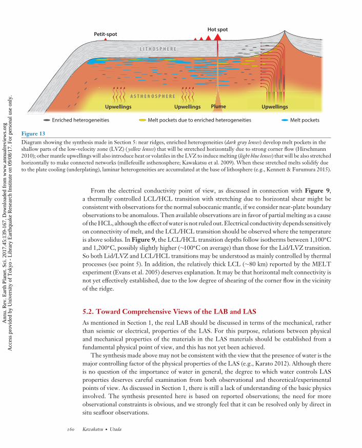
EA45CH06-Kawakatsu ARI 14 August 2017 12:51
L I T H O S P H E R EL I T H O S P H E R E
A S TA S T H E NH E N O S PO S P H E RH E R EE
Hot spotPetit-spot
Plume
Enriched heterogeneities Melt pockets due to enriched heterogeneities Melt pockets
Upwellings Upwellings Upwellings
Figure 13Diagram showing the synthesis made in Section 5: near ridges, enriched heterogeneities (dark gray lenses) develop melt pockets in theshallow parts of the low-velocity zone (LVZ) ( yellow lenses) that will be stretched horizontally due to strong corner flow (Hirschmann2010); other mantle upwellings will also introduce heat or volatiles in the LVZ to induce melting (light blue lenses) that will be also stretchedhorizontally to make connected networks (millefeuille asthenosphere; Kawakatsu et al. 2009). When these stretched melts solidify dueto the plate cooling (underplating), laminar heterogeneities are accumulated at the base of lithosphere (e.g., Kennett & Furumura 2015).
From the electrical conductivity point of view, as discussed in connection with Figure 9,a thermally controlled LCL/HCL transition with stretching due to horizontal shear might beconsistent with observations for the normal suboceanic mantle, if we consider near-plate boundaryobservations to be anomalous. Then available observations are in favor of partial melting as a causeof the HCL, although the effect of water is not ruled out. Electrical conductivity depends sensitivelyon connectivity of melt, and the LCL/HCL transition should be observed where the temperatureis above solidus. In Figure 9, the LCL/HCL transition depths follow isotherms between 1,100◦Cand 1,200◦C, possibly slightly higher (∼100◦C on average) than those for the Lid/LVZ transition.So both Lid/LVZ and LCL/HCL transitions may be understood as mainly controlled by thermalprocesses (see point 5). In addition, the relatively thick LCL (∼80 km) reported by the MELTexperiment (Evans et al. 2005) deserves explanation. It may be that horizontal melt connectivity isnot yet effectively established, due to the low degree of shearing of the corner flow in the vicinityof the ridge.
5.2. Toward Comprehensive Views of the LAB and LAS
As mentioned in Section 1, the real LAB should be discussed in terms of the mechanical, ratherthan seismic or electrical, properties of the LAS. For this purpose, relations between physicaland mechanical properties of the materials in the LAS materials should be established from afundamental physical point of view, and this has not yet been achieved.
The synthesis made above may not be consistent with the view that the presence of water is themajor controlling factor of the physical properties of the LAS (e.g., Karato 2012). Although thereis no question of the importance of water in general, the degree to which water controls LASproperties deserves careful examination from both observational and theoretical/experimentalpoints of view. As discussed in Section 1, there is still a lack of understanding of the basic physicsinvolved. The synthesis presented here is based on reported observations; the need for moreobservational constraints is obvious, and we strongly feel that it can be resolved only by direct insitu seafloor observations.
160 Kawakatsu · Utada
Ann
u. R
ev. E
arth
Pla
net.
Sci.
2017
.45:
139-
167.
Dow
nloa
ded
from
ww
w.a
nnua
lrev
iew
s.or
g A
cces
s pr
ovid
ed b
y U
nive
rsity
of
Tok
yo -
Lib
rary
Ear
thqu
ake
Res
earc
h In
stitu
te o
n 09
/08/
17. F
or p
erso
nal u
se o
nly.

EA45CH06-Kawakatsu ARI 14 August 2017 12:51
0 1,000 2,000
Kilometers
120˚E
60˚N
30˚N
30˚S
60˚S
EQ
150˚E 180˚E
Unitarray
Japan
United States
Ocean bottomdeployments
150˚W 120˚W 90˚W 60˚W
0 50 100 150 200
Seafloor age (Ma)
Longitude
Lati
tude
Figure 14Conceptual image of proposed Pacific Array: A unit array here consists of ∼10 BBOBSs/OBEMs, but actual array configuration shouldbe carefully optimized. The location of unit arrays is also chosen ad hoc. White crosses and small yellow circles are existing ocean-bottom deployments conducted by Japanese and US scientists, respectively. Abbreviations: BBOBS, broadband ocean-bottomseismometer; OBEM, ocean-bottom electromagnetometer.
Recent advances in ocean-bottom geophysical observations, together with advances in analy-sis methodology, have now enabled us to resolve the regional 1-D structure of the entire LAS,from the surface to a depth of ∼200 km, including seismic anisotropy (azimuthal), with deploy-ments of ∼10–15 BBOBSs and OBEMs, each for a year or so (Sections 3.2, 3.6). Thus, in situcharacterization of the physical properties of the entire oceanic LAS without a priori assumptionsfor the most shallow structure, the assumptions often made for global studies, has become pos-sible. We are now at an exciting stage in which large-scale array experiments in the ocean [e.g.,the Pacific Array (Figure 14): http://eri-ndc.eri.u-tokyo.ac.jp/PacificArray/] have become ap-proachable; such array observations, not only by giving regional constraints on 1-D structure(including seismic anisotropy) but also by sharing waveform data for global-scale waveform to-mography (e.g., Fichtner et al. 2010, French et al. 2013, Zhu & Tromp 2013), should drasticallyincrease our knowledge of how plate tectonics works beneath oceanic basins and help resolve thelarge-scale picture of the interior of the Earth.
DISCLOSURE STATEMENT
The authors are not aware of any affiliations, memberships, funding, or financial holdings thatmight be perceived as affecting the objectivity of this review.
www.annualreviews.org • Oceanic Lithosphere–Asthenosphere System 161
Ann
u. R
ev. E
arth
Pla
net.
Sci.
2017
.45:
139-
167.
Dow
nloa
ded
from
ww
w.a
nnua
lrev
iew
s.or
g A
cces
s pr
ovid
ed b
y U
nive
rsity
of
Tok
yo -
Lib
rary
Ear
thqu
ake
Res
earc
h In
stitu
te o
n 09
/08/
17. F
or p
erso
nal u
se o
nly.

EA45CH06-Kawakatsu ARI 14 August 2017 12:51
ACKNOWLEDGMENTS
We thank Jun Korenaga for discussion; Takashi Furumura, Azusa Shito, Kate Rychert, and AkikoTakeo for figures; and Brian Kennett for a preprint. The members of the NOMan (NormalOceanic Mantle) project helped us through their research. This research is partly supported byJSPS KAKENHI 22000003 and 15K13558.
LITERATURE CITED
Aki K. 1957. Space and time spectra of stationary stochastic waves with special reference to microtremors.Bull. Earthq. Res. Inst. 35:415–56
Aki K, Richards PG. 2002. Quantitative Seismology. Sausalito, CA: Univ. Sci. Books. 2nd ed.Akuhara T, Mochizuki K, Kawakatsu H, Takeuchi N. 2016. Nonlinear waveform analysis for water-layer
response and its application to high-frequency receiver function analysis using OBS array. Geophys. J. Int.206:1914–20
Anderson DL, Sammis C. 1970. Partial melting in the upper mantle. Phys. Earth Planet. Inter. 3:41–50Audet P. 2016. Receiver functions using OBS data: promises and limitations from numerical modelling and
examples from the Cascadia Initiative. Geophys. J. Int. 205:1740–55Baba K, Chave AD, Evans RL, Hirth G, Mackie RL. 2006. Mantle dynamics beneath the East Pacific Rise at
17◦S: insights from the Mantle Electromagnetic and Tomography (MELT) experiment. J. Geophys. Res.111:B02101
Baba K, Tada N, Zhang L, Liang P, Shimizu H, Utada H. 2013. Is the electrical conductivity of the westernPacific upper mantle normal? Geochem Geophys. Geosyst. 14:4969–79
Baba K, Utada H, Goto T, Kasaya T, Shimizu H, Tada N. 2010. Electrical conductivity imaging of thePhilippine Sea upper mantle using seafloor magnetotelluric data. Phys. Earth Planet. Inter. 183:44–62
Bagley B, Courtierband AM, Revenaugh J. 2009. Melting in the deep upper mantle oceanward of the Honshuslab. Phys. Earth Planet. Inter. 175:137–44
Bagley B, Revenaugh J. 2008. Upper mantle seismic shear discontinuities of the Pacific. J. Geophys. Res.113:B12301
Becker TW, Conrad CP, Schaeffer AJ, Lebedev S. 2014. Origin of azimuthal seismic anisotropy in oceanicplates and mantle. Earth Planet. Sci. Lett. 401:236–50
Blackman DK, Kendall JM. 2002. Seismic anisotropy in the upper mantle 2. Predictions for current plateboundary flow models. Geochem. Geophys. Geosyst. 3:8602
Booth CM, Forsyth DW, Weeraratne DS. 2014. Upper mantle Q structure beneath old seafloor in the westernPacific. J. Geophys. Res. Solid Earth 119:3448–61
Bozdag E, Trampert J. 2008. On crustal corrections in surface wave tomography. Geophys. J. Int. 172:1066–1082
Burgos G, Montagner JP, Beucler E, Capdeville Y, Mocquet A, Drilleau M. 2014. Oceanic lithosphere/asthenosphere boundary from surface wave dispersion data. J. Geophys. Res. Solid Earth 119:1079–93
Cox C, Constable SC, Chave A, Webb SC. 1986. Controlled-source electromagnetic sounding of the oceaniclithosphere. Nature 320:52–54
Crosby AG, McKenzie D, Sclater JG. 2006. The relationship between depth, age and gravity in the oceans.Geophys. J. Int. 166:553–73
Dai L, Karato S. 2014. High and highly anisotropic electrical conductivity of the asthenosphere due tohydrogen diffusion in olivine. Earth Planet. Sci. Lett. 408:79–86
Dalton CA, Ekstrom G, Dziewonski AM. 2008. The global attenuation structure of the upper mantle.J. Geophys. Res. 113:B09303
Dalton CA, Ekstrom G, Dziewonski AM. 2009. Global seismological shear velocity and attenuation: a com-parison with experimental observations. Earth Planet. Sci. Lett. 284:65–75
Debayle E, Ricard Y. 2013. Seismic observations of large-scale deformation at the bottom of fast-movingplates. Earth Planet. Sci. Lett. 376:165–77
Deuss A, Woodhouse JH. 2002. A systematic search for mantle discontinuities using SS-precursors. Geophys.Res. Lett. 29:90-1–90-4
162 Kawakatsu · Utada
Ann
u. R
ev. E
arth
Pla
net.
Sci.
2017
.45:
139-
167.
Dow
nloa
ded
from
ww
w.a
nnua
lrev
iew
s.or
g A
cces
s pr
ovid
ed b
y U
nive
rsity
of
Tok
yo -
Lib
rary
Ear
thqu
ake
Res
earc
h In
stitu
te o
n 09
/08/
17. F
or p
erso
nal u
se o
nly.

EA45CH06-Kawakatsu ARI 14 August 2017 12:51
Dorman J, Ewing M, Oliver J. 1960. Study of shear-velocity distribution in the upper mantle by mantleRayleigh waves. Bull. Seismol. Soc. Am. 50:87–115
Dunn RA, Forsyth DW. 2003. Imaging the transition between the region of mantle melt generation and thecrustal magma chamber beneath the southern East Pacific Rise with short-period Love waves. J. Geophys.Res. 108(B7):2352
Dziewonski AM, Anderson DL. 1981. Preliminary reference Earth model. Phys. Earth Planet. Inter. 25:297–356Ekstrom G, Dziewonski AM. 1998. The unique anisotropy of the Pacific upper mantle. Nature 394:168–72Evans RL, Hirth G, Baba K, Forsyth D, Chave A, Mackie R. 2005. Geophysical evidence from the MELT
area for compositional controls on oceanic plates. Nature 437:249–52Evans RL, Tarits P, Chave AD, White A, Heinson G, et al. 1999. Asymmetric electrical structure in the mantle
beneath the East Pacific Rise at 17◦S. Science 286:752–55Fei H, Wiedenbeck M, Yamasaki D, Katsura T. 2013. Small effect of water on upper-mantle rheology based
on silicon self-diffusion coefficients. Nature 498:213–15Ferreira AMG, Woodhouse JH, Visser K, Trampert J. 2010. On the robustness of global radially anisotropic
surface wave tomography. J. Geophys. Res. 115:B04313Fichtner A, Kennett B, Igel H, Bunge HP. 2010. Full waveform tomography for radially anisotropic structure:
new insights into present and past states of the Australasian upper mantle. Earth Planet. Sci. Lett. 290:270–80
Fischer KM. 2015. Seismological constraints on the lithosphere–asthenosphere boundary. In Treatise on Geo-physics, Vol. 1: Deep Earth Seismology, ed. G Schubert, pp. 587–612. Amsterdam: Elsevier. 2nd ed.
Fischer KM, Ford HA, Abt DL, Rychert CA. 2010. The lithosphere–asthenosphere boundary. Annu. Rev.Earth Planet. Sci. 38:551–75
Forsyth DW. 1975. The early structural evolution and anisotropy of the oceanic upper mantle. Geophys. J. R.Astron. Soc. 43:103–62
Forsyth DW, Li A. 2005. Array analysis of two-dimensional variations in surface wave phase velocity andazimuthal anisotropy in the presence of multipathing interference. In Seismic Earth: Array Analysis ofBroadband Seismograms, ed. A Levander, G Nolet, pp. 81–97. Washington, DC: Am. Geophys. Union
Foster A, Nettles M, Ekstrom G. 2014. Overtone interference in array-based Love-wave phase measurements.Bull. Seismol. Soc. Am. 104:2266–77
French S, Lekic V, Romanowicz B. 2013. Waveform tomography reveals channeled flow at the base of theoceanic asthenosphere. Science 342:227–30
Furumura T, Kennett BLN. 2005. Subduction zone guided waves and the heterogeneity structure of thesubducted plate: intensity anomalies in northern Japan. J. Geophys. Res. 110:B10302
Gaherty JB, Kato M, Jordan TH. 1999. Seismological structure of the upper mantle: a regional comparisonof seismic layering. Phys. Earth Planet. Inter. 110:21–41
Gaherty JB, Lizarralde D, Collins JA, Hirth G, Kim S. 2004. Mantle deformation during slow seafloorspreading constrained by observations of seismic anisotropy in the western Atlantic. Earth Planet. Sci.Lett. 228:255–65
Gaillard F, Mohammed M, Iacono-Marziano G, Pichavant M, Scaillet B. 2008. Carbonatite melts and electricalconductivity in the asthenosphere. Science 322:1363–65
Gardes E, Gaillard F, Tarits P. 2014. Toward a unified hydrous olivine electrical conductivity law. Geochem.Geophys. Geosyst. 15:4984–5000
Gu YJ, Dziewonski AM, Ekstrom G. 2001. Lehmann discontinuity beneath continents. Geophys. Res. Lett.28:4655–58
Gutenberg B. 1959. Physics of the Earth’s Interior. New York: ElsevierHarmon N, Forsyth D, Webb S. 2007. Using ambient seismic noise to determine short-period phase velocities
and shallow shear velocities in young oceanic lithosphere. Bull. Seismol. Soc. Am. 97:2009–23Hirano N, Takahashi E, Yamamoto J, Abe N, Ingle SP, et al. 2006. Volcanism in response to plate flexure.
Science 313:1426–28Hirschmann MM. 2010. Partial melt in the oceanic low velocity zone. Phys. Earth Planet. Inter. 179:60–71Hirschmann MM, Dasgupta R. 2009. The H/C ratios of Earth’s near-surface and deep reservoirs, and conse-
quences for deep Earth volatile cycles. Chem. Geol. 262:4–16
www.annualreviews.org • Oceanic Lithosphere–Asthenosphere System 163
Ann
u. R
ev. E
arth
Pla
net.
Sci.
2017
.45:
139-
167.
Dow
nloa
ded
from
ww
w.a
nnua
lrev
iew
s.or
g A
cces
s pr
ovid
ed b
y U
nive
rsity
of
Tok
yo -
Lib
rary
Ear
thqu
ake
Res
earc
h In
stitu
te o
n 09
/08/
17. F
or p
erso
nal u
se o
nly.

EA45CH06-Kawakatsu ARI 14 August 2017 12:51
Holtzman BK, Kohlstedt DL, Zimmerman ME, Heidelbach F, Hiraga T, Hustoft J. 2003. Melt segregationand strain partitioning: implications for seismic anisotropy and mantle flow. Science 301:1227–30
Jackson I, Faul UH, Skelton R. 2014. Elastically accommodated grain-boundary sliding: new insights fromexperiment and modeling. Phys. Earth Planet. Inter. 228:203–10
Jung H, Katayama I, Jian Z, Hiraga T, Karato S. 2006. Effect of water and stress on the lattice-preferredorientation of olivine. Tectonophysics 421:1–22
Kaneda K, Kodaira S, Nishizawa A, Morishita T, Takahashi N. 2010. Structural evolution of preexistingoceanic crust through intraplate igneous activities in the Marcus–Wake seamount chain. Geochem. Geophys.Geosyst. 11:Q10014
Karato S. 2012. On the origin of the asthenosphere. Earth Planet. Sci. Lett. 321–322:95–103Kawakatsu H. 2016. A new fifth parameter for transverse isotropy. Geophys. J. Int. 204:682–85Kawakatsu H, Kumar P, Takei Y, Shinohara M, Kanazawa T, et al. 2009. Seismic evidence for sharp
lithosphere–asthenosphere boundaries of oceanic plates. Science 324:499–502Kelbert A, Kuvshinov A, Velasky J, Toyama T, Ribaudo J, et al. 2014. Global 3-D electromagnetic forward
modelling: a benchmark study. Geophys. J. Int. 197:785–814Kennett BLN, Furumura T. 2013. High-frequency Po/So guided waves in the oceanic lithosphere: I—long-
distance propagation. Geophys. J. Int. 195:1862–77Kennett BLN, Furumura T. 2015. Toward the reconciliation of seismological and petrological perspectives
on oceanic lithosphere heterogeneity. Geochem. Geophys. Geosyst. 16:3129–41Kennett BLN, Furumura T, Zhao Y. 2014. High-frequency Po/So guided waves in the oceanic lithosphere:
II—heterogeneity and attenuation. Geophys. J. Int. 199:614–30Kennett BLN, Yoshizawa K. 2017. Lithospheric discontinuities beneath Australia: interaction of large-scale
and fine-scale structure. In Lithospheric Discontinuities, ed. H Yuan, B Romanowicz, AG Jones. Washington,DC: Am. Geophys. Union. In press
Key K, Constable S, Liu L, Pommier A. 2013. Electrical image of passive mantle upwelling beneath thenorthern East Pacific Rise. Nature 495:499–502
Key K, Constable S, Matsuno T, Evans R, Myer D. 2012. Electromagnetic detection of plate hydration dueto bending faults at the Middle America Trench. Earth Planet. Sci. Lett. 351–352:45–53
Korenaga J, Jordan TH. 2004. Physics of multiscale convection in Earth’s mantle: evolution of sublithosphericconvection. J. Geophys. Res. 109:B01405
Kumar P, Kawakatsu H. 2011. Imaging the seismic lithosphere–asthenosphere boundary of the oceanic plate.Geochem. Geophys. Geosyst. 12:Q01006
Kumar P, Kawakatsu H, Shinohara M, Kanazawa T, Araki E, Suyehiro K. 2011. P and S receiver functionanalysis of seafloor borehole broadband seismic data. J. Geophys. Res. 116:B12308
Kustowski B, Ekstrom G, Dziewonski AM. 2008. Anisotropic shear-wave velocity structure of the Earth’smantle: a global model. Earth Planet. Sci. Lett. 113:B06306
Leeds AR, Knopo L, Kausel EG. 1974. Variations of upper mantle structure under the Pacific Ocean. Science186:141–43
Leveque JJ, Cara M. 1985. Inversion of multimode surface wave data: evidence for sub-lithospheric anisotropy.Geophys. J. R. Astron. Soc. 83:753–73
Lin FC, Ritzwoller MH, Yang Y, Moschetti MP, Fouch MJ. 2010. Complex and variable crustal and uppermostmantle seismic anisotropy in the western United States. Nat. Geosci. 4:55–61
Lizarralde D, Gaherty JB, Collins JA, Hirth G, Kim SD. 2004. Spreading-rate dependence of melt extractionat mid-ocean ridges from mantle seismic refraction data. Nature 432:744–47
Long M, Silver PG. 2008. The subduction zone flow field from seismic anisotropy: a global view. Science319:315–18
MacGregor L, Sinha M, Constable S. 2001. Electrical resistivity structure of the Valu Fa Ridge, Lau Basin,from marine controlled-source electromagnetic sounding. Geophys. J. Int. 146:217–36
Maggi A, Debayle E, Priestley K, Barruol G. 2006a. Azimuthal anisotropy of the Pacific region. Earth Planet.Sci. Lett. 250:53–71
Maggi A, Debayle E, Priestley K, Barruol G. 2006b. Multimode surface waveform tomography of the PacificOcean: a closer look at the lithospheric cooling signature. Geophys. J. Int. 166:1384–97
164 Kawakatsu · Utada
Ann
u. R
ev. E
arth
Pla
net.
Sci.
2017
.45:
139-
167.
Dow
nloa
ded
from
ww
w.a
nnua
lrev
iew
s.or
g A
cces
s pr
ovid
ed b
y U
nive
rsity
of
Tok
yo -
Lib
rary
Ear
thqu
ake
Res
earc
h In
stitu
te o
n 09
/08/
17. F
or p
erso
nal u
se o
nly.
EA45CH06-Kawakatsu ARI 14 August 2017 12:51
Mainprice D. 2015. Seismic anisotropy of the deep Earth from a mineral and rock physics perspective. InTreatise on Geophysics, Vol. 2: Mineral Physics, ed. G Schubert, pp. 487–538. Amsterdam: Elsevier. 2nd ed.
Matsuno T, Seama N, Evans RL, Chave AD, Baba K, et al. 2010. Upper mantle electrical resistivity structurebeneath the central Mariana subduction system. Geochem. Geophys. Geosyst. 11:Q09003
Matsuno T, Suetsugu D, Baba K, Tada N, Shimizu H, et al. 2017. Mantle transition zone beneath a normalseafloor in the northwestern Pacific: electrical conductivity, seismic thickness, and water content. EarthPlanet. Sci. Lett. 462:189–98
McKenzie D, Jackson J, Priestley K. 2005. Thermal structure of oceanic and continental lithosphere. EarthPlanet. Sci. Lett. 233:337–49
Mei S, Kohlstedt DL. 2000a. Influence of water on plastic deformation of olivine aggregates. 1. Diffusioncreep regime. J. Geophys. Res. 105:21457–69
Mei S, Kohlstedt DL. 2000b. Influence of water on plastic deformation of olivine aggregates. 2. Dislocationcreep regime. J. Geophys. Res. 105:21471–81
Montagner JP. 1985. Seismic anisotropy of the Pacific Ocean inferred from long-period surface waves disper-sion. Phys. Earth Planet. Inter. 38:28–50
Naif S, Key K, Constable S, Evans RL. 2013. Melt-rich channel observed at the lithosphere-asthenosphereboundary. Nature 495:356–59
Nettles M, Dziewonski AM. 2008. Radially anisotropic shear velocity structure of the upper mantle globallyand beneath North America. J. Geophys. Res. 113:B02303
Nettles M, Dziewonski AM. 2011. Effect of higher-mode interference on measurements and models offundamental-mode surface-wave dispersion. Bull. Seismol. Soc. Am. 101:2270–80
Nishida K, Kawakatsu H, Obara K. 2008. Three-dimensional crustal S-wave velocity structure in Japan usingmicroseismic data recorded by Hi-net tiltmeters. J. Geophys. Res. 113:B10302
Nishimura CE, Forsyth DW. 1989. The anisotropic structure of the upper mantle in the Pacific. Geophys. J.Int. 96:203–29
Parsons B, McKenzie D. 1978. Mantle convection and the thermal structure of the plates. J. Geophys. Res.83:4485–96
Parsons B, Sclater J. 1977. An analysis of the variation of ocean floor bathymetry and heat flow with age.J. Geophys. Res. 82:803–27
Phipps-Morgan J, Morgan WJ, Zhang YS, Smith WHF. 1995. Observational hints for a plume-fed, sub-oceanic asthenosphere and its role in mantle convection. J. Geophys. Res. 100:12753–67
Pommier A, Leinenweber K, Kohlstedt D, Chao Q, Garnero E, et al. 2015. Experimental constraints on theelectrical anisotropy of the lithosphere-asthenosphere system. Nature 522:202–6
Priestley K, McKenzie D. 2006. The thermal structure of the lithosphere from shear wave velocities. EarthPlanet. Sci. Lett. 244:285–301
Priestley K, McKenzie D. 2013. The relationship between shear wave velocity, temperature, attenuation andviscosity in the shallow part of the mantle. Earth Planet. Sci. Lett. 381:78–91
Raitt RW, Shor GG, Francis TJG, Morris GB. 1969. Anisotropy of the Pacific upper mantle. J. Geophys. Res.74:3095–109
Revenaugh J, Jordan TH. 1991. Mantle layering from ScS reverberations: 3. The upper mantle. J. Geophys.Res. 96:781–810
Richards MA, Yang WS, Baumgardner JR, Bunge HP. 2001. Role of a low-viscosity zone in stabilizing platetectonics: implications for comparative terrestrial planetology. Geochem. Geophys. Geosyst. 2:1026
Ritzwoller MH, Shapiro NM, Zhong SJ. 2004. Cooling history of the Pacific lithosphere. J. Geophys. Res.226:69–84
Roth EG, Wiens DA, Dorman LM, Hildebrand J, Webb SC. 1999. Seismic attenuation tomography of theTonga-Fiji region using phase pair methods. J. Geophys. Res. 104(B3):4795–809
Rychert CA, Schmerr N, Harmon N. 2012. The Pacific lithosphere–asthenosphere boundary: seismic imagingand anisotropic constraints from SS waveforms. Geochem. Geophys. Geosyst. 13:Q0AK10
Rychert CA, Shearer PM. 2011. Imaging the lithosphere–asthenosphere boundary beneath the Pacific usingSS waveform modeling. J. Geophys. Res. 116:B07307
Schaeffer AJ, Lebedev S. 2013. Global shear speed structure of the upper mantle and transition zone. Geophys.J. Int. 194:417–49
www.annualreviews.org • Oceanic Lithosphere–Asthenosphere System 165
Ann
u. R
ev. E
arth
Pla
net.
Sci.
2017
.45:
139-
167.
Dow
nloa
ded
from
ww
w.a
nnua
lrev
iew
s.or
g A
cces
s pr
ovid
ed b
y U
nive
rsity
of
Tok
yo -
Lib
rary
Ear
thqu
ake
Res
earc
h In
stitu
te o
n 09
/08/
17. F
or p
erso
nal u
se o
nly.

EA45CH06-Kawakatsu ARI 14 August 2017 12:51
Schlue JW, Knopoff L. 1977. Shear-wave polarization anisotropy in the Pacific Basin. Geophys. J. R. Astron.Soc. 49:145–65
Schmerr N. 2012. The Gutenberg discontinuity: melt at the lithosphere-asthenosphere boundary. Science335:1480–83
Shankland TJ, Waff HS. 1977. Partial melting and electrical conductivity anomalies in the upper mantle.J. Geophys. Res. 82:5409–17
Shapiro NM, Campillo M, Stehly L, Ritzwoller MH. 2005. High-resolution surface-wave tomography fromambient seismic noise. Science 307:1615–18
Shimamura H, Asada T, Suyehiro K, Yamada T, Inatani H. 1983. Longshot experiments to study velocityanisotropy in the oceanic lithosphere of the northwestern Pacific. Phys. Earth Planet. Inter. 31:348–62
Shinohara M, Fukano T, Kanazawa T, Araki E, Suyehiro K, et al. 2008. Upper mantle and crustal seismicstructure beneath the northwestern Pacific basin using a seafloor borehole broadband seismometer andocean bottom seismometers. Phys. Earth Planet. Inter. 170:95–106
Shito A, Suetsugu D, Furumura T. 2015. Evolution of the oceanic lithosphere inferred from Po/So wavestraveling in the Philippine Sea Plate. J. Geophys. Res. Solid Earth 120:5238–48
Shito A, Suetsugu D, Furumura T, Sugioka H, Ito A. 2013. Small-scale heterogeneities in the oceanic litho-sphere inferred from guided waves. Geophys. Res. Lett. 40:1708–12
Smith DB, Ritzwoller MH, Shapiro NM. 2004. Stratification of anisotropy in the Pacific upper mantle.J. Geophys. Res. 109:B11309
Song TRA, Kawakatsu H. 2012. Subduction of oceanic asthenosphere: evidence from sub-slab seismicanisotropy. Geophys. Res. Lett. 39:L17301
Song TRA, Kawakatsu H. 2013. Subduction of oceanic asthenosphere: a critical appraisal in central Alaska.Earth Planet. Sci. Lett. 367:82–94
Song TRA, Kim YH. 2011. Anisotropic uppermost mantle in young subducted slab underplating CentralMexico. Nat. Geosci. 5:55–59
Stern TA, Henrys SA, Okaya D, Louie JN, Savage MK, et al. 2015. A seismic reflection image for the base ofa tectonic plate. Nature 518:85–90
Stixrude L, Lithgow-Bertelloni C. 2005. Mineralogy and elasticity of the oceanic upper mantle: origin of thelow-velocity zone. J. Geophys. Res. 110:B03204
Suetsugu D, Shiobara H. 2014. Broadband ocean-bottom seismology. Annu. Rev. Earth Planet. Sci. 42:27–43Tada N, Baba K, Utada H. 2014. Three-dimensional inversion of seafloor magnetotelluric data collected in
the Philippine Sea and the western margin of the northwest Pacific Ocean. Geochem. Geophys. Geosyst.15:2895–917
Takei Y. 2002. Effect of pore geometry on Vp /Vs : from equilibrium geometry to crack. J. Geophys. Res.107(B2):ECV6-1–12
Takei Y, Holtzman BK. 2009. Viscous constitutive relations of solid–liquid composites in terms of grainboundary contiguity: 1. Grain boundary diffusion control model. J. Geophys. Res. 114:B06205
Takei Y, Karasawa F, Yamauchi H. 2014. Temperature, grain size, and chemical controls on polycrystalanelasticity over a broad frequency range extending into the seismic range. J. Geophys. Res. Solid Earth119:5414–43
Takeo A, Kawakatsu H, Isse T, Nishida K, Sugioka H, et al. 2016. Seismic azimuthal anisotropy in the oceaniclithosphere and asthenosphere from broadband surface wave analysis of OBS array records at 60 Maseafloor. J. Geophys. Res. Solid Earth 121:1927–47
Takeo A, Nishida K, Isse T, Kawakatsu H, Shiobara H, et al. 2013. Radially anisotropic structure beneath theShikoku Basin from broadband surface wave analysis of ocean bottom seismometer records. J. Geophys.Res. Solid Earth 118:1–15
Takeuchi H, Press F, Kobayashi N. 1959. Rayleigh-wave evidence for the low-velocity zone in the mantle.Bull. Seismol. Soc. Am. 49:355–64
Tan Y, Helmberger DV. 2007. Trans-Pacific upper mantle shear velocity structure. J. Geophys. Res. 112:B08301Tanimoto T, Anderson DL. 1984. Mapping convection in the mantle. Geophys. Res. Lett. 11:287–90Tommasi A, Ishikawa A. 2014. Microstructures, composition, and seismic properties of the Ontong Java
Plateau mantle root. Geochem. Geophys. Geosyst. 15:4547–69
166 Kawakatsu · Utada
Ann
u. R
ev. E
arth
Pla
net.
Sci.
2017
.45:
139-
167.
Dow
nloa
ded
from
ww
w.a
nnua
lrev
iew
s.or
g A
cces
s pr
ovid
ed b
y U
nive
rsity
of
Tok
yo -
Lib
rary
Ear
thqu
ake
Res
earc
h In
stitu
te o
n 09
/08/
17. F
or p
erso
nal u
se o
nly.

EA45CH06-Kawakatsu ARI 14 August 2017 12:51
Tonegawa T, Helffrich G. 2012. Basal reflector under the Philippine Sea Plate. Geophys. J. Int. 189:659–68Toomey DR, Jousselin D, Dunn RA, Wilcock WSD, Detrick RS. 2007. Skew of mantle upwelling beneath
the East Pacific Rise governs segmentation. Nature 446:409–14Toramaru A, Fujii N. 1986. Connectivity of melt phase in a partially molten peridotite. J. Geophys. Res.
91:9239–52Utada H. 2015. Electromagnetic exploration of the oceanic mantle. Proc. Jpn. Acad. B 91:390–405Utada H, Baba K. 2014. Estimating the electrical conductivity of the melt phase of a partially molten astheno-
sphere from seafloor magnetotelluric sounding data. Phys. Earth Planet. Inter. 227:41–47Walker DA. 1977. High-frequency Pn phases observed in the Pacific at great distances. Science 197:257–59Weeraratne DS, Forsyth DW, Yang Y, Webb SC. 2007. Rayleigh wave tomography beneath intraplate volcanic
ridges in the South Pacific. J. Geophys. Res. 112:B06303White R, McKenzie D, O’Nions R. 1992. Oceanic crustal thickness from seismic measurements and rare earth
element inversions. J. Geophys. Res. 97:19683–715Yang Y, Forsyth DW, Weeraratne DS. 2007. Seismic attenuation near the East Pacific Rise and the origin of
the low-velocity zone. Earth Planet. Sci. Lett. 258:260–68Yoshii T, Kono Y, Ito K. 1976. Thickening of the oceanic lithosphere. In The Geophysics of the Pacific Ocean
Basin and Its Margin, ed. GH Sutton, MH Manghnani, R Moberly, EU McAfee, pp. 423–30. Washington,DC: Am. Geophys. Union
Yoshino T, Katsura T. 2013. Electrical conductivity of mantle minerals: effects of water in conductivityanomalies. Annu. Rev. Earth Planet. Sci. 41:605–28
Yoshizawa K. 2014. Radially anisotropic 3-D shear wave structure of the Australian lithosphere and astheno-sphere from multi-mode surface waves. Phys. Earth Planet. Inter. 235:33–48
Zhu H, Tromp J. 2013. Mapping tectonic deformation in the crust and upper mantle beneath Europe and theNorth Atlantic Ocean. Science 341:871–75
www.annualreviews.org • Oceanic Lithosphere–Asthenosphere System 167
Ann
u. R
ev. E
arth
Pla
net.
Sci.
2017
.45:
139-
167.
Dow
nloa
ded
from
ww
w.a
nnua
lrev
iew
s.or
g A
cces
s pr
ovid
ed b
y U
nive
rsity
of
Tok
yo -
Lib
rary
Ear
thqu
ake
Res
earc
h In
stitu
te o
n 09
/08/
17. F
or p
erso
nal u
se o
nly.

EA45_FrontMatter ARI 11 August 2017 17:21
Annual Reviewof Earth andPlanetary Sciences
Volume 45, 2017Contents
Researching the Earth—and a Few of Its NeighborsSusan Werner Kieffer � � � � � � � � � � � � � � � � � � � � � � � � � � � � � � � � � � � � � � � � � � � � � � � � � � � � � � � � � � � � � � � � � � � � � � � � � � 1
The Fascinating and Complex Dynamics of Geyser EruptionsShaul Hurwitz and Michael Manga � � � � � � � � � � � � � � � � � � � � � � � � � � � � � � � � � � � � � � � � � � � � � � � � � � � � � � � �31
Plant Evolution and Climate Over Geological TimescalesC. Kevin Boyce and Jung-Eun Lee � � � � � � � � � � � � � � � � � � � � � � � � � � � � � � � � � � � � � � � � � � � � � � � � � � � � � � � � � � �61
Origin and Evolution of Water in the Moon’s InteriorErik H. Hauri, Alberto E. Saal, Miki Nakajima, Mahesh Anand,
Malcolm J. Rutherford, James A. Van Orman, and Marion Le Voyer � � � � � � � � � � � � � � � �89
Major Questions in the Study of Primate OriginsMary T. Silcox and Sergi Lopez-Torres � � � � � � � � � � � � � � � � � � � � � � � � � � � � � � � � � � � � � � � � � � � � � � � � � � � 113
Seismic and Electrical Signatures of the Lithosphere–AsthenosphereSystem of the Normal Oceanic MantleHitoshi Kawakatsu and Hisashi Utada � � � � � � � � � � � � � � � � � � � � � � � � � � � � � � � � � � � � � � � � � � � � � � � � � � � � 139
Earth’s Continental Lithosphere Through TimeChris J. Hawkesworth, Peter A. Cawood, Bruno Dhuime, and Tony I.S. Kemp � � � � � � � 169
Aerosol Effects on Climate via Mixed-Phase and Ice CloudsT. Storelvmo � � � � � � � � � � � � � � � � � � � � � � � � � � � � � � � � � � � � � � � � � � � � � � � � � � � � � � � � � � � � � � � � � � � � � � � � � � � � � � � � 199
Hydrogeomorphic Ecosystem Responses to Natural andAnthropogenic Changes in the Loess Plateau of ChinaBojie Fu, Shuai Wang, Yu Liu, Jianbo Liu, Wei Liang, and Chiyuan Miao � � � � � � � � � � � 223
Interface Kinetics, Grain-Scale Deformation, and PolymorphismS.J.S. Morris � � � � � � � � � � � � � � � � � � � � � � � � � � � � � � � � � � � � � � � � � � � � � � � � � � � � � � � � � � � � � � � � � � � � � � � � � � � � � � � � 245
Back-Projection Imaging of EarthquakesEric Kiser and Miaki Ishii � � � � � � � � � � � � � � � � � � � � � � � � � � � � � � � � � � � � � � � � � � � � � � � � � � � � � � � � � � � � � � � � � � 271
Photochemistry of Sulfur Dioxide and the Origin of Mass-IndependentIsotope Fractionation in Earth’s AtmosphereShuhei Ono � � � � � � � � � � � � � � � � � � � � � � � � � � � � � � � � � � � � � � � � � � � � � � � � � � � � � � � � � � � � � � � � � � � � � � � � � � � � � � � � � � 301
Southeast Asia: New Views of the Geology of the Malay ArchipelagoRobert Hall � � � � � � � � � � � � � � � � � � � � � � � � � � � � � � � � � � � � � � � � � � � � � � � � � � � � � � � � � � � � � � � � � � � � � � � � � � � � � � � � � � 331
ix
Ann
u. R
ev. E
arth
Pla
net.
Sci.
2017
.45:
139-
167.
Dow
nloa
ded
from
ww
w.a
nnua
lrev
iew
s.or
g A
cces
s pr
ovid
ed b
y U
nive
rsity
of
Tok
yo -
Lib
rary
Ear
thqu
ake
Res
earc
h In
stitu
te o
n 09
/08/
17. F
or p
erso
nal u
se o
nly.

EA45_FrontMatter ARI 11 August 2017 17:21
Forming Planets via Pebble AccretionAnders Johansen and Michiel Lambrechts � � � � � � � � � � � � � � � � � � � � � � � � � � � � � � � � � � � � � � � � � � � � � � � � � 359
Tungsten Isotopes in PlanetsThorsten Kleine and Richard J. Walker � � � � � � � � � � � � � � � � � � � � � � � � � � � � � � � � � � � � � � � � � � � � � � � � � � � 389
Shape, Internal Structure, Zonal Winds, and Gravitational Field ofRapidly Rotating Jupiter-Like PlanetsKeke Zhang, Dali Kong, and Gerald Schubert � � � � � � � � � � � � � � � � � � � � � � � � � � � � � � � � � � � � � � � � � � � � 419
Effects of Partial Melting on Seismic Velocity and Attenuation: A NewInsight from ExperimentsYasuko Takei � � � � � � � � � � � � � � � � � � � � � � � � � � � � � � � � � � � � � � � � � � � � � � � � � � � � � � � � � � � � � � � � � � � � � � � � � � � � � � � � 447
Origin and Evolution of Regional Biotas: A Deep-Time PerspectiveMark E. Patzkowsky � � � � � � � � � � � � � � � � � � � � � � � � � � � � � � � � � � � � � � � � � � � � � � � � � � � � � � � � � � � � � � � � � � � � � � � 471
Statistics of Earthquake Activity: Models and Methods for EarthquakePredictability StudiesYosihiko Ogata � � � � � � � � � � � � � � � � � � � � � � � � � � � � � � � � � � � � � � � � � � � � � � � � � � � � � � � � � � � � � � � � � � � � � � � � � � � � � � 497
Tectonic Evolution of the Central Andean Plateau and Implicationsfor the Growth of PlateausCarmala N. Garzione, Nadine McQuarrie, Nicholas D. Perez, Todd A. Ehlers,
Susan L. Beck, Nandini Kar, Nathan Eichelberger, Alan D. Chapman,Kevin M. Ward, Mihai N. Ducea, Richard O. Lease, Christopher J. Poulsen,Lara S. Wagner, Joel E. Saylor, George Zandt, and Brian K. Horton � � � � � � � � � � � � � � 529
Climate and the Pace of Erosional Landscape EvolutionJ. Taylor Perron � � � � � � � � � � � � � � � � � � � � � � � � � � � � � � � � � � � � � � � � � � � � � � � � � � � � � � � � � � � � � � � � � � � � � � � � � � � � 561
The Rise of Animals in a Changing Environment: Global EcologicalInnovation in the Late EdiacaranMary L. Droser, Lidya G. Tarhan, and James G. Gehling � � � � � � � � � � � � � � � � � � � � � � � � � � � � � � 593
The Late Heavy BombardmentWilliam F. Bottke and Marc D. Norman � � � � � � � � � � � � � � � � � � � � � � � � � � � � � � � � � � � � � � � � � � � � � � � � � 619
Reconstructing Climate from GlaciersAndrew N. Mackintosh, Brian M. Anderson, and Raymond T. Pierrehumbert � � � � � � � � 649
Autogenic Sedimentation in Clastic StratigraphyElizabeth A. Hajek and Kyle M. Straub � � � � � � � � � � � � � � � � � � � � � � � � � � � � � � � � � � � � � � � � � � � � � � � � � � 681
Errata
An online log of corrections to Annual Review of Earth and Planetary Sciences articlesmay be found at http://www.annualreviews.org/errata/earth
x Contents
Ann
u. R
ev. E
arth
Pla
net.
Sci.
2017
.45:
139-
167.
Dow
nloa
ded
from
ww
w.a
nnua
lrev
iew
s.or
g A
cces
s pr
ovid
ed b
y U
nive
rsity
of
Tok
yo -
Lib
rary
Ear
thqu
ake
Res
earc
h In
stitu
te o
n 09
/08/
17. F
or p
erso
nal u
se o
nly.