seismic analysis using displacement …1.pdf22. seismic analysis using displacement loading direct...
TRANSCRIPT

22.
SEISMIC ANALYSIS USING DISPLACEMENT LOADING
Direct use of Earthquake Ground Displacement in a Dynamic Analysis has Inherent Numerical Errors
22.1 INTRODUCTION
{ XE "Displacement Seismic Loading" }Most seismic structural analyses are based on the relative-displacements formulation where the base accelerations are used as the basic loading. Hence, experience with the direct use of absolute earthquake displacement loading acting at the base of the structure has been limited. Several new types of numerical errors associated with the use of absolute seismic displacement loading are identified. Those errors are inherent in all methods of dynamic analysis and are directly associated with the application of displacement loading.
{ XE "Multi-Support Earthquake Motions" }It is possible for the majority of seismic analyses of structures to use the ground accelerations as the basic input, and the structural displacements produced are relative to the absolute ground displacements. In the case of multi-support input motions, it is necessary to formulate the problem in terms of the absolute ground motions at the different supports. However, the earthquake engineering profession has not established analysis guidelines to minimize the errors associated with that type of analysis. In this chapter, it will be shown that several new types of numerical errors can be easily introduced if absolute displacements are used as the basic loading.

22-2 STATIC AND DYNAMIC ANALYSIS
{ XE "Bridge Analysis" }A typical long-span bridge structure is shown in Figure 22.1. Different motions may exist at piers because of local site conditions or the time delay in the horizontal propagation of the earthquake motions in the rock. Therefore, several hundred different displacement records may be necessary to define the basic loading on the structure.
HARD ROCK
SOFT ROCK or SOIL
Figure 22.1 Long Bridge Structure With Multi-Support Input Displacements
The engineer/analyst must be aware that displacement loading is significantly different from acceleration loading with respect to the following possible errors:
1. The accelerations are linear functions within a time increment and an exact solution is normally used to solve the equilibrium equations. On the other hand, displacements derived from a linear acceleration function are a cubic function within each increment; therefore, a smaller time increment is required, or a higher order solution method must be used.
2. { XE "Relative Displacements" }The spatial distribution of the loads in the relative displacement formulation is directly proportional to the mass; and the 90 percent modal mass-participation rule can be used to ensure that the results are accurate. In the case of base displacement input, however, the modal mass-participation factors cannot be used to estimate possible errors. For absolute displacement loading, concentrated forces are applied at the joints near the fixed base of the structure; therefore, a large number of high-frequency modes are excited. Hence, alternative error estimations must be introduced and a very large number of modes may be required.

DISPLACEMENT LOADING 22-3
3. If the same damping is used for acceleration and displacement analyses, different results are obtained. This is because, for the same damping ratio, the effective damping associated with the higher frequency response is larger when displacement input is specified (see Table 19.1). Also, if mass proportional damping is used, additional damping is introduced because of the rigid body motion of the structure.
The dynamic equilibrium equations for absolute seismic displacement type of loading are derived. The different types of errors that are commonly introduced are illustrated by an analysis of a simple shear-wall structure.
22.2 EQUILIBRIUM EQUATIONS FOR DISPLACEMENT INPUT
For a lumped-mass system, the dynamic equilibrium equations in terms of the unknown joint displacements su within the superstructure and the specified absolute displacements bu at the base joints can be written as:
=
+
+
bb
s
bbbs
sbss
b
s
bbbs
sbss
b
s
bb
ss
R0
uu
KKKK
uu
CCCC
uu
M00M
&
&
&&
&& (22.1)
The mass, damping and stiffness matrices associated with those displacements are specified by ijijij KCM and,, . Note that the forces bR associated with the specified displacements are unknown and can be calculated after su has been evaluated.
Therefore, from Equation (22.1) the equilibrium equations for the superstructure only, with specified absolute displacements at the base joints, can be written as:
bsbbsbsssssssss uCuKuKuCuM &&&& −−=++ (22.2)
The damping loads bsbuC & can be numerically evaluated if the damping matrix is specified. However, the damping matrix is normally not defined. Therefore, those damping forces are normally neglected and the absolute equilibrium equations are written in the following form:

22-4 STATIC AND DYNAMIC ANALYSIS
∑=
=−=++J
jjjs tu
1
)(fuKuKuCuM bsbssssssss &&&
(22.3)
Each independent displacement record )(tu j is associated with the space function
jf that is the negative value of the j th column in the stiffness matrix sbK . The total number of displacement records is J , each associated with a specific displacement degree of freedom.
{ XE "Cubic Displacement Functions" }For the special case of a rigid-base structure, a group of joints at the base are subjected to the following three components of displacements, velocities and accelerations.
=
)()()(
tututu
z
y
x
bu ,
=
)()()(
tututu
z
y
x
&
&
&
& bu , and
=
)()()(
tututu
z
y
x
&&
&&
&&
&& bu (22.4)
The exact relationship between displacements, velocities and acceleration is presented in Appendix J.
The following change of variables is now possible:
bxyzrs uIuu += , bxyzrs uIuu &&& += , and bxyzrs uIuu &&&&&& += (22.5)
The matrix ][ zyxxyz IIII = and has three columns. The first column has unit values associated with the x displacements, the second column has unit values associated with the y displacements, and the third column has unit values associated with the z displacements. Therefore, the new displacements ru are relative to the specified absolute base displacements. Equation (22.2) can now be rewritten in terms of the relative displacements and the specified base displacements:
bsbxyzssbsbxyzssbxyzss
rssrssrss
uKIKuCICuIMuKuCuM
][][ +−+−−=++
&&&
&&&
(22.6)
The forces bsbxyzss uKIK ][ + associated with the rigid body displacement of the structure are zero. Because the physical damping matrix is almost impossible to

DISPLACEMENT LOADING 22-5
define, the damping forces on the right-hand side of the equation are normally neglected. Hence, the three-dimensional dynamic equilibrium equations, in terms of relative displacements, are normally written in the following approximate form:
)()()( tututu zyx
s
&&&&&&
&&&&&
zssyssxss
bxyzssrssrsrss
IMIMIMuIMuKuCuM
−−−=
−=++
(22.7)
Note that the spatial distribution of the loading in the relative formulations is proportional to the directional masses.
{ XE "Higher Mode Damping" }It must be noted that in the absolute displacement formulation, the stiffness matrix sbK only has terms associated with the joints adjacent to the base nodes where the displacements are applied. Therefore, the only loads, jf , acting on the structure are point loads acting at a limited number of joints. This type of spatial distribution of point loads excites the high frequency modes of the system as the displacements are propagated within the structure. Hence, the physical behavior of the analysis model is very different if displacements are applied rather than if the mass times the acceleration is used as the loading. Therefore, the computer program user must understand that both approaches are approximate for non-zero damping.
If the complete damping matrix is specified and the damping terms on the right-hand sides of Equations (22.2 and 22.6) are included, an exact solution of both the absolute and relative formulations will produce identical solutions.
22.3 USE OF PSEUDO-STATIC DISPLACEMENTS
An alternate formulations, which is restricted to linear problems, is possible for multi support displacement loading that involves the use of pseudo-static displacements, which are defined as:
bbsbssp TuuKKu =−= −1 (22.8)
The following change of variable is now introduced:

22-6 STATIC AND DYNAMIC ANALYSIS
and , bsbsbps uTuuuTuuTuuuuu &&&&&&&&& +=+=+=+= (22.9)
The substitution of Equations (9) into Equation (2) yields the following set of equilibrium equations:
bssbss
bss
TuKuTC
uTMuCuKuKuCuM bsbbsbssssss
−−
−−−=++
&
&&&&&&
(22.10)
Hence Equation (22.10) can be written in the following simplified form:
bssbss uTCCuTMuKuCuM sbssssss &&&&&& ][ +−−=++ (22.11)
Equation (22.11) is exact if the damping terms are included on the right-hand side of the equation. However, these damping terms are normally not defined and are neglected. Hence, different results will be obtained from this formulation when compared to the absolute displacement formulation. The pseudo-static displacements cannot be extended to nonlinear problems; therefore, it cannot be considered a general method that can be used for all structural systems.
22.4 SOLUTION OF DYNAMIC EQUILIBRIUM EQUATIONS
The absolute displacement formulation, Equation (22.3), and the relative formulation, Equation (22.7), can be written in the following generic form:
∑=
=++J
jjj tgttt
1
)()()()( fKuuCuM &&& (22.12)
Many different methods can be used to solve the dynamic equilibrium equations formulated in terms of absolute or relative displacements. The direct incremental numerical integration can be used to solve these equations. However, because of stability problems, large damping is often introduced in the higher modes, and only an approximate solution that is a function of the size of the time step used is obtained. The frequency domain solution using the Fast-Fourier-Transform, FFT, method also produces an approximate solution. Therefore, the errors identified in this paper exist for all methods of dynamic response analysis. Only the mode superposition method, for both linear acceleration and cubic

DISPLACEMENT LOADING 22-7
displacement loads, can be used to produce an exact solution. This approach is presented in Chapter 13.
22.5 NUMERICAL EXAMPLE
22.5.1 Example Structure
The problems associated with the use of absolute displacement as direct input to a dynamic analysis problem can be illustrated by the numerical example shown in Figure 22.2.
20@
15’=
300’
Properties:Thickness = 2.0 ftWidth =20.0 ftI = 27,648,000 in4
E = 4,000 ksiW = 20 kips /storyMx = 20/g = 0.05176 kip-sec2 /in Myy = 517.6 kip-sec2 -in Total Mass = 400 /gTypical Story Height h = 15 ft = 180 in.
A. 20 Story Shear Wall With Story Mass
B. Base Acceleration Loads Relative Formulation
)(tub&&
C. Displacement Loads Absolute Formulation
Typical Story Load
)(tub&&M
First Story Load
)(123 tu
hEI
b
First Story Moment
)(62 tu
hEI
b
x
z
Figure 22.2 Comparison of Relative and Absolute Displacement Seismic Analysis
Neglecting shear and axial deformations, the model of the structure has forty displacement degrees of freedom, one translation and one rotation at each joint. The rotational masses at the nodes have been included; therefore, forty modes of vibration exist. Note that loads associated with the specification of the absolute base displacements are concentrated forces at the joint near the base of the structure. The exact periods of vibration for these simple cantilever structures are summarized in Table 22.1 in addition to the mass, static and dynamic load-

22-8 STATIC AND DYNAMIC ANALYSIS
participation factors. The derivations of mass-participation factor, static-participation factors, and dynamic-participation factors are given in Chapter 13.
Table 22.1 Periods and Participation Factors for Exact Eigenvectors
Cumulative Sum of Load Participation Factors
Base Displacement Loading (Percentage) Mode
Number Period
(Seconds)
Cumulative Sum of Mass Participation
Factors X-Direction
(Percentage) Static Dynamic
1 1.242178 62.645 0.007 0.000 2 0.199956 81.823 0.093 0.000 3 0.072474 88.312 0.315 0.000 4 0.037783 91.565 0.725 0.002 5 0.023480 93.484 1.350 0.007 6 0.016227 94.730 2.200 0.023 7 0.012045 95.592 3.267 0.060 8 0.009414 96.215 4.529 0.130 9 0.007652 96.679 5.952 0.251 10 0.006414 97.032 7.492 0.437 11 0.005513 97.304 9.099 0.699 12 0.004838 97.515 10.718 1.042 13 0.004324 97.678 12.290 1.459 14 0.003925 97.804 13.753 1.930 15 0.003615 97.898 15.046 2.421 16 0.003374 97.966 16.114 2.886 17 0.003189 98.011 16.913 3.276 18 0.003052 98.038 17.429 3.551 19 0.002958 98.050 17.683 3.695 20 0.002902 98.053 17.752 3.736 21 0.002066 99.988 99.181 98.387
30 0.001538 99.999 99.922 99.832
40 0.001493 100.000 100.000 100.000

DISPLACEMENT LOADING 22-9
It is important to note that only four modes are required to capture over 90 percent of the mass in the x-direction. However, for displacement loading, 21 eigenvectors are required to capture the static response of the structure and the kinetic energy under rigid-body motion. Note that the period of the 21th mode is 0.002066 seconds, or approximately 50 cycles per second. However, this high frequency response is essential so that the absolute base displacement is accurately propagated into the structure.
22.5.2 Earthquake Loading
The acceleration, velocity and displacement base motions associated with an idealized near-field earthquake are shown in Figure 22.3. The motions have been selected to be simple and realistic so that this problem can be easily solved using different dynamic analysis programs.
gtu )(&&0.50 g 0.50 g
1.00 g
6 @ 0.1 Sec.
Time ACCELERATION
VELOCITY
DISPLACEMENT
19.32 in./sec
3.22 inches
gtu )(
gtu )(&
Figure 22.3 Idealized Near-Field Earthquake Motions
22.5.3 Effect of Time Step Size for Zero Damping
{ XE "Time Step Size" }To illustrate the significant differences between acceleration and displacement loading, this problem will be solved using all forty eigenvectors, zero damping and three different integration time steps. The
22-10 STATIC AND DYNAMIC ANALYSIS
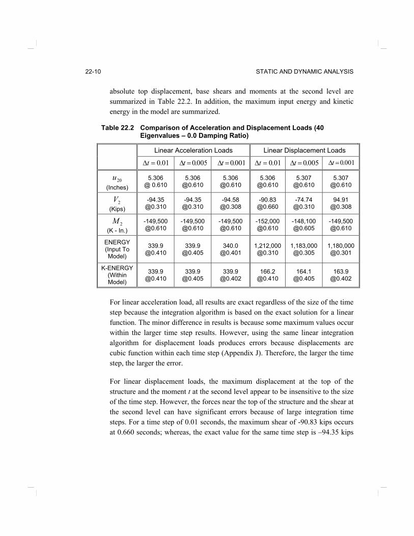
absolute top displacement, base shears and moments at the second level are summarized in Table 22.2. In addition, the maximum input energy and kinetic energy in the model are summarized.
Table 22.2 Comparison of Acceleration and Displacement Loads (40 Eigenvalues – 0.0 Damping Ratio)
Linear Acceleration Loads Linear Displacement Loads 01.0=∆t 005.0=∆t 001.0=∆t 01.0=∆t 005.0=∆t 001.0=∆t
20u (Inches)
5.306 @ 0.610
5.306 @0.610
5.306 @0.610
5.306 @0.610
5.307 @0.610
5.307 @0.610
2V (Kips)
-94.35 @0.310
-94.35 @0.310
-94.58 @0.308
-90.83 @0.660
-74.74 @0.310
94.91 @0.308
2M (K - In.)
-149,500 @0.610
-149,500 @0.610
-149,500 @0.610
-152,[email protected]
-148,100 @0.605
-149,[email protected]
ENERGY (Input To Model)
339.9 @0.410
339.9 @0.405
340.0 @0.401
1,212,[email protected]
1,183,000 @0.305
1,180,[email protected]
K-ENERGY (Within Model)
339.9 @0.410
339.9 @0.405
339.9 @0.402
166.2 @0.410
164.1 @0.405
163.9 @0.402
For linear acceleration load, all results are exact regardless of the size of the time step because the integration algorithm is based on the exact solution for a linear function. The minor difference in results is because some maximum values occur within the larger time step results. However, using the same linear integration algorithm for displacement loads produces errors because displacements are cubic function within each time step (Appendix J). Therefore, the larger the time step, the larger the error.
For linear displacement loads, the maximum displacement at the top of the structure and the moment t at the second level appear to be insensitive to the size of the time step. However, the forces near the top of the structure and the shear at the second level can have significant errors because of large integration time steps. For a time step of 0.01 seconds, the maximum shear of -90.83 kips occurs at 0.660 seconds; whereas, the exact value for the same time step is –94.35 kips

DISPLACEMENT LOADING 22-11
and occurs at 0.310 seconds. A time-history plot of both shears forces is shows in Figure 22.4.
Figure 22.4 Shear at Second Level Vs. Time With 01.0=∆t -Seconds and Zero Damping
The errors resulting from the use of large time steps are not large in this example because the loading is a simple function that does not contain high frequencies. However, the author has had experience with other structures, using real earthquake displacement loading, where the errors are over 100 percent using a time step of 0.01 seconds. The errors associated with the use of large time steps in a mode superposition analysis can be eliminated for linear elastic structures using the new exact integration algorithm presented in Chapter 13.
An examination of the input and kinetic energy clearly indicates that there is a major mathematical differences between acceleration loads (relative displacement formulation) and displacement loads (absolute displacement formulation). In the relative displacement formulation, a relatively small amount
-100
-80
-60
-40
-20
0
20
40
60
80
100
120
140
0.00 0.20 0.40 0.60 0.80 1.00 1.20 1.40 1.60 1.80 2.00TIME - Seconds
SHEA
R -
Kip
s
Linear Acceleration Loads, or Cubic Displacement Loads - Zero Damping - 40 Modes
Linear Displacement Loads - Zero Damping - 40 Modes
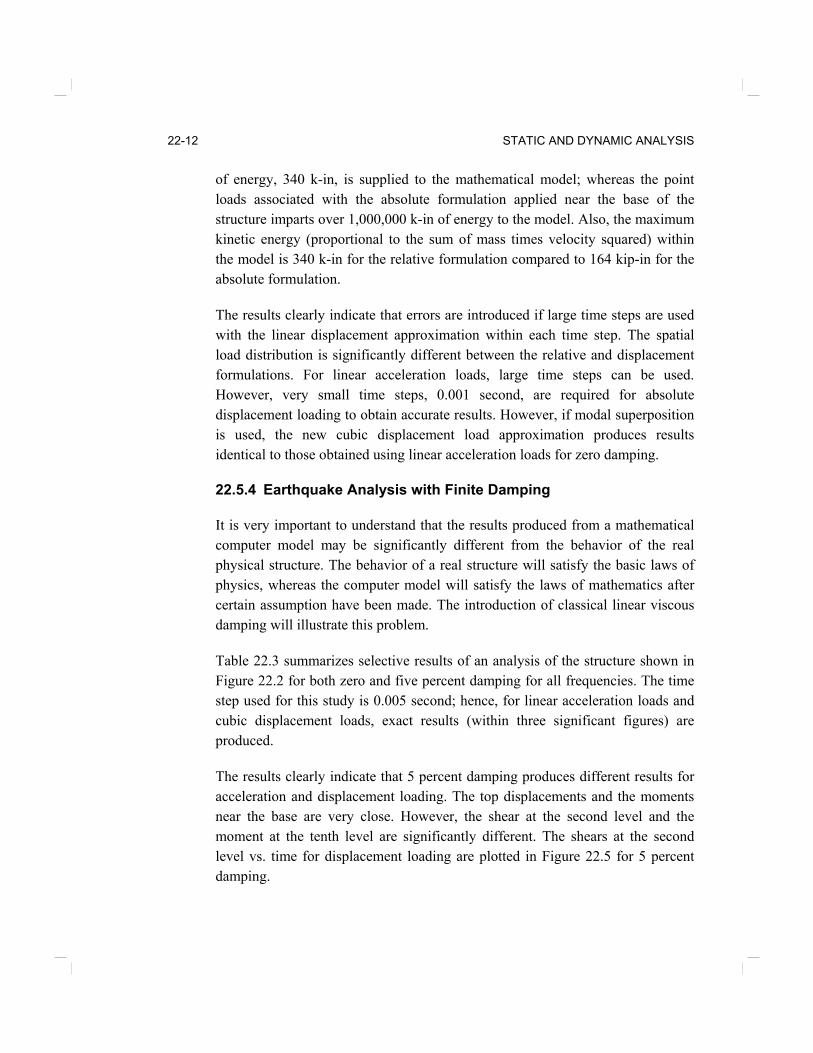
22-12 STATIC AND DYNAMIC ANALYSIS
of energy, 340 k-in, is supplied to the mathematical model; whereas the point loads associated with the absolute formulation applied near the base of the structure imparts over 1,000,000 k-in of energy to the model. Also, the maximum kinetic energy (proportional to the sum of mass times velocity squared) within the model is 340 k-in for the relative formulation compared to 164 kip-in for the absolute formulation.
The results clearly indicate that errors are introduced if large time steps are used with the linear displacement approximation within each time step. The spatial load distribution is significantly different between the relative and displacement formulations. For linear acceleration loads, large time steps can be used. However, very small time steps, 0.001 second, are required for absolute displacement loading to obtain accurate results. However, if modal superposition is used, the new cubic displacement load approximation produces results identical to those obtained using linear acceleration loads for zero damping.
22.5.4 Earthquake Analysis with Finite Damping
It is very important to understand that the results produced from a mathematical computer model may be significantly different from the behavior of the real physical structure. The behavior of a real structure will satisfy the basic laws of physics, whereas the computer model will satisfy the laws of mathematics after certain assumption have been made. The introduction of classical linear viscous damping will illustrate this problem.
Table 22.3 summarizes selective results of an analysis of the structure shown in Figure 22.2 for both zero and five percent damping for all frequencies. The time step used for this study is 0.005 second; hence, for linear acceleration loads and cubic displacement loads, exact results (within three significant figures) are produced.
The results clearly indicate that 5 percent damping produces different results for acceleration and displacement loading. The top displacements and the moments near the base are very close. However, the shear at the second level and the moment at the tenth level are significantly different. The shears at the second level vs. time for displacement loading are plotted in Figure 22.5 for 5 percent damping.

DISPLACEMENT LOADING 22-13
Table 22.3. Comparison of Acceleration and Displacement Loads for Different Damping (40 Eigenvalues, 0.005 Second Time Step)
Linear Acceleration Loads Cubic Displacement Loads
00.0=ξ 05.0=ξ 00.0=ξ 05.0=ξ
20u (Inch)
5.306 @ 0.610 -5.305 @ 1.230
4.939 @ 0.580 -4.217 @ 1.205
5.307 @ 0.610 -5.304 @ 1.230
4.913 @ 0.600 -4.198 @ 1.230
2V (Kips)
88.31 @ 0.130 -94.35 @ 0.310
84.30 @ 0.130 -95.78 @ 0.310
88.28 @ 0.135 -94.53 @ 0.310
135.1 @ 0.150 -117.1 @ 0.340
2M (K-in.)
148,900 @1.230 -149,500 @ 0.605
116,100 @1.200-136,300 @ 0.610
148,900 @1.230 -149,500 @ 0.605
115,300 @1.230-136,700 @ 0.605
10M (K-in.)
81,720 @ 0.290 -63,470 @ 0.495
77,530 @ 0.300 -64,790 @ 0.485
81,720 @ 0.290 -63,470 @ 0.495
80,480 @ 0.320 -59,840 @ 0.495
Figure 22.5 Shear at Second Level Vs. Time Due To Cubic Displacement Loading. (40 Eigenvalues – 005.0=∆t Seconds)
-140
-120
-100
-80
-60
-40
-20
0
20
40
60
80
100
120
140
0.00 0.50 1.00 1.50 2.00
TIME-Seconds
SHEA
R -
Kip
s
Linear Acceleration Loads - 5 Percent Damping - 40 Modes
Cubic Displacement Loads - 5 Percent Damping - 40 Modes

22-14 STATIC AND DYNAMIC ANALYSIS
The results shown in Figure 22.5 are physically impossible for a real structure because the addition of 5 percent damping to an undamped structure should not increase the maximum shear from 88.28 kips to 135.10 kips. The reason for this violation of the fundamental laws of physics is the invalid assumption of an orthogonal damping matrix required to produce classical damping.
Classical damping always has a mass-proportional damping component, as physically illustrated in Figure 22.6, which causes external velocity-dependent forces to act on the structure. For the relative displacement formulation, the forces are proportional to the relative velocities. Whereas for the case of the application of base displacement, the external force is proportional to the absolute velocity. Hence, for a rigid structure, large external damping forces can be developed because of rigid body displacements at the base of the structure. This is the reason that the shear forces increase as the damping is increased, as shown in Figure 22.6. For the case of a very flexible (or base isolated) structure, the relative displacement formulation will produce large errors in the shear forces because the external forces at a level will be carried direct by the dash-pot at that level. Therefore, neither formulation is physically correct.
. RELATIVE DISPLACEMENT FORMULATION ABSOLUTE DISPLACEMENT FORMULATION
ru su
xurxs uuu +=
xum &&
0IC xss =xu& 0IC xss ≠xu&
Figure 22.6 Example to Illustrate Mass-Proportional Component in Classical Damping.

DISPLACEMENT LOADING 22-15
These inconsistent damping assumptions are inherent in all methods of linear and nonlinear dynamic analysis that use classical damping or mass-proportional damping. For most applications, this damping-induced error may be small; however, the engineer/analyst has the responsibility to evaluate, using simple linear models, the magnitude of those errors for each different structure and earthquake loading.
22.5.5 The Effect of Mode Truncation
{ XE "Mode Truncation" }The most important difference between the use of relative and absolute displacement formulations is that higher frequencies are excited by base displacement loading. Solving the same structure using a different number of modes can identify this error. If zero damping is used, the equations of motions can be evaluated exactly for both relative and absolute displacement formulations and the errors associated with mode-truncation only can be isolated.
Selective displacements and member forces for both formulations are summarized in Table 22.4.
Table 22.4 Mode-Truncation Results - Exact Integration for 0.005 Second Time Steps – Zero Damping
Linear Acceleration Loads Cubic Displacement Loads Number of Modes
20u 2V 2M 10M 20u 2V 2M 10M
4 5.306 83.10 -149,400 81,320 5.307 -51,580 -1,441,000 346,800
10 5.306 -94.58 -149,500 81,760 5.307 -33,510 -286,100 642,100
21 5.306 -94.73 -149,500 81,720 5.307 -55,180 -4,576,000 78,840
30 5.306 -94.42 149,500 81,720 5.307 -11,060 -967,200 182,400
35 5.306 94,35 149,500 81,720 5.307 -71,320 -149,500 106,100
40 5.306 -94.35 -149,500 81,720 5.307 -94.53 -149,500 81,720
The results shown in Table 22.4 clearly indicate that only a few modes are required to obtain a converged solution using the relative displacement formulation. However, the results using the absolute displacement formulation are almost unbelievable. The reason for this is that the computational model and
22-16 STATIC AND DYNAMIC ANALYSIS
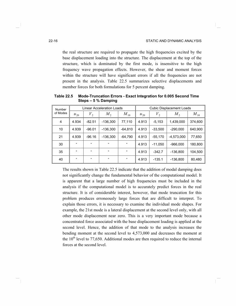
the real structure are required to propagate the high frequencies excited by the base displacement loading into the structure. The displacement at the top of the structure, which is dominated by the first mode, is insensitive to the high frequency wave propagation effects. However, the shear and moment forces within the structure will have significant errors if all the frequencies are not present in the analysis. Table 22.5 summarizes selective displacements and member forces for both formulations for 5 percent damping.
Table 22.5 Mode-Truncation Errors - Exact Integration for 0.005 Second Time Steps – 5 % Damping
Linear Acceleration Loads Cubic Displacement Loads Number of Modes
20u 2V 2M 10M 20u 2V 2M 10M
4 4.934 -82.51 -136,300 77,110 4.913 -5,153 1,439,000 374,600
10 4.939 -96.01 -136,300 -64,810 4.913 -33,500 -290,000 640,900
21 4.939 -96.16 -136,300 -64,790 4.913 -55,170 -4,573,000 77,650
30 “ “ “ “ 4.913 -11,050 -966,000 180,800
35 “ “ “ “ 4.913 -342.7 -136,800 104,500
40 “ “ “ “ 4.913 -135.1 -136,800 80,480
The results shown in Table 22.5 indicate that the addition of modal damping does not significantly change the fundamental behavior of the computational model. It is apparent that a large number of high frequencies must be included in the analysis if the computational model is to accurately predict forces in the real structure. It is of considerable interest, however, that mode truncation for this problem produces erroneously large forces that are difficult to interpret. To explain those errors, it is necessary to examine the individual mode shapes. For example, the 21st mode is a lateral displacement at the second level only, with all other mode displacement near zero. This is a very important mode because a concentrated force associated with the base displacement loading is applied at the second level. Hence, the addition of that mode to the analysis increases the bending moment at the second level to 4,573,000 and decreases the moment at the 10th level to 77,650. Additional modes are then required to reduce the internal forces at the second level.

DISPLACEMENT LOADING 22-17
22.6 USE OF LOAD DEPENDENT RITZ VECTORS
In Table 22.6 the results of an analysis using different numbers of Load Dependent Ritz vectors is summarized. In addition, mass, static and dynamic participation factors are presented.
Table 22.6 Results Using LDR Vectors- 0.005t =∆ Cubic Displacement Loading – Damping = 5 %
Number of Vectors 20u 2V 2M 10M Mass, Static and Dynamic
Load-Participation 4 4.913 111.4 -136,100 80,200 100. 100. 29.5 7 4.913 132.6 -136,700 80,480 100. 100. 75.9
10 4.913 134.5 -136,800 80,490 100. 100. 98.0 21 4.913 135.1 -136,800 80.480 100. 100. 100. 30 4.913 135.1 -136,800 80,480 100. 100. 100.
The use of LDR vectors virtually eliminates all problem associated with the use of the exact eigenvectors. The reason for this improved accuracy is that each set of LDR vectors contains the static response of the system. To illustrate this, the fundamental properties of a set of seven LDR vectors are summarized in Table 22.7.
Table 22.7 Periods and Participation Factors for LDR Vectors
Cumulative Sum of Load Participation Factors
Base Displacement Loading (Percentage)
Vector Number
Approximate Period
(Seconds)
Cumulative Sum of Mass Participation
Factors X-Direction
(Percentage) Static Dynamic
1 1.242178 62.645 0.007 0.000
2 0.199956 81.823 0.093 0.000
3 0.072474 88.312 0.315 0.000
4 0.037780 91.568 0.725 0.002
5 0.023067 93.779 1.471 0.009
6 0.012211 96.701 5.001 0.126
7 0.002494 100.000 100.00 75.882

22-18 STATIC AND DYNAMIC ANALYSIS
The first six LDR vectors are almost identical to the exact eigenvectors summarized in Table 22.1. However, the seventh vector, which is a linear combination of the remaining eigenvectors, contains the high frequency response of the system. The period associated with this vector is over 400 cycles per second; however, it is the most important vector in the analysis of a structure subjected to base displacement loading.
22.7 SOLUTION USING STEP-BY-STEP INTEGRATION
{ XE "Step By Step Integration" }The same problem is solved using direct integration by the trapezoidal rule, which has no numerical damping and theoretically conserves energy. However, to solve the structure with zero damping, a very small time step would be required. It is almost impossible to specify constant modal damping using direct integration methods. A standard method to add energy dissipation to a direct integration method is to add Rayleigh damping, in which only damping ratios can be specified at two frequencies. For this example 5 percent damping can be specified for the lowest frequency and at 30 cycles per second. Selective results are summarized in Table 22.8 for both acceleration and displacement loading.
Table 22.8 Comparison of Results Using Constant Modal Damping and the Trapezoidal Rule and Rayleigh Damping (0.005 Second Time Step)
Acceleration Loading Displacement Loading
Trapezoidal Rule Using
Rayleigh Damping
Exact Solution Using Constant, Modal
Damping 05.0=ξ
Trapezoidal Rule Using
Rayleigh Damping
Exact Solution Using Constant, Modal
Damping 05.0=ξ
20u (Inch)
4.924 @ 0.580 -4.217 @ 1.200
4.939 @ 0.580 -4.217 @ 1.205
4.912 @ 0.600 -4.182 @ 1.220
4.913 @ 0.600 -4.198 @ 1.230
2V (Kips)
86.61 @ 0.125 -95.953 @ 0.305
84.30 @ 0.130 -95.78 @ 0.310
89.3 @ 0.130 -93.9 @ 0.305
135.1 @ 0.150 -117.1 @ 0.340
2M (k–in.)
115,600 @ 1.185 -136,400 @ 0.605
116,100 @1.200 -136,300 @ 0.610
107.300 @ 1.225-126,300 @ 0.610
115,300 @1.230 -136,700 @ 0.605
10M (K-in.)
78,700 @ 0.285 -64,500 @ 0.485
77,530 @ 0.300 -64,790 @ 0.485
81.,30 @ 0.280 61,210@ 0.480
80,480 @ 0.320 -59,840 @ 0.495

DISPLACEMENT LOADING 22-19
It is apparent that the use of Rayleigh damping for acceleration loading produces a very good approximation of the exact solution using constant modal damping. However, for displacement loading, the use of Rayleigh damping, in which the high frequencies are highly damped and some lower frequencies are under damped, produces larger errors. A plot of the shears at the second level using the different methods is shown in Figure 22.7. It is not clear if the errors are caused by the Rayleigh damping approximation or by the use of a large time step.
It is apparent that errors associated with the unrealistic damping of the high frequencies excited by displacement loading are present in all step-by-step integration methods. It is a property of the mathematical model and is not associated with the method of solution of the equilibrium equations.
Figure 22.7 Comparison of Step-By-Step Solution Using the Trapezoidal Rule and Rayleigh Damping with Exact Solution (0.005 second time-step and 5% damping)
The effective damping in the high frequencies, using displacement loading and Rayleigh damping, can be so large that the use of large numerical integration time steps produces almost the same results as using small time steps. However,
-140
-120
-100
-80
-60
-40
-20
0
20
40
60
80
100
120
140
0.0 0.5 1.0 1.5 2.0
TIME - Seconds
SHEA
R -
Kip
s
Exact Cubic Displacement Solution - 5 % Modal Damping
Step By Step Solution - Rayleigh Damping

22-20 STATIC AND DYNAMIC ANALYSIS
the accuracy of the results cannot be justified using this argument, because the form of the Rayleigh damping used in the computer model is physically impossible within a real structure. In addition, the use of a numerical integration method that produces numerical energy dissipation in the higher modes may produce unrealistic result when compared to an exact solution using displacement loading.
22.8 SUMMARY
Several new sources of numerical errors associated with the direct application of earthquake displacement loading have been identified. Those problems are summarized as follows:
1. Displacement loading is fundamentally different from acceleration loading because a larger number of modes are excited. Hence, a very small time step is required to define the displacement record and to integrate the dynamic equilibrium equations. A large time step, such as 0.01 second, can cause significant unpredictable errors.
2. The effective damping associated with displacement loading is larger than that for acceleration loading. The use of mass proportional damping, inherent in Rayleigh and classical modal damping, cannot be physically justified.
3. Small errors in maximum displacements do not guarantee small errors in member forces.
4. The 90 percent mass participation rule, which is used to estimate errors for acceleration loading, does not apply to displacement loading. A larger number of modes are required to accurately predict member forces for absolute displacement loading.
5. For displacement loading, mode truncation in the mode superposition method may cause large errors in the internal member forces.
The following numerical methods can be used to minimize those errors:

DISPLACEMENT LOADING 22-21
1. A new integration algorithm based on cubic displacements within each time step allows the use of larger time steps.
2. To obtain accurate results, the static load-participation factors must be very close to 100 percent.
3. The use of LDR vectors will significantly reduce the number of vectors required to produce accurate results for displacement loading.
4. The example problem illustrates that the errors can be significant if displacement loading is applied based on the same rules used for acceleration loading. However, additional studies on different types of structures, such as bridge towers, must be conducted. Also, more research is required to eliminate or justify the differences in results produced by the relative and absolute displacement formulations for non-zero modal damping.
Finally, the state-of-the-art use of classical modal damping and Rayleigh damping contains mass proportional damping that is physically impossible. Therefore, the development of a new mathematical energy dissipation model is required if modern computer programs are to be used to accurately simulate the true dynamic behavior of real structures subjected to displacement loading.

22-22 STATIC AND DYNAMIC ANALYSIS