secular gravity variation at svalbard (norway) from ground

HAL Id: insu-00675762https://hal-insu.archives-ouvertes.fr/insu-00675762

Submitted on 23 Aug 2021

HAL is a multi-disciplinary open accessarchive for the deposit and dissemination of sci-entific research documents, whether they are pub-lished or not. The documents may come fromteaching and research institutions in France orabroad, or from public or private research centers.

L’archive ouverte pluridisciplinaire HAL, estdestinée au dépôt et à la diffusion de documentsscientifiques de niveau recherche, publiés ou non,émanant des établissements d’enseignement et derecherche français ou étrangers, des laboratoirespublics ou privés.

Distributed under a Creative Commons Attribution| 4.0 International License

Secular gravity variations at Svalbard (Norway) fromground observations and GRACE satellite data

Anthony Mémin, Yves Rogister, Jacques Hinderer, Ove Omang, Bernard Luck

To cite this version:Anthony Mémin, Yves Rogister, Jacques Hinderer, Ove Omang, Bernard Luck. Secular gravity vari-ations at Svalbard (Norway) from ground observations and GRACE satellite data. GeophysicalJournal International, Oxford University Press (OUP), 2011, 184, pp.1119-1130. �10.1111/j.1365-246X.2010.04922.x�. �insu-00675762�

https://hal-insu.archives-ouvertes.fr/insu-00675762

http://creativecommons.org/licenses/by/4.0/

http://creativecommons.org/licenses/by/4.0/

https://hal.archives-ouvertes.fr

Geophys. J. Int. (2011) 184, 1119–1130 doi: 10.1111/j.1365-246X.2010.04922.x

GJI

Gra

vity

,ge

ode

syan

dtide

s

Secular gravity variation at Svalbard (Norway) from groundobservations and GRACE satellite data

A. Memin,1 Y. Rogister,1 J. Hinderer,1 O. C. Omang2 and B. Luck1

1IPGS-EOST, CNRS/UdS, UMR 7516, 5 rue Rene Descartes, 67084 Strasbourg Cedex, France. E-mail: [email protected] Mapping Authority, 3507 Honefoss, Norway

Accepted 2010 December 10. Received 2010 December 9; in original form 2010 March 5

S U M M A R YThe Svalbard archipelago, Norway, is affected by both the present-day ice melting (PDIM)and Glacial Isostatic Adjustment (GIA) subsequent to the Last Pleistocene deglaciation. Theinduced deformation of the Earth is observed by using different techniques. At the GeodeticObservatory in Ny-Alesund, precise positioning measurements have been collected since 1991,a superconducting gravimeter (SG) has been installed in 1999, and six campaigns of absolutegravity (AG) measurements were performed between 1998 and 2007. Moreover, the GravityRecovery and Climate Experiment (GRACE) satellite mission provides the time variation ofthe Earth gravity field since 2002. The goal of this paper is to estimate the present rate ofice melting by combining geodetic observations of the gravity variation and uplift rate withgeophysical modelling of both the GIA and Earth’s response to the PDIM. We estimate thesecular gravity variation by superimposing the SG series with the six AG measurements. Wecollect published estimates of the vertical velocity based on GPS and VLBI data. We analysethe GRACE solutions provided by three groups (CSR, GFZ, GRGS). The crux of the problemlies in the separation of the contributions from the GIA and PDIM to the Earth’s deformation.To account for the GIA, we compute the response of viscoelastic Earth models having differentradial structures of mantle viscosity to the deglaciation histories included in the models ICE-3G or ICE-5G. To account for the effect of PDIM, we compute the deformation of an elasticEarth model for six models of ice-melting extension and rates. Errors in the gravity variationand vertical velocity are estimated by taking into account the measurement uncertainties andthe variability of the GRACE solutions and GIA and PDIM models. The ground observationsagree with models that involve a current ice loss of 25 km3 water equivalent yr−1 over Svalbard,whereas the space observations give a value in the interval [5, 18] km3 water equivalent yr−1.A better modelling of the PDIM, which would include the precise topography of the glaciersand altitude-dependency of ice melting, is necessary to decrease the discrepancy between thetwo estimates.

Key words: Satellite geodesy; Time variable gravity; Global change from geodesy; Arcticregion.

1 I N T RO D U C T I O N

The Svalbard archipelago, Norway, is affected by the post-glacialrebound, or Glacial Isostatic Adjustment (GIA), subsequent to thelast Pleistocene deglaciation that started 21 000 years ago and ended10 000 years ago. Moreover, most of the ice sheets in Svalbard(36 000 km2) are presently thinning (Kohler et al. 2007; Dowdeswellet al. 2008; Kaab 2008; Nuth et al. 2010). Both the last deglaciationand present-day ice melting (PDIM) induce deformation of theEarth. These two effects make Svalbard a very interesting zone tostudy to better understand the geodetic consequences of ice meltingat different timescales.

For many years (from 12 to 18 years), positioning observationswith different systems (GPS, VLBI, DORIS) have been collected

at the Geodetic Observatory in Ny-Alesund, Svalbard (e.g. Satoet al. 2006; Kierulf et al. 2009a). Kierulf et al. (2009b) study theground velocity and find that a predicted melting rate of 37 cmwater equivalent yr−1 (we yr−1) explains up to 60 per cent of theirobserved uplift, which is 8.2 ± 0.9 mm yr−1 in ITRF2005. Theyattribute the remaining 40 per cent to imperfect modelling and er-rors in determining the secular rate from observations. Since 1999,a superconducting gravimeter (SG) has been continuously record-ing the gravity changes and, from 1998 to 2007, six campaignsof absolute gravity (AG) measurements were performed at the SGstation, which also contributes to the Global Geodynamics Project(Crossley et al. 1999). Sato et al. (2006), who were interested inthe secular geodetic variations, concluded from the first four AGmeasurements and observed uplift rate that an ice melting rate of

C© 2011 The Authors 1119Geophysical Journal International C© 2011 RAS

Geophysical Journal InternationalD

ownloaded from

https://academic.oup.com

/gji/article/184/3/1119/625048 by guest on 23 August 2021

1120 A. Memin et al.

75 cm we yr−1 would explain the ground vertical velocity but onlyhalf of the gravity rate.

Since its launch in 2002, the Gravity Recovery and Climate Ex-periment (GRACE) satellite mission has provided a global map-ping of the time-varying gravity field of the Earth. These satel-lite gravimetry data have been used for the estimation of the ice-mass balance over ice-covered lands of various extension, such asGreenland, Antarctica (e.g. Chen et al. 2006c; Luthcke et al. 2006;Velicogna & Wahr 2006a; Velicogna & Wahr 2006b), Alaska andPatagonia (Tamisiea et al. 2005; Chen et al. 2006a; Chen et al. 2007;Luthcke et al. 2008). Their areas are respectively 12 × 106 km2,1.7 × 106 km2, 90 000 km2 and 17 000 km2. Rodell & Famiglietti(1999) compared the modelled variation of water storage to the ex-pected uncertainty associated to the estimate of that variation fromfuture GRACE observations. They concluded that 200 000 km2 isthe smallest area for which it will be possible to detect seasonal andannual changes. Rodell & Famiglietti (2001) later showed that theseasonal and annual changes of the smaller Illinois basin (UnitedStates, 145 800 km2) could be partly—up to 50 per cent—detectedby the GRACE mission. However, in spite of the size of the Alaskanand Patagonian ice sheets, which are smaller than the Illinois basin,the GRACE data have revealed a large signal over these regions thathas been associated with ice-mass loss of, respectively, 97 ± 13and 28 km3 we yr−1. These values agree with the estimates of ice-mass change derived from glaciology studies (Tamisiea et al. 2005;Chen et al. 2007; Luthcke et al. 2008). The size of the ice-coveredarea of the Svalbard archipelago being intermediate between thoseof Alaska and Patagonia, a sufficiently large amount of ice massvariation over Svalbard can be observed with the GRACE satellites.According to the latest elevation changes provided by ICESat laseraltimetry (Moholdt et al. 2010b), the average water equivalent bal-ance of Svalbard is −12 ± 4 cm we yr−1. The ocean that surroundsSvalbard slightly contributes to the gravimetric signal, from 0.8 ±0.8 to 1.9 ± 0.1 mm we yr−1 (see Quinn & Ponte 2010, for a re-view). Because the GRACE signal over Svalbard is approximately60 times larger, most of it can be attributed to land-mass changes.

We aim at providing new estimates of the PDIM over Svalbard.To do so, we have at our disposal updated gravity and precise posi-tioning measurements at the Ny-Alesund Geodetic Observatory, aswell as time-series of the Earth gravity field provided by the GRACEsatellite. To separate the GIA signal from the signal coming fromPDIM requires both phenomena to be modelled.

The outline of the paper goes as follows. In Section 2, we analyseground and satellite observations to estimate the gravity variationand ground vertical velocity over Svalbard. In Section 2.1, we firstderive the secular variation of gravity using six AG observations.We also calibrate the SG by superimposing its nine-year series andthe AG-derived trend. In Section 2.2, we analyse up to 6 years(2003–2009) of GRACE solutions. By considering solutions pro-vided by different centres [Center for Space Research (CSR), Geo-ForschungsZentrum (GFZ) and Groupe de Recherche en GeodesieSpatiale (GRGS)] and different lengths for the time-series (5 or6 yr), we provide uncertainties to the gravity variation observed bythe GRACE satellites. In Section 2.3, we collect uplift rates found inthe literature, they are obtained from GPS and VLBI observations.Next, in Section 3, we model the Earth response to ice melting.We successively consider the ground and space gravity variationsin Sections 3.1 and 3.2, respectively. We use the SELEN softwaredeveloped by Spada & Stocchi (2007) to compute the response of aviscoelastic earth model to the past deglaciation history included inthe model ICE-3G (Tushingham & Peltier 1991). To take the PDIMinto account, we compute the ground velocity and gravity rate of an

elastic earth model for two models of ice-thinning extension suc-cessively combined with three ice-thinning rates. In Section 4, wecompare the modelled gravity variation and vertical velocity result-ing from both the PDIM and GIA to the observed gravity variationand uplift rate. We consider ground observations in Section 4.1 andGRACE observations in Section 4.2. In Section 5, we discuss var-ious estimates of ice-volume changes. Finally, we summarize ourwork in Section 6.

2 O B S E RVAT I O N S O F G R AV I T YVA R I AT I O N A N D V E RT I C A L M O T I O N

2.1 Ground gravity measurements

A total of six observations with FG5 absolute gravimeters havebeen made between 1998 and 2007 at the Ny-Alesund SG station.Three European institutes participated in the gravity observations:the Bundesamt fuer Kartographie and Geodaesie (BKG, Frankfurt,Germany), Ecole et Observatoire des Sciences de la Terre (EOST,Strasbourg, France) and European Center for Geodynamics andSeismology (ECGS, Walferdange, G.-D. Luxembourg). Four of thesix observations (1998–2002) were reported in the paper by Satoet al. (2006). For each measurement, the gravity value at the heightof the AG dropping chamber was transferred to the ground by usinga constant vertical gradient of −0.3594 μGal mm−1. Moreover,corrections were applied to the raw data, owing to three geophysicalphenomena:

(i) the observed polar motion, provided by the International EarthRotation Service (IERS),

(ii) the observed tides, including the effect of ocean tide loading,and

(iii) the observed atmospheric pressure which is responsible fora gravity variation of −0.42 μGal hPa−1.

We apply the same corrections to the two additional AG obser-vations of 2004 and 2007. All the AG data are shown in Fig. 1 withtheir 3σ formal errors.

Sato et al. (2006) showed that using the observed parameters forthe tide and air pressure corrections, instead of the default ones pro-grammed in the processing package g provided by the manufacturerMicro-g, clearly improves the standard error of the estimated AGvalue. However, using different FG5 gravimeters can lead to gravityvalues with an rms error of up to 2 μGal (Robertsson et al. 2001).This was confirmed by comparing 13 absolute gravimeters (includ-ing 11 FG5) in 2003 (Francis et al. 2005): a standard deviation of1.9 μGal was obtained. Consequently, Sato et al. (2006) suggestedto add 2 μGal in quadrature to all the formal errors and fit the datawith the new error as a weight. They obtained a linear trend of−2.5 ± 0.9 μGal yr−1 (Fig. 1). By applying the same extra correc-tion to the formal errors of the 6 AG observations, we compute thetrend with the 3σ formal errors as a weight in the linear least-squarefitting of the data and obtained −1.02 ± 0.48 μGal yr−1, which isabout 41 per cent of the value found by Sato et al. (2006) who usedthe first four observations only.

We also analyse 9 yr (2000 January 1 to 2008 December 31) ofSG data at Ny-Alesund. We apply the three geophysical correctionslisted earlier. We use a degree-3 polynomial filtering with a 48 hwindow to remove the residuals of the tidal signal from the time-series. We correct for five offsets larger than 10 μGal mostly dueto the refilling of the SG dewar with liquid helium. Finally, wealso correct the SG data for a linear drift of 1.81 μGal yr−1 of

C© 2011 The Authors, GJI, 184, 1119–1130

Geophysical Journal International C© 2011 RAS

Dow

nloaded from https://academ

ic.oup.com/gji/article/184/3/1119/625048 by guest on 23 August 2021

Secular gravity variation at Svalbard 1121

Figure 1. Absolute Gravity (AG) measurements at Ny-Alesund (after subtraction of a mean value of 983 017 053.76 μGal). The slopes of the dashed (Satoet al. 2006) and solid (this study) lines are respectively −2.5 ± 0.9 and −1.02 ± 0.48 μGal yr−1. The observations were made by BKG (Bundesamt fuerKartographie and Geodaesie, Frankfurt, Germany), EOST (Ecole et Observatoire des Sciences de la Terre, Strasbourg, France) and ECGS (European Centerfor Geodynamics and Seismology, Walferdange, G.-D. Luxembourg).

Figure 2. Superposition of relative gravity observations with a Supercon-ducting Gravimeter (black curve) and AG measurements (red cross) at Ny-Alesund. The red dashed line is the AG linear trend shown as a solid blackline in Fig. 1.

instrumental origin by adjusting the SG and AG data. The correctedSG time-series is shown in Fig. 2.

The AG measurements have been made in early 1998 Septem-ber, late 2000 July, late 2001 and 2002 September, and early 2007June. At those different times of the year, both the hydrologic andperiodic signals have different amplitudes. To make sure that thesecular trend deduced from the AG measurements is linear and notaffected by the date of the measurements, we have to compare theAG values with the SG data. By correcting the SG drift to fit thesecular trend obtained from the AG measurements, we can compareboth data sets. If the linear trend deduced from the AG observationsis correct, the AG measurements must coincide with the SG data.Otherwise, the AG data are off the SG series. The superposition of

the AG and the SG data shows a very good agreement, confirm-ing the linear trend that we have estimated for the gravity rate inNy-Alesund.

2.2 Space gravity measurements

The releases 4 and 2 of the GRACE solutions provided respec-tively by the CSR/GFZ (Bettadpur 2007; Flechtner 2007) and GRGS(Bruinsma et al. 2010) centres are available as the fully normalizedspherical harmonic coefficients or Stokes coefficients Cm

n (t) andSm

n (t) of the monthly (CSR and GFZ) and 10-day (GRGS) gravitypotential V sat (θ , λ, a, t), which is at the surface of the Earth,

V sat(θ, λ, a, t)

= G M

a

Nmax∑n=2

n∑m=0

[Cm

n (t)Y m,cn (θ, λ) + Sm

n (t)Y m,sn (θ, λ)

], (1)

where θ is the colatitude, λ is the longitude, G is the Newtonianconstant of gravitation, M is the mass of the Earth, G M=3.986 ×1014 m3s−2, a= 6378 km is the mean equatorial radius, and Y m,c

n

(θ , λ) and Y m,sn (θ , λ) are the real cosine and sine fully normalized

spherical harmonics of degree n and order m, respectively. Whileother studies consider gravity anomalies (e.g. Matsuo & Heki 2010),we consider the gravity disturbance at a given by

gsat(θ, λ, a, t) = G M

a2

Nmax∑n=2

n∑m=0

(n + 1)

× [Cm

n (t)Y m,cn (θ, λ) + Sm

n (t)Y m,sn (θ, λ)

].

(2)

We estimate the gravity disturbance rates, �gsat, from the variationsof gsat with respect to the appropriate static fields taken over a 6-year period (2003 January–2009 January). We consider 72 monthlysolutions from CSR, 70 monthly solutions from GFZ and 210 10-day solutions from GRGS, all the solutions being computed upto the harmonic degree N max = 50. This is the maximum degree

C© 2011 The Authors, GJI, 184, 1119–1130


Dow




for which the GRGS provides harmonic coefficients and it corre-sponds to a spatial resolution of ∼400 km. The GRGS solutionsare stabilized during their generation process (http://bgi.grgs.fr) bygradually constraining the coefficients of degree 2 through degree50 to the coefficients of the static field (Bruinsma et al. 2010). Be-sides, we filter the monthly solutions of the CSR and GFZ centreswith a low-pass filter in the spectral domain. The low-pass filter isa cosine taper decreasing from 1 at n = 30 to 0 at n = 50 (e.g. deLinage et al. 2009). Finally, gravity variation �gsat is estimated witha least-square fitting of

g(t) =2∑

i=1

[ai cos(iωt) + bi sin(iωt)] + �gsatt + c, (3)

where ω = 2π/T and T = 1 yr. The ai’s and bi’s give the magnitudeof the annual (i = 1) and semi-annual (i = 2) cycles, and c is thestatic part of g · �gsat is shown in Fig. 3.

The three solutions show similar geophysical signals, for theycontain large patterns over Greenland and Fennoscandia. OverGreenland, the time-decreasing mass signal, implying negative grav-ity rates, has already been reported in previous studies (e.g. Howatet al. 2007; Barletta et al. 2008; Slobbe et al. 2009). OverFennoscandia, the post-glacial rebound due to the last deglaciationinduces the time-increasing mass signal, implying positive gravityrates, which can also be found in previous studies (e.g. Steffen et al.2008; Steffen et al. 2009). A signal over Svalbard with a magnitudesmaller than −0.5 μGal yr−1 can be seen in the CSR and GRGS so-lutions while it is smaller, in absolute value, for the GFZ solutions.To emphasize the geophysical signals that should be common to thethree solutions and decrease the magnitude of other uncorrelatedsignals, we compute the mean of the three solutions (Fig. 4, toppanel). The amplitude of the signal over Svalbard remains about−0.5 μGal yr−1 (Table 1).

We now investigate the influence of the length and variability ofthe solutions on the gravity trend. We compute the spatial mean ofthe GRACE signals over Svalbard for each solution and the averagesof the three solutions for the two time intervals 2003 January and2008 January and 2003 January and 2009 January. North–southstripes affect the GRACE solutions and, to a lesser extent, the meanof the gravity variation. To see the influence of the stripes, we makethe computation before and after applying the destriping filter ofSwenson & Wahr (2006), recently detailed by Duan et al. (2009).We compute the standard deviation of the gravity trend for the threesolutions and for the two time intervals.

Regarding the influence of the length of the time-series, Table 1shows that the gravity trends for the three solutions, either unde-striped or destriped, are smaller for the 2003–2008 time intervalthan for the 2003–2009 time interval. The differences range from0.15 to 0.37 μGal yr−1. The averages of the undestriped and de-striped solutions are respectively 0.28 and 0.20 μGal yr−1 smallerbetween 2003 and 2008 than between 2003 and 2009. Interannualgeophysical phenomena are probably responsible for the differencebetween the estimated gravity trends.

Table 1 also shows that the solutions provided by the three centresare very different. However, the destriping process decreases thediscrepancy and gives much smaller standard deviations for thedestriped solutions.

The observation of the gravity field should be as long as possibleto determine accurately its long-term non-periodic variation. Con-sequently, although the standard deviations for both the undestripedand destriped are smaller for the 2003–2008 solutions, we will baseour study on the 2003–2009 destriped solutions.

Figure 3. Gravity trends �gsat, in μGal yr−1, between 2003 January and2009 January deduced from the GRACE data. From top to bottom: CSR-RL04, GFZ-RL04 and GRGS-RL02 solutions. The CSR and GFZ solutionsare filtered with a cosine taper in the spectral domain for the harmonicdegrees between 30 and 50.

2.3 Ground velocity measurements

In this study we use the ground velocities provided in the literature.Noticing that a scale factor existed between the VLBI (1994–2004)and GPS data, Sato et al. (2006) corrected the two GPS time-series(1991–2004 and 1998–2004) and computed the average of all theobservations in the terrestrial reference frame ITRF2000. They ob-tained an uplift rate of 5.2 ± 0.6 mm yr−1. Rulke et al. (2008) pro-vide a GPS-only Terrestrial Reference Frame (TRF), the Potsdam-Dresden-Reprocessing TRF. In this TRF, the vertical velocities ofthe two stations NYAL (1994–2005) and NYA1 (1998–2005) atNy-Alesund are respectively 7.3 and 7.1 mm yr−1 which lead toa mean uplift rate of 7.2 mm yr−1 and a standard deviation of0.1 mm yr−1. In ITRF 2000 this rate approximately reduces to5.66 ± 0.3 mm yr−1, which is close to the rate obtained by Sato

C© 2011 The Authors, GJI, 184, 1119–1130


Dow




Figure 4. Top panel: mean of the gravity rates deduced from the CSR-RL04,GFZ-RL04 and GRGS-RL02 solutions of the GRACE data. The CSR andGFZ solutions have been previously filtered with a cosine taper in the spectraldomain between degrees 30 and 50. Middle panel: Earth gravity response�gGIA to the deglaciation history ICE-3G with the viscosity profile VP usedby Sato et al. (2006). Bottom panel: mean of the gravity rates deduced fromthe CSR, GFZ and GRGS solutions that have been destriped and correctedfor the GIA contribution. The unit is μGal yr−1.

et al. (2006). Recently, using VLBI, GPS and DORIS data, Kierulfet al. (2009a) derived a mean uplift rate of 8.2 ± 0.9 mm yr−1

in ITRF2005. Kierulf et al. (2009a), Kierulf et al. (2009b) showthat the geodetic observations suffer from the processing strategies.Indeed, they obtain vertical velocities of 10.8 and 7.6 mm yr−1,respectively, using GIPSY-PPP and GAMIT-DD solutions for theNYA1 GPS station between 1997 and 2007. Similar results are ob-tained for the second GPS station NYAL between 1991 and 2007.In ITRF2000, their mean uplift reduces to 6.43 ± 1.19 mm yr−1.

Whereas the dispersion of the published horizontal velocities isless than 1 mm yr−1, the vertical velocity takes on different val-

Table 1. Mean gravity trend over Svalbard for three GRACE solutions for5- and 6-year time intervals (from 2003 to either 2008 or 2009). The asteriskindicates that the mean is computed after applying the destriping filter ofSwenson & Wahr (2006). Two bottom lines: average and standard deviationσ of the three GRACE solutions.

Time interval2003 January to 2008

January2003 January to 2009

January

Solution Gravity trend (μGal yr−1)GRGS −0.99 −0.85∗ −0.80 −0.70∗CSR −0.85 −0.90∗ −0.57 −0.64∗GFZ −0.55 −0.95∗ −0.18 −0.77∗

Average −0.80 −0.90∗ −0.52 −0.70∗σ 0.22 0.05∗ 0.31 0.07∗

ues depending on the TRF, processing strategy and measurementmethod. According to Tregoning & Lambeck (2010), the origin ofITRF2000 may be closer to the centre of mass of Earth’s system thanthat of ITRF2005. This would lead to a better consistency betweenGPS uplift rates and GIA model predictions (Tregoning, personalcommunication, 2010). That was previously mentioned by Argus(2007). Using the errors as a weight, we compute the mean of thethree uplift rates in ITRF2000. We obtain 5.64 ± 1.57 mm yr−1 witha 3σ error.

3 M O D E L L I N G O F G I A A N D E L A S T I CD E F O R M AT I O N D U E T O P D I M

3.1 Modelling of ground gravity variation

Sato et al. (2006) computed the vertical displacement and gravityvariation associated to the GIA at Ny-Alesund up to the harmonicdegree 180. They considered a Maxwell Earth with the viscosityprofile VP listed in Table 2 and the deglaciation history containedin the model ICE-3G.

The computation by Sato et al. (2006) is more accurate thanthe one based on the publicly available SELEN software (Spada& Stocchi 2007), which will be used in Section 3.2, because theyconsider a time-dependent ocean function (Milne et al. 1999) asdescribed earlier by Okuno & Nakada (2002). With their VP theyobtained 1.88 ± 0.7 mm yr−1 and −0.31 ± 0.02 μGal yr−1 forthe uplift and gravity variation respectively, the uncertainties beingestimated from three different deglaciation histories (Sato et al.2006). We obtain a vertical velocity of 1.84 mm yr−1 by running theSELEN software. Using the value of −0.15 μGal mm−1 obtained byWahr et al. (1995) for the ratio between the viscous gravity variationand vertical velocity, we obtain a gravity rate of −0.28 μGal yr−1.

We now turn to the computation of the geodetic consequencesof the PDIM. First, we use two models of ice coverage. The firstis the SVAL model (Hagedoorn & Wolf 2003) in which the dis-tribution of the 16 major ice-masses is based on the location ofthe glaciers described by Hagen et al. (1993). The thinning icemasses are approximated by co-axial elliptical cylinders that givea simple representation of the ice-covered area and topography.This model is used by Sato et al. (2006). The second modelis based on the Digital Chart of the World (DCW). It providesa more realistic geographical location of the glaciers. The to-pography is provided by the GTOPO30 digital elevation model(http://edc.usgs.gov/products/elevation/gtopo30/gtopo30.html). Abetter location of the glaciers near Ny-Alesund is given by theDigital Elevation Model (DEM) from the SPIRIT project (Koronaet al. 2009).

C© 2011 The Authors, GJI, 184, 1119–1130


Dow




Table 2. Viscosity profiles VP, V1 and VM2 used to compute the Earth response to deglaciation historiesICE-3G and ICE-5G. ηu and ηl are, respectively, the viscosities of the upper and lower mantles, and L isthe thickness of the lithosphere. The values of L , ηu and ηl for the VP, V1 and VM2 profiles can be found,respectively, in the papers by Sato et al. (2006), Tushingham & Peltier (1991) and Braun et al. (2008).

Name Deglaciation model ηu (×1021 Pa s) ηl (×1021Pa s) L (km)

VP ICE-3G 0.5 10 100V1 ICE-3G 1 2 120

VM2 ICE-5G 0.5 2.6 90

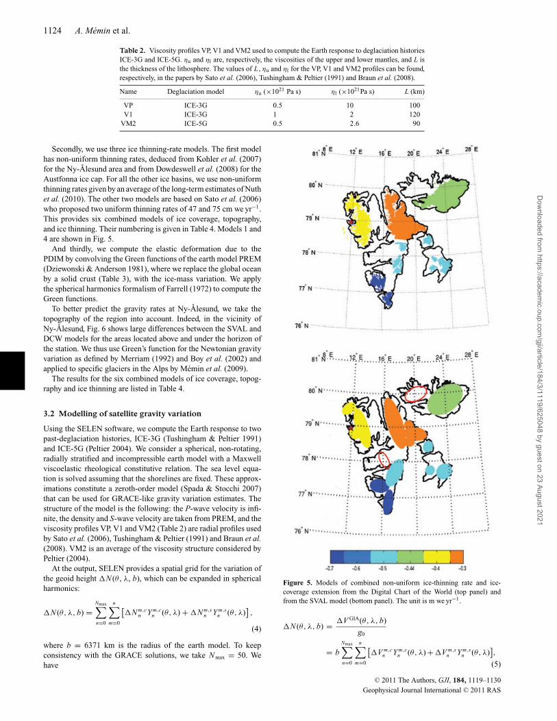
Secondly, we use three ice thinning-rate models. The first modelhas non-uniform thinning rates, deduced from Kohler et al. (2007)for the Ny-Alesund area and from Dowdeswell et al. (2008) for theAustfonna ice cap. For all the other ice basins, we use non-uniformthinning rates given by an average of the long-term estimates of Nuthet al. (2010). The other two models are based on Sato et al. (2006)who proposed two uniform thinning rates of 47 and 75 cm we yr−1.This provides six combined models of ice coverage, topography,and ice thinning. Their numbering is given in Table 4. Models 1 and4 are shown in Fig. 5.

And thirdly, we compute the elastic deformation due to thePDIM by convolving the Green functions of the earth model PREM(Dziewonski & Anderson 1981), where we replace the global oceanby a solid crust (Table 3), with the ice-mass variation. We applythe spherical harmonics formalism of Farrell (1972) to compute theGreen functions.

To better predict the gravity rates at Ny-Alesund, we take thetopography of the region into account. Indeed, in the vicinity ofNy-Alesund, Fig. 6 shows large differences between the SVAL andDCW models for the areas located above and under the horizon ofthe station. We thus use Green’s function for the Newtonian gravityvariation as defined by Merriam (1992) and Boy et al. (2002) andapplied to specific glaciers in the Alps by Memin et al. (2009).

The results for the six combined models of ice coverage, topog-raphy and ice thinning are listed in Table 4.

3.2 Modelling of satellite gravity variation

Using the SELEN software, we compute the Earth response to twopast-deglaciation histories, ICE-3G (Tushingham & Peltier 1991)and ICE-5G (Peltier 2004). We consider a spherical, non-rotating,radially stratified and incompressible earth model with a Maxwellviscoelastic rheological constitutive relation. The sea level equa-tion is solved assuming that the shorelines are fixed. These approx-imations constitute a zeroth-order model (Spada & Stocchi 2007)that can be used for GRACE-like gravity variation estimates. Thestructure of the model is the following: the P-wave velocity is infi-nite, the density and S-wave velocity are taken from PREM, and theviscosity profiles VP, V1 and VM2 (Table 2) are radial profiles usedby Sato et al. (2006), Tushingham & Peltier (1991) and Braun et al.(2008). VM2 is an average of the viscosity structure considered byPeltier (2004).

At the output, SELEN provides a spatial grid for the variation ofthe geoid height �N (θ , λ, b), which can be expanded in sphericalharmonics:

�N (θ, λ, b) =Nmax∑n=0

n∑m=0

[�N m,c

n Y m,cn (θ, λ) + �N m,s

n Y m,sn (θ, λ)

],

(4)

where b = 6371 km is the radius of the earth model. To keepconsistency with the GRACE solutions, we take N max = 50. Wehave

Figure 5. Models of combined non-uniform ice-thinning rate and ice-coverage extension from the Digital Chart of the World (top panel) andfrom the SVAL model (bottom panel). The unit is m we yr−1.

�N (θ, λ, b) = �V GIA(θ, λ, b)

g0

= bNmax∑n=0

n∑m=0

[�V m,c

n Y m,cn (θ, λ) +�V m,s

n Y m,sn (θ, λ)

],

(5)

C© 2011 The Authors, GJI, 184, 1119–1130


Dow




Table 3. Density, seismic wave velocities Vp and Vs and quality factorsQμ and Qκ of the crust that replaces the ocean layer in the PREM model ofDziewonski & Anderson (1981).

Density (kg m−3) Vp (m s−1) Vs (m s−1) Qμ Qκ

2600 5800 3200 600 57823

where �V GIA (θ , λ, b) is the variation of the gravity potentialinduced by the GIA at b and �V m,c

n and �V m,sn are its spherical

harmonic coefficients. g0 is the gravity at the surface of the earthmodel. The gravity variation at a, �gGIA (θ , λ, a), can then berecovered from

�gGIA(θ, λ, a) = G M

a2

Nmax∑n=2

n∑m=0

(n + 1)

(b

a

)n

× [�V m,c

n Y m,cn (θ, λ) + �V m,s

n Y m,sn (θ, λ)

] (6)

= G M

a3

Nmax∑n=2

n∑m=0

(n + 1)

(b

a

)n−1

× [�N m,c

n Y m,cn (θ, λ) + �N m,s

n Y m,sn (θ, λ)

],

(7)

to which the cosine taper filter described in Section 2.2 is thenapplied.

The gravity variation associated to the deglaciation history ICE-3G and viscosity profile VP is shown in Fig. 4 (middle panel).The bottom chart in Fig. 4 shows the destriped residual signal ofthe mean of the three GRACE solutions corrected for the GIAcontribution. Comparison with the top chart of Fig. 4, whichshows the uncorrected mean GRACE signal, reveals that the mass-loss pattern over Svalbard is enhanced after correction for theGIA.

In Table 5, we list the residual signals for the GRACE solutionsand their mean corrected for three GIA models, that is three couplesdeglaciation history—viscosity profile in the mantle, after applica-tion of the destriping filter of Swenson & Wahr (2006). The residualfor the mean GRACE solution is lower than −0.97 μGal yr−1 overSvalbard and the standard deviation is 0.11 μGal yr−1. In Section 4,we will estimate the volume of current ice loss separately fromspace and ground gravity measurements. To compare the two es-timates, we will use the same GIA correction, which is obtainedby combining the deglaciation history ICE-3G and viscosity profileVP.

Figure 6. Topography of the DCW-derived (top panel) and SVAL models (bottom panel) split between ice areas above (left panel) and under (right panel) thehorizon of Ny-Alesund (red star). The unit is m.

C© 2011 The Authors, GJI, 184, 1119–1130


Dow




Table 4. Modelled vertical velocity u (in mm yr−1), gravity rate ge (in μGal yr−1) due to the elastic deformation, and gravity rates gnt and gn due to theNewtonian attraction of the load respectively with and without topography taken into account. The ratios of gravity rates and vertical velocity are in μGal mm−1.The thinning rate in brackets is spatially variable.

Ice coverage/topography Thinning rate (m yr−1) u ge gnt gn (ge + gnt)/u (ge + gn)/u

1 – DCW/GTOPO30 [−0.7, −0.3] 1.51 −0.35 0.26 −0.06 −0.06 −0.272 – DCW/GTOPO30 −0.47 1.76 −0.39 0.24 −0.07 −0.09 −0.263 – DCW/GTOPO30 −0.75 2.80 −0.63 0.38 −0.09 −0.09 −0.26

4 – SVAL/SVAL [−0.7, −0.3] 1.27 −0.28 −0.01 −0.05 −0.23 −0.265 – SVAL/SVAL −0.47 2.03 −0.46 −0.02 −0.06 −0.24 −0.266 – SVAL/SVAL −0.75 3.22 −0.73 −0.03 −0.10 −0.24 −0.26

Table 5. Mean residual signal (in μGal yr−1) over Svalbard of the destripedGRACE-derived gravity variation between 2003 January and 2009 Januarycorrected for three combined deglaciation history-viscosity profile (Table 2).

ICE-3G + V1 ICE-3G + VP ICE-5G + VM2 σ

GRGS −0.97 −1.16 −1.15 0.11CSR −0.91 −1.10 −1.09 0.11GFZ −1.04 −1.24 −1.23 0.11

Mean −0.97 −1.17 −1.16 0.11

The gravity variation due to the PDIM is modelled with0.25◦ × 0.25◦ grids of ice-thickness variations such that the in-tegrated volumes of ice loss are approximately the same as themodels 4 (13 km3 yr−1), 5 (15 km3 yr−1) and 6 (25 km3 yr−1) listedin Table 4. An example of a grid is given on the left panel of Fig. 7.We expand the grids into series of spherical harmonics for which thecoefficients are �σ m,c

n and �σ m,sn and compute the gravity variation

induced by the different ice-thinning rates according to

�gPDIM(θ, λ, b) = 4πGNmax∑n=2

n∑m=0

n + 1

2n + 1(1 + k ′

n)

× [�σ m,c

n Y m,cn (θ, λ) + �σ m,s

n Y m,sn (θ, λ)

],

(8)

where k ′n is the load Love number of degree n for the gravity po-

tential. The cosine taper filter is also applied. As an example, thegravity variation due to the PDIM for model 4 is shown in Fig. 7(right panel). The gravity rate is smaller than −1 μGal yr−1, which

is larger in absolute value than the gravity variation accompanyingthe GIA. As the gravity variations due to the GIA and PDIM areof opposite signs, the removal of the GIA signal from the GRACEsolution enhances the remaining signal. Consequently, it really mat-ters to accurately compute the GIA before correcting the GRACEdata.

4 C O M PA R I S O N B E T W E E N T H E O RYA N D O B S E RVAT I O N

4.1 Ground measurements

Fig. 8 is a synthesis of all the computations made earlier. It showsthe gravity variation as a function of the secular vertical velocity.

The slope of the black solid line passing trough the origin is−0.15 μGal mm−1, which is the theoretical ratio between the gravityvariation and vertical displacement for a viscoelastic deformation(Wahr et al. 1995). From the point on this solid line that correspondsto the viscoelastic deformation computed by using the model ICE-3G + VP (Section 3.1), we draw the black dashed line with a slopeof −0.26 μGal mm−1, which is the theoretical ratio between thegravity variation and vertical displacement for the elastic deforma-tion generated by a surface loading over a spherical Earth model(de Linage et al. 2007). The gravity variation includes the directNewtonian attraction of the load and the effect owing to the elasticdeformation. In the specific case where the topography is neglected,

Figure 7. Left panel: Model 4 of ice thinning given in Table 4. Right panel: gravity variation �gPDIM due to the PDIM for the non-uniform thinning rate. Theunits are respectively m we yr−1 and μGal yr−1.

C© 2011 The Authors, GJI, 184, 1119–1130


Dow




Figure 8. Observed and computed gravity rate as a function of the uplift rate.The solid black line gives the GIA computed by Wahr et al. (1995). Its slopeis approximately −0.15 μGal mm−1. The dashed black line correspondsto the theoretical gravity-to-displacement ratio for the elastic deformationscomputed by de Linage et al. (2007). Its slope is −0.26 μGal mm−1. Thecomputations listed in Table 4, to which GIA contribution is added, arerepresented by the different items combined with colours listed in the legendof the figure. The red and green lines respectively correspond to the ratiodeduced for models 2, 3 and 5, 6 listed in Table 4 taking the topographyinto account. Error bars are that due to GIA modelling (Section 3.1). Therectangle gives the limits of the errors associated to the observations.

the black dashed line is the sum of the GIA and PDIM effects(Memin et al. 2010).

The SVAL rates are given by the green (with topography) andblack (without topography) items. The rates of the DCW-derivedmodels are the red (with topography) and blue (without topography)items. The squares and diamonds respectively correspond to thethinning rates of 47 and 75 cm we yr−1. The circles are for a non-uniform thinning rate ranging from 30 to 70 cm we yr−1. The redand green lines respectively correspond to the ratio deduced formodels 2, 3 and 5, 6 listed in Table 4, taking the topography intoaccount. They show how the topography provided by the SVAL andDCW models influences the gravity rate. The SVAL model has asmoother topography than the DCW model, which explains why thegreen line is closer than the red line to the black dashed line.

The green circle with a black contour and the dotted-dash rect-angle represent the observations with their error bars. The verticalvelocity (5.64 ± 1.57 mm yr−1) was obtained in Section 2.3. Thegravity rate (−1.02 ± 0.48 μGal yr−1) was obtained in Section 2.1.

The best agreement between theory and observation is obtainedfor the modelling based on the SVAL model with a PDIM ratecorresponding to a volume change of ∼25 km3 we yr−1 (75 cmwe yr−1) and the GIA computed with the ICE-3G + VP model.

4.2 GRACE data

Table 6 provides the residuals �gsat − �gGIA − �gPDIM, where�gsat is the gravity variation deduced from the mean of the GRGS,CSR and GFZ solutions (Section 2.2), �gGIA is the GIA contributionfor the ice-mass change history ICE-3G and viscosity profile VP(Table 2) and �gPDIM is the PDIM contribution for models 4 (Fig. 7),5 or 6 (Table 4). The residuals are computed as in Section 2.2. InFig. 9, we show the residuals after applying the destriping filter.

Table 6. Mean residual signal (in μGal yr−1) over Svalbard of the destripedGRACE-derived gravity variation between 2003 January and 2009 Januarycorrected for the deglaciation history ICE-3G, viscosity profile VP andPDIM models 4, 5 and 6 (Table 4).

4 5 6

GRGS −0.18 0.02 0.73CSR −0.12 0.08 0.78GFZ −0.25 −0.05 0.65

Mean −0.18 0.03 0.72

Figure 9. Mean gravity rates deduced from the CSR-RL04, GFZ-RL04and GRGS-RL02 solutions destriped and corrected for the GIA and PDIMcontributions. The CSR and GFZ solutions have been previously filteredwith a cosine taper in the spectral domain between degrees 30 and 50.From top to bottom, the PDIM rates are respectively non-uniform, −47 and−75 cm we yr−1. The unit is μGal yr−1.

C© 2011 The Authors, GJI, 184, 1119–1130


Dow




The PDIM models 4 and 5 combined with the GIA model provideresiduals that are respectively −0.19 and 0.02 μGal yr−1, the PDIMmodel 6 and the GIA model give residuals that are larger than0.65 μGal yr−1. For the time span 2003 January to 2009 January, theGRACE data provide a total volume of ice melting of approximately15 km3 we yr−1. Given the volume involved in a PDIM model andthe residuals, we can estimate the volume of ice loss needed to fit thegravity variation averaged from the GRGS, CSR and GFZ solutions.We obtain 15.5 ± 2.4 km3 we yr−1. That volume loss is closer tothe 8.8 ± 3 km3 we yr−1 estimated by Wouters et al. (2008) forthe period 2003 February to 2008 January than the 75 km3 we yr−1

proposed by Chen et al. (2006b) for the period 2002 April to 2005November.

The destriping filter may affect the estimated volume of ice loss.A similar analysis for the undestriped GRACE solutions leads to anice loss of 9.1 ± 4.2 km3 we yr−1.

5 D I S C U S S I O N

As shown in Section 4, the ground observations of gravity variationand vertical displacement are explained by a PDIM of 25 km3

we yr−1, whereas the GRACE-derived gravity variations providea PDIM comprised between, roughly, 5 and 18 km3 we yr−1, theupper limit being reached by the destriped solutions. This ratherlarge interval includes estimates of ice loss by glaciology studies(Table 7).

Indeed, Nuth et al. (2010) obtained a total ice loss of 9.7 ±0.55 km3 we yr−1 over 27 000 km2 by comparing altimetry fromICESat (2003–2007) to digital elevation models of 1965 and 1990.Dowdeswell et al. (2008) proposed a volume decrease comprised be-tween −2.5 and −4.5 km3 we yr−1 for the Austfonna ice cap, whichrepresents 8000 km2 of ice coverage. Using elevation measurements(GNSS surface profiles, airborne and ICESat laser altimetry) for theperiod 2002–2008, Moholdt et al. (2010a) proposed for Austfonnaan ice melting of 1.3 ± 0.5 km3 we yr−1. Therefore, the total vol-ume loss is comprised between 11 and 14.2 km3 we yr−1. Moholdtet al. (2010b) obtained from the analysis of ICESat laser altimetrydata over the time interval 2003–2008 a total loss of 4.3 ± 1.4 km3

we yr−1, excluding calving front retreat or advance.Ground gravimeters are very sensitive to the location of the

changing ice mass and, consequently, to the local effects. The ice-thinning rate of 75 cm we yr−1 for the SVAL model is a simplemodel; a more realistic model such as the DCW model with anice-thinning rate dependent on the altitude should be consideredto improve the estimate of the gravity rate. Actually, the thinningrate is larger in the lowest parts of the glaciers (e.g. Kohler et al.

2007; Kaab 2008; Nuth et al. 2010). Moreover, the mass distribu-tion of numerous surge-type glaciers in Svalbard changes in a veryshort time. Recently, Sund et al. (2009) reported that the Comfort-lessbreen glacier, located south of Ny-Alesund, started to surge in2006. Such a process may influence the gravity rate observed atNy-Alesund, especially if it is located in the neighbourhood of thestation. Contrary to the ground measurements, space gravimetricmethods such as GRACE measurements are sensitive to the totalmass loss and are not affected by local phenomena. The differenceof sensitivity is likely responsible for the discrepancy between thevolumes of ice loss deduced from GRACE and ground observations.Another ice-thinning distribution that, when integrated, would givethe same ice mass loss as GRACE data could provide vertical ve-locity and gravity rate similar to the ground observations.

6 C O N C LU S I O N S

We have added two new AG measurements to the previous fourobservations made at Ny-Alesund and obtained a new ground-observed gravity rate of −1.02 ± 0.48 μGal yr−1, in agreementwith the continuous SG series. Using the GRACE solutions pro-vided by the CSR, GFZ and GRGS groups for the period 2003 Jan-uary to 2009 January, we have derived the space gravity rate overSvalbard and Northern Europe. After filtering the CSR and GFZsolutions with a low-pass filter and showing similarities with theGRGS solutions, we have computed the mean of the destriped CSR,GFZ and GRGS solutions and obtained a gravity rate of −0.70 ±0.07 μGal yr−1 over Svalbard. The rate is somewhat lower (in ab-solute value) if we do not remove the stripes from the solutions: itis −0.52 ± 0.31 μGal yr−1.

We have used the ICE-3G deglaciation history (Tushingham &Peltier 1991) combined with the viscosity profile used by Satoet al. (2006) to model the viscous response of the Earth to thelast deglaciation. At this stage, the mean of the GRACE solutionscorrected for the GIA contribution shows, over Svalbard, a negativegravity rate, which emphasizes the present ice mass loss: −1.17 ±0.18 μGal yr−1 for the destriped solutions, −0.99 ± 0.46 μGal yr−1

if the stripes are not removed.Next, we have computed the elastic response of the Earth to the

PDIM. We have considered six models of PDIM by combiningtwo models of ice-thinning extension (SVAL and modified DCW)and three melting rates (spatially non-uniform, −47 cm we yr−1,−75 cm we yr−1). The modelled GIA has been added to the elasticdeformation due to the PDIM to compare the theoretical and ob-served geodetic parameters—the gravity variation given above andground vertical velocity reported by Sato et al. (2006), Rulke et al.

Table 7. Summary of estimates of ice loss in Svalbard from various studies. The asterisk indicates thatthe destriping filter of Swenson & Wahr (2006) has been applied to the GRACE solutions.

Data Reference Time interval Volume loss (km3 yr−1)

GRACE Chen et al. (2006b) 04.2002 to 11.2005 −75Wouters et al. (2008) 02.2003 to 01.2008 −8.8 ± 3

This study 01.2003 to 01.2009 −9.1 ± 4.2This study∗ 01.2003 to 01.2009 −15.5 ± 2.4

AG and SG This study 1998–2007 −25

ICESat and DEM Nuth et al. (2010) 1965/1990 to 2003/2007 −13.2 ± 1.55Dowdeswell et al. (2008) 1966–2006

ICESat and DEM Nuth et al. (2010) 1965/1990 to 2003/2007 −11 ± 1.05ICESat Moholdt et al. (2010a) 2002–2008

ICESat Moholdt et al. (2010b) 2003–2008 −4.3 ± 1.4

C© 2011 The Authors, GJI, 184, 1119–1130


Dow




(2008) and Kierulf et al. (2009a). The best agreement is obtainedwith the model of PDIM made up of the SVAL model and an icemelting rate of 75 cm we yr−1, which gives an annual loss of ice of25 km3 we. However, this does not agree with the smaller meltingrate (from 5 to 18 km3 we yr−1) derived from the GRACE solu-tions. Glaciology studies (Dowdeswell et al. 2008; Nuth et al. 2010;Moholdt et al. 2010a; Moholdt et al. 2010b) favour a volume of iceloss between 4 and 14.2 km3 we yr−1, which is similar to the in-terval obtained from the GRACE data. A part of the discrepancybetween the ice losses derived from ground and space observationscan probably be reduced by taking into account the topographyof the glaciers and the altitude dependency of ice melting in themodelling of PDIM.

A C K N OW L E D G M E N T S

We thank T. Sato for providing the SVAL model, E. Berthier forproviding the DCW ice coverage and useful suggestions and J. Trav-elletti for creating an ice coverage mask of the Ny-Alesund area.We thank two anonymous reviewers for their constructive com-ments. We acknowledge logistical and financial support from theFrench Polar Institute (Institut Paul-Emile Victor, IPEV). A. Meminacknowledges financial support from the Centre National d′EtudesSpatiales. Part of this work was supported by COST Action ES0701‘Improved constraints on models of Glacial Isostatic Adjustment’.

R E F E R E N C E S

Argus, D.F., 2007. Defining the translational velocity of the reference frameof Earth, Geophys. J. Int., 169, 830–838.

Barletta, V.R., Sabadini, R. & Bordoni, A., 2008. Isolating the PGR signalin the GRACE data: impact on mass balance estimates in Antarctica andGreenland, Geophys. J. Int., 172, 18–30.

Bettadpur, S., 2007. UTCSR level-2 processing standards document forlevel-2 product release 004, GRACE 327–742 (GR-CSR-03-03).

Boy, J.-P., Gegout, P. & Hinderer, J., 2002. Reduction of surface gravity datafrom global atmospheric pressure loading, Geophys. J. Int., 149, 534–545.

Braun, A., Kuo, C.-Y., Shum, C.K., Wu, P., van der Wal, W. & Fotopoulos,G., 2008. Glacial isostatic adjustment at the Laurentide ice sheet mar-gin: models and observations in the Great Lakes region, J. Geodyn., 46,165–173, doi: 10.1016/j.jog.2008.03.005.

Bruinsma, S., Lemoine, J.-M., Biancale, R. & Vales, N., 2010. CNES/GRGS10–day gravity field models (release 2) and their evaluation, Adv. SpaceRes., 45, 587–601.

Chen, J.L., Tapley, B.D. & Wilson, C.R., 2006a. Alaskan mountain glacialmelting observed by satellite gravimetry, Earth planet. Sci. Lett., 248,368–378.

Chen, J.L., Wilson, C.R. & Tapley, B.D., 2006b. Satellite gravity measure-ments confirm accelerated melting of Greenland ice sheet, Science, 313,1958, doi:10.1126/science.1129007.

Chen, J.L., Wilson, C.R., Blankenship, D.D. & Tapley, B.D., 2006c.Antarctic mass rates from GRACE, Geophys. Res. Lett., 33, L11502,doi:10.1029/2006GL026369.

Chen, J.L., Wilson, C.R., Tapley, B.D., Blankenship, D.D. & Ivins,E.R., 2007. Patagonia Icefield melting observed by Gravity Recoveryand Climate Experiment (GRACE), Geophys. Res. Lett., 34, L22501,doi:10.1029/2007GL031871.

Crossley, D. et al., 1999. Network of superconducting gravimeters benefitsa number of disciplines, EOS. Am. Geophys. Un., 80 (11), 125–126.

de Linage, C., Hinderer, J. & Rogister, Y., 2007. A search for the ratiobetween gravity variation and vertical displacement due to a surface load,Geophys. J. Int., 171, 986–994, doi:10.1111/j.1365-246X.2007.03613.x.

de Linage, C., Rivera, L., Hinderer, J., Boy, J.-P., Rogister, Y., Lambotte, S.& Biancale, R., 2009. Separation of coseismic and postseismic gravity

changes for the 2004 Sumatra-Andaman earthquake from 4.6 years ofGRACE observations and modelling of the coseismic change by normal-modes summation, Geophys. J. Int., 176, 695–714.

Dowdeswell, J.A., Benham, T.J., Strozzi, T. & Hagen, J.O., 2008. Icebergcalving flux and mass balance of the Austfonna ice cap on Nordaustlandet,Svalbard, J. Geophys. Res., 113, F03022, doi:10.1029/2007JF000905.

Duan, X.J., Guo, J.Y., Shum, C.K. & van der Wal, W., 2009. On the post-processing removal of correlated errors in GRACE temporal gravity fieldsolutions, J. Geod., 83, 1095–1106, doi:10.1007/s00190-009-0327-0.

Dziewonski, A.M. & Anderson, D.L., 1981. Preliminary reference Earthmodel, Phys. Earth planet. Inter., 25, 297–356.

Farrell, W.E., 1972. Deformation of the Earth by surface loads, Rev. Geophys.Space Phys., 10, 761–797.

Flechtner, F., 2007. GFZ level-2 processing standards document for level-2product release 004, GRACE 327–743 (GR-GFZ-STD-001), Rev. 1.0.

Francis, O. et al., 2005. Results of the international comparison of absolutegravimeters in Walferdange (Luxembourg) of November 2003, in IAGSymposia, Gravity, Geoid, and Space Missions, Vol. 129, pp. 272–275,Springer, Berlin.

Hagedoorn, J.M. & Wolf, D., 2003, Pleistocene and recent deglaciation inSvalbard: implications for tide-gauche, GPS and VLBI measurements,J. Geodyn., 35, 415–423, doi: 10.1016/S0264-3707(03)00004-8.

Hagen, J.O., Liestøl, D., Roland, E. & Jørgensen, T., 1993, Glacier Atlas ofSvalbard and Jan Mayen. Norsk Polarinstitutt, Oslo.

Howat, I.M., Joughin, I. & Scambos, T.A., 2007. Rapid Changesin Ice Discharge from Greenland Outlet Glaciers, Science, 315,1559–1561.

Kaab, A., 2008. Glacier volume changes using ASTER satellite stereo andICESat GLAS laser altimetry. A test study on Edgeø ya, Eastern Svalbard,IEEE Trans. Geosci. Remote Sens., 46, 10, 2823–2830.

Kierulf, H.P., Pettersen, B.R., MacMillan, D.S. & Willis, P., 2009a. Thekinematics of Ny-Alesund from space geodetic data, J. Geodyn., 48,37–46, doi: 10.1016/j.jog.2009.05.002.

Kierulf, H.P., Plag, H.-P. & Kohler, J., 2009b. Surface deformation inducedby present-day ice melting in Svalbard, Geophys. J. Int., 179, 1–13.

Kohler, J., James, T.D., Murray, T., Nuth, C., Brandt, O., Barrand,N.E., Aas, H.F. & Luckman, A., 2007. Acceleration in thinningrate on western Svalbard glaciers, Geophys. Res. Lett., 34, L18502,doi:10.1029/2007GL030681.

Korona, J., Berthier, E., Bernard, M., Remy, F. & Thouvenot, E., 2009.SPIRIT. SPOT 5 stereoscopic survey of Polar Ice: reference images andtopographies during the fourth International Polar Year (2007–2009),ISPRS J. Photogrammetry Remote Sens., 64(2), 204–212.

Luthcke, S.B., Zwally, H.J., Abdalati, W., Rowlands, D.D., Ray, R.D., Nerem,F.G., McCarthy, J.J. & Chinn, D.S., 2006. Recent Greenland ice mass lossby drainage system from satellite gravity observations, Science, 24, doi:10.1126/science.1130776.

Luthcke, S.B., Arendt, A.A., Rowlands, D.D., McCarthy, J.J. & Larsen, C.F.,2008. Recent glaciers mass changes in the Gulf of Alaska region fromGRACE mascon solutions, J. Glaciol., 54 (188), 2109–2112.

Matsuo, K. & Heki, K., 2010. Time-variable ice loss in Asian highmountains from satellite gravimetry, Earth planet. Sci. Lett., 290,30–36.

Milne, G.A., Mitrovica, J.X. & Davis, J.L., 1999. Near-field hydro-isostacy:the implementation of a revised seal-level equation, Geophys. J. Int., 139,464–482.

Memin, A., Rogister, Y., Hinderer, J., Llubes, M., Berthier, E. & Boy, J.-P.,2009. Ground deformation and gravity variations modelled from present-day ice thinning in the vicinity of glaciers, J. Geodyn., 48(3–5), 195–203,doi: 10.1016/j.jog.2009.09.006.

Memin, A., Rogister, Y. & Hinderer, J., 2010. Separation of the geode-tic consequences of past and present ice melting, Pure Appl. Geophys.,submitted.

Merriam, J.B., 1992. Atmospheric pressure and gravity, Geophys. J. Int.,109, 488–500.

Moholdt, G., Hagen, J.O., Eiken, T. & Schuler, T.V., 2010a. Geometricchanges and mass balance of the Austfonna ice cap, Svalbard, Cryosphere,4, 21–34.

C© 2011 The Authors, GJI, 184, 1119–1130


Dow




Moholdt, G., Nuth, C., Hagen, J.O. & Kohler, J., 2010b. Recent elevationchanges of Svalbard glaciers derived from ICESat laser altimetry, RemoteSens. Environ., 114(11), 2756–2767, doi:10.1016/j.rse.2010.06.008.

Nuth, C., Moholdt, G., Kohler, J., Hagen, J.O. & Kaab, A., 2010. Svalbardglacier elevation changes and contribution to sea level rise, J. geophys.Res., 115, F01008, doi:10.1029/2008JF001223.

Okuno, J. & Nakada, M., 2002. Contributions of ineffective ice load onsea-level and free-air gravity, ice sheet, sea level and the dynamic earth,J. Am. Geophys. Un., Geodynamics Series 29, 177–185.

Peltier, W.R., 2004. Global Glacial Isostasy and the Surface of the Ice-AgeEarth: the ICE-5G (VM2) Model and GRACE. Ann. Rev. Earth. Planet.Sci., 32, 111–149.

Quinn, K.J. & Ponte, R.M., 2010. Uncertainty in ocean mass trendsfrom GRACE, Geophys. J. Int., 181, 762–768, doi:10.1111/j.1365-245X.2010.04508.x.

Robertsson, L. et al., 2001. Results from the fifth international comparisonof absolute gravimeters, ICAG97, Metrologia, 38, 71–78.

Rodell, M. & Famiglietti, J.S., 1999. Detectability of variations in continentalwater storage from satellite observations of the time dependent gravityfield, Water Resour. Res., 35, 2705–2723.

Rodell, M. & Famiglietti, J.S., 2001. An analysis of terrestrial water storagevariations in Illinois with implications for the gravity recovery and climateexperiment (GRACE), Water Resour. Res., 37, 1327–1340.

Rulke, A., Dietrich, R., Fritsche, M., Rothacher, M. & Steigenberger,P., 2008. Realization of the Terrestrial Reference System by a re-processed global GPS network, J. geophys. Res., 113, B08409,doi:10.1029/2007JB005231.

Sato, T., Okuno, J., Hinderer, J., MacMillan, D.S., Plag, H.P., Francis, O.,Falk, R. & Fukuda, Y., 2006. A geophysical interpretation of the secu-lar displacement and gravity rates observed at Ny-Alesund, Svalbard inthe Arctic-effects of post-glacial rebound and present-day ice melting,Geophys. J. Int., 165, 729–743.

Slobbe, D.C., Ditmar, P. & Lindenbergh, R.C., 2009. Estimating the rates ofmass change, ice volume change and snow volume change in Greenlandfrom ICESat and GRACE data, Geophys. J. Int., 176, 95–106.

Spada, G. & Stocchi, P., 2007. SELEN: A Fortran 90 program for solvingthe ‘sea level equation’, Comput. Geosci., 33, 538–562.

Steffen, H., Denker, H. & Muller, J., 2008, Glacial isostatic adjustmentin Fennoscandia from GRACE data and comparison with geodynamicalmodels, J. Geodyn., 46, 155–164, doi: 10.1029/j.jog.2008.03.002.

Steffen, H., Gitlein, O., Denker, H., Muller, J. & Timmen, L., 2009, Presentrate of uplift in Fennoscandia from GRACE and absolute gravimetry,Tectonophysics, 474, 69–77, doi: 10.1016/j.tecto.2009.01.012.

Sund, M., Eiken, T., Hagen, J.O. & Kaab, A., 2009. Svalbard surgedynamics derived from geometric changes, Ann. Glaciol., 50 (52),doi:10.3189/172756409789624265.

Swenson, S. & Wahr, J., 2006. Post-processing removal of the cor-related errors in GRACE data, Geophys. Res. Lett., 33, L08402,doi:10.1029/2006GL025285.

Tamisiea, M.E., Leuliette, E.W., Davis, J.L. & Mitrovica, J.X., 2005.Constraining hydrological and cryospheric mass flux in southeasternAlaska using space-based gravity measurements, Geophys. Res. Lett.,32, L20501, doi:10.1029/2005GL023961.

Tregoning, P. & Lambeck, K., 2010. Origin of the ITRF: finding consistencybetween GPS and GIA models, EGU General Assembly, 12, EGU2010-7352.

Tushingham, A.M. & Peltier, W.R., 1991. ICE-3G: a new global modelof Late Pleistocene deglaciation based upon geophysical predictions ofpostglacial relative sea level change, J. geophys. Res., 96, 4497–4523.

Velicogna, I. & Wahr, J., 2006a. Measurements of time-variablegravity show mass loss in Antarctica, Science, 311, 1754,doi:10.1126/science.1123785.

Velicogna, I. & Wahr, J., 2006b Acceleration of Greenland ice mass loss inspring 2004, Science, 1754, doi:10.1038/nature05168.

Wahr, J., DaZhong, H. & Trupin, A., 1995. Predictions of vertical upliftcaused by changing polar ice volumes on a viscoelastic earth, Geophys.Res. Lett., 22(8), 977–980.

Wouters, B., Chambers, D. & Schrama, E.J.O., 2008. GRACE observessmall-scales mass loss in Greenland, Geophys. Res. Lett., 35, L20501,doi:10.1029/2008GL034816.

C© 2011 The Authors, GJI, 184, 1119–1130


Dow



secular gravity variation at svalbard (norway) from ground

Documents