section 5 root locus analysis - college of...
TRANSCRIPT

MAE 4421 – Control of Aerospace & Mechanical Systems
SECTION 5: ROOT‐LOCUS ANALYSIS

K. Webb MAE 4421
Introduction2

K. Webb MAE 4421
3
Introduction
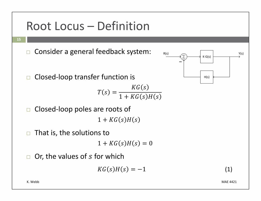
Consider a general feedback system:
Closed‐loop transfer function is
1
is the forward‐path transfer function May include controller and plant
is the feedback‐path transfer function Each are, in general, rational polynomials in
and

K. Webb MAE 4421
4
Introduction
So, the closed‐loop transfer function is
1
Closed‐loop zeros: Zeros of Poles of
Closed‐loop poles: A function of gain, Consistent with what we’ve already seen – feedback moves poles
K. Webb MAE 4421
5
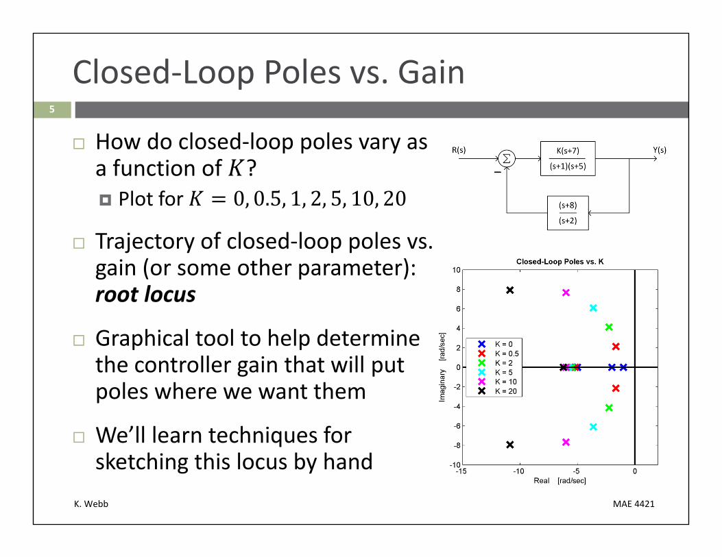
Closed‐Loop Poles vs. Gain
How do closed‐loop poles vary as a function of ? Plot for 0, 0.5, 1, 2, 5, 10, 20
Trajectory of closed‐loop poles vs. gain (or some other parameter): root locus
Graphical tool to help determine the controller gain that will put poles where we want them
We’ll learn techniques for sketching this locus by hand
K. Webb MAE 4421
6
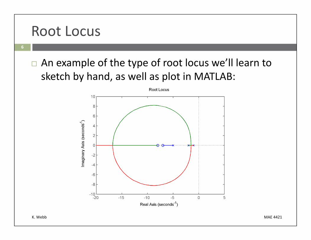
Root Locus
An example of the type of root locus we’ll learn to sketch by hand, as well as plot in MATLAB:

K. Webb MAE 4421
Evaluation of Complex Functions7
K. Webb MAE 4421
8
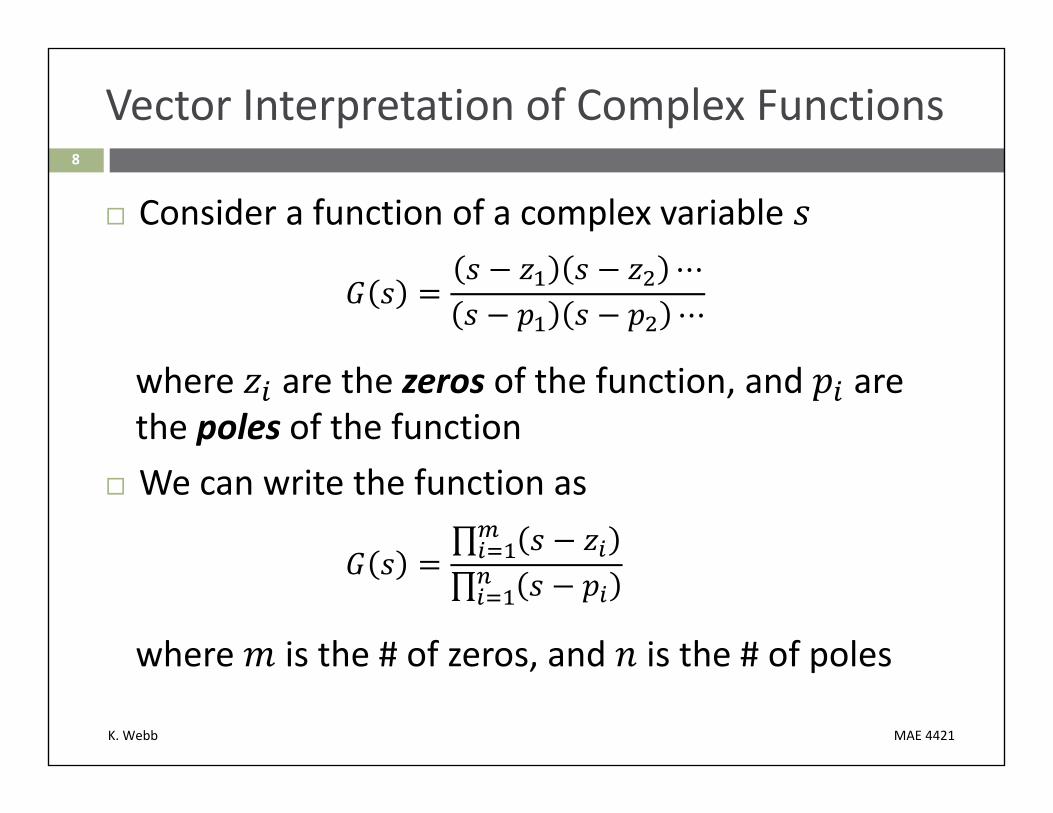
Vector Interpretation of Complex Functions
Consider a function of a complex variable ⋯⋯
where are the zeros of the function, and are the poles of the function
We can write the function as∏∏
where is the # of zeros, and is the # of poles

K. Webb MAE 4421
9
Vector Interpretation of Complex Functions
At any value of , i.e. any point in the complex plane, evaluates to a complex number Another point in the complex plane with magnitude and phase
∠where
∏∏
and∠ ∠
∠ ∠

K. Webb MAE 4421
10
Vector Interpretation of Complex Functions
Each term represents a vector from to the point, , at which we’re evaluating
Each represents a vector from to
For example:3
4 2 5 Zero at: 3 Poles at: , 1 2 and 4
Evaluate at

K. Webb MAE 4421
11
Vector Interpretation of Complex Functions
First, evaluate the magnitude
1 21 21 3 10
2 5
The resulting magnitude:2
2 10 5210
0.1414
∠
K. Webb MAE 4421
12
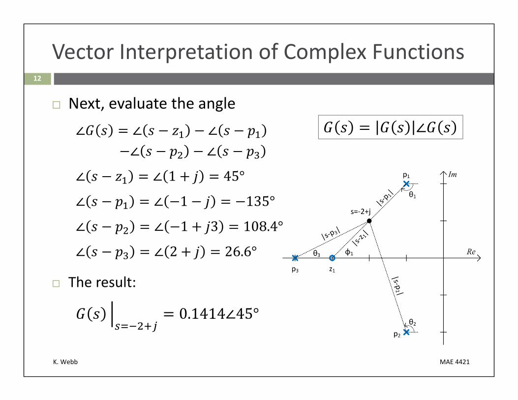
Vector Interpretation of Complex Functions
Next, evaluate the angle∠ ∠ ∠
∠ ∠
∠ ∠ 1 45°
∠ ∠ 1 135°
∠ ∠ 1 3 108.4°
∠ ∠ 2 26.6°
The result:
0.1414∠45°
∠

K. Webb MAE 4421
13
Finite vs. Infinite Poles and Zeros
Consider the following transfer function8
3 10 One finite zero: 8 Three finite poles: 0, 3, and 10
But, as → ∞lim→
∞∞ 0
This implies there must be a zero at ∞
All functions have an equal number of poles and zeros If has poles and zeros, where , then has
zeros at is an infinite complex number – infinite magnitude and some angle

K. Webb MAE 4421
The Root Locus14
K. Webb MAE 4421
15
Root Locus – Definition
Consider a general feedback system:
Closed‐loop transfer function is
1
Closed‐loop poles are roots of1
That is, the solutions to1 0
Or, the values of for which
1 (1)
K. Webb MAE 4421
16
Root Locus – Definition
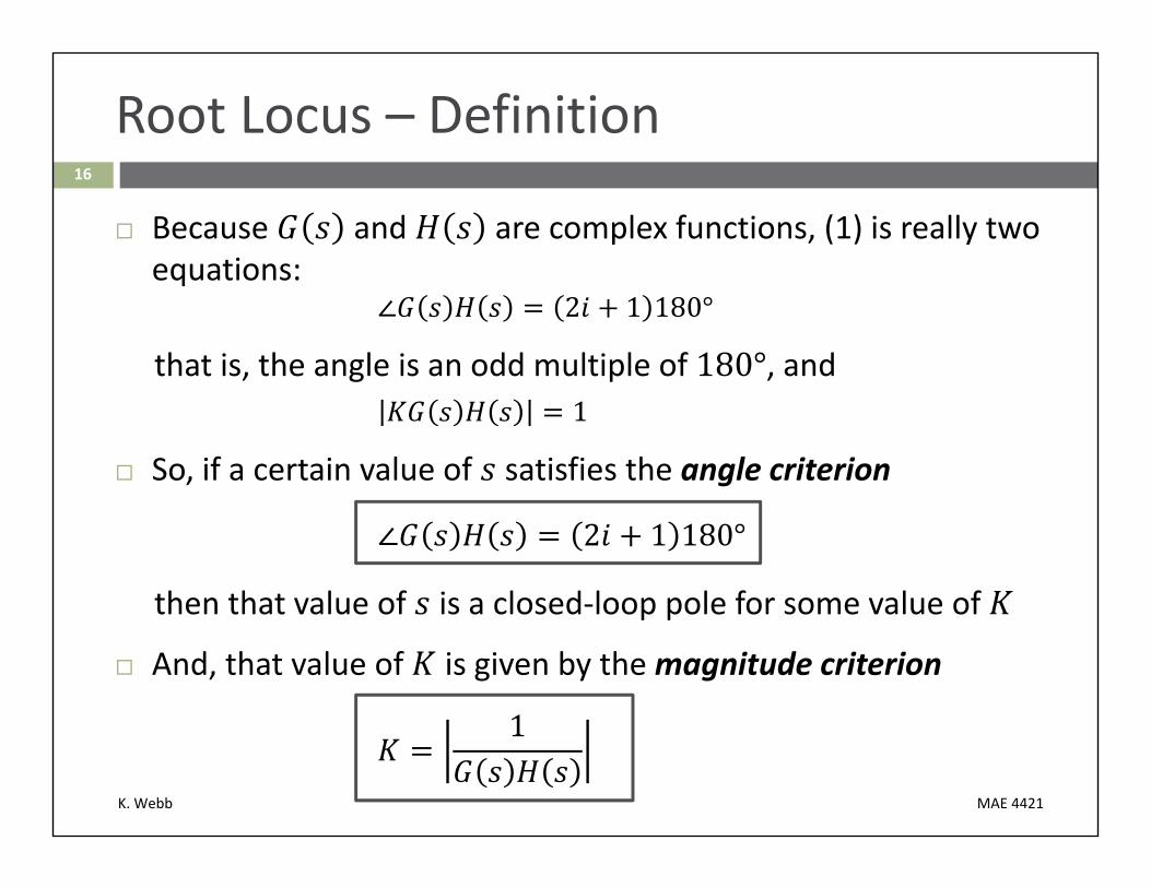
Because and are complex functions, (1) is really two equations:
∠ 2 1 180°
that is, the angle is an odd multiple of 180°, and1
So, if a certain value of satisfies the angle criterion
∠ 2 1 180°
then that value of is a closed‐loop pole for some value of
And, that value of is given by the magnitude criterion
1
K. Webb MAE 4421
17
Root Locus – Definition
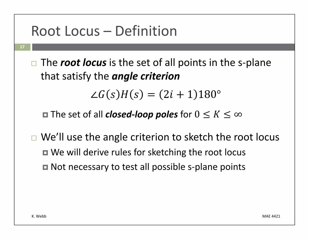
The root locus is the set of all points in the s‐plane that satisfy the angle criterion
The set of all closed‐loop poles for
We’ll use the angle criterion to sketch the root locusWe will derive rules for sketching the root locus Not necessary to test all possible s‐plane points

K. Webb MAE 4421
18
Angle Criterion – Example
Determine if 3 2 is on this system’s root locus
is on the root locus if it satisfies the angle criterion∠ 2 1 180°
From the pole/zero diagram∠ 135° 90°∠ 225° 2 1 180°
does not satisfy the angle criterion It is not on the root locus

K. Webb MAE 4421
19
Angle Criterion – Example
Is on the root locus? Now we have
∠ 135° 45° 180°
is on the root locus
What gain results in a closed‐loop pole at ? Use the magnitude criterion to determine
11 3 2 ⋅ 2 2
yields a closed‐loop pole at And at its complex conjugate, ̅ 2

K. Webb MAE 4421
Sketching the Root Locus20
K. Webb MAE 4421
21
Real‐Axis Root‐Locus Segments
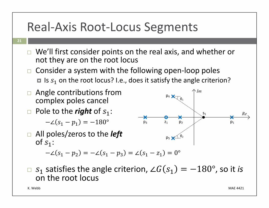
We’ll first consider points on the real axis, and whether or not they are on the root locus
Consider a system with the following open‐loop poles Is on the root locus? I.e., does it satisfy the angle criterion?
Angle contributions from complex poles cancel
Pole to the right of :∠ 180°
All poles/zeros to the leftof :
∠ ∠ ∠ 0°
satisfies the angle criterion, , so it ison the root locus
K. Webb MAE 4421
22
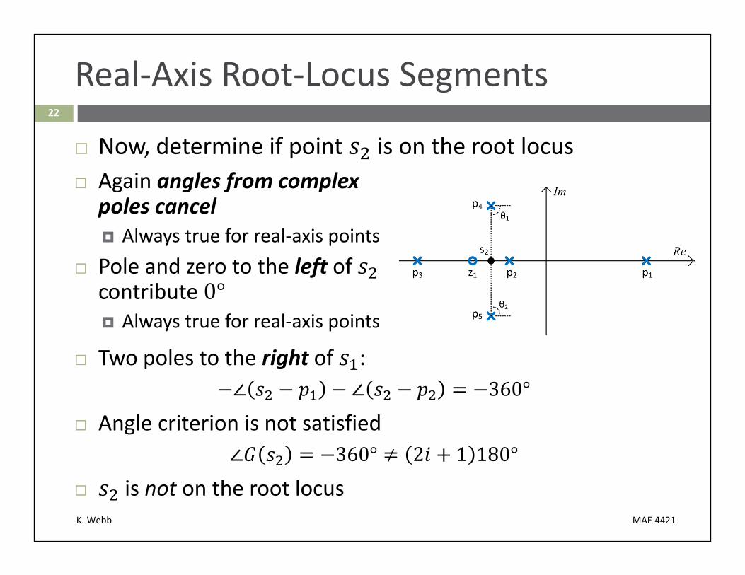
Real‐Axis Root‐Locus Segments
Now, determine if point is on the root locus Again angles from complex poles cancel Always true for real‐axis points
Pole and zero to the left of contribute 0° Always true for real‐axis points
Two poles to the right of : ∠ ∠ 360°
Angle criterion is not satisfied∠ 360° 2 1 180°
is not on the root locus
K. Webb MAE 4421
23
Real‐Axis Root‐Locus Segments
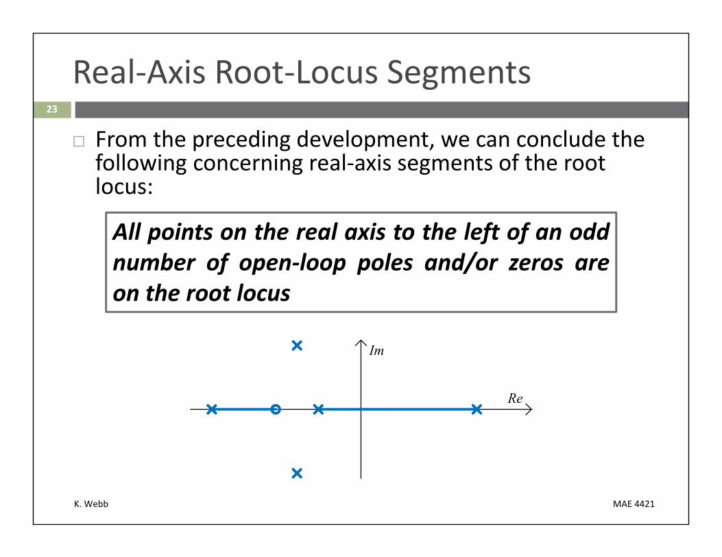
From the preceding development, we can conclude the following concerning real‐axis segments of the root locus:
All points on the real axis to the left of an oddnumber of open‐loop poles and/or zeros areon the root locus
K. Webb MAE 4421
24
Non‐Real‐Axis Root‐Locus Segments
Transfer functions of physically‐realizable systems are rational polynomials with real‐valuedcoefficients Complex poles/zeros come in complex‐conjugate pairs
Root locus is a plot of closed loop poles as varies from
Where does the locus start? Where does it end?
Root locus is symmetric about the real axis
K. Webb MAE 4421
25
Non‐Real‐Axis Root‐Locus Segments
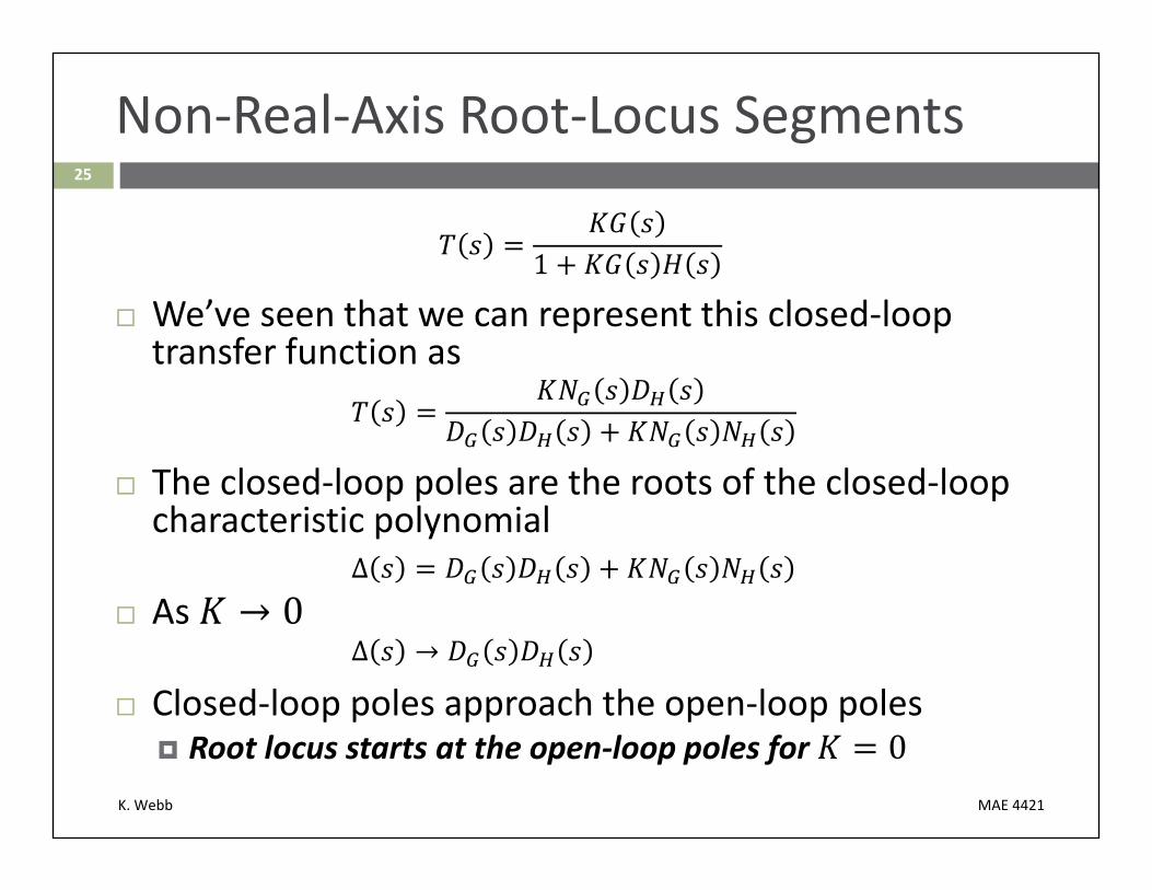
1
We’ve seen that we can represent this closed‐loop transfer function as
The closed‐loop poles are the roots of the closed‐loop characteristic polynomial
Δ As
Δ →
Closed‐loop poles approach the open‐loop poles Root locus starts at the open‐loop poles for 0
K. Webb MAE 4421
26
Non‐Real‐Axis Root‐Locus Segments
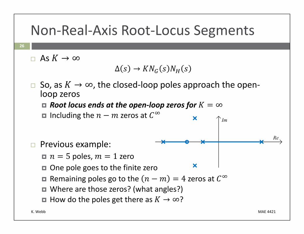
As → ∞Δ →
So, as → ∞, the closed‐loop poles approach the open‐loop zeros Root locus ends at the open‐loop zeros for ∞ Including the zeros at
Previous example: 5 poles, 1 zero One pole goes to the finite zero Remaining poles go to the 4 zeros at Where are those zeros? (what angles?) How do the poles get there as → ∞?

K. Webb MAE 4421
27
Non‐Real‐Axis Root‐Locus Segments
As , of the poles approach the finite zeros The remaining poles are at Looking back from , it appears that these poles all came from the same point on the real axis,
Considering only these poles, the corresponding root locus equation is
11
0
These poles travel from (approximately) to along asymptotes at angles of ,

K. Webb MAE 4421
28
Asymptote Angles –
To determine the angles of the asymptotes, consider a point, , very far from
If is on the root locus, then∠ 2 1 180°
That is, the angles from to sum to an odd multiple of
, 2 1 180°
Therefore, the angles of the asymptotes are
,
K. Webb MAE 4421
29
Asymptote Angles –
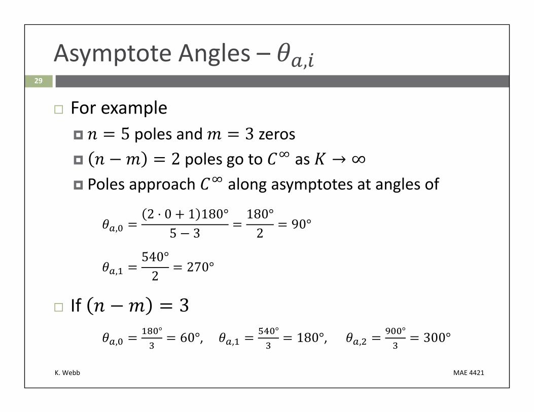
For example poles and zeros poles go to as Poles approach along asymptotes at angles of
,2 ⋅ 0 1 180°
5 3180°2 90°
,540°2 270°
If
,° 60°, ,
° 180°, ,° 300°
K. Webb MAE 4421
30
Asymptote Origin
The asymptotes come from a point, , on the real axis ‐where is located?
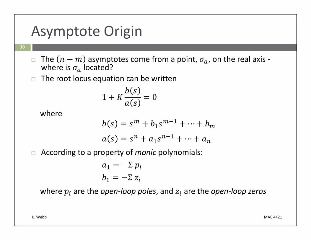
The root locus equation can be written
1 0
where⋯
⋯ According to a property of monic polynomials:
ΣΣ
where are the open‐loop poles, and are the open‐loop zeros

K. Webb MAE 4421
31
Asymptote Origin
The closed‐loop characteristic polynomial is⋯ ⋯
If 1 , i.e. at least two more poles than zeros, thenΣ
where are the closed‐loop poles The sum of the closed‐loop poles is:
Independent of Equal to the sum of the open‐loop poles
Σ Σ
The equivalent open‐loop location for the poles going to infinity is These poles, similarly, have a constant sum:

K. Webb MAE 4421
32
Asymptote Origin
As , of the closed‐loop poles go to the open loop zeros Their sum is the sum of the open‐loop zeros
The remainder of the poles go to Their sum is
The sum of all closed‐loop poles is equal to the sum of the open‐loop poles
The origin of the asymptotes is
K. Webb MAE 4421
33
Root Locus Asymptotes – Example
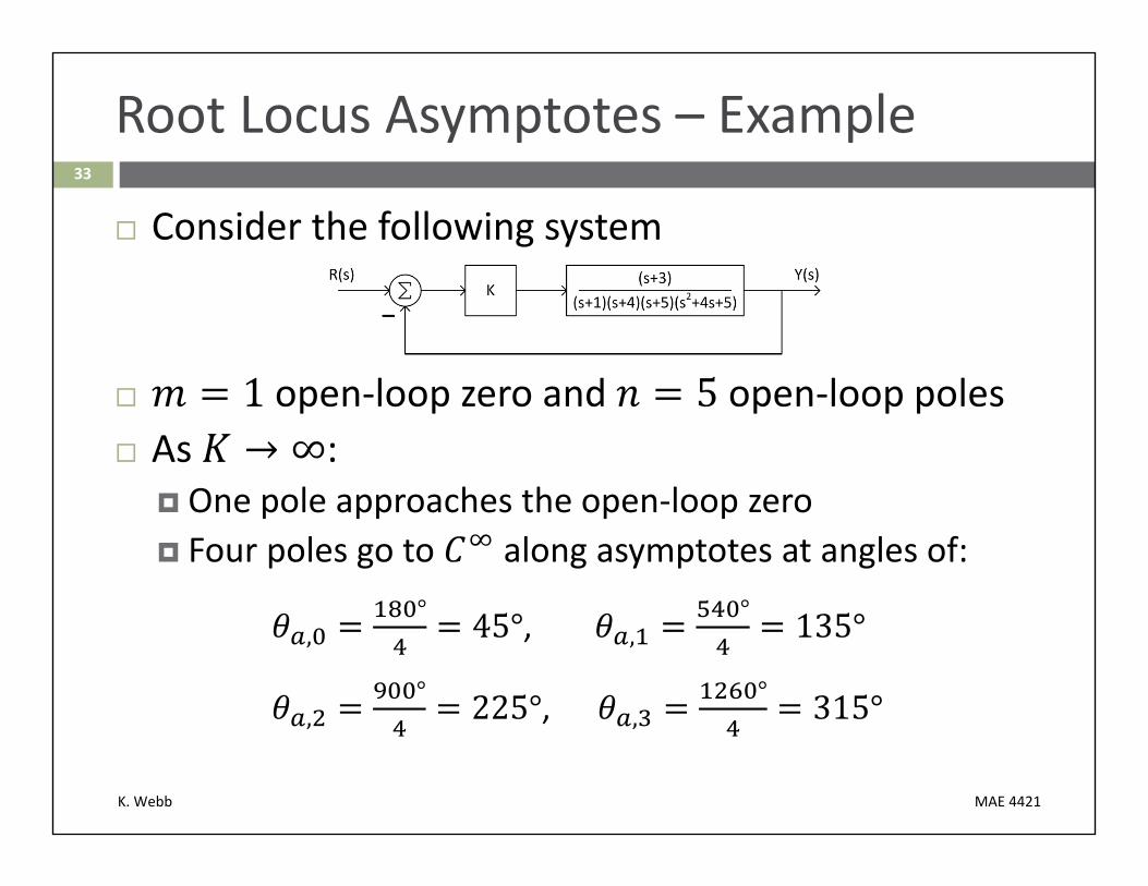
Consider the following system
open‐loop zero and open‐loop poles As :
One pole approaches the open‐loop zero Four poles go to along asymptotes at angles of:
,° 45°, ,
° 135°
,° 225°, ,
° 315°
K. Webb MAE 4421
34
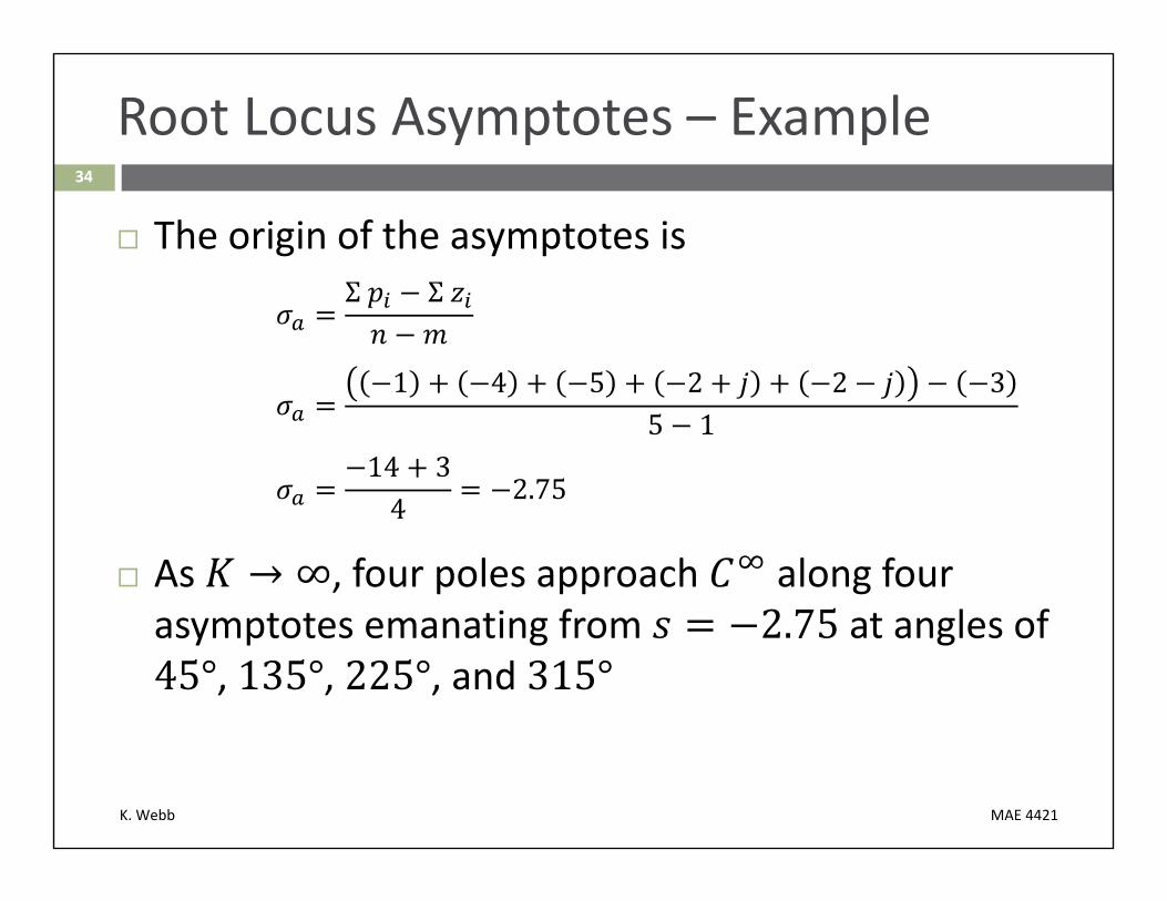
Root Locus Asymptotes – Example
The origin of the asymptotes isΣ Σ
1 4 5 2 2 35 1
14 34 2.75
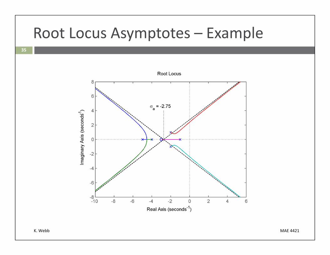
As , four poles approach along four asymptotes emanating from at angles of
, , , and
K. Webb MAE 4421
35
Root Locus Asymptotes – Example

K. Webb MAE 4421
Refining the Root Locus36

K. Webb MAE 4421
37
Refining the Root Locus
So far we’ve learned how to accurately sketch: Real‐axis root locus segments Root locus segments heading toward , but only far from
Root locus from previous example illustrates two additional characteristics we must address: Real‐axis breakaway/break‐in points
Angles of departure/arrival at complex poles/zeros
K. Webb MAE 4421
38
Real‐Axis Breakaway/Break‐In Points
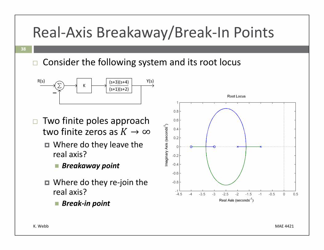
Consider the following system and its root locus
Two finite poles approach two finite zeros as → ∞ Where do they leave the real axis? Breakaway point
Where do they re‐join the real axis? Break‐in point
K. Webb MAE 4421
39
Real‐Axis Breakaway Points
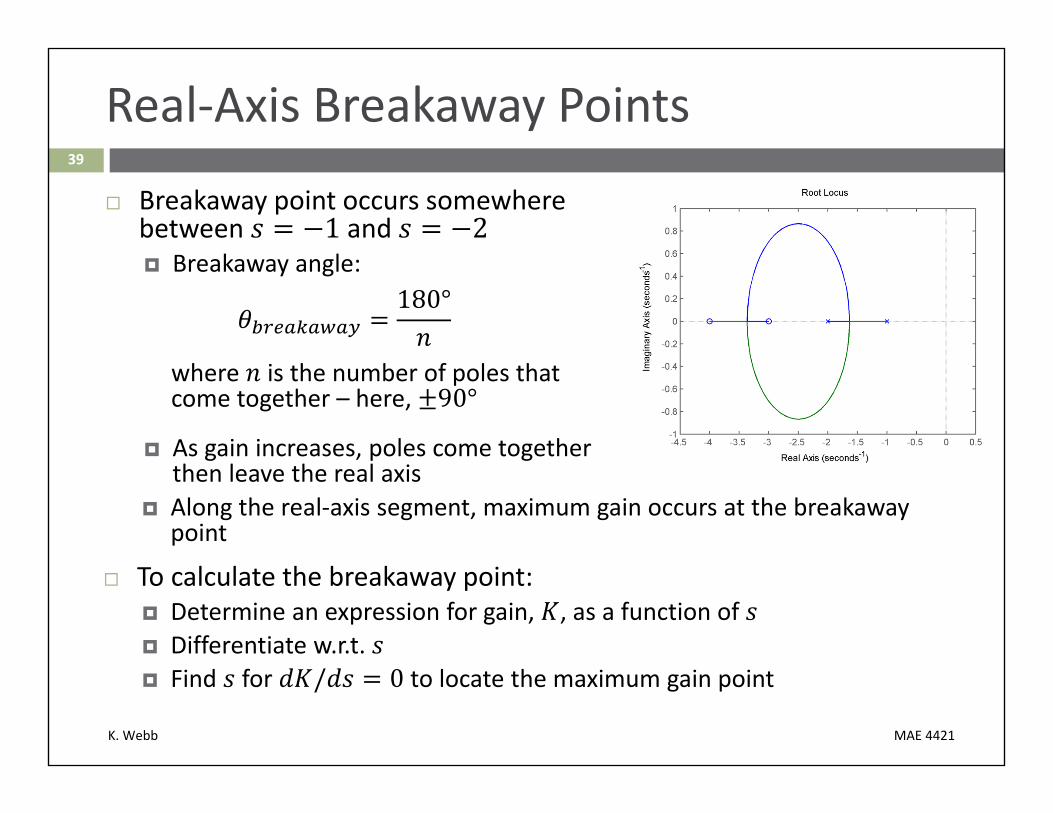
Breakaway point occurs somewhere between 1 and 2 Breakaway angle:
180°
where is the number of poles that come together – here, 90°
As gain increases, poles come together then leave the real axis
Along the real‐axis segment, maximum gain occurs at the breakaway point
To calculate the breakaway point: Determine an expression for gain, , as a function of Differentiate w.r.t. Find for / 0 to locate the maximum gain point
K. Webb MAE 4421
40
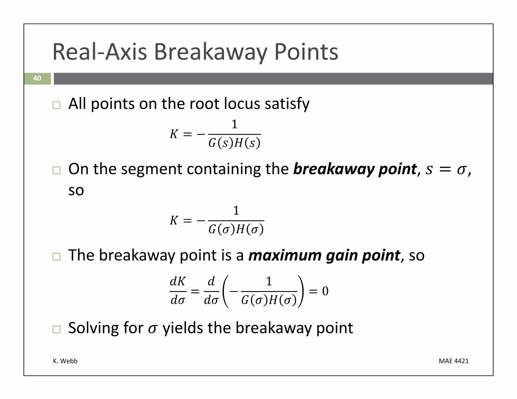
Real‐Axis Breakaway Points
All points on the root locus satisfy1
On the segment containing the breakaway point, , so
1
The breakaway point is a maximum gain point, so1
0
Solving for yields the breakaway point

K. Webb MAE 4421
41
Real‐Axis Breakaway Points
For our example, along the real axis1 1 2
3 43 27 12
Differentiating w.r.t. 7 12 2 3 3 2 2 7
7 12 0
Setting the derivative to zero7 12 2 3 3 2 2 7 0
4 20 22 01.63, 3.37
The breakaway point occurs at
K. Webb MAE 4421
42
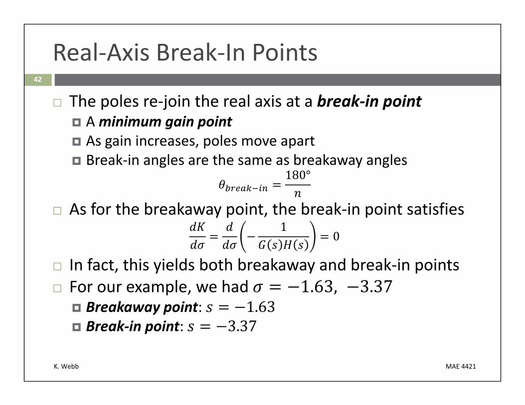
Real‐Axis Break‐In Points
The poles re‐join the real axis at a break‐in point A minimum gain point As gain increases, poles move apart Break‐in angles are the same as breakaway angles
180°
As for the breakaway point, the break‐in point satisfies 1
0
In fact, this yields both breakaway and break‐in points For our example, we had
Breakaway point: 1.63 Break‐in point: 3.37

K. Webb MAE 4421
43
Real‐Axis Breakaway/Break‐In Points
1.633.37
K. Webb MAE 4421
44
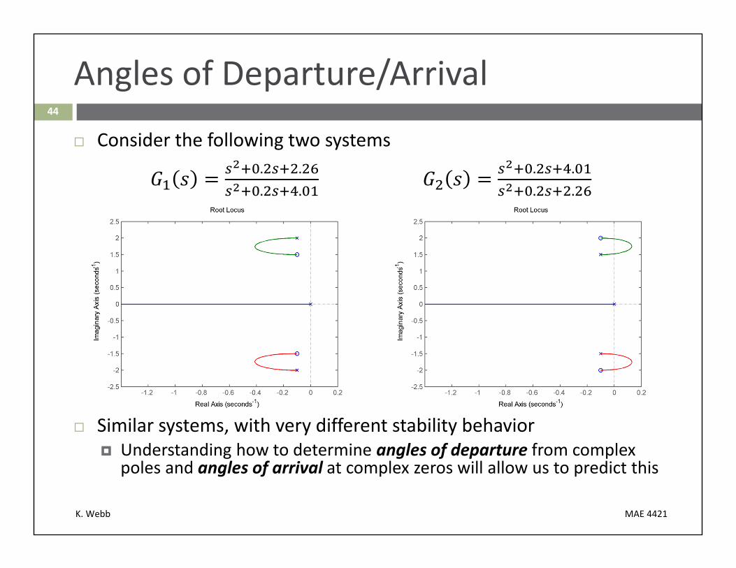
Angles of Departure/Arrival
Consider the following two systems. .. .
. .
. .
Similar systems, with very different stability behavior Understanding how to determine angles of departure from complex
poles and angles of arrival at complex zeros will allow us to predict this

K. Webb MAE 4421
45
Angle of Departure
To find the angle of departure from a pole, : Consider a test point, , very close to The angle from to is The angle from all other poles/zeros, / , to are approximated as the angle
from or to Apply the angle criterion to find
2 1 180°
Solving for the departure angle, :
180°
In words:
Σ∠ Σ∠ 180°

K. Webb MAE 4421
46
Angle of Departure
If we have complex‐conjugate open‐loop poles with multiplicity , then
2 1 180°
The different angles of departure from the multiple poles are
,∑ ∑ 2 1 180°
where
K. Webb MAE 4421
47
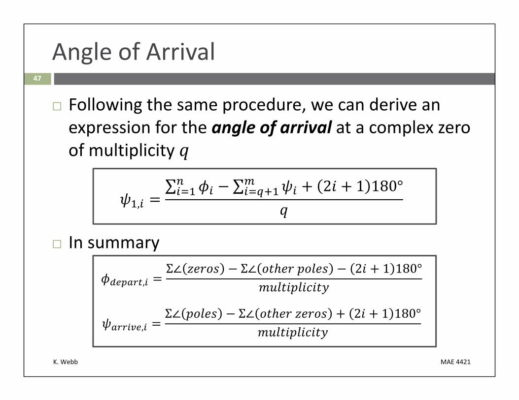
Angle of Arrival
Following the same procedure, we can derive an expression for the angle of arrival at a complex zero of multiplicity
,∑ ∑ 2 1 180°
In summary
,Σ∠ Σ∠ 2 1 180°
,Σ∠ Σ∠ 2 1 180°

K. Webb MAE 4421
48
Departure/Arrival Angles – Example
Angle of departure from
180°
90° 90° 90° 92.9° 180°
182.9°
Due to symmetry:182.9°
Angle of arrival at
180°
90° 90° 93.8° 90° 180°
183.8°, 183.8°

K. Webb MAE 4421
49
Departure/Arrival Angles – Example

K. Webb MAE 4421
50
Departure/Arrival Angles – Example
Next, consider the other system Angle of departure from
90° 90°90° 93.8° 180°
363.8° → 3.8°
3.8°
Angle of arrival at
90° 90° 92.9°90° 180°
362.9° → 2.9°2.9°

K. Webb MAE 4421
51
Departure/Arrival Angles – Example

K. Webb MAE 4421
52
‐Axis Crossing Points
To determine the location of a ‐axis crossing
Apply Routh‐Hurwitz Find value of that results in a row of zeros Marginal stability ‐axis poles
Roots of row preceding the zero row are ‐axis crossing points
Or, plot in MATLAB More on this later

K. Webb MAE 4421
53
Root Locus Sketching Procedure – Summary
1. Plot open‐loop poles and zeros in the s‐plane
2. Plot locus segments on the real axis to the left of an odd number of poles and/or zeros
3. For the poles going to , sketch asymptotes at angles , , centered at , where
,2 1 180°
∑ ∑
K. Webb MAE 4421
54
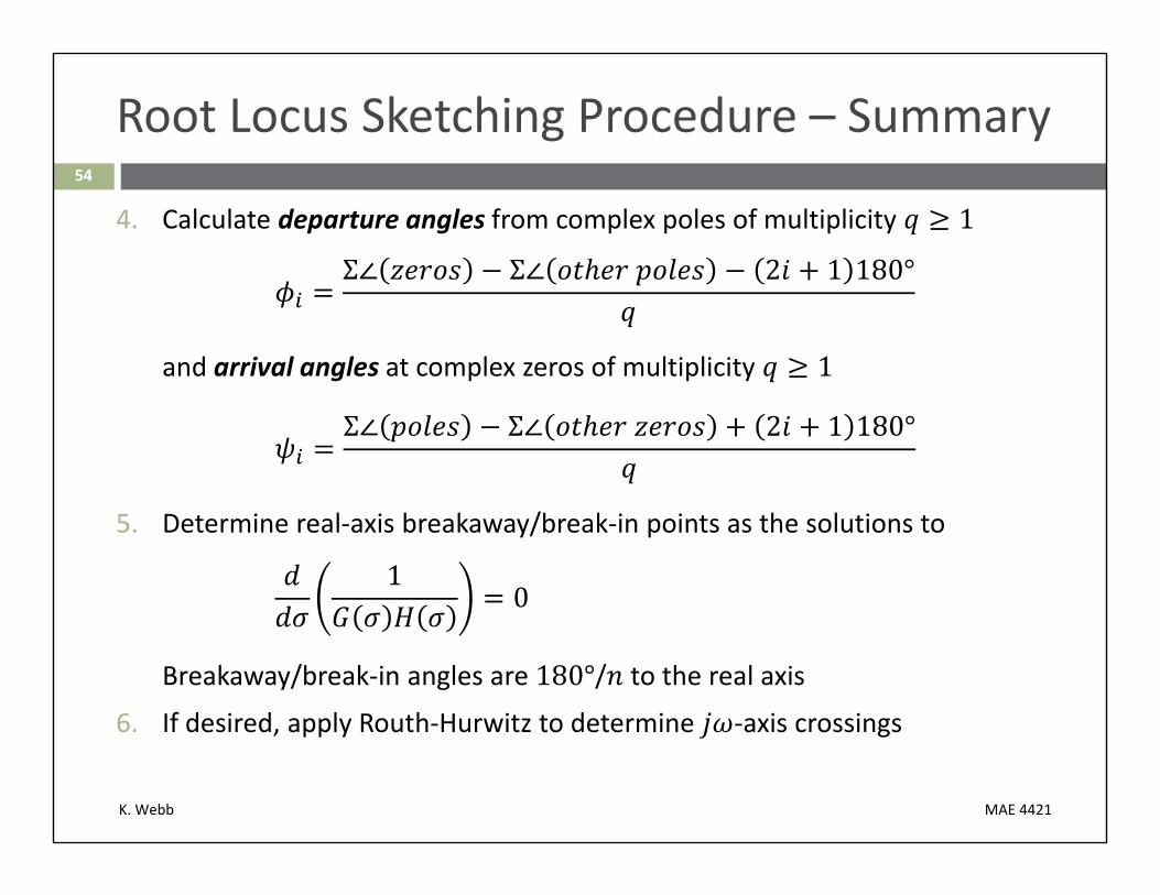
Root Locus Sketching Procedure – Summary
4. Calculate departure angles from complex poles of multiplicity 1
Σ∠ Σ∠ 2 1 180°
and arrival angles at complex zeros of multiplicity 1
Σ∠ Σ∠ 2 1 180°
5. Determine real‐axis breakaway/break‐in points as the solutions to
10
Breakaway/break‐in angles are 180°/ to the real axis
6. If desired, apply Routh‐Hurwitz to determine ‐axis crossings

K. Webb MAE 4421
55
Sketching the Root Locus – Example 1
Consider a satellite, controlled by a proportional‐derivative (PD) controller
A example of a double‐integrator plant We’ll learn about PD controllers in the next section Closed‐loop transfer function
1
Sketch the root locus Two open‐loop poles at the origin One open‐loop zero at 1

K. Webb MAE 4421
56
Sketching the Root Locus – Example 1
1. Plot open‐loop poles and zeros Two poles, one zero
2. Plot real‐axis segments To the left of the zero
3. Asymptotes to One pole goes to the finite
zero
One pole goes to ∞ at 180° ‐along the real axis

K. Webb MAE 4421
57
Sketching the Root Locus – Example 1
4. Departure/arrival angles No complex poles or zeros
5. Breakaway/break‐in points Breakaway occurs at multiple
roots – at 0 Break‐in point:
1 0
1 21 0
2 0 → 2, 0
2
K. Webb MAE 4421
58
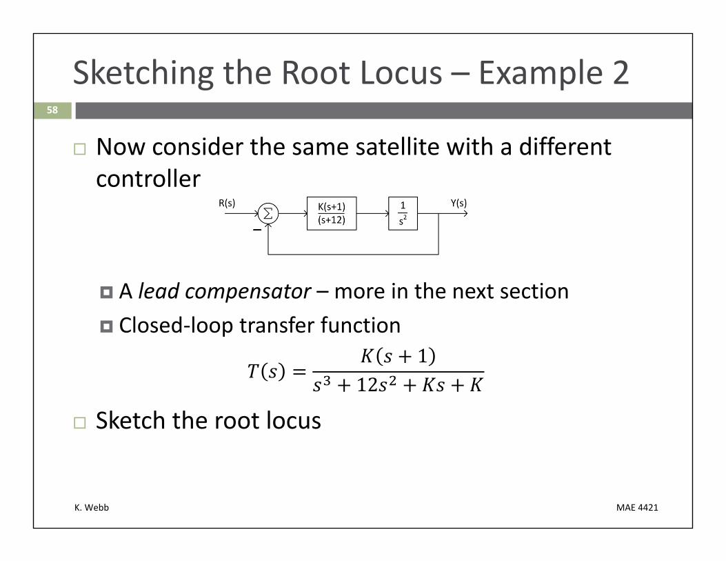
Sketching the Root Locus – Example 2
Now consider the same satellite with a different controller
A lead compensator – more in the next section Closed‐loop transfer function
112
Sketch the root locus
K. Webb MAE 4421
5.5
59
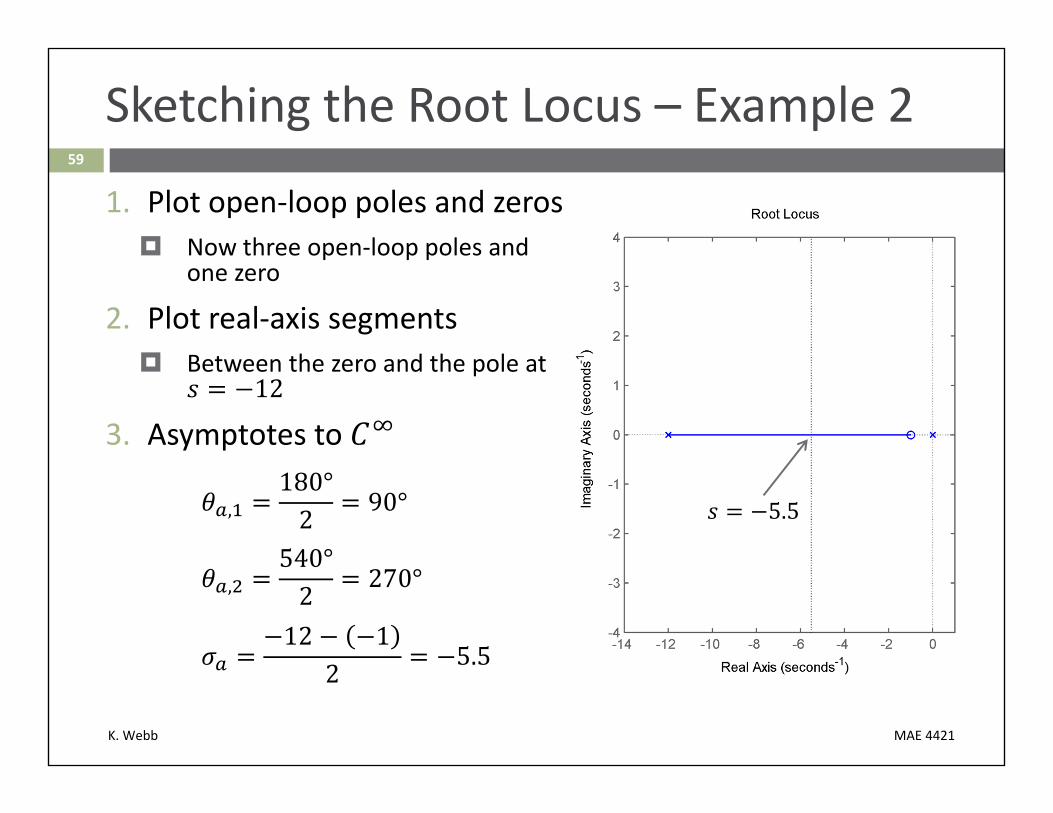
Sketching the Root Locus – Example 2
1. Plot open‐loop poles and zeros Now three open‐loop poles and
one zero
2. Plot real‐axis segments Between the zero and the pole at
12
3. Asymptotes to
,180°2 90°
,540°2 270°
12 12 5.5

K. Webb MAE 4421
60
Sketching the Root Locus – Example 2
4. Departure/arrival angles No complex open‐loop poles or zeros
5. Breakaway/break‐in points121 0
1 3 24 121 0
2 15 24 00, 2.31, 5.19
Breakaway: 0, 5.19 Break‐in: 2.31
2.31
5.19
K. Webb MAE 4421
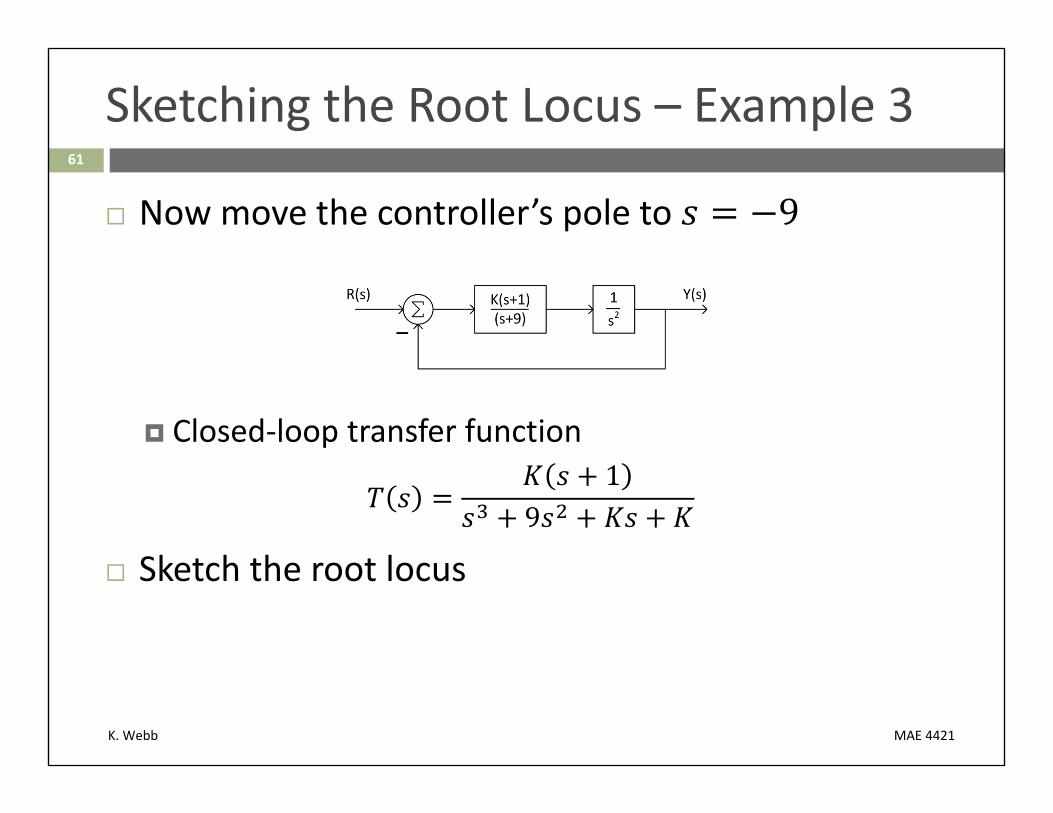
61
Sketching the Root Locus – Example 3
Now move the controller’s pole to
Closed‐loop transfer function1
9
Sketch the root locus
K. Webb MAE 4421
4
62
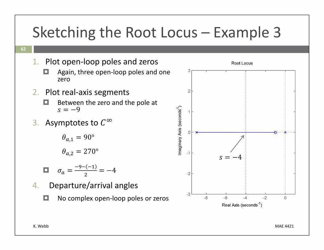
Sketching the Root Locus – Example 3
1. Plot open‐loop poles and zeros Again, three open‐loop poles and one
zero
2. Plot real‐axis segments Between the zero and the pole at
9
3. Asymptotes to
, 90°
, 270°
4
4. Departure/arrival angles No complex open‐loop poles or zeros

K. Webb MAE 4421
63
Sketching the Root Locus – Example 3
4. Breakaway/break‐in points91 0
1 3 18 91 0
2 12 18 00, 3, 3
Breakaway: 0, 3 Break‐in: 3
Three poles converge/diverge at 3
Breakaway angles: 0°, 120°, 240° Break‐in angles: 60°, 180°, 300°
3

K. Webb MAE 4421
Root Locus in MATLAB64
K. Webb MAE 4421
65
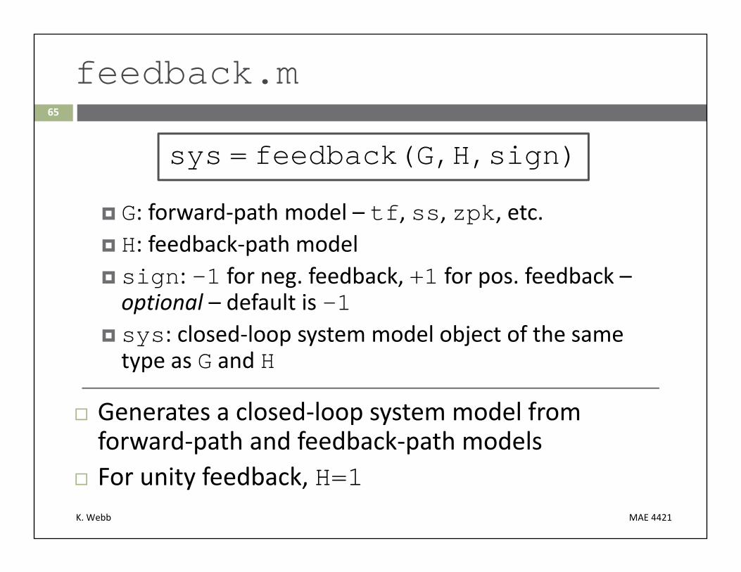
feedback.m
sys = feedback(G,H,sign)
G: forward‐path model – tf, ss, zpk, etc. H: feedback‐path model sign: -1 for neg. feedback, +1 for pos. feedback –optional – default is -1
sys: closed‐loop system model object of the same type as G and H
Generates a closed‐loop system model from forward‐path and feedback‐path models
For unity feedback, H=1

K. Webb MAE 4421
66
feedback.m
For example:
T=feedback(G,H);
T=feedback(G,1);
T=feedback(G1*G2,H);

K. Webb MAE 4421
67
rlocus.m
[r,K] = rlocus(G,K)
G: open‐loop model – tf, ss, zpk, etc. K: vector of gains at which to calculate the locus – optional –MATLAB will choose gains by default
r: vector of closed‐loop pole locations K: gains corresponding to pole locations in r
If no outputs are specified a root locus is plotted in the current (or new) figure window This is the most common use model, e.g.:
rlocus(G,K)

K. Webb MAE 4421
Generalized Root Locus68
K. Webb MAE 4421
69
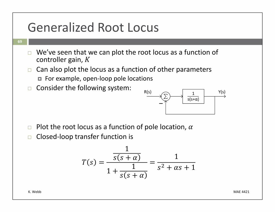
Generalized Root Locus
We’ve seen that we can plot the root locus as a function of controller gain,
Can also plot the locus as a function of other parameters For example, open‐loop pole locations
Consider the following system:
Plot the root locus as a function of pole location, Closed‐loop transfer function is
1
1 11
1
K. Webb MAE 4421
70
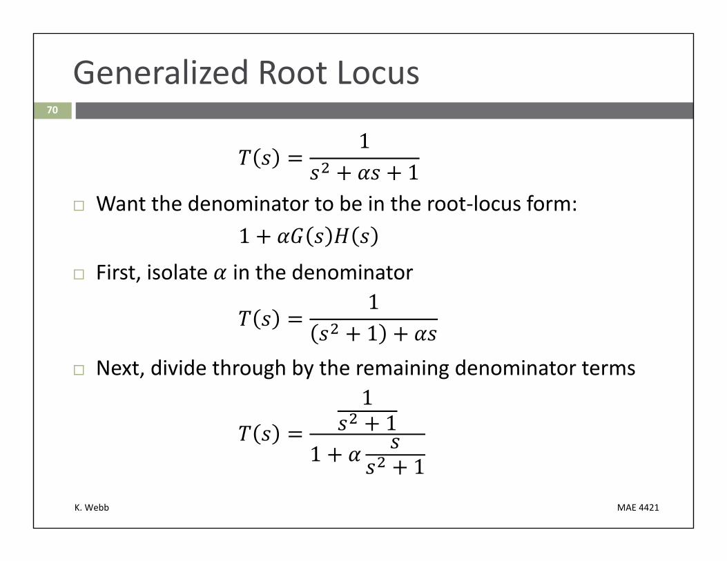
Generalized Root Locus
11
Want the denominator to be in the root‐locus form:1
First, isolate in the denominator11
Next, divide through by the remaining denominator terms11
1 1
K. Webb MAE 4421
71
Generalized Root Locus
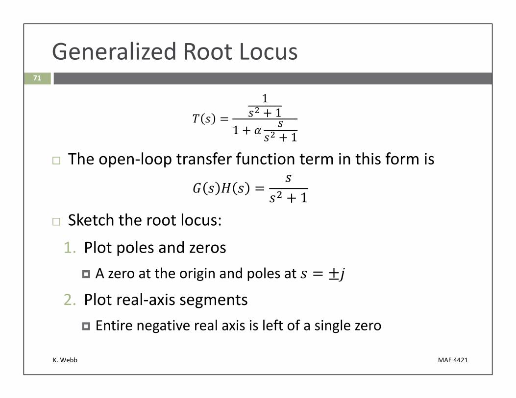
11
1 1
The open‐loop transfer function term in this form is
1 Sketch the root locus:1. Plot poles and zeros
A zero at the origin and poles at
2. Plot real‐axis segments Entire negative real axis is left of a single zero
K. Webb MAE 4421
72
Generalized Root Locus
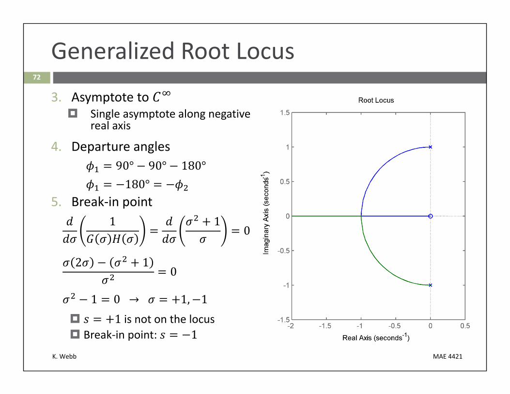
3. Asymptote to Single asymptote along negative
real axis
4. Departure angles90° 90° 180°180°
5. Break‐in point1 1
0
2 10
1 0 → 1, 1 1 is not on the locus Break‐in point: 1

K. Webb MAE 4421
Design via Gain Adjustment73
K. Webb MAE 4421
74
Design via Gain Adjustment
Root locus provides a graphical representation of closed‐loop pole locations vs. gain
We have known relationships (some approx.) between pole locations and transient response These apply to 2nd‐order systems with no zeros
Often, we don’t have a 2nd‐order system with no zeros Would still like a link between pole locations and transient response
Can sometimes approximate higher‐order systems as 2nd‐order Valid only under certain conditions Always verify response through simulation
K. Webb MAE 4421
75
Second‐Order Approximation
A higher‐order system with a pair of second‐order poles can reasonably be approximated as second‐order if:
1) Any higher‐order closed‐loop poles are either:a) at much higher frequency ( ~5 ) than the dominant
2nd‐order pair of poles, orb) nearly canceled by closed‐loop zeros
2) Closed‐loop zeros are either:a) at much higher frequency ( ~5 ) than the dominant
2nd‐order pair of poles, orb) nearly canceled by closed‐loop poles
K. Webb MAE 4421
76
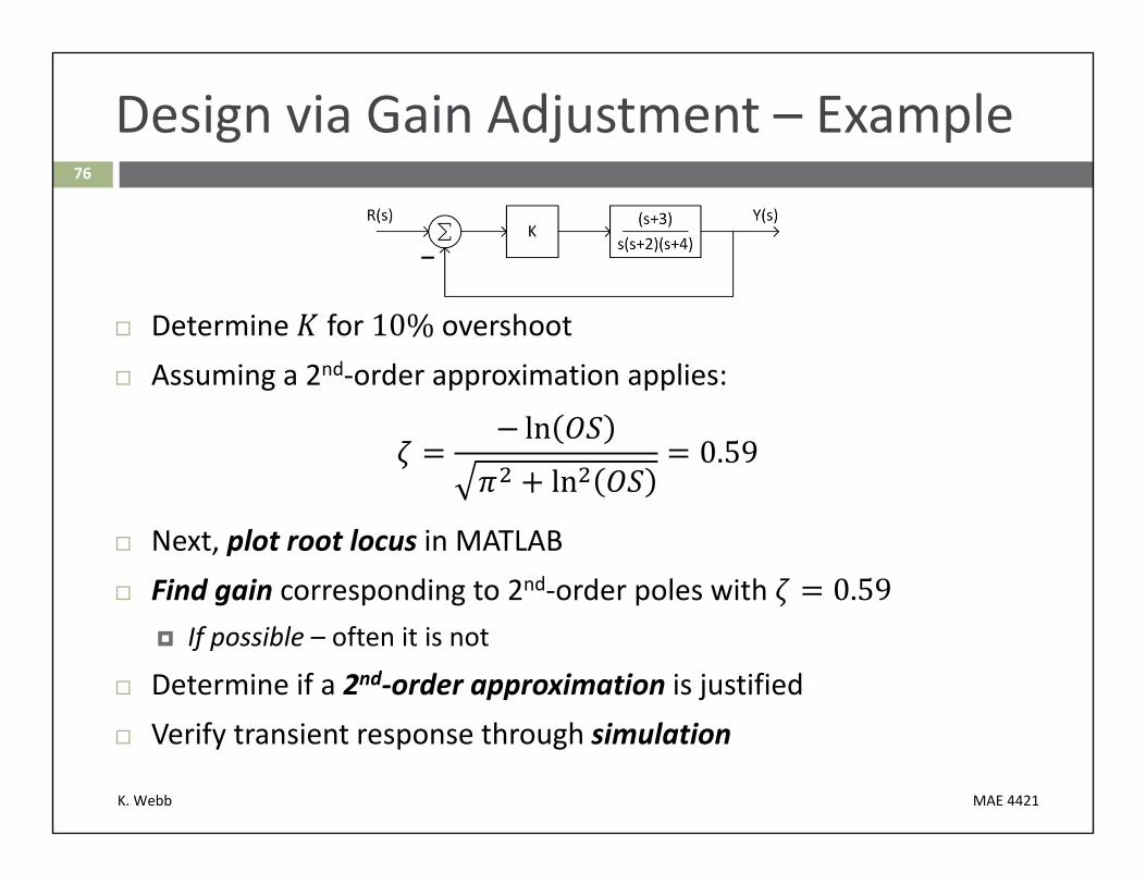
Design via Gain Adjustment – Example
Determine for 10% overshoot Assuming a 2nd‐order approximation applies:
lnln
0.59
Next, plot root locus in MATLAB Find gain corresponding to 2nd‐order poles with 0.59
If possible – often it is not
Determine if a 2nd‐order approximation is justified Verify transient response through simulation
K. Webb MAE 4421
77
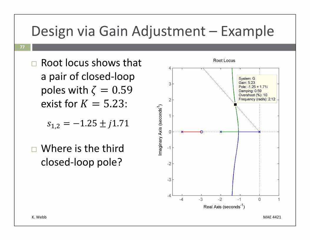
Design via Gain Adjustment – Example
Root locus shows that a pair of closed‐loop poles with exist for :
, 1.25 1.71
Where is the third closed‐loop pole?

K. Webb MAE 4421
78
Design via Gain Adjustment – Example
Third pole is at
Not high enough in frequency for its effect to be negligible
But, it is in close proximity to a closed‐loop zero
Is a 2nd‐order approximation justified? Simulate

K. Webb MAE 4421
79
Design via Gain Adjustment – Example
Step response compared to a true 2nd‐order system No third pole, no zero
Very similar response 11.14% overshoot
2nd‐order approximation is valid
Slight reduction in gain would yield 10% overshoot
K. Webb MAE 4421
80
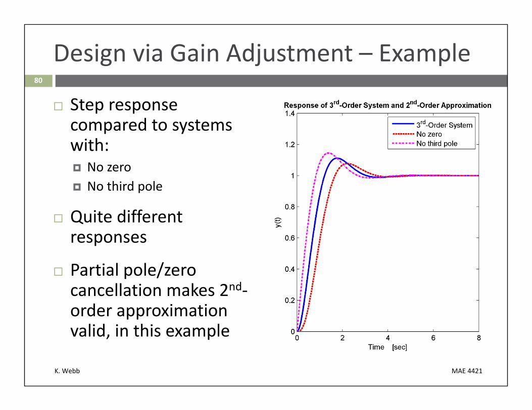
Design via Gain Adjustment – Example
Step response compared to systems with: No zero No third pole
Quite different responses
Partial pole/zero cancellation makes 2nd‐order approximation valid, in this example
K. Webb MAE 4421
81
When Gain Adjustment Fails
Root loci do not go through every point in the s‐plane Can’t always satisfy a single performance specification, e.g. overshoot or settling time
Can satisfy two specifications, e.g. overshoot and settling time, even less often
Also, gain adjustment affects steady‐state error performance In general, cannot simultaneously satisfy dynamic requirements and error requirements
In those cases, we must add dynamics to the controller A compensator