Secondary Trading Costs in the Municipal Bond Market

Lawrence E. Harris Michael S. Piwowar*

May 18, 2004 * Larry Harris is Chief Economist of the U.S. Securities and Exchange Commission, on assignment from the University of Southern California where he holds the Fred V. Keenan Chair in Finance. Mike Piwowar is a Visiting Academic Scholar in the SEC Office of Economic Analysis, on assignment from the Iowa State University where he is Assistant Professor of Finance. We thank Vance Anthony, Bill Dale, Amy Edwards, Martha Haines, Hal Johnson, Larry Lawrence, Janice Mitnick, Mark Zehner, and seminar participants at the SEC, Vanderbilt University and the University of Maryland for their suggestions and assistance with this project. The Securities and Exchange Commission, as a matter of policy, disclaims responsibility for any private publication or statement by any of its employees. The views expressed herein are those of the authors and do not necessarily reflect the views of the Commission or of the authors’ colleagues upon the staff of the Commission. All errors and omissions are the sole responsibility of the authors.

USC FBE FINANCE SEMINARpresented by Larry HarrisFRIDAY, August 27, 200410:30 am – 12:00 pm, Room: JKP-104

Secondary Trading Costs in the Municipal Bond Market

Abstract

Using new econometric methods, we separately estimate average transaction costs, as a

function of trade size, for over 167,000 bonds from a one-year sample of all U.S. municipal bond

trades. Unlike in equities, municipal bond transaction costs decrease with trade size and do not

depend significantly on trade frequency. Municipal bond trades are also substantially more

expensive than similar sized equity trades. We attribute these results to the lack of price

transparency in the bond markets. Additional cross-sectional analyses show that bond trading

costs decrease with credit quality and increase with instrument complexity, time to maturity, and

time since issuance. The results suggest that investors, and perhaps ultimately issuers, might

benefit if issuers issued simpler bonds.

Keywords: Municipal bonds, fixed income, liquidity, transaction cost measurement, effective

spreads, Municipal Securities Rulemaking Board, MSRB, transparency, market

microstructure, dealers.

2

Secondary Trading Costs in the Municipal Bond Market

The U.S. municipal bond market has very little trade price transparency and almost no

quote transparency. More than one million different municipal securities exist, but very few

trade with any regularity in the secondary market. Many of these instruments have complex

features that make pricing them difficult for uninformed traders. Not surprisingly, the municipal

bond market is not noted for its great liquidity.

This study examines secondary trading costs in the U.S. municipal bond market. We

propose and implement new methods for measuring transaction costs that we tailor to fully

exploit the data available in these markets. Using these methods, we characterize how features

of the market affect trading costs. We specifically design our methods to measure transaction

costs given the unique market structure of the municipal bond market and the very low trade

frequencies observed in most bonds. We estimate average transaction costs for bonds that trade

as few as six times during our one-year sample.

Our results show that municipal bond trades are significantly more expensive than

equivalent sized equity trades. Effective spreads in municipal bonds average about two percent

of price for retail size trades of 20,000 dollars and about one percent for institutional trade size

trades of 200,000 dollars.

Unlike in the equity markets where per-unit costs of trading increase with trade size, we

find that small trades are substantially more expensive than large trades. We attribute the

difference primarily to the lack of transparency in these markets. Large institutional traders

generally have a good sense of the values of municipal bonds, whereas small traders do not. Our

results are not simply due to fixed per-trade costs, which we explicitly model. Rather, they

appear to be a fundamental consequence of the market structure.

The prices and sizes of all municipal bond trades are currently available to the public on a

next day basis. During our sample period, trades were publicly available only if the bond traded

four or more times the previous day. Although our sample allows us to identify when such trade

reports were available, the high correlation between availability and trade rates unfortunately

makes it impossible to separately identify the effects of transparency from activity.

Surprisingly, actively traded bonds are not cheaper to trade than infrequently traded

bonds. This result may be due to the very high credit quality of the majority of the bonds in the

3

sample. Bonds from different issuers of similar high credit quality are functional substitutes for

each other.1 The result undoubtedly is also due to the lack of price transparency, which we

expect would decrease transaction costs for bonds that trade frequently.

Other results show that bond trading costs depend on credit quality and instrument

complexity. High quality bonds with simple terms are the cheapest bonds to trade. Buy-side

traders incur significantly higher transaction costs when trading complex bonds — bonds with

attached calls, sinking funds, credit enhancement, etc. — than when trading otherwise similar

simple bonds. These results suggest that issuers may be able raise funds at lower cost by

creating simpler bonds.

The discussion proceeds as follows. Section 1 very briefly describes the institutional

context in which bond traders incur transaction costs. Section 2 reviews related literature.

Section 3 describes our data and sample selection procedures and presents final sample

characteristics. Section 4 describes our transaction cost estimation methods. Sections 5 and 6

present the time-series and cross-sectional results, respectively. Section 7 concludes and

discusses the importance of the results in the context of current regulatory initiatives.

1. The Municipal Bond Market Municipal securities are debt obligations issued by over 50,000 units of state and local

governments such as cities, counties, and special authorities or districts. Well over one million

different municipal securities are outstanding, worth approximately 1.9 trillion dollars.2 The

interest earned on most municipal securities is exempt from federal and state income taxation.3

Municipal securities can be classified into two broad security types: bonds/notes and derivatives.

Municipal bonds and notes account for the vast majority of the principal amount of outstanding

municipal securities.4

Municipal bonds trade over-the-counter in dealer markets. No centralized exchange or

official trading hours exist. Broker-dealers execute virtually all customer transactions in a

1 Issuers may choose to enhance the “natural” credit quality of their bonds. Credit enhancement is discussed in the following section and explicitly modeled in our cross-sectional methods. 2 Issuers frequently conduct offerings that include several serial bonds and one or more term bonds. Serial bond offerings often have 10 or more separate securities with different maturities. 3 The Bond Market Association’s The Fundamentals of Municipal Bonds provides an excellent discussion of issues related to the tax exemption of municipal securities as well as a comprehensive overview of the municipal bond market in general. 4 The fundamental difference between municipal bonds and notes is the initial maturity. From this point forward, we collectively refer to municipal bonds and notes as simply “municipal bonds.”

4

principal capacity. Customers who want to trade municipal securities purchase and sell them

through brokers. Broker-dealers trade among themselves in the interdealer market to obtain

securities desired by customers or to manage their inventories. Interdealer brokers, called

brokers’ brokers, act as agents for municipal security broker-dealers.

Approximately 2,700 municipal securities brokers and dealers are registered with the

Municipal Securities Rulemaking Board (MSRB).5 Dealers must report all their trades to the

MSRB. The Bond Market Association maintains a web-based query system that allows investors

to search for MSRB trade information by security name at no cost.6 Data vendors, such as

Bloomberg, incorporate this information into their online products and two publications publish

prices for municipal securities: “The Bond Buyer” daily newspaper and Standard and Poor’s

“The Blue List of Current Municipal Offerings.”7

During our sample period, November 1999 through October 2000, the MSRB made trade

information publicly available with a one-day lag for bonds that traded four or more times on the

previous day. For November and December 1999, “Combined Daily Reports” provided daily

summary information – high, low, and average prices. Beginning January 2000, “Daily

Transaction Reports” began to disseminate transaction details on each reported trade. These

reports contain the CUSIP number, a short description of the issue, the par value traded, the time

of trade reported by the dealer, the price of the transaction, and an indicator of whether the trade

was a sale to a customer, a purchase from a customer, or an interdealer transaction. The MSRB

did not disseminate transaction price information on infrequently traded bonds (three or fewer

trades on the previous day) during our sample period. The threshold has since been lowered.8

We obtained our sample directly from the MSRB.

5 Hereinafter, we collectively refer to brokers and dealers as simply “dealers.” 6 The system can be found at http://www.investinginbonds.com/muni_bond_prices.htm. 7 “The Bond Buyer” and “The Blue List” are available at http://www.bondbuyer.com and http://www.bluelist.com, respectively. 8 In October 2000, the MSRB began disseminating transaction reports for infrequently traded securities on a one-month-lag basis. Over the next three years, the MSRB gradually lowered the transaction threshold for frequently traded securities and the report delay for the infrequently trades. Currently, information about all municipal bond transactions is disseminated by the MSRB on a one-day (T+1) basis. For more information, see http://www.msrb.org/msrb1/archive.asp.

5

2. Related Literature Numerous authors have considered how to accurately estimate transaction costs in equity

markets.9 However, equity-based approaches are not well suited to OTC bond markets. Bond

dealers do not post firm bid and ask quotes, bonds trade much less frequently than equities, and

the intraday time stamps on bond transactions are often not reported or are inaccurate. A few

studies have developed methods for estimating transaction costs specifically for bond markets.

Their methods and limitations are outlined below.

Chakravarty and Sarkar (2003), Hong and Warga (2000), and Schultz (2001) examine

daily bond transaction records of insurance companies available through National Association of

Insurance Companies (NAIC) filings. Chakravarty and Sarkar (2003) study municipal,

corporate, and government bond transactions, while Hong and Warga (2000) and Schultz (2001)

focus solely on corporate bonds. A limitation common to all three of these studies is that their

data contain only institutional trades.10 In contrast, we measure transaction costs for trades of all

sizes.

Chakravarty and Sarkar (2003) and Hong and Warga (2000) calculate a “realized bid-ask

spread per-bond-per-day” as the difference between the average sale price of a bond and the

average purchase price of a bond on a particular day. This method requires at least one purchase

and one sale of a bond on a given day to implement. This requirement eliminates a large

percentage of their sample observations and induces an obvious sample selection bias toward

more active bonds. Chakravarty and Sarkar find that the overall mean realized bid-ask spread

per-bond-per-day for their 1995-1997 sample of municipal bond transactions is about 22 cents

per 100 dollars traded.11

Schultz (2001) proposes a regression-based method to retain a much larger percentage of

his corporate bond observations. His approach estimates round-trip transaction costs by

regressing the difference between the observed trade price and an estimated contemporaneous

bid quote on a dummy variable that takes the value of one for buys and zero for sells. His data

9 Chapter 21 of Harris (2003) and the associated bibliography describe these methods. 10 Chakravarty and Sarkar (2003) report that the average dollar transaction for their municipal bond trades were about $3.4 million for buys and $3.9 million sells. 11 Chakravarty and Sarkar (2003) report that the mean bid-ask spreads per-bond-per-day are 32 cents for 1995, 21 cents for 1996, and 16 cents for 1997.

6

includes only month-end bid quotes, so he estimates within-month quotes using a three-step

procedure.12

Chen, Lesmond, and Wei (2002) extend Lesmond, Ogden, and Trzcinka’s (1999) indirect

estimate of equity transactions costs to corporate bonds. Their approach uses only daily closing

prices and no buy-sell indicators. The premise of their method is that measured prices will

reflect new information only if the information value of the informed marginal trader exceeds the

total liquidity costs. It assumes that a zero return day (including a non-trading day) is observed

when the true price changes by less than the transaction costs. Using this assumption and

applying a two-factor return-generating model, Chen et al (2002) back out an estimate of

transaction costs. The most obvious criticisms of this model are that it only uses information

from the last transaction on each day and treats all transactions as if they occurred at or near the

end of each trading day.

In a practitioner-oriented study, Hong and Warga (2003) use publicly available MSRB

transaction data to calculate various same-day effective spreads for municipal bonds with at least

one customer buy and one customer sell for the month of May 2000. They find that mean

(median) percentage spread for retail-size-only (<$100,000) transaction pairs are 2.5 (2.2)

percent. Their mean (median) percentage spread for institutional-size-only (>$100,000)

transaction pairs are 0.79 (0.40) percent. Consistent with our results, they find that transaction

costs are related to credit rating and time to expected maturity in their cross-section. However,

unlike our results, they do not find that transaction costs are significantly related to time since

issuance.

Our methods, detailed in Section 4, improve over earlier, and arguably more direct,

methods in several ways. We incorporate information from every transaction. Our transaction

cost model allows for non-trading and single-transaction days and explicitly incorporates buy-

sell indicators and transaction sizes. Frequently and infrequently traded bonds, retail and

institutional size transactions, and customer and interdealer trades are all included. Finally, we

12 Specifically, the first step takes the previous end-of-month quote and multiplies it by the percentage change in the prices of Treasury bonds over the month to predict the month-end quote. The percentage change in Treasury bond prices is calculated as the weighted average of the percentage price change of bonds with durations that bracket the bond’s duration, with the weights chosen so that the weighted average of the Treasury bonds’ durations equals the duration of the corporate bond. The second step subtracts the predicted quote from the actual end-of-month quote and divides by the number of days in the month to calculate an average daily prediction error. The third step estimates the within-month quote as the previous end-of-month price times the percentage change in the Treasury bonds plus the average daily prediction error up to the trade date.

7

explicitly model changes in bond values using municipal bond factor return indices that we

estimate using repeat sales methods.

Green, Hollifield, and Schürhoff (2003) (GHS) is most closely related to our study. They

develop a theoretical model of opaque dealer markets in which informational advantages give

dealers bargaining power over their less well-informed customers. The model predicts that the

per-unit costs of trading decrease with trade size. They confirm this prediction using data from

May 2000 to July 2001.

The two studies are similar in many respects. Both studies provide initial

characterizations of the MSRB data.13 Both studies measure transaction costs, although with

different methods, and both studies find that the costs of trading decrease with trade size.

The studies differ substantially in the methods used to estimate transaction costs. Our

study uses an econometric time-series model in which every trade is a unit of observation. GHS

focuses on closely spaced sequences of trades in which dealers buy bonds from a customer and

then distribute the bonds to other customers. For similar size transactions, GHS reports

transaction costs that are about 10 to 30 percent larger than ours at any given trade size. The

differences may be due to our different sample periods, to GHS’s exclusion of some transactions

on which dealers lost money because they could not match trades successfully, or to their focus

only on seller-initiated transaction sequences.14

The studies also differ substantially in their ancillary results. Most notably, our study

explores how bond complexity and credit quality are related to transaction costs whereas GHS

characterize how dealer markups vary by how dealers ultimately redistribute their purchases.

The above-mentioned studies all estimate bond trading costs from transaction records.

Many other studies also consider other liquidity issues in bond markets.15 These studies examine

trading volumes, liquidity price spreads, effective spreads inferred from prices, or spreads quoted

13 GHS obtained their data from PriMuni LLC whereas we obtained our data directly from the MSRB. The two data sets are essentially the same except that our version includes dealer identifications. Although we used this information to better model price variance associated with interdealer transactions, our transaction cost measurement methods do not require dealer identifications. Ironically, the GHS methods would have benefited somewhat from the use of this information. The benefit would not have been great, however, because, as GHS assert, most customer trade sequences in these thin markets only involve single dealers. 14 To a small extent, the differences also are due to difficulties associated with interpolating between their results and ours. Their Table 4 presents estimated cost averages within trade size buckets whereas our Table 2 presents average estimated costs for various trade sizes. Our interpolation analysis is available upon request.

8

by dealers in corporate or treasury markets, and some include markets with both retail and

institutional size transactions, but none uses methods similar to those discussed above or

implemented in this study.

3. Data and Sample

3.1 Data We obtained reports of every municipal bond trade from November 1999 through

October 2000 (254 trading days) from the Municipal Securities Rulemaking Board (MSRB)

Surveillance Database. We obtained information about the characteristics of the bonds from

Kennybase (“Kenny”) Database Services database. The Kenny data came to us in three

snapshots: December 12, 1999, February 19, 2000, and November 5, 2000.

The MSRB requires municipal securities dealers to report all customer and interdealer

transactions by midnight of the trade date. The MSRB combines all of the transactions to

produce publicly disseminated reports and the non-public Surveillance Database.

Each record in the Surveillance Database includes security identification information and

transaction information. The security identification information includes the CUSIP number, a

brief security description, dated date, interest rate, and maturity date. The transaction

information items include the trade date, time of trade, par value traded, dollar price traded,

reporting dealer identities, and indicators for customer and interdealer trades. For customer

trades, the data identify whether the customer was the buyer or the seller. For interdealer traders,

the data do not identify which dealer initiated the trade.

The original MSRB files contain 7,024,678 transaction records for 463,346 different

securities, representing about 2.6 trillion total dollar volume. Our sample selection procedure

includes a series of security characteristic filters and transaction filters. We delete securities with

unknown type, derivative securities, and variable rate bonds. Most variable rate municipal bonds

contain either daily or weekly reset frequencies, and they almost always contain put provisions.

As a result, variable rate bonds usually trade at prices exactly equal to their face values.16 These

15 See, for example, Sarig and Warga (1989), Amihud and Mendelson (1991), Blume, Keim, and Patel (1991), Cornell and Green (1991), Warga (1992), Elton and Green (1998), Alexander, Edwards, and Ferri (2000a and 2000b), Hotchkiss and Ronen (2002), Hotchkiss, Warga, and Jostova (2002), Kalimpalli and Warga (2002), and Downing and Zhang (2003). 16 During our sample period, over 80 percent of the variable-rate bonds contain either weekly or daily reset frequencies. Customer-initiated trades in the variable-rate bonds occurred at a price of exactly $100.00 for more than 90 percent of the trades and about 90 percent of their dollar volume.

9

three security characteristic filters collectively remove 6 percent of the number of securities and

transactions, and about 42 percent of the total dollar volume from the original files, most of

which is due to the variable rate bonds.

We then delete observations with missing price and/or volume data and filter obvious

data errors based on large price deviations.17 These two transaction filters collectively remove

less than 1 percent of the number of securities, the number of transactions, and the total dollar

volume traded.

Finally, we estimate the time series cost regressions outlined in Section 4 and delete

bonds for which the regressions are not over identified by at least one observation. Since

identification requires at least five observations, all bonds in the remaining sample have at least

six observations.18 The final sample consists of 167,851 bonds representing 5,399,283 trades

and 832 billion total dollar volume over the sample period.

Most bonds average less than one transaction per week. The average bond price is 96.50

dollars, representing a slight discount from a 100-dollar face value. The median bond price is

99.70 dollars.

California, New York, Texas, and Florida rank first through fourth, respectively, in the

number of bonds in the sample and in the total value traded in the sample. These four states

account for 38 percent of the total number of bonds and 40 percent of the total value traded.

Interestingly, Puerto Rico ranks only 30th in the total number of bonds in the sample, but 10th in

the total value traded. Interest income from securities issued by U.S. territories and possessions

is exempt from federal, state, and local income taxes in all 50 states.

We analyze both retail and institutional sized trades. Traders generally identify the line

between retail and institutional trades at 100,000 dollars. The median trade size of all trades

smaller than 100,000 dollars in our sample is 20,000 dollars. Accordingly, we choose 20,000

dollars as our representative retail trade size. Likewise, since the median size of all trades larger

than 100,000 dollars is 200,000 dollars, we choose 200,000 dollars as our representative

institutional trade size.

17 Because the time between two consecutive trades for many bonds often occurs over weeks or months, we do not rely on price deviation filters that use consecutive transactions. Our price deviation filters are based on deviations from the median price of the bond over the sample period, the median price of the bond looking backward and forward four trading days, and the daily median price. 18 Some bonds which traded six or more times do not appear in our sample because their cost regressions were not identified. For example, if all reported trades for a bond were purchases, the cost regression would not be identified.

10

Our analyses require estimates of several variables that characterize the retail and

institutional market segments for each bond. We estimate average retail and institutional trade

rates by counting trades smaller and larger than 100,000 dollars and adjusting for the number of

days that a bond was alive during the sample period. The adjustment takes into account bonds

that were issued, called, matured, etc. during the sample period. We likewise estimate retail and

institutional dollar volumes.

3.2 Bond Classifications Our cross-sectional analyses explore how bond transaction costs depend on trade

frequency, credit quality, bond complexity, issue size, time since issuance, and time to maturity.

We therefore need to characterize these attributes of the bonds in our sample.

A classification of the sample by trading activity appears in Panel A of Table 1. About

30 percent of the bonds in our analysis sample have 10 or fewer transaction observations. Since

our sample selection filters require a minimum of six trades, bonds in this group traded only 6, 7,

8, 9, or 10 times in the sample period. We are able to obtain reliable cost estimates for this low

trading activity subsample only because the number of bonds is large (50,977). The majority (56

percent) of bonds traded between 11 and 50 times during the sample period. We classify these

bonds into the medium trading activity category. We classify bonds as highly active if they had

between 51 and 1,000 trades. About 22,800 such bonds appear in the sample. These bonds

represent majorities of the trades and total value traded. We classify the small number of bonds

(85) that trade more than 1,000 times during the sample period as very highly active. These

bonds represent less than 0.1 percent of the total number of bonds in the sample, but more than 2

percent of the total number of trades and total value traded.

We have credit ratings from four agencies for the MSRB bonds in the Kenny snapshots

taken at the beginning, middle, and end of the sample period.19 After reviewing descriptions of

their bond ratings, we assigned each of their ratings to a common numeric scale that ranged from

one for bonds in default to 25 for AAA bonds. We use the average rating across agencies and

19 The three dominant rating agencies for municipal bonds are Moody’s Investors Service, Standard & Poor's, and Fitch Ratings, Ltd. The fourth rating agency is Duff & Phelps.

11

snapshots to quantify credit quality for each bond, after adjusting for average differences among

the agencies in their ratings.20

For illustrative purposes, we classify each bond into three grades based on its average

ratings: Superior (AA and above), all other investment grade (BBB to A), and speculative grade

(below BBB).21 The superior category includes 74 percent of the bonds, 77 percent of the trades,

and 78 percent of the total value trade in the sample (Table 1, Panel B). Most of the remainder

appears in the other investment grade category. A large fraction of rated bonds have superior

credit ratings because highly secure insurers insure them and because the issuers have taxing

authority. Unfortunately, we could not obtain a credit rating for a non-trivial percentage of our

sample bonds. These bonds represent 18 percent of the bonds in the sample, but only 13 percent

of the number of trades and total value traded.

Most of the bonds in the sample fall into the medium ($1 million - $10 million) issue size

category (Table 1, Panel C). Small bond issue sizes (less than $1 million) account for 24 percent

of the number of sample bonds, but only 9 percent and 4 percent of the number of trades and the

total value traded, respectively. Large bond issue sizes (greater than $10 million) account for

only 15 percent of the number of sample bonds, but 44 percent and 60 percent of the number of

trades and the total value traded, respectively.

20 A simple average of these ratings could introduce unwanted variation into our results if some agencies awarded higher ratings than other agencies, or if our translation scheme does not accurately reflect equivalent credit risks. Without adjustment, the average for a bond could depend on which agencies rated the bond. To remove this potential source of variation, for each of the six possible pairs of bond rating agencies, we identified all bonds that both agencies rated. From that sample, we computed the mean difference between our numeric translations of their ratings. If the means for all six pairs were based on the same bond samples, the six means would be spanned by only three differences among the means. In which case, these differences would be sufficient to adjust the ratings to put them all on a common basis. In practice, since the mean differences are based on different samples, the adjustments have to be estimated. We employed the following regression model:

CDCDCD

BDBDBD

BCBCBC

ADDAD

ACCAC

ABBAB

YYYYYY

εααεααεαα

εαεαεα

+−=+−=+−=

+=+=+=

where Yij represents the mean rating difference between agencies i and j, αi represents the unknown adjustment for the ith agency relative to the jth agency, and εij is the regression error term. We estimated the three adjustments using weighted least squares with the weights given by the inverse of the squared standard error of the mean difference. The model fits well with an R2 of 98 percent. Using our scale, we found that the S&P, Moody’s and Fitch ratings all had nearly identical means. The Duff ratings averaged one point (on a scale of 1 to 25) lower.

12

To characterize the complexity of the bonds in our sample, we identify six bond features

that complicate valuation analyses for investors. Callable bonds are redeemable by the issuer (in

whole, or in part) before the scheduled maturity under specific conditions, at specified times, and

at a stated price. About 60 percent of our sample bonds have call provisions. A sinking fund

provision requires the issuer to retire a specified portion of debt each year. About 22 percent of

our sample bonds have sinking fund provisions. Special redemption/extraordinary call features

are various optional or mandatory call provisions that the issuer has to redeem bonds upon the

occurrence of certain events from a predetermined source of funds.22 About 24 percent of our

sample bonds have special redemption/extraordinary call features. Nonstandard interest payment

frequency bonds pay interest at frequencies other than semiannual. About 7 percent of our

sample bonds have nonstandard interest payment frequencies. Nonstandard interest accrual basis

bonds do not accrue interest on a 30/360 capital appreciation basis. About 1 percent of our

sample bonds have nonstandard interest accrual methods. Credit enhancement occurs when an

issuer improves the credit rating of a particular security by purchasing the financial guarantee

(e.g., insurance, letter of credit) of a large financial intermediary, such as an insurance company

or bank. About 60 percent of our bonds are credit-enhanced.

Many bonds have several complexity features. Panel D of Table 1 summarizes the

distribution of the number of complexity features per bond. Only 14 percent of the sample bonds

contain no complexity features. About 65 percent of the sample bonds contain one or two

complexity features. However, these bonds only account for 54 percent and 56 percent of the

number of trades in the sample and the total dollar value traded, respectively. In contrast, the

more complex bonds account for only 21 percent of the number of sample bonds, but 36 percent

of the number of trades and 29 percent of the total dollar value traded.

Two relatively common bond features simplify valuation analyses. Prerefunded bonds

are outstanding securities that are refinanced by the proceeds of a newly issued security before

the first call date (escrowed-to-call) or maturity (escrowed-to-maturity). Super sinkers are

securities that must be called in fully before any other maturity in that offering can be called in.

In both cases, the actual life of the bond will very likely be much shorter than the maturity date.

21 The bond ratings at the beginning and end of our sample differed by one grade for 508 bonds (0.3 percent of the total). Dropping these bonds from the sample yields essentially identical results. Since the investigation of credit quality is only one objective of our study, we retained these bonds.

13

About 12 percent of the sample bonds are prerefunded or escrowed-to-maturity. Very few (less

than 1 percent) bonds are super sinkers.

Classifications by time since issuance and time to maturity appear in Panels E and F of

Table 1. Young bonds (zero to six months old) represent 19 percent of the number of bonds in

the sample, 18 percent of the trades, and 28 percent of the total value traded. Middle age bonds

(six months to five years old) represent 42 percent, 45 percent, and 48 percent of the number of

bonds, number of trades, and total valued traded in the sample, respectively. Bonds that are near

maturity (within six months) rarely trade. They represent less than 2 percent of the number of

bonds, number of trades, and total valued traded in the sample. Bonds that mature between six

months and five years represent 24 percent of the number of bonds in the sample and 14 percent

of the trades in the sample, but 15 percent of the total value traded. Bonds that are more than

five years from maturity represent 75 percent of the number of bonds in the sample and more

than 80 percent of the number of trades and the total value traded.

4. Transaction Cost Estimation Methods The MSRB data present three serious problems that our transaction cost measurement

methods address. First, since quotation data does not exist for the municipal bond market, we

cannot estimate transaction costs for each trade using standard transaction methods such as the

effective spread that are based on benchmark prices. Instead, we estimate transaction costs using

an econometric model.

The second problem is due to the scarcity of data for many bonds. Since our econometric

model does not benefit from information in contemporaneous observable benchmark prices, our

results are less precise than they would be if such information were available. We therefore

carefully specify our model to maximize the information that we can extract from small samples,

and we pay close attention to the uncertainties in our transaction cost estimates.

Finally, the time stamps reported in the MSRB data are often unreliable. We understand

that the times reported by dealers are often inaccurate because the dealers are not subject to

contemporaneous reporting requirements. Merging trades from different dealers by time

therefore may not yield the actual sequence of trades. We believe, however, that most dealers

22 For example, a catastrophe call mandates that an issuer retire bonds due to events beyond its control such as fire, condemnation by eminent domain, or when the tax-exempt status of the security is revoked.

14

generally reported their trades in chronological sequence. We discuss the implications of the

trade time stamp problem below when we discuss the estimation of our econometric model.

4.1 The Time-Series Estimation Model We assume that the price of trade t, Pt, is equal to the unobserved “true value” of the

bond at the time of the trade, Vt, plus or minus a price concession that depends on whether the

trade initiator is a buyer or seller. Our transaction cost estimation model separately estimates the

sizes of these price concessions for customer trades and for interdealer trades.

We assume that the absolute customer transaction cost, ( )tc S , measured as a fraction of

price, depends on the size of the trade, St, which we measure by the dollar value of the

transaction. We analyze relative transaction costs (cost as a fraction of price) and total dollar

value of the trade because these are the only quantities that ultimately interest traders. Our

estimate of ( )tc S is the effective half-spread. We specify a functional form for ( )tc S below.

Since the data do not identify the initiating side in an interdealer trade, we model the

percentage price concession associated with such trades by tδ , which we assume has zero mean

and variance given by 2δσ . Our methods allow us to specify and estimate the absolute interdealer

price concession as a function of the interdealer trade size, by conditioning 2

δσ on trade size. We

did not do so because the interdealer price concession generally is quite small compared to the

customer price concession and because modeling interdealer price concession would consume

additional degrees of freedom, which are quite valuable given the small numbers of trades for

most bonds.23

We also assume that tδ is serially independent and independent of all other variables in

the model.24 If we assume the interdealer trades are equally likely to be buyer-initiated as seller-

23 Interdealer trades often occur in pairs with the same time stamp and same trade size when two dealers trade through the intermediation of an interdealer broker. The spread between the prices represents the very small fee that the broker changes for its service. We combine these interdealer trade pair observations into a single observation and take the average price. 24 The dependence of inter-dealer trades on customer trades, and vice versa, contradicts this assumption. We discuss the consequences of this dependence below.

15

initiated, the standard deviation δσ is proportional to the average absolute interdealer price

concession.25

Using Qt to indicate with a value of 1, –1, or 0 whether the customer was a buyer, a

seller, or not present (interdealer trade), and DtI to indicate with a value 1 or 0 whether the trade

is an interdealer trade or not gives

(1) ( ) ( )1D

t t t t t tDt t t t t t t t t

t

Q Pc S I PP V Q Pc S I P V

Vδ

δ +

= + + = +

.

Taking logs of both sides and making two small approximations26 gives

(2) ( )ln ln Dt t t t t tP V Q c S I δ≈ + + .

Subtracting the same expression for trade s and dropping the approximation sign yields

(3) ( ) ( )P V D Dts ts t t s s t t s sr r Q c S Q c S I Iδ δ= + − + −

where Ptsr and V

tsr are respectively the continuously compounded bond price and “true value”

returns between trades t and s. We estimate this equation as a regression model after

representing the “true value” return Vtsr with a factor model whose terms are uncorrelated with the

other terms.

For this purpose, we decompose Vtsr into the linear sum of a time drift, a short-term

municipal bond factor return, a long-term municipal bond factor return, and a bond-specific

valuation factor, tsε :

(4) ( )5%Vts ts Avg ts Dif ts tsr Days CouponRate SLAvg SLDifβ β ε= − + + +

where tsDays counts the number of calendar days between trades t and s, CouponRate is the

bond coupon rate, tsSLAvg and tsSLDif are the average and difference, respectively, of

continuously compounded short- and long-term municipal bond index returns between trades t

and s. The first term models the continuously compounded bond price return that traders expect

25 Let Qcδ = where Q indicates with a value of 1 or –1 whether the trade is buyer- or seller-initiated, events which

we assume are equally probable, and let the absolute inter-dealer price concession c have mean µ and variance 2σ .

These assumptions imply ( )E 0δ = so that 2 2 2

δσ µ σ= + which implies 2

21δ

σσ µ

µ= + .

26 The approximations are reasonable because transaction cost generally is a small fraction of value, and because price generally is quite close to value.

16

when interest rates are constant and the bond’s coupon interest rate differs from five percent.27

The two index returns model municipal bond value changes due to shifts in interest rates and in

the pricing of tax-exempt interest.28 We estimate these indices using repeat sale methods.29 The

“true value” model uses the average of, and difference between, the two factor returns because

the two indices are highly correlated. We assume that the bond-specific valuation factor tsε has

mean zero and variance given by

(5) 2 2ts

Sessionsts SessionsN=εσ σ

where SessionstsN is the total number of trading sessions and fractions of trading sessions between

trades t and s.

We model customer transaction costs using the following additive expression:

(6) ( ) 0 1 21 logt t t

t

c S c c c SS

κ= + + +

where tκ represents variation in the actual customer transaction cost that is unexplained by the

average transaction cost function. This variation may be random or due to an inability of the

average transaction cost function to well represent average trade costs for all trade sizes. We

assume tκ has zero mean and variance given by 2κσ . We also assume that tκ is serially

independent and independent of all other variables in the model.

The three terms of the cost function together define a response function curve that

represents average trade costs. The following considerations motivated our choice of the terms

in this function. The constant term allows total transaction costs to grow in proportion to size. It

sets the level of the function. The second term characterizes any fixed costs per trade. The

distribution of fixed costs over trade size is particularly important for small trades. The final

term allows the costs per bond to vary by size, particularly for large trades. The log

27 All bond returns in this study are expressed in terms of the equivalent continuously compounded return to a five percent notional bond. Since we compute the bond price indices using the same convention, the specification of five percent for the notional bond does not affect the results. It only determines the extent to which the price indices trend over time. 28 The two-factor model allows the data to chose a benchmark index for the bond that reflects its duration. The duration can be hard to identify if the bond has attached options of which we might not be aware. We did not include a credit spread factor in the “true” value model because the variation in municipal bond credit spreads in our sample period was very small compared to the transaction costs that we are trying to estimate. The omission of this variable increases the theoretical residual variance in the model but it saves a degree of freedom, which is especially valuable given the small number of trades in most bonds in the sample.

17

transformation shrinks the trade size so that a constant percentage increase in trade size has the

same effect on the slope of the cost function at every size. To obtain the most precise results

possible, we also specified and estimated several other versions of the cost function. We discuss

these alternatives and present their estimates in Section 5.

Combining the last three equations gives our transaction cost estimation model:

(7)

( )

( ) ( )0 1 2

5%

1 1 log log

Pts ts

t s t s t t s st s

SLAvg ts SLDif ts ts

r Days CouponRate

c Q Q c Q Q c Q S Q SS S

SLAvg SLDifβ β η

− − =

− + − + −

+ + +

where the left hand side is simply the continuously compounded bond return expressed as the

equivalent rate on a notional five percent coupon bond, and

(8) D Dts ts t t s s t t s sQ Q I Iη ε κ κ δ δ= + − + −

is the regression error term. Our assumptions imply that the mean of the error term is zero and

its variance is given by

(9) ( )2 2 2 22Sessionsts ts Sessions ts tsN D Dδ κσ σ σ σ= + + −

where tsD equals 0, 1 or 2 depending on whether trades t and s represent 0, 1 or 2 interdealer

trades. Since the distributions of tκ and tδ have zero means, are serially independent, and

independent of everything else, the last four terms of (8) are independent of all the right hand

side terms in (7) despite the fact that both sets of terms involve the Q indicator variables.

In practice, interdealer trades often follow customer trades and vice versa as dealers move

inventory from one dealer’s customer to another dealer’s customer. This process ensures that

tδ will be positively correlated with 1tQ − and negatively correlated with 1tQ + . For example, a

customer sale to a dealer ( )1 1tQ − = − often is followed by the dealer initiating a sale with another

dealer at a discount ( )0tδ < , which in turn is followed by a customer buying the position from

the second dealer ( )1 1tQ + = . The positive correlation with the lagged trade causes our methods

to underestimate the customer transaction cost function. Fortunately, this underestimation is

offset by the negative correlation with the subsequent trade, which causes our methods to

29 To improve the accuracy of the repeat sale index estimates, we include in the repeat sale regression model terms that account for bond transaction costs.

18

overestimate the customer transaction cost function. A simulation study (not reported)

demonstrates that the two effects exactly offset each other when interdealer trades are interposed

between customer purchases and customer sales.

We estimate this model using an iterated weighted least squares method with the weights

given by the inverse of estimates of 2tsσ . This method ensures that we give the greatest weights

to trade pairs from which we expect to learn the most about transaction costs. We start the

iteration using reasonable guesses for the variance parameters that appear in (9) and separately

estimate equation (7) for each bond. In a single pooled regression, we then use constrained least

squares (with no intercept) to regress the squared errors from (7) on the variables that

premultiply the variances in (9) to obtain estimates of these variances.30 The constraints require

that the coefficients, which represent variances, all be non-negative. Using these variance

estimates, we then reestimate equation (7) for each bond and iterate until the estimates converge.

Since the OLS estimates of the model are consistent and the sample is very large, the estimates

converge very quickly.

The factor model for the unobserved bond value return adds two parameters to the model

that must be estimated. For all but the least actively traded bonds, the costs of these additional

degrees of freedom are small relative the benefits we obtain from extracting all available

information about transaction costs from trades that sometimes may be quite separated in time.

As noted above, the time stamps reported in the MSRB data are often unreliable.

Accordingly, we cannot properly sequence every transaction. Fortunately, this problem does not

affect the consistency of our estimates. Estimates of the coefficients in (7) will be consistent for

any ordering of the data as long as the regression error term is not correlated with the other

regressors. The precision of the estimates, however, will be greatest when the data are properly

ordered so that the total actual—as opposed to reported—distance between adjacent pairs of

ordered trades is as small as possible. When the data are poorly ordered, the residual errors will

be large, which will inflate the variance-covariance matrix of the coefficient estimates.

To obtain the most precise results possible, we experimented with the sequencing of the

data. For each bond in our sample, we tried two alternatives: 1) Sorting by date and time, and 2)

30 We pool the data across bonds to increase the precision of the variance estimates, which can be hard to estimate in small samples. Since the weighted regression results depend only on the ratios among the variances, and not on their absolute values, and since we believe that these ratios do not vary much across bonds, this decision probably does not have much effect on the results other than to increase their precision.

19

Sorting by date, dealer, and then time. Both methods produce virtually identical results, most

probably because only one dealer participates in most trades of a given bond on any given day.

We use the first sequencing method throughout the study.

4.2 The Cross-Sectional Methods Our cross-sectional analyses consider how estimated transaction costs vary across bonds.

We analyze both retail and institutional sized trades, which we respectively take to be 20,000 and

200,000 dollars, as discussed above.

The estimated quadratic cost function characterizes how costs vary by trade size. For a

given trade size S, the estimated cost implied by the model is the linear combination of the

estimated coefficients.

(10) ( ) 0 1 21ˆ ˆ ˆ ˆ logc S c c c SS

= + + .

The estimated error variance of this estimate is given by

(11) ( )( ) ˆ

11 1ˆˆ 1 log

log

cVar c S SS S

S

= Σ

where ˆcΣ is the estimated variance-covariance matrix of the estimators of 0c , 1c , and 2c .

The estimated values of the second and third cost function coefficients suffer somewhat

from a multicollinearity problem since their associated regressors are inversely correlated. Their

estimator errors therefore tend to be large and correlated with each other. This problem,

however, does not affect the linear combination of the coefficients, which is generally well

identified for trade sizes that are not far from the data. For trade sizes that are larger than the

trades upon which the estimates are based, the cost estimate error variance ultimately increases

with the square of log S. For trade sizes that are smaller than the trades upon which the estimates

are based, the cost estimate error variance ultimately increases (as sizes become smaller) with the

inverse of S squared.

The cross-sectional analyses reported below use cross-sectional regression models to

relate the estimated costs computed from (10) to various bond characteristics. We estimate these

models using weighted least squares where the weights are given by the inverse of the cost

20

estimate error variance in (11). This weighting procedure ensures that our results reflect the

information available in the data.

The weighting procedure allows us to include all bonds in our cross-sectional analyses

without worrying about whether any particular bond provides useful information about the trade

sizes in question. If trading in a bond cannot provide such information, its cost estimate error

variance will be very large and the bond will have essentially no effect on the results. This may

happen if the time-series regression is over identified by only one observation or if the time-

series regression sample has no trades near in size to the trade size being estimated. Our

weighting scheme thus allows us to endogenously choose the appropriate cross-sectional sample

for our various analyses.

The application of this method depends critically on the estimated error variance of the

cost estimates. These depend on the estimated variance-covariance matrices ˆcΣ , which depend

on the products of the inverse of the regression matrices of weighted sums of squares and cross

products times the regression mean squared errors. By chance, the latter multiplicand can be

estimated with extreme error. This happens when the model is only just barely identified, often

because the model would not be identified were it not for two prices being different by some

trivial amount. In this case, the mean squared error of the regression can be extremely small

(essentially zero) so that costs estimated from the regression coefficient estimates appear to be

extremely precise. With more than 150 thousand bonds in the sample, the problem arises often

enough by chance that it must be dealt with.

To ensure that this problem does not affect the results, we use a Bayesian shrinkage

estimator with a data-based informative prior to estimate the regression mean squared errors.

We then use the results to compute the estimated variance-covariance matrices ˆcΣ from the

inverse squares and cross products matrices. Appendix A describes our shrinkage estimator.

5. Time-Series Results We separately estimate the full time-series transaction cost estimation model (7) for all

fixed rate bonds that pass our security characteristic and transaction data filters. When

estimating the variance equation (9) using constrained least squares, we found that the non-

negativity constraint is binding at zero for 2Sessionsσ . This result indicates that the data are unable

to identify a bond-specific return variance factor after accounting for the two common index

21

factor returns that appear as independent variables, perhaps because 91 percent of the municipal

bonds for which one or more ratings are available are rated AA and above (Table 1, Panel B).31

Our inability to identify a bond-specific return factor suggests that bond-specific adverse

selection should not be a significant determinant of the costs of trading most municipal bonds.

Rather, these results suggest that most municipal bonds are good substitutes for each other when

they have similar financial terms.

Estimation of the variance equation (9) provides estimates of the standard deviation of

the price concession on interdealer trades, tδ , and of the standard deviation of the unexplained

component¸ tκ , of the customer cost function. The estimated standard deviation of the price

concession on interdealer trades is 87 basis points. If we assume that the interdealer price

concession is normally distributed, this standard deviation implies an average interdealer price

concession of 69 basis points.32 The average interdealer price concession is generally smaller

than the average transaction costs associated with most customer trades, which range between 1

and 3 percent for most trades in the sample (results presented below).

The estimated standard deviation of the unexplained customer cost component is 83 basis

points. This result indicates transaction costs vary substantially across trades. The variation may

be idiosyncratic or due to an inability of the cost function to well represent average trade costs

for all trade sizes. Results reported below suggest that the variation is mostly idiosyncratic.

Average customer transaction costs should be positive since customers in quote-driven

dealer markets, such as the municipal bond market, generally pay the bid/ask spread when

trading. Table 2 shows that a majority of the estimates are positive for all trade sizes, except the

10 million dollar trade size. The fraction that is negative rises with trade size because large

trades are less common than small trades in the sample. The estimates therefore are less accurate

at such sizes. The fraction also rises because large trades apparently are less costly than small

trades.

Figure 1 plots cross-sectional mean cost estimates across all bonds in the sample,

weighted by the inverse of their estimation error variances, for a wide range of trade sizes. Also

31 We derived this fraction by dividing the fraction of all sample bonds rated AA and above (74.2 percent) by the fraction of all bonds rated in the sample (81.8 percent). Results reported below in Section 6 suggest that most of the bonds for which ratings are missing (18.2 percent of all bonds) are of equal quality, on average. 32 The expected value of the absolute value of a zero mean normal variate is 2 π times its standard deviation.

22

plotted is the weighted average of the 95 percent confidence intervals associated with each bond

cost estimate. These average confidence intervals are much wider than the confidence intervals

associated with the cross-sectional means. The latter are essentially zero because of the

extremely large cross-sectional sample size. As expected, the average confidence interval is

widest where the data are sparsest.33

The estimated transaction costs decrease with trade size. The average round-trip

transaction cost for a representative retail order size of 20,000 dollars is 1.98 percent of price

(98.7Bps × 2), while the average round-trip cost for a representative institutional order size of

200,000 dollars is only 0.98 percent (49.1Bps × 2). These results may indicate that institutional

traders generally negotiate better prices than do retail traders, or that dealers price their trades to

cover fixed trade costs.

While both explanations may be valid, the shape of the average cost function suggests

that the former explanation is the more important. The dotted line plotted on Figure 1 plots the

OLS best fit of

(12) 0 11c a aS

= +

to the 11 average cost estimates used to construct the plotted average cost function. If the

decline in costs with increasing size were simply due to spreading a fixed cost ( 1a ) over greater

size, this line would closely fit the plotted average cost function. The results show that the line

very poorly represents these cost estimates. Although fixed costs probably account for much of

the curvature of the average cost function for small trades, they do not explain the reduction of

costs over the entire range.

The average cost function could be downward sloped if large traders choose to trade

bonds that are more liquid. The downward sloping average thus may be due to selection rather

than negotiation skills. To rule out this explanation, for each bond, we computed the derivative

of the cost function at various sizes. The last column of Table 2 shows that the average

derivative is negative, which suggests that the slope of the average is due to the average

derivative and not to sample selection.

33 The confidence intervals are for the point estimates of the cost function at given sizes, and not for the cost function as a whole. Since these confidence intervals depend on the same three estimated coefficients, they are highly correlated.

23

The downward sloping cost curve is surprising given the upward sloping costs that

characterize equity trades. We attribute the difference primarily to the lack of trade transparency

in the municipal bond market. Larger traders undoubtedly know more about values than do

smaller traders because they are more likely to be institutional traders who trade frequently. To

some extent, the difference may also be due to dealers soliciting liquidity from large buy side

institutions. Dealers who distribute bonds to their retail clients may occasionally obtain those

bonds from institutions. On such occasions, the dealers may demand liquidity from the

institutions, which would allow the institutions to obtain better prices.34

Differences in transparency also can explain the differences in average transaction costs

between the two markets. Effective spreads in equity markets for retail sized trades average less

than 40 basis points in contrast to the 198 basis points that we estimate for municipal bonds of

20,000 dollars.35 We cannot reasonably attribute this cost difference to adverse selection

because equities generally are subject to much more credit risk than are municipal bonds and

because most municipal bonds are extremely secure. Dealer inventory considerations also

cannot explain the differences since the superior credit quality of most municipal bonds make

them excellent substitutes for each other. The only credible explanation for the cost difference is

the different market structures, and the most important difference is transparency.

To determine the extent to which the average cost results depend on the functional form

chosen for the cost function, we specified and estimated six alternative functions. These

alternatives are:

(13a) ( ) 0 1 21 logt t

t

c S c c c SS

= + +

(13b) ( ) 20 1 2t t tc S c c S c S= + +

(13c) ( ) 2 30 1 2 3t t t tc S c c S c S c S= + + +

(13d) ( ) 0 1 21

t tt

c S c c c SS

= + +

(13e) ( ) 20 1 2 3

1t t t

t

c S c c c S c SS

= + + +

34 A tabulation (not reported) of the trade side by trade size shows that the ratio of dealer buys to sells is larger than for small trades. These results suggest that dealers buy size from institutions to distribute to retail investors.

24

(13f) ( ) 0 1 2 31 logt t t

t

c S c c c S c SS

= + + +

The results reported in this study are based on alternative (13a), which we introduced and

discussed in Section 4. Alternatives (13b) and (13c) are respectively the second and third degree

Taylor series expansions of ( )tc S . Alternatives (13d) and (13e) are respectively the second and

third degree Taylor series expansions of the total cost, ( )t tS c S . Finally, alternative (13f) is

alternative (13d) plus the log size term or equivalently, alternative (13a) plus the linear term.

Figure 2 plots the six estimated cost curves. The six curves are very close to each other.

This suggests that the average cost results do not depend much on the chosen functional form.

The main departures are for the two alternatives—(13b) and (13c)—that do not include the

inverse size term. These produce somewhat smaller cost estimates for the smaller retail sizes

than do the alternatives that include an inverse size term. These two alternatives produce

estimated costs that are flat for the smaller retail sizes whereas the other alternatives produce

decreasing estimates for these sizes. Since we expect that a fixed cost per trade should create

decreasing costs per bond for small trade sizes, we believe that alternatives (13b) and (13c)

underestimate costs for small trades rather than that the other alternatives overestimate these

costs. Accordingly, we chose an average cost function that includes an inverse size term.36

Since the four alternatives with such terms produce essentially similar results, we chose a three-

parameter alternative rather than a four-parameter alternative to obtain a parsimonious model

that conserves degrees of freedom.37 Finally, we chose alternative (13a) instead of alternative

35 Our transaction cost measures estimate effective half spreads. Thus, a cost of 98.7 basis points represents an effective spread of 198 basis points. 36 An additional consideration suggests that the functional forms in alternatives (13b) and (13c) are insufficiently flexible to model substantially higher costs for small trade sizes. Alternative (13c) is more flexible than alternative (13b) because it includes an additional curvature term (the cube term). The data use this additional flexibility to estimate higher costs than those estimated for alternative (13b) for the smaller retail sizes. This difference suggests that costs for the smaller retail sizes are underestimated by alternative (13b) and therefore possibly also by (13c).

Some evidence also suggests that the inclusion of an inverse term does not overestimate costs for the retail sized trades. In addition to the inverse size term, alternatives (13e) and (13f) also include other curvature terms (respectively, square and log terms) that the data can exploit to model curvature. Although these other curvature terms differ, the estimated small retail size costs are essentially identical. The data thus seem to favor the inverse term to model costs for small trade sizes. 37 The four-parameter alternatives are not attractive because their consumption of an additional degree of freedom substantially reduces the precision of their associated cost estimates. The additional degree of freedom also precludes computation of cost estimates for 18,041 infrequently traded bonds in the MSRB database.

25

(13d) because its average cost estimates are more similar to those of the four-parameter

alternatives (13e) and (13f), which we expect would better fit the data.38,39

The six panels of Figure 3 present mean estimated cost functions (similar to the mean

cost function presented in Figure 1) computed separately for each class of our six main

classification variables. Panel A presents results for our four trading activity classes.

Interestingly, transaction costs only appear to be significantly related to trading activity for the

most active (more than 1,000 trades) category. Transaction costs are the highest for this category

throughout the entire retail trade size ranges and most of the institutional trade size range. These

results are surprising since costs are invariably lower in active equity markets than in inactive

equity markets.

Results for our three credit quality grades appear in Panel B. Not surprisingly, highly

rated bonds are cheaper to trade than low rated bonds. The difference between the superior and

other investment grade bonds is negligible, but the difference between these two classes and the

speculative grade bonds show that high-yield bonds are more than twice as costly to trade as

investment grade bonds. These results suggest that adverse selection widens effective spreads in

low quality bonds.

Panel C plots mean cost estimates separately for small, median and large bonds issues.

Interestingly, transaction costs do not clearly vary across issue size categories.40 These results

are probably due to the high degree of substitutability among highly rated bonds that have

similar terms.

Panel D presents results for bonds grouped by complexity. As expected, transaction costs

are lowest for simple bonds and highest for the complex bonds.

38 The estimated standard deviations of the unexplained component¸ tκ , of the customer cost function provide additional support for our choice of alterative a. As noted above, this standard deviation may characterize idiosyncratic variation in trade costs or a failure of the cost function to adequately fit the data. Accordingly, these estimates should be smallest for the best fitting models. The estimates are nearly identical, which suggests that the six alternatives perform equally well. (The estimates range between 82.2 and 83.7 basis points.) As expected, the four-parameter alternatives have the three lowest variance estimates since they provide the greatest degree of functional flexibility. The alternatives that do not include the inverse size term (b and c) have the highest variance estimates among the alternatives having the same number of parameters. Finally, alternative a, the one analyzed in this paper, has the lowest variance among the three-parameter alternatives. 39 The first draft of this study used alternative (13b) with no qualitative difference in any of the cross-sectional analyses. 40 The estimates for the smallest issue size stop at one million dollars because the issues are so small.

26

Panel E plots mean cost estimates for bonds classified by time since issuance. In the

retail size range, transaction costs for younger bonds are lower than transaction costs for older

bonds. In the institutional size range, transaction costs do not vary across age categories

Finally, Panel F plots mean cost estimates for bonds classified by time to maturity.

Transaction costs are lower for bonds near maturity than for bonds farther from maturity.

The results reported in the various panels of Figure 3 are univariate results that do not

control for bond characteristics that may be correlated with trading activity, credit quality, bond

complexity, issue size, time to maturity or time since issuance, or for the correlations among

these characteristics. The next section describes the use regression analyses we used to

separately identify the contributions of these and other variables to total transaction costs.

6. Cross-sectional Determinants of Transaction Costs and Trading Activity

This section presents the results of regression models that characterize the cross-sectional

determinants of transaction costs and of trading activity. We examine transaction costs for

various trade sizes by weighting the observations by the inverse cost estimate error variance

associated with each size. As previously noted, this weighting scheme ensures that we focus the

analysis on those bonds that provide the most information about costs at that size.

The regressions are all reduced form models that exclude endogenous variables from the

set of explanatory variables. The joint determination of transaction costs and of trading activity

causes simultaneous equations problems. Demand theory suggests that investors trade more

when the cost of trading is low, and supply theory suggests that dealers offer more competitive

prices when substantial trading activity attracts many dealers. Transactions costs and trading

activity, therefore, are endogenous variables.

Unbiased econometric estimation of a structure model requires a set of instrumental

variables that are highly correlated with the dependent variables. Regrettably, our sample does

not include much exogenous information that explains why some bonds trade more often than do

other bonds.41 Without too little of such information, simultaneous equations methods become

noisy and unreliable. We therefore present only the reduced form results.

41 The high credit quality of most municipal bonds makes bonds with similar financial terms very good substitutes for each other. Economic fundamentals therefore will not likely explain why some bonds are more actively traded

27

The regressions include all variables that we believe could help identify the simultaneous

equilibrium described above. These variables all involve measures of scale. They are the log

total dollar value of

1. the bond,

2. all outstanding bonds issued by the issuer,

3. all municipal bonds outstanding in the issuer’s state, and

4. the gross state product of the issuers’ state times the maximum of the corporate, bank,

and personal income tax rates in issuer’s state.

The first two variables are closely correlated because they contain information about the

scale of the issuer. The third variable measures the supply of municipal bonds available in a

given state market, while the last variable contains information about the demand for municipal

bonds in a given state. These variables are correlated since both depend on the scale of the state.

Accordingly, the multicollinearity problem will make the estimated regression coefficients

difficult to interpret.

6.1 Cross-sectional Determinants of Transaction Costs Table 3 presents weighted least squares estimates of regressions that explain transaction

costs at various trade sizes. The dependent variables are the estimated percentage transaction

costs for the given trade sizes and the weights are given by the inverse cost estimate error

variances.

The positive and highly significant coefficients on inverse price for all trade sizes suggest

that a fixed cost component is important to municipal bond transactions. The coefficient

estimates suggest that traders pay about 50 cents per 1,000-dollar bond, most probably for

clearance and settlement.

Modeling the impact of credit on transaction costs is challenging because no credit rating

is available for a substantial fraction (18.2 percent) of the bonds in the sample. These bonds

were not rated or the ratings for these bonds are missing. To avoid losing observations with

missing values, we assigned a zero value to our credit index if the rating was missing, and

included a dummy variable that indicated missing credit. The sum of these two components of

the model represents the effect of credit on costs. The coefficient on the credit index indicates

than other bonds. For example, one bond issue might be purchased in its entirety by a few institutions that rarely trade while an otherwise identical issue might be distributed to retail traders who trade more frequently.

28

how cost varies with credit quality. The coefficient on the missing credit dummy indicates the

average impact of credit quality on costs for those bonds with missing credit. The ratio of these

two estimated coefficients produces a crude estimate of the average credit quality of the bonds

with missing credit.

The negative and highly significant coefficients on the credit quality index indicate that

higher rated bonds cost less to trade than do lower rated bonds. These results are consistent with

the well-known and well-tested adverse selection theory of spreads.

The ratios of the estimated coefficients for the missing credit dummy and the credit index

imply that the average credit qualities of the bonds for which no credit rating was available

ranged between 20.8 and 22.0 for the five trade size regressions. These results suggest that the

issuers of most of these bonds have similar credit ratings to the bonds with non-missing credit

ratings.

Five of the six complexity variables – callable, sinking fund, special

redemption/extraordinary call, credit enhanced, and nonstandard interest payment frequency –

have positive and significant coefficients for all trade sizes. The other complexity variable,

nonstandard interest accrual method, is positive and significant for all trade sizes except for the

one million dollar trade size. These results demonstrate that bond complexity is associated with

higher secondary market transaction costs.

The positive and highly significant coefficients on time since issuance indicate that newer

bonds are less expensive to trade than well-seasoned bonds. This result is consistent with well-

known characteristics in the government bond markets in which the costs of trading bonds-on-

the-run trade are lower than the costs of trading seasoned issues.

The positive and highly significant coefficients on time to maturity indicate that bonds

that mature soon are cheaper to trade than bonds that mature in the distant future. The negative

and highly significant coefficients on the variables that reflect bond features that decrease the

expected time to maturity—prerefunded and super sinker—collaborate these results. The greater

uncertainties associated with valuing long-term bonds as compared to short-term bonds probably

make the long-term bonds more expensive to trade.

The scale variables—the value of the bond issue, the value of all bonds issued by the

same issuer, and the value of all municipal bonds outstanding in the issuer’s state—are all

positively correlated. We include them all in each trade size regression because they each

29

represent different information. The multicollinearity problem, however, suggests that we

interpret the results with caution.

The signs of the estimated log issue size coefficients vary across the trade size

regressions and seem largely uninformative. The large number of cross-sectional observations

makes these results statistically significant, but they are not economically significant.

The results concerning issuer size and state size are interesting when taken together. For

retail trade sizes, estimated trading costs are smaller for the bonds of large issuers than of small

issuers. The bonds of large issuers may trade in more liquid markets because large issuers are

better known or because their different bonds are excellent substitutes for each other so that the

effective market size for any given bond is larger than it might otherwise seem. For institutional

trade sizes, state size seems to be more important than issuer size. Average trade costs are

lowest for bonds issued in states with high values of municipal bonds outstanding. These results

suggest that municipal bond markets are partially segmented by state, and that bonds that trade in

large state markets are better known.

Finally, bond transaction costs are greater in states where an indicator of the aggregate

benefit of holding municipal bonds is highest. Our indicator—the log of the product of the state

gross product times the maximum of the state personal, corporate, or bank income tax rates—

crudely estimates the state tax savings that may be associated with municipal bonds in that state.

The positive value of the estimated regression coefficient suggests that customers negotiate less

favorable terms when trading bonds from which they stand the most to benefit. This

explanation, however, does not seem consistent with the monotonic increase in the coefficient

estimates across the trade size regressions since we would expect that large traders would allow

the benefits of ownership to affect their negotiations less than smaller traders.42

Overall, the cross-sectional transaction cost results suggest that municipal bond

transaction costs are negatively related to credit rating and positively related to instrument

complexity. Some evidence indicates that retail investors are more adversely affected by

instrument complexity than institutional investors. Younger bonds and bonds with a shorter

42 One possible explanation involves large tax-exempt mutual funds that serve investors in states where investor demand is high (i.e., where the investor base is large and the benefits of holding municipal bonds are high). Since these funds may only hold municipal securities issued in those states, they may not have as much power to negotiate with dealers as do other traders.

30

time-to-expected-maturity are cheaper to trade than older bonds and bonds with a longer time-to-

expected-maturity.

7. Conclusion Municipal bonds are expensive for retail investors to trade. Using new econometric

methods that we tailor to the limited availability of bond market data, we find that effective

spreads in municipal bonds average almost 2 percent of price for representative retail-sized

trades (20,000 dollars). This is the equivalent of almost four months of total annual return for a

bond with a 6 percent yield-to-maturity.

Municipal bond trades are substantially more expensive than similar sized equity trades.

If the cost of trading 500 shares of a 40-dollar stock (20,000 dollars) were 2 percent, its effective

spread would be 80 cents. Observed effective spreads in equity markets for retail sized trades

are rarely that high, even for the most illiquid stocks. Those stocks for which transaction costs

are so high have vastly more credit risk than does the average municipal bond.

Retail-sized municipal bond trades are more expensive than institutional-sized trades.

Unlike in equities, municipal bond transaction costs decrease with trade size and do not depend

significantly on trade frequency.

We attribute these results to the lack of price transparency in the bond markets. We

expect that ongoing regulatory initiatives to increase transparency in the municipal bond market

will lead to liquidity improvements. These improvements should have the greatest impact on

retail investors.

Our cross-sectional analyses show that secondary bond transaction costs decrease with

credit quality and increase with instrument complexity. The complexity results suggest that

investors and issuers might benefit if simpler bonds were issued.

31

References

Alexander, Gordon, Amy Edwards, and Michael Ferri, 2000a, The determinants of trading

volume of high-yield corporate bonds, Journal of Financial Markets 3, 177-204.

Alexander, Gordon, Amy Edwards, and Michael Ferri, 2000b, What does Nasdaq’s high-yield

bond market reveal about bondholder-stockholder conflicts? Financial Management 29.

Amihud, Yakov, and Haim Mendelson, 1991, Liquidity, maturity, and yields on U.S. Treasury

securities, Journal of Finance 46, 1411-1425.

Blume, Marshall, Donald Keim, and Sandeep Patel, 1991, Returns and volatility of low-grade

bonds, Journal of Finance 46, 49-74.

Chakravarty, Sugato, Asani Sarkar, 2003, Trading costs in three U.S. bond markets, Journal of

Fixed Income, 13, 39-48.

Chen, Long, David Lesmond, and Jason Wei, 2002, Bond liquidity estimation and the liquidity

effect in yield spreads, working paper.

Cornell, Bradford, and Kevin Green, 1991, The investment performance of low-grade bond

funds, Journal of Finance 46, 29-48.

Downing, Chris, and Frank Zhang, 2003, Trading activity and price volatility in the municipal

bond market, forthcoming Journal of Finance.

Elton, Edwin, and Clifton Green, 1998, Tax and liquidity effects in pricing government bonds,

Journal of Finance 53, 1533-1562.

Green, Richard, Burton Hollifield, and Norman Schürhoff, 2003, Financial intermediation and

the costs of trading in an opaque market, working paper, Carnegie Mellon University.

Harris, Lawrence, 2003, Trading and Exchanges: Market Microstructure for Practitioners.

Oxford University Press: New York, NY.

Hong, Gwangheon, and Arthur Warga, 2000, An empirical study of bond market transactions,

Financial Analysts Journal 56, 32-46.

Hong, Gwangheon, and Arthur Warga, 2003, Municipal marketability, working paper.

Hotchkiss, Edith, and Tavy Ronen, 2002, The informational efficiency of the corporate bond

market: An intraday analysis, Review of Financial Studies 15, 1325-1354.

Hotchkiss, Edith, Arthur Warga, and Gergana Jostova, 2002, Determinants of corporate bond

trading: A comprehensive analysis, working paper.

32

Kalimpalli, Madhu, and Arthur Warga, 2002, Bid/ask spread, volatility and volume in the

corporate bond market, Journal of Fixed Income, March 2002.

Lesmond, David, Joseph Ogden, and Charles Trzcinka, 1999, A new estimate of transaction

costs, Review of Financial Studies 12, 1113-1141.

Sarig, Oded, and Arthur Warga, 1989, Bond price data and bond market liquidity, Journal of

Financial and Quantitative Analysis 24, 367-378.

Schultz, Paul, 2001, Corporate bond trading costs: A peek behind the curtain, Journal of Finance

56, 677-698.

The Bond Market Association, 2001, The Fundamentals of Municipal Bonds. John Wiley &

Sons, Inc: New York, NY.

Warga, Arthur, 1992, Bond returns, liquidity and missing data, Journal of Financial and

Quantitative Analysis 27, 605-616.

33

Table 1

Characteristics of Sample Bonds The credit quality index summarizes credit ratings from all agencies that reported ratings to the Kenny database, mapped to a numeric scale of 1 (in default) to 25 (AAA). The ratings for the various agencies are adjusted to equalize their means for comparable bonds. Complexity features include indications of whether the bond is callable, has a sinking fund, has special redemption or extraordinary call provisions, has an nonstandard interest payment frequency (different from semi-annual), pays interest on an nonstandard accrual basis, or is credit enhanced.

Bonds in sample Trades in sample Total value traded

($ millions) Characteristic Mean value Number Percent Number Percent Number Percent Panel A: Trading activity (number of trades)

Low 6-10

8.4 50,977 30.4 425,628 7.9 57,494 6.9

Medium 11-50

21.7 93,967 56.0 2,038,194 37.7 309,153 37.2

High 51-1,000

123.2 22,822 13.6 2,812,087 52.1 443,189 53.3

Very High > 1,000

1,451.5 85 0.1 123,374 2.3 22,165 2.7

Panel B: Credit quality index (1 to 25 scale) Superior

AA and above 24.5

(AA+/AAA) 124,487 74.2 4,166,651 77.2 647,931 77.9

Other Inv. BBB – A

19.6 (A/A+)

12,527 7.5 515,998 9.6 70,615 8.5

Speculative < BBB

11.7 (B/B+)

319 0.2 21,096 0.4 3,227 0.4

Missing N/A 30,518 18.2 695,538 12.9 110,229 13.2 Panel C: Issue size (millions of dollars)

Small <1

5.5 39,865 23.8 476,769 8.8 33,102 4.0

Medium 1-10

35.9 89,203 53.1 2,124,559 39.3 250,048 30.1

Large >10

293.1 25,645 15.3 2,385,053 44.2 495,677 59.6

Missing N/A 13,138 7.8 412,902 7.6 53,174 6.4 Panel D: Complexity (number of complexity features)

Simple 0

0.0 23,251 13.9 560,687 10.4 120,007 14.4

Typical 1-2

1.5 109,849 65.4 2,891,478 53.6 467,723 56.2

Complex 3 and above

3.2 34,751 20.7 1,947,118 36.1 244,271 29.4

Panel E: Time since issuance (years) Young

0 - 6months 0.1 31,994 19.1 943,401 17.5 230,022 27.6

Middle 6months – 5 years

2.4 70,399 41.9 2,439,858 45.2 400,200 48.1

Old > 5 years

8.8 65,458 39.0 2,016,024 37.3 201,780 24.3

Panel F: Time to maturity (years) Near Maturity 0 - 6months

0.3 2,541 1.5 41,305 0.8 15,449 1.9

Middle 6months – 5 years

2.9 40,319 24.0 776,929 14.4 127,285 15.3

Far From Maturity > 5 years

13.1 124,991 74.5 4,581,049 84.8 689,268 82.8

34

Table 2 Cross-sectional Characterizations of the Estimated Cost Functions This table presents cross-sectional statistics that characterize average trade costs for various trade sizes implied by the estimated coefficients of the transaction cost estimation model:

( )

( ) ( )0 1 2

5%

1 1 log log

Pts ts

t s t s t t s st s

SLAvg ts SLDif ts ts

r Days CouponRate

c Q Q c Q Q c Q S Q SS S

SLAvg SLDifβ β η

− − =

− + − + −

+ + +

.

The dependent variable is the continuously compounded return—expressed as the equivalent return to a notional five percent bond—between trades. Days counts the number of calendar days between trades and CouponRate is the bond coupon rate. SLAvg and SLDif are the average of, and difference between, long and short duration factor returns. The cost estimates—which are effective half-spreads—are obtained from time-series regressions estimated separated for each of the 167,851 bonds in the sample. The estimated costs for a trade of size S are computed

from ( ) 0 1 21ˆ ˆ ˆ logc S c c c SS

= + + . The slope of the average cost function at trade size S is

computed as ( ) 1 22

1 1ˆ ˆ ˆc S c cS S

′ = − + . The weights used to compute the weighted means are the

inverses of the estimated estimator variances of the respective cost and slope estimates.

Trade size ($1,000)

Weighted mean cost

(basis points) Median cost(basis points)

Fraction positive(percent)

Weighted mean slope of the cost function

(basis points per $1,000)

5 134.4 135.1 80.7 -0.434

10 117.3 109.8 88.8 -1.048

20 98.7 87.4 91.9 -0.705

50 77.2 63.0 90.5 -0.282

100 62.4 48.0 85.4 -0.130

200 49.1 36.1 78.4 -0.063

500 34.2 24.0 69.5 -0.026

1,000 24.4 16.0 63.3 -0.013

2,000 15.6 8.4 57.7 -0.007

5,000 5.8 1.6 51.8 -0.003

10,000 -0.8 0.4 48.5 -0.001

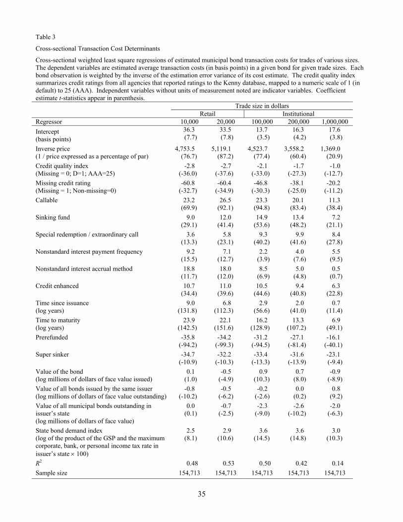
35

Table 3

Cross-sectional Transaction Cost Determinants

Cross-sectional weighted least square regressions of estimated municipal bond transaction costs for trades of various sizes. The dependent variables are estimated average transaction costs (in basis points) in a given bond for given trade sizes. Each bond observation is weighted by the inverse of the estimation error variance of its cost estimate. The credit quality index summarizes credit ratings from all agencies that reported ratings to the Kenny database, mapped to a numeric scale of 1 (in default) to 25 (AAA). Independent variables without units of measurement noted are indicator variables. Coefficient estimate t-statistics appear in parenthesis. Trade size in dollars Retail Institutional Regressor 10,000 20,000 100,000 200,000 1,000,000 Intercept (basis points)

36.3 (7.7)

33.5 (7.8)

13.7 (3.5)

16.3 (4.2)

17.6 (3.8)

Inverse price (1 / price expressed as a percentage of par)

4,753.5 (76.7)

5,119.1 (87.2)

4,523.7 (77.4)

3,558.2 (60.4)

1,369.0 (20.9)

Credit quality index (Missing = 0; D=1; AAA=25)

-2.8 (-36.0)

-2.7 (-37.6)

-2.1 (-33.0)

-1.7 (-27.3)

-1.0 (-12.7)

Missing credit rating (Missing = 1; Non-missing=0)

-60.8 (-32.7)

-60.4 (-34.9)

-46.8 (-30.3)

-38.1 (-25.0)

-20.2 (-11.2)

Callable 23.2 (69.9)

26.5 (92.1)

23.3 (94.8)

20.1 (83.4)

11.3 (38.4)

Sinking fund 9.0 (29.1)

12.0 (41.4)

14.9 (53.6)

13.4 (48.2)

7.2 (21.1)

Special redemption / extraordinary call 3.6 (13.3)

5.8 (23.1)

9.3 (40.2)

9.9 (41.6)

8.4 (27.8)

Nonstandard interest payment frequency 9.2 (15.5)

7.1 (12.7)

2.2 (3.9)

4.0 (7.6)

5.5 (9.5)

Nonstandard interest accrual method 18.8 (11.7)

18.0 (12.0)

8.5 (6.9)

5.0 (4.8)

0.5 (0.7)

Credit enhanced 10.7 (34.4)

11.0 (39.6)

10.5 (44.6)

9.4 (40.8)

6.3 (22.8)

Time since issuance (log years)

9.0 (131.8)

6.8 (112.3)

2.9 (56.6)

2.0 (41.0)

0.7 (11.4)

Time to maturity (log years)

23.9 (142.5)

22.1 (151.6)

16.2 (128.9)

13.3 (107.2)

6.9 (49.1)

Prerefunded -35.8 (-94.2)

-34.2 (-99.3)

-31.2 (-94.5)

-27.1 (-81.4)

-16.1 (-40.1)

Super sinker -34.7 (-10.9)

-32.2 (-10.3)

-33.4 (-13.3)

-31.6 (-13.9)

-23.1 (-9.4)

Value of the bond (log millions of dollars of face value issued)

0.1 (1.0)

-0.5 (-4.9)

0.9 (10.3)

0.7 (8.0)

-0.9 (-8.9)

Value of all bonds issued by the same issuer (log millions of dollars of face value outstanding)

-0.8 (-10.2)

-0.5 (-6.2)

-0.2 (-2.6)

0.0 (0.2)

0.8 (9.2)

Value of all municipal bonds outstanding in issuer’s state (log millions of dollars of face value)

0.0 (0.1)

-0.7 (-2.5)

-2.3 (-9.0)

-2.6 (-10.2)

-2.0 (-6.3)

State bond demand index (log of the product of the GSP and the maximum corporate, bank, or personal income tax rate in issuer’s state × 100)

2.5 (8.1)

2.9 (10.6)

3.6 (14.5)

3.6 (14.8)

3.0 (10.3)

R2 0.48 0.53 0.50 0.42 0.14 Sample size 154,713 154,713 154,713 154,713 154,713

36

Figure 1: Mean estimated transaction costs by trade size. This figure presents weighted cross-sectional mean estimated municipal bond transaction costs (in basis points) for the entire sample. The cost estimates plotted on the solid line are computed from estimated coefficients obtained from the time-series regression of equation (7) for each bond using equation (10). The estimated costs are effective half-spreads. The weights are given by the inverse of the cost estimate error variance that appears in (11). The points on either side of estimated cost function represent the weighted means of the 95 percent confidence intervals for the individual bond cost estimates. (Confidence intervals for the weighted mean estimates are indistinguishably different from the means for all but the largest trade sizes due to the large number of bonds in the sample.)

The dotted line plots the OLS best fit of 0 11c a aS

= + to the 11 cost estimates used to construct

this figure.

37

Figure 2: Mean estimated transaction costs for different cost function specifications. This figure presents cross-sectional weighted mean estimated municipal bond transaction costs (in basis points) for the entire bond sample for six different average cost function specifications. The different function forms are

a: ( ) 0 1 21 logt t

t

c S c c c SS

= + +

b: ( ) 20 1 2t t tc S c c S c S= + +

c: ( ) 2 30 1 2 3t t t tc S c c S c S c S= + + +

d: ( ) 0 1 21

t tt

c S c c c SS

= + +

e: ( ) 20 1 2 3

1t t t

t

c S c c c S c SS

= + + +

f: ( ) 0 1 2 31 logt t t

t

c S c c c S c SS

= + + +

The cost estimates for alternative a are computed from estimated coefficients obtained from the time-series regression of equation (7) for each bond using equation (10). The estimates for the other alternatives are obtained from analogous equations. The estimated costs are effective half-spreads. The weights are given by the inverse of the cost estimate error variance that appears in (11).

38

Panel A: Trading activity classes Panel B: Credit quality classes

Panel C: Issue size classes Panel D: Bond complexity classes

Panel E: Time since issuance Panel F: Time to maturity

Figure 3. Mean estimated transaction costs for various bond classifications. This figure presents weighted cross-sectional mean estimated municipal bond transaction costs (in basis points) computed separately for various bond classifications. The cost estimates are computed from estimated coefficients obtained from the time-series regression of equation (7) for each bond using equation (10). The estimated costs are effective half-spreads. The weights are given by the inverse of the cost estimate error variance that appears in (11). Bonds in the low, medium, high, and very high trade activity classes respectively have 10 or fewer transactions; 11 to 50 transactions, 51 to 1,000 transactions, and more than 1,000 transactions. Bonds in the superior, other investment, and speculative credit quality classes respectively include bonds rated AA and above, BBB to A, and below BBB. The small, medium and large issue size classes respectively include bonds smaller than one million dollars, between one and 10 million dollars, and above 10 million dollars. Bonds in the simple, typical and complex complexity classes respectively have zero, one to two, and three or more complexity features. Bonds in the young, middle, and old time since issuance categories respectively are bonds that were issued within the last six months, between six months and five years ago, and more than five years ago. Bonds in the near maturity, middle, and far from maturity categories respectively are bonds that with maturity dates within six months, between six months and five years, and more than five years.

39

Appendix A: The Residual Error Variance Shrinkage Estimator

This appendix presents the derivation of the Bayesian posterior distribution for the

residual error variance in a series of related regressions with given heteroskedastic error

structures using a data-based informative prior distribution. The variance 2iσ arises in the

following N equation regression model:

(B.1) ( )2~ N 0,i i i i

i i iσ

= +

Ω

y X β ε

ε

for 1i = to N. Each regression has in observations and k independent variables. The

distribution of the data is

(B.2) ( ) ( ) ( )1

2

1, , , exp2

i i i i i i ii i i i i n

i i

p σσ σ

− ′− − ∝ −

y X β Ω y X βy β X Ω .

We assume a diffuse prior for iβ

(B.3) ( ) 1ip ∝β

and an informative Inverted Gamma prior distribution for iσ :

(B.4) ( ) 2 221

1, isi

i

p s e ν σνσ ν

σ−

+∝ .

The parameters ν and 2s will be specified below. The second moment of this distribution is

(B.5) 2

22 E

2isνµ σ

ν′ = =

− for ν > 2

and the fourth moment is

(B.6) ( )( )

2 44

4 E2 4i

sνµ σν ν

′ = =− −

for ν > 4

so that the variance of 2iσ is

(B.7) ( )( ) ( )

2 42 2

4 2 224 2i

sVar νσ µ µν ν

′ ′= − =− −

.

The joint posterior distribution of iβ and iσ is

40

(B.8) ( ) ( ) ( ) ( ), , , , , , , , ,i i i i i i i i i i i ip s p p s pσ ν σ ν σ=β y X Ω β y β X Ω .

It is proportional to

(B.9) ( ) ( )2 1

1 2

1 exp2

i i i i i i ini i

sν

νσ σ

−

+ +

′+ − − −

y X β Ω y X β.

Re-expressing the quadratic form using the standard GLS estimates of iβ and 2iσ ,

(B.10) ( ) 11 1ˆi i i i i i i

−− −′ ′=β X Ω X X Ω y

and

(B.11) ( ) ( )1

2ˆ ˆ

ˆ i i i i i i ii

i

sn k

−′− −=

−

y X β Ω y X β ,

allows us to easily integrate out iβ to obtain the marginal posterior distribution for iσ :

(B.12)

( )

( ) ( ) ( )( )12 2

1 2 2

, , , , ,

ˆ ˆˆ1 1exp exp2 2i

i i i i i

i i i i i i ii in k ki i i i

p s

s n k sν

σ ν

νσ σ σ σ

−

+ − +

′ ′− − + − ∝ − −

β y X Ω

β β X Ω X β β

Integrating out iβ of this expression gives the marginal posterior distribution for iσ :

(B.13) ( )( ) ( )2 2

1 2

ˆ1ˆ, , , exp

2i

i ii

ii i i n k

i i

s n k sn k

n kp s s n ν

νν

νσ νσ σ+ − +

+ −+ − + − ∝ −

.

This distribution is an Inverted Gamma distribution with in kν+ − degrees of freedom and scale

parameter ( )2 2ˆi i

i

s n k sn k

νν

+ −+ −

so that the mean of the posterior distribution of 2iσ is

(B.14) ( )2 2

2

ˆ2

i i

i

s n k sn k

νµ

ν+ −

′ =+ − −

for 2in kν+ − > .

41

To specify the parameters s2 and ν that appear in the prior distribution for iσ , we equate

the degrees-of-freedom weighted cross-sectional mean and variance of 2is to their expected

values under the prior distribution. The weighted mean of 2is is

(B.15) ( )

( )

2

1

1

ˆN

i ii

N

ii

n k sM

n k

=

=

−=

−

∑

∑.

Its expected value is

(B.16) 2

E2

sM νν

=−

.

Equating the sample moment to the prior moment yields

(B.17) 2

2sM ν

ν=

−.

The weighted sample cross-sectional variance is

(B.18) ( ) ( )( )( )

222

ˆˆVar i i

ii

n k s MV s

n k− −

= =−

∑∑

.

Expanding ( ) ( )2 22 2 2 2 2 2ˆ ˆi i i i i is M s E E Mσ σ σ σ− = − + − + − gives

(B.19) ( ) ( ) ( )

( )( ) ( )( ) ( )( )

2 2 22 2 2 2 2

2 2 2 2 2 2 2 2 2 2

ˆ

ˆ ˆ2 2 2

i i i i i

i i i i i i i i i i

s E E M

s E s E M E E M

σ σ σ σ

σ σ σ σ σ σ σ σ

− + − + −

+ − − + − − + − −

The first square represents the error in the estimate of the ith residual error variance. We will

estimate its expectation using the sample variance of the ith residual error variance estimate,

which comes from its χ2 distribution. This variance is ( )4ˆ2 i is n k− . The second square

represents the distance between the ith residual error variance and the global variance estimate.

We will evaluate its expectation using the variance of the prior distribution for 2iσ , which is

given by (B.7). The third square is zero since our first identifying condition equated its two

terms by assumption. The first cross product term has zero expectation because the error in the

ith residual error variance estimate should be independent of the distance between the ith residual

error variance and the global variance estimate. The other two are zero given our first

identifying condition.

42

With these assumptions, the expectation of the weighted cross-sectional variance is

(B.20) ( )( ) ( ) ( )( ) ( )( )

4 2 42

2

ˆ2ˆE Var 2

4 2i i i

ii

n k s n k ssn k

νν ν

− −= +

− − −∑

∑.

Equating the sample and expected moments gives

(B.21) ( )( )

2 4

224 2

sV K νν ν

− =− −

where

(B.22) ( )

4i

i

sK

n k=

−∑

∑

The parameters s2 and ν must solve (B.17) and (B.21). Rearranging (B.17) gives

(B.23) ( )22 4 2 2s Mν ν= − .

Substituting this into (B.21) gives

(B.24) ( )

2

24

MV Kν

− =−

so that

(B.25) 2

42M

V Kν = +

−.

Rearranging (B.17) and substituting this expression into the result gives

(B.26) ( ) ( )( )

22

2

222 4

M V K MMs

V K Mνν

− +−= =

− +.