1

Second law versus variation principles

W.D. Bauer, email: W.D.BAUER@t-online.de

PACS codes: 5.70.Fh , 5.70.Jk, 61.255 Hq, 64.60 Fr, 64.60. -i, 64.75. +g,

keywords: polymer solution, phase transition, electric field, second law

Abstract:

The field-dependent equilibrium thermodynamics is derived with two methods: either by using the potential

formalism or by the statistical method. Therefore, Pontrjagin’s extremum principle of control theory is

applied to an extended ensemble average. This approach allows to derive the grand partition function of

thermodynamics as a result of a control problem with the Hamilton energy. Furthermore, the maximum

entropy principle follows and thereby the second law in a modified form. The derivation can predict second

law violations if cycles with irreversibilities in varying potential fields are included into consideration. This

conclusion is supported indirectly by experimental data from literature. As an example the upper maximum

gain efficiency of a cycle using the polymer solution polystyrene in cyclohexane as dielectrics is estimated to

less than 1 promille per cycle.

Note added in proof 28th October 2003: Comparing this preprint work with an analogous ferrofluidic system

discrepancies are is found which show that the concrete model proposed here in section 4 is insufficient to

settle the question. A way to solve the problem is proposed.

1. Introduction

The big success of the second law of thermodynamics relies on the fact that it predicts the

direction of the known irreversible processes correctly. The inherent problem with it is that it

is based on experience. Therefore, due to the axiomatic character of second law the question

arises incidentally, whether the second law is an overgeneralisation.

On the other hand unconsciously and without any notice, other basic concepts are used

2

H�H( S(33

r) ,33

r, ni(33

r) ) �U( S(33

r) ,33

r, ni(33

r) )

H( S(33

r) ,33

r, ni(33

r) ) �Mi PU

i( S(

33

r) ,33

r, ni(33

r) ) dni(33

r ) (1)

dH�( S(33

r) ,33

r, ni(33

r) ) 0H0S

�Mi P

0Ui

0Sdn

idS

� 1A

0H0 33r�

1AMi P

0Ui

033r dni

Ad33

r

� Mi

0H0n

i

� 0U0n

i

dni

(2)

sometimes in order to explain the direction of irreversibilities in thermodynamics. This can be

the case if a chemist speaks about that his reaction is "driven by enthalpy".

Landau and Lifshitz [1] obtain the direction of electro-thermodynamic irreversibilities by the

application of variational principles on potentials.

Because variational principles are included in the mathematics of a physical problem, the

question arises, whether the second law as additional physical principle becomes obsolete if

this purely mathematic aspect is included completely into consideration .

This article derives a field dependent equilibrium thermodynamic and checks the consistence

and equivalence of the second law against a purely mathematical approach using the

variational principles applied to potentials.

2. The derivation of the thermodynamic formalism including potential fields

The total Hamilton energy H* of a thermodynamic system including a potential field U is

where H is the Hamilton energy of the fluid without outer influence of the field. S is the

entropy , ni is the mole number of each particle, Ui is the partial potential energy of a species

i and is the space coordinate. Therefrom, the total differential follows33

r

3

T : 0H0S

�Mi P

0Ui

0Sdn

i

P� : 1A

0H0r

� 1AMi P

0Ui

0rdn

i

: P�Mi P

0Ui

0r!

i( r ) dr

µ�i

: 0H0n

i

� 0U0n

i

: µi�U

i

(3)

dH�T gdS g�T li dS li Pg�dV gP li �dV li �Mi

( µg�i

dn gi�µli �

idn li

i)

( T gT li ) dS ( Pg�P li �) dV�Mi

( µg�iµli �

i) dn

i0

(4)

T gT li

Pg�P li �µg�

iµli �

i

(5)

The derivatives of (2) can be identified as

The definitions are: T:=temperature, :=the global chemical potential of a substance (acc. toµ�i

the original definition of van der Waals and Kohnstam[2]), :=global pressure,P�

:=chemical potential of a substance, P:= empirical barometric or hydrostatic pressure ,µi

:=density of a species of particles and A:=unit area .!i: 0n

i/ A0r

The phase equilibrium in a potential field can be found if the variation of Hamilton energy H*

is minimized to zero in the equili brium. The second line of the last equation stems from the

constraints dS:=dSli = -dSg , dV:=Adr:=dVli = -dVg , dni:=dnili = -dni

g describing the

interchange or exchange of entropy, volume and particles between the different phases in

adjacent space cells. Therefore, the equilibrium conditions of the extended formalism are

Trivially, these equations hold as well in the same phase between adjacent space cells at rk and

rk+1 . Therefore, the equilibrium conditions above can be rewritten as well in the form

4

T( r 1) T( r 2)

r 1r 2

0T0 33r 0

P�( r 1) P�( r 2)

r 1r 2

0P�

0 33r 0

µ�i( r 1) µ�

i( r 2)

r 1r 2

0µ�i

0 33r 0

(6)

1ûR

jPûRj

0

H�( u) drj�extremum or P

ûRj

0

/H�( u) drj0 (7)

dd33

r0H�

0S 0 ;dd33

r0H�

0V 0 ;dd33

r0H�

0ni

0 (8)

The phase equili brium can be interpreted as well as the trivial case result of an optimization acc.

to Pontragin’s control theory where the total Hamilton energy is varied using aH�( u(33

r) )

control variable u which is identified as with . We have tou: ( S(33

r) ,33

V, ni(33

r) )33

V : A d33

r

solve

The problem can be interpreted as well as a trivial case of a Lagrange variational problem,

because H* does not depend explicitly from other variables than u and u itself is identified

with the "velocity coordinate" of the problem, compare analogous problems in more detail in

section 3. Under these very special conditions the Lagrange functional is either stationary

either it has an constant optimum value. Therefore, the solution of this problem are the Euler-

Lagrange equations

which are the conditions of equilibrium eq.(6) if one remembers the Maxwell relations eq.(3).

Some of the field extended equations in this section can be found in a different notation in[3].

5

PP( v , xi, T;

33

r) (9)

UPMi niM

ig( r ) dr (10)

H�H�U (11)

dH

d 3XP( 3X)

µi( 3X)

i 1, 2 . . . n1 (12)

Example:

The state of a real gaseous mixture is set near the critical point. The volume of mixture is

rotated at constant velocity in a centrifuge. Due to the centrifugal field, forces appear in the

solution which lead to space-dependent profiles of pressure, density and molar ratio. Here a

general method is presented how this problem can be solved numerically applying the

formalism above.

The equation of state of the fluid at a point is noted here generally by 33

r

where v( ) is the spec. volume , x i ( ) molar ratio and is the space parameter. 33

r33

r33

r

The mixture rule of the mean molecular weight in the centrifugal field is linear,g( r ) &2r

therefore the potential U is

The total Hamilton energy is

Therefore, the full thermodynamic state of the fluid in every space cell can be characterized

by

where and T is set constant during the calculation and is skipped therefore.3X ( v , xi)

The chemical potentials are

6

µiµ0

i ( p �, T) �RT ln ( fi / p �) (13)

ln QiZ

M1 ln Z

M� 1RT

�

v

P RTv

dv 1RT

�

v

Mn

k 1, k g i

dPdx

k T, v , x i gk

xkdv (14)

P�P( v ( rk) , x

i ( rk) ) P

r k

r ref

Mi!i

Mig( r ) dr

P( v ( rk�1) , x

i ( rk�1) ) P

r k�1

r ref

Mi!

iM

ig( r ) dr

(15)

µ�i µi ( v ( r

k) , xi ( r

k) ) � Pr k

r ref

Mig( r

k) dr

µi ( v ( rk�1) , x

i ( rk�1) ) � P

r k�1

r ref

Mig( r

k�1) dr

(16)

where are the standard potentials with p+ as the reference pressure. fi is the fugacityµ0i

calculated acc. to using a known formula of the fugacity coefficient Qi [4]fix

iPQ

i

ZM is defined as ZM =Pv /(RT).

For numerical calculation the space of the volume is divided in many infinitesimal small

adjacent compartments. If the complete local thermodynamic state (meaning spec. volume v,

composition xi , the empirical pressure P and potential U ) is known in one (reference)

compartment k of a vessel in a field it can be concluded on pressure and chemical potential in

the adjacent compartment k+1 due to the conditions of phase equilibrium. Due to the

equilibrium condition (6) the pressure relation between adjacent space cells at r k and r k+1 is

The second equation (15) is in effect the generalized law of hydrostatic or barometric

pressure. Analogously for the chemical potentials in adjacent space cells holds

7

Pµ

i k�1

P( 3Xk�1)

µi( 3X

k�1)i 1, 2 . . . n1 (17)

00x

i

1!

0P0r

Mig( r ) 0µ

i

0r 0

0xi

0G0r

00x

i

1!

0P0r

S0T0r

(18)

µi k�1

µi( 3X

k�1) i 1, 2 . . . n (19)

In order to obtain the full information of the state in the adjacent space cell k+1, the values of

of have to be calculated from the kth cell acc. to equation (15) and (16).( P, ui)

k�1

Then (17) has to be solved for . For the purposes of numerical calculation (in order to3Xk�1

avoid inaccuracies due to the integral in the calculation of P* ), however, it is recommended

to take an other equivalent representation of the thermodynamic state. Due to the phase

equilibrium conditions (eq.(6) ) and eq.(3) it holds

which proves 1) T =constant and 2) that the equation for P and the sum is linear*µix

i

dependent. Therefore, the equation for P in eq. (17) can be replaced by the equation for µn

and instead of eq. (17) the following system of equations has to be solved

If the equation of the thermodynamic state is solved for we have the full information3Xabout the fluid in the adjacent space compartment.

This iteration procedure is repeated over all space cells until the thermodynamic state of the

whole volume in the cylinder is determined completely.

Sometimes, under practical conditions no initial or reference values of the thermodynamic

state is known in any compartment. However, the total mass and the total molar ratios are

known. Then, additional equations describing the mass conservation of the different particles

8

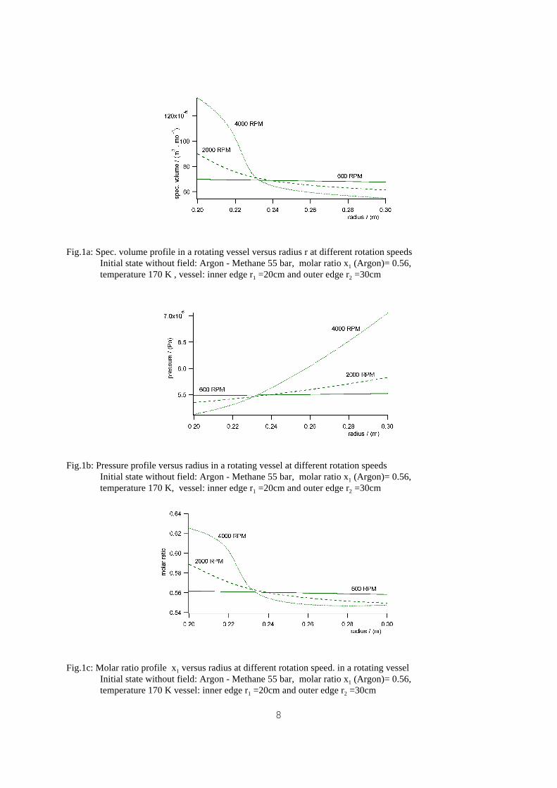
Fig.1a: Spec. volume profile in a rotating vessel versus radius r at different rotation speeds Initial state without field: Argon - Methane 55 bar, molar ratio x1 (Argon)= 0.56,temperature 170 K , vessel: inner edge r1 =20cm and outer edge r2 =30cm

Fig.1b: Pressure profile versus radius in a rotating vessel at different rotation speeds Initial state without field: Argon - Methane 55 bar, molar ratio x1 (Argon)= 0.56,temperature 170 K, vessel: inner edge r1 =20cm and outer edge r2 =30cm

Fig.1c: Molar ratio profile x1 versus radius at different rotation speed. in a rotating vesselInitial state without field: Argon - Methane 55 bar, molar ratio x1 (Argon)= 0.56,temperature 170 K vessel: inner edge r1 =20cm and outer edge r2 =30cm

9

I ( x ) Pt 0

t 1

L( x , �x ; t ) dt Extremum (20)

J ( x ) Pt 0

t 1

L( x , u; t ) dt Extremum (21)

Hpu L( x , u; t ) (22)

�pLx( x , u; t ) (23)

help to determine the full thermodynamic state which is shown in more detail in appendix 1.

As an example numerically calculated profiles of spec. volume v , molar ratio x i and pressure

P near the critical point are shown for the system Argon-Methane in fig. 1a)-c).

3. The statistical derivation of the thermodynamic formalism with fields

It is well known that the mechanic equations of motion can be found as solutions of a

Lagrange variational problem. The solution is obtained, if the functional L has an

extremum, where x(t0)=x0 and x(t1)=x1 are start and end point of the path.

The variational problem of mechanics can be regarded as well as a special case of a general

problem of control theory [5] where the control variable u(t) coincides with the velocity

variable . The functional of this special control theory problem is�x f ( u, x ; t ) u

with and . The Hamiltonian is defined to �x u, x ( t 0) x0, x ( t 1) x1

The adjunct system is defined to

10

HupL

u( x , u; t ) 0 (24)

ddt

L �x dLdx

0 (25)

Acc. to control theory the problem can be solved if the extremum of the Hamiltonian is found

If this equation is differentiated for t the solution is the Euler-Lagrange equation

because of and as defined above. �x u �pLx

The Hamiltonian has here a maximum for the chosen coordinates because Huu < 0.

In ref. [6] proofs of the different versions of Pontragin’s maximum principle can be found.

Similarly, as shown by Landau and Lifshitz [1], the Lagrangian of electrostatics can be varied

with respect to the electric coordinates E or D. If only one Maxwell relation is given the

other can be reconstructed by the variational formalism applied to any thermodynamic

potential. These results could be embedded in a more general mathematical framework [7]

which derives general relativity including all sub-theories using a Lagrange energy approach

developed to second order.

Therefore, because a thermodynamic system is a mechanic many particle system in a field,

similar variational features of the thermodynamic Hamiltonian should be expected.

In equilibrium, due to energy conservation, the Hamiltonian is constant. Then, the

mechanical time mean of the Hamiltonian is trivially identical to the Hamiltonian as well.

Acc. to the statistical approach the time mean of total energy of all particles is identical to

the ensemble average. Or in mathematic language (using the symbol ûT as measuring time

interval)

11

Htot

: 1ûT P

ûT

0

Mi

( 0i�U

i�M

j giU

ij) dt

PPW( 0K, ni ) 0

Kd0

Kdn

i

PPPW( 0, ni(33

r) ,33

r) 0 !( ni(33

r) ,33

r) dV(33

r ) d0dni(33

r)

(26)

0: Jkin�U

int( n

i(33

r) ,33

r) �U( ni(33

r) ,33

r) (27)

� : WH: W0! (28)

�� : �V0kT / µ� W� : W( kT) 2/ µ� V0 : kT / P� !�: !V0

0�: 0/ kT n �i: µ�n

i/ kT V � : V/ V0

(29)

is here the canonic probability distribution in the whole volume as defined inW( 0K, n

i)

Mayers book [8] p.6+7 with the eigenvalue of the total Hamilton energy JK .

In the third line is the probability function in a volume element dV( ) atW( 0, ni(33

r) ,33

r)33

r

the point and is a weighting function in which characterizes the total33

r !( n(33

r ) ,33

r )

particle number density profile. The mean Hamilton energy J at a point in the field is

where Jkin is the kinetic energy in the field, is the mean field potential between theUint

particles due to the real fluid behaviour and U is the energy due to the field from outside.

As shown above by control theory the mechanic Hamiltonian has an extremum. If this

feature is transferred from mechanics to thermodynamic notation as an ansatz analogously,

then at every space cell the Hamilton energy density function

should be a extremum as well.

For the following calculation all symbols are made dimensionless by defining

Now, the calculation from (20) -> (25) can be done analogously in thermodynamics as well

12

H: Mi

p 2i

2mi

�Mj gi

�( xix

j ) � ��: !�J�W� : E�W�

xi

� E� : !�J�

t �33

t : J�, n �i , V �

�xif ( x

i, u

i) u

i� 33

u : 0E�

0J� ,0E�

0n �i

,0E�

0V �

Lpiu

iH � 3L �

33

t: p 33

t.33

u��.33

1

(30)

Htotal

�PW�!�0� d0�

PW�!�0� dV �

PW�!�0� dn �i

� maximum (31)

0p0J� W�

0p0V � W�

0p0n �

i

W�

(32)

L �( J�) W� 0E�

0J� W�E�

L �( V �) W� 0E�

0V � W�E�

L �( ni�) W� 0E�

0n �i

W�E�

(33)

if the mechanical variables are exchanged by thermodynamical terms acc. to the following

table eq. (30) below (using the definition ):33

1 : ( 1, 1, . . . , 1)

The reduced Hamiltonian is optimized for every variable of separately��33

t

The adjunct variables are defined by the equationsp 33

t

The Lagrangians of this problem follow from the last line of eq.(30)3L

13

00J�

00E�

J� 0

0E� ( L �J�) 0W�

0J� �W� 0

00V �

00E�

V � 0

0E� ( L �V �) 0W�

0V � �W� 0

00n �

i

00E�

n�i

00E� ( L �

n �i) 0W�

0n �i

�W�0

(34)

W�W0�exp [ ( 0��V ��M n �

i) ] (35)

W�( ni, 0) W�

0exp [ ( 0P�V�M µ�in

i) / kT ] (36)

PPW�( n �, 0�) dn �d0�PPW( n, 0) dn d01 (37)

niPPn

iW( n

i, 0) dn

id0 (38)

Therefrom, three separate differential equation are obtained

The combined solution of these differential equations (34) is the distribution function

If the definitions of the reduced variables (29) are reinserted one obtains

This is Mayer’s master equation [8] which is extended here for systems containing space-

dependent potential fields. The norm is chosen to be

Therefrom, using (29), the standard representation of thermodynamics can be derived acc. to

the procedure presented in Mayer’s book [8] p.8. The mean number of particles in a volume

is then

The mean (always indicated by a bar) of Gibbs’s free energy is G

14

GPPM W( ni, 0) n

iµ�

idn

id0 (39)

0W

0µ�i

( kT) 1[ niV( 0P�/ 0µ�

i) ] W

T0W0T

( kT) 1[ P�VM niµ�

i�0VT( 0P�/ 0T) ] W

(40)

0P�

0µi

ni/ V

0P�

0T( VT) 1[ H�� P�VG�

] SV

(41)

SkPW� ln ( W�) dn �id0� (42)

From the master equation (36) and (29) is derived by differentiation

Both equations are summed up over all possibilities which give in sum 1 acc. to eq. (37).W

Therefore, each sum of all derivatives is zero and the relations between the corresponding

mean values (indicated by a bar) are

From the second equation (41) follows Shannon’s definition of entropy

It should be noted that the entropy of the field extended formalism of thermodynamics has

the same expression as without field. Therefrom, it can be concluded that the entropy of the

field extended thermodynamic formalism follows the maximum entropy principle as well,

because the proofs in textbooks like [9] can be applied accordingly.

15

H ( S, V, ni, P) H( S, V, n

i) �PPE dPdV

H( S, V, ni) � 1

2 PP2

00( 01)dV

H ´ ( S, V, ni, E) H( S, V, n

i) PPP dEdV

H( S, V, ni) 1

2 P00( 01) E2 dV

(43)

4. Second law violations due to potentials with saddle points

The minimum principle of potentials is derived in many textbooks of thermodynamics from

the second law [4]. In this section this procedure is reversed and the second law is derived

from the extremum behaviour of the Hamilton energy. As shown in [1] the second derivative

of the Hamilton energy can be obtained from the second derivative of the mathematical

variational or control problem and gives information about the direction of the

irreversibilities in a potential field. This information comes from mathematics alone and is

independent from any additional empirical or axiomatic input information like second law.

Therefore, the question has to be discussed whether the mathematical and the axiomatic

approach of equilibrium thermodynamics are equivalent.

Both approaches make the same prediction for thermodynamic standard cases where H is

convex and irreversibilities obey always dH<0. However, if saddle points exist, H can obey

dH>0 in certain directions of the state space. Then, it will be shown in the following that

Clausius’s version of second law can be "reversed".

The energies H' and H" of capacitively loaded thermodynamic systems are defined [1] by

where the definitions are := dielectric constant, E:= electric field and P:= electric00( 01)

polarisation. The same formulas can be written in differentials

16

dH´ ( S, V, ni, P) dH( S, V, n

i) �P( EdP) dV

dH´ ´ ( S, V, ni, E) dH( S, V, n

i) P( PdE) dV

(44)

ûHirrev

( P) <0 for S, V, niconstant

ûH ´irrev

( E) >0 for S, V, niconstant (45)

dG ( P, T, ni, P) dG( P, T, n

i) �P( EdP) dV

dG ´ ( P, T, ni, E) dG( P, T, n

i) P( PdE) dV

(46)

ûGirrev

( P) <0 for T, P, niconstant

ûG ´irrev

( E) >0 for T, P, niconstant (47)

Regarding the 2nd derivative of H’ and H’‘ with respect to the electric variables P or E,

comp. eq.(43), both of these potentials approach an thermodynamic extremum for irreversible

processes into thermodynamic equilibrium. For constant homogeneous dielectrics the

potential H'(S,V,n i , P) has a minimum, and H''(S,V,n i , E) has a maximum, if

> 0, dni=0 , dS=0 and dV=0. Therefore, acc.to [1], the following unequalities00( 01)

hold for irreversible changes of state

Due to the Legendre transformation formalism analogous expressions of eq.(43) and (44)

hold for free enthalpy, i.e.

and

In words, the equations (45) and (47) can be interpreted as a "electric Chatelier-Braun-

principle", which states for simple dielectrics that they tend to discharge themselves. Because

(47) will lead to second law violations it should be emphasized that the correctness of both

17

ûG ´ û312G ´rev�û23G ´

irrev0 (48)

û312G ´rev

,( ,23�1

P dE�,32P dE) dV,( lP dE) dV,( lE dP) dV<0 (49)

lH´´ ,( lPdE) dV�lTdS0 (50)

equations (47) is based either theoretically on the variation principle either experimentally on

material data as shown fig.2a and in section 4.

Now, an electric cycle is regarded which has an irreversible path into a maximum of G´´

at constant field E, comp. fig.2b and fig.3:

Because G'' is a potential for any closed cycle over three points(1->2->3->1) one obtains

According to the extremum principle(eq.(47)) �23G''irrev > 0 holds. Due to (48) follows

�312G''rev < 0 . Because of the isofield (E2=E3) irreversible change of state (2->3) it holds

also . This zero expression is added to the second formula of (46) which yields ,E2

E3PdE0

The sign of the right integral shows indicates a "gain" cycle which is reversed compared to

the hysteresis of a ferroelectric substance. Because the cycle proceeds isothermically (with

only one heat reservoir) the Clausius statement of second law is violated.

The proof is as follows: Due to energy conservation and because H" is a potential

holds. Therefrom, because the electric term is negative, comp. eq.(49), it follows that the net

heat exchange l T dS has a positive sign. This implies l dS>0 because T=constant . This

means that the cycle takes heat from the environment and gives off electrical work under

18

lSûS rev3�1�2�ûS irrev

2�3 >0 (51)

ûS rev3�1�2<0 (52)

ûS irrev2�3 >ûS rev

3�1�2 >0 (53)

isothermal conditions which is contrary to the Clausius formulation of the 2nd law. aIt should be noted that this proof is not in contradiction to the principle of maximum entropy.

Acc. to the calculation holds

Due to the maximum entropy principle it can be said that the entropy is higher at state 3 than

in the state 2. Therefore, it holds

meaning that heat is given off on the path 3->1->2 to the system environment which can be

calculated here from the thermodynamic potential because the entropy is a clearly defined

function of state on the reversible path. For the irreversible path, however, the entropy

difference must be calculated by applying energy conservation (50). Therefore, theûS irrev2�3

following inequalities hold due to (51) and (52)

This example illustrates that different formulations of second law may be not equivalent,

comp.[10].

19

(a8

3a4

�

�

�

�������!

Fig.2a: Dielectric constant � vs.volume fraction Q of the mixture nitrobenzene- 2,2,4-nitropenthaneat 29.5 C from [11]. The curve follows the series .02. 1�15. 1Q�36. 5Q219. 4Q3

Because of mixture processes in strong electric homogeneous field can obey 020/ 0Q2>0 for T, P, E, ni = constant. and J linear with resp. to E, ûG��( E) 00 û0( Q) E2V/ 2 > 0

Note that this is a material property which can violate Clausius’s version ofsecond law! comp.text and as well fig.2b) , fig. 3 and fig.4d).

Fig.2b: Qualitative diagram of polarisation P vs. electric field E or charge Q vs. voltage UIsotherm electric cycle of a material with .020/ 0Q2>01->2 charging the capacitance with voltage; 2->3 mixing both components by openinga tap, comp. fig 3. 3->1 discharging the capacitance Acc. to the diagram the orientation of the working area shows a gain hysteresis. The energyoutput can be enhanced by increasing E or U. Therefore, for very strong fields thisoutput can be higher than the constant energy �E input necessary to separate the components at zero field by centrifugation or chemical separation. comp. fig.2a) and 3

20

8 FRQVW�

8 FRQVW�PHFKDQLFDO�RU�FKHPLFDO�VHSDUDWLRQ

�( HOHFWULF�F\FOLQJ�������ZLWKJDLQ�K\VWHUHVLV

��(�LI�8�

������

�

� �

�

5. About the concrete realization of second law violating cycles

The following example shows principally the possible existence of a second law violating

cycle, comp. fig.3:

Step 1: The cycle starts -for example- with a 50:50 mixture of two liquid or gaseous

substances. It is assumed that the dielectric constant of the mixture has a mixture rule with

(Q:=volume fraction of one component). The mixture will be separated (for020/ 0Q2>0

instance by centrifugation) into two halves of 40% and 60% of concentration . Therefore, a

chemical or mechanical input energy is necessary for the separation. ûE

Step 2: Then, both halves of different concentration are used as dielectrics and are loaded

parallel with the same strong electric field E.

Fig.3: Principle of a second law violating cycle with a nonlinear dielectrics, comp. fig.2a .1) starting point, mixture 50:50 -> 2) after separation procedure 40:60 after energy input �E for instance by centrifugation -> 3) after applying astrong electric field -> 4) after the mixing process in the field -> 1) afterdischarging the capacitance. The work area of the capacitance, comp. fig 2b), can principally overcome the energy of the separation if the field is high enough.

21

1200( 01) E2v RT (54)

Step 3: After the charging process both halves are remixed in the field. Due to this

procedure the total dielectric constant decreases due to the material property .020/ 0Q2>0

Therefore, a current flows from the capacitance at constant voltage.

Step 4: Then, the whole capacitance is discharged and the cycle starts again after the

necessary relaxation time.

As shown in fig. 2b the electric work diagram of the capacitance shows a "gain" hysteresis.

In principle, in this simple model, the work gain area can be driven to infinity if the electric

field is driven to infinity. Therefore, the work gain of the electric cycle can be higher than

the defined energy input for separation. Due to energy conservation the differing amountûE

of energy between input and output has to come from the heat of environment. aOf course the realisation of this cycle is not so easy as the first idea but there exist some

experimental data which allow to get a first feeling of about what seems to be possible.

In 1965 Debye and Kleboth [11] investigated the influence of electric fields on phase

equilibria of liquids. They observed the following facts :

1) The influence of homogeneous fields on phase equilibria is weak due to the big difference

between the electric field energies applied compared with the chemical energies involved in

the mixture process. Comparing electric field energies with thermal energies

one obtains E = 6,13 . 108 V/m if values for water at room temperature are inserted in (54) .

This is higher than the breakdown voltage of stronger bulk plastic isolator materials like

Polyoxymethylen or Polyethylenenterphthalat [12] which can resist to more than 4,5. 107

V/m. Therefore, in order to avoid this principal problem it is recommended to look for

effects in the neighbourhood of a critical point.

22

2) Debye and Kleboth found mixtures whose phase diagram was influenced by strong

homogeneous fields. In order to obtain a field-induced decrease of the critical temperature in

a phase diagram of a solution, a nonlinear mixture rule of the dielectric constant with

was necessary, comp.fig.2a).020/ 0Q2>0

Debye and Kleboth investigated the turbidity of a solution nitrobenzene - 2,2,4-

trimethylpentane at critical concentration and temperatures slightly above the critical

temperature. If a strong field was applied to the solution the turbidity decreased confirming

that the critical temperature of the phase diagram of the mixture was shifted by the field to

lower values which was predicted by their theoretical considerations as well.

Similar investigation in homogeneous fields (but below the critical point) were done with

polymer solutions by Wirtz and Fuller [13] [14]. They investigated electrically induced sol-

gel phase transitions. To explain their experiments they used a Flory-Huggins model [13]

extended by an electric interaction term. They find that this model describes the qualitative

behaviour of their solutions correctly.

It can be shown for these solutions that an second law violating isothermal cycle is possible,

which is the electric analog of a Serogodsky or a van Platen cycle of binary mixtures

discussed recently in [15]. Compared with the example above, comp. fig.2a)-b) and fig.3 ,

the separation of the components is achieved here by the electrically induced phase transition

due to the nonlinearities of the dielectrics. No other thermodynamic, chemical or mechanic

processes are necessary to obtain the separation of the components of the mixture.

23

Fig 4a: Isothermic isobaric electric cycle of a diluted polymer solution as dielectric1) voltage U=0: system in 2-phase region 2) both volumes separated, rise of voltage from zero to U=const.: each volume compartment in 1-phase region 3 ) voltage U=const.: opening the tap and returning to the phase separation line by remixing

Fig.4b: Isothermal electric cycle in capacitor due to electrically induced phase transitions; charge Q vs. voltage U plotted; 1 starting at 2- phase region line with zero field, 1-2 applying a field

with tap closed, 2 opening the tap, 2-3 discharging and remixing in field,3 returning to starting point 1 by discharging the capacitor; a gain work area is predicted due to dG"(E)>0 during the irreversible mixing process.

24

Fig.4c: vs. volume fraction Q (with T :=temperature)[ 12�( T) ] N0. 5

phase diagram of a polymer solution with and without electric field E according to [13,14]; plot shows a modified Flory-parameter versus volume fraction Q

of polymers; points 1: E=0, 2-phases, both points 1 at the phase separation line; points 2: E=const., both points 2 of the splitted volume in 1- phase region; point 3: E=const., after opening the tap: point 3 is onthe phase separation line

Fig.4d: Dielectric constant � vs. volume fraction Q of polymers in a dilute solution;points 1, 2 and 3 refer to points in fig.4a)-c). According to the theory [13,14]d2�/dQ2>0 holds near the critical point. Therefore �(Q) has to turn to the left andthe dielectric constant has to decline during remixing 2->3. Observations at the similarsystem[11] support this prediction, comp . Fig.2a)

25

û23G ´irrev

û312G ´rev

G ´ 3G ´ 2 >0 (55)

The system is the experimental realization of the model system in the proof in section 4.

This closed splitted cycle is proceeded with a capacitor using as dielectrics a sol-gel mixture

like polystyrene in cyclohexane (upper critical point solution) or p-chlorostyrene in

ethylcarbitol (lower critical point solution). The composition of the solution is separated

periodically by a demixing phase transitions induced by switching off the field. After the

separation of both phases by splitting into two volumes they are remixed again (irreversible

path during the cycle !) after opening the separating tap in a strong field.

The cycle is started in the 2- phase region at zero field at the points 1, comp.fig. 4a)-c), where

the volume is split by closing the tap separating both phases. Then a strong homogeneous

electric field E is applied. At the point 2 the solution is separated in two phases each in a

different compartment. This is represented by the points 2' and 2'' in the fig. 4. Then, the tap

is opened and the solutions of both compartments are mixed. During the mixing (2->3) the

electric field is kept constant by discharging the capacitor during the decline of the dielectric

constant, cf. fig.4d). Then, in the phase diagram fig.4c) and as well in fig. 4a) +b), the mixed

solution is at the phase separation line at point 3. In the last step of the cycle the capacitor is

discharged completely and the system goes back into the 2-phase region to point 1 and

demixes. According to the theory, eq.(47),

Now, S*:=V´/V is defined as the splitting factor of the total volume V. V’ and V’‘ are the

volumes of the compartments each where V:=V´+V" . The difference of the free enthalpy is

written using the definition or G´ in (46) assuming to be dependent from Q and00( 01)

independent from E

26

û312G ´rev 1

2E2

200[ 0( Q( 1´ Ú2´ ) ) . S� �0( Q( 1´´ Ú2´´ ) ) . ( 1S�) ] V

�E3

0

V00[ 0( Q( 1´ Ú3´ ) ) . S��0( Q( 1´´ Ú3´´ ) ) . ( 1S�) ] Ed E(56)

f �( P) 1v

m

( Q/ N) ln Q� 12

( 12�( T) ) Q2� 16Q3 � ( �P2/ 2)

00( 0( Q) 1)

f ��( E) 1v

m

( Q/ N) ln Q� 12

( 12�( T) ) Q2� 16Q3 ( �E2/ 2) 00( 0( Q) 1)

(57)

The right side of the first line represents the stored linear combined field energy 1->2 of the

separated volume parts (points 2' and 2") at point 2, the second line stands for the field

energy difference (1->3) of both the connected compartments containing the coexisting

phases Q’ and Q". In the first line S*, J, Q’ and Q" are constant, in the second line S*, J, Q’ and

Q" are dependent from E in the 2-phase region.

Wirtz et al. [13,14] apply a Flory free-energy density approach of an incompressible dilute

monodisperse polymer solution to describe their systems. The "ansatz" is here

where N:= polymerisation number, J0:= dielectric constant of vacuum, J := dielectric

constant of the material, � := 1/(kT) with k :=Boltzmann number, vm :=monomer volume and

�(T) :=Flory parameter which depends on the temperature T and the material .

Due to the electrical fieldWelPUI dt PUdQPPEdPdV1/ 2. PP2/ ( J0( J1) ) dV

term of the first formula (57) is proportional to the electrical work Wel applied to the

system. In the second formula (57) the electrical field term is proportional to the negative

field energy which is the potential perceived by the dipolar matter. This equation is

equivalent to the Hamilton energy eq.(1). The chemical potential per volume µ* (E) follows

from (57)

27

µ�( E) : 0f ��

0Q ��� Eµ�( P) : 0f �

0Q ��� P 1

vm

1N� 1

Nln Q� ( 12�) Q� Q2

2 �00E2

2000Q

(58)

µ�( E) : 0f �( E) / 0Q 1v

m

1N� 1

Nln Q� ( 12�) Q� Q2

2� �00E2

2000Q (59)

02f �( E) / 0Q20µ�( E) / 0Q>0 (60)

02f �( E) / 0Q2 0µ�( E) / 0Q 003f �( E) / 0Q3 02µ�( E) / 0Q20

(61)

µ�0µ�( E) ( Q´ ) µ�( E) ( Q´ ´ )

PQ´ ´

Q´

[ µ�0µ�( E) ( Q) ] dQ P

Q´ ´

Q´

0µ�

0Q ��� EQdQ0(62)

However, both these formulas are not appropriate to calculate stability condition and phase

diagram because a derivation with (58) , comp. eq. (60) and (61), yield wrong results if one

compares it with the experiment and the calculation of [11] and [13].

Therefore, [11] and [13] choose another dependence of the chemical potential on the electric

field. With the abbreviation and thef 0 : ( ( Q/ N) ln Q� ( 12�) Q2/ 2�Q3/ 6) / vm

definitions the relevant chemical potential per volume isf �( E) : f 0�1/ 2. 00( 01) E2

The stability condition in a constant field is accordingly

A critical point is defined by the equations

Both definitions are supported by calculation and experiments of [11] and [13].

Consequently, the phase equilibrium is determined by the equations [13]

28

0Q0p� ( 1Q) 0s

�kQ( 1Q) (63)

The first equation describes the chemical potential to be equal in both phases. The second

equation is the Maxwell construction applied to the chemical potentia l µ+. The solution of

this system of equations can be done numerically. Qualitative results are in fig.4c) .

(It should be noted, that the ansatz (57) and (59) above differs from the references [11] and

[13] : First, both authors use an excess energy term of the field energy in (59) which neglects

per definition the terms linear in Q in the mixture rule of the dielectric constant. These terms

have to be included in the calculation of the profiles as shown in section 2, eq.(10).

Second, the authors in [11] and [13] include the contribution of vacuum polarization while

the calculation here relies on the definitions (43), (44) and (46).

Third, equation (59) is taken originally from [13]. The dimensions of this equation are

corrected with respect to the constant factor vm . The value vm is taken from from [16] p.797

It should be said that all these changes by the author here do not lead to any changing

consequences in the results and conclusions of both references [11] and [13].)

In fig.5 a polymer solution is placed in a cylindrical capacitor as dielectrics. If the

capacitance is charged a inhomogeneous electric field arises in the capacitance which

entrains a radial profile of the polymer volume fraction Q and also a radial profile of the

dielectric constant J. Because no function is known for the dielectric constant vs. Q the most simple non-linear

mixture rule is taken to be (k= factor, definition of indices p:=polymer , s:=solvent)

The density profile can be calculated by application of the equilibrium condition (6)

to the chemical potential (58). This yields the differential equation of the profile0µ�P/ 0r 0

29

0Q0r

C200�( 0p0

s�k ( 12Q( r ) ) )

12��Q( r ) / N�Q( r )v

m

� C2�k00

r 2r 3

(64)

1CP

r 2

r 1

dr2�J0J( r ) r h

(65)

with C defined as .C: Q/ ( 2�00h)

Equation (64) is solved by the program in appendix 2 for a state above the critical point. The

calculated profile is shown in fig.5 . Applying the formula of the cylindric capacitance C

the capacitance can be evaluated with the data in fig.5 using a tabel calculation program.

It is a interesting question whether the tap in the fig.4a can be avoided if the following cycle

is proceeded without tap using rectangular electric voltage pulses,comp.fig.6: The cycle of

the system starts if the field is switched off. The solution may be equally distributed for the 1-

phase system, or may be in the demixed state for the 2-phase system.

Fig.5: Volume fraction Q vs. radius r in a capacitance with cylindric geometry using as dielectrics aovercritical polymer solution polystyrene in cyclohexane .data of calculation: inner diameter 0.1mm, outer diameter 0.2 mm, height 50 cm, vm = 1.53*10-28, N = 1/(0.04)2, � = 0.539, �solvent = 5,�polymer = 35, k =-30, � = 1/(1.38*10-23 *300), charge Q = 2.5x 10-8, initial value Q( r1 =.1mm) = 5 %

30

Then, the capacitor is switched on so fast that the diffusion in the solution cannot foll ow.

Therefore, the capacitance is charged at the capacitance C(U=0). Then, if the voltage is high

and the voltage remains constant, the solution has time to diffuse and builds up the equili brium

profile at high field. So the capacitance decreases to the equili brium value C(U), comp. Fig 4d.

During this phase a current flows from the capacitance at constant high field. Then, the

capacitance C(U) is discharged again faster than diffusion and the cycle can start again after the

relaxation time necessary for the solution to reach the equili brium again. Therefore, the cycle

here could show an electrically induced "gain hysteresis" due to the relaxation of the dielectric

material. It is interesting to ask for the quantitative relevance of this cycle:

A loss was found in the numerical tests performed with the cylindric capacitance shown in fig.5

. However, the parallel geometry with homogeneous field + gravitation, see fig.4a (but without

Fig.6: Charge Q vs. voltage U of a gain cycle of a capacitance using a 2-phase polymer solution as dielectricsin a homogeneous electric field driven by rectangular voltage pulses, comp. textBold line: equilibrium capacity; weak lines: dynamic non-equilibrium capacities due to retardation

by diffusion. The work area is overdrawn, because the predicted gain effects are less than 1 O.1->2 fast charging, 2-3 relaxation of solution with decrease of J at constant voltage3->1 fast discharge of capacitance, the after a relaxation time the cycle can start again.

31

f �� 1v

m

( Q/ N) ln Q� 12

( 12�( T) ) Q2� 16Q3

�2

E200( 0( Q) 1) � gx�v

mL

( MpQ�M

s( 1Q) )(66)

0Q0h

gN( MpM

s) �Q( h)

L( 1�NQ( h) J0E2�NkvmQ( h) 2N�Q( h) �NQ( h) 2)

(67)

tap) shows the effect principally, even if the effect is negligible quantitatively, as shown in fig.7.

The result is obtained by the following consideration:

Because the gravitational field separates the different phases gravity is included in the ansatz.

Then, the free energy is (Mp/s:= molar mass of polymer or solvent, L:= Avogadro number)

The application of the equili brium conditions eq. (6) ( ) leads to theµ0f ��/ 0Qconst .

differential equation of the concentration profile of Q(h) vs. height h in the gravitational field

This problem is solved for E=5*107 V.cm-1 and for a volume of 10 cm height. The profile of

the volume fraction Q of the polymers between top and down is linear with height and shows ~

2O deviation per 10 cm at the chosen total concentration of Q=Qc =4% above the criti cal

point(�=.51<�c). This means that the influence of gravitation can be neglected against the

influence of strong electrical fields for a 1- phase system.

In a 2-phase solution the higher concentrated gel phase is the sediment, because the monomer

(Mstyrene = 104.144 g.mol-1) weights more than the solute (Ms = Mcyclohexane =84.162 g.mol-1) while

the specific volume of both components are nearly the same(v cyclohexane= 9.256x10-5 m3.kmol-1

[17], vstyrene =vmL= 9.2139x10-5 m3.kmol-1 and vm=1.53x10-28 m3 ).

The estimation of the gain of a complete electrical cycle is done under the following conditions:

If the solution is under the field E it is set always exactly at the criti cal point and mixes. If then

32

fromd 2µ�

dQ20: Q

CN1/ 2

fromdµ�

dQ 0: �C( E) �C( E0) 1

200�E2v

mk

(68)

Q�� t Q�

NQ� 6( t �1) ln ( t ) 12( t 1)

( t 1) 3

( 1/ 2�) N 2ln ( t ) ( t 2�t �1) 3( t 21)

[ 6( t �1) ln ( t ) 12( t 1) ] ( t 1) 3

(69)

J�0pQ��( 1Q�) J

s�kQ�( 1Q�)

J��0pQ���( 1Q��) J

s�kQ��( 1Q��) (70)

QCQ�S��( 1S�) Q�� (71)

the field is switched off the same solution changes to the demixed state in the two-phase area.

Applying the conditions of a critical point on (61) it follows with (59) and (63)

using the abbreviation .�C( E0) 0. 5�N1/ 2

The second equation allows to calculate a corresponding for the demixed and�( T) �C( E)

field free state of every corresponding field E applied at the critical point.

Now, by applying a known parameter representation of the phase separation line the volume

fractions of the sol Q’ and the gel phase Q" are calculated by a graphical method using the

source code in appendix 3. The equations of the parameter representation without field are [16]

The solutions Q’ and Q" from (69) determine the dielectric constants of the 2-phase system.

The splitting factor S* can be calculated by solving the relation

33

JJ�S��( 1S�) 0�� (72)

0c0

pQ

c� ( 1Q

c) 0

s�kQ

c( 1Q

c) (73)

�: ûEE� 0c

00

c1

(74)

for S*. This allows to calculate the combined effective dielectric constant of the 2-phase system.

This is compared against the mixed dielectric constant Jc at the critical point which is

Therefrom, the gain efficiency � of the electric cycle can be estimated acc. to

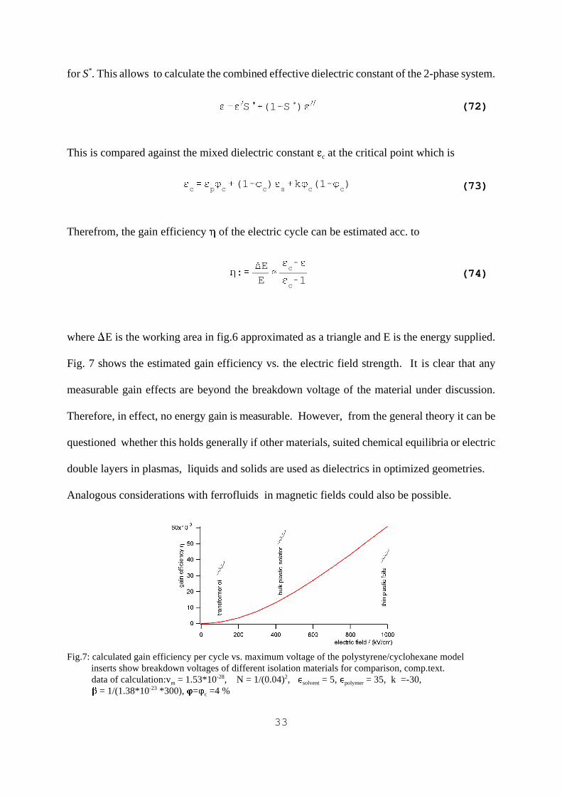
where �E is the working area in fig.6 approximated as a triangle and E is the energy supplied.

Fig. 7 shows the estimated gain eff iciency vs. the electric field strength. It is clear that any

measurable gain effects are beyond the breakdown voltage of the material under discussion.

Therefore, in effect, no energy gain is measurable. However, from the general theory it can be

questioned whether this holds generally if other materials, suited chemical equili bria or electric

double layers in plasmas, liquids and solids are used as dielectrics in optimized geometries.

Analogous considerations with ferrofluids in magnetic fields could also be possible.

Fig.7: calculated gain efficiency per cycle vs. maximum voltage of the polystyrene/cyclohexane model inserts show breakdown voltages of different isolation materials for comparison, comp.text. data of calculation:vm = 1.53*10-28, N = 1/(0.04)2, �solvent = 5, �polymer = 35, k =-30, � = 1/(1.38*10-23 *300), Q=Qc =4 %

34

Tab.1: analogous features between thermodynamics and mechanics

mechanics thermodynamics

time mean or least action functional ensemble average

Hamilton energy Hamilton energy

non-extremal state of functional non-equilibrium state

Legendre transformations, i.e. L, H Legendre transformations, i.e. U, H, F, G

Pontrjagin’s extremum principle extremum principle of potentials

second variation of the Hamiltonian "second law"

5.Conclusion

The analogies between mechanics and thermodynamics- shown in tab.1- suggest that the

direction of irreversibiliti es can be understood from a variation principle applied to the

Hamilton energy analogously to the extremum principle of Pontrjagin applied to mechanics.

Therefrom, it can be derived the grand partition distribution, the maximum entropy principle

and the second law in a modified form which can violate Clausius’s integral version if cycles

with changing potential fields are included into consideration. It was shown that this is not in

contradiction to the maximum entropy principle which also follows from the initial ansatz.

Acc. to a conventional view the described contradictions to second law would be due to a

forbidden "strange" material behaviour [18] due to a wrong or insufficient theoretical model.

Acc. to the purely mathematical approach of thermodynamics- presented here- strange material

behaviour is excluded a priori. All empirical information about a system is in the

thermodynamic potential describing the material behaviour. Therefrom, the application of all

possible variation principles allows to determine the directions of the irreversible processes.

Some experimental data speak in favour for the purely mathematical approach.

Therefore, all systems which show this theoretical contradiction between second law and the

second variation of Hamilton energy could be interesting for further research.

35

Note added in proof from 28th October 2003:

In the meantime experimental data of a analogous system with ferrofluids in magnetic fields

[18][19] are published which at first sight seem to sight contradict to the results of the

calculation in this article, because they show an instabilit y of the solution with a increasing

magnetic field. The corresponding calculations of these system [18] may be the current state of

the art today and seems to explain the data approximately even quantitatively, however, beside

the known problem of polydispersity, some deficiencies in the calculation make it diff icult to

determine exactly whether there is a loss or a gain in a cycle with ferrofluids. The following

critical points have been found:

1) The boundary condition at the phase boundary of a 2-phase ferrofluid system is not

accounted for. At the boundary holds B1 = B2 for phase 1 and 2 due to /.B = 0. Because

µ1

gg

µ2 holds follows H1

gg

H2. . The authors in [18] assume H1 = H2 . This can influence or

even reverse the result of the whole calculation.

2) A constant homogeneous field in the solution can be assumed in the solution only for special

bowl geometries [20]. They are not realized in the setup of [18]. The author do not discuss

either the influence either any space dependence of the field energy in the solution and therefore

overlook or neglect any gradients in concentration and pressure in the solution.

3) The authors in [14] calculate the phase equili brium assuming same osmotic pressure

equilibrium in both phases. This is surely qualitatively wrong because their calculation neglects

any force due to the field pressure terms which arise at the phase boundary due to the spatial

changing magnetic field energy. The use of a Maxwell construction [16] would avoid this

mistake.

The differences of the ferrofluid system with the system in this preprint point out to the fact that

the cited model of section 4 shown here and as well the models of [18,19] are insuff icient (In

36

°-B( x

i( r ) , r ) 0

0µ�i

0r ( xi( r ) , B( r ) ) 0

(75)

°-D( x

i( r ) , r ) 4�!

E

0µ�i

0r ( xi( r ) , E( r ) ) 0

(76)

section 4 they may be thermodynamically inconsistent). We sketch here only how to settle the

question but do not solve it here:

For the ferrofluid system one has to solve the partial equation system

where 0B is the magnetostatic potential and B is the magnetic field.

For the electrostatic system holds

where ' represents the charge distribution, which generates the field.

A look on the total change of field energy in the volume will answer the question and will

show whether energy flows in or out of a capacitance or coil during a mixing process and will

answer the question for the system discussed above.

37

Appendix 1: Algorithm to solve the phase equilibrium of mixture in a field, comp.section 2

Problem:

A volume containing a mixture Argon-Methane is rotated. The inner rim of the volume is at r1,

the outer rim at r2 , the cross section is constant. Without field applied the volume is fill ed with

a mixture of molar ratio xi , spec. volume v at temperature T.

Under the influence of the centrifugal field the mixture distributes inhomogeneously in the

volume. The distribution of spec. volume v, molar ratio xi and pressure P has to be calculated.

Solution:

In order to solve the problem the following subroutines are written which are listed here from

lowest to highest level. All iterating subroutines use the Newton-Raphson-technique.

PMu_VX : calculates the equations of state, P=P(v,xi ; T), µi=µi(v,xi ; T) We use a Bender equation of state (EOS) [19] with the material data:

Argon Methane mol. weight 39.948 16.043 crit. pressure/(Pa) 4865300 4598800 crit. volume/(m3/mol) 7.452985075e-5 9.9030865D-05 crit. temperature/(K) 150.69 190.56 Omega -.00234 .0086 Stiel factor .004493 .00539 fit constants of mixture: kij = .9977865068023702 Chi ij =1.033181352446963

EtaM =2.546215505163194

V_PX: inverts the EOS PMu_VX by solving P0 - P(v; xi , T) = 0 for v numerically

VX_Mu : inverts the EOS PMu_VX by solving µi0 - µi(v, xi ; T) = 0 for (v,xi) numerically

38

Ni( P

ref, x ref

i) M

m1

j 1

xi( r

j) A( r

j)

v ( rj)

ûr (77)

VOLUME : solves the complete thermodynamic state in a volume acc. to the methoddescribed in the example of section 2. The algorithm proceeds as follows:

q Define the number m of volume array cell, i.e. the partition of the volume . q Give pressure P0, temperature T0 and concentrations xi at one point rref

called the reference point q Using the subroutine V_PX invert numerically the equation of state at rref

and calculate v q Initialize the numbers of all particles in the volume, i.e. Ni = 0 q FROM volume array cell j = 1 TO m q Calculate all i nteresting thermodynamic data at rj using the EOS PMu_VX q Calculate dni (r

j), i.e. the number of particles of each sort i in this subsection dV(rj) q Ni=Ni+dNi(r j ) Add up the particle number in the compartment tothe total number of the array Calculate Pj+1 and in the adjacent volume section dVj+1 acc . to (15,16).µj �1

i q Invert numerically the equation of state at rj+1 and calculate v,,xi using the subroutine VX_Mu q NEXT J q Give out all calculated values .P j , v j , x j

i, µj

i

JACOBIMATRIX: calculates numerically all derivatives and vectors of the Jacobimatrixnecessary to solve the posed problem by the Newton-Raphson procedure

GAUSSALGORITHM: solves a linear system of equations

N_PX: calculates the reference values Pref and for the volume array under the x refi

constraint of mass conservation, meaning . N0iconstant

The basic idea of the main program routine N_PX is the following:

The total numbers Ni of particles calculated by the subroutine VOLUME are regarded as

numerical functions of the starting values Pref and xiref

In order to find the correct starting values Pref and xiref for the given particle numbers the N0

i

39

û33

N(33

X) Ni( P

ref, x ref

1 . . . x refn1 . . ) N0

i0 ( i 1, 2, . . . n) (78)

J_

. û33

Xû33

N(33

X)(79)

following equation has to be solved numerically for 33

X ( Pref

, x refi

)

This is done in two steps: First, the (subroutine) JACOBIMATRIX has to be calculatedJ_

which calls the subrotine VOLUME repetively in order to calculate the Ni necessary for the

numerical derivatives and the difference vector of JACOBIMATRIX .. Then, (the)û33

N(33

X)

GAUSSALGORITHM solves

for the step width to the next point of iteration using the data calculated by (the)û33

X

JACOBIMATRIX . If the accuracy of the calculation is too low the iteration restarts at the next

point of iteration. If the accuracy is high enough the iteration is stopped and the calculated

reference values are used to determine the full thermodynamic state calli ng the subroutine

VOLUME .

The principal structure of the whole program above is shown in fig.8 .

40

92/80(

92/80(

1B3;

_1 �1_!L L� �1�""

�����IL[HG�GDWD�������RI�PDWHULDOV����FRPSRVLWLRQ�������VZLWFKHV

HVWLPDWLRQ�RILQLWLDO�YDOXHV��3 ��[UHI UHI

L

���RXWSXW�RI�WKH�IXOOWKHUPRG\QDPLF�VWDWH�

3 3 ��UHI�QHX UHI�ROG �3[ [ �� [

UHIUHI�QHX UHI�ROG UHIL L L� �

-$&2%,0$75,;FDOOV

*$866$/*25,7+0

\HVQRFRUUHFW�LQLWLDO�YDOXHV��������������������3 ��[UHI UHI

L

Fig.8: The principal program structure for solving the problem from appendix 1, comp.text.

41

Appendix 2: The MATHEMATICA source code generating the profile in fig.5

eps[Q[r]] = epspolminusone*Q[r] + (1 - Q[r])*epssolvminusone + k*Q[r]*(1 - Q[r]) ELF[r] = Const/ r µ[r] = (1/N + Log[Q[r]]/ N + (1 - 2*�)*Q[r] + Q[r] 2 /2)/vm + �/2*diel*(ELF[r]) 2 * D[eps[Q[r]],Q[r]] Equation = D[µ[r], r] Solve[Equation == 0, Q'[r]]

diel = 8.854*10-12

vm = 1.53*10-28

N = 1/(0.04)2

� = 0.539 epssolvminusone = 4 epspolminusone = 34 k =-30 � = 1/(1.38*10-23 *300) Q = 2.5 *10-8

start = 0.0001 end = 0.0002 h = 0.5 Const =Q/(2*Pi*diel*h) Eschaetz = 2 * Const/(start + end) NDSolve[{Q'[r] ==-(Const2 *diel*�*(-epssolvminusone + epspolminusone + k*(1 - 2*Q[r])))/(r 3 *(Const2 *diel*�/r2 +(1-2*�+1/N+Q[r])/vm), Q[start] == 0.05},{Q},{r,start,end}] Plot[Evaluate[Q[r] /. %], {r, start, end}] phi[r_] := Evaluate[Q[r] /. %%] n = 10000 phi[start] Arr = Table[phi[start + i * (end - start)/n], {i, 0, n, 1}]; Arr >> Phi.txt

42

Appendix 3: The MATHEMATICA-code generating graphical solutions for calculating fig.7

diel = 8.854*10-12

� = 1/(1.38*10-23 *300)Qc = .04vm = 1.53 10-28

epspolminusone = 34epssolvminusone = 4k = -30epsnull = Qc*epspolminusone + (1 - Qc)*epssolvminusone + k*(1 - Qc)*QcEl = 1.2*107

�� = -diel*�*El^2 *k*vm/2� = .54 + ��N = 625Y0[t_] := (.5 - �)N^.5 + ((2*(t*t + t + 1)*Log[t] - 3*(t*t - 1))/((6*(t + 1)*Log[t] - 12*(t - 1))^.5*(t - 1)^1.5))ParametricPlot[{X[t], Y0[t]}, {t, 1.5, 2}]ParametricPlot[{t*X[t], Y0[t]}, {t, 1.5, 2}]

X1 = .7045X2 = 1.359T = X2/X1Q1 = X1*QcQ2 = X2*QcS = (Qc - Q2)/(Q1 - Q2)eps1 = Q1*epspolminusone + (1 - Q1)*epssolvminusone + k*Q1*(1 - Q1)eps2 = Q2*epspolminusone + (1 - Q2)*epssolvminusone + k*Q2*(1 - Q2)eps = S*eps1 + (1 - S)*eps2gain = (eps - epsnull)/epsnull

43

References:

1) L.D. Landau, E.M. Lifshitz Elektrodynamik der Kontinua , §18Akademie Verlag , Berlin 1990, 5. Auflage

2) V. Freise Chemische Thermodynamik BI Taschenbuch 1973 (in German)

3) J.U. Keller Thermodynamik der irreversiblen Prozesse, de Gruyter, Berlin, 1977 (in German)

4) K.Stephan, F. Mayinger Thermodynamik Bd.II Springer Verlag Berlin, New York 1988

5) Bronstein-Semendjajew Taschenbuch der Mathematik Harri Deutsch, Frankfurt, 1984

6) V.G. Boltyanskii Mathematical Methods of Optimal ControlHolt, Rinehart and Winston, Inc. New York 1971

7) V. Benci, D. Fortunato Foundations of Physics 28, No.2, 1998, p. 333 -352

8) J.E. Mayer Equilibrium Statistical MechanicsPergamon Press, Oxford,New York 1968

9) H.B. Callen Thermodynamics and an Introduction to Thermostatistics 2nd edition Wiley, New York, 1985

10) W. Muschik J. Non-Equil. Thermodyn. 23 (1998), p.87-98

44

11) P. Debye, K.J. Kleboth J. Chem. Phys. 42 (1965), p. 3155-3162

12) D. Spickermann Werkstoffe und Bauelemente der Elektrotechnik und ElektronikVogel-Verlag Würzburg 1978

13) D. Wirtz, G.G. Fuller Phys.Rev.Lett.71 (1993), p. 2236-2239

14) D. Wirtz, K. Berend, G.G. Fuller Macromolecules 25 (1992), p. 7234-7246

15) W.D. Bauer, W Muschik. J. Non-Equilib. Thermodyn. 23 (1998), p.141-158

16) J. Des Cloizeaux , G. Jannink Polymers in Solution Oxford University Press, Oxford 1987

17) R.C. Reid, J.M. Prausnitz, B.E. Poling The properties of gases & liquidsMcGraw-Hill New York 1987

18) G.A vanEwiik, G.J. Vroege Langmuir 18 (2002), p. 377-390

19 ) G.A vanEwiik, G.J. Vroege, and A.P. Philipse

J. Phys.: Condens. Matter 14 (2002) 4915-25

18) W. Muschik, H. Ehrentraut J. Non-Equilib. Thermodyn. 21, 1996, p. 175-192

19) W.D. Bauer, W. Muschik Archives of Thermodynamics Vol.19, No.3-4, 1998, p.59-83

45

20 ) J.D. Jackson Classical ElectrodynamicsSecond Edition

John Wiley, New York, Toronto 1975