mph program, biostatistics ii february 18, 2011 w.d....
TRANSCRIPT
MPH Program, Biostatistics II W.D. Dupont
February 18, 2011
9: Fixed Effects Analysis of Variance 9.1
IX. FIXED EFFECTS ANALYSIS OF VARIANCE
Regression analysis with categorical variables and one response measure per subject
One-way analysis of variance
Multiple comparisons issues
Reformulating analysis of variance as a linear regression model Non-parametric one-way analysis of variance
Two-Way Analysis of Variance
Analysis of Covariance
95% confidence intervals for group means 95% confidence intervals for the difference between group means Testing for homogeneity of standard deviations across groups
Fisher’s protected least significant difference approach Bonferroni’s multiple comparison adjustment
Kruskal-Wallis test Wilcoxon rank-sum test
Simultaneously evaluating two categorical risk factors
Analyzing models with both categorical and continuous covariates
© William D. Dupont, 2010, 2011Use of this file is restricted by a Creative Commons Attribution Non-Commercial Share Alike license.See http://creativecommons.org/about/licenses for details.
1. Analysis of Variance
Traditionally, analysis of variance referred to regression analysis with categorical variables.
Today, it is reasonable to consider analysis of variance as a special case of linear regression. In Stata the xi: prefix may be used with the regresscommand.
In the middle of this century, great ingenuity was expended to devise specially balanced experimental designs that could be solved with an electric calculator.
For example one-way analysis of variance involves comparing a continuous response variable in a number of groups defined by a single categorical variable.

MPH Program, Biostatistics II W.D. Dupont
February 18, 2011
9: Fixed Effects Analysis of Variance 9.2
A critical assumption of these analyses is that the error terms for each observation are independent and have the same normal distribution. This assumption is often reasonable as long as we only have one response observation per patient.
In contrast, we often have multiple observations per patient. In this case some of the parameters measure attributes of the individual patients in the study. Such attributes are called random effects. A model that has both random and fixed effects is called a mixed effects model or a repeated measures model.
These analyses assume that all parameters are attributes of the underlying population, and that we have obtained a representative sample of this population. These parameters measure attributes that are called fixed-effects.
where
1,2,…k are unknown parameters, and
ij are mutually independent, normally distributed error terms with mean 0 and standard deviation .
2. One-Way Analysis of Variance
Let ni be the number of subjects in the ith group
be the total number of study subjects
yij be a continuous response variable on the jth
patient from the ith group.
in n
E |ij iy i Under this model, the expected value of yij is
We assume for i = 1,2,…k; j = 1,2,…,ni that
yij = i + ij {9.1}

MPH Program, Biostatistics II W.D. Dupont
February 18, 2011
9: Fixed Effects Analysis of Variance 9.3
Models like {9.1} are called fixed-effects models because the parameters 1,2,…k are fixed constants that are attributes of the underlying population.
The response yij differs from i only because of the error term ij. Let
b1,b2,…bk be the least squares estimates of 1,2,…k, respectively,
22
1 1/
ink
ij ii j
s y y n k
and
be the mean squared error (MSE) estimate of 2 {9.2}
1/
in
i ij ij
y y n
be the sample mean for the ith group,
We estimate by s, which is called the root MSE. It can be shown that
and . A 95% confidence interval for i is
given by {9.3}
, ,i i i ib y E b 2 2E s
,0.025 /i n k iy t s n
We can calculate a statistic that has a F distribution with k-1 and n-k degrees of freedom when this null hypothesis is true.
We wish to test the null hypothesis that the expected response is the same in all groups. That is, we wish to test whether
{9.5}1 2 ... k
Note that model {9.1} assumes that the standard deviation of ij is the same for all groups. If it appears that there is appreciable variation in this standard deviation among groups then the 95% confidence interval for i should be estimated by
{9.4} 1,0.025ii n i iy t s n
where si is the sample standard deviation of yij within the ith group.
We reject the null hypothesis in favor of a multi-sided alternative hypothesis when the F statistic is sufficiently large.
MPH Program, Biostatistics II W.D. Dupont
February 18, 2011
9: Fixed Effects Analysis of Variance 9.4
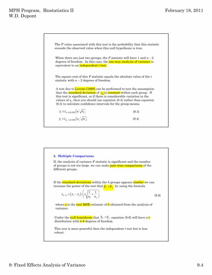
The P value associated with this test is the probability that this statistic exceeds the observed value when this null hypothesis is true.
When there are just two groups, the F statistic will have 1 and n – 2 degrees of freedom. In this case, the one-way analysis of variance is equivalent to an independent t test.
The square root of this F statistic equals the absolute value of the tstatistic with n – 2 degrees of freedom.
A test due to Levene (1960) can be performed to test the assumption that the standard deviation of ij is constant within each group. If this test is significant, or if there is considerable variation in the values of si, then you should use equation {9.4} rather than equation {9.3} to calculate confidence intervals for the group means.
,0.025i n k iy t s n {9.3}
1,0.025ii n i iy t s n {9.4}
If the standard deviations within the k groups appears similar we can increase the power of the test that by using the formula
{9.6}
i j
1 1/n k i j
i j
t y y sn n
3. Multiple Comparisons
If, the analysis of variance F statistic is significant and the number of groups is not too large, we can make pair-wise comparisons of the different groups.
This test is more powerful then the independent t test but is less robust.
i j Under the null hypothesis that equation {9.6} will have a tdistribution with n-k degrees of freedom.
where s is the root MSE estimate of obtained from the analysis of variance.

MPH Program, Biostatistics II W.D. Dupont
February 18, 2011
9: Fixed Effects Analysis of Variance 9.5
Alternately, a confidence interval based on the independent t test may be used if it appears unreasonable to assume a uniform standard deviation in all groups
{9.8}2,0.0251 1
i ji j n n pi j
y y t sn n
If the F test is not significant you should not report pair-wise significant differences unless they remain significant after a Bonferroni multiple comparisons adjustment (multiplying the P value by the number of pair wise tests.
A 95% confidence interval for the difference in population means between groups i and j is
,0.0251 1
i j n ki j
y y t sn n
{9.7}
If the number of groups is large and there is no natural ordering of the groups then a multiple comparisons adjustment may be advisable even if the F test is significant.
4. Fisher’s Protected Least Significant Difference(LSD) Approach to Multiple Comparisons
The idea of only analyzing subgroup effects (e.g. differences in group means) when the main effects (e.g. F test) are significant is known as known as Fisher’s Protected Least Significant Difference(LSD) Approach to Multiple Comparisons.
The F statistic tests the hypothesis that all of the group response means are simultaneously equal.
If we can reject this hypothesis it follows that some of the means must be different.
Fisher argued that in this situation you should be able to investigate which ones are different without having to pay a multiple comparisons penalty.
This approach is not guaranteed to preserve the experiment-wide Type I error probability, but makes sense in well structured experiments where the number of groups being examined is not too large.

MPH Program, Biostatistics II W.D. Dupont
February 18, 2011
9: Fixed Effects Analysis of Variance 9.6
5. Reformulating Analysis of Variance as a Linear Regression Model
A one-way analysis of variance is, in fact, a special case of the multiple regression model. Let
denote the response from the hth study subject, h = 1,2,…n, and let
hy
1 : if the patient is in the group
0 : otherwise
th th
hih i
x
Then model (9.1) can be rewritten
{9.9}
where h are mutually independent, normally distributed error terms with mean 0 and standard deviation . Note that model {9.9} is a special case of model (3.1). Thus, this analysis of variance is also a regression analysis in which all of the covariates are zero-one indicator variables.
2 2 3 3 ...h h h k hk hy x x x
i 1y 1iy yThe least squares estimates of and are and , respectively.
Also,
2 3
if the patient is from group 1E | , , ,
if the patient is from group 1
th
h h h hk thi
hy x x x
h i
Thus, is the expected response of patients in the first group and i is the expected difference in the response of patients in the ith and first groups.
We can use any multiple linear regression program to perform a one-way analysis of variance, although most software packages have a separate procedure for this task.

MPH Program, Biostatistics II W.D. Dupont
February 18, 2011
9: Fixed Effects Analysis of Variance 9.7
6. Non-parametric Methods
a) Kruskal-Wallis Test
The Kruskal-Wallis test is the non-parametric analog of the one-way analysis of variance (Kruskal and Wallis 1952).
Model {9.1} assumes that the terms are normally distributed and have the same standard deviation. If either of these assumptions is badly violated then the Kruskal-Wallis test should be used.
ij
The null hypothesis of this test is that the distributions of the response variables are the same in each group.
ijy
Suppose that patients are divided into k groups as in model {9.1}
and that is a continuous response variable on the jth patient
from the ith group.
We rank the values of yij from lowest to highest and let Ri be the sum of the ranks for the patients from the ith group.
Let
ni be the number of subjects in the ith group,
be the total number of study subjects.in n
When there are ties a slightly more complicated formula is used (see Steel and Torrie 1980).
212
3 11
i
i
RH n
n n n
If all of the values of yij are distinct (no ties) then the Kruskal-Wallis test statistic is
{9.10}

MPH Program, Biostatistics II W.D. Dupont
February 18, 2011
9: Fixed Effects Analysis of Variance 9.8
Under the null hypothesis, H will have a chi-squared distribution with k – 1 degrees of freedom as long as the number of patients in each group is reasonably large.
The non-parametric analog of the independent t-test is the Wilcoxon-Mann-Whitney rank-sum test. This rank-sum test and the Kruskal-Wallis test are equivalent when there are only two groups of patients.
Note that the value of H will be the same for any two data sets in which the data values have the same ranks. Increasing the largest observation or decreasing the smallest observation will have no effect on H. Hence, extreme outliers will not unduly affect this test.
7. Example: A Polymorphism in the Estrogen Receptor Gene
The human estrogen receptor gene contains a two-allele restrictionfragment length polymorphism that can be detected by Southern blots ofDNA digested with the PuvII restriction endonuclease. Bands at 1.6 kband/or 0.7 kb identify the genotype for these alleles.
Parl et al. (1989) studied the relationship between this genotype andage of diagnosis among 59 breast cancer patients.
MPH Program, Biostatistics II W.D. Dupont
February 18, 2011
9: Fixed Effects Analysis of Variance 9.9
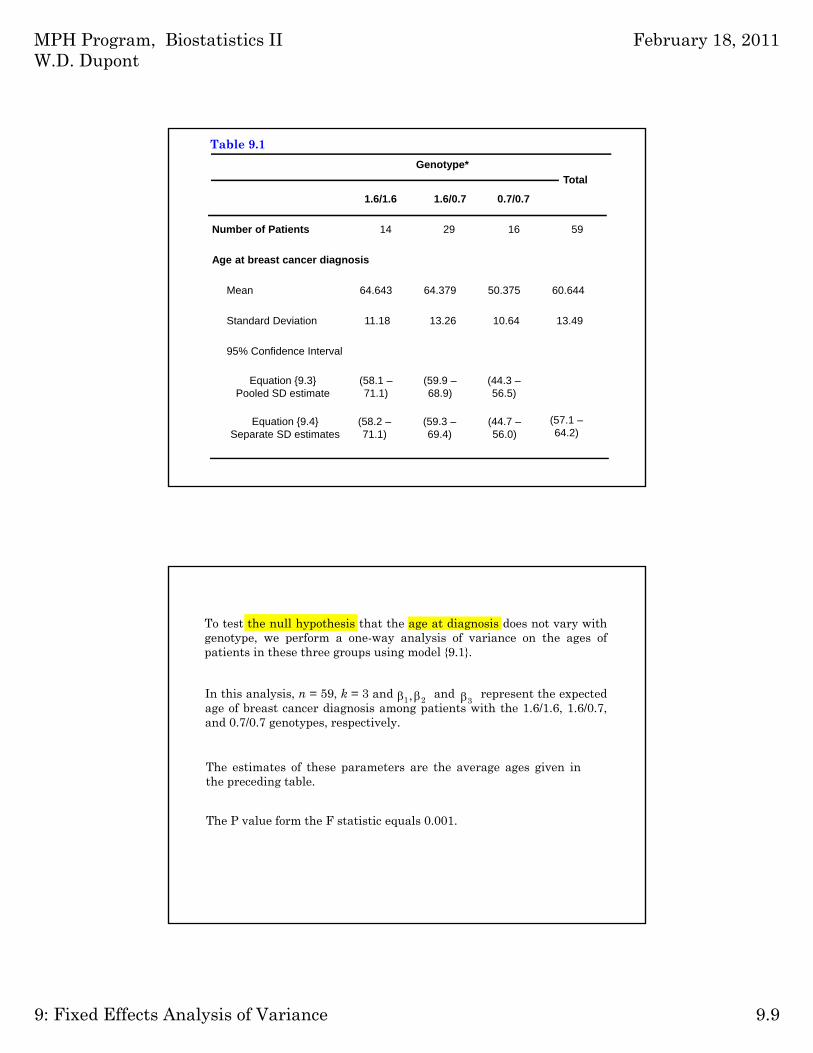
Number of Patients 14 29 16 59
Age at breast cancer diagnosis
Mean 64.643 64.379 50.375 60.644
Standard Deviation 11.18 13.26 10.64 13.49
95% Confidence Interval
Equation {9.3}Pooled SD estimate
(58.1 –71.1)
(59.9 –68.9)
(44.3 –56.5)
Genotype*
Total
1.6/1.6 1.6/0.7 0.7/0.7
Equation {9.4}Separate SD estimates
(58.2 –71.1)
(59.3 –69.4)
(44.7 –56.0)
(57.1 –64.2)
Table 9.1
To test the null hypothesis that the age at diagnosis does not vary withgenotype, we perform a one-way analysis of variance on the ages ofpatients in these three groups using model {9.1}.
The P value form the F statistic equals 0.001.
The estimates of these parameters are the average ages given inthe preceding table.
1 2, 3In this analysis, n = 59, k = 3 and and represent the expectedage of breast cancer diagnosis among patients with the 1.6/1.6, 1.6/0.7,and 0.7/0.7 genotypes, respectively.
MPH Program, Biostatistics II W.D. Dupont
February 18, 2011
9: Fixed Effects Analysis of Variance 9.10
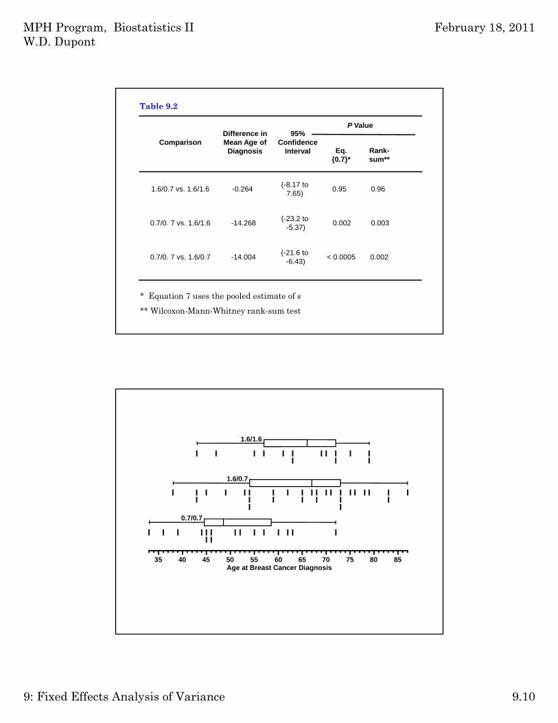
1.6/0.7 vs. 1.6/1.6 -0.264(-8.17 to
7.65)0.95 0.96
0.7/0. 7 vs. 1.6/1.6 -14.268(-23.2 to
-5.37)0.002 0.003
ComparisonDifference in Mean Age of
Diagnosis
95% Confidence
Interval
P Value
Eq. {0.7}*
Rank-sum**
0.7/0. 7 vs. 1.6/0.7 -14.004(-21.6 to
-6.43)< 0.0005 0.002
* Equation 7 uses the pooled estimate of s
** Wilcoxon-Mann-Whitney rank-sum test
Table 9.2
Age at Breast Cancer Diagnosis35 40 45 50 55 60 65 75 8570 80
0.7/0.7
1.6/0.7
1.6/1.6

MPH Program, Biostatistics II W.D. Dupont
February 18, 2011
9: Fixed Effects Analysis of Variance 9.11
8. One-Way Analyses of Variance using Stata
The following Stata log file and comments illustrate how to performthe one-way analysis of variance discussed in the preceding section.
* 10.8.ERpolymorphism.log. *. * Do a one-way analysis of variance to determine whether age. * at breast cancer diagnosis varies with estrogen receptor (ER). * genotype using the data of Parl et al. (1989).. *. use C:\WDDtext\10.8.ERpolymorphism.dta {1}. * Statistics > Summaries, tables, ... > Summary ... > Confidence intervals. ci age {2}
Variable | Obs Mean Std. Err. [95% Conf. Interval]-------------+-----------------------------------------------------------
age | 59 60.64407 1.756804 57.12744 64.16069
{1} This data set contains the age of diagnosis and estrogen receptor genotype of the 59 breast cancer patients studied by Parl et al. (1989). The genotypes 1.6/1.6, 1.6/0.7 and 0.7/0.7 are coded 1, 2 and 3 in the variable genotype, respectively.
{2} This ci command calculates the mean age of diagnosis (age) together with the associated 95% confidence interval. This confidence interval is calculated using equation {9.4}. The estimated standard error of the mean and the number of patients with non-missing ages is also given.

MPH Program, Biostatistics II W.D. Dupont
February 18, 2011
9: Fixed Effects Analysis of Variance 9.12
. * Statistics > Summaries, tables, ... > Summary ... > Confidence intervals
. by genotype: ci age {3}
_______________________________________________________________________________-> genotype = 1.6/1.6
Variable | Obs Mean Std. Err. [95% Conf. Interval]-------------+----------------------------------------------------------------
age | 14 64.64286 2.988269 58.1871 71.09862________________________________________________________________________________-> genotype = 1.6/0.7
Variable | Obs Mean Std. Err. [95% Conf. Interval]-------------+----------------------------------------------------------------
age | 29 64.37931 2.462234 59.33565 69.42297__________________________________________________________________________________-> genotype = 0.7/0.7
Variable | Obs Mean Std. Err. [95% Conf. Interval]-------------+---------------------------------------------------------------
age | 16 50.375 2.659691 44.706 56.044
{3} The command prefix by genotype: specifies that means and 95% confidence intervals are to be calculated for each of the three genotypes.

MPH Program, Biostatistics II W.D. Dupont
February 18, 2011
9: Fixed Effects Analysis of Variance 9.13
. *
. * The following graph type is not available in Stata version 8.0
. *
. graph7 age, by(genotype) box oneway {4}
{4} The graph7 command implements Stata Version 7 commands using version 7 syntax. The following graph is one that is not available in Version 8. The box and oneway options of this graph command create a graph that is similar to the Figure. See also Sections 10.7 and 10.8 of text for a prettier way of drawing this graph.
Age at Breast Cancer Diagnosis35 40 45 50 55 60 65 75 8570 80
0.7/0.7
1.6/0.7
1.6/1.6

MPH Program, Biostatistics II W.D. Dupont
February 18, 2011
9: Fixed Effects Analysis of Variance 9.14
{5} This oneway command performs a one-way analysis of varianceof age with respect to the three distinct values of genotype.
{6} The F statistic from this analysis equals 7.86. If the mean age of diagnosis in the target population is the same for all three genotypes, this statistic will have an F distribution with k – 1 = 3 – 1= 2 and n – k = 56 degrees of freedom. The probability that this statistic exceeds 7.86 is 0.001.
{7} The MSE estimate of is = 147.246.
{8} Bartlett’s test for equal variances (i.e. equal standard deviations) gives a P value of 0.58.
. * Statistics > Linear models and related > ANOVA/MANOVA > One-way ANOVA
. oneway age genotype {5}
Analysis of VarianceSource SS df MS F Prob > F
------------------------------------------------------------------------Between groups 2315.73355 2 1157.86678 7.86 0.0010 {6}Within groups 8245.79187 56 147.246283 {7}------------------------------------------------------------------------
Total 10561.5254 58 182.095266
Bartlett's test for equal variances: chi2(2) = 1.0798 Prob>chi2 = 0.583 {8}

MPH Program, Biostatistics II W.D. Dupont
February 18, 2011
9: Fixed Effects Analysis of Variance 9.15
. *
. * Test whether the standard deviations of age are equal in
. * patients with different genotypes.
. *
. * Statistics > Summaries, ... > Classical ... > Robust equal variance test
. robvar age, by(genotype)
| Summary of Age at DiagnosisGenotype | Mean Std. Dev. Freq.
------------+------------------------------------1.6/1.6 | 64.642857 11.181077 141.6/0.7 | 64.37931 13.259535 290.7/0.7 | 50.375 10.638766 16
------------+------------------------------------Total | 60.644068 13.494268 59
W0 = 0.83032671 df(2, 56) Pr > F = 0.44120161
W50 = 0.60460508 df(2, 56) Pr > F = 0.54981692
W10 = 0.79381598 df(2, 56) Pr > F = 0.45713722
This robvar command performs a test of the equality of variance among groups defined by genotype using methods of Levene (1960) and Brown and Forsythe (1974). These tests are less sensitive to departures from normality than Bartlett’s test. There is no evidence of heterogeneity of variance for age in these three groups.

MPH Program, Biostatistics II W.D. Dupont
February 18, 2011
9: Fixed Effects Analysis of Variance 9.16
. oneway age genotype
Analysis of VarianceSource SS df MS F Prob > F
------------------------------------------------------------------------Between groups 2315.73355 2 1157.86678 7.86 0.0010Within groups 8245.79187 56 147.246283------------------------------------------------------------------------
Total 10561.5254 58 182.095266
. *
. * Repeat analysis using linear regression
. *
. * Statistics > Linear models and related > Linear regression
. regress age i.genotype {9}
Source | SS df MS Number of obs = 59-------------+------------------------------ F( 2, 56) = 7.86
Model | 2315.73355 2 1157.86678 Prob > F = 0.0010Residual | 8245.79187 56 147.246283 R-squared = 0.2193
-------------+------------------------------ Adj R-squared = 0.1914Total | 10561.5254 58 182.095266 Root MSE = 12.135
------------------------------------------------------------------------------age | Coef. Std. Err. t P>|t| [95% Conf. Interval]
-------------+----------------------------------------------------------------genotype |
2 | -.2635468 3.949057 -0.07 0.947 -8.174458 7.647365 {10}3 | -14.26786 4.440775 -3.21 0.002 -23.1638 -5.371915
|_cons | 64.64286 3.243084 19.93 0.000 58.14618 71.13953 {11}
------------------------------------------------------------------------------
{10} The estimates of and in this example are = 64.379 – 64.643 = – 0.264 and = 50.375 – 64.643 = – 14.268, respectively. They are highlighted in the column labeled Coef. The 95% confidence intervals for and are calculated using equation {9.7}. The t statistics for testing the null hypotheses that = 0 and = 0 are – 0.07 and – 3.21, respectively. They are calculated using equation {9.6}. The highlighted values in this output are also given in Table 9.2.
2
2
3
3
3
2
2 1y y
3 1y y
{11} The estimate of is = 64.643. The 95% confidence interval for is calculated using equation {9.3}. These statistics are also given in Table 10.1.
1y
{9} This regress command preforms exactly the same one-way analysis of variance as the oneway command given above. Note that the F statistic, the P value for this statistic and the MSE estimate of are identical to that given by the oneway command. The syntax of the xi: prefix is explained in Section 5.10. The model used by this command is equation {9.9} with k = 3.

MPH Program, Biostatistics II W.D. Dupont
February 18, 2011
9: Fixed Effects Analysis of Variance 9.17
. lincom _cons + _Igenotype_2 {12}
( 1) _Igenotype_2 + _cons = 0.0
----------------------------------------------------------------------------age | Coef. Std. Err. t P>|t| [95% Conf. Interval]
-----------+----------------------------------------------------------------(1) | 64.37931 2.253322 28.57 0.000 59.86536 68.89326 {13}
----------------------------------------------------------------------------
. lincom _cons + _Igenotype_3
( 1) _Igenotype_3 + _cons = 0.0
----------------------------------------------------------------------------age | Coef. Std. Err. t P>|t| [95% Conf. Interval]
-----------+----------------------------------------------------------------(1) | 50.375 3.033627 16.61 0.000 44.29791 56.45209
----------------------------------------------------------------------------
{12} This lincom command estimates by = . A 95 % confidence interval for this estimate is also given. Note that equals the population mean age of diagnosis among women with the 1.6/0.7 genotype. Output from this and the next lincomcommand are also given in Table 9.1.
2 2ˆ̂ 2y
2
{13} This confidence interval is calculated using equation {9.3}.
MPH Program, Biostatistics II W.D. Dupont
February 18, 2011
9: Fixed Effects Analysis of Variance 9.18
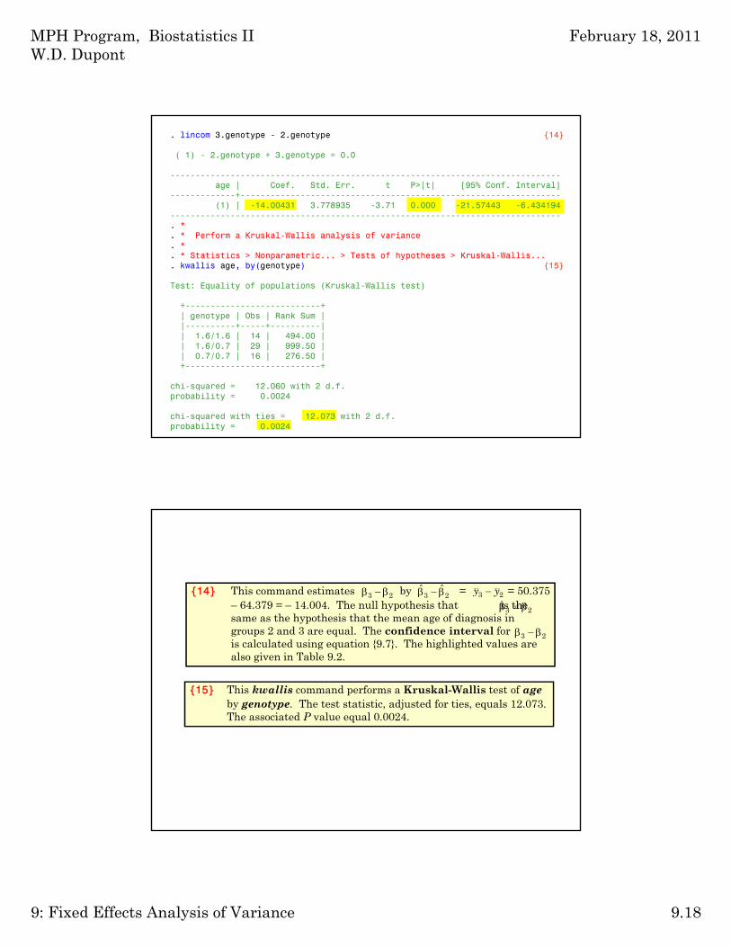
. lincom 3.genotype - 2.genotype {14}
( 1) - 2.genotype + 3.genotype = 0.0
------------------------------------------------------------------------------age | Coef. Std. Err. t P>|t| [95% Conf. Interval]
-------------+----------------------------------------------------------------(1) | -14.00431 3.778935 -3.71 0.000 -21.57443 -6.434194
------------------------------------------------------------------------------. *. * Perform a Kruskal-Wallis analysis of variance. *. * Statistics > Nonparametric... > Tests of hypotheses > Kruskal-Wallis.... kwallis age, by(genotype) {15}
Test: Equality of populations (Kruskal-Wallis test)
+---------------------------+| genotype | Obs | Rank Sum ||----------+-----+----------|| 1.6/1.6 | 14 | 494.00 || 1.6/0.7 | 29 | 999.50 || 0.7/0.7 | 16 | 276.50 |+---------------------------+
chi-squared = 12.060 with 2 d.f.probability = 0.0024
chi-squared with ties = 12.073 with 2 d.f.probability = 0.0024
{15} This kwallis command performs a Kruskal-Wallis test of ageby genotype. The test statistic, adjusted for ties, equals 12.073. The associated P value equal 0.0024.
{14} This command estimates by = = 50.375 – 64.379 = – 14.004. The null hypothesis that is the same as the hypothesis that the mean age of diagnosis in groups 2 and 3 are equal. The confidence interval for is calculated using equation {9.7}. The highlighted values are also given in Table 9.2.
3 2 3 2ˆ ˆ 3 2y y
3 2
3 2

MPH Program, Biostatistics II W.D. Dupont
February 18, 2011
9: Fixed Effects Analysis of Variance 9.19
. * Statistics > Nonparametric... > Tests... > Wilcoxon rank-sum test
. ranksum age if genotype !=3, by(genotype) {16}
Two-sample Wilcoxon rank-sum (Mann-Whitney) test
genotype | obs rank sum expected-------------+---------------------------------
1.6/1.6 | 14 310 3081.6/0.7 | 29 636 638
-------------+---------------------------------combined | 43 946 946
unadjusted variance 1488.67adjustment for ties -2.70
----------
adjusted variance 1485.97
Ho: age(genotype==1.6/1.6) = age(genotype==1.6/0.7)z = 0.052
Prob > |z| = 0.9586
{16} This command performs a Wilcoxon-Mann-Whitney rank-sumtest on the age of diagnosis of women with the 1.6/1.6 genotype versus the 1.6/0.7 genotype. The P value for this test is 0.96. The next two commands perform the other two pair-wise comparisons of age by genotype using this rank-sum test. The highlighted P values are included in Table 10.2.

MPH Program, Biostatistics II W.D. Dupont
February 18, 2011
9: Fixed Effects Analysis of Variance 9.20
. * Statistics > Nonparametric... > Tests... > Wilcoxon rank-sum test
. ranksum age if genotype ~=2, by(genotype)
Two-sample Wilcoxon rank-sum (Mann-Whitney) test
genotype | obs rank sum expected-------------+---------------------------------
1.6/1.6 | 14 289 2170.7/0.7 | 16 176 248
-------------+---------------------------------combined | 30 465 465
unadjusted variance 578.67adjustment for ties -1.67
----------adjusted variance 576.99
Ho: age(genotype==1.6/1.6) = age(genotype==0.7/0.7)z = 2.997
Prob > |z| = 0.0027
MPH Program, Biostatistics II W.D. Dupont
February 18, 2011
9: Fixed Effects Analysis of Variance 9.21
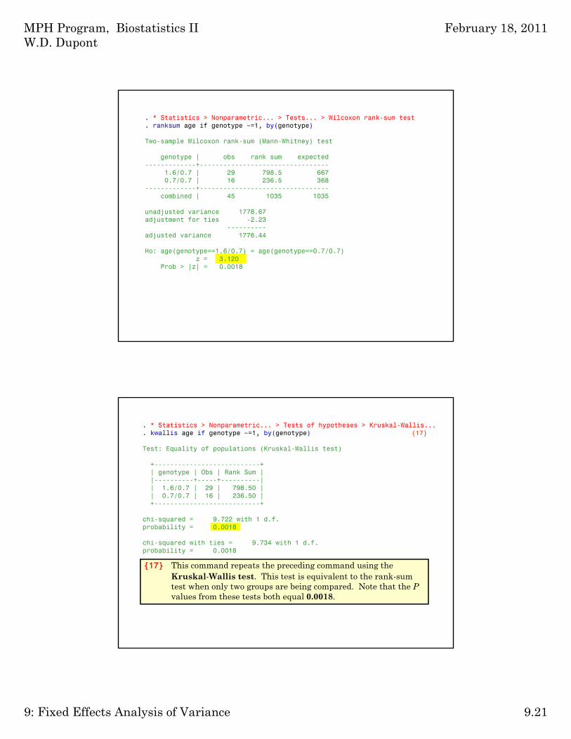
. * Statistics > Nonparametric... > Tests... > Wilcoxon rank-sum test
. ranksum age if genotype ~=1, by(genotype)
Two-sample Wilcoxon rank-sum (Mann-Whitney) test
genotype | obs rank sum expected-------------+---------------------------------
1.6/0.7 | 29 798.5 6670.7/0.7 | 16 236.5 368
-------------+---------------------------------combined | 45 1035 1035
unadjusted variance 1778.67adjustment for ties -2.23
----------adjusted variance 1776.44
Ho: age(genotype==1.6/0.7) = age(genotype==0.7/0.7)z = 3.120
Prob > |z| = 0.0018
. * Statistics > Nonparametric... > Tests of hypotheses > Kruskal-Wallis...
. kwallis age if genotype ~=1, by(genotype) {17}
Test: Equality of populations (Kruskal-Wallis test)
+---------------------------+| genotype | Obs | Rank Sum ||----------+-----+----------|| 1.6/0.7 | 29 | 798.50 || 0.7/0.7 | 16 | 236.50 |+---------------------------+
chi-squared = 9.722 with 1 d.f.probability = 0.0018
chi-squared with ties = 9.734 with 1 d.f.probability = 0.0018
{17} This command repeats the preceding command using the Kruskal-Wallis test. This test is equivalent to the rank-sum test when only two groups are being compared. Note that the Pvalues from these tests both equal 0.0018.

MPH Program, Biostatistics II W.D. Dupont
February 18, 2011
9: Fixed Effects Analysis of Variance 9.22
9. Two-Way Analysis of Variance, Analysis of Covariance, and Other Models
Fixed-effects analyses of variance generalize to a wide variety of complex models. For example, suppose that hypertensive patients were treated with either a placebo, a diuretic alone, a beta-blocker alone, or with both a diuretic and a beta-blocker. Then a model of the effect of treatment on diastolic blood pressure (DBP) might be
{9.11}1 1 2 2i i i iy x x
1ix 1: patient is on a diuretic0: otherwise
thi
=
2ix 1: patient is on a beta-blocker0: otherwise
thi
=
1 2
where
, and are unknown parameters,
is the DBP of the ith patient after some standard interval therapy , and
iy
are error terms that are independently and normally distributed with mean zero and standard deviation
i
Model {9.11} is an example of a fixed-effects, two-way analysis of variance.
A critical feature of this model is that each patient’s blood pressure is only observed once.
It is called two-way because each patient is simultaneously influenced by two covariates — in this case whether she did, or did not, receive a diuretic or a beta-blocker.
The model is additive since it assumes that the mean DBP of patients on both drugs is + 1 +2.
If this assumption is unreasonable, we can add an interaction term as in Section 3.12.
It is this feature that makes the independence assumption for the error term reasonable and makes this a fixed-effects model. In this model,
is the mean DBP of patients on placebo,
+ 1 is the mean DBP of patients on the diuretic alone,
+ 2 is the mean DBP of patients on the beta-blocker alone, and
+ 1 + 2 is the mean DBP of patients on both treatments.

MPH Program, Biostatistics II W.D. Dupont
February 18, 2011
9: Fixed Effects Analysis of Variance 9.23
10. Fixed Effects Analysis of Covariance
This refers to linear regression models with both categorical and continuous covariates. Inference from these models is called analysis of covariance.
These models no longer need the special consideration that they received in years passed and can be easily handled by the regress command.
where agei is the ith patient’s age, 3 is the parameter associated with age, and the other terms are as defined in model {9.11}. The analysis of model {9.12} would be an example of analysis of covariance.
1 1 2 2 3i i i i iy x x age
For example, we could add the patient’s age to model (9.11). This gives
{9.12}
Regression analysis with categorical variables and one response measure per subject
One-way analysis of variance: The oneway command
Multiple comparisons issues
Reformulating analysis of variance as a linear regression model Non-parametric one-way analysis of variance
Two-Way Analysis of Variance
Analysis of Covariance
95% confidence intervals for group means 95% confidence intervals for the difference between group means Testing for homogeneity of standard deviations across groups
The robvar command
Fisher’s protected least significant difference approach Bonferroni’s multiple comparison adjustment
Kruskal-Wallis test: The kwallis command Wilcoxon rank-sum test: The ranksum command
Simultaneously evaluating two categorical risk factors
Analyzing models with both categorical and continuous covariates
11. What we have covered

MPH Program, Biostatistics II W.D. Dupont
February 18, 2011
9: Fixed Effects Analysis of Variance 9.24
Cited Reference
Parl FF, Cavener DR, Dupont WD. Genomic DNA analysis of the estrogen receptor gene in breast cancer. Breast Cancer Research and Treatment1989;14:57-64.
For additional references on these notes see.
Dupont WD. Statistical Modeling for Biomedical Researchers: A Simple Introduction to the Analysis of Complex Data. 2nd ed. Cambridge, U.K.: Cambridge University Press; 2009.