seasonal variations of pavement layer moduli determined
TRANSCRIPT
The University of MaineDigitalCommons@UMaine
Electronic Theses and Dissertations Fogler Library
2007
Seasonal Variations of Pavement Layer ModuliDetermined Using In Situ Measurements ofPavement Stress and StrainLauren J. SwettUniversity of Maine - Main
Follow this and additional works at: http://digitalcommons.library.umaine.edu/etd
Part of the Civil and Environmental Engineering Commons
This Open-Access Thesis is brought to you for free and open access by DigitalCommons@UMaine. It has been accepted for inclusion in ElectronicTheses and Dissertations by an authorized administrator of DigitalCommons@UMaine.
Recommended CitationSwett, Lauren J., "Seasonal Variations of Pavement Layer Moduli Determined Using In Situ Measurements of Pavement Stress andStrain" (2007). Electronic Theses and Dissertations. 111.http://digitalcommons.library.umaine.edu/etd/111

SEASONAL VARIATIONS OF PAVEMENT LAYER MODULI DETERMINED
USING IN SITU MEASUREMENTS OF PAVEMENT STRESS AND STRAIN
By
Lauren J. Swett
B.S. University of Maine, 2004
A THESIS
Submitted in Partial Fulfillment of the
Requirements for the Degree of
Master of Science
(in Civil Engineering)
The Graduate School
The University of Maine
May, 2007
Advisory Committee:
Dana N. Humphrey, Professor, Civil and Environmental Engineering, Advisor
William G. Davids, Associate Professor, Civil and Environmental Engineering
Rajib B. Mallick, Associate Professor, Civil and Environmental Engineering, Worcester
Polytechnic Institute

LIBRARY RIGHTS STATEMENT
In presenting this thesis in partial fulfillment of the requirements for an advanced
degree at The University of Maine, I agree that the Library shall make it freely available
for inspection. I further agree that permission for "fair use" copying of this thesis for
scholarly purposes may be granted by the Librarian. It is understood that any copying or
publication of this thesis for financial gain shall not be allowed without my written
permission.
Signature:
Date:
SEASONAL VARIATIONS OF PAVEMENT LAYER MODULI DETERMINED
USING IN SITU MEASUREMENTS OF PAVEMENT STRESS AND STRAIN
By: Lauren J. Swett
Thesis Advisor: Dr. Dana N. Humphrey
An Abstract of the Thesis Presented in Partial Fulfillment of the Requirements for the
Degree of Master of Science (in Civil Engineering)
May, 2007
Pavement design procedures have advanced a great deal in recent years, changing
from empirical equations based on road tests in the 1950s to mechanistic-empirical
design procedures developed in the past few years. The resilient moduli for the asphalt
and soil layers of pavement sections are important properties necessary for pavement
design, and an accurate method for determining moduli under different conditions is
necessary.
The stiffness of pavement section layers changes with the season, and typically, a
road section will be the weakest during spring thaw due to loss of frozen soil stiffness,
and increases in water content. This is critical to consider for roadways that are traveled
by heavy truck traffic, where weight limits are implemented to reduce spring thaw
damage.
Resilient modulus is a form of the elastic modulus of soil. The value can be
calculated using a variety of methods. AASHTO has a procedure for laboratory
determination of resilient modulus, and correlations exist to estimate modulus based on

other soil properties. The most widely used method of calculating pavement layer moduli
is the backcalculation of moduli from deflection data obtained using a Falling Weight
Deflectometer.
The goal of this project was to collect in situ stress and strain data in an attempt to
calculate resilient modulus directly in the field. Temperature data was also collected to
help quantify the effect of freezing and thawing cycles on changes in modulus.
A section of Rt. 15 in Guilford, Maine was instrumented with strain gages, stress
gages, and climate related gages during the reconstruction of the roadway. Strain gages
and thermocouples were installed in the asphalt layer, and strain gages, pressure cells,
thermocouples, resistivity probes, and moisture gages were installed in the subbase and
subgrade layers. A data acquisition system was set up on site to collect both high speed
stress and strain responses, and static temperature, moisture, and resistivity responses.
Data was collected during the winter, spring, and summer of 2006. Stress and
strain responses were recorded for traffic loading due to normal truck traffic and
controlled loading with a MaineDOT dump truck with a known weight. A Falling
Weight Deflectometer was also used to acquire data for modulus backcalculation.
Asphalt strain responses were used to estimate the value of Nf, the number of
loading cycles required to cause fatigue cracking. Predicted and measured values of
strain in the asphalt and the soil were compared. In situ moduli were calculated using
recorded stresses and strains and related to FWD backcalculated moduli. These initial
results from the instrumented site were used to observe the effect of freezing and thawing
on pavement responses.

ii
DEDICATION
This thesis is dedicated to my parents Paul and Nancy Swett and my brother Michael who
have helped me more in the last 23 years than I will ever be able to thank them for.

iii
ACKNOWLEDGEMENTS
There are many people to acknowledge for their assistance with this project, both
directly and indirectly. First and foremost I need to thank my advisor, Professor Dana
Humphrey who has been so helpful throughout all of my time at the University of Maine.
From my summer job with the civil engineering department, to my thesis project and the
graduate classes I have taken with him, Dana’s enthusiasm has always made my
University of Maine experience a great one.
In addition to Professor Humphrey, my committee includes Professor William
Davids of the University of Maine, and Professor Rajib Mallick of Worcester Polytechnic
Institute. Bill Davids, with his unique style of encouragement, has managed to maintain
my interest in structural engineering even as I spent my graduate semesters concentrating
in geotechnical subjects. Rajib Mallick’s knowledge of pavement design and asphalt
properties has been indispensable on this project. The support of both Professors Davids
and Mallick has contributed a great deal to the success of this project.
This project was made possible through funding from the Maine Department of
Transportation. The assistance of Dale Peabody, Tim Soucie, the workers at the Guilford
maintenance garage, the three resident engineers I communicated with on the project,
Ervin Kirk, Jim Hosmer, and Court McCrea, and many other MaineDOT employees was
very much appreciated. The willingness of the general contractor K & K Construction to
work with us towards the completion of the project was appreciated as well.
While the outcome of a graduate project in the Civil Engineering Department is
ultimately the responsibility of one graduate student, the work of countless other students
is important to the project’s success. Sean O’Brien, a Master’s degree student from

iv
Worcester Polytechnic Institute helped with the installation of asphalt instrumentation,
and provided his expertise with the Falling Weight Deflectometer.
My brother, Michael Swett, graduate students Michael St. Pierre and Jeremy
Labbe, and Tim Soucie of the MaineDOT, were my work force for the installation and
monitoring of the instrumentation for my project. In addition, my uncle, my father, and
another graduate student, Justin Desjarlais, spent many hours with me driving to and
from Guilford, and sitting in the instrumentation shed taking readings. Through wind,
pouring rain, snow, and lots of mud, we made it through the project together.
Thank you to all of my fellow graduate students, my professors, and Pam Oakes
and Mary Burton. No matter what type of question I had, there was always a source for
answers! Finally thank you to my family. Above all, your support has helped me get to
where I am today. Thank you!
v
TABLE OF CONTENTS
DEDICATION.................................................................................................................... ii
ACKNOWLEDGEMENTS............................................................................................... iii
LIST OF TABLES............................................................................................................. ix
LIST OF FIGURES ............................................................................................................ x
Chapter 1 INTRODUCTION.............................................................................................. 1
1.1 Pavement Design Procedures.............................................................................. 1
1.2 Climate................................................................................................................ 2
1.3 Objective ............................................................................................................. 3
1.4 Organization of this Report................................................................................. 5
Chapter 2 LITERATURE REVIEW................................................................................... 6
2.1 Introduction......................................................................................................... 6
2.2 Definition of Resilient Modulus of Soil Materials ............................................. 7
2.3 Climatic Effects on Pavement Section Properties .............................................. 8
2.4 Modulus Calculation Methods.......................................................................... 10
2.4.1 Laboratory Testing.................................................................................... 10
2.4.2 Correlation of Modulus with Soil Properties ............................................ 13
2.4.3 Backcalculation......................................................................................... 15
2.4.3.1 Collecting Data ..................................................................................... 16
2.4.3.1.1 Preprocessing .................................................................................. 17
2.4.3.1.2 Additional Required Information.................................................... 17
2.4.3.2 Analytical Model .................................................................................. 17
2.4.3.2.1 Burmister’s Layered Theory ........................................................... 18

vi
2.4.3.2.2 Modified Boussinesq Theory.......................................................... 19
2.4.3.2.3 Finite Element Method ................................................................... 20
2.4.3.3 Material Model...................................................................................... 21
2.4.3.3.1 Linear .............................................................................................. 21
2.4.3.3.2 Nonlinear......................................................................................... 22
2.4.3.4 Model Implementation.......................................................................... 24
2.4.3.5 Comparison Criteria – Solving the Models .......................................... 25
2.4.3.5.1 Least Squares .................................................................................. 26
2.4.3.5.2 System Identification Process ......................................................... 29
2.4.3.5.3 Curvature Approach........................................................................ 29
2.4.3.6 Analysis and Use of Backcalculated Solution ...................................... 30
2.5 Pavement Section Property Verification by In Situ Instrumentation................ 31
2.5.1 Minnesota Road Research Project ............................................................ 31
2.5.2 Pennsylvania Superpave In Situ Stress/Strain Investigation .................... 32
2.5.3 Virginia Smart Road ................................................................................. 34
2.5.4 Auburn University NCAT Test Track ...................................................... 36
2.5.5 Ohio Department of Transportation.......................................................... 38
2.5.6 Montana .................................................................................................... 38
2.5.7 Louisiana Pavement Research Facility ..................................................... 40
2.5.8 Finland Road and Traffic Laboratory ....................................................... 41
2.6 Summary ........................................................................................................... 41
Chapter 3 INSTRUMENTATION.................................................................................... 44
3.1 Introduction....................................................................................................... 44
vii
3.2 Asphalt Strain Gage .......................................................................................... 47
3.3 Soil Strain Gage ................................................................................................ 52
3.4 Soil Pressure Cells ............................................................................................ 56
3.5 Thermocouples.................................................................................................. 61
3.6 Soil Resistivity Probe........................................................................................ 64
3.7 Soil Moisture Gages.......................................................................................... 65
3.8 Summary ........................................................................................................... 68
Chapter 4 PROJECT CONSTRUCTION ......................................................................... 70
4.1 General Roadway Construction Procedures and Materials .............................. 70
4.2 Gage Installation ............................................................................................... 74
4.3 Summary ........................................................................................................... 76
Chapter 5 DATA ACQUISITION.................................................................................... 77
5.1 Introduction....................................................................................................... 77
5.2 Dynamic Data Acquisition................................................................................ 77
5.3 Static Data Acquisition ..................................................................................... 87
5.4 Summary ........................................................................................................... 88
Chapter 6 RESULTS......................................................................................................... 89
6.1 Introduction....................................................................................................... 89
6.2 Climate Data ..................................................................................................... 91
6.3 Combining Pavement Responses with Climate Data........................................ 94
6.4 Asphalt Responses ............................................................................................ 98
6.4.1 Asphalt Tensile Strain............................................................................... 98
6.4.2 Asphalt Fatigue Cracking ....................................................................... 106
viii
6.5 Soil Responses ................................................................................................ 108
6.6 Soil Moduli from In Situ Measurements ........................................................ 113
6.7 Comparing Measured and Predicted Stress and Strain ................................... 120
6.8 Summary ......................................................................................................... 122
Chapter 7 SUMMARY AND CONCLUSIONS............................................................. 124
7.1 Summary ......................................................................................................... 124
7.1.1 Literature Review.................................................................................... 124
7.1.2 Instrumentation ....................................................................................... 125
7.1.3 Results..................................................................................................... 126
7.2 Conclusions..................................................................................................... 128
7.3 Recommendations........................................................................................... 129
REFERENCES ............................................................................................................... 131
APPENDICES ................................................................................................................ 136
Appendix A................................................................................................................. 137
Appendix B ................................................................................................................. 139
Appendix C ................................................................................................................. 145
Appendix D................................................................................................................. 219
Appendix E ................................................................................................................. 243
Appendix F ................................................................................................................. 253
Appendix G................................................................................................................. 309
BIOGRAPHY OF THE AUTHOR................................................................................. 319

ix
LIST OF TABLES
Table 3.1 Specified Instrumentation for the Guilford Site ............................................... 45
Table 3.2 Wire lengths, wire resistances, and gage amplifications for the PAST
gages. ........................................................................................................................ 49
Table 3.3 Strain gage resistances ...................................................................................... 51
Table 3.4 Moisture Gage Calibration Densities and In-place Water Contents................. 68
Table 4.1 Hot mix asphalt properties as reported by the Maine DOT.............................. 73
Table 5.1 Data Acquisition Components .......................................................................... 78
Table 6.1 Loading Methods for the 2006 winter, spring, and summer seasons ............... 90
Table 6.2 MaineDOT truck loading vehicle weights...................................................... 104
Table 6.3 Calculated number of load repetitions to cause fatigue cracking based
on tensile strain (parameter values from Huang, 2004) .......................................... 107
Table 6.4 FWD backcalculated moduli at the locations of the in situ soil stress
and strain gages on March 30, 2006 ....................................................................... 114
Table 6.5 Calculated Moduli........................................................................................... 118
Table C. 1 Asphalt Tensile Strain Gage Responses to Traffic Loading ......................... 146
Table G. 1 Soil Stress and Strain Responses and Calculated Modulus Values
for Subbase and Subgrade....................................................................................... 310

x
LIST OF FIGURES
Figure 1.1 The completed pavement (the left lane is contains the instrumentation) .......... 4
Figure 2.1 Soil response due to repeated loading in a triaxial test (Hjelmstad
and Taciroglu, 2000) ................................................................................................... 8
Figure 2.2 Typical triaxial setup used for the laboratory measurement of resilient
modulus (AASHTO, 2001) ....................................................................................... 11
Figure 2.3 Resilient modulus for New Hampshire soil samples before and after
freeze-thaw (Simonsen et al., 2002).......................................................................... 13
Figure 2.4 Example of FWD deflection measurement distribution (Mehta and
Roque, 2003)............................................................................................................. 16
Figure 2.5 Typical ILLI-PAVE cross section (Hoffman and Thompson, 1982) .............. 22
Figure 2.6 ILLI-PAVE subgrade material model (Hoffman and Thompson, 1982) ........ 23
Figure 2.7 Iterative procedure for backcalculating modulus (Zhou, et al., 1990) ............ 26
Figure 2.8 Newton’s Method for a single layer (Harichandran, et al., 1993)................... 28
Figure 2.9 Variation in tensile strain with vehicle speed (Stoffels, et al., 2006).............. 33
Figure 2.10 Variation in tensile strain for different layers of the pavement system
before and after the freeze-thaw system (Stoffels, et al., 2006)................................ 34
Figure 2.11 Calculated and measured horizontal transverse asphalt strain
(Al-Qadi, et al., 2004) ............................................................................................... 36
Figure 2.12 Variation in volumetric water content with time (Janoo and Shepherd,
2000) ......................................................................................................................... 39
Figure 2.13 Comparison of changes in moisture content and modulus throughout a
freeze-thaw season (Janoo and Shepherd, 2000) ...................................................... 40

xi
Figure 3.1 The Guilford instrumented road section plan and profile views ..................... 46
Figure 3.2 PAST gages (a) diagram and (b) photograph .................................................. 47
Figure 3.3 PAST installation: (a) gages with geotextile and asphalt binder;
(b) gages placed in binder/sand mix; (c) compaction by hand with heavy
roller; (d) paving over gages; (e) rubber tire roller compaction; (f) steel roller
compaction. ............................................................................................................... 50
Figure 3.4 Damaged gage locations and orientations ....................................................... 52
Figure 3.5 SSDT Soil Strain Gage (a) diagram and (b) photograph................................. 53
Figure 3.6 SSDT calibration (a) setup, (b) results for each of the four gages, and
(c) conversion equations for each gage..................................................................... 54
Figure 3.7 Installation of an SSDT; (a) base in mortar mix and (b) top plate in
place .......................................................................................................................... 55
Figure 3.8 Soil pressure cell (a) diagram and (b) photograph .......................................... 57
Figure 3.9 Pressure Cell Calibration (a) results and (b) conversion equations for
each gage................................................................................................................... 58
Figure 3.10 Pressure cell installation methods (a) one and (b) two.................................. 60
Figure 3.11 Typical soil strain gage and pressure cell layout for both the subbase
and subgrade gage installations ................................................................................ 60
Figure 3.12 Stages of thermocouple construction: (a) copper (blue coating) and
constantan (red coating) wires stripped and separated; (b) copper and
constantan wires crimped together; and (c) the crimped wires covered by a
heat shrink cap. ......................................................................................................... 61
Figure 3.13 Soil Thermocouple (a) diagram and (b) installation...................................... 62

xii
Figure 3.14 Asphalt thermocouple ready for paving ........................................................ 63
Figure 3.15 Frost resistivity probe (a) typical probe and (b) installation ......................... 64
Figure 3.16 Soil water content reflectometer.................................................................... 66
Figure 3.17 Moisture content calibration setup ................................................................ 67
Figure 3.18 Moisture content calibration chart................................................................. 68
Figure 4.1 Gradation of subgrade soil based on wet sieve and hydrometer analyses....... 71
Figure 4.2 Gradation of subbase aggregate based on wet sieve and hydrometer
analyses ..................................................................................................................... 72
Figure 4.3 Asphalt gradations as reported by the Maine DOT......................................... 73
Figure 4.4 Asphalt and subbase detail from MaineDOT project plans............................ 74
Figure 5.1 Data acquisition for (a) soil strain gages, (b) soil pressure cells, and
(c) asphalt strain gages.............................................................................................. 80
Figure 5.2 National Instruments LabVIEW 7.1: (a) multiple devices front panel,
(b) one device front panel, (c) multiple devices block diagram, (d) one
device block diagram ............................................................................................... 83
Figure 6.1 Zero degree isotherm for the thermocouple locations on the (a) left at
station 3+602 and on the (b) right at station 3+635. ................................................. 93
Figure 6.2 Cumulative freezing degree days from October 2005 through May 2006...... 94
Figure 6.3 Location of freezing and thawing fronts in March 2006................................. 95
Figure 6.4 (a) A standard six-axle loaded log truck along with plots of asphalt
strain due to a loaded log truck observed on March 9, 2006, from longitudinal
asphalt strain gages at station 3+599 (b) 498-003 and (c) 498-005.......................... 99

xiii
Figure 6.5 Typical asphalt strain plots for a loaded log truck observed on
March 10, 2006, from asphalt strain gages at station 3+599 (a) 498-003 and
(b) 498-005.............................................................................................................. 101
Figure 6.6 Asphalt strain response of transverse gage 498-006 for unloaded log
trucks on (a) March 24, 2006 and (b) March 28, 2006 ........................................... 102
Figure 6.7 In-situ measured and predicted strains at station 3+599 from FWD
loading on 3/30/06 .................................................................................................. 105
Figure 6.8 Layout of asphalt strain gages relative to the FWD drop location for
station 3+599........................................................................................................... 106
Figure 6.9 For a loaded 3-axle dump truck observed on June 16, 2006, plots of (a)
subbase stress, (b) subbase strain, (c) subgrade stress, and (d) subgrade
strain........................................................................................................................ 111
Figure 6.10 Typical plots for a loaded 2-axle MaineDOT dump truck observed
on July 13, 2006, (a) subbase stress and (b) strain and(c) subgrade stress
and (d) strain ........................................................................................................... 112
Figure 6.11 Interpolation of strain to the locations of pressure cells.............................. 115
Figure 6.12 Moduli values calculated using in situ stresses and strains for the
(a) subbase (at pressure cell A03.8’s location) and (b) subgrade (at pressure
cells A03.11 and A03.13 locations) ........................................................................ 116
Figure 6.13 In situ calculated moduli and FWD backcalculated moduli for the
(a) subbase and (b) subgrade................................................................................... 119
Figure 6.14 Changes in average moduli during the spring and summer of 2006 ........... 120
Figure 6.15 Ratio of measured strain to predicted asphalt tensile strain ........................ 121
xiv
Figure A. 1 Typical pavement cross section for the instrumented section from the
Maine DOT project plans........................................................................................ 137
Figure A. 2 Station 3+600 cross section from Maine DOT Plans. For each of the
included cross sections, solid lines represent final construction elevations,
and dashed lines represent the previous surface elevation...................................... 137
Figure A. 3 Station 3+610 cross section from Maine DOT Plans. ................................. 137
Figure A. 4 Station 3+620 cross section from Maine DOT Plans. ................................. 137
Figure A. 5 Station 3+626 cross section from Maine DOT Plans. ................................. 138
Figure A. 6 Station 3+640 cross section from Maine DOT Plans. ................................. 138
Figure A. 7 Station 3+645 cross section from Maine DOT Plans. ................................. 138
Figure B. 1 Soil Profile of Instrumented Section............................................................ 144
Figure C. 1 Asphalt Strain Gage 003, 3/9/06, Unloaded Log Truck .............................. 148
Figure C. 2 Asphalt Strain Gage 003, 3/9/06, Loaded Chip Truck ................................ 148
Figure C. 3 Asphalt Strain Gage 003, 3/9/06, Dual Axle Dump Truck.......................... 148
Figure C. 4 Asphalt Strain Gage 003, 3/9/06, Tanker Truck.......................................... 149
Figure C. 5 Asphalt Strain Gage 003, 3/9/06, Tractor Trailer Truck.............................. 149
Figure C. 6 Asphalt Strain Gage 003, 3/9/06, Loaded Log Truck.................................. 149
Figure C. 7 Asphalt Strain Gage 003, 3/10/06, Tanker Truck........................................ 150
Figure C. 8 Asphalt Strain Gage 003, 3/10/06, Loaded Log Truck 1............................. 150
Figure C. 9 Asphalt Strain Gage 003, 3/10/06, Loaded Log Truck 2............................. 150
Figure C. 10 Asphalt Strain Gage 003, 3/15/06, School Bus ......................................... 151
Figure C. 11 Asphalt Strain Gage 003, 3/15/06, Unloaded Log Truck 1 ....................... 151
Figure C. 12 Asphalt Strain Gage 003, 3/15/06, Unloaded Log Truck 2 ....................... 151
xv
Figure C. 13 Asphalt Strain Gage 003, 3/17/06, Loaded Dual-Axle Log Truck............ 152
Figure C. 14 Asphalt Strain Gage 003, 3/17/06, Tractor Trailer Truck.......................... 152
Figure C. 15 Asphalt Strain Gage 003, 3/24/06, Unloaded Log Truck 1 ....................... 152
Figure C. 16 Asphalt Strain Gage 003, 3/24/06, Unloaded Log Truck 2 ....................... 153
Figure C. 17 Asphalt Strain Gage 003, 3/24/06, Loaded Dual-Axle Log Truck............ 153
Figure C. 18 Asphalt Strain Gage 003, 3/24/06, Unloaded Flatbed Truck..................... 153
Figure C. 19 Asphalt Strain Gage 003, 3/24/06, Dual-Axle Box Truck......................... 154
Figure C. 20 Asphalt Strain Gage 003, 3/24/06, Unloaded Log Truck 3 ....................... 154
Figure C. 21 Asphalt Strain Gage 003, 3/24/06, Unloaded Log Truck 4 ....................... 154
Figure C. 22 Asphalt Strain Gage 003, 3/24/06, Unloaded Log Truck 5 ....................... 155
Figure C. 23 Asphalt Strain Gage 003, 3/24/06, Unloaded Log Truck 6 ....................... 155
Figure C. 24 Asphalt Strain Gage 003, 3/28/06, Loaded Log Truck 1........................... 155
Figure C. 25 Asphalt Strain Gage 003, 3/28/06, Loaded Dual-axle Log Truck ............. 156
Figure C. 26 Asphalt Strain Gage 003, 3/28/06, Unloaded Log Truck 1 ....................... 156
Figure C. 27 Asphalt Strain Gage 003, 3/28/06, Unloaded Log Truck 2 ....................... 157
Figure C. 28 Asphalt Strain Gage 003, 3/28/06, Unloaded Log Truck 3 ....................... 157
Figure C. 29 Asphalt Strain Gage 003, 3/28/06, Unloaded Log Truck 4 ....................... 157
Figure C. 30 Asphalt Strain Gage 003, 3/28/06, Partially Loaded Flatbed Truck.......... 158
Figure C. 31 Asphalt Strain Gage 003, 3/28/06, Tractor Trailer Truck.......................... 158
Figure C. 32 Asphalt Strain Gage 003, 3/28/06, Full Tractor Trailer Truck .................. 159
Figure C. 33 Asphalt Strain Gage 003, 3/28/06, Unloaded Log Truck 5 ....................... 159
Figure C. 34 Asphalt Strain Gage 003, 3/28/06, School Bus 1 ...................................... 160
Figure C. 35 Asphalt Strain Gage 003, 3/28/06, Tri-Axle Box Truck............................ 160
xvi
Figure C. 36 Asphalt Strain Gage 003, 3/28/06, Dual-Axle Truck, with logs................ 160
Figure C. 37 Asphalt Strain Gage 003, 3/28/06, School Bus 2 ...................................... 161
Figure C. 38 Asphalt Strain Gage 003, 3/28/06, Unloaded Log Truck 6 ....................... 161
Figure C. 39 Asphalt Strain Gage 003, 3/28/06, 1-Ton Pickup Truck with Logs .......... 161
Figure C. 40 Asphalt Strain Gage 003, 3/28/06, Unloaded Log Truck 7 ....................... 162
Figure C. 41 Asphalt Strain Gage 003, 3/28/06, Dual Axle Box Truck ......................... 162
Figure C. 42 Asphalt Strain Gage 003, 3/28/06, Loaded Log Truck 2........................... 163
Figure C. 43 Asphalt Strain Gage 003, 3/31/06, Unloaded Log Truck 1 ....................... 163
Figure C. 44 Asphalt Strain Gage 003, 3/31/06, Loaded Log Truck 1........................... 164
Figure C. 45 Asphalt Strain Gage 003, 3/31/06, Loaded Log Truck 2........................... 164
Figure C. 46 Asphalt Strain Gage 003, 3/31/06, Loaded Log Truck 3........................... 165
Figure C. 47 Asphalt Strain Gage 003, 3/31/06, Unloaded Log Truck 2 ....................... 165
Figure C. 48 Asphalt Strain Gage 003, 3/31/06, Unloaded Log Truck 3 ....................... 166
Figure C. 49 Asphalt Strain Gage 003, 3/31/06, Cement Tanker Truck ........................ 166
Figure C. 50 Asphalt Strain Gage 005, 3/9/06, Loaded Chip Truck .............................. 167
Figure C. 51 Asphalt Strain Gage 005, 3/9/06, Dual Axle Dump Truck........................ 167
Figure C. 52 Asphalt Strain Gage 005, 3/9/06, Tanker Truck........................................ 167
Figure C. 53 Asphalt Strain Gage 005, 3/9/06, Tractor Trailer Truck............................ 168
Figure C. 54 Asphalt Strain Gage 005, 3/9/06, Loaded Log Truck................................ 168
Figure C. 55 Asphalt Strain Gage 005, 3/10/06, Tanker Truck...................................... 168
Figure C. 56 Asphalt Strain Gage 005, 3/10/06, Loaded Log Truck 1........................... 169
Figure C. 57 Asphalt Strain Gage 005, 3/10/06, Loaded Log Truck 2........................... 169
Figure C. 58 Asphalt Strain Gage 005, 3/15/06, School Bus ......................................... 169
xvii
Figure C. 59 Asphalt Strain Gage 005, 3/15/06, Unloaded Log Truck 1 ....................... 170
Figure C. 60 Asphalt Strain Gage 005, 3/15/06, Unloaded Log Truck 2 ....................... 170
Figure C. 61 Asphalt Strain Gage 005, 3/17/06, Loaded Dual-Axle Log Truck............ 171
Figure C. 62 Asphalt Strain Gage 005, 3/17/06, Tractor Trailer Truck.......................... 172
Figure C. 63 Asphalt Strain Gage 005, 3/24/06, Unloaded Log Truck 1 ....................... 172
Figure C. 64 Asphalt Strain Gage 005, 3/24/06, Unloaded Log Truck 2 ....................... 172
Figure C. 65 Asphalt Strain Gage 005, 3/24/06, Loaded Dual-Axle Log Truck............ 173
Figure C. 66 Asphalt Strain Gage 005, 3/24/06, Unloaded Flatbed Truck..................... 173
Figure C. 67 Asphalt Strain Gage 005, 3/24/06, Dual-Axle Box Truck......................... 173
Figure C. 68 Asphalt Strain Gage 005, 3/24/06, Unloaded Log Truck 3 ....................... 174
Figure C. 69 Asphalt Strain Gage 005, 3/24/06, Unloaded Log Truck 4 ....................... 174
Figure C. 70 Asphalt Strain Gage 005, 3/24/06, Unloaded Log Truck 5 ....................... 174
Figure C. 71 Asphalt Strain Gage 005, 3/24/06, Unloaded Log Truck 6 ....................... 175
Figure C. 72 Asphalt Strain Gage 005, 3/28/06, Loaded Log Truck 1........................... 175
Figure C. 73 Asphalt Strain Gage 005, 3/28/06, Loaded Dual-axle Log Truck ............. 175
Figure C. 74 Asphalt Strain Gage 005, 3/28/06, Unloaded Log Truck 1 ....................... 176
Figure C. 75 Asphalt Strain Gage 005, 3/28/06, Unloaded Log Truck 3 ....................... 176
Figure C. 76 Asphalt Strain Gage 005, 3/28/06, Unloaded Log Truck 4 ....................... 176
Figure C. 77 Asphalt Strain Gage 005, 3/28/06, Partially Loaded Flatbed Truck.......... 177
Figure C. 78 Asphalt Strain Gage 005, 3/28/06, Tractor Trailer Truck.......................... 177
Figure C. 79 Asphalt Strain Gage 005, 3/28/06, Full Tractor Trailer Truck .................. 178
Figure C. 80 Asphalt Strain Gage 005, 3/28/06, Unloaded Log Truck 5 ....................... 178
Figure C. 81 Asphalt Strain Gage 005, 3/28/06, School Bus 1 ...................................... 178
xviii
Figure C. 82 Asphalt Strain Gage 005, 3/28/06, Tri-Axle Box Truck............................ 179
Figure C. 83 Asphalt Strain Gage 005, 3/28/06, Dual-Axle Truck, with logs................ 179
Figure C. 84 Asphalt Strain Gage 005, 3/28/06, School Bus 2 ...................................... 179
Figure C. 85 Asphalt Strain Gage 005, 3/28/06, Unloaded Log Truck 6 ....................... 180
Figure C. 86 Asphalt Strain Gage 005, 3/28/06, 1-Ton Pickup Truck with Logs .......... 180
Figure C. 87 Asphalt Strain Gage 005, 3/28/06, Unloaded Log Truck 7 ....................... 180
Figure C. 88 Asphalt Strain Gage 005, 3/28/06, Dual Axle Box Truck ......................... 180
Figure C. 89 Asphalt Strain Gage 005, 3/28/06, Loaded Log Truck 2........................... 181
Figure C. 90 Asphalt Strain Gage 005, 3/31/06, Unloaded Log Truck 1 ....................... 181
Figure C. 91 Asphalt Strain Gage 005, 3/31/06, Loaded Log Truck 1........................... 181
Figure C. 92 Asphalt Strain Gage 005, 3/31/06, Loaded Log Truck 2........................... 182
Figure C. 93 Asphalt Strain Gage 005, 3/31/06, Loaded Log Truck 3........................... 183
Figure C. 94 Asphalt Strain Gage 005, 3/31/06, Unloaded Log Truck 2 ....................... 183
Figure C. 95 Asphalt Strain Gage 005, 3/31/06, Unloaded Log Truck 3 ....................... 183
Figure C. 96 Asphalt Strain Gage 005, 3/31/06, Cement Tanker Truck ........................ 184
Figure C. 97 Asphalt Strain Gage 006, 3/15/06, School Bus ......................................... 185
Figure C. 98 Asphalt Strain Gage 006, 3/15/06, Unloaded Log Truck 1 ....................... 185
Figure C. 99 Asphalt Strain Gage 006, 3/15/06, Unloaded Log Truck 2 ....................... 185
Figure C. 100 Asphalt Strain Gage 006, 3/17/06, Loaded Dual-Axle Log Truck.......... 186
Figure C. 101 Asphalt Strain Gage 006, 3/17/06, Tractor Trailer Truck........................ 186
Figure C. 102 Asphalt Strain Gage 006, 3/24/06, Unloaded Log Truck 1 ..................... 186
Figure C. 103 Asphalt Strain Gage 006, 3/24/06, Unloaded Log Truck 2 ..................... 187
Figure C. 104 Asphalt Strain Gage 006, 3/24/06, Loaded Dual-Axle Log Truck.......... 187
xix
Figure C. 105 Asphalt Strain Gage 006, 3/24/06, Unloaded Flatbed Truck................... 187
Figure C. 106 Asphalt Strain Gage 006, 3/24/06, Dual-Axle Box Truck....................... 188
Figure C. 107 Asphalt Strain Gage 006, 3/24/06, Unloaded Log Truck 3 ..................... 188
Figure C. 108 Asphalt Strain Gage 006, 3/24/06, Unloaded Log Truck 4 ..................... 188
Figure C. 109 Asphalt Strain Gage 006, 3/24/06, Unloaded Log Truck 5 ..................... 189
Figure C. 110 Asphalt Strain Gage 006, 3/24/06, Unloaded Log Truck 6 ..................... 189
Figure C. 111 Asphalt Strain Gage 006, 3/28/06, Loaded Log Truck 1......................... 189
Figure C. 112 Asphalt Strain Gage 006, 3/28/06, Loaded Dual-axle Log Truck ........... 190
Figure C. 113 Asphalt Strain Gage 006, 3/28/06, Unloaded Log Truck 1 ..................... 190
Figure C. 114 Asphalt Strain Gage 006, 3/28/06, Unloaded Log Truck 2 ..................... 190
Figure C. 115 Asphalt Strain Gage 006, 3/28/06, Unloaded Log Truck 3 ..................... 191
Figure C. 116 Asphalt Strain Gage 006, 3/28/06, Unloaded Log Truck 4 ..................... 191
Figure C. 117 Asphalt Strain Gage 006, 3/28/06, Partially Loaded Flatbed Truck........ 191
Figure C. 118 Asphalt Strain Gage 006, 3/28/06, Tractor Trailer Truck........................ 191
Figure C. 119 Asphalt Strain Gage 006, 3/28/06, Full Tractor Trailer Truck ................ 192
Figure C. 120 Asphalt Strain Gage 006, 3/28/06, Unloaded Log Truck 5 ..................... 192
Figure C. 121 Asphalt Strain Gage 006, 3/28/06, School Bus 1 .................................... 192
Figure C. 122 Asphalt Strain Gage 006, 3/28/06, Tri-Axle Box Truck.......................... 193
Figure C. 123 Asphalt Strain Gage 006, 3/28/06, Dual-Axle Truck, with logs.............. 193
Figure C. 124 Asphalt Strain Gage 006, 3/28/06, School Bus 2 .................................... 193
Figure C. 125 Asphalt Strain Gage 006, 3/28/06, Unloaded Log Truck 6 ..................... 194
Figure C. 126 Asphalt Strain Gage 006, 3/28/06, Unloaded Log Truck 7 ..................... 194
Figure C. 127 Asphalt Strain Gage 006, 3/28/06, Dual Axle Box Truck ....................... 194
xx
Figure C. 128 Asphalt Strain Gage 006, 3/28/06, Loaded Log Truck 2......................... 195
Figure C. 129 Asphalt Strain Gage 006, 3/31/06, Unloaded Log Truck 1 ..................... 195
Figure C. 130 Asphalt Strain Gage 006, 3/31/06, Loaded Log Truck 1......................... 195
Figure C. 131 Asphalt Strain Gage 006, 3/31/06, Loaded Log Truck 2......................... 196
Figure C. 132 Asphalt Strain Gage 006, 3/31/06, Loaded Log Truck 3......................... 196
Figure C. 133 Asphalt Strain Gage 006, 3/31/06, Unloaded Log Truck 2 ..................... 197
Figure C. 134 Asphalt Strain Gage 006, 3/31/06, Unloaded Log Truck 3 ..................... 197
Figure C. 135 Asphalt Strain Gage 006, 3/31/06, Cement Tanker Truck ...................... 197
Figure C. 136 Asphalt Strain Gage 008, 3/9/06, Loaded Chip Truck ............................ 198
Figure C. 137 Asphalt Strain Gage 008, 3/9/06, Tanker Truck...................................... 198
Figure C. 138 Asphalt Strain Gage 008, 3/9/06, Tractor Trailer Truck.......................... 198
Figure C. 139 Asphalt Strain Gage 008, 3/9/06, Loaded Log Truck.............................. 198
Figure C. 140 Asphalt Strain Gage 008, 3/10/06, Tanker Truck.................................... 199
Figure C. 141 Asphalt Strain Gage 008, 3/10/06, Loaded Log Truck 1......................... 199
Figure C. 142 Asphalt Strain Gage 008, 3/10/06, Loaded Log Truck 2......................... 199
Figure C. 143 Asphalt Strain Gage 008, 3/17/06, Tractor Trailer Truck........................ 199
Figure C. 144 Asphalt Strain Gage 008, 3/24/06, Unloaded Log Truck 1 ..................... 200
Figure C. 145 Asphalt Strain Gage 008, 3/24/06, Unloaded Log Truck 2 ..................... 200
Figure C. 146 Asphalt Strain Gage 008, 3/24/06, Unloaded Log Truck 3 ..................... 200
Figure C. 147 Asphalt Strain Gage 008, 3/24/06, Unloaded Log Truck 4 ..................... 201
Figure C. 148 Asphalt Strain Gage 008, 3/24/06, Unloaded Log Truck 5 ..................... 201
Figure C. 149 Asphalt Strain Gage 008, 3/24/06, Unloaded Log Truck 6 ..................... 201
Figure C. 150 Asphalt Strain Gage 008, 3/28/06, Loaded Log Truck 1......................... 202

xxi
Figure C. 151 Asphalt Strain Gage 008, 3/28/06, Unloaded Log Truck 1 ..................... 202
Figure C. 152 Asphalt Strain Gage 008, 3/28/06, Unloaded Log Truck 2 ..................... 202
Figure C. 153 Asphalt Strain Gage 008, 3/28/06, Unloaded Log Truck 3 ..................... 203
Figure C. 154 Asphalt Strain Gage 008, 3/28/06, Unloaded Log Truck 4 ..................... 203
Figure C. 155 Asphalt Strain Gage 008, 3/28/06, Tractor Trailer Truck........................ 203
Figure C. 156 Asphalt Strain Gage 008, 3/28/06, Full Tractor Trailer Truck ................ 204
Figure C. 157 Asphalt Strain Gage 008, 3/28/06, Unloaded Log Truck 5 ..................... 204
Figure C. 158 Asphalt Strain Gage 008, 3/28/06, Unloaded Log Truck 6 ..................... 204
Figure C. 159 Asphalt Strain Gage 008, 3/28/06, Unloaded Log Truck 7 ..................... 205
Figure C. 160 Asphalt Strain Gage 008, 3/28/06, Loaded Log Truck 2......................... 205
Figure C. 161 Asphalt Strain Gage 008, 3/31/06, Unloaded Log Truck 1 ..................... 205
Figure C. 162 Asphalt Strain Gage 008, 3/31/06, Loaded Log Truck 1......................... 206
Figure C. 163 Asphalt Strain Gage 008, 3/31/06, Loaded Log Truck 2......................... 206
Figure C. 164 Asphalt Strain Gage 008, 3/31/06, Loaded Log Truck 3......................... 206
Figure C. 165 Asphalt Strain Gage 008, 3/31/06, Unloaded Log Truck 2 ..................... 207
Figure C. 166 Asphalt Strain Gage 008, 3/31/06, Unloaded Log Truck 3 ..................... 207
Figure C. 167 Asphalt Strain Gage 009, 3/17/06, Tractor Trailer Truck........................ 208
Figure C. 168 Asphalt Strain Gage 009, 3/24/06, Unloaded Log Truck 1 ..................... 208
Figure C. 169 Asphalt Strain Gage 009, 3/24/06, Unloaded Log Truck 2 ..................... 208
Figure C. 170 Asphalt Strain Gage 009, 3/24/06, Unloaded Log Truck 3 ..................... 209
Figure C. 171 Asphalt Strain Gage 009, 3/24/06, Unloaded Log Truck 4 ..................... 209
Figure C. 172 Asphalt Strain Gage 009, 3/24/06, Unloaded Log Truck 5 ..................... 209
Figure C. 173 Asphalt Strain Gage 009, 3/24/06, Unloaded Log Truck 6 ..................... 210
xxii
Figure C. 174 Asphalt Strain Gage 009, 3/28/06, Loaded Log Truck 1......................... 210
Figure C. 175 Asphalt Strain Gage 009, 3/28/06, Unloaded Log Truck 1 ..................... 210
Figure C. 176 Asphalt Strain Gage 009, 3/28/06, Unloaded Log Truck 2 ..................... 211
Figure C. 177 Asphalt Strain Gage 009, 3/28/06, Unloaded Log Truck 3 ..................... 211
Figure C. 178 Asphalt Strain Gage 009, 3/28/06, Unloaded Log Truck 4 ..................... 211
Figure C. 179 Asphalt Strain Gage 009, 3/28/06, Tractor Trailer Truck........................ 212
Figure C. 180 Asphalt Strain Gage 009, 3/28/06, Full Tractor Trailer Truck ................ 212
Figure C. 181 Asphalt Strain Gage 009, 3/28/06, Unloaded Log Truck 5 ..................... 213
Figure C. 182 Asphalt Strain Gage 009, 3/28/06, Unloaded Log Truck 6 ..................... 213
Figure C. 183 Asphalt Strain Gage 009, 3/28/06, Unloaded Log Truck 7 ..................... 214
Figure C. 184 Asphalt Strain Gage 009, 3/28/06, Loaded Log Truck 2......................... 214
Figure C. 185 Asphalt Strain Gage 009, 3/31/06, Unloaded Log Truck 1 ..................... 215
Figure C. 186 Asphalt Strain Gage 009, 3/31/06, Loaded Log Truck 1......................... 215
Figure C. 187 Asphalt Strain Gage 009, 3/31/06, Loaded Log Truck 2......................... 216
Figure C. 188 Asphalt Strain Gage 009, 3/31/06, Loaded Log Truck 3......................... 217
Figure C. 189 Asphalt Strain Gage 009, 3/31/06, Unloaded Log Truck 2 ..................... 217
Figure C. 190 Asphalt Strain Gage 009, 3/31/06, Unloaded Log Truck 3 ..................... 218
Figure D. 1 Soil Strain, 6/16/06, Loaded Tri-Axle Dump Truck ................................... 220
Figure D. 2 Soil Strain, 6/16/06, Loaded Tri-Axle Dump Truck ................................... 220
Figure D. 3 Soil Strain, 6/16/06, Loaded Tri-Axle Dump Truck ................................... 221
Figure D. 4 Soil Strain, 6/16/06, Loaded Tri-Axle Dump Truck ................................... 221
Figure D. 5 Soil Pressure, 6/16/06, Loaded Tri-Axle Dump Truck ............................... 222
Figure D. 6 Soil Pressure, 6/16/06, Loaded Tri-Axle Dump Truck ............................... 222

xxiii
Figure D. 7 Soil Pressure, 6/16/06, Loaded Tri-Axle Dump Truck ............................... 223
Figure D. 8 Soil Strain, 6/16/06, Concrete Mixer Truck ................................................ 224
Figure D. 9 Soil Strain, 6/16/06, Concrete Mixer Truck ................................................ 224
Figure D. 10 Soil Strain, 6/16/06, Concrete Mixer Truck .............................................. 225
Figure D. 11 Soil Strain, 6/16/06, Concrete Mixer Truck .............................................. 225
Figure D. 12 Soil Pressure, 6/16/06, Concrete Mixer Truck .......................................... 226
Figure D. 13 Soil Pressure, 6/16/06, Concrete Mixer Truck .......................................... 226
Figure D. 14 Soil Strain, 6/16/06, Loaded Tri-Axle Dump Truck ................................. 227
Figure D. 15 Soil Strain, 6/16/06, Loaded Tri-Axle Dump Truck ................................. 227
Figure D. 16 Soil Strain, 6/16/06, Loaded Tri-Axle Dump Truck ................................. 228
Figure D. 17 Soil Strain, 6/16/06, Loaded Tri-Axle Dump Truck ................................. 228
Figure D. 18 Soil Pressure, 6/16/06, Loaded Tri-Axle Dump Truck ............................. 229
Figure D. 19 Soil Pressure, 6/16/06, Loaded Tri-Axle Dump Truck ............................. 229
Figure D. 20 Soil Pressure, 6/16/06, Loaded Tri-Axle Dump Truck ............................. 230
Figure D. 21 Soil Strain, 6/16/06, Loaded Tri-Axle Dump Truck ................................. 231
Figure D. 22 Soil Strain, 6/16/06, Loaded Tri-Axle Dump Truck ................................. 231
Figure D. 23 Soil Strain, 6/16/06, Loaded Tri-Axle Dump Truck ................................. 232
Figure D. 24 Soil Strain, 6/16/06, Loaded Tri-Axle Dump Truck ................................. 232
Figure D. 25 Soil Pressure, 6/16/06, Loaded Tri-Axle Dump Truck ............................. 233
Figure D. 26 Soil Pressure, 6/16/06, Loaded Tri-Axle Dump Truck ............................. 233
Figure D. 27 Soil Pressure, 6/16/06, Loaded Tri-Axle Dump Truck ............................. 234
Figure D. 28 Soil Strain, 6/16/06, Loaded Tri-Axle Dump Truck ................................. 235
Figure D. 29 Soil Strain, 6/16/06, Loaded Tri-Axle Dump Truck ................................. 235

xxiv
Figure D. 30 Soil Strain, 6/16/06, Loaded Tri-Axle Dump Truck ................................. 236
Figure D. 31 Soil Strain, 6/16/06, Loaded Tri-Axle Dump Truck ................................. 236
Figure D. 32 Soil Pressure, 6/16/06, Loaded Tri-Axle Dump Truck ............................. 237
Figure D. 33 Soil Pressure, 6/16/06, Loaded Tri-Axle Dump Truck ............................. 237
Figure D. 34 Soil Pressure, 6/16/06, Loaded Tri-Axle Dump Truck ............................. 238
Figure D. 35 Soil Strain, 6/16/06, Loaded Flatbed Truck .............................................. 239
Figure D. 36 Soil Strain, 6/16/06, Loaded Flatbed Truck .............................................. 239
Figure D. 37 Soil Strain, 6/16/06, Loaded Flatbed Truck .............................................. 240
Figure D. 38 Soil Strain, 6/16/06, Loaded Flatbed Truck .............................................. 240
Figure D. 39 Soil Pressure, 6/16/06, Loaded Flatbed Truck .......................................... 241
Figure D. 40 Soil Pressure, 6/16/06, Loaded Flatbed Truck .......................................... 241
Figure D. 41 Soil Pressure, 6/16/06, Loaded Flatbed Truck .......................................... 242
Figure E. 1 Soil Pressure, 4/26/06, Loaded MaineDOT Dump Truck ........................... 244
Figure E. 2 Soil Pressure, 4/26/06, Loaded MaineDOT Dump Truck ........................... 244
Figure E. 3 Soil Pressure, 4/26/06, Loaded MaineDOT Dump Truck ........................... 245
Figure E. 4 Soil Pressure, 4/26/06, Loaded MaineDOT Dump Truck ........................... 245
Figure E. 5 Soil Pressure, 4/26/06, Loaded MaineDOT Dump Truck ........................... 246
Figure E. 6 Soil Pressure, 4/26/06, Loaded MaineDOT Dump Truck ........................... 246
Figure E. 7 Soil Pressure, 4/26/06, Loaded MaineDOT Dump Truck ........................... 247
Figure E. 8 Soil Pressure, 4/26/06, Loaded MaineDOT Dump Truck ........................... 247
Figure E. 9 Soil Pressure, 4/26/06, Loaded MaineDOT Dump Truck ........................... 248
Figure E. 10 Soil Strain, 4/26/06, Loaded MaineDOT Dump Truck ............................. 248
Figure E. 11 Soil Strain, 4/26/06, Loaded MaineDOT Dump Truck ............................. 249
xxv
Figure E. 12 Soil Strain, 4/26/06, Loaded MaineDOT Dump Truck ............................. 249
Figure E. 13 Soil Strain, 4/26/06, Loaded MaineDOT Dump Truck ............................. 250
Figure E. 14 Soil Strain, 4/26/06, Loaded MaineDOT Dump Truck ............................. 250
Figure E. 15 Soil Strain, 4/26/06, Loaded MaineDOT Dump Truck ............................. 251
Figure E. 16 Soil Strain, 4/26/06, Loaded MaineDOT Dump Truck ............................. 251
Figure E. 17 Soil Strain, 4/26/06, Loaded MaineDOT Dump Truck ............................. 252
Figure F. 1 Soil Strain, 7/13/06, Loaded MaineDOT Dump Truck................................ 254
Figure F. 2 Soil Strain, 7/13/06, Loaded MaineDOT Dump Truck................................ 254
Figure F. 3 Soil Strain, 7/13/06, Loaded MaineDOT Dump Truck................................ 255
Figure F. 4 Soil Strain, 7/13/06, Loaded MaineDOT Dump Truck................................ 255
Figure F. 5 Soil Strain, 7/13/06, Loaded MaineDOT Dump Truck................................ 256
Figure F. 6 Soil Strain, 7/13/06, Loaded MaineDOT Dump Truck................................ 256
Figure F. 7 Soil Pressure, 7/13/06, Loaded MaineDOT Dump Truck............................ 257
Figure F. 8 Soil Pressure, 7/13/06, Loaded MaineDOT Dump Truck............................ 257
Figure F. 9 Soil Pressure, 7/13/06, Loaded MaineDOT Dump Truck............................ 258
Figure F. 10 Soil Strain, 7/13/06, Loaded MaineDOT Dump Truck.............................. 258
Figure F. 11 Soil Strain, 7/13/06, Loaded MaineDOT Dump Truck.............................. 259
Figure F. 12 Soil Strain, 7/13/06, Loaded MaineDOT Dump Truck.............................. 259
Figure F. 13 Soil Pressure, 7/13/06, Loaded MaineDOT Dump Truck.......................... 260
Figure F. 14 Soil Pressure, 7/13/06, Loaded MaineDOT Dump Truck.......................... 260
Figure F. 15 Soil Pressure, 7/13/06, Loaded MaineDOT Dump Truck.......................... 261
Figure F. 16 Soil Strain, 7/13/06, Loaded MaineDOT Dump Truck.............................. 261
Figure F. 17 Soil Strain, 7/13/06, Loaded MaineDOT Dump Truck.............................. 262
xxvi
Figure F. 18 Soil Strain, 7/13/06, Loaded MaineDOT Dump Truck.............................. 262
Figure F. 19 Soil Pressure, 7/13/06, Loaded MaineDOT Dump Truck.......................... 263
Figure F. 20 Soil Pressure, 7/13/06, Loaded MaineDOT Dump Truck.......................... 263
Figure F. 21 Soil Pressure, 7/13/06, Loaded MaineDOT Dump Truck.......................... 264
Figure F. 22 Soil Strain, 7/13/06, Loaded MaineDOT Dump Truck.............................. 265
Figure F. 23 Soil Strain, 7/13/06, Loaded MaineDOT Dump Truck.............................. 265
Figure F. 24 Soil Strain, 7/13/06, Loaded MaineDOT Dump Truck.............................. 266
Figure F. 25 Soil Strain, 7/13/06, Loaded MaineDOT Dump Truck.............................. 266
Figure F. 26 Soil Strain, 7/13/06, Loaded MaineDOT Dump Truck.............................. 267
Figure F. 27 Soil Strain, 7/13/06, Loaded MaineDOT Dump Truck.............................. 267
Figure F. 28 Soil Pressure, 7/13/06, Loaded MaineDOT Dump Truck.......................... 268
Figure F. 29 Soil Pressure, 7/13/06, Loaded MaineDOT Dump Truck.......................... 268
Figure F. 30 Soil Pressure, 7/13/06, Loaded MaineDOT Dump Truck.......................... 269
Figure F. 31 Soil Strain, 7/13/06, Loaded MaineDOT Dump Truck.............................. 269
Figure F. 32 Soil Strain, 7/13/06, Loaded MaineDOT Dump Truck.............................. 270
Figure F. 33 Soil Strain, 7/13/06, Loaded MaineDOT Dump Truck.............................. 270
Figure F. 34 Soil Pressure, 7/13/06, Loaded MaineDOT Dump Truck.......................... 271
Figure F. 35 Soil Pressure, 7/13/06, Loaded MaineDOT Dump Truck.......................... 271
Figure F. 36 Soil Pressure, 7/13/06, Loaded MaineDOT Dump Truck.......................... 272
Figure F. 37 Soil Strain, 7/13/06, Loaded MaineDOT Dump Truck.............................. 272
Figure F. 38 Soil Strain, 7/13/06, Loaded MaineDOT Dump Truck.............................. 273
Figure F. 39 Soil Strain, 7/13/06, Loaded MaineDOT Dump Truck.............................. 273
Figure F. 40 Soil Pressure, 7/13/06, Loaded MaineDOT Dump Truck.......................... 274
xxvii
Figure F. 41 Soil Pressure, 7/13/06, Loaded MaineDOT Dump Truck.......................... 274
Figure F. 42 Soil Pressure, 7/13/06, Loaded MaineDOT Dump Truck.......................... 275
Figure F. 43 Soil Strain, 7/13/06, Loaded MaineDOT Dump Truck.............................. 276
Figure F. 44 Soil Strain, 7/13/06, Loaded MaineDOT Dump Truck.............................. 276
Figure F. 45 Soil Strain, 7/13/06, Loaded MaineDOT Dump Truck.............................. 277
Figure F. 46 Soil Strain, 7/13/06, Loaded MaineDOT Dump Truck.............................. 277
Figure F. 47 Soil Strain, 7/13/06, Loaded MaineDOT Dump Truck.............................. 278
Figure F. 48 Soil Strain, 7/13/06, Loaded MaineDOT Dump Truck.............................. 278
Figure F. 49 Soil Pressure, 7/13/06, Loaded MaineDOT Dump Truck.......................... 279
Figure F. 50 Soil Pressure, 7/13/06, Loaded MaineDOT Dump Truck.......................... 279
Figure F. 51 Soil Pressure, 7/13/06, Loaded MaineDOT Dump Truck.......................... 280
Figure F. 52 Soil Strain, 7/13/06, Loaded MaineDOT Dump Truck.............................. 280
Figure F. 53 Soil Strain, 7/13/06, Loaded MaineDOT Dump Truck.............................. 281
Figure F. 54 Soil Strain, 7/13/06, Loaded MaineDOT Dump Truck.............................. 281
Figure F. 55 Soil Pressure, 7/13/06, Loaded MaineDOT Dump Truck.......................... 282
Figure F. 56 Soil Pressure, 7/13/06, Loaded MaineDOT Dump Truck.......................... 282
Figure F. 57 Soil Pressure, 7/13/06, Loaded MaineDOT Dump Truck.......................... 283
Figure F. 58 Soil Strain, 7/13/06, Loaded MaineDOT Dump Truck.............................. 283
Figure F. 59 Soil Strain, 7/13/06, Loaded MaineDOT Dump Truck.............................. 284
Figure F. 60 Soil Strain, 7/13/06, Loaded MaineDOT Dump Truck.............................. 284
Figure F. 61 Soil Pressure, 7/13/06, Loaded MaineDOT Dump Truck.......................... 285
Figure F. 62 Soil Pressure, 7/13/06, Loaded MaineDOT Dump Truck.......................... 285
Figure F. 63 Soil Pressure, 7/13/06, Loaded MaineDOT Dump Truck.......................... 286
xxviii
Figure F. 64 Soil Strain, 7/13/06, Loaded MaineDOT Dump Truck.............................. 287
Figure F. 65 Soil Strain, 7/13/06, Loaded MaineDOT Dump Truck.............................. 287
Figure F. 66 Soil Strain, 7/13/06, Loaded MaineDOT Dump Truck.............................. 288
Figure F. 67 Soil Strain, 7/13/06, Loaded MaineDOT Dump Truck.............................. 288
Figure F. 68 Soil Strain, 7/13/06, Loaded MaineDOT Dump Truck.............................. 289
Figure F. 69 Soil Strain, 7/13/06, Loaded MaineDOT Dump Truck.............................. 289
Figure F. 70 Soil Pressure, 7/13/06, Loaded MaineDOT Dump Truck.......................... 290
Figure F. 71 Soil Pressure, 7/13/06, Loaded MaineDOT Dump Truck.......................... 290
Figure F. 72 Soil Pressure, 7/13/06, Loaded MaineDOT Dump Truck.......................... 291
Figure F. 73 Soil Strain, 7/13/06, Loaded MaineDOT Dump Truck.............................. 291
Figure F. 74 Soil Strain, 7/13/06, Loaded MaineDOT Dump Truck.............................. 292
Figure F. 75 Soil Strain, 7/13/06, Loaded MaineDOT Dump Truck.............................. 292
Figure F. 76 Soil Pressure, 7/13/06, Loaded MaineDOT Dump Truck.......................... 293
Figure F. 77 Soil Pressure, 7/13/06, Loaded MaineDOT Dump Truck.......................... 293
Figure F. 78 Soil Pressure, 7/13/06, Loaded MaineDOT Dump Truck.......................... 294
Figure F. 79 Soil Strain, 7/13/06, Loaded MaineDOT Dump Truck.............................. 294
Figure F. 80 Soil Strain, 7/13/06, Loaded MaineDOT Dump Truck.............................. 295
Figure F. 81 Soil Strain, 7/13/06, Loaded MaineDOT Dump Truck.............................. 295
Figure F. 82 Soil Pressure, 7/13/06, Loaded MaineDOT Dump Truck.......................... 296
Figure F. 83 Soil Pressure, 7/13/06, Loaded MaineDOT Dump Truck.......................... 296
Figure F. 84 Soil Pressure, 7/13/06, Loaded MaineDOT Dump Truck.......................... 297
Figure F. 85 Soil Strain, 7/13/06, Loaded MaineDOT Dump Truck.............................. 298
Figure F. 86 Soil Strain, 7/13/06, Loaded MaineDOT Dump Truck.............................. 298

xxix
Figure F. 87 Soil Strain, 7/13/06, Loaded MaineDOT Dump Truck.............................. 299
Figure F. 88 Soil Strain, 7/13/06, Loaded MaineDOT Dump Truck.............................. 299
Figure F. 89 Soil Strain, 7/13/06, Loaded MaineDOT Dump Truck.............................. 300
Figure F. 90 Soil Strain, 7/13/06, Loaded MaineDOT Dump Truck.............................. 300
Figure F. 91 Soil Pressure, 7/13/06, Loaded MaineDOT Dump Truck.......................... 301
Figure F. 92 Soil Pressure, 7/13/06, Loaded MaineDOT Dump Truck.......................... 301
Figure F. 93 Soil Pressure, 7/13/06, Loaded MaineDOT Dump Truck.......................... 302
Figure F. 94 Soil Strain, 7/13/06, Loaded MaineDOT Dump Truck.............................. 302
Figure F. 95 Soil Strain, 7/13/06, Loaded MaineDOT Dump Truck.............................. 303
Figure F. 96 Soil Strain, 7/13/06, Loaded MaineDOT Dump Truck.............................. 303
Figure F. 97 Soil Pressure, 7/13/06, Loaded MaineDOT Dump Truck.......................... 304
Figure F. 98 Soil Pressure, 7/13/06, Loaded MaineDOT Dump Truck.......................... 304
Figure F. 99 Soil Pressure, 7/13/06, Loaded MaineDOT Dump Truck.......................... 305
Figure F. 100 Soil Strain, 7/13/06, Loaded MaineDOT Dump Truck............................ 305
Figure F. 101 Soil Strain, 7/13/06, Loaded MaineDOT Dump Truck............................ 306
Figure F. 102 Soil Strain, 7/13/06, Loaded MaineDOT Dump Truck............................ 306
Figure F. 103 Soil Pressure, 7/13/06, Loaded MaineDOT Dump Truck........................ 307
Figure F. 104 Soil Pressure, 7/13/06, Loaded MaineDOT Dump Truck........................ 307
Figure F. 105 Soil Pressure, 7/13/06, Loaded MaineDOT Dump Truck........................ 308
Figure G. 1 Compiled Pressure Data for Gages at Stations 3+610/3+611.5 .................. 312
Figure G. 2 Compiled Pressure Data for Gages at Stations 3+640.5/3+642 .................. 312
Figure G. 3 Compiled Strain Data for Gages at Stations 3+610/3+611.5 ...................... 313
Figure G. 4 Compiled Strain Data for Gages at Stations 3+640.5/3+642 ...................... 313
xxx
Figure G. 5 Compiled Pressure Data for Gages at Stations 3+610/3+611.5 .................. 314
Figure G. 6 Compiled Strain Data for Gages at Stations 3+610/3+611.5 ...................... 314
Figure G. 7 Compiled Strain Data for Gages at Stations 3+640.5/3+642 ...................... 315
Figure G. 8 Asphalt Strain .............................................................................................. 316
Figure G. 9 Subbase Strain ............................................................................................. 316
Figure G. 10 Subgrade Strain.......................................................................................... 317
Figure G. 11 Subbase Stress ........................................................................................... 317
Figure G. 12 Subgrade Stress.......................................................................................... 318

1
Chapter 1
INTRODUCTION
The properties of the layers of asphalt and underlying granular material that make
up pavement systems need to be carefully considered for road design and maintenance.
Resilient moduli, the elastic moduli of pavement layers, are used by engineers to predict
how pavement will respond to traffic loading. In Maine, moduli values can change due
to the freezing and thawing of pavement soil layers. The variability caused by these
changes, in addition to the presence of heavy trucking on many Maine roads, makes an
accurate moduli calculation very important.
1.1 Pavement Design Procedures
AASHTO pavement design procedures used in the 1980s and 1990s were based
on empirical equations from AASHTO road tests completed in the late 1950s. The 1986
and 1993 design guides are of limited use today because they are based on a single
geographic location tested over forty years ago. In 1996, the AASHTO Joint Task Force
on Pavements began discussions to develop a mechanistic-empirical pavement design
guide to provide more accurate design procedures for use in different regions with
varying climates and pavement structures.
The National Cooperative Highway Research Program Project 1-37A resulted in a
final report published in March, 2004. The Guide for Mechanistic-Empirical Design of
New and Rehabilitated Pavement Structures (M-EPDG, 2004) provides engineers with a
comprehensive method to analyze pavement sections using a range of variables. The
guide is based on numerical models that require input traffic data, climate information,

2
material properties, and pavement structure details as input. The result is an estimation of
the amount of damage that the road will experience over the course of its service life.
An important input value that has an effect on the modeling of pavement response
is resilient modulus. The design guide includes three levels of input, resulting in varying
accuracy. While inputs are different, the mathematical models used for analysis are the
same for each level. Level 3 gives the least accurate results, as it does not necessarily use
project-specific data. Typical values obtained from tables and from general material
specifications are used to provide general results that are adequate for lower volume
roadways.
Level 2 is more accurate, but still does not provide the greatest precision. At this
level, properties are obtained from correlations and limited testing. Typical values from
databases of previous projects are used. While the information may not be site-specific,
it is still more precise than general table values. The results from this level of analysis
are the most similar to previous AASHTO procedure pavement designs.
Level 1 results in the most accurate pavement design representation. The input
values are specific to a project, and are obtained using extensive lab and field testing.
Level 1 input values are often obtained using a Falling Weight Deflectometer (FWD)
non-destructive testing apparatus. This level of accuracy requires many resources, and is
not possible for many projects. Level 1 is useful for high volume roads where damage
due to poor design could be dangerous or very costly.
1.2 Climate
The new mechanistic-empirical guide is different from other pavement analysis
techniques because it takes changes in climate into account in its design models. Old

3
methods had no accurate way of taking changing properties due to changing seasons into
account, instead assuming worst case values in analysis.
Specifically, the effect of freezing and thawing on material stiffness is a
significant issue that was addressed as part of the development of the new design guide.
When a soil undergoes freezing and thawing, the resilient modulus will be reduced,
whether the material is susceptible to frost action or not. During freezing, water is drawn
into the soil, and when thawing occurs, the pore water pressure is higher and suction is
reduced in the soil, causing the resilient modulus to be reduced. After sufficient elapsed
time after thawing, the pore water pressure dissipates back to a normal level, returning
the resilient modulus to a higher value.
1.3 Objective
To quantify the effect of freeze-thaw cycles on resilient modulus, an input value
for the new mechanistic-empirical design guide, a comparison of modulus data obtained
during different seasons needs to be made. Previous data from laboratory testing, and
non-destructive FWD test results have been compared to develop relationships between
climatic changes and stiffness. Lab testing is expensive, and may not be an accurate
representation of actual field conditions. FWD analysis requires backcalculation to
determine moduli, and actually needs an estimate of the initial modulus to start the
calculation procedure.
The objective of this project was to instrument an existing roadway as part of the
road’s reconstruction. Instruments to measure stress and strain in the pavement layers
were installed during construction, so that the instruments would become integral parts of
4
the road structure. In addition, gages were installed to measure environmental data
indicative of freezing and thawing, like temperature and moisture content.
While moduli calculated from in situ stresses and strains will not explicitly be the
soil resilient modulus, the goal is to use these “spot modulus” values to determine a
relationship between seasonal variations and pavement stresses and strains. This
relationship can be used to select resilient modulus as part of future pavement analysis.
There have been few fully instrumented pavement sections constructed, and this
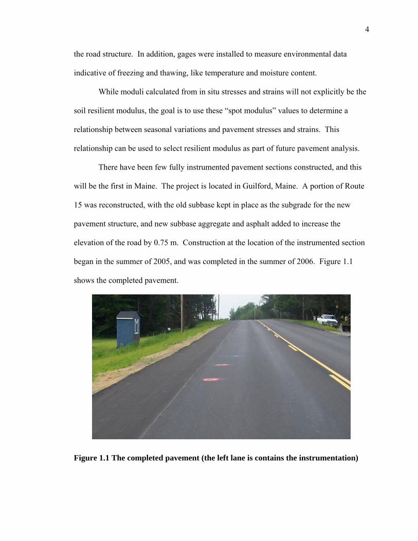
will be the first in Maine. The project is located in Guilford, Maine. A portion of Route
15 was reconstructed, with the old subbase kept in place as the subgrade for the new
pavement structure, and new subbase aggregate and asphalt added to increase the
elevation of the road by 0.75 m. Construction at the location of the instrumented section
began in the summer of 2005, and was completed in the summer of 2006. Figure 1.1
shows the completed pavement.
Figure 1.1 The completed pavement (the left lane is contains the instrumentation)

5
1.4 Organization of this Report
This thesis is divided into seven chapters, each describing different aspects of the
project. Chapter 2 is a literature review giving the definition of the resilient modulus and
current methods for calculating the value. Eight other field instrumentation projects are
also discussed.
Chapter 3 provides a description of the different gages that were installed as part
of the project. Each type of gage required different installation methods, which are also
included in the section. Chapter 4 gives more information about the overall construction
and installation process. Construction plans and additional material properties are
included in the appendices. The data acquisition system that was put in place after gage
installation is described in Chapter 5.
The results of the project are included in Chapter 6. This data includes both
environmental and pavement stress and strain values. Typical data is included in the
chapter, and graphs showing stress and strain data are included in the appendices.
Comparisons are made using data taken during the first half of the year 2006, and the
chapter also includes a discussion of these results. Chapter 7 includes a summary and
conclusions for the project. Recommendations for the continuation of the project and for
future pavement instrumentation are included.

6
Chapter 2
LITERATURE REVIEW
2.1 Introduction
The properties of the layers of asphalt and underlying granular material that make
up pavement systems need to be carefully considered for road design and maintenance.
Resilient moduli of asphalt, aggregate base, and subbase layers, are used by engineers to
predict how pavement layers will respond to traffic loading. The 1993 AASHTO Guide
for Design of Pavement Structures and the new Mechanistic Empirical Pavement Design
Guide (M-EPDG) from AASHTO and the National Cooperative Highway Research
Program both identify resilient modulus as the most important property required for the
design of pavement structures. Resilient modulus can be a complex value to obtain, and
in cold regions variations in pavement section stiffness due to seasonal changes in
temperature and moisture complicate the characterization of properties like moduli even
further.
This literature review will discuss the definition of resilient modulus and the
effect of cold climate on pavement section properties. Methods used for measuring or
computing moduli and other important properties will be described, along with field
instrumentation projects that have been carried out across the country in an attempt to
collect in situ data that can be used both for direct analysis and for the verification of
numerical models.

7
2.2 Definition of Resilient Modulus of Soil Materials
Resilient modulus (Mr) represents the stiffness of soil layers, replacing an
empirical “soil support value” that was used in earlier design procedures (Drumm, et al.,
1997). Resilient modulus is a form of the elastic modulus of a soil. The value is based
on recoverable strain experienced due to repeated loading from an unconfined
compression or triaxial compression test. In these types of tests, a soil sample is
subjected to cycles of loading, and the deformation or strain is recorded as the loading
cycle is repeated. The axial stress in an unconfined compression test or the axial stress
minus the confining stress in a triaxial compression test is divided by the recoverable
strain to obtain a value of resilient modulus (Joshi and Malla, 2006).
Hjelmstad and Taciroglu (2000) specifically looked at the behavior of granular
soil undergoing repeated loading in a triaxial test to define Mr. When a soil sample is
tested, the initial loading cycles produce inelastic deformations. As loading cycles
continue, the amount of plastic deformation decreases, until after a certain number of
cycles the response of the soil sample is elastic. This “shake down” is visible in Figure
2.1. On the cylindrical sample shown, σ1 is the axial stress and σ2 is the confining
pressure. The deviator stress is defined here as the axial stress minus the confining
pressure σ1 – σ2. As the loading cycles progress, the strain response becomes less plastic.
Once the soil experiences elastic deformation, the slope of the stress versus strain curve is
the resilient modulus.
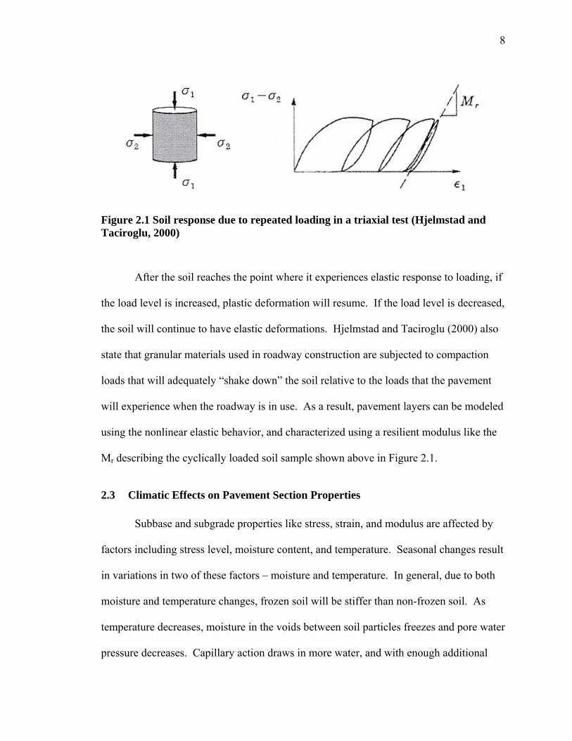
8
Figure 2.1 Soil response due to repeated loading in a triaxial test (Hjelmstad and Taciroglu, 2000)
After the soil reaches the point where it experiences elastic response to loading, if
the load level is increased, plastic deformation will resume. If the load level is decreased,
the soil will continue to have elastic deformations. Hjelmstad and Taciroglu (2000) also
state that granular materials used in roadway construction are subjected to compaction
loads that will adequately “shake down” the soil relative to the loads that the pavement
will experience when the roadway is in use. As a result, pavement layers can be modeled
using the nonlinear elastic behavior, and characterized using a resilient modulus like the
Mr describing the cyclically loaded soil sample shown above in Figure 2.1.
2.3 Climatic Effects on Pavement Section Properties
Subbase and subgrade properties like stress, strain, and modulus are affected by
factors including stress level, moisture content, and temperature. Seasonal changes result
in variations in two of these factors – moisture and temperature. In general, due to both
moisture and temperature changes, frozen soil will be stiffer than non-frozen soil. As
temperature decreases, moisture in the voids between soil particles freezes and pore water
pressure decreases. Capillary action draws in more water, and with enough additional
9
water, ice lenses can form, adding to the soil layer stiffness. This additional water will
cause a reduction in soil stiffness when the ice lenses thaw. Frozen soil layers and excess
water during thawing are variations that can make the analysis of parameters like layer
modulus difficult for projects in cold regions (Janoo and Berg, 2002).
Tests have been done to try to quantify the effect of freeze-thaw cycles on
resilient modulus. According to results discussed by Janoo and Berg (2002), for frozen
soil, modulus increases as the temperature decreases, reaching a maximum modulus at
approximately -8°C. Laboratory testing described by Simonsen, et al. (2002) also noted
that the most significant increase in modulus occurrs between 0 and -5°C. At lower
temperatures, the modulus will continue to increase, only at a much slower rate. The
same study showed that for a variety of soil types, the resilient modulus increased by a
factor of 10 to 600 when a soil was changed from room temperature to -10°C.
For thawing soils, the resilient modulus reaches its lowest point near complete
saturation, but rebounds back to an equilibrium point for saturation between 50 and 80%
(Janoo and Berg, 2002). After the freeze-thaw cycle, the modulus decreases 20 to 60%
depending on the soil type (Simonsen, et al., 2002). The modulus for thawed soil was
also stress dependent, increasing with increasing stress for granular soils, and decreasing
with increasing stress for fine grained soils. Moduli of the tested soils increased with
increasing density (Janoo and Berg, 2002).
Testing has been done, and more is required to develop better methods to account
for climate effects in the calculation of resilient modulus. Different roadway designs and
locations will experience climatic effects differently, and even changes in weather from
year to year will produce varying results.

10
2.4 Modulus Calculation Methods
There are a variety of methods used to determine layer resilient moduli. In the
“AASHTO Guide for Mechanistic-Empirical Design of New and Rehabilitated Pavement
Structures” (AASHTO, 1993), laboratory testing procedures are specified for obtaining
the most accurate results. For intermediate accuracy, correlations can be made to
calculate resilient modulus from other soil properties. To determine in situ moduli a
direct measurement method would be ideal but is impractical. Instead, backcalculation
techniques have been developed to calculate resilient modulus from field measurements.
2.4.1 Laboratory Testing
Repeated loading resilient modulus testing like the triaxial test mentioned earlier
can be used to calculate resilient modulus. AASHTO’s Standard Method of Test for
Determining the Resilient Modulus of Soils and Aggregate Materials, T307-99
(AASHTO, 2001) is the accepted resilient modulus laboratory procedure. Figure 2.2
shows a typical triaxial setup following the AASHTO specifications. A load cell with a
repeated load actuator applies cyclic haversine-shaped load pulses to the specimen.
Linear variable differential transformer (LVDTs) measure the deformation of the soil
sample during loading. The AASHTO specification provides procedures for the
preparation of test specimens, the resilient modulus test for subgrade soils, and the
resilient modulus test for subbase soils.
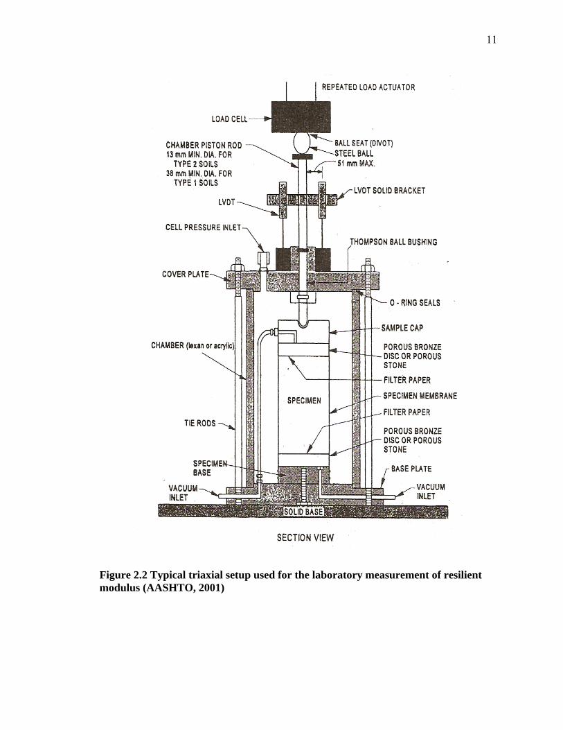
11
Figure 2.2 Typical triaxial setup used for the laboratory measurement of resilient modulus (AASHTO, 2001)

12
Laboratory tests are beneficial because conditions can be modified to test soils in
different temperature and moisture states. Temperature and moisture differences can be
tested in the laboratory in a much shorter time span than actual seasonal variations will
occur.
Accurately testing soil samples in the lab can be difficult, mainly because
laboratory conditions can never exactly represent the in situ conditions. The testing
procedures are also very expensive. Laboratory testing is often carried out as a
supplement to other methods of modulus determination. Lab results have been used to
verify resilient modulus results from mathematical models, and laboratory Mr values can
also be used as input “seed” modulus values for the field backcalculation procedure that
will be described later.
In New Hampshire, five soil samples were compacted at their optimum water
contents, and cyclically loaded in a triaxial cell. The soils ranged from fine-grained
marine clay and silty fine sand to coarse gravelly sand and glacial till, and each soil was
tested at its optimum water content. For this test series, the triaxial cells were placed in a
mechanically cooled climate chamber so that the effect of changes in temperature on
modulus could be observed. The triaxial test was a closed system, and no water was
added to or removed from the sample during the test. The results of these tests varied for
different soil types, but in general the results showed the trends of increasing stiffness for
freezing soils, and reducing stiffness for thawing soils. This difference in modulus can be
seen in Figure 2.3. When the freeze-thaw cycle takes place, there is a net volume
increase in the soil, and as the material thaws, it has a looser structure, and a lower
modulus (Simonsen et al., 2002).
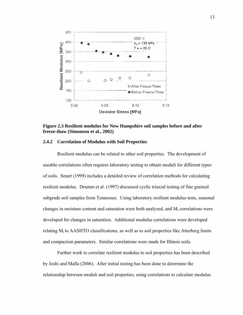
13
Figure 2.3 Resilient modulus for New Hampshire soil samples before and after freeze-thaw (Simonsen et al., 2002)
2.4.2 Correlation of Modulus with Soil Properties
Resilient modulus can be related to other soil properties. The development of
useable correlations often requires laboratory testing to obtain moduli for different types
of soils. Smart (1999) includes a detailed review of correlation methods for calculating
resilient modulus. Drumm et al. (1997) discussed cyclic triaxial testing of fine grained
subgrade soil samples from Tennessee. Using laboratory resilient modulus tests, seasonal
changes in moisture content and saturation were both analyzed, and Mr correlations were
developed for changes in saturation. Additional modulus correlations were developed
relating Mr to AASHTO classifications, as well as to soil properties like Atterberg limits
and compaction parameters. Similar correlations were made for Illinois soils.
Further work to correlate resilient modulus to soil properties has been described
by Joshi and Malla (2006). After initial testing has been done to determine the
relationship between moduli and soil properties, using correlations to calculate modulus

14
is a less expensive alternative to direct lab or field testing. Also, depending on the
properties that are correlated, seasonal variations in resilient modulus can be modeled.
For this work, the M-EPDG constitutive model for calculating resilient modulus was used
as the starting point.
32
1
k
a
oct
k
aaR PP
PkM ⎟⎟⎠
⎞⎜⎜⎝
⎛⎟⎟⎠
⎞⎜⎜⎝
⎛=
τθ (2.1)
In this equation, Pa is a normalizing stress (atmospheric pressure equal to 101.325 kPa at
sea level), θ is the bulk stress, and τoct is the octahedral shear stress. Regression
coefficients, k1, k2, and k3 vary depending on soil properties. For their work, Joshi and
Malla (2006) used linear regression first to calculate the three k values for different soil
samples. A second regression analysis was used to relate k to a variety of properties
including:
• Specimen and optimum moisture contents, and the ratio between the two values
• Specimen and optimum dry density, and the ratio between the two values
• Liquid limit
• Plastic limit
• Percent passing 75 mm, 50.8 mm, 37.5 mm, 25.4 mm, 19 mm, 12.7 mm,9.5 mm,
#4, #10, #40, #80, and #200 sieves
• Percent coarse sand (2-0.42 mm)
• Percent fine sand (0.42-0.074mm)
• Percent silt (0.074-0.002mm)
• Percent clay (0.002mm)

15
For different AASHTO soil types, equations for the calculation of the three k
values were developed in terms of these soil properties. A comparison between resilient
modulus predicted using regression coefficients calculated with these equations and
modulus values from laboratory testing showed good comparisons for A-1-b soils, while
for other AASHTO classifications, soils did not show comparable results.
2.4.3 Backcalculation
While there are different techniques used to find resilient modulus, a widely
accepted method is the backcalculation of moduli from field measurements. In order to
perform backcalculation, in situ deflection data is required. Equipment that has been
used in studies to determine in situ layer moduli includes the Benkelman beam, the Road
Rater, and the accelerometer, however the most commonly used device is the falling
weight deflectometer (FWD). This device measures deflection due to loading and
backcalculation can be carried out using the collected data.
The backcalculation of resilient moduli from FWD data involves six steps:
1) collecting data
2) choosing an analytical model
3) choosing a material model
4) choosing a method for implementing the models
5) using an optimization technique to solve the models
6) analyzing and using the backcalculated moduli results
These six steps will be discussed in detail.
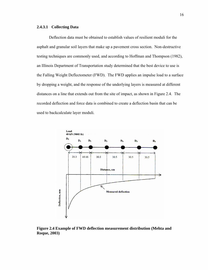
16
2.4.3.1 Collecting Data
Deflection data must be obtained to establish values of resilient moduli for the
asphalt and granular soil layers that make up a pavement cross section. Non-destructive
testing techniques are commonly used, and according to Hoffman and Thompson (1982),
an Illinois Department of Transportation study determined that the best device to use is
the Falling Weight Deflectometer (FWD). The FWD applies an impulse load to a surface
by dropping a weight, and the response of the underlying layers is measured at different
distances on a line that extends out from the site of impact, as shown in Figure 2.4. The
recorded deflection and force data is combined to create a deflection basin that can be
used to backcalculate layer moduli.
Figure 2.4 Example of FWD deflection measurement distribution (Mehta and Roque, 2003)

17
2.4.3.1.1 Preprocessing
After data has been collected, preprocessing can be used to improve the final back
calculated analysis. Techniques for dividing a length of roadway into subsections with
similar properties have been described by Sebaaly, et al. (2000), Grogan, et al. (1998),
and Hassan, et al. (2003). Grogan, et al. (1998) also described a normalization technique
so that the data points in a deflection basin correspond to a single load.
2.4.3.1.2 Additional Required Information
In addition to deflection data, other information about a roadway section is
needed to carry out backcalculation. The construction and maintenance history of a
roadway and the pavement profiles are important characteristics that can contribute to
variations in moduli (Grogan, et al., 1998). Sebaaly, et al. (2000) suggests using
construction records to determine the thickness of base and subbase layers, and taking
field cores to find the asphalt thickness. Material classifications, as well as temperature
and traffic data, may also be needed for the backcalculation procedure. Different
backcalculation and analysis procedures require varying amounts of information.
2.4.3.2 Analytical Model
The resilient modulus backcalculation process requires a step for calculating
deflections based on input seed moduli. Typical procedures use input values to create
deflection basins that can be compared to the collected data. There are different
calculation models available, including variations of layered elastic and finite element
theories, and many are built into computer programs that run through entire
backcalculation routines.

18
2.4.3.2.1 Burmister’s Layered Theory
Due to the layered structure of pavement sections, a layered elastic approach to
analysis is appropriate. According to Huang, (2004), Burmister’s layered theory is one
approach that is used for pavement design. The method can be used for a pavement
cross section that contains any number of layers each defined by a modulus and a
Poisson’s ratio. For the analysis, the section is loaded by a uniform force q, over a
circular area with radius a.
This procedure is implemented in the computer program KENLAYER for flexible
pavement design for layered elastic calculations. A governing differential equation exists
for the layered elastic model. Cylindrical coordinates, r in the radial direction and z in
the vertical direction, are used in the equation.
(2.2)
(2.3) To solve using the elastic method, a stress function, φ, which satisfies the
differential equation and given boundary and continuity conditions, is assumed. The
stresses and displacements in the pavement section can be calculated in terms of the
stress function, and the boundary and continuity conditions described here. The first
boundary condition is that the vertical stress underneath the circular load is equal to a
force, q. The second boundary condition is that there is no shear stress on the surface.
For a pavement cross section with n layers, 4(n-1) continuity conditions are used, where n
is the number of layers. These values correspond to the continuity of four factors:

19
vertical stress, vertical displacement, shear stress, and radial displacement at the
interfaces between layers. For example, a pavement cross section with three layers has
two layer interfaces and eight continuity conditions.
2.4.3.2.2 Modified Boussinesq Theory
The Boussinesq theory for an elastic half space is typically used to analyze a
homogenous mass (Huang, 2004), but combining the technique with the method of
equivalent thicknesses makes it applicable to multi-layered pavement systems. Zhou, et
al. (1990) discussed the BOUSDEF computer program that used the equivalent
thickness/Boussinesq combination as part of a moduli backcalculation technique.
The method of equivalent thicknesses states that multiple layers can be converted
into a single layer using a relationship that involves the modulus, E, Poisson’s ratio, µ,
and layer thickness, h. For a multilayered system like pavement, the equivalent thickness
of the ith layer is defined as
3/1
2
21
1 )1()1(
* ⎥⎦
⎤⎢⎣
⎡−−
∗=∑−
= i
n
n
in
iiei E
Ehh
µµ
(2.4)
Realistically, the modulus within a given layer in a pavement section should change as
depth increases, but using the method of equivalent thicknesses does not take this change
into account.
A correction factor is applied to the calculated equivalent thickness before the
value is used in a Boussinesq equation. This ensures that the results of the modified
Boussinesq method are comparable to an exact elastic theory. Once a layered pavement
system has been reduced to a single, corrected equivalent thickness, the Boussinesq
equations for deflection and stress can be used. The BOUSDEF computer program

20
performs these calculations as part of a routine to backcalculate pavement layer moduli.
Specifically, the program has a subroutine called DEFLECTION that runs through the
modified equivalent thickness/Boussinesq procedure.
2.4.3.2.3 Finite Element Method
As an alternative to layered elastic analysis, finite element methods can be used
for modulus calculation in a backcalculation procedure. According to Chou and Lytton
(1991), finite elements result in a more accurate solution in certain cases, but there are
many unknown parameters that make the process difficult and time consuming to
complete. There have also been some problems with using finite element analysis for
granular materials, but the method is still being developed for use in some
backcalculation programs.
The ILLI-PAVE program divides the pavement section into concentric rings and
uses finite elements to develop an axisymmetric solid of revolution that can be used for
modulus calculation. (Hoffman and Thompson, 1982; Huang, 2004)
FENLAP is a nonlinear finite element program used for pavement analysis
(Brunton and Almeida, 1991). With this program, initial stress characteristics are
determined based on material weights and initial site conditions. Stress due to loading is
calculated and used to determine new moduli. An iterative process is used until a stable
solution is found where all nonlinear elements in the finite element model have about the
same moduli.
With advances in computer systems, analysis capabilities have improved, and
accurate finite element models are being used more effectively. Finite element analysis is

21
mainly being considered for backcalculation because of its ability to model nonlinear
material behavior better than layered analysis.
2.4.3.3 Material Model
Pavement layers are nonlinear elastic or viscoelastic, but linear analysis methods
are typically used to construct approximate models that represent layers within a
pavement system. Although linear elastic theory does not exactly represent the actual
characteristics of pavement layers, the final values obtained with backcalculation are
accurate. In most cases, a nonlinear analysis does not lead to better results because many
assumptions need to be made in the backcalculation process (Mehta and Roque, 2003)
but nonlinear considerations are still made in some cases, especially for finite element
backcalculation techniques.
2.4.3.3.1 Linear
In linear elastic theory, material deformations are described by two values, the
elastic modulus and Poisson’s ratio. Values for Poisson’s ratio can usually be assumed,
leaving the elastic modulus, or the resilient modulus in the case of subgrade and subbase
design, as the only value that remains to be calculated. As long as the number of surface
deflections is equal to the number of pavement cross section layers with unknown
moduli, a linear elastic relationship can be used to calculate deflections in terms of input
initial moduli. (Chou and Lytton, 1991) The KENLAYER elastic layer program for
implementing Burmister’s Theory, described in the previous section, can be used to
analyze pavement as a linear system.
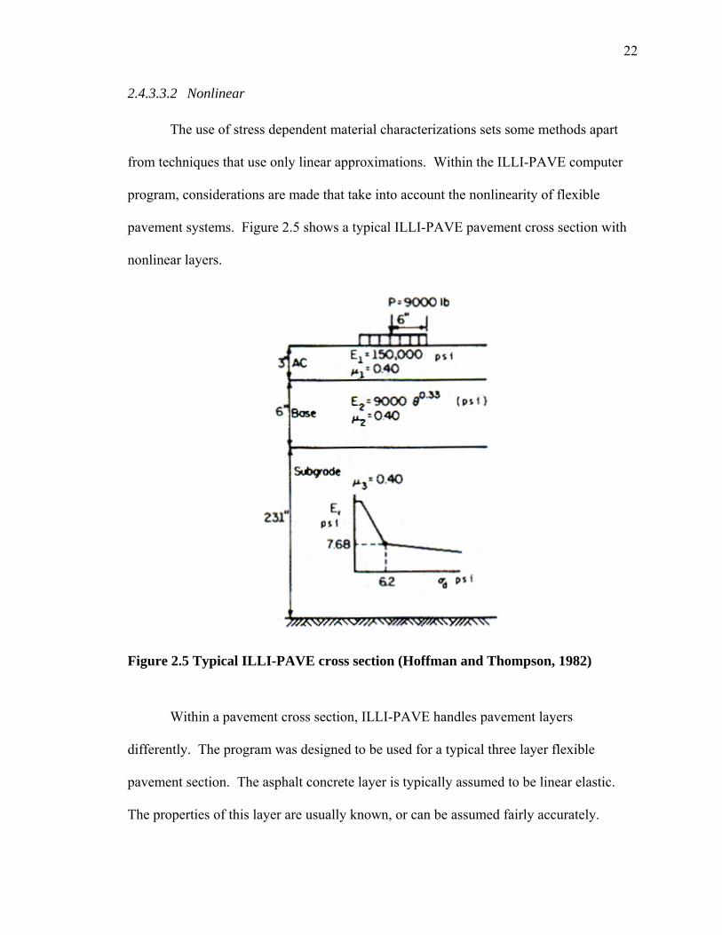
22
2.4.3.3.2 Nonlinear
The use of stress dependent material characterizations sets some methods apart
from techniques that use only linear approximations. Within the ILLI-PAVE computer
program, considerations are made that take into account the nonlinearity of flexible
pavement systems. Figure 2.5 shows a typical ILLI-PAVE pavement cross section with
nonlinear layers.
Figure 2.5 Typical ILLI-PAVE cross section (Hoffman and Thompson, 1982)
Within a pavement cross section, ILLI-PAVE handles pavement layers
differently. The program was designed to be used for a typical three layer flexible
pavement section. The asphalt concrete layer is typically assumed to be linear elastic.
The properties of this layer are usually known, or can be assumed fairly accurately.
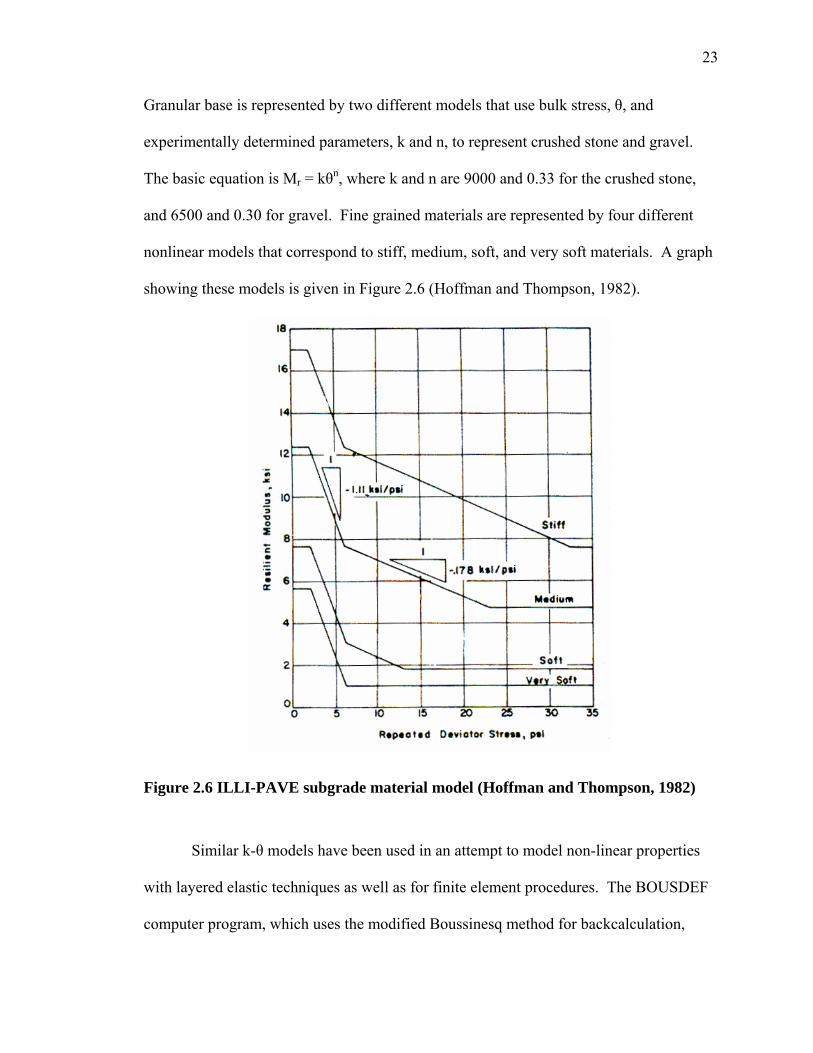
23
Granular base is represented by two different models that use bulk stress, θ, and
experimentally determined parameters, k and n, to represent crushed stone and gravel.
The basic equation is Mr = kθn, where k and n are 9000 and 0.33 for the crushed stone,
and 6500 and 0.30 for gravel. Fine grained materials are represented by four different
nonlinear models that correspond to stiff, medium, soft, and very soft materials. A graph
showing these models is given in Figure 2.6 (Hoffman and Thompson, 1982).
Figure 2.6 ILLI-PAVE subgrade material model (Hoffman and Thompson, 1982)
Similar k-θ models have been used in an attempt to model non-linear properties
with layered elastic techniques as well as for finite element procedures. The BOUSDEF
computer program, which uses the modified Boussinesq method for backcalculation,

24
considers Mr = k1θk2 in terms of bulk stress for coarse grained materials, and Mr = k1σd
k2
in terms of deviator stress for fine grained materials. The k coefficients vary depending
on material properties, and are based on laboratory test results (Zhou, et al., 1990).
2.4.3.4 Model Implementation
After analytical and material models are chosen for a backcalculation procedure, a
method needs to be chosen to implement the techniques. Some programs run multiple
iterations of these methods to obtain a solution, while other programs use solutions that
have been previously solved and stored in databases.
One computer program that utilizes a linear elastic calculation method is called
MODULUS. Scullion, et al. (1990) described the program, which can be run in three
different formats depending on the amount of information that a designer can input. The
first option utilizes a database of previously calculated deflection basins, and linear
elastic calculations are not carried out for the specific pavement section being analyzed.
Instead the database solution for a pavement cross-section with properties that closely
match the project cross section is chosen. With this implementation method, many
assumptions have to be made, possibly sacrificing accuracy but improving calculation
time.
A second option works well when more information is known, but not all of the
required parameters can be input. In this case, the linear elastic equations are used to
create a new database of deflection basins based on the information that is known about a
length of roadway. The database contains solutions for different variations of any
unknown parameters.

25
When the necessary data for linear elastic analysis is known, or can be assumed
for input, the third option of the MODULUS program is the best choice. In this case a
full analysis is completed for each iterative step of backcalculation. Many
backcalculation programs use this method of model implementation.
The ILLI-PAVE finite element program is ultimately used to create a database of
potential pavement layer conditions that correspond to modulus values. A database of
144 combinations can be created using four variables – asphalt thickness and modulus,
granular base thickness, and subgrade modulus. By creating a database of values to use
for backcalculation purposes, ILLI-PAVE can be used much more efficiently than
programs that require time consuming computer analysis (Hoffman and Thompson,
1982).
2.4.3.5 Comparison Criteria – Solving the Models
The basis for most backcalculation procedures is the comparison of a measured
deflection basin to a number of calculated basins. The calculated basin that best matches
the collected FWD data is chosen, and the input moduli that correspond to the calculated
basin are the moduli of the tested pavement section.
To choose the correct deflection basin, backcalculation programs implement a
variety of numerical routines that include iterative techniques and statistical regression
equations. The comparison criteria vary from program to program, but the goal of
finding the deflections that correspond to measured data is the same.
Zhou, et al (1990) gives a general explanation of the iterative process of
comparing calculated and measured deflections, which is summarized in Figure 2.7.
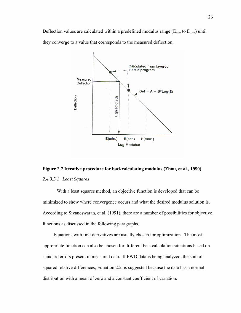
26
Deflection values are calculated within a predefined modulus range (Emin to Emax) until
they converge to a value that corresponds to the measured deflection.
Figure 2.7 Iterative procedure for backcalculating modulus (Zhou, et al., 1990)
2.4.3.5.1 Least Squares
With a least squares method, an objective function is developed that can be
minimized to show where convergence occurs and what the desired modulus solution is.
According to Sivaneswaran, et al. (1991), there are a number of possibilities for objective
functions as discussed in the following paragraphs.
Equations with first derivatives are usually chosen for optimization. The most
appropriate function can also be chosen for different backcalculation situations based on
standard errors present in measured data. If FWD data is being analyzed, the sum of
squared relative differences, Equation 2.5, is suggested because the data has a normal
distribution with a mean of zero and a constant coefficient of variation.

27
(2.5) In this equation, di
m is the measured deflection at location i, and dic(E,h) is the calculated
deflection at location i, based on E, unknown moduli of the pavement section layers, and
h, the unknown layer thicknesses.
Sivaneswaran, et al. (1991) used a nonlinear least squares optimization method
that involved the Levenberg-Marquardt technique. An approximation to the Hessian used
in this numerical method causes the solution for modulus to converge more rapidly than
with other techniques.
Harichandran, et al. (1993) used a slightly different objective function and
iterative technique. The function to be minimized is written in terms of measured
deflection, wj, calculated deflection jw) , and a weighted factor, α:
[ ]∑=
−=m
jjjj wwf
1
2)α (2.6)
For the optimization procedure, a modified Newton’s method was adopted. For a
pavement layer modulus backcalculation problem, this method will converge even if the
initial guess is poor. Looking at a simple example for pavement section consisting of
only one layer, a curve of deflection versus modulus can be graphed (see Figure 2.8). An
approximate slope can be determined from this graph, and can used to define the change
in moduli for different iterations.
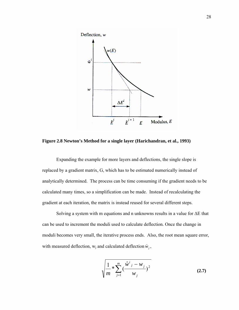
28
Figure 2.8 Newton’s Method for a single layer (Harichandran, et al., 1993)
Expanding the example for more layers and deflections, the single slope is
replaced by a gradient matrix, G, which has to be estimated numerically instead of
analytically determined. The process can be time consuming if the gradient needs to be
calculated many times, so a simplification can be made. Instead of recalculating the
gradient at each iteration, the matrix is instead reused for several different steps.
Solving a system with m equations and n unknowns results in a value for ∆E that
can be used to increment the moduli used to calculate deflection. Once the change in
moduli becomes very small, the iterative process ends. Also, the root mean square error,
with measured deflection, wj and calculated deflection jw) ,
∑=
−m
j j
jji
www
m 1
2)ˆ
(*1 (2.7)

29
is calculated to show that the computed and measured deflections are similar. For the
MICHBACK program described by Harichandran, a convergence criterion of 0.1% was
used.
2.4.3.5.2 System Identification Process
The general term for the technique of minimizing error between measured data
and a calculated model is system identification (Wang and Lytton, 1993). Within this
process, the strategy that is used for backcalculation is called the forward method, where
inputs are given, and the error between outputs is minimized. An inverse procedure also
exists where the error between inputs is minimized instead, but this method is more
complicated. For the system identification process, an iterative procedure based on a
Taylor Series expansion is used to recalculate specific parameters, until the error between
measured deflections and calculated deflections is minimized.
2.4.3.5.3 Curvature Approach
According to Mehta and Roque, (2003), minimizing error between collected and
calculated deflections is not the most accurate method. Instead, the curvature of
deflection basins, which is related to the stiffness of the material being analyzed, needs to
be compared and matched.
The procedure of matching the curvature involves multiple steps. First, the
measured deflection located the farthest from the applied load of the FWD needs to be
matched with a calculated deflection. This is done by varying the subgrade modulus.
Next, the deflection basins need to be compared to make sure that the measured and

30
computed basins do not cross each other at any point. After this has been ensured,
another point needs to correspond between the measured and calculated basins.
Although matching curvature is a more precise backcalculation option, little
information has been published about the technique. The optimization and convergence
methods described here have been used for backcalculation, and more techniques exist.
There is no one method that has been found to be the best for resilient moduli
backcalculation.
2.4.3.6 Analysis and Use of Backcalculated Solution
After a backcalculation procedure has been used, an analysis of the resilient
modulus solution needs to be carried out. The moduli that are calculated should be
checked to make sure that they fall between preset minimum and maximum values.
Moduli should also be compared to typical values, usually moduli obtained from
laboratory testing, to ensure that the backcalculated answer is realistic.
With some backcalculation techniques, there is the potential for obtaining more
than one answer for the same set of initial conditions. In the optimization step of the
backcalculation procedure, minimizing an objective function may not result in the
absolute minimum when local minimum values are present in the data. The MODULUS
backcalculation program has a convexity test that can be used to check for the presence
of local minimum values (Scullion, et al., 2000).
After resilient moduli have been calculated they can be used for additional
analysis. Grogan, et al. (1998) use layer moduli with traffic data to calculate stresses and
strains for the pavement system. Resilient modulus is also an input in AASHTO
pavement design procedures.

31
2.5 Pavement Section Property Verification by In Situ Instrumentation
Verification of FWD measurements and resilient modulus backcalculation can be
achieved in the field using instrumentation such as strain gages and pressure cells. There
are a number of instrumented roads being studied by departments of transportation and
research organizations in Minnesota, Pennsylvania, Virginia, Georgia, and other areas.
2.5.1 Minnesota Road Research Project
The Minnesota Road Research Project (MnROAD) consists of 40 test roadway
sections located 65 km west of Minneapolis-St. Paul. The test cells, as they are referred
to by MnROAD, are located on a mainline roadway as well as in a test loop constructed
for use with calibrated vehicles. For one MnROAD project, FWD tests were carried out
directly over strain gages installed at the bottom of the asphalt layer. Comparing the
FWD and strain gage data showed that strains resulting from FWD loading exhibited
linear elastic properties, validating the use of linear elastic methods for the
backcalculation of resilient modulus (Siddharthan, 2002).
MnROAD also installed temperature and moisture gages in some of the test cells.
With these gages, seasonal changes in temperature and moisture contents were recorded
along with FWD readings. A modified integrated climate model (ICM) was used to
make predictions of temperature, moisture content, and layer moduli, and these values
were compared with measured in situ values. There were good correlations between
measured and predicted values.
MnROAD’s project combined lab testing, FWD backcalculation, and field
instrumentation. Even with these three components, some soil parameters like dry
thermal conductivity, dry heat capacity, and coefficient of volume compressibility had to
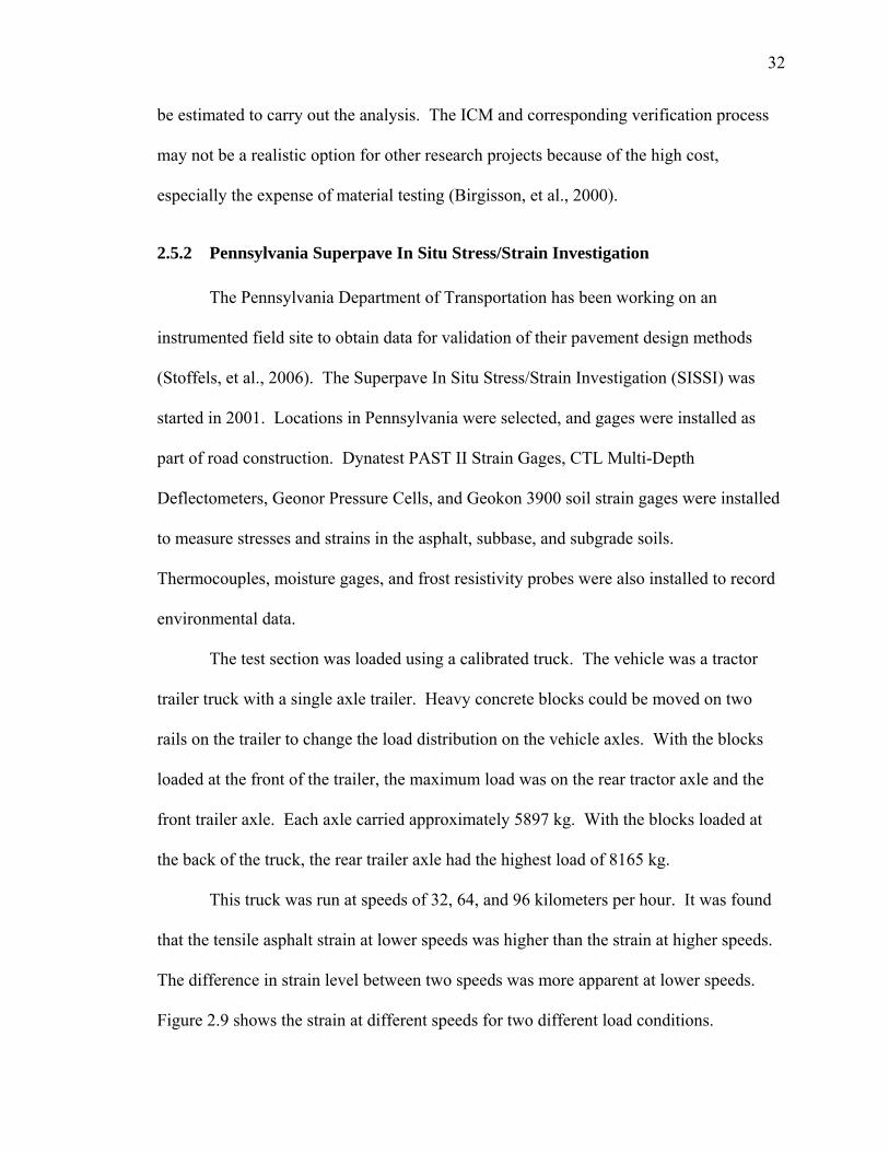
32
be estimated to carry out the analysis. The ICM and corresponding verification process
may not be a realistic option for other research projects because of the high cost,
especially the expense of material testing (Birgisson, et al., 2000).
2.5.2 Pennsylvania Superpave In Situ Stress/Strain Investigation
The Pennsylvania Department of Transportation has been working on an
instrumented field site to obtain data for validation of their pavement design methods
(Stoffels, et al., 2006). The Superpave In Situ Stress/Strain Investigation (SISSI) was
started in 2001. Locations in Pennsylvania were selected, and gages were installed as
part of road construction. Dynatest PAST II Strain Gages, CTL Multi-Depth
Deflectometers, Geonor Pressure Cells, and Geokon 3900 soil strain gages were installed
to measure stresses and strains in the asphalt, subbase, and subgrade soils.
Thermocouples, moisture gages, and frost resistivity probes were also installed to record
environmental data.
The test section was loaded using a calibrated truck. The vehicle was a tractor
trailer truck with a single axle trailer. Heavy concrete blocks could be moved on two
rails on the trailer to change the load distribution on the vehicle axles. With the blocks
loaded at the front of the trailer, the maximum load was on the rear tractor axle and the
front trailer axle. Each axle carried approximately 5897 kg. With the blocks loaded at
the back of the truck, the rear trailer axle had the highest load of 8165 kg.
This truck was run at speeds of 32, 64, and 96 kilometers per hour. It was found
that the tensile asphalt strain at lower speeds was higher than the strain at higher speeds.
The difference in strain level between two speeds was more apparent at lower speeds.
Figure 2.9 shows the strain at different speeds for two different load conditions.
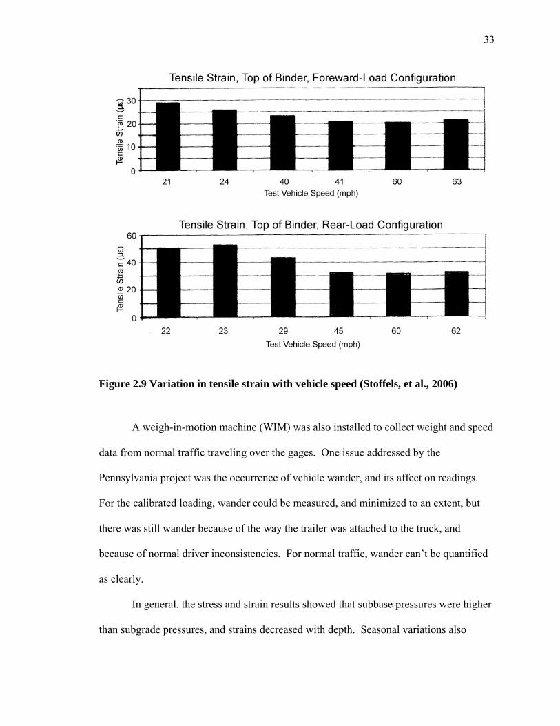
33
Figure 2.9 Variation in tensile strain with vehicle speed (Stoffels, et al., 2006)
A weigh-in-motion machine (WIM) was also installed to collect weight and speed
data from normal traffic traveling over the gages. One issue addressed by the
Pennsylvania project was the occurrence of vehicle wander, and its affect on readings.
For the calibrated loading, wander could be measured, and minimized to an extent, but
there was still wander because of the way the trailer was attached to the truck, and
because of normal driver inconsistencies. For normal traffic, wander can’t be quantified
as clearly.
In general, the stress and strain results showed that subbase pressures were higher
than subgrade pressures, and strains decreased with depth. Seasonal variations also
34
affected the response of the pavement section, and the environmental data collected from
the instrumented sites was available for the analysis of freeze-thaw issues. Figure 2.10
shows the variation of tensile strain with both depth and season.
Figure 2.10 Variation in tensile strain for different layers of the pavement system before and after the freeze-thaw system (Stoffels, et al., 2006)
2.5.3 Virginia Smart Road
The Virginia Smart Road is an extensive testing facility located in Blacksburg,
Virginia. The road’s instrumented sections have more than 500 instruments installed.
The gages were installed during construction, providing more accurate field conditions
than instruments that are installed into existing pavement systems (Diefenderfer, el al.,
2003).
The pavement sections contain gages to measure strains, stresses, deflections,
moisture, and temperature. RST pressure cells measure vertical stresses in asphalt,
subbase and subgrade layers. Dynatest PAST-II strain gages measure strains in the
asphalt and vibrating wire Geokon VCE-4200 strain gages measure strains in the soil

35
layers. Thermocouples were installed to measure temperature, and resistivity probes
measure frost depth. Time Domain Reflectometry gages measure volumetric water
content (Al-Qadi, et al., 2004). The stress and strain gages were installed in the wheel
path, while the environmental gages were installed in the roadway centerline (Loulizi, et
al., 2001).
Looking at data collected from the gages for a calibrated test truck, Al-Qadi, et al.
(2004) made some observations about the pavement section responses. A normalized
form of the vertical compressive stress pulse can be represented by a Haversine equation.
The values of both vertical compressive stresses and horizontal strains under the asphalt
layer are affected by temperature, while speed affects the magnitude of horizontal strain
and only the load duration for vertical stress.
Data from the instrumented section also provided field results to compare with
predicted results. Using linear elastic theory to model responses typically overestimates
pavement section responses at low temperatures, and underestimates responses at high
temperatures. A comparison of horizontal transverse asphalt strain measured at two
different speeds to strains calculated using three dimensional finite element analysis can
be seen in Figure 2.11.
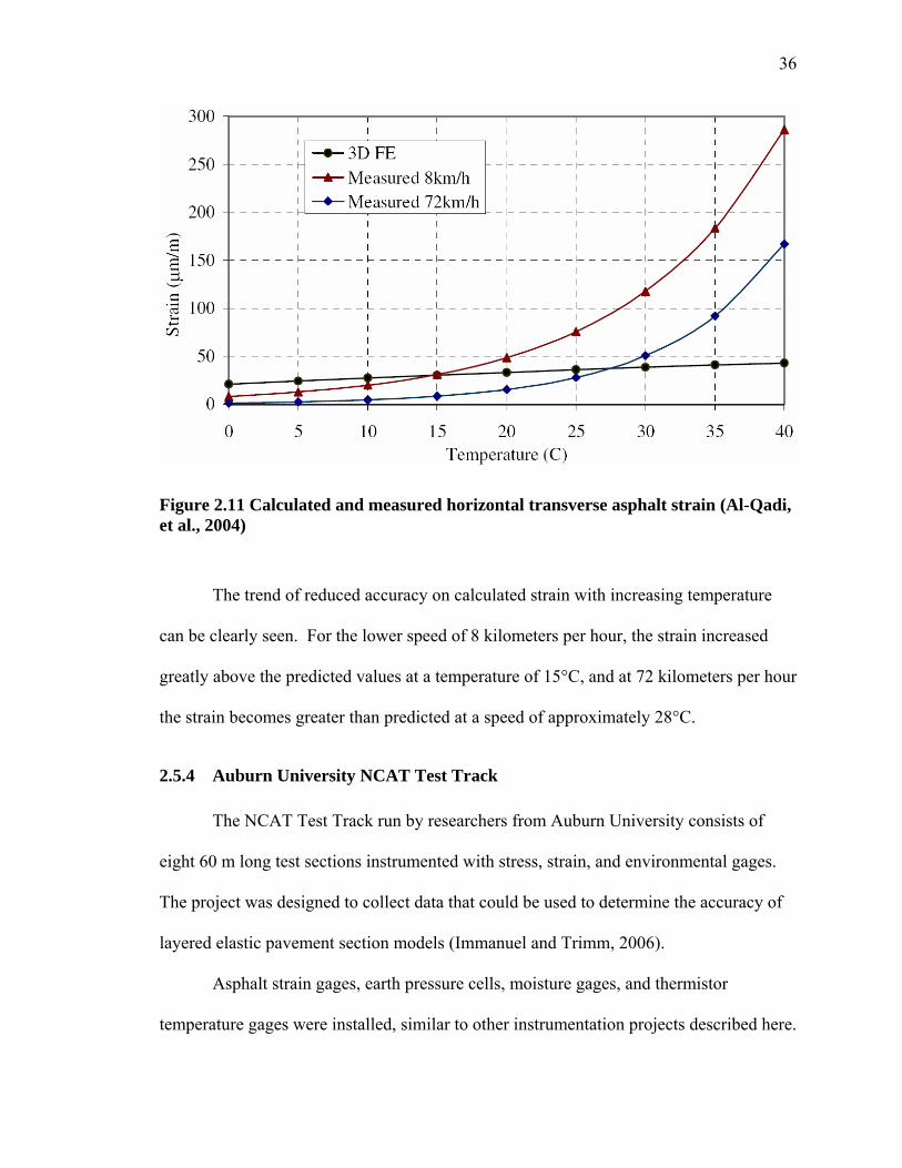
36
Figure 2.11 Calculated and measured horizontal transverse asphalt strain (Al-Qadi, et al., 2004)
The trend of reduced accuracy on calculated strain with increasing temperature
can be clearly seen. For the lower speed of 8 kilometers per hour, the strain increased
greatly above the predicted values at a temperature of 15°C, and at 72 kilometers per hour
the strain becomes greater than predicted at a speed of approximately 28°C.
2.5.4 Auburn University NCAT Test Track
The NCAT Test Track run by researchers from Auburn University consists of
eight 60 m long test sections instrumented with stress, strain, and environmental gages.
The project was designed to collect data that could be used to determine the accuracy of
layered elastic pavement section models (Immanuel and Trimm, 2006).
Asphalt strain gages, earth pressure cells, moisture gages, and thermistor
temperature gages were installed, similar to other instrumentation projects described here.

37
For the NCAT project, two additional types of gages were installed. Soil compression
gages measure the compression of soil compacted around a rod between two plates.
Miniature pressure cells measure stresses, and their small size reduced their influence as
discontinuities in the soil (Trimm, et al., 2004).
Over the course of two years, pressure data was collected once a week. For each
collection day, three passes of heavy vehicles with known weights were completed. With
this regular collection, data was obtained for a variety of environmental conditions. Also,
multiple passes were done on a single day to account for vehicle wander.
FWD deflection data was collected for the backcalculation of moduli values.
Using FWD calculations and collected temperature data, relationships between stiffness
and temperature were developed. Seasonal temperature variations had the greatest effect
on the asphalt layers, and as a result stresses in the pavement section are affected. In the
winter months, when lower temperatures cause an increase in asphalt stiffness, the
pressure in the subbase and subgrade will be less. The reverse is true in the summer,
when warmer asphalt has a lower stiffness causing higher soil pressures (Immanuel and
Trimm, 2006).
A prediction model was developed to calculate pressures based on the thickness
of the asphalt layer and the temperature 51 mm from the surface. For stresses less than
4.0 kPa in the base and 2.3 kPa in the subgrade, a layered elastic analysis gives an
adequate prediction, but for higher stresses, a more advanced model considering the non-
linearity of pavement systems needs to be developed (Immanuel and Trimm, 2006).

38
2.5.5 Ohio Department of Transportation
The Ohio Department of Transportation has worked with six universities in the
state to instrument 33 test sections (Kennedy and Everhart, 1998). A variety of gages
have been installed to measure strain, pressure, and displacement in both asphalt and
Portland cement concrete pavements. Frost resistivity probes, moisture gages,
thermistors, thermal conductivity probes, tensiometers, and piezometers were installed to
measure environmental data including temperature, moisture content, frost depth, soil
suction, and water table elevation.
The instrumented sections were tested using calibrated vehicles, and stress and
strain responses were recorded. These responses were used as comparisons to computer
modeled responses. The model was generated with a modified DYNA3D finite element
code, and initial material properties for the model were obtained from laboratory tests.
Additional development is required for the model, and with fully instrumented pavement
sections in place, data will be available to provide validation for the model.
2.5.6 Montana
Ten flexible pavement sites in Montana have been instrumented with gages to
provide moisture and temperature data. Volumetric water content was measured using
VITEL Hydra soil probes installed in the middle of the subbase aggregate, at the
subgrade level, and within the subgrade soil. Figure 2.12 shows the variation of
volumetric water content over time during freezing and thawing. The moisture content of
the soil can provide a good indication of thaw weakening.

39
Figure 2.12 Variation in volumetric water content with time (Janoo and Shepherd, 2000)
Each installed moisture probe also had a thermistor for measuring temperature.
Temperature readings can be used to determine the length of the freezing season and the
depth of frost penetration. A road rater was used to apply a force and record the resulting
pavement layer deflections at the test sites. This information was used in the WESDEF
computer program to backcalculate moduli values for the asphalt, subbase and subgrade.
The result of the project was a set of data that could be used to create a model showing
the reduction of modulus with increases in moisture content during spring thaw (Janoo
and Shepherd, 2000). This model can be seen in Figure 2.13. The graph shows
volumetric water content, back calculated modulus values for the fall and spring, and
moduli computed using the model.
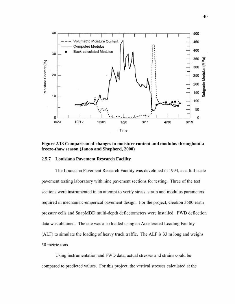
40
Figure 2.13 Comparison of changes in moisture content and modulus throughout a freeze-thaw season (Janoo and Shepherd, 2000)
2.5.7 Louisiana Pavement Research Facility
The Louisiana Pavement Research Facility was developed in 1994, as a full-scale
pavement testing laboratory with nine pavement sections for testing. Three of the test
sections were instrumented in an attempt to verify stress, strain and modulus parameters
required in mechanisic-emperical pavement design. For the project, Geokon 3500 earth
pressure cells and SnapMDD multi-depth deflectometers were installed. FWD deflection
data was obtained. The site was also loaded using an Accelerated Loading Facility
(ALF) to simulate the loading of heavy truck traffic. The ALF is 33 m long and weighs
50 metric tons.
Using instrumentation and FWD data, actual stresses and strains could be
compared to predicted values. For this project, the vertical stresses calculated at the
41
bottom of the subbase aggregate were 2 to 8 times higher than the measured stresses in all
cases. The following were suggested as possible reasons: stiffness of the pressure cells
could be very different from the stiffness of the surrounding soil; FWD modulus
backcalculation may have been incorrect; the elastic layer theory used may not have been
accurate; and the difference between a moving truck load and a single FWD point load.
Although actual values were not predicted correctly, the predicted values were able to
provide relative comparisons of moduli for the layers of the instrumented sections (Wu,
et al., 2006).
2.5.8 Finland Road and Traffic Laboratory
The Road and Traffic Laboratory in Finland performed studies using an FWD to
apply loads over strain gages (Linngren, 1991). The results of their project showed that
measured strains and backcalculated strains were comparable, but that with repeated
loading, resilient modulus did not always remain consistent. Linngren (1991) suggests
that the convergence step of the backcalculation process needs to be improved to reduce
modulus variability.
2.6 Summary
The resilient modulus of a soil can be defined as the deviator stress divided by
recoverable strain. Soil that is cyclically loaded initially experiences plastic deformation
until it reaches a point where deformation becomes elastic only. The slope of this portion
of the stress strain curve for cyclic loading is the resilient modulus. Resilient modulus is
greatly affected by climatic changes. Freezing and thawing cycles will result in
variations in modulus as described by three main points, first that frozen soil is typically

42
stiffer; second, capillary action draws in additional water during freezing, resulting in ice
lenses that add stiffness to soil layers; and third, additional water in the soil from melting
ice lenses will reduce soil stiffness during thaw.
Modulus can be calculated using three general techniques. Modulus can be
determined for soil samples in the laboratory using a cyclic loading resilient modulus test.
The AASHTO T307-99 procedure specifies the cyclical loading of a soil sample in a
triaxial apparatus to obtain resilient modulus. Correlations relating resilient modulus to
soil properties such as moisture content, grain size, and AASHTO classification have also
been developed. Although the resulting regression equations are limited to specific soils,
they are an inexpensive method of calculating resilient modulus when compared to
laboratory and field techniques.
The backcalculation of resilient modulus from deflection data, usually obtained
using an FWD, is one of the most common procedures used for determining in situ layer
moduli. The backcalculation procedure involves six steps: collecting data, choosing an
analytical model, choosing a material model, choosing a method for implementing the
models, using an optimization technique to solve the models, and analyzing and using the
backcalculated moduli results. There are a wide variety of options of models and
methods for each of these steps.
Pavement sections have been instrumented in the United States and Europe in an
attempt to gather in situ data that can be used both to create models for the calculation of
resilient modulus and other parameters, as well as to validate current models for
backcalculation and laboratory testing. Instrumentation like strain gages and pressure
cells were used to collect response data from normal traffic loading and calibrated truck

43
loading. The typical comparison made was between these stresses and strains and the
stress and strain values obtained using backcalculated moduli values obtained from FWD
data. As pavement instrumentation becomes more prevalent, the database available for
analysis will continue to increase.

44
Chapter 3
INSTRUMENTATION
3.1 Introduction
The project site is located in Guilford, Maine. A section of Route 15 between
Dover and Guilford, Maine underwent full depth reconstruction from 2004 through 2006.
A Maine Department of Transportation (MaineDOT) maintenance garage is located on
Route 15, partway through the reconstructed area. A 60 meter long section of road
located in front of the MaineDOT garage was used as the instrumented section. The lane
closest to the garage, for northwest-bound traffic, was chosen to have gages installed
during reconstruction. A shed previously used for a different University of Maine civil
engineering project was moved to the site, and was positioned on the side of the road at
station 3+620 (this project uses metric stationing), which is the center of the instrumented
section. In the descriptions that follow, all references to the left or right side of the
section relate to the shed as the center of the site. Gage wires were extended to the side
of the road in 19 mm (3/4 inch) PVC conduit. This conduit was connected to 38 mm (1½
inch) PVC conduit that ran parallel with the road back to the shed. The shed holds the
data acquisition equipment, and is connected to the Maine DOT garage’s existing electric
and internet lines. The data acquisition system is described in detail in Chapter 5.
Instrumentation was specified for the asphalt, subbase aggregate, and subgrade
soil layers at the test site. The instrumentation included 22 gages that were connected to
a high speed data acquisition system to collect dynamic stress and strain readings. An
additional 16 gages were monitored with static data acquisition to collect environmental
data that could be used to determine temperature, frost depth, and soil moisture content.

45
The combination of dynamic and environmental data was used to investigate pavement
layer responses, and the change in pavement section properties through changing seasons.
Eight different types of gages were used for the Guilford site and the different
types are listed in Table 3.1. Figure 3.1 below gives both plan and profile view of the site
and locations of the gages. The left and right sides of the instrumented section have the
same number and type of gages, but the layouts are different due to construction related
issues that will be discussed later in this chapter. Also, the left side of the shed will
eventually have a weigh-in-motion machine (WIM) installed. The WIM will record
vehicle weights and speeds for traffic that travels over the instrumented section.
Eventually, the WIM will be used to trigger the collection of stress and strain data for
heavy vehicles of interest.
Table 3.1 Specified Instrumentation for the Guilford Site Model/ Manufacturer Location Quantity Installation Date Dynamic Data Acquisition Asphalt Strain Gage PAST FTC IIA/
Dynatest Base of Asphalt Layer
12 9/6/05, 10/11/05
Soil Strain Gage SSDT FTC I/ Dynatest
Subbase and Subgrade Soil
4 6/13/05, 9/1/05, 9/13/05
Soil Pressure Cell SOPT FTC I/ Dynatest
Subbase and Subgrade Soil
4 6/13/05, 9/1/05, 9/13/05
Multidepth Deflectometer Dynatest Subbase and Subgrade Soil
2 Fall 2006
Static Data Acquisition Soil Thermocouple String PMC Corporation
(wire) Subbase and Subgrade Soil
2 6/13/05
Asphalt Thermocouple Omega Engineering, Inc. (wire)
Three Depths in Asphalt Layer
6 9/6/06, 9/7/05, 10/11/05, 10/12/05, 6/17/06
Soil Resistivity Probe ABF Manufacturing Subbase and Subgrade Soil
2 6/13/05
Soil Moisture Gage CS615/ Campbell Scientific
Subbase and Subgrade Soil
6 6/9/05, 6/13/05, 9/1/05
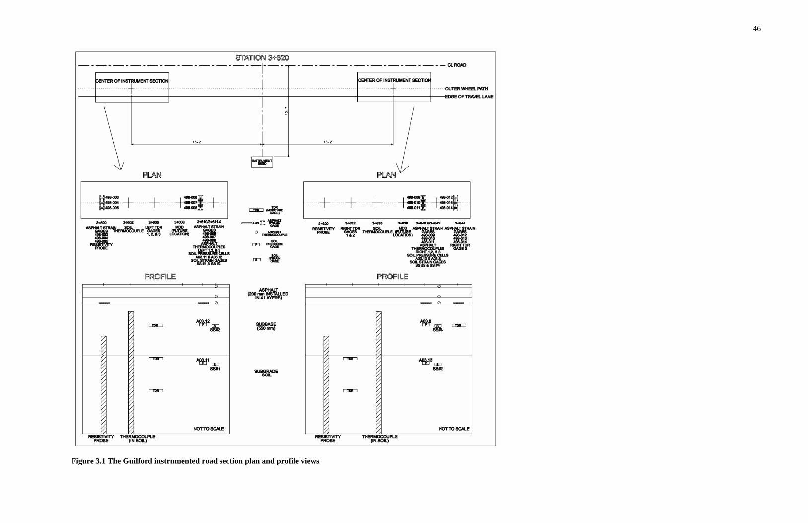
46
Figure 3.1 The Guilford instrumented road section plan and profile views
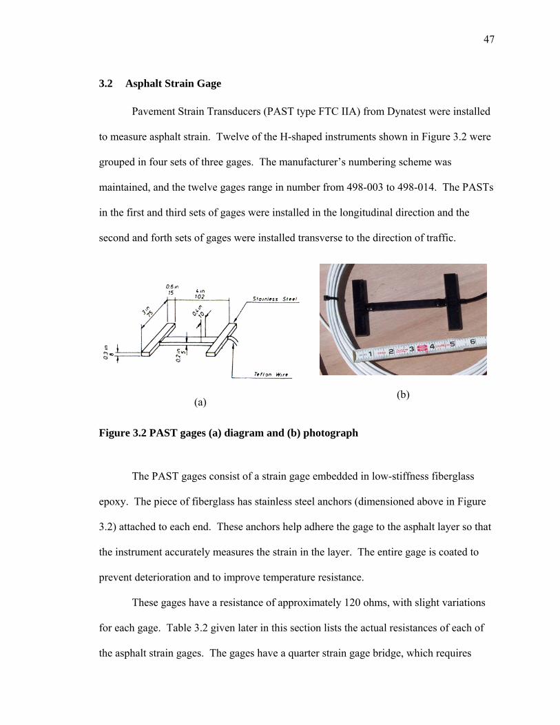
47
3.2 Asphalt Strain Gage
Pavement Strain Transducers (PAST type FTC IIA) from Dynatest were installed
to measure asphalt strain. Twelve of the H-shaped instruments shown in Figure 3.2 were
grouped in four sets of three gages. The manufacturer’s numbering scheme was
maintained, and the twelve gages range in number from 498-003 to 498-014. The PASTs
in the first and third sets of gages were installed in the longitudinal direction and the
second and forth sets of gages were installed transverse to the direction of traffic.
(a)
(b)
Figure 3.2 PAST gages (a) diagram and (b) photograph
The PAST gages consist of a strain gage embedded in low-stiffness fiberglass
epoxy. The piece of fiberglass has stainless steel anchors (dimensioned above in Figure
3.2) attached to each end. These anchors help adhere the gage to the asphalt layer so that
the instrument accurately measures the strain in the layer. The entire gage is coated to
prevent deterioration and to improve temperature resistance.
These gages have a resistance of approximately 120 ohms, with slight variations
for each gage. Table 3.2 given later in this section lists the actual resistances of each of
the asphalt strain gages. The gages have a quarter strain gage bridge, which requires
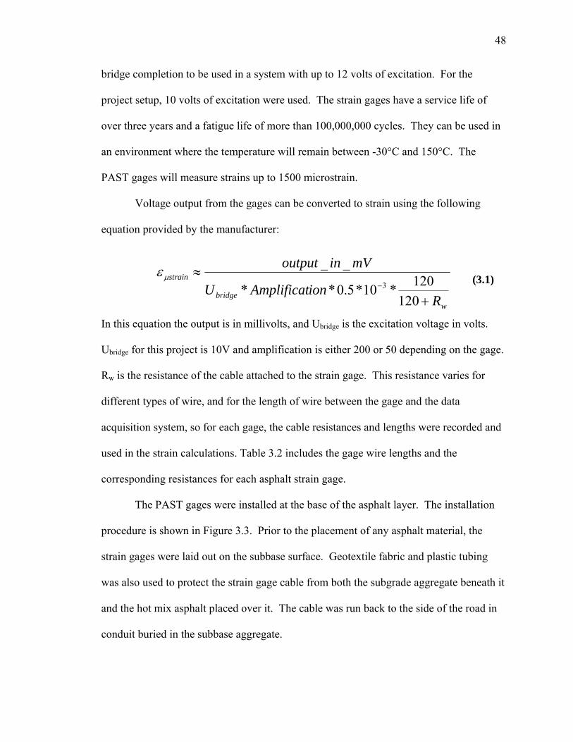
48
bridge completion to be used in a system with up to 12 volts of excitation. For the
project setup, 10 volts of excitation were used. The strain gages have a service life of
over three years and a fatigue life of more than 100,000,000 cycles. They can be used in
an environment where the temperature will remain between -30°C and 150°C. The
PAST gages will measure strains up to 1500 microstrain.
Voltage output from the gages can be converted to strain using the following
equation provided by the manufacturer:
wbridge
strain
RionAmplificatU
mVinoutput
+
≈−
120120*10*5.0**
__3
µε (3.1)
In this equation the output is in millivolts, and Ubridge is the excitation voltage in volts.
Ubridge for this project is 10V and amplification is either 200 or 50 depending on the gage.
Rw is the resistance of the cable attached to the strain gage. This resistance varies for
different types of wire, and for the length of wire between the gage and the data
acquisition system, so for each gage, the cable resistances and lengths were recorded and
used in the strain calculations. Table 3.2 includes the gage wire lengths and the
corresponding resistances for each asphalt strain gage.
The PAST gages were installed at the base of the asphalt layer. The installation
procedure is shown in Figure 3.3. Prior to the placement of any asphalt material, the
strain gages were laid out on the subbase surface. Geotextile fabric and plastic tubing
was also used to protect the strain gage cable from both the subgrade aggregate beneath it
and the hot mix asphalt placed over it. The cable was run back to the side of the road in
conduit buried in the subbase aggregate.
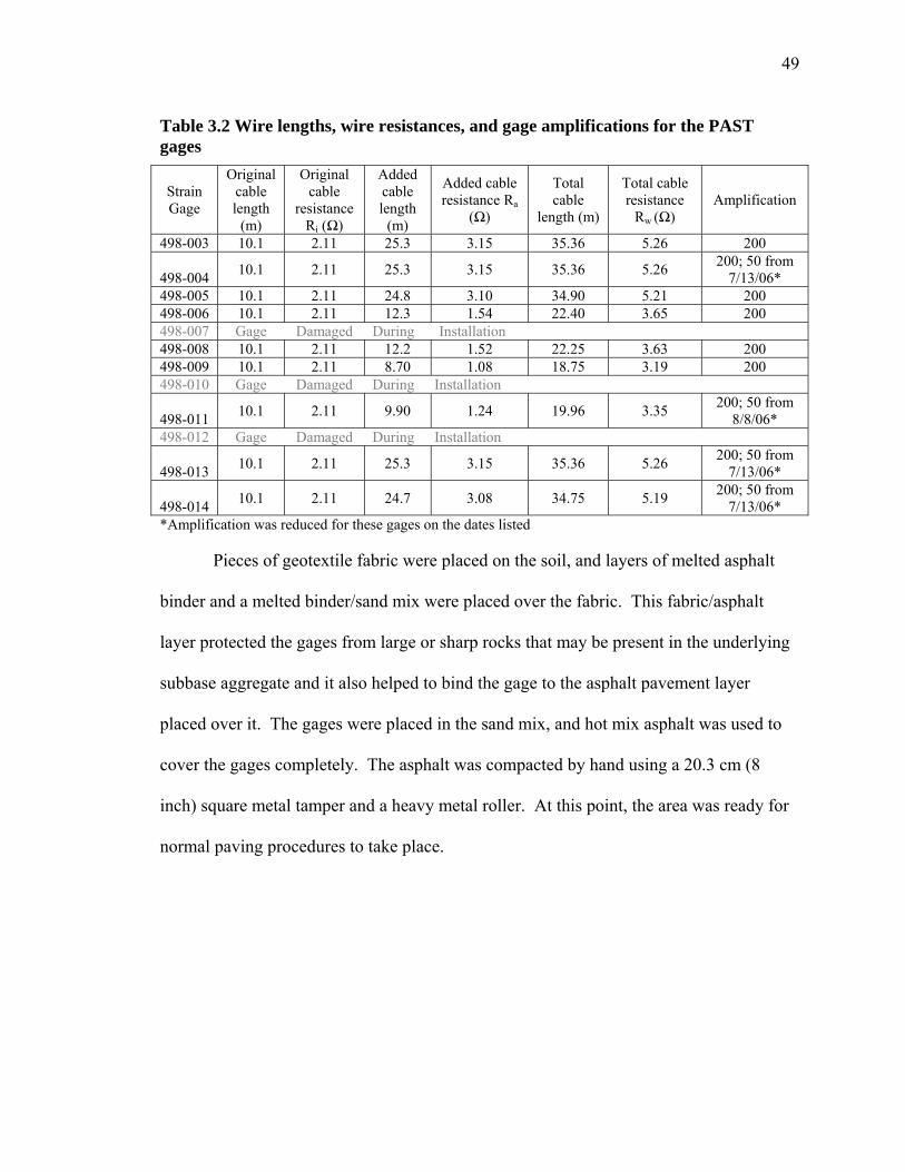
49
Table 3.2 Wire lengths, wire resistances, and gage amplifications for the PAST gages
Strain Gage
Original cable length
(m)
Original cable
resistance Ri (Ω)
Added cable length
(m)
Added cable resistance Ra
(Ω)
Total cable
length (m)
Total cable resistance
Rw (Ω) Amplification
498-003 10.1 2.11 25.3 3.15 35.36 5.26 200
498-004 10.1 2.11 25.3 3.15 35.36 5.26 200; 50 from 7/13/06*
498-005 10.1 2.11 24.8 3.10 34.90 5.21 200 498-006 10.1 2.11 12.3 1.54 22.40 3.65 200 498-007 Gage Damaged During Installation 498-008 10.1 2.11 12.2 1.52 22.25 3.63 200 498-009 10.1 2.11 8.70 1.08 18.75 3.19 200 498-010 Gage Damaged During Installation
498-011 10.1 2.11 9.90 1.24 19.96 3.35 200; 50 from 8/8/06*
498-012 Gage Damaged During Installation
498-013 10.1 2.11 25.3 3.15 35.36 5.26 200; 50 from 7/13/06*
498-014 10.1 2.11 24.7 3.08 34.75 5.19 200; 50 from 7/13/06*
*Amplification was reduced for these gages on the dates listed
Pieces of geotextile fabric were placed on the soil, and layers of melted asphalt
binder and a melted binder/sand mix were placed over the fabric. This fabric/asphalt
layer protected the gages from large or sharp rocks that may be present in the underlying
subbase aggregate and it also helped to bind the gage to the asphalt pavement layer
placed over it. The gages were placed in the sand mix, and hot mix asphalt was used to
cover the gages completely. The asphalt was compacted by hand using a 20.3 cm (8
inch) square metal tamper and a heavy metal roller. At this point, the area was ready for
normal paving procedures to take place.
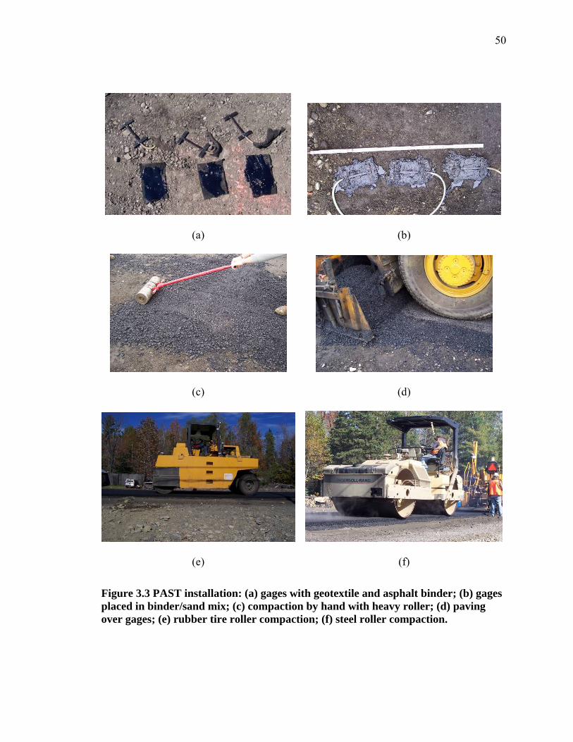
50
(a)
(b)
(c)
(d)
(e)
(f)
Figure 3.3 PAST installation: (a) gages with geotextile and asphalt binder; (b) gages placed in binder/sand mix; (c) compaction by hand with heavy roller; (d) paving over gages; (e) rubber tire roller compaction; (f) steel roller compaction.
51
Following paving, the resistance of each gage was checked using a multimeter to
determine if the gages had survived the paving process. Table 3.3 below lists the post-
paving resistances along with the original resistances for each gage. Three of the twelve
asphalt strain gages were damaged, and did not give any strain responses. PAST 498-
007, the middle transverse gage at location two was damaged during setup prior to
paving. It was installed even though one of its steel anchors had been broken off, but it
did not give any strain responses. PAST 498-010, the middle longitudinal gage at
location three was damaged during the paving process. The protective asphalt layer
placed on the gages either was not thick enough or was not compacted properly, and the
weight of the paver pushed the gage up out of the asphalt so that part of the gage was
exposed. Additional asphalt was added, but the gage had been damaged. PAST 498-012,
the transverse gage closest to the centerline at location four showed no physical signs of
damage before or during paving, and after paving the pavement layer was placed the
resistance was normal. However, a check of the gage resistances again after compaction
was completed showed that the strain gage was not responsive. Figure 3.4 shows the
locations and orientations of damaged gages relative to responsive gages.
Table 3.3 Strain gage resistances Strain Gage Initial Gage Resistance (Ω) Post Paving Gage Resistance (Ω)
498-003 122.5 123.5 498-004 122.4 122.7 498-005 122.4 123.0 498-006 122.3 122.6 498-007 122.3 Gage not responsive 498-008 122.3 121.8 498-009 122.4 125.5 498-010 122.1 Gage not responsive 498-011 122.3 124.1 498-012 122.2 Gage not responsive 498-013 122.2 124.1 498-014 122.4 124.4
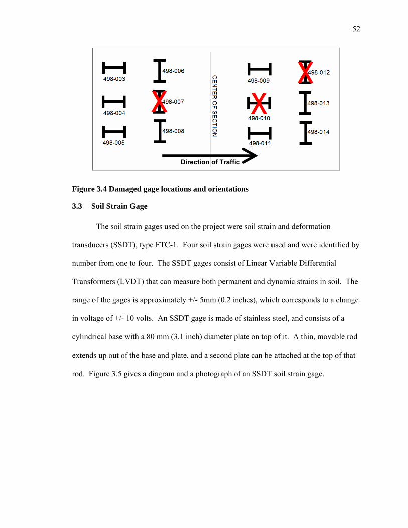
52
Figure 3.4 Damaged gage locations and orientations
3.3 Soil Strain Gage
The soil strain gages used on the project were soil strain and deformation
transducers (SSDT), type FTC-1. Four soil strain gages were used and were identified by
number from one to four. The SSDT gages consist of Linear Variable Differential
Transformers (LVDT) that can measure both permanent and dynamic strains in soil. The
range of the gages is approximately +/- 5mm (0.2 inches), which corresponds to a change
in voltage of +/- 10 volts. An SSDT gage is made of stainless steel, and consists of a
cylindrical base with a 80 mm (3.1 inch) diameter plate on top of it. A thin, movable rod
extends up out of the base and plate, and a second plate can be attached at the top of that
rod. Figure 3.5 gives a diagram and a photograph of an SSDT soil strain gage.
Direction of Traffic

53
(a)
(b)
Figure 3.5 SSDT Soil Strain Gage (a) diagram and (b) photograph.
The four SSDT gages used for the project were each connected to their own signal
conditioner. Strain gage number one was designated as the “master” device, and gages
two, three, and four were connected to gage one as “slave” devices. This setup allowed
the gages to run using the same power and ground sources and prevented interference
between the gages. The LVM-110 signal conditioners and the PSD 4-15 DC +/- 15 volt
power supply used for the project were made by Schaevitz Sensors specifically for use
with LVDTs.
Prior to installation, the gages were calibrated in the lab with their corresponding
signal conditioners. Figure 3.6 shows the calibration process. The strain gages were
connected through their signal conditioners to a multimeter. Two sets of dial calipers
were used, both to hold the gage at a specific extension and to measure that extension.
Voltage readings were taken with the multimeter for different extension measurements.
Potentiometers on the signal conditioners were used to set each gage so that the range of
+/- 5 mm was equivalent to a voltage range of +/- 10 V.
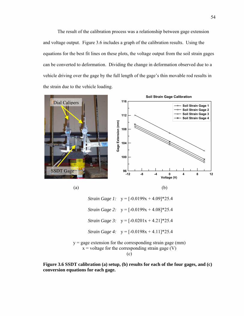
54
The result of the calibration process was a relationship between gage extension
and voltage output. Figure 3.6 includes a graph of the calibration results. Using the
equations for the best fit lines on these plots, the voltage output from the soil strain gages
can be converted to deformation. Dividing the change in deformation observed due to a
vehicle driving over the gage by the full length of the gage’s thin movable rod results in
the strain due to the vehicle loading.
(a)
-12 -8 -4 0 4 8 12Voltage (V)
96
100
104
108
112
116
Gag
e Ex
tens
ion
(mm
)
Soil Strain Gage 1Soil Strain Gage 2Soil Strain Gage 3Soil Strain Gage 4
Soil Strain Gage Calibration
(b)
Strain Gage 1:
Strain Gage 2:
Strain Gage 3:
Strain Gage 4:
y = [-0.0199x + 4.09]*25.4
y = [-0.0199x + 4.08]*25.4
y = [-0.0201x + 4.21]*25.4
y = [-0.0198x + 4.11]*25.4
y = gage extension for the corresponding strain gage (mm) x = voltage for the corresponding strain gage (V)
(c)
Figure 3.6 SSDT calibration (a) setup, (b) results for each of the four gages, and (c) conversion equations for each gage.
Dial Calipers
SSDT Gage
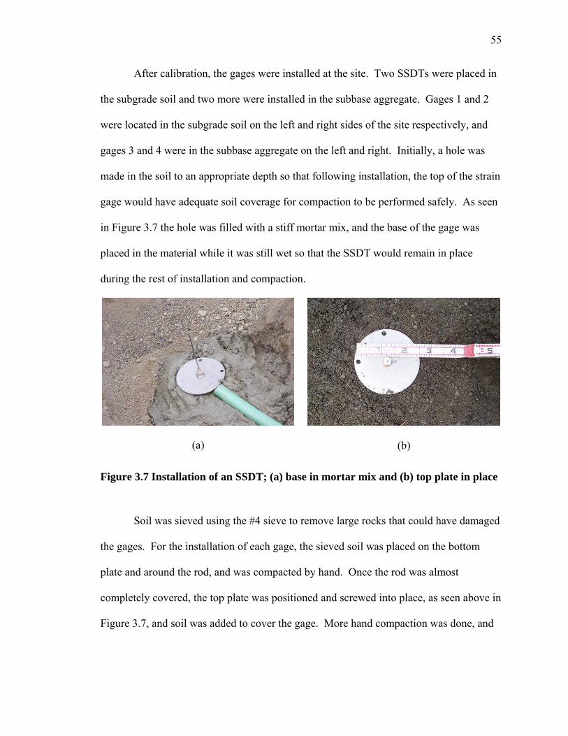
55
After calibration, the gages were installed at the site. Two SSDTs were placed in
the subgrade soil and two more were installed in the subbase aggregate. Gages 1 and 2
were located in the subgrade soil on the left and right sides of the site respectively, and
gages 3 and 4 were in the subbase aggregate on the left and right. Initially, a hole was
made in the soil to an appropriate depth so that following installation, the top of the strain
gage would have adequate soil coverage for compaction to be performed safely. As seen
in Figure 3.7 the hole was filled with a stiff mortar mix, and the base of the gage was
placed in the material while it was still wet so that the SSDT would remain in place
during the rest of installation and compaction.
(a)
(b)
Figure 3.7 Installation of an SSDT; (a) base in mortar mix and (b) top plate in place
Soil was sieved using the #4 sieve to remove large rocks that could have damaged
the gages. For the installation of each gage, the sieved soil was placed on the bottom
plate and around the rod, and was compacted by hand. Once the rod was almost
completely covered, the top plate was positioned and screwed into place, as seen above in
Figure 3.7, and soil was added to cover the gage. More hand compaction was done, and
56
the gage voltages were checked to ensure that the strain gages were within their +/- 10
volt range.
Ideally, these strain gages should be installed with their extension as close to the
position corresponding to -10 volts as possible, to provide the largest range for the
compression of the strain gage. In most cases, after compaction, the gages needed to be
uncovered because they were no longer close to -10 volts. The top plate was removed,
and more soil was added and compacted. The process was repeated until the soil between
the top and bottom strain gage plates was compacted enough to prevent excessive
movement during construction. The goal was to install the gage in a way that would
allow for the maximum range of response due to traffic driving over the road. Additional
compaction of the soil occurred due to construction equipment and traffic driving over
the road before the section was fully paved, so when readings were first taken from the
SSDTs, they were no longer at -10 volts.
Following installation of each gage, each SSDT was checked using a multimeter,
and all four SSDT gages were responsive.
3.4 Soil Pressure Cells
Vertical stresses in the soil are measured using four soil pressure cells that were
installed in the subgrade and subbase soils. The gages were Dynatest Soil Pressure
Transducers (SOPT), type FTC 1. The manufacturer’s designations were used and the
gages are referred to as A03.8, A03.11, A03.12, and A03.13.
The pressure cells were circular with a 68mm (2.6-inch) diameter, and are 13 mm
(0.5 inches) thick. Figure 3.8 gives a diagram and photograph of the SOPT gage. The
body of each pressure cell was constructed using titanium to help prevent deterioration of

57
the gages due to environmental conditions, as well as due to the wear of normal use. The
surface of each cell was covered with epoxy and sand, to improve performance in a
variety of types of soil. The SOPT cells have a hydraulic design, as described below, to
improve issues with linearity and sensitivity that have been encountered with other
pressure cell models. The interior of the cell is covered by a thin membrane, and an
integral pressure transducer measures the pressure inside the liquid-filled cell. The
pressure cell has an almost constant volume, so the gage is sensitive to pressure over its
entire area.
(a)
(b)
Figure 3.8 Soil pressure cell (a) diagram and (b) photograph
Each soil pressure cell’s internal transducer had a full strain gage bridge with a
maximum excitation voltage of 12 volts. The pressure cells were calibrated, and then
installed with a 12-volt DC power supply. The calibration procedure involved loading
each cell with weights, and recording the change in voltage that took place as a result of
the applied force. The voltage to weight relationship for each of the four gages is shown
in the plot in Figure 3.9.
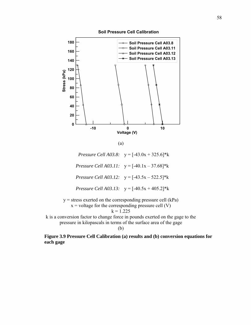
58
-10 0 10Voltage (V)
0
20
40
60
80
100
120
140
160
180
Stre
ss (k
Pa)
Soil Pressure Cell A03.8Soil Pressure Cell A03.11Soil Pressure Cell A03.12Soil Pressure Cell A03.13
Soil Pressure Cell Calibration
(a)
Pressure Cell A03.8:
Pressure Cell A03.11:
Pressure Cell A03.12:
Pressure Cell A03.13:
y = [-43.0x + 325.6]*k
y = [-40.1x – 37.68]*k
y = [-43.5x – 522.5]*k
y = [-40.5x + 405.2]*k
y = stress exerted on the corresponding pressure cell (kPa) x = voltage for the corresponding pressure cell (V)
k = 1.225 k is a conversion factor to change force in pounds exerted on the gage to the
pressure in kilopascals in terms of the surface area of the gage (b)
Figure 3.9 Pressure Cell Calibration (a) results and (b) conversion equations for each gage
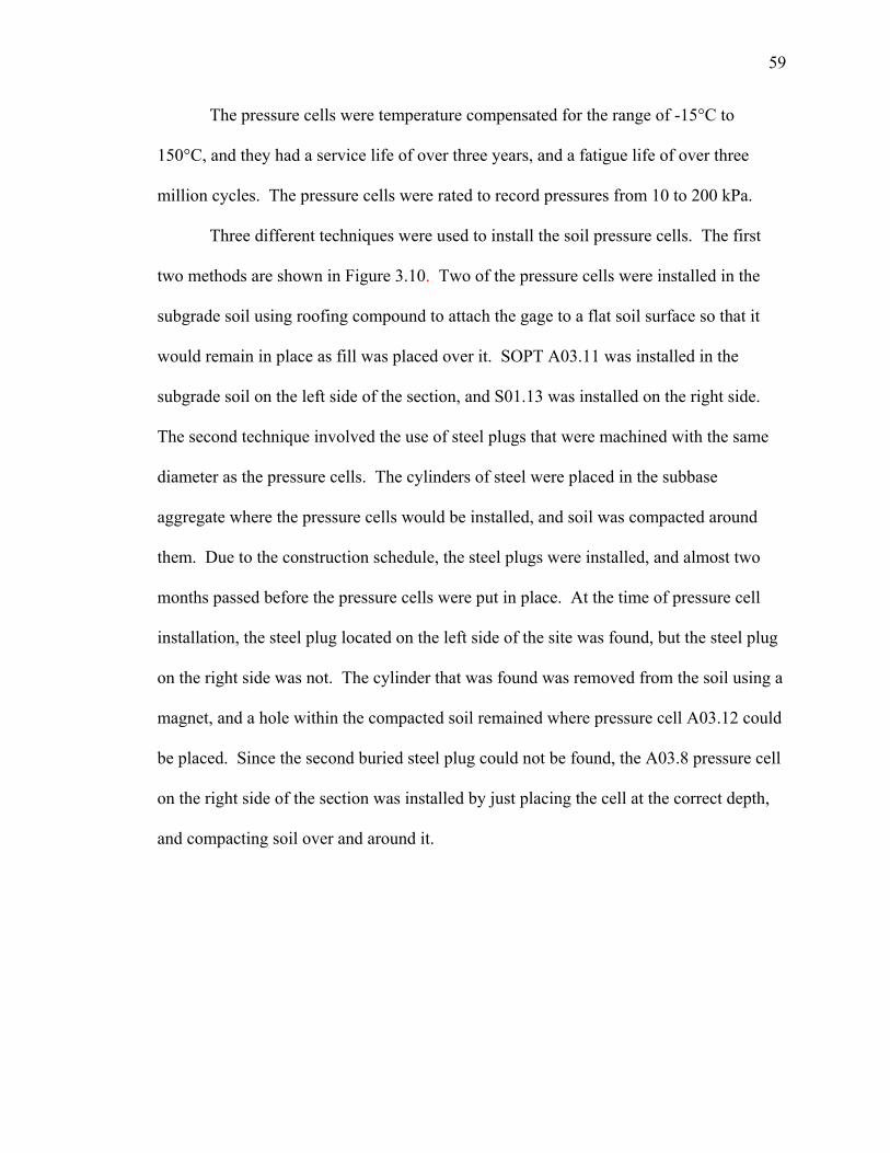
59
The pressure cells were temperature compensated for the range of -15°C to
150°C, and they had a service life of over three years, and a fatigue life of over three
million cycles. The pressure cells were rated to record pressures from 10 to 200 kPa.
Three different techniques were used to install the soil pressure cells. The first
two methods are shown in Figure 3.10. Two of the pressure cells were installed in the
subgrade soil using roofing compound to attach the gage to a flat soil surface so that it
would remain in place as fill was placed over it. SOPT A03.11 was installed in the
subgrade soil on the left side of the section, and S01.13 was installed on the right side.
The second technique involved the use of steel plugs that were machined with the same
diameter as the pressure cells. The cylinders of steel were placed in the subbase
aggregate where the pressure cells would be installed, and soil was compacted around
them. Due to the construction schedule, the steel plugs were installed, and almost two
months passed before the pressure cells were put in place. At the time of pressure cell
installation, the steel plug located on the left side of the site was found, but the steel plug
on the right side was not. The cylinder that was found was removed from the soil using a
magnet, and a hole within the compacted soil remained where pressure cell A03.12 could
be placed. Since the second buried steel plug could not be found, the A03.8 pressure cell
on the right side of the section was installed by just placing the cell at the correct depth,
and compacting soil over and around it.
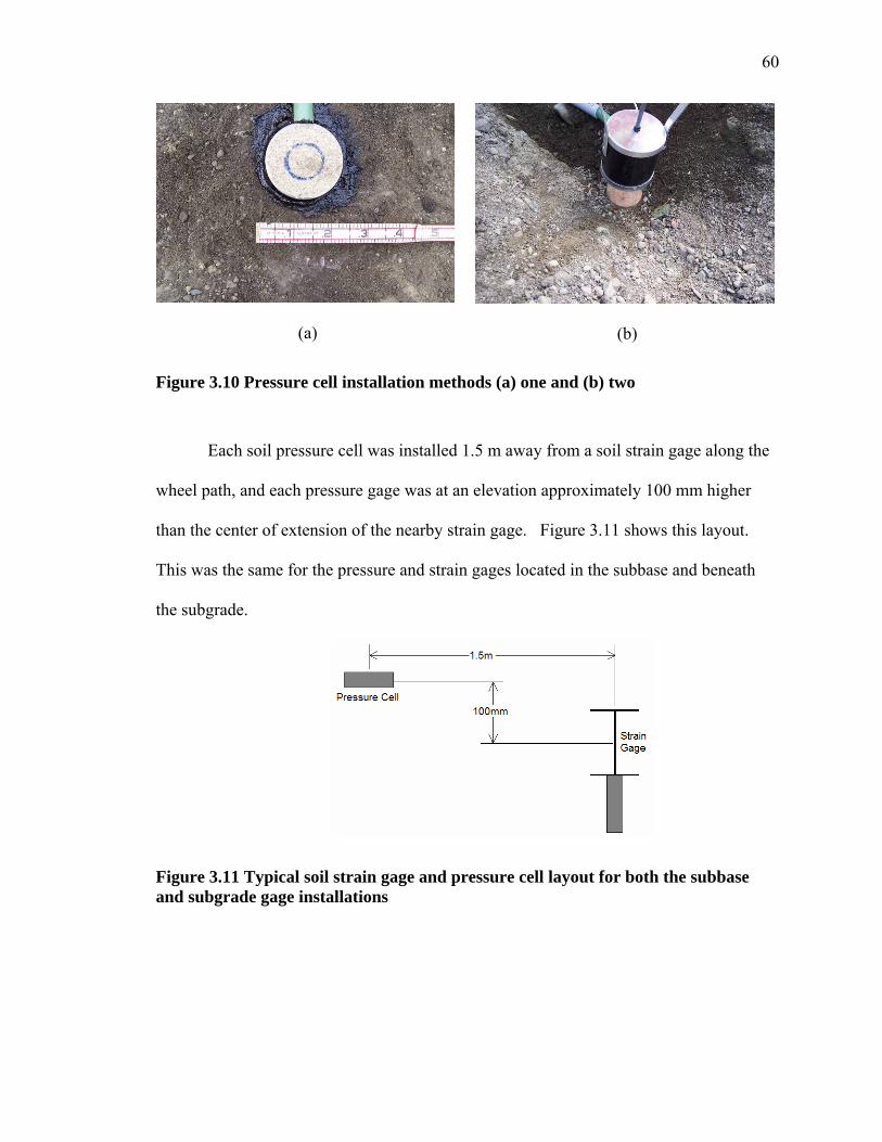
60
(a)
(b)
Figure 3.10 Pressure cell installation methods (a) one and (b) two
Each soil pressure cell was installed 1.5 m away from a soil strain gage along the
wheel path, and each pressure gage was at an elevation approximately 100 mm higher
than the center of extension of the nearby strain gage. Figure 3.11 shows this layout.
This was the same for the pressure and strain gages located in the subbase and beneath
the subgrade.
Figure 3.11 Typical soil strain gage and pressure cell layout for both the subbase and subgrade gage installations

61
3.5 Thermocouples
Thermocouples were installed at several depths to record temperatures in the
subgrade, subbase, and HMA layers. Thermocouples were constructed using 20-gauge
copper-constantan (Type T) wire pairs. The end of each wire pair was crimped with a
Quick Tip connection and protected with silicone and a heat-shrink cap as shown in
Figure 3.12. The bimetal reaction at the wire tip connection causes an electrical potential
that is proportional to the temperature difference between the end of the wire in the
ground and the end of the wire connected to a readout device. Using the reference
temperature of the readout device, the temperature in the ground can be calculated.
Figure 3.12 Stages of thermocouple construction: (a) copper (blue coating) and constantan (red coating) wires stripped and separated; (b) copper and constantan wires crimped together; and (c) the crimped wires covered by a heat shrink cap.
The soil temperatures were measured using two strings of twelve Type T
thermocouples. The twelve-pair wire used to construct each thermocouple string was
manufactured by the PMC Corporation (Model No. TX-212TE/TE061-20U). For each
string, the twelve thermocouples were mounted on a 2.1 m (7-ft) wooden dowel by
threading the wires through holes drilled in the dowel at the following spacing: the lowest
(a) (b) (c) Red
Blue

62
five thermocouples were spaced at 0.3 m (1 ft), and the next six were spaced at 0.15
meters (6 inches). The final thermocouple was left as a flier at the top of the string that
could be positioned in the ground away from the other eleven. This layout is shown in
Figure 3.13.
Prior to soil thermocouple installation, when the road surface was still at the
subgrade level, holes were drilled and held open with 7.6 centimeter (3 inch) diameter
PVC pipe. On the day that the subbase soil was being placed, the pipe was removed, the
wooden dowel with the thermocouple string attached to it was lowered into the hole and
backfilled with subgrade soil, with a portion of the dowel remaining above the subgrade
level. Another wooden dowel was used to tamp the soil around the thermocouples.
Figure 3.13 shows a thermocouple string ready for installation, just before the PVC pipe
is removed from the ground and replaced by the wooden dowel setup.
(units in cm)
(a)
(b)
Figure 3.13 Soil Thermocouple (a) diagram and (b) installation

63
The ends of the wires that would be connected to a readout box were run in PVC
conduit back to the side of the road. Subbase aggregate was backfilled over the conduit,
and around the exposed portion of the thermocouple string, and the top thermocouple
flier was positioned approximately one meter out from the dowel and covered with
additional soil. With adequate cover over the top of the thermocouple string, normal
subbase compaction was completed. This same procedure was used for both
thermocouple strings except that the thermocouple flier located on the right side of the
instrumented section was not positioned away from the rest of the string. The
thermocouples were placed so that the top of each string would be 0.4 to 0.5 meters
below finished grade.
The asphalt temperatures were measured at three depths using thermocouple wire
that was obtained from Omega Engineering, Inc. (Part # TT-T-20-SLE). This wire was
the same as the soil thermocouple wire except that it contained only a single pair of
copper-constantan wires instead of twelve pairs, and the Omega wire was covered in a
heavy duty coating that would withstand high paving temperatures. For installation the
temperature measuring ends of the wires were placed on the road surface as shown in
Figure 3.14, and paving was completed as normal over the sensors. The wires were
extended off and down away from the road in buried PVC conduit.
Figure 3.14 Asphalt thermocouple ready for paving
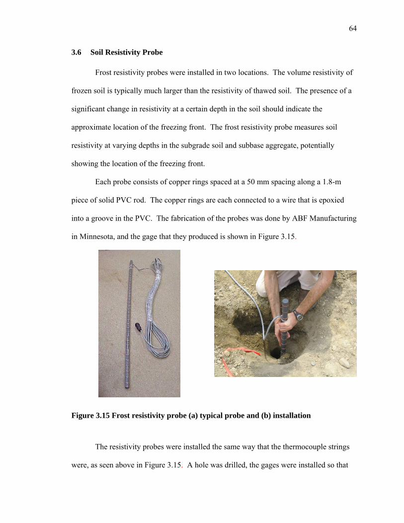
64
3.6 Soil Resistivity Probe
Frost resistivity probes were installed in two locations. The volume resistivity of
frozen soil is typically much larger than the resistivity of thawed soil. The presence of a
significant change in resistivity at a certain depth in the soil should indicate the
approximate location of the freezing front. The frost resistivity probe measures soil
resistivity at varying depths in the subgrade soil and subbase aggregate, potentially
showing the location of the freezing front.
Each probe consists of copper rings spaced at a 50 mm spacing along a 1.8-m
piece of solid PVC rod. The copper rings are each connected to a wire that is epoxied
into a groove in the PVC. The fabrication of the probes was done by ABF Manufacturing
in Minnesota, and the gage that they produced is shown in Figure 3.15.
Figure 3.15 Frost resistivity probe (a) typical probe and (b) installation
The resistivity probes were installed the same way that the thermocouple strings
were, as seen above in Figure 3.15. A hole was drilled, the gages were installed so that
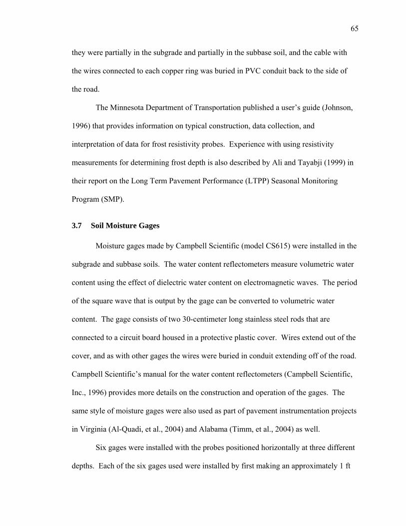
65
they were partially in the subgrade and partially in the subbase soil, and the cable with
the wires connected to each copper ring was buried in PVC conduit back to the side of
the road.
The Minnesota Department of Transportation published a user’s guide (Johnson,
1996) that provides information on typical construction, data collection, and
interpretation of data for frost resistivity probes. Experience with using resistivity
measurements for determining frost depth is also described by Ali and Tayabji (1999) in
their report on the Long Term Pavement Performance (LTPP) Seasonal Monitoring
Program (SMP).
3.7 Soil Moisture Gages
Moisture gages made by Campbell Scientific (model CS615) were installed in the
subgrade and subbase soils. The water content reflectometers measure volumetric water
content using the effect of dielectric water content on electromagnetic waves. The period
of the square wave that is output by the gage can be converted to volumetric water
content. The gage consists of two 30-centimeter long stainless steel rods that are
connected to a circuit board housed in a protective plastic cover. Wires extend out of the
cover, and as with other gages the wires were buried in conduit extending off of the road.
Campbell Scientific’s manual for the water content reflectometers (Campbell Scientific,
Inc., 1996) provides more details on the construction and operation of the gages. The
same style of moisture gages were also used as part of pavement instrumentation projects
in Virginia (Al-Quadi, et al., 2004) and Alabama (Timm, et al., 2004) as well.
Six gages were installed with the probes positioned horizontally at three different
depths. Each of the six gages used were installed by first making an approximately 1 ft
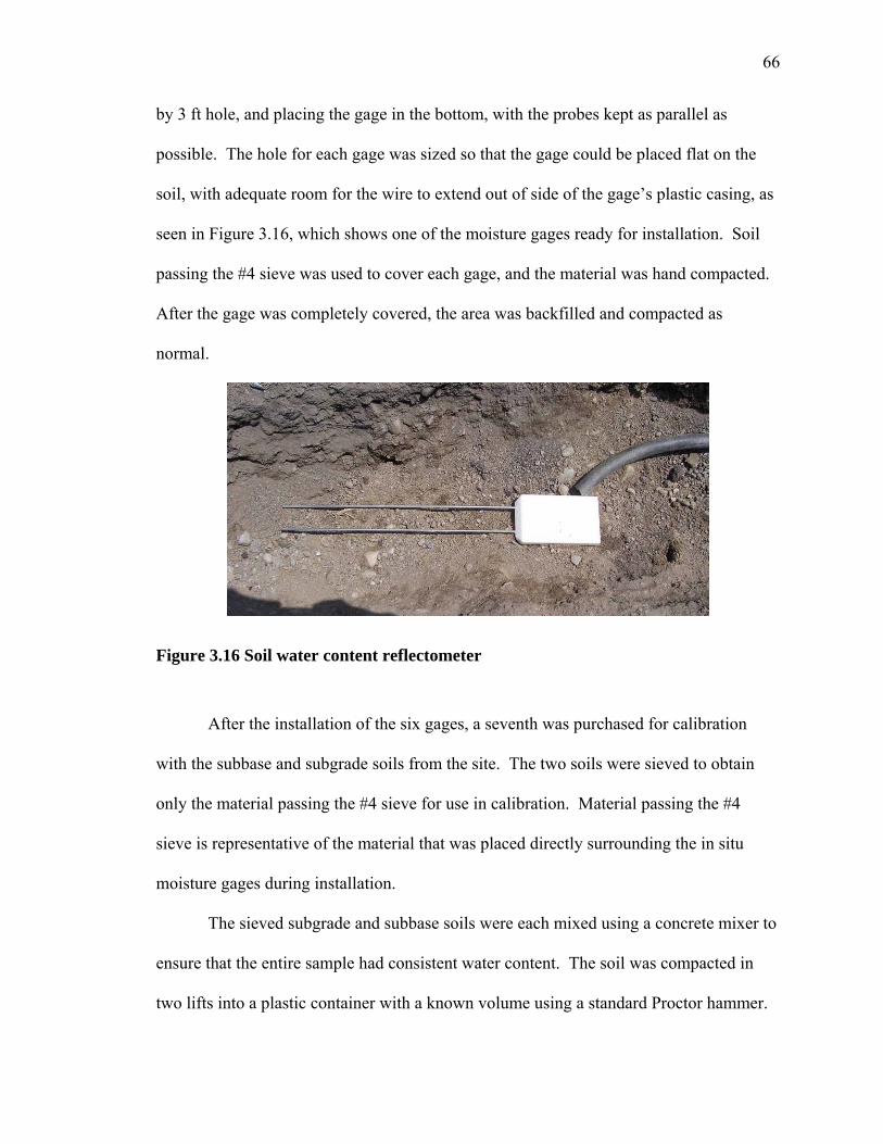
66
by 3 ft hole, and placing the gage in the bottom, with the probes kept as parallel as
possible. The hole for each gage was sized so that the gage could be placed flat on the
soil, with adequate room for the wire to extend out of side of the gage’s plastic casing, as
seen in Figure 3.16, which shows one of the moisture gages ready for installation. Soil
passing the #4 sieve was used to cover each gage, and the material was hand compacted.
After the gage was completely covered, the area was backfilled and compacted as
normal.
Figure 3.16 Soil water content reflectometer
After the installation of the six gages, a seventh was purchased for calibration
with the subbase and subgrade soils from the site. The two soils were sieved to obtain
only the material passing the #4 sieve for use in calibration. Material passing the #4
sieve is representative of the material that was placed directly surrounding the in situ
moisture gages during installation.
The sieved subgrade and subbase soils were each mixed using a concrete mixer to
ensure that the entire sample had consistent water content. The soil was compacted in
two lifts into a plastic container with a known volume using a standard Proctor hammer.
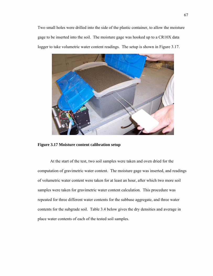
67
Two small holes were drilled into the side of the plastic container, to allow the moisture
gage to be inserted into the soil. The moisture gage was hooked up to a CR10X data
logger to take volumetric water content readings. The setup is shown in Figure 3.17.
Figure 3.17 Moisture content calibration setup
At the start of the test, two soil samples were taken and oven dried for the
computation of gravimetric water content. The moisture gage was inserted, and readings
of volumetric water content were taken for at least an hour, after which two more soil
samples were taken for gravimetric water content calculation. This procedure was
repeated for three different water contents for the subbase aggregate, and three water
contents for the subgrade soil. Table 3.4 below gives the dry densities and average in
place water contents of each of the tested soil samples.
68
Table 3.4 Moisture Gage Calibration Densities and In-place Water Contents
Subbase Subgrade Trial Dry Density (Mg/m3) Water Content Dry Density (Mg/m3) Water Content 1 1.75 1.7% 1.75 2.2% 2 1.51 6.5% 1.52 5.5% 3 1.79 10.4% 1.78 8.4%
The resulting relationships between the water contents calculated using samples
and the water contents recorded with the moisture gage are shown in Figure 3.18.
0.02 0.04 0.06 0.08 0.1 0.12 0.14 0.16 0.18 0.2 0.22Lab Tested Water Content (converted to volumetric)
0
0.04
0.08
0.12
0.16
0.2
0.24
CR
10x
Col
lect
ed V
olum
etric
Wat
er C
onte
nts
Subbase: Y = 0.94X + 0.01 (solid line)
Subgrade: Y = 0.62X + 0.04 (dashed line)
Figure 3.18 Moisture content calibration chart
3.8 Summary
The project site in Guilford, Maine was instrumented with a variety of gages to
provide data on the response of layers in the pavement system. Pressure cells and strain
gages were installed in the subbase aggregate and subgrade soil, and strain gages were
installed at the base of the asphalt layer. Frost, moisture, and temperature gages were
installed throughout the pavement cross section to provide climate data that can be used
for the analysis of freeze/thaw responses. The construction process and installation

69
schedule is described in Chapter 4. Following construction, all of the gages were
connected to a data acquisition system that is described in Chapter 5.

70
Chapter 4
PROJECT CONSTRUCTION
4.1 General Roadway Construction Procedures and Materials
The installation of most of the gages took place in the summer and fall of 2005.
K & K Construction, Inc. from Turner, Maine, was the general contractor and performed
most of earthwork for the project. Vaughan Thibodeau and Sons was the paving
subcontractor. Thibodeau provided the materials for their subsidiary Precision Paving,
which performed the actual paving work.
At the start of road construction, the existing pavement layer was removed from
the surface leaving the road at approximately the elevation of subgrade. In the
instrumented section, a layer of old asphalt approximately 75 mm thick was found near
the subgrade level at the time of gage installation. This layer should have been removed,
but due to the sequence of construction, the asphalt was not removed before some of the
instruments were installed, so it was left in place for the whole instrumented section. The
in place soil density at the subgrade level was measured using the sand cone test. The dry
density was 2.33 Mg/m3 (145 pcf), and the water content at the time of measurement was
3.2%. The gradation of the soil based on wet sieve and hydrometer tests is included in
Figure 4.1. Based on this gradation and the AASHTO classification system, the subgrade
soil is an A-1-b material. The material sampled for gradation, and classified here was
taken from the subgrade surface.
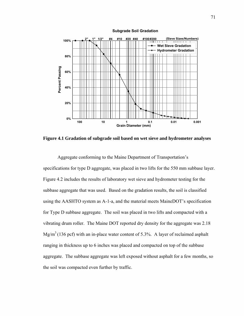
71
100 10 1 0.1 0.01 0.001Grain Diameter (mm)
0%
20%
40%
60%
80%
100%
Perc
ent P
assi
ng
2" 1" 1/2" #4 #10 #20 #40 #100#200
Wet Sieve GradationHydrometer Gradation
Subgrade Soil Gradation
(Sieve Sizes/Numbers)
Figure 4.1 Gradation of subgrade soil based on wet sieve and hydrometer analyses
Aggregate conforming to the Maine Department of Transportation’s
specifications for type D aggregate, was placed in two lifts for the 550 mm subbase layer.
Figure 4.2 includes the results of laboratory wet sieve and hydrometer testing for the
subbase aggregate that was used. Based on the gradation results, the soil is classified
using the AASHTO system as A-1-a, and the material meets MaineDOT’s specification
for Type D subbase aggregate. The soil was placed in two lifts and compacted with a
vibrating drum roller. The Maine DOT reported dry density for the aggregate was 2.18
Mg/m3 (136 pcf) with an in-place water content of 5.3%. A layer of reclaimed asphalt
ranging in thickness up to 6 inches was placed and compacted on top of the subbase
aggregate. The subbase aggregate was left exposed without asphalt for a few months, so
the soil was compacted even further by traffic.
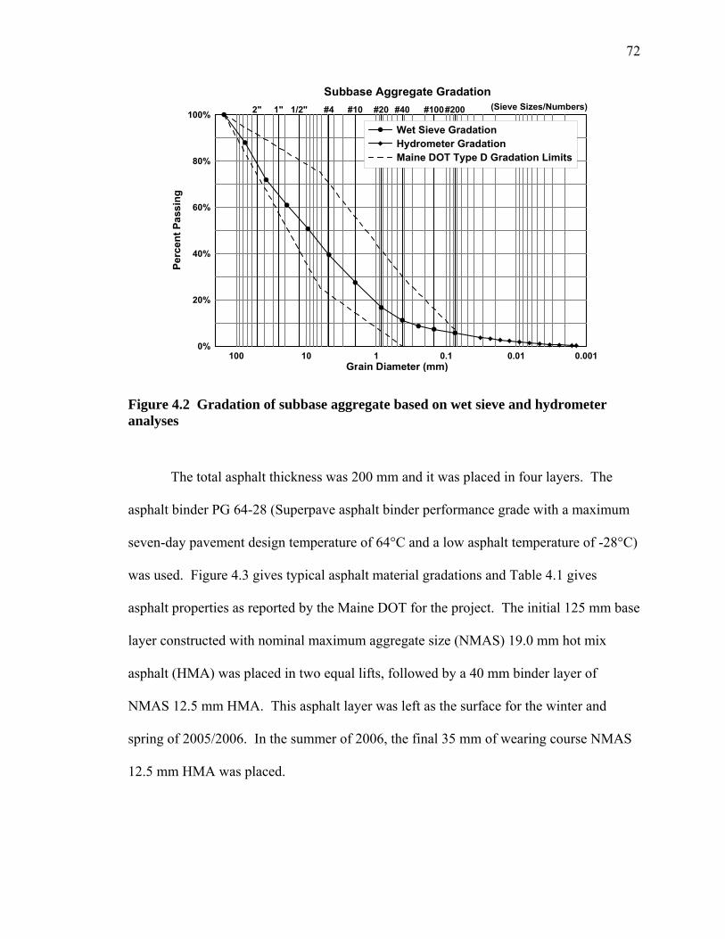
72
100 10 1 0.1 0.01 0.001Grain Diameter (mm)
0%
20%
40%
60%
80%
100%
Perc
ent P
assi
ng
2" 1" 1/2" #4 #10 #20 #40 #100#200
Wet Sieve GradationHydrometer GradationMaine DOT Type D Gradation Limits
Subbase Aggregate Gradation(Sieve Sizes/Numbers)
Figure 4.2 Gradation of subbase aggregate based on wet sieve and hydrometer analyses
The total asphalt thickness was 200 mm and it was placed in four layers. The
asphalt binder PG 64-28 (Superpave asphalt binder performance grade with a maximum
seven-day pavement design temperature of 64°C and a low asphalt temperature of -28°C)
was used. Figure 4.3 gives typical asphalt material gradations and Table 4.1 gives
asphalt properties as reported by the Maine DOT for the project. The initial 125 mm base
layer constructed with nominal maximum aggregate size (NMAS) 19.0 mm hot mix
asphalt (HMA) was placed in two equal lifts, followed by a 40 mm binder layer of
NMAS 12.5 mm HMA. This asphalt layer was left as the surface for the winter and
spring of 2005/2006. In the summer of 2006, the final 35 mm of wearing course NMAS
12.5 mm HMA was placed.
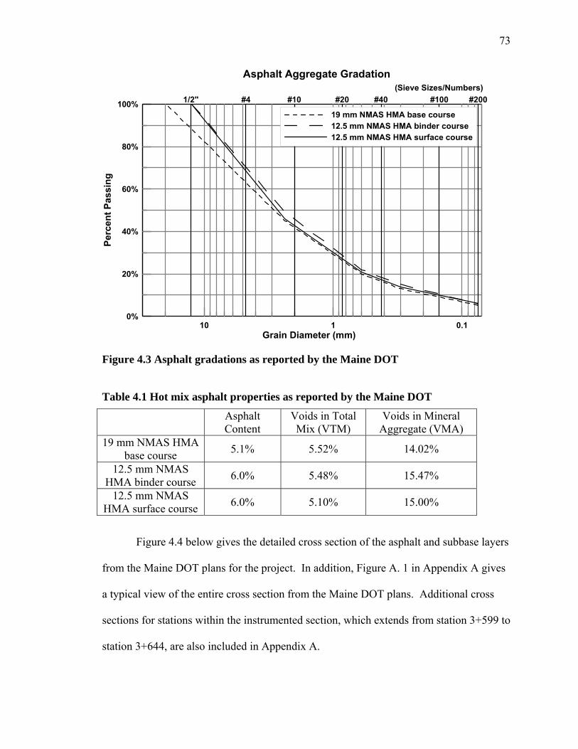
73
10 1 0.1Grain Diameter (mm)
0%
20%
40%
60%
80%
100%Pe
rcen
t Pas
sing
1/2" #4 #10 #20 #40 #100 #200
19 mm NMAS HMA base course12.5 mm NMAS HMA binder course12.5 mm NMAS HMA surface course
Asphalt Aggregate Gradation(Sieve Sizes/Numbers)
Figure 4.3 Asphalt gradations as reported by the Maine DOT
Table 4.1 Hot mix asphalt properties as reported by the Maine DOT
Asphalt Content
Voids in Total Mix (VTM)
Voids in Mineral Aggregate (VMA)
19 mm NMAS HMA base course 5.1% 5.52% 14.02%
12.5 mm NMAS HMA binder course 6.0% 5.48% 15.47%
12.5 mm NMAS HMA surface course 6.0% 5.10% 15.00%
Figure 4.4 below gives the detailed cross section of the asphalt and subbase layers
from the Maine DOT plans for the project. In addition, Figure A. 1 in Appendix A gives
a typical view of the entire cross section from the Maine DOT plans. Additional cross
sections for stations within the instrumented section, which extends from station 3+599 to
station 3+644, are also included in Appendix A.
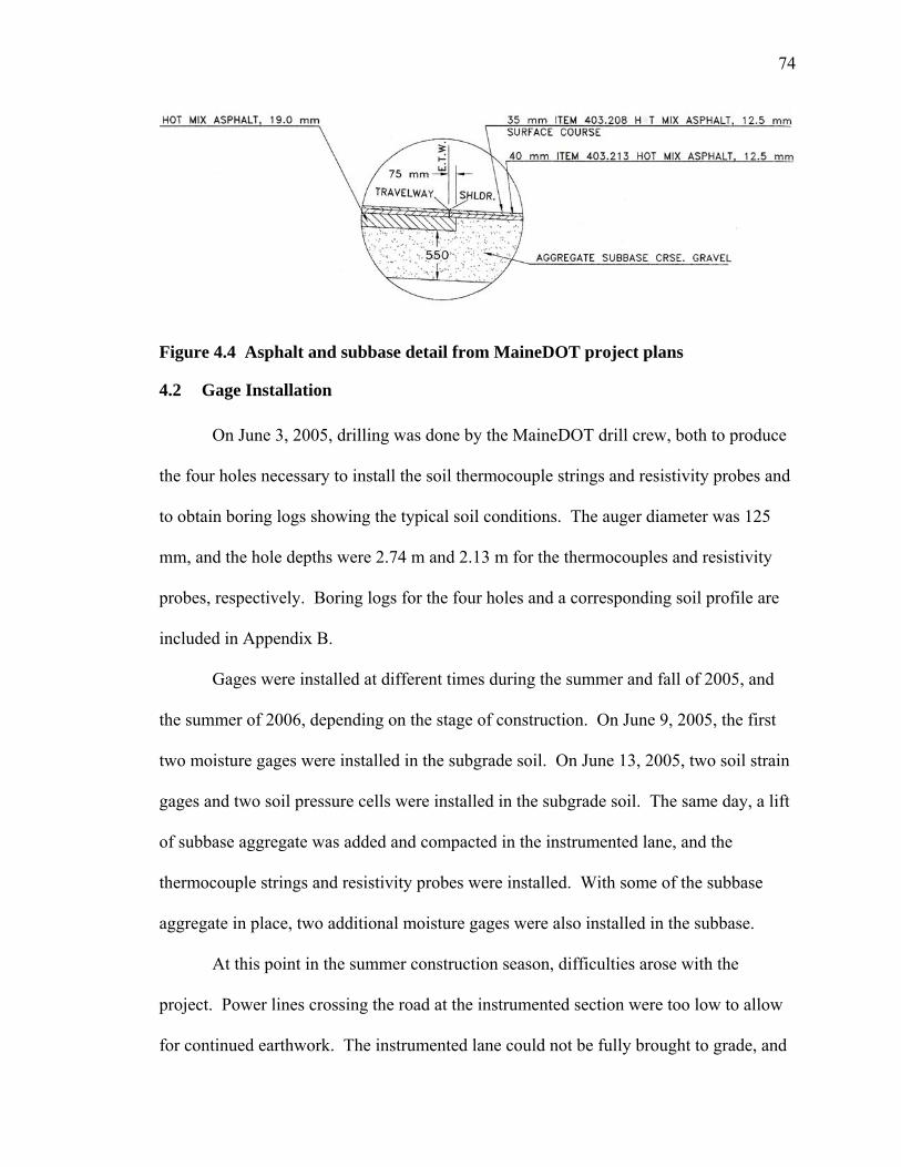
74
Figure 4.4 Asphalt and subbase detail from MaineDOT project plans
4.2 Gage Installation
On June 3, 2005, drilling was done by the MaineDOT drill crew, both to produce
the four holes necessary to install the soil thermocouple strings and resistivity probes and
to obtain boring logs showing the typical soil conditions. The auger diameter was 125
mm, and the hole depths were 2.74 m and 2.13 m for the thermocouples and resistivity
probes, respectively. Boring logs for the four holes and a corresponding soil profile are
included in Appendix B.
Gages were installed at different times during the summer and fall of 2005, and
the summer of 2006, depending on the stage of construction. On June 9, 2005, the first
two moisture gages were installed in the subgrade soil. On June 13, 2005, two soil strain
gages and two soil pressure cells were installed in the subgrade soil. The same day, a lift
of subbase aggregate was added and compacted in the instrumented lane, and the
thermocouple strings and resistivity probes were installed. With some of the subbase
aggregate in place, two additional moisture gages were also installed in the subbase.
At this point in the summer construction season, difficulties arose with the
project. Power lines crossing the road at the instrumented section were too low to allow
for continued earthwork. The instrumented lane could not be fully brought to grade, and

75
the opposite lane could not have any subbase aggregate added because the power lines
would be too low for truck traffic to travel safely underneath them. After one month, on
July 15, 2005, half of the instrumented section was brought up to grade, and a layer of
reclaimed asphalt was compacted at the subbase surface.
In September of 2005, after additional weather related construction delays, the left
side of the section was ready to be paved. On September 1, the thermocouple flier at the
top of the left soil thermocouple string was positioned in the subbase aggregate, and a
moisture gage, pressure cell and strain gage were installed in the subbase. On September
6, the initial layer of asphalt was placed and six asphalt strain gages and one asphalt
thermocouple were installed at the base of that layer. The following day, a second
asphalt thermocouple was installed with the second layer of asphalt. A joint in the
asphalt base was located just beyond the centerline of the instrumented section. After
this first paving, most of the right side of the section was still exposed at the subbase
level, although the locations of the previously installed soil resistivity, thermocouple, and
moisture gages on the right side were covered by the asphalt.
On September 13, after the right side of the instrumented section had been
brought to grade, a pressure cell, strain gage, and moisture gage were installed. The
moisture gage could not be installed at the same location of the previous two moisture
gages on the right side of the section because asphalt already covered the area. The layer
of asphalt also prevented a thermocouple flier from being positioned away from the right
thermocouple string.
On October 11, paving took place, and six asphalt strain gages and a
thermocouple were installed. On the left side of the section, the asphalt strain gages had
76
been placed in the locations over the resistivity probe and over the soil pressure/strain
gages. This setup had to be modified for the right side because of the asphalt that had
already been placed over the resistivity probe. On October 12, another asphalt
thermocouple was installed with the next pavement layer.
The final surface asphalt layer was not placed until the summer of 2006. On June
17, 2006, the entire instrumented section was paved with the surface course, and the final
two asphalt thermocouples were installed. Later in the summer of 2006, the entire Route
15 reconstruction project was completed.
4.3 Summary
Most of the instrumentation at the Guilford site was installed during the summers
of 2005 and 2006, prior to the completion of road construction. After the summer of
2005, a data acquisition system was installed, and is described in Chapter 5. After road
construction was finished in 2006, additional gages were to be installed, including a
weigh-in-motion machine, and multi-depth deflectometers. The complete instrumented
roadway will provide in-situ data that can be used for the analysis of pavement layer
responses.

77
Chapter 5
DATA ACQUISITION
5.1 Introduction
Each type of gage described has its own scheme of data acquisition. The dynamic
stress and strain gages connect to a computer system that allows for high speed data
collection, while the static environmental data gages are connected to a data acquisition
system that collects hourly readings.
5.2 Dynamic Data Acquisition
Two high speed PCI data acquisition boards were installed in a desktop PC to be
kept in the shed on site. The computer is a Dell Optiplex GX280 with an Intel Pentium 4
3.00 GHz processor, 1 GB of memory, and a 150 GB hard drive. The computer is
running Windows XP Pro, and has National Instruments LabVIEW 7.1 and Campbell
Scientific LoggerNet 2.1 data acquisition software installed.
The two data acquisition boards installed were part of the United Electronics
Industries, Inc. (UEI) Power DAQ 2 (PD2) series of multifunction data acquisition
boards. The PD2-MF-64-333/16L board has 64 single ended or 32 differential 16-bit
analog input channels. The board is capable of taking a total of 333,000 readings per
second and is equipped for gains of 1, 10, 100, and 1000. The PD2-MF-16-150/16L
board has the same characteristics, except that it has only 16 single ended or 8 differential
channels, and it collects up to 150,000 total readings per second. The two UEI boards
were capable of collecting data in the +/- 10 volt range
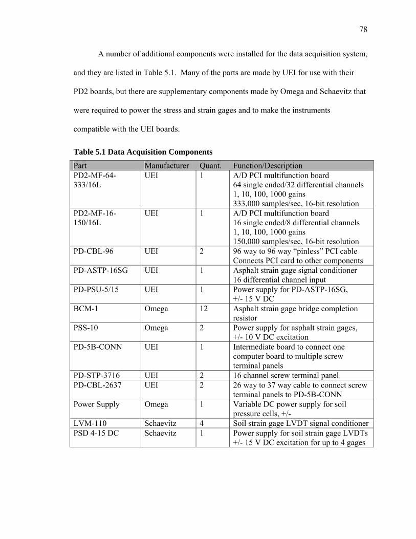
78
A number of additional components were installed for the data acquisition system,
and they are listed in Table 5.1. Many of the parts are made by UEI for use with their
PD2 boards, but there are supplementary components made by Omega and Schaevitz that
were required to power the stress and strain gages and to make the instruments
compatible with the UEI boards.
Table 5.1 Data Acquisition Components
Part Manufacturer Quant. Function/Description PD2-MF-64-333/16L
UEI 1 A/D PCI multifunction board 64 single ended/32 differential channels 1, 10, 100, 1000 gains 333,000 samples/sec, 16-bit resolution
PD2-MF-16-150/16L
UEI 1 A/D PCI multifunction board 16 single ended/8 differential channels 1, 10, 100, 1000 gains 150,000 samples/sec, 16-bit resolution
PD-CBL-96 UEI 2 96 way to 96 way “pinless” PCI cable Connects PCI card to other components
PD-ASTP-16SG UEI 1 Asphalt strain gage signal conditioner 16 differential channel input
PD-PSU-5/15 UEI 1 Power supply for PD-ASTP-16SG, +/- 15 V DC
BCM-1 Omega 12 Asphalt strain gage bridge completion resistor
PSS-10 Omega 2 Power supply for asphalt strain gages, +/- 10 V DC excitation
PD-5B-CONN UEI 1 Intermediate board to connect one computer board to multiple screw terminal panels
PD-STP-3716 UEI 2 16 channel screw terminal panel PD-CBL-2637 UEI 2 26 way to 37 way cable to connect screw
terminal panels to PD-5B-CONN Power Supply Omega 1 Variable DC power supply for soil
pressure cells, +/- LVM-110 Schaevitz 4 Soil strain gage LVDT signal conditioner PSD 4-15 DC Schaevitz 1 Power supply for soil strain gage LVDTs
+/- 15 V DC excitation for up to 4 gages

79
The soil strain gages are connected to their own signal conditioners, which were
described earlier with the explanation of the gages’ calibration procedure. The signal
conditioners are connected differentially to UEI’s PD-STP-3716 screw terminal panel
(STP). The soil pressure cells are connected differentially directly to their own STP.
Both STPs are connected to the PD-5BCONN, which serves as a connector back to the 64
channel board in the computer. Figure 5.1 shows the soil strain and soil pressure data
acquisition setups, along with the asphalt strain gage data acquisition system which is
described next.
The asphalt strain gages are each connected to an Omega Engineering, Inc. BCM-
1 bridge completion resistor, which provides bridge completion for the 120 ohm quarter
bridge strain gages. The twelve bridge completion resistors are connected to a signal
conditioning board made by UEI. The PD-ASTP-16SG strain gage signal conditioner is
powered by a +/- 15 volt DC power supply, and is also connected to two 10 volt DC
power supplies, which provide the power to the strain gages.

80
(a)
(b)
(c)
Figure 5.1 Data acquisition for (a) soil strain gages, (b) soil pressure cells, and (c) asphalt strain gages

81
The signal conditioner also provides amplification. For the asphalt strain gages,
the highest available amplification of 200 was initially chosen. After the instrumentation
was installed, the nine functioning asphalt strain gages could be zeroed using the
potentiometers on their bridge completion resistors. After the winter and spring season in
2005 and 2006, some of the asphalt strain gages could no longer be completely zeroed.
For these gages, an amplification of 200 caused their initial positions to be far from zero,
and in some cases, the amplified starting point was outside the +/- 10 V range of the data
acquisition boards. The addition of resistors to the bridge completion resistors allowed
the gages to be zeroed, but it was unknown how to account for this added resistance in
the calculation of strain from output voltage. A different approach was taken, and the
amplification was reduced. This parameter is included directly in the strain calculation,
and variations can be easily accounted for. As noted in Table 3.2 included earlier with
the description of the asphalt strain gages, the amplification on gages 498-004, 498-011,
498-013, and 498-014 were changed from 200 to 50.
Data was collected using the National Instruments LabVIEW version 7.1
software. Two different LabVIEW programs, or Virtual Instruments (VIs) were used
with the data acquisition system. The programming behind LabVIEW VIs is done in the
format of block diagrams. The VIs for this project were written by UEI to be used with
their data acquisition devices, and a few modifications were made to allow data to be
saved to a file and to change the precision of the readings that were collected.
Both VIs allowed for similar parameters to be modified. A resource string was
set up on the VI front panel prior to running the program. The resource string is a list of
parameter values in a specific order for the LabVIEW programs to read, so that the

82
computer will collect data from the gages correctly. The resource string had the
following format:
<deviceclass>://<IP Address>/Dev<DeviceID>/<Subsystem><ChannelList>
The device class for the both of the boards used was “pwrDAQ,” and the IP
Address did not need to be specified. The 64 channel board had the device ID “0” and
the 16 channel board had the device ID “1.” The subsystem for this format of data
collection is “Ai,” standing for analog input. The channel list varied depending on the
gages being used.
On the front panels, the minimum and maximum range values could be set, along
with the refresh rate, and the input mode of single ended versus differential readings.
The file path for the collected data was also specified on the VI front panels. While the
programs are running, a real time graphical display of voltage versus time can be seen, as
well as a recording of the total number of scans acquired.
The two VIs used for the project appear the same on their front panels, but they
are programmed to collect data differently. The VI “one board multiple channel sets 6
decimal places” allows the user to specify different collection parameters for different
sets of channels on one data acquisition board. The VI “multiple devices 6 decimal
places” lets the user set collection parameters for multiple boards at one time. The front
panels for these two VIs are compared in Figure 5.2 along with their corresponding block
diagrams.

83
Figure 5.2 National Instruments LabVIEW 7.1: (a) multiple devices front panel;
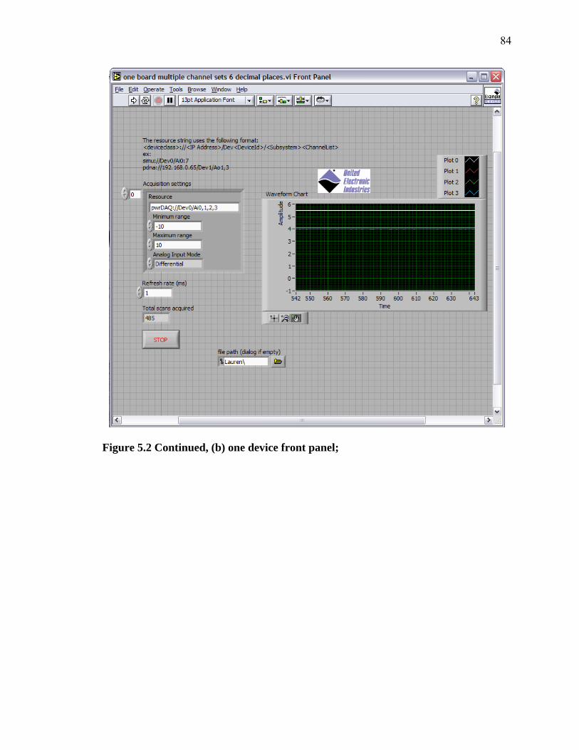
84
Figure 5.2 Continued, (b) one device front panel;

85
Figure 5.2 Continued, (c) multiple devices block diagram;
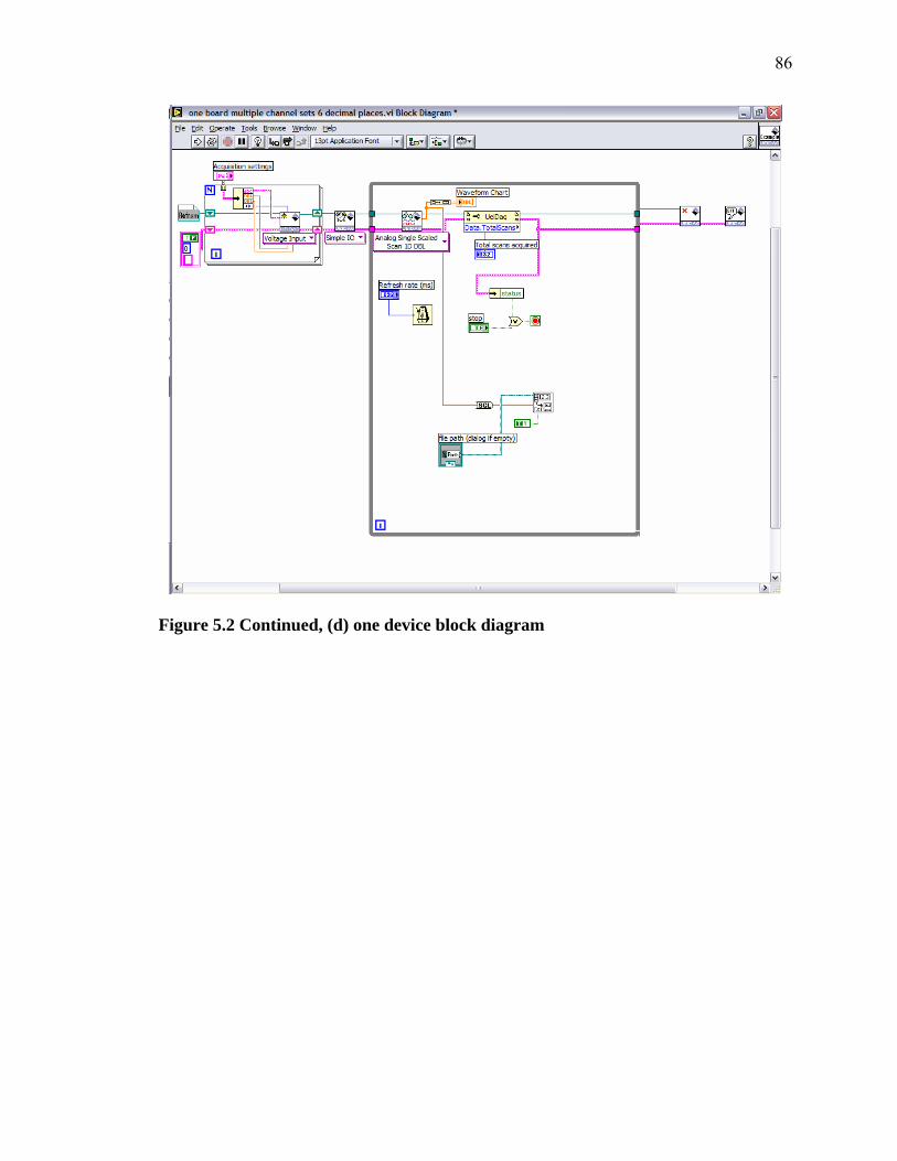
86
Figure 5.2 Continued, (d) one device block diagram

87
The LabVIEW output files are comma separated value text files containing
columns of voltages corresponding to individual channels. There were some difficulties
with data collection and the interpretation of the output files. The data files typically did
not display data in the same order as specified by the channel list in the resource string.
By graphing the data output, and using knowledge of typical gage outputs and the general
layout of the gages on the project site, the data files can be interpreted correctly. Using
the output data, and calibration equations discussed earlier, the voltage output can be
converted to either stress or strain.
5.3 Static Data Acquisition
The temperature, moisture, and resistivity gages were connected to dataloggers
made by Campbell Scientific, Inc. AM25T multiplexers were used with the dataloggers
for the thermocouples. Readout boxes manufactured by ABF Manufacturing were used
as the interface between the datalogger and the resistivity probes. The six moisture gages
were connected directly to a CR10X. Each CR10x was connected to a 12 volt battery,
which is kept continuously charged using the shed’s power.
Campbell Scientific’s LoggerNet 2.1 was used to compile programs to collect
data from the environmental gages. The programs were set up to record the date, time,
and battery voltage for each reading. Using LoggerNet’s built-in list of instructions, the
programs record appropriate data from the gages and convert it to corresponding values
of temperature, volumetric water content, and resistivity.
Data is obtained from the datalogger by connecting the CR10x to the computer in
the shed using an SC32A Optically Isolated RS232 Interface from Campbell Scientific.
The data is output in spreadsheet form for use in analysis.

88
5.4 Summary
Two different types of data acquisition systems were installed. The dynamic
stress and strain gages were connected to a high speed data collection system that
recorded data on a computer using the LabVIEW computer program. Environmental
gages, including the thermocouples, resistivity probes, and moisture gages were
connected to dataloggers which recorded and saved readings hourly. This data could then
be manually transferred to a computer for analysis. The entire data acquisition system
was installed after the summer of 2005, and remains onsite in an instrumentation shed.
89
Chapter 6
RESULTS
6.1 Introduction
After installation of the gages was complete, and data acquisition components
were in place, the system was ready to record data. The dynamic data acquisition system
was set up so that stresses and strains due to traffic loading could be collected during the
winter, spring, and summer of 2006. The system was not set up for continuous traffic
observations. Instead, data was collected for individual vehicles on specific days. The
weigh-in-motion (WIM) machine that will eventually be used to weigh vehicles and
trigger data acquisition could not be installed until the final asphalt layer was in place.
The final stages of road construction did not occur until the summer of 2006, and the
WIM was not set to be installed until the fall of that year, so no automated readings were
obtained at this stage of the project. Moreover, the weight of trucks passing over the
instrumentation was unknown except on days when a pre-weighted MaineDOT truck was
used.
Data collection was done for three different loading schemes, which are listed in
Table 6.1 along with the days when readings were taken. To take readings without using
the WIM machine, the Lab VIEW data collection software was manually started for each
vehicle of interest that was observed. Appendices C through F include plots of asphalt
strain, and soil stress and strain for vehicles observed on the dates listed in Table 6.1.
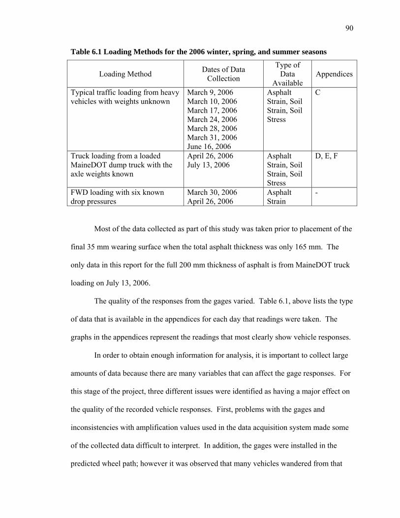
90
Table 6.1 Loading Methods for the 2006 winter, spring, and summer seasons
Loading Method Dates of Data Collection
Type of Data
Available Appendices
Typical traffic loading from heavy vehicles with weights unknown
March 9, 2006 March 10, 2006 March 17, 2006 March 24, 2006 March 28, 2006 March 31, 2006 June 16, 2006
Asphalt Strain, Soil Strain, Soil Stress
C
Truck loading from a loaded MaineDOT dump truck with the axle weights known
April 26, 2006 July 13, 2006
Asphalt Strain, Soil Strain, Soil Stress
D, E, F
FWD loading with six known drop pressures
March 30, 2006 April 26, 2006
Asphalt Strain
-
Most of the data collected as part of this study was taken prior to placement of the
final 35 mm wearing surface when the total asphalt thickness was only 165 mm. The
only data in this report for the full 200 mm thickness of asphalt is from MaineDOT truck
loading on July 13, 2006.
The quality of the responses from the gages varied. Table 6.1, above lists the type
of data that is available in the appendices for each day that readings were taken. The
graphs in the appendices represent the readings that most clearly show vehicle responses.
In order to obtain enough information for analysis, it is important to collect large
amounts of data because there are many variables that can affect the gage responses. For
this stage of the project, three different issues were identified as having a major effect on
the quality of the recorded vehicle responses. First, problems with the gages and
inconsistencies with amplification values used in the data acquisition system made some
of the collected data difficult to interpret. In addition, the gages were installed in the
predicted wheel path; however it was observed that many vehicles wandered from that

91
path. Finally, the stiffness of the pavement layers in combination with the depth of the
gages from the surface affects the output. This is most prominently seen in the soil
gages.
With the data that was collected from the different loading schemes, a variety of
analyses were carried out. In situ stress and strain data provides the opportunity to
calculate parameters like layer resilient moduli and the number of loading cycles to cause
fatigue cracking, in a way that avoids many of the assumptions that are required when
laboratory testing or backcalculation is used.
Calculated field values of moduli can be compared to other values to determine the
relationships between in situ conditions and the conditions that are used in the laboratory,
or are modeled in backcalculation procedures. Collected climate data was also used to
provide information on how the stress and strain responses in the field change with
changing environmental conditions.
6.2 Climate Data
Thermocouples in the soil and asphalt recorded temperature at different depths.
Some manual thermocouple readings were taken in the early months of 2006, and the
data acquisition system was set up and collecting data on March 3, 2006.
Temperatures in the subbase and subgrade were used to determine the locations of
the freezing and thawing fronts for the winter and spring of 2006. Figure 6.1 shows the
frost depths for the thermocouple strings located at station 3+602 to the left of the shed
and station 3+635 to the right of the shed. The maximum depth of frost penetration was
approximately 1.2 m. The continuous readings from the data acquisition system show the

92
thawing of the soil pavement layers taking place through the month of March. March 28
was the last date that frost was in the subgrade.
A weather station is located in Guilford approximately 8 km from the
instrumented site. Average daily temperature readings were obtained from the station for
2005 and 2006, and these temperatures were used to calculate the freezing index. The
freezing index is a measure of how cold the winter was based on both temperatures and
the duration of those temperatures.
The freezing index is obtained by first plotting cumulative degree days versus
time. The difference between the minimum and maximum values on the plot is the
freezing index. The freezing index for 2005/2006 was 575 °C-days, with a duration of
125 days. The mean freezing index for the project site is between 800 and 900 °C-days,
so the winter was mild compared to what was expected for the area. (Bigelow, 1969)
An analysis of the freezing degree days, Figure 6.2, shows no pronounced
thawing to correspond to the deep thawing shown by the thermocouple data in early
February. One possible reason for this discrepancy is that the soil temperature readings
from this time period were obtained using a handheld reader. This reader is less accurate
than the CR10x datalogger that was later installed to record temperatures.
The average daily temperatures used for freezing degree day calculations were not
from the project site, so the actual air temperatures at the instrumented section may have
been different. An accurate measurement of temperature representing the air temperature
at the surface of the pavement section is necessary. A thermocouple to measure air
temperature was installed in the spring, but was located in an area that was at some points
covered by snow, so the temperatures obtained would not always be accurate.

93
(a)
12/3
1/05
1/10
/06
1/20
/06
1/30
/06
2/9/
06
2/19
/06
3/1/
06
3/11
/06
3/21
/06
3/31
/06
4/10
/06
Date
55
50
45
40
35
30
25
20
15
10
5
0
Dep
th (i
n)
13001200110010009008007006005004003002001000
Dep
th (m
m)
Freezing Front (Continuous Readings)Thawing Front (Continuous Readings)Freezing Front (Manual Readings)
p
ManualThermocouple
Readings
ContinuousThermocoupleReadings
Depth of ShallowestSoil Thermocouple
(b)
12/3
1/05
1/10
/06
1/20
/06
1/30
/06
2/9/
06
2/19
/06
3/1/
06
3/11
/06
3/21
/06
3/31
/06
4/10
/06
Date
55
50
45
40
35
30
25
20
15
10
5
0
Dep
th (i
n)
13001200110010009008007006005004003002001000
Dep
th (m
m)
Freezing Front (Continuous Readings)Thawing Front (Continuous Readings)Freezing Front (Manual Readings)Thawing Front (Manual Readings)
p g
ManualThermocouple
Readings
ContinuousThermocoupleReadings
Depth of ShallowestSoil Thermocouple
Figure 6.1 Zero degree isotherm for the thermocouple locations on the (a) left at station 3+602 and on the (b) right at station 3+635.
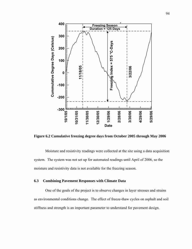
94
10/1
/05
10/3
1/05
11/3
0/05
12/3
0/05
1/29
/06
2/28
/06
3/30
/06
4/29
/06
5/29
/06
Date
-300
-200
-100
0
100
200
300
400
Cum
mul
ativ
e D
egre
e D
ays
(Cel
sius
)
Free
zing
Inde
x =
575
°C-D
ays
yFreezing Season
Duration = 125 Days
11/1
8/05
3/22
/06
Figure 6.2 Cumulative freezing degree days from October 2005 through May 2006
Moisture and resistivity readings were collected at the site using a data acquisition
system. The system was not set up for automated readings until April of 2006, so the
moisture and resistivity data is not available for the freezing season.
6.3 Combining Pavement Responses with Climate Data
One of the goals of the project is to observe changes in layer stresses and strains
as environmental conditions change. The effect of freeze-thaw cycles on asphalt and soil
stiffness and strength is an important parameter to understand for pavement design.
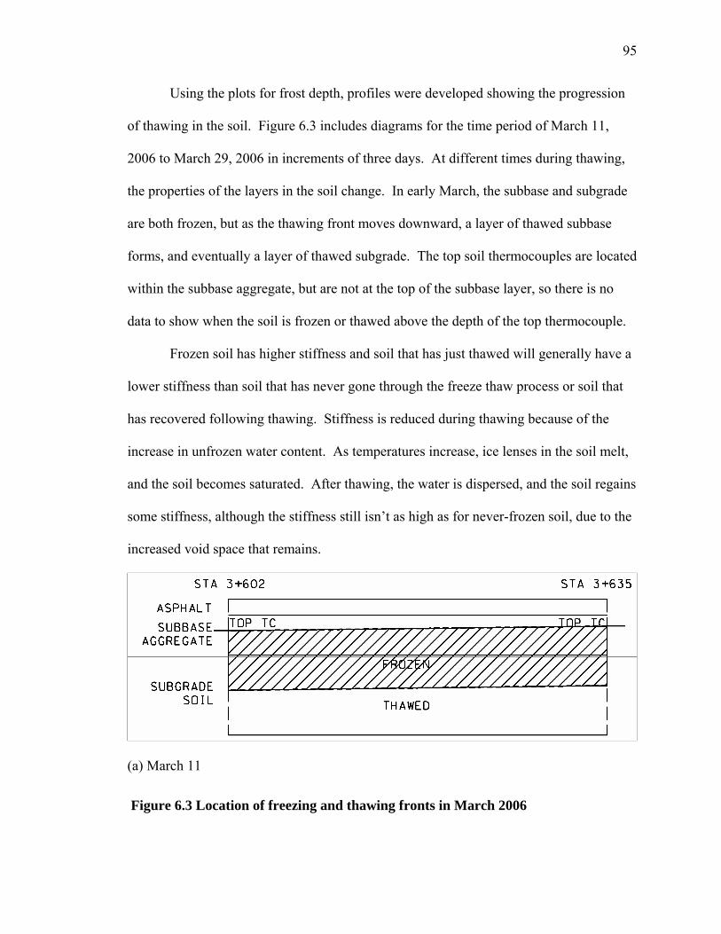
95
Using the plots for frost depth, profiles were developed showing the progression
of thawing in the soil. Figure 6.3 includes diagrams for the time period of March 11,
2006 to March 29, 2006 in increments of three days. At different times during thawing,
the properties of the layers in the soil change. In early March, the subbase and subgrade
are both frozen, but as the thawing front moves downward, a layer of thawed subbase
forms, and eventually a layer of thawed subgrade. The top soil thermocouples are located
within the subbase aggregate, but are not at the top of the subbase layer, so there is no
data to show when the soil is frozen or thawed above the depth of the top thermocouple.
Frozen soil has higher stiffness and soil that has just thawed will generally have a
lower stiffness than soil that has never gone through the freeze thaw process or soil that
has recovered following thawing. Stiffness is reduced during thawing because of the
increase in unfrozen water content. As temperatures increase, ice lenses in the soil melt,
and the soil becomes saturated. After thawing, the water is dispersed, and the soil regains
some stiffness, although the stiffness still isn’t as high as for never-frozen soil, due to the
increased void space that remains.
(a) March 11
Figure 6.3 Location of freezing and thawing fronts in March 2006
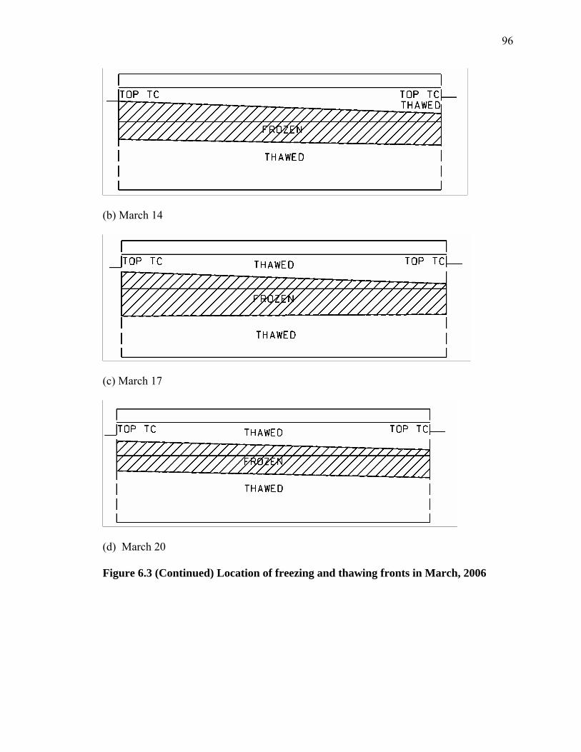
96
(b) March 14
(c) March 17
(d) March 20
Figure 6.3 (Continued) Location of freezing and thawing fronts in March, 2006
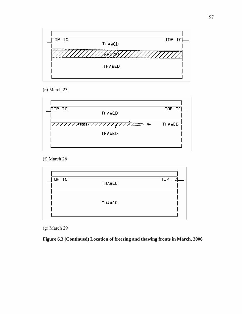
97
(e) March 23
(f) March 26
(g) March 29
Figure 6.3 (Continued) Location of freezing and thawing fronts in March, 2006

98
The stiffness of the pavement layers due to changing temperatures affects the
stress and strain responses of each layer. Data from normal traffic loading is available for
seven days in the time period from 3/9 to 3/31. For each observed vehicle, the asphalt
strain and soil stress and strain gages recorded values. During this time period, very few
loads were large enough to register a change in stress in the subbase and subgrade soils,
indicating that the material stiffness is increased due to the freezing, or near-freezing
conditions present in the soil and the asphalt. By the time MaineDOT truck loading took
place on March 26, 2006, the stresses recorded in the subbase and subgrade layers were
large enough to be measured.
6.4 Asphalt Responses
Traffic loading data was collected from different days during the first half of
2006. As described earlier, asphalt data was the easiest to interpret.
6.4.1 Asphalt Tensile Strain
Table C.1 in Appendix C includes maximum tensile strain values from traffic
loading for asphalt strain gages 498- 003, 005, 006, 008, and 009. The plots of tensile
asphalt strain due to traffic loading are included in Appendix C.
Figure 6.4 shows two typical asphalt strain plots. These plots are for a six-axle
loaded log truck observed on March 9, 2006. Figure 6.4 also includes a photograph of a
typical log truck. There is a single steering axle, with two axles at the front of the trailer,
and three axles at the back of the trailer. Each axle provides a separate strain response
that is represented by a peak on the strain plot from each gage.
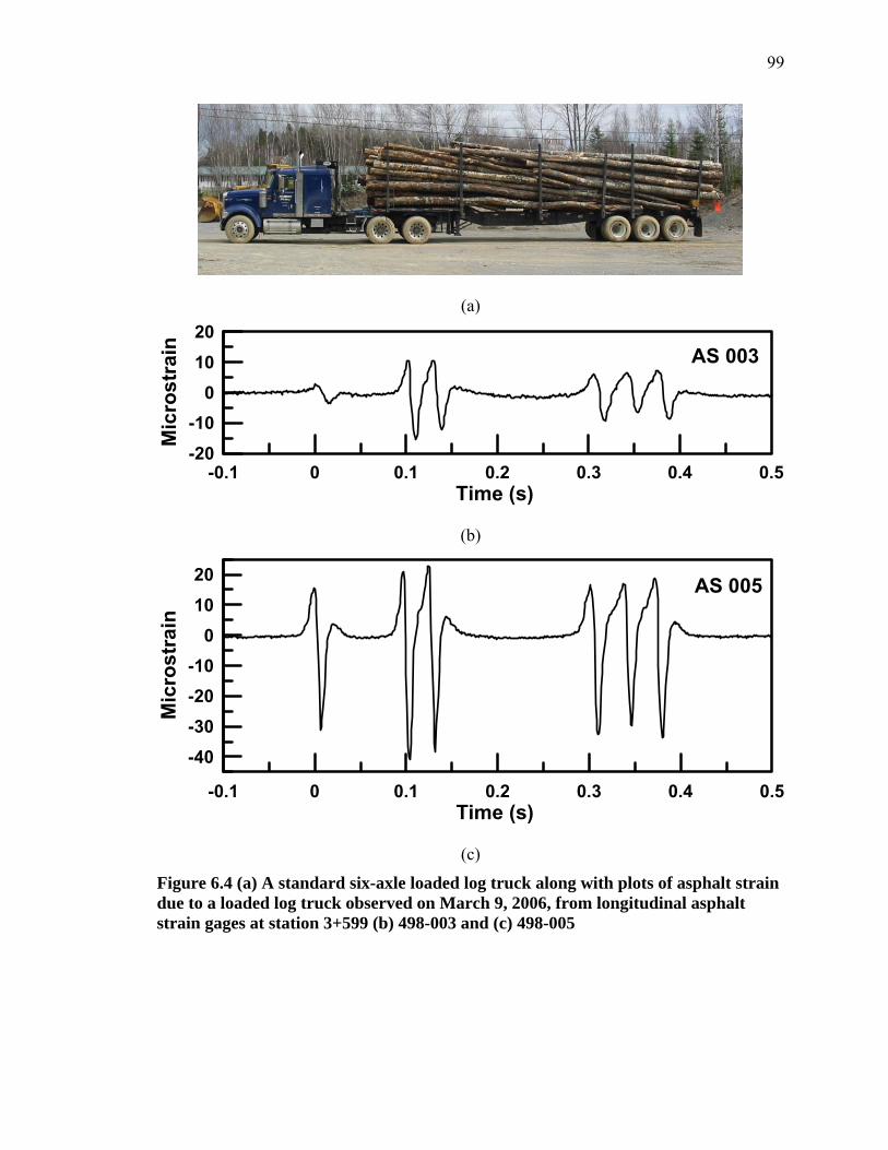
99
(a)
-0.1 0 0.1 0.2 0.3 0.4 0.5Time (s)
-20-10
01020
Mic
rost
rain AS 003
(b)
-0.1 0 0.1 0.2 0.3 0.4 0.5Time (s)
-40-30-20-10
01020
Mic
rost
rain
AS 005
(c)
Figure 6.4 (a) A standard six-axle loaded log truck along with plots of asphalt strain due to a loaded log truck observed on March 9, 2006, from longitudinal asphalt strain gages at station 3+599 (b) 498-003 and (c) 498-005

100
The strain values of interest are the maximum tensile or negative strains. The
plots shown above are for two longitudinal strain gages in the first group of three gages to
the left of the shed, located at approximately station 3+599. These are the first gages that
a vehicle drives over when it reaches the instrumented site. Referring back to the
instrumentation plan in Figure 3.1 in Chapter 3, asphalt strain gage 498-003 is located
closest to the road centerline, and gage 498-005 is located closest to the shoulder. Due to
data acquisition problems, readings from the middle gage 498-004 are not available.
For the March 9 vehicle shown in Figure 6.4, the strain response for each axle
load at different transverse locations (gages 498-003 and 498-005) at station 3+599 are
very different. Figure 6.5 below shows the response of these gages for a different loaded
six-axle log truck observed on March 10.
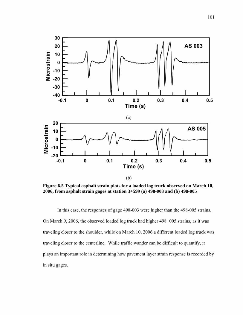
101
-0.1 0 0.1 0.2 0.3 0.4 0.5Time (s)
-40-30-20-10
0102030
Mic
rost
rain
AS 003
(a)
-0.1 0 0.1 0.2 0.3 0.4 0.5Time (s)
-20-10
01020
Mic
rost
rain AS 005
(b)
Figure 6.5 Typical asphalt strain plots for a loaded log truck observed on March 10, 2006, from asphalt strain gages at station 3+599 (a) 498-003 and (b) 498-005
In this case, the responses of gage 498-003 were higher than the 498-005 strains.
On March 9, 2006, the observed loaded log truck had higher 498+005 strains, as it was
traveling closer to the shoulder, while on March 10, 2006 a different loaded log truck was
traveling closer to the centerline. While traffic wander can be difficult to quantify, it
plays an important role in determining how pavement layer strain response is recorded by
in situ gages.
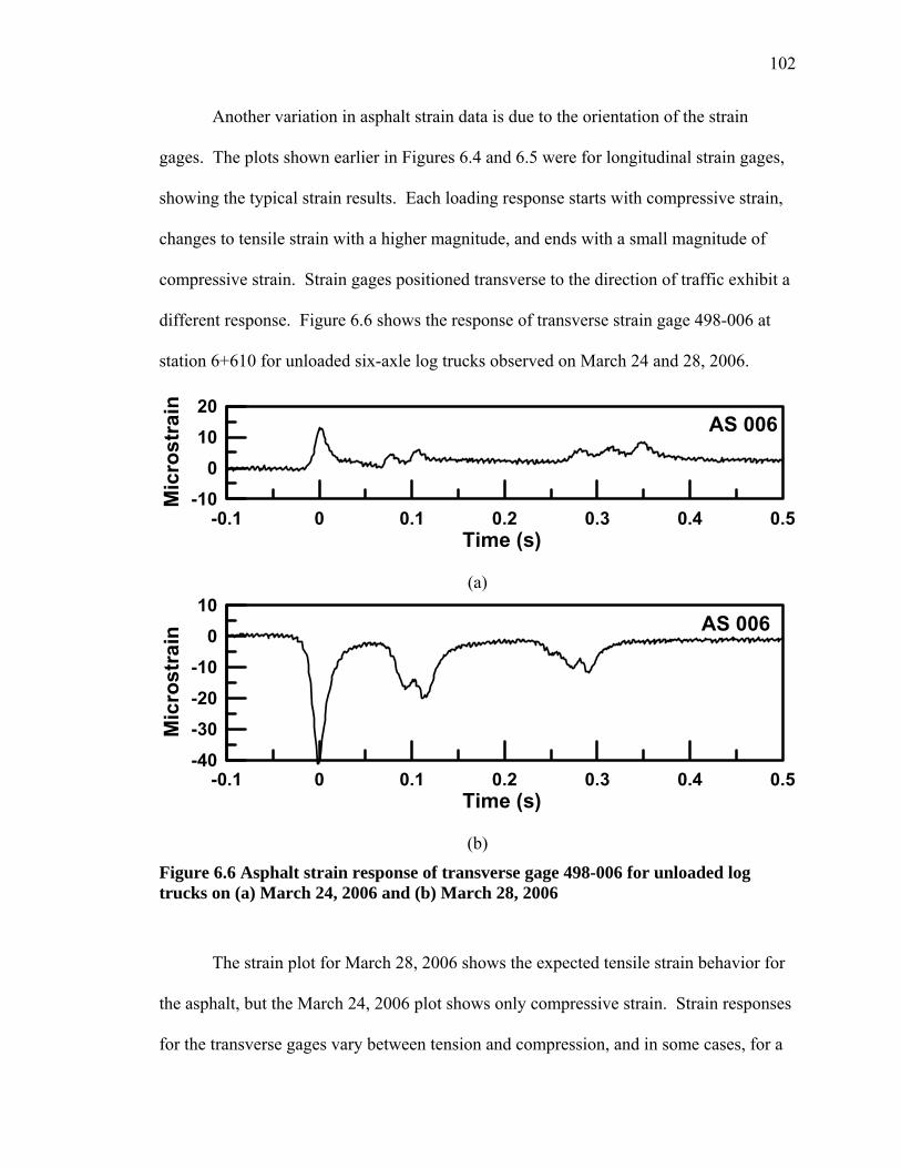
102
Another variation in asphalt strain data is due to the orientation of the strain
gages. The plots shown earlier in Figures 6.4 and 6.5 were for longitudinal strain gages,
showing the typical strain results. Each loading response starts with compressive strain,
changes to tensile strain with a higher magnitude, and ends with a small magnitude of
compressive strain. Strain gages positioned transverse to the direction of traffic exhibit a
different response. Figure 6.6 shows the response of transverse strain gage 498-006 at
station 6+610 for unloaded six-axle log trucks observed on March 24 and 28, 2006.
-0.1 0 0.1 0.2 0.3 0.4 0.5Time (s)
-100
1020
Mic
rost
rain
AS 006
(a)
-0.1 0 0.1 0.2 0.3 0.4 0.5Time (s)
-40-30-20-10
010
Mic
rost
rain AS 006
(b)
Figure 6.6 Asphalt strain response of transverse gage 498-006 for unloaded log trucks on (a) March 24, 2006 and (b) March 28, 2006
The strain plot for March 28, 2006 shows the expected tensile strain behavior for
the asphalt, but the March 24, 2006 plot shows only compressive strain. Strain responses
for the transverse gages vary between tension and compression, and in some cases, for a
103
single vehicle there will be a combination of tension and compression for different axles.
This could be explained by wander. It may be possible that the location of a vehicle on
the road as it travels over the gages causes the forces to be distributed differently. For a
longitudinal gage, the force is progressively exerted along the entire gage, while for a
transverse gage, the maximum force is exerted in only one location and distributed
outward to the rest of the gage.
For MaineDOT truck loading, the asphalt responses were similar to traffic
loading. Truck loading was done on two different days, and for each day, weight
information was obtained for the vehicles. Two heavy duty hand-portable truck scales
were used to obtain the force exerted by each vehicle tire. The scales were first placed
under the front tires, and weights were recorded; the scales were switched and used to
weigh the front tires again; the scales were moved to the back tires and weights were
recorded; and the scales were again switched to obtain a second set of weights.
On March 26, 2006, gross vehicle weights were available from a full-sized truck
scale, and the weight at each truck tire was recorded using the hand-portable scales.
Comparing the total vehicle weight to the truck tire weights showed that the results from
truck scale two were the most accurate. The sum of the four tire loads measured using
truck scale two was approximately 1% less than the measured gross vehicle weight, while
the sum of the loads from truck scale one gave a total weight that was low by 22%.
Portable scale two values are included in Table 6.2. On July 13, 2006, only the weights
at each truck tire and not gross vehicle weight were recorded, but based on experience on
the previous loading day, scale two data was used. Weights for all tires are listed in the
following table, although due to the gage locations, the weights that are most significant
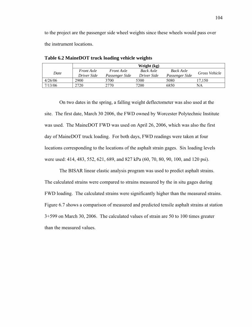
104
to the project are the passenger side wheel weights since these wheels would pass over
the instrument locations.
Table 6.2 MaineDOT truck loading vehicle weights Weight (kg)
Date Front Axle Driver Side
Front Axle Passenger Side
Back Axle Driver Side
Back Axle Passenger Side Gross Vehicle
4/26/06 2900 3700 5300 5080 17,150 7/13/06 2720 2770 7200 6850 NA
On two dates in the spring, a falling weight deflectometer was also used at the
site. The first date, March 30 2006, the FWD owned by Worcester Polytechnic Institute
was used. The MaineDOT FWD was used on April 26, 2006, which was also the first
day of MaineDOT truck loading. For both days, FWD readings were taken at four
locations corresponding to the locations of the asphalt strain gages. Six loading levels
were used: 414, 483, 552, 621, 689, and 827 kPa (60, 70, 80, 90, 100, and 120 psi).
The BISAR linear elastic analysis program was used to predict asphalt strains.
The calculated strains were compared to strains measured by the in situ gages during
FWD loading. The calculated strains were significantly higher than the measured strains.
Figure 6.7 shows a comparison of measured and predicted tensile asphalt strains at station
3+599 on March 30, 2006. The calculated values of strain are 50 to 100 times greater
than the measured values.
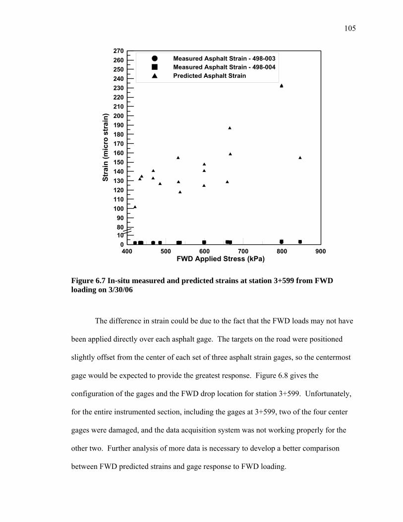
105
400 500 600 700 800 900FWD Applied Stress (kPa)
0108090
100110120130140150160170180190200210220230240250260270
Stra
in (m
icro
str
ain)
Measured Asphalt Strain - 498-003Measured Asphalt Strain - 498-004Predicted Asphalt Strain
Figure 6.7 In-situ measured and predicted strains at station 3+599 from FWD loading on 3/30/06
The difference in strain could be due to the fact that the FWD loads may not have
been applied directly over each asphalt gage. The targets on the road were positioned
slightly offset from the center of each set of three asphalt strain gages, so the centermost
gage would be expected to provide the greatest response. Figure 6.8 gives the
configuration of the gages and the FWD drop location for station 3+599. Unfortunately,
for the entire instrumented section, including the gages at 3+599, two of the four center
gages were damaged, and the data acquisition system was not working properly for the
other two. Further analysis of more data is necessary to develop a better comparison
between FWD predicted strains and gage response to FWD loading.

106
Figure 6.8 Layout of asphalt strain gages relative to the FWD drop location for station 3+599
Additional analysis was completed to compare predicted asphalt and soil stresses
and strains to gage responses recorded during MaineDOT dump truck loading. The
pavement layer properties obtained from FWD backcalculation were used to predict
stresses and strains due to the known vehicle weights on 7/13/06 given in Table 6.2. The
results of this analysis are included later in this section, following the discussion of
modulus, and provide more realistic data than the strain comparison seen above in Figure
6.7.
6.4.2 Asphalt Fatigue Cracking
The tensile strain values recorded for vehicle traffic can be utilized to help predict
the number of load repetitions required to cause fatigue cracking. The simplest form of
fatigue analysis requires only an input of the tensile strain at the base of the asphalt layer.
Huang (2004) provided an equation in the form
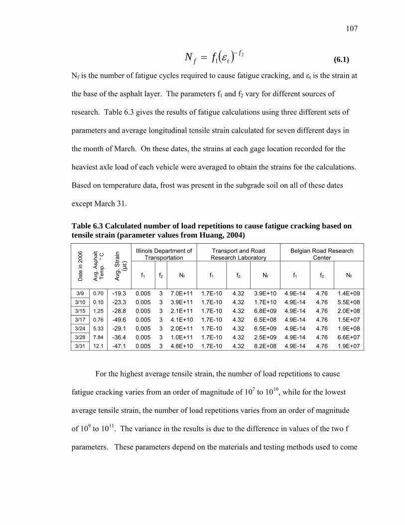
107
( ) 21
ftf fN −= ε (6.1)
Nf is the number of fatigue cycles required to cause fatigue cracking, and εt is the strain at
the base of the asphalt layer. The parameters f1 and f2 vary for different sources of
research. Table 6.3 gives the results of fatigue calculations using three different sets of
parameters and average longitudinal tensile strain calculated for seven different days in
the month of March. On these dates, the strains at each gage location recorded for the
heaviest axle load of each vehicle were averaged to obtain the strains for the calculations.
Based on temperature data, frost was present in the subgrade soil on all of these dates
except March 31.
Table 6.3 Calculated number of load repetitions to cause fatigue cracking based on tensile strain (parameter values from Huang, 2004)
Illinois Department of Transportation
Transport and Road Research Laboratory
Belgian Road Research Center
Dat
e in
200
6
Avg
. Asp
halt
Tem
p.
° C
Avg
. Stra
in
(µε)
f1 f2 Nf f1 f2 Nf f1 f2 Nf
3/9 0.70 -19.3 0.005 3 7.0E+11 1.7E-10 4.32 3.9E+10 4.9E-14 4.76 1.4E+09 3/10 0.10 -23.3 0.005 3 3.9E+11 1.7E-10 4.32 1.7E+10 4.9E-14 4.76 5.5E+08 3/15 1.25 -28.8 0.005 3 2.1E+11 1.7E-10 4.32 6.8E+09 4.9E-14 4.76 2.0E+08 3/17 0.76 -49.6 0.005 3 4.1E+10 1.7E-10 4.32 6.5E+08 4.9E-14 4.76 1.5E+07 3/24 5.33 -29.1 0.005 3 2.0E+11 1.7E-10 4.32 6.5E+09 4.9E-14 4.76 1.9E+08 3/28 7.84 -36.4 0.005 3 1.0E+11 1.7E-10 4.32 2.5E+09 4.9E-14 4.76 6.6E+07 3/31 12.1 -47.1 0.005 3 4.8E+10 1.7E-10 4.32 8.2E+08 4.9E-14 4.76 1.9E+07
For the highest average tensile strain, the number of load repetitions to cause
fatigue cracking varies from an order of magnitude of 107 to 1010, while for the lowest
average tensile strain, the number of load repetitions varies from an order of magnitude
of 109 to 1011. The variance in the results is due to the difference in values of the two f
parameters. These parameters depend on the materials and testing methods used to come
108
up with the values, and each of the three sets of parameters given above is the result of a
different study.
The Asphalt Institute and the Shell Oil Company also have equations for
calculating load repetitions to cause fatigue cracking. These equations are similar to
Equation 6.1 above, except that they include a term with asphalt modulus. With the
parameter values defined by the above two organizations, the modulus term has a smaller
effect on the final Nf value than the tensile strain term. This is why the modulus term can
be removed, and Equation 6.1 can be used instead (Huang, 2004).
The use of heavy trucks on roadways during spring thaw will result in more rapid
cracking of the asphalt. During the thawing period, the soil layers beneath the asphalt
lose stiffness. While the asphalt itself may have good stiffness, it has lost some of the
support from the underlying subbase and subgrade, and as a result, has a higher modulus.
Using the fatigue cracking equations to compare frozen and non-frozen pavement
sections will provide more insight into changing pavement properties. Also, with the in
situ measurement of pavement data, quantitative results can be compared directly to
actual pavement fatigue, to verify the design procedure for a particular pavement section.
6.5 Soil Responses
As with the asphalt gages, the soil gages were used to collect data for normal
traffic loading, MaineDOT truck loading, and FWD loading. Also similar to the asphalt
strains, the soil stress and strain responses are influenced by wander, but with soil gages
only beneath the center of the wheel path, it is not as easy to quantify this effect as with
the asphalt strain gages.
109
Electronic noise in gage readings also made the interpretation of the pressure cells
difficult. Noise consists of random changes in the gage outputs that are not due to actual
loading. The voltage output by the gages can vary while the gage is at rest due to outside
interference from electrical currents and nearby gages and wires, radio waves, and other
sources.
Figure 6.9 below shows soil strain and pressure at two depths for a loaded 3-axle
dump truck observed on June 16, 2006. The strain plots are clear, and while some noise
is present, it does not have a noticeable effect on the peak strain. The plots for pressure,
however, show a great deal of noise that registers within the range of +/- 50 kPa. At the
peak pressures, the noise is still present, and needs to be considered. When the pressure
cells are at rest, the noise is distributed relatively evenly above and below the x-axis, so it
is assumed that the noise will distributed similarly around the peak stress. The peak
stress is not taken as the highest point on the stress versus time curve. Instead it is
interpreted to be approximately at the mid-point of the noise.
Soil pressure and strain readings from earlier in the spring when the pavement
section was not completely thawed are even more difficult to interpret because the
response of the gages is reduced somewhat by the increased stiffness of the soil
surrounding the gages. The stiffness of the cooler asphalt over the subbase and subgrade
also reduces the response of the soil gages. Soil strain readings were collected on six
days during the spring thaw, but soil pressure responses were only seen for a few vehicles
on a couple of days. This could have been due to the presence of frozen soil, as well as
problems with data collection and soil response amplification. Plots for the collected
responses are in Appendix D.

110
Pressure readings from MaineDOT truck loading are easier to interpret. Figure
6.10 below shows stresses and strains at two soil depths for the two-axle loaded dump
truck. Difficulties experienced previously with collecting soil stress and strain data
together were eliminated by recording stress and strain data separately for different runs
with the same truck. Data acquisition was set up with a very small range to obtain more
precise readings. The soil pressure cell range for Maine DOT truck loading on April 26
was set for 0.013 volts to -0.005 volts, and on July 13, the range was 0.015 volts to -0.005
volts. This is in comparison to a range of 2 volts to -2 volts, the smallest range that would
allow data to be collected correctly for traffic loading observed on June 16. The effect of
wander was also reduced from normal traffic, because the truck driver was instructed to
aim for the same marked targets on each run.
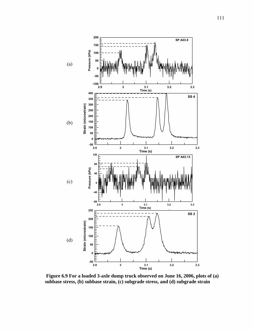
111
(a)
2.9 3 3.1 3.2 3.3Time (s)
-100
-50
0
50
100
150
200
Pres
sure
(kPa
)
SP A03.8
(b)
2.9 3 3.1 3.2 3.3Time (s)
-50
0
50
100
150
200
250
300
350
400
Stra
in (m
icro
stra
in)
SS 4
(c)
2.9 3 3.1 3.2 3.3Time (s)
-80
-40
0
40
80
120
Pres
sure
(kPa
)
SP A03.13
(d)
2.9 3 3.1 3.2 3.3Time (s)
-50
0
50
100
150
200
250
Stra
in (m
icro
stra
in)
SS 2
p
Figure 6.9 For a loaded 3-axle dump truck observed on June 16, 2006, plots of (a) subbase stress, (b) subbase strain, (c) subgrade stress, and (d) subgrade strain
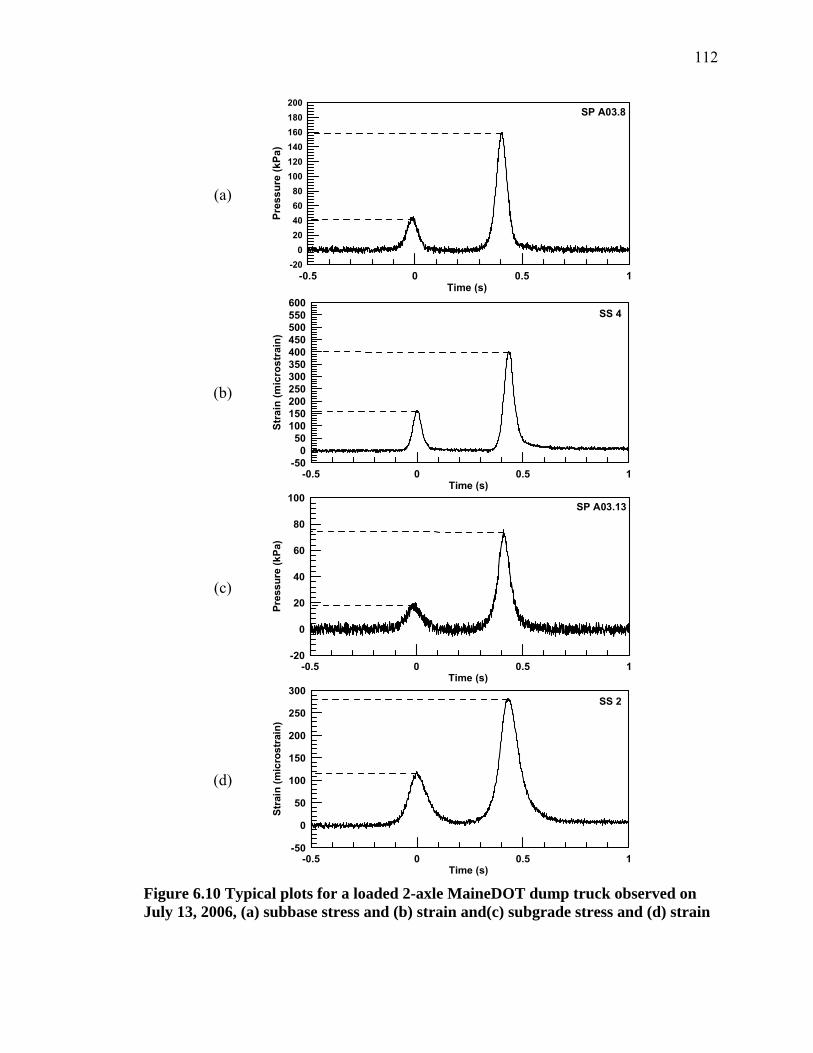
112
(a)
-0.5 0 0.5 1Time (s)
-200
20406080
100120140160180200
Pres
sure
(kPa
)
SP A03.8
(b)
-0.5 0 0.5 1Time (s)
-500
50100150200250300350400450500550600
Stra
in (m
icro
stra
in)
SS 4
(c)
-0.5 0 0.5 1Time (s)
-20
0
20
40
60
80
100
Pres
sure
(kPa
)
SP A03.13
(d)
-0.5 0 0.5 1Time (s)
-50
0
50
100
150
200
250
300
Stra
in (m
icro
stra
in)
SS 2
Figure 6.10 Typical plots for a loaded 2-axle MaineDOT dump truck observed on July 13, 2006, (a) subbase stress and (b) strain and(c) subgrade stress and (d) strain
113
The pressure readings still show more noise than the strain readings, but the peak
stresses are easier to distinguish. If noise was present at peak stresses, the interpolation
procedure described earlier was used to determine the actual stress. The plots were set up
so that stains could be determined to the nearest 5 microstrain, and stress to the nearest 2
kPa.
6.6 Soil Moduli from In Situ Measurements
Soil modulus represents the stiffness of a soil layer. Specifically, resilient
modulus is used in pavement analysis. Resilient modulus can be backcalculated from
FWD deflection data. At Worcester Polytechnic Institute, the deflection data from the
FWD loadings carried out on 3/30/06 and 4/26/06 were used to backcalculate subbase,
subgrade, and asphalt layer moduli. The backcalculation program EVERCALC 5.0
developed by the Washington State Department of Transportation was used. The soil
profile of the project used for the backcalculation procedure consisted of a semi-infinite
subgrade layer, a 533mm subbase layer, a 62.5 mm asphalt base layer, and a 102.5 mm
combined asphalt base and asphalt binder layer. The two top asphalt layers were
combined for analysis because thinner layers can make backcalculation more difficult.
FWD backcalculated layer moduli are included in Table 6.4.

114
Table 6.4 FWD backcalculated moduli at the locations of the in situ soil stress and strain gages on March 30, 2006
Station 3+610: Averaged for 6 FWD drops at each stress level Backcalculated Resilient Modulus (kPa)
Force (kN) Σ (kPa) Temp (°C) Asphalt Layer 1
Asphalt Layer 2 Subbase Subgrade
30.53 418.4 26.42 2186 28135 157 19434.65 474.8 26.42 3080 26803 154 19239.03 534.9 26.42 3762 23136 149 19543.88 601.4 26.42 4290 19880 143 19548.64 666.7 26.42 3492 25424 148 19659.64 817.4 26.42 5324 26773 124 205
Station 3+641 Averaged for 6 FWD drops at each stress level Backcalculated Resilient Modulus (kPa)
Force (kN) Σ (kPa) Temp (°C) Asphalt Layer 1
Asphalt Layer 2 Subbase Subgrade
30.12 412.8 26.67 1946 22710 138 19534.56 473.6 26.67 3143 18557 122 21639.03 534.9 26.67 1283 29179 106 17343.81 600.4 26.67 1867 27931 129 19748.63 666.5 26.67 1221 43655 132 19859.22 811.7 26.67 1076 31685 100 161
While the soil moduli values are reasonable, the asphalt moduli are more difficult
to understand. Further analysis with more data, taking into account different layer
configurations is required. In addition, the old HMA layer present in the subgrade may
play a role in understanding the data that the FWD provides. The presence of this layer
should be included in the analysis to determine the effect it has on other layer moduli
results.
The in situ soil gages measure stress and strain due to loading from each vehicle
that travels over the pavement, so for a given location in the soil, a resilient modulus
value can be calculated. This in situ modulus, calculated at different times during the
year can be used to show the relationship between soil stiffness and freeze/thaw.
To calculate values of in situ modulus, stress and strain values are needed for the
same locations. Pressure cells and strain gages are at stations 3+610 and 3+641 in the
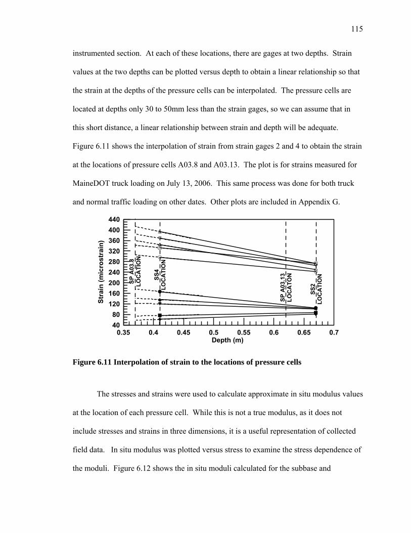
115
instrumented section. At each of these locations, there are gages at two depths. Strain
values at the two depths can be plotted versus depth to obtain a linear relationship so that
the strain at the depths of the pressure cells can be interpolated. The pressure cells are
located at depths only 30 to 50mm less than the strain gages, so we can assume that in
this short distance, a linear relationship between strain and depth will be adequate.
Figure 6.11 shows the interpolation of strain from strain gages 2 and 4 to obtain the strain
at the locations of pressure cells A03.8 and A03.13. The plot is for strains measured for
MaineDOT truck loading on July 13, 2006. This same process was done for both truck
and normal traffic loading on other dates. Other plots are included in Appendix G.
0.35 0.4 0.45 0.5 0.55 0.6 0.65 0.7Depth (m)
4080
120160200240280320360400440
Stra
in (m
icro
stra
in)
SS2
LOC
ATI
ON
SP A
03.8
LOC
ATI
ON
SP A
03.1
3LO
CA
TONSS
4LO
CA
TIO
N
Figure 6.11 Interpolation of strain to the locations of pressure cells
The stresses and strains were used to calculate approximate in situ modulus values
at the location of each pressure cell. While this is not a true modulus, as it does not
include stresses and strains in three dimensions, it is a useful representation of collected
field data. In situ modulus was plotted versus stress to examine the stress dependence of
the moduli. Figure 6.12 shows the in situ moduli calculated for the subbase and
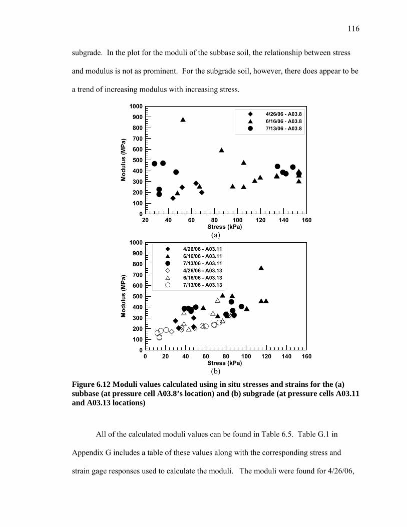
116
subgrade. In the plot for the moduli of the subbase soil, the relationship between stress
and modulus is not as prominent. For the subgrade soil, however, there does appear to be
a trend of increasing modulus with increasing stress.
20 40 60 80 100 120 140 160Stress (kPa)
0
100
200
300
400
500
600
700
800
900
1000
Mod
ulus
(MPa
)4/26/06 - A03.86/16/06 - A03.87/13/06 - A03.8
(a)
0 20 40 60 80 100 120 140 160Stress (kPa)
0
100
200
300
400
500
600
700
800
900
1000
Mod
ulus
(MPa
)
4/26/06 - A03.116/16/06 - A03.117/13/06 - A03.114/26/06 - A03.136/16/06 - A03.137/13/06 - A03.13
(b)
Figure 6.12 Moduli values calculated using in situ stresses and strains for the (a) subbase (at pressure cell A03.8’s location) and (b) subgrade (at pressure cells A03.11 and A03.13 locations)
All of the calculated moduli values can be found in Table 6.5. Table G.1 in
Appendix G includes a table of these values along with the corresponding stress and
strain gage responses used to calculate the moduli. The moduli were found for 4/26/06,

117
6/16/06, and 7/13/06. Average moduli were calculated on each of these dates, and it was
noted that the average moduli for the subbase and subgrade were approximately equal.
At the end of April, the modulus in both the subbase and subgrade was approximately
220 MPa, while in June and July, the average modulus for both the subbase and subgrade
was approximately 380 MPa.
Although 4/26/06 occurred after thawing of the soil had completed, the pavement
soil layers likely still had higher moisture contents, resulting in a lower modulus than
would occur later in the year, for example during June and July when soil moisture
contents likely had decreased. This is consistent with the average moduli found using
in-situ measured responses. However, interpretation of seasonal dependency of modulus
is complicated by the stress dependency of the subgrade modulus.
The moduli values obtained through backcalculation with FWD results follow this
pattern. Figure 6.12 shown earlier in this section included only in situ calculated moduli
values. The graphs have been redrawn here in Figure 6.13 to include FWD
backcalculated results. The stress exerted by the FWD loading on the asphalt surface is
much greater than the stress responses recorded by the soil pressure cells, and used for
modulus calculations. The stresses at the depth of the soil pressure cells due to the
influence of the FWD applied stresses were calculated and used in the Figure 6.13 plots.
The moduli obtained through FWD backcalculation on 3/30/06 were comparable to the
lowest values of moduli calculated using in situ measurements collected on 4/26/06,
6/16/06, and 7/13/06.
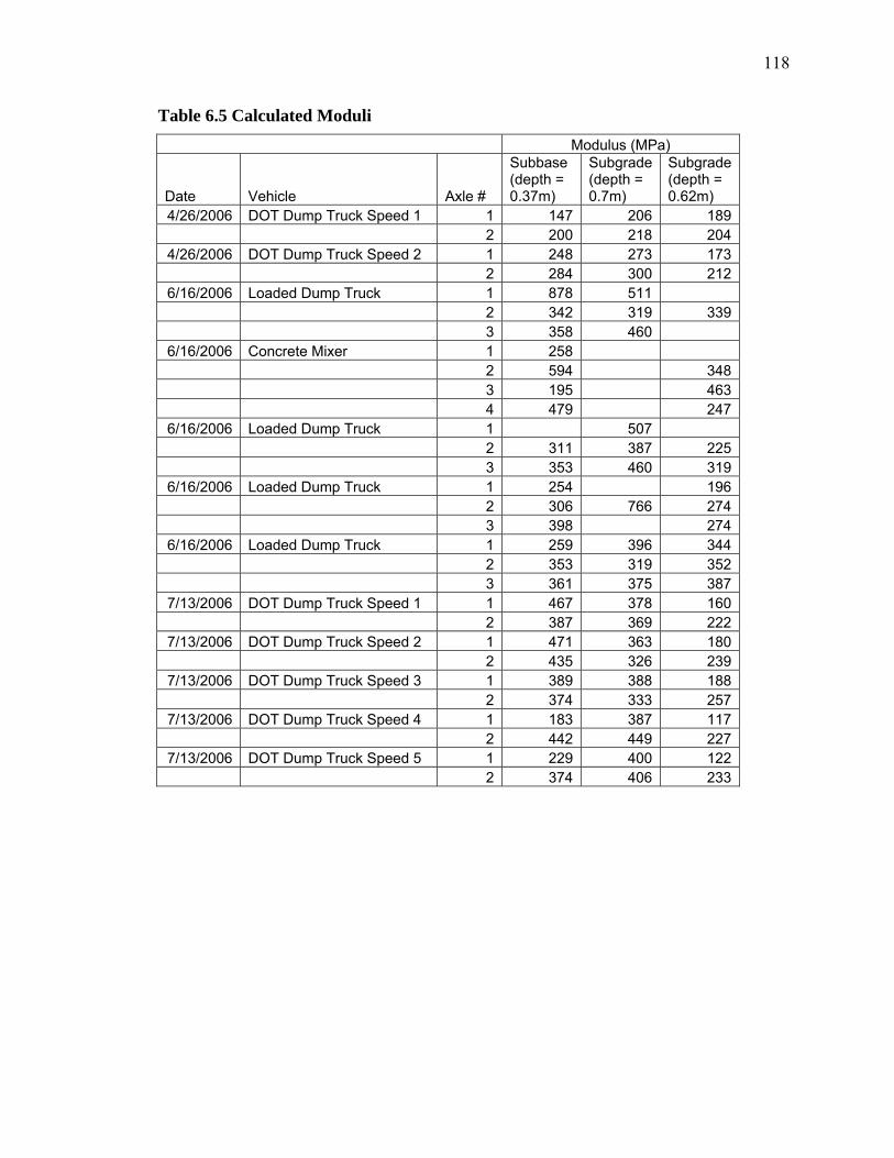
118
Table 6.5 Calculated Moduli Modulus (MPa)
Date Vehicle Axle #
Subbase (depth = 0.37m)
Subgrade (depth = 0.7m)
Subgrade (depth = 0.62m)
4/26/2006 DOT Dump Truck Speed 1 1 147 206 189 2 200 218 2044/26/2006 DOT Dump Truck Speed 2 1 248 273 173 2 284 300 2126/16/2006 Loaded Dump Truck 1 878 511 2 342 319 339 3 358 460 6/16/2006 Concrete Mixer 1 258 2 594 348 3 195 463 4 479 2476/16/2006 Loaded Dump Truck 1 507 2 311 387 225 3 353 460 3196/16/2006 Loaded Dump Truck 1 254 196 2 306 766 274 3 398 2746/16/2006 Loaded Dump Truck 1 259 396 344 2 353 319 352 3 361 375 3877/13/2006 DOT Dump Truck Speed 1 1 467 378 160 2 387 369 2227/13/2006 DOT Dump Truck Speed 2 1 471 363 180 2 435 326 2397/13/2006 DOT Dump Truck Speed 3 1 389 388 188 2 374 333 2577/13/2006 DOT Dump Truck Speed 4 1 183 387 117 2 442 449 2277/13/2006 DOT Dump Truck Speed 5 1 229 400 122 2 374 406 233
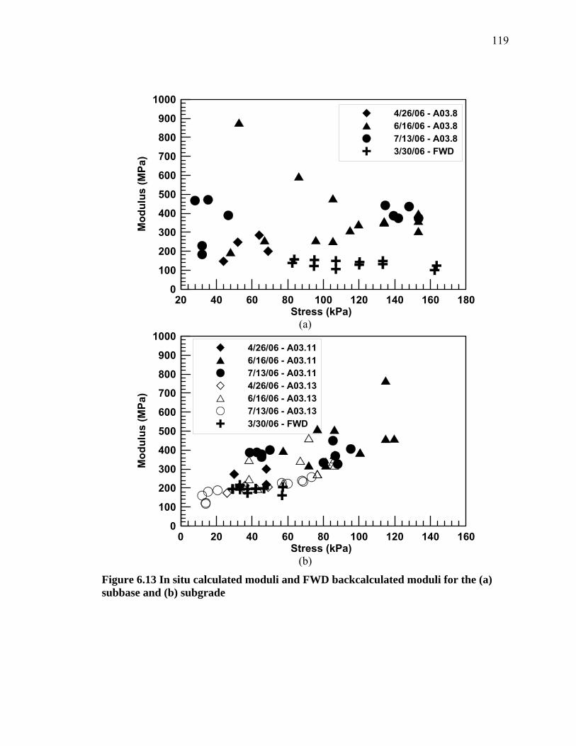
119
20 40 60 80 100 120 140 160 180Stress (kPa)
0
100
200
300
400
500
600
700
800
900
1000
Mod
ulus
(MPa
)
4/26/06 - A03.86/16/06 - A03.87/13/06 - A03.83/30/06 - FWD
(a)
0 20 40 60 80 100 120 140 160Stress (kPa)
0
100
200
300
400
500
600
700
800
900
1000
Mod
ulus
(MPa
)
4/26/06 - A03.116/16/06 - A03.117/13/06 - A03.114/26/06 - A03.136/16/06 - A03.137/13/06 - A03.133/30/06 - FWD
(b)
Figure 6.13 In situ calculated moduli and FWD backcalculated moduli for the (a) subbase and (b) subgrade
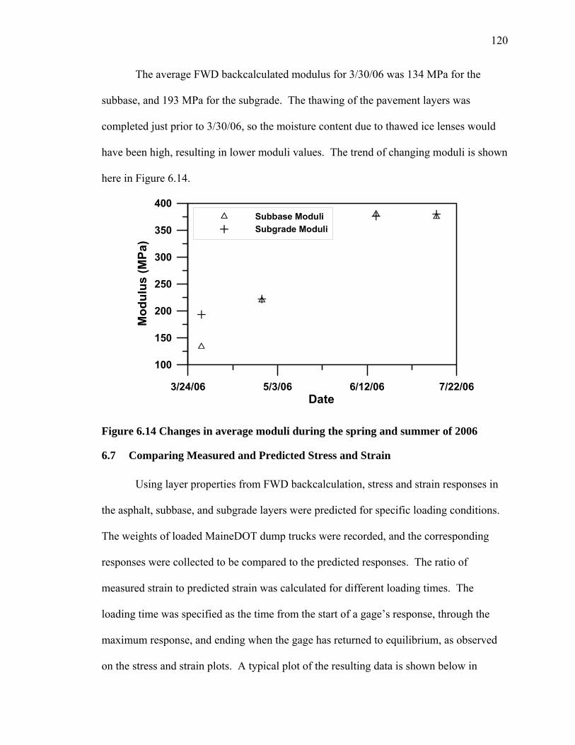
120
The average FWD backcalculated modulus for 3/30/06 was 134 MPa for the
subbase, and 193 MPa for the subgrade. The thawing of the pavement layers was
completed just prior to 3/30/06, so the moisture content due to thawed ice lenses would
have been high, resulting in lower moduli values. The trend of changing moduli is shown
here in Figure 6.14.
3/24/06 5/3/06 6/12/06 7/22/06Date
100
150
200
250
300
350
400
Mod
ulus
(MPa
)
Subbase ModuliSubgrade Moduli
Figure 6.14 Changes in average moduli during the spring and summer of 2006
6.7 Comparing Measured and Predicted Stress and Strain
Using layer properties from FWD backcalculation, stress and strain responses in
the asphalt, subbase, and subgrade layers were predicted for specific loading conditions.
The weights of loaded MaineDOT dump trucks were recorded, and the corresponding
responses were collected to be compared to the predicted responses. The ratio of
measured strain to predicted strain was calculated for different loading times. The
loading time was specified as the time from the start of a gage’s response, through the
maximum response, and ending when the gage has returned to equilibrium, as observed
on the stress and strain plots. A typical plot of the resulting data is shown below in
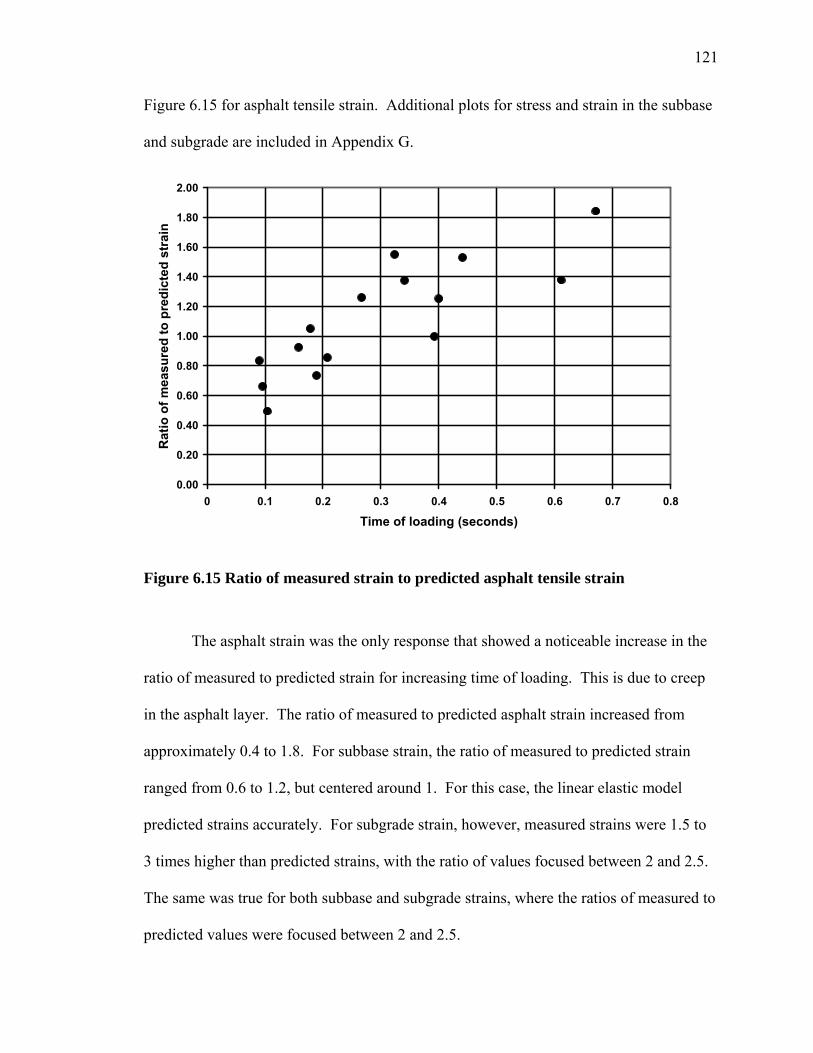
121
Figure 6.15 for asphalt tensile strain. Additional plots for stress and strain in the subbase
and subgrade are included in Appendix G.
0.00
0.20
0.40
0.60
0.80
1.00
1.20
1.40
1.60
1.80
2.00
0 0.1 0.2 0.3 0.4 0.5 0.6 0.7 0.8
Time of loading (seconds)
Rat
io o
f mea
sure
d to
pre
dict
ed s
trai
n
Figure 6.15 Ratio of measured strain to predicted asphalt tensile strain
The asphalt strain was the only response that showed a noticeable increase in the
ratio of measured to predicted strain for increasing time of loading. This is due to creep
in the asphalt layer. The ratio of measured to predicted asphalt strain increased from
approximately 0.4 to 1.8. For subbase strain, the ratio of measured to predicted strain
ranged from 0.6 to 1.2, but centered around 1. For this case, the linear elastic model
predicted strains accurately. For subgrade strain, however, measured strains were 1.5 to
3 times higher than predicted strains, with the ratio of values focused between 2 and 2.5.
The same was true for both subbase and subgrade strains, where the ratios of measured to
predicted values were focused between 2 and 2.5.

122
For this analysis, measured strains were typically greater than the predicted strains.
This is in contrast to the comparison between measured and predicted strains due to FWD
loading shown earlier. The difference between measured and calculated values was also
much less than in the earlier analysis. With more data from FWD backcalculation, and
more pavement response information for known loading conditions, the relationship
between measured in situ stresses and strains and values predicted using typical models
can be developed further.
6.8 Summary
Stress and strain in the layers of a pavement system were measured directly using
in situ gages. Typically, asphalt, subbase, and subgrade layers are defined using
parameters that are either backcalculated or determined with another method that doesn’t
directly involve in situ data. Laboratory testing, and correlations can provide satisfactory
results, the best option for finding values like layer resilient moduli would be a
calculation using data obtained directly from the pavement section.
Asphalt tensile strain was recorded for heavy truck loading. In addition, values of
asphalt strain were predicted using linear elastic analysis and FWD data. Asphalt tensile
strains were also used to predict the number of load repetitions required to cause fatigue
cracking.
Soil stress and strain responses due to vehicle loading were measured, and were
used for a direct calculation of layer moduli for the subbase and subgrade. FWD data
was also used to backcalculate layer moduli. Temperature data was recorded and the
freezing season was delineated. By combining pavement response results with climate

123
data, the expected characteristic of reduced subbase and subgrade stiffness during
thawing was observed.
The data obtained during the winter and spring of 2006 provided good initial
results, but further pavement responses, and more detailed climate data needs to be
collected during multiple freezing seasons in order to draw additional conclusions. The
effect of difficulties in collecting and interpreting some data can be reduced by collecting
a larger volume of data that can be analyzed. This will be possible with the use of the
Weigh-In-Motion machine which will allow for automated readings.

124
Chapter 7
SUMMARY AND CONCLUSIONS
The following chapter provides a summary of the work that has been completed
for this project, along with conclusions that can be drawn from the results obtained
through July 13, 2006. Finally, some recommendations are made for future work and
analysis.
7.1 Summary
This project was focused on the collection of loading responses and climate data
for a roadway section in Guilford, Maine. The goal of the project was to perform an
analysis of layer moduli and to observe the relationship between pavement section
stiffness and seasonal changes by using data obtained from in situ stress, strain, and
temperature gages.
7.1.1 Literature Review
A literature review was completed and includes information about resilient
modulus and the methods that are used to calculate layer moduli values. AASHTO’s
Standard Test for Determining the Resilient Modulus of Soils and Aggregate Material,
T307-99 provides laboratory procedures for measuring resilient modulus using triaxial
equipment. Correlations relating modulus to a variety of soil properties are also
available.
One of the most widely used methods for determining pavement layer moduli is
backcalculation of resilient modulus from Falling Weight Deflectometer deflection data.

125
The backcalculation process includes six steps, starting with the collection of data. An
appropriate analytical model, material model, a method for implementing the models, and
an optimization technique to solve the model are all chosen for the backcalculation
procedure. Finally, the backcalculated results are checked to make sure the values are
reasonable, and can then be used for analysis.
A number of projects have been completed using in situ instrumentation to collect
data that can be used to verify the properties of asphalt, subbase, and subgrade layers.
Both pavement layer response data and climate information have been analyzed to show
the relationship between the two data sets. The goal of this project is to observe the
relationship between pavement response and changes in the seasons.
7.1.2 Instrumentation
Six different types of gages were used in the roadway section in Guilford, Maine.
Soil strain gages and soil pressure cells were installed in the subbase aggregate and
subgrade soil layers, and strain gages were also placed at the base of the asphalt layer.
Soil resistivity probes and soil moisture reflectometers were installed in the subbase and
subgrade, and thermocouples were installed in both the soil and asphalt layers of the
pavement section. The University of Maine and Worcester Polytechnic Institute worked
with the Maine Department of Transportation and the general contractor during 2005 and
2006 to install the gages in a short section of roadway located in front of the MaineDOT
maintenance garage on Route 15 in Guilford, Maine.
Following the summer and fall of 2005, the gages were connected to a data
acquisition system located on-site. A dynamic data acquisition system was used for
stress and strain gages to collect very high speed data directly onto a computer using

126
National Instruments’ LabVIEW software. A static data acquisition system was set up to
collect hourly readings from the climate data gages.
During the winter, spring, and fall of 2006, data was collected for different types
of loading on the roadway section. Readings were taken for typical traffic loading, with
an emphasis placed on heavy vehicles, like six-axle log trucks. Loaded MaineDOT dump
trucks were used to load the pavement section on two days in 2006. With these trucks,
the loading weights and speeds could be controlled. A Falling Weight Deflectometer was
also used to load the pavement section to obtain deflection data for the backcalculation of
pavement layer moduli. Using the data that was collected, some initial conclusions could
be made.
7.1.3 Results
Most of the conclusions that can be made relate the response of asphalt, subbase,
and subgrade layers due to traffic loading to changes in the season. The theory is that the
stiffness of pavement layers will be high when the material is frozen and ice lenses are
present; stiffness will decrease during thaw as the layers become warmer, and ice lenses
melt, increasing the water content of the soil layers; and once stiffness has reached a
minimum value, water contents will begin to decrease, causing the soil layers to regain
some of their stiffness. Results obtained could be used to show that the trend of high
modulus in the winter and low modulus with spring thaw is correct; however accurate
moisture data needs to be recorded to determine the relationship between the moisture
and the change in modulus.
An observation of data collected from the asphalt strain gages showed an increase
in tensile strain over time due to spring thaw. Cold asphalt is stiff, and does not show as

127
much of a strain response, even to heavy loading, as asphalt that has warmed, and has
thawed soil layers beneath it. Specifically, looking at asphalt tensile strain readings taken
during the month of March, when thawing of the pavement section took place, there was
a trend of increasing strain. Directly related to the strain in the asphalt pavement is
fatigue cracking. The number of cycles of loading at a particular strain can be calculated
using the strain value.
Soil responses from the pressure cells and strain gages in the subbase and
subgrade showed similar results to the asphalt. The gages did not provide information on
the soil stress and strain during the winter and early spring prior to thawing, however as
the pavement section thawed, responses became more pronounced.
Using the subbase and subgrade stresses and strains, a direct calculation of layer
modulus was made for days in April, June, and July. FWD data was used to
backcalculate resilient modulus for one day in March. Even with the limited data
available, the expected trend in moduli was still observed. In March, during thaw, the
layer moduli were at their lowest. Following thaw, in April, the moduli had increased, as
the water content from melting ice lenses had decreased. By June and July, the moduli
had stabilized, and the pavement section layers appeared to reach a point of equilibrium.
Another observation made of the calculated moduli values from April, June, and
July was the possible stress dependence of resilient modulus. Increasing modulus with
increasing stress was seen for the subgrade moduli, but not for the subbase.
With more data, these trends can be further explored. Moduli during the winter
months when the layers are frozen need to be obtained to develop a profile of pavement
section stiffness for an entire year. Correlations also need to be developed between

128
directly calculated moduli and backcalculated moduli, so that more quantitative
comparisons can be made.
7.2 Conclusions
Using the results of the work completed for this thesis, some conclusions can be
made:
1. Loading responses collected using in situ instrumentation can provide stress
and strain data for the calculation of pavement section layer moduli.
2. In situ calculated moduli are comparable with values of resilient moduli
backcalculated using FWD deflection data.
3. In situ asphalt, subbase, and subgrade stresses and strains are comparable with
stresses and strains predicted using FWD data. The ratio of measured to
predicted asphalt strain increases from 0.4 to 1.8 with time of loading due to
material creep. The ratio for subbase strain was approximately 1, while the
ratios for subbase stress, and subgrade stresses and strains were focused
between 2 and 2.5.
4. In situ calculated moduli exhibit the expected trend of changing soil stiffness
with freezing and thawing. The resilient modulus of thawing soil will have a
much lower stiffness than frozen soil and non frozen soil that has reached
equilibrium following thaw.

129
7.3 Recommendations
The following recommendations can be made for future work with this project:
1. Use the weigh-in-motion machine as a triggering system for the data
acquisition system and the gages. Obtaining as much stress and strain data as
possible for traffic loading will provide the information necessary to develop
more detailed conclusions.
2. Optimize the data acquisition system to collect data accurately and easily.
The problems with the current data acquisition system made it difficult to
obtain the necessary data and to fully utilize the capabilities of the gages that
were installed. The solution to this problem will be to completely redesign the
data acquisition system.
3. Collect consistent stress, strain, and moisture data over the course of an entire
year to show how changes in moisture content affect pavement layer stiffness.
4. Using the database of information that is collected from this roadway, develop
models for the changes in stiffness in pavement layers due to changes in the
season. Models of pavement behavior would be useful for the design of
similar roadways in cold regions like Maine. The information could be put to
use when determining load limit requirements during spring thaw. Pavement
models will also be helpful in the implementation of the Mechanistic
Empirical Pavement Design Guide.
5. Pavement strain data and corresponding vehicle load information obtained
from the WIM should be used further to analyze fatigue cracking and rutting.
Potentially, the allowable vehicle weight at different times during the year can

130
be optimized, so that the strain on the road, and the number of vehicle
loadings that will cause fatigue cracking and rutting could be kept more
consistent throughout the year.
6. Perform additional FWD testing to predict stress, strain and stiffness. More
comparisons between measured and predicted values of these pavement layer
responses will help to verify the different methods available for determining
soil layer moduli.
This phase of the project has resulted in the installation of extensive
instrumentation in a roadway in Maine, and has included an initial analysis of pavement
responses. With more data from future years, and additional analysis the Guilford
instrumented pavement section will become a useful tool for pavement design in Maine.

131
REFERENCES
Ali, Hesham A., and Tayabji, Shiraz D. (1999), Determination of Frost Penetration in
LTPP Sections, Report No. FHWA-RD-99-088.
Al-Qadi, I. L., et al. (2004), "The Virginia Smart Road : The Impact of Pavement
Instrumentation on Understanding Pavement Performance," The Journal of APPT,
Vol. 83, pp. 427-466.
Bigelow, N., Jr. (1969), “Freezing index maps of Maine,” Technical Paper 69-5R,
Materials and Research Division, Maine State Highway Commission, Augusta,
ME, 11 pp.
Birgisson, Bjorn, et al. (2000), “Analytical Predictions of Seasonal Variations in Flexible
Pavements: Minnesota Road Research Project Site,” Transportation Research
Record, No. 1730, pp. 81-90.
Brunton, J.M. and de Almeida, J.R. (1991), “Modeling Material Nonlinearity in a
Pavement Backcalculation Procedure,” Transportation Research Record, No.
1377, pp. 99-106.
Campbell Scientific, Inc. (1996), CS615 Water Content Reflectometer Instruction
Manual, Version 8221-07.
Chou, Y.J., and Lytton, Robert L. (1991), “Accuracy and Consistency of Backcalculated
Pavement Layer Moduli,” Transportation Research Record, No. 1293, pp. 72-85.
Diefenderfer, Brian K., et al. (2003), “Development and Validation of a Model to Predict
Pavement Temperature Profile,” TRB 2003 Annual Meeting, 21 pp.

132
Drumm, et al. (1997), “Subgrade Resilient Modulus Correction for Saturation Effects,”
Journal of Geotechnical and Geoenvironmental Engineering, Vol. 123, No. 7, pp.
663-670.
Grogan, William P., et al. (1998), “Impact of FWD Testing Variability on Pavement
Evaluations,” Journal of Transportation Engineering, Vol. 124, No. 5, pp. 437-
442.
Harichandran, Ronald S., et al. (1993), “Modified Newton Algorithm for Backcalculation
of Pavement Layer Properties,” Transportation Research Record, No. 1384, pp.
15-22.
Hassan, Hossam F., et al. (2003), “Comparative Analysis of Using AASHTO and
WESDEF Approaches in Back-calculation of Pavement Layer Moduli,” Journal
of Transportation Engineering, Vol. 129, No. 3, pp. 322-329.
Hjelmstad, K.D., and Taciroglu, E. (2000), “Analysis and Implementation of Resilient
Modulus Models for Granular Soils,” Journal of Engineering Mechanics, Vol.
126, No. 8., pp 821-830.
Hoffman, Mario S., and Thompson, Marshall R. (1982), “Backcalculating Nonlinear
Resilient Moduli from Deflection Data,” Transportation Research Record, No.
852, pp. 42-51.
Huang, Yang H. (2004), Pavement Analysis and Design, Pearson Education, Inc., Upper
Saddle River, NJ.
Immanuel, S., and Timm, D.H. (2006), “Measured and Theoretical Pressures in Base and
Subgrade Layers Under Dynamic Truck Loading,” Airfield and Highway
Pavements, ASCE, pp. 155-166.

133
Jaanoo, Vincent, and Berg, Richard (1991), “Layer Moduli Determination During Freeze
Thaw Periods,” Transportation Research Record, No. 1377, pp. 26-35.
Janoo, Vincent, and Shepherd, Kent (2000), “Seasonal Variation of Moisture and
Subsurface Layer Moduli,” Transportation Research Record, No. 1709, pp. 98-
107.
Jin, Myung S., et al. (1994), “Seasonal Variation of Resilient Modulus of Subgrade
Soils,” Journal of Transportation Engineering, Vol. 120, No. 4, pp. 603-616.
Johnson, A.M. (1996), Users Guide to the Frost Resistivity Probe, Minnesota Department
of Transportation.
Joshi, Shraddha, and Malla, Ramesh B. (2006), “Resilient Modulus of Subgrade Soils A-
1-b, A-3, and A-7-6 using LTTP Data: Prediction Models with Experimental
Verification,” GEOCongress 2006, 6 pp.
Kennedy, James C., and Everhart, R. Douglas (1998), “Modeling Pavement Response to
Vehicular Traffic on Ohio Test Road,” Transportation Research Record, No.
1629, pp. 24-31.
Lenngren, Carl A. (1991), “Relating Deflection Data to Pavement Strain,” Transportation
Research Record, No. 1293, pp. 103-111.
Loulizi, Amara, et al. (2001), “Data Collection and Management of Instrumented Smart
Road Flexible Pavement Sections,” Transportation Research Record, No. 1769,
pp. 142-151.
Mehta, Yusuf, and Roque, Reynaldo (2003), “Evaluation of FWD Data for Determination
of Layer Moduli of Pavements,” Journal of Materials in Civil Engineering, Vol.
15, No. 1, pp. 25-31.

134
Scullion, T., et al. (1990), “MODULUS: A Microcomputer-Based Backcalculation
System,” Transportation Research Record, No. 1260, pp. 180-191.
Sebaaly, Peter E., et al. (2000), “Nevada’s Approach to the Backcalculation Process,”
Nondestructive Testing of Pavements and Backcalculation of Moduli: Third
Volume, STP 1375, ASTM, pp. 59-71.
Siddharthan, Raj V., et al. (2002), “Validation of a Pavement Response Model Using
Full-scale Field Tests,” The International Journal of Pavement Engineering, Vol.
3, No. 2, pp. 85-93.
Simonsen, Erik, et al. (2002), “Resilient Properties of Unbound Road Materials during
Seasonal Frost Conditions,” Journal of Cold Regions Engineering, Vol. 16, No. 1,
pp. 28-50.
Sivaneswaran, N., et al. (1991), “Advanced Backcalculation Using a Nonlinear Least
Squares Optimization Technique,” Transportation Research Record, No. 1293,
pp. 93-102.
Smart, Aaron (1999), Determination of Resilient Modulus for Maine Roadway Soils,
Thesis, Master of Science in Civil Engineering, University of Maine.
Stoffels, Shelley M., et al. (2006), “Field Instrumentation and Testing Data from
Pennsylvania’s Superpave In-Situ Stress/Strain Investigation,” Airfield and
Highway Pavements, ASCE, pp. 107-118.
Timm, David H., et al. (2004), Design and Instrumentation of the Structural Pavement
Experiment at the NCAT Test Track, NCAT Report 04-01.

135
Wang, Fuming and Lytton, Robert L. (1993), “System Identification Method for
Backcalculating Pavement Properties,” Transportation Research Record, No.
1384, pp. 1-7.
Wu, Zhong, et al. (2006), “Instrumentation and Accelerated Testing on Louisiana
Flexible Pavements,” Airfield and Highway Pavements, ASCE, pp. 119-130.
Zhou, Haiping, et al. (1990), “BOUSDEF: A Backcalculation Program for Determining
Moduli of a Pavement Structure,” Transportation Research Record, No. 1260, pp.
166-179.

136
APPENDICES
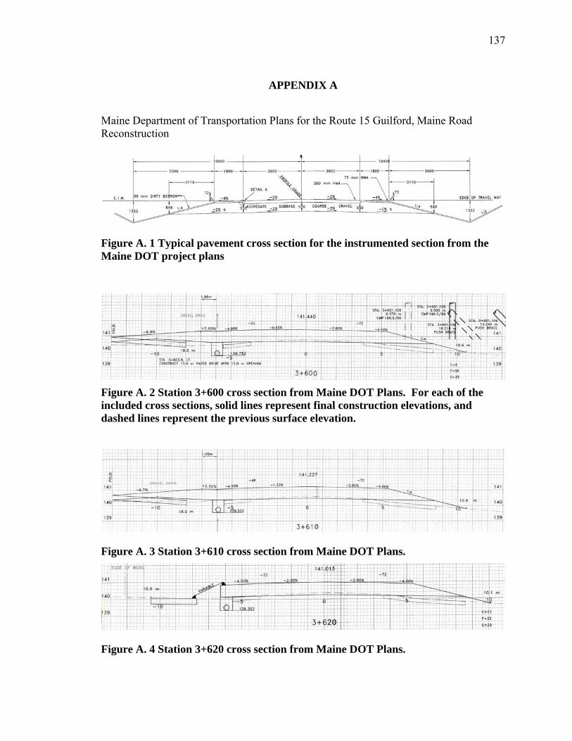
137
APPENDIX A
Maine Department of Transportation Plans for the Route 15 Guilford, Maine Road Reconstruction
Figure A. 1 Typical pavement cross section for the instrumented section from the Maine DOT project plans
Figure A. 2 Station 3+600 cross section from Maine DOT Plans. For each of the included cross sections, solid lines represent final construction elevations, and dashed lines represent the previous surface elevation.
Figure A. 3 Station 3+610 cross section from Maine DOT Plans.
Figure A. 4 Station 3+620 cross section from Maine DOT Plans.
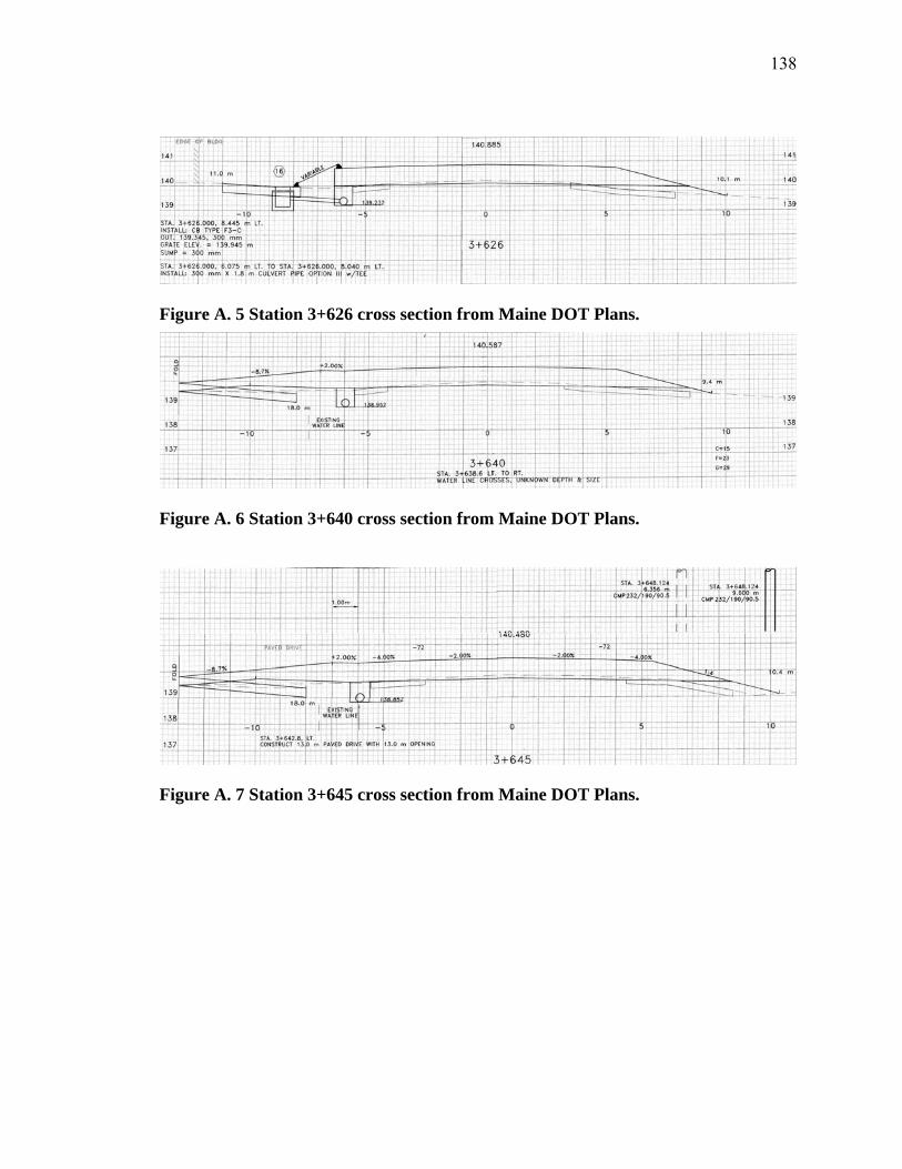
138
Figure A. 5 Station 3+626 cross section from Maine DOT Plans.
Figure A. 6 Station 3+640 cross section from Maine DOT Plans.
Figure A. 7 Station 3+645 cross section from Maine DOT Plans.

139
APPENDIX B
Boring logs and corresponding soil profile for the instrumented section.
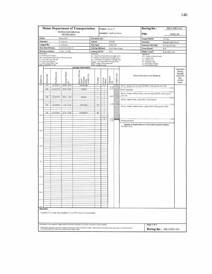
140

141
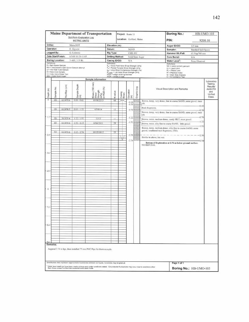
142
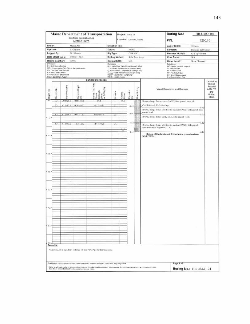
143
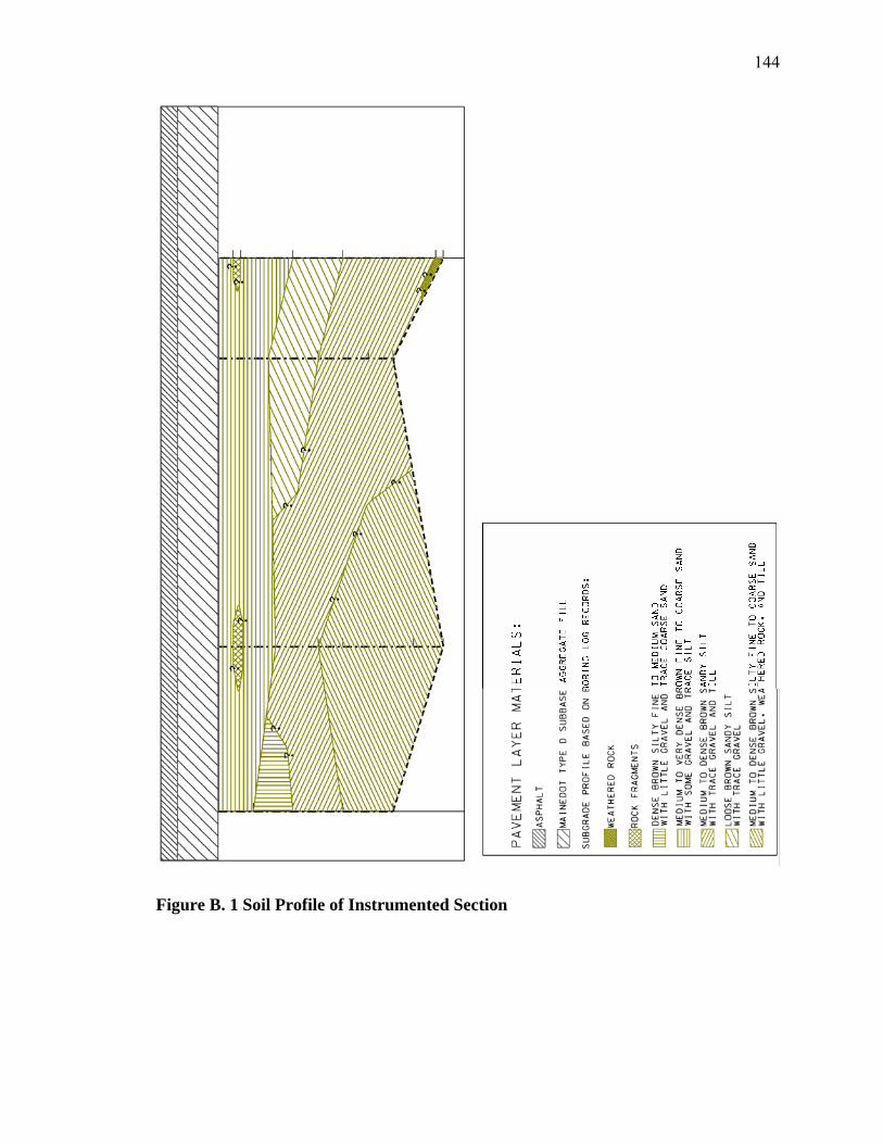
144
Figure B. 1 Soil Profile of Instrumented Section

145
APPENDIX C
Asphalt Tensile Strain - Asphalt Strain Gage Responses to Traffic Loading
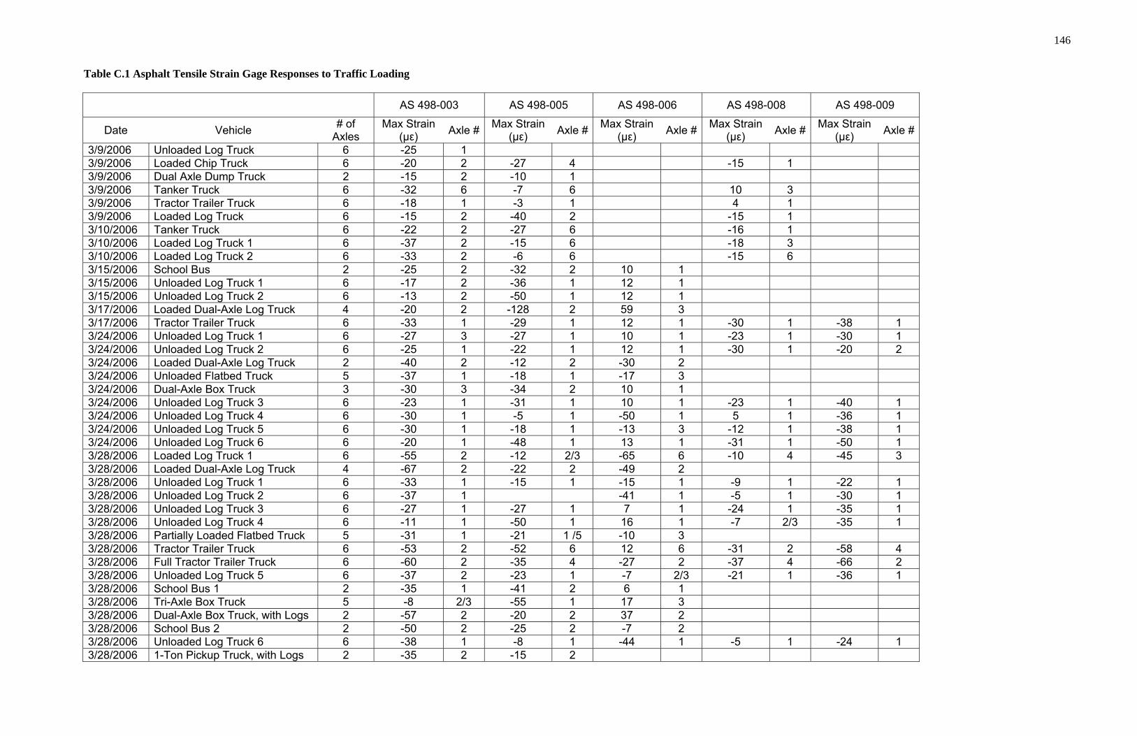
146
Table C.1 Asphalt Tensile Strain Gage Responses to Traffic Loading
AS 498-003 AS 498-005 AS 498-006 AS 498-008 AS 498-009
Date Vehicle # of Axles
Max Strain (µε) Axle # Max Strain
(µε) Axle # Max Strain (µε) Axle # Max Strain
(µε) Axle # Max Strain (µε) Axle #
3/9/2006 Unloaded Log Truck 6 -25 1 3/9/2006 Loaded Chip Truck 6 -20 2 -27 4 -15 1 3/9/2006 Dual Axle Dump Truck 2 -15 2 -10 1 3/9/2006 Tanker Truck 6 -32 6 -7 6 10 3 3/9/2006 Tractor Trailer Truck 6 -18 1 -3 1 4 1 3/9/2006 Loaded Log Truck 6 -15 2 -40 2 -15 1 3/10/2006 Tanker Truck 6 -22 2 -27 6 -16 1 3/10/2006 Loaded Log Truck 1 6 -37 2 -15 6 -18 3 3/10/2006 Loaded Log Truck 2 6 -33 2 -6 6 -15 6 3/15/2006 School Bus 2 -25 2 -32 2 10 1 3/15/2006 Unloaded Log Truck 1 6 -17 2 -36 1 12 1 3/15/2006 Unloaded Log Truck 2 6 -13 2 -50 1 12 1 3/17/2006 Loaded Dual-Axle Log Truck 4 -20 2 -128 2 59 3 3/17/2006 Tractor Trailer Truck 6 -33 1 -29 1 12 1 -30 1 -38 1 3/24/2006 Unloaded Log Truck 1 6 -27 3 -27 1 10 1 -23 1 -30 1 3/24/2006 Unloaded Log Truck 2 6 -25 1 -22 1 12 1 -30 1 -20 2 3/24/2006 Loaded Dual-Axle Log Truck 2 -40 2 -12 2 -30 2 3/24/2006 Unloaded Flatbed Truck 5 -37 1 -18 1 -17 3 3/24/2006 Dual-Axle Box Truck 3 -30 3 -34 2 10 1 3/24/2006 Unloaded Log Truck 3 6 -23 1 -31 1 10 1 -23 1 -40 1 3/24/2006 Unloaded Log Truck 4 6 -30 1 -5 1 -50 1 5 1 -36 1 3/24/2006 Unloaded Log Truck 5 6 -30 1 -18 1 -13 3 -12 1 -38 1 3/24/2006 Unloaded Log Truck 6 6 -20 1 -48 1 13 1 -31 1 -50 1 3/28/2006 Loaded Log Truck 1 6 -55 2 -12 2/3 -65 6 -10 4 -45 3 3/28/2006 Loaded Dual-Axle Log Truck 4 -67 2 -22 2 -49 2 3/28/2006 Unloaded Log Truck 1 6 -33 1 -15 1 -15 1 -9 1 -22 1 3/28/2006 Unloaded Log Truck 2 6 -37 1 -41 1 -5 1 -30 1 3/28/2006 Unloaded Log Truck 3 6 -27 1 -27 1 7 1 -24 1 -35 1 3/28/2006 Unloaded Log Truck 4 6 -11 1 -50 1 16 1 -7 2/3 -35 1 3/28/2006 Partially Loaded Flatbed Truck 5 -31 1 -21 1 /5 -10 3 3/28/2006 Tractor Trailer Truck 6 -53 2 -52 6 12 6 -31 2 -58 4 3/28/2006 Full Tractor Trailer Truck 6 -60 2 -35 4 -27 2 -37 4 -66 2 3/28/2006 Unloaded Log Truck 5 6 -37 2 -23 1 -7 2/3 -21 1 -36 1 3/28/2006 School Bus 1 2 -35 1 -41 2 6 1 3/28/2006 Tri-Axle Box Truck 5 -8 2/3 -55 1 17 3 3/28/2006 Dual-Axle Box Truck, with Logs 2 -57 2 -20 2 37 2 3/28/2006 School Bus 2 2 -50 2 -25 2 -7 2 3/28/2006 Unloaded Log Truck 6 6 -38 1 -8 1 -44 1 -5 1 -24 1 3/28/2006 1-Ton Pickup Truck, with Logs 2 -35 2 -15 2
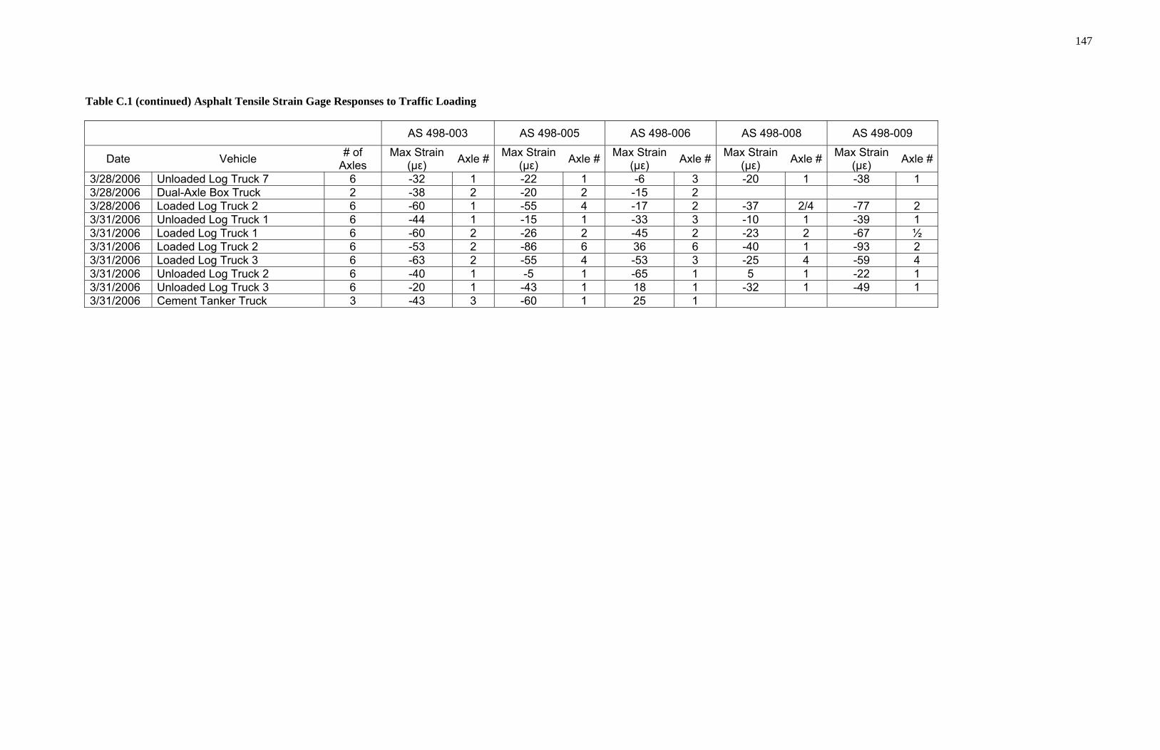
147
Table C.1 (continued) Asphalt Tensile Strain Gage Responses to Traffic Loading
AS 498-003 AS 498-005 AS 498-006 AS 498-008 AS 498-009
Date Vehicle # of Axles
Max Strain (µε) Axle # Max Strain
(µε) Axle # Max Strain (µε) Axle # Max Strain
(µε) Axle # Max Strain (µε) Axle #
3/28/2006 Unloaded Log Truck 7 6 -32 1 -22 1 -6 3 -20 1 -38 1 3/28/2006 Dual-Axle Box Truck 2 -38 2 -20 2 -15 2 3/28/2006 Loaded Log Truck 2 6 -60 1 -55 4 -17 2 -37 2/4 -77 2 3/31/2006 Unloaded Log Truck 1 6 -44 1 -15 1 -33 3 -10 1 -39 1 3/31/2006 Loaded Log Truck 1 6 -60 2 -26 2 -45 2 -23 2 -67 ½ 3/31/2006 Loaded Log Truck 2 6 -53 2 -86 6 36 6 -40 1 -93 2 3/31/2006 Loaded Log Truck 3 6 -63 2 -55 4 -53 3 -25 4 -59 4 3/31/2006 Unloaded Log Truck 2 6 -40 1 -5 1 -65 1 5 1 -22 1 3/31/2006 Unloaded Log Truck 3 6 -20 1 -43 1 18 1 -32 1 -49 1 3/31/2006 Cement Tanker Truck 3 -43 3 -60 1 25 1
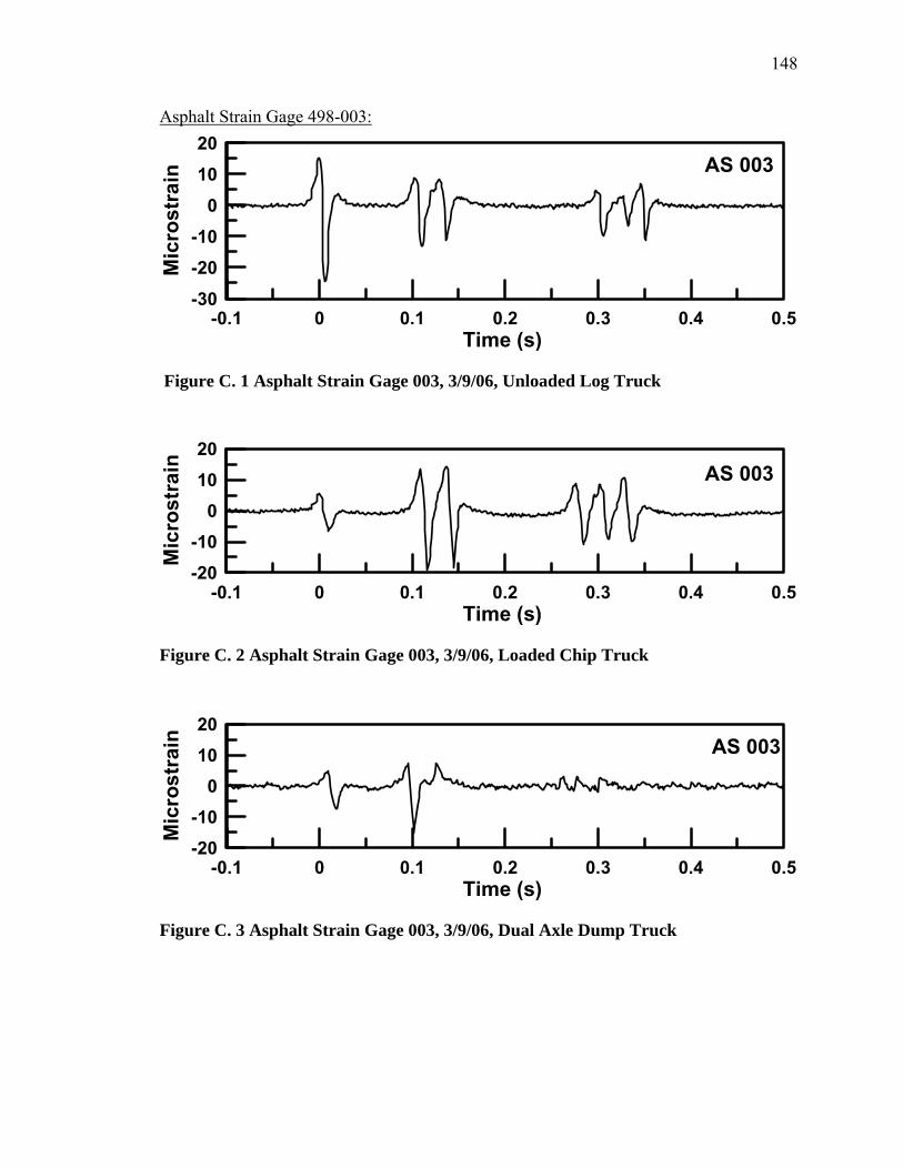
148
Asphalt Strain Gage 498-003:
-0.1 0 0.1 0.2 0.3 0.4 0.5Time (s)
-30
-20-10
01020
Mic
rost
rain AS 003
Figure C. 1 Asphalt Strain Gage 003, 3/9/06, Unloaded Log Truck
-0.1 0 0.1 0.2 0.3 0.4 0.5Time (s)
-20-10
01020
Mic
rost
rain AS 003
Figure C. 2 Asphalt Strain Gage 003, 3/9/06, Loaded Chip Truck
-0.1 0 0.1 0.2 0.3 0.4 0.5Time (s)
-20-10
01020
Mic
rost
rain AS 003
Figure C. 3 Asphalt Strain Gage 003, 3/9/06, Dual Axle Dump Truck
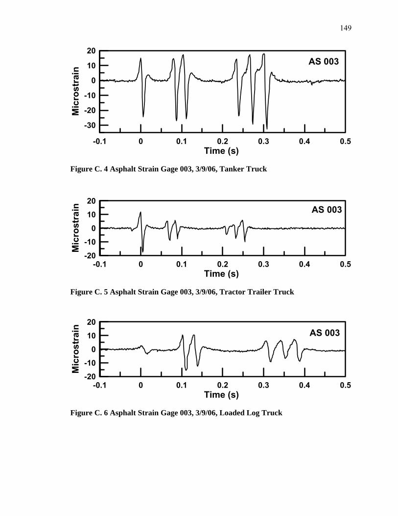
149
-0.1 0 0.1 0.2 0.3 0.4 0.5Time (s)
-30
-20
-10
0
10
20
Mic
rost
rain
AS 003
Figure C. 4 Asphalt Strain Gage 003, 3/9/06, Tanker Truck
-0.1 0 0.1 0.2 0.3 0.4 0.5Time (s)
-20-10
01020
Mic
rost
rain AS 003
Figure C. 5 Asphalt Strain Gage 003, 3/9/06, Tractor Trailer Truck
-0.1 0 0.1 0.2 0.3 0.4 0.5Time (s)
-20-10
01020
Mic
rost
rain AS 003
Figure C. 6 Asphalt Strain Gage 003, 3/9/06, Loaded Log Truck
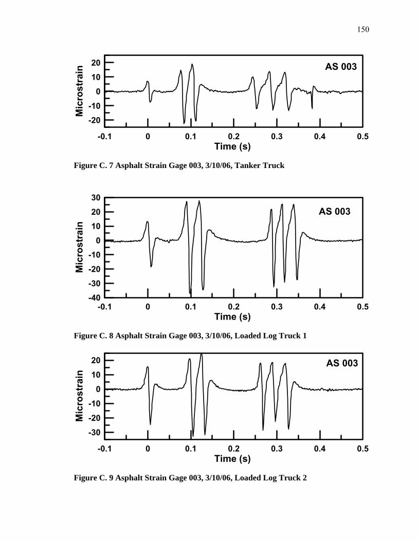
150
-0.1 0 0.1 0.2 0.3 0.4 0.5Time (s)
-20-10
01020
Mic
rost
rain AS 003
Figure C. 7 Asphalt Strain Gage 003, 3/10/06, Tanker Truck
-0.1 0 0.1 0.2 0.3 0.4 0.5Time (s)
-40-30-20-10
0102030
Mic
rost
rain
AS 003
Figure C. 8 Asphalt Strain Gage 003, 3/10/06, Loaded Log Truck 1
-0.1 0 0.1 0.2 0.3 0.4 0.5Time (s)
-30-20-10
01020
Mic
rost
rain
AS 003
Figure C. 9 Asphalt Strain Gage 003, 3/10/06, Loaded Log Truck 2
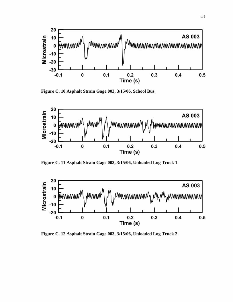
151
-0.1 0 0.1 0.2 0.3 0.4 0.5Time (s)
-30-20
-100
1020
Mic
rost
rain AS 003
Figure C. 10 Asphalt Strain Gage 003, 3/15/06, School Bus
-0.1 0 0.1 0.2 0.3 0.4 0.5Time (s)
-20-10
01020
Mic
rost
rain AS 003
Figure C. 11 Asphalt Strain Gage 003, 3/15/06, Unloaded Log Truck 1
-0.1 0 0.1 0.2 0.3 0.4 0.5Time (s)
-20-10
01020
Mic
rost
rain AS 003
Figure C. 12 Asphalt Strain Gage 003, 3/15/06, Unloaded Log Truck 2

152
-0.1 0 0.1 0.2 0.3 0.4 0.5Time (s)
-20-10
010
Mic
rost
rain AS 003
Figure C. 13 Asphalt Strain Gage 003, 3/17/06, Loaded Dual-Axle Log Truck
-0.1 0 0.1 0.2 0.3 0.4 0.5Time (s)
-30
-20
-10
0
10
20
Mic
rost
rain
AS 003
Figure C. 14 Asphalt Strain Gage 003, 3/17/06, Tractor Trailer Truck
-0.1 0 0.1 0.2 0.3 0.4 0.5Time (s)
-30
-20-10
01020
Mic
rost
rain AS 003
Figure C. 15 Asphalt Strain Gage 003, 3/24/06, Unloaded Log Truck 1

153
-0.1 0 0.1 0.2 0.3 0.4 0.5Time (s)
-30-20-10
01020
Mic
rost
rain AS 003
Figure C. 16 Asphalt Strain Gage 003, 3/24/06, Unloaded Log Truck 2
-0.1 0 0.1 0.2 0.3 0.4 0.5Time (s)
-50-40-30-20-10
01020
Mic
rost
rain
AS 003
Figure C. 17 Asphalt Strain Gage 003, 3/24/06, Loaded Dual-Axle Log Truck
-0.1 0 0.1 0.2 0.3 0.4 0.5Time (s)
-40-30-20-10
01020
Mic
rost
rain
AS 003
Figure C. 18 Asphalt Strain Gage 003, 3/24/06, Unloaded Flatbed Truck
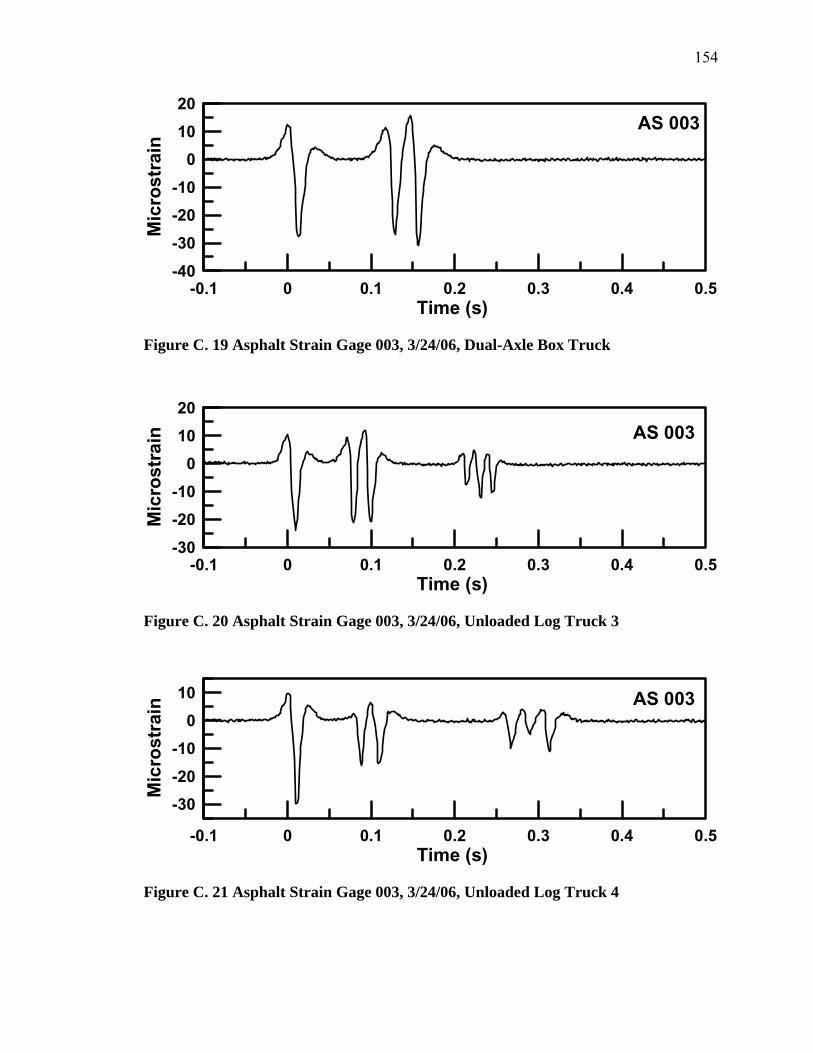
154
-0.1 0 0.1 0.2 0.3 0.4 0.5Time (s)
-40-30-20-10
01020
Mic
rost
rain
AS 003
Figure C. 19 Asphalt Strain Gage 003, 3/24/06, Dual-Axle Box Truck
-0.1 0 0.1 0.2 0.3 0.4 0.5Time (s)
-30
-20-10
01020
Mic
rost
rain AS 003
Figure C. 20 Asphalt Strain Gage 003, 3/24/06, Unloaded Log Truck 3
-0.1 0 0.1 0.2 0.3 0.4 0.5Time (s)
-30-20
-100
10
Mic
rost
rain AS 003
Figure C. 21 Asphalt Strain Gage 003, 3/24/06, Unloaded Log Truck 4
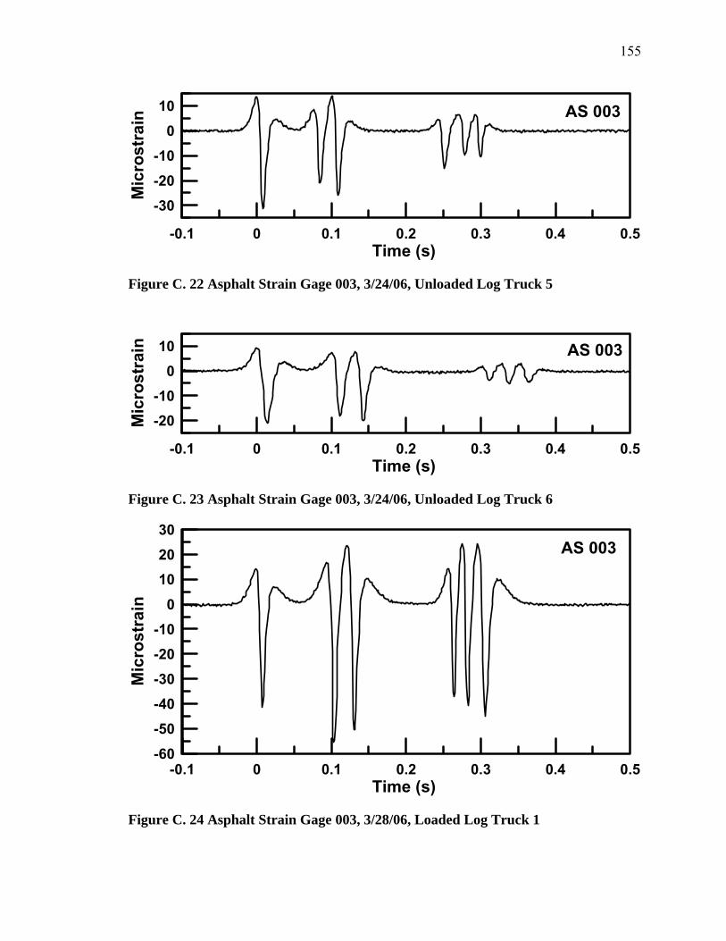
155
-0.1 0 0.1 0.2 0.3 0.4 0.5Time (s)
-30-20-10
010
Mic
rost
rain AS 003
Figure C. 22 Asphalt Strain Gage 003, 3/24/06, Unloaded Log Truck 5
-0.1 0 0.1 0.2 0.3 0.4 0.5Time (s)
-20-10
010
Mic
rost
rain AS 003
Figure C. 23 Asphalt Strain Gage 003, 3/24/06, Unloaded Log Truck 6
-0.1 0 0.1 0.2 0.3 0.4 0.5Time (s)
-60
-50-40-30-20-10
0
102030
Mic
rost
rain
AS 003
Figure C. 24 Asphalt Strain Gage 003, 3/28/06, Loaded Log Truck 1

156
-0.1 0 0.1 0.2 0.3 0.4 0.5Time (s)
-70
-60-50-40-30-20-10
010203040
Mic
rost
rain
AS 003
Figure C. 25 Asphalt Strain Gage 003, 3/28/06, Loaded Dual-axle Log Truck
-0.1 0 0.1 0.2 0.3 0.4 0.5Time (s)
-30-20
-100
10
Mic
rost
rain AS 003
Figure C. 26 Asphalt Strain Gage 003, 3/28/06, Unloaded Log Truck 1
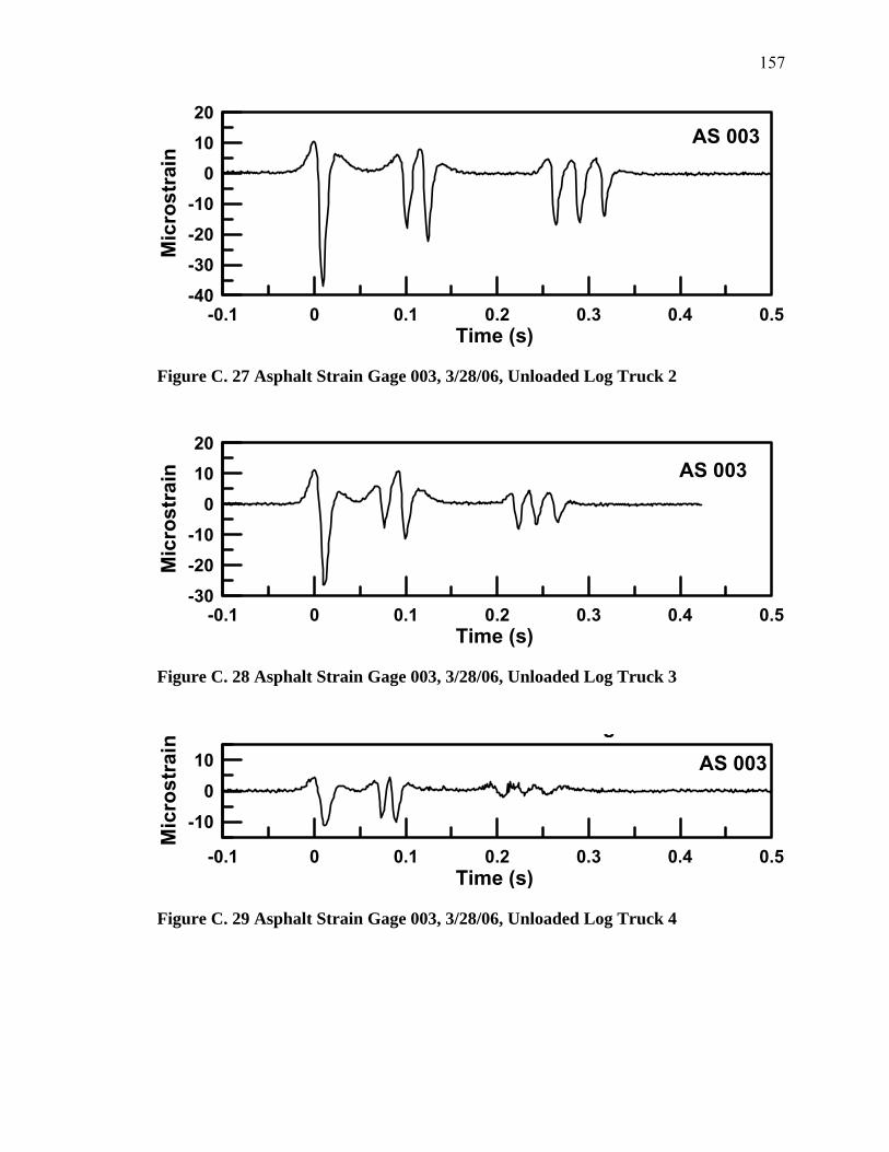
157
-0.1 0 0.1 0.2 0.3 0.4 0.5Time (s)
-40-30-20-10
01020
Mic
rost
rain
AS 003
Figure C. 27 Asphalt Strain Gage 003, 3/28/06, Unloaded Log Truck 2
-0.1 0 0.1 0.2 0.3 0.4 0.5Time (s)
-30
-20-10
01020
Mic
rost
rain AS 003
Figure C. 28 Asphalt Strain Gage 003, 3/28/06, Unloaded Log Truck 3
-0.1 0 0.1 0.2 0.3 0.4 0.5Time (s)
-100
10
Mic
rost
rain
g
AS 003
Figure C. 29 Asphalt Strain Gage 003, 3/28/06, Unloaded Log Truck 4
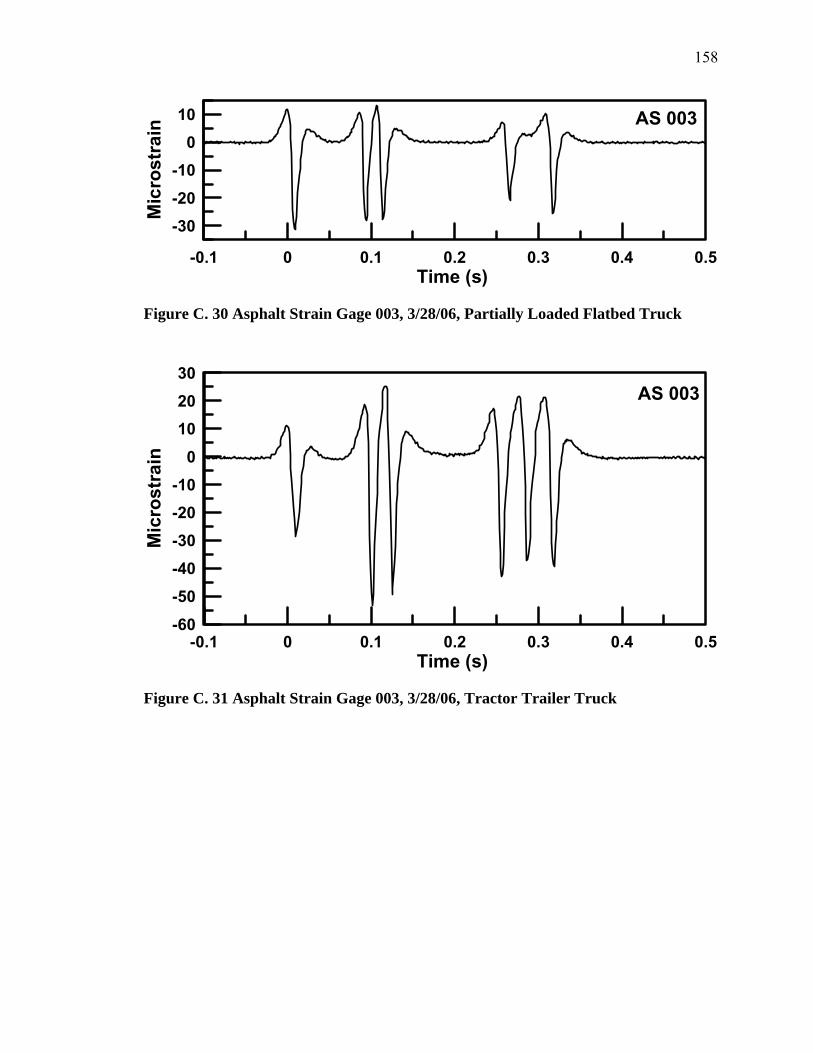
158
-0.1 0 0.1 0.2 0.3 0.4 0.5Time (s)
-30-20
-100
10
Mic
rost
rain AS 003
Figure C. 30 Asphalt Strain Gage 003, 3/28/06, Partially Loaded Flatbed Truck
-0.1 0 0.1 0.2 0.3 0.4 0.5Time (s)
-60
-50-40-30-20-10
0
102030
Mic
rost
rain
AS 003
Figure C. 31 Asphalt Strain Gage 003, 3/28/06, Tractor Trailer Truck

159
-0.1 0 0.1 0.2 0.3 0.4 0.5Time (s)
-60-50-40-30-20-10
010203040
Mic
rost
rain
AS 003
Figure C. 32 Asphalt Strain Gage 003, 3/28/06, Full Tractor Trailer Truck
-0.1 0 0.1 0.2 0.3 0.4 0.5Time (s)
-40-30-20-10
01020
Mic
rost
rain
AS 003
Figure C. 33 Asphalt Strain Gage 003, 3/28/06, Unloaded Log Truck 5
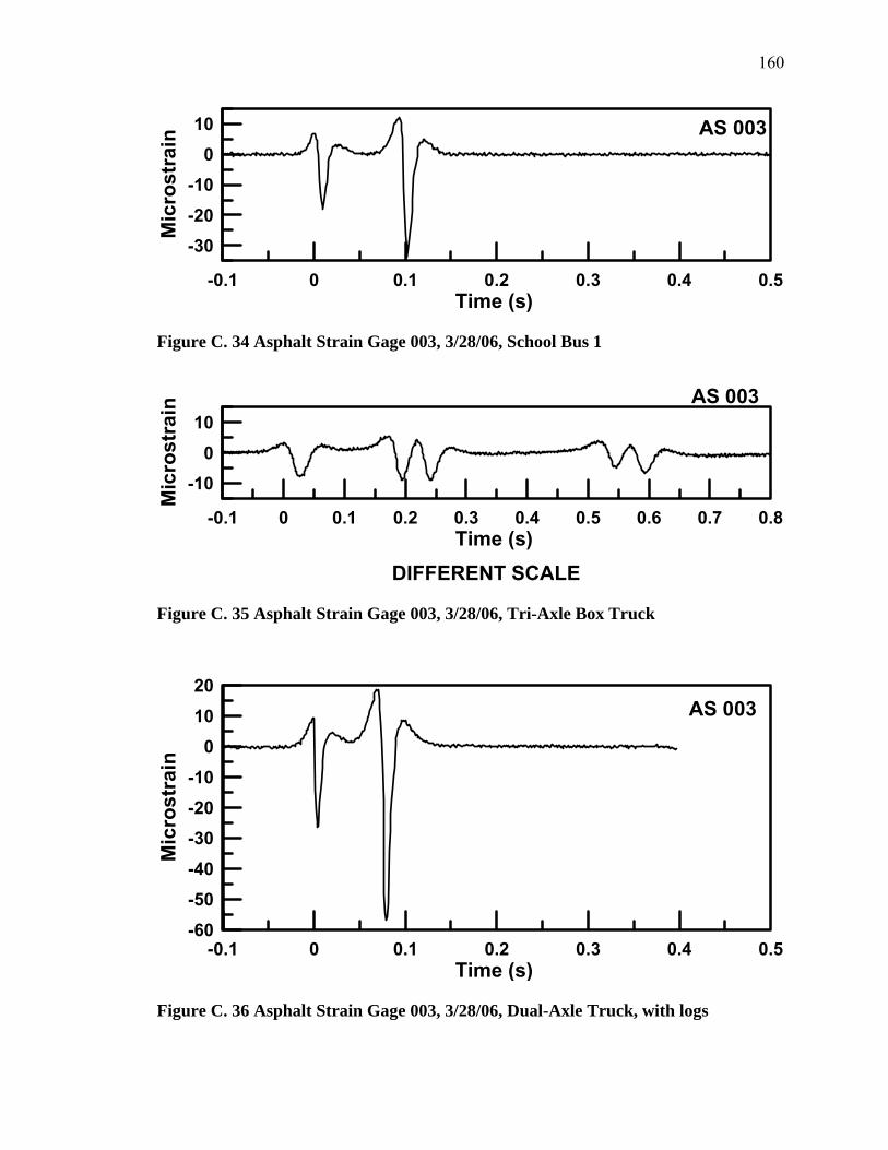
160
-0.1 0 0.1 0.2 0.3 0.4 0.5Time (s)
-30-20
-100
10
Mic
rost
rain AS 003
Figure C. 34 Asphalt Strain Gage 003, 3/28/06, School Bus 1
-0.1 0 0.1 0.2 0.3 0.4 0.5 0.6 0.7 0.8Time (s)
-100
10
Mic
rost
rain
DIFFERENT SCALE
AS 003
Figure C. 35 Asphalt Strain Gage 003, 3/28/06, Tri-Axle Box Truck
-0.1 0 0.1 0.2 0.3 0.4 0.5Time (s)
-60
-50-40
-30-20-10
01020
Mic
rost
rain
AS 003
Figure C. 36 Asphalt Strain Gage 003, 3/28/06, Dual-Axle Truck, with logs
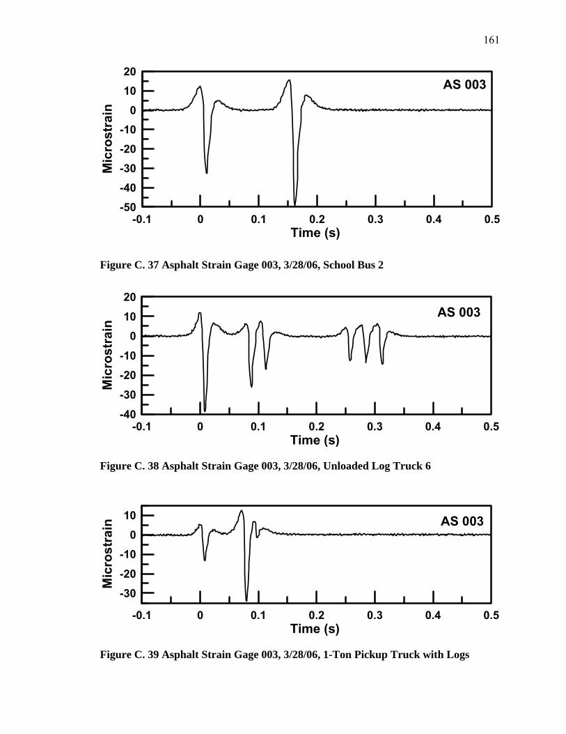
161
-0.1 0 0.1 0.2 0.3 0.4 0.5Time (s)
-50-40-30-20-10
01020
Mic
rost
rain
AS 003
Figure C. 37 Asphalt Strain Gage 003, 3/28/06, School Bus 2
-0.1 0 0.1 0.2 0.3 0.4 0.5Time (s)
-40-30-20-10
01020
Mic
rost
rain
AS 003
Figure C. 38 Asphalt Strain Gage 003, 3/28/06, Unloaded Log Truck 6
-0.1 0 0.1 0.2 0.3 0.4 0.5Time (s)
-30-20
-100
10
Mic
rost
rain AS 003
Figure C. 39 Asphalt Strain Gage 003, 3/28/06, 1-Ton Pickup Truck with Logs
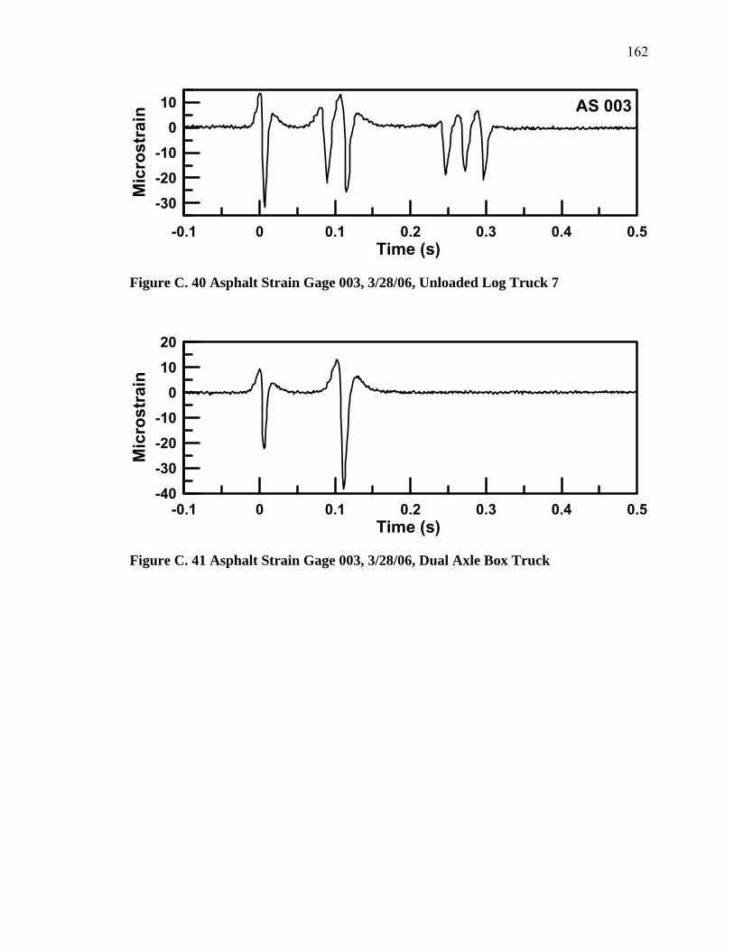
162
-0.1 0 0.1 0.2 0.3 0.4 0.5Time (s)
-30-20-10
010
Mic
rost
rain AS 003
Figure C. 40 Asphalt Strain Gage 003, 3/28/06, Unloaded Log Truck 7
-0.1 0 0.1 0.2 0.3 0.4 0.5Time (s)
-40-30-20-10
01020
Mic
rost
rain
Figure C. 41 Asphalt Strain Gage 003, 3/28/06, Dual Axle Box Truck
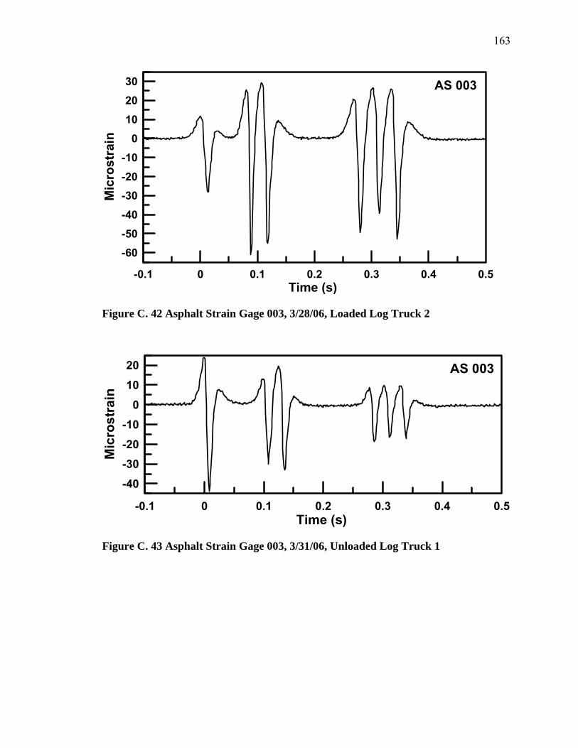
163
-0.1 0 0.1 0.2 0.3 0.4 0.5Time (s)
-60-50-40-30-20-10
0102030
Mic
rost
rain
AS 003
Figure C. 42 Asphalt Strain Gage 003, 3/28/06, Loaded Log Truck 2
-0.1 0 0.1 0.2 0.3 0.4 0.5Time (s)
-40-30-20-10
01020
Mic
rost
rain
AS 003
Figure C. 43 Asphalt Strain Gage 003, 3/31/06, Unloaded Log Truck 1
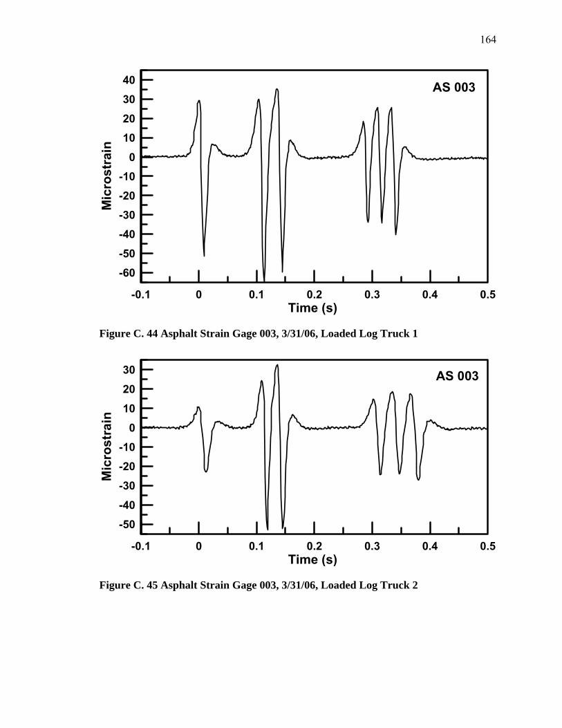
164
-0.1 0 0.1 0.2 0.3 0.4 0.5Time (s)
-60-50-40-30-20-10
0
1020
3040
Mic
rost
rain
AS 003
Figure C. 44 Asphalt Strain Gage 003, 3/31/06, Loaded Log Truck 1
-0.1 0 0.1 0.2 0.3 0.4 0.5Time (s)
-50-40-30-20-10
0102030
Mic
rost
rain
AS 003
Figure C. 45 Asphalt Strain Gage 003, 3/31/06, Loaded Log Truck 2
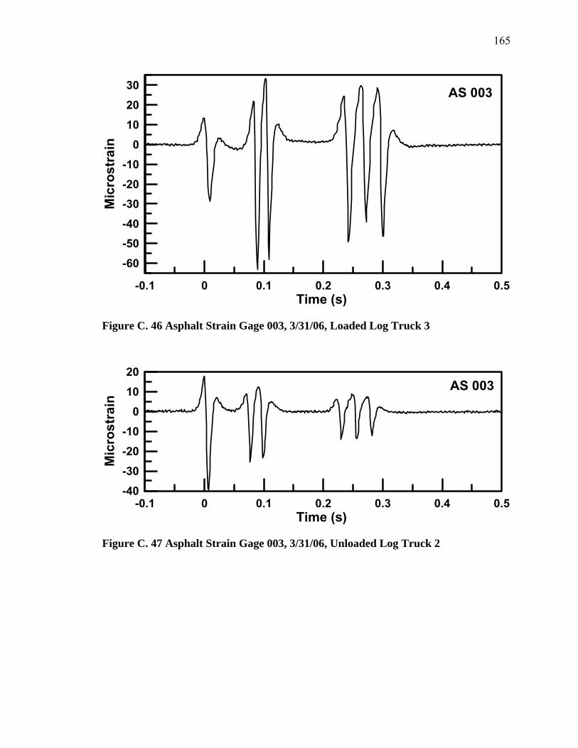
165
-0.1 0 0.1 0.2 0.3 0.4 0.5Time (s)
-60-50-40-30-20-10
0102030
Mic
rost
rain
AS 003
Figure C. 46 Asphalt Strain Gage 003, 3/31/06, Loaded Log Truck 3
-0.1 0 0.1 0.2 0.3 0.4 0.5Time (s)
-40-30-20-10
01020
Mic
rost
rain
AS 003
Figure C. 47 Asphalt Strain Gage 003, 3/31/06, Unloaded Log Truck 2
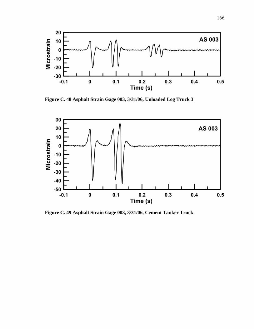
166
-0.1 0 0.1 0.2 0.3 0.4 0.5Time (s)
-30
-20-10
01020
Mic
rost
rain AS 003
Figure C. 48 Asphalt Strain Gage 003, 3/31/06, Unloaded Log Truck 3
-0.1 0 0.1 0.2 0.3 0.4 0.5Time (s)
-50-40-30
-20-10
010
2030
Mic
rost
rain
AS 003
Figure C. 49 Asphalt Strain Gage 003, 3/31/06, Cement Tanker Truck

167
Asphalt Strain Gage 498-005:
-0.1 0 0.1 0.2 0.3 0.4 0.5Time (s)
-30
-20-10
01020
Mic
rost
rain AS 005
Figure C. 50 Asphalt Strain Gage 005, 3/9/06, Loaded Chip Truck
-0.1 0 0.1 0.2 0.3 0.4 0.5Time (s)
-100
10
Mic
rost
rain
AS 005
Figure C. 51 Asphalt Strain Gage 005, 3/9/06, Dual Axle Dump Truck
-0.1 0 0.1 0.2 0.3 0.4 0.5Time (s)
-100
10
Mic
rost
rain
AS 005
Figure C. 52 Asphalt Strain Gage 005, 3/9/06, Tanker Truck
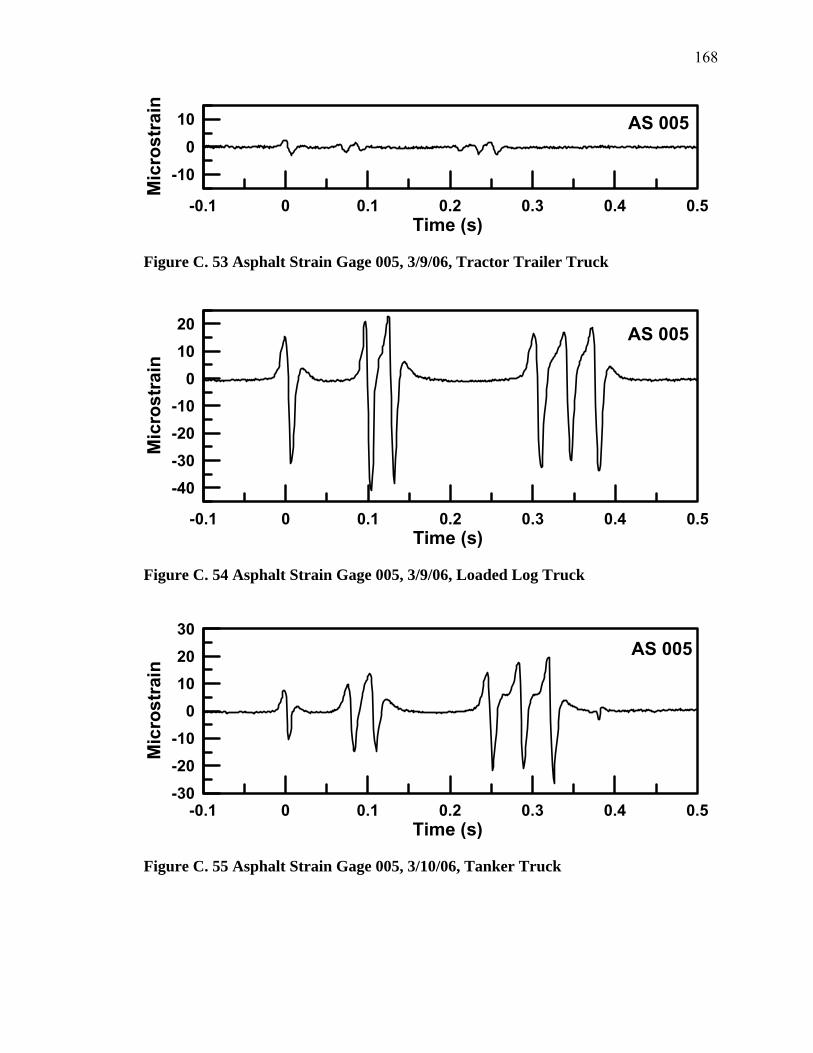
168
-0.1 0 0.1 0.2 0.3 0.4 0.5Time (s)
-100
10
Mic
rost
rain
AS 005
Figure C. 53 Asphalt Strain Gage 005, 3/9/06, Tractor Trailer Truck
-0.1 0 0.1 0.2 0.3 0.4 0.5Time (s)
-40-30-20-10
01020
Mic
rost
rain
AS 005
Figure C. 54 Asphalt Strain Gage 005, 3/9/06, Loaded Log Truck
-0.1 0 0.1 0.2 0.3 0.4 0.5Time (s)
-30-20-10
0102030
Mic
rost
rain
AS 005
Figure C. 55 Asphalt Strain Gage 005, 3/10/06, Tanker Truck

169
-0.1 0 0.1 0.2 0.3 0.4 0.5Time (s)
-20-10
01020
Mic
rost
rain AS 005
Figure C. 56 Asphalt Strain Gage 005, 3/10/06, Loaded Log Truck 1
-0.1 0 0.1 0.2 0.3 0.4 0.5Time (s)
-100
10
Mic
rost
rain
AS 005
Figure C. 57 Asphalt Strain Gage 005, 3/10/06, Loaded Log Truck 2
-0.1 0 0.1 0.2 0.3 0.4 0.5Time (s)
-30-20
-100
10
Mic
rost
rain
AS 005
Figure C. 58 Asphalt Strain Gage 005, 3/15/06, School Bus
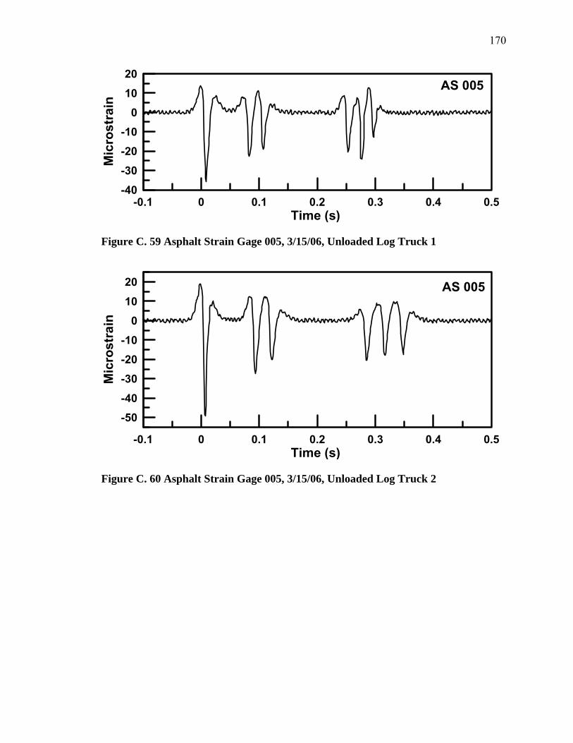
170
-0.1 0 0.1 0.2 0.3 0.4 0.5Time (s)
-40-30-20-10
01020
Mic
rost
rain
AS 005
Figure C. 59 Asphalt Strain Gage 005, 3/15/06, Unloaded Log Truck 1
-0.1 0 0.1 0.2 0.3 0.4 0.5Time (s)
-50-40-30-20-10
010
20
Mic
rost
rain
AS 005
Figure C. 60 Asphalt Strain Gage 005, 3/15/06, Unloaded Log Truck 2
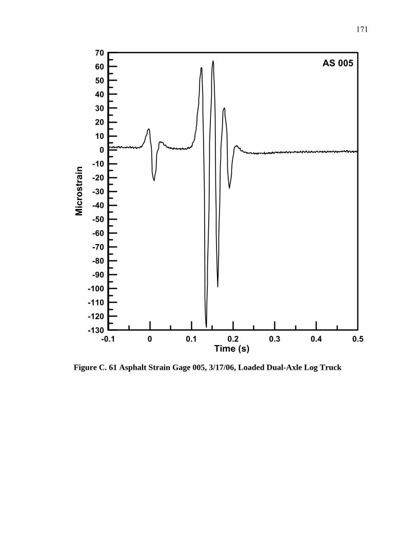
171
-0.1 0 0.1 0.2 0.3 0.4 0.5Time (s)
-130
-120-110-100-90-80-70-60-50
-40-30-20-10
010
203040506070
Mic
rost
rain
AS 005
Figure C. 61 Asphalt Strain Gage 005, 3/17/06, Loaded Dual-Axle Log Truck
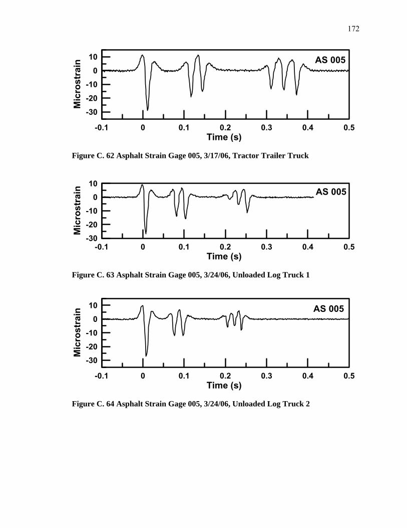
172
-0.1 0 0.1 0.2 0.3 0.4 0.5Time (s)
-30-20
-100
10
Mic
rost
rain AS 005
Figure C. 62 Asphalt Strain Gage 005, 3/17/06, Tractor Trailer Truck
-0.1 0 0.1 0.2 0.3 0.4 0.5Time (s)
-30-20-10
010
Mic
rost
rain AS 005
Figure C. 63 Asphalt Strain Gage 005, 3/24/06, Unloaded Log Truck 1
-0.1 0 0.1 0.2 0.3 0.4 0.5Time (s)
-30-20
-100
10
Mic
rost
rain AS 005
Figure C. 64 Asphalt Strain Gage 005, 3/24/06, Unloaded Log Truck 2

173
-0.1 0 0.1 0.2 0.3 0.4 0.5Time (s)
-20-10
010
Mic
rost
rain AS 005
Figure C. 65 Asphalt Strain Gage 005, 3/24/06, Loaded Dual-Axle Log Truck
-0.1 0 0.1 0.2 0.3 0.4 0.5Time (s)
-20-10
010
Mic
rost
rain
p y
AS 005
Figure C. 66 Asphalt Strain Gage 005, 3/24/06, Unloaded Flatbed Truck
-0.1 0 0.1 0.2 0.3 0.4 0.5Time (s)
-40-30-20-10
01020
Mic
rost
rain
AS 005
Figure C. 67 Asphalt Strain Gage 005, 3/24/06, Dual-Axle Box Truck
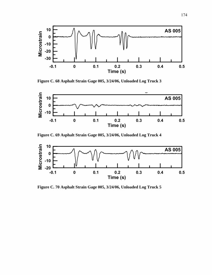
174
-0.1 0 0.1 0.2 0.3 0.4 0.5Time (s)
-30-20-10
010
Mic
rost
rain AS 005
Figure C. 68 Asphalt Strain Gage 005, 3/24/06, Unloaded Log Truck 3
-0.1 0 0.1 0.2 0.3 0.4 0.5Time (s)
-100
10
Mic
rost
rain
gAS 005
Figure C. 69 Asphalt Strain Gage 005, 3/24/06, Unloaded Log Truck 4
-0.1 0 0.1 0.2 0.3 0.4 0.5Time (s)
-20
-100
10
Mic
rost
rain AS 005
Figure C. 70 Asphalt Strain Gage 005, 3/24/06, Unloaded Log Truck 5
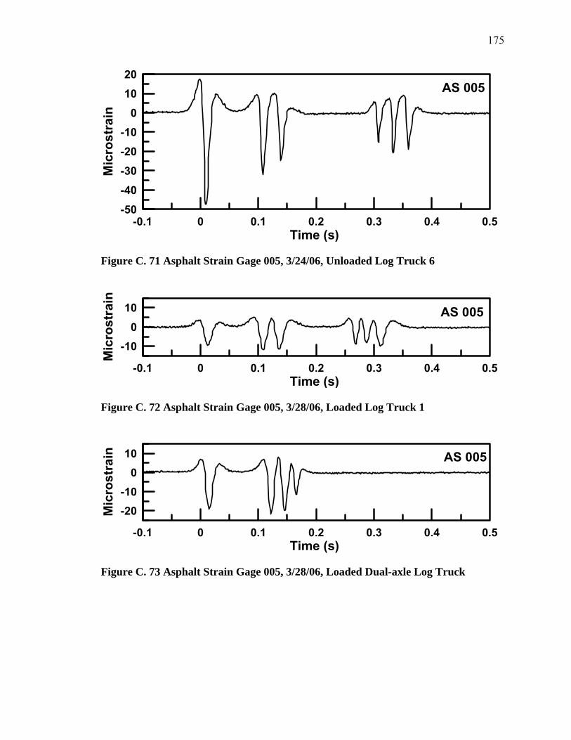
175
-0.1 0 0.1 0.2 0.3 0.4 0.5Time (s)
-50-40-30-20-10
01020
Mic
rost
rain
AS 005
Figure C. 71 Asphalt Strain Gage 005, 3/24/06, Unloaded Log Truck 6
-0.1 0 0.1 0.2 0.3 0.4 0.5Time (s)
-100
10
Mic
rost
rain
AS 005
Figure C. 72 Asphalt Strain Gage 005, 3/28/06, Loaded Log Truck 1
-0.1 0 0.1 0.2 0.3 0.4 0.5Time (s)
-20-10
010
Mic
rost
rain AS 005
Figure C. 73 Asphalt Strain Gage 005, 3/28/06, Loaded Dual-axle Log Truck
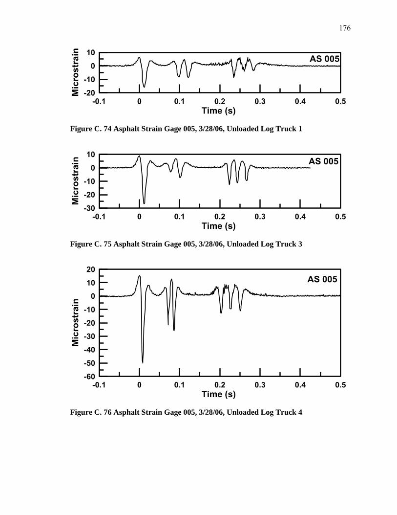
176
-0.1 0 0.1 0.2 0.3 0.4 0.5Time (s)
-20-10
010
Mic
rost
rain AS 005
Figure C. 74 Asphalt Strain Gage 005, 3/28/06, Unloaded Log Truck 1
-0.1 0 0.1 0.2 0.3 0.4 0.5Time (s)
-30-20-10
010
Mic
rost
rain AS 005
Figure C. 75 Asphalt Strain Gage 005, 3/28/06, Unloaded Log Truck 3
-0.1 0 0.1 0.2 0.3 0.4 0.5Time (s)
-60
-50-40-30-20-10
01020
Mic
rost
rain
AS 005
Figure C. 76 Asphalt Strain Gage 005, 3/28/06, Unloaded Log Truck 4
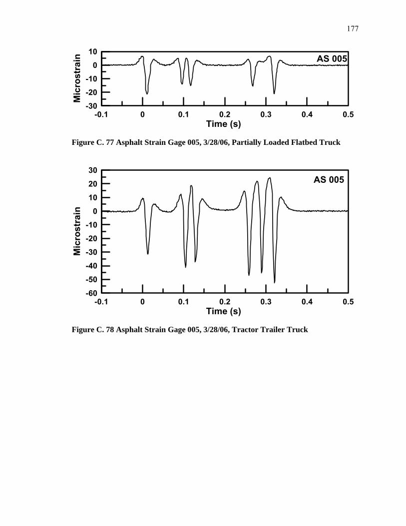
177
-0.1 0 0.1 0.2 0.3 0.4 0.5Time (s)
-30-20-10
010
Mic
rost
rain AS 005
Figure C. 77 Asphalt Strain Gage 005, 3/28/06, Partially Loaded Flatbed Truck
-0.1 0 0.1 0.2 0.3 0.4 0.5Time (s)
-60
-50-40-30-20-10
0102030
Mic
rost
rain
AS 005
Figure C. 78 Asphalt Strain Gage 005, 3/28/06, Tractor Trailer Truck
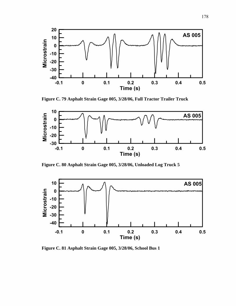
178
-0.1 0 0.1 0.2 0.3 0.4 0.5Time (s)
-40-30-20-10
01020
Mic
rost
rain
AS 005
Figure C. 79 Asphalt Strain Gage 005, 3/28/06, Full Tractor Trailer Truck
-0.1 0 0.1 0.2 0.3 0.4 0.5Time (s)
-30-20-10
010
Mic
rost
rain AS 005
Figure C. 80 Asphalt Strain Gage 005, 3/28/06, Unloaded Log Truck 5
-0.1 0 0.1 0.2 0.3 0.4 0.5Time (s)
-40-30-20-10
0
10
Mic
rost
rain
AS 005
Figure C. 81 Asphalt Strain Gage 005, 3/28/06, School Bus 1
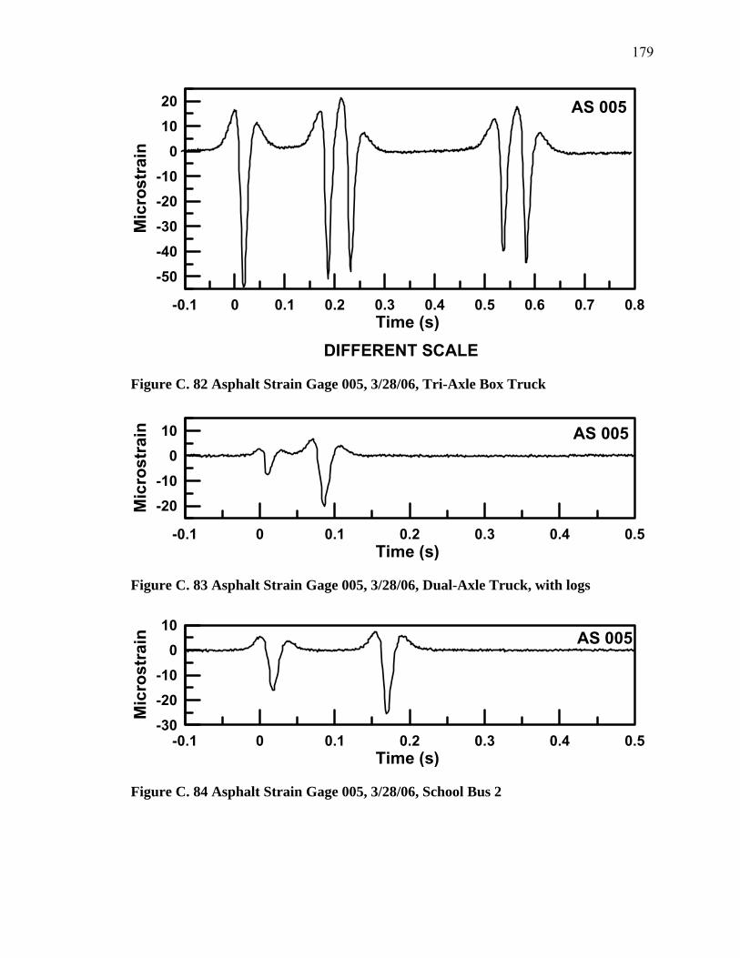
179
-0.1 0 0.1 0.2 0.3 0.4 0.5 0.6 0.7 0.8Time (s)
-50-40-30-20-10
01020
Mic
rost
rain
DIFFERENT SCALE
AS 005
Figure C. 82 Asphalt Strain Gage 005, 3/28/06, Tri-Axle Box Truck
-0.1 0 0.1 0.2 0.3 0.4 0.5Time (s)
-20-10
010
Mic
rost
rain AS 005
Figure C. 83 Asphalt Strain Gage 005, 3/28/06, Dual-Axle Truck, with logs
-0.1 0 0.1 0.2 0.3 0.4 0.5Time (s)
-30-20-10
010
Mic
rost
rain AS 005
Figure C. 84 Asphalt Strain Gage 005, 3/28/06, School Bus 2
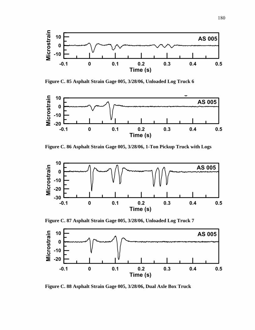
180
-0.1 0 0.1 0.2 0.3 0.4 0.5Time (s)
-100
10
Mic
rost
rain
AS 005
Figure C. 85 Asphalt Strain Gage 005, 3/28/06, Unloaded Log Truck 6
-0.1 0 0.1 0.2 0.3 0.4 0.5Time (s)
-20-10
010
Mic
rost
rain
gAS 005
Figure C. 86 Asphalt Strain Gage 005, 3/28/06, 1-Ton Pickup Truck with Logs
-0.1 0 0.1 0.2 0.3 0.4 0.5Time (s)
-30-20-10
010
Mic
rost
rain AS 005
Figure C. 87 Asphalt Strain Gage 005, 3/28/06, Unloaded Log Truck 7
-0.1 0 0.1 0.2 0.3 0.4 0.5Time (s)
-20-10
010
Mic
rost
rain AS 005
Figure C. 88 Asphalt Strain Gage 005, 3/28/06, Dual Axle Box Truck
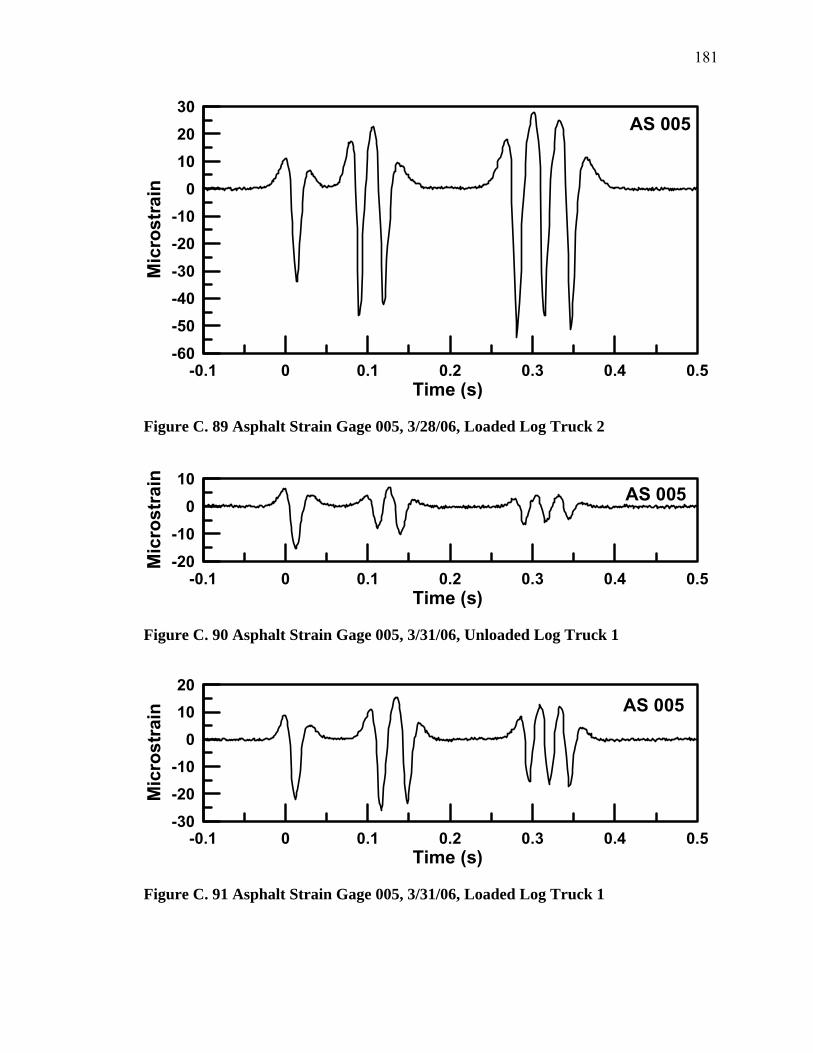
181
-0.1 0 0.1 0.2 0.3 0.4 0.5Time (s)
-60-50-40-30-20-10
0102030
Mic
rost
rain
AS 005
Figure C. 89 Asphalt Strain Gage 005, 3/28/06, Loaded Log Truck 2
-0.1 0 0.1 0.2 0.3 0.4 0.5Time (s)
-20-10
010
Mic
rost
rain
AS 005
Figure C. 90 Asphalt Strain Gage 005, 3/31/06, Unloaded Log Truck 1
-0.1 0 0.1 0.2 0.3 0.4 0.5Time (s)
-30
-20-10
01020
Mic
rost
rain AS 005
Figure C. 91 Asphalt Strain Gage 005, 3/31/06, Loaded Log Truck 1
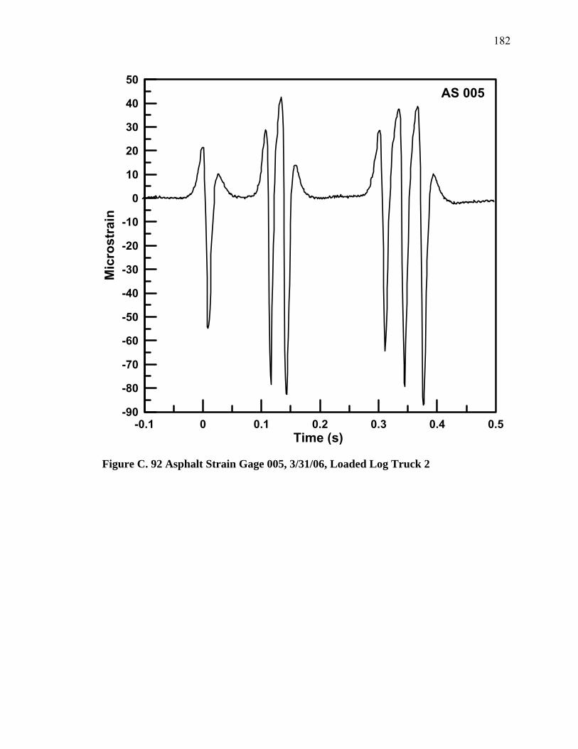
182
-0.1 0 0.1 0.2 0.3 0.4 0.5Time (s)
-90
-80
-70
-60
-50
-40
-30
-20
-10
0
10
20
30
40
50
Mic
rost
rain
AS 005
Figure C. 92 Asphalt Strain Gage 005, 3/31/06, Loaded Log Truck 2

183
-0.1 0 0.1 0.2 0.3 0.4 0.5Time (s)
-60
-50-40-30-20-10
0102030
Mic
rost
rain
AS 005
Figure C. 93 Asphalt Strain Gage 005, 3/31/06, Loaded Log Truck 3
-0.1 0 0.1 0.2 0.3 0.4 0.5Time (s)
-100
10
Mic
rost
rain
AS 005
Figure C. 94 Asphalt Strain Gage 005, 3/31/06, Unloaded Log Truck 2
-0.1 0 0.1 0.2 0.3 0.4 0.5Time (s)
-50-40-30-20-10
01020
Mic
rost
rain
AS 005
Figure C. 95 Asphalt Strain Gage 005, 3/31/06, Unloaded Log Truck 3
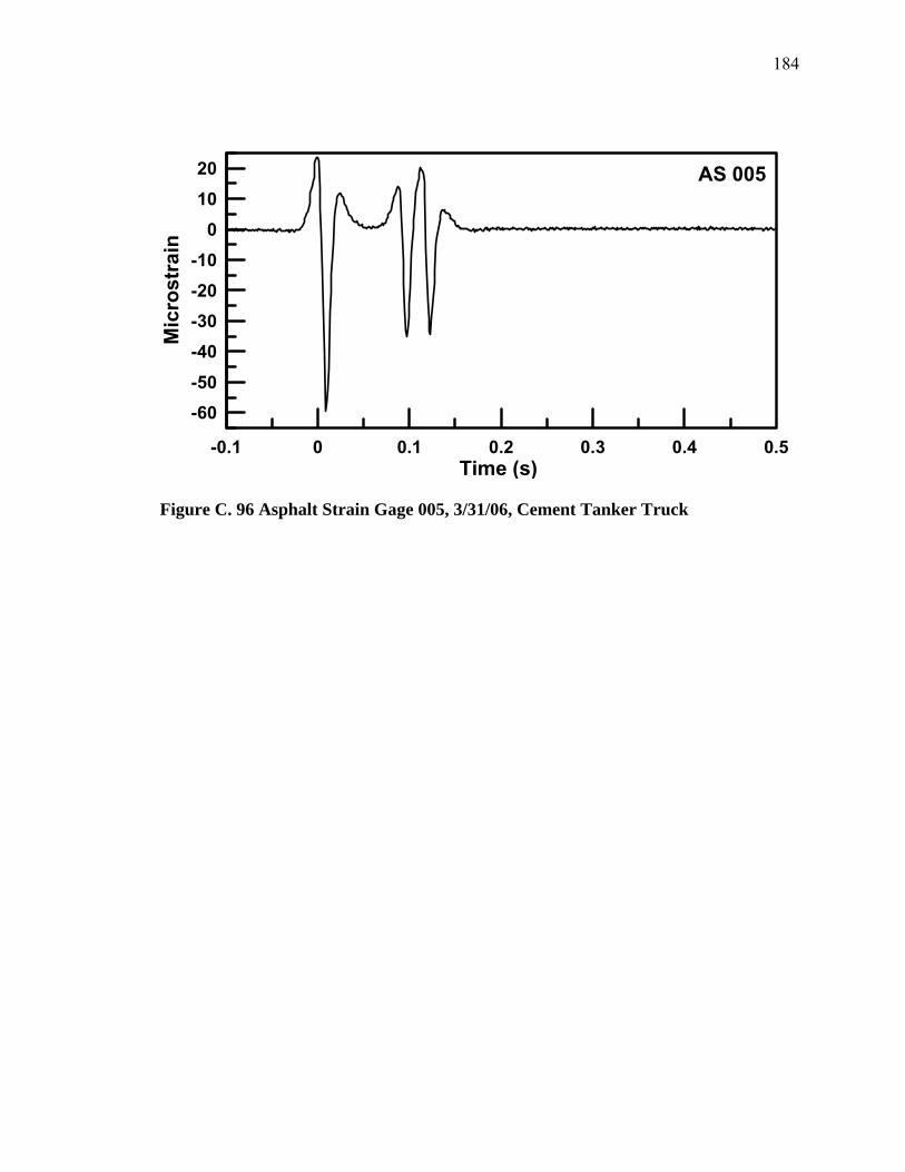
184
-0.1 0 0.1 0.2 0.3 0.4 0.5Time (s)
-60-50
-40-30-20-10
01020
Mic
rost
rain
AS 005
Figure C. 96 Asphalt Strain Gage 005, 3/31/06, Cement Tanker Truck

185
Asphalt Strain Gage 498-006:
-0.1 0 0.1 0.2 0.3 0.4 0.5Time (s)
-20-10
01020
Mic
rost
rain AS 006
Figure C. 97 Asphalt Strain Gage 006, 3/15/06, School Bus
-0.1 0 0.1 0.2 0.3 0.4 0.5Time (s)
-20-10
01020
Mic
rost
rain AS 006
Figure C. 98 Asphalt Strain Gage 006, 3/15/06, Unloaded Log Truck 1
-0.1 0 0.1 0.2 0.3 0.4 0.5Time (s)
-20-10
01020
Mic
rost
rain AS 006
Figure C. 99 Asphalt Strain Gage 006, 3/15/06, Unloaded Log Truck 2
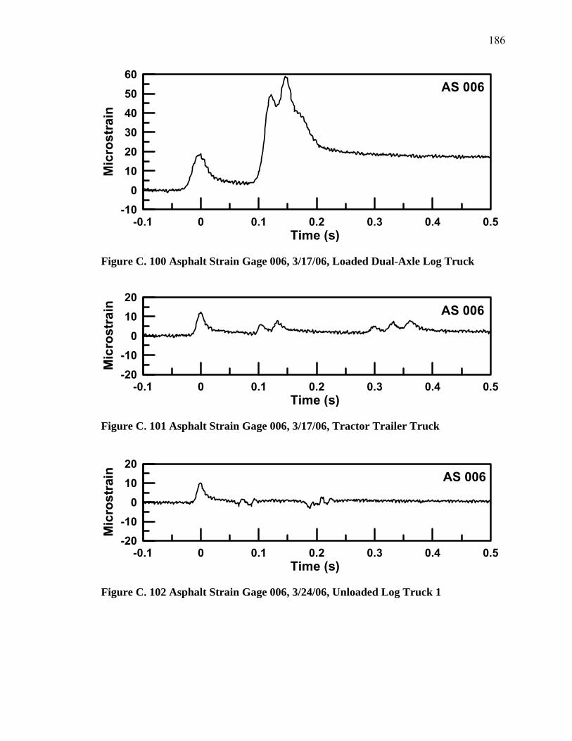
186
-0.1 0 0.1 0.2 0.3 0.4 0.5Time (s)
-100
102030405060
Mic
rost
rain
AS 006
Figure C. 100 Asphalt Strain Gage 006, 3/17/06, Loaded Dual-Axle Log Truck
-0.1 0 0.1 0.2 0.3 0.4 0.5Time (s)
-20-10
01020
Mic
rost
rain AS 006
Figure C. 101 Asphalt Strain Gage 006, 3/17/06, Tractor Trailer Truck
-0.1 0 0.1 0.2 0.3 0.4 0.5Time (s)
-20-10
01020
Mic
rost
rain AS 006
Figure C. 102 Asphalt Strain Gage 006, 3/24/06, Unloaded Log Truck 1
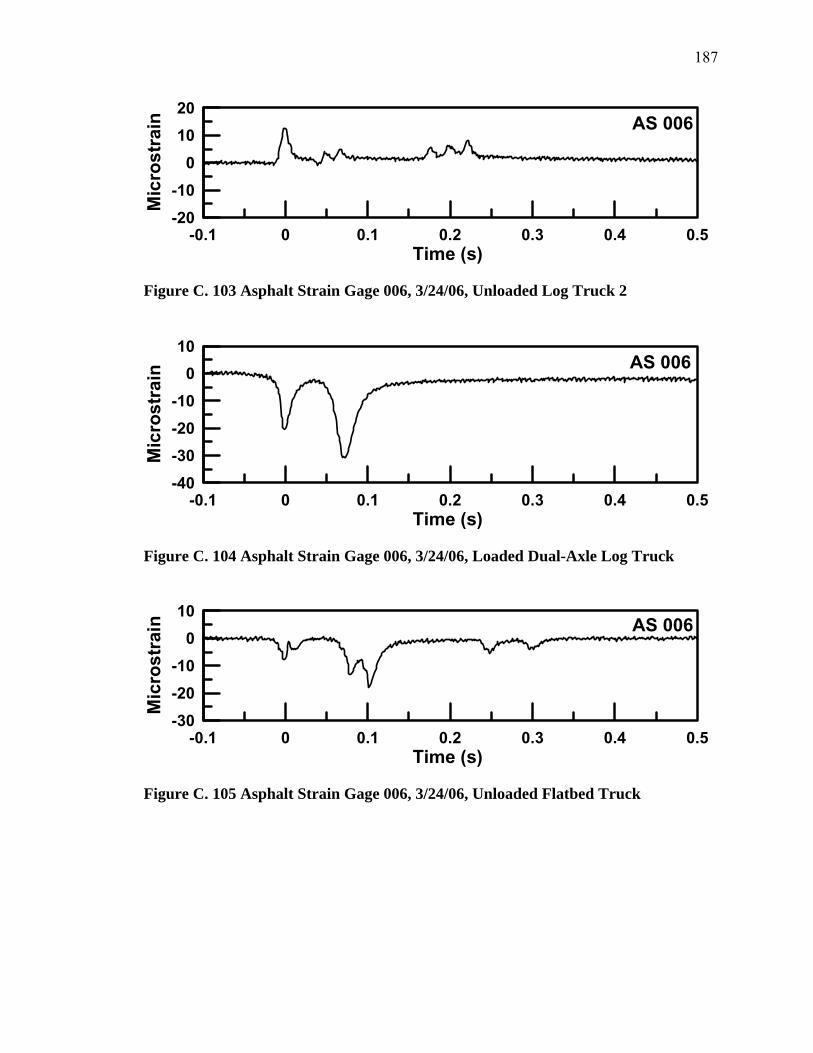
187
-0.1 0 0.1 0.2 0.3 0.4 0.5Time (s)
-20-10
01020
Mic
rost
rain AS 006
Figure C. 103 Asphalt Strain Gage 006, 3/24/06, Unloaded Log Truck 2
-0.1 0 0.1 0.2 0.3 0.4 0.5Time (s)
-40-30-20-10
010
Mic
rost
rain AS 006
Figure C. 104 Asphalt Strain Gage 006, 3/24/06, Loaded Dual-Axle Log Truck
-0.1 0 0.1 0.2 0.3 0.4 0.5Time (s)
-30-20-10
010
Mic
rost
rain AS 006
Figure C. 105 Asphalt Strain Gage 006, 3/24/06, Unloaded Flatbed Truck
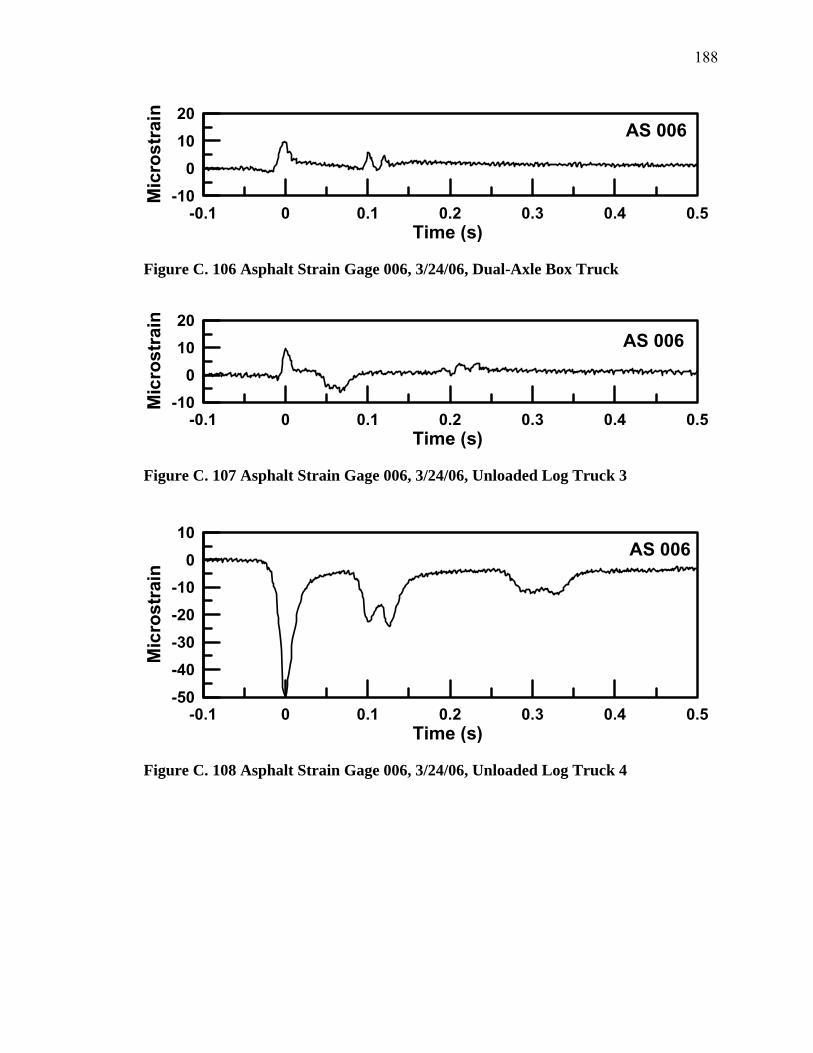
188
-0.1 0 0.1 0.2 0.3 0.4 0.5Time (s)
-100
1020
Mic
rost
rain
AS 006
Figure C. 106 Asphalt Strain Gage 006, 3/24/06, Dual-Axle Box Truck
-0.1 0 0.1 0.2 0.3 0.4 0.5Time (s)
-100
1020
Mic
rost
rain
AS 006
Figure C. 107 Asphalt Strain Gage 006, 3/24/06, Unloaded Log Truck 3
-0.1 0 0.1 0.2 0.3 0.4 0.5Time (s)
-50-40-30-20-10
010
Mic
rost
rain
AS 006
Figure C. 108 Asphalt Strain Gage 006, 3/24/06, Unloaded Log Truck 4
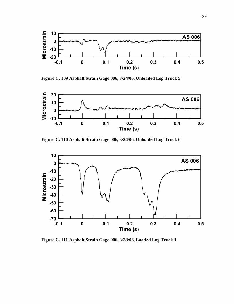
189
-0.1 0 0.1 0.2 0.3 0.4 0.5Time (s)
-20-10
010
Mic
rost
rain AS 006
Figure C. 109 Asphalt Strain Gage 006, 3/24/06, Unloaded Log Truck 5
-0.1 0 0.1 0.2 0.3 0.4 0.5Time (s)
-100
1020
Mic
rost
rain
AS 006
Figure C. 110 Asphalt Strain Gage 006, 3/24/06, Unloaded Log Truck 6
-0.1 0 0.1 0.2 0.3 0.4 0.5Time (s)
-70-60-50-40-30-20-10
010
Mic
rost
rain
AS 006
Figure C. 111 Asphalt Strain Gage 006, 3/28/06, Loaded Log Truck 1

190
-0.1 0 0.1 0.2 0.3 0.4 0.5Time (s)
-50
-40-30-20-10
010
Mic
rost
rain
AS 006
Figure C. 112 Asphalt Strain Gage 006, 3/28/06, Loaded Dual-axle Log Truck
-0.1 0 0.1 0.2 0.3 0.4 0.5Time (s)
-20-10
010
Mic
rost
rain
AS 006
Figure C. 113 Asphalt Strain Gage 006, 3/28/06, Unloaded Log Truck 1
-0.1 0 0.1 0.2 0.3 0.4 0.5Time (s)
-40
-30-20
-100
10
Mic
rost
rain AS 006
Figure C. 114 Asphalt Strain Gage 006, 3/28/06, Unloaded Log Truck 2
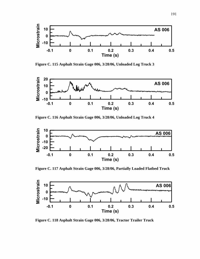
191
-0.1 0 0.1 0.2 0.3 0.4 0.5Time (s)
-100
10
Mic
rost
rain
AS 006
Figure C. 115 Asphalt Strain Gage 006, 3/28/06, Unloaded Log Truck 3
-0.1 0 0.1 0.2 0.3 0.4 0.5Time (s)
-100
1020
Mic
rost
rain
AS 006
Figure C. 116 Asphalt Strain Gage 006, 3/28/06, Unloaded Log Truck 4
-0.1 0 0.1 0.2 0.3 0.4 0.5Time (s)
-20-10
010
Mic
rost
rain AS 006
Figure C. 117 Asphalt Strain Gage 006, 3/28/06, Partially Loaded Flatbed Truck
-0.1 0 0.1 0.2 0.3 0.4 0.5Time (s)
-100
10
Mic
rost
rain
AS 006
Figure C. 118 Asphalt Strain Gage 006, 3/28/06, Tractor Trailer Truck
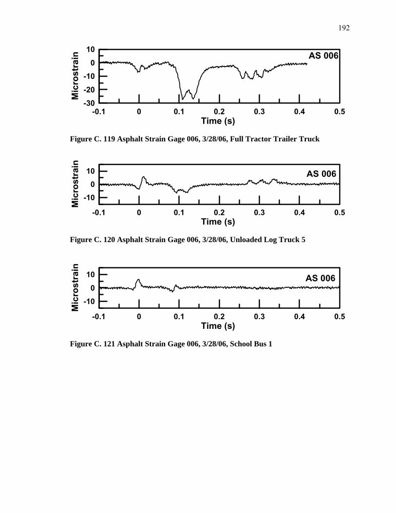
192
-0.1 0 0.1 0.2 0.3 0.4 0.5Time (s)
-30-20-10
010
Mic
rost
rain AS 006
Figure C. 119 Asphalt Strain Gage 006, 3/28/06, Full Tractor Trailer Truck
-0.1 0 0.1 0.2 0.3 0.4 0.5Time (s)
-100
10
Mic
rost
rain
AS 006
Figure C. 120 Asphalt Strain Gage 006, 3/28/06, Unloaded Log Truck 5
-0.1 0 0.1 0.2 0.3 0.4 0.5Time (s)
-100
10
Mic
rost
rain
AS 006
Figure C. 121 Asphalt Strain Gage 006, 3/28/06, School Bus 1

193
-0.1 0 0.1 0.2 0.3 0.4 0.5 0.6 0.7 0.8Time (s)
-100
1020
Mic
rost
rain
DIFFERENT SCALE
AS 006
Figure C. 122 Asphalt Strain Gage 006, 3/28/06, Tri-Axle Box Truck
-0.1 0 0.1 0.2 0.3 0.4 0.5Time (s)
-40-30-20-10
010
Mic
rost
rain AS 006
Figure C. 123 Asphalt Strain Gage 006, 3/28/06, Dual-Axle Truck, with logs
-0.1 0 0.1 0.2 0.3 0.4 0.5Time (s)
-100
10
Mic
rost
rain
AS 006
Figure C. 124 Asphalt Strain Gage 006, 3/28/06, School Bus 2
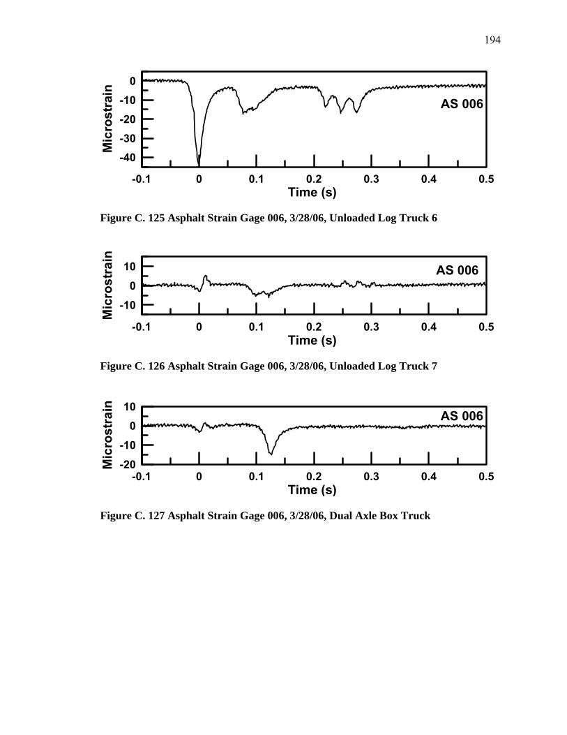
194
-0.1 0 0.1 0.2 0.3 0.4 0.5Time (s)
-40-30-20-10
0
Mic
rost
rain
AS 006
Figure C. 125 Asphalt Strain Gage 006, 3/28/06, Unloaded Log Truck 6
-0.1 0 0.1 0.2 0.3 0.4 0.5Time (s)
-100
10
Mic
rost
rain
AS 006
Figure C. 126 Asphalt Strain Gage 006, 3/28/06, Unloaded Log Truck 7
-0.1 0 0.1 0.2 0.3 0.4 0.5Time (s)
-20-10
010
Mic
rost
rain AS 006
Figure C. 127 Asphalt Strain Gage 006, 3/28/06, Dual Axle Box Truck
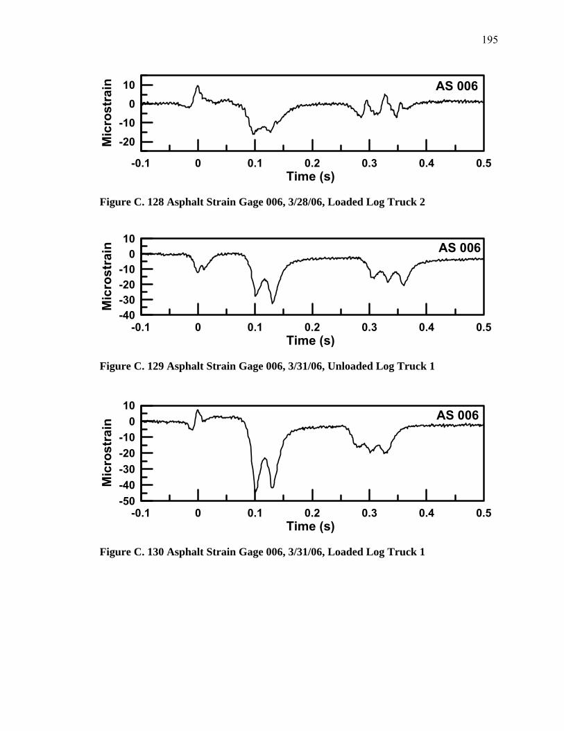
195
-0.1 0 0.1 0.2 0.3 0.4 0.5Time (s)
-20-10
010
Mic
rost
rain AS 006
Figure C. 128 Asphalt Strain Gage 006, 3/28/06, Loaded Log Truck 2
-0.1 0 0.1 0.2 0.3 0.4 0.5Time (s)
-40-30-20-10
010
Mic
rost
rain AS 006
Figure C. 129 Asphalt Strain Gage 006, 3/31/06, Unloaded Log Truck 1
-0.1 0 0.1 0.2 0.3 0.4 0.5Time (s)
-50-40-30-20-10
010
Mic
rost
rain
AS 006
Figure C. 130 Asphalt Strain Gage 006, 3/31/06, Loaded Log Truck 1

196
-0.1 0 0.1 0.2 0.3 0.4 0.5Time (s)
-10
010
203040
Mic
rost
rain AS 006
Figure C. 131 Asphalt Strain Gage 006, 3/31/06, Loaded Log Truck 2
-0.1 0 0.1 0.2 0.3 0.4 0.5Time (s)
-60-50-40-30-20-10
010
Mic
rost
rain
AS 006
Figure C. 132 Asphalt Strain Gage 006, 3/31/06, Loaded Log Truck 3
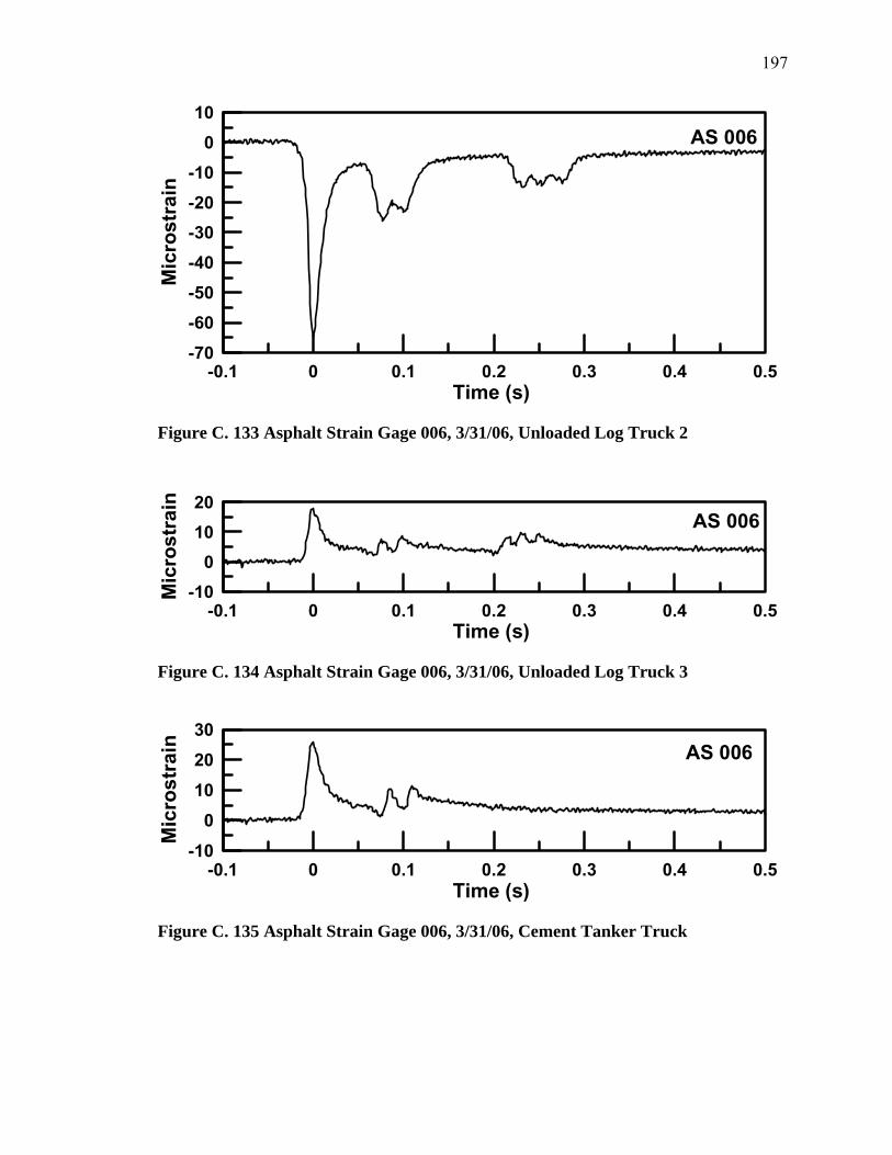
197
-0.1 0 0.1 0.2 0.3 0.4 0.5Time (s)
-70
-60-50-40-30-20-10
010
Mic
rost
rain
AS 006
Figure C. 133 Asphalt Strain Gage 006, 3/31/06, Unloaded Log Truck 2
-0.1 0 0.1 0.2 0.3 0.4 0.5Time (s)
-100
1020
Mic
rost
rain
AS 006
Figure C. 134 Asphalt Strain Gage 006, 3/31/06, Unloaded Log Truck 3
-0.1 0 0.1 0.2 0.3 0.4 0.5Time (s)
-100
102030
Mic
rost
rain AS 006
Figure C. 135 Asphalt Strain Gage 006, 3/31/06, Cement Tanker Truck
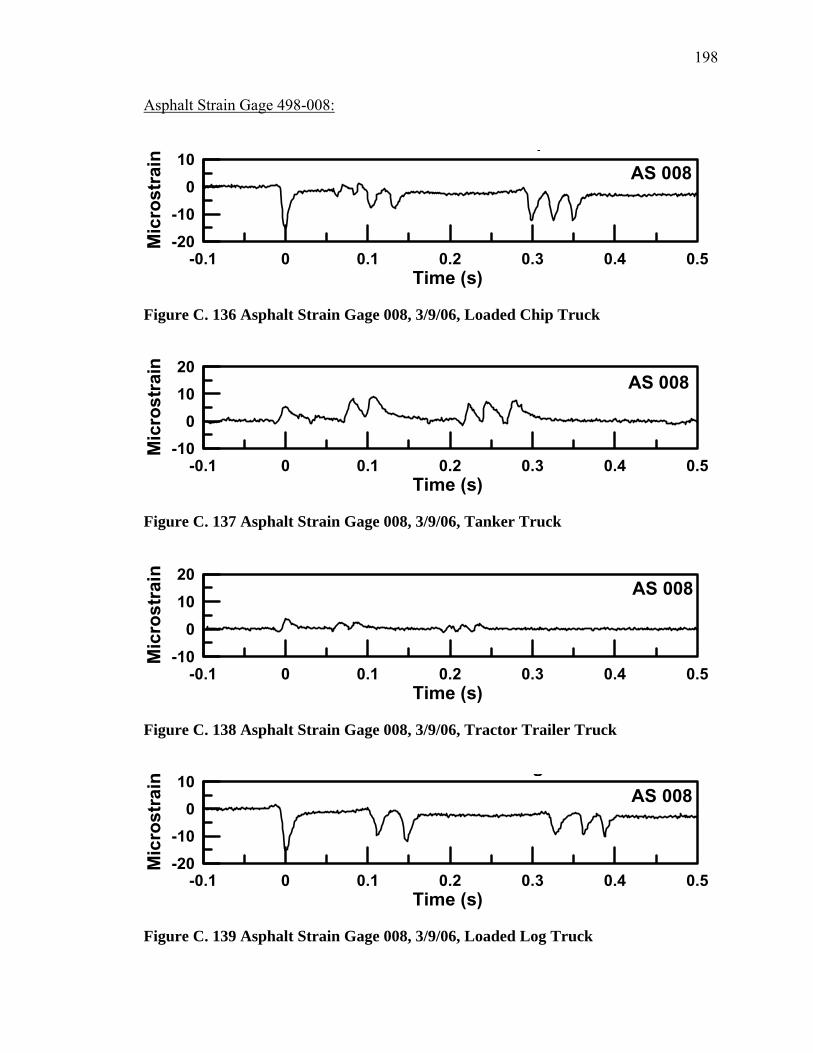
198
Asphalt Strain Gage 498-008:
-0.1 0 0.1 0.2 0.3 0.4 0.5Time (s)
-20-10
010
Mic
rost
rain
p
AS 008
Figure C. 136 Asphalt Strain Gage 008, 3/9/06, Loaded Chip Truck
-0.1 0 0.1 0.2 0.3 0.4 0.5Time (s)
-100
1020
Mic
rost
rain
AS 008
Figure C. 137 Asphalt Strain Gage 008, 3/9/06, Tanker Truck
-0.1 0 0.1 0.2 0.3 0.4 0.5Time (s)
-100
1020
Mic
rost
rain
AS 008
Figure C. 138 Asphalt Strain Gage 008, 3/9/06, Tractor Trailer Truck
-0.1 0 0.1 0.2 0.3 0.4 0.5Time (s)
-20
-100
10
Mic
rost
rain
gAS 008
Figure C. 139 Asphalt Strain Gage 008, 3/9/06, Loaded Log Truck
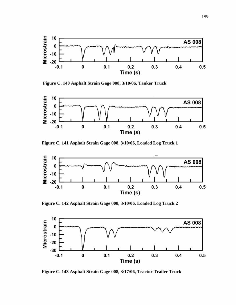
199
-0.1 0 0.1 0.2 0.3 0.4 0.5Time (s)
-20-10
010
Mic
rost
rain AS 008
Figure C. 140 Asphalt Strain Gage 008, 3/10/06, Tanker Truck
-0.1 0 0.1 0.2 0.3 0.4 0.5Time (s)
-20-10
010
Mic
rost
rain
g
AS 008
Figure C. 141 Asphalt Strain Gage 008, 3/10/06, Loaded Log Truck 1
-0.1 0 0.1 0.2 0.3 0.4 0.5Time (s)
-20-10
010
Mic
rost
rain
gAS 008
Figure C. 142 Asphalt Strain Gage 008, 3/10/06, Loaded Log Truck 2
-0.1 0 0.1 0.2 0.3 0.4 0.5Time (s)
-30-20-10
010
Mic
rost
rain AS 008
Figure C. 143 Asphalt Strain Gage 008, 3/17/06, Tractor Trailer Truck
200
-0.1 0 0.1 0.2 0.3 0.4 0.5Time (s)
-30-20-10
010
Mic
rost
rain AS 008
Figure C. 144 Asphalt Strain Gage 008, 3/24/06, Unloaded Log Truck 1
-0.1 0 0.1 0.2 0.3 0.4 0.5Time (s)
-30-20-10
010
Mic
rost
rain AS 008
Figure C. 145 Asphalt Strain Gage 008, 3/24/06, Unloaded Log Truck 2
-0.1 0 0.1 0.2 0.3 0.4 0.5Time (s)
-30-20-10
010
Mic
rost
rain AS 008
Figure C. 146 Asphalt Strain Gage 008, 3/24/06, Unloaded Log Truck 3
201
-0.1 0 0.1 0.2 0.3 0.4 0.5Time (s)
-100
1020
Mic
rost
rain
AS 008
Figure C. 147 Asphalt Strain Gage 008, 3/24/06, Unloaded Log Truck 4
-0.1 0 0.1 0.2 0.3 0.4 0.5Time (s)
-20
-100
10
Mic
rost
rain
AS 008
Figure C. 148 Asphalt Strain Gage 008, 3/24/06, Unloaded Log Truck 5
-0.1 0 0.1 0.2 0.3 0.4 0.5Time (s)
-30-20-10
010
Mic
rost
rain AS 008
Figure C. 149 Asphalt Strain Gage 008, 3/24/06, Unloaded Log Truck 6

202
-0.1 0 0.1 0.2 0.3 0.4 0.5Time (s)
-20-10
010
Mic
rost
rain AS 008
Figure C. 150 Asphalt Strain Gage 008, 3/28/06, Loaded Log Truck 1
-0.1 0 0.1 0.2 0.3 0.4 0.5Time (s)
-20-10
010
Mic
rost
rain
AS 008
Figure C. 151 Asphalt Strain Gage 008, 3/28/06, Unloaded Log Truck 1
-0.1 0 0.1 0.2 0.3 0.4 0.5Time (s)
-20-10
010
Mic
rost
rain AS 008
Figure C. 152 Asphalt Strain Gage 008, 3/28/06, Unloaded Log Truck 2
203
-0.1 0 0.1 0.2 0.3 0.4 0.5Time (s)
-30-20-10
010
Mic
rost
rain AS 008
Figure C. 153 Asphalt Strain Gage 008, 3/28/06, Unloaded Log Truck 3
-0.1 0 0.1 0.2 0.3 0.4 0.5Time (s)
-20-10
010
Mic
rost
rain AS 008
Figure C. 154 Asphalt Strain Gage 008, 3/28/06, Unloaded Log Truck 4
-0.1 0 0.1 0.2 0.3 0.4 0.5Time (s)
-40-30
-20-10
010
Mic
rost
rain
AS 008
Figure C. 155 Asphalt Strain Gage 008, 3/28/06, Tractor Trailer Truck
204
-0.1 0 0.1 0.2 0.3 0.4 0.5Time (s)
-40-30-20-10
010
Mic
rost
rain
AS 008
Figure C. 156 Asphalt Strain Gage 008, 3/28/06, Full Tractor Trailer Truck
-0.1 0 0.1 0.2 0.3 0.4 0.5Time (s)
-20-10
010
Mic
rost
rain AS 008
Figure C. 157 Asphalt Strain Gage 008, 3/28/06, Unloaded Log Truck 5
-0.1 0 0.1 0.2 0.3 0.4 0.5Time (s)
-30-20-10
010
Mic
rost
rain AS 008
Figure C. 158 Asphalt Strain Gage 008, 3/28/06, Unloaded Log Truck 6
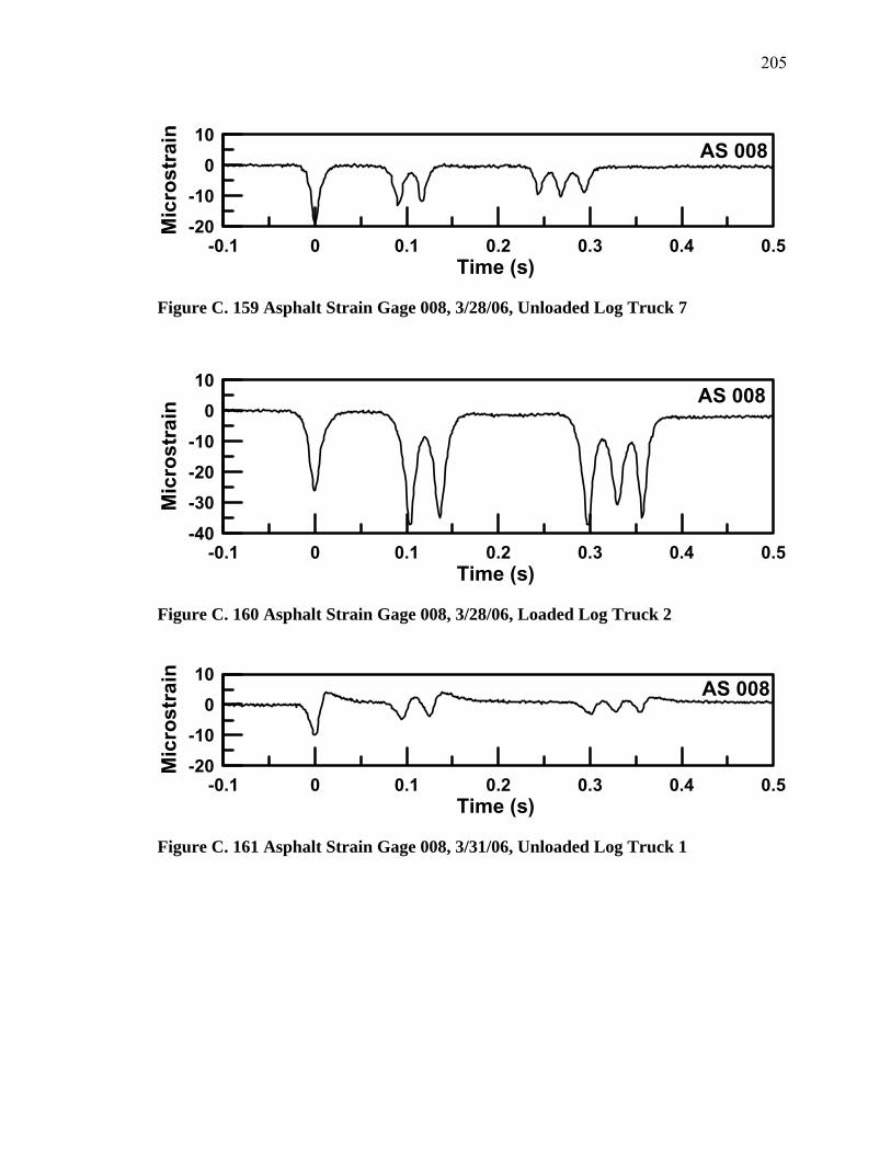
205
-0.1 0 0.1 0.2 0.3 0.4 0.5Time (s)
-20-10
010
Mic
rost
rain
AS 008
Figure C. 159 Asphalt Strain Gage 008, 3/28/06, Unloaded Log Truck 7
-0.1 0 0.1 0.2 0.3 0.4 0.5Time (s)
-40
-30-20-10
010
Mic
rost
rain
AS 008
Figure C. 160 Asphalt Strain Gage 008, 3/28/06, Loaded Log Truck 2
-0.1 0 0.1 0.2 0.3 0.4 0.5Time (s)
-20
-100
10
Mic
rost
rain AS 008
Figure C. 161 Asphalt Strain Gage 008, 3/31/06, Unloaded Log Truck 1

206
-0.1 0 0.1 0.2 0.3 0.4 0.5Time (s)
-30-20-10
010
Mic
rost
rain AS 008
Figure C. 162 Asphalt Strain Gage 008, 3/31/06, Loaded Log Truck 1
-0.1 0 0.1 0.2 0.3 0.4 0.5Time (s)
-40-30-20-10
010
Mic
rost
rain
AS 008
Figure C. 163 Asphalt Strain Gage 008, 3/31/06, Loaded Log Truck 2
-0.1 0 0.1 0.2 0.3 0.4 0.5Time (s)
-30-20-10
010
Mic
rost
rain AS 008
Figure C. 164 Asphalt Strain Gage 008, 3/31/06, Loaded Log Truck 3

207
-0.1 0 0.1 0.2 0.3 0.4 0.5Time (s)
-100
1020
Mic
rost
rain
AS 008
Figure C. 165 Asphalt Strain Gage 008, 3/31/06, Unloaded Log Truck 2
-0.1 0 0.1 0.2 0.3 0.4 0.5Time (s)
-40-30
-20-10
010
Mic
rost
rain
AS 008
Figure C. 166 Asphalt Strain Gage 008, 3/31/06, Unloaded Log Truck 3
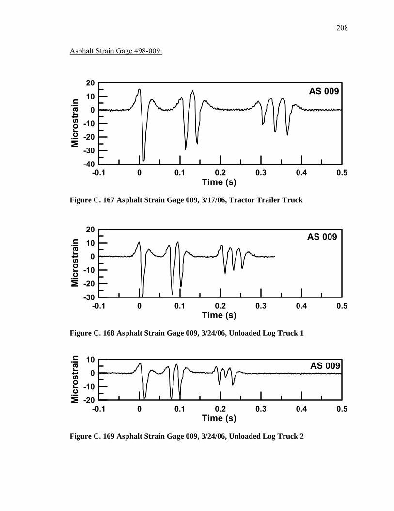
208
Asphalt Strain Gage 498-009:
-0.1 0 0.1 0.2 0.3 0.4 0.5Time (s)
-40-30-20-10
01020
Mic
rost
rain
AS 009
Figure C. 167 Asphalt Strain Gage 009, 3/17/06, Tractor Trailer Truck
-0.1 0 0.1 0.2 0.3 0.4 0.5Time (s)
-30
-20-10
01020
Mic
rost
rain
AS 009
Figure C. 168 Asphalt Strain Gage 009, 3/24/06, Unloaded Log Truck 1
-0.1 0 0.1 0.2 0.3 0.4 0.5Time (s)
-20-10
010
Mic
rost
rain AS 009
Figure C. 169 Asphalt Strain Gage 009, 3/24/06, Unloaded Log Truck 2
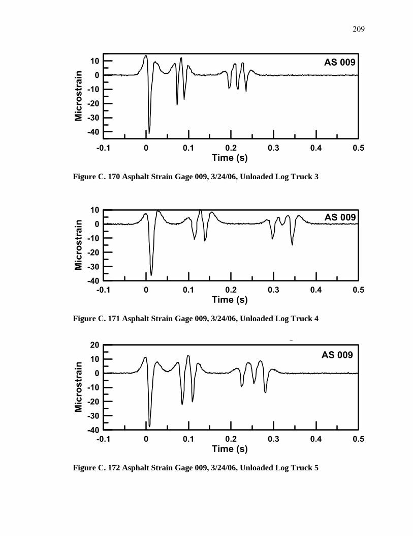
209
-0.1 0 0.1 0.2 0.3 0.4 0.5Time (s)
-40-30-20-10
010
Mic
rost
rain
AS 009
Figure C. 170 Asphalt Strain Gage 009, 3/24/06, Unloaded Log Truck 3
-0.1 0 0.1 0.2 0.3 0.4 0.5Time (s)
-40-30-20-10
010
Mic
rost
rain
AS 009
Figure C. 171 Asphalt Strain Gage 009, 3/24/06, Unloaded Log Truck 4
-0.1 0 0.1 0.2 0.3 0.4 0.5Time (s)
-40-30-20-10
01020
Mic
rost
rain
g
AS 009
Figure C. 172 Asphalt Strain Gage 009, 3/24/06, Unloaded Log Truck 5
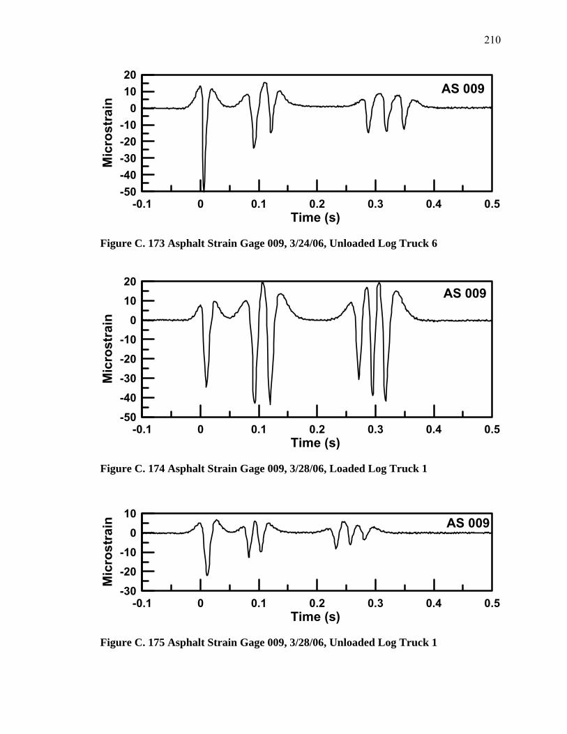
210
-0.1 0 0.1 0.2 0.3 0.4 0.5Time (s)
-50-40-30-20-10
01020
Mic
rost
rain
AS 009
Figure C. 173 Asphalt Strain Gage 009, 3/24/06, Unloaded Log Truck 6
-0.1 0 0.1 0.2 0.3 0.4 0.5Time (s)
-50-40-30-20-10
01020
Mic
rost
rain
AS 009
Figure C. 174 Asphalt Strain Gage 009, 3/28/06, Loaded Log Truck 1
-0.1 0 0.1 0.2 0.3 0.4 0.5Time (s)
-30-20-10
010
Mic
rost
rain AS 009
Figure C. 175 Asphalt Strain Gage 009, 3/28/06, Unloaded Log Truck 1
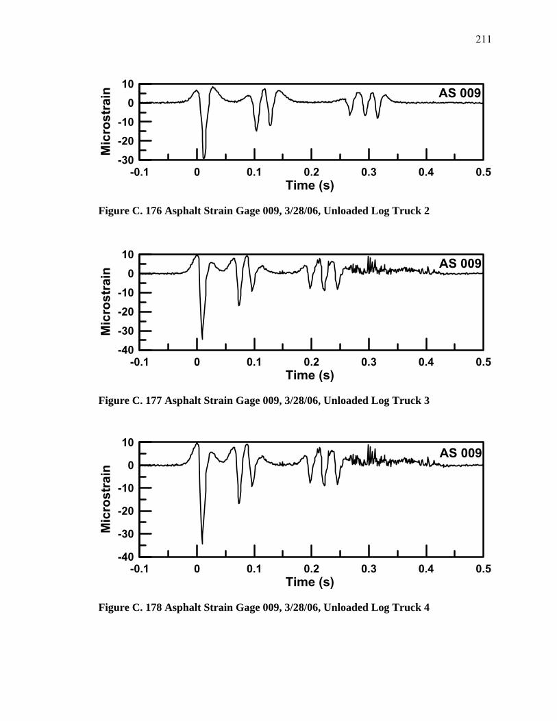
211
-0.1 0 0.1 0.2 0.3 0.4 0.5Time (s)
-30-20-10
010
Mic
rost
rain AS 009
Figure C. 176 Asphalt Strain Gage 009, 3/28/06, Unloaded Log Truck 2
-0.1 0 0.1 0.2 0.3 0.4 0.5Time (s)
-40-30
-20-10
010
Mic
rost
rain
AS 009
Figure C. 177 Asphalt Strain Gage 009, 3/28/06, Unloaded Log Truck 3
-0.1 0 0.1 0.2 0.3 0.4 0.5Time (s)
-40
-30
-20
-10
0
10
Mic
rost
rain
AS 009
Figure C. 178 Asphalt Strain Gage 009, 3/28/06, Unloaded Log Truck 4

212
-0.1 0 0.1 0.2 0.3 0.4 0.5Time (s)
-60-50-40-30-20-10
0
102030
Mic
rost
rain
AS 009
Figure C. 179 Asphalt Strain Gage 009, 3/28/06, Tractor Trailer Truck
-0.1 0 0.1 0.2 0.3 0.4 0.5Time (s)
-70-60-50-40-30-20-10
0102030
Mic
rost
rain
AS 009
Figure C. 180 Asphalt Strain Gage 009, 3/28/06, Full Tractor Trailer Truck
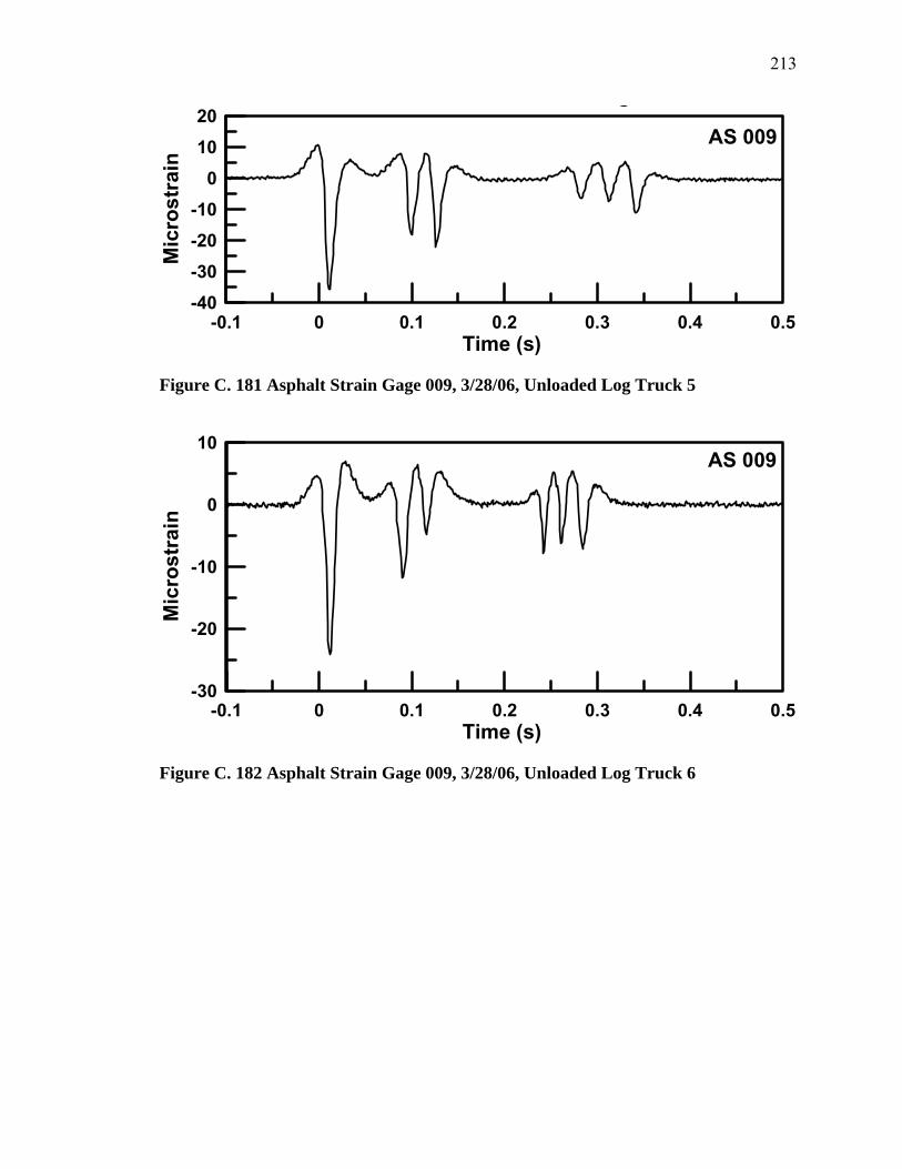
213
-0.1 0 0.1 0.2 0.3 0.4 0.5Time (s)
-40-30-20-10
01020
Mic
rost
rain
g
AS 009
Figure C. 181 Asphalt Strain Gage 009, 3/28/06, Unloaded Log Truck 5
-0.1 0 0.1 0.2 0.3 0.4 0.5Time (s)
-30
-20
-10
0
10
Mic
rost
rain
AS 009
Figure C. 182 Asphalt Strain Gage 009, 3/28/06, Unloaded Log Truck 6
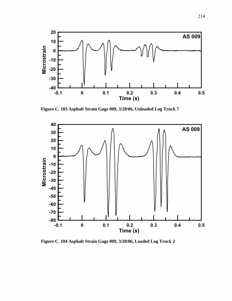
214
-0.1 0 0.1 0.2 0.3 0.4 0.5Time (s)
-40
-30
-20
-10
0
10
20
Mic
rost
rain
AS 009
Figure C. 183 Asphalt Strain Gage 009, 3/28/06, Unloaded Log Truck 7
-0.1 0 0.1 0.2 0.3 0.4 0.5Time (s)
-80-70-60-50-40-30-20-10
010
203040
Mic
rost
rain
AS 009
Figure C. 184 Asphalt Strain Gage 009, 3/28/06, Loaded Log Truck 2
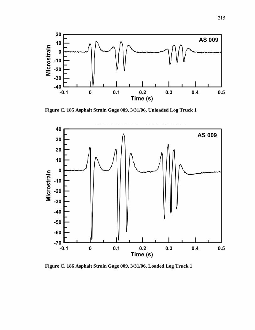
215
-0.1 0 0.1 0.2 0.3 0.4 0.5Time (s)
-40-30-20-10
01020
Mic
rost
rain
AS 009
Figure C. 185 Asphalt Strain Gage 009, 3/31/06, Unloaded Log Truck 1
-0.1 0 0.1 0.2 0.3 0.4 0.5Time (s)
-70
-60
-50
-40
-30
-20
-10
0
10
20
30
40
Mic
rost
rain
3/31/06 Truck 1b Loaded Truck
AS 009
Figure C. 186 Asphalt Strain Gage 009, 3/31/06, Loaded Log Truck 1

216
-0.1 0 0.1 0.2 0.3 0.4 0.5Time (s)
-100
-90-80-70
-60-50-40-30-20-10
01020304050
Mic
rost
rain
AS 009
Figure C. 187 Asphalt Strain Gage 009, 3/31/06, Loaded Log Truck 2
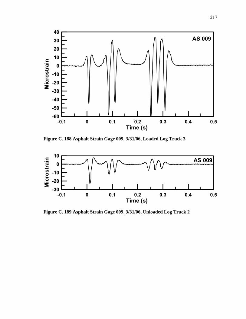
217
-0.1 0 0.1 0.2 0.3 0.4 0.5Time (s)
-60-50-40-30-20-10
010203040
Mic
rost
rain
AS 009
Figure C. 188 Asphalt Strain Gage 009, 3/31/06, Loaded Log Truck 3
-0.1 0 0.1 0.2 0.3 0.4 0.5Time (s)
-30-20-10
010
Mic
rost
rain AS 009
Figure C. 189 Asphalt Strain Gage 009, 3/31/06, Unloaded Log Truck 2
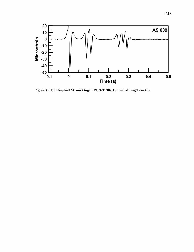
218
-0.1 0 0.1 0.2 0.3 0.4 0.5Time (s)
-50-40-30-20-10
01020
Mic
rost
rain
AS 009
Figure C. 190 Asphalt Strain Gage 009, 3/31/06, Unloaded Log Truck 3

219
APPENDIX D
Soil Strain and Stress – Plots of responses of soil strain gages and pressure cells to traffic
loading

220
2.8 2.9 3 3.1 3.2Time (s)
-50
0
50
100
150
200
250
Stra
in (m
icro
stra
in)
SS 1
Figure D. 1 Soil Strain, 6/16/06, Loaded Tri-Axle Dump Truck
3.5 3.6 3.7 3.8 3.9Time (s)
-50
0
50
100
150
200
250
Stra
in (m
icro
stra
in)
SS 2
p
Figure D. 2 Soil Strain, 6/16/06, Loaded Tri-Axle Dump Truck
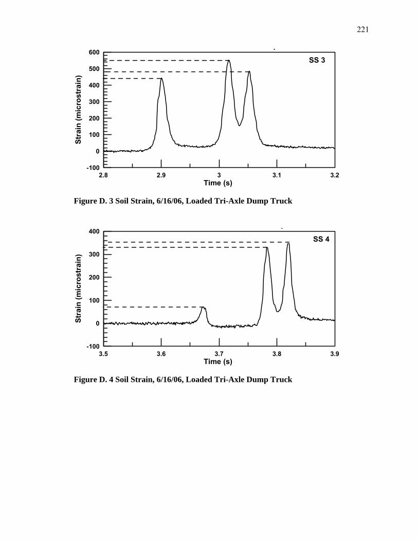
221
2.8 2.9 3 3.1 3.2Time (s)
-100
0
100
200
300
400
500
600
Stra
in (m
icro
stra
in)
SS 3
p
Figure D. 3 Soil Strain, 6/16/06, Loaded Tri-Axle Dump Truck
3.5 3.6 3.7 3.8 3.9Time (s)
-100
0
100
200
300
400
Stra
in (m
icro
stra
in)
SS 4
p
Figure D. 4 Soil Strain, 6/16/06, Loaded Tri-Axle Dump Truck
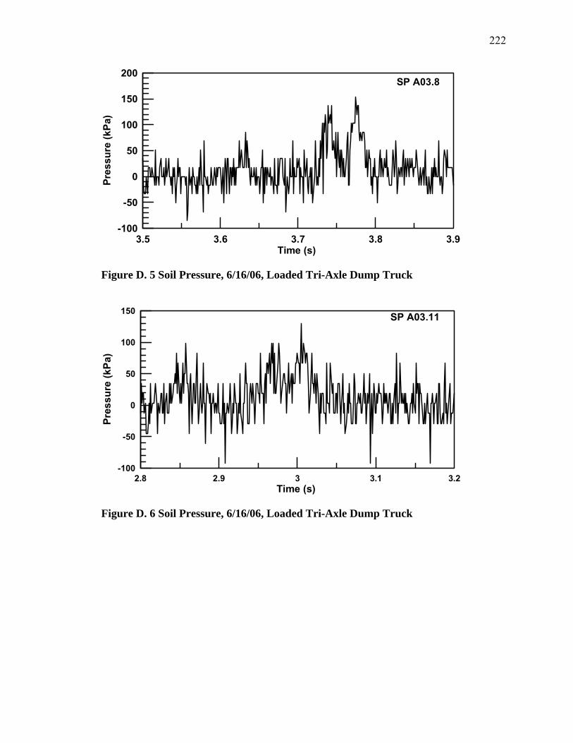
222
3.5 3.6 3.7 3.8 3.9Time (s)
-100
-50
0
50
100
150
200
Pres
sure
(kPa
)
SP A03.8
Figure D. 5 Soil Pressure, 6/16/06, Loaded Tri-Axle Dump Truck
2.8 2.9 3 3.1 3.2Time (s)
-100
-50
0
50
100
150
Pres
sure
(kPa
)
SP A03.11
Figure D. 6 Soil Pressure, 6/16/06, Loaded Tri-Axle Dump Truck
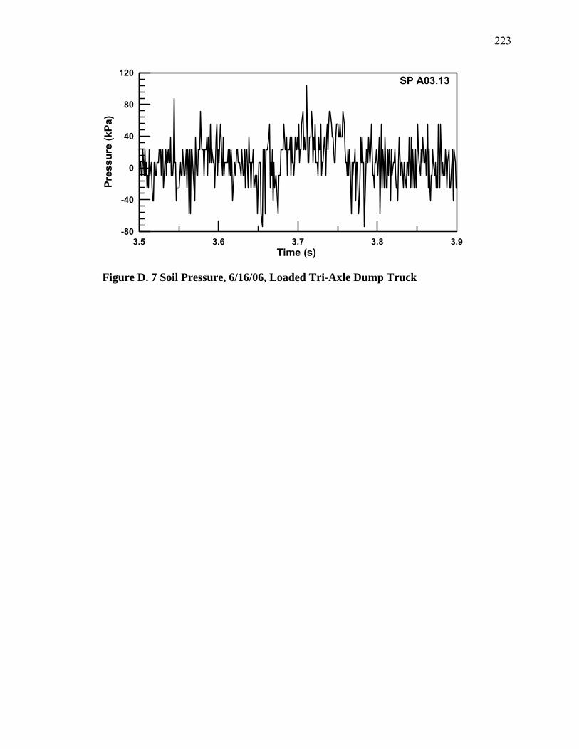
223
3.5 3.6 3.7 3.8 3.9Time (s)
-80
-40
0
40
80
120
Pres
sure
(kPa
)
SP A03.13
Figure D. 7 Soil Pressure, 6/16/06, Loaded Tri-Axle Dump Truck

224
0.5 0.6 0.7 0.8Time (s)
-20
0
20
40
60
80
100
120
140
160
Stra
in (m
icro
stra
in)
SS 1
Figure D. 8 Soil Strain, 6/16/06, Concrete Mixer Truck
1 1.1 1.2 1.3Time (s)
-20
0
20
40
60
80
100
120
140
160
Stra
in (m
icro
stra
in)
SS 2
Figure D. 9 Soil Strain, 6/16/06, Concrete Mixer Truck

225
0.5 0.6 0.7 0.8Time (s)
-40-20
020406080
100120140160180
Stra
in (m
icro
stra
in)
SS 3
Figure D. 10 Soil Strain, 6/16/06, Concrete Mixer Truck
1 1.1 1.2 1.3Time (s)
-50
0
50
100
150
200
250
Stra
in (m
icro
stra
in)
SS 4
Figure D. 11 Soil Strain, 6/16/06, Concrete Mixer Truck
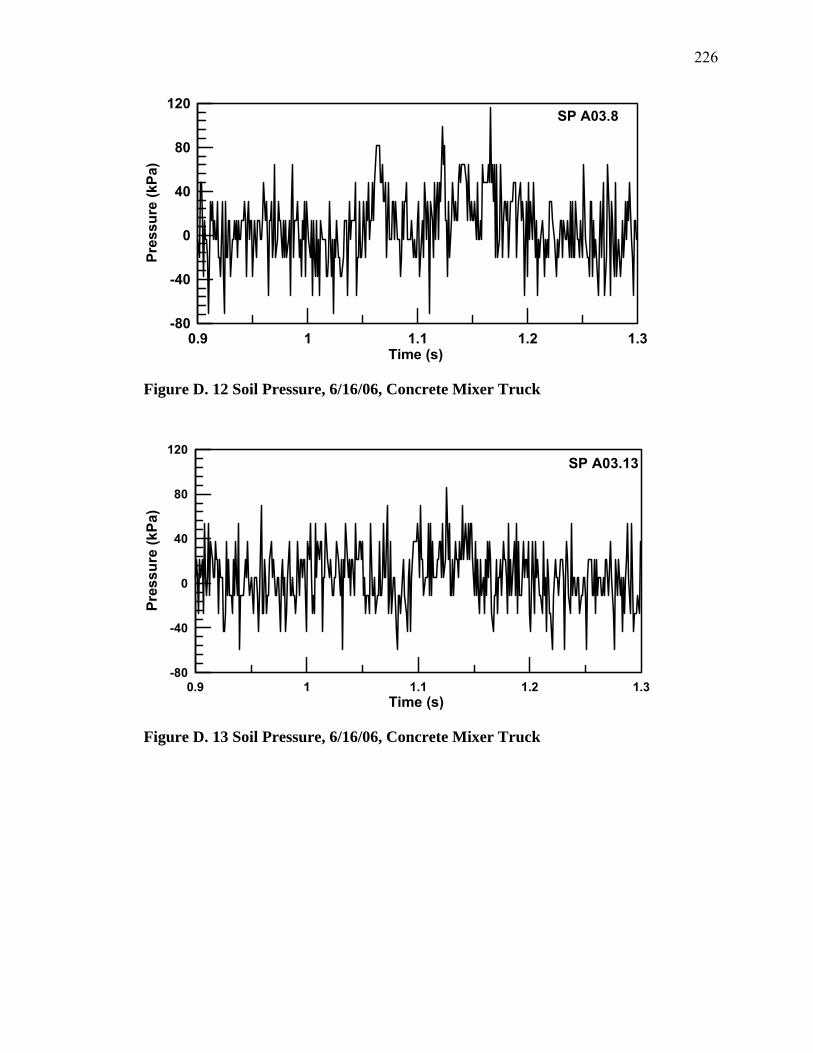
226
0.9 1 1.1 1.2 1.3Time (s)
-80
-40
0
40
80
120
Pres
sure
(kPa
)
SP A03.8
Figure D. 12 Soil Pressure, 6/16/06, Concrete Mixer Truck
0.9 1 1.1 1.2 1.3Time (s)
-80
-40
0
40
80
120
Pres
sure
(kPa
)
SP A03.13
Figure D. 13 Soil Pressure, 6/16/06, Concrete Mixer Truck

227
1.3 1.4 1.5 1.6 1.7Time (s)
-50
0
50
100
150
200
250
Stra
in (m
icro
stra
in)
SS 1
p
Figure D. 14 Soil Strain, 6/16/06, Loaded Tri-Axle Dump Truck
2 2.1 2.2 2.3 2.4Time (s)
-50
0
50
100
150
200
250
Stra
in (m
icro
stra
in)
SS 2
p
Figure D. 15 Soil Strain, 6/16/06, Loaded Tri-Axle Dump Truck

228
1.3 1.4 1.5 1.6 1.7Time (s)
-100
0
100
200
300
400
500
600
Stra
in (m
icro
stra
in)
SS 3
p
Figure D. 16 Soil Strain, 6/16/06, Loaded Tri-Axle Dump Truck
2 2.1 2.2 2.3 2.4Time (s)
-50
0
50
100
150
200
250
300
350
400
Stra
in (m
icro
stra
in)
SS 4
p
Figure D. 17 Soil Strain, 6/16/06, Loaded Tri-Axle Dump Truck
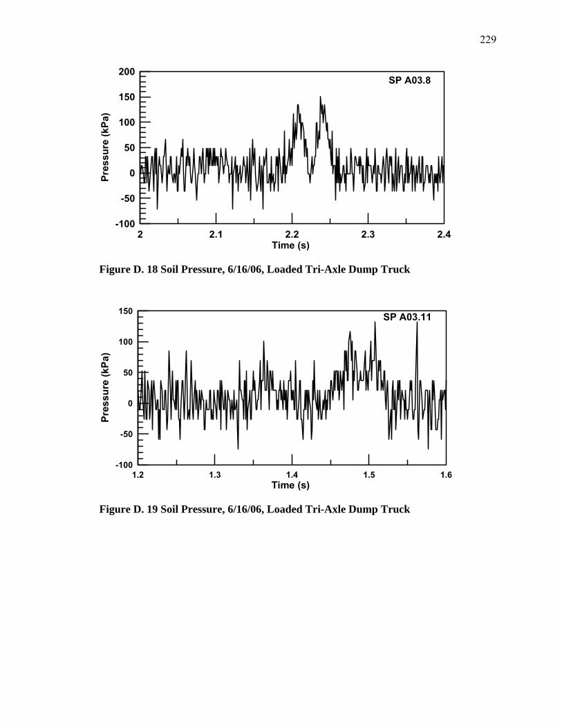
229
2 2.1 2.2 2.3 2.4Time (s)
-100
-50
0
50
100
150
200
Pres
sure
(kPa
)
SP A03.8
Figure D. 18 Soil Pressure, 6/16/06, Loaded Tri-Axle Dump Truck
1.2 1.3 1.4 1.5 1.6Time (s)
-100
-50
0
50
100
150
Pres
sure
(kPa
)
SP A03.11
Figure D. 19 Soil Pressure, 6/16/06, Loaded Tri-Axle Dump Truck
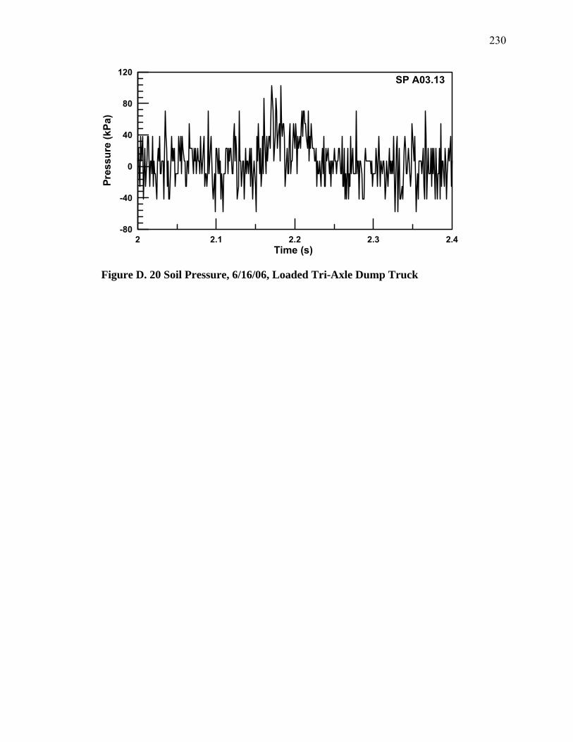
230
2 2.1 2.2 2.3 2.4Time (s)
-80
-40
0
40
80
120
Pres
sure
(kPa
)
SP A03.13
Figure D. 20 Soil Pressure, 6/16/06, Loaded Tri-Axle Dump Truck
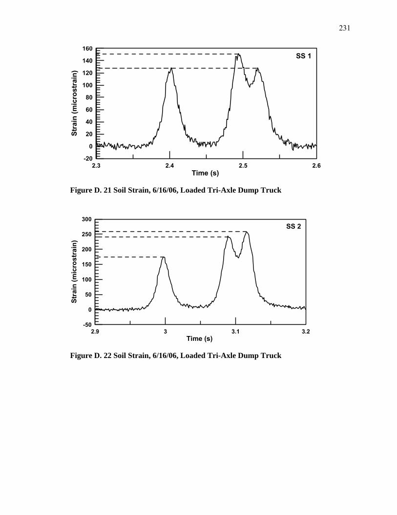
231
2.3 2.4 2.5 2.6Time (s)
-20
0
20
40
60
80
100
120
140
160
Stra
in (m
icro
stra
in)
SS 1
Figure D. 21 Soil Strain, 6/16/06, Loaded Tri-Axle Dump Truck
2.9 3 3.1 3.2Time (s)
-50
0
50
100
150
200
250
300
Stra
in (m
icro
stra
in)
SS 2
Figure D. 22 Soil Strain, 6/16/06, Loaded Tri-Axle Dump Truck
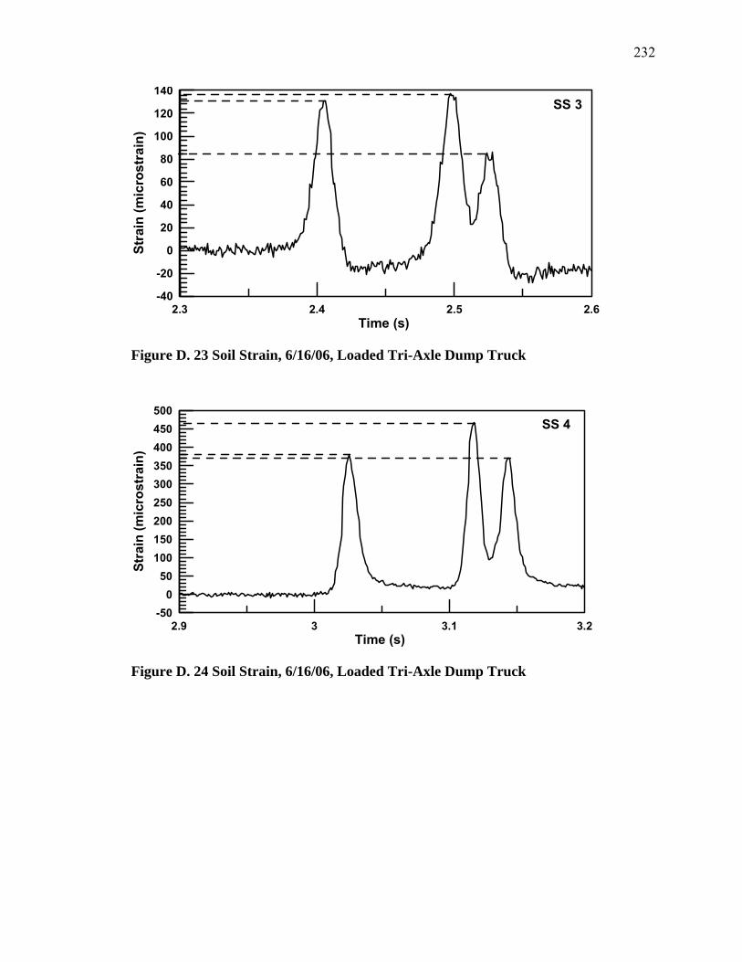
232
2.3 2.4 2.5 2.6Time (s)
-40
-20
0
20
40
60
80
100
120
140
Stra
in (m
icro
stra
in)
SS 3
Figure D. 23 Soil Strain, 6/16/06, Loaded Tri-Axle Dump Truck
2.9 3 3.1 3.2Time (s)
-500
50100150200250300350400450500
Stra
in (m
icro
stra
in)
SS 4
Figure D. 24 Soil Strain, 6/16/06, Loaded Tri-Axle Dump Truck
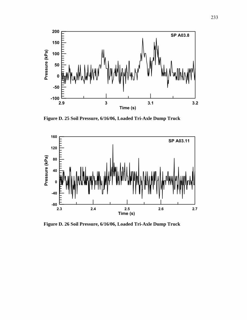
233
2.9 3 3.1 3.2Time (s)
-100
-50
0
50
100
150
200
Pres
sure
(kPa
)
SP A03.8
Figure D. 25 Soil Pressure, 6/16/06, Loaded Tri-Axle Dump Truck
2.3 2.4 2.5 2.6 2.7Time (s)
-80
-40
0
40
80
120
160
Pres
sure
(kPa
)
SP A03.11
Figure D. 26 Soil Pressure, 6/16/06, Loaded Tri-Axle Dump Truck
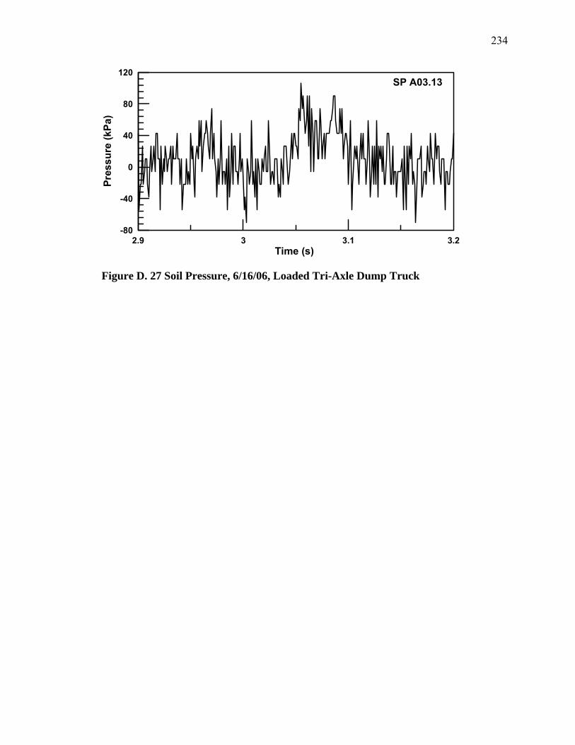
234
2.9 3 3.1 3.2Time (s)
-80
-40
0
40
80
120
Pres
sure
(kPa
)
SP A03.13
Figure D. 27 Soil Pressure, 6/16/06, Loaded Tri-Axle Dump Truck

235
2.2 2.3 2.4 2.5 2.6Time (s)
-50
0
50
100
150
200
250
Stra
in (m
icro
stra
in)
SS 1
p
Figure D. 28 Soil Strain, 6/16/06, Loaded Tri-Axle Dump Truck
2.9 3 3.1 3.2 3.3Time (s)
-50
0
50
100
150
200
250
Stra
in (m
icro
stra
in)
SS 2
p
Figure D. 29 Soil Strain, 6/16/06, Loaded Tri-Axle Dump Truck
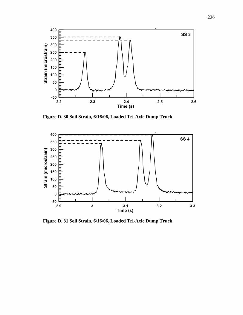
236
2.2 2.3 2.4 2.5 2.6Time (s)
-50
0
50
100
150
200
250
300
350
400
Stra
in (m
icro
stra
in)
SS 3
p
Figure D. 30 Soil Strain, 6/16/06, Loaded Tri-Axle Dump Truck
2.9 3 3.1 3.2 3.3Time (s)
-50
0
50
100
150
200
250
300
350
400
Stra
in (m
icro
stra
in)
SS 4
p
Figure D. 31 Soil Strain, 6/16/06, Loaded Tri-Axle Dump Truck
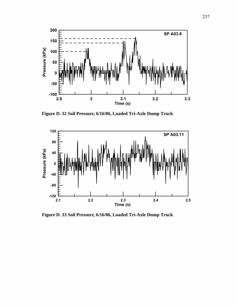
237
2.9 3 3.1 3.2 3.3Time (s)
-100
-50
0
50
100
150
200
Pres
sure
(kPa
)
SP A03.8
Figure D. 32 Soil Pressure, 6/16/06, Loaded Tri-Axle Dump Truck
2.1 2.2 2.3 2.4 2.5Time (s)
-120
-80
-40
0
40
80
120
Pres
sure
(kPa
)
SP A03.11
Figure D. 33 Soil Pressure, 6/16/06, Loaded Tri-Axle Dump Truck

238
2.9 3 3.1 3.2 3.3Time (s)
-80
-40
0
40
80
120
Pres
sure
(kPa
)
SP A03.13
Figure D. 34 Soil Pressure, 6/16/06, Loaded Tri-Axle Dump Truck
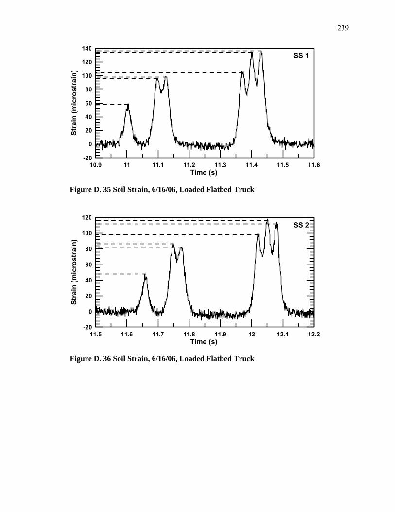
239
10.9 11 11.1 11.2 11.3 11.4 11.5 11.6Time (s)
-20
0
20
40
60
80
100
120
140
Stra
in (m
icro
stra
in)
SS 1
Figure D. 35 Soil Strain, 6/16/06, Loaded Flatbed Truck
11.5 11.6 11.7 11.8 11.9 12 12.1 12.2Time (s)
-20
0
20
40
60
80
100
120
Stra
in (m
icro
stra
in)
SS 2
Figure D. 36 Soil Strain, 6/16/06, Loaded Flatbed Truck
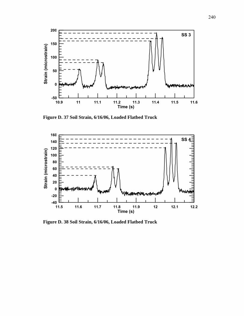
240
10.9 11 11.1 11.2 11.3 11.4 11.5 11.6Time (s)
-50
0
50
100
150
200
Stra
in (m
icro
stra
in)
SS 3
Figure D. 37 Soil Strain, 6/16/06, Loaded Flatbed Truck
11.5 11.6 11.7 11.8 11.9 12 12.1 12.2Time (s)
-40
-20
0
20
40
60
80
100
120
140
160
Stra
in (m
icro
stra
in)
SS 4
Figure D. 38 Soil Strain, 6/16/06, Loaded Flatbed Truck
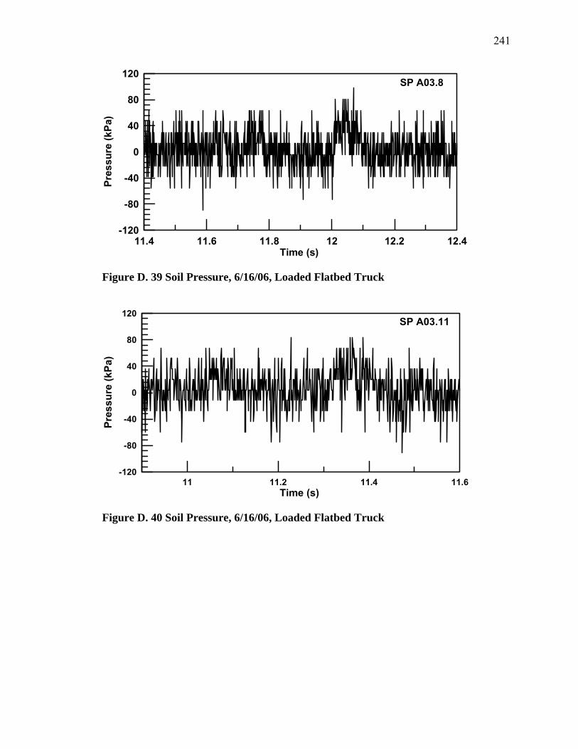
241
11.4 11.6 11.8 12 12.2 12.4Time (s)
-120
-80
-40
0
40
80
120
Pres
sure
(kPa
)
SP A03.8
Figure D. 39 Soil Pressure, 6/16/06, Loaded Flatbed Truck
11 11.2 11.4 11.6Time (s)
-120
-80
-40
0
40
80
120
Pres
sure
(kPa
)
SP A03.11
Figure D. 40 Soil Pressure, 6/16/06, Loaded Flatbed Truck
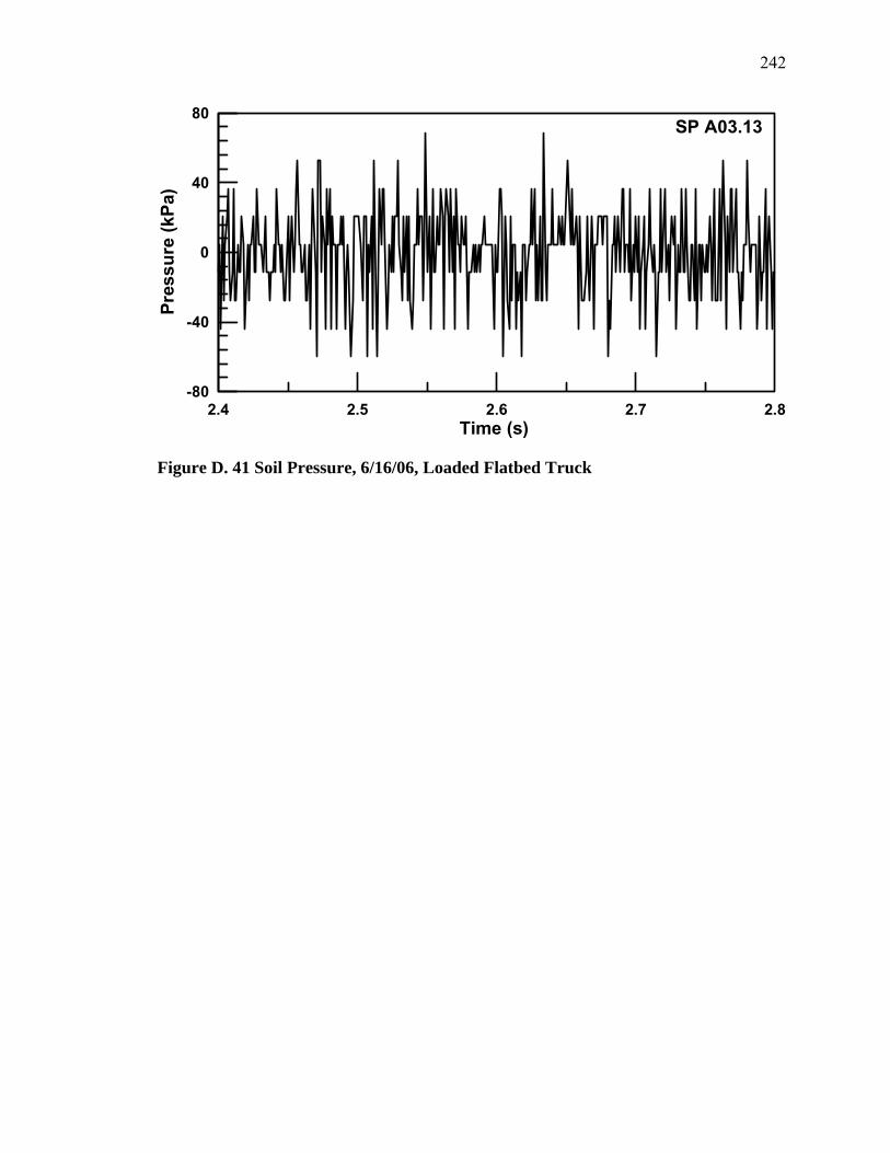
242
2.4 2.5 2.6 2.7 2.8Time (s)
-80
-40
0
40
80
Pres
sure
(kPa
)
SP A03.13
Figure D. 41 Soil Pressure, 6/16/06, Loaded Flatbed Truck

243
APPENDIX E
Plots of gage responses to MaineDOT dump truck loading – 4/26/06
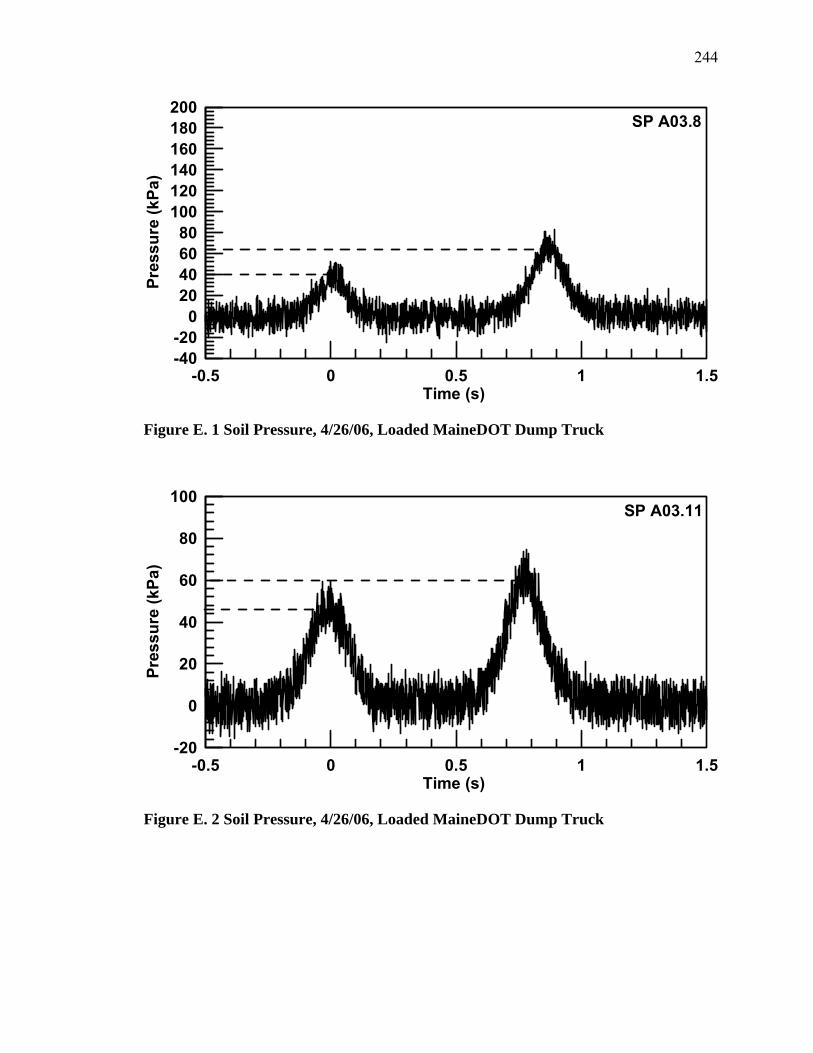
244
-0.5 0 0.5 1 1.5Time (s)
-40-20
020406080
100120140160180200
Pres
sure
(kPa
)
SP A03.8
Figure E. 1 Soil Pressure, 4/26/06, Loaded MaineDOT Dump Truck
-0.5 0 0.5 1 1.5Time (s)
-20
0
20
40
60
80
100
Pres
sure
(kPa
)
SP A03.11
Figure E. 2 Soil Pressure, 4/26/06, Loaded MaineDOT Dump Truck
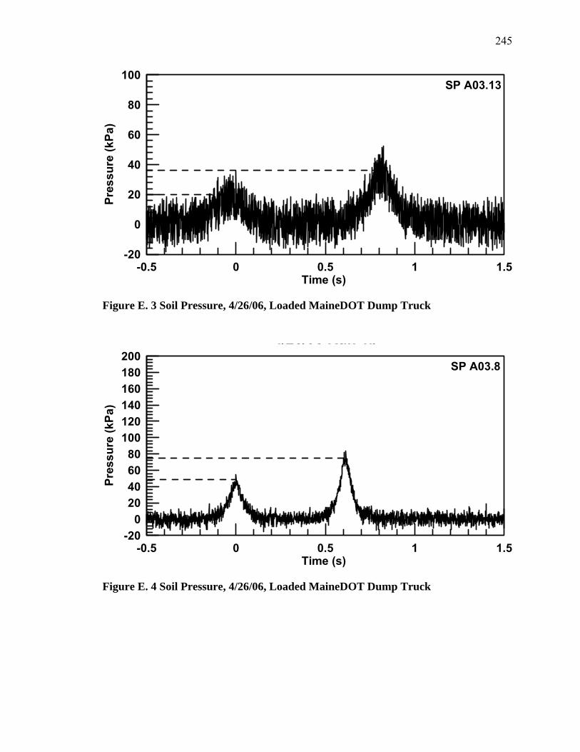
245
-0.5 0 0.5 1 1.5Time (s)
-20
0
20
40
60
80
100
Pres
sure
(kPa
)
SP A03.13
Figure E. 3 Soil Pressure, 4/26/06, Loaded MaineDOT Dump Truck
-0.5 0 0.5 1 1.5Time (s)
-200
20406080
100120140160180200
Pres
sure
(kPa
)
SP A03.8
4/26/06 Run 1b
Figure E. 4 Soil Pressure, 4/26/06, Loaded MaineDOT Dump Truck

246
-0.5 0 0.5 1 1.5Time (s)
-20
0
20
40
60
80
Pres
sure
(kPa
)
SP A03.11
Figure E. 5 Soil Pressure, 4/26/06, Loaded MaineDOT Dump Truck
-0.5 0 0.5 1 1.5Time (s)
-20
0
20
40
60
80
100
Pres
sure
(kPa
)
SP A03.13
Figure E. 6 Soil Pressure, 4/26/06, Loaded MaineDOT Dump Truck
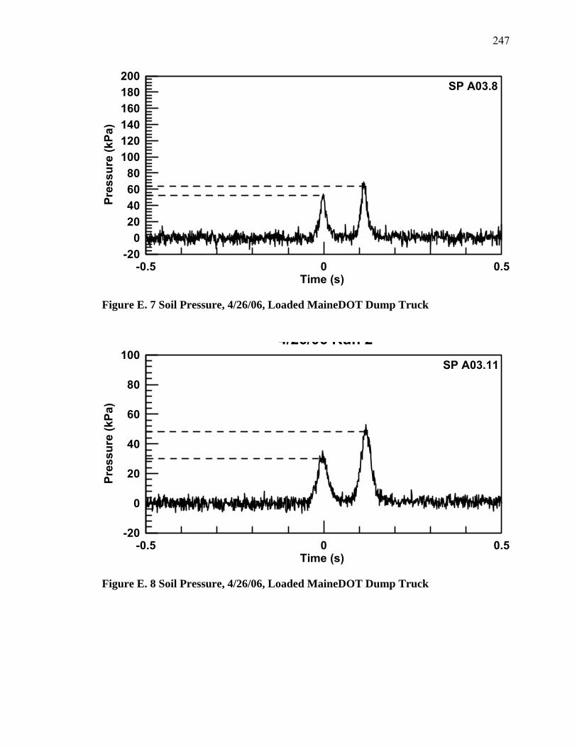
247
-0.5 0 0.5Time (s)
-200
20406080
100120140160180200
Pres
sure
(kPa
)
SP A03.8
Figure E. 7 Soil Pressure, 4/26/06, Loaded MaineDOT Dump Truck
-0.5 0 0.5Time (s)
-20
0
20
40
60
80
100
Pres
sure
(kPa
)
SP A03.11
4/26/06 Run 2
Figure E. 8 Soil Pressure, 4/26/06, Loaded MaineDOT Dump Truck
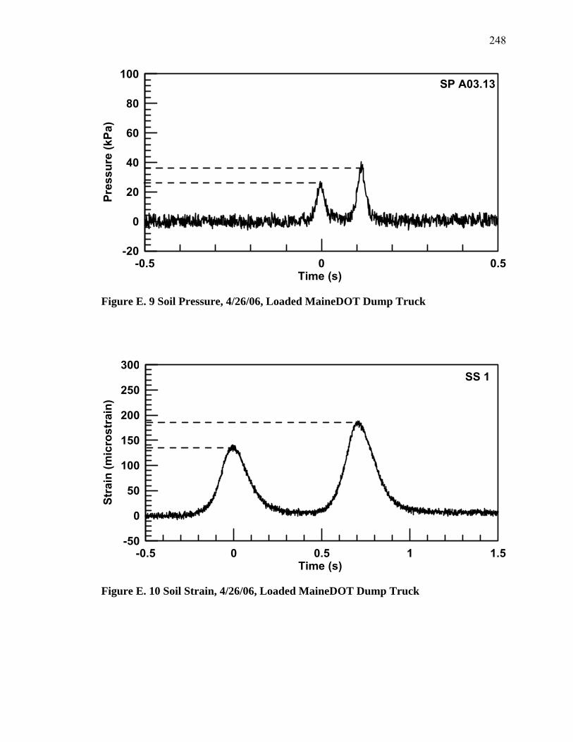
248
-0.5 0 0.5Time (s)
-20
0
20
40
60
80
100
Pres
sure
(kPa
)
SP A03.13
Figure E. 9 Soil Pressure, 4/26/06, Loaded MaineDOT Dump Truck
-0.5 0 0.5 1 1.5Time (s)
-50
0
50
100
150
200
250
300
Stra
in (m
icro
stra
in)
SS 1
Figure E. 10 Soil Strain, 4/26/06, Loaded MaineDOT Dump Truck

249
-0.5 0 0.5 1 1.5Time (s)
-50
0
50
100
150
200
250
300
Stra
in (m
icro
stra
in)
SS 2
Figure E. 11 Soil Strain, 4/26/06, Loaded MaineDOT Dump Truck
-0.5 0 0.5 1 1.5Time (s)
-500
50100150200250300350400450500550600
Stra
in (m
icro
stra
in)
SS 3
Figure E. 12 Soil Strain, 4/26/06, Loaded MaineDOT Dump Truck
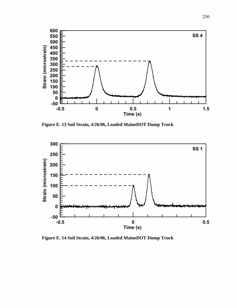
250
-0.5 0 0.5 1 1.5Time (s)
-500
50100150200250300350400450500550600
Stra
in (m
icro
stra
in)
SS 4
Figure E. 13 Soil Strain, 4/26/06, Loaded MaineDOT Dump Truck
-0.5 0 0.5Time (s)
-50
0
50
100
150
200
250
300
Stra
in (m
icro
stra
in)
SS 1
Figure E. 14 Soil Strain, 4/26/06, Loaded MaineDOT Dump Truck
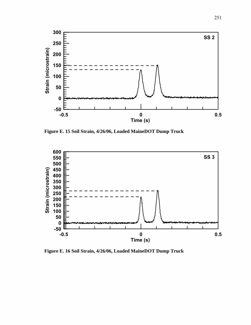
251
-0.5 0 0.5Time (s)
-50
0
50
100
150
200
250
300
Stra
in (m
icro
stra
in)
SS 2
Figure E. 15 Soil Strain, 4/26/06, Loaded MaineDOT Dump Truck
-0.5 0 0.5Time (s)
-500
50100150200250300350400450500550600
Stra
in (m
icro
stra
in)
SS 3
Figure E. 16 Soil Strain, 4/26/06, Loaded MaineDOT Dump Truck
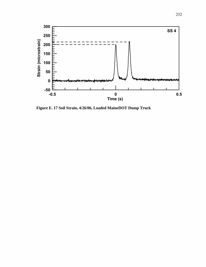
252
-0.5 0 0.5Time (s)
-50
0
50
100
150
200
250
300
Stra
in (m
icro
stra
in)
SS 4
Figure E. 17 Soil Strain, 4/26/06, Loaded MaineDOT Dump Truck

253
APPENDIX F
Plots of gage responses to MaineDOT dump truck loading – 7/13/06
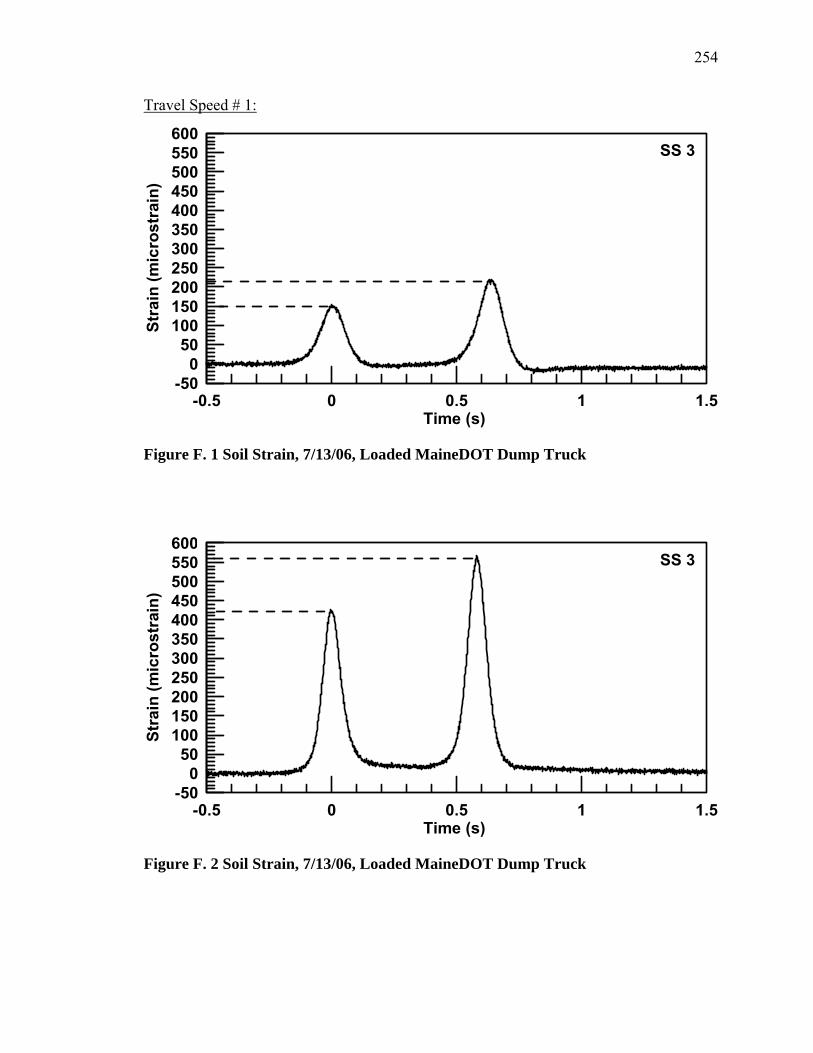
254
Travel Speed # 1:
-0.5 0 0.5 1 1.5Time (s)
-500
50100150200250300350400450500550600
Stra
in (m
icro
stra
in)
SS 3
Figure F. 1 Soil Strain, 7/13/06, Loaded MaineDOT Dump Truck
-0.5 0 0.5 1 1.5Time (s)
-500
50100150200250300350400450500550600
Stra
in (m
icro
stra
in)
SS 3
Figure F. 2 Soil Strain, 7/13/06, Loaded MaineDOT Dump Truck
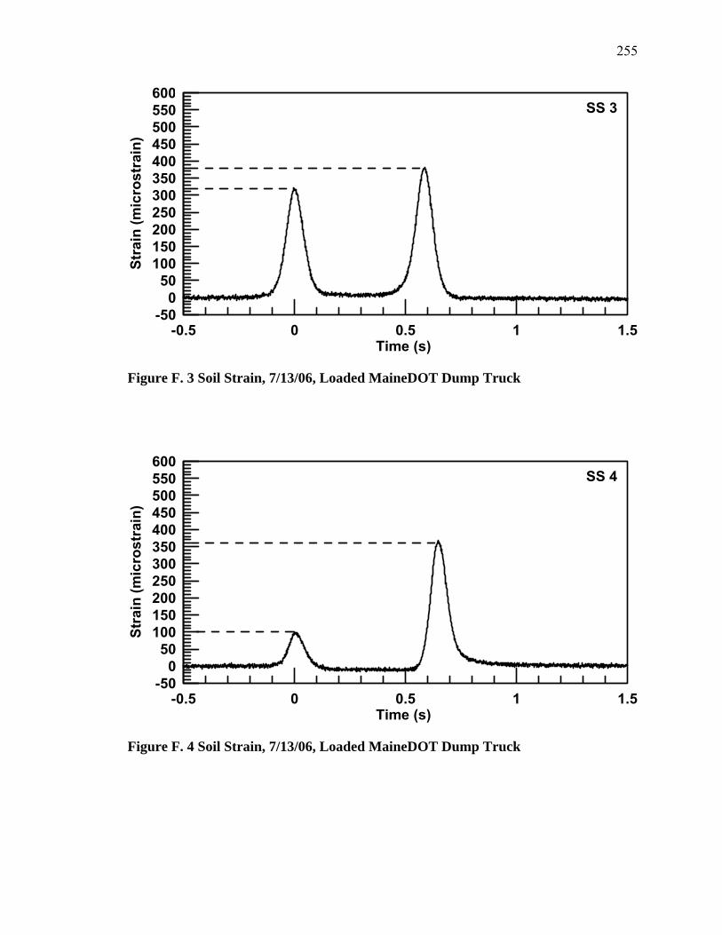
255
-0.5 0 0.5 1 1.5Time (s)
-500
50100150200250300350400450500550600
Stra
in (m
icro
stra
in)
SS 3
Figure F. 3 Soil Strain, 7/13/06, Loaded MaineDOT Dump Truck
-0.5 0 0.5 1 1.5Time (s)
-500
50100150200250300350400450500550600
Stra
in (m
icro
stra
in)
SS 4
Figure F. 4 Soil Strain, 7/13/06, Loaded MaineDOT Dump Truck
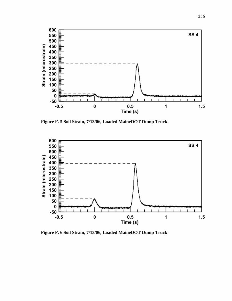
256
-0.5 0 0.5 1 1.5Time (s)
-500
50100150200250300350400450500550600
Stra
in (m
icro
stra
in)
SS 4
Figure F. 5 Soil Strain, 7/13/06, Loaded MaineDOT Dump Truck
-0.5 0 0.5 1 1.5Time (s)
-500
50100150200250300350400450500550600
Stra
in (m
icro
stra
in)
SS 4
Figure F. 6 Soil Strain, 7/13/06, Loaded MaineDOT Dump Truck
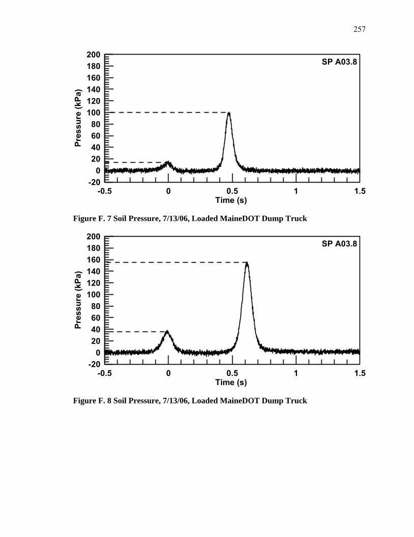
257
-0.5 0 0.5 1 1.5Time (s)
-200
20406080
100120140160180200
Pres
sure
(kPa
)
SP A03.8
Figure F. 7 Soil Pressure, 7/13/06, Loaded MaineDOT Dump Truck
-0.5 0 0.5 1 1.5Time (s)
-200
20406080
100120140160180200
Pres
sure
(kPa
)
SP A03.8
Figure F. 8 Soil Pressure, 7/13/06, Loaded MaineDOT Dump Truck
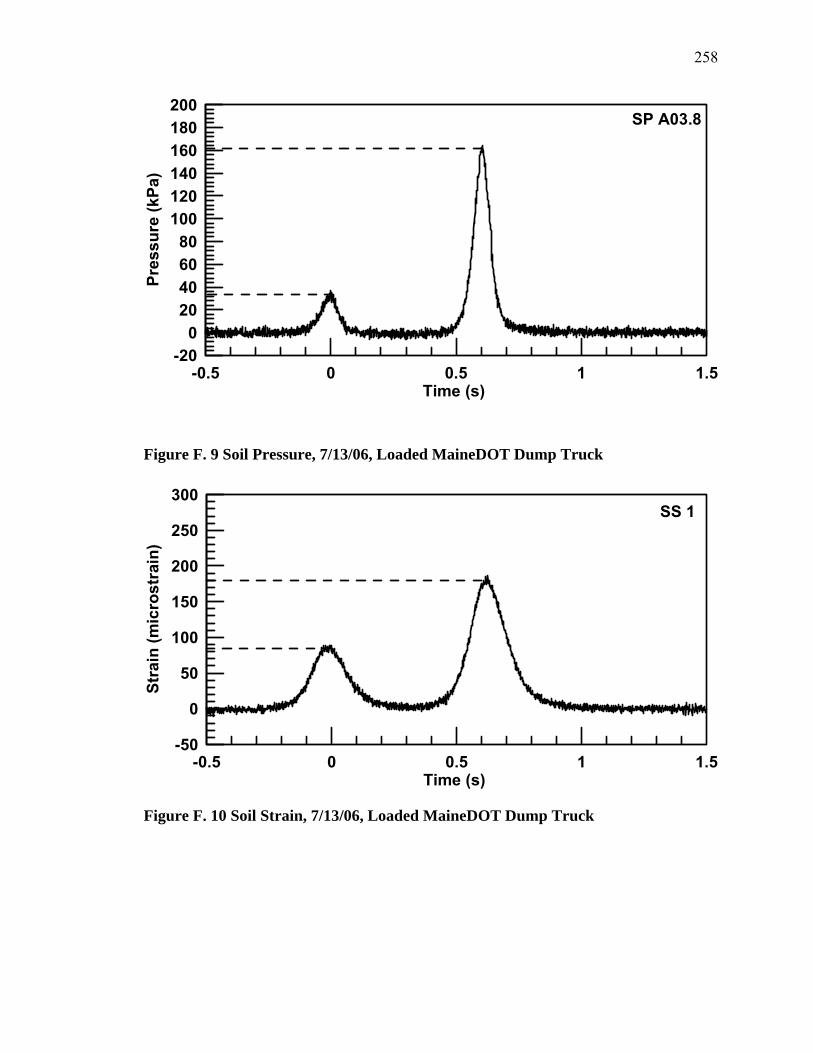
258
-0.5 0 0.5 1 1.5Time (s)
-200
20406080
100120140160180200
Pres
sure
(kPa
)
SP A03.8
Figure F. 9 Soil Pressure, 7/13/06, Loaded MaineDOT Dump Truck
-0.5 0 0.5 1 1.5Time (s)
-50
0
50
100
150
200
250
300
Stra
in (m
icro
stra
in)
SS 1
Figure F. 10 Soil Strain, 7/13/06, Loaded MaineDOT Dump Truck
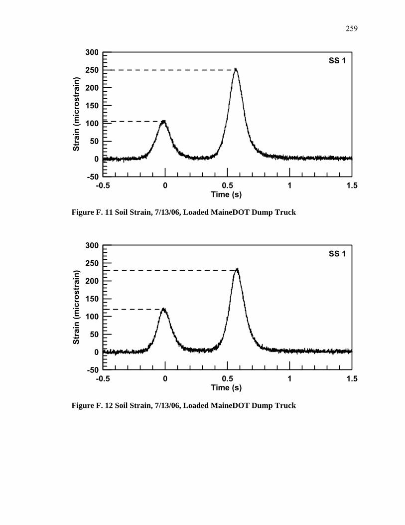
259
-0.5 0 0.5 1 1.5Time (s)
-50
0
50
100
150
200
250
300
Stra
in (m
icro
stra
in)
SS 1
Figure F. 11 Soil Strain, 7/13/06, Loaded MaineDOT Dump Truck
-0.5 0 0.5 1 1.5Time (s)
-50
0
50
100
150
200
250
300
Stra
in (m
icro
stra
in)
SS 1
Figure F. 12 Soil Strain, 7/13/06, Loaded MaineDOT Dump Truck

260
-0.5 0 0.5 1 1.5Time (s)
-20
0
20
40
60
80
100
Pres
sure
(kPa
)
SP A03.11
Figure F. 13 Soil Pressure, 7/13/06, Loaded MaineDOT Dump Truck
-0.5 0 0.5 1 1.5Time (s)
-20
0
20
40
60
80
100
Pres
sure
(kPa
)
SP A03.11
Figure F. 14 Soil Pressure, 7/13/06, Loaded MaineDOT Dump Truck
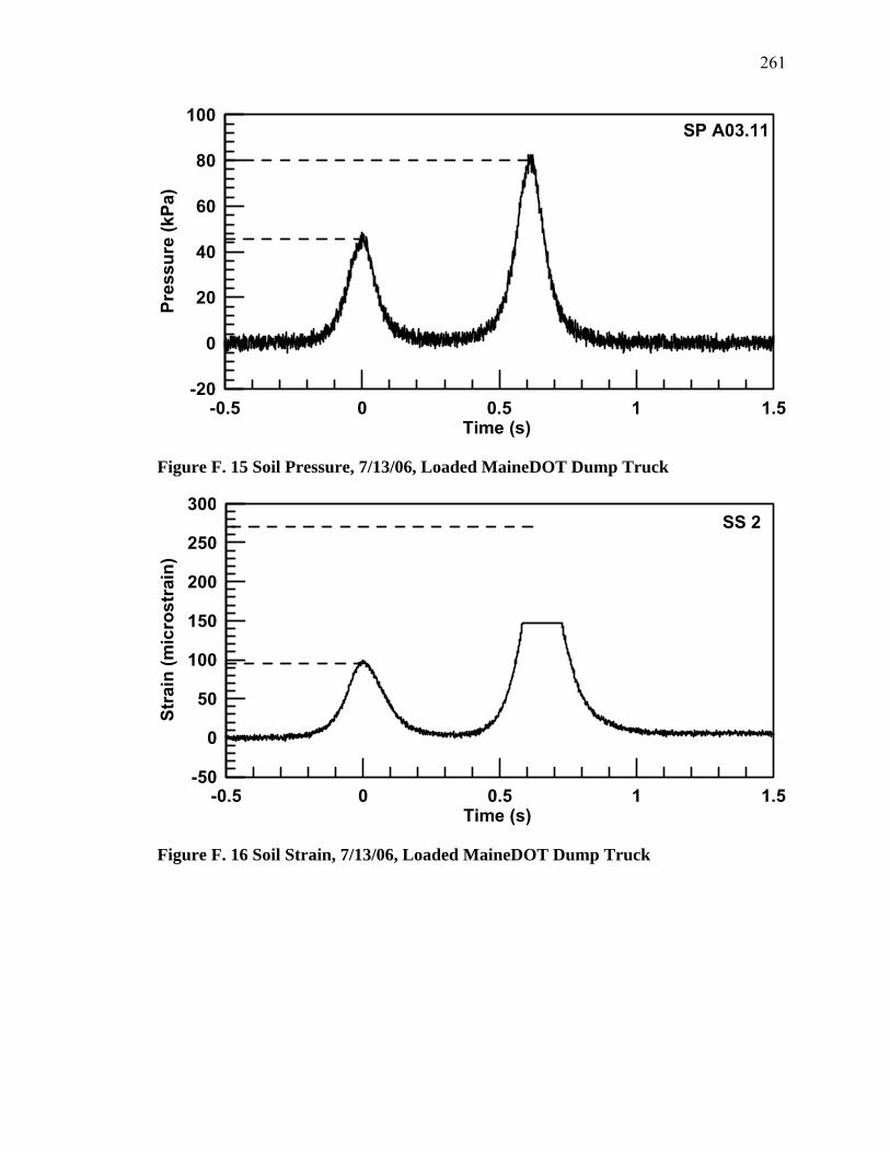
261
-0.5 0 0.5 1 1.5Time (s)
-20
0
20
40
60
80
100
Pres
sure
(kPa
)
SP A03.11
Figure F. 15 Soil Pressure, 7/13/06, Loaded MaineDOT Dump Truck
-0.5 0 0.5 1 1.5Time (s)
-50
0
50
100
150
200
250
300
Stra
in (m
icro
stra
in)
SS 2
Figure F. 16 Soil Strain, 7/13/06, Loaded MaineDOT Dump Truck
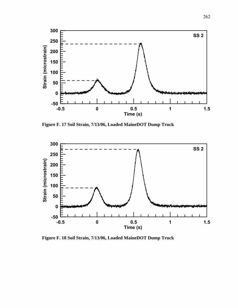
262
-0.5 0 0.5 1 1.5Time (s)
-50
0
50
100
150
200
250
300
Stra
in (m
icro
stra
in)
SS 2
Figure F. 17 Soil Strain, 7/13/06, Loaded MaineDOT Dump Truck
-0.5 0 0.5 1 1.5Time (s)
-50
0
50
100
150
200
250
300
Stra
in (m
icro
stra
in)
SS 2
Figure F. 18 Soil Strain, 7/13/06, Loaded MaineDOT Dump Truck
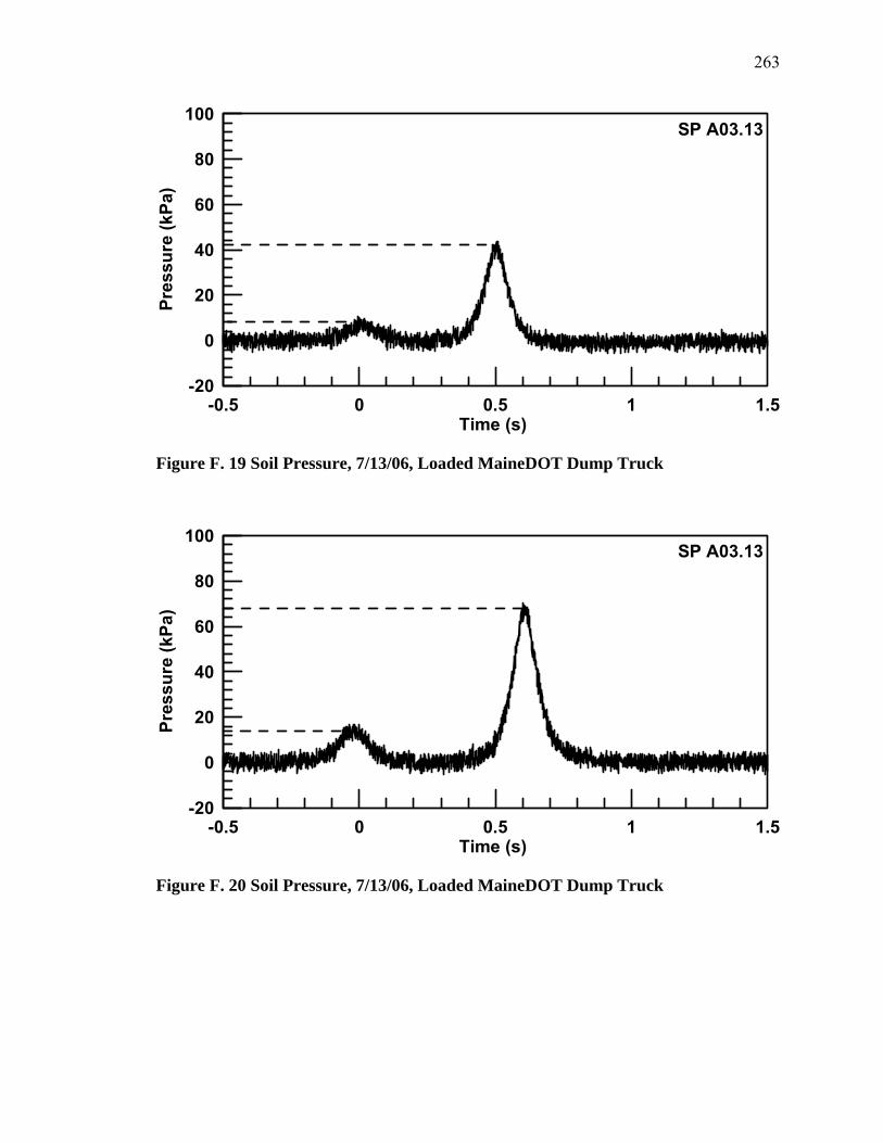
263
-0.5 0 0.5 1 1.5Time (s)
-20
0
20
40
60
80
100
Pres
sure
(kPa
)
SP A03.13
Figure F. 19 Soil Pressure, 7/13/06, Loaded MaineDOT Dump Truck
-0.5 0 0.5 1 1.5Time (s)
-20
0
20
40
60
80
100
Pres
sure
(kPa
)
SP A03.13
Figure F. 20 Soil Pressure, 7/13/06, Loaded MaineDOT Dump Truck

264
-0.5 0 0.5 1 1.5Time (s)
-20
0
20
40
60
80
100
Pres
sure
(kpa
)
SP A03.13
Figure F. 21 Soil Pressure, 7/13/06, Loaded MaineDOT Dump Truck
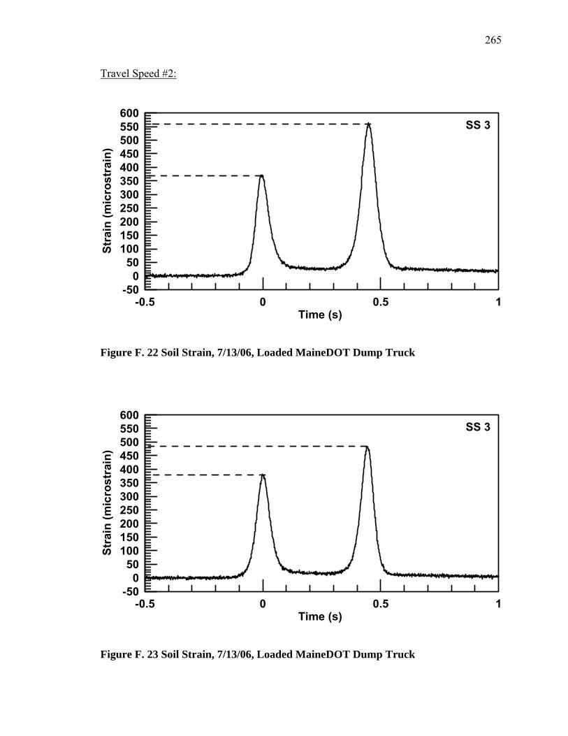
265
Travel Speed #2:
-0.5 0 0.5 1Time (s)
-500
50100150200250300350400450500550600
Stra
in (m
icro
stra
in)
SS 3
Figure F. 22 Soil Strain, 7/13/06, Loaded MaineDOT Dump Truck
-0.5 0 0.5 1Time (s)
-500
50100150200250300350400450500550600
Stra
in (m
icro
stra
in)
SS 3
Figure F. 23 Soil Strain, 7/13/06, Loaded MaineDOT Dump Truck

266
-0.5 0 0.5 1Time (s)
-500
50100150200250300350400450500550600
Stra
in (m
icro
stra
in)
SS 3
Figure F. 24 Soil Strain, 7/13/06, Loaded MaineDOT Dump Truck
-0.5 0 0.5 1Time (s)
-500
50100150200250300350400450500550600
Stra
in (m
icro
stra
in)
SS 4
Figure F. 25 Soil Strain, 7/13/06, Loaded MaineDOT Dump Truck
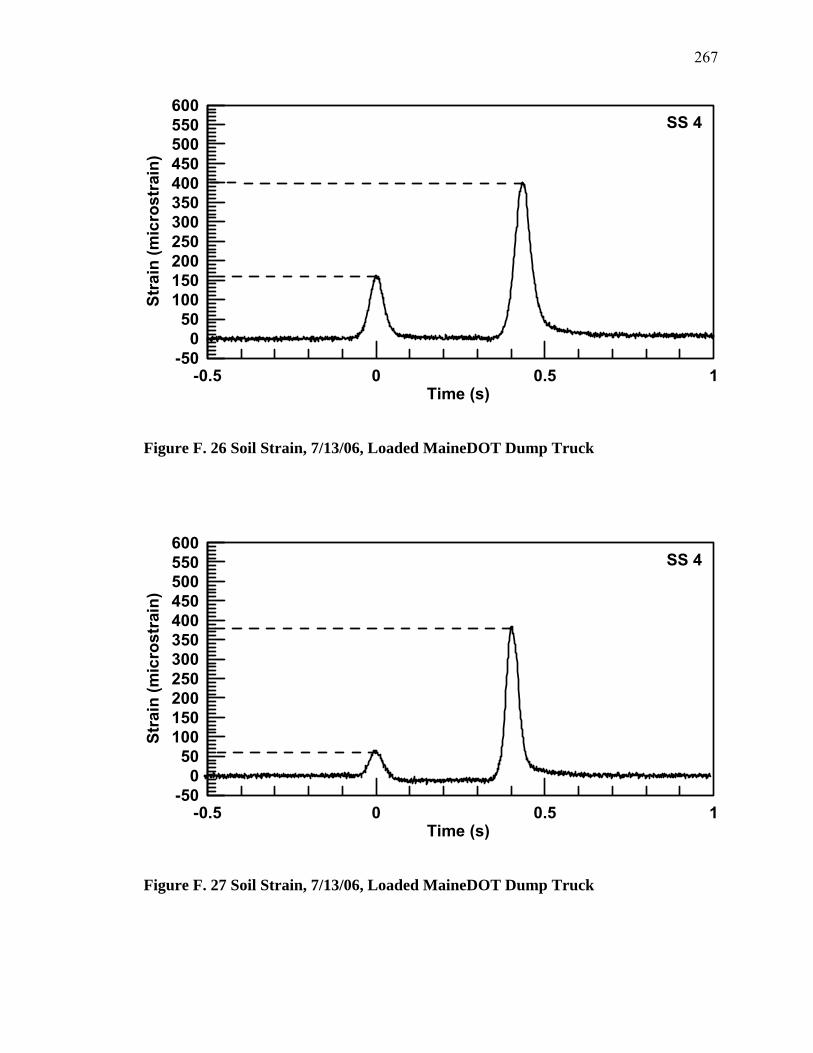
267
-0.5 0 0.5 1Time (s)
-500
50100150200250300350400450500550600
Stra
in (m
icro
stra
in)
SS 4
Figure F. 26 Soil Strain, 7/13/06, Loaded MaineDOT Dump Truck
-0.5 0 0.5 1Time (s)
-500
50100150200250300350400450500550600
Stra
in (m
icro
stra
in)
SS 4
Figure F. 27 Soil Strain, 7/13/06, Loaded MaineDOT Dump Truck
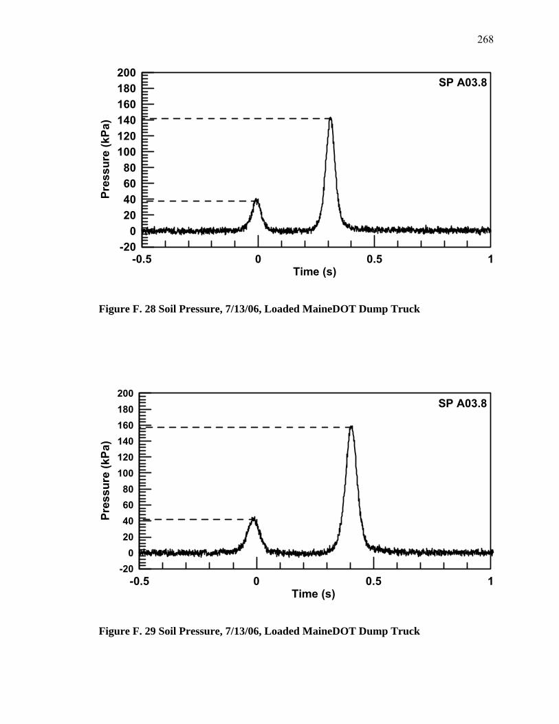
268
-0.5 0 0.5 1Time (s)
-200
20406080
100120140160180200
Pres
sure
(kPa
)
SP A03.8
Figure F. 28 Soil Pressure, 7/13/06, Loaded MaineDOT Dump Truck
-0.5 0 0.5 1Time (s)
-200
20406080
100120140160180200
Pres
sure
(kPa
)
SP A03.8
Figure F. 29 Soil Pressure, 7/13/06, Loaded MaineDOT Dump Truck
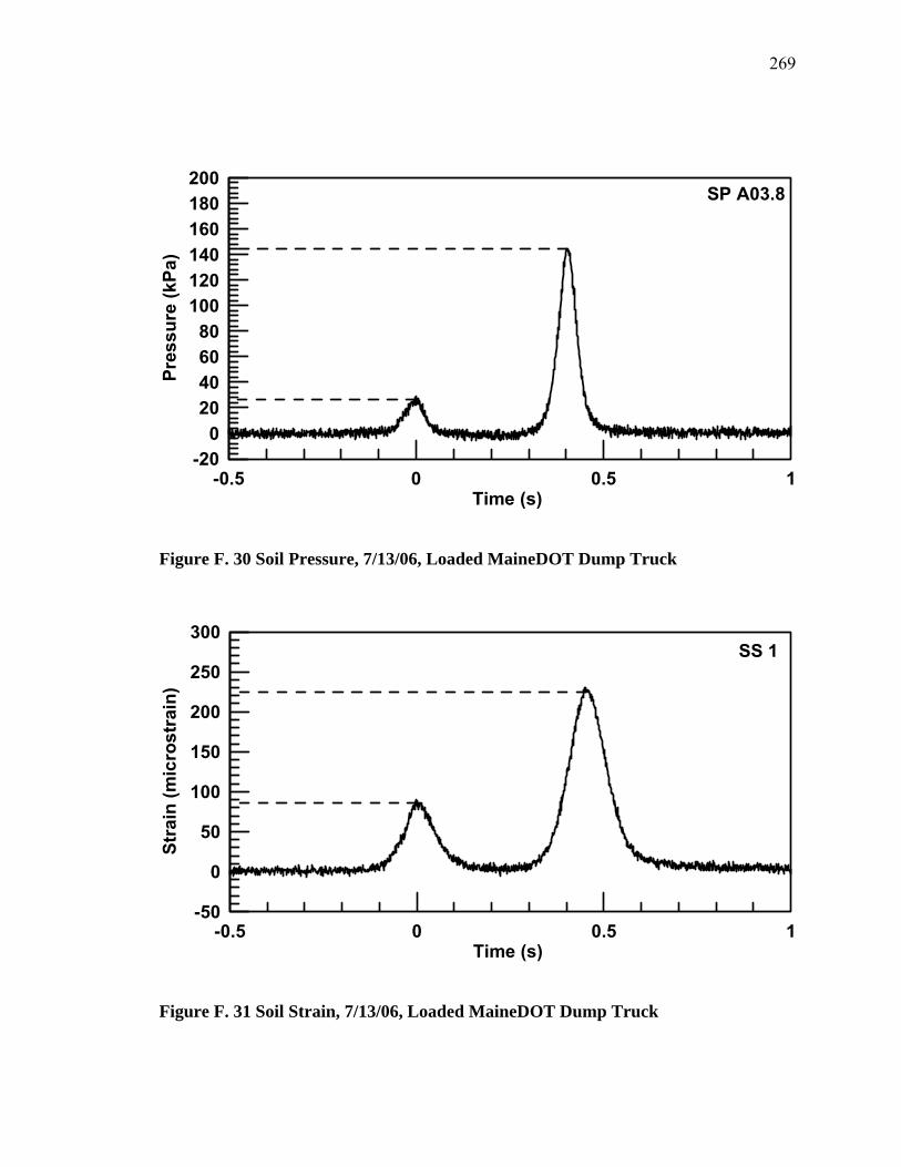
269
-0.5 0 0.5 1Time (s)
-200
20406080
100120140160180200
Pres
sure
(kPa
)SP A03.8
Figure F. 30 Soil Pressure, 7/13/06, Loaded MaineDOT Dump Truck
-0.5 0 0.5 1Time (s)
-50
0
50
100
150
200
250
300
Stra
in (m
icro
stra
in)
SS 1
Figure F. 31 Soil Strain, 7/13/06, Loaded MaineDOT Dump Truck
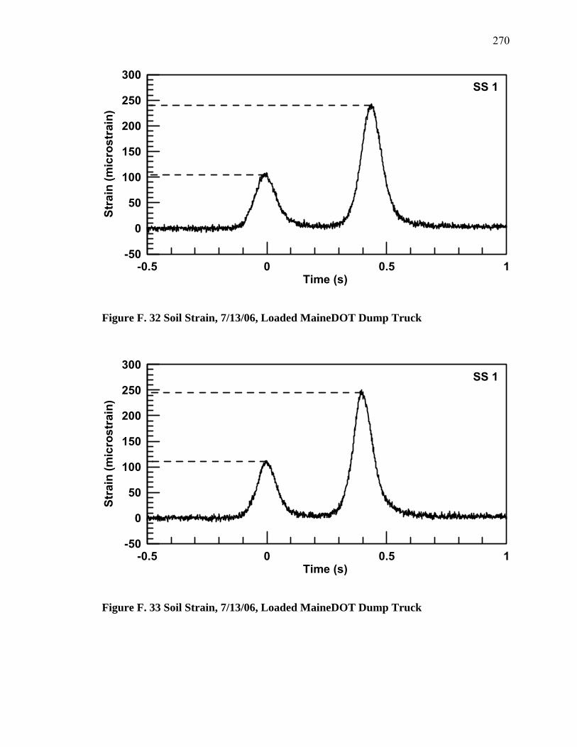
270
-0.5 0 0.5 1Time (s)
-50
0
50
100
150
200
250
300
Stra
in (m
icro
stra
in)
SS 1
Figure F. 32 Soil Strain, 7/13/06, Loaded MaineDOT Dump Truck
-0.5 0 0.5 1Time (s)
-50
0
50
100
150
200
250
300
Stra
in (m
icro
stra
in)
SS 1
Figure F. 33 Soil Strain, 7/13/06, Loaded MaineDOT Dump Truck
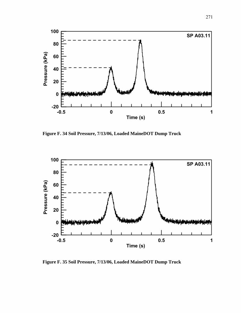
271
-0.5 0 0.5 1Time (s)
-20
0
20
40
60
80
100
Pres
sure
(kPa
)
SP A03.11
Figure F. 34 Soil Pressure, 7/13/06, Loaded MaineDOT Dump Truck
-0.5 0 0.5 1Time (s)
-20
0
20
40
60
80
100
Pres
sure
(kPa
)
SP A03.11
Figure F. 35 Soil Pressure, 7/13/06, Loaded MaineDOT Dump Truck
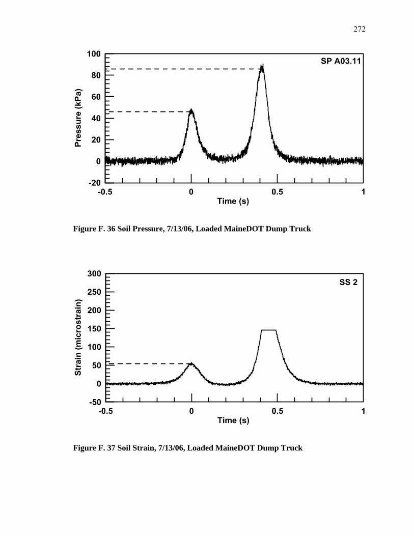
272
-0.5 0 0.5 1Time (s)
-20
0
20
40
60
80
100
Pres
sure
(kPa
)
SP A03.11
Figure F. 36 Soil Pressure, 7/13/06, Loaded MaineDOT Dump Truck
-0.5 0 0.5 1Time (s)
-50
0
50
100
150
200
250
300
Stra
in (m
icro
stra
in)
SS 2
Figure F. 37 Soil Strain, 7/13/06, Loaded MaineDOT Dump Truck

273
-0.5 0 0.5 1Time (s)
-50
0
50
100
150
200
250
300
Stra
in (m
icro
stra
in)
SS 2
Figure F. 38 Soil Strain, 7/13/06, Loaded MaineDOT Dump Truck
-0.5 0 0.5 1Time (s)
-50
0
50
100
150
200
250
300
Stra
in (m
icro
stra
in)
SS 2
Figure F. 39 Soil Strain, 7/13/06, Loaded MaineDOT Dump Truck
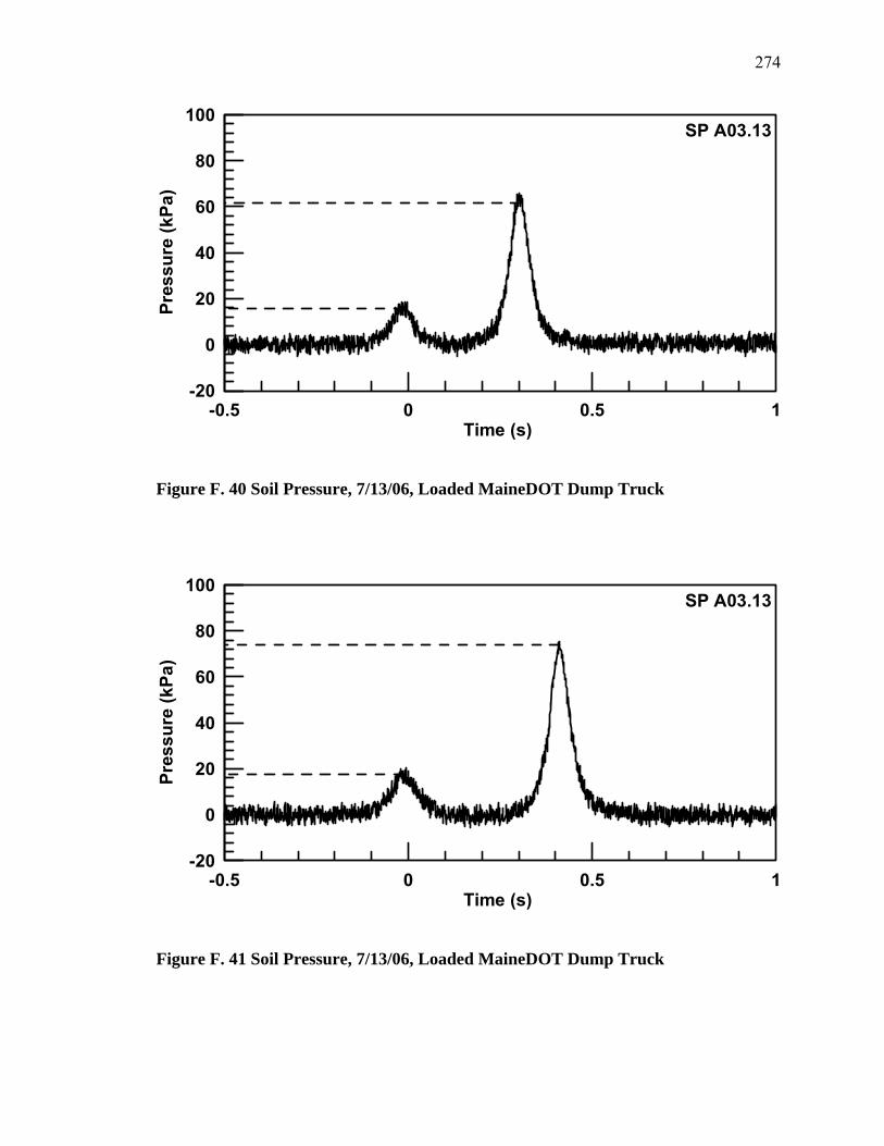
274
-0.5 0 0.5 1Time (s)
-20
0
20
40
60
80
100
Pres
sure
(kPa
)
SP A03.13
Figure F. 40 Soil Pressure, 7/13/06, Loaded MaineDOT Dump Truck
-0.5 0 0.5 1Time (s)
-20
0
20
40
60
80
100
Pres
sure
(kPa
)
SP A03.13
Figure F. 41 Soil Pressure, 7/13/06, Loaded MaineDOT Dump Truck
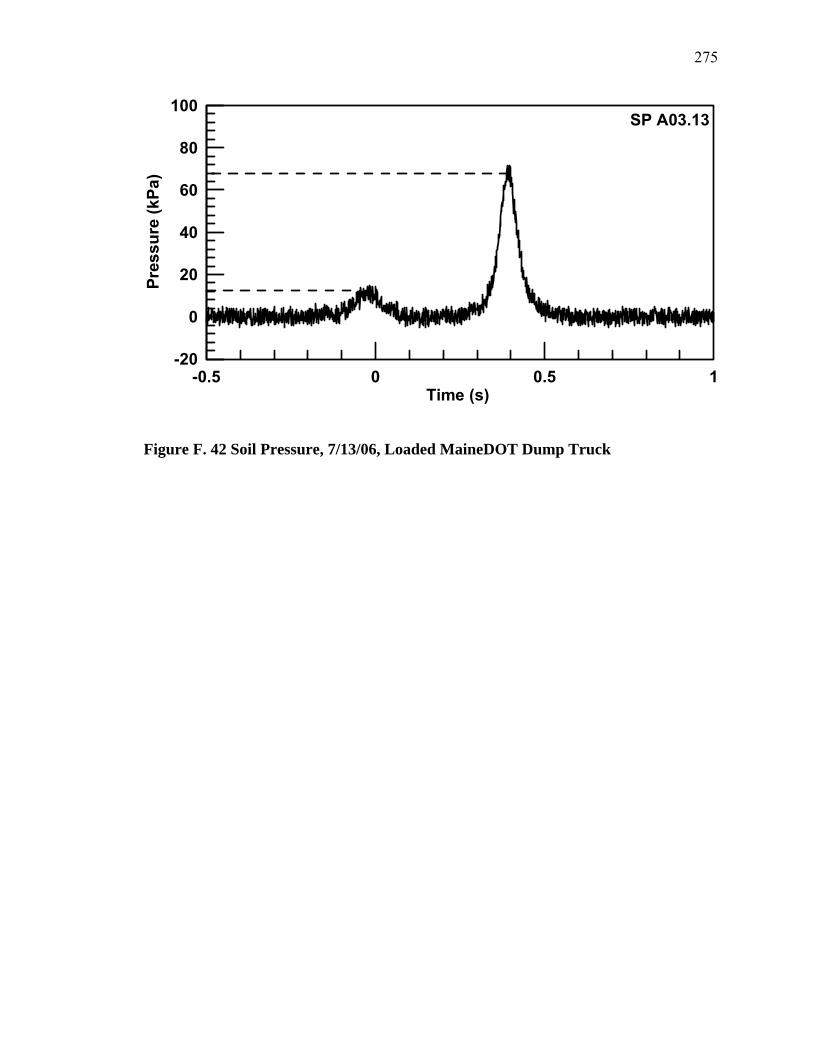
275
-0.5 0 0.5 1Time (s)
-20
0
20
40
60
80
100
Pres
sure
(kPa
)
SP A03.13
Figure F. 42 Soil Pressure, 7/13/06, Loaded MaineDOT Dump Truck
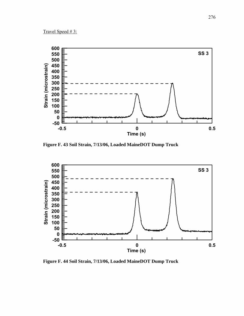
276
Travel Speed # 3:
-0.5 0 0.5Time (s)
-500
50100150200250300350400450500550600
Stra
in (m
icro
stra
in)
SS 3
Figure F. 43 Soil Strain, 7/13/06, Loaded MaineDOT Dump Truck
-0.5 0 0.5Time (s)
-500
50100150200250300350400450500550600
Stra
in (m
icro
stra
in)
SS 3
Figure F. 44 Soil Strain, 7/13/06, Loaded MaineDOT Dump Truck

277
-0.5 0 0.5Time (s)
-500
50100150200250300350400450500550600
Stra
in (m
icro
stra
in)
SS 3
Figure F. 45 Soil Strain, 7/13/06, Loaded MaineDOT Dump Truck
-0.5 0 0.5Time (s)
-500
50100150200250300350400450500550600
Stra
in (m
icro
stra
in)
SS 4
Figure F. 46 Soil Strain, 7/13/06, Loaded MaineDOT Dump Truck

278
-0.5 0 0.5Time (s)
-500
50100150200250300350400450500550600
Stra
in (m
icro
stra
in)
SS 4
Figure F. 47 Soil Strain, 7/13/06, Loaded MaineDOT Dump Truck
-0.5 0 0.5Time (s)
-500
50100150200250300350400450500550600
Stra
in (m
icro
stra
in)
SS 4
Figure F. 48 Soil Strain, 7/13/06, Loaded MaineDOT Dump Truck

279
-0.5 0 0.5Time (s)
-200
20406080
100120140160180200
Pres
sure
(kPa
)
SP A03.8
Figure F. 49 Soil Pressure, 7/13/06, Loaded MaineDOT Dump Truck
-0.5 0 0.5Time (s)
-200
20406080
100120140160180200
Pres
sure
(kPa
)
SP A03.8
Figure F. 50 Soil Pressure, 7/13/06, Loaded MaineDOT Dump Truck
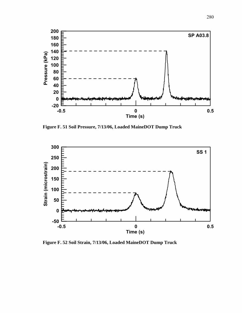
280
-0.5 0 0.5Time (s)
-200
20406080
100120140160180200
Pres
sure
(kPa
)
SP A03.8
Figure F. 51 Soil Pressure, 7/13/06, Loaded MaineDOT Dump Truck
-0.5 0 0.5Time (s)
-50
0
50
100
150
200
250
300
Stra
in (m
icro
stra
in)
SS 1
Figure F. 52 Soil Strain, 7/13/06, Loaded MaineDOT Dump Truck
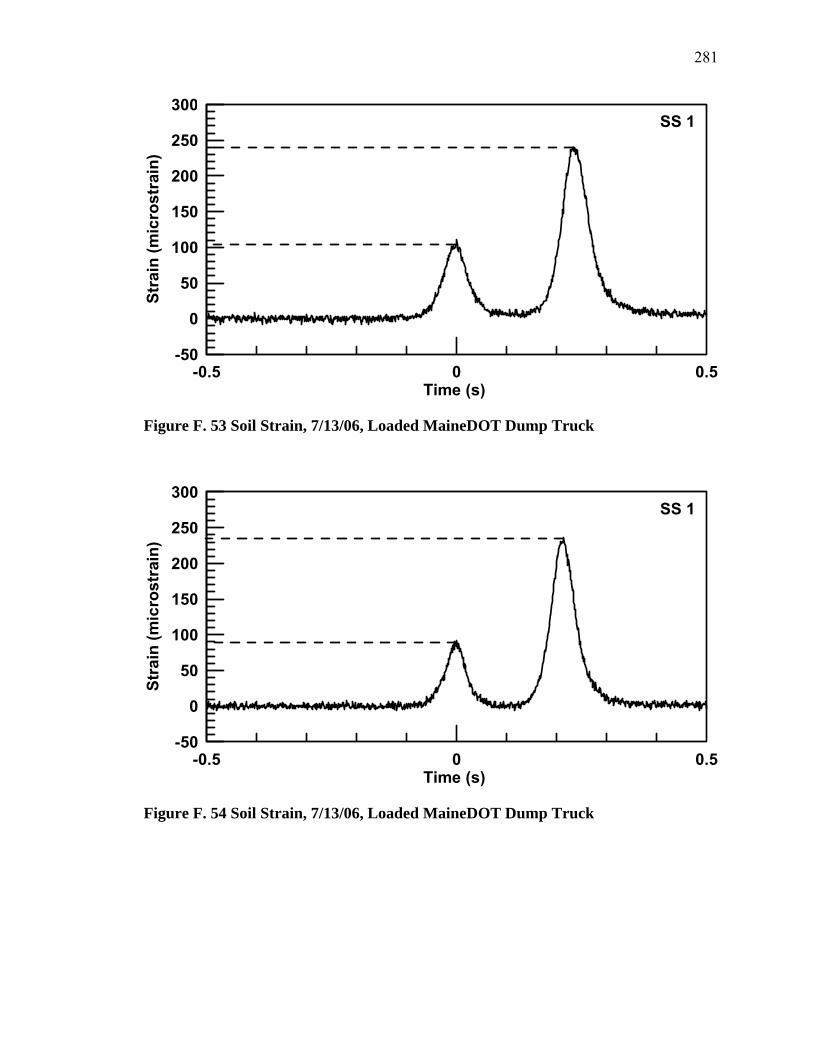
281
-0.5 0 0.5Time (s)
-50
0
50
100
150
200
250
300
Stra
in (m
icro
stra
in)
SS 1
Figure F. 53 Soil Strain, 7/13/06, Loaded MaineDOT Dump Truck
-0.5 0 0.5Time (s)
-50
0
50
100
150
200
250
300
Stra
in (m
icro
stra
in)
SS 1
Figure F. 54 Soil Strain, 7/13/06, Loaded MaineDOT Dump Truck
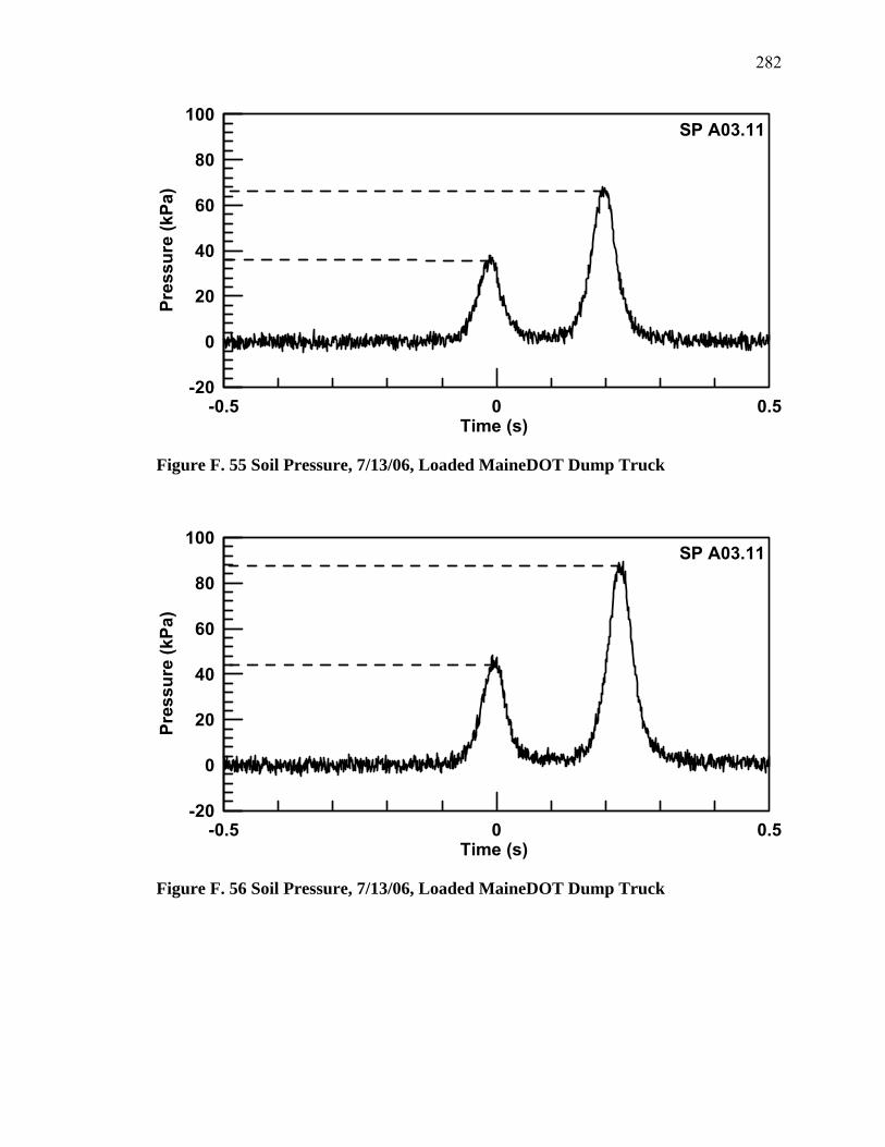
282
-0.5 0 0.5Time (s)
-20
0
20
40
60
80
100
Pres
sure
(kPa
)
SP A03.11
Figure F. 55 Soil Pressure, 7/13/06, Loaded MaineDOT Dump Truck
-0.5 0 0.5Time (s)
-20
0
20
40
60
80
100
Pres
sure
(kPa
)
SP A03.11
Figure F. 56 Soil Pressure, 7/13/06, Loaded MaineDOT Dump Truck

283
-0.5 0 0.5Time (s)
-20
0
20
40
60
80
100
Pres
sure
(kPa
)
SP A03.11
Figure F. 57 Soil Pressure, 7/13/06, Loaded MaineDOT Dump Truck
-0.5 0 0.5Time (s)
-50
0
50
100
150
200
250
300
Stra
in (m
icro
stra
in)
SS 2
Figure F. 58 Soil Strain, 7/13/06, Loaded MaineDOT Dump Truck
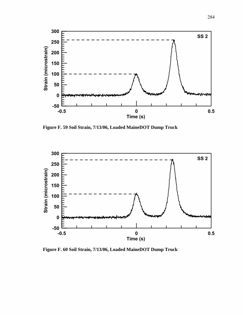
284
-0.5 0 0.5Time (s)
-50
0
50
100
150
200
250
300
Stra
in (m
icro
stra
in)
SS 2
Figure F. 59 Soil Strain, 7/13/06, Loaded MaineDOT Dump Truck
-0.5 0 0.5Time (s)
-50
0
50
100
150
200
250
300
Stra
in (m
icro
stra
in)
SS 2
Figure F. 60 Soil Strain, 7/13/06, Loaded MaineDOT Dump Truck
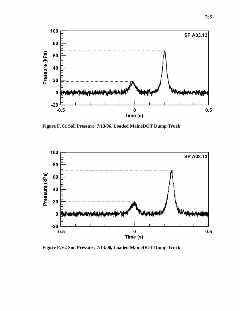
285
-0.5 0 0.5Time (s)
-20
0
20
40
60
80
100
Pres
sure
(kPa
)
SP A03.13
Figure F. 61 Soil Pressure, 7/13/06, Loaded MaineDOT Dump Truck
-0.5 0 0.5Time (s)
-20
0
20
40
60
80
100
Pres
sure
(kPa
)
SP A03.13
Figure F. 62 Soil Pressure, 7/13/06, Loaded MaineDOT Dump Truck

286
-0.5 0 0.5Time (s)
-20
0
20
40
60
80
100
Pres
sure
(kPa
)
SP A03.13
Figure F. 63 Soil Pressure, 7/13/06, Loaded MaineDOT Dump Truck
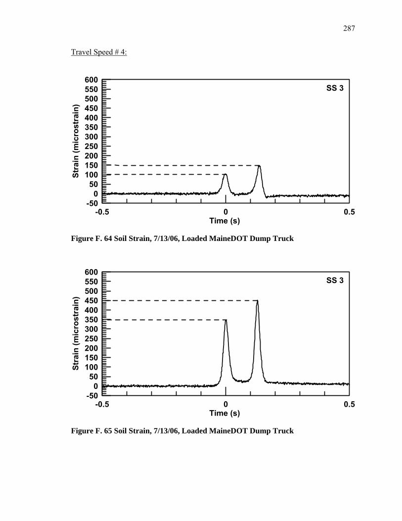
287
Travel Speed # 4:
-0.5 0 0.5Time (s)
-500
50100150200250300350400450500550600
Stra
in (m
icro
stra
in)
SS 3
Figure F. 64 Soil Strain, 7/13/06, Loaded MaineDOT Dump Truck
-0.5 0 0.5Time (s)
-500
50100150200250300350400450500550600
Stra
in (m
icro
stra
in)
SS 3
Figure F. 65 Soil Strain, 7/13/06, Loaded MaineDOT Dump Truck

288
-0.5 0 0.5Time (s)
-500
50100150200250300350400450500550600
Stra
in (m
icro
stra
in)
SS 3
Figure F. 66 Soil Strain, 7/13/06, Loaded MaineDOT Dump Truck
-0.5 0 0.5Time (s)
-500
50100150200250300350400450500550600
Stra
in (m
icro
stra
in)
SS 4
Figure F. 67 Soil Strain, 7/13/06, Loaded MaineDOT Dump Truck
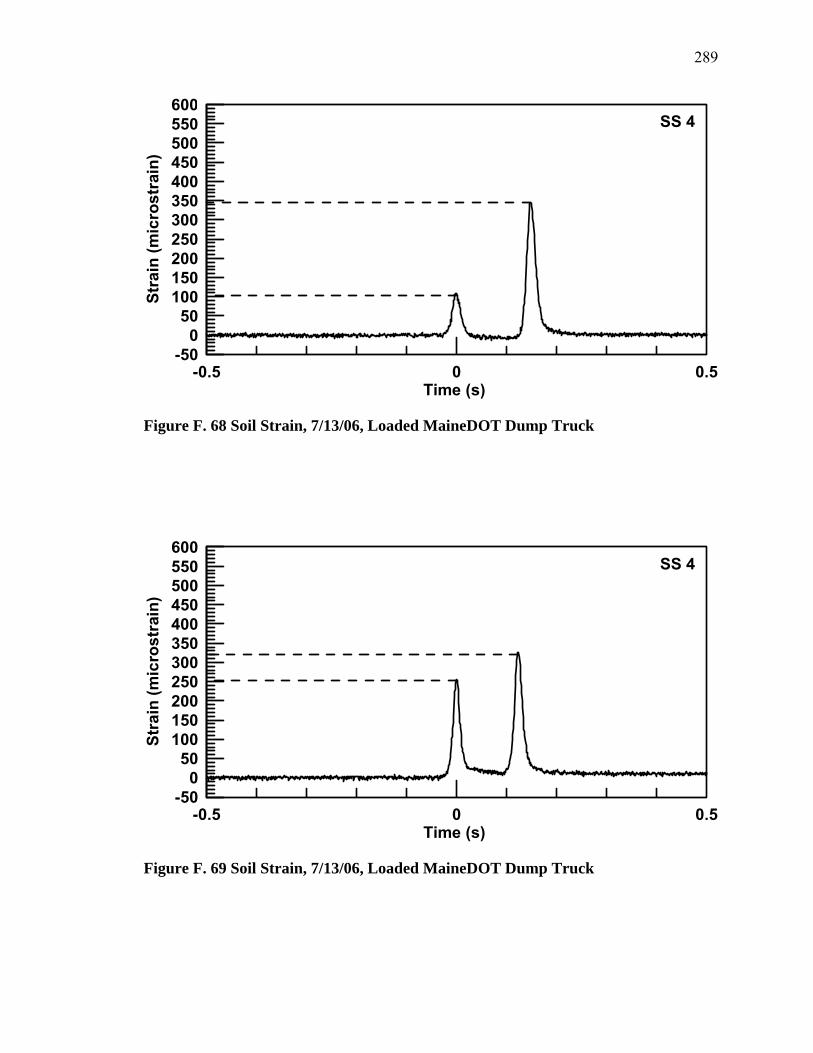
289
-0.5 0 0.5Time (s)
-500
50100150200250300350400450500550600
Stra
in (m
icro
stra
in)
SS 4
Figure F. 68 Soil Strain, 7/13/06, Loaded MaineDOT Dump Truck
-0.5 0 0.5Time (s)
-500
50100150200250300350400450500550600
Stra
in (m
icro
stra
in)
SS 4
Figure F. 69 Soil Strain, 7/13/06, Loaded MaineDOT Dump Truck
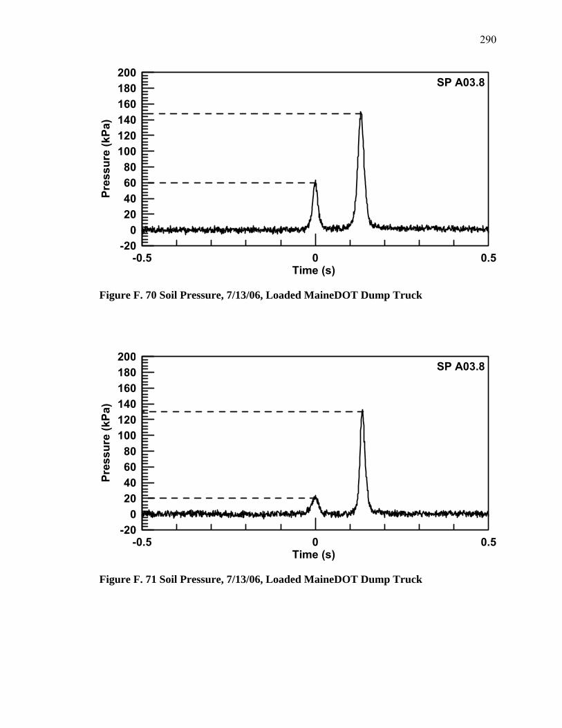
290
-0.5 0 0.5Time (s)
-200
20406080
100120140160180200
Pres
sure
(kPa
)
SP A03.8
Figure F. 70 Soil Pressure, 7/13/06, Loaded MaineDOT Dump Truck
-0.5 0 0.5Time (s)
-200
20406080
100120140160180200
Pres
sure
(kPa
)
SP A03.8
Figure F. 71 Soil Pressure, 7/13/06, Loaded MaineDOT Dump Truck
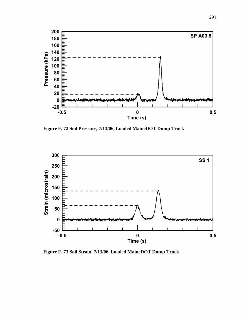
291
-0.5 0 0.5Time (s)
-200
20406080
100120140160180200
Pres
sure
(kPa
)
SP A03.8
Figure F. 72 Soil Pressure, 7/13/06, Loaded MaineDOT Dump Truck
-0.5 0 0.5Time (s)
-50
0
50
100
150
200
250
300
Stra
in (m
icro
stra
in)
SS 1
Figure F. 73 Soil Strain, 7/13/06, Loaded MaineDOT Dump Truck

292
-0.5 0 0.5Time (s)
-50
0
50
100
150
200
250
300
Stra
in (m
icro
stra
in)
SS 1
Figure F. 74 Soil Strain, 7/13/06, Loaded MaineDOT Dump Truck
-0.5 0 0.5Time (s)
-50
0
50
100
150
200
250
300
Stra
in (m
icro
stra
in)
SS 1
Figure F. 75 Soil Strain, 7/13/06, Loaded MaineDOT Dump Truck
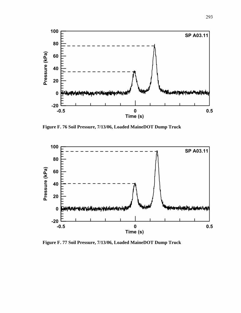
293
-0.5 0 0.5Time (s)
-20
0
20
40
60
80
100
Pres
sure
(kPa
)
SP A03.11
Figure F. 76 Soil Pressure, 7/13/06, Loaded MaineDOT Dump Truck
-0.5 0 0.5Time (s)
-20
0
20
40
60
80
100
Pres
sure
(kPa
)
SP A03.11
Figure F. 77 Soil Pressure, 7/13/06, Loaded MaineDOT Dump Truck
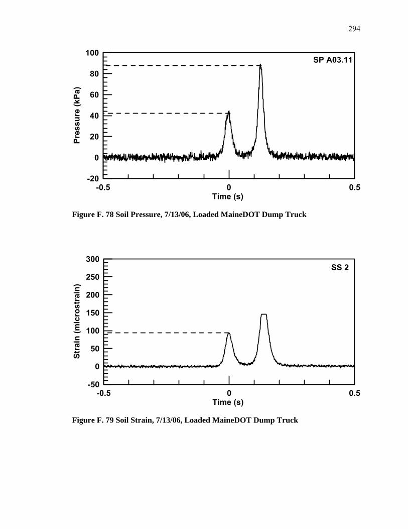
294
-0.5 0 0.5Time (s)
-20
0
20
40
60
80
100
Pres
sure
(kPa
)
SP A03.11
Figure F. 78 Soil Pressure, 7/13/06, Loaded MaineDOT Dump Truck
-0.5 0 0.5Time (s)
-50
0
50
100
150
200
250
300
Stra
in (m
icro
stra
in)
SS 2
Figure F. 79 Soil Strain, 7/13/06, Loaded MaineDOT Dump Truck

295
-0.5 0 0.5Time (s)
-50
0
50
100
150
200
250
300
Stra
in (m
icro
stra
in)
SS 2
Figure F. 80 Soil Strain, 7/13/06, Loaded MaineDOT Dump Truck
-0.5 0 0.5Time (s)
-50
0
50
100
150
200
250
300
Stra
in (m
icro
stra
in)
SS 2
Figure F. 81 Soil Strain, 7/13/06, Loaded MaineDOT Dump Truck
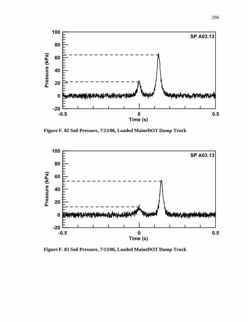
296
-0.5 0 0.5Time (s)
-20
0
20
40
60
80
100
Pres
sure
(kPa
)
SP A03.13
Figure F. 82 Soil Pressure, 7/13/06, Loaded MaineDOT Dump Truck
-0.5 0 0.5Time (s)
-20
0
20
40
60
80
100
Pres
sure
(kPa
)
SP A03.13
Figure F. 83 Soil Pressure, 7/13/06, Loaded MaineDOT Dump Truck
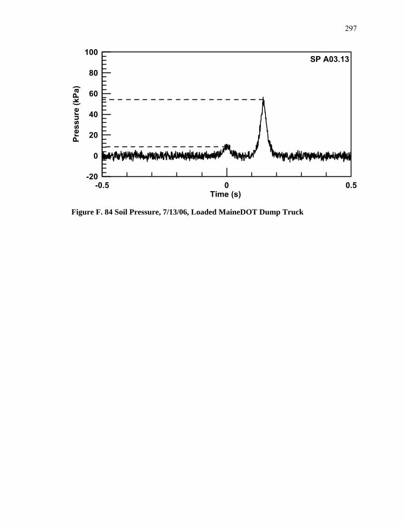
297
-0.5 0 0.5Time (s)
-20
0
20
40
60
80
100
Pres
sure
(kPa
)
SP A03.13
Figure F. 84 Soil Pressure, 7/13/06, Loaded MaineDOT Dump Truck
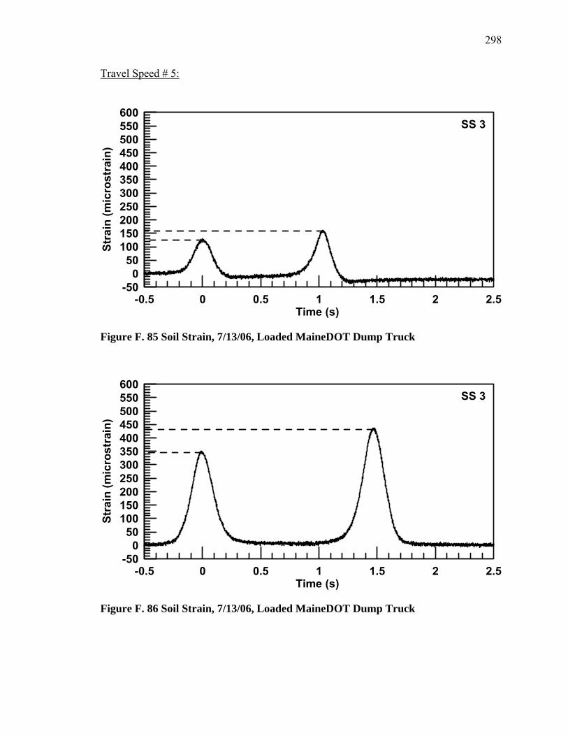
298
Travel Speed # 5:
-0.5 0 0.5 1 1.5 2 2.5Time (s)
-500
50100150200250300350400450500550600
Stra
in (m
icro
stra
in)
SS 3
Figure F. 85 Soil Strain, 7/13/06, Loaded MaineDOT Dump Truck
-0.5 0 0.5 1 1.5 2 2.5Time (s)
-500
50100150200250300350400450500550600
Stra
in (m
icro
stra
in)
SS 3
Figure F. 86 Soil Strain, 7/13/06, Loaded MaineDOT Dump Truck

299
-0.5 0 0.5 1 1.5 2 2.5Time (s)
-500
50100150200250300350400450500550600
Stra
in (m
icro
stra
in)
SS 3
Figure F. 87 Soil Strain, 7/13/06, Loaded MaineDOT Dump Truck
-0.5 0 0.5 1 1.5 2 2.5Time (s)
-500
50100150200250300350400450500550600
Stra
in (m
icro
stra
in)
SS 4
Figure F. 88 Soil Strain, 7/13/06, Loaded MaineDOT Dump Truck
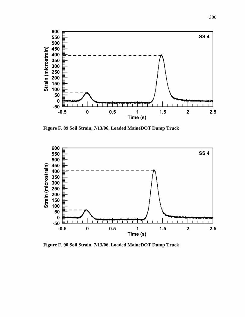
300
-0.5 0 0.5 1 1.5 2 2.5Time (s)
-500
50100150200250300350400450500550600
Stra
in (m
icro
stra
in)
SS 4
Figure F. 89 Soil Strain, 7/13/06, Loaded MaineDOT Dump Truck
-0.5 0 0.5 1 1.5 2 2.5Time (s)
-500
50100150200250300350400450500550600
Stra
in (m
icro
stra
in)
SS 4
Figure F. 90 Soil Strain, 7/13/06, Loaded MaineDOT Dump Truck
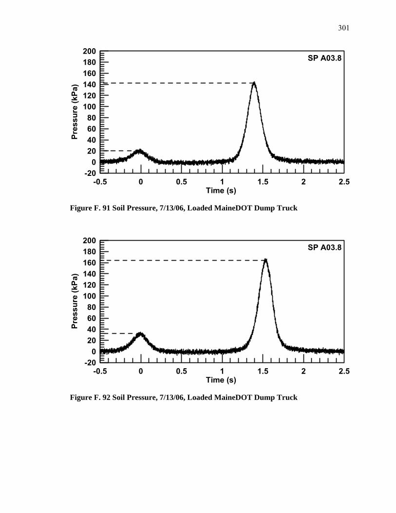
301
-0.5 0 0.5 1 1.5 2 2.5Time (s)
-200
20406080
100120140160180200
Pres
sure
(kPa
)
SP A03.8
Figure F. 91 Soil Pressure, 7/13/06, Loaded MaineDOT Dump Truck
-0.5 0 0.5 1 1.5 2 2.5Time (s)
-200
20406080
100120140160180200
Pres
sure
(kPa
)
SP A03.8
Figure F. 92 Soil Pressure, 7/13/06, Loaded MaineDOT Dump Truck
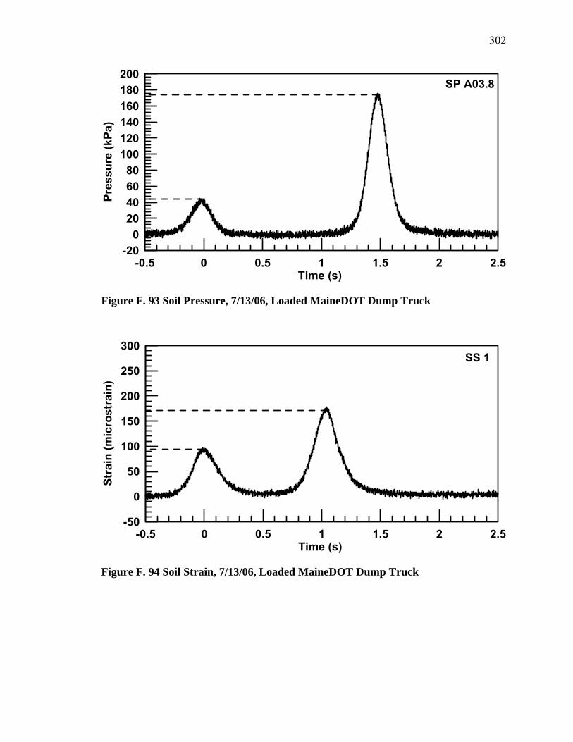
302
-0.5 0 0.5 1 1.5 2 2.5Time (s)
-200
20406080
100120140160180200
Pres
sure
(kPa
)
SP A03.8
Figure F. 93 Soil Pressure, 7/13/06, Loaded MaineDOT Dump Truck
-0.5 0 0.5 1 1.5 2 2.5Time (s)
-50
0
50
100
150
200
250
300
Stra
in (m
icro
stra
in)
SS 1
Figure F. 94 Soil Strain, 7/13/06, Loaded MaineDOT Dump Truck

303
-0.5 0 0.5 1 1.5 2 2.5Time (s)
-50
0
50
100
150
200
250
300
Stra
in (m
icro
stra
in)
SS 1
Figure F. 95 Soil Strain, 7/13/06, Loaded MaineDOT Dump Truck
-0.5 0 0.5 1 1.5 2 2.5Time (s)
-50
0
50
100
150
200
250
300
Stra
in (m
icro
stra
in)
SS 1
Figure F. 96 Soil Strain, 7/13/06, Loaded MaineDOT Dump Truck

304
-0.5 0 0.5 1 1.5 2 2.5Time (s)
-20
0
20
40
60
80
100
Pres
sure
(kPa
)
SP A03.11
Figure F. 97 Soil Pressure, 7/13/06, Loaded MaineDOT Dump Truck
-0.5 0 0.5 1 1.5 2 2.5Time (s)
-20
0
20
40
60
80
100
Pres
sure
(kPa
)
SP A03.11
Figure F. 98 Soil Pressure, 7/13/06, Loaded MaineDOT Dump Truck
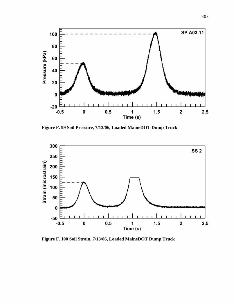
305
-0.5 0 0.5 1 1.5 2 2.5Time (s)
-20
0
20
40
60
80
100
Pres
sure
(kPa
)
SP A03.11
Figure F. 99 Soil Pressure, 7/13/06, Loaded MaineDOT Dump Truck
-0.5 0 0.5 1 1.5 2 2.5Time (s)
-50
0
50
100
150
200
250
300
Stra
in (m
icro
stra
in)
SS 2
Figure F. 100 Soil Strain, 7/13/06, Loaded MaineDOT Dump Truck
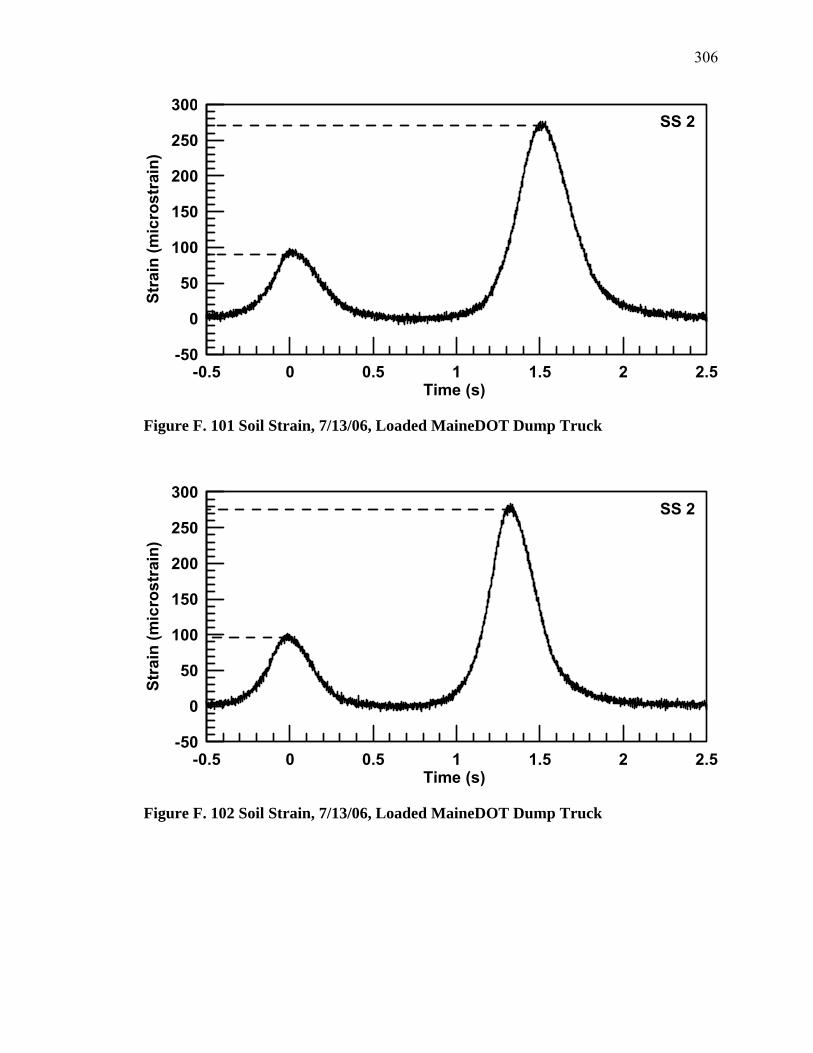
306
-0.5 0 0.5 1 1.5 2 2.5Time (s)
-50
0
50
100
150
200
250
300
Stra
in (m
icro
stra
in)
SS 2
Figure F. 101 Soil Strain, 7/13/06, Loaded MaineDOT Dump Truck
-0.5 0 0.5 1 1.5 2 2.5Time (s)
-50
0
50
100
150
200
250
300
Stra
in (m
icro
stra
in)
SS 2
Figure F. 102 Soil Strain, 7/13/06, Loaded MaineDOT Dump Truck
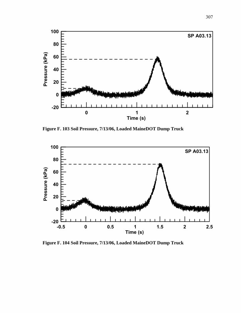
307
0 1 2Time (s)
-20
0
20
40
60
80
100
Pres
sure
(kPa
)
SP A03.13
Figure F. 103 Soil Pressure, 7/13/06, Loaded MaineDOT Dump Truck
-0.5 0 0.5 1 1.5 2 2.5Time (s)
-20
0
20
40
60
80
100
Pres
sure
(kPa
)
SP A03.13
Figure F. 104 Soil Pressure, 7/13/06, Loaded MaineDOT Dump Truck
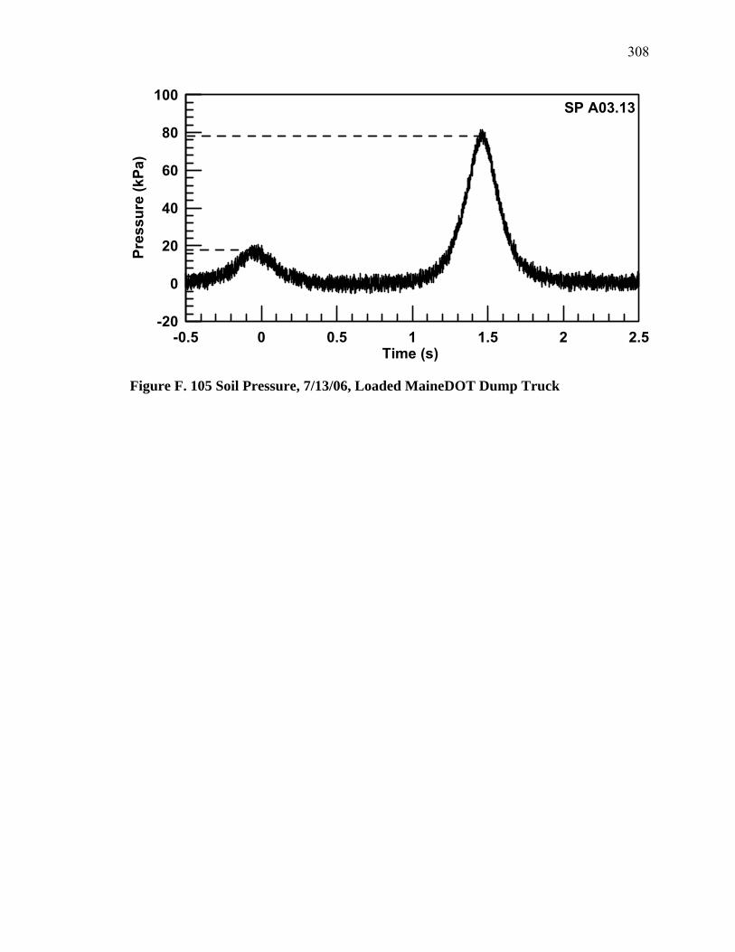
308
-0.5 0 0.5 1 1.5 2 2.5Time (s)
-20
0
20
40
60
80
100
Pres
sure
(kPa
)
SP A03.13
Figure F. 105 Soil Pressure, 7/13/06, Loaded MaineDOT Dump Truck

309
APPENDIX G
Compiled stress and strain data for modulus calculations
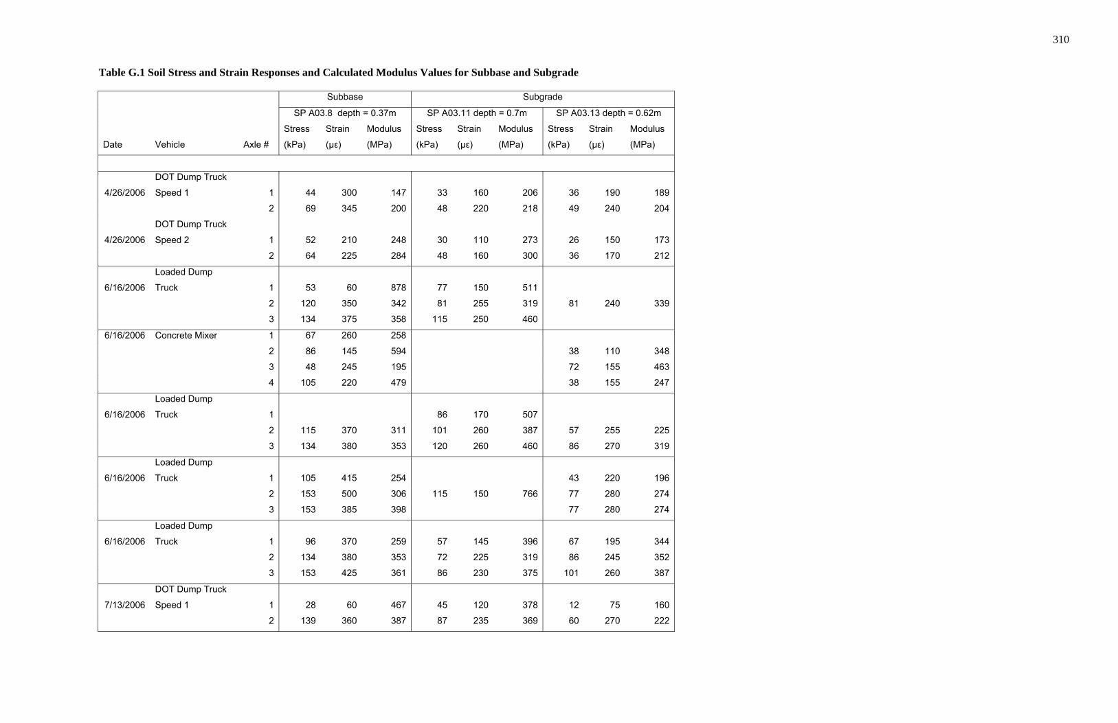
310
Table G.1 Soil Stress and Strain Responses and Calculated Modulus Values for Subbase and Subgrade Subbase Subgrade
SP A03.8 depth = 0.37m SP A03.11 depth = 0.7m SP A03.13 depth = 0.62m
Date Vehicle Axle #
Stress
(kPa)
Strain
(µε)
Modulus
(MPa)
Stress
(kPa)
Strain
(µε)
Modulus
(MPa)
Stress
(kPa)
Strain
(µε)
Modulus
(MPa)
4/26/2006
DOT Dump Truck
Speed 1 1 44 300 147 33 160 206 36 190 189
2 69 345 200 48 220 218 49 240 204
4/26/2006
DOT Dump Truck
Speed 2 1 52 210 248 30 110 273 26 150 173
2 64 225 284 48 160 300 36 170 212
6/16/2006
Loaded Dump
Truck 1 53 60 878 77 150 511
2 120 350 342 81 255 319 81 240 339
3 134 375 358 115 250 460
6/16/2006 Concrete Mixer 1 67 260 258
2 86 145 594 38 110 348
3 48 245 195 72 155 463
4 105 220 479 38 155 247
6/16/2006
Loaded Dump
Truck 1 86 170 507
2 115 370 311 101 260 387 57 255 225
3 134 380 353 120 260 460 86 270 319
6/16/2006
Loaded Dump
Truck 1 105 415 254 43 220 196
2 153 500 306 115 150 766 77 280 274
3 153 385 398 77 280 274
6/16/2006
Loaded Dump
Truck 1 96 370 259 57 145 396 67 195 344
2 134 380 353 72 225 319 86 245 352
3 153 425 361 86 230 375 101 260 387
7/13/2006
DOT Dump Truck
Speed 1 1 28 60 467 45 120 378 12 75 160
2 139 360 387 87 235 369 60 270 222

311
Table G.1 Continued
7/13/2006
DOT Dump Truck
Speed 2 1 35 75 471 45 125 363 15 85 180
2 148 340 435 88 270 326 68 285 239
7/13/2006
DOT Dump Truck
Speed 3 1 47 120 389 43 110 388 21 110 188
2 142 380 374 80 240 333 73 285 257
7/13/2006
DOT Dump Truck
Speed 4 1 32 175 183 39 100 387 14 120 117
2 135 305 442 85 190 449 57 250 227
7/13/2006
DOT Dump Truck
Speed 5 1 32 140 229 50 125 400 14 115 122
2 153 410 374 95 235 406 69 295 233
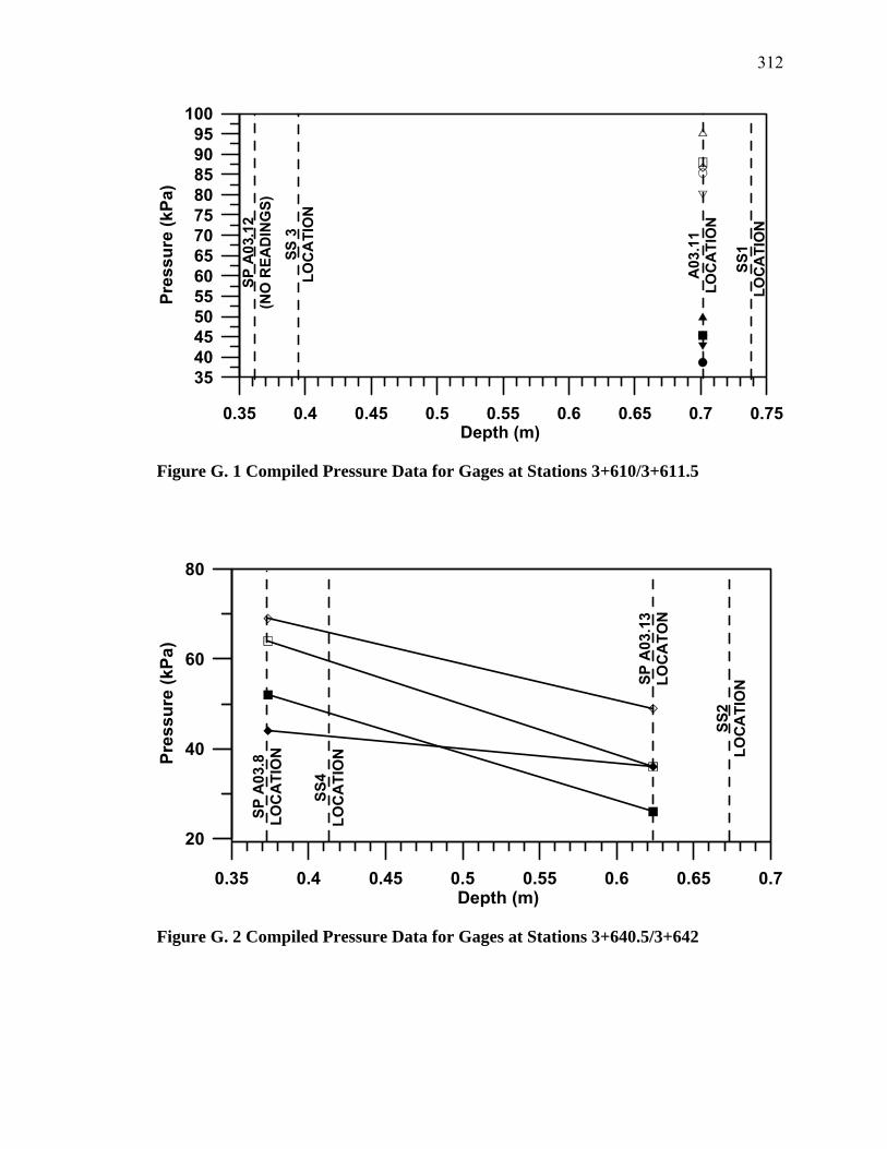
312
0.35 0.4 0.45 0.5 0.55 0.6 0.65 0.7 0.75Depth (m)
35404550556065707580859095
100
Pres
sure
(kPa
)
SP A
03.1
2(N
O R
EAD
ING
S)
SS 3
LOC
ATI
ON
A03
.11
LOC
ATI
ON
SS1
LOC
ATI
ON
Figure G. 1 Compiled Pressure Data for Gages at Stations 3+610/3+611.5
0.35 0.4 0.45 0.5 0.55 0.6 0.65 0.7Depth (m)
20
40
60
80
Pres
sure
(kPa
)
SS2
LOC
ATI
ON
SP A
03.8
LOC
ATI
ON
SP A
03.1
3LO
CA
TON
SS4
LOC
ATI
ON
Figure G. 2 Compiled Pressure Data for Gages at Stations 3+640.5/3+642
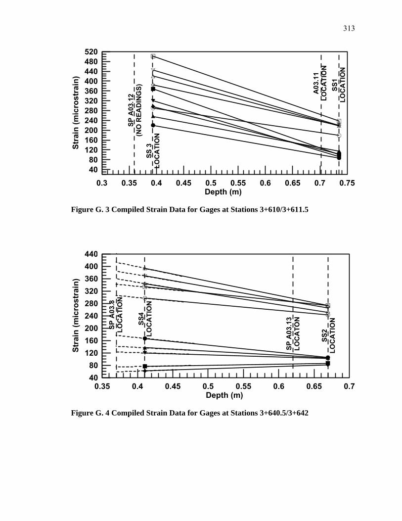
313
0.3 0.35 0.4 0.45 0.5 0.55 0.6 0.65 0.7 0.75Depth (m)
4080
120160200240280320360400440480520
Stra
in (m
icro
stra
in)
SP A
03.1
2(N
O R
EAD
ING
S)SS
3LO
CA
TIO
N
A03
.11
LOC
ATI
ON
SS1
LOC
ATI
ON
Figure G. 3 Compiled Strain Data for Gages at Stations 3+610/3+611.5
0.35 0.4 0.45 0.5 0.55 0.6 0.65 0.7Depth (m)
4080
120160200240280320360400440
Stra
in (m
icro
stra
in)
SS2
LOC
ATI
ON
SP A
03.8
LOC
ATI
ON
SP A
03.1
3LO
CA
TONSS
4LO
CA
TIO
N
Figure G. 4 Compiled Strain Data for Gages at Stations 3+640.5/3+642
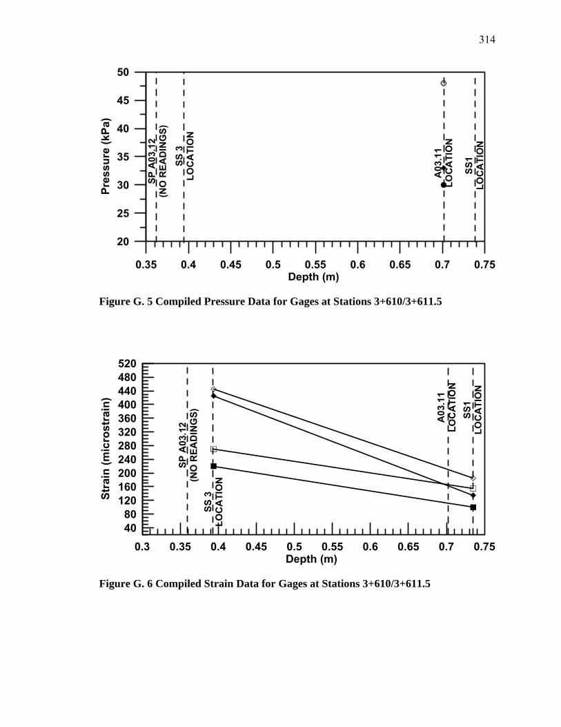
314
0.35 0.4 0.45 0.5 0.55 0.6 0.65 0.7 0.75Depth (m)
20
25
30
35
40
45
50
Pres
sure
(kPa
)
SP A
03.1
2(N
O R
EAD
ING
S)
SS 3
LOC
ATI
ON
A03
.11
LOC
ATI
ON
SS1
LOC
ATI
ON
Figure G. 5 Compiled Pressure Data for Gages at Stations 3+610/3+611.5
0.3 0.35 0.4 0.45 0.5 0.55 0.6 0.65 0.7 0.75Depth (m)
4080
120160200240280320360400440480520
Stra
in (m
icro
stra
in)
SP A
03.1
2(N
O R
EAD
ING
S)SS
3LO
CA
TIO
N
A03
.11
LOC
ATI
ON
SS1
LOC
ATI
ON
Figure G. 6 Compiled Strain Data for Gages at Stations 3+610/3+611.5

315
0.35 0.4 0.45 0.5 0.55 0.6 0.65 0.7Depth (m)
4080
120160200240280320360400440
Stra
in (m
icro
stra
in)
SS2
LOC
ATI
ON
SP A
03.8
LOC
ATI
ON
SP A
03.1
3LO
CA
TONSS
4LO
CA
TIO
N
Figure G. 7 Compiled Strain Data for Gages at Stations 3+640.5/3+642

316
Comparison of Predicted and Measured Stresses and Strains:
0.00
0.20
0.40
0.60
0.80
1.00
1.20
1.40
1.60
1.80
2.00
0 0.1 0.2 0.3 0.4 0.5 0.6 0.7 0.8
Time of loading (seconds)
Rat
io o
f mea
sure
d to
pre
dict
ed s
trai
n
Figure G. 8 Asphalt Strain
0
0.2
0.4
0.6
0.8
1
1.2
1.4
0 0.1 0.2 0.3 0.4 0.5 0.6
Time of loading (seconds)
Rat
io o
f mea
sure
d to
pre
dict
ed s
trai
n
Figure G. 9 Subbase Strain
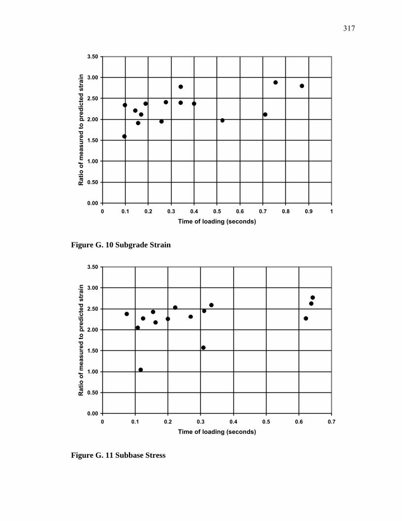
317
0.00
0.50
1.00
1.50
2.00
2.50
3.00
3.50
0 0.1 0.2 0.3 0.4 0.5 0.6 0.7 0.8 0.9 1
Time of loading (seconds)
Rat
io o
f mea
sure
d to
pre
dict
ed s
trai
n
Figure G. 10 Subgrade Strain
0.00
0.50
1.00
1.50
2.00
2.50
3.00
3.50
0 0.1 0.2 0.3 0.4 0.5 0.6 0.7
Time of loading (seconds)
Rat
io o
f mea
sure
d to
pre
dict
ed s
trai
n
Figure G. 11 Subbase Stress
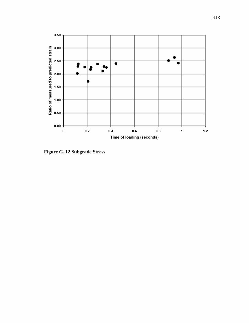
318
0.00
0.50
1.00
1.50
2.00
2.50
3.00
3.50
0 0.2 0.4 0.6 0.8 1 1.2
Time of loading (seconds)
Rat
io o
f mea
sure
d to
pre
dict
ed s
trai
n
Figure G. 12 Subgrade Stress

319
BIOGRAPHY OF THE AUTHOR
Lauren Swett was born in Bangor, Maine on September 14, 1983. She was raised
in Old Town, Maine and graduated from Old Town High School in 2001. She attended
the University of Maine and graduated in 2004 with a Bachelor’s degree in Civil and
Environmental Engineering. She stayed at the University of Maine, and continued on in
the Civil Engineering graduate program. For her graduate work, her concentration within
the program was geotechnical engineering.
In September of 2006, Lauren began working as a civil engineer for Woodard and
Curran, a Maine-based engineering consulting firm, at their office in Portland, Maine.
She is a candidate for the Master of Science degree in Civil Engineering from The
University of Maine in May, 2007.