in situ determination of elastic moduli of pavement ... · process which has been the missing link...
TRANSCRIPT

1. Report No.
FHWA/TX-87/46+437-2
4. Title and Subtitle
IN SITU DETERMINATION OF ELASTIC MODULI OF PAVEMENT SYSTEMS BY SPECTRAL-ANALYSIS-OFSURFACE-WAVES METHOD (THEORETICAL ASPECTS) 7. Authort s,l
Soheil Nazarian and Kenneth H. Stokoe, II
9, Performing Orgoniaation Nome and Address
Center for Transportation Research The University of Texas at Austin Austin, Texas 78712-1075
TECHNICAL REPORT STANDARD TITLE PAGE
3. Recipient' 1 Cotolog No.
5, Report Date
November 1986 6. Performing Orgoniaation Code
B. Performing Organization Report No.
Research Report 437-2
10. Worlc Unit No.
11. Contract or Grant No.
Research Study 3-8-85-437 t""";:;--;---:-""'"":'---::----:"'7"::-:------------------J 13. Type of Report and Period CoYered
12. Sponsoring Agency Nome ond Addre11
Texas State Department of Highways and Public Transportation; Transportation Planning Division
Interim
P. 0. Box 5051 14. Sponsoring Agency Code
Austin, Texas 78763-5051 15. Supplemantory Notal
Study conducted in cooperation with the U. s. Department of Transportation, Federal Highway Administration. Research Study Title: '~tilization of Surface Wave System for Measuring Moduli of Pavementstt
16. Abstract
The Spectral-Analysis-of-Surface-Waves (SASW) method is an in situ testing method for determining shear wave velocity profiles of soil sites and stiffness profiles of pavement systems. The method is nondestructive and is performed entirely from the pavement or ground surface. Measurements are made at strains below 0.001 percent where elastic properties of the materials are independent of strain amplitude. The key elements in SASW testing are the generation and measurement of surface waves. Transient impacts containing wide ranges of frequencies are transmitted to the pavement surface by means of simple hammers. Surface waves generated by these impacts are captured and recorded by the receivers using a spectral waveform analyzer. The analyzer is used to transform the waveforms into the frequency domain and then to perform spectral analyses on them. The points of interest from this operation are the phase information of the cross power spectrum and the coherence function. By evaluating the coherence function during testing, the range of frequencies which is not contaminated with random background noise can be quickly identified. Phase information from the cross power spectrum is indicative of the relative phase shift of each frequency propagating between the receivers. By knowing the distance between receivers and the phase shift for each frequency, phase velocity and wavelength associated with that frequency are calculated. One of the most important steps in SASW testing is the inversion process which has been the missing link in engineering applications. The theoretical foundation of the SASW method is discussed in detail in this report, with an emphasis placed on the theoretical aspects of the inversion process. 17. Kay Warda
Spectral-Analysis-of-Surface-Waves, SASW, theory, shear wave velocity, elastic modulus profiles, pavement sections, soil sites
18. Dlatrlllutlon Stet-ent
No restrictions. This document is available to the public through the National Technical Information Service, Springfield, Virginia 22161.
19, Security Clo .. lf. (of thla ......,t)
Unclassified
20. Security Cloaalf, (of thla page)
Unclassified
21· No. of Pagel 22. Price
134
Form DOT F 1700.7 ,, ... ,

IN SITU DETERMINATION OF ELASTIC MODULI OF PAVEMENT SYSTEMS BY SPECTRAL-ANALYSIS-OF-SURFACE-WAVES METHOD (THEORETICAL ASPECTS)
by
Soheil Nazarian K. H. Stokoe, II
Research Report Number 437-2
Utilization of Surface Wave System for Measuring Moduli of Pavements
Research Project 3-8-85-437
conducted for
Texas State Department of Highways and Public Transportation
in cooperation with the U.S. Department of Transportation Federal Highway Administration
by the
CENTER FOR TRANSPORTATION RESEARCH BUREAU OF ENGINEERING RESEARCH
THE UNIVERSITY OF TEXAS AT AUSTIN
November 1986

The contents of this report reflect the views of the authors, who are responsible for the facts and the accuracy of the data presented herein. The contents do not necessarily reflect the official views or policies of the Federal Highway Administration. This report does not constitute a standard, specification, or regulation.
i i

PREFACE
This report is the second report in a series of three reports on the
Spectral-Analysis-of-Surface-Waves (SASW) method. The first report is
pub 1 i shed under Research Report 368-1F and is a deta i 1 ed description of the
practical aspects of the SASW method. The third report will be published
under Research Project 1123 and will consist of a manual for an interactive
computer program called INVERT!. This program is essential for determining
the stiffnesses of the different 1 ayers from the in situ data. In this
volume, the theoretical aspects of SASW testing are described. Some practical
ex amp 1 es are provided so that a person not familiar with the method can
understand it.
The division of the reports on Projects 368, 437 and 1123 was necessary
so that readers with different levels of knowledge and interest could easily
access the required material. This division of reports also resulted from a
natural development of the SASW method. This report has been prepared in a
manner that permits the theoreti ca 1 background of the SASW method to be
understood without referring to the other reports.
The authors extend their sincere gratitude to personnel of the Texas
Department of Highways and Public Transportation for their continuous support
and enthusiasm throughout the course of this study.
November 1986
iii
Soheil Nazarian
Kenneth H. Stokoe, II


LIST OF REPORTS
Report No. 437-1, 11 Dynamic Interpretation of Dynaflect and Falling Weight Deflectometer Tests 11 by Ko-Young Shao, J.M. Roesset, and K.H. Stokoe, II, presents the results of analytical studies of the dynamic effects on measurements made with the Dynaflect and Falling Weight Deflectometer methods, based on the consideration of wave propagation including body waves (P-and S-waves) and Rayleigh (surface) waves.
Report No. 437-2, 11 In Situ Determination of Elastic Moduli of Pavement Systems by Spectral-Analysis-of-Surface-Waves Method (Theoretical Aspects), 11
by Soheil Nazarian and K.H. Stokoe, II, presents the pertinent theoretical aspects of wave propagation in a layered system (such as a pavement system) as they apply to the SASW method.
Report No. 437-3F, "Investigation of Variables Affecting In Situ Determination of Elastic Moduli of Pavement Systems by Surface Wave Method, 11 by J.C. Sheu, Ignacio Sanchez-Salinero, K.H. Stokoe, II, and J.M. Roesset, presents the results of experimental and analytical studies types, source-receiver configuration, wave solutions, that effect modulus measurements Surface-Wave (SASW) Method.
v
of variables, such as receiver reflections and analytical
by the Spectral-Analysis-of-


ABSTRACT
The Spectral-Analysis-of-Surface-Waves (SASW) method is an in situ
testing method for determining shear wave velocity profiles of soil sites and stiffness profiles of pavement systems. The method is nondestructive and is performed entirely from the pavement or ground surface. Measurements are made at strains below 0.001 percent where elastic properties of the materials are
independent of strain amplitude. The key elements in SASW testing are the
generation and measurement of surface waves. Transient impacts containing wide ranges of frequencies are transmitted to the pavement surface by means of
simple hammers. Surface waves generated by these impacts are captured and
recorded by the receivers using a spectral waveform analyzer. The analyzer is used to transform the waveforms into the frequency domain and then to perform
spectral analyses on them. The points of interest from this operation are the
phase information of the cross power spectrum and the coherence function. By eva 1 uati ng the coherence function during testing, the range of frequencies
which is not contaminated with random background noise can be quickly
identified. Phase information from the cross power spectrum is indicative of the relative phase shift of each frequency propagating between the receivers.
By knowing the distance between receivers and the phase shift for each
frequency, phase velocity and wavelength associated with that frequency are calculated. A dispersion curve is a plot of phase velocity versus wavelength. By applying an inversion process, an analytical technique for reconstructing the shear wave velocity profile from the dispersion curve, layering and the shear wave velocity and Young's modulus of each layer can be readily obtained. One of the most important steps in SASW testing is the inversion process which has been the missing link in engineering applications. The theoretical foundation of the SASW method is discussed in detail in this report, with an emphasis placed on the theoretical aspects of the inversion process.
vii


SUMMARY
The theoretical aspects of the Spectral-Analysis-of-Surface-Waves (SASW) method are presented herein. The SASW method is used to determine the shear wave velocity and elastic modulus profiles of pavement sections and soil sites. With this method, a transient vertical impulse is applied to the surface, and a group of surface waves with different frequencies are generated in the medium. These waves propagate along the surface with velocities that vary with frequency and the properties of the different layers comprising the medium. Propagation of the waves are monitored with two receivers a known distance apart at the surface. By analysis of the phase information of the cross power spectrum and by knowing the distance between receivers, phase velocity, shear wave velocity and moduli of each layer are determined.
This report contains a comprehensive discussion of the theories used in the in situ testing technique and the in-house data reduction procedure.
ix

IMPLEMENTATION STATEMENT
The Spectral-Analysis-of-Surface-Waves (SASW) method has many applications in material characterization of pavement systems. With this
method, elastic moduli and layer thicknesses of pavement systems can be evaluated in situ. The method can be utilized as a tool for quality control during construction and during regular maintenance inspections.
The method can be implemented to evaluate the integrity of flexible and
rigid pavements. Reduction of the experimental data collected in the field is
fully automated. The inversion process is not automated, as yet. The method has been emp 1 oyed at more than 35 pavement sites to study the precision and
re 1 i ability of the method. From this study it can be cone 1 uded that the thicknesses of different layers are generally within about ten percent of those measured from boreholes and the moduli are, on the average, within 20
percent of moduli measured with other independent methods employing in situ
seismic techniques.
xi

TABLE OF CONTENTS
PREFACE .................................................................... iii
LIST OF REPORTS .............................................................. v
ABSTRACT ................................................................... vi i
SUMMARY ..................................................................... i X
IMPLEMENTATION STATEMENT .................................................... xi
LIST OF TABLES .............................................................. xv
LIST OF FIGURES ........................................................... xvii
CHAPTER ONE. INTRODUCTION
1.1 Prob 1 em Statement .................................................. 1 1.2 Organization ....................................................... ! 1. 3 Overview of SASW Method ............................................ 2
1. 3.1 Genera 1 Background .......................................... 2 1.3.2 Field Procedure ............................................. 6
CHAPTER TWO. WAVE PROPAGATION IN A LAYERED HALF-SPACE
2.1 Introduction ....................................................... 9 2.2 Seismic Waves ...................................................... 9
2. 2 .1 Body Waves .................................................. 9 2. 2. 2 Surface Waves .............................................. 10
2.3 Seismic Wave Velocities ........................................... 13 2. 4 Elastic Constants ................................................. 15 2.5 Factors Affecting Elastic Moduli .................................. l9
2.5.1 Soil (or Subgrade) ......................................... 19 2.5.2 Base and Subbase ........................................... 22 2.5.3 Asphalt-Cement Concrete .................................... 26 2.5.4 Portland-Cement Concrete ................................... 26
2. 6 Summary ........................................................... 28
CHAPTER THREE. FREQUENCY DOMAIN ANALYSES APPLIED TO FIELD MEASUREMENTS
3.1 Introduction ...................................................... 29 3.2 Fourier Transform ................................................. 29
3.2.1 Theory of the Fourier Transform ............................ 29 3.2.2 Discrete Finite Transform (DFT) ............................ 32 3.2.3 Fast Fourier Transform (FFT) ............................... 35
xiii
xiv
3. 3 Spectra 1 Ana 1 yses ................................................. 38 3.3.1 Linear Spectrum ............................................ 41 3. 3. 2 Auto Power Spectrum ........................................ 41 3.3.3 Cross Power Spectrum ....................................... 45 3. 3. 4 Transfer Function .......................................... 45 3. 3. 5 Coherence Function ......................................... 4 7
3.4 Summary ........................................................... 49
CHAPTER FOUR. IN SITU EVALUATION OF PAVEMENTS
4.1 Introduction ...................................................... 51 4.2 Typical Nondestructive Testing of Pavements ....................... 52 4.3 Seismic Field Methods ............................................. 57
4. 3.1 Boreho 1 e Methods ........................................... 57 4. 3. 2 Surface Methods ............................................ 59
4.4 Crosshole Seismic Testing of Pavements ............................ 63 4.4.1 Testing Procedure .......................................... 63 4.4.2 Data Reduction ............................................. 65
4.5 Historical Development of Surface Wave Technique .................. 67 4. 6 Summary ........................................................... 75
CHAPTER FIVE. DISPERSIVE CHARACTERISTIC OF SURFACE WAVES
5.1 Introduction ...................................................... 77 5.2 Haskell-Thomson Approach .......................................... ao 5.3 Problems with the Haskell-Thomson Approach ........................ 90 5.4 Dunkin Approach ................................................... 91 5.5 Parametric Study of Dispersive Characteristic ..................... 93
5.5.1 Effect of Shear Wave Velocity .............................. 93 5.5.2 Effect of Poisson's Ratio .................................. 97 5. 5. 3 Effect of Mass Density ..................................... 99 5.5.4 Effect of Layer Thicknesses ................................ 99
5.6 Discussion on Propagation of Surface Waves ....................... 102 5. 7 Summary .......................................................... 105
CHAPTER SIX. CONCLUSIONS .................................................. 107
REFERENCES ................................................................. 109

Table
2.1
2.2
4.1
LIST OF TABLES
Page
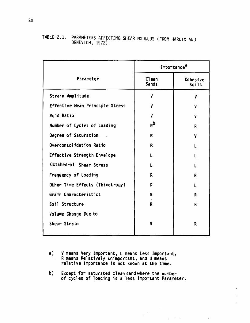
Parameters Affecting Shear Modulus (from Hardin and Drnevi ch, 1972) ................................................... 20
Summary of Average Modulus Values of Materials Determined from SASW Tests Performed at the Pavement Test Facility of the Texas Transportation Institute (from Nazarian and Stokoe, 1986b) ............................................................ 25
Characteristics of Common Nondestructive Testing Devices Used on Pavement (from Eagleson et al, 1981) ...................... 53
XV


Figure
1.1
1.2
2.1
2.2
2.3
2.4
2.5
2.6
2.7
2.8
2.9
2.10
3.1
3.2
3.3
LIST OF FIGURES
Page
General Configuration of SASW Testing .............................. 7
Schematic of Typical Experimental Arrangement for SASW Testing at Pavement Sites ..................................... 7
Characteristic Motion of Seismic Waves (from Bolt, 1976) .......... 11
Amplitude and Particle Motion Distribution with Depth for Rayleigh Waves .................................................... 12
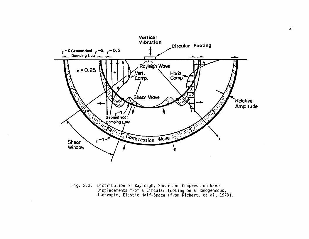
Distribution of Rayleigh, Shear and Compression Wave Displacements from a Circular Footing on a Homogeneous, Isotropic, Elastic Half-Space (from Richart et al, 1970) .......... 14
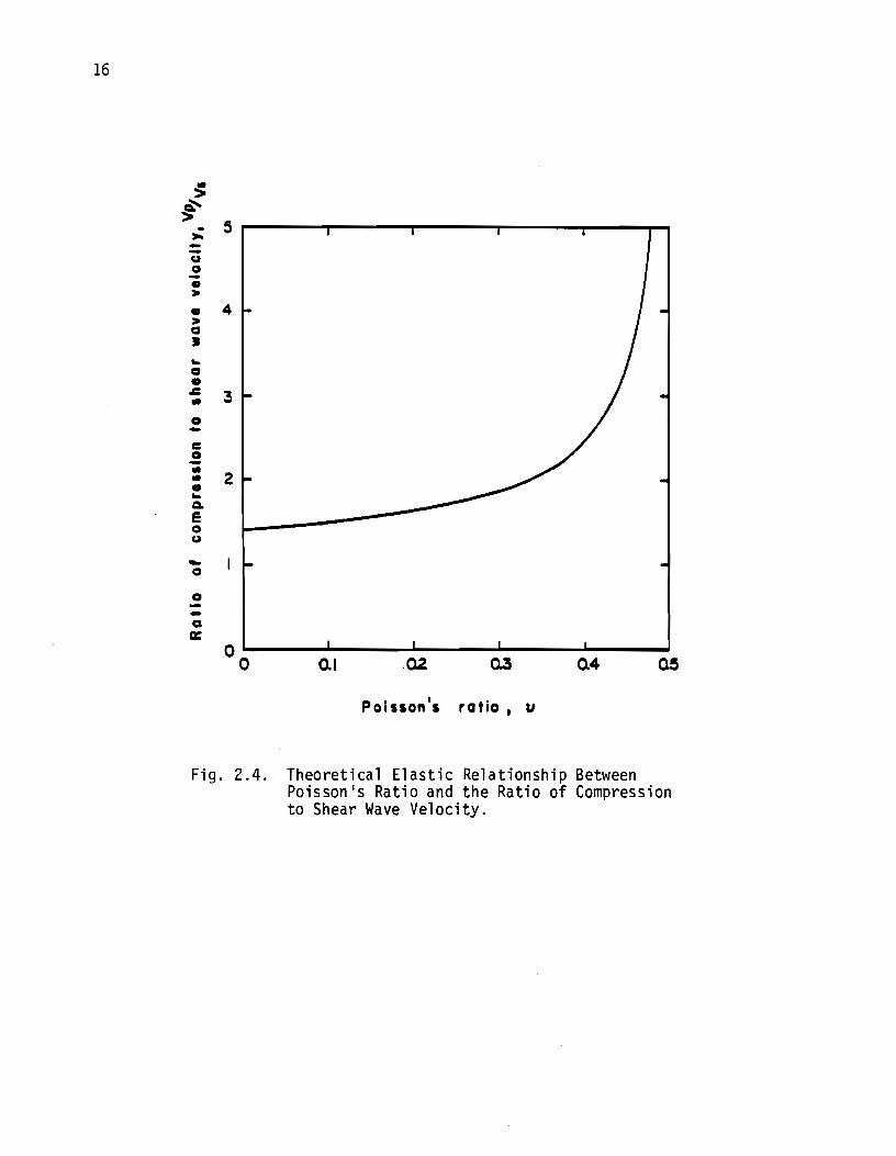
Theoretical Elastic Relationship between Poisson•s Ratio and the Ratio of Compression to Shear Wave Velocity ............... 16
Theoretical Elastic Relationship between Poisson•s Ratio and the Ratio of Rayleigh to Shear Wave Velocity .................. 17
Variation in Young•s Modulus with Strain Amplitude at Different Confining Pressures of an Unsaturated Clay Subgrade .......................................................... 21
Variation in Normalized Young•s Modulus with Strain Amp 1 itude of an Unsaturated Clay Subgrade ......................... 21
Variation in Normalized Shear Modulus with Shearing Strain and Confining Pressure (from Stokoe and Lodde, 1978) ....... 23
Variation of Poisson•s Ratio with Strain for Sedimented Kaolinite Tested in Unconfined Compression (from Krizek, 1977) ..................................................... 24
Effect of Temperature on Young•s Modulus of Asphaltic Concrete Material (inferred from VanderPoel, 1954) .............. 27
Representation of a Time Domain Signal and its Fourier Transform (from Heisey, et al, 1982) .............................. 30
Representation of Fourier Coefficients by a Rotating Phasor in the Complex Plane for Eqs. 3.4 to 3.6 ................... 33
Representation of Fourier Coefficients by a Rotating Phasor in the Complex Plane for Eqs. 3.7 to 3.9 ................... 34
xvii

xviii
Figure
3.4
3.5
3.6
3.7
3.8
3.9
3.10
3.11
3.12
3.13
4.1
4.2
4.3
4.4
4.5
4.6
Page
Schematic of Numerical Integration in Discrete Finite Transform ......................................................... 36
Comparison of Number of Operations in Computing the Fast Fourier Transform and Discrete Finite Transform (after Brigham, 1974) .................................................... 37
Illustration of Idealized and Actual Linear Systems ............... 39
Typical Set of Time Records from a Test on a Soil Site ............ 40
Real and Imaginary Components of Linear Spectrum of Channel 1 Determined from Averaging Five Travel-Time Records Like the Ones Shown in Fig. 3.7 ........................... 42
Magnitude and Phase Components of Linear Spectrum of Channel 1 Determined from Averaging Five Travel-Time Records Like the Ones Shown in Fig. 3.7 ........................... 43
Auto Power Spectra Determined from Averaging Five Time-Domain Records Like the Ones Shown in Fig. 3.7 ............... 44
Magnitude and Phase of Cross Power Spectrum Determined from Averaging Five Travel-Time Records Like the Ones Shown in Fig. 3.7 ................................................. 46
Magnitude and Phase of Transfer Function Determined from Averaging Five Travel-Time Records Like the Ones Shown i n F i g • 3 • 7 ...•.••.•••.•••••.•••••••...••.••••••••..••••.•••••••.. 48
Coherence Function Determined from Averaging the Spectral Functions from Five Travel-Time Records Like the Ones Shown in Fig. 3.7 ................................... 50
Configuration of Dynaflect Load Wheels and Geophones in Operating Position (from Uddin, et al, 1983) ................... 54
Schematic of Falling Deflectometer Device (from Uddin, 1984) ...................................................... 56
Schematic Representation of Borehole Seismic Methods (from Hoar, 1982) ................................................. 58
Schematic Representation of Surface Seismic Methods (from Hoar, 1982) ................................................. 61
Determination of Average Wavelength of Surface Waves from Steady-State Test (from Richart, et al, 1970) ................ 62
Shear Wave Velocity Profile From Measurements Presented in Fig. 4.5 ............................................. 62

Figure
4.7
4.8
4.9
4.10
4.11
4.12
5.1
5.2
5.3
5.4
5.5
5.6
5.7
5.8
xix
Page
Schematic of Crosshole Testing Technique at Pavement Sites ........ 64
Typical Crosshole Records for Determination of Shear Wave Trave 1 Times ........................................... 66
Typical Crosshole Records for Determination of Compression Wave Travel Times ..................................... 69
Wave Phase Velocity as a Function of Approximate Depth, Showing the Softening of a Base Course by Waves (II) and Its Gradual Recovery on Draining (III) (from Heukelom and Klomp, 1962). Case I Represents Testing When the Base Course was Only Partially Bui-lt ................................... 70
Profile of Shear Wave Velocity vs. Depth in Rock Determined Using the WES Procedure (after Fry, 1965) .............. 72
Comparison of Theoretical and Experimental Dispersion Curves for a Concrete layer Over Soil (from Jones, 1958) .......... 74
Illustration of Phase Velocity and Group Velocity (from VSheri ff, 1982) ................................................... 79
Idealized Model of a Heterogeneous Medium ......................... 81
Theoretical Dispersion Curves for a Layer Underlain by a Stiff Elastic Half-Space ......................................... 94
Theoretical Dispersion Curves for a Stiff Layer Underlain by an Elastic Half-Space .......................................... 96
Effect of Poisson's Ratio on Dispersion Curve ..................... 98
Effect of Mass Density on Dispersion Curve ....................... 100
Effect of Layer Thickness on Dispersion Curve .................... 101
Schematic of Difference Modes of Propagation of Surface Waves in a Plate ................................................. 104

CHAPTER ONE. INTRODUCTION
1.1 PROBLEM STATEMENT
A seismic method for in situ measurement of elastic modulus profiles of pavement systems has been under development for some time at the Center for Transportation Research at The University of Texas at Austin. This method is called the Spectral-Analysis-of Surface-Waves (SASW) method. The SASW method is based on generation and detection of elastic stress waves known as surface waves. Surface waves have a unique characteristic that, if the wavelength is varied, the velocity of propagation of surface waves also varies. This phenomenon is called dispersion. The dispersive characteristic of surface waves can be utilized to determine the layering and modulus profiles of pavement systems quite accurately. Surface waves have been used by investigators in the past but, due to a lack of a theoretical algorithm to determine the modulus profiles, little success was achieved. One of the major contributions of this research is development of such an algorithm. In addition, in situ testing time has been greatly accelerated through employment of the fast Fourier Transform (FFT) and spectral analyses now available with portable waveform analyzers.
To understand the theoretical basis of the SASW method, basic background material pertaining to this study are reviewed in depth herein. This report represents volume two of a three volume series on the SASW method. Volume one (Research Report 386-lF) presents the practical aspects of SASW testing. Volume three (Research Report 1123-1) consists of a manual for a computer program developed for data reduction (inversion).
1.2 ORGANIZATION
The organization of this report is as follows. The theoretical background on the propagation of seismic waves in elastic media is presented in Chapter Two. Both body waves and surface waves are presented, but the emphasis is placed on surface waves as generation and detection of surface waves is the basis of this study. In addition, relationships for determining
1

2
propagation velocities and elastic constants of material along with factors
affecting elastic moduli of soils (subgrade) and pavement layers are
presented.
In Chapter Three the principles of spectral analysis are discussed.
Spectral functions from an actual in situ test on subgrade with the SASW
method are included for clarity.
Existing in situ methods for determining elastic properties of soil and
pavement 1 ayers are reviewed in Chapter Four. A 1 i terature review of past
applications of surface waves is also presented.
Chapter Five contains a review of theoretical aspects concerning the
dispersive characteristic of surface waves. The Haskell-Thomson formulation
for the propagation of waves in an elastic, layered medium along with its
shortcomings and remedies for these problems are discussed. The
Haskell-Thomson method is suitable for computer generation of a theoretical
dispersion curve for a known stiffness profile. The extension of this work by
Dunkin, which eliminates numerical problems at high frequencies contained in
the Haskell-Thomson method, is included. Finally, a parametric study of
factors affecting the dispersion of surface waves and a discussion of types of
waves to be expected in different media, such as soil deposits and pavements,
concludes this chapter.
The report then concludes with a short summary presented in Chapter Six.
1.3 OVERVIEW OF SASW METHOD
To allow the reader to understand better the application of the theories introduced in the next chapters, a brief discussion of the SASW method is
included herein. All practical aspects of the SASW method are discussed in
detail in Nazarian and Stokoe (1985).
1.3.1 General Background
The Spectral-Analysis-of-Surface-Waves (SASW) method is a method of
seismic testing which has been developed for determining shear wave velocity
and shear modulus profiles at soil sites and Young's modulus profiles at
pavement sites (Nazarian, 1984). The SASW method is a nondestructive method
in which both the source and receivers are located on the ground surface. The

3
source is simply a transient vertical impact which generates a group of
surface waves of various frequencies that the medium transmits. Two vertical
receivers located on the surface monitor the propagation of surface wave
energy past them. By analysis of the phase information of the cross power
spectrum for each frequency determined between the two receivers, phase
velocity, shear wave velocity and finally elastic moduli are determined. The
key points in SASW testing are generation and measurement of surface waves
(Rayleigh waves). Rayleigh wave velocity, VR, is constant in a homogeneous
half-space and independent of the frequency. Each frequency, f, has a
corresponding wavelength, LR, according to:
Rayleigh wave and shear wave velocities are related by Poisson's ratio. In an
isotropic elastic half-space, the ratio of Rayleigh wave to shear wave
velocity increases as Poisson's ratio increases. The change in this ratio is
small, and it can be assumed that the ratio is approximately equal to 0.90
without introducing an error larger than five percent. (This point is
discussed in Section 2.3.)
If the stiffness of a site varies with depth, then the velocity of the
Rayleigh wave (R-wave) will vary with frequency. The variation of R-wave
velocity with frequency (wavelength) is called dispersion, and a plot of
surface wave velocity versus wavelength is called a dispersion curve. The
dispersion curve is developed from phase information of the cross power
spectrum. This information provides the relative phase between two signals
(two-channel recorder) at each frequency in the range of frequencies excited
in the SASW test. For a travel time equal to one period of the wave, the
phase difference is 360 degrees. Thus, for each frequency the travel time
between receivers can be calculated by:
t(f) = ~(f)/(360 • f) ( 1. 2)

4
where:
f = frequency, t(f) = travel time for a given frequency, and ~(f) = phase difference in degrees for a given frequency.
The distance between the receivers, X, is a known parameter. Therefore, R-wave velocity at a given frequency, VR(f), is simply calculated by:
(1.3)
and the corresponding wavelength of the R-wave is equal to:
(1.4)
By repeating the procedure outlined by Eqs. 1.2 through 1.4 for every frequency, the R-wave velocity corresponding to each wavelength is evaluated, and the dispersion curve is determined.
On the basis of studies at several soil sites, Heisey et al (1981) suggested that the distance between the receivers, X, should be less than two wavelengths and greater than one-third of a wavelength. This relationship can be expressed as:
(1.5)
As the velocities of different layers are unknown before testing, it is difficult to know if these limits are satisfied. Practically speaking, it is more appropriate to test with various distances between the receivers in the field and then evaluate the range of wavelengths over which reliable measurements were made. The relationship between receiver spacing and
wavelength is then better expressed as:
X/2 < LR < 3X (1.6)

5
The procedure is to select a spacing between receivers, perform the test, and
reduce the data to determine the wavelengths and velocities. The next step is to eliminate the points that do not satisfy Eq. 1.6.
Rayleigh wave velocities determined by this method are not actual velocities of the layer but are apparent R-wave velocities (known as phase
velocities). Existence of a layer with high or low velocity at the surface of the medium affects measurement of the velocities of the underlying layers.
Therefore, a method for evaluation of shear wave velocities from phase velocities is necessary in SASW testing.
Inversion of the dispersion curve, or (in short) inversion, is the procedure of determining the shear wave velocity profile from the dispersion
curve. Inversion consists of determination of the depth of each layer and the
actual shear wave velocity of each layer from the apparent R-wave velocity
versus wavelength information.
The inversion process used herein is based upon a modified version of
Thomson's (1950) and Haskell's (1953) matrix solution for elastic surface
waves in a layered solid media. To simplify the process of inversion, some
assumptions were made. These assumptions include: 1) the layers are
horizontal, 2) the velocity of each layer is constant, and 3) the layers are
homogeneous and linearly elastic.
The inversion process is an iterative process in which a shear wave
velocity profile is assumed and a theoretical dispersion curve is constructed.
The experimental and theoretical dispersion curves are compared and necessary
changes are made in the assumed shear wave velocity profile until the two curves (experimental and theoretical dispersion curves) match within a reasonable tolerance.
Once the shear wave velocities are determined, the following formulae are used to calculate shear and Young's moduli:
(1. 7)
and
E = 2G(l + v) ( 1.8)

6
where:
G = shear modulus, E = Young's modulus,
p = mass density (total unit weight divided by the acceleration of gravity), and
v =Poisson's ratio.
1.3.2 Field Procedure
The general configuration of the source, receivers, and recording
equipment is shown in Fig. 1.1. Acce 1 erometers are used as receivers for
close receiver spacings (4 ft and less), and geophones are used as receivers
for greater spacings. This is done to optimize recording of the wave
passage.
The common receivers midpoint (CRMP) geometry (Nazarian et al, 1983) is
used for testing. With this geometry the two receivers are moved away from an
imaginary centerline midway between the receivers at an equal pace, and the
source was moved so that the distance between the source and near receiver is
equal to or greater than the distance between the two receivers. In addition, the location of the source is reversed for each receiver spacing so that
forward and reverse profiles are run. This testing sequence is illustrated in Fig. 1. 2. Typi ca 11 y, distances between receivers of 0. 5, 1, 2, 4, and 8 ft are used at each pavement site.
Different sources are used. For close receiver spacings, a 4-oz hammer is used. For greater distances, 2.5- and 5-lb sledge hammers are employed.
The recording device is a Fourier spectral analyzer. A Fourier analyze~
is a digital osci1loscope that by means of a micro-processor attached to it
has the ability to perform directly in either the time or frequency domain.
Fourier analysis is a power tool in decomposition of complicated waveforms,
and testing cannot be performed without such an analysis.

Impulsive Source
-16 I
t
I
Oscilloscope
Spectral___.,;" Control Panel
Analyzer AOC Chi Ch2
Vertical
( Geophone or Accelerometer
'---1-----.n
d > X x {variable)
Fig. 1.1. General Configuration of SASW Testing.
-8 -4 i 4 8 16 0~ I Ft. :nn,. G~ol'lfi tn t. I I $' I T
tsU:l. 0.5 I I
'\7 Geophone ulsz t y Source '* 1
'\7''\l + + '\71"\1 2
I
"l.. I u * I L '\1 g 4 I
: '\1 I "\1 ' "
I
" 8 I
I
Fiq. 1.2. Schematic of Typical Experimental Arrangement for SASW Testing at Pavement Sites.
7


CHAPTER TWO. WAVE PROPAGATION IN A LAYERED HALF-SPACE
2.1 INTRODUCTION
An overview of wave propagation theory in a layered medium and the theory of elasticity pertaining to this study are presented in this chapter. The relationship between the stiffnesses of different materials, which is expressed in terms of elastic moduli, and wave velocities is also briefly discussed. In the last section, factors affecting the stiffness of materials are presented.
For engineering purposes, many soil and most pavement sites can be approximated by a layered half-space with reasonable accuracy; especially over the short distances (on the order of tens of feet) used in SASW testing. With this approximation, the profiles are assumed to be homogeneous and to extend to infinity in two horizontal directions while being heterogeneous in the vertical direction. This heterogeneity is often modelled by a number of layers with constant properties within each layer. In addition, it is assumed that the material in each layer is elastic and isotropic. The waves are assumed to be plane. Propagation of plane waves in a medium is independent of the properties of one direction, so that the solution of the wave equations reduces to a two-dimension a 1 prob 1 em. The coordinate system used in this study consists of a Cartesian system with the x-axis horizontal and positive to the right, and the z-axis vertical and positive downward. The y-axis is ignored due to the assumption of plane waves. A medium characterized by these assumptions is called an ideal medium, hereafter.
2.2 SEISMIC WAVES
2.2.1 Body Waves Wave motion created by a disturbance within an ideal whole space can be
described by two kinds of waves: compression waves and shear waves. These waves are collectively called body waves as they travel within the body of the medium. Compression and shear waves can be distinguished by the direction of particle motion relative to the direction of wave propagation.
9

10
Compression waves (also called dilatational waves, primary waves, or P-waves) exhibit a push-pull motion. As a result, wave propagation and particle motion are in the same direction, as shown in Fig. 2.1a. Compression waves travel faster than the other types of waves; hence, appear first in a direct travel time record.
Shear waves (also called distortional waves, secondary waves or S-waves) generate a shearing motion, which causes particle motion to occur perpendicularly to the direction of wave propagation as shown in Fig. 2.lb. Shear waves can be polarized. If the directions of propagation and particle motion are contained in a vertical plane, the wave is said to be vertically polarized and is called an SV-wave. However, if the direction of particle motion is perpendicular to a vertical plane containing the direction of propagation, the wave is said to be horizontally polarized and is termed an SH-wave. Shear waves travel slower than P-waves and thus appear as the second major wave type in a direct travel time record.
2.2.2 Surface Waves In a half-space, other types of waves occur in addition to body waves.
These waves are called surface waves. Many different types of surface waves have been identified and described. The two major types are Rayleigh waves
and Love waves. Surface waves propagate near the surface of the half-space. Rayleigh
waves (R-waves) propagate at a speed of approximately 90 percent of S-waves. Particle motion associated with R-waves is composed of both vertical and horizontal components, which, when combined, form a retrograde ellipse close to the surface (see Fig. 2.1d). However, as depth increases, R-wave particle motion changes to pure vertical and finally to a prograde ellipse as illustrated in Fig. 2.2. One can infer from Fig. 2.2 that the amplitude of motion attenuates quite rapidly with depth. At a depth equal to about 1.5 times the wavelength, the vertical component of the amplitude is approximately equal to ten percent of the original amplitude at the ground surface.
Particle motion associated with Love waves is confined to a horizontal plane and is perpendicular to the direction of wave propagation as shown in Fig. 2.1c. This type of surface wave can only exist when low-velocity layers are underlain by higher-velocity layers because the waves are generated by

Pwave
Undbturhed medium
ll
S wave
d
Fig. 2.1. Characteristic Motion of Seismic t•laves (from Bolt, 1976).
11

Direction of propoC)ation --.--
--- --- --0 ----Retrograde! t ___ --:- --Ellipse j- - - - - f:_ Pure vertacal
Prograde Ellipse
0--------
- ----o·----- --
Amplitude at Depth Z Amplitude at Surface
~0
1.2
Fig. 2.2. Amplitude and Particle Motion Distribution with Depth for Rayleigh Waves.
~~ ~ . . -.-:r ::I -'2,N :r-
....... N

13
total multiple reflections between the top and bottom surfaces of the
low-velocity layer. Other types of surface waves, such as Stonely waves which exist at the
boundary of a liquid and solid, are of less significance and are not discussed
herein. The propagation of body waves (shear and compression waves} and surface
waves (Rayleigh waves} away from a vertically vibrating circular source at the
surface of a homogeneous, isotropic, elastic half-space is shown in Fig. 2.3.
Miller and Pursey (1955) found that for the situation shown in Fig. 2.3,
approximately 67 percent of the input energy propagates in the form of R-waves
whi 1 e shear and compression waves carry 26 and 7 percent of the energy,
respectively. Compression and shear waves propagate radially outward from the
source, but R-waves propagate along a cylindrical wavefront near the surface.
Although, body waves trave 1 faster than surface waves, body waves attenuate
much faster at the surface than R-waves, due to geometrical damping. At the
surface of an elastic half-space, body waves attenuate in proportion to r-2,
where r is the distance from the source; whereas, surface wave amplitude
d . t. t -0.5 ecreases 1n propor 1on o r .
2.3 SEISMIC WAVE VELOCITIES
Seismic wave velocity is defined as the speed that a wave advances in the
medium. Wave velocity is a direct indication of the stiffness of the
material; higher wave velocities are associated with higher stiffnesses. By employing elastic theory, compression wave velocity can be defined as:
vP ; (2.1) where,
vP = compression wave velocity, ,\ = Lame's constant,
G = shear modulus, and
p = mass density.
r -2 Geometrical r -2 r-0. 5 ......._ OampinQ Low ...c.. ...,c...
II :Q.25
Shear Window
Vertical
VIbration Circular Footing
t / ~-a-,...__,
Fig. 2.3. Distribution of Rayleigh, Shear and Compression Wave Displacements from a Circular Footing on a Homogeneous, Isotropic, Elastic Half-Space (from Richart, et al, 1970).
Relative Amplitude
......
..p,

15
Shear wave velocity, Vs, is equal to:
(2.2)
For an isotropic and homogeneous material, compression and shear wave velocities are theoretically interrelated by Poisson's ratio. The relation
can be expressed as:
(2.3)
where v is the Poisson's ratio. A graphic illustration of Eq. 2.3 is shown in
Fig. 2.4. From this figure it can be seen that, for a constant shear wave velocity, compression wave velocity increases with an increase in Poisson's
ratio. For a value of Poisson's ratio of zero, the ratio of V to V is equal . p s to ./2, and for v = 0.5 (an incompressible material), this ratio is equal to i nfi ni ty.
Equation 2.3 can be rewritten as:
(2.4)
This equation can be used in the calculation of Poisson's ratio once V and V s p are known.
For an isotropic layer with constant properties, R-wave velocity and shear wave velocity are related by Poisson's ratio as well. Although, the ratio of R-wave to S-wave velocities increases as Poisson's ratio increases, the change in this ratio is not significant as shown in Fig. 2.5. For Poisson's ratio of zero and 0.5, this ratio changes from approximately 0.86 to 0. 95, respective 1 y, and it can be assumed that the ratio is equa 1 to 0. 90 without introducing an error larger than about five percent.
2.4 ELASTIC CONSTANTS
Propagation velocities per se have 1 imited use in engineering applications. In geotechnical earthquake engineering and soil dynamics, shear
modulus and its variation with strain is of interest. In transportation
16
~ ~ > 5 .
>o --~ 0 -• :110
• 4 :110 a • "" a • .c 3 .. 0 -c: 0 -..
2 .. • .. a. e a ~
-a
0 --a a:
00 0.1 .0,2 Q3
Poisson's ratio • u
Fig. 2.4. Theoretical Elastic Relationship Between Poisson's Ratio and the Ratio of Compression to Shear Wave Velocity.

.. 1.0 > ~
• ,.. -"
0.9 ,g • ,.. • ,..
0.8 0 • ... 0 • .&: .. 0 0.7 -
.&: Clll -• ,..
0.6 0 a:
-0
0 - o.s -0 0 0.1 Q.2 03 Q4 a:
Poisson's ratio, u
Fig. 2.5. Theoretical Elastic Relationship Between Poisson•s Ratio and the Ratio of Rayleigh to Shear Wave Velocity.
17
QS

18
engineering for material characterization and the design of overlays, Young's
moduli of the different layers should be measured. Calculation of elastic
moduli from propagation velocities is, thus, important.
Shear wave velocity, Vs, is used to calculate shear modulus, G, by:
2 G = p • V s (2.5)
in which p is the mass density. Mass density is equal to, yt/g, where Yt is
total unit weight of the material and g is gravitational acceleration. If
Poisson's ratio (or compression wave velocity) is known, other moduli can be
calculated for a given V5
. For an isotropic, homogeneous material, Young's
and shear moduli are related by:
E = 2G (1 + v) (2.6)
or,
E = 2pV~ (1 + v} (2.7)
In a medium where the material is restricted from deformation in two lateral
directions, the ratio of axial stress to axial strain is called constrained
modulus. Constrained modulus, M, is defined as:
2 M = p • V p
or in terms of Young's modulus and Poisson's ratio:
M = (1 - v) E I [(1 + v)(1 - 2v}]
(2.8)
(2.9}
Bulk modulus, B, is the ratio of hydrostatic stress to volumetric strain and
can be determined by:
B = M - 4/3 G (2.10)
19
2.5 FACTORS AFFECTING ELASTIC MODULI
2.5.1 Soil (or Subgrade) Based upon numerous laboratory tests, Hardin and Drnevich (1972) proposed
many parameters that affect shear moduli of soils. These parameters, a 1 ong with their degree of importance in affecting shear moduli, are tabulated in
Table 2.1. Hardin and Drnevich suggested that state of stress, void ratio, and strain amplitude are the main parameters affecting moduli measured in the
1 aboratory. However, for this study dea 1 i ng with in situ measurement of
moduli at small strains, the main factors affecting the elastic moduli and
wave velocities are void ratio and state of stress (confining stress).
Strain amplitude has essentially no effect on the in situ tests because
the measurements are performed at very low strains. Up to a shearing strain
amplitude of about 0.01 percent, shear moduli are nearly constant, with a
slight decrease in the strain range from 0.001 to 0.01 percent. This constant
modulus is called the elastic modulus or maximum modulus. Above a strain
level of 0.01 percent, moduli decrease significantly.
In Eqs. 2.6, it was shown that Young's modulus and shear modulus are
interrelated with Poisson's ratio. By means of Mohr circles, it can be shown
that normal strain and shear strain are also related. For uniaxial loading,
this relationship can be written as:
y = e:: (1 + v) (2.11)
where y and e: are shear and normal strains, respectively. Therefore, it is common to assume a similar strain dependency between Young's modulus and axial strain as has been found for shear modulus and shearing strain.
A typical example of the variation in Young's modulus, E, with normal strain, e:, for a stiff clay is shown in Figs. 2.6 and 2.7. An undisturbed sample of stiff clay from San Antonio, Texas was tested using the
resonant column method (Richart et al, 1970). The variation of E with loge:
at several confining pressures is shown in Fig. 2.6. As the confining stress
increases, the low-amplitude modulus increases, as shown in this figure.
Also, it is evident that below strain levels of 0.001, E is constant and
independent of strain at each pressure.
20
TABLE 2.1. PARAMETERS AFFECTING SHEAR ~10DULUS (FROM HARDIN AND DRNEVICH, 1972).
Importance a
Parameter C1 ean Cohesive Sands
Strain Amplitude v
Effective Mean Principle Stress v
Void Ratio v
Number of Cycles of Loading Rb
Degree of Saturation R
Overconsolidation Ratio R
Effective Strength Envelope L
Octahedral Shear Stress L
Frequency of Loading R
Other Time Effects (Thixotropy} R
Grain Characteristics R .
Soil Structure R
Yo l ume Change Due to
Shear Strain v
a} V means Very Important, L means Less Important, R means Relatively Unimportant, and U means relative importance is not known at the time.
b) Except for saturated c 1 ean sand where the number of cycles of loading is a less Important Parameter.
Soils
v
v
v
R
v
L
L
L
R
L
R
R
R

30~----------~~--~------~~ Confining Pressure, psi
G A2 Q Cl Cl ClCJ Cl a o4 - 2s- a '; Cl Cl '0 ~ al6 ..
LIJ 20 .. .. ., 'V :I :;
"'C 0 15 ~ 2
a Cl
Cl a 0
5 I ,J Ll ul t .1 ,] __.__t
10· 4 10-3 10-z 1o-• Single Amplitude Axial Strain, c , percent
Fig. 2.6. Variation in Young's Modulus with Strain Amplitude at Cifferent Confining Pressures of an Unsaturated Clay Subgrade.
Confining A 2
Pressure, psi
0 4 'V 8
-
-
Cl 16 ¢32
OA I 10-4 10-~ 10-2 10-
Single Amplitude Axial Strain, • , percent
Fig. 2.7. Variation in Normalized Young's Modulus with Strain Amplitude of an Unsaturated Clay Subgrade.
21

22
The effect of strain on modulus is easily seen by plotting the variation
of normalized modulus, E/Emax' versus log e: as shown in Fig. 2.7. In this figure, Emax is taken as the maximum value of Young's modulus at each confining pres sure. It can be seen that normalized modulus is constant below
a strain of about 0.001 percent and is equal to E Also all the max modulus-strain curves are nearly independent of confining pressure once they are normalized. If a normalized modulus-strain curve such as that shown in Fig. 2.7 is available for the material, then moduli at higher strains can be
determined once Emax has been measured. This idea is a very important concept in using in situ small-strain measurements to estimate nonlinear moduli.
Similar modulus-strain trends also occur with shear moduli as shown in Fig. 2.8 for a soft clay from the San Francisco Bay area.
Several studies performed on Poisscm's ratios of different soils show that they are strain dependent. Chen (1948) reported Poisson's ratio as low as 0.1 for sma 11-stra in measurements on sand. Krizek ( 1977) reported the variation of Poisson's ratio with strain based upon measurements in unconfined compression tests. His data are shown in Fig. 2.9. The range of Poisson's ratio in this figure is from 0.10 for near zero strain to 0.50 for 10 percent strain. Hardin (1978) recommends using values for Poisson's ratio between zero and 0.20 for low-strain tests on soil, with a mean value of 0.12.
2.5.2 Base and Subbase Two types of base and subbase materials are usually used, granular or
treated materials. Granular base and subbase materials demonstrate the same characteristic as natural soil deposits. The base or subbase material are sometimes treated by additives such as cement, bitumen, or lime. In this situation, the moduli of the layer depends on additional factors such as type of aggregate and percentage of additive. Typical values of Young's moduli for
granular and treated layers are in the range of 15 to 110 ksi (100 to 750 MPa)
and 50 to 2000 ksi (350 to 14000 MPa), respectively. Poisson's ratios of these materials are on the order of 0.20 to 0.45 (Yoder and Witczak, 1975).
Nazarian and Stokoe (1986b) recently performed SASW tests at nine sites at the pavement test facility of Texas A&M University pavement test facility. Properties of different materials are given in Table 2.2. It can be seen that the modu 1; of untreated . materia 1 s such as sandy grave 1 , sandy c 1 ay, and

)(
c E
(!) ..... Effective (!) 0.8 Confining .. ., mbol Pressure :I -:I 0 10 psi '& 0.6 ::E t:fl 20 psi .. <:;f) 40 psi c ~0.4 0 80 psi (J)
Fig. 2.8. Variation in Normalized Shear Modulus with Shearing Strain and Confining Pressure (from Stokoe and Lodde~ 1978).
23

24
0.6
0 0
:;: 0.4 a a:: en - Fabric c 0 en o Highly Oriented en 0.2 ~ ~ Intermediate
~ o Highly Random
0 0 2 4 6 8
Axial Strain in Percent
Fig. 2.9. Variation of Poisson's Ratio with Strain for Sedimented Kaolinite Tested in Unconfined Compression (from Krizek, 1977).
0
10

25
TABLE 2. 2. SUt4MARY OF AVERAGE MODULUS VALUES OF MATERIALS DETERMINED FR0~1 SASW TESTS PERFORMED AT THE PAVEMENT TEST FACILITY OF THE TEXAS TRANSPORTATION INSTITUTE (FROM NAZARIAN AND STOKOE, 1986b).
Site
2
4
7
9
10
11
16
17
18
*AC: LS: LS+C: LS+L: GR: SC: PC:
Average Modulus of Each Material,
AC* LS LS+C
409 545 2500
338 509 3390
338 362 2727
314 977 --500 60 --605 32 --371 -- 2700
395 -- --395 -- --
Hot Mix Asphalt Concrete Crushed Limestone Crushed Limestone+ 4% Cement Crushed Limestone + 2% Lime Sandy Gravel Sandy Clay Plastic Clay
LS+L
--------------
1340
1200
ksi
GR sc PC
-- -- 34
-- -- 33
-- -- 17
29 -- --25 -- --25 -- --33 -- ---- 51 ---- 50 --

26
plastic clay is close to the lower limit reported by Yoder and Witczak (1975). The modulus of crushed 1 imestone varies from 30 to 1000 ksi. Exposure to moisture and the effects of time have probab 1 y caused such a wide range of variation in this modulus. The lime-treated materials exhibit variations closer to the upper bound of values of treated materials reported by Yoder and Witczak. However, the cement-stabilized layers represent moduli higher than those reported by Yoder and Witczak (1975).
2.5.3 Asphalt-Cement Concrete The main factor that affects the moduli of asphaltic materials, besides
the mixture properties, is temperature. Typical variation of elastic moduli with temperature is shown in Fig. 2.10 for a bi tumenous samp 1 e. As the temperature in creases the materia 1 behaves more viscous 1 y resu 1t i ng in a decrease in the modulus (VanderPoel, 1954). The age of the material affects the modulus; with time, asphaltic materials become stiffer. The other factor that has some effect on the asphaltic material is the level of strain (or stress). The variation of modulus with strain level is similar to the effect of temperature; that is, the modulus de creases with increase in strain level. Unfortunately, no figure indicating the trend of this variation could be found in the literature, but it seems that the asphaltic material should behave somewhat like the soil samples shown in Fig. 2.7 and 2.8. Typical values of Young's modulus and Poisson's ratio of asphaltic material are in the range of 200 to 1100 ksi (1400 to 7700 MPa) and 0.25 to 0.40, respectively. Total unit weight of this material is on the order of 125 to 145 pcf (19 to 23 kN/m3).
Modulus values obtained by Nazarian and Stokoe (1986b) at the Texas Transportation Institute's pavement test facility is in the range reported above (see Table 2.2, column 2).
2.5.4 Portland-Cement Concrete The factor that affects the modulus of concrete, ignoring the method of
preparation and curing, are type of aggregate and water-cement ratio. The concrete used in overlay of roads and runways are of high quality and are very stiff, and it is expected to behave elastically under most of the loads imposed by vehicular traffic. The elastic modulus of concrete as reported by Yoder and Witczak (1975) ranges from 3000 to 6000 ksi (21 to 42 GPa) and

107 ~----~~----~-------r------~------~
104
o~----~2-o-----40~-----s~o------a·o-----,o~o
Fig. 2.10.
Temperature, degrees F
Effect of Temperature on Young's r~odulus of Asphaltic Concrete Material (inferred from VanderPoel, 1954}.
27

28
Poisson's ratio varies from 0.10 to 0.25. The unit weight of concrete is
typically 140 to 150 pcf {21 to 23 kN/m3). Values of compression wave velocity for concrete range from 10,000 to 14,000 fps (3000 to 4300 m/sec), where the upper 1 i mit corresponds to competent concrete and the 1 ower 1 ; mit (below 11,000 fps) usually represents poor concrete.
2.6 SUMMARY
In this chapter, the different types of waves that propagate in a layered medium are presented. Waves of most importance to this study are compression, shear and Rayleigh waves. The propagation velocities of these waves are defined, and the relationship of material stiffness to propagation velocities are presented. Also, factors that affect the stiffness of different types of materials such as soil, asphalt-cement concrete, and portland-cement concrete are discussed. In soils, strain amplitude has the most effect on elastic moduli, but it can be neglected in this study as testing is being performed in the low-strain range where moduli are independent of strain (strains less than about 0.001 percent). Therefore, the major parameters that affect moduli of soils are void ratio and state of stress. Temperature and age are parameters that affect moduli the most for aspha 1 t concrete, whi 1 e for portland-cement concrete, type of aggregate, water-cement ratio and curing are the significant factors.

CHAPTER THREE. FREQUENCY DOMAIN ANALYSES APPLIED TO FIELD MEASUREMENTS
3.1 INTRODUCTION
Analyses in the frequency domain have been employed for many years as a helpful analytical tool in studying linear systems. However, even with significant computer capabilities, algorithms based upon the Fourier transform are not efficient enough to be applied in the field to actual engineering problems because of the prohibitive amount of time required for computation (even on main-frame computers). With the development of the fast Fourier transform, many aspects of engineering dealing with vibration theory and dynamic systems were revolutionized, and new areas could be explored economically and efficiently. The fast Fourier transform and spectral analyses are now widely used in field and laboratory testing. These frequency domain analyses form one of the key components of SASW testing and therefore are discussed briefly, herein.
3.2 FOURIER TRANSFORM
The Fourier transform is employed to decompose an arbitrary function in the time domain into a group of harmonic waves. Each waveform is defined by its frequency, amplitude and phase lead or lag. If the Fourier transform is properly performed, no information is lost or added; but it is possible to extract additional information from the data which was obscured in the time domain. As one example, a signal in the time domain is shown in Fig. 3.1a, and its Fourier transform is shown in Fig. 3.1b. Although a periodicity can be detected from the time domain record (Fig. 3.1a), it is very difficult, if not impossible, to measure the amplitude and frequency of the waves contained in this waveform. However, this information can be easily obtained from Fig. 3.1b.
3.2.1 Theory of the Fourier Transform A waveform in the time domain, h(t), can be written in terms of a group
of harmonic waves by:
29

30
REAL
a. a SEC 1. 2BSS
a. Signal in the Time Domain.
4.Bee9
.
.
.
MAG . ---! _)\... \...
a. a l I I I I I I I I
a. a HZ 2EJB.BB
b. Signal in the Frequency Domain.
Fig. 3.1. Representation of a Time Domain Signal and Its Fourier Transform (from Heisey, et al, 1932).

00
h(t} = a0/2 + L [an cos(nw
0t} + bn sin(nw
0t)]
n=l
31
(3.1)
where coefficients an and bn are called the Fourier coefficients and w0
is called the fundamental frequency. Coefficient a
0 represents the average value
of the function h(t} over one period (and is analogous to a DC offset). Parameters an and bn can be written as:
(3.2)
- 2 .J-r+To b - r- h(t) sin(nw
0t)dt
n o -r (3.3}
where T0
(= 2~/w0 } is the fundamental period. Alternatively, Eq. 3.1 can be written in terms of one trigonometrical
function.
in which
and
00
h(t) = A0/2 + L An sin(nw0 t + ;n} n=l
(3.4}
(3.5}
(3. 6)
In terms of complex functions, Eq. 3.4 can be written using Euler•s identity as:
00
h(t} = L en exp(jnw0t} (3.7}
n=-oo where
(3.8}

32
and j is 1-1 as normally used in mathematical representations. Substituting Eqs. 3.2 and 3.3 into Eq. 3.8 results in:
(3.9)
To clarify Eqs. 3.4 through 3.9 in more physical terms, the principle of rotating phasors can be utilized. The representation of Fourier coefficients by a phasor for Eqs. 3.4 through 3.6 is shown in Fig. 3.2 while the phasor for Eqs. 3.7 through 3.9 is shown in Fig. 3.3.
The Fourier integral transform of a signal is defined as:
H(f) = J:~ h(t) exp (-j2~ft)dt (3.10)
where, H(f) is the frequency domain representation of function h(t). Similarly, the inverse transform can be written as:
h(f) = J:~ H(t) exp (j2~ft)dt (3.11)
The negative frequencies are introduced for mathematical convenience.
3.2.2 Discrete Finite Transform (OFT) To incorporate the theory discussed in the last section into a computer
algorithm, the Fourier transform should be done digitally. In other words, the integrals introduced in Eqs. 3.10 and 3.11 should be performed numerically. This matter will cause three distinct problems.
First, although the desired result is a continuous function, its value at discrete points can be calculated. As such, Eq. 3.10 can be written as:
(3.12)

33
Imaginary
Real
Fig. 3.2. Representation of Fourier Coefficients by a Rotating Phasor in the Complex Plane for Eqs. 3.4 to 3.6.

34
Imaginary
bn/2
an/2
Fig. 3.3. Representation of Fourier Coefficients by a Rotating Phasor in the Complex Plane for Eqs. 3.7 to 3.9.
35
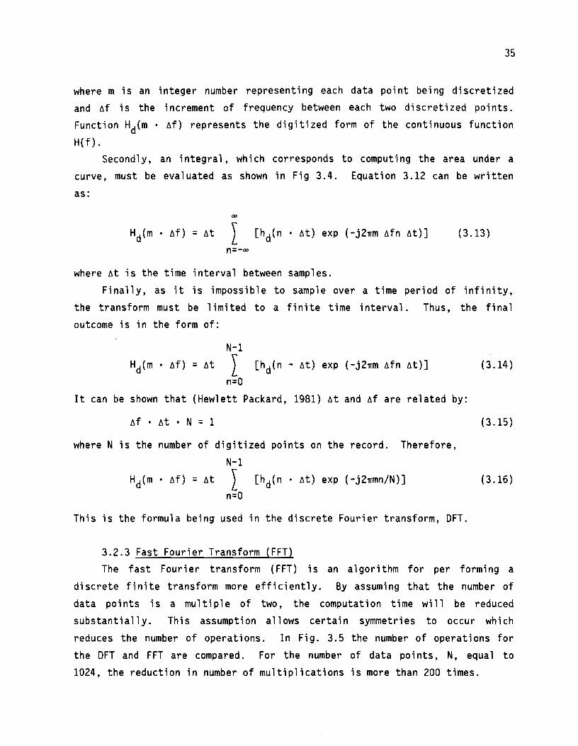
where m is an integer number representing each data point being discretized and llf is the increment of frequency between each two discretized points.
Function Hd(m • llf) represents the digitized form of the continuous function
H(f). Secondly, an integral, which corresponds to computing the area under a
curve, must be evaluated as shown in Fig 3.4. Equation 3.12 can be written
as:
"" Hd(m • llf) = lit I [hd(n • lit) exp (-j2~m Afn At)] (3.13)
n=-oo
where lit is the time interval between samples. Finally, as it is impossible to sample over a time period of infinity,
the transform must be limited to a finite time interval. Thus, the final outcome is in the form of:
N-1
Hd(m • Af) = At I [hd(n - lit) exp (-j2~m llfn At)] (3.14) n=O
It can be shown that (Hewlett Packard, 1981) At and Af are related by:
llf • At • N = 1
where N is the number of digitized points on the record. Therefore,
N-1
Hd(m • Af) = At 2 [hd(n • lit) exp (-j2~mn/N)] n=O
This is the formula being used in the discrete Fourier transform, OFT.
3.2.3 Fast Fourier Transform (FFT)
(3.15)
(3.16)
The fast Fourier transform (FFT) is an algorithm for per forming a
discrete finite transform more efficiently. By assuming that the number of
data points is a multiple of two, the computation time will be reduced substantially. This assumption allows certain symmetries to occur which
reduces the number of operations. In Fig. 3.5 the number of operations for
the DFT and FFT are compared. For the number of data points, N, equal to 1024, the reduction in number of multiplications is more than 200 times.

36
CJ (t)
CJ(t) = h(t)exp (-j2 -rm~ft)
~t ~t ~t
Time, t
Fig. 3.4. Schematic of Numerical Integration in Discrete Finite Transform.

1024 0 0 Q
IIC
(/) c 0 -0 u .~ 512~~--+-----~--~------~ -:; ~
0 256~~--~--~~----------~ .8 FFT E 128 1--11--1---+-:~-+---r----1 ~ 64 l--f--i---:':2F---+----r-----l
64128 256 512 1024 Number of Points
Fig. 3.5. Comparison of Number of Operations in Computing the Fast Fourier Transform and Discrete Finite Transform (after Brigham, 1974).
37

38
3.3 SPECTRAL ANALYSES
Severa 1 types of measurements can be made in the frequency domain once the signals are Fourier transformed. Spectral analyses are basically statistical operations on one or two signals in the frequency domain.
Measurements are often made on two channels of data. The first channel is usua 11 y named the "i nput 11 and the second one is termed the "output". Spectral analyses are either the correlation of the input or of the output with itself, or correlation of these two, considering that the object being tested is a 1 i near system. The ide a 1 i zed and actua 1 mode 1 s being used in spectral analyses are shown in Fig. 3.6. In the idealized model, Fig. 3.6a, it is assumed that the output, y(t), results from the input, x(t), that goes through the linear system. But in actuality, the input, x(t), is contaminated with background noise, shown as n(t), and the output after going through the system consists of a response due to x(t) and n(t) and also is distorted by additional background noise, named m(t), after going through the system.
The advantage of spectral analyses, other than identifying the amplitude and phase of each frequency component in the waveform, is that relationsnips between two signals can be easily identified. Ease of operation in the frequency do main is another advantage of spectral analyses. For example, an integration in the time domain is equivalent to a simple multiplication in the frequency domain. Also, in most measurements in the frequency domain, triggering does not have to be synchronized. Therefore, it is quite simple to average signals which results in enhancing the records being measured. If the background noise is random and the actual signals are repeatable, the averaging of several records will be (theoretically) free of undesirable noise. The average value of a random process tends toward zero, whereas the average of a repeatable signal is presumably representative of the "true 11
value of the actual signal. In other words by averaging signals one is able to get outcomes which are represented more closely by an idealized model as shown in Fig. 3.6a rather than the actual model.
In the remainder of this section, the functions used in frequency domain measurements in SASW testing are discussed. For each function, the outcomes for the two time records shown in Fig. 3.7 are presented for more clarity.

II I t II npu "Output11
X (t)
X (t} X(f) ..
Linear System
a. Idealized System
u(tl
y(t} '{(f)
m(t) M(f)
y(t} X(f) - U(fi Linear Y(f)
n(t) System
nl(t}
N (f) N'(f)
Note:
b. Actual System
x(t) = Input due to Experiment, y(t) = Output due to Experiment, n(t) = Noise Source at Input,
n'(t) = Output due to Noise at Input, m (t) = Noise Source at Output, u (t) = x(t) + n(t) = Actual Input,
--
v(t) -V(f)-
v (t) = y(t) + n•(t) + m(t) =Actual Output.
Capital letters denote the Fourier Transform of the functions described.
Fig. 3.6. Illustration of Idealized and Actual Linear Systems.
39

40
0.4 .-----....----,...----...-----
Channel I
-0.4~-----~----~~------~------J 0 160 320
Time, msec
-0.15 .---------,r-------,r------.,,...-----
Channel 2
0
-0.15:------L---~r------'----~...J 0 16 320
Time, msec
Fig. 3.7. Typical Set of Time Records from a Test on a Soil Site.

41
3.3.1 Linear Spectrum The linear spectrum is simply the Fourier transform of a signal.
Mathematically, it can be presented as:
+oo
Sx(f) = j_® x(t) exp(-j2~nt)dt (3.17)
where Sx(f) and x(t) are the linear spectrum and actual time records, respectively. The linear spectrum consists of real and imaginary components (shown in Fig. 3.8) or interchangeably a magnitude and a phase (as shown in
Fig. 3.9). In SASW testing, the linear spectra are the initial functions evaluated
in the field. These functions are then used to obtain the other spectral functions discussed next.
3.3.2 Auto Power Spectrum The auto power spectrum is defined as:
(3.18)
* where Gxx(f) is the auto power spectrum and Sx(f) the complex conjugate of the linear spectrum, Sx(f). The magnitude of the cross power spectrum is equal to the magnitude of linear spectrum squared. However, as the linear spectrum is multiplied by its complex conjugate, Gxx(f) is a real valued function.
An excellent and rapid means of enhancing the quality of data collected in the field is the averaging of several records. (The writers have found that three to five averages typi ca 11 y gives a good representation of the frequency components.) In addition, the advantage of using Gxx(f) over Sx(f) in averaging is that no synchronized triggering is needed to evaluate Gxx(f) when signaled averaged; whereas, a sophisticated triggering system is required
for determining averaged values of Sx(f). However, each function yields the same information.
The auto power spectrum is often used to identify the dominant frequencies (sometimes called natural frequencies) of a system.
Auto power spectra for the two channels of time domain data in Fig. 3.7 are presented in Fig. 3.10. One can see that the higher frequencies (600 to

42
-~ E .. >. ... 0 c: ·a. 0 E -
5 (Ordinate represents values of an's shown in Fi~. 3.2)
-5~------~------~--------~------~ 0
5
0
400 Frequency, Hz
800
(Ordinate represents values of bn's shown in Fig. 3.2)
Frequency, Hz
Fig. 3.8. Real and Imaginary Components of Linear Spectrum of Channel 1 Determined from Averaging Five Travel-Time Records Like the Ones Shown in Fig. 3.7.
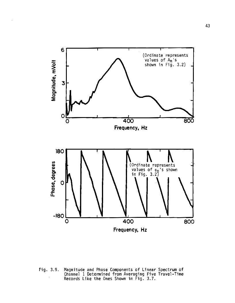
.. cu .,., :::::. -·-c: 0 0 :i
6 (Ordinate represents values of An's shown in Fig. 3.2)
0--------~------~~--------------~~ 0 400
en cu cu ...
180
0 cu .,., aj 0 en 0 .s:: a.
Frequency, Hz
~ ~ (Ordinate represents values of ¢0's shown in Fig. 3.2)
400 Frequency, Hz
Fig. 3.9. Magnitude and Phase Components of Linear Spectrum of Channel 1 Determined from Averaging Five Travel-Time Records Like the Ones Shown in Fig. 3. 7.
800
43

44
1.50
400 800 Frequency, Hz
0.50r-----.------....-----...-----
Channel 2
400 Frequency, Hz
800
Fig. 3.10. Auto Power Spectra Determined from Averaging Five Time-Domain Records Like the Ones Shown in Fig. 3.7.
45
800 Hz} have attenuated faster than lower frequencies. This point just shows that the earth acts as a low-pass filter. In general, the waves have attenuated by a factor of about three at the lower frequencies.
3.3.3 Cross Power Spectrum The cross power spectrum, Gyx(f), is defined by:
(3.19)
* where, SY(f) is the linear spectrum of the output and Sx{f) is the complex conjugate of the linear spectrum of the input. This function is a complex function and can be presented with real and imaginary components, or as shown in Fig. 3.11, with magnitude and phase. The magnitude corresponds to the mutual power between the input and output signals. The phase is indicative of the relative phase between the two signals due to any time delay or propagation delay. As the phase is a relative phase, synchronized triggering is not necessary.
Practically speaking, the phase of cross power spectrum is used to determine the travel times of surface waves at different frequencies. At each frequency, the associated phase is determined. A phase shift of 360 degrees corresponds to a travel time equal to one period. (The period, T, is the reciprocal of frequency, f.) Therefore, the ratio of phase shift over 360 degrees is equal to the ratio of travel time, t, over period, i.e.:
_L =! 360 T
t --L.T--L 1 - 360 - 360 • f
This process is described in detail in Nazarian and Stokoe, (1985).
3.3.4 Transfer Function
(3.20)
(3.21)
The ratio of the linear spectra of output over input is termed the
transfer function, H(f), or frequency response function and is defined as:

46
o.5or------r---........ ---....,......----N --~ -a) "C ~0.25 ·-c:: C'l c
:::e
en (L) (L) ._ C'l Cl,)
"C .. 0
(L) en c
.&::. a.
400 Frequency, Hz
400 Frequency, Hz
800
800
Fig. 3.11. Magnitude and Phase of Cross Power Spectrum Determined from Averaging Five Travel-Time Records Like the Ones Shown in Fig. 3.7.

47
H(f) = S (f)/S (f) y X (3.22)
If the numerator and denominator are multi p 1 i ed by the comp 1 ex conjugate of the linear spectrum of the input signal so that:
H(f) (3.23)
the numerator and denominator represent the cross power spectrum and auto power spectrum of the input, respectively, i.e.:
H(f) (3.24)
These functions [Gyx(f) and Gxx(f)]are usually determined before the transfer function is determined. As such, it is preferable to calculate H(f) from Eq. 3. 24. The transfer function is a comp 1 ex number at each frequency. The magnitude is equal to the magnitude of the cross power spectrum normalized by the magnitude of the auto power spectrum of the input. The phase is identical to that of the cross power spectrum as the auto power spectrum in the denominator is a real-valued function. Therefore, the phase information of the transfer function can be used (just as done with the cross power spectrum) to calculate the travel times of surface waves. The magnitude and phase information of the transfer function are illustrated in Fig. 3.12.
The transfer function is used to identify natural frequencies and damping properties of a linear system.
3.3.5 Coherence Function The coherence function is the ratio of the output power caused by the
measured input to the tota 1 measured output. function, y
2(f), is defined as: Mathemat i ca 11 y, the coherence
(3.25)

48
Q) "'C ::J
1.00
·2 0.50 0 c :e
0~------~------~~----~~------~ 0 400 800 Frequency, Hz
ISO
V) Q,) Q) ... 0 Q)
"'C 0 . 5( c .c a..
-18o.__ ___ ..l..-__;;,.;;::j...__~ ___ ......__ ...... _ __,
0 400 800 Frequency, Hz
Fig. 3.12. Magnitude and Phase of Transfer Function Determined from Averaging Five Travel-Time Records Like the Ones Shown in Fig. 3.7.

49
If the system is ideal, as shown in Fig. 3.6a, the coherence will be equal to unity for a 11 frequencies. But if some noise is present, the coherence may differ from unity. The coherence function is related to signal-to-noise ratio, (S/N), by:
(3.26)
The coherence function is a good too 1 for assessing the qua 1 i ty of the observed signals. The coherence function should be used on averaged signals as for one set of input and output the coherence function is equa 1 to one. The coherence function for five averages of the signals such as those shown in Fig. 3.7 is presented in Fig. 3.13. {All functions in Figs. 3.8 through 3.13 are from five averages.) A coherence value close to one indicates good correlation between the input. and the output signals. However, a low coherence may not necessarily suggest bad corre 1 ati on between the signals. Some reasons for low coherence besides the presence of noise are nonlinearity of the system, low resolution of the frequency bandwidth, and multiple input signals in the system.
3.4 SUMMARY
In this chapter, analyses in the frequency domain are presented as these analyses are instrumental in this study. The Fourier transform, discrete finite transform {OFT) and fast Fourier transform {FFT) are discussed. Spectral functions including 1 i near spectrum, auto and cross power spectra, transfer function and coherence function are defined. An illustrative example is presented for each function determined from five averages of time-domain records like the one shown in Fig. 3.7.

50
1.10 I I r
a> ., ::» 0.60 !--c:: C't 0
:::E
t- -
0.100 '-------L'----4~..&...----....&.'---8~0~0
Frequency, Hz
Fig. 3.13. Coherence Function Determined from Averaging the Spectral Functions from Five Travel-Time Records Like the Ones Shwon in Fig. 3.7.

CHAPTER FOUR. IN SITU EVALUATION OF PAVEMENTS
4.1 INTRODUCTION
It is a widely held belief that the most accurate means of determining in situ properties of different layers in a pavement system is by field testing. The general premise of this belief has certainly been proven true at
geotechnical sites by numerous studies in earthquake engineering. On the other hand, laboratory testing is essential in understanding the influence of various parameters on the behavior of materials such as pavement materials.
However, the exact numerical values of properties determined by laboratory
tests must be carefully used and can be substantially in error due to problems such as non-representative samples, improper stress state during testing, and mechanical disturbance from sampling. As such, it is prudent to use field testing should be used to evaluate material properties whenever possible.
There are two basic approaches used today to eva 1 uate the properties of
pavement systems in the field. The first approach is to employ high intensity loads in an attempt to evaluate the nonlinear behavior of pavements. Elastic
theory is then used to backca 1 cul ate the modulus profi 1 es of the pavement system. The advantage of this approach is that an equivalent nonlinear modulus of the pavement may be determ1ned. However, if these moduli are used
to determine the stresses and strains in the pavement system. substantia 1
errors may occur because the modulus profile is approximated with only three or four equivalent moduli and, hence, may only be appropriate for calculating surface displacements under loads similar to those used to evaluate the equivalent moduli.
The second approach is to determine elastic moduli in situ and to perform laboratory tests on representative samples to define the decrease of modulus
with strain (and to some extent with stress). Then, by incorporating these
two (laboratory and field) results, the actual nonlinear bheavior of the
pavement system is determined. Over thirty years of research in earthquake
engineering have shown that the second approach is very realistic; especially
if one uses normalized moduli as shown in Figs. 2.6 and 2.7.
51

52
The Falling Weight Deflectometer device is a good example of the first testing approach, and the SASW testing method falls in the second category.
In this chapter, the most common nondestructive testing techniques used to evaluate the in situ properties of pavements are reviewed. In addition, several in situ seismic tests, which have been used mainly in geotechnical engineering but which have application to pavements, are included. A historical review of the use of surface waves (Rayleigh waves) in pavement evaluation then concludes the chapter.
4.2 TYPICAL NONDESTRUCTIVE TESTING OF PAVEMENTS
Nondestructive testing of pavements is norma 11 y done by making surface measurements of the response of a pavement structure to an externa 1 force. The response is generally in terms of measurement of surface deflections at several points. Elastic theory coupled with a layered medium is then employed to back-calculate the elastic properties of different layers by matching measured deflections with those calculated from a static load on the layered system.
Lytton et al (1975) studied different nondestructive methods in some detail. The major differences between different methods is the way the load is imparted to the pavement and the number and position of points at which deflections are measured. The characteristics of some deflection measuring devices are presented in Table 4.1. The methods that are based upon application of static loads consist of the Plate loading test, Benkelman beam, traveling deflectometer, Lacroix deflectograph, and curvature meter (Haas and Hudson, 1978). Vibratory nondestructive methods apply a steady state load to the pavement surface after applying some static seating load. The main devices in this category are the dynaflect, road rator, Waterways Experiment Station (WES) vibrator, and Federal Highway Administration (FHWA) thumper. Devices that use an impact as the source are the falling weight deflectometer, Ca 1 i forni a (CAL) impulse testing, and Washington State University impulse
testing. The most dominant devices in nondestructive testing of pavements are the
Dynaflect and falling weight deflectometer (FWD). A schematic of a dynaflect device is shown in Fig. 4.1. A peak-to-peak dynamic force of 1000 lb (4500 N)

TABLE 4. 1.
Device Static load 16f
(l) (2)
Benkelman Variable Beam Single Axle
Load
Dynafl ect 1000
Road Rator 1500-7000
falling Variable Weight
Defl ectometer
CHARACTERISTICS OF COMMON NONDESTRUCTIVE TESTING DEVICES USED ON PAVEMENT (FROM EAGLESON ET AL~ 1981).
Dynamic load loading load Number of 16f Concept Frequency, Hz Deflection
Sensors*
(3) (4) (5) (6)
- Static - 1
1000 Counter- 8 5 rotating
Weights
1000-8000 Electro- 10-80 4 hydrau 1 ic Vibrator
1500 to 24000 Drop Wide Range** 5 to 7 Weight
Spacing,+ in.
(7)
-
12
12
12
* Sensors are velocity transducers except for Benkelman Beam which a dial gauge is used. ** Duration of about 25 msec. + Between adjacent receivers.
I
I
U1 w

54
No.2No 3 Loading Wheels, · No.4No.S 1
Geopfiones
a. The Dvnaflect Svstem in Operatinq Position.
Loading
Wheelsl=P.
T . Geophones
10" • Nt' No.2 No.3 No. No.s ... -· ·-·-t-·-·._·-·-<ir·-·<b-1011 . li ~ 12" .,. 12" * 12~ !. c:b 4"
i T b. Confiquration of Load Wheels and Geoohones.
Fig. 4. 1. Configuration of Dynaflect Load Wheels and Geophones in Operating Position (from Uddin, et a 1 , 1983).

55
is generated by two counter-rotating eccentric masses at a frequency of 8 Hz.
This force is transmitted to the pavement by two, 4-in. (10-cm) wide wheels. Five equally spaced geophones are used to measure deflections of the pavement system due to the load as shown in Fig. 4.1.
The falling weight deflectometer (FWD) is quite similar to the dynaflect device. The main differences are basically in the number of receivers, as seven geophones are used, and the load. A schematic of FWD is shown in Fig. 4. 2. The 1 oad is deve 1 oped by dropping a weight on a p 1 ate set on the pavement surface. The energy of the impact can be varied by changing the drop
height or drop weight. The peak loading force varies from 1.5 to 24 kips (6.6
to 106 kN). The duration of impulse is around 25 to 30 msec, which simulates the duration of a load imposed by a moving wheel at 40 mph (64 km/h).
In both the Dynaflect and FWD, placement of the receivers and deployment of the loads can be done from a towing vehicle. However, the testing process for the FWD is more sophisticated and is controlled by a desk-top computer.
In the analysis of the load-deflection measurements, the pavement is modelled as a multilayered linear elastic system, and each layer is
characterized by Young 1 s modulus and Poisson 1 s ratio. A computer program
based upon linear elastic theory with static loading is then used to predict the deflections at the measurement points. Computed and measured deflections
are compared and necessary adjustments in the value of the elastic modulus of each layer are made until measured and computed deflections compare well. This process is called "deflection-basin fitting".
The major assumptions in the deflection-basin fitting approach are: 1. the dynamic load can be replaced by an equal static load, 2. measured dynamic deflections are assumed equal to theoretical static
deflections, and 3. the subgrade has constant stiffness and is extended to infinity or
to a rigid layer underlying the subgrade at some depth.
The main advantages of these two methods are mobility and rapid testing
in the field. However, these methods do not yield a unique solution as several combinations of moduli can be determined to produce a theoretical
basin which matches the experimental deflection basin. This nonuniqueness
becomes more pronounced as the number of layers assumed in the theoretical
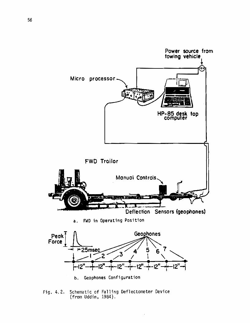
56
Micro processor
FWD Trailor
Power source from towing vehicle
HP-85 desk top computer
. Manual Controls'\
a. FWD in Operating Position
b. Geophones Configuration
Fig. 4.2. Schematic of Falling Deflectometer Device (from Uddin, 1984).

57
profiles is increased. As such, the number of layers are normally limited to
three or four and the thickness of each layer must be assumed. A recent study on the effects of different parameters involved in
basin-fitting by Shao et al (1986) has shown that the dynamic nature of the load and the presence of bedrock at shallow depths may cause significant errors in basin-fitting. A second study by Nazarian and Stokoe (1986b) has shown that, with the receiver set-up used in both the Dynaflect and FWD, the algorithms used in basin-fitting is not sensitive to the properties of top thin layers in the pavement. As a result, continued work on the data analysis algorithms used by the FWD and dynaflect are underway on Project 1123.
4.3 SEISMIC FIELD METHODS
Seismic field methods have become a standard means of in situ evaluation of low-strain moduli of soils in geotechnical engineering. These methods are based on wave propagation in elastic media as discussed in Chapter Two. The methods normally involve applying a transient or steady-state excitation at one point in the medium and detecting the response at two or more locations. Wave velocities are determined from the recorded responses, and moduli are calculated using Eqs. 2.5 through 2.10.
In situ measurement of soil properties by wave propagation techniques can be summarized in the following six steps:
1. set up receivers at known distances from the source, 2. generate an impulse with the source, 3. measure travel time of wavefront from source to receivers, 4. calculate wave velocity (distance divided by time), 5. calculate elastic soil properties, and then 6. repeat steps 1 to 5 for different source/receiver locations. In situ seismic methods can be categorized into two main groups; borehole
methods and surface methods. Each group is discussed in the following sections.
4.3.1 Borehole Methods In these methods, one or more boreho 1 es are uti 1i zed as i 11 ustrated in
Fig. 4.3, and compression (P) and shear (S) wave velocities are measured at

58
s*
a. - C ron hole b.- Downhole
Fig. 4. 3. Schematic Representation of Borehole Seismic Methods (from Hoar, 1982).

59
different depths in the soi 1 deposit. The most common boreho 1 e methods are
the crosshole and downhole. In the crosshole method, at least two boreholes
are required. On the other hand, the downhole method can be performed with a
single borehole. As a result, the cost efficiency offered by the downhole
method often results in its selection at geotechnical sites when the choice is
between these two borehole methods.
The ray paths of the seismic waves in boreholes tests are generally
assumed to be directly between the source and receiver as illustrated in Fig.
4. 3. The variation in soil properties with depth is then determined by
changing the location of the source and/or receivers and repeating the test.
In pavement studies, borehole methods are infrequently used due to the
fact that these techniques are time consuming and specialized personnel are
required. However, to verify independently the results of SASW tests,
crosshole tests have been used in studies performed by the writers.
Therefore, a detailed description of the crosshole test as applied to
pavements is presented in Section 4.4.
The downho 1 e test can be briefly described as fo 11 ows. Genera 11 y, a
wooden plank source is placed on the ground surface and receivers are placed
in the borehole (Patel, 1981). Usually only S-waves are measured because the
casing typically adversely affects the P-wave results (at soil sites).
Properties of materials in the near-vertical direction are predominantly
measured. Advantages of the downhole test are placement of the source on the
surface, minimum refraction problems and the need for only one borehole.
However, as the depth increases, the path length of the wave increases, and
the qua 1 i ty of the signa 1 s decreases. Downho 1 e tests have not been used in
pavement evaluation to the writers• knowledge but are widely used in
geotechnical engineering. Downhole testing could, however, be applied to
pavement sites.
4.3.2 Surface Methods
In these methods both the source and receivers are located on the
surface. Thus, there is an economical advantage in these methods relative to
borehole seismic methods in that no boreholes are required. Common surface
methods are:
1. refraction,
2. reflection,
3. steady-state surface waves, and
4. spectral analysis of surface waves!
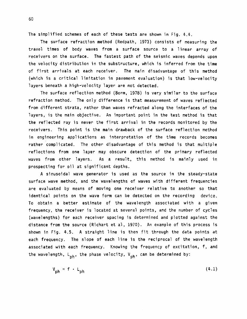
60
The simplified schemes of each of these tests are shown in Fig. 4.4.
The surface refraction method (Redpath, 1973) consists of measuring the travel times of body waves from a surface source to a linear array of receivers on the surface. The fastest path of the seismic waves depends upon the velocity distribution in the substructure, which is inferred from the time of first arrivals at each receiver. The main disadvantage of this method (which is a critical limitation in pavement evaluation) is that low-velocity layers beneath a high-velocity layer are not detected.
The surface reflection method (Borm, 1978) is very similar to the surface
refraction method. The only difference is that measurement of waves reflected
from different strata, rather than waves refracted along the interfaces of the layers, is the main objective. An important point in the test method is that the reflected ray is never the first arrival in the records monitored by the
receivers. This point is the main drawback of the surface reflection method in engineering applications as interpretation of the time records becomes
rather complicated. The other disadvantage of this method is that multiple
reflections from one layer may obscure detection of the primary reflected waves from other layers. As a result, this method is mainly used in
prospecting for oil at significant depths. A s i nusoi da 1 wave generator is used as the source in the steady-state
surface wave method, and the wavelengths of waves with different frequencies are evaluated by means of moving one receiver relative to another so that identical points on the wave form can be detected on the recording device. To obtain a better estimate of the wavelength associated with a given frequency, the receiver is located at several points, and the number of cycles (wavelengths) for each receiver spacing is determined and plotted against the distance from the source (Richart et al, 1970). An example of this process is shown in Fig. 4.5. A straight line is then fit through the data points at
each frequency. The slope of each line is the reciprocal of the wavelength
associated with each frequency. Knowing the frequency of excitation, f, and
the wavelength, Lph' the phase velocity, Vph' can be determined by:
(4.1)

a.- Surface Refraction
s
b.- Surface Reflection l S(t) • A sin Qll
c.- Steady-State Raylaigh Wave
t I (I)~ impulse loading
d.- Rayleigh Wave Dispersion
Fig. 4.4. Schematic Representation of Surface Seismic Methods (from Hoar, 1932).
61

62
-0
Q; .0 E :l z
18r-.-~~-,-.~~~.-.-.-~-r-r-.-.--rPr-~,--r~~~~
17
16
15
0
Distance from Source, ft
Fig. 4.5. Determination of Average Wavelength of Surface Waves from Steady-State Test (from Richart, et al, 1970} .
.::
"' ' 0.3 a:: _j
c 0. 04 (l)
0
Cl' 0.5 ~ 0. E 0.6 0 (j)
0.7 (l)
~ 0.8 . ;:; 2. 09 w 10 0 (l) u .E ~
1.5 -::J (j)
Q)
E ~ 2.0 0 ~ Q)
2.5 1:.
0. 3.0 (l)
0 100 700
Shear Wove Ve1oc1ty, ft I sec
Fig. 4.6. Shear Wave Velocity Profile from Measurements Presented in Fig. 4.5.

63
The effective depth of sampling is assumed to be 1/2 to 1/3 of the wavelength,
and the shear wave velocity is assumed to be in the range of one to 1.1 times the phase velocity.
As an example, the shear wave velocity profile obtained from the steady-state test shown in Fig. 4.5 is included in Fig. 4.6. Richart, et al ( 1970) assumed that the effective depth of samp 1 i ng is equa 1 to 1/3 of the wavelength and that the shear and phase velocities are equal.
Conceptually, the method involving spectral analysis of surface waves
(SASW) is identical to the steady-state method. One of the main differences is the excitation source, which is transient in the SASW method. One benefit of a transient impact is that it can excite a wide range of frequencies with each impact. Thus, it is poss i b 1 e to record many different frequencies with one impact. A detailed discussion of the practical aspects of this method is presented in Nazarian and Stokoe (1985) while the historical development is presented in Section 4.5.
The other major difference between the SASW test and the original surface wave test is development of the inversion process. The inversion process is a
rigorous means of determining the modulus and thickness of each layer from the dispersion curve as opposed to the approximate method used by Richart et al (1970). Theoretical aspects of the inversion process are discussed in Chapter
Five.
4.4 CROSSHOLE SEISMIC TESTING OF PAVEMENTS
4.4.1 Testing Procedure A schematic of the testing procedure on pavement sites is shown in Fig.
4. 7. In this procedure, each boreho 1 e is advanced to the appropriate depth using solid-stem augers. At each testing depth, the drilling operation is stopped, the source is firmly placed at the borehole bottom, and then it is pushed approximately 6 in. (15 em) into the material if possible. The
receivers are placed at the same depth in the receiver boreholes and are firmly pushed into the material to ensure good coupling between the receivers
and surrounding material. A vertical transient impulse is then applied to the source. This impulse generates P- and S-waves which are detected by receivers
in the other holes as they pass by.

64
X (variable)
~ ~.._Source
Borehole
c::::=O :::. ,. ... Dri IIi, g
roa
= 1.0 ft
~ertical velocity _..,.....,. transducer
(far trigger)
Thin-walled sampler
X (variable)
@__Receiver I Bare hale
A. Plan View
B. Cross-Sectional View
.. j
@_Receiver 2 Borehole
Fig. 4.7. Schematic of Crosshole Testing Technique at Pavement Sites.

65
The source consists of a samp 1 i ng tube attached to a rod. A vert i ca 1
velocity transducer secured to the rod just above the sampling tube serves as the trigger for the recording device. This trigger activates the recording device at essentially the instant body waves are created in the material at
the bottom of the source. The receivers consist of three-dimensional velocity transducers in which
three receivers are oriented in three perpendicular directions (i.e., vertical and two perpendicular horizontal directions). The receivers are placed on the borehole bottom and then properly oriented with orientation rods which extend from the receivers to the surface. The receivers and transducer 1 ocated on the source are connected to the recording device (a digital oscilloscope) through a switching box. By means of the switching box, the geophones with proper orientation for the wave motion to be measured are easily selected.
The vertical impulse to the rod is applied by an ordinary hammer. A vertical impulse transmitted through a medium generates P- and SV-waves which can be detected by radi a 1 hori zonta 1 and vert i ca 1 geophones, respective 1 y. Records of receiver outputs are saved on magnetic diskettes for future reference and in-house data reduction.
4.4.2 Data Reduction Typical travel time records from the crosshole tests are shown in Fig.
4.8. The record in Fig. 4.8a consists of the output from the source receiver (upper trace) and the output from the vertical receiver in the first receiver borehole (lower trace). The record in Fig. 4.8b consists of the outputs from vertical receivers in the first and second receiver boreholes (upper and lower traces, respectively).
The upper trace in Fig. 4.8b is composed of three basic parts. The first part, the left side, is the initial smooth portion of the trace. This results from the fact that the impulse has started the trace moving across the
osci 11 oscope screen, but no energy has yet arrived at the transducer in the first receiver borehole. The second part consists of the time between the first arrival, denoted by P, and the second arrival, denoted by S, which consists of waves of 1 ower amp 1 i tude and higher frequency re 1 at i ve to the remainder of the trace. This portion of the trace is considered to represent energy transmitted by the P-wave. The third part of the trace consists of

66
Record length= 10.25 msec Full Scale Sensatav1ty
Source Receiver
Vertical
I
Receiver in 1---++----J.----._ Borehole Rl
(a) Direct Measurement
:tlOV
:t40mV
Record length: 20. so msec Full Scale Sensitivity
p
Vertical Receiver in 1----'--""" BoreholeRI
(b) Interval Measurement
Fig. 4.8. Typical Crosshole Records for Determination of Shear Wave Travel Times.
:t40mV
:t20mV

67
waves of higher amplitude and lower frequency due, at least initially, to the
arrival of the shear wave. The shear wave arrivals are identified as the beginning of the first large-amplitude energy excursion (Stokoe and Woods, 1972) and are marked as S in the figure.
Determination of the direct shear wave travel time from the source to receiver 1 is the time from the initiation of the impulse (marked as I in the upper trace of Fig. 4.8a) until the initial shear wave arrival at borehole R1.
This time is denoted as tDS in Fig. 4.8a. Determination of the interval shear wave travel time is illustrated in Fig. 4.8b. This is the time for the shear
wave to propagate between the two receiver boreholes and is denoted as tiS in the figure. Interval travel times minimize many of the variables which can affect these measurements (Stokoe and Hoar, 1978).
Other travel time records similar to the one shown in Fig. 4.8 but with
radial horizontal receivers are also obtained at all depths to improve the
accuracy and resolution with which P-wave travel times could be determined.
One set of these records is shown in Fig. 4.9. Direct and interval travel
times of the P-waves are shown as t 0p and tiP' respectively.
4.5 HISTORICAL DEVELOPMENT OF SURFACE WAVE TECHNIQUE
Existence of surface waves was first discussed by Rayleigh (1887), and
the first simple theoretical seismograph illustrating the existence of body
and Rayleigh waves was presented by Lamb (1904). These simplified models were the corner stone for tremendous advancements in identifying and interpreting seismic records. For instance, surface waves, usua 11 y generated by
earthquakes or exp 1 os ions, have been used for geophys i ca 1 prospecting and identifying the proper ties of the crust and mantle of the earth. The contribution of the geophysicists over the last 100 years to the advancement of determination of properties of materials in situ is so extensive that it cannot be covered in this section. However, application of the theoretical
and experimental achievements of geophysicists in material characterization
tailored for use in civil engineering projects is discussed.
The first known use of surface waves to determine soil properties for engineering purposes was credited to the German Society of Soil Mechanics
before World War II {DEGEBO, 1938). The primary interest of that study was to

68
investigate the response of a foundation to steady-state vibration. A rotating-mass oscillator was used as a source to excite foundations in the range of frequencies between 10 and 60 Hz. Due to the lack of sensitive receivers in that period, excessive loads had to be imposed on the soil to generate adequate signals. As a result, nonlinear behavior was generated in the soil and somewhat unsuccessful application of the method occurred (primarily because the nonlinear behavior was not taken into account).
Bergstrom and Linderholm carried out similar tests in Sweden in 1946. This work was done on a fairly uniform soil which resulted in the surface waves exhibiting little dispersion in the study range of 14 to 32 Hz. They compared Young's moduli determined from surface wave and plate bearing tests in an attempt to correlate the modulus of subgrade reaction with Young's modulus. Plates with different diameters were used in the plate bearing tests. They found that the moduli of subgrade reaction from the large-diameter plates correlated well with the dynamic moduli from the surface wave tests. However, results from the smaller-diameter plates did not yield any appreciable relationship between the subgrade and dynamic moduli.
Van der Poel (1951) and Nijboer and Van der Poel (1953) investigated a
flexible pavement system in Holland using surface waves. The range of frequencies in their tests was 10 to 60 Hz which corresponded to waves predominantly propagating in the subgrade soil.
Heukelom and Klomp (1962) used steady-state vibrators to perform surfac~ wave tests on pavements. Mechanical and electrodynamic vibrators were used to generate low frequency (4 to 60 Hz) and high frequency (greater than 60 Hz) waves in their tests. The effect of drainage of the subgrade after a flood was investigated. The S-wave velocity profiles from their investigation are shown in Fig. 4.10. The material profile of the site, which was located on a runway, was not described; however, the layering in the profile is shown graphically in the figure. The ordinate which is titled as the approximate depth in Fig. 4.10, corresponds to one-half of the wavelength at each frequency. The abscissa is equa 1 to the phase ve 1 ocity determined at each frequency. In other words, they assumed an effective depth of sampling equal to 1/2 of the wavelength and a shear wave velocity equal to the phase velocity at each frequency.

Source Receiver
I~
Horizontal P f Receiver in 1-----~----!'-" Borehole Rl ~
Horizontal Receiver in Borehole Rl
Horizontal Receiver in Borehole R2
Record
(a) Direct Measurement
Record length: 10.25 msec
(b) Interval Measurement
Full Scale Sensitivity
±IOmV
±10 mV
±10 mV
Fig. 4.9. Typical Crosshole Records for Determ·ination of Compression Wave Travel Times.
69

70
E u ..
.s:::. +-l
0
50
Wave Phase Velocity, m/s
100 200 300
~ ~/2(cm) QJ 100 +-l ttl E
X 0 s... c.
~ 150
200
Fig. 4 .10. Wave Phase Velocity as a Function of Approximate Depth, Showing the Softening of a Base Course by Water (II) and its Gradual Recovery on Draining (III), (from Heukelom and Klomp, 1962). Case I Represents Testing When the Base Course was Only Partially Built.

71
The curve in Fig. 4.10 denoted as I is the Vs profile determined by
Heukelom and Klomp from tests performed when the base course was "half-way finished". The second and third curves (marked as II and III, respectively,) are from tests carried out after the finishing of the base and after the wearing course had been placed. Apparently, due the seasonal precipitation, the site was flooded, and the near-surface material became substantially softer (curve II, in Fig. 4.10). From the third test (curve III), they concluded, that as the water content of the material decreased, the stiffness increased. Unfortunately, they could not excite high enough frequencies to sample the pavement layers under investigation. (Note: The writers research shows that Heukelom and Klomp would have had to excite frequencies in the range of 3000 to 10,000 Hz to evaluate the upper pavement layer.)
The U.S. Army Engineer Waterways Experiment Station (WES) has used steady-state vibrations to determine elastic properties of in situ soils over the past 20 to 25 years. Ballard (1964), Fry (1965), Maxwell and Fry (1967),
Ballard and Casagrande (1967), Cunny and Fry (1973), and Ballard and Chang (1973), among others, investigated numerous sites with the surface wave technique. The tests were carried out according to specifications set by WES which are described in detail by Maxwell and Fry (1965). The sources were either electromagnetic vibrators (for generating high frequencies) or mechani ca 1 vibrators using counter'-rotati ng eccentric masses to generate 1 ow frequencies (up to 60 Hz). The WES procedure for obtaining the shear wave velocity profile from phase-velocity/wavelength data is identical to that of Heukelom and Klomp (1962), just discussed.
As an example of the WES procedure, the shear wave velocity profile from a site located in Buckboard Mesa, Nevada investigated by Fry (1965) is shown in Fig. 4.11. The site consists of a layer of residual soil that gradually turns into dense basalt. The approximate depths correspond to one-half of the wave 1 engths, and the shear wave ve 1 oci ties are assumed to be i denti ca 1 to propagation velocities measured in situ. Cunny and Fry (1973) compared in situ elastic moduli from surface waves tests with moduli obtained by resonant column tests at 14 sites. Cunny and Fry concluded that the laboratory-determined shear and Young's moduli were generally within 50
percent of the in situ moduli. They seemed to conclude that the WES procedure for handling surface wave data was acceptable. Woods and Richart (1967)
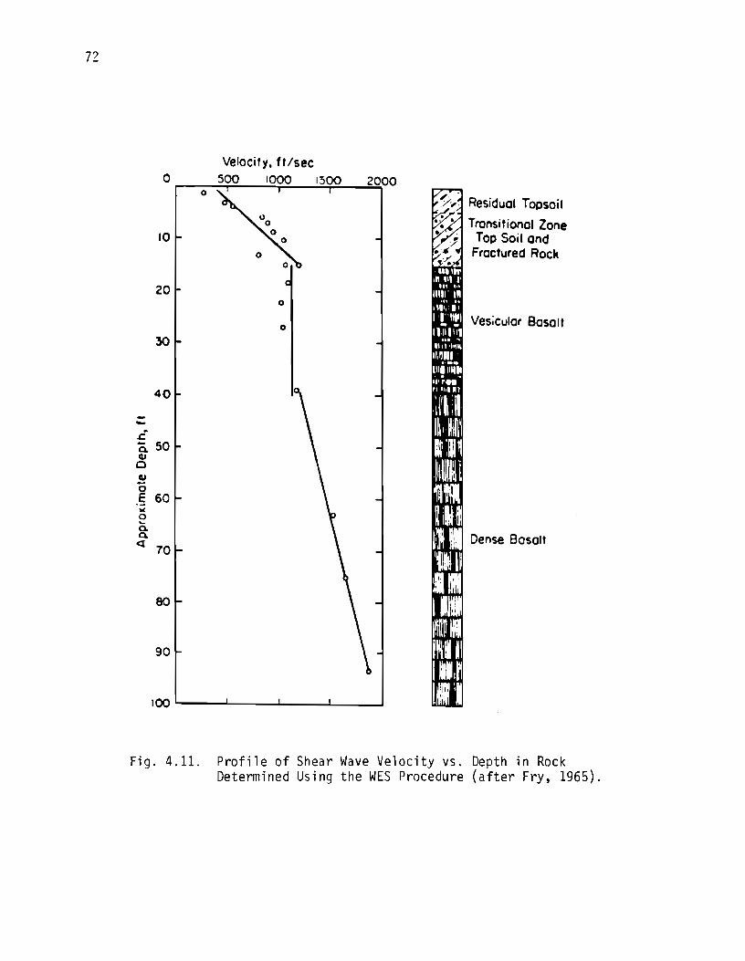
72
40
--.t! 0. 50 Q.J
0
~ 0
.§ )(
0 ... Q. Q.
<%
60
70
80
90
100 .__ __ .~....--__ .~.._ __ .~..-_ ___.
Dense Basalt
Fig. 4.11. Profile of Shear Wave Velocity vs. Depth in Rock Determined Using the WES Procedure (after Fry, 1965).
73
performed a series of surface wave tests in conjunction with a testing program
set up to study the effect of trenches in screening elastic waves. They followed the procedure proposed by WES and also tacitly assumed the procedure
was acceptable. The greatest recent contribution in theoretical and practical aspects of
surface wave testing on pavements was by Jones (1958). He proposed an analytical procedure to compute the moduli of different layers in a pavement system. An example of his investigation on a pavement section consisting of a 9-in. (23-cm) thick (nominally) concrete layer over subgrade is shown in Fig. 4.12. He assumed that the subgrade was a liquid layer and treated the
concrete slab as a plate. From his study he reported the thickness of the concrete as 9.5 in. (24 em). Upon coring, the concrete thickness was found to
be quite close to 9.5 in. (24 em). Four groups of investigators have employed the spectral analysis of
surface waves principles, mentioned in Section 4.2.2, to collect data in situ.
Wi 11 i ams ( 1981) used a vi bra tor connected to broad-band noise generator (as opposed to a sine wave-generator) and a hammer as a source. These two sources, and sources similar to them, have the ability to generate waves over a wide range of frequencies. If the waves generated by these sources are
captured on an appropriate recording device, Fourier transformed, and spectral
analyses performed on them, the testing time can be reduced quite significantly (see Nazarian and Stokoe, 1985). Williams' interest was solely limited to constructing the experimental dispersion curves, and he did not report any shear wave velocity profile.
Heisey, et al (1982) used hammer blows to generate transient signals to construct the dispersion curves. He used a spectral analyzer as the recording device which accelerated the in-house data reduction several fold over Wi 11 i ams' approach (a tape recorder). Based upon tests on sever a 1 soi 1 and pavement sites, Heisey suggested an effective depth of sampling equal to 1/3 of the wave 1 ength for each frequency. He a 1 so divided the surface wave
velocities measured in the field by a factor approximately equal to 0.90 to obtain shear wave velocities.
Neilson and Baird (1975, and 1977) and Baird (1982) from the New Mexico Engineering Research Institute constructed a van to collect surface wave data conveniently. This van consists of a system operators area and a support

74
911 of Concrete V5 •9100 fps
., = 0.25
(Half- space)
Vp• ~000 fps
a. Material Profile
o.---------------~-
o Experimental
-- Theoretica I
b. Dispersion Curves
Fig. 4.12. Comparison of Theoretical and Experimental Dispersion Curves for a Concrete Layer Over Soil (from Jones, 1958).

75
equipment area. A data acquisition system along with a system to control the
deployment of an impact system are located in the system operators area. The support equipment area houses a 215-1 b ( 950-N) programmab 1 e drop weight and two generators. The height of the drop and the weight of the loading system can be changed. The drop weight impacts a 12-in. (30-cm) diameter plate. The impulses are simultaneously monitored with as many as eight accelerometers. The data reduction is rather arbitrary and requires empirical correction factors to obtain moduli of the different layers. In other words, no rigorous inversion process was developed in this program.
A series of investigations was performed by Baker and Stevens (1983). A hydrohammer (soil compactor) was used as the seismic source. The travel time records were recorded on a 16-channel digital tape recorder. Data reduction is based upon constructing and matching of a synthetic travel time record (seismogram) with the experimental one obtained in the field.
In summary, in all the investigations reported above, in situ testing procedures may differ; however, invariably the goal is to determine the relationship between the propagation velocity of surface waves and wavelengths, called a dispersion curve. The next step is then to obtain a shear wave velocity-depth relationship based upon the dispersion information. In all the studies [except Jones (1958), and Baker and Stevens (1983)] the dispersive characteristic of surface waves was neglected, and after the dispersion curve was constructed, some approximate procedure was used to assess the shear wave velocity profile. In other words, the Vs profile was obtained by simply changing the scale of the axes of the dispersion curve. Generally, use of this process will not accurately predict the shear wave velocities. The reasons. for this inaccuracy and an alternative process for determining the shear wave velocity profile from a given dispersion curve are presented in Chapter Five.
4.6 SUMMARY
In situ seismic methods used in determining dynamic stiffnesses of soil deposits and pavement systems are discussed in this chapter. Downho 1 e and crosshole tests are the most popular methods used in geotechnical engineering projects. To date, crosshole testing is more desirable for pavement systems

76
as it yields more accurate and repeatable results once any refraction problems are taken into account. In the pavements area, the Oynaflect and the falling weight deflectometer are the most commonly used in situ testing techniques. These techniques are rapid in the field but have undesirable drawbacks in data reduction due to possible nonuniqueness of the solutions.
The historical development and employment of the surface wave method is also presented. Basic field testing with the method has evolved from steady-state vibrators and tape recorders to transient impacts and waveform analyzers as the availability to take sophisticated electronics into the field has increased. However, data reduction in most geotechnical engineering cases is based on arbitrary criteria which are generally in error. The data reduction prob 1 em is discussed in the next chapter and a improved so 1 uti on (inversion) is proposed. This improved solution has been implemented in an interactive computer program, INVERT1, which is discussed in Report No. 1123-1 (Nazarian and Stokoe, 1986c).
CHAPTER FIVE. DISPERSIVE CHARACTERISTIC OF SURFACE WAVES
5.1 INTRODUCTION
In a homogeneous, isotropic, elastic, half-space, the velocities of
surface waves do not vary with frequency. However, si nee the properties of
pavement systems ex hi bit variations with depth (are not homogeneous
vertically), surface wave velocities vary with frequency. This frequency
dependency of wave velocity in a heterogeneous medium is termed dispersion,
and surface waves are thus said to be dispersive. A plot of wave velocity
versus frequency (or wavelength) is called a dispersion curve. It is this
dispersive characteristic of surface waves that is the fundamental basis of
the SASW method.
The dispersive characteristic of surface waves can be demonstrated by
means of either phase or group velocity. Phase velocity is defined as the
velocity with which a seismic disturbance of a single frequency propagates in
the medium. Group velocity, on the other hand, is the velocity of groups of
frequencies in a seismogram in a dispersive medium. Definition of phase and
group velocities is based upon the principle of stationary phase which
indicates that significant arrivals in the seismogram occur when the phase is
stationary with respect to frequency. The phase is stationary several
wavelengths away from the source and near the maximum or minimum of the
wavelet. In a medium in which the velocity varies with frequency, the wave train changes shape as it propagates, and, therefore, group velocity differs from phase velocity, especially when the wave propagates over a long distance.
Phase and group velocities are related by:
dV h vg = vph + k--afl ( 5.1)
with
k = w/Vph (5.2)
77

78
where:
vg = group velocity,
Vpn = phase velocity, k = wave number, and w = rotational frequency.
As an example, the time records of waves propagating in a medium at different distances from the source are shown in Fig. 5.1. The lines corresponding to
phase and group velocities are also shown in this figure. Phase velocity is found by a best fit 1 i ne through the troughs or peaks at the zeros of the
wavelets. However, group velocity is obtained by drawing a straight line
(best fit line) connecting the maximum or minimum envelopes. In Fig. 5.1, the troughs are used for determining phase velocity. In practice, phase velocity
is often determined first as a function of frequency, and group velocity is
calculated using Eq. 5.1. In this study, only phase velocities are
considered. Group velocities are disregarded herein because phase velocities
contain all the information required to calculate elastic moduli of the
pavements. It should also be mentioned that throughout this chapter apparent
Rayleigh wave velocity and phase velocity are used interchangeably and are
considered synonymous. The study of dispersion of waves in a horizontally-layered half-space
relies upon derivation of the so-called dispersion function (i.e., the relationship between phase velocity and frequency). Thomson (1950) introduced the first matrix solution of this problem. However, his work contained an error in the sense that continuity of strains was assumed at layer interfaces as opposed to displacements. Haskell (1953) reworked Thomson's procedure imposing continuity of displacements at layer interfaces and thus developed the first successful matrix solution of Rayleigh wave motion in a layered
system. In the c 1 ass i ca 1 approach, the dispersion function and wave 1 engths {or
frequencies) are obtained by vanishing a determinant whose elements are
functions of mass densities and elastic moduli of the layers as well as phase
velocities and frequencies. The Haskell-Thomson technique builds up the
(surface wave) dispersion function as the product of layer matrices which
relate the displacement components as well as the stress components acting on the interface to those associ a ted with the next interface. The product of

QJ u s... ::s 0
V')
E 0 s...
'+-QJ u c:::: tO +-> V) .....
0
.... tO +-> c:::: 0 N ..... s... 0
:::r:
I
a I
I I
I 'I
I I I
1
I
* vph
I I
I I * I vg
I
1
1
•
----~~·---------------· •
I
----~------------------------~•~ Time
*Vph and v9 are phase and group velocities respectively
Fig. 5.1. Illustration of Phase Velocity and Group Velocity (from Sheriff, 1982).
79

30
these layer matrices then relates the stress and displacement components of
motion at the deepest interface to those at the free surface. The Haskell-Thomson solution exhibits numerical difficulties at high
frequencies. These difficulties are caused by the computation of squares of exponential terms leading to loss of significant figures in the components of
certain matrix products. Knopoff (1964), Dunkin (1965), Thrower (1965), Schwab and Knopoff (1970), and Watson (1970) suggest methods to solve this
problem. The works of Dunkin, Thrower, and Watson are all extensions of the original Haskell-Thomson matrix formulation. Knopoff's technique begins with
the immediate construction of the dispersion function by means of
determinants, and then analyzes or decomposes these determinants into a
product of interface matrices which are from submatrices of the determinants.
Each of these interface submatrices relates the components of motion in the layer on one side of the interface to those in the layer on the other side.
In this chapter the Haskell-Thomson technique along with its numerical
difficulties at high frequencies are first discussed. Dunkin•s approach to
circumvent these numerical difficulties is also presented as this approach is
employed in the inversion process discussed in Nazarian and Stokoe (1985) and Nazarian and Stokoe (1986c). Thrower's approach is quite similar to Dunkin•s
solution which is described in this chapter. However, Thrower suggested some
slight modifications to determine the solution to propagation of surface waves in a layered system which becomes softer with depth. As Thrower's solution is very similar to Dunkin's solution, his work is not repeated herein. The final section of this chapter includes a study of factors affecting the dispersion function.
5.2 HASKELL-THOMSON APPROACH
Many problems in geophysics involve propagation of elastic surface waves
in a layered half-space. Usually the half-space is divided into homogeneous
and isotropic solid layers as shown in Fig. 5.2. In the nth layer,
displacements un and wn in directions x and z, respectively, and ozn and Txzn' normal and shear stresses on horizontal planes, respectively, can be expressed
in terms of two potentials:

31
X z=O
VSI t Vp1 , P1 I dl Ze
Vsz' Vpz' Pz 2 dz Zz
V53 ' Vp3 'p3 3 ds
z z3
~----------~---------~-
~-------~-------------
~--------------------------------~--------~zn-1
V5n, Vpn, Pn n dn ~--------------------------------~--------~zn
~---------------------
,__ ______________________ _ N -I
N
Half- space )
-----
Fig. 5. 2. Idealized Model of a Heterogeneous t1edium.
82
~n = a scalar potential corresponding to compression waves, and
$ = a vector potential corresponding to shear waves. n
As mentioned before, it was assumed that the condition of plane strain exists.
As a result of this assumption, it can be shown that the x- and z-components
of the vector potential $n are equal to zero. For simplicity, they-component of the vector potential (i.e. potential corresponding to shear in the x-z
plane) will be called ~n' hereafter. layer as solutions of the equations:
a2~ 2 _ 1 n
v ~n - '\f2 at 2 sn
These potentials are obtained for each
(5.3)
(5.4)
where the operator 'V 2 is the Laplacian operator and is defined as:
(5.5)
Once again, due to assumption of p 1 ane strain, it can be shown that the
derivative of the potentials with respect to y is equal to zero so that Eq.
5.5 can be written as:
(5.6)
For a harmonic wave, the potentials ~n and ~n can be Fourier transformed with respect to time and x so that the result can be written as:
~n = ~n exp[-i(wt-kx)] ( 5. 7)
~n = ~n exp[-i(wt-kx)] ( 5 .8)

83
where,
= 1-1:,
~n =amplitude of potential ~n'
~n =amplitude of potential wn' and k = wave number of phase velocity as defined in Eq. 5.2.
By substituting Eqs. 5.7 and 5.8 into Eq. 5.3 and 5.4, the amplitudes ~n and
~n satisfy the equations:
d2~ n
dz 2 -
d2~ n
dz 2 =
where:
r2 = k2 n
s2 = k2 n
r2 n
s2 n
--
<~>n
~n
k 2 pn
k 2 sn
(5.9)
(5.10)
(5.11)
(5.12)
in which kpn = w/Vpn and ksn = w/Vsn are defined as wave numbers for compression and shear waves in the nth layer, respectively.
The solutions of Eqs. 5.9 and 5.10 can be written as:
(5.13)
(5.14)
In Eqs. 5.13 and 5.14, z is depth to the surface which is bound between z 1 n-and zn (top and bottom of layer n, respectively). Parameters Upn and Usn are coefficients of terms corresponding to upgoing P- and S-waves, respectively.
Similarly, Dpn and D5n correspond to coefficients of terms associated with
downward propagating P- and S-waves in the nth layer. It is convenient to
rewrite Eqs. 5.13 and 5.14 as:
(5.15)

84
(5.16)
where:
c~~up(z) = upn exp[irn(z-zn_1)] (5.17)
clldn{z) = Dpn exp[-irn(z-zn_1)] (5.18)
'~'up(z) = usn exp[isn(z-zn_1)] (5.19)
'fdn{z) = Dsn exp[-isn(z-zn_1)] (5.20)
Let the vector ~n(z) be defined as:
(5.21)
The displacements un and wn from elastic theory are equal to:
(5.22)
(5.23)
and the stresses ozn and ~xzn are equal to (for simplicity ozn and ~xzn are replaced by on and ~n):
where:
An = Lame's constant of the nth layer, and
Gn = shear modulus of the nth layer.
(5.24)
(5.25)

85
In terms of potentials ~n and Yn, the stresses can be expressed as (using Eqs.
5.22 and 5.23):
(5.26)
a2~ a2y a2y ~n = Gn (2 azax - ax 2 + az 2) (5.27)
Once again as a matter of convenience, another vector, Sn(z), is introduced so that:
At any point in layer n, Dn and Sn are related by:
or
Matrix Tn is a 4x4 matrix defined as:
ik
ik -r ik n
-c n
-b n
-a n
(5.28)
(5.29a)
(5.29b)
(5.30)

86
with
a = G (k 2 - s 2 ) n n n n (5.31)
(5.32)
(5.33)
in which kn, rn and sn are defined in Eqs. 5.2, 5.11 and 5.12, respectively; and Gn is the shear modulus of layer n.
Furthermore, the potentials at the top and bottom of the nth 1 ayer are
related by:
(5.34)
where:
0 0
0 0
(5.35) 0 0 exp(-irndn) 0
0 0 0 exp(-isndn)
and dn = zn - zn_1 (thickness of layer n). Since the stresses and displacements in the two layers at the nth layer interface (i.e., top of layer
n+1 and bottom of layer n) should be equal, one can write:
If Eq. 5.29a is substituted in Eq. 5.36,the result will be:
( 5. 37)

87
Parameter 4/n(zn) is then substituted by the right hand side of Eq. 5.34, so
that:
(5.38)
Once again Eq. 5.29b is utilized to rewrite Eq. 5.38 in the form of:
(5.39)
If a matrix Qn is defined as:
(5.40)
then Eq. 5.39 can be written as:
( 5.41)
Matrix Qn has two functions. First, Qn allows continuity of stresses and
displacements at an interface, and second it defines the stresses and
displacements at each point in the layer. Equation 5.41 can be uti1 ized to
re 1 ate the di sp 1 acements and stresses at the ground surface to those at the
deepest interface by:
S (z ) = Q • Q N N-1 N-1 N-2 (5.42)
or
(5.43)
where:
N-1
R' = n 0; (5.44)
i=l

88
In Eq. 5.44, TT denotes the product of all the Q matrices in Eq. 5.42. By
substituting Eq. 5.29b into Eq. 5.44 , one can write:
(5.45)
or
(5.46)
where:
N-1
IT Q. 1
(5.47)
i=l
If the surface of half-space is free of tractions, s1(0) is given by:
or (5.48)
In addition, for an excitation on the surface of the half-space, waves in the last layer can only travel downwards (radiation condition) so that:
T ~N(ZN-1} = [~up(ZN-1), ~up(zN-1), ~dn(zN-1), ~dn(ZN-1}]
= [ 0, 0, T ~dn(ZN-1}, ~dn(ZN-1}]
If Eqs. 5.48 and 5.49 are incorporated in Eq. 5.46, the result will be:
(5.49)

89 I
0 rll I
r12 1 r13 I
r14 u1(o)
0 r21 r22 1 r23 r24 w1 (0) (5.50) I ------ = ------,-----
~dn(ZN-1) r31 r32 ~ r33 r34 0
'dn( 2N-l) r41 I
r42 1 r43 r44 0 I
The matrix and two vectors in Eq. 5.50 can be partitioned into submatrices as
indicated by the dotted lines, such that:
0 B
= (5.51)
A 0
which leads to two equations.
It is much more convenient mathematically to solve the equation
Rll • B + R12 • 0 = 0 (5.52)
or
R11 • B = 0 (5.53)
For a nontrivial solution
(5.54)
This equation, which is a function of frequency and phase velocity, is the
desired solution to the problem of propagation of surface waves in a layered
medium which is simply called the dispersion function.
If there are N layers in the medium, there will be 4N-2 boundary
conditions to be satisfied; namely, continuity of two displacement components

90
and two stress components at each interface, and vanishing of stresses at the
free surface. These 4N-2 equations contain 4N-2 unknowns. As such, the Haskell-Thomson matrix solution can be programmed easily for computer use.
5.3 PROBLEMS WITH THE HASKELL-THOMSON APPROACH
It was shown that the solution to the dispersion function requires finding the roots of the determinant of matrix R11 in the last section. At high frequencies some components of matrix R11 become large, causing a loss of significant figures in terms in the dispersion function which, in turn, make it i mposs i b 1 e to obtain accurate va 1 ues of the roots. The source of this discrepancy is discussed herein.
If Eq. 5.47 is expanded as shown below:
N-1
R = T~ 1 ' n Q; = T~ 1
' QN-1 • QN-2 ... QN ... Q2 • Q1 i=l
by substituting for Qn from Eq. 5.40, the R-matrix can be written as:
R = -1 TN ' QN-1 • QN-2 R = T-1 • Q Q N N-1 • N-2
or
where:
Z = T-1 Q Q Q • T N ' N-1 ' N-2 ... N+1 n
W = T-1 Q Q Q N • n-1 · · · 2 ' 1
(5.55)
(5.57)
Then by using Eq. 5.35, each element of matrix R, rij' is a linear combination of the exponentials of layer n, i.e.,

Rij =a; exp(irndn) + a2 exp(isndn) + a3 exp(-irndn) +
a4 exp(-isndn)
91
(5.58)
Parameters a1 , a2, a3, and a4 are known multiplication of the three matrices Z, En, and the determinant of submatrix R11 , these terms exponentials; for instance terms of exp{irndn),
parameters computed from W. Therefore, in computing
will contain squares of
(5.59)
If for a given frequency and phase velocity, the determinant of R11 is computed, and if the value of rn becomes large and positive, the first term on the right hand side of Eq. 5.56 will be dominant and will cause a loss in the significant figures retained in det(R11 ) with regard to the other terms. However, these terms will cancel out eventually. Therefore, if somehow these terms can be omitted before calculating the determinant of matrix R11 , the problem can be avoided. This is the approach advocated by Dunkin and discussed next.
5.4 DUNKIN APPROACH
To reformulate the Haskell-Thomson formulation to allow the use of high frequencies in the solution of the dispersion function, Dunkin (1965) took advantage of two theorems. Theorem one indicates that if there are n matrices of order of 2 or greater, the second order subdeterminants of the product of these matrices (being multiplied) are equal to the products of the subdetermi nant of each matrix where the summed pair of indices are only distinct pairs of distinct indices. To clarify this theorem, consider n matrices A1 to An and a matrix P such that:
If P~~~ is a second order subdeterminant of matrix P, i.e.:
pl~1 = P;k. pjl- pil. pjk
then:
(5.60)
(5.61)

92
(5.61)
where a I~~ is the second order subdetermi nant of matrix Al constructed from
elements amo' amp' ano' and anp· Also this theorem indicates that one can choose mn to be 12, 13, 14, etc., but one never includes both 12 and 21, for example.
The second theoreom is that subdeterminants of the Q matrices defined in Eq. 5.40 do not contain products of like exponentials. By inspecting Eq 5.35,
En is a diagonal matrix with:
ejij - 0 kl - for ij -t: kl
By employing theoreom one to Eq. 5.40, it can be shown that:
lij - t lij • e lab • t led qn kl - n ab n cd n kl
(5.63)
(5.64)
where tn and tn are the second order subdeterminants of Tn_ 1 and Tn, respectively. Consequently, by using Eq. 5.63, Eq. 5.64 can be rearranged to:
(5.65)
The importance of the two theorems becomes apparent when they are applied to Eq. 5.53. Using the first theoreom, Eq. 5.54 can be written as:
_ 112 _- 112 lab lef det (Rll) - r 12- tN ab·qN-1 cd ···· q1 12 (5.66)
which is a 1 i near expression in the second order subdetermi nants of any Qn matrix. By the second theoreom, this expression does not contain any products
of 1 ike exponenti a 1 s. Therefore, if the expressions for the subdetermi nants
of the Qn are used as the basis of calculation (as opposed to elements of Qn) the numerical cancellation of like exponentials, such as exp(2rndn) discussed in the 1 ast section, is not necessary si nee such terms have a 1 ready been
omitted. Therefore, by direct calculation of the submatrices instead of direct multiplication of the elements of the matrices, the numerical
difficulties discussed in Section 5.3 for high frequencies are solved.

93
5.5 PARAMETRIC STUDY OF DISPERSIVE CHARACTERISTIC
In Section 5.2 the dispersion function was calculated. This function is a relati~nship between frequency and phase velocity. Now, if different frequencies are assumed and the phase velocity associated with each frequency is calculated and plotted, the outcome will be a curve called a dispersion curve. The shape of a dispersion curve is affected by three independent properties of the material composing each layer for a given profile which are:
1. shear wave velocity, 2. Poisson•s ratio, and 3. mass density.
However, other combinations of these parameters can be assumed; such as replacing shear wave velocity by shear modulus or using compression wave velocity instead of Poisson•s ratio. In the remainder of this chapter, the effect of each of these factors is discussed. These parameters can be studied more effectively by means of simple cases of two- or three-layered systems. As such, each parameter is discussed by means of se 1 ect i ng simp 1 e cases,. and then the results are generalized for more complex conditions.
Another parameter which affects the dispersion curve is the thickness of each layer. As layer thicknesses change, the shape of the dispersion curve changes accordingly. This matter is studied as well.
Solution to the dispersion function yields many roots at each frequency. The smallest root is called the solution to the fundamental mode, and others are termed the solution to higher modes. The dispersion curves presented herein correspond to roots of the fundamental mode and curves representing higher modes are disregarded.
5.5.1 Effect of Shear Wave Velocity In an elastic medium, surface waves are dispersive only if a velocity
contrast exists in the layering. To illustrate this point, consider a layer of soi 1 over 1 yi ng bedrock. Assume that the shear wave ve 1 oci ty of the soi 1
layer is 1/3 of the shear wave velocity of the bedrock. The dispersion curve for this profile is shown by the solid l"ine in Fig. 5.3. In the figure, wavelengths are normalized relative to the height of the soil layer, and phase velocities are normalized relative to the shear wave velocity of the soil
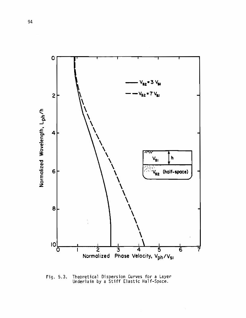
94
.1: ...... .1: Q.
....J .
.1: -0' c: Q.l
"ii· > c ~ -c Q.l N -c E ... 0 z
V52•3 V11
2 ~ --v12 •7V11
\ \ \ \ \ 4 \ \ \ \ I"AV
\ v,. h
\ ·.·:: ... · ..
6 \ .·:.:. v. (half-space)
\ \.. S2
\ \ \
8 \ \ \ \ \
10 0
Normalized
Fig. 5.3. Theoretical Dispersion Curves for a Layer Underlain by a Stiff Elastic Half-Space.
7

95
layer. At short wavelengths, the phase velocities are close to the R-wave
velocity of the top layer. In other words, for waves with short wavelengths (relative to the height of the layer) the half-space has very little effect on
the dispersion curve. Hence, for these short wavelengths, the top layer acts
like a half-space by itself.
The other extreme involves long wavelengths (say eight to ten times the
thickness of the top 1 ayer and 1 anger). In this case phase ve 1 oci ties are
quite close to the R-wave velocity of the rock which means that the top layer
does not have an appreciable affect on the dispersion curve. However, between
these two extremes there is a transition zone in which the phase velocity is
greater than the R-wave ve 1 oc i ty of the top 1 ayer and 1 ess than the R-wave
velocity of the half-space.
The extent of this transition zone in the intermediate wavelengths
depends on the velocity contrast between the layers. This point is
illustrated by the dashed 1 ine in Fig. 5.3 which represents the dispersion
curve for the same 1 ayeri ng used in the examp 1 e above except that the shear
wave velocity of the half-space is seven times greater than that of the top
layer. For the first case (1:3), the transition zone is from about a
normalized wavelength of one to eight, and the phase velocity is approximately
equal to R-wave velocity of the half-space at a wavelength of ten. In the
second case (1:7), in which the half-space is about 50 times stiffer than the
soil layer, at a normalized wavelength of ten, phase velocity is only on the
order of 70 percent of the R-wave velocity of the half-space. In this case,
at short wavelengths phase velocities are about the same as the first case (1:3); however, phase velocities become close to the R-wave velocity of the
half-space at much longer wavelengths (about a normalized wavelength of 20). The same trend is true in the case of a high-velocity layer, say
concrete, underlain by a softer half-space (soil). Dispersion curves
corresponding to the the same layering as used in the first example (Fig.
5.3), except that now the ratios of the shear wave velocities of the layers
are reversed, are shown in Fig. 5.4. In the first case the velocity ratio is
equal to seven (dashed line). This velocity contrast corresponds to a ratio
of elastic moduli of approximately 50 for equal mass densities and Poisson's
ratios. The dispersion curve consists of two branches. The branch marked as
I is similar to the dispersion curve for the flexural mode of a plate (see

96
.c ..... .c a.
2
..J 4
.s:! -Cl c Cl,) -Cl,) >
~ "'0 6 Cl,) N ·-0 E ,_ 0 z
8
I I I I I I ,,
I I I I I I I
I@ I I I
'
/ /
/ /
/ /
/
/
®/'
I
,' I
/
// /
h
---Vsi=7Vs2
---V11 =3Vt2
Normalized Phase Velocity, V ph/Vs2
Fig. 5.4. Theoretical Dispersion Curves for a Stiff Layer Underlain by an Elastic Half-Space.
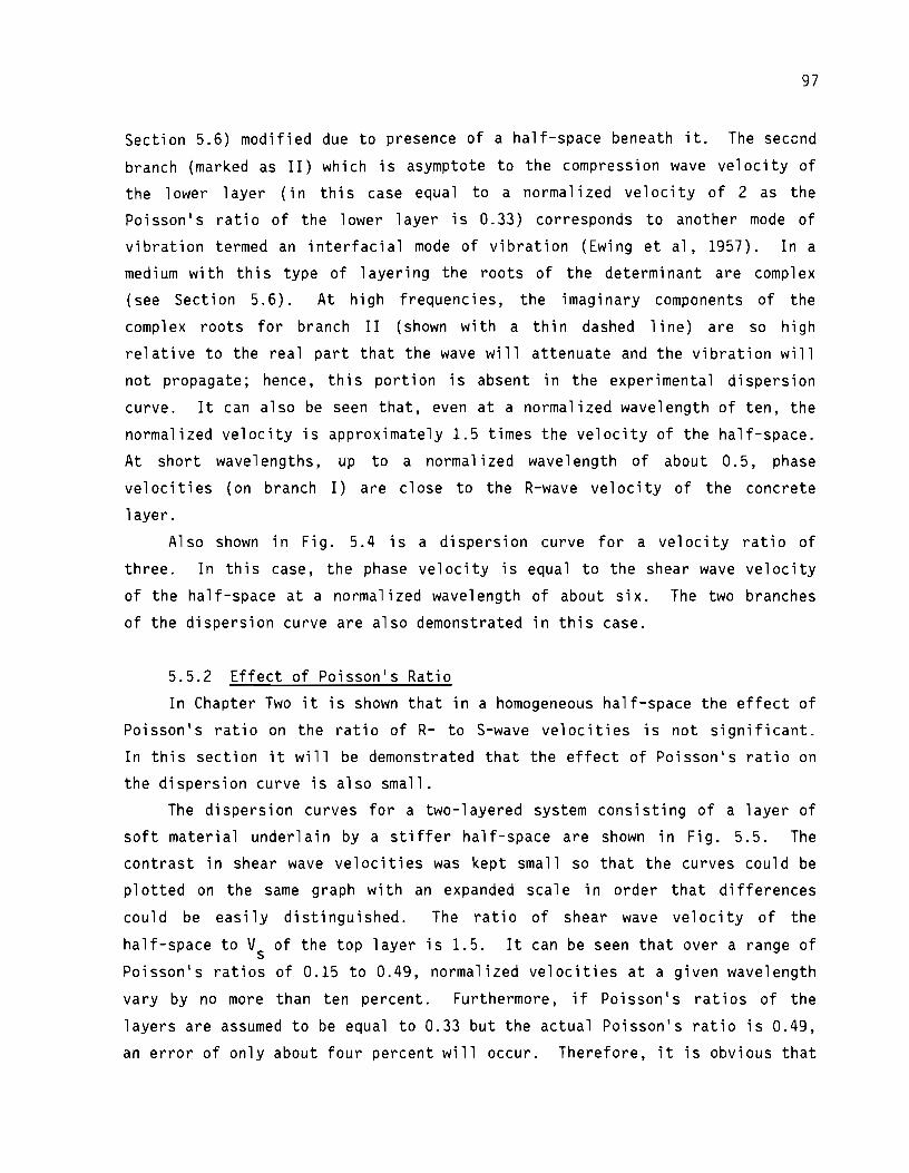
97
Section 5.6) modified due to presence of a half-space beneath it. The second
branch (marked as II) which is asymptote to the compression wave velocity of
the lower layer (in this case equal to a normalized velocity of 2 as the
Poisson's ratio of the lower layer is 0.33) corresponds to another mode of
vibration termed an interfacial mode of vibration (Ewing et al, 1957). In a
medium with this type of layering the roots of the determinant are complex
(see Section 5.6). At high frequencies, the imaginary components of the
complex roots for branch II (shown with a thin dashed line) are so high
relative to the real part that the wave will attenuate and the vibration will
not propagate; hence, this portion is absent in the experimental dispersion
curve. It can also be seen that, even at a normalized wavelength of ten, the
normalized velocity is approximately 1.5 times the velocity of the half-space.
At short wave 1 engths, up to a norma 1 i zed wave 1 ength of about 0. 5, phase
velocities (on branch I) are close to the R-wave velocity of the concrete
layer.
Also shown in Fig. 5.4 is a dispersion curve for a velocity ratio of
three. In this case, the phase velocity is equal to the shear wave velocity
of the half-space at a normalized wavelength of about six. The two branches
of the dispersion curve are also demonstrated in this case.
5.5.2 Effect of Poisson's Ratio
In Chapter Two it is shown that in a homogeneous half-space the effect of
Poisson's ratio on the ratio of R- to S-wave velocities is not significant.
In this section it will be demonstrated that the effect of Poisson's ratio on
the dispersion curve is also small.
The dispersion curves for a two-layered system consisting of a layer of
soft material underlain by a stiffer half-space are shown in Fig. 5.5. The
contrast in shear wave velocities was kept small so that the curves could be
plotted on the same graph with an expanded scale in order that differences
could be easily distinguished. The ratio of shear wave velocity of the
half-space to Vs of the top layer is 1.5. It can be seen that over a range of
Poisson's ratios of 0.15 to 0.49, normalized velocities at a given wavelength
vary by no more than ten percent. Furthermore, if Poisson's ratios of the
layers are assumed to be equal to 0.33 but the actual Poisson's ratio is 0.49,
an error of only about four percent will occur. Therefore, it is obvious that

98
0 •
\ \ \ '· ,,.
'· ' .......... ........... ......... , ........... , '
' '· ' ' .c
' ' ..... .c
' Q.
' -I 4 \ .. \ .c
\ -0 c
' \ cu a> > v1• v2 • 0.15 \ c :c -- v1•v2 •0.33
\ \ 00 6 - ·- v1•v2•0.49 • cu
\ \ N ·--c \ E h Vsa• 111
\ ... ; 0 z
Vsz • 112 \ \. (half-space) .., \ ' 8
' .
' V12/V11 •1.5
' I I •
I 10 . 0.9 1.0 1.1 1.2 1.3 1.4
Normalized Phase Velocity. Vph/Vs,
Fig. 5.5. Effect of Poisson's Ratio on Dispersion Curve.

99
for practical applications one can select reasonable values for Poisson•s
ratio of the material in a pavement system without introducing significant
errors in the construction of the dispersion curve.
5.5.3 Effect of Mass Density
The effect of varying mass densities on the dispersion curve is on the
order of the effect of varying Poisson•s ratios. The absolute values of mass
densities of different layers do not affect the shape of the dispersion curve,
but the contrast in mass densities causes some changes in the curve. As an
example of this effect, consider the dispersion curves for a layer of softer
material underlain by a stiffer half-space (ratio of the shear velocities of
1.5) shown in Fig. 5.6. Two extreme cases are used. In the first case, the
mass densities of the two 1 ayers are equa 1 . In the second case, it was
assumed that the half-space has a mass density 1.5 times greater than that of
the top layer. The dispersion curves, as shown in Fig. 5.6, do not deviate
much, with the maximum difference on the order of six percent.
5.5.4 Effect of Layer Thicknesses
For a given profile if the thicknesses of all layers are changed by a
constant factor, the shape of the dispersion curve is not altered, but the
curve is scaled proportional to the constant factor. This point is
illustrated in Fig. 5.7 where the dispersion curves for several three-layered
systems are shown. The two top 1 ayers each have a thickness of h/2 so that
depth to the half-space is equal to h.
In the first case, the S-wave velocity of the second 1 ayer was assumed
equal to that of the half-space. This assumption resulted in a two-layered
system with the thickness of the top layer equal to h/2. The dispersion curve
for this system is shown by the solid line in Fig. 5.7. The wavelengths in
the figure are normalized relative to h (not h/2).
In the second case, the S-wave velocity of the intermediate layer (second
1 ayer) was changed to equa 1 the S-wave ve 1 oci ty of the first 1 ayer. The
profile in this case is identical to the profile of the first case, except
that the thickness of the top layer is now equal to h (twice as thick as the
first case). The dispersion curve for this profile is shown by the dashed
line in Fig. 5.7.

100
0
- Pa!Pz•l -- P./P. •2/3 I 2
2
J:. ...... J:. Q.
...J 4 .. J:. -CJ'I c .!! CD > 0
3= "'0 6 CD N -0 E ...
h 0 V51 , P1 z Vsz,Pz
8 (Half -space)
VsziVs, •1.5
10~----~~----~------~----~~----~ 0.9 1.0 1.1 1.2 I. 3 I. 4 Normalized Phase Velocity, Vph IV 51
Fig. 5.6. Effect of Mass Density on Dispersion Curve.

.1:!
' &r: ..J .. .1:! -0' c: Q,) -Q,)
> 0 ~
"0 Q,) N ·--0 E ... 0 z
0
2
4
6
8 \..
\ -- V51 =1/3V52=113 V55 -·- V51 =2/3V52 =1/3V55 --- V51=Vs2 = I/3Vss
\ . \\. \ ' \ .
\ ' ', '· ', ' ', \
', \
Vs1 h/2
Vs2 h/2
Vss Half-Space
', \ \ . \ \ \ . \ \ \ . \ \ \ . \ \ \ . \ \ \ . \ \ \ .
Normalized Phase Velocity, Vph/V51
Fig. 5.7. Effect of Layer Thickness on Dispersion Curve.
101

102
The shape of the two curves are quite similar. However, the curve from the first case (with a depth to the half-space of h/2) approaches the low-frequency asymptote, which is equal to the R-wave velocity of the
ha 1 f-space, at much shorter wave 1 engths. If the curve in this case had been normalized relative to h/2 {as oppose to h), the curves from the first and the second cases would have been identical.
The third curve shown in Fig 5.6 corresponds to a case where the S-wave
velocity of the second layer, Vs2, has an intermediate value, between vs1 and vs3. It can be seen that as the stiffness of the intermediate layer increases the dispersion curve is shifted towards higher phase velocities.
It should be mentioned that the curves in Figs. 5.2 and 5.6 for the case, where layering and shear wave velocities are identical (1:3 case), differ because different Poisson•s ratios were used. It should also be mentioned that it is not necessary to know layer thicknesses when inverting the measured dispersion curve. This section was included simply to show the effect of layer thickness on the dispersion curve.
5.6 DISCUSSION ON PROPAGATION OF SURFACE WAVES
The values of r2 and s2 (defined in Eqs. 5.11 and 5.12) in the
half-space, for say a two-layer system, play an important role with regard to the type of wave propagated. Different characteristics of motion can be expected depending upon va 1 ues of r2 and s2. If r and s are rea 1 ( i . e. , r2
and s2 are positive), which means that the S- and P-wave velocities are greater than the phase velocity, the roots of the dispersion equation are real and correspond to normal propagation modes of the surface waves. In this situation the waves propagate without attenuation as no material damping is incorporated in elastic theory.
If r2, s2, or both become negative, r or s will become imaginary which
will result in roots of the dispersion function which are imaginary and
analogous to leaky modes {Aki and Richards, 1980). In leaky modes the amplitudes of waves decay rapidly with distance from the source, and a
substantial amount of energy is transmitted to the adjacent layer. In soil sites the stiffness of different layers gradually increases with
depth so that normal modes of propagation of Rayleigh waves are anticipated.
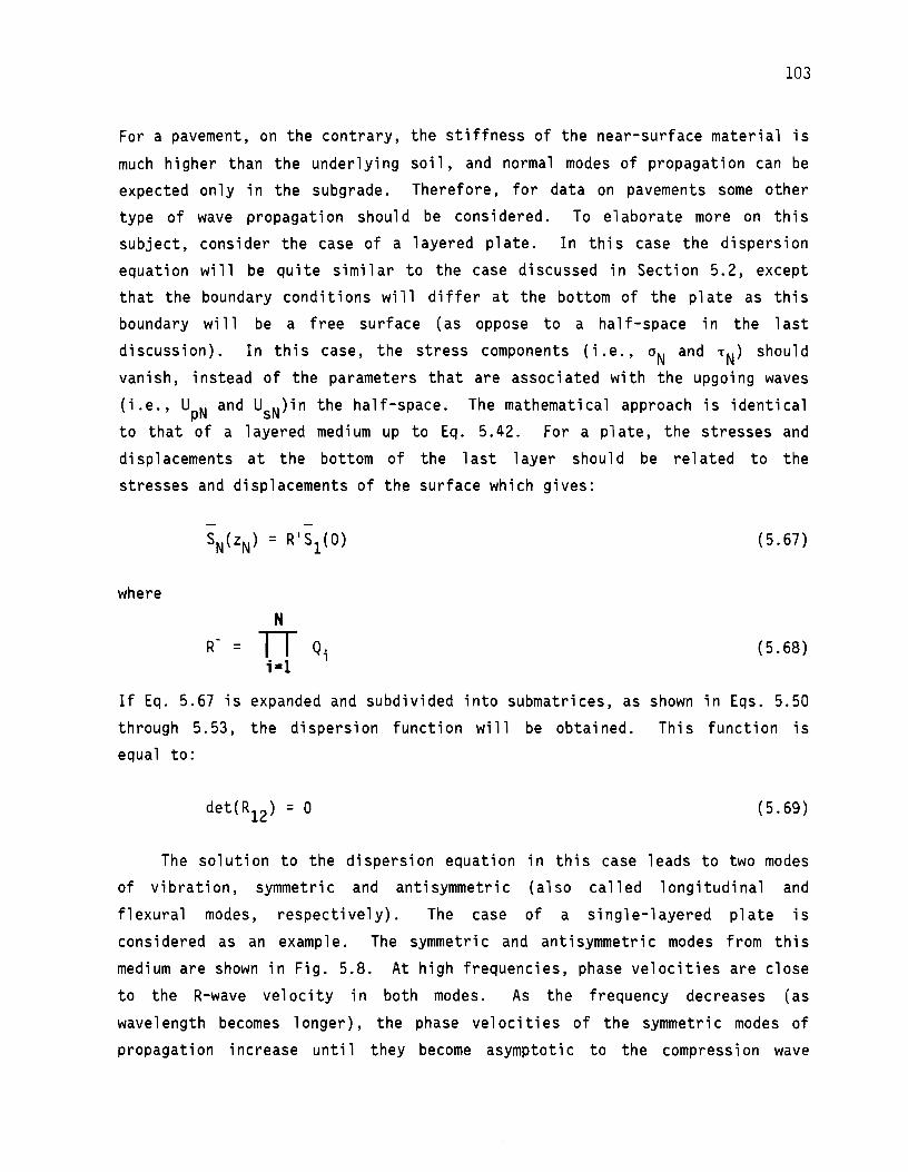
103
For a pavement, on the contrary, the stiffness of the near-surface material is
much higher than the underlying soil, and normal modes of propagation can be expected only in the subgrade. Therefore, for data on pavements some other type of wave propagation should be considered. To elaborate more on this subject, consider the case of a layered plate. In this case the dispersion
equation will be quite similar to the case discussed in Section 5.2, except that the boundary conditions will differ at the bottom of the plate as this boundary will be a free surface (as oppose to a half-space in the last
discussion). In this case, the stress components (i.e., oN and -rN) should vanish, instead of the parameters that are associated with the upgoing waves
(i.e., UpN and UsN)in the half-space. The mathematical approach is identical to that of a layered medium up to Eq. 5.42. For a plate, the stresses and displacements at the bottom of the last layer should be related to the stresses and displacements of the surface which gives:
(5.67)
where
N
R = TT Qi ;-1
(5.68)
If Eq. 5.67 is expanded and subdivided into submatrices, as shown in Eqs. 5.50 through 5.53, the dispersion function will be obtained. This function is equal to:
(5.69)
The solution to the dispersion equation in this case leads to two modes of vibration, symmetric and antisymmetric (also called longitudinal and
flexural modes, respectively). The case of a single-layered plate is
considered as an example. The symmetric and antisymmetric modes from this medium are shown in Fig. 5.8. At high frequencies, phase velocities are close
to the R-wave velocity in both modes. As the frequency decreases (as
wavelength becomes longer), the phase velocities of the symmetric modes of
propagation increase until they become asymptotic to the compression wave

104
~ ...... ~ Q.
....J .. ~ -01 c .!! cu > O· ;= -,:, cu ..... ·--0 E ... 0 z
o~---------------,-r----------------~
2.5
Antisymmetricol Mode
5~----------------~~----------------~ 0 2
Normalized Phose Velocity, Vph/V51
Fig. 5. 8. Schematic of Difference Modes of Propagation of Surface Waves in a Plate.

105
velocity of the plate. On the contrary, in the antisymmetric modes, phase
velocities decrease with decreasing frequencies to a minimum of zero. Meeker and Meitzler (1964) have a detailed discussion on the characteristics of
different modes, and the reader is referred to that paper for more
information. As the phase vel oci ties from experimenta 1 tests on pavements decrease
with decreasing wavelengths, modes similar to antisymmetric modes of
propagation in a plate can describe these systems more appropriately. To
analyze experimental data from systems with velocities greater than the
subgrade material, Thrower (1965) has shown that the assumption of a plate on
a half-space can be used adequately to model a pavement system.
5.7 SUMMARY
In this chapter, the Haskell-Thomson procedure for determining the
dispersion function (Eq. 5.54) is discussed. It is shown that at high
frequencies this procedure encounters numerical problems. The Dunkin
extension of the Haskell-Thomson formulation for solution of the dispersion
function at high frequencies is briefly presented. Finally, factors affecting
the dispersion function are examined. The main parameters affecting this
function are shear wave velocity, mass density and Poisson's ratio of the
material composing each layer. It is demonstrated that the effect of the last
two parameters is not significant and, in pract i ca 1 cases, is 1 ess than five
percent. Also the effect of intermediate layers is discussed. As the velocities of the intermediate layers increase, the dispersion curve is shifted towards higher phase velocities. The chapter is concluded with a
discussion of types of propagation expected to occur in a pavement system.


CHAPTER SIX. CONCLUSIONS
In this report the theoretical aspects of the SASW method are reviewed. It is shown that all steps taken to collect wave velocities in the field and to reduce the field data are based on sound theoretical principles and a minimal number of simplifying assumptions are used.
The theory of elastic wave propagation is utilized to determine the propagation velocity of surface waves. An introduction to wave propagation
theory is included. To perform the in situ tests more rapidly, spectral analysis and Fourier transform principles are utilized. An overview of
spectral analyses and the usefulness of each function are described. To determine meaningful modulus profiles as well as the thicknesses of
different layers, an algorithm required for determining modulus profiles from velocity of propagation of surface waves from different wavelengths has been developed. The general process for which the algorithm is employed is called inversion herein. The theory behind this algorithm is described in a logical and simplified manner in Chapter 5.
Overall, it is shown that all steps of the SASW method are based on sound theory, and the manner in which the test is performed and the data are reduced is consistent with the theoretical basis.
107


REFERENCES
1. Aki, K., and Richards, P.G. (1980), Quantitative Seismology, Theory and Methods, Vol. 1, W.H. Freeman and Company, San Francisco, 557 pp.
2. Anderson, D.G., and Woods, R.D. (1975), "Comparison of Field and Laboratory Shear Moduli," Proceedings, Conference on In Situ Measurement of Soil Properties, ASCE, Vol. I, Raleigh, North Carolina, pp. 69-92.
3. Baird, G.T. (1982), "Wave Propagation Method of Pavement Evaluation, .. New Mexico Engineering Research Institute, University of New Mexico, Albuquerque, New Mexico.
4. Ballard, R.F., Jr. (1964), 11 Determination of Soil Shear Moduli at Depths by In Situ Vibratory Techniques, 11 Miscellaneous Paper No. 4-691, U.S. Army Engineer Waterways Experiment Station, Vicksburg, Mississippi.
5. Ballard, R.F., Jr., and Casagrande, D.R. (1967), 11 Dynamic Foundation Investigations, TAA-2A Radar Site, Cape Kennedy, Florida," Miscellaneous Paper 4-87~, U.S. Army Engineer Waterways Experiment Station, Vicksburg, Mississippi.
6. Ballard, R.F., Jr., and Chang, F.K. (1973), 11 Rapid Subsurface Exploration; Review of Selected Geophysical Techniques," Miscellenaous Paper No. S-69-30, U.S. Army Engineer Waterways Experiment Station, Vicksburg, Mississippi.
7. Baker, T.G., and Stevens, J.L. (1983), "Shallow Shear Wave Velocity and Q Structures at the El Centro Strong-Motion Acce 1 erograph Array, 11
Geophysical Research Letters, Vol. 10, No.9, pp. 853-856.
8. Bergstrom, S.G., and Linderholm, S. (1946), 11 0ynamisk Metod att Utrona Ultiga Marklagers Genomsnittliga Elasticitetsegens kaper, 11 Handlinger NO. 1, Svenska Forsknings-Institutet for Cement och Betong Vid. Kungl. Tekniska, Hogskolan.
9. Bolt, B.A. (1976), Nuclear Explosions and Earthquakes, W.H. Freeman and Co., San Francisco, 309 pp.
10. Borm, G.W. (1978), "Methods from Exploration Seismology: Reflection, Refraction and Boreho 1 e Prospecting, 11 Proceedings of the Conference on Dynamical Methods in Soil and Rock Mechanics, Karlsruhe, Germany, Vol. Ill, pp. 87-114.
11. Brigham, E.O. (1974), The Fast Fourier Transform, Prentice-Hall, Inc., Englewood Cliffs, New Jersey, 253 pp.
12. Chen, L.S. (1948), 11 An Investigation of Stress-Strain and Strength Characteristics of Cohesionless Soils by Triaxial Compression Tests." Proceedings, Second International Conference on Soil Mechanics and Foundation Engineering, Rotterdam, Vol. V.
109
110
13. Cunny, R.W., and Fry, Z.B. (1973), "Vibratory In Situ and Laboratory Soil Moduli Compared," Journal of the Soil Mechanics and Foundations Division, ASCE, Vol. 99, No. SM12, pp. 1055-1076.
14. DEGEBO (1938), "Deutsche Gesellschaft fur Bodenmechanik," Vol. 4, Springer, Berlin.
15. Dunkin, J.W. (1965), "Computation of Modal Solutions in Layered, Elastic· Media at High Frequencies," Bulletin of Seismological Society of America, Vol. 55, No.2, pp. 335-358.
16. Eagleson, B., Heisey, J.S., Hudson, W.R., Meyer, A.H., and Stokoe, K.H., II (1981), "Comparison of Falling Weight Deflectometer and Dynaflect for Pavement Evaluation," Report No. 256-1, Center for Transportation Research, University of Texas, Austin, Texas.
17. Ewing, W.H., Jardetzky, W.S., and Press, L.C.R. (1957), Elastic Waves in Layered Media, McGraw-Hill Book Company, New York, 380 pp.
18. Fry, Z.B. (1965), 11 Dynamic Soils Investigations Project Buggy, Buckboard Mesa Nevada Test Site, Mercury, Nevada, 11 Miscellaneous Paper No. 4-666~ U.S. Army Engineer Waterways Experiment Station, Vicksburg, Mississippi.
19. Haas, R., and Hudson, W.R. (1978), Pavement Management Systems, McGraw Hill Book Co., New York, New York, 456 pages.
20. Haskell, N.A. (1953), "The Dispersion of Surface Waves in Multilayered Media, 11 Bulletin of Seismological Society of America, Vol. 43, No. 1, pp. 17-34.
21. Hardin, B.O. (1978), "The Nature of Stress-Strain Behavior in Soils, 11
Proceedings, Conference on Earthquake Engineering and Soil Dynamics, ASCE, Pasadena, California, Vol. I.
22. Hardin, B.O., and Drnevich, V.P. (1972), "Shear Modulus and Damping in Soils: Measurement and Parameter Effects," Journal of the Soil Mechanics and Foundations Division, ASCE, Vol. 95, No. SM6, pp. 603-624.
23. Heisey, J.S., Stokoe, K.H., II, Hudson, W.R., and Meyer, A.H. (1982), "Determination of In Situ Shear Wave Velocities from Spectral Analysis of Surface Waves," Research Report 256-2, Center for Transportation Research, The University of Texas at Austin, 277 pp.
24. Heukelom, W., and Klomp, J.G. (1962), "Dynamic Testing as a Means of Controlling Pavements During and After Construction," Proceedings, International Conference on Structural Design of Asphalt Pavements, Ann Arbor, Michigan, pp. 495-510.
25. Hewellet Packard (1981), 11 The Fundamentals of Signal Analysis," Application Note 243, Hewellet Packard Co., USA, 57 pages.

111
26. Hoar, R.J. (1982), "Field Measurement of Seismic Wave Velocity and Attenuation for Dynamic Analyses," Ph.D. Dissertation, The University of Texas, Austin, Texas, 479 pages.
27. Jones, R. (1958), 11 ln Situ Measurment of the Dynamic Properties of Soil by Vibration Methods, 11 Geotechnique, Vol. III, No. 1.
28. Knopoff, L. (1964), 11 A Matrix Method for Elastic Wave Problems, 11 Bulletin of Seismological Society of America, Vol. 54, No. 1, pp. 431-438.
29. Krizek, R.J. (1977), 11 Fabric Effects on Strength and Deformation of Kaolin Clay," Proceedings, Ninth International Conference on Soil Mechanics and Foundation Engineering, Tokyo, Japan, Vol. I.
30. Lamb, H. (1904), "On the Propagation of Tremors Over the Surface of an Elastic Solid," Philosophical Transactions of the Royal Society of London, Vol. A203, pp. 1-42.
31. Lytton, R.L., Moore, W.M., and Mahoney, J.P. (1975), "Pavement Evaluation: Phase I, Pavement Evaluation Equipment," Report No. FHWA-RD-75-78, Federal Highways Administration, Washington, D.C.
32. Maxwell, A.A., and Fry, F.B. (1967), 11 A Procedure for Determining Elastic Modul of In Situ Soils by Dynamic Techniques," Proceedings, International Symposium on Wave Propagation and Dynamic Properties of Earth Materials, Albuquerque, New Mexico, pp. 913-920.
33. Meeker, T.R., and Meitzler, A.H. (1964), Physical Acoustics, Vol .1, Part A, Academic Press, New York, New York, pp. 111-167.
34. Miller, G.F., and Pursey, H. (1955), "On the Partition of Energy Between Elastic Waves in a Semi-Infininte Solid, 11 Proceedings, Royal Society of London, A, vol. 233, pp. 55-69.
35. Nazarian, S. (1984), 11 In Situ Determination of Elastic Moduli of Soil Deposits and Pavement Systems by Spectra l-Ana 1 ys is-of-Surface-Wave Method, 11 Ph.D. Dissertation, The University of Texas at Austin, 446 pp.
36. Nazarian, S., Stoko~, K.H., II, and Hudson, W.R. (1983), "Use of Spectral Analysis of Surface Waves for Determination of Moduli and Thicknesses of Pavement Systems, 11 Transportation Research Record, No. 945, Washington, D.C., pp. 38-45.
37. Nazarian, S., and Stokoe, K.H., II (1985), "In Situ Determination of Elastic Moduli of Pavement Systems by Spectral-Analysis-of-Surface -Waves Method (Practical Aspects," Research Report 368-1F, Center for Transportation Research, The University of Texas at Austin, 161 pp.

112
38. Nazarian, S., and Stokoe, K.H., II (1986a), 11 Analytical Study of the Sensitivity of the Falling Weight Deflectometer Device to Determining Moduli of Farm-to-Market Roads," Technical Memorandum No. lAC (86-87) 0936-3, Center for Transportation Research, The University of Texas at Austin, 28 pp.
39. Nazarian, S., and Stokoe, K.H., II (1986b), 11 Evaluation of the Sensitivity of the SASW Method in Determining Thicknesses of Layers in Pavement Systems, 11 Technical Memorandum No. lAC (86-87) 0946-4, Center for Transportation Research, The University of Texas at Austin, 42 pp.
40. Nazarian, S., and Stokoe, K.H., II (1986c), 11 Users Guide for Interactive Program "INVERT 11 Used in INversion of Dispersion Curves," Research Report 1123-1, Center for Transportation Research, The University of Texas at Austin, (in press).
41. Neilson, J.R., and Baird, G.T. (1975), "Air Force System for Nondestructive Tsting of Pavements, 11 Symposium on Nondestructive Testing and Evaluation of Airport Pavements, Vicksburg, Mississippi.
42. Neilson, J.P., and Baird, G.T. (1977), "Evaluation of an Impulse Testing Technique for Nondestructive Testing of Pavements, 11 Research Report CEEDO-TR-77-46, Tyndall Air Force Base, Panama City, Florida.
43. Nijober, L.W., and Van der Poel, C. (1953), "A Study of Vibration Phenomena in Asphaltic Road Construction, .. Proceedings, Association of Asphaltic Pavement Technology, pp. 197-231.
44. Ogura, K. (1979), "Development of a Suspension TypeS-Wave Log System," Technical Note TN-34, OYO corporation, Tokyo, Japan, 23 pp.
45. Patel, N.S. (1981), "Generation and Attenuation of Seismic Waves in Downhole Testing, 11 M.S. Thesis, The University of Texas, Austin, Texas, 411 pp.
46. Rayleigh, L. (1887), "On Waves Propagated Along the Plane Surface of an Elastic Solid, 11 Proceedings, London Mathematical Society, Vol. 17, pp. 4-11.
47. Redpath, B.B. (1973), "Seismic Refraction Exploration for Engineering Site Investigation, 11 Report TRE-73-4, U.S. Army Engineer Waterways Experiment Station, Corps of Engineers, Vicksburg, Mississippi, 52 pp.
48. Richart, F .E., Jr., Hall, J.R., Jr., and Woods, R.D. (1970), Vibrations of Soils and Foundations, Prentice-Hall, Inc., Englewood Cliffs, New Jersey, 414 pp.
49. Schwab, F., and Knopoff, L. {1970), 11 Surface Wave Dispersion Computations," Bulletin of Seismological Society of America, Vol. 60, No. 2, pp. 321-344.

113
50. Shao, K-Y, Roesset, J.M., and Stokoe, K.H., II, (1986), "Dynamic Interpreation of Dynaflect and Falling Weight Deflectometer Tests on Pavement Systems," Research Report Number 437-1, Center for Transportation Research, The University of Texas, Austin, Texas, {in press).
51. Sheriff, R.E. (1982), Encyclopedia Dictionary of Exploration Geophysics, Society of Exploration Geophysicists Publication, Tulsa, 266 pp.
52. Stokoe, K.H., II, and Chen, A.T.F. (1980), "Effects on Site Response of Methods of Estimating In Situ Soil Behavior," Proceedings, Seventh World Conference on Earthquake Engineering, Turkey.
53. Stokoe, K.H., II, and Hoar, R.J. (1978), "Variables Affecting in Situ Seismic Measureements," Proceedings, Conference on Earthquake Engineering and Soil Dynamics, ASCE, Pasadena, California, Vol. II, pp 919-939.
54. Stokoe, K.H., II, and Lodde, P.F. (1978), "Dynamic Response of San Francisco Bay Mud," Proceedings, Conference on Earthquake Engineering and Soil Dynamics, ASCE, Pasadena, California, Vol. II, pp. 940-959.
55. Stokoe, K.H., II, and Woods, R.D. (1972), 11 In Situ Shear Wave Velocity by Cross-Hole Method," Journal of the Soil Mechanics and Foundations Division, ASCE, Vol. 98, No. SM5, pp. 443-460.
56. Thomson, W.T. (1950), "Transmission of Elastic Waves Through a Stratified solid Medium," Journal of Sound Vibration, Vol. 2, No. 3, pp. 210-226/
57. Thrower, E.N. (1965), "The Computation of the Dispersion of Elastic Waves in Layered Media," Journal of Sound Vibration, Vol. 2, No. 3, pp. 210-226.
58. Uddin, W., Nazarian, S., Hudson, W.R., Meyer, A.H., and Stokoe, K.H., II (1983), "Investigations into Dynaflect Deflections in Relation to Location/Temperature Parameters and In Situ Material Characterization of Rigid Pavements," Research Report 256-5, Center for Transportation Research, The University of Texas at Austin.
59. Van der Poel, C. (1951), "Dynamic Testing of Road Construction," Journal of Applied chemistry, Vol. 1, No. 7, pp. 281-290.
60. Van der Poel, C. (1954), "A General System Describing the Visco-Elastic Properties of Bitumens and Its Relation to Routine Test Data, 11 Shell Bitumen Reprint No. 9, Shell Laboratories-Komink-likeke.
61. Watson, T.H. (1970), "A Note on Fast Computation of Rayleigh Wave Dispersion in the Layered Elastic Half-Space," Bulletin of Seismological Society of america, vol. 60, No. 1, pp. 161-166.
62. Williams, 0. {1981), 11 Rayleigh Wave Velocity Measurements Using Broad Band Frequency Sources," Miscellaneous Paper EL-81-3, U.S. Army Engineer Waterways Experiment Station~ Vicksburg, Mississippi, 31 pp.

114
63. Woods, R.D., and Richart, F.E., Jr. (1967), "Screening of Elastic Surface Waves by Trenches, 11 Proceedings. Internati ana 1 Symposi urn on Wave Propagation and Dynamic Properties of Earth Materials, Albuquerque, New Mexico, pp. 275-290.
64. Yoder, E.J., and Witczack, M.W. (1975), 11 Principles of Pavement Design, John Wiley & Sons, Inc., New York, New York, 2nd Edition, 711 pp.