Scott Domains for Denotational Semantics andProgram Extraction

Ulrich BergerSwansea University

Workshop Domains

Oxford, 7-8 July 2018

1 / 46

Overview

1. Domains

2. Computability

3. Denotational semantics

4. Program extraction

5. Brouwer’s thesis

6. Concurrency and the law of excluded middle

2 / 46

Domains

From the abstract of Dana Scott’s

DOMAINS FOR DENOTATIONAL SEMANTICS (1982)

“The purpose of the theory of domains is to give models for spaceson which to define computable functions. . . .

. . . There are several choices of a suitable category of domains, butthe basic one which has the simplest properties is the onesometimes called consistently complete algebraic cpo’s. . . . ”

3 / 46

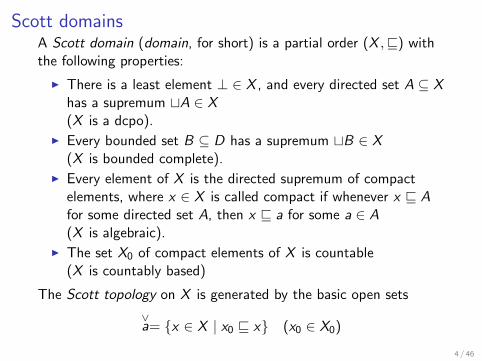
Scott domainsA Scott domain (domain, for short) is a partial order (X ,v) withthe following properties:

I There is a least element ⊥ ∈ X , and every directed set A ⊆ Xhas a supremum tA ∈ X(X is a dcpo).

I Every bounded set B ⊆ D has a supremum tB ∈ X(X is bounded complete).

I Every element of X is the directed supremum of compactelements, where x ∈ X is called compact if whenever x v Afor some directed set A, then x v a for some a ∈ A(X is algebraic).

I The set X0 of compact elements of X is countable(X is countably based)

The Scott topology on X is generated by the basic open sets

∨a= {x ∈ X | x0 v x} (x0 ∈ X0)

4 / 46

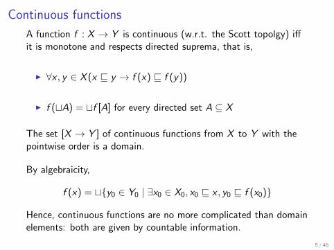
Continuous functions

A function f : X → Y is continuous (w.r.t. the Scott topolgy) iffit is monotone and respects directed suprema, that is,

I ∀x , y ∈ X (x v y → f (x) v f (y))

I f (tA) = tf [A] for every directed set A ⊆ X

The set [X → Y ] of continuous functions from X to Y with thepointwise order is a domain.

By algebraicity,

f (x) = t{y0 ∈ Y0 | ∃x0 ∈ X0, x0 v x , y0 v f (x0)}

Hence, continuous functions are no more complicated than domainelements: both are given by countable information.

5 / 46

The category of Scott domains

Scott domains and continuous functions form a cartesin closedcategory.

Cartesian closure essentially means the homeomorphism

[X × Y → Z ] ' [X → [Y → Z ]]

Due to the presence of ⊥ the category of domains doesn’t haveco-products but there are ’approximations’ to the co-product suchas the separated sum X + Y that adds a new bottom element tothe disjoint sum of X and Y .

6 / 46

Fixed points

Fixed point combinator

Every continuous endofunction f : X → X has a least fixed point

Y (f ) = tn∈Nf n(⊥) ∈ X

Moreover, Y : [X → X ]→ X is continuous.

Recursive domain equations

In the category DOMe of domains with embeddings everycontinuous endofunctor has a least fixed point up to isomorphism.

7 / 46

Reflexive domains

Scott was the first to construct a non-trivial domain D∞isomorphic to its own function space:

D∞ ' [D∞ → D∞]

This construction can be generalized using the fact that in DOMe

the continuous function space operation

(X ,Y ) 7→ [X → Y ]

is a continuous (co-variant!) functor in both arguments.

8 / 46

From DOMAINS FOR DENOTATIONAL SEMANTICS:

“ . . . This category of domains is studied in this paper from a new,and it is to be hoped, simpler point of view incorporating theapproaches of many authors into a unified presentation. Briefly,the domains of elements are represented set theoretically with theaid of structures called information systems. These systems arevery familiar from mathematical logic, and their use seems toaccord well with intuition. . . . ”

9 / 46

Information systemsInformation systems, roughly speaking, treat compact elements asthe primary objects and view the points of a domain as a derivedconcept (ideals of compacts).

Advantages (from my point of view):

I No category theory needed.

I ’Information system equations’ can be solved up to equality.

I Constructions like the universal domain become very easy.

I The finiteness of compact elements becomes obvious andequally obvious become the:

I notion of a continuous function,I notion of a computable domain element,I effectiveness of domain constructions,I effectiveness of the solutions to recursive domain equations.

Information system considerably influenced the foundations ofconstructive mathematics (e.g. in point-free topology).

10 / 46

Beyond Scott domainsMany variants of domains have been studied.

Weakening the axioms allows for more domain constructions, e.g.

I continuous domains (real interval domain),I SFP-domains (power domains),

. . . strengthening them or adding structure yields refinements, e.g.I coherence spaces (linear logic/functions),I stable domains (sequentiality)I qualitative domainsI probabilistic domainsI richer topology (negative information, Lawson Topology)

Other directions, e.g.:

I Domain-theoretic models of exact real number computationI Stone dualityI Synthetic domain theoryI Domain theory in logical formI Equilogical spaces

11 / 46

Computabilityx ∈ X is computable if the set of its compact approximations

{x0 ∈ X0 | x0 v x}

is recursively enumerable (w.r.t. some coding of the compactelements).

Ershov (1977) related this notion of computability to his theory ofnumberings and showed its remarkable robustness:

I The computable elements of a domain admit a principlenumbering.

I Rice-Shapiro Theorem (1959): A set of computable domainelements is completely enumerable iff it is effectively open.

I Myhill-Sheperdson Theorem (1959): A function on thecomputable elements of a domain is an effective operation iffit is effectively continuous

12 / 46

Partial continuous functionals

Due to cartesian closure, domains provide a natural model ofpartial higher-type functionals:

D(0) = N⊥ = the flat domain of natural numbers.

D(ρ→ σ) = [D(ρ)→ D(σ)]

Plotkin 1977: A partial continuous functional is effectivelycontinuous (computable as a domain element) iff it can be definedin PCF (basic arithmetic, λ-calculus, recursion (Y )) extended bythe functions

I parallel or (1 ∨ ⊥ = ⊥∨ 1 = 1, 0 ∨ 0 = 0)

I continuous existential (∃2(f ) = 1 if f (n) = 1, ∃2(f ) = 0 iff (⊥) = 0).

13 / 46

Total continuous functionals

Ershov 1977: The hereditarily total continuous functionalscoincide with the Kleene-Kreisel countable/continuousfunctionals.

Kreisel-Lacombe-Shoenfield 1959/Ershov 1976: Thehereditarily computably total continuous functionals coincidewith hereditarily effective operations (HEO). See alsoSpreen/Young 1984 for this result in a topological setting.

Normann 2000: A total continuous functional is computable(as a domain element) iff it is PCF-definable.

14 / 46

Program semantics

Consider a programming language with a given operationalsemantics, e.g. LCF.

Denotational semantics interprets a program M as an element [[M]]of a domain.

Goals:

I Computational Adequacy: If [[M]] = d for some data, thatis, discrete defined value d , then the computation of Mterminates with result d .

I Full abstraction If M and N are operationally equivalent inall contexts, then [[M]] = [[N]].

15 / 46

Program semantics (some results)

I Plotkin 1977: Scott domains are computationally adequate forPCF + ∨ + ∃2 with a call-by-name operational semantics.

I Plotkin 1977: Scott domains are fully abstract for PCF + ∨ .

[Proof: The functions [[M]] and [[N]] are continuous and hencecomplete determined by their values at compact arguments.The latter are definable in PCF+ ∨ ]

I Fully abstract models of PCF: Milner (syntactic, 1977),Abramsky, Jagadeesan, Malacaria, Hyland, Ong, Nickau(games, 1994), Bucciarelli, Ehrhard, Curien, Berry, Jung,Stoughton, McCusker, . . .

16 / 46

Program semantics (II)

I B 2005: Strong computational adequacy for PCF with strictdomain semantics: If [[M]]s 6= ⊥, then M is stronglynormalizing.

I Coquand, Spiwack 2006: Strong computational adequacy forDependent Type Theory using a reflexive domain.

I B 2009/2018: Computational adequacy for extensions of typefree PCF using a suitable reflexive domain.

The proofs use compact domain elements as a substitute for finitetypes. Induction on types is replaced by induction on the rank of acompact element, rk(x0) ∈ N.

(1) rk(Pair(x0, x1)) > rk(xi ).(2) rk(Fun(f0)) > rk(f0(x)) and f0(x) = f0(x0) for some compact

x0 v x .17 / 46

Program Extraction

The Curry-Howard correspondence states that intuitionistic proofscorrespond to programs.

Kleene’s realizability:

From a proof of a formula A one can extract a number e such that{e} realizes A.

({e} is the partial recursive fuction with index e)

We work with a similar notion of realizability but our realizers areelements of the domain

D ' Nil{}+ Pair(D × D) + Fun([D → D]).

18 / 46

Soundness

Soundness Theorem

From a proof of A one can extract a program M (in untyped PCF)such that [[M]] (∈ D) realizes A.

Proof. Induction on proofs using the equational theory of D andthe denotational semantics of programs.

Program Extraction Theorem

From a proof of a Σ-formula A one can extract a program Mevaluating to a data d realizing A.

Proof. Take the program from the Soundness Theorem and applycomputational adequacy.

19 / 46

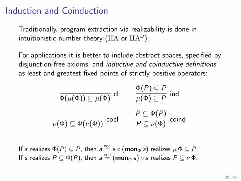
Induction and Coinduction

Traditionally, program extraction via realizability is done inintuitionistic number theory (HA or HAω).

For applications it is better to include abstract spaces, specified bydisjunction-free axioms, and inductive and coinductive definitionsas least and greatest fixed points of strictly positive operators:

Φ(µ(Φ)) ⊆ µ(Φ)cl

Φ(P) ⊆ P

µ(Φ) ⊆ Pind

ν(Φ) ⊆ Φ(ν(Φ))cocl

P ⊆ Φ(P)

P ⊆ ν(Φ)coind

If s realizes Φ(P) ⊆ P, then arec= s ◦ (monΦ a) realizes µΦ ⊆ P.

If s realizes P ⊆ Φ(P), then arec= (monΦ a) ◦ s realizes P ⊆ ν Φ.

20 / 46

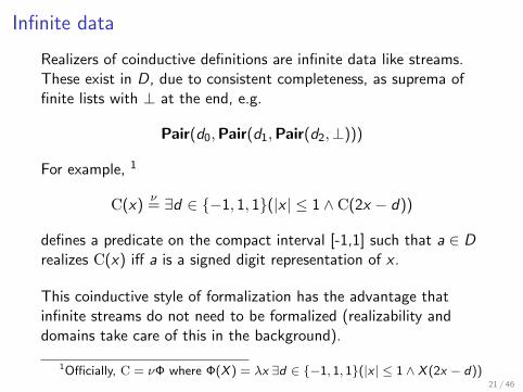
Infinite data

Realizers of coinductive definitions are infinite data like streams.These exist in D, due to consistent completeness, as suprema offinite lists with ⊥ at the end, e.g.

Pair(d0,Pair(d1,Pair(d2,⊥)))

For example, 1

C(x)ν= ∃d ∈ {−1, 1, 1}(|x | ≤ 1 ∧ C(2x − d))

defines a predicate on the compact interval [-1,1] such that a ∈ Drealizes C(x) iff a is a signed digit representation of x .

This coinductive style of formalization has the advantage thatinfinite streams do not need to be formalized (realizability anddomains take care of this in the background).

1Officially, C = νΦ where Φ(X ) = λx ∃d ∈ {−1, 1, 1}(|x | ≤ 1 ∧ X (2x − d))21 / 46

PE in constructive analysisBased on coinductive specifications of real numbers andcontinuous real functions parts of constructive analysis have beenfomalized, implemenmted and programs extracted.

See for example:

B, Kenji Miyamoto, Helmut Schwichtenberg, Monika Seisenberger.Minlog - A Tool for Program Extraction for Supporting Algebra andCoalgebra. LNCS 6859, 2011.

Fredric Forsberg, Kenji Miyamoto, Helmut Schwichtenberg. ProgramExtraction from Nested Definitions. LNCS 7988, 2013.

B., Kenji Miyamoto, Helmut Schwichtenberg, Hideki Tsuiki. A Logic forGray-code computation. In: Concepts of Proof in Mathematics,Philosophy, and Computer Science, de Gruyter, 2016.

B., Dieter Spreen. A Coinductive Approach to Computing with CompactSets. Journal of Logic and Analysis 8, 2016.

22 / 46

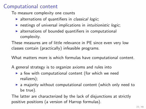
Computational contentTo measure complexity one counts

I alternations of quantifiers in classical logic;

I nestings of universal implications in intuitionistic logic;

I alternations of bounded quantifiers in computationalcomplexity.

These measures are of little relevance in PE since even very lowclasses contain (practically) infeasible programs.

What matters more is which formulas have computational content.

A general strategy is to organize axioms and rules into

I a few with computational content (for which we needrealizers);

I a majority without computational content (which only need tobe true).

The latter are characterized by the lack of disjunctions at strictlypositive positions (a version of Harrop formulas).

23 / 46

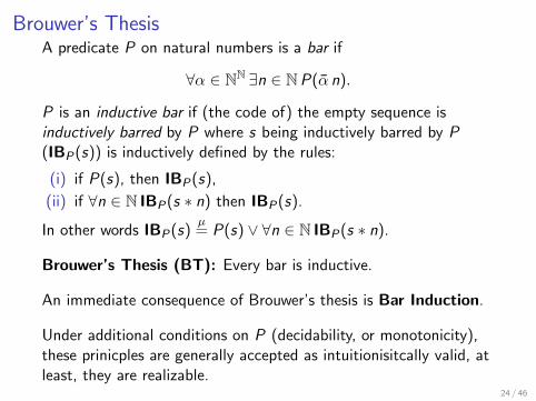
Brouwer’s ThesisA predicate P on natural numbers is a bar if

∀α ∈ NN ∃n ∈ NP(α n).

P is an inductive bar if (the code of) the empty sequence isinductively barred by P where s being inductively barred by P(IBP(s)) is inductively defined by the rules:

(i) if P(s), then IBP(s),

(ii) if ∀n ∈ N IBP(s ∗ n) then IBP(s).

In other words IBP(s)µ= P(s) ∨ ∀n ∈ N IBP(s ∗ n).

Brouwer’s Thesis (BT): Every bar is inductive.

An immediate consequence of Brouwer’s thesis is Bar Induction.

Under additional conditions on P (decidability, or monotonicity),these prinicples are generally accepted as intuitionisitcally valid, atleast, they are realizable.

24 / 46

Problems with BT

Brouwer’s thesis

∀α ∈ NN ∃n ∈ NP(α n) → IBP(〈〉)

has a few disadvantages (from the viewpoint of PE):

1. It has computational content, which, however, is useless.

2. It is confined to arithmetic.

3. Its premise and conclusion are both too strong for manyapplications.

25 / 46

An abstract and non-computational version of BTThe accessible part of a binary relation ≺, is defined inductively by

Acc≺(x)µ= ∀y ≺ x Acc≺(y)

Dually, the property of having a path through ≺ is definedcoinductively by

Path≺(x)ν= ∃y ≺ x Path≺(y)

The wellfounded part of ≺ is defined as the complement of Path≺,

Wf≺(x)Def= ¬Path≺(x)

Connection with BT: Set s ≺ tDef= ¬P(s) ∧ ∃n ∈ N s = t ∗ n.

I If P is decidable, then IBP = Acc≺.

I Classically, if Wf≺(〈〉), then P is a bar.

Hence, we propose the axiom:

BT0 ∀x (Wf≺(x)→ Acc≺(x))26 / 46

Virtues of BT0

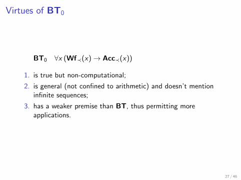
BT0 ∀x (Wf≺(x)→ Acc≺(x))

1. is true but non-computational;

2. is general (not confined to arithmetic) and doesn’t mentioninfinite sequences;

3. has a weaker premise than BT, thus permitting moreapplications.

27 / 46

Bar Induction

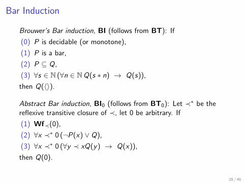
Brouwer’s Bar induction, BI (follows from BT): If

(0) P is decidable (or monotone),

(1) P is a bar,

(2) P ⊆ Q,

(3) ∀s ∈ N (∀n ∈ NQ(s ∗ n) → Q(s)),

then Q(〈〉).

Abstract Bar induction, BI0 (follows from BT0): Let ≺∗ be thereflexive transitive closure of ≺, let 0 be arbitrary. If

(1) Wf≺(0),

(2) ∀x ≺∗ 0 (¬P(x) ∨ Q),

(3) ∀x ≺∗ 0 (∀y ≺ xQ(y) → Q(x)),

then Q(0).

28 / 46

Further useful consequences of BT0

Markov’s principle: If P is decidable, then¬¬∃n ∈ NP(n) → ∃n ∈ NP(n)

[set in BT0, m ≺ n :Def= ¬P(n) ∧m = n + 1 and

QDef= ∃n ∈ NP(n)]

Wellfounded induction: If ∀x(∀y ≺ x P(y) → P(x)), then∀x ∈Wf≺ P(x).

Archimedean induction: If ∀x 6= 0 ((|x | ≤ 1→ Q(2x))→ Q(x)),then ∀x 6= 0Q(x).

[set y ≺ x :Def= |x | ≤ 1 ∧ y = 2x and use the (non-computational)

Archimedean property (∀n ∈ N|x | ≤ 2−n → x = 0) to show that∀x 6= 0Wf≺(x). ]

Feeling: All useful realizable principles can be split into anon-computational part (such as BT0) and an instance ofinduction or coinduction.

29 / 46

Concurrency and LEM (j.w.w. Hideki Tsuiki)

The starting point for this work was:

Hideki Tsuiki. Real Number Computation through Gray CodeEmbedding. TCS 284(2):467–485, 2002.

I Infinite Gray code for real numbers admits one undefined digit.

I This requires programs with two concurrently operatingreading heads with possibly nondeterministic results (IM2machines).

I Can such programs be extracted from proofs?

30 / 46

Parallelism in Exact Real Number Computation

I Potts, Edalat, Escardo noticed in 1997 that computing withthe interval domain as a model of real numbers appears torequire a parallel if-then-else operation.

I In fact, this parallelism is unavoidable (Escardo, Hofmann,Streicher, 2004).

Computing with TTE representations (e.g. Cauchy- or signeddigit representation) does not require parallelism, while Graycode (though very similar to signed digits) requires parallelism.

I Denotational models of nondeterministic computation arewell-known in Domain Theory (starting with Plotkin’spowerdomain 1976) and Relational Semantics (Bucciarelli,Ehrhard, Manzonetto 2011).

31 / 46

Concurrency and partiality

Given: Processes p1, p2 such that

I at least one pi is guaranteed to terminate,

I each terminating pi will produce a correct result

Task: Combine the pi to obtain a correct result.

Solution: Run p1, p2 concurrently. As soon as one pi terminates,deliver the result and kill p3−i .

We will introduce an extension of intuitionistic logic enabling theextraction of such kind of programs (together with correctnessproofs).

32 / 46

Logic and program for concurrency

I We add a new formula construct A1 ∨p

A2 which admitsconcurrent processes as realizers . . .

I . . . and add a new program constructor Amb(a1, a2) for theconcurrent execution of the processes ai (motivated byMcCarthy’s Amb).

I Amb(a1, a2) realizes A1 ∨p

A2 iff at least one ai is defined and,if defined, ai realize Ai .

33 / 46

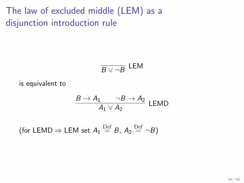
The law of excluded middle (LEM) as adisjunction introduction rule

B ∨ ¬B LEM

is equivalent to

B → A1 ¬B → A2

A1 ∨ A2LEMD

(for LEMD⇒ LEM set A1Def= B, A2

Def= ¬B)

34 / 46

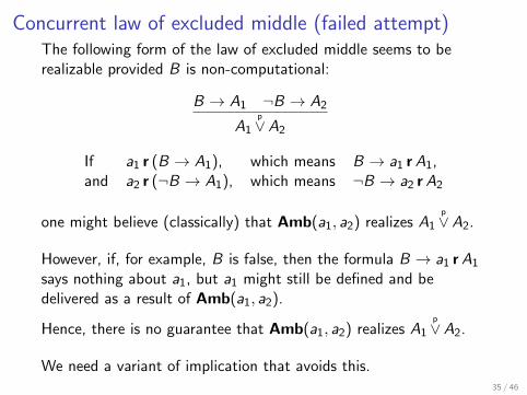
Concurrent law of excluded middle (failed attempt)The following form of the law of excluded middle seems to berealizable provided B is non-computational:

B → A1 ¬B → A2

A1 ∨p

A2

If a1 r (B → A1), which means B → a1 rA1,and a2 r (¬B → A1), which means ¬B → a2 rA2

one might believe (classically) that Amb(a1, a2) realizes A1 ∨p

A2.

However, if, for example, B is false, then the formula B → a1 rA1

says nothing about a1, but a1 might still be defined and bedelivered as a result of Amb(a1, a2).

Hence, there is no guarantee that Amb(a1, a2) realizes A1 ∨p

A2.

We need a variant of implication that avoids this.35 / 46

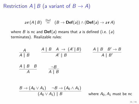
Restriction A ||B (a variant of B → A)

a r (A ||B)Def= (B → Def(a)) ∧ (Def(a)→ a rA)

where B is nc and Def(a) means that a is defined (i.e. {a}terminates). Realizable rules:

AA || B

A || B A → (A′ ||B)

A′ || BA || B B ′ → B

A || B ′

A || B B

A¬B

A || B

B → (A0 ∨ A1) ¬B → (A0 ∧ A1)

(A0 ∨ A1) || B where A0,A1 must be nc

36 / 46

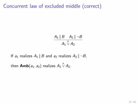
Concurrent law of excluded middle (correct)

A1 ||B A2 || ¬BA1 ∨

p

A2

If a1 realizes A1 ||B and a2 realizes A2 || ¬B,

then Amb(a1, a2) realizes A1 ∨p

A2.

37 / 46

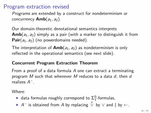
Program extraction revisedPrograms are extended by a construct for nondeterminism orconcurrency Amb(a1, a2).

Our domain-theoretic denotational semantics interpretsAmb(a1, a2) simply as a pair (with a marker to distinguish it fromPair(a1, a2) (no powerdomains needed).

The interpretation of Amb(a1, a2) as nondeterminism is onlyreflected in the operational semantics (see next slide).

Concurrent Program Extraction Theorem

From a proof of a data formula A one can extract a terminatingprogram M such that whenever M reduces to a data d , then drealizes A−.

Where:

I data formulas roughly correspond to Σ01-formulas,

I A− is obtained from A by replacing ∨p

by ∨ and || by ←.38 / 46

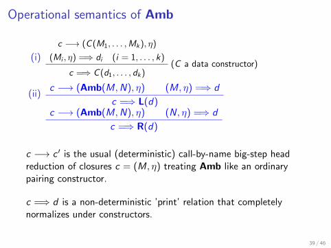
Operational semantics of Amb

(i)

c −→ (C (M1, . . . ,Mk), η)

(Mi , η) =⇒ di (i = 1, . . . , k)(C a data constructor)

c =⇒ C (d1, . . . , dk)

(ii)c −→ (Amb(M,N), η) (M, η) =⇒ d

c =⇒ L(d)c −→ (Amb(M,N), η) (N, η) =⇒ d

c =⇒ R(d)

c −→ c ′ is the usual (deterministic) call-by-name big-step headreduction of closures c = (M, η) treating Amb like an ordinarypairing constructor.

c =⇒ d is a non-deterministic ’print’ relation that completelynormalizes under constructors.

39 / 46

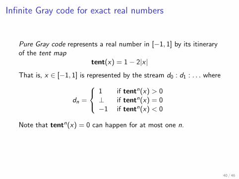
Infinite Gray code for exact real numbers

Pure Gray code represents a real number in [−1, 1] by its itineraryof the tent map

tent(x) = 1− 2|x |

That is, x ∈ [−1, 1] is represented by the stream d0 : d1 : . . . where

dn =

1 if tentn(x) > 0⊥ if tentn(x) = 0−1 if tentn(x) < 0

Note that tentn(x) = 0 can happen for at most one n.

40 / 46

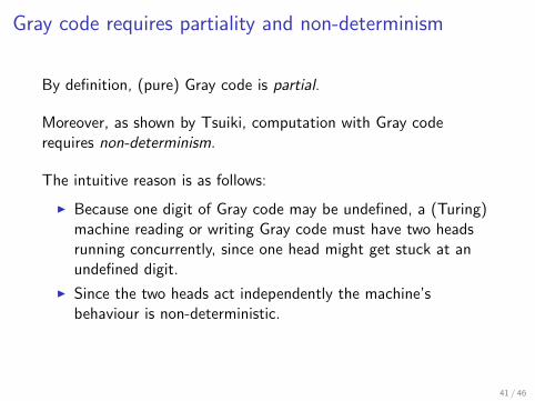
Gray code requires partiality and non-determinism

By definition, (pure) Gray code is partial.

Moreover, as shown by Tsuiki, computation with Gray coderequires non-determinism.

The intuitive reason is as follows:

I Because one digit of Gray code may be undefined, a (Turing)machine reading or writing Gray code must have two headsrunning concurrently, since one head might get stuck at anundefined digit.

I Since the two heads act independently the machine’sbehaviour is non-deterministic.

41 / 46

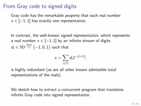
From Gray code to signed digits

Gray code has the remarkable property that each real numberx ∈ [−1, 1] has exactly one representation.

In contrast, the well-known signed representation, which representsa real number x ∈ [−1, 1] by an infinite stream of digits

di ∈ SDDef= {−1, 0, 1} such that

x =∑i∈N

di2−(i+1),

is highly redundant (as are all other known admissible totalrepresentations of the reals).

We sketch how to extract a concurrent program that translatesinfinite Gray code into signed representation.

42 / 46

From Gray code to signed digit representationWe write S(A) for A∨

p

A.

SDDef= {−1, 0, 1}

IdDef= [d/2− 1/2, d/2 + 1/2]

C(x)ν= ∃d ∈ SD (x ∈ Id ∧ C(2x − d))

C2(x)ν= S(∃d ∈ SD (x ∈ Id ∧ C2(2x − d)))

G(x)ν= (x 6= 0→ x ≤ 0 ∨ x ≥ 0) ∧G(tent(x))

s rC iff s is a signed digit representation of x .

s rG iff s is an infinite Gray code of x .

s rC2 iff s is a non-deterministic signed digit rep. of x .

C ⊆ G is easy. Our main goal is to show G ⊆ C2.43 / 46

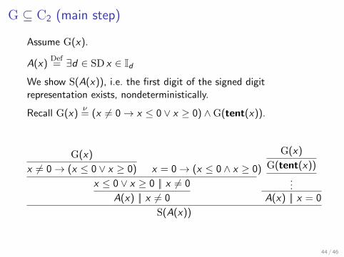
G ⊆ C2 (main step)

Assume G(x).

A(x)Def= ∃d ∈ SD x ∈ Id

We show S(A(x)), i.e. the first digit of the signed digitrepresentation exists, nondeterministically.

Recall G(x)ν= (x 6= 0→ x ≤ 0 ∨ x ≥ 0) ∧G(tent(x)).

G(x)

x 6= 0→ (x ≤ 0 ∨ x ≥ 0) x = 0→ (x ≤ 0 ∧ x ≥ 0)

x ≤ 0 ∨ x ≥ 0 || x 6= 0

A(x) || x 6= 0

G(x)

G(tent(x))

...A(x) || x = 0

S(A(x))

44 / 46

Conclusion

Domain theory is a work horse in program semantics and programextraction.

Without domains most of the work in program semantics andprogram extraction would have not been possible.

45 / 46

Thanks

Dear Professor Scott

Thanks for giving us domains!

Happy Birthday !!

46 / 46