denotational semantics - university of colorado boulderbec/courses/csci5535/reading/densem.pdf ·...
TRANSCRIPT
Denotational
Semantics____________________________________________________________________________
____________________________________________________________________________
____________________________________________________________________________
A METHODOLOGY FOR LANGUAGE DEVELOPMENT____________________________________________________________________________
____________________________________________________________________________
David A. Schmidt
Copyright notice: Copyright ! 1997 by David A. Schmidt. Permission to reproduce this
material must be obtained from the author.
Author’s address: David Schmidt, Department of Computing and Information Sciences, 234
Nichols Hall, Kansas State University, Manhattan, KS 66506. [email protected]
Contents
Preface viii
Chapter 0
INTRODUCTION ________________________________________________________________________________________________ 1
Methods for Semantics Specification 2
Suggested Readings 3
Chapter 1
SYNTAX ______________________________________________________________________________________________________________ 5
1.1 Abstract Syntax Definitions 9
1.2 Mathematical and Structural Induction 12
Suggested Readings 15
Exercises 15
Chapter 2
SETS, FUNCTIONS, AND DOMAINS ______________________________________________________________ 17
2.1 Sets 17
2.1.1 Constructions on Sets 18
2.2 Functions 20
2.2.1 Representing Functions as Sets 21
2.2.2 Representing Functions as Equations 24
2.3 Semantic Domains 25
2.3.1 Semantic Algebras 25
Suggested Readings 27
Exercises 27
Chapter 3
DOMAIN THEORY I: SEMANTIC ALGEBRAS ____________________________________________ 30
3.1 Primitive Domains 30
3.2 Compound Domains 34
3.2.1 Product 34
3.2.2 Disjoint Union 35
3.2.3 Function Space 39
3.2.4 Lifted Domains and Strictness 42iii
iv Contents
3.3 Recursive Function Definitions 44
3.4 Recursive Domain Definitions 46
3.5 Summary 46
Suggested Readings 48
Exercises 48
Chapter 4
BASIC STRUCTURE OF DENOTATIONAL DEFINITIONS ________________________ 54
4.1 The Valuation Function 54
4.2 Format of a Denotational Definition 57
4.3 A Calculator Language 59
Suggested Readings 63
Exercises 63
Chapter 5
IMPERATIVE LANGUAGES ____________________________________________________________________________ 66
5.1 A Language with Assignment 66
5.1.1 Programs are Functions 72
5.2 An Interactive File Editor 73
5.2.1 Interactive Input and Partial Syntax 78
5.3 A Dynamically Typed Language with Input and Output 80
5.4 Altering the Properties of Stores 82
5.4.1 Delayed Evaluation 82
5.4.2 Retaining Multiple Stores 86
5.4.3 Noncommunicating Commands 87
Suggested Readings 88
Exercises 88
Chapter 6
DOMAIN THEORY II: RECURSIVELY DEFINED FUNCTIONS ________________ 94
6.1 Some Recursively Defined Functions 95
6.2 Partial Orderings 98
6.3 Continuous Functions 102
6.4 Least Fixed Points 103
6.5 Domains are Cpos 104
6.6 Examples 109
6.6.1 Factorial Function 109
6.6.2 Copyout Function 110
6.6.3 Double Recursion 111
6.6.4 Simultaneous Definitions 111
v
6.6.5 The While-Loop 112
6.6.6 Soundness of Hoare’s Logic 115
6.7 Reasoning about Least Fixed Points 117
Suggested Readings 119
Exercises 120
Chapter 7
LANGUAGES WITH CONTEXTS ____________________________________________________________________ 125
7.1 A Block-Structured Language 127
7.1.1 Stack-Managed Storage 134
7.1.2 The Meanings of Identifiers 136
7.2 An Applicative Language 137
7.2.1 Scoping Rules 140
7.2.2 Self-Application 143
7.2.3 Recursive Declarations 145
7.3 Compound Data Structures 148
Suggested Readings 154
Exercises 154
Chapter 8
ABSTRACTION, CORRESPONDENCE, AND QUALIFICATION ________________ 160
8.1 Abstraction 161
8.1.1 Recursive Bindings 164
8.2 Parameterization 165
8.2.1 Polymorphism and Typing 167
8.3 Correspondence 170
8.4 Qualification 171
8.5 Orthogonality 173
Suggested Readings 174
Exercises 174
Chapter 9
CONTROL AS A SEMANTIC DOMAIN __________________________________________________________ 178
9.1 Continuations 178
9.1.1 Other Levels of Continuations 181
9.2 Exception Mechanisms 182
9.3 Backtracking Mechanisms 183
9.4 Coroutine Mechanisms 183
9.5 Unrestricted Branching Mechanisms 187
vi Contents
9.6 The Relationship between Direct and Continuation Semantics 193
Suggested Readings 195
Exercises 195
Chapter 10
IMPLEMENTATION OF DENOTATIONAL DEFINITIONS ________________________ 199
10.1 A General Method of Implementation 199
10.1.1 The SIS and SPS Systems 200
10.2 Static Semantics Processing 201
10.3 The Structure of the Evaluator 203
10.3.1 A Stack-Based Evaluator 204
10.3.2 PSP and Appel’s System 208
10.4 Combinator-Based Semantic Notations 209
10.4.1 The Plumb and CERES Systems 211
10.5 Transformations on the Semantic Definition 212
10.5.1 First-Order Data Objects 212
10.5.2 Global Variables 214
10.5.3 Control Structures 217
10.6 Implementation of Continuation-Based Definitions 218
10.6.1 The CGP and VDMMethods 222
10.7 Correctness of Implementation and Full Abstraction 223
Suggested Readings 225
Exercises 226
Chapter 11
DOMAIN THEORY III: RECURSIVE DOMAIN SPECIFICATIONS __________ 230
11.1 Reflexive Domains Have Infinite Elements 230
11.2 The Inverse Limit Construction 234
11.3 Applications 241
11.3.1 Linear Lists 242
11.3.2 Self-Applicative Procedures 243
11.3.3 Recursive Record Structures 244
Suggested Readings 245
Exercises 245
Chapter 12
NONDETERMINISM AND CONCURRENCY ________________________________________________ 250
12.1 Powerdomains 251
12.2 The Guarded Command Language 251
vii
12.3 Concurrency and Resumption Semantics 254
12.4 An Alternative Semantics for Concurrency 258
12.5 The Powerdomain Structure 265
12.5.1 Discrete Powerdomains 266
12.5.2 General Powerdomains 268
Suggested Readings 274
Exercises 274
Bibliography 217
Preface
Denotational semantics is a methodology for giving mathematical meaning to programming
languages and systems. It was developed by Christopher Strachey’s Programming Research
Group at Oxford University in the 1960s. The method combines mathematical rigor, due to the
work of Dana Scott, with notational elegance, due to Strachey. Originally used as an analysis
tool, denotational semantics has grown in use as a tool for language design and implementa-
tion.
This book was written to make denotational semantics accessible to a wider audience and
to update existing texts in the area. I have presented the topic from an engineering viewpoint,
emphasizing the descriptional and implementational aspects. The relevant mathematics is also
included, for it gives rigor and validity to the method and provides a foundation for further
research.
The book is intended as a tutorial for computing professionals and as a text for university
courses at the upper undergraduate or beginning graduate level. The reader should be
acquainted with discrete structures and one or more general purpose programming languages.
Experience with an applicative-style language such as LISP, ML, or Scheme is also helpful.
CONTENTS OF THE BOOK __________________________________________________________________________________________________
The Introduction and Chapters 1 through 7 form the core of the book. The Introduction pro-
vides motivation and a brief survey of semantics specification methods. Chapter 1 introduces
BNF, abstract syntax, and structural induction. Chapter 2 lists those concepts of set theory
that are relevant to semantic domain theory. Chapter 3 covers semantic domains, the value sets
used in denotational semantics. The fundamental domains and their related operations are
presented. Chapter 4 introduces basic denotational semantics. Chapter 5 covers the semantics
of computer storage and assignment as found in conventional imperative languages. Nontradi-
tional methods of store evaluation are also considered. Chapter 6 presents least fixed point
semantics, which is used for determining the meaning of iterative and recursive definitions.
The related semantic domain theory is expanded to include complete partial orderings;
‘‘predomains’’ (complete partial orderings less ‘‘bottom’’ elements) are used. Chapter 7 cov-
ers block structure and data structures.
Chapters 8 through 12 present advanced topics. Tennent’s analysis of procedural abstrac-
tion and general binding mechanisms is used as a focal point for Chapter 8. Chapter 9 analyzes
forms of imperative control and branching. Chapter 10 surveys techniques for converting a
denotational definition into a computer implementation. Chapter 11 contains an overview of
Scott’s inverse limit construction for building recursively defined domains. Chapter 12 closes
the book with an introduction to methods for understanding nondeterminism and concurrency.
Throughout the book I have consistently abused the noun ‘‘access,’’ treating it as a verb.
Also, ‘‘iff’’ abbreviates the phrase ‘‘if and only if.’’
viii
Preface ix
ORGANIZATION OF A COURSE ________________________________________________________________________________________
The book contains more material than what can be comfortably covered in one term. A course
plan should include the core chapters; any remaining time can be used for Chapters 8 through
12, which are independent of one another and can be read in any order. The core can be han-
dled as follows:
• Present the Introduction first. You may wish to give a one lecture preview of Chapter 4.
A preview motivates the students to carefully study the material in the background
Chapters 1 through 3.
• Cover all of Chapters 1 and 2, as they are short and introduce crucial concepts.
• Use Chapter 3 as a ‘‘reference manual.’’ You may wish to start at the summary Section
3.5 and outline the structures of semantic domains. Next, present examples of semantic
algebras from the body of the chapter.
• Cover all of Chapter 4 and at least Sections 5.1 and 5.4 from Chapter 5. If time allows,
cover all of Chapter 5.
• Summarize Chapter 6 in one or two lectures for an undergraduate course. This summary
can be taken from Section 6.1. A graduate course should cover all of the chapter.
• Cover as much of Chapter 7 as possible.
REFERENCES AND EXERCISES ________________________________________________________________________________________
Following each chapter is a short list of references that suggests further reading. Each refer-
ence identifies the author and the year of publication. Letters a, b, c, and so on, are used if the
author has multiple references for a year. The references are compiled in the bibliography in
the back of the book. I have tried to make the bibliography current and complete, but this
appears to be an impossible task, and I apologize to those researchers whose efforts I have
unintentionally omitted.
Exercises are provided for each chapter. The order of a chapter’s exercises parallels the
order of presentation of the topics in the chapter. The exercises are not graded according to
difficulty; an hour’s effort on a problem will allow the reader to make that judgment and will
also aid development of intuitions about the significant problems in the area.
ACKNOWLEDGEMENTS ____________________________________________________________________________________________________
Many people deserve thanks for their assistance, encouragement, and advice. In particular, I
thank Neil Jones for teaching me denotational semantics; Peter Mosses for answering my
questions; Robin Milner for allowing me to undertake this project while under his employ;
Paul Chisholm for encouraging me to write this book and for reading the initial draft; Allen
Stoughton for many stimulating discussions; Colin Stirling for being an agreeable office mate;
and my parents, family, and friends in Kansas, for almost everything else.
John Sulzycki of Allyn and Bacon deserves special thanks for his interest in the project,
x Preface
and Laura Cleveland, Sue Freese, and Jane Schulman made the book’s production run
smoothly. The reviewers Jim Harp, Larry Reeker, Edmond Schonberg, and Mitchell Wand
contributed numerous useful suggestions. (I apologize for the flaws that remain in spite of
their efforts.) Those instructors and their students who used preliminary drafts as texts deserve
thanks; they are Jim Harp, Austin Melton, Colin Stirling, David Wise, and their students at the
universities of Lowell, Kansas State, Edinburgh, and Indiana, respectively. My students at
Edinburgh, Iowa State, and Kansas State also contributed useful suggestions and corrections.
Finally, the text would not have been written had I not been fortunate enough to spend
several years in Denmark and Scotland. I thank the people at Aarhus University, Edinburgh
University, Heriot-Watt University, and The Fiddler’s Arms for providing stimulating and
congenial environments.
I would be pleased to receive comments and corrections from the readers of this book.
Introduction
Any notation for giving instructions is a programming language. Arithmetic notation is a pro-
gramming language; so is Pascal. The input data format for an applications program is also a
programming language. The person who uses an applications program thinks of its input com-
mands as a language, just like the program’s implementor thought of Pascal when he used it to
implement the applications program. The person who wrote the Pascal compiler had a similar
view about the language used for coding the compiler. This series of languages and viewpoints
terminates at the physical machine, where code is converted into action.
A programming language has three main characteristics:
1. Syntax: the appearance and structure of its sentences.
2. Semantics: the assignment of meanings to the sentences. Mathematicians use meanings
like numbers and functions, programmers favor machine actions, musicians prefer audi-
ble tones, and so on.
3. Pragmatics: the usability of the language. This includes the possible areas of application
of the language, its ease of implementation and use, and the language’s success in
fulfilling its stated goals.
Syntax, semantics, and pragmatics are features of every computer program. Let’s con-
sider an applications program once again. It is a processor for its input language, and it has
two main parts. The first part, the input checker module (the parser), reads the input and
verifies that it has the proper syntax. The second part, the evaluation module, evaluates the
input to its corresponding output, and in doing so, defines the input’s semantics. How the sys-
tem is implemented and used are pragmatics issues.
These characteristics also apply to a general purpose language like Pascal. An interpreter
for Pascal also has a parser and an evaluation module. A pragmatics issue is that the interpreta-
tion of programs is slow, so we might prefer a compiler instead. A Pascal compiler transforms
its input program into a fast-running, equivalent version in machine language.
The compiler presents some deeper semantic questions. In the case of the interpreter, the
semantics of a Pascal program is defined entirely by the interpreter. But a compiler does not
define the meaning— it preserves the meaning of the Pascal program in the machine language
program that it constructs. The semantics of Pascal is an issue independent of any particular
compiler or computer. The point is driven home when we implement Pascal compilers on two
different machines. The two different compilers preserve the same semantics of Pascal.
Rigorous definitions of the syntax and semantics of Pascal are required to verify that a com-
piler is correctly implemented.
The area of syntax specification has been thoroughly studied, and Backus-Naur form
(BNF) is widely used for defining syntax. One of reasons the area is so well developed is that
a close correspondence exists between a language’s BNF definition and its parser: the
definition dictates how to build the parser. Indeed, a parser generator system maps a BNF
definition to a guaranteed correct parser. In addition, a BNF definition provides valuable docu-
mentation that can be used by a programmer with minimal training.
Semantics definition methods are also valuable to implementors and programmers, for
they provide:1
2 Introduction
1. A precise standard for a computer implementation. The standard guarantees that the
language is implemented exactly the same on all machines.
2. Useful user documentation. A trained programmer can read a formal semantics definition
and use it as a reference to answer subtle questions about the language.
3. A tool for design and analysis. Typically, systems are implemented before their designers
study pragmatics. This is because few tools exist for testing and analyzing a language.
Just as syntax definitions can be modified and made error-free so that fast parsers result,
semantic definitions can be written and tuned to suggest efficient, elegant implementa-
tions.
4. Input to a compiler generator. A compiler generator maps a semantics definition to a
guaranteed correct implementation for the language. The generator reduces systems
development to systems specification and frees the programmer from the most mundane
and error prone aspects of implementation.
Unfortunately, the semantics area is not as well developed as the syntax area. This is for
two reasons. First, semantic features are much more difficult to define and describe. (In fact,
BNF’s utility is enhanced because those syntactic aspects that it cannot describe are pushed
into the semantics area! The dividing line between the two areas is not fixed.) Second, a stan-
dard method for writing semantics is still evolving. One of the aims of this book is to advocate
one promising method.
METHODS FOR SEMANTICS SPECIFICATION ______________________________________________________________
Programmers naturally take the meaning of a program to be the actions that a machine takes
upon it. The first versions of programming language semantics used machines and their
actions as their foundation.
The operational semantics method uses an interpreter to define a language. The meaning
of a program in the language is the evaluation history that the interpreter produces when it
interprets the program. The evaluation history is a sequence of internal interpreter
configurations.
One of the disadvantages of an operational definition is that a language can be understood
only in terms of interpreter configurations. No machine-independent definition exists, and a
user wanting information about a specific language feature might as well invent a program
using the feature and run it on a real machine. Another problem is the interpreter itself: it is
represented as an algorithm. If the algorithm is simple and written in an elegant notation, the
interpreter can give insight into the language. Unfortunately, interpreters for nontrivial
languages are large and complex, and the notation used to write them is often as complex as
the language being defined. Operational definitions are still worthy of study because one need
only implement the interpreter to implement the language.
The denotational semantics method maps a program directly to its meaning, called its
denotation. The denotation is usually a mathematical value, such as a number or a function.
No interpreters are used; a valuation function maps a program directly to its meaning.
A denotational definition is more abstract than an operational definition, for it does not
Methods for Semantics Specification 3
specify computation steps. Its high-level, modular structure makes it especially useful to
language designers and users, for the individual parts of a language can be studied without
having to examine the entire definition. On the other hand, the implementor of a language is
left with more work. The numbers and functions must be represented as objects in a physical
machine, and the valuation function must be implemented as the processor. This is an ongo-
ing area of study.
With the axiomatic semantics method, the meaning of a program is not explicitly given
at all. Instead, properties about language constructs are defined. These properties are
expressed with axioms and inference rules from symbolic logic. A property about a program
is deduced by using the axioms and rules to construct a formal proof of the property. The
character of an axiomatic definition is determined by the kind of properties that can be proved.
For example, a very simple system may only allow proofs that one program is equal to
another, whatever meanings they might have. More complex systems allow proofs about a
program’s input and output properties.
Axiomatic definitions are more abstract than denotational and operational ones, and the
properties proved about a program may not be enough to completely determine the program’s
meaning. The format is best used to provide preliminary specifications for a language or to
give documentation about properties that are of interest to the users of the language.
Each of the three methods of formal semantics definition has a different area of applica-
tion, and together the three provide a set of tools for language development. Given the task of
designing a new programming system, its designers might first supply a list of properties that
they wish the system to have. Since a user interacts with the system via an input language, an
axiomatic definition is constructed first, defining the input language and how it achieves the
desired properties. Next, a denotational semantics is defined to give the meaning of the
language. A formal proof is constructed to show that the semantics contains the properties that
the axiomatic definition specifies. (The denotational definition is a model of the axiomatic
system.) Finally, the denotational definition is implemented using an operational definition.
These complementary semantic definitions of a language support systematic design, develop-
ment, and implementation.
This book emphasizes the denotational approach. Of the three semantics description
methods, denotational semantics is the best format for precisely defining the meaning of a pro-
gramming language. Possible implementation strategies can be derived from the definition as
well. In addition, the study of denotational semantics provides a good foundation for under-
standing many of the current research areas in semantics and languages. A good number of
existing languages, such as ALGOL60, Pascal, and LISP, have been given denotational
semantics. The method has also been used to help design and implement languages such as
Ada, CHILL, and Lucid.
SUGGESTED READINGS ______________________________________________________________________________________________________
Surveys of formal semantics: Lucas 1982; Marcotty, Ledgaard, & Bochman 1976; Pagan
1981
4 Introduction
Operational semantics: Ollengren 1974; Wegner 1972a, 1972b
Denotational semantics: Gordon 1979; Milne & Strachey 1976; Stoy 1977; Tennent 1976
Axiomatic semantics: Apt 1981; Hoare 1969; Hoare & Wirth 1973
Complementary semantics definitions: deBakker 1980; Donohue 1976; Hoare & Lauer
1974
Languages with denotational semantics definitions: SNOBOL: Tennent 1973
LISP: Gordon 1973, 1975, 1978; Muchnick & Pleban 1982
ALGOL60: Henhapl & Jones 1982; Mosses 1974
Pascal: Andrews & Henhapl 1982; Tennent 1977a
Ada: Bjorner & Oest 1980; Donzeau-Gouge 1980; Kini, Martin, & Stoughton 1982
Lucid: Ashcroft & Wadge 1982
CHILL: Branquart, Louis, & Wodon 1982
Scheme: Muchnick & Pleban 1982
Chapter 1 !!!!!!!!!!!!!!!!!!!!!!!!!!!!!!!!!!!!!!!!!!!!!!!!!!!!!!!!
Syntax
A programming language consists of syntax, semantics, and pragmatics. We formalize syntax
first, because only syntactically correct programs have semantics. A syntax definition of a
language lists the symbols for building words, the word structure, the structure of well formed
phrases, and the sentence structure. Here are two examples:
1. Arithmetic: The symbols include the digits from 0 to 9, the arithmetic operators +, !,
", and /, and parentheses. The numerals built from the digits and the operators are the
words. The phrases are the usual arithmetic expressions, and the sentences are just the
phrases.
2. A Pascal-like programming language: The symbols are the letters, digits, operators,
brackets, and the like, and the words are the identifiers, numerals, and operators. There
are several kinds of phrases: identifiers and numerals can be combined with operators to
form expressions, and expressions can be combined with identifiers and other operators
to form statements such as assignments, conditionals, and declarations. Statements are
combined to form programs, the ‘‘sentences’’ of Pascal.
These examples point out that languages have internal structure. A notation known as
Backus-Naur form (BNF) is used to precisely specify this structure.
A BNF definition consists of a set of equations. The left-hand side of an equation is
called a nonterminal and gives the name of a structural type in the language. The right-hand
side lists the forms which belong to the structural type. These forms are built from symbols
(called terminal symbols) and other nonterminals. The best introduction is through an exam-
ple.
Consider a description of arithmetic. It includes two equations that define the structural
types of digit and operator:
<digit> ::= 0 | 1 | 2 | 3 | 4 | 5 | 6 | 7 | 8 | 9
<operator> ::= + | ! | " | /
Each equation defines a group of objects with common structure. To be a digit, an object must
be a 0 or a 1 or a 2 or a 3 . . . or a 9. The name to the left of the equals sign (::=) is the
nonterminal name <digit>, the name of the structural type. Symbols such as 0, 1, and +
are terminal symbols. Read the vertical bar (|) as ‘‘or.’’
Another equation defines the numerals, the words of the language:
<numeral> ::= <digit> | <digit> <numeral>
The name <digit> comes in handy, for we can succinctly state that an object with numeral
structure must either have digit structure or . . . or what? The second option says that a
numeral may have the structure of a digit grouped (concatenated) with something that has a
known numeral structure. This clever use of recursion permits us to define a structural type
5
6 Syntax
that has an infinite number of members.
The final rule is:
<expression> ::= <numeral> | ( <expression> )
| <expression> <operator> <expression>
An expression can have one of three possible forms: it can be a numeral, or an expression
enclosed in parentheses, or two expressions grouped around an operator.
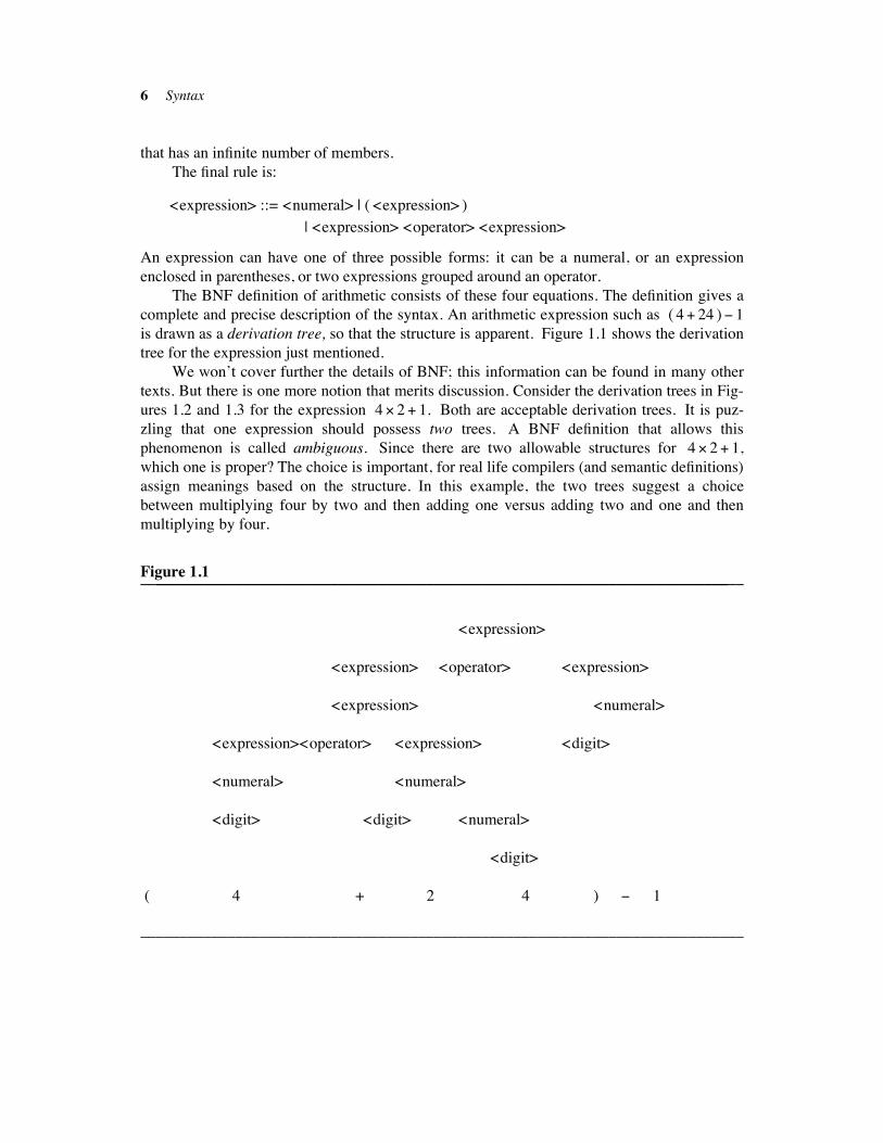
The BNF definition of arithmetic consists of these four equations. The definition gives a
complete and precise description of the syntax. An arithmetic expression such as ( 4# 24 )! 1
is drawn as a derivation tree, so that the structure is apparent. Figure 1.1 shows the derivation
tree for the expression just mentioned.
We won’t cover further the details of BNF; this information can be found in many other
texts. But there is one more notion that merits discussion. Consider the derivation trees in Fig-
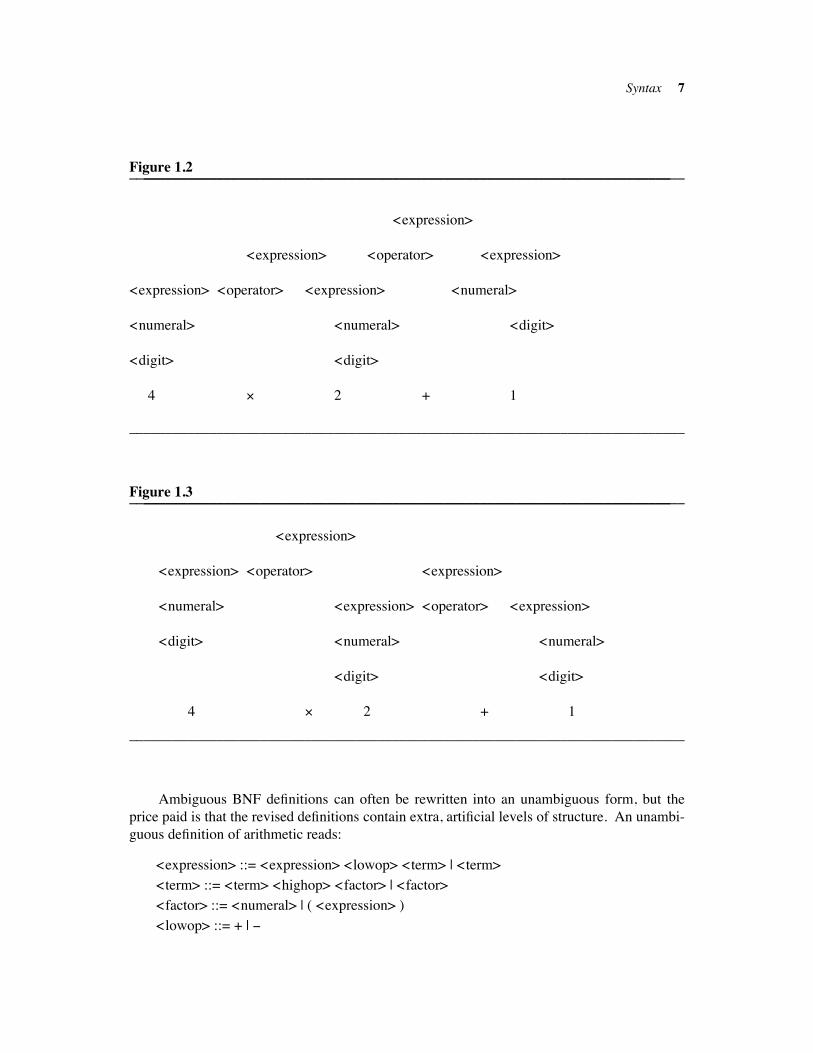
ures 1.2 and 1.3 for the expression 4" 2# 1. Both are acceptable derivation trees. It is puz-
zling that one expression should possess two trees. A BNF definition that allows this
phenomenon is called ambiguous. Since there are two allowable structures for 4" 2# 1,
which one is proper? The choice is important, for real life compilers (and semantic definitions)
assign meanings based on the structure. In this example, the two trees suggest a choice
between multiplying four by two and then adding one versus adding two and one and then
multiplying by four.
Figure 1.1____________________________________________________________________________________________________________________________________________________
<expression>
<expression> <operator> <expression>
<expression> <numeral>
<expression><operator> <expression> <digit>
<numeral> <numeral>
<digit> <digit> <numeral>
<digit>
( 4 + 2 4 ) ! 1
____________________________________________________________________________
Syntax 7
Figure 1.2____________________________________________________________________________________________________________________________________________________
<expression>
<expression> <operator> <expression>
<expression> <operator> <expression> <numeral>
<numeral> <numeral> <digit>
<digit> <digit>
4 " 2 + 1
____________________________________________________________________________
Figure 1.3____________________________________________________________________________________________________________________________________________________
<expression>
<expression> <operator> <expression>
<numeral> <expression> <operator> <expression>
<digit> <numeral> <numeral>
<digit> <digit>
4 " 2 + 1
____________________________________________________________________________
Ambiguous BNF definitions can often be rewritten into an unambiguous form, but the
price paid is that the revised definitions contain extra, artificial levels of structure. An unambi-
guous definition of arithmetic reads:
<expression> ::= <expression> <lowop> <term> | <term>
<term> ::= <term> <highop> <factor> | <factor>
<factor> ::= <numeral> | ( <expression> )
<lowop> ::= + | !
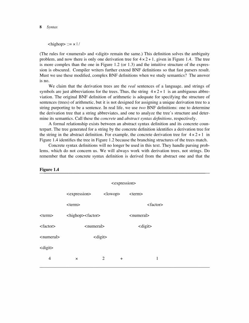
8 Syntax
<highop> ::= " | /
(The rules for <numeral> and <digit> remain the same.) This definition solves the ambiguity
problem, and now there is only one derivation tree for 4" 2# 1, given in Figure 1.4. The tree
is more complex than the one in Figure 1.2 (or 1.3) and the intuitive structure of the expres-
sion is obscured. Compiler writers further extend BNF definitions so that fast parsers result.
Must we use these modified, complex BNF definitions when we study semantics? The answer
is no.
We claim that the derivation trees are the real sentences of a language, and strings of
symbols are just abbreviations for the trees. Thus, the string 4" 2# 1 is an ambiguous abbre-
viation. The original BNF definition of arithmetic is adequate for specifying the structure of
sentences (trees) of arithmetic, but it is not designed for assigning a unique derivation tree to a
string purporting to be a sentence. In real life, we use two BNF definitions: one to determine
the derivation tree that a string abbreviates, and one to analyze the tree’s structure and deter-
mine its semantics. Call these the concrete and abstract syntax definitions, respectively.
A formal relationship exists between an abstract syntax definition and its concrete coun-
terpart. The tree generated for a string by the concrete definition identifies a derivation tree for
the string in the abstract definition. For example, the concrete derivation tree for 4" 2# 1 in
Figure 1.4 identifies the tree in Figure 1.2 because the branching structures of the trees match.
Concrete syntax definitions will no longer be used in this text. They handle parsing prob-
lems, which do not concern us. We will always work with derivation trees, not strings. Do
remember that the concrete syntax definition is derived from the abstract one and that the
Figure 1.4____________________________________________________________________________________________________________________________________________________
<expression>
<expression> <lowop> <term>
<term> <factor>
<term> <highop><factor> <numeral>
<factor> <numeral> <digit>
<numeral> <digit>
<digit>
4 " 2 + 1
____________________________________________________________________________
Syntax 9
abstract syntax definition is the true definition of language structure.
1.1 ABSTRACT SYNTAX DEFINITIONS !!!!!!!!!!!!!!!!!!!!!!!!!!!!!!!!!!!!!!!!!!!!!!!!!!!!!!!!!!!!!!!!!!!!!!!!!!!!
Abstract syntax definitions describe structure. Terminal symbols disappear entirely if we study
abstract syntax at the word level. The building blocks of abstract syntax are words (also called
tokens, as in compiling theory) rather than terminal symbols. This relates syntax to semantics
more closely, for meanings are assigned to entire words, not to individual symbols.
Here is the abstract syntax definition of arithmetic once again, where the numerals,
parentheses, and operators are treated as tokens:
<expression> ::= <numeral> | <expression> <operator> <expression>
| left-paren <expression> right-paren
<operator> ::= plus | minus | mult | div
<numeral> ::= zero | one | two | . . . | ninety-nine | one-hundred | . . .
The structure of arithmetic remains, but all traces of text vanish. The derivation trees have the
same structure as before, but the tree’s leaves are tokens instead of symbols.
Set theory gives us an even more abstract view of abstract syntax. Say that each nonter-
minal in a BNF definition names the set of those phrases that have the structure specified by
the nonterminal’s BNF rule. But the rule can be discarded: we introduce syntax builder opera-
tions, one for each form on the right-hand side of the rule.
Figure 1.5 shows the set theoretic formulation of the syntax of arithmetic.
The language consists of three sets of values: expressions, arithmetic operators, and
numerals. The members of the Numeral set are exactly those values built by the ‘‘operations’’
(in this case, they are really constants) zero, one, two, and so on. No other values are members
of the Numeral set. Similarly, the Operator set contains just the four values denoted by the
constants plus, minus, mult, and div. Members of the Expression set are built with the three
operations make-numeral-into-expression, make-compound-expression, and make-bracketed-
expression. Consider make-numeral-into-expression; it converts a value from the Numeral set
into a value in the Expression set. The operation reflects the idea that any known numeral
can be used as an expression. Similarly, make-compound-expression combines two
known members of the Expression set with a member of the Operation set to build a member
of the Expression set. Note that make-bracketed-expression does not need parenthesis tokens
to complete its mapping; the parentheses were just ‘‘window dressing.’’ As an example, the
expression 4 + 12 is represented by make-compound-expression (make-numeral-into-
expression(four), plus, make-numeral-into-expression(twelve)).
When we work with the set theoretic formulation of abstract syntax, we forget about
words and derivation trees and work in the world of sets and operations. The set theoretic
approach reinforces our view that syntax is not tied to symbols; it is a matter of structure. We
use the term syntax domain for a collection of values with common syntactic structure. Arith-
metic has three syntax domains.
In this book, we use a more readable version of set-theoretic abstract syntax due to
10 Syntax
Figure 1.5____________________________________________________________________________________________________________________________________________________
Sets:
Expression
Op
Numeral
Operations:
make-numeral-into-expression: Numeral"Expression
make-compound-expression: Expression"Op"Expression"Expression
make-bracketed-expression: Expression"Expression
plus: Op
minus: Op
mult: Op
div: Op
zero: Numeral
one: Numeral
two: Numeral. . .
ninety-nine: Numeral
one-hundred: Numeral. . .
____________________________________________________________________________
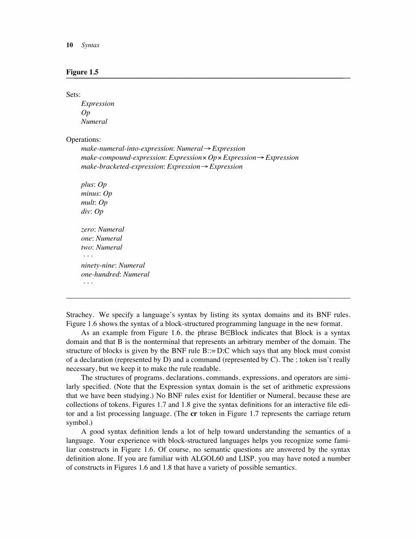
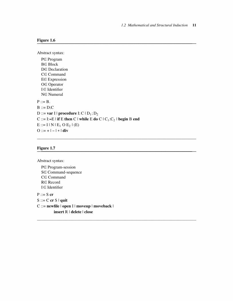
Strachey. We specify a language’s syntax by listing its syntax domains and its BNF rules.
Figure 1.6 shows the syntax of a block-structured programming language in the new format.
As an example from Figure 1.6, the phrase B#Block indicates that Block is a syntax
domain and that B is the nonterminal that represents an arbitrary member of the domain. The
structure of blocks is given by the BNF rule B::= D;C which says that any block must consist
of a declaration (represented by D) and a command (represented by C). The ; token isn’t really
necessary, but we keep it to make the rule readable.
The structures of programs, declarations, commands, expressions, and operators are simi-
larly specified. (Note that the Expression syntax domain is the set of arithmetic expressions
that we have been studying.) No BNF rules exist for Identifier or Numeral, because these are
collections of tokens. Figures 1.7 and 1.8 give the syntax definitions for an interactive file edi-
tor and a list processing language. (The cr token in Figure 1.7 represents the carriage return
symbol.)
A good syntax definition lends a lot of help toward understanding the semantics of a
language. Your experience with block-structured languages helps you recognize some fami-
liar constructs in Figure 1.6. Of course, no semantic questions are answered by the syntax
definition alone. If you are familiar with ALGOL60 and LISP, you may have noted a number
of constructs in Figures 1.6 and 1.8 that have a variety of possible semantics.
1.2 Mathematical and Structural Induction 11
Figure 1.6____________________________________________________________________________________________________________________________________________________
Abstract syntax:
P# Program
B# Block
D# Declaration
C# Command
E# Expression
O# Operator
I# Identifier
N# Numeral
P ::= B.
B ::= D;C
D ::= var I | procedure I; C | D1; D2
C ::= I:$E | if E then C | while E do C | C1;C2 | begin B end
E ::= I | N | E1 O E2 | (E)
O ::= + | ! | $ | div
____________________________________________________________________________
Figure 1.7____________________________________________________________________________________________________________________________________________________
Abstract syntax:
P# Program-session
S# Command-sequence
C# Command
R# Record
I# Identifier
P ::= S cr
S ::= C cr S | quit
C ::= newfile | open I | moveup | moveback |
insert R | delete | close
____________________________________________________________________________
12 Syntax
Figure 1.8____________________________________________________________________________________________________________________________________________________
Abstract syntax:
P# Program
E# Expression
L# List
A# Atom
P ::= E,P | end
E ::= A | L | head E | tail E | let A$E1 in E2
L ::= (A L) | ()
____________________________________________________________________________
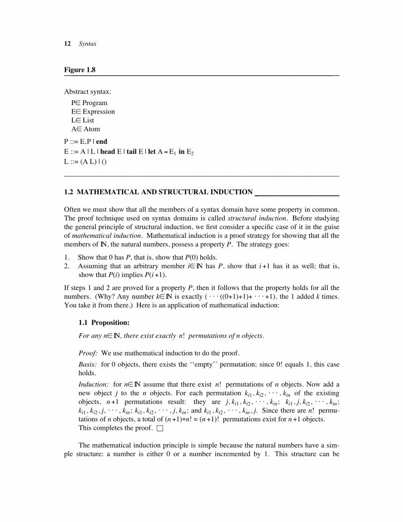
1.2 MATHEMATICAL AND STRUCTURAL INDUCTION !!!!!!!!!!!!!!!!!!!!!!!!!!!!!!!!!!!!!!!!!!!!!!
Often we must show that all the members of a syntax domain have some property in common.
The proof technique used on syntax domains is called structural induction. Before studying
the general principle of structural induction, we first consider a specific case of it in the guise
of mathematical induction. Mathematical induction is a proof strategy for showing that all the
members of IN, the natural numbers, possess a property P. The strategy goes:
1. Show that 0 has P, that is, show that P(0) holds.
2. Assuming that an arbitrary member i# IN has P, show that i #1 has it as well; that is,
show that P(i) implies P(i#1).
If steps 1 and 2 are proved for a property P, then it follows that the property holds for all the
numbers. (Why? Any number k# IN is exactly ( . . . ((0#1)#1)# . . . #1), the 1 added k times.
You take it from there.) Here is an application of mathematical induction:
1.1 Proposition:
For any n# IN, there exist exactly n! permutations of n objects.
Proof: We use mathematical induction to do the proof.
Basis: for 0 objects, there exists the ‘‘empty’’ permutation; since 0! equals 1, this case
holds.
Induction: for n# IN assume that there exist n! permutations of n objects. Now add a
new object j to the n objects. For each permutation ki1, ki2, . . . , kin of the existing
objects, n#1 permutations result: they are j, ki1, ki2, . . . , kin; ki1, j, ki2, . . . , kin;
ki1, ki2, j, . . . , kin; ki1, ki2, . . . , j, kin; and ki1, ki2, . . . , kin, j. Since there are n! permu-
tations of n objects, a total of (n#1)$n! = (n#1)! permutations exist for n#1 objects.
This completes the proof.
The mathematical induction principle is simple because the natural numbers have a sim-
ple structure: a number is either 0 or a number incremented by 1. This structure can be
1.2 Mathematical and Structural Induction 13
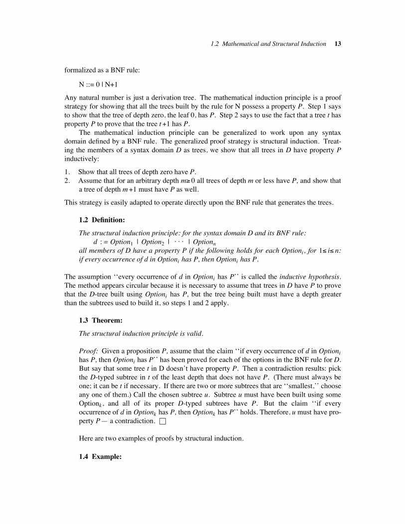
formalized as a BNF rule:
N ::= 0 | N+1
Any natural number is just a derivation tree. The mathematical induction principle is a proof
strategy for showing that all the trees built by the rule for N possess a property P. Step 1 says
to show that the tree of depth zero, the leaf 0, has P. Step 2 says to use the fact that a tree t has
property P to prove that the tree t #1 has P.
The mathematical induction principle can be generalized to work upon any syntax
domain defined by a BNF rule. The generalized proof strategy is structural induction. Treat-
ing the members of a syntax domain D as trees, we show that all trees in D have property P
inductively:
1. Show that all trees of depth zero have P.
2. Assume that for an arbitrary depth m% 0 all trees of depth m or less have P, and show that
a tree of depth m#1 must have P as well.
This strategy is easily adapted to operate directly upon the BNF rule that generates the trees.
1.2 Definition:
The structural induction principle: for the syntax domain D and its BNF rule:
d : = Option1 | Option2 | . . . | Optionn
all members of D have a property P if the following holds for each Optioni, for 1& i& n:
if every occurrence of d in Optioni has P, then Optioni has P.
The assumption ‘‘every occurrence of d in Optioni has P’’ is called the inductive hypothesis.
The method appears circular because it is necessary to assume that trees in D have P to prove
that the D-tree built using Optioni has P, but the tree being built must have a depth greater
than the subtrees used to build it, so steps 1 and 2 apply.
1.3 Theorem:
The structural induction principle is valid.
Proof: Given a proposition P, assume that the claim ‘‘if every occurrence of d in Optioni
has P, then Optioni has P’’ has been proved for each of the options in the BNF rule for D.
But say that some tree t in D doesn’t have property P. Then a contradiction results: pick
the D-typed subtree in t of the least depth that does not have P. (There must always be
one; it can be t if necessary. If there are two or more subtrees that are ‘‘smallest,’’ choose
any one of them.) Call the chosen subtree u. Subtree u must have been built using some
Optionk , and all of its proper D-typed subtrees have P. But the claim ‘‘if every
occurrence of d in Optionk has P, then Optionk has P’’ holds. Therefore, u must have pro-
perty P— a contradiction.
Here are two examples of proofs by structural induction.
1.4 Example:
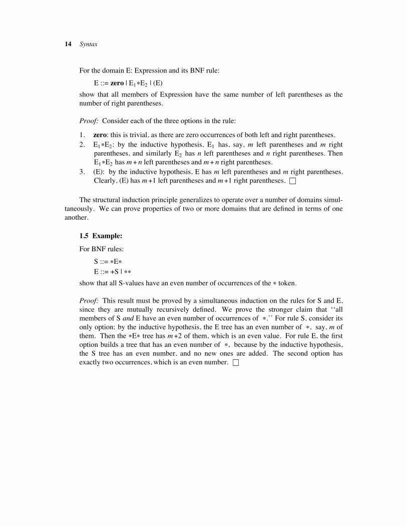
14 Syntax
For the domain E: Expression and its BNF rule:
E ::= zero | E1$E2 | (E)
show that all members of Expression have the same number of left parentheses as the
number of right parentheses.
Proof: Consider each of the three options in the rule:
1. zero: this is trivial, as there are zero occurrences of both left and right parentheses.
2. E1$E2: by the inductive hypothesis, E1 has, say, m left parentheses and m right
parentheses, and similarly E2 has n left parentheses and n right parentheses. Then
E1$E2 has m# n left parentheses and m# n right parentheses.
3. (E): by the inductive hypothesis, E has m left parentheses and m right parentheses.
Clearly, (E) has m#1 left parentheses and m#1 right parentheses.
The structural induction principle generalizes to operate over a number of domains simul-
taneously. We can prove properties of two or more domains that are defined in terms of one
another.
1.5 Example:
For BNF rules:
S ::= $E$
E ::= +S | $$
show that all S-values have an even number of occurrences of the $ token.
Proof: This result must be proved by a simultaneous induction on the rules for S and E,
since they are mutually recursively defined. We prove the stronger claim that ‘‘all
members of S and E have an even number of occurrences of $.’’ For rule S, consider its
only option: by the inductive hypothesis, the E tree has an even number of $, say, m of
them. Then the $E$ tree has m#2 of them, which is an even value. For rule E, the first
option builds a tree that has an even number of $, because by the inductive hypothesis,
the S tree has an even number, and no new ones are added. The second option has
exactly two occurrences, which is an even number.
Suggested Readings 15
SUGGESTED READINGS !!!!!!!!!!!!!!!!!!!!!!!!!!!!!!!!!!!!!!!!!!!!!!!!!!!!!!!!!!!!!!!!!!!!!!!!!!!!!!!!!!!!!!!!!!!!!!!!!!!!!!
Backus-Naur form: Aho & Ullman 1977; Barrett & Couch 1979; Cleaveland & Uzgalis
1977; Hopcroft & Ullman 1979; Naur et al. 1963
Abstract syntax: Barrett & Couch 1979; Goguen, Thatcher, Wagner, & Wright 1977; Gor-
don 1979; Henderson 1980; McCarthy 1963; Strachey 1966, 1968, 1973
Mathematical and structural induction: Bauer & Wossner 1982; Burstall 1969; Manna
1974; Manna & Waldinger 1985; Wand 1980
EXERCISES !!!!!!!!!!!!!!!!!!!!!!!!!!!!!!!!!!!!!!!!!!!!!!!!!!!!!!!!!!!!!!!!!!!!!!!!!!!!!!!!!!!!!!!!!!!!!!!!!!!!!!!!!!!!!!!!!!!!!!!!!!!!
1. a. Convert the specification of Figure 1.6 into the classic BNF format shown at the
beginning of the chapter. Omit the rules for <Identifier> and <Numeral>. If the
grammar is ambiguous, point out which BNF rules cause the problem, construct
derivation trees that demonstrate the ambiguity, and revise the BNF definition into a
nonambiguous form that defines the same language as the original.
b. Repeat part a for the definitions in Figures 1.7 and 1.8.
2. Describe an algorithm that takes an abstract syntax definition (like the one in Figure 1.6)
as input and generates as output a stream containing the legal sentences in the language
defined by the definition. Why isn’t ambiguity a problem?
3. Using the definition in Figure 1.5, write the abstract syntax forms of these expressions:
a. 12
b. ( 4 + 14 ) $ 3
c. ( ( 7 / 0 ) )
Repeat a-c for the definition in Figure 1.6; that is, draw the derivation trees.
4. Convert the language definition in Figure 1.6 into a definition in the format of Figure 1.5.
What advantages does each format have over the other? Which of the two would be easier
for a computer to handle?
5. Alter the BNF rule for the Command domain in Figure 1.6 to read:
C ::= S | S;C
S ::= I:$E | if E then C | while E do C | begin B end
Draw derivation trees for the old and new definitions of Command. What advantages
does one form have over the other?
6. Using Strachey-style abstract syntax (like that in Figures 1.6 through 1.8), define the
abstract syntax of the input language to a program that maintains a data base for a grocery
store’s inventory. An input program consists of a series of commands, one per line; the
16 Syntax
commands should specify actions for:
a. Accessing an item in the inventory (perhaps by catalog number) to obtain statistics
such as quantity, wholesale and selling prices, and so on.
b. Updating statistical information about an item in the inventory
c. Creating a new item in the inventory;
d. Removing an item from the inventory;
e. Generating reports concerning the items on hand and their statistics.
7. a. Prove that any sentence defined by the BNF rule in Example 1.4 has more
occurrences of zero than occurrences of $.
b. Attempt to prove that any sentence defined by the BNF rule in Example 1.4 has more
occurrences of zero than of (. Where does the proof break down? Give a counterex-
ample.
8. Prove that any program in the language in Figure 1.6 has the same number of begin
tokens as the number of end tokens.
9. Formalize and prove the validity of simultaneous structural induction.
10. The principle of transfinite induction on the natural numbers is defined as follows: for a
property P on IN, if for arbitrary n% 0, ((for all m< n, P(m) holds ) implies P(n) holds),
then for all n% 0, P(n) holds.
a. Prove that the principle of transfinite induction is valid.
b. Find a property that is provable by transfinite induction and not by mathematical
induction.
11. Both mathematical and transfinite induction can be generalized. A relation <. 'D"D is a
well-founded ordering iff there exist no infinitely descending sequences in D, that is, no
sequences of the form dn.> dn!1
.> dn!2.> . . . , where .> $ <. -1.
a. The general form of mathematical induction operates over a pair (D, <. ), where all
the members of D form one sequence d0 <. d1 <. d2 <. . . . <. di <. . . . . (Thus <. is a
well-founded ordering.)
i. State the principle of generalized mathematical induction and prove that the prin-
ciple is sound.
ii. What is <. for D$ IN?
iii. Give an example of another set with a well-founded ordering to which generalized
mathematical induction can apply.
b. The general form of transfinite induction operates over a pair (D, <. ), where <. is a
well founded ordering.
i. State the principle of general transfinite induction and prove it valid.
ii. Show that there exists a well-founded ordering on the words in a dictionary and
give an example of a proof using them and general transfinite induction.
iii. Show that the principle of structural induction is justified by the principle of gen-
eral transfinite induction.
Chapter 2 !!!!!!!!!!!!!!!!!!!!!!!!!!!!!!!!!!!!!!!!!!!!!!!!!!!!!!!!
Sets, Functions, and Domains
Functions are fundamental to denotational semantics. This chapter introduces functions
through set theory, which provides a precise yet intuitive formulation. In addition, the con-
cepts of set theory form a foundation for the theory of semantic domains, the value spaces
used for giving meaning to languages. We examine the basic principles of sets, functions, and
domains in turn.
2.1 SETS !!!!!!!!!!!!!!!!!!!!!!!!!!!!!!!!!!!!!!!!!!!!!!!!!!!!!!!!!!!!!!!!!!!!!!!!!!!!!!!!!!!!!!!!!!!!!!!!!!!!!!!!!!!!!!!!!!!!!!!!!!!!!!!!!!
A set is a collection; it can contain numbers, persons, other sets, or (almost) anything one
wishes. Most of the examples in this book use numbers and sets of numbers as the members
of sets. Like any concept, a set needs a representation so that it can be written down. Braces
are used to enclose the members of a set. Thus, { 1, 4, 7 } represents the set containing the
numbers 1, 4, and 7. These are also sets:
{ 1, { 1, 4, 7 }, 4 }
{ red, yellow, grey }
{ }
The last example is the empty set, the set with no members, also written as !.
When a set has a large number of members, it is more convenient to specify the condi-
tions for membership than to write all the members. A set S can be defined by S" { x | P(x) },
which says that an object a belongs to S iff (if and only if) a has property P, that is, P(a) holds
true. For example, let P be the property ‘‘is an even integer.’’ Then { x | x is an even integer }
defines the set of even integers, an infinite set. Note that ! can be defined as the set
{ x | x"x }. Two sets R and S are equivalent, written R" S, if they have the same members.
For example, { 1, 4, 7 } " { 4, 7, 1 }.
These sets are often used in mathematics and computing:
1. Natural numbers: IN" { 0, 1, 2, . . . }
2. Integers: Z| " { . . . , #2, #1, 0, 1, 2, . . . }
3. Rational numbers: Q| " { x | for p$Z| and q$Z| , q " 0, x" p/q }
4. Real numbers: IR " { x | x is a point on the line
#2 #1 0 1 2
}
5. Characters: C| " { x | x is a character}
6. Truth values (Booleans): IB " { true, false }
The concept of membership is central to set theory. We write x$S to assert that x is a
member of set S. The membership test provides an alternate way of looking at sets. In the17
18 Sets, Functions, and Domains
above examples, the internal structure of sets was revealed by ‘‘looking inside the braces’’ to
see all the members inside. An external view treats a set S as a closed, mysterious object to
which we can only ask questions about membership. For example, ‘‘does 1$ S hold?,’’ ‘‘does
4$ S hold?,’’ and so on. The internal structure of a set isn’t even important, as long as
membership questions can be answered. To tie these two views together, set theory supports
the extensionality principle: a set R is equivalent to a set S iff they answer the same on all
tests concerning membership:
R" S if and only if, for all x, x$R holds iff x$S holds
Here are some examples using membership:
1$ { 1, 4, 7 } holds
{ 1 }$ { 1, 4, 7 } does not hold
{ 1 }$ { { 1 }, 4, 7 } holds
The extensionality principle implies the following equivalences:
{ 1, 4, 7 } " { 4, 1, 7 }
{ 1, 4, 7 } " { 4, 1, 7, 4 }
A set R is a subset of a set S if every member of R belongs to S:
R% S if and only if, for all x, x$R implies x$S
For example,
{ 1 }% { 1, 4, 7 }
{ 1, 4, 7 }% { 1, 4, 7 }
{ }% { 1, 4, 7 }
all hold true but { 1 }%/ { { 1 }, 4, 7 }.
2.1.1 Constructions on Sets !!!!!!!!!!!!!!!!!!!!!!!!!!!!!!!!!!!!!!!!!!!!!!!!!!!!!!!!!!!!!!!!!!!!!!!!!!!!!!!!!!!!!!!!!!!!!!!!!!!!
The simplest way to build a new set from two existing ones is to union them together; we
write R& S to denote the set that contains the members of R and S and no more. We can define
set union in terms of membership:
for all x, x$R& S if and only if x$R or x$S
Here are some examples:
{ 1, 2 }& { 1, 4, 7 } " { 1, 2, 4, 7 }
{ }& { 1, 2 } " { 1, 2 }
{ { } }& { 1, 2 } " { { }, 1, 2 }
The union operation is commutative and associative; that is, R& S" S&R and
(R& S)& T " R& (S& T). The concept of union can be extended to join an arbitrary number of
2.1.1 Constructions on Sets 19
sets. If R0, R1, R2, . . . is an infinite sequence of sets, i"0& '
Ri stands for their union. For exam-
ple, Z| " i"0& '
{ #i, . . . ,#1, 0, 1, . . . , i } shows how the infinite union construction can build an
infinite set from a group of finite ones.
Similarly, the intersection of sets R and S, R( S, is the set that contains only members
common to both R and S:
for all x, x$R( S if and only if x$R and x$S
Intersection is also commutative and associative.
An important concept that can be defined in terms of sets (though it is not done here) is
the ordered pair. For two objects x and y, their pairing is written (x,y). Ordered pairs are use-
ful because of the indexing operations fst and snd, defined such that:
fst(x,y)" x
snd(x,y)" y
Two ordered pairs P and Q are equivalent iff fst P" fst Q and snd P" snd Q. Pairing is useful
for defining another set construction, the product construction. For sets R and S, their product
R# S is the set of all pairs built from R and S:
R# S" { (x,y) | x$R and y$S }
Both pairing and products can be generalized from their binary formats to n-tuples and n-
products.
A form of union construction on sets that keeps the members of the respective sets R and
S separate is called disjoint union (or sometimes, sum):
R$ S" { (zero, x) | x$R }& { (one, y) | y$S }
Ordered pairs are used to ‘‘tag’’ the members of R and S so that it is possible to examine a
member and determine its origin.
We find it useful to define operations for assembling and disassembling members of
R$ S. For assembly, we propose inR and inS, which behave as follows:
for x$R, inR(x)" (zero, x)
for y$S, inS(y)" (one, y)
To remove the tag from an element m$ R$ S, we could simply say snd(m), but will instead
resort to a better structured operation called cases. For any m$R$ S, the value of:
cases m of
isR(x)) . . . x . . .
[] isS(y)) . . . y . . .
end
is ‘‘ . . . x . . . ’’ when m" (zero, x) and is ‘‘ . . . y . . . ’’ when m" (one, y). The cases operation
makes good use of the tag on the sum element; it checks the tag before removing it and using
the value. Do not be confused by the isR and isS phrases. They are not new operations. You
20 Sets, Functions, and Domains
should read the phrase isR(x)) . . . x . . . as saying, ‘‘if m is an element whose tag component
is R and whose value component is x, then the answer is . . . x . . . .’’ As an example, for:
f(m)" cases m of
isIN(n)) n$1
[] isIB(b)) 0
end
f(inIN(2)) " f(zero, 2) " 2 $ 1 " 3, but f(inIB(true)) " f(one, true) " 0.
Like a product, the sum construction can be generalized from its binary format to n-sums.
Finally, the set of all subsets of a set R is called its powerset:
IP(R)" { x | x%R }
{ }$ IP(R) and R$ IP(R) both hold.
2.2 FUNCTIONS !!!!!!!!!!!!!!!!!!!!!!!!!!!!!!!!!!!!!!!!!!!!!!!!!!!!!!!!!!!!!!!!!!!!!!!!!!!!!!!!!!!!!!!!!!!!!!!!!!!!!!!!!!!!!!!!!!!!
Functions are rather slippery objects to catch and examine. A function cannot be taken apart
and its internals examined. It is like a ‘‘black box’’ that accepts an object as its input and then
transforms it in some way to produce another object as its output. We must use the ‘‘external
approach’’ mentioned above to understand functions. Sets are ideal for formalizing the
method. For two sets R and S, f is a function from R to S, written f : R) S, if, to each member
of R, f associates exactly one member of S. The expression R) S is called the arity or func-
tionality of f. R is the domain of f; S is the codomain of f. If x$R holds, and the element
paired to x by f is y, we write f(x)" y. As a simple example, if R" { 1, 4, 7 }, S" { 2, 4, 6 }, and
f maps R to S as follows:
R S
f
1 2
4 4
7 6
then f is a function. Presenting an argument a to f is called application and is written f(a). We
don’t know how f transforms 1 to 2, or 4 to 6, or 7 to 2, but we accept that somehow it does;
the results are what matter. The viewpoint is similar to that taken by a naive user of a com-
puter program: unaware of the workings of a computer and its software, the user treats the
program as a function, as he is only concerned with its input-output properties. An exten-
sionality principle also applies to functions. For functions f : R) S and g: R) S, f is equal to
2.2 Functions 21
g, written f " g, iff for all x$R, f(x)" g(x).
Functions can be combined using the composition operation. For f : R) S and g : S) T,
g % f is the function with domain R and codomain T such that for all x: R, g % f(x)" g(f(x)).
Composition of functions is associative: for f and g as given above and h : T)U,
h % (g % f) " (h % g) % f.Functions can be classified by their mappings. Some classifications are:
1. one-one: f : R) S is a one-one (1-1) function iff for all x$R and y$R, f(x)" f(y) implies
x" y.
2. onto: f : R) S is an onto function iff S" { y | there exists some x$R such that f(x)"y }.
3. identity: f : R)R is the identity function for R iff for all x$R, f(x)" x.
4. inverse: for some f : R) S, if f is one-one and onto, then the function g : S)R, defined
as g(y)" x iff f(x)" y is called the inverse function of f. Function g is denoted by f#1.
Functions are used to define many interesting relationships between sets. The most
important relationship is called an isomorphism: two sets R and S are isomorphic if there exist
a pair of functions f : R) S and g : S) R such that g % f is the identity function for R and f % gis the identity function for S. The maps f and g are called isomorphisms. A function is an iso-
morphism if and only if it is one-one and onto. Further, the inverse f#1 of isomorphism f is
also an isomorphism, as f#1 % f and f % f#1 are both identities. Here are some examples:
1. R" { 1, 4, 7 } is isomorphic to S" { 2, 4, 6 }; take f : R) S to be f(1)"2, f(4)"6, f(7)"4;
and g : S)R to be g(2)"1, g(4)"7, g(6)"4.
2. For sets A and B, A#B is isomorphic to B#A; take f : A #B)B#A to be f(a,b)" (b,a).
3. IN is isomorphic to Z| ; take f : IN)Z| to be:
f(x)" #((x$1)/2)
x/2
if x is odd
if x is even
You are invited to calculate the inverse functions in examples 2 and 3.
2.2.1 Representing Functions as Sets !!!!!!!!!!!!!!!!!!!!!!!!!!!!!!!!!!!!!!!!!!!!!!!!!!!!!!!!!!!!!!!!!!!!!!!!!!!!!!!!!!!!!!
We can describe a function via a set. We collect the input-output pairings of the function into
a set called its graph. For function f : R) S, the set:
graph(f)" { (x, f(x)) | x$R }
is the graph of f. Here are some examples:
1. f : R) S in example 1 above:
graph(f)" { (1,2), (4,6), (7,4) }
2. the successor function on Z| :
graph(succ)" { . . . , (#2,#1), (#1,0), (0,1), (1,2), . . . }
3. f : IN)Z| in example 3 above:
graph(f)" { (0,0), (1,#1), (2,1), (3,#2), (4,2), . . . }
In every case, we list the domain and codomain of the function to avoid confusion about
22 Sets, Functions, and Domains
which function a graph represents. For example, f : IN) IN such that f(x)"x has the same graph
as g : IN)Z| such that g(x)"x, but they are different functions.
We can understand function application and composition in terms of graphs. For applica-
tion, f(a)"b iff (a,b) is in graph(f). Let there be a function apply such that
f(a)" apply(graph(f), a). Composition is modelled just as easily; for graphs f : R) S and
g : S) T:
graph(g % f)" { (x,z) | x$R and there exists a y$S
such that (x,y)$graph (f) and (y,z)$ graph(g) }
Functions can have arbitrarily complex domains and codomains. For example, if R and S
are sets, so is R# S, and it is reasonable to make R# S the domain or codomain of a function.
If it is the domain, we say that the function ‘‘needs two arguments’’; if it is the codomain, we
say that it ‘‘returns a pair of values.’’ Here are some examples of functions with compound
domains or codomains:
1. add : (IN# IN)) IN
graph (add)" { ((0,0), 0), ((1,0), 1), ((0,1), 1), ((1,1), 2), ((2,1), 3), . . . }
2. duplicate : R) (R#R), where R" { 1, 4, 7 }
graph(duplicate)" { (1, (1,1)), (4,(4,4)), (7, (7,7)) }
3. which-part : (IB$IN)) S, where S" { isbool, isnum }
graph (which-part)" { ((zero, true), isbool), ((zero, false), isbool),
((one, 0), isnum), ((one,1), isnum),
((one, 2), isnum), . . . , ((one, n), isnum), . . . }
4. make-singleton : IN) IP(IN)
graph (make-singleton)" { (0, { 0 }), (1, { 1 }), . . . , (n, { n }), . . . }
5. nothing : IB( IN) IB
graph (nothing)" { }
The graphs make it clear how the functions behave when they are applied to arguments.
For example, apply(graph(which-part), (one, 2))" isnum. We see in example 4 that a function
can return a set as a value (or, for that matter, use one as an argument). Since a function can be
represented by its graph, which is a set, we will allow functions to accept other functions as
arguments and produce functions as answers. Let the set of functions from R to S be a set
whose members are the graphs of all functions whose domain is R and codomain is S. Call
this set R) S. Thus the expression f : R) S also states that f’s graph is a member of the set
R) S. A function that uses functions as arguments or results is called a higher-order func-
tion. The graphs of higher-order functions become complex very quickly, but it is important
to remember that they do exist and everything is legal under the set theory laws. Here are
some examples:
6. split-add : IN) (IN) IN). Function split-add is the addition function ‘‘split up’’ so that it
can accept its two arguments one at a time. It is defined as split-add(x) " g, where
g : IN) IN is g(y) " add (x,y). The graph gives a lot of insight:
2.2.1 Representing Functions as Sets 23
graph (split-add)" { ( 0, { (0,0), (1,1), (2,2), . . . } ),
( 1, { (0,1), (1,2), (2,3), . . . } ),
( 2, { (0,2), (1,3), (2,4), . . . } ), . . . }
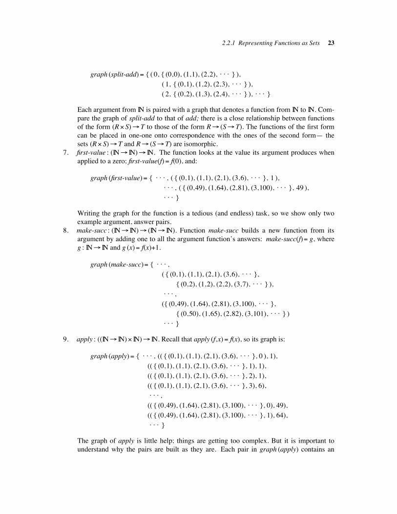
Each argument from IN is paired with a graph that denotes a function from IN to IN. Com-
pare the graph of split-add to that of add; there is a close relationship between functions
of the form (R# S)) T to those of the form R) (S) T). The functions of the first form
can be placed in one-one onto correspondence with the ones of the second form— the
sets (R# S)) T and R) (S) T) are isomorphic.
7. first-value : (IN) IN)) IN. The function looks at the value its argument produces when
applied to a zero; first-value(f)" f(0), and:
graph (first-value)" { . . . , ( { (0,1), (1,1), (2,1), (3,6), . . . }, 1 ),. . . , ( { (0,49), (1,64), (2,81), (3,100), . . . }, 49 ),. . . }
Writing the graph for the function is a tedious (and endless) task, so we show only two
example argument, answer pairs.
8. make-succ : (IN) IN)) (IN) IN). Function make-succ builds a new function from its
argument by adding one to all the argument function’s answers: make-succ(f)" g, where
g : IN) IN and g (x)" f(x)$1.
graph (make-succ)" { . . . ,
( { (0,1), (1,1), (2,1), (3,6), . . . },
{ (0,2), (1,2), (2,2), (3,7), . . . } ),. . . ,
({ (0,49), (1,64), (2,81), (3,100), . . . },
{ (0,50), (1,65), (2,82), (3,101), . . . } ). . . }
9. apply : ((IN) IN)# IN)) IN. Recall that apply (f,x)" f(x), so its graph is:
graph (apply)" { . . . , (( { (0,1), (1,1), (2,1), (3,6), . . . }, 0 ), 1),
(( { (0,1), (1,1), (2,1), (3,6), . . . }, 1), 1),
(( { (0,1), (1,1), (2,1), (3,6), . . . }, 2), 1),
(( { (0,1), (1,1), (2,1), (3,6), . . . }, 3), 6),. . . ,
(( { (0,49), (1,64), (2,81), (3,100), . . . }, 0), 49),
(( { (0,49), (1,64), (2,81), (3,100), . . . }, 1), 64),. . . }
The graph of apply is little help; things are getting too complex. But it is important to
understand why the pairs are built as they are. Each pair in graph (apply) contains an
24 Sets, Functions, and Domains
argument and an answer, where the argument is itself a set, number pair.
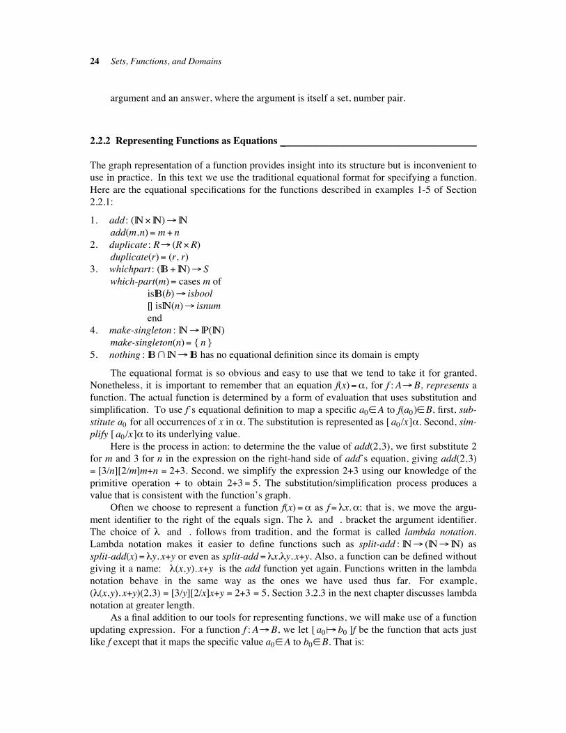
2.2.2 Representing Functions as Equations !!!!!!!!!!!!!!!!!!!!!!!!!!!!!!!!!!!!!!!!!!!!!!!!!!!!!!!!!!!!!!!!!!!!!!!!!!!!
The graph representation of a function provides insight into its structure but is inconvenient to
use in practice. In this text we use the traditional equational format for specifying a function.
Here are the equational specifications for the functions described in examples 1-5 of Section
2.2.1:
1. add: (IN# IN)) IN
add(m,n)" m $ n
2. duplicate: R) (R#R)
duplicate(r)" (r, r)
3. whichpart : (IB $ IN)) S
which-part(m)" cases m of
isIB(b)) isbool
[] isIN(n)) isnum
end
4. make-singleton : IN) IP(IN)
make-singleton(n)" { n }
5. nothing : IB( IN) IB has no equational definition since its domain is empty
The equational format is so obvious and easy to use that we tend to take it for granted.
Nonetheless, it is important to remember that an equation f(x)"*, for f : A)B, represents a
function. The actual function is determined by a form of evaluation that uses substitution and
simplification. To use f’s equational definition to map a specific a0$A to f(a0)$B, first, sub-
stitute a0 for all occurrences of x in *. The substitution is represented as [ a0/x]*. Second, sim-
plify [ a0/x]* to its underlying value.
Here is the process in action: to determine the the value of add(2,3), we first substitute 2
for m and 3 for n in the expression on the right-hand side of add’s equation, giving add(2,3)
" [3/n][2/m]m$n " 2$3. Second, we simplify the expression 2+3 using our knowledge of the
primitive operation + to obtain 2$3 " 5. The substitution/simplification process produces a
value that is consistent with the function’s graph.
Often we choose to represent a function f(x)"* as f " +x.*; that is, we move the argu-
ment identifier to the right of the equals sign. The + and . bracket the argument identifier.
The choice of + and . follows from tradition, and the format is called lambda notation.
Lambda notation makes it easier to define functions such as split-add : IN) (IN) IN) as
split-add(x)" +y. x$y or even as split-add " +x.+y. x$y. Also, a function can be defined without
giving it a name: +(x,y). x$y is the add function yet again. Functions written in the lambda
notation behave in the same way as the ones we have used thus far. For example,
(+(x,y). x$y)(2,3) " [3/y][2/x]x$y " 2$3 " 5. Section 3.2.3 in the next chapter discusses lambda
notation at greater length.
As a final addition to our tools for representing functions, we will make use of a function
updating expression. For a function f : A)B, we let [ a0 &&) b0 ]f be the function that acts just
like f except that it maps the specific value a0$A to b0$B. That is:
2.2.2 Representing Functions as Equations 25
([ a0 &&) b0 ]f)(a0)" b0
([ a0 &&) b0 ]f)(a)" f(a) for all other a$A such that a" a0
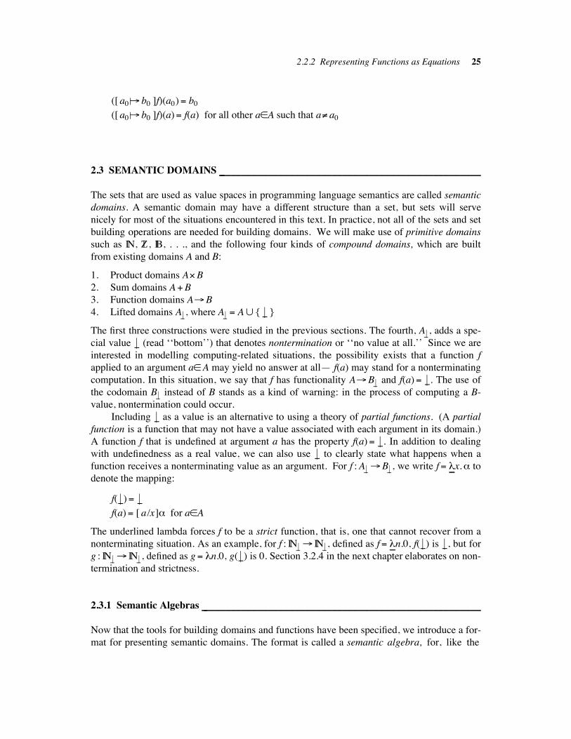
2.3 SEMANTIC DOMAINS !!!!!!!!!!!!!!!!!!!!!!!!!!!!!!!!!!!!!!!!!!!!!!!!!!!!!!!!!!!!!!!!!!!!!!!!!!!!!!!!!!!!!!!!!!!!!!!!!!!!
The sets that are used as value spaces in programming language semantics are called semantic
domains. A semantic domain may have a different structure than a set, but sets will serve
nicely for most of the situations encountered in this text. In practice, not all of the sets and set
building operations are needed for building domains. We will make use of primitive domains
such as IN, Z| , IB, . . ., and the following four kinds of compound domains, which are built
from existing domains A and B:
1. Product domains A#B
2. Sum domains A$B
3. Function domains A)B
4. Lifted domains A&! , where A&! " A& { &# }
The first three constructions were studied in the previous sections. The fourth, A&! , adds a spe-
cial value &# (read ‘‘bottom’’) that denotes nontermination or ‘‘no value at all.’’ Since we are
interested in modelling computing-related situations, the possibility exists that a function f
applied to an argument a$A may yield no answer at all— f(a) may stand for a nonterminating
computation. In this situation, we say that f has functionality A)B &! and f(a)" &#. The use of
the codomain B &! instead of B stands as a kind of warning: in the process of computing a B-
value, nontermination could occur.
Including &# as a value is an alternative to using a theory of partial functions. (A partial
function is a function that may not have a value associated with each argument in its domain.)
A function f that is undefined at argument a has the property f(a)" &#. In addition to dealing
with undefinedness as a real value, we can also use &# to clearly state what happens when a
function receives a nonterminating value as an argument. For f : A&!)B&! , we write f " +!!x.* to
denote the mapping:
f( &#)" &#f(a)" [ a/x]* for a$A
The underlined lambda forces f to be a strict function, that is, one that cannot recover from a
nonterminating situation. As an example, for f : IN&!) IN&! , defined as f " +!!n.0, f( &#) is &#, but for
g : IN&!) IN&! , defined as g" +n.0, g( &#) is 0. Section 3.2.4 in the next chapter elaborates on non-
termination and strictness.
2.3.1 Semantic Algebras !!!!!!!!!!!!!!!!!!!!!!!!!!!!!!!!!!!!!!!!!!!!!!!!!!!!!!!!!!!!!!!!!!!!!!!!!!!!!!!!!!!!!!!!!!!!!!!!!!!!!!!!!!
Now that the tools for building domains and functions have been specified, we introduce a for-
mat for presenting semantic domains. The format is called a semantic algebra, for, like the
26 Sets, Functions, and Domains
algebras studied in universal algebra, it is the grouping of a set with the fundamental opera-
tions on that set. We choose the algebra format because it:
1. Clearly states the structure of a domain and how its elements are used by the functions.
2. Encourages the development of standard algebra ‘‘modules’’ or ‘‘kits’’ that can be used
in a variety of semantic definitions.
3. Makes it easier to analyze a semantic definition concept by concept.
4. Makes it straightforward to alter a semantic definition by replacing one semantic algebra
with another.
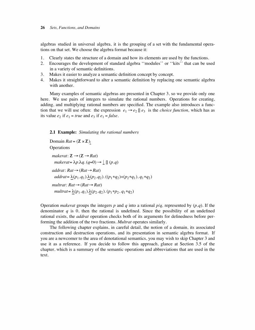
Many examples of semantic algebras are presented in Chapter 3, so we provide only one
here. We use pairs of integers to simulate the rational numbers. Operations for creating,
adding, and multiplying rational numbers are specified. The example also introduces a func-
tion that we will use often: the expression e1 ) e2 [] e3 is the choice function, which has as
its value e2 if e1 " true and e3 if e1 " false.
2.1 Example: Simulating the rational numbers
Domain Rat " (Z| #Z| )&!
Operations
makerat: Z| ) (Z| )Rat)
makerat" +p.+q. (q"0)) &# [] (p,q)
addrat : Rat) (Rat)Rat)
addrat" +!!(p1,q1).+!!(p2,q2). ((p1,q2)$(p2,q1), q1,q2)
multrat : Rat) (Rat)Rat)
multrat" +!!(p1,q1).+!!(p2,q2). (p1,p2, q1,q2)
Operation makerat groups the integers p and q into a rational p/q, represented by (p,q). If the
denominator q is 0, then the rational is undefined. Since the possibility of an undefined
rational exists, the addrat operation checks both of its arguments for definedness before per-
forming the addition of the two fractions. Multrat operates similarly.
The following chapter explains, in careful detail, the notion of a domain, its associated
construction and destruction operations, and its presentation in semantic algebra format. If
you are a newcomer to the area of denotational semantics, you may wish to skip Chapter 3 and
use it as a reference. If you decide to follow this approach, glance at Section 3.5 of the
chapter, which is a summary of the semantic operations and abbreviations that are used in the
text.
Suggested Readings 27
SUGGESTED READINGS !!!!!!!!!!!!!!!!!!!!!!!!!!!!!!!!!!!!!!!!!!!!!!!!!!!!!!!!!!!!!!!!!!!!!!!!!!!!!!!!!!!!!!!!!!!!!!!!!!!!!!
Naive set theory: Halmos 1960; Manna & Waldinger 1985
Axiomatic set theory: Devlin 1969; Enderton 1977; Lemmon 1969
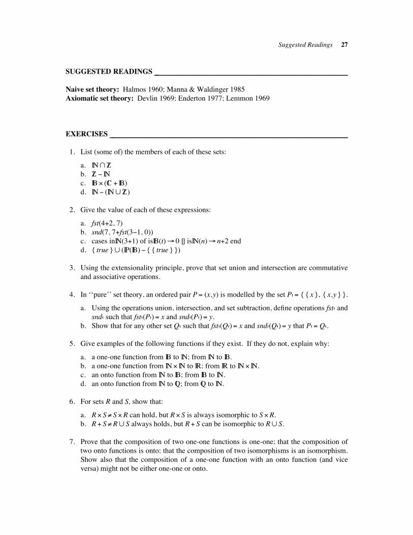
EXERCISES !!!!!!!!!!!!!!!!!!!!!!!!!!!!!!!!!!!!!!!!!!!!!!!!!!!!!!!!!!!!!!!!!!!!!!!!!!!!!!!!!!!!!!!!!!!!!!!!!!!!!!!!!!!!!!!!!!!!!!!!!!!!
1. List (some of) the members of each of these sets:
a. IN(Z|
b. Z| # IN
c. IB # (C| $ IB)
d. IN# (IN&Z| )
2. Give the value of each of these expressions:
a. fst(4$2, 7)
b. snd(7, 7$fst(3#1, 0))
c. cases inIN(3$1) of isIB(t)) 0 [] isIN(n)) n$2 end
d. { true }& (IP(IB)# { { true } })
3. Using the extensionality principle, prove that set union and intersection are commutative
and associative operations.
4. In ‘‘pure’’ set theory, an ordered pair P" (x,y) is modelled by the set P'" { { x }, { x,y } }.
a. Using the operations union, intersection, and set subtraction, define operations fst' and
snd' such that fst'(P')" x and snd'(P')" y.
b. Show that for any other set Q' such that fst'(Q')" x and snd'(Q')" y that P'" Q'.
5. Give examples of the following functions if they exist. If they do not, explain why:
a. a one-one function from IB to IN; from IN to IB.
b. a one-one function from IN# IN to IR; from IR to IN# IN.
c. an onto function from IN to IB; from IB to IN.
d. an onto function from IN to Q| ; from Q| to IN.
6. For sets R and S, show that:
a. R# S" S#R can hold, but R# S is always isomorphic to S#R.
b. R$ S"R& S always holds, but R$ S can be isomorphic to R& S.
7. Prove that the composition of two one-one functions is one-one; that the composition of
two onto functions is onto; that the composition of two isomorphisms is an isomorphism.
Show also that the composition of a one-one function with an onto function (and vice
versa) might not be either one-one or onto.
28 Sets, Functions, and Domains
8. Using the definition of split-add in Section 2.2.1, determine the graphs of:
a. split-add(3)
b. split-add(split-add(2)(1))
9. Determine the graphs of:
a. split-sub : Z| )Z| )Z| such that split-sub(x)" g, where g : Z| )Z| is g(y)" x # y
b. split-sub : IN) IN)Z| , where the function is defined in part a.
10. The previous two exercises suggest that there is an underlying concept for ‘‘splitting’’ a
function. For a set D, we define curryD : ((D#D))D) ) (D) (D)D)) to be
curryD(f)" g, where g(x)" h, where h(y)" f(x,y). Write out (part of) the graph for
curryIB : ((IB # IB) ) IB) ) (IB) (IB) IB)).
11. For IB " { true, false } and IN" { 0, 1, 2, . . . }, what are the functionalities of the func-
tions represented by these graphs?
a. { (true, 0), (false, 1) }
b. { ((true, 0), (true, true)), ((true, 1), (true, false)), ((true, 2), (true, false)), . . . , ((false, 0), (false, true)), ((false, 1), (false, false)), ((false, 2),
(false, false)), . . . }
c. { ({ (true, true), (false, true) }, true), ({ (true, true), (false, false) }, false), . . . , ({ (true, false), (false, true) }, true), . . . }
12. Use the definitions in Section 2.2.2 to simplify each of the following expressions:
a. make-singleton(add(3,2))& { 4 }
b. add(snd(duplicate(4)), 1)
c. which-part(inIN(add(2,0)))
d. ([ 3&&) { 4 } ]make-singleton)(2)
e. ([ 3&&) { 4 } ]make-singleton)(3)
13. For the equational definition fac(n)" (n"0)) 1 [] n,fac(n#1), show that the following
properties hold (hint: use mathematical induction):
a. For all n$ IN, fac(n) has a unique value, that is, fac is a function.
b. For all n$ IN, fac(n$2) > n.
14. List the elements in these domains:
a. (IB # IB) &!
b. IB &! # IB &!
c. (IB # IB)$ IB
d. (IB $ IB) &!
e. IB &! $ IB &!
f. IB) IB &!
g. (IB) IB) &!
Exercises 29
15. Simplify these expressions using the algebra in Example 2.1:
a. addrat (makerat (3) (2)) (makerat (1) (3))
b. addrat (makerat (2) (0)) (multrat (makerat (3) (2)) (makerat (1) (3)))
c. (+r. one) (makerat (1) (0))
d. (+!!r. one) (makerat (1) (0))
e. (+(r, s). addrat(r) (s)) ( (makerat (2) (1)), (makerat (3) (2)) )
f. (+(r, s). r) ( (makerat (2) (1)), (makerat (1) (0)) )
16. The sets introduced in Section 2.1 belong to naive set theory, which is called such
because it is possible to construct set definitions that are nonsensical.
a. Show that the definition { x | x$/x } is a nonsensical definition; that is, no set exists
that satisfies the definition.
b. Justify why the domain constructions in Section 2.3 always define sensical sets.
Chapter 3 !!!!!!!!!!!!!!!!!!!!!!!!!!!!!!!!!!!!!!!!!!!!!!!!!!!!!!!!
Domain Theory I: Semantic Algebras
Before we can study the semantics of programming languages, we must establish a suitable
collection of meanings for programs. We employ a framework called domain theory: the
study of ‘‘structured sets’’ and their operations. A programmer might view domain theory as
‘‘data structures for semantics.’’ Nonetheless, domain theory is a formal branch of
(computing-related) mathematics and can be studied on its own.
The fundamental concept in domain theory is a semantic domain, a set of elements
grouped together because they share some common property or use. The set of natural
numbers is a useful semantic domain; its elements are structurally similar and share common
use in arithmetic. Other examples are the Greek alphabet and the diatonic (musical) scale.
Domains may be nothing more than sets, but there are situations in which other structures such
as lattices or topologies are used instead. We can use domains without worrying too much
about the underlying mathematics. Sets make good domains, and you may safely assume that
the structures defined in this chapter are nothing more than the sets discussed in Chapter 2.
Chapter 6 presents reasons why domains other than sets might be necessary.
Accompanying a domain is a set of operations. The operations are functions that need
arguments from the domain to produce answers. Operations are defined in two parts. First, the
operation’s domain and codomain are given by an expression called the operation’s func-
tionality. For an operation f, its functionality f: D1"D2" . . . "Dn!A says that f needs an
argument from domain D1 and one from D2, . . ., and one from Dn to produce an answer in
domain A. Second, a description of the operation’s mapping is specified. The description is
usually an equational definition, but a set graph, table, or diagram may also be used.
A domain plus its operations constitutes a semantic algebra. Many examples of semantic
algebras are found in the following sections.
3.1 PRIMITIVE DOMAINS !!!!!!!!!!!!!!!!!!!!!!!!!!!!!!!!!!!!!!!!!!!!!!!!!!!!!!!!!!!!!!!!!!!!!!!!!!!!!!!!!!!!!!!!!!!!!!!!!!
A primitive domain is a set that is fundamental to the application being studied. Its elements
are atomic and they are used as answers or ‘‘semantic outputs.’’ For example, the real
numbers are a primitive domain for a mathematician, as are the notes in the key of C for a
musician, as are the words of a dictionary for a copyeditor, and so on. Here is the most com-
monly used primitive domain:
3.1 Example: The natural numbers
Domain Nat# IN
Operations
zero : Nat
30
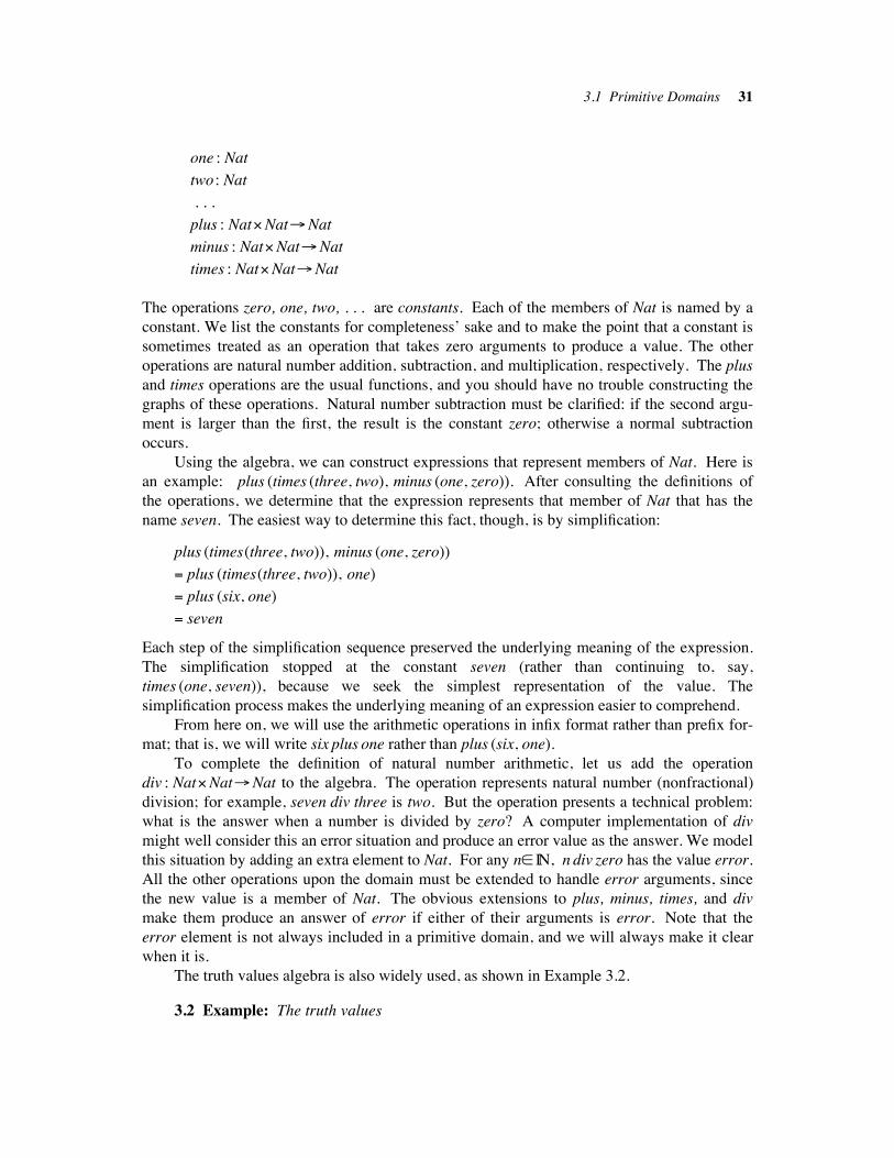
3.1 Primitive Domains 31
one : Nat
two : Nat
. . .
plus : Nat"Nat!Nat
minus : Nat"Nat!Nat
times : Nat"Nat!Nat
The operations zero, one, two, . . . are constants. Each of the members of Nat is named by a
constant. We list the constants for completeness’ sake and to make the point that a constant is
sometimes treated as an operation that takes zero arguments to produce a value. The other
operations are natural number addition, subtraction, and multiplication, respectively. The plus
and times operations are the usual functions, and you should have no trouble constructing the
graphs of these operations. Natural number subtraction must be clarified: if the second argu-
ment is larger than the first, the result is the constant zero; otherwise a normal subtraction
occurs.
Using the algebra, we can construct expressions that represent members of Nat. Here is
an example: plus (times (three, two), minus (one, zero)). After consulting the definitions of
the operations, we determine that the expression represents that member of Nat that has the
name seven. The easiest way to determine this fact, though, is by simplification:
plus (times(three, two)), minus (one, zero))
# plus (times(three, two)), one)
# plus (six, one)
# seven
Each step of the simplification sequence preserved the underlying meaning of the expression.
The simplification stopped at the constant seven (rather than continuing to, say,
times (one, seven)), because we seek the simplest representation of the value. The
simplification process makes the underlying meaning of an expression easier to comprehend.
From here on, we will use the arithmetic operations in infix format rather than prefix for-
mat; that is, we will write six plus one rather than plus (six, one).
To complete the definition of natural number arithmetic, let us add the operation
div : Nat"Nat!Nat to the algebra. The operation represents natural number (nonfractional)
division; for example, seven div three is two. But the operation presents a technical problem:
what is the answer when a number is divided by zero? A computer implementation of div
might well consider this an error situation and produce an error value as the answer. We model
this situation by adding an extra element to Nat. For any n" IN, n div zero has the value error.
All the other operations upon the domain must be extended to handle error arguments, since
the new value is a member of Nat. The obvious extensions to plus, minus, times, and div
make them produce an answer of error if either of their arguments is error. Note that the
error element is not always included in a primitive domain, and we will always make it clear
when it is.
The truth values algebra is also widely used, as shown in Example 3.2.
3.2 Example: The truth values
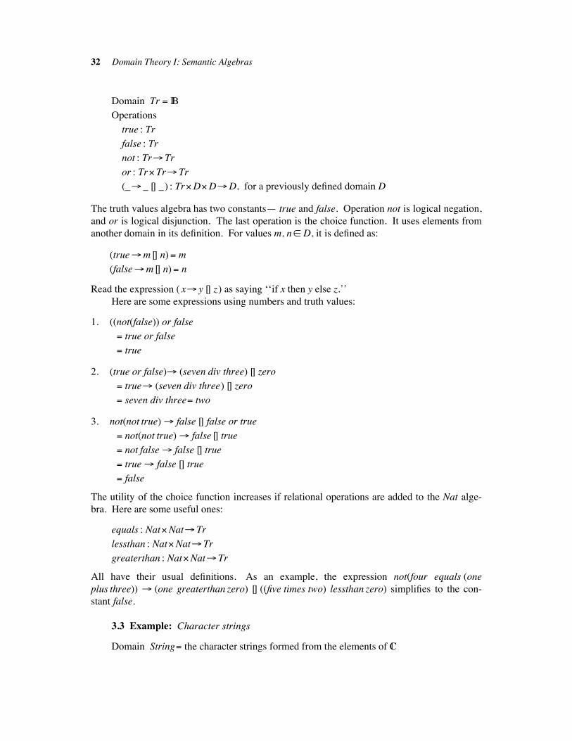
32 Domain Theory I: Semantic Algebras
Domain Tr # IB
Operations
true : Tr
false : Tr
not : Tr! Tr
or : Tr" Tr! Tr
(_! _ [] _) : Tr"D"D!D, for a previously defined domain D
The truth values algebra has two constants— true and false. Operation not is logical negation,
and or is logical disjunction. The last operation is the choice function. It uses elements from
another domain in its definition. For values m, n" D, it is defined as:
(true!m [] n)# m
(false!m [] n)# n
Read the expression ( x! y [] z) as saying ‘‘if x then y else z.’’
Here are some expressions using numbers and truth values:
1. ((not(false)) or false
# true or false
# true
2. (true or false)! (seven div three) [] zero
# true! (seven div three) [] zero
# seven div three# two
3. not(not true) ! false [] false or true
# not(not true) ! false [] true
# not false ! false [] true
# true ! false [] true
# false
The utility of the choice function increases if relational operations are added to the Nat alge-
bra. Here are some useful ones:
equals : Nat"Nat! Tr
lessthan : Nat"Nat! Tr
greaterthan : Nat"Nat! Tr
All have their usual definitions. As an example, the expression not(four equals (one
plus three)) ! (one greaterthan zero) [] ((five times two) lessthan zero) simplifies to the con-
stant false.
3.3 Example: Character strings
Domain String# the character strings formed from the elements of C|
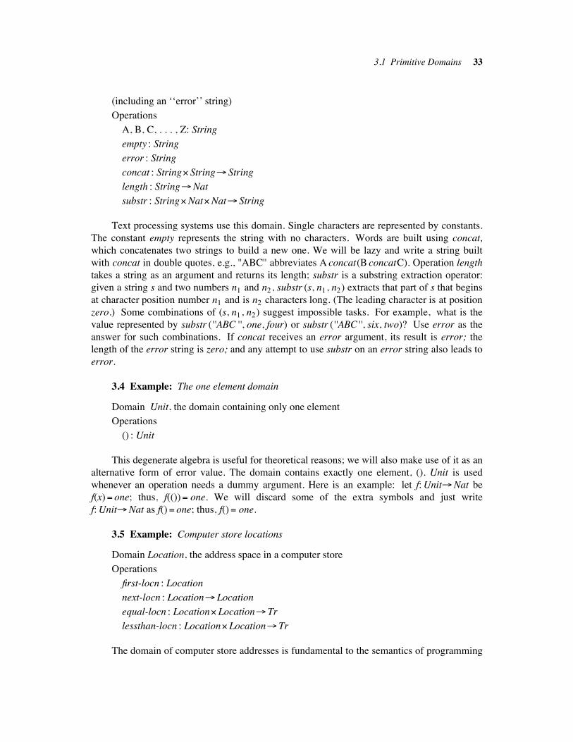
3.1 Primitive Domains 33
(including an ‘‘error’’ string)
Operations
A, B, C, . . . , Z: String
empty : String
error : String
concat : String" String! String
length : String!Nat
substr : String"Nat"Nat! String
Text processing systems use this domain. Single characters are represented by constants.
The constant empty represents the string with no characters. Words are built using concat,
which concatenates two strings to build a new one. We will be lazy and write a string built
with concat in double quotes, e.g., ''ABC'' abbreviates A concat(B concatC). Operation length
takes a string as an argument and returns its length; substr is a substring extraction operator:
given a string s and two numbers n1 and n2, substr (s, n1, n2) extracts that part of s that begins
at character position number n1 and is n2 characters long. (The leading character is at position
zero.) Some combinations of (s, n1, n2) suggest impossible tasks. For example, what is the
value represented by substr (''ABC '', one, four) or substr (''ABC'', six, two)? Use error as the
answer for such combinations. If concat receives an error argument, its result is error; the
length of the error string is zero; and any attempt to use substr on an error string also leads to
error.
3.4 Example: The one element domain
Domain Unit, the domain containing only one element
Operations
() : Unit
This degenerate algebra is useful for theoretical reasons; we will also make use of it as an
alternative form of error value. The domain contains exactly one element, (). Unit is used
whenever an operation needs a dummy argument. Here is an example: let f: Unit!Nat be
f(x)# one; thus, f(())# one. We will discard some of the extra symbols and just write
f: Unit!Nat as f()# one; thus, f()# one.
3.5 Example: Computer store locations
Domain Location, the address space in a computer store
Operations
first-locn : Location
next-locn : Location! Location
equal-locn : Location" Location! Tr
lessthan-locn : Location" Location! Tr
The domain of computer store addresses is fundamental to the semantics of programming
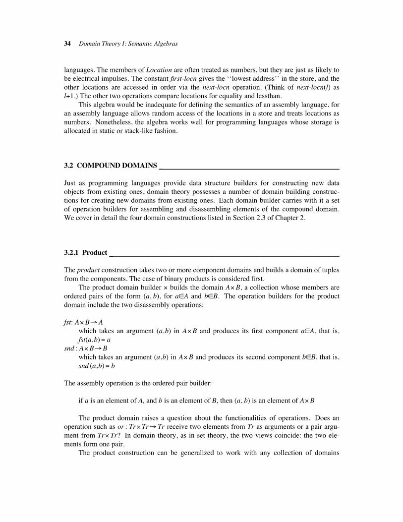
34 Domain Theory I: Semantic Algebras
languages. The members of Location are often treated as numbers, but they are just as likely to
be electrical impulses. The constant first-locn gives the ‘‘lowest address’’ in the store, and the
other locations are accessed in order via the next-locn operation. (Think of next-locn(l) as
l$1.) The other two operations compare locations for equality and lessthan.
This algebra would be inadequate for defining the semantics of an assembly language, for
an assembly language allows random access of the locations in a store and treats locations as
numbers. Nonetheless, the algebra works well for programming languages whose storage is
allocated in static or stack-like fashion.
3.2 COMPOUND DOMAINS !!!!!!!!!!!!!!!!!!!!!!!!!!!!!!!!!!!!!!!!!!!!!!!!!!!!!!!!!!!!!!!!!!!!!!!!!!!!!!!!!!!!!!!!!!!!!!!!!!
Just as programming languages provide data structure builders for constructing new data
objects from existing ones, domain theory possesses a number of domain building construc-
tions for creating new domains from existing ones. Each domain builder carries with it a set
of operation builders for assembling and disassembling elements of the compound domain.
We cover in detail the four domain constructions listed in Section 2.3 of Chapter 2.
3.2.1 Product !!!!!!!!!!!!!!!!!!!!!!!!!!!!!!!!!!!!!!!!!!!!!!!!!!!!!!!!!!!!!!!!!!!!!!!!!!!!!!!!!!!!!!!!!!!!!!!!!!!!!!!!!!!!!!!!!!!!!!!!!!!!
The product construction takes two or more component domains and builds a domain of tuples
from the components. The case of binary products is considered first.
The product domain builder " builds the domain A"B, a collection whose members are
ordered pairs of the form (a, b), for a"A and b"B. The operation builders for the product
domain include the two disassembly operations:
fst: A"B!A
which takes an argument (a,b) in A"B and produces its first component a"A, that is,
fst(a,b)# a
snd : A"B!B
which takes an argument (a,b) in A"B and produces its second component b"B, that is,
snd (a,b)# b
The assembly operation is the ordered pair builder:
if a is an element of A, and b is an element of B, then (a, b) is an element of A"B
The product domain raises a question about the functionalities of operations. Does an
operation such as or : Tr" Tr! Tr receive two elements from Tr as arguments or a pair argu-
ment from Tr" Tr? In domain theory, as in set theory, the two views coincide: the two ele-
ments form one pair.
The product construction can be generalized to work with any collection of domains
3.2.1 Product 35
A1, A2, . . . , An , for any n> 0. We write (x1, x2, . . . , xn) to represent an element of
A1"A2" . . . " An . The subscripting operations fst and snd generalize to a family of n opera-
tions: for each i from 1 to n, #i denotes the operation such that (a1, a2, . . . , an)#i # ai .
Theoretically, it is possible to construct products from an infinite number of component
domains, but infinite products raise some technical problems which are considered in exercise
16 in Chapter 6.
Example 3.6 shows a semantic algebra built with the product construction.
3.6 Example: Payroll information: a person’s name, payrate, and hours worked
Domain Payroll-record# String"Rat"Rat
(Note: Rat is the domain defined in Example 2.1 in Chapter 2)
Operations
new-employee : String!Payroll-record
new-employee(name)# (name, minimum-wage, 0),
where minimum-wage"Rat is some fixed value from Rat
and 0 is the Rat value (makerat (0) (1))
update-payrate : Rat"Payroll-record!Payroll-record
update-payrate (pay, employee)# (employee#1, pay, employee#3)
update-hours : Rat"Payroll-record!Payroll-record
update-hours (hours, employee)# (employee#1, employee#2, hours
addrat employee#3)
compute-pay : Payroll-record!Rat
compute-pay (employee)# (employee#2) multrat (employee#3)
This semantic algebra is useful for the semantics of a payroll program. The components of the
domain represent an employee’s name, hourly wage, and the cumulative hours worked for the
week. Here is an expression built with the algebra’s operations:
compute-pay(update-hours(35, new-employee(''J.Doe'')))
# compute-pay(update-hours(35, (''J.Doe'', minimum-wage, 0)))
# compute-pay((''J.Doe'', minimum-wage, 0)#1, (''J.Doe'', minimum-wage, 0)#2,
35 addrat (''J.Doe'', minimum-wage, 0)#3)
# compute-pay(''J.Doe'', minimum-wage, 35 addrat 0)
# minimum-wage multrat 35
3.2.2 Disjoint Union !!!!!!!!!!!!!!!!!!!!!!!!!!!!!!!!!!!!!!!!!!!!!!!!!!!!!!!!!!!!!!!!!!!!!!!!!!!!!!!!!!!!!!!!!!!!!!!!!!!!!!!!!!!!!!!!
The construction for unioning two or more domains into one domain is disjoint union (or
sum).
36 Domain Theory I: Semantic Algebras
For domains A and B, the disjoint union builder + builds the domain A$B, a collection
whose members are the elements of A and the elements of B, labeled to mark their origins. The
classic representation of this labeling is the ordered pair (zero, a) for an a"A and (one, b) for a
b"B.
The associated operation builders include two assembly operations:
inA: A!A$B
which takes an a"A and labels it as originating from A; that is, inA(a)# (zero, a), using
the pair representation described above.
inB: B!A$B
which takes a b"B and labels it as originating from B, that is, inB(b)# (one, b).
The ‘‘type tags’’ that the assembly operations place onto their arguments are put to good use
by the disassembly operation, the cases operation, which combines an operation on A with one
on B to produce a disassembly operation on the sum domain. If d is a value from A$B and
f(x)#e1 and g(y)#e2 are the definitions of f: A!C and g:B!C, then:
(cases d of isA(x)! e1 [] isB(y)! e2 end)
represents a value in C. The following properties hold:
(cases inA(a) of isA(x)! e1 [] isB(y)! e2 end) # [a/x]e1 # f(a)
and
(cases inB(b) of isA(x)! e1 [] isB(y)! e2 end) # [b/y]e2 # g(b)
The cases operation checks the tag of its argument, removes it, and gives the argument to the
proper operation.
Sums of an arbitrary number of domains can be built. We write A1 $A2 $ . . . $ An to
stand for the disjoint union of domains A1, A2, . . . , An . The operation builders generalize in
the obvious way.
As a first example, we alter the Payroll-record domain of Example 3.6 to handle workers
who work either the day shift or the night shift. Since the night shift is less desirable, employ-
ees who work at night receive a bonus in pay. These concepts are represented with a disjoint
union construction in combination with a product construction.
3.7 Example: Revised payroll information
Domain Payroll-rec#String" (Day$Night)"Rat
where Day#Rat and Night#Rat
(The names Day and Night are aliases for two occurrences of Rat. We use
dwage"Day and nwage"Night in the operations that follow.)
Operations
newemp : String!Payroll-rec
newemp(name)# (name, inDay(minimum-wage), 0)
move-to-dayshift : Payroll-rec!Payroll-rec
3.2.2 Disjoint Union 37
move-to-dayshift(employee)#( employee#1,
(cases (employee#2) of isDay(dwage)! inDay(dwage)
[] isNight(nwage)! inDay(nwage) end),
employee#3 )
move-to-nightshift : Payroll-rec!Payroll-rec
move-to-nightshift(employee)# ( employee#1,
(cases (employee#2) of isDay(dwage)! inNight(dwage)
[] isNight(nwage)! inNight(nwage) end),
employee#3 )
. . .
compute-pay : Payroll-rec!Rat
compute-pay(employee)# (cases (employee#2) of
isDay(dwage)! dwage multrat (employee#3)
[] isNight(nwage)! (nwage
multrat 1.5) multrat (employee#3)
end)
A person’s wage is labeled as being either a day wage or a night wage. A new employee
is started on the day shift, signified by the use of inDay in the operation newemp. The opera-
tions move-to-dayshift and move-to-nightshift adjust the label on an employee’s wage. Opera-
tion compute-pay computes a time-and-a-half bonus for a night shift employee. Here is an
example: if jdoe is the expression newemp(''J.Doe'') # (''J.Doe'', inDay(minimum-wage), 0),
and jdoe-thirty is update-hours(30, jdoe), then:
compute-pay(jdoe-thirty)
# (cases jdoe-thirty#2 of
isDay(wage)! wage multrat (jdoe-thirty#3)
[] isNight(wage)! (wage multrat 1.5) multrat (jdoe-thirty#3)
end)
# (cases inDay(minimum-wage) of
isDay(wage)! wage multrat 30
[] isNight(wage)! wage multrat 1.5 multrat 30
end)
# minimum-wage multrat 30
The tag on the component inDay(minimum-wage) of jdoe-thirty’s record helps select the
proper pay calculation.
The primitive domain Tr can be nicely modelled using the Unit domain and the disjoint
union construction.
3.8 Example: The truth values as a disjoint union
38 Domain Theory I: Semantic Algebras
Domain Tr#TT$FF
where TT#Unit and FF#Unit
Operations
true : Tr
true# inTT()
false : Tr
false# inFF()
not : Tr! Tr
not(t)# cases t of isTT()! inFF() [] isFF()! inTT() end
or : Tr" Tr! Tr
or(t, u)# cases t of
isTT()! inTT()
[] isFF()! (cases u of isTT()! inTT() [] isFF()! inFF() end)
end
The dummy argument () isn’t actually used in the operations— the tag attached to it is the
important information. For this reason, no identifier names are used in the clauses of the cases
statements; () is used there as well. We can also define the choice function:
(t! e1 [] e2)# (cases t of isTT()! e1 [] isFF()! e2 end)
As a third example, for a domain D with an error element, the collection of finite lists of
elements from D can be defined as a disjoint union. The domain
D $# Unit$D$ (D"D)$ (D" (D"D))$ . . .
captures the idea: Unit represents those lists of length zero (namely the empty list), D contains
those lists containing one element, D"D contains those lists of two elements, and so on.
3.9 Example: Finite lists
Domain D $
Operations
nil : D $
nil# inUnit()
cons : D"D $!D $
cons(d, l)# cases l of
isUnit()! inD(d)
[] isD(y)! inD"D(d,y)
[] isD"D(y)! inD"(D"D)(d,y)
[] . . . end
hd : D$!D
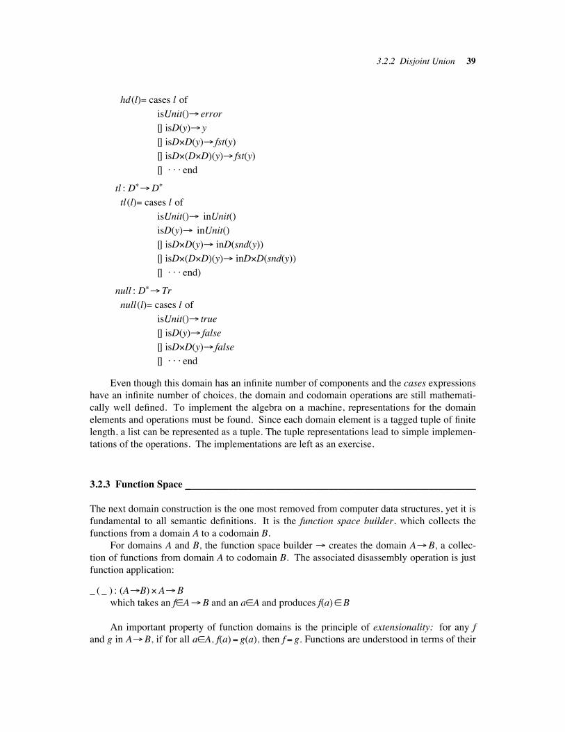
3.2.2 Disjoint Union 39
hd(l)# cases l of
isUnit()! error
[] isD(y)! y
[] isD"D(y)! fst(y)
[] isD"(D"D)(y)! fst(y)
[] . . . end
tl : D$!D$
tl(l)# cases l of
isUnit()! inUnit()
isD(y)! inUnit()
[] isD"D(y)! inD(snd(y))
[] isD"(D"D)(y)! inD"D(snd(y))
[] . . . end)
null : D$! Tr
null(l)# cases l of
isUnit()! true
[] isD(y)! false
[] isD"D(y)! false
[] . . . end
Even though this domain has an infinite number of components and the cases expressions
have an infinite number of choices, the domain and codomain operations are still mathemati-
cally well defined. To implement the algebra on a machine, representations for the domain
elements and operations must be found. Since each domain element is a tagged tuple of finite
length, a list can be represented as a tuple. The tuple representations lead to simple implemen-
tations of the operations. The implementations are left as an exercise.
3.2.3 Function Space !!!!!!!!!!!!!!!!!!!!!!!!!!!!!!!!!!!!!!!!!!!!!!!!!!!!!!!!!!!!!!!!!!!!!!!!!!!!!!!!!!!!!!!!!!!!!!!!!!!!!!!!!!!!!!!!
The next domain construction is the one most removed from computer data structures, yet it is
fundamental to all semantic definitions. It is the function space builder, which collects the
functions from a domain A to a codomain B.
For domains A and B, the function space builder ! creates the domain A!B, a collec-
tion of functions from domain A to codomain B. The associated disassembly operation is just
function application:
_ ( _ ) : (A!B)"A!B
which takes an f"A!B and an a"A and produces f(a)"B
An important property of function domains is the principle of extensionality: for any f
and g in A!B, if for all a"A, f(a)# g(a), then f # g. Functions are understood in terms of their
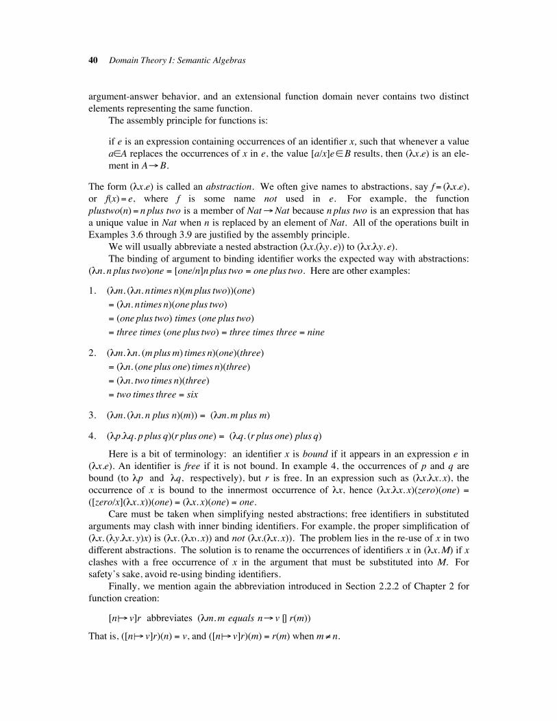
40 Domain Theory I: Semantic Algebras
argument-answer behavior, and an extensional function domain never contains two distinct
elements representing the same function.
The assembly principle for functions is:
if e is an expression containing occurrences of an identifier x, such that whenever a value
a"A replaces the occurrences of x in e, the value [a/x]e"B results, then (%x.e) is an ele-
ment in A!B.
The form (%x.e) is called an abstraction. We often give names to abstractions, say f # (%x.e),
or f(x)# e, where f is some name not used in e. For example, the function
plustwo(n) # n plus two is a member of Nat!Nat because n plus two is an expression that has
a unique value in Nat when n is replaced by an element of Nat. All of the operations built in
Examples 3.6 through 3.9 are justified by the assembly principle.
We will usually abbreviate a nested abstraction (%x.(%y. e)) to (%x.%y. e).
The binding of argument to binding identifier works the expected way with abstractions:
(%n. n plus two)one # [one/n]n plus two # one plus two. Here are other examples:
1. (%m. (%n. ntimes n)(m plus two))(one)
# (%n. ntimes n)(one plus two)
# (one plus two) times (one plus two)
# three times (one plus two) # three times three # nine
2. (%m.%n. (m plus m) times n)(one)(three)
# (%n. (one plus one) times n)(three)
# (%n. two times n)(three)
# two times three # six
3. (%m. (%n. n plus n)(m)) # (%m. m plus m)
4. (%p.%q. p plus q)(r plus one) # (%q. (r plus one) plus q)
Here is a bit of terminology: an identifier x is bound if it appears in an expression e in
(%x.e). An identifier is free if it is not bound. In example 4, the occurrences of p and q are
bound (to %p and %q, respectively), but r is free. In an expression such as (%x.%x. x), the
occurrence of x is bound to the innermost occurrence of %x, hence (%x.%x. x)(zero)(one) #([zero/x](%x. x))(one) # (%x. x)(one) # one.
Care must be taken when simplifying nested abstractions; free identifiers in substituted
arguments may clash with inner binding identifiers. For example, the proper simplification of
(%x. (%y.%x. y)x) is (%x. (%x'. x)) and not (%x.(%x. x)). The problem lies in the re-use of x in two
different abstractions. The solution is to rename the occurrences of identifiers x in (%x. M) if x
clashes with a free occurrence of x in the argument that must be substituted into M. For
safety’s sake, avoid re-using binding identifiers.
Finally, we mention again the abbreviation introduced in Section 2.2.2 of Chapter 2 for
function creation:
[n %%! v]r abbreviates (%m. m equals n! v [] r(m))
That is, ([n %%! v]r)(n) # v, and ([n %%! v]r)(m) # r(m) when m& n.
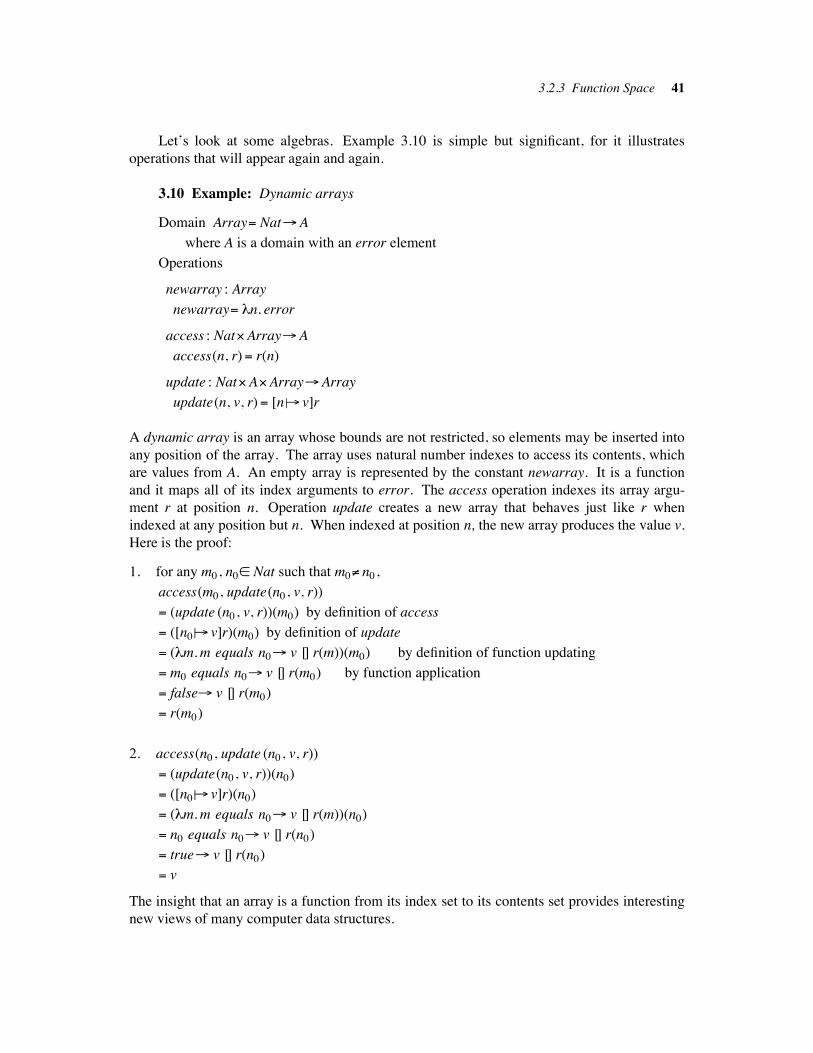
3.2.3 Function Space 41
Let’s look at some algebras. Example 3.10 is simple but significant, for it illustrates
operations that will appear again and again.
3.10 Example: Dynamic arrays
Domain Array# Nat!A
where A is a domain with an error element
Operations
newarray : Array
newarray# %n. error
access : Nat"Array!A
access(n, r)# r(n)
update : Nat"A"Array!Array
update(n, v, r)# [n %%! v]r
A dynamic array is an array whose bounds are not restricted, so elements may be inserted into
any position of the array. The array uses natural number indexes to access its contents, which
are values from A. An empty array is represented by the constant newarray. It is a function
and it maps all of its index arguments to error. The access operation indexes its array argu-
ment r at position n. Operation update creates a new array that behaves just like r when
indexed at any position but n. When indexed at position n, the new array produces the value v.
Here is the proof:
1. for any m0, n0" Nat such that m0& n0,
access(m0, update(n0, v, r))
# (update (n0, v, r))(m0) by definition of access
# ([n0 %%! v]r)(m0) by definition of update
# (%m. m equals n0! v [] r(m))(m0) by definition of function updating
# m0 equals n0! v [] r(m0) by function application
# false! v [] r(m0)
# r(m0)
2. access(n0, update (n0, v, r))
# (update(n0, v, r))(n0)
# ([n0 %%! v]r)(n0)
# (%m. m equals n0! v [] r(m))(n0)
# n0 equals n0! v [] r(n0)
# true! v [] r(n0)
# v
The insight that an array is a function from its index set to its contents set provides interesting
new views of many computer data structures.
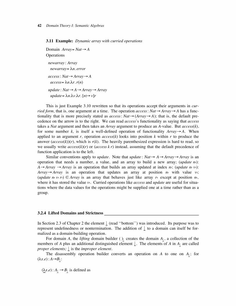
42 Domain Theory I: Semantic Algebras
3.11 Example: Dynamic array with curried operations
Domain Array# Nat!A
Operations
newarray : Array
newarray# %n. error
access : Nat!Array!A
access# %n.%r. r(n)
update : Nat!A!Array!Array
update# %n.%v.%r. [n %%! v]r
This is just Example 3.10 rewritten so that its operations accept their arguments in cur-
ried form, that is, one argument at a time. The operation access : Nat!Array!A has a func-
tionality that is more precisely stated as access : Nat! (Array!A); that is, the default pre-
cedence on the arrow is to the right. We can read access’s functionality as saying that access
takes a Nat argument and then takes an Array argument to produce an A-value. But access(k),
for some number k, is itself a well-defined operation of functionality Array!A. When
applied to an argument r, operation access(k) looks into position k within r to produce the
answer (access(k))(r), which is r(k). The heavily parenthesized expression is hard to read, so
we usually write access(k)(r) or (access k r) instead, assuming that the default precedence of
function application is to the left.
Similar conventions apply to update. Note that update : Nat! A!Array!Array is an
operation that needs a number, a value, and an array to build a new array; (update n'):A!Array !Array is an operation that builds an array updated at index n'; (update n' v'):Array!Array is an operation that updates an array at position n' with value v';(update n' v' r') " Array is an array that behaves just like array r' except at position n',where it has stored the value v'. Curried operations like access and update are useful for situa-
tions where the data values for the operations might be supplied one at a time rather than as a
group.
3.2.4 Lifted Domains and Strictness !!!!!!!!!!!!!!!!!!!!!!!!!!!!!!!!!!!!!!!!!!!!!!!!!!!!!!!!!!!!!!!!!!!!!!!!!!!!!!!!!!!!!!
In Section 2.3 of Chapter 2 the element %' (read ‘‘bottom’’) was introduced. Its purpose was to
represent undefinedness or nontermination. The addition of %' to a domain can itself be for-
malized as a domain-building operation.
For domain A, the lifting domain builder ( )%! creates the domain A%! , a collection of the
members of A plus an additional distinguished element %'. The elements of A in A %! are called
proper elements; %' is the improper element.
The disassembly operation builder converts an operation on A to one on A%!; for
(%x.e) : A!B %!:
(%!!x.e) : A %!!B%! is defined as
3.2.4 Lifted Domains and Strictness 43
(%!!x.e) %' # %'(%!!x.e)a # [a/x]e for a& %'
An operation that maps a %' argument to a %' answer is called strict. Operations that map %' to a
proper element are called nonstrict. Let’s do an example.
(%!!m. zero)((%!!n. one) %')
# (%!!m. zero) %', by strictness
# %'
On the other hand, (%p. zero) : Nat %!!Nat %! is nonstrict, and:
(%p. zero)((%!!n. one) %')
# [(%!!n. one) %' /p]zero, by the definition of application
# zero
In the first example, we must determine whether the argument to (%!!m.zero) is proper or
improper before binding it to m. We make the determination by simplifying the argument. If
it simplifies to a proper value, we bind it to m; if it simplifies to %', we take the result of the
application to be %'. This style of ‘‘argument first’’ simplification is known as a call-by-value
evaluation. It is the safe way of simplifying strict abstractions and their arguments. In the
second example, the argument ((%!!n.one) %') need not be simplified before binding it to p.
We use the following abbreviation:
(let x# e1 in e2) for (%!!x. e2)e1
Call this a let expression. It makes strict applications more readable because its ‘‘argument
first’’ appearance matches the ‘‘argument first’’ simplification strategy that must be used. For
example:
1. let m# (%x. zero) %' in m plus one
# let m# zero in m plus one
# zero plus one # one
2. let m# one plus two in let n# (%!!p. m) %' in m plus n
# let m# three in let n# (%!!p. m) %' in m plus n
# let n# (%!!p. three) %' in three plus n
# let n# %' in three plus n
# %'
Here is an example using the lifting construction; it uses the algebra of Example 3.11:
3.12 Example: Unsafe arrays of unsafe values
Domain Unsafe# Array %! ,
where Array# Nat! Tr' is from Example 3.11
(A in Example 3.11 becomes Tr')and Tr'# (IB( {error}) %!
44 Domain Theory I: Semantic Algebras
Operations
new-unsafe: Unsafe
new-unsafe# newarray
access-unsafe: Nat %!!Unsafe!Tr'access-unsafe# %!!n.%!!r. (access n r)
update-unsafe: Nat %!! Tr'!Unsafe!Unsafe
update-unsafe# %!!n.%t.%!!r. (update n t r)
The algebra models arrays that contain truth values that may be improper. The constant new-
unsafe builds a proper array that maps all of its arguments to the error value. An array access
becomes a tricky business, for either the index or the array argument may be improper. Opera-
tion access-unsafe must check the definedness of its arguments n and r before it passes them
on to access, which performs the actual indexing. The operation update-unsafe is similarly
paranoid, but an improper truth value may be stored into an array. Here is an evaluation of an
expression (let not' # %!!t. not(t)):
let start-array # new-unsafe
in update-unsafe(one plus two)(not'( %'))(start-array)
# let start-array # newarray
in update-unsafe(one plus two)(not'( %'))(start-array)
# let start-array # (%n. error)
in update-unsafe(one plus two)(not'( %'))(start-array)
# update-unsafe(one plus two)(not'( %'))(%n. error)
# update-unsafe(three)(not'( %'))(%n. error)
# update (three)(not'( %'))(%n. error)
# [three %%! not'( %') ] (%n. error)
# [three %%! %' ] (%n. error)
You should study each step of this simplification sequence and determine where call-by-value
simplifications were used.
3.3 RECURSIVE FUNCTION DEFINITIONS !!!!!!!!!!!!!!!!!!!!!!!!!!!!!!!!!!!!!!!!!!!!!!!!!!!!!!!!!!!!!!!!!!!!
If you read the description of the assembly principle for functions carefully, you will note that
the definition f(x1, . . . , xn)# e does not permit f itself to appear in e. There is good reason: a
recursive definition may not uniquely define a function. Here is an example:
q(x)# x equals zero! one [] q(x plus one)
This specification apparently defines a function in IN! IN%! . The following functions all
satisfy q’s definition in the sense that they have exactly the behavior required by the equation:
3.3 Recursive Function Definitions 45
f1(x)# %'
one otherwise
if x# zero
f2(x)# two
one otherwise
if x# zero
f3(x)# one
and there are infinitely many others. Routine substitution verifies that f3 is a meaning of q:
for any n"Nat, n equals zero! one [] f3(n plus one)
# n equals zero! one [] one by the definition of f3
# one by the definition of the choice function
# f3(n)
Similar derivations also show that f1 and f2 are meanings of q. So which of these functions
does q really stand for, if any? Unfortunately, the tools as currently developed are not sophis-
ticated enough to answer this question. The problem will be dealt with in Chapter 6, because
recursive function definitions are essential for defining the semantics of iterative and recursive
constructs.
Perhaps when you were reading the above paragraph, you felt that much ado was made
about nothing. After all, the specification of q could be typed into a computer, and surely the
computer would compute function f1. However, the computer gives an operational semantics
to the specification, treating it as a program, and the function expressions in this chapter are
mathematical values, not programs. It is clearly important that we use only those function
expressions that stand for unique values. For this reason, recursive function specifications are
suspect.
On the positive side, it is possible to show that functions defined recursively over abstract
syntax arguments do denote unique functions. Structural induction comes to the rescue. We
examine this specific subcase because denotational definitions utilize functions that are recur-
sively defined over abstract syntax.
The following construction is somewhat technical and artificial, but it is sufficient for
achieving the goal. Let a language L be defined by BNF equations:
B1 ::= Option11 | Option12 | . . . | Option1m
B2 ::= Option21 | Option22 | . . . | Option2m
. . .
Bn ::= Optionn 1 | Optionn 2 | . . . | Optionnm
and let Bi be a function symbol of type Bi!Di for all 1) i) n. For an Optionij , let
Sij 1, Sij 2, . . . , Sijk be the nonterminal symbols used in Optionij , and let Bijl represent the Bl
appropriate for each Sijl (for example, if Sijl#Bp , then Bijl#Bp).
3.13 Theorem:
If, for each Bi in L’s definition and each Optionij of Bi ’s rule, there exists an equation of
form:
46 Domain Theory I: Semantic Algebras
Bi(Optionij)# fij(Bij 1(Sij 1), Bij 2(Sij 2), . . . , Bijk(Sijk))
where fij is a function of functionality Dij1"Dij2" . . . "Dijk !Di, then the set of equa-
tions uniquely defines a family of functions Bi : Bi!Di for 1) i) n.
Proof: The proof is by a simultaneous structural induction on the rules of L. We show
that each Bi(Option ij) is uniquely defined for a syntax tree of form Optionij . Let
Bi(Option ij) be defined as above. By the inductive hypothesis, for 1) l) k, each Bijl(Sijl)
is uniquely defined. Since fij is a function, its application to the Bijl(Sijl)’s yields a
unique answer, so Bi(Option ij) is uniquely defined. The equations for all the Option ij’s
of rule Bi taken together define a unique function Bi : Bi!Di .
3.4 RECURSIVE DOMAIN DEFINITIONS !!!!!!!!!!!!!!!!!!!!!!!!!!!!!!!!!!!!!!!!!!!!!!!!!!!!!!!!!!!!!!!!!!!!!!!!
We have used an equation format for naming semantic domains. For example, Payroll-
record# String"Rat"Rat associates the name Payroll-record with a product domain. In
later chapters, we will see that certain programming language features require domains whose
structure is defined in terms of themselves. For example, Alist#Unit$ (A"Alist) defines a
domain of linear lists of A-elements. Like the recursively defined operations mentioned in the
previous section, a domain may not be uniquely defined by a recursive definition.
What’s more, equations such as F# F!Nat, specifying the collection of functions that
accept themselves as arguments to produce numeric answers, apparently have no solution at
all! (It is not difficult to show that the cardinality of the collection of all functions from F to
Nat is larger than F’s cardinality.) Chapter 11 provides a method for developing solutions to
recursive domain definitions.
3.5 SUMMARY !!!!!!!!!!!!!!!!!!!!!!!!!!!!!!!!!!!!!!!!!!!!!!!!!!!!!!!!!!!!!!!!!!!!!!!!!!!!!!!!!!!!!!!!!!!!!!!!!!!!!!!!!!!!!!!!!!!!!!!!
Here is a summary of the domain constructions and their operations that were covered in this
chapter.
1. Domain construction: primitive domain, e.g., natural numbers, truth values
Operation builders: the operations and constants that are presented in the semantic alge-
bra. For example, the choice function is presented with the Tr algebra; it is
(e1 ! e2 [] e3)"A, for e1" IB, e2,e3"A.
Simplification properties: as dictated by the definition of the operations, e.g., not(true)
simplifies to false because the pair (true, false) is found in the graph of the operation not.
The simplification properties of the choice function are:
true! e2 [] e3 # e2
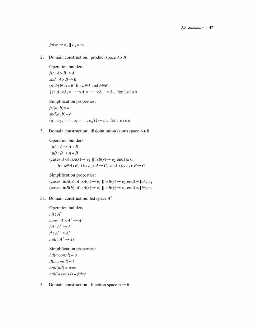
3.5 Summary 47
false! e2 [] e3 # e3
2. Domain construction: product space A"B
Operation builders:
fst : A"B!A
snd : A"B!B
(a, b)" A"B for a"A and b"B
#i : A1"A2" . . . "Ai" . . . "An !Ai , for 1) i ) n
Simplification properties:
fst(a, b)# a
snd(a, b)# b
(a1, a2, . . . , ai , . . . , an)#i# ai , for 1) i) n
3. Domain construction: disjoint union (sum) space A$B
Operation builders:
inA : A!A$B
inB : B!A$B
(cases d of isA(x)! e1 [] isB(y)! e2 end)" C
for d"A$B, (%x.e1): A!C, and (%y.e2): B!C
Simplification properties:
(cases inA(a) of isA(x)! e1 [] isB(y)! e2 end) # [a/x]e1
(cases inB(b) of isA(x)! e1 [] isB(y)! e2 end) # [b/y]e2
3a. Domain construction: list space A$
Operation builders:
nil : A$
cons : A "A$ !A$
hd : A$ !A
tl : A$ !A$
null : A$ ! Tr
Simplification properties:
hd(a cons l)# a
tl(a cons l)# l
null(nil) # true
null(a cons l)# false
4. Domain construction: function space A!B
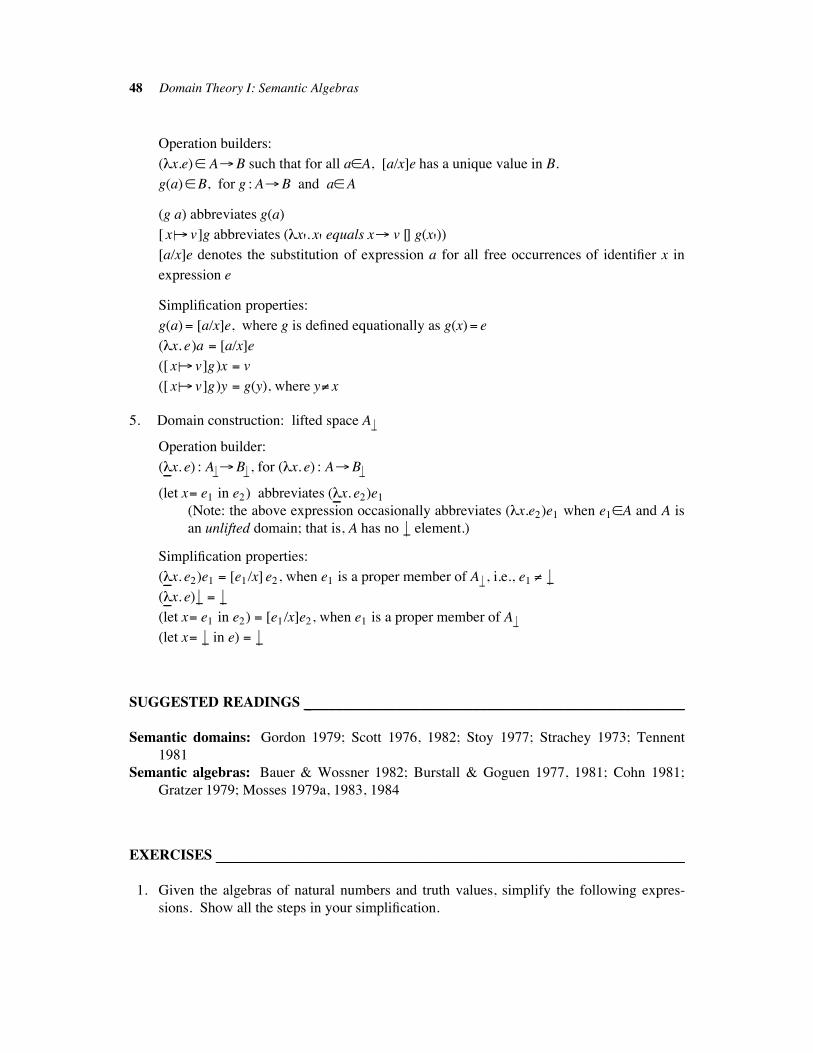
48 Domain Theory I: Semantic Algebras
Operation builders:
(%x.e)" A!B such that for all a"A, [a/x]e has a unique value in B.
g(a)"B, for g : A!B and a"A
(g a) abbreviates g(a)
[ x %%! v]g abbreviates (%x'. x' equals x! v [] g(x'))[a/x]e denotes the substitution of expression a for all free occurrences of identifier x in
expression e
Simplification properties:
g(a)# [a/x]e, where g is defined equationally as g(x)# e
(%x. e)a # [a/x]e
([ x %%! v]g)x # v
([ x %%! v]g)y # g(y), where y& x
5. Domain construction: lifted space A %!
Operation builder:
(%!!x. e) : A %!!B%! , for (%x. e) : A!B%!
(let x# e1 in e2) abbreviates (%!!x. e2)e1
(Note: the above expression occasionally abbreviates (%x.e2)e1 when e1"A and A is
an unlifted domain; that is, A has no %' element.)
Simplification properties:
(%!!x. e2)e1 # [e1 /x] e2, when e1 is a proper member of A %! , i.e., e1 & %'(%!!x. e) %' # %'(let x# e1 in e2) # [e1/x]e2, when e1 is a proper member of A %!
(let x# %' in e) # %'
SUGGESTED READINGS !!!!!!!!!!!!!!!!!!!!!!!!!!!!!!!!!!!!!!!!!!!!!!!!!!!!!!!!!!!!!!!!!!!!!!!!!!!!!!!!!!!!!!!!!!!!!!!!!!!!!!
Semantic domains: Gordon 1979; Scott 1976, 1982; Stoy 1977; Strachey 1973; Tennent
1981
Semantic algebras: Bauer & Wossner 1982; Burstall & Goguen 1977, 1981; Cohn 1981;
Gratzer 1979; Mosses 1979a, 1983, 1984
EXERCISES !!!!!!!!!!!!!!!!!!!!!!!!!!!!!!!!!!!!!!!!!!!!!!!!!!!!!!!!!!!!!!!!!!!!!!!!!!!!!!!!!!!!!!!!!!!!!!!!!!!!!!!!!!!!!!!!!!!!!!!!!!!!
1. Given the algebras of natural numbers and truth values, simplify the following expres-
sions. Show all the steps in your simplification.
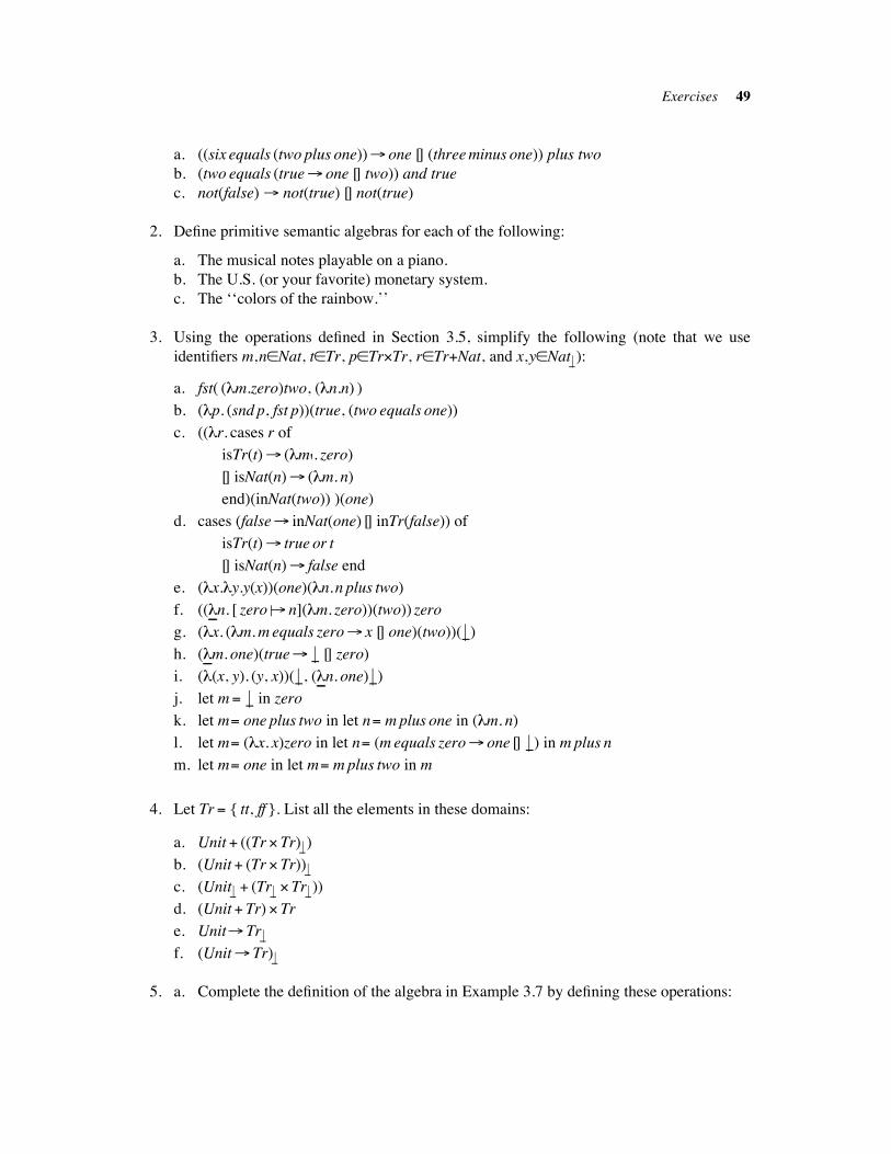
Exercises 49
a. ((six equals (two plus one))! one [] (three minus one)) plus two
b. (two equals (true! one [] two)) and true
c. not(false) ! not(true) [] not(true)
2. Define primitive semantic algebras for each of the following:
a. The musical notes playable on a piano.
b. The U.S. (or your favorite) monetary system.
c. The ‘‘colors of the rainbow.’’
3. Using the operations defined in Section 3.5, simplify the following (note that we use
identifiers m,n"Nat, t"Tr, p"Tr"Tr, r"Tr$Nat, and x,y"Nat %!):
a. fst( (%m.zero)two, (%n.n) )
b. (%p. (snd p, fst p))(true, (two equals one))
c. ((%r. cases r of
isTr(t)! (%m'. zero)
[] isNat(n)! (%m. n)
end)(inNat(two)) )(one)
d. cases (false! inNat(one) [] inTr(false)) of
isTr(t)! true or t
[] isNat(n)! false end
e. (%x.%y.y(x))(one)(%n.n plus two)
f. ((%!!n. [ zero %%! n](%m. zero))(two)) zero
g. (%x. (%m. m equals zero! x [] one)(two))( %')
h. (%!!m. one)(true! %' [] zero)
i. (%(x, y). (y, x))( %', (%!!n. one) %')
j. let m # %' in zero
k. let m# one plus two in let n# m plus one in (%m. n)
l. let m# (%x. x)zero in let n# (m equals zero! one [] %') in m plus n
m. let m# one in let m# m plus two in m
4. Let Tr # { tt, ff }. List all the elements in these domains:
a. Unit $ ((Tr" Tr) %!)
b. (Unit$ (Tr " Tr))%!
c. (Unit%! $ (Tr %! " Tr %!))
d. (Unit$ Tr) " Tr
e. Unit! Tr %!
f. (Unit! Tr) %!
5. a. Complete the definition of the algebra in Example 3.7 by defining these operations:
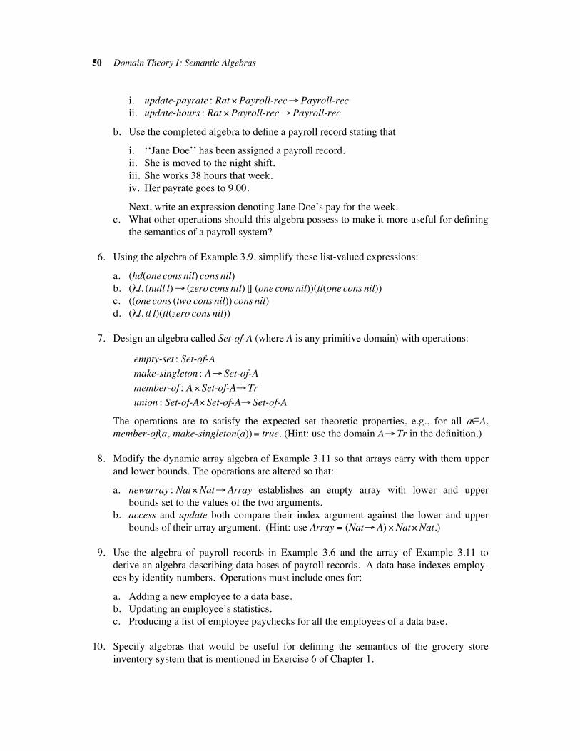
50 Domain Theory I: Semantic Algebras
i. update-payrate : Rat "Payroll-rec!Payroll-rec
ii. update-hours : Rat "Payroll-rec!Payroll-rec
b. Use the completed algebra to define a payroll record stating that
i. ‘‘Jane Doe’’ has been assigned a payroll record.
ii. She is moved to the night shift.
iii. She works 38 hours that week.
iv. Her payrate goes to 9.00.
Next, write an expression denoting Jane Doe’s pay for the week.
c. What other operations should this algebra possess to make it more useful for defining
the semantics of a payroll system?
6. Using the algebra of Example 3.9, simplify these list-valued expressions:
a. (hd(one cons nil) cons nil)
b. (%l. (null l)! (zero cons nil) [] (one cons nil))(tl(one cons nil))
c. ((one cons (two cons nil)) cons nil)
d. (%l. tl l)(tl(zero cons nil))
7. Design an algebra called Set-of-A (where A is any primitive domain) with operations:
empty-set : Set-of-A
make-singleton : A! Set-of-A
member-of : A " Set-of-A!Tr
union : Set-of-A" Set-of-A! Set-of-A
The operations are to satisfy the expected set theoretic properties, e.g., for all a"A,
member-of(a, make-singleton(a))# true. (Hint: use the domain A! Tr in the definition.)
8. Modify the dynamic array algebra of Example 3.11 so that arrays carry with them upper
and lower bounds. The operations are altered so that:
a. newarray : Nat"Nat!Array establishes an empty array with lower and upper
bounds set to the values of the two arguments.
b. access and update both compare their index argument against the lower and upper
bounds of their array argument. (Hint: use Array # (Nat!A)"Nat"Nat.)
9. Use the algebra of payroll records in Example 3.6 and the array of Example 3.11 to
derive an algebra describing data bases of payroll records. A data base indexes employ-
ees by identity numbers. Operations must include ones for:
a. Adding a new employee to a data base.
b. Updating an employee’s statistics.
c. Producing a list of employee paychecks for all the employees of a data base.
10. Specify algebras that would be useful for defining the semantics of the grocery store
inventory system that is mentioned in Exercise 6 of Chapter 1.
Exercises 51
11. a. Describe the graphs of the following operations:
i. (_ ! a [] b) : IB!D, for a, b"D
ii. fst : A"B!A and snd : A"B!B
iii. inA : A!A$B, inB : B!A$B, and (cases _ of isA(a)! f(a)
[] isB(b)! g(b) end) : A$B!C, for f: A!C and g : B!C
iv. (%x. E) : A!B, for expression E such that for all a"A, [a/x]E is a unique value in
B
v. (%!!x. E) : A %!!B%! , for (%x. E) : A!B%!
b. Using the definitions in part a, prove that the simplification rules in Section 3.5 are
sound; that is, for each equality L #R, prove that the set-theoretic value of L equals
the set-theoretic value of R. (Note: most of the proofs will be trivial, but they are still
well worth doing, for they justify all of the derivations in the rest of the book!)
12. The assembly and disassembly operations of compound domains were chosen because
they possess certain universal properties (the term is taken from category theory; see
Herrlich and Strecker 1973). Prove the following universal properties:
a. For arbitrary functions g1: C!A and g2: C!B, there exists a unique function
f: C!A"B such that fst & f # g1 and snd & f # g2 .
b. For arbitrary functions g1: A!C and g2: B!C, there exists a unique function
f: A$B!C such that f & inA # g1 and f & inB # g2 .
c. For arbitrary function g: A"B!C, there exists a unique function f:A!B!C such
that (f(a))(b)# g(a, b).
d. For arbitrary function g: A!B %! , there exists a unique function f: A%!!B%! such that
f( %')# %' and f(a)# g(a), for a"A.
13. The function notation defined in this chapter is a descendant of a symbol manipulation
system known as the lambda calculus. The abstract syntax of lambda expressions is
defined as:
E ::= (E1 E2) | (%I.E) | I
Lambda expressions are simplified using the *-rule:
((%I.E1)E2) #> [ E2/I ]E1
which says that an occurrence of ((%I.E1)E2) in a lambda expression can be rewritten to
[ E2/I ]E1 in the expression. All bound identifiers in E1 are renamed so as not to clash
with the free identifiers in E2. We write M#>$N if M rewrites to N due to zero or more
applications of the *-rule.
a. Using the *-rule, simplify the following expressions to a final (normal) form, if one
exists. If one does not exist, explain why.
i. ((%x. (x y))(%z. z)
ii. ((%x. ((%y. (x y))x))(%z. w))
iii. ((((%f. (%g. (%x. ((f x)(g x)))))(%m.(%n. (n m))))(%n. z))p)
iv. ((%x.(x x)) (%x. (x x)))
52 Domain Theory I: Semantic Algebras
v. ((%f. ((%g. ((f f) g))(%h. (k h))))(%x. (%y.y)))
vi. (%g. ((%f. ((%x.(f (x x))) (%x. (f (x x))))) g))
b. In addition to the *-rule, the lambda calculus includes the following two rules:
+-rule : (%x. E) #> (%y. [y/x]E)
,-rule : (%x. (E x)) #> E where x does not occur free in E
Redo the simplifications of i-vi in a, making use of the ,-rule whenever possible.
What value do you see in the +-rule?
c. A famous result regarding the lambda calculus is that it can be used to simulate com-
putation on truth values and numbers.
i. Let true be the name of the lambda expression (%x.%y. x) and let false be the name
of the lambda expression (%x.%y. y). Show that ((true E1) E2)#>$E1 and
((false E1) E2)#>$E2. Define lambda expressions not, and, and or that behave
like their Boolean operation counterparts, e.g., (not true)#>$false,
((or false)true)#>$true, and so on.
ii. Let 0 be the name of the lambda expression (%x.%y.y), 1 be the name of the
expression (%x.%y.(x y)), 2 be the name of the expression (%x.%y.(x(x y))), 3 be the
name of the expression (%x.%y.(x(x(xy)))), and so on. Prove that the lambda
expression succ defined as (%z.%x.%y.(x ((z x) y))) rewrites a number to its succes-
sor, that is, (succ n) #>$n$$1. There also exists a lambda expression pred such
that (pred 0)#>$0 and (pred n$$1)#>$n (but we won’t give it here, as it is some-
what ungainly).
d. Recursively defined functions can also be simulated in the lambda calculus. First, let
Y be the name of the expression (%f. ((%x. (f (x x))) (%x. (f (x x))))).
i. Show that for any expression E, there exists an expression W such that
(Y E)#>$(W W), and that (W W)#>$(E (W W)). Hence, (Y E) #>$
E(E(E( . . . E(W W) . . . ))).
ii. Using the lambda expressions that you defined in the previous parts of this exer-
cise, define a recursive lambda expression add that performs addition on the
numbers defined in part ii of b, that is, ((add m) n) #>$m$$n. (Hint: first define an
expression IF such that (((IF 0) E1) E2)#>$E1 and (((IF n$$1) E1) E2)#>$E2.) Say
that your definition of add has the form add # %x.%y. . . . add . . . . Let ADD be
the lambda expression (Y (%h.%x.%y. . . . h . . . )). Show that
((ADD m) n) #>$m$$n.
14. a. Give examples of recursive definitions of the form n# . . . n . . . that have no solu-
tion; have multiple solutions; have exactly one solution.
b. State requirements under which a recursively defined function f: Nat!A has a unique
solution. Use mathematical induction to prove your claim. Next, generalize your
answer for recursively defined functions g: A$ !B. How do your requirements resem-
ble the requirements used to prove Theorem 3.13?
15. Show that each of the following recursively defined sets has a solution.
Exercises 53
a. Nlist # Unit $ (IN"Nlist)
b. N # Unit $N
c. A# A
d. Blist # IB "Blist.
Do any of them have a unique solution?
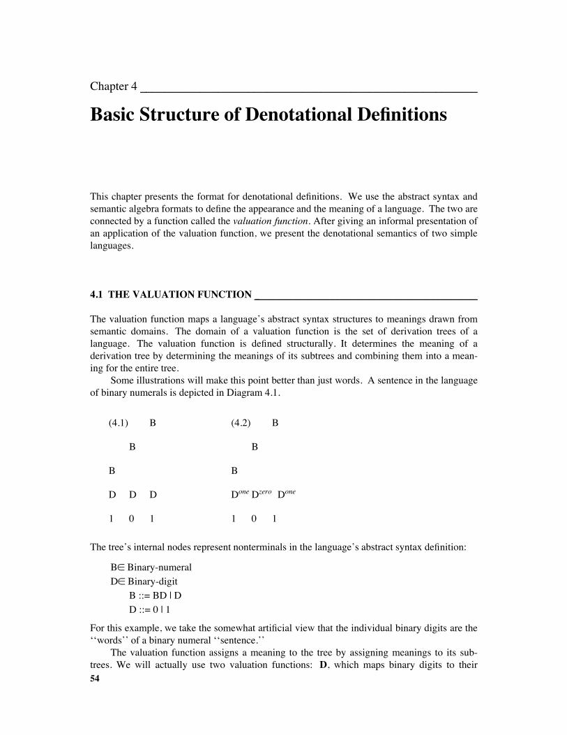
Chapter 4 !!!!!!!!!!!!!!!!!!!!!!!!!!!!!!!!!!!!!!!!!!!!!!!!!!!!!!!!
Basic Structure of Denotational Definitions
This chapter presents the format for denotational definitions. We use the abstract syntax and
semantic algebra formats to define the appearance and the meaning of a language. The two are
connected by a function called the valuation function. After giving an informal presentation of
an application of the valuation function, we present the denotational semantics of two simple
languages.
4.1 THE VALUATION FUNCTION !!!!!!!!!!!!!!!!!!!!!!!!!!!!!!!!!!!!!!!!!!!!!!!!!!!!!!!!!!!!!!!!!!!!!!!!!!!!!!!!!!!!!!
The valuation function maps a language’s abstract syntax structures to meanings drawn from
semantic domains. The domain of a valuation function is the set of derivation trees of a
language. The valuation function is defined structurally. It determines the meaning of a
derivation tree by determining the meanings of its subtrees and combining them into a mean-
ing for the entire tree.
Some illustrations will make this point better than just words. A sentence in the language
of binary numerals is depicted in Diagram 4.1.
(4.1) B (4.2) B
B B
B B
D D D Done Dzero Done
1 0 1 1 0 1
The tree’s internal nodes represent nonterminals in the language’s abstract syntax definition:
B! Binary-numeral
D! Binary-digit
B ::= BD | D
D ::= 0 | 1
For this example, we take the somewhat artificial view that the individual binary digits are the
‘‘words’’ of a binary numeral ‘‘sentence.’’
The valuation function assigns a meaning to the tree by assigning meanings to its sub-
trees. We will actually use two valuation functions: D, which maps binary digits to their
54
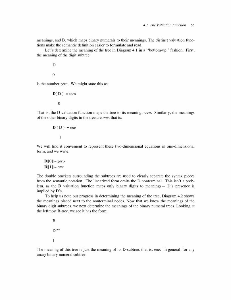
4.1 The Valuation Function 55
meanings, and B, which maps binary numerals to their meanings. The distinct valuation func-
tions make the semantic definition easier to formulate and read.
Let’s determine the meaning of the tree in Diagram 4.1 in a ‘‘bottom-up’’ fashion. First,
the meaning of the digit subtree:
D
0
is the number zero. We might state this as:
D( D ) " zero
0
That is, the D valuation function maps the tree to its meaning, zero. Similarly, the meanings
of the other binary digits in the tree are one; that is:
D ( D ) " one
1
We will find it convenient to represent these two-dimensional equations in one-dimensional
form, and we write:
D[[0]]" zero
D[[1]]" one
The double brackets surrounding the subtrees are used to clearly separate the syntax pieces
from the semantic notation. The linearized form omits the D nonterminal. This isn’t a prob-
lem, as the D valuation function maps only binary digits to meanings— D’s presence is
implied by D’s.
To help us note our progress in determining the meaning of the tree, Diagram 4.2 shows
the meanings placed next to the nonterminal nodes. Now that we know the meanings of the
binary digit subtrees, we next determine the meanings of the binary numeral trees. Looking at
the leftmost B-tree, we see it has the form:
B
Done
1
The meaning of this tree is just the meaning of its D-subtree, that is, one. In general, for any
unary binary numeral subtree:
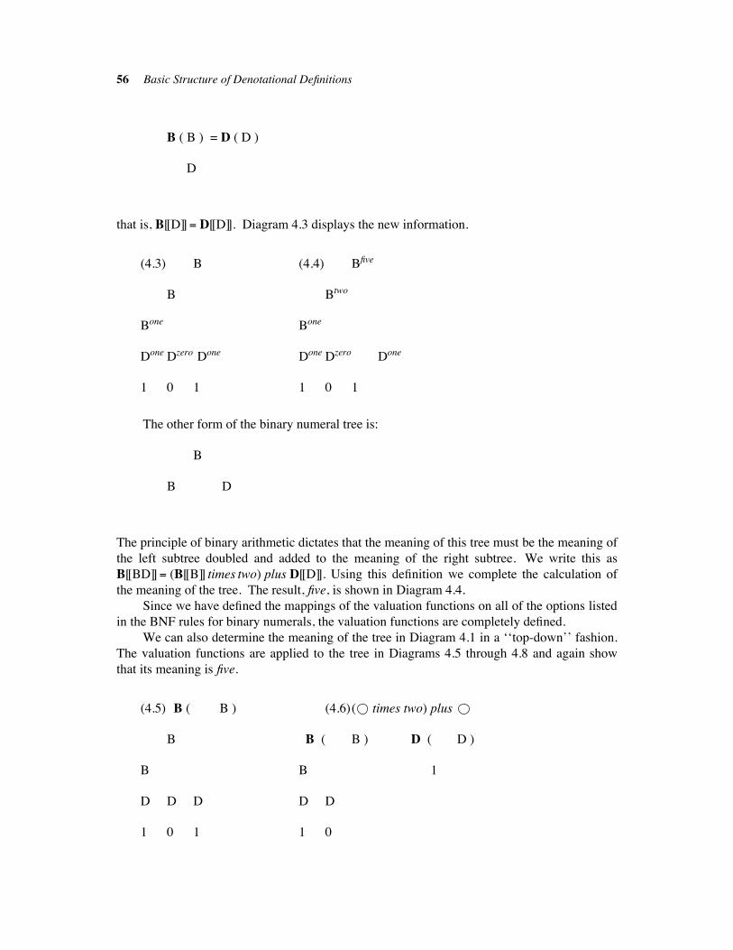
56 Basic Structure of Denotational Definitions
B ( B ) = D ( D )
D
that is, B[[D]]" D[[D]]. Diagram 4.3 displays the new information.
(4.3) B (4.4) Bfive
B Btwo
Bone Bone
Done Dzero Done Done Dzero Done
1 0 1 1 0 1
The other form of the binary numeral tree is:
B
B D
The principle of binary arithmetic dictates that the meaning of this tree must be the meaning of
the left subtree doubled and added to the meaning of the right subtree. We write this as
B[[BD]]" (B[[B]] times two) plus D[[D]]. Using this definition we complete the calculation of
the meaning of the tree. The result, five, is shown in Diagram 4.4.
Since we have defined the mappings of the valuation functions on all of the options listed
in the BNF rules for binary numerals, the valuation functions are completely defined.
We can also determine the meaning of the tree in Diagram 4.1 in a ‘‘top-down’’ fashion.
The valuation functions are applied to the tree in Diagrams 4.5 through 4.8 and again show
that its meaning is five.
(4.5) B ( B ) (4.6)( times two) plus
B B ( B ) D ( D )
B B 1
D D D D D
1 0 1 1 0
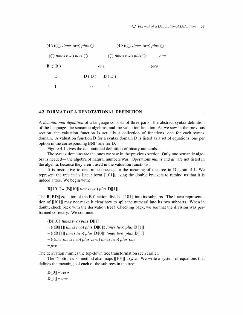
4.2 Format of a Denotational Definition 57
(4.7)( times two) plus (4.8)( times two) plus
( times two) plus ( times two) plus one
B ( B ) one zero
D D ( D ) D ( D )
1 0 1
4.2 FORMAT OF A DENOTATIONAL DEFINITION !!!!!!!!!!!!!!!!!!!!!!!!!!!!!!!!!!!!!!!!!!!!!!!!!!!!!!!!
A denotational definition of a language consists of three parts: the abstract syntax definition
of the language, the semantic algebras, and the valuation function. As we saw in the previous
section, the valuation function is actually a collection of functions, one for each syntax
domain. A valuation function D for a syntax domain D is listed as a set of equations, one per
option in the corresponding BNF rule for D.
Figure 4.1 gives the denotational definition of binary numerals.
The syntax domains are the ones we saw in the previous section. Only one semantic alge-
bra is needed— the algebra of natural numbers Nat. Operations minus and div are not listed in
the algebra, because they aren’t used in the valuation functions.
It is instructive to determine once again the meaning of the tree in Diagram 4.1. We
represent the tree in its linear form [[101]], using the double brackets to remind us that it is
indeed a tree. We begin with:
B[[101]]" (B[[10]] times two) plus D[[1]]
The B[[BD]] equation of the B function divides [[101]] into its subparts. The linear representa-
tion of [[101]] may not make it clear how to split the numeral into its two subparts. When in
doubt, check back with the derivation tree! Checking back, we see that the division was per-
formed correctly. We continue:
(B[[10]] times two) plus D[[1]]
" (((B[[1]] times two) plus D[[0]]) times two) plus D[[1]]
" (((D[[1]] times two) plus D[[0]]) times two) plus D[[1]]
" (((one times two) plus zero) times two) plus one
" five
The derivation mimics the top-down tree transformation seen earlier.
The ‘‘bottom-up’’ method also maps [[101]] to five. We write a system of equations that
defines the meanings of each of the subtrees in the tree:
D[[0]]" zero
D[[1]]" one
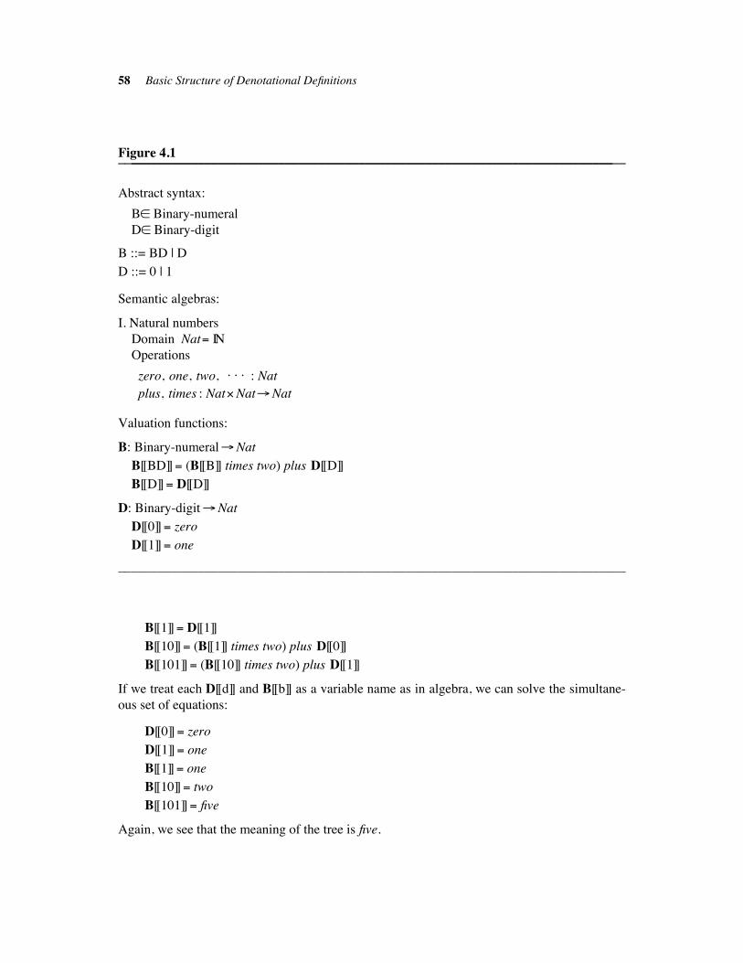
58 Basic Structure of Denotational Definitions
Figure 4.1____________________________________________________________________________________________________________________________________________________
Abstract syntax:
B! Binary-numeral
D! Binary-digit
B ::= BD | D
D ::= 0 | 1
Semantic algebras:
I. Natural numbers
Domain Nat" IN
Operations
zero, one, two, . . . : Nat
plus, times : Nat#Nat"Nat
Valuation functions:
B: Binary-numeral"Nat
B[[BD]]" (B[[B]] times two) plus D[[D]]
B[[D]]" D[[D]]
D: Binary-digit"Nat
D[[0]]" zero
D[[1]]" one
____________________________________________________________________________
B[[1]]" D[[1]]
B[[10]]" (B[[1]] times two) plus D[[0]]
B[[101]]" (B[[10]] times two) plus D[[1]]
If we treat each D[[d]] and B[[b]] as a variable name as in algebra, we can solve the simultane-
ous set of equations:
D[[0]]" zero
D[[1]]" one
B[[1]]" one
B[[10]]" two
B[[101]]" five
Again, we see that the meaning of the tree is five.
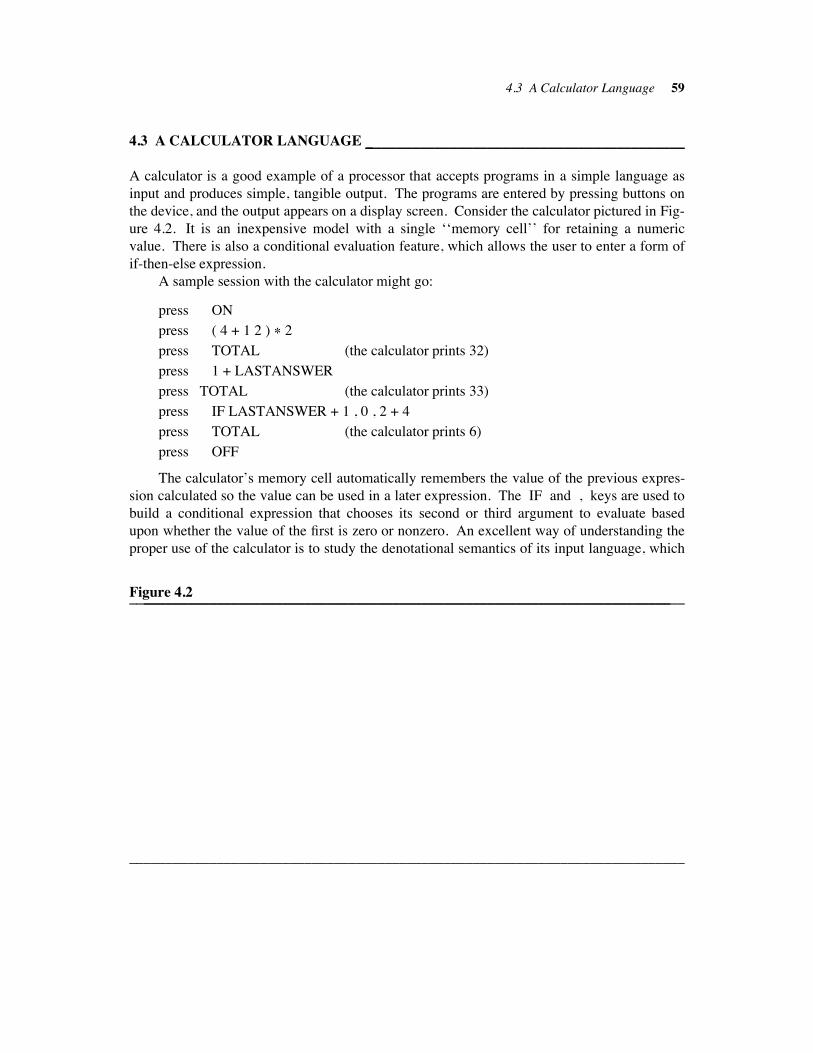
4.3 A Calculator Language 59
4.3 A CALCULATOR LANGUAGE !!!!!!!!!!!!!!!!!!!!!!!!!!!!!!!!!!!!!!!!!!!!!!!!!!!!!!!!!!!!!!!!!!!!!!!!!!!!!!!!!!!!!!
A calculator is a good example of a processor that accepts programs in a simple language as
input and produces simple, tangible output. The programs are entered by pressing buttons on
the device, and the output appears on a display screen. Consider the calculator pictured in Fig-
ure 4.2. It is an inexpensive model with a single ‘‘memory cell’’ for retaining a numeric
value. There is also a conditional evaluation feature, which allows the user to enter a form of
if-then-else expression.
A sample session with the calculator might go:
press ON
press ( 4 + 1 2 ) # 2
press TOTAL (the calculator prints 32)
press 1 + LASTANSWER
press TOTAL (the calculator prints 33)
press IF LASTANSWER + 1 , 0 , 2 + 4
press TOTAL (the calculator prints 6)
press OFF
The calculator’s memory cell automatically remembers the value of the previous expres-
sion calculated so the value can be used in a later expression. The IF and , keys are used to
build a conditional expression that chooses its second or third argument to evaluate based
upon whether the value of the first is zero or nonzero. An excellent way of understanding the
proper use of the calculator is to study the denotational semantics of its input language, which
Figure 4.2____________________________________________________________________________________________________________________________________________________
____________________________________________________________________________
60 Basic Structure of Denotational Definitions
is given in Figure 4.3.
The abstract syntax indicates that a session with the calculator consists of pressing the
ON key and entering an expression sequence. An expression sequence is one or more expres-
sions, separated by occurrences of TOTAL, terminated by the OFF key. The syntax for an
expression follows the usual abstract syntax for arithmetic. Since the words of the language
are numerals, no BNF rule is given for the syntax domain Numeral.
The semantic algebras show that the calculator reasons with two kinds of semantic
objects: truth values and natural numbers. The phrase n!Nat in the Nat algebra’s definition
reminds us that all occurrences of identifier n in the valuation equations stand for an element
of domain Nat. The same holds for the phrase t!Tr. This convention is used in all the
remaining semantic definitions in this book.
We can learn much about the calculator language from its semantic algebras. Apparently,
the members of Nat will be the meanings of numerals and expressions in the calculator
language, but Tr has no obvious representation of its elements in the syntax. This suggests
that the calculator has some internal mechanism for doing logical reasoning, but the full power
of that mechanism is not given to the user. This is confirmed by the presence of the equals
operation in the algebra for Nat; the calculator can do arithmetic comparisons, but no com-
parison operator is included in the syntax. Therefore, we must take care to understand the syn-
tactic construct whose semantic equation utilizes the equals operation.
There are four valuation functions for the language:
P: Program"Nat #
S: Expr-sequence"Nat"Nat #
E: Expression"Nat"Nat
N: Numeral"Nat
A good part of the calculator’s semantics can be understood from studying the functionalities
of the valuation functions. The P function maps a program to its meaning, which is a list of
natural numbers. The reason for using the codomain Nat # is found from the syntax: a pro-
gram has the form [[ON S]], where [[S]] stands for a sequence of expressions. If each expres-
sion has a numeric value, then a sequence of them is list of numbers. The list represents the
sequence of outputs displayed by the calculator during a session. This is confirmed by the
functionality of S, which maps an expression sequence and a number to the desired number
list. But what is the extra number used for? Recall that the calculator has a memory cell,
which retains the value of the most recently evaluated expression. The number is the value in
the memory cell. Perhaps the functionality should be written:
S: Expr-sequence"Memory-cell"Nat # , where Memory-cell"Nat
Two important features of denotational definitions are expressed in S’s functionality.
First, the global data structures in a language’s processor can be modelled as arguments to the
valuation functions. There are no ‘‘global variables’’ for functions, so all such structures must
be specified as arguments so that they are of use in the semantics. Second, the meaning of a
syntactic construct can be a function. S’s functionality states that ‘‘the meaning of an expres-
sion sequence is a function from a memory cell to a list of numbers.’’ This seems confusing,
for we might think that the meaning of an expression sequence is a list of numbers itself and
not a function. The point is that the content of the memory cell is needed to evaluate the
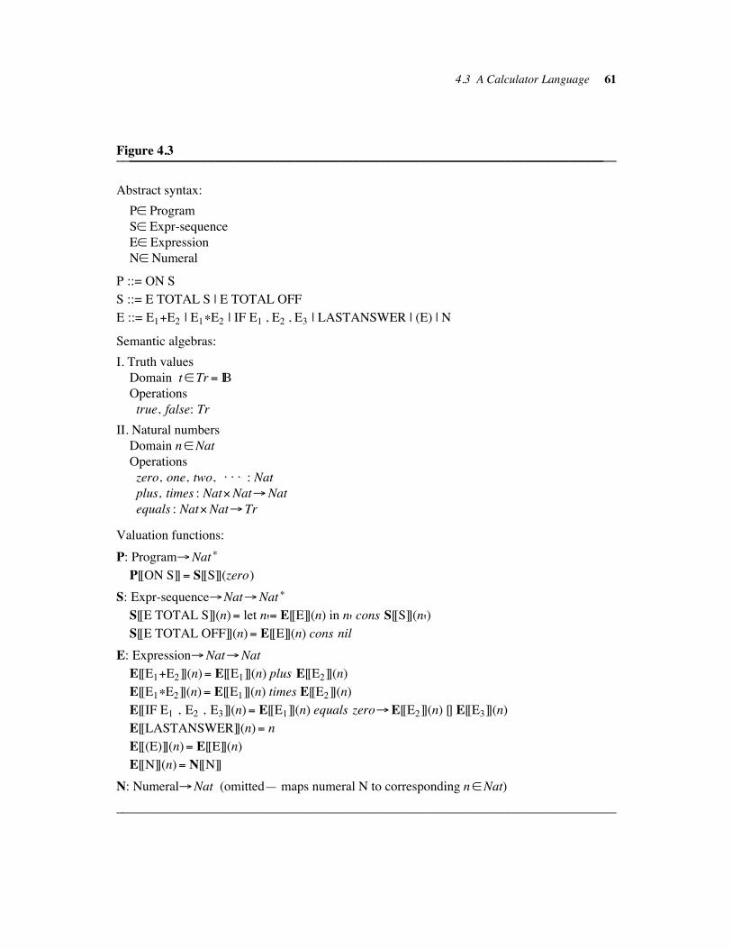
4.3 A Calculator Language 61
Figure 4.3____________________________________________________________________________________________________________________________________________________
Abstract syntax:
P! Program
S! Expr-sequence
E! Expression
N! Numeral
P ::= ON S
S ::= E TOTAL S | E TOTAL OFF
E ::= E1$E2 | E1#E2 | IF E1 , E2 , E3 | LASTANSWER | (E) | N
Semantic algebras:
I. Truth values
Domain t!Tr " IB
Operations
true, false: Tr
II. Natural numbers
Domain n!Nat
Operations
zero, one, two, . . . : Nat
plus, times : Nat#Nat"Nat
equals : Nat#Nat" Tr
Valuation functions:
P: Program"Nat #
P[[ON S]]" S[[S]](zero)
S: Expr-sequence"Nat"Nat #
S[[E TOTAL S]](n)" let n'" E[[E]](n) in n' cons S[[S]](n')S[[E TOTAL OFF]](n)" E[[E]](n) cons nil
E: Expression"Nat"Nat
E[[E1$E2]](n)" E[[E1]](n) plus E[[E2]](n)
E[[E1#E2]](n)" E[[E1]](n) times E[[E2]](n)
E[[IF E1 , E2 , E3]](n)" E[[E1]](n) equals zero"E[[E2]](n) [] E[[E3]](n)
E[[LASTANSWER]](n)" n
E[[(E)]](n)" E[[E]](n)
E[[N]](n)" N[[N]]
N: Numeral"Nat (omitted— maps numeral N to corresponding n!Nat)
____________________________________________________________________________
62 Basic Structure of Denotational Definitions
sequence— the value in the cell may be accessed via the ‘‘LASTANSWER’’ key. The func-
tionality notes the dependence of the value of the expression sequence upon the memory cell.
Let’s consider the semantic equations. The equation for P[[ON S]] states that the meaning
of a program session follows from the meaning of the expression sequence [[S]]. The equation
also says that the memory cell is initialized to zero when the calculator is turned on. The
cell’s value is passed as an argument to the valuation function for the sequence.
As indicated by the functionality for S, an expression sequence uses the value of the
memory cell to compute a list of numbers. The equation for S[[E TOTAL S]] describes the
meaning of a sequence of two or more expressions: the meaning of the first one, [[E]], is
appended to the front of the list of values that follows from [[S]]. We can list the corresponding
actions that the calculator would take:
1. Evaluate [[E]] using cell n, producing value n'.2. Print n' out on the display.
3. Place n' into the memory cell.
4. Evaluate the rest of the sequence [[S]] using the cell.
Note how each of these four steps are represented in the semantic equation:
1. is handled by the expression E[[E]](n), binding it to the variable n'.2. is handled by the expression n' cons . . . .
3. and 4. are handled by the expression S[[S]](n').
Nonetheless, the right-hand side of S[[E TOTAL S]] is a mathematical value. Note that the
same value is represented by the expression:
E[[E]](n) cons S[[S]] (E[[E]](n))
which itself suggests that [[E]] be evaluated twice. This connection between the structure of
function expressions and operational principles will be examined in detail in later chapters. In
the meantime, it can be used to help understand the meanings denoted by the function expres-
sions.
The meaning of S[[E TOTAL OFF]] is similar. Since [[E]] is the last expression to be
evaluated, the list of subsequent outputs is just nil.
Of the semantic equations for expressions, the ones for [[LASTANSWER]] and
[[IF E1, E2, E3]] are of interest. The [[LASTANSWER]] operator causes a lookup of the value
in the memory cell. The meaning of the IF expression is a conditional. The equals operation
is used here. The test value, [[E1]], is evaluated and compared with zero. If it equals zero,
E[[E2]](n) is taken as the value of the conditional, else E[[E3]](n) is used. Hence, the expres-
sion [[E1]] in the first position of the conditional takes on a logical meaning in addition to its
numeric one. This is a source of confusion in the calculator language and is a possible area for
improvement of the language.
One last remark: equations such as E[[(E)]](n)" E[[E]](n) may also be written as
E[[(E)]]" $n. E[[E]](n), making use of the abstraction notation, or even as E[[(E)]]" E[[E]]
(why?). This will be done in later examples.
A simplification of a sample calculator program is instructional:
P[[ON 2$1 TOTAL IF LASTANSWER , 2 , 0 TOTAL OFF]]
" S[[2$1 TOTAL IF LASTANSWER , 2 , 0 TOTAL OFF]](zero)
4.3 A Calculator Language 63
" let n'" E[[2$1]](zero)
in n' cons S[[IF LASTANSWER , 2 , 0 TOTAL OFF]](n')
Simplifying E[[2$1]](zero) leads to the value three, and we have:
let n'" three in n' cons S[[IF LASTANSWER , 2 , 0 TOTAL OFF]](n')" three cons S[[IF LASTANSWER , 2 , 0 TOTAL OFF]](three)
" three cons (E[[IF LASTANSWER , 2 , 0]](three) cons nil)
If we work on the conditional, we see that:
E[[IF LASTANSWER , 2 , 0]](three)
" E[[LASTANSWER]](three) equals zero"E[[2]](three) [] E[[0]](three)
" three equals zero" two [] zero
" false" two [] zero " zero
This gives as the final result the list:
three cons (zero cons nil)
Each of the simplification steps preserved the meaning of P[[ 2$1 TOTAL
IF LASTANSWER , 2 , 0 TOTAL OFF ]]. The purpose of simplification is to produce an
equivalent expression whose meaning is more obvious than the original’s. The simplification
process is of interest in itself, for it shows how the calculator operates on input. If the denota-
tional definition is used as a specification for the calculator, the definition plus simplification
strategy show a possible implementation of the calculator. A simple-minded implementation
would use functions, parameters, and an evaluation strategy corresponding to the
simplification sequence just seen. It only takes a bit of insight, however, to notice that the
numeral argument can be converted into a global memory cell. The derivation of a processor
for a language from its denotational specification will be repeatedly touched upon in future
chapters.
SUGGESTED READINGS !!!!!!!!!!!!!!!!!!!!!!!!!!!!!!!!!!!!!!!!!!!!!!!!!!!!!!!!!!!!!!!!!!!!!!!!!!!!!!!!!!!!!!!!!!!!!!!!!!!!!!
Jones 1982a; Gordon 1979; Milne & Strachey 1976; Pagan 1981; Stoy 1977; Tennent 1977,
1981
EXERCISES !!!!!!!!!!!!!!!!!!!!!!!!!!!!!!!!!!!!!!!!!!!!!!!!!!!!!!!!!!!!!!!!!!!!!!!!!!!!!!!!!!!!!!!!!!!!!!!!!!!!!!!!!!!!!!!!!!!!!!!!!!!!
1. Use the binary numeral semantics in Figure 4.1 to determine the meanings of the follow-
ing derivation trees:
a. [[0011]]
b. [[000]]
64 Basic Structure of Denotational Definitions
c. [[111]]
2. Here is an alternative abstract syntax for the language of binary numerals:
N! Numeral
B! Bin-Numeral
D! Bin-digit
N ::= B
B ::= DB | D
D ::= 0 | 1
Define the valuation function that maps a binary numeral to its value. (Hint: define
P : Numeral"Nat and B : Bin-numeral" (Value# Scale), where Value" Nat is the
value of the numeral, and Scale" { one, two, four, eight, . . . } remembers the scale (phy-
sical size) of the numeral.)
3. a. In a fashion similar to that in Figure 4.1, define a denotational semantics for the
language of base 8 numerals, Octal. Let E be the valuation function E : Octal"Nat.
b. Prove the following equivalence: E[[015]]" B[[1101]].
c. Construct an algorithm that maps an octal numeral to binary form. Use the respective
denotational semantics for Octal and Binary-numeral to prove that your algorithm is
correct.
4. Simplify these calculator programs to their meanings in Nat# :
a. [[ON 1$(IF LASTANSWER , 4 , 1) TOTAL LASTANSWER TOTAL
5#2 TOTAL OFF]]
b. [[ON 5 TOTAL 5 TOTAL 10 TOTAL OFF]]
c. [[ON LASTANSWER TOTAL OFF]]
5. Augment the calculator so that it can compare two values for equality: add an " button
to its panel and augment the BNF rule for Expression to read: E ::= . . . | E1"E2
a. Write the semantic equation for E[[E1"E2]].
b. What changes must be made to the other parts of the denotational definition to
accommodate the new construct? Make these changes. Do you think the new version
of the calculator is an improvement over the original?
6. Alter the calculator semantics in Figure 4.3 so that the memory cell argument to S and E
becomes a memory stack; that is, use Nat# in place of Nat as an argument domain to S
and E.
a. Adjust the semantics so that the last answer is pushed onto the memory stack and the
LASTANSWER button accesses the top value on the stack.
b. Augment the syntax of the calculator language so that the user can explicitly pop
values off the memory stack.
Exercises 65
7. Use the denotational definition in Figure 4.3 to guide the coding of a test implementation
of the calculator in Pascal (or whatever language you choose). What do the semantic
algebras become in the implementation? How are the valuation equations realized? What
does the memory cell become? What questions about the implementation doesn’t the
denotational definition answer?
8. Design, in the following stages, a calculator for manipulating character string expres-
sions:
a. List the semantic algebras that the calculator will need.
b. List the operations that the calculator will provide to the user.
c. Define the abstract syntax of these operations.
d. Define the valuation functions that give meaning to the abstract syntax definition.
Can these four steps be better accomplished in another order? Is the order even impor-
tant?
9. If you are familiar with attribute grammars, describe the relationship between a denota-
tional definition of a language and its attribute grammar definition. What corresponds to
inherited attributes in the denotational definition? What are the synthesized attributes?
Define attribute grammars for the binary numerals language and the calculator language.
10. Consider the compiler-oriented aspects of a denotational definition: if there existed a
machine with hardwired instructions plus, times, and representations of numbers, the
definition in Figure 4.1 could be used as a syntax-directed translation scheme for binary
numbers to machine code. For example:
B[[101]]" (((one times two) plus zero) times two) plus one
is the ‘‘compiled code’’ for the input program [[101]]; the syntax pieces are mapped to
their denotations, but no simplifications are performed. The machine would evaluate this
program to five. With this idea in mind, propose how a compiler for the calculator
language of Figure 4.3 might be derived from its denotational definition. Propose a
machine for executing compiled calculator programs.
Chapter 5 !!!!!!!!!!!!!!!!!!!!!!!!!!!!!!!!!!!!!!!!!!!!!!!!!!!!!!!!
Imperative Languages
Most sequential programming languages use a data structure that exists independently of any
program in the language. The data structure isn’t explicitly mentioned in the language’s syn-
tax, but it is possible to build phrases that access it and update it. This data structure is called
the store, and languages that utilize stores are called imperative. The fundamental example of
a store is a computer’s primary memory, but file stores and data bases are also examples. The
store and a computer program share an intimate relationship:
1. The store is critical to the evaluation of a phrase in a program. A phrase is understood in
terms of how it handles the store, and the absence of a proper store makes the phrase
nonexecutable.
2. The store serves as a means of communication between the different phrases in the pro-
gram. Values computed by one phrase are deposited in the store so that another phrase
may use them. The language’s sequencing mechanism establishes the order of communi-
cation.
3. The store is an inherently ‘‘large’’ argument. Only one copy of store exists at any point
during the evaluation.
In this chapter, we study the store concept by examining three imperative languages. You
may wish to study any subset of the three languages. The final section of the chapter presents
some variants on the store and how it can be used.
5.1 A LANGUAGE WITH ASSIGNMENT !!!!!!!!!!!!!!!!!!!!!!!!!!!!!!!!!!!!!!!!!!!!!!!!!!!!!!!!!!!!!!!!!!!!!!!!!!
The first example language is a declaration-free Pascal subset. A program in the language is a
sequence of commands. Stores belong to the domain Store and serve as arguments to the
valuation function:
C: Command! Store"!! Store"!
The purpose of a command is to produce a new store from its store argument. However, a
command might not terminate its actions upon the store— it can ‘‘loop.’’ The looping of a
command [[C]] with store s has semantics C[[C]]s# "". (This explains why the Store domain is
lifted: "" is a possible answer.) The primary property of nontermination is that it creates a
nonrecoverable situation. Any commands [[C']] following [[C]] in the evaluation sequence will
not evaluate. This suggests that the function C[[C']]: Store"!! Store"! be strict; that is, given a
nonrecoverable situation, C[[C']] can do nothing at all. Thus, command composition is
C[[C1;C2]]# C[[C2]] $ C[[C1]].
Figure 5.1 presents the semantic algebras for the imperative language. The Store domain
models a computer store as a mapping from the identifiers of the language to their values. The
66
5.1 A Language with Assignment 67
Figure 5.1____________________________________________________________________________________________________________________________________________________
I. Truth Values
Domain t# Tr# IB
Operations
true, false : Tr
not : Tr! Tr
II. Identifiers
Domain i# Id# Identifier
III. Natural Numbers
Domain n# Nat# IN
Operations
zero, one, . . . : Nat
plus : Nat%Nat!Nat
equals : Nat%Nat! Tr
IV. Store
Domain s# Store# Id!Nat
Operations
newstore: Store
newstore# $i. zero
access: Id! Store!Nat
access# $i. $s. s(i)
update: Id!Nat! Store! Store
update# $i.$n.$s. [ i ""! n]s
____________________________________________________________________________
operations upon the store include a constant for creating a new store, an operation for access-
ing a store, and an operation for placing a new value into a store. These operations are exactly
those described in Example 3.11 of Chapter 3.
The language’s definition appears in Figure 5.2.
The valuation function P states that the meaning of a program is a map from an input
number to an answer number. Since nontermination is possible, "" is also a possible
‘‘answer,’’ hence the rightmost codomain of P is Nat "! rather than just Nat. The equation for P
says that the input number is associated with identifier [[A]] in a new store. Then the program
body is evaluated, and the answer is extracted from the store at [[Z]].
The clauses of the C function are all strict in their use of the store. Command composi-
tion works as described earlier. The conditional commands are choice functions. Since the
68 Imperative Languages
Figure 5.2____________________________________________________________________________________________________________________________________________________
Abstract syntax:
P# Program
C# Command
E# Expression
B# Boolean-expr
I# Identifier
N# Numeral
P ::= C.
C ::= C1;C2 | if B then C | if B then C1 else C2 | I:#E | diverge
E ::= E1&E2 | I | N
B ::= E1#E2 | 'B
Semantic algebras:
(defined in Figure 5.1)
Valuation functions:
P: Program!Nat!Nat "!
P[[C.]]# $n. let s# (update[[A]] n newstore) in
let s'# C[[C]]s in (access[[Z]] s')
C: Command! Store "!! Store "!
C[[C1;C2]]# $!!s. C[[C2]] (C[[C1]]s)
C[[if B then C]]# $!!s. B[[B]]s!C[[C]]s[] s
C[[if B then C1 else C2]]# $!!s. B[[B]]s!C[[C1]]s[] C[[C2]]s
C[[I:#E]]# $!!s. update[[I]] (E[[E]]s) s
C[[diverge]]# $!!s. ""
E: Expression! Store!Nat
E[[E1&E2]]# $s. E[[E1]]s plus E[[E2]]s
E[[I]]# $s. access [[I]] s
E[[N]]# $s. N[[N]]
B: Boolean-expr!Store! Tr
B[[E1#E2]]# $s. E[[E1]]s equals E[[E2]]s
B[['B]]# $s. not(B[[B]]s)
N: Numeral!Nat (omitted)
____________________________________________________________________________
5.1 A Language with Assignment 69
expression (e1! e2 [] e3) is nonstrict in arguments e2 and e3, the value of C[[if B then C]]s is s
when B[[B]]s is false, even if C[[C]]s# "". The assignment statement performs the expected
update; the [[diverge]] command causes nontermination.
The E function also needs a store argument, but the store is used in a ‘‘read only’’ mode.
E’s functionality shows that an expression produces a number, not a new version of store; the
store is not updated by an expression. The equation for addition is stated so that the order of
evaluation of [[E1]] and [[E2]] is not important to the final answer. Indeed, the two expressions
might even be evaluated in parallel. A strictness check of the store is not needed, because C
has already verified that the store is proper prior to passing it to E.
Here is the denotation of a sample program with the input two:
P[[Z:#1; if A#0 then diverge; Z:#3.]](two)
# let s# (update[[A]] two newstore) in
let s' # C[[Z:#1; if A#0 then diverge; Z:#3]]s
in access[[Z]] s'Since (update[[A]] two newstore) is ( [ [[A]]""! two] newstore), that is, the store that maps [[A]]
to two and all other identifiers to zero, the above expression simplifies to:
let s' # C[[Z:#1; if A#0 then diverge; Z:#3]] ( [ [[A]]""! two] newstore)
in access[[Z]] s'From here on, we use s1 to stand for ( [ [[A]]! two] newstore). Working on the value bound to
s' leads us to derive:
C[[Z:#1; if A#0 then diverge; Z:#3]]s1
# ($!!s. C[[if A#0 then diverge; Z:#3]] (C[[Z:#1]]s))s1
The store s1 is a proper value, so it can be bound to s, giving:
C[[if A#0 then diverge; Z:#3]] (C[[Z:#1]]s1)
We next work on C[[Z:#1]]s1:
C[[Z:#1]]s1
# ($!!s. update[[Z]] (E[[1]]s) s) s1
# update[[Z]] (E[[1]]s1) s1
# update[[Z]] (N[[1]]) s1
# update[[Z]] one s1
# [ [[Z]]""! one] [ [[A]]""! two] newstore
which we call s2. Now:
C[[if A#0 then diverge; Z:#3]]s2
# ($!!s. C[[Z:#3]] (($!!s. B[[A#0]]s!C[[diverge]]s[] s)s))s2
# C[[Z:#3]] (($!!s. B[[A#0]]s!C[[diverge]]s[] s)s2)
# C[[Z:#3]] (B[[A#0]]s2!C[[diverge]]s2 [] s2)
Note that C[[diverge]]s2 # ($!!s. "")s2 # "", so nontermination is the result if the test has value
70 Imperative Languages
true. Simplifying the test, we obtain:
B[[A#0]]s2# ($s. E[[A]]s equals E[[0]]s)s2
# E[[A]]s2 equals E[[0]]s2
# (access[[A]] s2) equals zero
Examining the left operand, we see that:
access[[A]] s2
# s2[[A]]
# ( [ [[Z]]""! one] [ [[A]]""! two] newstore) [[A]]
# ( [ [[A]]""! two] newstore) [[A]] (why?)
# two
Thus, B[[A#0]]s2 # false, implying that C[[if A#0 then diverge]]s2 # s2 . Now:
C[[Z:#3]]s2
# [ [[Z]]""! three]s2
The denotation of the entire program is:
let s' # [ [[Z]]""! three]s2 in access[[Z]] s'# access[[Z]] [ [[Z]]""! three]s2
# ( [ [[Z]]""! three]s2) [[Z]]
# three
We obtain a much different denotation when the input number is zero:
P[[Z:#1; if A#0 then diverge; Z:#3.]](zero)
# let s' # C[[Z:#1; if A#0 then diverge; Z:#3]]s3 in access[[Z]] s'where s3 # [ [[A]]""! zero] newstore. Simplifying the value bound to s' leads to:
C[[Z:#1; if A#0 then diverge; Z:#3]]s3
# C[[if A#0 then diverge; Z:#3]]s4
where s4 # [ [[Z]]""! one]s3. As for the conditional, we see that:
B[[A#0]]s4 ! C[[diverge]]s4 [] s4
# true! C[[diverge]]s4 [] s4
# C[[diverge]]s4
# ($!!s. "")s4
# ""
So the value bound to s' is C[[Z:#3]] "". But C[[Z:#3]] "" # ($!!s. update[[Z]] (E[[3]]s) s) "" # "".
Because of the strict abstraction, the assignment isn’t performed. The denotation of the pro-
gram is:
let s'# "" in access[[Z]] s'
5.1 A Language with Assignment 71
which simplifies directly to "". (Recall that the form (let x# e1 in e2) represents ($!!x. e2)e1.) The
undefined store forces the value of the entire program to be undefined.
The denotational definition is also valuable for proving properties such as program
equivalence. As a simple example, we show for distinct identifiers [[X]] and [[Y]] that the com-
mand C[[X:#0; Y:#X&1]] has the same denotation as C[[Y:#1; X:#0]]. The proof strategy goes
as follows: since both commands are functions in the domain Store"!! Store"! , it suffices to
prove that the two functions are equal by showing that both produce same answers from same
arguments. (This is because of the principle of extensionality mentioned in Section 3.2.3.)
First, it is easy to see that if the store argument is "", both commands produce the answer "". If
the argument is a proper value, let us call it s and simplify:
C[[X:#0; Y:#X&1]]s
# C[[Y:#X&1]] (C[[X:#0]]s)
# C[[Y:#X&1]] ( [ [[X]]""! zero]s)
# update[[Y]] (E[[X&1]] ( [ [[X]]""! zero]s)) ( [ [[X]]""! zero]s)
# update[[Y]] one [ [[X]]""! zero]s
# [ [[Y]]""! one] [ [[X]]""! zero]s
Call this result s1. Next:
C[[Y:#1; X:#0]]s
# C[[X:#0]] (C[[Y:#1]]s)
# C[[X:#0]] ( [ [[Y]]""! one]s)
# [ [[X]]""! zero] [ [[Y]]""! one]s
Call this result s2. The two values are defined stores. Are they the same store? It is not possi-
ble to simplify s1 into s2 with the simplification rules. But, recall that stores are themselves
functions from the domain Id!Nat. To prove that the two stores are the same, we must show
that each produces the same number answer from the same identifier argument. There are
three cases to consider:
1. The argument is [[X]]: then s1[[X]] # ( [ [[Y]]""! one] [ [[X]]""! zero]s) [[X]] #( [ [[X]]""! zero]s) [[X]] # zero; and s2 [[X]] # ( [ [[X]]""! zero] [ [[Y]]""! one]s) [[X]] # zero.
2. The argument is [[Y]]: then s1[[Y]] # ( [ [[Y]]""! one] [ [[X]]""! zero]s) [[Y]] # one; and
s2 [[Y]] # ( [ [[X]]""! zero] [ [[Y]]""! one]s) [[Y]] # ( [ [[Y]]""! one]s) [[Y]] # one.
3. The argument is some identifier [[I]] other than [[X]] or [[Y]]: then s1[[I]] # s[[I]] and s2[[I]]
# s[[I]].
Since s1 and s2 behave the same for all arguments, they are the same function. This implies
that C[[X:#0; Y:#X&1]] and C[[Y:#1; X:#0]] are the same function, so the two commands are
equivalent. Many proofs of program properties require this style of reasoning.
72 Imperative Languages
5.1.1 Programs Are Functions !!!!!!!!!!!!!!!!!!!!!!!!!!!!!!!!!!!!!!!!!!!!!!!!!!!!!!!!!!!!!!!!!!!!!!!!!!!!!!!!!!!!!!!!!!!!!!!!
The two sample simplification sequences in the previous section were operational-like: a pro-
gram and its input were computed to an answer. This makes the denotational definition
behave like an operational semantics, and it is easy to forget that functions and domains are
even involved. Nonetheless, it is possible to study the denotation of a program without sup-
plying sample input, a feature that is not available to operational semantics. This broader view
emphasizes that the denotation of a program is a function.
Consider again the example [[Z:#1; if A#0 then diverge; Z:#3]]. What is its meaning?
It’s a function from Nat to Nat "!:
P[[Z:#1; if A#0 then diverge; Z:#3.]]
# $n. let s# update[[A]] n newstore in
let s' # C[[Z:#1; if A#0 then diverge; Z:#3]]s
in access[[Z]] s'# $n. let s# update[[A]] n newstore in
let s' # ($!!s. ($!!s. C[[Z:#3]] (C[[if A#0 then diverge]]s))s)(C[[Z:#1]]s)
in access[[Z]] s'# $n. let s# update[[A]] n newstore in
let s' # ($!!s. ($!!s. update[[Z]] three s)
(($!!s. (access[[A]] s) equals zero! ($!!s. "")s [] s)s))
(($!!s. update[[Z]] one s)s)
in access[[Z]] s'which can be restated as:
$n. let s# update[[A]] n newstore in
let s' # (let s'1 # update[[Z]] one s in
let s'2 # (access[[A]] s'1) equals zero! ($!!s. "")s'1 [] s'1in update[[Z]] three s'2)
in access[[Z]] s'The simplifications taken so far have systematically replaced syntax constructs by their func-
tion denotations; all syntax pieces are removed (less the identifiers). The resulting expression
denotes the meaning of the program. (A comment: it is proper to be concerned why a phrase
such as E[[0]]s was simplified to zero even though the value of the store argument s is
unknown. The simplification works because s is an argument bound to $!!s. Any undefined
stores are ‘‘trapped’’ by $!!s. Thus, within the scope of the $!!s, all occurrences of s represent
defined values.)
The systematic mapping of syntax to function expressions resembles compiling. The
function expression certainly does resemble compiled code, with its occurrences of tests,
accesses, and updates. But it is still a function, mapping an input number to an output number.
As it stands, the expression does not appear very attractive, and the intuitive meaning of
the original program does not stand out. The simplifications shall proceed further. Let s0 be
(update[[A]] n newstore). We simplify to:
5.1.1 Programs Are Functions 73
$n. let s' # (let s'1 # update[[Z]] one s0 in
let s'2 # (access[[A]] s'1) equals zero! ($!!s. "")s'1 [] s'1in update[[Z]] three s'2)
in access[[Z]] s'We use s1 for (update[[Z]] one s0); the conditional in the value bound to s'2 is:
(access[[A]] s1) equals zero! "" [] s1
# n equals zero! "" [] s1
The conditional can be simplified no further. We can make use of the following property;
‘‘for e2 # Store"! such that e2 % "", let s # (e1 ! "" [] e2) in e3 equals e1 ! "" [] [e2/s]e3.’’ (The
proof is left as an exercise.) It allows us to state that:
let s'2 # (n equals zero! "" [] s1) in update[[Z]] three s'2# n equals zero! "" [] update[[Z]] three s1
This reduces the program’s denotation to:
$n. let s'# (n equals zero! "" [] update[[Z]] three s1) in access[[Z]] s'The property used above can be applied a second time to show that this expression is just:
$n. n equals zero! "" [] access[[Z]] (update[[Z]] three s1)
which is:
$n. n equals zero! "" [] three
which is the intuitive meaning of the program!
This example points out the beauty in the denotational semantics method. It extracts the
essence of a program. What is startling about the example is that the primary semantic argu-
ment, the store, disappears completely, because it does not figure in the input-output relation
that the program describes. This program does indeed denote a function from Nat to Nat "! .
Just as the replacement of syntax by function expressions resembles compilation, the
internal simplification resembles compile-time code optimization. When more realistic
languages are studied, such ‘‘optimizations’’ will be useful for understanding the nature of
semantic arguments.
5.2 AN INTERACTIVE FILE EDITOR !!!!!!!!!!!!!!!!!!!!!!!!!!!!!!!!!!!!!!!!!!!!!!!!!!!!!!!!!!!!!!!!!!!!!!!!!!!!!!!!
The second example language is an interactive file editor. We define a file to be a list of
records, where the domain of records is taken as primitive. The file editor makes use of two
levels of store: the primary store is a component holding the file edited upon by the user, and
the secondary store is a system of text files indexed by their names. The domains are listed in
Figure 5.3.
The edited files are values from the Openfile domain. An opened file r1, r2, . . . , rlast is
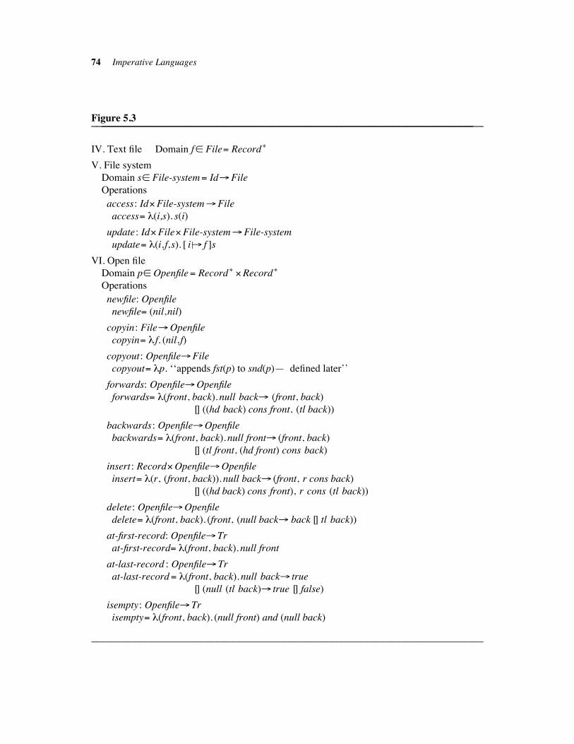
74 Imperative Languages
Figure 5.3____________________________________________________________________________________________________________________________________________________
IV. Text file Domain f# File# Record&
V. File system
Domain s# File-system# Id!File
Operations
access: Id%File-system!File
access# $(i,s). s(i)
update: Id%File%File-system!File-system
update# $(i, f,s). [ i ""! f ]s
VI. Open file
Domain p# Openfile# Record& %Record&
Operations
newfile: Openfile
newfile# (nil,nil)
copyin: File!Openfile
copyin# $ f. (nil, f)
copyout: Openfile!File
copyout# $p. ‘‘appends fst(p) to snd(p)— defined later’’
forwards: Openfile!Openfile
forwards# $(front, back). null back! (front, back)
[] ((hd back) cons front, (tl back))
backwards: Openfile!Openfile
backwards# $(front, back). null front! (front, back)
[] (tl front, (hd front) cons back)
insert : Record%Openfile!Openfile
insert# $(r, (front, back)). null back! (front, r cons back)
[] ((hd back) cons front), r cons (tl back))
delete: Openfile!Openfile
delete# $(front, back). (front, (null back! back [] tl back))
at-first-record: Openfile!Tr
at-first-record# $(front, back). null front
at-last-record : Openfile!Tr
at-last-record# $(front, back). null back! true
[] (null (tl back)! true [] false)
isempty: Openfile!Tr
isempty# $(front, back). (null front) and (null back)
____________________________________________________________________________
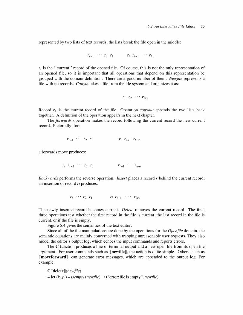
5.2 An Interactive File Editor 75
represented by two lists of text records; the lists break the file open in the middle:
ri"1. . . r2 r1 ri ri&1
. . . rlast
ri is the ‘‘current’’ record of the opened file. Of course, this is not the only representation of
an opened file, so it is important that all operations that depend on this representation be
grouped with the domain definition. There are a good number of them. Newfile represents a
file with no records. Copyin takes a file from the file system and organizes it as:
r1 r2 . . . rlast
Record r1 is the current record of the file. Operation copyout appends the two lists back
together. A definition of the operation appears in the next chapter.
The forwards operation makes the record following the current record the new current
record. Pictorially, for:
ri "1 . . . r2 r1 ri ri &1 rlast
a forwards move produces:
ri ri "1 . . . r2 r1 ri &1 . . . rlast
Backwards performs the reverse operation. Insert places a record r behind the current record;
an insertion of record r' produces:
ri . . . r2 r1 r' ri &1 . . . rlast
The newly inserted record becomes current. Delete removes the current record. The final
three operations test whether the first record in the file is current, the last record in the file is
current, or if the file is empty.
Figure 5.4 gives the semantics of the text editor.
Since all of the file manipulations are done by the operations for the Openfile domain, the
semantic equations are mainly concerned with trapping unreasonable user requests. They also
model the editor’s output log, which echoes the input commands and reports errors.
The C function produces a line of terminal output and a new open file from its open file
argument. For user commands such as [[newfile]], the action is quite simple. Others, such as
[[moveforward]], can generate error messages, which are appended to the output log. For
example:
C[[delete]](newfile)
# let (k',p')# isempty (newfile)! (''error:file is empty'', newfile)
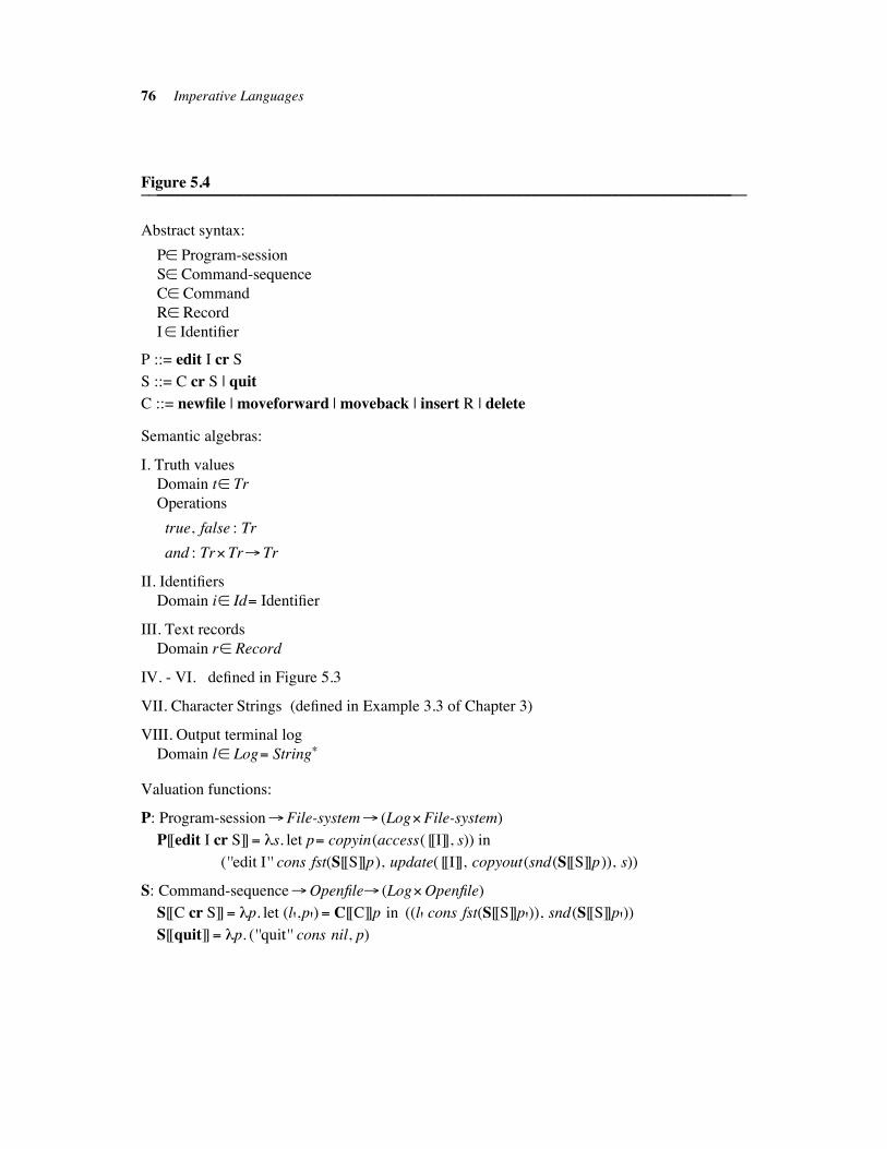
76 Imperative Languages
Figure 5.4____________________________________________________________________________________________________________________________________________________
Abstract syntax:
P# Program-session
S# Command-sequence
C# Command
R# Record
I# Identifier
P ::= edit I cr S
S ::= C cr S | quit
C ::= newfile | moveforward | moveback | insert R | delete
Semantic algebras:
I. Truth values
Domain t# Tr
Operations
true, false : Tr
and : Tr% Tr! Tr
II. Identifiers
Domain i# Id# Identifier
III. Text records
Domain r# Record
IV. - VI. defined in Figure 5.3
VII. Character Strings (defined in Example 3.3 of Chapter 3)
VIII. Output terminal log
Domain l# Log# String&
Valuation functions:
P: Program-session!File-system! (Log%File-system)
P[[edit I cr S]]# $s. let p# copyin(access( [[I]], s)) in
(''edit I'' cons fst(S[[S]]p), update( [[I]], copyout(snd(S[[S]]p)), s))
S: Command-sequence!Openfile! (Log%Openfile)
S[[C cr S]]# $p. let (l',p')# C[[C]]p in ((l' cons fst(S[[S]]p')), snd(S[[S]]p'))S[[quit]]# $p. (''quit'' cons nil, p)
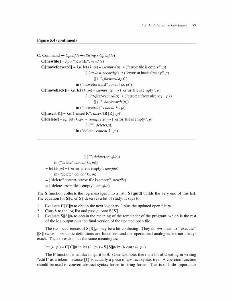
5.2 An Interactive File Editor 77
Figure 5.4 (continued)____________________________________________________________________________________________________________________________________________________
C: Command!Openfile! (String%Openfile)
C[[newfile]]# $p. (''newfile'', newfile)
C[[moveforward]]# $p. let (k',p')# isempty(p)! (''error:file is empty'', p)
[] ( at-last-record(p)! (''error: at back already'', p)
[] ('''', forwards(p)) )
in (''moveforward'' concat k', p'))C[[moveback]]# $p. let (k',p')# isempty (p)! (''error:file is empty'', p)
[] ( at-first-record(p)! (''error: at front already'', p) )
[] ('''', backwards(p))
in (''moveback'' concat k', p')C[[insert R]]# $p. (''insert R'', insert(R[[R]], p))
C[[delete]]# $p. let (k',p')# isempty(p)! (''error:file is empty'', p)
[] ('''', delete(p))
in (''delete'' concat k', p')
____________________________________________________________________________
[] ('''', delete(newfile))
in (''delete'' concat k', p'))# let (k',p')# (''error:file is empty'', newfile)
in (''delete'' concat k', p')# (''delete'' concat ''error:file is empty'', newfile)
# (''delete error:file is empty'', newfile)
The S function collects the log messages into a list. S[[quit]] builds the very end of this list.
The equation for S[[C cr S]] deserves a bit of study. It says to:
1. Evaluate C[[C]]p to obtain the next log entry l' plus the updated open file p'.2. Cons l' to the log list and pass p' onto S[[S]].
3. Evaluate S[[S]]p' to obtain the meaning of the remainder of the program, which is the rest
of the log output plus the final version of the updated open file.
The two occurrences of S[[S]]p' may be a bit confusing. They do not mean to ‘‘execute’’
[[S]] twice— semantic definitions are functions, and the operational analogies are not always
exact. The expression has the same meaning as:
let (l', p')# C[[C]]p in let (l'', p'')# S[[S]]p' in (l' cons l'', p'')
The P function is similar in spirit to S. (One last note: there is a bit of cheating in writing
''edit I'' as a token, because [[I]] is actually a piece of abstract syntax tree. A coercion function
should be used to convert abstract syntax forms to string forms. This is of little importance
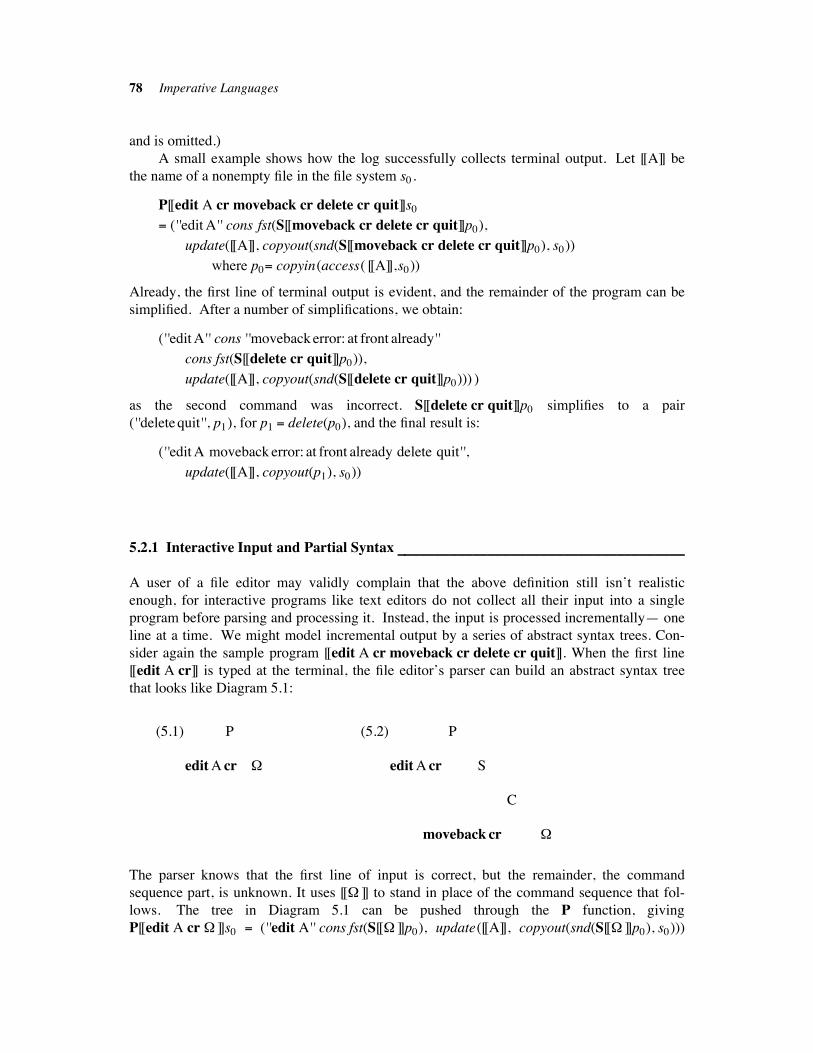
78 Imperative Languages
and is omitted.)
A small example shows how the log successfully collects terminal output. Let [[A]] be
the name of a nonempty file in the file system s0.
P[[edit A cr moveback cr delete cr quit]]s0
# (''edit A'' cons fst(S[[moveback cr delete cr quit]]p0),
update([[A]], copyout(snd(S[[moveback cr delete cr quit]]p0), s0))
where p0# copyin(access( [[A]],s0))
Already, the first line of terminal output is evident, and the remainder of the program can be
simplified. After a number of simplifications, we obtain:
(''edit A'' cons ''moveback error: at front already''
cons fst(S[[delete cr quit]]p0)),
update([[A]], copyout(snd(S[[delete cr quit]]p0))) )
as the second command was incorrect. S[[delete cr quit]]p0 simplifies to a pair
(''delete quit'', p1), for p1 # delete(p0), and the final result is:
(''edit A moveback error: at front already delete quit'',
update([[A]], copyout(p1), s0))
5.2.1 Interactive Input and Partial Syntax !!!!!!!!!!!!!!!!!!!!!!!!!!!!!!!!!!!!!!!!!!!!!!!!!!!!!!!!!!!!!!!!!!!!!!!!!!!!
A user of a file editor may validly complain that the above definition still isn’t realistic
enough, for interactive programs like text editors do not collect all their input into a single
program before parsing and processing it. Instead, the input is processed incrementally— one
line at a time. We might model incremental output by a series of abstract syntax trees. Con-
sider again the sample program [[edit A cr moveback cr delete cr quit]]. When the first line
[[edit A cr]] is typed at the terminal, the file editor’s parser can build an abstract syntax tree
that looks like Diagram 5.1:
(5.1) P (5.2) P
edit A cr ' edit A cr S
C
moveback cr '
The parser knows that the first line of input is correct, but the remainder, the command
sequence part, is unknown. It uses [[' ]] to stand in place of the command sequence that fol-
lows. The tree in Diagram 5.1 can be pushed through the P function, giving
P[[edit A cr ' ]]s0 # (''edit A'' cons fst(S[[' ]]p0), update([[A]], copyout(snd(S[[' ]]p0), s0)))
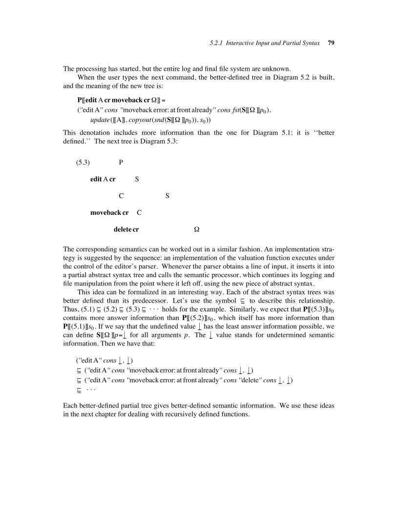
5.2.1 Interactive Input and Partial Syntax 79
The processing has started, but the entire log and final file system are unknown.
When the user types the next command, the better-defined tree in Diagram 5.2 is built,
and the meaning of the new tree is:
P[[edit A cr moveback cr']]#
(''edit A'' cons ''moveback error: at front already'' cons fst(S[[' ]]p0),
update([[A]], copyout(snd(S[[' ]]p0)), s0))
This denotation includes more information than the one for Diagram 5.1; it is ‘‘better
defined.’’ The next tree is Diagram 5.3:
(5.3) P
edit A cr S
C S
moveback cr C
delete cr '
The corresponding semantics can be worked out in a similar fashion. An implementation stra-
tegy is suggested by the sequence: an implementation of the valuation function executes under
the control of the editor’s parser. Whenever the parser obtains a line of input, it inserts it into
a partial abstract syntax tree and calls the semantic processor, which continues its logging and
file manipulation from the point where it left off, using the new piece of abstract syntax.
This idea can be formalized in an interesting way. Each of the abstract syntax trees was
better defined than its predecessor. Let’s use the symbol """"" to describe this relationship.
Thus, (5.1) """"" (5.2) ""
""" (5.3) """"" . . . holds for the example. Similarly, we expect that P[[(5.3)]]s0
contains more answer information than P[[(5.2)]]s0, which itself has more information than
P[[(5.1)]]s0. If we say that the undefined value "" has the least answer information possible, we
can define S[[' ]]p# "" for all arguments p. The "" value stands for undetermined semantic
information. Then we have that:
(''edit A'' cons "", "")
""""" (''edit A'' cons ''moveback error: at front already'' cons "", "")
""""" (''edit A'' cons ''moveback error: at front already'' cons ''delete'' cons "", "")
""""" . . .
Each better-defined partial tree gives better-defined semantic information. We use these ideas
in the next chapter for dealing with recursively defined functions.
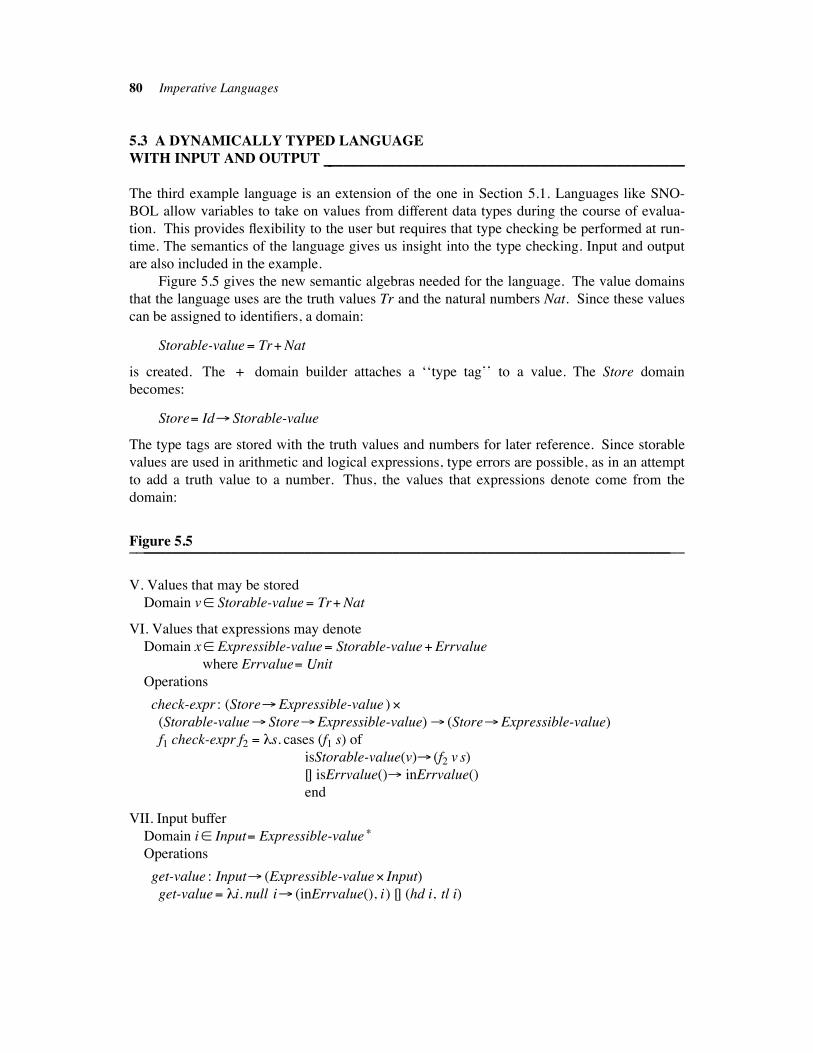
80 Imperative Languages
5.3 A DYNAMICALLY TYPED LANGUAGE
WITH INPUT AND OUTPUT !!!!!!!!!!!!!!!!!!!!!!!!!!!!!!!!!!!!!!!!!!!!!!!!!!!!!!!!!!!!!!!!!!!!!!!!!!!!!!!!!!!!!!!!!!!!!!!!
The third example language is an extension of the one in Section 5.1. Languages like SNO-
BOL allow variables to take on values from different data types during the course of evalua-
tion. This provides flexibility to the user but requires that type checking be performed at run-
time. The semantics of the language gives us insight into the type checking. Input and output
are also included in the example.
Figure 5.5 gives the new semantic algebras needed for the language. The value domains
that the language uses are the truth values Tr and the natural numbers Nat. Since these values
can be assigned to identifiers, a domain:
Storable-value# Tr&Nat
is created. The + domain builder attaches a ‘‘type tag’’ to a value. The Store domain
becomes:
Store# Id! Storable-value
The type tags are stored with the truth values and numbers for later reference. Since storable
values are used in arithmetic and logical expressions, type errors are possible, as in an attempt
to add a truth value to a number. Thus, the values that expressions denote come from the
domain:
Figure 5.5____________________________________________________________________________________________________________________________________________________
V. Values that may be stored
Domain v# Storable-value# Tr&Nat
VI. Values that expressions may denote
Domain x# Expressible-value# Storable-value&Errvalue
where Errvalue# Unit
Operations
check-expr : (Store!Expressible-value )%(Storable-value! Store!Expressible-value) ! (Store!Expressible-value)
f1 check-expr f2 # $s. cases (f1 s) of
isStorable-value(v)! (f2 v s)
[] isErrvalue()! inErrvalue()
end
VII. Input buffer
Domain i# Input# Expressible-value &
Operations
get-value : Input! (Expressible-value% Input)
get-value# $i. null i! (inErrvalue(), i) [] (hd i, tl i)
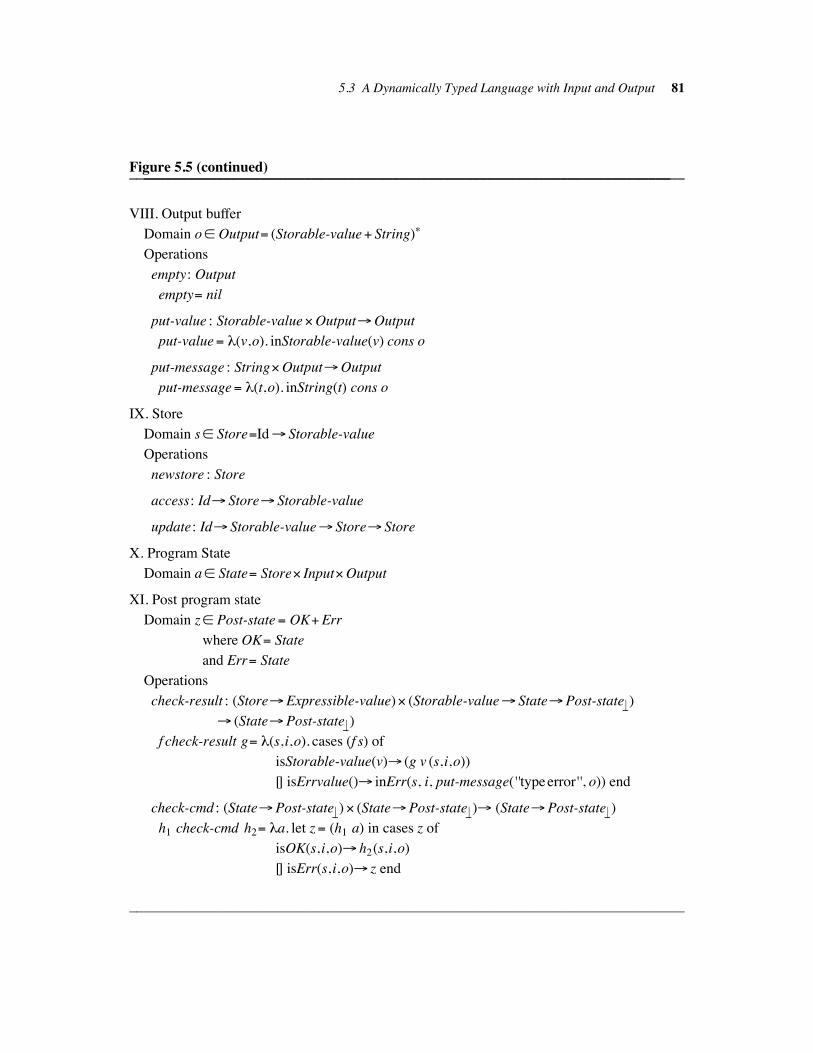
5.3 A Dynamically Typed Language with Input and Output 81
Figure 5.5 (continued)____________________________________________________________________________________________________________________________________________________
VIII. Output buffer
Domain o# Output# (Storable-value& String)&
Operations
empty: Output
empty# nil
put-value : Storable-value%Output!Output
put-value# $(v,o). inStorable-value(v) cons o
put-message : String%Output!Output
put-message# $(t,o). inString(t) cons o
IX. Store
Domain s# Store#Id! Storable-value
Operations
newstore : Store
access: Id! Store! Storable-value
update: Id! Storable-value! Store! Store
X. Program State
Domain a# State# Store% Input%Output
XI. Post program state
Domain z# Post-state# OK&Err
where OK# State
and Err# State
Operations
check-result : (Store!Expressible-value)% (Storable-value! State!Post-state "!)
! (State!Post-state "!)
f check-result g# $(s, i,o). cases (f s) of
isStorable-value(v)! (g v (s,i,o))
[] isErrvalue()! inErr(s, i, put-message(''type error'', o)) end
check-cmd : (State!Post-state "!)% (State!Post-state "!)! (State!Post-state "!)
h1 check-cmd h2# $a. let z # (h1 a) in cases z of
isOK(s, i,o)! h2(s,i,o)
[] isErr(s, i,o)! z end
____________________________________________________________________________
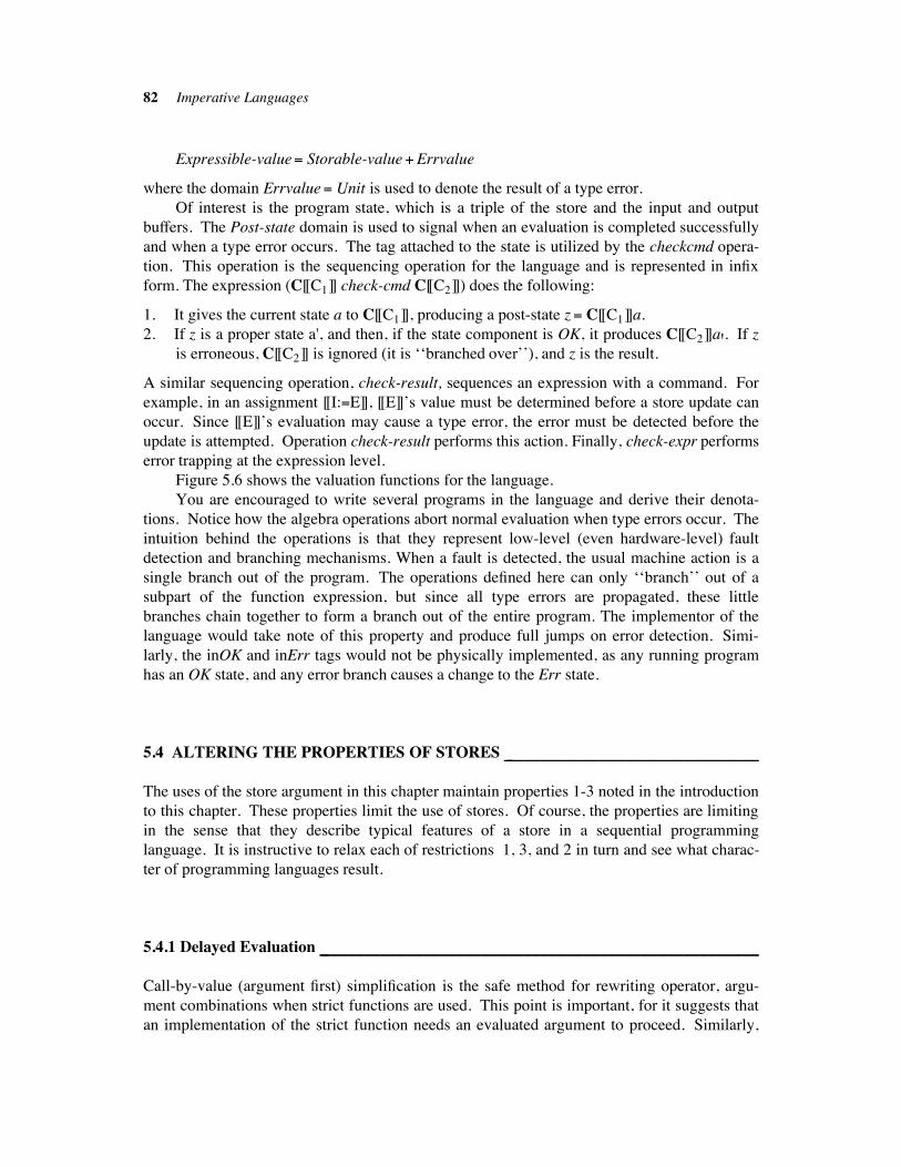
82 Imperative Languages
Expressible-value# Storable-value&Errvalue
where the domain Errvalue# Unit is used to denote the result of a type error.
Of interest is the program state, which is a triple of the store and the input and output
buffers. The Post-state domain is used to signal when an evaluation is completed successfully
and when a type error occurs. The tag attached to the state is utilized by the checkcmd opera-
tion. This operation is the sequencing operation for the language and is represented in infix
form. The expression (C[[C1]] check-cmd C[[C2]]) does the following:
1. It gives the current state a to C[[C1]], producing a post-state z # C[[C1]]a.
2. If z is a proper state a', and then, if the state component is OK, it produces C[[C2]]a'. If z
is erroneous, C[[C2]] is ignored (it is ‘‘branched over’’), and z is the result.
A similar sequencing operation, check-result, sequences an expression with a command. For
example, in an assignment [[I:#E]], [[E]]’s value must be determined before a store update can
occur. Since [[E]]’s evaluation may cause a type error, the error must be detected before the
update is attempted. Operation check-result performs this action. Finally, check-expr performs
error trapping at the expression level.
Figure 5.6 shows the valuation functions for the language.
You are encouraged to write several programs in the language and derive their denota-
tions. Notice how the algebra operations abort normal evaluation when type errors occur. The
intuition behind the operations is that they represent low-level (even hardware-level) fault
detection and branching mechanisms. When a fault is detected, the usual machine action is a
single branch out of the program. The operations defined here can only ‘‘branch’’ out of a
subpart of the function expression, but since all type errors are propagated, these little
branches chain together to form a branch out of the entire program. The implementor of the
language would take note of this property and produce full jumps on error detection. Simi-
larly, the inOK and inErr tags would not be physically implemented, as any running program
has an OK state, and any error branch causes a change to the Err state.
5.4 ALTERING THE PROPERTIES OF STORES !!!!!!!!!!!!!!!!!!!!!!!!!!!!!!!!!!!!!!!!!!!!!!!!!!!!!!!!!!!!!!
The uses of the store argument in this chapter maintain properties 1-3 noted in the introduction
to this chapter. These properties limit the use of stores. Of course, the properties are limiting
in the sense that they describe typical features of a store in a sequential programming
language. It is instructive to relax each of restrictions 1, 3, and 2 in turn and see what charac-
ter of programming languages result.
5.4.1 Delayed Evaluation !!!!!!!!!!!!!!!!!!!!!!!!!!!!!!!!!!!!!!!!!!!!!!!!!!!!!!!!!!!!!!!!!!!!!!!!!!!!!!!!!!!!!!!!!!!!!!!!!!!!!!!!!!
Call-by-value (argument first) simplification is the safe method for rewriting operator, argu-
ment combinations when strict functions are used. This point is important, for it suggests that
an implementation of the strict function needs an evaluated argument to proceed. Similarly,
5.4.1 Delayed Evaluation 83
Figure 5.6____________________________________________________________________________________________________________________________________________________
Abstract syntax:
P# Program
C# Command
E# Expression
I# Id
N# Numeral
P ::= C.
C ::= C1;C2 | I:#E | if E then C1 else C2 | read I | write E | diverge
E ::= E1&E2 | E1#E2 | 'E | (E) | I | N | true
Semantic algebras:
I. Truth values (defined in Figure 5.1)
II. Natural numbers (defined in Figure 5.1)
III. Identifiers (defined in Figure 5.1)
IV. Character strings (defined in Example 3.5 of Chapter 3)
V. - XI. (defined in Figure 5.5)
Valuation functions:
P: Program! Store! Input!Post-state "!
P[[C.]]# $s.$i. C[[C]] (s, i, empty)
C: Command! State!Post-state "!
C[[C1;C2]]# C[[C1]] check-cmd C[[C2]]
C[[I:#E]]# E[[E]] check-result ($v.$(s, i,o). inOK((update[[I]] v s), i, o))
C[[if E then C1 else C2]]# E[[E]] check-result
($v.$(s, i,o). cases v of
isTr(t)! (t!C[[C1]] [] C[[C2]] )(s,i,o)
[] isNat(n)! inErr(s, i, put-message(''bad test'', o)) end)
C[[read I]]# $(s, i,o). let (x,i')# get-value(i) in
cases x of
isStorable-value(v)! inOK((update[[I]] v s), i', o)
[] isErrvalue()! inErr(s, i', put-message(''bad input'', o)) end
C[[write E]]# E[[E]] check-result ($v.$(s, i,o). inOK(s, i, put-value(v,o)))
C[[diverge]]# $a. ""
84 Imperative Languages
Figure 5.6 (continued)____________________________________________________________________________________________________________________________________________________
E: Expression! Store!Expressible-value
E[[E1&E2]]# E[[E1]] check-expr
($v. cases v of
isTr(t)!$s. inErrvalue()
[] isNat(n)!E[[E2]] check-expr
($v'.$s. cases v ' of
isTr(t')! inErrvalue()
[] isNat(n')! inStorable-value(inNat(n plus n')) end)
end)
E[[E1#E2]]# ‘‘similar to above equation’’
E[['E]]# E[[E]] check-expr
($v.$s. cases v of
isTr(t)! inStorable-value(inTr(not t))
[] isNat(n)! inErrvalue() end)
E[[(E)]]# E[[E]]
E[[I]]# $s. inStorable-value(access [[I]] s)
E[[N]]# $s. inStorable-value(inNat(N[[N]]))
E[[true]]# $s. inStorable-value(inTr(true))
N:Numeral!Nat (omitted)
____________________________________________________________________________
call-by-name (argument last) simplification is the safe method for handling arguments to non-
strict functions. Here is an example: consider the nonstrict function f# ($x. zero) of domain
Nat "!!Nat "! . If f is given an argument e whose meaning is "", then f(e) is zero. Argument e’s
simplification may require an infinite number of steps, for it represents a nonterminating
evaluation. Clearly, e should not be simplified if given to a nonstrict f.
The Store-based operations use only proper arguments and a store can only hold values
that are proper. Let’s consider how stores might operate with improper values. First, say that
expression evaluation can produce both proper and improper values. Alter the Store domain to
be Store# Id!Nat "! . Now improper values may be stored. Next, adjust the update operation
to be: update : Id!Nat "!! Store! Store, update# $i.$n.$s. [ i ""! n]s. An assignment state-
ment uses update to store the value of an expression [[E]] into the store. If [[E]] represents a
‘‘loop forever’’ situation, then E[[E]]s# "". But, since update is nonstrict in its second argu-
ment, (update [[I]] (E[[E]]s) s) is defined. From the operational viewpoint, unevaluated or par-
tially evaluated expressions may be stored into s. The form E[[E]]s need not be evaluated until
it is used; the arrangement is called delayed (or lazy) evaluation. Delayed evaluation provides
the advantage that the only expressions evaluated are the ones that are actually needed for
5.4.1 Delayed Evaluation 85
computing answers. But, once E[[E]]’s value is needed, it must be determined with respect to
the store that was active when [[E]] was saved. To understand this point, consider this code:
begin
X:#0;
Y:#X&1;
X:#4
resultis Y
where the block construct is defined as:
K: Block! Store "!!Nat "!
K[[begin C resultis E]]# $!!s. E[[E]] (C[[C]]s)
(Note: E now has functionality E : Expression! Store"!!Nat "! , and it is strict in its store
argument.) At the final line of the example, the value of [[Y]] must be determined. The
semantics of the example, with some proper store s0, is:
K[[begin X:#0; Y:#X&1; X:#4 resultis Y]]s0
# E[[Y]] (C[[X:#0; Y:#X&1; X:#4]]s0)
# E[[Y]] (C[[Y:#X&1; X:#4]] (C[[X:#0]]s0))
# E[[Y]] (C[[Y:#X&1; X:#4]] (update[[X]] (E[[0]]s0) s0))
At this point, (E[[0]]s0) need not be simplified; a new, proper store, s1
# (update[[X]] E[[0]]s0 s0) is defined regardless. Continuing through the other two commands,
we obtain:
s3 # update[[X]] (E[[4]]s2) s2
where s2# update[[Y]] (E[[X&1]]s1) s1
and the meaning of the block is:
E[[Y]]s3 # access[[Y]] s3
# E[[X&1]]s1
# E[[X]]s1 plus one
# (access[[X]] s1) plus one)
# E[[0]]s0 plus one
# zero plus one# one
The old version of the store, version s1, must be retained to obtain the proper value for [[X]] in
[[X&1]]. If s3 was used instead, the answer would have been the incorrect five.
Delayed evaluation can be carried up to the command level by making the C, E, and K
functions nonstrict in their store arguments. The surprising result is that only those commands
that have an effect on the output of a program need be evaluated. Convert all strict abstractions
($!!s. e) in the equations for C in Figure 5.2 to the nonstrict forms ($s. e). Redefine access and
update to be:
86 Imperative Languages
access : Identifier! Store"!!Nat "!
access# $i.$!!s. s(i)
update : Identifier!Nat "!! Store"!! Store"!
update# $i.$m.$p. ($i'. i' equals i ! m [] (access i' p))
Then, regardless of the input store s, the program:
begin
X:#0;
diverge;
X:#2
resultis X&1
has the value three! This is because C[[X:#0; diverge]]s# "", and:
E[[X&1]] (C[[X:#2]] "")
# E[[X&1]] (update[[X]] (E[[2]] "") ""), as C is nonstrict
# E[[X&1]] ( [ [[X]]""!E[[2]] "" ] ""), as update is nonstrict
# E[[X]] ( [ [[X]]""!E[[2]] "" ] "") plus one
# (access[[X]] ( [ [[X]]""!E[[2]] "" ] "")) plus one
# E[[2]] "" plus one
# two plus one, as E is nonstrict
# three
The derivation suggests that only the last command in the block need be evaluated to obtain
the answer. Of course, this goes against the normal left-to-right, top-to-bottom sequentiality
of command evaluation, so the nonstrict handling of stores requires a new implementation
strategy.
5.4.2 Retaining Multiple Stores !!!!!!!!!!!!!!!!!!!!!!!!!!!!!!!!!!!!!!!!!!!!!!!!!!!!!!!!!!!!!!!!!!!!!!!!!!!!!!!!!!!!!!!!!!!!!!
Relaxing the strictness condition upon stores means that multiple values of stores must be
present in an evaluation. Must an implementation of any of the languages defined earlier in
this chapter use multiple stores? At first glance, the definition of addition:
E[[E1&E2]]# $s. E[[E1]]s plus E[[E2]]s
apparently does need two copies of the store to evaluate. Actually, the format is a bit deceiv-
ing. An implementation of this clause need only retain one copy of the store s because both
E[[E1]] and E[[E2]] use s in a ‘‘read only’’ mode. Since s is not updated by either, the equation
should be interpreted as saying that the order of evaluation of the two operands to the addition
is unimportant. They may even be evaluated in parallel. The obvious implementation of the
store is a global variable that both operands may access.
This situation changes when side effects occur within expression evaluation. If we add
5.4.2 Retaining Multiple Stores 87
the block construct to the Expression syntax domain and define its semantics to be:
E[[begin C resultis E]]# $!!s. let s' # C[[C]]s in E[[E]]s'then expressions are no longer ‘‘read only’’ objects. An implementation faithful to the seman-
tic equation must allow an expression to own a local copy of store. The local store and its
values disappear upon completion of expression evaluation. To see this, you should perform
the simplification of C[[X:#(begin Y:#Y&1 resultis Y)&Y]]. The incrementation of [[Y]] in the
left operand is unknown to the right operand. Further, the store that gets the new value of [[X]]
is exactly the one that existed prior to the right-hand side’s evaluation.
The more conventional method of integrating expression-level updates into a language
forces any local update to remain in the global store and thus affect later evaluation. A more
conventional semantics for the block construct is:
K[[begin C resultis E]]# $!!s. let s' # C[[C]]s in (E[[E]]s', s')
The expressible value and the updated store form a pair that is the result of the block.
5.4.3 Noncommunicating Commands !!!!!!!!!!!!!!!!!!!!!!!!!!!!!!!!!!!!!!!!!!!!!!!!!!!!!!!!!!!!!!!!!!!!!!!!!!!!!!!!!!!!
The form of communication that a store facilitates is the building up of side effects that lead to
some final value. The purpose of a command is to advance a computation a bit further by
drawing upon the values left in the store by previous commands. When a command is no
longer allowed to draw upon the values, the communication breaks down, and the language no
longer has a sequential flavor.
Let’s consider an example that makes use of multiple stores. Assume there exists some
domain D with an operation combine : D%D!D. If combine builds a ‘‘higher-quality’’ D-
value from its two D-valued arguments, a useful store-based, noncommunicating semantics
might read:
Domain s# Store# Id!D
C: Command! Store "!! Store "!
C[[C1;C2]]# $!!s. join (C[[C1]]s) (C[[C2]]s)
where join : Store "!! Store "!! Store "!
join # $!!s1 .$!!s2 . ($i. s1(i) combine s2(i))
These clauses suggest parallel but noninterfering execution of commands. Computing is
divided between [[C1]] and [[C2]] and the partial results are joined using combine. This is a
nontraditional use of parallelism on stores; the traditional form of parallelism allows interfer-
ence and uses the single-store model. Nonetheless, the above example is interesting because it
suggests that noncommunicating commands can work together to build answers rather than
deleting each other’s updates.
88 Imperative Languages
SUGGESTED READINGS !!!!!!!!!!!!!!!!!!!!!!!!!!!!!!!!!!!!!!!!!!!!!!!!!!!!!!!!!!!!!!!!!!!!!!!!!!!!!!!!!!!!!!!!!!!!!!!!!!!!!!
Semantics of the store and assignment: Barron 1977; Donohue 1977; Friedman et al. 1984;
Landin 1965; Strachey 1966, 1968
Interactive systems: Bjo/ rner and Jones 1982; Cleaveland 1980
Dynamic typing: Tennent 1973
Delayed evaluation: Augustsson 1984; Friedman & Wise 1976; Henderson 1980; Henderson
& Morris 1976
EXERCISES !!!!!!!!!!!!!!!!!!!!!!!!!!!!!!!!!!!!!!!!!!!!!!!!!!!!!!!!!!!!!!!!!!!!!!!!!!!!!!!!!!!!!!!!!!!!!!!!!!!!!!!!!!!!!!!!!!!!!!!!!!!!
1. Determine the denotations of the following programs in Nat "! when they are used with the
input data value one:
a. P[[Z:#A.]]
b. P[[(if A#0 then diverge else Y:#A&1);Z:#Y.]]
c. P[[diverge; Z:#0.]]
2. Determine the denotations of the programs in the previous exercise without any input;
that is, give their meanings in the domain Nat!Nat "! .
3. Give an example of a program whose semantics with respect to Figure 5.2, is the denota-
tion ($n. one). Does an algorithmic method exist for listing all the programs with exactly
this denotation?
4. Show that the following properties hold with respect to the semantic definition of Figure
5.2:
a. P[[Z:#0; if A#0 then Z:#A.]]# P[[Z:#0.]]
b. For any C# Command, C[[diverge; C]]# C[[diverge]]
c. For all E1, E2# Expression, E[[E1&E2]]# E[[E2&E1]]
d. For any B# Boolean-expr, C1, C2# Command,
C[[if B then C1 else C2]]# C[[if'B then C2 else C1]].
e. There exist some B# Boolean-expr and C1, C2# Command such that
C[[if B then C1; if'B thenC2]]% C[[if B then C1 else C2]]
(Hint: many of the proofs will rely on the extensionality of functions.)
5. a. Using structural induction, prove the following: for every E# Expression in the
language of Figure 5.2, for any I# Identifier, E'# Expression, and s# Store,
E[[[E'/I]E]]s # E[[E]](update [[I]] E[[E']]s s).
b. Use the result of part a to prove: for every B# Boolean-expr in the language of Fig-
ure 5.2, for every I# Identifier, E'# Expression, and s# Store, B[[[E'/I]B]]s #B[[B]](update [[I]] E[[E']]s s).
Exercises 89
6. Say that the Store algebra in Figure 5.1 is redefined so that the domain is
s# Store'# (Id%Nat)& .
a. Define the operations newstore', access', and update' to operate upon the new domain.
(For this exercise, you are allowed to use a recursive definition for access'. The
definition must satisfy the properties stated in the solution to Exercise 14, part b, of
Chapter 3.) Must the semantic equations in Figure 5.2 be adjusted to work with the
new algebra?
b. Prove that the definitions created in part a satisfy the properties: for all i# Id, n#Nat,
and s# Store':
access' i newstore'# zero
access' i (update' i n s)# n
access' i (update' j n s)# (access' i s), for j % i
How do these proofs relate the new Store algebra to the original? Try to define a
notion of ‘‘equivalence of definitions’’ for the class of all Store algebras.
7. Augment the Command syntax domain in Figure 5.2 with a swap command:
C ::= . . . | swap I1, I2
The action of swap is to interchange the values of its two identifier variables. Define the
semantic equation for swap and prove that the following property holds for any J# Id
and s# Store: C[[swap J, J]]s# s. (Hint: appeal to the extensionality of store functions.)
8. a. Consider the addition of a Pascal-like cases command to the language of Figure 5.2.
The syntax goes as follows:
C# Command
G# Guard
E# Expression
C ::= . . . | case E of G end
G ::= N:C; G | N:C
Define the semantic equation for C[[case E of G end]] and the equations for the valua-
tion function G : Guard! (Nat % Store)! Store "! . List the design decisions that must
be made.
b. Repeat part a with the rule G ::= N:C | G1; G2
9. Say that the command [[test E on C]] is proposed as an extension to the langauge of Fig-
ure 5.2. The semantics is:
C[[test E on C]]# $!!s. let s' # C[[C]]s in E[[E]]s' equals zero ! s' [] s
What problems do you see with implementing this construct on a conventional machine?
10. Someone proposes a version of ‘‘parallel assignment’’ with semantics:
C[[I1, I2 :#E1, E2]]# $!!s. let s' # (update[[I1]] E[[E1]]s s)
90 Imperative Languages
in update [[I2]] E[[E2]]s' s'Show, via a counterexample, that the semantics does not define a true parallel assign-
ment. Propose an improvement. What is the denotation of [[J, J :# 0, 1]] in your seman-
tics?
11. In a LUCID-like language, a family of parallel assignments are performed in a construct
known as a block. The syntax of a block B is:
B ::= begin A end
A ::= Inew:#E | A1§A2
The block is further restricted so that all identifiers on the left hand sides of assignments
in a block must be distinct. Define the semantics of the block construct.
12. Add the diverge construction to the syntax of Expression in Figure 5.2 and say that
E[[diverge]]# $s. "". How does this addition impact:
a. The functionalities and semantic equations for C, E, and B?
b. The definition and use of the operations update, plus, equals, and not? What is your
opinion about allowing the possibility of nontermination in expression evaluation?
What general purpose imperative languages do you know of that guarantee termina-
tion of expression evaluation?
13. The document defining the semantics of Pascal claims that the order of evaluation of
operands in an (arithmetic) expression is left unspecified; that is, a machine may evaluate
the operands in whatever order it pleases. Is this concept expressed in the semantics of
expressions in Figure 5.2? However, recall that Pascal expressions may contain side
effects. Let’s study this situation by adding the construct [[C in E]]. Its evaluation first
evaluates [[C]] and then evaluates [[E]] using the store that was updated by [[C]]. The store
(with the updates) is passed on for later use. Define E[[C in E]]. How must the functional-
ity of E change to accommodate the new construct? Rewrite all the other semantic equa-
tions for E as needed. What order of evaluation of operands does your semantics
describe? Is it possible to specify a truly nondeterminate order of evaluation?
14. For some defined store s0, give the denotations of each of the following file editor pro-
grams, using the semantics in Figure 5.4:
a. P[[edit A cr newfile cr insert R0 cr insert R1 quit]]s0. Call the result (log1, s1).
b. P[[edit A cr moveforward cr delete cr insert R2 quit]]s1, where s1 is from part a.
Call the new result (log2, s2).
c. P[[edit A cr insert R3 cr quit]]s2, where s2 is from part b.
15. Redo part a of the previous question in the style described in Section 5.2.1, showing the
partial syntax trees and the partial denotations produced at each step.
16. Extend the file editor of Figure 5.4 to be a text editor: define the internal structure of the
Exercises 91
Record semantic domain in Figure 5.3 and devise operations for manipulating the words
in a record. Augment the syntax of the language so that a user may do manipulations on
the words within individual records.
17. Design a programming language for performing character string manipulation. The
language should support fundamental operations for pattern matching and string manipu-
lation and possess assignment and control structure constructs for imperative program-
ming. Define the semantic algebras first and then define the abstract syntax and valuation
functions.
18. Design a semantics for the grocery store data base language that you defined in Exercise
6 of Chapter 1. What problems arise because the abstract syntax was defined before the
semantic algebras? What changes would you make to the language’s syntax after this
exercise?
19. In the example in Section 5.3, the Storable-value domain is a subdomain of the
Expressible-value domain; that is, every storable value is expressible. What problems
arise when this isn’t the case? What problems/situations arise when an expressible value
isn’t storable? Give examples.
20. In the language of Figure 5.6, what is P[[write 2; diverge.]]? Is this a satisfactory denota-
tion for the program? If not, suggest some revisions to the semantics.
21. Alter the semantics of the language of Figure 5.6 so that an expressible value error causes
an error message to be placed into the output buffer immediately (rather than letting the
command in which the expressible value is embedded report the message later).
22. Extend the Storable-value algebra of Figure 5.5 so that arithmetic can be performed on
the (numeric portion of) storable values. In particular, define operations:
plus' : Storable-value% Storable-value!Expressible-value
not' : Storable-value!Expressible-value
equals' : Storable-value% Storable-value!Expressible-value
so that the equations in the E valuation function can be written more simply, e.g.,
E[[E1&E2]]# E[[E1]]s check-expr ($v1. E[[E2]]s check-expr ($v2. v1 plus' v2))
Rewrite the other equations of E in this fashion. How would the new versions of the stor-
able value operations be implemented on a computer?
23. Alter the semantics of the language of Figure 5.6 so that a variable retains the type of the
first identifier that is assigned to it.
24. a. Alter the Store algebra in Figure 5.5 so that:
Store# Index! Storable-value&
92 Imperative Languages
where Index# Id& Input&Output
Input# Unit
Output# Unit
that is, the input and output buffers are kept in the store and indexed by tags. Define
the appropriate operations. Do the semantic equations require alterations?
b. Take advantage of the new definition of storage by mapping a variable to a history of
all its updates that have occurred since the program has been running.
25. Remove the command [[read I]] from the language of Figure 5.6 and place the construct
[[read]] into the syntax of expressions.
a. Give the semantic equation for E[[read]].
b. Prove that C[[read I]]# C[[I:# read]].
c. What are the pragmatic advantages and disadvantages of the new construct?
26. Suppose that the Store domain is defined to be Store# Id! (Store!Nat) and the seman-
tic equation for assignment is:
C[[I:#E]]# $!!s. update [[I]] (E[[E]]) s
a. Define the semantic equations for the E valuation function.
b. How does this view of expression evaluation differ from that given in Figures 5.1 and
5.2? How is the new version like a macroprocessor? How is it different?
27. If you are familiar with data flow and demand-driven languages, comment on the resem-
blance of the nonstrict version of the C valuation function in Section 5.4.1 to these forms
of computation.
28. Say that a vendor has asked you to design a simple, general purpose, imperative program-
ming language. The language will include concepts of expression and command. Com-
mands update the store; expressions do not. The control structures for commands
include sequencing and conditional choice.
a. What questions should you ask the vendor about the language’s design? Which
design decisions should you make without consulting the vendor first?
b. Say that you decide to use denotational semantics to define the semantics of the
language. How does its use direct and restrict your view of:
i. What the store should be?
ii. How stores are accessed and updated?
iii. What the order of evaluation of command and expression subparts should be?
iv. How the control structures order command evaluation?
29. Programming language design has traditionally worked from a ‘‘bottom up’’ perspective;
that is, given a physical computer, a machine language is defined for giving instructions
to the computer. Then, a second language is designed that is ‘‘higher level’’ (more con-
cise or easier for humans to use) than the first, and a translator program is written to
Exercises 93
translate from the second language to the first.
Why does this approach limit our view as to what a programming language should
be? How might we break out of this approach by using denotational semantics to design
new languages? What biases do we acquire when we use denotational semantics?
Chapter 6 !!!!!!!!!!!!!!!!!!!!!!!!!!!!!!!!!!!!!!!!!!!!!!!!!!!!!!!!
Domain Theory II: Recursively Defined Func-tions
The examples in Chapter 5 provide strong evidence that denotational semantics is an expres-
sive and convenient tool for language definition. Yet a few gaps remain to be filled. In Figure
5.3, the copyout function, which concatenates two lists, is not given. We can specify copyout
using an iterative or recursive specification, but at this point neither is allowed in the function
notation.
A similar situation arises with the semantics of a Pascal-like while-loop:
B: Boolean-expression
C: Command
C ::= . . . | while B do C | . . .
Here is a recursive definition of its semantics: for B: Boolean-expression ! Store! Tr and
C: Command! Store"!! Store"!:
C[[while B do C]]# "!!s. B[[B]]s!C[[while B do C]] (C[[C]]s) [] s
Unfortunately, the clause violates a rule of Chapter 3: the meaning of a syntax phrase may be
defined only in terms of the meanings of its proper subparts. We avoid this problem by stating:
C[[while B do C]]# w
where w : Store "!! Store "! is w # "!!s. B[[B]]s!w(C[[C]]s) [] s
But the recursion remains, for the new version exchanges the recursion in the syntax for recur-
sion in the function notation.
We have steadfastly avoided recursion in function definitions because Section 3.3 showed
that a recursive definition might not define a unique function. Recall the recursive
specification of function q: Nat!Nat "! from Section 3.3:
q# "n. n equals zero! one[] q(n plus one)
Whatever q stands for, it must map a zero argument to one. Its behavior for other arguments,
however, is not so clear. All the specification requires is that the answer for a nonzero argu-
ment n be the same as that for n plus one, its successor. A large number of functions satisfy
this criterion. One choice is the function that maps zero to one and all other arguments to "#.
We write this function’s graph as { (zero, one) } (rather than { (zero, one), (one, "#),
(two, "#), . . . }, treating the (n, "#) pairs as ‘‘ghost members’’). This choice is a natural one for
programming, for it corresponds to what happens when the definition is run as a routine on a
machine. But it is not the only choice. The graph { (zero, one), (one, four), (two, four),
(three, four), . . . } denotes a function that also has the behavior specified by q— zero maps to
94

95
one and all other arguments map to the same answer as their successors. In general, any func-
tion whose graph is of the form { (zero, one), (one, k), (two, k), . . . }, for some k$Nat "! ,
satisfies the specification. For a programmer, the last graph is an unnatural choice for the
meaning of q, but a mathematician might like a function with the largest possible graph
instead, the claim being that a ‘‘fuller’’ function gives more insight. In any case, a problem
exists: a recursive specification may not define a unique function, so which one should be
selected as the meaning of the specification? Since programming languages are implemented
on machines, we wish to choose the function that suits operational intuitions. Fortunately, a
well-developed theory known as least fixed point semantics establishes the meaning of recur-
sive specifications. The theory:
1. Guarantees that the specification has at least one function satisfying it.
2. Provides a means for choosing a ‘‘best’’ function out of the set of all functions satisfying
the specification.
3. Ensures that the function selected has a graph corresponding to the conventional opera-
tional treatment of recursion: the function maps an argument a to a defined answer b iff
the operational evaluation of the specification with the representation of argument a pro-
duces the representation of b in a finite number of recursive invocations.
Two simple examples of recursive specifications will introduce all the important concepts
in the theory. The theory itself is formalized in Sections 6.2 through 6.5. If you are willing to
accept that recursive specifications do indeed denote unique functions, you may wish to read
only Sections 6.1 and 6.6.
6.1 SOME RECURSIVELY DEFINED FUNCTIONS !!!!!!!!!!!!!!!!!!!!!!!!!!!!!!!!!!!!!!!!!!!!!!!!!!!!!!!!!!
Perhaps the best known example of a recursive function specification is the factorial function.
Since it is so well understood, it makes an excellent testing ground for the theory. Its
specification is fac: Nat!Nat "! such that:
fac(n)# n equals zero! one[] n times (fac(n minus one))
This specification differs from q’s because only one function satisfies the specification: the
factorial function, whose graph is { (zero, one), (one, one),
(two, two), (three, six), . . . , (i, i!), . . . }. The graph will be the key to understanding the
meaning of the specification. Note that it is an infinite set. It is often difficult for people to
understand infinite objects; we tend to learn about them by considering their finite subparts
and building up, step by step, toward the object. We can study the factorial function in this
way by evaluating sample arguments with fac. Since the function underlying the recursive
specification is not formally defined at the moment, an arrow (#>) will be used when a recur-
sive unfolding is made.
Here is an evaluation using fac:
fac(three) #> three equals zero! one[] three times fac(three minus one)
# three times fac(three minus one)
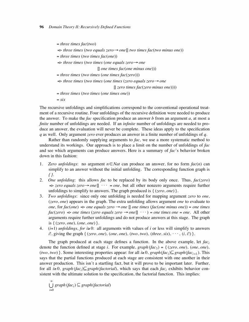
96 Domain Theory II: Recursively Defined Functions
# three times fac(two)
#> three times (two equals zero! one[] two times fac(two minus one))
# three times (two times fac(one))
#> three times (two times (one equals zero! one
[] one times fac(one minus one)))
# three times (two times (one times fac(zero)))
#> three times (two times (one times (zero equals zero! one
[] zero times fac(zero minus one))))
# three times (two times (one times one))
# six
The recursive unfoldings and simplifications correspond to the conventional operational treat-
ment of a recursive routine. Four unfoldings of the recursive definition were needed to produce
the answer. To make the fac specification produce an answer b from an argument a, at most a
finite number of unfoldings are needed. If an infinite number of unfoldings are needed to pro-
duce an answer, the evaluation will never be complete. These ideas apply to the specification
q as well. Only argument zero ever produces an answer in a finite number of unfoldings of q.
Rather than randomly supplying arguments to fac, we use a more systematic method to
understand its workings. Our approach is to place a limit on the number of unfoldings of fac
and see which arguments can produce answers. Here is a summary of fac’s behavior broken
down in this fashion:
1. Zero unfoldings: no argument n$Nat can produce an answer, for no form fac(n) can
simplify to an answer without the initial unfolding. The corresponding function graph is
{ }.
2. One unfolding: this allows fac to be replaced by its body only once. Thus, fac(zero)
#> zero equals zero! one[] . . . # one, but all other nonzero arguments require further
unfoldings to simplify to answers. The graph produced is { (zero, one) }.
3. Two unfoldings: since only one unfolding is needed for mapping argument zero to one,
(zero, one) appears in the graph. The extra unfolding allows argument one to evaluate to
one, for fac(one) #> one equals zero ! one [] one times (fac(one minus one)) # one times
fac(zero) #> one times (zero equals zero ! one[] . . . ) # one times one # one. All other
arguments require further unfoldings and do not produce answers at this stage. The graph
is { (zero, one), (one, one) }.
4. (i$1) unfoldings, for i% 0: all arguments with values of i or less will simplify to answers
i!, giving the graph { (zero, one), (one, one), (two, two), (three, six), . . . , (i, i!) }.
The graph produced at each stage defines a function. In the above example, let faci
denote the function defined at stage i. For example, graph (fac3) # { (zero, one), (one, one),
(two, two) }. Some interesting properties appear: for all i% 0, graph(faci)& graph(faci$1). This
says that the partial functions produced at each stage are consistent with one another in their
answer production. This isn’t a startling fact, but it will prove to be important later. Further,
for all i% 0, graph (faci)& graph(factorial), which says that each faci exhibits behavior con-
sistent with the ultimate solution to the specification, the factorial function. This implies:
i#0' (
graph (faci) & graph(factorial)
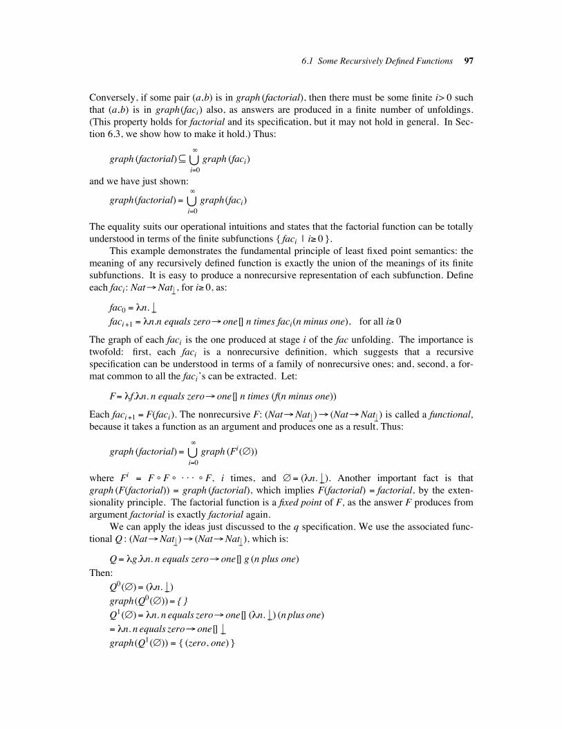
6.1 Some Recursively Defined Functions 97
Conversely, if some pair (a,b) is in graph (factorial), then there must be some finite i> 0 such
that (a,b) is in graph(faci) also, as answers are produced in a finite number of unfoldings.
(This property holds for factorial and its specification, but it may not hold in general. In Sec-
tion 6.3, we show how to make it hold.) Thus:
graph (factorial)& i#0' (
graph (faci)
and we have just shown:
graph(factorial)# i#0' (
graph(faci)
The equality suits our operational intuitions and states that the factorial function can be totally
understood in terms of the finite subfunctions { faci | i% 0 }.
This example demonstrates the fundamental principle of least fixed point semantics: the
meaning of any recursively defined function is exactly the union of the meanings of its finite
subfunctions. It is easy to produce a nonrecursive representation of each subfunction. Define
each faci: Nat!Nat "! , for i% 0, as:
fac0 # "n. "#faci$1 # "n.n equals zero! one[] n times faci(n minus one), for all i% 0
The graph of each faci is the one produced at stage i of the fac unfolding. The importance is
twofold: first, each faci is a nonrecursive definition, which suggests that a recursive
specification can be understood in terms of a family of nonrecursive ones; and, second, a for-
mat common to all the faci’s can be extracted. Let:
F# "f."n. n equals zero! one[] n times (f(n minus one))
Each faci$1 # F(faci). The nonrecursive F: (Nat!Nat "!)! (Nat!Nat "!) is called a functional,
because it takes a function as an argument and produces one as a result. Thus:
graph (factorial)# i#0' (
graph (Fi()))
where Fi # F % F % . . . % F, i times, and )# ("n. "#). Another important fact is that
graph (F(factorial)) # graph (factorial), which implies F(factorial) # factorial, by the exten-
sionality principle. The factorial function is a fixed point of F, as the answer F produces from
argument factorial is exactly factorial again.
We can apply the ideas just discussed to the q specification. We use the associated func-
tional Q : (Nat!Nat "!)! (Nat!Nat "!), which is:
Q# "g."n. n equals zero! one[] g (n plus one)
Then:
Q0())# ("n. "#)
graph(Q0()))# { }
Q1())# "n. n equals zero! one[] ("n. "#) (n plus one)
# "n. n equals zero! one[] "#graph(Q1())) # { (zero, one) }
98 Domain Theory II: Recursively Defined Functions
Q2()) # Q(Q()))
# "n. n equals zero! one[] ((n plus one) equals zero! one[] "#)
graph(Q2())) #{ (zero, one) }
At this point a convergence has occurred: for all i% 1, graph(Qi())) # { (zero, one) }. It fol-
lows that:
i#0' (
graph(Qi()))# { (zero, one) }
Let qlimit denote the function that has this graph. It is easy to show that Q(qlimit)# qlimit,
that is, qlimit is a fixed point of Q.
Unlike the specification fac, q has many possible solutions. Recall that each one must
have a graph of the form { (zero, one), (one, k), . . . , (i, k), . . . } for some k$ Nat "! . Let qk be
one of these solutions. We can show that:
1. qk is a fixed point of Q, that is, Q(qk)# qk.
2. graph(qlimit)& graph (qk).
Fact 1 says that the act of satisfying a specification is formalized by the fixed point property—
only fixed points of the associated functional are possible meanings of the specification. Fact
2 states that the solution obtained using the stages of unfolding method is the smallest of all
the possible solutions. For this reason, we call it the least fixed point of the functional.
Now the method for providing a meaning for a recursive specification is complete. Let a
recursive specification f #F(f) denote the least fixed point of functional F, that is, the function
associated with i#0' (
graph(Fi())). The three desired properties follow: a solution to the
specification exists; the criterion of leastness is used to select from the possible solutions; and,
since the method for constructing the function exactly follows the usual operational treatment
of recursive definitions, the solution corresponds to the one determined computationally.
The following sections formalize the method.
6.2 PARTIAL ORDERINGS !!!!!!!!!!!!!!!!!!!!!!!!!!!!!!!!!!!!!!!!!!!!!!!!!!!!!!!!!!!!!!!!!!!!!!!!!!!!!!!!!!!!!!!!!!!!!!!!!!
The theory is formalized smoothly if the subset relation used with the function graphs is gen-
eralized to a partial ordering. Then elements of semantic domains can be directly involved in
the set theoretical reasoning. For a domain D, a binary relation r& D&D (or r : D&D! IB) is
represented by the infix symbol ###"" D , or just ##
#"" if the domain of usage is clear. For a, b$D, we
read a ###"" b as saying ‘‘a is less defined than b.’’
6.1 Definition:
A relation ###"" : D&D! IB is a partial ordering upon D iff ##
#"" is:
1. reflexive: for all a$D, a ###"" a;
2. antisymmetric: for all a, b$D, a ###"" b and b ##
#"" a imply a# b.
3. transitive: for all a, b, c$D, a ###"" b and b ##
#"" c imply a ###"" c.
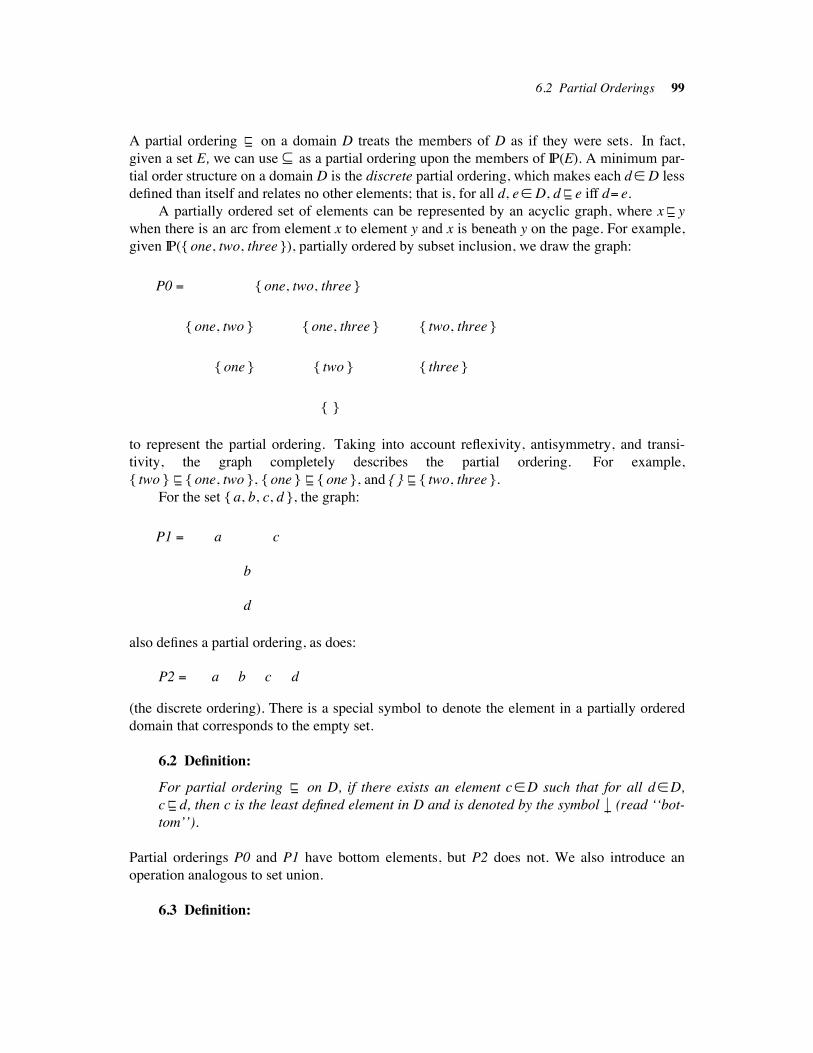
6.2 Partial Orderings 99
A partial ordering ###"" on a domain D treats the members of D as if they were sets. In fact,
given a set E, we can use & as a partial ordering upon the members of IP(E). A minimum par-
tial order structure on a domain D is the discrete partial ordering, which makes each d$ D less
defined than itself and relates no other elements; that is, for all d, e$ D, d ###"" e iff d# e.
A partially ordered set of elements can be represented by an acyclic graph, where x ###"" y
when there is an arc from element x to element y and x is beneath y on the page. For example,
given IP({ one, two, three }), partially ordered by subset inclusion, we draw the graph:
P0 # { one, two, three }
{ one, two } { one, three } { two, three }
{ one } { two } { three }
{ }
to represent the partial ordering. Taking into account reflexivity, antisymmetry, and transi-
tivity, the graph completely describes the partial ordering. For example,
{ two } ###"" { one, two }, { one } ##
#"" { one }, and { } ###"" { two, three }.
For the set { a, b, c, d }, the graph:
P1 # a c
b
d
also defines a partial ordering, as does:
P2 # a b c d
(the discrete ordering). There is a special symbol to denote the element in a partially ordered
domain that corresponds to the empty set.
6.2 Definition:
For partial ordering ###"" on D, if there exists an element c$D such that for all d$D,
c ###"" d, then c is the least defined element in D and is denoted by the symbol "# (read ‘‘bot-
tom’’).
Partial orderings P0 and P1 have bottom elements, but P2 does not. We also introduce an
operation analogous to set union.
6.3 Definition:
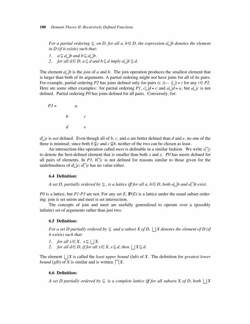
100 Domain Theory II: Recursively Defined Functions
For a partial ordering ###"" on D, for all a, b$ D, the expression a"--"b denotes the element
in D (if it exists) such that:
1. a ###"" a"--"b and b ##
#"" a"--"b.
2. for all d$ D, a ###"" d and b ##
#"" d imply a"--"b ###"" d.
The element a"--"b is the join of a and b. The join operation produces the smallest element that
is larger than both of its arguments. A partial ordering might not have joins for all of its pairs.
For example, partial ordering P2 has joins defined only for pairs (i, i)— i"--"i # i for any i$ P2.
Here are some other examples: for partial ordering P1, c"--"d# c and a"--"d# a, but a"--"c is not
defined. Partial ordering P0 has joins defined for all pairs. Conversely, for:
P3 # a
b c
d e
d"--"e is not defined. Even though all of b, c, and a are better defined than d and e, no one of the
three is minimal; since both b ###"" / c and c ##
#"" / b, neither of the two can be chosen as least.
An intersection-like operation called meet is definable in a similar fashion. We write x"--"yto denote the best-defined element that is smaller than both x and y. P0 has meets defined for
all pairs of elements. In P3, b"--"c is not defined for reasons similar to those given for the
undefinedness of d"--"e; d"--"e has no value either.
6.4 Definition:
A set D, partially ordered by ###"" , is a lattice iff for all a, b$ D, both a"--"b and a"--"b exist.
P0 is a lattice, but P1-P3 are not. For any set E, IP(E) is a lattice under the usual subset order-
ing: join is set union and meet is set intersection.
The concepts of join and meet are usefully generalized to operate over a (possibly
infinite) set of arguments rather than just two.
6.5 Definition:
For a set D partially ordered by ###"" and a subset X of D,
#X denotes the element of D (if
it exists) such that:
1. for all x$ X, x ###"" #
X.
2. for all d$ D, if for all x$ X, x ###"" d, then
#X ###"" d.
The element#
X is called the least upper bound (lub) of X. The definition for greatest lower
bound (glb) of X is similar and is written#
X.
6.6 Definition:
A set D partially ordered by ###"" is a complete lattice iff for all subsets X of D, both
#X
6.2 Partial Orderings 101
and#
X exist.
The standard example of a complete lattice is the powerset lattice IP(E). Any lattice with a
finite number of elements must be a complete lattice. Not all lattices are complete, however;
consider the set F# { x | x is a finite subset of IN } partially ordered by subset inclusion. F is
clearly a lattice, as joins and meets of finite sets yield finite sets, but F is not complete, for the
lub of the set S # { { zero }, { zero, one }, { zero, one, two }, . . . } is exactly IN, which is not
in F.
A complete lattice D must always have a bottom element, for#
D# "#. Dually,#
D
denotes an element represented by "# (top).
The definitions of lattice and complete lattice are standard ones and are included for com-
pleteness’ sake. The theory for least fixed point semantics doesn’t require domains to be lat-
tices. The only property needed from partially ordered sets is that lubs exist for those sets
representing the subfunction families. This motivates two important definitions.
6.7 Definition:
For a partially ordered set D, a subset X of D is a chain iff X is nonempty and for all
a, b$X, a ###"" b or b ##
#"" a.
A chain represents a family of elements that contain information consistent with one another.
(Recall the family of functions developed in the stages of unfolding of fac in Section 6.1.)
Chains can be finite or infinite; in partial order P1, { d, b, a } forms a chain, as does { c }, but
{ a, c } does not. The lub of a finite chain is always the largest element in the chain. This
does not hold for infinite chains: consider again the set S defined above, which is a chain in
both lattice F and complete lattice IP(IN).
Since chains abstract the consistent subfunction families, it is important to ensure that
such chains always have lubs. A lattice may not have lubs for infinite chains, so ordinary lat-
tices are not suitable. On the other hand, requiring a domain to be a complete lattice is too
strong. The compromise settled upon is called a complete partial ordering.
6.8 Definition:
1. A partially ordered set D is a complete partial ordering (cpo) iff every chain in D
has a least upper bound in D.
2. A partially ordered set D is a pointed complete partial ordering (pointed cpo) iff it is
a complete partial ordering and it has a least element.
The partial orderings P0 through P3 are cpos, but only P0 and P1 are pointed cpos. The exam-
ples suggest that the requirements for being a cpo are quite weak. The solutions for recursive
function specifications are found as elements within pointed cpos.
102 Domain Theory II: Recursively Defined Functions
6.3 CONTINUOUS FUNCTIONS !!!!!!!!!!!!!!!!!!!!!!!!!!!!!!!!!!!!!!!!!!!!!!!!!!!!!!!!!!!!!!!!!!!!!!!!!!!!!!!!!!!!!!!!!!
When the partial order relation ###"" was introduced, ##
#"" was read as ‘‘is less defined than.’’ For
functions, we judged definedness in terms of their graphs: a function f is less defined than a
function g if f’s graph is a subset of g’s. The totally undefined function ("n. "#) contains no
answer-producing information at all, and it is appropriate that its graph is the empty set and
that ("n. "#) ###"" f for all functions f. The graph representation of a function provides a way to
‘‘look inside’’ the function and judge its information content. In general, any element d of an
arbitrary domain D might be thought of as a set-like object, containing ‘‘atoms’’ of informa-
tion. Then, ###"" D can still be thought of as a subset relation, and the least upper bound operator
can still be thought of as set union.
Now consider what a function does to its arguments. A function f: A!B is a transforma-
tion agent, converting an element x$ A to some f(x)$ B. How should this be accomplished?
If x is thought of as a set of ‘‘atoms,’’ then f transforms x by mapping x’s atoms into the B
domain and recombining them there. If x ###"" A y, an application of f should produce the analo-
gous situation in B. A function f: A!B is monotonic iff for all x, y$ A, x ###"" Ay implies
f(x) ###"" Bf(y). The condition is justified by practical issues in computing: a procedure for
transforming a data structure such as an array performs the transformation by altering the
array’s subparts one at a time, combining them to form a new value. The procedure denotes a
monotonic function. Nonmonotonic functions tend to be nasty entities, often impossible to
implemement. A famous example of a nonmonotonic function is program-halts : Nat "!! IB,
program-halts(x)#falsetrue
if x# "#
if x* "#
program-halts is nonmonotonic. Consider a proper number n. It is always the case that "# ###"" n,
but it is normally not the case that program-halts( "#) ###"" program-halts(n), that is, false ##
#"" true,
as false is not less defined than true— their information contents are disjoint.
For the moment, pretend that an implementation of program-halts exists and call its
coded procedure PGM-HALTS. PGM-HALTS could see if a program P terminates with its
input A, for P represents a function in domain Nat!Nat "! , A represents a natural number, so
PGM-HALTS(P(A)) returns TRUE or FALSE based upon whether or not P halts with A. It is
easy to see how PGM-HALTS might return a TRUE value (it runs P(A) and once P(A) stops
and outputs a numeral, it returns TRUE), but how can PGM-HALTS ever tell that P(A) will
run forever (that is, be undefined) so that it can return FALSE? There is no obvious solution;
in fact, there is no solution at all— this is the famous ‘‘halting problem’’ of computability
theory: program-halts cannot be implemented on any computing machine.
We require that all the functions used in denotational semantics be monotonic. The
requirement guarantees that any family of subfunctions "#, F( "#), F(F( "#)), . . . , Fi( "#), . . .
generated by a monotonic functional F is a chain.
A condition stronger than monotonicity is needed to develop least fixed point semantics.
Just as the binary join operation was generalized to the lub operation, the monotonicity condi-
tion is generalized to continuity.
6.9 Definition:
6.4 Least Fixed Points 103
For cpos A and B, a monotonic function f: A!B is continuous iff for any chain X& A,
f(#
X)# #
{ f(x) | x$X }.
A continuous function preserves limits of chains. That is, f(#
X) contains exactly the same
information as that obtained by mapping all the x’s to f(x)’s and joining the results. The reason
that we use continuous functions is that we require the property graph(#
{ Fi()) | i % 0 }) &
i#0' (
{ graph(Fi())) | i % 0 }, which was noted in Section 6.1 in the fac example.
Continuous functions suggest a strategy for effectively processing objects of infinite size
(information content). For some infinite object Y, it may not be possible to place a representa-
tion of Y in the computer store, so f(Y) simply isn’t computable in the conventional way. But
if Y is the least upper bound of a chain { yi | i$IN } where each yi has finite size, and f is a
continuous function, then each yi can be successively stored and f applied to each. The needed
value f(Y) is built up piece by piece as f(y0) "--" f(y1) "--" f(y2) "--" . . . . Since { f(yi) | i$IN } con-
stitutes a chain and f is continuous, f(Y)# #
{ f(yi) | i$IN }. (This was the same process used
for determining the graph of the factorial function.) Of course, to completely compute the
answer will take an infinite amount of time, but it is reassuring that every piece of the answer
f(Y) will appear within a finite amount of time.
Continuity is such an important principle that virtually all of the classical areas of
mathematics utilize it in some form.
6.4 LEAST FIXED POINTS !!!!!!!!!!!!!!!!!!!!!!!!!!!!!!!!!!!!!!!!!!!!!!!!!!!!!!!!!!!!!!!!!!!!!!!!!!!!!!!!!!!!!!!!!!!!!!!!!!
A functional is a continuous function f: D!D; usually D is a domain of form A!B, but it
doesn’t have to be.
6.10 Definition:
For a functional F: D!D and an element d$ D, d is a fixed point of F iff F(d)# d.
Further, d is the least fixed point of F if, for all e$ D, F(e)# e implies d ###"" e.
6.11 Theorem:
If the domain D is a pointed cpo, then the least fixed point of a continuous functional
F: D!D exists and is defined to be fix F# #
{ Fi( "#) | i% 0 }, where
Fi # F % F % . . . % F, i times.
Proof: First, fix F is a fixed point of F, as
F(fix F)# F(#
{ Fi( "#) | i% 0 })
# #
{ F(Fi( "#) | i% 0 } by continuity of F
# #
{ Fi( "#) | i% 1 }
# #
{ Fi( "#) | i% 0 } as F0( "#)# "# and "# ###"" F( "#)
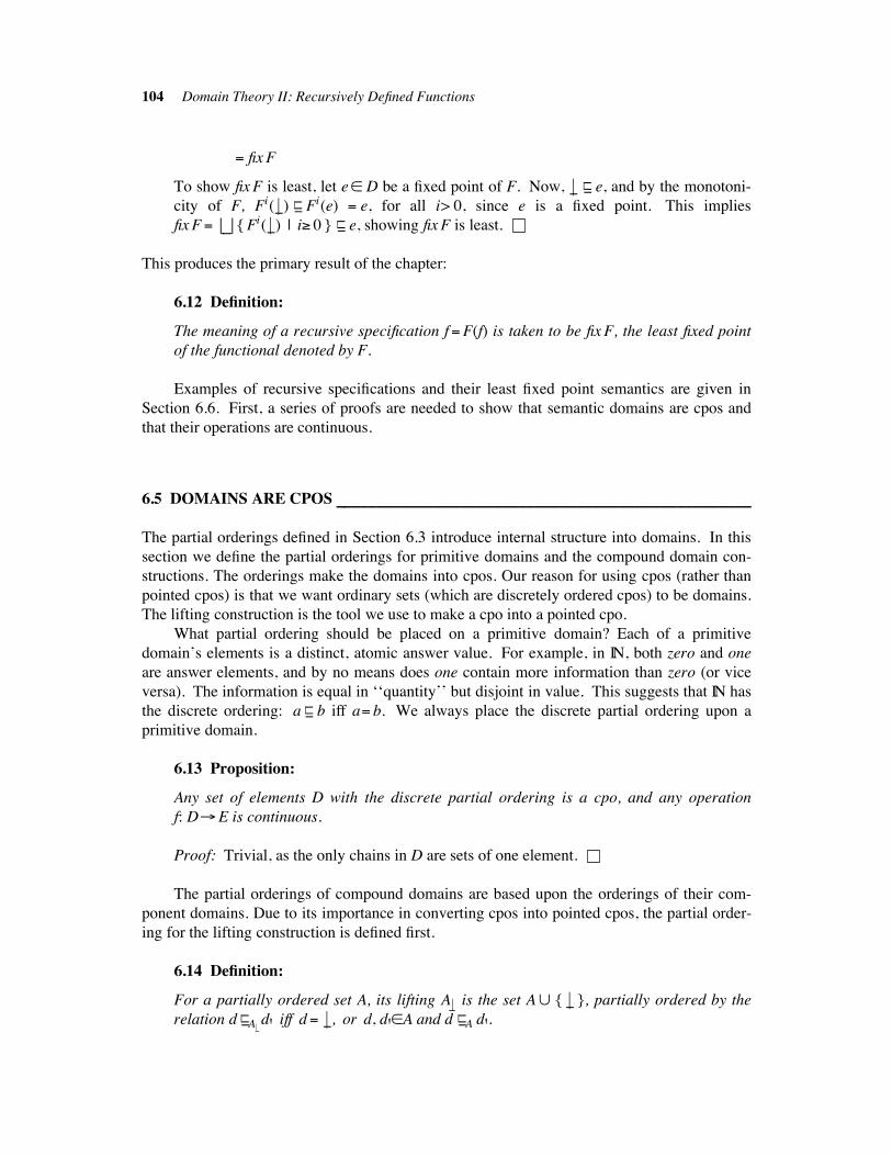
104 Domain Theory II: Recursively Defined Functions
# fix F
To show fix F is least, let e$ D be a fixed point of F. Now, "# ###"" e, and by the monotoni-
city of F, Fi( "#) ###"" Fi(e) # e, for all i> 0, since e is a fixed point. This implies
fix F# #
{ Fi( "#) | i% 0 } ###"" e, showing fix F is least.
This produces the primary result of the chapter:
6.12 Definition:
The meaning of a recursive specification f #F(f) is taken to be fix F, the least fixed point
of the functional denoted by F.
Examples of recursive specifications and their least fixed point semantics are given in
Section 6.6. First, a series of proofs are needed to show that semantic domains are cpos and
that their operations are continuous.
6.5 DOMAINS ARE CPOS !!!!!!!!!!!!!!!!!!!!!!!!!!!!!!!!!!!!!!!!!!!!!!!!!!!!!!!!!!!!!!!!!!!!!!!!!!!!!!!!!!!!!!!!!!!!!!!!!!!!
The partial orderings defined in Section 6.3 introduce internal structure into domains. In this
section we define the partial orderings for primitive domains and the compound domain con-
structions. The orderings make the domains into cpos. Our reason for using cpos (rather than
pointed cpos) is that we want ordinary sets (which are discretely ordered cpos) to be domains.
The lifting construction is the tool we use to make a cpo into a pointed cpo.
What partial ordering should be placed on a primitive domain? Each of a primitive
domain’s elements is a distinct, atomic answer value. For example, in IN, both zero and one
are answer elements, and by no means does one contain more information than zero (or vice
versa). The information is equal in ‘‘quantity’’ but disjoint in value. This suggests that IN has
the discrete ordering: a ###"" b iff a# b. We always place the discrete partial ordering upon a
primitive domain.
6.13 Proposition:
Any set of elements D with the discrete partial ordering is a cpo, and any operation
f: D!E is continuous.
Proof: Trivial, as the only chains in D are sets of one element.
The partial orderings of compound domains are based upon the orderings of their com-
ponent domains. Due to its importance in converting cpos into pointed cpos, the partial order-
ing for the lifting construction is defined first.
6.14 Definition:
For a partially ordered set A, its lifting A"! is the set A' { "# }, partially ordered by the
relation d ###"" A"!
d' iff d# "#, or d, d'$A and d ###"" A d'.
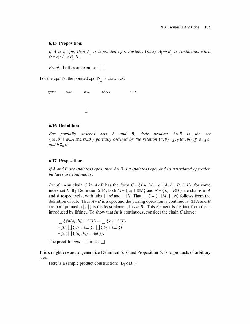
6.5 Domains Are Cpos 105
6.15 Proposition:
If A is a cpo, then A"! is a pointed cpo. Further, ("!!x.e) : A"!!B"! is continuous when
("x.e) : A!B"! is.
Proof: Left as an exercise.
For the cpo IN, the pointed cpo IN"! is drawn as:
zero one two three . . .
"#
6.16 Definition:
For partially ordered sets A and B, their product A&B is the set
{ (a, b) | a$A and b$B } partially ordered by the relation (a, b) ###"" A&B (a', b') iff a ##
#"" A a'and b ##
#"" B b'.
6.17 Proposition:
If A and B are (pointed) cpos, then A&B is a (pointed) cpo, and its associated operation
builders are continuous.
Proof: Any chain C in A&B has the form C # { (ai, bi) | ai$A, bi$B, i$I }, for some
index set I. By Definition 6.16, both M# { ai | i$I } and N # { bi | i$I } are chains in A
and B respectively, with lubs#
M and#
N. That#
C # (#
M,#
N) follows from the
definition of lub. Thus A&B is a cpo, and the pairing operation is continuous. (If A and B
are both pointed, ( "#, "#) is the least element in A&B. This element is distinct from the "#introduced by lifting.) To show that fst is continuous, consider the chain C above:
#{ fst(ai , bi) | i$I } #
#{ ai | i$I }
# fst(#
{ ai | i$I }, #
{ bi | i$I })
# fst(#
{ (ai, bi) | i$I }).
The proof for snd is similar.
It is straightforward to generalize Definition 6.16 and Proposition 6.17 to products of arbitrary
size.
Here is a sample product construction: IB "!& IB "! #
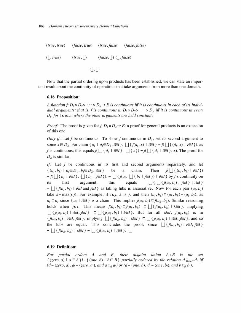
106 Domain Theory II: Recursively Defined Functions
(true, true) (false, true) (true, false) (false, false)
( "#, true) (true, "#) (false, "#) ( "#, false)
( "#, "#)
Now that the partial ordering upon products has been established, we can state an impor-
tant result about the continuity of operations that take arguments from more than one domain.
6.18 Proposition:
A function f: D1&D2& . . . &Dn!E is continuous iff it is continuous in each of its indivi-
dual arguments; that is, f is continuous in D1&D2& . . . &Dn iff it is continuous in every
Di, for 1+ i+ n, where the other arguments are held constant.
Proof: The proof is given for f: D1&D2!E; a proof for general products is an extension
of this one.
Only if: Let f be continuous. To show f continuous in D1, set its second argument to
some x$ D2. For chain { di | di$D1, i$I },#
{ f(di , x) | i$I } # f(#
{ (di, x) | i$I }), as
f is continuous; this equals f(#
{ di | i$I },#
{ x }) # f(#
{ di | i$I }, x). The proof for
D2 is similar.
If: Let f be continuous in its first and second arguments separately, and let
{ (ai, bi) | ai$D1, bi$D2, i$I } be a chain. Then f(#
{ (ai, bi) | i$I })
# f(#
{ ai | i$I },#
{ bj | j$I }), # #
{ f(ai , #{ bj | j$I }) | i$I } by f’s continuity on
its first argument; this equals#
{#
{ f(ai , bj) | j$I } | i$I }
# #
{ f(ai , bj) | i$I and j$I } as taking lubs is associative. Now for each pair (ai, bj)
take k# max(i, j). For example, if i+ j, k is j, and then (ai, bj) ###"" (ak, bk)# (aj , bj), as
ai ###"" aj since { ai | i$I } is a chain. This implies f(ai , bj) ##
#"" f(ak , bk). Similar reasoning
holds when j+ i. This means f(ai , bj) ###"" f(ak , bk) ##
#"" #
{ f(ak , bk) | k$I }, implying
#{ f(ai , bj) | i$I, j$I } ##
#"" #
{ f(ak , bk) | k$I }. But for all k$I, f(ak , bk) is in
{ f(ai , bj) | i$I, j$I }, implying#
{ f(ak , bk) | k$I } ###"" #
{ f(ai , bj) | i$I, j$I }, and so
the lubs are equal. This concludes the proof, since#
{ f(ai , bj) | i$I, j$I }
# #
{ f(ak , bk) | k$I } # #
{ f(ai , bi) | i$I }.
6.19 Definition:
For partial orders A and B, their disjoint union A$B is the set
{ (zero, a) | a$ A }' { (one, b) | b$ B } partially ordered by the relation d ###"" A$B d' iff
(d# (zero, a), d'# (zero, a'), and a ###"" A a') or (d# (one, b), d'# (one, b'), and b ##
#"" B b').
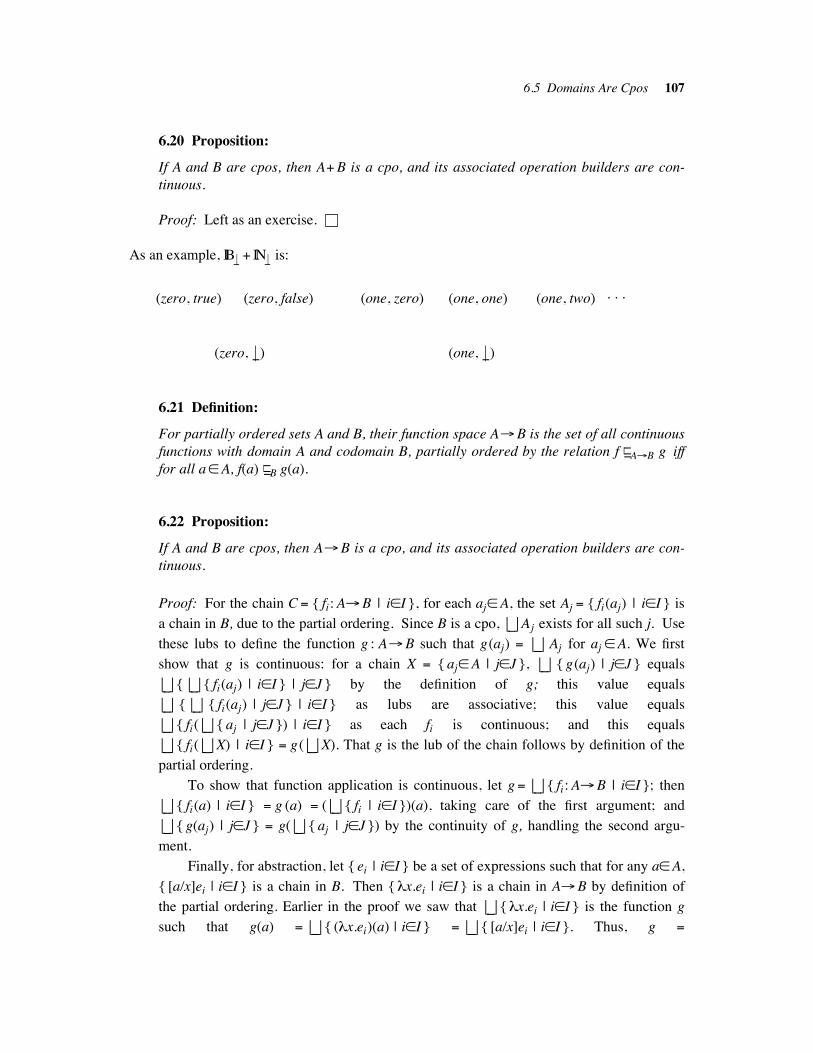
6.5 Domains Are Cpos 107
6.20 Proposition:
If A and B are cpos, then A$B is a cpo, and its associated operation builders are con-
tinuous.
Proof: Left as an exercise.
As an example, IB "! $ IN"! is:
(zero, true) (zero, false) (one, zero) (one, one) (one, two) . . .
(zero, "#) (one, "#)
6.21 Definition:
For partially ordered sets A and B, their function space A!B is the set of all continuous
functions with domain A and codomain B, partially ordered by the relation f ###"" A!B g iff
for all a$A, f(a) ###"" B g(a).
6.22 Proposition:
If A and B are cpos, then A!B is a cpo, and its associated operation builders are con-
tinuous.
Proof: For the chain C # { fi : A!B | i$I }, for each aj$A, the set Aj # { fi(aj) | i$I } is
a chain in B, due to the partial ordering. Since B is a cpo,#
Aj exists for all such j. Use
these lubs to define the function g : A!B such that g(aj) # #Aj for aj $A. We first
show that g is continuous: for a chain X # { aj$A | j$J },#
{ g(aj) | j$J } equals
#{#
{ fi(aj) | i$I } | j$J } by the definition of g; this value equals
#{#
{ fi(aj) | j$J } | i$I } as lubs are associative; this value equals
#{ fi( #
{ aj | j$J }) | i$I } as each fi is continuous; and this equals
#{ fi( #
X) | i$I } # g(#
X). That g is the lub of the chain follows by definition of the
partial ordering.
To show that function application is continuous, let g# #
{ fi : A!B | i$I }; then
#{ fi(a) | i$I } # g (a) # (
#{ fi | i$I })(a), taking care of the first argument; and
#{ g(aj) | j$J } # g(
#{ aj | j$J }) by the continuity of g, handling the second argu-
ment.
Finally, for abstraction, let { ei | i$I } be a set of expressions such that for any a$A,
{ [a/x]ei | i$I } is a chain in B. Then { "x.ei | i$I } is a chain in A!B by definition of
the partial ordering. Earlier in the proof we saw that#
{ "x.ei | i$I } is the function g
such that g(a) # #
{ ("x.ei)(a) | i$I } # #
{ [a/x]ei | i$I }. Thus, g #
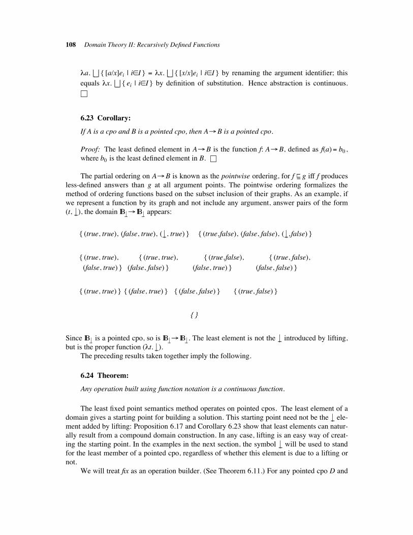
108 Domain Theory II: Recursively Defined Functions
"a.#
{ [a/x]ei | i$I } # "x.#
{ [x/x]ei | i$I } by renaming the argument identifier; this
equals "x.#
{ ei | i$I } by definition of substitution. Hence abstraction is continuous.
6.23 Corollary:
If A is a cpo and B is a pointed cpo, then A!B is a pointed cpo.
Proof: The least defined element in A!B is the function f: A!B, defined as f(a)# b0 ,
where b0 is the least defined element in B.
The partial ordering on A!B is known as the pointwise ordering, for f ###"" g iff f produces
less-defined answers than g at all argument points. The pointwise ordering formalizes the
method of ordering functions based on the subset inclusion of their graphs. As an example, if
we represent a function by its graph and not include any argument, answer pairs of the form
(t, "#), the domain IB "!! IB "! appears:
{ (true, true), (false, true), ( "#, true) } { (true,false), (false, false), ( "#, false) }
{ (true, true), { (true, true), { (true,false), { (true, false),
(false, true) } (false, false) } (false, true) } (false, false) }
{ (true, true) } { (false, true) } { (false, false) } { (true, false) }
{ }
Since IB "! is a pointed cpo, so is IB "!! IB "! . The least element is not the "# introduced by lifting,
but is the proper function ("t. "#).
The preceding results taken together imply the following.
6.24 Theorem:
Any operation built using function notation is a continuous function.
The least fixed point semantics method operates on pointed cpos. The least element of a
domain gives a starting point for building a solution. This starting point need not be the "# ele-
ment added by lifting: Proposition 6.17 and Corollary 6.23 show that least elements can natur-
ally result from a compound domain construction. In any case, lifting is an easy way of creat-
ing the starting point. In the examples in the next section, the symbol "# will be used to stand
for the least member of a pointed cpo, regardless of whether this element is due to a lifting or
not.
We will treat fix as an operation builder. (See Theorem 6.11.) For any pointed cpo D and
6.5 Domains Are Cpos 109
continuous function F:D!D, fix F denotes the lub of the chain induced from F. From here
on, any recursive specification f #F(f) is taken as an abbreviation for f # fix F.
Since it is important to know if a cpo is pointed, the following rules are handy:
ispointed(P)# false, where P is a primitive domain
ispointed (A&B)# ispointed (A) and ispointed (B)
ispointed (A$B)# false
ispointed (A!B)# ispointed (B)
ispointed(A"!)# true
6.6 EXAMPLES !!!!!!!!!!!!!!!!!!!!!!!!!!!!!!!!!!!!!!!!!!!!!!!!!!!!!!!!!!!!!!!!!!!!!!!!!!!!!!!!!!!!!!!!!!!!!!!!!!!!!!!!!!!!!!!!!!!!!!
Now that the theory is developed, we present a number of old and new recursive function
specifications and determine their least fixed point semantics.
6.6.1 Factorial Function !!!!!!!!!!!!!!!!!!!!!!!!!!!!!!!!!!!!!!!!!!!!!!!!!!!!!!!!!!!!!!!!!!!!!!!!!!!!!!!!!!!!!!!!!!!!!!!!!!!!!!!!!!
We examine the factorial function and its specification once more. Recall that
fac : Nat!Nat "! is defined as:
fac# "n. n equals zero! one[] n times fac(n minus one)
which is an acceptable definition, since Nat "! is a pointed cpo, implying that Nat!Nat "! is also.
(Here is one small, technical point: the specification should actually read:
fac# "n. n equals zero! one [] (let n'# fac(n minus one) in n times n')
because times uses arguments from Nat and not from Nat "! . We gloss over this point and say
that times is strict on Nat "! arguments.) The induced functional
F : (Nat!Nat "!)! (Nat!Nat "!) is:
F# "f."n. n equals zero! one[] n times f(n minus one)
The least fixed point semantics of fac is fix F# #
{ faci | i% 0 }, where:
fac0 # ("n. "#) # "#$Nat!Nat "!
faci$1 # F (faci) for i% 0
These facts have been mentioned before. What we examine now is the relationship between
fix F and the operational evaluation of fac. First, the fixed point property says that
fix F# F(fix F). This identity is a useful simplification rule. Consider the denotation of the
phrase (fix F)(three). Why does this expression stand for six? We use equals-for-equals substi-
tution to simplify the original form:
110 Domain Theory II: Recursively Defined Functions
(fix F)(three)
# (F (fix F))(three), by the fixed point property
# (("f."n. n equals zero! one[] n times f(n minus one))(fix F))(three)
# ("n. n equals zero! one[] n times (fix F)(n minus one))(three)
We see that the fixed point property justifies the recursive unfolding rule that was informally
used in Section 6.1.
Rather than expanding (fix F) further, we bind three to n:
# three equals zero! one[] three times (fix F)(three minus one)
# three times (fix F)(two)
# three times (F(fix F))(two)
# three times (("f."n. n equals zero! one[] n times f(n minus one))(fix F))(two)
# three times ("n.n equals zero! one[] n times (fix F)(n minus one))(two)
The expression (fix F) can be expanded at will:
# three times (two times (fix F)(one)) . . .
# three times (two times (one times (fix F)(zero))) . . .
# six
6.6.2 Copyout Function !!!!!!!!!!!!!!!!!!!!!!!!!!!!!!!!!!!!!!!!!!!!!!!!!!!!!!!!!!!!!!!!!!!!!!!!!!!!!!!!!!!!!!!!!!!!!!!!!!!!!!!!!!
The interactive text editor in Figure 5.3 utilized a function called copyout for converting an
internal representation of a file into an external form. The function’s definition was not
specified because it used recursion. Now we can alleviate the omission. The domains
File# Record, and Openfile # Record, &Record, were used. Function copyout converts an
open file into a file by appending the two record lists. A specification of copyout:
Openfile!File"! is:
copyout # "(front, back). null front! back
[] copyout((tl front), ((hd front) cons back))
It is easy to construct the appropriate functional F; copyout has the meaning (fix F). You
should prove that the function Fi( "#) is capable of appending list pairs whose first component
has length i # 1 or less. This implies that the lub of the Fi( "#) functions, (fix F), is capable of
concatenating all pairs of lists whose first component has finite length.
Here is one more remark about copyout: its codomain was stated above as File"! , rather
than just File, as originally given in Figure 5.3. The new codomain was used because least
fixed point semantics requires that the codomain of any recursively defined function be
pointed. If we desire a recursive version of copyout that uses File as its codomain, we must
6.6.2 Copyout Function 111
apply the results of Exercise 14 of Chapter 3 and use a primitive recursive-like definition. This
is left as an important exercise. After you have studied all of the examples in this chapter, you
should determine which of them can be handled without least fixed point semantics by using
primitive recursion. The moral is that least fixed point semantics is a powerful and useful tool,
but in many cases we can deal quite nicely without it.
6.6.3 Double Recursion !!!!!!!!!!!!!!!!!!!!!!!!!!!!!!!!!!!!!!!!!!!!!!!!!!!!!!!!!!!!!!!!!!!!!!!!!!!!!!!!!!!!!!!!!!!!!!!!!!!!!!!!!!!!
Least fixed point semantics is helpful for understanding recursive specifications that may be
difficult to read. Consider this specification for g : Nat!Nat "!:
g# "n. n equals zero! one[] (g(n minus one) plus g(n minus one)) minus one
The appropriate functional F should be obvious. We gain insight by constructing the graphs
for the first few steps of the chain construction:
graph(F0( "#))# { }
graph(F1( "#))# { (zero, one) }
graph(F2( "#))# { (zero, one), (one, one) }
graph(F3( "#))# { (zero, one), (one, one), (two, one) }
You should be able to construct these graphs yourself and verify the results. For all i% 0,
graph(Fi$1( "#))# { (zero, one), (one, one), . . . , (i, one) }, implying (fix F) # "n. one. The
recursive specification disguised a very simple function.
6.6.4 Simultaneous Definitions !!!!!!!!!!!!!!!!!!!!!!!!!!!!!!!!!!!!!!!!!!!!!!!!!!!!!!!!!!!!!!!!!!!!!!!!!!!!!!!!!!!!!!!!!!!!!!!!
Some recursive specifications are presented as a collection of mutually recursive
specifications. Here is a simple example of an f: Nat!Nat "! and a g : Nat!Nat "! such that
each function depends on the other to produce an answer:
f # "x. x equals zero! g(zero) [] f(g(x minus one)) plus two
g# "y. y equals zero! zero[] y times f(y minus one)
Identifier g is free in f’s specification and f is free in g’s. Attempting to solve f’s or g’s
circularity separately creates a problem, for there is no guarantee that f is defined without a
well-defined function for g, and no function for g can be produced without a function for f.
This suggests that the least fixed points for f and g be formed simultaneously. We build a
functional over pairs:
F: ((Nat!Nat "!)& (Nat!Nat "!))! ((Nat!Nat "!)& (Nat!Nat "!)),
F# "(f,g). ( "x. x equals zero! g(zero) [] f(g(x minus one)) plus two,
"y. y equals zero! zero[] y times f(y minus one) )
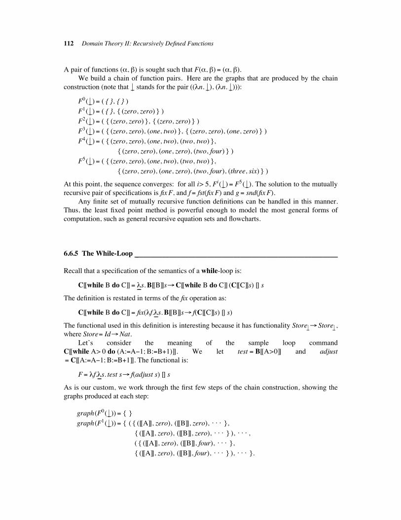
112 Domain Theory II: Recursively Defined Functions
A pair of functions (-, .) is sought such that F(-, .)# (-, .).
We build a chain of function pairs. Here are the graphs that are produced by the chain
construction (note that "# stands for the pair (("n. "#), ("n. "#))):
F0( "#)# ( { }, { } )
F1( "#)# ( { }, { (zero, zero) } )
F2( "#)# ( { (zero, zero) }, { (zero, zero) } )
F3( "#)# ( { (zero, zero), (one, two) }, { (zero, zero), (one, zero) } )
F4( "#)# ( { (zero, zero), (one, two), (two, two) },
{ (zero, zero), (one, zero), (two, four) } )
F5( "#)# ( { (zero, zero), (one, two), (two, two) },
{ (zero, zero), (one, zero), (two, four), (three, six) } )
At this point, the sequence converges: for all i> 5, Fi( "#)# F5( "#). The solution to the mutually
recursive pair of specifications is fix F, and f # fst(fix F) and g# snd(fix F).
Any finite set of mutually recursive function definitions can be handled in this manner.
Thus, the least fixed point method is powerful enough to model the most general forms of
computation, such as general recursive equation sets and flowcharts.
6.6.5 The While-Loop !!!!!!!!!!!!!!!!!!!!!!!!!!!!!!!!!!!!!!!!!!!!!!!!!!!!!!!!!!!!!!!!!!!!!!!!!!!!!!!!!!!!!!!!!!!!!!!!!!!!!!!!!!!!!!
Recall that a specification of the semantics of a while-loop is:
C[[while B do C]]# "!!s. B[[B]]s!C[[while B do C]] (C[[C]]s) [] s
The definition is restated in terms of the fix operation as:
C[[while B do C]]# fix("f."!!s. B[[B]]s! f(C[[C]]s) [] s)
The functional used in this definition is interesting because it has functionality Store"!! Store"! ,
where Store# Id!Nat.
Let’s consider the meaning of the sample loop command
C[[while A> 0 do (A:#A#1; B:#B$1)]]. We let test # B[[A>0]] and adjust
# C[[A:#A#1; B:#B$1]]. The functional is:
F# "f."!!s. test s! f(adjust s) [] s
As is our custom, we work through the first few steps of the chain construction, showing the
graphs produced at each step:
graph(F0( "#))# { }
graph(F1( "#))# { ( { ([[A]], zero), ([[B]], zero), . . . },
{ ([[A]], zero), ([[B]], zero), . . . } ), . . . ,
( { ([[A]], zero), ([[B]], four), . . . },
{ ([[A]], zero), ([[B]], four), . . . } ), . . . }.
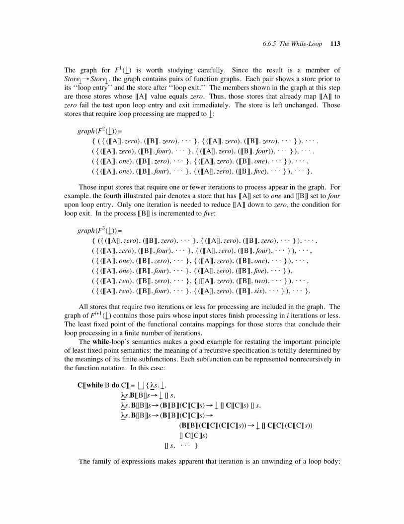
6.6.5 The While-Loop 113
The graph for F1( "#) is worth studying carefully. Since the result is a member of
Store "!! Store"! , the graph contains pairs of function graphs. Each pair shows a store prior to
its ‘‘loop entry’’ and the store after ‘‘loop exit.’’ The members shown in the graph at this step
are those stores whose [[A]] value equals zero. Thus, those stores that already map [[A]] to
zero fail the test upon loop entry and exit immediately. The store is left unchanged. Those
stores that require loop processing are mapped to "#:
graph(F2( "#))#
{ ( { ([[A]], zero), ([[B]], zero), . . . }, { ([[A]], zero), ([[B]], zero), . . . } ), . . . ,
( { ([[A]], zero), ([[B]], four), . . . }, { ([[A]], zero), ([[B]], four)), . . . } ), . . . ,
( { ([[A]], one), ([[B]], zero), . . . }, { ([[A]], zero), ([[B]], one), . . . } ), . . . ,
( { ([[A]], one), ([[B]], four), . . . }, { ([[A]], zero), ([[B]], five), . . . } ), . . . }.
Those input stores that require one or fewer iterations to process appear in the graph. For
example, the fourth illustrated pair denotes a store that has [[A]] set to one and [[B]] set to four
upon loop entry. Only one iteration is needed to reduce [[A]] down to zero, the condition for
loop exit. In the process [[B]] is incremented to five:
graph(F3( "#))#
{ ({ ([[A]], zero), ([[B]], zero), . . . }, { ([[A]], zero), ([[B]], zero), . . . } ), . . . ,
( { ([[A]], zero), ([[B]], four), . . . }, { ([[A]], zero), ([[B]], four), . . . } ), . . . ,
( { ([[A]], one), ([[B]], zero), . . . }, { ([[A]], zero), ([[B]], one), . . . } ), . . . ,
( { ([[A]], one), ([[B]], four), . . . }, { ([[A]], zero), ([[B]], five), . . . } ),
( { ([[A]], two), ([[B]], zero), . . . }, { ([[A]], zero), ([[B]], two), . . . } ), . . . ,
( { ([[A]], two), ([[B]], four), . . . }, { ([[A]], zero), ([[B]], six), . . . } ), . . . }.
All stores that require two iterations or less for processing are included in the graph. The
graph of Fi$1( "#) contains those pairs whose input stores finish processing in i iterations or less.
The least fixed point of the functional contains mappings for those stores that conclude their
loop processing in a finite number of iterations.
The while-loop’s semantics makes a good example for restating the important principle
of least fixed point semantics: the meaning of a recursive specification is totally determined by
the meanings of its finite subfunctions. Each subfunction can be represented nonrecursively in
the function notation. In this case:
C[[while B do C]]##
{ "!!s. "#,
"!!s.B[[B]]s! "# [] s,
"!!s. B[[B]]s! (B[[B]](C[[C]]s)! "# [] C[[C]]s) [] s,
"!!s. B[[B]]s! (B[[B]](C[[C]]s)!
(B[[B]](C[[C]](C[[C]]s))! "# [] C[[C]](C[[C]]s))
[] C[[C]]s)
[] s, . . . }
The family of expressions makes apparent that iteration is an unwinding of a loop body;
114 Domain Theory II: Recursively Defined Functions
this corresponds to the operational view. Can we restate this idea even more directly? Recall
that C[[diverge]]# "!!s. "#. Substituting the commands into the set just constructed gives us:
C[[while B do C]]##
{ C[[diverge]],
C[[if B then diverge else skip]],
C[[if B then (C; if B then diverge else skip) else skip]],
C[[if B then (C; if B then
(C; if B then diverge else skip)
else skip) else skip]], . . . }
A family of finite noniterative programs represents the loop. It is easier to see what is happen-
ing by drawing the abstract syntax trees:
diverge if if if
B diverge skip B ; skip B ; skip . . .
C if C if
B diverge skip B ; skip
C if
B diverge skip
At each stage, the finite tree becomes larger and better defined. The obvious thing to do is to
place a partial ordering upon the trees: for all commands C, diverge ###"" C, and for commands
C1 and C2, C1 ###"" C2 iff C1 and C2 are the same command type (have the same root node) and
all subtrees in C1 are less defined than the corresponding trees in C2. This makes families of
trees like the one above into chains. What is the lub of such a chain? It is the infinite tree
corresponding to:
if B then (C; if B then (C; if B then (C; . . . ) else skip) else skip) else skip
Draw this tree, and define L # if B then (C; L) else skip. The while-loop example has led
researchers to study languages that contain infinite programs that are represented by recursive
definitions, such as L. The goal of such studies is to determine the semantics of recursive and
iterative constructs by studying their circularity at the syntax level. The fundamental discovery
of this research is that, whether the recursion is handled at the syntax level or at the semantics
level, the result is the same: C[[while B do C]]# C[[L]]. An introduction to this approach is
found in Guessarian (1981). We stay with resolving circularity in the semantics, due to our
large investment in the existing forms of abstract syntax, structural induction, and least fixed
point semantics. Finally, the infinite tree L is abbreviated:
6.6.5 The While-Loop 115
if or
B
B ; skip
C C
Every flowchart loop can be read as an abbreviation for an infinite program. This brings us
back to representations of functions again, for the use of finite loops to represent infinite
flowcharts parallels the use of finite function expressions to denote infinite objects— func-
tions. The central issue of computability theory might be stated as the search for finite
representations of infinite objects.
6.6.6 Soundness of Hoare’s Logic !!!!!!!!!!!!!!!!!!!!!!!!!!!!!!!!!!!!!!!!!!!!!!!!!!!!!!!!!!!!!!!!!!!!!!!!!!!!!!!!!!!!!!!!!!
The facts that we uncovered in the previous example come to good use in a proof of soundness
of Hoare’s logic for a while-loop language. Hoare’s logic is an axiomatic semantics, where
axioms and inference rules specify the behavior of language constructs. In Hoare’s logic, a
behavioral property of a command [[C]] is expressed as a proposition P{C}Q. P and Q are
Boolean expressions describing properties of the program variables used in [[C]]. Informally
interpreted, the proposition says ‘‘if P holds true prior to the evaluation of C and if C ter-
minates, then Q holds true after the evaluation of C.’’ A formal interpretation of the proposi-
tion using denotational semantics is: ‘‘P{C}Q is valid iff for all s$ Store, B[[P]]s# true and
C[[C]]s* "# imply B[[Q]](C[[C]]s)# true.’’
Figure 6.1 presents Hoare’s logic for commands in Figure 5.2 augmented by the while-
loop. Lack of space prevents us from specifying some example prop-ositions and performing
their verification. But we will show that the axiom and rules in the figure are sound; that is, if
the antecedent propositions to a rule are valid, then the consequent of the rule is also valid.
The significance of the soundness proof is that the axiom and rules are more than empty
definitions— they are theorems with respect to the language’s denotational semantics. Thus,
the axiomatic definition is complementary to the denotational one in the sense described in the
Introduction.
Here is the proof of soundness:
1. Axiom a: For arbitrary Boolean expressions P and Q, identifier [[x]], and expression [[E]],
we must show that B[[[E/x]P]]s# true and C[[x:#E]]s* "# imply that B[[P]][[[x]]""!E[[E]]s]s
# true. But this claim was proved in Exercise 5 of Chapter 5.
2. Rule b: We assume each of the three antecedents of the rule to be valid. To show the con-
sequent, we are allowed to assume B[[P]]s # true and C[[C1;C2]]s * "#; we must prove that
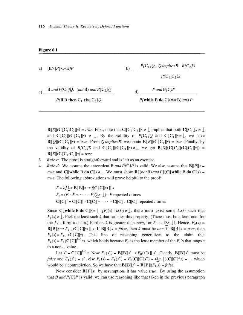
116 Domain Theory II: Recursively Defined Functions
Figure 6.1____________________________________________________________________________________________________________________________________________________
P{C1}Q, Q implies R, R{C2}Sa) [E/x]P{x:#E}P b) __________________________
P{C1;C2}S
B and P{C1}Q, (not B) and P{C2}Q P and B{C}Pc) ________________________________ d) __________________________
P{if B then C1 else C2}Q P{while B do C}(not B) and P
____________________________________________________________________________
B[[S]](C[[C1;C2]]s) # true. First, note that C[[C1;C2]]s * "# implies that both C[[C1]]s * "#and C[[C2]](C[[C1]]s) * "#. By the validity of P{C1}Q and C[[C1]]s* "#, we have
B[[Q]](C[[C1]]s) # true. From Q implies R, we obtain B[[R]](C[[C1]]s) # true. Finally, by
the validity of R{C2}S and C[[C2]](C[[C1]]s)* "#, we get B[[S]](C[[C2]](C[[C1]]s)) #
B[[S]](C[[C1;C2]]s) # true.
3. Rule c: The proof is straightforward and is left as an exercise.
4. Rule d: We assume the antecedent B and P{C}P is valid. We also assume that B[[P]]s #
true and C[[while B do C]]s* "#. We must show B[[(not B) and P]](C[[while B do C]]s) #
true. The following abbreviations will prove helpful to the proof:
F# "f."!!s. B[[B]]s! f(C[[C]]s) [] s
Fi # (F % F % . . . % F)("!!s. "#), F repeated i times
C[[C]]i # C[[C]] % C[[C]] % . . . % C[[C]], C[[C]] repeated i times
Since C[[while B do C]]s# #
{Fi(s) | i% 0}* "#, there must exist some k% 0 such that
Fk(s)* "#. Pick the least such k that satisfies this property. (There must be a least one, for
the Fi’s form a chain.) Further, k is greater than zero, for F0 is ("!!s. "#). Hence, Fk(s) #
B[[B]]s!Fk#1(C[[C]]s) [] s. If B[[B]]s # false, then k must be one; if B[[B]]s # true, then
Fk(s)#Fk#1(C[[C]]s). This line of reasoning generalizes to the claim that
Fk(s)#F1(C[[C]]k#1s), which holds because Fk is the least member of the Fi’s that maps s
to a non- "# value.
Let s, # C[[C]]k#1s. Now F1(s,) # B[[B]]s, !F0(s,) [] s, . Clearly, B[[B]]s, must be
false and F1(s,) # s, , else Fk(s) # F1(s,) # F0(C[[C]]s,) # ("!!s. "#)(C[[C]]ks) # "#, which
would be a contradiction. So we have that B[[B]]s, # B[[B]](Fk s) # false.
Now consider B[[P]]s: by assumption, it has value true. By using the assumption
that B and P{C}P is valid, we can use reasoning like that taken in the previous paragraph
6.6.6 Soundness of Hoare Logic 117
to prove for 0+ i + k that B[[P]](C[[C]]i s) # true. Hence, B[[(not B) and P]]s, #
B[[(not B) and P]](Fk s) # true.
Now we complete the proof. We know that Fk ###"" fix F # C[[while B do C]]. Hence,
Fk(s) ###"" C[[while B do C]]s, and true # B[[(not B) and P]](Fk s) ##
#""
B[[(not B) and P]](C[[while B do C]]s) by the monotonicity of B[[(not B) and P]]. But this
implies that B[[(not B) and P]](C[[while B do C]]s) # true, because IB is discretely ordered.
6.7 REASONING ABOUT LEAST FIXED POINTS !!!!!!!!!!!!!!!!!!!!!!!!!!!!!!!!!!!!!!!!!!!!!!!!!!!!!!!!!!!!
We use mathematical induction to reason about numbers and structural induction to reason
about derivation trees. An induction principle is useful for reasoning about recursively
specified functions. Since the meaning of a recursively specified function is the limit of the
meanings of its finite subfunctions, the fixed point induction principle proves a property about
a recursively defined function by proving it for its finite subfunctions: if all the subfunctions
have the property, then the least fixed point must have it as well.
We begin by formalizing the notion of ‘‘property’’ as an inclusive predicate. A predicate
P is a (not necessarily continuous) function from a domain D to IB.
6.25 Definition:
A predicate P: D! IB is inclusive iff for every chain C&D, if P(c)# true for every c$C,
then P(#
C)# true also.
We only work with inclusive predicates.
Say that for a recursively defined function f: A!B, f # F(f), we wish to show that P(f)
holds true. If P is an inclusive predicate, then we can use the fact that f # fix F as follows:
1. Show that P( "#) holds, for "#$ A!B.
2. Assuming for arbitrary i% 0, that P(Fi( "#)) holds, show that P(Fi$1( "#)) holds.
Mathematical induction guarantees that for all n% 0, P(Fn( "#)) holds. Since P is inclusive, we
have that P(fix F) holds.
A more elegant form of this reasoning is fixed point induction.
6.26 Definition:
The fixed point induction principle: For a pointed cpo D, a continuous functional
F: D!D, and an inclusive predicate P: D! IB, if:
1. P( "#) holds.
2. For arbitrary d$ D, when P(d) holds, then P(F(d)) holds.
then P(fix F) holds as well.
The proof of the validity of the fixed point induction principle is left as an exercise.
Fixed point induction helps us to show that the g function defined in the example of Sec-
tion 6.6.3 is indeed the constant function that maps its arguments to one.
118 Domain Theory II: Recursively Defined Functions
6.27 Proposition:
For all n$ Nat, g(n)* "# implies g(n)# one.
Proof: We use fixed point induction on the predicate P(f) # ‘‘for all n$ Nat, f(n)* "#implies f(n)# one. ’’ For the basis step, we must show that P("m. "#) holds. For an arbi-
trary n$Nat, ("m. "#)(n)# "#, so the claim is vacuously satisfied. For the inductive step,
we assume the inductive hypothesis P(f) and show P(F(f)). For an arbitrary n$ Nat, we
must consider the following two cases to determine the value of F(f)(n):
1. n equals zero: then F(f)(n)# one, and this satisfies the claim.
2. n is greater than zero: then F(f)(n) # (f(n minus one) plus f(n minus one)) minus one.
Consider the value of f(n minus one):
a. If it is "#, then since plus and minus are strict, F(f)(n)# "#, and the claim is vacu-
ously satisifed.
b. If it is non- "#, then by the inductive hypothesis f(n minus one)# one, and simple
arithmetic shows that F(f)(n)# one.
How do we know that the predicate we just used is inclusive? It is difficult to see how
the logical connectives ‘‘for all,’’ ‘‘implies,’’ ‘‘and,’’ ‘‘*,’’ etc., all fit together to make an
inclusive predicate. The following criterion is helpful.
6.28 Proposition:
(Manna, Ness, & Vuillemin, 1972) Let f be a recursively defined function that we wish to
reason about. A logical assertion P is an inclusive predicate if P has the form:
for all d1$D1, . . . , dm$Dm , ANDn
j#1 (OR
p
k#1 Qjk)
for m% 0, n% 0, p% 0, where Qjk can be either:
1. A predicate using only d1, . . . , dm as free identifiers.
2. An expression of form E1 ###"" E2 , where E1 and E2 are function expressions using only
f, d1, . . . , dm as free identifiers.
So an inclusive predicate can be a universally quantified conjunction of disjunctions. Here is
an example: ‘‘for all n$Nat, ( "# ###"" f(n)) and (n equals one or f(n) ##
#"" zero).’’ By using the fol-
lowing logical equivalences (among others) we can show that a large variety of predicates are
inclusive:
(E1 ###"" E2) and (E2 ##
#"" E1) iff (E1 #E2)
(P1 implies P2) iff ((not P1) or P2)
(not(not P1)) iff P1
(P1 or (P2 and P3)) iff ((P1 or P2) and (P1 or P3))
For example, the predicate used in the proof of Proposition 6.27 is inclusive because we can
use the logical equivalences just mentioned to place the predicate in the form specified in Pro-
position 6.28. The proof of Proposition 6.27 was conducted with the predicate in its original
6.7 Reasoning about Least Fixed Points 119
form, but it’s important to verify that the predicate is convertible to an inclusive one.
Fixed point induction is primarily useful for showing equivalences of program constructs.
Here is one example: we define the semantics of a repeat-loop to be:
C[[repeat C until B]]# fix("f."!!s. let s' # C[[C]]s in B[[B]]s'! s' [] (f s'))
6.29 Proposition:
For any command [[C]] and Boolean expression [[B]], C[[C; while'B do C]]
# C[[repeat C until B]].
Proof: The fixed point induction must be performed over the two recursive definitions
simultaneously. The predicate we use is:
P(f, g)# ‘‘for all s$ Store "! , f(C[[C]]s)# (g s)’’
For the basis step, we must show that P(("s. "#), ("s. "#)) holds, but this is obvious. For the
inductive step, the inductive hypothesis is P(f, g), and we must show that P(F(f), G(g))
holds, where:
F# ("f."!!s. B[['B]]s! f(C[[C]]s) [] s)
G# ("f."!!s. let s' # C[[C]]s in B[[B]]s'! s'[] (f s'))
For an arbitrary s$ Store "! , if s# "#, then F(f)(C[[C]] "#) # "# # G(g)( "#), because C[[C]], F(f),
and G(g) are all strict. (The fact that C[[C]] is strict for any C$Command requires a
small, separate proof and is left as an exercise.) On the other hand, if s* "#, then consider
the value of C[[C]]s. If it is "#, then again F(f)( "#) # "# # (let s' # "# in B[[B]]s'! s' [] (g s')))# G(g)( "#). So say that C[[C]]s is some defined store s0. We have that:
F(f)(s0)# B[['B]]s0 ! f(C[[C]]s0) [] s0 # B[[B]]s0 ! s0 [] f(C[[C]]s0)
and
G(g)(s)# B[[B]]s0 ! s0 [] (g s0)
By the inductive hypothesis, it follows that f(C[[C]]s0)# (g s0). This implies that
F(f)(s0)# G(g)(s), which completes the proof.
SUGGESTED READINGS !!!!!!!!!!!!!!!!!!!!!!!!!!!!!!!!!!!!!!!!!!!!!!!!!!!!!!!!!!!!!!!!!!!!!!!!!!!!!!!!!!!!!!!!!!!!!!!!!!!!!!
Least fixed points: Bird 1976; Guessarian 1981; Kleene, 1952; Park 1969; Manna 1974;
Manna, Ness, & Vuillemin 1972; Manna & Vuillemin 1972; Rogers 1967
Complete partial orderings: Birkhoff 1967; Gierz, et al. 1980; Kamimura & Tang 1983,
1984a; Milner 1976; Plotkin 1982; Reynolds 1977; Scott 1976, 1980a, 1982a; Wads-
worth 1978
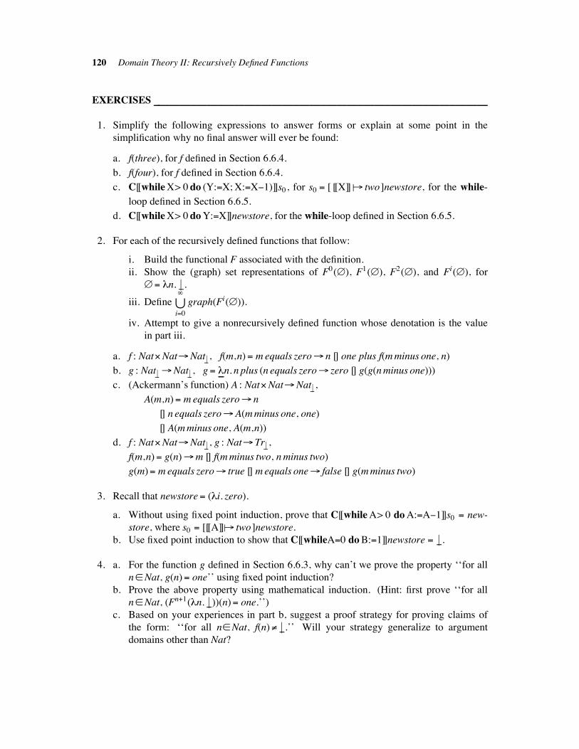
120 Domain Theory II: Recursively Defined Functions
EXERCISES !!!!!!!!!!!!!!!!!!!!!!!!!!!!!!!!!!!!!!!!!!!!!!!!!!!!!!!!!!!!!!!!!!!!!!!!!!!!!!!!!!!!!!!!!!!!!!!!!!!!!!!!!!!!!!!!!!!!!!!!!!!!
1. Simplify the following expressions to answer forms or explain at some point in the
simplification why no final answer will ever be found:
a. f(three), for f defined in Section 6.6.4.
b. f(four), for f defined in Section 6.6.4.
c. C[[while X> 0 do (Y:#X; X:#X#1)]]s0, for s0 # [ [[X]] ""! two]newstore, for the while-
loop defined in Section 6.6.5.
d. C[[while X> 0 do Y:#X]]newstore, for the while-loop defined in Section 6.6.5.
2. For each of the recursively defined functions that follow:
i. Build the functional F associated with the definition.
ii. Show the (graph) set representations of F0()), F1()), F2()), and Fi()), for
)# "n. "#.
iii. Definei#0'(
graph(Fi())).
iv. Attempt to give a nonrecursively defined function whose denotation is the value
in part iii.
a. f : Nat&Nat!Nat "! , f(m,n)# m equals zero! n [] one plus f(m minus one, n)
b. g : Nat "!!Nat "! , g # "!!n. n plus (n equals zero! zero [] g(g(n minus one)))
c. (Ackermann’s function) A : Nat&Nat!Nat "! ,
A(m,n)# m equals zero! n
[] n equals zero!A(m minus one, one)
[] A(m minus one, A(m,n))
d. f : Nat&Nat!Nat "! , g : Nat! Tr "! ,
f(m,n)# g(n)!m [] f(m minus two, n minus two)
g(m)# m equals zero! true [] m equals one! false [] g(m minus two)
3. Recall that newstore# ("i. zero).
a. Without using fixed point induction, prove that C[[while A> 0 do A:#A#1]]s0 # new-
store, where s0 # [[[A]]""! two]newstore.
b. Use fixed point induction to show that C[[whileA#0 do B:#1]]newstore # "#.
4. a. For the function g defined in Section 6.6.3, why can’t we prove the property ‘‘for all
n$Nat, g(n)# one’’ using fixed point induction?
b. Prove the above property using mathematical induction. (Hint: first prove ‘‘for all
n$Nat, (Fn$1("n. "#))(n)# one.’’)
c. Based on your experiences in part b, suggest a proof strategy for proving claims of
the form: ‘‘for all n$Nat, f(n)* "#.’’ Will your strategy generalize to argument
domains other than Nat?
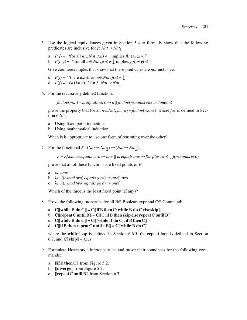
Exercises 121
5. Use the logical equivalences given in Section 5.4 to formally show that the following
predicates are inclusive for f : Nat!Nat "!
a. P(f)# ‘‘for all n$Nat, f(n)* "# implies f(n) ###"" zero’’
b. P(f, g)# ‘‘for all n$Nat, f(n)* "# implies f(n)# g(n)’’
Give counterexamples that show that these predicates are not inclusive:
c. P(f)# ‘‘there exists an n$Nat, f(n)# "#’’
d. P(f)# ‘‘f * ("n.n),’’ for f : Nat!Nat "!
6. For the recursively defined function:
factoo(m,n)# m equals zero! n[] factoo(m minus one, m times n)
prove the property that for all n$Nat, fac(n)# factoo(n,one), where fac is defined in Sec-
tion 6.6.1:
a. Using fixed point induction.
b. Using mathematical induction.
When is it appropriate to use one form of reasoning over the other?
7. For the functional F : (Nat!Nat "!)! (Nat!Nat "!),
F# "f."m. m equals zero! one [] m equals one! f(m plus two) [] f(m minus two)
prove that all of these functions are fixed points of F:
a. "n. one
b. "n. ((n mod two) equals zero)! one[] two
c. "n. ((n mod two) equals zero)! one[] "#
Which of the three is the least fixed point (if any)?
8. Prove the following properties for all B$ Boolean-expr and C$ Command:
a. C[[while B do C]]# C[[if B then C; while B do C else skip]]
b. C[[repeat C until B]]# C[[C; if B then skip else repeat C until B]]
c. C[[while B do C]]# C[[(while B do C); if B then C]]
d. C[[if B then repeat C until'B]]# C[[while B do C]]
where the while-loop is defined in Section 6.6.5, the repeat-loop is defined in Section
6.7, and C[[skip]]# "!!s. s.
9. Formulate Hoare-style inference rules and prove their soundness for the following com-
mands:
a. [[if B then C]] from Figure 5.2.
b. [[diverge]] from Figure 5.2.
c. [[repeat C until B]] from Section 6.7.
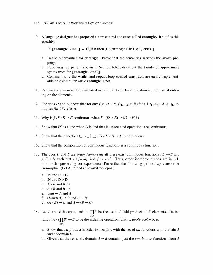
122 Domain Theory II: Recursively Defined Functions
10. A language designer has proposed a new control construct called entangle. It satifies this
equality:
C[[entangle B in C]] # C[[if B then (C; (entangle B in C); C) else C]]
a. Define a semantics for entangle. Prove that the semantics satisfies the above pro-
perty.
b. Following the pattern shown in Section 6.6.5, draw out the family of approximate
syntax trees for [[entangle B in C]].
c. Comment why the while- and repeat-loop control constructs are easily implement-
able on a computer while entangle is not.
11. Redraw the semantic domains listed in exercise 4 of Chapter 3, showing the partial order-
ing on the elements.
12. For cpos D and E, show that for any f, g : D!E, f ###"" D!E g iff (for all a1, a2 $A, a1 ##
#"" A a2
implies f(a1) ###"" B g(a2)).
13. Why is fix F : D!E continuous when F : (D!E)! (D!E) is?
14. Show that D, is a cpo when D is and that its associated operations are continuous.
15. Show that the operation (_! _ [] _) : Tr&D&D !D is continuous.
16. Show that the composition of continuous functions is a continuous function.
17. The cpos D and E are order isomorphic iff there exist continuous functions f:D!E and
g: E!D such that g % f # idD and f % g # idE . Thus, order isomorphic cpos are in 1-1,
onto, order preserving correspondence. Prove that the following pairs of cpos are order
isomorphic. (Let A, B, and C be arbitrary cpos.)
a. IN and IN$ IN
b. IN and IN& IN
c. A&B and B&A
d. A$B and B$A
e. Unit!A and A
f. (Unit&A)!B and A!B
g. (A&B)!C and A! (B!C)
18. Let A and B be cpos, and leta:A/B be the usual A-fold product of B elements. Define
apply : A& (a:A/B)!B to be the indexing operation; that is, apply(a,p)# p0a.
a. Show that the product is order isomorphic with the set of all functions with domain A
and codomain B.
b. Given that the semantic domain A!B contains just the continuous functions from A
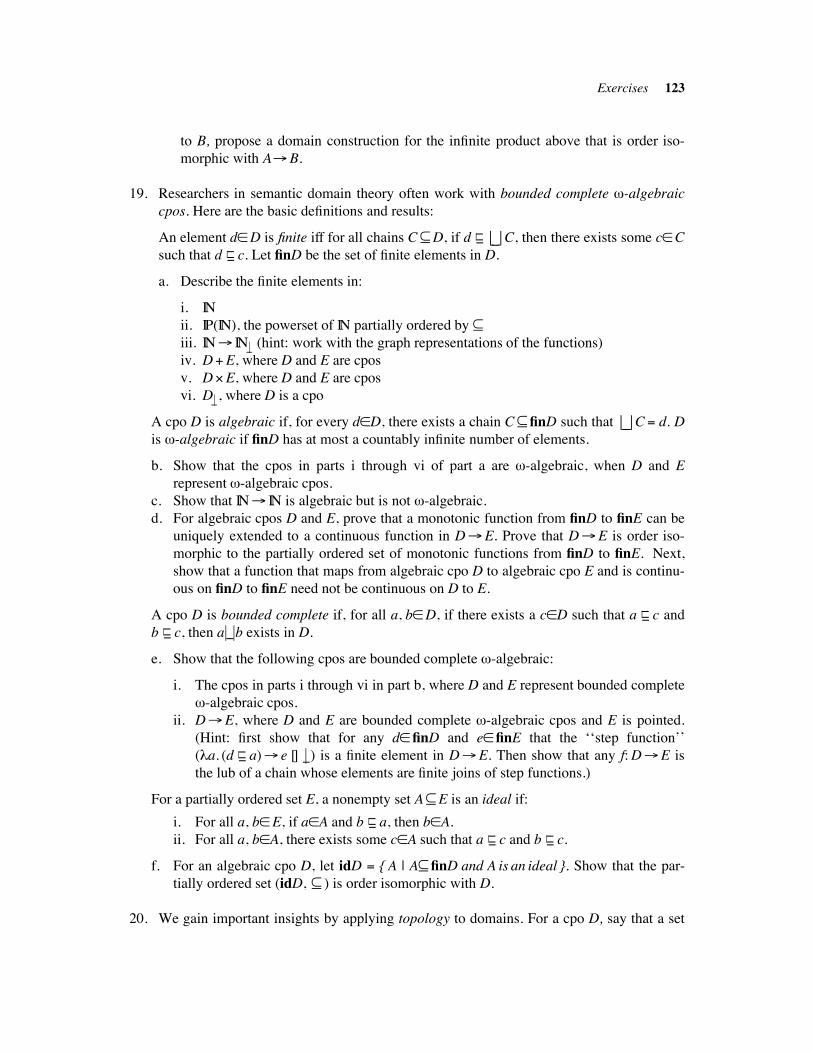
Exercises 123
to B, propose a domain construction for the infinite product above that is order iso-
morphic with A!B.
19. Researchers in semantic domain theory often work with bounded complete 1-algebraic
cpos. Here are the basic definitions and results:
An element d$D is finite iff for all chains C&D, if d ###"" #
C, then there exists some c$C
such that d ###"" c. Let finD be the set of finite elements in D.
a. Describe the finite elements in:
i. IN
ii. IP(IN), the powerset of IN partially ordered by &
iii. IN! IN"! (hint: work with the graph representations of the functions)
iv. D$E, where D and E are cpos
v. D&E, where D and E are cpos
vi. D"! , where D is a cpo
A cpo D is algebraic if, for every d$D, there exists a chain C&finD such that#
C # d. D
is 1-algebraic if finD has at most a countably infinite number of elements.
b. Show that the cpos in parts i through vi of part a are 1-algebraic, when D and E
represent 1-algebraic cpos.
c. Show that IN! IN is algebraic but is not 1-algebraic.
d. For algebraic cpos D and E, prove that a monotonic function from finD to finE can be
uniquely extended to a continuous function in D!E. Prove that D!E is order iso-
morphic to the partially ordered set of monotonic functions from finD to finE. Next,
show that a function that maps from algebraic cpo D to algebraic cpo E and is continu-
ous on finD to finE need not be continuous on D to E.
A cpo D is bounded complete if, for all a, b$D, if there exists a c$D such that a ###"" c and
b ###"" c, then a"--"b exists in D.
e. Show that the following cpos are bounded complete 1-algebraic:
i. The cpos in parts i through vi in part b, where D and E represent bounded complete
1-algebraic cpos.
ii. D!E, where D and E are bounded complete 1-algebraic cpos and E is pointed.
(Hint: first show that for any d$finD and e$finE that the ‘‘step function’’
("a. (d ###"" a)! e [] "#) is a finite element in D!E. Then show that any f: D!E is
the lub of a chain whose elements are finite joins of step functions.)
For a partially ordered set E, a nonempty set A&E is an ideal if:
i. For all a, b$E, if a$A and b ###"" a, then b$A.
ii. For all a, b$A, there exists some c$A such that a ###"" c and b ##
#"" c.
f. For an algebraic cpo D, let idD # { A | A&finD and A is an ideal }. Show that the par-
tially ordered set (idD, & ) is order isomorphic with D.
20. We gain important insights by applying topology to domains. For a cpo D, say that a set
124 Domain Theory II: Recursively Defined Functions
U&D is a Scott-open set iff:
i. It is closed upwards: for all a$ U, b$ D, if a ###"" b, then b$U.
ii. It contains a lub only if it contains a ‘‘tail’’ of the chain: for all chains C&D, if
#C$U, then there exists some c$C such that c$U.
A collection of sets S& IP(D) is a topology on D iff:
i. Both { } and D belong to S.
ii. For any R& S,'R$ S, that is, S is closed under arbitrary unions.
iii. For any U, V$ S, U2V$ S, that is, S is closed under binary intersections.
a. Show that for any cpo D that the collection of Scott-open sets forms a topology on D.
b. Describe the Scott-open sets for these cpos: Nat, Tr "! , Tr "! & Tr "! , Nat!Nat,
Nat!Nat "! .
c. Show that every element d$D is characterized by a unique collection of Scott-open
sets, that is, prove that for all distinct d, e$D, there exists some Scott-open set U&D
such that (d$U and e$/ U) or (e$U and d$/ U). (Hint: first show that the set
D# { e | e ###"" d}, for any d$D, is Scott-open; use this result in your proof.)
Part c says that the Scott-open sets have the T0-separation property. Because of this
result, we treat the Scott-open sets as ‘‘detectable properties’’ of D-elements. Each ele-
ment is identified by the properties that it satisfies.
d. Show that for all d, e$D, d ###"" e iff for all open sets U&D, d$U implies e$U.
A function f: D!E is topologically continuous iff for all open sets U&E, f#1(U) is open
in D. That is, a set of answer values share a property only because their corresponding
arguments also share a property.
e. Prove that a function f: D!E is chain-continuous (see Definition 6.9) iff it is topo-
logically continuous (with respect to the Scott-topologies on D and E).
21. Section 6.1 is a presentation of Kleene’s first recursion theorem, which states that the
meaning of a recursive specification f #F(f) that maps arguments in IN to answers in IN
(or nontermination) is exactly the union of the Fi()) approximating functions. The proof
of the theorem (see Kleene 1952, or Rogers 1967) doesn’t mention continuity or pointed
cpos. Why do we require these concepts for Chapter 6?
Chapter 7 !!!!!!!!!!!!!!!!!!!!!!!!!!!!!!!!!!!!!!!!!!!!!!!!!!!!!!!!
Languages with Contexts
Virtually all languages rely on some notion of context. The context in which a phrase is used
influences its meaning. In a programming language, contexts are responsible for attributing
meanings to identifiers. There are several possible notions of a programming language con-
text; let’s consider two of them. The first, a simplistic view, is that the store establishes the
context for a phrase. The view works with the languages studied in Chapter 5, but it does sug-
gest that the context within the block:
begin
integer X; integer Y;
Y:"0;
X:"Y;
Y:"1;
X:"Y+1
end
is constantly changing. This is counterintuitive; surely the declarations of the identifiers X
and Y establish the context of the block, and the commands within the block operate within
that context. A second example:
begin integer X;
X:"0;
begin real X;
X:"1.5
end;
X:"X+1
end
shows that the meaning of an identifier isn’t just its storable value. In this example, there are
two distinct definitions of X. The outer X denotes an integer object, while the inner X is a
real object. These objects are different; X happens to be the name used for both of them. Any
potential ambiguities in using X are handled by the scope rules of ALGOL60. The ‘‘objects’’
mentioned are in actuality computer storage locations, and the primary meaning of an
ALGOL60 identifier is the location bound to it. The version of context we choose to use is the
set of identifier, storage location pairs that are accessible at a textual position. Each position
in the program resides within a unique context, and the context can be determined without run-
ning the program.
In denotational semantics, the context of a phrase is modelled by a value called an
environment. Environments possess several distinctive properties:
1. As mentioned, an environment establishes a context for a syntactic phrase, resolving any
ambiguities concerning the meaning of identifiers.
2. There are as many environment values as there are distinct contexts in a program.125
126 Languages with Contexts
Multiple environments may be maintained during program evaluation.
3. An environment is (usually) a static object. A phrase uses the same environment each
time it is evaluated with the store.
An environment argument wasn’t needed for the languages in Chapter 5, because the pro-
grams in the languages used exactly one environment. The single environment was ‘‘pasted
onto’’ the store, giving a map from identifiers to storable values. In this chapter, that simple
model is split apart into two separate components, the environment and the store.
The primary real-life example of an environment is a complier’s symbol table. A com-
piler uses a symbol table to translate a source program into compiled code. The symbol table
contains an entry for each identifier in the program, listing the identifier’s data type, its mode
of usage (variable, constant, parameter, . . .), and its relative location in the run-time computer
store. Since a block-structured language allows multiple uses of the same identifier, the sym-
bol table is responsible for resolving naming conflicts. The schemes for implementation are
many: one is to keep a different symbol table for each block of the program (the portions in
common between blocks may be shared); another is to build the table as a single stack, which
is incremented and decremented upon respective entry and exit for a block. Symbol tables
may be entirely compile-time objects, as in ALGOL68 and standard Pascal, or they can be
run-time objects, as in SNOBOL4, or they can be used in both phases, as in ALGOL60.
Those portions of a semantics definition that use an environment to resolve context ques-
tions are sometimes called the static semantics. The term traditionally describes compile-time
actions such as type-checking, scope resolution, and storage calculation. Static semantics may
be contrasted with the ‘‘real’’ production of meaning, which takes the name dynamic seman-
tics. Code generation and execution comprise the implementation-oriented version of
dynamic semantics. In general, the separation of static from dynamic semantics is rarely clear
cut, and we will not attempt formal definitions here.
Environments are used as arguments by the valuation functions. The meaning of a com-
mand is now determined by the function:
C: Command!Environment! Store! Store#!
The meaning of a command as a Store! Store#! function is determined once an environment
establishes the context for the command. An environment belongs to the domain:
Environment" Identifier!Denotable-value
The Denotable-value domain contains all the values that identifiers may represent. This
domain varies widely from language to language and its structure largely determines the char-
acter of the language.
In this chapter, we study language features whose semantics are understood in terms of
environments. These features include declarations, block structure, scoping mechanisms,
recursive bindings, and compound data structures. The concepts are presented within the
framework of two languages: an imperative block-structured language and an applicative
language.
7.1 A Block-Structured Language 127
7.1 A BLOCK-STRUCTURED LANGUAGE !!!!!!!!!!!!!!!!!!!!!!!!!!!!!!!!!!!!!!!!!!!!!!!!!!!!!!!!!!!!!!!!!!!!!!
The basic principles and uses of environments are seen in the semantics of a simple block-
structured language. The language is similar to the one defined in Figure 5.2, but includes
declarations and blocks. The new semantic domains are listed in Figure 7.1.
The more realistic store requires a primitive domain of storage locations, and the loca-
tions domain is listed first. The operations are the same as in the algebra in Example 3.4 of
Chapter 3: first-locn is a constant, marking the first usable location in a store; next-locn maps
a location to its immediate successor in a store; equal-locn checks for equality of two values;
and lessthan-locn compares two locations and returns a truth value based on the locations’
relative values.
The collection of values that identifiers may represent is listed next. Of the three com-
ponents of the Denotable-value domain, the Location domain holds the denotations of variable
identifiers, the Nat domain holds the meanings of constant identifiers, and the Errvalue
domain holds the meaning for undeclared identifiers.
For this language, an environment is a pair. The first component is the function that
maps identifiers to their denotable values. The second component is a location value, which
marks the extent of the store reserved for declared variables. In this example, the environment
takes the responsibility for assigning locations to variables. This is done by the reserve-locn
operation, which returns the next usable location. Although it is not made clear by the alge-
bra, the structure of the language will cause the locations to be used in a stack-like fashion.
The emptyenv must be given the location marking the beginning of usable space in the store so
that it can build the initial environment.
The store is a map from storage locations to storable values, and the operations are the
obvious ones. Errors during evaluation are possible, so the store will be labeled with the
status of the evaluation. The check operation uses the tags to determine if evaluation should
continue.
Figure 7.2 defines the block-structured language and its semantics.
Since the Denotable-value domain contains both natural numbers and locations, denot-
able value errors may occur in a program; for example, an identifier with a number denotation
might be used where an identifier with a location denotation is required. An identifier with an
erroneous denotable value always induces an error. Expressible value errors occur when an
expressible value is inappropriately used.
The P valuation function requires a store and a location value, the latter marking the
beginning of the store’s free space. The K function establishes the context for a block. The D
function augments an environment. The composition of declarations parallels the composition
of commands. A constant identifier declaration causes an environment update, where the
identifier is mapped to its numeral value in the environment. The denotation of a variable
declaration is more involved: a new location is reserved for the variable. This location, l',plus the current environment, e ', are used to create the environment in which the variable [[I]]
binds to inLocation(l').Of the equations for the C function, the one for composition deserves the most study.
First, consider the check operation. If command C[[C1]]e maps a store into an erroneous post-
store, then check traps the error and prevents C[[C2]]e from altering the store. This would be
implemented as a branch around the code for [[C2]]. The environment is also put to good use:
128 Languages with Contexts
Figure 7.1____________________________________________________________________________________________________________________________________________________
V. Storage locations
Domain l" Location
Operations
first-locn : Location
next-locn : Location! Location
equal-locn : Location! Location! Tr
lessthan-locn : Location! Location! Tr
VI. Denotable values
Domain d" Denotable-value" Location$Nat$Errvalue
where Errvalue" Unit
VII. Environment: a map to denotable values and the maximum store location
Domain e" Environment" (Id!Denotable-value)% Location
Operations
emptyenv: Location!Environment
emptyenv" #l. ((#i. inErrvalue ()), l)
accessenv: Id!Environment!Denotable-value
accessenv" #i.#(map, l). map(i)
updateenv: Id!Denotable-value!Environment!Environment
updateenv" #i.#d.#(map, l). ([ i ##! d]map, l)
reserve-locn : Environment! (Location%Environment)
reserve-locn" #(map, l). (l, (map, next-locn(l)))
VIII. Storable values
Domain v" Storable-value"Nat
IX. Stores
Domain s" Store" Location! Storable-value
Operations
access: Location! Store! Storable-value
access" #l.#s. s(l)
update: Location! Storable-value! Store! Store
update" #l.#v.#s. [ l ##! v]s
X. Run-time store, labeled with status of computation
Domain p" Poststore" OK $Err
where OK"Err" Store
7.1 A Block-Structured Language 129
Figure 7.1 (continued)____________________________________________________________________________________________________________________________________________________
Operations
return: Store!Poststore
return" #s. inOK(s)
signalerr : Store!Poststore
signalerr" #s. inErr(s)
check: (Store!Poststore #!)! (Poststore#!!Poststore #!)
check f" #!! p. cases p of
isOK(s)! (f s)
[] isErr(s)! p end
____________________________________________________________________________
130 Languages with Contexts
Figure 7.2____________________________________________________________________________________________________________________________________________________
Abstract syntax:
P" Program
K" Block
D" Declaration
C" Command
E" Expression
B" Boolean-expr
I" Identifier
N" Numeral
P ::= K.
K ::= begin D; C end
D ::= D1;D2 | const I=N | var I
C ::= C1;C2 | I:"E | while B do C | K
E ::= E1$E2 | I | N
Semantic algebras:
I.-III. Natural numbers, truth values, identifiers
(defined in Figure 5.1)
IV. Expressible values
Domain x" Expressible-value" Nat$ Errvalue
where Errvalue" Unit
V.-X. (defined in Figure 7.1)
Valuation functions:
P: Program!Location! Store!Poststore #!
P[[K.]]" #l. K[[K]](emptyenv l)
K: Block!Environment! Store!Poststore #!
K[[begin D;C end]]" #e. C[[C]](D[[D]]e)
D: Declaration!Environment!Environment
D[[D1;D2]]" D[[D2]] & D[[D1]]
D[[const I"N]]" updateenv[[I]] inNat(N[[N]])
D[[var I]]" #e.let (l',e')" (reserve-locn e) in (updateenv[[I]] inLocation(l') e')
C: Command!Environment! Store!Poststore #!
C[[C1;C2]]" #e. (check(C[[C2]] e)) & (C[[C1]] e)
7.1 A Block-Structured Language 131
Figure 7.2 (continued)____________________________________________________________________________________________________________________________________________________
C[[I:"E]]" #e.#s. cases (accessenv[[I]] e) of
isLocation(l)! (cases (E[[E]]e s) of
isNat(n)! (return(update l n s))
[] isErrvalue()! (signalerr s) end)
[] isNat(n)! (signalerr s)
[] isErrvalue()! (signalerr s) end
C[[while B do C]]" #e. fix(#f.#s. cases (B[[B]]e s) of
isTr(t)! (t! (check f) & (C[[C]]e) [] return)(s)
[] isErrvalue()! (signalerr s) end)
C[[K]]" K[[K]]
E: Expression!Environment! Store!Expressible-value
E[[E1$E2]]" #e.#s. cases (E[[E1]]e s) of
isNat(n1)! (cases (E[[E2]]e s) of
isNat(n2)! inNat(n1 plus n2)
[] isErrvalue()! inErrvalue() end)
[] isErrvalue()! inErrvalue() end
E[[I]]"#e.#s. cases (accessenv[[I]] e) of
isLocation(l)! inNat(access l s)
[] isNat(n)! inNat(n)
[] isErrvalue()! inErrvalue() end
E[[N]]" #e.#s. inNat(N[[N]])
B: Boolean-expr !Environment! Store! (Tr$Errvalue) (omitted)
N: Numeral!Nat (omitted)
__________________________________________________________________________
commands [[C1]] and [[C2]] are both evaluated in the context represented by e. This point is
important, for [[C1]] could be a block with local declarations. It would need its own local
environment to process its commands. However, C[[C2]] retains its own copy of e, so the
environments created within C[[C1]] do not affect C[[C2]]’s version. (Of course, whatever
alterations C[[C1]]e makes upon the store are passed to C[[C2]]e.) This language feature is
called static scoping. The context for a phrase in a statically scoped language is determined
solely by the textual position of the phrase. One of the benefits of static scoping is that any
identifier declared within a block may be referenced only by the commands within that block.
This makes the management of storage locations straightforward. So-called dynamically
scoped languages, whose contexts are not totally determined by textual position, will be stu-
died in a later section.
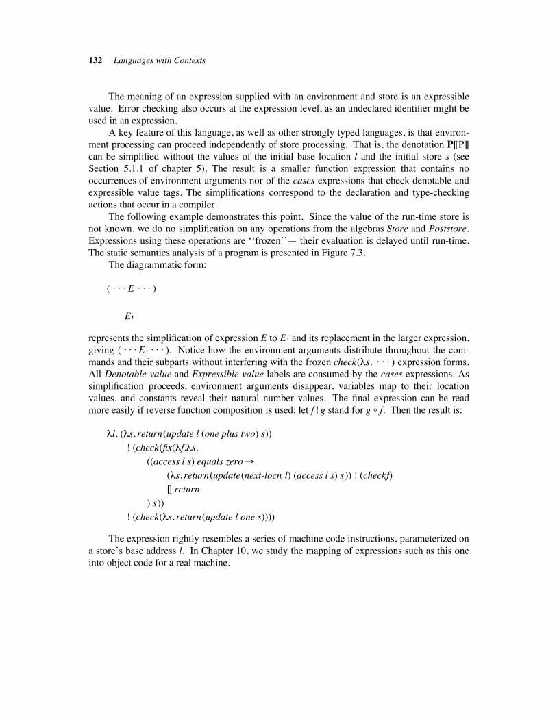
132 Languages with Contexts
The meaning of an expression supplied with an environment and store is an expressible
value. Error checking also occurs at the expression level, as an undeclared identifier might be
used in an expression.
A key feature of this language, as well as other strongly typed languages, is that environ-
ment processing can proceed independently of store processing. That is, the denotation P[[P]]
can be simplified without the values of the initial base location l and the initial store s (see
Section 5.1.1 of chapter 5). The result is a smaller function expression that contains no
occurrences of environment arguments nor of the cases expressions that check denotable and
expressible value tags. The simplifications correspond to the declaration and type-checking
actions that occur in a compiler.
The following example demonstrates this point. Since the value of the run-time store is
not known, we do no simplification on any operations from the algebras Store and Poststore.
Expressions using these operations are ‘‘frozen’’— their evaluation is delayed until run-time.
The static semantics analysis of a program is presented in Figure 7.3.
The diagrammatic form:
( . . . E . . . )
E '
represents the simplification of expression E to E ' and its replacement in the larger expression,
giving ( . . . E ' . . . ). Notice how the environment arguments distribute throughout the com-
mands and their subparts without interfering with the frozen check(#s. . . . ) expression forms.
All Denotable-value and Expressible-value labels are consumed by the cases expressions. As
simplification proceeds, environment arguments disappear, variables map to their location
values, and constants reveal their natural number values. The final expression can be read
more easily if reverse function composition is used: let f ! g stand for g & f. Then the result is:
#l. (#s. return(update l (one plus two) s))
! (check(fix(#f.#s.
((access l s) equals zero!
(#s. return(update(next-locn l) (access l s) s)) ! (checkf)
[] return
) s))
! (check(#s. return(update l one s))))
The expression rightly resembles a series of machine code instructions, parameterized on
a store’s base address l. In Chapter 10, we study the mapping of expressions such as this one
into object code for a real machine.
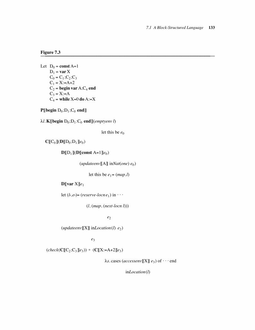
7.1 A Block-Structured Language 133
Figure 7.3____________________________________________________________________________________________________________________________________________________
Let D0 " const A"1
D1 " var X
C0 " C1;C2;C3
C1 " X:"A$2
C2 " begin var A;C4 end
C3 " X:"A
C4 " while X"0 do A:"X
P[[begin D0;D1;C0 end]]
#l. K[[begin D0;D1:C0 end]](emptyenv l)
let this be e0
C[[C0]](D[[D0;D1]]e0)
D[[D1]](D[[const A"1]]e0)
(updateenv[[A]] inNat(one) e0)
let this be e1" (map,l)
D[[var X]]e1
let (l',e')" (reserve-locne1) in . . .
(l, (map, (next-locn l)))
e2
(updateenv[[X]] inLocation(l) e2)
e3
(check(C[[C2;C3]]e3)) & (C[[X:"A$2]]e3)
#s. cases (accessenv[[X]] e3) of . . . end
inLocation(l)

134 Languages with Contexts
Figure 7.3 (continued)____________________________________________________________________________________________________________________________________________________
cases (E[[A$2]]e3 s) of . . . end
inNat(one plus two)
return(update l (one plus two) s)
(check(C[[C3]]e3)) & (C[[begin var A; C4 end]]e3)
C[[C4]](D[[var A]]e3)
(updateenv[[A]] inLocation (next-locn l) e4)
e5
C[[while X"0 doA:"X]]e5
fix(#f.#s. cases (B[[X"0]]e5 s) of . . . end
inTr((access l s) equals zero)
((access l s) equals zero!
(checkf) & (C[[A:"X]]e5) [] return) s
#s. return(update(next-locn l) (access l s) s)
C[[X:"A]]e3
#s. return(update l one s)
____________________________________________________________________________
7.1.1 Stack-Managed Storage !!!!!!!!!!!!!!!!!!!!!!!!!!!!!!!!!!!!!!!!!!!!!!!!!!!!!!!!!!!!!!!!!!!!!!!!!!!!!!!!!!!!!!!!!!!!!!!!!!
The store of a block-structured language is used in a stack-like fashion— locations are bound
to identifiers sequentially using nextlocn, and a location bound to an identifier in a local block
is freed for re-use when the block is exited. The re-use of locations happens automatically due
to the equation for C[[C1;C2]]. Any locations bound to identifiers in [[C1]] are reserved by the
environment built from e for C[[C1]], but C[[C2]] re-uses the original e (and its original loca-
tion marker), effectively deallocating the locations.
Stack-based storage is a significant characteristic of block-structured programming
languages, and the Store algebra deserves to possess mechanisms for stack-based allocation
and deallocation. Let’s move the storage calculation mechanism over to the store algebra.
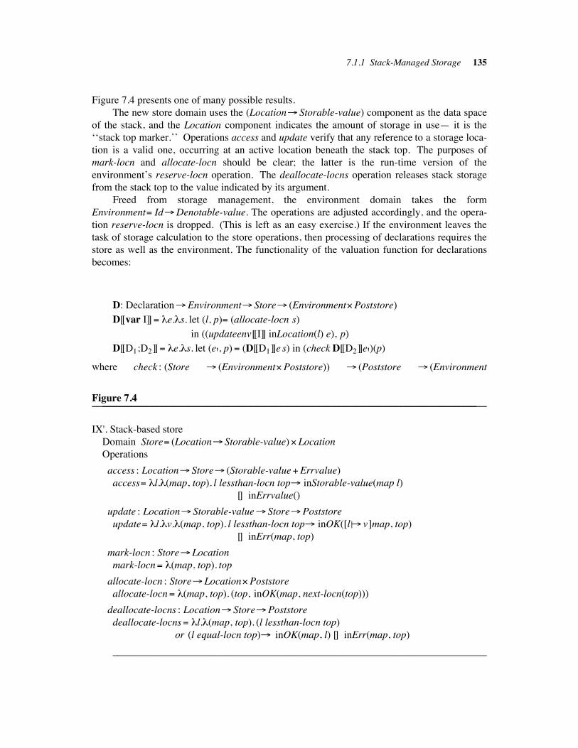
7.1.1 Stack-Managed Storage 135
Figure 7.4 presents one of many possible results.
The new store domain uses the (Location! Storable-value) component as the data space
of the stack, and the Location component indicates the amount of storage in use— it is the
‘‘stack top marker.’’ Operations access and update verify that any reference to a storage loca-
tion is a valid one, occurring at an active location beneath the stack top. The purposes of
mark-locn and allocate-locn should be clear; the latter is the run-time version of the
environment’s reserve-locn operation. The deallocate-locns operation releases stack storage
from the stack top to the value indicated by its argument.
Freed from storage management, the environment domain takes the form
Environment" Id!Denotable-value. The operations are adjusted accordingly, and the opera-
tion reserve-locn is dropped. (This is left as an easy exercise.) If the environment leaves the
task of storage calculation to the store operations, then processing of declarations requires the
store as well as the environment. The functionality of the valuation function for declarations
becomes:
D: Declaration!Environment! Store! (Environment%Poststore)
D[[var I]]" #e.#s. let (l, p)" (allocate-locn s)
in ((updateenv[[I]] inLocation(l) e), p)
D[[D1;D2]]" #e.#s. let (e', p)" (D[[D1]]e s) in (check D[[D2]]e')(p)
where check : (Store ! (Environment%Poststore)) ! (Poststore ! (Environment
Figure 7.4____________________________________________________________________________________________________________________________________________________
IX'. Stack-based store
Domain Store" (Location! Storable-value)% Location
Operations
access : Location! Store! (Storable-value$Errvalue)
access" #l.#(map, top). l lessthan-locn top! inStorable-value(map l)
[] inErrvalue()
update : Location! Storable-value! Store!Poststore
update" #l.#v.#(map, top). l lessthan-locn top! inOK([l ##! v]map, top)
[] inErr(map, top)
mark-locn : Store! Location
mark-locn" #(map, top). top
allocate-locn : Store! Location%Poststore
allocate-locn" #(map, top). (top, inOK(map, next-locn(top)))
deallocate-locns : Location! Store!Poststore
deallocate-locns" #l.#(map, top). (l lessthan-locn top)
or (l equal-locn top)! inOK(map, l) [] inErr(map, top)
________________________________________________________________________
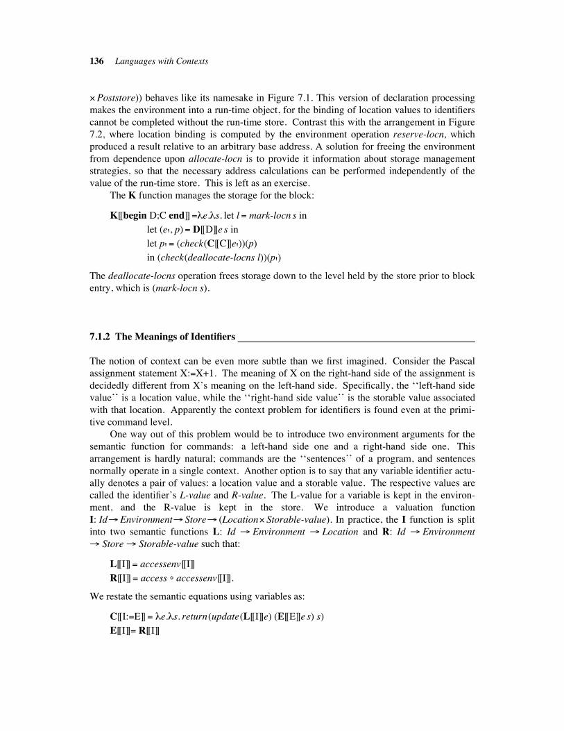
136 Languages with Contexts
%Poststore)) behaves like its namesake in Figure 7.1. This version of declaration processing
makes the environment into a run-time object, for the binding of location values to identifiers
cannot be completed without the run-time store. Contrast this with the arrangement in Figure
7.2, where location binding is computed by the environment operation reserve-locn, which
produced a result relative to an arbitrary base address. A solution for freeing the environment
from dependence upon allocate-locn is to provide it information about storage management
strategies, so that the necessary address calculations can be performed independently of the
value of the run-time store. This is left as an exercise.
The K function manages the storage for the block:
K[[begin D;C end]]"#e.#s. let l " mark-locn s in
let (e', p)" D[[D]]e s in
let p' " (check(C[[C]]e'))(p)
in (check(deallocate-locns l))(p')
The deallocate-locns operation frees storage down to the level held by the store prior to block
entry, which is (mark-locn s).
7.1.2 The Meanings of Identifiers !!!!!!!!!!!!!!!!!!!!!!!!!!!!!!!!!!!!!!!!!!!!!!!!!!!!!!!!!!!!!!!!!!!!!!!!!!!!!!!!!!!!!!!!!!!!
The notion of context can be even more subtle than we first imagined. Consider the Pascal
assignment statement X:"X+1. The meaning of X on the right-hand side of the assignment is
decidedly different from X’s meaning on the left-hand side. Specifically, the ‘‘left-hand side
value’’ is a location value, while the ‘‘right-hand side value’’ is the storable value associated
with that location. Apparently the context problem for identifiers is found even at the primi-
tive command level.
One way out of this problem would be to introduce two environment arguments for the
semantic function for commands: a left-hand side one and a right-hand side one. This
arrangement is hardly natural; commands are the ‘‘sentences’’ of a program, and sentences
normally operate in a single context. Another option is to say that any variable identifier actu-
ally denotes a pair of values: a location value and a storable value. The respective values are
called the identifier’s L-value and R-value. The L-value for a variable is kept in the environ-
ment, and the R-value is kept in the store. We introduce a valuation function
I: Id!Environment! Store! (Location% Storable-value). In practice, the I function is split
into two semantic functions L: Id ! Environment ! Location and R: Id ! Environment
! Store ! Storable-value such that:
L[[I]]" accessenv[[I]]
R[[I]]" access & accessenv[[I]].
We restate the semantic equations using variables as:
C[[I:"E]]" #e.#s. return(update(L[[I]]e) (E[[E]]e s) s)
E[[I]]" R[[I]]
7.1.2 The Meanings of Identifiers 137
The definitions are a bit simplistic because they assume that all identifiers are variables. Con-
stant identifiers can be integrated into the scheme — a declaration such as [[const A"N]] sug-
gests L[[A]]e" inErrvalue(). (What should (R[[A]]e s) be?)
Yet another view to take is that the R-value of a variable identifier is a function of its L-
value. The ‘‘true meaning’’ of a variable is its L-value, and a ‘‘coercion’’ occurs when a vari-
able is used on the right-hand side of an assignment. This coercion is called dereferencing.
We formalize this view as:
J: Id!Environment!Denotable-value
J[[I]]" #e. (accessenv[[I]] e)
C[[I:"E]]" #e.#s. return(update(J[[I]]e) (E[[E]]e s) s)
E[[I]]" #e.#s. dereference (J[[I]]e) s
where dereference: Location! Store! Storable-value
dereference" access
An identifier’s meaning is just its denotable value. Those identifiers with locations as
their meanings (the variables) are dereferenced when an expressible value is needed. This is
the view that was taken in the previous sections.
The implicit use of dereferencing is so common in general purpose programming
languages that we take it for granted, despite the somewhat unorthodox appearance of com-
mands such as X"X+1 in FORTRAN. Systems-oriented programming languages such as
BCPL, Bliss, and C use an explicit dereferencing operator. For example, in BCPL expressible
values include locations, and the appropriate semantic equations are:
E[[I]]" #e.#s. inLocation(J[[I]]e)
E[[@E]]" #e.#s. cases (E[[E]]e s) of
isLocation(l)! (dereference l s)
[] . . . end
The @ symbol is the dereferencing operator. The meaning of X:=X+1 in BCPL is decidedly
different from that of X:=@X+1.
7.2 AN APPLICATIVE LANGUAGE !!!!!!!!!!!!!!!!!!!!!!!!!!!!!!!!!!!!!!!!!!!!!!!!!!!!!!!!!!!!!!!!!!!!!!!!!!!!!!!!!!!!
The next example language using environments is an applicative language. An applicative
language contains no variables. All identifiers are constants and can be given attributes but
once, at their point of definition. Without variables, mechanisms such as assignment are
superfluous and are dropped. Arithmetic is an applicative language. Another example is the
minimal subset of LISP known as ‘‘pure LISP.’’ The function notation that we use to define
denotational definitions can also be termed an applicative language. Since an applicative
language has no variables, its semantics can be specified without a Store domain. The
environment holds the attributes associated with the identifiers.
The language that we study is defined in Figure 7.5. It is similar to pure LISP. A
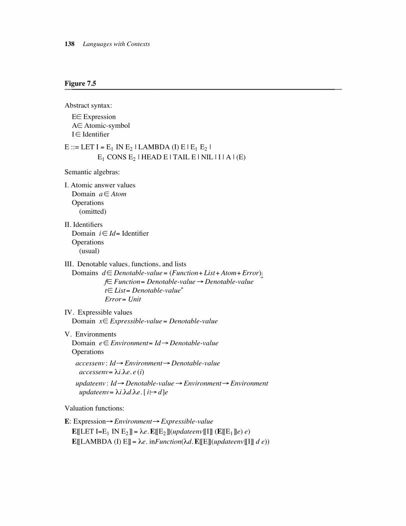
138 Languages with Contexts
Figure 7.5____________________________________________________________________________________________________________________________________________________
Abstract syntax:
E" Expression
A" Atomic-symbol
I" Identifier
E ::= LET I " E1 IN E2 | LAMBDA (I) E | E1 E2 |
E1 CONS E2 | HEAD E | TAIL E | NIL | I | A | (E)
Semantic algebras:
I. Atomic answer values
Domain a" Atom
Operations
(omitted)
II. Identifiers
Domain i" Id" Identifier
Operations
(usual)
III. Denotable values, functions, and lists
Domains d" Denotable-value" (Function$ List$Atom$Error)#!f" Function" Denotable-value!Denotable-value
t" List" Denotable-value$
Error" Unit
IV. Expressible values
Domain x" Expressible-value" Denotable-value
V. Environments
Domain e" Environment" Id!Denotable-value
Operations
accessenv : Id!Environment!Denotable-value
accessenv" #i.#e. e (i)
updateenv : Id!Denotable-value!Environment!Environment
updateenv" #i.#d.#e. [ i ##! d]e
Valuation functions:
E: Expression!Environment!Expressible-value
E[[LET I"E1 IN E2]]" #e. E[[E2]](updateenv[[I]] (E[[E1]]e) e)
E[[LAMBDA (I) E]]" #e. inFunction(#d. E[[E]](updateenv[[I]] d e))
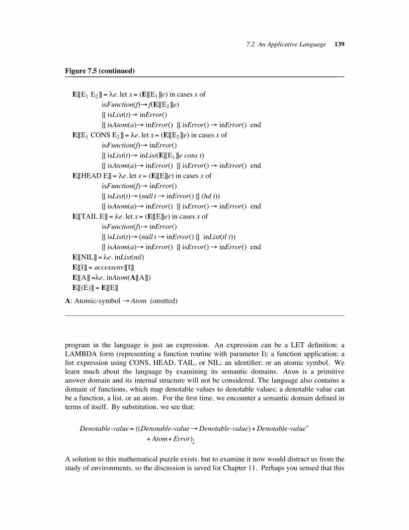
7.2 An Applicative Language 139
Figure 7.5 (continued)____________________________________________________________________________________________________________________________________________________
E[[E1 E2]]" #e. let x" (E[[E1]]e) in cases x of
isFunction(f)! f(E[[E2]]e)
[] isList(t)! inError()
[] isAtom(a)! inError() [] isError()! inError() end
E[[E1 CONS E2]]" #e. let x" (E[[E2]]e) in cases x of
isFunction(f)! inError()
[] isList(t)! inList(E[[E1]]e cons t)
[] isAtom(a)! inError() [] isError()! inError() end
E[[HEAD E]]" #e. let x" (E[[E]]e) in cases x of
isFunction(f)! inError()
[] isList(t)! (null t! inError() [] (hd t))
[] isAtom(a)! inError() [] isError()! inError() end
E[[TAIL E]]" #e. let x" (E[[E]]e) in cases x of
isFunction(f)! inError()
[] isList(t)! (null t! inError() [] inList(tl t))
[] isAtom(a)! inError() [] isError()! inError() end
E[[NIL]]" #e. inList(nil)
E[[I]]" accessenv[[I]]
E[[A]]"#e. inAtom(A[[A]])
E[[(E)]]" E[[E]]
A: Atomic-symbol !Atom (omitted)
____________________________________________________________________________
program in the language is just an expression. An expression can be a LET definition; a
LAMBDA form (representing a function routine with parameter I); a function application; a
list expression using CONS, HEAD, TAIL, or NIL; an identifier; or an atomic symbol. We
learn much about the language by examining its semantic domains. Atom is a primitive
answer domain and its internal structure will not be considered. The language also contains a
domain of functions, which map denotable values to denotable values; a denotable value can
be a function, a list, or an atom. For the first time, we encounter a semantic domain defined in
terms of itself. By substitution, we see that:
Denotable-value" ((Denotable-value!Denotable-value)$Denotable-value$
$Atom$Error)#!
A solution to this mathematical puzzle exists, but to examine it now would distract us from the
study of environments, so the discussion is saved for Chapter 11. Perhaps you sensed that this
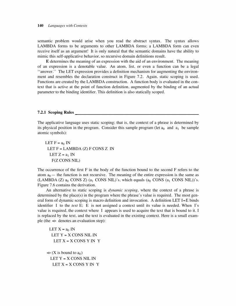
140 Languages with Contexts
semantic problem would arise when you read the abstract syntax. The syntax allows
LAMBDA forms to be arguments to other LAMBDA forms; a LAMBDA form can even
receive itself as an argument! It is only natural that the semantic domains have the ability to
mimic this self-applicative behavior, so recursive domain definitions result.
E determines the meaning of an expression with the aid of an environment. The meaning
of an expression is a denotable value. An atom, list, or even a function can be a legal
‘‘answer.’’ The LET expression provides a definition mechanism for augmenting the environ-
ment and resembles the declaration construct in Figure 7.2. Again, static scoping is used.
Functions are created by the LAMBDA construction. A function body is evaluated in the con-
text that is active at the point of function definition, augmented by the binding of an actual
parameter to the binding identifier. This definition is also statically scoped.
7.2.1 Scoping Rules !!!!!!!!!!!!!!!!!!!!!!!!!!!!!!!!!!!!!!!!!!!!!!!!!!!!!!!!!!!!!!!!!!!!!!!!!!!!!!!!!!!!!!!!!!!!!!!!!!!!!!!!!!!!!!!!!!
The applicative language uses static scoping; that is, the context of a phrase is determined by
its physical position in the program. Consider this sample program (let a0 and a1 be sample
atomic symbols):
LET F " a0 IN
LET F " LAMBDA (Z) F CONS Z IN
LET Z " a1 IN
F(Z CONS NIL)
The occurrence of the first F in the body of the function bound to the second F refers to the
atom a0— the function is not recursive. The meaning of the entire expression is the same as
(LAMBDA (Z) a0 CONS Z) (a1 CONS NIL)’s, which equals (a0 CONS (a1 CONS NIL))’s.
Figure 7.6 contains the derivation.
An alternative to static scoping is dynamic scoping, where the context of a phrase is
determined by the place(s) in the program where the phrase’s value is required. The most gen-
eral form of dynamic scoping is macro definition and invocation. A definition LET I"E binds
identifier I to the text E; E is not assigned a context until its value is needed. When I’s
value is required, the context where I appears is used to acquire the text that is bound to it. I
is replaced by the text, and the text is evaluated in the existing context. Here is a small exam-
ple (the "> denotes an evaluation step):
LET X " a0 IN
LET Y " X CONS NIL IN
LET X " X CONS Y IN Y
"> (X is bound to a0)
LET Y " X CONS NIL IN
LET X " X CONS Y IN Y
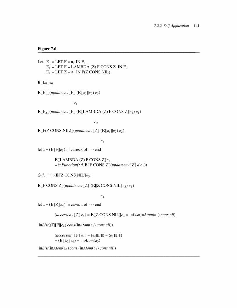
7.2.2 Self-Application 141
Figure 7.6____________________________________________________________________________________________________________________________________________________
Let E0 " LET F " a0 IN E1
E1 " LET F " LAMBDA (Z) F CONS Z IN E2
E2 " LET Z " a1 IN F(Z CONS NIL)
E[[E0]]e0
E[[E1]](updateenv[[F]] (E[[a0]]e0) e0)
e1
E[[E2]](updateenv[[F]] (E[[LAMBDA (Z) F CONS Z]]e1) e1)
e2
E[[F(Z CONS NIL)]](updateenv[[Z]] (E[[a1]]e2) e2)
e3
let x" (E[[F]]e3) in cases x of . . . end
E[[LAMBDA (Z) F CONS Z]]e1
" inFunction(#d. E[[F CONS Z]](updateenv[[Z]] d e1))
(#d. . . . )(E[[Z CONS NIL]]e3)
E[[F CONS Z]](updateenv[[Z]] (E[[Z CONS NIL]]e3) e1)
e4
let x" (E[[Z]]e4) in cases x of . . . end
(accessenv[[Z]] e4) " E[[Z CONS NIL]]e3 " inList(inAtom(a1) cons nil)
inList((E[[F]]e4) cons(inAtom(a1) cons nil))
(accessenv[[F]] e4) " (e4[[F]]) " (e1[[F]])
" (E[[a0]]e0) " inAtom(a0)
inList(inAtom(a0) cons (inAtom(a1) cons nil))
____________________________________________________________________________
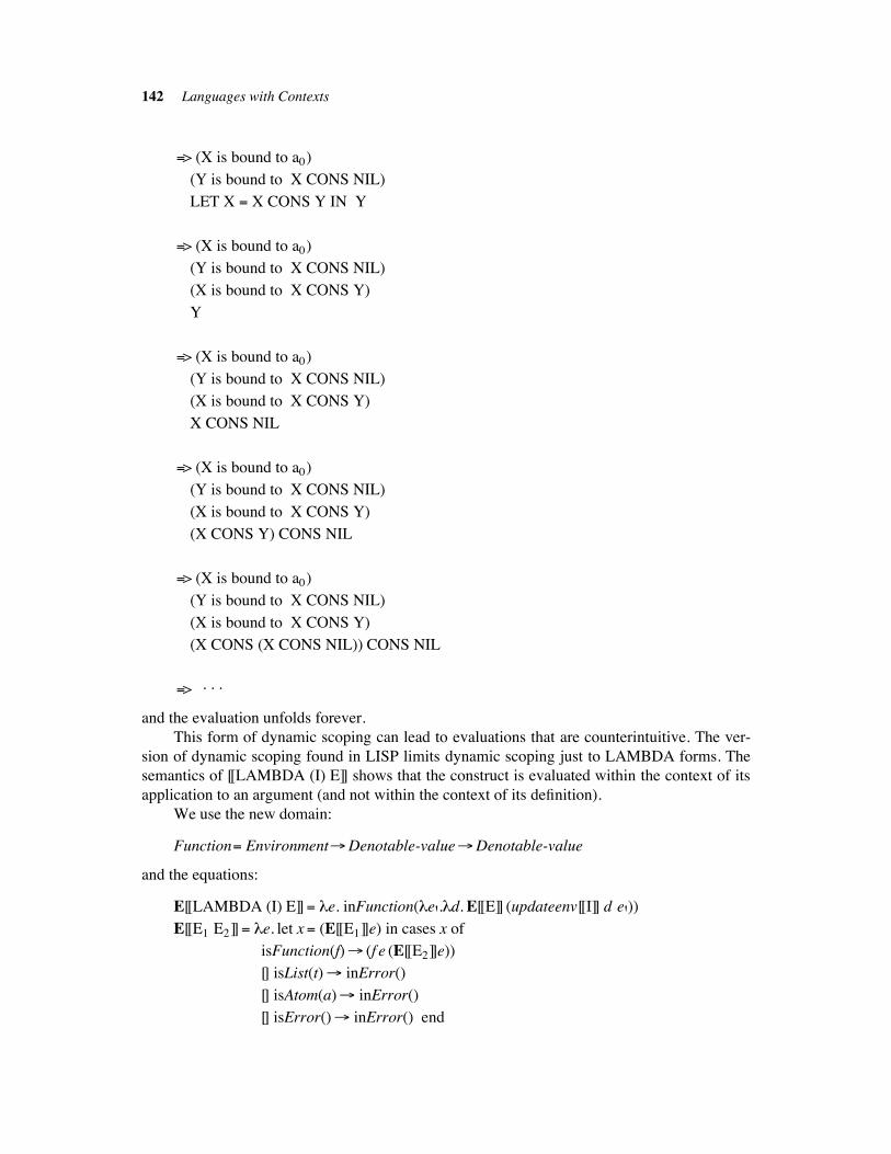
142 Languages with Contexts
"> (X is bound to a0)
(Y is bound to X CONS NIL)
LET X " X CONS Y IN Y
"> (X is bound to a0)
(Y is bound to X CONS NIL)
(X is bound to X CONS Y)
Y
"> (X is bound to a0)
(Y is bound to X CONS NIL)
(X is bound to X CONS Y)
X CONS NIL
"> (X is bound to a0)
(Y is bound to X CONS NIL)
(X is bound to X CONS Y)
(X CONS Y) CONS NIL
"> (X is bound to a0)
(Y is bound to X CONS NIL)
(X is bound to X CONS Y)
(X CONS (X CONS NIL)) CONS NIL
"> . . .
and the evaluation unfolds forever.
This form of dynamic scoping can lead to evaluations that are counterintuitive. The ver-
sion of dynamic scoping found in LISP limits dynamic scoping just to LAMBDA forms. The
semantics of [[LAMBDA (I) E]] shows that the construct is evaluated within the context of its
application to an argument (and not within the context of its definition).
We use the new domain:
Function" Environment!Denotable-value!Denotable-value
and the equations:
E[[LAMBDA (I) E]]" #e. inFunction(#e'.#d. E[[E]] (updateenv[[I]] d e'))E[[E1 E2]]" #e. let x" (E[[E1]]e) in cases x of
isFunction(f)! (f e (E[[E2]]e))
[] isList(t)! inError()
[] isAtom(a)! inError()
[] isError()! inError() end
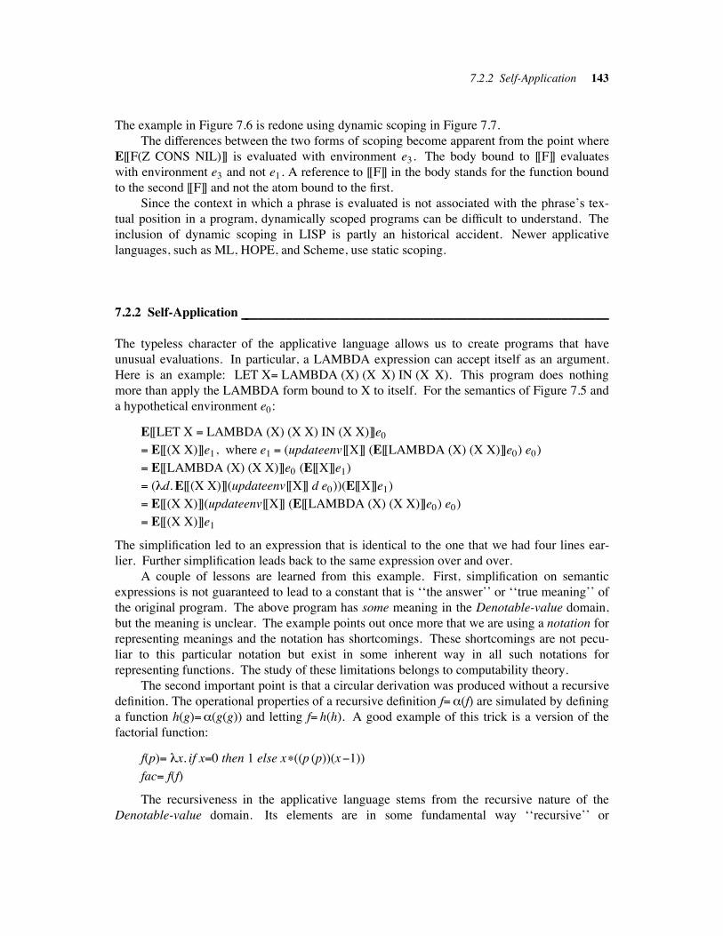
7.2.2 Self-Application 143
The example in Figure 7.6 is redone using dynamic scoping in Figure 7.7.
The differences between the two forms of scoping become apparent from the point where
E[[F(Z CONS NIL)]] is evaluated with environment e3. The body bound to [[F]] evaluates
with environment e3 and not e1. A reference to [[F]] in the body stands for the function bound
to the second [[F]] and not the atom bound to the first.
Since the context in which a phrase is evaluated is not associated with the phrase’s tex-
tual position in a program, dynamically scoped programs can be difficult to understand. The
inclusion of dynamic scoping in LISP is partly an historical accident. Newer applicative
languages, such as ML, HOPE, and Scheme, use static scoping.
7.2.2 Self-Application !!!!!!!!!!!!!!!!!!!!!!!!!!!!!!!!!!!!!!!!!!!!!!!!!!!!!!!!!!!!!!!!!!!!!!!!!!!!!!!!!!!!!!!!!!!!!!!!!!!!!!!!!!!!!!
The typeless character of the applicative language allows us to create programs that have
unusual evaluations. In particular, a LAMBDA expression can accept itself as an argument.
Here is an example: LET X" LAMBDA (X) (X X) IN (X X). This program does nothing
more than apply the LAMBDA form bound to X to itself. For the semantics of Figure 7.5 and
a hypothetical environment e0:
E[[LET X " LAMBDA (X) (X X) IN (X X)]]e0
" E[[(X X)]]e1, where e1 " (updateenv[[X]] (E[[LAMBDA (X) (X X)]]e0) e0)
" E[[LAMBDA (X) (X X)]]e0 (E[[X]]e1)
" (#d. E[[(X X)]](updateenv[[X]] d e0))(E[[X]]e1)
" E[[(X X)]](updateenv[[X]] (E[[LAMBDA (X) (X X)]]e0) e0)
" E[[(X X)]]e1
The simplification led to an expression that is identical to the one that we had four lines ear-
lier. Further simplification leads back to the same expression over and over.
A couple of lessons are learned from this example. First, simplification on semantic
expressions is not guaranteed to lead to a constant that is ‘‘the answer’’ or ‘‘true meaning’’ of
the original program. The above program has some meaning in the Denotable-value domain,
but the meaning is unclear. The example points out once more that we are using a notation for
representing meanings and the notation has shortcomings. These shortcomings are not pecu-
liar to this particular notation but exist in some inherent way in all such notations for
representing functions. The study of these limitations belongs to computability theory.
The second important point is that a circular derivation was produced without a recursive
definition. The operational properties of a recursive definition f"%(f) are simulated by defining
a function h(g)"%(g(g)) and letting f" h(h). A good example of this trick is a version of the
factorial function:
f(p)" #x. if x"0 then 1 else x$((p (p))(x&1))
fac" f(f)
The recursiveness in the applicative language stems from the recursive nature of the
Denotable-value domain. Its elements are in some fundamental way ‘‘recursive’’ or
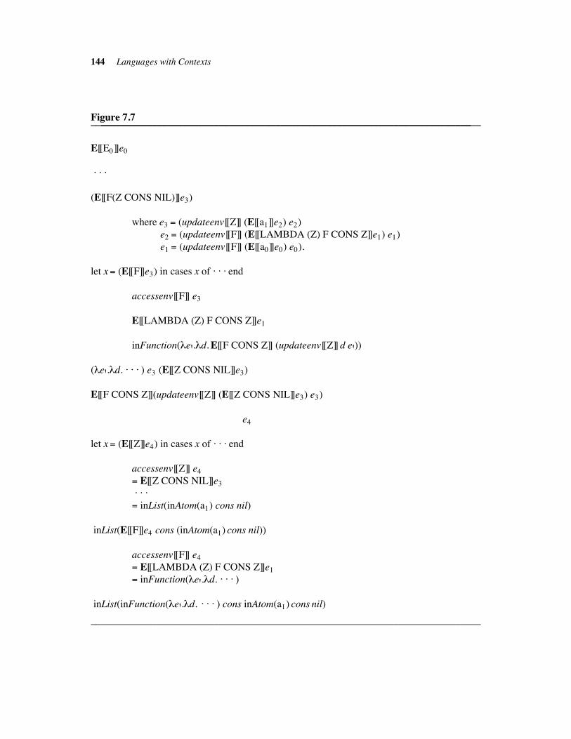
144 Languages with Contexts
Figure 7.7____________________________________________________________________________________________________________________________________________________
E[[E0]]e0
. . .
(E[[F(Z CONS NIL)]]e3)
where e3 " (updateenv[[Z]] (E[[a1]]e2) e2)
e2 " (updateenv[[F]] (E[[LAMBDA (Z) F CONS Z]]e1) e1)
e1 " (updateenv[[F]] (E[[a0]]e0) e0).
let x" (E[[F]]e3) in cases x of . . . end
accessenv[[F]] e3
E[[LAMBDA (Z) F CONS Z]]e1
inFunction(#e'.#d. E[[F CONS Z]] (updateenv[[Z]] d e'))
(#e'.#d. . . . ) e3 (E[[Z CONS NIL]]e3)
E[[F CONS Z]](updateenv[[Z]] (E[[Z CONS NIL]]e3) e3)
e4
let x" (E[[Z]]e4) in cases x of . . . end
accessenv[[Z]] e4
" E[[Z CONS NIL]]e3. . .
" inList(inAtom(a1) cons nil)
inList(E[[F]]e4 cons (inAtom(a1) cons nil))
accessenv[[F]] e4
" E[[LAMBDA (Z) F CONS Z]]e1
" inFunction(#e'.#d. . . . )
inList(inFunction(#e'.#d. . . . ) cons inAtom(a1) cons nil)
____________________________________________________________________________
7.2.3 Recursive Definitions 145
‘‘infinite.’’ The nature of an element in a recursively defined semantic domain is more
difficult to understand than the recursive specification of an element in a nonrecursive domain.
Chapter 11 examines this question in detail.
Finally, it is conceivable that the meaning of the example program is #&— the
simplification certainly suggests that no semantic information is contained in the program. In
fact, this is the case, but to prove it so is nontrivial. Any such proof needs knowledge of the
method used to build the domain that satisfies the recursive domain specification.
7.2.3 Recursive Definitions !!!!!!!!!!!!!!!!!!!!!!!!!!!!!!!!!!!!!!!!!!!!!!!!!!!!!!!!!!!!!!!!!!!!!!!!!!!!!!!!!!!!!!!!!!!!!!!!!!!!!!
Now we add a mechanism for defining recursive LAMBDA forms and give it a simple seman-
tics with the fix operation. We add two new clauses to the abstract syntax for expressions:
E ::= . . . | LETREC I " E1 IN E2 | IFNULL E1 THEN E2 ELSE E3
The LETREC clause differs from the LET clause because all occurrences of identifier I in E1
refer to the I being declared. The IF clause is an expression conditional for lists, which will be
used to define useful recursive functions on lists.
First, the semantics of the conditional construct is:
E[[IFNULL E1 THEN E2 ELSE E3]]" #e. let x" (E[[E1]]e) in cases x of
isFunction(f)! inError()
[] isList(t)! ((null t)! (E[[E2]]e) [] (E[[E3]]e))
[] isAtom(a)! inError()
[] isError()! inError() end
The semantics of the LETREC expression requires a recursively defined environment:
E[[LETREC I"E1 IN E2]]" #e. E[[E2]]e'where e'" updateenv[[I]] (E[[E1]]e') e
E[[E2]] requires an environment that maps [[I]] to E[[E1]]e' for some e'. But to support recursive
invocations, e' must contain the mapping of [[I]] to E[[E1]]e' as well. Hence e' is defined in
terms of itself. This situation is formally resolved with least fixed point semantics. We write:
E[[LETREC I"E1 IN E2]]" #e. E[[E2]](fix (#e'. updateenv[[I]] (E[[E1]]e') e))
The functional G" (#e'. updateenv[[I]] (E[[E1]]e') e) : Environment !Environment generates
the family of subfunctions approximating the recursive environment. This family is:
G0 " #i. #&G1 " updateenv[[I]] (E[[E1]](G0)) e
" updateenv[[I]] (E[[E1]] (#i. #&)) e
G2 " updateenv[[I]] (E[[E1]](G1)) e
" updateenv[[I]] (E[[E1]] (updateenv[[I]] (E[[E1]](#i. #&)) e)) e
146 Languages with Contexts
. . .
Gi$1 " updateenv (E[[E1]](Gi)) e
Each subenvironment Gi$1 produces a better-defined meaning for [[I]] than its predecessor Gi
and acts like e otherwise. A subenvironment Gi$1 is able to handle i recursive references to
[[I]] in [[E1]] before becoming exhausted and producing #&. The limit of the chain of suben-
vironments is an environment that can handle an unlimited number of recursive references.
Rest assured that you don’t need to remember all these details to define and use recursive
environments. We give the details to demonstrate that fixed point theory has intuitive and
practical applications.
Now consider this example:
LETREC F " LAMBDA (X) IFNULL X THEN NIL ELSE a0 CONS F(TAIL X)
IN F(a1 CONS a2 CONS NIL)
Function F transforms a list argument into a list of the same length containing only a0 atoms.
The value of the above expression is the same as (a0 CONS a0 CONS NIL). Figure 7.8 shows
the simplification. References to [[F]] in E1 and E2 are resolved by the recursive environment.
Now that we have seen several examples, comments about the LET construct are in
order. The purpose of LET is similar to that of the constant declaration construct in Figure
7.2. In fact, E[[LET I " E1 IN E2]] equals E[[ [ E1/I ] E2 ]], where [[ [ E1/I ] E2 ]] denotes the phy-
sical substitution of expression [[E1]] for all free occurrences of [[I]] in [[E2]], with renaming of
the identifiers in [[E2]] as needed. (The proof of this claim is left as an exercise.) As an exam-
ple:
LET X " a0 IN
LET Y " X CONS NIL IN
(HEAD Y) CONS X CONS NIL
rewrites to the simpler program:
LET Y " a0 CONS NIL IN
(HEAD Y) CONS a0 CONS NIL
which rewrites to:
(HEAD (a0 CONS NIL)) CONS a0 CONS NIL
which rewrites to:
a0 CONS a0 CONS NIL
These rewriting steps preserve the semantics of the original program. The rewritings are a
form of computing, just like the computing done on an arithmetic expression.
The LETREC construct also possesses a substitution principle: for [[LETREC I
" E1 IN E2]], all free occurrences of [[I]] in [[E2]] are replaced by [[E1]], and to complete the
substitution, any free occurrences of [[I]] in the resulting expression are also replaced (until
they are completely eliminated). Of course, the number of substitutions is unbounded:
LETREC I" %(I) IN '(I) writes to '(%(I)), then to '(%(%(I))), then to '(%(%(%(I)))) . . . , and
so on. This is expected, since the environment that models the recursion uses fix to generate a
similar chain of semantic values. Complete substitution isn’t feasible for producing answers in
a finite amount of time, so the substitutions must be perfomed more cautiously: occurrences of
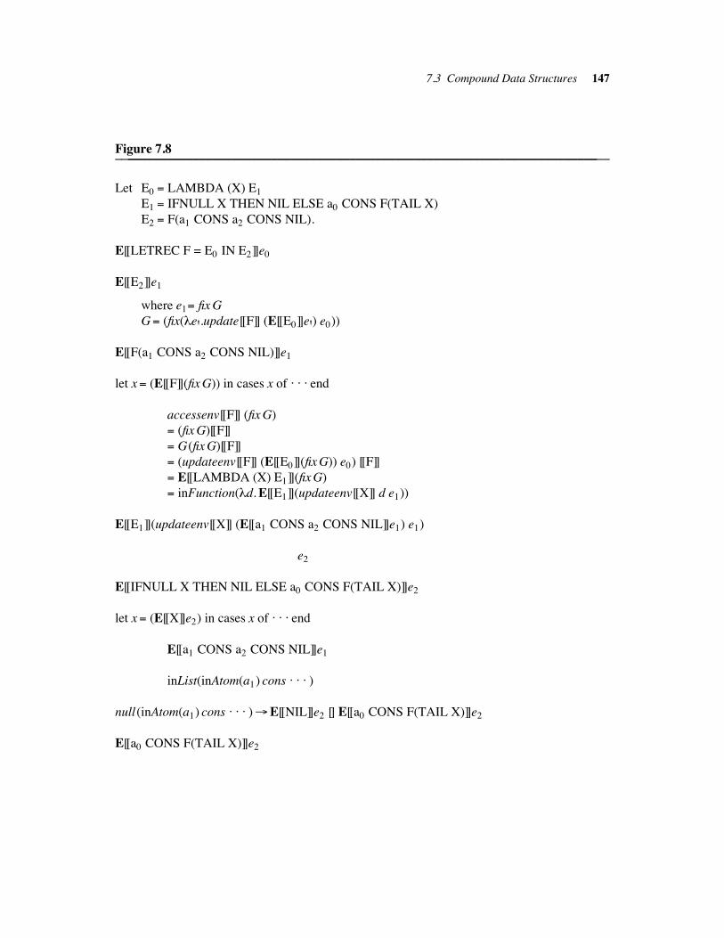
7.3 Compound Data Structures 147
Figure 7.8____________________________________________________________________________________________________________________________________________________
Let E0 " LAMBDA (X) E1
E1 " IFNULL X THEN NIL ELSE a0 CONS F(TAIL X)
E2 " F(a1 CONS a2 CONS NIL).
E[[LETREC F = E0 IN E2]]e0
E[[E2]]e1
where e1" fix G
G" (fix(#e'.update[[F]] (E[[E0]]e') e0))
E[[F(a1 CONS a2 CONS NIL)]]e1
let x" (E[[F]](fix G)) in cases x of . . . end
accessenv[[F]] (fix G)
" (fix G)[[F]]
" G(fix G)[[F]]
" (updateenv[[F]] (E[[E0]](fix G)) e0) [[F]]
" E[[LAMBDA (X) E1]](fix G)
" inFunction(#d. E[[E1]](updateenv[[X]] d e1))
E[[E1]](updateenv[[X]] (E[[a1 CONS a2 CONS NIL]]e1) e1)
e2
E[[IFNULL X THEN NIL ELSE a0 CONS F(TAIL X)]]e2
let x" (E[[X]]e2) in cases x of . . . end
E[[a1 CONS a2 CONS NIL]]e1
inList(inAtom(a1) cons . . . )
null(inAtom(a1) cons . . . )!E[[NIL]]e2 [] E[[a0 CONS F(TAIL X)]]e2
E[[a0 CONS F(TAIL X)]]e2
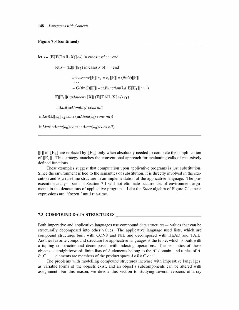
148 Languages with Contexts
Figure 7.8 (continued)____________________________________________________________________________________________________________________________________________________
let x" (E[[F(TAIL X)]]e2) in cases x of . . . end
let x" (E[[F]]e2) in cases x of . . . end
accessenv[[F]] e2 " e1[[F]] " (fix G)[[F]]. . .
" G(fix G)[[F]] " inFunction(#d. E[[E1]] . . . )
E[[E1]](updateenv[[X]] (E[[TAIL X]]e2) e1)
inList(inAtom(a 0) cons nil)
inList(E[[a0]]e2 cons (inAtom(a0) cons nil))
inList(inAtom(a0) cons inAtom(a0) cons nil)
____________________________________________________________________________
[[I]] in [[E2]] are replaced by [[E1]] only when absolutely needed to complete the simplification
of [[E2]]. This strategy matches the conventional approach for evaluating calls of recursively
defined functions.
These examples suggest that computation upon applicative programs is just substitution.
Since the environment is tied to the semantics of substitution, it is directly involved in the exe-
cution and is a run-time structure in an implementation of the applicative language. The pre-
execution analysis seen in Section 7.1 will not eliminate occurrences of environment argu-
ments in the denotations of applicative programs. Like the Store algebra of Figure 7.1, these
expressions are ‘‘frozen’’ until run-time.
7.3 COMPOUND DATA STRUCTURES !!!!!!!!!!!!!!!!!!!!!!!!!!!!!!!!!!!!!!!!!!!!!!!!!!!!!!!!!!!!!!!!!!!!!!!!!!!!!!
Both imperative and applicative languages use compound data structures— values that can be
structurally decomposed into other values. The applicative language used lists, which are
compound structures built with CONS and NIL and decomposed with HEAD and TAIL.
Another favorite compound structure for applicative languages is the tuple, which is built with
a tupling constructor and decomposed with indexing operations. The semantics of these
objects is straightforward: finite lists of A elements belong to the A$ domain, and tuples of A,
B, C, . . . elements are members of the product space A%B%C % . . . .
The problems with modelling compound structures increase with imperative languages,
as variable forms of the objects exist, and an object’s subcomponents can be altered with
assignment. For this reason, we devote this section to studying several versions of array
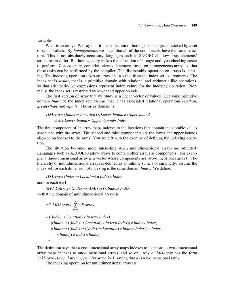
7.3 Compound Data Structures 149
variables.
What is an array? We say that it is a collection of homogeneous objects indexed by a set
of scalar values. By homogeneous, we mean that all of the components have the same struc-
ture. This is not absolutely necessary; languages such as SNOBOL4 allow array elements’
structures to differ. But homogeneity makes the allocation of storage and type-checking easier
to perform. Consequently, compiler-oriented languages insist on homogeneous arrays so that
these tasks can be performed by the compiler. The disassembly operation on arrays is index-
ing. The indexing operation takes an array and a value from the index set as arguments. The
index set is scalar, that is, a primitive domain with relational and arithmetic-like operations,
so that arithmetic-like expressions represent index values for the indexing operation. Nor-
mally, the index set is restricted by lower and upper bounds.
The first version of array that we study is a linear vector of values. Let some primitive
domain Index be the index set; assume that it has associated relational operations lessthan,
greaterthan, and equals. The array domain is:
1DArray" (Index! Location)% Lower-bound %Upper-bound
where Lower-bound " Upper-bound" Index
The first component of an array maps indexes to the locations that contain the storable values
associated with the array. The second and third components are the lower and upper bounds
allowed on indexes to the array. You are left with the exercise of defining the indexing opera-
tion.
The situation becomes more interesting when multidimensional arrays are admitted.
Languages such as ALGOL60 allow arrays to contain other arrays as components. For exam-
ple, a three-dimensional array is a vector whose components are two-dimensional arrays. The
hierarchy of multidimensional arrays is defined as an infinite sum. For simplicity, assume the
index set for each dimension of indexing is the same domain Index. We define:
1DArray" (Index! Location) % Index% Index
and for each n( 1:
(n+1)DArray" (Index! nDArray)% Index% Index
so that the domain of multidimensional arrays is:
a" MDArray" m "1)*
mDArray
" ((Index! Location) % Index% Index)
$ ((Index! ((Index! Location) % Index% Index))% Index% Index)
$ ((Index! ((Index! ((Index! Location) % Index% Index))% Index
% Index)) % Index% Index)
$ . . .
The definition says that a one-dimensional array maps indexes to locations, a two-dimensional
array maps indexes to one-dimensional arrays, and so on. Any a"MDArray has the form
inkDArray (map, lower, upper) for some k( 1, saying that a is a k-dimensional array.
The indexing operation for multidimensional arrays is:
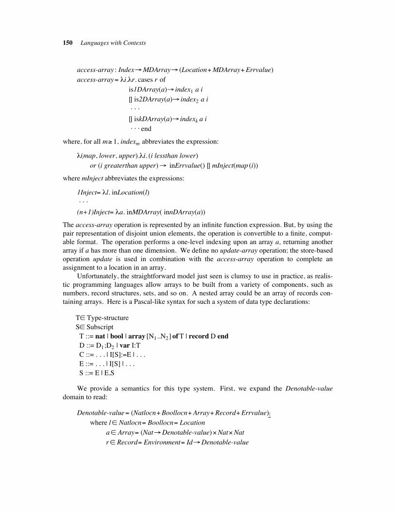
150 Languages with Contexts
access-array : Index!MDArray! (Location$MDArray$Errvalue)
access-array" #i.#r. cases r of
is1DArray(a)! index1 a i
[] is2DArray(a)! index2 a i . . .
[] iskDArray(a)! indexk a i . . . end
where, for all m( 1, indexm abbreviates the expression:
#(map, lower, upper).#i. (i lessthan lower)
or (i greaterthan upper)! inErrvalue() [] mInject(map (i))
where mInject abbreviates the expressions:
1Inject" #l. inLocation(l) . . .
(n+1)Inject" #a. inMDArray( innDArray(a))
The access-array operation is represented by an infinite function expression. But, by using the
pair representation of disjoint union elements, the operation is convertible to a finite, comput-
able format. The operation performs a one-level indexing upon an array a, returning another
array if a has more than one dimension. We define no update-array operation; the store-based
operation update is used in combination with the access-array operation to complete an
assignment to a location in an array.
Unfortunately, the straightforward model just seen is clumsy to use in practice, as realis-
tic programming languages allow arrays to be built from a variety of components, such as
numbers, record structures, sets, and so on. A nested array could be an array of records con-
taining arrays. Here is a Pascal-like syntax for such a system of data type declarations:
T" Type-structure
S" Subscript
T ::= nat | bool | array [N1..N2] of T | record D end
D ::= D1;D2 | var I:T
C ::= . . . | I[S]:"E | . . .
E ::= . . . | I[S] | . . .
S ::= E | E,S
We provide a semantics for this type system. First, we expand the Denotable-value
domain to read:
Denotable-value" (Natlocn$Boollocn$Array$Record$Errvalue)#!
where l" Natlocn" Boollocn" Location
a" Array" (Nat!Denotable-value)%Nat%Nat
r" Record" Environment" Id!Denotable-value
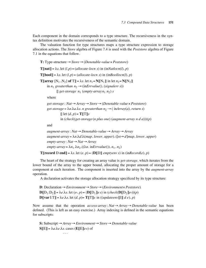
7.3 Compound Data Structures 151
Each component in the domain corresponds to a type structure. The recursiveness in the syn-
tax definition motivates the recursiveness of the semantic domain.
The valuation function for type structures maps a type structure expression to storage
allocation actions. The Store algebra of Figure 7.4 is used with the Poststore algebra of Figure
7.1 in the equations that follow.
T: Type-structure! Store! (Denotable-value%Poststore)
T[[nat]]" #s. let (l,p)" (allocate-locn s) in (inNatlocn(l), p)
T[[bool]]" #s. let (l,p)" (allocate-locn s) in (inBoollocn(l), p)
T[[array [N1..N2] of T]]" #s. let n1"N[[N1]] in let n2"N[[N2]]
in n1 greaterthan n2 ! (inErrvalue(), (signalerr s))
[] get-storage n1 (empty-array n1 n2) s
where
get-storage : Nat!Array! Store! (Denotable-value%Poststore)
get-storage" #n.#a.#s. n greaterthan n2 ! ( inArray(a), return s)
[] let (d, p)" T[[T]]s
in (check(get-storage (n plus one) (augment-array n d a)))(p)
and
augment-array : Nat!Denotable-value!Array!Array
augment-array" #n.#d.#(map, lower, upper). ([n ##! d]map, lower, upper)
empty-array : Nat!Nat!Array
empty-array" #n1 .#n2 .((#n. inErrvalue()), n1, n2)
T[[record D end]]" #s. let (e, p)" (D[[D]] emptyenv s) in (inRecord(e), p)
The heart of the strategy for creating an array value is get-storage, which iterates from the
lower bound of the array to the upper bound, allocating the proper amount of storage for a
component at each iteration. The component is inserted into the array by the augment-array
operation.
A declaration activates the storage allocation strategy specificed by its type structure:
D: Declaration!Environment! Store! (Environment%Poststore)
D[[D1;D2]]" #e.#s. let (e', p)" (D[[D1]]e s) in (check(D[[D2]]e'))(p)
D[[var I:T]]" #e.#s. let (d, p)" T[[T]]s in ((updateenv[[I]] d e), p)
Now assume that the operation access-array : Nat!Array!Denotable-value has been
defined. (This is left as an easy exercise.) Array indexing is defined in the semantic equations
for subscripts:
S: Subscript!Array!Environment! Store!Denotable-value
S[[E]]" #a.#e.#s. cases (E[[E]]es) of. . .
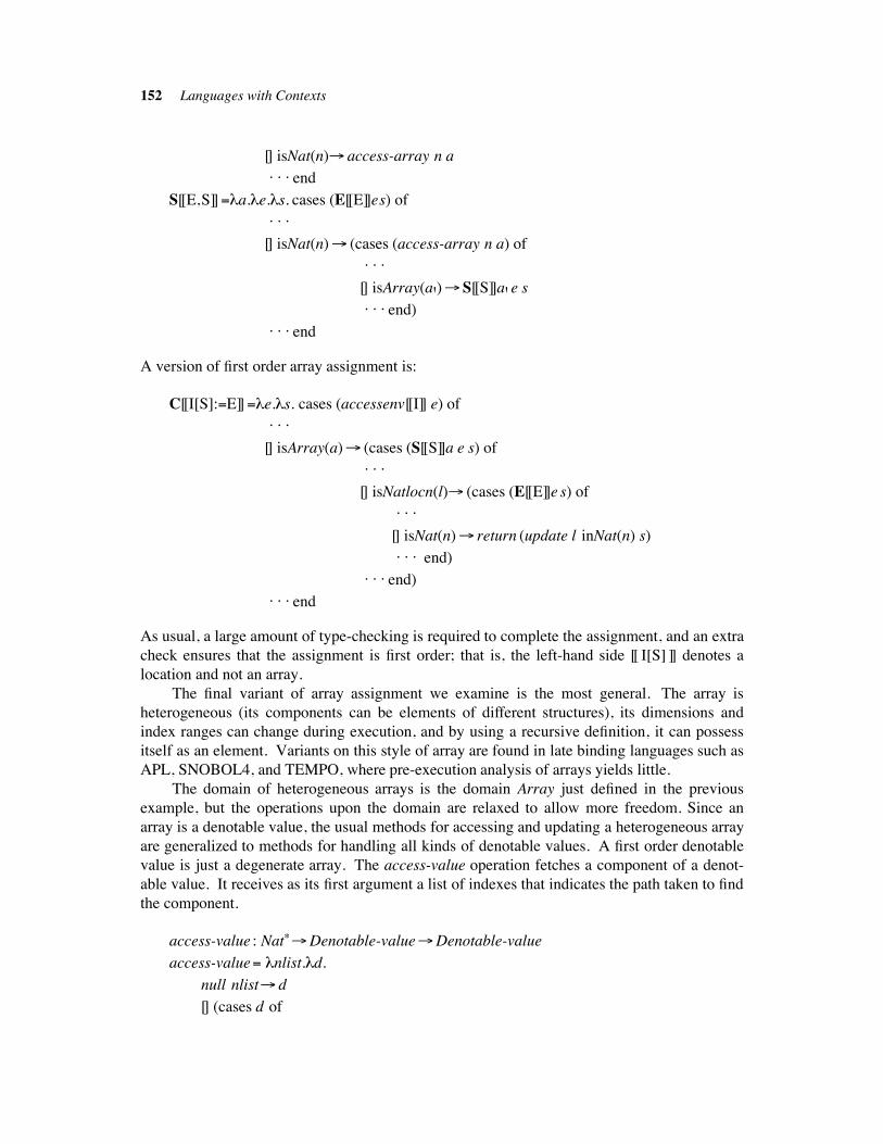
152 Languages with Contexts
[] isNat(n)! access-array n a. . . end
S[[E,S]]"#a.#e.#s. cases (E[[E]]es) of. . .
[] isNat(n)! (cases (access-array n a) of. . .
[] isArray(a')! S[[S]]a' e s. . . end)
. . . end
A version of first order array assignment is:
C[[I[S]:"E]]"#e.#s. cases (accessenv[[I]] e) of. . .
[] isArray(a)! (cases (S[[S]]a e s) of. . .
[] isNatlocn(l)! (cases (E[[E]]e s) of. . .
[] isNat(n)! return (update l inNat(n) s). . . end)
. . . end). . . end
As usual, a large amount of type-checking is required to complete the assignment, and an extra
check ensures that the assignment is first order; that is, the left-hand side [[ I[S] ]] denotes a
location and not an array.
The final variant of array assignment we examine is the most general. The array is
heterogeneous (its components can be elements of different structures), its dimensions and
index ranges can change during execution, and by using a recursive definition, it can possess
itself as an element. Variants on this style of array are found in late binding languages such as
APL, SNOBOL4, and TEMPO, where pre-execution analysis of arrays yields little.
The domain of heterogeneous arrays is the domain Array just defined in the previous
example, but the operations upon the domain are relaxed to allow more freedom. Since an
array is a denotable value, the usual methods for accessing and updating a heterogeneous array
are generalized to methods for handling all kinds of denotable values. A first order denotable
value is just a degenerate array. The access-value operation fetches a component of a denot-
able value. It receives as its first argument a list of indexes that indicates the path taken to find
the component.
access-value : Nat$!Denotable-value!Denotable-value
access-value" #nlist.#d.
null nlist! d
[] (cases d of
7.3 Compound Data Structures 153
isNatlocn(l)! inErrvalue(). . .
[] isArray(map, lower, upper)!
let n" hd nlist in
(n lessthan lower) or (n greaterthan upper)! inErrvalue()
[] (access-value (tl nlist) (map n)). . . end)
The operation searches through the structure of its denotable value argument until the
component is found. An empty index list signifies that the search has ended. A nonempty list
means that the search can continue if the value is an array. If so, the array is indexed at posi-
tion (hd nlist) and the search continues on the indexed component.
The updating operation follows a similar strategy, but care must be taken to preserve the
outer structure of an array while the search continues within its subparts. The argument new-
value is inserted into the array current-value at index nlist:
update-value : Nat $!Denotable-value!Denotable-value!Denotable-value
update-value" #nlist.#new-value #current-value .
null nlist! new-value
[] (cases current-value of
isNatlocn(l)! inErrvalue(). . .
[] isArray(map, lower, upper)!
let n" hd nlist in
let new-lower" (n lessthan lower! n [] lower) in
let new-upper" (n greaterthan upper! n [] upper)
in augment-array n (update-value (tl nlist) new-value (map n))
(map, new-lower, new-upper). . .
[] isErrvalue()! augment-array n (update-value (tl nlist) new-value
inErrvalue()) (empty-array n n). . . end)
where
augment-array : Nat!Denotable-value!Array!Denotable-value
augment-array"#n.#d.#(map, lower, upper).inArray([i ##! d]map, lower, upper)
If an index list causes a search deeper into an array structure than what exists, the
‘‘isErrvalue()! . . . ’’ clause creates another dimension to accommodate the index list. Thus
an array can grow extra dimensions. If an index from the index list falls outside of an array’s
bounds, the ‘‘isArray( . . . )! . . . ’’ clause expands the arrays’s bounds to accommodate the
index. Thus an array can change its bounds. The outer structure of a searched array is
preserved by the augment-array operation, which inserts the altered component back into the
154 Languages with Contexts
structure of the indexed array. Note that update-value builds a new denotable value; it does not
alter the store. A separate dereferencing step is necessary to cause conventional assignment.
The exercises continue the treatment of this and other kinds of array.
SUGGESTED READINGS !!!!!!!!!!!!!!!!!!!!!!!!!!!!!!!!!!!!!!!!!!!!!!!!!!!!!!!!!!!!!!!!!!!!!!!!!!!!!!!!!!!!!!!!!!!!!!!!!!!!!!
Semantics of block structure: Henhapl & Jones 1982; Landin 1965; Meyer 1983; Mosses
1974; Oles 1985; Reynolds 1981; Strachey 1968
Semantics of applicative languages: Abelson & Sussman 1985; Gordon 1973, 1975;
Muchnick & Pleban 1982; Reynolds 1970; Steele & Sussman 1978
Semantics of compound data structures: Abelson & Sussman 1985; Andrews & Henhapl
1982; Gordon 1979; Jones & Muchnick 1978; Tennent 1977
EXERCISES !!!!!!!!!!!!!!!!!!!!!!!!!!!!!!!!!!!!!!!!!!!!!!!!!!!!!!!!!!!!!!!!!!!!!!!!!!!!!!!!!!!!!!!!!!!!!!!!!!!!!!!!!!!!!!!!!!!!!!!!!!!!
1. a. Let the domain Location be Nat. (Thus, first-locn" zero, next-locn" (#l. l plus one),
etc.) Using the strategy of not simplifying away occurrences of access, update,
check, or return, simplify P[[begin var A; A:"2; begin var B; B:"A$1 end end.]] as
far as possible.
b. Let the result of part a be called Object-code. Do one step of simplification to the
expression Object-code(zero).
c. Let the result of part b be called Loaded-object-code. Simplify the expression
Loaded-object-code(newstore) to a post-store value.
2. Extend the language in Figure 7.2 to include declarations of variables of Boolean type;
that is:
D ::= . . . | bool var I
and expressions of boolean type:
E ::= . . . | true | ''E
Adjust the semantic algebras and the semantic equations to accommodate the extensions.
3. Augment the language of Figure 7.2 to include procedures:
D ::= . . . | proc I"C
and procedure invocations:
C ::= . . . | call I
Now augment the Denotable-value domain with the summand Proc " Store!Poststore #!to accommodate procedures.
a. If the semantics of procedure definition is written D[[proc I"C]] "#e. (updateenv [[I]] inProc(C[[C]]e) e), write the semantic equation for C[[call I]].
Exercises 155
What kind of scoping is used?
b. Say that the domain Proc is changed to be Proc " Environment ! Store !Post-
store #! . Write the semantic equations for procedure definition and invocation. What
kind of scoping is used?
4. a. For the semantics of Figure 7.2, show that there exist identifiers I and J and a com-
mand C such that B[[begin var I; var J; C end]] + B[[begin var J; var I; C end]].
b. Revise the language’s semantics so that for all identifiers I and J and command C, the
above inequality becomes an equality. Using structural induction, prove this.
c. Does the semantics you defined in part b support the equality
B[[begin var I; I:"I end]] " return?
5. a. Define the semantics of the ALGOL60 for-loop.
b. Define the semantics of the Pascal for-loop. (Recall that the loop index may not be
altered within the loop’s body.)
6. It is well known that the environment object in Figure 7.2 can be implemented as a single
global stack. Where is the stack concept found in the semantic equations?
7. The semantics in Figure 7.2 is somewhat simple minded in that the block
[[begin var A; const A"0; C end]] has a nonerroneous denotation.
a. What is [[A]]’s denotation in [[C]]?
b. Adjust the semantics of declarations so that redeclaration of identifiers in a block pro-
duces an error denotation for the block.
8. Use structural induction to prove that the semantics in Figure 7.2 is constructed so that if
any command in a program maps a store to an erroneous post-store, then the denotation
of the entire program is exactly that erroneous post-store.
9. a. Add to the language of Figure 7.2 the declaration [[var I:"E]]. What problems arise in
integrating the new construct into the existing valuation function D for declarations?
b. Attempt to handle the problems noted in part a by using a new declaration valuation
function:
D : Declaration!Environment! (Store!Poststore)
! (Environment% (Store!Poststore))
B[[begin D; C end]]" #e. let (e', c)" D[[D]]e return in ((check C[[C]]e') & c)
Write the semantic equations for D[[D1;D2]] and D[[var I:"E]] in the new format.
10. Make the needed adjustments so that the stack-based store model of Figure 7.4 can be
used with the semantics of Figure 7.2.
11. A design deficiency of the language in Figure 7.2 is its delayed reporting of errors. For
example, a denotable value error occurs in the assignment [[B:"A$1]] when [[A]] is not
156 Languages with Contexts
previously declared. The error is only reported when the run-time store is mapped to an
erroneous post-store. The error reporting need not be delayed until run-time: consider
the valuation function C : Command!Environment!Compiled-code, where
Compiled-code" (Store!Poststore)$Error-message. Rewrite the semantics of Figure
7.2 using the new form of C so that an expressible value or denotable value error in a
command leads to an Error-message denotation.
12. Extend the language of Figure 7.2 with pointers. In particular, set
Denotable-value" Natlocn$Ptrlocn$Nat$Errvalue
where Natlocn" Location (locations that hold numbers)
Ptrlocn" Location (locations that hold pointers)
Errvalue" Unit.
Augment the syntax of the language and give the semantics of pointer declaration, dere-
ferencing, assignment, and dynamic storage allocation. How does the integration of
pointers into the language change the stack-based storage model?
13. Augment the file editor language of Figure 5.4 with environments by introducing the
notion of window into the editor. A user of the file editor can move from one window to
another and be able to manipulate more than one file concurrently during a session.
14. Give an example of a programming language whose notion of R-value for an identifier is
not a function of the identifier’s L-value.
15. Using the semantic definition of Figure 7.5, determine the denotations of the following
expressions:
a. [[LET N" a0 IN LET N"N CONS NIL IN TAIL N]]
b. [[LET G"LAMBDA (X) X IN LET G"LAMBDA (Y) (G Y) IN (G a0)]]
c. [[LET F "LAMBDA(X) (X X) IN LET G" (F F) IN a0]]
Redo parts a through c using the LISP-style dynamic scoping semantics of Section 7.2.1.
16. Using structural induction, prove the following claim for the semantics of Figure 7.5: for
all I" Identifier, E1, E2" Expression, E[[LET I"E1 IN E2]] " E[[[E1/I]E2]].
17. a. Using the semantics of the LETREC construct in Section 7.2.3, determine the denota-
tions of the following examples:
i. [[LETREC APPEND " LAMBDA (L1) LAMBDA (L2)
IFNULL L1 THEN L2 ELSE (HEAD L1) CONS (APPEND
(TAIL L1) L2) IN APPEND (a0 CONS NIL) (a1 CONS NIL)]]
ii. [[LETREC L " a 0 CONS L IN HEAD L]]
iii. [[LETREC L " HEAD L IN L]]
b. Reformulate the semantics of the language so that a defined denotation for part ii
above is produced. Does the new semantics practice ‘‘lazy evaluation’’?
Exercises 157
18. In LISP, a denotable value may be CONSed to any other denotable value (not just a list),
producing a dotted pair. For example, [[A CONS (LAMBDA (I) I)]] is a dotted pair.
Reformulate the semantics in Figure 7.5 to allow dotted pairs. Redo the denotations of
the programs in exercises 15 and 17.
19. Formulate a semantics for the applicative language of Section 7.2 that uses macro
substitution-style dynamic scoping.
20. Define the appropriate construction and destruction constructs for the record structure
defined in Section 7.3. Note that the denotation of a record is a ‘‘little environment.’’
Why does this make a block construct such as the Pascal with statement especially
appropriate? Define the semantics of a with-like block statement.
21. a. Integrate the domain of one-dimensional arrays 1DArray into the language of Figure
7.2. Define the corresponding assembly and disassembly operations and show the
denotations of several example programs using the arrays.
b. Repeat part a with the domain of multidimensional arrays MDArray.
c. Repeat part a with the Pascal-like type system and domain of arrays Array.
22. After completing Exercise 21, revise your answers to handle arrays whose bounds are set
by expressions calculated at runtime, e.g., for part c above use: T ::= . . . |
array [E1..E2] of T
23. After completing Exercise 21, adjust the semantics of the assignment statement [[I:"E]] so
that:
a. If [[I]] is an array denotable value and (E[[E]]e s) is an expressible value from the same
domain as the array’s components, then a copy of (E[[E]]e s) is assigned to each of the
array’s components;
b. If [[I]] is an array denotable value and (E[[E]]e s) is an array expressible value of
‘‘equivalent type,’’ then the right-hand side value is bound to the left-hand side value.
24. Rewrite the valuation function for type structures so that it uses the Environment and
Store algebras of Figure 7.1; that is, T : Type-structure!Environment! (Denotable-
value%Environment), and the valuation function for declarations reverts to the D :
Declaration !Environment!Environment of Figure 7.2. Which of the two versions of
T and D more closely describes type processing in a Pascal compiler? In a Pascal inter-
preter? Which version of T do you prefer?
25. Consider the domain of one-dimensional arrays; the denotations of the arrays might be
placed in the environment (that is, an array is a denotable value) or the store (an array is a
storable value). Show the domain algebras and semantic equations for both treatments of
one-dimensional arrays. Comment on the advantages and disadvantages of each treat-
ment with respect to understandability and implementability.
26. In FORTRAN, an array is treated as a linear allocation of storage locations; the lower
158 Languages with Contexts
bound on an array is always one. Define the domain of one dimensional FORTRAN
arrays to be Location%Nat (that is, the location of the first element in the array and the
upper bound of the array). Show the corresponding operations for allocating storage for
an array, indexing, and updating an array.
27. Strachey claimed that the essential characteristics of a language are delineated by its
Denotable-value, Expressible-value, and Storable-value domains.
a. Give examples of programming languages such that:
i. Every expressible value is storable but is not necessarily denotable; every storable
value is expressible but is not necessarily denotable; a denotable value is not
necessarily expressible or storable.
ii. Every denotable value is expressible and storable; every storable value is expres-
sible and denotable; an expressible value is not necessarily denotable or storable.
iii. Every denotable value is expressible and storable; every expressible value is
denotable and storable; every storable value is denotable and expressible.
b. Repeat part a with Expressible-value " (Nat $ Tr $ Location $ Expressible-
value$)#!; with Expressible-value " ((Id ! Expressible-value) $Nat) #! .
c. Pick your favorite general purpose programming language and list its denotable,
expressible, and storable value domains. What limitations of the language become
immediately obvious from the domains’ definitions? What limitations are not obvi-
ous?
28. Language design is often a process of consolidation, that is, the integration of desirable
features from other languages into a new language. Here is a simple example. Say that
you wish to integrate the notion of imperative updating, embodied in the language in Fig-
ure 7.2, with the notion of value-returning construct, found in the language of Figure 7.5.
That is, you desire an imperative language in which every syntactic construct has an asso-
ciated expressible value (see ALGOL68 or full LISP).
a. Design such a language and give its denotational semantics. Does the language’s
syntax look more like the language in Figure 7.2 or 7.5?
b. Repeat part a so that the new language appears more like the other figure (7.5 or 7.2)
than the language in part a did. Comment on how the characteristics of the two
languages were influenced by your views of the languages’ syntax definitions.
Attempt this exercise once again by:
c. Integrating an imperative-style data structure, the array, with an expression-based,
applicative notation like that of Figure 7.5.
d. Integrating an applicative-style list structure with a command-based, imperative nota-
tion like that of Figure 7.2.
29. The function notation used for denotational semantics definitions has its limitations, and
one of them is its inability to simply express the Pascal-style hierarchy of data-type. If
you were asked to define an imperative programming language with simple and
Exercises 159
compound data-types, and you knew nothing of the ALGOL/Pascal tradition, what kinds
of data-types would you be led to develop if you used denotational semantics as a design
tool? What pragmatic advantages and disadvantages do you see in this approach?
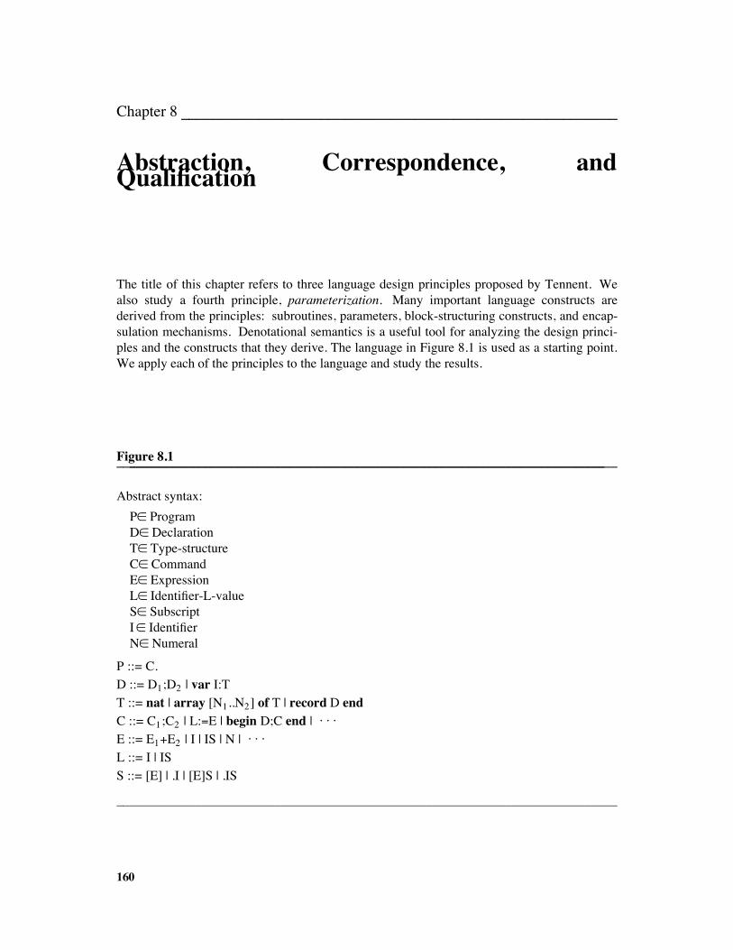
Chapter 8 !!!!!!!!!!!!!!!!!!!!!!!!!!!!!!!!!!!!!!!!!!!!!!!!!!!!!!!!
Abstraction, Correspondence, andQualification
The title of this chapter refers to three language design principles proposed by Tennent. We
also study a fourth principle, parameterization. Many important language constructs are
derived from the principles: subroutines, parameters, block-structuring constructs, and encap-
sulation mechanisms. Denotational semantics is a useful tool for analyzing the design princi-
ples and the constructs that they derive. The language in Figure 8.1 is used as a starting point.
We apply each of the principles to the language and study the results.
Figure 8.1____________________________________________________________________________________________________________________________________________________
Abstract syntax:
P! Program
D! Declaration
T! Type-structure
C! Command
E! Expression
L! Identifier-L-value
S! Subscript
I! Identifier
N! Numeral
P ::= C.
D ::= D1;D2 | var I:T
T ::= nat | array [N1..N2] of T | record D end
C ::= C1;C2 | L:"E | begin D;C end | . . .
E ::= E1#E2 | I | IS | N | . . .
L ::= I | IS
S ::= [E] | .I | [E]S | .IS
____________________________________________________________________________
160
8.1 Abstraction 161
8.1 ABSTRACTION !!!!!!!!!!!!!!!!!!!!!!!!!!!!!!!!!!!!!!!!!!!!!!!!!!!!!!!!!!!!!!!!!!!!!!!!!!!!!!!!!!!!!!!!!!!!!!!!!!!!!!!!!!!!!!!!
The first design principle is the principle of abstraction. Programmers sometimes use the term
abstraction for a specification that hides some irrelevant computational details. In Chapter 3
we used the term to describe a function expression of form ("x.M). The usage is appropriate,
for the expression specifies a function, hiding the details regarding the value x that is used in
M. We also gave abstractions names, e.g., square" ("n. n times n). The name enhances the
abstraction’s worth, for we can refer to the abstraction by mentioning its name, e.g.,
square(two).
Most programming languages support the creation of named expressions; a Pascal pro-
cedure is an abstraction of a command. We execute the command by mentioning its name.
Both a definition mechanism and an invocation mechanism are necessary. Tennent coined the
noun abstract to describe a named expression that is invoked by mentioning its name. An
abstract has both a name and a body. If its body is an expression from a syntax domain B, the
abstract can be invoked by using its name any place in a program where a B-expression is syn-
tactically legal.
The principle of abstraction states that any syntax domain of a language may have
definition and invocation mechanisms for abstracts.
A Pascal procedure is an example of a command abstract. We might also create expres-
sion abstracts, declaration abstracts, type abstracts, and so on. Let [[define I"V]] be an abstract.
[[I]] is the abstract’s name and [[V]] is its body. The denotable value of [[I]] is V[[V]]. If V[[V]]
is a function denotation, then are the arguments to the function provided at the point of
definition of the abstract or at the point of its invocation? This is an important question and
we study its answer through an example.
We augment the language in Figure 8.1 with definition and invocation mechanisms for
command abstracts, which we call procedures. The definition mechanism is added to the BNF
rule for declarations:
D ::= D1;D2 | var I:T | proc I"C
and the invocation mechanism appears in the rule for commands:
C ::= C1;C2 | L:"E | begin D;C end | I | . . .
Recall that the valuation function used in Chapter 7 for commands has functionality
C: Command#Environment# Store#Poststore $! . The denotation of the abstract’s body can
be any of the following:
1. C[[C]] : Environment# Store#Poststore $!: the environment and store that are used with
the body are the ones that are active at the point of invocation. This corresponds to
dynamic scoping.
2. (C[[C]]e) : Store#Poststore $!: the environment active at the point of definition is bound
to the body, and the store that is used is the one active at the point of invocation. This
corresponds to static scoping.
3. (C[[C]]e s)! Poststore $!: the procedure is completely evaluated at the point of definition,
and [[I]] is bound to a constant Poststore $! value. This option is unknown in existing
languages for command abstracts.
162 Abstraction, Correspondence, and Qualification
These three options list the possible scoping mechanisms for command abstracts. For
now, let us choose option 2 and define the semantic domain of procedures to be
Proc" Store#Poststore $! . The denotations of procedure identifiers come from Proc:
Denotable-value" Natlocn#Array#Record#Proc
The semantic equations for procedure definition and invocation are:
D[[proc I"C]]" "e."s. ((updateenv[[I]] inProc(C[[C]]e) e), (return s))
C[[I]]" "e."s. cases (accessenv[[I]] e) of
isNatlocn(l)# (signalerr s). . .
[] isProc(q)# (q s) end
(Recall that D: Declaration#Environment# Store# (Environment%Poststore).) Since we
chose static scoping, (C[[C]]e) is bound to [[I]] in the environment, and the store is supplied at
invocation-time. The definitions of the other two options are left as exercises.
Similar issues arise for expression abstracts (functions). For:
D ::= . . . | fcn I"E
E ::= E1#E2 | . . . | I
an ALGOL68-like constant definition results when the environment and store are bound at the
point of definition. If just the environment is bound at the point of definition, a FORTRAN-
style function results. If neither are bound at the point of definition, a text macro definition
results.
An interesting hybrid of procedure and function is the function procedure, which is a
command abstract that is invoked by an Expression-typed identifier. This construct is found
in Pascal. The function procedure must return an expressible value as its result. A possible
syntax for a function procedure is:
D ::= . . . | fcnproc I"C resultis E
Its inclusion causes a profound change in the semantics of expressions, for an expression can
now alter the value of the store. Further, an invoked function procedure might not terminate.
The valuation function for expressions must take the form:
E : Expression#Environment# Store# (Expressible-value%Poststore)$!
If we use static scoping, the equations for definition and invocation are:
D[[fcnproc I"C resultis E]]" "e."s. ((updateenv[[I]]
inFcn-proc((check(E[[E]]e)) & (C[[C]]e)) e), (return s))
where check : (Store# (Expressible-value%Poststore) $!)
# (Poststore# (Expressible-value%Poststore) $!)
traps errors and nontermination
8.1 Abstraction 163
E[[I]]" "e."s. cases (accessenv[[I]] e) of
isNatlocn(l)# ((access l s), (return s)). . .
[] isFcn-proc(f)# (f s) end
All of the other semantic equations for the E function must be revised to cope with the com-
plications arising from side effects and nontermination. This is left as an exercise.
Declaration abstractions follow the pattern seen thus far for commands and expressions.
The syntax is:
D ::= D1;D2 | var I:T | . . . | module I"D | I
We call the new construct a module. The invocation of a module activates the declarations in
the module’s body. Since there is no renaming of declarations, multiple invocations of the
same module in a block cause a redefinition error.
We also have type abstracts:
D ::= . . . | type I"T
T ::= nat | . . . | I
The definition and invocation of type abstracts follow the usual pattern:
D[[type I"T]]" "e."s. ((updateenv[[I]] inType(T[[T]]e) e), (return s))
T : Type-structure#Environment# Store# (Denotable-value%Poststore)
T[[I]]" "e."s. cases (accessenv[[I]] e) of
isNatlocn(l)# (inErrvalue(), (signalerr s)). . .
[] isType(v)# (v s) end
An issue raised by type abstraction is: when are two variables equivalent in type? There
are two possible answers. The first, structure equivalence, states that two variables are type-
equivalent if they have identical storage structures. Structure equivalence is used in
ALGOL68. The second, occurrence equivalence, also known as name equivalence, states that
two variables are type-equivalent if they are defined with the same occurrence of a type
expression. A version of occurrence equivalence is used in Pascal. Consider these declara-
tions:
type M " nat;
type N " array [1..3] of M;
var A: nat;
var B: M;
var C: M;
var D: N;
var E: array [2..4] of nat
164 Abstraction, Correspondence, and Qualification
Variables A and B are structure-equivalent but not occurrence-equivalent, because they are
defined with different occurrences of type expressions, A with nat and B with M. Variables B
and C are both structure- and occurrence-equivalent; C and D are neither. Variables D and E
are clearly not occurrence-equivalent, but are they structure-equivalent? The two have the
same structure in the store but have unequal structures, due to different range bounds, in the
environment. The question has no best answer. A similar problem exists for two variable
record structures that differ only in their components’ selector names or in the ordering of their
components. The semantics of declaration and assignment given in Chapter 7 naturally
enforces structure equivalence on types.
If we wish to define the semantics of these variants of type-checking, we must add more
information to the denotable values. For arrays, the domain
Array" (Index#Denotable-value)% Index% Index
is inadequate for occurrence equivalence checking and barely adequate for structure
equivalence checking. (Why?) A formal description of either kind of equivalence checking is
not simple, and the complexity found in the semantic definitions is mirrored in their imple-
mentations. The area is still a subject of active research.
8.1.1 Recursive Bindings !!!!!!!!!!!!!!!!!!!!!!!!!!!!!!!!!!!!!!!!!!!!!!!!!!!!!!!!!!!!!!!!!!!!!!!!!!!!!!!!!!!!!!!!!!!!!!!!!!!!!!!!
The semantics of a recursively defined abstract is straightforward; for the hypothetical
abstract:
D ::= . . . | rec abs I"M | . . .
where abs could be proc, fcn, class, or whatever, a statically scoped, recursive version is:
D[[rec abs I"M]]" "e."s. (e', (return s))
where e'" (updateenv[[I]] inM(M[[M]]e') e)
As we saw in Chapter 7, the recursively defined environment e' causes a reference to identifier
[[I]] in [[M]] to be resolved with e'. This produces a recursive invocation.
What sort of abstracts make good use of recursive bindings? Certainly procedures do.
Perhaps the most important aspect of recursive invocations is the means for terminating them.
In this regard, the if-then-else command serves well, for it makes it possible to choose
whether to continue the recursive invocations or not. We can increase the utility of recursive
expression and type abstracts by adding conditional constructs to their domains:
E ::= E1#E2 | . . . | if E1 then E2 else E3
T ::= nat | . . . | if E then T1 else T2
Some applications are given in the exercises.
8.2 Parameterization 165
8.2 PARAMETERIZATION !!!!!!!!!!!!!!!!!!!!!!!!!!!!!!!!!!!!!!!!!!!!!!!!!!!!!!!!!!!!!!!!!!!!!!!!!!!!!!!!!!!!!!!!!!!!!!!!!!
Abstracts usually carry parameters, which are dummy identifiers that are replaced by values
when the abstract is invoked. The dummy identifiers are the formal parameters and the
expressions that replace them are the actual parameters. If a formal parameter [[I]] is used in
an abstract’s body in positions where a B-construct is syntactically allowed, then the actual
parameter bound to [[I]] must be an expression from the B syntax domain. Abstracts may have
expression parameters, command parameters, type parameters, and so on.
The principle of parameterization states that a formal parameter to an abstract may be
from any syntax domain. The denotation of an abstract’s body [[V]] parameterized on
identifiers [[I1]], . . . , [[In]] is a function of form ("p1 . . . . ."pn . V[[V]] . . . ). What are the
denotations of the actual parameters? There are a number of options, and an example is the
best means for study.
All parameterized abstracts in this section use only one parameter. Consider a procedure,
parameterized on a member of the Expression domain, defined by the syntax:
D ::= . . . | proc I1(I2)"C
C ::= C1;C2 | . . . | I(E)
If the abstract is statically scoped, then the domain of procedures is
Proc" Param# Store#Poststore $! . The semantics of the abstract is:
D[[proc I1(I2)"C]]" "e."s. ((updateenv[[I1]]
inProc("a. C[[C]](updateenv[[I2]] a e)) e), (return s)).
C[[I(E)]]" "e."s. cases (accessenv[[I]] e) of
isNatlocn(l)# (signalerr s). . .
[] isProc(q)# (q ( . . . E[[E]] . . . ) s)
end
The expression ( . . . E[[E]] . . . ) represents the denotation of the actual parameter, a member
of domain Param. Recall that E: Expression #Environment # Store #Expressible-value is
the functionality of the valuation function for expressions. The options for the denotation of
the actual parameter are:
1. (E[[E]]e s)! Expressible-value: the actual parameter is evaluated with the environment
and store active at the point of invocation. This is implemented as call-by-value.
2. (E[[E]]e): Store#Expressible-value: the actual parameter is given the invocation
environment, but it uses the stores active at the occurrences of its corresponding formal
parameter in the procedure body. This is implemented as ALGOL60-style call-by-name.
3. E[[E]]: Environment# Store#Expressible-value: the actual parameter uses the environ-
ment and the store active at the occurrences of its corresponding formal parameter in the
procedure. This is implemented as call-by-text.
4. A fourth option used in some languages is to take the actual parameter domain Param to
be Location. This is implemented as call-by-reference. Call-by-reference transmission
166 Abstraction, Correspondence, and Qualification
presents a problem when a nonvariable expression is used as an actual parameter. Since
the denotation must be a location value, the usual strategy is to allocate a new location
that holds the expressible value of the parameter. This problem is a result of improper
language design. A solution is to make an explicit distinction in the language’s syntax
definition between Identifier L-values and Identifier R-values, as we did in Figure 2.1. A
call-by-reference parameter is not an expressible value, but the denotation of an L-value
construct, and identifiers that are Expression parameters are R-value constructs.
We conducted the above analysis assuming that expression evaluation always terminated;
that is, Expressible-value had no $$ element. When nontermination of actual parameter evalua-
tion is a possibility, then each of the four options mentioned above may evaluate their actual
parameter expressions in two ways:
1. Immediate evaluation: the value of the actual parameter is calculated before its binding to
the formal parameter. This is described by making a’s binding strict in:
D[[proc I1(I2)" C]]" "e."s. ((updateenv[[I1]]
inProc("!!a. C[[C]](updateenv[[I2]] a e)) e), (return s))
2. Delayed evaluation: the value of the actual parameter need be calculated only upon its
use in the body of the procedure. In this case, the semantic equation for procedure
definition is left in its original form— the value, whether it be proper or improper, is
bound into the procedure’s environment.
The term call-by-value is normally used to mean immediate evaluation to an expressible value,
while call-by-need and lazy evaluation are used to mean delayed evaluation to an expressible
value. (The difference between the latter two is that, once an evaluation of an argument does
proceed, call-by-need is required to finish it, whereas lazy evaluation need only evaluate the
argument to the point that the required subpart of the argument is produced.) Most applica-
tions of options 2 through 4 use immediate evaluation. The parameter domain and strictness
questions can be raised for all syntactic domains of actual parameters. You should consider
these issues for command, declaration, and type parameters to procedures and functions.
One of the more interesting parameterized abstracts is the parameterized type expression.
For syntax:
D ::= . . . | type I1(I2)"T | . . .
T ::= . . . | I(T) | . . .
type structures such as:
type STACKOF(T) " record
var ST: array [1..k] of T;
var TOP: nat
end
can be written. An invocation such as var X: STACKOF(nat) allocates storage for the two
components of the record: X.ST refers to an array of k number variables, and X.TOP refers to
8.2.1 Polymorphism and Typing 167
a number variable. The semantics of parameterized type abstractions is left as an exercise.
8.2.1 Polymorphism and Typing !!!!!!!!!!!!!!!!!!!!!!!!!!!!!!!!!!!!!!!!!!!!!!!!!!!!!!!!!!!!!!!!!!!!!!!!!!!!!!!!!!!!!!!!!!!!
An operation is polymorphic if its argument can be from more than one semantic domain. The
answer it produces is dependent upon the domains of its arguments. As an example, a general
purpose addition operation might produce an integer sum from two integer arguments and a
rational sum from two rational arguments. This operation might be assigned functionality:
(Integer% Integer)% (Rational%Rational)# Integer%Rational
Unfortunately, the dependence of the codomain on the domain isn’t clearly stated in this
description. The graph of the operation is the union of the integer addition and rational addi-
tion operations. Polymorphic operations do not fit cleanly into the domain theory of Chapter 3,
and our semantic notation does not include them.
Polymorphism does appear in general purpose programming languages. Strachey dis-
tinguished between two kinds: ad hoc polymorphism (also called overloading) and
parametric polymorphism. An ad hoc polymorphic operator ‘‘behaves differently’’ for argu-
ments of different types, whereas a parametric polymorphic operation ‘‘behaves the same’’ for
all types. (We won’t attempt more specific definitions because the concepts have proved
notoriously difficult to formalize.) In Pascal, a typed language, the + symbol is overloaded,
because it performs integer addition, floating point addition, and set union, all unrelated opera-
tions. A Pascal compiler determines the context in which the operator appears and associates a
specific meaning with +. In contrast, the hd operator in Edinburgh ML is parametric. It can
extract the head integer from a list of integers, the head character from a list of characters, and,
in general, the head & from an &-list. hd is a general purpose function, and it is implemented
as a general purpose operation. Regardless of the type of argument, the same structural mani-
pulation of a list is performed.
The denotational semantics of an overloaded operator is straightforward to express. Here
is a semantic equation for the Pascal addition expression:
E[[E1#E2]]" "e."s. cases (E[[E1]]e s) of
isNat(n1)# (cases (E[[E2]]e s) of
isNat(n2)# inNat(n1 plus n2). . . end)
. . .
[] isRat(r1)# (cases (E[[E2]]e s) of. . .
[] isRat(r2)# inRat(r1 addrat r2). . . end)
. . .
[] isSet(t1)# . . . inSet(t1 union t2) . . .
. . . end
168 Abstraction, Correspondence, and Qualification
A pre-execution analysis like that performed in Figure 7.3 can determine which of plus,
addrat, or union is the denotation of the +.
Parametric polymorphic operations are more difficult to handle; we give one method for
doing so. Consider the hd operator again. In ML, numbers, lists, tuples, sums, function
spaces, and the like, are all data types. Its expressible value domain balloons to:
Exprval" (Nat #Exprval' # (Exprval%Exprval)#
(Exprval#Exprval)# (Exprval#Exprval)#Errvalue)$!
The hd operator manipulates an expressible value list:
E[[hd E]]" "e. let x" E[[E]]e in cases x of
isNat(n)# inErrvalue()
[] isExprval'(l)# hd l
[] . . . end
The disadvantage of this formulation is that Nat-lists such as (two cons one cons nil) become
inExprval'(inNat(two) cons inNat(one) cons nil). We would prefer that hd operate directly
upon Nat-lists, Nat%Nat-lists, and the like, but both theoretical problems (mathematically, the
hd operation literally becomes too ‘‘large’’ to be well defined) and notational problems (try to
define hd in the existing semantic notation) arise. The real problem lies in our version of
domain theory. Our domains live in a rigid hierarchy, and there exists no ‘‘universal domain’’
that includes all the others as subdomains. If a universal domain U did exist, we could define
a single operation hd' : U#U that maps those elements of U that ‘‘look like’’ &-lists to ele-
ments in U that ‘‘look like’’ &-values. Then E[[hd E]] " "e. hd'(E[[E]]e). A number of
researchers, most notably McCracken and Reynolds, have developed domain theories for
universal domains and parametric polymorphism.
We next consider polymorphic parameterized abstracts. The parameterized abstracts in
the previous section are untyped— no restrictions (beyond syntax domain compatibility) are
placed on the formal and actual parameters. This is the version of abstraction used in untyped
languages such as BCPL and LISP. If the untyped version of parameterized abstract is used in
a typed language such as Pascal, the abstraction acts polymorphically. Consider a command
abstract whose denotation lies in the domain Proc " Expressible-value # Store # Poststore $! .
A procedure’s actual parameter can be an integer, a truth value, an array, or whatever else is a
legal expressible value.
However, a typed programming language like Pascal requires that formal parameters be
labeled with type expressions. The expression acts as a precondition or guard: only actual
parameters whose type structures match the formal parameter’s are allowed as arguments. The
advantages of typing— pre-execution type equivalence verification, increased user understand-
ing of abstracts, and efficient execution— are well known.
We use the syntax
D ::= . . . | proc I1(I2:T)"C
C ::= . . . | I(E) | . . .
for procedures that receive actual parameters from the Expression syntax domain. The value
bound to [[I2]] must have type structure [[T]].
8.2.1 Polymorphism and Typing 169
The semantics of typed parameters can be handled in two ways: (1) the type information
can guard entry to the abstract at invocation; (2) the abstract’s denotation is restricted at
definition to a function whose domain is exactly that specified by the type. To define the first
version, we use a valuation function:
T'': Type-structure#Environment#Expressible-value
# (Expressible-value#Errvalue)
such that (T''[[T]]e x) determines whether or not x has data type [[T]]. If it does, the result is
inExpressible-value(x); otherwise it is inErrvalue(). T'' is a type-equivalence checker. The
semantics of statically scoped procedure declaration is:
D[[proc I1(I2:T)"C]]" "e."s. ((updateenv[[I1]]
inProc("x. cases (T'[[T]]e x) of
isExpressible-value(x')#C[[C]](updateenv[[I2]] x' e)
[] isErrvalue()# signalerr end)
e), (return s))
The second version fragments the Proc domain by making it into a family of procedure
domains:
Nat-proc" Nat# Store#Poststore $!
Array-proc" Array# Store#Poststore $!
Record-proc" Record# Store#Poststore $!
For simplicity, we give only three kinds of parameter domains. (You are given the problem of
formulating a complete hierarchy of domains for Pascal.) Another version of the T'' function is
needed. First, we define:
Type-tag" Nat-tag #Array-tag#Record-tag#Err-tag
where Nat-tag " Array-tag" Record-tag" Err-tag" Unit
Each non-Err-tag corresponds to one of the parameter domains. The valuation function T'' :Type-structure#Environment# Type-tag maps the formal parameter’s type information to a
type tag value in the obvious fashion. A declaration of a typed procedure has semantics:
D[[proc I1(I2:T)"C]]" "e."s. cases (T'[[T]]e) of
isNat-tag()# ((updateenv[[I1]] inNat-proc("n. C[[C]](updateenv[[I2]]
inNat(n) e)) e), (return s))
isArray-tag()#
((updateenv[[I1]] inArray-proc("a. C[[C]](updateenv[[I2]]
inArray(a) e)) e), (return s))
isRecord-tag()# (similar to above)
isErr-tag()# (e, (signalerr s))
end
170 Abstraction, Correspondence, and Qualification
This semantics explicity restricts the abstract’s argument domain by selecting a particular
function at the point of definition. More specific information exists about the data type of the
parameter, and a more thorough pre-execution analysis can be performed.
Both of these two description methods have drawbacks. You are left with the problem of
finding a better solution to parameter-type enforcement.
8.3 CORRESPONDENCE !!!!!!!!!!!!!!!!!!!!!!!!!!!!!!!!!!!!!!!!!!!!!!!!!!!!!!!!!!!!!!!!!!!!!!!!!!!!!!!!!!!!!!!!!!!!!!!!!!!!!!
The principle of correspondence is simply stated: for any parameter binding mechanism, there
may exist a corresponding definition mechanism, and vice versa. That is, if elements from a
domain D may be denotable values of formal parameter identifiers, then elements from D may
be denotable values of declared identifiers, and vice versa. Since an environment is a map
from identifiers to denotable values, and a declared identifier is used no differently than a
parameter identifier, the correspondence principle makes full use of the semantic domains.
The correspondence between the two forms of binding becomes clear when their seman-
tic equations are compared. Consider once again a statically scoped command abstract with a
single parameter; let D be the domain of parameter denotations. Equations for definition and
invocation read:
D[[proc I1(I2)"C]]" "e."s. ((updateenv[[I1]]
inProc("d. C[[C]](updateenv[[I2]] inD(d) e)) e), (return s))
C[[I(M)]]" "e."s. cases (accessenv[[I]] e) of. . .
[] isProc(q)# q( . . . M[[M]] . . . ) s. . . end
We see that inD( . . . M[[M]] . . . ) is bound to [[I2]] in [[C]]’s environment. We can build a
definition construct with similar semantics:
D[[define I"M]]" "e."s. ((updateenv[[I]] inD( . . . M[[M]] . . . ) e), (return s))
Thus, C[[begin proc I(I')"C; I(M) end]] " C[[begin define I'"M; C end]] for phrases [[M]] and
[[C]] that contain no free occurrences of [[I]]. The questions we raised in Section 8.2 regarding
the domains of formal parameters now apply to declared identifiers as well.
The correspondence principle may also be practiced in the other direction. When we con-
sider the definition form for variables:
D[[var I:T]]" "e."s. let (d, p)" (T[[T]]e s) in ((updateenv[[I]] d e), p)
we see that the value bound to [[I]] is an activated type denotation; that is, a reference to newly
allocated storage, rather than an expressible value. (Perhaps we should write variable
definitions as [[I" ref T]].) The corresponding binding mechanism is:
8.3 Correspondence 171
D[[proc I1(I2)"C]]" "e."s. ((updateenv[[I1]]
inProc("d. C[[C]](updateenv[[I2]] d e)) e, (return s))
C[[I(T)]]" "e."s. cases (accessenv[[I]] e) of. . .
[] isProc(q)# let (d, p)" (T[[T]]e s) in (check(q d))(p). . . end
Storage for a data object of type [[T]] is allocated when the procedure is invoked, and a refer-
ence to the storage is the denotation bound to the parameter. This form of parameter transmis-
sion allocates local variables for a procedure. You should study the differences between the
version of C[[I(T)]] given above and the version induced by the correspondence principle from
[[type I"T]].
The principle of parameterization can be derived from the principles of abstraction and
correspondence by first uniformly generating all possible abstraction forms and then deriving
the parameter forms corresponding to the definitions.
8.4 QUALIFICATION !!!!!!!!!!!!!!!!!!!!!!!!!!!!!!!!!!!!!!!!!!!!!!!!!!!!!!!!!!!!!!!!!!!!!!!!!!!!!!!!!!!!!!!!!!!!!!!!!!!!!!!!!!!!
The principle of qualification is that every syntax domain may have a block construct for
admitting local declarations. The language of Figure 8.1 already has a block construct in the
Command domain. Blocks for the other domains take on similar forms:
E ::= . . . | begin D within E end | . . .
D ::= . . . | begin D1 within D2 end | . . .
T ::= . . . | begin D within T end | . . .
and so on. For a syntax domain M, the semantics of an M-block [[begin D within M end]] is
M[[M]] with an environment augmented by the definitions [[D]]. The definitions’ scope extends
no further than [[M]]. Assuming the usual static scoping, we state the semantics of the M-block
as:
M: M#Environment# Store# (M%Poststore)
M[[begin D within M end]]" "e."s. let (e',p)" (D[[D]]e s)
in (check(M[[M]]e'))(p)
This format applies to Command blocks, Expression blocks, Type blocks, and so on. A techn-
ical problem arises for Declaration blocks. The scope of local definitions [[D1]] of block
[[begin D1 within D2 end]] should extend only as far as [[D2]], but the D valuation function
defined in Figure 7.2 processes its environment argument as if it were a store— the additions
to the environment are retained beyond the scope of the declaration block. A solution is to
make the denotation of a declaration be a list of binding pairs:
172 Abstraction, Correspondence, and Qualification
D : Declaration#Environment# Store#
((Identifier%Denotable-value)' %Poststore)
Thus, (D[[D]]e s) denotes the bindings (and the post-store) defined by [[D]] and not the environ-
ment that results when those bindings are added to e. D’s definition and the semantics of
declaration blocks are left as exercises.
A number of useful constructions result from the the qualification principle. For exam-
ple, a Declaration block used within a Declaration abstract creates a Modula-style module.
Here is an example that models a natural number-containing stack:
module STACK-OF-NAT "
begin
var ST: array [1..k] of nat;
var TOP: nat
within
proc PUSH(I: nat) " if TOP"k then skip
else (TOP:"TOP#1; ST[TOP]:"I);
proc POP " if TOP"0 then skip else TOP:"TOP$1;
fcn TOP " if TOP"0 then error else ST[TOP];
proc INITIALIZE " TOP:"0
end
The declaration var STACK-OF-NAT creates procedures PUSH, POP, TOP, INITIALIZE,
and function TOP. The variables ST and TOP are local definitions that are hidden from out-
side access.
Type blocks are also useful. First, recall that the syntax of a record structure is:
T ::= . . . | record D end | . . .
Since the body of a record is a declaration, records of variables, procedures, functions, or
whatever are allowed. These make semantic sense as well, for Record " Identifier #
Denotable-value and Denotable-value " (Natlocn #Array #Record #Proc# . . . ) $! . Since
Type blocks allow local variables to a type structure, we can create a SIMULA-style class.
Here is an example of a type definition for a stack class parameterized on the element type:
type STACK-OF(X) "
begin
var ST: array[1..k] of X;
var TOP: nat
within record
proc PUSH(I:X) " . . . (as before)
proc POP " . . .
fcn TOP " . . .
proc INITIALIZE " . . .
8.4 Qualification 173
end
end
A definition var A: STACK-OF(nat) creates a record with components A.PUSH,
A.POP, A.TOP, and A.INITIALIZE. One technical point must be resolved: the type parame-
ter X has two roles in the definition. It induces storage allocation in the definition
var ST: array [1..k] of X and it does type equivalence checking in proc PUSH(I:X). Both
the T and T'' valuation functions are needed.
8.5 ORTHOGONALITY !!!!!!!!!!!!!!!!!!!!!!!!!!!!!!!!!!!!!!!!!!!!!!!!!!!!!!!!!!!!!!!!!!!!!!!!!!!!!!!!!!!!!!!!!!!!!!!!!!!!!!!!
The introduction to this chapter stated that the abstraction, parameterization, correspondence,
and qualification principles were tools for programming language design. Any programming
language can be uniformly extended along the lines suggested by the principles to produce a
host of user conveniences. The design principles encourage the development of an orthogonal
language.
What is orthogonality? A precise definition is difficult to produce, but languages that are
called orthogonal tend to have a small number of core concepts and a set of ways of uniformly
combining these concepts. The semantics of the combinations are uniform; no special restric-
tions exist for specific instances of combinations. Here are two examples. First, the syntax
domain Expression is an example of a core concept. An expression should have equal rights
and uniform semantics in all contexts where it can be used. In ALGOL68, any legal member
of Expression may be used as an index for an array; e.g., ‘‘A[4+(F(X)-1)]’’ is acceptable. The
semantics of the expression interacts uniformly with the semantics of the array-indexing
operation, regardless of what the expression is. This does not hold in FORTRAN IV, where
there are restrictions on which forms of Expression can be used as indexes— the expression
4# (F(X)$ 1) is too complex to be a FORTRAN array index. The semantics of expressions is
not uniformly handled by the FORTRAN-indexing operation. A second example is the
specification of a result type for a function. In Pascal, only values from the scalar types can be
results from function procedures. In contrast, ML allows a function to return a value from any
legal type whatsoever.
Orthogonality reduces the mental overhead for understanding a language. Because it
lacks special cases and restrictions, an orthogonal language definition is smaller and its imple-
mentation can be organized to take advantage of the uniformity of definition. The principles
introduced in this chapter provide a methodology for introducing orthogonal binding concepts.
In general, the denotational semantics method encourages the orthogonal design of a language.
A valuation function assigns a uniform meaning to a construct regardless of its context.
Further, the semantic domains and function notation encourage uniform application of
concepts— if some members of a semantic domain are processed by an operation, then
arrangements must be made to handle all of them. The compactness of a language’s denota-
tional definition can be taken as a measure of the degree of the language’s orthogonality.
174 Abstraction, Correspondence, and Qualification
SUGGESTED READINGS !!!!!!!!!!!!!!!!!!!!!!!!!!!!!!!!!!!!!!!!!!!!!!!!!!!!!!!!!!!!!!!!!!!!!!!!!!!!!!!!!!!!!!!!!!!!!!!!!!!!!!
Semantics of abstraction and parameterization: Berry 1981; Gordon 1979; Plotkin 1975;
Tennent 1977b
Semantics of qualification and correspondence: Ganzinger 1983; Goguen & Parsaye-
Ghomi 1981; Tennent 1977b, 1981
Polymorphism & typing: Demers, Donohue, & Skinner 1978; Kahn, MacQueen, & Plotkin
1984; McCracken 1984; MacQueen & Sethi 1982; Reynolds 1974, 1981, 1985
EXERCISES !!!!!!!!!!!!!!!!!!!!!!!!!!!!!!!!!!!!!!!!!!!!!!!!!!!!!!!!!!!!!!!!!!!!!!!!!!!!!!!!!!!!!!!!!!!!!!!!!!!!!!!!!!!!!!!!!!!!!!!!!!!!
1. Describe the different scoping mechanisms possible for the Declaration, Type-structure,
Identifier-L-value, and Subscript abstracts derived from Figure 8.1. Write the semantic
equations for the various scoping mechanisms and give examples of use of each of the
abstracts.
2. Consider the interaction of differently scoped abstracts:
a. Which forms of scoping of expression abstracts are compatible with statically scoped
command abstracts? With dynamically scoped command abstracts?
b. Repeat part a for differently scoped declaration abstracts and command abstracts; for
differently scoped type abstracts and command abstracts; for differently scoped
declaration abstracts and expression abstracts.
3. Apply the abstraction principle to the language in Figure 5.2 to create command
abstracts. Define the semantics of command abstracts in each of the two following ways:
a. The denotations of command abstracts are kept in a newly created semantic argument,
the environment. Since variable identifiers are used as arguments to the store, what
problems arise from this semantics? Show how the problems are solved by forcing
variable identifiers to map to location values in the environment.
b. The denotations of command abstracts are kept in the store; that is,
Store" Identifier# (Nat #Proc)$! , where Proc" Store $!# Store$! . What advantages
and drawbacks do you see in this semantics?
4. Consider the interaction of parameter-passing mechanisms and scoping mechanisms.
Using their semantic definitions as a guide, comment on the pragmatics of each of the
parameter transmission methods in Section 8.2 with statically scoped command abstracts;
with dynamically scoped command abstracts.
5. In addition to those mentioned in Section 8.2, there are other parameter transmission
methods for expressions. Define the semantics of:
a. Pascal-style call-by-value: the actual parameter is evaluated to an expressible value, a
new location is allocated, and the expressible value is placed in the new location’s
Exercises 175
cell. Assignment to the new location is allowed within the abstract’s body.
b. PL/1-style call-by-value-result: an Identifier-L-value parameter is evaluated to a loca-
tion. The value in that location is copied into a newly allocated cell. Upon the termi-
nation of the abstract, the value in the new cell is copied into the location that the
actual parameter denotes.
c. Imperative call-by-need: like ALGOL60-style call-by-name, except that the first time
that the actual parameter is evaluated to an expressible value, that value becomes the
value associated with the parameter in all subsequent uses. (That is, for the first use of
the parameter in the abstract, the parameter behaves like a call-by-name parameter.
Thereafter, it behaves like a call-by-value parameter.)
What are the pragmatics of these parameter-passing mechanisms?
6. Define the syntax and semantics of a command abstract that takes a tuple of parameters.
7. An alternative to defining recursive abstracts via recursively defined environments is
defining them through the store. Let:
Store" Location # (Nat # . . . # Proc# . . . ) $!
where Proc" Store#Poststore $!
be a version of store that holds command abstracts. For D :
Declaration#Environment# Store# (Environment%Poststore), let:
D[[proc I"C]]" "e. "s. let (l, p)" allocate-locn s in
let e'" updateenv [[I]] l e
in (e', (check(return & (update l inProc(C[[C]]e'))))(p) )
be the semantics of procedure declaration.
a. Write the semantic equation for procedure invocation. Explain the mechanics of
recursive invocation. Why is it that recursive calls can occur, but fix does not appear
in the semantics of declaration? Under what circumstances does the use of [[I]] in [[C]]
not cause a recursive invocation?
b. Suggest how this semantics might be extended to allow self-modifying procedures.
8. A variation on expression parameters that was not mentioned in Section 8.2 is the follow-
ing: ("e. E[[E]]e s) : Environment#Expressible-value.
a. Revise the semantic equations to fit this form. Explain how this would be imple-
mented.
b. Show why this form of parameter transmission could easily lead to access errors in
the store.
9. Revise the list-processing language given in Figure 7.5 to be typed:
i. Set the domain Atom to be Nat.
ii. Assign to each well-formed member of the Expression syntax domain a type.
For example, [[1]] has type ‘‘nat,’’ [[1 CONS NIL]] has type ‘‘nat list,’’ and
176 Abstraction, Correspondence, and Qualification
[[(LAMBDA (X: nat list) (HEAD X))]] has type ‘‘nat list## nat.’’
a. Alter the language’s semantics so that the data typing is enforced; that is, ill-typed
expressions have an erroneous denotable value.
b. What is the data type of [[NIL]]? Is the construct overloaded or is it parametrically
polymorphic?
c. Are there any expressions that have well-defined denotations in the untyped
language but have erroneous denotations in the typed language? (Hint: consider the
example of self-application in Section 7.2.2.)
d. Which constructs in the language could be profitably made polymorphic?
e. Are the recursively defined semantic domains absolutely needed to give a denota-
tional semantics to the typed language? (Hint: consider your answer to part c and
study the hierarchy MDArray in Section 7.3.)
10. Install occurrence equivalence type-checking into the semantics of an imperative
language that uses the definition structures of Figure 8.1.
11. a. Define the semantics of these constructs:
E ::= . . . | if E1 then E2 else E3
T ::= . . . | if E then T1 else T2
b. Define the semantics of these abstracts:
D ::= . . . | rec fcn I1(I2)"E | rec type I1(I2)"T
for expression parameters I2.
c. Give examples of useful recursively defined functions and types using the constructs
defined in parts a and b.
12. Add parameterized command abstracts to the language of Figure 5.6 but do not include
data type information for the formal parameters to the abstracts. In Section 8.2.1, it was
suggested that this form of abstract appears to be polymorphic to the user. Why is this
form of polymorphism appropriate for this particular language? But why do the
polymorphic abstracts have limited utility in this example? How must the language’s
core operation set be extended to make good use of the polymorphism? Make these
extensions and define their semantics.
13. Here is an example of a parameterized abstract in which formal parameters are parameter-
ized on other formal parameters: [[proc stack(T; op: T#T); C]].
a. Show how this example is derived from the correspondence principle.
b. Give a denotational semantics to this example.
14. Formalize the semantics of the principle of correspondence.
15. Give the semantics of the Expression, Declaration, and Type blocks listed in Section 8.4.
Exercises 177
16. What form of parameter transmission is induced by the correspondence principle from
the ALGOL68 variable declaration [[loc int I:"E]]?
17. For each language listed below, apply the design principles described in this chapter. For
each principle, document your design decisions regarding syntax, semantics, and prag-
matics.
a. The calculator language in Figure 4.3.
b. The imperative language in Figures 5.1 and 5.2.
c. The applicative language in Figure 7.5.
18. Using the language in Figure 7.2:
a. Use the principle of abstraction to develop expression and command abstract
definition constructs. Give their semantics.
b. Use the principle of correspondence to develop the corresponding parameter forms
and parameter transmission mechanisms for the abstracts. Give their semantics.
c. What other forms of parameters and parameter transmission would we obtain if part b
was redone using the principle of parameterization? Give their semantics.
19. Milne has proposed a variety of composition operations for declarations. Three of them
are:
a. [[D1 and D2]]: the declarations in [[D1]] and [[D2]] are evaluated simultaneously, and
the resulting bindings are the union of the two.
b. [[D1 within D2]]: [[D1]]’s bindings are given to [[D2]] for local use. The bindings that
result are just [[D2]]’s.
c. [[D1; D2]]: [[D1]]’s bindings are passed on to [[D2]]. The result is [[D2]]’s bindings
unioned with those bindings of [[D1]] that are not superceded by [[D2]]’s.
Define the semantics of these forms of composition, paying careful attention to erroneous
forms of composition (e.g., in part a, [[D1]] and [[D2]] share a common identifier).
20. Use the version of T : Type-structure#Environment# (Denotable-
value%Environment) defined in Exercise 24 of Chapter 7 with the version of D :
Declaration#Environment#Environment in Figure 7.1 of Chapter 7 to redefine all of
the examples of the language design principles in Chapter 8. Describe the pragmatics of
the new definitions versus the ones in Chapter 8.
21. The design principles in this chapter set useful bounds for language extension. Nonethe-
less, economy of design is another valuable feature of a programming language. After
you have worked either Exercise 17 or 18, comment on the pragmatics of the constructs
you have derived. Which of the new constructs are better discarded? Why aren’t
language design and formal semantics definition the same thing?
Chapter 9 !!!!!!!!!!!!!!!!!!!!!!!!!!!!!!!!!!!!!!!!!!!!!!!!!!!!!!!!
Control as a Semantic Domain
The sequencing found in programs’ denotations is somewhat illusionary. Sequencing is an
operational concept, and function definitions contain no actual ‘‘sequencing,’’ regardless of
their format. The sequencing is suggested by the simplification strategies for function notation.
A simplification step corresponds roughly to an operational evaluation step, and the order in
which the simplifications occur suggests an operational semantics. More than one
simplification strategy may be acceptable, however, so the operational ideas do not predom-
inate the definition.
The style of denotational semantics we have been using is called direct semantics. Direct
semantics definitions tend to use lower-order expressions (that is, nonfunctional values and
functions on them) and emphasize the compositional structure of a language. The equation:
E[[E1"E2]]# !s. E[[E1]]s plus E[[E2]]s
is a good example. The equation gives a simple exposition of side-effect-free addition. The
order of evaluation of the operands isn’t important, and any simplification strategy works fine.
One of the aims of the denotational semantics method is to make the meanings of program
constructs clear without relying on operational mechanisms, and in this regard direct seman-
tics performs well.
Languages designed for low-level or general application confront their users with the
concept of control. Control might be defined as the evaluation ordering of a program’s con-
structs. A language that promotes control as a primary feature provides the user with the abil-
ity to affect the control; that is, to change the order of evaluation. Control is an argument that
the user can seize and alter. An example of a control argument is the stack of activation
records maintained in support of an executing program. The stack contains the sequencing
information that ‘‘drives’’ the program, and altering the stack alters the program’s future order
of evaluation.
The semantic argument that models control is called a continuation. Continuations were
first developed for modelling unrestricted branches (‘‘gotos’’) in general purpose languages,
but their utility in developing nonstandard evaluation orderings has made them worthy of
study in their own right. This chapter presents a number of forms of continuations and their
uses.
9.1 CONTINUATIONS !!!!!!!!!!!!!!!!!!!!!!!!!!!!!!!!!!!!!!!!!!!!!!!!!!!!!!!!!!!!!!!!!!!!!!!!!!!!!!!!!!!!!!!!!!!!!!!!!!!!!!!!!!
We begin with a small example that uses a control argument. Consider an imperative
language similar to the one in Figure 7.2 augmented with a FORTRAN-like stop command.
The evaluation of a stop in a program causes a branch to the very end of the program, cancel-
ling the evaluation of all remaining statements. The output store that the program produces is
178
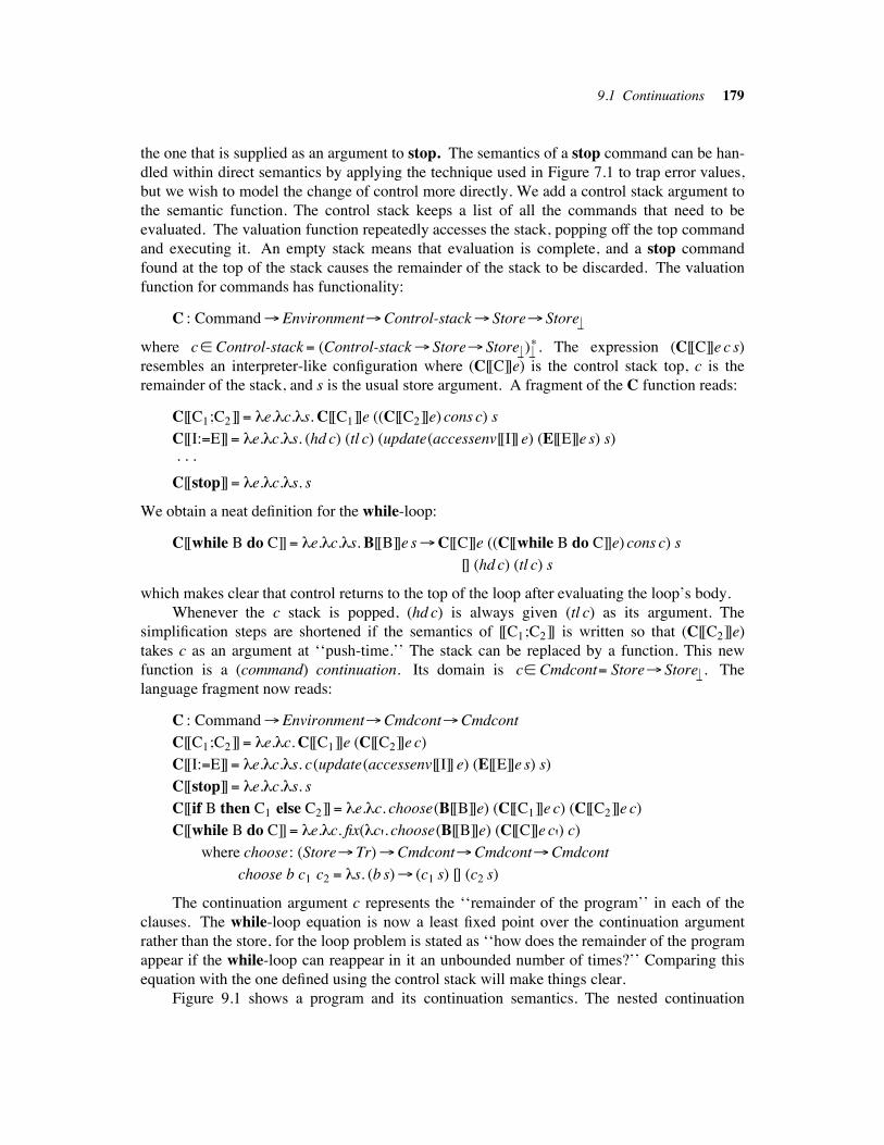
9.1 Continuations 179
the one that is supplied as an argument to stop. The semantics of a stop command can be han-
dled within direct semantics by applying the technique used in Figure 7.1 to trap error values,
but we wish to model the change of control more directly. We add a control stack argument to
the semantic function. The control stack keeps a list of all the commands that need to be
evaluated. The valuation function repeatedly accesses the stack, popping off the top command
and executing it. An empty stack means that evaluation is complete, and a stop command
found at the top of the stack causes the remainder of the stack to be discarded. The valuation
function for commands has functionality:
C : Command"Environment"Control-stack" Store" Store $!
where c# Control-stack# (Control-stack" Store" Store $!) $!$ . The expression (C[[C]]e c s)
resembles an interpreter-like configuration where (C[[C]]e) is the control stack top, c is the
remainder of the stack, and s is the usual store argument. A fragment of the C function reads:
C[[C1;C2]]# !e.!c.!s. C[[C1]]e ((C[[C2]]e) cons c) s
C[[I:#E]]# !e.!c.!s. (hd c) (tl c) (update(accessenv[[I]] e) (E[[E]]e s) s) . . .
C[[stop]]# !e.!c.!s. s
We obtain a neat definition for the while-loop:
C[[while B do C]]# !e.!c.!s. B[[B]]e s"C[[C]]e ((C[[while B do C]]e) cons c) s
[] (hd c) (tl c) s
which makes clear that control returns to the top of the loop after evaluating the loop’s body.
Whenever the c stack is popped, (hd c) is always given (tl c) as its argument. The
simplification steps are shortened if the semantics of [[C1;C2]] is written so that (C[[C2]]e)
takes c as an argument at ‘‘push-time.’’ The stack can be replaced by a function. This new
function is a (command) continuation. Its domain is c# Cmdcont# Store" Store$! . The
language fragment now reads:
C : Command"Environment"Cmdcont"Cmdcont
C[[C1;C2]]# !e.!c. C[[C1]]e (C[[C2]]e c)
C[[I:#E]]# !e.!c.!s. c(update(accessenv[[I]] e) (E[[E]]e s) s)
C[[stop]]# !e.!c.!s. s
C[[if B then C1 else C2]]# !e.!c. choose(B[[B]]e) (C[[C1]]e c) (C[[C2]]e c)
C[[while B do C]]# !e.!c. fix(!c'. choose(B[[B]]e) (C[[C]]e c') c)
where choose: (Store" Tr)"Cmdcont"Cmdcont"Cmdcont
choose b c1 c2 # !s. (b s)" (c1 s) [] (c2 s)
The continuation argument c represents the ‘‘remainder of the program’’ in each of the
clauses. The while-loop equation is now a least fixed point over the continuation argument
rather than the store, for the loop problem is stated as ‘‘how does the remainder of the program
appear if the while-loop can reappear in it an unbounded number of times?’’ Comparing this
equation with the one defined using the control stack will make things clear.
Figure 9.1 shows a program and its continuation semantics. The nested continuation
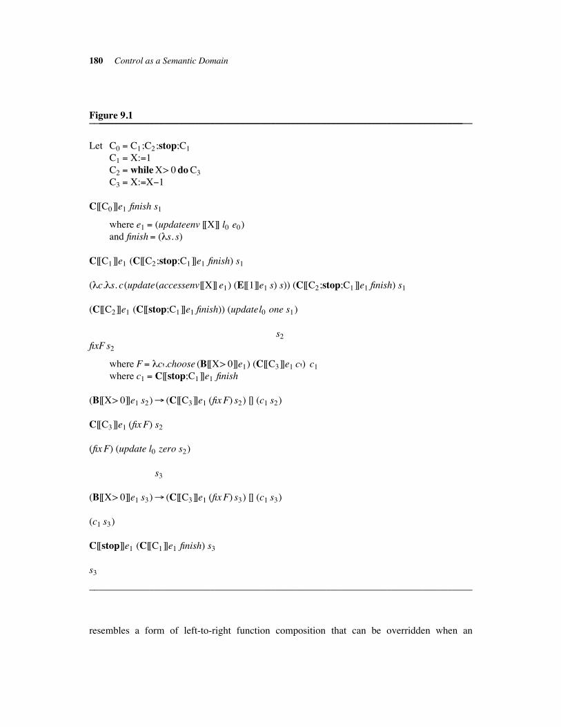
180 Control as a Semantic Domain
Figure 9.1____________________________________________________________________________________________________________________________________________________
Let C0 # C1;C2;stop;C1
C1 # X:#1
C2 # while X> 0 do C3
C3 # X:#X%1
C[[C0]]e1 finish s1
where e1 # (updateenv [[X]] l0 e0)
and finish # (!s. s)
C[[C1]]e1 (C[[C2;stop;C1]]e1 finish) s1
(!c.!s. c(update(accessenv[[X]] e1) (E[[1]]e1 s) s)) (C[[C2;stop;C1]]e1 finish) s1
(C[[C2]]e1 (C[[stop;C1]]e1 finish)) (updatel0 one s1)
s2
fixF s2
where F# !c'.choose (B[[X> 0]]e1) (C[[C3]]e1 c') c1
where c1 # C[[stop;C1]]e1 finish
(B[[X> 0]]e1 s2)" (C[[C3]]e1 (fix F) s2) [] (c1 s2)
C[[C3]]e1 (fix F) s2
(fix F) (update l0 zero s2)
s3
(B[[X> 0]]e1 s3)" (C[[C3]]e1 (fix F) s3) [] (c1 s3)
(c1 s3)
C[[stop]]e1 (C[[C1]]e1 finish) s3
s3
____________________________________________________________________________
resembles a form of left-to-right function composition that can be overridden when an
9.1 Continuations 181
extraordinary condition (e.g., a stop command) occurs. Herein lies the utility of continuations,
for normal function composition could not be overidden in a direct semantics definition.
The abstractions in the semantic equations are all nonstrict. The continuations eliminate
the need for strict abstractions on the store arguments. You can see the reason in the definition
for the while-loop: the value of (C[[while B do C]]e c s) is undefined, iff all finite expansions
of the loop map s to undefined, iff c is not applied to any store in any finite expansion. The
remainder of the program (that is, c) is never reached when a ‘‘loop forever’’ situation is
encountered. A semantic equation C[[C]]# !c.!s. c( . . . s . . . ) defines a construct [[C]] that is
guaranteed to terminate, for c is applied to the updated store. An equation
C[[C]]# !c.!s. ( . . . ) c s defines a construct whose termination is not guaranteed, so both c and
s are carried along for use by ( . . . ).
Since a continuation represents a program’s complete computation upon a store, the con-
tinuation may contain some final ‘‘cleaning up’’ instructions that produce a final output. For
example, the finish continuation used in Figure 9.1 might also be defined as
finish # (!s. ''done''), which would make all the command continuations into mappings from
stores to character strings. The general form of the command continuation domain is:
c#Cmdcont# Store"Answer
where Answer can be the domain of stores, output buffers, messages, or whatever. This gen-
eralization makes continuations especially suitable for handling unusual outputs.
9.1.1 Other Levels of Continuations !!!!!!!!!!!!!!!!!!!!!!!!!!!!!!!!!!!!!!!!!!!!!!!!!!!!!!!!!!!!!!!!!!!!!!!!!!!!!!!!!!!!!!
The semantic equations defined in the previous section show that the command valuation
function can be written in continuation style and coexist with other valuation functions written
in the direct style. Nonetheless, let’s consider representing the valuation function for expres-
sions in the continuation style. Recall that
E: Expression"Environment" Store"Expressible-value is the functionality of the valua-
tion function. In continuation form, expression evaluation breaks into explicit steps. In terms
of the control stack analogy, an expression continuation resembles a stack of evaluation steps
for computing the value of an expression. Expression continuations for some expressions will
create intermediate values that must be saved along the way. This suggests:
k# Exprcont# Expressible-value" Store"Answer'The expressible value argument to an expression continuation is the intermediate value of the
partially evaluated expression. The Answer' domain will be considered shortly.
The semantic equations for some of the expression constructs read as follows:
E: Expression"Environment"Exprcont" Store"Answer'E[[E1"E2]]# !e.!k. E[[E1]]e (!n1. E[[E2]]e (!n2. k(n1 plus n2)))
E[[I]]# !e.!k.!s. k(access(accessenv[[I]] e) s) s
E[[N]]# !e.!k. k(N[[N]])
Notice how the steps in the addition expression are spelled out by the nested continuation:
182 Control as a Semantic Domain
[[E1]] evaluates and binds to n1; [[E2]] evaluates and binds to n2; and k, the subsequent evalua-
tion, carries on with (n1 plus n2).
How do the expression continuations integrate with the command continuations? The
answer is tied to the structure of Answer'. If the ultimate answer of an expression is the value
of the expression, that is, Answer'# Expressible-value, then two different levels of control
result: expression level control and command level control. The interface between the two is a
bit awkward:
C[[I:#E]]# !e.!c.!s. c(update(accessenv[[I]] e) (E[[E]]e fin s) s)
where fin# Exprcont is fin# !n.!s. n
If Answer'# Answer, then the two levels of control integrate nicely:
C[[I:#E]]# !e.!c.!s. E[[E]]e (!n.!s'. c(update(accessenv[[I]] e) n s')) s
Now Exprcont# Expressible-value"Cmdcont, which makes clear that the purpose of a series
of expression evaluation steps is to produce a value and return back to the level of command
control. In an implementation, the code for evaluating expressions exists on the same control
stack as the code for evaluating commands.
In a similar fashion, continuations can be introduced into the other valuation functions of
a language. Even the operations of the semantic algebras can be converted. As an example, a
completely sequentialized version of assignment reads:
C[[I:#E]]# !e.!c. accessenv' [[I]] e (!l. E[[E]]e (!n. update' l n c))
where
accessenv' : Identifier"Environment" (Location"Cmdcont)"Cmdcont
accessenv'# !i.!e.!m. m(e(i))
and update' : Location"Expressible-value"Cmdcont"Cmdcont
update'# !l.!n.!c.!s. c([ l $$" n]s)
An assignment statement determines its left-hand-side value first, then its right-hand-side
value, and then the update.
Figure 9.5 shows a complete imperative language using command and expression con-
tinuations.
9.2 EXCEPTION MECHANISMS !!!!!!!!!!!!!!!!!!!!!!!!!!!!!!!!!!!!!!!!!!!!!!!!!!!!!!!!!!!!!!!!!!!!!!!!!!!!!!!!!!!!!!!!
We can use continuations to develop exception-handling mechanisms. An exception handler
is a procedure that is invoked when an extraordinary situation occurs that cannot be handled
by the usual order of evaluation. Control transfers to the handler procedure, which adjusts the
state so that computation may resume. Exception handlers of various forms can be found in
PL/1, ML, CLU, Ada, Scheme, and many other languages.
On the invocation of an exception handler, the continuation that owns the store surrenders
the store to the handler, which is also a continuation. The handler repairs the store and
9.2 Exception Mechanisms 183
relinquishes control to a continuation representing some remainder of the computation. Figure
9.2 presents a simple version that meshes with the language in Section 9.1.
An exception is signaled by [[raise I]], which discards the existing continuation and
extracts the continuation for [[I]] from the environment. The handler [[on I do C]] applies its
body to the store and yields control to the continuation that represents the commands follow-
ing the enclosing begin-end block.
It is disconcerting that the continuation c in the configuration (C[[raise I]]e c s) is dis-
carded. It suggests that the complete plan of evaluation is abandoned when an exception
handler is invoked. Actually, this is not true: the continuation assigned to the handler ‘‘over-
laps’’ the one that was discarded; the commands following the current active block are
evaluated as planned. You are left with the exercise of revising the definition so that this pro-
perty is explicit.
9.3 BACKTRACKING MECHANISMS !!!!!!!!!!!!!!!!!!!!!!!!!!!!!!!!!!!!!!!!!!!!!!!!!!!!!!!!!!!!!!!!!!!!!!!!!!!!!!
A useful variant of exception handling is the ‘‘undoing’’ of evaluation steps back to a
configuration that is ‘‘safe.’’ This version of exception handling is called backtracking. Back-
tracking is an integral feature of programming languages designed for heuristic problem-
solving: if a problem solving strategy fails, a backtrack is taken to a configuration that allows
an alternative strategy to be applied. These ‘‘strategies’’ are continuations.
We integrate a backtracking facility into a language by using a failure continuation. The
continuation representing the usual evaluation sequence is called the success continuation. The
failure continuation is invoked when backtracking is needed. Maintenance of the failure con-
tinuation is done by certain constructs in the language: exception-handler definitions, choice
constructs, cut points, and so on. Figure 9.3 presents a programming language that resembles a
propositional version of PROLOG.
The success continuation is built from the subgoals in the conjunctive construct [[C1,C2]].
The failure continuation is updated by the choice construct [[C1 or C2]], which chooses the
strategy indicated by goal [[C1]] and saves alternative strategy [[C2]] in the failure continuation;
and by the break point construct [[cut]], which disallows backtracking past the point marked by
the break point. The success continuation is applied when an endpoint [[succeedwith F]] is
encountered, and the store is updated about the achievement. Similarly, the failure continua-
tion is applied when a [[fail]] construct is encountered. The or construct saves the store in its
failure continuation so that the updates done in an unsuccessful strategy are undone. This
treatment of the store violates the usual ‘‘sequentiality’’ of store processing, and you are left
with the exercise of finding an alternative semantics that is ‘‘sequential.’’
9.4 COROUTINE MECHANISMS !!!!!!!!!!!!!!!!!!!!!!!!!!!!!!!!!!!!!!!!!!!!!!!!!!!!!!!!!!!!!!!!!!!!!!!!!!!!!!!!!!!!!!!!
Section 9.3 generalized from using one continuation to two; now we generalize to a family of
them. A system of continuations that activate one another can be used to design a coroutine
184 Control as a Semantic Domain
Figure 9.2____________________________________________________________________________________________________________________________________________________
Abstract syntax:
D# Declaration
C# Command
I# Identifier
D ::= D1;D2 | . . . | on I do C
C ::= begin D;C end | . . . | raise I
Semantic algebras:
I. Program outputs
Domain Answer# (Store" String) $!
II. Command continuations
Domain c# Cmdcont# Store"Answer
Operations
fin : Cmdcont
fin# !s. inStore(s)
err : Cmdcont
err# !s. inString(''error'')
III. Denotable values
Domain Denotable-value# Cmdcont"Nat" . . .
IV. Environments
Domain e# Environment# Identifier"Denotable-value
Operations (usual)
Valuation functions:
D: Declaration"Environment"Cmdcont"Environment
D[[D1;D2]]# !e.!c. D[[D2]] (D[[D1]]e c) c
D[[on I do C]]# !e.!c. update[[I]] inCmdcont(C[[C]]e c) e
C: Command"Environment"Cmdcont"Cmdcont
C[[begin D;C end]]# !e.!c. C[[C]] (D[[D]]e c) c
C[[raise I]]# !e.!c. cases (accessenv[[I]] e) of
isCmdcont(c')" c'[] isNat(n)" err
[] . . . end
____________________________________________________________________________
9.4 Coroutine Mechanisms 185
Figure 9.3____________________________________________________________________________________________________________________________________________________
Abstract syntax:
P# Program
D# Declaration
C# Command
I# Identifier
F# Primitive-operator
P ::= D. ?C
D ::= D1 .D2 | I & C
C ::= C1,C2 | C1 or C2 | I | succeedwith F | fail | cut
Semantic algebras:
I. Program outputs
Domain Answer# Store" String
II. Stores
Domain s# Store
186 Control as a Semantic Domain
Figure 9.3 (continued)____________________________________________________________________________________________________________________________________________________
III. Continuations
Domain c# Cmdcont# Store"Answer
fc# Failure-cont# Cmdcont
sc# Success-cont# Failure-cont"Cmdcont
Operations
succeeded : Success-cont
succeeded# !fc.!s. inStore(s)
failed : Failure-cont
failed # !s. inString(''failure'')
IV. Evaluation strategies
Domain Strategy# Success-cont"Failure-cont"Cmdcont
V. Environments
Domain e# Environment# Identifier" Strategy
Operations
emptyenv: Environment
emptyenv# !i. (!sc.!fc. fc)
accessenv: Identifier"Environment" Strategy (usual)
updateenv: Identifier" Strategy"Environment"Environment (usual)
Valuation functions:
P: Program"Cmdcont
P[[D. ?C]]# C[[C]] (D[[D]] emptyenv) succeeded failed
D: Declaration"Environment"Environment
D[[D1.D2]]# D[[D2]] % D[[D1]]
D[[I&C]]# !e. updateenv[[I]] (C[[C]]e) e
C: Command"Environment" Strategy
C[[C1,C2]]# !e.!sc. C[[C1]]e (C[[C2]]e sc)
C[[C1 or C2]]# !e.!sc.!fc.!s. C[[C1]]e sc (!s'. C[[C2]]e sc fc s) s
C[[I]]# accessenv [[I]]
C[[succeedwith F]]# !e.!sc.!fc. !s. sc fc (F[[F]]s)
C[[fail]]# !e.!sc.!fc. fc
C[[cut]]# !e.!sc.!fc. sc failed
F: Primitive-operator" Store" Store (omitted)
____________________________________________________________________________
system. Unlike a subroutine, a coroutine need not complete all the steps in its continuation
9.4 Coroutine Mechanisms 187
before relinquishing control to another. A program configuration carries along a collection of
partially completed continuations, representing the coroutines in the system. Let us call this
collection a coroutine environment. When a coroutine is invoked, the current active continua-
tion is saved in the coroutine environment. The invoked continuation is selected from the
coroutine environment and placed in control of the configuration.
A language supporting coroutines is presented in Figure 9.4.
In addition to the usual command continuation domain and the newly introduced corou-
tine environment domain, a domain of coroutine continuations is needed to handle the corou-
tine environment. The resume operation invokes a coroutine by storing the current coroutine
continuation and extracting the invoked one. The identifier carried in the coroutine environ-
ment is set to the name of the coroutine now in control of the configuration.
9.5 UNRESTRICTED BRANCHING MECHANISMS !!!!!!!!!!!!!!!!!!!!!!!!!!!!!!!!!!!!!!!!!!!!!!!!!!!!!!!!
We can generalize the coroutine mechanism so that it does not save the continuation of the
calling coroutine when another coroutine is invoked. This creates the form of branching
known as the goto. Without the promise to resume a coroutine at its point of release, the
domain of coroutine environments becomes unnecessary, and the coroutine continuation
domain becomes the command continuation domain. From here on, we speak not of corou-
tines, but of labeled commands; the [[resume I]] command is now [[goto I]].
The continuation associated with a label is kept in the usual environment, which is a
static object (unlike the coroutine environment), because the command continuation associated
with a label is determined by the label’s textual position in the program. We handle a branch
by placing the continuation associated with the destination label in control:
C[[goto I]]# !e.!c. accessenv[[I]] e.
Figure 9.5 presents a definition for a language with unrestricted branches.
So far we have ignored mutual recursion in invocations, but we must now confront the
issue if backwards branches are to be allowed. What does a branch continuation look like?
Since continuations model the remainder of a program, a continuation for a label [[I]] must not
only contain the denotation for the one command labeled by [[I]], but the denotation of the
remainder of the program that follows [[I]]: if [[I]] labels command [[Ci]], the continuation ci
associated with [[I]] is (C[[Ci]]e ci"1), where ci"1 is the continuation for the commands that fol-
low [[Ci]].
Now consider a block with n distinct labels: [[begin D; I1:C1; I2:C2; . . . In:Cn end]].
The continuations are:
c1 # (C[[C1]]e' c2)
c2 # (C[[C2]]e' c3) . . .
cn%1 # (C[[Cn%1]]e' cn)
cn # (C[[Cn]]e' c)
where e'# (updateenv[[I1]] inCmdcont(c1)
(updateenv[[I2]] inCmdcont(c2)
188 Control as a Semantic Domain
Figure 9.4____________________________________________________________________________________________________________________________________________________
Abstract syntax:
B# BlockD# DeclarationC# CommandI# Identifier
B ::= D; initiate I
D ::= D1;D2 | coroutine I#C
C ::= C1;C2 | resume I | I:#E
Semantic algebras:
I. Command continuations
Domain Cmdcont# Store"Answer $!
II. Coroutine continuations and the environments holding them
Domains c# Coroutine-cont# Coroutine-env"Cmdcont
e# Coroutine-env# ((Identifier"Coroutine-cont)& Identifier)$!Operations
quit : Coroutine-cont
err: Coroutine-cont
empty-env : Identifier"Coroutine-env
empty-env# !i. ((!i '. err), i)
initialize : Identifier"Coroutine-cont"Coroutine-env"Coroutine-env
initialize# !i.!c.!e. let (map, caller)# e in ([ i $$" c ]map, caller)
resume: Identifier"Coroutine-cont"Coroutine-env"Cmdcont
resume# !i.!c.!e. let (map, caller)# e in
let map'# [ caller $$" c ]map
in (map' i) (map', i)
Valuation functions:
B: Block"Cmdcont
B[[D; initiate I]]# resume[[I]] quit (D[[D]](empty-env [[I]]))
D: Declaration"Coroutine-env"Coroutine-env
D[[D1;D2]]# D[[D2]] % D[[D1]]
D[[coroutine I#C]]# initialize[[I]] (C[[C]] quit)
C: Command"Coroutine-cont"Coroutine-env"Cmdcont
C[[C1;C2]]# C[[C1]] % C[[C2]]
C[[resume I]]# resume[[I]]
C[[I:#E]]# !c.!e.!s. c e (update[[I]] (E[[E]]s) s)
____________________________________________________________________________
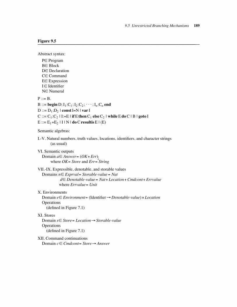
9.5 Unrestricted Branching Mechanisms 189
Figure 9.5____________________________________________________________________________________________________________________________________________________
Abstract syntax:
P# Program
B# Block
D# Declaration
C# Command
E# Expression
I# Identifier
N# Numeral
P ::= B.
B ::= begin D; I1:C1; I2:C2; . . . ; In:Cn end
D ::= D1;D2 | const I#N | var I
C ::= C1;C2 | I:#E | if E then C1 else C2 | while E do C | B | goto I
E ::= E1"E2 | I | N | do C resultis E | (E)
Semantic algebras:
I.-V. Natural numbers, truth values, locations, identifiers, and character strings
(as usual)
VI. Semantic outputs
Domain a# Answer# (OK"Err)$!where OK# Store and Err# String
VII.-IX. Expressible, denotable, and storable values
Domains n# Exprval# Storable-value# Nat
d# Denotable-value# Nat" Location"Cmdcont"Errvalue
where Errvalue# Unit
X. Environments
Domain e# Environment# (Identifier"Denotable-value)& Location
Operations
(defined in Figure 7.1)
XI. Stores
Domain s# Store# Location" Storable-value
Operations
(defined in Figure 7.1)
XII. Command continuations
Domain c# Cmdcont# Store"Answer
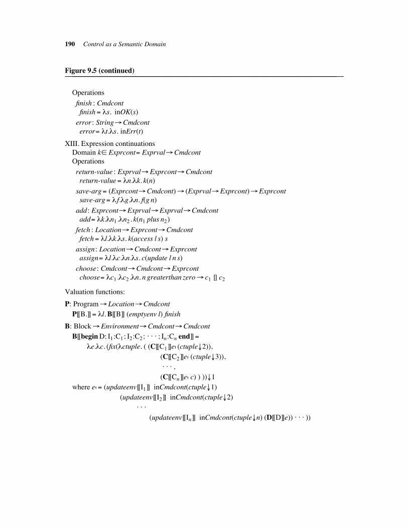
190 Control as a Semantic Domain
Figure 9.5 (continued)____________________________________________________________________________________________________________________________________________________
Operations
finish : Cmdcont
finish # !s. inOK(s)
error: String"Cmdcont
error# !t.!s. inErr(t)
XIII. Expression continuations
Domain k# Exprcont# Exprval"Cmdcont
Operations
return-value : Exprval"Exprcont"Cmdcont
return-value# !n.!k. k(n)
save-arg# (Exprcont"Cmdcont)" (Exprval"Exprcont)"Exprcont
save-arg# ! f.!g.!n. f(g n)
add: Exprcont"Exprval"Exprval"Cmdcont
add# !k.!n1 .!n2 . k(n1 plus n2)
fetch : Location"Exprcont"Cmdcont
fetch# !l.!k.!s. k(access l s) s
assign : Location"Cmdcont"Exprcont
assign# !l.!c.!n.!s. c(update l n s)
choose: Cmdcont"Cmdcont"Exprcont
choose# !c1 .!c2 .!n. n greaterthan zero" c1 [] c2
Valuation functions:
P: Program" Location"Cmdcont
P[[B.]]# !l. B[[B]] (emptyenv l) finish
B: Block"Environment"Cmdcont"Cmdcont
B[[begin D; I1:C1; I2:C2; . . . ; In:Cn end]]#
!e.!c. (fix(!ctuple. ( (C[[C1]]e' (ctuple'2)),
(C[[C2]]e' (ctuple'3)),. . . ,
(C[[Cn]]e' c) ) ))'1
where e'# (updateenv[[I1]] inCmdcont(ctuple'1)
(updateenv[[I2]] inCmdcont(ctuple'2). . .
(updateenv[[In]] inCmdcont(ctuple'n) (D[[D]]e)) . . . ))
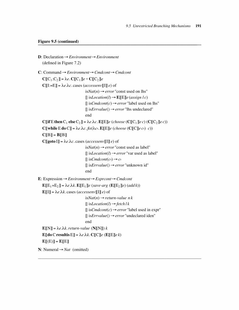
9.5 Unrestricted Branching Mechanisms 191
Figure 9.5 (continued)____________________________________________________________________________________________________________________________________________________
D: Declaration"Environment"Environment
(defined in Figure 7.2)
C: Command"Environment"Cmdcont"Cmdcont
C[[C1;C2]]# !e. C[[C1]]e % C[[C2]]e
C[[I:#E]]# !e.!c. cases (accessenv[[I]] e) of
isNat(n)" error ''const used on lhs''
[] isLocation(l)"E[[E]]e (assign l c)
[] isCmdcont(c)" error ''label used on lhs''
[] isErrvalue()" error ''lhs undeclared''
end
C[[if E then C1 else C2]]# !e.!c. E[[E]]e (choose (C[[C1]]e c) (C[[C2]]e c))
C[[while E do C]]# !e.!c. fix(!c'. E[[E]]e (choose (C[[C]]e c') c))
C[[B]]# B[[B]]
C[[goto I]]# !e.!c. cases (accessenv[[I]] e) of
isNat(n)" error ''const used as label''
[] isLocation(l)" error ''var used as label''
[] isCmdcont(c')" c'[] isErrvalue()" error ''unknown id''
end
E: Expression"Environment"Exprcont"Cmdcont
E[[E1"E2]]# !e.!k. E[[E1]]e (save-arg (E[[E2]]e) (add k))
E[[I]]# !e.!k. cases (accessenv[[I]] e) of
isNat(n)" return-value n k
[] isLocation(l)" fetch l k
[] isCmdcont(c)" error ''label used in expr''
[] isErrvalue()" error ''undeclared iden''
end
E[[N]]# !e.!k. return-value (N[[N]]) k
E[[do C resultis E]]# !e.!k. C[[C]]e (E[[E]]e k)
E[[(E)]]# E[[E]]
N: Numeral"Nat (omitted)
____________________________________________________________________________
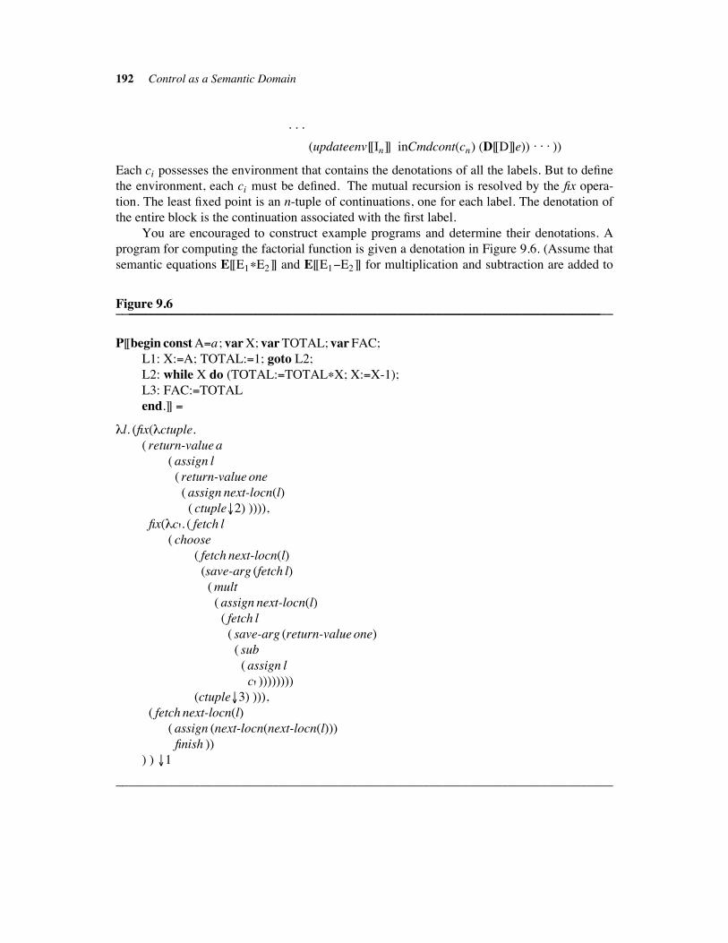
192 Control as a Semantic Domain
. . .
(updateenv[[In]] inCmdcont(cn) (D[[D]]e)) . . . ))
Each ci possesses the environment that contains the denotations of all the labels. But to define
the environment, each ci must be defined. The mutual recursion is resolved by the fix opera-
tion. The least fixed point is an n-tuple of continuations, one for each label. The denotation of
the entire block is the continuation associated with the first label.
You are encouraged to construct example programs and determine their denotations. A
program for computing the factorial function is given a denotation in Figure 9.6. (Assume that
semantic equations E[[E1$E2]] and E[[E1%E2]] for multiplication and subtraction are added to
Figure 9.6____________________________________________________________________________________________________________________________________________________
P[[begin const A#a ; var X; var TOTAL; var FAC;
L1: X:#A; TOTAL:#1; goto L2;
L2: while X do (TOTAL:#TOTAL$X; X:#X-1);
L3: FAC:#TOTAL
end.]] #
!l. (fix(!ctuple.
( return-value a
( assign l
( return-value one
( assign next-locn(l)
( ctuple'2) )))),
fix(!c'. ( fetch l
( choose
( fetch next-locn(l)
(save-arg (fetch l)
( mult
( assign next-locn(l)
( fetch l
( save-arg (return-value one)
( sub
( assign l
c' ))))))))(ctuple'3) ))),
( fetch next-locn(l)
( assign (next-locn(next-locn(l)))
finish ))
) ) '1
____________________________________________________________________________
9.5 Unrestricted Branching Mechanisms 193
the language. The equations have the same format as the one for addition, using operations
mult and sub respectively instead of add.) The denotation in Figure 9.6 is simplified to the
stage where all abstract syntax pieces and environment arguments have been written away.
The denotation of the factorial program is the first component of the least fixed point of a
functional; the functional maps a triple of command continuations to a triple of command con-
tinuations. Examining the functional’s body, we see that component number i of the triple is
the denotation of the commands labeled by identifier Li in the program. A jump to label Lk
has the denotation (ctuple'k). Each component of the tuple is a deeply nested continuation
whose actions upon the store can be read from left to right. The actions are low level and
resemble conventional assembly language instructions. This feature is exploited in the next
chapter.
9.6 THE RELATIONSHIP BETWEEN DIRECT AND
CONTINUATION SEMANTICS !!!!!!!!!!!!!!!!!!!!!!!!!!!!!!!!!!!!!!!!!!!!!!!!!!!!!!!!!!!!!!!!!!!!!!!!!!!!!!!!!!!!!!!!!!!!
A question of interest is the exact relationship between a language’s direct semantics
definition and its continuation semantics definition. We would like to prove that the two
definitions map the same program to equal denotations. But, since the internal structures of the
semantics definitions are so dissimilar, the proof can be quite difficult. A related question is
whether or not we can derive a continuation semantics definition for a language from its direct
semantics definition. Both questions are studied in the following example.
Let CD: Command" Store$!" Store$! be a valuation function written in direct semantics
style. Say that we desire a valuation function CC : Command " Cmdcont " Cmdcont,
Cmdcont # Store$! " Store $! , in continuation style such that CD is equivalent to CC . The
equivalence can be stated as CD[[C]] # CC[[C]](!s. s). But this property will be difficult to
prove by induction. Recall that in Section 9.1 we saw the format CC[[C]]# !c.!s. c(f(s)) for a
terminating command [[C]] that performs f to the store. Since CD[[C]] describes [[C]]’s actions
in isolation, the equality:
CC[[C]]c s # c(CD[[C]]s)
holds. This equality generalizes the earlier definition of equivalence; it is called a congruence,
and two definitions that satisfy a congruence are called congruent.
What about a command that might not terminate? Then CD[[C]]s might be $%, so what
should CC[[C]]c s be? If we require strict continuations, then the congruence still holds:
CC[[C]]c s # c(CD[[C]]s) # c( $%) # $%. Sethi and Tang (1980) suggest that a continuation seman-
tics for a simple language be derived from its direct semantics definition by defining
CC[[C]]c s # c(CD[[C]]s) for each construct [[C]] in the language. We then apply an inductive
hypothesis to simplify c(CD[[C]]s) into a more satisfactory form. Some derivations follow.
First, for CD[[C1;C2]] # !!!s. CD[[C2]](CD[[C1]]s), define:
CC[[C1;C2]] # !c.!!!s. c(CD[[C1;C2]]s)
# !c.!!!s. c(CD[[C2]](CD[[C1]]s))
Since CD[[C1]]s# Store$! , we can use the inductive hypothesis that CC[[C2]]c s # c(CD[[C2]]s)
194 Control as a Semantic Domain
to obtain the value !c.!!!s. CC[[C2]]c (CD[[C1]]s). But CC[[C2]]c is a command continuation, so
we apply the inductive hypothesis for [[C1]] to obtain !c.!!!s. CC[[C1]] (CC[[C2]]c) s. By exten-
sionality and the inductive hypothesis that CC[[C2]] is strict, we obtain:
CC[[C1;C2]]# CC[[C1]] % CC[[C2]]
Second, for CD[[if B then C1 else C2]] # !!!s. B[[B]]s"CD[[C1]]s [] CD[[C2]]s, we define:
CC[[if B then C1 else C2]] # !c.!!!s. c(CD[[if B then C1 else C2]]s)
# !c.!!!s. c(B[[B]]s " CD[[C1]]s [] CD[[C2]]s)
B[[B]]s is a defined truth value, so a cases analysis gives the value
!c.!!!s. B[[B]]s" c(CD[[C1]]s) [] c(CD[[C2]]s). By the inductive hypothesis for [[C1]] and [[C2]],
we obtain:
CC[[if B then C1 else C2]]# !c.!!!s. B[[B]]s"CC[[C1]]c s [] CC[[C2]]c s
Deriving the continuation semantics for a while-loop is a bit more involved. For
CD[[while B do C]]# fix(!f.!!!s. B[[B]]s" f(CD[[C]]s) [] s), we define:
CC[[while B do C]]# !c.!!!s. c(CD[[while B do C]]s)
The presence of fix thwarts our attempts at simplification. Let:
FD # !f.!!!s. B[[B]]s" f(CD[[C]]s) [] s
We hope to find a corresponding functional FC such that (fix FC)c s # c((fix FD)s). Even though
we haven’t a clue as to what FC should be, we begin constructing a fixed point induction proof
of this equality and derive FC as we go. The admissible predicate we use is:
P(fC , fD) # ‘‘for all c#Cmdcont and s# Store $! , (fC c s) # c(fD s)’’
where fC : Cmdcont"Cmdcont and fD : Store$!" Store$! .
For the basis step, we have fC # (!c.!!!s. $%) and fD # (!!!s. $%); the proof follows immediately
from strictness. For the inductive step, the inductive hypothesis is (fC c s)# c(fD s); we wish to
prove that (FC fC) c s # c((FD fD)s), deriving FC in the process. We derive:
c((FD fD)s)
# c((!!!s. B[[B]]s " fD(CD[[C]]s) [] s)s)
# c(B[[B]]s " fD(CD[[C]]s) [] s)
when s is proper. This equals:
B[[B]]s" c(fD(CD[[C]]s)) [] (c s), by distributing c across the conditional
# B[[B]]s" (fC c)(CD[[C]]s) [] (c s), by the inductive hypothesis
# B[[B]]s" CC[[C]](fC c)s [] (c s)
by the structural induction hypothesis on CD[[C]], because (fC c)#Cmdcont. If we let:
FC # !g.!c.!!!s. B[[B]]s"CC[[C]](g c) s [] (c s)
9.6 The Relationship between Direct and Continuation Semantics 195
then we are finished:
CC[[while B do C]]# fix(!g.!c.!!!s. B[[B]]s"CC[[C]](g c) s [] (c s))
The definition of while used in Figure 9.5 can be proved equal to this one with another
fixed point induction proof.
The continuation semantics CC is congruent to CD because it was defined directly from
the congruence predicate. The proof of congruence is just the derivation steps read backwards.
Few congruences between semantic definitions are as easy to prove as the one given here.
Milne and Strachey (1976), Reynolds (1974b), and Stoy (1981) give examples of nontrivial
semantics definitions and proofs of congruence.
SUGGESTED READINGS !!!!!!!!!!!!!!!!!!!!!!!!!!!!!!!!!!!!!!!!!!!!!!!!!!!!!!!!!!!!!!!!!!!!!!!!!!!!!!!!!!!!!!!!!!!!!!!!!!!!!!
Continuations: Abdali 1975; Jensen 1978; Mazurkiewicz 1971; Milne & Strachey 1976;
Strachey & Wadsworth 1974; Stoy 1977
Control mechanisms: Bjo/ rner & Jones 1982; Friedman et al. 1984; Jones 1982b; Reynolds
1972; Strachey & Wadsworth 1974
Congruences between definitions: Meyer & Wand 1985; Morris 1973; Milne & Strachey
1976; Royer 1985; Reynolds 1974b; Sethi & Tang 1980; Stoy 1981
EXERCISES !!!!!!!!!!!!!!!!!!!!!!!!!!!!!!!!!!!!!!!!!!!!!!!!!!!!!!!!!!!!!!!!!!!!!!!!!!!!!!!!!!!!!!!!!!!!!!!!!!!!!!!!!!!!!!!!!!!!!!!!!!!!
1. Add to the syntax of the language in Figure 7.2 the command exitblock, which causes a
forward branch to the end of the current block.
a. Without using continuations, integrate the exitblock construct into the semantics with
as little fuss as possible. (Hint: adjust the Poststore domain and check operation.)
b. Rewrite the semantics in continuation style and handle exitblock by discarding the
current continuation and replacing it by another.
c. Repeat parts a and b for an exitloop command that causes a branch out of the inner-
most loop; for a jump L command that causes a forward branch to a command
labeled by identifier L.
2. Convert the operations in the Nat, Environment, and Store algebras of Figure 7.1 into
continuation style.
a. Modify the access operation so that an access of an uninitialized storage cell leads
directly to an error message.
b. Introduce a division operation that handles division by zero with an error message.
c. Rewrite the semantic equations in Figure 7.2 to use the new algebras.
3. A language’s control features can be determined from the continuation domains that it
196 Control as a Semantic Domain
uses.
a. Propose the forms of branching mechanisms that will likely appear when a semantic
definition uses each of the following domains:
i. Declaration-cont# Environment"Cmdcont
ii. Denotable-value-cont# Denotable-value"Cmdcont
iii. Nat-cont# Nat"Cmdcont
iv. Location-cont# Location"Exprcont
b. A reasonable functionality for the continuation version of natural number addition is
add : Nat"Nat-cont. For each of parts i through iv, propose operations that use the
continuation domain defined.
4. Newcomers to the continuation semantics method often remark that the denotation of a
program appears to be ‘‘built backwards.’’
a. How does this idea relate to the loading of a control stack prior to interpretation? To
the compilation of a program?
b. Notice that the semantic equations of Figure 9.5 do not mention any Store-valued
objects. Consider replacing the Cmdcont algebra by a version of the Store algebra;
formulate operations for the domain Cmdcont# Store. Do programs in the new
semantics ‘‘compute backwards’’?
c. Jensen (1978) noted a strong resemblance between continuation style semantics and
weakest precondition semantics (Dijkstra 1976). Let Pred be the syntax domain of
predicate calculus expressions. The symbols ‘‘B’’ and ‘‘p’’ stand for elements of
Pred. Here is the weakest precondition semantics of a small language:
wp([[C1;C2]], p)# wp([[C1]], wp([[C2]],p))
wp([[I:#E]], p)# [E/I]p
wp([[if B then C1 else C2]], p)# ([[B]] and wp([[C1]], p))
or ((not[[B]]) and wp([[C2]], p))
wp([[while B do C]], p)# (there exists i( 0 such that Hi(p))
where H0(p)# (not([[B]]) and p)
and Hi"1(p)# wp([[if B then C else skip]], Hi(p))
and wp([[skip]], p)# p
Now consider the continuation semantics of the language. In particular, let
P : Pred"Predicate be the valuation function for predicates, where
Predicate# Store" Tr' and Tr' # Unit $! . Let true : Tr' be () and false : Tr' be $%. Define
Cmdcont# Predicate. Using the semantic equations in Section 9.1, show that
C[[C]]p# P(wp([[C]], p)).
5. Rework the semantics of Figure 9.5 so that a distinction is made between compile-time
errors and run-time computations. In particular, create the following domains:
Pgmcont# Compile-err " (Location"Computation)
Cmdcont# Compile-err "Computation
Exercises 197
Exprcont# Compile-err " (Expressible-value"Computation)
Compile-err# String
Computation # Store"Answer
Answer# (Store "Run-err)$!
Run-err# String
Formulate the semantics so that a denotable or expressible value error in a program [[P]]
implies that P[[P]]# inCompile-err(t), for some message t, and a type-correct program has
denotation P[[P]]# in(Location"Computation)(f).
6. Design an imperative language that establishes control at the expression level but not at
the command level. That is, the E valuation function uses expression continuations, but
the C valuation function is in direct semantics style. What pragmatic advantages and
disadvantages do you see?
7. Apply the principles of abstraction, parameterization, correspondence, and qualification
to the language in Figure 9.5.
8. PL/1 supports exception handlers that are invoked by machine level faults. For example,
a user can code the handler [[on zerodivide do C]], which is raised automatically when a
division by zero occurs.
a. Add the zero division exception handler to the language defined by Figures 9.2 and
9.5.
b. The user can disable an exception handler by the command [[no I]], where [[I]] is the
name of an exception handler, either built in or user defined. Add this feature to the
language.
9. In ML, exception handlers are dynamically scoped. Revise the definition in Figure 9.2 to
use dynamic scoping of handlers. How does this affect the raising of exceptions and exits
from blocks? (Consider exceptions raised from within invoked procedures.)
10. One form of coroutine structure places a hierarchy on the coroutines; a coroutine can
‘‘own’’ other coroutines. Call these the parent and child coroutines, respectively. Child
coroutines are declared local to the parent, and only a parent can call a child. A child
coroutine can pause and return control to its parent but can-not resume its siblings or
other nonrelated coroutines. Design a language with hierarchical coroutines.
11. Modify the semantics of the backtracking language in Figure 9.3 so that the commands
can recursively invoke one another.
12. Extend the list processing language in Figure 7.5 to allow jumps in expression evalua-
tion. Augment the syntax of expressions by:
E ::= . . . | catch E | throw E
The [[catch E]] construct is the intended destination of any [[throw E']] evaluated within
198 Control as a Semantic Domain
[[E]]. The value catch produces is the value of [[E']]. Evaluation of [[throw E]] aborts nor-
mal evaluation and the value of [[E]] is communicated to the nearest enclosing [[catch]].
Give the semantics of these constructs.
13. Derive the continuation semantics corresponding to the direct semantics of expressions,
using the method in Section 9.6 and the congruence EC[[E]]k s # k(ED[[E]]s) s, for:
a. The E valuation function in Figure 5.2.
b. The E valuation function in Figure 7.5.
14. Prove that the direct and continuation semantics of the language in Section 9.6 are also
congruent in an operational sense: prove that CD[[C]]s simplifies to s' iff CC[[C]]c s
simplifies to c(s').
15. Consider the conditions under which a designer uses continuation domains in a language
definition.
a. What motivates their introduction into the definition?
b. Under what conditions should some valuation functions map to continuations and
others to noncontinuation values?
c. What characteristics of a language must result if continuation domains are placed in
the language definition?
d. Are languages with continuation definitions easier to reason about (e.g., in program
equivalence proofs) than languages with direct definitions?
e. What freedom of choice of implementations is lost when continuation domains are
used?
Chapter 10 !!!!!!!!!!!!!!!!!!!!!!!!!!!!!!!!!!!!!!!!!!!!!!!!!!!!!!!
Implementation of Denotational Definitions
A language’s implementation should be guided by its semantics definition. In this chapter, we
survey techniques for deriving a compiler from a language’s semantics and examine some of
the existing automated tools for compiler generation. We also consider issues regarding the
correctness of implementations.
10.1 A GENERAL METHOD OF IMPLEMENTATION !!!!!!!!!!!!!!!!!!!!!!!!!!!!!!!!!!!!!!!!!!!!!!!!!!!!
In the previous chapters, we saw many examples of programs that were mapped to their dento-
tations and simplified to answers. The simplifications resemble the computational steps that
occur in a conventional implementation. They suggest a simple, general implementation tech-
nique: treat the semantic notation as a ‘‘machine language’’ and implement an evaluator for
the semantic notation. The denotational equations translate a program to its denotation, and the
evaluator applies simplification rules to the denotation until all possible simplifications are
performed.
As an example, consider the semantic definition in Figure 5.2. The translation of the pro-
gram [[Z:"A#1]] is the expression:
P[[Z:"A#1]] "
!n. let s " (update[[A]] n newstore) in
let s'" (!!!s. update[[Z]] (!s. (!s. access[[A]] s)s plus (!s. one)s)s s)s
in (access[[Z]] s')
(We have not bothered to expand the Store algebra operators to their underlying function
forms, e.g., access to (!i.!s. s(i)). This keeps the overall expression readable. Also, Store-
level operations are often treated specially.) The expression is applied to its run-time data, say
the number four, and is given to the evaluator, which applies the simplification rules. The
number five is the simplified result and is the output of the evaluator.
Let’s call this approach the compile-evaluate method. There is a simple variation on the
method. The example in Section 5.1 suggests that we can simultaneously translate a program
into its denotation and evaluate it with its run-time arguments. For example, the expression
P[[Z:"A#1]] four is translated to the intermediate form:
(!n. let s " (update[[A]] n newstore) in
let s'" C[[Z:"A#1]]s in (access[[Z]] s'))four
which is simplified to the expression:
199
200 Implementation of Denotational Definitions
let s'" C[[Z:"A#1]]([ [[A]] $$" four]newstore) in (access[[Z]] s')
which is translated to the expression:
let s'" (!!!s. update[[Z]] E[[A#1]]s s)([ [[A]]$$" four]newstore) in (access[[Z]] s')
which is simplified to:
let s'" update[[Z]] (E[[A#1]]([ [[A]]$$" four]newstore)) ([ [[A]]$$" four]newstore)
in (access[[Z]] s')
and so on. The result is again five. This is an interpreter approach; the denotational definition
and evaluator interact to map a source program directly to its output value. The compile-
evaluate method is more commonly used by the existing systems that implement semantic
definitions. It is closer in spirit to a conventional compiler-based system and seems to be more
amenable to optimizations.
10.1.1 The SIS and SPS Systems !!!!!!!!!!!!!!!!!!!!!!!!!!!!!!!!!!!!!!!!!!!!!!!!!!!!!!!!!!!!!!!!!!!!!!!!!!!!!!!!!!!!!!!!!!!!
Two compiler generator systems based on the compile-evaluate method are Mosses’s Seman-
tics Implementation System (SIS) and Wand’s Semantics Prototyping System (SPS). SIS was
the first compiler generating system based on denotational semantics. Figure 10.1 shows the
components and data flow of the system.
SIS consists of a parser generator and an encoder generator. The parser generator pro-
duces an SLR(1) parser from an input BNF definition coded in a notation called GRAM. The
semantic definition, coded in DSL, is read by the encoder generator, which produces an
encoder, that is, a translator from abstract syntax trees to ‘‘LAMB-denotations.’’ A source
program is parsed by the parser and is translated by the encoder. The source program’s denota-
tion plus its input values are passed to the evaluator for simplification. The definitions of run-
time operations (such as the operations from the Store algebra) are supplied at this time. The
evaluator uses a call-by-need simplification strategy: an expression (!x.M)N simplifies to M,
and the binding (x, N) is retained by the evaluator in an environment table. When an
occurrence of x is encountered in M, N is fetched from the table, simplified to its value v, and
used for x. The binding (x,v) replaces (x, N) in the table. This strategy handles combinations
more efficiently than the usual textual substitution method.
SIS is coded in BCPL. It has been used to implement a number of test languages. Its
strengths include its simplicity and generality— virtually any denotational definition can be
implemented using SIS. The system’s primary weakness is its inefficiency: the generated
compilers are large and the compiled programs run slowly. Nonetheless, SIS is an important
example of an automated system that produces a correct compiler from a language’s formal
specification. It has inspired many researchers to develop more efficient and specialized sys-
tems.
Wand’s SPS system is based on existing software tools. The system’s parser generator is
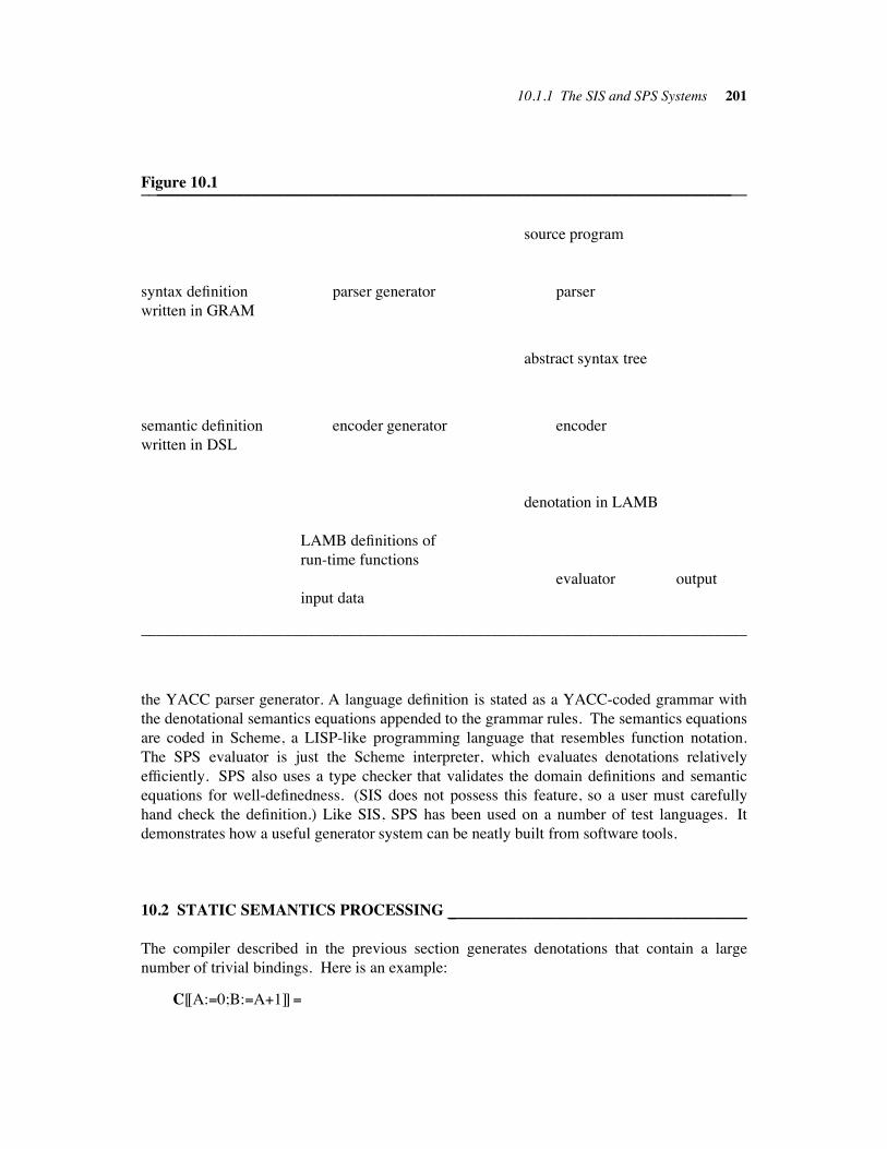
10.1.1 The SIS and SPS Systems 201
Figure 10.1____________________________________________________________________________________________________________________________________________________
source program
syntax definition parser generator parser
written in GRAM
abstract syntax tree
semantic definition encoder generator encoder
written in DSL
denotation in LAMB
LAMB definitions of
run-time functions
evaluator output
input data
____________________________________________________________________________
the YACC parser generator. A language definition is stated as a YACC-coded grammar with
the denotational semantics equations appended to the grammar rules. The semantics equations
are coded in Scheme, a LISP-like programming language that resembles function notation.
The SPS evaluator is just the Scheme interpreter, which evaluates denotations relatively
efficiently. SPS also uses a type checker that validates the domain definitions and semantic
equations for well-definedness. (SIS does not possess this feature, so a user must carefully
hand check the definition.) Like SIS, SPS has been used on a number of test languages. It
demonstrates how a useful generator system can be neatly built from software tools.
10.2 STATIC SEMANTICS PROCESSING !!!!!!!!!!!!!!!!!!!!!!!!!!!!!!!!!!!!!!!!!!!!!!!!!!!!!!!!!!!!!!!!!!!!!!!!!!
The compiler described in the previous section generates denotations that contain a large
number of trivial bindings. Here is an example:
C[[A:"0;B:"A#1]]"
202 Implementation of Denotational Definitions
!!!s. (!!!s. update[[B]] (!s. (!s. access[[A]] s)s plus (!s. one)s)s s)
((!!!s. update[[A]] (!s. zero)s s)s)
Trivial bindings of the form (!s. E)s should be simplified to E prior to run-time. We call these
compile-time simplifications partial evaluation or even static semantics processing. Static
semantics processing performs those evaluation steps that are not dependent on run-time
values. In traditional compilers, static semantics processing includes declaration processing,
type checking, and constant folding.
How do we determine which simplifications to perform? We call an expression unfrozen
if it can be simplified before run-time. A frozen expression may not be simplified. Once we
decide which semantic algebras define run-time values, we freeze the operations in those alge-
bras. An example of an algebra that is typically frozen is the Store algebra. The algebras of
truth values and numbers are frozen if the evaluation of Boolean and arithmetic expressions is
left until run-time. (In compilers that do constant folding, Tr and Nat are unfrozen.)
During static semantics processing, we simplify each subexpression of a denotation as far
as possible until we encounter a frozen operation; then we are forced to stop. Say that the
Store and Nat algebras are frozen in the above example. Then the subexpression
(!!!s. update [[A]] (!s. zero)s s)s simplifies to (update [[A]] zero s), but no further, because
update is a frozen operation. The simplified subexpression itself is now ‘‘frozen.’’ Frozen
subexpressions impact other simplifications; a combination (!x. M)N, where N is a frozen
subexpression, is not simplified. (But M itself may be simplified.) Also, some static semantics
simplifiers refuse to simplify (!x. M)N if unfrozen N is a nonconstant or nonidentifier and
occurs free in M more than once, for the resulting expression would be larger, not smaller,
than the original.
For the above example with the Store and Nat algebras frozen, static semantics produces:
!!!s. (!!!s.update[[B]] ((access[[A]] s) plus one) s) (update[[A]] zero s)
which is the expected ‘‘machine code’’ for the command.
Static semantics processing is most useful for simplifying denotations that contain
environment arguments. Recall the block-structured language in Section 7.1. Environments
process declarations, reserve storage, and map identifiers to denotable values. Environment-
related actions are traditionally performed at compile-time. The example in that section
showed that the denotation of a program can be simplified to a point where all references to
environment arguments disappear. The simplifications are exactly those that would be per-
formed during static semantics processing, because the Environment algebra is unfrozen.
The SIS system does static semantics processing. However, SIS does not freeze any
expressions; it simplifies every possible subexpression. The method works because the
definitions of the frozen operators (such as the Store-based ones) are not supplied until run-
time. Thus, any expression using a run-time operation is not simplifiable.
10.3 The Structure of the Evaluator 203
10.3 THE STRUCTURE OF THE EVALUATOR !!!!!!!!!!!!!!!!!!!!!!!!!!!!!!!!!!!!!!!!!!!!!!!!!!!!!!!!!!!!!!!!
We use the equalities in Section 3.5 to simplify expressions. From here on, we treat the equal-
ities as rewriting rules. An equality M"N induces a rewriting rule M "> N; an occurrence of M
in an expression is reduced (simplified) to N by the rule. For example, (!x. M)N "> [N/x]M is
a rewriting rule, and is in fact a rather famous one, called the #-rule. An expression whose
structure matches the left hand side of a rewriting rule is a redex, and the expression that
results from reducing a redex is called its contractum. We write E1 "> E2 if expression E1
rewrites to E2 in one step and write E1 ">$ E2 if zero or more steps are used. An expression
that contains no redexes is in normal form. We say that an expression has a normal form if it
can be reduced to an expression in normal form. Not all expressions have normal forms (e.g.,
(!x. x x)(!x. x x), where x%G"G"G). An important feature of the rules for function notation
is that if an expression does have a normal form then it is unique. This property follows from
the confluence (Church-Rosser) property: if E1 ">$ E2 and E1 ">
$ E3, then some E4 exists
such that E2 ">$ E4 and E3 ">
$ E4.
An evaluator applies rewriting rules to its argument until a normal form (if it exists) is
reached. The evaluator should apply the rules in a fashion that is sufficient for achieving a
normal form. (For example, (!y. zero) ((!x. x x) (!x. x x)) has the normal form zero, but per-
petually reducing the argument (!x. x x)(!x. x x) will never produce it.) A strategy sufficient for
reducing an expression to normal form is the leftmost-outermost method: at each reduction
step, we reduce the leftmost redex that is not contained within another redex. (We make the
statement that the leftmost-outermost method is sufficient with the understanding that a combi-
nation (!!!x. M)N, where N itself is a function, argument combination, should be ‘‘read back-
wards’’ as ‘‘N(M.x!!!).’’ Recall that a strict abstraction requires a proper argument, hence its
argument must be reduced until its proper structure— a pair, injection, abstraction, number, or
whatever— appears. Then the #-reduction is made.) Here is a leftmost-outermost reduction:
(!x. (x x)zero)((!y. (!!!z. z))((!x. x x)(!x. x x)))
"> (((!y. (!!!z. z))((!x. x x)(!x. x x))) ((!y. (!!!z. z))((!x. x x)(!x. x x))))zero
"> ((!!!z. z) ((!y. (!!!z. z))((!x. x x)(!x. x x))))zero
"> ((!!!z. z) (!!!z. z))zero
"> (!!!z. z)zero
"> zero
One way of implementing the leftmost-outermost reduction strategy is to represent the
expression to be reduced as a tree. The evaluator does a left-to-right, depth-first traversal of the
tree. When a node in the tree is visited, the evaluator determines if the subtree whose root is
the visited node is a redex. If it is not, the evaluator visits the next node in its traversal. But if
it is, the evaluator removes the tree, does the reduction, and inserts the contractum for the
redex. The next node visited is the parent node of the contractum’s, for the evaluator must
backtrack up the tree to see if the insertion of the contractum created a new outermost redex.
An inefficiency of the tree reduction method lies in its reduction of a redex (!x. M)N:
occurrences of N must be inserted in place of occurrences of x in M in the contractum. A
traversal of M’s tree is required for the insertions. Then, M is traversed a second time to reduce
its redexes. These two traversals can be combined into one: the evaluator can insert an N for
an x when it encounters x during its traversal of M for reductions. In the meantime, the binding
204 Implementation of Denotational Definitions
of x to N can be kept in an environment. An environment is a collection of identifier, expres-
sion pairs, chained together in the shape of an inverted tree. The environment holds the argu-
ments bound to identifiers as a result of #-reductions. Every node in the expression tree has a
pointer into the environment. The pointer points to a linked list (that is, a path in the inverted
tree) of the bindings that belong to the node. The inverted tree structure of the environment
results because distinct nodes sometimes share bindings in their lists.
When a redex R" (!x. M)N reduces to M, the binding (x, N) is chained to the front of the
list pointed to by M’s environment pointer. M’s new pointer points to the binding (x, N) fol-
lowed by the previous list of bindings. When a free occurrence of x is visited in M, the evalua-
tor follows the environment pointer attached to x to find the first pair (x, N) in the chain of
bindings. N (and its pointer) replace x in the expression. A clever evaluator evaluates x by
leaving N in its place in the environment and simplifying it there. Once N reduces to a proper
value, that value is copied over into the expression tree in x’s place. Subsequent lookups of x
in the environment find the reduced value. This approach is known as call-by-need evaluation.
10.3.1 A Stack-Based Evaluator !!!!!!!!!!!!!!!!!!!!!!!!!!!!!!!!!!!!!!!!!!!!!!!!!!!!!!!!!!!!!!!!!!!!!!!!!!!!!!!!!!!!!!!!!!!!!!
The tree traversal method is slow and bulky. There is too much copying of contractums in
place of redexes into the expression tree, and there is too much backtracking during tree
traversal. Further, the representation of the expression as a tree occupies a wasteful amount of
space. We can represent the leftmost-outermost reduction of an expression in a more conven-
tional form. We use a stack-based machine as an evaluator; an expression is translated into a
sequence of machine instructions that describes a leftmost-outermost reduction of the expres-
sion. The traversal and reduction steps can be translated into machine code because function
expressions are statically scoped, so environment maintenance is routine, and because the
traversal path through the expression can be calculated from the structure of the expression.
Figure 10.2 shows the stack machine. We call it the VEC-machine because it possesses three
components:
1. A temporary value stack, v, which holds subexpressions that have been reduced to proper
values and expressions whose evaluation has been postponed.
2. An environment, e, which stacks environment pointers and establishes the scope of the
current expression being reduced.
3. A code stack, c, which holds the machine instructions for the reduction. Rather than
using an instruction counter, we treat the instructions as a stack. The top instruction on
the stack is the one executed, and a stack pop corresponds to an increment of the instruc-
tion counter to the next instruction in the code.
We represent a machine configuration as a triple (v e c). Each of the three components in
the configuration is represented in the form a1:a2: . . . :an , where a1 is the top value on the
component’s stack.
Two of the machine’s key data structures are the environment pointer and the closure. An
environment pointer is a pointer value to a linked list of identifier, value bindings. (Read the
@ symbol as saying ‘‘a pointer to.’’) All the bindings are kept in the environment tree, which
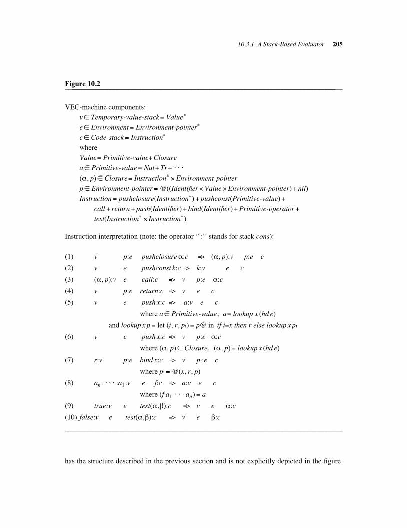
10.3.1 A Stack-Based Evaluator 205
Figure 10.2____________________________________________________________________________________________________________________________________________________
VEC-machine components:
v% Temporary-value-stack" Value $
e% Environment" Environment-pointer$
c% Code-stack" Instruction$
where
Value" Primitive-value#Closure
a% Primitive-value" Nat# Tr# . . .
(&, p)% Closure" Instruction$ %Environment-pointer
p% Environment-pointer" @((Identifier%Value%Environment-pointer)# nil)
Instruction " pushclosure(Instruction$)# pushconst(Primitive-value)#
call# return# push(Identifier)# bind(Identifier)#Primitive-operator#
test(Instruction$ % Instruction$)
Instruction interpretation (note: the operator ‘‘:’’ stands for stack cons):
(1) v p:e pushclosure&:c "> (&, p):v p:e c
(2) v e pushconst k:c "> k:v e c
(3) (&, p):v e call:c "> v p:e &:c
(4) v p:e return:c "> v e c
(5) v e push x:c "> a:v e c
where a% Primitive-value, a" lookup x (hd e)
and lookup x p" let (i, r, p')" p@ in if i"x then r else lookup x p'(6) v e push x:c "> v p:e &:c
where (&, p)% Closure, (&, p)" lookup x (hd e)
(7) r:v p:e bind x:c "> v p':e c
where p'" @(x, r, p)
(8) an: . . . :a1:v e f:c "> a:v e c
where (f a1. . . an)" a
(9) true:v e test(&,#):c "> v e &:c
(10) false:v e test(&,#):c "> v e #:c
____________________________________________________________________________
has the structure described in the previous section and is not explicitly depicted in the figure.
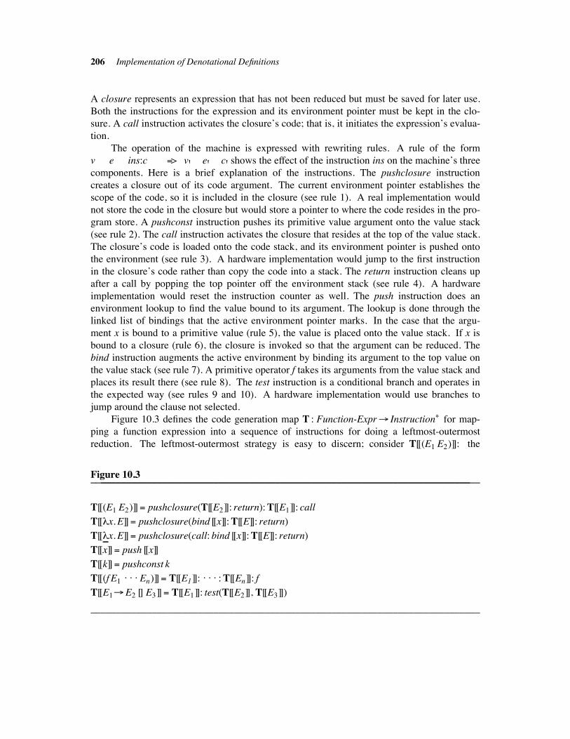
206 Implementation of Denotational Definitions
A closure represents an expression that has not been reduced but must be saved for later use.
Both the instructions for the expression and its environment pointer must be kept in the clo-
sure. A call instruction activates the closure’s code; that is, it initiates the expression’s evalua-
tion.
The operation of the machine is expressed with rewriting rules. A rule of the form
v e ins:c "> v' e' c' shows the effect of the instruction ins on the machine’s three
components. Here is a brief explanation of the instructions. The pushclosure instruction
creates a closure out of its code argument. The current environment pointer establishes the
scope of the code, so it is included in the closure (see rule 1). A real implementation would
not store the code in the closure but would store a pointer to where the code resides in the pro-
gram store. A pushconst instruction pushes its primitive value argument onto the value stack
(see rule 2). The call instruction activates the closure that resides at the top of the value stack.
The closure’s code is loaded onto the code stack, and its environment pointer is pushed onto
the environment (see rule 3). A hardware implementation would jump to the first instruction
in the closure’s code rather than copy the code into a stack. The return instruction cleans up
after a call by popping the top pointer off the environment stack (see rule 4). A hardware
implementation would reset the instruction counter as well. The push instruction does an
environment lookup to find the value bound to its argument. The lookup is done through the
linked list of bindings that the active environment pointer marks. In the case that the argu-
ment x is bound to a primitive value (rule 5), the value is placed onto the value stack. If x is
bound to a closure (rule 6), the closure is invoked so that the argument can be reduced. The
bind instruction augments the active environment by binding its argument to the top value on
the value stack (see rule 7). A primitive operator f takes its arguments from the value stack and
places its result there (see rule 8). The test instruction is a conditional branch and operates in
the expected way (see rules 9 and 10). A hardware implementation would use branches to
jump around the clause not selected.
Figure 10.3 defines the code generation map T : Function-Expr" Instruction$ for map-
ping a function expression into a sequence of instructions for doing a leftmost-outermost
reduction. The leftmost-outermost strategy is easy to discern; consider T[[(E1 E2)]]: the
Figure 10.3____________________________________________________________________________________________________________________________________________________
T[[(E1 E2)]]" pushclosure(T[[E2]]: return): T[[E1]]: call
T[[!x. E]]" pushclosure(bind [[x]]: T[[E]]: return)
T[[!!!x. E]]" pushclosure(call: bind [[x]]: T[[E]]: return)
T[[x]]" push [[x]]
T[[k]]" pushconst k
T[[(f E1. . . En)]]" T[[E1]]: . . . : T[[En]]: f
T[[E1"E2 [] E3]]" T[[E1]]: test(T[[E2]], T[[E3]])
____________________________________________________________________________
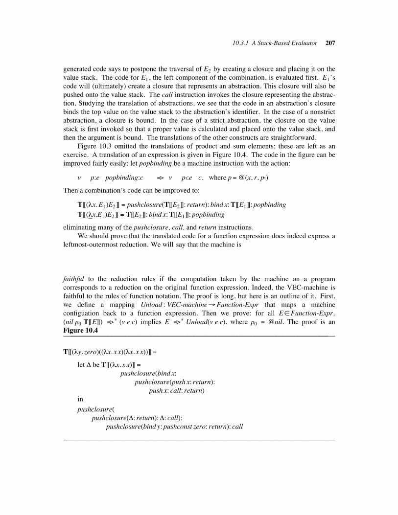
10.3.1 A Stack-Based Evaluator 207
generated code says to postpone the traversal of E2 by creating a closure and placing it on the
value stack. The code for E1, the left component of the combination, is evaluated first. E1’s
code will (ultimately) create a closure that represents an abstraction. This closure will also be
pushed onto the value stack. The call instruction invokes the closure representing the abstrac-
tion. Studying the translation of abstractions, we see that the code in an abstraction’s closure
binds the top value on the value stack to the abstraction’s identifier. In the case of a nonstrict
abstraction, a closure is bound. In the case of a strict abstraction, the closure on the value
stack is first invoked so that a proper value is calculated and placed onto the value stack, and
then the argument is bound. The translations of the other constructs are straightforward.
Figure 10.3 omitted the translations of product and sum elements; these are left as an
exercise. A translation of an expression is given in Figure 10.4. The code in the figure can be
improved fairly easily: let popbinding be a machine instruction with the action:
v p:e popbinding:c "> v p':e c, where p" @(x, r, p')
Then a combination’s code can be improved to:
T[[(!x. E1)E2]] " pushclosure(T[[E2]]: return): bind x: T[[E1]]: popbinding
T[[(!!!x.E1)E2]] " T[[E2]]: bind x: T[[E1]]: popbinding
eliminating many of the pushclosure, call, and return instructions.
We should prove that the translated code for a function expression does indeed express a
leftmost-outermost reduction. We will say that the machine is
faithful to the reduction rules if the computation taken by the machine on a program
corresponds to a reduction on the original function expression. Indeed, the VEC-machine is
faithful to the rules of function notation. The proof is long, but here is an outline of it. First,
we define a mapping Unload : VEC-machine"Function-Expr that maps a machine
configuation back to a function expression. Then we prove: for all E%Function-Expr,
(nil p0 T[[E]]) ">$ (v e c) implies E ">$ Unload(v e c), where p0 " @nil. The proof is an
Figure 10.4____________________________________________________________________________________________________________________________________________________
T[[(!y. zero)((!x. x x)(!x. x x))]]"
let ' be T[[(!x. x x)]]"pushclosure(bind x:
pushclosure(push x: return):
push x: call: return)
in
pushclosure(
pushclosure(': return):': call):
pushclosure(bind y: pushconst zero: return): call
____________________________________________________________________________
208 Implementation of Denotational Definitions
induction on the number of machine moves. The basis, zero moves, is the proof that
Unload(nil p0 T[[E]])" E; the inductive step follows from the proof that (v e c) "> (v' e' c')implies Unload(v e c) ">$ Unload(v' e' c'). Unload’s definition and the proof are left as exer-
cises.
Another aspect of the correctness of the VEC-machine is its termination properties: does
the machine produce a completely simplified answer exactly when the reduction rules do?
Actually, the VEC-machine is conservative. It ceases evaluation on an abstraction when the
abstraction has no argument; the abstraction’s body is not simplified. Nonetheless, the
machine does reduce to final answers those terms that reduce to nonabstraction (hereafter
called first-order) values. The VEC-machine resembles a real-life machine in this regard.
The VEC-machine evaluates function expressions more efficiently than the reduction
rules because it uses its stacks to hold intermediate values. Rather than searching through the
expression for a redex, the code deterministically traverses through the expression until (the
code for) a redex appears on the top of the c stack. Simplified values are moved to the v
stack— substitutions into the expression are never made.
Here is the current version of the compile-evaluate method that we have developed. The
compile step is:
1. Map a program P to its denotation P[[P]].
2. Perform static semantics analysis on P[[P]], producing a denotation d.
3. Map d to its machine code T[[d]].
The evaluate step is: load T[[d]] into the VEC-machine, creating a configuration
(nil @nil T[[d]]), and run the machine to a final configuration (r:v e nil). The answer is r.
10.3.2 PSP and Appel’s System !!!!!!!!!!!!!!!!!!!!!!!!!!!!!!!!!!!!!!!!!!!!!!!!!!!!!!!!!!!!!!!!!!!!!!!!!!!!!!!!!!!!!!!!!!!!!!
Paulson’s Semantic Processor (PSP) system generates compilers that map programs into stack
machine code. The PSP evaluator resembles the stack architecture just developed. In PSP, a
language is defined with semantic grammars, a hybrid of denotational semantics and attribute
grammars. The semantic grammar for a language is input to the grammar analyzer, which
produces a language description file containing an LALR(1) parse table and the semantic
equations for the language. Figure 10.5 shows the components.
The universal translator uses the language description file to compile a source program.
A source program is parsed, mapped to its function expression form, partially evaluated, and
mapped to stack machine code.
The static semantics stage in PSP does more than just partial evaluation. It also enforces
contextual constraints (such as data type compatibility) that are specified in the semantic
grammar. Efficient representations of abstractions and data values (like stores) are created.
PSP has been used to generate a compiler for a large subset of Pascal; the generated compiler
runs roughly 25 times slower than a handwritten one but is smaller than the handwritten com-
piler.
Appel’s compiler-generating system produces compilers that translate source programs to
register machine code. Static semantics and code generation are simultaneously performed by
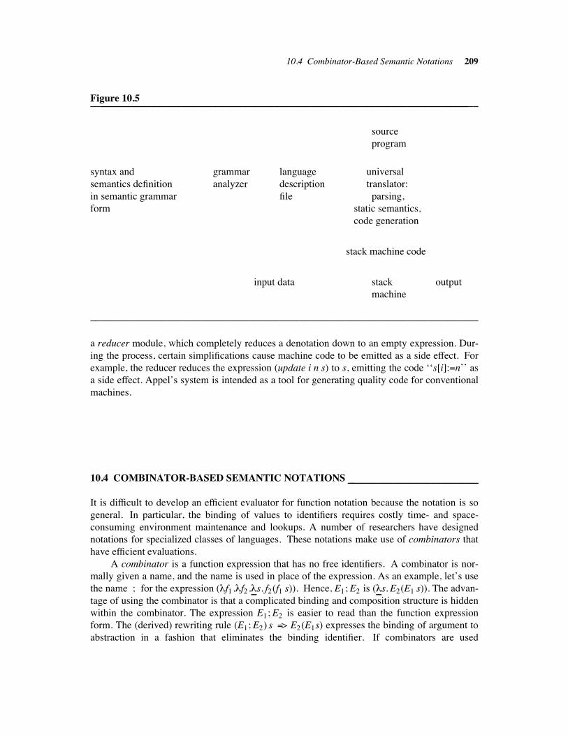
10.4 Combinator-Based Semantic Notations 209
Figure 10.5____________________________________________________________________________________________________________________________________________________
source
program
syntax and grammar language universal
semantics definition analyzer description translator:
in semantic grammar file parsing,
form static semantics,
code generation
stack machine code
input data stack output
machine
____________________________________________________________________________
a reducer module, which completely reduces a denotation down to an empty expression. Dur-
ing the process, certain simplifications cause machine code to be emitted as a side effect. For
example, the reducer reduces the expression (update i n s) to s, emitting the code ‘‘s[i]:"n’’ as
a side effect. Appel’s system is intended as a tool for generating quality code for conventional
machines.
10.4 COMBINATOR-BASED SEMANTIC NOTATIONS !!!!!!!!!!!!!!!!!!!!!!!!!!!!!!!!!!!!!!!!!!!!!!!!!!
It is difficult to develop an efficient evaluator for function notation because the notation is so
general. In particular, the binding of values to identifiers requires costly time- and space-
consuming environment maintenance and lookups. A number of researchers have designed
notations for specialized classes of languages. These notations make use of combinators that
have efficient evaluations.
A combinator is a function expression that has no free identifiers. A combinator is nor-
mally given a name, and the name is used in place of the expression. As an example, let’s use
the name ; for the expression (!f1 .!f2 .!!!s. f2(f1 s)). Hence, E1; E2 is (!!!s. E2(E1 s)). The advan-
tage of using the combinator is that a complicated binding and composition structure is hidden
within the combinator. The expression E1; E2 is easier to read than the function expression
form. The (derived) rewriting rule (E1; E2) s "> E2(E1s) expresses the binding of argument to
abstraction in a fashion that eliminates the binding identifier. If combinators are used
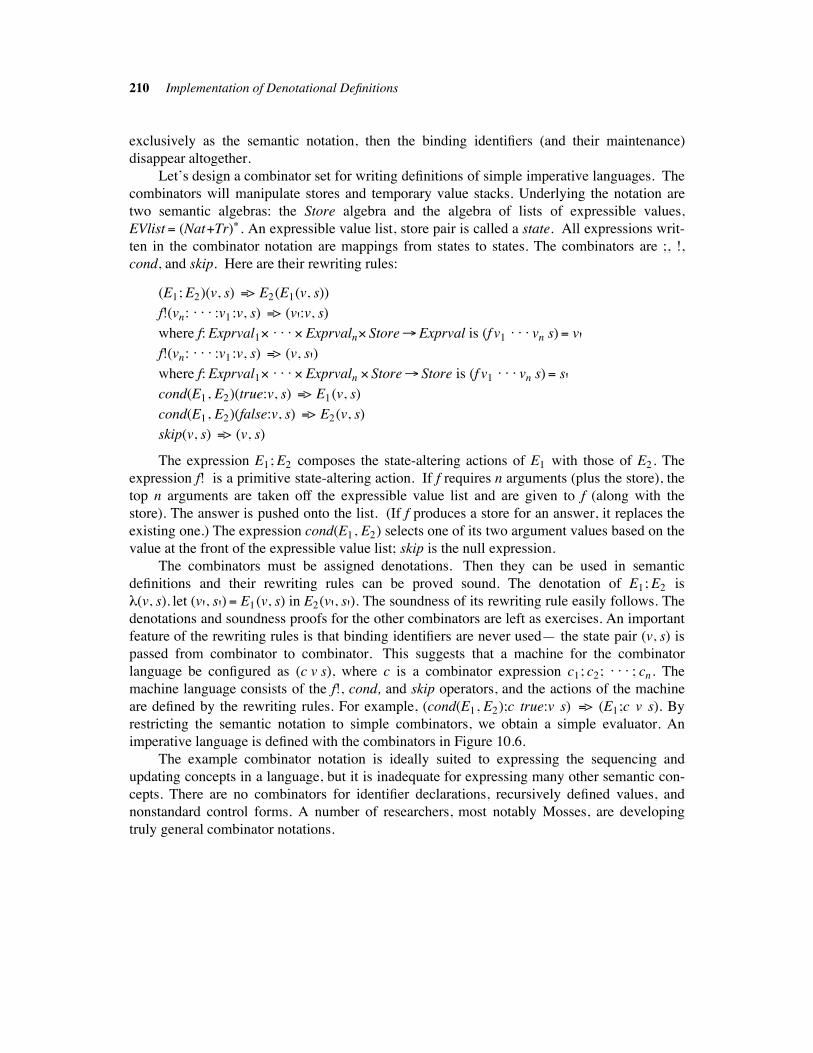
210 Implementation of Denotational Definitions
exclusively as the semantic notation, then the binding identifiers (and their maintenance)
disappear altogether.
Let’s design a combinator set for writing definitions of simple imperative languages. The
combinators will manipulate stores and temporary value stacks. Underlying the notation are
two semantic algebras: the Store algebra and the algebra of lists of expressible values,
EVlist " (Nat#Tr)$ . An expressible value list, store pair is called a state. All expressions writ-
ten in the combinator notation are mappings from states to states. The combinators are ;, !,
cond, and skip. Here are their rewriting rules:
(E1; E2)(v, s) "> E2(E1(v, s))
f!(vn: . . . :v1 :v, s) "> (v':v, s)
where f: Exprval1% . . . % Exprvaln% Store"Exprval is (f v1 . . . vn s)" v'
f!(vn: . . . :v1 :v, s) "> (v, s')where f: Exprval1% . . . % Exprvaln % Store" Store is (f v1
. . . vn s)" s'cond(E1, E2)(true:v, s) "> E1(v, s)
cond(E1, E2)(false:v, s) "> E2(v, s)
skip(v, s) "> (v, s)
The expression E1; E2 composes the state-altering actions of E1 with those of E2. The
expression f! is a primitive state-altering action. If f requires n arguments (plus the store), the
top n arguments are taken off the expressible value list and are given to f (along with the
store). The answer is pushed onto the list. (If f produces a store for an answer, it replaces the
existing one.) The expression cond(E1, E2) selects one of its two argument values based on the
value at the front of the expressible value list; skip is the null expression.
The combinators must be assigned denotations. Then they can be used in semantic
definitions and their rewriting rules can be proved sound. The denotation of E1; E2 is
!(v, s). let (v', s')" E1(v, s) in E2(v', s'). The soundness of its rewriting rule easily follows. The
denotations and soundness proofs for the other combinators are left as exercises. An important
feature of the rewriting rules is that binding identifiers are never used— the state pair (v, s) is
passed from combinator to combinator. This suggests that a machine for the combinator
language be configured as (c v s), where c is a combinator expression c1; c2; . . . ; cn. The
machine language consists of the f!, cond, and skip operators, and the actions of the machine
are defined by the rewriting rules. For example, (cond(E1, E2);c true:v s) "> (E1;c v s). By
restricting the semantic notation to simple combinators, we obtain a simple evaluator. An
imperative language is defined with the combinators in Figure 10.6.
The example combinator notation is ideally suited to expressing the sequencing and
updating concepts in a language, but it is inadequate for expressing many other semantic con-
cepts. There are no combinators for identifier declarations, recursively defined values, and
nonstandard control forms. A number of researchers, most notably Mosses, are developing
truly general combinator notations.
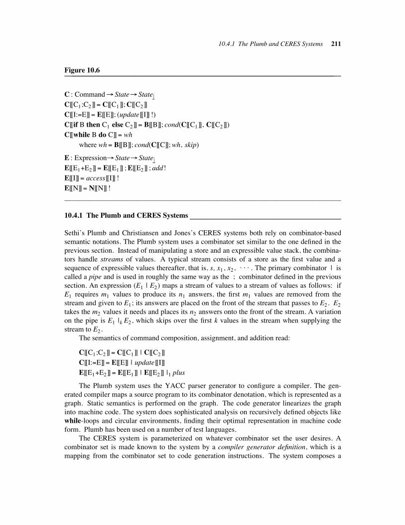
10.4.1 The Plumb and CERES Systems 211
Figure 10.6____________________________________________________________________________________________________________________________________________________
C : Command" State" State $!
C[[C1;C2]]" C[[C1]]; C[[C2]]
C[[I:"E]]" E[[E]]; (update[[I]] !)
C[[if B then C1 else C2]]" B[[B]]; cond(C[[C1]], C[[C2]])
C[[while B do C]]" wh
where wh " B[[B]]; cond(C[[C]]; wh, skip)
E : Expression" State" State $!
E[[E1#E2]]" E[[E1]] ; E[[E2]] ; add!
E[[I]]" access[[I]] !
E[[N]]" N[[N]] !
____________________________________________________________________________
10.4.1 The Plumb and CERES Systems !!!!!!!!!!!!!!!!!!!!!!!!!!!!!!!!!!!!!!!!!!!!!!!!!!!!!!!!!!!!!!!!!!!!!!!!!!!!!!!!!!
Sethi’s Plumb and Christiansen and Jones’s CERES systems both rely on combinator-based
semantic notations. The Plumb system uses a combinator set similar to the one defined in the
previous section. Instead of manipulating a store and an expressible value stack, the combina-
tors handle streams of values. A typical stream consists of a store as the first value and a
sequence of expressible values thereafter, that is, s, x1, x2, . . . . The primary combinator | is
called a pipe and is used in roughly the same way as the ; combinator defined in the previous
section. An expression (E1 | E2) maps a stream of values to a stream of values as follows: if
E1 requires m1 values to produce its n1 answers, the first m1 values are removed from the
stream and given to E1; its answers are placed on the front of the stream that passes to E2. E2
takes the m2 values it needs and places its n2 answers onto the front of the stream. A variation
on the pipe is E1 |k E2, which skips over the first k values in the stream when supplying the
stream to E2.
The semantics of command composition, assignment, and addition read:
C[[C1;C2]]" C[[C1]] | C[[C2]]
C[[I:"E]]" E[[E]] | update[[I]]
E[[E1#E2]]" E[[E1]] | E[[E2]] |1 plus
The Plumb system uses the YACC parser generator to configure a compiler. The gen-
erated compiler maps a source program to its combinator denotation, which is represented as a
graph. Static semantics is performed on the graph. The code generator linearizes the graph
into machine code. The system does sophisticated analysis on recursively defined objects like
while-loops and circular environments, finding their optimal representation in machine code
form. Plumb has been used on a number of test languages.
The CERES system is parameterized on whatever combinator set the user desires. A
combinator set is made known to the system by a compiler generator definition, which is a
mapping from the combinator set to code generation instructions. The system composes a
212 Implementation of Denotational Definitions
language’s semantic definition with the compiler generator definition to generate the compiler
for the language. CERES is designed to be a development tool for a variety of applications,
rather than a compiler generator for a narrow class of languages. It also has been used on test
languages.
10.5 TRANSFORMATIONS ON THE SEMANTIC DEFINITION !!!!!!!!!!!!!!!!!!!!!!!!!!!!!!!!!!!!
Yet another approach to implementation is to transform the denotational definition into an
easily implementable form. The transformations exploit structural properties in the definitions:
domains such as Environment and Store are made into data structures, store arguments are
converted into global variables, command denotations become machine code, and so on. The
correctness of the transformations is justified with respect to the rewriting rules of the seman-
tic notation; that is, the transformed definition has a reduction strategy that parallels the one
used on the original definition. This section presents several useful transformations.
10.5.1 First-Order Data Objects !!!!!!!!!!!!!!!!!!!!!!!!!!!!!!!!!!!!!!!!!!!!!!!!!!!!!!!!!!!!!!!!!!!!!!!!!!!!!!!!!!!!!!!!!!!!!!
Those semantic algebras that define data structures should have nonfunctional domains. Then
their values are simpler to represent and their associated operations are easier to optimize. We
convert a function domain D" A" B into a first-order (that is, nonfunctional) domain by
representing the members of D by tuples (or lists or arrays). The conversion is called defunc-
tionalization. Consider the Store algebra presented in Figure 5.1. A store is an abstraction
value, and a construction operation such as update builds an abstraction from its arguments.
The defunctionalized version of the algebra is presented in Figure 10.7.
A defunctionalized store value is a now a tuple, tagged with the name of the operation
that built it. When a store tuple is used by the access operation, (eval i s) simulates function
application. The definition of eval is built directly from the old definitions of the construction
operations newstore and update.
The defunctionalized Store domain is not isomorphic to the original one (prove this), but
every store that was representable using the former versions of the Store operations is
representable with the new versions. A proof of correctness of the transformation exploits this
fact to verify that any reduction using a higher-order store is successfully simulated by a
reduction that uses the corresponding first-order store. Further, any reduction using a first-
order store parallels a reduction that uses a higher-order store. The proof is left as an exercise.
Figure 10.8 shows a reduction with first-order stores.
It is usually straightforward to convert a defunctionalized algebra into a more efficient
form. For example, store tuples are just lists of identifier, number pairs, and an empty store is
an empty list. Once an identifier is updated with a new value, its former value is forever inac-
cessible. This suggests that a store be modelled as an array; that is, Store "i:Identifier(
Nat; the
access and update operations become array indexing and updating.
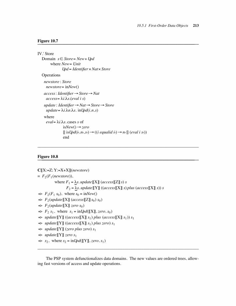
10.5.1 First-Order Data Objects 213
Figure 10.7____________________________________________________________________________________________________________________________________________________
IV.' Store
Domain s% Store" New#Upd
where New" Unit
Upd" Identifier%Nat% Store
Operations
newstore : Store
newstore" inNew()
access : Identifier" Store"Nat
access" !i.!s.(eval i s)
update : Identifier"Nat" Store" Store
update" !i.!n.!s. inUpd(i,n,s)
where
eval" !i.!s. cases s of
isNew()" zero
[] isUpd(i',n',s')" ((i equalid i')" n' [] (eval i s'))end
____________________________________________________________________________
Figure 10.8____________________________________________________________________________________________________________________________________________________
C[[X:"Z; Y:"X#X]](newstore)
= F2(F1(newstore)),
where F1 " !!!s. update[[X]] (access[[Z]] s) s
F2 " !!!s. update[[Y]] ((access[[X]] s) plus (access[[X]] s)) s
"> F2(F1 s0), where s0 " inNew()
"> F2(update[[X]] (access[[Z]] s0) s0)
"> F2(update[[X]] zero s0)
"> F2 s1, where s1 " inUpd([[X]], zero, s0)
"> update[[Y]] ((access[[X]] s1) plus (access[[X]] s1)) s1
"> update[[Y]] ((access[[X]] s1) plus zero) s1
"> update[[Y]] (zero plus zero) s1
"> update[[Y]] zero s1
"> s2, where s2 " inUpd([[Y]], zero, s1)
____________________________________________________________________________
The PSP system defunctionalizes data domains. The new values are ordered trees, allow-
ing fast versions of access and update operations.
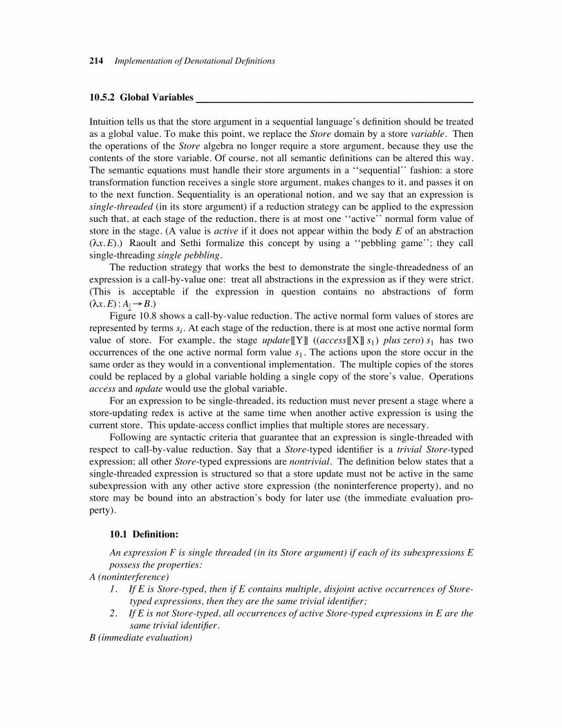
214 Implementation of Denotational Definitions
10.5.2 Global Variables !!!!!!!!!!!!!!!!!!!!!!!!!!!!!!!!!!!!!!!!!!!!!!!!!!!!!!!!!!!!!!!!!!!!!!!!!!!!!!!!!!!!!!!!!!!!!!!!!!!!!!!!!!
Intuition tells us that the store argument in a sequential language’s definition should be treated
as a global value. To make this point, we replace the Store domain by a store variable. Then
the operations of the Store algebra no longer require a store argument, because they use the
contents of the store variable. Of course, not all semantic definitions can be altered this way.
The semantic equations must handle their store arguments in a ‘‘sequential’’ fashion: a store
transformation function receives a single store argument, makes changes to it, and passes it on
to the next function. Sequentiality is an operational notion, and we say that an expression is
single-threaded (in its store argument) if a reduction strategy can be applied to the expression
such that, at each stage of the reduction, there is at most one ‘‘active’’ normal form value of
store in the stage. (A value is active if it does not appear within the body E of an abstraction
(!x. E).) Raoult and Sethi formalize this concept by using a ‘‘pebbling game’’; they call
single-threading single pebbling.
The reduction strategy that works the best to demonstrate the single-threadedness of an
expression is a call-by-value one: treat all abstractions in the expression as if they were strict.
(This is acceptable if the expression in question contains no abstractions of form
(!x. E) : A$!"B.)
Figure 10.8 shows a call-by-value reduction. The active normal form values of stores are
represented by terms si . At each stage of the reduction, there is at most one active normal form
value of store. For example, the stage update[[Y]] ((access[[X]] s1) plus zero) s1 has two
occurrences of the one active normal form value s1. The actions upon the store occur in the
same order as they would in a conventional implementation. The multiple copies of the stores
could be replaced by a global variable holding a single copy of the store’s value. Operations
access and update would use the global variable.
For an expression to be single-threaded, its reduction must never present a stage where a
store-updating redex is active at the same time when another active expression is using the
current store. This update-access conflict implies that multiple stores are necessary.
Following are syntactic criteria that guarantee that an expression is single-threaded with
respect to call-by-value reduction. Say that a Store-typed identifier is a trivial Store-typed
expression; all other Store-typed expressions are nontrivial. The definition below states that a
single-threaded expression is structured so that a store update must not be active in the same
subexpression with any other active store expression (the noninterference property), and no
store may be bound into an abstraction’s body for later use (the immediate evaluation pro-
perty).
10.1 Definition:
An expression F is single threaded (in its Store argument) if each of its subexpressions E
possess the properties:
A (noninterference)
1. If E is Store-typed, then if E contains multiple, disjoint active occurrences of Store-
typed expressions, then they are the same trivial identifier;
2. If E is not Store-typed, all occurrences of active Store-typed expressions in E are the
same trivial identifier.
B (immediate evaluation)
10.5.2 Global Variables 215
1. If E = (!!!x. M): Store"D, then all free Store-typed identifiers in M are x.
2. If E = (!!!x. M): C"D, and C is not Store-typed, then M contains no active Store-
typed expressions.
The noninterference property directly prevents the update-access conflict from arising in
active expressions. The immediate evaluation property guarantees that an abstraction will also
avoid conflict when it is reduced and its body is made active.
Let’s look at some examples; let C: Command" Store$!" Store$! and
E: Expression" Store"Expressible-value. First, the expression C[[C2]](C[[C1]]s) is single-
threaded. The call-by-value reduction strategy lock-steps the reduction so that C[[C1]]’s reduc-
tions must be performed before C[[C2]]’s. Another example of compliance is
(!s. E[[E1]]s plus E[[E2]]s), for all the Store-typed subterms in it are trivial.
In contrast, (C[[C1]]s combine C[[C2]]s) violates clause A1, for C[[C1]]s and C[[C2]]s are
nontrivial and disjoint and active in the same subterm. When the abstraction is given a store,
which of the two commands should be reduced first? If a single store variable is used, an
incorrect final store will likely result. Next, E[[E]](C[[C]]s) violates property A2, because
(C[[C]]s) creates a local side effect that must be forgotten after the reduction of E[[E]].
Apparently E[[E]] needs its own local copy of the store. The expression (!!!s. C[[C]]s') violates
B1, for the store s' is hidden in the abstraction body, and it could be used at some later time in
the reduction when a different store is current. Finally, (!n. update [[I]] n s) violates B2 and
introduces the same problem. All of these constructs would be difficult to implement on a
sequential machine.
A denotational definition is single-threaded if all of its semantic equations are. Given a
single-threaded denotational definition, we make the Store algebra into a Store ‘‘module’’ and
replace all occurrences of stores in the semantic equations with the value () : Unit. Figure 10.9
shows the new version of the language in Figure 5.2. (Note: the expressions E2 and E3 are
treated as inactive in (E1 "E2 [] E3).)
The () markers are passed as arguments in place of store values. A () marker is a
‘‘pointer’’ to the store variable, awarding access rights. But, more importantly, () is a control
marker, for a denotation (!(). E) can reduce (that is, ‘‘get control’’) only when it receives the
(). The transformation has exposed the underlying store-based control in the programming
language.
A program’s denotation is no longer a single function expression E, but a pair (E, s),
where s is the current value of the store variable. Rewrite rules operate on the expression, store
pairs; for example, the new version of the #-rule is
( . . . (!x.M)N . . . , s) "> ( . . . [N/x]M . . . , s). The rewriting rules that manipulate the store
are:
( . . . (access i ()) . . . , s) "> ( . . . n . . . , s) where eval i s " n
( . . . (update i n ()) . . . , s) "> ( . . . () . . . , inUpd(i, n, s))
The command in Figure 10.8 is reduced with a store variable in Figure 10.10.
A machine implementation of the transformed denotational definition would treat the
store variable as a machine component and access and update as machine instructions. The
VEC-machine in Figure 10.2 becomes the VECS-machine, and it uses a machine configuration
(v e c s). The modification of Figure 10.2 to include the store variable is left as an exercise.
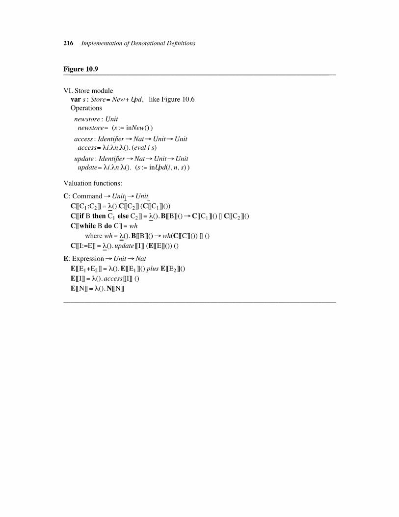
216 Implementation of Denotational Definitions
Figure 10.9____________________________________________________________________________________________________________________________________________________
VI. Store module
var s : Store" New#Upd, like Figure 10.6
Operations
newstore : Unit
newstore" (s :" inNew() )
access : Identifier"Nat"Unit"Unit
access" !i.!n.!(). (eval i s)
update : Identifier"Nat"Unit"Unit
update" !i.!n.!(). (s :" inUpd(i, n, s) )
Valuation functions:
C: Command"Unit $!"Unit $!
C[[C1;C2]]" !!!().C[[C2]] (C[[C1]]())
C[[if B then C1 else C2]]" !!!(). B[[B]]()"C[[C1]]() [] C[[C2]]()
C[[while B do C]]" wh
where wh " !!!(). B[[B]]()"wh(C[[C]]()) [] ()
C[[I:"E]]" !!!(). update[[I]] (E[[E]]()) ()
E: Expression"Unit"Nat
E[[E1#E2]]" !(). E[[E1]]() plus E[[E2]]()
E[[I]]" !(). access[[I]] ()
E[[N]]" !(). N[[N]]
____________________________________________________________________________
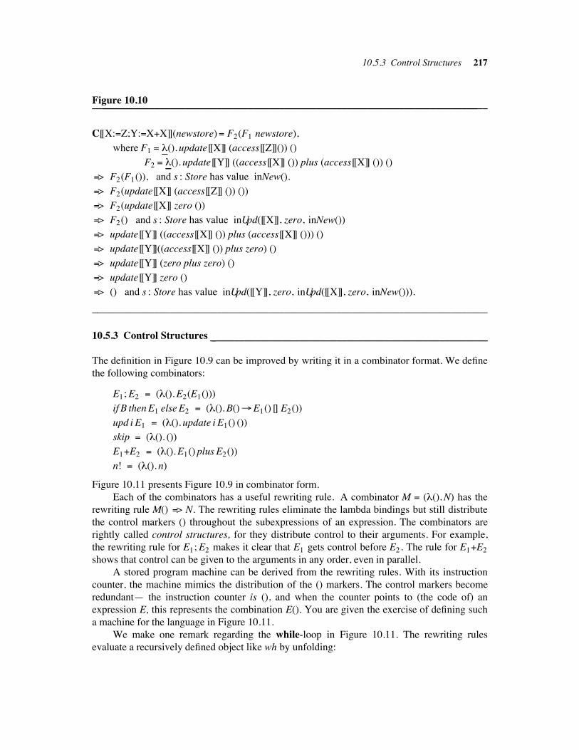
10.5.3 Control Structures 217
Figure 10.10____________________________________________________________________________________________________________________________________________________
C[[X:"Z;Y:"X#X]](newstore)" F2(F1 newstore),
where F1 " !!!(). update[[X]] (access[[Z]]()) ()
F2 " !!!(). update[[Y]] ((access[[X]] ()) plus (access[[X]] ()) ()
"> F2(F1()), and s : Store has value inNew().
"> F2(update[[X]] (access[[Z]] ()) ())
"> F2(update[[X]] zero ())
"> F2() and s : Store has value inUpd([[X]], zero, inNew())
"> update[[Y]] ((access[[X]] ()) plus (access[[X]] ())) ()
"> update[[Y]]((access[[X]] ()) plus zero) ()
"> update[[Y]] (zero plus zero) ()
"> update[[Y]] zero ()
"> () and s : Store has value inUpd([[Y]], zero, inUpd([[X]], zero, inNew())).
____________________________________________________________________________
10.5.3 Control Structures !!!!!!!!!!!!!!!!!!!!!!!!!!!!!!!!!!!!!!!!!!!!!!!!!!!!!!!!!!!!!!!!!!!!!!!!!!!!!!!!!!!!!!!!!!!!!!!!!!!!!!!!
The definition in Figure 10.9 can be improved by writing it in a combinator format. We define
the following combinators:
E1; E2 " (!(). E2(E1()))
if B then E1 else E2 " (!(). B()"E1() [] E2())
upd i E1 " (!(). update i E1() ())
skip " (!(). ())
E1#E2 " (!(). E1() plus E2())
n! " (!(). n)
Figure 10.11 presents Figure 10.9 in combinator form.
Each of the combinators has a useful rewriting rule. A combinator M " (!(). N) has the
rewriting rule M() "> N. The rewriting rules eliminate the lambda bindings but still distribute
the control markers () throughout the subexpressions of an expression. The combinators are
rightly called control structures, for they distribute control to their arguments. For example,
the rewriting rule for E1; E2 makes it clear that E1 gets control before E2. The rule for E1#E2
shows that control can be given to the arguments in any order, even in parallel.
A stored program machine can be derived from the rewriting rules. With its instruction
counter, the machine mimics the distribution of the () markers. The control markers become
redundant— the instruction counter is (), and when the counter points to (the code of) an
expression E, this represents the combination E(). You are given the exercise of defining such
a machine for the language in Figure 10.11.
We make one remark regarding the while-loop in Figure 10.11. The rewriting rules
evaluate a recursively defined object like wh by unfolding:
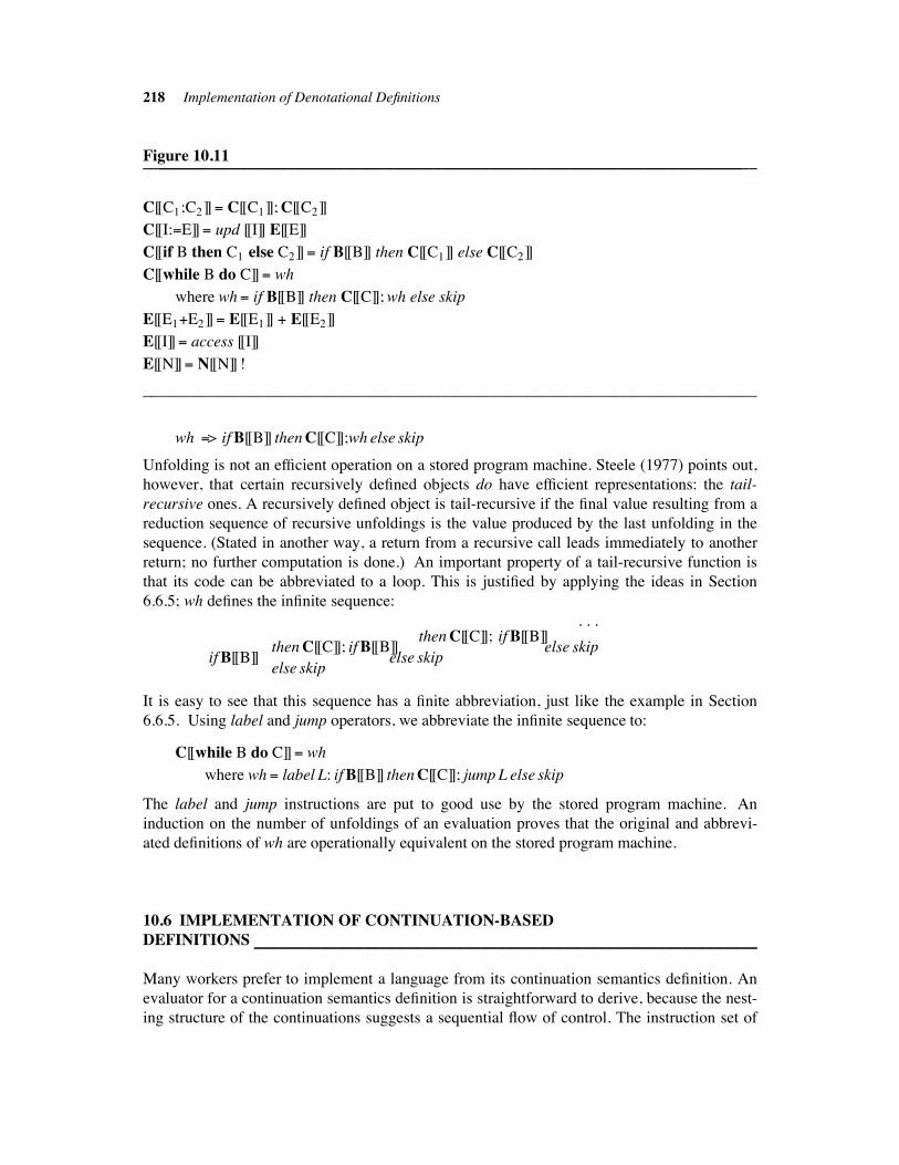
218 Implementation of Denotational Definitions
Figure 10.11____________________________________________________________________________________________________________________________________________________
C[[C1;C2]]" C[[C1]]; C[[C2]]
C[[I:"E]]" upd [[I]] E[[E]]
C[[if B then C1 else C2]]" if B[[B]] then C[[C1]] else C[[C2]]
C[[while B do C]]" wh
where wh " if B[[B]] then C[[C]]; wh else skip
E[[E1#E2]]" E[[E1]] # E[[E2]]
E[[I]]" access [[I]]
E[[N]]" N[[N]] !
____________________________________________________________________________
wh "> if B[[B]] then C[[C]];wh else skip
Unfolding is not an efficient operation on a stored program machine. Steele (1977) points out,
however, that certain recursively defined objects do have efficient representations: the tail-
recursive ones. A recursively defined object is tail-recursive if the final value resulting from a
reduction sequence of recursive unfoldings is the value produced by the last unfolding in the
sequence. (Stated in another way, a return from a recursive call leads immediately to another
return; no further computation is done.) An important property of a tail-recursive function is
that its code can be abbreviated to a loop. This is justified by applying the ideas in Section
6.6.5; wh defines the infinite sequence:
. . . then C[[C]]; if B[[B]]
then C[[C]]; if B[[B]] else skip if B[[B]] else skip
else skip
It is easy to see that this sequence has a finite abbreviation, just like the example in Section
6.6.5. Using label and jump operators, we abbreviate the infinite sequence to:
C[[while B do C]]" wh
where wh " label L: if B[[B]] then C[[C]]; jump L else skip
The label and jump instructions are put to good use by the stored program machine. An
induction on the number of unfoldings of an evaluation proves that the original and abbrevi-
ated definitions of wh are operationally equivalent on the stored program machine.
10.6 IMPLEMENTATION OF CONTINUATION-BASED
DEFINITIONS !!!!!!!!!!!!!!!!!!!!!!!!!!!!!!!!!!!!!!!!!!!!!!!!!!!!!!!!!!!!!!!!!!!!!!!!!!!!!!!!!!!!!!!!!!!!!!!!!!!!!!!!!!!!!!!!!!!!!!!!
Many workers prefer to implement a language from its continuation semantics definition. An
evaluator for a continuation semantics definition is straightforward to derive, because the nest-
ing structure of the continuations suggests a sequential flow of control. The instruction set of
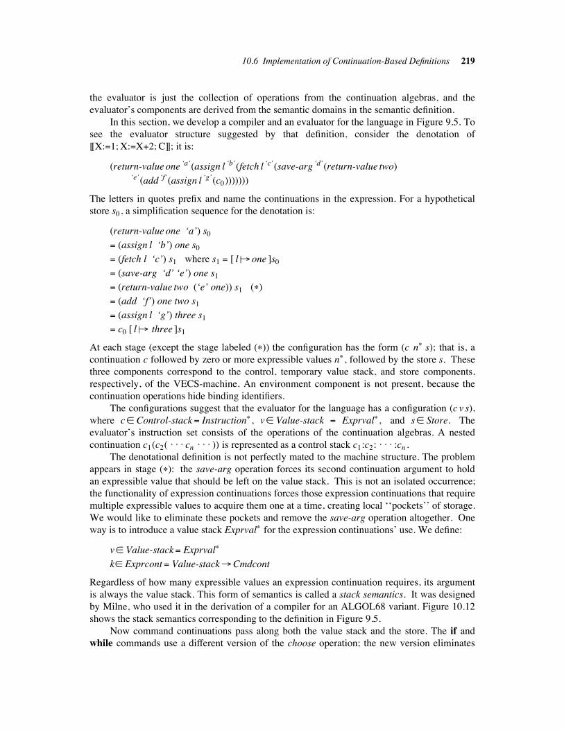
10.6 Implementation of Continuation-Based Definitions 219
the evaluator is just the collection of operations from the continuation algebras, and the
evaluator’s components are derived from the semantic domains in the semantic definition.
In this section, we develop a compiler and an evaluator for the language in Figure 9.5. To
see the evaluator structure suggested by that definition, consider the denotation of
[[X:"1; X:"X#2; C]]; it is:
(return-value one ‘a’(assign l ‘b’(fetch l ‘c’(save-arg ‘d’(return-value two)
‘e’(add ‘f’(assign l ‘g’(c0)))))))
The letters in quotes prefix and name the continuations in the expression. For a hypothetical
store s0, a simplification sequence for the denotation is:
(return-value one ‘a’) s0
" (assign l ‘b’) one s0
" (fetch l ‘c’) s1 where s1 " [ l $$" one ]s0
" (save-arg ‘d’ ‘e’) one s1
" (return-value two (‘e’ one)) s1 ($)
" (add ‘f’) one two s1
" (assign l ‘g’) three s1
" c0 [ l $$" three ]s1
At each stage (except the stage labeled ($)) the configuration has the form (c n$ s); that is, a
continuation c followed by zero or more expressible values n$ , followed by the store s. These
three components correspond to the control, temporary value stack, and store components,
respectively, of the VECS-machine. An environment component is not present, because the
continuation operations hide binding identifiers.
The configurations suggest that the evaluator for the language has a configuration (c v s),
where c% Control-stack" Instruction$ , v% Value-stack " Exprval$, and s% Store. The
evaluator’s instruction set consists of the operations of the continuation algebras. A nested
continuation c1(c2( . . . cn . . . )) is represented as a control stack c1:c2: . . . :cn .
The denotational definition is not perfectly mated to the machine structure. The problem
appears in stage ($): the save-arg operation forces its second continuation argument to hold
an expressible value that should be left on the value stack. This is not an isolated occurrence;
the functionality of expression continuations forces those expression continuations that require
multiple expressible values to acquire them one at a time, creating local ‘‘pockets’’ of storage.
We would like to eliminate these pockets and remove the save-arg operation altogether. One
way is to introduce a value stack Exprval$ for the expression continuations’ use. We define:
v% Value-stack" Exprval$
k% Exprcont" Value-stack"Cmdcont
Regardless of how many expressible values an expression continuation requires, its argument
is always the value stack. This form of semantics is called a stack semantics. It was designed
by Milne, who used it in the derivation of a compiler for an ALGOL68 variant. Figure 10.12
shows the stack semantics corresponding to the definition in Figure 9.5.
Now command continuations pass along both the value stack and the store. The if and
while commands use a different version of the choose operation; the new version eliminates
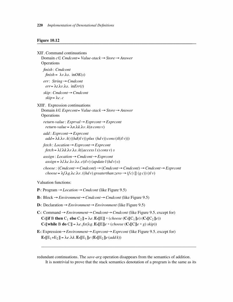
220 Implementation of Denotational Definitions
Figure 10.12____________________________________________________________________________________________________________________________________________________
XII'. Command continuations
Domain c% Cmdcont" Value-stack" Store"Answer
Operations
finish : Cmdcont
finish " !v.!s. inOK(s)
err: String"Cmdcont
err" !t.!v.!s. inErr(t)
skip: Cmdcont"Cmdcont
skip" !c. c
XIII'. Expression continuations
Domain k% Exprcont" Value-stack" Store"Answer
Operations
return-value : Exprval"Exprcont"Exprcont
return-value" !n.!k.!v. k(n cons v)
add : Exprcont"Exprcont
add" !k.!v. k( ((hd(tl v)) plus (hd v)) cons (tl(tl v)))
fetch : Location"Exprcont"Exprcont
fetch" !l.!k.!v.!s. k((access l s) cons v) s
assign : Location"Cmdcont"Exprcont
assign " !l.!c.!v.!s. c(tl v) (update l (hd v) s)
choose : (Cmdcont"Cmdcont)" (Cmdcont"Cmdcont)"Cmdcont"Exprcont
choose" !f.!g.!c.!v. ((hd v) greaterthan zero" (f c) [] (g c)) (tl v)
Valuation functions:
P': Program" Location"Cmdcont (like Figure 9.5)
B': Block"Environment"Cmdcont"Cmdcont (like Figure 9.5)
D': Declaration"Environment"Environment (like Figure 9.5)
C': Command"Environment"Cmdcont"Cmdcont (like Figure 9.5, except for)
C''[[if B then C1 else C2]]" !e. E''[[E]] & (choose (C''[[C1]]e) (C''[[C2]]e))
C''[[while B do C]]" !e. fix(!g. E''[[E]]e & (choose (C''[[C]]e & g) skip))
E': Expression"Environment"Exprcont"Exprcont (like Figure 9.5, except for)
E''[[E1#E2]]" !e.!k. E''[[E1]]e (E''[[E2]]e (add k))
__________________________________________________________________________
redundant continuations. The save-arg operation disappears from the semantics of addition.
It is nontrivial to prove that the stack semantics denotation of a program is the same as its
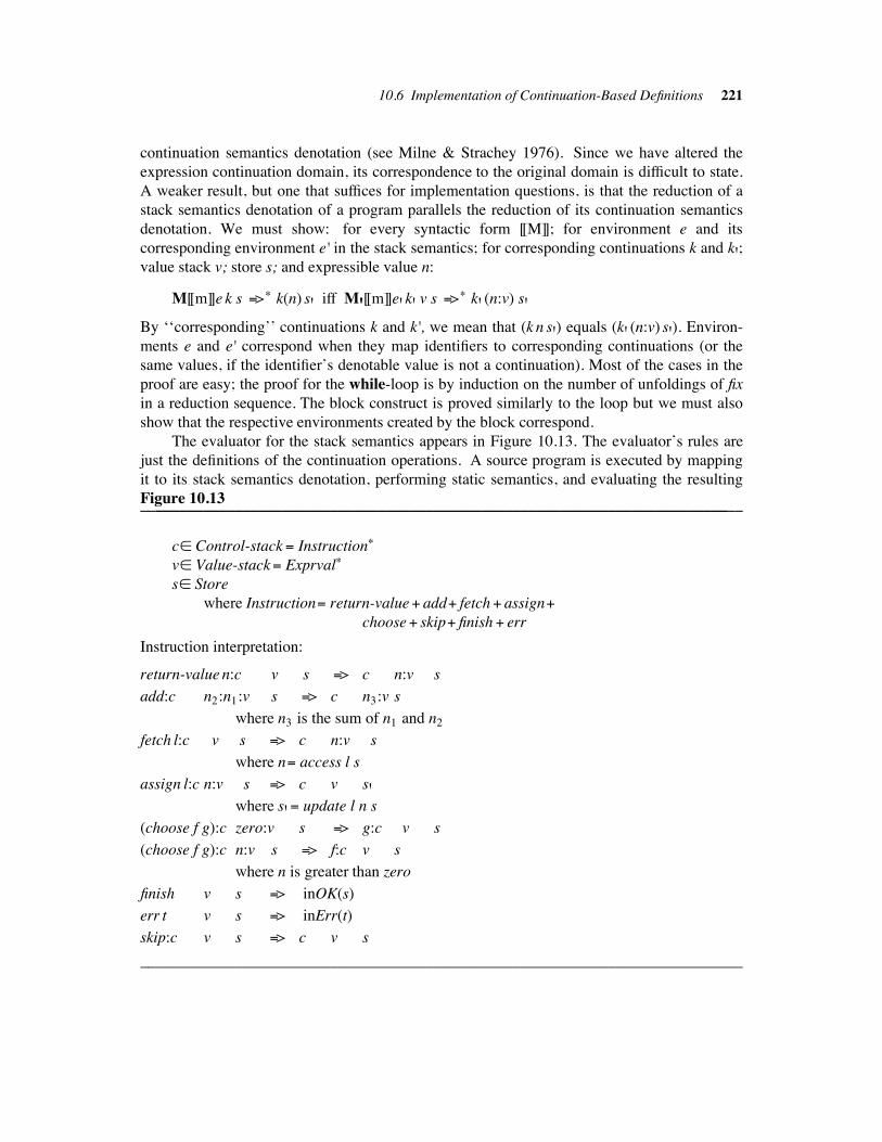
10.6 Implementation of Continuation-Based Definitions 221
continuation semantics denotation (see Milne & Strachey 1976). Since we have altered the
expression continuation domain, its correspondence to the original domain is difficult to state.
A weaker result, but one that suffices for implementation questions, is that the reduction of a
stack semantics denotation of a program parallels the reduction of its continuation semantics
denotation. We must show: for every syntactic form [[M]]; for environment e and its
corresponding environment e' in the stack semantics; for corresponding continuations k and k';value stack v; store s; and expressible value n:
M[[m]]e k s ">$ k(n) s' iff M''[[m]]e' k' v s ">$ k' (n:v) s'By ‘‘corresponding’’ continuations k and k', we mean that (k n s') equals (k' (n:v) s'). Environ-
ments e and e' correspond when they map identifiers to corresponding continuations (or the
same values, if the identifier’s denotable value is not a continuation). Most of the cases in the
proof are easy; the proof for the while-loop is by induction on the number of unfoldings of fix
in a reduction sequence. The block construct is proved similarly to the loop but we must also
show that the respective environments created by the block correspond.
The evaluator for the stack semantics appears in Figure 10.13. The evaluator’s rules are
just the definitions of the continuation operations. A source program is executed by mapping
it to its stack semantics denotation, performing static semantics, and evaluating the resulting
Figure 10.13____________________________________________________________________________________________________________________________________________________
c% Control-stack" Instruction$
v% Value-stack" Exprval$
s% Store
where Instruction" return-value# add# fetch# assign#choose# skip# finish # err
Instruction interpretation:
return-value n:c v s "> c n:v s
add:c n2:n1:v s "> c n3:v s
where n3 is the sum of n1 and n2
fetch l:c v s "> c n:v s
where n" access l s
assign l:c n:v s "> c v s'where s'" update l n s
(choose f g):c zero:v s "> g:c v s
(choose f g):c n:v s "> f:c v s
where n is greater than zero
finish v s "> inOK(s)
err t v s "> inErr(t)
skip:c v s "> c v s
____________________________________________________________________________
222 Implementation of Denotational Definitions
continuation on the evaluator.
A similar method for inducing the temporary value stack has been developed by Wand.
He does not introduce a value stack domain but inserts ‘‘argument steering’’ combinators into
the semantic equations instead. Run-time configurations take the form (c n1 . . . nm s). The net
result is the same, but the proof that the new semantic definition is equal to the original is
much simpler than the one needed for our example. Wand’s research papers document the
method.
Although the instruction set for the interpreter is in place, fix operators still appear in
those translated programs containing while-loops and labels. The fixed point simplification
property (fix F)"F(fix F) can be used by the interpreter, but we choose to introduce the opera-
tion while f do g, representing the expression fix(!c'. f & (choose (g & c') skip)) so that
C[[while B do C]] " !e. while E[[E]]e do C[[C]]e. The evaluation rule is:
while f do h:c v s "> f:(choose (h:while f do h) skip):c v s
The gotos present a more serious problem. A block with labels does not have a simple,
tail-recursive expansion like the while-loop. One solution is to carry over the language’s
environment argument into the evaluator to hold the continuations associated with the labels.
A goto causes a lookup into the environment and a reloading of the control stack with the con-
tinuation associated with the goto.
The problem with the gotos is better resolved when an instruction counter is incorporated
into the evaluator, jump and jumpfalse instructions are added, and the code for blocks is gen-
erated with jumps in it. A continuation (ctuple)i) is a tail-recursive call to the ith ctuple com-
ponent. If the ith component begins at label L, we generate jump L. (Also, the while-loop can
be compiled to conventional loop code.) The proof of correctness of these transformations is
involved and you are referred to Milne & Strachey (1976) and Sethi (1981).
10.6.1 The CGP and VDM Methods !!!!!!!!!!!!!!!!!!!!!!!!!!!!!!!!!!!!!!!!!!!!!!!!!!!!!!!!!!!!!!!!!!!!!!!!!!!!!!!!!!!!!!
Raskovsky’s Code Generator Process (CGP) is a transformation-oriented compiler generation
method. It transforms a denotational definition into a BCPL-coded code generator in a series
of transformation steps. Each transformation exploits a property of the semantic definition.
Defunctionalization, continuation introduction, and global variable introduction for stores and
environments are examples of transformations. The generated compiler maps source programs
to BCPL code; the evaluator is the BCPL system. The system has been used to develop com-
pilers for nontrivial languages such as GEDANKEN.
Bjo/ rner and Jones advocate a stepwise transformation method that also uses transforma-
tions described in this chapter. Their work is part of a software development methodology
known as the Vienna Development Method (VDM). VDM system specifications are denota-
tional definitions; the semantic notation is a continuation-style, combinator-based notation
called META-IV. Evaluators for VDM specifications are derived using the ideas in the previ-
ous section. Compilers, data bases, and other systems software have been specified and imple-
mented using the method. See Bjo/ rner and Jones, 1978 and 1982, for a comprehensive
10.6.1 The CGP and VDM Methods 223
presentation.
10.7 CORRECTNESS OF IMPLEMENTATION AND
FULL ABSTRACTION !!!!!!!!!!!!!!!!!!!!!!!!!!!!!!!!!!!!!!!!!!!!!!!!!!!!!!!!!!!!!!!!!!!!!!!!!!!!!!!!!!!!!!!!!!!!!!!!!!!!!!!!!!
In previous sections, we stated criteria for correctness of implementation. We now consider
the general issue of correctness and provide standards for showing that an operational seman-
tics definition is complementary to a denotational one. The study leads to a famous research
problem known as the full abstraction problem.
Recall that an operational semantics definition of a language is an interpreter. When the
interpreter evaluates a program, it generates a sequence of machine configurations that define
the program’s operational semantics. We can treat the interpreter as an evaluation relation ">that is defined by rewriting rules. A program’s operational semantics is just its reduction
sequence. For a source language L, we might define an interpreter that reduces L-programs
directly. However, we have found it convenient to treat L’s semantic function P : L"D as a
syntax-directed translation scheme and use it to translate L-programs to function expressions.
Then we interpret the function expressions. Let e% Function-expr be a function expression
representation of a source program after it has been translated by P. Since expressions are
treated as syntactic entities by the interpreter for function expressions, we write e1 * e2 to
assert that the denotations of the function expressions e1 and e2 are the same value.
Let I be the set of interpreter configurations and let + : Function-expr" I be a mapping
that loads a function expression into an initial interpreter configuration. A configuration is
final if it cannot be reduced further. The set of final interpreter configurations is called Fin.
We also make use of an ‘‘abstraction’’ map , : I"Function-expr, which restores the function
expression corresponding to an interpreter configuation. The minimum required to claim that
an operational semantics definition is complementary to a denotational one is a form of sound-
ness we call faithfulness.
10.2 Definition:
An operational semantics "> is faithful to the semantics of Function-expr if for all
e%Function-expr and i% I, +(e) ">$ i implies e * ,(i).
Faithfulness by itself is not worth much, for the interpreter can have an empty set of evalua-
tion rules and be faithful. Therefore, we define some subset Ans of Function-expr to be answer
forms. For example, the set of constants in Nat can be an answer set, as can the set of all nor-
mal forms. A guarantee of forward progress to answers is a form of completeness we call ter-
mination.
10.3 Definition:
An operational semantics "> is terminating in relation to the semantics of Function-expr
if, for all e%Function-expr and a%Ans, if e * a, then there exists some i%Fin such that
+(e) ">$ i, ,(i)% Ans, and ,(i) * a.
224 Implementation of Denotational Definitions
Termination is the converse of faithfulness, restricted to the i in Fin. We use the requirement
,(i) * a (rather than ,(i) " a) because two elements of Ans may share the same value (e.g.,
normal form answers (!t. t" a [] b) and (!t. not(t)" b [] a) are distinct answers with the same
value). If Ans is a set whose elements all have distinct values (e.g., the constants in Nat), then
,(i) must be a. If the operational semantics is faithful, then the requirement that ,(i) * a is
always satisfied.
We apply the faithfulness and termination criteria to the compile-evaluate method
described in Sections 10.1 and 10.3. Given a denotational definition P : L"D, we treat P as a
syntax-directed translation scheme to function expressions. For program [[P]], the expression
P[[P]] is loaded into the interpreter. In its simplest version, the interpreter requires no extra
data structures, hence both + and , are identity maps. Recall that the interpreter uses a
leftmost-outermost reduction strategy. A final configuration is a normal form. An answer is a
(non- $-) normal form expression. By exercise 11 in Chapter 3, the reductions preserve the
meaning of the function expression, so the implementation is faithful. In Section 10.3 we
remarked that the leftmost-outermost method always locates a normal form for an expression
if one exists. Hence the method is terminating.
The definitions of faithfulness and termination are also useful to prove that a low-level
operational semantics properly simulates a high-level one: let (the symmetric, transitive clo-
sure of) the evaluation relation for the high-level interpreter define * and let the low-level
evaluation relation define ">. Ans is the set of final configurations for the high-level inter-
preter, and Fin is the set of final configurations for the low-level one. This method was used in
Sections 10.3 and 10.6.
There are other versions of termination properties. We develop these versions using the
function expression interpreter. In this case, + and , are identity maps, and the Ans and Fin
sets are identical, so we dispense with the two maps and Fin and work directly with the func-
tion expressions and Ans. We define a context to be a function expression with zero or more
‘‘holes’’ in it. If we view a context as a derivation tree, we find that zero or more of its leaves
are nonterminals. We write a hypothetical context as C[ ]. When we use an expression E to fill
the holes in a context C[ ], giving a well-formed expression, we write C[E]. We fill the holes
by attaching E’s derivation tree to all the nonterminal leaves in C[ ]’s tree. The formalization
of contexts is left as an exercise.
A context provides an operating environment for an expression and gives us a criterion
for judging information content and behavior. For example, we can use structural induction to
prove that for expressions M and N and context C[ ], M ---$$ N implies that C[M] --
-$$ C[N]. We
write M.--$$ N if, for all contexts C[ ] and a% Ans, C[M] ">$ a implies that C[N] ">$ a' and
a* a'. We write M.. N if M.--$$ N and N .-
-$$ M and say that M and N are operationally equivalent.
The following result is due to Plotkin (1977).
10.4 Proposition:
If "> is faithful to the semantics of Function-expr, then "> is terminating iff for all
M, N%Function-expr, M*N implies M.. N.
Proof: Left as an exercise.
This result implies that denotational semantics equality implies operational equivalence under
10.7 Correctness of Implementation and Full Abstraction 225
the assumption that the operational semantics is faithful and terminating. Does the converse
hold? That is, for a faithful and terminating operational semantics, does operational
equivalence imply semantic equality? If it does, we say that the denotational semantics of
Function-expr is fully abstract in relation to its operational semantics.
Plotkin (1977) has shown that the answer to the full abstractness question for Function-
expr and its usual interpreter is no. Let Fb: (Tr $! % Tr $!)" Tr $! be the function expression:
!a. let t1 " a(true, $-) in
t1 " (let t2 " a( $-, true) in
t2 " (let t3 " a(false, false) in
t3 " $- [] b)
[] $-)
[] $-
We see that Ftrue ---$$ /Ffalse (and vice versa) by considering the continuous function
v : Tr $! % Tr $!" Tr $! whose graph is { (( $-, true), true), ((true, $-), true), ((true, true), true),
((true, false), true), ((false, true), true), ((false, false), false) } (as usual, pairs ((m, n), $-) are
omitted). The function v is the ‘‘parallel or’’ function, and Ftrue(v)" true but Ffalse(v)" false.
But Plotkin proved, for the language of function expressions and its usual operational seman-
tics, that Ftrue .. Ffalse! The reason that the two expressions are operationally equivalent is that
‘‘parallel’’ functions like v are not representable in the function notation; the notation and its
interpreter are inherently ‘‘sequential.’’
There are two possibilities for making the denotational semantics of Function-expr fully
abstract in relation to its interpreter. One is to extend Function-expr so that ‘‘parallel’’ func-
tions are representable. Plotkin did this by restricting the Ans set to be the set of constants for
Nat and Tr and introducing a parallel conditional operation par-cond : Tr $! %D$! %D$!"D$! , for
D% { Nat, Tr }, with reduction rules:
par-cond(true, d1, d2) "> d1
par-cond(false, d1, d2) "> d2
par-cond( $-, d, d) "> d
Then v" !(t1 , t2). par-cond(t1, true, t2). Plotkin showed that the extended notation and its
denotational semantics are fully abstract in relation to the operational semantics.
Another possibility for creating a fully abstract semantics is to reduce the size of the
semantic domains so that the nonrepresentable ‘‘parallel’’ functions are no longer present. A
number of researchers have proposed domain constructions that do this. The constructions are
nontrivial, and you should research the suggested readings for further information.
SUGGESTED READINGS !!!!!!!!!!!!!!!!!!!!!!!!!!!!!!!!!!!!!!!!!!!!!!!!!!!!!!!!!!!!!!!!!!!!!!!!!!!!!!!!!!!!!!!!!!!!!!!!!!!!!!
General compiler generating systems: Appel 1985; Ganzinger, Ripken & Wilhelm 1977;
Jones 1980; Mosses 1975, 1976, 1979; Paulson 1982, 1984; Pleban 1984; Wand 1983
Static semantics processing: Ershov 1978; Jones et al. 1985; Mosses 1975; Paulson 1982
226 Implementation of Denotational Definitions
Sethi 1981
Rewriting rules & evaluators for function notation: Berry & Levy 1979; Burge 1975;
Hoffman & O’Donnell 1983; Huet & Oppen 1980; Landin 1964; Vegdahl 1984
Combinator systems & evaluators: Christiansen & Jones 1983; Clarke et al. 1980; Curry &
Feys 1958; Hudak & Krantz 1984; Hughes 1982; Mosses 1979a, 1980, 1983a, 1984;
Raoult & Sethi 1982; Sethi 1983; Turner 1979
Transformation methods: Bjo/ rner & Jones 1978, 1982; Georgeff 1984; Hoare 1972; Raoult
& Sethi 1984; Raskovsky & Collier 1980; Raskovsky 1982; Reynolds 1972; Schmidt
1985a, 1985b; Steele 1977; Steele & Sussman 1976a, 1976b
Continuation-based implementation techniques: Clinger 1984; Henson & Turner 1982;
Milne & Strachey 1976; Nielson 1979; Polak 1981; Sethi 1981; Wand 1980a, 1982a,
1982b, 1983, 1985b
Full abstraction: Berry, Curien, & Levy 1983; Milner 1977; Mulmuley 1985; Plotkin 1977;
Stoughton 1986
EXERCISES !!!!!!!!!!!!!!!!!!!!!!!!!!!!!!!!!!!!!!!!!!!!!!!!!!!!!!!!!!!!!!!!!!!!!!!!!!!!!!!!!!!!!!!!!!!!!!!!!!!!!!!!!!!!!!!!!!!!!!!!!!!!
1. a. Using the semantics of Figure 5.2, evaluate the program P[[Z:"A#1]]four using the
compile-evaluate method and using the interpreter method.
b. Repeat part a for the program P[[begin var A; A:"A#1 end]] l0 (!l. zero) and the
language of Figures 7.1 and 7.2.
2. If you have access to a parser generator system such as YACC and a functional language
implementation such as Scheme, ML, or LISP, implement an SPS-like compiler generat-
ing system for denotational semantics.
3. Using the criteria for determining unfrozen expressions, work in detail the static seman-
tics processing of:
a. The example in Section 10.2.
b. The program in part b of Exercise 1 (with the Store, Nat, and Tr algebras frozen).
c. The program in Figure 7.6 (with the Function, List, and Environment algebras frozen;
and again with just the Function and List algebras frozen).
4. Let the Store algebra be unfrozen; redo the static semantics of parts a and b of Exercise
3. Why don’t real life compilers perform a similar service? Would this approach work
well on programs containing loops?
5. The example of static semantics simplification in Section 10.2 showed combinations of
the form (!!!s.M)s simplified to M. Why is this acceptable in the example? When is it
not?
6. Recall that the simplification rule for the fix operation is (fix F)" F(fix F). How should
this rule be applied during static semantics analysis? Consider in particular the cases of:
Exercises 227
i. Recursively defined environments e" fix(!e'. . . . ).
ii. Recursively defined commands and procedures p" fix(!p.!!!s. . . . ).
7. A number of researchers have proposed that a language’s valuation function be divided
into a static semantics valuation function and a dynamic semantics valuation function:
CS: Command"Environment" Tr
CD: Command"Environment'" ((Store"Poststore)#Err)
such that a well typed command [[C]] has denotation CS[[C]]" true and a denotation
CD[[C]] in the summand (Store"Poststore). Similarly, an ill typed program has a deno-
tation of false with respect to CS and an inErr() denotation with respect to CD .
a. Formulate these valuation functions for the language in Figures 7.1 and 7.2.
b. Comment on the advantages of this approach for implementing the language. Are
there any disadvantages?
8. a. Perform leftmost-outermost reductions on the following expressions. If the expres-
sion does not appear to have a normal form, halt your reduction and justify your deci-
sion.
i. (!x. zero)((!x. x x)(!x. x x))
ii. (!!!x. zero)((!x. x x)(!x. x x))
iii. ((!x.!y. y(y x))(one plus one))(!z. z times z)
iv. ((!!!x.!!!y. y(y x))(one plus one))(!z. z times z)
v. ((!!!x.!!!y. y(y x))(one plus one))(!!!z. z times z)
b. Redo part a, representing the expressions as trees. Show the traversal through the
trees that a tree evaluator would take.
9. Implement the tree evaluator for function notation. (It is easiest to implement it in a
language that supports list processing.) Next, improve the evaluator to use an environ-
ment table. Finally, improve the evaluator to use call-by-need evaluation.
10. Evaluate the code segment pushclosure(': return):': call from Figure 10.4 on the VEC-
machine.
11. Translate the expressions in exercise 8 into VEC-machine code and evaluate them on the
VEC-machine.
12. Improve the code generation map T for the VEC-machine so that it generates assembly
code that contains jumps and conditional jumps.
13. Improve the VEC-machine so that push x becomes push ‘‘offset,’’ where ‘‘offset’’ is the
offset into the environment where the value bound to x can be found. Improve the code
generation map so it correctly calculates the offsets for binding identifiers.
228 Implementation of Denotational Definitions
14. Augment the VEC-machine with instructions for handling pairs and sum values. Write
the translations T[[(E1, E2)]] and T[[cases E1 of G]], where G ::" inI1(I2)"E [] G | end.
15. Compile the programs in Exercise 3 to VEC-code after static semantics has been per-
formed. Can you suggest an efficient way to perform static semantics?
16. a. Augment the combinator language definition in Figure 10.7 with combinators for
building environments.
b. Rewrite the semantics of the language in Figures 7.1 and 7.2 in combinator form.
c. Propose a method for doing static semantics analysis on the semantics in part b.
17. Convert the Store algebra in Figure 10.7 into one that manipulates ordered tree values.
Are the new versions of access and update more efficient than the existing ones?
18. a. Verify that the C and E valuation functions of the language of Figure 5.2 are single-
threaded. Does the P function satisfy the criteria of Definition 10.1? Is it single-
threaded?
b. Extend Definition 10.1 so that a judgement can be made about the single-
threadedness of the language in Figures 7.1 and 7.2. Is that language single-threaded?
Derive control combinators for the language.
19. An alternative method of generating a compiler from a continuation semantics of a
language is to replace the command and expression continuation algebras by algebras of
machine code. Let Code be the domain of machine code programs for a VEC-like stack
machine, and use the following two algebras in place of the command and expression
continuation algebras in Figure 9.5 (note: the ‘‘:’’ denotes the code concatenation opera-
tor):
XII'. Command code
Domain c%Cmdcont" Code
Operations
finish " stop
error" !t. pushconst t
XIII'. Expression code
Domain k% Exprcont" Code
Operations
return-value" !n.!k. pushconst n: k
save-arg" !f.!g. f(g)
add" !k. add: k
fetch" !l.!k. pushvar l: k
assign " !l.!c. storevar l: c
choose" !c1 .!c2 . jumpzero L1: c1: jump L2: label L1: c2: label L2
Exercises 229
a. Generate the denotations of several programs using the new algebras.
b. Outline a proof that shows the new algebras are faithful to the originals in an opera-
tional sense.
20. Revise the stack semantics in Figure 10.13 so that the expressible value stack isn’t used
by command continuations; that is, the Cmdcont domain remains as it is in Figure 9.5,
but the stack is still used by the Exprcont domain, that is, Exprcont is defined as in Figure
10.13. What are the pragmatics of this semantics and its implementation?
21. a. Prove that the evaluator with an environment in Section 10.3 is faithful and terminat-
ing in relation to the evaluator in Section 10.1.
b. Prove that the VEC-machine in Section 10.3.1 is faithful and terminating in relation
to the evaluator with environment in Section 10.3 when the answer set is limited to
first-order normal forms.
c. Prove that the defunctionalized version of a semantic algebra is faithful and terminat-
ing in relation to the original version of the algebra.
22. Prove that the properties of faithfulness and termination compose; that is, for operational
semantics A, B, and C, if C is faithful/terminating in relation to B, and B is
faithful/terminating in relation to A, then C is faithful/terminating in relation to A.
23. a. Give the graph of the function par-cond : Tr $! %D$! %D$!"D$! for D% { Nat, Tr },
prove that the function is continuous, and prove that its rewriting rules are sound.
b. Attempt to define the graph of a continuous function par-cond : Tr $! %D%D"D for
arbitrary D and show that its rewriting rules in Section 10.7 are sound. What goes
wrong?
Chapter 11 !!!!!!!!!!!!!!!!!!!!!!!!!!!!!!!!!!!!!!!!!!!!!!!!!!!!!!!
Domain Theory III: Recursive DomainSpecifications
Several times we have made use of recursively defined domains (also called reflexive
domains) of the form D" F(D). In this chapter, we study recursively defined domains in
detail, because:
1. Recursive definitions are natural descriptions for certain data structures. For example, the
definition of binary trees, Bintree " (Data # (Data $Bintree $Bintree))%! , clearly states
that a binary tree is a leaf of data or two trees joined by a root node of data. Another
example is the definition of linear lists of A-elements Alist " (Nil # (A $Alist)) %! , where
Nil " Unit. The definition describes the internal structure of the lists better than the A!
domain does. Alist’s definition also clearly shows why the operations cons, hd, tl, and
null are essential for assembling and disassembling lists.
2. Recursive definitions are absolutely necessary to model certain programming language
features. For example, procedures in ALGOL60 may receive procedures as actual param-
eters. The domain definition must read Proc " Param" Store" Store%! , where Param "Int#Real# . . . #Proc, to properly express the range of parameters.
Like the recursively defined functions in Chapter 6, recursively defined domains require
special construction. Section 11.1 introduces the construction through an example, Section
11.2 develops the technical machinery, and Section 11.3 presents examples of reflexive
domains.
11.1 REFLEXIVE DOMAINS HAVE INFINITE ELEMENTS !!!!!!!!!!!!!!!!!!!!!!!!!!!!!!!!!!!!!!!!!!
We motivated the least fixed point construction in Chapter 6 by treating a recursively defined
function f as an operational definition— f’s application to an argument a was calculated by
recursively unfolding f’s definition as needed. If the combination (f a) simplified to an answer
b in a finite number of unfoldings, the function satisfying the recursive specification mapped a
to b as well. We used this idea to develop a sequence of functions that approximated the solu-
tion; a sequence member fi resulted from unfolding f’s specification i times. The fi’s formed a
chain whose least upper bound was the function satisfying the recursive specification. The key
to finding the solution was building the sequence of approximations. A suitable way of com-
bining these approximations was found and the problem was solved.
Similarly, we build a solution to a recursive domain definition by building a sequence of
approximating domains. The elements in each approximating domain will be present in the
solution domain, and each approximating domain Di will be a subdomain of approximating
domain Di#1; that is, the elements and partial ordering structure of Di are preserved in Di#1.
230
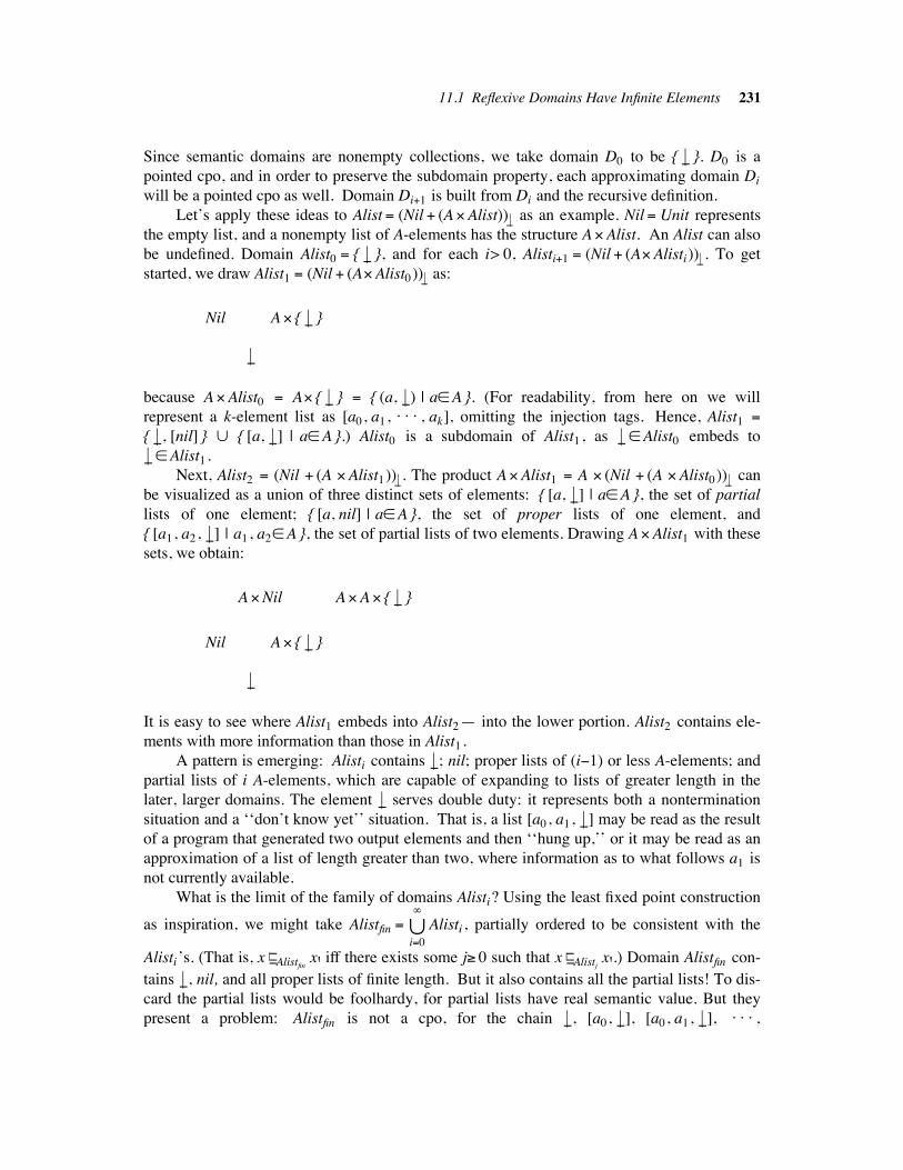
11.1 Reflexive Domains Have Infinite Elements 231
Since semantic domains are nonempty collections, we take domain D0 to be { %# }. D0 is a
pointed cpo, and in order to preserve the subdomain property, each approximating domain Di
will be a pointed cpo as well. Domain Di#1 is built from Di and the recursive definition.
Let’s apply these ideas to Alist " (Nil # (A$Alist)) %! as an example. Nil " Unit represents
the empty list, and a nonempty list of A-elements has the structure A$Alist. An Alist can also
be undefined. Domain Alist0 " { %# }, and for each i> 0, Alisti#1 " (Nil # (A$Alisti))%! . To get
started, we draw Alist1 " (Nil # (A$Alist0))%! as:
Nil A$ { %# }
%#
because A$Alist0 " A$ { %# } " { (a, %#) | a$A }. (For readability, from here on we will
represent a k-element list as [a0, a1, . . . , ak], omitting the injection tags. Hence, Alist1 "{ %#, [nil] } % { [a, %#] | a$A }.) Alist0 is a subdomain of Alist1 , as %#$Alist0 embeds to
%#$Alist1 .
Next, Alist2 " (Nil # (A $Alist1))%! . The product A$Alist1 " A $ (Nil # (A $Alist0))%! can
be visualized as a union of three distinct sets of elements: { [a, %#] | a$A }, the set of partial
lists of one element; { [a, nil] | a$A }, the set of proper lists of one element, and
{ [a1, a2, %#] | a1, a2$A }, the set of partial lists of two elements. Drawing A$Alist1 with these
sets, we obtain:
A$Nil A$A$ { %# }
Nil A$ { %# }
%#
It is easy to see where Alist1 embeds into Alist2— into the lower portion. Alist2 contains ele-
ments with more information than those in Alist1 .
A pattern is emerging: Alisti contains %#; nil; proper lists of (i#1) or less A-elements; and
partial lists of i A-elements, which are capable of expanding to lists of greater length in the
later, larger domains. The element %# serves double duty: it represents both a nontermination
situation and a ‘‘don’t know yet’’ situation. That is, a list [a0, a1, %#] may be read as the result
of a program that generated two output elements and then ‘‘hung up,’’ or it may be read as an
approximation of a list of length greater than two, where information as to what follows a1 is
not currently available.
What is the limit of the family of domains Alisti? Using the least fixed point construction
as inspiration, we might take Alistfin " i"0%&
Alisti , partially ordered to be consistent with the
Alisti’s. (That is, x ###%% Alistfin
x' iff there exists some j' 0 such that x ###%% Alistj
x'.) Domain Alistfin con-
tains %#, nil, and all proper lists of finite length. But it also contains all the partial lists! To dis-
card the partial lists would be foolhardy, for partial lists have real semantic value. But they
present a problem: Alistfin is not a cpo, for the chain %#, [a0, %#], [a0, a1, %#], . . . ,
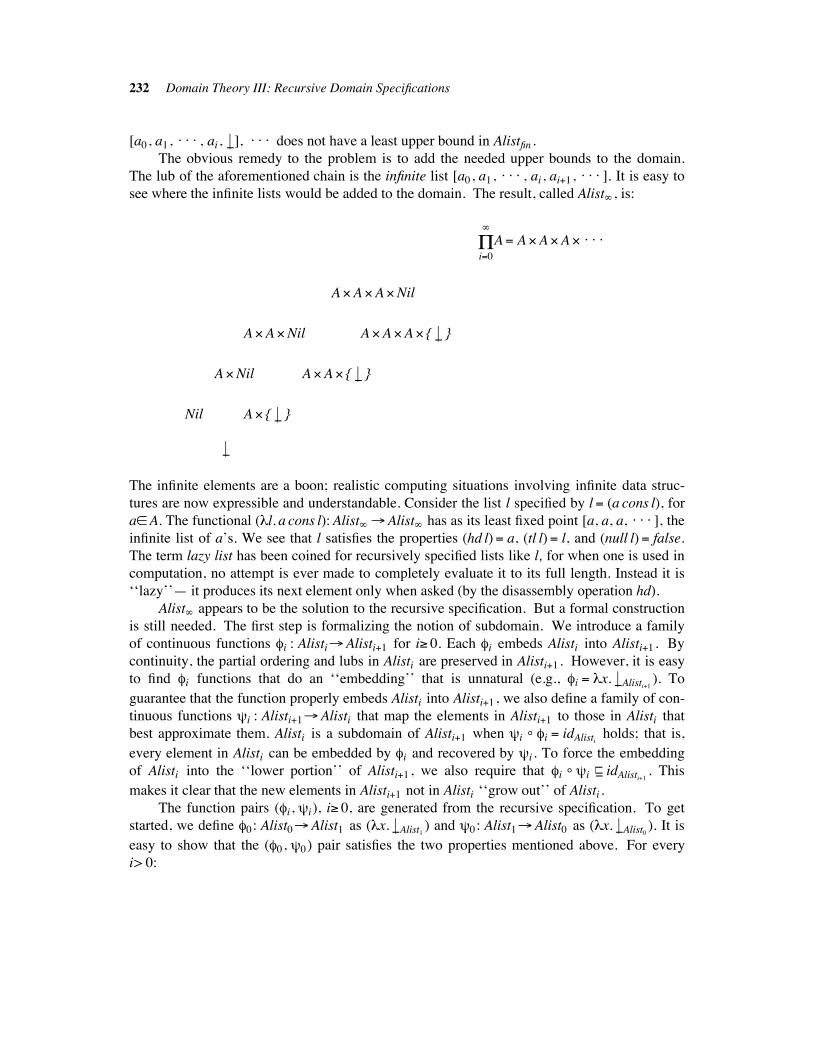
232 Domain Theory III: Recursive Domain Specifications
[a0, a1, . . . , ai , %#], . . . does not have a least upper bound in Alistfin .
The obvious remedy to the problem is to add the needed upper bounds to the domain.
The lub of the aforementioned chain is the infinite list [a0, a1, . . . , ai , ai#1, . . . ]. It is easy to
see where the infinite lists would be added to the domain. The result, called Alist& , is:
i"0(&
A" A$A$A$ . . .
A$A$A$Nil
A$A$Nil A$A$A$ { %# }
A$Nil A$A$ { %# }
Nil A$ { %# }
%#
The infinite elements are a boon; realistic computing situations involving infinite data struc-
tures are now expressible and understandable. Consider the list l specified by l " (a cons l), for
a$A. The functional ()l. a cons l): Alist& "Alist& has as its least fixed point [a, a, a, . . . ], the
infinite list of a’s. We see that l satisfies the properties (hd l)" a, (tl l)" l, and (null l)" false.
The term lazy list has been coined for recursively specified lists like l, for when one is used in
computation, no attempt is ever made to completely evaluate it to its full length. Instead it is
‘‘lazy’’— it produces its next element only when asked (by the disassembly operation hd).
Alist& appears to be the solution to the recursive specification. But a formal construction
is still needed. The first step is formalizing the notion of subdomain. We introduce a family
of continuous functions *i : Alisti"Alisti#1 for i' 0. Each *i embeds Alisti into Alisti#1 . By
continuity, the partial ordering and lubs in Alisti are preserved in Alisti#1 . However, it is easy
to find *i functions that do an ‘‘embedding’’ that is unnatural (e.g., *i " )x. %#Alisti#1). To
guarantee that the function properly embeds Alisti into Alisti#1 , we also define a family of con-
tinuous functions +i : Alisti#1"Alisti that map the elements in Alisti#1 to those in Alisti that
best approximate them. Alisti is a subdomain of Alisti#1 when +i & *i " idAlistiholds; that is,
every element in Alisti can be embedded by *i and recovered by +i . To force the embedding
of Alisti into the ‘‘lower portion’’ of Alisti#1 , we also require that *i & +i ###%% idAlisti#1
. This
makes it clear that the new elements in Alisti#1 not in Alisti ‘‘grow out’’ of Alisti .
The function pairs (*i, +i), i' 0, are generated from the recursive specification. To get
started, we define *0: Alist0"Alist1 as ()x. %#Alist1) and +0: Alist1"Alist0 as ()x. %#Alist0
). It is
easy to show that the (*0, +0) pair satisfies the two properties mentioned above. For every
i> 0:
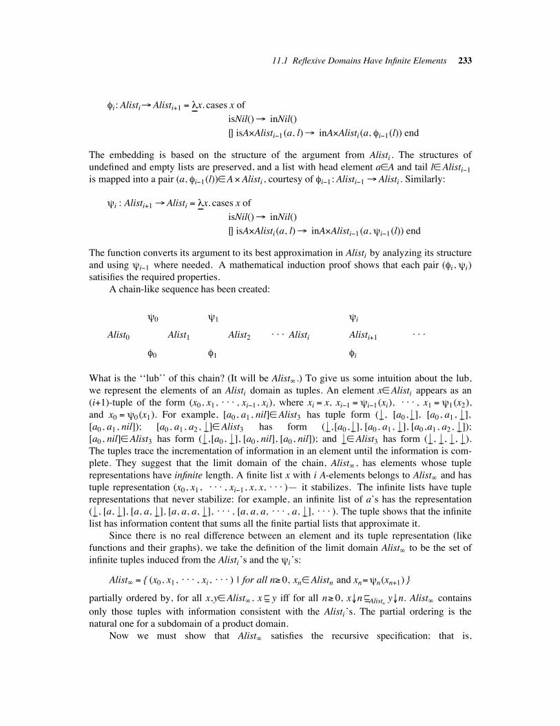
11.1 Reflexive Domains Have Infinite Elements 233
*i: Alisti"Alisti#1 " )!!x. cases x of
isNil()" inNil()
[] isA$Alisti#1(a, l)" inA$Alisti(a, *i#1(l)) end
The embedding is based on the structure of the argument from Alisti . The structures of
undefined and empty lists are preserved, and a list with head element a$A and tail l$Alisti#1
is mapped into a pair (a, *i#1(l))$A$Alisti , courtesy of *i#1: Alisti#1 "Alisti . Similarly:
+i : Alisti#1 "Alisti " )!!x. cases x of
isNil()" inNil()
[] isA$Alisti (a, l)" inA$Alisti#1(a, +i#1(l)) end
The function converts its argument to its best approximation in Alisti by analyzing its structure
and using +i#1 where needed. A mathematical induction proof shows that each pair (*i, +i)
satisifies the required properties.
A chain-like sequence has been created:
+0 +1 +i
Alist0 Alist1 Alist2. . . Alisti Alisti#1
. . .
*0 *1 *i
What is the ‘‘lub’’ of this chain? (It will be Alist& .) To give us some intuition about the lub,
we represent the elements of an Alisti domain as tuples. An element x$Alisti appears as an
(i#1)-tuple of the form (x0, x1, . . . , xi#1, xi), where xi " x, xi#1 " +i#1(xi), . . . , x1 " +1(x2),
and x0 " +0(x1). For example, [a0, a1, nil]$Alist3 has tuple form ( %#, [a0, %#], [a0, a1, %#],
[a0, a1, nil]); [a0, a1, a2, %#]$Alist3 has form ( %#, [a0, %#], [a0, a1, %#], [a0,a1, a2, %#]);
[a0, nil]$Alist3 has form ( %#, [a0, %#], [a0, nil], [a0, nil]); and %#$Alist3 has form ( %#, %#, %#, %#).
The tuples trace the incrementation of information in an element until the information is com-
plete. They suggest that the limit domain of the chain, Alist& , has elements whose tuple
representations have infinite length. A finite list x with i A-elements belongs to Alist& and has
tuple representation (x0, x1, . . . , xi#1, x, x, . . . )— it stabilizes. The infinite lists have tuple
representations that never stabilize: for example, an infinite list of a’s has the representation
( %#, [a, %#], [a, a, %#], [a, a, a, %#], . . . , [a, a, a, . . . , a, %#], . . . ). The tuple shows that the infinite
list has information content that sums all the finite partial lists that approximate it.
Since there is no real difference between an element and its tuple representation (like
functions and their graphs), we take the definition of the limit domain Alist& to be the set of
infinite tuples induced from the Alisti’s and the +i’s:
Alist& " { (x0, x1, . . . , xi, . . . ) | for all n' 0, xn$Alistn and xn"+n(xn#1) }
partially ordered by, for all x,y$Alist& , x ###%% y iff for all n' 0, x,n ##
#%% Alistny,n. Alist& contains
only those tuples with information consistent with the Alisti’s. The partial ordering is the
natural one for a subdomain of a product domain.
Now we must show that Alist& satisfies the recursive specification; that is,
234 Domain Theory III: Recursive Domain Specifications
Alist& " (Nil# (A$Alist&))%! .
Unfortunately this equality doesn’t hold! The problem is that the domain on the right-hand
side uses the one on the left-hand side as a component— the left-hand side domain is a set of
tuples but the right-hand side one is a lifted disjoint union. The situation isn’t hopeless, how-
ever, as the two domains have the same size (cardinality) and possess the same partial ordering
structure. The two domains are order isomorphic. The isomorphism is proved by functions
- : Alist& " (Nil# (A$Alist&))%! and . : (Nil# (A$Alist&))%!"Alist& such that . & - " idAlist&
and - & . " idNil#(A$Alist&))%!. The - function exposes the list structure inherent in an Alist&
element, and the . map gives the tuple representation of list structured objects.
The isomorphism property is strong enough that Alist& may be considered a solution of
the specification. The - and . maps are used in the definitions of operations on the domain.
For example, head : Alist& "A%! is defined as:
head" )!!x. cases -(x) of isNil()" %# [] isA$Alist& (a,l)" a end
tail : Alist& "Alist& is similar. The map construct: A $Alist& "Alist& is construct(a, x)
" .(inA$Alist& (a, x)). These conversions of structure from Alist& to list form and back are
straightforward and weren’t mentioned in the examples in the previous chapters. The isomor-
phism maps can always be inserted when needed.
The - and . maps are built from the (*i, +i) pairs. A complete description is presented
in the next section.
11.2 THE INVERSE LIMIT CONSTRUCTION !!!!!!!!!!!!!!!!!!!!!!!!!!!!!!!!!!!!!!!!!!!!!!!!!!!!!!!!!!!!!!!!!!
The method just described is the inverse limit construction. It was developed by Scott as a
justification of Strachey’s original development of denotational semantics. The formal details
of the construction are presented in this section. The main result is that, for any recursive
domain specification of form D" F(D) (where F is an expression built with the constructors of
Chapter 3 such that F(E) is a pointed cpo when E is), there is a domain D& that is isomorphic
to F(D&). D& is the least such pointed cpo that satisfies the specification. If you take faith in
the above claims, you may wish to skim this section and proceed to the examples in Section
11.3.
Our presentation of the inverse limit construction is based on an account by Reynolds
(1972) of Scott’s results. We begin by formalizing the relationship between the *i and +i
maps.
11.1 Definition:
For pointed cpos D and D', a pair of continuous functions (f: D"D', g : D'"D) is a
retraction pair iff:
1. g & f " idD
2. f & g ###%% idD'
11.2 The Inverse Limit Construction 235
f is called an embedding and g is called a projection.
11.2 Proposition:
The composition (f2 & f1 , g1 & g2) of retraction pairs (f1: D"D', g1: D'"D) and
(f2: D'"D'', g2: D''"D') is itself a retraction pair.
Proof: (g1 & g2) & (f2 & f1) " g1 & (g2 & f2) & f1) " g1 & idD' & f1 " g1 & f1 " idD . The proof
that (f2 & f1) & (g1 & g2) ###%% idD''
is similar.
11.3 Proposition:
An embedding (projection) has a unique corresponding projection (embedding).
Proof: Let (f, g1) and (f,g2) both be retraction pairs. We must show that g1 " g2 . First,
f & g1 ###%% idD'
which implies g2 & f & g1 ###%% g2 & idD'
by the monotonicity of g2. But
g2 & f & g1 " (g2 & f) & g1 " idD & g1 " g1 , implying g1 ###%% g2. Repeating the above deriva-
tion with g1 and g2 swapped gives g1 ###%% g2, implying that g1 " g2 . The uniqueness of an
embedding f to a projection g is left as an exercise.
11.4 Proposition:
The components of a retraction pair are strict functions.
Proof: Left as an exercise.
Retraction pairs are special cases of function pairs (f: D"D', g : D'"D) for cpos D and
D'. Since we will have use for function pairs that may not be retraction pairs on pointed cpos,
we assign the name r-pair to a function pair like the one just seen.
11.5 Definition:
For cpos D and D', a continuous pair of functions (f: D"D', g : D'"D) is called an r-
pair and is written (f,g): D/"D'. The operations on r-pairs are:
1. Composition: for (f1,g1) : D/"D' and (f2, g2) : D'/"D'',
(f2,g2) & (f1,g1) : D/"D'' is defined as (f2 & f1 , g1 & g2).
2. Reversal: for (f,g) : D/"D', (f,g)R : D'/"D is defined as (g,f).
The reversal of a retraction pair might not be a retraction pair. The identity r-pair for the
domain D/"D is idD/"D " (idD , idD). It is easy to show that the composition and reversal
operations upon r-pairs are continuous. We use the letters r, s, t, . . . to denote r-pairs.
11.6 Proposition:
236 Domain Theory III: Recursive Domain Specifications
For r-pairs r : D/"D' and s : D'/"D'':
1. (r & s)R " sR & rR
2. (rR)R " r.
Proof: Left as an exercise.
When we build a solution to D" F(D), we build the approximating domains { Di | i' 0 }
from an initial domain D0 by systematically applying the domain construction F. We use a
similar procedure to generate the r-pairs (*i,+i) : Di/"Di#1 from a starting pair (*0, +0).
First, the domain builders defined in Chapter 3 are extended to build r-pairs.
11.7 Definition:
For r-pairs r " (f, g) : C/"E and s " (f', g') : C'/"E ', let:
1. r$ s denote:
( ()(x,y). (f(x), f'(y))), ()(x,y). (g(x), g'(y))) ) : C $C'/"E$E '
2. r# s denote:
( ()x. cases x of isC(c)" inE(f(c)) [] isC'(c)" inE '(f'(c)) end,
()x. cases y of isE(e)" inC(g(e)) [] isE '(e)" inC'(g'(e)) end) )
: C#C'/"E#E '
3. r" s denote: (()x. f' & x & g), ()y. g' & y & f)) : (C"C')/" (E"E ')
4. (r)%! denote: (()!!x. f x), ()!!y. g y)) : C %!/"E%!
For D" F(D), the domain expression F determines a construction for building a new
domain F(A) from an argument domain A and a construction for building a new r-pair F(r)
from an argument r-pair r. For example, the recursive specification Nlist" (Nil# (Nat$Nlist)) %!gives a construction F(D) " ((Nil#(Nat$D))%! such that, for any cpo A, (Nil# (Nat$A))%! is also
a cpo, and for any r-pair r, (Nil# (Nat$ r))%! is an r-pair. The r-pair is constructed using
Definition 11.7; the r-pairs corresponding to Nil and Nat in the example are the identity r-pairs
(idNil , idNil) and (idNat , idNat), respectively. You are left with the exercise of formalizing what
a ‘‘domain expression’’ is. Once you have done so, produce a structural induction proof of the
following important lemma.
11.8 Lemma:
For any domain expression F and r-pairs r : D/"D' and s : D'/"D'':
1. F(idE/"E)" id F(E)/"F(E)
2. F(s) & F(r)" F(s & r)
3. (F(r))R " F(rR)
4. if r is a retraction pair, then so is F(r)
The lemma holds for the domain expressions built with the domain calculus of Chapter 3.
Now that r-pairs and their fundamental properties have been stated, we formulate the
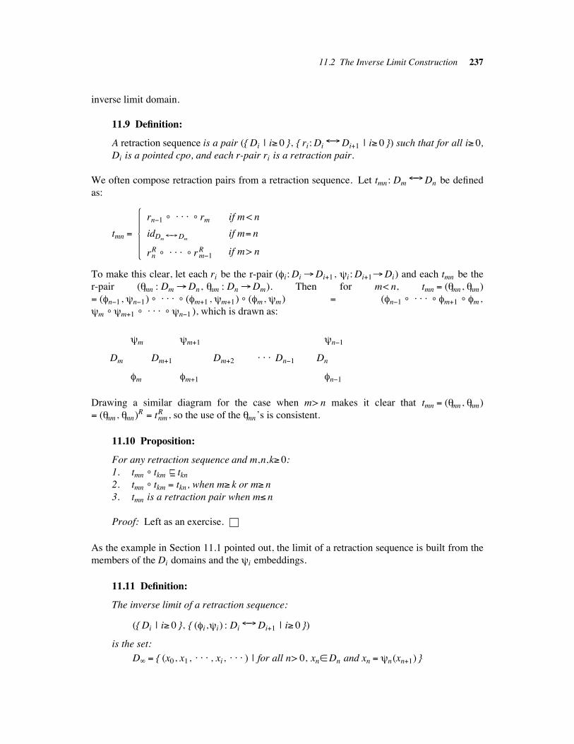
11.2 The Inverse Limit Construction 237
inverse limit domain.
11.9 Definition:
A retraction sequence is a pair ({ Di | i' 0 }, { ri: Di/"Di#1 | i' 0 }) such that for all i' 0,
Di is a pointed cpo, and each r-pair ri is a retraction pair.
We often compose retraction pairs from a retraction sequence. Let tmn : Dm/"Dn be defined
as:
tmn "
rnR &
. . . & rm#1R
idDm/"Dm
rn#1 & . . . & rm
if m> n
if m" n
if m< n
To make this clear, let each ri be the r-pair (*i: Di "Di#1, +i : Di#1"Di) and each tmn be the
r-pair (0mn : Dm "Dn , 0nm : Dn "Dm). Then for m< n, tmn " (0mn , 0nm)
" (*n#1, +n#1) & . . . & (*m#1 , +m#1) & (*m , +m) " (*n#1 &
. . . & *m#1 & *m ,
+m & +m#1 & . . . & +n#1 ), which is drawn as:
+m +m#1 +n#1
Dm Dm#1 Dm#2. . . Dn#1 Dn
*m *m#1 *n#1
Drawing a similar diagram for the case when m> n makes it clear that tmn " (0mn , 0nm)
" (0nm , 0mn)R " tnmR , so the use of the 0mn’s is consistent.
11.10 Proposition:
For any retraction sequence and m,n,k' 0:
1. tmn & tkm ###%% tkn
2. tmn & tkm " tkn , when m' k or m' n
3. tmn is a retraction pair when m1 n
Proof: Left as an exercise.
As the example in Section 11.1 pointed out, the limit of a retraction sequence is built from the
members of the Di domains and the +i embeddings.
11.11 Definition:
The inverse limit of a retraction sequence:
({ Di | i' 0 }, { (*i,+i) : Di/"Di#1 | i' 0 })
is the set:
D& " { (x0, x1, . . . , xi, . . . ) | for all n> 0, xn$Dn and xn " +n(xn#1) }
238 Domain Theory III: Recursive Domain Specifications
partially ordered by the relation: for all x,y$D& , x ###%% y iff for all n' 0, x,n ##
#%% Dny,n.
11.12 Theorem:
D& is a pointed cpo.
Proof: Recall that each Di in the retraction sequence is a pointed cpo. First,
%#D&" ( %#D0
, %#D1, . . . , %#Di
, . . . )$ D& , since every +i( %#Di#1)" %#Di
, by Proposition 11.4.
Second, for any chain C " { ci | i$ I } in D& , the definition of the partial ordering on D&
makes Cn " { ci,n | i$ I } a chain in Dn with a lub of#
Cn , n' 0. Now +n(#
Cn#1)
" #
{+n(ci,(n#1)) | i$ I } " #
{ ci,n | i$ I } " #
Cn . Hence
(#
C0,#
C1, . . . ,#
Ci , . . . ) belongs to D& . It is clearly the lub of C.
Next, we show how a domain expression generates a retraction sequence.
11.13 Proposition:
If domain expression F maps a pointed cpo E to a pointed cpo F(E), then the pair:
({ Di | D0 " { %# }, Di#1 " F(Di), for i' 0 },
{ (*i, +i) : Di/"Di#1 | *0 " ()x. %#D1
), +0 " ()x. %#D0),
(*i#1, +i#1)" F(*i , +i), for i' 0) }
is a retraction sequence.
Proof: From Lemma 11.8, part 4, and mathematical induction.
Thus, the inverse limit D& exists for the retraction sequence generated by F. The final task is
to show that D& is isomorphic to F(D&) by defining functions - : D& "F(D&) and
. : F(D&)"D& such that . & - " idD&and - & . " idF(D&) . Just as the elements of D& were
built from elements of the Di’s, the maps - and . are built from the retraction pairs (*i, +i).
For m' 0:
tm& : Dm/"D& is:
(0m& , 0&m)" ( ()x. (0m0(x), 0m1(x), . . . , 0mi(x), . . . )), ()x. x,m) )
t&m : D&/"Dm is: (0&m , 0m&)" tm&
R
t&& : D&/"D& is: (0&& , 0&&)" (idD&
, idD&)
You are given the exercises of showing that 0m& : Dm"D& is well defined and proving the fol-
lowing proposition.
11.14 Proposition:
Proposition 11.10 holds when & subscripts are used in place of m and n in the tmn pairs.
Since each tm& is a retraction pair, the value 0m&(0&m(x)) is less defined than x$D& . As m
increases, the approximations to x become better. A pleasing and important result is that as m
tends toward &, the approximations approach identity.
11.2 The Inverse Limit Construction 239
11.15 Lemma:
idD&" #
&
m"0
0m& & 0&m.
Proof: For every m' 0, tm& is a retraction pair, so 0m& & 0&m ###%% idD&
. Because
{ 0m& & 0&m | m' 0 } is a chain in D& "D& ,#
&
m"0
0m& & 0&m ###%% idD&
holds. Next, for any
x" (x0, x1, . . . , xi, . . . )$ D& and any i' 0, 0i& & 0& i(x) " 0i&(0& i(x)) "
(0i0(x,i), 0i1(x,i),..., 0ii(x,i), . . . ). Since 0ii(x,i) " (x,i) " xi, each mth component of
tuple x will appear as the mth component in 0m&(0&m(x)), for all m' 0. So x ###%%
#
&
m"0
(0m& & 0&m)(x) " (#
&
m"0
0m& & 0&m)(x). By extensionality, idD& ###%% #
&
m"0
0m& & 0&m , which
implies the result.
11.16 Corollary:
idD&/"D&
" #
&
m"0
tm& & t&m
11.17 Corollary:
idF(D&)/"F(D&) " #
&
m"0
F(tm&) & F(t&m)
Proof: idF(D&)/"F(D&) " F(idD&/"D&
), by Lemma 11.8, part 1
" F(#
&
m"0
tm& & t&m), by Corollary 11.16
" #
&
m"0
F(tm& & t&m), by continuity
" #
&
m"0
F(tm&) & F(t&m), by Lemma 11.8, part 2
The isomorphism maps are defined as a retraction pair (-, .) in a fashion similar to the r-pairs
in Corollaries 11.16 and 11.17. The strategy is to combine the two r-pairs into one on
D&/"F(D&):
(-, .) : D&/"F(D&)"
#
&
m"0
F(tm&) & t&(m#1)
The r-pair structure motivates us to write the isomorphism requirements in the form
(-, .)R & (-, .)" idD&/"D&
and (-, .) & (-, .)R " idF(D&)/"F(D&) . The proofs require the
following technical lemmas.
11.18 Lemma:
For any m' 0, F(t&m) & (-, .) " t& (m#1)
240 Domain Theory III: Recursive Domain Specifications
Proof: F(t&m) & (-, .)
" F(t&m) & #&
n"0
F(t n&) & t& (n#1)
" #
&
n"0
F(t&m) & F(tn&) & t& (n#1), by continuity
" #
&
n"0
F(t&m & tn&) & t& (n#1), by Lemma 11.8, part 2
" #
&
n"0
F(tnm) & t& (n#1), by Proposition 11.14
" #
&
n"0
t(n#1)(m#1) & t& (n#1)
By Proposition 11.14, t(n#1)(m#1) & t& (n#1) " t& (m#1), for n'm. Thus, the least upper bound
of the chain is t& (m#1).
11.19 Lemma:
For any m' 0, (-, .) & t(m#1)& " F(tm&)
Proof: Similar to the proof of Lemma 11.18 and left as an exercise.
11.20 Theorem:
(-, .)R & (-, .)" idD&/"D&
Proof: (-, .)R & (-, .)" (#
&
m"0
F(tm&) & t& (m#1))R & (-, .)
" (#
&
m"0
(F(tm&) & t& (m#1))R) & (-, .), by continuity of R
" (#
&
m"0
t& (m#1)R & F(tm&)R) & (-, .), by Proposition 11.6
" (#
&
m"0
t(m#1)& & F(t&m)) & (-, .), by Lemma 11.8, part 3
" #
&
m"0
t(m#1)& & F(t&m) & (-, .), by continuity
" #
&
m"0
t(m#1)& & t&(m#1) , by Lemma 11.18
" #
&
m"0
tm& & t&m , as t0& & t& 0 ###%% t1& & t&1
" idD&/"D&
, by Corollary 11.16
11.21 Theorem:
(-, .) & (-, .)R " idF(D&)/"F(D&)
Proof: Similar to the proof of Theorem 11.20 and left as an exercise.
Analogies of the inverse limit method to the least fixed point construction are strong. So
11.2 The Inverse Limit Construction 241
far, we have shown that D& is a ‘‘fixed point’’ of the ‘‘chain’’ generated by a ‘‘functional’’ F.
To complete the list of parallels, we can show that D& is the ‘‘least upper bound’’ of the
retraction sequence. For the retraction sequence ({ Di | i' 0 }, { (*i, +i) | i' 0 }) generated by F,
assume that there exists a pointed cpo D' and retraction pair (-', .') : D'/"F(D') such that
(-', .') proves that D' is isomorphic to F(D'). Then define the following r-pairs:
t'0& : D0/"D' as (()x. %#D'
), ()x. %#D0))
t'(m#1)& : Dm#1/"D' as (.', -') & F(t'm&)
Each t'm& is a retraction pair, and { t'm& & t&m | m' 0 } is a chain in D&/"D'. Next, define
(2, 3) : D&/"D' to be
#
&
m"0
t'm& & t&m . We can show that (2, 3) is a retraction pair; that is, D&
embeds into D'. Since D' is arbitrary, D& must be the least pointed cpo solution to the retrac-
tion sequence.
We gain insight into the structure of the isomorphism maps - and . by slightly abusing
our notation. Recall that a domain expression F is interpreted as a map on r-pairs. F is
required to work upon r-pairs because it must ‘‘invert’’ a function’s domain and codomain to
construct a map upon function spaces (see Definition 11.7, part 3). The inversion is done with
the function’s r-pair mate. But for retraction components, the choice of mate is unique (by
Proposition 11.3). So, if r-pair r " (f, g) is a retraction pair, let F(f, g) be alternatively written
as (Ff, Fg), with the understanding that any ‘‘inversions’’ of f or g are fulfilled by the
function’s retraction mate. Now the definition of (-, .), a retraction pair, can be made much
clearer:
(-, .)" #
&
m"0
F(tm&) & t& (m#1)
" #
&
m"0
F(0m& ,0&m) & (0& (m#1), 0(m#1)&)
" #
&
m"0
(F0m& , F0&m) & (0& (m#1), 0(m#1)&)
" #
&
m"0
(F0m& & 0& (m#1), 0(m#1)& & F0&m)
" (#
&
m"0
F0m& & 0& (m#1), #
&
m"0
0(m#1)& & F0&m)
We see that - : D& "F(D&) maps an x$D& to an element x(m#1)$Dm#1 and then maps xm#1
to an F-structured element whose components come from D& . The steps are performed for
each m> 0, and the results are joined. The actions of . : F(D&)"D& are similarly inter-
preted. This roundabout method of getting from D& to F(D&) and back has the advantage of
being entirely representable in terms of the elements of the retraction sequence. We exploit
this transparency in the examples in the next section.
11.3 APPLICATIONS !!!!!!!!!!!!!!!!!!!!!!!!!!!!!!!!!!!!!!!!!!!!!!!!!!!!!!!!!!!!!!!!!!!!!!!!!!!!!!!!!!!!!!!!!!!!!!!!!!!!!!!!!!!!
We now examine three recursive domain specifications and their inverse limit solutions. The
tuple structure of the elements of the limit domain and the isomorphism maps give us deep
242 Domain Theory III: Recursive Domain Specifications
insights into the nature and uses of recursively defined domains.
11.3.1 Linear Lists !!!!!!!!!!!!!!!!!!!!!!!!!!!!!!!!!!!!!!!!!!!!!!!!!!!!!!!!!!!!!!!!!!!!!!!!!!!!!!!!!!!!!!!!!!!!!!!!!!!!!!!!!!!!!!!!!!
This was the example in Section 11.1. For the recursive definition Alist" (Nil# (A$Alist)) %! ,
the retraction sequence is ({ Dn | n' 0 }, { (*n, +n) | n' 0 }), where:
D0 " { %# }
Di#1 " (Nil# (A$Di))%!
and
*0 : D0 "D1 " ()x. %#D1)
+0 : D1 "D0 " ()x. %#D0)
*i : Di "Di#1 " (idNil # (idA $ *i#1))%!
" )!!x. cases x of
isNil()" inNil()
[] isA$Di#1(a,d)" inA$Di(a, *i#1(d)) end
+i : Di#1 "Di " (idNil # (idA $+i#1))%!
" )!!x. cases x of
isNil()" inNil()
[] isA$Di(a,d)" inA$Di#1(a, +i#1(d)) end
An element in Dn is a list with n or less A-elements. The map 0mn : Dm "Dn converts a
list of m (or less) A-elements to one of n (or less) A-elements. If m> n, the last m#n elements
are truncated and replaced by %#. If m1 n, the list is embedded intact into Dn . An Alist& element
is a tuple x" (x0, x1, . . . , xi, . . . ), where each xi is a list from Di and xi and xi#1 agree on
their first i A-elements, because xi " +i(xi#1). The map 0&m : Alist&"Dm projects an infinite
tuple into a list of m elements 0&m(x)" xi , and 0m& : Dm"Alist& creates the tuple correspond-
ing to an m-element list 0m&(l) " (0m0(l), 0m1(l), . . . , 0mm(l), 0m(m#1), . . . ), where 0mk(l) " l for
k'm. It is easy to see that any finite list has a unique representation in Alist& , and Lemma
11.15 clearly holds. But why can we treat Alist& as if it were a domain of lists? And where are
the infinite lists? The answers to both these questions lie with - : Alist&"F(Alist&). It is
defined as:
-"#
&
m"0
(idNil # (idA $ 0m&))%! & 0& (m#1)
"#
&
m"0
()!!x. cases x of
isNil()" inNil()
[] isA$Dm(a,d)" inA$Alist& (a, 0m&(d))
end) & 0& (m#1)
- reveals the list structure in an Alist& tuple. A tuple x$Alist& represents:
11.3.1 Linear Lists 243
1. The undefined list when -(x)" %# (then x is ( %#, %#, %#, . . . )).
2. The nil list when -(x)" inNil() (then x is ( %#, [nil], [nil], . . . )).
3. A list whose head element is a and tail component is d when -(x)" inA$Alist& (a, d)
(then x is ( %#, [a,0&0(d)], [a,0&1(d)], . . . , [a,0& (i#1)(d)], . . . )). -(d) shows the list struc-
ture in the tail.
As described in Section 11.1, an infinite list is represented by a tuple x such that for all
i' 0 xi4 xi#1. Each xi$Di is a list with i (or less) A-elements; hence the kth element of the
infinite list that x represents is embedded in those xj such that j' k. - finds the kth element: it
is ak , where -(x) " inA$Alist& (a1, d2), and -(di) " inA$Alist& (ai, di#1), for i> 1.
The inverse map to - is .: F(Alist&)"Alist& . It embeds a list into Alist& so that opera-
tions like cons: A$Alist&"Alist& have well-formed definitions. For a$A and x$Alist& ,
.(a, d) " ( %#, [a,0&0(x)], [a,0&1(x)], . . . , [a,0& (i#1)(x)], . . . ). The isomorphism properties of
- and . assure us that this method of unpacking and packing tuples is sound and useful.
11.3.2 Self-Applicative Procedures !!!!!!!!!!!!!!!!!!!!!!!!!!!!!!!!!!!!!!!!!!!!!!!!!!!!!!!!!!!!!!!!!!!!!!!!!!!!!!!!!!!!!!!!
Procedures in ALGOL60 can take other procedures as arguments, even to the point of self-
application. A simplified version of this situation is Proc" Proc"A%! . The family of pointed
cpos that results begins with:
D0 " { %# }
D1 " D0 "A%!
The argument domain to D1-level procedures is just the one-element domain, and the
members of D1 are those functions with graphs of form { ( %#, a) }, for a$ A %! .
D2 " D1 "A%!
A D2-level procedure accepts D1-level procedures as arguments.
Di#1 " Di "A%!
In general, a Di#1-level procedure accepts Di-level arguments. (Note that Di#1, Di#2, . . . are
all embedded in Di .) If we sum the domains, the result,i"05&
Di , resembles a Pascal-like hierar-
chy of procedures. But we want a procedure to accept arguments from a level equal to or
greater than the procedure’s own. The inverse limit’s elements do just that.
Consider an element (p0, p1, . . . , pi , . . . )$ Proc&. It has the capability of handling a
procedure argument at any level. For example, an argument qk: Dk is properly handled by pk#1,
and the result is pk#1(qk). But the tuple is intended to operate upon arguments in Proc&, and
these elements no longer have ‘‘levels.’’ The solution is simple: take the argument q$ Proc&and map it down to level D0 (that is, 0&0(q)) and apply p1 to it; map it down to level D1 (that
is, 0&1(q)) and apply p2 to it; . . .; map it down to level Di (that is, 0& i(q)) and apply pi#1 to it;
. . . ; and lub the results! This is precisely what - : Proc& "F(Proc&) does:
-" #
&
m"0
(0m& " idA%!) & 0& (m#1)
244 Domain Theory III: Recursive Domain Specifications
" #
&
m"0
()x. idA%! & x & 0&m) & 0& (m#1)
The application p(q) is actually (-(p))(q). Consider -(p); it has value:
-(p)" #
&
m"0
()x. idA%! & x & 0&m)(0& (m#1)(p))
" #
&
m"0
(0& (m#1)(p)) & 0&m
" #
&
m"0
(p,(m#1)) & 0&m
" #
&
m"0
pm#1 & 0&m
Thus:
(-(p))(q) " (#
&
m"0
pm#1 & 0&m)(q)
" #
&
m"0
pm#1(0&m(q))
" #
&
m"0
pm#1(q,m)
" #
&
m"0
pm#1(qm)
The scheme is general enough that even self-application is understandable.
11.3.3 Recursive Record Structures !!!!!!!!!!!!!!!!!!!!!!!!!!!!!!!!!!!!!!!!!!!!!!!!!!!!!!!!!!!!!!!!!!!!!!!!!!!!!!!!!!!!!!!!
Recall that the most general form of record structure used in Chapter 7 was:
Record" Id"Denotable-value
Denotable-value" (Record#Nat# . . . ) %!
Mutually defined sets of equations like the one above can also be handled by the inverse limit
technique. We introduce m-tuples of domain equations, approximation domains, and r-pairs.
The inverse limit is an m-tuple of domains. In this example, m"2, so a pair of retraction
sequences are generated. We have:
R0 " Unit
D0 " Unit
Ri#1 " Id"Di
Di#1 " (Ri #Nat # . . . ) %! , for i' 0
and
R*0 : R0 "R1 " ()x. %#R1)
R+0 : R1 "R0 " ()x. %#R0)
D*0 : D0 "D1 " ()x. %#D1)
11.3.3 Recursive Record Structures 245
D+0 : D1 "D0 " ()x. %#D0)
R*i : Ri "Ri#1 " ()x. D*i#1 & x & idId)
R+i : Ri#1 "Ri " ()x. D+i#1 & x & idId)
D*i : Di "Di#1 " (R*i#1 # idNat # . . . ) %!
D+i : Di#1 "Di " (R+i#1 # idNat # . . . ) %! , for i> 0
The inverse limits are Record& and Denotable-value&. Two pairs of isomorphism maps result:
(R-, R.) and (D-, D.). Elements of Record& represent record structures that map identifiers
to values in Denotable-value&. Denotable-value& contains Record& as a component, hence
any r$Record& exists as the denotable value inRecord&(r). Actually, the previous sentence is
a bit imprecise— (Record& #Nat # . . . ) %! contains Record& as a component, and an
r$Record& is embedded in Denotable-value& by writing D.(inRecord&(r)). Like all the
other inverse limit domains, Denotable-value& and Record& are domains of infinite tuples,
and the isomorphism maps are necessary for unpacking and packing the denotable values and
records.
Consider the recursively defined record:
r " [ [[A]] %%" inNat(zero) ] [ [[B]] %%" inRecord&(r) ] ()i. %#)
Record r contains an infinite number of copies of itself. Any indexing sequence
(r [[B]] [[B]] . . . [[B]]) produces r again. Since Record& is a pointed cpo, the recursive definition
of r has a least fixed point solution, which is a tuple in Record&. You should consider how the
least fixed point solution is calculated in Record& and why the structure of r is more complex
than that of a recursively defined record from a nonrecursive domain.
SUGGESTED READINGS !!!!!!!!!!!!!!!!!!!!!!!!!!!!!!!!!!!!!!!!!!!!!!!!!!!!!!!!!!!!!!!!!!!!!!!!!!!!!!!!!!!!!!!!!!!!!!!!!!!!!!
Inverse limit construction: Plotkin 1982; Reynolds 1972; Scott 1970, 1971, 1972; Scott &
Strachey 1971
Generalizations & alternative approaches: Adamek & Koubek 1979; Barendregt 1977,
1981; Gunter 1985a, 1985b, 1985c; Kamimura & Tang 1984a; Kanda 1979; Lehman &
Smyth 1981; Milner 1977; Scott 1976, 1983; Smyth & Plotkin 1982; Stoy 1977; Wand
1979
EXERCISES !!!!!!!!!!!!!!!!!!!!!!!!!!!!!!!!!!!!!!!!!!!!!!!!!!!!!!!!!!!!!!!!!!!!!!!!!!!!!!!!!!!!!!!!!!!!!!!!!!!!!!!!!!!!!!!!!!!!!!!!!!!!
1. Construct the approximating domains D0, D1, D2, . . . , Di#1 for each of the following:
a. N " (Unit #N) %!b. Nlist " IN%! $Nlist
c. Mlist " (IN$Mlist) %!d. P" P" IB %!
e. Q" (Q" IB) %!
246 Domain Theory III: Recursive Domain Specifications
Describe the structure of D& for each of the above.
2. Define the domain D" D" (D#Unit) %! . What D& element is the denotation of each of the
following?
a. ()d. %#)
b. ()d. inD(d))
c. f " ()d. inD(f))
3. Let Nlist " (Nat!)%! and Natlist " (Unit # (Nat $Natlist)) %! .
a. What lists does Natlist have that Nlist does not?
b. Define cons : Nat $Nlist"Nlist for Nlist. Is your version strict in its second argu-
ment? Is it possible to define a version of cons that is nonstrict in its second argu-
ment? Define a cons operation for Natlist that is nonstrict in its second argument.
c. Determine the denotation of l$Nlist in l " zero cons l and of l$Natlist in
l " zero cons l.
d. A lazy list is an element of Natlist that is built with the nonstrict version of cons.
Consider the list processing language in Figure 7.5. Make the Atom domain be Nat,
and make the List domain be a domain of lazy lists of denotable values. Redefine the
semantics. Write an expression in the language whose denotation is the list of all the
positive odd numbers.
4. One useful application of the domain Natlist " (Unit # (Nat $Natlist)) %! is to the semantics
of programs that produce infinite streams of output.
a. Consider the language of Figure 9.5. Let its domain Answer be Natlist. Redefine the
command continuations finish : Cmdcont to be finish " ()s. inUnit()) and
error : String"Cmdcont to be error " ()t.)s. %#). Add this command to the language:
C[[print E]]" )e.)c. E[[E]]()n.)s. inNat$Natlist(n, (c s)))
Prove for e$Environment, c$Cmdcont, and s$ Store that C[[while
1 do print 0]]e c s is an infinite list of zeros.
b. Construct a programming language with a direct semantics that can also generate
streams. The primary valuation functions are PD: Program " Store "Natlist and
CD: Command "Environment " Store "Poststore, where Poststore " Natlist
$ Store%! . (Hint: make use of an operation strict : (A"B)" (A%!"B), where B is a
pointed cpo, such that:
strict(f)( %#)" %#B , that is, the least element in B
strict(f)(a)" f(a), for a proper value a$A
Then define the composition of command denotations f, g$ Store"Poststore as:
g!f " )s. ()(l, p). ()(l', p'). (l append l', p'))(strict(g)(p)))(f s)
where append : Natlist $Natlist"Natlist is the list concatenation operation and is
nonstrict in its second argument.) Prove that CD[[while 1 do print 0]]e s is an infinite
Exercises 247
list of zeros.
c. Define a programming language whose programs map an infinite stream of values and
a store to an infinite stream of values. Define the language using both direct and con-
tinuation styles. Attempt to show a congruence between the two definitions.
5. a. The specification of record r in Section 11.3 is incomplete because the isomorphism
maps are omitted. Insert them in their proper places.
b. How can recursively defined records be used in a programming language? What
pragmatic disadvantages result?
6. a. Why does the inverse limit method require that a domain expression f in D" F(D)
map pointed cpos to pointed cpos?
b. Why must we work with r-pairs when an inverse limit domain is always built from a
sequence of retraction pairs?
c. Can a retraction sequence have a domain D0 that is not { %#}? Say that a retraction
sequence had D0 " Unit %! . Does an inverse limit still result? State the conditions
under which IB %! could be used as D0 in a retraction sequence generated from a
domain expression F in D" F(D). Does the inverse limit satisfy the isomorphism? Is
it the least such domain that does so?
7. a. Show the approximating domains D0, D1, . . . , Di for each of the following:
i. D" D"D
ii. D" D %!"D%!
iii. D" (D"D)%!
b. Recall the lambda calculus system that was introduced in exercise 11 of Chapter 3.
Once again, its syntax is:
E ::= (E1 E2) | ()I. E) | I
Say that the meaning of a lambda-expression ()I.E) is a function. Making use of the
domain Environment" Identifier"D with the usual operations, define a valuation
function E : Lambda-expression "Environment"D for each of the three versions of
D defined in part a. Which of the three semantics that you defined is extensional; that
is, in which of the three does the property ‘‘(for all [[E]], E[[(E1 E)]]" E[[(E2 E)]])
implies E[[E1]]" E[[E2]]’’ hold? (Warning: this is a nontrivial problem.)
c. For each of the three versions of E that you defined in part b, prove that the 3-rule is
sound, that is, prove:
E[[()I. E1)E2]]" E[[[E2/I]E1]]
d. Augment the syntax of the lambda-calculus with the abstraction form ()val I.E). Add
the following reduction rule:
3val-rule: ()val I. E1)E2 "> [E2/I]E1
where E2 is not a combination (E1' E2')
248 Domain Theory III: Recursive Domain Specifications
Define a semantics for the new version of abstraction for each of the three versions of
valuation function in part b and show that the 3val-rule is sound with respect to each.
8. For the definition D" D"D, show that an inverse limit can be generated starting from
D0 " Unit %! and that D& is a nontrivial domain. Prove that this inverse limit is the smallest
nontrivial domain that satisfies the definition.
9. Scott proposed the following domain for modelling flowcharts:
C " (Skip#Assign #Comp #Cond) %!
where Skip" Unit represents the skip command
Assign is a set of primitive assigment commands
Comp " C $C represents command composition
Cond " Bool $C $C represents conditional
Bool is a set of primitive Boolean expressions
a. What relationship does domain C have to the set of derivation trees of a simple
imperative language? What ‘‘trees’’ are lacking? Are there any extra ones?
b. Let wh(b, c) be the C-value wh(b, c) " inCond(b, inComp(c, wh(b, c)), inSkip()), for
c$C and b$Bool. Using the methods outlined in Section 6.6.5, draw a tree-like pic-
ture of the denotation of wh(b0, c0). Next, write the tuple representation of the value
as it appears in C& .
c. Define a function sem : C" Store%!" Store%! that maps a member of C to a store
transformation function. Define a congruence between the domains Bool and
Boolean-expr and between Assign and the collection of trees of the form [[I:"E]].
Prove for all b$Bool and its corresponding [[B]] and for c$C and its corresponding
[[C]] that sem(wh(b, c)) " C[[while B do C]].
10. The domain I" (Dec$ I)%! , where Dec" { 0, 1, . . . , 9 }, defines a domain that contains
infinite lists of decimal digits. Consider the interval [0,1], that is, all the real numbers
between 0 and 1 inclusive.
a. Show that every value in [0,1] has a representation in I. (Hint: consider the decimal
representation of a value in the interval.) Are the representations unique? What do the
partial lists in I represent?
b. Recall that a number in [0,1] is rational if it is represented by a value m/n, for
m,n$ IN. Say that an I-value is recursive if it is representable by a (possibly recur-
sive) function expression f " 2. Is every rational number recursive? Is every recursive
value rational? Are there any nonrecursive values in I?
c. Call a domain value transcendental if it does not have a function expression represen-
tation. State whether or not there are any transcendental values in the following
domains. (IN has none.)
i. IN$ IN
ii. IN" IN
iii. Nlist " (IN$Nlist) %!
Exercises 249
iv. N " (Unit #N) %!
11. Just as the inverse limit D& is determined by its approximating domains Di , a function
g : D& "C is determined by a family of approximating functions. Let
G" { gi: Di "C | i' 0 } be a family of functions such that, for all i' 0, gi#1 & *i " gi . (That
is, the maps always agree on elements in common.)
a. Prove that for all i' 0, gi &+i ###%% gi#1.
b. Prove that there exists a unique g : D& "C such that for all i' 0, g & 0i& " gi . Call g the
mediating morphism for G, and write g" med G.
c. For a continuous function h : D& "C, define the family of functions
H" { hi: Di "C | i' 0, hi " h & 0i& }.
i. Show that hi#1 & *i " hi for each i' 0.
ii. Prove that h" med H and that H" { (med H) & 0i& | i' 0 }.
Thus, the approximating function families are in 1-1, onto correspondence with the
continuous functions in D& "C.
d. Define the approximating function family for the map hd : Alist"A %! , Alist "(Unit # (A $ Alist)) %! , hd " )l. cases -(l) of isUnit()" %# [] isA$Alist(a, l)" a end.
Describe the graph of each hdi .
e. Let pi: Di " IB be a family of continuous predicates. Prove that for all i' 0, pi holds
for di $Di , (that is, pi(di)" true) iff med { pi | i' 0 }(d)" true, where
d" (d0, d1, . . . , di , . . . ) : D& . Conversely, let P : D& " IB be a continuous predicate.
Prove that P holds for a d$D& (that is, P(d)" true) iff for all i' 0, P & 0i&(di)" true.
f. Results similar to those in parts a through c hold for function families
{ fi : C"Di | i' 0 } such that for all i' 0, fi " +i & fi#1. Prove that there exists a unique
f: C"D& such that for all i' 0, fi " 0& i & f.
Chapter 12 !!!!!!!!!!!!!!!!!!!!!!!!!!!!!!!!!!!!!!!!!!!!!!!!!!!!!!!
Nondeterminism and Concurrency
A program is deterministic if its evaluations on the same input always produce the same out-
put. The evaluation strategy for a deterministic program might not be unique. For example,
side effect-free arithmetic addition can be implemented in more than one fashion:
1. Evaluate the left operand; evaluate the right operand; add.
2. Evaluate the right operand; evaluate the left operand; add.
3. Evaluate the two operands in parallel; add.
A program is nondeterministic if it has more than one allowable evaluation strategy and
different evaluation strategies lead to different outputs. One example of a nondeterministic
construct is addition with side effects, using the three evaluation strategies listed above. If an
operand contains a side effect, then the order of evaluation of the operands can affect the final
result. This situation is considered a result of bad language design, because elementary arith-
metic is better behaved. It is somewhat surprising that the situation is typically resolved by
outlawing all but one of the allowable evaluation strategies and embracing hidden side effects!
There are situations where nondeterminism is acceptable. Consider an error-handling
routine that contains a number of commands, each indexed by a specific error condition. If a
run-time error occurs, the handler is invoked to diagnose the problem and to compensate for it.
Perhaps the diagnosis yields multiple candidate error conditions. Only one correction com-
mand is executed within the handler, so the choice of which one to use may be made nondeter-
ministically.
A concept related to nondeterminism is parallel evaluation. Some language constructs
can be naturally evaluated in parallel fashion, such as side effect-free addition using the third
strategy noted above. This ‘‘nice’’ form of parallelism, where the simultaneous evaluation of
subparts of the construct do not interact, is called noninterfering parallelism. In interfering
parallelism, there is interaction, and the relative speeds of the evaluations of the subparts do
affect the final result. We call a concurrent language one that uses interfering parallelism in its
evaluation of programs. The classic example of a concurrent language is an imperative
language that evaluates in parallel commands that share access and update rights to a common
variable.
We require new tools to specify the semantics of nondeterministic and concurrent
languages. A program’s answer denotation is no longer a single value d from a domain D, but
a set of values { d0, d1, . . . , di , . . . } describing all the results possible from the different
evaluations. The set of values is an element from the powerdomain IP(D). The powerdomain
corresponds to the powerset in Chapter 2, but the underlying mathematics of the domain-based
version is more involved. The members of IP(D) must be related in terms of both subset pro-
perties and the partial ordering properties of D. Unfortunately, there is no best powerdomain
construction, and a number of serious questions remain regarding the theory.
Section 12.1 describes the properties of the powerdomain construction, and Section 12.2
250
12.1 Powerdomains 251
uses it to model a nondeterministic language. Section 12.3 presents one approach to model-
ling interfering parallelism. Section 12.4 presents an alternative approach to nondeterministic
and parallel evaluation, and Section 12.5 gives an overview to the mathematics underlying
powerdomain construction.
12.1 POWERDOMAINS !!!!!!!!!!!!!!!!!!!!!!!!!!!!!!!!!!!!!!!!!!!!!!!!!!!!!!!!!!!!!!!!!!!!!!!!!!!!!!!!!!!!!!!!!!!!!!!!!!!!!!!!
The powerdomain construction builds a domain of sets of elements. For domain A, the power-
domain builder IP(_) creates the domain IP(A), a collection whose members are sets X!A. The
associated assembly operations are:
" : IP(A), a constant that denotes the smallest element in IP(A).
{ _ } : A# IP(A), which maps its argument a$A to the singleton set { a }.
_%_ : IP(A)" IP(A)# IP(A), the binary union operation, which combines its two arguments
M# { a0, a1, . . . } and N# { b0, b1, . . . } into the set
M%N # { a0, a1, . . . , b0, b1, . . . }.
The disassembly operation builder for powerdomains converts an operation on A-
elements into one on IP(A)-elements.
For f: A# IP(B), there exists a unique operation f++: IP(A)# IP(B) such that for any
M$ IP(A), f++(M)# %{ f(m) | m$M }.
The operation builder can be applied to operations g: A#B to produce a function in the
domain IP(A)# IP(B): use (&a. { g(a) })++ .
12.2 THE GUARDED COMMAND LANGUAGE !!!!!!!!!!!!!!!!!!!!!!!!!!!!!!!!!!!!!!!!!!!!!!!!!!!!!!!!!!!!!!!!
A well-defined programming language depends on explicit evaluation strategies as little as
possible. Imperative languages require sequencing at the command level to clarify the order of
updates to the store argument. The sequencing is critical to understanding command composi-
tion, but it need not be imposed on the other command builders. As an example, a useful gen-
eralization of the conditional command if B then C1 else C2 is the multichoice cases com-
mand:
cases
B1 : C1;
B2 : C2;. . .
Bn : Cn
end
252 Nondeterminism and Concurrency
A command Ci is executed when test Bi evaluates to true. A problem is that more than one Bi
may hold. Normally, we want only one command in the cases construct to be evaluated, so we
must make a choice. The traditional choice is to execute the ‘‘first’’ Ci , reading from ‘‘top to
bottom,’’ whose test Bi holds, but this choice adds little to the language. A better solution is
to nondeterministically choose any one of the candidate commands whose test holds. In
Dijkstra (1976), this form of conditional naturally meshes with the development of programs
from formal specifications. As an exercise, we define a denotational semantics of the impera-
tive language proposed by Dijkstra.
Dijkstra’s language, called the guarded command language, is an assignment language
augmented by the nondeterministic conditional command and a nondeterministic multitest
loop, which iterates as long as one of its tests is true. The language is presented in Figure 12.1.
The domain of possible answers of a nondeterministic computation is a powerdomain of
post-store elements. The operation of primary interest is then, which sequences two nondeter-
ministic commands. The semantics of an expression (f1 thenf2)(s) says that f1 operates on s,
producing a set of post-stores. Each post-store is passed through f2 to produce an answer set.
The answer sets are unioned.
The functionality of the C valuation function points out that a command represents a non-
deterministic computation. The semantic equations for the conditional and loop commands
both use an auxiliary valuation function T to determine if at least one of the tests (guards) of
the construct holds. In the case of the conditional, failure of all guards causes an abortion;
failure of all the guards of the loop construct causes exit of the loop. The G function defines
the meaning of a conditional/loop body. The updates of all the guarded commands whose
tests hold are joined together, and a set of stores result.
Here is a small example. For:
C0 # G1 [] G2
G1 # X' 0#Y:#1
G2 # X# 0#Y:#0
we derive:
C[[C0]]# C[[G1 [] G2]]
# &s. T[[G1 [] G2]]s#G[[G1 [] G2]]s [] abort s
# &s. (B[[X' 0]]s) or(B[[X# 0]]s)#G[[G1 [] G2]]s [] abort s
(B[[X' 0]]s) or(B[[X# 0]]s) must be true, so we simplify to:
&s. G[[G1 [] G2]]s # &s. (B[[X' 0]]s#C[[Y:#1]]s [] noanswer)
join (B[[X# 0]]s#C[[Y:#0]]s [] noanswer)
Consider a store s0 such that (access[[X]] s0) is greater than zero. Then the above expression
simplifies to:
(C[[Y:#1]]s0) join noanswer
# return(s1)%", where s1 # (update[[Y]] one s0)
# { inStore(s1) }%"
Similarly, for a store s'0 such that (access[[X]] s'0) is zero, we see that the expression
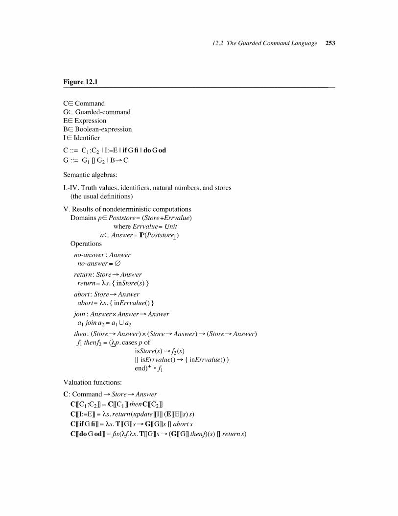
12.2 The Guarded Command Language 253
Figure 12.1____________________________________________________________________________________________________________________________________________________
C$ Command
G$ Guarded-command
E$ Expression
B$ Boolean-expression
I$ Identifier
C ::= C1;C2 | I:#E | if Gfi | do G od
G ::= G1 [] G2 | B#C
Semantic algebras:
I.-IV. Truth values, identifiers, natural numbers, and stores
(the usual definitions)
V. Results of nondeterministic computations
Domains p$Poststore# (Store$Errvalue)
where Errvalue# Unit
a$ Answer# IP(Poststore %!)
Operations
no-answer : Answer
no-answer# "
return: Store#Answer
return# &s. { inStore(s) }
abort : Store#Answer
abort# &s. { inErrvalue() }
join : Answer"Answer#Answer
a1 join a2 # a1% a2
then: (Store#Answer)" (Store#Answer)# (Store#Answer)
f1 thenf2 # (&!!p. cases p of
isStore(s)# f2(s)
[] isErrvalue()# { inErrvalue() }
end)++& f1
Valuation functions:
C: Command# Store#Answer
C[[C1;C2]]# C[[C1]] thenC[[C2]]
C[[I:#E]]# &s. return(update[[I]] (E[[E]]s) s)
C[[if Gfi]]# &s. T[[G]]s#G[[G]]s [] abort s
C[[do G od]]# fix(&f.&s. T[[G]]s# (G[[G]] thenf)(s) [] return s)
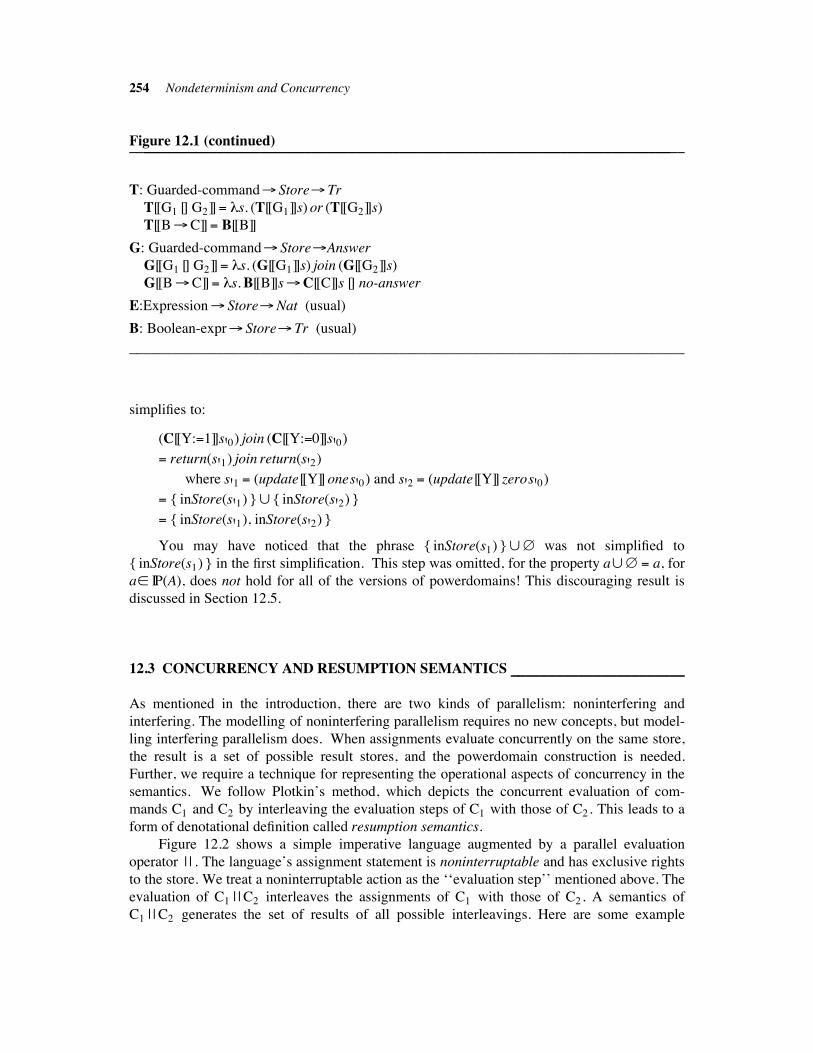
254 Nondeterminism and Concurrency
Figure 12.1 (continued)____________________________________________________________________________________________________________________________________________________
T: Guarded-command# Store# Tr
T[[G1 [] G2]]# &s. (T[[G1]]s) or (T[[G2]]s)
T[[B#C]]# B[[B]]
G: Guarded-command# Store#Answer
G[[G1 [] G2]]# &s. (G[[G1]]s) join (G[[G2]]s)
G[[B#C]]# &s. B[[B]]s#C[[C]]s [] no-answer
E:Expression# Store#Nat (usual)
B: Boolean-expr# Store# Tr (usual)
____________________________________________________________________________
simplifies to:
(C[[Y:#1]]s'0) join (C[[Y:#0]]s'0)
# return(s'1) join return(s'2)
where s'1 # (update[[Y]] ones'0) and s'2 # (update[[Y]] zeros'0)
# { inStore(s'1) }% { inStore(s'2) }
# { inStore(s'1), inStore(s'2) }
You may have noticed that the phrase { inStore(s1) }%" was not simplified to
{ inStore(s1) } in the first simplification. This step was omitted, for the property a%" # a, for
a$ IP(A), does not hold for all of the versions of powerdomains! This discouraging result is
discussed in Section 12.5.
12.3 CONCURRENCY AND RESUMPTION SEMANTICS !!!!!!!!!!!!!!!!!!!!!!!!!!!!!!!!!!!!!!!!!!!!!!
As mentioned in the introduction, there are two kinds of parallelism: noninterfering and
interfering. The modelling of noninterfering parallelism requires no new concepts, but model-
ling interfering parallelism does. When assignments evaluate concurrently on the same store,
the result is a set of possible result stores, and the powerdomain construction is needed.
Further, we require a technique for representing the operational aspects of concurrency in the
semantics. We follow Plotkin’s method, which depicts the concurrent evaluation of com-
mands C1 and C2 by interleaving the evaluation steps of C1 with those of C2. This leads to a
form of denotational definition called resumption semantics.
Figure 12.2 shows a simple imperative language augmented by a parallel evaluation
operator | | . The language’s assignment statement is noninterruptable and has exclusive rights
to the store. We treat a noninterruptable action as the ‘‘evaluation step’’ mentioned above. The
evaluation of C1 | | C2 interleaves the assignments of C1 with those of C2. A semantics of
C1 | | C2 generates the set of results of all possible interleavings. Here are some example
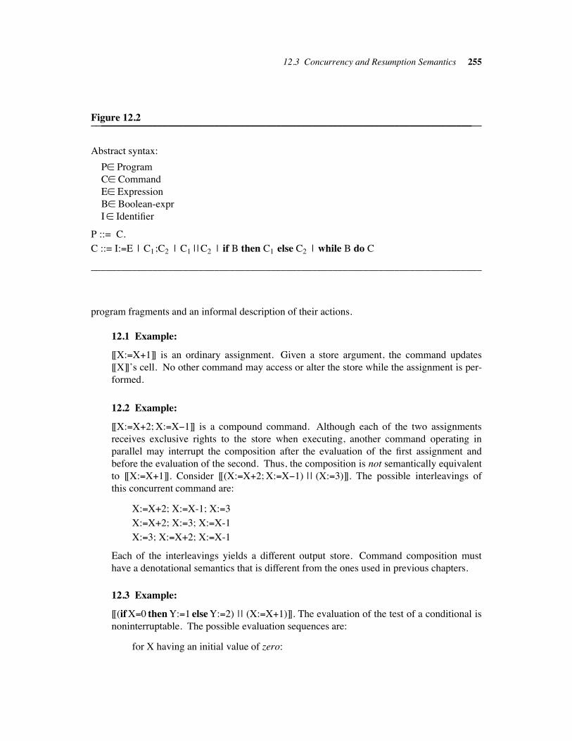
12.3 Concurrency and Resumption Semantics 255
Figure 12.2____________________________________________________________________________________________________________________________________________________
Abstract syntax:
P$ Program
C$ Command
E$ Expression
B$ Boolean-expr
I$ Identifier
P ::= C.
C ::= I:#E | C1;C2 | C1 | | C2 | if B then C1 else C2 | while B do C
____________________________________________________________________________
program fragments and an informal description of their actions.
12.1 Example:
[[X:#X$1]] is an ordinary assignment. Given a store argument, the command updates
[[X]]’s cell. No other command may access or alter the store while the assignment is per-
formed.
12.2 Example:
[[X:#X$2; X:#X(1]] is a compound command. Although each of the two assignments
receives exclusive rights to the store when executing, another command operating in
parallel may interrupt the composition after the evaluation of the first assignment and
before the evaluation of the second. Thus, the composition is not semantically equivalent
to [[X:#X$1]]. Consider [[(X:#X$2; X:#X(1) | | (X:#3)]]. The possible interleavings of
this concurrent command are:
X:#X+2; X:#X-1; X:#3
X:#X+2; X:#3; X:#X-1
X:#3; X:#X+2; X:#X-1
Each of the interleavings yields a different output store. Command composition must
have a denotational semantics that is different from the ones used in previous chapters.
12.3 Example:
[[(if X#0 then Y:#1 else Y:#2) | | (X:#X$1)]]. The evaluation of the test of a conditional is
noninterruptable. The possible evaluation sequences are:
for X having an initial value of zero:
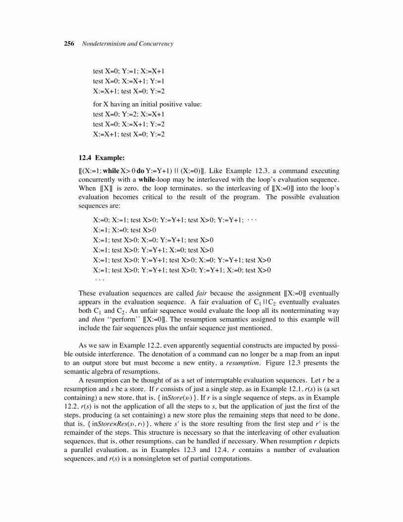
256 Nondeterminism and Concurrency
test X#0; Y:#1; X:#X+1
test X#0; X:#X+1; Y:#1
X:#X+1; test X#0; Y:#2
for X having an initial positive value:
test X#0; Y:#2; X:#X+1
test X#0; X:#X+1; Y:#2
X:#X+1; test X#0; Y:#2
12.4 Example:
[[(X:#1; while X> 0 do Y:#Y$1) | | (X:#0)]]. Like Example 12.3, a command executing
concurrently with a while-loop may be interleaved with the loop’s evaluation sequence.
When [[X]] is zero, the loop terminates, so the interleaving of [[X:#0]] into the loop’s
evaluation becomes critical to the result of the program. The possible evaluation
sequences are:
X:#0; X:#1; test X>0; Y:#Y+1; test X>0; Y:#Y+1; . . .
X:#1; X:#0; test X>0
X:#1; test X>0; X:#0; Y:#Y+1; test X>0
X:#1; test X>0; Y:#Y+1; X:#0; test X>0
X:#1; test X>0; Y:#Y+1; test X>0; X:#0; Y:#Y+1; test X>0
X:#1; test X>0; Y:#Y+1; test X>0; Y:#Y+1; X:#0; test X>0 . . .
These evaluation sequences are called fair because the assignment [[X:#0]] eventually
appears in the evaluation sequence. A fair evaluation of C1 | | C2 eventually evaluates
both C1 and C2. An unfair sequence would evaluate the loop all its nonterminating way
and then ‘‘perform’’ [[X:#0]]. The resumption semantics assigned to this example will
include the fair sequences plus the unfair sequence just mentioned.
As we saw in Example 12.2, even apparently sequential constructs are impacted by possi-
ble outside interference. The denotation of a command can no longer be a map from an input
to an output store but must become a new entity, a resumption. Figure 12.3 presents the
semantic algebra of resumptions.
A resumption can be thought of as a set of interruptable evaluation sequences. Let r be a
resumption and s be a store. If r consists of just a single step, as in Example 12.1, r(s) is (a set
containing) a new store, that is, { inStore(s') }. If r is a single sequence of steps, as in Example
12.2, r(s) is not the application of all the steps to s, but the application of just the first of the
steps, producing (a set containing) a new store plus the remaining steps that need to be done,
that is, { inStore"Res(s', r') }, where s' is the store resulting from the first step and r' is the
remainder of the steps. This structure is necessary so that the interleaving of other evaluation
sequences, that is, other resumptions, can be handled if necessary. When resumption r depicts
a parallel evaluation, as in Examples 12.3 and 12.4, r contains a number of evaluation
sequences, and r(s) is a nonsingleton set of partial computations.
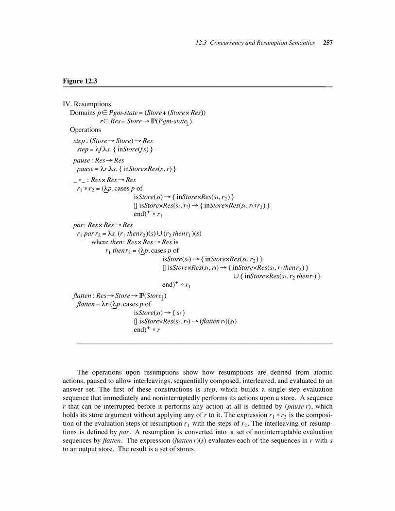
12.3 Concurrency and Resumption Semantics 257
Figure 12.3____________________________________________________________________________________________________________________________________________________
IV. Resumptions
Domains p$ Pgm-state# (Store$ (Store"Res))
r$ Res# Store# IP(Pgm-state%!)
Operations
step : (Store# Store)#Res
step# &f.&s. { inStore(f s) }
pause : Res#Res
pause# &r.&s. { inStore"Res(s, r) }
_ )_ : Res"Res#Res
r1 ) r2 # (&!!p. cases p of
isStore(s')# { inStore"Res(s', r2) }
[] isStore"Res(s', r')# { inStore"Res(s', r')r2) }
end)++& r1
par : Res"Res#Res
r1 par r2 # &s. (r1 thenr2)(s)% (r2 thenr1)(s)
where then: Res"Res#Res is
r1 thenr2 # (&!!p. cases p of
isStore(s')# { inStore"Res(s', r2) }
[] isStore"Res(s', r')# { inStore"Res(s', r' thenr2) }
% { inStore"Res(s', r2 thenr') }
end)++& r1
flatten : Res# Store# IP(Store %!)
flatten# &r.(&!!p. cases p of
isStore(s')# { s' }
[] isStore"Res(s', r')# (flatten r')(s')end)++
& r
________________________________________________________________________
The operations upon resumptions show how resumptions are defined from atomic
actions, paused to allow interleavings, sequentially composed, interleaved, and evaluated to an
answer set. The first of these constructions is step, which builds a single step evaluation
sequence that immediately and noninterruptedly performs its actions upon a store. A sequence
r that can be interrupted before it performs any action at all is defined by (pause r), which
holds its store argument without applying any of r to it. The expression r1 ) r2 is the composi-
tion of the evaluation steps of resumption r1 with the steps of r2. The interleaving of resump-
tions is defined by par. A resumption is converted into a set of noninterruptable evaluation
sequences by flatten. The expression (flatten r)(s) evaluates each of the sequences in r with s
to an output store. The result is a set of stores.
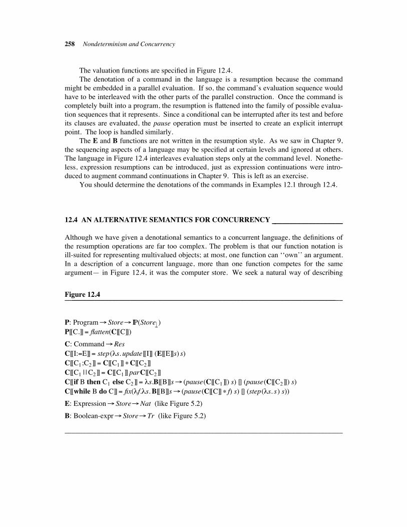
258 Nondeterminism and Concurrency
The valuation functions are specified in Figure 12.4.
The denotation of a command in the language is a resumption because the command
might be embedded in a parallel evaluation. If so, the command’s evaluation sequence would
have to be interleaved with the other parts of the parallel construction. Once the command is
completely built into a program, the resumption is flattened into the family of possible evalua-
tion sequences that it represents. Since a conditional can be interrupted after its test and before
its clauses are evaluated, the pause operation must be inserted to create an explicit interrupt
point. The loop is handled similarly.
The E and B functions are not written in the resumption style. As we saw in Chapter 9,
the sequencing aspects of a language may be specified at certain levels and ignored at others.
The language in Figure 12.4 interleaves evaluation steps only at the command level. Nonethe-
less, expression resumptions can be introduced, just as expression continuations were intro-
duced to augment command continuations in Chapter 9. This is left as an exercise.
You should determine the denotations of the commands in Examples 12.1 through 12.4.
12.4 AN ALTERNATIVE SEMANTICS FOR CONCURRENCY !!!!!!!!!!!!!!!!!!!!!!!!!!!!!!!!!!!!!!
Although we have given a denotational semantics to a concurrent language, the definitions of
the resumption operations are far too complex. The problem is that our function notation is
ill-suited for representing multivalued objects; at most, one function can ‘‘own’’ an argument.
In a description of a concurrent language, more than one function competes for the same
argument— in Figure 12.4, it was the computer store. We seek a natural way of describing
Figure 12.4____________________________________________________________________________________________________________________________________________________
P: Program# Store# IP(Store %!)
P[[C.]]# flatten(C[[C]])
C: Command#Res
C[[I:#E]]# step(&s. update[[I]] (E[[E]]s) s)
C[[C1;C2]]# C[[C1]] )C[[C2]]
C[[C1 | | C2]]# C[[C1]] parC[[C2]]
C[[if B then C1 else C2]]# &s.B[[B]]s# (pause(C[[C1]]) s) [] (pause(C[[C2]]) s)
C[[while B do C]]# fix(&f.&s. B[[B]]s# (pause(C[[C]] ) f) s) [] (step(&s. s) s))
E: Expression# Store#Nat (like Figure 5.2)
B: Boolean-expr# Store# Tr (like Figure 5.2)
____________________________________________________________________________
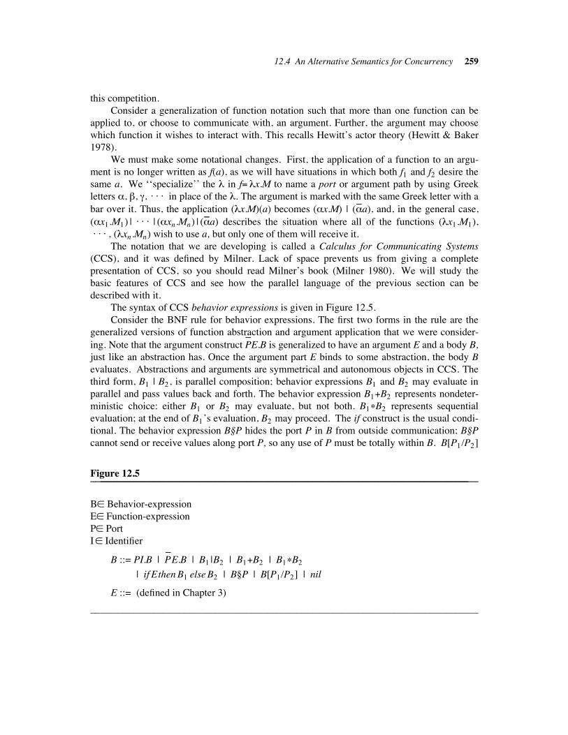
12.4 An Alternative Semantics for Concurrency 259
this competition.
Consider a generalization of function notation such that more than one function can be
applied to, or choose to communicate with, an argument. Further, the argument may choose
which function it wishes to interact with. This recalls Hewitt’s actor theory (Hewitt & Baker
1978).
We must make some notational changes. First, the application of a function to an argu-
ment is no longer written as f(a), as we will have situations in which both f1 and f2 desire the
same a. We ‘‘specialize’’ the & in f# &x.M to name a port or argument path by using Greek
letters *, +, ,, . . . in place of the &. The argument is marked with the same Greek letter with a
bar over it. Thus, the application (&x.M)(a) becomes (*x.M) | (*__
a), and, in the general case,
(*x1.M1) | . . . | (*xn.Mn) | (*__
a) describes the situation where all of the functions (&x1.M1), . . . , (&xn.Mn) wish to use a, but only one of them will receive it.
The notation that we are developing is called a Calculus for Communicating Systems
(CCS), and it was defined by Milner. Lack of space prevents us from giving a complete
presentation of CCS, so you should read Milner’s book (Milner 1980). We will study the
basic features of CCS and see how the parallel language of the previous section can be
described with it.
The syntax of CCS behavior expressions is given in Figure 12.5.
Consider the BNF rule for behavior expressions. The first two forms in the rule are the
generalized versions of function abstraction and argument application that we were consider-
ing. Note that the argument construct P__
E.B is generalized to have an argument E and a body B,
just like an abstraction has. Once the argument part E binds to some abstraction, the body B
evaluates. Abstractions and arguments are symmetrical and autonomous objects in CCS. The
third form, B1 | B2, is parallel composition; behavior expressions B1 and B2 may evaluate in
parallel and pass values back and forth. The behavior expression B1$B2 represents nondeter-
ministic choice: either B1 or B2 may evaluate, but not both. B1)B2 represents sequential
evaluation; at the end of B1’s evaluation, B2 may proceed. The if construct is the usual condi-
tional. The behavior expression B§P hides the port P in B from outside communication; B§P
cannot send or receive values along port P, so any use of P must be totally within B. B[P1/P2]
Figure 12.5____________________________________________________________________________________________________________________________________________________
B$ Behavior-expression
E$ Function-expression
P$ Port
I$ Identifier
B ::= PI.B | P__
E.B | B1 |B2 | B1$B2 | B1)B2
| if Ethen B1 else B2 | B§P | B[P1/P2] | nil
E ::= (defined in Chapter 3)
____________________________________________________________________________
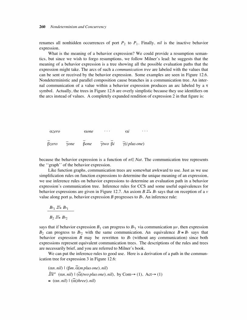
260 Nondeterminism and Concurrency
renames all nonhidden occurrences of port P2 to P1. Finally, nil is the inactive behavior
expression.
What is the meaning of a behavior expression? We could provide a resumption seman-
tics, but since we wish to forgo resumptions, we follow Milner’s lead: he suggests that the
meaning of a behavior expression is a tree showing all the possible evaluation paths that the
expression might take. The arcs of such a communication tree are labeled with the values that
can be sent or received by the behavior expression. Some examples are seen in Figure 12.6.
Nondeterministic and parallel composition cause branches in a communication tree. An inter-
nal communication of a value within a behavior expression produces an arc labeled by a -
symbol. Actually, the trees in Figure 12.6 are overly simplistic because they use identifiers on
the arcs instead of values. A completely expanded rendition of expression 2 in that figure is:
*zero *one . . . *i . . .
+_
zero ,_one +
_one ,
_two +
_i ,
_(i plus one)
because the behavior expression is a function of n$ Nat. The communication tree represents
the ‘‘graph’’ of the behavior expression.
Like function graphs, communication trees are somewhat awkward to use. Just as we use
simplification rules on function expressions to determine the unique meaning of an expression,
we use inference rules on behavior expressions to determine an evaluation path in a behavior
expression’s communication tree. Inference rules for CCS and some useful equivalences for
behavior expressions are given in Figure 12.7. An axiom B(#'v B' says that on reception of a v
value along port ', behavior expression B progresses to B'. An inference rule:
B'1 (#'v B'1____________
B2 (#'v B'2
says that if behavior expression B1 can progress to B'1 via communication 'v, then expression
B2 can progress to B'2 with the same communication. An equivalence B . B' says that
behavior expression B may be rewritten to B' (without any communication) since both
expressions represent equivalent communication trees. The descriptions of the rules and trees
are necessarily brief, and you are referred to Milner’s book.
We can put the inference rules to good use. Here is a derivation of a path in the commun-
ication tree for expression 3 in Figure 12.6:
(*n. nil) | (+m.*__
(m plus one). nil)
(#+two (*n. nil) | (*
__(two plus one). nil), by Com# (1), Act# (1)
. (*n. nil) | (*__
(three). nil)
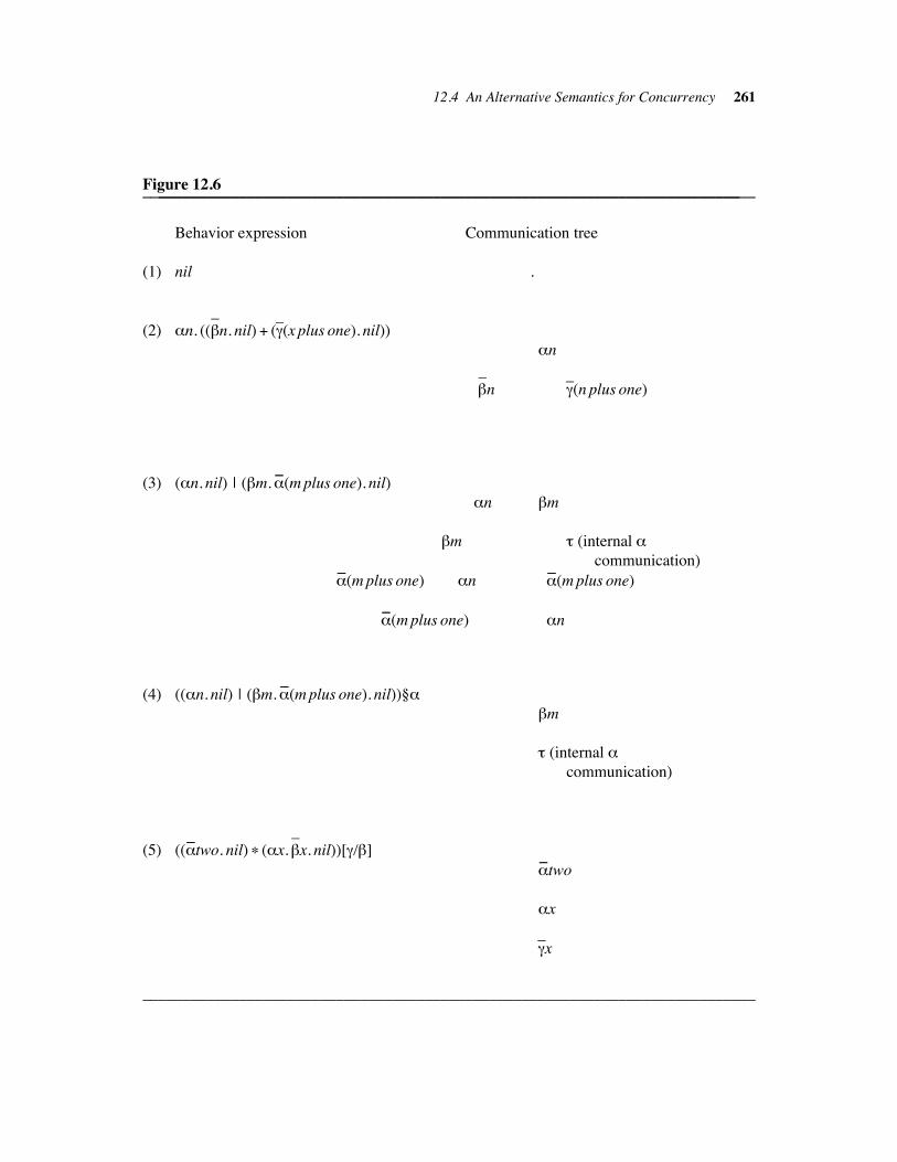
12.4 An Alternative Semantics for Concurrency 261
Figure 12.6____________________________________________________________________________________________________________________________________________________
Behavior expression Communication tree
(1) nil .
(2) *n. ((+_
n. nil) $ (,_(x plus one). nil))
*n
+_
n ,_(n plus one)
(3) (*n. nil) | (+m.*__
(m plus one). nil)
*n +m
+m - (internal *
communication)
*__
(m plus one) *n *__
(m plus one)
*__
(m plus one) *n
(4) ((*n. nil) | (+m.*__
(m plus one). nil))§*
+m
- (internal *
communication)
(5) ((*__
two. nil) ) (*x.+_
x. nil))[,/+]
*__
two
*x
,_x
____________________________________________________________________________
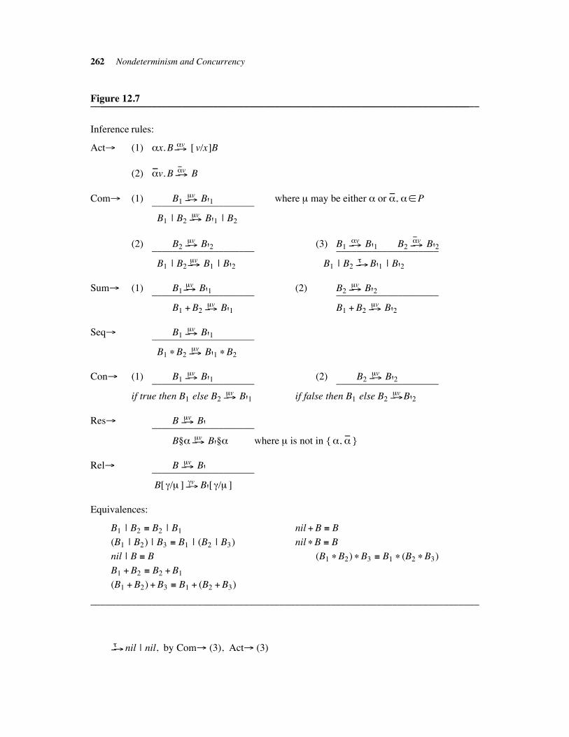
262 Nondeterminism and Concurrency
Figure 12.7____________________________________________________________________________________________________________________________________________________
Inference rules:
Act# (1) *x. B(#*v [ v/x]B
(2) *__
v. B(#*__
v B
Com# (1) B1 (#'v B'1 where ' may be either * or *
__, *$P____________________
B1 | B2 (#'v B'1 | B2
(2) B2 (#'v B'2 (3) B1 (#
*v B'1 B2 (#*__
v B'2____________________ ____________________
B1 | B2(#'v B1 | B'2 B1 | B2 (#
- B'1 | B'2
Sum# (1) B1(#'v B'1 (2) B2 (#
'v B'2____________________ ____________________
B1 $B2 (#'v B'1 B1 $B2 (#
'v B'2
Seq# B1 (#'v B'1____________________
B1 )B2 (#'v B'1 )B2
Con# (1) B1 (#'v B'1 (2) B2 (#
'v B'2____________________ ____________________
if true then B1 else B2 (#'v B'1 if false then B1 else B2 (#
'v B'2
Res# B (#'v B'____________________
B§*(#'v B'§* where ' is not in {*, *
__}
Rel# B (#'v B'____________________
B[ ,/' ](#,v B'[ ,/' ]
Equivalences:
B1 | B2 . B2 | B1 nil $B . B
(B1 | B2) | B3 . B1 | (B2 | B3) nil )B . B
nil | B . B (B1 )B2) )B3 . B1 ) (B2 )B3)
B1 $B2 . B2 $B1
(B1 $B2)$B3 . B1 $ (B2 $B3)
____________________________________________________________________________
(#- nil | nil, by Com# (3), Act# (3)
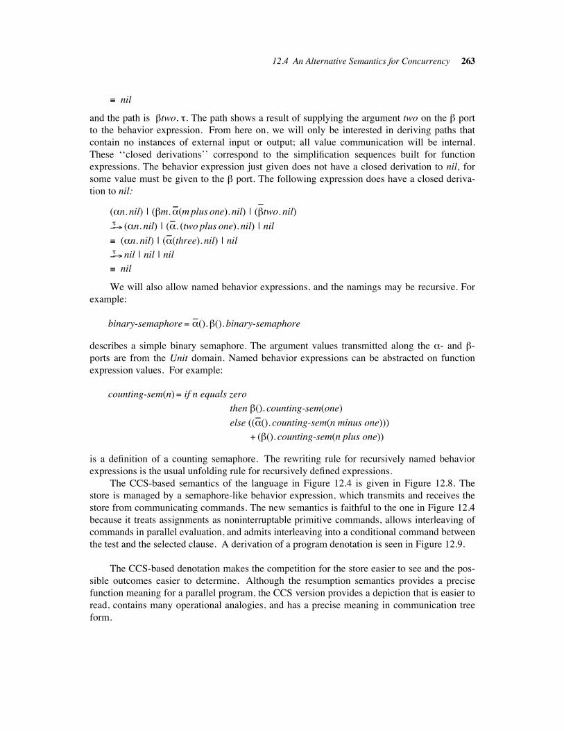
12.4 An Alternative Semantics for Concurrency 263
. nil
and the path is +two, -. The path shows a result of supplying the argument two on the + port
to the behavior expression. From here on, we will only be interested in deriving paths that
contain no instances of external input or output; all value communication will be internal.
These ‘‘closed derivations’’ correspond to the simplification sequences built for function
expressions. The behavior expression just given does not have a closed derivation to nil, for
some value must be given to the + port. The following expression does have a closed deriva-
tion to nil:
(*n. nil) | (+m.*__
(m plus one). nil) | (+_
two. nil)
(#- (*n. nil) | (*
__. (two plus one). nil) | nil
. (*n. nil) | (*__
(three). nil) | nil
(#- nil | nil | nil
. nil
We will also allow named behavior expressions, and the namings may be recursive. For
example:
binary-semaphore# *__
().+(). binary-semaphore
describes a simple binary semaphore. The argument values transmitted along the *- and +-
ports are from the Unit domain. Named behavior expressions can be abstracted on function
expression values. For example:
counting-sem(n)# if n equals zero
then +(). counting-sem(one)
else ((*__
(). counting-sem(n minus one)))
$ (+(). counting-sem(n plus one))
is a definition of a counting semaphore. The rewriting rule for recursively named behavior
expressions is the usual unfolding rule for recursively defined expressions.
The CCS-based semantics of the language in Figure 12.4 is given in Figure 12.8. The
store is managed by a semaphore-like behavior expression, which transmits and receives the
store from communicating commands. The new semantics is faithful to the one in Figure 12.4
because it treats assignments as noninterruptable primitive commands, allows interleaving of
commands in parallel evaluation, and admits interleaving into a conditional command between
the test and the selected clause. A derivation of a program denotation is seen in Figure 12.9.
The CCS-based denotation makes the competition for the store easier to see and the pos-
sible outcomes easier to determine. Although the resumption semantics provides a precise
function meaning for a parallel program, the CCS version provides a depiction that is easier to
read, contains many operational analogies, and has a precise meaning in communication tree
form.
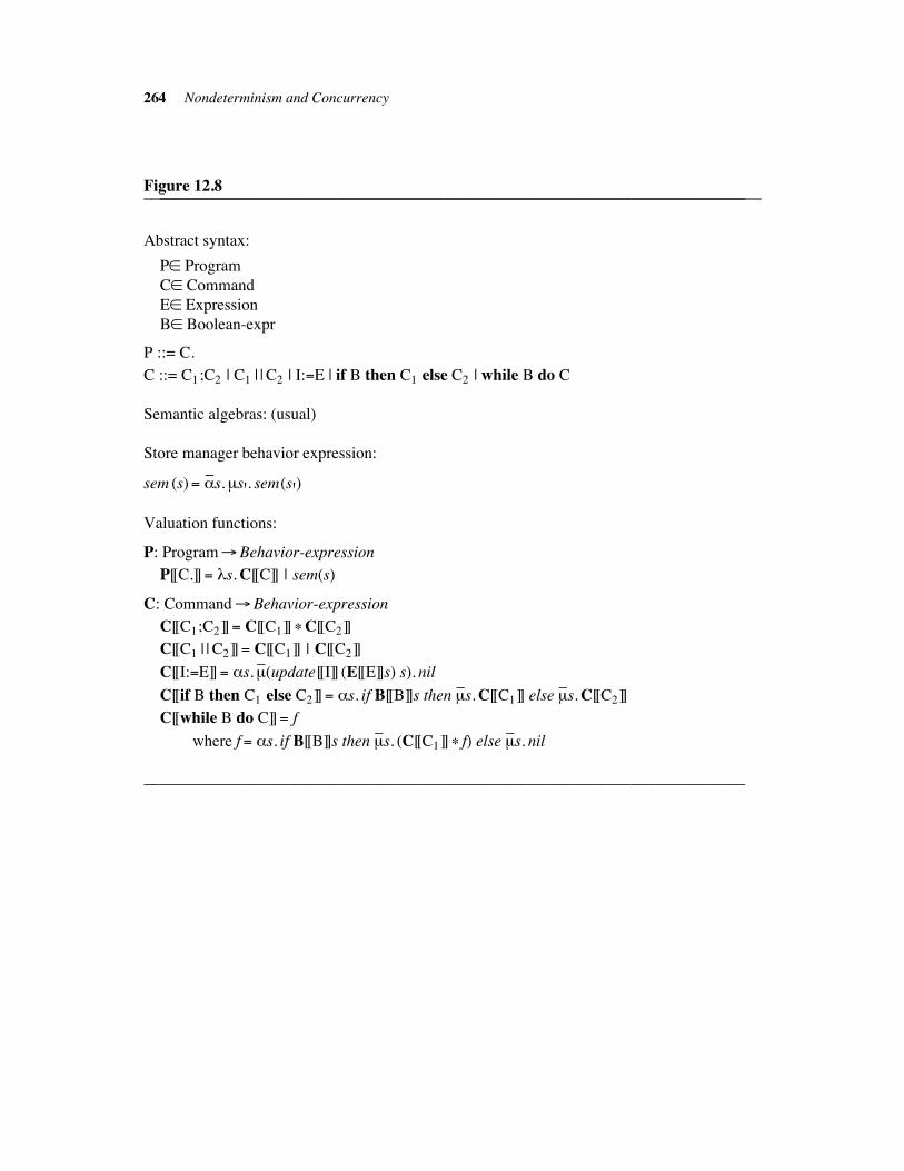
264 Nondeterminism and Concurrency
Figure 12.8____________________________________________________________________________________________________________________________________________________
Abstract syntax:
P$ Program
C$ Command
E$ Expression
B$ Boolean-expr
P ::= C.
C ::= C1;C2 | C1 | | C2 | I:#E | if B then C1 else C2 | while B do C
Semantic algebras: (usual)
Store manager behavior expression:
sem (s)# *__
s.'s'. sem(s')
Valuation functions:
P: Program#Behavior-expression
P[[C.]]# &s. C[[C]] | sem(s)
C: Command#Behavior-expression
C[[C1;C2]]# C[[C1]] )C[[C2]]
C[[C1 | | C2]]# C[[C1]] | C[[C2]]
C[[I:#E]]# *s.'_
(update[[I]] (E[[E]]s) s). nil
C[[if B then C1 else C2]]# *s. if B[[B]]s then '_
s. C[[C1]] else '_
s. C[[C2]]
C[[while B do C]]# f
where f # *s. if B[[B]]s then '_
s. (C[[C1]] ) f) else '_
s. nil
__________________________________________________________________________
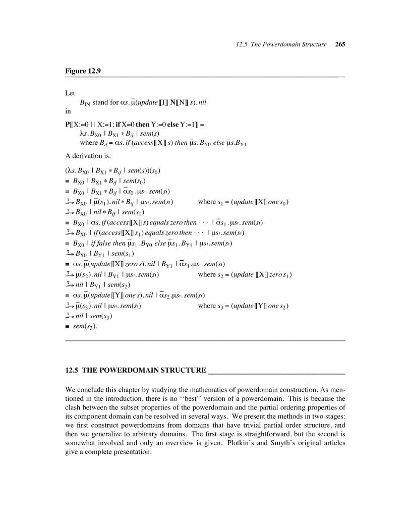
12.5 The Powerdomain Structure 265
Figure 12.9____________________________________________________________________________________________________________________________________________________
Let
BIN stand for *s.'_
(update[[I]] N[[N]] s). nil
in
P[[X:#0 | | X:#1; if X#0 then Y:#0 else Y:#1]]#&s. BX0 | BX1 )Bif | sem(s)
where Bif # *s. if (access[[X]] s) then '_
s. BY0 else '_
s.BY1
A derivation is:
(&s. BX0 | BX1 )Bif | sem(s))(s0)
. BX0 | BX1 )Bif | sem(s0)
. BX0 | BX1 )Bif | *__
s0 .'s'. sem(s')
(#- BX0 | '
_(s1). nil )Bif | 's'. sem(s') where s1 # (update[[X]] one s0)
(#- BX0 | nil )Bif | sem(s1)
. BX0 | *s. if (access[[X]] s) equals zero then . . . | *__
s1 .'s'. sem(s')
(#- BX0 | if (access[[X]] s1) equals zero then . . . | 's'. sem(s'). BX0 | if false then '
_s1 . BY0 else '
_s1 . BY1 | 's'. sem(s')
(#- BX0 | BY1 | sem(s1)
. *s.'_
(update[[X]] zero s). nil | BY1 | *__
s1 .'s'. sem(s')
(#- '
_(s2). nil | BY1 | 's'. sem(s') where s2 # (update [[X]] zero s1)
(#- nil | BY1 | sem(s2)
. *s.'_
(update[[Y]] one s). nil | *__
s2 .'s'. sem(s')
(#- '
_(s3). nil | 's'. sem(s') where s3 # (update[[Y]] one s2)
(#- nil | sem(s3)
. sem(s3).
____________________________________________________________________________
12.5 THE POWERDOMAIN STRUCTURE !!!!!!!!!!!!!!!!!!!!!!!!!!!!!!!!!!!!!!!!!!!!!!!!!!!!!!!!!!!!!!!!!!!!!!!!
We conclude this chapter by studying the mathematics of powerdomain construction. As men-
tioned in the introduction, there is no ‘‘best’’ version of a powerdomain. This is because the
clash between the subset properties of the powerdomain and the partial ordering properties of
its component domain can be resolved in several ways. We present the methods in two stages:
we first construct powerdomains from domains that have trivial partial order structure, and
then we generalize to arbitrary domains. The first stage is straightforward, but the second is
somewhat involved and only an overview is given. Plotkin’s and Smyth’s original articles
give a complete presentation.
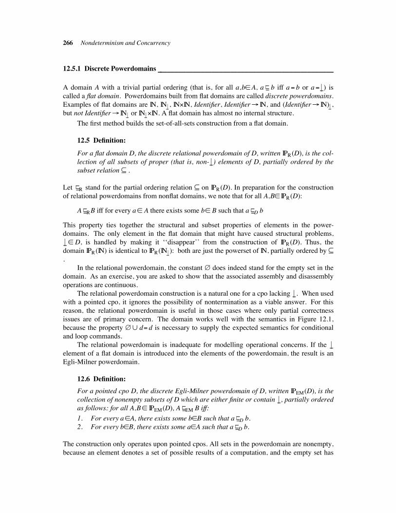
266 Nondeterminism and Concurrency
12.5.1 Discrete Powerdomains !!!!!!!!!!!!!!!!!!!!!!!!!!!!!!!!!!!!!!!!!!!!!!!!!!!!!!!!!!!!!!!!!!!!!!!!!!!!!!!!!!!!!!!!!!!!!!!!
A domain A with a trivial partial ordering (that is, for all a,b$A, a (((%% b iff a# b or a# %() is
called a flat domain. Powerdomains built from flat domains are called discrete powerdomains.
Examples of flat domains are IN, IN%! , IN"IN, Identifier, Identifier# IN, and (Identifier# IN)%! ,
but not Identifier# IN%! or IN%!"IN. A flat domain has almost no internal structure.
The first method builds the set-of-all-sets construction from a flat domain.
12.5 Definition:
For a flat domain D, the discrete relational powerdomain of D, written IPR(D), is the col-
lection of all subsets of proper (that is, non- %() elements of D, partially ordered by the
subset relation ! .
Let (((%% R stand for the partial ordering relation ! on IPR(D). In preparation for the construction
of relational powerdomains from nonflat domains, we note that for all A,B$ IPR(D):
A (((%% RB iff for every a$ A there exists some b$ B such that a ((
(%% D b
This property ties together the structural and subset properties of elements in the power-
domains. The only element in the flat domain that might have caused structural problems,
%($ D, is handled by making it ‘‘disappear’’ from the construction of IPR(D). Thus, the
domain IPR(IN) is identical to IPR(IN%!): both are just the powerset of IN, partially ordered by !
.
In the relational powerdomain, the constant " does indeed stand for the empty set in the
domain. As an exercise, you are asked to show that the associated assembly and disassembly
operations are continuous.
The relational powerdomain construction is a natural one for a cpo lacking %(. When used
with a pointed cpo, it ignores the possibility of nontermination as a viable answer. For this
reason, the relational powerdomain is useful in those cases where only partial correctness
issues are of primary concern. The domain works well with the semantics in Figure 12.1,
because the property "% d# d is necessary to supply the expected semantics for conditional
and loop commands.
The relational powerdomain is inadequate for modelling operational concerns. If the %(element of a flat domain is introduced into the elements of the powerdomain, the result is an
Egli-Milner powerdomain.
12.6 Definition:
For a pointed cpo D, the discrete Egli-Milner powerdomain of D, written IPEM(D), is the
collection of nonempty subsets of D which are either finite or contain %(, partially ordered
as follows: for all A,B$ IPEM(D), A (((%% EM B iff:
1. For every a$A, there exists some b$B such that a (((%% D b.
2. For every b$B, there exists some a$A such that a (((%% D b.
The construction only operates upon pointed cpos. All sets in the powerdomain are nonempty,
because an element denotes a set of possible results of a computation, and the empty set has
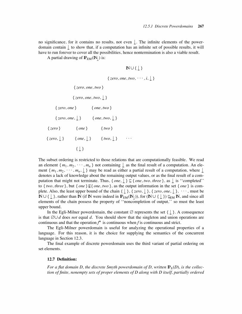
12.5.1 Discrete Powerdomains 267
no significance, for it contains no results, not even %(. The infinite elements of the power-
domain contain %( to show that, if a computation has an infinite set of possible results, it will
have to run forever to cover all the possibilities, hence nontermination is also a viable result.
A partial drawing of IPEM(IN%!) is:
IN% { %( }
{ zero, one, two, . . . , i, %( }
{ zero, one, two }
{ zero, one, two, %( }
{ zero, one } { one, two }
{ zero, one, %( } { one, two, %( }
{ zero } { one } { two }
{ zero, %( } { one, %( } { two, %( } . . .
{ %( }
The subset ordering is restricted to those relations that are computationally feasible. We read
an element { m1, m2, . . . , mn } not containing %( as the final result of a computation. An ele-
ment { m1, m2, . . . , mn , %( } may be read as either a partial result of a computation, where %(denotes a lack of knowledge about the remaining output values, or as the final result of a com-
putation that might not terminate. Thus, { one, %( } (((%% { one, two, three }, as %( is ‘‘completed’’
to { two, three }, but { one } (((%% / { one, two }, as the output information in the set { one } is com-
plete. Also, the least upper bound of the chain { %( }, { zero, %( }, { zero, one, %( }, . . . , must be
IN% { %( }, rather than IN (if IN were indeed in IPEM(IN%!)), for (IN% { %( }) (((%% EM IN, and since all
elements of the chain possess the property of ‘‘noncompletion of output,’’ so must the least
upper bound.
In the Egli-Milner powerdomain, the constant " represents the set { %( }. A consequence
is that "% d does not equal d. You should show that the singleton and union operations are
continuous and that the operation f++ is continuous when f is continuous and strict.
The Egli-Milner powerdomain is useful for analyzing the operational properties of a
language. For this reason, it is the choice for supplying the semantics of the concurrent
language in Section 12.3.
The final example of discrete powerdomain uses the third variant of partial ordering on
set elements.
12.7 Definition:
For a flat domain D, the discrete Smyth powerdomain of D, written IPS(D), is the collec-
tion of finite, nonempty sets of proper elements of D along with D itself, partially ordered
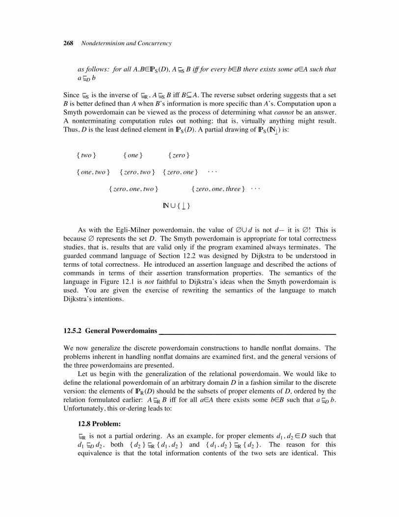
268 Nondeterminism and Concurrency
as follows: for all A,B$IPS(D), A (((%% S B iff for every b$B there exists some a$A such that
a (((%% D b
Since (((%% S is the inverse of ((
(%% R, A (((%% S B iff B!A. The reverse subset ordering suggests that a set
B is better defined than A when B’s information is more specific than A’s. Computation upon a
Smyth powerdomain can be viewed as the process of determining what cannot be an answer.
A nonterminating computation rules out nothing; that is, virtually anything might result.
Thus, D is the least defined element in IPS(D). A partial drawing of IPS(IN%!) is:
{ two } { one } { zero }
{ one, two } { zero, two } { zero, one } . . .
{ zero, one, two } { zero, one, three } . . .
IN% { %( }
As with the Egli-Milner powerdomain, the value of "% d is not d— it is "! This is
because " represents the set D. The Smyth powerdomain is appropriate for total correctness
studies, that is, results that are valid only if the program examined always terminates. The
guarded command language of Section 12.2 was designed by Dijkstra to be understood in
terms of total correctness. He introduced an assertion language and described the actions of
commands in terms of their assertion transformation properties. The semantics of the
language in Figure 12.1 is not faithful to Dijkstra’s ideas when the Smyth powerdomain is
used. You are given the exercise of rewriting the semantics of the language to match
Dijkstra’s intentions.
12.5.2 General Powerdomains !!!!!!!!!!!!!!!!!!!!!!!!!!!!!!!!!!!!!!!!!!!!!!!!!!!!!!!!!!!!!!!!!!!!!!!!!!!!!!!!!!!!!!!!!!!!!!!!
We now generalize the discrete powerdomain constructions to handle nonflat domains. The
problems inherent in handling nonflat domains are examined first, and the general versions of
the three powerdomains are presented.
Let us begin with the generalization of the relational powerdomain. We would like to
define the relational powerdomain of an arbitrary domain D in a fashion similar to the discrete
version: the elements of IPR(D) should be the subsets of proper elements of D, ordered by the
relation formulated earlier: A (((%% R B iff for all a$A there exists some b$B such that a ((
(%% D b.
Unfortunately, this or-dering leads to:
12.8 Problem:
(((%% R is not a partial ordering. As an example, for proper elements d1, d2 $D such that
d1 (((%% D d2, both { d2 } ((
(%% R { d1, d2 } and { d1, d2 } (((%% R { d2 }. The reason for this
equivalence is that the total information contents of the two sets are identical. This
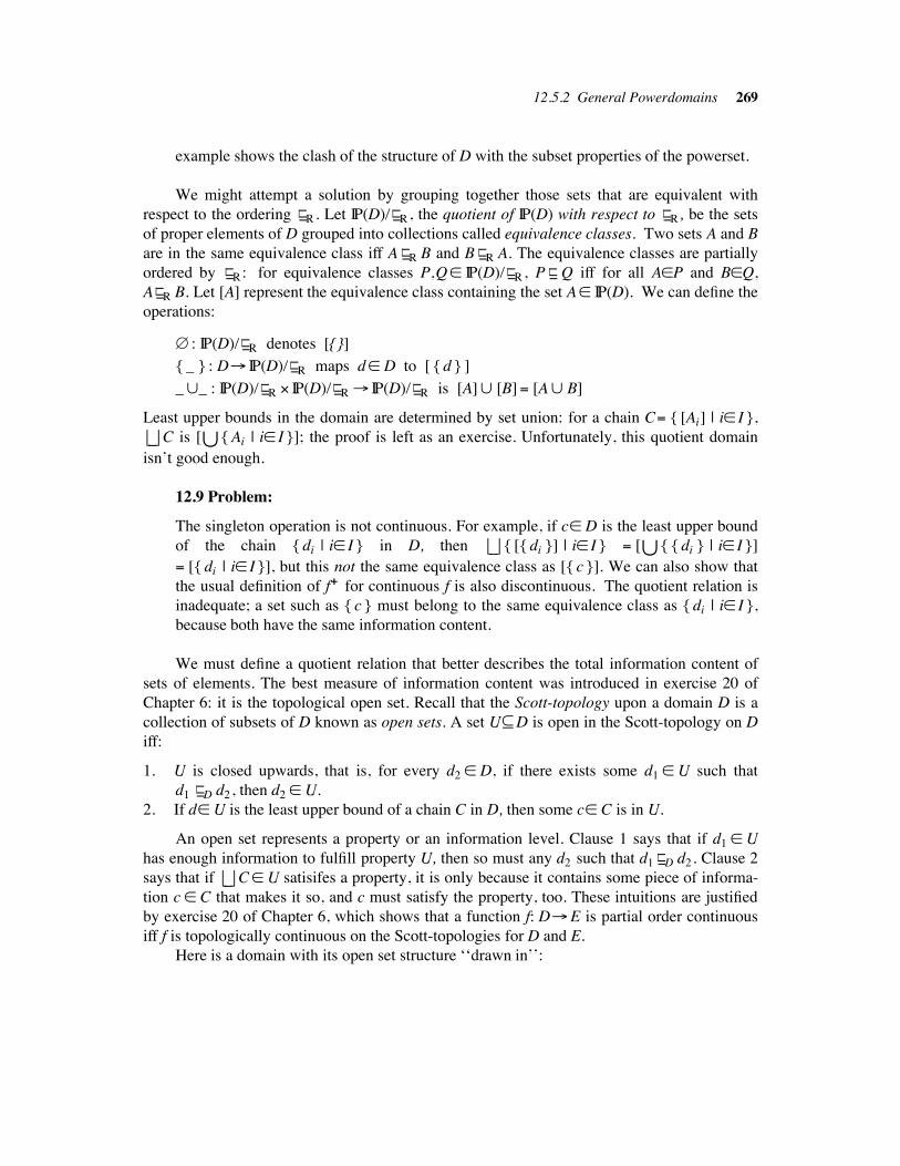
12.5.2 General Powerdomains 269
example shows the clash of the structure of D with the subset properties of the powerset.
We might attempt a solution by grouping together those sets that are equivalent with
respect to the ordering (((%% R. Let IP(D)/((
(%% R, the quotient of IP(D) with respect to (((%% R , be the sets
of proper elements of D grouped into collections called equivalence classes. Two sets A and B
are in the same equivalence class iff A (((%% R B and B ((
(%% R A. The equivalence classes are partially
ordered by (((%% R: for equivalence classes P,Q$ IP(D)/((
(%% R, P (((%% Q iff for all A$P and B$Q,
A(((%% R B. Let [A] represent the equivalence class containing the set A$ IP(D). We can define the
operations:
" : IP(D)/(((%% R denotes [{}]
{ _ } : D# IP(D)/(((%% R maps d$ D to [ { d } ]
_%_ : IP(D)/(((%% R " IP(D)/((
(%% R # IP(D)/(((%% R is [A]% [B]# [A% B]
Least upper bounds in the domain are determined by set union: for a chain C# { [Ai] | i$ I },
( C is [%{ Ai | i$ I }]; the proof is left as an exercise. Unfortunately, this quotient domain
isn’t good enough.
12.9 Problem:
The singleton operation is not continuous. For example, if c$ D is the least upper bound
of the chain { di | i$ I } in D, then ( { [{ di }] | i$ I } # [%{ { di } | i$ I }]
# [{ di | i$ I }], but this not the same equivalence class as [{ c }]. We can also show that
the usual definition of f++ for continuous f is also discontinuous. The quotient relation is
inadequate; a set such as { c } must belong to the same equivalence class as { di | i$ I },
because both have the same information content.
We must define a quotient relation that better describes the total information content of
sets of elements. The best measure of information content was introduced in exercise 20 of
Chapter 6: it is the topological open set. Recall that the Scott-topology upon a domain D is a
collection of subsets of D known as open sets. A set U!D is open in the Scott-topology on D
iff:
1. U is closed upwards, that is, for every d2 $ D, if there exists some d1 $ U such that
d1 (((%% D d2, then d2 $ U.
2. If d$ U is the least upper bound of a chain C in D, then some c$ C is in U.
An open set represents a property or an information level. Clause 1 says that if d1 $ U
has enough information to fulfill property U, then so must any d2 such that d1 (((%% D d2. Clause 2
says that if ( C$ U satisifes a property, it is only because it contains some piece of informa-
tion c $ C that makes it so, and c must satisfy the property, too. These intuitions are justified
by exercise 20 of Chapter 6, which shows that a function f: D#E is partial order continuous
iff f is topologically continuous on the Scott-topologies for D and E.
Here is a domain with its open set structure ‘‘drawn in’’:
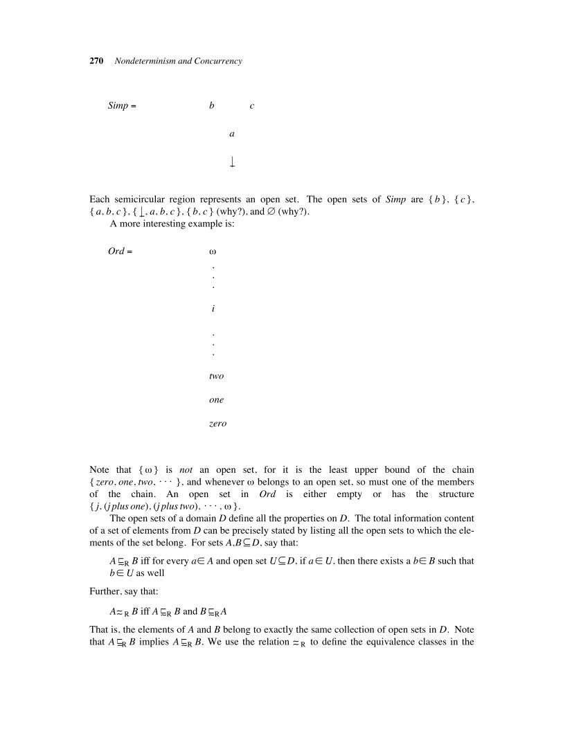
270 Nondeterminism and Concurrency
Simp # b c
a
%(
Each semicircular region represents an open set. The open sets of Simp are { b }, { c },
{ a, b, c }, { %(, a, b, c }, { b, c } (why?), and " (why?).
A more interesting example is:
Ord # /
.
.
.
i
.
.
.
two
one
zero
Note that {/ } is not an open set, for it is the least upper bound of the chain
{ zero, one, two, . . . }, and whenever / belongs to an open set, so must one of the members
of the chain. An open set in Ord is either empty or has the structure
{ j, (j plus one), (j plus two), . . . , / }.
The open sets of a domain D define all the properties on D. The total information content
of a set of elements from D can be precisely stated by listing all the open sets to which the ele-
ments of the set belong. For sets A,B!D, say that:
A 0((%% R B iff for every a$ A and open set U!D, if a$ U, then there exists a b$ B such that
b$ U as well
Further, say that:
A00 R B iff A 0((%% R B and B 0(
(%% RA
That is, the elements of A and B belong to exactly the same collection of open sets in D. Note
that A (((%% R B implies A 0(
(%% R B. We use the relation 00 R to define the equivalence classes in the
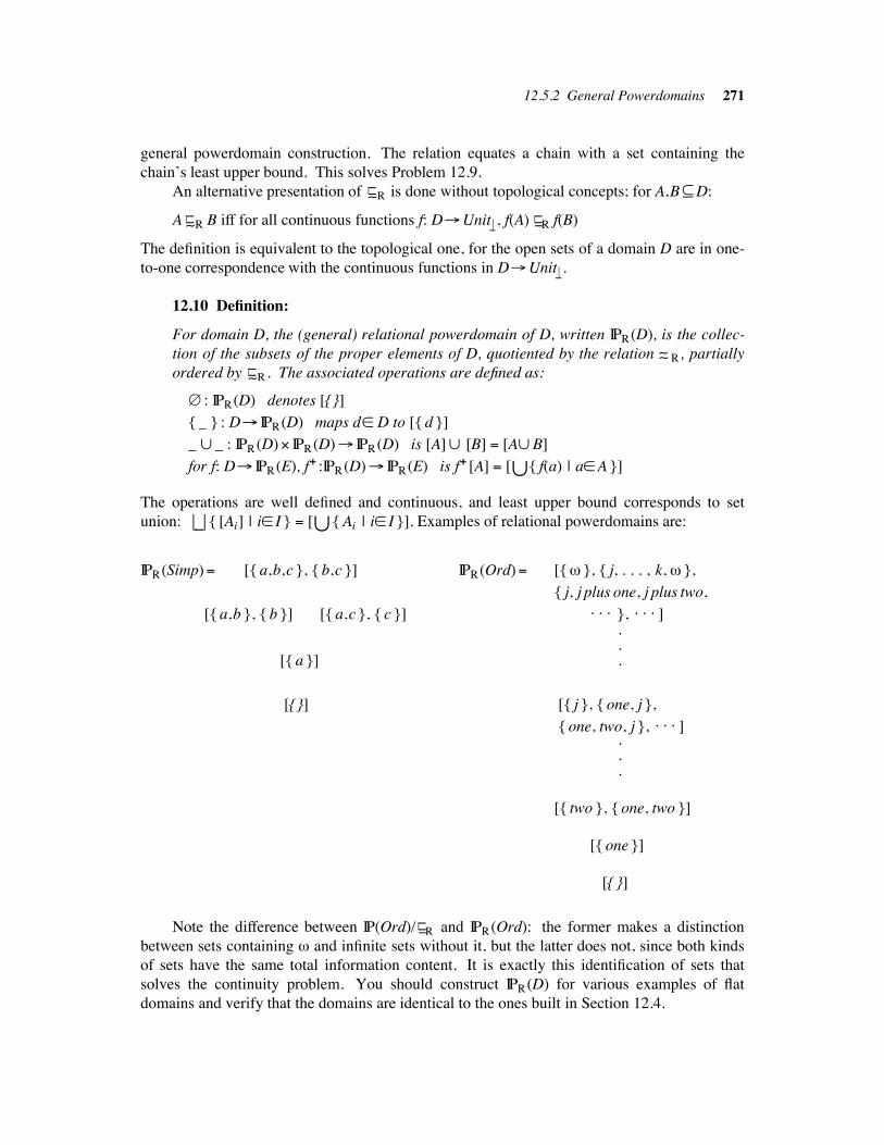
12.5.2 General Powerdomains 271
general powerdomain construction. The relation equates a chain with a set containing the
chain’s least upper bound. This solves Problem 12.9.
An alternative presentation of 0((%% R is done without topological concepts; for A,B!D:
A 0((%% R B iff for all continuous functions f: D#Unit %! , f(A) ((
(%% R f(B)
The definition is equivalent to the topological one, for the open sets of a domain D are in one-
to-one correspondence with the continuous functions in D#Unit %! .
12.10 Definition:
For domain D, the (general) relational powerdomain of D, written IPR(D), is the collec-
tion of the subsets of the proper elements of D, quotiented by the relation 00 R , partially
ordered by 0((%% R . The associated operations are defined as:
" : IPR(D) denotes [{}]
{ _ } : D# IPR(D) maps d$ D to [{ d }]
_ % _ : IPR(D)" IPR(D)# IPR(D) is [A]% [B] # [A%B]
for f: D# IPR(E), f++:IPR(D)# IPR(E) is f++[A] # [%{ f(a) | a$A }]
The operations are well defined and continuous, and least upper bound corresponds to set
union: ( { [Ai] | i$ I } # [%{ Ai | i$ I }]. Examples of relational powerdomains are:
IPR(Simp)# [{ a,b,c }, { b,c }] IPR(Ord)# [{/ }, { j, . . . , k, / },
{ j, j plus one, j plus two,
[{ a,b }, { b }] [{ a,c }, { c }] . . . }, . . . ]..
[{ a }] .
[{}] [{ j }, { one, j },
{ one, two, j }, . . . ]...
[{ two }, { one, two }]
[{ one }]
[{ }]
Note the difference between IP(Ord)/(((%% R and IPR(Ord): the former makes a distinction
between sets containing / and infinite sets without it, but the latter does not, since both kinds
of sets have the same total information content. It is exactly this identification of sets that
solves the continuity problem. You should construct IPR(D) for various examples of flat
domains and verify that the domains are identical to the ones built in Section 12.4.
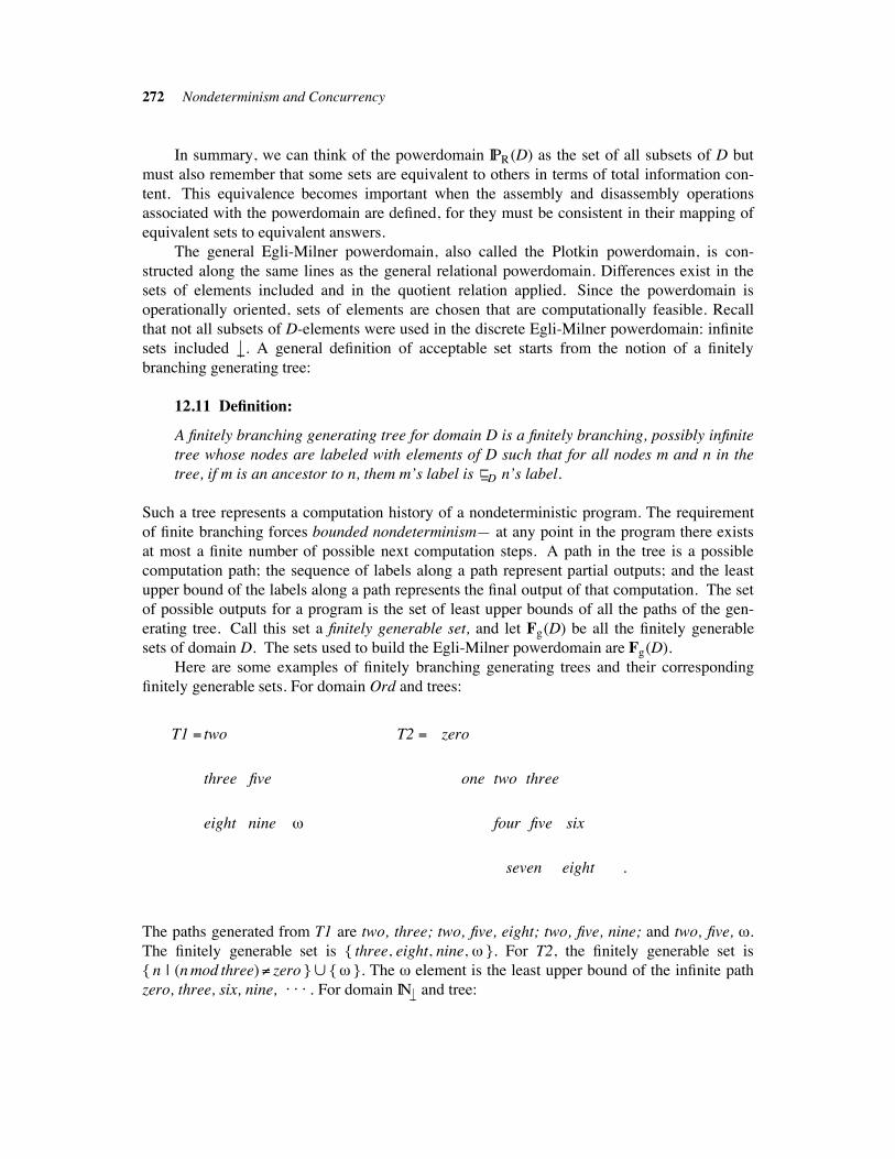
272 Nondeterminism and Concurrency
In summary, we can think of the powerdomain IPR(D) as the set of all subsets of D but
must also remember that some sets are equivalent to others in terms of total information con-
tent. This equivalence becomes important when the assembly and disassembly operations
associated with the powerdomain are defined, for they must be consistent in their mapping of
equivalent sets to equivalent answers.
The general Egli-Milner powerdomain, also called the Plotkin powerdomain, is con-
structed along the same lines as the general relational powerdomain. Differences exist in the
sets of elements included and in the quotient relation applied. Since the powerdomain is
operationally oriented, sets of elements are chosen that are computationally feasible. Recall
that not all subsets of D-elements were used in the discrete Egli-Milner powerdomain: infinite
sets included %(. A general definition of acceptable set starts from the notion of a finitely
branching generating tree:
12.11 Definition:
A finitely branching generating tree for domain D is a finitely branching, possibly infinite
tree whose nodes are labeled with elements of D such that for all nodes m and n in the
tree, if m is an ancestor to n, them m’s label is (((%% D n’s label.
Such a tree represents a computation history of a nondeterministic program. The requirement
of finite branching forces bounded nondeterminism— at any point in the program there exists
at most a finite number of possible next computation steps. A path in the tree is a possible
computation path; the sequence of labels along a path represent partial outputs; and the least
upper bound of the labels along a path represents the final output of that computation. The set
of possible outputs for a program is the set of least upper bounds of all the paths of the gen-
erating tree. Call this set a finitely generable set, and let Fg(D) be all the finitely generable
sets of domain D. The sets used to build the Egli-Milner powerdomain are Fg(D).
Here are some examples of finitely branching generating trees and their corresponding
finitely generable sets. For domain Ord and trees:
T1 # two T2 # zero
three five one two three
eight nine / four five six
seven eight .
The paths generated from T1 are two, three; two, five, eight; two, five, nine; and two, five, /.
The finitely generable set is { three, eight, nine, / }. For T2, the finitely generable set is
{ n | (n mod three)1 zero }% {/ }. The / element is the least upper bound of the infinite path
zero, three, six, nine, . . . . For domain IN%! and tree:
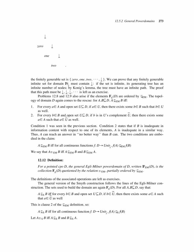
12.5.2 General Powerdomains 273
%(
zero %(
one %(
two .
the finitely generable set is { zero, one, two, . . . , %( }. We can prove that any finitely generable
infinite set for domain IN%! must contain %(: if the set is infinite, its generating tree has an
infinite number of nodes; by Konig’s lemma, the tree must have an infinite path. The proof
that this path must be %(, %(, %(, . . . is left as an exercise.
Problems 12.8 and 12.9 also arise if the elements Fg(D) are ordered by (((%% EM. The topol-
ogy of domain D again comes to the rescue: for A,B!D, A 0((%% EM B iff:
1. For every a$ A and open set U! D, if a$ U, then there exists some b$ B such that b$ U
as well.
2. For every b$ B and open set U! D, if b is in U’s complement U__
, then there exists some
a$ A such that a$ U__
as well.
Condition 1 was seen in the previous section. Condition 2 states that if B is inadequate in
information content with respect to one of its elements, A is inadequate in a similar way.
Thus, A can reach an answer in ‘‘no better way’’ than B can. The two conditions are embo-
died in the claim:
A 0((%% EM B iff for all continuous functions f: D#Unit %! , f(A) ((
(%% EM f(B)
We say that A00 EM B iff A 0((%% EM B and B 0(
(%% EM A.
12.12 Definition:
For a pointed cpo D, the general Egli-Milner powerdomain of D, written IPEM(D), is the
collection Fg(D) quotiented by the relation 00 EM , partially ordered by 0((%% EM .
The definitions of the associated operations are left as exercises.
The general version of the Smyth construction follows the lines of the Egli-Milner con-
struction. The sets used to build the domain are again Fg(D). For all A,B!D, say that:
A 0((%% S B iff for every b$ B and open set U!D, if b$ U
__, then there exists some a$ A such
that a$ U__
as well
This is clause 2 of the 0((%% EM definition, so:
A 0((%% S B iff for all continuous function f: D#Unit %! , f(A) ((
(%% S f(B)
Let A00 S B iff A 0((%% S B and B 0(
(%% S A.

274 Nondeterminism and Concurrency
12.13 Definition:
For pointed cpo D, the general Smyth powerdomain of D, written IPS(D), is the collection
Fg(D) quotiented by the relation 00 S , partially ordered by 0((%% S .
The operations upon IPS(D) are the expected ones.
SUGGESTED READINGS !!!!!!!!!!!!!!!!!!!!!!!!!!!!!!!!!!!!!!!!!!!!!!!!!!!!!!!!!!!!!!!!!!!!!!!!!!!!!!!!!!!!!!!!!!!!!!!!!!!!!!
Nondeterminism & parallelism: Apt & Olderog 1984; Apt & Plotkin 1981; Dijkstra 1976;
Hennessy & Plotkin 1979; Hewitt & Baker 1978; Main & Benson 1984; Park 1981
CCS: Milner 1980, 1983, 1985
Powerdomains: Abramsky 1983; Nielsen, Plotkin, & Winskel 1981; Plotkin 1976, 1982a,
1982b; Smyth 1978, 1983
EXERCISES !!!!!!!!!!!!!!!!!!!!!!!!!!!!!!!!!!!!!!!!!!!!!!!!!!!!!!!!!!!!!!!!!!!!!!!!!!!!!!!!!!!!!!!!!!!!!!!!!!!!!!!!!!!!!!!!!!!!!!!!!!!!
1. a. Draw IPR(D), IPEM(D), and IPS(D) for each of the following D:
i. IN
ii. IN%!
iii. IB %! " IB %!
iv. IB# IB
v. IB#Unit %!
b. Draw:
i. IPR(IPR(IB %!))
ii. IPEM(IPEM(IB %!))
iii. IPS(IPS(IB %!))
2. For a flat domain D, model a set A$ IP(D) as a function A : D#Unit %! such that d$ D
belongs to A iff A(d)# ().
a. Define the appropriate functions for ", { _ }, _%_. To which version of discrete
powerdomain is D#Unit %! isomorphic?
b. What goes wrong when using A : D# IB and saying that d$ A iff A(d)# true? What
goes wrong when the definition in part a is applied to nonflat domains?
3. Revise the semantics of the guarded command language of Figure 12.1 so that
Answer# IPS(Poststore). Rewrite the valuation functions so that a command [[C]] that
always terminates with a store s0 has denotation C[[C]]s0 1".
4. Redefine the semantics of the if statement in Figure 12.4 so that interruption and
Exercises 275
interleaving may not occur between evaluation of the test and the first step of evaluation
of the chosen clause. Do the same with the semantics of if in Figure 12.8.
5. (Plotkin) Extend the syntax of the language of Figure 12.2 to include [[critical C]], a criti-
cal region construct. Define the resumption and CCS semantics for the construct so that
[[C]] evaluates to completion without interruption.
6. a. Let C[[skip]]# step(&s. s) be added to the language in Figure 12.4. Show that
C[[skip;skip]]1C[[skip]], but that P[[skip;skip]]# P[[skip]].
b. Let the CCS semantics of the construct be C[[skip]]# nil; show that
C[[skip;skip]]# C[[skip]].
7. Give two commands in the language of Figure 12.8:
a. That have the same semantics for the relational powerdomain but different semantics
for the Egli-Milner and Smyth powerdomains.
b. That have the same semantics for the Smyth powerdomain but different semantics for
the Egli-Milner and relational powerdomains.
8. Consider the domain of expression resumptions:
Expr-res # Store # IP((Expressible-value " Store) $ (Store"Expr-res))
a. Use Expr-res to define the semantics of interleaved evaluation of expressions E ::=
E1$E2 | N | I .
b. Integrate the semantics you defined in part a with the language in Figure 12.4.
c. Repeat parts a and b using CCS semantics and the semantics in Figure 12.8.
9. a. Show (or describe) all the closed derivations of the program in Figure 12.9. Draw the
corresponding behavior tree, showing just the closed derivations.
b. Using the semantics in Figure 12.8, draw the behavior tree denotations for C[[X:#0]]
and C[[if X:#0 then Y:#0 else Y:#1]].
10. Rewrite the semantics of the guarded command language using CCS.
11. Use resumption semantics to redefine the semantics of the PROLOG-like language of
Figure 9.3 so that the denotation of a program is a set of all the possible successful
evaluation strategies that a program can take. Repeat the exercise for CCS semantics.
12. Give a resumption semantics to the CCS notation. Prove the soundness of the derivation
rules in Figure 12.7.
13. a. What similarities exist between the resumption semantics method of Section 12.3 and
the behavior trees model of Section 12.4? What are the primary differences?
b. What similarities exist between behavior trees and finite generating trees? What are
the primary differences?
276 Nondeterminism and Concurrency
14. Prove that the { _ }, _%_ and f$ operations are well defined in Definition 12.10; that is,
show that the choice of representatives A and B in [A]% [B] and f$[A] do not affect the
result.
15. Attempt to solve Problem 12.9 by defining A0((%% R B iff ( { a | a$A } ((
(%% ( { b | b$B }.
What goes wrong?
16. A set U!A is (Scott-) closed if A(U is open in the Scott-topology on A.
a. Prove that U! A is closed iff:
i. For all d, e$A, if d$U and e (((%% d then e$U.
ii. For all directed D!A, D!U implies ( D$U.
b. Prove that if cpo A is pointed, the relational powerdomain IPR(A) is isomorphic to the
collection of all the nonempty closed subsets of A partially ordered by subset inclu-
sion.
17. a. Why must f : D# IP(E) be strict to build f$ : IP(D)# IP(E) in the case of the Egli-
Milner and Smyth powerdomains?
b. What problems arise in building and using the Egli-Milner and Smyth powerdomains
when D is not pointed?
18. For x,y$ IP(D), for which versions of the powerdomains do the following hold?
a. x (((%% x% y
b. x% y (((%% x
c. x# { x }%"
c. "# x%"
d. x% x# x
19. a. Consider IPR'(D), a variant of the relational powerdomain such that the elements con-
sist of all subsets of a cpo D, quotiented by 00 R, partially ordered by 0((%% R . What is
unsatisfactory about IPR'(D)?
b. In a similar fashion, comment on the suitability of IPEM'(D), built from all subsets of
D, quotiented by 00 EM, partially ordered by 0((%% EM.
c. In a similar fashion, comment on the suitability of IPS'(D), built from all the subsets
of D, quotiented by 00 S, partially ordered by 0((%% S .
20. a. For each of the powerdomain constructions, attempt to define a continuous function
_in_ : D " IP(D)# IB such that for all d$D, U!D, d in [U]# true iff d$U. (Hint:
first attempt to define in for the discrete powerdomains and then generalize.)
b. For each of the powerdomain constructions upon which you succeeded in defining in,
for all d$D, U,V!D:
i. Attempt to show d in ([U]% [V]) # true iff d in [U] # true or d in [V]# true.
ii. Attempt to define a continuous function 2 : IP(D)" IP(D)# IP(D) such that
d in ([U]2 [V]) # true iff d in [U] # true and d in [V] # true.
Bibliograpy
The bibliography that follows was prepared originally with a software program called refer
that is no longer available. As a result, the raw bibliography must be reproduced here.
%A S. K. Abdali %T A lambda-calculus model of programming languages— jumps and functions %J J. of Com-
puter Languages %V 1 %D 1975 %P 303-320
%A H. Abelson %A G. Sussman %T Structure and Interpretation of Computer Programs %I MIT Press/McGraw-
Hill %C New York %D 1984
%A S. Abramsky %T On semantic foundations for applicative multiprogramming %B LNCS 154: Proc. 10th
ICALP %C Berlin %I Springer %D 1982 %P 1-14
%A S. Abramsky %T Experiments, powerdomains, and fully abstract models for applicative multiprogramming
%B LNCS 158: Foundations of Computation Theory %I Springer %C Berlin %D 1983 %P 1-13
%A J. Adamek %A V. Koubek %T Least fixed point of a functor %J Journal of Computer and System Sciences
%V 19 %D 1979 %P 163-178
%A A. Aho %A J. D. Ullman %T Principles of Compiler Design %I Addison-Wesley %C Reading, Mass. %D
1977
%A E. R. Anderson %A F. C. Belz %T Issues in the formal specification of programming languages %B Formal
Description of Programming Concepts %E E. J. Neuhold %I North-Holland %C Amsterdam %D 1978
%A E. R. Anderson %A F. C. Belz %A E. K. Blum %T SEMANOL (73): A metalanguage for programming the
semantics of programming languages %J Acta Informatica %V 6 %D 1976 %P 109-132
%A D. Andrews %A W. Henhapl %T Pascal %B Formal Specification and Software Development %E D. Bjo/ rner
and C. Jones %I Prentice-Hall %C Englewood Cliffs, N.J. %D 1982 %P 175-252
%A A. Appel %T Semantics-directed code generation %B Proc. 12th ACM Symp. on Prin. of Prog. Lang. %C
New Orleans %D 1985 %P 315-324
%A K. R. Apt %T Equivalence of operational and denotational semantics for a fragment of Pascal %B Formal
Descriptions of Programming Concepts %E E. J. Neuhold %I North-Holland %C Amsterdam %D 1978 %P
141-163
%A K. R. Apt %T Ten years of Hoare’s logic: a survey— part I %J ACM Trans. on Prog. Lang. and Systems %V
3 %D 1981 %P 431-483
%A K. R. Apt %T Ten years of Hoare’s logic: a survey— part II: nondeterminism %J Theoretical Computer Sci-
ence %V 28 %D 1984 %P 83-110
%A K. R. Apt %A A. Olderog %T Proof rules and transformations dealing with fairness %J Science of Comp. Pro-
gramming %V 3 %D 1983 %P 65-100
%A K. Apt %A G. D. Plotkin %T A Cook’s tour of countable nondeterminism %B LNCS 115: Proc. 9th ICALP
%I Springer %C Berlin %D 1981 %P 479-494
%A M. A. Arbib %A E. G. Manes %T The pattern-of-calls expansion is the canonical fixpoint for recursive
277
278 Bibliograpy
definitions %J Journal of the ACM %D 1982 %V 29 %P 577-602
%A E. Artesiano %A G. Costa %T Languages with reducing reflexive types %B LNCS 85: Proc. 7th ICALP %I
Springer %C Berlin %D 1980
%A E. A. Ashcroft %A W. W. Wadge %T Lucid, a nonprocedural language with iteration %J Comm. of the ACM
%V 20 %D 1977 %P 519-526
%A E. A. Ashcroft %A W. W. Wadge %T Prescription for semantics %J ACM Trans. on Prog. Lang. and Sys.
%V 4 %D 1982 %P 283-194
%A L. Augustsson %T A compiler for lazy ML %B Proc. ACM Conf. on LISP and Functional Programming %C
Austin, Texas %D 1984 %P 218-227
%A J. Backus %T Can programming be liberated from the von Neumann style? A functional style and its algebra
of programs %J Comm. of the ACM %V 21 %D 1978 %P 613-641
%A J. W. deBakker %T Recursive programs as predicate transformers %B Formal Descriptions of Programming
Concepts %E E.J. Neuhold %I North-Holland %C Amsterdam %D 1978 %P 165-181
%A J. W. deBakker %T Mathematical Theory of Program Correctness %I Prentice-Hall %D 1980 %C Englewood
Cliffs, N.J.
%A H. Barendregt %T The type free lambda calculus %B Handbook of Mathematical Logic %E J. Barwise %I
North-Holland %C Amsterdam %D 1977 %P 1091-1132
%A H. Barendregt %T The Lambda Calculus— Its Syntax and Semantics %I North-Holland %C Amsterdam %D
1981
%A H. Barendregt %T Introduction to lambda calculus %J Niew Archief Voor Wiskunde %V 4 %D 1984 %P
337-372
%A W. A. Barrett %A J. D. Couch %T Compiler Construction: Theory and Practice %I S.R.A. %C Chicago %D
1979
%A D. W. Barron %T An Introduction to the Study of Programming Languages %I Cambridge University Press
%C Cambridge %D 1977
%A F. L. Bauer %A H. Wossner %T Algorithmic Language and Program Development %I Springer %C Berlin
%D 1982
%A D. M. Berry %T Remarks on R. D. Tennent’s language design methods based on semantic principles %J Acta
Informatica %V 15 %D 1981 %P 83-98
%A D. M. Berry %T A denotational semantics for shared memory parallelism and nondeterminism %J Acta Infor-
matica %V 21 %D 1985 %P 599-628
%A G. Berry %T Some syntactic and categorical constructions of lambda calculus models %J Report 80 %I
INRIA %C Sophia Antipolis %D 1981
%A G. Berry %A J.-J. Levy %T A survey of some syntactic results of the lambda calculus %B LNCS 74: Proc. 8th
Symp. Math. Foundations of Computer Science %I Springer %C Berlin %D 1979 %P 552-566
%A G. Berry %A P.-L. Curien %T Sequential algorithms on concrete data structures %J Theoretical Computer
Science %V 20 %D 1982 %P 265-322
Bibliograpy 279
%A G. Berry %A P.-L. Curien %A J.-J. Levy %T Full abstraction for sequential languages: the state of the art %D
1982 %B Proc. French-American Seminar on Semantics %C Fontainebleau, France %D 1982
%A R. S. Bird %T Programs and Machines %I Wiley %C New York %D 1976
%A G. Birkhoff %T Lattice Theory, 3rd Edition %I American Mathematical Society %C Providence, R.I. %D
1967
%A D. Bjo/ rner %T The Vienna development method %B LNCS 75: Mathematical studies of information process-
ing %I Springer %C Berlin %D 1978 %P 326-359
%Q Bjo/ rner, D., ed. %T LNCS 86: Abstract Software Specifications %I Springer %C Berlin %D 1980
%A Bjo/ rner, D., ed. %T Formal Description of Programming Concepts II %I North-Holland %C Amsterdam %D
1983
%A D. Bjo/ rner %A C. B. Jones, eds. %T LNCS 61: The Vienna Development Method: the Metalanguage %I
Springer %C Berlin %D 1978
%A D. Bjo/ rner %A C. B. Jones %T Formal Specification and Software Development %I Prentice-Hall %C Engle-
wood Cliffs, N.J. %D 1982
%A D. Bjo/ rner %A O. N. Oest %T LNCS 98: Towards a formal description of Ada %I Springer %C Berlin %D
1980
%A A. Blikle %A A. Tarlecki %T Naive denotational semantics %B Proc. IFIP Congress 83 %I North-Holland
%C Amsterdam %D 1983 %P 345-356
%A J. Bodwin %A L. Bradley %A J. Kanda %A D. Little %A U. Pleban %T Experience with an experimental
compiler-compiler based on denotational semantics %B Proc. SIGPLAN 82 Symp. on Compiler Construction,
SIGPLAN Notices %V 17 %D 1982 %P 216-229
%Q Bohm, C., ed. %T LNCS 37: Lambda-calculus and Computer Science Theory %I Springer %C Berlin %D
1975
%A P. Branquart %A G. Louis %A P. Wodon %T LNCS 128: An Analytical Description of CHILL, the CCITT
High Level Language %I Springer %C Berlin %D 1982
%A S. D. Brookes %T A fully abstract semantics and a proof system for an ALGOL-like language with sharing
%B LNCS: Proc. Workshop on Foundations of Programming Semantics %I Springer %C Berlin %D 1985a
%Q Brookes, S. D., A. W. Roscoe, and G. Winskel, eds. %T LNCS 197: Seminar on Concurrency %I Springer
%C Berlin %D 1985
%A W. H. Burge %T Recursive Programming Techniques %I Addison-Wesley %C Reading, Mass. %D 1975
%A R. Burstall %T Proving properties of programs by structural induction %J Computer Journal %V 12 %P 41-48
%D 1969
%A R. Burstall %A J. Darlington %T A transformation system for developing recursive programs %J Journal of
the ACM %V 24 %P 44-67 %D 1977
%A R. Burstall %A J. Goguen %T Putting theories together to make specifications %B Proc. 5th Int. Joint Conf.
on Artificial Intelligence %C Cambridge, Mass. %D 1977 %P 1045-1058
280 Bibliograpy
%A R. Burstall %A J. Goguen %T Algebras, theories, and freeness: an introduction for computer scientists %B
Proc. Marktoberdorf Summer School on Theoretical Foundations of Programming Methodology %D August 1981
%A R. M. Burstall %A D. B. MacQueen %A D. T. Sannella %T HOPE: an experimental applicative language %R
CSR-62-80 %I Computer Science Dept., Edinburgh University %C Edinburgh, Scotland %D 1981
%A H. Christiansen %A N. D. Jones %T Control flow treatment in a simple semantics-directed compiler %B For-
mal Descriptions of Programming Concepts II %E D. Bjo/ rner %I North-Holland %C Amsterdam %D 1983 %P
73-97
%A A. Church %T The Calculi of Lambda Conversion %I Princeton Univ. Press %C Princeton, N.J. %D 1951
%A T. J. Clarke %A P. J. Gladstone %A C. D. MacClean %A A. C. Norman %T SKIM— the S, K, I reduction
machine %B Proc. ACM LISP conference %D 1980 %P 128-135
%A J. C. Cleaveland %T Mathematical specifications %J ACM SIGPLAN Notices %V 15-12 %D 1980 %P 31-42
%A J. C. Cleaveland %A R. C. Uzgalis %T Grammars for Programming Languages %I Elsevier %C New York
%D 1977
%A W. Clinger %T Foundations of actor semantics %R Ph.D. thesis, AI lab report AI-TR-633 %I MIT %D 1981
%A W. Clinger %T Summary of the Scheme 311 compiler: an exercise in denotational semantics %B Proc. ACM
Symp. on LISP and Functional Programming %C Austin, Texas %D August, 1984 %P 356-364
%A A. J. Cohn %T The equivalence of two semantic definitions: a case study in LCF %J SIAM J. of Computing
%V 12 %D 1983 %P 267-285
%A P. M. Cohn %T Universal Algebra (rev. ed.) %I D. Reidel Pub. %C Boston %D 1981
%A B. Courcelle %A I. Guessarian %T On some classes of interpretations %J J. of Computer and System Sciences
%V 17 %D 1978 %P 388-413
%A P. Cousot %A R. Cousot %T Abstract interpretation: a unified lattice model for static analysis of programs %B
Poc. 4th ACM Symp. on Prin. of Prog. Lang. %C Los Angeles %D 1977 %P 238-252
%A P. Cousot %A R. Cousot %T Systematic design of program analysis frameworks %B Proc. 6th ACM Symp.
on Prin. of Prog. Lang. %C San Antonio, Texas %D 1979 %P 269-282
%A P.-L. Curien %T Categorical combinatory logic %B LNCS 194: Proc. 12th ICALP %I Springer %C Berlin
%D 1985 %P 130-139
%A H. B. Curry %A R. Feys %T Combinatory Logic, Vol. 1 %I North-Holland %C Amsterdam %D 1958
%A J. Darlington %A P. Henderson %A D. Turner, eds. %T Functional Programming and its Applications %I
Cambridge Univ. Press %C Cambridge %D 1982
%A A. Demers %A J. Donohue %A G. Skinner %T Data types as values: polymorphism, type-checking, and
encapsulation %B Proc. 5th ACM Symp. on Prin. of Prog. Lang. %D 1978 %C Tucson, Arizona %P 23-30
%A K. J. Devlin %T Fundamentals of Contemporary Set Theory %I Springer %C Berlin %D 1979
%A E. W. Dijkstra %T A Discipline of Programming %I Prentice-Hall %C Englewood Cliffs, N.J. %D 1976
%A J. Donahue %T LNCS 42: Complementary Definitions of Programming Language Semantics %I Springer %C
Bibliograpy 281
Berlin %D 1976
%A J. Donahue %T Locations considered unnecessary %J Acta Informatica %V 8 %P 221-242 %D 1977
%A J. Donohue %T On the semantics of ‘data type’ %J SIAM J. of Computing %D 1979 %V 8 %P 546-560
%A V. Donzeau-Gouge %T On the formal description of Ada %B LNCS 94: Semantics-Directed Compiler Gen-
eration %I Springer %C Berlin %D 1980 %E N.D. Jones
%A V. Donzeau-Gouge %T Denotational definition of properties of program computations %B Program Flow
Analysis: Theory and Applications %E S.S. Muchnick and N. D. Jones %I Prentice-Hall %C Englewood Cliffs,
N.J. %D 1982 %P 343-379
%A P. Dybjer %T Using domain algebras to prove the correctness of a compiler %B LNCS 182: Proc. 2nd Symp.
on Theoretical Aspects of Comp. Sci. %I Springer %C Berlin %D 1985 %P 98-108
%A H. Enderton %T A Mathematical Introduction to Logic %I Academic Press %D 1974 %C New York
%A H. Enderton %T Elements of Set Theory %I Academic Press %C New York %D 1977
%A E. P. Ershov %T On the essence of compilation %B Formal Description of Programming Concepts %E E.J.
Neuhold %I North-Holland %C Amsterdam %D 1978
%A E. P. Ershov %T Mixed computation: potential applications and problems for study %J Theoretical Computer
Science %V 18 %D 1982 %P 41-68
%A J. Fairbairn %T PONDER and its type system %R Tech. rpt. 31 %I Computer Laboratory, University of Cam-
bridge %D 1982
%A R. E. Filman %A D. E. Friedman %T Coordinated Computing %I McGraw-Hill %C New York %D 1984
%A D. Friedman %A D. S. Wise %T CONS should not evaluate its arguments %B Proc. 3rd ICALP %C Edin-
burgh %E S. Michaelson and R. Milner %P 257-284 %D 1976
%Q Friedman, D., M. Wand, C. Haynes, E. Kohlbecker, and W. Clinger %T Programming Languages: A
Hitchhiker’s Guide to the Meta-Universe %R Course notes, Computer Science Dept. %I Indiana Univ. %D 1984
%A H. Ganzinger %A K. Ripken %A R. Wilhelm %T Automatic generation of optimizing multipass compilers
%B Proc. IFIP Congress 77 %I North-Holland %C Amsterdam %D 1977 %P 535-540
%A H. Ganzinger %T Transforming denotational semantics into practical attribute grammars %B LNCS 94:
Semantics-Directed Compiler Generation %E N.D. Jones %I Springer %C Berlin %D 1980 %P 1-69
%A H. Ganzinger %T Denotational semantics for languages with modules %B Formal Description of Program-
ming Concepts II %E D. Bjo/ rner %I North-Holland %C Amsterdam %D 1983 %P 3-23
%A H. Ganzinger %A R. Giegerich %A U. Moncke %A R. Wilhelm %T A truly generative semantics-directed
compiler generator %B Proc. ACM SIGPLAN 82 Symp. on Compiler Construction %C Boston %D 1982 %P
172-184 %J ACM SIGPLAN Notices 17-6
%A M.-C. Gaudel %T Specification of compilers as abstract data type representations %B LNCS 94: Semantics-
directed compiler generation %I Springer %C Berlin %D 1980 %P 140-164
%A M.-C. Gaudel %T Compiler definitions from formal definitions of programming languages: a survey %B
LNCS 107: Formalization of Programming Concepts %I Springer %C Berlin %D 1981 %P 96-114
282 Bibliograpy
%A M. Georgeff %T Transformations and reduction strategies for typed lambda expressions %J ACM Trans. on
Prog. Lang. and Sys. %V 6 %D 1984 %P 603-631
%A Gierz, G. %A K. H. Hoffmann %A K. Keimel %A J. D. Lawson %A M. Mislove %A D. S. Scott %T A Com-
pendium of Continuous Lattices %I Springer %C Berlin %D 1980
%A H. Glaser %A C. Hankin %A D. Till %T Principles of Functional Programming %I Prentice-Hall %C Engle-
wood Cliffs, N.J. %D 1985
%A J. A. Goguen %T Some design principles and theory for OBJ-0 %B LNCS 75: Mathematical Studies of Infor-
mation Processing %E E. Blum, M. Paul, and S. Takasu %I Springer %C Berlin %D 1979 %P 425-471
%A J. A. Goguen %A K. Parsaye-Ghomi %T Algebraic denotational semantics using parameterized abstract
modules %B LNCS 107: Formalization of Programming Concepts %E J. Diaz %E I. Ramos %I Springer %C Ber-
lin %D 1981 %P 292-309
%A Goguen, G. %A J. W. Thatcher %A E. G. Wagner %A J. B. Wright %T Initial algebra semantics and continu-
ous algebras %J Journal of the ACM %V 24 %D 1977 %P 68-95
%A M. J. C. Gordon %T Models of Pure LISP %R Experimental Programming Reports 31 %I Machine Intelli-
gence Dept., Edinburgh Univ. %C Scotland %D 1973
%A M. J. C. Gordon %T Towards a semantic theory of dynamic binding %R STAN-CS-75-507 %I Computer Sci-
ence Dept., Stanford Univ. %D 1975
%A M. J. C. Gordon %B Proc. Int. Symp. on Proving and Improving Programs %C Arc-et-Senans, France %T
Operational reasoning and denotational semantics %D 1978 %P 83-98
%A M. J. C. Gordon %T The Denotational Description of Programming Languages %I Springer %C Berlin %D
1979
%A M. J. C. Gordon %A R. Milner %A C. Wadsworth %T LNCS 78: Edinburgh LCF %I Springer %C Berlin %D
1979
%A G. Gratzer %T Universal Algebra, 2nd Edition %I Springer %C Berlin %D 1979
%A I. Grief %A A. Meyer %T Specifying the semantics of while-programs: a tutorial and critique of a paper by
Hoare and Lauer %J ACM Trans. of Prog. Lang. and Sys. %V 3 %D 1981 %P 484-507
%A I. Guessarian %T LNCS 99: Algebraic Semantics %I Springer %C Berlin %D 1981
%A C. Gunter %T Profinite domains for recursive domain equations %R Tech. rpt. CMU-CS-85-107 %I Computer
Science Dept., Carnegie-Mellon Univ. %C Pittsburgh %D 1985a
%A C. Gunter %T Comparing categories of domains %B LNCS: Proc. Workshop on Mathematical Foundations of
Programming Semantics %I Springer %C Berlin %D 1985b
%A C. Gunter %T A universal domain technique for profinite posets %B LNCS 194: Proc. 12th ICALP %I
Springer %C Berlin %D 1985c %P 232-243
%A P. Halmos %T Naive Set Theory %I Van Nostrand %C Princeton %D 1960
%A J. Halpern %A J. Williams %A E. Wimmers %A T. Winkler %T Denotational semantics and rewrite rules for
FP %B Proc. 12th ACM Symp. on Princ. of Prog. Lang. %C New Orleans %D 1986 %P 108-120
Bibliograpy 283
%A P. Henderson %T Functional Programming %I Prentice-Hall %C Englewood Cliffs, N.J. %D 1980
%A P. Henderson %A L. Morris %T A lazy evaluator %B 3rd ACM Symp. on Prin. of Prog. Lang. %D 1976 %P
95-103
%A W. Henhapl %A C. Jones %T ALGOL 60 %B Formal Specification and Software Development %E D.
Bjo/ rner and C. Jones %I Prentice-Hall %C Englewood Cliffs, N.J. %D 1982 %P 141-174
%A M. Hennessy %A G. D. Plotkin %T Full abstraction for a simple parallel programming language %B LNCS
74: Proc. Math. Foundations of Comp. Sci. %I Springer %C Berlin %D 1979
%A M. C. Henson %A R. Turner %T Completion semantics and interpreter generation %B Proc. 9th ACM Symp.
on Prin. of Prog. Lang. %C Albuquerque, N.M. %D 1982 %P 242-254
%A H. Herrlich %A G. E. Strecker %T Category Theory %I Allyn and Bacon %C Boston %D 1973
%A C. Hewitt %A H. Baker %T Actors and continuous functionals %B Formal Description of Programming Con-
cepts %E E. J. Neuhold %I North-Holland %C Amsterdam %D 1978 %P 367-390
%A C. A. R. Hoare %T An axiomatic basis for computer programming %J Comm. of the ACM %V 12 %D 1969
%P 576-580
%A C. A. R. Hoare %T Proof of correctness of data representations %J Acta Informatica %V 1 %D 1972 %P
271-281
%A C. A. R. Hoare %T Recursive data structures %J Int. J. of Computer and Info. Sciences %V 4 %D 1975 %P
105-132
%A C. A. R. Hoare %A P. E. Lauer %T Consistent and complementary formal theories of the semantics of pro-
gramming languages %J Acta Informatica %V 3 %D 1974 %P 135-153
%A C. A. R. Hoare %A N. Wirth %T An axiomatic definition of the programming language Pascal %J Acta Infor-
matica %D 1973 %V 2 %P 335-355
%A C. M. Hoffman %A M. J. O’Donnell %T Programming with equations %J ACM Trans. Prog. Lang. and Sys-
tems %V 4 %D 1983 %P 83-112
%A J. Hopcroft %A J. Ullman %T Introduction to Automata Theory, Languages, and Computation %I Addison-
Wesley %C Reading, Mass. %D 1979
%A P. Hudak %A D. Krantz %T A combinator-based compiler for a functional language %B Proc. 11th ACM
Symp. on Prin. of Prog. Lang. %C Salt Lake City, Utah %D 1984 %P 122-132
%A G. Huet %A D. C. Oppen %T Equations and rewrite rules: a survey %B Formal Language Theory %E R.
Book %I Academic Press %C New York %D 1980
%A R. J. Hughes %T Super combinators: a new implementation method for applicative languages %B Proc. ACM
Symp. on LISP and Functional Programming %D 1982 %P 1-10
%A K. Jensen %T Connection between Dijkstra’s predicate transformers and denotational continuation semantics
%R Report DAIMI PB-86 %D 1978 %I Computer Science Dept., Aarhus Univ. %C Denmark
%A T. Johnsson %T Efficient compilation of lazy evaluation %B Proc. ACM SIGPLAN 84 Conference on Com-
piler Construction %J ACM SIGPLAN Notices %V 19-6 %D 1984 %P 58-69
284 Bibliograpy
%A J. B. Johnston %T The contour model of block structured processes %J ACM SIGPLAN Notices %V 6 %D
1971 %P 55-82
%A C. Jones %T Modelling concepts of programming languages %B Formal Specification and Software Develop-
ment %E D. Bjo/ rner and C. Jones %I Prentice-Hall %C Englewood Cliffs, N.J. %D 1982a %P 85-124
%A C. Jones %T More on exception mechanisms %B Formal Specification and Software Development %I
Prentice-Hall %C Englewood Cliffs, N.J. %D 1982b %P 125-140 %E D. Bjo/ rner and C. Jones
%Q Jones, N. D., ed. %T LNCS 94: Semantics-Directed Compiler Generation %I Springer %C Berlin %D 1980a
%A N. D. Jones %T Flow analysis of lambda expressions %B LNCS 85: Proc. 7th ICALP %I Springer %D 1980b
%C Berlin
%A N. D. Jones %A S. S. Muchnick %T LNCS 66: TEMPO: A Unified Treatment of Binding Time and Parameter
Passing Concepts in Programming Languages %I Springer %C Berlin %D 1978
%A N. D. Jones %A S. S. Muchnick %T A fixed-program machine for combinator expression evaluation %B Proc.
ACM Conf. on LISP and Functional Programming %D 1982
%A N. D. Jones %A D. A. Schmidt %T Compiler generation from denotational semantics %B LNCS 94:
Semantics-Directed Compiler Generation %I Springer %C Berlin %D 1980 %P 70-93
%A N. D. Jones %A P. Sestoft %A H. Sondergaard %T An experiment in partial evaluation: the generation of a
compiler generator %J ACM SIGPLAN Notices %V 20-8 %D 1985 %P 82-87
%A G. Kahn %A D. B. MacQueen %A G. D. Plotkin, eds. %T LNCS 173: Semantics of Data Types %I Springer
%C Berlin %D 1984
%A T. Kamimura %A A. Tang %T Algebraic relations and presentations %J Theoretical Comp. Science %V 27
%D 1983 %P 39-60
%A T. Kamimura %A A. Tang %T Effectively given spaces %J Theoretical Comp. Science %V 29 %D 1984a %P
155-166
%A T. Kamimura %A A. Tang %T Total objects of domains %J Theoretical Comp. Science %D 1984b
%A A. Kanda %T Data types as initial algebras %B 19th Symp. on Foundations of Comp. Science %D 1978
%A A. Kanda %T Effective solutions of recursive domain equations %R Ph.D. thesis %I University of Warwick
%D 1979
%A K. Karlsson %A K. Petersson %T Notes from the Aspenas symposium on functional languages and computer
architectures %J ACM SIGPLAN Notices %V 17-11 %D 1982 %P 14-23
%A V. Kini %A D. Martin %A A. Stoughton %T Testing the INRIA Ada formal definition: the USC-ISI formal
semantics project %B Proc. ADATec Meeting %D 1982
%A S. C. Kleene %T Introduction to Metamathematics %I Van Nostrand %C Princeton, N.J. %D 1952
%A D. Knuth %T The semantics of context free languages %J Math. Systems Theory %V 2 %D 1968 %P 127-145
%O (Corrigenda, vol. 5, p. 95, 1971)
%A J. Lambek %T From lambda-calculus to cartesian closed categories %B To H.B. Curry: Essays on Combina-
tory Logic, Lambda Calculus and Formalism %E J. P. Seldin and J. R. Hindley %I Academic Press %C New York
Bibliograpy 285
%D 1980 %P 375-402
%A P. Landin %T The mechanical evaluation of expressions %J Computer Journal %V 6 %D 1964 %P 308-320
%A P. Landin %T A correspondence between ALGOL60 and Church’s lambda notation %J Comm. of the ACM
%V 8 %D 1965 %P 89-101, 158-165
%A P. Landin %A R. Burstall %T Programs and their proofs: an algebraic approach %B Machine Intelligence 4
%E D. Michie %I Edinburgh Univ. Press %D 1969 %P 17-44
%A H. Ledgard %T Ten mini-languages: a study of topical issues in programming languages %J ACM Computing
Surveys %V 3 %D 1971 %P 115-146
%A J. A. N. Lee %T Computer Semantics %I Van Nostrand-Reinhold %C New York %D 1972
%A D. J. Lehmann %A M. B. Smyth %T Algebraic specification of data types: a synthetic approach %J Math.
Systems Theory %V 14 %P 97-139 %D 1981
%A E. J. Lemmon %T Beginning Logic %I Thomas Nelson and Sons, Pub. %C London %D 1965
%A E. J. Lemmon %T Introduction to Axiomatic Set Theory %I Routledge and Kegan Paul, Ltd. %C London %D
1968
%A J.-J. Levy %T An algebraic interpretation of the lambda-beta-kappa-calculus and an application of a labelled
lambda calculus %J Theoretical Computer Science %V 2 %D 1976 %P 97-114
%A G. T. Ligler %T A mathematical approach to language design %B Proc. 2nd ACM Symp. on Prin. of Prog.
Lang. %C Palo Alto, Cal. %D 1975
%A G. T. Ligler %T Surface properties of programming language constructs %J Theoretical Comp. Science %V 2
%D 1976
%A P. Lucas %T Main approaches to formal semantics %B Formal Specification and Software Development %E
D. Bjo/ rner and C. Jones %I Prentice-Hall %C Englewood Cliffs, N.J. %D 1982 %P 3-24
%A P. Lucas %A K. Walk %T On the formal definition of PL/1 %J Annual Review in Automatic Programming %I
Pergammon Press %C London %D 1963 %V 6 %P 105-152
%A J. McCarthy %T Towards a mathematical science of computation %B Proc. IFIP Congress 63 %I North-
Holland %D 1963 %C Amsterdam %P 21-28
%A J. McCarthy %A J. Painter %T The correctness of a compiler for arithmetic expressions %B Mathematical
Aspects of Computer Science, Proc. Symp. Applied Math. 19 %I American Math. Society %D 1967 %P 33-41
%A N. McCracken %T The typechecking of programs with implicit type structure %B LNCS 173: Semantics of
Data Types %I Springer %C Berlin %D 1984 %P 301-316
%A J. R. McGraw %T The Val language: description and analysis %J ACM Trans. on Prog. Lang. and Systems
%V 4 %D 1982 %P 44-82
%A D. B. MacQueen %A R. Sethi %T A semantic model of types for applicative languages %B Proc. ACM Conf.
on LISP and Functional Programming %D 1982 %C Pittsburgh %P 243-252
%A D. B. MacQueen %A G. Plotkin %A R. Sethi %T An ideal model for recursive polymorphic types %B Proc.
11th ACM Symp. on Princ. of Prog. Lang. %C Salt Lake City, Utah %D 1984 %P 165-174
286 Bibliograpy
%A M. Main %A D. Benson %T Functional behavior of nondeterministic and concurrent programs %J Informa-
tion and Control %D 1984 %V 62 %P 144-189
%Q Manes, E. G., ed. %T LNCS 25: Category Theory Applied to Computation and Control %I Springer %C Ber-
lin %D 1975
%A Z. Manna %T Mathematical Theory of Computation %I McGraw-Hill %C New York %D 1974
%A Z. Manna %A J. Vuillemin %T Fixpoint approach to the theory of computation %J Comm. of the ACM %D
1972 %V 15 %P 528-536
%A Z. Manna %A S. Ness %A J. Vuillemin %T Inductive methods for proving properties of programs %J ACM
SIGPLAN Notices %V 7-1 %D 1972 %P 27-50
%A Z. Manna %A R. Waldinger %T The Logical Basis for Computer Programming, Vol. 1 %I Addison Wesley
%C Reading, Mass. %D 1985
%A M. Marcotty %A H. F. Ledgaard %A G. V. Bochmann %T A sampler of formal definitions %J ACM Comput-
ing Surveys %V 8 %P 191-276 %D 1976
%A G. Markowski %T A motivation and generalization of Scott’s notion of a continuous lattice %B LNM 871:
Continuous Lattices %I Springer %C Berlin %D 1981 %P 298-307
%A G. Markowski %A B. K. Rosen %T Bases for chain-complete posets %J IBM J. or Research and Development
%V 20 %D 1976 %P 138-147
%A M. Mauny %A P. L. Curien %A G. Cousineau %T The categorical abstract machine %B Proc. IFIP Conf. on
Functional Programming Languages and Computer Architecture %C Nancy, France %D Sept. 1985
%A B. H. Mayoh %T Attribute grammars and mathematical semantics %J SIAM Journal of Computing %V 10
%D 1981 %P 503-518
%A A. C. Melton %A D. A. Schmidt %T A topological framework for cpos lacking bottom elements %B LNCS:
Mathematical Foundations of Programming Semantics %I Springer %C Berlin %D 1986
%A A. Mazurkiewicz %T Proving algorithms by tail functions %J Information and Control %V 18 %D 1970 %P
220-226
%A A. R. Meyer %T What is a model of the lambda calculus? %J Information and Control %V 52 %D 1982 %P
87-122
%A A. R. Meyer %T Understanding ALGOL: a view of a recent convert to denotational semantics %B Proc. IFIP
Congress 1983 %I North-Holland %C Amsterdam %D 1983 %P 951-962
%A A. Meyer %A M. Wand %T Continuation semantics in the typed lambda-calculus %B LNCS 193: Proc. Log-
ics of Programs %I Springer %C Berlin %D 1985 %P 219-224
%A R. Milne %T Transforming predicate transformers %B Formal Description of Programming Concepts %E E.J.
Neuhold %I North-Holland %C Amsterdam %D 1978
%A R. Milne %A C. Strachey %T A Theory of Programming Language Semantics %I Chapman and Hall %C
London %D 1976
%A R. Milner %T Models of LCF %B Mathematical Centre Tracts 82: Foundations of Computer Science II, part 2
%D 1976a %P 49-63 %E J. de Bakker %E K. Apt %I Mathematisch Centrum %C Amsterdam
Bibliograpy 287
%A R. Milner %T Program semantics and mechanized proof %B Mathematical Centre Tracts 82: Foundations of
Computer Science II, part 2 %D 1976b %P 3-44 %E J. de Bakker %E K. Apt %I Mathematisch Centrum %C
Amsterdam
%A R. Milner %T Fully abstract models of typed lambda-calculi %J Theoretical Computer Science %V 4 %D
1977 %P 1-22
%A R. Milner %T A theory of type polymorphism in programming %J J. of Computer and System Sciences %V
17 %D 1978 %P 348-375
%A R. Milner %T LNCS 92: A Calculus of Communicating Systems %I Springer %C Berlin %D 1980
%A R. Milner %T Calculi for synchrony and asynchrony %J Theoretical Comp. Sci. %V 25 %D 1983 %P
267-310
%A R. Milner %T Lectures on a Calculus for Communicating Systems %B LNCS 197: Seminar on Concurrency
%I Springer %C Berlin %D 1985 %P 197-220
%A D. Milos %A U. Pleban %A G. Loegel %T Direct implementation of compiler specifications or the Pascal P-
code compiler revisited %B Proc. 11th ACM Symp. on Princ. of Prog. Lang. %C Salt Lake City, Utah %D 1984
%P 196-207
%A J. Mitchell %T Coercion and type inference %B Proc. 11th ACM Symp. on Pric. of Prog. Lang. %C Salt Lake
City, Utah %D 1984 %P 175-185
%A F. L. Morris %T Advice on structuring compilers and proving them correct %B Proc. 1st ACM Symp. on Prin.
of Prog. Lang. %C Boston %D 1973 %P 144-152
%A J. H. Morris %T Lambda-calculus models of programming languages %R Ph.D. thesis, Project MAC report
TR-57 %I MIT %C Cambridge, Mass. %D 1968
%A J. H. Morris %A B. Wegbreit %T Subgoal induction %J Comm. of the ACM %V 20 %P 209-222 %D 1977
%A P. D. Mosses %T The mathematical semantics of Algol60 %R Tech. monograph PRG12 %I Programming
Research Group, Oxford Univ., Oxford %D 1974
%A P. D. Mosses %T Mathematical semantics and compiler generation %R Ph.D. Thesis, Oxford University %D
1975
%A P. D. Mosses %T Compiler generation using denotational semantics %B LNCS 45: Proc. Math. Foundations
of Comp. Science %I Springer %C Berlin %D 1976 %P 436-441
%A P. D. Mosses %T Making denotational semantics less concrete %B Workshop on semantics of programming
languages %C Bad Honnef, Germany %D 1977 %O Univ. of Dortmund, FRG, tech. rpt. 41.
%A P. D. Mosses %T Modular denotational semantics %R draft 1979-3-17, Computer science dept., Aarhus Univ.
%C Aarhus, Denmark %D 1979a
%A P. D. Mosses %T SIS— semantics implementation system: reference manual and user guide %R Report
DAIMI MD-30 %I Computer Science Dept., Aarhus University %D 1979b
%A P. D. Mosses %T SIS— semantics implementation system: tested examples %R Report DAIMI MD-33 %I
Computer Science Dept., Aarhus University %D 1979c
%A P. D. Mosses %T A constructive approach to compiler correctness %B LNCS 85: 7th ICALP %D 1980 %I
288 Bibliograpy
Springer %C Berlin
%A P. D. Mosses %T Abstract semantic algebras! %B Formal Description of Programming Concepts II %P 45-72
%E D. Bjo/ rner %I North-Holland %C Amsterdam %D 1983a
%A P. D. Mosses %T A short course on denotational semantics %R Course notes, Facultad de Informatica,
Universidad del Pais Vasco %C San Sebastian, Spain %D 1983b
%A P. D. Mosses %T A basic abstract semantic algebra %B LNCS 173: Semantics of data types %I Springer %D
1984 %C Berlin %P 87-108
%A S. S. Muchnick %A U. Pleban %T A semantic comparison of LISP and Scheme %B Proc. ACM Conf. on
LISP and Functional Programming %D 1982 %P 56-64
%A K. Mulmuley %T Full abstraction and semantic equivalence %R Ph.D. thesis %I Computer Science Dept.,
Carnegie-Mellon University, Pittsburgh, PA %D 1985
%A A. Mycroft %T Abstract interpretation and optimizing transformations for applicative programs %R Ph.D.
thesis %I Computer Science Dept., University of Edinburgh, Scotland %D 1981
%Q Naur, P., et. al. %T Revised report on the algorithmic language ALGOL60 %J Comm. of the ACM %V 6 %P
1-17 %D 1963
%A Nielsen, M. %A G. D. Plotkin %A G. Winskel %T Petri nets, event structures, and domains %J Theoretical
Comp. Science %V 13 %D 1981 %P 85-108
%A Nielson, F. %T Compiler writing using denotational semantics %R Report DAIMI TR-10 %I Computer sci-
ence dept., Aarhus Univ. %C Denmark %D 1979
%A Nielson, F. %T A denotational framework for data flow analysis %J Acta Informatica %V 18 %D 1983 %P
265-288
%A F. Nielson %T Program transformations in a denotational setting %J ACM Trans. on Prog. Lang. and Sys.
%V 7 %D 1985 %P 359-379
%A M. Nivat %T On the interpretation of recursive polyadic program schemes %J Symp. Mathematica %V 15
%D 1975 %P 255-281
%A B. Nordstrom %A K. Petersson %T Types and specifications %B Proc. IFIP Congress 83 %I North-Holland
%C Amsterdam %D 1983 %P 915-920
%A F. Oles %T Type algebras, functor categories, and block structure %B Algebraic Methods in Semantics %E
M. Nivat and J. Reynolds %I Cambridge Univ. Press %C Cambridge %D in press
%A A. Ollengren %T Definition of Programming Languages by Interpreting Automata %I Academic Press %D
1974 %C New York
%A F. G. Pagan %T Semantics of Programming Languages: A Panoramic Primer %I Prentice-Hall %C Englewood
Cliffs, N.J. %D 1981
%A L. Paulson %T A semantics-directed compiler generator %B Proc. 9th ACM Symp. on Prin. of Prog. Lang.
%D 1982 %P 224-233
%A L. Paulson %T Compiler generation from denotational semantics %B Methods and Tools for Compiler Con-
struction %E B. Lorho %P Cambridge Univ. Press %D 1984 %P 219-250
Bibliograpy 289
%A D. Park %T Fixpoint induction and proofs of program properties %B Machine Intelligence %V 5 %D 1969
%P 59-78 %E Meltzer %E D. Michie %I Edinburgh Univ. Press %C Edinburgh
%A D. Park %T A predicate transformer for weak fair iteration %B Proc., 6th IBM Symp. on Math. Foundations
of Computer Science %C Hakene, Japan %D 1981
%A U. Pleban %T Compiler prototyping using formal semantics %B Proc. SIGPLAM 84 Symp. on Compiler Con-
struction %C Montreal %D June, 1984 %P 94-105 %J SIGPLAN Notices 19-6
%A G. D. Plotkin %T Call-by-name, call-by-value and the lambda calculus %J Theoretical Computer Science %V
1 %D 1975 %P 125-159
%A G. D. Plotkin %T A powerdomain construction %J SIAM J. of Computing %V 5 %D 1976 %P 452-487
%A G. D. Plotkin %T LCF considered as a programming language %J Theoretical Comp. Science %V 5 %D 1977
%P 223-255
%A G. D. Plotkin %T A structural approach to operational semantics %R Report DAIMI FN-19 %I Computer Sci-
ence Dept., Aarhus Univ. %D 1981
%A G. D. Plotkin %T Dijkstra’s predicate transformers and Smyth’s powerdomains %B LNCS 86: Abstract
Software Specifications %I Springer %C Berlin %D 1982a %P 527-553
%A G. D. Plotkin %T A powerdomain for countable nondeterminism %B LNCS 140: Proc. 9th ICALP %I
Springer %D 1982b %P 412-428
%A G. D. Plotkin %T The category of complete partial orders: a tool for making meanings %R Postgraduate lec-
ture notes, Computer Science Dept., Univ. of Edinburgh %C Edinburgh %D 1982c
%A W. Polak %T Program verification based on denotational semantics %B Proc. 8th ACM Symp. on Prin. of
Prog. Lang. %D 1981a
%A W. Polak %T LNCS 124: Compiler Specification and Verification %I Springer %C Berlin %D 1981b
%A M. R. Raskovsky %T A correspondence between denotational semantics and code generation %R Ph.D. thesis
%I Univ. of Essex %D 1982a
%A M. R. Raskovsky %T Denotational semantics as a specification of code generators %B Proc. ACM SIGPLAN
82 Symp. on Compiler Construction %C Boston %D 1982b %P 230-244 %J ACM SIGPLAN Notices 17-6
%A M. R. Raskovsky %A P. Collier %T From standard to implementation denotational semantics %B LNCS 94:
Semantics-Directed Compiler Generation %E N.D. Jones %I Springer %C Berlin %D 1980 %P 94-139
%A J.-C. Raoult %A R. Sethi %T Properties of a notation for combining functions %B LNCS 140: Proc. 9th
ICALP %I Springer %C Berlin %D 1982 %P 429-441
%A J.-C. Raoult %A R. Sethi %T The global storage needs of a subcomputation %B Proc. ACM Symp. on Prin. of
Prog. Lang. %C Salt Lake City, Utah %D 1984 %P 148-157
%A J. C. Reynolds %T GEDANKEN— a simple typeless language based on the principle of completeness and the
reference concept %J Comm. of the ACM %V 13 %D 1970 %P 308-319
%A J. C. Reynolds %T Definitional interpreters for higher order programming languages %B Proc. ACM Annual
Conf. %D 1972a %P 717-740
290 Bibliograpy
%A J. C. Reynolds %T Notes on a lattice-theoretic approach to the theory of computation %R Report, Systems and
Info. Sciences Dept., Syracuse Univ. %C Syracuse, N.Y. %D 1972b
%A J. C. Reynolds %T Towards a theory of type structure %B LNCS 19: Proc. Paris Programming Symp. %I
Springer %C Berlin %D 1974a %P 408-425
%A J. C. Reynolds %T On the relation between direct and continuation semantics %B LNCS 14: Proc. 2nd ICALP
%I Springer %C Berlin %D 1974b %P 157-168
%A J. C. Reynolds %T Semantics of the domain of flow diagrams %J J. of the ACM %V 24 %D 1977 %P
484-503
%A J. C. Reynolds %T The essence of Algol %B Int. Symp. on Algorithmic Languages %E J. de Bakker %E van
Vliet %I North-Holland %C Amsterdam %D 1981 %P 345-372
%A J. C. Reynolds %T Types, abstraction, and parametric polymorphism %B Proc. IFIP Congress %E R.E.A.
Mason %I North-Holland %C Amsterdam %D 1983 %P 513-524
%A J. C. Reynolds %T Three approaches to type structure %B LNCS 185: Mathematical Foundations of Software
Development %I Springer %C Berlin %D 1985 %P 97-138
%A H. Richards %T An applicative programming bibliography %R Report %I Burroughs Corp., Austin Research
Center %C Austin, Texas %D 1985
%A H. R. Rogers %T Theory of Recursive Functions and Effective Computability %I McGraw-Hill %C New
York %D 1967
%A V. Royer %T Deriving stack semantics congruent to standard denotational semantics %B LNCS 182: Proc.
2nd Symp. on Theoretical Aspects of Comp. Sci. %I Springer %C Berlin %D 1985 %P 299-309
%A R. Rustin, ed. %T Formal Semantics of Programming Languages %I Prentice-Hall %C Englewood Cliffs, N.J.
%D 1972
%A L. E. Sanchis %T Data types as lattices: retractions, closures, and projections %J RAIRO Informatique
theorique %V 11 %D 1977 %P 329-344
%A D. A. Schmidt %T State transition machines for lambda-calculus expressions %B LNCS 94: Semantics-
Directed Compiler Generation %I Springer %C Berlin %D 1980 %P 415-440
%A D. A. Schmidt %T Detecting global variables in denotational specifications %J ACM Trans. on Prog. Lang.
and Sys. %V 7 %D 1985a %P 299-310
%A D. A. Schmidt %T An implementation from a direct semantics definition %B LNCS: Proc. Workshop on Pro-
grams as Data Objects %I Springer %C Berlin %D 1985b
%A D. S. Scott %T The lattice of flow diagrams %B LNM 188: Semantics of Algorithmic Languages %E E.
Engeler %I Springer %C Berlin %P 311-366 %D 1970
%A D. S. Scott %T Outline of a mathematical theory of computation %R Tech. monograph PRG-2 %I Program-
ming Research Group, Univ. of Oxford %D 1971
%A D. S. Scott %T Continuous lattices %B LNM 274: Proc. Dahlhousie Conf. %I Springer %C Berlin %P
97-136 %D 1972
%A D. S. Scott %T Data types as lattices %J SIAM J. of Computing %V 5 %D 1976 %P 522-587
Bibliograpy 291
%A D. S. Scott %T Lectures on a mathematical theory of computation %R Report PRG-19, Programming
Research Group, Univ. of Oxford %D 1980a
%T Relating theories of the lambda calculus %A D. S. Scott %B To H. B. Curry: Essays on Combinatory Logic,
Lambda Calculus and Formalism %E J. P. Seldin %E J. R. Hindley %I Academic Press %C New York %D 1980b
%P 403-450
%A D. S. Scott %T Domains for denotational semantics %B LNCS 140: Proc. 9th ICALP %I Springer %C Berlin
%D 1982a %P 577-613
%A D. S. Scott %T Some ordered sets in computer science %B Ordered Sets %E I. Rival %I D. Reidel Pub. %D
1982b %P 677-718
%A D. S. Scott %A C. Strachey %T Towards a mathematical semantics for computer languages %R Tech. mono-
graph PRG-6 %I Programming Research Group, Univ. of Oxford %D 1971
%A R. Sethi %T Control flow aspects of semantics-directed compiling %J ACM Trans. on Prog. Lang. and Sys-
tems %V 5 %D 1983 %P 554-596
%A R. Sethi %T Circular expressions: elimination of static environments %B LNCS 115: Proc. 8th ICALP %I
Springer %D 1981 %C Berlin %P 378-392
%A R. Sethi %A A. Tang %T Transforming direct into continuation semantics for a simple imperative language
%D 1978 %R Unpublished manuscript
%A R. Sethi %A A. Tang %T Constructing call-by-value continuation semantics %J J. of the ACM %V 27 %D
1980 %P 580-597
%A M. B. Smyth %T Effectively given domains %J Theoretical Comp. Science %V 5 %D 1977 %P 257-274
%A M. B. Smyth %T Powerdomains %D 1978 %P 23-36 %J J. of Computer and System Sciences
%A M. B. Smyth %T Power domains and predicate transformers: a topological view %B LNCS 154: Proc. 10th
ICALP %I Springer %C Berlin %D 1982 %P 662-675
%A M. B. Smyth %T The largest cartesian closed category of domains %J Theoretical Computer Science %V 27
%D 1983 %P 109-120
%A M. B. Smyth %A G. D. Plotkin %T The category-theoretic solution of recursive domain equations %J SIAM
J. of Computing %V 11 %D 1982 %P 761-783
%A G. L. Steele %T Debunking the ‘expensive procedure call’ myth %B Proc. ACM Annual Conf. %D 1977 %P
153-162
%A G. L. Steele %A G. J. Sussman %T LAMBDA: the ultimate imperative %R AI memo 353 %I AI Lab., MIT
%D 1976a
%A G. L. Steele %A G. J. Sussman %T LAMBDA: the ultimate declarative %R AI Memo 379 %I AI Lab., MIT
%D 1976b
%A G. L. Steele %A G. J. Sussman %T The revised report on SCHEME %R AI Memo 452 %I MIT %C Cam-
bridge, Mass. %D 1978
%A A. Stoughton %R Ph.D. thesis %I Computer Science Dept., University of Edinburgh %C Edinburgh, Scotland
%D 1986
292 Bibliograpy
%A J. E. Stoy %T Denotational Semantics: The Scott-Strachey Approach to Programming Language Theory %I
MIT Press %C Cambridge, Mass. %D 1977
%A J. E. Stoy %T The congruence of two programming language definitions %J Theoretical Comp. Science %V
13 %D 1981 %P 151-174
%A J. E. Stoy %T Some mathematical aspects of functional programming %B Functional Programming and its
Applications %E J. Darlington, et. al. %I Cambridge Univ. Press %C Cambridge %D 1982 %P 217-252
%A C. Strachey %T Towards a formal semantics %B Formal Language Description Languages %I North-Holland
%C Amsterdam %D 1966 %P 198-220 %E T.B. Steele
%A C. Strachey %T Fundamental concepts in programming languages %R Unpublished manuscript %I Program-
ming Research Group, Univ. of Oxford %D 1968
%A C. Strachey %T The varieties of programming language %R Tech. monograph PRG-10 %I Programming
Research Group, Univ. of Oxford %D 1973
%A C. Strachey %A C. P. Wadsworth %T Continuations: a mathematical semantics for handling full jumps %R
Tech. monograph PRG-11 %I Programming Research Group, Univ. of Oxford %D 1974
%A R. D. Tennent %T Mathematical semantics of SNOBOL4 %B Proc. 1st ACM Symp. on Prin. of Prog. Lang.
%C Boston %D 1973 %P 95-107
%A R. D. Tennent %T The denotational semantics of programming languages %J Comm. of the ACM %D 1976
%V 19 %P 437-452
%A R. D. Tennent %T A denotational definition of the programming language Pascal %R Tech. report 77-47 %I
Department of Computing and Information Sciences, Queen’s Univ. %C Kingston, Ontario %D 1977a
%A R. D. Tennent %T Language design methods based on semantic principles %J Acta Informatica %V 8 %D
1977b %P 97-112
%A R. D. Tennent %T On a new approach to representation-independent data classes %J Acta Informatica %V 8
%D 1977c %P 315-324
%A R. D. Tennent %T Principles of Programming Languages %I Prentice-Hall %C Englewood Cliffs, N.J. %D
1981
%A R. D. Tennent %T Semantics of inference control %B LNCS 140: Proc. 9th ICALP %I Springer %C Berlin
%D 1982 %P 532-545
%A J. Thatcher %A E. Wagner %A J. Wright %T More on advice on structuring compilers and proving them
correct %B LNCS 71: Proc. 6th ICALP %I Springer %C Berlin %D 1979 %P 596-615
%A D. Turner %T A new implementation technique for applicative languages %J Software Practice and Experi-
ence %V 9 %P 31-49 %D 1979
%A S. R. Vegdahl %T A survey of proposed architectures for the execution of functional languages %J IEEE
Trans. on Computers %V c-33 %D 1984
%A T. Vickers %T Quokka: a translator generator using denotational semantics %R Report %I Computer Science
Dept., University of New South Wales %C Kensington, Australia %D 1985
%A J. Vuillemin %T Correct and optimal implementations of recursion in a simple programming language %J J.
Bibliograpy 293
of Computer and System Sciences %D 1974 %V 9 %P 1050-1071
%A C. P. Wadsworth %T The relation between computational and denotational properties for Scott’s D!-models
of the lambda-calculus %J SIAM J. of Computing %V 5 %D 1976 %P 488-521
%A C. P. Wadsworth %T Approximate reductions and lambda calculus models %J SIAM J. of Computing %V 7
%D 1978 %P 337-356
%A C. P. Wadsworth %R Postgraduate lecture notes on domain theory %I Computer science dept., Univ. of Edin-
burgh %D 1978
%A M. Wand %T Fixed point constructions in order-enriched categories %J Theoretical Computer Science %V 8
%D 1979 %P 13-30
%A M. Wand %T Continuation-based program transformation strategies %J J. of the ACM %D 1980a %V 27 %P
164-180
%A M. Wand %T Induction, Recursion, and Programming %I Elsevier North Holland %C New York %D 1980b
%A M. Wand %T Semantics-directed machine architecture %B ACM Symp. on Prin. of Prog. Lang. %D 1982a
%P 234-241
%A M. Wand %T Deriving target code as a representation of continuation semantics %J ACM Trans. on Prog.
Lang. and Systems %V 4 %D 1982b %P 496-517
%A M. Wand %T Different advice on structuring compilers and proving them correct %I Computer Science Dept.,
Indiana University, Bloomington %D 1982c
%A M. Wand %T Loops in combinator-based compilers %J Information and Control %V 57 %D 1983 %P
148-164
%A M. Wand %T A types-as-sets semantics for Milner-style polymorphism %B Proc. ACM Conf. on Princ. of
Prog. Lang. %C Salt Lake City, Utah %D 1984a %P 158-164
%A M. Wand %T A semantic prototyping system %B Proc. SIGPLAN ‘84 Symp. on Compiler Construction %C
Montreal %D 1984b %P 213-221
%A M. Wand %T Embedding type structure in semantics %B Proc. 12th ACM Symp. on Princ. of Prog. Lang.
%C New Orleans %D 1985a %P 1-6
%A M. Wand %T From interpreter to compiler: a representational derivation %B LNCS: Proc. Workshop on Pro-
grams as Data Objects %I Springer %C Berlin %D 1985b
%A S. Ward %T Functional domains of applicative languages %R Project MAC Report TR-136 %I MIT %C
Cambridge, Mass. %D 1974
%A P. Wegner %T The Vienna Definition language %J ACM Computing Surveys %V 4 %D 1972a %P 5-63
%A P. Wegner %T Programming language semantics %B Formal Semantics of Programming Languages %E R.
Rustin %I Prentice-Hall %C Englewood Cliffs, N.J. %D 1972b %P 149-248
%Q vanWijngaarden, A., et. al. %T Report on the algorithmic language ALGOL68 %J Numer. Math. %V 14 %D
1969 %P 79-218
%A G. Winskel %T Events in computation %R Ph.D. thesis, Univ. of Edinburgh %C Scotland %D 1980
294 Bibliograpy