scheduling parallel tasks under multiple resources: list

HAL Id: hal-01681567https://hal.inria.fr/hal-01681567v2

Submitted on 21 Feb 2018

HAL is a multi-disciplinary open accessarchive for the deposit and dissemination of sci-entific research documents, whether they are pub-lished or not. The documents may come fromteaching and research institutions in France orabroad, or from public or private research centers.

L’archive ouverte pluridisciplinaire HAL, estdestinée au dépôt et à la diffusion de documentsscientifiques de niveau recherche, publiés ou non,émanant des établissements d’enseignement et derecherche français ou étrangers, des laboratoirespublics ou privés.

Scheduling Parallel Tasks under Multiple Resources:List Scheduling vs. Pack Scheduling

Hongyang Sun, Redouane Elghazi, Ana Gainaru, Guillaume Aupy, PadmaRaghavan

To cite this version:Hongyang Sun, Redouane Elghazi, Ana Gainaru, Guillaume Aupy, Padma Raghavan. SchedulingParallel Tasks under Multiple Resources: List Scheduling vs. Pack Scheduling. [Research Report]RR-9140, Inria Bordeaux Sud-Ouest. 2018. �hal-01681567v2�

https://hal.inria.fr/hal-01681567v2

https://hal.archives-ouvertes.fr

ISS

N02

49-6

399

ISR

NIN

RIA

/RR

--91

40--

FR+E

NG

RESEARCHREPORTN° 9140January 2018

Project-Team Tadaam

Scheduling Parallel Tasksunder MultipleResources: ListScheduling vs. PackSchedulingHongyang Sun, Redouane Elghazi, Ana Gainaru, Guillaume Aupy,Padma Raghavan

RESEARCH CENTREBORDEAUX – SUD-OUEST

200 avenue de la Vieille Tour33405 Talence Cedex

Scheduling Parallel Tasks under MultipleResources: List Scheduling vs. Pack

Scheduling

Hongyang Sun∗, Redouane Elghazi†, Ana Gainaru∗, GuillaumeAupy‡, Padma Raghavan∗

Project-Team Tadaam

Research Report n° 9140 — January 2018 — 29 pages

∗ Vanderbilt University, Nashville TN, USA† Ecole Normale Superieure de Lyon, France‡ Inria & University of Bordeaux

Abstract: Scheduling in High-Performance Computing (HPC) has been traditionally centeredaround computing resources (e.g., processors/cores). The ever-growing amount of data producedby modern scientific applications start to drive novel architectures and new computing frameworksto support more efficient data processing, transfer and storage for future HPC systems. This trendtowards data-driven computing demands the scheduling solutions to also consider other resources(e.g., I/O, memory, cache) that can be shared amongst competing applications. In this paper, westudy the problem of scheduling HPC applications while exploring the availability of multiple typesof resources that could impact their performance. The goal is to minimize the overall executiontime, or makespan, for a set of moldable tasks under multiple-resource constraints. Two schedulingparadigms, namely, list scheduling and pack scheduling, are compared through both theoreticalanalyses and experimental evaluations. Theoretically, we prove, for several algorithms falling inthe two scheduling paradigms, tight approximation ratios that increase linearly with the numberof resource types. As the complexity of direct solutions grows exponentially with the number ofresource types, we also design a strategy to indirectly solve the problem via a transformation to asingle-resource-type problem, which can significantly reduce the algorithms’ running times withoutcompromising their approximation ratios. Experiments conducted on Intel Knights Landing withtwo resource types (processor cores and high-bandwidth memory) and simulations designed onmore resource types confirm the benefit of the transformation strategy and show that pack-basedscheduling, despite having a worse theoretical bound, offers a practically promising and easy-to-implement solution, especially when more resource types need to be managed.

Key-words: Scheduling; KNL.

Ordonnancement de taches paralleles sousmultiples ressources : Ordonnancement de

Listes vs ordonnancement de Packs

Resume : L’ordonnancement en Calcul Haute-Performance est tradition-nellement centre autour des ressources de calculs (processeurs, cœurs). Suitea l’explosion des quantites de donnees dans les applications scientifiques, denouvelles architectures et nouveaux paradigmes de calcul apparaissent poursoutenir plus efficacement les calculs diriges par l’acces aux donnees. Nouspresentons ici des solutions algorithmiques qui prennent en compte cette multi-tude de ressources.

Mots-cles : Ordonnancement, KNL.

Scheduling Parallel Tasks under Multiple Resources: List vs. Pack 4

1 Introduction

Scientific discovery now relies increasingly on data and its management. Large-scale simulations produce an ever-growing amount of data that has to be pro-cessed and analyzed. As an example, it was estimated that the Square KilometerArray (SKA) could generate an exabyte of raw data a day by the time it is com-pleted [3]. In the past, scheduling in High-Performance Computing (HPC) hasbeen mostly compute-based (with a primary focus on the processor/core re-source) [30]. In general, data management is deferred as a second step separatefrom the data generation. The data created would be gathered and stored ondisks for data scientists to study later. This will no longer be feasible, as stud-ies have shown that these massive amounts of data are becoming increasinglydifficult to process [9].

To cope with the big-data challenge, new frameworks such as in-situ and in-transit computing [7] have emerged. The idea is to use a subset of the computingresources to process data as they are created. The results of this processing canthen be used to re-inject information in the subsequent simulation in order tomove the data towards a specific direction. In addition, architectural improve-ments have been designed to help process the data at hand. Emerging platformsare now equipped with more levels of memory/storage (e.g., NVRAM, burstbuffers, data nodes) and better data transfer support (e.g., high-bandwidthmemory, cache-partitioning technology) that can be exploited by concurrentapplications.

In view of such trend towards data-driven computing, this work presentstechniques on how to efficiently schedule competing applications given thismulti-tier memory hierarchy. We go even further by considering in our schedul-ing model any resource (e.g., I/O, memory, cache) that can be shared or parti-tioned amongst these applications and that can impact their performance. Thegoal is to design, analyze and evaluate scheduling solutions that explore theavailability of these multiple resource types in order to reduce the overall execu-tion time, or makespan, for a set of applications. The applications in this workare modeled as independent moldable tasks whose execution times vary depend-ing on the different resources available to them (see Section 3 for the formaldefinition of moldable tasks). This general model is particularly representativeof the in-situ/in-transit workflows, where different analysis functions have to beapplied to different subsets of the data generated.

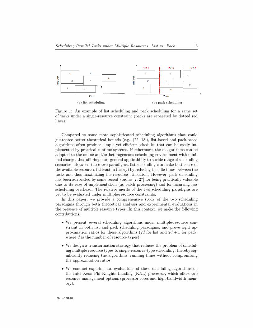
We focus on two scheduling paradigms, namely, list scheduling and packscheduling. In list scheduling, all tasks are first organized in a priority list. Then,the tasks are assigned in sequence to the earliest available resources that can fitthem. In pack scheduling, the tasks are first partitioned into a series of packs,which are then executed one after another. Tasks within each pack are scheduledconcurrently and a pack cannot start until all tasks in the previous pack havecompleted. Both scheduling paradigms have been studied by the literature,mostly under a single-resource constraint (see Section 2 for a literature review).Figure 1 shows an example of applying both scheduling paradigms to a sameset of tasks under a single-resource constraint.

RR n° 9140


(a) list scheduling (b) pack scheduling

Figure 1: An example of list scheduling and pack scheduling for a same setof tasks under a single-resource constraint (packs are separated by dotted redlines).

Compared to some more sophisticated scheduling algorithms that couldguarantee better theoretical bounds (e.g., [22, 18]), list-based and pack-basedalgorithms often produce simple yet efficient schedules that can be easily im-plemented by practical runtime systems. Furthermore, these algorithms can beadopted to the online and/or heterogeneous scheduling environment with mini-mal change, thus offering more general applicability to a wide range of schedulingscenarios. Between these two paradigms, list scheduling can make better use ofthe available resources (at least in theory) by reducing the idle times between thetasks and thus maximizing the resource utilization. However, pack schedulinghas been advocated by some recent studies [2, 27] for being practically valuabledue to its ease of implementation (as batch processing) and for incurring lessscheduling overhead. The relative merits of the two scheduling paradigms areyet to be evaluated under multiple-resource constraints.

In this paper, we provide a comprehensive study of the two schedulingparadigms through both theoretical analyses and experimental evaluations inthe presence of multiple resource types. In this context, we make the followingcontributions:

• We present several scheduling algorithms under multiple-resource con-straint in both list and pack scheduling paradigms, and prove tight ap-proximation ratios for these algorithms (2d for list and 2d + 1 for pack,where d is the number of resource types).

• We design a transformation strategy that reduces the problem of schedul-ing multiple resource types to single-resource-type scheduling, thereby sig-nificantly reducing the algorithms’ running times without compromisingthe approximation ratios.

• We conduct experimental evaluations of these scheduling algorithms onthe Intel Xeon Phi Knights Landing (KNL) processor, which offers tworesource management options (processor cores and high-bandwidth mem-ory).

RR n° 9140


• We project the performance of both list- and pack-based scheduling solu-tions under more than two resource types using simulations on syntheticparallel workloads that extend some classical speedup profiles.

Overall, the experimental/simultion results confirm the benefit of the trans-formation strategy and show that pack scheduling, despite having a slightlyworse theoretical bound, can indeed offer a practically promising yet easy-to-implement solution compared to its list counterpart, especially when more re-source types need to be managed. The insights derived from these results willbe especially relevant to the emerging architectures that will likely offer in theresource management systems more scheduling possibilities across the memoryhierarchy to embrace the shift towards data-driven computing.

The rest of this paper is organized as follows. Section 2 reviews some relatedwork. Section 3 formally defines the multiple-resource-type scheduling model.Section 4 presents several scheduling solutions and proves their approximationratios. Section 5 is devoted to experimental evaluation of different algorithmsand heuristics. Finally, Section 6 concludes the paper with hints on futuredirections.

2 Related Work

2.1 Parallel Task Models

Many parallel task models exist in the scheduling literature. Feitelson [8] classi-fied parallel tasks into three categories, namely, rigid tasks, moldable tasks andmalleable tasks. A rigid task requires a fixed amount of resources (e.g., num-ber of processors) to execute. A moldable task can be executed with a varyingamount of resources, but once the task has started the resource allocation can-not be changed. The most flexible model is the one of malleable tasks, whichallows the amount of resources executing the task to vary at any time duringthe execution. For the latter two models, two important parameters are thespeedup function and the total area (or work). The speedup function relatesthe execution time of a task to the amount of resources allocated to it, and thetotal area is defined as the product of execution time and resource allocation.Many prior works [2, 5, 22] have assumed that the speedup of a task is a non-decreasing function of the amount of allocated resources (hence the executiontime is a non-increasing function) and that the total area is a non-decreasingfunction of the allocated resources. One example is the well-known Amdahl’slaw [1], which specifies the speedup of executing a parallel task with s sequen-tial fraction using p processors as 1/(s+ 1−s

p ). Another example used by some

scheduling literature [4, 25, 14] is the speedup function pα, where p representsthe amount of allocated resources to the task and α ≤ 1 is a constant. In par-ticular, this function has been observed for processor resources when executingparallel matrix operations [24] as well as for characterizing the cache behaviorsin terms of the miss rate of data access (which is directly related to the executiontime) [15]. We refer to this function as the power law.

RR n° 9140


All works above apply to the case with a single resource type, and, to thebest of our knowledge, no explicit speedup model is known to include multipleresource types. In Section 5, we extend these speedup functions to constructsynthetic parallel tasks with multiple-resource demands. We also perform aprofiling study of the Stream benchmark [21] on a recent Intel Xeon Phi ar-chitecture that includes two resource types (processor core and high-bandwidthmemory).

2.2 Parallel Task Scheduling

Scheduling a set of independent parallel tasks to minimize the makespan isknown to be strongly NP-complete [11], thus much attention has been directedat designing approximation or heuristic algorithms. Most prior works focusedon allocating a single resource type (i.e., processors) to the tasks, and the con-structed schedules are either pack-based (also called shelf-based or level-based)or list-based.

Approximation Algorithms

Scheduling rigid tasks with contiguous processor allocation can be consideredas a rectangle packing or 2D-strip packing problem. For this problem, Coff-man et al. [6] showed that the Next-Fit Decreasing Height (NFDH) algorithm is3-approximation and the First-Fit Decreasing-Height (FFDH) algorithm is 2.7-approximation. Both algorithms pack rectangles onto shelves, which are equiv-alent to creating pack-based schedules. The first result (i.e., 3-approximation)has also been extended to the case of moldable task scheduling [2, 29]. Tureket al. [29] presented a strategy to extend any algorithm for scheduling rigidtasks into an algorithm for scheduling moldable tasks in polynomial time. Thestrategy preserves the approximation ratio provided that the makespan for therigid-task problem satisfies certain conditions. The complexity of such an exten-sion was improved in [20] with possibly a worse schedule than the one obtainedin [29] but without compromising the approximation ratio. Thanks to thesestrategies, a 2-approximation algorithm was devised for moldable tasks basedon list scheduling [29, 20], extending the same ratio previously known for rigidtasks [29, 10]. Using dual-approximation techniques, Mounie et al. [22] pre-sented a 1.5-approximation algorithm for moldable tasks while assuming thatthe total area of a task is a non-decreasing function of the allocated processors.Also for moldable tasks, Jansen and Porkolab [18] presented, for any ε > 0, a(1+ε)-approximation scheme when the number of processors is a fixed constant.

While all results above are for scheduling under a single resource type, onlya few papers have considered scheduling under multiple resource types. Gareyand Graham [10] proved that a simple list-scheduling algorithm is (d + 1)-approximation for rigid tasks, where d is the number of resource types. Heet al. [17] proved the same asymptotic result for scheduling a set of malleablejobs, each represented as a direct acyclic graph (DAG) of unit-size tasks. Formoldable tasks, Shachnai and Turek [26] presented a technique to transform a

RR n° 9140


c-approximation algorithm on a single resource type to a c · d-approximationalgorithm on d types of resources. Partially inspired by these results, this pa-per presents techniques and algorithms with improved approximations for packscheduling and new algorithms for list scheduling under multiple resource types.

Heuristics

Some papers have proposed heuristic solutions for multiple-resource-type schedul-ing under various different models and objectives. Leinberger et al. [19] con-sidered rigid tasks and proposed two heuristics that attempt to balance theusage of different resource types through backfilling strategies. He et al. [16]studied online scheduling of DAG-based jobs and proposed a multi-queue bal-ancing heuristic to balance the sizes of the queues that contain ready tasksunder different resource types. Ghodsi et al. [12] proposed Dominant ResourceFairness (DRF), a multiple-resource-type scheduling algorithm for user taskswith fixed resource demands. It aims at ensuring the resource allocation fair-ness among all users by identifying the dominant resource share for each userand maximizing the minimum dominant share across all users. Grandl et al. [13]considered scheduling malleable tasks under four resource types (CPU, memory,disk and network), and designed a heuristic, called Tetris, that packs tasks toa cluster of machines. This is similar to pack-based scheduling but instead ofcreating packs in time it creates them in space. Tetris works by selecting a taskwith the highest correlation between the task’s peak resource demands and themachine’s resource availabilities, with the aim of minimizing resource fragmen-tation. NoroozOliaee et al. [23] considered a similar cluster scheduling problembut with two resources only (CPU and memory). They showed that the simpleBest Fit plus Shortest Task First scheduling outperforms other packing heuris-tics (e.g., First Fit, FCFS) in terms of resource utilization and task queueingdelays.

3 Model

This sections presents a formal model of the scheduling problem, which wecall d-Resource-Scheduling. Suppose a platform has d different types of re-sources subject to allocation (e.g., processor, memory, cache). For each resourcetype i, there is a total amount P (i) of resources available. Consider a set of nindependent tasks (or jobs), all of which are released at the same time on theplatform, so the problem corresponds to scheduling a batch of applications inHPC environment. For each task j, its execution time tj(~pj) is a function of

the resource allocation vector ~pj = (p(1)j , p

(2)j , · · · , p(d)j ), where p

(i)j denotes the

amount of the i-th resource allocated to task j. In reality, the execution timesare typically obtained by application profiling or interpolation and curve-fittingfrom historic data. Suppose ~pj and ~qj are two resource allocation vectors, and

we define ~pj � ~qj if p(i)j ≤ q

(i)j for all 1 ≤ i ≤ d. Here, the execution time is

assumed to be a non-increasing function of the resource allocation, i.e., ~pj � ~qj

RR n° 9140


implies tj(~pj) ≥ tj(~qj). This means that increasing the allocation of any onetype of resource without decreasing the others will not increase the execution

time1. We also assume that the resource allocations p(i)j ’s and the total amount

of resources P (i)’s are all integer values. This holds naturally true for discreteresources such as processors2. For other resources (e.g., memory, cache), itcan be justified as most practical resource management systems allocate theresources in discrete chunks (e.g., memory blocks, cache lines). Note that sometasks may not require all resource types in order to execute, hence its resource

allocation p(i)j for a particular resource can be zero, in which case the execution

time remains validly defined. In contrast, other tasks may require a minimumamount of certain resource in order to execute. In this case, the execution timecan be defined as infinity for any amount of resource below this threshold. Themodel is flexible to handle both scenarios.

In this paper, we focus on moldable task scheduling [8], where the amountof resources allocated to a task can be freely selected by the scheduler at launchtime but they cannot be changed after the task has started the execution. Mold-able task scheduling strikes a good balance between practicality and perfor-mance by incurring less overhead than malleable task scheduling yet achievingmore flexible task executions than rigid task scheduling. For the d-Resource-Scheduling problem, the scheduler needs to decide, for each task j, a resourceallocation vector ~pj along with a starting time sj . At any time t, a task is said tobe active if it has started but not yet completed, i.e., t ∈ [sj , sj + tj(~pj)). Let Jtdenote the set of active tasks at time t. For a solution to be valid, the resourcesused by the active tasks at any time should not exceed the total amount of

available resources for each resource type, i.e.,∑j∈Jt p

(i)j ≤ P (i) for all t and i.

The objective is to minimize the maximum completion time, or the makespan,of all tasks, i.e., T = maxj(sj + tj(~pj)).

Since d-Resource-Scheduling is a generalization of classical makespanminimization problem with a single resource type, it is strongly NP-complete.Hence, we are interested in designing approximation and heuristic algorithms.In this paper, we will focus on and compare two major scheduling paradigms,namely, list scheduling and pack scheduling. A scheduling algorithm S is saidto be c-approximation if its makespan satisfies TS ≤ c · Topt for any instance,where Topt denotes the makespan by an optimal moldable scheduler. Note thatthe optimal scheduler needs not be restricted to either list scheduling or packscheduling.

1This assumption is not restrictive, as we can discard an allocation ~qj that satisfies ~pj � ~qjand tj(~pj) < tj(~qj). This is because any valid schedule that allocates ~qj to task j can bereplaced by a valid schedule that allocates ~pj to the task without increasing the executiontime, thus rendering ~qj useless.

2We do not allow fractional processor allocation (typically realized by timesharing a pro-cessor among several tasks) as assumed by some prior work.

RR n° 9140


4 Theoretical Analysis

In this section, we present polynomial-time algorithms for the d-Resource-Scheduling problem under both list- and pack-scheduling paradigms, and weprove tight approximation ratios for these algorithms.

4.1 Preliminaries

We start with some preliminary definitions that will be used throughout theanalysis. Table 1 provides a summary of the main notations used.

Definition 1. Define p = (~p1, ~p2, · · ·, ~pn)T to be a resource allocation matrix

for all tasks, where ~pj = (p(1)j , p

(2)j , · · ·, p(d)j ) is a resource allocation vector for

task j.

Definition 2. Given a resource allocation matrix p for the d-Resource-Schedulingproblem, we define the following:

• For task j, aj(~pj)=∑di=1

p(i)j

P (i) · tj(~pj) is the task’s area3;

• A(p) =∑nj=1 aj(~pj) is the total area of all tasks;

• tmax(p) = maxj tj(~pj) is the maximum execution time of all tasks;

• L(p, s) = max(A(p)

s , tmax(p))

for any s > 0.

The last quantity L(p, s) is related to the lower bound of the makespan. Inparticular, we define

Lmin(s) = minpL(p, s) , (1)

and we will show later that it is a lower bound on the makespan when s is setto be d.

In the following, we will present two general techniques for constructing thescheduling solutions. The first technique is a two-phase approach, similarly tothe one considered in scheduling under a single resource type [20]:

• Phase 1 : Determines a resource allocation matrix for all the tasks;

• Phase 2 : Constructs a rigid schedule based on the fixed resource allocationof the first phase.

The second technique is a transformation strategy that reduces the d-Resource-Scheduling problem to the 1-Resource-Scheduling problem, which is thensolved and whose solution is transformed back to the original problem.

Section 4.2 presents a resource allocation strategy (Phase 1 ). Section 4.3presents a transformation strategy, followed by rigid task scheduling schemes(Phase 2 ) in Section 4.4 under both pack and list scheduling. Finally, Sec-tion 4.5 puts these different components together and presents several completescheduling solutions.

3Rigorously, we define aj(~pj) =∞ if ∃i, s.t. p(i)j = 0 and tj(~pj) =∞.

RR n° 9140


Table 1: List of Notations.

For platform

d Number of resource types

P (i) Total amount of i-th type of resource (i = 1, · · ·, d)For any task j

p(i)j Amount of i-th type of resource allocated to task j

~pj Resource allocation vector of task j

tj(~pj) Execution time of task j with vector ~pjaj(~pj) Area of task j with vector ~pjsj Starting time of task j

For set of all tasks

n Number of all tasks

p Resource allocation matrix for all tasks

A(p) Total area of all tasks with matrix p

tmax(p) Maximum execution time of all tasks with matrix p

T (p) Makespan of all tasks with matrix p

L(p, s) Maximum of A(p)/s and tmax(p) for any s > 0

Lmin(s) Minimum L(p, s) over all matrix p

4.2 A Resource Allocation Strategy

This section describes a resource allocation strategy for the first phase of thescheduling algorithm. It determines the amounts of resources allocated to eachtask, which are then used to schedule the tasks in the second phase as a rigidtask scheduling problem.

The goal is to find efficiently a resource allocation matrix that minimizesL(p, s), i.e.,

psmin = arg minp

L(p, s) . (2)

Let P =∏di=1(P (i) + 1) denote the number of all possible allocations for each

task, including the ones with zero amount of resource under a particular re-source type. A straightforward implementation takes O(Pn) time, which growsexponentially with the number of tasks n. Algorithm 1 presents a resource al-location strategy RAd(s) that achieves this goal in O(nP (logP + log n + d))time. Note that when the amounts of resources under different types are in thesame order, i.e., P (i) = O(Pmax) for all i = 1, · · ·, d, where Pmax = maxi P

(i),the running time grows exponentially with the number of resource types d, i.e.,the complexity contains O(P dmax). Since the number of resource types is usuallya small constant (less than 4 or 5), the algorithm runs in polynomial time undermost realistic scenarios.

The algorithm works as follows. First, it linearizes and sorts all P resourceallocation vectors for each task and eliminates any allocation that results inboth a higher execution time and a larger total area (Lines 2-17), for sucha vector can be replaced by another one that leads to the same or smaller

RR n° 9140


Algorithm 1: Resource Allocation Strategy RAd(s)

Input: Set of n tasks, execution time tj(~p) ∀j, ~p and resource limit P (i) ∀iOutput: Resource allocation matrix ps

min = arg minp L(p, s)

1 begin

2 P ←∏d

i=1(P (i)+1);3 A← 0;4 for j = 1 to n do5 Linearize all P resource allocation vectors for task j in an array res alloc

and sort it in non-decreasing order of task execution time;6 admissible allocationsj ← list();7 min area ←∞;8 for h = 1 to P do9 ~p ← res alloc(h);

10 if aj(~p) < min area then11 min area← aj(~p);12 admissible allocationsj .append(~p);

13 ~pj ← admissible allocationsj .last element();14 A← A + aj(~pj);

15 Build a priority queue Q of n tasks with their longest execution time tj(~pj)’s aspriorities;

16 Lmin =∞;17 while Q.size() = n do18 k ← Q.highest priority element();19 ~pk ← admissible allocationsk.last element();20 tmax = tk(~pk);

21 L = max(As, tmax

);

22 if L < Lmin then23 Lmin ← L;

24 psmin ← (~p1, ~p2, · · · , ~pn)T ;

25 if As≥ tmax then

26 break;

27 admissible allocationsk.pop last();28 Q.remove highest priority element();29 if admissible allocationsk.nonempty() then30 ~p ′k ← admissible allocationsk.last element();31 A← A + ak(~p ′k )− ak(~pk);32 Q.insert element(k) with priority tk(~p ′k );

RR n° 9140


Lmin(s) (Equation (1)). Each task then ends up with an array of admissibleallocations in increasing order of execution time and decreasing order of totalarea. The complexity for this part is O

(n(P logP+Pd)

), which is dominated by

sorting each task’s allocations and computing its area. Then, the algorithm goesthrough all possible tmax, i.e., the maximum execution time, from the remainingadmissible allocations, and for each tmax considered, it computes the minimumtotal area A and hence the associated L value (Lines 18-40). This is achievedby maintaining the tasks in a priority queue with their longest execution timesas priorities and updating the queue with a task’s new priority when its nextlongest execution time is considered. The algorithm terminates either when atleast one task has exhausted its admissible allocations, in which case the priorityqueue will have fewer than n tasks (Line 20), or when L becomes dominated byAs (Line 30), since the total area only increases and the maximum execution timedecreases during this process. As the allocation is only changed for one taskwhen a new tmax is considered, the total area can be updated by keeping trackof the area change due to this task alone (Line 36). The algorithm considersat most nP possible tmax values and the complexity at each step is dominatedby updating the priority queue, which takes O(log n) time, and by updatingthe total area, which takes O(d) time, so the overall complexity for this part isO(nP (log n+ d)

).

Now, we show that the resource allocation matrix psmin returned by Algo-rithm 1 while setting the parameter s to be d can be used by a rigid taskscheduling strategy in the second phase to achieve good approximations.

Theorem 1. If a rigid task scheduling algorithm Rd that uses the resourceallocation matrix pdmin obtained by the strategy RAd(d) produces a makespan

TRd(pdmin) ≤ c · Lmin(d) , (3)

then the two-phase algorithm RAd(d)+Rd is c-approximation for the d-Resource-Scheduling problem.

To prove the above theorem, let us define popt to be the resource allo-cation matrix of an optimal schedule, and let Topt denote the correspond-ing optimal makespan. We will show in the following lemma that Lmin(d)serves as a lower bound on Topt. Then, Theorem 1 follows directly, sinceTRAd(d)+Rd = TRd(pdmin) ≤ c · Lmin(d) ≤ c · Topt.

Lemma 1. Topt ≥ Lmin(d).

Proof. We will prove that, given a resource allocation matrix p, the makespanproduced by any rigid task scheduler using p must satisfy T (p) ≥ tmax(p)

and T (p) ≥ A(p)d . Thus, for the optimal schedule, which uses popt, we have

Topt ≥ max(tmax(popt), A(popt)

d

)= L(popt, d) ≥ Lmin(d). The last inequality is

because Lmin(d) is the minimum L(p, d) among all possible resource allocationsincluding popt (Equation (1)).

The first bound T (p) ≥ tmax(p) is trivial since the makespan of any scheduleshould be at least the execution time of the longest task. For the second bound,

RR n° 9140


we have, in any valid schedule with makespan T (p), that:

A(p) =

n∑j=1

d∑i=1

p(i)j

P (i)· tj(~pj)

=

d∑i=1

1

P (i)

n∑j=1

p(i)j · tj(~pj)

≤d∑i=1

1

P (i)· P (i) · T (p)

= d · T (p) .

The inequality is because P (i) · T (p) is the maximum volume for resource typei that can be allocated to all the tasks within a total time of T (p).

4.3 A Transformation Strategy

This section describes a strategy to indirectly solve the d-Resource-Schedulingproblem via a transformation to the 1-Resource-Scheduling problem.

Algorithm 2 presents the transformation strategy TF, which contains threesteps. First, any instance I of the d-Resource-Scheduling problem is trans-formed to an instance I ′ of the 1-Resource-Scheduling problem. Then, I ′ issolved by any moldable task scheduler under a single resource type. Lastly, thesolution obtained for I ′ is transformed back to obtain a solution for the originalinstance I. The complexity of the transformation alone (without solving theinstance I ′) is O(nQd), dominated by the first step of the strategy, where Q isdefined as the Least Common Multiple (LCM) of all the P (i)’s. Note that ifQ is in the same order as the maximum amount of resource Pmax = maxi P

(i)

among all resource types (e.g., when P (i)’s are in powers of two), the complex-ity becomes linear in Pmax. In contrast, the complexity of solving the problemdirectly (by relying on Algorithm 1) contains P dmax. Thus, the transformationstrategy can greatly reduce an algorithm’s running time, especially when moreresource types need to be scheduled (see our simulation results in Section 5.4).

In the subsequent analysis, we will use the following notations:

• For the transformed instance I ′: Let q = (q1′ , q2′ , · · · , qn′)T denote theresource allocation for the transformed tasks. L′min(s) is the minimumL′(q, s) as defined in Equation (1), and T ′M1

denotes the makespan pro-duced by a moldable task scheduler M1 for the 1-Resource-Schedulingproblem.

• For the original instance I: Recall that Lmin(s) denotes the minimumL(p, s) defined in Equation (1), and let TTF+M1

denote the makespanproduced by the algorithm TF+M1, which combines the transformationstrategy TF and the scheduler M1 for a single resource type.

RR n° 9140


Algorithm 2: Transformation Strategy TF

Input: Set of n tasks, execution time tj(~p) ∀j, ~p, resource limit P (i) ∀iOutput: Starting time sj and resource allocation vector ~pj ∀j(1) Transform d-Resource-Scheduling instance I to 1-Resource-Scheduling

instance I′;• I′ has the same number n of tasks as I;

• The resource limit for the only resource of I′ is Q = lcmi=1···d

P (i);

• For any task j′ in I′, its execution time with any amount of resource

q ∈ {0, 1, 2, · · · , Q} is defined as tj′ (q) = tj((b q·P(i)

Qc)i=1···d);

(2) Solve the 1-Resource-Scheduling instance I′;(3) Transform 1-Resource-Scheduling solution S′ back tod-Resource-Scheduling solution S;

• For any task j in I, its starting time is sj = sj′ , where sj′ is the starting time of task

j′ in I′, and its resource allocation vector is ~pj = (bqj′ ·P

(i)

Qc)i=1···d, where qj′ is the

allocation of the only resource for task j′ in I′.

We show that the transformation achieves good approximation for the d-Resource-Scheduling problem if the solution for the 1-Resource-Schedulingproblem satisfies certain property.

Theorem 2. For any transformed instance I ′ of the 1-Resource-Schedulingproblem, if a moldable task scheduler M1 under a single resource type producesa makespan

T ′M1≤ c · L′min(d) , (4)

then the algorithm TF+M1 is c-approximation for the d-Resource-Schedulingproblem.

Before proving the approximation, we first show that the schedule obtainedfor I via the transformation strategy is valid and that the makespan for I ′ ispreserved.

Lemma 2. Any valid solution by scheduler M1 for I ′ transforms back to a validsolution by algorithm TF + M1 for I, and TTF+M1 = T ′M1

.

Proof. According to Steps (1) and (3) of the transformation, the execution timefor each task j in I is the same as that of j′ in I ′, i.e., tj(~pj) = tj′(qj′). Hence,the makespan is equal for both I and I ′, since the corresponding tasks also havethe same starting time, i.e., sj = sj′ .

If the schedule for I ′ is valid, i.e.,∑j′∈J′t

qj′ ≤ Q ∀t, then we have∑j∈Jt p

(i)j =∑

j∈Jtbqj′ ·P

(i)

Q c ≤ P (i)

Q

∑j′∈J′t

qj′ ≤ P (i) ∀i, t, rendering the schedule for I validas well.

The following lemma relates the makespan lower bound of the transformedinstance to that of the original instance.

Lemma 3. L′min(d) ≤ Lmin(d).

RR n° 9140


Proof. We will show that given any resource allocation p for I, there existsan allocation q(p) for I ′ such that L′(q(p), d) ≤ L(p, d). Thus, for pdmin thatleads to Lmin(d), there is a corresponding q(pdmin) that satisfies L′(q(pdmin), d) ≤L(pdmin, d) = Lmin(d), and therefore L′min(d) = minq L

′(q, d) ≤ L′(q(pdmin), d) ≤Lmin(d).

Consider any resource allocation p = (~p1, ~p2, · · · , ~pn)T for I. For each task j,let kj denote its dominating resource type in terms of the proportion of resource

used, i.e., kj = arg minip(i)j

P (i) . We construct q(p) = (q1′ , q2′ , · · · , qn′)T for I ′ by

setting, for each task j′, an allocation qj′ =p(kj)

j ·QP (kj)

. As P (kj) divides Q, qj′ is

an integer and hence a valid allocation.According to Step (1) of the transformation, the execution time of task j′ in

I ′ satisfies

tj′(qj′) = tj((bp(kj)j · P (i)

P (kj)c)i=1···d) ≤ tj(~pj) .

The inequality is because p(i)j ≤ b

p(kj)

j ·P (i)

P (kj)c ∀i, which we get by the choice of kj

and the integrality of p(i)j , and because we assumed that the execution time is a

non-increasing function of each resource allocation (in Section 3). As a result,the area of each task j′ in I ′ also satisfies

aj′(qj′)=qj′

Qtj′(qj′)≤

p(kj)j

P (kj)tj(~pj)≤

d∑i=1

p(i)j

P (i)tj(~pj)=aj(~pj).

Hence, the maximum execution times and the total areas for the two in-stances I ′ and I satisfy t′max(q(p)) = maxj′ tj′(qj′) ≤ maxj tj(~pj) = tmax(p)and A′(q(p)) =

∑j′ aj′(qj′) ≤

∑j aj(~pj) = A(p). This leads to L′(q(p), d) =

max(A′(q(p))

d , t′max(q(p)))≤ max

(A(p)d , tmax(p)

)= L(p, d).

(Proof of Theorem 2). Based on the above results, we can derive:

TTF+M1= T ′M1

(Lemma 2)

≤ c · L′min(d) (Equation (4))

≤ c · Lmin(d) (Lemma 3)

≤ c · Topt . (Lemma 1)

4.4 Rigid Task Scheduling

This section presents strategies to schedule rigid tasks under fixed resourceallocations. The strategies include both list-based and pack-based scheduling.The results extend the theoretical analyses of single-resource-type scheduling[29, 2] to account for the presence of multiple resource types.

RR n° 9140


4.4.1 List Scheduling

We first present a list-based scheduling strategy for a set of rigid tasks undermultiple resource types. A list-based algorithm arranges the set of tasks in a list.At any moment starting from time 0 and whenever an existing task completesexecution and hence releases resources, the algorithm scans the list of remainingtasks in sequence and schedules the first one that fits, i.e., there is sufficientamount of resource to satisfy the task under each resource type. Algorithm 3presents the list scheduling strategy LSd with d resource types, and it extendsthe algorithm presented in [29] for scheduling under a single resource type. Thecomplexity of the algorithm is O(n2d), since scheduling each task incurs a costof O(nd) by scanning the taskList and updating the resource availability forthe times in sortedT imeList.

Algorithm 3: List Scheduling Strategy LSd

Input: Resource allocation matrix p for the tasks and resource limit P (i) ∀iOutput: Starting time sj ∀jbegin

Arrange the tasks in a list taskList;sortedT imeList← {0};while taskList.nonempty() do

t = sortedT imeList.pop first();for j = 1 to taskList.size() do

if task j fits at time t thenSchedule task j at time t, i.e., sj = t;sortedT imeList.insert(sj + tj(~pj));Update available resources for all times before sj + tj(~pj);

The following lemma shows the performance of this list scheduling scheme.

Lemma 4. For a set of rigid tasks with a resource allocation matrix p, the listscheduling algorithm LSd achieves, for any parameter s ≥ 1, a makespan

TLSd(p) ≤ 2s · L(p, s) . (5)

Proof. We will prove in the following that TLSd(p) ≤ 2·max(tmax(p), A(p)

). For

any s ≥ 1, it will then lead to TLSd(p) ≤ 2s ·max(tmax(p), A(p)

s

)= 2s ·L(p, s).

First, suppose the makespan satisfies TLSd(p) ≤ 2tmax(p), then the claimholds trivially. Otherwise, we will show TLSd(p) ≤ 2A(p), thus proving the

claim. To this end, consider any time t ∈ [0,TLSd

(p)

2 ], and define t′ = t+TLSd

(p)

2 .

Since tmax(p) <TLSd

(p)

2 by our assumption, any task that is active at time t′ has

not been scheduled at time t. Define U(i)t =

∑j∈Jt

p(i)j

P (i) to be the total utilization

for resource of type i at time t. Therefore, we should have ∃i, s.t. U(i)t +U

(i)t′ ≥

1, for otherwise any active task at time t′ could have been scheduled by the

RR n° 9140


algorithm at time t or earlier. Thus, we can express the total area as:

A(p) =

∫ TLSd(p)

t=0

d∑i=1

U(i)t dt

=

∫ TLSd(p)

2

t=0

d∑i=1

(U

(i)t + U

(i)t′

)dt

≥ TLSd(p)

2.

4.4.2 Pack Scheduling

We now present a pack-based scheduling strategy. Recall that a pack containsseveral concurrently executed tasks that start at the same time and the tasks inthe next pack cannot start until all tasks in the previous pack have completed.Algorithm 4 presents the pack scheduling strategy PSd with d resource types.It extends the algorithm presented in [2] for scheduling under a single resourcetype. Specifically, the tasks are first sorted in non-increasing order of executiontimes (which are fixed due to fixed resource allocations). Then, they are assignedone by one to the last pack if it fits, i.e., there is sufficient amount of resourceunder each resource type. Otherwise, a new pack is created and the task isassigned to the new pack. The complexity of the algorithm is O

(n(log n+ d)

),

which is dominated by the sorting of the tasks and by checking the fitness ofeach task in the pack.

Algorithm 4: Packing Scheduling Strategy PSd

Input: Resource allocation matrix p for the tasks and resource limit P (i) ∀iOutput: Set of packs {B1, B2, · · · } containing the tasks and starting times Sm for

each pack Bm

beginSorted the tasks in non-increasing order of execution time tj(~pj);m← 1;B1 ← ∅;S1 ← 0;for j = 1 to n do

if task j fits in pack Bm thenBm ← Bm ∪ {j};

elsem← m + 1;Bm ← {j};Sm ← Sm−1 + maxj∈Bm−1

tj(~pj);

The following lemma shows the performance of this pack scheduling scheme.

Lemma 5. For a set of rigid tasks with a resource allocation matrix p, the packscheduling algorithm PSd achieves, for any parameter s > 0, a makespan

TPSd(p) ≤ (2s+ 1) · L(p, s) . (6)

RR n° 9140


Proof. We will prove in the following that TPSd(p) ≤ 2A(p) + tmax(p), which

will then lead to TPSd(p) ≤ (2s+ 1) ·max(A(p)

s , tmax(p))

= (2s+ 1) · L(p, s).Suppose the algorithm creates M packs in total. For each pack Bm, where

1 ≤ m ≤ M , let Am denote the total area of the tasks in the pack, i.e., Am =∑j∈Bm aj(~pj), and let Tm denote the total execution time of the pack, which

is the same as the execution time of the longest task in the pack, i.e., Tm =maxj∈Bm tj(~pj).

Consider the time when the algorithm tries to assign a task j to pack Bmand fails due to insufficient amount of i-th resource, whose remaining amountis denoted by p(i). As the tasks are handled by decreasing execution time, we

have Am ≥(

1− p(i)

P (i)

)tj(~pj). Also, because task j cannot fit in pack Bm, it

means that its allocation p(i)j on resource i is at least p(i). This task is then

assigned to pack Bm+1, so we have Am+1 ≥ aj(~pj) ≥ p(i)

P (i) tj(~pj). Since task j isthe first task put in the pack and all the following tasks have smaller executiontimes, we have Tm+1 = tj(~pj). Hence,

Am +Am+1 ≥ tj(~pj) = Tm+1 .

Summing the above inequality over m, we get∑Mm=2 Tm ≤ 2

∑Mm=1Am =

2A(p). Finally, as the longest task among all tasks is assigned to the first

pack, i.e., T1 = tmax(p), we get the makespan TPSd(p) =∑Mm=1 Tm ≤ 2A(p) +

tmax(p).

4.5 Putting Them Together

This section combines various strategies presented in the previous sections toconstruct several moldable task scheduling algorithms under multiple resourcetypes. Two solutions are presented for the d-Resource-Scheduling prob-lem under each scheduling paradigm (list vs. pack) depending on if the prob-lem is solved directly or indirectly via a transformation to the 1-Resource-Scheduling problem. The following shows the combinations of the two solu-tions:

Direct-based solution: RAd(d) + Rd

Transform-based solution: TF + RA1(d) + R1

Here, RA denotes the resource allocation strategy (Algorithm 1), TF denotesthe transformation strategy (Algorithm 2), and R denotes the rigid task schedul-ing strategy LS or PS (Algorithm 3 or 4). Four algorithms can be resulted fromthe above combinations, and we call them D(irect)-Pack, D(irect)-List,T(ransform)-Pack and T(ransform)-List, respectively.

We point out that when the LCM of all the P (i)’s is dominated by Pmax

(e.g., when P (i)’s are powers of two), the transform-based solution will reducethe overall complexity of the direct-based solution exponentially, thus signifi-cantly improving the algorithms’ running times. The approximation ratios of

RR n° 9140


the transform-based solutions, however, will not be compromised. The followingtheorem proves the ratios of these algorithms.

Theorem 3. The list-based algorithms (D-List and T-List) are 2d-approximationsand pack-based algorithms (D-Pack and T-Pack) are (2d+1)-approximations.Moreover, the bounds are asymptotically tight for the respective algorithms.

Proof. We prove the approximation ratios for the two pack-based schedulingalgorithms. The proof for the list-based algorithms is very similar and henceomitted.

For D-Pack (RAd(d)+PSd): Using pdmin found by RAd(d), we have TPSd(pdmin) ≤(2d+1) ·L(pdmin, d) = (2d+1) ·Lmin(d) from Lemma 5 (by setting s = d). Then,based on Theorem 1, we get TRAd(d)+PSd ≤ (2d+ 1) · Topt.

For T-Pack (TF + RA1(d) + PS1): Applying PS1 to the transformedinstance using qdmin found by RA1(d), we have T ′RA1(d)+PS1

= T ′PS1(qdmin) ≤

(2d+1) ·L′(qdmin, d) = (2d+1) ·L′min(d) from Lemma 5 (again by setting s = d).Then, based on Theorem 2, we get TTF+RA1(d)+PS1

≤ (2d+ 1) · Topt.Now, we show that the approximation ratios are tight. To this end, we

define in the following a partial profile for each task, i.e., the execution timesfor some resource allocation vectors, together with t(0, · · · , 0) =∞. To adhereto the non-increasing execution time assumption (in Section 3), we define theexecution time for each remaining vector ~p of the task as t(~p) = min~q�~p t(~q),thus making these choices irrelevant to the scheduling algorithms.

For both pack-based algorithms, we construct an instance that contains n =2dP +d+ 1 tasks and total amount of resource P (i) = P , ∀i = 1,· · ·, d. We referto the first task as task 0, and define its execution time as t0(1, · · · , 1) = P .The following describes the remaining 2dP + d tasks, which are indexed usingi ∈ [1, d] and j ∈ [0, 2P ]. Specifically, for each i, we have:

• ti,0(0, · · ·, 0, P, P, 0, · · ·, 0) = 1, where the P appears in positions i and i−1(if i− 1 ≥ 1);

• ∀j1 ∈ [1, P ], ti,j1(0, · · ·, 0, P − 1, 0, · · ·, 0) = 1, where the P − 1 appears inpositions i;

• ∀j2 ∈ [P + 1, 2P ], ti,j2(0, · · ·, 0, 2, 0, · · ·, 0) = 1, where the 2 appears inpositions i.

We can add different values in the range of [0, ε] to the above execution timesin such a way that forces the algorithms to assign each task to a pack of itsown, which can be achieved by placing them in the desired order. In particular,task 0 will be placed first. Then, for each i ∈ [1, d], task (i, 0) will be placed,followed by tasks (i, j1) and tasks (i, j2) in alternating order. In this case, bothpack-based algorithms will have a makespan T = (2d+1)P +d+O(nε). On theother hand, the optimal algorithm is able to schedule task 0 together with tasks(i, 0) in P + O(ε) time, followed by tasks (i, j2) in 2 + O(ε) time, and finallytasks (i, j2) in 2 +O(ε) time, thus having a makespan Topt = P + 4 +O(ε). By

setting ε = 1n , we have T

Topt= (2d+1)P+d+O(1)

P+O(1) , so limP→∞

TTopt

= 2d+ 1.

RR n° 9140


For both list-based algorithms, we construct an instance that contains n = 2dtasks and total amount of resource P (i) = 2P , ∀i = 1, · · ·, d. For each task j,we define two relevant allocations:

• tj(0, · · ·, 0, P, 0, · · ·, 0) = 1, where the P appears in position d j2e;

• tj(P + 1, 0, · · ·, 0) = P−1P+1 .

Based on the resource allocation strategy, the first allocation is discarded byboth list-based algorithms (for having both longer execution time and largerarea). Thus, using the second allocation, any list-based algorithm is forcedto schedule the tasks sequentially one after another, resulting in a makespanT = 2dP−1P+1 . The optimal algorithm chooses instead the first allocation andschedules all tasks at the same time with a makespan Topt = 1. Therefore, wehave lim

P→∞TTopt

= 2d.

5 Experiments

In this section, we conduct experiments and simulations whose goals are twofold:(i) to validate the theoretical underpinning of moldable task scheduling; and(ii) to compare the practical performance of various list- and pack-schedulingschemes under multiple resource types.

Experiments are performed on an Intel Xeon Phi Knights Landing (KNL)machine with 64 cores and 112GB available memory, out of which 16GB arehigh-bandwidth fast memory (MCDRAM) and the rest are slow memory (DDR).MCDRAM has ≈5x the bandwidth of DDR [28], thus offering a higher data-transfer rate. The applications we run are from a modified version of the Streambenchmark [21] configured to explore the two available resources of KNL (coresand fast memory) with different resource allocations. Simulations are furtherconducted to project the performance under more resource types using syntheticworkloads that extend some classical speedup profiles.

5.1 Evaluated Algorithms

Each algorithm in Section 4.5 is evaluated with two variants, depending on ifit is list-based or pack-based. A list-based algorithm can arrange the tasks ac-cording to two widely applied heuristics: Shortest Processing Time First (SPT)and Longest Processing Time First (LPT), before scheduling them as shown inAlgorithm 3. For pack-based scheduling, Algorithm 4 applies the Next Fit (NF)heuristic, which assigns a task to the last pack created. First Fit (FF) is an-other heuristic that assigns a task to the first pack in which the task fits. Fromthe analysis, the approximation ratio can only be improved with this heuristic.Coupling these heuristics with the two solutions (direct vs. transformation)under the two scheduling paradigms (list vs. pack), we have a total of eightscheduling algorithms that we will evaluate in the experiments.

RR n° 9140


5.2 Application Profiling

In order to manage the fast memory as a resource, we first configure the KNLmachine in flat mode [28], where MCDRAM and DDR together form the entireaddressable memory. We will also explore MCDRAM in cache mode later (seenext subsection). The applications in the Stream benchmark are then modifiedby allocating a specified portion of their memory footprints on MCDRAM (andthe remaining on DDR), thereby impacting the overall data-transfer efficiencyand hence the execution time. The profiles are obtained by varying both thenumber of cores (1-64) and the amount of fast memory (16GB divided into 20chunks) allocated to each application and recording their corresponding execu-tion times. In addition, we vary the total memory footprints of the applicationsto create tasks of different sizes.

Figure 2 shows the profiles of the triad application when its memory foot-print occupies 100%, 80% and 60% of the fast memory, respectively. Similarprofiles are also observed for the other applications (e.g., write, ddot) in thebenchmark. First, we observe that the execution time is inversely proportionalto the number of allocated cores, suggesting that the application has nearly per-fect speedup. Also, the execution time reduces linearly as more fast memory isallocated to the point where the application’s memory footprint fits entirely infast memory; after that the execution time remains fairly constant since allocat-ing additional fast memory no longer benefits the execution. The profiled datafor different applications under various sizes are subsequently used to computethe schedules by different algorithms, which are then implemented on the KNLnode for performance comparison.

5.3 Experimental Results

In order to validate our theoretical analysis and to compare the performanceof different algorithms, we implement a basic scheduler that executes the tasksaccording to the schedules given by these algorithms based on the applicationprofiles. Each task is launched at the specified time using the specified amountof resources (cores and fast memory) on the KNL machine. If any requiredresource of a task is not available at start time because of the delays in the pre-ceding tasks (possibly due to performance variations), the execution of the taskwill be correspondingly delayed until there are enough resources available. Weexpect the delay (if any) to be small for each task but the effect can accumulatethroughout the course of the schedule. This additional overhead is assessed inour experiments.

Figure 3(a) shows the makespans of the eight scheduling algorithms normal-ized by the theoretical lower bound (Equation (1) with s = d; see also Lemma 1)while running 150 tasks. We have also varied the number of tasks but observedno significant difference in their relative performance. First, we can see that thescheduling overhead, which manifests as the difference between the theoreticalprediction and the experimental result, is less than 10% for all algorithms. Ingeneral, list scheduling (left four) and pack scheduling (right four) have compa-

RR n° 9140


(a) 100% (b) 80%

(c) 60%

Figure 2: Profiles of the triad application in Stream benchmark when its mem-ory footprint occupies 100%, 80% and 60% of the entire fast memory.

rable performance despite that the former admits a better theoretical bound.Moreover, transform-based solutions fare slightly better than direct-based solu-tions due to the balanced resource requirements of different applications in thebenchmark. Lastly, in line with the intuition and conventional wisdom, LPTand FF are effective for reducing the makespan for list and pack scheduling,respectively, except for the T-List algorithm, which incurs a larger overheadwith the LPT variant in the actual execution.

Figure 3(b) further compares the makespans of four transform-based algo-rithms when MCDRAM is not used in flat mode (in which case all data areallocated on the slow DDR memory), and when KNL is configured in cachemode (in which case MCDRAM serves as a last-level cache to DDR). In bothcases, only one type of resource (i.e., cores) is scheduled, and as a result, thetransformation produces the same solutions as the direct-based schedules. Notsurprisingly, cores-only scheduling in flat mode has the worst makespan forall algorithms, since MCDRAM is completely unutilized in this case. Having

RR n° 9140


(a) (b)

Figure 3: (a) Normalized makespans of eight scheduling algorithms; (b)Makespans of four transform-based scheduling algorithms in three different re-source management configurations.

MCDRAM as cache to DDR significantly improves the makespan, but due tointerference from concurrently running applications, the makespan is still worsethan scheduling both cores and MCDRAM in flat mode. The results confirmthe benefit of explicitly managing multiple resource types for improving theapplication performance.

5.4 Simulation Results with More Resource Types

In this section, we conduct simulations to project the performance of list-basedand pack-based scheduling algorithms under more resource types. We simulateup to four types of resources that could represent different type of componentssuch as CPUs, GPUs, fast memory, I/O bandwidth. All elements that wouldbe shared between different applications and needed for one execution. Thetotal amount of discrete resource for each type is set to be 64, 32, 16 and8, respectively. Due to the lack of realistic application profiles under multiple-resource constraints, we generate synthetic workloads by extending two classicalspeedup functions (described in Section 2.1) to model moldable applications:

• Extended Amdahl’s law [1]: (i) 1/(s0 +

∑di=1

sip(i)

);

(ii) 1/(s0 + 1−s0∏d

i=1 p(i)

); (iii) 1/

(s0 + maxi=1..d

sip(i)

).

• Extended power law [24, 15]: (i) 1/(∑d

i=1si

(p(i))αi

);

(ii)∏di=1(p(i))αi ; (iii) 1/

(maxi=1..d

si(p(i))αi

).

The extension of both speedup laws comes in three different flavors (i.e., sum,product, max ), characterizing how allocations of different resource types work

RR n° 9140


(a) (b)

Figure 4: (a) Normalized makespans and (b) running times of four schedulingalgorithms with up to four different resource types.

together to contribute to the overall application speedup (i.e., sequential, collab-orative, concurrent). In the simulations, we generate 150 tasks, each randomlyselected from the six extended profiles. The sequential fraction s0 is uniformlygenerated in (0, 0.2], and the parallel fraction si for each resource type i is uni-

formly generated in (0, 1] and normalized to make sure that∑di=1 si = 1 − s0.

The parameter αi is uniformly generated in [0.3, 1). The total work of a task ischosen uniformly from a range normalized between 0 and 1 (the relative perfor-mance of the algorithms is not affected by the normalization).

Figure 4 plots the performance distributions of the scheduling algorithmswith up to four resource types. Each boxplot is obtained by running 100 in-stances. Only LPT (for list) and FF (for pack) are included, since they havebetter overall performance. First, we observe that the normalized makespans in-deed increase with the number of resource types, corroborating the theoreticalanalyses, although they are far below those predicted by the worst-case ap-proximation ratios. Also, list-based schedules now produce consistently smallermakespans compared to the pack-based ones, which we believe is due to thelarger variability in the simulated task profiles than that of the Stream bench-mark. This allows the list-based schedules to explore more effectively the gapsbetween successive task executions (as reflected by the theoretical bounds).However, the makespan difference between the two scheduling paradigms be-comes smaller with more resource types, suggesting that pack-based schedulingis promising when more resource types are to be managed. Finally, transform-based solutions are superior compared to the direct-based ones in terms of bothmakespan and algorithm running time (for which there are 2-3 orders of mag-nitude difference with more than two resource types). In general, for workloadswith balanced resource requirements, transform-based scheduling is expected tooffer both fast and efficient scheduling solutions.

Lastly, we point out that it may seem in Figure 4(a) that the makespan in-

RR n° 9140


creases with more resource types. In fact, it is the ratio to the optimal solution(or lower bound), not the makespan itself, that increases with d. In practice, thevalue of that optimal solution will decrease with more resource types, since thereis more room for optimization. Hence, scheduling more resource types poten-tially improves the overall makespan, which is what we observed experimentallywhen managing one and two types of resources as shown in Figure 3(b).

6 Conclusion and Future Work

List scheduling and pack scheduling are two scheduling paradigms that havebeen studied extensively in the past. While most prior works focused on schedul-ing under a single resource type, in this paper we joined a handful of re-searchers on scheduling under multiple-resource constraints in these two schedul-ing paradigms. Our analyses and evaluation results show that scheduling be-comes more difficult with increasing number of resource types, but consideringall available resources is essential for improving the application performance.Despite the better theoretical bound of list scheduling, pack scheduling has beenshown to have comparable or, in some scenarios, even better performance, espe-cially when more types of resources are included in the scheduling decision. Theresults offer useful insights to the design of emerging architectures and systemsthat need to incorporate multiple dimensions in the resource management.

Future work will be devoted to the design of improved list or pack schedul-ing algorithms (or any other practical algorithms beyond the two schedulingparadigms) with multiple-resource constraints. An immediate open questionis whether the 2d-approximation for list scheduling can be improved, e.g., to(d + 1)-approximation as proven by Garey and Graham for rigid tasks [10],which is equivalent to Phase 2 of our list-based algorithm but with fixed re-source allocation. Given our list algorithm’s lower bound of 2d for moldabletasks (Theorem 3), any improvement will likely be achieved through the designof more sophisticated resource allocation strategies (Phase 1) or through a morecoupled design/analysis of the two phases. Prior work [22] on scheduling undera single-resource type has shed light on some possible directions (e.g., by usingdual approximation).

Acknowledgements

We would like to thank Nicolas Denoyelle for sharing the code to run the mod-ified Stream benchmark on the KNL processor. This research is supported inpart by the National Science Foundation under the award CCF 1719674. Fi-nally, we would like to thank the reviewers for useful comments.

RR n° 9140


References

[1] G. M. Amdahl. Validity of the single processor approach to achieving largescale computing capabilities. In AFIPS’67, pages 483–485, 1967.

[2] G. Aupy, M. Shantharam, A. Benoit, Y. Robert, and P. Raghavan. Co-scheduling algorithms for high-throughput workload execution. Journal ofScheduling, 19(6):627–640, 2016.

[3] H. Barwick. SKA telescope to generate more data than entire Internetin 2020. https://www.computerworld.com.au/article/392735/ska_

telescope_generate_more_data_than_entire_internet_2020/, 2011.

[4] O. Beaumont and A. Guermouche. Task scheduling for parallel multifrontalmethods. In Euro-Par, pages 758–766, 2007.

[5] K. P. Belkhale and P. Banerjee. An approximate algorithm for the par-titionable independent task scheduling problem. In ICPP, pages 72–75,1990.

[6] E. G. Coffman, M. R. Garey, D. S. Johnson, and R. E. Tarjan. Performancebounds for level-oriented two-dimensional packing algorithms. SIAM J.Comput., 9(4):808–826, 1980.

[7] M. Dreher and B. Raffin. A flexible framework for asynchronous in situ andin transit analytics for scientific simulations. In CCGrid, pages 277–286,2014.

[8] D. G. Feitelson. Job scheduling in multiprogrammed parallel systems (ex-tended version). IBM Research Report RC19790(87657), 1997.

[9] A. Gainaru, G. Aupy, A. Benoit, F. Cappello, Y. Robert, and M. Snir.Scheduling the I/O of HPC applications under congestion. In IPDPS, pages1013–1022, 2015.

[10] M. R. Garey and R. L. Graham. Bounds for multiprocessor scheduling withresource constraints. SIAM J. Comput., 4(2):187–200, 1975.

[11] M. R. Garey and D. S. Johnson. Computers and Intractability: A Guideto the Theory of NP-Completeness. W. H. Freeman & Co., New York, NY,USA, 1979.

[12] A. Ghodsi, M. Zaharia, B. Hindman, A. Konwinski, S. Shenker, and I. Sto-ica. Dominant resource fairness: Fair allocation of multiple resource types.In Proceedings of the 8th USENIX Conference on Networked Systems De-sign and Implementation, pages 323–336, 2011.

[13] R. Grandl, G. Ananthanarayanan, S. Kandula, S. Rao, and A. Akella.Multi-resource packing for cluster schedulers. SIGCOMM Comput. Com-mun. Rev., 44(4):455–466, Aug. 2014.

RR n° 9140

https://www.computerworld.com.au/article/392735/ska_telescope_generate_more_data_than_entire_internet_2020/

https://www.computerworld.com.au/article/392735/ska_telescope_generate_more_data_than_entire_internet_2020/


[14] A. Guermouche, L. Marchal, B. Simon, and F. Vivien. Scheduling trees ofmalleable tasks for sparse linear algebra. In Proceedings of the Euro-ParConference, pages 479–490, 2015.

[15] A. Hartstein, V. Srinivasan, T. Puzak, and P. Emma. On the nature ofcache miss behavior: Is it

√2? J. Instruction-Level Parallelism, 2008.

[16] Y. He, J. Liu, and H. Sun. Scheduling functionally heterogeneous systemswith utilization balancing. In IPDPS, pages 1187–1198, 2011.

[17] Y. He, H. Sun, and W.-J. Hsu. Adaptive scheduling of parallel jobs onfunctionally heterogeneous resources. In ICPP, page 43, 2007.

[18] K. Jansen and L. Porkolab. Linear-time approximation schemes for schedul-ing malleable parallel tasks. In SODA, pages 490–498, 1999.

[19] W. Leinberger, G. Karypis, and V. Kumar. Job scheduling in the presenceof multiple resource requirements. In Supercomputing, 1999.

[20] W. Ludwig and P. Tiwari. Scheduling malleable and nonmalleable paralleltasks. In SODA, pages 167–176, 1994.

[21] J. D. McCalpin. STREAM: Sustainable memory bandwidth in high per-formance computers. Technical report, University of Virginia, 1991-2007.http://www.cs.virginia.edu/stream/.

[22] G. Mounie, C. Rapine, and D. Trystram. A 3/2-approximation algorithmfor scheduling independent monotonic malleable tasks. SIAM J. Comput.,37(2):401–412, 2007.

[23] M. NoroozOliaee, B. Hamdaoui, M. Guizani, and M. B. Ghorbel. On-line multi-resource scheduling for minimum task completion time in cloudservers. In INFOCOM Workshops, 2014.

[24] G. N. S. Prasanna and B. R. Musicus. Generalized multiprocessor schedul-ing and applications to matrix computations. IEEE Trans. Parallel Distrib.Syst., 7(6):650––664, 1996.

[25] P. Sanders and J. Speck. Efficient parallel scheduling of malleable tasks.In IPDPS, pages 1156–1166, 2011.

[26] H. Shachnai and J. J. Turek. Multiresource malleable task scheduling.Technical report, IBM T.J. Watson Research Center, 1994.

[27] M. Shantharam, Y. Youn, and P. Raghavan. Speedup-aware co-schedulesfor efficient workload management. Parallel Proc. Letters, 23(2), 2013.

[28] A. Sodani, R. Gramunt, J. Corbal, H.-S. Kim, K. Vinod, S. Chinthamani,S. Hutsell, R. Agarwal, and Y.-C. Liu. Knights Landing: Second-generationIntel Xeon Phi product. IEEE Micro, 36(2):34–46, 2016.

RR n° 9140


[29] J. Turek, J. L. Wolf, and P. S. Yu. Approximate algorithms schedulingparallelizable tasks. In SPAA, 1992.

[30] A. B. Yoo, M. A. Jette, and M. Grondona. Slurm: Simple linux utility forresource management. In JSSPP, pages 44–60, 2003.

RR n° 9140

RESEARCH CENTREBORDEAUX – SUD-OUEST

200 avenue de la Vieille Tour33405 Talence Cedex

PublisherInriaDomaine de Voluceau - RocquencourtBP 105 - 78153 Le Chesnay Cedexinria.fr

ISSN 0249-6399

scheduling parallel tasks under multiple resources: list

Documents