scheduling irregular parallel computations on hierarchical...
TRANSCRIPT
Scheduling Irregular Parallel Computationson Hierarchical Caches
Guy E. BlellochCarnegie Mellon University
Pittsburgh, PA [email protected]
Jeremy T. FinemanCarnegie Mellon University
Pittsburgh, PA [email protected]
Phillip B. GibbonsIntel Labs PittsburghPittsburgh, PA USA
Harsha Vardhan SimhadriCarnegie Mellon University
Pittsburgh, PA [email protected]
ABSTRACTFor nested-parallel computations with low depth (span, crit-ical path length) analyzing the work, depth, and sequentialcache complexity suffices to attain reasonably strong boundson the parallel runtime and cache complexity on machinemodels with either shared or private caches. These bounds,however, do not extend to general hierarchical caches, dueto limitations in (i) the cache-oblivious (CO) model usedto analyze cache complexity and (ii) the schedulers used tomap computation tasks to processors. This paper presentsthe parallel cache-oblivious (PCO) model, a relatively simplemodification to the CO model that can be used to accountfor costs on a broad range of cache hierarchies. The firstchange is to avoid capturing artificial data sharing amongparallel threads, and the second is to account for parallelism-memory imbalances within tasks. Despite the more restric-tive nature of PCO compared to CO, many algorithms havethe same asymptotic cache complexity bounds.
The paper then describes a new scheduler for hierarchi-cal caches, which extends recent work on “space-boundedschedulers” to allow for computations with arbitrary workimbalance among parallel subtasks. This scheduler attainsprovably good cache performance and runtime on parallelmachine models with hierarchical caches, for nested-parallelcomputations analyzed using the PCO model. We showthat under reasonable assumptions our scheduler is “workefficient” in the sense that the cost of the cache misses areevenly balanced across the processors—i.e., the runtime canbe determined within a constant factor by taking the totalcost of the cache misses analyzed for a computation and di-viding it by the number of processors. In contrast, to furthersupport our model, we show that no scheduler can achievesuch bounds (optimizing for both cache misses and runtime)if work, depth, and sequential cache complexity are the onlyparameters used to analyze a computation.
Permission to make digital or hard copies of all or part of this work forpersonal or classroom use is granted without fee provided that copies arenot made or distributed for profit or commercial advantage and that copiesbear this notice and the full citation on the first page. To copy otherwise, torepublish, to post on servers or to redistribute to lists, requires prior specificpermission and/or a fee.SPAA’11, June 4–6, 2011, San Jose, California, USACopyright 2011 ACM 978-1-4503-0743-7/11/06 ...$10.00.
Categories and Subject DescriptorsF.2 [Theory of Computation]: Analysis of Algorithmsand Problem Complexity; D.2.8 [Software Engineering]:Metrics—complexity measures, performance measures; D.1.3[Programming Techniques]: Concurrent Programming—Parallel programming
General TermsAlgorithms, Theory
KeywordsParallel hierarchical memory, Cost models, Schedulers, Anal-ysis of parallel algorithms, Cache complexity
1. INTRODUCTIONBecause of limited bandwidths on real parallel machines
locality can be critical to achieving good performance forparallel programs. To account for this in the design of algo-rithms, many locality-aware parallel models have been sug-gested [2,6,18,19,23,24]. This work has contributed signifi-cantly to our understanding of locality in parallel algorithms.
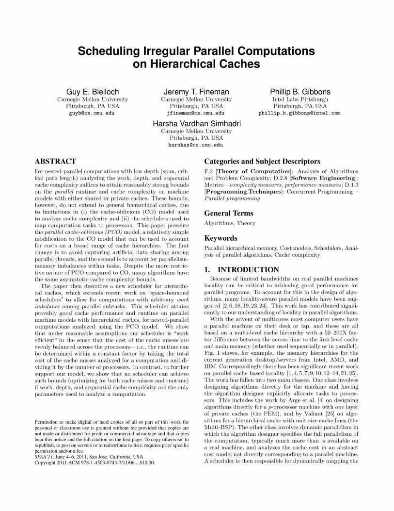
With the advent of multicores most computer users havea parallel machine on their desk or lap, and these are allbased on a multi-level cache hierarchy with a 50–200X fac-tor difference between the access time to the first level cacheand main memory (whether used sequentially or in parallel).Fig. 1 shows, for example, the memory hierarchies for thecurrent generation desktop/servers from Intel, AMD, andIBM. Correspondingly there has been significant recent workon parallel cache based locality [1,4,5,7,9,10,12–14,21,25].The work has fallen into two main classes. One class involvesdesigning algorithms directly for the machine and havingthe algorithm designer explicitly allocate tasks to proces-sors. This includes the work by Arge et al. [4] on designingalgorithms directly for a p-processor machine with one layerof private caches (the PEM), and by Valiant [25] on algo-rithms for a hierarchical cache with unit-size cache lines (theMulti-BSP). The other class involves dynamic parallelism inwhich the algorithm designer specifies the full parallelism ofthe computation, typically much more than is available ona real machine, and analyzes the cache cost in an abstractcost model not directly corresponding to a parallel machine.A scheduler is then responsible for dynamically mapping the
computation onto the processors in a manner that boundsthe cost as a function of the analyzed costs. Dynamic paral-lelism has important advantages, including being much sim-pler, potentially machine independent, and much closer tohow users actually code on these machines using languagessuch as OpenMP, Cilk++, Intel TBB, and the MicrosoftTask Parallel Library. However, the abstraction makes itharder to achieve good performance.
A pair of common abstract measures for capturing par-allel cache based locality are the number of misses given asequential ordering of a parallel computation [1, 9, 10, 21],and the depth (span, critical path length) of the compu-tation. The cache-oblivious (CO) model (a.k.a., the idealcache model) [20] can be used for analyzing the misses in thesequential ordering, giving a cache complexity Q(n; M, B)where n is the size of the problem, M is a single cache sizeand B a single block size. One can show, for example, thatany nested-parallel computation with sequential cache com-plexity Q and depth D will cause at most Q + O(pDM/B)total misses when run with an appropriate scheduler on pprocessors, each with a private cache of size M and blocksize B [1]. Unfortunately, current dynamic parallelism ap-proaches have important limitations: they either apply to hi-erarchies of only private or only shared caches [1,9,10,16,21],require some strict balance criteria [7,15], or require a jointalgorithm/scheduler analysis [7, 13–16].
In this paper we present a model and a scheduler thatenable an algorithm analysis that is independent ofboth the parallel machine and the scheduler, allowfor irregular computations with arbitrary imbalanceamong tasks, and work on hierarchies of shared andprivate caches (as in Fig. 1). The approach is limited tonested-parallel computations, but this includes a very broadset of algorithms, including most divide-and-conquer, data-parallel, and CREW PRAM-like algorithms.
The approach is based on three components. The first is acache cost model (the Parallel Cache-Oblivious (PCO)model). As with the standard CO model the cache cost isderived in terms of a single cache size M and a single blocksize B giving a cache complexity Q∗(n; M, B) independentof the number of processors. The model for a sequentialstrand of computation remains the same. When a task tforks a set of child tasks, however, the child tasks start withthe same cache state; this contrasts with the standard COanalysis based on a sequential ordering of the child tasks. Inparticular if t fits in M all child tasks start with the cachestate of the parent at the fork point, and at the join pointthe union of their locations are included in the cache stateof the parent. If the task does not fit in M then the cachestate is emptied at the fork and join points. This modelignores (incidental) data reuse among parallel subcompu-tations and accounts for reuse only when there is a serialrelationship between instructions accessing the same data.As we show, this enables tighter bounds when mapping com-putations onto, for example, shared caches. For the same Mand B the cache cost in the PCO model may be higher thanin the CO model. For a variety of fundamental parallel al-gorithms, however, including quicksort, sample sort, matrixmultiplication, matrix inversion, sparse-matrix multiplica-tion, and convex hulls, the asymptotic bounds are not af-fected, while the higher baseline enables a provably efficientmapping to parallel hierarchies for arbitrary nested-parallelcomputations.
The second is a new cost metric that penalizes large im-balance in the ratio of space to parallelism in subtasks. Wepresent a lower bound that indicates that some form ofparallelism-space imbalance penalty is required. Intuitivelythis is because on any given parallel memory hierarchy asdepicted in Fig. 1, the cache resources are linked to the pro-cessing resources: each cache is shared by a fixed numberof processors. Therefore any large imbalance between spaceand processor requirements will require either processors tobe under-utilized or caches to be over-subscribed. As in thebasic PCO model, the cost bQα(n; M, B) for inputs of sizen is asymptotically equal to that of the standard sequentialcache cost Q(n; M, B) for many problems.
The third is a new“space-bounded scheduler”that extendsrecent work of Chowdhury et al. [14]. A space-boundedscheduler accepts dynamically parallel programs that havebeen annotated with space requirements for each recursivesubcomputation called a “task.” These schedulers run ev-ery task in a cache that just fits it (i.e., no lower cachewill fit it), and once assigned, tasks are not migrated acrosscaches. We show that any space-bounded scheduler guar-antees that the number of misses across all caches at eachlevel i of the machine’s hierarchy is at most Q∗(n; Mi, Bi),where Q∗(n; Mi, Bi) is the cost in the basic PCO model withproblem size n, cache size Mi, and cache-line size Bi.
In contrast to previous work, we describe a space-boundedscheduler that allows parallel subtasks to be scheduled ondifferent levels in the memory hierarchy, thus allowing sig-nificant imbalance in the sizes of tasks. Furthermore, weshow that our space-bounded scheduler achieves efficient to-tal running time, as long as the parallelism of the machineis sufficient with respect to the parallelism of the algorithm.Specifically, we show that our scheduler executes a cache-oblivious computation on a homogeneous h-level parallelmemory hierarchy having p processors in time:
O
vh
Phi=0
bQα(n; Mi, B) · Ci
p
!,
where Mi is the size of each level-i cache, B is the uniformcache-line size, Ci is the cost of a level-i cache miss, and vh
is an overhead defined in Theorem 6. For any algorithms
where bQα(n; M, B) is asymptotically equal to the optimalsequential cache-oblivious cost Q(n; M, B) for the problem,and under conditions where vh is constant, this is optimalacross all levels of the cache. For example, a parallel sample
sort (that uses imbalanced subtasks) gives bQα(n; M, B) =O((n/B) logM (n/B)), which matches the optimal sequentialcache complexity for sorting, implying optimality on parallelcache hierarchies using our scheduler.
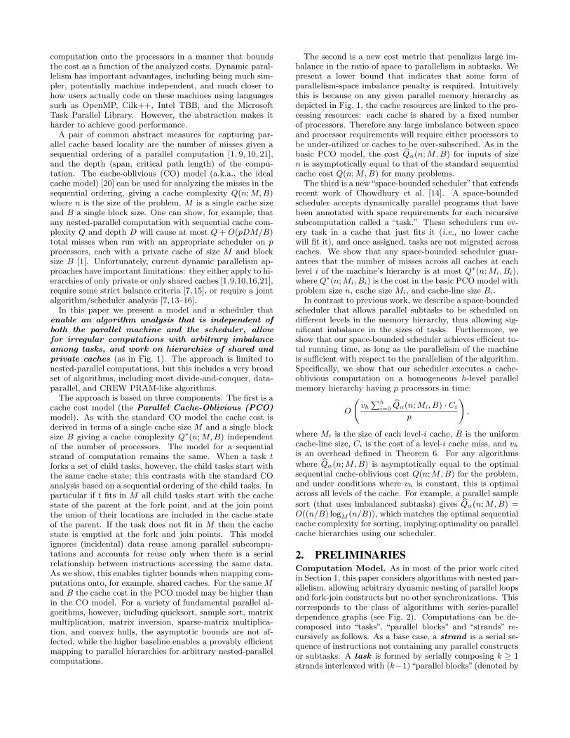
2. PRELIMINARIESComputation Model. As in most of the prior work citedin Section 1, this paper considers algorithms with nested par-allelism, allowing arbitrary dynamic nesting of parallel loopsand fork-join constructs but no other synchronizations. Thiscorresponds to the class of algorithms with series-paralleldependence graphs (see Fig. 2). Computations can be de-composed into “tasks”, “parallel blocks” and “strands” re-cursively as follows. As a base case, a strand is a serial se-quence of instructions not containing any parallel constructsor subtasks. A task is formed by serially composing k ≥ 1strands interleaved with (k−1)“parallel blocks” (denoted by
Memory: up to 1 TB
4 of these
24 MB
32 KB
128 KB 128 KB
8 of these
P
32 KB
P
24 MB
32 KB
128 KB 128 KB
8 of these
P
32 KB
P
L3
L2
L1
Memory: up to 512 GB
4 of these
12 MB
64 KB
512 KB 512 KB
12 of these
P
64 KB
P
12 MB
64 KB
512 KB 512 KB
12 of these
P
64 KB
P
L3
L2
L1
(a) 32-processor Intel Xeon 7500 (b) 48-processor AMD Opteron 6100
196 MB 196 MB
Memory: Up to 3 TB
4 of these
L4
L3
L2
L1
6 of these
24 MB
1.5 MB 1.5 MB
4 of these
128 KB
P
128 KB
P
24 MB
1.5 MB 1.5 MB
4 of these
128 KB
P
128 KB
P
6 of these
24 MB
1.5 MB 1.5 MB
4 of these
128 KB
P
128 KB
P
24 MB
1.5 MB 1.5 MB
4 of these
128 KB
P
128 KB
P
Memory: Mh = ∞, Bh
Mh−1, Bh−1 Mh−1, Bh−1 Mh−1, Bh−1 Mh−1, Bh−1
M1, B1 M1, B1 M1, B1 M1, B1 M1, B1
h
fhfh−1 . . . f1
fh
f1P P P f1
P P P f1P P P f1
P P P f1P P P
Cost: Ch−1
Cost: Ch−2
(c) 96-processor IBM z196 (d) PMH model of [3]
Figure 1: Memory hierarchies of current generation architectures from Intel, AMD, and IBM, plus an exampleabstract parallel hierarchy model. Each cache (rectangle) is shared by all processors (circles) in its subtree.
f
Task
Strand
Parallel Block
g
Figure 2: Decomposing the computation: tasks,strands and parallel blocks
t = s1; b1; . . . ; sk). A parallel block is formed by composingin parallel one or more tasks with a fork point before all ofthem and a join point after (denoted by b = t1‖t2‖ . . . ‖tk).A parallel block can be, for example, a parallel loop or someconstant number of recursive calls. The top-level computa-tion is a task. The span (a.k.a., depth) of a computationis the length of the longest path in the dependence graph.
The nested-parallel model assumes all strands share a sin-gle memory. We say two strands are concurrent if they arenot ordered in the dependence graph. Concurrent reads (i.e.,concurrent strands reading the same memory location) arepermitted, but not data races (i.e., concurrent strands thatread or write the same location with at least one write).
Machine Model: The Parallel Memory Hierarchymodel. Following prior work addressing multi-level parallel
hierarchies [3,7,10,12–14,25], we model parallel machines us-ing a tree-of-caches abstraction. For concreteness, we use asymmetric variant of the parallel memory hierarchy (PMH)model [3] (see Fig. 1(d)), which is consistent with many othermodels [7, 10, 12–14]. A PMH consists of a height-h tree ofmemory units, called caches. We assume that each cache isan ideal cache. The leaves of the tree are at level-0 and anyinternal node has level one greater than its children. Theleaves (level-0 nodes) are processors, and the level-h rootcorresponds to an infinitely large main memory. We do notassume inclusive caches, meaning that a memory locationmay be stored in a low-level cache without being stored atall ancestor caches. We can extend the model to supportinclusive caches, but then we must assume larger cache sizesto accommodate the inclusion.
Each level in the tree is parameterized by four parame-ters: M i, Bi, Ci, and fi. We denote the capacity of eachlevel-i cache by M i. Memory transfers between a cache andits child occur at the granularity of cache lines. We useBi ≥ 1 to denote the line size of a level-i cache, or the sizeof contiguous data transferred from a level-(i+1) cache to itslevel-i child. If a processor accesses data that is not residentin its level-1 cache, a level-1 cache miss occurs. More gen-erally, a level-(i+1) cache miss occurs whenever a level-icache miss occurs and the requested line is not resident inthe parent level-(i + 1) cache; once the data becomes resi-dent in the level-(i+1) cache, a level-i cache request may beserviced by loading the size-Bi+1 line into the level-i cache.The cost of a level-i cache miss is denoted by Ci ≥ 1, wherethis cost represents the amount of time to load the corre-sponding line into the level-i cache under full load. Thus,
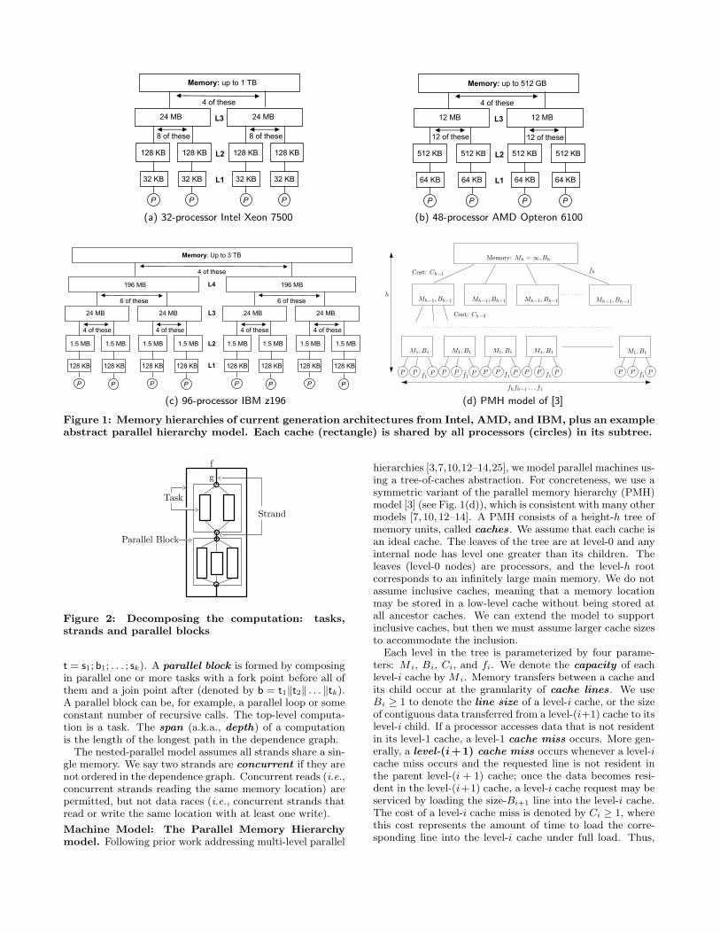
Task t forks subtasks t1 and t2,with κ = l1, l2, l3
t1 accesses l1, l4, l5 incurring 2 missest2 accesses l2, l4, l6 incurring 2 misses
At the join point: κ′ = l1, l2, l3, l4, l5, l6
Figure 3: Example applying the PCO model (Defi-nition 2) to a parallel block. Here, Q∗(t; M, B; κ) = 4.
Ci models both the latency and the bandwidth constraintsof the system (whichever is worse under full load). The costof an access at a processor that misses at all levels up toand including level-j is thus C′
j =Pj
i=0 Ci. We use fi ≥ 1to denote the number of level-(i − 1) caches below a singlelevel-i cache, also called the fanout . As in [1], we assumethe model maintains DAG consistent shared memory withthe BACKER algorithm [11]. This is a weak consistencymodel and assumes that cache lines are merged on writingback to memory thus avoiding “false sharing” issues.
We assume that the number of lines in any nonleaf cacheis greater than the sums of the number of lines in all itsimmediate children, i.e., M i/Bi ≥ fiM i−1/Bi−1 for 1 <i ≤ h, and M1/B1 ≥ f1. The miss cost Ch and line sizeBh are not defined for the root of the tree as there is nolevel-(h+1) cache. The leaves (processors) have no capacity(M0 = 0), and they have B0 = C0 = 1. Also, Bi ≥ Bi−1
for 0 < i < h. Finally, we call the entire subtree rooted ata level-i cache a level-i cluster , and we call its child level-(i−1) clusters subclusters. We use pi =
Qij=1 fj to denote
the total number of processors in a level-i cluster.
3. THE PCO MODELIn this section, we present the Parallel Cache-Oblivious
model, a simple, high-level model for algorithm analysis. Asin the sequential cache-oblivious (CO) model [20], in theParallel Cache-Oblivious (PCO) model there is a mem-ory of unbounded size and a single cache with size M , line-size B (in words), and optimal (i.e., furthest into the future)replacement policy. The cache state κ consists of the set ofcache lines resident in the cache at a given time. When alocation in a non-resident line l is accessed and the cache isfull, l replaces in κ the line accessed furthest into the future,incurring a cache miss.
To extend the CO model to parallel computations, oneneeds to define how to analyze the number of cache missesduring execution of a parallel block. Analyzing using a se-quential ordering of the subtasks in a parallel block (as inmost prior work1) is problematic for mapping to even a sin-gle shared cache, as the following theorem demonstrates forthe CO model:
Theorem 1. Consider a PMH comprised of a single cacheshared by p > 1 processors, with cache-line size B, cache sizeM ≥ pB, and a memory (i.e., h = 2). Then there exists aparallel block such that for any greedy scheduler2 the number
1Two prior works not using the sequential ordering are theconcurrent cache-oblivious model [5] and the ideal distributedcache model [21], but both design directly for p processorsand consider only a single level of private caches.2In a greedy scheduler, a processor remains idle only if thereis no ready-to-execute task.
of cache misses is nearly a factor of p larger than the cachecomplexity on the CO model.
Proof. Consider a parallel block that forks off p identicaltasks, each consisting of a strand reading the same set of Mmemory locations from M/B blocks. In the CO model, afterthe first M/B misses, all other accesses are hits, yielding atotal cost of M/B misses in the CO model.
Any greedy schedule on p processors executes all strandsat the same time, incurring simultaneous cache misses (forthe same line) on each processor. Thus, the parallel blockincurs p(M/B) misses. ut
The gap arises because a sequential ordering accounts forsignificant reuse among the subtasks in the block, but aparallel execution cannot exploit reuse unless the line hasbeen loaded earlier.
To overcome this difficulty, we instead use an approachof (i) ignoring any data reuse among the subtasks and (ii)flushing the cache at each fork and join point of any taskthat does not fit within the cache, as follows. Let loc(t; B)denote the set of distinct cache lines accessed by task t, andS(t; B) = |loc(t; B)| · B denote its size (also let s(t; B) =|loc(t; B)| denote the size in terms of number of cache lines).Let Q(c; M, B; κ) be the cache complexity of c in the sequen-tial CO model when starting with cache state κ.
Definition 2. [Parallel Cache-Oblivious Model] For cacheparameters M and B the cache complexity of a strand s,parallel block b, or task t starting at state κ is defined as:strand:
Q∗(s; M, B; κ) = Q(s; M, B; κ)
parallel block: For b = t1‖t2‖ . . . ‖tk,
Q∗(b; M, B; κ) =
kXi=1
Q∗(ti; M, B; κ)
task: For t = c1; c2; . . . ; ck,
Q∗(t; M, B; κ) =
kXi=1
Q∗(ci; M, B; κi−1) ,
where κi = ∅ if S(t; B) > M , and κi = κ ∪ij=1 loc(cj ; B) if
S(t; B) ≤ M .
We use Q∗(c; M, B) to denote a computation c startingwith an empty cache, Q∗(n; M, B) when n is a parameterof the computation, and Q∗(c; 0, 1) to denote the compu-tational work. Note that by setting M to 0, we force theanalysis to count every instruction that touches even a reg-ister and hence effectively corresponds to instruction count.
Comments on the definition: Since a task t alternates be-tween strands and parallel blocks the definition effectivelyclears the cache at every fork and join point in t whenS(t; B) > M . This is perhaps more conservative than re-quired but leads to a simple model and does not seem to af-fect bounds. Since in a parallel block all subtasks start withthe same cache state, no sharing is assumed among paral-lel blocks. If an algorithms wants to share a value loadedfrom memory, then the load should occur before the fork.The notion of furthest in the future for Q in a strand mightseem ill-defined since the future might entail parallel tasks.However, all future references fit into cache until reachinga supertask that does not fit in cache, at which point the
Problem Span Cache Complexity Q∗
Scan (prefix sums, etc.) O(log n) O(dn/Be)Matrix Transpose (n×m matrix) [20] O(log(n + m)) O(dnm/Be)Matrix Multiplication (
√n×
√n matrix) [20] O(
√n) O(dn1.5/Be/
√M + 1)
Matrix Inversion (√
n×√
n matrix) O(√
n) O(dn1.5/Be/√
M + 1)
Quicksort [22] O(log2 n) O(dn/Be(1 + logdn/(M + 1)e))Sample Sort [10] O(log2 n) O(dn/BedlogM+2 ne)Sparse-Matrix Vector Multiply [10] O(log2 n) O(dm/B + n/(M + 1)1−εe)
(m nonzeros, nε edge separators)
Convex Hull (e.g., see [8]) O(log2 n) O(dn/BedlogM+2 ne)Barnes Hut tree (e.g., see [8]) O(log2 n) O(dn/Be(1 + logdn/(M + 1)e))
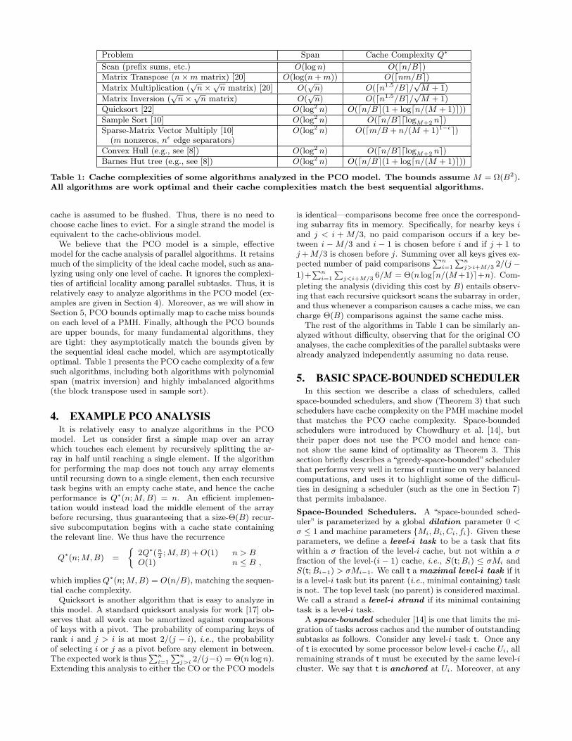
Table 1: Cache complexities of some algorithms analyzed in the PCO model. The bounds assume M = Ω(B2).All algorithms are work optimal and their cache complexities match the best sequential algorithms.
cache is assumed to be flushed. Thus, there is no need tochoose cache lines to evict. For a single strand the model isequivalent to the cache-oblivious model.
We believe that the PCO model is a simple, effectivemodel for the cache analysis of parallel algorithms. It retainsmuch of the simplicity of the ideal cache model, such as ana-lyzing using only one level of cache. It ignores the complexi-ties of artificial locality among parallel subtasks. Thus, it isrelatively easy to analyze algorithms in the PCO model (ex-amples are given in Section 4). Moreover, as we will show inSection 5, PCO bounds optimally map to cache miss boundson each level of a PMH. Finally, although the PCO boundsare upper bounds, for many fundamental algorithms, theyare tight: they asymptotically match the bounds given bythe sequential ideal cache model, which are asymptoticallyoptimal. Table 1 presents the PCO cache complexity of a fewsuch algorithms, including both algorithms with polynomialspan (matrix inversion) and highly imbalanced algorithms(the block transpose used in sample sort).
4. EXAMPLE PCO ANALYSISIt is relatively easy to analyze algorithms in the PCO
model. Let us consider first a simple map over an arraywhich touches each element by recursively splitting the ar-ray in half until reaching a single element. If the algorithmfor performing the map does not touch any array elementsuntil recursing down to a single element, then each recursivetask begins with an empty cache state, and hence the cacheperformance is Q∗(n; M, B) = n. An efficient implemen-tation would instead load the middle element of the arraybefore recursing, thus guaranteeing that a size-Θ(B) recur-sive subcomputation begins with a cache state containingthe relevant line. We thus have the recurrence
Q∗(n; M, B) =
2Q∗(n
2; M, B) + O(1) n > B
O(1) n ≤ B ,
which implies Q∗(n; M, B) = O(n/B), matching the sequen-tial cache complexity.
Quicksort is another algorithm that is easy to analyze inthis model. A standard quicksort analysis for work [17] ob-serves that all work can be amortized against comparisonsof keys with a pivot. The probability of comparing keys ofrank i and j > i is at most 2/(j − i), i.e., the probabilityof selecting i or j as a pivot before any element in between.The expected work is thus
Pni=1
Pnj>i 2/(j−i) = Θ(n log n).
Extending this analysis to either the CO or the PCO models
is identical—comparisons become free once the correspond-ing subarray fits in memory. Specifically, for nearby keys iand j < i + M/3, no paid comparison occurs if a key be-tween i − M/3 and i − 1 is chosen before i and if j + 1 toj +M/3 is chosen before j. Summing over all keys gives ex-pected number of paid comparisons
Pni=1
Pnj>i+M/3 2/(j −
1)+Pn
i=1
Pj<i+M/3 6/M = Θ(n logdn/(M +1)e+n). Com-
pleting the analysis (dividing this cost by B) entails observ-ing that each recursive quicksort scans the subarray in order,and thus whenever a comparison causes a cache miss, we cancharge Θ(B) comparisons against the same cache miss.
The rest of the algorithms in Table 1 can be similarly an-alyzed without difficulty, observing that for the original COanalyses, the cache complexities of the parallel subtasks werealready analyzed independently assuming no data reuse.
5. BASIC SPACE-BOUNDED SCHEDULERIn this section we describe a class of schedulers, called
space-bounded schedulers, and show (Theorem 3) that suchschedulers have cache complexity on the PMH machine modelthat matches the PCO cache complexity. Space-boundedschedulers were introduced by Chowdhury et al. [14], buttheir paper does not use the PCO model and hence can-not show the same kind of optimality as Theorem 3. Thissection briefly describes a “greedy-space-bounded” schedulerthat performs very well in terms of runtime on very balancedcomputations, and uses it to highlight some of the difficul-ties in designing a scheduler (such as the one in Section 7)that permits imbalance.
Space-Bounded Schedulers. A “space-bounded sched-uler” is parameterized by a global dilation parameter 0 <σ ≤ 1 and machine parameters Mi, Bi, Ci, fi. Given theseparameters, we define a level-i task to be a task that fitswithin a σ fraction of the level-i cache, but not within a σfraction of the level-(i − 1) cache, i.e., S(t; Bi) ≤ σMi andS(t; Bi−1) > σMi−1. We call t a maximal level-i task if itis a level-i task but its parent (i.e., minimal containing) taskis not. The top level task (no parent) is considered maximal.We call a strand a level-i strand if its minimal containingtask is a level-i task.
A space-bounded scheduler [14] is one that limits the mi-gration of tasks across caches and the number of outstandingsubtasks as follows. Consider any level-i task t. Once anyof t is executed by some processor below level-i cache Ui, allremaining strands of t must be executed by the same level-icluster. We say that t is anchored at Ui. Moreover, at any
point in time, consider the maximal level-i tasks t1, t2, . . . , tk
anchored to level-i cache Ui. ThenPk
j=1 S(tj ; Bi) ≤ Mi.That is to say, the total space used by tasks anchored to Ui
does not exceed Ui’s capacity. Finally, we consider strands.Whereas a task is anchored to a single cache, a level-i strandis anchored to caches along a level-i to level-1 path in thememory hierarchy. When a level-i strand is anchored to alevel-j < i cache, it is treated as a task that takes σMj
space, thereby preventing (many) other tasks/strands frombeing anchored at the same cache.
We relax the usual definition of greedy scheduler in thefollowing: A greedy-space-bounded scheduler is a space-bounded scheduler in which a processor remains idle onlyif there is no ready-to-execute strand that can be anchoredto the processor (and appropriate ancestor caches) withoutviolating the space-bounded constraints.
Cache Bounds: PCO Cache Complexity is OptimalFor Space-Bounded Schedulers. The following theoremimplies that a nested-parallel computation scheduled withany space-bounded scheduler achieves optimal cache perfor-mance, with respect to the PCO model. A main idea of theproof is that each task reserves sufficient cache space andhence never needs to evict a previously loaded cache line.
Theorem 3. Consider a PMH and any dilation parame-ter 0 < σ ≤ 1. Let t be a level-i task. Then for all memory-hierarchy levels j ≤ i, the number of level-j cache missesincurred by executing t with any space-bounded scheduler isat most Q∗(t; σMj , Bj).
Proof. Let Ui be the level-i cache to which t is assigned.Observe that t uses space at most σMi. Moreover, by defini-tion of the space-bounded scheduler, the total space neededfor tasks assigned to Ui is at most Mi, and hence no linefrom t need ever be evicted from U ’s level-i cache. Thus,an instruction x in t accessing a line ` does not exhibit alevel-i cache miss if there is an earlier-executing instructionin t that also accesses `. Any instruction serially precedingx must execute earlier than x. Hence, the parallel cachecomplexity Q∗(t; σMi, Bi) is an upper bound on the actualnumber of level-i cache misses.
We next extend the proof for lower-level caches. First,let us consider a level-i strand s belonging to task t. ThePCO model states that for any Mj<i, the cache complex-ity of a level-i strand matches the serial cache complexityof the strand beginning from an initially empty state. Con-sider each cache partitioned such that a level-i strand canuse only the σMj capacity of a level-(j < i) cache awardedto it by the space-bounded scheduler. Then the number ofmisses is indeed as though the strand executed on a seriallevel-(i − 1) memory hierarchy with σMj cache capacity ateach level j. Hence, Q∗(s; σMj , Bj) is an upper bound onthe actual number of level-j cache misses incurred while exe-cuting the strand s. (The actual number may be less becausean optimal replacement policy may not partition the cachesand the cache state is not initially empty.)
Finally, to complete the proof for all memory-hierarchylevels j, we assume inductively that the theorem holds for allmaximal subtasks of t. The PCO model assumes an emptyinitial level-j cache state for any maximal level-j subtask oft, as S(t; Bj) > σMj . Thus, the level-j cache complexity fort is defined as Q∗(t; σMj , Bj) =
Pt′∈A(t) Q∗(t′; σMj , Bj , ∅),
where A(t) is the set of all level-i strands and nearest max-
imal subtasks of t. Since the theorem holds inductively forthose tasks and strands in A(t), it holds for t. ut
In contrast, there is no such optimality result for theCO model: Theorem 1 (showing a factor of p gap) readilyextends to any greedy-space-bounded scheduler, using thesame proof.
Runtime Bounds: A Simple Space-Bounded Sched-uler and its Limitations. While all space-bounded sched-ulers achieve optimal cache complexity, they vary in totalrunning time. Greedy-space-bounded schedulers, like thescheduler in [14], perform well for computations that arevery well balanced. At a high level, a greedy-space-boundedscheduler operates on tasks anchored at each cache. Thesetasks are “unrolled” to produce maximal tasks, which arein turn anchored at descendant caches. If a processor Pbecomes idle and a strand is ready, we assume P beginsworking on a strand immediately (i.e., we ignore scheduleroverheads). If multiple strands are available, one is chosenarbitrarily. Our main scheduler is based on a greedy-space-bounded scheduler, and an operational description of bothis included in [8].
Chowdhury et al. [14] present analyses of a (nearly) greedy-space-bounded scheduler (which includes minor enhance-ments violating the greedy principle). These analyses arealgorithm specific and rely on the balance of the underly-ing computation. A more general performance theorem isincluded in the associated technical report [8]. Along withour main theorem (Theorem 6), these analyses all use recur-sive application of Brent’s theorem to obtain a total runningtime: small recursive tasks are assumed inductively to exe-cute quickly, and the larger tasks are analyzed using Brent’stheorem with respect to a single-level machine of coarsergranularity.
The following are the types of informal structural restric-tions imposed on the underlying algorithms to guaranteeefficient scheduling with a greedy-space-bounded schedulerand previous work. For more precise, sufficient restrictions,see the technical report [8].
1. When multiple tasks are anchored at the same cache,they should have similar structure and work. More-over, none of them should fall on a much longer paththrough the computation. If this condition is relaxed,then some anchored task may fall on the critical path.It is important to guarantee each task a fair share ofprocessing resources without leaving many processorsidle.
2. Tasks of the same size should have the same paral-lelism.
3. The nearest maximal descendant tasks of a given taskshould have roughly the same size. Relaxing this con-dition allows two or more tasks at different levels of thememory hierarchy to compete for the same resources.Guaranteeing that each of these tasks gets enough pro-cessing resources becomes a challenge.
In addition to these balance conditions, the previous anal-yses exploit preloading of tasks: the memory used by a taskis assumed to be loaded (quickly) into the cache before exe-cuting the task. For array-based algorithms preloading is areasonable requirement. When the blocks to be loaded arenot contiguous, however, it may be computationally chal-
lenging to determine which blocks should be loaded. Re-moving the preloading requirement complicates the analy-sis, which then must account for high-level cache misses thatmay occur as a result of tasks anchored at lower-level caches.
Our new scheduler in Section 7 relaxes all of these bal-ance conditions, allowing for more asymmetric computa-tions. Moreover, we do not assume preloading. To facili-tate analysis of less regular computations, we first define amore holistic measure of the balance of the algorithm in Sec-tion 6 and then prove our performance bounds with respectto this metric. This balance metric has the added benefit ofseparating the algorithm analysis from the scheduler.
6. EXTENDING PCO FOR IMBALANCEIn the PMH (or any machine with shared caches), all
caches are associated with a set of processors. It thereforestands to reason that if a task needs memory M but does nothave sufficient parallelism to make use of a cache of appro-priate size, that either processors will sit idle or additionalmisses will be required. This might be true even if there isplenty of parallelism on average in the computation. Thefollowing lower-bound makes this intuition more concrete.
Theorem 4. (Lower Bound) Consider a PMH comprisedof a single cache shared by p > 1 processors with parametersB = 1, M and C, and a memory (i.e., h = 2). Thenfor all r ≥ 1, there exists a computation with n = rpMmemory accesses, Θ(n/p) span, and Q∗(M, B) = pM , suchthat for any scheduler, the runtime on the PMH is at leastnC/(C + p) ≥ (1/2)min(n, nC/p).
Proof. Consider a computation that forks off p > 1 par-allel tasks. Each task is sequential (a single strand) andloops over touching M locations, distinct from any othertask (i.e., a total of Mp locations are touched). Each taskthen repeats touching the same M locations in the sameorder a total of r times, for a total of n = rMp accesses.Because M fits within the cache, only a task’s first M ac-cesses are misses and the rest are hits in the PCO model.The total cache complexity is thus only Q∗(M, B) = Mp forB = 1 and any r ≥ 1.
Now consider an execution (schedule) of this computationon a shared cache of size M with p processors and a misscost of C. Divide the execution into consecutive sequencesof M timesteps, called rounds. Because it takes 1 (on ahit) or C ≥ 1 (on a miss) units of time for a task to access alocation, no task reads the same memory location twice inthe same round. Thus, a memory access costs 1 only if itis to a location in memory at the start of the round and Cotherwise. Because a round begins with at most M locationsin memory, the total number of accesses during a round is atmost (Mp−M)/C+M by a packing argument. Equivalently,in a full round, M processor steps execute at a rate of 1access per step, and the remaining Mp−M processor stepscomplete 1/C accesses per step, for an average “speed” of1/p + (1 − 1/p)/C < 1/p + 1/C accesses per step. Thisbound holds for all rounds except the first and last. In thefirst round, the cache is empty, so the processor speed is1/C. The final round may include at most M fast steps,and the remaining steps are slow. Charging the last round’sfast steps to the first round’s slow steps proves an average“speed”of at most 1/p+1/C accesses per processor timestep.Thus, the computation requires at least n/(p(1/p+1/C)) =nC/(C +p) time to complete all accesses. When C ≥ p, this
time is at least nC/(2C) = n/2. When C ≤ p, this time isat least nC/(2p). ut
The proof shows that even though there is plenty of par-allelism overall and a fraction of at most 1/r of the accessesare misses in Q∗, an optimal scheduler either executes tasks(nearly) sequentially (if C ≥ p) or incurs a cache miss on(nearly) every access (if C ≤ p).
This indicates that some cost must be charged to accountfor the space-parallelism imbalance. We extend PCO witha cost metric that charges for such imbalance, but does notcharge for imbalance in subtask size. When coupled withour scheduler in Section 7, the metric enables PCO boundsto effectively map to PMH runtime, even for highly-irregularcomputations.
The metric aims to estimate the degree of parallelism thatcan be utilized by a symmetric hierarchy as a function ofthe size of the computation. Intuitively, a computation ofsize S with “parallelism” α ≥ 0 should be able to use p =O(Sα) processors effectively. This intuition works well foralgorithms where parallelism is polynomial in the size of theproblem.
More formally, we define a notion of effective cache com-
plexity bQα(c) for a computation c based on the definition
of Q∗. Just as for Q∗, bQα() for tasks, parallel blocks andstrands is defined inductively based on the composition rulesdescribed in section 2 for building a computation. (Note thatsince work is just a special case of Q∗, obtained by substi-tuting M = 0, the following metric can be used to computeeffective work just like effective cache complexity).
Definition 5. [PCO extended for imbalance] For cacheparameters M and B and parallelism α, the effective cachecomplexity of a strand s, parallel block b, or task t startingat cache state κ is defined as:strand: Let t be the nearest containing task of strand sbQα(s; M, B; κ) = Q∗(s; M, B; κ)× s(t; B)α
parallel block: For b = t1‖t2‖ . . . ‖tk in task t,bQα(b; M, B; κ) =
max
(s(t; B)α maxi
n bQα(ti;M,B;κ)
s(ti;B)α
o(depth dominated)P
ibQα(ti; M, B; κ) (work dominated)
task: For t = c1; c2; . . . ; ck,
bQα(t; M, B; κ) =
kXi=1
bQα(ci; M, B; κi) ,
where κi is defined as in Definition 2.
In the rule for parallel block, the depth dominated termcorresponds to limiting the number of processors available todo the work on each subproblem ti to s(ti)
α. This throttling
yields a span (depth) bQα(ti)/s(ti)α for each task and the
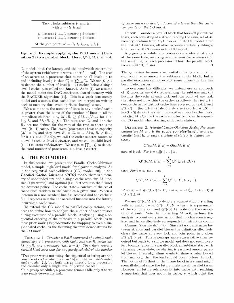
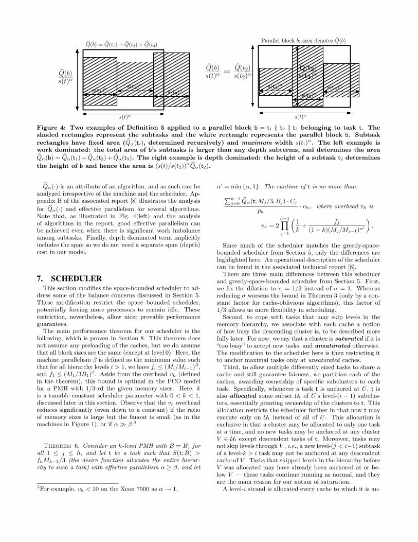
effective cache complexity is then the maximum of the spansover the subtasks multiplied by the number of processors forthe parallel block b, which is s(t; B)α (see Fig. 4).
We say that an algorithm is α-efficient if Q∗(n; M, B) =
O( bQα(n; M, B)), where n denotes the input size. This α-efficiency occurs trivially if the work term always dominates,but can also happen if sometimes the depth term dominates.The maximum α for which an algorithm is α-efficient spec-ifies the effective parallelism .
s(t)α
Q(b)s(t)α
s(t2)α
Q(b) = Q(t1) + Q(t2) + Q(t3)
s(t1)α
s(t3)α
s(t)α
Q(b)s(t)α =
Q(t2)s(t2)α
Q(t2)s(t2)α
s(t2)α
Parallel block b; area denotes Q(b)
s(t1)α
s(t3)α
Figure 4: Two examples of Definition 5 applied to a parallel block b = t1 ‖ t2 ‖ t3 belonging to task t. Theshaded rectangles represent the subtasks and the white rectangle represents the parallel block b. Subtask
rectangles have fixed area ( bQα(ti), determined recursively) and maximum width s(ti)α. The left example is
work dominated: the total area of b’s subtasks is larger than any depth subterms, and determines the areabQα(b) = bQα(t1) + bQα(t2) + bQα(t3). The right example is depth dominated: the height of a subtask t2 determines
the height of b and hence the area is (s(t)/s(t2))α bQα(t2).
bQα(·) is an attribute of an algorithm, and as such can beanalyzed irrespective of the machine and the scheduler. Ap-pendix B of the associated report [8] illustrates the analysis
for bQα(·) and effective parallelism for several algorithms.Note that, as illustrated in Fig. 4(left) and the analysisof algorithms in the report, good effective parallelism canbe achieved even when there is significant work imbalanceamong subtasks. Finally, depth dominated term implicitlyincludes the span so we do not need a separate span (depth)cost in our model.
7. SCHEDULERThis section modifies the space-bounded scheduler to ad-
dress some of the balance concerns discussed in Section 5.These modification restrict the space bounded scheduler,potentially forcing more processors to remain idle. Theserestriction, nevertheless, allow nicer provable performanceguarantees.
The main performance theorem for our scheduler is thefollowing, which is proven in Section 8. This theorem doesnot assume any preloading of the caches, but we do assumethat all block sizes are the same (except at level 0). Here, themachine parallelism β is defined as the minimum value suchthat for all hierarchy levels i > 1, we have fi ≤ (Mi/Mi−1)
β ,and f1 ≤ (M1/3B1)
β . Aside from the overhead vh (definedin the theorem), this bound is optimal in the PCO modelfor a PMH with 1/3-rd the given memory sizes. Here, kis a tunable constant scheduler parameter with 0 < k < 1,discussed later in this section. Observe that the vh overheadreduces significantly (even down to a constant) if the ratioof memory sizes is large but the fanout is small (as in themachines in Figure 1), or if α β.3
Theorem 6. Consider an h-level PMH with B = Bj forall 1 ≤ j ≤ h, and let t be a task such that S(t; B) >fhMh−1/3 (the desire function allocates the entire hierar-chy to such a task) with effective parallelism α ≥ β, and let
3For example, vh < 10 on the Xeon 7500 as α → 1.
α′ = min α, 1. The runtime of t is no more than:Ph−1j=0
bQα(t; Mj/3, Bj) · Cj
ph· vh, where overhead vh is
vh = 2
h−1Yj=1
„1
k+
fj
(1− k)(Mj/Mj−1)α′
«.
Since much of the scheduler matches the greedy-space-bounded scheduler from Section 5, only the differences arehighlighted here. An operational description of the schedulercan be found in the associated technical report [8].
There are three main differences between this schedulerand greedy-space-bounded scheduler from Section 5. First,we fix the dilation to σ = 1/3 instead of σ = 1. Whereasreducing σ worsens the bound in Theorem 3 (only by a con-stant factor for cache-oblivious algorithms), this factor of1/3 allows us more flexibility in scheduling.
Second, to cope with tasks that may skip levels in thememory hierarchy, we associate with each cache a notionof how busy the descending cluster is, to be described morefully later. For now, we say that a cluster is saturated if it is“too busy” to accept new tasks, and unsaturated otherwise.The modification to the scheduler here is then restricting itto anchor maximal tasks only at unsaturated caches.
Third, to allow multiple differently sized tasks to share acache and still guarantee fairness, we partition each of thecaches, awarding ownership of specific subclusters to eachtask. Specifically, whenever a task t is anchored at U , t isalso allocated some subset Ut of U ’s level-(i − 1) subclus-ters, essentially granting ownership of the clusters to t. Thisallocation restricts the scheduler further in that now t mayexecute only on Ut instead of all of U . This allocation isexclusive in that a cluster may be allocated to only one taskat a time, and no new tasks may be anchored at any clusterV ∈ Ut except descendent tasks of t. Moreover, tasks maynot skip levels through V , i.e., a new level-(j < i−1) subtaskof a level-k > i task may not be anchored at any descendentcache of V . Tasks that skipped levels in the hierarchy beforeV was allocated may have already been anchored at or be-low V — these tasks continue running as normal, and theyare the main reason for our notion of saturation.
A level-i strand is allocated every cache to which it is an-
chored, i.e., exactly one cache at every level below i. Incontrast, a level-i task t is anchored only to a level-i cacheand allocated potentially many level-(i− 1) subclusters, de-pending on its size. We say that the size-s = S(t; Bi) taskt desires gi(s) level-(i− 1) clusters, gi to be specified later.When anchoring t to a level-i cache U , let q be the num-ber of unsaturated and unallocated subclusters of U . Selectthe most unsaturated minq, gi(s) of these subclusters andallocate them to t.
For each cache, there may be one anchored maximal taskthat is underallocated , meaning that it receives fewer sub-clusters than it desires. The only underallocated task is themost recent task that caused the cache to transition from be-ing unsaturated to saturated. Whenever a subcluster freesup, allocate it to the underallocated task. If assigning a sub-cluster causes the underallocated task to achieve its desire,it is no longer underallocated, and future free subclustersbecome available to other tasks.
Scheduler details. We now describe the two missing de-tails of the scheduler, namely the notion of saturation, aswell as the desire function gi, which specifies for a particu-lar task size the number of desired subclusters.
One difficulty is trying to schedule tasks with large desireson partially assigned clusters. We continue assigning tasksbelow a cluster until that cluster becomes saturated. Butwhat if the last job has large desire? To compensate, ournotion of saturation leaves a bit of slack, guaranteeing thatthe last task scheduled can get some minimum amount ofcomputing power. Roughly speaking, we set aside a con-stant fraction of the subclusters at each level as a reserve.The cluster becomes saturated when all other subclustershave been allocated. The last task scheduled, the one thatcauses the cluster to become saturated, may be allocatedsubclusters from the reserve.
There is some tradeoff in selecting the reserve constanthere. If a large constant is reserved, we may only allocatea small fraction of clusters at each level, thereby wasting alarge fraction of all processing power at each level. If, onthe other hand, the constant is small, then the last taskscheduled may run too slowly. Our analysis will count thefirst against the work of the computation and the secondagainst the depth.
Designing a good function to describe saturation and thereserved subclusters is complicated by the fact that task as-signments may skip levels in the hierarchy. The notion ofsaturation thus cannot just count the number of saturatedor allocated subclusters — instead, we consider the degree towhich a subcluster is utilized. For a cluster U with subclus-ters V1, V2, . . . , Vfi (fi > 1), define the utilization functionµ(U) as follows:
µ(U) =
8>><>>:min
n1, 1
kfi
Pfii=1 µ′(Vi)
oif U is a level-(≥ 2)
cluster
min1, xf1k
if U is a level-1 cluster withx allocated processors
and
µ′(V ) =
(1 if V is allocated
µ(V ) otherwise,
where k ∈ (0, 1), the value (1− k) specifying the fraction ofprocessors to reserve. For a cluster U with just one subclus-ter V , µ(U) = µ(V ). To understand the remainder of this
section, it is sufficient to think of k as 1/2. We say that Uis saturated when µ(U) = 1 and unsaturated otherwise.
It remains to define the desire function gi for level i in thehierarchy. A natural choice for gi is gi(S) = dS/(Mi/fi)e =dSfi/Mie. That is, associate with each subcluster a 1/fi
fraction of the space in the level-i cache — if a task uses xtimes this fraction of total space, it should receive x subclus-ters. It turns out that this desire does not yield good sched-uler performance with respect to our notion of balancedcache complexity. In particular it does not give enoughparallel slackness to properly load-balance subtasks acrosssubclusters.
Instead, we use gi(S) = minfi, max1, bf(3S/Mi)α′c,
where α′ = minα, 1. What this says is that a maxi-mal level-i task is allocated one subcluster when it has sizeS(t; Bi) = Mi/(3f
1/α′
i ), and the number of subclusters al-located to t increases by a factor of 2 whenever the size of
t increases by a factor of 21/α′ . It reaches the maximumnumber of subclusters when it has size S(t; Bi) = Mi−1/3.We define g(S) = gi(S)pi−1 if S ∈ (Mi−1/3, Mi/3].
For simplicity we assumed in our model that all memoryis preallocated, which includes stack space. This assump-tion would be problematic for algorithms with α > 1 or foralgorithms which are highly dynamic. However, it is easyto remove this restriction by allowing temporary allocationinside a task, and assume this space can be shared amongparallel tasks in the analysis of Q∗. To make our boundswork this would require that for every cache we add an ad-ditional number of lines equal to the sum of the sizes of thesubclusters. This augmentation would account even for thevery worst case where all memory is temporarily allocated.
The analysis of this scheduler is in Section 8, summarizedby Theorem 6. There are a couple of challenges that arisein the analysis. First, while it is easy to separate the runtime of a task on a sequential machine in to a sum of thecache miss costs for each level, it is not as easy on a paral-lel machine. Periods of waiting on cache misses at severallevels at multiple processors can be interleaved in a complexmanner. Our separation lemma (lemma 9) addresses thisissue by bounding the run time by the sum of its cache costs
at different levels ( bQα(t; M,Bi) · Ci).Second, whereas a simple greedy-space-bounded sched-
uler applied to balanced tasks lends itself to an easy anal-ysis through an inductive application of Brent’s theorem,we have to tackle the problem of subtasks skipping levelsin the hierarchy and partially allocated caches. At a highlevel, the analysis of Theorem 6 recursively decomposes amaximal level-i task into its nearest maximal descendentlevel-j < i tasks. By inductively assuming that these tasksfinish “quickly enough,” we combine the subproblems withrespect to the level-i cache analogous to Brent’s theorem, ar-guing that a) when all subclusters are busy, a large amountof productive work occurs, b) and when subclusters are idle,all tasks have been allocated sufficient resources to progressat a sufficiently quick rate. Our carefully planned alloca-tion and reservations of clusters as described earlier in thissection are critical to this proof.
8. ANALYSIS OF THE SCHEDULERThis section presents the analysis of our scheduler, proving
several lemmas leading up to Theorem 6. First, the followinglemma implies that the capacity restriction of each cache is
subsumed by the scheduling decision of only assigning tasksto unallocated, unsaturated clusters.
Lemma 7. Any unsaturated level-i cluster U has at leastMi/3 capacity available and at least one subcluster that isboth unsaturated and unallocated.
Proof. The fact that an unsaturated cluster has an un-saturated, unallocated cluster follows from the definition.Any saturated or allocated subcluster Vi has µ′(Vi) = 1.Thus, for unsaturated cluster U with subclusters V1, . . . , Vfi ,
we have 1 > (1/kfi)Pfi
j=1 µ′(Vi) ≥ (1/fi)Pfi
j=1 µ′(Vi), and
it follows that some µ′(Vi) < 1.We now argue that if U is unsaturated, then it has at least
Mi/3 capacity remaining. This fact is trivial for fi = 1, as inthat case at most one task is allocated. Suppose that taskst1, t2, . . . , tk are anchored to an unsaturated cluster and havedesires x1, x2, . . . , xk. Since U is unsaturated
Pki=1 xi ≤
fi − 1, which implies xi ≤ fi − 1 for all i. We will show thatthe ratio of space to desire, S(ti; B)/xi, is at most 2Mi/3fi
for all tasks anchored to U , which impliesPk
i=1 S(ti; B) ≤2Mi/3.
Since a task with desire x ∈ 1, 2, . . . , fi − 1 has size at
most (Mi/3)((x+1)/fi)1/α′ , where α′ = minα, 1 ≤ 1, the
ratio of its space to its desire x is at most (Mi/3x)((x +
1)/fi)1/α′ . Letting q = 1/α′ ≥ 1, we have the space-to-
desire ratio r bounded by
r ≤ Mi
3· (x + 1)q
x· 1
fqi
≤ 2Mi
3· (x + 1)q
x + 1· 1
fqi
≤ 2Mi
3fi· (x + 1)q−1
fq−1i
≤ 2Mi
3fi ut
Latency added cost. Section 6 introduced effective cache
complexity bQα(·), which is algorithmic measure. To analyzethe scheduler, however, it is important to consider whencache misses occur. To factor in the effect of the cache misscosts, we define the latency added effective work, denoted
by cW ∗α(·), of a computation with respect to the particular
PMH. Latency added effective work is only for use in theanalysis of the scheduler, and does not need to be analyzedby an algorithm designer.
The latency added effective work is similar to the effec-tive cache complexity, but instead of counting just instruc-tions, we add the cost of cache misses at each instruction.The cost ρ(x) of an instruction x accessing location m isρ(x) = W (x) + C′
i if the scheduler causes the instruction xto fetch m from a level i cache on the given PMH. Using
this per-instruction cost, we define effective work cW ∗α(.) of
a computation using structural induction in a manner that
is deliberately similar to that of bQα(.).
Definition 8 (Latency added cost). For cost ρ(x)of instruction x, the latency added effective work of atask t, or a strand s or parallel block b nested inside t isdefined as:strand: cW ∗
α(s) = s(t; B)αXx∈s
ρ(x).
parallel block: For b = t1‖t2‖ . . . ‖tk,
cW ∗α(b) = max
(s(t; B)α max
i
( cW ∗α(ti)
s(ti; B)α
),X
i
cW ∗α(ti)
).
(1)
task: For t = c1; c2; . . . ; ck,
cW ∗α(t) =
kXi=1
cW ∗α(ci). (2)
Because of the large number of parameters involved (Mi,B, Cii etc.), it is undesirable to compute the latency addedwork directly for an algorithm. Instead, we will show a nicerelationship between latency added work and effective work.
We first show that cW ∗α(·) (and ρ(·), on which it is based)
can be decomposed into a per (cache) level costs cW (i)α (·) that
can each be analyzed in terms of that level’s parameters(Mi, B, Ci). We then show that these costs can be put
together to provide an upper bound oncW ∗α(·). For i ∈ [h−1],cW (i)
α (c) of a computation c is computed exactly like cW ∗α(c)
using a different base case: for each instruction x in c, ifthe memory access at x costs at least C′
i, assign a cost ofρi(x) = Ci to that node. Else, assign a cost of ρi(x) = 0.
Further, we set ρ0(x) = W (x), and define cW (0)α (c) in terms
of ρo(·). It also follows from these definitions that ρ(x) =Ph−1i=0 ρi(x) for all instructions x.
Lemma 9. Separation Lemma: For an h-level PMHwith B = Bj for all 1 ≤ j ≤ h and computation A, wehave
cW ∗α(A) ≤
h−1Xi=0
cW (i)α (A).
Proof. The proof is based on induction on the struc-ture of the computation (in terms of its decomposition into block, tasks and strands). For the base case of the in-duction, consider the sequential thread (or strand) s at thelowest level in the call tree. If S(s) denotes the space of taskimmediately enclosing s, then by definition
cW ∗α(s) =
Xx∈s
ρ(x)
!· s(s; B)α ≤
Xx∈s
h−1Xi=0
ρi(x)
!· s(s; B)α
=
h−1Xi=0
Xx∈s
ρi(x) · s(s; B)α
!=
h−1Xi=0
cW (i)α (s).
For a series composition of strands and blocks with in atask t = x1; x2; . . . ; xk,
cW ∗α(t) =
kXi=1
cW ∗α(xi) ≤
kXi=1
hXl=0
cW (h)α (xi) =
hXl=0
cW (l)α (x)
For a parallel block b inside task t consisting of tasks
timi=1, consider the equation 1 for cW ∗
α(b) which is the max-imum of m + 1 terms, the (m + 1)-th term being a summa-tion. Suppose that of these terms, the term that determinescW ∗
α(b) is the k-th term (denote this by Tk). Similarly, con-
sider the equation 1 for evaluating each of cW (l)α (b) and sup-
pose that the kl-th term (denoted by T(l)kl
) on the right hand
side determines the value of cW (l)α (b). Then,
cW ∗α(b)
s(t; B)α= Tk ≤
h−1Xl=0
T(l)k ≤
h−1Xl=0
T(l)kl
=
Ph−1l=0
cW (l)α (b)
s(t; B)α, (3)
which completes the proof. Note that we did not use thefact that some of the components were work or cache com-plexities. The proof only depended on the fact that ρ(x) =
Ph−1i=0 ρi(x) and the structure of the composition rules given
by equations 2, 1. ρ could have been replaced with any otherkind of work and ρi with its decomposition. ut
The previous lemma indicates that the latency added workcan be separated into costs per cache level. The followinglemma then relates these separated costs to effective cache
complexity bQα(·).
Lemma 10. Consider an h-level PMH with B = Bj forall 1 ≤ j ≤ h and a computation c. If c is scheduled on thisPMH using a space-bounded scheduler with dilation σ = 1/3,
then cW ∗α(c) ≤
Ph−1i=0
bQα(c; Mi/3, B) · Ci.
Proof. (Sketch) The function cW (i)α (·) is monotonic in
that if it is computed based on function ρ′i(·) instead of ρi(x),where ρ′i(x) ≤ ρi(x) for all instructions x, then the formerestimate would be no more than the latter. It then followsfrom the definitions of cW (i)
α (·) and ρi(·), that cW (i)α (c) ≤bQα(c; Mi/3, B) ·Ci for all computations c, i ∈ 0, 1, . . . , h−
1. Lemma 9 then implies that for any computation c:cW ∗α(c) ≤
Ph−1i=0
bQα(c; Mi/3, B) · Ci. ut
Finally, we prove the main lemma, bounding the runningtime of a task with respect to the remaining utilization theclusters it has been allocated. At a high level, the anal-ysis recursively decomposes a maximal level-i task into itsnearest maximal descendent level-j < i tasks. We assumeinductively that these tasks finish “quickly enough.” Finally,we combine the subproblems with respect to the level-i cacheanalogous to Brent’s theorem, arguing that a) when all sub-clusters are busy, a large amount of productive work occurs,b) and when subclusters are idle, all tasks make sufficientprogress. Whereas this analysis outline is consistent witha simple analysis of the greedy scheduler and that in [14],here we address complications that arise due to partially al-located caches and subtasks skipping levels in the hierarchy.
Lemma 11. Consider an h-level PMH with B = Bj forall 1 ≤ j ≤ h and a computation to schedule with α ≥ β,and let α′ = min α, 1. Let Ni be a task or strand whichhas been assigned a set Ut of q ≤ gi(S(Ni; B)) level-(i − 1)subclusters by the scheduler. Letting
PV ∈Ut
(1 − µ(V )) = r
(by definition, r ≤ |Ut| = q), the running time of Ni is atmost:cW ∗
α(Ni)
rpi−1· vi, where overhead vi is
vi = 2
i−1Yj=1
„1
k+
fi
(1− k)(Mi/Mi−1)α′
«.
Proof. We prove the claim on run time using inductionon the levels.Induction: Assume that all child maximal tasks of Ni haverun times as specified above. Now look at the set of clustersUt assigned to Ni. At any point in time, either:
1. all of them are saturated.
2. at least one of the subcluster is unsaturated and thereare no jobs waiting in the queue R(Ni). More specif-ically, the job on the critical path (χ(Ni)) is running.Here, critical path χ(Ni) is the set of strictly ordered
immediate child subtasks that have the largest sumof effective depths. We would argue in this case thatprogress is being made along the critical path at a rea-sonable rate.
Assuming q > 1, we will now bound the run time requiredto complete Ni by bounding the number of cycles the abovetwo phases use. Consider the first phase. A job x ∈ C(Ni)(subtasks of Ni) when given an appropriate number of pro-cessors (as specified by the function g) can not have an over-
head of more than vi−1, i.e., it uses at most cW ∗α(x)vi−1 in-
dividual processor clock cycles. Since in the first phase, atleast k fraction of available subclusters under Ut are alwaysallocated (at least rpi−1 clock cycles put together) to somesubtask of Ni, it can not last for more thanXx∈C(Ni)
1
k
cW ∗α(x)
rpi−1·vi−1 <
1
k
cW ∗α(Ni)
rpi−1·vi−1 number of cycles.
For the second phase, we argue that the critical path runsfast enough because we do not underallocate processing re-sources for any subtask by more than a factor of (1− k) asagainst that indicated by the g function. Specifically, con-sider a job x along the critical path χ(Ni). Suppose x is amaximal level-j(x) task, j(x) < i. If the job is allocated sub-clusters below a level-j(x) subcluster V , then V was unsat-urated at the time of allocation. Therefore, when the sched-uler picked the gj(x)(S(x; B)) most unsaturated subclustersunder V (call this set V),
Pv∈V µ(v) ≥ (1−k)gj(x)(S(x; B)).
When we run x on V using the subclusters V, its run timeis at mostcW ∗
α(x)
(P
v∈V µ(v))pj(x)−1
· vj(x)−1 <cW ∗
α(x) · vj(x)−1
(1− k)g(S(x; Bj(x)))
=cW ∗
α(x)
s(x; B)α
s(x; B)α
g(S(x; Bj(x)))
vj(x)−1
1− k
time. Amongst all subtasks x of Ni, the ratio s(x;B)α
g(S(x;Bj(x)))
is maximum when when S(x; B) = Mi−1/3, where the ratiois (Mi−1/3B)α/pi−1. Summing the run times of all jobsalong the critical path would give us an upper bound fortime spent in phase two. This would be at mostX
x∈χ(Ni)
cW ∗α(x)
(1− k)g(S(x; B))· vi−1
=X
x∈χ(Ni)
cW ∗α(x)
s(x; B)α· s(x; B)α
g(S(x; B))· vi−1
1− k
≤
0@ Xx∈χ(Ni)
cW ∗α(x)
s(x; B)α
1A · (Mi−1/3B)α
pi−1· vi−1
1− k
≤cW ∗
α(Ni)
s(Ni; B)α· (Mi−1/3B)α
pi−1· vi−1
1− k(by defn. of cW ∗
α())
=cW ∗
α(Ni)
rpi−1· r(Mi−1/3B)α
s(Ni; B)α· vi−1
1− k
≤cW ∗
α(Ni)
rpi−1· q(Mi−1/3B)α
s(Ni; B)α· vi−1
1− k
≤cW ∗
α(Ni)
rpi−1· fi
(1− k)(Mi/Mi−1)α′· vi−1 (by defn. of g).
Putting together the run times of both the phases, we havean upper bound of
cW ∗α(Ni)
rpi−1vi−1 ·
„1
k+
fi
(1− k)(Mi/Mi−1)α′
«=cW ∗
α(Ni)
rpi−1· vi.
If q = 1, Ni would get allocated just one (i−1)-subclusterV , and of course, all the (yet unassigned) (i−2) subclustersV below V . Then, we can view this scenario as Ni runningon the (i − 1)-level hierarchy. Memory accesses and cachelatency costs are charged the same way as before with outmodification so that the effective work of Ni would still becW ∗
α(Ni). By inductive hypothesis, we know that the runtime of Ni would be at mostcW ∗
α(Ni)
(P
V ∈V(1− µ(V )))pi−2· vi−1
which is at mostcW∗
α(Ni)
rpi−1· vi since
PV ∈V(1− µ(V )) ≥ rfi−1
and vi−1 < vi.Base case (i = 1): N1 has q = r processors available, allunder a shared cache. If q = 1, the claim is clearly true. Ifq > 1, since there is no further anchoring beneath the level-1cache (since M0 = 0), we can use Brent’s theorem on the
latency added effective work to bound the run time:cW∗
α(N1)
r
added to the critical path length, which is at mostcW∗
α(N1)
s(N1;B)α .
This sum is at mostcW ∗α(N1)
r
„1 +
q
s(N1; B)α
«≤cW ∗
α(N1)
r
„1 +
g(S(N1; B))
s(N1; B)α
«≤cW ∗
α(N1)
r
„1 +
S(N1; B)α
s(N1; B)α· f1
(M1/3)α
«≤cW ∗
α(N1)
r× 2. ut
Theorem 6 follows from Lemmas 10 and 11, starting on asystem with no utilization.
9. CONCLUSIONThe paper described models that capture the “locality”
of an algorithm independently of the machine or how thecomputation is mapped onto the machine either by handor by a scheduler. In particular the models are just basedon the structure of the program: they make no referenceto processors, and use only two simple cache parameters,one capturing temporal locality (M) and one spatial locality(B), and one parallelism parameter (α). The models modifythe sequential cache-oblivious model to avoid capturing falsedependences and to account for memory-parallelism imbal-ances. The paper also developed a scheduler that can guar-antee strong bounds when mapping the costs analyzed inthe model to cache misses and runtime on parallel machineswith tree-of-caches hierarchies. We expect the model canalso be used for other types of machines with hierarchicallocality.
Acknowledgments. This work is partially supported bythe National Science Foundation under grant number CCF-1018188, as well as under the NSF/CRA sponsored CIFel-lows program. We are grateful to Intel, IBM, and Microsoftfor generous gifts that have helped support this work.
10. REFERENCES[1] U. A. Acar, G. E. Blelloch, and R. D. Blumofe. The data
locality of work stealing. In Theory of Computing Systems,2000.
[2] B. Alpern, L. Carter, E. Feig, and T. Selker. The uniformmemory hierarchy model of computation. Algorithmica, 12,1994.
[3] B. Alpern, L. Carter, and J. Ferrante. Modeling parallelcomputers as memory hierarchies. In Programming Modelsfor Massively Parallel Computers, 1993.
[4] L. Arge, M. T. Goodrich, M. Nelson, and N. Sitchinava.Fundamental parallel algorithms for private-cache chipmultiprocessors. In SPAA, 2008.
[5] M. A. Bender, J. T. Fineman, S. Gilbert, and B. C.Kuszmaul. Concurrent cache-oblivious B-trees. In SPAA,2005.
[6] G. Bilardi, A. Pietracaprina, G. Pucci, and F. Silvestri.Network-oblivious algorithms. In IPDPS, 2007.
[7] G. E. Blelloch, R. A. Chowdhury, P. B. Gibbons,V. Ramachandran, S. Chen, and M. Kozuch. Provably goodmulticore cache performance for divide-and-conqueralgorithms. In SODA, 2008.
[8] G. E. Blelloch, J. T. Fineman, P. B. Gibbons, and H. V.Simhadri. A cache-oblivious model for parallel memoryhierarchies. Technical Report CMU-CS-10-154, ComputerScience Department, Carnegie Mellon University, 2010.
[9] G. E. Blelloch and P. B. Gibbons. Effectively sharing acache among threads. In SPAA, 2004.
[10] G. E. Blelloch, P. B. Gibbons, and H. V. Simhadri.Low-depth cache oblivious algorithms. In SPAA, 2010.
[11] R. D. Blumofe, M. Frigo, C. F. Joerg, C. E. Leiserson, andK. H. Randall. Dag-consistent distributed shared memory.In IPPS, 1996.
[12] R. A. Chowdhury and V. Ramachandran. Thecache-oblivious gaussian elimination paradigm: theoreticalframework, parallelization and experimental evaluation. InSPAA, 2007.
[13] R. A. Chowdhury and V. Ramachandran. Cache-efficientdynamic programming algorithms for multicores. In SPAA,2008.
[14] R. A. Chowdhury, F. Silvestri, B. Blakeley, andV. Ramachandran. Oblivious algorithms for multicores andnetwork of processors. In IPDPS, 2010.
[15] R. Cole and V. Ramachandran. Efficient resource obliviousscheduling of multicore algorithms. manuscript, 2010.
[16] R. Cole and V. Ramachandran. Resource oblivious sortingon multicores. In ICALP, 2010.
[17] T. H. Cormen, C. E. Leiserson, R. L. Rivest, and C. Stein.Introduction to Algorithms, 2nd Edition. MIT Press, 2001.
[18] D. Culler, R. Karp, D. Patterson, A. Sahay, K. E. Schauser,E. Santos, R. Subramonian, and T. von Eicken. Logp:towards a realistic model of parallel computation.SIGPLAN Not., 28(7), 1993.
[19] P. de la Torre and C. P. Kruskal. Submachine locality inthe bulk synchronous setting. In Euro-Par, Vol. II, 1996.
[20] M. Frigo, C. E. Leiserson, H. Prokop, andS. Ramachandran. Cache-oblivious algorithms. In FOCS,1999.
[21] M. Frigo and V. Strumpen. The cache complexity ofmultithreaded cache oblivious algorithms. In SPAA, 2006.
[22] P. Kumar. Cache oblivious algorithms. In U. Meyer,P. Sanders, and J. Sibeyn, editors, Algorithms for MemoryHierarchies. Springer, 2003.
[23] C. E. Leiserson. Fat-Trees: Universal networks forhardware-efficient supercomputing. IEEE Transactions onComputers, C–34(10), 1985.
[24] L. G. Valiant. A bridging model for parallel computation.CACM, 33(8), 1990.
[25] L. G. Valiant. A bridging model for multi-core computing.In ESA, 2008.