Scalings for eddy buoyancy transfer across continental slopes under retrograde winds

Yan Wanga, and Andrew L. Stewartb

aDepartment of Ocean Science and Hong Kong Branch of Southern Marine Science & Engineering Guangdong Laboratory, The Hong Kong University of Scienceand Technology, Hong Kong, China

bDepartment of Atmospheric and Oceanic Sciences, University of California, Los Angeles, CA 90095, USA

Abstract

Baroclinic eddy restratification strongly influences the ocean’s general circulation and tracer budgets, and has been routinelyparameterized via the Gent-McWilliams (GM) scheme in coarse-resolution ocean climate models. These parameterizations havebeen improved via refinements of the GM eddy transfer coefficient using eddy-resolving simulations and theoretical developments.However, previous efforts have focused primarily on the open ocean, and the applicability of existing GM parameterization ap-proaches to continental slopes remains to be addressed. In this study, we use a suite of eddy-resolving, process-oriented simulationsto test scaling relationships between eddy buoyancy diffusivity, mean flow properties, and topographic geometries in simulations ofbaroclinic turbulence over continental slopes. We focus on the case of retrograde (i.e., opposing the direction of topographic wavepropagation) winds, a configuration that arises commonly around the margins of the subtropical gyres.

Three types of scalings are examined, namely, the GEOMETRIC framework developed by Marshall et al. (2012) [A frameworkfor parameterizing eddy potential vorticity fluxes. J. Phys. Oceanogr. 42, 539-557], a new “Cross-Front” (CF) scaling derived viadimensional arguments, and the mixing length theory (MLT)-based scalings tested recently by Jansen et al. (2015) [Parameterizationof eddy fluxes based on a mesoscale energy budget. Ocean Model. 92, 28-41] over a flat ocean bed. The present study emphasizesthe crucial role of the local slope parameter, defined as the ratio between the topographic slope and the depth-averaged isopycnalslope, in controlling the nonlinear eddy buoyancy fluxes. Both the GEOMETRIC framework and the CF scaling can reproducethe depth-averaged eddy buoyancy transfer across alongshore-uniform continental slopes, for suitably chosen constant prefactors.Generalization of these scalings across both continental slope and open ocean environments requires the introduction of prefactorsthat depend on the local slope parameter via empirically derived analytical functions. In contrast, the MLT-based scalings fail toquantify the eddy buoyancy transfer across alongshore-uniform continental slopes when constant prefactors are adopted, but canreproduce the cross-slope eddy flux when the prefactors are adapted via empirical functions of the local slope parameter. Applicationof these scalings in prognostic ocean simulations also depends on an accurate representation of standing eddies associated with thetopographic corrugations of the continental slope. These findings offer a basis for extending existing approaches to parameterizingtransient eddies, and call for future efforts to parameterize standing eddies in coarse-resolution ocean climate models.

Keywords:Mesoscale eddies, continental slopes, eddy parameterization, eddy transfer coefficient, eddy-mean flow interactions.

1. Introduction

Continental slopes compromise a large fraction of the steep-est areas of the sea floor (LaCasce, 2017), and connect the shal-low continental shelves and the deep open ocean (Cacchioneet al., 2002). The topographic potential vorticity (PV) gradientimposed by continental slopes is typically two to three ordersof magnitude larger than the local planetary vorticity gradient(Cherian and Brink, 2018), favoring the orientation of large-scale flows along the slope (Brink, 2016) and inhibiting cross-slope transfer (e.g., Olascoaga et al. 2006). Most along-slopeflows, however, are also associated with sharp density frontsand horizontal velocity shears that may be subject to baroclinicand barotropic instabilities (LaCasce et al., 2019), from whichmesoscale eddies can develop and mediate the cross-slope ex-change (e.g., Bower et al., 1985). Indeed, mesoscale eddiesare increasingly documented to control the transport of heat,salt, and biogeochemical tracers between the coastal and the

open oceans, and consequently modulate water mass forma-tions and ocean general circulation (Spall, 2004; Pickart andSpall, 2007; Spall, 2010; Jungclaus and Mellor, 2000; Serra andAmbar, 2002; Dinniman et al., 2011; Nøst et al., 2011; Hatter-mann et al., 2014; Stewart and Thompson, 2012, 2015).

Increases in computing power have allowed global oceanmodels to be run with a horizontal grid spacing as fine as 0.1o

(e.g. Uchida et al. 2017), resolving mesoscale at low and mid-latitudes in the open ocean. However, even with such a fine res-olution, mesoscale eddies cannot be resolved over continentalslopes (Hallberg, 2013). The rapid decrease of the ocean depthleads to a decrease of the Rossby deformation radius and thusfiner scales of unstable baroclinic modes compared to those inthe open ocean. In addition, recent studies have revealed thatbaroclinic modes tend to be surface intensified over steep to-pography (LaCasce, 2017) and require high vertical resolutionto simulate in ocean models cast in geopotential coordinates

Preprint submitted to Ocean Modelling March 3, 2020

(e.g. Stewart et al., 2017). Numerical experiments on freelyevolving and wind-driven baroclinic turbulence over topogra-phy point towards a bottom-intensified eddy energy sink dueto topographic rectification even in the absence of tides (Mer-ryfield and Holloway 1999; Venaille 2012; Wang and Stew-art 2018, WS18 hereafter), indicating that eddy effects at thesurface substantially differ from those near the sloping bottom(e.g. LaCasce 1998; LaCasce and Brink 2000). This invitesthe question: to what extent do existing eddy parameterizationsadopted by today’s ocean climate models capture eddy behav-iors over continental slopes?

The most widely used approach to parameterizing mesoscaleeddies in coarse-resolution ocean climate models is a com-bination of the Gent and McWilliams (1990, GM hereafter)scheme, which works to flatten isopycnals and release poten-tial energy, and the Redi (1982) scheme, which serves to fluxtracers downgradient along isopycnals. This approach hingesupon the prescription of the GM and Redi eddy transfer coeffi-cients, which measure the strengths of adiabatic buoyancy andisopycnal mixing by transient eddies, respectively, dependingon the large-scale, explicitly resolved flow properties. In thequasi-geostrophic (QG) ocean interior, the GM transfer coeffi-cent can be approximately related to the Redi transfer coeffi-cient (Abernathey et al., 2013), therefore accurate constructionof the former may shed light on the latter.

Various schemes have been proposed to construct the GMeddy transfer coefficient using properties of the resolved flow.For instance, the mixing length theory (MLT hereafter, Prandtl1925) paradigm formulates the GM transfer coefficient as theproduct of an eddy length scale and a characteristic eddy ve-locity (or equivalently the product of an inverse eddy timescale and the squared eddy length scale), multiplied by anon-dimensional prefactor coefficient (e.g. Green 1970; Stone1972; Visbeck et al. 1997; Eden and Greatbatch 2008; Cessi2008; Jansen et al. 2015). Other formulations have been de-rived from mathematical constraints on the eddy stress tensor(e.g. Marshall et al. 2012; Bachman et al. 2017; Mak et al.2017, 2018), from scalings diagnosed from numerical experi-ments (e.g. Bachman and Fox-Kemper 2013), and from kine-matic consideration of fluid parcel motions (Fox-Kemper et al.,2008). Although these approaches have achieved increasing fi-delity in their representation of eddy restratification and trans-port in the open ocean (Griffies, 2004), they are not necessarilytransferable to continental slopes.

Previous studies of cross-slope eddy buoyancy transfer haverelied principally on the modified QG Eady (1949) or Phillips(1954) models, which predict that the ratio between the bottomslope and the isopycnal slope, denoted by the slope parameterδ, determines the stability of along-slope flows (Blumsack andGierasch, 1972; Mechoso, 1980; Spall, 2004; Isachsen, 2011;Pennel et al., 2012; Poulin et al., 2014; Hetland, 2017; LaCasceet al., 2019; Manucharyan and Isachsen, 2019). Specifically, forδ < 0, corresponding to prograde (i.e. in the same direction asthe topographic wave propagation) flows, both the wavelengthsand the growth rates of unstable waves decrease as the magni-tude of δ increases. By contrast, for δ > 0, corresponding to ret-rograde (i.e. opposite to the direction of topographic wave prop-

agation) flows, the linear growth rate instead increases, but thendrops to zero for δ > 1. The linear prediction has proved to bequalitatively useful in interpreting the nonlinear eddy buoyancytransfer in prograde fronts via primitive equation simulationsand laboratory experiments (Spall, 2004; Isachsen, 2011; Pen-nel et al., 2012; Poulin et al., 2014; Ghaffari et al., 2018). Thiscontrasts with retrograde flows, in which the nonlinear eddymixing persists (WS18, Manucharyan and Isachsen 2019), andmay even be enhanced, when δ exceeds 1 (e.g. Isachsen 2011;Stewart and Thompson 2013). A theoretical basis for interpret-ing the variation of nonlinear eddy buoyancy flux with the slopeparameter in retrograde fronts remains elusive (Isachsen, 2011).

Most of the aforementioned studies have also chosen to ne-glect the influence of topographic canyons/ridges on eddy buoy-ancy transfer across continental slopes. However, this choicecarries certain caveats, because topographic canyons/ridgeswere found to be ubiquitous along realistic continental margins(see Fig. 5 of Harris and Whiteway (2011) for a global distribu-tion of submarine canyons). A number of studies have revealedthat topographic canyons/ridges can substantially enhance theonshore intrusions of mass and physical/biogeochemical prop-erties in retrograde slope fronts (e.g. Kampf 2007; Allen andHickey 2010), which are directly linked to the arrested to-pographically trapped waves over canyons/ridges (Zhang andLentz, 2017, 2018).

A paradigm for constructing the GM-based eddy transfer co-efficient that accounts for the effects of the bottom slope isyet to be developed. Such a paradigm should incorporate theaforementioned nonlinear eddy characteristics over continentalslopes, particularly in retrograde fronts where linear predictionsproved to be ineffective. This article serves as a first step to fillthis crucial gap by constructing multiple slope-aware and nu-merically implementable scalings of the depth-averaged cross-slope eddy buoyancy mixing, focusing on the case of flowsdriven by retrograde wind forcing. In the limit of a flat oceanbed, most scalings reduce to the formulations that have beentested in previous studies. Consistent with the findings of Har-ris and Whiteway (2011), we also investigate to what extenttopographic canyons/ridges may impact the proposed scalingsfor transient eddy buoyancy fluxes. The rest of this article isorganized as follows. In Section 2, we describe the model con-figurations employed in this study, compare the key character-istics of wind-driven flows over an alongshore-uniform slopeand over a corrugated slope, and highlight the quantitative in-fluence of topographic corrugation on eddy buoyancy transfer.In Section 3, we propose the scalings for the depth-averagededdy buoyancy mixing across alongshore-uniform continentalslopes. In Section 4, we assess the transferability of these scal-ings to alongshore-corrugated slopes. Discussion and conclu-sion follow in Section 5.

2. Numerical simulations

In this section, we describe the model configuration of our sim-ulations, illustrate the simulated flow characters, and quantifythe cross-slope eddy buoyancy fluxes. All experiments use theMIT general circulation model (MITgcm hereafter, Marshall

1

Table 1: List of parameters used in the reference model run. Italics indicateparameters that are independently varied between model runs.

Value DescriptionLx 800 km Zonal domain sizeLy 500 km Meridional domain sizeH 4000 m Maximum ocean depthZs 2250 m Slope mid-depthHs 3500 m Shelf heightYs 200 km Mean mid-slope offshore positionλt +∞ km Alongshore bathymetric wavelengthYt 0 km Mid-slope position excursionWs 50 km Slope half-widthYw 200 km Peak wind stress positionLr 50 km Width of northern relaxationTr 7 days Northern relaxation timescaleτo 0.05N m−2 Wind stress maximumLw 400 km Meridional wind stress widthρ0 1000 kg m−3 Reference densityα 1 × 10−4 oC−1 Thermal expansion coefficientCp 4000 J kg−1 oC−1 Specific heat of seawaterg 9.81 m2 s−1 Gravitational constantf0 1×10−4s−1 Coriolis parameterAm

4 2.9 × 108m4s−1 Biharmonic viscosity4x 2 km Horizontal grid spacing4z 10.5 m–103.8 m Vertical level spacing4t 131 s Time step size

et al. 1997), the quantitative performance of which in simulat-ing continenal shelf/slope eddies has been evaluated in WS18against an isopycnal-coordinate model and a terrain-followingcoordinate model.

2.1. Reference model configurationThe configuration of our reference simulation follows that of

WS18, the most salient details of which are reiterated here, withreference physical parameters summarized in Table 1. We con-sider a zonal channel with a continental shelf of 500 m depthlocated at the southern boundary of the domain. The shelf isdeeper than most realistic continental shelves (e.g. Cacchioneet al. 2002) to ensure that the flow field over the shelf and slopeis adequately resolved. The ocean depth is 4000 m at the north-ern boundary and shoals from the center of the domain towardthe shelf across an idealized continental slope. Specifically, thebathymetry z = h(x, y) is defined by

h(x, y) = −Zs −12

Hs tanh[y − Ys − Ytsin (2πx/λt)

Ws

], (1)

where x ∈ [−Lx/2, Lx/2] is the along-slope distance (longitude)from the domain center, y ∈ [0, Ly] is the offshore distance (lat-itude), Zs = 2250 m denotes the slope mid-depth, Hs = 3500m represents the shelf height, and Ws = 50 km is the slopehalf-width. The latitude of the center of the continental slopevaries longitudinally (see Fig. 1), with mean position Ys = 200km, wavelength λt, and onshore/offshore excursion amplitudeYt. The channel spans 800 km and 500 km in the along-slopeand cross-slope directions, respectively. Throughout this work,we will use “along-slope” and “longitudinal” or “zonal” inter-changeably, and similarly for the “cross-slope” with “latitudi-nal” or “meridional”. The channel is posed on an f -plane, witha Coriolis parameter f0 = 1 × 10−4s−1, as changes in depth

dominate the background PV gradient, and so the slope can bethought of as being oriented in any direction relative to meridi-ans.

We use a horizontal grid spacing of 2 km and 70 verticallevels, with vertical grid spacing increasing from 10 m at thesurface to over 100 m at the ocean bed. Partial grid cells with aminimum non-dimensional fraction of 0.1 are used to improverepresentation of flows over the continental slope (Griffies et al.,2000). Simulations conducted at higher (1 km) horizontal gridresolution or based on 133 vertical levels yielded no qualitativedifferences from the results reported below.

The channel is forced at the surface by a steady alongshorewind stress with a cross-shore profile defined by

τx = −τo · sin2 (y/Lw) , 0 < y < Lw. (2)

Here τo =0.05 N/m2 denotes the maximum strength of wind,which coincides with the mean offshore slope position Ys = 200km, Lw = 400 km measures for the width of forcing in the off-shore direction, and the negative sign on the right-hand side of(2) corresponds to retrograde (i.e. westward) wind stress. Nosurface buoyancy flux is prescribed. At the ocean bed, thechannel is subject to a drag stress with quadratic coefficientCd = 2.5 × 10−3, serving as a sink for energy and momentumimparted by the surface wind stress.

Periodic boundary conditions are used in the alongshore di-rection. No-normal-flow conditions are imposed at the shore-ward and offshore edges of the domain. The potential tem-perature is restored to a reference exponential profile across asponge layer of 50 km width at the northern boundary, with amaximum relaxation time scale of 7 days, to facilitate the evo-lution of ocean flow into a statistically steady state. This effec-tively fixes the first baroclinic Rossby deformation radius

Ld =

∫ 0−|h| Ns dz

π f0, (3)

at approximately 18 km in the deep open ocean, where Ns is thebuoyancy frequency.

The surface K-Profile Parameterization (KPP) (Large et al.,1994) is used with its default setting for the reference simu-lation. Because almost no difference is yielded by replacingthe KPP with a large diffusivity of 100 m2/s for parameteriz-ing convective instabilities, all subsequent experiments followthe latter option for computational efficiency. In addition, anexplicit biharmonic viscosity is used for numerical stability.

2.2. Experiments

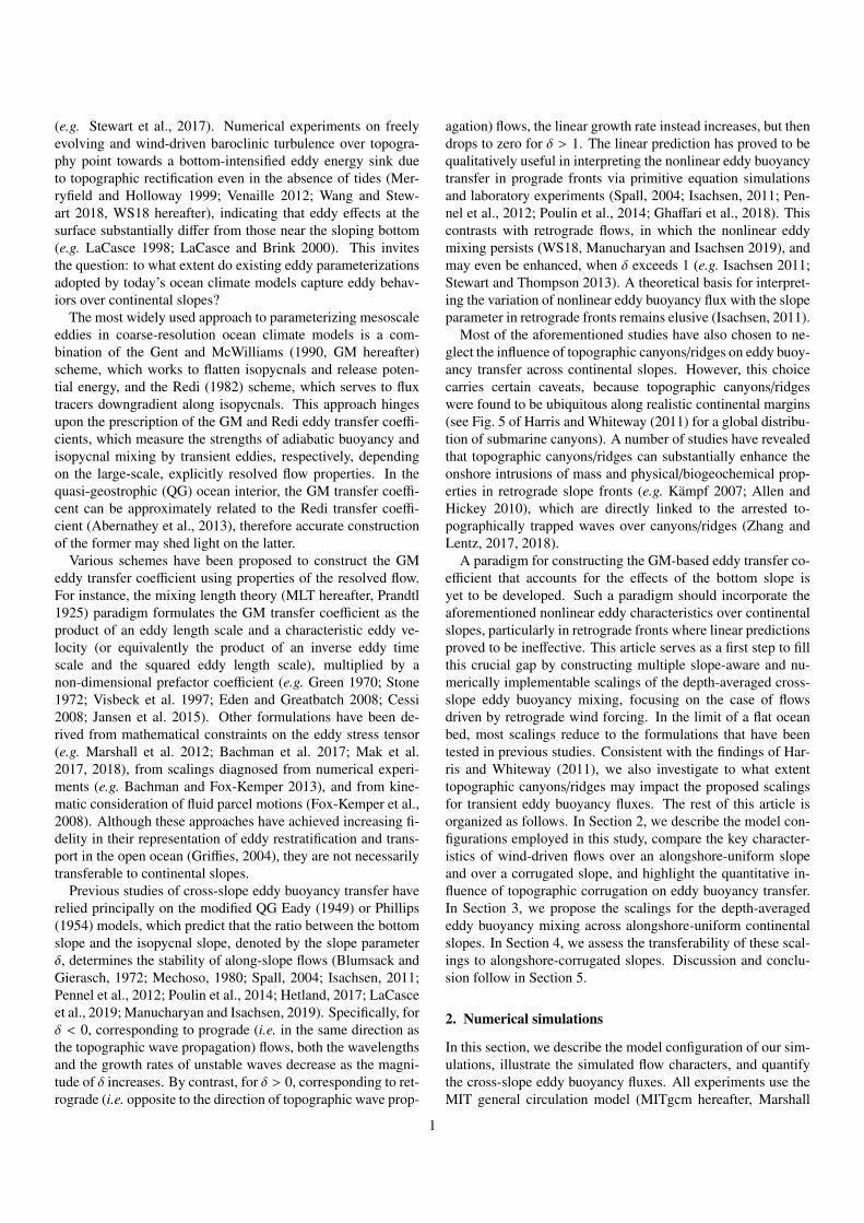
A suite of experiments are performed by varying the refer-ence settings in §2.1. Specifically, we independently adjust themaximum strength of wind, the thermal expansion coefficient,and importantly, the slope geometry, for each simulation, whichare summarized in Table 2. We vary these dimensional parame-ters in such a way as to cover a wide range of continental slopeconfigurations, characterized by five non-dimensional numbersdiscussed below, and meanwhile avoid redundant runs.

2

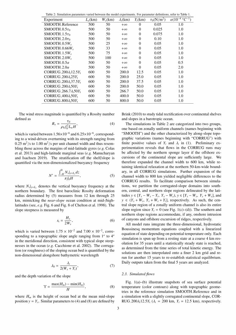
Table 2: Simulation parameters varied between the model experiments. For parameter definitions, refer to Table 1.

Experiment Ly(km) Ws(km) λt(km) Yt(km) τ0(N/m2) α(10−4 oC−1)SMOOTH Reference 500 50 +∞ 0 0.05 1.0SMOOTH 0.5τ0 500 50 +∞ 0 0.025 1.0SMOOTH 1.5τ0 500 50 +∞ 0 0.075 1.0SMOOTH 2.0τ0 500 50 +∞ 0 0.10 1.0SMOOTH 0.5Ws 500 25 +∞ 0 0.05 1.0SMOOTH 0.66Ws 500 33 +∞ 0 0.05 1.0SMOOTH 1.5Ws 500 75 +∞ 0 0.05 1.0SMOOTH 2.0Ws 500 100 +∞ 0 0.05 1.0SMOOTH 0.5α 500 50 +∞ 0 0.05 0.5SMOOTH 2.0α 500 50 +∞ 0 0.05 2.0CORRUG 200λt12.5Yt 600 50 200.0 12.5 0.05 1.0CORRUG 200λt25Yt 600 50 200.0 25.0 0.05 1.0CORRUG 200λt37.5Yt 600 50 200.0 37.5 0.05 1.0CORRUG 200λt50Yt 600 50 200.0 50.0 0.05 1.0CORRUG 266.7λt50Yt 600 50 266.7 50.0 0.05 1.0CORRUG 400λt50Yt 600 50 400.0 50.0 0.05 1.0CORRUG 800λt50Yt 600 50 800.0 50.0 0.05 1.0

The wind stress magnitude is quantified by a Rossby numberdefined as

Rτ =τ0

ρ0 f 20 LwH

, (4)

which is varied between 1.56×10−6 and 6.25×10−6, correspond-ing to a wind-driven overturning with its strength ranging from0.25 m2/s to 1.00 m2/s per unit channel width and thus resem-bling those across the margins of mid-latitude gyres (e.g. Colaset al. 2013) and high-latitude marginal seas (e.g. Manucharyanand Isachsen 2019). The stratification off the shelf/slope isquantified via the non-dimensionalized buoyancy frequency

N∗ =

∫ 0−H Ns|y=Ly dz

π f0H, (5)

where Ns|y=Ly denotes the vertical buoyancy frequency at thenorthern boundary. The first baroclinic Rossby deformationradius determined by (5) measures from 12 km through 25km, mimicking the near-slope ocean condition at mid-/high-latitudes (see, e.g. Fig. 6 and Fig. 8 of Chelton et al. 1998). Theslope steepness is measured by

st =Hs

2Ws, (6)

which is varied between 1.75 × 10−2 and 7.00 × 10−2, corre-sponding to a topographic slope angle ranging from 1o to 4o

in the meridional direction, consistent with typical slope steep-nesses in the ocean (e.g. Cacchione et al. 2002). The corruga-tion (or roughness) of the sloping ocean bed is quantified by thenon-dimensional alongshore bathymetric wavelength

λ0 =λt

2(Ws + Yt), (7)

and the depth variation of the slope

Υ =max(Hm) −min(Hm)

H, (8)

where Hm is the height of ocean bed at the mean mid-slopeposition y = Ys. Similar parameters to (4) and (8) are defined by

Brink (2010) to study tidal rectification over continental shelvesand slopes in a barotropic ocean.

The simulations in Table 2 are categorized into two groups,one based on zonally uniform channels (names beginning with“SMOOTH”) and the other characterized by along-slope topo-graphic variations (names beginning with “CORRUG”) withfinite positive values of Yt and λt in (1). Preliminary ex-perimentation reveals that flows in the CORRUG runs maybe affected by the northern sponge layer if the offshore ex-cursions of the continental slope are sufficiently large. Wetherefore expanded the channel width to 600 km, while re-taining identical relaxation at the northern 50-km-wide bound-ary, in all CORRUG simulations. Further expansion of thechannel width to 800 km yielded negligible differences to theCORRUG results. To facilitate comparison between simula-tions, we partition the corrugated-slope domains into south-ern, central, and northern slope regions delineated by the lati-tudes y ∈ [Ys −Ws − Yt, Ys −Ws), y ∈ [Ys −Ws, Ys + Ws], andy ∈ (Ys + Ws, Ys + Ws + Yt], respectively. As such, the cen-tral slope region of a zonally uniform channel is also its entireslope region since Yt = 0 (see Fig. 1(c)–(d)). The southern andnorthern slope regions accommodate, if any, onshore intrusionof canyons and offshore excursion of ridges, respectively.

All model runs integrate the three-dimensional, hydrostaticBoussinesq momentum equations coupled with a linearizedequation of state depending on potential temperature only. Eachsimulation is spun up from a resting state at a coarse 4 km res-olution for 35 years until a statistically steady state is reached,as determined from the time series of total kinetic energy. Thesolutions are then interpolated onto a finer 2 km grid and re-run for another 15 years to re-establish statistical equilibrium.Daily outputs taken from the final 5 years are analyzed.

2.3. Simulated flows

Fig. 1(a)–(b) illustrate snapshots of sea surface potentialtemperature (color contours) along with topographic geome-tries in the reference simulation SMOOTH Reference and ina simulation with a slightly corrugated continental slope, COR-RUG 200λt12.5Yt (λt = 200 km, Yt = 12.5 km), respectively.

3

Figure 1: Schematic illustrations of the slope bathymetry used in (a) SMOOTH Reference and (b) CORRUG 200λt12.5Yt simulations, superposed by the snapshotsof sea surface potential temperature (color), selected bathymetric contours (black), and selected quasi-streamlines of the time-mean sea surface horizontal velocity(white). Time-/zonal-mean eddy kinetic energy as a function of depth and offshore distance for the (c) SMOOTH Reference and (d) CORRUG 200λt12.5Yt runs,superposed by time-/zonal-mean isopycnals (dashed contours, interval: 1oC) and alongshore velocity profiles (solid contours, interval: 0.1 m/s). The velocitycontours u = 0 m/s are highlighted with bold lines. The upper panels of (c)–(d) illustrate the reference wind stress profile (blue line) used in this study, with negativesigns corresponding to the retrograde direction. The northern sponge layer in the SMOOTH Reference run is shadowed with dark gray in panel (c), and not shownfor the CORRUG 200λt12.5Yt run (in the latter the sponge layer lies between 550 and 600 km offshore). In panel (d), both the deepest and shallowest bathymetrycontours at each latitude are plotted to illustrate the slight corrugation of the slope. The latitudes dividing the shelf/slope and slope/deep ocean are indicated byblack dashed lines in panels (c)–(d). In panel (d), the northern and the southern slope regions are shadowed (see text in §2.2 for definitions of these regions).

Selected isobaths (black contours) and quasi-streamlines1 of thetime-mean horizontal velocity field uh at sea surface (white con-tours) are superposed on the potential temperature, where • de-notes a time average over the 5-year-long analysis period. Vig-orous eddies are visible in both simulations. However, whilethe surface mean flow is almost exactly aligned with the iso-baths in Fig. 1(a), standing meanders2 with horizontal scalescomparable to the zonal extent of the topographic variationsarise and traverse the isobaths in Fig. 1(b). Numerous studieshave shown that standing meanders in retrograde flows over acorrugated shelf/slope result from the arrested PV waves gen-

1The time-mean surface horizontal velocity fields in our simulations arenot exactly divergence-free. The quasi-streamlines are selected contours of thequasi-streamfunction calculated as ψsurf (x, y) =

∫ y0 u(x, y)

∣∣∣∣z=0

dy.2In this article we use the terms standing meanders, stationary meanders,

and standing eddies interchangeably.

erated by topographic variations (Allen, 1975; Wang and Moo-ers, 1976; Csanady, 1978; Brink, 1986, 1991; Connolly et al.,2014; Zhang and Lentz, 2017, 2018), similar to those foundin the Antarctic Circumpolar Current over a topographic ridge(Treguier and McWilliams, 1990; Stevens and Ivchenko, 1997;Abernathey and Cessi, 2014; Thompson and Naveira Garabato,2014; Stewart and Hogg, 2017). Accompanying the standingmeanders is the lower contrast of potential temperature betweenthe shelf/slope and the open ocean, suggesting stronger restrat-ification compared to the case shown in Fig. 1(a).

In Fig. 1(c)–(d), we quantify the time/zonal-averages of po-tential temperature

⟨θ⟩

and zonal velocity 〈u〉, superposed onthe logarithms of zonally averaged eddy kinetic energy (EKE)12

⟨u′2 + v′2

⟩per unit mass, where 〈•〉 = 1

Lx

∮• dx denotes the

zonal-mean operator and the prime denotes the deviation of aquantity from its time-mean. EKE exhibits similar structuresand magnitudes between the simulations. However, in the pres-

4

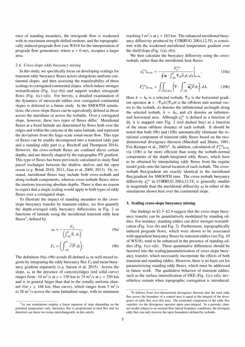
ence of standing meanders, the retrograde flow is weakenedwith its maximum strength shifted onshore, and the topographi-cally induced prograde flow (see WS18 for the interpretation ofprograde flow generation), where u > 0 m/s, occupies a largerarea.

2.4. Cross-slope eddy buoyancy mixingIn this study, we specifically focus on developing scalings for

transient eddy buoyancy fluxes across alongshore-uniform con-tinental slopes, and then assessing the transferability of thesescalings to corrugated continental slopes, which induce strongerrestratification (Fig. 1(a)–(b)) and support weaker retrogradeflows (Fig. 1(c)–(d)). For brevity, a detailed examination ofthe dynamics of mesoscale eddies over corrugated continentalslopes is deferred to a future study. In the SMOOTH simula-tions, the cross-slope fluxes can be equivalently defined as thoseacross the meridians or across the isobaths. Over a corrugatedslope, however, these two types of fluxes differ. Meridionalfluxes at a fixed latitude are determined by flows both over theridges and within the canyons at the same latitude, and representthe deviations from the large-scale zonal-mean flow. This typeof fluxes can be readily decomposed into a transient eddy partand a standing eddy part (e.g. Bischoff and Thompson 2014).However, the cross-isobath fluxes are confined above certaindepths, and are directly shaped by the topographic PV gradient.This type of fluxes has been previously calculated to study fluidparcel exchanges between the shallow shelves and the openocean (e.g. Brink 2010, 2011; Gan et al. 2009, 2013). Or, re-stated, meridional fluxes may include both cross-isobath andalong-isobath components, whereas cross-isobath fluxes stressthe motions traversing absolute depths. There is thus no reasonto expect that a single scaling would apply to both types of eddyfluxes over a corrugated slope.

To illustrate the impact of standing meanders to the cross-slope buoyancy transfer by transient eddies, we first quantifythe depth-averaged eddy buoyancy diffusivities in Fig. 2 asfunctions of latitude using the meridional transient eddy heatfluxes3, defined by

κθ = −Fθ⟨∫ 0

−|h| θy dz⟩ , (9a)

Fθ =

⟨∫ 0

−|h|v′θ′ dz

⟩. (9b)

The definition (9a)–(9b) avoids ill-defined κθ in well-mixed re-gions by integrating the eddy buoyancy flux Fθ and mean buoy-ancy gradient separately (e.g. Jansen et al. 2015). Across theslope, κθ in the presence of canyons/ridges (red solid curve)ranges from -10 m2/s at y = 150 km to 74 m2/s at y = 250 kmand is in general larger than that in the zonally uniform chan-nel (for y ≥ 168 km, blue curve), which ranges from 5 m2/sto 26 m2/s across the same latitudinal range, with its minimum

3As our simulations employ a linear equation of state depending on thepotential temperature only, buoyancy flux is proportional to heat flux and wetherefore use these two terms interchangeably in this article.

reaching 3 m2/s at y ' 163 km. The enhanced meridional buoy-ancy diffusivity produced by CORRUG 200λt12.5Yt is consis-tent with the weakened meridional temperature gradient overthe shelf/slope (Fig. 1(a)–(b)).

We then calculate the buoyancy diffusivity using the cross-isobath, rather than the meridional, heat fluxes:

κisoθ |h=h0 = −

F isoθ∮

n ·∫ 0−|h| ∇Hθ dz ds

∣∣∣∣∣∣h=h0

, (10a)

F isoθ |h=h0 =

∫∫|h|≤|h0 |

(∇ ·

∫ 0

−|h|u′hθ′dz

)dA. (10b)

Here h = h0 is a selected isobath, ∇H is the horizontal gradi-ent operator, n = −∇Hh/|∇Hh| is the offshore unit normal vec-tor to the isobath, ds denotes the infinitesimal arclength alongthe selected isobath, h = h0, and dA denotes an infinitesi-mal horizontal area. Although κiso

θ is defined as a function of|h|, it is mapped onto Fig. 2 (red dashed line) as a functionof the mean offshore distance of each isobath. It should benoted that both (9b) and (10b) automatically eliminate the ro-tational component of transient eddy fluxes based on the two-dimensional divergence theorem (Marshall and Shutts, 1981;Fox-Kemper et al., 2003)4. In addition, calculation of F iso

θ |h=h0

via (10b) is far more efficient than using the isobath-normalcomponents of the depth-integrated eddy fluxes, which haveto be obtained by interpolating eddy fluxes from the regularmodel grids onto the lateral location of each isobath. The cross-isobath flux/gradient are exactly identical to the meridionalflux/gradient for SMOOTH runs. The cross-isobath buoyancydiffusivity κiso

θ in CORRUG 200λt12.5Yt is generally smallerin magnitude than the meridional diffusivity κθ in either of thesimulations shown here over the continental slope.

3. Scaling cross-slope buoyancy mixing

Our findings in §2.3–§2.4 suggest that the cross-slope buoy-ancy transfer can be quantitatively modulated by standing ed-dies. For instance, standing eddies can drive stronger restratifi-cation (Fig. 1(a)–(b) and Fig. 2). Furthermore, topographicallyinduced prograde flows, which were shown to be associatedwith upgradient buoyancy fluxes by transient eddies (see Fig. 10of WS18), tend to be enhanced in the presence of standing ed-dies (Fig. 1(c)–(d)). These quantitative differences should befactored into the scaling/parameterization of cross-slope buoy-ancy transfer, which necessarily incorporate the effects of bothtransient and standing eddies. However, there is no basis yet forparameterizing standing eddy fluxes, which must be addressedin future work. The qualitative behavior of transient eddies,such as the surface intensification of EKE (Fig. 1(c)–(d)), nev-ertheless remain when topographic corrugation is introduced.

4It follows from two-dimensional divergence theorem that the total eddyflux across the boundary of a control area is equal to the integral of the diver-gence of eddy flux over this area. The rotational component of the eddy fluxvanishes via the divergence operator upon area-integral. In a periodic chan-nel model subject to no-normal-flow lateral boundary conditions, the divergenteddy flux can only traverse the open boundaries defined by isobaths.

5

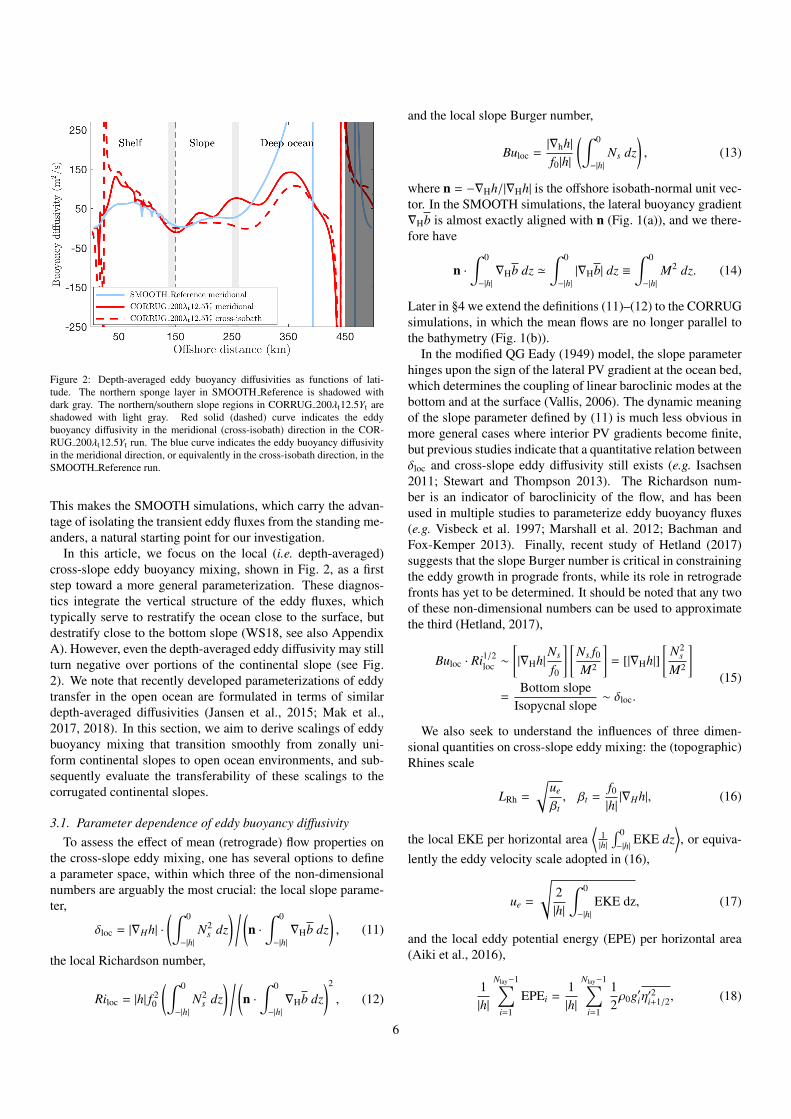
Figure 2: Depth-averaged eddy buoyancy diffusivities as functions of lati-tude. The northern sponge layer in SMOOTH Reference is shadowed withdark gray. The northern/southern slope regions in CORRUG 200λt12.5Yt areshadowed with light gray. Red solid (dashed) curve indicates the eddybuoyancy diffusivity in the meridional (cross-isobath) direction in the COR-RUG 200λt12.5Yt run. The blue curve indicates the eddy buoyancy diffusivityin the meridional direction, or equivalently in the cross-isobath direction, in theSMOOTH Reference run.

This makes the SMOOTH simulations, which carry the advan-tage of isolating the transient eddy fluxes from the standing me-anders, a natural starting point for our investigation.

In this article, we focus on the local (i.e. depth-averaged)cross-slope eddy buoyancy mixing, shown in Fig. 2, as a firststep toward a more general parameterization. These diagnos-tics integrate the vertical structure of the eddy fluxes, whichtypically serve to restratify the ocean close to the surface, butdestratify close to the bottom slope (WS18, see also AppendixA). However, even the depth-averaged eddy diffusivity may stillturn negative over portions of the continental slope (see Fig.2). We note that recently developed parameterizations of eddytransfer in the open ocean are formulated in terms of similardepth-averaged diffusivities (Jansen et al., 2015; Mak et al.,2017, 2018). In this section, we aim to derive scalings of eddybuoyancy mixing that transition smoothly from zonally uni-form continental slopes to open ocean environments, and sub-sequently evaluate the transferability of these scalings to thecorrugated continental slopes.

3.1. Parameter dependence of eddy buoyancy diffusivityTo assess the effect of mean (retrograde) flow properties on

the cross-slope eddy mixing, one has several options to definea parameter space, within which three of the non-dimensionalnumbers are arguably the most crucial: the local slope parame-ter,

δloc = |∇Hh| ·(∫ 0

−|h|N2

s dz) / (

n ·∫ 0

−|h|∇Hb dz

), (11)

the local Richardson number,

Riloc = |h| f 20

(∫ 0

−|h|N2

s dz) / (

n ·∫ 0

−|h|∇Hb dz

)2

, (12)

and the local slope Burger number,

Buloc =|∇hh|f0|h|

(∫ 0

−|h|Ns dz

), (13)

where n = −∇Hh/|∇Hh| is the offshore isobath-normal unit vec-tor. In the SMOOTH simulations, the lateral buoyancy gradient∇Hb is almost exactly aligned with n (Fig. 1(a)), and we there-fore have

n ·∫ 0

−|h|∇Hb dz '

∫ 0

−|h||∇Hb| dz ≡

∫ 0

−|h|M2 dz. (14)

Later in §4 we extend the definitions (11)–(12) to the CORRUGsimulations, in which the mean flows are no longer parallel tothe bathymetry (Fig. 1(b)).

In the modified QG Eady (1949) model, the slope parameterhinges upon the sign of the lateral PV gradient at the ocean bed,which determines the coupling of linear baroclinic modes at thebottom and at the surface (Vallis, 2006). The dynamic meaningof the slope parameter defined by (11) is much less obvious inmore general cases where interior PV gradients become finite,but previous studies indicate that a quantitative relation betweenδloc and cross-slope eddy diffusivity still exists (e.g. Isachsen2011; Stewart and Thompson 2013). The Richardson num-ber is an indicator of baroclinicity of the flow, and has beenused in multiple studies to parameterize eddy buoyancy fluxes(e.g. Visbeck et al. 1997; Marshall et al. 2012; Bachman andFox-Kemper 2013). Finally, recent study of Hetland (2017)suggests that the slope Burger number is critical in constrainingthe eddy growth in prograde fronts, while its role in retrogradefronts has yet to be determined. It should be noted that any twoof these non-dimensional numbers can be used to approximatethe third (Hetland, 2017),

Buloc · Ri1/2loc ∼

[|∇Hh|

Ns

f0

] [Ns f0M2

]= [|∇Hh|]

[N2

s

M2

]=

Bottom slopeIsopycnal slope

∼ δloc.

(15)

We also seek to understand the influences of three dimen-sional quantities on cross-slope eddy mixing: the (topographic)Rhines scale

LRh =

√ue

βt, βt =

f0|h||∇Hh|, (16)

the local EKE per horizontal area⟨

1|h|

∫ 0−|h| EKE dz

⟩, or equiva-

lently the eddy velocity scale adopted in (16),

ue =

√2|h|

∫ 0

−|h|EKE dz, (17)

and the local eddy potential energy (EPE) per horizontal area(Aiki et al., 2016),

1|h|

Nlay−1∑i=1

EPEi =1|h|

Nlay−1∑i=1

12ρ0g′iη

′2i+1/2, (18)

6

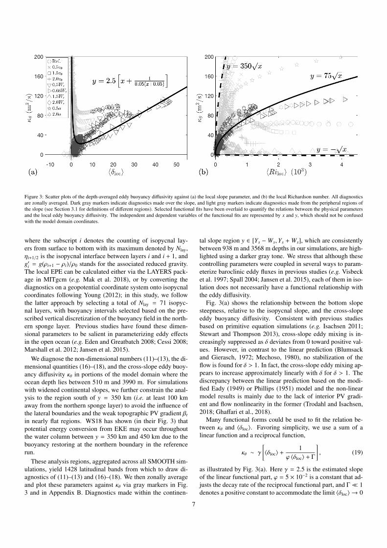
Figure 3: Scatter plots of the depth-averaged eddy buoyancy diffusivity against (a) the local slope parameter, and (b) the local Richardson number. All diagnosticsare zonally averaged. Dark gray markers indicate diagnostics made over the slope, and light gray markers indicate diagnostics made from the peripheral regions ofthe slope (see Section 3.1 for definitions of different regions). Selected functional fits have been overlaid to quantify the relations between the physical parametersand the local eddy buoyancy diffusivity. The independent and dependent variables of the functional fits are represented by x and y, which should not be confusedwith the model domain coordinates.

where the subscript i denotes the counting of isopycnal lay-ers from surface to bottom with its maximum denoted by Nlay,ηi+1/2 is the isopycnal interface between layers i and i + 1, andg′i = g(ρi+1 − ρi)/ρ0 stands for the associated reduced gravity.The local EPE can be calculated either via the LAYERS pack-age in MITgcm (e.g. Mak et al. 2018), or by converting thediagnostics on a geopotential coordinate system onto isopycnalcoordinates following Young (2012); in this study, we followthe latter approach by selecting a total of Nlay = 71 isopyc-nal layers, with buoyancy intervals selected based on the pre-scribed vertical discretization of the buoyancy field in the north-ern sponge layer. Previous studies have found these dimen-sional parameters to be salient in parameterizing eddy effectsin the open ocean (e.g. Eden and Greatbatch 2008; Cessi 2008;Marshall et al. 2012; Jansen et al. 2015).

We diagnose the non-dimensional numbers (11)–(13), the di-mensional quantities (16)–(18), and the cross-slope eddy buoy-ancy diffusivity κθ in portions of the model domain where theocean depth lies between 510 m and 3990 m. For simulationswith widened continental slopes, we further constrain the anal-ysis to the region south of y = 350 km (i.e. at least 100 kmaway from the northern sponge layer) to avoid the influence ofthe lateral boundaries and the weak topographic PV gradient βt

in nearly flat regions. WS18 has shown (in their Fig. 3) thatpotential energy conversion from EKE may occur throughoutthe water column between y = 350 km and 450 km due to thebuoyancy restoring at the northern boundary in the referencerun.

These analysis regions, aggregated across all SMOOTH sim-ulations, yield 1428 latitudinal bands from which to draw di-agnostics of (11)–(13) and (16)–(18). We then zonally averageand plot these parameters against κθ via gray markers in Fig.3 and in Appendix B. Diagnostics made within the continen-

tal slope region y ∈ [Ys −Ws,Ys + Ws], which are consistentlybetween 938 m and 3568 m depths in our simulations, are high-lighted using a darker gray tone. We stress that although thesecontrolling parameters were coupled in several ways to param-eterize baroclinic eddy fluxes in previous studies (e.g. Visbecket al. 1997; Spall 2004; Jansen et al. 2015), each of them in iso-lation does not necessarily have a functional relationship withthe eddy diffusivity.

Fig. 3(a) shows the relationship between the bottom slopesteepness, relative to the isopycnal slope, and the cross-slopeeddy buoyancy diffusivity. Consistent with previous studiesbased on primitive equation simulations (e.g. Isachsen 2011;Stewart and Thompson 2013), cross-slope eddy mixing is in-creasingly suppressed as δ deviates from 0 toward positive val-ues. However, in contrast to the linear prediction (Blumsackand Gierasch, 1972; Mechoso, 1980), no stabilization of theflow is found for δ > 1. In fact, the cross-slope eddy mixing ap-pears to increase approximately linearly with δ for δ > 1. Thediscrepancy between the linear prediction based on the modi-fied Eady (1949) or Phillips (1951) model and the non-linearmodel results is mainly due to the lack of interior PV gradi-ent and flow nonlinearity in the former (Trodahl and Isachsen,2018; Ghaffari et al., 2018).

Many functional forms could be used to fit the relation be-tween κθ and 〈δloc〉. Favoring simplicity, we use a sum of alinear function and a reciprocal function,

κθ ∼ γ

[〈δloc〉 +

1ϕ 〈δloc〉 + Γ

], (19)

as illustrated by Fig. 3(a). Here γ = 2.5 is the estimated slopeof the linear functional part, ϕ = 5 × 10−2 is a constant that ad-justs the decay rate of the reciprocal functional part, and Γ � 1denotes a positive constant to accommodate the limit 〈δloc〉 → 0

7

(i.e. nearly flat ocean bed case). It should be noted that there isno theoretical basis for the functional fit (19). Following pre-vious studies (e.g. Stewart and Thompson 2013), our approachis entirely empirical. The least-squares error produced by (19)decreases by a factor of 2 compared to a linear functional fit ifdiagnostics from both the continental slope and the open oceanregions are accounted for. When diagnostics from the continen-tal shelf are also included, the relation (19) generates a slightlylarger error than a linear fit, partly due to the emergence ofnegative eddy diffusivity and local slope parameter. This issuecan be fixed by replacing the reciprocal function in (19) withan exponential decay. However, our key findings reported inlater sections do not qualitatively depend on such modifications.Crucially, the mathematically simple form of (19) helps to sim-plify our analysis contrasted to most other nonlinear functions.The eddy diffusivity is then predicted to reach its minimum as〈δloc〉' 4.42 ∼ O(1). As the ocean bed becomes steeper, eddymixing starts to be constrained by the linear functional part of(19). For 〈δloc〉 → +∞ (i.e. zero projection of isopycnal slope inthe cross-slope direction), this simple approximation becomesunbounded. We return to this point and discuss potential regu-larizations for this issue in §5.

Fig. 3(b) exhibits widespread scatter of the local Richardsonnumber 〈Riloc〉 against the eddy diffusivity κθ. Further examina-tion suggests the relation

κθ ∼ γ⟨10−3Riloc

⟩1/2, (20)

with γ varying from -1 to 350 depending on the simulations andgeographic locations. Similar to (19), the relation (20) is em-pirical, selected from many possible nonlinear fits. The casesexhibiting weakly negative values of γ are those dominated byeddy destratification, which are relatively rare in the SMOOTHsimulations (see §4). Over continental slopes, γ ' 75 yieldsa good fit for all simulations, with the least-squares errorsmaller than from an optimized linear fit by a factor of approxi-mately 1.85. These results may seem counter-intuitive as higherRichardson number suggests weaker baroclinicity of the along-slope flow and thus lower available potential energy reservoir.In the classical Eady (1949) model, baroclinic mode growthrate is exactly proportional to f0/

√Ri (e.g. Pedlosky 1987;

Vallis 2006), suggesting an anti-correlation between κθ and〈Riloc〉

1/2 if the linear modes govern the eddy mixing. Exist-ing eddy parameterizations also treat the Eady growth rate as akey parameter (e.g. Visbeck et al. 1997; Marshall et al. 2012).

The relationships between the eddy diffusivity and the otherselected parameters, (13) and (16)–(18), are shown in AppendixB. Of the potential controlling parameters explored, only thelocal slope parameter δloc (in isolation) exhibits a strong func-tional relation with the eddy diffusivity in both the continen-tal slope and open ocean environments. Although the lo-cal Richardson number Riloc constrains eddy buoyancy fluxesacross the continental slope, and has been incorporated in ex-isting eddy parameterizations (e.g. Visbeck et al. 1997; Mar-shall et al. 2012; Bachman and Fox-Kemper 2013), the eddybuoyancy diffusivity cannot be scaled by Riloc alone in the openocean environment. Other parameters (in isolation) may ex-

hibit functional relationships with the eddy diffusivity in theopen ocean, but not over the continental slope (see AppendixB). These findings suggests that existing eddy parameteriza-tions may be adaptable to continental slopes via the introduc-tion of a dependence on the local slope parameter, as shown inthe following sections.

3.2. Scaling of eddy mixing via the GEOMETRIC framework

The observation that κθ tends to scale with 〈Riloc〉1/2 (Fig.

3(b)) motivates the application of a recently developedparadigm of eddy parameterization that combines the squareroot of the Richardson number with the total eddy energy,namely, the GEOMETRIC framework (Marshall et al., 2012;Bachman et al., 2017; Mak et al., 2017, 2018). Specifically,Marshall et al. (2012) defined

κGeom = γGeomNs

M2 E = γGeom

√Ri

f0E, (21)

based on a geometric constraint on the Eliassen-Palm flux ten-sor in quasi-geostrophic flows. Here γGeom is a non-dimensionalprefactor, whose magnitude is bounded by unity, and E denotesthe sum of the EKE and the EPE per unit mass. In a coarse-resolution ocean model, if an additional prognostic equation forthe subgrid eddy energy budget is implemented (e.g. Mak et al.2018), the only free parameter in (21) is γGeom, which containsthe information about the partition between the EKE and EPE,and the anisotropy of the eddy buoyancy fluxes (Marshall et al.,2012).

It should be noted that the cross-slope eddy diffusivity canturn negative, even in a depth-averaged sense, over zonally uni-form slopes (Fig. 3). This contradicts other eddy parameteri-zations that permit vertically local destratification of flows bybaroclinic eddies, but ensure net potential energy destructionacross a full water column (e.g. Ferrari et al. 2010). This fur-ther motivates the application of the GEOMETRIC frameworkover steep slopes: the coefficient γGeom may become predomi-nantly negative across a water column if the relative orientationof the eddy buoyancy flux to the mean buoyancy gradient issufficiently small (Marshall et al., 2012).

Fig. 4(a) demonstrates the performance of the local GEO-METRIC scaling,

κGeom = γ

√Riloc

f0Eloc, (22a)

Eloc =1|h|

∫ 0

−|h|EKE dz +

Nlay−1∑i=1

EPEi

, (22b)

in quantifying κθ over continental slopes. Here γ = γGeom =

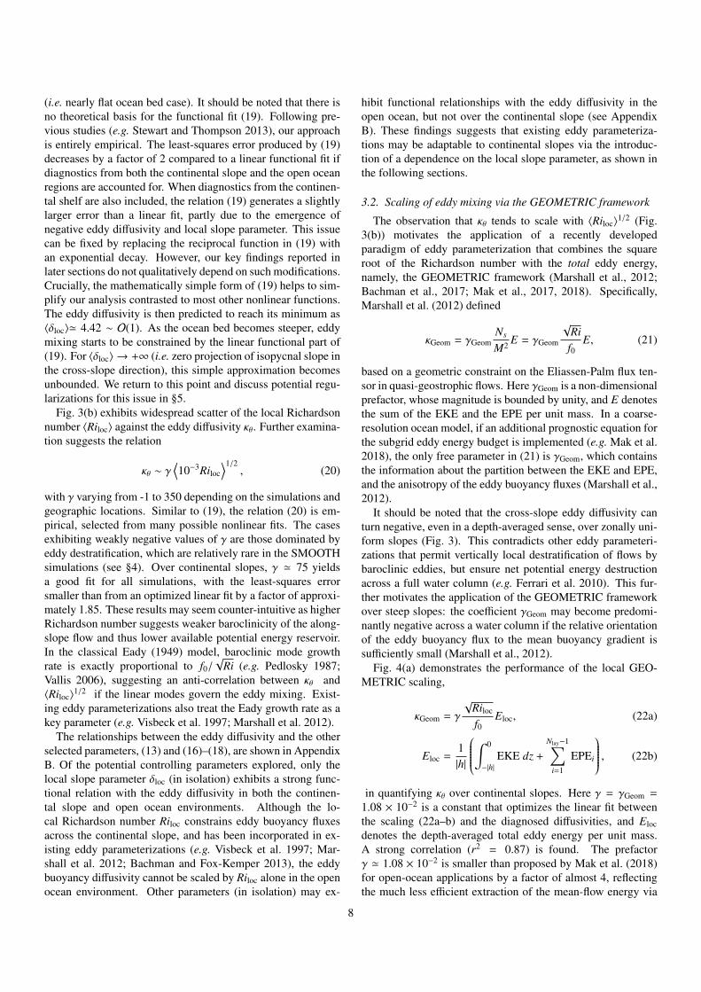
1.08 × 10−2 is a constant that optimizes the linear fit betweenthe scaling (22a–b) and the diagnosed diffusivities, and Elocdenotes the depth-averaged total eddy energy per unit mass.A strong correlation (r2 = 0.87) is found. The prefactorγ ' 1.08 × 10−2 is smaller than proposed by Mak et al. (2018)for open-ocean applications by a factor of almost 4, reflectingthe much less efficient extraction of the mean-flow energy via

8

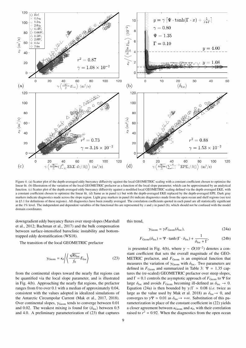
Figure 4: (a) Scatter plot of the depth-averaged eddy buoyancy diffusivity against the local GEOMETRIC scaling with a constant coefficient chosen to optimize thelinear fit. (b) Illustration of the variation of the local GEOMETRIC prefactor as a function of the local slope parameter, which can be approximated by an analyticalfunction. (c) Scatter plot of the depth-averaged eddy buoyancy diffusivity against a modified local GEOMETRIC scaling defined via the depth-averaged EKE, witha constant coefficient chosen to optimize the linear fit. (d) Same as in panel (c) but with the depth-averaged EKE replaced by the depth-averaged EPE. Dark graymarkers indicate diagnostics made across the slope region. Light gray markers in panel (b) indicate diagnostics made from the open ocean and shelf regions (see textin §3.1 for definitions of these regions). All diagnostics have been zonally averaged. The correlation coefficients quoted in each panel are all statistically significantat the 1% level. The independent and dependent variables of the functional fits are represented by x and y in panel (b), which should not be confused with the modeldomain coordinates.

downgradient eddy buoyancy fluxes over steep slopes (Marshallet al., 2012; Bachman et al., 2017) and the bulk compensationbetween surface-intensified baroclinic instability and bottom-trapped eddy destratification (WS18).

The transition of the local GEOMETRIC prefactor

γGeom = κθ

/ ⟨ √Riloc

f0Eloc

⟩(23)

from the continental slopes toward the nearly flat regions canbe quantified via the local slope parameter, and is illustratedin Fig. 4(b). Approaching the nearly flat regions, the prefactorranges from 0 to over 0.1 with a median of approximately 0.04,consistent with the values adopted in idealized simulations ofthe Antarctic Circumpolar Current (Mak et al., 2017, 2018).Over continental slopes, γGeom tends to converge between 0.01and 0.02. The weakest mixing is found for 〈δloc〉 between 0.5and 4.0. A preliminary parameterization of (23) that captures

this trend,

γGeom = γFGeom(δloc), (24a)

FGeom(δloc) = Ψ · tanh (Γ · δloc) +1

δloc + Γ, (24b)

is presented in Fig. 4(b), where γ ∼ O(10−2) denotes a con-stant coefficient that sets the overall magnitude of the GEO-METRIC prefactor, and FGeom is an empirical function thatmeasures the variation of γGeom with δloc. Two parameters aredefined in FGeom and summarized in Table 3: Ψ = 1.35 cap-tures the (re-scaled) GEOMETRIC prefactor over steep slopes,and Γ = 0.1 controls the asymptotic approach of FGeom to Ψ forlarge δloc and avoids FGeom becoming ill-defined as δloc → 0.Equation (24a) is then bounded by γ/Γ ' 0.08 (i.e. twice aslarge as the value used by Mak et al. 2018) as δloc→ 0, andconverges to γΨ ' 0.01 as δloc→ +∞. Substitution of this pa-rameterization in place of the constant coefficient in (22) yieldsa closer agreement between κGeom and κθ, with their correlationraised to r2 = 0.92. When the diagnostics from the open ocean

9

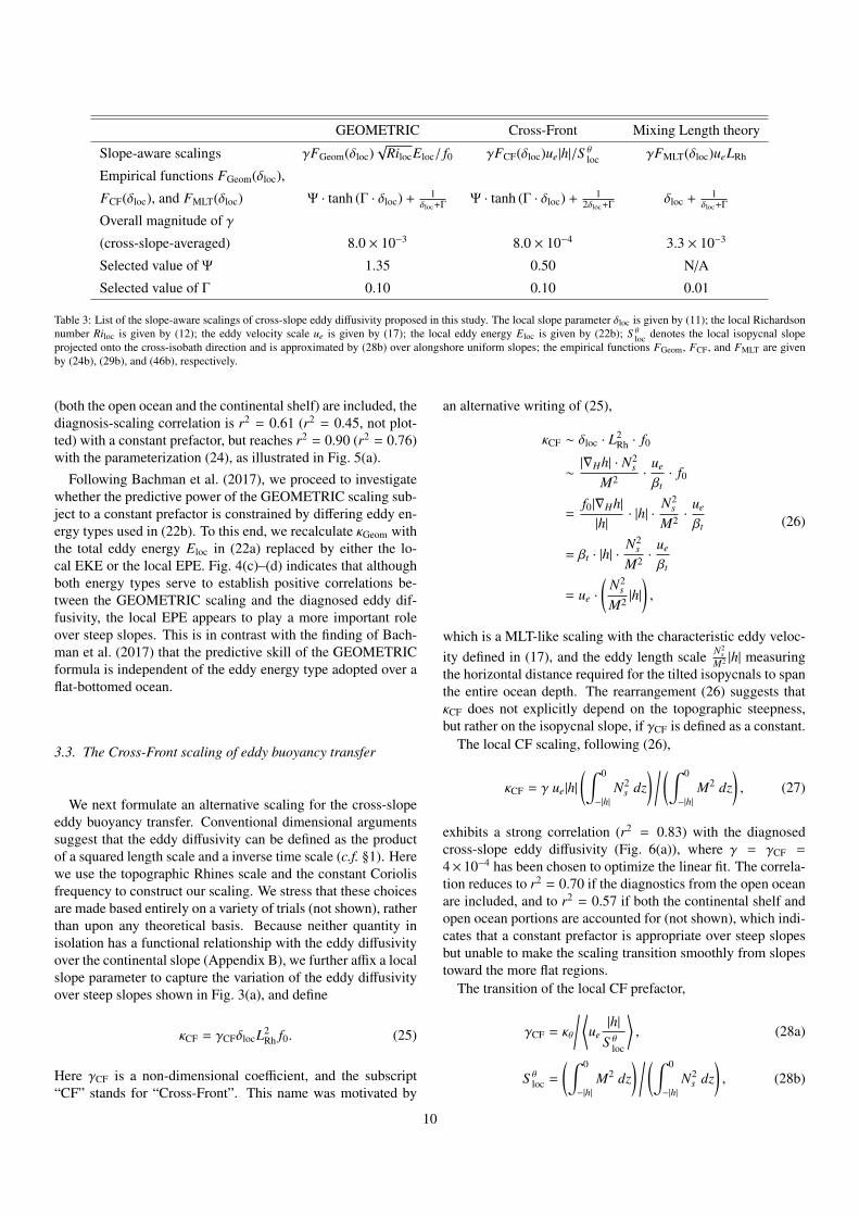
GEOMETRIC Cross-Front Mixing Length theory

Slope-aware scalings γFGeom(δloc)√

RilocEloc/ f0 γFCF(δloc)ue|h|/S θloc γFMLT(δloc)ueLRh

Empirical functions FGeom(δloc),

FCF(δloc), and FMLT(δloc) Ψ · tanh (Γ · δloc) + 1δloc+Γ

Ψ · tanh (Γ · δloc) + 12δloc+Γ

δloc + 1δloc+Γ

Overall magnitude of γ

(cross-slope-averaged) 8.0 × 10−3 8.0 × 10−4 3.3 × 10−3

Selected value of Ψ 1.35 0.50 N/A

Selected value of Γ 0.10 0.10 0.01

Table 3: List of the slope-aware scalings of cross-slope eddy diffusivity proposed in this study. The local slope parameter δloc is given by (11); the local Richardsonnumber Riloc is given by (12); the eddy velocity scale ue is given by (17); the local eddy energy Eloc is given by (22b); S θ

loc denotes the local isopycnal slopeprojected onto the cross-isobath direction and is approximated by (28b) over alongshore uniform slopes; the empirical functions FGeom, FCF, and FMLT are givenby (24b), (29b), and (46b), respectively.

(both the open ocean and the continental shelf) are included, thediagnosis-scaling correlation is r2 = 0.61 (r2 = 0.45, not plot-ted) with a constant prefactor, but reaches r2 = 0.90 (r2 = 0.76)with the parameterization (24), as illustrated in Fig. 5(a).

Following Bachman et al. (2017), we proceed to investigatewhether the predictive power of the GEOMETRIC scaling sub-ject to a constant prefactor is constrained by differing eddy en-ergy types used in (22b). To this end, we recalculate κGeom withthe total eddy energy Eloc in (22a) replaced by either the lo-cal EKE or the local EPE. Fig. 4(c)–(d) indicates that althoughboth energy types serve to establish positive correlations be-tween the GEOMETRIC scaling and the diagnosed eddy dif-fusivity, the local EPE appears to play a more important roleover steep slopes. This is in contrast with the finding of Bach-man et al. (2017) that the predictive skill of the GEOMETRICformula is independent of the eddy energy type adopted over aflat-bottomed ocean.

3.3. The Cross-Front scaling of eddy buoyancy transfer

We next formulate an alternative scaling for the cross-slopeeddy buoyancy transfer. Conventional dimensional argumentssuggest that the eddy diffusivity can be defined as the productof a squared length scale and a inverse time scale (c.f. §1). Herewe use the topographic Rhines scale and the constant Coriolisfrequency to construct our scaling. We stress that these choicesare made based entirely on a variety of trials (not shown), ratherthan upon any theoretical basis. Because neither quantity inisolation has a functional relationship with the eddy diffusivityover the continental slope (Appendix B), we further affix a localslope parameter to capture the variation of the eddy diffusivityover steep slopes shown in Fig. 3(a), and define

κCF = γCFδlocL2Rh f0. (25)

Here γCF is a non-dimensional coefficient, and the subscript“CF” stands for “Cross-Front”. This name was motivated by

an alternative writing of (25),

κCF ∼ δloc · L2Rh · f0

∼|∇Hh| · N2

s

M2 ·ue

βt· f0

=f0|∇Hh||h|

· |h| ·N2

s

M2 ·ue

βt

= βt · |h| ·N2

s

M2 ·ue

βt

= ue ·

(N2

s

M2 |h|),

(26)

which is a MLT-like scaling with the characteristic eddy veloc-ity defined in (17), and the eddy length scale N2

sM2 |h| measuring

the horizontal distance required for the tilted isopycnals to spanthe entire ocean depth. The rearrangement (26) suggests thatκCF does not explicitly depend on the topographic steepness,but rather on the isopycnal slope, if γCF is defined as a constant.

The local CF scaling, following (26),

κCF = γ ue|h|(∫ 0

−|h|N2

s dz) / (∫ 0

−|h|M2 dz

), (27)

exhibits a strong correlation (r2 = 0.83) with the diagnosedcross-slope eddy diffusivity (Fig. 6(a)), where γ = γCF =

4× 10−4 has been chosen to optimize the linear fit. The correla-tion reduces to r2 = 0.70 if the diagnostics from the open oceanare included, and to r2 = 0.57 if both the continental shelf andopen ocean portions are accounted for (not shown), which indi-cates that a constant prefactor is appropriate over steep slopesbut unable to make the scaling transition smoothly from slopestoward the more flat regions.

The transition of the local CF prefactor,

γCF = κθ

/ ⟨ue|h|

S θloc

⟩, (28a)

S θloc =

(∫ 0

−|h|M2 dz

) / (∫ 0

−|h|N2

s dz), (28b)

10

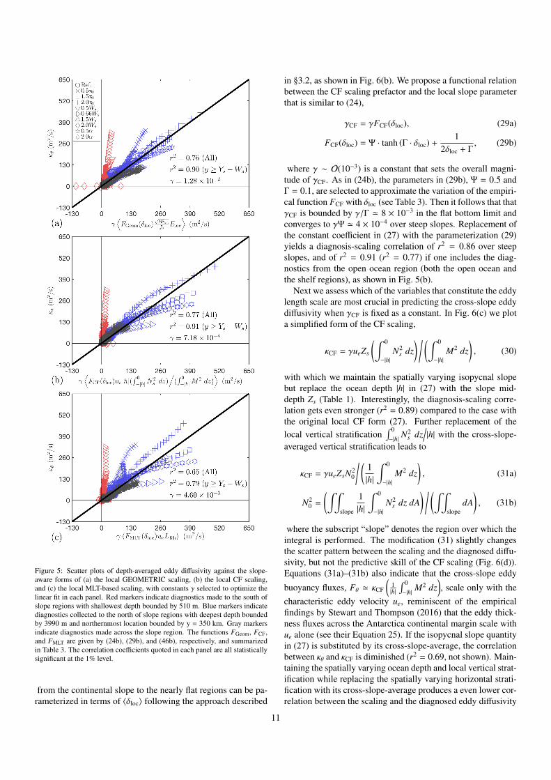
Figure 5: Scatter plots of depth-averaged eddy diffusivity against the slope-aware forms of (a) the local GEOMETRIC scaling, (b) the local CF scaling,and (c) the local MLT-based scaling, with constants γ selected to optimize thelinear fit in each panel. Red markers indicate diagnostics made to the south ofslope regions with shallowest depth bounded by 510 m. Blue markers indicatediagnostics collected to the north of slope regions with deepest depth boundedby 3990 m and northernmost location bounded by y = 350 km. Gray markersindicate diagnostics made across the slope region. The functions FGeom, FCF,and FMLT are given by (24b), (29b), and (46b), respectively, and summarizedin Table 3. The correlation coefficients quoted in each panel are all statisticallysignificant at the 1% level.

from the continental slope to the nearly flat regions can be pa-rameterized in terms of 〈δloc〉 following the approach described

in §3.2, as shown in Fig. 6(b). We propose a functional relationbetween the CF scaling prefactor and the local slope parameterthat is similar to (24),

γCF = γFCF(δloc), (29a)

FCF(δloc) = Ψ · tanh (Γ · δloc) +1

2δloc + Γ, (29b)

where γ ∼ O(10−3) is a constant that sets the overall magni-tude of γCF. As in (24b), the parameters in (29b), Ψ = 0.5 andΓ = 0.1, are selected to approximate the variation of the empiri-cal function FCF with δloc (see Table 3). Then it follows that thatγCF is bounded by γ/Γ ' 8 × 10−3 in the flat bottom limit andconverges to γΨ ' 4 × 10−4 over steep slopes. Replacement ofthe constant coefficient in (27) with the parameterization (29)yields a diagnosis-scaling correlation of r2 = 0.86 over steepslopes, and of r2 = 0.91 (r2 = 0.77) if one includes the diag-nostics from the open ocean region (both the open ocean andthe shelf regions), as shown in Fig. 5(b).

Next we assess which of the variables that constitute the eddylength scale are most crucial in predicting the cross-slope eddydiffusivity when γCF is fixed as a constant. In Fig. 6(c) we plota simplified form of the CF scaling,

κCF = γueZs

(∫ 0

−|h|N2

s dz) / (∫ 0

−|h|M2 dz

), (30)

with which we maintain the spatially varying isopycnal slopebut replace the ocean depth |h| in (27) with the slope mid-depth Zs (Table 1). Interestingly, the diagnosis-scaling corre-lation gets even stronger (r2 = 0.89) compared to the case withthe original local CF form (27). Further replacement of thelocal vertical stratification

∫ 0−|h| N

2s dz

/|h| with the cross-slope-

averaged vertical stratification leads to

κCF = γueZsN20

/ (1|h|

∫ 0

−|h|M2 dz

), (31a)

N20 =

(∫∫slope

1|h|

∫ 0

−|h|N2

s dz dA) / (∫∫

slopedA

), (31b)

where the subscript “slope” denotes the region over which theintegral is performed. The modification (31) slightly changesthe scatter pattern between the scaling and the diagnosed diffu-sivity, but not the predictive skill of the CF scaling (Fig. 6(d)).Equations (31a)–(31b) also indicate that the cross-slope eddy

buoyancy fluxes, Fθ ' κCF

(1|h|

∫ 0−|h| M

2 dz), scale only with the

characteristic eddy velocity ue, reminiscent of the empiricalfindings by Stewart and Thompson (2016) that the eddy thick-ness fluxes across the Antarctica continental margin scale withue alone (see their Equation 25). If the isopycnal slope quantityin (27) is substituted by its cross-slope-average, the correlationbetween κθ and κCF is diminished (r2 = 0.69, not shown). Main-taining the spatially varying ocean depth and local vertical strat-ification while replacing the spatially varying horizontal strati-fication with its cross-slope-average produces a even lower cor-relation between the scaling and the diagnosed eddy diffusivity

11

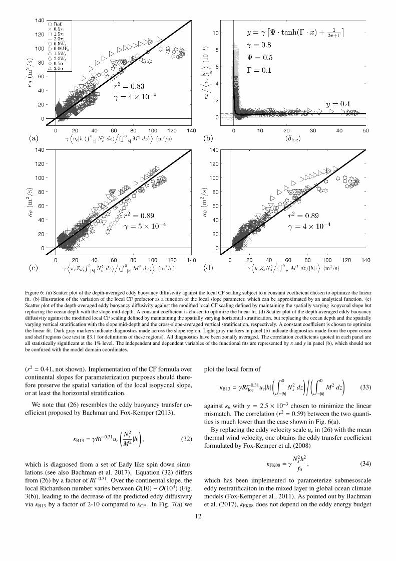
Figure 6: (a) Scatter plot of the depth-averaged eddy buoyancy diffusivity against the local CF scaling subject to a constant coefficient chosen to optimize the linearfit. (b) Illustration of the variation of the local CF prefactor as a function of the local slope parameter, which can be approximated by an analytical function. (c)Scatter plot of the depth-averaged eddy buoyancy diffusivity against the modified local CF scaling defined by maintaining the spatially varying isopycnal slope butreplacing the ocean depth with the slope mid-depth. A constant coefficient is chosen to optimize the linear fit. (d) Scatter plot of the depth-averaged eddy buoyancydiffusivity against the modified local CF scaling defined by maintaining the spatially varying horizontal stratification, but replacing the ocean depth and the spatiallyvarying vertical stratification with the slope mid-depth and the cross-slope-averaged vertical stratification, respectively. A constant coefficient is chosen to optimizethe linear fit. Dark gray markers indicate diagnostics made across the slope region. Light gray markers in panel (b) indicate diagnostics made from the open oceanand shelf regions (see text in §3.1 for definitions of these regions). All diagnostics have been zonally averaged. The correlation coefficients quoted in each panel areall statistically significant at the 1% level. The independent and dependent variables of the functional fits are represented by x and y in panel (b), which should notbe confused with the model domain coordinates.

(r2 = 0.41, not shown). Implementation of the CF formula overcontinental slopes for parameterization purposes should there-fore preserve the spatial variation of the local isopycnal slope,or at least the horizontal stratification.

We note that (26) resembles the eddy buoyancy transfer co-efficient proposed by Bachman and Fox-Kemper (2013),

κB13 = γRi−0.31ue

(N2

s

M2 |h|), (32)

which is diagnosed from a set of Eady-like spin-down simu-lations (see also Bachman et al. 2017). Equation (32) differsfrom (26) by a factor of Ri−0.31. Over the continental slope, thelocal Richardson number varies between O(10) − O(103) (Fig.3(b)), leading to the decrease of the predicted eddy diffusivityvia κB13 by a factor of 2-10 compared to κCF. In Fig. 7(a) we

plot the local form of

κB13 = γRi−0.31loc ue|h|

(∫ 0

−|h|N2

s dz) / (∫ 0

−|h|M2 dz

)(33)

against κθ with γ = 2.5 × 10−3 chosen to minimize the linearmismatch. The correlation (r2 = 0.59) between the two quanti-ties is much lower than the case shown in Fig. 6(a).

By replacing the eddy velocity scale ue in (26) with the meanthermal wind velocity, one obtains the eddy transfer coefficientformulated by Fox-Kemper et al. (2008)

κFK08 = γN2

s h2

f0, (34)

which has been implemented to parameterize submesoscaleeddy restratificaiton in the mixed layer in global ocean climatemodels (Fox-Kemper et al., 2011). As pointed out by Bachmanet al. (2017), κFK08 does not depend on the eddy energy budget

12

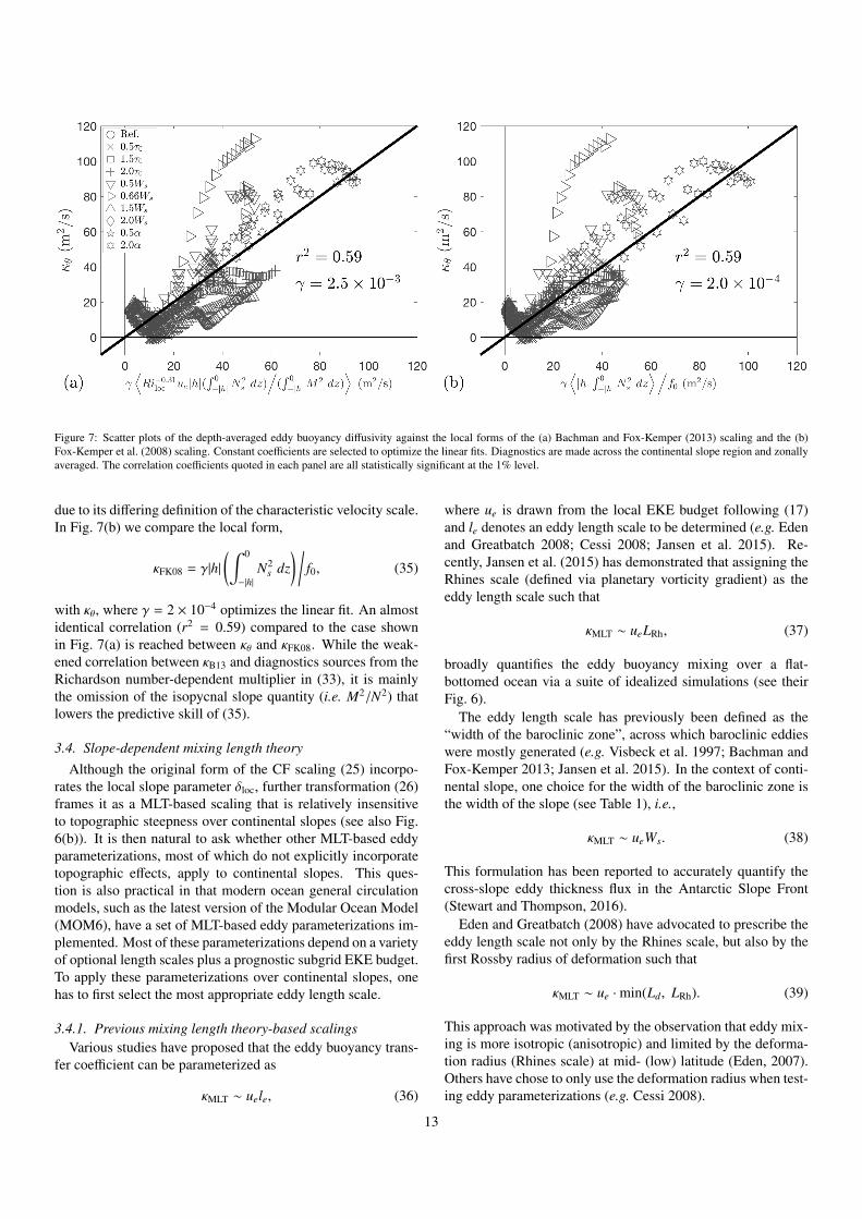
Figure 7: Scatter plots of the depth-averaged eddy buoyancy diffusivity against the local forms of the (a) Bachman and Fox-Kemper (2013) scaling and the (b)Fox-Kemper et al. (2008) scaling. Constant coefficients are selected to optimize the linear fits. Diagnostics are made across the continental slope region and zonallyaveraged. The correlation coefficients quoted in each panel are all statistically significant at the 1% level.

due to its differing definition of the characteristic velocity scale.In Fig. 7(b) we compare the local form,

κFK08 = γ|h|(∫ 0

−|h|N2

s dz) /

f0, (35)

with κθ, where γ = 2 × 10−4 optimizes the linear fit. An almostidentical correlation (r2 = 0.59) compared to the case shownin Fig. 7(a) is reached between κθ and κFK08. While the weak-ened correlation between κB13 and diagnostics sources from theRichardson number-dependent multiplier in (33), it is mainlythe omission of the isopycnal slope quantity (i.e. M2/N2) thatlowers the predictive skill of (35).

3.4. Slope-dependent mixing length theoryAlthough the original form of the CF scaling (25) incorpo-

rates the local slope parameter δloc, further transformation (26)frames it as a MLT-based scaling that is relatively insensitiveto topographic steepness over continental slopes (see also Fig.6(b)). It is then natural to ask whether other MLT-based eddyparameterizations, most of which do not explicitly incorporatetopographic effects, apply to continental slopes. This ques-tion is also practical in that modern ocean general circulationmodels, such as the latest version of the Modular Ocean Model(MOM6), have a set of MLT-based eddy parameterizations im-plemented. Most of these parameterizations depend on a varietyof optional length scales plus a prognostic subgrid EKE budget.To apply these parameterizations over continental slopes, onehas to first select the most appropriate eddy length scale.

3.4.1. Previous mixing length theory-based scalingsVarious studies have proposed that the eddy buoyancy trans-

fer coefficient can be parameterized as

κMLT ∼ uele, (36)

where ue is drawn from the local EKE budget following (17)and le denotes an eddy length scale to be determined (e.g. Edenand Greatbatch 2008; Cessi 2008; Jansen et al. 2015). Re-cently, Jansen et al. (2015) has demonstrated that assigning theRhines scale (defined via planetary vorticity gradient) as theeddy length scale such that

κMLT ∼ ueLRh, (37)

broadly quantifies the eddy buoyancy mixing over a flat-bottomed ocean via a suite of idealized simulations (see theirFig. 6).

The eddy length scale has previously been defined as the“width of the baroclinic zone”, across which baroclinic eddieswere mostly generated (e.g. Visbeck et al. 1997; Bachman andFox-Kemper 2013; Jansen et al. 2015). In the context of conti-nental slope, one choice for the width of the baroclinic zone isthe width of the slope (see Table 1), i.e.,

κMLT ∼ ueWs. (38)

This formulation has been reported to accurately quantify thecross-slope eddy thickness flux in the Antarctic Slope Front(Stewart and Thompson, 2016).

Eden and Greatbatch (2008) have advocated to prescribe theeddy length scale not only by the Rhines scale, but also by thefirst Rossby radius of deformation such that

κMLT ∼ ue ·min(Ld, LRh). (39)

This approach was motivated by the observation that eddy mix-ing is more isotropic (anisotropic) and limited by the deforma-tion radius (Rhines scale) at mid- (low) latitude (Eden, 2007).Others have chose to only use the deformation radius when test-ing eddy parameterizations (e.g. Cessi 2008).

13

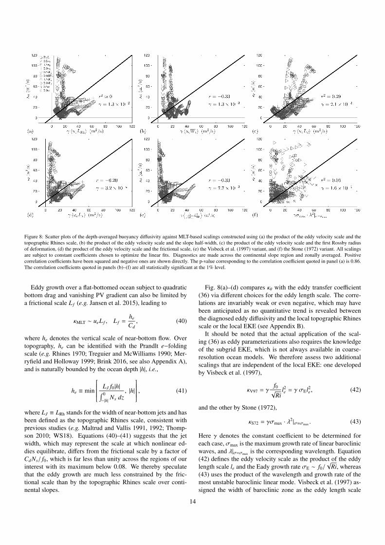
Figure 8: Scatter plots of the depth-averaged buoyancy diffusivity against MLT-based scalings constructed using (a) the product of the eddy velocity scale and thetopographic Rhines scale, (b) the product of the eddy velocity scale and the slope half-width, (c) the product of the eddy velocity scale and the first Rossby radiusof deformation, (d) the product of the eddy velocity scale and the frictional scale, (e) the Visbeck et al. (1997) variant, and (f) the Stone (1972) variant. All scalingsare subject to constant coefficients chosen to optimize the linear fits. Diagnostics are made across the continental slope region and zonally averaged. Positivecorrelation coefficients have been squared and negative ones are shown directly. The p-value corresponding to the correlation coefficient quoted in panel (a) is 0.86.The correlation coefficients quoted in panels (b)–(f) are all statistically significant at the 1% level.

Eddy growth over a flat-bottomed ocean subject to quadraticbottom drag and vanishing PV gradient can also be limited bya frictional scale L f (e.g. Jansen et al. 2015), leading to

κMLT ∼ ueL f , L f =he

Cd, (40)

where he denotes the vertical scale of near-bottom flow. Overtopography, he can be identified with the Prandlt e−foldingscale (e.g. Rhines 1970; Treguier and McWilliams 1990; Mer-ryfield and Holloway 1999; Brink 2016, see also Appendix A),and is naturally bounded by the ocean depth |h|, i.e.,

he ≡ min

LJ f0|h|∫ 0−|h| Ns dz

, |h|

, (41)

where LJ ≡ LRh stands for the width of near-bottom jets and hasbeen defined as the topographic Rhines scale, consistent withprevious studies (e.g. Maltrud and Vallis 1991, 1992; Thomp-son 2010; WS18). Equations (40)–(41) suggests that the jetwidth, which may represent the scale at which nonlinear ed-dies equilibrate, differs from the frictional scale by a factor ofCdNs/ f0, which is far less than unity across the regions of ourinterest with its maximum below 0.08. We thereby speculatethat the eddy growth are much less constrained by the fric-tional scale than by the topographic Rhines scale over conti-nental slopes.

Fig. 8(a)–(d) compares κθ with the eddy transfer coefficient(36) via different choices for the eddy length scale. The corre-lations are invariably weak or even negative, which may havebeen anticipated as no quantitative trend is revealed betweenthe diagnosed eddy diffusivity and the local topographic Rhinesscale or the local EKE (see Appendix B).

It should be noted that the actual application of the scal-ing (36) as eddy parameterizations also requires the knowledgeof the subgrid EKE, which is not always available in coarse-resolution ocean models. We therefore assess two additionalscalings that are independent of the local EKE: one developedby Visbeck et al. (1997),

κV97 = γf0√

Ril2e = γ σEl2e , (42)

and the other by Stone (1972),

κS72 = γσmax · λ2|σ=σmax . (43)

Here γ denotes the constant coefficient to be determined foreach case, σmax is the maximum growth rate of linear baroclinicwaves, and λ|σ=σmax is the corresponding wavelength. Equation(42) defines the eddy velocity scale as the product of the eddylength scale le and the Eady growth rate σE ∼ f0/

√Ri, whereas

(43) uses the product of the wavelength and growth rate of themost unstable baroclinic linear mode. Visbeck et al. (1997) as-signed the width of baroclinic zone as the eddy length scale

14

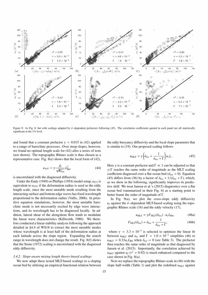
Figure 9: As Fig. 8, but with scalings adapted by δ−dependent prefactors following (45). The correlation coefficients quoted in each panel are all statisticallysignificant at the 1% level.

and found that a constant prefactor γ = 0.015 in (42) appliedto a range of baroclinic processes. Over steep slopes, however,we found no optimal length scale for (42) after a series of tests(not shown). The topographic Rhines scale is thus chosen as arepresentative case. Fig. 8(e) shows that the local form of (42),

κV97 = γf0√

RilocL2

Rh, (44)

is uncorrelated with the diagnosed diffusivity.Under the Eady (1949) or Phillips (1954) model setup, κS72 is

equivalent to κV97 if the deformation radius is used as the eddylength scale, since the most unstable mode resulting from theinteracting surface and bottom edge waves has fixed wavelengthproportional to the deformation radius (Vallis, 2006). In prim-itive equation simulations, however, the most unstable baro-clinic mode is not necessarily excited by edge wave interac-tions, and its wavelength has to be diagnosed locally. In ad-dition, lateral shear of the alongshore flow tends to modulatethe linear wave characteristics (Killworth, 1980). We there-fore conducted a linear stability analysis following the approachdetailed in §4.4 of WS18 to extract the most unstable modeswhose wavelength is at least half of the deformation radius ateach latitude across the slope region. Expanding the searchrange in wavelength does not change the result. Fig. 8(f) showsthat the Stone (1972) scaling is uncorrelated with the diagnosededdy diffusivity.

3.4.2. Slope-aware mixing length theory-based scalingsWe now adapt these tested MLT-based scalings to a sloping

ocean bed by utilizing an empirical functional relation between

the eddy buoyancy diffusivity and the local slope parameter thatis similar to (19). Our proposed scaling follows

κMLT = γ

(δloc +

1δloc + Γ

)uele. (45)

Here γ is a constant prefactor and Γ � 1 can be adjusted so thatγ/Γ reaches the same order of magnitude as the MLT scalingcoefficient diagnosed over a flat ocean bed (δloc = 0). Equation(45) differs from (36) by a factor of δloc + 1/(δloc + Γ), which,as we show in the following, significantly improves its predic-tive skill. We treat Jansen et al.’s (2015) diagnostics over a flatocean bed (summarized in their Fig. 6) as a starting point tobetter frame the order of magnitude of Γ.

In Fig. 9(a), we plot the cross-slope eddy diffusivityκθ against the δ−dependent MLT-based scaling using the topo-graphic Rhines scale (16) and the eddy velocity (17),

κMLT = γFMLT(δloc) · ueLRh, (46a)

FMLT(δloc) = δloc +1

δloc + Γ, (46b)

where γ = 3.3 × 10−3 is selected to optimize the linear fitbetween κMLT and κθ, and Γ = 1.0 × 10−2 simplifies (46) toκMLT = 0.33ueLRh when δloc→ 0 (see Table 3). The prefactorthen reaches the same order of magnitude as that diagnosed byJansen et al. (2015). Importantly, the correlation achieved byκMLT against κθ (r2 = 0.92) is much enhanced compared to thecase shown in Fig. 8(a).

Next we replace the topographic Rhines scale in (46) with theslope half-width (Table 1) and plot the redefined κMLT against

15

κθ in Fig. 9(b). The prefactor γ = 4.0 × 10−4 is again chosen tooptimize the diagnosis-scaling linear fit, which combined withΓ = 1.0 × 10−2 makes the prefactor asymptote to 4.0 × 10−2

in the flat bottom-limit, consistent with the value diagnosed byJansen et al. (2015) when the “baroclinic width” was chosenas their eddy mixing length. The correlation between κθ andκMLT (r2 = 0.82) slightly drops compared to the case shown inFig. 9(a).

Over steep slopes, the topographic Rhines scale is compara-ble in magnitude to the first Rossby radius of deformation dueto the suppressed eddy velocity scale and the increase of topo-graphic PV gradient. In Fig. 9(c), we plot the relationship be-tween the slope-aware κMLT, with LRh substituted by Ld in (46),and the diagnosed eddy diffusivity. Here γ = 1.9 × 10−3 hasthe same order of magnitude as the prefactor when LRh servesas the mixing length. However, Γ = 1.0 × 10−3 makes the fullcoefficient of κMLT approach O (1) in the flat-bottomed ocean,similar to the magnitude diagnosed by Jansen et al. (2015). Thecorrelation is similarly strong (r2 = 0.90) as in the case shownin Fig. 9(a).

Although we expect that the frictional scale to be less rel-evant over steep slopes, adopting L f as the mixing length in(46) and assuming that LJ = LRh in (41) nevertheless yield astrong correlation between κMLT and κθ (r2 = 0.83), as shownin Fig. 9(d). The prefactor has again been adjusted to optimizethe diagnosis-scaling linear fit and to account for the magnitudeof the MLT-based scaling reported by Jansen et al. (2015). Thestrong correlation does not imply that the eddy mixing is fric-tionally controlled over steep slopes, but rather that the local

buoyancy frequency(∫ 0−|h| Ns dz

) /|h| does not vary significantly

(the variation is within a factor of 2 across the entire channel),leading to L f ∼ LRh based on (40)–(41).

Fig. 9(a)–(d) indicates that the scaling (45) is insensitive tothe eddy length scale chosen over steep slopes, as long as theeddy velocity scale ue is used. Implementation of (45) shouldtherefore prioritize the optimal mixing length scale that makesthe scaling transition smoothly from the slope toward the openocean. If the diagnostics from the open ocean (both the shelfand the open ocean) are included in the comparison, the corre-lation of the Rhines scale-based κMLT (46) with the diagnoseddiffusivity reduces to r2 = 0.79 (r2 = 0.65), as shown in Fig.5(c). Defining the frictional length scale, which is partly de-pendent on the topographic Rhines scale, as the mixing lengthin (45) slightly modifies the diagnosis-scaling correlation: thecorrelation coefficient is r2 = 0.71 if the open ocean is includedand r2 = 0.52 if both the shelf and the open ocean are included(not shown). In contrast, neither the deformation radius nor theslope half-width produces a diagnosis-scaling correlation bet-ter than r2 = 0.06 if the open ocean diagnostics are included.Our findings therefore suggest that the Rhines scale is the mostsuitable choice for the eddy mixing length, mirroring findingsof Jansen et al. (2015) in the context of a flat-bottomed ocean.

In Fig. 9(e)–(f) we also test the slope-aware forms of the localVisbeck et al. (1997) scaling

κV97 = γFMLT ·f0√

RilocL2

Rh, (47)

and the local Stone (1972) scaling

κS72 = γFMLT · σmax · λ2|σ=σmax . (48)

These formulations do not show significant improvements inpredictive skill compared to their slope-unaware counterparts.Our findings suggest that accurate implementation of the MLT-based scaling for steep slopes depends crucially on the subgridEKE budget.

4. Impact of along-slope topographic variations

§3.2–§3.4 suggest that eddy buoyancy mixing across con-tinental slopes can be reproduced via the GEOMETRIC scal-ing, the CF scaling, or the δ−dependent MLT-based scalingthat incorporates the eddy velocity scale ue and the topographicRhines scale LRh. While both the GEOMETRIC scaling andthe CF scaling are able to quantify the eddy transfer acrosssteep slopes with suitably-chosen constant prefactors, they re-quire δ-dependent prefactors to transition from the slope tothe open ocean. In this section, we investigate the extent towhich these slope-aware scaling frameworks apply to continen-tal slopes featuring topographic canyons and ridges, over whichstanding meanders lead to stronger restratification, and the to-pographically induced prograde flows tend to penetrate to theupper ocean (c.f. §2.3).

4.1. Meridional vs cross-isobath eddy mixingIn the context of corrugated continental slope, we face a

choice as whether to compare the scalings with the eddy buoy-ancy diffusivity directed across meridians (9a) or across iso-baths (10a). To address this, we first assess the functionaldependence of eddy diffusivity on the two most crucial non-dimensional parameters over steep slopes: the local slope pa-rameter and the local Richardson number (c.f. §3.1). There issome freedom in defining these two parameters in the presenceof canyons/ridges because the mean geostrophic currents do notfollow the isobaths (Fig. 1(b)). One choice would be to com-pletely neglect the zonal variations in the topography and meanflow, and define these two parameters via the meridional com-ponents of the mean buoyancy and bathymetry gradients. How-ever, the resulting δloc and Riloc exhibit no correlation with themeridional eddy buoyancy transfer (not shown). Instead, weuse the local slope parameter and the local Richardson num-ber defined by (11) and (12), respectively. That is, we ignorethe cross-isobath part of the mean flow, and assume that theeddy buoyancy transfer, either in the meridional direction or inthe cross-isobath direction, is determined by the along-isobathcomponent of the large-scale geostrophic current.

In Fig 10(a), we compare the zonally averaged slope param-eter 〈δloc〉 with the meridional eddy buoyancy diffusivity κθ.Diagnostics have been drawn from three zonal regions acrossthe channel: (i) the region peripheral to the northern/southernslope regions with ocean depths between 510 m and 3990 m andlying south of y = 450 km, (ii) the northern/southern slope re-gions, and (iii) the central slope region. Diagnostics from theseregions have been plotted with light gray, dark gray, and blue

16

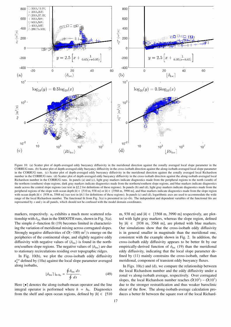
Figure 10: (a) Scatter plot of depth-averaged eddy buoyancy diffusivity in the meridional direction against the zonally averaged local slope parameter in theCORRUG runs. (b) Scatter plot of depth-averaged eddy buoyancy diffusivity in the cross-isobath direction against the along-isobath-averaged local slope parameterin the CORRUG runs. (c) Scatter plot of depth-averaged eddy buoyancy diffusivity in the meridional direction against the zonally averaged local Richardsonnumber in the CORRUG runs. (d) Scatter plot of depth-averaged eddy buoyancy diffusivity in the cross-isobath direction against the along-isobath-averaged localRichardson number in the CORRUG runs. In panels (a) and (c), light gray markers indicate diagnostics made from the peripheral regions to the north (south) ofthe northern (southern) slope regions, dark gray markers indicate diagnostics made from the northern/southern slope regions, and blue markers indicate diagnosticsmade across the central slope regions (see text in §2.2 for definitions of these regions). In panels (b) and (d), light gray markers indicate diagnostics made from theperipheral regions of the slope with ocean depth |h| ∈ [510 m, 938 m] or |h| ∈ [3568 m, 3990 m], and blue markers indicate diagnostics made from the slope regionwith ocean depth |h| ∈ [938 m, 3568 m] (see text in §4.1 for definitions of these regions). In panels (c) and (d), logarithmic axes are used to accommodate the widerange of the local Richardson number. The functional fit from Fig. 3(a) is presented in (a)–(b). The independent and dependent variables of the functional fits arerepresented by x and y in all panels, which should not be confused with the model domain coordinates.

markers, respectively. κθ exhibits a much more scattered rela-tionship with δloc than in the SMOOTH runs, shown in Fig. 3(a).The simple δ−function fit (19) becomes limited in characteriz-ing the variation of meridional mixing across corrugated slopes.Strongly negative diffusivities of O(−100) m2/s emerge on theperipheries of the continental slope, and slightly negative eddydiffusivity with negative values of 〈δloc〉 is found in the north-ern/southen slope regions. The negative values of 〈δloc〉 are dueto stationary recirculations residing over topographic ridges.

In Fig. 10(b), we plot the cross-isobath eddy diffusivityκisoθ defined by (10a) against the local slope parameter averaged

along isobaths,

bδloce |h=h0 =

∮δloc ds∮

ds. (49)

Here b•e denotes the along-isobath-mean operator and the lineintegral operator is performed where h = h0. Diagnosticsfrom the shelf and open ocean regions, defined by |h| ∈ [510

m, 938 m] and |h| ∈ [3568 m, 3990 m] respectively, are plot-ted with light gray markers, whereas the slope region, definedby |h| ∈ [938 m, 3568 m], are plotted with blue markers.Our simulations show that the cross-isobath eddy diffusivityis in general smaller in magnitude than the meridional one,consistent with the example shown in Fig. 2. In addition, thecross-isobath eddy diffusivity appears to be better fit by ourempirically-derived function of δloc (19) than the meridionaleddy diffusivity, indicating that the local slope parameter de-fined by (11) mainly constrains the cross-isobath, rather thanmeridional, component of transient eddy buoyancy fluxes.

In Figs. 10(c) and (d), we compare the relationship betweenthe local Richardson number and the eddy diffusivity under azonal vs along-isobath average, respectively. Over corrugatedslopes, the local Richardson number reaches O(102) − O(107)due to the stronger restratification and thus weaker baroclinicshear of the flow. The along-isobath-average calculation pro-duces a better fit between the square root of the local Richard-

17

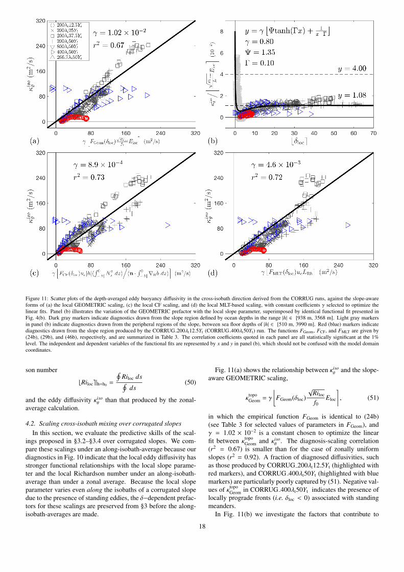
Figure 11: Scatter plots of the depth-averaged eddy buoyancy diffusivity in the cross-isobath direction derived from the CORRUG runs, against the slope-awareforms of (a) the local GEOMETRIC scaling, (c) the local CF scaling, and (d) the local MLT-based scaling, with constant coefficients γ selected to optimize thelinear fits. Panel (b) illustrates the variation of the GEOMETRIC prefactor with the local slope parameter, superimposed by identical functional fit presented inFig. 4(b). Dark gray markers indicate diagnostics drawn from the slope region defined by ocean depths in the range |h| ∈ [938 m, 3568 m]. Light gray markersin panel (b) indicate diagnostics drawn from the peripheral regions of the slope, between sea floor depths of |h| ∈ [510 m, 3990 m]. Red (blue) markers indicatediagnostics drawn from the slope region produced by the CORRUG 200λt12.5Yt (CORRUG 400λt50Yt) run. The functions FGeom, FCF, and FMLT are given by(24b), (29b), and (46b), respectively, and are summarized in Table 3. The correlation coefficients quoted in each panel are all statistically significant at the 1%level. The independent and dependent variables of the functional fits are represented by x and y in panel (b), which should not be confused with the model domaincoordinates.

son number

bRiloce|h=h0 =

∮Riloc ds∮

ds(50)

and the eddy diffusivity κisoθ than that produced by the zonal-

average calculation.

4.2. Scaling cross-isobath mixing over corrugated slopesIn this section, we evaluate the predictive skills of the scal-

ings proposed in §3.2–§3.4 over corrugated slopes. We com-pare these scalings under an along-isobath-average because ourdiagnostics in Fig. 10 indicate that the local eddy diffusivity hasstronger functional relationships with the local slope parame-ter and the local Richardson number under an along-isobath-average than under a zonal average. Because the local slopeparameter varies even along the isobaths of a corrugated slopedue to the presence of standing eddies, the δ−dependent prefac-tors for these scalings are preserved from §3 before the along-isobath-averages are made.

Fig. 11(a) shows the relationship between κisoθ and the slope-

aware GEOMETRIC scaling,

κtopoGeom = γ

⌊FGeom(δloc)

√Riloc

f0Eloc

⌉, (51)

in which the empirical function FGeom is identical to (24b)(see Table 3 for selected values of parameters in FGeom), andγ = 1.02 × 10−2 is a constant chosen to optimize the linearfit between κ

topoGeom and κiso

θ . The diagnosis-scaling correlation(r2 = 0.67) is smaller than for the case of zonally uniformslopes (r2 = 0.92). A fraction of diagnosed diffusivities, suchas those produced by CORRUG 200λt12.5Yt (highlighted withred markers), and CORRUG 400λt50Yt (highlighted with bluemarkers) are particularly poorly captured by (51). Negative val-ues of κtopo

Geom in CORRUG 400λt50Yt indicates the presence oflocally prograde fronts (i.e. δloc < 0) associated with standingmeanders.

In Fig. 11(b) we investigate the factors that contribute to

18

the diversion of diagnosed eddy diffusivity from the theoret-ical prediction by plotting the diagnosed GEOMETRIC pref-actor against the local slope parameter, as in Fig. 4(b). Thisplot shows that the empirical relation between γGeom and δloc inthe SMOOTH simulations approximately applies to the COR-RUG simulations. However, as the ocean bed becomes steeper,the diagnosed prefactor exhibits more scatter in the CORRUGsimulations than in the SMOOTH simulations. Specifically, for〈δloc〉 > 10, the diagnosed GEOMETRIC prefactor ranges be-tween [0.94, 1.84] in the SMOOTH simulations but between[0.06, 1.87] in the CORRUG simulations.

In Fig. 11(c) we plot κisoθ against the slope-aware CF scaling,

κtopoCF = γ

FCF(δloc)ue|h|

∫ 0−|h| N

2s dz∣∣∣∣n · ∫ 0

−|h| ∇hb dz∣∣∣∣ , (52)

in which n = −∇Hh/|∇Hh|, FCF is identical to (29b) (see Table3 for selected values of parameters in FCF), and γ = 8.9 × 10−4

is selected to optimize the linear fit. The diagnosis-scaling cor-relation (r2 = 0.73) is slightly stronger than that in Fig. 11(a),but remains weaker than for the case of zonally uniform slopes(r2 = 0.86). As in the GEOMETRIC case, the weaker agree-ment between the diagnosed diffusivity and the scaling (52)shown in Fig. 11(c) is partly due to the outlying results fromCORRUG 200λt12.5Yt and CORRUG 400λt50Yt.

In Fig. 11(d) we contrast κisoθ against the slope aware MLT-

based scaling

κtopoMLT = γ bFMLT(δloc)ueLRhe , (53)

in which FMLT is identical to (46b) (see Table 3 for selectedvalue of parameter in FMLT), and γ = 4.6 × 10−3 optimizesthe linear fit. The diagnosis-scaling correlation (r2 = 0.72) iscomparable to those produced by the GEOMETRIC and the CFscalings. The weaker agreement between the diagnosed dif-fusivity and the scaling (53) contrasted to the SMOOTH case(r2 = 0.92) is again partly attributed to the outlying results fromCORRUG 200λt12.5Yt and CORRUG 400λt50Yt.

4.3. Cross-slope-averaged scaling of cross-slope eddy mixing

In the flat-bottomed ocean context, Jansen et al. (2015) pro-posed a parameterization using the bulk-averaged eddy mixingover an entire baroclinic zone, rather than using horizontally-local properties. This approach may also be favored over con-tinental slopes, as topographic corrugation leads to increasedscatter of the diagnosed eddy diffusivity against the scalingsproposed in this study (see Fig. 11). In addition, WS18have shown that the eddy energy transfer becomes non-local(e.g. Chen et al. 2014) across steep slopes, and any closureof the subgrid eddy energy, from which the eddy velocity isprovided, based on the local production/dissipation balance(e.g. Cessi 2008) may become inaccurate. In Fig. 12, we plotthe diagnosed cross-isobath eddy diffusivity {κiso

θ } against thethree slope-aware scalings after averaging over the continentalslope regions, defined by ocean depths in the range |h| ∈ [938m, 3568 m], where {•} denotes the bulk area-mean operator.

Diagnostics from both the SMOOTH (black markers) and theCORRUG (blue markers) simulations are included. All threescalings produce strong correlations (r2 > 0.80) with the diag-nosed diffusivity across our suite of simulations. The bulk eddytransfer coefficients in the SMOOTH simulations are particu-larly closely reproduced, with correlations exceeding r2 = 0.89,and reaching r2 = 0.98 for the MLT case.

5. Discussion and conclusion

Accurate representation of mesoscale eddy effects in coarse-resolution ocean climate models remains a pressing challengefor the oceanographic community. Mid-latitude mesoscale ed-dies over continental slopes, in particular, cannot be resolvedeven in eddy-permitting global ocean models (Hallberg, 2013).Existing approaches of eddy parameterization have mostly beendeveloped based on the open ocean turbulent properties and arethus independent of the bottom topography, which may lead toincorrect water mass formations and adjustment of ocean gen-eral circulations over continental slopes.

In this article, we have examined three numerically imple-mentable scalings for eddy buoyancy transfer across retrogradeslope fronts: the GEOMETRIC scaling originally developed byMarshall et al. (2012), a new Cross-Front scaling derived via di-mensional analysis, and the mixing length theory (MTL)-basedscaling (Prandtl, 1925). We demonstrate that both the GEO-METRIC framework and the CF scaling are capable of quan-tifying the eddy diffusivity over the continental slope, in isola-tion, following the selection of suitable constant prefactor co-efficients. However, in order to capture the eddy mixing acrossboth the continental slope and the open ocean, all three scalingapproaches require the insertion of a prefactor that depends onthe slope parameter δ.

We have shown that by making the prefactor a simple analyti-cal function of the local slope parameter, each of these scalingsis able to reproduce the depth-averaged eddy mixing over theslope and in the open ocean (c.f. Fig. 5). However, over conti-nental shelves, the eddy transfer coefficients are much less wellcaptured by these scalings. The reason for this is unclear andmust be addressed in future work based on the studies focus-ing on continental shelves (e.g. Brink 2016). It should be notedthat the continental shelves in our simulations are set to be un-realistically deep in order to isolate the cross-slope eddy fluxes,and therefore may have limited applicability to cross-shelf eddyfluxes.

Table 3 summarizes our proposed slope-aware scalings, withparameter values chosen based on our cross-slope-averaged cal-culation (Fig. 12), which maximizes the agreements betweenthe scalings and the diagnosed eddy diffusivity. The prefactorfor both the GEOMETRIC framework and the CF scaling canbe constructed as the sum of a sigmoid function (e.g. hyperbolictangent in this study) and a decay function (e.g. reciprocal func-tion in this study) of the local slope parameter, which convergeto empirical constants over the flat ocean bed and over steepslopes. For MLT-based scaling, we propose a linear functionof δloc combined with a decay function. However, this func-tion becomes unbounded if the isopycnals are completely flat

19

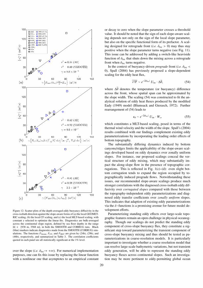
Figure 12: Scatter plots of the depth-averaged eddy buoyancy diffusivity in thecross-isobath direction against the slope-aware forms of (a) the local GEOMET-RIC scaling, (b) the local CF scaling, and (c) the local MLT-based scaling, withconstant γ selected to optimize the linear fits. Diagnostics are bulk-averagedacross the continental slope region, defined by sea floor depths in the range|h| ∈ [938 m, 3568 m], in both the SMOOTH and CORRUG runs. Black(blue) markers indicate diagnostics made from the SMOOTH (CORRUG) sim-ulations. The functions FGeom, FCF, and FMLT are given by (24b), (29b), and(46b), respectively, and summarized in Table 3. The correlation coefficientsquoted in each panel are all statistically significant at the 1% level.

over the slope (i.e. δloc→ +∞). For numerical implementationpurposes, one can fix this issue by replacing the linear functionwith a nonlinear one that asymptotes to an empirical constant

or decay to zero when the slope parameter crosses a thresholdvalue. It should be noted that the sign of each slope-aware scal-ing depends not only on the sign of the local slope parameter,but also on the specific functional form of its prefactor. A scal-ing designed for retrograde front (i.e. δloc > 0) may thus staypositive when the slope parameter turns negative (see Fig. 11).This issue can be addressed by adding a switch-like heavisidefunction of δloc that shuts down the mixing across a retrogradefront when δloc turns negative.

In the context of buoyancy-driven prograde front (i.e. δloc <0), Spall (2004) has previously proposed a slope-dependentscaling for the eddy heat flux,

v′θ′ ∼ e−2|δloc | Utw · ∆θ, (54)

where ∆θ denotes the temperature (or buoyancy) differenceacross the front, whose spatial span can be approximated bythe slope width. The scaling (54) was constructed to fit the an-alytical solution of eddy heat fluxes produced by the modifiedEady (1949) model (Blumsack and Gierasch, 1972). Furtherrearrangement of (54) leads to

κθ ∼ e−2|δloc | Utw ·Ws, (55)

which constitutes a MLT-based scaling, posed in terms of thethermal wind velocity and the width of the slope. Spall’s (2004)results combined with our findings complement existing eddyparameterizations by incorporating the leading order effects ofbottom topography.

The substantially differing dynamics induced by bottomcanyons/ridges limits the applicability of the slope-aware scal-ings developed based on eddy dynamics over zonally uniformslopes. For instance, our proposed scalings conceal the ver-tical structure of eddy mixing, which may substantially im-pact the along-slope flow in the presence of topographic cor-rugations. This is reflected in Fig. 1(c)–(d): even slight bot-tom corrugation tends to expand the region occupied by to-pographically induced prograde flows. Notwithstanding theseissues, our recommended slope-aware scalings produce muchstronger correlations with the diagnosed cross-isobath eddy dif-fusivity over corrugated slopes compared with those betweenthe topography-independent eddy parameterizations and diag-nosed eddy transfer coefficients over zonally uniform slopes.This indicates that adaption of existing eddy parameterizationsvia the δ−functions is a promising avenue for future model de-velopment efforts.

Parameterizing standing eddy effects over large-scale topo-graphic features remain an open challenge in physical oceanog-raphy. Though our scalings do not predict the standing eddycomponent of cross-slope buoyancy flux, they constitute a sig-nificant step toward parameterizing the transient component ofcross-slope buoyancy mixing and thus should be tested as pa-rameterizations in coarse-resolution models. It is particularlyimportant to investigate whether a coarse resolution model thatcan resolve large-scale bathymetric variations, but not transienteddy generation, will be able to represent the standing eddybuoyancy fluxes across continental slopes. Such an investiga-tion may be more pertinent to eddy-permitting global ocean

20

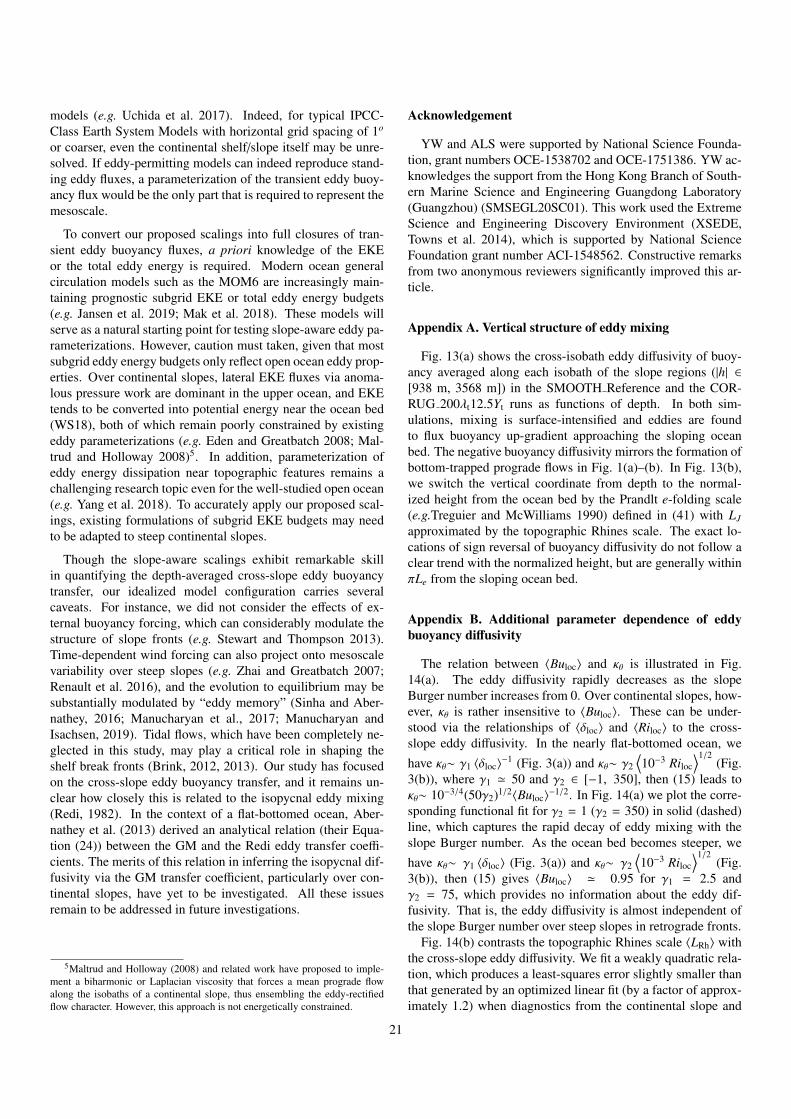
models (e.g. Uchida et al. 2017). Indeed, for typical IPCC-Class Earth System Models with horizontal grid spacing of 1o

or coarser, even the continental shelf/slope itself may be unre-solved. If eddy-permitting models can indeed reproduce stand-ing eddy fluxes, a parameterization of the transient eddy buoy-ancy flux would be the only part that is required to represent themesoscale.

To convert our proposed scalings into full closures of tran-sient eddy buoyancy fluxes, a priori knowledge of the EKEor the total eddy energy is required. Modern ocean generalcirculation models such as the MOM6 are increasingly main-taining prognostic subgrid EKE or total eddy energy budgets(e.g. Jansen et al. 2019; Mak et al. 2018). These models willserve as a natural starting point for testing slope-aware eddy pa-rameterizations. However, caution must taken, given that mostsubgrid eddy energy budgets only reflect open ocean eddy prop-erties. Over continental slopes, lateral EKE fluxes via anoma-lous pressure work are dominant in the upper ocean, and EKEtends to be converted into potential energy near the ocean bed(WS18), both of which remain poorly constrained by existingeddy parameterizations (e.g. Eden and Greatbatch 2008; Mal-trud and Holloway 2008)5. In addition, parameterization ofeddy energy dissipation near topographic features remains achallenging research topic even for the well-studied open ocean(e.g. Yang et al. 2018). To accurately apply our proposed scal-ings, existing formulations of subgrid EKE budgets may needto be adapted to steep continental slopes.

Though the slope-aware scalings exhibit remarkable skillin quantifying the depth-averaged cross-slope eddy buoyancytransfer, our idealized model configuration carries severalcaveats. For instance, we did not consider the effects of ex-ternal buoyancy forcing, which can considerably modulate thestructure of slope fronts (e.g. Stewart and Thompson 2013).Time-dependent wind forcing can also project onto mesoscalevariability over steep slopes (e.g. Zhai and Greatbatch 2007;Renault et al. 2016), and the evolution to equilibrium may besubstantially modulated by “eddy memory” (Sinha and Aber-nathey, 2016; Manucharyan et al., 2017; Manucharyan andIsachsen, 2019). Tidal flows, which have been completely ne-glected in this study, may play a critical role in shaping theshelf break fronts (Brink, 2012, 2013). Our study has focusedon the cross-slope eddy buoyancy transfer, and it remains un-clear how closely this is related to the isopycnal eddy mixing(Redi, 1982). In the context of a flat-bottomed ocean, Aber-nathey et al. (2013) derived an analytical relation (their Equa-tion (24)) between the GM and the Redi eddy transfer coeffi-cients. The merits of this relation in inferring the isopycnal dif-fusivity via the GM transfer coefficient, particularly over con-tinental slopes, have yet to be investigated. All these issuesremain to be addressed in future investigations.

5Maltrud and Holloway (2008) and related work have proposed to imple-ment a biharmonic or Laplacian viscosity that forces a mean prograde flowalong the isobaths of a continental slope, thus ensembling the eddy-rectifiedflow character. However, this approach is not energetically constrained.

Acknowledgement

YW and ALS were supported by National Science Founda-tion, grant numbers OCE-1538702 and OCE-1751386. YW ac-knowledges the support from the Hong Kong Branch of South-ern Marine Science and Engineering Guangdong Laboratory(Guangzhou) (SMSEGL20SC01). This work used the ExtremeScience and Engineering Discovery Environment (XSEDE,Towns et al. 2014), which is supported by National ScienceFoundation grant number ACI-1548562. Constructive remarksfrom two anonymous reviewers significantly improved this ar-ticle.

Appendix A. Vertical structure of eddy mixing

Fig. 13(a) shows the cross-isobath eddy diffusivity of buoy-ancy averaged along each isobath of the slope regions (|h| ∈[938 m, 3568 m]) in the SMOOTH Reference and the COR-RUG 200λt12.5Yt runs as functions of depth. In both sim-ulations, mixing is surface-intensified and eddies are foundto flux buoyancy up-gradient approaching the sloping oceanbed. The negative buoyancy diffusivity mirrors the formation ofbottom-trapped prograde flows in Fig. 1(a)–(b). In Fig. 13(b),we switch the vertical coordinate from depth to the normal-ized height from the ocean bed by the Prandlt e-folding scale(e.g.Treguier and McWilliams 1990) defined in (41) with LJ

approximated by the topographic Rhines scale. The exact lo-cations of sign reversal of buoyancy diffusivity do not follow aclear trend with the normalized height, but are generally withinπLe from the sloping ocean bed.

Appendix B. Additional parameter dependence of eddybuoyancy diffusivity

The relation between 〈Buloc〉 and κθ is illustrated in Fig.14(a). The eddy diffusivity rapidly decreases as the slopeBurger number increases from 0. Over continental slopes, how-ever, κθ is rather insensitive to 〈Buloc〉. These can be under-stood via the relationships of 〈δloc〉 and 〈Riloc〉 to the cross-slope eddy diffusivity. In the nearly flat-bottomed ocean, wehave κθ∼ γ1 〈δloc〉

−1 (Fig. 3(a)) and κθ∼ γ2

⟨10−3 Riloc

⟩1/2(Fig.

3(b)), where γ1 ' 50 and γ2 ∈ [−1, 350], then (15) leads toκθ∼ 10−3/4(50γ2)1/2〈Buloc〉

−1/2. In Fig. 14(a) we plot the corre-sponding functional fit for γ2 = 1 (γ2 = 350) in solid (dashed)line, which captures the rapid decay of eddy mixing with theslope Burger number. As the ocean bed becomes steeper, wehave κθ∼ γ1 〈δloc〉 (Fig. 3(a)) and κθ∼ γ2

⟨10−3 Riloc

⟩1/2(Fig.

3(b)), then (15) gives 〈Buloc〉 ' 0.95 for γ1 = 2.5 andγ2 = 75, which provides no information about the eddy dif-fusivity. That is, the eddy diffusivity is almost independent ofthe slope Burger number over steep slopes in retrograde fronts.

Fig. 14(b) contrasts the topographic Rhines scale 〈LRh〉 withthe cross-slope eddy diffusivity. We fit a weakly quadratic rela-tion, which produces a least-squares error slightly smaller thanthat generated by an optimized linear fit (by a factor of approx-imately 1.2) when diagnostics from the continental slope and

21

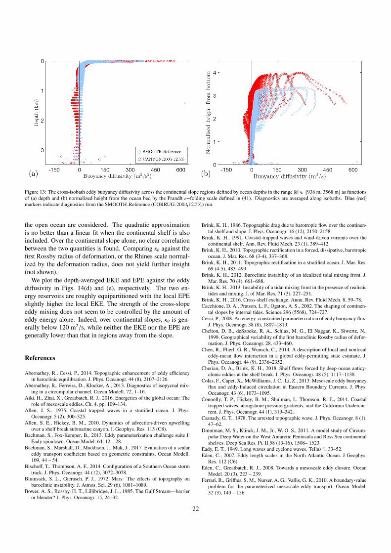
Figure 13: The cross-isobath eddy buoyancy diffusivity across the continental slope regions defined by ocean depths in the range |h| ∈ [938 m, 3568 m] as functionsof (a) depth and (b) normalized height from the ocean bed by the Prandlt e−folding scale defined in (41). Diagnostics are averaged along isobaths. Blue (red)markers indicate diagnostics from the SMOOTH Reference (CORRUG 200λt12.5Yt) run.

the open ocean are considered. The quadratic approximationis no better than a linear fit when the continental shelf is alsoincluded. Over the continental slope alone, no clear correlationbetween the two quantities is found. Comparing κθ against thefirst Rossby radius of deformation, or the Rhines scale normal-ized by the deformation radius, does not yield further insight(not shown).

We plot the depth-averaged EKE and EPE against the eddydiffusivity in Figs. 14(d) and (e), respectively. The two en-ergy reservoirs are roughly equipartitioned with the local EPEslightly higher the local EKE. The strength of the cross-slopeeddy mixing does not seem to be controlled by the amount ofeddy energy alone. Indeed, over continental slopes, κθ is gen-erally below 120 m2/s, while neither the EKE nor the EPE aregenerally lower than that in regions away from the slope.

References

Abernathey, R., Cessi, P., 2014. Topographic enhancement of eddy efficiencyin baroclinic equilibration. J. Phys. Oceanogr. 44 (8), 2107–2126.

Abernathey, R., Ferreira, D., Klocker, A., 2013. Diagnostics of isopycnal mix-ing in a circumpolar channel. Ocean Modell. 72, 1–16.

Aiki, H., Zhai, X., Greatbatch, R. J., 2016. Energetics of the global ocean: Therole of mesoscale eddies. Ch. 4, pp. 109–134.

Allen, J. S., 1975. Coastal trapped waves in a stratified ocean. J. Phys.Oceanogr. 5 (2), 300–325.

Allen, S. E., Hickey, B. M., 2010. Dynamics of advection-driven upwellingover a shelf break submarine canyon. J. Geophys. Res. 115 (C8).

Bachman, S., Fox-Kemper, B., 2013. Eddy parameterization challenge suite I:Eady spindown. Ocean Model. 64, 12 – 28.

Bachman, S., Marshall, D., Maddison, J., Mak, J., 2017. Evaluation of a scalareddy transport coefficient based on geometric constraints. Ocean Modell.109, 44 – 54.

Bischoff, T., Thompson, A. F., 2014. Configuration of a Southern Ocean stormtrack. J. Phys. Oceanogr. 44 (12), 3072–3078.

Blumsack, S. L., Gierasch, P. J., 1972. Mars: The effects of topography onbaroclinic instability. J. Atmos. Sci. 29 (6), 1081–1089.

Bower, A. S., Rossby, H. T., Lillibridge, J. L., 1985. The Gulf Stream—barrieror blender? J. Phys. Oceanogr. 15, 24–32.

Brink, K. H., 1986. Topographic drag due to barotropic flow over the continen-tal shelf and slope. J. Phys. Oceanogr. 16 (12), 2150–2158.

Brink, K. H., 1991. Coastal-trapped waves and wind-driven currents over thecontinental shelf. Ann. Rev. Fluid Mech. 23 (1), 389–412.

Brink, K. H., 2010. Topographic rectification in a forced, dissipative, barotropicocean. J. Mar. Res. 68 (3-4), 337–368.

Brink, K. H., 2011. Topographic rectification in a stratified ocean. J. Mar. Res.69 (4-5), 483–499.

Brink, K. H., 2012. Baroclinic instability of an idealized tidal mixing front. J.Mar. Res. 70 (4), 661–688.

Brink, K. H., 2013. Instability of a tidal mixing front in the presence of realistictides and mixing. J. of Mar. Res. 71 (3), 227–251.

Brink, K. H., 2016. Cross-shelf exchange. Annu. Rev. Fluid Mech. 8, 59–78.Cacchione, D. A., Pratson, L. F., Ogston, A. S., 2002. The shaping of continen-

tal slopes by internal tides. Science 296 (5568), 724–727.Cessi, P., 2008. An energy-constrained parameterization of eddy buoyancy flux.

J. Phys. Oceanogr. 38 (8), 1807–1819.Chelton, D. B., deSzoeke, R. A., Schlax, M. G., El Naggar, K., Siwertz, N.,

1998. Geographical variability of the first baroclinic Rossby radius of defor-mation. J. Phys. Oceanogr. 28, 433–460.

Chen, R., Flierl, G. R., Wunsch, C., 2014. A description of local and nonlocaleddy-mean flow interaction in a global eddy-permitting state estimate. J.Phys. Oceanogr. 44 (9), 2336–2352.

Cherian, D. A., Brink, K. H., 2018. Shelf flows forced by deep-ocean anticy-clonic eddies at the shelf break. J. Phys. Oceanogr. 48 (5), 1117–1138.

Colas, F., Capet, X., McWilliams, J. C., Li, Z., 2013. Mesoscale eddy buoyancyflux and eddy-Induced circulation in Eastern Boundary Currents. J. Phys.Oceanogr. 43 (6), 1073–1095.

Connolly, T. P., Hickey, B. M., Shulman, I., Thomson, R. E., 2014. Coastaltrapped waves, alongshore pressure gradients, and the California Undercur-rent. J. Phys. Oceanogr. 44 (1), 319–342.

Csanady, G. T., 1978. The arrested topographic wave. J. Phys. Oceanogr. 8 (1),47–62.

Dinniman, M. S., Klinck, J. M., Jr., W. O. S., 2011. A model study of Circum-polar Deep Water on the West Antarctic Peninsula and Ross Sea continentalshelves. Deep Sea Res. Pt. II 58 (13-16), 1508– 1523.

Eady, E. T., 1949. Long waves and cyclone waves. Tellus 1, 33–52.Eden, C., 2007. Eddy length scales in the North Atlantic Ocean. J Geophys.

Res. 112 (C6).Eden, C., Greatbatch, R. J., 2008. Towards a mesoscale eddy closure. Ocean

Model. 20 (3), 223 – 239.Ferrari, R., Griffies, S. M., Nurser, A. G., Vallis, G. K., 2010. A boundary-value

problem for the parameterized mesoscale eddy transport. Ocean Model.32 (3), 143 – 156.

22

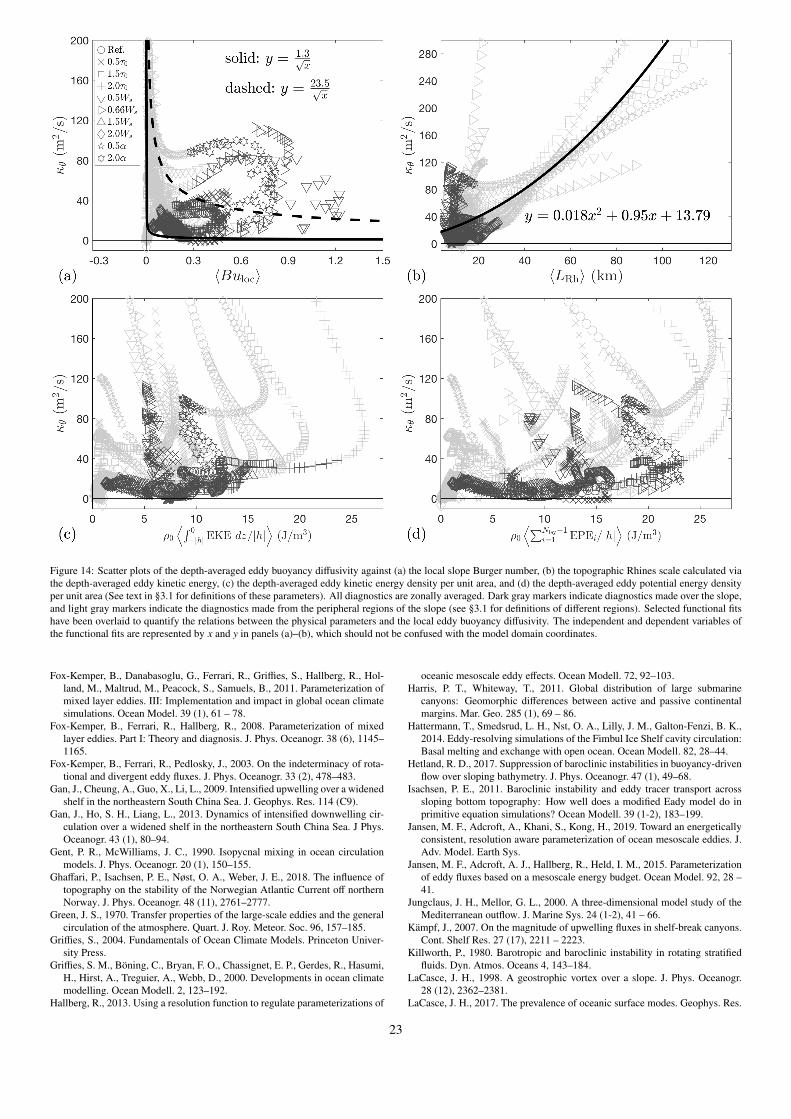
Figure 14: Scatter plots of the depth-averaged eddy buoyancy diffusivity against (a) the local slope Burger number, (b) the topographic Rhines scale calculated viathe depth-averaged eddy kinetic energy, (c) the depth-averaged eddy kinetic energy density per unit area, and (d) the depth-averaged eddy potential energy densityper unit area (See text in §3.1 for definitions of these parameters). All diagnostics are zonally averaged. Dark gray markers indicate diagnostics made over the slope,and light gray markers indicate the diagnostics made from the peripheral regions of the slope (see §3.1 for definitions of different regions). Selected functional fitshave been overlaid to quantify the relations between the physical parameters and the local eddy buoyancy diffusivity. The independent and dependent variables ofthe functional fits are represented by x and y in panels (a)–(b), which should not be confused with the model domain coordinates.

Fox-Kemper, B., Danabasoglu, G., Ferrari, R., Griffies, S., Hallberg, R., Hol-land, M., Maltrud, M., Peacock, S., Samuels, B., 2011. Parameterization ofmixed layer eddies. III: Implementation and impact in global ocean climatesimulations. Ocean Model. 39 (1), 61 – 78.

Fox-Kemper, B., Ferrari, R., Hallberg, R., 2008. Parameterization of mixedlayer eddies. Part I: Theory and diagnosis. J. Phys. Oceanogr. 38 (6), 1145–1165.

Fox-Kemper, B., Ferrari, R., Pedlosky, J., 2003. On the indeterminacy of rota-tional and divergent eddy fluxes. J. Phys. Oceanogr. 33 (2), 478–483.

Gan, J., Cheung, A., Guo, X., Li, L., 2009. Intensified upwelling over a widenedshelf in the northeastern South China Sea. J. Geophys. Res. 114 (C9).

Gan, J., Ho, S. H., Liang, L., 2013. Dynamics of intensified downwelling cir-culation over a widened shelf in the northeastern South China Sea. J Phys.Oceanogr. 43 (1), 80–94.

Gent, P. R., McWilliams, J. C., 1990. Isopycnal mixing in ocean circulationmodels. J. Phys. Oceanogr. 20 (1), 150–155.

Ghaffari, P., Isachsen, P. E., Nøst, O. A., Weber, J. E., 2018. The influence oftopography on the stability of the Norwegian Atlantic Current off northernNorway. J. Phys. Oceanogr. 48 (11), 2761–2777.

Green, J. S., 1970. Transfer properties of the large-scale eddies and the generalcirculation of the atmosphere. Quart. J. Roy. Meteor. Soc. 96, 157–185.

Griffies, S., 2004. Fundamentals of Ocean Climate Models. Princeton Univer-sity Press.

Griffies, S. M., Boning, C., Bryan, F. O., Chassignet, E. P., Gerdes, R., Hasumi,H., Hirst, A., Treguier, A., Webb, D., 2000. Developments in ocean climatemodelling. Ocean Modell. 2, 123–192.

Hallberg, R., 2013. Using a resolution function to regulate parameterizations of

oceanic mesoscale eddy effects. Ocean Modell. 72, 92–103.Harris, P. T., Whiteway, T., 2011. Global distribution of large submarine

canyons: Geomorphic differences between active and passive continentalmargins. Mar. Geo. 285 (1), 69 – 86.

Hattermann, T., Smedsrud, L. H., Nst, O. A., Lilly, J. M., Galton-Fenzi, B. K.,2014. Eddy-resolving simulations of the Fimbul Ice Shelf cavity circulation:Basal melting and exchange with open ocean. Ocean Modell. 82, 28–44.

Hetland, R. D., 2017. Suppression of baroclinic instabilities in buoyancy-drivenflow over sloping bathymetry. J. Phys. Oceanogr. 47 (1), 49–68.

Isachsen, P. E., 2011. Baroclinic instability and eddy tracer transport acrosssloping bottom topography: How well does a modified Eady model do inprimitive equation simulations? Ocean Modell. 39 (1-2), 183–199.

Jansen, M. F., Adcroft, A., Khani, S., Kong, H., 2019. Toward an energeticallyconsistent, resolution aware parameterization of ocean mesoscale eddies. J.Adv. Model. Earth Sys.

Jansen, M. F., Adcroft, A. J., Hallberg, R., Held, I. M., 2015. Parameterizationof eddy fluxes based on a mesoscale energy budget. Ocean Model. 92, 28 –41.

Jungclaus, J. H., Mellor, G. L., 2000. A three-dimensional model study of theMediterranean outflow. J. Marine Sys. 24 (1-2), 41 – 66.

Kampf, J., 2007. On the magnitude of upwelling fluxes in shelf-break canyons.Cont. Shelf Res. 27 (17), 2211 – 2223.

Killworth, P., 1980. Barotropic and baroclinic instability in rotating stratifiedfluids. Dyn. Atmos. Oceans 4, 143–184.

LaCasce, J. H., 1998. A geostrophic vortex over a slope. J. Phys. Oceanogr.28 (12), 2362–2381.

LaCasce, J. H., 2017. The prevalence of oceanic surface modes. Geophys. Res.

23

Lett. 44 (21), 11,097–11,105.LaCasce, J. H., Brink, K. H., 2000. Geostrophic turbulence over a slope. J.

Phys. Oceanogr. 30 (6), 1305–1324.LaCasce, J. H., Escartin, J., Chassignet, E. P., Xu, X., 2019. Jet instability

over smooth, corrugated, and realistic bathymetry. J. Phys. Oceanogr. 49 (2),585–605.

Large, W. G., McWilliams, J. C., Doney, S. C., 1994. Oceanic vertical mixing:A review and a model with a nonlocal boundary layer parameterization. Rev.Geophys. 32, 363–403.

Mak, J., Maddison, J. R., Marshall, D. P., Munday, D. R., 2018. Implementationof a geometrically informed and energetically constrained mesoscale eddyparameterization in an ocean circulation model. J. Phys. Oceanogr. 48 (10),2363–2382.

Mak, J., Marshall, D., Maddison, J., Bachman, S., 2017. Emergent eddy satura-tion from an energy constrained eddy parameterisation. Ocean Model. 112,125 – 138.

Maltrud, M., Holloway, G., 2008. Implementing biharmonic Neptune in aglobal eddying ocean model. Ocean Modelling 21 (1), 22 – 34.

Maltrud, M. E., Vallis, G. K., 1991. Energy spectra and coherent structuresin forced two-dimensional and beta-plane turbulence. J. Fluid Mech. 228,321–342.

Maltrud, M. E., Vallis, G. K., 1992. Generation of mean flow and jets on a Betaplane and over topography. J. Phys. Oceanogr. 23, 1346–1362.

Manucharyan, G. E., Isachsen, P. E., 2019. Critical Role of Continental Slopesin Halocline and Eddy Dynamics of the Ekman-Driven Beaufort Gyre. JGeophys. Res. 124 (4), 2679–2696.

Manucharyan, G. E., Thompson, A. F., Spall, M. A., 2017. Eddy memory modeof multidecadal variability in residual-mean ocean circulations with applica-tion to the Beaufort Gyre. J. Phys. Oceanogr. 47 (4), 855–866.

Marshall, D. P., Maddison, J. R., Berloff, P. S., 2012. A framework for parame-terizing eddy potential vorticity fluxes. J. Phys. Oceanogr. 42, 539–557.

Marshall, J., Adcroft, A., Hill, C., Perelman, L., Heisey, C., 1997. A finite-volume, incompressible Navier Stokes model for studies of the ocean onparallel computers. J. Geophys. Res. 102 (C3), 5753–5766.

Marshall, J., Shutts, G., 1981. A note on rotational and divergent eddy fluxes.J. Phys. Oceanogr. 11 (12), 1677–1680.

Mechoso, C. R., 1980. Baroclinic instability of flows along sloping boundaries.J. Atmos. Sci. 37 (6), 1393–1399.

Merryfield, W. J., Holloway, G., 1999. Eddy fluxes and topography in stratifiedquasi-geostrophic models. J. Fluid Mech. 380, 59–80.

Nøst, O. A., Biuw, M., Tverberg, V., Lydersen, C., Hattermann, T., Zhou, Q.,Smedsrud, L. H., Kovacs, K. M., 2011. Eddy overturning of the AntarcticSlope Front controls glacial melting in the Eastern Weddell Sea. J. Geophys.Res. 116 (C11).

Olascoaga, M. J., Rypina, I. I., Brown, M. G., Beron-Vera, F. J., Kocak, H.,Brand, L. E., Halliwell, G. R., Shay, L. K., 2006. Persistent transport barrieron the West Florida Shelf. Geophys. Res. Lett. 33, L22603.

Pedlosky, J., 1987. Geophysical Fluid Dynamics, 2nd Edition. Springer.Pennel, R., Stegner, A., Beranger, K., 2012. Shelf impact on buoyant coastal

current instabilities. J. Phys. Oceanogr. 42 (1), 39–61.Phillips, N., 1951. A simple three-dimensional model for the study of large-

scale extratropical flow patterns. J. Atmos. Sci. 8, 381–394.Phillips, N. A., 1954. Energy transformations and meridional circulations asso-

ciated with simple baroclinic waves in a two -level quasi-geostrophic model.Tellus 6, 273–286.

Pickart, R. S., Spall, M. A., 2007. Impact of Labrador Sea Convection onthe North Atlantic Meridional Overturning Circulation. J. Phys. Oceanogr.37 (9), 2207–2227.

Poulin, F. J., Stegner, A., Hernandez-Arencibia, M., Marrero-Dıaz, A., Sangra,P., 2014. Steep shelf stabilization of the coastal Bransfield Current: Linearstability analysis. J. Phys. Oceanogr. 44, 714–732.

Prandtl, L., 1925. Bericht ber untersuchungen zur ausgebildeten turbulenz.Zeitschr. Angew. Math. Mech. 5 (2), 136–139.

Redi, M. H., 1982. Oceanic isopycnal mixing by coordinate rotation. J. Phys.Oceanogr. 12 (10), 1154–1158.

Renault, L., Molemaker, M. J., McWilliams, J. C., Shchepetkin, A. F., Lemari,F., Chelton, D., Illig, S., Hall, A., 2016. Modulation of wind work by oceaniccurrent interaction with the atmosphere. J. Phys. Oceanogr. 46 (6), 1685–1704.

Rhines, P., 1970. Edge-, bottom-, and Rossby waves in a rotating stratified fluid.Geophys. Astrophys. Fluid Dyn. 1, 273–302.

Serra, N., Ambar, I., 2002. Eddy generation in the Mediterranean undercurrent.Deep Sea Res. Pt. II 49 (19), 4225 – 4243.

Sinha, A., Abernathey, R. P., 2016. Time scales of Southern Ocean eddy equi-libration. J. Phys. Oceanogr. 46 (9), 2785–2805.

Spall, M. A., 2004. Boundary currents and watermass transformation inmarginal seas. J. Phys. Oceanogr. 34 (5), 1197–1213.

Spall, M. A., 2010. Dynamics of downwelling in an eddy-resolving convectivebasin. J. Phys. Oceanogr. 40 (10), 2341–2347.

Stevens, D. P., Ivchenko, V. O., 1997. The zonal momentum balance in aneddy-resolving general-circulation model of the Southern Ocean. Q. J. RoyalMeteorol. Soc. 123 (540), 929–951.

Stewart, A. L., Hogg, A. M., 2017. Reshaping the Antarctic Circumpolar Cur-rent via Antarctic Bottom Water export. J. Phys. Oceanogr. 47 (10), 2577–2601.

Stewart, A. L., Thompson, A. F., 2012. Sensitivity of the ocean’s deep over-turning circulation to easterly Antarctic winds. Geophys. Res. Lett. 39 (18),L18604.

Stewart, A. L., Thompson, A. F., 2013. Connecting Antarctic cross-slope ex-change with Southern Ocean overturning. J. Phys. Oceanogr. 43, 1453–1471.

Stewart, A. L., Thompson, A. F., 2015. The Neutral Density Temporal ResidualMean overturning circulation. Ocean Modelling 90, 44–56.

Stewart, A. L., Thompson, A. F., 2016. Eddy generation and jet formationvia dense water outflows across the Antarctic continental slope. J. Phys.Oceanogr. 46, 3729–3750.

Stewart, K. D., Hogg, A. M., Griffies, S. M., Heerdegen, A. P., Ward, M. L.,Spence, P., England, M. H., 2017. Vertical resolution of baroclinic modes inglobal ocean models. Ocean Modell. 113, 50–65.

Stone, P. H., 1972. A simplified radiative-dynamical model for the static stabil-ity of rotating atmospheres. J. Atmos. Sci. 29, 405–418.

Thompson, A. F., 2010. Jet formation and evolution in baroclinic turbulencewith simple topography. J. Phys. Oceanogr. 40, 257–278.

Thompson, A. F., Naveira Garabato, A. C., 2014. Equilibration of the Antarc-tic Circumpolar Current by standing meanders. J. Phys. Oceanogr. 44 (7),1811–1828.

Towns, J., Cockerill, T., Dahan, M., Foster, I., Gaither, K., Grimshaw, A., Ha-zlewood, V., Lathrop, S., Lifka, D., Peterson, G. D., Roskies, R., Scott,J. R., Wilkins-Diehr, N., Sept 2014. XSEDE: Accelerating scientific discov-ery. Computing in Science Engineering 16 (5), 62–74.

Treguier, A. M., McWilliams, J. C., 1990. Topographic influences on wind-driven, stratified flow in a beta-plane channel: An idealized model for theAntarctic Circumpolar Current. J. Phys. Oceanogr. 20 (3), 321–343.

Trodahl, M., Isachsen, P. E., 2018. Topographic influence on baroclinic insta-bility and the mesoscale eddy field in the Northern North Atlantic Oceanand the Nordic Seas. J. Phys. Oceanogr. 48 (11), 2593–2607.

Uchida, T., Abernathey, R., Smith, S., 2017. Seasonality of eddy kinetic energyin an eddy permitting global climate model. Ocean Modell. 118, 41 – 58.

Vallis, G. K., 2006. Atmospheric and Oceanic Fluid Dynamics. Cambridge Uni-versity.

Venaille, A., 2012. Bottom-trapped currents as statistical equilibrium statesabove topographic anomalies 699, 500–510.

Visbeck, M., Marshall, J., Haine, T., Spall, M., 1997. Specification of eddytransfer coefficients in coarse-resolution ocean circulation models. J. Phys.Oceanor. 27, 381–402.

Wang, D., Mooers, C. N. K., 1976. Coastal-trapped waves in a continuouslystratified ocean. J. Phys. Oceanogr. 6 (6), 853–863.

Wang, Y., Stewart, A. L., 2018. Eddy dynamics over continental slopes underretrograde winds: Insights from a model inter-comparison. Ocean Modell.121, 1 – 18.

Yang, L., Nikurashin, M., Hogg, A. M., Sloyan, B. M., 2018. Energy loss fromtransient eddies due to lee wave generation in the Southern Ocean. J. Phys.Oceanogr. 48 (12), 2867–2885.

Young, W. R., 2012. An exact Thickness-Weighted Average formulation of theBoussinesq equations. J. Phys. Oceanogr. 42 (5), 692–707.

Zhai, X., Greatbatch, R. J., 2007. Wind work in a model of the northwest At-lantic Ocean. Geophys. Res. Lett. 34 (4).

Zhang, W. G., Lentz, S. J., 2017. Wind-driven circulation in a shelf valley. PartI: Mechanism of the asymmetrical response to along-shelf winds in oppositedirections. J. Phys. Oceanogr. 47 (12), 2927–2947.

Zhang, W. G., Lentz, S. J., 2018. Wind-driven circulation in a shelf valley. PartII: Dynamics of the along-valley velocity and transport. J. Phys. Oceanogr.

24

48 (4), 883–904.

25