Scaling the Throughput of Wireless Mesh Networks via Physical Carrier

Sensing and Two-Radio Multi-Channel Architecture

Jing Zhu*, Sumit Roy*, Xingang Guo**, and W. Steven Conner**

*Department of Electrical EngineeringU of Washington, Seattle, WA

**Communications Technology LabIntel Corporation, Hillsboro, OR

Outline of Presentation

• Mesh Networks: Introduction, Architecture

• Enhancing Aggregate (Network) Throughput 1. Enhance spatial reuse via optimal physical carrier sensing 2. Multiple Orthogonal Channels (frequency reuse) Channel Allocation with clustering

• Multi-Radio, Multi-channel Architecture Towards a soft-radio architecture for high-performance MESH

Mesh Networks: Salient Features Scalability for coverage

Single hop Multi-hop (mesh) Heterogeneous Nodes, Hierarchy

Mobile Clients, APs, SoftAPs (router) Multiple PHY technologies

WiFi, WiMAX, UWB, …

Challenge for MAC in Mesh- Current MAC Protocols (e.g. 802.11) are not optimized for Mesh

low efficiency, poor fairness, …

Key Solution Approach: Spatial Reuse + Channel Reuse

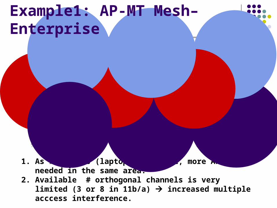
1. As # clients (laptops) increase, more APs are needed in the same area.

2. Available # orthogonal channels is very limited (3 or 8 in 11b/a) increased multiple acccess interference.

Example1: AP-MT Mesh–Enterprise

Example 2: Wireless AP-AP Mesh

Gateway

GatewayAccessPoint

Mobile Terminal BSS

BSS

BSS

Link Capacity

PHY Optimization: MIMO, Adaptive Coded Modulation, etc.

Frequency Plan: 3 (11b), 7 (11a), ? (11n)Topology Control

MAC Optimization

How to scale a MESH?

Network Throughput

=

Frequency (Channel) Reuse

Spatial Reuse

X X

Our Focus

Outline

CSMA/CA – the core of 802.11 MAC Spatial Reuse and Physical Carrier Sensing

Implementation of PCS in OPNET: Simulation of Spatial Reuse

Enhance Physical Carrier Sensing SchemeOptimal PCS threshold through tuning: PCS adaptation

Channel Reuse: Two-Radio Multi-Channel Clustering Architecture

Next-gen: Adaptive MAC Framework for Mesh

CSMA/CA – basic 802.11 MAC

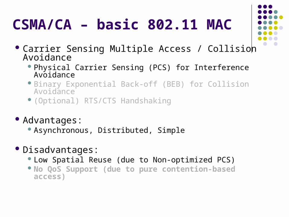
Carrier Sensing Multiple Access / Collision Avoidance

Physical Carrier Sensing (PCS) for Interference AvoidanceBinary Exponential Back-off (BEB) for Collision Avoidance (Optional) RTS/CTS Handshaking

Advantages: Asynchronous, Distributed, Simple

Disadvantages:Low Spatial Reuse (due to Non-optimized PCS)No QoS Support (due to pure contention-based

access)

Spatial Reuse Multiple communications using the same channel/freq happen

simultaneously at different locations w/o interfering each other Received SINR Model:

Physical Carrier Sensing A station samples the energy in the medium and initiates

transmission only if the reading is below a threshold threshold optimization

0.00E+00

1.00E+06

2.00E+06

3.00E+06

4.00E+06

5.00E+06

6.00E+06

6 7 8 9 10 11 12 13 14 15 16 17 18 19 20 21 22 23

SNIR (dB)

On

e-H

op

Ca

pa

cit

y (

bp

s)

1 Mbps

2 Mbps

5.5 Mbps

11 Mbps

Hidden node Problem Revisited

R

I1

I2 …

Any node outside of transmission range of Tx and Rx could be a hidden node, which cannot be prevented by using RTS/CTS!

A1

B1

B2

RxTx

Hidden Node: A node that cannot hear the current transmission but will cause the failure of the transmission if it transmits.

Hidden Nodes in a MESH

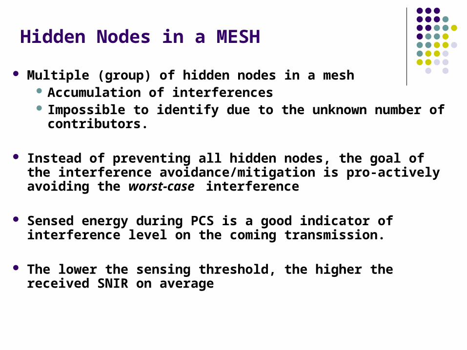
Multiple (group) of hidden nodes in a mesh Accumulation of interferences Impossible to identify due to the unknown number of

contributors.

Instead of preventing all hidden nodes, the goal of the interference avoidance/mitigation is pro-actively avoiding the worst-case interference

Sensed energy during PCS is a good indicator of interference level on the coming transmission.

The lower the sensing threshold, the higher the received SNIR on average

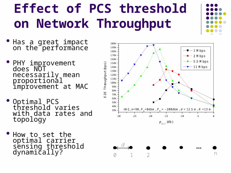
Has a great impact on the performance

PHY improvement does NOT necessarily mean proportional improvement at MAC

Optimal PCS threshold varies with data rates and topology

How to set the optimal carrier sensing threshold dynamically?

-30 -25 -20 -15 -10 -5 0

30k40k50k60k70k80k90k

100k110k120k130k140k150k160k170k180k190k200k

=2, n=90, Ptx=0dbm, P

N = - 200dbm, d = 12.5 m, R =13 m

1 Mbps 2 Mbps 5.5 Mbps 11 Mbps

E2E

Thr

ough

put (

bps)

pcs_t

(db)

...d

0 1 2 n

Effect of PCS threshold on Network Throughput

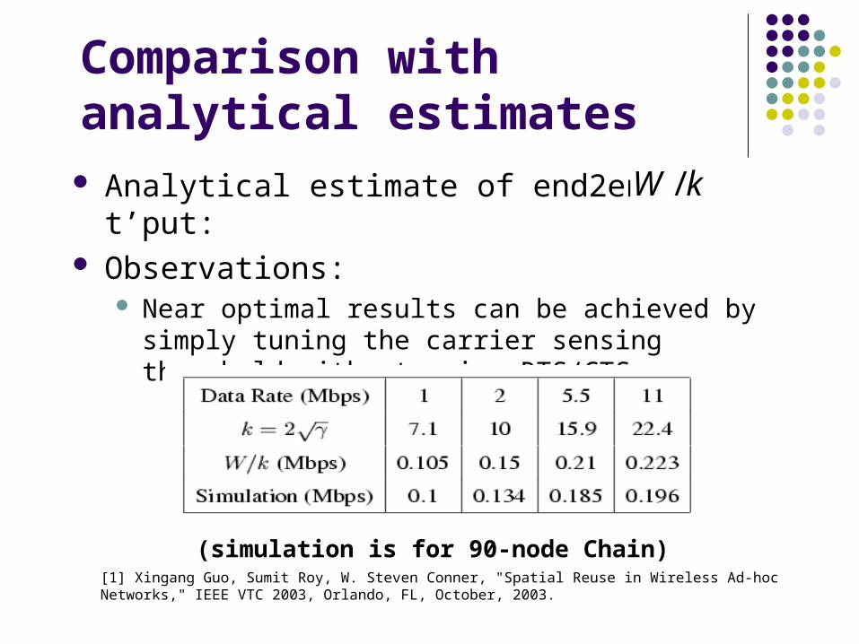
Analytical estimate of end2end t’put: Observations:

Near optimal results can be achieved by simply tuning the carrier sensing threshold without using RTS/CTS

(simulation is for 90-node Chain)

kW /

[1] Xingang Guo, Sumit Roy, W. Steven Conner, "Spatial Reuse in Wireless Ad-hoc Networks," IEEE VTC 2003, Orlando, FL, October, 2003.

Comparison with analytical estimates

Optimal PCS Threshold

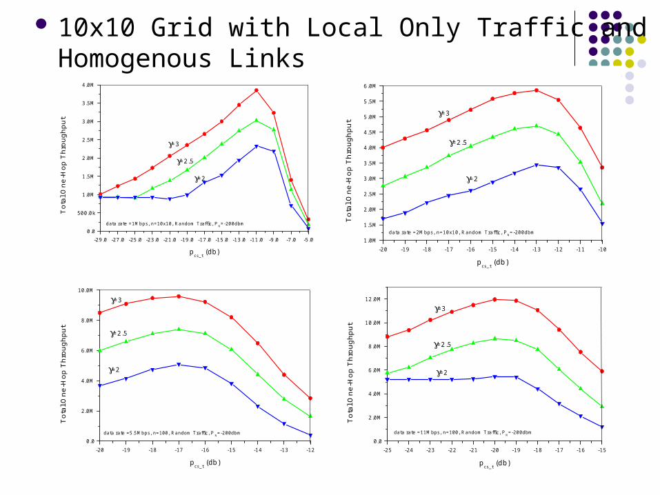
Assumptions:Co-location of receiver and transmitterHomogenous links (same reception power) Ignore background noiseSaturation traffic load

Result: Optimal PCS Threshold ≈ 1/S0, where S0 is the SINR

threshold for sustaining the maximum link throughputS0 = 11dB, 14dB, 18dB, and 21dB for 802.11b 1Mbps,

2Mbps, 5.5Mbps, and 11Mbps, respectively.

-29.0 -27.0 -25.0 -23.0 -21.0 -19.0 -17.0 -15.0 -13.0 -11.0 -9.0 -7.0 -5.00.0

500.0k

1.0M

1.5M

2.0M

2.5M

3.0M

3.5M

4.0M

=2.5

=3

=2

data rate =1Mbps, n=10x10, Random Traffic, PN=-200dbm

Tot

al O

ne-H

op T

hrou

ghpu

t

pcs_t

(db) -20 -19 -18 -17 -16 -15 -14 -13 -12 -11 -101.0M

1.5M

2.0M

2.5M

3.0M

3.5M

4.0M

4.5M

5.0M

5.5M

6.0M

=2.5

=3

=2

data rate =2Mbps, n=10x10, Random Traffic, PN=-200dbm

Tot

al O

ne-H

op T

hrou

ghpu

t

pcs_t

(db)

-20 -19 -18 -17 -16 -15 -14 -13 -120.0

2.0M

4.0M

6.0M

8.0M

10.0M

=2.5

=3

=2

data rate =5.5Mbps, n=100, Random Traffic, PN=-200dbm

Tot

al O

ne-H

op T

hrou

ghpu

t

pcs_t

(db)

-25 -24 -23 -22 -21 -20 -19 -18 -17 -16 -150.0

2.0M

4.0M

6.0M

8.0M

10.0M

12.0M

=2.5

=3

=2

data rate =11Mbps, n=100, Random Traffic, PN=-200dbm

Tot

al O

ne-H

op T

hrou

ghpu

t

pcs_t

(db)

10x10 Grid with Local Only Traffic and Homogenous Links

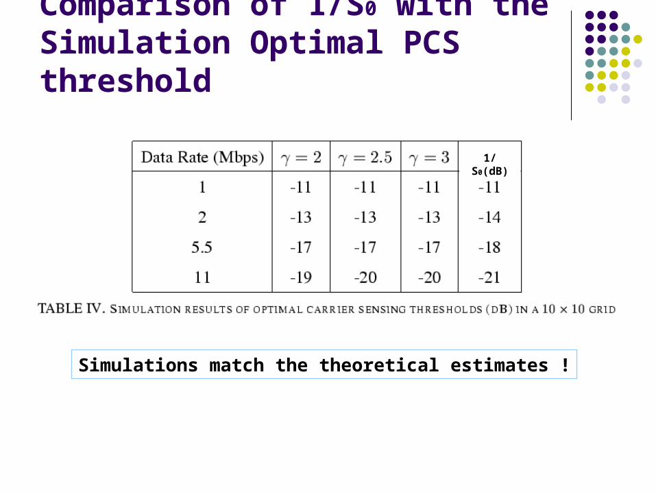
Comparison of 1/S0 with the Simulation Optimal PCS threshold

1/S0(dB)

Simulations match the theoretical estimates !

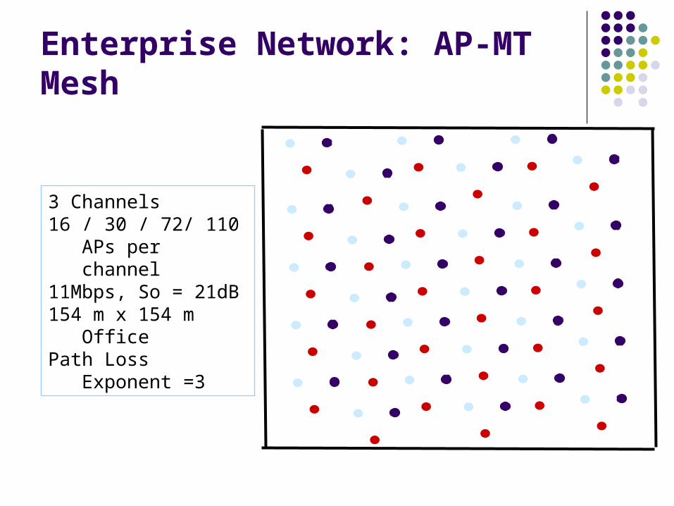
Enterprise Network: AP-MT Mesh

3 Channels16 / 30 / 72/ 110 APs

per channel11Mbps, So = 21dB154 m x 154 m OfficePath Loss Exponent =3

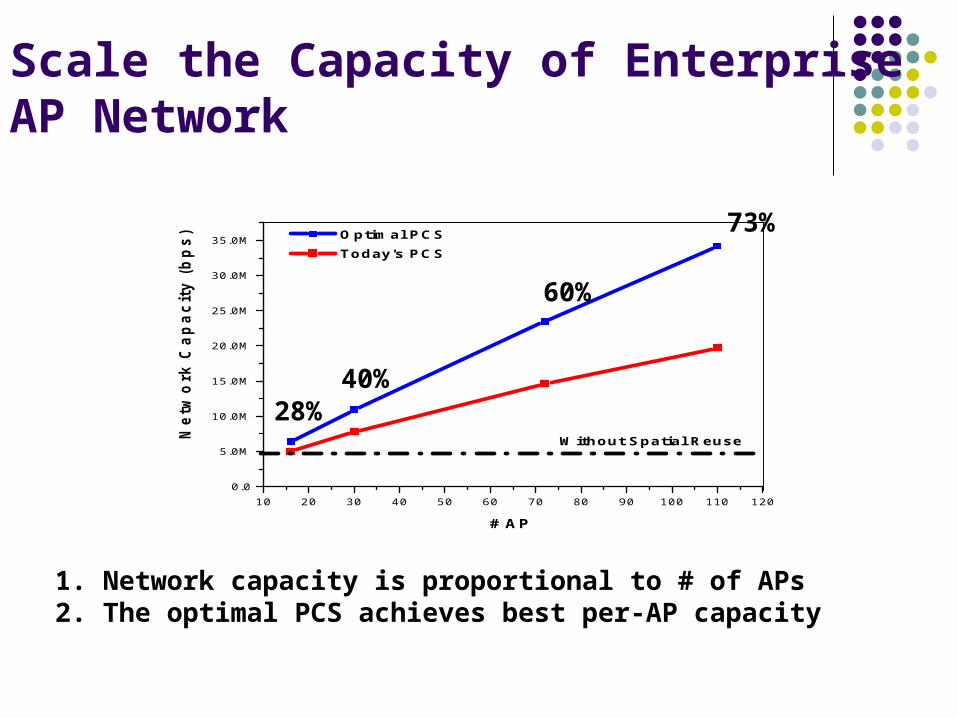
Scale the Capacity of Enterprise AP Network

10 20 30 40 50 60 70 80 90 100 110 1200.0

5.0M

10.0M

15.0M

20.0M

25.0M

30.0M

35.0M

Without Spatial Reuse

Optimal PCS Today's PCS

Netw

ork

Cap

acit

y (

bp

s)

# AP

1. Network capacity is proportional to # of APs2. The optimal PCS achieves best per-AP capacity

28%40%

60%

73%

Summary: Spatial-Reuse for a single-channel MESH

Spatial-Reuse – the key to improve the aggregate throughput of a single-channel mesh links sufficiently separated can transmit simultaneously

without interfering each other

Limitations: Not effective for a small scale network, i.e. the required

minimum separation distance could be high. For example, >7 hops in a regular chain network with

802.11b 1Mbps and path loss exponent = 2. Further Scaling the Throughput with Multiple Channels!

Scaling the Throughput with Multiple Channels

Takes advantage of multiple channels (even multiple bands) 8 orthogonal channels in 802.11 a 3 orthogonal channels in 802.11 b UWB, 802.11, and 802.16

Channel Bonding (wider channel BW) is another alternative Increases peak link rate but does not translate to proportional

MAC throughput increase Lack of backward compatibility: proprietary solution

Multi-channel Approaches – Our Choice No change on channel BW Use all available channels through the network Key issues: channel allocation

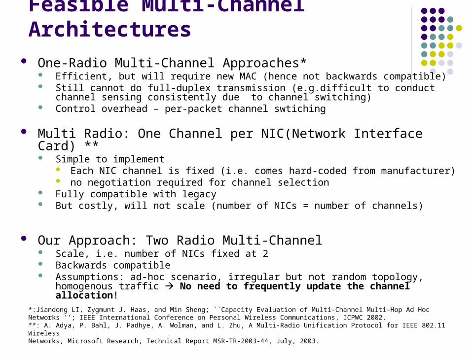
Feasible Multi-Channel Architectures One-Radio Multi-Channel Approaches*

Efficient, but will require new MAC (hence not backwards compatible) Still cannot do full-duplex transmission (e.g.difficult to conduct channel sensing consistently

due to channel switching) Control overhead – per-packet channel swtiching

Multi Radio: One Channel per NIC(Network Interface Card) ** Simple to implement

Each NIC channel is fixed (i.e. comes hard-coded from manufacturer) no negotiation required for channel selection

Fully compatible with legacy But costly, will not scale (number of NICs = number of channels)

Our Approach: Two Radio Multi-Channel Scale, i.e. number of NICs fixed at 2 Backwards compatible Assumptions: ad-hoc scenario, irregular but not random topology, homogenous traffic No

need to frequently update the channel allocation!

*:Jiandong LI, Zygmunt J. Haas, and Min Sheng; ``Capacity Evaluation of Multi-Channel Multi-Hop Ad Hoc Networks ''; IEEE International Conference on Personal Wireless Communications, ICPWC 2002. **: A. Adya, P. Bahl, J. Padhye, A. Wolman, and L. Zhu, A Multi-Radio Unification Protocol for IEEE 802.11 WirelessNetworks, Microsoft Research, Technical Report MSR-TR-2003-44, July, 2003.

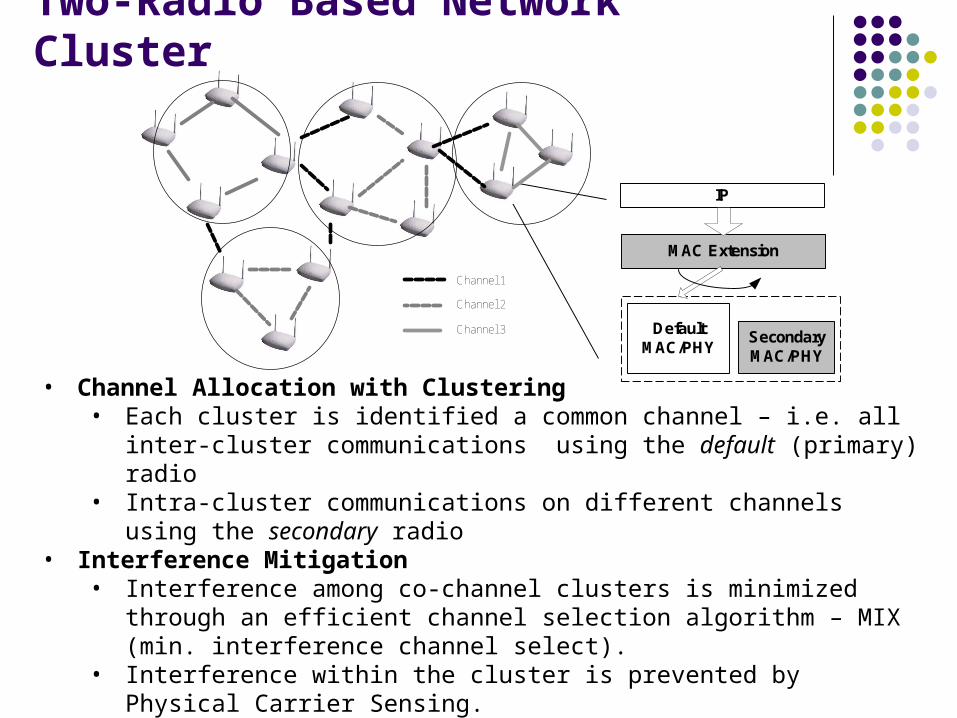
Two-Radio Based Network Cluster

• Channel Allocation with Clustering • Each cluster is identified a common channel – i.e. all inter-cluster

communications using the default (primary) radio• Intra-cluster communications on different channels using the secondary

radio• Interference Mitigation

• Interference among co-channel clusters is minimized through an efficient channel selection algorithm – MIX (min. interference channel select).

• Interference within the cluster is prevented by Physical Carrier Sensing.• Legacy compatible: legacy APs connect to mesh via default radio.

Channel 1

Channel 2

Channel 3 DefaultMAC/PHY

SecondaryMAC/PHY

MAC Extension

IP

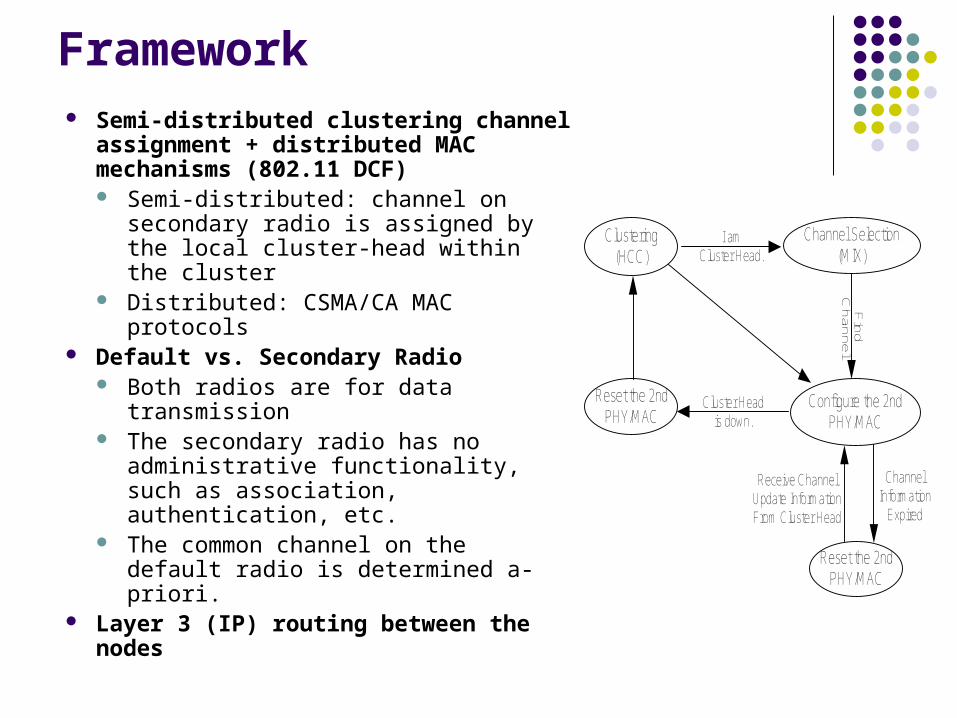
Framework Semi-distributed clustering channel

assignment + distributed MAC mechanisms (802.11 DCF) Semi-distributed: channel on

secondary radio is assigned by the local cluster-head within the cluster

Distributed: CSMA/CA MAC protocols

Default vs. Secondary Radio Both radios are for data

transmission The secondary radio has no

administrative functionality, such as association, authentication, etc.

The common channel on the default radio is determined a-priori.

Layer 3 (IP) routing between the nodes

Clustering(HCC)

Channel Selection (MIX)

I am Cluster Head.

Configure the 2nd PHY/MAC

Fin

d

Channel

Cluster Head is down.

Reset the 2nd PHY/MAC

Reset the 2nd PHY/MAC

Receive Channel Update Information From Cluster Head

Channel Information

Expired

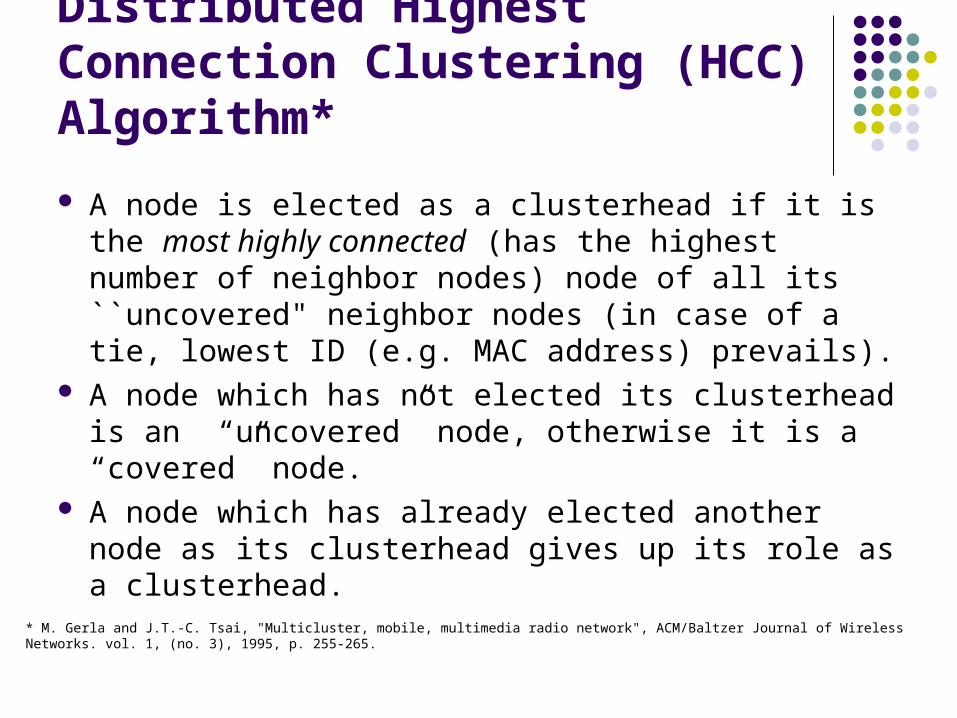
Distributed Highest Connection Clustering (HCC) Algorithm*

A node is elected as a clusterhead if it is the most highly connected (has the highest number of neighbor nodes) node of all its ``uncovered" neighbor nodes (in case of a tie, lowest ID (e.g. MAC address) prevails).

A node which has not elected its clusterhead is an “uncovered” node, otherwise it is a “covered” node.

A node which has already elected another node as its clusterhead gives up its role as a clusterhead.

* M. Gerla and J.T.-C. Tsai, "Multicluster, mobile, multimedia radio network", ACM/Baltzer Journal of Wireless Networks. vol. 1, (no. 3), 1995, p. 255-265.

Clustering Procedure

Step 1: All nodes have their neighbor list ready (every node should know its neighbors, how many)

Step 2: All nodes broadcast their own neighboring information, i.e., the number of neighbors, to its neighborhood.

Step 3: A node that has got such information from all its neighbors can decide its status (clusterhead or slave)

MIX – Minimum Interference Channel Selection On-Air energy estimation per channel

t0: estimation starting time T: estimation period Ei(t): on-air energy at time t on channel i

k: Selected Channel

T

dttEE

Tt

t i

i

0

0

)(

}),...,2,1{|min(| niEEk ik

Forwarding Table (MAC Extension)

Neighbor MAC/PHY

192.168.0.2 Secondary

Neighbor MAC/PHY

192.168.0.2 Default

192.168.0.4 Secondary

Neighbor MAC/PHY

192.168.0.1 Secondary

192.168.0.3 Default

192.168.0.1

192.168.0.2

192.168.0.3

192.168.0.4

Neighbor MAC/PHY

192.168.0.3 SecondaryCluster 1

Cluster 2

An IP packet will be forwarded to default or Secondary MAC/PHY according to the forwarding table in the MAC Extension layer.

DefaultMAC/PHY

SecondaryMAC/PHY

MAC Extension

IP

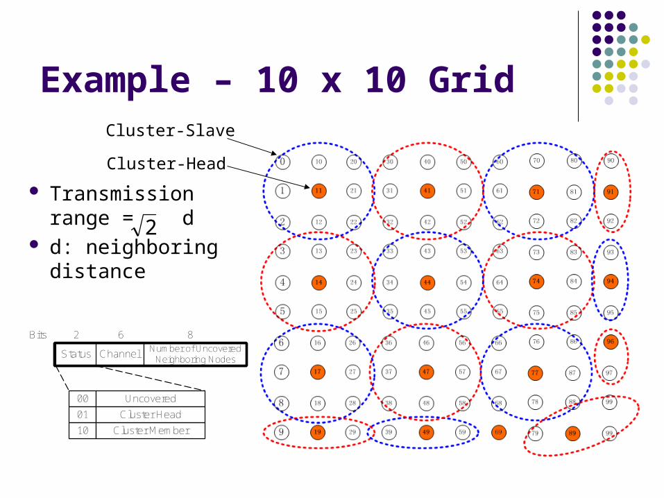
Example – 10 x 10 Grid

Cluster-Head

Cluster-Slave

Transmission range = d

d: neighboring distance

2

ChannelStatus

6Number of UncoveredNeighboring Nodes

8Bits 2

00

01

10

Uncovered

Cluster Head

Cluster Member

Simulation Topology

Random, Local, and Saturate Traffic

10 x 10 Grid 802.11 b 1Mbps 3 orthogonal channels Path Loss Exponent = 3 Packet Size =1024

Bytes Dash Circle: Cluster Dark node: Cluster-Head

0

1

2

3

4

5

10

11

12

13

14

15

20

21

22

23

24

25

30

31

32

33

34

35

40

41

42

43

44

45

50

51

52

53

54

55

60

61

62

63

64

65

71

72

73

74

75

76

91

92

93

94

95

96

81

82

83

84

85

866

7

8

9

16

17

18

19

26

27

28

29

36

37

38

39

46

47

48

49

56

57

58

59

66

67

68

69

77

78

79

70

97

99

99

90

87

88

89

80

Channel 1 Channel 2

B1 B2 B3 B4 B5 B6 B7 B8 B9 B10

A1 A2 A3 A4 A5 A6 A7 A8 A9 A10

C1 C2 C3 C4 C5 C6 C7 C8 C9 C10

Tracing One-Hop Aggregate Throughput

The new multi-channel and two radio architecture achieves 3X performance, compared to a traditional single-channel and single-radio mesh.

0 100 200 300 400 5000

1M

2M

3M

4M

5M

6M

7M

8M

9MData Rate = 1MbpsPacket Size = 1024 BytesPath Loss Exponent = 3

Traditional Single-Channel and Single-Radio Mesh

Clustering Multi-Channel and Two-Radio Architecture

Th

rou

gh

pu

t (b

ps)

Time (sec.)

Throughput Distribution

Location-dependent fairness problem : Links Ai experience worse interference environment than links Bi and Ci, leading to the oscillation of the throughput distribution.

Future Work: How Physical Carrier Sensing could mitigate the location dependent fairness problem?

0 100 200 300 400 500 600 700

100

1000

10000

100000 C10C9C8

C7

C6

C5C4C3C2C1 B10

B9

B8

B7B6B5

B4B3B2B1

A10

A9

A8

A7

A6A5

A4A3

A2

A1

On

e-H

op

Th

rou

gh

pu

t (b

ps)

Link

Clustering Multi-Channel and Two-Radio Mesh Traditional Single-Channel and Single-Radio Mesh

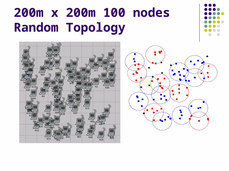
200m x 200m 100 nodes Random Topology

Performance Comparison in Random Topology

a) Tracing Aggregate Throughput b) Throughput Distribution

Performance gain of aggregate throughput is almost 3x (10Mbps vs. 3.5Mbps)

0 100 200 300 400 5000

1M

2M

3M

4M

5M

6M

7M

8M

9M

10M

Data Rate = 1MbpsPacket Size = 1024 BytesPath Loss Exponent = 3

Traditional Single-Channel and Single-Radio Mesh

Clustering Multi-Channel and Two-Radio Architecture

Thr

ough

put

(bp

s)

Time (sec.)

100 200 300 400

100

1000

10000

100000

On

e-H

op T

hro

ugh

put (

bps)

Link

Clustering Multi-Channel and Two-Radio Mesh Traditional Single-Channel and Single-Radio Mesh