scaled v. ordinal v. nominal data(3)
TRANSCRIPT

This presentation will assist you in determining if the data associated with the problem you are working on

This presentation will assist you in determining if the data associated with the problem you are working on
Participant Score
A 10
B 11
C 12
D 12
E 12
F 13
G 14

This presentation will assist you in determining if the data associated with the problem you are working on
Participant Score
A 10
B 11
C 12
D 12
E 12
F 13
G 14

This presentation will assist you in determining if the data associated with the problem you are working on is:

This presentation will assist you in determining if the data associated with the problem you are working on is:
Scaled

This presentation will assist you in determining if the data associated with the problem you are working on is:
Scaled
Ordinal
This presentation will assist you in determining if the data associated with the problem you are working on is:
Scaled
Ordinal
Nominal Proportional
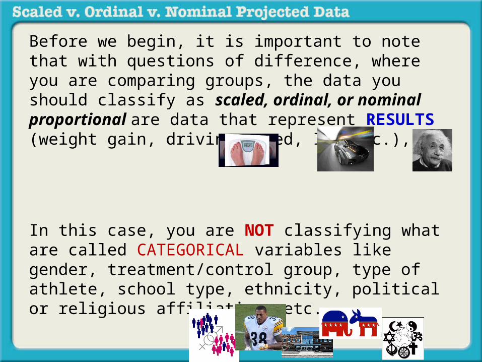
Before we begin, it is important to note that with questions of difference, where you are comparing groups, the data you should classify as scaled, ordinal, or nominal proportional are data that represent RESULTS (weight gain, driving speed, IQ, etc.),
In this case, you are NOT classifying what are called CATEGORICAL variables like gender, treatment/control group, type of athlete, school type, ethnicity, political or religious affiliation, etc.

What is scaled data?

What is scaled data?
Note – scaled data has two subcategories (1) interval data (no zero point but equal
intervals) and (2) ratio data (a zero point and equal
intervals)
What is scaled data?
For the purposes of this presentation we will not discuss these further but just focus on both as scaled data.
Scaled data is data that has a couple of attributes.

We will describe those attributes with illustrations from a scaled variable:

We will describe those attributes with illustrations from a scaled variable: Temperature.

Attribute #1 – scaled data assume a quantity.
Meaning that 2 is more than 3 and 4 is more than 3 and 20 is less than 30, etc.
For example: 40 degrees is more than 30 degrees. 110 degrees isless than 120 degrees.
Attribute #1 – scaled data assume a quantity.
Meaning that 2 is more than 3 and 4 is more than 3 and 20 is less than 30, etc.
For example: 40 degrees is more than 30 degrees. 110 degrees isless than 120 degrees.

Attribute #1 – scaled data assume a quantity.
Meaning that 3 is more than 2 and 4 is more than 3 and 20 is less than 30, etc.
For example: 40 degrees is more than 30 degrees. 110 degrees isless than 120 degrees.

Attribute #1 – scaled data assume a quantity.
Meaning that 3 is more than 2 and 4 is more than 3 and 20 is less than 30, etc.
For example: 40 degrees is more than 30 degrees. 110 degrees isless than 120 degrees.

Attribute #1 – scaled data assume a quantity.
Meaning that 3 is more than 2 and 4 is more than
3 and 20 is less than 30, etc.
For example: 40 degrees is more than 30 degrees. 110 degrees isless than 120 degrees.

Attribute #1 – scaled data assume a quantity.
Meaning that 3 is more than 2 and 4 is more than 3 and 20 is less than 30, etc.
For example: 40 degrees is more than 30 degrees. 110 degrees isless than 120 degrees.
100 degrees is more than 40 degrees

Attribute #1 – scaled data assume a quantity.
Meaning that 3 is more than 2 and 4 is more than 3 and 20 is less than 30, etc.
For example: 40 degrees is more than 30 degrees. 110 degrees isless than 120 degrees.
60 degrees is less than 80 degrees

Attribute #1 – scaled data assume a quantity.
Meaning that 3 is more than 2 and 4 is more than 3 and 20 is less than 30, etc.
For example: 40 degrees is more than 30 degrees. 110 degrees isless than 120 degrees.
60 degrees is less than 80 degrees
If the data represents varying amounts then this is the first requirement for data to be
considered - scaled.

Attribute #2

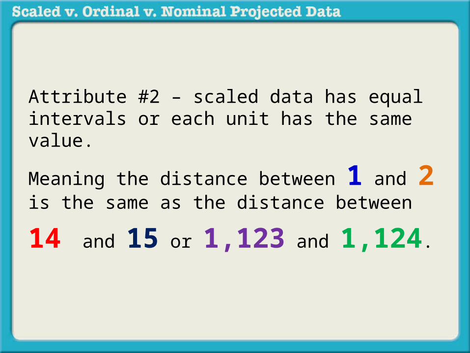
Attribute #2 – scaled data has equal intervals or each unit has the same value.
Attribute #2 – scaled data has equal intervals or each unit has the same value.
Meaning the distance between 1 and 2 is the same as
the distance between 14 and 15 or 1,123 and
1,124.

Attribute #2 – scaled data has equal intervals or each unit has the same value.
Meaning the distance between 1 and 2 is the same as
the distance between 14 and 15 or 1,123 and
1,124. They all have a unit value of 1 between them.

In our temperature example:
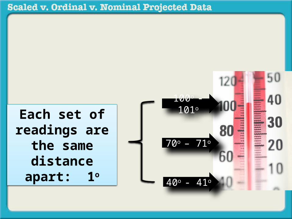
40o - 41o
100o - 101o
70o – 71o
Each set of readings are the same distance
apart: 1o

40o - 41o
100o - 101o
70o – 71o
Each set of readings are the same distance
apart: 1o
The point here is that each unit value is the same across the
entire scale of numbers

40o - 41o
100o - 101o
70o – 71o
Each set of readings are the same distance
apart: 1o
Note, this is not the case with ordinal numbers where 1st place in a marathon might be 2:03 hours, 2nd place 2:05 and 3rd place 2:43.
They are not equally spaced!

What does a scaled data set look like?

Here are some examples:

Height

HeightPersons HeightCarly 5’ 3”Celeste 5’ 6”Donald 6’ 3”Dunbar 6’ 1”Ernesta 5’ 4”

Height
Attribute #1: We are dealing with amounts
Persons HeightCarly 5’ 3”Celeste 5’ 6”Donald 6’ 3”Dunbar 6’ 1”Ernesta 5’ 4”

HeightPersons HeightCarly 5’ 3”Celeste 5’ 6”Donald 6’ 3”Dunbar 6’ 1”Ernesta 5’ 4”
Attribute #2: There are equal intervals across the scale. One inch is the same value regardless of where you are on the scale.

Intelligence Quotient (IQ)
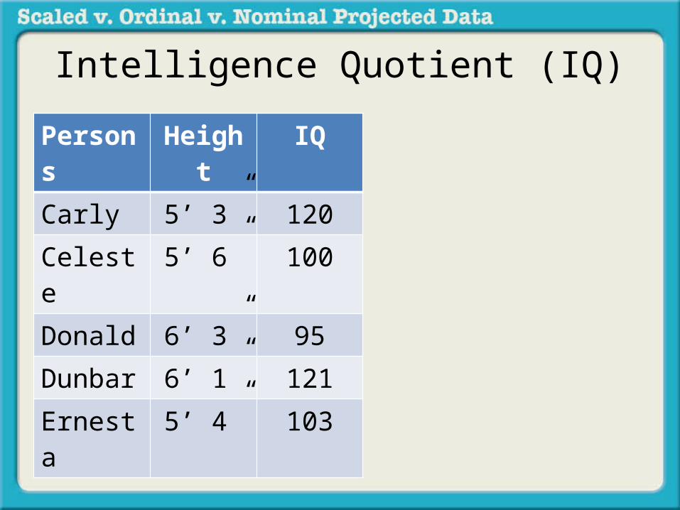
Intelligence Quotient (IQ)Persons Height IQCarly 5’ 3” 120Celeste 5’ 6” 100Donald 6’ 3” 95Dunbar 6’ 1” 121Ernesta 5’ 4” 103

Intelligence Quotient (IQ)Persons Height IQCarly 5’ 3” 120Celeste 5’ 6” 100Donald 6’ 3” 95Dunbar 6’ 1” 121Ernesta 5’ 4” 103
Attribute #1: We are dealing with amounts

Intelligence Quotient (IQ)Persons Height IQCarly 5’ 3” 120Celeste 5’ 6” 100Donald 6’ 3” 95Dunbar 6’ 1” 121Ernesta 5’ 4” 103
Attribute #2: Supposedly there are equal intervals across this scale. A little harder to prove but most researchers go with it.

Pole Vaulting Placement

Pole Vaulting PlacementPersons Height IQ PVPCarly 5’ 3” 120 3rd
Celeste 5’ 6” 100 5th
Donald 6’ 3” 95 1st
Dunbar 6’ 1” 121 4th
Ernesta 5’ 4” 103 2nd

Pole Vaulting PlacementPersons Height IQ PVPCarly 5’ 3” 120 3rd
Celeste 5’ 6” 100 5th
Donald 6’ 3” 95 1st
Dunbar 6’ 1” 121 4th
Ernesta 5’ 4” 103 2nd
Attribute #1: We are dealing with amounts

Pole Vaulting PlacementPersons Height IQ PVPCarly 5’ 3” 120 3rd
Celeste 5’ 6” 100 5th
Donald 6’ 3” 95 1st
Dunbar 6’ 1” 121 4th
Ernesta 5’ 4” 103 2nd
Attribute #2: We are NOT dealing with equal intervals. 1st place (16’0”) and 2nd place (15’8”) are not the same distance from one another as 2nd Place and 3rd place (12’2”).

Based on this explanation is your data scaled?

If your data is scaled as shown in these examples, select

If your data is scaled as shown in these examples, select
Scaled
Ordinal
Nominal Proportional
We have now demonstrated scaled data and given you a brief introduction to ordinal data.
Once again, ordinal data is data that is ranked:

Once again, ordinal data is data that is ranked:

In other words,

Ordinal scales use numbers to represent relative amounts of an attribute.

Ordinal scales use numbers to represent relative amounts of an attribute.
1st Place16’ 3”

Ordinal scales use numbers to represent relative amounts of an attribute.
1st Place16’ 3”
2nd Place16’ 1”

Ordinal scales use numbers to represent relative amounts of an attribute.
1st Place16’ 3”
2nd Place16’ 1”
3rd Place15’ 2”
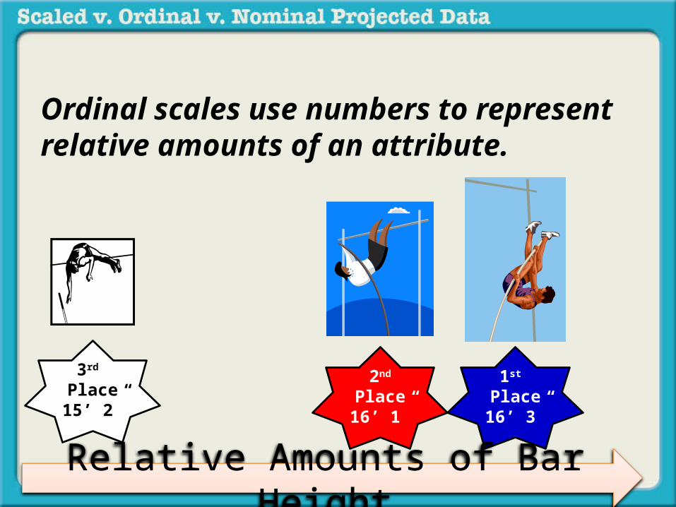
Ordinal scales use numbers to represent relative amounts of an attribute.
3rd Place15’ 2”
2nd Place16’ 1”
1st Place16’ 3”
Relative Amounts of Bar Height

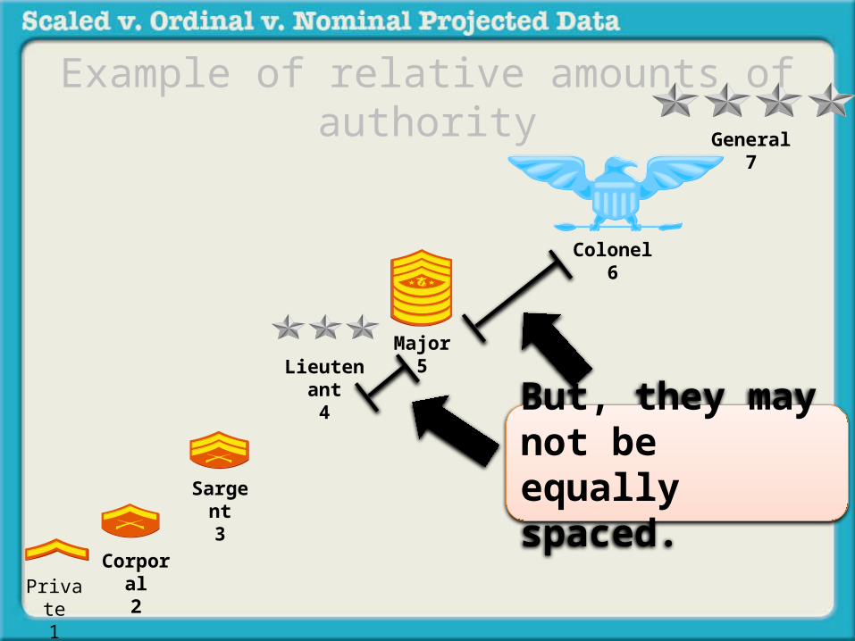
Example of relative amounts of authority

Corporal2
Sargent3
Lieutenant4
Major5
Colonel6
General7
Private1
Example of relative amounts of authority

Corporal2
Sargent3
Lieutenant4
Major5
Colonel6
General7
Private1
Notice how we are dealing with amounts of authority
Example of relative amounts of authority

Corporal2
Sargent3
Lieutenant4
Major5
Colonel6
General7
Private1
But,
Example of relative amounts of authority

Corporal2
Sargent3
Lieutenant4
Major5
Colonel6
General7
Private1
But, they may not be equally spaced.
Example of relative amounts of authority

Corporal2
Sargent3
Lieutenant4
Major5
Colonel6
General7
Private1
But, they may not be equally spaced.
Example of relative amounts of authority
Corporal2
Sargent3
Lieutenant4
Major5
Colonel6
General7
Private1
But, they may not be equally spaced.
Example of relative amounts of authority
You can tell if you have an ordinal data set when the data is described as ranks.

You can tell if you have an ordinal data set when the data is described as ranks.
Persons Pole Vault Placement
Carly 3rd
Celeste 5th
Donald 1st
Dunbar 4th
Ernesta 2nd

Or in percentiles
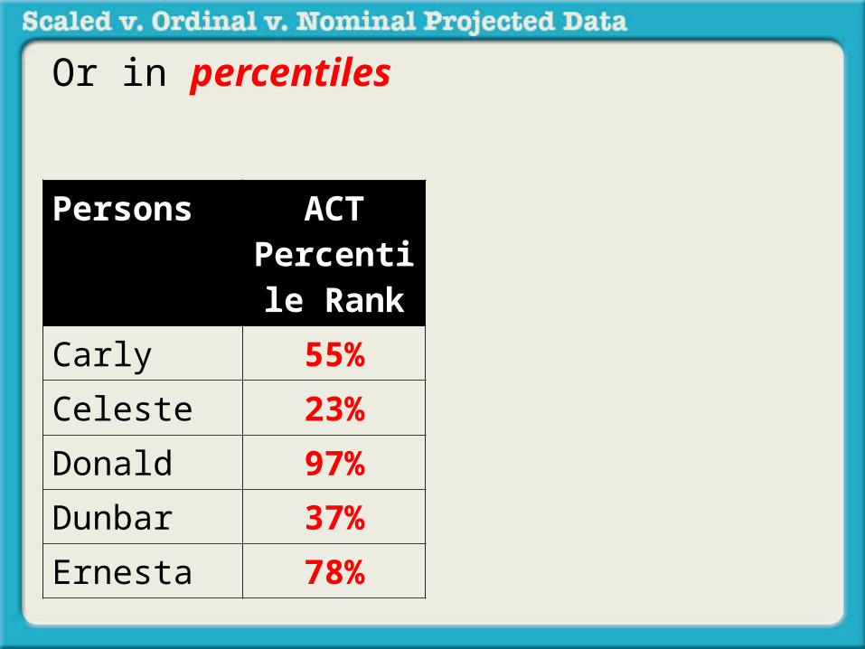
Or in percentiles
Persons ACT Percentile
RankCarly 55%Celeste 23%Donald 97%Dunbar 37%Ernesta 78%

If your data is ranked as shown in these examples, select

If your data is ranked as shown in these examples, select
Scaled
Ordinal
Nominal Proportional

Finally, let’s see what data looks like when it is nominal proportional:
Nominal data is different from scaled or ordinal,

Nominal data is different from scaled or ordinal, because they do not deal with amounts

Nominal data is different from scaled or ordinal, because they do not deal with amounts nor equal intervals.

For example,

Nationality is a variable that does not have amounts nor equal intervals.

1 = Canadian
2 = American

1 = Canadian
2 = American
Being Canadian is not numerically or quantitatively more than being
American

1 = Canadian
2 = American
The numbers 1 and 2 do not represent amounts. They are just a way to distinguish the two groups numerically.
We could have just as easily used 1s for Americans and 2s for Canadians

We could have just as easily used 1s for Americans and 2s for Canadians
1 = Canadian
2 = American

We could have just as easily used 1s for Americans and 2s for Canadians
1 = American
2 = Canadian

Other examples:

Religious Affiliation

Religious Affiliation1 - Buddhist
2 - Catholic
3 - Jew
4 - Mormon
5 - Muslim
6 - Protestant

Gender

Gender1 - Male
2 - Female

Preference

Preference:
1. People who prefer chocolate ice-cream

Preference:
1. People who prefer chocolate ice-cream
2. People who dislike chocolate ice-cream

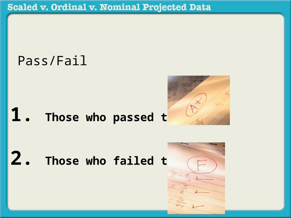
Pass/Fail
Pass/Fail
1. Those who passed the test
Pass/Fail
1. Those who passed the test
2. Those who failed the test
The word “Nom” in “nominal” means “name”.

The word “Nom” in nominal means “name”. Essentially we are using data to name, identify, distinguish, classify or categorize.

Other names for nominal data are categorical or frequency data.
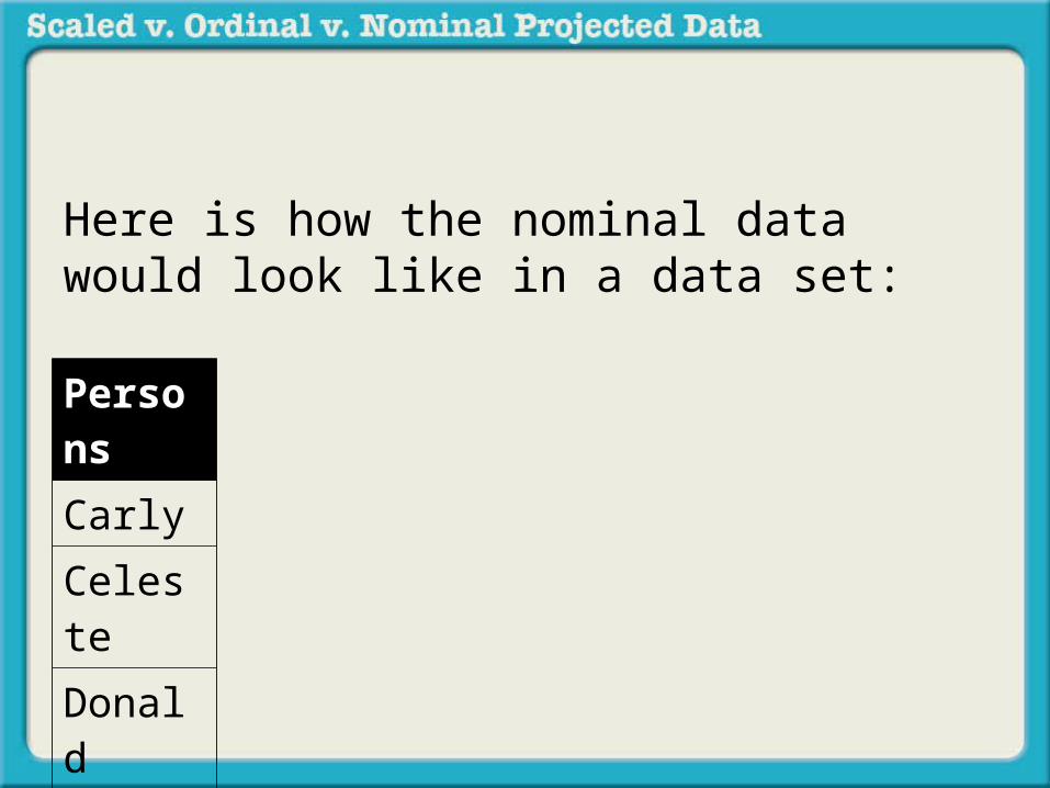
Here is how the nominal data would look like in a data set:
Here is how the nominal data would look like in a data set:
PersonsCarlyCelesteDonaldDunbarErnesta

Here is how the nominal data would look like in a data set:
Persons GenderCarlyCelesteDonaldDunbarErnesta

Here is how the nominal data would look like in a data set:
Persons GenderCarlyCelesteDonaldDunbarErnesta
1 = Male2 = Female

Here is how the nominal data would look like in a data set:
Persons GenderCarly 2Celeste 2Donald 1Dunbar 1Ernesta 2
1 = Male2 = Female
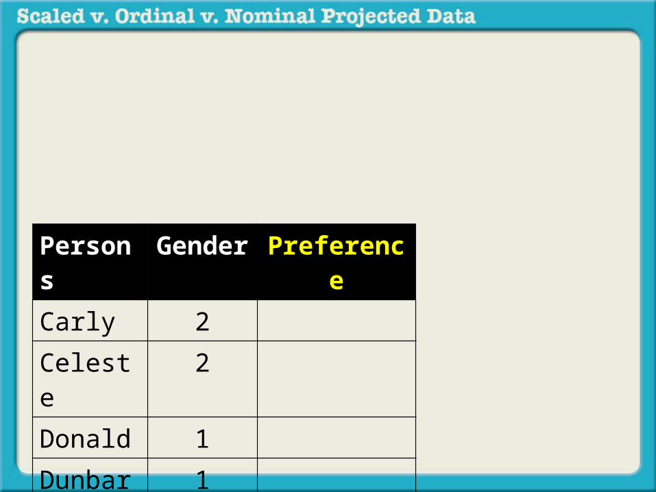
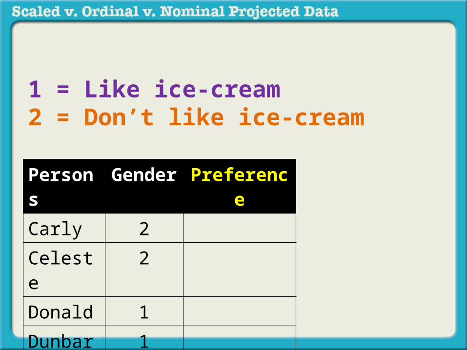
Persons Gender PreferenceCarly 2Celeste 2Donald 1Dunbar 1Ernesta 2
Persons Gender PreferenceCarly 2Celeste 2Donald 1Dunbar 1Ernesta 2
1 = Like ice-cream2 = Don’t like ice-cream

Persons Gender PreferenceCarly 2 1Celeste 2 1Donald 1 1Dunbar 1 2Ernesta 2 2
1 = Like ice-cream2 = Don’t like ice-cream

Persons Gender PreferenceCarly 2 1Celeste 2 1Donald 1 1Dunbar 1 2Ernesta 2 2
Religion

Persons Gender PreferenceCarly 2 1Celeste 2 1Donald 1 1Dunbar 1 2Ernesta 2 2
Religion
1 - Buddhist2 - Catholic3 - Jew4 - Mormon5 - Muslim6 - Protestant

Persons Gender PreferenceCarly 2 1Celeste 2 1Donald 1 1Dunbar 1 2Ernesta 2 2
Religion42561
1 - Buddhist2 - Catholic3 - Jew4 - Mormon5 - Muslim6 - Protestant

Now that we know what nominal data is,

What is nominal proportional data?

What is nominal proportional data?
Scaled
Ordinal
Nominal Proportional

Nominal proportional data is simply the proportion of individuals who are in one category as opposed to another.

For example,
In the data set below:

In the data set below:
Persons GenderCarly 2Celeste 2Donald 1Dunbar 1Ernesta 2

Persons GenderCarly 2Celeste 2Donald 1Dunbar 1Ernesta 2
3 out of 5 persons are female

Persons GenderCarly 2Celeste 2Donald 1Dunbar 1Ernesta 2
Or 60% are female

Persons GenderCarly 2Celeste 2Donald 1Dunbar 1Ernesta 2
That means 2 out of 5 are male

Persons GenderCarly 2Celeste 2Donald 1Dunbar 1Ernesta 2
Or 40% are male

In such cases you may not see a data set,

you may just see a question like this:

A claim is made that four out of five veterans (or 80%) are supportive of the current conflict. After you sample five veterans you find that three out of five (or 60%) are supportive. In terms of statistical significance does this result support or invalidate this claim?

If you were to put these results in a data set it would look like this:

VeteransABCDE

Veterans SupportiveABCDE
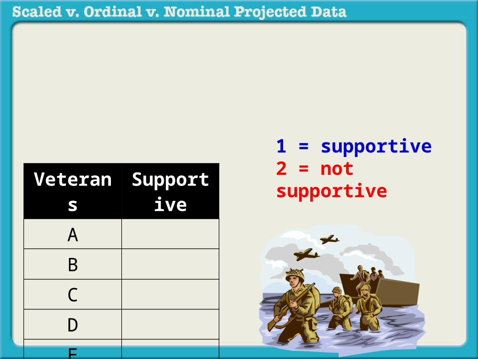
Veterans SupportiveABCDE
1 = supportive2 = not supportive

Veterans SupportiveA 2B 2C 1D 1E 1
1 = supportive2 = not supportive

Veterans SupportiveA 2B 2C 1D 1E 1
1 = supportive2 = not supportive
If the question is stated in terms of percentages (e.g., 60% of veterans were supportive), then that percentage is nominal proportional data

If your data is nominal proportional as shown in these examples, select

If your data is nominal proportional as shown in these examples, select
Scaled
Ordinal
Nominal Proportional

That concludes this explanation of scaled, ordinal and nominal proportional data.