scalable and sound low-rank tensor learning
TRANSCRIPT
Scalable and Sound Low-Rank Tensor Learning
Hao Cheng] Yaoliang Yu∗ Xinhua Zhang‡ Eric Xing∗ Dale Schuurmans†
University of Washington] CMU∗ NICTA and ANU‡ University of Alberta†
Abstract
Many real-world data arise naturally as ten-sors. Equipped with a low rank prior, learn-ing algorithms can benefit from exploiting therich dependency encoded in a tensor. De-spite its prevalence in low-rank matrix learn-ing, trace norm ceases to be tractable in ten-sors and therefore most existing works resortto matrix unfolding. Although some theoreti-cal guarantees are available, these approachesmay lose valuable structure information andare not scalable in general. To address thisproblem, we propose directly optimizing thetensor trace norm by approximating its dualspectral norm, and we show that the approx-imation bounds can be efficiently convertedto the original problem via the generalizedconditional gradient algorithm. The result-ing approach is scalable to large datasets,and matches state-of-the-art recovery guar-antees. Experimental results on tensor com-pletion and multitask learning confirm thesuperiority of the proposed method.
1 Introduction
Real-world data are complex and usually exhibit richstructures that learning algorithms can significantlybenefit from. For instance, data in the vectorial formcan be sparse while in the matrix form can have lowrank. More general multi-way correlations are oftenobserved in tensor form data, i.e. multi-dimensional ar-rays [1]. Examples include multi-channel images, videosequences, chemical compound processes, brain EEGsignals, etc. Additionally, tensors are often used as im-portant tools for modeling and estimation. Most no-tably, they can be applied as the high order momentsin latent variable models [2] such as independent com-
Appearing in Proceedings of the 19th International Con-ference on Artificial Intelligence and Statistics (AISTATS)2016, Cadiz, Spain. JMLR: W&CP volume 51. Copyright2016 by the authors.
ponent analysis, mixture and topic models, etc. Dueto the wide applicability, a lot of works have focusedon factorizing, completing, and learning a tensor ofinterest.
The most straightforward solution to low-rank ten-sor decomposition is arguably alternating least squares(ALS) or block-coordinate based methods [1, 3]. Withrelatively high efficiency, they are generically applica-ble in practice. In the case of completing a d × d × dtensor using z observed entries, the complexity is onlyO(zr), where r is the intended rank. However, they arebased on nonconvex optimization whose globally opti-mal solution is generally intractable to find. Therefore,the analysis of sample complexity and recovery boundsis generally hard, leaving the recent results restrictedto strong assumptions such as the absence of noise orthe access to the truth rank [e.g. 2, 4, 5].
A prevalent class of theoretically sound approaches arebased on convex relaxations of the rank function. Inlow-rank matrix learning, the utilization of trace normhas achieved remarkable success since the seminal workof [6]. Extension to tensors is conceptually straightfor-ward, based on the generic framework of atomic norm[7]. Recently, [8] provided excellent theoretical sup-port for the tensor trace norm. However, many com-putational tractability properties of matrices do notcarry over to tensors. For instance, the tensor rankcan (far) exceed the maximum dimension, and a low-rank approximation may not even exist [9]. Indeed, itis also NP-hard to decide the tensor rank and tensortrace norm, see e.g. [10].
To work around the tractability barrier, approxima-tions are in order. A large body of algorithms unfoldthe tensor into matrices, and then apply well estab-lished matrix techniques, e.g., minimizing the (matrix)trace norm as a proxy of the rank [11–16]. However,this may be unsatisfying because a genuinely “low-rank” tensor can nevertheless have large or even fullrank in all matrix unfoldings. It also brings aboutscalability issues as the most efficient implementationof proximal gradient methods or ADMM costs at leastO(zd) time. As a result, most matricization based al-gorithms do not scale to large tensors.
Scalable and Sound Low-Rank Tensor Learning
The aim of this paper is therefore to design approxi-mate models which are both scalable and theoreticallysound. Instead of directly approximating the tensortrace norm, we resort to its dual norm—tensor spec-tral norm, because it is much easier to approximate.We provide a simple algorithm to compute the tensorspectral norm with sound approximation bounds, andits computational cost is similar to that of ALS (Sec-tion 4). A key challenge is then to utilize this approxi-mation as an oracle, and to find a solution for the orig-inal optimization problem with suboptimality guaran-tee. We show that this translation can be achievedby using the recent generalized conditional gradientalgorithm [17, 18], and furthermore O(1/ε) rates ofconvergence can be derived for this approximate ora-cle setting. Finally we study the sample complexityof the proposed algorithm in Section 5, and demon-strate that it does match the state-of-the-art boundsof matricization based models. Therefore, we obtainan algorithm which is efficient in both computationand inference. In experiments on tensor completionand multitask learning, our method significantly out-performs existing methods in generalization and effi-ciency.
2 Preliminaries
We first review some preliminaries. A tensor is identi-fied as a multi-dimensional array A ∈ Rd1×d2×···×dK ,where K is the order and dk is the dimension of thek-th mode. Without loss of generality, we assumethroughout that d1 ≥ d2 ≥ · · · ≥ dK . Following [1],we define the mode-k multiplication of a tensor with
some matrix U∈Rdk×dk as
(A×k U)i1,...,ik−1 ,ık,ik+1,...,iK =∑dk
ik=1Ai1,...,ik−1,ik,ik+1,...,iKUık,ik .
Note that the dimension of the k-th mode of the prod-uct A×kU changes from dk to dk. As usual, we definethe inner product of two tensors with the same size as〈A,B〉 :=
∑i1,...,iK
Ai1,...,iKBi1,...,iK . and the induced
Frobenius norm ‖A‖F :=√〈A,A〉.
We can unfold (or flatten) a tensor into a 2-D matrix
as follows. For any 1 ≤ k ≤ K, A(k) ∈ Rdk×(∏
j 6=k dj),
with its(ik, 1 +
∑Kj=1,j 6=k(ij − 1)
∏Km=j+1,m6=k dm
)-th
entry beingAi1,...,iK . Like matrices, we can decomposea tensor into a linear combination of primitives. First,we define rank-1 (pure) tensors as T = u⊗v⊗ · · ·⊗ z,where the K factors u ∈ Rd1 , . . . , z ∈ RdK form theouter product Ti1,i2,...,iK = ui1vi2 · · · ziK , ∀i1, . . . , iK .Then, the Candecomp-Parafac (CP) decomposition ofthe tensor A refers to
A =∑ri=1 ui⊗vi⊗ · · ·⊗ zi, (1)
and the lowest possible value of r is called the rank ofA. Surprisingly, the tensor rank could well exceed anydimension dk. In general, a well known bound states
∀k, rank(A(k)) ≤ rank(A) ≤∏j 6=k rank(A(j)), (2)
where recall that rank(A(k)) is upper bounded by thek-th dimension dk. Note that even when the tensorrank is small, the mode-k unfolding A(k) can still havelarge or even full matrix rank for all k, which suggeststhat treating a genuine tensor as a folded matrix couldlose a lot of structure.
Numerically finding a CP decomposition or the ten-sor rank is intractable [10]. Block coordinate descent,i.e. alternatively optimizing each factor matrix withall others fixed, can lead to a local optimum. We cau-tion that when K > 2, deflation, i.e. finding the rank-1factors successively, can be far from optimal [19].
3 Low-Rank Tensor Learning
Learning a low-rank tensor can be formulated as thefollowing optimization problem:
infW `(W) + λ · rank(W), (3)
where λ ≥ 0 is the regularization constant. The lossfunction ` measures the discrepancy between the es-timate tensor W and the data tensor X (suppressedin our notation). Some useful instantiations of ` canbe found in Section 6, and here we use as a concreteexample the tensor completion problem, with `(W) =
`tc(W) = ‖P(W −X )‖2F, where P : Rd1×···×dK →Rd1×···×dK is the (linear) sampling operator that fillsunobserved entries with 0. We are particularly inter-ested in finding a low-rank estimate, induced by pe-nalizing the tensor rank. This bias can be beneficialin multiple ways: a). It is a valid prior in many ap-plications; b). It leads to simpler models with po-tentially better generalization performance; c). It im-proves scalability by reducing the cost in computationand storage, as we shall see.
Although appealing in theory, the tensor rank is com-putationally intractable [10]. For matrices, the tracenorm relaxation [6, 20] has been remarkably success-ful, serving as a convex surrogate of the matrix rank.It is thus natural to extend this principle to tensors,using the atomic norm framework of [7]. We start witha set of atoms (primitives), convexify it if necessary,and then construct the Minkowski gauge function asthe appropriate regularizer for promoting the atoms.It is demonstrated in [7] that this yields the “best”convex regularizer in an appropriate sense.
Adapting to the low-rank tensor learning problem (3),we choose the atoms to be rank-1 tensors:
A := u1⊗ · · ·⊗uK : ∀k,uk ∈ Rdk , ‖uk‖2 ≤ 1. (4)
Hao Cheng], Yaoliang Yu∗, Xinhua Zhang‡, Eric Xing∗, Dale Schuurmans†
Upon convexification we can construct the tensor tracenorm [TTN, e.g. 21, 22]:
‖A‖tr := infρ ≥ 0 : A ∈ ρ · conv(A). (5)
Clearly (5) is a norm on Rd1×···×dK, and its dualnorm—tensor spectral norm (TSN)—is given by
‖A‖sp := max‖B‖tr≤1 〈A,B〉 = maxB∈A 〈A,B〉 (6)
= max∀k,‖uk‖2≤1 〈A,u1⊗ · · ·⊗uK〉 . (7)
Specializing to matrices (K = 2) we recover the famil-iar trace norm and the usual spectral norm.
3.1 Main formulation
We can now obtain a convex relaxation of (3) by re-placing the tensor rank with the TTN,
minW `(W) + λ · ‖W‖tr . (8)
Assuming ` is convex, (8) is a convex problem. Thisconvexity appears to be a significant step towardstractability, and numerous efficient algorithms havebeen proposed for the matrix case (K = 2). However,almost no1 significant effort has been made for K ≥ 3.[8], for instance, proved some theoretical advantages ofusing TTN, but no practical algorithm was provided.The underlying reason is that TTN, albeit being con-vex, is itself intractable [10]! Consequently, one mightwonder what is the benefit of replacing the originalintractable problem (3) with another convex but stillintractable one (8)? The answer in short is: the latterprovides more favorable approximation bounds and fa-cilitates more effective algorithms in practice—not allintractable problems are equally “hard”.
Indeed, it is a standard practice to attack NP-hardproblems with approximate guarantees (additive ormultiplicative). We recall the definition of a multi-plicative α-approximate algorithm:
Definition 1. Consider a class of optimization prob-lems 0 ≤ OPTf = infw f(w), where f belongs to somefunction class F . Fix α > 0. An algorithm is α-approximate if for all f ∈ F it always outputs w∗f such
that f(w∗f ) ≤ 1αOPTf .
There is a hierarchy of NP-hard problems that can besolved approximately: some admits polynomial timeapproximation (e.g. Knapsack); some admits a con-stant approximation (e.g. max-cut); and still somehas guarantees depending on the problem size, whichis the case in (6) as will be shown below. We will de-velop an efficient α-approximate algorithm for solvingthe relaxation (8). The convexity in (8), although notleading directly to tractability, will play a key role inour reasoning and development.
1After this work was completed, N. Rao kindly broughtto our attention a related work [23], which also applied animproved conditional gradient to tensor completion, but noapproximation guarantee was provided.
4 Efficient Approximate Algorithm
The most straightforward attempt to solve (8)is to ap-proximate the TTN. However, different from the ma-trix trace norm, it is not the sum of (natural) “singularvalues”, and the definition in (5) does not provide anexplicit form that allows convenient and analyzable ap-proximation. By contrast, the definition of TSN in (6)exhibits much “simpler” and more explicit structure(though also NP-hard), where the constraints decou-ple over modes with variables uk lying in standardEuclidean balls. So a natural strategy is to first ap-proximate the TSN with good guarantee, and then de-sign optimization algorithms that convert this boundto the optimization bound of the original problem (8).
4.1 Approximating the Tensor SpectralNorm
To design an efficient algorithm for approximatingTSN, we first resort to a celebrated result from convexgeometry [24]. Let Bd2 be the Euclidean norm ball ina d dimensional space (d is a superscript in Bd2). Wecan find in polynomial time (at most) d points pi,such that their convex hull Pd (a polytope) satisfiesPd ⊆ Bd2 ⊆ c
√dPd, where c is some universal constant.
In particular we can use the unit L1 ball Bd1: clearlyBd1 ⊆ Bd2 ⊆
√dBd1. By counting the volume, it can be
proved that the factor√d here is the best possible [25].
Specializing to the TSN, we simply replace each Eu-clidean ball constraint with an L1 ball, and evaluatethe inner product in (6) at each of the vertices of thepolytope. Since the matrix trace norm is tractable,we need only execute this polytopal approximation forthe last K − 2 modes, i.e., solving the approximation
max 〈A,u1⊗ · · ·⊗uK〉 , s.t. ∀i ≥ 3, ui ∈ Pdi , (9)
where also u1 ∈ Bd12 ,u2 ∈ Bd22 .
For each of the∏Kk=3 dk vertices p3⊗ · · ·⊗pK , we
evaluate the matrix spectral norm ‖A ×3 p3 · · · ×KpK‖2 and take the maximum among them. Since thevertices of L1 balls are canonical basis vectors, thisamounts to taking each matrix slice of A, hence wecall it the slicing approach. It yields the optimalsolution for (9), and translates to an α=
∏Kk=3
√1/dk
approximate solution for the TSN (6). The overall
computational cost is O(∏Kk=1 dk), which can be fur-
ther reduced after embarrassing parallelization. Thisis much faster than existing matricization approaches[11–16], which cost O(
∏Kk=1dk
∑Kk=1dk) due to multi-
ple full matrix SVDs.
A number of approximations of TSN is available in theliterature [e.g., 26], all leading to the same α guaranteehere. We can easily combine them by picking the bestone. Although the approximation ratio depends on

Scalable and Sound Low-Rank Tensor Learning
the problem size, it is only a worst case bound whichis likely not tight. Perhaps more surprisingly, this is(up to logarithmic factors) the best result that we areaware of, despite being derived from such a straightfor-ward polytopal approximation (more delicate tradeoffbetween computational cost and approximation qual-ity is available in Appendix B). Significantly new ideasseem necessary for further improvement. In practiceit is much more effective to perform block coordinateascent (BCA) over (6) through all uk, initialized withthe solution of (9). This is the strategy we use in ourexperiment. However, we also observed that randomlyinitializing BCA did not yield a result as good—a prov-ably good initialization such as using (9) turns out tobe crucial.
Computational efficiency. A key advantage ofthis scheme is that the computational efficiency can befurther improved by utilizing the sparsity in A. Sup-pose A has z nonzeros entries. Then the optimizationin (9) can be solved in O(z) time (independent of di-mension), because the cost of computing the spectralnorm of a matrix is linear in the number of nonzeroentries. The subsequent BCA can also be performedin O(z) time per iteration, and [27] proposed a highlyoptimized algorithm.
4.2 Conditional Gradient with ApproximateSpectral Norm
Equipped with an effective approximation of TSN, thechallenge remains to design an efficient optimizationalgorithm which leverages this approximation guaran-tee and finds an α-approximate solution to the originalTTN regularized problem (8). We discover that thisconversion can be accomplished by the recently devel-oped generalized conditional gradient [GCG, 17, 18],which extends the traditional conditional gradient al-gorithm [28] to the (unconstrained) regularized prob-lem. Technically, we further assume ` is smooth (i.e.its gradient is Lipschitz continuous),
The basic GCG algorithm in [17] successively linearizesthe loss ` at the current iterate Wt, finds an updatedirection in the unit ball of TTN:
Oracle: Zt ∈ argminZ:‖Z‖tr≤1 〈Z,∇`(Wt)〉 , (10)
and update byWt+1 = (1−ηt)Wt+ηtβtZt, with somestep size ηt ∈ [0, 1] and scaling factor
βt = argminβ≥0 `((1− ηt)Wt + ηtβZt) + λ · ηtβ. (11)
It is crucial to observe that the oracle problem (10) isexactly the same as the optimization involved in thedefinition of TSN (6). Therefore the above approxima-tion of TSN readily provides an α-approximate solu-tion to the oracle problem here. So the final question
to resolve is whether or how GCG is “robust” againstsuch approximate oracles. Theorem 1 provides an en-couraging answer.
Theorem 1. Let ` ≥ 0 be convex, smooth, and havebounded sublevel sets. Denote f(W) = `(W) + λ ·‖W‖tr. Suppose in each iteration t, we find Zt thatsolves the oracle (10) α-approximately, Then for allWand for all t ≥ 1, running GCG with ηt = 2
t+2 leads to
f(Wt) − f(W)α ≤ 2C
t+3 , where C is some constant thatdoes not depend on t or α.
The proof is relegated to Appendix C. Theorem 1 en-sures that the GCG procedure is (asymptotically) α-approximate when equipped with the α-approximateoracle in (10). For instance, if α = 1/2, then GCG isat most twice worse than the (possibly intractable)optimum. We note that [29] considered a differentmultiplicative approximation, requiring in each stepan approximate solution of min‖Z‖≤1 〈Z,∇`(Wt)〉 −〈Wt,∇`(Wt)〉 . Unfortunately, this is usually hard toachieve due to the second changing term. On theother hand, [29] were still able to prove exact opti-mality while Theorem 1 here yields only an approxi-mate guarantee. We noted in passing that a similarstrategy appeared independently in [30] for hard ma-trix factorizations. In Appendix C, we further showthat Theorem 1 can be generalized by replacing TTNwith any convex positive homogeneous function.
Note this conversion is enabled by the convexity of f ,which is facilitated by the use of TTN despite its ownintractability. The polytopal approximation techniqueused for TSN, however, cannot be directly applied tothe original problem (8), or in other numerical algo-rithms (e.g., proximal gradient). It is enabled by thelinearization step (10) in GCG, where constraints in(6) decouple over modes and Euclidean balls can be ap-proximated analytically and efficiently. Happily, anyimprovement on computing TSN immediately trans-lates to the same amount for the tensor learning prob-lem (8).
4.3 Local acceleration
A very efficient acceleration strategy was proposed in[17] for matrices. Pleasantly, we can extend their trickto the new tensor setting, starting with a variationalform for the tensor trace norm:
Theorem 2 (Variational formula). Fix A ∈Rd1×···×dK and let t ≥
∏Kk=1 dk. Then,
‖A‖tr = min
Σti=1 ‖ui‖2 · · · ‖zi‖2
(12)
= min
1K Σ
ti=1 ‖ui‖
K2 + · · ·+ ‖zi‖K2
, (13)
where the minimum is taken w.r.t. all factorizationsA=
∑ti=1ui⊗ · · ·⊗ zi, ui∈Rd1 , . . . , zi∈RdK .
Hao Cheng], Yaoliang Yu∗, Xinhua Zhang‡, Eric Xing∗, Dale Schuurmans†
Algorithm 1: α-Approximate GCG for solving low-rank tensor learning (8) with local search
1 Set W0 = 0, U0 = . . . = Z0 = [ ], s0 = 0.2 for t = 1, 2, . . . do3 find (ut, . . . , zt) that yields α-approximate spectral norm of −∇`(Wt−1) ; // §4.14 (at, bt)← argmina≥0,b≥0 `(a · Wt−1 + b · ut⊗ · · ·⊗ zt) + λ(a · st + b) ; // §4.25 Uinit ← ( K
√atUt−1,
K√btut), . . . , Zinit ← ( K
√atZt−1,
K√btzt) ;
6 find Ut, . . . , Zt such that Ft(Ut, . . . , Zt) ≤ Ft(Uinit, . . . , Zinit) ; // §4.37 Wt ← It ×1 Ut · · · ×K Zt ; // Implicitly maintained in implementation
8 st ← 1K
∑ti=1 ‖(Ut):i‖
K2 + · · ·+ ‖(Zt):i‖K2 ; // Upper bound on TTN, Thm 2
The first equality is well-known thanks toGrothendieck’s work on the tensor product ofBanach spaces. Our proof in Appendix C gives anexplicit bound on t, the number of rank-1 factors.In Appendix D we argue that the above variationalforms should be preferred than some existing ones.
We now make use of Theorem 2 to further acceler-ate GCG. The entire procedure for solving the tensorlearning problem (8) is summarized in Algorithm 1.After the (t−1)-th iteration of GCG (line 7), we get anexplicit low-rank representation of the current iterateWt−1 =
∑t−1i=1 ui⊗ · · ·⊗ zi. Instead of using the fixed
step size ηt = 2t+2 to combine Wt−1 and the newly
found atom ut⊗ · · ·⊗ zt (line 3) as in Theorem 1, weoptimize it along with the scaling factor β (line 4, afterchange of variable to a, b). To improve convergence, welocally minimize the surrogate function (line 6):
Ft(U , . . . , Z) := `(Σti=1 U:i⊗ · · ·⊗ Z:i) + (14)
λK Σ
ti=1 ‖(U):i‖K2 + · · ·+ ‖(Z):i‖K2 ,
simply replacing the intractable TTN with the vari-ational form (12). We expect the surrogate prob-lem (with fixed t) to be reasonably close to theoriginal problem (8), hence a local (smooth) uncon-strained minimization of (14) should improve the it-erate Wt−1 of GCG. Adopting proper initialization toensure monotonic progress (line 5), the convergenceguarantee in Theorem 1 is retained.
Although local optimization does not improve conver-gence rate in the worst case, empirically it much ac-celerates convergence by allowing the factors found inpast iterations to be re-optimized in the context of newones. This provides much more freedom than merelyoptimizing their weights as in the vanilla GCG. Fasterconvergence also results in simpler models which im-proves generalization performance in general. Interest-ingly, GCG with local search bears much resemblanceto ALS, but with the key difference being that thenumber of factors is not fixed, and new factors areincorporated in a greedy fashion. This potentially al-leviates the issue of local optimum suffered by ALS.
Computational efficiency. Note in Algorithm 1,Wt is always represented via CP decomposition Wt =∑ti=1 ui⊗ · · ·⊗ zi, which is cheap to maintain and un-
derpins the seamless integration of GCG and localsearch. The most costly step in Algorithm 1 is com-puting the gradients ∂`
∂ui, . . . , ∂`∂zi
given ∇`(Wt−1), for
which a naive approach takes O(K∏Kk=1 dk) time. We
show in Appendix E that this cost can be reduced toO(∏Kk=1 dk) via dynamic programming.
A key merit of GCG lies in its ability to effectivelyutilize both the sparsity in tensor completion, andthe low rank of the optimal solution. Assuming thetensor has z nonzeros, the approximate oracle costsO(z) time, and at iteration t the gradients in localsearch cost O(zt) [27], on par with ALS. t is typi-cally low since the optimal solution has low rank, al-lowing GCG to converge fast. As a result, its overallcost is much cheaper than matricization based meth-ods, which require O(z
∑k dk) computation for singu-
lar value thresholding on a sparse matrix that is notnecessarily low-rank in intermediate steps. Finally, thespace cost is only O(z + t
∑k dk), much less than the
O(∏k dk) of matricization approaches.
5 Sample Complexity Comparisons
Arguably, for any tractable approximation of TSN, wecan directly use its dual in the optimization objective(8), in lieu of TTN. This raises the question of whynot directly analyze their sample complexity, and whydo we analyze its deviation from TTN. This is be-cause using TTN as a gold standard allows us to infersuggestively that a solution based on tighter approxi-mation of TSN will lead to as good or better samplecomplexity. For example, once we establish the samplecomplexity for the slicing algorithm (below), then in-tuitively it should not deteriorate when conjoined withBCA, which improves the approximation of TSN. Weleave a rigorous analysis for future work.
To give some theoretical underpinnings, let us consider
Scalable and Sound Low-Rank Tensor Learning
concretely the tensor completion problem:
minW
∑q
i=1‖Li(W)‖(i) s.t. 〈Ai,W〉 = bi, (15)
where each Ai is a Gaussian random tensor, e.g.,the entries of Ai are i.i.d. standard normal, andbi = 〈Ai,W0〉 for some unknown low-rank tensor W0.For simplicity, let d1 = · · · = dK = d. The linear mapsLi are fromRd×· · ·×Rd toRmi , and the norm ‖·‖(i) isdefined on the corresponding range space Rmi . In par-ticular, we will compare the following two approaches:
• Matricization: q = K, and for i = 1, . . . , q, Li :
Rd×· · ·×Rd → Rd×RdK−1
,W 7→ W(i), and ‖ ·‖(i)is the matrix trace norm on Rd ×RdK−1
.
• Slicing: q = dK−2, and for i = 1, . . . , q, Li : Rd ×· · · ×Rd → Rd ×Rd, W 7→ W:,:,i3,...,iK , and ‖ · ‖(i)is the matrix trace norm on Rd × Rd, where i =∑Kj=3 d
j−3ij is the d-ary expansion.
The matricization case has been widely studied in [e.g.11–15, 31], while the slicing case does not appear tobe widely appreciated. We used slicing in Section 4.1to approximate the TSN.
We are interested in deciding the least number of ob-servations m that still allows recoveringW0 (with highprobability) by solving (15). Obviously, the recoveryis successful iff W0 is the unique minimizer of (15).Let us recall the following result:
Theorem 3 ([31, 32]). Suppose W0 6=⋂i≤q null(Li).
For each i, define Li = sup06=x∈Rmi
‖x‖(i)‖x‖F . Set κi =
dK‖Li(W0)‖2(i)L2
i ‖Li‖2‖W0‖2F. Then for m ≤ O(mini κi), with high
probability W0 is not the unique minimizer of (15),while for m ≥ O(maxi κi), with high probability W0 isthe unique minimizer.
We apply this theorem to the matricization and theslicing approach above. Note first that in both casesLi =
√d and the operator norm ‖Li‖ = 1. Thus, for
successful recovery we need to compare:
dK−1
‖W0‖2Fmaxi‖(W0)(i)‖2tr vs. dK−1
‖W0‖2Fmaxi‖(W0):,:,i3,...,iK‖2tr.
Clearly, both are on the same orderO(dK−1) but we al-ways have maxi ‖(W0)(i)‖2tr ≥ maxi ‖(W0):,:,i3,...,iK‖2tr,i.e., the slicing approach (latter) always has a smallerproblem dependent constant. This can make a big dif-ference: We could obtain the correct order O(dK−1) byusing say even the `1 norm with Li :W 7→ W:,i2,...,iK .Only the problem dependent term inside the max func-tion reflects how different norms match the problemstructure (e.g. low-rank). We note that by using amore balanced unfolding, [31] was able to improve the
order O(dK−1), at the expense of potentially increas-ing the problem dependent term. On the other hand,the slicing norm is particularly computational friendly:it can be embarrassingly parallelized. Moreover, whenAi are sampling operators, the problem becomes com-pletely separable and we need only complete each sliceindependently.
We wish to point out a second difference betweenthe matricization approach and the proposed α-approximate GCG with the slicing norm: The latternot only recovers a low-rank tensor, it also finds a CPdecomposition that certifies the low-rank assumption.In contrast, the matricization approach can only re-cover the tensor, but it never explicitly finds a usableCP decomposition.
A large body of works deal directly with the tensorrank function, e.g. [1, 33, 34]. Nonconvex optimiza-tion tools are employed to get a local minima, whoseformal guarantee, to our best knowledge, is largelyunknown. Under the restrictive orthogonal CP as-sumption (which may not exist in general), [4] justifiedan extended form of power iteration while [2] provedstrong guarantees by restricting the rank. It may bepossible to strengthen our results by combining ideasfrom them.
6 Experiments
We study the empirical performance of Algorithm 1on two low-rank learning problems: tensor comple-tion and multitask learning. Local optimization (14)in GCG was solved by LBFGS. ALS was tested in allcases, with gradients computed by the state-of-the-artalgorithm for efficiency [27].
6.1 Low-Rank Tensor Completion
Two state-of-the-art algorithms were used for compar-ison: HaLRTC [14] which uses the weighted matrixtrace norm; and a tighter relaxation by [35], referred toas RpLRTC. [14, Eq 11] also considered a non-convexParafac regularizer that is similar to the variationalform of tensor trace norm. Since its performance hasbeen shown inferior to HaLRTC, we will not include itin the comparison. Also note the analysis of [4] doesnot consider our noisy setting. For all methods, we se-lected the value of λ via a validation set, which alwaysconsisted of 10% of the whole dataset. The rank inALS was set to the true value on synthetic data, andwas selected via a validation set on real data.
Synthetic data. We first generated a 3-order tensorZ0 ∈ Rd×d×d using the CP decomposition (1), whereui,vi, zi were drawn i.i.d. from the standard normal
Hao Cheng], Yaoliang Yu∗, Xinhua Zhang‡, Eric Xing∗, Dale Schuurmans†
Density (p)2 4 6 8
Tes
t RS
E
0
0.2
0.4
0.6
0.8
1GCGALSHaLRTCRpLRTC
(a) RSE vs p (train%)
Size of tensor100 200 300 400
Tes
t RS
E
0
0.2
0.4
0.6
0.8
1
GCGALSHaLRTC
(b) RSE vs d (tensor size)
CP Rank (r)5 10 15 20 25 30
Tes
t RS
E
0.2
0.4
0.6
0.8
1
GCGALSHaLRTCRpLRTC
(c) RSE vs r (CP rank)
Time in seconds0 5 10 15 20 25
Tes
t RS
E
0
0.2
0.4
0.6
0.8
1GCGALS
(d) RSE vs training time
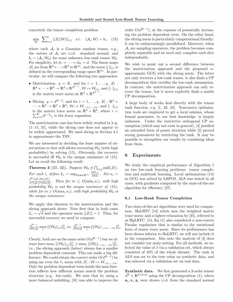
Figure 1: Test RSE on synthetic data generated by CP decomposition. RpLRTC is not included in (b) becauseit gets very slow when d ≥ 200.
distribution. So rank(Z0) ≤ r and we loosely call r therank. Zi,j,k := (Z0
i,j,k − mean(Z0)) /(d1.5std(Z0)) +ξi,j,k, where mean and std stand for the mean and stan-dard deviation, respectively, and ξi,j,k are i.i.d. Gaus-sians with zero mean and variance 0.12. We randomlypicked p% elements of Z as observations for training,and the reconstructed tensor W was compared withZ0 on the rest (90 − p)% entries. The whole processwas repeated 10 times, and we report the average ofRSE :=
∥∥Wte −Z0te
∥∥F/∥∥Z0
te
∥∥F
[14].
Figures 1(a) to 1(c) show the test RSE as a functionof density p of the training data, the size d, and theCP rank r respectively. In all plots, parameters notvarying in the x-axis were set to the default values:p = 1, r = 10, and d = 100. Clearly, in all casesGCG yields significantly more accurate completionsthan ALS, HaLRTC, and RpLRTC. Fixing d and r,GCG clearly outperforms when the tensor is sparse(p = 1 or 2). In real datasets such as Yelp and Nellbelow, less than 1% entries are observed, and there-fore it is indeed an interesting regime. ALS exhibitshigher variance suggesting susceptibility to local min-ima. With fixed p and r, increasing the size of tensorallows both ALS and GCG to reduce test RSE. But itbenefits GCG much more thanks to its convexity. Fi-nally, increasing the CP rank makes the problem chal-lenging for all methods. This is reasonable becausethe sample size is fixed. Overall, the results confirmhigher faithfulness of GCG in low-rank tensor comple-tion than nonconvex methods and matricization basedregularizers when the tensor is sparse.
Computational time is another key aspect of compari-son. To make the comparison fair, we set d = 100, p =8, r = 10 so that ALS and GCG achieve similar RSE.HaLRTC and RpLRTC are not included because theyscale much more poorly. Figure 1(d) shows that GCGis much more efficient than ALS in reducing the testRSE.
Image inpainting. Images are naturally repre-sented as a “width (259)” × “height (247)” × “RGB
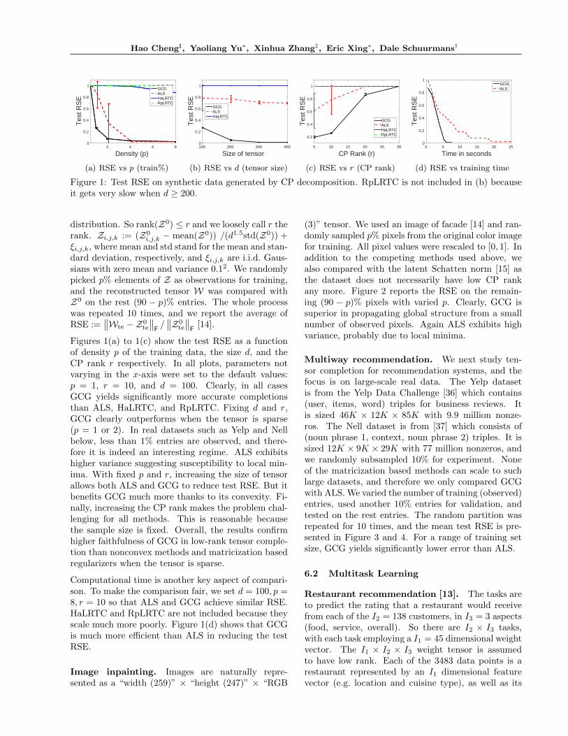
(3)” tensor. We used an image of facade [14] and ran-domly sampled p% pixels from the original color imagefor training. All pixel values were rescaled to [0, 1]. Inaddition to the competing methods used above, wealso compared with the latent Schatten norm [15] asthe dataset does not necessarily have low CP rankany more. Figure 2 reports the RSE on the remain-ing (90 − p)% pixels with varied p. Clearly, GCG issuperior in propagating global structure from a smallnumber of observed pixels. Again ALS exhibits highvariance, probably due to local minima.
Multiway recommendation. We next study ten-sor completion for recommendation systems, and thefocus is on large-scale real data. The Yelp datasetis from the Yelp Data Challenge [36] which contains(user, items, word) triples for business reviews. Itis sized 46K × 12K × 85K with 9.9 million nonze-ros. The Nell dataset is from [37] which consists of(noun phrase 1, context, noun phrase 2) triples. It issized 12K × 9K × 29K with 77 million nonzeros, andwe randomly subsampled 10% for experiment. Noneof the matricization based methods can scale to suchlarge datasets, and therefore we only compared GCGwith ALS. We varied the number of training (observed)entries, used another 10% entries for validation, andtested on the rest entries. The random partition wasrepeated for 10 times, and the mean test RSE is pre-sented in Figure 3 and 4. For a range of training setsize, GCG yields significantly lower error than ALS.
6.2 Multitask Learning
Restaurant recommendation [13]. The tasks areto predict the rating that a restaurant would receivefrom each of the I2 = 138 customers, in I3 = 3 aspects(food, service, overall). So there are I2 × I3 tasks,with each task employing a I1 = 45 dimensional weightvector. The I1 × I2 × I3 weight tensor is assumedto have low rank. Each of the 3483 data points is arestaurant represented by an I1 dimensional featurevector (e.g. location and cuisine type), as well as its
Scalable and Sound Low-Rank Tensor Learning
Density (p)2 4 6 8
Tes
t RS
E
0
0.2
0.4
0.6
0.8
1 GCGALSHaLRTCLatent normRpLRTC
Figure 2: Image inpainting
0 0.5 1 1.5 2 2.5 3 3.5
x 107
0.4
0.45
0.5
0.55
0.6
0.65
0.7
0.75
Number of training examples
Tes
t RS
E
GCGALS
Figure 3: Test RSE on Yelp
0 0.5 1 1.5 2 2.5 3 3.5
x 107
0.5
0.6
0.7
0.8
0.9
1
Number of training examples
Tes
t RS
E
GCGALS
Figure 4: Test RSE on Nell
Sample Size500 1000 1500 2000 2500
Tes
t MS
E
0.4
0.5
0.6
0.7
0.8GCGALSMLMTLCScaled latent norm
Figure 5: Restaurant rating prediction
Sample Size2000 4000 6000 8000 10000
Exp
lain
ed V
aria
nce
-10
0
10
20
30
40
GCGALSMLMTLCScaled latent norm
Figure 6: School grade prediction
I2 × I3 number of ratings. Predicting these ratingsconstitutes I2 × I3 regression problems, each with an`2 loss.
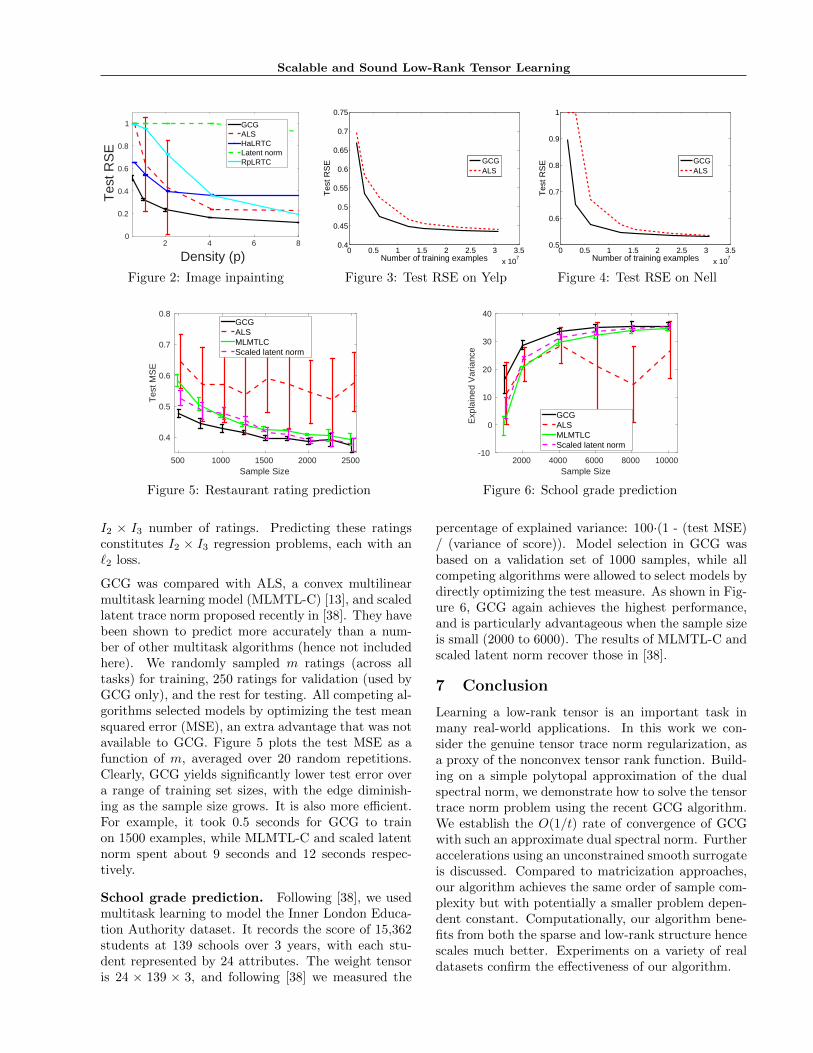
GCG was compared with ALS, a convex multilinearmultitask learning model (MLMTL-C) [13], and scaledlatent trace norm proposed recently in [38]. They havebeen shown to predict more accurately than a num-ber of other multitask algorithms (hence not includedhere). We randomly sampled m ratings (across alltasks) for training, 250 ratings for validation (used byGCG only), and the rest for testing. All competing al-gorithms selected models by optimizing the test meansquared error (MSE), an extra advantage that was notavailable to GCG. Figure 5 plots the test MSE as afunction of m, averaged over 20 random repetitions.Clearly, GCG yields significantly lower test error overa range of training set sizes, with the edge diminish-ing as the sample size grows. It is also more efficient.For example, it took 0.5 seconds for GCG to trainon 1500 examples, while MLMTL-C and scaled latentnorm spent about 9 seconds and 12 seconds respec-tively.
School grade prediction. Following [38], we usedmultitask learning to model the Inner London Educa-tion Authority dataset. It records the score of 15,362students at 139 schools over 3 years, with each stu-dent represented by 24 attributes. The weight tensoris 24 × 139 × 3, and following [38] we measured the
percentage of explained variance: 100·(1 - (test MSE)/ (variance of score)). Model selection in GCG wasbased on a validation set of 1000 samples, while allcompeting algorithms were allowed to select models bydirectly optimizing the test measure. As shown in Fig-ure 6, GCG again achieves the highest performance,and is particularly advantageous when the sample sizeis small (2000 to 6000). The results of MLMTL-C andscaled latent norm recover those in [38].
7 Conclusion
Learning a low-rank tensor is an important task inmany real-world applications. In this work we con-sider the genuine tensor trace norm regularization, asa proxy of the nonconvex tensor rank function. Build-ing on a simple polytopal approximation of the dualspectral norm, we demonstrate how to solve the tensortrace norm problem using the recent GCG algorithm.We establish the O(1/t) rate of convergence of GCGwith such an approximate dual spectral norm. Furtheraccelerations using an unconstrained smooth surrogateis discussed. Compared to matricization approaches,our algorithm achieves the same order of sample com-plexity but with potentially a smaller problem depen-dent constant. Computationally, our algorithm bene-fits from both the sparse and low-rank structure hencescales much better. Experiments on a variety of realdatasets confirm the effectiveness of our algorithm.
Hao Cheng], Yaoliang Yu∗, Xinhua Zhang‡, Eric Xing∗, Dale Schuurmans†
References
[1] T. G. Kolda and B. W. Bader. Tensor decomposi-tions and applications. SIAM Review, 51:455–500,2009.
[2] A. Anandkumar, R. Ge, and M. Janzam-ina. Guaranteed non-orthogonal tensor decom-position via alternating rank-1 updates, 2014.ArXiv:1402.5180v2.
[3] M. Mørup and L. K. Hansen. Automatic relevancedetermination for multi-way models. Journal ofChemometrics, 23(7-8):352–363, 2009.
[4] P. Jain and S. Oh. Provable tensor factorizationwith missing data. In NIPS. 2014.
[5] V. Kuleshov, A. Chaganty, and P. Liang. Tensorfactorization via matrix factorization. In AIS-TATS. 2015.
[6] E. J. Candes and B. Recht. Exact matrix com-pletion via convex optimization. Foundations ofComputational Mathematics, 9:717–772, 2009.
[7] V. Chandrasekaran, B. Recht, P. A. Parrilo, andA. S.Willsky. The convex geometry of linear in-verse problems. Foundations of ComputationalMathematics, 12(6):805–849, 2012.
[8] M. Yuan and C.-H. Zhang. On tensor completionvia nuclear norm minimization. Foundations ofComputational Mathematics, to appear.
[9] V. D. Silva and L.-H. Lim. Tensor rank and theill-posedness of the best low-rank approximationproblem. SIAM Journal on Matrix Analysis andApplications, 30(3):1084–1127, 2008.
[10] C. J. Hillar and L.-H. Lim. Most tensor problemsare NP-hard. Journal of ACM, 60(6):45:1–45:39,2013.
[11] M. Signoretto, L. D. Lathauwer, and J. A. K.Suykens. Nuclear norms for tensors and their usefor convex multilinear estimation. Tech. Rep. 10-186, ESAT-SISTA, K. U. Leuven, 2010.
[12] S. Gandy, B. Recht, and I. Yamada. Tensor com-pletion and low-n-rank tensor recovery via convexoptimization. Inverse Problems, 27:1–19, 2011.
[13] B. Romera-Paredes, M. Aung, N. Bianchi-Berthouze, and M. Pontil. Multilinear multitasklearning. In ICML. 2013.
[14] J. Liu, P. Musialski, P. Wonka, and J. Ye. Tensorcompletion for estimating missing values in visualdata. IEEE Transactions on Pattern Analysis andMachine Intelligence, 35(1):208–220, 2013.
[15] R. Tomioka and T. Suzuki. Convex tensor decom-position via structured schatten norm regulariza-tion. In NIPS. 2013.
[16] D. Goldfarb and Z. Qin. Robust low-rank tensorrecovery: Models and algorithms. SIAM Journalon Matrix Analysis and Applications, 35:225–253,2014.
[17] X. Zhang, Y. Yu, and D. Schuurmans. Acceler-ated training for matrix-norm regularization: Aboosting approach. In NIPS. 2012.
[18] Z. Harchaoui, A. Juditsky, and A. Ne-mirovski. Conditional gradient algorithms fornorm-regularized smooth convex optimization.Mathematical Programming, 152:75–112, 2015.
[19] A. Stegeman and P. Comon. Subtracting a bestrank-1 approximation may increase tensor rank.Linear Algebra and its Applications, 433:1276–1300, 2010.
[20] M. Fazel, H. Hindi, and S. P. Boyd. A rank min-imization heuristic with application to minimumorder system approximation. In American Con-trol Conference, pp. 4734–4739. 2001.
[21] L.-H. Lim and P. Comon. Blind multilinear identi-fication. IEEE Transactions on Information The-ory, 60(2):1260–1280, 2014.
[22] H. Derksen. On the nuclear norm and the singularvalue decomposition of tensors. Foundations ofComputational Mathematics, to appear.
[23] N. Rao, P. Shah, and S. Wright. Forward - back-ward greedy algorithms for atomic norm regular-ization, 2014. ArXiv:1404.5692.
[24] M. Kochol. Constructive approximation of a ballby polytopes. Math Slovaca, 44(1):99–105, 1994.
[25] I. Barany and Z. Furedi. Approximation of thesphere by polytopes having few vertices. Pro-ceedings of the American Mathematical Society,102(3):651–659, 1988.
[26] Z. Li, S. He, and S. Zhang. Approximation Meth-ods for Polynomial Optimization: Models, Algo-rithms, and Applications. Springer, 2012.
[27] J. H. Choi and S. Vishwanathan. Dfacto: Dis-tributed factorization of tensors. In NIPS. 2014.
[28] M. Frank and P. Wolfe. An algorithm forquadratic programming. Naval Research LogisticsQuarterly, 3(1-2):95–110, 1956.
[29] S. Lacoste-Julien, M. Jaggi, M. Schmidt, andP. Pletscher. Block-Coordinate Frank-Wolfe op-timization for structured svms. In ICML. 2013.
[30] F. Bach. Convex relaxations of structured matrixfactorizations, 2013. HAL:00861118.
[31] C. Mu, B. Huang, J. Wright, and D. Goldfarb.Square deal: Lower bounds and improved relax-ations for tensor recovery. In ICML. 2014.
Scalable and Sound Low-Rank Tensor Learning
[32] D. Amelunxen, M. Lotz, M. B. McCoy, and J. A.Tropp. Living on the edge: phase transitions inconvex programs with random data. Informationand Inference, 3(3):224–294, 2014.
[33] J. Nie and L. Wang. Semidefinite relaxations forbest rank-1 tensor approximations. SIAM Journalon Matrix Analysis and Applications, 35(3):1155–1179, 2014.
[34] B. Jiang, S. Ma, and S. Zhang. Tensor princi-pal component analysis via convex optimization.Mathematical Programming, 150:423–457, 2015.
[35] B. Romera-Paredes and M. Pontil. A new convexrelaxation for tensor completion. In NIPS. 2013.
[36] Https://www.yelp.com/dataset challenge/dataset.
[37] U. Kang, E. Papalexakis, A. Harpale, andC. Faloutsos. Gigatensor: Scaling tensor analy-sis up by 100 times - algorithms and discoveries.In KDD. 2012.
[38] K. Wimalawarne, M. Sugiyama, and R. Tomioka.Multitask learning meets tensor factorization:task imputation via convex optimization. InNIPS. 2014.
[39] S. Becker, J. Bobin, and E. J. Candes. NESTA:A fast and accurate first-order method for sparserecovery. SIAM Journal on Imaging Sciences,4(1):1–39, 2009.
[40] R. Bro. PARAFAC: Tutorial and applications.Chemometrics and Intelligent Laboratory Sys-tems, 38:147–171, 1997.
[41] S. Engelen, S. Frosch, and B. Jorgensen. A fullyrobust parafac method for analyzing fluorescencedata. Journal of Chemometrics, 23(3-4):124–131,2009.
Hao Cheng], Yaoliang Yu∗, Xinhua Zhang‡, Eric Xing∗, Dale Schuurmans†
A Matricization
A tensor A can be unfolded into a matrix A in various ways. We focus here on 2-way unfoldings that specifya proper partition of 1, . . . ,K := [K] = m1, . . . ,mp ∪ n1, . . . , nq, an integer-valued row index function r,and a column index function c, such that Ai1,...,iK 7→ Ar(im1 ,...,imp ), c(in1 ,...,inq )
. This is simply a rearrangementof the entries in A hence preserves its Frobenius norm. We use the notation A(r,c) for the 2-way unfolding underthe index functions r and c.
The above tensor unfolding interacts conveniently with the mode-k multiplication, once we define a suitablematrix Kronecker product. Fix two row index functions r and r. The Kronecker product of p matrices U ∈Rdm1
×dm1 , . . . ,W ∈ Rdmp×dmp is a matrix that has size∏pk=1 dmk
×∏pk=1 dmk
and satisfies
(U · · ·W )ı,i = Uım1 ,im1· · ·Wımp ,imp
, (16)
where ı = r(ım1, . . . , ımp
) and i = r(im1, . . . , imp
).
Similar definitions can be made using two column index functions c and c. It is just algebra to verify that
(A×1 U1 · · · ×K UK)(r,c) = (Um1 · · · Ump) A(r,c) (Un1 · · · Unq )>, (17)
where the first and second group of Kronecker product use (r, r) and (c, c) respectively.
Example 1 (Mode-k unfolding A(k)). To illustrate the above definition, let us consider the partition [K] =k ∪ 1, . . . , k − 1, k + 1, . . .K and the index functions
c(i1, . . . , ik−1, ik+1, . . . , iK) = 1 +∑j 6=k
(ij − 1)∏
m>j,m 6=k
dm,
and r(ik) = ik. This is called the mode-k unfolding, together with the notation A(k). Here reduces to the usual
matrix Kronecker product, and (A×k U)(k) = UA(k). For matrices, we simply have A(1) = A, A(2) = A>, and
A×1 U ×2 V = UAV >.
Example 2 (Balanced mode-k unfolding A[k]). The mode-k unfolding above yields an extremely unbalancedmatrix with size dk ×
∏j 6=k dj. A more balanced unfolding is proposed in [31], consisting of the partition [K] =
1, . . . , k ∪ k + 1, . . .K and the index functions
r(i1, . . . , ik) = 1 +
k∑j=1
(ij − 1)∏
k≥m≥j+1
dm
c(ik+1, . . . , iK) = 1 +
K∑j=k+1
(ij − 1)∏
m≥j+1
dm,
with r, c similarly defined. The resulting matrix, denoted as A[k], has size∏kj=1 dj ×
∏Kj=k+1 dj. For k = bK/2c,
the unfolding is more like a square matrix, which can be beneficial in completion tasks [31].
B Approximating Tensor Spectral Norm
Let Bd2 be the Euclidean norm ball in a d dimensional space (d is a superscript in Bd2). We can approximateBd2 with a polytope, based on a celebrated result from convex geometry [24]: For any d, n ≥ 2 we can find inpolynomial time (at most) dn points pi, such that their convex hull Pd satisfies
Pd ⊆ Bd2 ⊆ 1c
√d
n log dPd, (18)
Scalable and Sound Low-Rank Tensor Learning
where c is some universal constant. For n = 1, we can simply take the unit ball of the 1-norm, denoted as Bd1,and get a similar result
Bd1 ⊆ Bd2 ⊆√dBd1. (19)
By counting the volume, it can be proved that the factors in (18) and (19) are the best possible respectively [25].
Specializing to the tensor spectral norm, we simply replace each Euclidean ball constraint with its polytopalapproximation as suggested in (18) or (19), and evaluate the inner product at each of the vertices of the polytope.Since the matrix trace norm is tractable, we need only execute the polytopal approximation for the last K − 2balls, i.e., solving the approximation
maxu1∈B
d12 ,u2∈B
d22 ,u3∈Pd3 ,...,uK∈PdK
〈A,u1⊗ · · ·⊗uK〉 . (20)
So for each vertex p3⊗ · · ·⊗pK (with∏Kk=3(dk)n of them), we evaluate the matrix spectral norm ‖A×3p3 · · ·×K
pK‖2 and pick the maximum. This yields the optimal solution for (20), which immediately translates to an
α = O(∏Kk=3
√nd−1k log dk) approximate solution for the tensor spectral norm (6). If we set n = 1 and use (19),
then α =∏Kk=3
√1/dk and only
∏Kk=3 dk matrix spectral norms need to be checked. The overall computational
cost is O(∏Kk=1 dk). It is also easy to reduce each factor dk to the smaller constant rank(A(k)), or simply
rank(A). For n ≥ 2 we get a log dk factor improvement in the approximation guarantee, at the expense of amore complicated and costly implementation.
C Proofs omitted in Section 4
Theorem 1. Let ` ≥ 0 be convex, smooth, and have bounded sublevel sets. Denote f(W) = `(W) + λ · κ(W).Suppose in each iteration t, we find Zt that satisfies
κ(Zt) ≤ 1, 〈Zt,∇`(Wt)〉 ≥ α · maxκ(Z)≤1
〈Z,∇`(Wt)〉 . (21)
Then for all W and for all t ≥ 1, running GCG with ηt = 2t+2 leads to f(Wt) − f(W)
α ≤ 2Ct+3 , where C is some
constant that does not depend on t or α.
Recall that the function ` is smooth if its gradient is Lipschitz continuous with respect to some norm ‖·‖, namelythat for all W and Z,
`(Z) ≤ `(W) + 〈Z −W,∇`(W)〉+L
2‖Z −W‖2, (22)
for some constant L := L‖·‖ ≥ 0. The least squares loss in fact satisfies (22) with equality and L = 2.
Proof. Let W be arbitrary and s = κ(W). Let Wt+1 be the output of GCG at iteration t+ 1 and Wt+1 be the
Hao Cheng], Yaoliang Yu∗, Xinhua Zhang‡, Eric Xing∗, Dale Schuurmans†
improved iterate after local search. The following chain of inequalities can be easily verified:
f(Wt+1) ≤ f(Wt+1)
= `(Wt+1) + λ · κ(Wt+1)
= ` ((1− ηt)Wt + ηtβtZt) + λ · κ((1− ηt)Wt + ηtβtZt) (definition of Wt+1)
≤ ` ((1− ηt)Wt + ηtβtZt) + λ(1− ηt)κ(Wt) + ληtβtκ(Zt) (sublinearity of κ)
≤ ` ((1− ηt)Wt + ηtβtZt) + λ(1− ηt)κ(Wt) + ληtβt (definition of Zt)
≤ `(
(1− ηt)Wt + ηts
αZt)
+ λ(1− ηt)κ(Wt) + ληts
α(definition of βt)
≤ f(Wt) + ηt
⟨ sαZt −Wt,∇`(Wt)
⟩+L∥∥ sαZt −Wt
∥∥22
η2t − ληtκ(Wt) + ληts
α(inequality (22))
≤ minZ:κ(Z)≤1
f(Wt) + ηt 〈sZ −Wt,∇`(Wt)〉+L∥∥ sαZt −Wt
∥∥22
η2t − ληtκ(Wt) + ληts
α(definition of Zt)
= minZ:κ(Z)≤s
f(Wt) + ηt 〈Z −Wt,∇`(Wt)〉+L∥∥ sαZt −Wt
∥∥22
η2t − ληtκ(Wt) + ληts
α(homogeneity of κ)
≤ minZ:κ(Z)≤s
f(Wt) + ηt(`(Z)− `(Wt)) +L∥∥ sαZt −Wt
∥∥22
η2t − ληt · κ(Wt) + ληts
α(convexity of `)
= (1− ηt)f(Wt) + ηt minZ:κ(Z)≤s
(`(Z) + λ · sα
) +L∥∥ sαZt −Wt
∥∥22
η2t
≤ (1− ηt)f(Wt) + ηtf(W)
α+L∥∥ sαZt −Wt
∥∥22
η2t (` ≥ 0 and α ∈ (0, 1]).
Therefore,
f(Wt+1)− f(W)
α≤ (1− ηt)
(f(Wt)−
f(W)
α
)+L∥∥ sαZt −Wt
∥∥22
η2t .
Recall that ηt = 2t+2 . An easy induction argument establishes that
f(Wt+1)− f(W)
α≤ 2C
t+ 3,
where C := supt L∥∥ sαZt −Wt
∥∥2 ≤ 2L(κ2(W)/α2 + D2) < ∞, since Wt is in the sublevel set of Z : f(Z) ≤f(W1), whose radius is assumed to be bounded by D.
Theorem 2. Fix A ∈ Rd1×···×dK and t ≥∏Kk=1 dk, then
‖A‖tr = min
Σti=1 ‖ui‖2 · · · ‖zi‖2
(23)
= min
1K Σ
ti=1 ‖ui‖
K2 + · · ·+ ‖zi‖K2
, (24)
where the minimum is taken w.r.t. all factorizations A =∑ti=1 ui⊗ · · ·⊗ zi, ui ∈ Rd1 , . . . , zi ∈ RdK .
Proof. We first note that the atomic set A in (4) is compact, so is its convex hull conv(A). Moreover, A isconnected. Recall that the trace norm is defined in (5) via the gauge function κ. Since conv(A) is compact with0 in its interior, we know the infimum in (5) is attained. Thus there exist ρ ≥ 0 and C ∈ conv(A) so that A = ρCand ‖A‖tr = κ(A) = ρ. Applying Caratheodory’s theorem we know C =
∑ti=1 σiui⊗ · · ·⊗ zi for some σi ≥ 0,∑
i σi = 1, ui⊗ · · ·⊗ zi ∈ A and t ≤∏Kk=1 dk. Let ui = K
√ρσiui, · · · , zi = K
√ρσizi we know ‖A‖tr is at least the
right-hand side of (24).
On the other hand, for any A =∑ti=1 ui⊗ · · ·⊗ zi, denoting σi = ‖ui‖2 · · · ‖zi‖2 (6= 0 w.l.o.g.), we have
A = (∑i σi) ·
∑ti=1
σi∑tj=1 σj
Ai, where Ai := ui
‖ui‖2⊗ · · ·⊗ zi
‖zi‖2∈ A. Thus, appealing to the definition (5) we
know ‖A‖tr ≤∑i σi, i.e. (23) holds with ≤.
Scalable and Sound Low-Rank Tensor Learning
To complete the proof, we apply the arithmetic-geometric mean inequality:∑i‖ui‖2 · · · ‖zi‖2 ≤
1K
∑i‖ui‖K2 + · · ·+ ‖zi‖K2 .
(Of course, other elementary symmetric functions can be similarly used in Theorem 2.)
D Comparison with alternative variational forms
We compare the variational forms in Theorem 2 to some existing ones in the tensor literature. Firstly, theregularization function ∑
i‖ui‖22 + · · ·+ ‖zi‖22 , (25)
is extensively used in finding CP decompositions, since otherwise the factors could blow up in a way thatstill maintains their sum, the so-called degeneracy problem [9]. A second reason for employing (25) is that itadds strict convexity w.r.t. each factor hence guarantees the convergence of block coordinate ascent. However,both reasons to promote (25), albeit valid, are weak; there are certainly other, perhaps even better, candidateregularizations. For instance, (24) enjoys both properties, with the additional equivalence to the trace norm,which potentially could lead to a low rank solution. The second variational form, appeared in [13], is
‖C‖2F + ‖U‖2F + · · ·+ ‖Z‖2F, (26)
where A = C ×1 U · · · ×K Z is the Tucker decomposition. [13] used (26) to avoid the scaling ambiguity—a weakmotivation for the particular form (26) indeed. Let us show that neither (25) nor (26) is equivalent to the tracenorm. From this regard, the variational forms in Theorem 2 are advantageous and perhaps should be favoredmore often in practice.
Example 3. We first prove (25) is not equivalent to the trace norm. Let A = σu⊗ · · ·⊗ z be a rank-1 tensorwith σ > 0 and ‖u‖2 = · · · = ‖z‖2 = 1. It is easy to see that ‖A‖tr = σ. Consider the function:
f(A) := min∑
i‖ui‖22 + · · ·+ ‖zi‖22
,
where the minimum is taken w.r.t. to all factorizations A =∑i ui⊗ · · ·⊗ zi. Clearly,
f(A) ≤ K · σ2/K .
Choose an appropriate σ > 1 we thus have f(A) < ‖A‖tr. Of course, for any positive constant c, we can chooseappropriate σ such that c · f(A) < ‖A‖tr. Thus (25) is not proportional to the trace norm.
For the function (26), we similarly define
g(A) := inf‖C‖2F + ‖U‖2F + · · ·+ ‖Z‖2F
,
where the infimum is taken w.r.t. all Tucker decompositions A = C ×1 U · · · ×K Z. This removes the dependenceof (26) on a particular Tucker decomposition (which may not be unique). Consider the same rank-1 tensor A asabove, we have g(A) ≤ (K + 1)σ2/(K+1) while ‖A‖tr = σ. Again, choosing σ large we have c · g(A) < ‖A‖tr forany positive constant c. Note that even for K = 2, g(A) is not proportional to the trace norm.
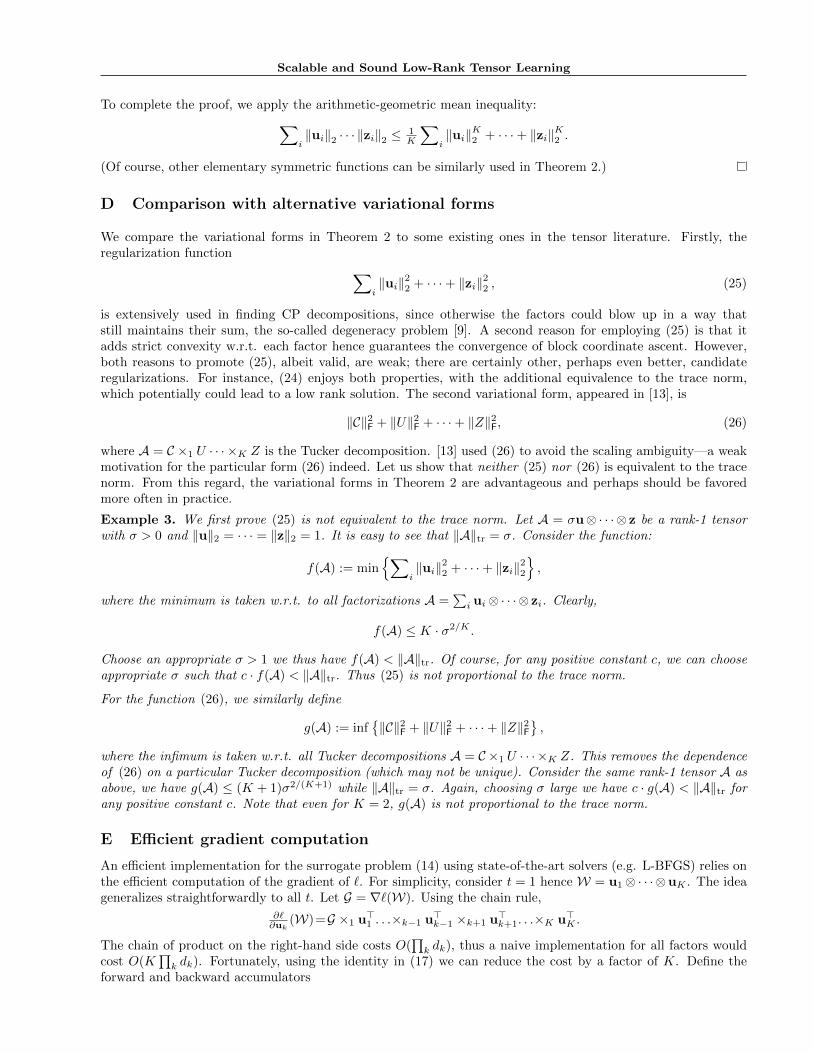
E Efficient gradient computation
An efficient implementation for the surrogate problem (14) using state-of-the-art solvers (e.g. L-BFGS) relies onthe efficient computation of the gradient of `. For simplicity, consider t = 1 hence W = u1⊗ · · ·⊗uK . The ideageneralizes straightforwardly to all t. Let G = ∇`(W). Using the chain rule,
∂`∂uk
(W)=G ×1 u>1 . . .×k−1 u>k−1 ×k+1 u>k+1. . .×K u>K .
The chain of product on the right-hand side costs O(∏k dk), thus a naive implementation for all factors would
cost O(K∏k dk). Fortunately, using the identity in (17) we can reduce the cost by a factor of K. Define the
forward and backward accumulators
Hao Cheng], Yaoliang Yu∗, Xinhua Zhang‡, Eric Xing∗, Dale Schuurmans†
Fk := G ×1 u>1 . . .×k−1 u>k−1, Bk := uk+1 ⊗ . . .⊗ uK ,
with F1 := G and BK := 1. Then we have
∂`∂uk
(W) = Fk ×k+1 u>k+1 . . .×K u>K = (Fk)(k)Bk.
So we need only compute Fk,Bk, costing O(∏k dk). Since for all k the multiplication (Fk)(k)Bk costs
O(∏j≥k dj), the overall time and space costs are both O(
∏k dk). Clearly the computational savings are possible
due to our explicit low-rank representation, which is not available in other matricization approaches.
F Comparison on completing tensors with low-rank Tucker decompositions
We repeated all comparisons conducted for low CP rank on low Tucker rank: Z0 = S ×1 U1 ×2 U2 ×3 U3, whereS ∈ Rr×r×r and Ui ∈ Rn×r. Our setting here is exactly the same as Section 6.1. Again, all entries of S and Uiwere drawn i.i.d. from a unit normal. We set the default p=20, σ=0.1, r=5 (hence CP rank ≤ 25), and n=50.Figure 7 shows that even in this case TTN still outperforms HaLRTC and RpLRTC (abbreviated as RP).
0.1 0.2 0.3 0.4 0.50
0.2
0.4
0.6
0.8
1
Fraction of Observations (p%)
Tes
t RS
E
TTNHaLRTCRP
(a) RSE vs p (train%)
2 4 6 80
0.1
0.2
0.3
Rank(r)
Tes
t RS
E
TTNHaLRTCRP
(b) RSE vs r (rank)
10−4
10−2
10010
−2
10−1
Noise variance σ2
Tes
t RS
E
TTNHaLRTCRP
(c) RSE vs σ (noise std)
20 30 40 50 600
0.2
0.4
0.6
Size(n)
Tes
t RS
E
TTNHaLRTCRP
(d) RSE vs n (tensor size)
Figure 7: Test RSE on synthetic data generated by Tucker decomposition with rank r × r × r.
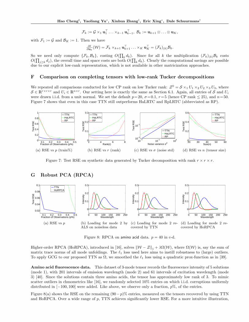
G Robust PCA (RPCA)
0.1 0.2 0.3 0.4 0.5
0.02
0.04
0.06
0.08
0.1
Fraction of Observations (p%)
Tes
t RS
E
TTNHoRPCA
(a) RSE vs p
0 50 100 150 200 250
0
0.1
0.2
0.3
Wavelength
Inte
nsity
(b) Loading for mode 2 byALS on noiseless data
0 50 100 150 200 250
0
0.1
0.2
0.3
Wavelength
Inte
nsity
(c) Loading for mode 2 re-covered by TTN
0 50 100 150 200 250
0
0.1
0.2
0.3
Wavelength
Inte
nsity
(d) Loading for mode 2 re-covered by HoRPCA
Figure 8: RPCA on amino acid data. p = 40 in c-d.
Higher-order RPCA (HoRPCA), introduced in [16], solves ‖W − Z‖1 + λΩ(W), where Ω(W) is, say the sum ofmatrix trace norms of all mode unfoldings. The `1 loss used here aims to instill robustness to (large) outliers.To apply GCG to our proposed TTN as Ω, we smoothed the `1 loss using a quadratic prox-function as in [39].
Amino acid fluorescence data. This dataset of 3-mode tensor records the fluorescence intensity of 5 solutions(mode 1), with 201 intervals of emission wavelength (mode 2) and 61 intervals of excitation wavelength (mode3) [40]. Since the solutions contain three amino acids, the tensor has approximately low rank of 3. To mimicscatter outliers in chmometrics like [16], we randomly selected 10% entries on which i.i.d. corruptions uniformlydistributed in [−100, 100] were added. Like above, we observe only a fraction, p%, of the entries.
Figure 8(a) shows the RSE on the remaining (90−p)% entries, measured on the tensors recovered by using TTNand HoRPCA. Over a wide range of p, TTN achieves significantly lower RSE. For a more intuitive illustration,
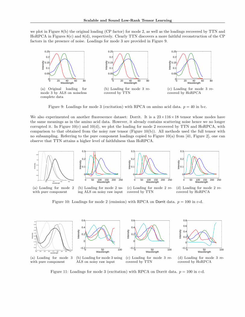
Scalable and Sound Low-Rank Tensor Learning
we plot in Figure 8(b) the original loading (CP factor) for mode 2, as well as the loadings recovered by TTN andHoRPCA in Figures 8(c) and 8(d), respectively. Clearly TTN discovers a more faithful reconstruction of the CPfactors in the presence of noise. Loadings for mode 3 are provided in Figure 9.
0 20 40 60 800
0.05
0.1
0.15
0.2
0.25
Wavelength
Inte
nsity
(a) Original loading formode 3 by ALS on noiselesscomplete data
0 20 40 60 800
0.05
0.1
0.15
0.2
0.25
Wavelength
Inte
nsity
(b) Loading for mode 3 re-covered by TTN
0 20 40 60 800
0.05
0.1
0.15
0.2
0.25
Wavelength
Inte
nsity
(c) Loading for mode 3 re-covered by HoRPCA
Figure 9: Loadings for mode 3 (excitation) with RPCA on amino acid data. p = 40 in b-c.
We also experimented on another fluorescence dataset: Dorrit. It is a 23×116×18 tensor whose modes havethe same meanings as in the amino acid data. However, it already contains scattering noise hence we no longercorrupted it. In Figure 10(c) and 10(d), we plot the loading for mode 2 recovered by TTN and HoRPCA, withcomparison to that obtained from the noisy raw tensor (Figure 10(b)). All methods used the full tensor withno subsampling. Referring to the pure component loadings copied to Figure 10(a) from [41, Figure 2], one canobserve that TTN attains a higher level of faithfulness than HoRPCA.
environment the excitation ranging from 200 to 230 nm and theemission below 250 was excluded from the data set before furtheranalysis. This gives a data set with dimensions (27 116 18). Afour-component PARAFAC model seems to be the most suitable[13,25]. The excitation and emission loadings that should beobtained are depicted in Figure 2.All samples contain severe Rayleigh scatter, which are element-
wise outliers. Moreover, from previous investigations four samples(sample number 2, 3, 5, and 10) were marked as outlying samples[13]. However, Engelen and Hubert [1] investigated the data byrobust PARAFAC and found that sample 10 is rather a border casethat an outlier.Hence, the Dorrit data set comprises both types of outliers,
which makes these data highly suitable for comparing theproposed combined robust PARAFAC model with the model
obtained from the classical PARAFAC method and the samplerobust PARAFAC approach and the automated scatter identifi-cation procedure in combination with classical PARAFAC. Theresults of fitting the four PARAFAC algorithms are shown in termsof estimated excitation and emission spectra in Figure 3.The proposed combined PARAFAC algorithm was the only one
providing excitation and emission loadings which are in agreementwith the pure component spectra shown in Figure 2. The otherthree methods lacked accuracy, because the outlying samples andoutlying elements deteriorated these models.Furthermore, outliers of type 1 were marked in a similar way as
by the robust sample PARAFAC procedure. The diagnostic plot,introduced for these purposes in Engelen and Hubert [1], couldalso be applied to the combined method. Only the computationof the residual distance, which is placed on the vertical axis of the
Table IV. Simulation results for data containing scatter and bad leverage points
Method Classic Scatter Sample Combined
Bad leverage points 10% 20% 10% 20% 10% 20% 10% 20%
MSE 0.128 0.149 0.103 0.129 0.103 0.106 0.0627 0.0659
Angle (B,B) 0.218 0.228 0.166 0.192 0.243 0.233 0.0643 0.0607
Angle (C,C) 0.199 0.221 0.176 0.204 0.105 0.105 0.0406 0.0401
PVE 0.682 0.678 0.743 0.721 0.744 0.770 0.845 0.858
Table V. Simulation results for data containing scatter and residual outliers
Method Classic Scatter Sample Combined
Residual outliers 10% 20% 10% 20% 10% 20% 10% 20%
MSE 0.119 0.138 0.0701 0.0884 0.112 0.131 0.0629 0.0602
Angle (B,B) 0.240 0.264 0.0920 0.148 0.236 0.254 0.0564 0.0503
Angle (C,C) 0.153 0.209 0.0971 0.156 0.136 0.194 0.0396 0.0399
PVE 0.708 0.672 0.828 0.791 0.724 0.690 0.845 0.858
300 350 400 4500
0.05
0.1
0.15
0.2
0.25
Inte
nsi
ty
wavelength
Emission Loadings
230 240 250 260 270 280 290 300 3100
0.05
0.1
0.15
0.2
0.25
0.3
0.35
0.4
0.45
0.5
Inte
nsi
ty
wavelength
Excitation Loadings
Figure 2. The pure component emission (left) and excitation (right) spectra of the Dorrit data.
www.interscience.wiley.com/journal/cem Copyright 2009 John Wiley & Sons, Ltd. J. Chemometrics 2009; 23: 124–131
S. Engelen, S. Frosch and B. M. Jørgensen
128
(a) Loading for mode 2with pure component
0 50 100 150 200 250
0
0.1
0.2
0.3
Wavelength
Inte
nsity
(b) Loading for mode 2 us-ing ALS on noisy raw input
0 50 100 150 200 250
0
0.1
0.2
0.3
Wavelength
Inte
nsity
(c) Loading for mode 2 re-covered by TTN
0 50 100 150 200 250
0
0.1
0.2
0.3
Wavelength
Inte
nsity
(d) Loading for mode 2 re-covered by HoRPCA
Figure 10: Loadings for mode 2 (emission) with RPCA on Dorrit data. p = 100 in c-d.
environment the excitation ranging from 200 to 230 nm and theemission below 250 was excluded from the data set before furtheranalysis. This gives a data set with dimensions (27 116 18). Afour-component PARAFAC model seems to be the most suitable[13,25]. The excitation and emission loadings that should beobtained are depicted in Figure 2.All samples contain severe Rayleigh scatter, which are element-
wise outliers. Moreover, from previous investigations four samples(sample number 2, 3, 5, and 10) were marked as outlying samples[13]. However, Engelen and Hubert [1] investigated the data byrobust PARAFAC and found that sample 10 is rather a border casethat an outlier.Hence, the Dorrit data set comprises both types of outliers,
which makes these data highly suitable for comparing theproposed combined robust PARAFAC model with the model
obtained from the classical PARAFAC method and the samplerobust PARAFAC approach and the automated scatter identifi-cation procedure in combination with classical PARAFAC. Theresults of fitting the four PARAFAC algorithms are shown in termsof estimated excitation and emission spectra in Figure 3.The proposed combined PARAFAC algorithm was the only one
providing excitation and emission loadings which are in agreementwith the pure component spectra shown in Figure 2. The otherthree methods lacked accuracy, because the outlying samples andoutlying elements deteriorated these models.Furthermore, outliers of type 1 were marked in a similar way as
by the robust sample PARAFAC procedure. The diagnostic plot,introduced for these purposes in Engelen and Hubert [1], couldalso be applied to the combined method. Only the computationof the residual distance, which is placed on the vertical axis of the
Table IV. Simulation results for data containing scatter and bad leverage points
Method Classic Scatter Sample Combined
Bad leverage points 10% 20% 10% 20% 10% 20% 10% 20%
MSE 0.128 0.149 0.103 0.129 0.103 0.106 0.0627 0.0659
Angle (B,B) 0.218 0.228 0.166 0.192 0.243 0.233 0.0643 0.0607
Angle (C,C) 0.199 0.221 0.176 0.204 0.105 0.105 0.0406 0.0401
PVE 0.682 0.678 0.743 0.721 0.744 0.770 0.845 0.858
Table V. Simulation results for data containing scatter and residual outliers
Method Classic Scatter Sample Combined
Residual outliers 10% 20% 10% 20% 10% 20% 10% 20%
MSE 0.119 0.138 0.0701 0.0884 0.112 0.131 0.0629 0.0602
Angle (B,B) 0.240 0.264 0.0920 0.148 0.236 0.254 0.0564 0.0503
Angle (C,C) 0.153 0.209 0.0971 0.156 0.136 0.194 0.0396 0.0399
PVE 0.708 0.672 0.828 0.791 0.724 0.690 0.845 0.858
300 350 400 4500
0.05
0.1
0.15
0.2
0.25
Inte
nsity
wavelength
Emission Loadings
230 240 250 260 270 280 290 300 3100
0.05
0.1
0.15
0.2
0.25
0.3
0.35
0.4
0.45
0.5
Inte
nsity
wavelength
Excitation Loadings
Figure 2. The pure component emission (left) and excitation (right) spectra of the Dorrit data.
www.interscience.wiley.com/journal/cem Copyright 2009 John Wiley & Sons, Ltd. J. Chemometrics 2009; 23: 124–131
S. Engelen, S. Frosch and B. M. Jørgensen
128
(a) Loading for mode 3with pure component
0 50 100−0.2
0
0.2
0.4
0.6
Wavelength
Inte
nsity
(b) Loading for mode 3 usingALS on noisy raw input
0 50 100−0.2
0
0.2
0.4
0.6
Wavelength
Inte
nsity
(c) Loading for mode 3 re-covered by TTN
0 50 100−0.2
0
0.2
0.4
0.6
0.8
Wavelength
Inte
nsity
(d) Loading for mode 3 re-covered by HoRPCA
Figure 11: Loadings for mode 3 (excitation) with RPCA on Dorrit data. p = 100 in c-d.