scalable tensor factorizations for incomplete datai - arxiv · scalable tensor factorizations for...
TRANSCRIPT
Scalable Tensor Factorizations for Incomplete DataI
Evrim Acara,1, Daniel M. Dunlavyc,1, Tamara G. Koldab,1,∗, Morten Mørupd
aTUBITAK-UEKAE, Gebze, Turkey.bSandia National Laboratories, Livermore, CA 94551-9159.
cSandia National Laboratories, Albuquerque, NM 87123-1318.dTechnical University of Denmark, 2800 Kgs. Lyngby, Denmark.
Abstract
The problem of incomplete data—i.e., data with missing or unknown values—inmulti-way arrays is ubiquitous in biomedical signal processing, network trafficanalysis, bibliometrics, social network analysis, chemometrics, computer vision,communication networks, etc. We consider the problem of how to factorizedata sets with missing values with the goal of capturing the underlying latentstructure of the data and possibly reconstructing missing values (i.e., tensorcompletion). We focus on one of the most well-known tensor factorizations thatcaptures multi-linear structure, CANDECOMP/PARAFAC (CP). In the pres-ence of missing data, CP can be formulated as a weighted least squares problemthat models only the known entries. We develop an algorithm called CP-WOPT(CP Weighted OPTimization) that uses a first-order optimization approach tosolve the weighted least squares problem. Based on extensive numerical exper-iments, our algorithm is shown to successfully factorize tensors with noise andup to 99% missing data. A unique aspect of our approach is that it scales tosparse large-scale data, e.g., 1000× 1000× 1000 with five million known entries(0.5% dense). We further demonstrate the usefulness of CP-WOPT on tworeal-world applications: a novel EEG (electroencephalogram) application wheremissing data is frequently encountered due to disconnections of electrodes andthe problem of modeling computer network traffic where data may be absentdue to the expense of the data collection process.
Keywords: missing data, incomplete data, tensor factorization,CANDECOMP, PARAFAC, optimization
IA preliminary conference version of this paper has appeared as [1].∗Corresponding authorEmail addresses: [email protected] (Evrim Acar), [email protected]
(Daniel M. Dunlavy), [email protected] (Tamara G. Kolda), [email protected] (MortenMørup)
1This work was funded by the Laboratory Directed Research & Development (LDRD)program at Sandia National Laboratories, a multiprogram laboratory operated by SandiaCorporation, a Lockheed Martin Company, for the United States Department of Energy’s
Preprint submitted for publication May 14, 2010
arX
iv:1
005.
2197
v1 [
mat
h.N
A]
12
May
201
0
1. Introduction
Missing data can arise in a variety of settings due to loss of information,errors in the data collection process, or costly experiments. For instance, inbiomedical signal processing, missing data can be encountered during EEG anal-ysis, where multiple electrodes are used to collect the electrical activity alongthe scalp. If one of the electrodes becomes loose or disconnected, the signal iseither lost or discarded due to contamination with high amounts of mechanicalnoise. We also encounter the missing data problem in other areas of data min-ing, such as packet losses in network traffic analysis [2] and occlusions in imagesin computer vision [3]. Many real-world data with missing entries are ignoredbecause they are deemed unsuitable for analysis, but this work contributes tothe growing evidence that such data can be analyzed.
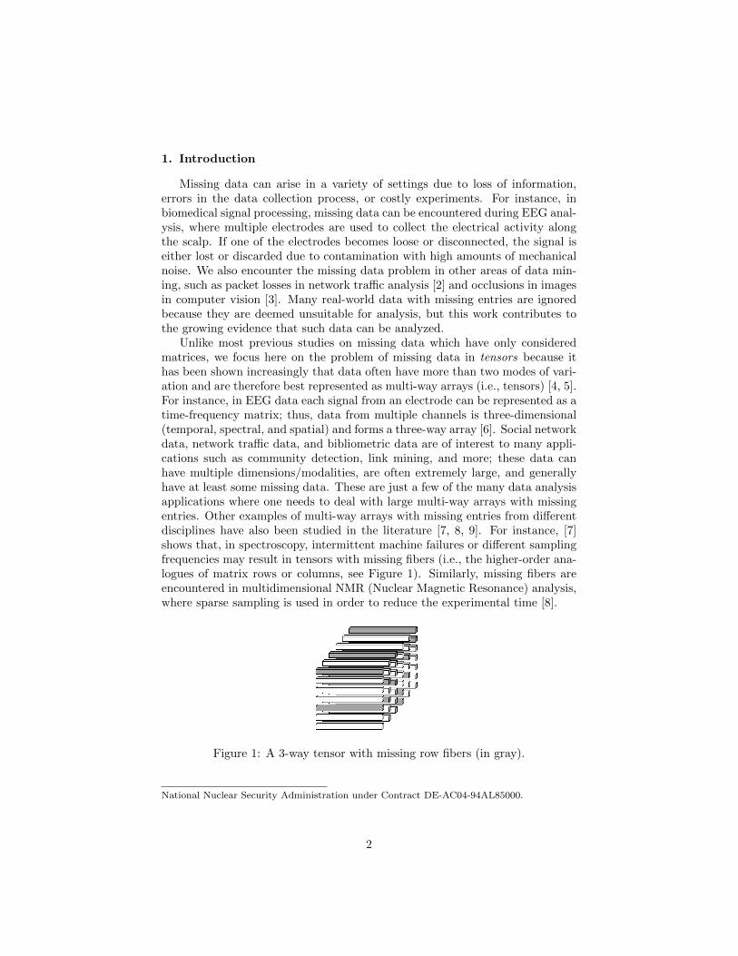
Unlike most previous studies on missing data which have only consideredmatrices, we focus here on the problem of missing data in tensors because ithas been shown increasingly that data often have more than two modes of vari-ation and are therefore best represented as multi-way arrays (i.e., tensors) [4, 5].For instance, in EEG data each signal from an electrode can be represented as atime-frequency matrix; thus, data from multiple channels is three-dimensional(temporal, spectral, and spatial) and forms a three-way array [6]. Social networkdata, network traffic data, and bibliometric data are of interest to many appli-cations such as community detection, link mining, and more; these data canhave multiple dimensions/modalities, are often extremely large, and generallyhave at least some missing data. These are just a few of the many data analysisapplications where one needs to deal with large multi-way arrays with missingentries. Other examples of multi-way arrays with missing entries from differentdisciplines have also been studied in the literature [7, 8, 9]. For instance, [7]shows that, in spectroscopy, intermittent machine failures or different samplingfrequencies may result in tensors with missing fibers (i.e., the higher-order ana-logues of matrix rows or columns, see Figure 1). Similarly, missing fibers areencountered in multidimensional NMR (Nuclear Magnetic Resonance) analysis,where sparse sampling is used in order to reduce the experimental time [8].
Figure 1: A 3-way tensor with missing row fibers (in gray).
National Nuclear Security Administration under Contract DE-AC04-94AL85000.
2
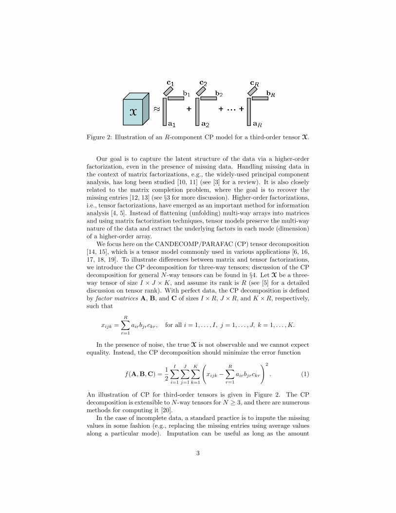
Figure 2: Illustration of an R-component CP model for a third-order tensor X.
Our goal is to capture the latent structure of the data via a higher-orderfactorization, even in the presence of missing data. Handling missing data inthe context of matrix factorizations, e.g., the widely-used principal componentanalysis, has long been studied [10, 11] (see [3] for a review). It is also closelyrelated to the matrix completion problem, where the goal is to recover themissing entries [12, 13] (see §3 for more discussion). Higher-order factorizations,i.e., tensor factorizations, have emerged as an important method for informationanalysis [4, 5]. Instead of flattening (unfolding) multi-way arrays into matricesand using matrix factorization techniques, tensor models preserve the multi-waynature of the data and extract the underlying factors in each mode (dimension)of a higher-order array.
We focus here on the CANDECOMP/PARAFAC (CP) tensor decomposition[14, 15], which is a tensor model commonly used in various applications [6, 16,17, 18, 19]. To illustrate differences between matrix and tensor factorizations,we introduce the CP decomposition for three-way tensors; discussion of the CPdecomposition for general N -way tensors can be found in §4. Let X be a three-way tensor of size I × J ×K, and assume its rank is R (see [5] for a detaileddiscussion on tensor rank). With perfect data, the CP decomposition is definedby factor matrices A, B, and C of sizes I ×R, J ×R, and K ×R, respectively,such that
xijk =
R∑r=1
airbjrckr, for all i = 1, . . . , I, j = 1, . . . , J, k = 1, . . . ,K.
In the presence of noise, the true X is not observable and we cannot expectequality. Instead, the CP decomposition should minimize the error function
f(A,B,C) =1
2
I∑i=1
J∑j=1
K∑k=1
(xijk −
R∑r=1
airbjrckr
)2
. (1)
An illustration of CP for third-order tensors is given in Figure 2. The CPdecomposition is extensible to N -way tensors for N ≥ 3, and there are numerousmethods for computing it [20].
In the case of incomplete data, a standard practice is to impute the missingvalues in some fashion (e.g., replacing the missing entries using average valuesalong a particular mode). Imputation can be useful as long as the amount
3
of missing data is small; however, performance degrades for large amounts ofmissing data [10, 1]. As a better alternative, factorizations of the data withimputed values for missing entries can be used to re-impute the missing valuesand the procedure can be repeated to iteratively determine suitable values forthe missing entries. Such a procedure is an example of the expectation max-imization (EM) algorithm [21]. Computing CP decompositions by combiningthe alternating least squares method, which computes the factor matrices oneat a time, and iterative imputation (denoted EM-ALS in this paper) has beenshown to be quite effective and has the advantage of often being simple and fast.Nevertheless, as the amount of missing data increases, the performance of thealgorithm may suffer since the initialization and the intermediate models usedto impute the missing values will increase the risk of converging to a less thanoptimal factorization [7]. Also, the poor convergence of alternating methodsdue to their vulnerability to flatlining, i.e., stagnation, is noted in [3].
In this paper, though, we focus on using a weighted version of the errorfunction to ignore missing data and model only the known entries. In that case,nonlinear optimization can be used to directly solve the weighted least squaresproblem for the CP model. The weighted version of (1) is
fW(A,B,C) =1
2
I∑i=1
J∑j=1
K∑k=1
{wijk
(xijk −
R∑r=1
airbjrckr
)}2
, (2)
where W, which is the same size as X, is a nonnegative weight tensor definedas
wijk =
{1 if xijk is known,
0 if xijk is missing,for all i = 1, . . . , I, j = 1, . . . , J, k = 1, . . . ,K.
Our contributions in this paper are summarized as follows. (a) We developa scalable algorithm called CP-WOPT (CP Weighted OPTimization) for tensorfactorizations in the presence of missing data. CP-WOPT uses first-order opti-mization to solve the weighted least squares objective function over all the fac-tor matrices simultaneously. (b) We show that CP-WOPT can scale to sparse,large-scale data using specialized sparse data structures, significantly reducingthe storage and computation costs. (c) Using extensive numerical experimentson simulated data sets, we show that CP-WOPT can successfully factor ten-sors with noise and up to 99% missing data. In many cases, CP-WOPT issignificantly faster than the best published direct optimization method in theliterature [7]. (d) We demonstrate the applicability of the proposed algorithmon a real data set in a novel EEG application where data is incomplete due tofailures of particular electrodes. This is a common occurrence in practice, andour experiments show that even if signals from almost half of the channels aremissing, underlying brain activities can still be captured using the CP-WOPTalgorithm, illustrating the usefulness of our proposed method. (e) In additionto tensor factorizations, we also show that CP-WOPT can be used to addressthe tensor completion problem in the context of network traffic analysis. We
4

use the factors captured by the CP-WOPT algorithm to reconstruct the tensorand illustrate that even if there is a large amount of missing data, the algorithmis able to keep the relative error in the missing entries close to the modelingerror.
The paper is organized as follows. We introduce the notation used through-out the paper in §2. In §3, we discuss related work in matrix and tensor factor-izations. The computation of the function and gradient values for the generalN -way weighted version of the error function and the presentation of the CP-WOPT method are given in §4. Numerical results on both simulated and realdata are given in §5. Conclusions and future work are discussed in §6.
2. Notation
Tensors of order N ≥ 3 are denoted by Euler script letters (X,Y,Z), ma-trices are denoted by boldface capital letters (A,B,C), vectors are denoted byboldface lowercase letters (a,b, c), and scalars are denoted by lowercase letters(a, b, c). Columns of a matrix are denoted by boldface lower letters with a sub-script (a1,a2,a3 are first three columns of A). Entries of a matrix or a tensorare denoted by lowercase letters with subscripts, i.e., the (i1, i2, . . . , iN ) entryof an N -way tensor X is denoted by xi1i2···iN .
An N -way tensor can be rearranged as a matrix; this is called matricization,also known as unfolding or flattening. The mode-n matricization of a tensorX ∈ RI1×I2×···×IN is denoted by X(n) and arranges the mode-n one-dimensional“fibers” to be the columns of the resulting matrix; see [1, 5] for details.
Given two tensors X and Y of equal size I1 × I2 × · · · × IN , their Hadamard(elementwise) product is denoted by X ∗ Y and defined as
(X ∗ Y)i1i2···iN = xi1i2···iN yi1i2···iN for all in ∈ {1, . . . , In} and n ∈ {1, . . . , N}
The inner product of two same-sized tensors X,Y ∈ RI1×I2×···×IN is the sum ofthe products of their entries, i.e.,
〈X,Y 〉 =
I1∑i1=1
I2∑i2=1
· · ·IN∑iN=1
xi1i2···iN yi1i2···iN .
For a tensor X of size I1 × I2 × · · · × IN , its norm is ‖X ‖ =√〈X,X 〉. For
matrices and vectors, ‖ · ‖ refers to the analogous Frobenius and two-norm,respectively. We can also define a weighted norm as follows. Let X and W betwo tensors of size I1 × I2 × · · · × IN . Then the W-weighted norm of X is
‖X ‖W = ‖W ∗X ‖ .
Given a sequence of matrices A(n) of size In × R for n = 1, . . . , N , thenotation JA(1),A(2), . . . ,A(N)K defines an I1×I2×· · ·×IN tensor whose elementsare given by(JA(1),A(2), . . . ,A(N)K
)i1i2···iN
=
R∑r=1
N∏n=1
a(n)inr, for in ∈ {1, . . . , In}, n ∈ {1, . . . , N}.
5

For just two matrices, this reduces to familiar expressions: JA,BK = ABT.Using the notation defined here, (2) can be rewritten as
fW(A,B,C) =1
2‖X− JA,B,CK ‖2W .
3. Related Work in Factorizations with Missing Data
In this section, we first review the approaches for handling missing data inmatrix factorizations and then discuss how these techniques have been extendedto tensor factorizations.
3.1. Matrix Factorizations
Matrix factorization in the presence of missing entries is a problem that hasbeen studied for several decades; see, e.g., [10, 11]. The problem is typicallyformulated analogously to (2) as
fW(A,B) =1
2
∥∥∥X−ABT∥∥∥2
W. (3)
A common procedure for solving this problem is EM which combines imputationand alternation [7, 22]. In this approach, the missing values of X are imputedusing the current model, X = ABT, as follows:
X = W ∗X + (1−W) ∗ X,
where 1 is the matrix of all ones. Once X is generated, the matrices A and Bcan then be alternatingly updated according to the error function 1
2‖X−ABT‖2(e.g., using the linear least squares method). See [22, 23] for further discussionof the EM method in the missing data and general weighted case.
Recently, a direct nonlinear optimization approach was proposed for matrixfactorization with missing data [3]. In this case, (3) is solved directly using a2nd-order damped Newton method. This new method is compared to otherstandard techniques based on some form of alternation and/or imputation aswell as hybrid techniques that combine both approaches. Overall, the conclusionis that nonlinear optimization strategies are key to successful matrix factoriza-tion. Moreover, the authors observe that the alternating methods tend to takemuch longer to converge to the solution even though they make faster progressinitially. This work is theoretically the most related to what we propose—themain differences are 1) we focus on tensors rather than matrices, and 2) we usefirst-order rather than second-order optimization methods (we note that firstorder methods are mentioned as future work in [3]).
A major difference between matrix and tensor factorizations is worth notinghere. In [22, 3], the lack of uniqueness in matrix decompositions is discussed.Given any invertible matrix G, JA,BK = JAG,BG−TK. This means that thereis an infinite family of equivalent solutions to (3). In [3], regularization is rec-ommended as a partial solution; however regularization can only control scaling
6
indeterminacies and not rotational freedom. In the case of the CP model, of-ten a unique solution (including trivial indeterminacies of scaling and columnpermutation) can be recovered exactly; see, e.g., [5] for further discussion onuniqueness of the CP decomposition.
Factorization of matrices with missing entries is also closely related to thematrix completion problem. In matrix completion, one tries to recover the miss-ing matrix entries using the low-rank structure of the matrix. Recent work inthis area [12, 13] shows that even if a small amount of matrix entries are avail-able and those are corrupted with noise, it is still possible to recover the missingentries up to the level of noise. In [13], it is also discussed how this problemrelates to the field of compressive sensing, which exploits structures in datato generate more compact representations of the data. Practically speaking,the difference between completion and factorization is how success is measured.Factorization methods aim to increase accuracy in the factors; in other words,capture the underlying phenomena as well as possible. Completion methods,on the other hand, seek accuracy in filling in the missing data. Obviously, oncea factorization has been computed, it can be used to reconstruct the missingentries. In fact, many completion methods use this procedure.
3.2. Tensor Factorizations
The EM procedure discussed for matrices has also been widely employed fortensor factorizations with missing data. If the current model is JA,B,CK, thenwe fill in the missing entries of X to produce a complete tensor according to
X = W ∗X + (1−W) ∗ JA,B,CK,
where 1 is the tensor of all ones the same size as W. The factor matrices arethen updated using alternating least squares (ALS) as those that best fit X. See,e.g., [24, 25] for further details. As noted previously, we denote this method asEM-ALS.
Paatero [26] and Tomasi and Bro [7] have investigated direct nonlinear ap-proaches based on Gauss-Newton (GN). The code from [26] is not widely avail-able; therefore, we focus on [7] and its INDAFAC (INcomplete DAta paraFAC)procedure which specifically uses the Levenberg-Marquardt version of GN forfitting the CP model to data with missing entries. The primary application in[7] is missing data in chemometrics experiments. This approach is comparedto EM-ALS with the result being that INDAFAC and EM-ALS perform almostequally well in general with the exception that INDAFAC is more accurate fordifficult problems, i.e., higher collinearity and systematically missing patternsof data. In terms of computational efficiency, EM-ALS is usually faster butbecomes slower than INDAFAC as the percentage of missing entries increasesand also depending on the missing entry patterns.
Both INDAFAC and CP-WOPT address the problem of fitting the CP modelto incomplete data sets by solving (2). The difference is that INDAFAC isbased on second-order optimization while CP-WOPT is first-order with a goalof scaling to larger problem sizes.
7
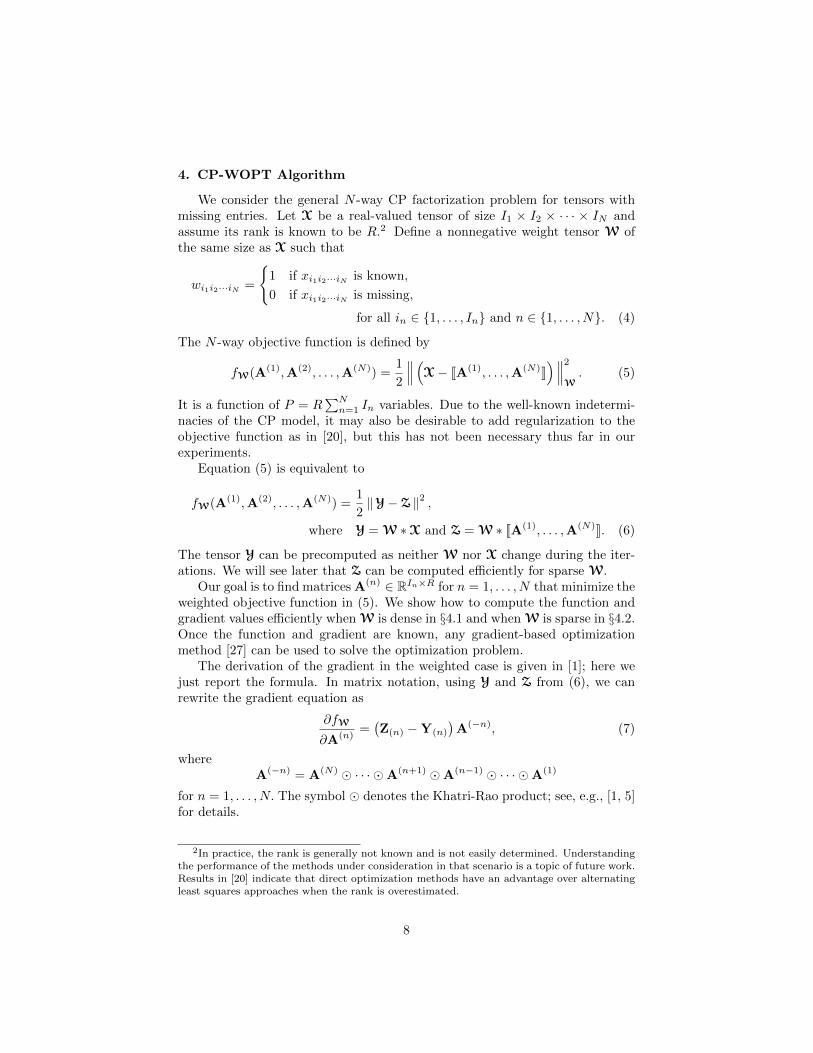
4. CP-WOPT Algorithm
We consider the general N -way CP factorization problem for tensors withmissing entries. Let X be a real-valued tensor of size I1 × I2 × · · · × IN andassume its rank is known to be R.2 Define a nonnegative weight tensor W ofthe same size as X such that
wi1i2···iN =
{1 if xi1i2···iN is known,
0 if xi1i2···iN is missing,
for all in ∈ {1, . . . , In} and n ∈ {1, . . . , N}. (4)
The N -way objective function is defined by
fW(A(1),A(2), . . . ,A(N)) =1
2
∥∥∥(X− JA(1), . . . ,A(N)K)∥∥∥2
W. (5)
It is a function of P = R∑Nn=1 In variables. Due to the well-known indetermi-
nacies of the CP model, it may also be desirable to add regularization to theobjective function as in [20], but this has not been necessary thus far in ourexperiments.
Equation (5) is equivalent to
fW(A(1),A(2), . . . ,A(N)) =1
2‖Y−Z ‖2 ,
where Y = W ∗X and Z = W ∗ JA(1), . . . ,A(N)K. (6)
The tensor Y can be precomputed as neither W nor X change during the iter-ations. We will see later that Z can be computed efficiently for sparse W.
Our goal is to find matrices A(n) ∈ RIn×R for n = 1, . . . , N that minimize theweighted objective function in (5). We show how to compute the function andgradient values efficiently when W is dense in §4.1 and when W is sparse in §4.2.Once the function and gradient are known, any gradient-based optimizationmethod [27] can be used to solve the optimization problem.
The derivation of the gradient in the weighted case is given in [1]; here wejust report the formula. In matrix notation, using Y and Z from (6), we canrewrite the gradient equation as
∂fW
∂A(n)=(Z(n) −Y(n)
)A(−n), (7)
whereA(−n) = A(N) � · · · �A(n+1) �A(n−1) � · · · �A(1)
for n = 1, . . . , N. The symbol � denotes the Khatri-Rao product; see, e.g., [1, 5]for details.
2In practice, the rank is generally not known and is not easily determined. Understandingthe performance of the methods under consideration in that scenario is a topic of future work.Results in [20] indicate that direct optimization methods have an advantage over alternatingleast squares approaches when the rank is overestimated.
8
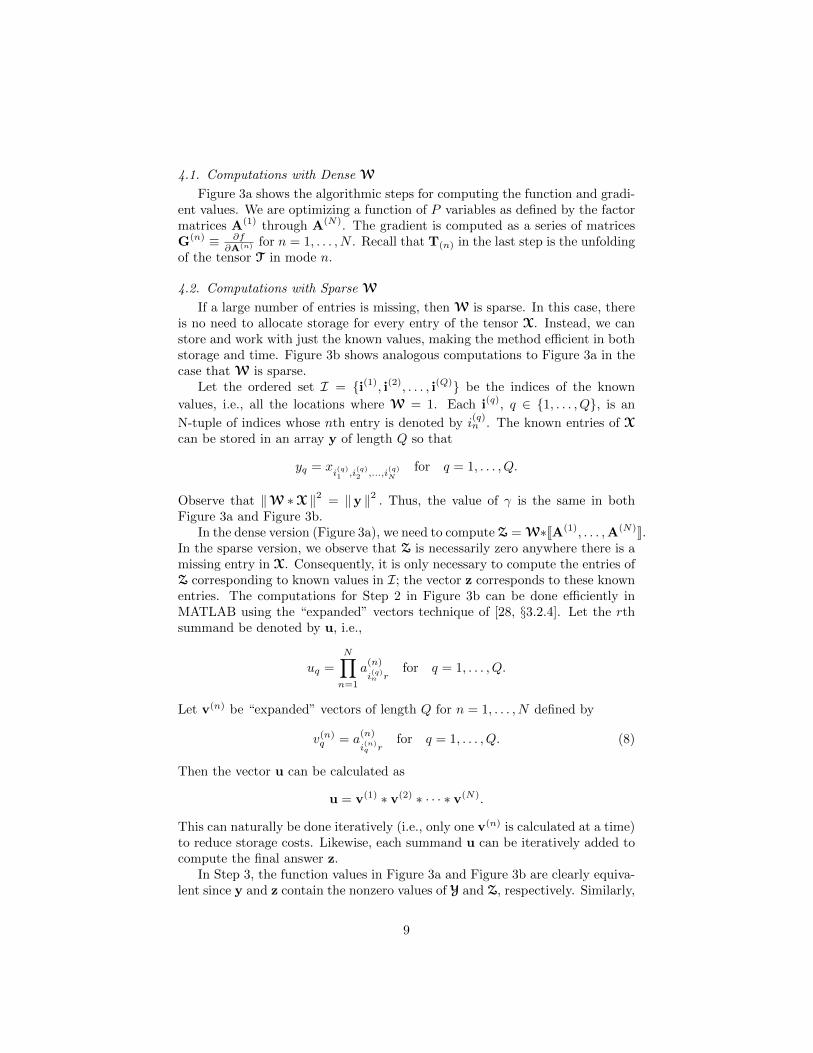
4.1. Computations with Dense W
Figure 3a shows the algorithmic steps for computing the function and gradi-ent values. We are optimizing a function of P variables as defined by the factormatrices A(1) through A(N). The gradient is computed as a series of matricesG(n) ≡ ∂f
∂A(n) for n = 1, . . . , N . Recall that T(n) in the last step is the unfoldingof the tensor T in mode n.
4.2. Computations with Sparse W
If a large number of entries is missing, then W is sparse. In this case, thereis no need to allocate storage for every entry of the tensor X. Instead, we canstore and work with just the known values, making the method efficient in bothstorage and time. Figure 3b shows analogous computations to Figure 3a in thecase that W is sparse.
Let the ordered set I = {i(1), i(2), . . . , i(Q)} be the indices of the known
values, i.e., all the locations where W = 1. Each i(q), q ∈ {1, . . . , Q}, is an
N-tuple of indices whose nth entry is denoted by i(q)n . The known entries of X
can be stored in an array y of length Q so that
yq = xi(q)1 ,i
(q)2 ,...,i
(q)N
for q = 1, . . . , Q.
Observe that ‖W ∗X ‖2 = ‖y ‖2 . Thus, the value of γ is the same in bothFigure 3a and Figure 3b.
In the dense version (Figure 3a), we need to compute Z = W∗JA(1), . . . ,A(N)K.In the sparse version, we observe that Z is necessarily zero anywhere there is amissing entry in X. Consequently, it is only necessary to compute the entries ofZ corresponding to known values in I; the vector z corresponds to these knownentries. The computations for Step 2 in Figure 3b can be done efficiently inMATLAB using the “expanded” vectors technique of [28, §3.2.4]. Let the rthsummand be denoted by u, i.e.,
uq =
N∏n=1
a(n)
i(q)n r
for q = 1, . . . , Q.
Let v(n) be “expanded” vectors of length Q for n = 1, . . . , N defined by
v(n)q = a
(n)
i(n)q r
for q = 1, . . . , Q. (8)
Then the vector u can be calculated as
u = v(1) ∗ v(2) ∗ · · · ∗ v(N).
This can naturally be done iteratively (i.e., only one v(n) is calculated at a time)to reduce storage costs. Likewise, each summand u can be iteratively added tocompute the final answer z.
In Step 3, the function values in Figure 3a and Figure 3b are clearly equiva-lent since y and z contain the nonzero values of Y and Z, respectively. Similarly,
9

1. Assume Y = W ∗X and γ = ‖Y ‖2 are precomputed.
2. Compute Z = W ∗ JA(1), . . . ,A(N)K.
3. Compute function value: f = 12γ − 〈Y,Z 〉+ 1
2 ‖Z ‖2.
4. Compute T = Y−Z.
5. Compute gradient matrices: G(n) = −T(n)A(−n) for n = 1, . . . , N .
(a) Dense W.
1. Let I = {i(1), i(2), . . . , i(Q)} be an ordered set of all the locations whereW = 1, i.e., the indices of the known values. Let y be the length-Qvector of the values of X at the locations indicated by I. Assume y andγ = ‖y ‖2 are precomputed.
2. Compute the Q-vector z as
zq =
R∑r=1
N∏n=1
a(n)
i(q)n r
for q = 1, . . . , Q.
3. Compute function value: f = 12γ − yTz + 1
2 ‖ z ‖2.
4. Compute t = y − z.
5. Compute gradient matrices G(n) for n = 1, . . . , N as follows:
g(n)jr = −
Q∑q=1
q:i(q)n =j
tq N∏m=1m 6=n
a(m)
i(q)m r
.
(b) Sparse W.
Figure 3: CP-WOPT computation of function value and gradient.
10
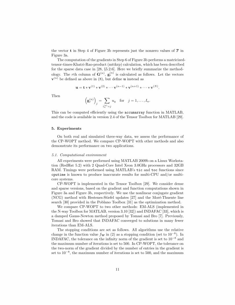
the vector t in Step 4 of Figure 3b represents just the nonzero values of T inFigure 3a.
The computation of the gradients in Step 6 of Figure 3b performs a matricized-tensor-times-Khatri-Rao-product (mttkrp) calculation, which has been describedfor the sparse data case in [28, §5.2.6]. Here we briefly summarize the method-
ology. The rth column of G(n), g(n)r is calculated as follows. Let the vectors
v(n) be defined as above in (8), but define u instead as
u = t ∗ v(1) ∗ v(2) ∗ · · ·v(n−1) ∗ v(n+1) ∗ · · · ∗ v(N).
Then (g(n)r
)j
=∑i(q)n =j
uq for j = 1, . . . , In.
This can be computed efficiently using the accumarray function in MATLAB,and the code is available in version 2.4 of the Tensor Toolbox for MATLAB [29].
5. Experiments
On both real and simulated three-way data, we assess the performance ofthe CP-WOPT method. We compare CP-WOPT with other methods and alsodemonstrate its performance on two applications.
5.1. Computational environment
All experiments were performed using MATLAB 2009b on a Linux Worksta-tion (RedHat 5.2) with 2 Quad-Core Intel Xeon 3.0GHz processors and 32GBRAM. Timings were performed using MATLAB’s tic and toc functions sincecputime is known to produce inaccurate results for multi-CPU and/or multi-core systems.
CP-WOPT is implemented in the Tensor Toolbox [29]. We consider denseand sparse versions, based on the gradient and function computations shown inFigure 3a and Figure 3b, respectively. We use the nonlinear conjugate gradient(NCG) method with Hestenes-Stiefel updates [27] and the More-Thuente linesearch [30] provided in the Poblano Toolbox [31] as the optimization method.
We compare CP-WOPT to two other methods: EM-ALS (implemented inthe N-way Toolbox for MATLAB, version 3.10 [32]) and INDAFAC [33], which isa damped Gauss-Newton method proposed by Tomasi and Bro [7]. Previously,Tomasi and Bro showed that INDAFAC converged to solutions in many feweriterations than EM-ALS.
The stopping conditions are set as follows. All algorithms use the relativechange in the function value fW in (2) as a stopping condition (set to 10−8). InINDAFAC, the tolerance on the infinity norm of the gradient is set to 10−8 andthe maximum number of iterations is set to 500. In CP-WOPT, the tolerance onthe two-norm of the gradient divided by the number of entries in the gradient isset to 10−8, the maximum number of iterations is set to 500, and the maximum
11
number of function evaluations is set to 10000. In EM-ALS, the maximumnumber of iterations (equivalent to one function evaluation) is set to 10000.
All the methods under consideration are iterative methods. We used mul-tiple starting points for each randomly generated problem. The first startingpoint is generated using the n-mode singular vectors 3 of X with missing entriesreplaced by zero. In our preliminary experiments, this starting procedure pro-duced significantly better results than random initializations, even with largeamounts of missing data. In order to improve the chances of reaching the globalminimum, additional starting points were generated randomly. The same set ofstarting points was used by all the methods in the same order.
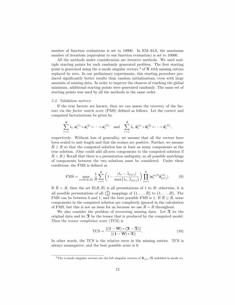
5.2. Validation metrics
If the true factors are known, then we can assess the recovery of the fac-tors via the factor match score (FMS) defined as follows. Let the correct andcomputed factorizations be given by
R∑r=1
λr a(1)r ◦ a(2)
r ◦ · · · ◦ a(N)r and
R∑r=1
λr a(1)r ◦ a(2)
r ◦ · · · ◦ a(N)r ,
respectively. Without loss of generality, we assume that all the vectors havebeen scaled to unit length and that the scalars are positive. Further, we assumeR ≥ R so that the computed solution has at least as many components as thetrue solution. (One could add all-zero components to the computed solution ifR < R.) Recall that there is a permutation ambiguity, so all possible matchingsof components between the two solutions must be considered. Under theseconditions, the FMS is defined as
FMS = maxσ∈Π(R,R)
1
R
R∑r=1
(1−
|λr − λσ(r)|max{λr, λσ(r)}
) N∏n=1
|a(n)Tr a
(n)σ(r)|. (9)
If R = R, then the set Π(R, R) is all permutations of 1 to R; otherwise, it is
all possible permutations of all(RR
)mappings of {1, . . . , R} to {1, . . . , R}. The
FMS can be between 0 and 1, and the best possible FMS is 1. If R ≥ R, somecomponents in the computed solution are completely ignored in the calculationof FMS, but this is not an issue for us because we use R = R throughout.
We also consider the problem of recovering missing data. Let X be theoriginal data and let X be the tensor that is produced by the computed model.Then the tensor completion score (TCS) is
TCS =‖(1−W) ∗ (X− X)‖‖(1−W) ∗X‖
. (10)
In other words, the TCS is the relative error in the missing entries. TCS isalways nonnegative, and the best possible score is 0.
3The n-mode singular vectors are the left singular vectors of X(n) (X unfolded in mode n).
12

5.3. Simulated data
We consider the performance of the methods on moderately-sized problemsof sizes 50 × 40 × 30, 100 × 80 × 60, and 150 × 120 × 90. For all sizes, we setthe number of components in the CP model to be R = 5. We test 60%, 70%,80%, 90%, and 95% missing data. The experiments show that the underlyingfactors can be captured even if the CP model is fit to a tensor with a significantamount of missing data; this is because the low-rank structure of the tensoris being exploited. A rank-R CP model for a tensor of size I × J × K hasR(I + J + K − 1) + 1 degrees of freedom. The reason that the factors can berecovered accurately, even with 95% missing data, is that there is still a lotmore data than variables, i.e., the size of the data is equal to 0.05 IJK whichis much greater than the R(I + J + K − 1) + 1 variables for large values of I,J ,and K. Because it is a nonlinear problem, we do not know exactly how manydata entries are needed in order to recover a CP model of a low-rank tensor;however, a lower bound for the number of entries needed in the matrix case hasbeen derived in [12].
5.3.1. Generating simulated data
We create the test problems as follows. Assume that the tensor size isI × J ×K and that the number of factors is R. We generate factor matrices A,B, and C of sizes I ×R, J ×R, and K ×R, respectively, by randomly choosingeach entry from N (0, 1) and then normalizing every column to unit length. Notethat this method of generating the factor matrices ensures that the solution isunique with probability one for the sizes and number of components that weare considering because R� min{I, J,K}.4
We then create the data tensor as
X = JA,B,CK + η‖X ‖‖N ‖
N.
Here N is a noise tensor (of the same size as X) with entries randomly selectedfrom N (0, 1), and η is the noise parameter. We use η = 10% in our experiments.
Finally, we set some entries of each generated tensor to be missing accord-ing to an indicator tensor W. We consider two situations for determining themissing data: randomly missing entries and, in Appendix B, structured missingdata in the form of randomly missing fibers. In the case of randomly missingentries, W is a binary tensor such that exactly bMIJKc randomly selected en-tries are set to zero, where M ∈ (0, 1) defines the percentage of missing data.We require that every slice of W (in every direction) have at least one nonzerobecause otherwise we have no chance of recovering the factor matrices; this isrelated to the problem of coherence in the matrix completion problem where itis well-known that missing an entire row (or a column) of a matrix means that
4Since each matrix has R linearly independent columns with probability one and the k-rank(i.e., the maximum value k such that any k columns are linearly independent) of each factormatrix is R, we satisfy the necessary conditions defined by Kruskal [34] for uniqueness.
13
the true factors can never be recovered. For each problem size and missing datapercentage, thirty independent test problems are generated.
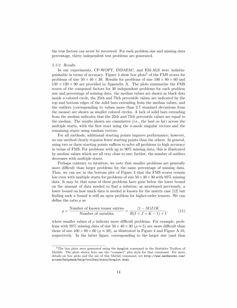
5.3.2. Results
In our experiments, CP-WOPT, INDAFAC, and EM-ALS were indistin-guishable in terms of accuracy. Figure 4 show box plots5 of the FMS scores forproblems of size 50 × 40 × 30. Results for problems of size 100 × 80 × 60 and150 × 120 × 90 are provided in Appendix A. The plots summarize the FMSscores of the computed factors for 30 independent problems for each problemsize and percentage of missing data: the median values are shown as black dotsinside a colored circle, the 25th and 75th percentile values are indicated by thetop and bottom edges of the solid bars extending from the median values, andthe outliers (corresponding to values more than 2.7 standard deviations fromthe means) are shown as smaller colored circles. A lack of solid bars extendingfrom the median indicates that the 25th and 75th percentile values are equal tothe median. The results shown are cumulative (i.e., the best so far) across themultiple starts, with the first start using the n-mode singular vectors and theremaining starts using random vectors.
For all methods, additional starting points improve performance; however,no one method clearly requires fewer starting points than the others. In general,using two or three starting points suffices to solve all problems to high accuracyin terms of FMS. For problems with up to 90% missing data, this is illustratedby median values which are all very close to one; further, the number of outliersdecreases with multiple starts.
Perhaps contrary to intuition, we note that smaller problems are generallymore difficult than larger problems for the same percentage of missing data.Thus, we can see in the bottom plot of Figure 4 that the FMS scores remainlow even with multiple starts for problems of size 50×40×30 with 95% missingdata. It may be that some of these problems have gone below the lower boundon the amount of data needed to find a solution; as mentioned previously, alower bound on how much data is needed is known for the matrix case [12] butfinding such a bound is still an open problem for higher-order tensors. We candefine the ratio ρ as
ρ =Number of known tensor entries
Number of variables=
(1−M)IJK
R(I + J +K − 1) + 1, (11)
where smaller values of ρ indicate more difficult problems. For example, prob-lems with 95% missing data of size 50× 40× 30 (ρ ≈ 5) are more difficult thanthose of size 100× 80× 60 (ρ ≈ 20), as illustrated in Figure 4 and Figure A.10,respectively. In the latter figure, corresponding to the larger size (and thus
5The box plots were generated using the boxplot command in the Statistics Toolbox ofMatlab. The plots shown here use the “compact” plot style for that command. For moredetails on box plots and the use of this Matlab command, see http://www.mathworks.com/
access/helpdesk/help/toolbox/stats/boxplot.html.
14
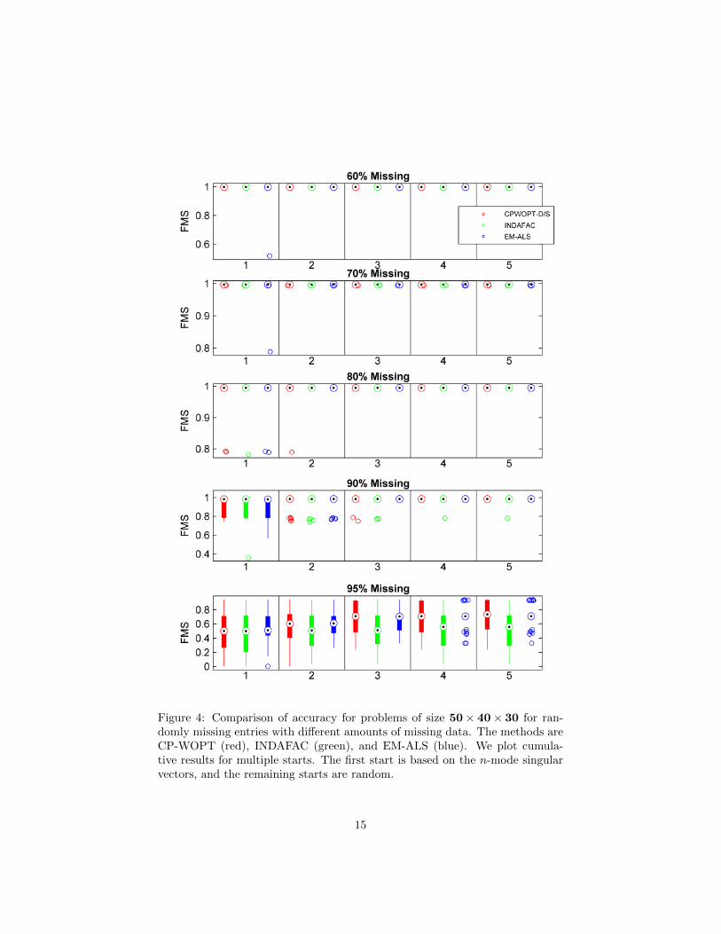
Figure 4: Comparison of accuracy for problems of size 50× 40× 30 for ran-domly missing entries with different amounts of missing data. The methods areCP-WOPT (red), INDAFAC (green), and EM-ALS (blue). We plot cumula-tive results for multiple starts. The first start is based on the n-mode singularvectors, and the remaining starts are random.
15

larger value of ρ), nearly all problems are solved to high accuracy by all meth-ods. Since this is a nonlinear problem, ρ does not tell the entire story, but it isat least a partial indicator of problem difficulty.
The differentiator between the methods is computational time required. Fig-ure 5 shows a comparison of the sparse and dense versions of CPWOPT, alongwith INDAFAC and EM-ALS. The timings reported in the figure are the sumof the times for all starting points. The y-axis is time in seconds on a log scale.We present results for time rather than iterations because the iterations forINDAFAC are much more expensive than those for CPWOPT or EM-ALS. Wemake several observations. For missing data levels up to 80%, the dense versionof CPWOPT is faster than INDAFAC, but EM-ALS is the fastest overall. For90% and 95% missing data, the sparse version of CPWOPT is fastest (by morethan a factor of 10 in some cases) with the exception of the case of 90% missingdata for problems of size 150× 120× 90. However, for this latter case, the dif-ference is not significant; furthermore, there are two problems where EM-ALSrequired more than 10 times the median to find a correct factorization.
As demonstrated in earlier studies [1, 7], problems with structured missingdata are generally more difficult than those with randomly missing values. Wepresent results for problems of structured missing data in Appendix B. Theset-up is the same as we have used here, except that we only go up to 90%missing data because the accuracy of all methods degrades significantly afterthat point. The results indicate that accuracies of all methods start to diminishat lower percentages of structured missing data than for those problems withrandomly missing data. Timings of the methods also indicate similar behaviorin the case of structure missing data: With 80% or less missing data EM-ALS isfastest, whereas the sparse version of CP-WOPT is in general faster when thereis 90% missing data.
Because it ignores missing values (random or structured), a major advantageof CP-WOPT is its ability to perform sparse computations, enabling it to scaleto very large problems. Neither INDAFAC nor EM-ALS can do this. Thedifficulty with EM-ALS is that it must impute all missing values; therefore, itloses any speed or scalability advantage of sparsity since it ultimately operateson dense data. Although INDAFAC also ignores missing values, its scalabilityis limited due to the expense of solving the Newton equation. Even though theNewton system is extremely sparse, we can see that the method is expensiveeven for moderate-sized problems such as those discussed in this section. In thenext section, we consider very large problems, demonstrating this strength ofCP-WOPT.
5.4. Large-scale simulated data
A unique feature of CP-WOPT is that it can be applied to problems thatare too large to fit in memory if dense storage were used. We consider twosituations:
(a) 500× 500× 500 with 99% missing data (1.25 million known values), and(b) 1000× 1000× 1000 with 99.5% missing data (5 million known values).
16

Figure 5: Comparison of timings for randomly missing entries for the total timefor all starting points for different problem sizes and different amounts of missingdata. The methods are CP-WOPT-Dense (red), CP-WOPT-Sparse (magenta),INDAFAC (green), and EM-ALS (blue).
17
5.4.1. Generating large-scale simulated data
The method for generating test problems of this size is necessarily differ-ent than the one for smaller problems presented in the previous section be-cause we cannot, for example, generate a full noise tensor. In fact, the tensorsY = JA,B,CK (the noise-free data) and N (the noise) are never explicitly fullyformed for the large problems studied here.
Let the tensor size be I × J × K and the missing value rate be M . Wegenerate the factor matrices as described in §5.3, using R = 5 components.Next, we create the set I with (1 −M)IJK randomly generated indices; thisset represents the indices of the known (non-missing) values in our tests. Thebinary indicator tensor W is stored as a sparse tensor [28] and defined by
wijk =
{1 if (i, j, k) ∈ I,0 otherwise.
Rather than explicitly forming all of Y = JA,B,CK, we only calculate its valuesfor those indices in I. This is analogous to the calculations described for Step 2of Figure 3b. All missing entries of Y are set to zero, and Y is stored as a sparsetensor. Finally, we set
X = Y + η‖X ‖‖N ‖
N,
where N is a sparse noise tensor such that
nijk =
{N (0, 1) if (i, j, k) ∈ I,0 otherwise.
For each problem size, ten independent test problems are generated. The initialguess is generated by computing the n-mode singular vectors of the tensor withmissing values filled in by zeros.
5.4.2. Results for CP-WOPT on large-scale data
The computational set-up was the same as that described in §5.1 except thatthe tolerance for the two-norm of the gradient divided by the number of entriesin the gradient was set to 10−10 (previously 10−8). The results across all tenruns for each problem size are shown in Figure 6.
In the 500×500×500 case, storing a dense version of the tensor (assuming 8bytes per entry) would require exactly 1GB. Storing just 1% of the data (1.25Mentries) in sparse format (assuming 32 bytes per entry, 8 for the value and 8 foreach of the indices) requires only 40MB. In our randomly generated experiments,all ten problems were solved with an FMS score greater than 0.99, with solvetimes ranging between 200 and 1000 seconds.
In the 1000×1000×1000 case, storing a dense version of the tensor would re-quire 8GB. Storing just 0.5% of the data as a sparse tensor (5M entries) requires160MB. In our randomly generated experiments, only nine of the ten problemswere solved with an FMS score greater than 0.99. The solve times ranged from
18
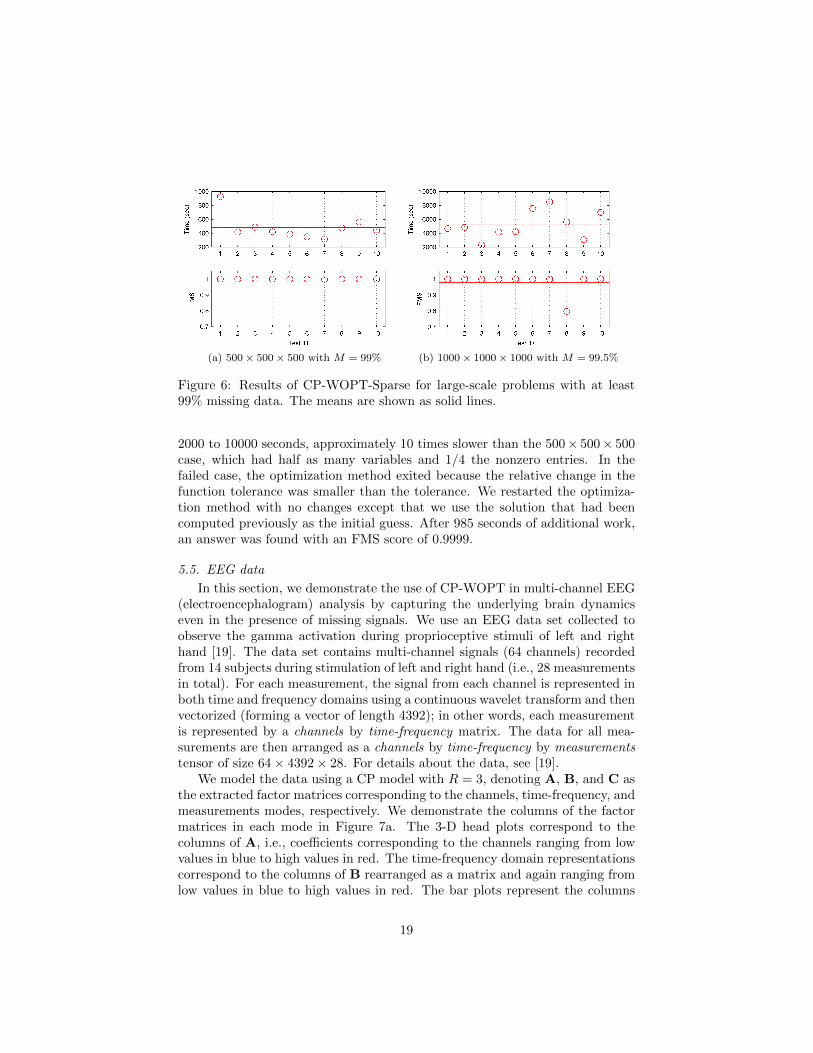
(a) 500 × 500 × 500 with M = 99% (b) 1000 × 1000 × 1000 with M = 99.5%
Figure 6: Results of CP-WOPT-Sparse for large-scale problems with at least99% missing data. The means are shown as solid lines.
2000 to 10000 seconds, approximately 10 times slower than the 500× 500× 500case, which had half as many variables and 1/4 the nonzero entries. In thefailed case, the optimization method exited because the relative change in thefunction tolerance was smaller than the tolerance. We restarted the optimiza-tion method with no changes except that we use the solution that had beencomputed previously as the initial guess. After 985 seconds of additional work,an answer was found with an FMS score of 0.9999.
5.5. EEG data
In this section, we demonstrate the use of CP-WOPT in multi-channel EEG(electroencephalogram) analysis by capturing the underlying brain dynamicseven in the presence of missing signals. We use an EEG data set collected toobserve the gamma activation during proprioceptive stimuli of left and righthand [19]. The data set contains multi-channel signals (64 channels) recordedfrom 14 subjects during stimulation of left and right hand (i.e., 28 measurementsin total). For each measurement, the signal from each channel is represented inboth time and frequency domains using a continuous wavelet transform and thenvectorized (forming a vector of length 4392); in other words, each measurementis represented by a channels by time-frequency matrix. The data for all mea-surements are then arranged as a channels by time-frequency by measurementstensor of size 64× 4392× 28. For details about the data, see [19].
We model the data using a CP model with R = 3, denoting A, B, and C asthe extracted factor matrices corresponding to the channels, time-frequency, andmeasurements modes, respectively. We demonstrate the columns of the factormatrices in each mode in Figure 7a. The 3-D head plots correspond to thecolumns of A, i.e., coefficients corresponding to the channels ranging from lowvalues in blue to high values in red. The time-frequency domain representationscorrespond to the columns of B rearranged as a matrix and again ranging fromlow values in blue to high values in red. The bar plots represent the columns
19
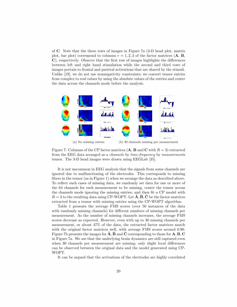
of C. Note that the three rows of images in Figure 7a (3-D head plot, matrixplot, bar plot) correspond to columns r = 1, 2, 3 of the factor matrices (A, B,C), respectively. Observe that the first row of images highlights the differencesbetween left and right hand stimulation while the second and third rows ofimages pertain to frontal and parietal activations that are shared by the stimuli.Unlike [19], we do not use nonnegativity constraints; we convert tensor entriesfrom complex to real values by using the absolute values of the entries and centerthe data across the channels mode before the analysis.
(a) No missing entries (b) 30 channels missing per measurement
Figure 7: Columns of the CP factor matrices (A, B and C with R = 3) extractedfrom the EEG data arranged as a channels by time-frequency by measurementstensor. The 3-D head images were drawn using EEGLab [35].
It is not uncommon in EEG analysis that the signals from some channels areignored due to malfunctioning of the electrodes. This corresponds to missingfibers in the tensor (as in Figure 1) when we arrange the data as described above.To reflect such cases of missing data, we randomly set data for one or more ofthe 64 channels for each measurement to be missing, center the tensor acrossthe channels mode ignoring the missing entries, and then fit a CP model withR = 3 to the resulting data using CP-WOPT. Let A, B, C be the factor matricesextracted from a tensor with missing entries using the CP-WOPT algorithm.
Table 1 presents the average FMS scores (over 50 instances of the datawith randomly missing channels) for different numbers of missing channels permeasurement. As the number of missing channels increases, the average FMSscores decrease as expected. However, even with up to 30 missing channels permeasurement, or about 47% of the data, the extracted factor matrices matchwith the original factor matrices well, with average FMS scores around 0.90.Figure 7b presents the images for A, B and C corresponding to those for A,B,Cin Figure 7a. We see that the underlying brain dynamics are still captured evenwhen 30 channels per measurement are missing; only slight local differencescan be observed between the original data and the model generated using CP-WOPT.
It can be argued that the activations of the electrodes are highly correlated
20
and even if some of the electrodes are removed, the underlying brain dynamicscan still be captured. However, in these experiments we do not set the samechannels to missing for each measurement; the channels are randomly missingfrom each measurement. There are cases when a CP model may not be able torecover factors when data has certain patterns of missing values, e.g., missingthe signals from the same side of the brain for all measurements. However, suchdata is not typical in practice.
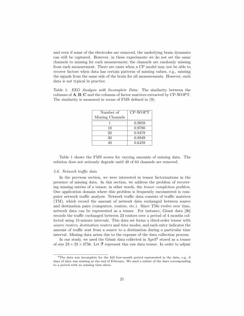
Table 1: EEG Analysis with Incomplete Data: The similarity between thecolumns of A,B,C and the columns of factor matrices extracted by CP-WOPT.The similarity is measured in terms of FMS defined in (9).
Number of CP-WOPTMissing Channels
1 0.995910 0.978020 0.947830 0.894940 0.6459
Table 1 shows the FMS scores for varying amounts of missing data. Thesolution does not seriously degrade until 40 of 64 channels are removed.
5.6. Network traffic data
In the previous section, we were interested in tensor factorizations in thepresence of missing data. In this section, we address the problem of recover-ing missing entries of a tensor; in other words, the tensor completion problem.One application domain where this problem is frequently encountered is com-puter network traffic analysis. Network traffic data consists of traffic matrices(TM), which record the amount of network data exchanged between sourceand destination pairs (computers, routers, etc.). Since TMs evolve over time,network data can be represented as a tensor. For instance, Geant data [36]records the traffic exchanged between 23 routers over a period of 4 months col-lected using 15-minute intervals. This data set forms a third-order tensor withsource routers, destination routers and time modes, and each entry indicates theamount of traffic sent from a source to a destination during a particular timeinterval. Missing data arises due to the expense of the data collection process.
In our study, we used the Geant data collected in April6 stored as a tensorof size 23× 23× 2756. Let T represent this raw data tensor. In order to adjust
6The data was incomplete for the full four-month period represented in the data, e.g., 6days of data was missing at the end of February. We used a subset of the data correspondingto a period with no missing time slices.
21

for scaling bias in the amount of traffic, we preprocess T as X = log(T + 1).Figure 8 presents the results of 2-component CP model (i.e., R = 2); the firstand second row correspond the first and second column of the factor matrices ofthe model, respectively. This CP model fits the data well but not perfectly andthere is some unexplained variation left in the residuals. Let X be the tensorconstructed using the computed factor matrices. The modeling error, defined as‖X−X‖‖X ‖ , is approximately 0.31 for the 2-component CP model computed. Even
though extracting more components slightly lowers the modeling error, modelswith more components do not look appropriate for the data.
Figure 8: Factor matrices extracted from Geant data using a 2-component CPmodel. The first row illustrates the first column of the factor matrices in eachmode and the second row shows the second column of the factor matrices.
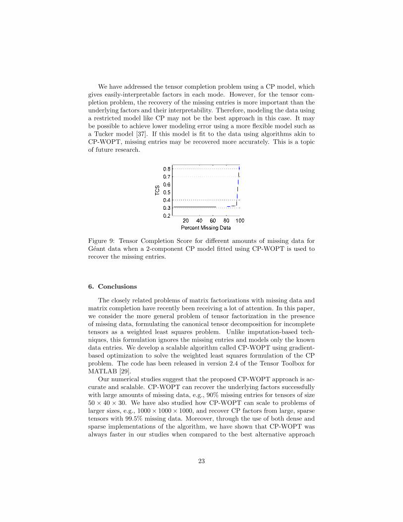
In order to assess the performance of CP-WOPT in terms of recoveringmissing data, randomly chosen entries of X are set to missing and a 2-componentCP model is fit to the altered data. The extracted factor matrices are thenused to reconstruct the data and fill in the missing entries. These recoveredvalues are compared with the actual values based on the tensor completionscore (TCS) defined in (10). Figure 9 presents the average TCS (across 30instances) for different amounts of missing data. We observe that the averageTCS is around 0.31 when there is little missing data and increases very slowlyas we increase the amount of missing data. The average TCS is only slightlyhigher, approximately 0.33, even when 95% of the entries are missing. However,the average TCS increases sharply when the amount of missing data is 99%.Note that even if there is no missing data, there will be completion error dueto the modeling error, i.e., 0.31. Figure 9 demonstrates the robustness of CP-WOPT, illustrating that the TCS can be kept close to the level of the modelingerror using this method, even when the amount of missing data is high.
22
We have addressed the tensor completion problem using a CP model, whichgives easily-interpretable factors in each mode. However, for the tensor com-pletion problem, the recovery of the missing entries is more important than theunderlying factors and their interpretability. Therefore, modeling the data usinga restricted model like CP may not be the best approach in this case. It maybe possible to achieve lower modeling error using a more flexible model such asa Tucker model [37]. If this model is fit to the data using algorithms akin toCP-WOPT, missing entries may be recovered more accurately. This is a topicof future research.
Figure 9: Tensor Completion Score for different amounts of missing data forGeant data when a 2-component CP model fitted using CP-WOPT is used torecover the missing entries.
6. Conclusions
The closely related problems of matrix factorizations with missing data andmatrix completion have recently been receiving a lot of attention. In this paper,we consider the more general problem of tensor factorization in the presenceof missing data, formulating the canonical tensor decomposition for incompletetensors as a weighted least squares problem. Unlike imputation-based tech-niques, this formulation ignores the missing entries and models only the knowndata entries. We develop a scalable algorithm called CP-WOPT using gradient-based optimization to solve the weighted least squares formulation of the CPproblem. The code has been released in version 2.4 of the Tensor Toolbox forMATLAB [29].
Our numerical studies suggest that the proposed CP-WOPT approach is ac-curate and scalable. CP-WOPT can recover the underlying factors successfullywith large amounts of missing data, e.g., 90% missing entries for tensors of size50 × 40 × 30. We have also studied how CP-WOPT can scale to problems oflarger sizes, e.g., 1000× 1000× 1000, and recover CP factors from large, sparsetensors with 99.5% missing data. Moreover, through the use of both dense andsparse implementations of the algorithm, we have shown that CP-WOPT wasalways faster in our studies when compared to the best alternative approach
23
based on second-order optimization (INDAFAC) and even faster than EM-ALSfor high percentages of missing data.
We consider the practical use of CP-WOPT algorithm in two different appli-cations which demonstrate the effectiveness of CP-WOPT even when there maybe low correlation with a multi-linear model. In multi-channel EEG analysis,the factors extracted by the CP-WOPT algorithm can capture brain dynamicseven if signals from some channels are missing, suggesting that practitionerscan now make better use of incomplete data in their analyses. We note that theEEG data was centered by using the means of only the known entries; however,robust techniques for centering incomplete data are needed and is a topic offuture investigation. In network traffic analysis, CP-WOPT algorithm can beused in the context of tensor completion and recover the missing network trafficdata.
Although 90% or more missing data may not seem practical, there are situa-tions where it is useful to purposely omit data. For example, if the data is verylarge, excluding some data will speed up the computation and enable it to fit inmemory (for large-scale data like the example of a 1000×1000×1000 tensor thatwould normally require 8GB of storage). It is also common to leave out datafor the purpose of rank determination or model assessment via cross-validation.For these reasons, it is useful to consider high degrees of missing data.
In future studies, we plan to extend our results in several directions. We willinclude constraints such as non-negativity and penalties to encourage sparsity,which enable us to find more meaningful latent factors from large-scale sparsedata. Finally, we will consider the problem of collective factorizations withmissing data, where we are jointly factoring multiple tensors with shared factors.
Appendix A. Additional comparisons for randomly missing data
Figures A.10 and A.11 show box plots of the FMS scores for problems of size100×80×60 and 150×120×90, respectively. See §5.3 and Figure 4 for a detaileddescription of the experimental setup and the results for analogous problems ofsize 50 × 40 × 30. We can see from these figures that the three methods beingcompared (CP-WOPT, INDAFAC, EM-ALS) are indistinguishable in terms ofaccuracy, as was the case for the smaller sized problems. Furthermore, compa-rable improvements using multiple starts can be seen for these larger problems;we are able to solve a majority of the problems with very high accuracy usingfive or fewer starting points (the n-mode singular vectors used as the basis forthe first run and random points used for the others).
Appendix B. Comparisons for structured missing data
We use the same experimental set-up as described in §5.3, with the exceptionthat we performed experiments using problems with up to 90% missing data (asopposed to 95%) and we only show results for three starting point (the firstis the n-mode singular vectors and the remaining two are random). In the
24
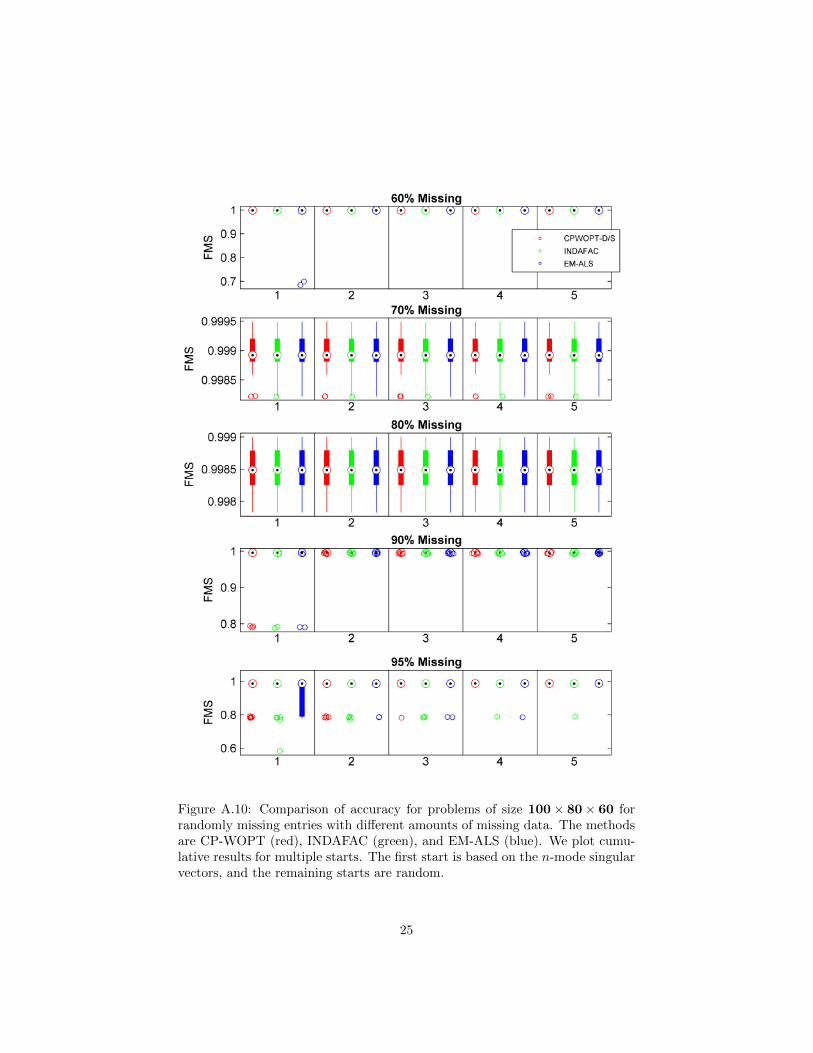
Figure A.10: Comparison of accuracy for problems of size 100× 80× 60 forrandomly missing entries with different amounts of missing data. The methodsare CP-WOPT (red), INDAFAC (green), and EM-ALS (blue). We plot cumu-lative results for multiple starts. The first start is based on the n-mode singularvectors, and the remaining starts are random.
25

Figure A.11: Comparison of accuracy for problems of size 150× 120× 90 forrandomly missing entries with different amounts of missing data. The methodsare CP-WOPT (red), INDAFAC (green), and EM-ALS (blue). We plot cumu-lative results for multiple starts. The first start is based on the n-mode singularvectors, and the remaining starts are random.
26

case of randomly missing fibers, without loss of generality, we consider missingfibers in the third mode only. In that case, W is an I × J binary matrix withexactly bMIJc randomly selected entries are set to zero, and the binary tensorW is created by stacking K copies of W together. We again require that everyslice of W (in every direction) have at least one nonzero, which is equivalentto requiring that W has no zero rows or columns. For each problem size andmissing data percentage, thirty independent test problems were generated.
The average FMS results are presented in Figures B.12, B.13 and B.14 forproblems of sizes 50× 40× 30, 100× 80× 60 and 150× 120× 90, respectively.As for the problems with randomly missing data, we see that as the percentageof missing data increases, the average FMS scores tend to decrease. However,one notable difference is that the average FMS scores for structured missingdata are in general lower than those for problems with comparable amounts ofrandomly missing data. This indicates that problems with structured missingdata are more difficult than those with randomly missing data.
The computational times required to compute the CP models using thedifferent methods are present in Figure B.15, where we observe comparableresults to those presented in Figure 5 for the problems with randomly missingdata. With 80% or less structured missing data EM-ALS is fastest, whereas thesparse version of CP-WOPT is in general faster when there is more than 80%missing data.
Acknowledgments
We thank David Gleich and the anonymous referees for helpful commentswhich greatly improved the presentation of this manuscript.
[1] E. Acar, D. M. Dunlavy, T. G. Kolda, M. Mørup, Scalable tensor factoriza-tions with missing data, in: Proceedings of the Tenth SIAM InternationalConference on Data Mining, SIAM, 2010, pp. 701–712.URL http://www.siam.org/proceedings/datamining/2010/dm10_061_
acare.pdf
[2] Y. Zhang, M. Roughan, W. Willinger, L. Qiu, Spatio-temporal compressivesensing and internet traffic matrices, in: SIGCOMM ’09: Proceedings ofthe ACM SIGCOMM 2009 conference on Data communication, ACM, NewYork, NY, USA, 2009, pp. 267–278. doi:10.1145/1592568.1592600.
[3] A. M. Buchanan, A. W. Fitzgibbon, Damped Newton algorithms for matrixfactorization with missing data, in: CVPR’05: 2005 IEEE Computer Soci-ety Conference on Computer Vision and Pattern Recognition, Vol. 2, IEEEComputer Society, 2005, pp. 316–322. doi:10.1109/CVPR.2005.118.
[4] E. Acar, B. Yener, Unsupervised multiway data analysis: A literature sur-vey, IEEE Transactions on Knowledge and Data Engineering 21 (1) (2009)6–20. doi:10.1109/TKDE.2008.112.
27
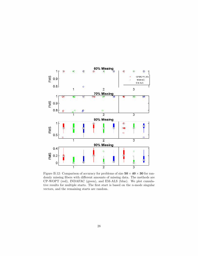
Figure B.12: Comparison of accuracy for problems of size 50× 40× 30 for ran-domly missing fibers with different amounts of missing data. The methods areCP-WOPT (red), INDAFAC (green), and EM-ALS (blue). We plot cumula-tive results for multiple starts. The first start is based on the n-mode singularvectors, and the remaining starts are random.
28
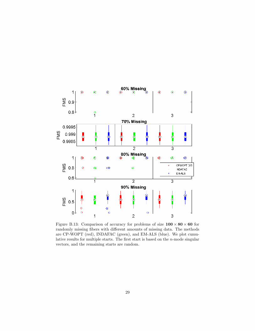
Figure B.13: Comparison of accuracy for problems of size 100× 80× 60 forrandomly missing fibers with different amounts of missing data. The methodsare CP-WOPT (red), INDAFAC (green), and EM-ALS (blue). We plot cumu-lative results for multiple starts. The first start is based on the n-mode singularvectors, and the remaining starts are random.
29

Figure B.14: Comparison of accuracy for problems of size 150× 120× 90 forrandomly missing fibers with different amounts of missing data. The methodsare CP-WOPT (red), INDAFAC (green), and EM-ALS (blue). We plot cumu-lative results for multiple starts. The first start is based on the n-mode singularvectors, and the remaining starts are random.
30
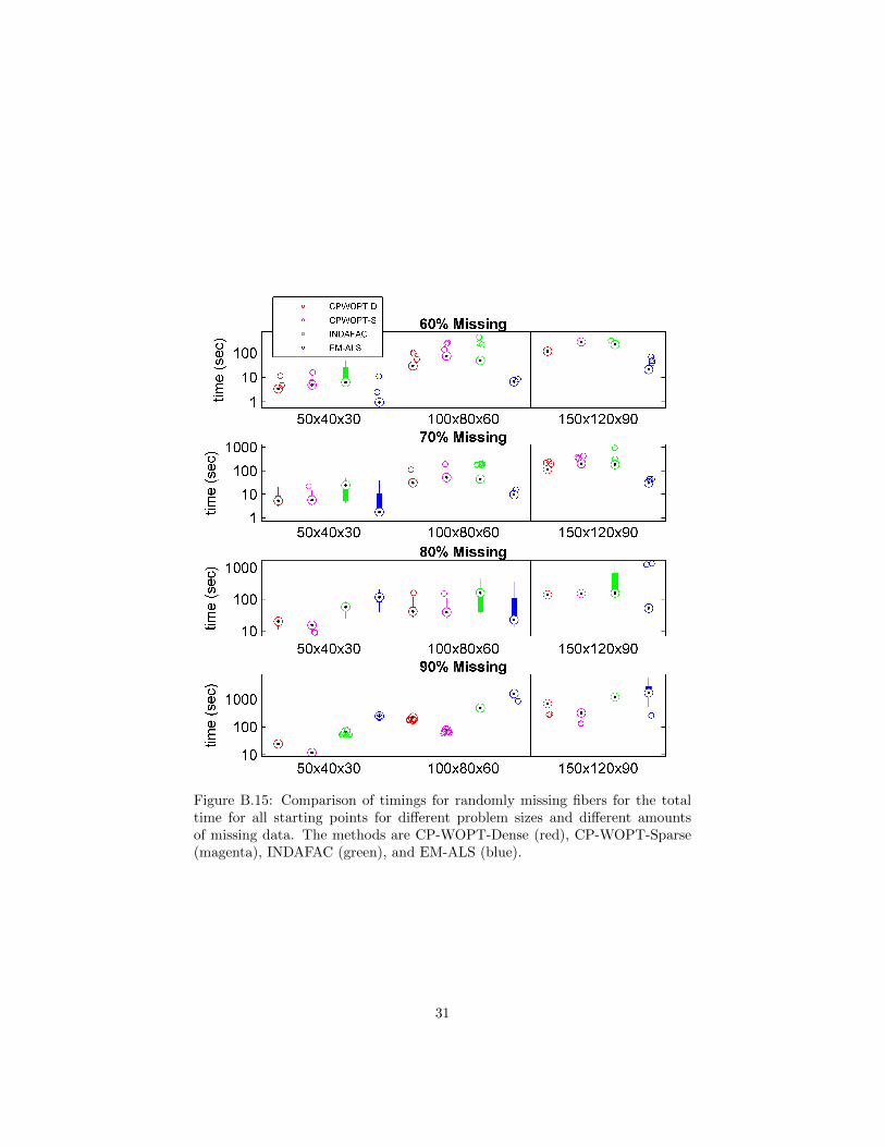
Figure B.15: Comparison of timings for randomly missing fibers for the totaltime for all starting points for different problem sizes and different amountsof missing data. The methods are CP-WOPT-Dense (red), CP-WOPT-Sparse(magenta), INDAFAC (green), and EM-ALS (blue).
31

[5] T. G. Kolda, B. W. Bader, Tensor decompositions and applications, SIAMReview 51 (3) (2009) 455–500. doi:10.1137/07070111X.
[6] F. Miwakeichi, E. Martınez-Montes, P. A. Valds-Sosa, N. Nishiyama,H. Mizuhara, Y. Yamaguchi, Decomposing EEG data into space-time-frequency components using parallel factor analysis, NeuroImage 22 (3)(2004) 1035–1045. doi:10.1016/j.neuroimage.2004.03.039.
[7] G. Tomasi, R. Bro, PARAFAC and missing values, Chemometrics and In-telligent Laboratory Systems 75 (2) (2005) 163–180. doi:10.1016/j.
chemolab.2004.07.003.
[8] V. Y. Orekhov, I. Ibraghimov, M. Billeter, Optimizing resolution in mul-tidimensional NMR by three-way decomposition, Journal of BiomolecularNMR 27 (2003) 165–173. doi:10.1023/A:1024944720653.
[9] X. Geng, K. Smith-Miles, Z.-H. Zhou, L. Wang, Face image modeling bymultilinear subspace analysis with missing values, in: MM ’09: Proceedingsof the seventeen ACM international conference on Multimedia, ACM, 2009,pp. 629–632. doi:10.1145/1631272.1631373.
[10] A. Ruhe, Numerical computation of principal components when severalobservations are missing, Tech. Rep. UMINF-48-74, Department of Infor-mation Processing, Institute of Mathematics and Statistics, University ofUmea, Umea, Sweden (1974).
[11] K. R. Gabriel, S. Zamir, Lower rank approximation of matrices by leastsquares approximation with any choice of weights, Technometrics 21 (4)(1979) 489–498.URL http://www.jstor.org/stable/1268288
[12] E. J. Candes, T. Tao, The power of convex relaxation: Near-optimal matrixcompletion, arXiv:0903.1476v1 (Mar. 2009).URL http://arxiv.org/abs/0903.1476
[13] E. J. Candes, Y. Plan, Matrix completion with noise, arXiv:0903.3131v1(Mar. 2009).URL http://arxiv.org/abs/0903.3131
[14] J. D. Carroll, J. J. Chang, Analysis of individual differences in multidimen-sional scaling via an N-way generalization of “Eckart-Young” decomposi-tion, Psychometrika 35 (1970) 283–319. doi:10.1007/BF02310791.
[15] R. A. Harshman, Foundations of the PARAFAC procedure: Modelsand conditions for an “explanatory” multi-modal factor analysis, UCLAworking papers in phonetics 16 (1970) 1–84, available at http://www.
psychology.uwo.ca/faculty/harshman/wpppfac0.pdf.
32
[16] T. G. Kolda, B. W. Bader, J. P. Kenny, Higher-order web link analysisusing multilinear algebra, in: ICDM 2005: Proceedings of the 5th IEEEInternational Conference on Data Mining, IEEE Computer Society, 2005,pp. 242–249. doi:10.1109/ICDM.2005.77.
[17] R. Bro, Review on multiway analysis in chemistry—2000–2005, CriticalReviews in Analytical Chemistry 36 (3–4) (2006) 279–293. doi:10.1080/
10408340600969965.
[18] E. Acar, C. A. Bingol, H. Bingol, R. Bro, B. Yener, Multiway analysisof epilepsy tensors, Bioinformatics 23 (13) (2007) i10–i18. doi:10.1093/
bioinformatics/btm210.
[19] M. Mørup, L. K. Hansen, S. M. Arnfred, ERPWAVELAB a toolbox formulti-channel analysis of time-frequency transformed event related poten-tials, Journal of Neuroscience Methods 161 (2) (2007) 361–368. doi:
10.1016/j.jneumeth.2006.11.008.
[20] E. Acar, T. Kolda, D. Dunlavy, An optimization approach for fitting canon-ical tensor decompositions, Tech. Rep. SAND2009-0857, Sandia NationalLaboratories, Albuquerque, New Mexico and Livermore, California (2009).
[21] A. P. Dempster, N. M. Laird, D. B. Rubin, Maximum likelihood fromincomplete data via the em algorithm, Journal of the Royal StatisticalSociety, Series B 39 (1) (1977) 1–38.
[22] N. Srebro, T. Jaakkola, Weighted low-rank approximations, in: IMCL-2003: Proceedings of the Twentieth International Conference on MachineLearning, 2003, pp. 720–727.
[23] H. A. L. Kiers, Weighted least squares fitting using ordinary leastsquares algorithms, Psychometrika 62 (2) (1997) 215–266. doi:10.1007/
BF02295279.
[24] R. Bro, Multi-way analysis in the food industry: Models, algorithms, andapplications, Ph.D. thesis, University of Amsterdam, available at http:
//www.models.kvl.dk/research/theses/ (1998).
[25] B. Walczak, D. L. Massart, Dealing with missing data: Part I, Chemo-metrics and Intelligent Laboratory Systems 58 (1) (2001) 15–27. doi:
10.1016/S0169-7439(01)00131-9.
[26] P. Paatero, A weighted non-negative least squares algorithm for three-way“PARAFAC” factor analysis, Chemometrics and Intelligent LaboratorySystems 38 (2) (1997) 223–242. doi:10.1016/S0169-7439(97)00031-2.
[27] J. Nocedal, S. J. Wright, Numerical Optimization, Springer, 1999.
[28] B. W. Bader, T. G. Kolda, Efficient MATLAB computations with sparseand factored tensors, SIAM Journal on Scientific Computing 30 (1) (2007)205–231. doi:10.1137/060676489.
33
[29] B. W. Bader, T. G. Kolda, MATLAB tensor toolbox version 2.4, http://csmr.ca.sandia.gov/~tgkolda/TensorToolbox/ (last accessed March,2010).
[30] J. J. More, D. J. Thuente, Line search algorithms with guaranteed sufficientdecrease, ACM Transactions on Mathematical Software 20 (3) (1994) 286–307. doi:10.1145/192115.192132.
[31] D. M. Dunlavy, T. G. Kolda, E. Acar, Poblano v1.0: A Matlab toolbox forgradient-based optimization, Tech. Rep. SAND2010-1422, Sandia NationalLaboratories, Albuquerque, NM and Livermore, CA (Mar. 2010).
[32] C. A. Andersson, R. Bro, The N-way toolbox for MATLAB, Chemometricsand Intelligent Laboratory Systems 52 (1) (2000) 1–4, see also http://www.
models.kvl.dk/source/nwaytoolbox/. doi:10.1016/S0169-7439(00)
00071-X.
[33] G. Tomasi, Incomplete data PARAFAC (INDAFAC), http://www.
models.kvl.dk/source/indafac/index.asp (last accessed May, 2009).
[34] J. B. Kruskal, Three-way arrays: rank and uniqueness of trilinear decom-positions, with application to arithmetic complexity and statistics, Lin-ear Algebra and its Applications 18 (2) (1977) 95–138. doi:10.1016/
0024-3795(77)90069-6.
[35] A. Delorme, S. Makeig, EEGLAB: An open source toolbox for analysisof single-trial EEG dynamics, J. Neurosci. Meth. 134 (2004) 9–21. doi:
10.1016/j.jneumeth.2003.10.009.
[36] S. Uhlig, B. Quoitin, J. Lepropre, S. Balon, Providing public intradomaintraffic matrices to the research community, ACM SIGCOMM ComputerCommunication Review 36 (1) (2006) 83–86. doi:10.1145/1111322.
1111341.
[37] L. R. Tucker, Some mathematical notes on three-mode factor analysis,Psychometrika 31 (1966) 279–311. doi:10.1007/BF02289464.
34