sc.nahrainuniv.edu.iq§كرم عباس جاسم قسم... · chapter 1 introduction to statistics...
TRANSCRIPT

MATHEMATICAL STATISTICSLecture Note
Akram Al-sabbaghAl-Nahrain University


CONTENTS
iii


CHAPTER 1
INTRODUCTION TO STATISTICS
1.1 Basic Probability
This chapter is a reminder of some basics in probability and statistics, it contains some definitions and examples that wewill be using in the rest of this notes. Probability or chance can be measured on a scale which runs from zero to one,where zero represents impossibility and one represents certainty.
1.1.1 Sample Space
A sample space, Ω, is the set of all possible outcomes of an experiment. The sample space can be classified into two maincategories: discrete, where the space contains a finite or countable number of distinct point, and continuous when thespace contains an uncountable distinct sample points. An event E is defined to be a subset of the sample space, E ⊆ Ω.
EXAMPLE 1.1
A manufacturer has five seemingly identical computer terminals available for shipping. Unknown to her, two of thefive are defective. A particular order calls for two of the terminals and is filled by randomly selecting two of the fivethat are available.
a List the sample space for this experiment.
b Let A denote the event that the order is filled with two non defective terminals. List the sample points in A.
c List the possible outcome for event B where both terminals are defective.
d Let C represent the case where at least one of the terminals is defective.
Please enter \offprintinfo(Title, Edition)(Author)at the beginning of your document.
1
2 INTRODUCTION TO STATISTICS
Solution.
a Let the two defective terminals be labelled D1 and D2 and let the three good terminals be labelled G1, G2, and G3.Any single sample point will consist of a list of the two terminals selected for shipment. The simple events may bedenoted by
E1 = D1, D2, E5 = D2, G1, E8 = G1, G2, E10 = G2, G3.E2 = D1, G1, E6 = D2, G2, E9 = G1, G3,E3 = D1, G2, E7 = D2, G3,E4 = D1, G3,
Thus, The sample space Ω contains 10 sample points Ω = E1, E2, . . . , E10.
b Event A = E8, E9, E10.
c B = E1.
d C = E1, E2, E3, E4, E5, E6, E7
J
1.1.2 Probability Axioms
Suppose Ω is a sample space associated with an experiment. To every event A in Ω (A is a subset of Ω), we assign anumber, P (A), called the probability of A, so that the following axioms hold:
1. P (a) ≥ 0.
2. P (Ω) = 1.
3. If A1, A2, A3, . . . form a sequence of pairwise mutually exclusive events in Ω (Ai ∩Aj = ∅ for i 6= j), then:
P (A1 ∪A2 ∪A3 ∪ . . . ) =
∞∑i=1
P (Ai).
Other Consequences:
(i) P (A) = 1− P (A), therefore P (φ) = 0.
(ii) For any two events A1 and A2 we have the addition rule:
P (A1 ∪A2) = P (A1) + P (A2)− P (A1 ∩A2)
.
EXAMPLE 1.2
Following example (??), evaluate:
a Assign probabilities to the simple events in such a way that the information about the experiment is use.
b Find the probability of event A,B,C.
c Find the probability of A ∩B, A ∪ C and B ∩ C.
BASIC PROBABILITY 3
Solution. a Because the terminals are selected at random, any pair of terminals is as likely to be selected as any otherpair. Thus, P (Ei) = 1/10, for i = 1, 2, . . . , 10, is a reasonable assignment of probabilities.
d Since A = E8 ∪ E9 ∪ E10, then P (A) = P (E8) + P (E9) + P (E10) = 3/10.
Also, P (B) = 1/10 and P (C) = 7/10.
c Since A ∩B = ∅, then P (A ∩B) = 0.
A ∪ C = Ω, then P (A ∪ C) = 1.
B ∩ C = E1, then P (B ∩ C) = 1/10.J
1.1.3 Conditional Probability
Suppose P (A2) 6= 0. The conditional probability of the event A1 given that the probability of the event E2 is known, isdefined as:
P (A1|A2) =P (A1 ∩A2)
P (A2).
The conditional probability is undefined if P (A2) = 0. The conditional probability formula above yields the multiplica-tion rule:
P (A1 ∩A2) = P (A1)P (A2|A1) (1.1)= P (A2)P (A1|A2)
1.1.4 Independence
Suppose that events A1 and A2 are in sample space Ω, A1 and A2 are said to be independent if
P (A1 ∩A2) = P (A1)P (A2).
In the case of conditional probability, this implies to P (A1|A2) = P (A1) and P (A2|A1) = P (A2). That means thatthe knowledge of the occurrence of one of the events does not affect the likelihood of occurrence of the other. For moregeneral case, A1, A2, . . . are pairwise independent if P (Ai ∩ Aj) = P (Ai)P (Aj), for all i 6= j. They are mutuallyindependent if for all subsets P (∩jAj) =
∏j P (Aj).
EXAMPLE 1.3
Back again to example (??), evaluate the probability of the event A given B and B given C.
Solution.P (A|B) =
P (A ∩B)
P (B)= 0.
P (B|C) =P (B ∩ C)
P (C)=
1/10
7/10= 1/7.
J
Partition Law: Suppose B1, B2, . . . , Bk are mutually exclusive and exhaustive events, (i.e. Bi ∩ Bj = ∅, for all i 6= jand ∪iBi = Ω ). Let A be any event, then
P (A) =
k∑j=1
P (A|Bj)P (Bj).
4 INTRODUCTION TO STATISTICS
. Bayes’ Law: Suppose B1, B2, . . . , Bk are mutually exclusive and exhaustive events and A is any event, then
P (Bj |A) =P (A|Bj)P (Bj)
P (A)=
P (A|Bj)P (Bj)∑i P (A|Bi)P (Bi)
.
EXAMPLE 1.4
(Cancer diagnosis) A screening programme for a certain type of cancer has reliabilities P (A|D) = 0 : 98,P (A|D) = 0 : 05, where D is the event “disease is present” and A is the event “test gives a positive result”. Itis known that 1 in 10,000 of the population has the disease. Suppose that an individual’s test result is positive. Whatis the probability that the person has the disease?
Solution. We require P (D|A). First, we need to find P (A):
P (A) = P (A|D)P (D) + P (A|D)P (D) = 0.98× 0.0001 + 0.05× 0.9999 = 0.050093.
By the use of Bayes’ rule;
P (D|A) =P (A|D)P (D)
P (D)=
0.0001× 0.98
0.050093= 0.002.
Therefore, the person is still very unlikely to have the disease even though the test is positive. J
EXAMPLE 1.5
(Bertrand’s Box Paradox) Three indistinguishable boxes contain black and white beads as shown: [ww], [wb], [bb].A box is chosen at random and a bead chosen at random from the selected box. What is the probability of that the[wb] box was chosen given that selected bead was white?
Solution. Let E represent the event of choosing the [wb] box, W is the event of that the selected bead is white. Bypartition law: P (W ) = 1× 1
3 + 12 ×
13 + 0× 1
3 . Then, using Bayes’ rule gives:
P (E|W ) =P (E)P (W |E)
P (W )=
13 ×
12
12
=1
3.
This means, even though a bead from the selected box has been seen, the probability that the box is [wb] is still 1/3. J
1.2 Random Variables
A Random variable X is a real-valued function for which the domain is a sample space. Given a random experimentwith sample space Ω, then X : Ω→ R. The space of the r.v X is the set of real numbers A = x : x = X(ω), ω ∈ Ω.Furthermore, for any event A ⊂ A, then there is an event Ψ ⊂ Ω, such that P (A) = PrX ∈ A = P (Ψ), whereΨ = ω : ω ∈ Ω, X(ω) ∈ A and A = x : x = X(ω), ω ∈ Ψ, knowing that P (A) satisfy the probability axiom ??.Note: A r.v X is called discrete if it defined on a discrete sample space (countable or finite), and it is called a continuousr.v otherwise.
RANDOM VARIABLES 5
EXAMPLE 1.6
Toss a coin twice, the the sample space is: Ω = HH,HT, TH, TT, suppose a r.v X represent the number ofheads. Then:
X(ω) =
0, if ω = TT
1, if ω = TH,HT
2, if ω = HH
(1.2)
Therefore, the space of X is A = x : x = 0, 1, 2, and the probability of x = 0, 1, 2: PrX = 0 = 1/4,PrX = 1 = 1/2 and PrX = 2 = 1/4.
Assume the eventA = x : x = 0, 1 ⊂ A, then P (A) = Pr(X ∈ A) = Pr(X = 0, 1) = Pr(X = 0)+Pr(X =1) = 3/4.
EXAMPLE 1.7
Let A = x : 0 < x < 2 be the sample space of a r.v X . For each event A ⊂ A, we define the probability setfunction P (A) as
P (A) =
∫x∈A
3
8x2dx, x ∈ A (1.3)
= 0, e.w
If A1 = x : 0 < x < 1/2 and A2 = x : 1/2 < x < 1. Find the P (A1), P (Ac1), P (A2), P (Ac2), P (A1 ∩A2), P (A1 ∪A2)
Solution.
P (A1) =
∫x∈A1
3
8x2dx =
3
8
∫ 1/2
0
x2dx =1
64.
P (Ac1) = 1− P (A1) = 1− 1
64=
63
64.
P (A2) =
∫x∈A2
3
8x2dx =
3
8
∫ 1
1/2
x2dx =7
8.
P (Ac2) = 1− P (A2) = 1− 7
8=
1
8.
Since A1 ∩A2 = ∅, Then P (A1 ∩A2) = 0, and then
P (A1 ∪A2) = P (A1) + P (A2) =57
64.
J
EXAMPLE 1.8
Let A = x : x = 1, 2, . . . be the sample space of a r.v X . For each event A ⊂ A, we define the probability setfunction P (A) as
P (A) = Pr(X ∈ A) =∑x∈A
(1
2
)x, x ∈ A

6 INTRODUCTION TO STATISTICS
If A = x : x = 1, 2, B = x : x = 2, 3, C = x : x = 1, 3, 5, . . . . Find P (A), P (B), P (C), P (Ac), P (Bc),P (Cc), P (A ∩B), and P (A ∪B).
Solution.
P (A) =∑x∈A
(1
2
)x=
2∑x=1
(1
2
)x=
1
2+
(1
2
)2
=3
4⇒ P (Ac) =
1
4
P (B) =∑x∈B
(1
2
)x=
3∑x=2
(1
2
)x=
(1
2
)2
+
(1
2
)3
=3
8⇒ P (Bc) =
5
8
P (C) =∑x∈C
(1
2
)x=
∞∑x=1,step2
(1
2
)x=
1
2+
(1
2
)3
+
(1
2
)5
+ · · · = 1/2
1− (1/2)2=
2
3⇒ P (Cc) =
1
3
A ∩B = x : x = 2 ⇒ P (A ∩B) =∑
x∈A∩B
(1
2
)x=
(1
2
)2
=1
4
P (A ∪B) = P (A) + P (B)− P (A ∩B) ==3
4+
7
8− 1
4=
7
8J

CHAPTER 2
DISTRIBUTION OF RANDOM VARIABLES
2.1 The Probability Density Function (PDF)
Notationally, we will use an upper case letter, such as X or Y , to denote a random variable and a lower case letter, suchas x or y, to denote a particular value that a random variable may assume. For example, let X denote any one of the sixpossible values that could be observed on the upper face when a die is tossed. After the die is tossed, the number actuallyobserved will be denoted by the symbol x. Note that X is a random variable, but the specific observed value, x, is notrandom.
It is now meaningful to talk about the probability that X takes on the value x, denoted by Pr(X = x).
Definition: The probability that X takes on the value x, Pr(X = x), is defined as the sum of the probabilities of allsample points in Ω that are assigned the value x. We will sometimes denote Pr(X = x) by p(x) or f(x). Because p(x)or f(x) is a function that assigns probabilities to each value x of the random variable X .
Definition: The probability distribution for a discrete variable X can be represented by a formula, a table, or a graphthat provides p(x) = Pr(X = x) for all x.
EXAMPLE 2.1
A supervisor in a manufacturing plant has three men and three women working for him. He wants to choose twoworkers for a special job. Not wishing to show any biases in his selection, he decides to select the two workers atrandom. Let X denote the number of women in his selection. Find the probability distribution for X .
Solution. The supervisor can select two workers from six in(
62
)= 15 ways. Hence Ω contains 15 sample points,
which we assume to be equally likely because random sampling was employed. Thus, Pr(Ei) = 1/15, i = 1, 2, . . . , 15.
Please enter \offprintinfo(Title, Edition)(Author)at the beginning of your document.
7
8 DISTRIBUTION OF RANDOM VARIABLES
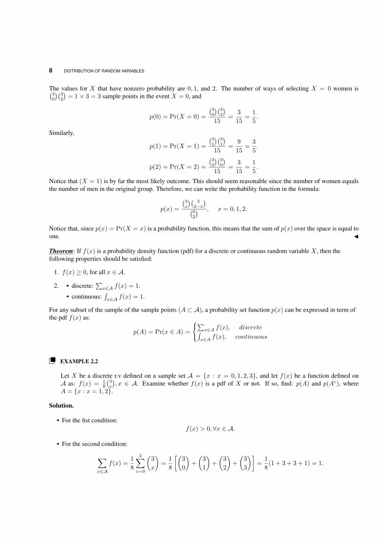
The values for X that have nonzero probability are 0, 1, and 2. The number of ways of selecting X = 0 women is(30
)(32
)= 1× 3 = 3 sample points in the event X = 0, and
p(0) = Pr(X = 0) =
(30
)(32
)15
=3
15=
1
5.
Similarly,
p(1) = Pr(X = 1) =
(31
)(31
)15
=9
15=
3
5.
p(2) = Pr(X = 2) =
(32
)(30
)15
=3
15=
1
5.
Notice that (X = 1) is by far the most likely outcome. This should seem reasonable since the number of women equalsthe number of men in the original group. Therefore, we can write the probability function in the formula:
p(x) =
(3x
)(3
2−x)(
62
) , x = 0, 1, 2.
Notice that, since p(x) = Pr(X = x) is a probability function, this means that the sum of p(x) over the space is equal toone. J
Theorem: If f(x) is a probability density function (pdf) for a discrete or continuous random variable X , then thefollowing properties should be satisfied:
1. f(x) ≥ 0, for all x ∈ A.
2. discrete:∑x∈A f(x) = 1.
continuous:∫x∈A f(x) = 1.
For any subset of the sample of the sample points (A ⊂ A), a probability set function p(x) can be expressed in term ofthe pdf f(x) as:
p(A) = Pr(x ∈ A) =
∑x∈A f(x), discrete∫
x∈A f(x), continuous
EXAMPLE 2.2
Let X be a discrete r.v defined on a sample set A = x : x = 0, 1, 2, 3, and let f(x) be a function defined onA as: f(x) = 1
8
(3x
), x ∈ A. Examine whether f(x) is a pdf of X or not. If so, find: p(A) and p(Ac), where
A = x : x = 1, 2.
Solution.
For the fist condition:f(x) > 0,∀x ∈ A.
For the second condition:
∑x∈A
f(x) =1
8
3∑x=0
(3
x
)=
1
8
[(3
0
)+
(3
1
)+
(3
2
)+
(3
3
)]=
1
8(1 + 3 + 3 + 1) = 1.
THE PROBABILITY DENSITY FUNCTION (PDF) 9
This proves that f(x) is a pdf of X . Hence,
p(A) =∑x∈A
f(x) =1
8
2∑x=1
(3
x
)=
1
8
[(3
1
)+
(3
2
)]=
3
4,
and p(Ac) = 1− p(A) = 1− 34 = 1
4 . J
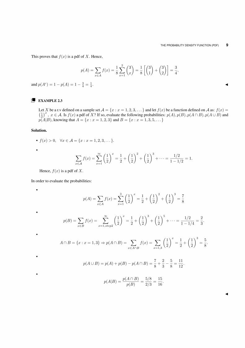
EXAMPLE 2.3
LetX be a r.v defined on a sample setA = x : x = 1, 2, 3, . . . and let f(x) be a function defined onA as: f(x) =(12
)x, x ∈ A. Is f(x) a pdf of X? If so, evaluate the following probabilities: p(A), p(B), p(A ∩B), p(A ∪B) and
p(A|B), knowing that A = x : x = 1, 2, 3 and B = x : x = 1, 3, 5, . . .
Solution.
f(x) > 0, ∀x ∈ A = x : x = 1, 2, 3, . . . .
∑x∈A
f(x) =
∞∑x=1
(1
2
)x=
1
2+
(1
2
)2
+
(1
2
)3
+ · · · = 1/2
1− 1/2= 1.
Hence, f(x) is a pdf of X .
In order to evaluate the probabilities:
p(A) =∑x∈A
f(x) =
3∑x=1
(1
2
)x=
1
2+
(1
2
)2
+
(1
2
)3
=7
8
p(B) =∑x∈B
f(x) =
∞∑x=1,step2
(1
2
)x=
1
2+
(1
2
)3
+
(1
2
)5
+ · · · = 1/2
1− 1/4=
2
3.
A ∩B = x : x = 1, 3 ⇒ p(A ∩B) =∑
x∈A∩Bf(x) =
∑x=1,3
(1
2
)x=
1
2+
(1
2
)3
=5
8.
p(A ∪B) = p(A) + p(B)− p(A ∩B) =7
8+
2
3− 5
8=
11
12.
p(A|B) =p(A ∩B)
p(B)=
5/8
2/3=
15
16.
J
10 DISTRIBUTION OF RANDOM VARIABLES
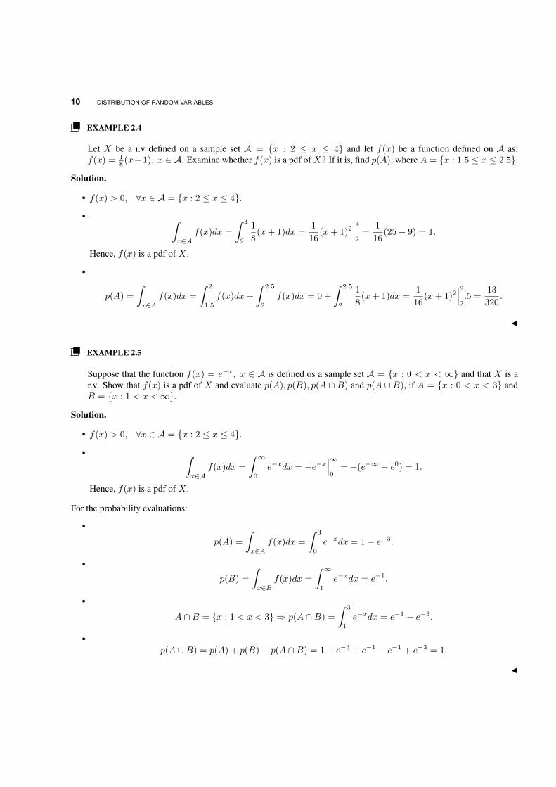
EXAMPLE 2.4
Let X be a r.v defined on a sample set A = x : 2 ≤ x ≤ 4 and let f(x) be a function defined on A as:f(x) = 1
8 (x+1), x ∈ A. Examine whether f(x) is a pdf of X? If it is, find p(A), where A = x : 1.5 ≤ x ≤ 2.5.
Solution.
f(x) > 0, ∀x ∈ A = x : 2 ≤ x ≤ 4.
∫x∈A
f(x)dx =
∫ 4
2
1
8(x+ 1)dx =
1
16(x+ 1)2
∣∣∣42
=1
16(25− 9) = 1.
Hence, f(x) is a pdf of X .
p(A) =
∫x∈A
f(x)dx =
∫ 2
1.5
f(x)dx+
∫ 2.5
2
f(x)dx = 0 +
∫ 2.5
2
1
8(x+ 1)dx =
1
16(x+ 1)2
∣∣∣22.5 =
13
320.
J
EXAMPLE 2.5
Suppose that the function f(x) = e−x, x ∈ A is defined os a sample set A = x : 0 < x < ∞ and that X is ar.v. Show that f(x) is a pdf of X and evaluate p(A), p(B), p(A ∩ B) and p(A ∪ B), if A = x : 0 < x < 3 andB = x : 1 < x <∞.
Solution.
f(x) > 0, ∀x ∈ A = x : 2 ≤ x ≤ 4.
∫x∈A
f(x)dx =
∫ ∞0
e−xdx = −e−x∣∣∣∞0
= −(e−∞ − e0) = 1.
Hence, f(x) is a pdf of X .
For the probability evaluations:
p(A) =
∫x∈A
f(x)dx =
∫ 3
0
e−xdx = 1− e−3.
p(B) =
∫x∈B
f(x)dx =
∫ ∞1
e−xdx = e−1.
A ∩B = x : 1 < x < 3 ⇒ p(A ∩B) =
∫ 3
1
e−xdx = e−1 − e−3.
p(A ∪B) = p(A) + p(B)− p(A ∩B) = 1− e−3 + e−1 − e−1 + e−3 = 1.
J
THE PROBABILITY DENSITY FUNCTION (PDF) 11
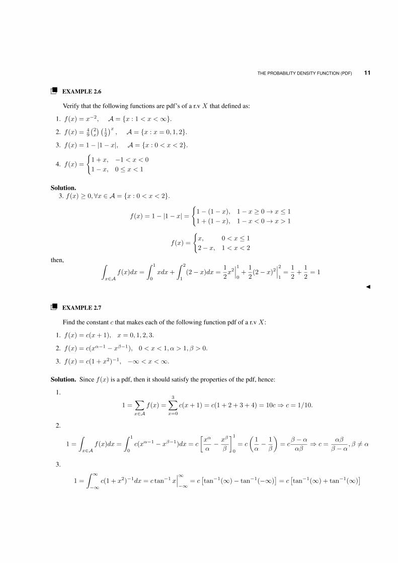
EXAMPLE 2.6
Verify that the following functions are pdf’s of a r.v X that defined as:
1. f(x) = x−2, A = x : 1 < x <∞.
2. f(x) = 49
(2x
) (12
)x, A = x : x = 0, 1, 2.
3. f(x) = 1− |1− x|, A = x : 0 < x < 2.
4. f(x) =
1 + x, −1 < x < 0
1− x, 0 ≤ x < 1
Solution.3. f(x) ≥ 0,∀x ∈ A = x : 0 < x < 2.
f(x) = 1− |1− x| =
1− (1− x), 1− x ≥ 0→ x ≤ 1
1 + (1− x), 1− x < 0→ x > 1
f(x) =
x, 0 < x ≤ 1
2− x, 1 < x < 2
then, ∫x∈A
f(x)dx =
∫ 1
0
xdx+
∫ 2
1
(2− x)dx =1
2x2∣∣∣10
+1
2(2− x)2
∣∣∣21
=1
2+
1
2= 1
J
EXAMPLE 2.7
Find the constant c that makes each of the following function pdf of a r.v X:
1. f(x) = c(x+ 1), x = 0, 1, 2, 3.
2. f(x) = c(xα−1 − xβ−1), 0 < x < 1, α > 1, β > 0.
3. f(x) = c(1 + x2)−1, −∞ < x <∞.
Solution. Since f(x) is a pdf, then it should satisfy the properties of the pdf, hence:
1.
1 =∑x∈A
f(x) =
3∑x=0
c(x+ 1) = c(1 + 2 + 3 + 4) = 10c⇒ c = 1/10.
2.
1 =
∫x∈A
f(x)dx =
∫ 1
0
c(xα−1 − xβ−1)dx = c
[xα
α− xβ
β
]1
0
= c
(1
α− 1
β
)= c
β − ααβ
⇒ c =αβ
β − α, β 6= α
3.
1 =
∫ ∞−∞
c(1 + x2)−1dx = c tan−1 x∣∣∣∞−∞
= c[tan−1(∞)− tan−1(−∞)
]= c
[tan−1(∞) + tan−1(∞)
]
12 DISTRIBUTION OF RANDOM VARIABLES
= 2c tan−1(∞) = 2cπ
2⇒ c =
1
π.
J
Definition: The Mode of the distribution is the value of x that maximises the pdf f(x) of a r.v X . Note that the modeof a continuous r.v is the solution of f ′(x) = 0 and f(x) < 0. Also, the mode may not be existed or a distribution mayhave more than one mode.
EXAMPLE 2.8
Find the mode for the following pdf’s:
1. f(x) =(
12
)x, x = 1, 2, 3, . . . .
2. f(x) = 12x2(1− x), 0 < x < 1.
Solution.
1. f(x) =(
12
)x, x = 1, 2, 3, . . . , then x = 1 is the mode.
2. f(x) = 12x2(1− x), 0 < x < 1⇒ f ′(x) = 12(2x− 3x2), set f ′(x) = 0:
12(2x− 3x2) = 0⇒ x = 0, 2/3.
then, f ′′(x) = 12(2− 6x) = 24(1− 3x).
f ′′(0) = 24(1− 0) = 24 > 0
f ′′(2/3) = 24(1− 3(2/3)) = −24 < 0
hence, x = 2/3 is the mode.
J
2.1.1 The Probability Density Function in n−Dimensional Space
Let X1, X2, . . . , Xn be an n r.v’s (discrete or continuous) defined on n−D sample space A, and let Pr(X1 = x1, X2 =x2, . . . , Xn = xn) = f(x1, x2, . . . , xn) be a function defined on A, such that:
1. f(x1, x2, . . . , xn) ≥ 0,∀(x1, x2, . . . , xn) ∈ A.
2.
1 =
∑∑· · ·∑
(x1,x2,...,xn)∈A f(x1, x2, . . . , xn)∫ ∫·· ·∫
(x1,x2,...,xn)∈A f(x1, x2, . . . , xn)dx1, dx2, . . . , dxn
Then the function f(x1, x2, . . . , xn) is called pdf of r.v’s X1, X2, . . . , Xn. Furthermore, for all event A ⊂ A, theprobability of A, p(A), can be expressed in terms of the pdf by:
p(A) = Pr(X1, X2, . . . , Xn) ∈ A =
∑∑· · ·∑
(x1,x2,...,xn)∈A f(x1, x2, . . . , xn).∫ ∫·· ·∫
(x1,x2,...,xn)∈A f(x1, x2, . . . , xn)dx1, dx2, . . . , dxn.

THE PROBABILITY DENSITY FUNCTION (PDF) 13
EXAMPLE 2.9
Let X and Y be discrete r.v’s defined on a sample space A = (x, y) : x = 1, 2, 3; y = 1, 2, and let f(x, y) be afunction defined on A by f(x, y) = 1
21 (x+ y), (x, y) ∈ A.
1. Is f(x, y) a pdf of X and Y ?
2. If so, find p(A) and p(Ac), where A = (x, y) : x = 1, 2; y = 1.
Solution.
1. - f(x, y) > 0, ∀(x, y) ∈ A.-
∑∑(x,y)∈A
f(x, y) =
3∑x=1
2∑y=1
1
21(x+ y) =
1
21
3∑x=1
[(x+ 1) + (x+ 2)]
=1
21
3∑x=1
(2x+ 3) =1
21[5 + 7 + 9] = 1.
Then f(x, y) is a pdf of X and Y .
2.
p(A) =∑ ∑
(x,y)∈A
f(x, y) =
2∑x=1
1∑y=1
1
21(x+ y) =
1
21
2∑x=1
(x+ 1) =1
21(2 + 3) =
5
21
⇒ p(Ac) = 1− 5
21=
16
21.
J
EXAMPLE 2.10
Let X and Y be two r.v’s defined on a sample space A = (x, y) : x = 1, 2, . . . ; y = 0, 1, 2, and let f(x, y) be afunction defined on A by
f(x, y) =
(2
y
)(1
2
)x+2
, (x, y) ∈ A
1. Is f(x, y) a pdf of X and Y ?
2. Find p(A), where A = (x, y) : x = 1, 3, 5, . . . ; y = 1.
Solution.
1. - f(x, y) > 0, ∀(x, y) ∈ A.- ∑∑
(x,y)∈Af(x, y) =
∞∑x=1
2∑y=0
(2
y
)(1
2
)x+2
=
∞∑x=1
(1
2
)x+2 [(2
0
)+
(2
1
)+
(2
2
)]
=
∞∑x=1
(1
2
)x+2
(1 + 2 + 1) = 4
[(1
2
)3
+
(1
2
)4
+
(1
2
)5
+ . . .
]= 4
(1/2)3
1− (1/2)= 1
14 DISTRIBUTION OF RANDOM VARIABLES
Then f(x, y) is a pdf of X and Y .
2.
p(A) =∑∑
(x,y)∈Af(x, y) =
∞∑x=1,step2
1∑y=1
(2
y
)(1
2
)x+2
=
∞∑x=1,step2
(1
2
)x+2(2
1
)= 2
∞∑x=1,step2
(1
2
)x+2
= 2
[(1
2
)3
+
(1
2
)5
+
(1
2
)7
+ . . .
]= 2
(1/2)3
1− (1/2)2=
1
3.
J
EXAMPLE 2.11
Let X and Y be continuous r.v’s defined on a sample space A = (x, y) : 0 < x < 2; 2 < y < 4, and let f(x, y)be a function defined on A as f(x, y) = 1
8 (6− x− y), (x, y) ∈ A
1. Is f(x, y) a pdf of X and Y ?
2. Find p(A), where A = (x, y) : 0 < x < 1; 2 < y < 3.
Solution.
1. - f(x, y) ≥ 0, ∀(x, y) ∈ A.- ∫ ∫
(x,y)∈Af(x, y) =
∫ 2
x=0
∫ 4
y=2
1
8(6− x− y)dydx =
1
8
∫ 2
0
[6y − xy − y2
2
]4
2
dx
=1
8
∫ 2
0
[(24− 4x− 8)− (12− 2x− 2)] dx =1
8
∫ 2
0
(6− 2x)dx =1
8
[6x− x2
]20
=12− 4
8= 1
Then f(x, y) is a pdf of X and Y .
2.
p(A) =
∫ ∫(x,y)∈A
f(x, y) =
∫ 1
x=0
∫ 3
y=2
1
8(6− x− y)dydx = · · · = 3
8
J
EXAMPLE 2.12
X and Y are two r.v’s defined on a sample space A = (x, y) : 0 < x < y < 1, and let f(x, y) = 2 (x, y) ∈ A isa function defined on A. is f(x, y) a pdf of X and Y ?
Solution.
- f(x, y) = 2 > 0, ∀(x, y) ∈ A.
- ∫ ∫(x,y)∈A
f(x, y) = 2
∫ 1
x=0
∫ 1
y=x
dydx = 2
∫ 1
0
y∣∣∣1xdx = 2
∫ 1
0
(1− x)dx = 2
[x− x2
2
]1
0
= 2(1− 1
2) = 1
CUMULATIVE DISTRIBUTION FUNCTION (CDF) 15
Then f(x, y) is a pdf of X and Y . J
Note: If f(x1, x2, . . . , xn) is a pdf of r.v’s X1, X2, . . . , Xn defined on a sample space A = (x1, x2, . . . , xn) : −∞ <xi <∞; i = 1, 2, . . . , n, and if event A ⊂ A, where A = (x1, x2, . . . , xn) : ai < xi < bi; i = 1, 2, . . . , n. Then theprobability of A is:
p(A) = Prai < xi < bi; i = 1, 2, . . . , n =
b1∑x1=a1
b2∑x2=a2
· · ·bn∑
xn=an
f(x1, x2, . . . , xn)
b1∫x1=a1
b2∫x2=a2
· · ·bn∫
xn=an
f(x1, x2, . . . , xn)dx1, dx2, . . . , dxn
EXAMPLE 2.13
Find the constant c that makes the function f(x, y) = ce−x−y, 0 < x < y <∞ a pdf of r.v’s X and Y .
Solution. Since f(x, y) is a pdf of X and Y , then by definition∫ ∫
(x,y)∈A f(x, y)dxdy = 1:
1 = c
∫ ∞x=0
∫ ∞y=x
e−x−ydydx = c
∫ ∞0
e−x[∫ ∞
x
e−ydy
]dx = c
∫ ∞0
e−x[−e−y
]∞xdx
= c
∫ ∞0
e−x(0 + e−x)dx = c
∫ ∞0
e−2xdx = c
[1
2e−2x
]∞0
= c(0 +1
2) =
c
2.
Therefore, c = 2. J
2.2 Cumulative Distribution Function (CDF)
Definition: The cumulative distribution function or the probability distribution of a r.v X , denoted by F (x) = Pr(X ≤x),−∞ < x <∞. Let X be a r.v has a pdf f(x) defined on a sample space A, we define:
F (x) = Pr(X ≤ x) = Pr(−∞ < x <∞) =
x∑
t=−∞f(t), discrete.
x∫t=−∞
f(t)dt, continuous.
EXAMPLE 2.14
Suppose that X has a pdf p(x), defined on x = 0, 1, 2 as:
p(x) =
(2
x
)(1
2
)x(1
2
)2−x
, x = 0, 1, 2.
Find F (x) for all x.
Solution. From the pdf p(x), we have: p(0) = 1/4, p(1) = 1/2, p(2) = 1/4. In order to find the distribution functionF (x), from definition of F (x) = Pr(X ≤ x), we should evaluate the probability for four regions of x:
−∞ < x < 0, 0 ≤ x < 1, 1 ≤ x < 2 and 2 ≤ x <∞.
16 DISTRIBUTION OF RANDOM VARIABLES
For x < 0: Because the only value of X that are assigned positive probabilities are 0, 1 and 2; and that non of thesevalues are less than 0, then f(x) = 0, ∀ −∞ < x < 0.
For 0 ≤ x < 1:
F (x) = Pr(0 ≤ x < 1) = Pr(X < 0) + Pr(X = 0) = 0 +1
4=
1
4.
For 1 ≤ x < 2:
F (x) = Pr(1 ≤ x < 2) = Pr(X = 0) + Pr(X = 1) =1
4+
1
2=
3
4.
For x ≥ 2:
F (x) = Pr(X ≥ 2) = Pr(X < 0) + Pr(0 ≤ X ≤ 1) + Pr(1 ≤ X < 2) = 0 +1
4+
3
4= 1.
Therefore, the distribution probability is:
F (x) = Pr(X ≤ x) =
0, x < 0
1/4, 0 ≤ x < 1
3/4, 1 ≤ x < 2
1, x ≥ 2
J
Notes:
1. F (−∞) = limx→−∞
F (x) = 0.
2. F (∞) = limx→∞
F (x) = 1.
3. F (x) is a non-decreasing function of x, if x1 < x2 then F (x1) ≤ F (x2).
4. 0 ≤ F (x) ≤ 1, because 0 ≤ Pr(X ≤ x) ≤ 1.
5. For a continuous r.v X , the pdf could be evaluated in terms of the cdf as:
f(x) =d
dxF (x).
6. For a discrete r.v X , the pdf could be evaluated in terms of the cdf as:
f(x) = Pr(X = x) = Pr(X ≤ x)− Pr(X ≤ x− 1) = F (x)− F (x− 1).
EXAMPLE 2.15
Let the r.v has a pdf f(x) = x6 ; x = 1, 2, 3. Find the cdf of X
Solution.
F (x) = Pr(X ≤ x) =
x∑τ=−∞
f(τ) =
x∑τ=1
τ
6=
1
6(1 + 2 + · · ·+ x) =
x(x+ 1)
12
∴ F (x) =
0, x < 1x(x+1)
12 , 1 ≤ x < 3
1, x ≥ 3
J
CUMULATIVE DISTRIBUTION FUNCTION (CDF) 17
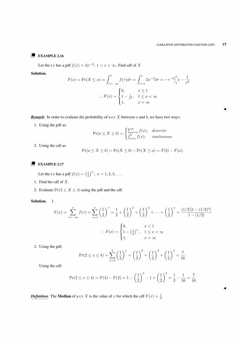
EXAMPLE 2.16
Let the r.v has a pdf f(x) = 2x−3; 1 < x <∞. Find cdf of X
Solution.F (x) = Pr(X ≤ x) =
∫ x
τ=−∞f(τ)dτ =
∫ x
τ=1
2x−3dτ = −τ−2∣∣∣x11− 1
x2
∴ F (x) =
0, x ≤ 1
1− 1x2 , 1 ≤ x <∞
1, x =∞J
Remark: In order to evaluate the probability of a r.v X between a and b, we have two ways:
1. Using the pdf as:
Pr(a ≤ X ≤ b) =
∑bx=a f(x), discrete∫ b
x=af(x), continuous
2. Using the cdf as:Pr(a ≤ X ≤ b) = Pr(X ≤ b)− Pr(X ≤ a) = F (b)− F (a).
EXAMPLE 2.17
Let the r.v has a pdf f(x) =(
12
)x; x = 1, 2, 3, . . . .
1. Find the cdf of X .
2. Evaluate Pr(2 ≤ X ≤ 4) using the pdf and the cdf.
Solution. 1.
F (x) =x∑
τ=−∞f(τ) =
x∑τ=1
(1
2
)τ=
1
2+
(1
2
)2
+
(1
2
)3
+ · · ·+(
1
2
)x=
(1/2)[1− (1/2)x]
1− (1/2)
∴ F (x) =
0, x < 1
1−(
12
)x, 1 ≤ x <∞
1, x =∞
2. Using the pdf:
Pr(2 ≤ x ≤ 4) =
4∑x=2
(1
2
)x=
(1
2
)2
+
(1
2
)3
+
(1
2
)4
=7
16.
Using the cdf:
Pr(2 ≤ x ≤ 4) = F (4)− F (2) = 1−(
1
2
)4
− 1 +
(1
2
)2
=1
2− 1
16=
7
16
J
Definition: The Median of a r.v X is the value of x for which the cdf F (x) = 12 .
18 DISTRIBUTION OF RANDOM VARIABLES
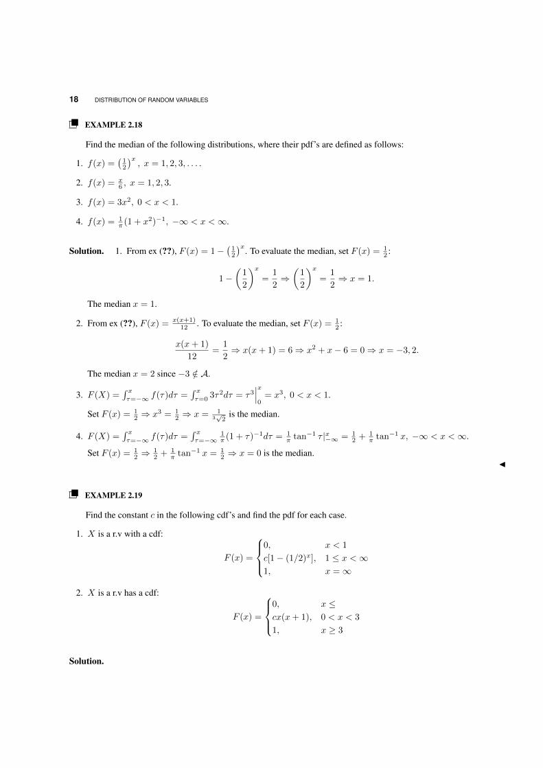
EXAMPLE 2.18
Find the median of the following distributions, where their pdf’s are defined as follows:
1. f(x) =(
12
)x, x = 1, 2, 3, . . . .
2. f(x) = x6 , x = 1, 2, 3.
3. f(x) = 3x2, 0 < x < 1.
4. f(x) = 1π (1 + x2)−1, −∞ < x <∞.
Solution. 1. From ex (??), F (x) = 1−(
12
)x. To evaluate the median, set F (x) = 1
2 :
1−(
1
2
)x=
1
2⇒(
1
2
)x=
1
2⇒ x = 1.
The median x = 1.
2. From ex (??), F (x) = x(x+1)12 . To evaluate the median, set F (x) = 1
2 :
x(x+ 1)
12=
1
2⇒ x(x+ 1) = 6⇒ x2 + x− 6 = 0⇒ x = −3, 2.
The median x = 2 since −3 /∈ A.
3. F (X) =∫ xτ=−∞ f(τ)dτ =
∫ xτ=0
3τ2dτ = τ3∣∣∣x0
= x3, 0 < x < 1.
Set F (x) = 12 ⇒ x3 = 1
2 ⇒ x = 13√
2is the median.
4. F (X) =∫ xτ=−∞ f(τ)dτ =
∫ xτ=−∞
1π (1 + τ)−1dτ = 1
π tan−1 τ |x−∞ = 12 + 1
π tan−1 x, −∞ < x <∞.
Set F (x) = 12 ⇒
12 + 1
π tan−1 x = 12 ⇒ x = 0 is the median.
J
EXAMPLE 2.19
Find the constant c in the following cdf’s and find the pdf for each case.
1. X is a r.v with a cdf:
F (x) =
0, x < 1
c[1− (1/2)x], 1 ≤ x <∞1, x =∞
2. X is a r.v has a cdf:
F (x) =
0, x ≤cx(x+ 1), 0 < x < 3
1, x ≥ 3
Solution.

CUMULATIVE DISTRIBUTION FUNCTION (CDF) 19
1. Since F (x) is a cdf, then: F (∞) = 1⇒ c[1− (1/2)∞] = 1⇒ c(1− 0) = 1⇒ c = 1. then:
F (x) =
0, x < 1
1−(
12
)x, 1 ≤ x <∞
1, x =∞
Therefore, the pdf f(x) = F (x)− F (x− 1):
f(x) = 1−(
1
2
)x− 1 +
(1
2
)x−1
=
(1
2
)x−1
−(
1
2
)x=
(1
2
)x−1(1− 1
2
)∴ f(x) =
(1
2
)x, x = 1, 2, 3, . . .
2. Since F (∞) is a cdf, then: F (3) = 1⇒ 3c(3 + 1) = 1⇒ 12c = 1⇒ c = 12 , then:
F (x) =
0, x ≤ 0112x(x+ 1), 0 < x < 3
1, x ≥ 3
Therefore, the pdf f(x) = F ′(x):
∴ f(x) =1
12(2x+ 1), 0 < x < 3
J
EXAMPLE 2.20
Find the cdf of the r.v X which has a pdf f(x) =
x, 0 < x < 1
2− x, 1 ≤ x < 2
Solution.
F (x) = Pr(X ≤ x) =
0, x ≤ 0x∫0
f(τ)dτ =x∫0
τdτ = 12τ
2∣∣∣x0
= 12x
2, 0 < x < 1
1∫0
f(τ)dτ +x∫1
f(τ)dτ = 1− 12 (2− x)2, 1 ≤ x < 2
1, x ≥ 2
J
2.2.1 The Cumulative Distribution Function in n−Dimensional Space
Let X1, X2, . . . , Xn be n r.v’s defined on an n−Dimensional sample spaceA with pdf f(x1, x2, . . . , xn). We define thecdf of X1, X2, . . . , Xn as:
F (x1, x2, . . . , xn) = Pr(X1 ≤ x1, X2 ≤ x2, . . . , Xn ≤ xn)
=
x1∑τ1=−∞
x2∑τ2=−∞
· · ·xn∑
τn=−∞f(τ1, τ2, . . . , τn), discrete.
x1∫τ1=−∞
x2∫τ2=−∞
· · ·xn∫
τn=−∞f(τ1, τ2, . . . , τn)dτ1dτ2 . . . dτn, continuous.
20 DISTRIBUTION OF RANDOM VARIABLES
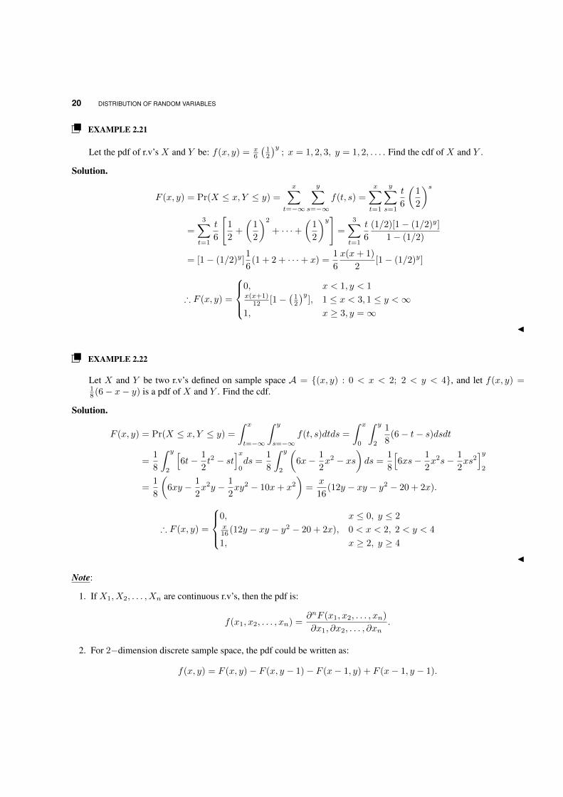
EXAMPLE 2.21
Let the pdf of r.v’s X and Y be: f(x, y) = x6
(12
)y; x = 1, 2, 3, y = 1, 2, . . . . Find the cdf of X and Y .
Solution.
F (x, y) = Pr(X ≤ x, Y ≤ y) =
x∑t=−∞
y∑s=−∞
f(t, s) =
x∑t=1
y∑s=1
t
6
(1
2
)s
=
3∑t=1
t
6
[1
2+
(1
2
)2
+ · · ·+(
1
2
)y]=
3∑t=1
t
6
(1/2)[1− (1/2)y]
1− (1/2)
= [1− (1/2)y]1
6(1 + 2 + · · ·+ x) =
1
6
x(x+ 1)
2[1− (1/2)y]
∴ F (x, y) =
0, x < 1, y < 1x(x+1)
12 [1−(
12
)y], 1 ≤ x < 3, 1 ≤ y <∞
1, x ≥ 3, y =∞J
EXAMPLE 2.22
Let X and Y be two r.v’s defined on sample space A = (x, y) : 0 < x < 2; 2 < y < 4, and let f(x, y) =18 (6− x− y) is a pdf of X and Y . Find the cdf.
Solution.
F (x, y) = Pr(X ≤ x, Y ≤ y) =
∫ x
t=−∞
∫ y
s=−∞f(t, s)dtds =
∫ x
0
∫ y
2
1
8(6− t− s)dsdt
=1
8
∫ y
2
[6t− 1
2t2 − st
]x0ds =
1
8
∫ y
2
(6x− 1
2x2 − xs
)ds =
1
8
[6xs− 1
2x2s− 1
2xs2]y
2
=1
8
(6xy − 1
2x2y − 1
2xy2 − 10x+ x2
)=
x
16(12y − xy − y2 − 20 + 2x).
∴ F (x, y) =
0, x ≤ 0, y ≤ 2x16 (12y − xy − y2 − 20 + 2x), 0 < x < 2, 2 < y < 4
1, x ≥ 2, y ≥ 4
J
Note:
1. If X1, X2, . . . , Xn are continuous r.v’s, then the pdf is:
f(x1, x2, . . . , xn) =∂nF (x1, x2, . . . , xn)
∂x1, ∂x2, . . . , ∂xn.
2. For 2−dimension discrete sample space, the pdf could be written as:
f(x, y) = F (x, y)− F (x, y − 1)− F (x− 1, y) + F (x− 1, y − 1).
TRANSFORMATION OF VARIABLES (CDF TECHNIQUE) 21
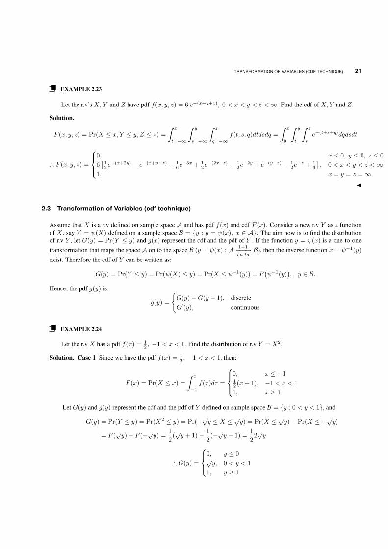
EXAMPLE 2.23
Let the r.v’s X , Y and Z have pdf f(x, y, z) = 6 e−(x+y+z), 0 < x < y < z <∞. Find the cdf of X,Y and Z.
Solution.
F (x, y, z) = Pr(X ≤ x, Y ≤ y, Z ≤ z) =
∫ x
t=−∞
∫ y
s=−∞
∫ z
q=−∞f(t, s, q)dtdsdq =
∫ x
0
∫ y
t
∫ z
s
e−(t+s+q)dqdsdt
∴ F (x, y, z) =
0, x ≤ 0, y ≤ 0, z ≤ 0
6[
12e−(x+2y) − e−(x+y+z) − 1
6e−3x + 1
2e−(2x+z) − 1
2e−2y + e−(y+z) − 1
2e−z + 1
6
], 0 < x < y < z <∞
1, x = y = z =∞J
2.3 Transformation of Variables (cdf technique)
Assume that X is a r.v defined on sample space A and has pdf f(x) and cdf F (x). Consider a new r.v Y as a functionof X , say Y = ψ(X) defined on a sample space B = y : y = ψ(x), x ∈ A. The aim now is to find the distributionof r.v Y , let G(y) = Pr(Y ≤ y) and g(x) represent the cdf and the pdf of Y . If the function y = ψ(x) is a one-to-onetransformation that maps the space A on to the space B (y = ψ(x) : A 1−1−−−→
on toB), then the inverse function x = ψ−1(y)
exist. Therefore the cdf of Y can be written as:
G(y) = Pr(Y ≤ y) = Pr(ψ(X) ≤ y) = Pr(X ≤ ψ−1(y)) = F(ψ−1(y)
), y ∈ B.
Hence, the pdf g(y) is:
g(y) =
G(y)−G(y − 1), discreteG′(y), continuous
EXAMPLE 2.24
Let the r.v X has a pdf f(x) = 12 , −1 < x < 1. Find the distribution of r.v Y = X2.
Solution. Case 1 Since we have the pdf f(x) = 12 , −1 < x < 1, then:
F (x) = Pr(X ≤ x) =
∫ x
−1
f(τ)dτ =
0, x ≤ −112 (x+ 1), −1 < x < 1
1, x ≥ 1
Let G(y) and g(y) represent the cdf and the pdf of Y defined on sample space B = y : 0 < y < 1, and
G(y) = Pr(Y ≤ y) = Pr(X2 ≤ y) = Pr(−√y ≤ X ≤ √y) = Pr(X ≤ √y)− Pr(X ≤ −√y)
= F (√y)− F (−√y) =
1
2(√y + 1)− 1
2(−√y + 1) =
1
22√y
∴ G(y) =
0, y ≤ 0√y, 0 < y < 1
1, y ≥ 1
22 DISTRIBUTION OF RANDOM VARIABLES
Then, the pdf g(y) = G′(y) = 12√y , 0 < y < 1.
Case 2 The pdf of r.v X f(x) = 12 , −1 < x < 1. Let G(y) and g(y) be the cdf and pdf of Y = X2 with sample space
B = y : 0 < y < 1. Then:
G(y) = Pr(Y ≤ y) = Pr(X2 ≤ y) = Pr(−√y ≤ X ≤ √y) =
√y∫
−√y
f(x)dx =
√y∫
−√y
1
2dx =
√y
∴ G(y) =
0, y ≤ 0√y, 0 < y < 1
1, y ≥ 1
J
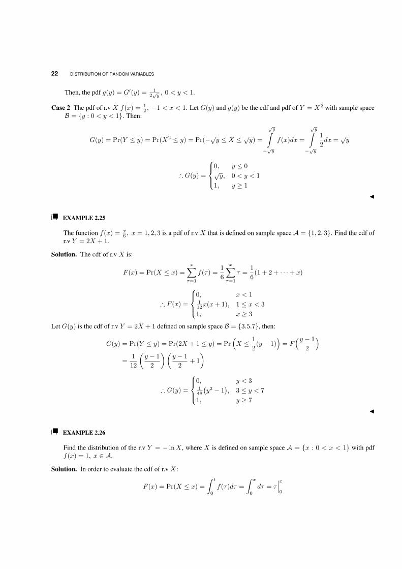
EXAMPLE 2.25
The function f(x) = x6 , x = 1, 2, 3 is a pdf of r.v X that is defined on sample space A = 1, 2, 3. Find the cdf of
r.v Y = 2X + 1.
Solution. The cdf of r.v X is:
F (x) = Pr(X ≤ x) =
x∑τ=1
f(τ) =1
6
x∑τ=1
τ =1
6(1 + 2 + · · ·+ x)
∴ F (x) =
0, x < 1112x(x+ 1), 1 ≤ x < 3
1, x ≥ 3
Let G(y) is the cdf of r.v Y = 2X + 1 defined on sample space B = 3.5.7, then:
G(y) = Pr(Y ≤ y) = Pr(2X + 1 ≤ y) = Pr(X ≤ 1
2(y − 1)
)= F
(y − 1
2
)=
1
12
(y − 1
2
)(y − 1
2+ 1
)
∴ G(y) =
0, y < 3148
(y2 − 1
), 3 ≤ y < 7
1, y ≥ 7
J
EXAMPLE 2.26
Find the distribution of the r.v Y = − lnX , where X is defined on sample space A = x : 0 < x < 1 with pdff(x) = 1, x ∈ A.
Solution. In order to evaluate the cdf of r.v X:
F (x) = Pr(X ≤ x) =
∫ t
0
f(τ)dτ =
∫ x
0
dτ = τ∣∣∣x0
MATHEMATICAL EXPECTATION 23
∴ F (x) =
0, x ≤ 0
x, 0 < x < 1
1, x ≥ 1
Assume G(y) and g(y) represent the cdf and pdf of r.v Y = − lnX defined on sample space B = y : 0 < y <∞,
G(y) = Pr(Y ≤ y) = Pr(− lnX ≤ y) = Pr(lnX ≥ y) = Pr(X ≥ e−y)
= 1− Pr(X ≤ e−y) = 1− F(e−y)
∴ G(y) =
0, y ≤ 0
1− e−y, 0 < y <∞1, y =∞
This leads to the pdf of r.v Y , g(y) = G′(y) = e−y, y ∈ B J
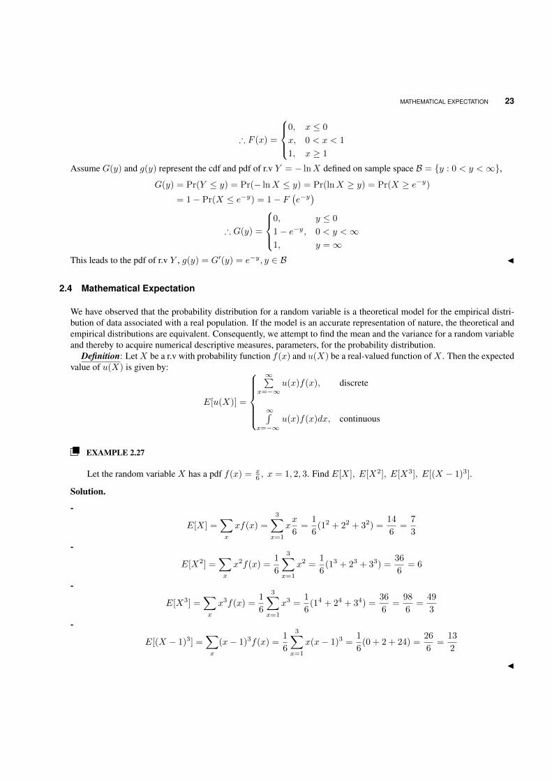
2.4 Mathematical Expectation
We have observed that the probability distribution for a random variable is a theoretical model for the empirical distri-bution of data associated with a real population. If the model is an accurate representation of nature, the theoretical andempirical distributions are equivalent. Consequently, we attempt to find the mean and the variance for a random variableand thereby to acquire numerical descriptive measures, parameters, for the probability distribution.
Definition: LetX be a r.v with probability function f(x) and u(X) be a real-valued function ofX . Then the expectedvalue of u(X) is given by:
E[u(X)] =
∞∑x=−∞
u(x)f(x), discrete
∞∫x=−∞
u(x)f(x)dx, continuous
EXAMPLE 2.27
Let the random variable X has a pdf f(x) = x6 , x = 1, 2, 3. Find E[X], E[X2], E[X3], E[(X − 1)3].
Solution.
-
E[X] =∑x
xf(x) =
3∑x=1
xx
6=
1
6(12 + 22 + 32) =
14
6=
7
3
-
E[X2] =∑x
x2f(x) =1
6
3∑x=1
x2 =1
6(13 + 23 + 33) =
36
6= 6
-
E[X3] =∑x
x3f(x) =1
6
3∑x=1
x3 =1
6(14 + 24 + 34) =
36
6=
98
6=
49
3
-
E[(X − 1)3] =∑x
(x− 1)3f(x) =1
6
3∑x=1
x(x− 1)3 =1
6(0 + 2 + 24) =
26
6=
13
2
J
24 DISTRIBUTION OF RANDOM VARIABLES
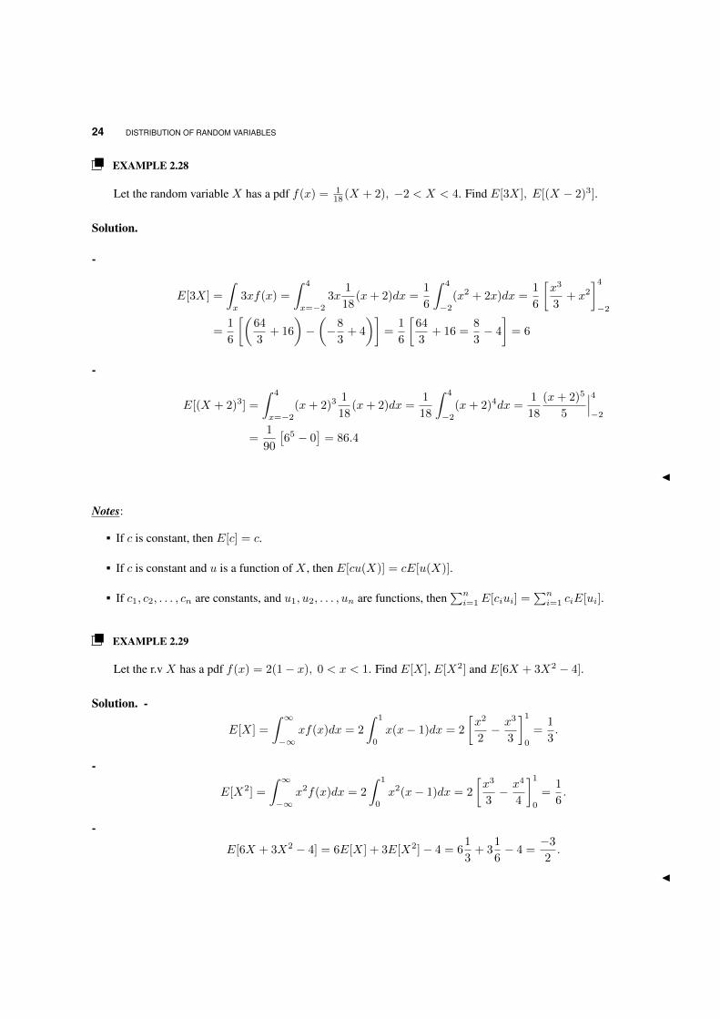
EXAMPLE 2.28
Let the random variable X has a pdf f(x) = 118 (X + 2), −2 < X < 4. Find E[3X], E[(X − 2)3].
Solution.
-
E[3X] =
∫x
3xf(x) =
∫ 4
x=−2
3x1
18(x+ 2)dx =
1
6
∫ 4
−2
(x2 + 2x)dx =1
6
[x3
3+ x2
]4
−2
=1
6
[(64
3+ 16
)−(−8
3+ 4
)]=
1
6
[64
3+ 16 =
8
3− 4
]= 6
-
E[(X + 2)3] =
∫ 4
x=−2
(x+ 2)3 1
18(x+ 2)dx =
1
18
∫ 4
−2
(x+ 2)4dx =1
18
(x+ 2)5
5
∣∣∣4−2
=1
90
[65 − 0
]= 86.4
J
Notes:
If c is constant, then E[c] = c.
If c is constant and u is a function of X , then E[cu(X)] = cE[u(X)].
If c1, c2, . . . , cn are constants, and u1, u2, . . . , un are functions, then∑ni=1E[ciui] =
∑ni=1 ciE[ui].
EXAMPLE 2.29
Let the r.v X has a pdf f(x) = 2(1− x), 0 < x < 1. Find E[X], E[X2] and E[6X + 3X2 − 4].
Solution. -
E[X] =
∫ ∞−∞
xf(x)dx = 2
∫ 1
0
x(x− 1)dx = 2
[x2
2− x3
3
]1
0
=1
3.
-
E[X2] =
∫ ∞−∞
x2f(x)dx = 2
∫ 1
0
x2(x− 1)dx = 2
[x3
3− x4
4
]1
0
=1
6.
-
E[6X + 3X2 − 4] = 6E[X] + 3E[X2]− 4 = 61
3+ 3
1
6− 4 =
−3
2.
J
MATHEMATICAL EXPECTATION 25
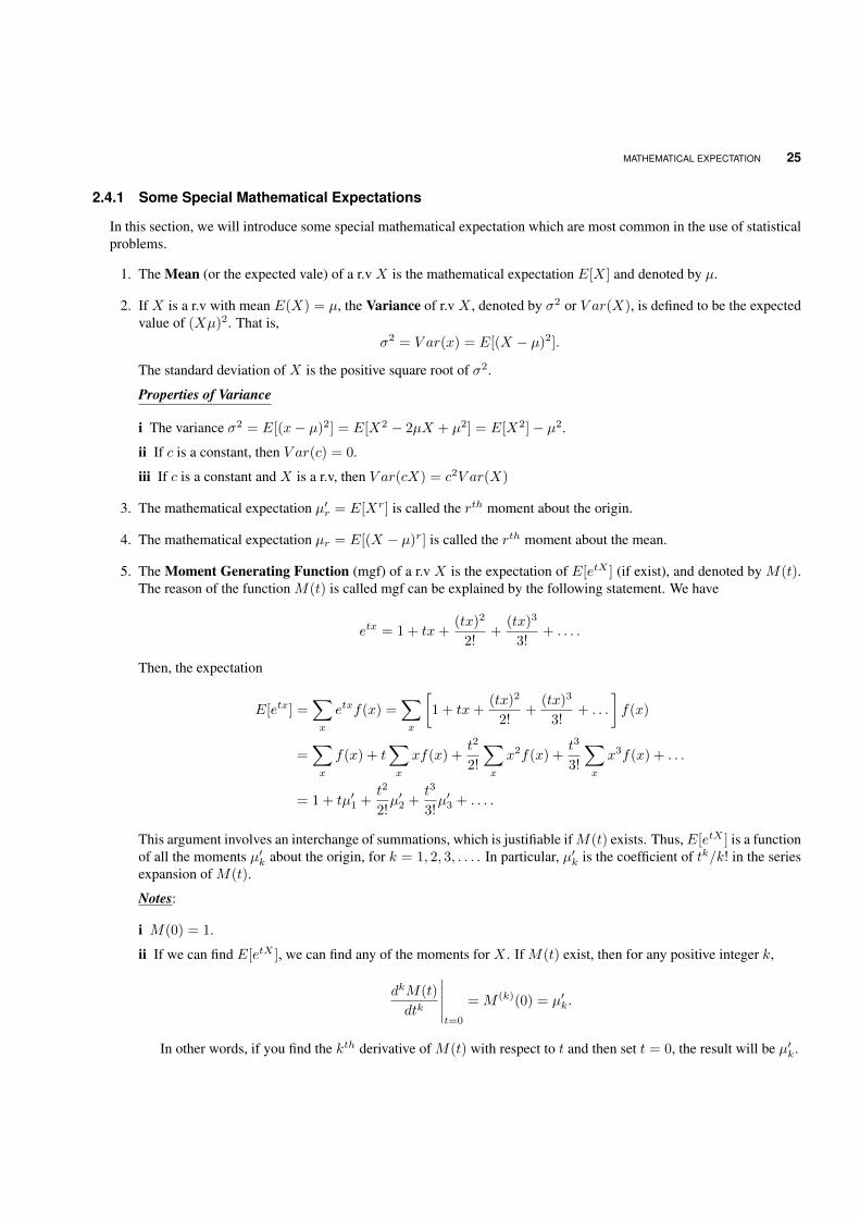
2.4.1 Some Special Mathematical Expectations
In this section, we will introduce some special mathematical expectation which are most common in the use of statisticalproblems.
1. The Mean (or the expected vale) of a r.v X is the mathematical expectation E[X] and denoted by µ.
2. If X is a r.v with mean E(X) = µ, the Variance of r.v X , denoted by σ2 or V ar(X), is defined to be the expectedvalue of (Xµ)2. That is,
σ2 = V ar(x) = E[(X − µ)2].
The standard deviation of X is the positive square root of σ2.
Properties of Variance
i The variance σ2 = E[(x− µ)2] = E[X2 − 2µX + µ2] = E[X2]− µ2.
ii If c is a constant, then V ar(c) = 0.
iii If c is a constant and X is a r.v, then V ar(cX) = c2V ar(X)
3. The mathematical expectation µ′r = E[Xr] is called the rth moment about the origin.
4. The mathematical expectation µr = E[(X − µ)r] is called the rth moment about the mean.
5. The Moment Generating Function (mgf) of a r.v X is the expectation of E[etX ] (if exist), and denoted by M(t).The reason of the function M(t) is called mgf can be explained by the following statement. We have
etx = 1 + tx+(tx)2
2!+
(tx)3
3!+ . . . .
Then, the expectation
E[etx] =∑x
etxf(x) =∑x
[1 + tx+
(tx)2
2!+
(tx)3
3!+ . . .
]f(x)
=∑x
f(x) + t∑x
xf(x) +t2
2!
∑x
x2f(x) +t3
3!
∑x
x3f(x) + . . .
= 1 + tµ′1 +t2
2!µ′2 +
t3
3!µ′3 + . . . .
This argument involves an interchange of summations, which is justifiable ifM(t) exists. Thus,E[etX ] is a functionof all the moments µ′k about the origin, for k = 1, 2, 3, . . . . In particular, µ′k is the coefficient of tk/k! in the seriesexpansion of M(t).
Notes:
i M(0) = 1.
ii If we can find E[etX ], we can find any of the moments for X . If M(t) exist, then for any positive integer k,
dkM(t)
dtk
∣∣∣∣∣t=0
= M (k)(0) = µ′k.
In other words, if you find the kth derivative of M(t) with respect to t and then set t = 0, the result will be µ′k.
26 DISTRIBUTION OF RANDOM VARIABLES
iii If we set ξ(t) = lnM(t), then
ξ′(t) =M ′(t)
M(t)⇒ ξ′(0) =
M ′(0)
M(0)=E[X]
1= µ
ξ′′(t) =M(t)M ′′(t)−M ′(t)M ′(t)
[M(t)]2⇒ ξ′′(0) =
M(0)M ′′(0)− [M ′(0)]2
[M(0)]2
⇒ ξ′′(0) =E[X2]− µ2
12= σ2.
EXAMPLE 2.30
The probability distribution of a r.v Y is given in the following table. Find the mean, variance and standard deviationof Y .
Probability distribution of Yy 0 1 2 3
p(y) 1/8 1/4 3/8 1/4
Solution. By definition:
µ = E[Y ] =
3∑y=0
yp(y) = 0(1/8) + 1(1/4) + 2(3/8) + 3(1/4) = 1.75
σ2 = E[(Y−µ)2] =
3∑y=0
(y−µ)2p(y) = (0−1.75)2(1/8)+(1−1.75)2(1/4)+(2−1.75)2(3/8)+(3−1.75)2(1/4) = 0.9375
or
E[Y 2] =
3∑y=0
y2p(y) = (0)2(1/8) + (1)2(1/4) + (2)2(3/8) + (3)2(1/4) = 4
∴ σ2 = E[Y 2]− µ2 = 4− (1.75)2 = 0.9275
and thenσ = +
√σ2 =
√0.9375 = 0.97
J
EXAMPLE 2.31
The manager of an industrial plant is planning to buy a new machine of either type A or type B. If t denotes thenumber of hours of daily operation, the number of daily repairs Y1 required to maintain a machine of type A isa random variable with mean and variance both equal to 0.10t. The number of daily repairs Y2 for a machineof type B is a random variable with mean and variance both equal to 0.12t. The daily cost of operating A isCA(t) = 10t + 30Y 2
1 ; for B it is CB(t) = 8t + 30Y 22 . Assume that the repairs take negligible time and that each
night the machines are tuned so that they operate essentially like new machines at the start of the next day. Whichmachine minimizes the expected daily cost if a workday consists of (a) 10 hours and (b) 20 hours?
MATHEMATICAL EXPECTATION 27
Solution. The expected daily cost for A is
E[CA(t)] = E[10t+ 30Y 21 ] = 10t+ 30E[Y 2
1 ]
= 10t+ 30V ar(Y1) + (E[Y1])2 = 10t+ 30[0.10t+ (0.10t)2]
= 13t+ 0.3t2.
In this calculation, we used the known values for V ar(Y1) and E(Y1) and the fact that V ar(Y1) = E(Y 21 ) − [E(Y1)]2
to obtain that E(Y 21 ) = V ar(Y1) + [E(Y1)]2 = 0.10t+ (0.10t)2. Similarly,
E[CB(t)] = E[8t+ 30Y 22 ] = 8t+ 30E[Y 2
2 ]
= 8t+ 30V (Y2) + (E[Y2])2 = 8t+ 30[0.12t+ (0.12t)2]
= 11.6t+ 0.432t2.
Thus, for scenario (a) where t = 10,
E[CA(10)] = 160 and E[CB(10)] = 159.2,
which results in the choice of machine B.For scenario (b), t = 20 and
E[CA(20)] = 380 and E[CB(20)] = 404.8,
resulting in the choice of machine A.In conclusion, machines of type B are more economical for short time periods because of their smaller hourly operating
cost. For long time periods, however, machines of type A are more economical because they tend to be repaired lessfrequently. J
EXAMPLE 2.32
A retailer for a petroleum product sells a random amount X each day. Suppose that X , measured in thousands ofgallons, has the probability density function f(x) = 3
8x2, 0 ≤ x ≤ 2. The retailer’s profit turns out to be 100$for
each 1000 gallons sold if X ≤ 1 and 40$extra per 1000 gallons if X > 1. Find the retailer’s expected profit for anygiven day.
Solution. Let p(x) denote the retailer’s daily profit. Then
p(x) =
100X, 0 ≤ X ≤ 1,
140X, 1 ≤ X ≤ 2.
We want to find expected profit; by definition, the expectation is:
E[p(X)] =
∫x
p(x)f(x)dx =
∫ 1
0
100x
[3
8x2
]dx+
∫ 2
1
140x
[3
8x2
]dx
=
[300
(8)(4)x4
]1
0
+
[420
(8)(4)x4
]2
1
= 206.25
Thus, the retailer can expect a profit of 206.25$on the daily sale of this particular product. J
28 DISTRIBUTION OF RANDOM VARIABLES
EXAMPLE 2.33
Find the mean and variance, if exist, for each of the following distributions, with pdf’s:
1. f(x) = x15 , x = 1, 2, 3, 4, 5.
2. f(x) = 12 (x+ 1), −1 < x < 1.
3. f(x) = x−2, 1 < x <∞.
4. f(x) = e−x, 0 < x <∞.
5. f(x) = 38x
2, 0 ≤ x ≤ 2
Solution.
1.
µ = E[X] =∑x
xf(x) =
5∑x=1
xx
15=
1
15(12 + 22 + 32 + 42 + 52) =
11
3.
E[X2] =∑x
x2f(x) =
5∑x=1
x2 x
15=
1
15(13 + 23 + 33 + 43 + 53) = 15.
σ2 = V ar(X) = E[X2]− µ2 = 15−(
11
3
)2
= 15− 121
9=
14
9.
2.
µ = E[X] =
∫x
xf(x)dx =
∫ 1
−1
x1
2(x+ 1)dx =
1
2
[x3
3+x2
2
]1
−1
=1
2
[(1
3+
1
2
)−(−1
3+
1
2
)]=
1
3.
E[X2] =
∫x
x2f(x)dx =
∫ 1
−1
x1
2(x+ 1)dx =
1
2
[x4
4+x3
3
]1
−1
=1
3.
σ2 = V ar(X) = E[X2]− µ2 =1
3− 1
9=
2
9.
3.
µ = E[X] =
∫x
xf(x)dx =
∫ ∞1
xx−2dx =
∫ ∞1
1
xdx = lnx
∣∣∣∞1
= ln∞− ln 1 =∞− 0 =∞.
Therefore, the mean µ does not exist, hence the variance σ2 does not exist neither.
4.
µ = E[X] =
∫x
xf(x)dx =
∫ ∞0
xe−xdx = −xe−x − e−x∣∣∣∞0
= (0− 0)− (0− 1) = 1.
E[X2] =
∫x
x2f(x)dx =
∫ ∞0
xe−xdx = −x2e−x − 2xe−x − 2e−x∣∣∣∞0
= 2.
σ2 = E[X2]− µ2 = 2− (1)2 = 1.
5.
µ = E[X] =
∫ ∞−∞
xf(x)dx =
∫ 2
0
x3
8x2dx =
3
8
x4
4
∣∣∣∣∣2
0
= 1.5.
MATHEMATICAL EXPECTATION 29
E[X2] =
∫ ∞−∞
x2f(x)dx =
∫ 2
0
x2 3
8x2dx =
3
8
x5
5
∣∣∣∣∣2
0
= 2.4
σ2 = V ar(X) = E[X2]− (E[X])2 = 2.4− (1.5)2 = 0.15
J
EXAMPLE 2.34
Let the r.v X has a pdf f(x) =(
12
)x, x = 1, 2, 3, . . . , then:
1. Find the mgf of X .
2. Evaluate the mean and variance of X using the mgf.
Solution.
1. The mgf M(t) is the expectation of the function etX , then
M(t) = E[etX ] =∑x
etxf(x) =
∞∑x=1
etx(
1
2
)x=
∞∑x=1
(et
2
)x=et
2+
(et
2
)2
+
(et
2
)3
+ · · · = (et/2)
1− (et/2)
∴M(t) =et
2− et, t 6= ln 2.
2. Check M(0) = e0
2−e0 = 12−1 = 1. now
M ′(t) =(2− et)et − et(−et)
(2− et)2=
2et − e2t + e2t
(2− et)2=
2et
(2− et)2
M ′(0) =2e0
(2− e0)2=
2
(2− 1)2= 2 = µ
and that
M ′′(t) =(2− et)22et − 2et2(2− et)(−et)
(2− et)4=
(2− et)2et + 4e2t
(2− et)3
M ′′(0) =(2− 1)2 + 4
(2− 1)3= 6 = E[X2]
thenσ2 = E[X2]− µ2 = 6− 4 = 2.
or, we consider the function ξ(t) = lnM(t) = t− ln(2− et), then
ξ′(t) = 1 +et
2− et⇒ ξ′(0) = 1 +
1
2− 1= 2 = µ
and
ξ′′(t) =(2− et)et − et(−et)
(2− et)2=
2et
(2− et)2⇒ ξ′′(0) =
2
(2− 1)2= 2 = σ2.
J
30 DISTRIBUTION OF RANDOM VARIABLES
EXAMPLE 2.35
Find the mgf of a r.v X that has a pdf f(x) = xe−x, 0 < x <∞, then evaluate the mean and variance of X .
Solution. The mgf od r.v X is the expectation of etX ,
M(t) = E[etX ] =
∫x
etxf(x)dx =
∫ ∞0
etxxe−xdx =
∫ ∞0
xe−(1−t)xdx =
[−xe
−(1−t)x
1− t− e−(1−t)x
(1− t)2
]∞0
Therefore,
M(t) =1
(1− t)2, t < 1.
In order to evaluate µ and σ2, we have the mgf M(t) = (1− t)−2,
M ′(t) = 2(1− t)−3 ⇒M ′(0) = 2 = µ
M ′′(t) = 6(1− t)−4 ⇒M ′′(0) = 6 = E[X2]
∴ σ2 = E[X2]− µ2 = 6− 4 = 2
or, we consider the function ξ(t) = lnM(t) = −2 ln(1− t), then
ξ′(t) =2
1− t⇒ ξ′(0) = 2 = µ
ξ′′(t) = 2(1− t)−2 ⇒ ξ′′(0) = 2 = σ2
J
EXAMPLE 2.36
A manufacturing company ships its product in two different sizes of truck trailers. Each shipment is made in a trailerwith dimensions 8 feet × 10 feet × 30 feet or 8 feet × 10 feet × 40 feet. If 30% of its shipments are made by using30-foot trailers and 70% by using 40-foot trailers, find the mean volume shipped per trailer load. (Assume that thetrailers are always full.)
Solution. Assume that the volume of the 30-foot trailers is v1 and the 40-foot trailers is v2, then:
v1 = 8× 10× 30 = 2400 feet3.
v2 = 8× 10× 40 = 3200 feet3.
since we have the probability of shipping throughout v1 and v2 are:
p(v1) = 30% =3
10p(v2) = 70% =
7
10.
Therefore, the expected shipping volume is:
E[V ] =
2∑i=1
vip(vi) = 2400× 3
10+ 3200× 7
10= 2990 feet3.
J
MATHEMATICAL EXPECTATION 31
EXAMPLE 2.37
In a gambling game a person draws a single card from an ordinary 52-card playing deck. A person is paid 15$fordrawing a jack or a queen and 5$ for drawing a king or an ace. A person who draws any other card pays 4$. If aperson plays this game, what is the expected gain?
Solution. Let the r.v X represents the outcome of the draw. Then, the player gain could be represented as:
g =
15, x = J,Q
5, x = K,A
−4, x = 2, 3, 4, 5, 6, 7, 8, 9, 10
Since we have(
524
)= 1
13 ways of drawing a card, then the probability of drawing any number or shape is equal to 113 ,
i.e:
Probability distribution of Xx 2 3 . . . 10 J Q K A
p(x) 1/13 1/13 . . . 1/13 1/13 1/13 1/13 1/13
Then, the expected gain of the played is calculated by:
E[G] =∑
gp(x) =
[9
((−4)× 1
13
)+ 2
((5)× 1
13
)+ 2
((15)× 1
13
)]=−36
13+
10
13+
30
13=
4
13= 0.307.
J
EXAMPLE 2.38
A builder of houses needs to order some supplies that have a waiting time Y for delivery, with a continuous uniformdistribution over the interval from 1 to 4 days
(p(y) = 1
3 , 1 ≤ y ≤ 4). Because he can get by without them for 2
days, the cost of the delay is fixed at 100$ for any waiting time up to 2 days. After 2 days, however, the cost of thedelay is 100$ + 20$ per day (prorated) for each additional day. That is, if the waiting time is 3.5 days, the cost ofthe delay is 100$ + 20$(1.5) = 130$. Find the expected value of the builder’s cost due to waiting for supplies.
Solution. Assume that the cost of waiting the supplies Wc, and Y is the r.v that represents the number of waiting days,then:
Wc =
100, 1 ≤ y ≤ 2
100 + 20(y − 2), 2 < y ≤ 4
Therefore, expected value of the builder’s cost due to waiting for supplies is
E[Wc] =
∫Wcp(y)dy =
∫ 2
1
1001
3dy +
∫ 4
2
(100 + 20(y − 2))1
3dy
=100
3y∣∣∣21
+100
3y∣∣∣42
+20
3
[y2
2− 2y
]4
2
=100
3+
200
3+
40
3=
340
3= 113.33
J
32 DISTRIBUTION OF RANDOM VARIABLES
2.4.2 Tchebyshev’s Inequality
In order to find the upper and lower bounds for certain probability, we will need to prove some theorems. These boundsare not necessarily close to the exact probability.
Theorem: Let u(X) be a non-negative function of a r.v X whose pdf f(x), −∞ < x <∞. If E[u(X)] exist, then forall positive constant c,
Pr[u(X) ≥ c] ≤ E[u(X)]
c.
Theorem: Tchebyshev Inequality: Let X be a r.v with mean µ and finite variance σ2. Then, for any constant k > 0,
Pr(|X − µ| < kσ
)≥ 1− 1
k2, or Pr
(|X − µ| ≥ kσ
)≤ 1
k2
Two important aspects of this result should be pointed out. First, the result applies for any probability distribution.Second, the results of the theorem are very conservative in the sense that the actual probability that X is in the intervalµ± kσ usually exceeds the lower bound for the probability, 1− 1/k2, by a considerable amount.
Proof : Consider the previous theorem by taking u(X) = (X − µ)2 and c2 = k2σ2, then
Pr[(X − µ)2 ≥ k2σ2
]≤E[(X − µ)2
]k2σ2
=σ2
k2σ2=
1
k2
Since (x− µ)2 ≥ k2σ2 ⇔ |x− µ| ≥ kσ. It follows,
Pr(|X − µ| ≥ kσ
)≤ 1
k2
EXAMPLE 2.39
Let the r.v X has a pdf f(x) = 12√
3, −√
3 < x <√
3. Find The exact value of Pr(|X − µ| ≥ 3
2σ)
andPr(|X − µ| ≥ 2σ
), and then compare those results with their upper bounds.
Solution. First of all, we need to find the mean µ and the variance σ2. Then
µ = E[X] =
∫x
xf(x)dx =1
2√
3
∫ √3
−√
3
xdx = 0.
E[X2] =
∫x
x2f(x)dx =1
2√
3
∫ √3
−√
3
x2dx = 1.
σ2 = E[X2]− µ2 = 1⇒ σ = 1.
The exact value of probability
Pr(|X − µ| ≥ 3
2σ)
= Pr(|X| ≥ 3
2
)= 1− Pr
(|X| < 3
2
)= 1− Pr
(− 3
2< X <
3
2
)= 1−
∫ 3/2
−3/2
f(x)dx = 1− 1
2√
3
∫ 3/2
−3/2
dx = 1−√
3
2= 0.134
To compare with the probability upper bound, we will use Tchebyshev inequality, to find this upper bound for probabilityPr(|X − µ| ≥ 3
2σ)
Pr(|X| ≥ 3
2
)≤(
3
2
)2
=4
9= 0.44.

MATHEMATICAL EXPECTATION 33
It is clear that the exact probability (0.134) is less than the upper bound (0.44).For the next part, we do the same. The exact value of probability
Pr(|X − µ| ≥ 2σ
)= Pr
(|X| ≥ 2
)= 1− Pr
(|X| < 2
)= 1− Pr
(− 2 < X < 2
)= 1−
∫ 2
−2
f(x)dx = 1−
[∫ √3
−2
f(x)dx+
∫ √3
−√
3
f(x)dx+
∫ 2
√3
f(x)dx
]= 1− (0 + 1 + 0) = 0
To compare with the probability upper bound, we will use Tchebyshev inequality, to find this upper bound for probabilityPr(|X − µ| ≥ 2σ
)Pr(|X| ≥ 2
)≤ 1
22= 0.25.
It is clear that the exact probability (0) is less than the upper bound (0.25). J
Note: We may have the mean µ and variance σ2 for a distribution whose pdf is not available for some reason. In thiscase, to find a certain probability, we use Tchebyshev inequality to find the upper or lower bound for this probability.
EXAMPLE 2.40
Let the r.v X has mean µ = 3 and variance σ2 = 4. Use Tchebyshev inequality to determine a lower bound forPr(−2 < X < 8).
Solution. To use the Tchebyshev inequality, we need to get to the form Pr[|X − µ| < kσ
]= 1− 1
k2 . Then
Pr(− 2 < X < 8
)= Pr
(− 2− 3 < X − µ < 8− 3
)= Pr
(− 5 < X − µ < 5
)= Pr
(|X − µ| < 5
)= Pr
(|X − µ| < 5
2σ)≥ 1−
(2
5
)2
= 1− 4
25=
21
25= 0.85
J
EXAMPLE 2.41
The number of customers per day at a sales counter, Y , has been observed for a long period of time and found tohave mean 20 and standard deviation 2. The probability distribution of Y is not known. What can be said about theprobability that, tomorrow, Y will be greater than 16 but less than 24?
Solution. We want to find Pr(16 < Y < 24). From Tchebyshev inequality we know, for any k ≥ 0, Pr(|Y − µ| <kσ) ≥ 1− 1/k2, or
Pr[(µ− kσ) < Y < (µ+ kσ)
]≥ 1− 1
k2.
Because µ = 20 and σ = 2, it follows that µ− kσ = 16 and µ+ kσ = 24 if k = 2. Thus
Pr(16 < Y < 24
)= Pr
(µ− 2σ < Y < µ+ 2σ
)≥ 1− 1
22=
3
4.
In other words, tomorrow’s customer total will be between 16 and 24 with a fairly high probability (at least 3/4).Notice that if σ were 1, k would be 4, and
Pr(16 < Y < 24
)= Pr
(µ− 4σ < Y < µ+ 4σ
)≥ 1− 1
42=
15
16.
Thus, the value of σ has considerable effect on probabilities associated with intervals. J
34 DISTRIBUTION OF RANDOM VARIABLES
EXAMPLE 2.42
Suppose that experience has shown that the length of time T (in minutes) required to conduct a periodic maintenancecheck on a dictating machine follows a gamma distribution with mean µ = 6.2 and variance σ2 = 12.4. A newmaintenance worker takes 22.5 minutes to check the machine. Does this length of time to perform a maintenancecheck disagree with prior experience?
Solution. We know that µ = 6.2 and σ2 = 12.4⇒ σ =√
12.4 = 3.52. We need to evaluate Pr(T ≥ 22.5), then
Pr(T − µ ≥ 22.5− µ
). Notice that t = 22.5 minutes exceeds the mean µ = 6.2 minutes by 16.3 minutes, or k = 16.3/3.52 = 4.63 standarddeviations. Then from Tchebysheff’s theorem,
Pr(|T − 6.2| ≥ 16.3
)= Pr
(|T − µ| ≥ 4.63σ
)≤ 1
(4.63)2= 0.0466.
This probability is based on the assumption that the distribution of maintenance times has not changed from prior ex-perience. Then, observing that Pr(T ≥ 22.5) is small, we must conclude either that our new maintenance worker hasgenerated by chance a lengthy maintenance time that occurs with low probability or that the new worker is somewhatslower than preceding ones. Considering the low probability for Pr(T ≥ 22.5), we favour the latter view. J
CHAPTER 3
SOME SPECIAL MATHEMATICAL DISTRIBUTIONS
As stated in Chapter ??, a random variable is a real-valued function defined over a sample space. Consequently, a randomvariable can be used to identify numerical events that are of interest in an experiment. For any r.v, we can define manydistribution functions in order to be able to calculate probabilities for certain events. In this chapter, we will introducesome special probability distribution for some discrete and continuous r.v’s.
3.1 Discrete Distributions
In this section, some of the most important and popular distributions for discrete r.v are presented. Both the pdf and cdfis derived and some important properties and mathematical expectation for these distribution are obtained.
3.1.1 Binomial Distribution
Some experiments consist of the observation of a sequence of identical and independent trials, each of which can result inone of two outcomes.For instance, each item leaving a manufacturing production line is either defective or non-defective.Each shot in a sequence of firings at a target can result in a hit or a miss, and each of n persons questioned prior to a localelection either favors candidate Jones or does not. In this section we are concerned with experiments, known as binomialexperiments, that exhibit the following characteristics.
Definition: A binomial experiment possesses the following properties:
1. The experiment consists of a fixed number, n, of identical trials.
2. Each trial results in one of two outcomes: success, S, or failure, F .
Please enter \offprintinfo(Title, Edition)(Author)at the beginning of your document.
35
36 SOME SPECIAL MATHEMATICAL DISTRIBUTIONS
3. The probability of success on a single trial is equal to some value p and remains the same from trial to trial. Theprobability of a failure is equal to q = (1− p).
4. The trials are independent.
5. The random variable of interest, X , the number of successes observed during the n trials.
Determining whether a particular experiment is a binomial experiment requires examining the experiment for eachof the characteristics just listed. Notice that the random variable of interest is the number of successes observed in then trials. It is important to realize that a success is not necessarily “good” in the everyday sense of the word. In ourdiscussions, success is merely a name for one of the two possible outcomes on a single trial of an experiment.
Definition: A random variable X is said to have a binomial distribution based on n trials with success probability p ifand only if
f(x) =
(n
x
)pxqn−x, x = 0, 1, 2, . . . , n and 0 ≤ p ≤ 1,
and is denoted by X ∼ B(n, p).
The term binomial experiment derives from the fact each trial results in one of two possible outcomes and that theprobabilities p(y), y = 0, 1, 2, . . . , n, are terms of the binomial expansion
(p+ q)n =
(n
0
)pnq0 +
(n
1
)pn−1q1 +
(n
2
)pn−2q2 + · · ·+
(n
n
)p0qn.
Now, in order to verify that f(x) is a valid pdf, one can easily prove that
1. f(x) > 0, ∀x ∈ A = x : x = 0, 1, 2, . . . , n.
2. Since f(x) satisfies the binomial expansion, and that p+ q = 1, then∑x
f(x) =
n∑x=0
(n
x
)pxqn−x = (p+ q)n = 1n = 1.
The binomial probability distribution has many applications because the binomial experiment occurs in sampling fordefectives in industrial quality control, in the sampling of consumer preference or voting populations, and in many otherphysical situations. We will illustrate with a few examples.
EXAMPLE 3.1
Suppose that a lot of 5000 electrical fuses contains 5% defectives. If a sample of 5 fuses is tested, find the probabilityof observing at least one defective.
Solution. It is reasonable to assume thatX , the number of defectives observed, has an approximate binomial distributionwith p = 0.5, and q = 0.95. Thus,
Pr(at least one defective) = 1− f(0) = 1−(
5
0
)p0q5
= 1− (0.95)5 = 1− 0.774 = 0.226
Notice that there is a fairly large chance of seeing at least one defective, even though the sample is quite small. J
The Cumulative Distribution Function: The cdf of X that has a binomial pdf is defined as:
F (x) = Pr(X ≤ x) =
x∑τ=0
f(τ) =
x∑τ=0
(n
τ
)pτqn−τ .
DISCRETE DISTRIBUTIONS 37
In practice, it is not easy or convenient to use the above form of the cfd to calculate the probability at certain point F (x).Instead, we use Table 1 (p: 839-841)
EXAMPLE 3.2
The large lot of electrical fuses of the last example is supposed to contain only 5% defectives. If n = 20 fuses arerandomly sampled from this lot, find the probability that at least four defectives will be observed.
Solution. LettingX denote the number of defectives in the sample, we assume the binomial model forX , with p = 0.05.Thus,
Pr(X ≥ 4) = 1− Pr(X ≤ 3),
and using Table 1, we obtain
Pr(X ≤ 3) =
3∑x=0
f(x) = 0.984
The value 0.984 is found in the table labelled n = 20 in Table 1. Then, the probability of getting at least 4 defective fusesis
Pr(X ≥ 4) = 1− 0.984 = 0.016.
This probability is quite small. If we did indeed observe more than three defectives out of 20 fuses, we might suspectthat the reported 5% defect rate is erroneous. J
The Moment Generating Function: The mgf of X could be evaluated as:
M(t) = E[etX]
=∑x
etxf(x) =
n∑x=0
etx(n
x
)pxqn−x =
n∑x=0
(n
x
)(pet)xqn−x
=(pet + q
)n, −∞ < t <∞
Mean and Variance: Let X be a binomial random variable based on n trials and success probability p. Then
µ = E[X] = np and σ2 = V ar(X) = npq.
The derivation of the mean and variance could be done in three different ways; (1) by the direct approach of E[X], (2)differentiating the mgf M(t), or (3) the differentiation of the function ln(M(t)). We will use the second way to evaluatethe mean and variance as:
M ′(t) = npet(pet + q
)n−1 ⇒M ′(0) = np = E[X] = µ.
M ′′(t) = np[(n− 1)pe2t
(pet + q
)n−2+ et
(pet + q
)n−1]
M ′′(0) = np[(n− 1)p+ 1] = np(np− p+ 1) = np(np+ q) = n2p2 + npq = E[X2]
∴ V ar(X) = σ2 = E[X2]− µ2 = n2p2 + npq − n2p2 = npq
38 SOME SPECIAL MATHEMATICAL DISTRIBUTIONS
EXAMPLE 3.3
Let the r.v X ∼ b(7, 0.5). Write down the pdf and mgf of X . Then find µ and σ2. Evaluate Pr(X ≤ 2),Pr(3 < X ≤ 5), Pr(X = 5).
Solution. Since X ∼ b(7, 0.5), then the pdf of X
f(x) = Pr(X = x) =
(7
x
)(1
2
)x(1
2
)7−x
=
(7
x
)(1
2
)7
, x = 0, 1, 2, . . . , 7
The mgf of X
M(t) =
(1
2et +
1
2
)7
Mean and Variance: µ = np = 72 , and σ2 = npq = 7
4 .
Pr(X ≤ 2) = 0.2266
Pr(3 < X ≤ 5) = Pr(X ≤ 5)− Pr(X < 3) = Pr(X ≤ 5)− Pr(X ≤ 2) = 0.9375− 0.2266 = 0.7109.
Pr(X = 5) = Pr(X ≤ 5)− Pr(X ≤ 4) = 0.9375− 0.7734 = 0.1641.J
EXAMPLE 3.4
A die is tossed 5 times. What is the probability of obtaining exactly three two’s?
Solution. The probability of getting two’s from a die tossing is p = 16 . Then, the probability of getting anything
else is q = 56 . If we assume that a r.v X represents the number of two’s in 5 tosses, then X ∼ b(5, 1
6 ) with pdff(x) =
(5x
) (16
)x ( 56
)5−x, x = 0, 1, 2, 3, 4, 5. Therefore:
Pr(X = 3) = f(3) =
(5
3
)(1
6
)3(5
6
)2
= 0.0322
. J
EXAMPLE 3.5
Let the r.v X ∼ b(7, p) and that Pr(X = 3) = Pr(X = 4). Find µ and σ2, and then evaluate Pr(X = 3).
Solution. Since X has a binomial pdf, f(x) = Pr(X = x) =(
7x
)pxq7−x, x = 0, 1, . . . , 7 and since we have Pr(X =
3) = Pr(X = 4), then
f(3) = f(4)⇒(
7
3
)p3q4 =
(7
4
)p4q3 ⇒ p = q ⇒ p = 1− p⇒ p =
1
2.
Therefore,
µ = np =7
2and σ2 = npq =
7
4.
Then,Pr(X = 3) = Pr(x ≤ 3)− Pr(x ≤ 2) = 0.5− 0.2266 = 0.2734.
J

DISCRETE DISTRIBUTIONS 39
3.1.2 The Geometric Distribution
The random variable with the geometric probability distribution is associated with an experiment that shares some of thecharacteristics of a binomial experiment. This experiment also involves identical and independent trials, each of whichcan result in one of two outcomes: success or failure. The probability of success is equal to p and is constant from trial totrial. However, instead of the number of successes that occur in n trials, the geometric random variable X is the numberof the trial on which the first success occurs. Thus, the experiment consists of a series of trials that concludes with thefirst success. Consequently, the experiment could end with the first trial if a success is observed on the very first trial, orthe experiment could go on indefinitely.
Definition: A random variable X is said to have a geometric probability distribution if
f(x) = qx−1p, x = 1, 2, 3, . . . , 0 ≤ p ≤ 1,
orf(x) = qxp, x = 0, 1, 2, . . . , 0 ≤ p ≤ 1,
We denote to X as X ∼ Geo(p).
To prove that f(x) is a valid pdf,
1. f(x) > 0, ∀x ∈ A = x : x = 1, 2, . . . .
2. We need to evaluate∑x f(x), then
∞∑x=0
qxp = p(1 + q + q2 + q3 + . . .
)= p
1
1− q= p
1
p= 1
The geometric probability distribution is often used to model distributions of lengths of waiting times.
EXAMPLE 3.6
Suppose that the probability of engine malfunction during any one-hour period is p = 0.02. Find the probability thata given engine will survive two hours.
Solution. Letting Y denote the number of one-hour intervals until the first malfunction, we have
Pr(survive two hours) = Pr(Y ≥ 3) =
∞∑y=3
f(y).
Because∑∞y=1 f(y) = 1,
Pr(survive two hours) = 1−2∑y=1
f(y)
= 1− p− qp = 1− 0.02− (0.98)(0.02) = 0.9604.
J
The Cumulative Distribution Function: The cdf of r.v X which has a Geometric pdf is:
F (x) = Pr(X ≤ x) =
x∑τ=0
f(τ) =
x∑τ=0
qτp = p(1 + q + q2 + q3 + · · ·+ qx)
=
0, x < 0
1− qx+1, 0 ≤ x <∞1, x =∞

40 SOME SPECIAL MATHEMATICAL DISTRIBUTIONS
The Moment Generating Function: We can obtain the mgf of r.v X by evaluating the expectation E[etX], that is
M(t) = E[etX]
=∑x
etxf(x) =
∞∑x=0
etXqxp = p[1 + (qet) + (qet)2 + . . .
]=
p
1− qet, t 6= ln
(1
q
).
Mean and Variance: If X is a r.v with a geometric distribution, then we define the mean µ and variance σ2 as
µ = E[X] =q
pand σ2 = V ar(X) =
1− pp2
.
As it was mention previously, we can prove that in three different ways. This time, we will use the property ofψ(t) = ln(M(t)). Hence ψ(t) = lnM(t) = ln p− ln(1− qet), and the derivative of of ψ gives
ψ′(t) =qet
1− qet⇒ ψ′(0) =
q
1− q=q
p= µ
and,
ψ′′(t) =(1− qet)qet − (qet)(qet)
(1− qet)2⇒ ψ′′(0) =
(1− q)(q) + q2
(1− q)2=
q
p2= σ2
EXAMPLE 3.7
Let the r.v X ∼ Geo( 23 ). Answer the following:
1. Write down the pdf, cdf and mgf of X .
2. Find µ and σ2.
3. Evaluate Pr(X ≥ 3) by using both the pdf and cdf.
4. Evaluate Pr(X ≥ 5|X ≥ 2).
Solution. 1. pdf: f(x) =(
23
) (13
)x, x = 0, 1, 2, . . . .
cdf:
F (x) =
0, x < 0
1−(
13
)x+1, 0 ≤ x <∞
1, x =∞
mgf: M(t) =2/3
1− 13et
=2
3− et.
2. µ =q
p=
1/3
2/3=
1
2and σ2 =
q
p2=
1/3
4/9=
3
2.
3. Using pdf: Pr(X ≥ 3) = 1− Pr(X < 3) = 1− Pr(X ≤ 2), then
Pr(X ≥ 3) = 1−2∑
x=0
f(x) = 1− [f(0) + f(1) + f(2)]1− 2
3
[1 +
1
3+
1
9
]=
1
27.
DISCRETE DISTRIBUTIONS 41
Using cdf: Pr(X ≥ 3) = 1− Pr(X ≤ 2) = 1− F (2) = 1− 1 +(
13
)3= 1
27 .
4. According to the conditional probability,
Pr(X ≥ 5|X ≥ 2) =Pr(X ≥ 5 ∩X ≥ 2)
Pr(X ≥ 2)=
Pr(X ≥ 5)
Pr(X ≥ 5)=
1− Pr(X ≤ 4)
1− Pr(X ≤ 1)=
(1/3)5
(1/3)2=
1
27.
J
3.1.3 Negative Binomial Distribution
A random variable with a negative binomial distribution originates from a context much like the one that yields thegeometric distribution. Again, we focus on independent and identical trials, each of which results in one of two outcomes:success or failure. The probability p of success stays the same from trial to trial. The geometric distribution handles thecase where we are interested in the number of the trial on which the first success occurs. What if we are interested inknowing the number of the trial on which the second, third, or fourth success occurs? The distribution that applies to therandom variable X equal to the number of the trial on which the rth success occurs (r = 2, 3, 4, etc.) is the negativebinomial distribution.
Definition: A r.v X is said to have negative binomial distribution, denoted by X ∼ Nb(r, p), Is X has the pdf f(x),such that:
f(x) =
(x− 1
r − 1
)prqx−r, x = r, r + 1, r + 2, . . . , 0 ≤ p ≤ 1.
Or
f(x) =
(x+ r − 1
x
)prqx, x = 0, 1, 2, . . . , 0 ≤ p ≤ 1.
Note: The Maclaurian’s series expansion of:
(1− a)−r =1 + ra+r(r + 1)
2!a2 +
r(r + 1)(r + 2)
3!a3 + . . .
=
(r − 1
0
)a0 +
(r
1
)a1 +
(r + 1
2
)a2 +
(r + 2
3
)a3 + . . .
=
∞∑x=0
(x+ r − 1
x
)ax, r = 1, 2, 3, . . .
In order to verify that f(x) is a valid pdf, we note that
1. f(x) > 0, ∀x ∈ A = x : x = 0, 1, 2, . . . .
2.∑xf(x) =
∞∑x=0
(x+r−1x
)prqx = pr
∞∑x=0
(x+r−1x
)qx = pr(1− q)−r = 1.
EXAMPLE 3.8
A geological study indicates that an exploratory oil well drilled in a particular region should strike oil with probability0.2. Find the probability that the third oil strike comes on the fifth well drilled.
Solution. Assuming independent drilling and probability 0.2 of striking oil with any one well, let X denote the numberof the trial on which the third oil strike occurs. Then it is reasonable to assume thatX has a negative binomial distributionwith p = 0.2. Because we are interested in r = 3 and x = 5,
Pr(X = 5) = f(5) =
(4
2
)(0.2)3(0.8)2 = 6(0.008)(0.64) = 0.0307.
42 SOME SPECIAL MATHEMATICAL DISTRIBUTIONS
J
The Moment Generating Function: The mgf of X could be presented as:
M(t) = E[etX]
=
∞∑x=0
etx(x+ r − 1
x
)prqx = pr
∞∑x=0
(x+ r − 1
x
)(qet)x = pr(1− qet)−r
M(t) =
(p
1− qet
)r, t 6= − ln q.
Mean and Variance: If X is a random variable with a negative binomial distribution,
µ = E[X] =r
pand σ2 = V ar(X) =
rq
p2
EXAMPLE 3.9
A large stockpile of used pumps contains20% that are in need of repair. A maintenance worker is sent to the stockpilewith three repair kits. She selects pumps at random and tests them one at a time. If the pump works, she sets it asidefor future use. However, if the pump does not work, she uses one of her repair kits on it. Suppose that it takes 10minutes to test a pump that is in working condition and 30 minutes to test and repair a pump that does not work.Find the mean and variance of the total time it takes the maintenance worker to use her three repair kits.
Solution. Let X denote the number of the trial on which the third nonfunctioning pump is found. It follows that X has anegative binomial distribution with p = 0.2. Thus, E(X) = 3/(0.2) = 15 and V ar(X) = 3(0.8)/(0.2)2 = 60. Becauseit takes an additional 20 minutes to repair each defective pump, the total time necessary to use the three kits is
T = 10X + 3(20).
Therefore, the expected time is,E[T ] = 10E[X] + 60 = 10(15) + 60 = 210,
andV ar(T ) = 102V ar(X) = (100)(60) = 6000.
Thus, the total time necessary to use all three kits has mean 210 and standard deviation√
6000 = 77.46.J
3.1.4 The Hypergeometric Probability Distribution
Suppose that a population contains a finite number N of elements that possess one of two characteristics. Thus, r of theelements might be red and b = N − r, black. A sample of n elements is randomly selected from the population, and therandom variable of interest is X , the number of red elements in the sample. This random variable has what is known asthe hypergeometric probability distribution. For example, the number of workers who are women, X , in Example ?? hasthe hypergeometric distribution.
Definition: A random variable X is said to have a hypergeometric probability distribution if and only if
f(x) =
(rx
)(N−rn−x
)(Nn
) , x = 0, 1, 2, . . . , n and x ≤ r, n− y ≤ N − r.
1. We can easily notice that f(x) ≥ 0,∀x, since(ab
)> 0, ifa > b, and
(ab
)= 0, if b > a.

DISCRETE DISTRIBUTIONS 43
2. Notice that:n∑i=0
(r
i
)(N − rn− i
)=
(N
n
).
Therefore,n∑x=0
(rx
)(N−rn−x
)(Nn
) =
(Nn
)(Nn
) = 1.
This verifies that f(x) is a valid pdf of the r.v X .
EXAMPLE 3.10
An important problem encountered by personnel directors and others faced with the selection of the best in a finiteset of elements is exemplified by the following scenario. From a group of 20 Ph.D. engineers, 10 are randomlyselected for employment. What is the probability that the 10 selected include all the 5 best engineers in the group of20?
Solution. For this example N = 20, n = 10, and r = 5. That is, there are only 5 in the set of 5 best engineers, and weseek the probability that Y = 5, where Y denotes the number of best engineers among the ten selected. Then
f(y) =
(55
)(155
)(2010
) =
(15!
5!10!
)(10!10!
20!
)=
21
1292= 0.0162.
J
Mean and Variance: If X is a random variable with a hypergeometric distribution,
µ = E[X] =nr
N, and σ2 = V ar(X) = n
( rN
)(N − rN
)(N − nN − 1
).
EXAMPLE 3.11
An industrial product is shipped in lots of 20. Testing to determine whether an item is defective is costly, and hencethe manufacturer samples his production rather than using a 100% inspection plan. A sampling plan, constructed tominimize the number of defectives shipped to customers, calls for sampling five items from each lot and rejectingthe lot if more than one defective is observed. (If the lot is rejected, each item in it is later tested.) If a lot containsfour defectives, what is the probability that it will be rejected? What is the expected number of defectives in thesample of size 5? What is the variance of the number of defectives in the sample of size 5?
Solution. Let X equal the number of defectives in the sample. Then N = 20, r = 4, and n = 5. The lot will be rejectedif X = 2, 3, or 4. Then
Pr(rejecting the lot) = Pr(X ≥ 2) = f(2) + f(3) + f(4)
= 1− f(0)− f(1) = 1−(
40
)(165
)(205
) −(
41
)(164
)(204
)= 1− 0.2817− 0.4694 = 0.2487
The mean and variance of the number of defectives in the sample of size 5 are
µ =(5)(4)
20= 1 and σ2 = 5
(4
20
)(20− 4
20
)(20− 5
20− 1
)= 0.632.
J

44 SOME SPECIAL MATHEMATICAL DISTRIBUTIONS
3.1.5 The Poisson Distribution
The Poisson probability distribution often provides a good model for the probability distribution of the number X ofrare events that occur in space, time, volume, or any other dimension, where λ is the average value of X . Examples ofrandom variables with approximate Poisson distributions are the number of telephone calls handled by a switchboard ina time interval, the number of radioactive particles that decay in a particular time period, the number of errors a typistmakes in typing a page, and the number of automobiles using a freeway access ramp in a ten-minute interval.
Definition: A random variable X is said to have a Poisson probability distribution if and only if
f(x) =λx
x!e−λ, x = 0, 1, 2, . . . , λ > 0,
and is denoted by X ∼ P (λ)
1. f(x) > 0,∀x.
2. Since eλ =∑ ∞
limx=0
λx
x! , then
∑x
f(x) =
∞∑x=0
e−λλx
x!= e−λ
∞∑x=0
λx
x!= e−λeλ = 1.
EXAMPLE 3.12
Suppose that a random system of police patrol is devised so that a patrol officer may visit a given beat locationX = 0, 1, 2, 3, . . . times per half-hour period, with each location being visited an average of once per time period.Assume that X possesses, approximately, a Poisson probability distribution. Calculate the probability that the patrolofficer will miss a given location during a half-hour period. What is the probability that it will be visited once?Twice? At least once?
Solution. For this example the time period is a half-hour, and the mean number of visits per half-hour interval is λ = 1.Then
f(x) =(1)xe−1
x!=e−1
x!, x = 0, 1, 2, . . . .
The event that a given location is missed in a half-hour period corresponds to (X = 0), and
Pr(X = 0) = f(0) =e−1
0!= e−1 = 0.368.
Similarly,
Pr(X = 1) = f(1) =e−1
1!= e−1 = 0.368.
and
Pr(X = 2) = f(2) =e−1
2!=e−1
2= 0.184.
The probability that the location is visited at least once is the event (X ≥ 1). Then
Pr(X ≥ 1) =
∞∑x=1
f(x) = 1− f(0) = 1− e−1 = 0.632.
J
DISCRETE DISTRIBUTIONS 45
The Cumulative Distribution Function: The case in Poisson distribution is similar to the Binomial distribution. The cdfof X is very complicated, as
F (x) = Pr(X ≤ x) =
x∑τ=0
λτ
τ !e−λ.
The approximated value of Piosson cdf could be found in tables (2).
The Moment Generating Function: The mgf of r.v X is:
M(t) = E[etX]
=
∞∑x=0
etxλx
x!e−λ = e−λ
∞∑x=0
(λet)x
x!= e−λeλe
t
M(t) = eλ(et−1)
Mean and Variance: If X is a r.v possessing a Poisson distribution with parameter λ, then
µ = E[X] = λ, and σ2 = V ar(X) = λ.
In order to prove that, set ψ(t) = lnM(t) = λ(et − 1). Then
ψ′(t) = λet ⇒ ψ′(0) = λe0 = λ = µ
ψ′′(t) = λet ⇒ ψ′′(0) = λe0 = λ = σ2
EXAMPLE 3.13
Let the r.v X ∼ P (2).Find µ and σ2. Evaluate Pr(X ≥ 1), Pr(2 ≤ X ≤ 5) and Pr(X = 3).
Solution. Since λ = 2, then: µ = σ2 = 2.
- Pr(X ≥ 1) = 1− Pr(X ≤ 0) = 1−1∑
x=0f(x) = 1− (f(0) + f(1)) = 1− 0.1353 = 0.8646.
- Pr(2 ≤ X ≤ 5) = F (5)− f(1) = 0.9834− 0.4060 = 0.5774.
- Pr(X = 3) = f(3) = e−2 23
3! = e−2 43 = 0.1804.
J
EXAMPLE 3.14
Industrial accidents occur according to a Poisson process with an average of three accidents per month. During thelast two months, ten accidents occurred. Does this number seem highly improbable if the mean number of accidentsper month, µ, is still equal to 3?
Solution. The number of accidents in two months, X , has a Poisson probability distribution with mean λ∗ = 2(3) = 6.The probability that X is as large as 10 is
Pr(X ≥ 10) =
∞∑x=10
6x
x!e−6.
The tedious calculation required to find Pr(X ≥ 10) can be avoided by using Table 2,
Pr(X ≥ 10) = 1− Pr(X ≤ 9) = 1− 0.9161 = 0.0839
46 SOME SPECIAL MATHEMATICAL DISTRIBUTIONS
It is not highly improbable to happen. J
Theorem: Let the r.v X ∼ b(n, p). For large n→∞ and small p→ 0. Then X could be approximated aslimn→∞
b(n, p) = P (λ), where λ = np.
EXAMPLE 3.15
Let the r.v X ∼ b(3000, 0.001). Find Pr(X = 5).
Solution. Since X ∼ b(n, p) with a large value of n = 3000 and small value of p = 0.001. Then according to the abovetheorem, we can approximate that X ∼ λ, where λ = np = (3000)(0.001) = 3. Then:
Pr(X = 5) = Pr(X ≤ 5)− Pr(X ≤ 4) = 0.9161− 0.8153 = 0.1008.
J
3.2 Continuous Distribution
In this section, some of the most important and popular distributions for continuous r.v are presented. Both the pdf andcdf is derived and some important properties and mathematical expectation for these distribution are obtained.
3.2.1 The Uniform Distribution
Suppose that a bus always arrives at a particular stop between 8:00 and 8:10 A.M. and that the probability that the buswill arrive in any given subinterval of time is proportional only to the length of the subinterval. That is, the bus is aslikely to arrive between 8:00 and 8:02 as it is to arrive between 8:06 and 8:08. Let X denote the length of time a personmust wait for the bus if that person arrived at the bus stop at exactly 8:00. If we carefully measured in minutes how longafter 8:00 the bus arrived for several mornings, we could develop a relative frequency histogram for the data. From thedescription just given, it should be clear that the relative frequency with which we observed a value of X between 0 and2 would be approximately the same as the relative frequency with which we observed a value of X between 6 and 8. Therandom variable X just discussed is an example of a random variable that has a uniform distribution. The general formfor the density function of a random variable with a uniform distribution is as follows.
Definition: If a < b, a r.v X is said to have a continuous uniform pdf on the interval (a, b) if and only if the densityfunction of X is:
f(x) =1
b− a, a ≤ x ≤ b
If X has a uniform distribution, then X is denoted by X ∼ U(a, b).
In order to check that f(X) is a pdf, we note that:
1. f(x) > 0, ∀x ∈ (a, b).
2.∫xf(x)dx =
∫ ba
dxb−a = x
b−a∣∣ba
= b−ab−a = 1.

CONTINUOUS DISTRIBUTION 47
EXAMPLE 3.16
Arrivals of customers at a checkout counter follow a Poisson distribution. It is known that, during a given 30-minuteperiod, one customer arrived at the counter. Find the probability that the customer arrived during the last 5 minutesof the 30-minute period.
Solution. As just mentioned, the actual time of arrival follows a uniform distribution over the interval of (0, 30). If Xdenotes the arrival time, then
Pr(25 < X < 30) =
∫ 30
25
1
30dx =
30− 25
30=
5
30=
1
6.
The probability of the arrival occurring in any other 5-minute interval is also 1/6. J
The Cumulative Distribution Function: The cdf of X is derived as
F (x) = Pr(X ≤ x) =
∫ x
−∞f(τ)dτ =
∫ x
a
dτ
b− a=
τ
b− a
∣∣∣xa
Therefore:
F (x) =
0, x < ax−ab−a , a ≤ x < b
1, x ≥ b
Mean and Variance: If a < b and X is a r.v uniformly distributed on the interval (a, b), then
µ = E[X] =a+ b
2and σ2 = V ar(X) =
(b− a)2
12.
It is easy to evaluate the mean and variance of X by direct definition as
E[X] =
∫ b
a
x
b− adx =
x2
2(b− a)
∣∣∣ba
=b2 − a2
2(b− a)=b+ a
2.
also
E[X2] =
∫ b
a
x2
b− adx =
x3
3(b− a)
∣∣∣ba
=b3 − a3
3(b− a)=b2 + ab+ a2
3,
therefore
σ2 = E[X2]− µ2 =b2 + ab+ a2
3−(b+ a
2
)2
=(b− a)2
12.
EXAMPLE 3.17
Let the r.v X ∼ U(a, b) with µ = 1 and σ2 = 43 . Find Pr(X < 0).
Solution. Since the mean µ = 1 and
µ =a+ b
2= 1⇒ a+ b = 2 (3.1)
also, the variance σ2 = 43 , and
σ2 =(b− a)2
12=
4
3⇒ (b− a)2 = 16⇒ b− a = ±4 (3.2)

48 SOME SPECIAL MATHEMATICAL DISTRIBUTIONS
Consider a + b = 2 and b − a = −4. Hence b = −1 and a = 3. This is non applicable because X ∼ U(a, b) andtherefore a < b. Then, a+ b = 2 and b− a = 4. Hence, b = 3 and a = −1.
∴ f(x) =1
b− a=
1
3− (−1)=
1
4, −1 < x < 3.
Therefore,
Pr(x < 0) =
0∫−1
f(x)dx =1
4
0∫−1
dx =1
4.
J
EXAMPLE 3.18
If a parachutist lands at a random point on a line between markers A and B, find the probability that he is closer toA than to B. Find the probability that his distance to A is more than three times his distance to B.
Solution. Consider the landing point X is a r.v and X ∼ (A,B), then for the first part of the question, we assume thatX −A < B −X , and
Pr(X −A < B −X) = Pr(2X < B +A) = Pr
(X <
B +A
2
)= F
(B +A
2
)= F
(B +A
2
)=
B+A2 −AB −A
=A+B−2A
2
B −A=
1
2.
For the second part, assuming that X −A > 3(B −X), and that
Pr(X −A > 3(B −X)) = Pr(4X > 3B +A) = Pr
(X >
3B +A
4
)= 1− F
(3B +A
4
)= 1− F
(3B +A
4
)= 1−
3B+A4 −AB −A
= 1−3B+A−4A
4
B −A= 1−
3(B−A)4
B −A= 1− 3
4=
1
4.
J
3.2.2 Gamma Distribution
Some random variables are always non-negative and for various reasons yield distributions of data that are skewed (non-symmetric) to the right. That is, most of the area under the density function is located near the origin, and the densityfunction drops gradually as x increases. A skewed probability density function is shown in Figure ??

CONTINUOUS DISTRIBUTION 49
Figure 3.1 A skewed probability density function
A family of pdf’s that yields a wide variety of skewed distributional shapes is the gamma family. To define thefamily of gamma distributions, we first need to introduce a function that plays an important role in many branches ofmathematics.
Gamma Function: For any α > 0, the gamma function Γ(α) is defined by
Γ(α) =
∞∫0
xα−1e−xdx.
The most important properties of the gamma function are the following:
1. For any α > 0, Γ(α) = (α− 1)Γ(α− 1). (via integration by parts).
2. For any positive integer, n, Γ(n) = (n− 1)!.
3. Γ( 12 ) =
√π.
Probability Density Function: A random variable X is said to have a gamma distribution with parameters α > 0 andβ > 0 if and only if the density function of X is
f(x) =xα−1e−
xβ
βαΓ(α), 0 ≤ x <∞
and X is denoted by X ∼ G(α, β). To prove that f(x) is a valid pdf, we need to check:
1. f(x) > 0, ∀x ∈ [0,∞).
2. to prove the unity of integration, we use the gamma function, then∫x
f(x)dx =
∫ ∞0
1
βαΓ(α)xα−1e−
xβ dx
Let y = xβ ⇒ x = βy ⇒ dx = βdy. Then∫ ∞
0
f(x)dx =
∫ ∞0
1
βαΓ(α)(βy)α−1e−yβdy =
1
Γ(α)
∫ ∞0
yα−1e−ydy =1
Γ(α)Γ(α) = 1.
Therefore, f(x) is a pdf.
50 SOME SPECIAL MATHEMATICAL DISTRIBUTIONS
Cumulative Distribution Function: In the special case when α is an integer, cdf of a gamma distributed r.v can beexpressed as a sum of certain Poisson probabilities. However, if α is not an integer, it is impossible to give aclosed-form expression for ∫ x
0
1
βαΓ(α)τα−1e−
τβ dτ
This integral is called an incomplete gamma function, and except when α = 1 (an exponential distribution), it isimpossible to obtain areas under the gamma density function by direct integration. There are not many tables of F (x)available; in Table A.4, we present a small tabulation for α = 1, 2, . . . , 10, β = 1 and x = 1, 2, . . . , 15.
Moment Generating Function: The moment generating function of a gamma random variable is
M(t) =1
(1− βt)α, t <
1
β.
We use the definition of the mgf to prove it, such as
M(t) = E[etX ] =
∫ ∞0
etx1
βαΓ(α)xα−1e−
xβ dx =
1
βαΓ(α)
∫ ∞0
xα−1e−1β (1−βt)xdx
Set y =(
1−βtβ
)x⇒ x =
(β
1−βt
)y ⇒ dx =
(β
1−βt
)dy, then
M(t) =1
βαΓ(α)
∫ ∞0
(βy
1− βt
)α−1
e−y(
β
1− βt
)dy =
1
βαΓ(α)
(β
1− βt
)α ∫ ∞0
yα−1e−ydy =1
(1− βt)α.
Mean and Variance: If X has a gamma distribution with parameters α and β, then
µ = E[X] = αβ, and σ2 = V ar(X) = αβ2.
We can prove that either with direct integration or using the logarithm for the mgf.
ψ(t) = ln(M(t)) = −α ln(1− βt)⇒ ψ′(t) =αβ
(1− βt)⇒ ψ′(0) = αβ = µ.
and
ψ′′(t) =αβ2
(1− βt)2⇒ ψ′′(0) = αβ2 = σ2.
EXAMPLE 3.19
Let the r.v X ∼ G(3, 2). Write down the pdf and mgf of X . Find the mean µ and variance σ2. Evaluate theprobability Pr(12.6 < x < 16.8).
Solution. Since we have α = 3 and β = 2, then the pdf of X is
f(x) =1
23Γ(3)x3−1e−
x2 =
1
16x2e−
x2 , 0 < x <∞.
then, the mgf is
M(t) =1
(1− 2t)3.
also, µ = αβ = 6 and σ2 = αβ2 = 12. Finally,
Pr(12.6 < X < 16.8) =
16.8∫12.6
f(x) =1
16
16.8∫12.6
x2e−x2 dx = 0.04.
J
CONTINUOUS DISTRIBUTION 51
EXAMPLE 3.20
Find the constant c so that the function f(x) = cx5e−3x, 0 < x <∞ is a pdf.
Solution. Since f(x) is a pdf, then
1 =
∫ ∞0
f(x)dx = c
∫ ∞0
x5e−3xdx = cΓ(6)
36
∫ ∞0
36
Γ(6)x6−1e−3xdx =
5!c
36
Therefore, c = 36
5! . J
EXAMPLE 3.21
Suppose the survival time X in weeks of a randomly selected male mouse exposed to 240 rads of gamma radiationhas a gamma distribution with α = 8 and β = 1. What is the expected survival time for the mouse? what is theprobability that the mouse could survive between 6 and 12 weeks and the probability of it survives at least 3 weeks?
Solution. Since X ∼ G(8, 1), then the expected survival time in weeks is E[X] = αβ = (8)(1) = 8 weeks.The probability that a mouse survives between 6 and 12 weeks is
Pr(6 ≤ X ≤ 12) = Pr(X ≤ 12)− Pr(X ≤ 6) = 0.911− 0.256 = 0.655.
The probability that a mouse survives at least 3 weeks is
Pr(X ≥ 3) = 1− Pr(X ≤ 3) = 1− 0.012 = 0.998.
J
3.2.3 The Exponential Distribution
The family of exponential distributions provides probability models that are widely used in engineering and sciencedisciplines. For example, the exponential density function is often useful for modelling the length of life of electroniccomponents.
Definition: A r.v X is said to have an exponential distribution with parameter λ > 0 if the pdf of X is
f(x) =1
λe−
xλ , x ≥ 0.
The r.v is denoted by X ∼ Exp(λ). In order to prove that f(x) is a valid pdf, we can simply prove
1. f(x) > 0, ∀x ∈ (0,∞).
2. It is easy to prove that the integral∫x
f(x)dx =
∫ ∞0
1
λe−
xλ dx = −e− xλ
∣∣∣∞0
= −(e−∞ − e0) = 1.
Note: The exponential pdf is a special case of the general gamma pdf in which α = 1 and β has been replaced by 1/λ.
The Cumulative Distribution Function: The cdf of a r.v that is exponentially distributed could be evaluate as
F (x) = Pr(X ≤ x) =
∫ x
−∞f(τ)dτ =
∫ x
0
1
λe−
τλ dτ = −e− τλ
∣∣∣x0
= 1− e− xλ ,
52 SOME SPECIAL MATHEMATICAL DISTRIBUTIONS
therefore
F (x) =
0, x ≤ 0
1− e− xλ , 0 < x <∞1, x =∞
The Moment Generating Function: The mgf of X is also evaluated for exponential distributed r.v as
M(t) = E[etX ] =
∫x
etxf(x)dx =
∫ ∞0
etx1
λe−
xλ dx =
∫ ∞0
1
λe−
1λ (1−λt)x = −e
− 1λ (1−λt)x
(1− λt)
∣∣∣∞0
=1
1− λt, t <
1
λ.
Mean and Variance:If X is an exponential r.v with parameter λ, then
µ = E[X] = λ and σ2 = V ar(X) = λ2.
The proof simply follows directly from the mean and variance of the gamma distribution with α = 1.
Note: When λ = 1, then r.v X ∼ Exp(1) is said to have a standard exponential distribution with pdff(x) = e−x, 0 < x <∞.
EXAMPLE 3.22
Let the r.v X ∼ Exp(λ). If Pr(X ≤ 1) = Pr(X > 1). Find µ and σ2.
Solution. Since Pr(X ≤ 1) = Pr(x > 1) = 1 − Pr(X ≤ 1)⇒ 2 Pr(X ≤ 1) = 1 ⇒ Pr(X ≤ 1) = 12 . Therefore,
using the cdf F (x) = 1− e− xλ , 0 < x <∞, then
Pr(X ≤ 1) = F (1) = 1− e− 1λ =
1
2⇒ e−
1λ =
1
2⇒ − 1
λ= ln
(1
2
)= ln(1)− ln(2) = 0− ln(2) = − ln(2)
⇒ λ =1
ln(2).
Hence, µ = λ = 1ln(2) and σ2 = λ2 =
(1
ln(2)
)2
. J
EXAMPLE 3.23
If a r.v X ∼ Exp(2). Find Pr(X ≤ 1|X ≤ 2).
Solution.
Pr(X ≤ 1|X ≤ 2) =Pr(X ≤ 1 ∩X ≤ 2)
Pr(X ≤ 2)=
Pr(X ≤ 1)
Pr(X ≤ 2)=F (1)
F (2)=
1− e− 12
1− e−1.
J
CONTINUOUS DISTRIBUTION 53
EXAMPLE 3.24
The response time X at an on-line computer terminal (the elapsed time between the end of a user’s inquiry and thebeginning of the system’s response to that inquiry) has an exponential distribution with expected response time equalto 5 s. Then E[X] = λ = 5 s. Find the probability that the response time is at most 10 s and the probability thatresponse time is between 5 and 10 s.
Solution. The probability that the response time is at most 10 s is
Pr(X ≤ 10) = F (10) = 1− e− 105 = 1− e−2 = 0.865.
The probability that response time is between 5 and 10 s is
Pr(5 ≤ X ≤ 10) = F (10)− F (5) = (1− e−2)− (1− e−1) = 0.233.
J
EXAMPLE 3.25
One-hour carbon monoxide concentrations in air samples from a large city have an approximately exponential dis-tribution with mean 3.6 ppm (parts per million).
a Find the probability that the carbon monoxide concentration exceeds 9 ppm during a randomly selected one-hourperiod.
b A traffic-control strategy reduced the mean to 2.5 ppm. Now find the probability that the concentration exceeds 9 ppm.
Solution. Since X ∼ Exp(λ), and the mean of carbon monoxide concentrations in air is 3.6, then
Pr(X ≥ 9) = 1− Pr(X ≤ 9) = 1− F (9) = 1− (1− e− 93.6 ) = 0.082
If the mean of carbon monoxide concentrations in air is reduced to 2.5, then
Pr(X ≥ 9) = 1− Pr(X ≤ 9) = 1− F (9) = 1− (1− e− 92.5 ) = 0.027.
J
3.2.4 Chi-Square Distribution
Let ν be a positive integer. A random variable X is said to have a chi-square distribution with ν degrees of freedom (dof)if X is a gamma-distributed r.v with parameters α = ν/2 and β = 2. Such random variables occur often in statisticaltheory. The motivation behind calling the parameter ν the degrees of freedom of the Chi-square distribution rests on oneof the major ways for generating a random variable with this distribution.
The Probability Density Function: The r.v X is said to have a Chi-square distribution if it has a pdf
f(x) =1
2ν/2Γ(ν/2)x(ν/2)−1e−x/2, x ≥ 0.
and is denoted by X ∼ χ2(ν).

54 SOME SPECIAL MATHEMATICAL DISTRIBUTIONS
The Cumulative Distribution Function: As the case of the gamma distribution, the cdf of chi-square distribution isindeterminable as the integral
F (x) = Pr(X ≤ x) =
∫ x
0
1
2(ν/2)Γ(ν/2)τ (ν/2)−1e−(τ/2)dτ
is almost impossible to solve. However, values of this integral corresponding to specific values of x and ν are given inthe tables.
The Moment Generating Function: The mgf of the r.v X ∼ χ2(ν) is
M(t) = E[etX ] =1
(1− 2t)ν/2, t <
1
2.
Mean and Variance: Since X ∼ χ2(ν) is equal to X ∼ G(ν2 , 2), then the mean and variance are
µ = E[X] = ν and σ2 = V ar(X) = 2ν.
EXAMPLE 3.26
Let the r.v X has an mgf M(t) = (1 − 2t)−8. What is the distribution of X? Find µ and σ2. Evaluate Pr(6.97 <X < 26.3).
Solution. The given mgf is for a r.v X ∼ G(8, 2) or X ∼ χ2(16), with dof ν = 16. Therefore µ = ν = 16 andσ2 = 2ν = 32.
The probability of
Pr(7.96 < X < 26.3) = Pr(X < 26.3)− Pr(X < 7.96) = 0.95− 0.05 = 0.9.
J
3.2.5 The Beta Distribution
The beta density function is a two-parameter density function defined over the closed interval 0 ≤ x ≤ 1. It is often usedas a model for proportions, such as the proportion of impurities in a chemical product or the proportion of time that amachine is under repair.
The Probability Density Function: A r.v X is said to have a beta probability distribution with parameters α > 0 andβ > 0, denoted by X ∼ Be(α, β), if the density function of X is
f(x) =xα−1(1− x)β−1
B(α, β), 0 ≤ x ≤ 1,
where B(α, β), the beta function, is defined as
B(α, β) =
∫ 1
0
xα−1(1− x)β−1dx =Γ(α)Γ(β)
Γ(α+ β).
To prove that f(x) is a pdf, we need to check that
1. f(x) > r, ∀x ∈ (0, 1).
CONTINUOUS DISTRIBUTION 55
2. To show that∫x
f(x)dx = 1. Consider the integral I =∫ 1
0xα−1(1− x)β−1dx. Successive integration by parts
gives
(1− x)β−1 xα−1
−(β − 1)(1− x)β−2 xα
α
(β − 1)(β − 2)(1− x)β−3 xα+1
α(α+1)
...... xα+2
α(α+1)(α+2)
±(β − 1)(β − 2) . . . [β − (β − 1)](1− x)β−β ...
0 xα+β−1
α(α+1)...(α+β−1)
∴ I =1
αxα(1− x)β−1 +
(β − 1)
α(α+ 1)xα+1(1− x)β−2 +
(β − 1)(β − 2)
α(α+ 1)(α+ 2)xα+2(1− x)β−3 + . . .
+(β − 1)(β − 2) . . . 3× 2× 1
α(α+ 1)(α+ 2) . . . (α+ β − 1)xα+β−1
∣∣∣10
=(β − 1)(β − 2) . . . 3× 2× 1
α(α+ 1)(α+ 2) . . . (α+ β − 1)=
(β − 1)!
α(α+ 1)(α+ 2) . . . (α+ β − 1)× (α− 1)(α− 2) . . . 3× 2× 1
(α− 1)(α− 2) . . . 3× 2× 1
∴ I =(β − 1)!(α− 1)!
(α+ β − 1)!=
Γ(α)Γ(β)
Γ(α+ β).
Thus, the integral of f(x) is
Γ(α+ β)
Γ(α)Γ(β)
∫ 1
0
xα−1(1− x)β−1dx =Γ(α+ β)
Γ(α)Γ(β)× Γ(α)Γ(β)
Γ(α+ β)= 1
Note: In the case of α = β = 1, the beta distribution reduces to be a standard uniform, that is Be(1, 1) ≡ U(0, 1).
The Cumulative Distribution Function: The cdf for the beta r.v is commonly called the incomplete beta function and isdenoted by
F (x) =
∫ x
0
τα−1(1− τ)β−1
B(α, β)dτ.
A tabulation of F (x) is given in Tables of the Incomplete Beta Function (Pearson, 1968). When α and β are bothpositive integers, F (x) is related to the binomial probability function.
Mean and Variance: If X is a beta distributed r.v with parameters α > 0 and β > 0, then
µ = E[X] =α
α+ βand σ2 = V ar(X) =
αβ
(α+ β)2(α+ β + 1).
We can derive the rth moment by the direct definition and by the use of the same technique we used to prove the unityof the pdf integration, then we can find that
E[Xr] =Γ(α+ β)Γ(α+ r)
Γ(α)Γ(α+ β + r), r = 1, 2, 3, . . .
In order to derive the mean and variance, set r = 1, 2 to get
r = 1⇒ µ =Γ(α+ β)Γ(α+ 1)
Γ(α)Γ(α+ β + 1)=
(α+ β − 1)! α!
(α− 1)! (α+ β)!=
α
α+ β.
r = 2⇒ α(α+ 1)
(α+ β + 1)(α+ β)⇒ σ2 = E[X2]− µ2 =
αβ
(α+ β + 1)(α+ β)2.
56 SOME SPECIAL MATHEMATICAL DISTRIBUTIONS
EXAMPLE 3.27
Find the constant c in the pdf: f(x) = c x19(1− x)29, 0 < x < 1.
Solution. Since f(x) is a pdf, then
1 = c
∫ 1
0
x19(1− x)29dx = cΓ(20)Γ(30)
Γ(50)
∫ 1
0
Γ(50)
Γ(20)Γ(30)x20−1(1− x)30−1dx
⇒ c =Γ(50)
Γ(20)Γ(30).
J
EXAMPLE 3.28
A gasoline wholesale distributor has bulk storage tanks that hold fixed supplies and are filled every Monday. Ofinterest to the wholesaler is the proportion of this supply that is sold during the week. Over many weeks of observa-tion, the distributor found that this proportion could be modelled by a beta distribution with α = 4 and β = 2. Findthe probability that the wholesaler will sell at least 90% of his stock in a given week.
Solution. If Y denotes the proportion sold during the week, then
f(y) =Γ(4 + 2)
Γ(4)Γ(2)y3(1− y), 0 ≤ y ≤ 1.
and therefore,
Pr(Y > 0.9) =
∫ 1
0.9
f(y)dy = 20
∫ 1
0.9
y3(1− y)dy = 20
y4
4
∣∣∣10.9− y5
5
∣∣∣10.9
= (20)(0.004) = 0.08.
It is not very likely that 90% of the stock will be sold in a given week. J
3.2.6 The Normal Distribution
The normal distribution with the familiar bell shape is the most important one in all of probability and statistics. Manynumerical populations have distributions that can be fit very closely by an appropriate normal curve. Examples includeheights, weights, and other physical characteristics, measurement errors in scientific experiments, measurements on fos-sils, reaction times in psychological experiments, measurements of intelligence and aptitude, scores on various tests, andnumerous economic measures and indicators. Even when the underlying distribution is discrete, the normal curve oftengives an excellent approximation. In addition, even when individual variables themselves are not normally distributed,sums and averages of the variables will under suitable conditions have approximately a normal distribution; this is thecontent of the Central Limit Theorem discussed in the following chapters.
Probability Density Function: A continuous r.v X is said to have a normal distribution with parameters µ and σ2,where −∞ < µ <∞ and σ > 0, if the pdf of X is
f(x) =1
σ√
2πe−
(x−µ)2
2σ2 , ∞ < x <∞.
The r.v X is denoted by X ∼ N(µ, σ2). Here is a proof that the normal curve satisfies the pdf requirement:
1. f(x) > 0, ∀x ∈ (−∞,∞).
CONTINUOUS DISTRIBUTION 57
2. In order to satisfy∫xf(x)dx = 1, we will need to use some special technique. First of all consider the integral
I =∫∞−∞ e−x
2/2dx. Then
I2 =
∫ ∞−∞
e−x2/2dx
∫ ∞−∞
e−y2/2dy
=
∫ ∞−∞
∫ ∞−∞
e−(x2+y2)/2dxdy
Use the Polar transformation by setting, x = r cos θ, 0 ≤ r <∞ and y = r sin θ, 0 ≤ θ ≤ 2π. Also, the Jacobianfor the transformation is
J =∂(x, y)
∂(r, θ)=
∣∣∣∣∣ ∂x∂r
∂x∂θ
∂y∂r
∂y∂θ
∣∣∣∣∣ =
∣∣∣∣∣ cos θ −r sin θ
sin θ r cos θ
∣∣∣∣∣ = r cos2 θ + r sin2 θ = r.
Then, dxdy = |J |drdθ = rdrdθ. This implies that the integral I2 can be written as
I2 =
∫ ∞r=0
∫ 2π
θ=0
e−r2/2rdrdθ = 2π
∫ ∞r=0
re−r2/2dr = −(2π)
[e−r
2/2]∞
0= 2π
Hence, I =∫∞−∞ e−x
2/2dx =√
2π. Back to the Normal distribution function,∫ ∞−∞
f(x)dx =1√2πσ
∫ ∞−∞
e−(x−µ)2
2σ2 dx,
set y = x−µσ ⇒ x = σy + µ, then⇒ dx = σdy and
1√2πσ
∫ ∞−∞
e−y2/2σdy =
1√2π
√2π = 1.
This proves that f(x) is a pdf.
Cumulative Distribution Function: There is no a closed form expression for the cdf of a normal distributed r.v becausethe integral F (x) = Pr(X ≤ x) =
∫ x−∞ f(τ)dτ has no analytic solution. hence, its evaluation requires the use of
numerical integration techniques. However, in literature, tables are approximated for the case of standard Normaldistribution, that is X ∼ N(0, 1).
Definition: The normal distribution with mean µ = 0 and σ2 = 1 is called the standard normal distribution. A r.v thathas a standard normal distribution is called a standard normal random variable and will be denoted by Z. The pdf of Z is
f(z) =1√2π
e−z2/2, −∞ < z <∞.
The cdf of Z is F (z) = Pr(Z ≤ z) =∫ z−∞ f(τ)dτ , which we will denote by Φ(z).
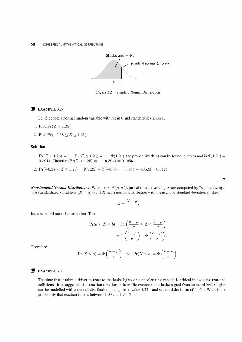
58 SOME SPECIAL MATHEMATICAL DISTRIBUTIONS
Figure 3.2 Standard Normal Distribution
EXAMPLE 3.29
Let Z denote a normal random variable with mean 0 and standard deviation 1.
1. Find Pr(Z > 1.25).
2. Find Pr(−0.38 ≤ Z ≤ 1.25).
Solution.
1. Pr(Z > 1.25) = 1− Pr(Z ≤ 1.25) = 1− Φ(1.25), the probability Φ(z) can be found in tables and is Φ(1.25) =0.8944. Therefore Pr(Z > 1.25) = 1− 0.8944 = 0.1056.
2. Pr(−0.38 ≤ Z ≤ 1.25) = Φ(1.25)− Φ(−0.38) = 0.8944− 0.3520 = 0.5424.
J
Nonstandard Normal Distributions: When X ∼ N(µ, σ2), probabilities involving X are computed by “standardizing.”The standardized variable is (X − µ)/σ. If X has a normal distribution with mean µ and standard deviation σ, then
Z =X − µσ
,
has a standard normal distribution. Thus
Pr(a ≤ X ≤ b) = Pr
(a− µσ≤ Z ≤ b− µ
σ
)= Φ
(b− µσ
)− Φ
(a− µσ
).
Therefore,
Pr(X ≤ a) = Φ
(a− µσ
)and Pr(X ≤ b) = Φ
(b− µσ
).
EXAMPLE 3.30
The time that it takes a driver to react to the brake lights on a decelerating vehicle is critical in avoiding rear-endcollisions. It is suggested that reaction time for an in-traffic response to a brake signal from standard brake lightscan be modelled with a normal distribution having mean value 1.25 s and standard deviation of 0.46 s. What is theprobability that reaction time is between 1.00 and 1.75 s?
CONTINUOUS DISTRIBUTION 59
Solution. Let X denote reaction time, then standardizing gives
1 ≤ X ≤ 1.75
if and only if1− 1.25
0.46≤ x− 1.25
0.46≤ 1.75− 1.25
0.46.
Thus
Pr(1 ≤ X ≤ 1.75) = Pr
(1− 1.25
0.46≤ Z ≤ 1.75− 1.25
0.46
)= Pr(−0.54 ≤ Z ≤ 1.09) = Φ(1.09)− Φ(−0.54)
= 0.8621− 0.2946 = 0.5675.
J
EXAMPLE 3.31
If the r.v X ∼ N(µ, σ2), such that Pr(X ≤ 60) = 0.1 and Pr(X > 90) = 0.05. Find µ and σ2.
Solution. Since X ∼ N(µ, σ2), then Z = X−µσ ∼ N(0, 1). Hence
0.1 = Pr(X ≤ 60) = Pr
(X − µσ
≤ 60− µσ
)= Pr
(Z ≤ 60− µ
σ
).
From Φ(z) tables, we can find that 60−µσ = −1.282.
Similarly,
0.05 = Pr(X > 90) = Pr
(X − µσ
>90− µσ
)= Pr
(Z >
90− µσ
)= 1− Pr
(Z ≤ 90− µ
σ
).
From Φ(z) tables, we can find that 90−µσ = 1.645. Then, it is easy to find that µ = 73.1 and σ = 10.2. J
Note:
1. If a r.v X ∼ N(0, 1), then the r.v Y = X2 ∼ χ2(1).
2. If a r.v Z ∼ N(0, 1), then Pr(Z ≤ −a) = Pr(Z > a).
3. If a r.v Z ∼ N(0, 1), then Pr(−a ≤ Z ≤ a) = 2 Pr(Z ≤ a)− 1
Moment Generating Function: The mgf of a r.v X ∼ N(µ, σ2) is
M(t) = E[etX ] = eµt+12σ
2t2
To prove that,
M(t) =
∫ ∞−∞
etxf(x)dx =1√2πσ
∫ ∞−∞
etxe−(x−µ)2
2σ2 dx =1√2πσ
∫ ∞−∞
e−1
2σ2(x2−2µx+µ2−2σ2tx)dx,
take
x2 − 2µx+ µ2 − 2σ2tx = x2 − 2(µ+ σ2t)x+ (µ+ σ2t)2 − (µ+ σ2t)2 + µ2
= [x− (µ+ σ2t)]2 − µ− 2µσ2t− σ4t2 + µ2
= [x− (µ+ σ2t)]2 − 2(µt+1
2σ2t2)σ2.
60 SOME SPECIAL MATHEMATICAL DISTRIBUTIONS
Therefore,
M(t) =1√2πσ
∫ ∞−∞
e−1
2σ2[x−(µ+σ2t)]2 eµt+
12σ
2t2dx = eµt+12σ
2t2∫ ∞−∞
1√2πσ
e−1
2σ2[x−(µ+σ2t)]2 dx.
That gives M(t) = eµt+12σ
2t2 since the integral is equal to one.
EXAMPLE 3.32
Let the r.v X has an mgf of M(t) = e5t+2t2 . What is the distribution of X? Find Pr(3 ≤ X ≤ 7)
Solution. We can rewrite the mgf as M(t) = e5t+ 12 4t2 , which means that X ∼ N(5, 4) with µ = 5 and σ2 = 4.
To find the probability,
Pr(3 ≤ X ≤ 7) = Pr
(3− 5
2≤ Z ≤ 7− 5
2
)= Pr(−1 ≤ Z ≤ 1) = 2 Pr(Z ≤ 1)− 1
= 2(0.841)− 1 = 1.682− 1 = 0.682.
J
CHAPTER 4
MULTIVARIATE PROBABILITY DISTRIBUTIONS
4.1 Introduction
In Chapters ?? and ??, we studied probability models for a single random variable. Many problems in probability andstatistics lead to models involving several random variables simultaneously. For example, a gambler playing blackjack isinterested in the event of drawing both an ace and a face card from a 52-card deck. A biologist, observing the number ofanimals surviving in a litter, is concerned about the intersection of these events:
A: The litter contains n animals.
B: x animals survive.
Similarly, observing both the height and the weight of an individual represents the intersection of a specific pair of eventsassociated with height–weight measurements. In this chapter, we first discuss probability models for the joint behaviourof several random variables, putting special emphasis on the case in which the variables are independent of each other.We then study expected values of functions of several random variables, including covariance and correlation as measuresof the degree of association between two variables. Then we will considers conditional distributions, the distributions ofrandom variables given the values of other random variables.
4.2 Bivariate and Multivariate Probability Distributions
There are many experimental situations in which more than one r.v will be of interest to an investigator. We shall firstconsider joint probability distributions for two discrete r.v’s, then for two continuous variables, and finally for more thantwo variables.
Please enter \offprintinfo(Title, Edition)(Author)at the beginning of your document.
61
62 MULTIVARIATE PROBABILITY DISTRIBUTIONS
4.2.1 Joint Probability Density Function
We already defined the pdf of more that one r.v in Chapter ?? as: Let X1 and X2 be two r.vs, then the Joint pdf of X1
and X2 is given by:
f(x1, x2) = Pr(X1 = x1, X2 = x2) =
∑x1
∑x2
f(x1, x2), discrete∫x1
∫x2
f(x1, x2)dx1dx2, continuous
EXAMPLE 4.1
A local supermarket has three checkout counters. Two customers arrive at the counters at different times when thecounters are serving no other customers. Each customer chooses a counter at random, independently of the other.Let X1 denote the number of customers who choose counter 1 and X2, the number who select counter 2. Find thejoint probability function of X1 and X2.
Solution. We might proceed with the derivation in many ways. The most direct is to consider the sample space associatedwith the experiment. Let the pair i, j denote the simple event that the first customer chose counter i and the secondcustomer chose counter j , where i, j = 1, 2, and 3. Using the mn rule, the sample space consists of 3 × 3 = 9 samplepoints. Under the assumptions given earlier, each sample point is equally likely and has probability 1/9. The samplespace associated with the experiment is
S = [1, 1, 1, 2, 1, 3, 2, 1, 2, 2, 2, 3, 3, 1, 3, 2, 3, 3].
Notice that sample point 1, 1 is the only sample point corresponding to (X1 = 2, X2 = 0) and hence Pr(X1 =2, X2 = 0) = 1/9. Similarly, Pr(X1 = 1, X2 = 1) = Pr(1, 2 or 2, 1) = 2/9. Table 5.1 contains the probabilitiesassociated with each possible pair of values for X1 and X2—that is, the joint probability function for X1 and X2.
Probability function for X1 and X2
x2 \ x1 0 1 2
0 1/9 2/9 1/91 2/9 2/9 02 1/9 0 0
J
EXAMPLE 4.2
A bank operates both a drive-up facility and a walk-up window. On a randomly selected day, let X = the proportionof time that the drive-up facility is in use (at least one customer is being served or waiting to be served) and Y =the proportion of time that the walk-up window is in use. Then the set of possible values for (X,Y ) is the rectangleD(x, y) : 0 ≤ x ≤ 1; 0 ≤ y ≤ 1. Suppose the joint pdf of (X,Y ) is f(x, y) = 6
5 (x+y2), 0 ≤ x ≤ 1, 0 ≤ y ≤ 1.Verify that f(x, y) is a valid pdf. Evaluate Pr
(0 ≤ x ≤ 1
4 , 0 ≤ Y ≤ 14
).
Solution. To verify that this is a legitimate pdf, note that f(x, y) > 0 and∫ ∞−∞
∫ ∞−∞
f(x, y)dxdy =
∫ 1
0
∫ 1
0
6
5(x+ y2)dxdy =
∫ 1
0
∫ 1
0
6
5xdxdy +
∫ 1
0
∫ 1
0
6
5y2dxdy
=
∫ 1
0
6
5xdx(1− 0) +
∫ 1
0
6
5y2dy(1− 0) =
6
10x2∣∣∣10
+6
15y3∣∣∣10
=6
10+
6
15= 1
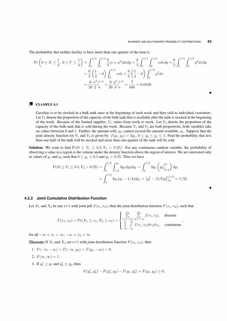
BIVARIATE AND MULTIVARIATE PROBABILITY DISTRIBUTIONS 63
The probability that neither facility is busy more than one-quarter of the time is
Pr
(0 ≤ X ≤ 1
4, 0 ≤ Y ≤ 1
4
)=
∫ 1/4
0
∫ 1/4
0
6
5(x+ y2)dxdy =
6
5
∫ 1/4
0
∫ 1/4
0
xdxdy +6
5
∫ 1/4
0
∫ 1/4
0
y2dxdy
=6
5
(1
4− 0
)∫ 1/4
0
xdx+6
5
(1
4− 0
)∫ 1/4
0
y2dx
=6
20
x2
2
∣∣∣1/40
+6
20
y3
3
∣∣∣1/40
=7
640= 0.0109.
J
EXAMPLE 4.3
Gasoline is to be stocked in a bulk tank once at the beginning of each week and then sold to individual customers.Let Y1 denote the proportion of the capacity of the bulk tank that is available after the tank is stocked at the beginningof the week. Because of the limited supplies, Y1 varies from week to week. Let Y2 denote the proportion of thecapacity of the bulk tank that is sold during the week. Because Y1 and Y2 are both proportions, both variables takeon values between 0 and 1. Further, the amount sold, y2, cannot exceed the amount available, y1. Suppose that thejoint density function for Y1 and Y2 is given by: f(y1, y2) = 3y1, 0 ≤ y2 ≤ y1 ≤ 1. Find the probability that lessthan one-half of the tank will be stocked and more than one-quarter of the tank will be sold.
Solution. We want to find Pr(0 ≤ Y1 ≤ 0.5, Y2 > 0.25). For any continuous random variable, the probability ofobserving a value in a region is the volume under the density function above the region of interest. We are interested onlyin values of y1 and y2 such that 0 ≤ y1 ≤ 0.5 and y2 > 0.25. Thus we have
Pr(0 ≤ Y1 ≤ 0.5, Y2 > 0.25) =
∫ 1/2
0
∫ y1
1/4
3y1dy2dy1 =
∫ 1/2
0
3y1
(y2
∣∣∣y11/4
)dy1
=
∫ 1/2
0
3y1(y1 − 1/4)dy1 =[y3
1 − (3/8)y21
]1/20
= 1/32.
J
4.2.2 Joint Cumulative Distribution Function
Let X1 and X2 be any r.v’s with joint pdf f(x1, x2), then the joint distribution function F (x1, x2), such that
F (x1, x2) = Pr(X1 ≤ x1, X2 ≤ x2) =
x1∑
τ1=−∞
x2∑τ2=−∞
f(τ1, τ2), discretex1∫−∞
x2∫−∞
f(τ1, τ2)dτ1dτ2, continuous,
for all −∞ < x1 <∞, −∞ < x2 <∞.
Theorem: If X1 and X2 are r.v’s with joint distribution function F (x1, x2), then
1. F (−∞,−∞) = F (−∞, y2) = F (y1,−∞) = 0.
2. F (∞,∞) = 1.
3. If y∗1 ≥ y1 and y∗2 ≥ y2, then
F (y∗1 , y∗2)− F (y∗1 , y2)− F (y1, y
∗2) + F (y1, y2) ≥ 0.
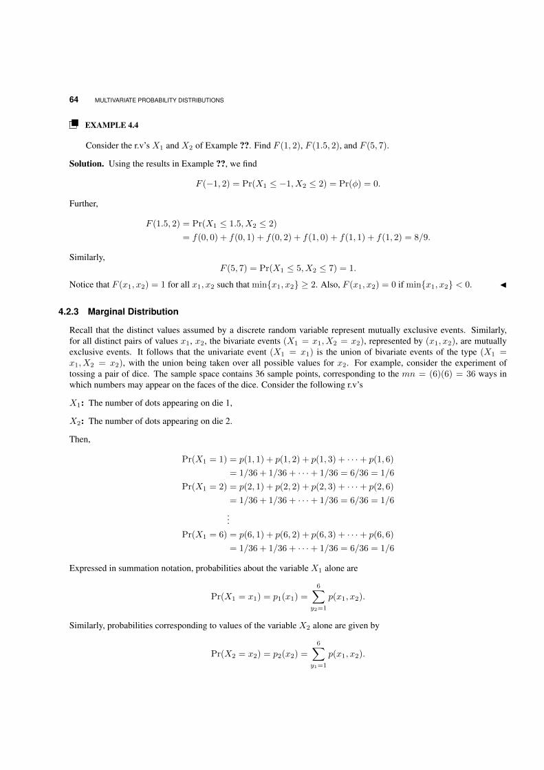
64 MULTIVARIATE PROBABILITY DISTRIBUTIONS
EXAMPLE 4.4
Consider the r.v’s X1 and X2 of Example ??. Find F (1, 2), F (1.5, 2), and F (5, 7).
Solution. Using the results in Example ??, we find
F (−1, 2) = Pr(X1 ≤ −1, X2 ≤ 2) = Pr(φ) = 0.
Further,
F (1.5, 2) = Pr(X1 ≤ 1.5, X2 ≤ 2)
= f(0, 0) + f(0, 1) + f(0, 2) + f(1, 0) + f(1, 1) + f(1, 2) = 8/9.
Similarly,F (5, 7) = Pr(X1 ≤ 5, X2 ≤ 7) = 1.
Notice that F (x1, x2) = 1 for all x1, x2 such that minx1, x2 ≥ 2. Also, F (x1, x2) = 0 if minx1, x2 < 0. J
4.2.3 Marginal Distribution
Recall that the distinct values assumed by a discrete random variable represent mutually exclusive events. Similarly,for all distinct pairs of values x1, x2, the bivariate events (X1 = x1, X2 = x2), represented by (x1, x2), are mutuallyexclusive events. It follows that the univariate event (X1 = x1) is the union of bivariate events of the type (X1 =x1, X2 = x2), with the union being taken over all possible values for x2. For example, consider the experiment oftossing a pair of dice. The sample space contains 36 sample points, corresponding to the mn = (6)(6) = 36 ways inwhich numbers may appear on the faces of the dice. Consider the following r.v’s
X1: The number of dots appearing on die 1,
X2: The number of dots appearing on die 2.
Then,
Pr(X1 = 1) = p(1, 1) + p(1, 2) + p(1, 3) + · · ·+ p(1, 6)
= 1/36 + 1/36 + · · ·+ 1/36 = 6/36 = 1/6
Pr(X1 = 2) = p(2, 1) + p(2, 2) + p(2, 3) + · · ·+ p(2, 6)
= 1/36 + 1/36 + · · ·+ 1/36 = 6/36 = 1/6
...Pr(X1 = 6) = p(6, 1) + p(6, 2) + p(6, 3) + · · ·+ p(6, 6)
= 1/36 + 1/36 + · · ·+ 1/36 = 6/36 = 1/6
Expressed in summation notation, probabilities about the variable X1 alone are
Pr(X1 = x1) = p1(x1) =
6∑y2=1
p(x1, x2).
Similarly, probabilities corresponding to values of the variable X2 alone are given by
Pr(X2 = x2) = p2(x2) =
6∑y1=1
p(x1, x2).
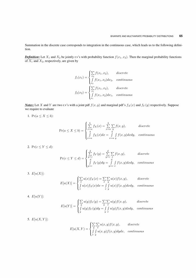
BIVARIATE AND MULTIVARIATE PROBABILITY DISTRIBUTIONS 65
Summation in the discrete case corresponds to integration in the continuous case, which leads us to the following defini-tion.
Definition: Let X1 and X2 be jointly r.v’s with probability function f(x1, x2). Then the marginal probability functionsof X1 and X2, respectively, are given by
f1(x1) =
∑x2
f(x1, x2), discrete∫x2
f(x1, x2)dx2, continuous
f2(x2) =
∑x1
f(x1, x2), discrete∫x1
f(x1, x2)dx1, continuous
Notes: Let X and Y are two r.v’s with a joint pdf f(x, y) and marginal pdf’s fX(x) and fY (y) respectively. Supposewe require to evaluate
1. Pr(a ≤ X ≤ b):
Pr(a ≤ X ≤ b) =
b∑
x=afX(x) =
b∑x=a
∑yf(x, y), discrete
b∫x=a
fX(x)dx =b∫
x=a
∫y
f(x, y)dxdy, continuous
2. Pr(c ≤ Y ≤ d):
Pr(c ≤ Y ≤ d) =
d∑y=c
fY (y) =d∑y=c
∑xf(x, y), discrete
d∫y=c
fY (y)dy =d∫
y=c
∫x
f(x, y)dxdy, continuous
3. E[u(X)]:
E[u(X)] =
∑xu(x)fX(x) =
∑x
∑yu(x)f(x, y), discrete∫
x
u(x)fX(x)dx =∫x
∫y
u(x)f(x, y)dxdy, continuous
4. E[u(Y )]:
E[u(Y )] =
∑yu(y)fY (y) =
∑y
∑xu(y)f(x, y), discrete∫
y
u(y)fY (y)dy =∫y
∫x
u(y)f(x, y)dxdy, continuous
5. E[u(X,Y )]:
E[u(X,Y ) =
∑y
∑xu(x, y)f(x, y), discrete∫
x
∫y
u(x, y)f(x, y)dydx, continuous
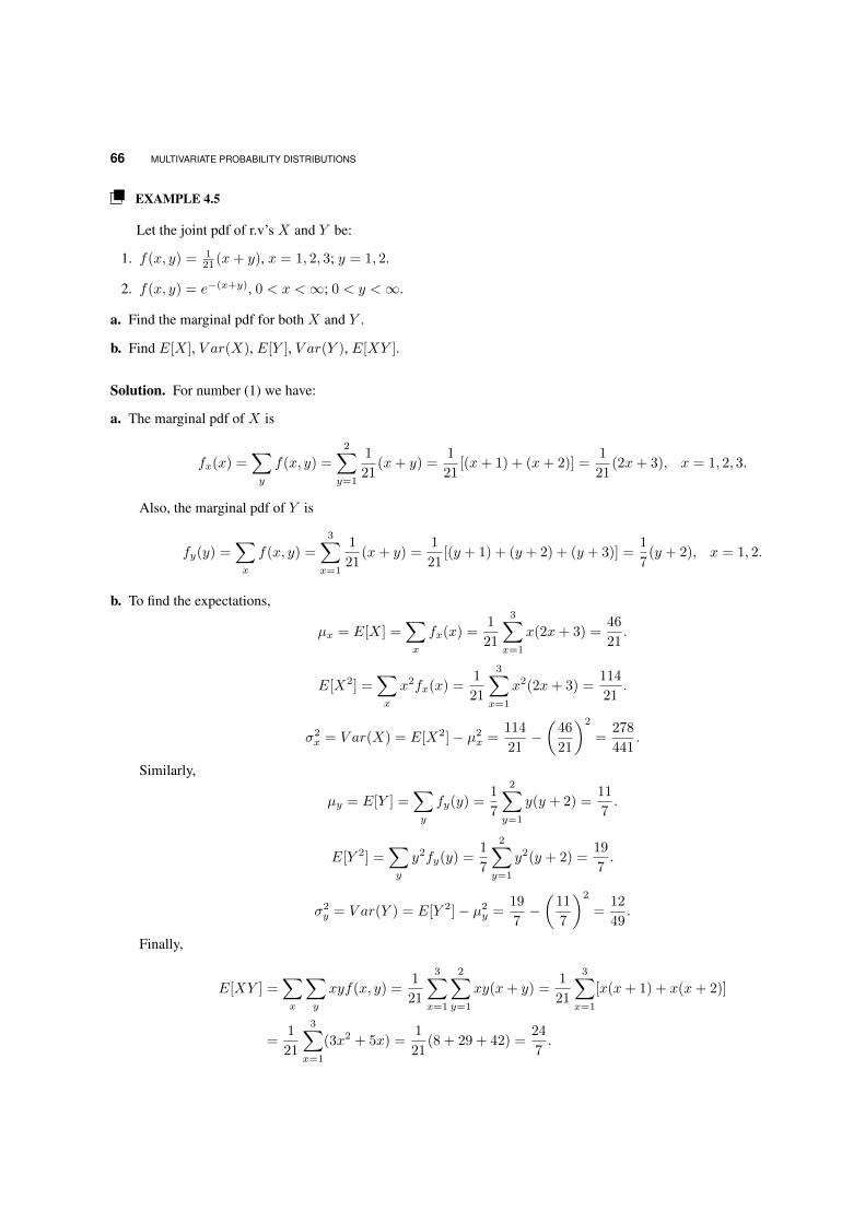
66 MULTIVARIATE PROBABILITY DISTRIBUTIONS
EXAMPLE 4.5
Let the joint pdf of r.v’s X and Y be:
1. f(x, y) = 121 (x+ y), x = 1, 2, 3; y = 1, 2.
2. f(x, y) = e−(x+y), 0 < x <∞; 0 < y <∞.
a. Find the marginal pdf for both X and Y .
b. Find E[X], V ar(X), E[Y ], V ar(Y ), E[XY ].
Solution. For number (1) we have:
a. The marginal pdf of X is
fx(x) =∑y
f(x, y) =
2∑y=1
1
21(x+ y) =
1
21[(x+ 1) + (x+ 2)] =
1
21(2x+ 3), x = 1, 2, 3.
Also, the marginal pdf of Y is
fy(y) =∑x
f(x, y) =
3∑x=1
1
21(x+ y) =
1
21[(y + 1) + (y + 2) + (y + 3)] =
1
7(y + 2), x = 1, 2.
b. To find the expectations,
µx = E[X] =∑x
fx(x) =1
21
3∑x=1
x(2x+ 3) =46
21.
E[X2] =∑x
x2fx(x) =1
21
3∑x=1
x2(2x+ 3) =114
21.
σ2x = V ar(X) = E[X2]− µ2
x =114
21−(
46
21
)2
=278
441.
Similarly,
µy = E[Y ] =∑y
fy(y) =1
7
2∑y=1
y(y + 2) =11
7.
E[Y 2] =∑y
y2fy(y) =1
7
2∑y=1
y2(y + 2) =19
7.
σ2y = V ar(Y ) = E[Y 2]− µ2
y =19
7−(
11
7
)2
=12
49.
Finally,
E[XY ] =∑x
∑y
xyf(x, y) =1
21
3∑x=1
2∑y=1
xy(x+ y) =1
21
3∑x=1
[x(x+ 1) + x(x+ 2)]
=1
21
3∑x=1
(3x2 + 5x) =1
21(8 + 29 + 42) =
24
7.
BIVARIATE AND MULTIVARIATE PROBABILITY DISTRIBUTIONS 67
For number (2) we have:
a. The marginal pdf of X is
fx(x) =
∫y
f(x, y)dy =
∫ ∞0
e−(x+y)dy = −e−x[e−y]∞0
= e−x, 0 < x <∞.
Also, the marginal pdf of Y is
fy(y) =
∫x
f(x, y)dx =
∫ ∞0
e−(x+y)dx = −e−y[e−x
]∞0
= e−y, 0 < y <∞.
b. To find the expectations,
µx = E[X] =
∫x
xfx(x)dx =
∫ ∞0
xe−xdx = 1 = E[Y ] = µy.
E[X2] =
∫x
x2fx(x)dx =
∫ ∞0
x2e−xdx = 2 = E[Y 2].
σ2x = V ar(X) = E[X2]− µ2
x = 2− (1)2 = 1 = σ2y = V ar(Y )
Finally,
E[XY ] =
∫x
∫y
xyf(x, y)dxdy =
∫ ∞0
∫ ∞0
xye−(x+y)dxdy
=
(∫ ∞0
xe−xdx
)(∫ ∞0
ye−ydy
)= (1)(1) = 1.
J
Definition: If f(x, y) and F (x, y) are the joint pdf and cdf of r.v’s X and Y . Then the marginal cdf of X and Y ,respectively , are
Fx(x) = F (x,∞) and Fy(y) = F (∞, y).
and are defined as
Fx(x) =
x∑
τ=−∞fx(τ), discrete,
x∫−∞
fx(τ)dτ, continuous.
and
Fy(y) =
y∑
τ=−∞fy(τ), discrete,
y∫−∞
fy(τ)dτ, continuous.
68 MULTIVARIATE PROBABILITY DISTRIBUTIONS
EXAMPLE 4.6
Back to the last example and find the joint cdf of X and Y , then find the marginal cdf for both X and Y .
Solution. For number (1) we have f(x, y) = 121 (x+ y), x = 1, 2, 3; y = 1, 2. Then
F (x, y) =
x∑τ=1
y∑κ=1
f(τ, κ) =1
21
x∑τ=1
y∑κ=1
(τ + κ) =1
21
x∑τ=1
[(τ + 1) + (τ + 2) + · · ·+ (τ + y)] (4.1)
=1
21
x∑τ=1
[yτ +
y(y + 1)
2
]=
1
21
[yx(x+ 1)
2+xy(y + 1)
2
]=
1
42xy(x+ y + 2),
hence
F (x, y) =
0, x < 1, y < 1142xy(x+ y + 2), 1 ≤ x < 3, 1 ≤ y < 2
1, x ≥ 3, y ≥ 2
The marginal cdf of X is
Fx(x) = F (x, 2) =
0, x < 1121x(x+ 4), 1 ≤ x < 3
1, x ≥ 3
Similarly, the marginal cdf of Y is
Fy(y) = F (3, y) =
0, y < 1114y(y + 5), 1 ≤ y < 2
1, y ≥ 2
For number (2) we have f(x, y) = e−(x+y), 0 < x <∞; 0 < y <∞. Then
F (x, y) =
∫ x
−∞
∫ y
−∞f(τ, κ)dτdκ =
∫ x
0
∫ y
0
e−(τ+κ)dτdκ =
(∫ x
0
e−τdτ
)(∫ y
0
e−κdκ
)=[−e−τ
]x0
[−e−κ
]y0,
hence
F (x, y) =
0, x ≤ 0, y ≤ 0
(1− e−x)(1− e−y), 0 < x < inf, 0 < y <∞1, x = y =∞
The marginal cdf of X is
Fx(x) = F (x,∞) =
0, x ≤ 0
1− e−x, 0 < x < inf
1, x =∞
The marginal cdf of Y is
Fy(y) = F (∞, y) =
0, y ≤ 0
1− e−y, 0 < y < inf
1, y =∞
J
BIVARIATE AND MULTIVARIATE PROBABILITY DISTRIBUTIONS 69
Remarks:
1. The joint moment generating function (mgf) of the two r.v’s X and Y with a joint pdf f(x, y) is defined as
M(t1, t2) = E[et1X+t2Y ] =
∑x
∑yet1X+t2Y f(x, y), discrete∫
x
∫y
et1X+t2Y f(x, y)dxdy, continuous
and satisfy M(0, 0) = 1.
2. The marginal mgf of X and Y can be obtained by
MX(t1) = E[et1X ] = M(t1, 0), and MY (t2) = E[et2Y ] = M(0, t2).
3. We can evaluate the mean and variance for both X and Y using the mgf as
E[XnY m] =∂n+mM(t1, t2)
∂tn1∂tm2
∣∣∣∣∣t1=t2=0
4.2.4 Conditional Distribution
The distribution of Y can depend strongly on the value of another variable X . For example, if X is height and Y isweight, the distribution of weight for men who are 180 cm tall is very different from the distribution of weight for shortmen. The conditional distribution of Y given X = x describes for each possible x how probability is distributed overthe set of possible y values. We define the conditional distribution of Y given X , but the conditional distribution of Xgiven Y can be obtained by just reversing the roles of X and Y . Both definitions are analogous to that of the conditionalprobability Pr(A|B) as the ratio Pr(A ∪B)/Pr(B).
Definition: If X and Y are jointly r.v’s with joint density function f(x, y), then the conditional pdf of X given Y = y is
fX|Y = Pr(X = x|Y = y) =Pr(X = x, Y = y)
Pr(Y = y)=f(x, y)
fY (y),
also, conditional pdf of Y given X = x is
fY |X = Pr(Y = y|X = x) =Pr(Y = y,X = x)
Pr(X = x)=f(x, y)
fX(x).
Definition: If X and Y are jointly r.v’s with joint density function f(x, y), then the conditional distribution function ofX given Y = y and Y given X = x are
F (x|y) = Pr(X ≤ x|Y = y), and F (y|x) = Pr(Y ≤ y|X = x).
EXAMPLE 4.7
Let the joint pdf of r.v’s X and Y be f(x, y) = e−y , 0 < x < y <∞. Find the following
1. The conditional pdf of both X given Y and Y given X .
2. E[X|Y = y], V ar(X|Y = y), E[Y |X = x] and V ar[Y |X = x].
3. Evaluate the probabilities: Pr(1 ≤ X ≤ 2) and Pr(1 ≤ X ≤ 2|Y = 2).
70 MULTIVARIATE PROBABILITY DISTRIBUTIONS
Solution. We have the joint pdf f(x, y) = e−y , 0 < x < y <∞, then the marginal pdf of X and Y are
fX(x) =
∫y
f(x, y)dy =
∫ ∞x
e−ydy = −e−y∣∣∣∞x
= e−x, 0 < x <∞.
and
fY (y) =
∫x
f(x, y)dx =
∫ y
0
e−ydy = e−yx∣∣∣y0
= ye−y, 0 < y <∞.
1. The conditional pdf of X given Y = y is
f1(x|y) =f(x, y)
fY (y)=
e−y
ye−y=
1
y, 0 < x < y, for any 0 < y <∞.
The conditional pdf of Y given X = x is
f2(y|x) =f(x, y)
fX(x)=e−y
e−x= e−(y−x), x < y <∞, for any 0 < x <∞.
2. To evaluate the expectations:
E[X|Y = y] = µx|y =
∫x
xf1(x|y)dx =
∫ y
0
x1
ydx =
1
y
[x2
2
]y0
=y
2.
E[X2|Y = y] =
∫x
x2f1(x|y)dx =
∫ y
0
x2 1
ydx =
1
y
[x3
3
]y0
=y2
3.
∴ σ2x|y = E[X2|Y = y]− µ2
x|y =y2
3−(y
2
)2
=y2
12.
Similarly,
E[Y |X = x] = µy|x =
∫y
yf2(y|x)dy =
∫ ∞x
ye−(y−x)dx = ex∫ ∞x
ye−ydy
= ex[−ye−y − e−y
]∞x
= ex(xe−x + e−x) = x+ 1.
E[Y 2|X = x] =
∫y
y2f2(y|x)dy =
∫ ∞x
y2e−(y−x)dx = ex∫ ∞x
y2e−ydy
= ex[−y2e−y − 2ye−y − 2e−y
]∞x
= ex(x2e−x + 2xe−x + 2e−x) = x2 + 2x+ 2.
σy|x = E[Y 2|X = x]− µ2y|x = x2 + 2x+ 2− (x+ 1)2 = 1.
3. To Evaluate the probabilities:
Pr(1 ≤ X ≤ 2) =
∫ 2
1
fX(x)dx =
∫ 2
1
e−xdx = −e−x∣∣∣21
= e−1 − e−2.
Pr(1 ≤ X ≤ 2|Y = 2) =
∫ 2
1
f1(x|y = 2)dx =
∫ 2
1
1
2dx =
x
2
∣∣∣21
=1
2(2− 1) =
1
2.
J
BIVARIATE AND MULTIVARIATE PROBABILITY DISTRIBUTIONS 71
EXAMPLE 4.8
A soft-drink machine has a random amount Y in supply at the beginning of a given day and dispenses a randomamount X during the day (with measurements in gallons). It is not resupplied during the day, and hence X ≤ Y .It has been observed that X and Y have a joint density function f(x, y) = 1
2 , 0 ≤ x ≤ y ≤ 2. That is, the points(x, y) are uniformly distributed over the triangle with the given boundaries. Find the conditional density of X givenY = y. Evaluate the probability that less than 1/2 gallon will be sold, given that the machine contains 1.5 gallons atthe start of the day.
Solution. The marginal density of Y is given by
fY (y) =
∫x
f(x, y)dx =
∫ y
0
1
2dx =
y
2, 0 ≤ y ≤ 2.
Note that fY (y) > 0 if and only if 0 < y2. Thus, for any 0 < y ≤ 2,
f(x|y) =f(x, y)
fY (y)=
1/2
y/2=
1
y, 0 ≤ x ≤ y.
Also, f(x|y) is undefined if y ≤ 0 or y > 2. The probability of interest is
Pr(X ≤ 1|Y = 1.5) =
∫ 1/2
0
f(x|y = 1.5)dx =
∫ 1/2
0
1
1.5dx =
1/2
3/2=
1
3.
J
EXAMPLE 4.9
Let the r.v X has a pdf f(x) and cdf F (x). Define f(x|X > x0) = f(x)1−F (x0) , x0 < x <∞ and x0 is a fixed number.
1. Show that f(x|X > x0) be a conditional pdf of X given X > x0.
2. Consider f(x) = e−x, 0 < x <∞. Compute Pr(X > 2|X > 1).
Solution. 1. To prove that f(x|X > x0) is a pdf, we check
- f(x|X > x0) ≥ 0, because f(x) ≥ 0 and 1− F (x0) > 0.
- The unity of integration,∫ ∞x0
f(x|X > x0)dx =
∫ ∞x0
f(x)
1− F (x0)dx =
1
1− F (x0)
∫ ∞x0
f(x)dx =1
1− F (x0)[F (x)]
∞x0
=F (∞)− F (x0)
1− F (x0)=
1− F (x0)
1− F (x0)= 1.
2. Since we have the pdf f(x) = e−x and the cdf is defined as: F (x) = 1− e−x (exponential distribution). Therefore,
f(x|X > 1) =f(x)
1− F (1)=
e−x
1− 1 + e−1= e · e−x, 1 < x <∞.
Now, to compute the probability
Pr(X > 2|X > 1) =
∫ ∞2
f(x|X > 1)dx =
∫ ∞2
e · e−xdx = −e[e−x
]∞2
= −e(0− e−2) = e−1.
J
72 MULTIVARIATE PROBABILITY DISTRIBUTIONS
4.2.5 Independent Random Variables
In many situations, information about the observed value of one of the two variables X and Y gives information aboutthe value of the other variable. In Example ?? we saw two dependent r.v’s, for which probabilities associated with Xdepended on the observed value of Y . In other examples, this is not always the case. Probabilities associated with Xwere the same, regardless of the observed value of Y . We now present a formal definition of independence of r.v’s. Twoevents A and B are independent if Pr(A ∪B) = Pr(A)× Pr(B).
Definition: Two random variables X and Y with joint density function f(x, y) and marginal density functions fX(x)and fY (y), are said to be independent if for every pair of x and y values,
f(x, y) = fX(x) · fY (y), ∀(x, y).
we can also define the independence in terms of the joint cdf and the marginal cdf’s FX(x) and FY (y) of X and Y , then
F (x, y) = FX(x) · FY (y),
for every pair of real numbers (x, y).
For the die-tossing problem of Section ??, show that X1 and X2 are independent since each of the 36 sample pointswas given probability 1/36. Consider, for example, the point (1, 2). We know that p(1, 2) = 1/36. Also, p1(1) =Pr(X1 = 1) = 1/6 and p2(2) = Pr(X2 = 2) = 1/6. Hence, p(1, 2) = p1(1)p2(2). The same is true for all other valuesfor x1 and x2, and it follows that X1 and X2 are independent.
Note: If two r.v’s X and Y are independent, we have
f1(x|y) =f(x, y)
fY (y)=fX(x) · fY (y)
fY (y)= fX(x).
and
f2(y|x) =f(x, y)
fX(x)=fX(x) · fY (y)
fX(x)= fY (y).
EXAMPLE 4.10
Back to example ?? and examine whether or not X and Y are independent.
Solution. In example ?? we have two cases:
1. The first case where X and Y are two discrete r.v’s with joint pdf f(x, y) = 121 (x + y), x = 1, 2, 3; y = 1, 2. and
marginal pdf’s fX(x) = 121 (2x+ 3), x = 1, 2, 3 and fY (y) = 1
7 (y+ 2), y = 1, 2. In order to check if X and Y areindependent,
fX(x) · fY (y) =1
217(2x+ 3)(y + 2) 6= 1
21(x+ y) = f(x, y).
Therefore X and Y are dependent r.v’s.
2. The second case where X and Y are two continuous r.v’s with joint pdf f(x, y) = e−(x+y), 0 < x, y < ∞, andmarginal pdf’s fX(x) = e−x, 0 < x < ∞ and fY (y) = e−y , 0 < y < ∞. In order to check if X and Y areindependent,
fX(x) · fY (y) = e−x · e−y = e−(x+y) = f(x, y),
this implies that X and Y are independent.
J
EXPECTED VALUES, COVARIANCE, AND CORRELATION 73
Properties: Let X and Y are two independent r.v’s, then:
1. Pr(a ≤ X ≤ b, c ≤ Y ≤ d) = Pr(a ≤ X ≤ b) · Pr(c ≤ Y ≤ d).
2. E[u(X) · v(Y )] = E[u(X)] · E[v(Y )].
3. M(t1, t2) = MX(t1) ·MY (t2).
EXAMPLE 4.11
Let the joint mgf of r.v’s X and Y is: M(t1, t2) = et21
1−2t2
1−2t2. Find the marginal mgf’s for both X and Y and test
whether X and Y are independent.
Solution. We can simply find the marginal mgf’s for X and Y as
MX(t1) = M(t1, 0) = et21 , and MY (t2) = M(0, t2) = (1− 2t2)−1.
In order to test if X and Y are independent,
MX(t1) ·MY (t2) =et
21
1− 2t26= M(t1, t2),
therefore X and Y are dependent. J
theorem: Let X and Y have a joint density f(x, y), Then X and Y are independent r.v’s if and only if
f(x, y) = g(x)h(y)
where g(x) is a non-negative function of x alone and h(y) is a non-negative function of y alone.
EXAMPLE 4.12
Let X and Y have a joint density given by: f(x, y) = 2x, 0 ≤ x ≤ 1, 0 ≤ y ≤ 1. Are X and Y independentvariables?
Solution. Notice that f(x, y) is positive for 0 ≤ x ≤ 1 and 0 ≤ y ≤ 1. Further, f(x, y) = g(x)h(y), where
g(x) = x, 0 ≤ x ≤ 1, and h(y) = 2, 0 ≤ y ≤ 1.
Therefore, X and Y are independent r.v’s. Notice that g(x) and h(y), as defined here, are not density functions, although2g(x) and h(y2)/2 are densities. J
4.3 Expected Values, Covariance, and Correlation
We previously saw that any function u(X) of a single r.v X is itself a r.v. However, to compute E[u(X)], it was notnecessary to obtain the probability distribution of u(X); instead, E[u(X)] was computed as a weighted average of u(X)values, where the weight function was the pdf f(x) of X . A similar result holds for a function u(X,Y ) of two jointlydistributed r.v’s.
74 MULTIVARIATE PROBABILITY DISTRIBUTIONS
EXAMPLE 4.13
Let X and Y have joint density given by: f(x, y) = 2x, 0 ≤ x ≤ 1; 0 ≤ y ≤ 1. Find E[XY ], E[X] and V ar(X).
Solution. From expectation definition we obtain
- The expected value of E[XY ] is:
E[XY ] =
∫ 1
0
∫ 1
0
xyf(x, y)dxdy =
∫ 1
0
∫ 1
0
xy(2x)dxdy =
∫ 1
0
y
[2x3
3
]1
0
dy
=2
3
∫ 1
0
ydy =2
3
[y2
2
]1
0
=1
3.
- The expected value of E[X] is:
E[X] =
∫ 1
0
∫ 1
0
xf(x, y)dxdy =
∫ 1
0
∫ 1
0
x(2x)dxdy =
∫ 1
0
[2x3
3
]1
0
dy
=2
3
∫ 1
0
dy =2
3[y]
10 =
2
3.
- To find V ar(X) we need to find E[X2] first, then:
E[X2] =
∫ 1
0
∫ 1
0
x2f(x, y)dxdy =
∫ 1
0
∫ 1
0
x2(2x)dxdy =
∫ 1
0
[2x4
4
]1
0
dy
=1
2
∫ 1
0
dy =1
2[y]
10 =
1
2.
Therefore,
V ar(X) = E[X2]− (E[X])2 =1
2−(
2
3
)2
=1
18.
J
EXAMPLE 4.14
A process for producing an industrial chemical yields a product containing two types of impurities. For a specifiedsample from this process, let X denote the proportion of impurities in the sample and let Y denote the proportion oftype I impurities among all impurities found. Suppose that the joint distribution of X and Y can be modelled by thepdf: f(x, y) = 2(1 − x), 0 ≤ x ≤ 1; 0 ≤ y ≤ 1. Find the expected value of the proportion of type I impurities inthe sample.
Solution. Because X is the proportion of impurities in the sample and Y is the proportion of type I impurities amongthe sample impurities, it follows that XY is the proportion of type I impurities in the entire sample. Thus, we want tofind E[XY ]:
E[XY ] =
∫ 1
0
∫ 1
0
2xy(1− x)dxdy = 2
∫ 1
0
x(1− x)
(1
2
)dx =
∫ 1
0
(x− x2)dx
=
[x2
2− x3
3
]1
0
=1
2− 1
3=
1
6.
Therefore, we would expect 1/6 of the sample to be made up of type I impurities. J
EXPECTED VALUES, COVARIANCE, AND CORRELATION 75
4.3.1 The Covariance and Correlation Coefficient
Intuitively,we think of the dependence of two random variables X and Y as implying that one variable, say X , eitherincreases or decreases as Y2 changes. We will confine our attention to two measures of dependence: the covariancebetween two random variables and their correlation coefficient.
4.3.1.1 The Covariance When two random variables X and Y are not independent, it is frequently of interest toassess how strongly they are related to each other. The average value of (X − µx)(Y − µy) provides a measure of thelinear dependence between X and Y . This quantity, E[(X − µx)(Y − µy)], is called the covariance of X and Y .
Definition: If X and Y are r.v’s with means µx and µy and variances σ2x and σ2
y , respectively, the covariance of X andY is defined as
Cov(X,Y ) = E[(X − µx)(Y − µy)].
The larger the absolute value of the covariance ofX and Y , the greater the linear dependence betweenX and Y . Positivevalues indicate that X increases as Y increases; negative values indicate that X decreases as Y increases. A zero valueof the covariance indicates that the variables are uncorrelated and that X and Y are independent.
Note: From the definition of the covariance, we can find the relation between the variances and covariance of the twor.v’s X and Y as the following:
Cov(X,Y ) = E[(X − µx)(Y − µy)] = E[XY − µxY − µyX + µxµy] = E[XY ]− µxE[Y ]− µyE[X] + µxµy
= E[XY ]− µxµy − µyµx + µxµy = E[XY ]− µxµy
EXAMPLE 4.15
Let the joint pdf of r.v’s X and Y is defined as f(x, y) = x+ y, 0 < x < 1, 0 < y < 1. Compute the covariance ofX and Y .
Solution. In order to evaluate the covariance of X and Y , we need to calculate first µx and µy . So lets start withcomputing the marginal pdf’s for both X and Y . Then,
fX(x) =
∫y
f(x, y)dy =
∫ 1
0
(x+ y)dy =
[xy +
1
2y2
]1
0
= x+1
2, 0 < x < 1.
andfY (y) = y +
1
2, 0 < y < 1.
Secondly, we have to evaluate µx and µy , thus
µx = E[X] =
∫x
xfX(x)dx =
∫ 1
0
x (x+ 1/2) dx =
[x3
3+x2
4
]1
0
=7
12.
Similarly, µy = 712 . Now the expected value of XY is calculated by
E[XY ] =
∫x
∫y
xyf(x, y)dxdy =
∫ 1
0
∫ 1
0
xy(x+ y)dxdy =
∫ 1
0
∫ 1
0
(x2y + xy2)dxdy
=
∫ 1
0
[x2y2
2+xy3
3
]1
0
dx =
∫ 1
0
(x2
2+x
3
)dx =
[x3
6+x2
6
]1
0
=1
3.
Therefore, the covariance of X and Y is
Cov(X,Y ) = E[XY ]− µxµy =1
3−(
7
12
)(7
12
)= − 1
144.
J

76 MULTIVARIATE PROBABILITY DISTRIBUTIONS
EXAMPLE 4.16
A nut company markets cans of deluxe mixed nuts containing almonds, cashews, and peanuts. Suppose the netweight of each can is exactly 1 lb, but the weight contribution of each type of nut is random. Because the threeweights sum to 1, a joint probability model for any two gives all necessary information about the weight of the thirdtype. Let X = the weight of almonds in a selected can and Y = the weight of cashews. Then the region of positivedensity is D = (x, y) : 0 ≤ x ≤ 1, 0 ≤ y ≤ 1;x + y ≤ 1. Now let the joint pdf for (X,Y ) be f(x, y) = 24xy,0 ≤ x ≤ 1, 0 ≤ y ≤ 1; x+ y ≤ 1. Find the probability that the two types of nuts together make up at most 50% ofthe can. Find The marginal pdf for almonds. Evaluate the expected amount of almonds and of cashews at each can.Then find the covariance of X and Y .
Solution. - Let A = (x, y) : 0 ≤ x ≤ 1, 0 ≤ y ≤ 1;x + y ≤ 0.5, and we need to calculate the probability of eventA, that is
Pr(X,Y ) ∈ A =
∫∫A
f(x, y)dxdy =
∫ 0.5
0
∫ 0.5−x
0
24xydydx = 0.0625.
- The marginal pdf for almonds is obtained by holdingX fixed at x and integrating f(x, y) along the vertical line throughx:
fX(x) =
∫ 1−x
0
f(x, y)dy =
∫ 1−x
0
24xydy = 12x(1− x)2, 0 ≤ x ≤ 1.
- The expected amount of almond at each can is obtained as:
µx = E[X] =
∫ 1
0
xfX(x)dx =
∫ 1
0
12x2(1− x)2dx =2
5.
Similarly, the expected amount of cashews at these cans can be easily evaluated by by replacing x by y in fX(x).Then we get µy = 2
5 .
- Finally, to examine how those two r.v’s are related to each other, we calculate the covariance of X and Y . Then
E[XY ] =
∫ 1
0
∫ 1−x
0
xy24xydydx =2
15.
Thus,
Cov(X,Y ) = E[XY ]− µxµy =2
15−(
2
5
)(2
5
)=
2
15− 4
25= − 2
75.
A negative covariance is reasonable here because more almonds in the can implies fewer cashews.J
Note: If X , Y and Z are r.v’s and a and b are constants, then
Cov(aX + bY, Z) = aCov(X,Z) + bCov(Y, Z).
4.3.1.2 Correlation Coefficient It is difficult to employ the covariance as an absolute measure of dependence becauseits value depends upon the scale of measurement. This problem can be eliminated by standardizing its value and usingthe correlation coefficient, ρ, a quantity related to the covariance and defined as
ρ =Cov(X,Y )
σxσy.
where σx and σy are the standard deviations of X and Y , respectively. The sign of the correlation coefficient is thesame as the sign of the covariance. Thus, ρ > 0 indicates that Y increases as X increases, and ρ = +1 implies perfectcorrelation, with all points falling on a straight line with positive slope. A value of ρ = 0 implies zero covariance andno correlation. A negative coefficient of correlation implies a decrease in Y as X increases, and ρ = −1 implies perfectcorrelation, with all points falling on a straight line with negative slope.
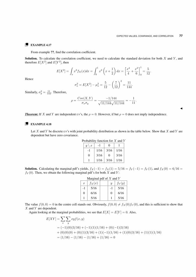
EXPECTED VALUES, COVARIANCE, AND CORRELATION 77
EXAMPLE 4.17
From example ??, find the correlation coefficient.
Solution. To calculate the correlation coefficient, we need to calculate the standard deviation for both X and Y , andtherefore E[X2] and E[Y 2], then
E[X2] =
∫x
x2fX(x)dx =
∫ 1
0
x2
(x+
1
2
)dx =
[x4
4+x3
6
]1
0
=5
12.
Hence
σ2x = E[X2]− µ2
x =5
12−(
7
12
)2
=11
144.
Similarly, σ2y = 11
144 . Therefore,
ρ =Cov(X,Y )
σxσy=
−1/144√11/144
√11/144
= − 1
11.
J
Theorem: If X and Y are independent r.v’s, the ρ = 0. However, if but ρ = 0 does not imply independence.
EXAMPLE 4.18
Let X and Y be discrete r.v’s with joint probability distribution as shown in the table below. Show that X and Y aredependent but have zero covariance.
Probability function for X and Yy \ x -1 0 1
-1 1/16 3/16 1/160 3/16 0 3/161 1/16 3/16 1/16
Solution. Calculating the marginal pdf’s yields, fX(−1) = fX(1) = 5/16 = fY (−1) = fY (1), and fX(0) = 6/16 =fY (0). Then, we obtain the following marginal pdf’s for both X and Y :
Marginal pdf of X and Yx fX(x) y fY (y)
-1 5/16 -1 5/160 6/16 0 6/161 5/16 1 5/16
The value f(0, 0) = 0 in the centre cell stands out. Obviously, f(0, 0) 6= fX(0)fY (0), and this is sufficient to show thatX and Y are dependent.
Again looking at the marginal probabilities, we see that E[X] = E[Y ] = 0. Also,
E[XY ] =∑x
∑y
xyf(x, y)
= (−1)(0)(3/16) + (−1)(1)(1/16) + (0)(−1)(3/16)
+ (0)(0)(0) + (0)(1)(3/16) + (1)(−1)(1/16) + (1)(0)(3/16) + (1)(1)(1/16)
= (1/16)− (1/16)− (1/16) + (1/16) = 0

78 MULTIVARIATE PROBABILITY DISTRIBUTIONS
Thus,Cov(X, y) = E[XY ]− E[X]E[Y ] = 0− (0)(0) = 0
This example shows that if the covariance of two r.v’s is zero, the variables need not be independent. J
EXAMPLE 4.19
Annie and Alvie have agreed to meet for lunch between noon (0:00 p.m.) and 1:00 p.m. Denote Annie’s arrival timeby X , Alvie’s by Y , and suppose X and Y are independent with pdf’s:
fX(x) = 3x2, 0 ≤ x ≤ 1 : and fY (y) = 2y, 0 ≤ y ≤ 1.
What is the expected amount of time that the one who arrives first must wait for the other person?
Solution. First of all, the joint pdf of X and Y is found by:
f(x, y) = fX(x) · fY (y) = 3x2 × 2y = 6x2y
Assuming that X and Y are the arrival time of Annie and Alive respectively give as that the waiting time of the one whocomes first is u(X,Y ) = |X − Y |, then the expected waiting time is E[|X − Y |], and since
u(X,Y ) = |X − Y | =
X − Y, x− y ≥ 0⇒ x ≥ y ⇒ 0 ≤ y ≤ x ≤ 1,
Y −X, x− y < 0⇒ x < y ⇒ 0 < x < y < 1,
and then
E[|X − Y |] =
∫ 1
0
∫ x
0
(x− y)(6x2y)dydx+
∫ 1
0
∫ y
0
(y − x)(6x2y)dxdy
=1
6+
1
12=
1
4.
Therefore, the expected waiting time for anyone who comes first is 1/4 of an hour. J
CHAPTER 5
FUNCTION OF RANDOM VARIABLES
5.1 Introduction
In Chapter ?? we discussed the problem of starting with a single r.v X , forming some function of X , such as X2 oreX , to obtain a new r.v Y = h(X), and investigating the distribution of this new r.v. We now generalize this scenarioby starting with more than a single r.v. Consider as an example a system having a component that can be replaced justonce before the system itself expires. Let X1 denote the lifetime of the original component and X2 the lifetime of thereplacement component. Then any of the following functions of X1 and X2 may be of interest to an investigator:
1. The total lifetime X1 +X2.
2. The ratio of lifetimes X1/X2; for example, if the value of this ratio is 2, the original component lasted twice as longas its replacement.
3. The ratio X1/(X1 +X2), which represents the proportion of system lifetime during which the original componentoperated.
To determine the probability distribution for a function of n random variables, X1, X2, . . . , Xn, we must find the jointprobability distribution for the r.v’s themselves. We generally assume that observations are obtained through randomsampling. We will assume throughout the remainder of this text that populations are large in comparison to the samplesize and consequently that the random variables obtained through a random sample are in fact independent of one another.We will present three methods for finding the probability distribution for a function of random variables.
Consider r.v’sX1, X2, . . . , Xn and a function U(X1, X2, . . . , Xn), denoted simply as U . We will present two methodto find the probability function of the function of r.v’s.
Please enter \offprintinfo(Title, Edition)(Author)at the beginning of your document.
79
80 FUNCTION OF RANDOM VARIABLES
5.2 The Joint pdf of a Function of Random Variables
Given set of r.v’s X1, X2, . . . , Xn, consider forming new r.v’s Yi = ui(X1, X2, . . . , Xn), i = 1, . . . , k, k ≤ n.
f(x1, x2, . . . , xn) = the joint pdf of the original r.v’s,g(y1, y2, . . . , yk) = the joint pdf of the new r.v’s.
We now focus on finding the joint distribution of these new variables. For our next study, we will use the term randomsample which is defined as:
Definition: (Random Sample): Let X1, X2, . . . , Xn be independent r.v’s each of which has the same pdf f(x), that isfi(xi) = f(xi), i = 1, 2, . . . , n, then the joint pdf of these r.v’s f(x1, x2, . . . , xn) =
∏ni=1 f(xi). Hence, the r.v’s
X1, X2, . . . , Xn are said to constitute a random sample (r.s) of size n from a distribution F (x).
For instant, if the two r.v’s X1 ∼ N(µ1, σ21) and X2 ∼ N(µ2, σ
22) are independent with joint pdf
f(x, y) =
2∏i=1
fi(xi) =
1√2πσ2
1
e− 1
2
(x1 − µ1
σ1
)2 1√
2πσ22
e− 1
2
(x2 − µ2
σ2
)2 .
Therefore, X1 and X2 are said to be a r.s of size two.
Definition: A function of one or more r.v’s which is not depend on any unknown parameter is called a Statistic. Forexample, Y =
∑Xi is a statistic, while Y = X − µ/σ is not a statistic unless µ and σ is known. A statistic is any
quantity whose value can be calculated from sample data. Therefore, a statistic is a random variable and will be denotedby an upper case letter; a lower case letter is used to represent the calculated or observed value of the statistic.
Definitions: Let X1, X2, . . . , Xn be a r.s of size n from any distribution, we define
1. The statistic X = 1n
n∑i=1
Xi is called the sample mean.
2. The statistic S2 = 1n−1
[n∑i=1
(X2i − nX
)]is called the sample variance.
5.2.1 The Method of Transformations
We will illustrate the method of transformations in two cases. The first is when the r.v’s X1, X2, . . . , Xn are discrete,and the second case for continuous set of r.v’s X1, X2, . . . , Xn.
5.2.1.1 Discrete r.v’s Let X1, X2, . . . , Xn be n r.v’s of discrete type defined on the n-dimensional space A withjoint pdf f(x1, x2, . . . , xn). Let the r.v’s Yi = ui(X1, X2, . . . , Xn), i = 1, 2, . . . , k and k ≤ n be functions ofX1, X2, . . . , Xn. The joint pdf of Y1, Y2, . . . , Yk is required. If k < n, we will introduce additional new r.v’s Yk+1 =uk+1(X1, X2, . . . , Xn), Yk+2 = uk+2(X1, X2, . . . , Xn), dotsYn = un(X1, X2, . . . , Xn), so that the function yi =ui(X1, X2, . . . , Xn), i = 1, 2, . . . , n are defined to be one-to-one transformation that maps the spaceA of Xi onto thespace B of Yi with inverse transforms xi = ωi(y1, y2, . . . , yn), i = 1, 2, . . . , n. Then the joint pdf of Y1, Y2, . . . , Yn isdefined as:
g(y1, y2, . . . , yn) = f(ω1(y1, y2, . . . , yn), ω2(y1, y2, . . . , yn), . . . , ωn(y1, y2, . . . , yn)).
Therefore, the joint pdf of Y1, Y2, . . . , Yk is
g∗(y1, y2, . . . , yk) =∑yk+1
∑yk+2
· · ·∑yn
g(y1, y2, . . . , yn).
We can also evaluate the marginal pdf of each r.v Yi using the definition of the marginal density function.
THE JOINT PDF OF A FUNCTION OF RANDOM VARIABLES 81
EXAMPLE 5.1
Let the r.v X has a pdf f(x) = x15 , x = 1, 2, 3, 4, 5. Find the pdf of the r.v Y = 2X + 1.
Solution. The function y = 2x+ 1 defines a one-to-one transformation that maps the space A = x : x = 1, 2, 3, 4, 5onto the space B = y : y = 3, 5, 7, 9, 11 with inverse x = 1
2 (y − 1). Then the pdf of Y is
g(y) = f
(y − 1
2
)=
1
30(y − 1), y = 3, 5, 7, 9, 11.
J
EXAMPLE 5.2
Let the r.v X ∼ b(n, p). What is the distribution of r.v Y = n−X?
Solution. The pdf of X is given by: f(x) =(nx
)pxqn−x, x = 0, 1, . . . , n. The function y = n− x defines a one-to-one
transform that maps the spaceA = x : x = 0, 1, . . . , n onto the space B = y : y = 0, 1, . . . , n with inverse functionof x = n− y. Then the pdf of Y is
g(y) = f(n− y) =
(n
n− y
)pn−yqn−(n−y) =
(n
y
)qypn−y, y = 0, 1, . . . , n.
Hence, the r.v Y ∼ b(n, q). J
EXAMPLE 5.3
Suppose that X1 and X2 are two independent r.v’s where X1 ∼ P (λ1) and X2 ∼ P (λ2) (i.e X1 and X2 are a r.s ofsize 2). Find the distribution of the r.v Y = X1 +X2.
Solution. Since X1 and X2 are a r.s, then the joint pdf of X1 and X2 can be determined as
f(x1, x2) = f1(x1)× f2(x2) =e−λ1λx1
1
x1!· e−λ2λx2
2
x2!=e−(λ1+λ2)λx1
1 λx22
x1!x2!, xi = 0, 1, 2, . . . ; i = 1, 2.
J
Consider, beside Y = X1 +X2, Z = X2. The functions y = x1 + x2 and z = x2 define one-to-one transformation thatmaps the space A = (x1, x2) : xi = 0, 1, 2, . . . ; i = 1, 2 onto the space B = (y, z) : 0 ≤ z ≤ y ≤ ∞, with inversefunctions x1 = y − z and x2 = z. Then the joint pdf of Y and Z is
g(y, z) = f(y − z, z) =e−(λ1+λ2)λy−z1 λz2
(y − z)!z!, (y, z) ∈ B.
Now, the marginal pdf of Y is obtained by
gY (y) =∑z
g(y, z) = e−(λ1+λ2)
y∑z=0
λy−z1 λz2(y − z)!z!
=e−(λ1+λ2)
y!
y∑z=0
y!
(y − z)!z!λy−z1 λz2
=e−(λ1+λ2)
y!
y∑z=0
(y
z
)λz2λ
y−z1 =
e−(λ1+λ2)(λ1 + λ2)y
y!, y = 0, 1, 2, . . . .
Therefore Y ∼ P (λ1 + λ2).Note: We can prove that if X1, X2, . . . , Xn are r.s of size n and Xi ∼ P (λi), then Y =
∑ni=1Xi ∼ P (
∑ni=1 λi).

82 FUNCTION OF RANDOM VARIABLES
EXAMPLE 5.4
Let X1 and X2 be independent r.v’s of discrete type with joint pdf f(x1, x2) = f1(x1) · f2(x2), where fi(xi) is themarginal pdf of Xi, i = 1, 2. Consider Yi = ui(Xi), i = 1, 2 define one-to-one transformation from A onto B.Show that the r.v’s Y1 = u1(X1) and Y2 = u2(X2) are also independent.
Solution. Given f(x1, x2) = f1(x1) · f2(x2) where f(x1, x2) is the joint pdf of X1 and X2 with fi(xi) is the marginalpdf of Xi, i = 1, 2.
Also the functions yi = ui(xi), i = 1, 2 maps A onto B, then the inverse functions xi = ωi(yi), i = 1, 2. Then thejoint pdf of Y1 and Y2 is:
g(y1, y2) = f(ω1(y1), ω2(y2)) = f1(ω1(y1)) · f2(ω2(y2)).
J
Then, the marginal pdf of Y1 is obtained by
g1(y1) =∑y2
g(y1, y2) = f1(ω1(y1))∑y2
f2(ω2(y2)) = c1f1(ω1(y1)),
similarly, the marginal pdf of Y2 is
g2(y2) =∑y1
g(y1, y2) = f2(ω2(y2))∑y1
f1(ω1(y1)) = c2f2(ω2(y2)).
In order to verify the independence of Y1 and Y2, we need to prove that g(y1, y2) = g1(y1) · g2(y2). Therefore
g1(y1) · g2(y2) = c1f1(ω1(y1)) · c2f2(ω2(y2)) = c1c2f1(ω1(y1)) · f2(ω2(y2))
= c1c2g(y1, y2),
⇒ g(y1, y2) =1
c1c2g1(y1) · g2(y2).
Since g(y1, y2) is the joint pdf of Y1 and Y2, then
1 =∑y1
∑y2
g(y1, y2) =∑y1
∑y2
1
c1c2g1(y1) · g2(y2) =
1
c1c2
[∑y1
g1(y1)
][∑y2
g2(y2)
]
=1
c1c2⇒ c1c2 = 1
∴g(y1, y2) = g1(y1) · g2(y2).
This implies that Y1 and Y2 are independent r.v’s.
5.2.1.2 Continuous r.v’s In the case of continuous r.v’s we assume the same environment as it was with the dis-crete case. Let X1, X2, . . . , Xn be n r.v’s of continuous type defined on the n-dimensional space A with joint pdff(x1, x2, . . . , xn). Let the r.v’s Yi = ui(X1, X2, . . . , Xn), i = 1, 2, . . . , k (k ≤ n) be functions ofX1, X2, . . . , Xn. Thejoint pdf of Y1, Y2, . . . , Yk is required. If k < n, we will introduce additional new r.v’s Yk+1 = uk+1(X1, X2, . . . , Xn),Yk+2 = uk+2(X1, X2, . . . , Xn), dotsYn = un(X1, X2, . . . , Xn), so that the function yi = ui(X1, X2, . . . , Xn),i = 1, 2, . . . , n are defined to be one-to-one transformation that maps the spaceA of Xi onto the space B of Yi withinverse transforms xi = ωi(y1, y2, . . . , yn), i = 1, 2, . . . , n. In this case, we will need to calculate the Jacobian n × ndeterminant of the first partial derivatives as:
J =∂(x1, x2, . . . , xn)
∂(y1, y2, . . . , yn)=
∣∣∣∣∣∣∣∣∣∣∣
∂x1
∂y1∂x1
∂y2. . . ∂x1
∂yn∂x2
∂y1∂x2
∂y2. . . ∂x2
∂yn...
.... . .
...∂xn∂y1
∂xn∂y2
. . . ∂xn∂yn
∣∣∣∣∣∣∣∣∣∣∣
THE JOINT PDF OF A FUNCTION OF RANDOM VARIABLES 83
Then the joint pdf of Y1, Y2, . . . , Yn is defined as:
g(y1, y2, . . . , yn) = |J | × f(ω1(y1, y2, . . . , yn), ω2(y1, y2, . . . , yn), . . . , ωn(y1, y2, . . . , yn)),
and finally, the joint pdf of Y1, Y2, . . . , Yk is
g∗(y1, y2, . . . , yk) =
∫yk+1
∫yk+2
· · ·∫yn
g(y1, y2, . . . , yn)dyk+1dyk+2 . . . dyn.
We can also evaluate the marginal pdf of each r.v Yi using the definition of the marginal density function.
EXAMPLE 5.5
Let the r.v X has a pdf f(x) = 3x2, 0 < x < 1. Find the pdf of the r.v Y = X3 and evaluate Pr( 12 < Y < 3
4 ).
Solution. The function y = x3 is a one-to-one function from A = x : 0 < x < 1 onto B = y : 0 < y < 1 withinverse function x = y1/3. The Jacobian in the 1-dimensional case is obtained as
J =∂x
∂y=
1
3y−2/3.
Therefore, the pdf of the r.v Y is
g(y) = f(y1/3)|J | = 3(y1/3)2 1
3y−2/3 = 1, 0 < y < 1.
Now, to evaluate the probability Pr( 12 < Y < 3
4 ),
Pr
(1
2< Y <
3
4
)=
∫ 3/4
1/2
dy = y∣∣∣3/41/2
=3
4− 1
2=
1
4.
J
EXAMPLE 5.6
Let the r.v X ∼ U(0, 1). Find and name the distribution of the r.v Y = −2 lnX .
Solution. The function y = −2 lnx is a one-to-one function that maps A = x : 0 < x < 1 onto B = y : 0 < y <
∞, with inverse function x = e−12y . The Jacobian,
J =∂x
∂y= −1
2e−
12y.
Then, the pdf of Y can be obtained as
g(y) = |J |f(e−12y) = (1)
1
2e−
12y =
1
2e−
12y, 0 < y <∞
Hence, the r.v Y ∼ Exp(2). J
84 FUNCTION OF RANDOM VARIABLES
EXAMPLE 5.7
Let X1 and X2 be a r.s of size 2 from N(0, 1). Define the r.v’s Y1 = X1 + X2 and Y2 = X1 −X2. Find the jointpdf of Y1 and Y2 and show that they are independent.
Solution. The joint pdf of X1 and X2 is:
f(x1, x2) = f1(x1)× f2(x2) =1
2πe−
12π (X2
1+X22 ), −∞ < xi <∞; i = 1, 2.
The functions y1 = x1 + x2, y2 = x1 − x2 define as one-to-one functions that map the space A = (x1, x2) : −∞ <xi < ∞; i = 1, 2 onto the space B = (y1, y2) : −∞ < yi < ∞; i = 1, 2, with inverses x1 = 1
2 (y1 + y2) andx2 = 1
2 (y1 − y2). The Jacobian can be calculated as
J =∂(x1, x2)
∂(y1, y2)=
∣∣∣∣∣ ∂x1
∂y1∂x1
∂y2∂x2
∂y1∂x2
∂y2
∣∣∣∣∣ =
∣∣∣∣∣ 12
12
12 − 1
2
∣∣∣∣∣ = −1
4− 1
4= −1
2.
Therefore, the joint pdf of y1 and y2 is
g(y1, y2) = f
(1
2(y1 + y2),
1
2(y1 − y2)
)× |J |.
taking the term x21 + x2
2:
x21 + x2
2 =1
4(y1 + y2)2 +
1
4(y1 − y2)2 =
1
4
[y2
1 + 2y1y2 + y22 + y2
1 − 2y1y2 + y22
]=
1
4(2y2
1 + 2y22) =
1
2(y2
1 + y22).
Therefore,
g(y1, y2) =1
4πe−
14 (y21+y22), −∞ < yi <∞; i = 1, 2.
To verify if Y1 and Y2 are independent or not, we need to find the marginal pdf’s for both Y1 and Y2. Then, the marginalpdf of Y1 is
g1(y1) =
∫y2
g(y1, y2)dy2 =1
4πe−
14y
21
∫ ∞−∞
e−14y
22dy2 =
√2π√
2
4πe−
14y
21
∫ ∞−∞
1√2π√
2e−
14y
22dy2
=1√
2π√
2e−
12
y212 −∞ < y1 <∞.
That is Y1 ∼ N(0, 2). Similarly, the marginal pdf of Y2 is g2(y2) = 1√2π√
2e−
12
y222 , −∞ < y1 < ∞, which means that
Y2 ∼ N(0, 2). Then,
g1(y1) · g2(y2) =1√
2π√
2e−
12
y212 × 1√
2π√
2e−
12
y222 =
1
4πe−
14 (y21+y22) = g(y1, y2).
Therefore, Y1 and Y2 are independent r.v’s. J
EXAMPLE 5.8
Let X1 and X2 be a r.s of size 2 from U(0, 1). Define the r.v’s Y1 = X1 + X2 and Y2 = X1 −X2. Find the jointpdf of Y1 and Y2. Also, find marginal pdf’s for both Y1 and Y2.
Solution. The joint pdf of X1 and X2 is f(x1, x2) = 0, 0 < xi < 1, i = 1, 2.
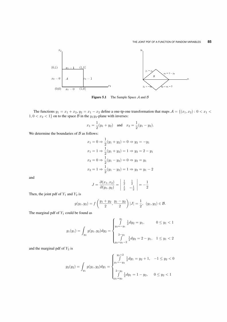
THE JOINT PDF OF A FUNCTION OF RANDOM VARIABLES 85
Figure 5.1 The Sample Space A and B
The functions y1 = x1 + x2, y2 = x1 − x2 define a one-tp-one transformation that maps A = (x1, x2) : 0 < x1 <1, 0 < x2 < 1 on to the space B in the y1y2-plane with inverses:
x1 =1
2(y1 + y2) and x2 =
1
2(y1 − y2).
We determine the boundaries of B as follows:
x1 = 0⇒ 1
2(y1 + y2) = 0⇒ y2 = −y1
x1 = 1⇒ 1
2(y1 + y2) = 1⇒ y2 = 2− y1
x2 = 0⇒ 1
2(y1 − y2) = 0⇒ y2 = y1
x2 = 1⇒ 1
2(y1 − y2) = 1⇒ y2 = y1 − 2
and
J =∂(x1, x2)
∂(y1, y2)=
∣∣∣∣∣ 12
12
12 − 1
2
∣∣∣∣∣ = −1
2
Then, the joint pdf of Y1 and Y2 is
g(y1, y2) = f
(y1 + y2
2,y1 − y2
2
)|J | = 1
2, (y1, y2) ∈ B.
The marginal pdf of Y1 could be found as
g1(y1) =
∫y2
g(y1, y2)dy2 =
y1∫y2=−y1
12dy2 = y1, 0 ≤ y1 < 1
2−y1∫y2=y1−2
12dy2 = 2− y1, 1 ≤ y1 < 2
and the marginal pdf of Y2 is
g2(y2) =
∫y1
g(y1, y2)dy1 =
y2+2∫y1=−y2
12dy1 = y2 + 1, −1 ≤ y2 < 0
2−y2∫y1=y2
12dy1 = 1− y2, 0 ≤ y2 < 1
86 FUNCTION OF RANDOM VARIABLES
J
EXAMPLE 5.9
Consider n = 3 identical components with independent lifetimes X1, X2, X3, each having an exponential distribu-tion with parameter 1/λ. If the first component is used until it fails, replaced by the second one which remains inservice until it fails, and finally the third component is used until failure, then the total lifetime of these componentsis Y = X1 +X2 +X3. Find the distribution of total lifetime.
Solution. The joint pdf of X1, X2 and X3 is f(x1, x2, x3) = λ3e−λ(x1+x2+x3), 0 < xi < ∞, i = 1, 2, 3. We definetwo other new variables Y1 = X1 and Y2 = X1 + X2 (so that Y1 < Y2 < Y ). Then the functions y = x1 + x2 + x3,y2 = x1 + x2 and y1 = x1 define a one-tp-one transformation that maps A = (x1, x2, x3) : 0 < xi < ∞, i = 1, 2, 3onto the space B = (y1, y2, y3) : 0 < y1 < y2 < y <∞, with inverses:
x1 = y1, x2 = y2 − y1 and x3 = y − y2.
The Jacobian is calculated as
J =∂(x1, x2, x3)
∂(y1, y2, y)=
∣∣∣∣∣∣∣1 0 0
−1 1 0
0 −1 1
∣∣∣∣∣∣∣ = 1
Then, the joint pdf of Y1, Y2 and Y is
g(y1, y2, y) = f(y1, y2 − y1, y − y2)|J | = λ3e−λy, 0 < y1 < y2 < y <∞.
Finally, the marginal pdf of Y is
g∗(y) =
∫y1
∫y2
g(y1, y2, y)dy1dy2 =
∫ y
0
∫ y
y1
λ3e−λydy1dy2 =
∫ y
0
λ3e−λy[y2
]yy1dy1
=
∫ y
0
λ3e−λy(y − y1)dy1 = λ3e−λy[yy1 −
y21
2
]y0
= λ3e−λy[y2 − y2
2
]=λ3
2y2e−λy, 0 < y <∞.
J
5.3 Order Statistics
Many functions of random variables of interest in practice depend on the relative magnitudes of the observed variables.For instance, we may be interested in the fastest time in an automobile race or the heaviest mouse among those fed ona certain diet. Thus, we often order observed random variables according to their magnitudes. The resulting orderedvariables are called order statistics.
Formally, let X1, X2, . . . , Xn denote independent continuous random variables with distribution function F (x) anddensity function f(x). We denote the ordered random variables Xi by Y1, Y2, . . . , Yn, where Y1 ≤ Y2 ≤ · · · ≤ Yn.where
Y1 = the smallest among X1, X2, . . . , Xn
Y2 = the second smallest among X1, X2, . . . , Xn
...Y n = the largest among X1, X2, . . . , Xn
ORDER STATISTICS 87
i.e, Y1 = minX1, X2, . . . , Xn and Yn = maxX1, X2, . . . , Xn.
Notes:
1. In most applications, the unordered set of r.v’s Xi is usually taken to be a r.s of size n.
2. We only consider the continuous type of r.v’s.
5.3.1 The distribution of Order Statistics
Let X1, X2, . . . , Xn be a r.s of size n from a continuous distribution having a pdf of f(x) and cdf F (x), where the jointpdf of those r.v’s is
f(x1, x2, . . . , xn) =
n∏i=1
f(xi), −∞ < xi <∞; i = 1, 2, . . . , n.
Suppose that Y1, Y2, . . . , Yn is a ordered sample of the original r.s, that is Y1 = minX1, X2, . . . , Xn and Yn =maxX1, X2, . . . , Xn. The probability density functions for Y1 and Yn can be found using the method of distributionfunctions. We will derive the density function of Yn first. Because Yn is the maximum of X1, X2, . . . , Xn, the event(Yn ≤ y) will occur if and only if the events (Xi ≤ y) occur for every i = 1, 2, . . . , n. That is,
Pr(Yn ≤ y) = Pr(X1 ≤ y,X2 ≤ y, . . . , Xn ≤ y).
Because the Xi are independent and Pr(Xi ≤ y) = F (y) for i = 1, 2, . . . , n, it follows that the distribution functionof Yn is given by
FYn(y) = Pr(Yn ≤ y) = Pr(X1 ≤ y) Pr(X2 ≤ y) . . .Pr(Xn ≤ y) = [F (y)]n.
Letting gn(y) denote the density function of Yn, we see that, on taking derivatives of both sides,
gn(y) = n[F (y)]n−1f(y).
The density function for Y1 can be found in a similar manner. The distribution function of Y1 is
FY1(y) = Pr(Y1 ≤ y) = 1− Pr(Y1 > y).
Because Y1 is the minimum of X1, X2, . . . , Xn, it follows that the event (Y1 > y) occurs if and only if the events(Xi > y) occur for i = 1, 2, . . . , n. Because the Xi are independent and Pr(Yi > y) = 1F (y) for i = 1, 2, . . . , n, wesee that
FY1(y) = Pr(Y1 ≤ y) = 1− Pr(Y1 > y)
= 1− Pr(X1 > y,X2 > y, . . . ,Xn > y)
= 1− [Pr(X1 > y) Pr(X2 > y) . . .Pr(Xn > y)] = 1− [1− F (y)]n.
Thus, if g1(y) denotes the density function of Y1, differentiation of both sides of the last expression yields
g1(y) = n[1− F (y)]n−1f(y).
In general, The marginal pdf of the kth order statistic Yk could be derived as
gk(y) =n!
(k − 1)!(n− k)![F (y)]k−1[1− F (y)]n−kf(y), −∞ < y <∞.
88 FUNCTION OF RANDOM VARIABLES
EXAMPLE 5.10
Let Y1 < Y2 < Y3 < Y4 be the order statistics of a r.s of size 4 from a distribution having a pdf of f(x) = 2x,0 < x < 1. Compute Pr(Y3 > 1/2) and E[Y3].
Solution. Since the pdf of the r.s is f(x) = 2x, 0 < x < 1. Then we can find the cdf as
F (x) =
∫ x
−∞f(τ)dτ =
∫ x
0
2τdτ = τ∣∣∣x0
= x2.
Now, since n = 4 and k = 3, then the pdf of Y3 is
g3(y) =4!
2!1!y4(1− y2)2y = 24y5(1− y2), 0 < y < 1.
Hence, the probability
Pr
(Y3 >
1
2
)=
∫ 1
1/2
g3(y)dy =
∫ 1
1/2
24y5(1− y2)dy = 24
[y6
6− y8
8
]1
1/2
= 0.949.
The mean value of Y3 is
E[Y3] =
∫ 1
0
yg3(y)dy = 24
∫ 1
0
y6(1− y2)dy = 24
[y7
7− y9
9
]1
0
=16
21.
J
EXAMPLE 5.11
Let X1, X2, . . . , Xn be a r.s of size n from Exp(λ). Find the distribution of the first order statistics Y1.
Solution. Since X ∼ Exp(λ), then f(x) = 1λe−x/λ, 0 < x <∞, and the cdf F (x) = 1− e−x/λ. Therefore, the pdf of
Y1 is given by
g1(y) = n[1− F (y)]n−1f(y) = n[1− 1 + e−
yλ
]n−1 1
λe−
yλ =
n
λ
[e−
yλ
]n−1
e−yλ =
n
λe−
nλ y, 0 < y <∞.
J
EXAMPLE 5.12
Electronic components of a certain type have a length of life X , with probability density given by: f(x) =(1/100)e−x/100, x > 0. (Length of life is measured in hours.) Suppose that two such components operate in-dependently and in series in a certain system (hence, the system fails when either component fails). Find the densityfunction for Y , the length of life of the system.
Solution. Because the system fails at the first component failure, Y = minX1, X2, whereX1 andX2 are independentr.v’s with the given density. Then, because F (x) = 1− e−x/100, for x ≥ 0,
g1(y) = n[1− F (y)]n−1f(y) = 2e−y
100e−
y100
100=
1
50e−
y50 , y > 0.
Thus, the minimum of two exponentially distributed random variables has an exponential distribution. Notice that themean length of life for each component is 100 hours, whereas the mean length of life for the system is E[Y ] = 50 =100/2. J
ORDER STATISTICS 89
EXAMPLE 5.13
Let X denote the contents of a one-gallon container, and suppose that its pdf is f(x) = 2x for 0 < x < 1 (and 0otherwise) with corresponding cdf F (x) = x2 in the interval of positive density. Consider a random sample of foursuch containers. Determine the expected value of Y4 − Y1, the difference between the contents of the most-filledcontainer and the least-filled container.
Solution. To determine Y4 − Y1, the sample range, The pdf’s of Y4 and Y1 are
g4(y) = n[F (y)]n−1f(y) = 4(y2)3 · 2y = 8y7, 0 ≤ y ≤ 1,
andg1(y) = n[1− F (y)]n1f(y) = 4(1− y2)3 · 2y = 8y(1− y2)3, 0 ≤ y ≤ 1.
Therefore, the expected value of Y4 − Y1 is
E[Y4 − Y1] = E[Y4]− E[Y1] =
∫ 1
0
y · 8y7dy −∫ 1
0
y · 8y(1− y2)3dy = 0.889− 0.406 = 0.483.
If random samples of four containers were repeatedly selected and the sample range of contents determined for each one,the long run average value of the range would be 0.483. J
5.3.2 Joint Distribution of the Order Statistics
Consider a r.s X1, X2, . . . , Xn of size n with a joint pdf
f(x1, x2, . . . , xn) = f(x1) · f(x2) . . . f(xn),
and f(xi) is the marginal pdf of each r.v Xi. Then joint pdf of r.v’s Y1, Y2, . . . , Yn is presented as:
g(y1, y2, . . . , yn) = n!f(y1, y2, . . . , yn) = n!
n∏i=1
f(yi), −∞ < y1 < y2 < · · · < yn <∞.
We can also derive the joint pdf of any two order statistics, if h and k are two integers such that 1 ≤ h < k ≤ n, thejoint density of Yh and Yk is given by
gh,k(yh, yk) =n!
(h− 1)!(k − h− 1)!(n− k)![F (yh)]h−1[F (yk)− F (yh)]k−h−1[1− F (yk)]n−kf(yh)f(yk),
−∞ < xh < xk <∞
EXAMPLE 5.14
If Y1 < Y2 < · · · < Yn be the order statistics of a r.s of size n from N(µ, σ2). Find the joint pdf of Y1, Y2, . . . , Yn.
Solution. The joint pdf of the order statistics Y1, Y2, . . . , Yn is
g(y1, y2, . . . , yn) = n!
n∏i=1
f(yi) = n!(2π)−n2 σ−ne−
12σ2
∑ni=1(yi−µ)2 , −∞ < y1 < y2 < · · · < yn.
J

90 FUNCTION OF RANDOM VARIABLES
EXAMPLE 5.15
Let Y1, Y2, Y3 be the order statistics of a r.s of size 3 from U(0, 1).
1. Find the joint pdf of Y1 and Y3.
2. Find the marginal pdf of Z = Y3 − Y1.
Solution. Since Y1, Y2, Y3 be the order statistics of a r.s of size 3 from U(0, 1), then: f(x) = 1, 0 < x < 1. and
F (x) =
0, x ≤ 0
x, 0 < x < 1
1, x ≥ 1
1. In order to get the joint pdf of Y1 and Y3, we have n = 3, h = 1 and k = 3. Therefore,
g1,3(y1, y3) =3!
0!1!0![F (y1)]0[F (y3)− F (y1)]1[1− F (y3)]0f(y1)f(y3) = 6(y3 − y1), 0 < y1 < y3 < 1.
2. We have the transformation Z = Y3 − Y1, set W = Y3. Now, the one-to-one functions z = y3 − y1, w = y3 mapthe space A = (y1, y3) : 0 < y1 < y3 < 1 onto B = (z, w) : 0 < z < w < 1, with inverses y1 = w − z andy3 = w, and
J =∂(y1, y3)
∂(z, w)=
∣∣∣∣∣ −1 1
0 1
∣∣∣∣∣ = −1.
Then, the joint pdf of Z and W is
h(z, w) = g1,3(w − z, w)|J | = 6(w − (w − z)) = 6z, 0 < z < w < 1.
The marginal pdf of Z is
h1(z) =
∫w
h(z, w)dw =
∫ 1
z
6zdw = 6z[w]1z
= 6z(1− z), 0 < z < 1.
J
CHAPTER 6
SAMPLING DISTRIBUTIONS
6.1 Introduction
This chapter helps make the transition between probability and inferential statistics. Given a sample of n observationsfrom a population, we will be calculating estimates of the population mean, median, standard deviation, and variousother population characteristics (parameters). Prior to obtaining data, there is uncertainty as to which of all possiblesamples will occur. Because of that, estimates such as x, x and s will vary from one sample to another. The behaviourof such estimates in repeated sampling is described by what are called sampling distributions. Any particular samplingdistribution will give an indication of how close the estimate is likely to be to the value of the parameter being estimated.We will start with some important definition and theorems that are needed in what follows.
Recall the definitions from Chapter‘??, which are
Definition: A function of one or more r.v’s which is not depend on any unknown parameter is called a Statistic. Forexample, Y =
∑Xi is a statistic, while Y = X − µ/σ is not a statistic unless µ and σ is known. A statistic is any
quantity whose value can be calculated from sample data. Therefore, a statistic is a random variable and will be denotedby an upper case letter; a lower case letter is used to represent the calculated or observed value of the statistic.
Definitions: Let X1, X2, . . . , Xn be a r.s of size n from any distribution, we define
1. The statistic X = 1n
n∑i=1
Xi is called the sample mean.
2. The statistic S2 = 1n−1
[n∑i=1
(X2i − nX
)]is called the sample variance.
Please enter \offprintinfo(Title, Edition)(Author)at the beginning of your document.
91
92 SAMPLING DISTRIBUTIONS
EXAMPLE 6.1
The time that it takes to serve a customer at the cash register in a mini-market is a r.v having an exponential distribu-tion with parameter 1/λ. Suppose X1 and X2 are service times for two different customers, assumed independentof each other. Consider the total service time To = X1 +X2 for the two customers, also a statistic. The cdf of To is,for t ≥ 0,
FTo(t) = Pr(To ≤ t) = Pr(X1 +X2 ≤ t) =
∫∫(x1,x2):x1+x2≤t
f(x1, x2)dx1dx2
=
∫ t
0
∫ t−x1
0
λe−λx1 · λe−λx2dx2dx1 =
∫ t
0
(λe−λx1 − λe−λt)dx1 = 1− e−λt − λte−λx1
The pdf of To is obtained by differentiating FTo(t):
fTo(t) = λ2te−λt, t ≥ 0. (6.1)
This is a gamma pdf (α = 2 and β = 1/λ).The pdf of X = To/2 can be obtained by the cdf method of Section as
fX(x) = 4λ2xe−2λx, x ≥ 0. (6.2)
The mean and variance of the underlying exponential distribution are µ = 1/λ and σ2 = 1/λ2. Using expres-sions‘(??) and (??), it can be verified that E[X] = 1/λ, V ar(X) = 1/(2λ2), E[To] = 2/λ and V ar(To) = 2/λ2.These results again suggest some general relationships between means and variances of X , To, and the underlyingdistribution.
6.2 Sampling Distributions Related to the Normal Distribution
We have already noted that many phenomena observed in the real world have relative frequency distributions that can bemodelled adequately by a normal probability distribution. Thus, in many applied problems, it is reasonable to assume thatthe observable random variables in a random sample, X1, X2, . . . , Xn, are independent with the same normal densityfunction. We present it formally in the following theorem.
Theorem 1:
Let X1, X2, . . . , Xn be independent r.v’s with mgf of Xi, i = 1, 2, . . . , n is MXi(ti). Then the r.v Y =∑ni=1 kiXi has
an mgf MY (t) =∏ni=1MXi(ti).
Proof :
In order to evaluate the mgf of Y =∑ni=1 kiXi, we consider
MY (t) = E[etY]
= E[et∑ni=1 kiXi
]= E
[n∏i=1
etkiXi
]
=
n∏i=1
E[etkiXi
]=
n∏i=1
MXi(kit).
Theorem 2:
SAMPLING DISTRIBUTIONS RELATED TO THE NORMAL DISTRIBUTION 93
Let X1, X2, . . . , Xn be independent r.v’s where Xi ∼ N(µi, σ2i ), i = 1, 2, . . . , n. Then the r.v Y =
n∑i=1
kiXi has a
normal distribution, N(
n∑i=1
kiµi,n∑i=1
k2i σ
2i
).
Proof :
Since each Xi ∼ N(µi, σ2i ), then the mgf of any Xi is MXi(ti) = eµiti+
12σ
2i t
2i , for each i = 1, 2, . . . , n.
If MY (t) is the mgf of Y , the according to theorem 1,
MY (t) =
n∏i=1
MXi(kit) =
n∏i=1
eµikit+12σ
2i k
2i t
2
= e(∑ni=1 kiµi)t+
12 (∑ni=1 k
2i σ
2i )t2 ,
Which is the mgf of the r.v Y ∼ N(∑ni=1 kiµi,
∑ni=1 k
2i σ
2i )
Note: If X1, X2, . . . , Xn from theorem 2 represent a r.s of size n from N(µ, σ2), then the r.v
Y =
n∑i=1
kiXi ∼ N
(µ
n∑i=1
ki, σ2
n∑i=1
k2i
).
Theorem 3: (The Distribution of X)
Let X1, X2, . . . , Xn be a random sample of size n from a normal distribution with mean µ and variance σ2. ThenX = 1
n
∑ni=1Xi is normally distributed with mean µX = µ and variance σ2
X= σ2/n, i.e X ∼ N(µ, σ2/n).
Proof :
Since Xi ∼ N(µ, σ2), and X = 1n
∑ni=1Xi =
∑ni=1
1nXi. Then, according Theorem 2, taking ki = 1/2,
X ∼ N
(n∑i=1
1
nµ,
n∑i=1
1
n2σ2
)≡ N
(µ, σ2/n
).
EXAMPLE 6.2
X1, X2, . . . , X25 be a r.s of size 25 from N(75, 100). Find Pr(71 < X < 79).
Solution. We have n = 25, µ = 75 and σ2 = 100, and since each Xi ∼ N(75, 100), then according Theorem 2
X ∼ N(70, 100/25) ≡ N(75, 4).
Therefore,
Pr(71 < X < 79) = Pr
(71− 75
2<X − 75
2<
79− 75
2
)= Pr(−2 < Y < 2)
= 2 Pr(Y < 2)− 1 = 2(0.977)− 1 = 0.954
J
94 SAMPLING DISTRIBUTIONS
EXAMPLE 6.3
A bottling machine can be regulated so that it discharges an average of µ ounces per bottle. It has been observedthat the amount of fill dispensed by the machine is normally distributed with σ = 1 ounce. A sample of n = 9filled bottles is randomly selected from the output of the machine on a given day (all bottled with the same machinesetting), and the ounces of fill are measured for each. Find the probability that the sample mean will be within 0.3ounce of the true mean µ for the chosen machine setting.
Solution. IfX1, X2, . . . , X9 denote the ounces of fill to be observed, then we know that theXi’s are normally distributedwith mean µ and variance σ2 = 1 for i = 1, 2, . . . , 9. Therefore, by Theorem 2, X possesses a normal samplingdistribution with mean µX = µ and variance σ2
X= σ2/n = 1/9. We want to find
Pr(|X − µ| ≤ 0.3) = Pr(−0.3 ≤ X − µ ≤ 0.3) = Pr
(− 0.3
σ/√n≤ X − µσ/√n≤ 0.3
σ/√n
)= Pr
(− 0.3
1/√
9≤ Z ≤ 0.3
1/√
9
)= Pr(−0.9 ≤ Z ≤ 0.9) = 2(0.1841)− 1 = 0.6318.
Thus, the probability is only 0.6318 that the sample mean will be within 0.3 ounce of the true population mean. J
EXAMPLE 6.4
The time that it takes a randomly selected rat of a certain subspecies to find its way through a maze is a normallydistributed r.v with µ = 1.5 min and σ = 0.35 min. Suppose five rats are selected. Let X1, . . . , X5 denote theirtimes in the maze. Assuming the Xi’s to be a random sample from this normal distribution, what is the probabilitythat the total time To = X1 + · · · + X5 for the five is between 6 and 8 min? Determination of the probability thatthe sample average time X is at most 2.0 min.
Solution. By Theorem 2, To has a normal distribution with µo = nµ = 5(1.5) = 7.5 and variance σ2o = nσ2 =
5(0.1225) = 0.6125, so σo = 0.783. To standardise To, subtract µo and divide by σo:
Pr(6 ≤ To ≤ 8) = Pr
(6− 7.5
0.783≤ Z ≤ 8− 7.5
0.783
)= Pr(−1.92 ≤ Z ≤ 0.64) = 0.7115
To determination of the probability that the sample average time X (a normally distributed variable) is at most 2 min,we require µX = µ = 1.5 and σX = σ/
√n = 0.35/
√5 = 0.1565. Then
Pr(X ≤ 2) = Pr
(Z ≤ 2− 1.5
0.1565
)= Pr(Z ≤ 3.19) = 0.9993.
J
Theorem 4
Let X1, X2, . . . , Xn be a r.s of size n from a normal distribution with mean µ and variance σ2. Then Zi = (Xi − µ)/σare independent, standard normal random variables, i = 1, 2, . . . , n, and
n∑i=1
Z2i =
n∑i=1
(Xi − µσ
)2
has a χ2 distribution with n degrees of freedom (df).
THE CENTRAL LIMIT THEOREM 95
EXAMPLE 6.5
If Z1, Z2, . . . , Z6 denotes a r.s from the standard normal distribution, find a number b such that
Pr
(n∑i=1
Z2i ≤ b
)= 0.95.
Solution. By Theorem 4,∑6i=1 Z
2i has a χ2 distribution with 6 df. Looking at the tables, in the row headed 6 df and the
column headed χ20.05, we see the number 12.5916. Thus,
Pr
(6∑i=1
Z2i > 12.9516
)= 0.05 ≡ Pr
(6∑i=1
Z2i ≤ 12.9516
)= 0.95,
and b = 12.5916 is the 0.95 quantile (95th percentile) of the sum of the squares of six independent standard normalrandom variables. J
Theorem 5: (The Distribution of (n−1)S2
σ2 )
Let X1, X2, . . . , Xn be a random sample of size n from a normal distribution with mean µ and variance σ2. Then
(n− 1)S2
σ2=
1
σ2
n∑i=1
(Xi − X)2
has a χ2 distribution with (n− 1) df. Also, X and S2 are independent r.v’s, i.e, (n−1)S2
σ2 ∼ χ2(n− 1).
EXAMPLE 6.6
Let X1, X2, . . . , X6 be a r.s of size 6 from N(µ, 10). Find Pr(2.3 < S2 < 22.2)
Solution. Since Xi ∼ N(µ, 10), for i = 1, 2, . . . , 6. Then, according Theorem 5, (n−1)S2
σ2 = 5S2
10 = S2
2 ∼ χ2(5).Therefore,
Pr(2.3 < S2 < 22.2) = Pr
(2.3
2<S2
2<
22.2
2
)= Pr(1.15 < Y < 11.1)
= Pr(Y < 11.1)− Pr(Y < 1.15) = 0.95− 0.05 = 0.9.
J
6.3 The Central Limit Theorem
If we sample from a normal population, Theorem 3 tells us that X has a normal sampling distribution. But what canwe say about the sampling distribution of X if the variables Xi are not normally distributed? Fortunately, X will havea sampling distribution that is approximately normal if the sample size is large. The formal statement of this result iscalled the central limit theorem.
Theorem:(The Central Limit Theorem)
Let X1, X2, . . . , Xn be a random sample from a distribution with mean µ and variance σ2. Then, in the limit as n→∞,the standardised versions of X and To have the standard normal distribution. That is,
limn→∞
Pr
(X − µσ/√n≤ z)
= Pr(Z ≤ z)

96 SAMPLING DISTRIBUTIONS
or
limn→∞
Pr
(To − nµσ√n≤ z)
= Pr(Z ≤ z)
on another words,
Y =X − µσ/√n
=To − nµσ√n∼ N(0, 1).
EXAMPLE 6.7
Let X1, X2, . . . , Xn be a r.s of size n = 75 from U(0, 1). Approximate Pr(0.45 < X < 0.55), where X is thesample mean.
Solution. Since X ∼ U(0, 1), then µ = 12 and σ2 = 1
12 . Then according to the central limit theorem, the r.v Y = X−µσ/√n
has a limiting N(0, 1), that is
Y =
√n(X − µ)
σ=
√75(X − µ)√
1/12=√
(75)(12)(X − 0.5) = 30(X − 0.5).
The approximate value of
Pr(0.45 < X < 0.55) = Pr[30(0.45− 0.5) < 30(X − 0.5) < 30(0.55− 0.5)]
= Pr(−1.5 < Y < 1.5) = 2 Pr(Y ≤ 1.5)− 1
= 2(0.933)− 1 = 0.866.
J
EXAMPLE 6.8
The service times for customers coming through a checkout counter in a retail store are independent random variableswith mean 1.5 minutes and variance 1.0. Approximate the probability that 100 customers can be served in less than2 hours of total service time.
Solution. If we let Xi denote the service time for the ith customer, then we want
Pr
(100∑i=1
Xi ≤ 120
)= Pr
(X ≤ 120
100
)= Pr(X ≤ 1.2).
Because the sample size is large, the central limit theorem tells us that X is approximately normally distributed withmean µXX = µ = 1.5 and variance σ2
X= σ2/n = 1/100. Therefore, using the tables, we have
Pr(X ≤ 1.2) = Pr
(X − 1.5
1/√
100≤ 1.2− 1.5
1/√
100
)≈ Pr[Z ≤ (1.2− 1.5)10] = Pr(Z ≤ −3) = 0.0013.
Thus, the probability that 100 customers can be served in less than 2 hours is approximately 0.0013. This small proba-bility indicates that it is virtually impossible to serve 100 customers in only 2 hours. J
CHAPTER 7
POINT ESTIMATION
7.1 Introduction
Given a parameter of interest, such as a population mean µ or population proportion p, the objective of point estimationis to use a sample to compute a number that represents in some sense a good guess for the true value of the parameter.The resulting number is called a point estimate. In Section 7.1, we present some general concepts of point estimation. InSection 7.2, we describe and illustrate two important methods for obtaining point estimates: the method of moments andthe method of maximum likelihood.
Obtaining a point estimate entails calculating the value of a statistic such as the sample mean X or sample standarddeviation S. We should therefore be concerned that the chosen statistic contains all the relevant information about theparameter of interest. The idea of no information loss is made precise by the concept of sufficiency.
7.2 General Concepts and Criteria
Statistical inference is frequently directed toward drawing some type of conclusion about one or more parameters (popu-lation characteristics). To do so requires that an investigator obtain sample data from each of the populations under study.Conclusions can then be based on the computed values of various sample quantities.
Definition: A Point Estimator of a parameter θ is a single number that can be regarded as a sensible value for θ. Apoint estimate is obtained by selecting a suitable statistic and computing its value from the given sample data. Theselected statistic is called the point estimator of θ.
Notes:
1. we will denote to the estimate of an unknown parameter θ by θ.
Please enter \offprintinfo(Title, Edition)(Author)at the beginning of your document.
97
98 POINT ESTIMATION
2. Many different estimators (rules for estimating) may be obtained for the same population parameter.
3. The sample mean X = 1n
∑ni=1Xi is one possible point estimator of the population mean µ.
EXAMPLE 7.1
An automotive manufacturer has developed a new type of bumper, which is supposed to absorb impacts with lessdamage than previous bumpers. The manufacturer has used this bumper in a sequence of 25 controlled crashesagainst a wall, each at 10 mph, using one of its compact car models. Let X = the number of crashes that result inno visible damage to the automotive. The parameter to be estimated is p = the proportion of all such crashes thatresult in no damage [alternatively, p = Pr(no damage in a single crash)]. If X is observed to be x = 15, the mostreasonable estimator and estimate are
estimator p =X
nestimate =
x
n=
15
25= 0.6
If for each parameter of interest there were only one reasonable point estimator, there would not be much to pointestimation. In most problems, though, there will be more than one reasonable estimator.
7.2.1 The Bias and Mean Square Error of Point Estimators
Suppose we have two measuring instruments; one instrument has been accurately calibrated, but the other systematicallygives readings smaller than the true value being measured. When each instrument is used repeatedly on the same object,because of measurement error, the observed measurements will not be identical. However, the measurements producedby the first instrument will be distributed about the true value in such a way that on average this instrument measureswhat it purports to measure, so it is called an unbiased instrument. The second instrument yields observations that havea systematic error component or bias. In other words, we would like the mean or expected value of the distribution ofestimates to equal the parameter estimated; that is, E[θ] = θ. Point estimators that satisfy this property are said to beunbiased.
Definition: Let θ be a point estimator for a parameter θ. Then θ is an unbiased estimator if E[θ] = θ. If E[θ] 6= θ, θ issaid to be biased. the difference B(θ) = E[θ]− θ is called the bias of θ.
In the best of all possible worlds, we could find an estimator θ for which θ = θ always. However, θ is a function of thesample Xi’s, so it is a random variable. For some samples, θ will yield a value larger than θ, whereas for other samplesθ will underestimate θ. If we write
θ = θ + error of estimation
then an accurate estimator would be one resulting in small estimation errors, so that estimated values will be near thetrue value.
A popular way to quantify the idea of θ being close to θ is to consider the squared error (θ−θ)2. An omnibus measureof accuracy is the mean squared error (expected squared error), which entails averaging the squared error over all possiblesamples and resulting estimates.
Definition: The mean square error of a point estimator θ is
MSE(θ) = E[(θ − θ)2].
The mean square error of an estimator θ, MSE(θ), is a function of both its variance and its bias. If B(θ) denotes thebias of the estimator θ, it can be shown that, since
V ar(X) = E[X2]− (E[X])2 ⇒ E[X2] = V ar(X) + (E[X])2,
then,MSE(θ) = V ar(θ) + [B(θ)]2.
GENERAL CONCEPTS AND CRITERIA 99
EXAMPLE 7.2
Consider once again estimating a population proportion of “successes” p. The natural estimator of p is the sampleproportion of successes p = X/n. The number of successes X in the sample has a binomial distribution withparameters n and p, so E[X] = np and V ar(X) = np(1− p). The expected value of the estimator is
E[p] = E
[X
n
]=
1
nE[X] =
1
nnp = p.
Thus the bias of p is p− p = 0, and therefore p is an unbiased estimator. Giving the mean squared error as
E[(p− p)2] = V ar(p) + 02 = V ar
(X
n
)=
1
n2V ar(X) =
p(1− p)n
.
Now consider the alternative estimator p = (X + 2)/(n+ 4). That is, add two successes and two failures to thesample and then calculate the sample proportion of successes. The bias of the alternative estimator is
E
[X + 2
n+ 4
]− p =
1
n+ 4E[X + 2]− p =
np+ 2
n+ 4− p =
2/n− 4p/n
1 + 4/n.
This bias is not zero unless p = 0.5. The variance of the estimator is
V ar
(X + 2
n+ 4
)=
1
(n+ 4)2V ar(X + 2) =
V ar(X)
(n+ 4)2=np(1− p)(n+ 4)2
=p(1− p)
n+ 8 + 16/n.
This variance approaches zero as the sample size increases. The mean squared error of the alternative estimator is
MSE(p) =p(1− p)
n+ 8 + 16/n+
(2/n− 4p/n
1 + 4/n
)2
.
7.2.2 Some Common Unbiased Point Estimators
In this section, we focus on some estimators that merit consideration on the basis of intuition. For example, it seemsnatural to use the sample mean X to estimate the population mean µ and S2 as the sample variance unbiased estimatorof σ2. Also to use the sample proportion p = x/n to estimate a binomial parameter p.
Propositions:
1. When X is a binomial r.v with parameters n and p, the sample proportion p = X/n is an unbiased estimator of p.
2. If X1, X2, . . . , Xn is a random sample from a distribution with mean µ, then X is an unbiased estimator of µ.
EXAMPLE 7.3
Let X1, X2, . . . , Xn be a random sample with E[Xi] = µ and V ar(Xi) = σ2. Show that
S2 =1
n− 1
n∑i=1
(Xi − X)2
is an unbiased estimator for σ2.
100 POINT ESTIMATION
Solution. It can be shown that
n∑i=1
(Xi − X)2 =
n∑i=1
X2i −
1
n
(n∑i=1
Xi
)2
=
n∑i=1
X2i − nX2.
Hence
E
[n∑i=1
(Xi − X)2
]= E
[n∑i=1
X2i
]− nE[X2].
Notice thatE[X2i ] is the same for i = 1, 2, . . . , n. We use this and the fact that the variance of a r.v is given by V ar(X) =
E[X2]−(E[X])2 to conclude thatE[X2i ] = V ar(Xi)+(E[Xi])
2 = σ2+µ2,E[X2] = V ar(X)+(E[X])2 = σ2/n+µ2,and that
E
[n∑i=1
(Xi − X)2
]=
n∑i=1
(σ2 + µ2)− n(σ2
n+ µ2
)= n(σ2 + µ2)− n
(σ2
n+ µ2
)= nσ2 − σ2 = (n− 1)σ2.
It follows that
E[S2] =1
n− 1E
[n∑i=1
(Xi − X)2
]=
1
n− 1(n− 1)σ2 = σ2,
so we see that S2 is an unbiased estimator for σ2. J
Proposition: Among all estimators of θ that are unbiased, choose the one that has minimum variance. The resulting θ Iscalled the minimum variance unbiased estimator (MVUE) of θ. Since MSE = variance+ (bias)2, seeking anunbiased estimator with minimum variance is the same as seeking an unbiased estimator that has minimum meansquared error.
Definition: The standard error of an estimator θ is its standard deviation σθ =
√V ar(θ). If the standard error itself
involves unknown parameters whose values can be estimated, substitution of these estimates into sθ yields the estimatedstandard error (estimated standard deviation) of the estimator. The estimated standard error can be denoted either by σθ(theˆover σ emphasises that σθ is being estimated) or by Sθ.
EXAMPLE 7.4
Assuming that breakdown voltage is normally distributed, µ = X is the best estimator of µ. If the value of σ isknown to be 1.5, the standard error of X is σX = σ/
√n = 1.5/
√20 = 0.335. If, as is usually the case, the
value of σ is unknown, the estimate σ = s = 1.462 is substituted into σX to obtain the estimated standard errorσX = sX = s/
√n = 1.462/
√20 = 0.327.
EXAMPLE 7.5
Back to Example ??, the standard error of p = X/n is
σp =√V ar(X/n) =
√V ar(X)
n2=
√npq
n2=
√pq
n.
Since p and q = 1− p are unknown (else why estimate?), we substitute p = x/n and q = 1− x/n into σp, yieldingthe estimated standard error σp =
√pq/n =
√(0.6)(0.4)/25 = 0.098. Alternatively, since the largest value of pq
is attained when p = q = 0.5, an upper bound on the standard error is√
1/(4n) = 0.1.
METHODS OF POINT ESTIMATION 101
7.3 Methods of Point Estimation
So far the point estimators we have introduced were obtained via intuition and/or educated guesswork. We now discusstwo “constructive” methods for obtaining point estimators: the method of moments and the method of maximum like-lihood. By constructive we mean that the general definition of each type of estimator suggests explicitly how to obtainthe estimator in any specific problem. Although maximum likelihood estimators are generally preferable to momentestimators because of certain efficiency properties, they often require significantly more computation than do momentestimators. It is sometimes the case that these methods yield unbiased estimators.
7.3.1 The method of Moment
The basic idea of this method is to equate certain sample characteristics, such as the mean, to the corresponding popula-tion expected values. Then solving these equations for unknown parameter values yields the estimators.
Definition: Let X1, X2, . . . , Xn be a r.s from pdf f(x). For k = 1, 2, 3, . . . , the kth population moment, or kth momentof the distribution f(x), is µr = E[Xk]. The kth sample moment is Mr = (1/n)
∑ni=1X
ki .
Thus the first population moment is E[X] = µ and the first sample moment is∑Xi/n = X . The second population
and sample moments are E[X2] and∑X2i /n, respectively. The population moments will be functions of any unknown
parameters θ1, θ2, . . . .
Definition: Let X1, X2, . . . , Xn be a random sample from a distribution with pdf f(x; θ1, . . . , θm), where θ1, . . . , θm
are parameters whose values are unknown. Then the moment estimators θ1, . . . , θm are obtained by equating the firstm sample moments to the corresponding first m population moments and solving for θ1, . . . , θm.
EXAMPLE 7.6
Let X1, X2, . . . , Xn be a r.s of size n from P (λ). Estimate λ by the method of moment.
Solution. Since Xi ∼ P (λ), then f(x;λ) = e−λλx
x! , x = 0, 1, . . . . In this case, we have one unknown parameter, λ, sowe set
µr = Mr at λ = λ, r = 1
therefore,
µ1 = E[X] = λ and M1 =1
n
n∑i=1
xi ⇒ λ =1
n
n∑i=1
xi = x
So, λ = x is the moment estimate of λ. J
EXAMPLE 7.7
Let X1, X2, . . . , Xn be a r.s of size n from Exp(1/θ). Estimate λ by the method of moment.
Solution. Since X ∼ Exp(1/θ), then f(x) = θe−θx, 0 < x <∞. In this case, we have one unknown parameter, λ, sowe set
X =1
θ⇒ θ =
1
x.
J
102 POINT ESTIMATION
EXAMPLE 7.8
Let X1, X2, . . . , Xn be a random sample from a gamma distribution with parameters α and β. Find the Momentestimators for α and β.
Solution. Since Xi ∼ G(α, β), then µ = E[X] = αβ and E[X2] = β2Γ(α + 2)/Γ(α) = β2(α + 1)α. Then Themoment estimators of α and β are obtained by solving
X = αβ,1
n
n∑i=1
X2i = α(α+ 1)β2.
Since α(α+ 1)β2 = α2β2 + αβ2 and the first equation implies α2β2 = (X)2, the second equation becomes
1
n
∑X2i = (X)2 + αβ2.
Now dividing each side of this second equation by the corresponding side of the first equation and substituting back givesthe estimators
α =(X)2
1n
∑X2i − (X)2
=n(X)2
(n− 1)S2, β =
1n
∑X2i − (X)2
X=
(n− 1)S2
n(X)2
J
EXAMPLE 7.9
Let X1, . . . , Xn be a r.s from a generalized negative binomial distribution with parameters r and p. Estimate thevalue of r and p.
Solution. Since E[X] = r(1− p)/p and V ar(X) = r(1− p)/p2, E[X2] = V ar(X) + (E[X])2 = r(1− p)(r − rp+1)/p2. Equating
E[X] = X and E[X2] = (1/n)∑
X2i
eventually gives,
p =X
1n
∑X2i − (X)2
=nX
(n− 1)S2, r =
(X)2
1n
∑X2i − (X)2 − X
=n(X)2
(n− 1)S2 − X.
J
7.3.2 Maximum Likelihood Method
The method of maximum likelihood was first introduced by R. A. Fisher, a geneticist and statistician, in the 1920s. Moststatisticians recommend this method, at least when the sample size is large, since the resulting estimators have certaindesirable efficiency properties
Definition: The Likelihood Function of a r.s X1, X2, . . . , Xn of size n from a distribution with a pdf f(x) withparameters θ1, θ2, . . . , θm, is defined to be the joint pdf of the n r.v’s X1, X2, . . . , Xn which is considered as a functionof θ’s and denoted by L(θ; x), i.e
L(θ; x) = L(θ1, θ2, . . . , θm;x1, x2, . . . , xn) = f(x; θ) =
n∏i=1
f(xi).
METHODS OF POINT ESTIMATION 103
The maximum likelihood estimates θ1, θ2, . . . , θm are those values of the θi’s that maximize the likelihood function,so that
L(x1, x2, . . . , xn; θ1, θ2, . . . , θm) ≥ L(x1, x2, . . . , xn; θ1, θ2, . . . , θm), ∀θ1, θ2, . . . , θm
When the Xi’s are substituted in place of the xi’s, the maximum likelihood estimators (mle’s) result.
Notes:
1. Many likelihood functions satisfy the condition that mle is the solution of the likelihood equations
∂L(θ; x)
∂θr= 0, at θ =
ˆθ, r = 1, 2, . . . ,m.
2. Since L(θ; x) and lnL(θ; x) have their maxima at the same value of θ, so it is some times easier to find themaximum of the logarithm of the likelihood function. In this case, the mle θ of θ which maximises L(θ; x) may begiven by the solution of
∂ lnL(θ; x)
∂θr= 0, at θ =
ˆθ, r = 1, 2, . . . ,m.
EXAMPLE 7.10
Let X1, X2, . . . , Xn be a r.s of size n from Bernoulli distribution with a parameter p (X ∼ Ber(p)). Estimate pusing the maximum likelihood method.
Solution. Since X ∼ Ber(p), then the pdf of X is: f(x) = px(1− p)1−x, x = 0, 1. The likelihood function is
L(p;x1, . . . , xn) = f(x1, . . . , xn; p) =
n∏i=1
f(xi) =
n∏i=1
pxi(1− p)1−xi = p∑xi(1− p)n−
∑xi
It is easier to maximise lnL(p, x1, . . . , xn), and
ln l(p; x) = (
n∑i=1
xi) ln p+ (n−n∑i=1
) ln(1− p),
Hence,
∂ lnL
∂p=
∑ni=1 xip
−n−
∑ni=1 xi
1− p∂ lnL
∂p
∣∣∣p=p
= 0⇒∑ni=1 xip
−n−
∑ni=1 xi
1− p= 0⇒ nx
p=n− nx1− p
J
Therefore,nx− nxp = np− nxp⇒ p = x
Then, X is the mle of p.
104 POINT ESTIMATION
EXAMPLE 7.11
Let X1, X2, . . . , Xn be a r.s from a normal distribution with mean µ and variance σ2. Find the MLEs of µ and σ2.
Solution. Since, X ∼ N(µ, σ2), then f(x) = 1√2πσ
e−(x−µ)2
2σ2 , −∞ < x <∞. The likelihood function is
L(ν, σ2; x) = f(x1, x2, . . . , xn;µ, σ2) =
n∏i=1
f(xi) =
n∏i=1
1√2πσ
e−(xi−µ)
2
2σ2
=
(1
2πσ2
)n/2exp
[−1
2σ2
n∑i=1
(xi − µ)2
].
Further,
lnL(µ, σ2; x) = −n2
lnσ2 − n
2ln 2π − 1
2σ2
n∑i=1
(xi − µ)2.
The MLEs of µ and σ2 are the values that make lnL(µ, σ2; x) a maximum. Taking derivatives with respect to µ and σ2,we obtain
∂ lnL(µ, σ2; x)
∂µ=
1
σ2
n∑i=1
(xi − µ),
and∂ lnL(µ, σ2; x)
∂σ= −
(n2
)( 1
σ2
)+
1
2σ4
n∑i=1
(xi − µ)2.
Setting these derivatives equal to zero and solving simultaneously, we obtain from the first equation
1
σ
2 n∑i=1
(xi − µ) = 0, orn∑i=1
xi − nµ = 0, and µ =1
n
n∑i=1
xi = x.
Substituting x for µ in the second equation and solving for σ2, we have
−( nσ2
)+
1
σ4
n∑i=1
(xi − x)2 = 0, or σ2 =1
n
n∑i=1
(xi − x)2.
J
EXAMPLE 7.12
Let X1, X2, . . . , Xn be a r.s of size n from Gamma distribution with parameters α and β. Find the MLEs α and β.
Solution. The pdf of a r.v X ∼ G(α, β) is: f(x) = 1Γ(α)βαx
α−1e−x/β , 0 < x <∞. The likelihood function is
L(ℵ, β; x) =
n∏i=1
f(xi) =
n∏i=1
1
Γ(α)βαxα−1i e−xi/β = [Γ(α)]−nβ−nα
(n∏i=1
xi
)α−1
e−1β
∑ni=1 xi ,
Also,
lnL(α, β; x) = −n ln Γ(α)− nα lnβ + (α− 1)
n∑i=1
lnxi −1
β
n∑i=1
xi.
METHODS OF POINT ESTIMATION 105
Now, to maximise lnL(α, β; x),∂ lnL
∂α= −nψ(α)− n lnβ +
n∑i=1
lnxi,
where, ψ(α) = ddα ln Γ(α). Also
∂ lnL(α, β; x)
∂β= −nα
β+
1
β2
n∑i=1
xi.
Set ∂ lnL∂α = 0 and ∂ lnL
∂β = 0 at α = α and β = β, we have
− nψ(α)− n ln β +
n∑i=1
lnxi = 0 (7.1)
and
− nα
β+
1
β
n∑i=1
xi = 0 ⇒ nα =nx
β⇒ αβ = x. (7.2)
From equations (??) and (??), we get
−nψ(α)− lnx
α+
n∑i=1
lnxi = 0⇒ −nψ(α)− n ln x+ n ln α+
n∑i=1
lnxi,
hence
n[ln α− ψ(α)] = n ln x−n∑i=1
lnxi (7.3)
There is no analytical solution for equation (??) because of ψ(α). In this case, we need to approximate the value of αand β by the use of numerical methods. J