sas 9.3 sql procedure user's guide

SAS® 9.3 SQL ProcedureUser’s Guide

SAS® Documentation

The correct bibliographic citation for this manual is as follows: SAS Institute Inc 2011. SAS® 9.3 SQL Procedure User’s Guide. Cary, NC: SAS Institute Inc.

SAS® 9.3 SQL Procedure User’s Guide

Copyright © 2011, SAS Institute Inc., Cary, NC, USA

ISBN 978-1-60764-892-5

All rights reserved. Produced in the United States of America.

For a hardcopy book: No part of this publication may be reproduced, stored in a retrieval system, or transmitted, in any form or by any means, electronic, mechanical, photocopying, or otherwise, without the prior written permission of the publisher, SAS Institute Inc.

For a Web download or e-book:Your use of this publication shall be governed by the terms established by the vendor at the time you acquire this publication.

The scanning, uploading, and distribution of this book via the Internet or any other means without the permission of the publisher is illegal and punishable by law. Please purchase only authorized electronic editions and do not participate in or encourage electronic piracy of copyrighted materials. Your support of others' rights is appreciated.

U.S. Government License Rights; Restricted Rights: Use, duplication, or disclosure of this software and related documentation by the U.S. government is subject to the Agreement with SAS Institute and the restrictions set forth in FAR 52.227–19 Commercial Computer Software-Restricted Rights (June 1987).

SAS Institute Inc., SAS Campus Drive, Cary, North Carolina 27513.

Printing 3, May 2017

SAS® Publishing provides a complete selection of books and electronic products to help customers use SAS software to its fullest potential. For more information about our e-books, e-learning products, CDs, and hard-copy books, visit the SAS Publishing Web site at support.sas.com/publishing or call 1-800-727-3228.

SAS® and all other SAS Institute Inc. product or service names are registered trademarks or trademarks of SAS Institute Inc. in the USA and other countries. ® indicates USA registration.

Other brand and product names are registered trademarks or trademarks of their respective companies.

http://support.sas.com/publishing

http://support.sas.com/publishing

Contents

About This Book . . . . . . . . . . . . . . . . . . . . . . . . . . . . . . . . . . . . . . . . . . . . . . . . . . . . . . . . ixWhat’s New in the SAS 9.3 SQL Procedure . . . . . . . . . . . . . . . . . . . . . . . . . . . . . . . . . xiiiRecommended Reading . . . . . . . . . . . . . . . . . . . . . . . . . . . . . . . . . . . . . . . . . . . . . . . . . xvii

PART 1 Using the SQL Procedure 1

Chapter 1 • Introduction to the SQL Procedure . . . . . . . . . . . . . . . . . . . . . . . . . . . . . . . . . . . . . . . . 3What Is SQL? . . . . . . . . . . . . . . . . . . . . . . . . . . . . . . . . . . . . . . . . . . . . . . . . . . . . . . . . . . 3What Is the SQL Procedure? . . . . . . . . . . . . . . . . . . . . . . . . . . . . . . . . . . . . . . . . . . . . . . 3Terminology . . . . . . . . . . . . . . . . . . . . . . . . . . . . . . . . . . . . . . . . . . . . . . . . . . . . . . . . . . . 4Comparing PROC SQL with the SAS DATA Step . . . . . . . . . . . . . . . . . . . . . . . . . . . . . 5Notes about the Example Tables . . . . . . . . . . . . . . . . . . . . . . . . . . . . . . . . . . . . . . . . . . . 7

Chapter 2 • Retrieving Data from a Single Table . . . . . . . . . . . . . . . . . . . . . . . . . . . . . . . . . . . . . . 19Overview of the SELECT Statement . . . . . . . . . . . . . . . . . . . . . . . . . . . . . . . . . . . . . . . 20Selecting Columns in a Table . . . . . . . . . . . . . . . . . . . . . . . . . . . . . . . . . . . . . . . . . . . . . 22Creating New Columns . . . . . . . . . . . . . . . . . . . . . . . . . . . . . . . . . . . . . . . . . . . . . . . . . . 27Sorting Data . . . . . . . . . . . . . . . . . . . . . . . . . . . . . . . . . . . . . . . . . . . . . . . . . . . . . . . . . . 37Retrieving Rows That Satisfy a Condition . . . . . . . . . . . . . . . . . . . . . . . . . . . . . . . . . . . 44Summarizing Data . . . . . . . . . . . . . . . . . . . . . . . . . . . . . . . . . . . . . . . . . . . . . . . . . . . . . 56Grouping Data . . . . . . . . . . . . . . . . . . . . . . . . . . . . . . . . . . . . . . . . . . . . . . . . . . . . . . . . 64Filtering Grouped Data . . . . . . . . . . . . . . . . . . . . . . . . . . . . . . . . . . . . . . . . . . . . . . . . . . 69Validating a Query . . . . . . . . . . . . . . . . . . . . . . . . . . . . . . . . . . . . . . . . . . . . . . . . . . . . . 71

Chapter 3 • Retrieving Data from Multiple Tables . . . . . . . . . . . . . . . . . . . . . . . . . . . . . . . . . . . . . 73Introduction . . . . . . . . . . . . . . . . . . . . . . . . . . . . . . . . . . . . . . . . . . . . . . . . . . . . . . . . . . . 73Selecting Data from More than One Table by Using Joins . . . . . . . . . . . . . . . . . . . . . . 74Using Subqueries to Select Data . . . . . . . . . . . . . . . . . . . . . . . . . . . . . . . . . . . . . . . . . . . 95When to Use Joins and Subqueries . . . . . . . . . . . . . . . . . . . . . . . . . . . . . . . . . . . . . . . . 101Combining Queries with Set Operators . . . . . . . . . . . . . . . . . . . . . . . . . . . . . . . . . . . . 102

Chapter 4 • Creating and Updating Tables and Views . . . . . . . . . . . . . . . . . . . . . . . . . . . . . . . . 109Introduction . . . . . . . . . . . . . . . . . . . . . . . . . . . . . . . . . . . . . . . . . . . . . . . . . . . . . . . . . . 110Creating Tables . . . . . . . . . . . . . . . . . . . . . . . . . . . . . . . . . . . . . . . . . . . . . . . . . . . . . . . 110Inserting Rows into Tables . . . . . . . . . . . . . . . . . . . . . . . . . . . . . . . . . . . . . . . . . . . . . . 114Updating Data Values in a Table . . . . . . . . . . . . . . . . . . . . . . . . . . . . . . . . . . . . . . . . . 118Deleting Rows . . . . . . . . . . . . . . . . . . . . . . . . . . . . . . . . . . . . . . . . . . . . . . . . . . . . . . . 120Altering Columns . . . . . . . . . . . . . . . . . . . . . . . . . . . . . . . . . . . . . . . . . . . . . . . . . . . . . 121Creating an Index . . . . . . . . . . . . . . . . . . . . . . . . . . . . . . . . . . . . . . . . . . . . . . . . . . . . . 124Deleting a Table . . . . . . . . . . . . . . . . . . . . . . . . . . . . . . . . . . . . . . . . . . . . . . . . . . . . . . 126Using SQL Procedure Tables in SAS Software . . . . . . . . . . . . . . . . . . . . . . . . . . . . . . 126Creating and Using Integrity Constraints in a Table . . . . . . . . . . . . . . . . . . . . . . . . . . 126Creating and Using PROC SQL Views . . . . . . . . . . . . . . . . . . . . . . . . . . . . . . . . . . . . 129

Chapter 5 • Programming with the SQL Procedure . . . . . . . . . . . . . . . . . . . . . . . . . . . . . . . . . . 135Introduction . . . . . . . . . . . . . . . . . . . . . . . . . . . . . . . . . . . . . . . . . . . . . . . . . . . . . . . . . . 136Using PROC SQL Options to Create and Debug Queries . . . . . . . . . . . . . . . . . . . . . . 136

Improving Query Performance . . . . . . . . . . . . . . . . . . . . . . . . . . . . . . . . . . . . . . . . . . . 140Accessing SAS System Information by Using DICTIONARY Tables . . . . . . . . . . . . 144Using SAS Data Set Options with PROC SQL . . . . . . . . . . . . . . . . . . . . . . . . . . . . . . 151Using PROC SQL with the SAS Macro Facility . . . . . . . . . . . . . . . . . . . . . . . . . . . . . 152Formatting PROC SQL Output by Using the REPORT Procedure . . . . . . . . . . . . . . . 160Accessing a DBMS with SAS/ACCESS Software . . . . . . . . . . . . . . . . . . . . . . . . . . . . 162Using the Output Delivery System with PROC SQL . . . . . . . . . . . . . . . . . . . . . . . . . . 169

Chapter 6 • Practical Problem-Solving with PROC SQL . . . . . . . . . . . . . . . . . . . . . . . . . . . . . . . 171Overview . . . . . . . . . . . . . . . . . . . . . . . . . . . . . . . . . . . . . . . . . . . . . . . . . . . . . . . . . . . . 172Computing a Weighted Average . . . . . . . . . . . . . . . . . . . . . . . . . . . . . . . . . . . . . . . . . 172Comparing Tables . . . . . . . . . . . . . . . . . . . . . . . . . . . . . . . . . . . . . . . . . . . . . . . . . . . . . 174Overlaying Missing Data Values . . . . . . . . . . . . . . . . . . . . . . . . . . . . . . . . . . . . . . . . . 176Computing Percentages within Subtotals . . . . . . . . . . . . . . . . . . . . . . . . . . . . . . . . . . . 179Counting Duplicate Rows in a Table . . . . . . . . . . . . . . . . . . . . . . . . . . . . . . . . . . . . . . 181Expanding Hierarchical Data in a Table . . . . . . . . . . . . . . . . . . . . . . . . . . . . . . . . . . . . 183Summarizing Data in Multiple Columns . . . . . . . . . . . . . . . . . . . . . . . . . . . . . . . . . . . 186Creating a Summary Report . . . . . . . . . . . . . . . . . . . . . . . . . . . . . . . . . . . . . . . . . . . . . 188Creating a Customized Sort Order . . . . . . . . . . . . . . . . . . . . . . . . . . . . . . . . . . . . . . . . 191Conditionally Updating a Table . . . . . . . . . . . . . . . . . . . . . . . . . . . . . . . . . . . . . . . . . . 194Updating a Table with Values from Another Table . . . . . . . . . . . . . . . . . . . . . . . . . . . 197Creating and Using Macro Variables . . . . . . . . . . . . . . . . . . . . . . . . . . . . . . . . . . . . . . 199Using PROC SQL Tables in Other SAS Procedures . . . . . . . . . . . . . . . . . . . . . . . . . . 203

PART 2 SQL Procedure Reference 207

Chapter 7 • SQL Procedure . . . . . . . . . . . . . . . . . . . . . . . . . . . . . . . . . . . . . . . . . . . . . . . . . . . . . . 209Overview . . . . . . . . . . . . . . . . . . . . . . . . . . . . . . . . . . . . . . . . . . . . . . . . . . . . . . . . . . . . 210Syntax: SQL Procedure . . . . . . . . . . . . . . . . . . . . . . . . . . . . . . . . . . . . . . . . . . . . . . . . 212Examples: SQL Procedure . . . . . . . . . . . . . . . . . . . . . . . . . . . . . . . . . . . . . . . . . . . . . . 246

Chapter 8 • SQL SELECT Statement Clauses . . . . . . . . . . . . . . . . . . . . . . . . . . . . . . . . . . . . . . . 293Dictionary . . . . . . . . . . . . . . . . . . . . . . . . . . . . . . . . . . . . . . . . . . . . . . . . . . . . . . . . . . . 293

Chapter 9 • SQL Procedure Components . . . . . . . . . . . . . . . . . . . . . . . . . . . . . . . . . . . . . . . . . . 307Overview . . . . . . . . . . . . . . . . . . . . . . . . . . . . . . . . . . . . . . . . . . . . . . . . . . . . . . . . . . . . 307Dictionary . . . . . . . . . . . . . . . . . . . . . . . . . . . . . . . . . . . . . . . . . . . . . . . . . . . . . . . . . . . 308

PART 3 Appendixes 361

Appendix 1 • SQL Macro Variables and System Options . . . . . . . . . . . . . . . . . . . . . . . . . . . . . . 363Dictionary . . . . . . . . . . . . . . . . . . . . . . . . . . . . . . . . . . . . . . . . . . . . . . . . . . . . . . . . . . . 363

Appendix 2 • PROC SQL and the ANSI Standard . . . . . . . . . . . . . . . . . . . . . . . . . . . . . . . . . . . . 375

Appendix 3 • Source for SQL Examples . . . . . . . . . . . . . . . . . . . . . . . . . . . . . . . . . . . . . . . . . . . . 381Overview . . . . . . . . . . . . . . . . . . . . . . . . . . . . . . . . . . . . . . . . . . . . . . . . . . . . . . . . . . . . 381EMPLOYEES . . . . . . . . . . . . . . . . . . . . . . . . . . . . . . . . . . . . . . . . . . . . . . . . . . . . . . . . 381HOUSES . . . . . . . . . . . . . . . . . . . . . . . . . . . . . . . . . . . . . . . . . . . . . . . . . . . . . . . . . . . . 382MATCH_11 . . . . . . . . . . . . . . . . . . . . . . . . . . . . . . . . . . . . . . . . . . . . . . . . . . . . . . . . . 382PROCLIB.DELAY . . . . . . . . . . . . . . . . . . . . . . . . . . . . . . . . . . . . . . . . . . . . . . . . . . . . 383

vi Contents

PROCLIB.HOUSES . . . . . . . . . . . . . . . . . . . . . . . . . . . . . . . . . . . . . . . . . . . . . . . . . . . 384PROCLIB.MARCH . . . . . . . . . . . . . . . . . . . . . . . . . . . . . . . . . . . . . . . . . . . . . . . . . . . 385PROCLIB.PAYLIST2 . . . . . . . . . . . . . . . . . . . . . . . . . . . . . . . . . . . . . . . . . . . . . . . . . 386PROCLIB.PAYROLL . . . . . . . . . . . . . . . . . . . . . . . . . . . . . . . . . . . . . . . . . . . . . . . . . 386PROCLIB.PAYROLL2 . . . . . . . . . . . . . . . . . . . . . . . . . . . . . . . . . . . . . . . . . . . . . . . . 389PROCLIB.SCHEDULE2 . . . . . . . . . . . . . . . . . . . . . . . . . . . . . . . . . . . . . . . . . . . . . . . 390PROCLIB.STAFF . . . . . . . . . . . . . . . . . . . . . . . . . . . . . . . . . . . . . . . . . . . . . . . . . . . . 390PROCLIB.STAFF2 . . . . . . . . . . . . . . . . . . . . . . . . . . . . . . . . . . . . . . . . . . . . . . . . . . . 393PROCLIB.SUPERV2 . . . . . . . . . . . . . . . . . . . . . . . . . . . . . . . . . . . . . . . . . . . . . . . . . . 393STORES . . . . . . . . . . . . . . . . . . . . . . . . . . . . . . . . . . . . . . . . . . . . . . . . . . . . . . . . . . . . 394SURVEY . . . . . . . . . . . . . . . . . . . . . . . . . . . . . . . . . . . . . . . . . . . . . . . . . . . . . . . . . . . 394

Glossary . . . . . . . . . . . . . . . . . . . . . . . . . . . . . . . . . . . . . . . . . . . . . . . . . . . . . 395Index . . . . . . . . . . . . . . . . . . . . . . . . . . . . . . . . . . . . . . . . . . . . . . . . . . . . . . . . 399

Contents vii

viii Contents

About This Book

Syntax Conventions for the SAS Language

Overview of Syntax Conventions for the SAS LanguageSAS uses standard conventions in the documentation of syntax for SAS language elements. These conventions enable you to easily identify the components of SAS syntax. The conventions can be divided into these parts:

• syntax components

• style conventions

• special characters

• references to SAS libraries and external files

Syntax ComponentsThe components of the syntax for most language elements include a keyword and arguments. For some language elements, only a keyword is necessary. For other language elements, the keyword is followed by an equal sign (=).

keywordspecifies the name of the SAS language element that you use when you write your program. Keyword is a literal that is usually the first word in the syntax. In a CALL routine, the first two words are keywords.

In the following examples of SAS syntax, the keywords are the first words in the syntax:

CHAR (string, position)CALL RANBIN (seed, n, p, x);ALTER (alter-password)BEST w.REMOVE <data-set-name>

In the following example, the first two words of the CALL routine are the keywords:

CALL RANBIN(seed, n, p, x)

The syntax of some SAS statements consists of a single keyword without arguments:

DO;... SAS code ...

ix

END;

Some system options require that one of two keyword values be specified:

DUPLEX | NODUPLEX

argumentspecifies a numeric or character constant, variable, or expression. Arguments follow the keyword or an equal sign after the keyword. The arguments are used by SAS to process the language element. Arguments can be required or optional. In the syntax, optional arguments are enclosed between angle brackets.

In the following example, string and position follow the keyword CHAR. These arguments are required arguments for the CHAR function:

CHAR (string, position)

Each argument has a value. In the following example of SAS code, the argument string has a value of 'summer', and the argument position has a value of 4:x=char('summer', 4);

In the following example, string and substring are required arguments, while modifiers and startpos are optional.

FIND(string, substring <,modifiers> <,startpos>

Note: In most cases, example code in SAS documentation is written in lowercase with a monospace font. You can use uppercase, lowercase, or mixed case in the code that you write.

Style ConventionsThe style conventions that are used in documenting SAS syntax include uppercase bold, uppercase, and italic:

UPPERCASE BOLDidentifies SAS keywords such as the names of functions or statements. In the following example, the keyword ERROR is written in uppercase bold:

ERROR<message>;

UPPERCASEidentifies arguments that are literals.

In the following example of the CMPMODEL= system option, the literals include BOTH, CATALOG, and XML:

CMPMODEL = BOTH | CATALOG | XML

italicsidentifies arguments or values that you supply. Items in italics represent user-supplied values that are either one of the following:

• nonliteral arguments In the following example of the LINK statement, the argument label is a user-supplied value and is therefore written in italics:

LINK label;

• nonliteral values that are assigned to an argument

In the following example of the FORMAT statement, the argument DEFAULT is assigned the variable default-format:

FORMAT = variable-1 <, ..., variable-n format ><DEFAULT = default-format>;

x About This Book

Items in italics can also be the generic name for a list of arguments from which you can choose (for example, attribute-list). If more than one of an item in italics can be used, the items are expressed as item-1, ..., item-n.

Special CharactersThe syntax of SAS language elements can contain the following special characters:

=an equal sign identifies a value for a literal in some language elements such as system options.

In the following example of the MAPS system option, the equal sign sets the value of MAPS:

MAPS = location-of-maps

< >angle brackets identify optional arguments. Any argument that is not enclosed in angle brackets is required.

In the following example of the CAT function, at least one item is required:

CAT (item-1 <, ..., item-n>)

|a vertical bar indicates that you can choose one value from a group of values. Values that are separated by the vertical bar are mutually exclusive.

In the following example of the CMPMODEL= system option, you can choose only one of the arguments:

CMPMODEL = BOTH | CATALOG | XML

...an ellipsis indicates that the argument or group of arguments following the ellipsis can be repeated. If the ellipsis and the following argument are enclosed in angle brackets, then the argument is optional.

In the following example of the CAT function, the ellipsis indicates that you can have multiple optional items:

CAT (item-1 <, ..., item-n>)

'value' or “value”indicates that an argument enclosed in single or double quotation marks must have a value that is also enclosed in single or double quotation marks.

In the following example of the FOOTNOTE statement, the argument text is enclosed in quotation marks:

FOOTNOTE <n> <ods-format-options 'text' | “text”>;

;a semicolon indicates the end of a statement or CALL routine.

In the following example each statement ends with a semicolon: data namegame; length color name $8; color = 'black'; name = 'jack'; game = trim(color) || name; run;

Syntax Conventions for the SAS Language xi

References to SAS Libraries and External FilesMany SAS statements and other language elements refer to SAS libraries and external files. You can choose whether to make the reference through a logical name (a libref or fileref) or use the physical filename enclosed in quotation marks. If you use a logical name, you usually have a choice of using a SAS statement (LIBNAME or FILENAME) or the operating environment's control language to make the association. Several methods of referring to SAS libraries and external files are available, and some of these methods depend on your operating environment.

In the examples that use external files, SAS documentation uses the italicized phrase file-specification. In the examples that use SAS libraries, SAS documentation uses the italicized phrase SAS-library. Note that SAS-library is enclosed in quotation marks:

infile file-specification obs = 100;libname libref 'SAS-library';

xii About This Book

What’s New in the SAS 9.3 SQL Procedure

Overview

PROC SQL reference information from the Base SAS Procedures Guide and SAS SQL system options from the SAS Language Reference: Dictionary have been moved to this book, SAS SQL Procedure User’s Guide. This enables our customers to access PROC SQL information in one location. The following are new features and enhancements:

• ability to optimize the PUT function

• ability to reuse the LIBNAME statement database connection

• additional PROC SQL statement options

• additional macro variable specifications for the INTO clause

• additional dictionary table

• additional system macro variable

• updated output examples

In the second maintenance release for SAS 9.3, the following enhancements have been made:

• modified the default value for the SQLGENERATION= option

• added security for password-protected SAS views

Ability to Optimize the PUT Function

The following reduce PUT options and system options have been modified to optimize the PUT function:

• REDUCEPUTOBS=

• REDUCEPUTVALUES=

• SQLREDUCEPUTOBS=

• SQLREDUCEPUTVALUES=

xiii

Ability to Reuse the LIBNAME Statement Database Connection

The database connection that is established with the LIBNAME statement can be reused in the CONNECT statement. The keyword USING has been added to implement this feature.

Additional PROC SQL Statement Options

The following PROC SQL statement options have been added to help control execution and output of results:

• STOPONTRUNC

• WARNRECURS | NOWARNRECURS

Additional Macro Variable Specifications for the INTO Clause

The following macro variable specifications have been added to the syntax for the INTO clause of the SELECT statement:

• TRIMMED option

• unbounded macro-variable range

Additional Dictionary Table

The VIEW_SOURCES dictionary table view has been added.

Additional System Macro Variable

The SYS_SQLSETLIMIT macro variable has been added for use with PROC SQL to improve database processing.

xiv SQL Procedure

Updated Output Examples

Where applicable, all of the LISTING output examples have been updated to show the new ODS HTML output. The new SAS 9.3 output defaults apply only to the SAS windowing environment under Microsoft Windows and UNIX. For more information, see Chapter 1, “New Output Defaults in SAS 9.3,” in SAS Output Delivery System: User's Guide.

Modified the Default Value for the SQLGENERATION= Option

The default value for the SQLGENERATION= LIBNAME option and system option was modified to include Aster nCluster and Greenplum. For more information, see “SQLGENERATION= System Option” on page 364.

Added Security for Password-Protected SAS Views

In the second maintenance release for SAS 9.3, security has been enhanced for password-protected SAS views. Before the second maintenance release for SAS 9.3, Read- or Write-protected SAS views could be defined using the DESCRIBE VIEW statement without having to specify a password. Now, to define any password-protected SAS view, regardless of the level of protection, you must specify a password. If the SAS view was created with more than one password, you must specify its most restrictive password if you want to access a definition of the view. For more information, see “DESCRIBE Statement” on page 238.

Added Security for Password-Protected SAS Views xv

xvi SQL Procedure

Recommended Reading

• Base SAS Procedures Guide

• Cody's Data Cleaning Techniques Using SAS Software

• Combining and Modifying SAS Data Sets: Examples

• SAS/GRAPH: Reference

• SAS Language Reference: Concepts

• SAS Language Reference: Dictionary

• SAS Macro Language: Reference

For a complete list of SAS books, go to support.sas.com/bookstore. If you have questions about which titles you need, please contact a SAS Book Sales Representative:

SAS BooksSAS Campus DriveCary, NC 27513-2414Phone: 1-800-727-3228Fax: 1-919-677-8166E-mail: [email protected] address: support.sas.com/bookstore

xvii

mailto:[email protected]

http://support.sas.com/bookstore

xviii Recommended Reading

Part 1

Using the SQL Procedure

Chapter 1Introduction to the SQL Procedure . . . . . . . . . . . . . . . . . . . . . . . . . . . . . . . . 3

Chapter 2Retrieving Data from a Single Table . . . . . . . . . . . . . . . . . . . . . . . . . . . . . . 19

Chapter 3Retrieving Data from Multiple Tables . . . . . . . . . . . . . . . . . . . . . . . . . . . . . 73

Chapter 4Creating and Updating Tables and Views . . . . . . . . . . . . . . . . . . . . . . . . 109

Chapter 5Programming with the SQL Procedure . . . . . . . . . . . . . . . . . . . . . . . . . . 135

Chapter 6Practical Problem-Solving with PROC SQL . . . . . . . . . . . . . . . . . . . . . . 171

1

Chapter 1

Introduction to the SQL Procedure

What Is SQL? . . . . . . . . . . . . . . . . . . . . . . . . . . . . . . . . . . . . . . . . . . . . . . . . . . . . . . . . . 3

What Is the SQL Procedure? . . . . . . . . . . . . . . . . . . . . . . . . . . . . . . . . . . . . . . . . . . . . . 3

Terminology . . . . . . . . . . . . . . . . . . . . . . . . . . . . . . . . . . . . . . . . . . . . . . . . . . . . . . . . . . 4Tables . . . . . . . . . . . . . . . . . . . . . . . . . . . . . . . . . . . . . . . . . . . . . . . . . . . . . . . . . . . . . 4Queries . . . . . . . . . . . . . . . . . . . . . . . . . . . . . . . . . . . . . . . . . . . . . . . . . . . . . . . . . . . . 5Views . . . . . . . . . . . . . . . . . . . . . . . . . . . . . . . . . . . . . . . . . . . . . . . . . . . . . . . . . . . . . 5Null Values . . . . . . . . . . . . . . . . . . . . . . . . . . . . . . . . . . . . . . . . . . . . . . . . . . . . . . . . . 5

Comparing PROC SQL with the SAS DATA Step . . . . . . . . . . . . . . . . . . . . . . . . . . . 5

Notes about the Example Tables . . . . . . . . . . . . . . . . . . . . . . . . . . . . . . . . . . . . . . . . . . 7

What Is SQL?Structured Query Language (SQL) is a standardized, widely used language that retrieves and updates data in relational tables and databases.

A relation is a mathematical concept that is similar to the mathematical concept of a set. Relations are represented physically as two-dimensional tables that are arranged in rows and columns. Relational theory was developed by E. F. Codd, an IBM researcher, and first implemented at IBM in a prototype called System R. This prototype evolved into commercial IBM products based on SQL. The Structured Query Language is now in the public domain and is part of many vendors' products.

What Is the SQL Procedure?The SQL procedure is the Base SAS implementation of Structured Query Language. PROC SQL is part of Base SAS software, and you can use it with any SAS data set (table). Often, PROC SQL can be an alternative to other SAS procedures or the DATA step. You can use SAS language elements such as global statements, data set options, functions, informats, and formats with PROC SQL just as you can with other SAS procedures. PROC SQL enables you to perform the following tasks:

• generate reports

• generate summary statistics

• retrieve data from tables or views

3

• combine data from tables or views

• create tables, views, and indexes

• update the data values in PROC SQL tables

• update and retrieve data from database management system (DBMS) tables

• modify a PROC SQL table by adding, modifying, or dropping columns

PROC SQL can be used in an interactive SAS session or within batch programs, and it can include global statements, such as TITLE and OPTIONS.

Terminology

TablesA PROC SQL table is the same as a SAS data file. It is a SAS file of type DATA. PROC SQL tables consist of rows and columns. The rows correspond to observations in SAS data files, and the columns correspond to variables. The following table lists equivalent terms that are used in SQL, SAS, and traditional data processing.

Table 1.1 Comparing Equivalent Terms

SQL Term SAS Term Data Processing Term

table SAS data file file

row observation record

column variable field

You can create and modify tables by using the SAS DATA step, or by using the PROC SQL statements that are described in Chapter 4, “Creating and Updating Tables and Views,” on page 109. Other SAS procedures and the DATA step can read and update tables that are created with PROC SQL.

SAS data files can have a one-level name or a two-level name. Typically, the names of temporary SAS data files have only one level, and the data files are stored in the WORK library. PROC SQL assumes that SAS data files that are specified with a one-level name are to be read from or written to the WORK library, unless you specify a USER library. You can assign a USER library with a LIBNAME statement or with the SAS system option USER=. For more information about how to work with SAS data files and libraries, see “Temporary and Permanent SAS Data Sets” in Chapter 2 of Base SAS Procedures Guide.

DBMS tables are tables that were created with other software vendors' database management systems. PROC SQL can connect to, update, and modify DBMS tables, with some restrictions. For more information, see “Accessing a DBMS with SAS/ACCESS Software” on page 162.

4 Chapter 1 • Introduction to the SQL Procedure

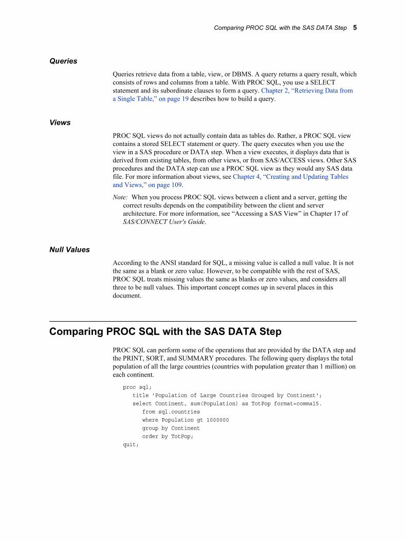
QueriesQueries retrieve data from a table, view, or DBMS. A query returns a query result, which consists of rows and columns from a table. With PROC SQL, you use a SELECT statement and its subordinate clauses to form a query. Chapter 2, “Retrieving Data from a Single Table,” on page 19 describes how to build a query.

ViewsPROC SQL views do not actually contain data as tables do. Rather, a PROC SQL view contains a stored SELECT statement or query. The query executes when you use the view in a SAS procedure or DATA step. When a view executes, it displays data that is derived from existing tables, from other views, or from SAS/ACCESS views. Other SAS procedures and the DATA step can use a PROC SQL view as they would any SAS data file. For more information about views, see Chapter 4, “Creating and Updating Tables and Views,” on page 109.

Note: When you process PROC SQL views between a client and a server, getting the correct results depends on the compatibility between the client and server architecture. For more information, see “Accessing a SAS View” in Chapter 17 of SAS/CONNECT User's Guide.

Null ValuesAccording to the ANSI standard for SQL, a missing value is called a null value. It is not the same as a blank or zero value. However, to be compatible with the rest of SAS, PROC SQL treats missing values the same as blanks or zero values, and considers all three to be null values. This important concept comes up in several places in this document.

Comparing PROC SQL with the SAS DATA StepPROC SQL can perform some of the operations that are provided by the DATA step and the PRINT, SORT, and SUMMARY procedures. The following query displays the total population of all the large countries (countries with population greater than 1 million) on each continent.

proc sql; title 'Population of Large Countries Grouped by Continent'; select Continent, sum(Population) as TotPop format=comma15. from sql.countries where Population gt 1000000 group by Continent order by TotPop;quit;

Comparing PROC SQL with the SAS DATA Step 5

Output 1.1 Sample SQL Output

Here is a SAS program that produces the same result.

title 'Large Countries Grouped by Continent';proc summary data=sql.countries; where Population > 1000000; class Continent; var Population; output out=sumPop sum=TotPop;run;

proc sort data=SumPop; by totPop;run;

proc print data=SumPop noobs; var Continent TotPop; format TotPop comma15.; where _type_=1;run;


Output 1.2 Sample DATA Step Output

This example shows that PROC SQL can achieve the same results as Base SAS software but often with fewer and shorter statements. The SELECT statement that is shown in this example performs summation, grouping, sorting, and row selection. It also displays the query's results without the PRINT procedure.

PROC SQL executes without using the RUN statement. After you invoke PROC SQL you can submit additional SQL procedure statements without submitting the PROC statement again. Use the QUIT statement to terminate the procedure.

Notes about the Example TablesFor all examples, the following global statement is in effect:

libname sql 'SAS-data-library';

The tables that are used in this document contain geographic and demographic data. The data is intended to be used for the PROC SQL code examples only; it is not necessarily up-to-date or accurate.

Note: You can find instructions for downloading these data sets at http://ftp.sas.com/samples/A56936. These data sets are valid for SAS 9 as well as previous versions of SAS.

Notes about the Example Tables 7

http://ftp.sas.com/samples/A56936

http://ftp.sas.com/samples/A56936

The COUNTRIES table contains data that pertains to countries. The Area column contains a country's area in square miles. The UNDate column contains the year a country entered the United Nations, if applicable.

Output 1.3 COUNTRIES (Partial Output)

The WORLDCITYCOORDS table contains latitude and longitude data for world cities. Cities in the Western hemisphere have negative longitude coordinates. Cities in the


Southern hemisphere have negative latitude coordinates. Coordinates are rounded to the nearest degree.

Output 1.4 WORLDCITYCOORDS (Partial Output)


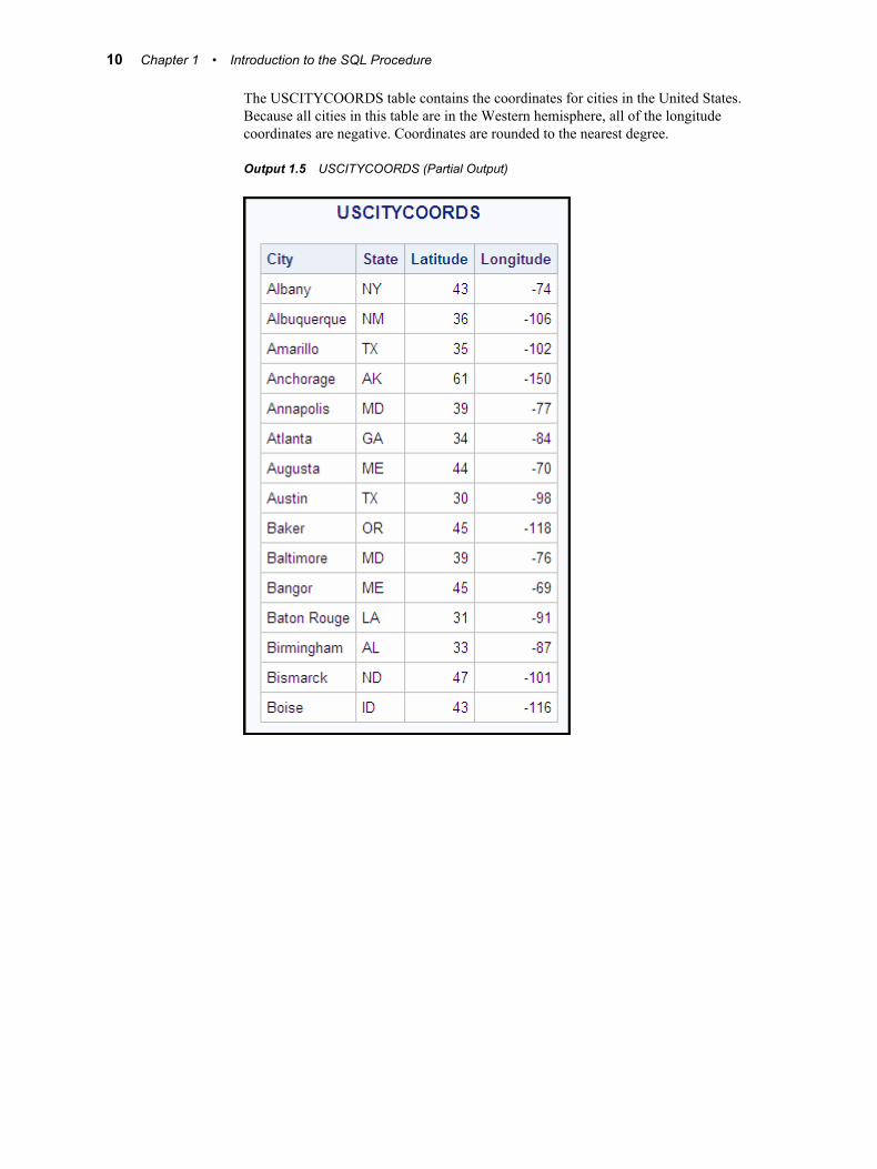
The USCITYCOORDS table contains the coordinates for cities in the United States. Because all cities in this table are in the Western hemisphere, all of the longitude coordinates are negative. Coordinates are rounded to the nearest degree.

Output 1.5 USCITYCOORDS (Partial Output)


The UNITEDSTATES table contains data that is associated with the states. The Statehood column contains the date when the state was admitted into the Union.

Output 1.6 UNITEDSTATES (Partial Output)


The POSTALCODES table contains postal code abbreviations.

Output 1.7 POSTALCODES (Partial Output)


The WORLDTEMPS table contains average high and low temperatures from various international cities.

Output 1.8 WORLDTEMPS (Partial Output)


The OILPROD table contains oil production statistics from oil-producing countries.

Output 1.9 OILPROD (Partial Output)


The OILRSRVS table lists approximate oil reserves of oil-producing countries.

Output 1.10 OILRSRVS (Partial Output)


The CONTINENTS table contains geographic data that relates to world continents.

Output 1.11 CONTINENTS


The FEATURES table contains statistics that describe various types of geographical features, such as oceans, lakes, and mountains.

Output 1.12 FEATURES (Partial Output)


Chapter 2

Retrieving Data from a Single Table

Overview of the SELECT Statement . . . . . . . . . . . . . . . . . . . . . . . . . . . . . . . . . . . . . 20How to Use the SELECT Statement . . . . . . . . . . . . . . . . . . . . . . . . . . . . . . . . . . . . . 20SELECT and FROM Clauses . . . . . . . . . . . . . . . . . . . . . . . . . . . . . . . . . . . . . . . . . . 20WHERE Clause . . . . . . . . . . . . . . . . . . . . . . . . . . . . . . . . . . . . . . . . . . . . . . . . . . . . 21ORDER BY Clause . . . . . . . . . . . . . . . . . . . . . . . . . . . . . . . . . . . . . . . . . . . . . . . . . 21GROUP BY Clause . . . . . . . . . . . . . . . . . . . . . . . . . . . . . . . . . . . . . . . . . . . . . . . . . 21HAVING Clause . . . . . . . . . . . . . . . . . . . . . . . . . . . . . . . . . . . . . . . . . . . . . . . . . . . . 21Ordering the SELECT Statement . . . . . . . . . . . . . . . . . . . . . . . . . . . . . . . . . . . . . . . 22

Selecting Columns in a Table . . . . . . . . . . . . . . . . . . . . . . . . . . . . . . . . . . . . . . . . . . . . 22Selecting All Columns in a Table . . . . . . . . . . . . . . . . . . . . . . . . . . . . . . . . . . . . . . . 22Selecting Specific Columns in a Table . . . . . . . . . . . . . . . . . . . . . . . . . . . . . . . . . . . 23Eliminating Duplicate Rows from the Query Results . . . . . . . . . . . . . . . . . . . . . . . 25Determining the Structure of a Table . . . . . . . . . . . . . . . . . . . . . . . . . . . . . . . . . . . . 27

Creating New Columns . . . . . . . . . . . . . . . . . . . . . . . . . . . . . . . . . . . . . . . . . . . . . . . . 27Adding Text to Output . . . . . . . . . . . . . . . . . . . . . . . . . . . . . . . . . . . . . . . . . . . . . . . 27Calculating Values . . . . . . . . . . . . . . . . . . . . . . . . . . . . . . . . . . . . . . . . . . . . . . . . . . 29Assigning a Column Alias . . . . . . . . . . . . . . . . . . . . . . . . . . . . . . . . . . . . . . . . . . . . 30Referring to a Calculated Column by Alias . . . . . . . . . . . . . . . . . . . . . . . . . . . . . . . 31Assigning Values Conditionally . . . . . . . . . . . . . . . . . . . . . . . . . . . . . . . . . . . . . . . . 32Replacing Missing Values . . . . . . . . . . . . . . . . . . . . . . . . . . . . . . . . . . . . . . . . . . . . 35Specifying Column Attributes . . . . . . . . . . . . . . . . . . . . . . . . . . . . . . . . . . . . . . . . . 36

Sorting Data . . . . . . . . . . . . . . . . . . . . . . . . . . . . . . . . . . . . . . . . . . . . . . . . . . . . . . . . . 37Overview of Sorting Data . . . . . . . . . . . . . . . . . . . . . . . . . . . . . . . . . . . . . . . . . . . . . 37Sorting by Column . . . . . . . . . . . . . . . . . . . . . . . . . . . . . . . . . . . . . . . . . . . . . . . . . . 38Sorting by Multiple Columns . . . . . . . . . . . . . . . . . . . . . . . . . . . . . . . . . . . . . . . . . . 38Specifying a Sort Order . . . . . . . . . . . . . . . . . . . . . . . . . . . . . . . . . . . . . . . . . . . . . . 39Sorting by Calculated Column . . . . . . . . . . . . . . . . . . . . . . . . . . . . . . . . . . . . . . . . . 40Sorting by Column Position . . . . . . . . . . . . . . . . . . . . . . . . . . . . . . . . . . . . . . . . . . . 41Sorting by Columns That Are Not Selected . . . . . . . . . . . . . . . . . . . . . . . . . . . . . . . 42Specifying a Different Sorting Sequence . . . . . . . . . . . . . . . . . . . . . . . . . . . . . . . . . 43Sorting Columns That Contain Missing Values . . . . . . . . . . . . . . . . . . . . . . . . . . . . 43

Retrieving Rows That Satisfy a Condition . . . . . . . . . . . . . . . . . . . . . . . . . . . . . . . . . 44Using a Simple WHERE Clause . . . . . . . . . . . . . . . . . . . . . . . . . . . . . . . . . . . . . . . . 44Retrieving Rows Based on a Comparison . . . . . . . . . . . . . . . . . . . . . . . . . . . . . . . . 45Retrieving Rows That Satisfy Multiple Conditions . . . . . . . . . . . . . . . . . . . . . . . . . 47Using Other Conditional Operators . . . . . . . . . . . . . . . . . . . . . . . . . . . . . . . . . . . . . 49Using Truncated String Comparison Operators . . . . . . . . . . . . . . . . . . . . . . . . . . . . 53Using a WHERE Clause with Missing Values . . . . . . . . . . . . . . . . . . . . . . . . . . . . . 54

Summarizing Data . . . . . . . . . . . . . . . . . . . . . . . . . . . . . . . . . . . . . . . . . . . . . . . . . . . . 56

19

Overview of Summarizing Data . . . . . . . . . . . . . . . . . . . . . . . . . . . . . . . . . . . . . . . . 56Using Aggregate Functions . . . . . . . . . . . . . . . . . . . . . . . . . . . . . . . . . . . . . . . . . . . 56Summarizing Data with a WHERE Clause . . . . . . . . . . . . . . . . . . . . . . . . . . . . . . . 57Displaying Sums . . . . . . . . . . . . . . . . . . . . . . . . . . . . . . . . . . . . . . . . . . . . . . . . . . . . 58Combining Data from Multiple Rows into a Single Row . . . . . . . . . . . . . . . . . . . . 59Remerging Summary Statistics . . . . . . . . . . . . . . . . . . . . . . . . . . . . . . . . . . . . . . . . . 59Using Aggregate Functions with Unique Values . . . . . . . . . . . . . . . . . . . . . . . . . . . 61Summarizing Data with Missing Values . . . . . . . . . . . . . . . . . . . . . . . . . . . . . . . . . 62

Grouping Data . . . . . . . . . . . . . . . . . . . . . . . . . . . . . . . . . . . . . . . . . . . . . . . . . . . . . . . 64Grouping by One Column . . . . . . . . . . . . . . . . . . . . . . . . . . . . . . . . . . . . . . . . . . . . 64Grouping without Summarizing . . . . . . . . . . . . . . . . . . . . . . . . . . . . . . . . . . . . . . . . 64Grouping by Multiple Columns . . . . . . . . . . . . . . . . . . . . . . . . . . . . . . . . . . . . . . . . 65Grouping and Sorting Data . . . . . . . . . . . . . . . . . . . . . . . . . . . . . . . . . . . . . . . . . . . . 66Grouping with Missing Values . . . . . . . . . . . . . . . . . . . . . . . . . . . . . . . . . . . . . . . . . 67

Filtering Grouped Data . . . . . . . . . . . . . . . . . . . . . . . . . . . . . . . . . . . . . . . . . . . . . . . . 69Overview of Filtering Grouped Data . . . . . . . . . . . . . . . . . . . . . . . . . . . . . . . . . . . . 69Using a Simple HAVING Clause . . . . . . . . . . . . . . . . . . . . . . . . . . . . . . . . . . . . . . . 69Choosing between HAVING and WHERE . . . . . . . . . . . . . . . . . . . . . . . . . . . . . . . 70Using HAVING with Aggregate Functions . . . . . . . . . . . . . . . . . . . . . . . . . . . . . . . 70

Validating a Query . . . . . . . . . . . . . . . . . . . . . . . . . . . . . . . . . . . . . . . . . . . . . . . . . . . . 71

Overview of the SELECT Statement

How to Use the SELECT StatementThis chapter shows you how to perform the following tasks:

• retrieve data from a single table by using the SELECT statement

• validate the correctness of a SELECT statement by using the VALIDATE statement

With the SELECT statement, you can retrieve data from tables or data that is described by SAS data views.

Note: The examples in this chapter retrieve data from tables that are SAS data sets. However, you can use all of the operations that are described here with SAS data views.

The SELECT statement is the primary tool of PROC SQL. You use it to identify, retrieve, and manipulate columns of data from a table. You can also use several optional clauses within the SELECT statement to place restrictions on a query.

SELECT and FROM ClausesThe following simple SELECT statement is sufficient to produce a useful result:

select Name from sql.countries;

The SELECT statement must contain a SELECT clause and a FROM clause, both of which are required in a PROC SQL query. This SELECT statement contains the following:

• a SELECT clause that lists the Name column

20 Chapter 2 • Retrieving Data from a Single Table

• a FROM clause that lists the table in which the Name column resides

WHERE ClauseThe WHERE clause enables you to restrict the data that you retrieve by specifying a condition that each row of the table must satisfy. PROC SQL output includes only those rows that satisfy the condition. The following SELECT statement contains a WHERE clause that restricts the query output to only those countries that have a population that is greater than 5,000,000 people:

select Name from sql.countries where Population gt 5000000;

ORDER BY ClauseThe ORDER BY clause enables you to sort the output from a table by one or more columns. That is, you can put character values in either ascending or descending alphabetical order, and you can put numerical values in either ascending or descending numerical order. The default order is ascending. For example, you can modify the previous example to list the data by descending population:

select Name from sql.countries where Population gt 5000000 order by Population desc;

GROUP BY ClauseThe GROUP BY clause enables you to break query results into subsets of rows. When you use the GROUP BY clause, you use an aggregate function in the SELECT clause or a HAVING clause to instruct PROC SQL how to group the data. For details about aggregate functions, see “Summarizing Data” on page 56. PROC SQL calculates the aggregate function separately for each group. When you do not use an aggregate function, PROC SQL treats the GROUP BY clause as if it were an ORDER BY clause, and any aggregate functions are applied to the entire table.

The following query uses the SUM function to list the total population of each continent. The GROUP BY clause groups the countries by continent, and the ORDER BY clause puts the continents in alphabetical order:

select Continent, sum(Population) from sql.countries group by Continent order by Continent;

HAVING ClauseThe HAVING clause works with the GROUP BY clause to restrict the groups in a query's results based on a given condition. PROC SQL applies the HAVING condition after grouping the data and applying aggregate functions. For example, the following query restricts the groups to include only the continents of Asia and Europe:

select Continent, sum(Population)

Overview of the SELECT Statement 21

from sql.countries group by Continent having Continent in ('Asia', 'Europe') order by Continent;

Ordering the SELECT StatementWhen you construct a SELECT statement, you must specify the clauses in the following order:

1. SELECT

2. FROM

3. WHERE

4. GROUP BY

5. HAVING

6. ORDER BY

Note: Only the SELECT and FROM clauses are required.

The PROC SQL SELECT statement and its clauses are discussed in further detail in the following sections.

Selecting Columns in a TableWhen you retrieve data from a table, you can select one or more columns by using variations of the basic SELECT statement.

Selecting All Columns in a TableUse an asterisk in the SELECT clause to select all columns in a table. The following example selects all columns in the SQL.USCITYCOORDS table, which contains latitude and longitude values for U.S. cities:

libname sql 'SAS-library';

proc sql outobs=12; title 'U.S. Cities with Their States and Coordinates'; select * from sql.uscitycoords;

Note: The OUTOBS= option limits the number of rows (observations) in the output. OUTOBS= is similar to the OBS= data set option. OUTOBS= is used throughout this document to limit the number of rows that are displayed in examples.

Note: In the tables used in these examples, latitude values that are south of the Equator are negative. Longitude values that are west of the Prime Meridian are also negative.


Output 2.1 Selecting All Columns in a Table

Note: When you select all columns, PROC SQL displays the columns in the order in which they are stored in the table.

Selecting Specific Columns in a TableTo select a specific column in a table, list the name of the column in the SELECT clause. The following example selects only the City column in the SQL.USCITYCOORDS table:


proc sql outobs=12; title 'Names of U.S. Cities'; select City from sql.uscitycoords;

Selecting Columns in a Table 23

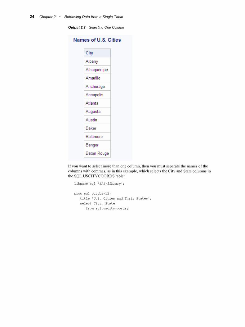
Output 2.2 Selecting One Column

If you want to select more than one column, then you must separate the names of the columns with commas, as in this example, which selects the City and State columns in the SQL.USCITYCOORDS table:


proc sql outobs=12; title 'U.S. Cities and Their States'; select City, State from sql.uscitycoords;


Output 2.3 Selecting Multiple Columns

Note: When you select specific columns, PROC SQL displays the columns in the order in which you specify them in the SELECT clause.

Eliminating Duplicate Rows from the Query ResultsIn some cases, you might want to find only the unique values in a column. For example, if you want to find the unique continents in which U.S. states are located, then you might begin by constructing the following query:


proc sql outobs=12; title 'Continents of the United States'; select Continent from sql.unitedstates;

Selecting Columns in a Table 25

Output 2.4 Selecting a Column with Duplicate Values

You can eliminate the duplicate rows from the results by using the DISTINCT keyword in the SELECT clause. Compare the previous example with the following query, which uses the DISTINCT keyword to produce a single row of output for each continent that is in the SQL.UNITEDSTATES table:


proc sql; title 'Continents of the United States'; select distinct Continent from sql.unitedstates;

Output 2.5 Eliminating Duplicate Values

Note: When you specify all of a table's columns in a SELECT clause with the DISTINCT keyword, PROC SQL eliminates duplicate rows, or rows in which the values in all of the columns match, from the results.


Determining the Structure of a TableTo obtain a list of all of the columns in a table and their attributes, you can use the DESCRIBE TABLE statement. The following example generates a description of the SQL.UNITEDSTATES table. PROC SQL writes the description to the log.


proc sql; describe table sql.unitedstates;

Log 2.1 Determining the Structure of a Table (Partial Log)

NOTE: SQL table SQL.UNITEDSTATES was created like:

create table SQL.UNITEDSTATES( bufsize=12288 ) ( Name char(35) format=$35. informat=$35. label='Name', Capital char(35) format=$35. informat=$35. label='Capital', Population num format=BEST8. informat=BEST8. label='Population', Area num format=BEST8. informat=BEST8., Continent char(35) format=$35. informat=$35. label='Continent', Statehood num );

Creating New ColumnsIn addition to selecting columns that are stored in a table, you can create new columns that exist for the duration of the query. These columns can contain text or calculations. PROC SQL writes the columns that you create as if they were columns from the table.

Adding Text to OutputYou can add text to the output by including a string expression, or literal expression, in a query. The following query includes two strings as additional columns in the output:


proc sql outobs=12; title 'U.S. Postal Codes'; select 'Postal code for', Name, 'is', Code from sql.postalcodes;

Creating New Columns 27

Output 2.6 Adding Text to Output

To prevent the column headings Name and Code from printing, you can assign a label that starts with a special character to each of the columns. PROC SQL does not output the column name when a label is assigned, and it does not output labels that begin with special characters. For example, you could use the following query to suppress the column headings that PROC SQL displayed in the previous example:


proc sql outobs=12; title 'U.S. Postal Codes'; select 'Postal code for', Name label='#', 'is', Code label='#' from sql.postalcodes;


Output 2.7 Suppressing Column Headings in Output

Calculating ValuesYou can perform calculations with values that you retrieve from numeric columns. The following example converts temperatures in the SQL.WORLDTEMPS table from Fahrenheit to Celsius:


proc sql outobs=12; title 'Low Temperatures in Celsius'; select City, (AvgLow - 32) * 5/9 format=4.1 from sql.worldtemps;

Note: This example uses the FORMAT attribute to modify the format of the calculated output. For more information, see “Specifying Column Attributes” on page 36.


Output 2.8 Calculating Values

Assigning a Column AliasBy specifying a column alias, you can assign a new name to any column within a PROC SQL query. The new name must follow the rules for SAS names. The name persists only for that query.

When you use an alias to name a column, you can use the alias to reference the column later in the query. PROC SQL uses the alias as the column heading in output. The following example assigns an alias of LowCelsius to the calculated column from the previous example:


proc sql outobs=12; title 'Low Temperatures in Celsius'; select City, (AvgLow - 32) * 5/9 as LowCelsius format=4.1 from sql.worldtemps;


Output 2.9 Assigning a Column Alias to a Calculated Column

Referring to a Calculated Column by AliasWhen you use a column alias to refer to a calculated value, you must use the CALCULATED keyword with the alias to inform PROC SQL that the value is calculated within the query. The following example uses two calculated values, LowC and HighC, to calculate a third value, Range:


proc sql outobs=12; title 'Range of High and Low Temperatures in Celsius'; select City, (AvgHigh - 32) * 5/9 as HighC format=5.1, (AvgLow - 32) * 5/9 as LowC format=5.1, (calculated HighC - calculated LowC) as Range format=4.1 from sql.worldtemps;

Note: You can use an alias to refer to a calculated column in a SELECT clause, a WHERE clause, or ORDER BY clause.


Output 2.10 Referring to a Calculated Column by Alias

Note: Because this query sets a numeric format of 4.1 on the HighC, LowC, and Range columns, the values in those columns are rounded to the nearest tenth. As a result of the rounding, some of the values in the HighC and LowC columns do not reflect the range value output for the Range column. When you round numeric data values, this type of error sometimes occurs. If you want to avoid this problem, then you can specify additional decimal places in the format.

Assigning Values Conditionally

Using a Simple CASE ExpressionCASE expressions enable you to interpret and change some or all of the data values in a column to make the data more useful or meaningful.

You can use conditional logic within a query by using a CASE expression to conditionally assign a value. You can use a CASE expression anywhere that you can use a column name.

The following table, which is used in the next example, describes the world climate zones (rounded to the nearest degree) that exist between Location 1 and Location 2:


Table 2.1 World Climate Zones

Climate zone Location 1

Latitude at Location 1 Location 2

Latitude at Location 2

North Frigid North Pole 90 Arctic Circle 67

North Temperate

Arctic Circle 67 Tropic of Cancer 23

Torrid Tropic of Cancer 23 Tropic of Capricorn -23

South Temperate

Tropic of Capricorn -23 Antarctic Circle -67

South Frigid Antarctic Circle -67 South Pole -90

In this example, a CASE expression determines the climate zone for each city based on the value in the Latitude column in the SQL.WORLDCITYCOORDS table. The query also assigns an alias of ClimateZone to the value. You must close the CASE logic with the END keyword.


proc sql outobs=12; title 'Climate Zones of World Cities'; select City, Country, Latitude, case when Latitude gt 67 then 'North Frigid' when 67 ge Latitude ge 23 then 'North Temperate' when 23 gt Latitude gt -23 then 'Torrid' when -23 ge Latitude ge -67 then 'South Temperate' else 'South Frigid' end as ClimateZone from sql.worldcitycoords order by City;


Output 2.11 Using a Simple CASE Expression

Using the CASE-OPERAND FormYou can also construct a CASE expression by using the CASE-OPERAND form, as in the following example. This example selects states and assigns them to a region based on the value of the Continent column:


proc sql outobs=12; title 'Assigning Regions to Continents'; select Name, Continent, case Continent when 'North America' then 'Continental U.S.' when 'Oceania' then 'Pacific Islands' else 'None' end as Region from sql.unitedstates;

Note: When you use the CASE-OPERAND form of the CASE expression, the conditions must all be equality tests. That is, they cannot use comparison operators or other types of operators, as are used in “Using a Simple CASE Expression” on page 32.


Output 2.12 Using a CASE Expression in the CASE-OPERAND Form

Replacing Missing ValuesThe COALESCE function enables you to replace missing values in a column with a new value that you specify. For every row that the query processes, the COALESCE function checks each of its arguments until it finds a nonmissing value, and then returns that value. If all of the arguments are missing values, then the COALESCE function returns a missing value. For example, the following query replaces missing values in the LowPoint column in the SQL.CONTINENTS table with the words Not Available:


proc sql; title 'Continental Low Points'; select Name, coalesce(LowPoint, 'Not Available') as LowPoint from sql.continents;


Output 2.13 Using the COALESCE Function to Replace Missing Values

The following CASE expression shows another way to perform the same replacement of missing values. However, the COALESCE function requires fewer lines of code to obtain the same results:


proc sql; title 'Continental Low Points'; select Name, case when LowPoint is missing then 'Not Available' else Lowpoint end as LowPoint from sql.continents;

Specifying Column AttributesYou can specify the following column attributes, which determine how SAS data is displayed:

• FORMAT=

• INFORMAT=

• LABEL=

• LENGTH=

If you do not specify these attributes, then PROC SQL uses attributes that are already saved in the table or, if no attributes are saved, then it uses the default attributes.

The following example assigns a label of State to the Name column and a format of COMMA10. to the Area column:


proc sql outobs=12;


title 'Areas of U.S. States in Square Miles'; select Name label='State', Area format=comma10. from sql.unitedstates;

Note: Using the LABEL= keyword is optional. For example, the following two select clauses are the same:

select Name label='State', Area format=comma10.

select Name 'State', Area format=comma10.

Output 2.14 Specifying Column Attributes

Sorting Data

Overview of Sorting DataYou can sort query results with an ORDER BY clause by specifying any of the columns in the table, including columns that are not selected or columns that are calculated.

Unless an ORDER BY clause is included in the SELECT statement, then a particular order to the output rows, such as the order in which the rows are encountered in the queried table, cannot be guaranteed, even if an index is present. Without an ORDER BY clause, the order of the output rows is determined by the internal processing of PROC SQL, the default collating sequence of SAS, and your operating environment. Therefore, if you want your result table to appear in a particular order, then use the ORDER BY clause.

Sorting Data 37

For more information and examples, see the “ORDER BY Clause” on page 305.

Sorting by ColumnThe following example selects countries and their populations from the SQL.COUNTRIES table and orders the results by population:


proc sql outobs=12; title 'Country Populations'; select Name, Population format=comma10. from sql.countries order by Population;

Note: When you use an ORDER BY clause, you change the order of the output but not the order of the rows that are stored in the table.

Note: The PROC SQL default sort order is ascending.

Output 2.15 Sorting by Column

Sorting by Multiple ColumnsYou can sort by more than one column by specifying the column names, separated by commas, in the ORDER BY clause. The following example sorts the SQL.COUNTRIES table by two columns, Continent and Name:



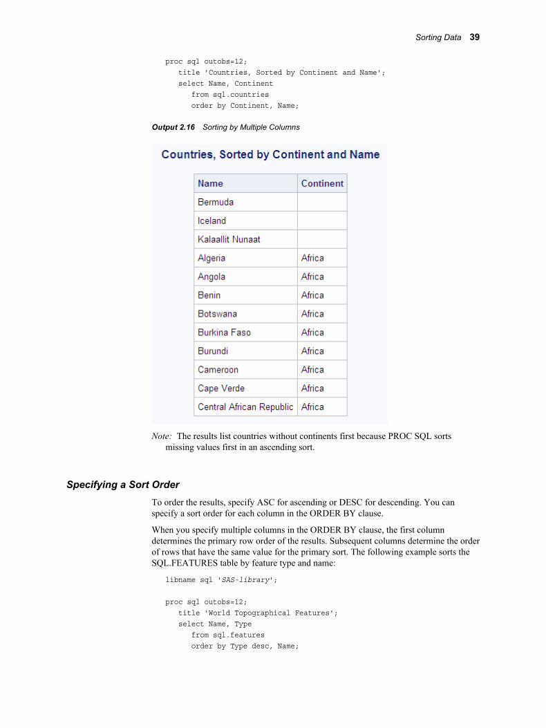
proc sql outobs=12; title 'Countries, Sorted by Continent and Name'; select Name, Continent from sql.countries order by Continent, Name;

Output 2.16 Sorting by Multiple Columns

Note: The results list countries without continents first because PROC SQL sorts missing values first in an ascending sort.

Specifying a Sort OrderTo order the results, specify ASC for ascending or DESC for descending. You can specify a sort order for each column in the ORDER BY clause.

When you specify multiple columns in the ORDER BY clause, the first column determines the primary row order of the results. Subsequent columns determine the order of rows that have the same value for the primary sort. The following example sorts the SQL.FEATURES table by feature type and name:


proc sql outobs=12; title 'World Topographical Features'; select Name, Type from sql.features order by Type desc, Name;

Sorting Data 39

Note: The ASC keyword is optional because the PROC SQL default sort order is ascending.

Output 2.17 Specifying a Sort Order

Sorting by Calculated ColumnYou can sort by a calculated column by specifying its alias in the ORDER BY clause. The following example calculates population densities and then performs a sort on the calculated Density column:


proc sql outobs=12; title 'World Population Densities per Square Mile'; select Name, Population format=comma12., Area format=comma8., Population/Area as Density format=comma10. from sql.countries order by Density desc;


Output 2.18 Sorting by Calculated Column

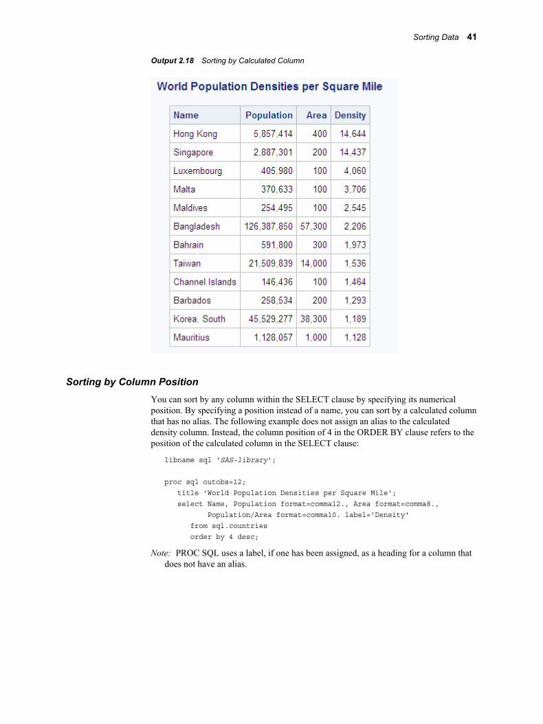
Sorting by Column PositionYou can sort by any column within the SELECT clause by specifying its numerical position. By specifying a position instead of a name, you can sort by a calculated column that has no alias. The following example does not assign an alias to the calculated density column. Instead, the column position of 4 in the ORDER BY clause refers to the position of the calculated column in the SELECT clause:


proc sql outobs=12; title 'World Population Densities per Square Mile'; select Name, Population format=comma12., Area format=comma8., Population/Area format=comma10. label='Density' from sql.countries order by 4 desc;

Note: PROC SQL uses a label, if one has been assigned, as a heading for a column that does not have an alias.

Sorting Data 41

Output 2.19 Sorting by Column Position

Sorting by Columns That Are Not SelectedYou can sort query results by columns that are not included in the query. For example, the following query returns all the rows in the SQL.COUNTRIES table and sorts them by population, even though the Population column is not included in the query:


proc sql outobs=12; title 'Countries, Sorted by Population'; select Name, Continent from sql.countries order by Population;


Output 2.20 Sorting by Columns That Are Not Selected

Specifying a Different Sorting SequenceSORTSEQ= is a PROC SQL statement option that specifies the sorting sequence for PROC SQL to use when a query contains an ORDER BY clause. Use this option only if you want to use a sorting sequence other than your operating environment's default sorting sequence. Possible values include ASCII, EBCDIC, and some languages other than English. For example, in an operating environment that supports the EBCDIC sorting sequence, you could use the following option in the PROC SQL statement to set the sorting sequence to EBCDIC:

proc sql sortseq=ebcdic;

Note: SORTSEQ= affects only the ORDER BY clause. It does not override your operating environment's default comparison operations for the WHERE clause.

Operating Environment InformationSee the SAS documentation for your operating environment for more information about the default and other sorting sequences for your operating environment.

Sorting Columns That Contain Missing ValuesPROC SQL sorts nulls, or missing values, before character or numeric data. Therefore, when you specify ascending order, missing values appear first in the query results.

The following example sorts the rows in the CONTINENTS table by the LowPoint column:


Sorting Data 43

proc sql; title 'Continents, Sorted by Low Point'; select Name, LowPoint from sql.continents order by LowPoint;

Because three continents have a missing value in the LowPoint column, those continents appear first in the output. Note that because the query does not specify a secondary sort, rows that have the same value in the LowPoint column, such as the first three rows of output, are not displayed in any particular order. In general, if you do not explicitly specify a sort order, then PROC SQL output is not guaranteed to be in any particular order.

Output 2.21 Sorting Columns That Contain Missing Values

Retrieving Rows That Satisfy a ConditionThe WHERE clause enables you to retrieve only rows from a table that satisfy a condition. WHERE clauses can contain any of the columns in a table, including columns that are not selected.

Using a Simple WHERE ClauseThe following example uses a WHERE clause to find all countries that are in the continent of Europe and their populations:


proc sql outobs=12; title 'Countries in Europe'; select Name, Population format=comma10. from sql.countries


where Continent = 'Europe';

Output 2.22 Using a Simple WHERE Clause

Retrieving Rows Based on a ComparisonYou can use comparison operators in a WHERE clause to select different subsets of data. The following table lists the comparison operators that you can use:

Table 2.2 Comparison Operators

SymbolMnemonic Equivalent Definition Example

= EQ equal to where Name = 'Asia';

^= or ~= or ¬= or <> NE not equal to where Name ne 'Africa';

> GT greater than where Area > 10000;

< LT less than where Depth < 5000;

Retrieving Rows That Satisfy a Condition 45


>= GE greater than or equal to

where Statehood >= '01jan1860'd;

<= LE less than or equal to where Population <= 5000000;

The following example subsets the SQL.UNITEDSTATES table by including only states with populations greater than 5,000,000 people:


proc sql; title 'States with Populations over 5,000,000'; select Name, Population format=comma10. from sql.unitedstates where Population gt 5000000 order by Population desc;


Output 2.23 Retrieving Rows Based on a Comparison

Retrieving Rows That Satisfy Multiple ConditionsYou can use logical, or Boolean, operators to construct a WHERE clause that contains two or more expressions. The following table lists the logical operators that you can use:

Table 2.3 Logical (Boolean) Operators


& AND specifies that both the previous and following conditions must be true

Continent = 'Asia' and Population > 5000000



! or | or ¦ OR specifies that either the previous or the following condition must be true

Population < 1000000 or Population > 5000000

^ or ~ or ¬ NOT specifies that the following condition must be false

Continent not 'Africa'

The following example uses two expressions to include only countries that are in Africa and that have a population greater than 20,000,000 people:


proc sql; title 'Countries in Africa with Populations over 20,000,000'; select Name, Population format=comma10. from sql.countries where Continent = 'Africa' and Population gt 20000000 order by Population desc;

Output 2.24 Retrieving Rows That Satisfy Multiple Conditions

Note: You can use parentheses to improve the readability of WHERE clauses that contain multiple, or compound, expressions, such as the following:

where (Continent = 'Africa' and Population gt 2000000) or (Continent = 'Asia' and Population gt 1000000)


Using Other Conditional Operators

Overview of Using Other Conditional OperatorsYou can use many different conditional operators in a WHERE clause. The following table lists other operators that you can use:

Table 2.4 Conditional Operators

Operator Definition Example

ANY specifies that at least one of a set of values obtained from a subquery must satisfy a given condition

where Population > any (select Population from sql.countries)

ALL specifies that all of the values obtained from a subquery must satisfy a given condition

where Population > all (select Population from sql.countries)

BETWEEN-AND tests for values within an inclusive range

where Population between 1000000 and 5000000

CONTAINS tests for values that contain a specified string

where Continent contains 'America';

EXISTS tests for the existence of a set of values obtained from a subquery

where exists (select * from sql.oilprod);

IN tests for values that match one of a list of values

where Name in ('Africa', 'Asia');

IS NULL or IS MISSING

tests for missing values where Population is missing;

LIKE tests for values that match a specified pattern1

where Continent like 'A%';

=* tests for values that sound like a specified value

where Name =* 'Tiland';

Note: All of these operators can be prefixed with the NOT operator to form a negative condition.

1 You can use a percent symbol (%) to match any number of characters. You can use an underscore (_) to match one arbitrary character.


Using the IN OperatorThe IN operator enables you to include values within a list that you supply. The following example uses the IN operator to include only the mountains and waterfalls in the SQL.FEATURES table:


proc sql outobs=12; title 'World Mountains and Waterfalls'; select Name, Type, Height format=comma10. from sql.features where Type in ('Mountain', 'Waterfall') order by Height;

Output 2.25 Using the IN Operator

Using the IS MISSING OperatorThe IS MISSING operator enables you to identify rows that contain columns with missing values. The following example selects countries that are not located on a continent. That is, these countries have a missing value in the Continent column:

proc sql; title 'Countries with Missing Continents'; select Name, Continent from sql.countries where Continent is missing;

Note: The IS NULL operator is the same as, and interchangeable with, the IS MISSING operator.


Output 2.26 Using the IS MISSING Operator

Using the BETWEEN-AND OperatorsTo select rows based on a range of values, you can use the BETWEEN-AND operators. This example selects countries that have latitudes within five degrees of the Equator:

proc sql outobs=12; title 'Equatorial Cities of the World'; select City, Country, Latitude from sql.worldcitycoords where Latitude between -5 and 5;

Note: In the tables used in these examples, latitude values that are south of the Equator are negative. Longitude values that are west of the Prime Meridian are also negative.

Note: Because the BETWEEN-AND operators are inclusive, the values that you specify in the BETWEEN-AND expression are included in the results.


Output 2.27 Using the BETWEEN-AND Operators

Using the LIKE OperatorThe LIKE operator enables you to select rows based on pattern matching. For example, the following query returns all countries in the SQL.COUNTRIES table that begin with the letter Z and are any number of characters long, or end with the letter a and are five characters long:


proc sql; title1 'Country Names that Begin with the Letter "Z"'; title2 'or Are 5 Characters Long and End with the Letter "a"'; select Name from sql.countries where Name like 'Z%' or Name like '____a';


Output 2.28 Using the LIKE Operator

The percent sign (%) and underscore (_) are wildcard characters. For more information about pattern matching with the LIKE comparison operator, see Chapter 7, “SQL Procedure,” on page 209.

Using Truncated String Comparison OperatorsTruncated string comparison operators are used to compare two strings. They differ from conventional comparison operators in that, before executing the comparison, PROC SQL truncates the longer string to be the same length as the shorter string. The truncation is performed internally; neither operand is permanently changed. The following table lists the truncated comparison operators:

Table 2.5 Truncated String Comparison Operators

Symbol Definition Example

EQT equal to truncated strings where Name eqt 'Aust';

GTT greater than truncated strings where Name gtt 'Bah';

LTT less than truncated strings where Name ltt 'An';

GET greater than or equal to truncated strings where Country get 'United A';

LET less than or equal to truncated strings where Lastname let 'Smith';


Symbol Definition Example

NET not equal to truncated strings where Style net 'TWO';

The following example returns a list of U.S. states that have 'New ' at the beginning of their names:

proc sql; title '"New" U.S. States'; select Name from sql.unitedstates where Name eqt 'New ';

Output 2.29 Using a Truncated String Comparison Operator

Using a WHERE Clause with Missing ValuesIf a column that you specify in a WHERE clause contains missing values, then a query might provide unexpected results. For example, the following query returns all features from the SQL.FEATURES table that have a depth of less than 500 feet:


/* incorrect output */

proc sql outobs=12; title 'World Features with a Depth of Less than 500 Feet'; select Name, Depth from sql.features where Depth lt 500 order by Depth;


Output 2.30 Using a WHERE Clause with Missing Values (Incorrect Output)

However, because PROC SQL treats missing values as smaller than nonmissing values, features that have no depth listed are also included in the results. To avoid this problem, you could adjust the WHERE expression to check for missing values and exclude them from the query results, as follows:


/* corrected output */

proc sql outobs=12; title 'World Features with a Depth of Less than 500 Feet'; select Name, Depth from sql.features where Depth lt 500 and Depth is not missing order by Depth;


Output 2.31 Using a WHERE Clause with Missing Values (Corrected Output)

Summarizing Data

Overview of Summarizing DataYou can use an aggregate function (or summary function) to produce a statistical summary of data in a table. The aggregate function instructs PROC SQL in how to combine data in one or more columns. If you specify one column as the argument to an aggregate function, then the values in that column are calculated. If you specify multiple arguments, then the arguments or columns that are listed are calculated.

Note: When more than one argument is used within an SQL aggregate function, the function is no longer considered to be an SQL aggregate or summary function. If there is a like-named Base SAS function, then PROC SQL executes the Base SAS function and the results that are returned are based on the values for the current row. If no like-named Base SAS function exists, then an error will occur. For example, if you use multiple arguments for the AVG function, an error will occur because there is no AVG function for Base SAS.

When you use an aggregate function, PROC SQL applies the function to the entire table, unless you use a GROUP BY clause. You can use aggregate functions in the SELECT or HAVING clauses.

Note: See “Grouping Data” on page 64 for information about producing summaries of individual groups of data within a table.

Using Aggregate FunctionsThe following table lists the aggregate functions that you can use:

Table 2.6 Aggregate Functions

Function Definition

AVG, MEAN mean or average of values

COUNT, FREQ, N number of nonmissing values


Function Definition

CSS corrected sum of squares

CV coefficient of variation (percent)

MAX largest value

MIN smallest value

NMISS number of missing values

PRT probability of a greater absolute value of Student's t

RANGE range of values

STD standard deviation

STDERR standard error of the mean

SUM sum of values

SUMWGT sum of the WEIGHT variable values1

T Student's t value for testing the hypothesis that the population mean is zero

USS uncorrected sum of squares

VAR variance

Note: You can use most other SAS functions in PROC SQL, but they are not treated as aggregate functions.

Summarizing Data with a WHERE Clause

Overview of Summarizing Data with a WHERE ClauseYou can use aggregate, or summary functions, by using a WHERE clause. For a complete list of the aggregate functions that you can use, see Table 2.6 on page 56.

Using the MEAN Function with a WHERE ClauseThis example uses the MEAN function to find the annual mean temperature for each country in the SQL.WORLDTEMPS table. The WHERE clause returns countries with a mean temperature that is greater than 75 degrees.


proc sql outobs=12;

1 In the SQL procedure, each row has a weight of 1.

Summarizing Data 57

title 'Mean Temperatures for World Cities'; select City, Country, mean(AvgHigh, AvgLow) as MeanTemp from sql.worldtemps where calculated MeanTemp gt 75 order by MeanTemp desc;

Note: You must use the CALCULATED keyword to reference the calculated column.

Output 2.32 Using the MEAN Function with a WHERE Clause

Displaying SumsThe following example uses the SUM function to return the total oil reserves for all countries in the SQL.OILRSRVS table:


proc sql; title 'World Oil Reserves'; select sum(Barrels) format=comma18. as TotalBarrels from sql.oilrsrvs;

Note: The SUM function produces a single row of output for the requested sum because no nonaggregate value appears in the SELECT clause.


Output 2.33 Displaying Sums

Combining Data from Multiple Rows into a Single RowIn the previous example, PROC SQL combined information from multiple rows of data into a single row of output. Specifically, the world oil reserves for each country were combined to form a total for all countries. Combining, or rolling up, of rows occurs when the following conditions exist:

• The SELECT clause contains only columns that are specified within an aggregate function.

• The WHERE clause, if there is one, contains only columns that are specified in the SELECT clause.

Remerging Summary StatisticsThe following example uses the MAX function to find the largest population in the SQL.COUNTRIES table and displays it in a column called MaxPopulation. Aggregate functions, such as the MAX function, can cause the same calculation to repeat for every row. This occurs whenever PROC SQL remerges data. Remerging occurs whenever any of the following conditions exist:

• The SELECT clause references a column that contains an aggregate function that is not listed in a GROUP BY clause.

• The SELECT clause references a column that contains an aggregate function and other column or columns that are not listed in the GROUP BY clause.

• One or more columns or column expressions that are listed in a HAVING clause are not included in a subquery or a GROUP BY clause.

In this example, PROC SQL writes the population of China, which is the largest population in the table:


proc sql outobs=12; title 'Largest Country Populations'; select Name, Population format=comma20., max(Population) as MaxPopulation format=comma20. from sql.countries order by Population desc;

Summarizing Data 59

Output 2.34 Using Aggregate Functions

In some cases, you might need to use an aggregate function so that you can use its results in another calculation. To do this, you need only to construct one query for PROC SQL to automatically perform both calculations. This type of operation also causes PROC SQL to remerge the data.

For example, if you want to find the percentage of the total world population that resides in each country, then you construct a single query that performs the following tasks:

• obtains the total world population by using the SUM function

• divides each country's population by the total world population

PROC SQL runs an internal query to find the sum and then runs another internal query to divide each country's population by the sum.


proc sql outobs=12; title 'Percentage of World Population in Countries'; select Name, Population format=comma14., (Population / sum(Population) * 100) as Percentage format=comma8.2 from sql.countries order by Percentage desc;

Note: When a query remerges data, PROC SQL displays a note in the log to indicate that data remerging has occurred.


Output 2.35 Remerging Summary Statistics

Using Aggregate Functions with Unique Values

Counting Unique ValuesYou can use DISTINCT with an aggregate function to cause the function to use only unique values from a column.

The following query returns the number of distinct, nonmissing continents in the SQL.COUNTRIES table:


proc sql; title 'Number of Continents in the COUNTRIES Table'; select count(distinct Continent) as Count from sql.countries;

Output 2.36 Using DISTINCT with the COUNT Function

Summarizing Data 61

Note: You cannot use select count(distinct *) to count distinct rows in a table. This code generates an error because PROC SQL does not know which duplicate column values to eliminate.

Counting Nonmissing ValuesCompare the previous example with the following query, which does not use the DISTINCT keyword. This query counts every nonmissing occurrence of a continent in the SQL.COUNTRIES table, including duplicate values:


proc sql; title 'Countries for Which a Continent is Listed'; select count(Continent) as Count from sql.countries;

Output 2.37 Effect of Not Using DISTINCT with the COUNT Function

Counting All RowsIn the previous two examples, countries that have a missing value in the Continent column are ignored by the COUNT function. To obtain a count of all rows in the table, including countries that are not on a continent, you can use the following code in the SELECT clause:

proc sql; title 'Number of Countries in the SQL.COUNTRIES Table'; select count(*) as Number from sql.countries;

Output 2.38 Using the COUNT Function to Count All Rows in a Table

Summarizing Data with Missing Values

Overview of Summarizing Data with Missing ValuesWhen you use an aggregate function with data that contains missing values, the results might not provide the information that you expect because many aggregate functions ignore missing values.


Finding Errors Caused by Missing ValuesThe AVG function returns the average of only the nonmissing values. The following query calculates the average length of three features in the SQL.FEATURES table: Angel Falls and the Amazon and Nile rivers:


/* unexpected output */

proc sql; title 'Average Length of Angel Falls, Amazon and Nile Rivers'; select Name, Length, avg(Length) as AvgLength from sql.features where Name in ('Angel Falls', 'Amazon', 'Nile');

Output 2.39 Finding Errors Caused by Missing Values (Unexpected Output)

Because no length is stored for Angel Falls, the average includes only the values for the Amazon and Nile rivers. Therefore, the average contains unexpected output results.

Compare the results from the previous example with the following query, which includes a COALESCE expression to handle missing values:

/* modified output */

proc sql; title 'Average Length of Angel Falls, Amazon and Nile Rivers'; select Name, Length, coalesce(Length, 0) as NewLength, avg(calculated NewLength) as AvgLength from sql.features where Name in ('Angel Falls', 'Amazon', 'Nile');

Output 2.40 Finding Errors Caused by Missing Values (Modified Output)

Summarizing Data 63

Grouping DataThe GROUP BY clause groups data by a specified column or columns. When you use a GROUP BY clause, you also use an aggregate function in the SELECT clause or in a HAVING clause to instruct PROC SQL in how to summarize the data for each group. PROC SQL calculates the aggregate function separately for each group.

Grouping by One ColumnThe following example sums the populations of all countries to find the total population of each continent:


proc sql; title 'Total Populations of World Continents'; select Continent, sum(Population) format=comma14. as TotalPopulation from sql.countries where Continent is not missing group by Continent;

Note: Countries for which a continent is not listed are excluded by the WHERE clause.

Output 2.41 Grouping by One Column

Grouping without SummarizingWhen you use a GROUP BY clause without an aggregate function, PROC SQL treats the GROUP BY clause as if it were an ORDER BY clause and displays a message in the log that informs you that this has happened. The following example attempts to group high and low temperature information for each city in the SQL.WORLDTEMPS table by country:



proc sql outobs=12; title 'High and Low Temperatures'; select City, Country, AvgHigh, AvgLow from sql.worldtemps group by Country;

The output and log show that PROC SQL transforms the GROUP BY clause into an ORDER BY clause.

Output 2.42 Grouping without Aggregate Functions

Log 2.2 Grouping without Aggregate Functions (Partial Log)

WARNING: A GROUP BY clause has been transformed into an ORDER BY clause because

neither the SELECT clause nor the optional HAVING clause of the associated table-expression referenced a summary function.

Grouping by Multiple ColumnsTo group by multiple columns, separate the column names with commas within the GROUP BY clause. You can use aggregate functions with any of the columns that you select. The following example groups by both Location and Type, producing total square miles for the deserts and lakes in each location in the SQL.FEATURES table:


Grouping Data 65

proc sql; title 'Total Square Miles of Deserts and Lakes'; select Location, Type, sum(Area) as TotalArea format=comma16. from sql.features where type in ('Desert', 'Lake') group by Location, Type;

Output 2.43 Grouping by Multiple Columns

Grouping and Sorting DataYou can order grouped results with an ORDER BY clause. The following example takes the previous example and adds an ORDER BY clause to change the order of the Location column from ascending order to descending order:


proc sql; title 'Total Square Miles of Deserts and Lakes'; select Location, Type, sum(Area) as TotalArea format=comma16. from sql.features where type in ('Desert', 'Lake') group by Location, Type order by Location desc;


Output 2.44 Grouping with an ORDER BY Clause

Grouping with Missing Values

Finding Grouping Errors Caused by Missing ValuesWhen a column contains missing values, PROC SQL treats the missing values as a single group. This can sometimes provide unexpected results.

In this example, because the SQL.COUNTRIES table contains some missing values in the Continent column, the missing values combine to form a single group that has the total area of the countries that have a missing value in the Continent column:


/* unexpected output */

proc sql outobs=12; title 'Areas of World Continents'; select Name format=$25., Continent, sum(Area) format=comma12. as TotalArea from sql.countries group by Continent order by Continent, Name;

The output is incorrect because Bermuda, Iceland, and Kalaallit Nunaat are not actually part of the same continent. However, PROC SQL treats them that way because they all have a missing character value in the Continent column.

Grouping Data 67

Output 2.45 Finding Grouping Errors Caused by Missing Values (Unexpected Output)

To correct the query from the previous example, you can write a WHERE clause to exclude the missing values from the results:

/* modified output */

proc sql outobs=12; title 'Areas of World Continents'; select Name format=$25., Continent, sum(Area) format=comma12. as TotalArea from sql.countries where Continent is not missing group by Continent order by Continent, Name;


Output 2.46 Adjusting the Query to Avoid Errors Due to Missing Values (Modified Output)

Note: Aggregate functions, such as the SUM function, can cause the same calculation to repeat for every row. This occurs whenever PROC SQL remerges data. See “Remerging Summary Statistics” on page 59 for more information about remerging.

Filtering Grouped Data

Overview of Filtering Grouped DataYou can use a HAVING clause with a GROUP BY clause to filter grouped data. The HAVING clause affects groups in a way that is similar to the way in which a WHERE clause affects individual rows. When you use a HAVING clause, PROC SQL displays only the groups that satisfy the HAVING expression.

Using a Simple HAVING ClauseThe following example groups the features in the SQL.FEATURES table by type and then displays only the numbers of islands, oceans, and seas:


proc sql; title 'Numbers of Islands, Oceans, and Seas'; select Type, count(*) as Number from sql.features group by Type

Filtering Grouped Data 69

having Type in ('Island', 'Ocean', 'Sea') order by Type;

Output 2.47 Using a Simple HAVING Clause

Choosing between HAVING and WHEREThe differences between the HAVING clause and the WHERE clause are shown in the following table. Because you use the HAVING clause when you work with groups of data, queries that contain a HAVING clause usually also contain the following:

• a GROUP BY clause

• an aggregate function

Note: If you use a HAVING clause without a GROUP BY clause and if the query references at least one aggregate function, PROC SQL treats the input data as if it all comes from a single group of data.

Table 2.7 Differences between the HAVING Clause and WHERE Clause

HAVING clause attributes WHERE clause attributes

is typically used to specify conditions for including or excluding groups of rows from a table.

is used to specify conditions for including or excluding individual rows from a table.

must follow the GROUP BY clause in a query, if used with a GROUP BY clause.

must precede the GROUP BY clause in a query, if used with a GROUP BY clause.

is affected by a GROUP BY clause, when there is no GROUP BY clause, the HAVING clause is treated like a WHERE clause.

is not affected by a GROUP BY clause.

is processed after the GROUP BY clause and any aggregate functions.

is processed before a GROUP BY clause, if there is one, and before any aggregate functions.

Using HAVING with Aggregate FunctionsThe following query returns the populations of all continents that have more than 15 countries:



proc sql; title 'Total Populations of Continents with More than 15 Countries'; select Continent, sum(Population) as TotalPopulation format=comma16., count(*) as Count from sql.countries group by Continent having count(*) gt 15 order by Continent;

The HAVING expression contains the COUNT function, which counts the number of rows within each group.

Output 2.48 Using HAVING with the COUNT Function

Validating a QueryThe VALIDATE statement enables you to check the syntax of a query for correctness without submitting it to PROC SQL. PROC SQL displays a message in the log to indicate whether the syntax is correct.


proc sql; validate select Name, Statehood from sql.unitedstates where Statehood lt '01Jan1800'd;

Log 2.3 Validating a Query (Partial Log)

3 proc sql;4 validate5 select Name, Statehood6 from sql.unitedstates7 where Statehood lt '01Jan1800'd;NOTE: PROC SQL statement has valid syntax.

The following example shows an invalid query and the corresponding log message:

Validating a Query 71


proc sql; validate select Name, Statehood from sql.unitedstates where lt '01Jan1800'd;

Log 2.4 Validating an Invalid Query (Partial Log)

3 proc sql;4 validate5 select Name, Statehood6 from sql.unitedstates7 where lt '01Jan1800'd; ------------ 22 76ERROR 22-322: Syntax error, expecting one of the following: !, !!, &, *, **,

+, -, /, <, <=, <>, =, >, >=, ?, AND, CONTAINS, EQ, GE,GROUP, GT, HAVING, LE, LIKE, LT, NE, OR, ORDER, ^=, |, ||, ~=.

ERROR 76-322: Syntax error, statement will be ignored.

NOTE: The SAS System stopped processing this step because of errors.


Chapter 3

Retrieving Data from Multiple Tables

Introduction . . . . . . . . . . . . . . . . . . . . . . . . . . . . . . . . . . . . . . . . . . . . . . . . . . . . . . . . . . 73

Selecting Data from More than One Table by Using Joins . . . . . . . . . . . . . . . . . . . 74Overview of Selecting Data from More than One Table by Using Joins . . . . . . . . . 74Inner Joins . . . . . . . . . . . . . . . . . . . . . . . . . . . . . . . . . . . . . . . . . . . . . . . . . . . . . . . . . 75Outer Joins . . . . . . . . . . . . . . . . . . . . . . . . . . . . . . . . . . . . . . . . . . . . . . . . . . . . . . . . 84Specialty Joins . . . . . . . . . . . . . . . . . . . . . . . . . . . . . . . . . . . . . . . . . . . . . . . . . . . . . 87Using the Coalesce Function in Joins . . . . . . . . . . . . . . . . . . . . . . . . . . . . . . . . . . . . 90Comparing DATA Step Match-Merges with PROC SQL Joins . . . . . . . . . . . . . . . 91

Using Subqueries to Select Data . . . . . . . . . . . . . . . . . . . . . . . . . . . . . . . . . . . . . . . . . 95Single-Value Subqueries . . . . . . . . . . . . . . . . . . . . . . . . . . . . . . . . . . . . . . . . . . . . . 95Multiple-Value Subqueries . . . . . . . . . . . . . . . . . . . . . . . . . . . . . . . . . . . . . . . . . . . . 96Correlated Subqueries . . . . . . . . . . . . . . . . . . . . . . . . . . . . . . . . . . . . . . . . . . . . . . . . 97Testing for the Existence of a Group of Values . . . . . . . . . . . . . . . . . . . . . . . . . . . . 98Multiple Levels of Subquery Nesting . . . . . . . . . . . . . . . . . . . . . . . . . . . . . . . . . . . . 99Combining a Join with a Subquery . . . . . . . . . . . . . . . . . . . . . . . . . . . . . . . . . . . . . 100

When to Use Joins and Subqueries . . . . . . . . . . . . . . . . . . . . . . . . . . . . . . . . . . . . . . 101

Combining Queries with Set Operators . . . . . . . . . . . . . . . . . . . . . . . . . . . . . . . . . . 102Working with Two or More Query Results . . . . . . . . . . . . . . . . . . . . . . . . . . . . . . 102Producing Unique Rows from Both Queries (UNION) . . . . . . . . . . . . . . . . . . . . . 103Producing Rows That Are in Only the First Query Result (EXCEPT) . . . . . . . . . 104Producing Rows That Belong to Both Query Results (INTERSECT) . . . . . . . . . . 105Concatenating Query Results (OUTER UNION) . . . . . . . . . . . . . . . . . . . . . . . . . . 106Producing Rows from the First Query or the Second Query . . . . . . . . . . . . . . . . . 107

Introduction

This chapter shows you how to perform the following tasks:

• select data from more than one table by joining the tables together

• use subqueries to select data from one table based on data values from another table

• combine the results of more than one query by using set operators

Note: Unless otherwise noted, the PROC SQL operations that are shown in this chapter apply to views as well as tables. For more information about views, see Chapter 4, “Creating and Updating Tables and Views,” on page 109.

73

Selecting Data from More than One Table by Using Joins

Overview of Selecting Data from More than One Table by Using Joins

The data that you need for a report could be located in more than one table. In order to select the data from the tables, join the tables in a query. Joining tables enables you to select data from multiple tables as if the data were contained in one table. Joins do not alter the original tables.

The most basic type of join is simply two tables that are listed in the FROM clause of a SELECT statement. The following query joins the two tables that are shown in Output 3.1 on page 74 and creates Output 3.2 on page 75.

proc sql; title 'Table One and Table Two'; select * from one, two;

proc sql; title 'Table One'; select * from one;

title 'Table Two'; select * from two;

quit;

Output 3.1 Table One, Table Two

74 Chapter 3 • Retrieving Data from Multiple Tables

Output 3.2 Cartesian Product of Table One and Table Two

Joining tables in this way returns the Cartesian product of the tables. Each row from the first table is combined with every row from the second table. When you run this query, the following message is written to the SAS log:

Log 3.1 Cartesian Product Log Message

NOTE: The execution of this query involves performing one or more Cartesian product joins that can not be optimized.

The Cartesian product of large tables can be huge. Typically, you want a subset of the Cartesian product. You specify the subset by declaring the join type.

There are two types of joins:

• Inner Joins return a result table for all the rows in a table that have one or more matching rows in the other table or tables that are listed in the FROM clause.

• Outer Joins are inner joins that are augmented with rows that did not match with any row from the other table in the join. There are three types of outer joins: left, right, and full.

Inner Joins

Overview of Inner Joins

An inner join returns only the subset of rows from the first table that matches rows from the second table. You can specify the columns that you want to be compared for matching values in a WHERE clause.

The following code adds a WHERE clause to the previous query. The WHERE clause specifies that only rows whose values in column X of Table One match values in column

Selecting Data from More than One Table by Using Joins 75

X of Table Two should appear in the output. Compare this query's output to Output 3.2 on page 75.

proc sql; title 'Table One and Table Two'; select * from one, two where one.x=two.x;

Output 3.3 Table One and Table Two Joined

The output contains only one row because only one value in column X matches from each table. In an inner join, only the matching rows are selected. Outer joins can return nonmatching rows; they are covered in “Outer Joins” on page 84.

Note that the column names in the WHERE clause are prefixed by their table names. This is known as qualifying the column names, and it is necessary when you specify columns that have the same name from more than one table. Qualifying the column name avoids creating an ambiguous column reference.

Using Table AliasesA table alias is a temporary, alternate name for a table. You specify table aliases in the FROM clause. Table aliases are used in joins to qualify column names and can make a query easier to read by abbreviating table names.

The following example compares the oil production of countries to their oil reserves by joining the OILPROD and OILRSRVS tables on their Country columns. Because the Country columns are common to both tables, they are qualified with their table aliases. You could also qualify the columns by prefixing the column names with the table names.

Note: The AS keyword is optional.


proc sql outobs=6; title 'Oil Production/Reserves of Countries'; select * from sql.oilprod as p, sql.oilrsrvs as r where p.country = r.country;


Output 3.4 Abbreviating Column Names by Using Table Aliases

Note that each table's Country column is displayed. Typically, once you have determined that a join is functioning correctly, you include just one of the matching columns in the SELECT clause.

Specifying the Order of Join OutputYou can order the output of joined tables by one or more columns from either table. The next example's output is ordered in descending order by the BarrelsPerDay column. It is not necessary to qualify BarrelsPerDay, because the column exists only in the OILPROD table.


proc sql outobs=6; title 'Oil Production/Reserves of Countries'; select p.country, barrelsperday 'Production', barrels 'Reserves' from sql.oilprod p, sql.oilrsrvs r where p.country = r.country order by barrelsperday desc;

Output 3.5 Ordering the Output of Joined Tables


Creating Inner Joins Using INNER JOIN KeywordsThe INNER JOIN keywords can be used to join tables. The ON clause replaces the WHERE clause for specifying columns to join. PROC SQL provides these keywords primarily for compatibility with the other joins (OUTER, RIGHT, and LEFT JOIN). Using INNER JOIN with an ON clause provides the same functionality as listing tables in the FROM clause and specifying join columns with a WHERE clause.

This code produces the same output as the previous code but uses the INNER JOIN construction.

proc sql ; select p.country, barrelsperday 'Production', barrels 'Reserves' from sql.oilprod p inner join sql.oilrsrvs r on p.country = r.country order by barrelsperday desc;

Joining Tables Using Comparison OperatorsTables can be joined by using comparison operators other than the equal sign (=) in the WHERE clause. For more information about comparison operators, see “Retrieving Rows Based on a Comparison” on page 45. In this example, all U.S. cities in the USCITYCOORDS table are selected that are south of Cairo, Egypt. The compound WHERE clause specifies the city of Cairo in the WORLDCITYCOORDS table and joins USCITYCOORDS and WORLDCITYCOORDS on their Latitude columns, using a less-than (lt) operator.


proc sql; title 'US Cities South of Cairo, Egypt'; select us.City, us.State, us.Latitude, world.city, world.latitude from sql.worldcitycoords world, sql.uscitycoords us where world.city = 'Cairo' and us.latitude lt world.latitude;

Output 3.6 Using Comparison Operators to Join Tables

When you run this query, the following message is written to the SAS log:


Log 3.2 Comparison Query Log Message

NOTE: The execution of this query involves performing one or more Cartesian product joins that can not be optimized.

Recall that you see this message when you run a query that joins tables without specifying matching columns in a WHERE clause. PROC SQL also displays this message whenever tables are joined by using an inequality operator.

The Effects of Null Values on JoinsMost database products treat nulls as distinct entities and do not match them in joins. PROC SQL treats nulls as missing values and as matches for joins. Any null will match with any other null of the same type (character or numeric) in a join.

The following example joins Table One and Table Two on column B. There are null values in column B of both tables. Notice in the output that the null value in row c of Table One matches all the null values in Table Two. This is probably not the intended result for the join.

proc sql; title 'One and Two Joined'; select one.a 'One', one.b, two.a 'Two', two.b from one, two where one.b=two.b;


Output 3.7 Joining Tables That Contain Null Values

In order to specify only the nonmissing values for the join, use the IS NOT MISSING operator:

proc sql; select one.a 'One', one.b, two.a 'Two', two.b from one, two where one.b=two.b and one.b is not missing;


Output 3.8 Results of Adding IS NOT MISSING to Joining Tables That Contain Null Values

Creating Multicolumn JoinsWhen a row is distinguished by a combination of values in more than one column, use all the necessary columns in the join. For example, a city name could exist in more than one country. To select the correct city, you must specify both the city and country columns in the joining query's WHERE clause.

This example displays the latitude and longitude of capital cities by joining the COUNTRIES table with the WORLDCITYCOORDS table. To minimize the number of rows in the example output, the first part of the WHERE expression selects capitals with names that begin with the letter L from the COUNTRIES table.


proc sql; title 'Coordinates of Capital Cities'; select Capital format=$12., Name format=$12., City format=$12., Country format=$12., Latitude, Longitude from sql.countries, sql.worldcitycoords where Capital like 'L%' and Capital = City;

London occurs once as a capital city in the COUNTRIES table. However, in WORLDCITYCOORDS, London is found twice: as a city in England and again as a city in Canada. Specifying only Capital = City in the WHERE expression yields the following incorrect output:

Output 3.9 Selecting Capital City Coordinates (incorrect output)


Notice in the output that the inner join incorrectly matches London, England, to both London, Canada, and London, England. By also joining the country name columns together (COUNTRIES.Name to WORLDCITYCOORDS.Country), the rows match correctly.


proc sql; title 'Coordinates of Capital Cities'; select Capital format=$12., Name format=$12., City format=$12., Country format=$12., latitude, longitude from sql.countries, sql.worldcitycoords where Capital like 'L%' and Capital = City and Name = Country;

Output 3.10 Selecting Capital City Coordinates (correct output)

Selecting Data from More than Two TablesThe data that you need could be located in more than two tables. For example, if you want to show the coordinates of the capitals of the states in the United States, then you need to join the UNITEDSTATES table, which contains the state capitals, with the USCITYCOORDS table, which contains the coordinates of cities in the United States. Because cities must be joined along with their states for an accurate join (similarly to the previous example), you must join the tables on both the city and state columns of the tables.

Joining the cities, by joining the UNITEDSTATES.Capital column to the USCITYCOORDS.City column, is straightforward. However, in the UNITEDSTATES table the Name column contains the full state name, while in USCITYCOORDS the states are specified by their postal code. It is therefore impossible to directly join the two tables on their state columns. To solve this problem, it is necessary to use the POSTALCODES table, which contains both the state names and their postal codes, as an intermediate table to make the correct relationship between UNITEDSTATES and USCITYCOORDS. The correct solution joins the UNITEDSTATES.Name column to the POSTALCODES.Name column (matching the full state names), and the POSTALCODES.Code column to the USCITYCOORDS.State column (matching the state postal codes).


title 'Coordinates of State Capitals';proc sql outobs=10;


select us.Capital format=$15., us.Name 'State' format=$15., pc.Code, c.Latitude, c.Longitude from sql.unitedstates us, sql.postalcodes pc, sql.uscitycoords c where us.Capital = c.City and us.Name = pc.Name and pc.Code = c.State;

Output 3.11 Selecting Data from More than Two Tables

Showing Relationships within a Single Table Using Self-JoinsWhen you need to show comparative relationships between values in a table, it is sometimes necessary to join columns within the same table. Joining a table to itself is called a self-join, or reflexive join. You can think of a self-join as PROC SQL making an internal copy of a table and joining the table to its copy.

For example, the following code uses a self-join to select cities that have average yearly high temperatures equal to the average yearly low temperatures of other cities.


proc sql; title "Cities' High Temps = Cities' Low Temps"; select High.City format $12., High.Country format $12., High.AvgHigh, ' | ', Low.City format $12., Low.Country format $12., Low.AvgLow from sql.worldtemps High, sql.worldtemps Low where High.AvgHigh = Low.AvgLow and High.city ne Low.city and High.country ne Low.country;

Notice that the WORLDTEMPS table is assigned two aliases, High and Low. Conceptually, this makes a copy of the table so that a join can be made between the table


and its copy. The WHERE clause selects those rows that have high temperature equal to low temperature.

The WHERE clause also prevents a city from being joined to itself (City ne City and Country ne Country), although, in this case, it is highly unlikely that the high temperature would be equal to the low temperature for the same city.

Output 3.12 Joining a Table to Itself (Self-Join)

Outer Joins

Overview of Outer JoinsOuter joins are inner joins that are augmented with rows from one table that do not match any row from the other table in the join. The resulting output includes rows that match and rows that do not match from the join's source tables. Nonmatching rows have null values in the columns from the unmatched table. Use the ON clause instead of the WHERE clause to specify the column or columns on which you are joining the tables. However, you can continue to use the WHERE clause to subset the query result.

Including Nonmatching Rows with the Left Outer Join


A left outer join lists matching rows and rows from the left-hand table (the first table listed in the FROM clause) that do not match any row in the right-hand table. A left join is specified with the keywords LEFT JOIN and ON.

For example, to list the coordinates of the capitals of international cities, join the COUNTRIES table, which contains capitals, with the WORLDCITYCOORDS table, which contains cities' coordinates, by using a left join. The left join lists all capitals, regardless of whether the cities exist in WORLDCITYCOORDS. Using an inner join would list only capital cities for which there is a matching city in WORLDCITYCOORDS.


proc sql outobs=10; title 'Coordinates of Capital Cities'; select Capital format=$20., Name 'Country' format=$20., Latitude, Longitude from sql.countries a left join sql.worldcitycoords b on a.Capital = b.City and a.Name = b.Country order by Capital;

Output 3.13 Left Join of COUNTRIES and WORLDCITYCOORDS

Including Nonmatching Rows with the Right Outer Join

A right join, specified with the keywords RIGHT JOIN and ON, is the opposite of a left join: nonmatching rows from the right-hand table (the second table listed in the FROM clause) are included with all matching rows in the output. This example reverses the join


of the last example; it uses a right join to select all the cities from the WORLDCITYCOORDS table and displays the population only if the city is the capital of a country (that is, if the city exists in the COUNTRIES table).


proc sql outobs=10; title 'Populations of Capitals Only'; select City format=$20., Country 'Country' format=$20., Population from sql.countries right join sql.worldcitycoords on Capital = City and Name = Country order by City;

Output 3.14 Right Join of COUNTRIES and WORLDCITYCOORDS

Selecting All Rows with the Full Outer Join

A full outer join, specified with the keywords FULL JOIN and ON, selects all matching and nonmatching rows. This example displays the first ten matching and nonmatching rows from the City and Capital columns of WORLDCITYCOORDS and COUNTRIES. Note that the pound sign (#) is used as a line split character in the labels.


proc sql outobs=10; title 'Populations and/or Coordinates of World Cities'; select City '#City#(WORLDCITYCOORDS)' format=$20.,


Capital '#Capital#(COUNTRIES)' format=$20., Population, Latitude, Longitude from sql.countries full join sql.worldcitycoords on Capital = City and Name = Country;

Output 3.15 Full Outer Join of COUNTRIES and WORLDCITYCOORDS

Specialty Joins

Overview of Specialty JoinsThree types of joins—cross joins, union joins, and natural joins—are special cases of the standard join types.

Including All Combinations of Rows with the Cross JoinA cross join is a Cartesian product; it returns the product of two tables. Like a Cartesian product, a cross join's output can be limited by a WHERE clause.

This example shows a cross join of the tables One and Two:

data one; input X Y $; datalines;1 22 3;

data two; input W Z $;


datalines;2 53 64 9;run;

proc sql; title 'Table One'; select * from one;

title 'Table Two'; select * from two;

title;quit;

Output 3.16 Tables One and Two

proc sql; title 'Table One and Table Two'; select * from one cross join two;

Output 3.17 Cross Join


Like a conventional Cartesian product, a cross join causes a note regarding Cartesian products in the SAS log.

Including All Rows with the Union JoinA union join combines two tables without attempting to match rows. All columns and rows from both tables are included. Combining tables with a union join is similar to combining them with the OUTER UNION set operator (see “Combining Queries with Set Operators” on page 102). A union join's output can be limited by a WHERE clause.

This example shows a union join of the same One and Two tables that were used earlier to demonstrate a cross join:

proc sql; select * from one union join two;

Output 3.18 Union Join

Matching Rows with a Natural JoinA natural join automatically selects columns from each table to use in determining matching rows. With a natural join, PROC SQL identifies columns in each table that have the same name and type; rows in which the values of these columns are equal are returned as matching rows. The ON clause is implied.

This example produces the same results as the example in “Specifying the Order of Join Output” on page 77:


proc sql outobs=6; title 'Oil Production/Reserves of Countries'; select country, barrelsperday 'Production', barrels 'Reserve' from sql.oilprod natural join sql.oilrsrvs order by barrelsperday desc;


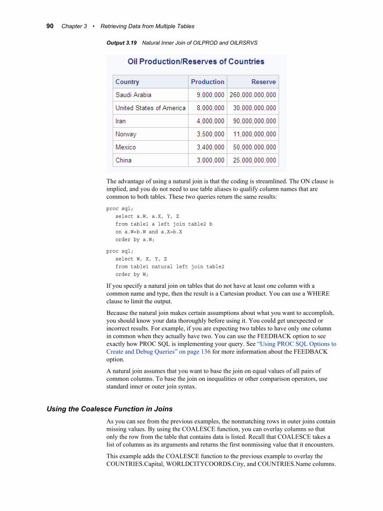
Output 3.19 Natural Inner Join of OILPROD and OILRSRVS

The advantage of using a natural join is that the coding is streamlined. The ON clause is implied, and you do not need to use table aliases to qualify column names that are common to both tables. These two queries return the same results:

proc sql; select a.W, a.X, Y, Z from table1 a left join table2 b on a.W=b.W and a.X=b.X order by a.W;

proc sql; select W, X, Y, Z from table1 natural left join table2 order by W;

If you specify a natural join on tables that do not have at least one column with a common name and type, then the result is a Cartesian product. You can use a WHERE clause to limit the output.

Because the natural join makes certain assumptions about what you want to accomplish, you should know your data thoroughly before using it. You could get unexpected or incorrect results. For example, if you are expecting two tables to have only one column in common when they actually have two. You can use the FEEDBACK option to see exactly how PROC SQL is implementing your query. See “Using PROC SQL Options to Create and Debug Queries” on page 136 for more information about the FEEDBACK option.

A natural join assumes that you want to base the join on equal values of all pairs of common columns. To base the join on inequalities or other comparison operators, use standard inner or outer join syntax.

Using the Coalesce Function in JoinsAs you can see from the previous examples, the nonmatching rows in outer joins contain missing values. By using the COALESCE function, you can overlay columns so that only the row from the table that contains data is listed. Recall that COALESCE takes a list of columns as its arguments and returns the first nonmissing value that it encounters.

This example adds the COALESCE function to the previous example to overlay the COUNTRIES.Capital, WORLDCITYCOORDS.City, and COUNTRIES.Name columns.


COUNTRIES.Name is supplied as an argument to COALESCE because some islands do not have capitals.


proc sql outobs=10; title 'Populations and/or Coordinates of World Cities'; select coalesce(Capital, City,Name)format=$20. 'City', coalesce(Name, Country) format=$20. 'Country', Population, Latitude, Longitude from sql.countries full join sql.worldcitycoords on Capital = City and Name = Country;

Output 3.20 Using COALESCE in Full Outer Join of COUNTRIES and WORLDCITYCOORDS

COALESCE can be used in both inner and outer joins. For more information about COALESCE, see “Replacing Missing Values” on page 35.

Comparing DATA Step Match-Merges with PROC SQL Joins

Overview of Comparing DATA Step Match-Merges with PROC SQL JoinsMany SAS users are familiar with using a DATA step to merge data sets. This section compares merges to joins. DATA step match-merges and PROC SQL joins can produce the same results. However, a significant difference between a match-merge and a join is that you do not have to sort the tables before you join them.

When All of the Values MatchWhen all of the values match in the BY variable and there are no duplicate BY variables, you can use an inner join to produce the same result as a match-merge. To demonstrate


this result, here are two tables that have the column Flight in common. The values of Flight are the same in both tables:

FLTSUPER FLTDEST

Flight Supervisor Flight Destination

145 Kang 145 Brussels 150 Miller 150 Paris 155 Evanko 155 Honolulu

FLTSUPER and FLTDEST are already sorted by the matching column Flight. A DATA step merge produces Output 3.21 on page 92.

data fltsuper;input Flight Supervisor $;datalines;145 Kang 150 Miller 155 Evanko ;data fltdest;input Flight Destination $;datalines;145 Brussels150 Paris155 Honolulu;run;

data merged; merge FltSuper FltDest; by Flight;run;

proc print data=merged noobs; title 'Table MERGED';run;

Output 3.21 Merged Tables When All the Values Match

With PROC SQL, presorting the data is not necessary. The following PROC SQL join gives the same result as that shown in Output 3.21 on page 92.

proc sql; title 'Table MERGED'; select s.flight, Supervisor, Destination from fltsuper s, fltdest d


where s.Flight=d.Flight;

When Only Some of the Values MatchWhen only some of the values match in the BY variable, you can use an outer join to produce the same result as a match-merge. To demonstrate this result, here are two tables that have the column Flight in common. The values of Flight are not the same in both tables:

FLTSUPER FLTDEST


145 Kang 145 Brussels 150 Miller 150 Paris 155 Evanko 165 Seattle 157 Lei

A DATA step merge produces Output 3.22 on page 93:

data merged; merge fltsuper fltdest; by flight;run;proc print data=merged noobs; title 'Table MERGED';run;

Output 3.22 Merged Tables When Some of the Values Match

To get the same result with PROC SQL, use an outer join so that the query result will contain the nonmatching rows from the two tables. In addition, use the COALESCE function to overlay the Flight columns from both tables. The following PROC SQL join gives the same result as that shown in Output 3.22 on page 93:

proc sql; select coalesce(s.Flight,d.Flight) as Flight, Supervisor, Destination from fltsuper s full join fltdest d on s.Flight=d.Flight;


When the Position of the Values Is ImportantWhen you want to merge two tables and the position of the values is important, you might need to use a DATA step merge. To demonstrate this idea, here are two tables to consider:

FLTSUPER FLTDEST


145 Kang 145 Brussels 145 Ramirez 145 Edmonton 150 Miller 150 Paris 150 Picard 150 Madrid 155 Evanko 165 Seattle 157 Lei

For Flight 145, Kang matches with Brussels and Ramirez matches with Edmonton. Because the DATA step merges data based on the position of values in BY groups, the values of Supervisor and Destination match appropriately. A DATA step merge produces Output 3.23 on page 94:

data merged; merge fltsuper fltdest; by flight;run;proc print data=merged noobs; title 'Table MERGED';run;

Output 3.23 Match-Merge of the FLTSUPER and FLTDEST Tables

PROC SQL does not process joins according to the position of values in BY groups. Instead, PROC SQL processes data only according to the data values. Here is the result of an inner join for FLTSUPER and FLTDEST:

proc sql; title 'Table JOINED'; select *


from fltsuper s, fltdest d where s.Flight=d.Flight;

Output 3.24 PROC SQL Join of the FLTSUPER and FLTDEST Tables

PROC SQL builds the Cartesian product and then lists the rows that meet the WHERE clause condition. The WHERE clause returns two rows for each supervisor, one row for each destination. Because Flight has duplicate values and there is no other matching column, there is no way to associate Kang only with Brussels, Ramirez only with Edmonton, and so on.

For more information about DATA step match-merges, see SAS Statements: Reference.

Using Subqueries to Select DataWhile a table join combines multiple tables into a new table, a subquery (enclosed in parentheses) selects rows from one table based on values in another table. A subquery, or inner query, is a query expression that is nested as part of another query expression. Depending on the clause that contains it, a subquery can return a single value or multiple values. Subqueries are most often used in the WHERE and the HAVING expressions.

Single-Value SubqueriesA single-value subquery returns a single row and column. It can be used in a WHERE or HAVING clause with a comparison operator. The subquery must return only one value, or else the query fails and an error message is printed to the log.

This query uses a subquery in its WHERE clause to select U.S. states that have a population greater than Belgium. The subquery is evaluated first, and then it returns the population of Belgium to the outer query.


proc sql; title 'U.S. States with Population Greater than Belgium';

Using Subqueries to Select Data 95

select Name 'State' , population format=comma10. from sql.unitedstates where population gt (select population from sql.countries where name = "Belgium");

Internally, this is what the query looks like after the subquery has executed:

proc sql; title 'U.S. States with Population Greater than Belgium'; select Name 'State', population format=comma10. from sql.unitedstates where population gt 10162614;

The outer query lists the states whose populations are greater than the population of Belgium.

Output 3.25 Single-Value Subquery

Multiple-Value SubqueriesA multiple-value subquery can return more than one value from one column. It is used in a WHERE or HAVING expression that contains IN or a comparison operator that is modified by ANY or ALL. This example displays the populations of oil-producing countries. The subquery first returns all countries that are found in the OILPROD table. The outer query then matches countries in the COUNTRIES table to the results of the subquery.


proc sql outobs=5; title 'Populations of Major Oil Producing Countries'; select name 'Country', Population format=comma15. from sql.countries where Name in (select Country from sql.oilprod);


Output 3.26 Multiple-Value Subquery Using IN

If you use the NOT IN operator in this query, then the query result will contain all the countries that are not contained in the OILPROD table.


proc sql outobs=5; title 'Populations of NonMajor Oil Producing Countries'; select name 'Country', Population format=comma15. from sql.countries where Name not in (select Country from sql.oilprod);

Output 3.27 Multiple-Value Subquery Using NOT IN

Correlated SubqueriesThe previous subqueries have been simple subqueries that are self-contained and that execute independently of the outer query. A correlated subquery requires a value or values to be passed to it by the outer query. After the subquery runs, it passes the results back to the outer query. Correlated subqueries can return single or multiple values.

This example selects all major oil reserves of countries on the continent of Africa.


proc sql;


title 'Oil Reserves of Countries in Africa'; select * from sql.oilrsrvs o where 'Africa' = (select Continent from sql.countries c where c.Name = o.Country);

The outer query selects the first row from the OILRSRVS table and then passes the value of the Country column, Algeria, to the subquery. At this point, the subquery internally looks like this:

(select Continent from sql.countries c where c.Name = 'Algeria');

The subquery selects that country from the COUNTRIES table. The subquery then passes the country's continent back to the WHERE clause in the outer query. If the continent is Africa, then the country is selected and displayed. The outer query then selects each subsequent row from the OILRSRVS table and passes the individual values of Country to the subquery. The subquery returns the appropriate values of Continent to the outer query for comparison in its WHERE clause.

Note that the WHERE clause uses an = (equal) operator. You can use an = (equal) operator if the subquery returns only a single value. However, if the subquery returns multiple values, then you must use IN or a comparison operator with ANY or ALL. For detailed information about the operators that are available for use with subqueries, see Chapter 7, “SQL Procedure,” on page 209.

Output 3.28 Correlated Subquery

Testing for the Existence of a Group of ValuesThe EXISTS condition tests for the existence of a set of values. An EXISTS condition is true if any rows are produced by the subquery, and it is false if no rows are produced. Conversely, the NOT EXISTS condition is true when a subquery produces an empty table.

This example produces the same result as Output 3.28 on page 98. EXISTS checks for the existence of countries that have oil reserves on the continent of Africa. Note that the WHERE clause in the subquery now contains the condition Continent = 'Africa' that was in the outer query in the previous example.


proc sql;


title 'Oil Reserves of Countries in Africa'; select * from sql.oilrsrvs o where exists (select Continent from sql.countries c where o.Country = c.Name and Continent = 'Africa');

Output 3.29 Testing for the Existence of a Group of Values

Multiple Levels of Subquery NestingSubqueries can be nested so that the innermost subquery returns a value or values to be used by the next outer query. Then, that subquery's value or values are used by the next outer query, and so on. Evaluation always begins with the innermost subquery and works outward.

This example lists cities in Africa that are in countries with major oil reserves.

1. The innermost query is evaluated first. It returns countries that are located on the continent of Africa.

2. The outer subquery is evaluated. It returns a subset of African countries that have major oil reserves by comparing the list of countries that was returned by the inner subquery against the countries in OILRSRVS.

3. Finally, the WHERE clause in the outer query lists the coordinates of the cities that exist in the WORLDCITYCOORDS table whose countries match the results of the outer subquery.


proc sql; title 'Coordinates of African Cities with Major Oil Reserves'; select * from sql.worldcitycoords 3 where country in 2 (select Country from sql.oilrsrvs o where o.Country in 1 (select Name from sql.countries c where c.Continent='Africa'));


Output 3.30 Multiple Levels of Subquery Nesting

Combining a Join with a SubqueryYou can combine joins and subqueries in a single query. Suppose that you want to find the city nearest to each city in the USCITYCOORDS table. The query must first select a city A, compute the distance from a city A to every other city, and finally select the city with the minimum distance from city A. This can be done by joining the USCITYCOORDS table to itself (self-join) and then determining the closest distance between cities by using another self-join in a subquery.

This is the formula to determine the distance between coordinates:

SQRT(((Latitude2−Latitude1)**2) + ((Longitude2−Longitude1)**2))

Although the results of this formula are not exactly accurate because of the distortions caused by the curvature of the earth, they are accurate enough for this example to determine whether one city is closer than another.


proc sql outobs=10; title 'Neighboring Cities'; select a.City format=$10., a.State, a.Latitude 'Lat', a.Longitude 'Long', b.City format=$10., b.State, b.Latitude 'Lat', b.Longitude 'Long', sqrt(((b.latitude-a.latitude)**2) + ((b.longitude-a.longitude)**2)) as dist format=6.1 from sql.uscitycoords a, sql.uscitycoords b where a.city ne b.city and calculated dist = (select min(sqrt(((d.latitude-c.latitude)**2) + ((d.longitude-c.longitude)**2))) from sql.uscitycoords c, sql.uscitycoords d where c.city = a.city and c.state = a.state and d.city ne c.city) order by a.city;


Output 3.31 Combining a Join with a Subquery

The outer query joins the table to itself and determines the distance between the first city A1 in table A and city B2 (the first city that is not equal to city A1) in Table B. PROC SQL then runs the subquery. The subquery does another self-join and calculates the minimum distance between city A1 and all other cities in the table other than city A1. The outer query tests to see whether the distance between cities A1 and B2 is equal to the minimum distance that was calculated by the subquery. If they are equal, then a row that contains cities A1 and B2 with their coordinates and distance is written.

When to Use Joins and SubqueriesUse a join or a subquery any time that you reference information from multiple tables. Joins and subqueries are often used together in the same query. In many cases, you can solve a data retrieval problem by using a join, a subquery, or both. Here are some guidelines for using joins and queries.

• If your report needs data that is from more than one table, then you must perform a join. Whenever multiple tables (or views) are listed in the FROM clause, those tables become joined.

• If you need to combine related information from different rows within a table, then you can join the table with itself.

• Use subqueries when the result that you want requires more than one query and each subquery provides a subset of the table involved in the query.

• If a membership question is asked, then a subquery is usually used. If the query requires a NOT EXISTS condition, then you must use a subquery because NOT EXISTS operates only in a subquery; the same principle holds true for the EXISTS condition.

When to Use Joins and Subqueries 101

• Many queries can be formulated as joins or subqueries. Although the PROC SQL query optimizer changes some subqueries to joins, a join is generally more efficient to process.

Combining Queries with Set Operators

Working with Two or More Query ResultsPROC SQL can combine the results of two or more queries in various ways by using the following set operators:

UNIONproduces all unique rows from both queries.

EXCEPTproduces rows that are part of the first query only.

INTERSECTproduces rows that are common to both query results.

OUTER UNIONconcatenates the query results.

The operator is used between the two queries, for example:

select columns from table set-operatorselect columns from table;

Place a semicolon after the last SELECT statement only. Set operators combine columns from two queries based on their position in the referenced tables without regard to the individual column names. Columns in the same relative position in the two queries must have the same data types. The column names of the tables in the first query become the column names of the output table. For information about using set operators with more than two query results, see the Chapter 7, “SQL Procedure,” on page 209. The following optional keywords give you more control over set operations:

ALLdoes not suppress duplicate rows. When the keyword ALL is specified, PROC SQL does not make a second pass through the data to eliminate duplicate rows. Thus, using ALL is more efficient than not using it. ALL is not allowed with the OUTER UNION operator.

CORRESPONDING (CORR)overlays columns that have the same name in both tables. When used with EXCEPT, INTERSECT, and UNION, CORR suppresses columns that are not in both tables.

Each set operator is described and used in an example based on the following two tables.


Output 3.32 Tables Used in Set Operation Examples

Whereas join operations combine tables horizontally, set operations combine tables vertically. Therefore, the set diagrams that are included in each section are displayed vertically.

Producing Unique Rows from Both Queries (UNION)

The UNION operator combines two query results. It produces all the unique rows that result from both queries. That is, it returns a row if it occurs in the first table, the second, or both. UNION does not return duplicate rows. If a row occurs more than once, then only one occurrence is returned.

proc sql; title 'A UNION B'; select * from sql.a union select * from sql.b;

Output 3.33 Producing Unique Rows from Both Queries (UNION)

Combining Queries with Set Operators 103

You can use the ALL keyword to request that duplicate rows remain in the output.

proc sql; title 'A UNION ALL B'; select * from sql.a union all select * from sql.b;

Output 3.34 Producing Rows from Both Queries (UNION ALL)

Producing Rows That Are in Only the First Query Result (EXCEPT)

The EXCEPT operator returns rows that result from the first query but not from the second query. In this example, the row that contains the values 3 and three exists in the first query (table A) only and is returned by EXCEPT.

proc sql; title 'A EXCEPT B'; select * from sql.a except select * from sql.b;


Output 3.35 Producing Rows That Are in Only the First Query Result (EXCEPT)

Note that the duplicated row in Table A containing the values 2 and two does not appear in the output. EXCEPT does not return duplicate rows that are unmatched by rows in the second query. Adding ALL keeps any duplicate rows that do not occur in the second query.

proc sql; title 'A EXCEPT ALL B'; select * from sql.a except all select * from sql.b;

Output 3.36 Producing Rows That Are in Only the First Query Result (EXCEPT ALL)

Producing Rows That Belong to Both Query Results (INTERSECT)

The INTERSECT operator returns rows from the first query that also occur in the second.

proc sql; title 'A INTERSECT B'; select * from sql.a intersect select * from sql.b;


Output 3.37 Producing Rows That Belong to Both Query Results (INTERSECT)

The output of an INTERSECT ALL operation contains the rows produced by the first query that are matched one-to-one with a row produced by the second query. In this example, the output of INTERSECT ALL is the same as INTERSECT.

Concatenating Query Results (OUTER UNION)

The OUTER UNION operator concatenates the results of the queries. This example concatenates tables A and B.

proc sql; title 'A OUTER UNION B'; select * from sql.a outer union select * from sql.b;

Output 3.38 Concatenating the Query Results (OUTER UNION)


Notice that OUTER UNION does not overlay columns from the two tables. To overlay columns in the same position, use the CORRESPONDING keyword.

proc sql; title 'A OUTER UNION CORR B'; select * from sql.a outer union corr select * from sql.b;

Output 3.39 Concatenating the Query Results (OUTER UNION CORR)

Producing Rows from the First Query or the Second Query

There is no keyword in PROC SQL that returns unique rows from the first and second table, but not rows that occur in both. Here is one way that you can simulate this operation:

(query1 except query2) union (query2 except query1)

This example shows how to use this operation.

proc sql; title 'A EXCLUSIVE UNION B'; (select * from sql.a except select * from sql.b) union (select * from sql.b except


select * from sql.a);

Output 3.40 Producing Rows from the First Query or the Second Query

The first EXCEPT returns one unique row from the first table (table A) only. The second EXCEPT returns one unique row from the second table (table B) only. The middle UNION combines the two results. Thus, this query returns the row from the first table that is not in the second table, as well as the row from the second table that is not in the first table.


Chapter 4

Creating and Updating Tables and Views

Introduction . . . . . . . . . . . . . . . . . . . . . . . . . . . . . . . . . . . . . . . . . . . . . . . . . . . . . . . . . 110

Creating Tables . . . . . . . . . . . . . . . . . . . . . . . . . . . . . . . . . . . . . . . . . . . . . . . . . . . . . . 110Creating Tables from Column Definitions . . . . . . . . . . . . . . . . . . . . . . . . . . . . . . . 110Creating Tables from a Query Result . . . . . . . . . . . . . . . . . . . . . . . . . . . . . . . . . . . 111Creating Tables like an Existing Table . . . . . . . . . . . . . . . . . . . . . . . . . . . . . . . . . . 113Copying an Existing Table . . . . . . . . . . . . . . . . . . . . . . . . . . . . . . . . . . . . . . . . . . . 113Using Data Set Options . . . . . . . . . . . . . . . . . . . . . . . . . . . . . . . . . . . . . . . . . . . . . 113

Inserting Rows into Tables . . . . . . . . . . . . . . . . . . . . . . . . . . . . . . . . . . . . . . . . . . . . 114Inserting Rows with the SET Clause . . . . . . . . . . . . . . . . . . . . . . . . . . . . . . . . . . . 114Inserting Rows with the VALUES Clause . . . . . . . . . . . . . . . . . . . . . . . . . . . . . . . 115Inserting Rows with a Query . . . . . . . . . . . . . . . . . . . . . . . . . . . . . . . . . . . . . . . . . 116

Updating Data Values in a Table . . . . . . . . . . . . . . . . . . . . . . . . . . . . . . . . . . . . . . . 118Updating All Rows in a Column with the Same Expression . . . . . . . . . . . . . . . . . 118Updating Rows in a Column with Different Expressions . . . . . . . . . . . . . . . . . . . 119Handling Update Errors . . . . . . . . . . . . . . . . . . . . . . . . . . . . . . . . . . . . . . . . . . . . . 120

Deleting Rows . . . . . . . . . . . . . . . . . . . . . . . . . . . . . . . . . . . . . . . . . . . . . . . . . . . . . . . 120

Altering Columns . . . . . . . . . . . . . . . . . . . . . . . . . . . . . . . . . . . . . . . . . . . . . . . . . . . . 121Adding a Column . . . . . . . . . . . . . . . . . . . . . . . . . . . . . . . . . . . . . . . . . . . . . . . . . . 121Modifying a Column . . . . . . . . . . . . . . . . . . . . . . . . . . . . . . . . . . . . . . . . . . . . . . . . 123Deleting a Column . . . . . . . . . . . . . . . . . . . . . . . . . . . . . . . . . . . . . . . . . . . . . . . . . 124

Creating an Index . . . . . . . . . . . . . . . . . . . . . . . . . . . . . . . . . . . . . . . . . . . . . . . . . . . . 124Using PROC SQL to Create Indexes . . . . . . . . . . . . . . . . . . . . . . . . . . . . . . . . . . . 125Tips for Creating Indexes . . . . . . . . . . . . . . . . . . . . . . . . . . . . . . . . . . . . . . . . . . . . 125Deleting Indexes . . . . . . . . . . . . . . . . . . . . . . . . . . . . . . . . . . . . . . . . . . . . . . . . . . . 125

Deleting a Table . . . . . . . . . . . . . . . . . . . . . . . . . . . . . . . . . . . . . . . . . . . . . . . . . . . . . 126

Using SQL Procedure Tables in SAS Software . . . . . . . . . . . . . . . . . . . . . . . . . . . . 126

Creating and Using Integrity Constraints in a Table . . . . . . . . . . . . . . . . . . . . . . . 126

Creating and Using PROC SQL Views . . . . . . . . . . . . . . . . . . . . . . . . . . . . . . . . . . 129Overview of Creating and Using PROC SQL Views . . . . . . . . . . . . . . . . . . . . . . . 129Creating Views . . . . . . . . . . . . . . . . . . . . . . . . . . . . . . . . . . . . . . . . . . . . . . . . . . . . 129Describing a View . . . . . . . . . . . . . . . . . . . . . . . . . . . . . . . . . . . . . . . . . . . . . . . . . 130Updating a View . . . . . . . . . . . . . . . . . . . . . . . . . . . . . . . . . . . . . . . . . . . . . . . . . . . 130Embedding a LIBNAME in a View . . . . . . . . . . . . . . . . . . . . . . . . . . . . . . . . . . . . 131Deleting a View . . . . . . . . . . . . . . . . . . . . . . . . . . . . . . . . . . . . . . . . . . . . . . . . . . . 132Specifying In-Line Views . . . . . . . . . . . . . . . . . . . . . . . . . . . . . . . . . . . . . . . . . . . . 132Tips for Using SQL Procedure Views . . . . . . . . . . . . . . . . . . . . . . . . . . . . . . . . . . 133

109

Using SQL Procedure Views in SAS Software . . . . . . . . . . . . . . . . . . . . . . . . . . . 134

Introduction

This chapter shows you how to perform the following tasks:

• create a table

• update tables

• alter existing tables

• delete a table

• create indexes

• use integrity constraints in table creation

• create views

Creating TablesThe CREATE TABLE statement enables you to create tables without rows from column definitions or to create tables from a query result. You can also use CREATE TABLE to copy an existing table.

Creating Tables from Column DefinitionsYou can create a new table without rows by using the CREATE TABLE statement to define the columns and their attributes. You can specify a column's name, type, length, informat, format, and label.

The following CREATE TABLE statement creates the NEWSTATES table:

proc sql; create table sql.newstates (state char(2), /* 2–character column for */ /* state abbreviation */

date num /* column for date of entry into the US */ informat=date9. /* with an informat */ format=date9., /* and format of DATE9. */ population num); /* column for population */

The table NEWSTATES has three columns and 0 rows. The char(2) modifier is used to change the length for State.

Use the DESCRIBE TABLE statement to verify that the table exists and to see the column attributes. The following DESCRIBE TABLE statement writes a CREATE TABLE statement to the SAS log:

proc sql; describe table sql.newstates;

110 Chapter 4 • Creating and Updating Tables and Views

Log 4.1 Table Created from Column Definitions

1 proc sql;2 describe table sql.newstates;NOTE: SQL table SQL.NEWSTATES was created like:

create table SQL.NEWSTATES( bufsize=8192 ) ( state char(2), date num format=DATE9. informat=DATE9., population num );

DESCRIBE TABLE writes a CREATE TABLE statement to the SAS log even if you did not create the table with the CREATE TABLE statement. You can also use the CONTENTS statement in the DATASETS procedure to get a description of NEWSTATES.

Creating Tables from a Query ResultTo create a PROC SQL table from a query result, use a CREATE TABLE statement, and place it before the SELECT statement. When a table is created this way, its data is derived from the table or view that is referenced in the query's FROM clause. The new table's column names are as specified in the query's SELECT clause list. The column attributes (the type, length, informat, and format) are the same as those of the selected source columns.

The following CREATE TABLE statement creates the DENSITIES table from the COUNTRIES table. The newly created table is not displayed in SAS output unless you query the table. Note the use of the OUTOBS option, which limits the size of the DENSITIES table to 10 rows.


proc sql outobs=10; title 'Densities of Countries'; create table sql.densities as select Name 'Country' format $15., Population format=comma10.0, Area as SquareMiles, Population/Area format=6.2 as Density from sql.countries;

select * from sql.densities;

Creating Tables 111

Output 4.1 Table Created from a Query Result

The following DESCRIBE TABLE statement writes a CREATE TABLE statement to the SAS log:

proc sql; describe table sql.densities;

Log 4.2 SAS Log for DESCRIBE TABLE Statement for DENSITIES

NOTE: SQL table SQL.DENSITIES was created like:

create table SQL.DENSITIES( bufsize=8192 ) ( Name char(35) format=$15. informat=$35. label='Country', Population num format=COMMA10. informat=BEST8. label='Population', SquareMiles num format=BEST8. informat=BEST8. label='SquareMiles', Density num format=6.2 );

In this form of the CREATE TABLE statement, assigning an alias to a column renames the column, but assigning a label does not. In this example, the Area column has been renamed to SquareMiles, and the calculated column has been named Densities. However, the Name column retains its name, and its display label is Country.


Creating Tables like an Existing TableTo create an empty table that has the same columns and attributes as an existing table or view, use the LIKE clause in the CREATE TABLE statement. In the following example, the CREATE TABLE statement creates the NEWCOUNTRIES table with six columns and 0 rows and with the same column attributes as those in COUNTRIES. The DESCRIBE TABLE statement writes a CREATE TABLE statement to the SAS log:

proc sql; create table sql.newcountries like sql.countries;

describe table sql.newcountries;

Log 4.3 SAS Log for DESCRIBE TABLE Statement for NEWCOUNTRIES

NOTE: SQL table SQL.NEWCOUNTRIES was created like:

create table SQL.NEWCOUNTRIES( bufsize=16384 ) ( Name char(35) format=$35. informat=$35., Capital char(35) format=$35. informat=$35. label='Capital', Population num format=BEST8. informat=BEST8. label='Population', Area num format=BEST8. informat=BEST8., Continent char(35) format=$35. informat=$35. label='Continent', UNDate num format=YEAR4. );

Copying an Existing TableA quick way to copy a table using PROC SQL is to use the CREATE TABLE statement with a query that returns an entire table. This example creates COUNTRIES1, which contains a copy of all the columns and rows that are in COUNTRIES:

create table countries1 as select * from sql.countries;

Using Data Set OptionsYou can use SAS data set options in the CREATE TABLE statement. The following CREATE TABLE statement creates COUNTRIES2 from COUNTRIES. The DROP= option deletes the UNDate column, and UNDate does not become part of COUNTRIES2:

create table countries2 as select * from sql.countries(drop=UNDate);

Creating Tables 113

Inserting Rows into TablesUse the INSERT statement to insert data values into tables. The INSERT statement first adds a new row to an existing table, and then inserts the values that you specify into the row. You specify values by using a SET clause or VALUES clause. You can also insert the rows resulting from a query. Under most conditions, you can insert data into tables through PROC SQL and SAS/ACCESS views. For more information, see “Updating a View” on page 130.

Inserting Rows with the SET ClauseWith the SET clause, you assign values to columns by name. The columns can appear in any order in the SET clause. The following INSERT statement uses multiple SET clauses to add two rows to NEWCOUNTRIES:


proc sql;create table sql.newcountries like sql.countries;

proc sql;title "World's Largest Countries"; insert into sql.newcountries select * from sql.countries where population ge 130000000;

proc sql; insert into sql.newcountries set name='Bangladesh', capital='Dhaka', population=126391060 set name='Japan', capital='Tokyo', population=126352003; title "World's Largest Countries"; select name format=$20., capital format=$15., population format=comma15.0 from sql.newcountries;


Output 4.2 Rows Inserted with the SET Clause

Note the following features of SET clauses:

• As with other SQL clauses, use commas to separate columns. In addition, you must use a semicolon after the last SET clause only.

• If you omit data for a column, then the value in that column is a missing value.

• To specify that a value is missing, use a blank in single quotation marks for character values and a period for numeric values.

Inserting Rows with the VALUES ClauseWith the VALUES clause, you assign values to a column by position. The following INSERT statement uses multiple VALUES clauses to add rows to NEWCOUNTRIES. Recall that NEWCOUNTRIES has six columns, so it is necessary to specify a value or an appropriate missing value for all six columns. See the results of the DESCRIBE TABLE statement in “Creating Tables like an Existing Table” on page 113 for information about the columns of NEWCOUNTRIES.


proc sql; insert into sql.newcountries values ('Pakistan', 'Islamabad', 123060000, ., ' ', .) values ('Nigeria', 'Lagos', 99062000, ., ' ', .); title "World's Largest Countries"; select name format=$20., capital format=$15., population format=comma15.0 from sql.newcountries;

Inserting Rows into Tables 115

Output 4.3 Rows Inserted with the Values Clause

Note the following features of VALUES clauses:

• As with other SQL clauses, use commas to separate columns. In addition, you must use a semicolon after the last VALUES clause only.

• If you omit data for a column without indicating a missing value, then you receive an error message and the row is not inserted.

• To specify that a value is missing, use a space in single quotation marks for character values and a period for numeric values.

Inserting Rows with a QueryYou can insert the rows from a query result into a table. The following query returns rows for large countries (more than 130 million in population) from the COUNTRIES table. The INSERT statement adds the data to the empty table NEWCOUNTRIES, which was created earlier in “Creating Tables like an Existing Table” on page 113:


proc sql; create table sql.newcountries like sql.countries;

proc sql; title "World's Largest Countries"; insert into sql.newcountries select * from sql.countries where population ge 130000000;

select name format=$20., capital format=$15., population format=comma15.0


from sql.newcountries;

Output 4.4 Rows Inserted with a Query

If your query does not return data for every column, then you receive an error message, and the row is not inserted. For more information about how PROC SQL handles errors during data insertions, see “Handling Update Errors” on page 120.

Inserting Rows into Tables 117

Updating Data Values in a TableYou can use the UPDATE statement to modify data values in tables and in the tables that underlie PROC SQL and SAS/ACCESS views. For more information about updating views, see “Updating a View” on page 130. The UPDATE statement updates data in existing columns; it does not create new columns. To add new columns, see “Altering Columns” on page 121 and “Creating New Columns” on page 27. The examples in this section update the original NEWCOUNTRIES table.

Updating All Rows in a Column with the Same ExpressionThe following UPDATE statement increases all populations in the NEWCOUNTRIES table by 5%:

/* code for all examples in updating section */libname sql 'SAS-library';

proc sql; delete from sql.newcountries; insert into sql.newcountries select * from sql.countries where population ge 130000000;

proc sql; update sql.newcountries set population=population*1.05; title "Updated Population Values"; select name format=$20., capital format=$15., population format=comma15.0 from sql.newcountries;

Output 4.5 Updating a Column for All Rows


Updating Rows in a Column with Different ExpressionsIf you want to update some, but not all, of a column's values, then use a WHERE expression in the UPDATE statement. You can use multiple UPDATE statements, each with a different expression. However, each UPDATE statement can have only one WHERE clause. The following UPDATE statements result in different population increases for different countries in the NEWCOUNRTRIES table.



proc sql; update sql.newcountries set population=population*1.05 where name like 'B%';

update sql.newcountries set population=population*1.07 where name in ('China', 'Russia');

title "Selectively Updated Population Values"; select name format=$20., capital format=$15., population format=comma15.0 from sql.newcountries;

Output 4.6 Selectively Updating a Column

You can accomplish the same result with a CASE expression:

update sql.newcountries set population=population* case when name like 'B%' then 1.05 when name in ('China', 'Russia') then 1.07 else 1

Updating Data Values in a Table 119

end;

If the WHEN clause is true, then the corresponding THEN clause returns a value that the SET clause then uses to complete its expression. In this example, when Name starts with the letter B, the SET expression becomes population=population*1.05.

CAUTION:Make sure that you specify the ELSE clause. If you omit the ELSE clause, then each row that is not described in one of the WHEN clauses receives a missing value for the column that you are updating. This happens because the CASE expression supplies a missing value to the SET clause, and the Population column is multiplied by a missing value, which produces a missing value.

Handling Update ErrorsWhile you are updating or inserting rows in a table, you might receive an error message that the update or insert cannot be performed. By using the UNDO_POLICY= option, you can control whether the changes that have already been made will be permanent.

The UNDO _POLICY= option in the PROC SQL and RESET statements determines how PROC SQL handles the rows that have been inserted or updated by the current INSERT or UPDATE statement up to the point of error.

UNDO_POLICY=REQUIREDis the default. It undoes all updates or inserts up to the point of error.

UNDO_POLICY=NONEdoes not undo any updates or inserts.

UNDO_POLICY=OPTIONALundoes any updates or inserts that it can undo reliably.

Note: Alternatively, you can set the SQLUNDOPOLICY system option. For more information, see “SQLUNDOPOLICY= System Option” on page 373.

Deleting RowsThe DELETE statement deletes one or more rows in a table or in a table that underlies a PROC SQL or SAS/ACCESS view. For more information about deleting rows from views, see “Updating a View” on page 130. The following DELETE statement deletes the names of countries that begin with the letter R:

proc sql; delete from sql.newcountries;

insert into sql.newcountries select * from sql.countries where population ge 130000000;

proc sql; delete from sql.newcountries where name like 'R%';

A note in the SAS log tells you how many rows were deleted.


Log 4.4 SAS Log for DELETE Statement

NOTE: 1 row was deleted from SQL.NEWCOUNTRIES.

Note: For PROC SQL tables, SAS deletes the data in the rows but retains the space in the table.

CAUTION:If you omit a WHERE clause, then the DELETE statement deletes all the rows from the specified table or the table that is described by a view. The rows are not deleted from the table until it is re-created.

Altering ColumnsThe ALTER TABLE statement adds, modifies, and deletes columns in existing tables. You can use the ALTER TABLE statement with tables only; it does not work with views. A note appears in the SAS log that describes how you have modified the table.

Adding a ColumnThe ADD clause adds a new column to an existing table. You must specify the column name and data type. You can also specify a length (LENGTH=), format (FORMAT=), informat (INFORMAT=), and a label (LABEL=). The following ALTER TABLE statement adds the numeric data column Density to the NEWCOUNTRIES table:


proc sql; alter table sql.newcountries add density num label='Population Density' format=6.2;

title "Population Density Table"; select name format=$20., capital format=$15., population format=comma15.0, density from sql.newcountries;

Altering Columns 121

Output 4.7 Adding a New Column

The new column is added to NEWCOUNTRIES, but it has no data values. The following UPDATE statement changes the missing values for Density from missing to the appropriate population densities for each country:

proc sql; update sql.newcountries set density=population/area;

title "Population Density Table"; select name format=$20., capital format=$15., population format=comma15.0, density from sql.newcountries;

Output 4.8 Filling in the New Column's Values

For more information about how to change data values, see “Updating Data Values in a Table” on page 118.


You can accomplish the same update by using an arithmetic expression to create the Population Density column as you re-create the table:

proc sql; create table sql.newcountries as select *, population/area as density label='Population Density' format=6.2 from sql.newcountries;

See “Calculating Values” on page 29 for another example of creating columns with arithmetic expressions.

Modifying a ColumnYou can use the MODIFY clause to change the width, informat, format, and label of a column. To change a column's name, use the RENAME= data set option. You cannot change a column's data type by using the MODIFY clause.

The following MODIFY clause permanently changes the format for the Population column:

proc sql; delete from sql.newcountries; create table sql.newcountries as select * from sql.countries where population ge 130000000;

proc sql; title "World's Largest Countries"; alter table sql.newcountries modify population format=comma15.; select name, population from sql.newcountries;

Output 4.9 Modifying a Column Format

Altering Columns 123

You might have to change a column's width (and format) before you can update the column. For example, before you can prefix a long text string to Name, you must change the width and format of Name from 35 to 60. The following statements modify and update the Name column:

proc sql; title "World's Largest Countries"; alter table sql.newcountries modify name char(60) format=$60.; update sql.newcountries set name='The United Nations member country is '||name; select name from sql.newcountries;

Output 4.10 Changing a Column's Width

Deleting a ColumnThe DROP clause deletes columns from tables. The following DROP clause deletes UNDate from NEWCOUNTRIES:

proc sql; alter table sql.newcountries drop undate;

Creating an IndexAn index is a file that is associated with a table. The index enables access to rows by index value. Indexes can provide quick access to small subsets of data, and they can enhance table joins. You can create indexes, but you cannot instruct PROC SQL to use an index. PROC SQL determines whether it is efficient to use the index. Some columns might not be appropriate for an index. In general, create indexes for columns that have many unique values or are columns that you use regularly in joins.


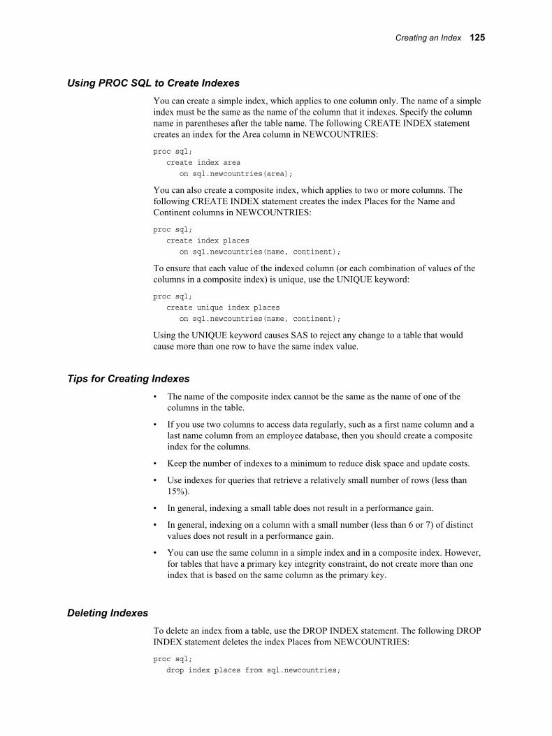
Using PROC SQL to Create IndexesYou can create a simple index, which applies to one column only. The name of a simple index must be the same as the name of the column that it indexes. Specify the column name in parentheses after the table name. The following CREATE INDEX statement creates an index for the Area column in NEWCOUNTRIES:

proc sql; create index area on sql.newcountries(area);

You can also create a composite index, which applies to two or more columns. The following CREATE INDEX statement creates the index Places for the Name and Continent columns in NEWCOUNTRIES:

proc sql; create index places on sql.newcountries(name, continent);

To ensure that each value of the indexed column (or each combination of values of the columns in a composite index) is unique, use the UNIQUE keyword:

proc sql; create unique index places on sql.newcountries(name, continent);

Using the UNIQUE keyword causes SAS to reject any change to a table that would cause more than one row to have the same index value.

Tips for Creating Indexes• The name of the composite index cannot be the same as the name of one of the

columns in the table.

• If you use two columns to access data regularly, such as a first name column and a last name column from an employee database, then you should create a composite index for the columns.

• Keep the number of indexes to a minimum to reduce disk space and update costs.

• Use indexes for queries that retrieve a relatively small number of rows (less than 15%).

• In general, indexing a small table does not result in a performance gain.

• In general, indexing on a column with a small number (less than 6 or 7) of distinct values does not result in a performance gain.

• You can use the same column in a simple index and in a composite index. However, for tables that have a primary key integrity constraint, do not create more than one index that is based on the same column as the primary key.

Deleting IndexesTo delete an index from a table, use the DROP INDEX statement. The following DROP INDEX statement deletes the index Places from NEWCOUNTRIES:

proc sql; drop index places from sql.newcountries;

Creating an Index 125

Deleting a TableTo delete a PROC SQL table, use the DROP TABLE statement:

proc sql; drop table sql.newcountries;

Using SQL Procedure Tables in SAS SoftwareBecause PROC SQL tables are SAS data files, you can use them as input to a DATA step or to other SAS procedures. For example, the following PROC MEANS step calculates the mean for Area for all countries in COUNTRIES:

proc means data=sql.countries mean maxdec=2; title "Mean Area for All Countries"; var area;run;

Output 4.11 Using a PROC SQL Table in PROC MEANS

Creating and Using Integrity Constraints in a Table

Integrity constraints are rules that you specify to guarantee the accuracy, completeness, or consistency of data in tables. All integrity constraints are enforced when you insert, delete, or alter data values in the columns of a table for which integrity constraints have been defined. Before a constraint is added to a table that contains existing data, all the data is checked to determine that it satisfies the constraints.

You can use general integrity constraints to verify that data in a column is one of the following:

• nonmissing

• unique


• both nonmissing and unique

• within a specified set or range of values

You can also apply referential integrity constraints to link the values in a specified column (called a primary key) of one table to values of a specified column in another table. When linked to a primary key, a column in the second table is called a foreign key.

When you define referential constraints, you can also choose what action occurs when a value in the primary key is updated or deleted.

• You can prevent the primary key value from being updated or deleted when matching values exist in the foreign key. This is the default.

• You can allow updates and deletions to the primary key values. By default, any affected foreign key values are changed to missing values. However, you can specify the CASCADE option to update foreign key values instead. Currently, the CASCADE option does not apply to deletions.

You can choose separate actions for updates and for deletions.

Note: Integrity constraints cannot be defined for views.

The following example creates integrity constraints for a table, MYSTATES, and another table, USPOSTAL. The constraints are as follows:

• state name must be unique and nonmissing in both tables

• population must be greater than 0

• continent must be either North America or Oceania

proc sql; create table sql.mystates (state char(15), population num, continent char(15),

/* contraint specifications */ constraint prim_key primary key(state), constraint population check(population gt 0), constraint continent check(continent in ('North America', 'Oceania')));

create table sql.uspostal (name char(15), code char(2) not null, /* constraint specified as */ /* a column attribute */ constraint for_key foreign key(name) /* links NAME to the */ references sql.mystates /* primary key in MYSTATES */

on delete restrict /* forbids deletions to STATE */ /* unless there is no */ /* matching NAME value */

on update set null); /* allows updates to STATE, */ /* changes matching NAME */ /* values to missing */

Creating and Using Integrity Constraints in a Table 127

The DESCRIBE TABLE statement displays the integrity constraints in the SAS log as part of the table description. The DESCRIBE TABLE CONSTRAINTS statement writes only the constraint specifications to the SAS log.

proc sql; describe table sql.mystates; describe table constraints sql.uspostal;

Log 4.5 SAS Log Showing Integrity Constraints

NOTE: SQL table SQL.MYSTATES was created like:

create table SQL.MYSTATES( bufsize=8192 ) ( state char(15), population num, continent char(15) );create unique index state on SQL.MYSTATES(state);

-----Alphabetic List of Integrity Constraints----- Integrity Where On On# Constraint Type Variables Clause Reference Delete Update--------------------------------------------------------------------------------49 continent Check continent in

('North America', 'Oceania') -48 population Check population>0

-47 prim_key Primary Key state

for_key Referential name SQL. Restrict Set Null USPOSTAL NOTE: SQL table SQL.USPOSTAL ( bufsize=8192 ) has the following integrity constraints:

-----Alphabetic List of Integrity Constraints----- Integrity On On # Constraint Type Variables Reference Delete Update ----------------------------------------------------------------------------- 1 _NM0001_ Not Null code 2 for_key Foreign Key name SQL.MYSTATES Restrict SetNull

Integrity constraints cannot be used in views. For more information about integrity constraints, see SAS Language Reference: Concepts.


Creating and Using PROC SQL Views

Overview of Creating and Using PROC SQL ViewsA PROC SQL view contains a stored query that is executed when you use the view in a SAS procedure or DATA step. Views are useful for the following reasons:

• often save space, because a view is frequently quite small compared with the data that it accesses

• prevent users from continually submitting queries to omit unwanted columns or row

• shield sensitive or confidential columns from users while enabling the same users to view other columns in the same table

• ensure that input data sets are always current, because data is derived from tables at execution time

• hide complex joins or queries from users

Creating ViewsTo create a PROC SQL view, use the CREATE VIEW statement, as shown in the following example:


proc sql; title 'Current Population Information for Continents'; create view sql.newcontinents as select continent, sum(population) as totpop format=comma15. label='Total Population', sum(area) as totarea format=comma15. label='Total Area' from sql.countries group by continent;

select * from sql.newcontinents;

Creating and Using PROC SQL Views 129

Output 4.12 An SQL Procedure View

Note: In this example, each column has a name. If you are planning to use a view in a procedure that requires variable names, then you must supply column aliases that you can reference as variable names in other procedures. For more information, see “Using SQL Procedure Views in SAS Software” on page 134.

Describing a ViewThe DESCRIBE VIEW statement writes a description of the PROC SQL view to the SAS log. The following SAS log describes the view NEWCONTINENTS, which is created in “Creating Views” on page 129:

proc sql; describe view sql.newcontinents;

Log 4.6 SAS Log from DESCRIBE VIEW Statement

NOTE: SQL view SQL.NEWCONTINENTS is defined as:

select continent, SUM(population) as totpop label='Total Population' format=COMMA15.0, SUM(area) as totarea label='Total Area' format=COMMA15.0 from SQL.COUNTRIES group by continent;

To define a password-protected SAS view, you must specify a password. If the SAS view was created with more than one password, you must specify its most restrictive password if you want to access a definition of the view.For more information, see “DESCRIBE Statement” on page 238.

Updating a ViewYou can update data through a PROC SQL and SAS/ACCESS view with the INSERT, DELETE, and UPDATE statements, under the following conditions.


• You can update only a single table through a view. The underlying table cannot be joined to another table or linked to another table with a set operator. The view cannot contain a subquery.

• If the view accesses a DBMS table, then you must have been granted the appropriate authorization by the external database management system (for example, ORACLE). You must have installed the SAS/ACCESS software for your DBMS. See the SAS/ACCESS documentation for your DBMS for more information about SAS/ACCESS views.

• You can update a column in a view by using the column's alias, but you cannot update a derived column, that is, a column that is produced by an expression. In the following example, you can update SquareMiles, but not Density:

proc sql; create view mycountries as select Name, area as SquareMiles, population/area as Density from sql.countries;

• You can update a view that contains a WHERE clause. The WHERE clause can be in the UPDATE clause or in the view. You cannot update a view that contains any other clause, such as ORDER BY, HAVING, and so on.

Embedding a LIBNAME in a ViewYou can embed a SAS LIBNAME statement or a SAS/ACCESS LIBNAME statement in a view by using the USING LIBNAME clause. When PROC SQL executes the view, the stored query assigns the libref. For SAS/ACCESS librefs, PROC SQL establishes a connection to a DBMS. The scope of the libref is local to the view and does not conflict with any identically named librefs in the SAS session. When the query finishes, the libref is disassociated. The connection to the DBMS is terminated and all data in the library becomes unavailable.

The advantage of embedded librefs is that you can store engine-host options and DBMS connection information, such as passwords, in the view. That, in turn, means that you do not have to remember and reenter that information when you want to use the libref.

Note: The USING LIBNAME clause must be the last clause in the SELECT statement. Multiple clauses can be specified, separated by commas.

In the following example, the libref OILINFO is assigned and a connection is made to an ORACLE database:

proc sql; create view sql.view1 as select * from oilinfo.reserves as newreserves using libname oilinfo oracle user=username pass=password path='dbms-path';

For more information about the SAS/ACCESS LIBNAME statement, see the SAS/ACCESS documentation for your DBMS.

The following example embeds a SAS LIBNAME statement in a view:

proc sql;


create view sql.view2 as select * from oil.reserves using libname oil 'SAS-data-library';

Deleting a ViewTo delete a view, use the DROP VIEW statement:

proc sql; drop view sql.newcontinents;

Specifying In-Line ViewsIn some cases, you might want to use a query in a FROM clause instead of a table or view. You could create a view and refer to it in your FROM clause, but that process involves two steps. To save the extra step, specify the view in-line, enclosed in parentheses, in the FROM clause.

An in-line view is a query that appears in the FROM clause. An in-line view produces a table internally that the outer query uses to select data. Unlike views that are created with the CREATE VIEW statement, in-line views are not assigned names and cannot be referenced in other queries or SAS procedures as if they were tables. An in-line view can be referenced only in the query in which it is defined.

In the following query, the populations of all Caribbean and Central American countries are summed in an in-line query. The WHERE clause compares the sum with the populations of individual countries. Only countries that have a population greater than the sum of Caribbean and Central American populations are displayed.


proc sql; title 'Countries With Population GT Caribbean Countries'; select w.Name, w.Population format=comma15., c.TotCarib from (select sum(population) as TotCarib format=comma15. from sql.countries where continent = 'Central America and Caribbean') as c, sql.countries as w where w.population gt c.TotCarib;


Output 4.13 Using an In-Line View

Tips for Using SQL Procedure Views• Avoid using an ORDER BY clause in a view. If you specify an ORDER BY clause,

then the data must be sorted each time that the view is referenced.

• If data is used many times in one program or in multiple programs, then it is more efficient to create a table rather than a view. If a view is referenced often in one program, then the data must be accessed at each reference.

• If the view resides in the same SAS library as the contributing table or tables, then specify a one-level name in the FROM clause. The default for the libref for the FROM clause's table or tables is the libref of the library that contains the view. This prevents you from having to change the view if you assign a different libref to the SAS library that contains the view and its contributing table or tables. This tip is used in the view that is described in “Creating Views” on page 129.

• Avoid creating views that are based on tables whose structure might change. A view is no longer valid when it references a nonexistent column.

• When you process PROC SQL views between a client and a server, getting the correct results depends on the compatibility between the client and server architecture. For more information, see “Accessing a SAS View” in Chapter 17 of SAS/CONNECT User's Guide.


Using SQL Procedure Views in SAS SoftwareYou can use PROC SQL views as input to a DATA step or to other SAS procedures. The syntax for using a PROC SQL view in SAS is the same as that for a PROC SQL table. For an example, see “Using SQL Procedure Tables in SAS Software” on page 126.


Chapter 5

Programming with the SQL Procedure

Introduction . . . . . . . . . . . . . . . . . . . . . . . . . . . . . . . . . . . . . . . . . . . . . . . . . . . . . . . . . 136

Using PROC SQL Options to Create and Debug Queries . . . . . . . . . . . . . . . . . . . 136Overview of Using PROC SQL Options to Create and Debug Queries . . . . . . . . . 136Restricting Row Processing with the INOBS= and OUTOBS= Options . . . . . . . . 136Limiting Iterations with the LOOPS= Option . . . . . . . . . . . . . . . . . . . . . . . . . . . . 137Checking Syntax with the NOEXEC Option and the VALIDATE Statement . . . . 137Expanding SELECT * with the FEEDBACK Option . . . . . . . . . . . . . . . . . . . . . . 138Timing PROC SQL with the STIMER Option . . . . . . . . . . . . . . . . . . . . . . . . . . . . 138Resetting PROC SQL Options with the RESET Statement . . . . . . . . . . . . . . . . . . 139

Improving Query Performance . . . . . . . . . . . . . . . . . . . . . . . . . . . . . . . . . . . . . . . . . 140Overview of Improving Query Performance . . . . . . . . . . . . . . . . . . . . . . . . . . . . . 140Using Indexes to Improve Performance . . . . . . . . . . . . . . . . . . . . . . . . . . . . . . . . . 140Using the Keyword ALL in Set Operations . . . . . . . . . . . . . . . . . . . . . . . . . . . . . . 141Omitting the ORDER BY Clause When Creating Tables and Views . . . . . . . . . . 141Using In-Line Views versus Temporary Tables . . . . . . . . . . . . . . . . . . . . . . . . . . . 141Comparing Subqueries with Joins . . . . . . . . . . . . . . . . . . . . . . . . . . . . . . . . . . . . . 141Using WHERE Expressions with Joins . . . . . . . . . . . . . . . . . . . . . . . . . . . . . . . . . 141Optimizing the PUT Function . . . . . . . . . . . . . . . . . . . . . . . . . . . . . . . . . . . . . . . . 142Replacing References to the DATE, TIME, DATETIME, and

TODAY Functions . . . . . . . . . . . . . . . . . . . . . . . . . . . . . . . . . . . . . . . . . . . . . . . 144Disabling the Remerging of Data When Using Summary Functions . . . . . . . . . . . 144

Accessing SAS System Information by Using DICTIONARY Tables . . . . . . . . . . 144What Are Dictionary Tables? . . . . . . . . . . . . . . . . . . . . . . . . . . . . . . . . . . . . . . . . . 144Retrieving Information about DICTIONARY Tables and SASHELP Views . . . . 146Using DICTIONARY.TABLES . . . . . . . . . . . . . . . . . . . . . . . . . . . . . . . . . . . . . . . 148Using DICTIONARY.COLUMNS . . . . . . . . . . . . . . . . . . . . . . . . . . . . . . . . . . . . 149DICTIONARY Tables and Performance . . . . . . . . . . . . . . . . . . . . . . . . . . . . . . . . 150

Using SAS Data Set Options with PROC SQL . . . . . . . . . . . . . . . . . . . . . . . . . . . . 151

Using PROC SQL with the SAS Macro Facility . . . . . . . . . . . . . . . . . . . . . . . . . . . 152Overview of Using PROC SQL with the SAS Macro Facility . . . . . . . . . . . . . . . . 152Creating Macro Variables in PROC SQL . . . . . . . . . . . . . . . . . . . . . . . . . . . . . . . . 152Concatenating Values in Macro Variables . . . . . . . . . . . . . . . . . . . . . . . . . . . . . . . 155Defining Macros to Create Tables . . . . . . . . . . . . . . . . . . . . . . . . . . . . . . . . . . . . . 156Using the PROC SQL Automatic Macro Variables . . . . . . . . . . . . . . . . . . . . . . . . 157

Formatting PROC SQL Output by Using the REPORT Procedure . . . . . . . . . . . 160

Accessing a DBMS with SAS/ACCESS Software . . . . . . . . . . . . . . . . . . . . . . . . . . 162Overview of Accessing a DBMS with SAS/ACCESS Software . . . . . . . . . . . . . . 162Connecting to a DBMS by Using the LIBNAME Statement . . . . . . . . . . . . . . . . . 163

135

Connecting to a DBMS by Using the SQL Procedure Pass-Through Facility . . . . 166Updating PROC SQL and SAS/ACCESS Views . . . . . . . . . . . . . . . . . . . . . . . . . . 168

Using the Output Delivery System with PROC SQL . . . . . . . . . . . . . . . . . . . . . . . 169

Introduction

This section shows you how to do the following:

• use PROC SQL options to create and debug queries

• improve query performance

• access dictionary tables and how they are useful in gathering information about the elements of SAS

• use PROC SQL with the SAS macro facility

• use PROC SQL with the REPORT procedure

• access DBMSs by using SAS/ACCESS software

• format PROC SQL output by using the SAS Output Delivery System (ODS)

Using PROC SQL Options to Create and Debug Queries

Overview of Using PROC SQL Options to Create and Debug QueriesPROC SQL supports options that can give you greater control over PROC SQL while you are developing a query:

• The INOBS=, OUTOBS=, and LOOPS= options reduce query execution time by limiting the number of rows and the number of iterations that PROC SQL processes.

• The EXEC and VALIDATE statements enable you to quickly check the syntax of a query.

• The FEEDBACK option expands a SELECT * statement into a list of columns that the statement represents.

• The PROC SQL STIMER option records and displays query execution time.

You can set an option initially in the PROC SQL statement, and then use the RESET statement to change the same option's setting without ending the current PROC SQL step.

Restricting Row Processing with the INOBS= and OUTOBS= Options

When you are developing queries against large tables, you can reduce the time that it takes for the queries to run by reducing the number of rows that PROC SQL processes. Subsetting the tables with WHERE statements is one way to do this. Using the INOBS= and the OUTOBS= options are other ways.

136 Chapter 5 • Programming with the SQL Procedure

The INOBS= option restricts the number of rows that PROC SQL takes as input from any single source. For example, if you specify INOBS=10, then PROC SQL uses only 10 rows from any table or view that is specified in a FROM clause. If you specify INOBS=10 and join two tables without using a WHERE clause, then the resulting table (Cartesian product) contains a maximum of 100 rows. The INOBS= option is similar to the SAS system option OBS=.

The OUTOBS= option restricts the number of rows that PROC SQL displays or writes to a table. For example, if you specify OUTOBS=10 and insert values into a table by using a query, then PROC SQL inserts a maximum of 10 rows into the resulting table. OUTOBS= is similar to the SAS data set option OBS=.

In a simple query, there might be no apparent difference between using INOBS or OUTOBS. However, at other times it is important to choose the correct option. For example, taking the average of a column with INOBS=10 returns an average of only 10 values from that column.

Limiting Iterations with the LOOPS= OptionThe LOOPS= option restricts PROC SQL to the number of iterations that are specified in this option through its inner loop. By setting a limit, you can prevent queries from consuming excessive computer resources. For example, joining three large tables without meeting the join-matching conditions could create a huge internal table that would be inefficient to process. Use the LOOPS= option to prevent this from happening.

You can use the number of iterations that are reported in the SQLOOPS macro variable (after each PROC SQL statement is executed) to gauge an appropriate value for the LOOPS= option. For more information, see “Using the PROC SQL Automatic Macro Variables” on page 157.

If you use the PROMPT option with the INOBS=, OUTOBS=, or LOOPS= options, you are prompted to stop or continue processing when the limits set by these options are reached.

Checking Syntax with the NOEXEC Option and the VALIDATE Statement

To check the syntax of a PROC SQL step without actually executing it, use the NOEXEC option or the VALIDATE statement. The NOEXEC option can be used once in the PROC SQL statement, and the syntax of all queries in that PROC SQL step will be checked for accuracy without executing them. The VALIDATE statement must be specified before each SELECT statement in order for that statement to be checked for accuracy without executing. If the syntax is valid, then a message is written to the SAS log to that effect. If the syntax is invalid, then an error message is displayed. The automatic macro variable SQLRC contains an error code that indicates the validity of the syntax. For an example of the VALIDATE statement used in PROC SQL, see “Validating a Query” on page 71. For an example of using the VALIDATE statement in a SAS/AF application, see “Using the PROC SQL Automatic Macro Variables” on page 157.

Note: There is an interaction between the PROC SQL EXEC and ERRORSTOP options when SAS is running in a batch or noninteractive session. For more information, see Chapter 7, “SQL Procedure,” on page 209.

Using PROC SQL Options to Create and Debug Queries 137

Expanding SELECT * with the FEEDBACK OptionThe FEEDBACK option expands a SELECT * (ALL) statement into the list of columns that the statement represents. Any PROC SQL view is expanded into the underlying query, all expressions are enclosed in parentheses to indicate their order of evaluation, and the PUT function optimizations that are performed on the query are displayed. The FEEDBACK option also displays the resolved values of macros and macro variables.

For example, the following query is expanded in the SAS log:


proc sql feedback; select * from sql.countries;

Log 5.1 Expanded SELECT * Statement

NOTE: Statement transforms to:

select COUNTRIES.Name, COUNTRIES.Capital, COUNTRIES.Population, COUNTRIES.Area, COUNTRIES.Continent, COUNTRIES.UNDate from SQL.COUNTRIES;

Timing PROC SQL with the STIMER OptionCertain operations can be accomplished in more than one way. For example, there is often a join equivalent to a subquery. Consider factors such as readability and maintenance, but generally you will choose the query that runs fastest. The SAS system option STIMER shows you the cumulative time for an entire procedure. The PROC SQL STIMER option shows you how fast the individual statements in a PROC SQL step are running. This enables you to optimize your query.

Note: For the PROC SQL STIMER option to work, the SAS system option STIMER must also be specified.

This example compares the execution times of two queries. Both queries list the names and populations of states in the UNITEDSTATES table that have a larger population than Belgium. The first query does this with a join; the second with a subquery. Log 5.2 on page 139 shows the STIMER results from the SAS log.


proc sql stimer ; select us.name, us.population from sql.unitedstates as us, sql.countries as w where us.population gt w.population and w.name = 'Belgium'; select Name, population from sql.unitedstates where population gt (select population from sql.countries where name = 'Belgium');


Log 5.2 Comparing Run Times of Two Queries

4 proc sql stimer ;NOTE: SQL Statement used: real time 0.00 seconds cpu time 0.01 seconds 5 select us.name, us.population6 from sql.unitedstates as us, sql.countries as w7 where us.population gt w.population and8 w.name = 'Belgium';NOTE: The execution of this query involves performing one or more Cartesian product joins that can not be optimized.NOTE: SQL Statement used: real time 0.10 seconds cpu time 0.05 seconds 9 10 select Name, population11 from sql.unitedstates12 where population gt13 (select population from sql.countries14 where name = 'Belgium');NOTE: SQL Statement used: real time 0.09 seconds cpu time 0.09 seconds

Compare the CPU time of the first query (that uses a join), 0.05 seconds, with 0.09 seconds for the second query (that uses a subquery). Although there are many factors that influence the run times of queries, generally a join runs faster than an equivalent subquery.

Resetting PROC SQL Options with the RESET StatementUse the RESET statement to add, drop, or change the options in the PROC SQL statement. You can list the options in any order in the PROC SQL and RESET statements. Options stay in effect until they are reset.

This example first uses the NOPRINT option to prevent the SELECT statement from displaying its result table in SAS output. The RESET statement then changes the NOPRINT option to PRINT (the default) and adds the NUMBER option, which displays the row number in the result table.

proc sql noprint; title 'Countries with Population Under 20,000'; select Name, Population from sql.countries;reset print number; select Name, Population from sql.countries where population lt 20000;

Using PROC SQL Options to Create and Debug Queries 139

Output 5.1 Resetting PROC SQL Options with the RESET Statement

Improving Query Performance

Overview of Improving Query PerformanceThere are several ways to improve query performance, including the following:

• using indexes and composite indexes

• using the keyword ALL in set operations when you know that there are no duplicate rows, or when it does not matter if you have duplicate rows in the result table

• omitting the ORDER BY clause when you create tables and views

• using in-line views instead of temporary tables (or vice versa)

• using joins instead of subqueries

• using WHERE expressions to limit the size of result tables that are created with joins

• using either PROC SQL options, SAS system options, or both to replace a PUT function in a query with a logically equivalent expression

• replacing references to the DATE, TIME, DATETIME, and TODAY functions in a query with their equivalent constant values before the query executes

• disabling the remerging of data when summary functions are used in a query

Using Indexes to Improve PerformanceIndexes are created with the CREATE INDEX statement in PROC SQL or with the MODIFY and INDEX CREATE statements in the DATASETS procedure. Indexes are stored in specialized members of a SAS library and have a SAS member type of INDEX. The values that are stored in an index are automatically updated if you make a change to the underlying data.

Indexes can improve the performance of certain classes of retrievals. For example, if an indexed column is compared to a constant value in a WHERE expression, then the index will likely improve the query's performance. Indexing the column that is specified in a correlated reference to an outer table also improves a subquery's (and hence, query's) performance. Composite indexes can improve the performance of queries that compare


the columns that are named in the composite index with constant values that are linked using the AND operator. For example, if you have a compound index in the columns CITY and STATE, and the WHERE expression is specified as WHERE CITY='xxx' AND STATE='yy', then the index can be used to select that subset of rows more efficiently. Indexes can also benefit queries that have a WHERE clause in this form:

... where var1 in (select item1 from table1) ...

The values of VAR1 from the outer query are found in the inner query by using the index. An index can improve the processing of a table join, if the columns that participate in the join are indexed in one of the tables. This optimization can be done for equijoin queries only—that is, when the WHERE expression specifies that table1.X=table2.Y.

Using the Keyword ALL in Set OperationsSet operators such as UNION, OUTER UNION, EXCEPT, and INTERSECT can be used to combine queries. Specifying the optional ALL keyword prevents the final process that eliminates duplicate rows from the result table. You should use the ALL form when you know that there are no duplicate rows or when it does not matter whether the duplicate rows remain in the result table.

Omitting the ORDER BY Clause When Creating Tables and ViewsIf you specify the ORDER BY clause when a table or view is created, then the data is always displayed in that order unless you specify another ORDER BY clause in a query that references that table or view. As with any sorting procedure, using ORDER BY when retrieving data has certain performance costs, especially on large tables. If the order of your output is not important for your results, then your queries will typically run faster without an ORDER BY clause.

Using In-Line Views versus Temporary TablesIt is often helpful when you are exploring a problem to break a query down into several steps and create temporary tables to hold the intermediate results. After you have worked through the problem, combining the queries into one query by using in-line views can be more efficient. However, under certain circumstances it is more efficient to use temporary tables. You should try both methods to determine which is more efficient for your case.

Comparing Subqueries with JoinsMany subqueries can also be expressed as joins. Generally, a join is processed at least as efficiently as the subquery. PROC SQL stores the result values for each unique set of correlation columns temporarily, thereby eliminating the need to calculate the subquery more than once.

Using WHERE Expressions with JoinsWhen joining tables, you should specify a WHERE expression. Joins without WHERE expressions are often time-consuming to evaluate because of the multiplier effect of the Cartesian product. For example, joining two tables of 1,000 rows each without specifying a WHERE expression or an ON clause, produces a result table with one million rows.

Improving Query Performance 141

PROC SQL executes and obtains the correct results in unbalanced WHERE expressions (or ON join expressions) in an equijoin, as shown here, but handles them inefficiently:

where table1.columnA-table2.columnB=0

It is more efficient to rewrite this clause to balance the expression so that columns from each table are on alternate sides of the equals condition:

where table1.columnA=table2.columnB

PROC SQL sequentially processes joins that do not have an equijoin condition evaluating each row against the WHERE expression: that is, joins without an equijoin condition are not evaluated using sort-merge or index-lookup techniques. Evaluating left and right outer joins is generally comparable to, or only slightly slower than, a standard inner join. A full outer join usually requires two passes over both tables in the join, although PROC SQL tries to store as much data as possible in buffers. Thus for small tables, an outer join might be processed with only one physical read of the data.

Optimizing the PUT Function

Reducing the PUT FunctionThere are several ways that you can improve the performance of a query by optimizing the PUT function. If you reference tables in a database, eliminating references to PUT functions can enable more of the query to be passed to the database. It can simplify SELECT statement evaluation for the default Base SAS engine.

There are five possible evaluations that are performed when optimizing the PUT function:

• Functions, including PUT, that contain literal values.

• PUT functions in the WHERE and HAVING clauses that contain formats that are supplied by SAS.

• PUT functions in the WHERE and HAVING clauses that contain user-defined formats.

• PUT functions in any part of the SELECT statement that contain user-defined formats that are defined with an OTHER= clause.

• PUT functions that are deployed inside the database.

Controlling PUT Function Optimization• If you specify either the PROC SQL REDUCEPUT= option or the

SQLREDUCEPUT= system option, SAS optimizes the PUT function before the query is executed.

The following SELECT statements are examples of queries that would be optimized:

select x, y from sqllibb where (PUT(x, abc.) in ('yes', 'no'));select x from sqlliba where (PUT(x, udfmt.) = trim(left('small')));

• For databases that allow implicit pass-through when the row count for a table is not known, PROC SQL allows the optimization in order for the query to be executed by the database. When the PROC SQL REDUCEPUT= option or the SQLREDUCEPUT= system option is set to DBMS, BASE, or ALL, PROC SQL considers the value of the PROC SQL REDUCEPUTOBS= option or the SQLREDUCEPUTOBS= system option and determines whether to optimize the PUT function. The PROC SQL REDUCEPUTOBS= option or the SQLREDUCEPUTOBS= system option specifies the minimum number of rows that


must be in a table in order for PROC SQL to consider optimizing the PUT function in a query. For databases that do not allow implicit pass-through, PROC SQL does not perform the optimization, and more of the query is performed by SAS.

• Some formats, especially user-defined formats, can contain many format values. Depending on the number of matches for a given PUT function expression, the resulting expression can list many format values. If the number of format values becomes too large, the query performance can degrade. When the PROC SQL REDUCEPUT= option or the SQLREDUCEPUT= system option is set to DBMS, BASE, or ALL, PROC SQL considers the value of the PROC SQL REDUCEPUTVALUES= option or the SQLREDUCEPUTVALUES= system option and determines whether to optimize the PUT function in a query. For databases that do not allow implicit pass-through, PROC SQL does not perform the optimization, and more of the query is performed by SAS.

For more information, see the REDUCEPUT=, REDUCEPUTOBS=, and REDUCEPUTVALUES= options in Chapter 7, “SQL Procedure,” on page 209, and the SQLREDUCEPUT=, SQLREDUCEPUTOBS=, and SQLREDUCEPUTVALUES= system options in Appendix 1, “SQL Macro Variables and System Options,” on page 363.

Note: PROC SQL can consider both the REDUCEPUTOBS= and the REDUCEPUTVALUES= options (or SQLREDUCEPUTOBS= and SQLREDUCEPUTVALUES= system options) when trying to determine whether to optimize the PUT function.

Deploying the PUT Function and SAS Formats inside a DBMSSAS/ACCESS software for relational databases enables you to use the format publishing macro to deploy or publish the PUT function implementation to the database as a function named SAS_PUT(). As with any other programming function, the SAS_PUT() function can take one or more input parameters and return an output value. The default value for the SQLMAPPUTTO system option is SAS_PUT. After the SAS_PUT() function is deployed in the database, you can use the SAS_PUT() function as you would use any standard SQL function inside the database.

In addition, the SAS_PUT() function supports the use of SAS formats in SQL queries that are submitted to the database. You can use the format publishing macro to publish to the database both the formats that are supplied by SAS and the custom formats that you create with the FORMAT procedure.

By publishing the PUT function implementation to the database as the SAS_PUT() function to support the use of SAS formats, and by packaging both the formats that are supplied by SAS and the custom formats that you create with the FORMAT procedure, the following advantages are realized:

• The entire SQL query can be processed inside the database.

• The SAS format processing leverages the DBMS's scalable architecture.

• The results are grouped by the formatted data, and are extracted from the database.

Note: If you use the SQL_FUNCTIONS= LIBNAME statement option to remap the PUT function (for example, SAS_PUT( )), then the SQL_FUNCTIONS= LIBNAME option takes precedence over the SQLMAPPUTTO= system option. For more information, see “SQL_FUNCTIONS= LIBNAME Option” in SAS/ACCESS for Relational Databases: Reference.

T I P Using both the SQLREDUCEPUT= system option (or the PROC SQL REDUCEPUT= option) and the SAS_PUT() function can result in a significant performance boost.

Improving Query Performance 143

For more information about using the In-database format publishing macro and the SQLMAPPUTTO system option, see SAS/ACCESS for Relational Databases: Reference.

Replacing References to the DATE, TIME, DATETIME, and TODAY Functions

When the PROC SQL CONSTDATETIME option or the SQLCONSTDATETIME system option is set, PROC SQL evaluates the DATE, TIME, DATETIME, and TODAY functions in a query once, and uses those values throughout the query. Computing these values once ensures consistent results when the functions are used multiple times in a query, or when the query executes the functions close to a date or time boundary. When referencing database tables, performance is enhanced because it allows more of the query to be passed down to the database.

For more information, see the “SQLCONSTDATETIME System Option” on page 363or the CONSTDATETIME option in the Base SAS Procedures Guide.

Note: If you specify both the PROC SQL REDUCEPUT option or the SQLREDUCEPUT= system option and the PROC SQL CONSTDATETIME option or the SQLCONSTDATETIME system option, PROC SQL replaces the DATE, TIME, DATETIME, and TODAY functions with their respective values in order to determine the PUT function value before the query executes.

Disabling the Remerging of Data When Using Summary FunctionsWhen you use a summary function in a SELECT clause or a HAVING clause, PROC SQL might remerge the data. Remerging the data involves two passes through the data. If you set the PROC SQL NOREMERGE option or the NOSQLREMERGE system option, PROC SQL will not process the remerging of data. When referencing database tables, performance is enhanced because it enables more of the query to be passed down to the database.

For more information, see the PROC SQL statement REMERGE option in the Base SAS Procedures Guide and the SQLREMERGE system option in Appendix 1, “SQL Macro Variables and System Options,” on page 363.

Accessing SAS System Information by Using DICTIONARY Tables

What Are Dictionary Tables?DICTIONARY tables are special read-only PROC SQL tables or views. They retrieve information about all the SAS libraries, SAS data sets, SAS system options, and external files that are associated with the current SAS session. For example, the DICTIONARY.COLUMNS table contains information such as name, type, length, and format, about all columns in all tables that are known to the current SAS session.

PROC SQL automatically assigns the DICTIONARY libref. To get information from DICTIONARY tables, specify DICTIONARY.table-name in the FROM clause in a SELECT statement in PROC SQL.


DICTIONARY.table-name is valid in PROC SQL only. However, SAS provides PROC SQL views, based on the DICTIONARY tables, that can be used in other SAS procedures and in the DATA step. These views are stored in the SASHELP library and are commonly called “SASHELP views.”

For an example of a DICTIONARY table, see “Example 6: Reporting from DICTIONARY Tables” on page 258.

The following table describes the DICTIONARY tables that are available and shows the associated SASHELP views for each table.

Table 5.1 DICTIONARY Tables and Associated SASHELP Views

DICTIONARY TableSASHELP View Description

CATALOGS VCATALG Contains information about known SAS catalogs.

CHECK_CONSTRAINTS VCHKCON Contains information about known check constraints.

COLUMNS VCOLUMN Contains information about columns in all known tables.

CONSTRAINT_COLUMN_USAGE VCNCOLU Contains information about columns that are referred to by integrity constraints.

CONSTRAINT_TABLE_USAGE VCNTABU Contains information about tables that have integrity constraints defined on them.

DATAITEMS VDATAIT Contains information about known information map data items.

DESTINATIONS VDEST Contains information about known ODS destinations.

DICTIONARIES VDCTNRY Contains information about all DICTIONARY tables.

ENGINES VENGINE Contains information about SAS engines.

EXTFILES VEXTFL Contains information about known external files.

FILTERS VFILTER Contains information about known information map filters.

FORMATS VFORMAT

VCFORMAT

Contains information about currently accessible formats and informats.

FUNCTIONS VFUNC Contains information about currently accessible functions.

GOPTIONS VGOPT

VALLOPT

Contains information about currently defined graphics options (SAS/GRAPH software). SASHELP.VALLOPT includes SAS system options as well as graphics options.

INDEXES VINDEX Contains information about known indexes.

INFOMAPS VINFOMP Contains information about known information maps.

Accessing SAS System Information by Using DICTIONARY Tables 145

DICTIONARY TableSASHELP View Description

LIBNAMES VLIBNAM Contains information about currently defined SAS libraries.

MACROS VMACRO Contains information about currently defined macro variables.

MEMBERS VMEMBER

VSACCES

VSCATLG

VSLIB

VSTABLE

VSTABVW

VSVIEW

Contains information about all objects that are in currently defined SAS libraries. SASHELP.VMEMBER contains information for all member types; the other SASHELP views are specific to particular member types (such as tables or views).

OPTIONS VOPTION

VALLOPT

Contains information about SAS system options. SASHELP.VALLOPT includes graphics options as well as SAS system options.

REFERENTIAL_CONSTRAINTS VREFCON Contains information about referential constraints.

REMEMBER VREMEMB Contains information about known remembers.

STYLES VSTYLE Contains information about known ODS styles.

TABLE_CONSTRAINTS VTABCON Contains information about integrity constraints in all known tables.

TABLES VTABLE Contains information about known tables.

TITLES VTITLE Contains information about currently defined titles and footnotes.

VIEWS VVIEW Contains information about known data views.

VIEW_SOURCES Not available Contains a list of tables (or other views) referenced by the SQL or DATASTEP view, and a count of the number of references.

Retrieving Information about DICTIONARY Tables and SASHELP Views

To see how each DICTIONARY table is defined, submit a DESCRIBE TABLE statement. This example shows the definition of DICTIONARY.TABLES:

proc sql; describe table dictionary.tables;

The results are written to the SAS log.


Log 5.3 Definition of DICTIONARY.TABLES

NOTE: SQL table DICTIONARY.TABLES was created like:

create table DICTIONARY.TABLES ( libname char(8) label='Library Name', memname char(32) label='Member Name', memtype char(8) label='Member Type', dbms_memtype char(32) label='DBMS Member Type', memlabel char(256) label='Data Set Label', typemem char(8) label='Data Set Type', crdate num format=DATETIME informat=DATETIME label='Date Created', modate num format=DATETIME informat=DATETIME label='Date Modified', nobs num label='Number of Physical Observations', obslen num label='Observation Length', nvar num label='Number of Variables', protect char(3) label='Type of Password Protection', compress char(8) label='Compression Routine', encrypt char(8) label='Encryption', npage num label='Number of Pages', filesize num label='Size of File', pcompress num label='Percent Compression', reuse char(3) label='Reuse Space', bufsize num label='Bufsize', delobs num label='Number of Deleted Observations', nlobs num label='Number of Logical Observations', maxvar num label='Longest variable name', maxlabel num label='Longest label', maxgen num label='Maximum number of generations', gen num label='Generation number', attr char(3) label='Data Set Attributes', indxtype char(9) label='Type of Indexes', datarep char(32) label='Data Representation', sortname char(8) label='Name of Collating Sequence', sorttype char(4) label='Sorting Type', sortchar char(8) label='Charset Sorted By', reqvector char(24) format=$HEX48 informat=$HEX48 label='Requirements Vector', datarepname char(170) label='Data Representation Name', encoding char(256) label='Data Encoding', audit char(8) label='Audit Trail Active?', audit_before char(8) label='Audit Before Image?', audit_admin char(8) label='Audit Admin Image?', audit_error char(8) label='Audit Error Image?', audit_data char(8) label='Audit Data Image?', num_character num label='Number of Character Variables', num_numeric num label='Number of Numeric Variables' );

Similarly, you can use the DESCRIBE VIEW statement in PROC SQL to determine how a SASHELP view is defined. Here is an example:

proc sql; describe view sashelp.vtable;


Log 5.4 Description of SASHELP.VTABLE

NOTE: SQL view SASHELP.VSTABVW is defined as:

select libname, memname, memtype from DICTIONARY.MEMBERS where (memtype='VIEW') or (memtype='DATA') order by libname asc, memname asc;

Using DICTIONARY.TABLESDICTIONARY tables are commonly used to monitor and manage SAS sessions because the data is more easily manipulated than the output from other sources such as PROC DATASETS. You can query DICTIONARY tables the same way you query any other table, including subsetting with a WHERE clause, ordering the results, and creating PROC SQL views.

Note that many character values in the DICTIONARY tables are stored as all-uppercase characters; you should design your queries accordingly.

Because DICTIONARY tables are read-only objects, you cannot insert rows or columns, alter column attributes, or add integrity constraints to them.

Note: For DICTIONARY.TABLES and SASHELP.VTABLE, if a table is read-protected with a password, then the only information that is listed for that table is the library name, member name, member type, and type of password protection. All other information is set to missing.

Note: An error occurs if DICTIONARY.TABLES is used to retrieve information about an SQL view that exists in one library but has an input table from a second library that has not been assigned.

The following query uses a SELECT and subsetting WHERE clause to retrieve information about permanent tables and views that appear in the SQL library:

libname sql '\\sashq\root\pub\pubdoc\doc\901\authoring\sqlproc\miscsrc\sasfiles\';options nodate nonumber linesize=80 pagesize=60;


proc sql; title 'All Tables and Views in the SQL Library'; select libname, memname, memtype, nobs from dictionary.tables where libname='SQL';


Output 5.2 Tables and Views Used in This Document

Using DICTIONARY.COLUMNSDICTIONARY tables are useful when you want to find specific columns to include in reports. The following query shows which of the tables that are used in this document contain the Country column:



proc sql; title 'All Tables That Contain the Country Column'; select libname, memname, name from dictionary.columns where name='Country' and libname='SQL';

Output 5.3 Using DICTONARY.COLUMNS to Locate Specific Columns

DICTIONARY Tables and PerformanceWhen querying a DICTIONARY table, SAS launches a discovery process that gathers information that is pertinent to that table. Depending on the DICTIONARY table that is being queried, this discovery process can search libraries, open tables, and execute views. Unlike other SAS procedures and the DATA step, PROC SQL can mitigate this process by optimizing the query before the discovery process is launched. Therefore, although it is possible to access DICTIONARY table information with SAS procedures or the DATA step by using the SASHELP views, it is often more efficient to use PROC SQL instead.

Note: You cannot use data set options with DICTIONARY tables.

For example, the following programs produce the same result, but the PROC SQL step runs much faster because the WHERE clause is processed before the tables that are referenced by the SASHELP.VCOLUMN view are opened:

data mytable; set sashelp.vcolumn; where libname='WORK' and memname='SALES';run;

proc sql; create table mytable as select * from sashelp.vcolumn where libname='WORK' and memname='SALES';quit;

Note: SAS does not maintain DICTIONARY table information between queries. Each query of a DICTIONARY table launches a new discovery process.

If you are querying the same DICTIONARY table several times in a row, then you can get even faster performance by creating a temporary SAS data set (with the DATA step SET statement or the PROC SQL CREATE TABLE AS statement) with the information that you want and running your query against that data set.


When you query DICTIONARY.TABLES or SASHELP.VTABLE, all the tables and views in all the libraries that are assigned to the SAS session are opened to retrieve the requested information.

You can use a WHERE clause to help restrict which libraries are searched. However, the WHERE clause will not process most function calls such as UPCASE.

For example, if where UPCASE (libname) ='WORK' is used, the UPCASE function prevents the WHERE clause from optimizing this condition. All libraries that are assigned to the SAS session are searched. Searching all the libraries could cause an unexpected increase in search time, depending on the number of libraries that are assigned to the SAS session.

All librefs and SAS table names are stored in uppercase. If you supply values for LIBNAME and MEMNAME values in uppercase, and you remove the UPCASE function, the WHERE clause will be optimized and performance will be improved. In the previous example, the code would be changed to where libname='WORK'.

Note: If you query table information from a library that is assigned to an external database, and you use the LIBNAME statement PRESERVE_TAB_NAMES=YES option or the PRESERVE_COL_NAMES=YES option, and you provide the table or column name as it appears in the database, you do not need to use the UPCASE function.

Using SAS Data Set Options with PROC SQLIn PROC SQL, you can apply most of the SAS data set options, such as KEEP= and DROP=, to tables or SAS/ACCESS views any time you specify a table or SAS/ACCESS view. In the SQL procedure, SAS data set options that are separated by spaces are enclosed in parentheses. The data set options immediately follow the table or SAS/ACCESS view name. In the following PROC SQL step, the RENAME= data set option renames LNAME to LASTNAME for the STAFF1 table. The OBS= data set option restricts the number of rows that are read from STAFF1 to 15:

proc sql; create table staff1(rename=(lname=lastname)) as select * from staff(obs=15);

SAS data set options can be combined with SQL statement arguments. In the following PROC SQL step, the PW= data set option assigns a password to the TEST table, and the ALTER= data set option assigns an ALTER password to the STAFF1 table:

proc sql; create table test (a character, b numeric, pw=cat); create index staffidx on staff1 (lastname, alter=dog);

In this PROC SQL step, the PW= data set option assigns a password to the ONE table. The password is used when inserting a row and updating the table.

proc sql; create table one(pw=red, col1 num, col2 num, col3 num); quit;

Using SAS Data Set Options with PROC SQL 151

proc sql; insert into one(pw=red, col1, col3) values(1, 3);quit;proc sql; update one(pw=red) set col2 = 22 where col2 = . ;quit;

You cannot use SAS data set options with DICTIONARY tables because DICTIONARY tables are read-only objects.

The only SAS data set options that you can use with PROC SQL views are data set options that assign and provide SAS passwords: READ=, WRITE=, ALTER=, and PW=.

For more information about SAS data set options, see SAS Data Set Options: Reference.

Using PROC SQL with the SAS Macro Facility

Overview of Using PROC SQL with the SAS Macro FacilityThe macro facility is a programming tool that you can use to extend and customize SAS software. The macro facility reduces the amount of text that you must enter to perform common or repeated tasks and improves the efficiency and usefulness of your SQL programs.

The macro facility enables you to assign a name to character strings or groups of SAS programming statements. Thereafter, you can work with the names rather than with the text itself. For more information about the SAS macro facility, see SAS Macro Language: Reference.

Macro variables provide an efficient way to replace text strings in SAS code. The macro variables that you create and name are called user-defined macro variables. The macros variables that are defined by SAS are called automatic macro variables. PROC SQL produces six automatic macro variables (SQLOBS, SQLRC, SQLOOPS, SQLEXITCODE, SQLXRC, and SQLXMSG) to help you troubleshoot your programs. For more information, see “Using the PROC SQL Automatic Macro Variables” on page 157.

Creating Macro Variables in PROC SQL

Overview of Creating Macro Variables in PROC SQLOther software vendors' SQL products allow the embedding of SQL into another language. References to variables (columns) of that language are termed host-variable references. They are differentiated from references to columns in tables by names that are prefixed with a colon. The host-variable stores the values of the object-items that are listed in the SELECT clause.

The only host language that is currently available in SAS is the macro language, which is part of Base SAS software. When a calculation is performed on a column's value, its result can be stored, using :macro-variable, in the macro facility. The result can then be referenced by that name in another PROC SQL query or SAS procedure. Host-variable


can be used only in the outer query of a SELECT statement, not in a subquery. Host-variable cannot be used in a CREATE statement.

If the query produces more than one row of output, then the macro variable will contain only the value from the first row. If the query has no rows in its output, then the macro variable is not modified. If the macro variable does not exist yet, it will not be created. The PROC SQL macro variable SQLOBS contains the number of rows that are produced by the query.

Note: The SQLOBS automatic macro variable is assigned a value after the SQL SELECT statement executes.

Creating Macro Variables from the First Row of a Query ResultIf you specify a single macro variable in the INTO clause, then PROC SQL assigns the variable the value from the first row only of the appropriate column in the SELECT list. In this example, &country1 is assigned the value from the first row of the Country column, and &barrels1 is assigned the value from the first row of the Barrels column. The NOPRINT option prevents PROC SQL from displaying the results of the query. The %PUT statement writes the contents of the macro variables to the SAS log.


proc sql noprint; select country, barrels into :country1, :barrels1 from sql.oilrsrvs; %put &country1 &barrels1;

Log 5.5 Creating Macro Variables from the First Row of a Query Result

4 proc sql noprint;5 select country, barrels6 into :country1, :barrels1 7 from sql.oilrsrvs;8 9 %put &country1 &barrels1;Algeria 9,200,000,000NOTE: PROCEDURE SQL used: real time 0.12 seconds

Creating a Macro Variable from the Result of an Aggregate FunctionA useful feature of macro variables is that they enable you to display data values in SAS titles. The following example prints a subset of the WORLDTEMPS table and lists the highest temperature in Canada in the title:


proc sql outobs=12; reset noprint; select max(AvgHigh) into :maxtemp from sql.worldtemps where country = 'Canada';reset print; title "The Highest Temperature in Canada: &maxtemp"; select city, AvgHigh format 4.1

Using PROC SQL with the SAS Macro Facility 153

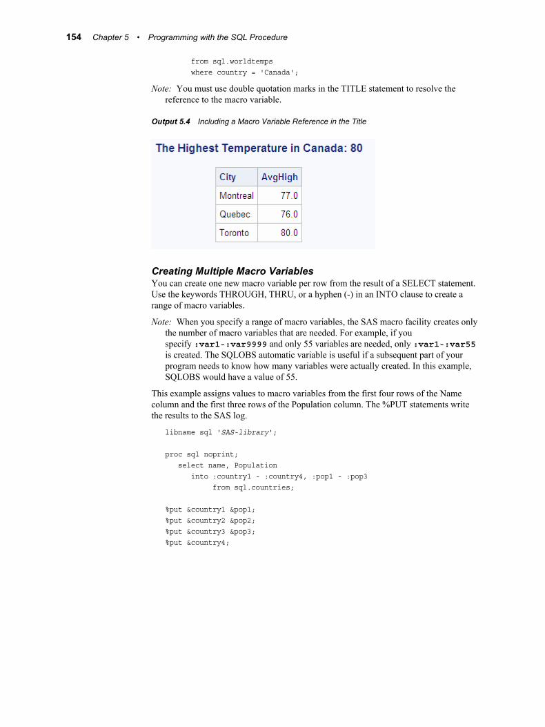
from sql.worldtemps where country = 'Canada';

Note: You must use double quotation marks in the TITLE statement to resolve the reference to the macro variable.

Output 5.4 Including a Macro Variable Reference in the Title

Creating Multiple Macro VariablesYou can create one new macro variable per row from the result of a SELECT statement. Use the keywords THROUGH, THRU, or a hyphen (-) in an INTO clause to create a range of macro variables.

Note: When you specify a range of macro variables, the SAS macro facility creates only the number of macro variables that are needed. For example, if you specify :var1-:var9999 and only 55 variables are needed, only :var1-:var55 is created. The SQLOBS automatic variable is useful if a subsequent part of your program needs to know how many variables were actually created. In this example, SQLOBS would have a value of 55.

This example assigns values to macro variables from the first four rows of the Name column and the first three rows of the Population column. The %PUT statements write the results to the SAS log.


proc sql noprint; select name, Population into :country1 - :country4, :pop1 - :pop3 from sql.countries;

%put &country1 &pop1;%put &country2 &pop2;%put &country3 &pop3;%put &country4;


Log 5.6 Creating Multiple Macro Variables

4 proc sql noprint;5 select name, Population6 into :country1 - :country4, :pop1 - :pop37 from sql.countries;8 9 %put &country1 &pop1;Afghanistan 1707032310 %put &country2 &pop2;Albania 340740011 %put &country3 &pop3;Algeria 2817113212 %put &country4;Andorra

Concatenating Values in Macro VariablesYou can concatenate the values of one column into one macro variable. This form is useful for building a list of variables or constants. Use the SEPARATED BY keywords to specify a character to delimit the values in the macro variable.

This example assigns the first five values from the Name column of the COUNTRIES table to the &countries macro variable. The INOBS option limits PROC SQL to using the first five rows of the COUNTRIES table. A comma and a space are used to delimit the values in the macro variable.


proc sql noprint inobs=5; select Name into :countries separated by ', ' from sql.countries;

%put &countries;

Log 5.7 Concatenating Values in Macro Variables

4 proc sql noprint inobs=5;5 select Name6 into :countries separated by ', '7 from sql.countries;WARNING: Only 5 records were read from SQL.COUNTRIES due to INOBS= option.8 9 %put &countries;Afghanistan, Albania, Algeria, Andorra, Angola

The leading and trailing blanks are trimmed from the values before the macro variables are created. If you do not want the blanks to be trimmed, then add NOTRIM to the INTO clause. Here is the previous example with NOTRIM added:


proc sql noprint inobs=5; select Name into :countries separated by ',' NOTRIM from sql.countries;


%put &countries;

Log 5.8 Concatenating Values in Macro Variables

1 proc sql noprint inobs=5;2 select Name3 into :countries separated by ',' NOTRIM4 from sql.countries;WARNING: Only 5 records were read from SQL.COUNTRIES due to INOBS= option.5 6 %put &countries;Afghanistan ,Albania ,Algeria ,Andorra ,Angola

Defining Macros to Create TablesMacros are useful as interfaces for table creation. You can use the SAS macro facility to help you create new tables and add rows to existing tables.

The following example creates a table that lists people to serve as referees for reviews of academic papers. No more than three people per subject are allowed in a table. The macro that is defined in this example checks the number of referees before it inserts a new referee's name into the table. The macro has two parameters: the referee's name and the subject matter of the academic paper.


proc sql;create table sql.referee (Name char(15), Subject char(15));

/* define the macro */%macro addref(name,subject);%local count;

/* are there three referees in the table? */reset noprint; select count(*) into :count from sql.referee where subject="&subject";

%if &count ge 3 %then %do; reset print; title "ERROR: &name not inserted for subject – &subject.."; title2 " There are 3 referees already."; select * from sql.referee where subject="&subject"; reset noprint; %end;

%else %do; insert into sql.referee(name,subject) values("&name","&subject"); %put NOTE: &name has been added for subject – &subject..; %end;


%mend;

Submit the %ADDREF() macro with its two parameters to add referee names to the table. Each time you submit the macro, a message is written to the SAS log.

%addref(Conner,sailing);%addref(Fay,sailing);%addref(Einstein,relativity);%addref(Smythe,sailing);%addref(Naish,sailing);

Log 5.9 Defining Macros to Create Tables

34 %addref(Conner,sailing);NOTE: 1 row was inserted into SQL.REFEREE.

NOTE: Conner has been added for subject - sailing.35 %addref(Fay,sailing);NOTE: 1 row was inserted into SQL.REFEREE.

NOTE: Fay has been added for subject - sailing.36 %addref(Einstein,relativity);NOTE: 1 row was inserted into SQL.REFEREE.

NOTE: Einstein has been added for subject - relativity.37 %addref(Smythe,sailing);NOTE: 1 row was inserted into SQL.REFEREE.

NOTE: Smythe has been added for subject - sailing.38 %addref(Naish,sailing);

The output has a row added with each execution of the %ADDREF() macro. When the table contains three referee names, it is displayed in SAS output with the message that it can accept no more referees.

Output 5.5 Result Table and Message Created with SAS Macro Language Interface

Using the PROC SQL Automatic Macro VariablesPROC SQL sets up macro variables with certain values after it executes each statement. These macro variables can be tested inside a macro to determine whether to continue executing the PROC SQL step.


After each PROC SQL statement has executed, the following macro variables are updated with these values:

SQLEXITCODEcontains the highest return code that occurred from some types of SQL insert failures. This return code is written to the SYSERR macro variable when PROC SQL terminates.

SQLOBScontains the number of rows that were processed by an SQL procedure statement. For example, the SQLOBS macro variable contains the number of rows that were formatted and displayed in SAS output by a SELECT statement or the number of rows that were deleted by a DELETE statement.

When the NOPRINT option is specified, the value of the SQLOBS macro variable depends on whether an output table, single macro variable, macro variable list, or macro variable range is created:

• If no output table, macro variable list, or macro variable range is created, then SQLOBS contains the value 1.

• If an output table is created, then SQLOBS contains the number of rows in the output table.

• If a single macro variable is created, then SQLOBS contains the value 1.

• If a macro variable list or macro variable range is created, then SQLOBS contains the number of rows that are processed to create the macro variable list or range.

If an SQL view is created, then SQLOBS contains the value 0.

Note: The SQLOBS automatic macro variable is assigned a value after the SQL SELECT statement executes.

SQLOOPScontains the number of iterations that the inner loop of PROC SQL processes. The number of iterations increases proportionally with the complexity of the query. For more information, see “Limiting Iterations with the LOOPS= Option” on page 137 and LOOPS= in the Base SAS Procedures Guide.

SQLRCcontains the following status values that indicate the success of the SQL procedure statement:

0PROC SQL statement completed successfully with no errors.

4PROC SQL statement encountered a situation for which it issued a warning. The statement continued to execute.

8PROC SQL statement encountered an error. The statement stopped execution at this point.

12PROC SQL statement encountered an internal error, indicating a bug in PROC SQL that should be reported to SAS Technical Support. These errors can occur only during compile time.


16PROC SQL statement encountered a user error. For example, this error code is used, when a subquery (that can return only a single value) evaluates to more than one row. These errors can be detected only during run time.

24PROC SQL statement encountered a system error. For example, this error is used, if the system cannot write to a PROC SQL table because the disk is full. These errors can occur only during run time.

28PROC SQL statement encountered an internal error, indicating a bug in PROC SQL that should be reported to SAS Technical Support. These errors can occur only during run time.

The value of SQLRC can vary based on the value of the PROC SQL statement UNDO_POLICY= option or the SQLUNDOPOLICY system option.

For example, the values for the SQLRC return code differ based on the value of the UNDO_POLICY= option or the SQLUNDOPOLICY system option if you attempt to insert duplicate values into an index that is defined using the CREATE UNIQUE INDEX statement:

• If you set the UNDO_POLICY= option or the SQLUNDOPOLICY system option to either REQUIRED or OPTIONAL, and you attempt to insert a duplicate index value, SAS creates and tries to maintain a copy of the table before and after updates are applied. SAS detects an error condition and supplies a return code to PROC SQL, which stops execution as soon as the error condition is received. SQLRC contains the value 24.

• If you set the UNDO_POLICY= option or the SQLUNDOPOLICY system option to NONE and you attempt to insert a duplicate index value, SAS does not create a before-and-after copy of the table. SAS does not detect an error condition and does not supply a return code to PROC SQL, which attempts to continue to process the updates. SQLRC contains the value 8.

SQLXMSGcontains descriptive information and the DBMS-specific return code for the error that is returned by the pass-through facility.

Note: Because the value of the SQLXMSG macro variable can contain special characters (such as &, %, /, *, and ;), use the %SUPERQ macro function when printing the following value: %put %superq(sqlxmsg); For information about the %SUPERQ function, see SAS Macro Language: Reference.

SQLXRCcontains the DBMS-specific return code that is returned by the pass-through facility.

Macro variables that are generated by PROC SQL follow the scoping rules for %LET. For more information about macro variable scoping, see SAS Macro Language: Reference.

Users of SAS/AF software can access these automatic macro variables in SAS Component Language (SCL) programs by using the SYMGET function. The following example uses the VALIDATE statement in a SAS/AF software application to check the syntax of a block of code. Before it issues the CREATE VIEW statement, the application checks that the view is accessible.

submit sql immediate; validate &viewdef;end submit;


if symget('SQLRC') gt 4 then do; ... the view is not valid ... end;else do; submit sql immediate; create view &viewname as &viewdef; end submit;end;

The following example retrieves the data from the COUNTRIES table, but does not display the table because the NOPRINT option is specified in the PROC SQL statement. The %PUT macro language statement displays the three automatic macro variable values in the SAS log. For more information about the %PUT statement and the SAS macro facility, see SAS Macro Language: Reference.


proc sql noprint; select * from sql.countries;%put SQLOBS=*&sqlobs* SQLOOPS=*&sqloops* SQLRC=*&sqlrc*;

Log 5.10 Using the PROC SQL Automatic Macro Variables

SQLOBS=*1* SQLOOPS=*11* SQLRC=*0*

Notice that the value of SQLOBS is 1. When the NOPRINT option is used and no table or macro variables are created, SQLOBS returns a value of 1 because only one row is processed.

Note: You can use the _AUTOMATIC_ option in the %PUT statement to list the values of all automatic macro variables. The list depends on the SAS products that are installed at your site.

Formatting PROC SQL Output by Using the REPORT Procedure

SQL provides limited output formatting capabilities. Some SQL vendors add output formatting statements to their products to address these limitations. SAS has reporting tools that enhance the appearance of PROC SQL output.

For example, SQL cannot display only the first occurrence of a repeating value in a column in its output. The following example lists cities in the USCITYCOORDS table. Notice the repeating values in the State column.


proc sql outobs=10; title 'US Cities'; select State, City, latitude, Longitude from sql.uscitycoords order by state;


Output 5.6 USCITYCOORDS Table Showing Repeating State Values

The following code uses PROC REPORT to format the output so that the state codes appear only once for each state group. A WHERE clause subsets the data so that the report lists the coordinates of cities in Pacific Rim states only. For more information about PROC REPORT, see the Base SAS Procedures Guide.


proc sql noprint; create table sql.cityreport as select * from sql.uscitycoords group by state;

proc report data=sql.cityreport headline nowd headskip; title 'Coordinates of U.S. Cities in Pacific Rim States'; column state city ('Coordinates' latitude longitude); define state / order format=$2. width=5 'State'; define city / order format=$15. width=15 'City'; define latitude / display format=4. width=8 'Latitude'; define longitude / display format=4. width=9 'Longitude'; where state='AK' or state='HI' or state='WA' or state='OR' or state='CA';run;

Formatting PROC SQL Output by Using the REPORT Procedure 161

Output 5.7 PROC REPORT Output Showing the First Occurrence Only of Each State Value

Accessing a DBMS with SAS/ACCESS Software

Overview of Accessing a DBMS with SAS/ACCESS SoftwareSAS/ACCESS software for relational databases provides an interface between SAS software and data in other vendors' database management systems (DBMSs). SAS/ACCESS software provides dynamic access to DBMS data through the


SAS/ACCESS LIBNAME statement and the PROC SQL pass-through facility. The LIBNAME statement enables you to assign SAS librefs to DBMS objects such as schemas and databases. The pass-through facility enables you to interact with a DBMS by using its SQL syntax without leaving your SAS session.

It is recommended that you use the SAS/ACCESS LIBNAME statement to access your DBMS data because it is usually the fastest and most direct method of accessing DBMS data. The LIBNAME statement offers the following advantages:

• Significantly fewer lines of SAS code are required to perform operations in your DBMS. For example, a single LIBNAME statement establishes a connection to your DBMS, enables you to specify how your data is processed, and enables you to easily browse your DBMS tables in SAS.

• You do not need to know your DBMS's SQL language to access and manipulate your DBMS data. You can use SAS procedures, such as PROC SQL, or DATA step programming on any libref that references DBMS data. You can read, insert, update, delete, and append data, as well as create and drop DBMS tables by using normal SAS syntax.

• The LIBNAME statement provides more control over DBMS operations such as locking, spooling, and data type conversion through the many LIBNAME options and data set options.

• The LIBNAME engine optimizes the processing of joins and WHERE clauses by passing these operations directly to the DBMS to take advantage of the indexing and other processing capabilities of your DBMS.

An exception to this recommendation occurs when you need to use SQL that does not conform to the ANSI standard. The SAS/ACCESS LIBNAME statement accepts only ANSI standard for SQL, but the PROC SQL pass-through facility accepts all the extensions to SQL that are provided by your DBMS. Another advantage of this access method is that pass-through facility statements enable the DBMS to optimize queries when the queries have summary functions (such as AVG and COUNT), GROUP BY clauses, or columns that were created by expressions (such as the COMPUTED function).

For more information about SAS/ACCESS software, see SAS/ACCESS for Relational Databases: Reference.

Connecting to a DBMS by Using the LIBNAME Statement

Overview of Connecting to a DBMS by Using the LIBNAME StatementUse the LIBNAME statement to read from and write to a DBMS object as if it were a SAS data set. After connecting to a DBMS table or view by using the LIBNAME statement, you can use PROC SQL to interact with the DBMS data.

For many DBMSs, you can directly access DBMS data by assigning a libref to the DBMS by using the SAS/ACCESS LIBNAME statement. Once you have associated a libref with the DBMS, you can specify a DBMS table in a two-level SAS name and work with the table like any SAS data set. You can also embed the LIBNAME statement in a PROC SQL view. For more information, see the “CREATE VIEW Statement” on page 235.

PROC SQL takes advantage of the capabilities of a DBMS by passing it certain operations whenever possible. For example, before implementing a join, PROC SQL checks to determine whether the DBMS can perform the join. If it can, then PROC SQL passes the join to the DBMS, which enhances performance by reducing data movement

Accessing a DBMS with SAS/ACCESS Software 163

and translation. If the DBMS cannot perform the join, then PROC SQL processes the join. Using the SAS/ACCESS LIBNAME statement can often provide you with the performance benefits of the SQL procedure pass-through facility without writing DBMS-specific code.

Note: You can use the DBIDIRECTEXEC system option to send a PROC SQL CREATE TABLE AS SELECT statement or a DELETE statement directly to the database for execution, which could result in CPU and I/O performance improvement. For more information, see the SAS/ACCESS documentation for your DBMS.

To use the SAS/ACCESS LIBNAME statement, you must have SAS/ACCESS software installed for your DBMS. For more information about the SAS/ACCESS LIBNAME statement, see the SAS/ACCESS documentation for your DBMS.

Querying a DBMS TableThis example uses PROC SQL to query the Oracle table PAYROLL. The PROC SQL query retrieves all job codes and provides a total salary amount for each job code.

Note: By default, Oracle does not order the output results. To specify the order in which rows are displayed in the output results, you must use the ORDER BY clause in the SELECT statement.

libname mydblib oracle user=user-id password=password path=path-name schema=schema-name;

proc sql; select jobcode label='Jobcode', sum(salary) as total label='Total for Group' format=dollar11.2 from mydblib.payroll group by jobcode;quit;


Output 5.8 Output from Querying a DBMS Table

Creating a PROC SQL View of a DBMS TablePROC SQL views are stored query expressions that read data values from their underlying files, which can include SAS/ACCESS views of DBMS data. While DATA step views of DBMS data can be used only to read the data, PROC SQL views of DBMS data can be used to update the underlying data if the following conditions are met:

• The PROC SQL view is based on only one DBMS table (or on a DBMS view that is based on only one DBMS table).

• The PROC SQL view has no calculated fields.

The following example uses the LIBNAME statement to connect to an ORACLE database, create a temporary PROC SQL view of the ORACLE table SCHEDULE, and print the view by using the PRINT procedure. The LIBNAME engine optimizes the processing of joins and WHERE clauses by passing these operations directly to the DBMS to take advantage of DBMS indexing and processing capabilities.

libname mydblib oracle user=user-id password=passwordproc sql; create view LON as select flight, dates, idnum from mydblib.schedule


where dest='LON';quit;

proc print data=work.LON noobs;run;

Output 5.9 Output from the PRINT Procedure

Connecting to a DBMS by Using the SQL Procedure Pass-Through Facility

What Is the Pass-Through Facility?The SQL procedure pass-through facility enables you to send DBMS-specific SQL statements directly to a DBMS for execution. The pass-through facility uses a SAS/ACCESS interface engine to connect to the DBMS. Therefore, you must have SAS/ACCESS software installed for your DBMS.

You submit SQL statements that are DBMS-specific. For example, you pass Transact-SQL statements to a Sybase database. The pass-through facility's basic syntax is the


same for all the DBMSs. Only the statements that are used to connect to the DBMS and the SQL statements are DBMS-specific.

With the pass-through facility, you can perform the following tasks:

• Establish a connection with the DBMS by using a CONNECT statement and terminate the connection with the DISCONNECT statement.

• Send nonquery DBMS-specific SQL statements to the DBMS by using the EXECUTE statement.

• Retrieve data from the DBMS to be used in a PROC SQL query with the CONNECTION TO component in a SELECT statement's FROM clause.

You can use the pass-through facility statements in a query, or you can store them in a PROC SQL view. When a view is stored, any options that are specified in the corresponding CONNECT statement are also stored. Thus, when the PROC SQL view is used in a SAS program, SAS can automatically establish the appropriate connection to the DBMS.

For more information, see the CONNECT statement, the DISCONNECT statement, the EXECUTE statement, and the CONNECTION TO statement in Appendix 1, “SQL Macro Variables and System Options,” on page 363, and the pass-through facility for relational databases in SAS/ACCESS for Relational Databases: Reference.

Note: SAS procedures that perform multipass processing cannot operate on PROC SQL views that store pass-through facility statements, because the pass-through facility does not allow reopening of a table after the first record has been retrieved. To work around this limitation, create a SAS data set from the view and use the SAS data set as the input data set.

Return CodesAs you use PROC SQL statements that are available in the pass-through facility, any errors are written to the SAS log. The return codes and messages that are generated by the pass-through facility are available to you through the SQLXRC and SQLXMSG macro variables. Both macro variables are described in “Using the PROC SQL Automatic Macro Variables” on page 157.

Pass-Through ExampleIn this example, SAS/ACCESS connects to an ORACLE database by using the alias ora2, selects all rows in the STAFF table, and displays the first 15 rows of data by using PROC SQL.

proc sql outobs=15; connect to oracle as ora2 (user=user-id password=password); select * from connection to ora2 (select lname, fname, state from staff); disconnect from ora2;quit;


Output 5.10 Output from the Pass-Through Facility Example

Updating PROC SQL and SAS/ACCESS ViewsYou can update PROC SQL and SAS/ACCESS views by using the INSERT, DELETE, and UPDATE statements, under the following conditions:

• If the view accesses a DBMS table, then you must have been granted the appropriate authorization by the external database management system (for example, DB2). You must have installed the SAS/ACCESS software for your DBMS. For more information about SAS/ACCESS views, see the SAS/ACCESS interface guide for your DBMS.

• You can update only a single table through a view. The table cannot be joined to another table or linked to another table with a set-operator. The view cannot contain a subquery.

• You can update a column in a view by using the column's alias, but you cannot update a derived column—that is, a column that is produced by an expression. In the following example, you can update the column SS, but not WeeklySalary:

create view EmployeeSalaries as select Employee, SSNumber as SS, Salary/52 as WeeklySalary from employees;


• You cannot update a view that contains an ORDER BY.

Note: Beginning with SAS 9, PROC SQL views, the pass-through facility, and the SAS/ACCESS LIBNAME statement are the preferred ways to access relational DBMS data. SAS/ACCESS views are no longer recommended. You can convert existing SAS/ACCESS views to PROC SQL views by using the CV2VIEW procedure. For more information, see Chapter 33, “CV2VIEW Procedure” in SAS/ACCESS for Relational Databases: Reference.

Using the Output Delivery System with PROC SQL

The Output Delivery System (ODS) enables you to produce the output from PROC SQL in a variety of different formats such as PostScript, HTML, or list output. ODS defines the structure of the raw output from SAS procedures and from the SAS DATA step. The combination of data with a definition of its output structure is called an output object. Output objects can be sent to any of the various ODS destinations, which include listing, HTML, output, and printer. When new destinations are added to ODS, they automatically become available to PROC SQL, to all other SAS procedures that support ODS, and to the DATA step. For more information about ODS, see the SAS Output Delivery System: User's Guide.

The following example opens the HTML destination and specifies ODSOUT.HTM as the file that will contain the HTML output. The output from PROC SQL is sent to ODSOUT.HTM.

Note: This example uses filenames that might not be valid in all operating environments. To run the example successfully in your operating environment, you might need to change the file specifications.

Note: Some browsers require an extension of HTM or HTML on the filename.


ods html body='odsout.htm'; proc sql outobs=12; title 'Coordinates of U.S. Cities'; select * from sql.uscitycoords;

Using the Output Delivery System with PROC SQL 169

Output 5.11 ODS HTML Output


Chapter 6

Practical Problem-Solving with PROC SQL

Overview . . . . . . . . . . . . . . . . . . . . . . . . . . . . . . . . . . . . . . . . . . . . . . . . . . . . . . . . . . . 172

Computing a Weighted Average . . . . . . . . . . . . . . . . . . . . . . . . . . . . . . . . . . . . . . . . 172Problem . . . . . . . . . . . . . . . . . . . . . . . . . . . . . . . . . . . . . . . . . . . . . . . . . . . . . . . . . . 172Background Information . . . . . . . . . . . . . . . . . . . . . . . . . . . . . . . . . . . . . . . . . . . . . 172Solution . . . . . . . . . . . . . . . . . . . . . . . . . . . . . . . . . . . . . . . . . . . . . . . . . . . . . . . . . . 173How It Works . . . . . . . . . . . . . . . . . . . . . . . . . . . . . . . . . . . . . . . . . . . . . . . . . . . . . 174

Comparing Tables . . . . . . . . . . . . . . . . . . . . . . . . . . . . . . . . . . . . . . . . . . . . . . . . . . . 174Problem . . . . . . . . . . . . . . . . . . . . . . . . . . . . . . . . . . . . . . . . . . . . . . . . . . . . . . . . . . 174Background Information . . . . . . . . . . . . . . . . . . . . . . . . . . . . . . . . . . . . . . . . . . . . . 175Solution . . . . . . . . . . . . . . . . . . . . . . . . . . . . . . . . . . . . . . . . . . . . . . . . . . . . . . . . . . 175How It Works . . . . . . . . . . . . . . . . . . . . . . . . . . . . . . . . . . . . . . . . . . . . . . . . . . . . . 176

Overlaying Missing Data Values . . . . . . . . . . . . . . . . . . . . . . . . . . . . . . . . . . . . . . . . 176Problem . . . . . . . . . . . . . . . . . . . . . . . . . . . . . . . . . . . . . . . . . . . . . . . . . . . . . . . . . . 176Background Information . . . . . . . . . . . . . . . . . . . . . . . . . . . . . . . . . . . . . . . . . . . . . 176Solution . . . . . . . . . . . . . . . . . . . . . . . . . . . . . . . . . . . . . . . . . . . . . . . . . . . . . . . . . . 177How It Works . . . . . . . . . . . . . . . . . . . . . . . . . . . . . . . . . . . . . . . . . . . . . . . . . . . . . 178

Computing Percentages within Subtotals . . . . . . . . . . . . . . . . . . . . . . . . . . . . . . . . . 179Problem . . . . . . . . . . . . . . . . . . . . . . . . . . . . . . . . . . . . . . . . . . . . . . . . . . . . . . . . . . 179Background Information . . . . . . . . . . . . . . . . . . . . . . . . . . . . . . . . . . . . . . . . . . . . . 179Solution . . . . . . . . . . . . . . . . . . . . . . . . . . . . . . . . . . . . . . . . . . . . . . . . . . . . . . . . . . 180How It Works . . . . . . . . . . . . . . . . . . . . . . . . . . . . . . . . . . . . . . . . . . . . . . . . . . . . . 181

Counting Duplicate Rows in a Table . . . . . . . . . . . . . . . . . . . . . . . . . . . . . . . . . . . . 181Problem . . . . . . . . . . . . . . . . . . . . . . . . . . . . . . . . . . . . . . . . . . . . . . . . . . . . . . . . . . 181Background Information . . . . . . . . . . . . . . . . . . . . . . . . . . . . . . . . . . . . . . . . . . . . . 181Solution . . . . . . . . . . . . . . . . . . . . . . . . . . . . . . . . . . . . . . . . . . . . . . . . . . . . . . . . . . 182How It Works . . . . . . . . . . . . . . . . . . . . . . . . . . . . . . . . . . . . . . . . . . . . . . . . . . . . . 183

Expanding Hierarchical Data in a Table . . . . . . . . . . . . . . . . . . . . . . . . . . . . . . . . . 183Problem . . . . . . . . . . . . . . . . . . . . . . . . . . . . . . . . . . . . . . . . . . . . . . . . . . . . . . . . . . 183Background Information . . . . . . . . . . . . . . . . . . . . . . . . . . . . . . . . . . . . . . . . . . . . . 183Solution . . . . . . . . . . . . . . . . . . . . . . . . . . . . . . . . . . . . . . . . . . . . . . . . . . . . . . . . . . 184How It Works . . . . . . . . . . . . . . . . . . . . . . . . . . . . . . . . . . . . . . . . . . . . . . . . . . . . . 185

Summarizing Data in Multiple Columns . . . . . . . . . . . . . . . . . . . . . . . . . . . . . . . . . 186Problem . . . . . . . . . . . . . . . . . . . . . . . . . . . . . . . . . . . . . . . . . . . . . . . . . . . . . . . . . . 186Background Information . . . . . . . . . . . . . . . . . . . . . . . . . . . . . . . . . . . . . . . . . . . . . 186Solution . . . . . . . . . . . . . . . . . . . . . . . . . . . . . . . . . . . . . . . . . . . . . . . . . . . . . . . . . . 187How It Works . . . . . . . . . . . . . . . . . . . . . . . . . . . . . . . . . . . . . . . . . . . . . . . . . . . . . 187

Creating a Summary Report . . . . . . . . . . . . . . . . . . . . . . . . . . . . . . . . . . . . . . . . . . . 188

171

Problem . . . . . . . . . . . . . . . . . . . . . . . . . . . . . . . . . . . . . . . . . . . . . . . . . . . . . . . . . . 188Background Information . . . . . . . . . . . . . . . . . . . . . . . . . . . . . . . . . . . . . . . . . . . . . 188Solution . . . . . . . . . . . . . . . . . . . . . . . . . . . . . . . . . . . . . . . . . . . . . . . . . . . . . . . . . . 189How It Works . . . . . . . . . . . . . . . . . . . . . . . . . . . . . . . . . . . . . . . . . . . . . . . . . . . . . 190

Creating a Customized Sort Order . . . . . . . . . . . . . . . . . . . . . . . . . . . . . . . . . . . . . . 191Problem . . . . . . . . . . . . . . . . . . . . . . . . . . . . . . . . . . . . . . . . . . . . . . . . . . . . . . . . . . 191Background Information . . . . . . . . . . . . . . . . . . . . . . . . . . . . . . . . . . . . . . . . . . . . . 191Solution . . . . . . . . . . . . . . . . . . . . . . . . . . . . . . . . . . . . . . . . . . . . . . . . . . . . . . . . . . 192How It Works . . . . . . . . . . . . . . . . . . . . . . . . . . . . . . . . . . . . . . . . . . . . . . . . . . . . . 193

Conditionally Updating a Table . . . . . . . . . . . . . . . . . . . . . . . . . . . . . . . . . . . . . . . . 194Problem . . . . . . . . . . . . . . . . . . . . . . . . . . . . . . . . . . . . . . . . . . . . . . . . . . . . . . . . . . 194Background Information . . . . . . . . . . . . . . . . . . . . . . . . . . . . . . . . . . . . . . . . . . . . . 194Solution . . . . . . . . . . . . . . . . . . . . . . . . . . . . . . . . . . . . . . . . . . . . . . . . . . . . . . . . . . 195How It Works . . . . . . . . . . . . . . . . . . . . . . . . . . . . . . . . . . . . . . . . . . . . . . . . . . . . . 196

Updating a Table with Values from Another Table . . . . . . . . . . . . . . . . . . . . . . . . 197Problem . . . . . . . . . . . . . . . . . . . . . . . . . . . . . . . . . . . . . . . . . . . . . . . . . . . . . . . . . . 197Background Information . . . . . . . . . . . . . . . . . . . . . . . . . . . . . . . . . . . . . . . . . . . . . 197Solution . . . . . . . . . . . . . . . . . . . . . . . . . . . . . . . . . . . . . . . . . . . . . . . . . . . . . . . . . . 198How It Works . . . . . . . . . . . . . . . . . . . . . . . . . . . . . . . . . . . . . . . . . . . . . . . . . . . . . 199

Creating and Using Macro Variables . . . . . . . . . . . . . . . . . . . . . . . . . . . . . . . . . . . . 199Problem . . . . . . . . . . . . . . . . . . . . . . . . . . . . . . . . . . . . . . . . . . . . . . . . . . . . . . . . . . 199Background Information . . . . . . . . . . . . . . . . . . . . . . . . . . . . . . . . . . . . . . . . . . . . . 200Solution . . . . . . . . . . . . . . . . . . . . . . . . . . . . . . . . . . . . . . . . . . . . . . . . . . . . . . . . . . 200How It Works . . . . . . . . . . . . . . . . . . . . . . . . . . . . . . . . . . . . . . . . . . . . . . . . . . . . . 203

Using PROC SQL Tables in Other SAS Procedures . . . . . . . . . . . . . . . . . . . . . . . . 203Problem . . . . . . . . . . . . . . . . . . . . . . . . . . . . . . . . . . . . . . . . . . . . . . . . . . . . . . . . . . 203Background Information . . . . . . . . . . . . . . . . . . . . . . . . . . . . . . . . . . . . . . . . . . . . . 203Solution . . . . . . . . . . . . . . . . . . . . . . . . . . . . . . . . . . . . . . . . . . . . . . . . . . . . . . . . . . 204How It Works . . . . . . . . . . . . . . . . . . . . . . . . . . . . . . . . . . . . . . . . . . . . . . . . . . . . . 205

Overview

This section shows you examples of solutions that PROC SQL can provide. Each example includes a statement of the problem to solve, background information that you must know to solve the problem, the PROC SQL solution code, and an explanation of how the solution works.

Computing a Weighted Average

ProblemYou want to compute a weighted average of a column of values.

Background InformationThere is one input table, called Sample, that contains the following data:

172 Chapter 6 • Practical Problem-Solving with PROC SQL

data Sample; do i=1 to 10; Value=2983*ranuni(135); Weight=33*rannor(579); if mod(i,2)=0 then Gender='M'; else Gender='F'; output; end; drop i;

proc print data=Sample; title 'Sample Data for Weighted Average';run;

Output 6.1 Sample Input Table for Weighted Averages

Note that some of the weights are negative.

SolutionUse the following PROC SQL code to obtain weighted averages that are shown in the following output:

proc sql; title 'Weighted Averages from Sample Data'; select Gender, sum(Value*Weight)/sum(Weight) as WeightedAverage from (select Gender, Value, case when Weight gt 0 then Weight else 0 end as Weight from Sample) group by Gender;

Computing a Weighted Average 173

Output 6.2 PROC SQL Output for Weighted Averages

How It WorksThis solution uses an in-line view to create a temporary table that eliminates the negative data values in the Weight column. The in-line view is a query that performs the following tasks:

• selects the Gender and Value columns.

• uses a CASE expression to select the value from the Weight column. If Weight is greater than zero, then it is retrieved. If Weight is less than zero, then a value of zero is used in place of the Weight value.

(select Gender, Value, case when Weight>0 then Weight else 0 end as Weight from Sample)

The first, or outer, SELECT statement in the query, performs the following tasks:

• selects the Gender column

• constructs a weighted average from the results that were retrieved by the in-line view

The weighted average is the sum of the products of Value and Weight divided by the sum of the Weights.

select Gender, sum(Value*Weight)/sum(Weight) as WeightedAverage

Finally, the query uses a GROUP BY clause to combine the data so that the calculation is performed for each gender.

group by Gender;

Comparing Tables

ProblemYou have two copies of a table. One of the copies has been updated. You want to see which rows have been changed.


Background InformationThere are two tables, the OLDSTAFF table and NEWSTAFF table. The NEWSTAFF table is a copy of OLDSTAFF. Changes have been made to NEWSTAFF. You want to find out what changes have been made.

Output 6.3 Sample Input Tables for Table Comparison

SolutionTo display only the rows that have changed in the new version of the table, use the EXCEPT set operator between two SELECT statements.

Comparing Tables 175

proc sql; title 'Updated Rows'; select * from newstaff except select * from oldstaff;

Output 6.4 Rows That Have Changed

How It WorksThe EXCEPT operator returns rows from the first query that are not part of the second query. In this example, the EXCEPT operator displays only the rows that have been added or changed in the NEWSTAFF table.

Note: Any rows that were deleted from OLDSTAFF will not appear.

Overlaying Missing Data Values

ProblemYou are forming teams for a new league by analyzing the averages of bowlers when they were members of other bowling leagues. When possible you will use each bowler's most recent league average. However, if a bowler was not in a league last year, then you will use the bowler's average from the prior year.

Background InformationThere are two tables, LEAGUE1 and LEAGUE2, that contain bowling averages for last year and the prior year respectively. The structure of the tables is not identical because the data was compiled by two different secretaries. However, the tables do contain essentially the same type of data.

data league1;input @1 Fullname $20. @21 Bowler $4. @29 AvgScore 3.;cards;Alexander Delarge 4224 164John T Chance 4425Jack T Colton 4264 1412 141Andrew Shepherd 4189 185;


data league2;input @1 FirstName $10. @12 LastName $15. @28 AMFNo $4. @38 AvgScore 3.;cards;Alex Delarge 4224 156Mickey Raymond 1412 4264 174Jack Chance 4425Patrick O'Malley 4118 164;

proc sql;title 'Bowling Averages from League1';select * from league1;title 'Bowling Averages from League2';select * from league2;

Output 6.5 Sample Input Tables for Overlaying Missing Values

SolutionThe following PROC SQL code combines the information from two tables, LEAGUE1 and LEAGUE2. The program uses all the values from the LEAGUE1 table, if available, and replaces any missing values with the corresponding values from the LEAGUE2 table. The results are shown in the following output.

proc sql; title "Averages from Last Year's League When Possible";

Overlaying Missing Data Values 177

title2 "Supplemented when Available from Prior Year's League"; select coalesce(lastyr.fullname,trim(prioryr.firstname) ||' '||prioryr.lastname)as Name format=$26., coalesce(lastyr.bowler,prioryr.amfno)as Bowler, coalesce(lastyr.avgscore,prioryr.avgscore)as Average format=8. from league1 as lastyr full join league2 as prioryr on lastyr.bowler=prioryr.amfno order by Bowler;

Output 6.6 PROC SQL Output for Overlaying Missing Values

How It WorksThis solution uses a full join to obtain all rows from LEAGUE1 as well as all rows from LEAGUE2. The program uses the COALESCE function on each column so that, whenever possible, there is a value for each column of a row. Using the COALESCE function on a list of expressions that is enclosed in parentheses returns the first nonmissing value that is found. For each row, the following code returns the AvgScore column from LEAGUE1 for Average:

coalesce(lastyr.avgscore,prioryr.avgscore) as Average format=8.

If this value of AvgScore is missing, then COALESCE returns the AvgScore column from LEAGUE2 for Average. If this value of AvgScore is missing, then COALESCE returns a missing value for Average.

In the case of the Name column, the COALESCE function returns the value of FullName from LEAGUE1 if it exists. If not, then the value is obtained from LEAGUE2 by using both the TRIM function and concatenation operators to combine the first name and last name columns:

trim(prioryr.firstname)||' '||prioryr.lastname

Finally, the table is ordered by Bowler. The Bowler column is the result of the COALESCE function.

coalesce(lastyr.bowler,prioryr.amfno)as Bowler

Because the value is obtained from either table, you cannot confidently order the output by either the value of Bowler in LEAGUE1 or the value of AMFNo in LEAGUE 2, but only by the value that results from the COALESCE function.


Computing Percentages within Subtotals

ProblemYou want to analyze answers to a survey question to determine how each state responded. Then you want to compute the percentage of each answer that a given state contributed. For example, what percentage of all NO responses came from North Carolina?

Background InformationThere is one input table, called SURVEY, that contains the following data (the first ten rows are shown):

data survey; input State $ Answer $ @@; datalines;NY YES NY YES NY YES NY YES NY YES NY YES NY NO NY NO NY NO NC YES NC YES NC YES NC YES NC YES NC YES NC YES NC YES NC YES NC YES NC YESNC YES NC YES NC YES NC YES NC YES NC YES NC YES NC YES NC YES NC NONC NO NC NO NC NO NC NO NC NO NC NO NC NO NC NO NC NO NC NONC NO NC NO NC NO NC NO NC NO NC NO NC NO NC NO NC NO NC NONC NO NC NO NC NO PA YES PA YES PA YES PA YES PA YES PA YES PA YESPA YES PA YES PA NO PA NO PA NO PA NO PA NO PA NO PA NO PA NO PA NO PA NO PA NO PA NO PA NO PA NO PA NO PA NO PA NO PA NOVA YES VA YES VA YES VA YES VA YES VA YES VA YES VA YES VA YES VA YESVA YES VA YES VA YES VA YES VA YES VA YES VA YES VA YES VA YES VA NOVA NO VA NO VA NO VA NO VA NO VA NO VA NO VA NO VA NO VA NOVA NO VA NO VA NO VA NO VA NO VA NO;

proc print data=Survey(obs=10); title 'Sample Data for Subtotal Percentages';run;

Computing Percentages within Subtotals 179

Output 6.7 Input Table for Computing Subtotal Percentages (Partial Output)

SolutionUse the following PROC SQL code to compute the subtotal percentages:

proc sql; title1 'Survey Responses'; select survey.Answer, State, count(State) as Count, calculated Count/Subtotal as Percent format=percent8.2 from survey, (select Answer, count(*) as Subtotal from survey group by Answer) as survey2 where survey.Answer=survey2.Answer group by survey.Answer, State;quit;


Output 6.8 PROC SQL Output That Computes Percentages within Subtotals

How It WorksThis solution uses a subquery to calculate the subtotal counts for each answer. The code joins the result of the subquery with the original table and then uses the calculated state count as the numerator and the subtotal from the subquery as the denominator for the percentage calculation.

The query uses a GROUP BY clause to combine the data so that the calculation is performed for State within each answer.

group by survey.Answer, State;

Counting Duplicate Rows in a Table

ProblemYou want to count the number of duplicate rows in a table and generate an output column that shows how many times each row occurs.

Background InformationThere is one input table, called DUPLICATES, that contains the following data:

data Duplicates; input LastName $ FirstName $ City $ State $; datalines;Smith John Richmond VirginiaJohnson Mary Miami FloridaSmith John Richmond VirginiaReed Sam Portland OregonDavis Karen Chicago IllinoisDavis Karen Chicago Illinois

Counting Duplicate Rows in a Table 181

Thompson Jennifer Houston TexasSmith John Richmond VirginiaJohnson Mary Miami Florida;

proc print data=Duplicates; title 'Sample Data for Counting Duplicates';run;

Output 6.9 Sample Input Table for Counting Duplicates

SolutionUse the following PROC SQL code to count the duplicate rows:

proc sql; title 'Duplicate Rows in DUPLICATES Table'; select *, count(*) as Count from Duplicates group by LastName, FirstName, City, State having count(*) > 1;

Output 6.10 PROC SQL Output for Counting Duplicates


How It WorksThis solution uses a query that performs the following:

• selects all columns

• counts all rows

• groups all of the rows in the Duplicates table by matching rows

• excludes the rows that have no duplicates

Note: You must include all of the columns in your table in the GROUP BY clause to find exact duplicates.

Expanding Hierarchical Data in a Table

ProblemYou want to generate an output column that shows a hierarchical relationship among rows in a table.

Background InformationThere is one input table, called EMPLOYEES, that contains the following data:

data Employees; input ID $ LastName $ FirstName $ Supervisor $; datalines;1001 Smith John 10021002 Johnson Mary None1003 Reed Sam None1004 Davis Karen 10031005 Thompson Jennifer 10021006 Peterson George 10021007 Jones Sue 10031008 Murphy Janice 10031009 Garcia Joe 1002;

proc print data=Employees; title 'Sample Data for Expanding a Hierarchy';run;

Expanding Hierarchical Data in a Table 183

Output 6.11 Sample Input Table for Expanding a Hierarchy

You want to create output that shows the full name and ID number of each employee who has a supervisor, along with the full name and ID number of that employee's supervisor.

SolutionUse the following PROC SQL code to expand the data:

proc sql; title 'Expanded Employee and Supervisor Data'; select A.ID label="Employee ID", trim(A.FirstName)||' '||A.LastName label="Employee Name", B.ID label="Supervisor ID", trim(B.FirstName)||' '||B.LastName label="Supervisor Name" from Employees A, Employees B where A.Supervisor=B.ID and A.Supervisor is not missing;


Output 6.12 PROC SQL Output for Expanding a Hierarchy

How It WorksThis solution uses a self-join (reflexive join) to match employees and their supervisors. The SELECT clause assigns aliases of A and B to two instances of the same table and retrieves data from each instance. From instance A, the SELECT clause performs the following:

• selects the ID column and assigns it a label of Employee ID

• selects and concatenates the FirstName and LastName columns into one output column and assigns it a label of Employee Name

From instance B, the SELECT clause performs the following:

• selects the ID column and assigns it a label of Supervisor ID

• selects and concatenates the FirstName and LastName columns into one output column and assigns it a label of Supervisor Name

In both concatenations, the SELECT clause uses the TRIM function to remove trailing spaces from the data in the FirstName column, and then concatenates the data with a single space and the data in the LastName column to produce a single character value for each full name.

trim(A.FirstName)||' '||A.LastName label="Employee Name"

When PROC SQL applies the WHERE clause, the two table instances are joined. The WHERE clause conditions restrict the output to only those rows in table A that have a supervisor ID that matches an employee ID in table B. This operation provides a supervisor ID and full name for each employee in the original table, except for those who do not have a supervisor.

where A.Supervisor=B.ID and A.Supervisor is not missing;

Note: Although there are no missing values in the Employees table, you should check for and exclude missing values from your results to avoid unexpected results. For example, if there were an employee with a blank supervisor ID number and an employee with a blank ID, then they would produce an erroneous match in the results.

Expanding Hierarchical Data in a Table 185

Summarizing Data in Multiple Columns

ProblemYou want to produce a grand total of multiple columns in a table.

Background InformationThere is one input table, called SALES, that contains the following data:

data Sales; input Salesperson $ January February March; datalines;Smith 1000 650 800Johnson 0 900 900Reed 1200 700 850Davis 1050 900 1000Thompson 750 850 1000Peterson 900 600 500Jones 800 900 1200Murphy 700 800 700Garcia 400 1200 1150;

proc print data=Sales; title 'Sample Data for Summarizing Data from Multiple Columns';run;


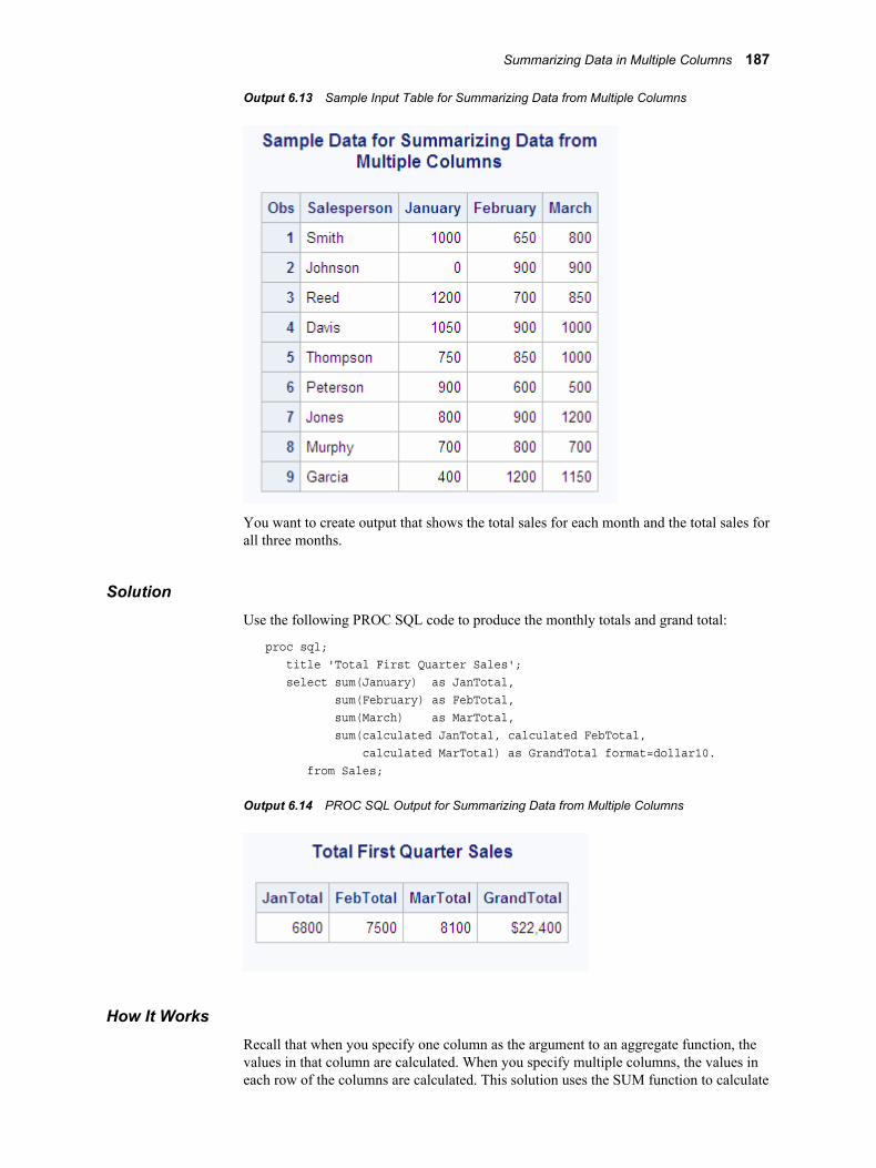
Output 6.13 Sample Input Table for Summarizing Data from Multiple Columns

You want to create output that shows the total sales for each month and the total sales for all three months.

SolutionUse the following PROC SQL code to produce the monthly totals and grand total:

proc sql; title 'Total First Quarter Sales'; select sum(January) as JanTotal, sum(February) as FebTotal, sum(March) as MarTotal, sum(calculated JanTotal, calculated FebTotal, calculated MarTotal) as GrandTotal format=dollar10. from Sales;

Output 6.14 PROC SQL Output for Summarizing Data from Multiple Columns

How It WorksRecall that when you specify one column as the argument to an aggregate function, the values in that column are calculated. When you specify multiple columns, the values in each row of the columns are calculated. This solution uses the SUM function to calculate

Summarizing Data in Multiple Columns 187

the sum of each month's sales, and then uses the SUM function a second time to total the monthly sums into one grand total.

sum(calculated JanTotal, calculated FebTotal, calculated MarTotal) as GrandTotal format=dollar10.

An alternative way to code the grand total calculation is to use nested functions:

sum(sum(January), sum(February), sum(March)) as GrandTotal format=dollar10.

Creating a Summary Report

ProblemYou have a table that contains detailed sales information. You want to produce a summary report from the detail table.

Background InformationThere is one input table, called SALES, that contains detailed sales information. There is one record for each sale for the first quarter that shows the site, product, invoice number, invoice amount, and invoice date.

data sales; input Site $ Product $ Invoice $ InvoiceAmount InvoiceDate $; datalines;V1009 VID010 V7679 598.5 980126V1019 VID010 V7688 598.5 980126V1032 VID005 V7771 1070 980309V1043 VID014 V7780 1070 980309V421 VID003 V7831 2000 980330V421 VID010 V7832 750 980330V570 VID003 V7762 2000 980302V659 VID003 V7730 1000 980223V783 VID003 V7815 750 980323V985 VID003 V7733 2500 980223V966 VID001 V5020 1167 980215V98 VID003 V7750 2000 980223;

proc sql; title 'Sample Data to Create Summary Sales Report'; select * from sales;quit;


Output 6.15 Sample Input Table for Creating a Summary Report

You want to use this table to create a summary report that shows the sales for each product for each month of the quarter.

SolutionUse the following PROC SQL code to create a column for each month of the quarter, and use the summary function SUM in combination with the GROUP BY statement to accumulate the monthly sales for each product:

proc sql; title 'First Quarter Sales by Product'; select Product, sum(Jan) label='Jan', sum(Feb) label='Feb', sum(Mar) label='Mar' from (select Product, case when substr(InvoiceDate,3,2)='01' then InvoiceAmount end as Jan, case when substr(InvoiceDate,3,2)='02' then InvoiceAmount end as Feb, case when substr(InvoiceDate,3,2)='03' then InvoiceAmount end as Mar from work.sales) group by Product;

Creating a Summary Report 189

Output 6.16 PROC SQL Output for a Summary Report

Note: Missing values in the matrix indicate that no sales occurred for that given product in that month.

How It WorksThis solution uses an in-line view to create three temporary columns, Jan, Feb, and Mar, based on the month part of the invoice date column. The in-line view is a query that performs the following:

• selects the product column

• uses a CASE expression to assign the value of invoice amount to one of three columns, Jan, Feb, or Mar, depending on the value of the month part of the invoice date column

case when substr(InvoiceDate,3,2)='01' then InvoiceAmount end as Jan,case when substr(InvoiceSate,3,2)='02' then InvoiceAmount end as Feb,case when substr(InvoiceDate,3,2)='03' then InvoiceAmount end as Mar

The first, or outer, SELECT statement in the query performs the following:

• selects the product

• uses the summary function SUM to accumulate the Jan, Feb, and Mar amounts

• uses the GROUP BY statement to produce a line in the table for each product

Notice that dates are stored in the input table as strings. If the dates were stored as SAS dates, then the CASE expression could be written as follows:

case when month(InvoiceDate)=1 then InvoiceAmount end as Jan,case when month(InvoiceDate)=2 then InvoiceAmount end as Feb,case


when month(InvoiceDate)=3 then InvoiceAmount end as Mar

Creating a Customized Sort Order

ProblemYou want to sort data in a logical, but not alphabetical, sequence.

Background InformationThere is one input table, called CHORES, that contains the following data:

data chores; input Project $ Hours Season $; datalines;weeding 48 summerpruning 12 wintermowing 36 summermulching 17 fallraking 24 fallraking 16 springplanting 8 springplanting 8 fallsweeping 3 winteredging 16 summerseeding 6 springtilling 12 springaerating 6 springfeeding 7 summerrolling 4 winter;

proc sql;title 'Garden Chores';select * from chores;quit;

Creating a Customized Sort Order 191

Output 6.17 Sample Input Data for a Customized Sort

You want to reorder this chore list so that all the chores are grouped by season, starting with spring and progressing through the year. Simply ordering by Season makes the list appear in alphabetical sequence: fall, spring, summer, winter.

SolutionUse the following PROC SQL code to create a new column, Sorter, that will have values of 1 through 4 for the seasons spring through winter. Use the new column to order the query, but do not select it to appear:

proc sql; title 'Garden Chores by Season in Logical Order'; select Project, Hours, Season from (select Project, Hours, Season, case when Season = 'spring' then 1 when Season = 'summer' then 2 when Season = 'fall' then 3 when Season = 'winter' then 4 else . end as Sorter from chores) order by Sorter;


Output 6.18 PROC SQL Output for a Customized Sort Sequence

How It WorksThis solution uses an in-line view to create a temporary column that can be used as an ORDER BY column. The in-line view is a query that performs the following:

• selects the Project, Hours, and Season columns

• uses a CASE expression to remap the seasons to the new column Sorter: spring to 1, summer to 2, fall to 3, and winter to 4

(select project, hours, season, case when season = 'spring' then 1 when season = 'summer' then 2 when season = 'fall' then 3 when season = 'winter' then 4 else . end as sorter from chores)

The first, or outer, SELECT statement in the query performs the following:

• selects the Project, Hours, and Season columns

Creating a Customized Sort Order 193

• orders rows by the values that were assigned to the seasons in the Sorter column that was created with the in-line view

Notice that the Sorter column is not included in the SELECT statement. That causes a note to be written to the log indicating that you have used a column in an ORDER BY statement that does not appear in the SELECT statement. In this case, that is exactly what you wanted to do.

Conditionally Updating a Table

ProblemYou want to update values in a column of a table, based on the values of several other columns in the table.

Background InformationThere is one table, called INCENTIVES, that contains information about sales data. There is one record for each salesperson that includes a department code, a base pay rate, and sales of two products, gadgets and whatnots.

data incentives; input @1 Name $18. @20 Department $2. Payrate Gadgets Whatnots; datalines;Lao Che M2 8.00 10193 1105Jack Colton U2 6.00 9994 2710Mickey Raymond M1 12.00 6103 1930Dean Proffit M2 11.00 3000 1999Antoinette Lily E1 20.00 2203 4610Sydney Wade E2 15.00 4205 3010Alan Traherne U2 4.00 5020 3000Elizabeth Bennett E1 16.00 17003 3003;

proc sql; title 'Sales Data for Incentives Program'; select * from incentives;quit;


Output 6.19 Sample Input Data to Conditionally Change a Table

You want to update the table by increasing each salesperson's payrate (based on the total sales of gadgets and whatnots) and taking into consideration some factors that are based on department code.

Specifically, anyone who sells over 10,000 gadgets merits an extra $5 per hour. Anyone selling between 5,000 and 10,000 gadgets also merits an incentive pay, but E Department salespersons are expected to be better sellers than those in the other departments, so their gadget sales incentive is $2 per hour compared to $3 per hour for those in other departments. Good sales of whatnots also entitle sellers to added incentive pay. The algorithm for whatnot sales is that the top level (level 1 in each department) salespersons merit an extra $.50 per hour for whatnot sales over 2,000, and level 2 salespersons merit an extra $1 per hour for sales over 2,000.

SolutionUse the following PROC SQL code to create a new value for the Payrate column. Actually Payrate is updated twice for each row, once based on sales of gadgets, and again based on sales of whatnots:

proc sql; update incentives set payrate = case when gadgets > 10000 then payrate + 5.00 when gadgets > 5000 then case when department in ('E1', 'E2') then payrate + 2.00 else payrate + 3.00 end else payrate end; update incentives set payrate = case when whatnots > 2000 then

Conditionally Updating a Table 195

case when department in ('E2', 'M2', 'U2') then payrate + 1.00 else payrate + 0.50 end else payrate end; title 'Adjusted Payrates Based on Sales of Gadgets and Whatnots'; select * from incentives;

Output 6.20 PROC SQL Output for Conditionally Updating a Table

How It WorksThis solution performs consecutive updates to the payrate column of the incentive table. The first update uses a nested case expression, first determining a bracket that is based on the amount of gadget sales: greater than 10,000 calls for an incentive of $5, between 5,000 and 10,000 requires an additional comparison. That is accomplished with a nested case expression that checks department code to choose between a $2 and $3 incentive.

update incentives set payrate = case when gadgets > 10000 then payrate + 5.00 when gadgets > 5000 then case when department in ('E1', 'E2') then payrate + 2.00 else payrate + 3.00 end else payrate end;


The second update is similar, though simpler. All sales of whatnots over 2,000 merit an incentive, either $.50 or $1 depending on the department level, that again is accomplished by means of a nested case expression.

update incentives set payrate = case when whatnots > 2000 then case when department in ('E2', 'M2', 'U2') then payrate + 1.00 else payrate + 0.50 end else payrate end;

Updating a Table with Values from Another Table

ProblemYou want to update the SQL.UNITEDSTATES table with updated population data.

Background InformationThe SQL.NEWPOP table contains updated population data for some of the U.S. states.


proc sql;title 'Updated U.S. Population Data';select state, population format=comma10. label='Population' from sql.newpop;

Updating a Table with Values from Another Table 197

Output 6.21 Table with Updated Population Data

SolutionUse the following PROC SQL code to update the population information for each state in the SQL.UNITEDSTATES table:

proc sql;title 'UNITEDSTATES';update sql.unitedstates as u set population=(select population from sql.newpop as n where u.name=n.state) where u.name in (select state from sql.newpop);select Name format=$17., Capital format=$15., Population, Area, Continent format=$13., Statehood format=date9. from sql.unitedstates;

/* use this code to generate output so you don't overwrite the sql.unitedstates table */options ls=84;proc sql outobs=10;title 'UNITEDSTATES';create table work.unitedstates as select * from sql.unitedstates;update work.unitedstates as u set population=(select population from sql.newpop as n


where u.name=n.state) where u.name in (select state from sql.newpop); select Name format=$17., Capital format=$15., Population, Area, Continent format=$13., Statehood format=date9. from work.unitedstates;

Output 6.22 SQL.UNITEDSTATES with Updated Population Data (Partial Output)

How It WorksThe UPDATE statement updates values in the SQL.UNITEDSTATES table (here with the alias U). For each row in the SQL.UNITEDSTATES table, the in-line view in the SET clause returns a single value. For rows that have a corresponding row in SQL.NEWPOP, this value is the value of the Population column from SQL.NEWPOP. For rows that do not have a corresponding row in SQL.NEWPOP, this value is missing. In both cases, the returned value is assigned to the Population column.

The WHERE clause ensures that only the rows in SQL.UNITEDSTATES that have a corresponding row in SQL.NEWPOP are updated, by checking each value of Name against the list of state names that is returned from the in-line view. Without the WHERE clause, rows that do not have a corresponding row in SQL.NEWPOP would have their Population values updated to missing.

Creating and Using Macro Variables

ProblemYou want to create a separate data set for each unique value of a column.

Creating and Using Macro Variables 199

Background InformationThe SQL.FEATURES data set contains information about various geographical features around the world.

libname sql 'C:\Public\examples';

proc sql outobs=10;title 'FEATURES'; select Name format=$15., Type,Location format =$15.,Area, Height, Depth, Length from sql.features;

Output 6.23 FEATURES (Partial Output)

SolutionTo create a separate data set for each type of feature, you could go through the data set manually to determine all the unique values of Type, and then write a separate DATA step for each type (or a single DATA step with multiple OUTPUT statements). This approach is labor-intensive, error-prone, and impractical for large data sets. The following PROC SQL code counts the unique values of Type and puts each value in a separate macro variable. The SAS macro that follows the PROC SQL code uses these macro variables to create a SAS data set for each value. You do not need to know beforehand how many unique values there are or what the values are.

proc sql noprint; select count(distinct type) into :n from sql.features; select distinct type


into :type1 - :type%left(&n) from sql.features;quit;

%macro makeds; %do i=1 %to &n; data &&type&i (drop=type); set sql.features; if type="&&type&i"; run; %end;%mend makeds;%makeds;

Creating and Using Macro Variables 201

Log 6.1 Log

240 proc sql noprint;

241 select count(distinct type)

242 into :n

243 from sql.features;

244 select distinct type

245 into :type1 - :type%left(&n)

246 from sql.features;

247 quit;

NOTE: PROCEDURE SQL used (Total process time):

real time 0.04 seconds

cpu time 0.03 seconds

248

249 %macro makeds;

250 %do i=1 %to &n;

251 data &&type&i (drop=type);

252 set sql.features;

253 if type="&&type&i";

254 run;

255 %end;

256 %mend makeds;

257 %makeds;

NOTE: There were 74 observations read from the data set SQL.FEATURES.

NOTE: The data set WORK.DESERT has 7 observations and 6 variables.

NOTE: DATA statement used (Total process time):




NOTE: The data set WORK.ISLAND has 6 observations and 6 variables.





NOTE: The data set WORK.LAKE has 10 observations and 6 variables.





NOTE: The data set WORK.MOUNTAIN has 18 observations and 6 variables.





NOTE: The data set WORK.OCEAN has 4 observations and 6 variables.





NOTE: The data set WORK.RIVER has 12 observations and 6 variables.





NOTE: The data set WORK.SEA has 13 observations and 6 variables.





NOTE: The data set WORK.WATERFALL has 4 observations and 6 variables.





How It WorksThis solution uses the INTO clause to store values in macro variables. The first SELECT statement counts the unique variables and stores the result in macro variable N. The second SELECT statement creates a range of macro variables, one for each unique value, and stores each unique value in one of the macro variables. Note the use of the %LEFT function, which trims leading blanks from the value of the N macro variable.

The MAKEDS macro uses all the macro variables that were created in the PROC SQL step. The macro uses a %DO loop to execute a DATA step for each unique value, writing rows that contain a given value of Type to a SAS data set of the same name. The Type variable is dropped from the output data sets.

For more information about SAS macros, see SAS Macro Language: Reference.

Using PROC SQL Tables in Other SAS Procedures

ProblemYou want to show the average high temperatures in degrees Celsius for European countries on a map.

Background InformationThe SQL.WORLDTEMPS table has average high and low temperatures for various cities around the world.

proc sql outobs=10;title 'WORLDTEMPS'; select City, Country,avghigh, avglow from sql.worldtemps;

Using PROC SQL Tables in Other SAS Procedures 203

Output 6.24 WORLDTEMPS (Partial Output)

SolutionUse the following PROC SQL and PROC GMAP code to produce the map. You must license SAS/GRAPH software to use PROC GMAP.

options fmtsearch=(sashelp.mapfmts);

proc sql; create table extremetemps as select country, round((mean(avgHigh)-32)/1.8) as High, input(put(country,$glcsmn.), best.) as ID from sql.worldtemps where calculated id is not missing and country in (select name from sql.countries where continent='Europe') group by country;quit;

proc gmap map=maps.europe data=extremetemps all; id id; block high / levels=3; title 'Average High Temperatures for European Countries'; title2 'Degrees Celsius'run;quit;


Output 6.25 PROC GMAP Output

How It WorksThe SAS system option FMTSEARCH= tells SAS to search in the SASHELP.MAPFMTS catalog for map-related formats. In the PROC SQL step, a temporary table is created with Country, High, and ID columns. The calculation round((mean(avgHigh)-32)/1.8) does the following:

1. For countries that are represented by more than one city, the mean of the cities' average high temperatures is used for that country.

2. That value is converted from degrees Fahrenheit to degrees Celsius.

3. The result is rounded to the nearest degree.

The PUT function uses the $GLCSMN. format to convert the country name to a country code. The INPUT function converts this country code, which is returned by the PUT function as a character value, into a numeric value that can be understood by the GMAP procedure. See SAS Functions and CALL Routines: Reference for details about the PUT and INPUT functions.

The WHERE clause limits the output to European countries by checking the value of the Country column against the list of European countries that is returned by the in-line view. Also, rows with missing values of ID are eliminated. Missing ID values could be produced if the $GLCSMN. format does not recognize the country name.

The GROUP BY clause is required so that the mean temperature can be calculated for each country rather than for the entire table.

Using PROC SQL Tables in Other SAS Procedures 205

The PROC GMAP step uses the ID variable to identify each country and places a block representing the High value on each country on the map. The ALL option ensures that countries (such as the United Kingdom in this example) that do not have High values are also drawn on the map. In the BLOCK statement, the LEVELS= option specifies how many response levels are used in the graph. For more information about the GMAP procedure, see SAS/GRAPH: Reference.


Part 2

SQL Procedure Reference

Chapter 7SQL Procedure . . . . . . . . . . . . . . . . . . . . . . . . . . . . . . . . . . . . . . . . . . . . . . . . . 209

Chapter 8SQL SELECT Statement Clauses . . . . . . . . . . . . . . . . . . . . . . . . . . . . . . . . 293

Chapter 9SQL Procedure Components . . . . . . . . . . . . . . . . . . . . . . . . . . . . . . . . . . . . 307

207

Chapter 7

SQL Procedure

Overview . . . . . . . . . . . . . . . . . . . . . . . . . . . . . . . . . . . . . . . . . . . . . . . . . . . . . . . . . . . 210What Is the SQL Procedure? . . . . . . . . . . . . . . . . . . . . . . . . . . . . . . . . . . . . . . . . . 210What Are PROC SQL Tables? . . . . . . . . . . . . . . . . . . . . . . . . . . . . . . . . . . . . . . . . 210What Are Views? . . . . . . . . . . . . . . . . . . . . . . . . . . . . . . . . . . . . . . . . . . . . . . . . . . 211SQL Procedure Coding Conventions . . . . . . . . . . . . . . . . . . . . . . . . . . . . . . . . . . . 211

Syntax: SQL Procedure . . . . . . . . . . . . . . . . . . . . . . . . . . . . . . . . . . . . . . . . . . . . . . . 212PROC SQL Statement . . . . . . . . . . . . . . . . . . . . . . . . . . . . . . . . . . . . . . . . . . . . . . 215ALTER TABLE Statement . . . . . . . . . . . . . . . . . . . . . . . . . . . . . . . . . . . . . . . . . . . 225CONNECT Statement . . . . . . . . . . . . . . . . . . . . . . . . . . . . . . . . . . . . . . . . . . . . . . 228CREATE INDEX Statement . . . . . . . . . . . . . . . . . . . . . . . . . . . . . . . . . . . . . . . . . 229CREATE TABLE Statement . . . . . . . . . . . . . . . . . . . . . . . . . . . . . . . . . . . . . . . . . 231CREATE VIEW Statement . . . . . . . . . . . . . . . . . . . . . . . . . . . . . . . . . . . . . . . . . . 235DELETE Statement . . . . . . . . . . . . . . . . . . . . . . . . . . . . . . . . . . . . . . . . . . . . . . . . 237DESCRIBE Statement . . . . . . . . . . . . . . . . . . . . . . . . . . . . . . . . . . . . . . . . . . . . . . 238DISCONNECT Statement . . . . . . . . . . . . . . . . . . . . . . . . . . . . . . . . . . . . . . . . . . . 239DROP Statement . . . . . . . . . . . . . . . . . . . . . . . . . . . . . . . . . . . . . . . . . . . . . . . . . . . 240EXECUTE Statement . . . . . . . . . . . . . . . . . . . . . . . . . . . . . . . . . . . . . . . . . . . . . . . 241INSERT Statement . . . . . . . . . . . . . . . . . . . . . . . . . . . . . . . . . . . . . . . . . . . . . . . . . 242RESET Statement . . . . . . . . . . . . . . . . . . . . . . . . . . . . . . . . . . . . . . . . . . . . . . . . . . 244SELECT Statement . . . . . . . . . . . . . . . . . . . . . . . . . . . . . . . . . . . . . . . . . . . . . . . . . 244UPDATE Statement . . . . . . . . . . . . . . . . . . . . . . . . . . . . . . . . . . . . . . . . . . . . . . . . 244VALIDATE Statement . . . . . . . . . . . . . . . . . . . . . . . . . . . . . . . . . . . . . . . . . . . . . . 245

Examples: SQL Procedure . . . . . . . . . . . . . . . . . . . . . . . . . . . . . . . . . . . . . . . . . . . . . 246Example 1: Creating a Table and Inserting Data into It . . . . . . . . . . . . . . . . . . . . . 246Example 2: Creating a Table from a Query's Result . . . . . . . . . . . . . . . . . . . . . . . 248Example 3: Updating Data in a PROC SQL Table . . . . . . . . . . . . . . . . . . . . . . . . . 250Example 4: Joining Two Tables . . . . . . . . . . . . . . . . . . . . . . . . . . . . . . . . . . . . . . . 252Example 5: Combining Two Tables . . . . . . . . . . . . . . . . . . . . . . . . . . . . . . . . . . . . 255Example 6: Reporting from DICTIONARY Tables . . . . . . . . . . . . . . . . . . . . . . . . 258Example 7: Performing an Outer Join . . . . . . . . . . . . . . . . . . . . . . . . . . . . . . . . . . 260Example 8: Creating a View from a Query's Result . . . . . . . . . . . . . . . . . . . . . . . . 266Example 9: Joining Three Tables . . . . . . . . . . . . . . . . . . . . . . . . . . . . . . . . . . . . . . 269Example 10: Querying an In-Line View . . . . . . . . . . . . . . . . . . . . . . . . . . . . . . . . 273Example 11: Retrieving Values with the SOUNDS-LIKE Operator . . . . . . . . . . . 275Example 12: Joining Two Tables and Calculating a New Value . . . . . . . . . . . . . . 277Example 13: Producing All the Possible Combinations of the

Values in a Column . . . . . . . . . . . . . . . . . . . . . . . . . . . . . . . . . . . . . . . . . . . . . . . 280Example 14: Matching Case Rows and Control Rows . . . . . . . . . . . . . . . . . . . . . . 286Example 15: Counting Missing Values with a SAS Macro . . . . . . . . . . . . . . . . . . 289

209

Overview

What Is the SQL Procedure?The SQL procedure implements Structured Query Language (SQL) for SAS. SQL is a standardized, widely used language that retrieves data from and updates data in tables and the views that are based on those tables.

The SAS SQL procedure enables you to

• retrieve and manipulate data that is stored in tables or views.

• create tables, views, and indexes on columns in tables.

• create SAS macro variables that contain values from rows in a query's result.

• add or modify the data values in a table's columns or insert and delete rows. You can also modify the table itself by adding, modifying, or dropping columns.

• send DBMS-specific SQL statements to a database management system (DBMS) and retrieve DBMS data.

The following figure summarizes the variety of source material that you can use with PROC SQL and what the procedure can produce.

Figure 7.1 PROC SQL Input and Output

PROC SQL tables

(SAS data files)

SAS data views

(PROC SQL views)

(DATA step views)

(SAS/ACCESS views)

DBMS tables

DBMS tables

reports

PROC SQL views

PROC

SQL

PROC SQL tables

(SAS data files)

macro variables

What Are PROC SQL Tables?A PROC SQL table is synonymous with a SAS data file and has a member type of DATA. You can use PROC SQL tables as input into DATA steps and procedures.

You create PROC SQL tables from SAS data files, from SAS views, or from DBMS tables by using PROC SQL's pass-through facility or the SAS/ACCESS LIBNAME statement. The pass-through facility is described in “Connecting to a DBMS by Using the SQL Procedure Pass-Through Facility” on page 166. The SAS/ACCESS LIBNAME statement is described in “Connecting to a DBMS by Using the LIBNAME Statement” on page 163.

In PROC SQL terminology, a row in a table is the same as an observation in a SAS data file. A column is the same as a variable.

210 Chapter 7 • SQL Procedure

What Are Views?A SAS view defines a virtual data set that is named and stored for later use. A view contains no data but describes or defines data that is stored elsewhere. There are three types of SAS views:

• PROC SQL views

• SAS/ACCESS views

• DATA step views.

You can refer to views in queries as if they were tables. The view derives its data from the tables or views that are listed in its FROM clause. The data that is accessed by a view is a subset or superset of the data that is in its underlying tables or views.

A PROC SQL view is a SAS data set of type VIEW that is created by PROC SQL. A PROC SQL view contains no data. It is a stored query expression that reads data values from its underlying files, which can include SAS data files, SAS/ACCESS views, DATA step views, other PROC SQL views, or DBMS data. When executed, a PROC SQL view's output can be a subset or superset of one or more underlying files.

SAS/ACCESS views and DATA step views are similar to PROC SQL views in that they are both stored programs of member type VIEW. SAS/ACCESS views describe data in DBMS tables from other software vendors. DATA step views are stored DATA step programs.

Note: Starting in SAS System 9, PROC SQL views, the pass-through facility, and the SAS/ACCESS LIBNAME statement are the preferred ways to access relational DBMS data; SAS/ACCESS views are no longer recommended. You can convert existing SAS/ACCESS views to PROC SQL views by using the CV2VIEW procedure. For more information, see Chapter 33, “CV2VIEW Procedure” in SAS/ACCESS for Relational Databases: Reference.

You can update data through a PROC SQL or SAS/ACCESS view with certain restrictions. See “Updating PROC SQL and SAS/ACCESS Views” on page 168.

You can use all types of views as input to DATA steps and procedures.

Note: In this chapter, the term view collectively refers to PROC SQL views, DATA step views, and SAS/ACCESS views, unless otherwise noted.

Note: When the contents of an SQL view are processed (by a DATA step or a procedure), the referenced data set must be opened to retrieve information about the variables that is not stored in the view. If that data set has a libref associated with it that is not defined in the current SAS code, then an error will result. You can avoid this error by specifying a USING clause in the CREATE VIEW statement. See “CREATE VIEW Statement” on page 235 for details.

Note: When you process PROC SQL views between a client and a server, getting the correct results depends on the compatibility between the client and server architecture. For more information, see “Accessing a SAS View” in Chapter 17 of SAS/CONNECT User's Guide.

SQL Procedure Coding ConventionsBecause PROC SQL implements Structured Query Language, it works somewhat differently from other Base SAS procedures, as described here:

Overview 211

• When a PROC SQL statement is executed, PROC SQL continues to run until a QUIT statement, a DATA step, or another SAS procedure is executed. Therefore, you do not need to repeat the PROC SQL statement with each SQL statement. You need to repeat the PROC SQL statement only if you execute a QUIT statement, a DATA step, or another SAS procedure between SQL statements.

• SQL procedure statements are divided into clauses. For example, the most basic SELECT statement contains the SELECT and FROM clauses. Items within clauses are separated with commas in SQL, not with blanks as in other SAS code. For example, if you list three columns in the SELECT clause, then the columns are separated with commas.

• The SELECT statement, which is used to retrieve data, also automatically writes the output data to the Output window unless you specify the NOPRINT option in the PROC SQL statement. Therefore, you can display your output or send it to a list file without specifying the PRINT procedure.

• The ORDER BY clause sorts data by columns. In addition, tables do not need to be presorted by a variable for use with PROC SQL. Therefore, you do not need to use the SORT procedure with your PROC SQL programs.

• A PROC SQL statement runs when you submit it; you do not have to specify a RUN statement. If you follow a PROC SQL statement with a RUN statement, then SAS ignores the RUN statement and submits the statements as usual.

Syntax: SQL ProcedureTips: Supports the Output Delivery System. For more information, see Chapter 3, “Output

Delivery System: Basic Concepts,” in SAS Output Delivery System: User's Guide.You can use any global statements. For more information, see Chapter 2, “Fundamental Concepts for Using Base SAS Procedures,” in Base SAS Procedures Guide. You can use data set options any time a table name or view name is specified. For more information, see “Using SAS Data Set Options with PROC SQL” on page 151..Regular type indicates the name of a component that is described in Chapter 9, “SQL Procedure Components,” on page 307 view-name indicates a SAS view of any type.


PROC SQL <option(s)>;ALTER TABLE table-name

<ADD <CONSTRAINT> constraint-clause<, … constraint-clause>><ADD column-definition<, … column-definition>><DROP CONSTRAINT constraint-name <, … constraint-name>><DROP column<, … column>><DROP FOREIGN KEY constraint-name><DROP PRIMARY KEY><MODIFY column-definition<, … column-definition>>

;CREATE <UNIQUE> INDEX index-name

ON table-name ( column <, … column>);CREATE TABLE table-name

(column-specification<, …column-specification | constraint-specification>);

CREATE TABLE table-name LIKE table-name2;CREATE TABLE table-name AS query-expression

<ORDER BY order-by-item<, … order-by-item>>;CREATE VIEW proc-sql-view AS query-expression

<ORDER BY order-by-item<, … order-by-item>><USING libname-clause<, … libname-clause>> ;

DELETE FROM table-name|proc-sql-view |sas/access-view <AS alias>

<WHERE sql-expression>;DESCRIBE TABLE table-name <, … table-name>;DESCRIBE VIEW proc-sql-view <, … proc-sql-view>;DESCRIBE TABLE CONSTRAINTS table-name <, … table-name>;DROP INDEX index-name <, … index-name>

FROM table-name;DROP TABLE table-name <, … table-name>;DROP VIEW view-name <, … view-name>;INSERT INTO table-name|sas/access-view|proc-sql-view <(column<, … column>)>

SET column=sql-expression <, … column=sql-expression>< column=sql-expression <, … column=sql-expression>>

INSERT INTO table-name|sas/access-view|proc-sql-view <(column<, … column>)>VALUES (value <, … value>)

<… VALUES (value <, … value>)>;INSERT INTO table-name|sas/access-view|proc-sql-view

<(column<, …column>)> query-expression;RESET <option(s)>;

Syntax: SQL Procedure 213

SELECT <DISTINCT> object-item <, …object-item><INTO macro-variable-specification <, … macro-variable-specification>>FROM from-list<WHERE sql-expression><GROUP BY group-by-item <, … group-by-item>><HAVING sql-expression><ORDER BY order-by-item <, … order-by-item>>;

UPDATE table-name|sas/access-view|proc-sql-view <AS alias>SET column=sql-expression <, … column=sql-expression>

< column=sql-expression <, … column=sql-expression>><WHERE sql-expression>;

VALIDATE query-expression;To connect to a DBMS and send it a DBMS-specific nonquery SQL statement, use this form:PROC SQL;

CONNECT TO dbms-name <AS alias><(connect-statement-argument-1=value <… connect-statement-argument-n=value>)><(database-connection-argument-1=value <… database-connection-argument-n=value>)>;

EXECUTE (dbms-SQL-statement)BY dbms-name|alias;

<DISCONNECT FROM dbms-name|alias;><QUIT;>To connect to a DBMS and query the DBMS data, use this form:PROC SQL;

CONNECT TO dbms-name <AS alias><(connect-statement-argument-1=value <… connect-statement-argument-n=value>)><(database-connection-argument-1=value <… database-connection-argument-n=value>)>;

SELECT column-listFROM CONNECTION TO dbms-name|alias

(dbms-query)optional PROC SQL clauses;

<DISCONNECT FROM dbms-name|alias;><QUIT;>

Statement Task

PROC SQL Create, maintain, retrieve, and update data in tables and views that are based on these tables

ALTER TABLE Modify, add, or drop columns

CONNECT Establish a connection with a DBMS

CREATE INDEX Create an index on a column

CREATE TABLE Create a PROC SQL table

CREATE VIEW Create a PROC SQL view

DELETE Delete rows


Statement Task

DESCRIBE Display a definition of a table or view

DISCONNECT Terminate the connection with a DBMS

DROP Delete tables, views, or indexes

EXECUTE Send a DBMS-specific nonquery SQL statement to a DBMS

INSERT Add rows

RESET Reset options that affect the procedure environment without restarting the procedure

SELECT Select and execute rows

UPDATE Modify values

VALIDATE Verify the accuracy of your query

PROC SQL StatementPROC SQL Statement

SyntaxPROC SQL <option(s)>;

Summary of Optional Arguments

Control executionCONSTDATETIME|NOCONSTDATETIMEDQUOTE=ANSI|SASERRORSTOP|NOERRORSTOPEXEC|NOEXECEXITCODEINOBS=nIPASSTHRU|NOIPASSTHRULOOPS=nNOCONSTDATETIMENOERRORSTOPNOEXECNOIPASSTHRUNOPROMPTNOREMERGENOSTIMERNOTHREADS

PROC SQL Statement 215

OUTOBS=nPROMPT|NOPROMPTREDUCEPUT=ALL|NONE|DBMS|BASEREDUCEPUTOBS=nREDUCEPUTVALUES=nREMERGE|NOREMERGESTIMER|NOSTIMERSTOPONTRUNCTHREADS|NOTHREADSUNDO_POLICY=NONE|OPTIONAL|REQUIRED

Control outputBUFFERSIZE=n|nK|nM|nGDOUBLE|NODOUBLEFEEDBACK|NOFEEDBACKFLOW<=n <m>>|NOFLOWNODOUBLENOFEEDBACKNOFLOWNONUMBERNOPRINTNOSORTMSGNOWARNRECURSNUMBER|NONUMBERPRINT|NOPRINTSORTMSG|NOSORTMSGSORTSEQ=sort-tableWARNRECURS|NOWARNRECURS

Optional ArgumentsBUFFERSIZE=n|nK|nM|nG

specifies the internal transient buffer page size for the PROC SQL paged memory subsystem. PROC SQL uses this subsystem to help implement operations such as joins, aggregations, and intersections. The output is in multiples of 1 (bytes), 1024 (kilobytes), 1,048,576 (megabytes), or 1,073,741,824 (gigabytes). For example, a value of 65536 specifies a page size of 65536 bytes, and a value of 64k specifies a page size of 65536 bytes.

BUFFERSIZE can also be specified in a RESET statement for use in particular queries.

Default 0, which causes SAS to use the minimum optimal page size for the operating environment.

CONSTDATETIME|NOCONSTDATETIMEspecifies whether the SQL procedure replaces references to the DATE, TIME, DATETIME, and TODAY functions in a query with their equivalent constant values before the query executes. Computing these values once ensures consistency of


results when the functions are used multiple times in a query or when the query executes the functions close to a date or time boundary.

When the NOCONSTDATETIME option is set, PROC SQL evaluates these functions in a query each time it processes an observation.

Default CONSTDATETIME

Interaction If both the CONSTDATETIME option and the REDUCEPUT= option on page 220 are specified, PROC SQL replaces the DATE, TIME, DATETIME, and TODAY functions with their respective values in order to determine the PUT function value before the query executes.

Tip Alternatively, you can set the SQLCONSTDATETIME system option. The value that is specified in the SQLCONSTDATETIME system option is in effect for all SQL procedure statements, unless the PROC SQL CONSTDATETIME option is set. The value of the CONSTDATETIME option takes precedence over the SQLCONSTDATETIME system option. The RESET statement can also be used to set or reset the CONSTDATETIME option. However, changing the value of the CONSTDATETIME option does not change the value of the SQLCONSTDATETIME system option. For more information, see the “SQLCONSTDATETIME System Option” on page 363.

DOUBLE|NODOUBLEdouble-spaces the report.

Default NODOUBLE

Example “Example 5: Combining Two Tables” on page 255

DQUOTE=ANSI|SASspecifies whether PROC SQL treats values within double quotation marks (" ") as variables or strings. With DQUOTE=ANSI, PROC SQL treats a quoted value as a variable. This feature enables you to use the following as table names, column names, or aliases:

• reserved words such as AS, JOIN, GROUP, and so on

• DBMS names and other names that are not normally permissible in SAS.

The quoted value can contain any character.

With DQUOTE=SAS, values within double quotation marks are treated as strings.

Default SAS

ERRORSTOP|NOERRORSTOPspecifies whether PROC SQL stops executing if it encounters an error. In a batch or noninteractive session, ERRORSTOP instructs PROC SQL to stop executing the statements but to continue checking the syntax after it has encountered an error.

NOERRORSTOP instructs PROC SQL to execute the statements and to continue checking the syntax after an error occurs.

Default NOERRORSTOP in an interactive SAS session; ERRORSTOP in a batch or noninteractive session

Interaction This option is useful only when the EXEC option is in effect.


Tips ERRORSTOP has an effect only when SAS is running in the batch or noninteractive execution mode.

NOERRORSTOP is useful if you want a batch job to continue executing SQL procedure statements after an error is encountered.

EXEC|NOEXECspecifies whether a statement should be executed after its syntax is checked for accuracy.

Default EXEC

Tip NOEXEC is useful if you want to check the syntax of your SQL statements without executing the statements.

See ERRORSTOP on page 217

EXITCODEspecifies whether PROC SQL clears an error code for any SQL statement. Error codes are assigned to the SQLEXITCODE macro variable.

Default 0

Tip The exit code can be reset to the default value between PROC SQL statements with the “RESET Statement” on page 244.

See “Using the PROC SQL Automatic Macro Variables” on page 157

FEEDBACK|NOFEEDBACKspecifies whether PROC SQL displays, in the SAS log, PROC SQL statements after view references are expanded or certain other transformations of the statement are made.

This option has the following effects:

• Any asterisk (for example, SELECT *) is expanded into the list of qualified columns that it represents.

• Any PROC SQL view is expanded into the underlying query.

• Macro variables are resolved.

• Parentheses are shown around all expressions to further indicate their order of evaluation.

• Comments are removed.

Default NOFEEDBACK

FLOW<=n <m>>|NOFLOWspecifies that character columns longer than n are flowed to multiple lines. PROC SQL sets the column width at n and specifies that character columns longer than n are flowed to multiple lines. When you specify FLOW=n m, PROC SQL floats the width of the columns between these limits to achieve a balanced layout. Specifying FLOW without arguments is equivalent to specifying FLOW=12 200.

Default NOFLOW


INOBS=nrestricts the number of rows (observations) that PROC SQL retrieves from any single source.

Tip This option is useful for debugging queries on large tables.

IPASSTHRU|NOIPASSTHRUspecifies whether implicit pass through is enabled or disabled.

Implicit pass through is enabled when PROC SQL is invoked. You can disable it for a query or series of queries. The primary reasons that you might want to disable implicit pass through are as follows:

• DBMSs use SQL2 semantics for NULL values, which behave somewhat differently than SAS missing values.

• PROC SQL might do a better job of query optimization.

Default IPASSTHRU

See The documentation on the pass-through facility for your DBMS in SAS/ACCESS for Relational Databases: Reference.

LOOPS=nrestricts PROC SQL to n iterations through its inner loop. You use the number of iterations reported in the SQLOOPS macro variable (after each SQL statement is executed) to discover the number of loops. Set a limit to prevent queries from consuming excessive computer resources. For example, joining three large tables without meeting the join-matching conditions could create a huge internal table that would be inefficient to execute.

See “Using the PROC SQL Automatic Macro Variables” on page 157

NOCONSTDATETIMESee “CONSTDATETIME|NOCONSTDATETIME” on page 216

NODOUBLESee “DOUBLE|NODOUBLE” on page 217

NOERRORSTOPSee “ERRORSTOP|NOERRORSTOP” on page 217

NOEXECSee “EXEC|NOEXEC” on page 218

NOFEEDBACKSee “FEEDBACK|NOFEEDBACK” on page 218

NOFLOWSee “FLOW<=n <m>>|NOFLOW” on page 218.

NOIPASSTHRUSee “IPASSTHRU|NOIPASSTHRU” on page 219

NONUMBERSee “NUMBER|NONUMBER” on page 220

NOPRINTSee “PRINT|NOPRINT” on page 220

NOPROMPTSee “PROMPT|NOPROMPT” on page 220


NOREMERGESee “REMERGE|NOREMERGE” on page 222

NOSORTMSGSee “SORTMSG|NOSORTMSG” on page 223

NOSTIMERSee “STIMER|NOSTIMER” on page 223

NOTHREADSSee “THREADS|NOTHREADS” on page 223

NOWARNRECURSSee “WARNRECURS|NOWARNRECURS” on page 224

NUMBER|NONUMBERspecifies whether the SELECT statement includes a column called ROW, which is the row (or observation) number of the data as the rows are retrieved.

Default NONUMBER

Example “Example 4: Joining Two Tables” on page 252

OUTOBS=nrestricts the number of rows (observations) in the output. For example, if you specify OUTOBS=10 and insert values into a table using a query expression, then the SQL procedure inserts a maximum of 10 rows. Likewise, OUTOBS=10 limits the output to 10 rows.

PRINT|NOPRINTspecifies whether the output from a SELECT statement is printed.

Default PRINT

Interaction NOPRINT affects the value of the SQLOBS automatic macro variable. For more information, see “Using the PROC SQL Automatic Macro Variables” on page 157.

Tip NOPRINT is useful when you are selecting values from a table into macro variables and do not want anything to be displayed.

PROMPT|NOPROMPTmodifies the effect of the INOBS=, OUTOBS=, and LOOPS= options. If you specify the PROMPT option and reach the limit specified by INOBS=, OUTOBS=, or LOOPS=, then PROC SQL prompts you to stop or continue. The prompting repeats if the same limit is reached again.

Default NOPROMPT

REDUCEPUT=ALL|NONE|DBMS|BASEspecifies the engine type to use to optimize a PUT function in a query. The PUT function is replaced with a logically equivalent expression. The engine type can be one of the following values:

ALLspecifies to consider the optimization of all PUT functions, regardless of the engine that is used by the query to access the data.

NONEspecifies to not optimize any PUT function.


DBMSspecifies to consider the optimization of all PUT functions in a query performed by a SAS/ACCESS engine.

Requirement The first argument to the PUT function must be a variable that is obtained by a table. The table must be accessed using a SAS/ACCESS engine.

BASEspecifies to consider the optimization of all PUT functions in a query performed by a SAS/ACCESS engine or a Base SAS engine.

Default DBMS

Interactions If both the REDUCEPUT= option and the CONSTDATETIME option are specified, PROC SQL replaces the DATE, TIME, DATETIME, and TODAY functions with their respective values to determine the PUT function value before the query executes.

If the query also contains a WHERE or HAVING clause, the evaluation of the WHERE or HAVING clause is simplified.

Tip Alternatively, you can set the SQLREDUCEPUT= system option. The value that is specified in the SQLREDUCEPUT= system option is in effect for all SQL procedure statements, unless the REDUCEPUT= option is set. The value of the REDUCEPUT= option takes precedence over the SQLREDUCEPUT= system option. The RESET statement can also be used to set or reset the REDUCEPUT= option. However, changing the value of the REDUCEPUT= option does not change the value of the SQLREDUCEPUT= system option. For more information, see the “SQLREDUCEPUT= System Option” on page 368.

REDUCEPUTOBS=nwhen the REDUCEPUT= option is set to DBMS, BASE, or ALL, specifies the minimum number of observations that must be in a table for PROC SQL to consider optimizing the PUT function in a query.

Default 0, which indicates that there is no minimum number of observations in a table for PROC SQL to optimize the PUT function.

Range 0 – 263–1, or approximately 9.2 quintillion

Requirement n must be an integer

Interaction The REDUCEPUTOBS= option works only for DBMSs that record the number of observations in a table. If your DBMS does not record the number of observations, but you create row counts on your table, the REDUCEPUTOBS= option will work.

Tip Alternatively, you can set the SQLREDUCEPUTOBS= system option. The value that is specified in the SQLREDUCEPUTOBS= system option is in effect for all SQL procedure statements, unless the REDUCEPUTOBS= option is set. The value of the REDUCEPUTOBS= option takes precedence over the SQLREDUCEPUTOBS= system option. The RESET statement can also be used to set or reset the REDUCEPUTOBS= option. However,


changing the value of the REDUCEPUTOBS= option does not change the value of the SQLREDUCEPUTOBS= system option. For more information, see the “SQLREDUCEPUTOBS= System Option” on page 369.

REDUCEPUTVALUES=nwhen the REDUCEPUT= option is set to DBMS, BASE, or ALL, specifies the maximum number of SAS format values that can exist in a PUT function expression for PROC SQL to consider optimizing the PUT function in a query.

Default 100

Range 100 – 3,000


Interaction If the number of SAS format values in a PUT function expression is greater than this value, PROC SQL does not optimize the PUT function.

Tips Alternatively, you can set the SQLREDUCEPUTVALUES= system option. The value that is specified in the SQLREDUCEPUTVALUES= system option is in effect for all SQL procedure statements, unless the REDUCEPUTVALUES= option is set. The value of the REDUCEPUTVALUES= option takes precedence over the SQLREDUCEPUTVALUES= system option. The RESET statement can also be used to set or reset the REDUCEPUTVALUES= option. However, changing the value of the REDUCEPUTVALUES= option does not change the value of the SQLREDUCEPUTVALUES= system option. For more information, see “SQLREDUCEPUTVALUES= System Option” on page 370.

The value for REDUCEPUTVALUES= is used for each individual optimization. For example, if you have a PUT function in a WHERE clause, and another PUT function in a SELECT statement, and both have user-defined formats with contained values, the value of REDUCEPUTVALUES= is applied separately for the clause and the statement.

REMERGE|NOREMERGESpecifies whether PROC SQL can process queries that use remerging of data. The remerge feature of PROC SQL makes two passes through a table, using data in the second pass that was created in the first pass, in order to complete a query. When the NOREMERGE system option is set, PROC SQL cannot process remerging of data. If remerging is attempted when the NOREMERGE option is set, an error is written to the SAS log.

Default REMERGE

Tip Alternatively, you can set the SQLREMERGE system option. The value that is specified in the SQLREMERGE system option is in effect for all SQL procedure statements, unless the PROC SQL REMERGE option is set. The value of the REMERGE option takes precedence over the SQLREMERGE system option. The RESET statement can also be used to set or reset the REMERGE option. However, changing the value of the REMERGE option does not change the value of the SQLREMERGE


system option. For more information, see “SQLREMERGE System Option” on page 372.

See “Remerging Data” on page 354

SORTMSG|NOSORTMSGCertain operations, such as ORDER BY, can sort tables internally using PROC SORT. Specifying SORTMSG requests information from PROC SORT about the sort and displays the information in the log.

Default NOSORTMSG

SORTSEQ=sort-tablespecifies the collating sequence to use when a query contains an ORDER BY clause. Use this option only if you want a collating sequence other than your system's or installation's default collating sequence.

See SORTSEQ= option in SAS National Language Support (NLS): Reference Guide.

STIMER|NOSTIMERspecifies whether PROC SQL writes timing information to the SAS log for each statement, rather than as a cumulative value for the entire procedure. For this option to work, you must also specify the SAS system option STIMER. Some operating environments require that you specify this system option when you invoke SAS. If you use the system option alone, then you receive timing information for the entire SQL procedure, not on a statement-by-statement basis.

Default NOSTIMER

STOPONTRUNCspecifies to not insert or update a row that contains data larger than the column when a truncation error occurs. This applies only when using the SET clause in an INSERT or UPDATE statement.

THREADS|NOTHREADSoverrides the SAS system option THREADS|NOTHREADS for a particular invocation of PROC SQL unless the system option is restricted. (See Restriction.) THREADS|NOTHREADS can also be specified in a RESET statement for use in particular queries. When THREADS is specified, PROC SQL uses parallel processing in order to increase the performance of sorting operations that involve large amounts of data. For more information about parallel processing, see SAS Language Reference: Concepts.

Default value of SAS system option THREADS|NOTHREADS.

Restriction Your site administrator can create a restricted options table. A restricted options table specifies SAS system option values that are established at start-up and cannot be overridden. If the THREADS | NOTHREADS system option is listed in the restricted options table, any attempt to set it is ignored and a warning message is written to the SAS log.

Interaction When THREADS|NOTHREADS has been specified in a PROC SQL statement or a RESET statement, there is no way to reset the option to its default (that is, the value of the SAS system option THREADS|NOTHREADS) for that invocation of PROC SQL.


UNDO_POLICY=NONE|OPTIONAL|REQUIREDspecifies how PROC SQL handles updated data if errors occur while you are updating data. You can use UNDO_POLICY= to control whether your changes are permanent.

NONEkeeps any updates or inserts.

OPTIONALreverses any updates or inserts that it can reverse reliably.

REQUIREDreverses all inserts or updates that have been done to the point of the error. In some cases, the UNDO operation cannot be done reliably. For example, when a program uses a SAS/ACCESS view, it might not be able to reverse the effects of the INSERT and UPDATE statements without reversing the effects of other changes at the same time. In that case, PROC SQL issues an error message and does not execute the statement. Also, when a SAS data set is accessed through a SAS/SHARE server and is opened with the data set option CNTLLEV=RECORD, you cannot reliably reverse your changes.

This option can enable other users to update newly inserted rows. If an error occurs during the insert, then PROC SQL can delete a record that another user updated. In that case, the statement is not executed, and an error message is issued.

Default REQUIRED

Tips If you are updating a data set using the SPD Engine, you can significantly improve processing performance by setting UNDO_POLICY=NONE. However, ensure that NONE is an appropriate setting for your application.

Alternatively, you can set the SQLUNDOPOLICY system option. The value that is specified in the SQLUNDOPOLICY= system option is in effect for all SQL procedure statements, unless the PROC SQL UNDO_POLICY= option is set. The value of the UNDO_POLICY= option takes precedence over the SQLUNDOPOLICY= system option. The RESET statement can also be used to set or reset the UNDO_POLICY= option. However, changing the value of the UNDO_POLICY= option does not change the value of the SQLUNDOPOLICY= system option. After the procedure completes, it reverts to the value of the SQLUNDOPOLICY= system option. For more information, see the “SQLUNDOPOLICY= System Option” on page 373.

WARNRECURS|NOWARNRECURSspecifies whether a warning displays in the SAS log for recursive references.

NOWARNRECURS specifies to display recursive references in a note, instead of as a warning in the SAS log.

Default WARNRECURS

DetailsNote: Options can be added, removed, or changed between PROC SQL statements with

the “RESET Statement” on page 244.


ALTER TABLE StatementAdds columns to, drops columns from, and changes column attributes in an existing table. Adds, modifies, and drops integrity constraints from an existing table.

Restrictions: You cannot use any type of view in an ALTER TABLE statement.You cannot use ALTER TABLE on a table that is accessed by an engine that does not support UPDATE processing.You must use at least one ADD, DROP, or MODIFY clause in the ALTER TABLE statement.

See: “Example 3: Updating Data in a PROC SQL Table” on page 250

SyntaxALTER TABLE table-name

<ADD CONSTRAINT constraint-name constraint-clause<, … constraint-name constraint-clause>><ADD constraint-specification<, … constraint-specification>><ADD column-definition<, … column-definition>><DROP CONSTRAINT constraint-name <, … constraint-name>><DROP column<, … column>><DROP FOREIGN KEY constraint-name><DROP PRIMARY KEY><MODIFY column-definition<, … column-definition>>

;

Required Arguments<ADD CONSTRAINT constraint-nameconstraint-specification<, ... constraint-

nameconstraint-specification>>adds the integrity constraint that is specified in constraint-specification and assigns constraint-name to it.

<ADD constraint-specification<, ... constraint-specification>>adds the integrity constraint that is specified in constraint-specification and assigns a default name to it. The default constraint name has the form that is shown in the following table:

Default Name Constraint Type

_NMxxxx_ Not null

_UNxxxx_ Unique

_CKxxxx_ Check

_PKxxxx_ Primary key

_FKxxxx_ Foreign key

ALTER TABLE Statement 225

In these default names, xxxx is a counter that begins at 0001.

<ADD column-definition<, ... column-definition>>adds the column or columns that are specified in each column-definition.

columnnames a column in table-name.

column-definitionSee “column-definition” on page 312

constraintis one of the following integrity constraints:

CHECK (WHERE-clause)specifies that all rows in table-name satisfy the WHERE-clause.

DISTINCT (column<, ... column>)specifies that the values of each column must be unique. This constraint is identical to UNIQUE.

FOREIGN KEY (column<, ... column>)REFERENCES table-name <ON DELETE referential-action> <ON UPDATE referential-action>

specifies a foreign key, that is, a set of columns whose values are linked to the values of the primary key variable in another table (the table-name that is specified for REFERENCES). The referential-actions are performed when the values of a primary key column that is referenced by the foreign key are updated or deleted.

Restriction When defining overlapping primary key and foreign key constraints, the variables in a data file are part of both a primary key and a foreign key definition. If you use the exact same variables, then the variables must be defined in a different order. The foreign key's update and delete referential actions must both be RESTRICT.

NOT NULL (column)specifies that column does not contain a null or missing value, including special missing values.

PRIMARY KEY (column<,…column>)specifies one or more primary key columns, that is, columns that do not contain missing values and whose values are unique.

Restriction When you are defining overlapping primary key and foreign key constraints, the variables in a data file are part of both a primary key definition and a foreign key definition. If you use the exact same variables, then the variables must be defined in a different order.

UNIQUE (column<,…column>)specifies that the values of each column must be unique. This constraint is identical to DISTINCT.

constraint-namespecifies a name for the constraint that is being specified. The name must be a valid SAS name.

Note: The names PRIMARY, FOREIGN, MESSAGE, UNIQUE, DISTINCT, CHECK, and NOT cannot be used as values for constraint-name.


constraint-specificationconsists of

constraint <MESSAGE='message-string' <MSGTYPE=message-type>>

<DROP column<,…column>>deletes each column from the table.

<DROP CONSTRAINTconstraint-name<,…constraint-name>>deletes the integrity constraint that is referenced by each constraint-name. To find the name of an integrity constraint, use the DESCRIBE TABLE CONSTRAINTS clause. (See “DESCRIBE Statement” on page 238.)

<DROP FOREIGN KEY constraint-name>Removes the foreign key constraint that is referenced by constraint-name.

Note: The DROP FOREIGN KEY clause is a DB2 extension.

<DROP PRIMARY KEY>Removes the primary key constraint from table-name.

Note: The DROP PRIMARY KEY clause is a DB2 extension.

message-stringspecifies the text of an error message that is written to the log when the integrity constraint is not met. The maximum length of message-string is 250 characters.

message-typespecifies how the error message is displayed in the SAS log when an integrity constraint is not met.

NEWLINEthe text that is specified for MESSAGE= is displayed as well as the default error message for that integrity constraint.

USERonly the text that is specified for MESSAGE= is displayed.

<MODIFY column-definition<, ... column-definition>>changes one or more attributes of the column that is specified in each column-definition.

referential-actionspecifies the type of action to be performed on all matching foreign key values.

CASCADEallows primary key data values to be updated, and updates matching values in the foreign key to the same values. This referential action is currently supported for updates only.

RESTRICTprevents the update or deletion of primary key data values if a matching value exists in the foreign key. This referential action is the default.

SET NULLallows primary key data values to be updated, and sets all matching foreign key values to NULL.

table-name

• in the ALTER TABLE statement, refers to the name of the table that is to be altered.

• in the REFERENCES clause, refers to the name of table that contains the primary key that is referenced by the foreign key.

ALTER TABLE Statement 227

table-name can be a one-level name, a two-level libref.table name, or a physical pathname that is enclosed in single quotation marks.

WHERE-clausespecifies a SAS WHERE clause. Do not include the WHERE keyword in the WHERE clause.

Details

Specifying Initial Values of New ColumnsWhen the ALTER TABLE statement adds a column to the table, it initializes the column's values to missing in all rows of the table. Use the UPDATE statement to add values to the new column or columns.

Changing Column AttributesIf a column is already in the table, then you can change the following column attributes by using the MODIFY clause: length, informat, format, and label. The values in a table are either truncated or padded with blanks (if character data) as necessary to meet the specified length attribute.

You cannot change a character column to numeric and vice versa. To change a column's data type, drop the column and then add it (and its data) again, or use the DATA step.

Note: You cannot change the length of a numeric column with the ALTER TABLE statement. Use the DATA step instead.

Renaming ColumnsYou cannot use the RENAME= data set option with the ALTER TABLE statement to change a column's name. However, you can use the RENAME= data set option with the CREATE TABLE or SELECT statement. For more information about the RENAME= data set option, see the section on SAS data set options in SAS Data Set Options: Reference.

Indexes on Altered ColumnsWhen you alter the attributes of a column and an index has been defined for that column, the values in the altered column continue to have the index defined for them. If you drop a column with the ALTER TABLE statement, then all the indexes (simple and composite) in which the column participates are also dropped. See “CREATE INDEX Statement” on page 229 for more information about creating and using indexes.

Integrity ConstraintsUse ALTER TABLE to modify integrity constraints for existing tables. Use the CREATE TABLE statement to attach integrity constraints to new tables. For more information about integrity constraints, see the section on SAS files in SAS Language Reference: Concepts.

CONNECT StatementEstablishes a connection with a DBMS that SAS/ACCESS software supports.

Requirement: SAS/ACCESS software is required. For more information about this statement, see your SAS/ACCESS documentation.


See: “Connecting to a DBMS by Using the SQL Procedure Pass-Through Facility” on page 166

SyntaxCONNECT TO dbms-name <AS alias><(connect-statement-argument-1=value <… connect-statement-argument-n=value>)><(database-connection-argument-1=value <… database-connection-argument-n=value>)>;CONNECT USING libname <AS alias>;

Required Argumentsalias

specifies an alias that has 1 to 32 characters. The keyword AS must precede alias. Some DBMSs allow more than one connection. The optional AS clause enables you to name the connections so that you can refer to them later.

connect-statement-argument=valuespecifies values for arguments that indicate whether you can make multiple connections, shared or unique connections, and so on, to the database. These arguments are optional, but if they are included, then they must be enclosed in parentheses. See SAS/ACCESS for Relational Databases: Reference for more information about these arguments.

database-connection-argument=valuespecifies values for the DBMS-specific arguments that are needed by PROC SQL in order to connect to the DBMS. These arguments are optional for most databases, but if they are included, then they must be enclosed in parentheses. For more information, see the SAS/ACCESS documentation for your DBMS.

dbms-nameidentifies the DBMS that you want to connect to (for example, ORACLE or DB2).

libnamespecifies the LIBNAME where a DBMS connection has already been established. The LIBNAME can be reused in the SQL procedure using the CONNECT statement.

CREATE INDEX StatementCreates indexes on columns in tables.

Restriction: You cannot use CREATE INDEX on a table that is accessed with an engine that does not support UPDATE processing.

SyntaxCREATE <UNIQUE> INDEX index-name

ON table-name ( column <, … column>);

Required Argumentscolumn

specifies a column in table-name.

CREATE INDEX Statement 229

index-namenames the index that you are creating. If you are creating an index on one column only, then index-name must be the same as column. If you are creating an index on more than one column, then index-name cannot be the same as any column in the table.

table-namespecifies a PROC SQL table.

Details

Indexes in PROC SQLAn index stores both the values of a table's columns and a system of directions that enable access to rows in that table by index value. Defining an index on a column or set of columns enables SAS, under certain circumstances, to locate rows in a table more quickly and efficiently. Indexes enable PROC SQL to execute the following classes of queries more efficiently:

• comparisons against a column that is indexed

• an IN subquery where the column in the inner subquery is indexed

• correlated subqueries, where the column being compared with the correlated reference is indexed

• join-queries, where the join-expression is an equals comparison and all the columns in the join-expression are indexed in one of the tables being joined.

SAS maintains indexes for all changes to the table, whether the changes originate from PROC SQL or from some other source. Therefore, if you alter a column's definition or update its values, then the same index continues to be defined for it. However, if an indexed column in a table is dropped, then the index on it is also dropped.

You can create simple or composite indexes. A simple index is created on one column in a table. A simple index must have the same name as that column. A composite index is one index name that is defined for two or more columns. The columns can be specified in any order, and they can have different data types. A composite index name cannot match the name of any column in the table. If you drop a composite index, then the index is dropped for all the columns named in that composite index.

UNIQUE KeywordThe UNIQUE keyword causes SAS to reject any change to a table that would cause more than one row to have the same index value. Unique indexes guarantee that data in one column, or in a composite group of columns, remains unique for every row in a table. A unique index can be defined for a column that includes NULL or missing values if each row has a unique index value.

Managing IndexesYou can use the CONTENTS statement in the DATASETS procedure to display a table's index names and the columns for which they are defined. You can also use the DICTIONARY tables INDEXES, TABLES, and COLUMNS to list information about indexes. For more information, see “Accessing SAS System Information by Using DICTIONARY Tables” on page 144.

See the section on SAS files in SAS Language Reference: Concepts for a further description of when to use indexes and how they affect SAS statements that handle BY-group processing.


CREATE TABLE StatementCreates PROC SQL tables.

See: “Example 1: Creating a Table and Inserting Data into It” on page 246“Example 2: Creating a Table from a Query's Result” on page 248

SyntaxCREATE TABLE table-name

(column-specification<, …column-specification | constraint-specification>);CREATE TABLE table-name LIKE table-name2;CREATE TABLE table-name AS query-expression

<ORDER BY order-by-item<, … order-by-item>>;

Required Argumentscolumn-constraint

is one of the following:

CHECK (WHERE-clausespecifies that all rows in table-name satisfy the WHERE-clause.

DISTINCTspecifies that the values of the column must be unique. This constraint is identical to UNIQUE.

NOT NULLspecifies that the column does not contain a null or missing value, including special missing values.

PRIMARY KEYspecifies that the column is a primary key column, that is, a column that does not contain missing values and whose values are unique.

Restriction When defining overlapping primary key and foreign key constraints, the variables in a data file are part of both a primary key and a foreign key definition. If you use the exact same variables, then the variables must be defined in a different order.

REFERENCEStable-name <ON DELETE referential-action><ON UPDATE referential-action>

specifies that the column is a foreign key, that is, a column whose values are linked to the values of the primary key variable in another table (the table-name that is specified for REFERENCES). The referential-actions are performed when the values of a primary key column that is referenced by the foreign key are updated or deleted.

Restriction When you are defining overlapping primary key and foreign key constraints, the variables in a data file are part of both a primary key definition and a foreign key definition. If you use the exact same variables, then the variables must be defined in a different

CREATE TABLE Statement 231

order. The foreign key's update and delete referential actions must both be RESTRICT.

UNIQUEspecifies that the values of the column must be unique. This constraint is identical to DISTINCT.

Note: If you specify column-constraint, then SAS automatically assigns a name to the constraint. The constraint name has the form the following form, where xxxx is a counter that begins at 0001.

Default name Constraint type

_CKxxxx_ Check

_FKxxxx_ Foreign key

_NMxxxx_ Not Null

_PKxxxx_ Primary key

_UNxxxx_ Unique

column-definitionSee “column-definition” on page 312

column-specificationconsists of

column-definition <column-constraint>

constraintis one of the following:

CHECK WHERE-clausespecifies that all rows in table-name satisfy the WHERE-clause.

DISTINCT (column<, … column>specifies that the values of each column must be unique. This constraint is identical to UNIQUE.

FOREIGN KEY (column<, … column>)REFERENCES table-name<ON DELETE referential-action> <ON UPDATE

referential-action>specifies a foreign key, that is, a set of columns whose values are linked to the values of the primary key variable in another table (the table-name that is specified for REFERENCES). The referential-actions are performed when the values of a primary key column that is referenced by the foreign key are updated or deleted.

Restriction When you are defining overlapping primary key and foreign key constraints, the variables in a data file are part of both a primary key definition and a foreign key definition. If you use the exact same variables, then the variables must be defined in a different order. The foreign key's update and delete referential actions must both be RESTRICT.


NOT NULL (column)specifies that column does not contain a null or missing value, including special missing values.

PRIMARY KEY (column<, …column>)specifies one or more primary key columns, that is, columns that do not contain missing values and whose values are unique.

Restriction When defining overlapping primary key and foreign key constraints, the variables in a data file are part of both a primary key and a foreign key definition. If you use the exact same variables, then the variables must be defined in a different order.

UNIQUE (column<, …column>)specifies that the values of each column must be unique. This constraint is identical to DISTINCT.

constraint-namespecifies a name for the constraint that is being specified. The name must be a valid SAS name.

Note: The names PRIMARY, FOREIGN, MESSAGE, UNIQUE, DISTINCT, CHECK, and NOT cannot be used as values for constraint-name.

constraint-specificationconsists of

CONSTRAINT constraint-name constraint <MESSAGE='message-string'<MSGTYPE=message-type>>

message-stringspecifies the text of an error message that is written to the log when the integrity constraint is not met. The maximum length of message-string is 250 characters.

message-typespecifies how the error message is displayed in the SAS log when an integrity constraint is not met.

NEWLINEthe text that is specified for MESSAGE= is displayed as well as the default error message for that integrity constraint.

USERonly the text that is specified for MESSAGE= is displayed.

ORDER BY order-by-itemsorts the rows in table-name by the values of each order-by-item. See “ORDER BY Clause” on page 305.

query-expressioncreates table-name from the results of a query. See “query-expression” on page 334.

referential-actionspecifies the type of action to be performed on all matching foreign key values.

CASCADEallows primary key data values to be updated, and updates matching values in the foreign key to the same values. This referential action is currently supported for updates only.

CREATE TABLE Statement 233

RESTRICToccurs only if there are matching foreign key values. This referential action is the default.

SET NULLsets all matching foreign key values to NULL.

table-name

• in the CREATE TABLE statement, refers to the name of the table that is to be created. You can use data set options by placing them in parentheses immediately after table-name. See “Using SAS Data Set Options with PROC SQL” on page 151.

• in the REFERENCES clause, refers to the name of table that contains the primary key that is referenced by the foreign key.

table-name2creates table-name with the same column names and column attributes as table-name2, but with no rows.

WHERE-clausespecifies a SAS WHERE clause. Do not include the WHERE keyword in the WHERE clause.

Details

Creating a Table without Rows• The first form of the CREATE TABLE statement creates tables that automatically

map SQL data types to tables that are supported by SAS. Use this form when you want to create a new table with columns that are not present in existing tables. It is also useful if you are running SQL statements from an SQL application in another SQL-based database.

• The second form uses a LIKE clause to create a table that has the same column names and column attributes as another table. To drop any columns in the new table, you can specify the DROP= data set option in the CREATE TABLE statement. The specified columns are dropped when the table is created. Indexes are not copied to the new table.

Both of these forms create a table without rows. You can use an INSERT statement to add rows. Use an ALTER TABLE statement to modify column attributes or to add or drop columns.

Creating a Table from a Query Expression• The third form of the CREATE TABLE statement stores the results of any query

expression in a table and does not display the output. It is a convenient way to create temporary tables that are subsets or supersets of other tables.

When you use this form, a table is physically created as the statement is executed. The newly created table does not reflect subsequent changes in the underlying tables (in the query expression). If you want to continually access the most current data, then create a view from the query expression instead of a table. See “CREATE VIEW Statement” on page 235.

CAUTION:Recursive table references can cause data integrity problems. While it is possible to recursively reference the target table of a CREATE TABLE AS


statement, doing so can cause data integrity problems and incorrect results. Constructions such as the following should be avoided: proc sql; create table a as select var1, var2 from a;

Integrity ConstraintsYou can attach integrity constraints when you create a new table. To modify integrity constraints, use the ALTER TABLE statement.

The following interactions apply to integrity constraints when they are part of a column specification.

• You cannot specify compound primary keys.

• The check constraint that you specify in a column specification does not need to reference that same column in its WHERE clause.

• You can specify more than one integrity constraint.

• You can specify the MSGTYPE= and MESSAGE= options on a constraint.

For more information about integrity constraints, see the section on SAS files in SAS Language Reference: Concepts.

CREATE VIEW StatementCreates a PROC SQL view from a query expression.

See: “What Are Views?” on page 211“Example 8: Creating a View from a Query's Result” on page 266

SyntaxCREATE VIEW proc-sql-view <(column-name-list)> AS query-expression

<ORDER BY order-by-item<, … order-by-item>><USING libname-clause<, … libname-clause>> ;

Required Argumentscolumn-name-list

is a comma-separated list of column names for the view, to be used in place of the column names or aliases that are specified in the SELECT clause. The names in this list are assigned to columns in the order in which they are specified in the SELECT clause. If the number of column names in this list does not equal the number of columns in the SELECT clause, then a warning is written to the SAS log.

query-expressionSee “query-expression” on page 334

libname-clauseis one of the following:

LIBNAME libref <engine> ' SAS-library' <option(s)> <engine-host-option(s)>LIBNAME libref SAS/ACCESS-engine-name<SAS/ACCESS-engine-connection-option(s)><SAS/ACCESS-engine-LIBNAME-option(s)>

CREATE VIEW Statement 235

See SAS Statements: Reference for information about the Base SAS LIBNAME statement. See SAS/ACCESS for Relational Databases: Reference for information about the LIBNAME statement for relational databases.

order-by-itemSee “ORDER BY Clause” on page 305

proc-sql-view specifies the name for the PROC SQL view that you are creating. See “What Are Views?” on page 211 for a definition of a PROC SQL view.

Details

Sorting Data Retrieved by ViewsPROC SQL enables you to specify the ORDER BY clause in the CREATE VIEW statement. When a view with an ORDER BY clause is accessed, and the ORDER BY clause directly affects the order of the results, its data is sorted and displayed as specified by the ORDER BY clause. However, if the ORDER BY clause does not directly affect the order of the results (for example, if the view is specified as part of a join), then PROC SQL ignores the ORDER BY clause in order to enhance performance.

Note: If the ORDER BY clause is omitted, then a particular order to the output rows, such as the order in which the rows are encountered in the queried table, cannot be guaranteed—even if an index is present. Without an ORDER BY clause, the order of the output rows is determined by the internal processing of PROC SQL, the default collating sequence of SAS, and your operating environment. Therefore, if you want your results to appear in a particular order, then use the ORDER BY clause.

Note: If you specify the NUMBER option in the PROC SQL statement when you create your view, then the ROW column appears in the output. However, you cannot order by the ROW column in subsequent queries. See the description of “NUMBER|NONUMBER” on page 220.

Librefs and Stored ViewsYou can refer to a table name alone (without the libref) in the FROM clause of a CREATE VIEW statement if the table and view reside in the same SAS library, as in this example:

create view proclib.view1 as select * from invoice where invqty>10;

In this view, VIEW1 and INVOICE are stored permanently in the SAS library referenced by PROCLIB. Specifying a libref for INVOICE is optional.

Updating ViewsYou can update a view's underlying data with some restrictions. See “Updating PROC SQL and SAS/ACCESS Views” on page 168.

Embedded LIBNAME StatementsThe USING clause enables you to store DBMS connection information in a view by embedding the SAS/ACCESS LIBNAME statement inside the view. When PROC SQL executes the view, the stored query assigns the libref and establishes the DBMS connection using the information in the LIBNAME statement. The scope of the libref is local to the view, and will not conflict with any identically named librefs in the SAS


session. When the query finishes, the connection to the DBMS is terminated and the libref is deassigned.

The USING clause must be the last clause in the CREATE VIEW statement. Multiple LIBNAME statements can be specified, separated by commas. In the following example, a connection is made and the libref ACCREC is assigned to an ORACLE database.

create view proclib.view1 as select * from accrec.invoices as invoices using libname accrec oracle user=usernamepass=password path='dbms-path';

For more information about the SAS/ACCESS LIBNAME statement, see the SAS/ACCESS documentation for your DBMS.

Note: Starting in SAS System 9, PROC SQL views, the pass-through facility, and the SAS/ACCESS LIBNAME statement are the preferred ways to access relational DBMS data; SAS/ACCESS views are no longer recommended. You can convert existing SAS/ACCESS views to PROC SQL views by using the CV2VIEW procedure. For more information, see Chapter 33, “CV2VIEW Procedure” in SAS/ACCESS for Relational Databases: Reference.

You can also embed a SAS LIBNAME statement in a view with the USING clause, which enables you to store SAS libref information in the view. Just as in the embedded SAS/ACCESS LIBNAME statement, the scope of the libref is local to the view, and it will not conflict with an identically named libref in the SAS session.

create view work.tableview as select * from proclib.invoices using libname proclib'SAS-library';

DELETE StatementRemoves one or more rows from a table or view that is specified in the FROM clause.

Restriction: You cannot use DELETE FROM on a table that is accessed by an engine that does not support UPDATE processing.

See: “Example 5: Combining Two Tables” on page 255

SyntaxDELETE

FROM table-name|sas/access-view|proc-sql-view <AS alias><WHERE sql-expression>;


assigns an alias to table-name, sas/access-view, or proc-sql-view.

sas/access-viewspecifies a SAS/ACCESS view that you are deleting rows from.

DELETE Statement 237

proc-sql-viewspecifies a PROC SQL view that you are deleting rows from. proc-sql-view can be a one-level name, a two-level libref.view name, or a physical pathname that is enclosed in single quotation marks.

sql-expressionSee “sql-expression” on page 342

table-namespecifies the table that you are deleting rows from. table-name can be a one-level name, a two-level libref.table name, or a physical pathname that is enclosed in single quotation marks.

CAUTION:Recursive table references can cause data integrity problems. Although it is possible to recursively reference the target table of a DELETE statement, doing so can cause data integrity problems and incorrect results. Constructions such as the following should be avoided:

proc sql; delete from a where var1 > (select min(var2) from a);

Details

Deleting Rows through ViewsYou can delete one or more rows from a view's underlying table, with some restrictions. See “Updating PROC SQL and SAS/ACCESS Views” on page 168.

CAUTION:If you omit a WHERE clause, the DELETE statement deletes all of the rows from the specified table or the table that is described by a view. The rows are not actually deleted from the table until it is re-created.

DESCRIBE StatementDisplays a PROC SQL definition in the SAS log.

Restriction: PROC SQL views are the only type of view allowed in a DESCRIBE VIEW statement.

See: “Example 6: Reporting from DICTIONARY Tables” on page 258

SyntaxDESCRIBE TABLE table-name <, … table-name>;DESCRIBE VIEW proc-sql-view <, … proc-sql-view>;DESCRIBE TABLE CONSTRAINTS table-name <, … table-name>;

Required Argumentstable-name

specifies a PROC SQL table. table-name can be a one-level name, a two-level libref.table name, or a physical pathname that is enclosed in single quotation marks.


proc-sql-viewspecifies a PROC SQL view. proc-sql-view can be a one-level name, a two-level libref.view name, or a physical pathname that is enclosed in single quotation marks.

Details• The DESCRIBE TABLE statement writes a CREATE TABLE statement to the SAS

log for the table specified in the DESCRIBE TABLE statement, regardless of how the table was originally created (for example, with a DATA step). If applicable, SAS data set options are included with the table definition. If indexes are defined on columns in the table, then CREATE INDEX statements for those indexes are also written to the SAS log.

When you are transferring a table to a DBMS that SAS/ACCESS software supports, it is helpful to know how it is defined. To find out more information about a table, use the FEEDBACK option or the CONTENTS statement in the DATASETS procedure.

• The DESCRIBE VIEW statement writes a view definition to the SAS log. If you use a PROC SQL view in the DESCRIBE VIEW statement that is based on or derived from another view, then you might want to use the FEEDBACK option in the PROC SQL statement. This option displays in the SAS log how the underlying view is defined and expands any expressions that are used in this view definition. The CONTENTS statement in DATASETS procedure can also be used with a view to find out more information.

To define any password-protected SAS view, you must specify a password. If the SAS view was created with more than one password, you must specify its most restrictive password if you want to access a definition of the view. For example, to define a SAS view that has both Read and Write protection, you must specify its Write password. Similarly, to define a view that has both Read and Alter protection, you must specify its Alter password. (Alter is the more restrictive of the two.)For more information, see “Using Passwords with Views” in Chapter 34 of SAS Language Reference: Concepts.

• The DESCRIBE TABLE CONSTRAINTS statement lists the integrity constraints that are defined for the specified table or tables. However, names of the foreign key data set variables that reference the primary key constraint will not be displayed as part of the primary key constraint's DESCRIBE TABLE output.

DISCONNECT StatementEnds the connection with a DBMS that a SAS/ACCESS interface supports.


See: “Connecting to a DBMS by Using the SQL Procedure Pass-Through Facility” on page 166

SyntaxDISCONNECT FROM dbms-name|alias;

DISCONNECT Statement 239


specifies the alias that is defined in the CONNECT statement.

dbms-namespecifies the DBMS from which you want to end the connection (for example, DB2 or ORACLE). The name that you specify should match the name that is specified in the CONNECT statement.

Details• An implicit COMMIT is performed before the DISCONNECT statement ends the

DBMS connection. If a DISCONNECT statement is not submitted, then implicit DISCONNECT and COMMIT actions are performed and the connection to the DBMS is broken when PROC SQL terminates.

• PROC SQL continues executing until you submit a QUIT statement, another SAS procedure, or a DATA step.

DROP StatementDeletes tables, views, or indexes.

Restriction: You cannot use DROP TABLE or DROP INDEX on a table that is accessed by an engine that does not support UPDATE processing.

SyntaxDROP TABLE table-name <, … table-name>;DROP VIEW view-name <, … view-name>;DROP INDEX index-name <, … index-name>FROM table-name;

Required Argumentsindex-name

specifies an index that exists on table-name.

table-namespecifies a PROC SQL table. table-name can be a one-level name, a two-level libref.table name, or a physical pathname that is enclosed in single quotation marks.

view-namespecifies a SAS view of any type: PROC SQL view, SAS/ACCESS view, or DATA step view. view-name can be a one-level name, a two-level libref.view name, or a physical pathname that is enclosed in single quotation marks.

Details• If you drop a table that is referenced in a view definition and try to execute the view,

then an error message is written to the SAS log that states that the table does not exist. Therefore, remove references in queries and views to any tables and views that you drop.


• If you drop a table with indexed columns, then all the indexes are automatically dropped. If you drop a composite index, then the index is dropped for all the columns that are named in that index.

• You can use the DROP statement to drop a table or view in an external database that is accessed with the pass-through facility or SAS/ACCESS LIBNAME statement, but not for an external database table or view that a SAS/ACCESS view describes.

EXECUTE StatementSends a DBMS-specific SQL statement to a DBMS that a SAS/ACCESS interface supports.


See: “Connecting to a DBMS by Using the SQL Procedure Pass-Through Facility” on page 166SQL documentation for your DBMS

SyntaxEXECUTE (dbms-SQL-statement)BY dbms-name|alias;


specifies an optional alias that is defined in the CONNECT statement. Note that alias must be preceded by the keyword BY.

dbms-nameidentifies the DBMS to which you want to direct the DBMS statement (for example, ORACLE or DB2).

dbms-SQL-statementis any DBMS-specific SQL statement, except the SELECT statement, which can be executed by the DBMS-specific dynamic SQL. The SQL statement can contain a semicolon. The SQL statement can be case-sensitive, depending on your data source, and it is passed to the data source exactly as you enter it.

Details• If your DBMS supports multiple connections, then you can use the alias that is

defined in the CONNECT statement. This alias directs the EXECUTE statements to a specific DBMS connection.

• Any return code or message that is generated by the DBMS is available in the macro variables SQLXRC and SQLXMSG after the statement completes.

ExampleThe following example, after the connection, uses the EXECUTE statement to drop a table, create a table, and insert a row of data.

proc sql; execute(drop table ' My Invoice ') by db;

EXECUTE Statement 241

execute(create table ' My Invoice '( ' Invoice Number ' LONG not null, ' Billed To ' VARCHAR(20), ' Amount ' CURRENCY, ' BILLED ON ' DATETIME)) by db; execute(insert into ' My Invoice ' values( 12345, 'John Doe', 123.45, #11/22/2003#)) by db;quit;

INSERT StatementAdds rows to a new or existing table or view.

Restriction: You cannot use INSERT INTO on a table that is accessed with an engine that does not support UPDATE processing.

See: “Example 1: Creating a Table and Inserting Data into It” on page 246

SyntaxINSERT INTO table-name|sas/access-view|proc-sql-view <(column<, … column>)>


INSERT INTO table-name|sas/access-view|proc-sql-view <(column<, … column>)>VALUES (value <, … value>)

<… VALUES (value <, … value>)>;INSERT INTO table-name|sas/access-view|proc-sql-view <(column<, …column>)> query-expression;


specifies the column into which you are inserting rows.

proc-sql-viewspecifies a PROC SQL view into which you are inserting rows. proc-sql-view can be a one-level name, a two-level libref.view name, or a physical pathname that is enclosed in single quotation marks.

query-expressionSee “query-expression” on page 334

sas/access-viewspecifies a SAS/ACCESS view into which you are inserting rows.


Restriction You cannot use a logical operator (AND, OR, or NOT) in an expression in a SET clause.

table-namespecifies a PROC SQL table into which you are inserting rows. table-name can be a one-level name, a two-level libref.table name, or a physical pathname that is enclosed in single quotation marks.


valueis a data value.

CAUTION:Recursive table references can cause data integrity problems. Although it is possible to recursively reference the target table of an INSERT statement, doing so can cause data integrity problems and incorrect results. Constructions such as the following should be avoided:

proc sql; insert into a select var1, var2 from a where var1 > 0;

Details

Methods for Inserting Values• The first form of the INSERT statement uses the SET clause, which specifies or

alters the values of a column. You can use more than one SET clause per INSERT statement, and each SET clause can set the values in more than one column. Multiple SET clauses are not separated by commas. If you specify an optional list of columns, then you can set a value only for a column that is specified in the list of columns to be inserted.

• The second form of the INSERT statement uses the VALUES clause. This clause can be used to insert lists of values into a table. You can either give a value for each column in the table or give values just for the columns specified in the list of column names. One row is inserted for each VALUES clause. Multiple VALUES clauses are not separated by commas. The order of the values in the VALUES clause matches the order of the column names in the INSERT column list or, if no list was specified, the order of the columns in the table.

• The third form of the INSERT statement inserts the results of a query expression into a table. The order of the values in the query expression matches the order of the column names in the INSERT column list or, if no list was specified, the order of the columns in the table.

Note: If the INSERT statement includes an optional list of column names, then only those columns are given values by the statement. Columns that are in the table but not listed are given missing values.

Inserting Rows through ViewsYou can insert one or more rows into a table through a view, with some restrictions. See “Updating PROC SQL and SAS/ACCESS Views” on page 168.

Adding Values to an Indexed ColumnIf an index is defined on a column and you insert a new row into the table, then that value is added to the index. You can display information about indexes with

• the CONTENTS statement in the DATASETS procedure. For more information, see the “CONTENTS Statement” in Chapter 15 of Base SAS Procedures Guide.

• the DICTIONARY.INDEXES table. For more information, see “Accessing SAS System Information by Using DICTIONARY Tables” on page 144.

For more information about creating and using indexes, see the “CREATE INDEX Statement” on page 229.

INSERT Statement 243

RESET StatementResets PROC SQL options without restarting the procedure.

See: “Example 5: Combining Two Tables” on page 255

SyntaxRESET <option(s)>;

Required ArgumentRESET

The RESET statement enables you to add, drop, or change the options in PROC SQL without restarting the procedure. For more information, see “PROC SQL Statement” on page 215 for a description of the options.

SELECT StatementSelects columns and rows of data from tables and views.

Restriction: The clauses in the SELECT statement must appear in the order shown.

See: Chapter 8, “SQL SELECT Statement Clauses,” on page 293“table-expression” on page 359“query-expression” on page 334

SyntaxSELECT <DISTINCT> object-item <, …object-item>

<INTO macro-variable-specification <, … macro-variable-specification>>FROM from-list<WHERE sql-expression><GROUP BY group-by-item <, … group-by-item>><HAVING sql-expression><ORDER BY order-by-item <, … order-by-item>>;

UPDATE StatementModifies a column's values in existing rows of a table or view.

Restriction: You cannot use UPDATE on a table that is accessed by an engine that does not support UPDATE processing.

See: “Example 3: Updating Data in a PROC SQL Table” on page 250


SyntaxUPDATE table-name|sas/access-view|proc-sql-view <AS alias>


<WHERE sql-expression>;


assigns an alias to table-name, sas/access-view, or proc-sql-view.

columnspecifies a column in table-name, sas/access-view, or proc-sql-view.

sas/access-viewspecifies a SAS/ACCESS view.


Restriction You cannot use a logical operator (AND, OR, or NOT) in an expression in a SET clause.

table-namespecifies a PROC SQL table. table-name can be a one-level name, a two-level libref.table name, or a physical pathname that is enclosed in single quotation marks.

proc-sql-viewspecifies a PROC SQL view. proc-sql-view can be a one-level name, a two-level libref.view name, or a physical pathname that is enclosed in single quotation marks.

DetailsYou can update one or more rows of a table through a view, with some restrictions. See “Updating PROC SQL and SAS/ACCESS Views” on page 168.

• Any column that is not modified retains its original values, except in certain queries using the CASE expression. See “CASE Expression” on page 310 for a description of CASE expressions.

• To add, drop, or modify a column's definition or attributes, use the ALTER TABLE statement, described in “ALTER TABLE Statement” on page 225.

• In the SET clause, a column reference on the left side of the equal sign can also appear as part of the expression on the right side of the equal sign. For example, you could use this expression to give employees a $1,000 holiday bonus:

set salary=salary + 1000

• If you omit the WHERE clause, then all the rows are updated. When you use a WHERE clause, only the rows that meet the WHERE condition are updated.

• When you update a column and an index has been defined for that column, the values in the updated column continue to have the index defined for them.

VALIDATE StatementChecks the accuracy of a query expression's syntax and semantics without executing the expression.

VALIDATE Statement 245

SyntaxVALIDATE query-expression;

Required Argumentquery-expression

See “query-expression” on page 334

Details• The VALIDATE statement writes a message in the SAS log that states that the query

is valid. If there are errors, then VALIDATE writes error messages to the SAS log.

• The VALIDATE statement can also be included in applications that use the macro facility. When used in such an application, VALIDATE returns a value that indicates the query expression's validity. The value is returned through the macro variable SQLRC (a short form for SQL return code). For example, if a SELECT statement is valid, then the macro variable SQLRC returns a value of 0. See “Using the PROC SQL Automatic Macro Variables” on page 157 for more information.

Examples: SQL Procedure

Example 1: Creating a Table and Inserting Data into ItFeatures: CREATE TABLE statement

column-modifierINSERT statement

VALUES clauseSELECT clauseFROM clause

Table name: PROCLIB.PAYLIST

This example creates the table PROCLIB.PAYLIST and inserts data into it.

Program

libname proclib 'SAS-library';

proc sql; create table proclib.paylist (IdNum char(4), Gender char(1), Jobcode char(3), Salary num, Birth num informat=date7. format=date7., Hired num informat=date7.


format=date7.);

insert into proclib.paylist values('1639','F','TA1',42260,'26JUN70'd,'28JAN91'd) values('1065','M','ME3',38090,'26JAN54'd,'07JAN92'd) values('1400','M','ME1',29769.'05NOV67'd,'16OCT90'd)

values('1561','M',null,36514,'30NOV63'd,'07OCT87'd) values('1221','F','FA3',.,'22SEP63'd,'04OCT94'd);

title 'PROCLIB.PAYLIST Table';

select * from proclib.paylist;

proc printto; run;

Program Description

Declare the PROCLIB library. The PROCLIB library is used in these examples to store created tables.


Create the PROCLIB.PAYLIST table. The CREATE TABLE statement creates PROCLIB.PAYLIST with six empty columns. Each column definition indicates whether the column is character or numeric. The number in parentheses specifies the width of the column. INFORMAT= and FORMAT= assign date informats and formats to the Birth and Hired columns.

proc sql; create table proclib.paylist (IdNum char(4), Gender char(1), Jobcode char(3), Salary num, Birth num informat=date7. format=date7., Hired num informat=date7. format=date7.);

Insert values into the PROCLIB.PAYLIST table. The INSERT statement inserts data values into PROCLIB.PAYLIST according to the position in the VALUES clause. Therefore, in the first VALUES clause, 1639 is inserted into the first column, F into the second column, and so on. Dates in SAS are stored as integers with 0 equal to January 1, 1960. Suffixing the date with a d is one way to use the internal value for dates.

insert into proclib.paylist values('1639','F','TA1',42260,'26JUN70'd,'28JAN91'd) values('1065','M','ME3',38090,'26JAN54'd,'07JAN92'd) values('1400','M','ME1',29769.'05NOV67'd,'16OCT90'd)

Include missing values in the data. The value null represents a missing value for the character column Jobcode. The period represents a missing value for the numeric column Salary.

values('1561','M',null,36514,'30NOV63'd,'07OCT87'd) values('1221','F','FA3',.,'22SEP63'd,'04OCT94'd);

Example 1: Creating a Table and Inserting Data into It 247

Specify the title.

title 'PROCLIB.PAYLIST Table';

Display the entire PROCLIB.PAYLIST table. The SELECT clause selects columns from PROCLIB.PAYLIST. The asterisk (*) selects all columns. The FROM clause specifies PROCLIB.PAYLIST as the table to select from.


proc printto; run;

HTML Output

Output 7.1 Inserting Data into a Table

Example 2: Creating a Table from a Query's ResultFeatures: CREATE TABLE statement

AS query expressionSELECT clause

column aliasFORMAT= column-modifierobject-item

Other features: data set optionOBS=

Table names: PROCLIB.PAYROLLPROCLIB.BONUS

Details

This example builds a column with an arithmetic expression and creates the PROCLIB.BONUS table from the query's result.

proc sql outobs=10; title 'PROCLIB.PAYROLL';


title2 'First 10 Rows Only'; select * from proclib.payroll; title;

Figure 7.2 Query Result from PROCLIB.PAYROLL

Program


proc sql; create table proclib.bonus as

select IdNumber, Salary format=dollar8., salary*.025 as Bonus format=dollar8. from proclib.payroll;

title 'BONUS Information';

select * from proclib.bonus(obs=10);

Program Description



Create the PROCLIB.BONUS table. The CREATE TABLE statement creates the table PROCLIB.BONUS from the result of the subsequent query.

proc sql; create table proclib.bonus as

Example 2: Creating a Table from a Query's Result 249

Select the columns to include. The SELECT clause specifies that three columns will be in the new table: IdNumber, Salary, and Bonus. FORMAT= assigns the DOLLAR8. format to Salary. The Bonus column is built with the SQL expression salary*.025.

select IdNumber, Salary format=dollar8., salary*.025 as Bonus format=dollar8. from proclib.payroll;

Specify the title.

title 'BONUS Information';

Display the first 10 rows of the PROCLIB.BONUS table. The SELECT clause selects columns from PROCLIB.BONUS. The asterisk (*) selects all columns. The FROM clause specifies PROCLIB.BONUS as the table to select from. The OBS= data set option limits the printing of the output to 10 rows.

select * from proclib.bonus(obs=10);

Output

Output 7.2 Creating a Table from a Query

Example 3: Updating Data in a PROC SQL TableFeatures: ALTER TABLE statement

DROP clauseMODIFY clause

UPDATE statement


SET clauseCASE expression

Table name: EMPLOYEES

This example updates data values in the EMPLOYEES table and drops a column.

Program to Create the Employee Table

proc sql; title 'Employees Table'; select * from Employees;

Program Description

Display the entire EMPLOYEES table. The SELECT clause displays the table before the updates. The asterisk (*) selects all columns for display. The FROM clause specifies EMPLOYEES as the table to select from.

proc sql; title 'Employees Table'; select * from Employees;

Output 7.3 Employees Table

Program to Update the Employee Table

proc sql;update employees set salary=salary* case when jobcode like '__1' then 1.04 else 1.025 end;

alter table employees modify salary num format=dollar8. drop phone;

title 'Updated Employees Table';

select * from employees;

Example 3: Updating Data in a PROC SQL Table 251

Program Description

Update the values in the Salary column. The UPDATE statement updates the values in EMPLOYEES. The SET clause specifies that the data in the Salary column be multiplied by 1.04 when the job code ends with a 1 and 1.025 for all other job codes. (The two underscores represent any character.) The CASE expression returns a value for each row that completes the SET clause.

proc sql;update employees set salary=salary* case when jobcode like '__1' then 1.04 else 1.025 end;

Modify the format of the Salary column and delete the Phone column. The ALTER TABLE statement specifies EMPLOYEES as the table to alter. The MODIFY clause permanently modifies the format of the Salary column. The DROP clause permanently drops the Phone column.

alter table employees modify salary num format=dollar8. drop phone;

Specify the title.

title 'Updated Employees Table';

Display the entire updated EMPLOYEES table. The SELECT clause displays the EMPLOYEES table after the updates. The asterisk (*) selects all columns.

select * from employees;

Output

Output 7.4 Updated Employees Table

Example 4: Joining Two TablesFeatures: FROM clause

table alias


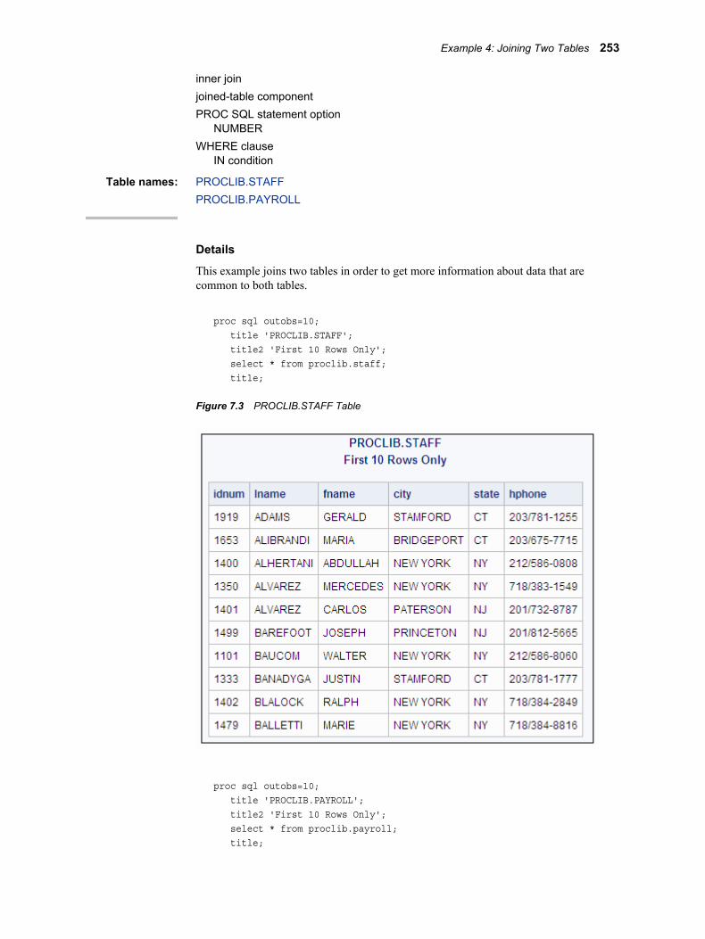
inner joinjoined-table componentPROC SQL statement option

NUMBERWHERE clause

IN condition

Table names: PROCLIB.STAFFPROCLIB.PAYROLL

Details

This example joins two tables in order to get more information about data that are common to both tables.

proc sql outobs=10; title 'PROCLIB.STAFF'; title2 'First 10 Rows Only'; select * from proclib.staff; title;

Figure 7.3 PROCLIB.STAFF Table

proc sql outobs=10; title 'PROCLIB.PAYROLL'; title2 'First 10 Rows Only'; select * from proclib.payroll; title;

Example 4: Joining Two Tables 253

Figure 7.4 PROCLIB.PAYROLL Table

Program


proc sql number;

title 'Information for Certain Employees Only';

/* Select the columns to display. The SELECT clause selects the columns toshow in the output. */ select Lname, Fname, City, State, IdNumber, Salary, Jobcode

from proclib.staff, proclib.payroll

where idnumber=idnum and idnum in ('1919', '1400', '1350', '1333');

Program Description



Add row numbers to PROC SQL output. NUMBER adds a column that contains the row number.

proc sql number;

Specify the title.

title 'Information for Certain Employees Only';


/* Select the columns to display. The SELECT clause selects the columns toshow in the output. */ select Lname, Fname, City, State, IdNumber, Salary, Jobcode

Specify the tables from which to obtain the data. The FROM clause lists the tables to select from.

from proclib.staff, proclib.payroll

Specify the join criterion and subset the query. The WHERE clause specifies that the tables are joined on the ID number from each table. WHERE also further subsets the query with the IN condition, which returns rows for only four employees.

where idnumber=idnum and idnum in ('1919', '1400', '1350', '1333');

Output 7.5 Information for Certain Employees Only

Example 5: Combining Two TablesFeatures: DELETE statement

IS conditionRESET statement option

DOUBLEUNION set operator

Table names: PROCLIB.NEWPAYPROCLIB.PAYLISTPROCLIB.PAYLIST2

Input Tables

This example creates a new table, PROCLIB.NEWPAY, by concatenating two other tables: PROCLIB.PAYLIST and PROCLIB.PAYLIST2.

proc sql;title 'PROCLIB.PAYLIST Table';

Example 5: Combining Two Tables 255


Figure 7.5 PROCLIB.PAYLIST Table

proc sql;title 'PROCLIB.PAYLIST2 Table'; select * from proclib.PAYLIST2;title;

Figure 7.6 PROCLIB.PAYLIST2 Table

Program


proc sql; create table proclib.newpay as select * from proclib.paylist union select * from proclib.paylist2;

delete from proclib.newpay where jobcode is missing or salary is missing;

reset double;

title 'Personnel Data';


select * from proclib.newpay;

Program Description



Create the PROCLIB.NEWPAY table. The SELECT clauses select all the columns from the tables that are listed in the FROM clauses. The UNION set operator concatenates the query results that are produced by the two SELECT clauses.

proc sql; create table proclib.newpay as select * from proclib.paylist union select * from proclib.paylist2;

Delete rows with missing Jobcode or Salary values. The DELETE statement deletes rows from PROCLIB.NEWPAY that satisfy the WHERE expression. The IS condition specifies rows that contain missing values in the Jobcode or Salary column.

delete from proclib.newpay where jobcode is missing or salary is missing;

Reset the PROC SQL environment and double-space the output. RESET changes the procedure environment without stopping and restarting PROC SQL. The DOUBLE option double-spaces the output. (The DOUBLE option has no effect on ODS output.)

reset double;

Specify the title.

title 'Personnel Data';

Display the entire PROCLIB.NEWPAY table. The SELECT clause selects all columns from the newly created table, PROCLIB.NEWPAY.

select * from proclib.newpay;

Example 5: Combining Two Tables 257

Output

Output 7.6 Personnel Data

Example 6: Reporting from DICTIONARY TablesFeatures: DESCRIBE TABLE statement

DICTIONARY.table-name component

Table name: DICTIONARY.MEMBERS

This example uses DICTIONARY tables to show a list of the SAS files in a SAS library. If you do not know the names of the columns in the DICTIONARY table that you are querying, then use a DESCRIBE TABLE statement with the table.

Program


proc sql; describe table dictionary.members;

title 'SAS Files in the PROCLIB Library';

select memname, memtype from dictionary.members where libname='PROCLIB';

Program Description




List the column names from the DICTIONARY.MEMBERS table. DESCRIBE TABLE writes the column names from DICTIONARY.MEMBERS to the SAS log.

proc sql; describe table dictionary.members;

Specify the title.

title 'SAS Files in the PROCLIB Library';

Display a list of files in the PROCLIB library. The SELECT clause selects the MEMNAME and MEMTYPE columns. The FROM clause specifies DICTIONARY.MEMBERS as the table to select from. The WHERE clause subsets the output to include only those rows that have a libref of PROCLIB in the LIBNAME column.

select memname, memtype from dictionary.members where libname='PROCLIB';

Log

277 options nodate pageno=1 source linesize=80 pagesize=60;278279 proc sql;280 describe table dictionary.members;NOTE: SQL table DICTIONARY.MEMBERS was created like:

create table DICTIONARY.MEMBERS ( libname char(8) label='Library Name', memname char(32) label='Member Name', memtype char(8) label='Member Type', engine char(8) label='Engine Name', index char(32) label='Indexes', path char(1024) label='Path Name' );

281 title 'SAS Files in the PROCLIB Library';282283 select memname, memtype284 from dictionary.members285 where libname='PROCLIB';

Example 6: Reporting from DICTIONARY Tables 259

HTML Output

Output 7.7 SAS Files in the PROCLIB Library

Example 7: Performing an Outer JoinFeatures: joined-table component

left outer joinSELECT clause

COALESCE functionWHERE clause

CONTAINS condition

Table names: PROCLIB.PAYROLLPROCLIB.PAYROLL2

Details

This example illustrates a left outer join of the PROCLIB.PAYROLL and PROCLIB.PAYROLL2 tables.

proc sql outobs=10; title 'PROCLIB.PAYROLL'; title2 'First 10 Rows Only'; select * from proclib.payroll order by idnumber; title;


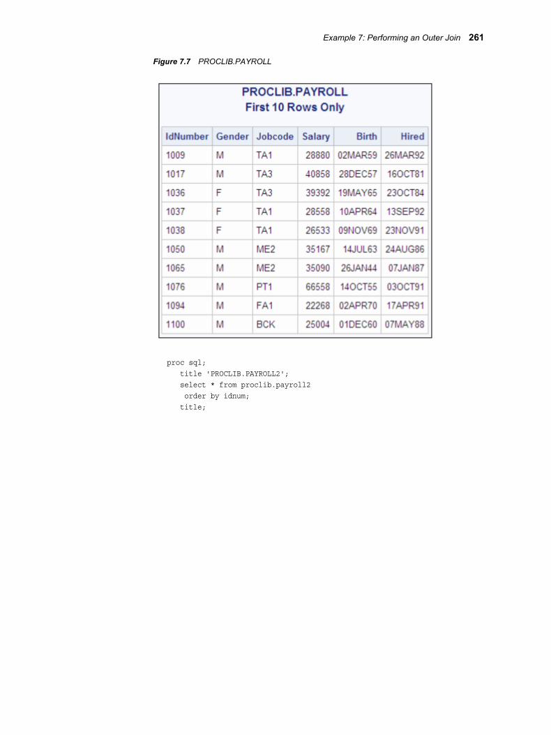
Figure 7.7 PROCLIB.PAYROLL

proc sql; title 'PROCLIB.PAYROLL2'; select * from proclib.payroll2 order by idnum; title;

Example 7: Performing an Outer Join 261

Figure 7.8 PROCLIB.PAYROLL2

Program Using OUTER JOIN Based on ID Number


proc sql outobs=10;

title 'Most Current Jobcode and Salary Information';

select p.IdNumber, p.Jobcode, p.Salary, p2.jobcode label='New Jobcode', p2.salary label='New Salary' format=dollar8.

from proclib.payroll as p left join proclib.payroll2 as p2

on p.IdNumber=p2.idnum;

Program Description



Limit the number of output rows. OUTOBS= limits the output to 10 rows.

proc sql outobs=10;

Specify the title for the first query.



Select the columns. The SELECT clause lists the columns to select. Some column names are prefixed with a table alias because they are in both tables. LABEL= and FORMAT= are column modifiers.

select p.IdNumber, p.Jobcode, p.Salary, p2.jobcode label='New Jobcode', p2.salary label='New Salary' format=dollar8.

Specify the type of join. The FROM clause lists the tables to join and assigns table aliases. The keywords LEFT JOIN specify the type of join. The order of the tables in the FROM clause is important. PROCLIB.PAYROLL is listed first and is considered the “left” table. PROCLIB.PAYROLL2 is the “right” table.

from proclib.payroll as p left join proclib.payroll2 as p2

Specify the join criterion. The ON clause specifies that the join be performed based on the values of the ID numbers from each table.

on p.IdNumber=p2.idnum;

Output for OUTER JOIN

As the output shows, all rows from the left table, PROCLIB.PAYROLL, are returned. PROC SQL assigns missing values for rows in the left table, PAYROLL, that have no matching values for IdNum in PAYROLL2.

Program Using COALESCE and LEFT JOIN

proc sql outobs=10;


select p.idnumber, coalesce(p2.jobcode,p.jobcode) label='Current Jobcode',


coalesce(p2.salary,p.salary) label='Current Salary' format=dollar8.

from proclib.payroll p left join proclib.payroll2 p2 on p.IdNumber=p2.idnum;

Program Description

proc sql outobs=10;

Specify the title for the second query.


Select the columns and coalesce the Jobcode columns. The SELECT clause lists the columns to select. COALESCE overlays the like-named columns. For each row, COALESCE returns the first nonmissing value of either P2.JOBCODE or P.JOBCODE. Because P2.JOBCODE is the first argument, if there is a nonmissing value for P2.JOBCODE, COALESCE returns that value. Thus, the output contains the most recent job code information for every employee. LABEL= assigns a column label.

select p.idnumber, coalesce(p2.jobcode,p.jobcode) label='Current Jobcode',

Coalesce the Salary columns. For each row, COALESCE returns the first nonmissing value of either P2.SALARY or P.SALARY. Because P2.SALARY is the first argument, if there is a nonmissing value for P2.SALARY, then COALESCE returns that value. Thus, the output contains the most recent salary information for every employee.

coalesce(p2.salary,p.salary) label='Current Salary' format=dollar8.

Specify the type of join and the join criterion. The FROM clause lists the tables to join and assigns table aliases. The keywords LEFT JOIN specify the type of join. The ON clause specifies that the join is based on the ID numbers from each table.

from proclib.payroll p left join proclib.payroll2 p2 on p.IdNumber=p2.idnum;


Output for COALESCE and LEFT JOIN

Output 7.8 Most Current Jobcode and Salary Information

Program to Subset the Query

proc sql;

title 'Most Current Information for Ticket Agents'; select p.IdNumber, coalesce(p2.jobcode,p.jobcode) label='Current Jobcode', coalesce(p2.salary,p.salary) label='Current Salary' from proclib.payroll p left join proclib.payroll2 p2 on p.IdNumber=p2.idnum where p2.jobcode contains 'TA';

Program Description

Subset the query. The WHERE clause subsets the left join to include only those rows containing the value TA.

proc sql;

title 'Most Current Information for Ticket Agents'; select p.IdNumber, coalesce(p2.jobcode,p.jobcode) label='Current Jobcode', coalesce(p2.salary,p.salary) label='Current Salary' from proclib.payroll p left join proclib.payroll2 p2 on p.IdNumber=p2.idnum where p2.jobcode contains 'TA';


Output for Subset of the Query

Output 7.9 Query Results with the Value TA

Example 8: Creating a View from a Query's ResultFeatures: CREATE VIEW statement

GROUP BY clauseSELECT clause

COUNT functionHAVING clause

Other features: AVG summary functiondata set option

PW=

Table names: PROCLIB.PAYROLLPROCLIB.JOBS

Details

This example creates the PROC SQL view PROCLIB.JOBS from the result of a query expression.

proc sql outobs=10; title 'PROCLIB.PAYROLL'; title2 'First 10 Rows Only'; select * from proclib.payroll order by idnumber; title;


Figure 7.9 PROCLIB.PAYROLL

Program


proc sql; create view proclib.jobs(pw=red) as

select Jobcode, count(jobcode) as number label='Number',

avg(int((today()-birth)/365.25)) as avgage format=2. label='Average Age', avg(salary) as avgsal format=dollar8. label='Average Salary'

from payroll

group by jobcode having avgage ge 30;

title 'Current Summary Information for Each Job Category'; title2 'Average Age Greater Than or Equal to 30';

select * from proclib.jobs(pw=red);

title2;

Program Description


Example 8: Creating a View from a Query's Result 267


Create the PROCLIB.JOBS view. CREATE VIEW creates the PROC SQL view PROCLIB.JOBS. The PW= data set option assigns password protection to the data that is generated by this view.

proc sql; create view proclib.jobs(pw=red) as

Select the columns. The SELECT clause specifies four columns for the view: Jobcode and three columns, Number, AVGAGE, and AVGSAL, whose values are the products functions. COUNT returns the number of nonmissing values for each job code because the data is grouped by Jobcode. LABEL= assigns a label to the column.

select Jobcode, count(jobcode) as number label='Number',

Calculate the Avgage and Avgsal columns. The AVG summary function calculates the average age and average salary for each job code.

avg(int((today()-birth)/365.25)) as avgage format=2. label='Average Age', avg(salary) as avgsal format=dollar8. label='Average Salary'

Specify the table from which the data is obtained. The FROM clause specifies PAYROLL as the table to select from. PROC SQL assumes the libref of PAYROLL to be PROCLIB because PROCLIB is used in the CREATE VIEW statement.

from payroll

Organize the data into groups and specify the groups to include in the output. The GROUP BY clause groups the data by the values of Jobcode. Thus, any summary statistics are calculated for each grouping of rows by value of Jobcode. The HAVING clause subsets the grouped data and returns rows for job codes that contain an average age of greater than or equal to 30.

group by jobcode having avgage ge 30;

Specify the titles.

title 'Current Summary Information for Each Job Category'; title2 'Average Age Greater Than or Equal to 30';

Display the entire PROCLIB.JOBS view. The SELECT statement selects all columns from PROCLIB.JOBS. PW=RED is necessary because the view is password protected.

select * from proclib.jobs(pw=red);

title2;


Output

Output 7.10 View Created from the Results of a Query

Example 9: Joining Three TablesFeatures: FROM clause

joined-table componentWHERE clause

Table names: PROCLIB.STAFF2PROCLIB.SCHEDULE2PROCLIB.SUPERV2

Example 9: Joining Three Tables 269

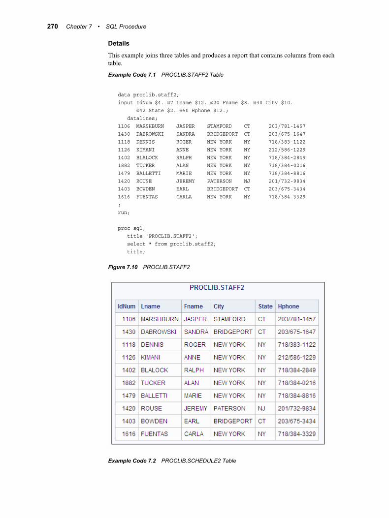
Details

This example joins three tables and produces a report that contains columns from each table.

Example Code 7.1 PROCLIB.STAFF2 Table

data proclib.staff2;input IdNum $4. @7 Lname $12. @20 Fname $8. @30 City $10. @42 State $2. @50 Hphone $12.; datalines;1106 MARSHBURN JASPER STAMFORD CT 203/781-14571430 DABROWSKI SANDRA BRIDGEPORT CT 203/675-16471118 DENNIS ROGER NEW YORK NY 718/383-11221126 KIMANI ANNE NEW YORK NY 212/586-12291402 BLALOCK RALPH NEW YORK NY 718/384-28491882 TUCKER ALAN NEW YORK NY 718/384-02161479 BALLETTI MARIE NEW YORK NY 718/384-88161420 ROUSE JEREMY PATERSON NJ 201/732-98341403 BOWDEN EARL BRIDGEPORT CT 203/675-34341616 FUENTAS CARLA NEW YORK NY 718/384-3329;run;

proc sql; title 'PROCLIB.STAFF2'; select * from proclib.staff2; title;

Figure 7.10 PROCLIB.STAFF2

Example Code 7.2 PROCLIB.SCHEDULE2 Table


data proclib.schedule2; input flight $3. +5 date date7. +2 dest $3. +3 idnum $4.; format date date7.; informat date date7.; datalines;132 01MAR94 BOS 1118132 01MAR94 BOS 1402219 02MAR94 PAR 1616219 02MAR94 PAR 1478622 03MAR94 LON 1430622 03MAR94 LON 1882271 04MAR94 NYC 1430271 04MAR94 NYC 1118579 05MAR94 RDU 1126579 05MAR94 RDU 1106;run;

proc sql; title 'PROCLIB.SCHEDULE2'; select * from proclib.schedule2; title;

Figure 7.11 PROCLIB.SCHEDULE2

Example Code 7.3 PROCLIB.SUPERV2 Table

data proclib.superv2; input supid $4. +8 state $2. +5 jobcat $2.; label supid='Supervisor Id' jobcat='Job Category'; datalines;1417 NJ NA1352 NY NA

Example 9: Joining Three Tables 271

1106 CT PT1442 NJ PT1118 NY PT1405 NJ SC1564 NY SC1639 CT TA1126 NY TA1882 NY ME;run;

proc sql; title 'PROCLIB.SUPERV2'; select * from proclib.superv2 title;

Figure 7.12 PROCLIB.SUPERV2

Program


proc sql; title 'All Flights for Each Supervisor'; select s.IdNum, Lname, City 'Hometown', Jobcat, Flight, Date

from proclib.schedule2 s, proclib.staff2 t, proclib.superv2 v

where s.idnum=t.idnum and t.idnum=v.supid;


Program Description



Select the columns. The SELECT clause specifies the columns to select. IdNum is prefixed with a table alias because it appears in two tables.

proc sql; title 'All Flights for Each Supervisor'; select s.IdNum, Lname, City 'Hometown', Jobcat, Flight, Date

Specify the tables to include in the join. The FROM clause lists the three tables for the join and assigns an alias to each table.

from proclib.schedule2 s, proclib.staff2 t, proclib.superv2 v

Specify the join criteria. The WHERE clause specifies the columns that join the tables. The STAFF2 and SCHEDULE2 tables have an IdNum column, which has related values in both tables. The STAFF2 and SUPERV2 tables have the IdNum and SUPID columns, which have related values in both tables.

where s.idnum=t.idnum and t.idnum=v.supid;

Output

Output 7.11 ID Values from All Three Tables Are Included

Example 10: Querying an In-Line ViewFeatures: FROM clause

in-line view

Table names: PROCLIB.STAFF2PROCLIB.SCHEDULE2PROCLIB.SUPERV2

Example 10: Querying an In-Line View 273

This example shows an alternative way to construct the query that is explained in “Example 9: Joining Three Tables” on page 269 by joining one of the tables with the results of an in-line view. The example also shows how to rename columns with an in-line view.

Program


proc sql; title 'All Flights for Each Supervisor'; select three.*, v.jobcat

from (select lname, s.idnum, city, flight, date from proclib.schedule2 s, proclib.staff2 t where s.idnum=t.idnum)

as three (Surname, Emp_ID, Hometown, FlightNumber, FlightDate),

proclib.superv2 v where three.Emp_ID=v.supid;

Program Description



Select the columns. The SELECT clause selects all columns that are returned by the in-line view (which will have the alias Three assigned to it), plus one column from the third table (which will have the alias V assigned to it).

proc sql; title 'All Flights for Each Supervisor'; select three.*, v.jobcat

Specify the in-line query. Instead of including the name of a table or view, the FROM clause includes a query that joins two of the three tables. In the in-line query, the SELECT clause lists the columns to select. IdNum is prefixed with a table alias because it appears in both tables. The FROM clause lists the two tables for the join and assigns an alias to each table. The WHERE clause specifies the columns that join the tables. The STAFF2 and SCHEDULE2 tables have an IdNum column, which has related values in both tables.

from (select lname, s.idnum, city, flight, date from proclib.schedule2 s, proclib.staff2 t where s.idnum=t.idnum)

Specify an alias for the query and names for the columns. The alias Three refers to the results of the in-line view. The names in parentheses become the names for the columns in the view.

as three (Surname, Emp_ID, Hometown, FlightNumber, FlightDate),


Join the results of the in-line view with the third table. The WHERE clause specifies the columns that join the table with the in-line view. Note that the WHERE clause specifies the renamed Emp_ID column from the in-line view.

proclib.superv2 v where three.Emp_ID=v.supid;

Output

Output 7.12 Query of an In-Line View

Example 11: Retrieving Values with the SOUNDS-LIKE OperatorFeatures: ORDER BY clause

SOUNDS-LIKE operator

Table name: PROCLIB.STAFF

This example returns rows based on the functionality of the SOUNDS-LIKE operator in a WHERE clause. The SOUNDS-LIKE operator is based on the SOUNDEX algorithm for identifying words that sound alike. The SOUNDEX algorithm is English-biased and is less useful for languages other than English. For more information about the “SOUNDEX Function” in SAS Functions and CALL Routines: Reference algorithm, see SAS Functions and CALL Routines: Reference.

Details

proc sql outobs=10; title 'PROCLIB.STAFF'; title2 'First 10 Rows Only'; select * from proclib.staff; title;

Example 11: Retrieving Values with the SOUNDS-LIKE Operator 275

Figure 7.13 PROCLIB.STAFF

Program to Select Names That Sound like 'Johnson'


proc sql; title "Employees Whose Last Name Sounds Like 'Johnson'"; select idnum, upcase(lname), fname from proclib.staff

where lname=*"Johnson" order by 2;

Program Description



Select the columns and the table from which the data is obtained. The SELECT clause selects all columns from the table in the FROM clause, PROCLIB.STAFF.

proc sql; title "Employees Whose Last Name Sounds Like 'Johnson'"; select idnum, upcase(lname), fname from proclib.staff

Subset the query and sort the output. The WHERE clause uses the SOUNDS-LIKE operator to subset the table by those employees whose last name sounds like Johnson. The ORDER BY clause orders the output by the second column.

where lname=*"Johnson"


order by 2;

Output for Names That Sound like 'Johnson'

Output 7.13 Employees Whose Last Name Sounds like 'Johnson'

Program to Select Names That Sound like 'Sanders'

SOUNDS-LIKE is useful, but there might be instances where it does not return every row that seems to satisfy the condition. PROCLIB.STAFF has an employee with the last name SANDERS and an employee with the last name SANYERS. The algorithm does not find SANYERS, but it does find SANDERS and SANDERSON.

proc sql;title "Employees Whose Last Name Sounds Like 'Sanders'"; select * from proclib.staff where lname=*"Sanders" order by 2;

Output for Names That Sound like 'Sanders'

Output 7.14 Employees Whose Last Name Sounds like 'Sanders'

Example 12: Joining Two Tables and Calculating a New ValueFeatures: GROUP BY clause

HAVING clause

Example 12: Joining Two Tables and Calculating a New Value 277

SELECT clauseABS functionFORMAT= column-modifierLABEL= column-modifierMIN summary function** operator, exponentiationSQRT function

Table names: STORESHOUSES

Details

This example joins two tables in order to compare and analyze values that are unique to each table yet have a relationship with a column that is common to both tables.

proc sql; title 'STORES Table'; title2 'Coordinates of Stores'; select * from stores; title 'HOUSES Table'; title2 'Coordinates of Houses'; select * from houses;title;

The tables contain X and Y coordinates that represent the location of the stores and houses.


Figure 7.14 STORES and HOUSES Tables

Program

proc sql; title 'Each House and the Closest Store'; select house, store label='Closest Store', sqrt((abs(s.x-h.x)**2)+(abs(h.y-s.y)**2)) as dist label='Distance' format=4.2 from stores s, houses h

group by house having dist=min(dist);

Program Description

Specify the query. The SELECT clause specifies three columns: HOUSE, STORE, and DIST. The arithmetic expression uses the square root function (SQRT) to create the values of DIST, which contain the distance from HOUSE to STORE for each row. The double asterisk (**) represents exponentiation. LABEL= assigns a label to STORE and to DIST.

proc sql; title 'Each House and the Closest Store'; select house, store label='Closest Store', sqrt((abs(s.x-h.x)**2)+(abs(h.y-s.y)**2)) as dist label='Distance' format=4.2

Example 12: Joining Two Tables and Calculating a New Value 279

from stores s, houses h

Organize the data into groups and subset the query. The minimum distance from each house to all the stores is calculated because the data are grouped by house. The HAVING clause specifies that each row be evaluated to determine whether its value of DIST is the same as the minimum distance from that house to any store.

group by house having dist=min(dist);

Output

Note that two stores are tied for shortest distance from house2.

Output 7.15 New Value, Distance, Calculated from Two Tables

Example 13: Producing All the Possible Combinations of the Values in a Column

Features: CASE expressionjoined-table componentCross joinSELECT clause

DISTINCT keyword

Table names: PROCLIB.MARCHFLIGHTS

Details

This example joins a table with itself to get all the possible combinations of the values in a column.

proc sql outobs=10; title 'PROCLIB.MARCH'; title2 'First 10 Rows Only'; select * from proclib.march;

title;


Figure 7.15 PROCLIB.MARCH

Program to Create the Flights Table


proc sql; create table flights as select distinct dest from proclib.march;

title 'Cities Serviced by the Airline';

select * from flights;

Program Description



Create the FLIGHTS table. The CREATE TABLE statement creates the table FLIGHTS from the output of the query. The SELECT clause selects the unique values of Dest. DISTINCT specifies that only one row for each value of city be returned by the query and stored in the table FLIGHTS. The FROM clause specifies PROCLIB.MARCH as the table to select from.

proc sql; create table flights as select distinct dest from proclib.march;

Specify the title.

Example 13: Producing All the Possible Combinations of the Values in a Column 281

title 'Cities Serviced by the Airline';

Display the entire FLIGHTS table.

select * from flights;

Output for Flights Table

Output 7.16 Cities Serviced by the Airline

Program Using Conventional Join

proc sql;

title 'All Possible Connections';

select f1.Dest, case when f1.dest ne ' ' then 'to and from' end, f2.Dest

from flights as f1, flights as f2

where f1.dest < f2.dest

order by f1.dest;

Program Description

proc sql;

Specify the title.

title 'All Possible Connections';

Select the columns. The SELECT clause specifies three columns for the output. The prefixes on DEST are table aliases to specify which table to take the values of Dest from. The CASE expression creates a column that contains the character string to and from.

select f1.Dest, case when f1.dest ne ' ' then 'to and from' end,


f2.Dest

Specify the type of join. The FROM clause joins FLIGHTS with itself and creates a table that contains every possible combination of rows (a Cartesian product). The table contains two rows for each possible route. For example, PAR <-> WAS and WAS <-> PAR.

from flights as f1, flights as f2

Specify the join criterion. The WHERE clause subsets the internal table by choosing only those rows where the name in F1.Dest sorts before the name in F2.Dest. Thus, there is only one row for each possible route.

where f1.dest < f2.dest

Sort the output. ORDER BY sorts the result by the values of F1.Dest.

order by f1.dest;


Output Using Conventional Join

Output 7.17 All Possible Connections

Program Using Cross Join

/* */proc sql; title 'All Possible Connections'; select f1.Dest, case when f1.dest ne ' ' then 'to and from' end, f2.Dest from flights as f1 cross join flights as f2 where f1.dest < f2.dest


order by f1.dest;

Program Description

Specify a cross join. Because a cross join is functionally the same as a Cartesian product join, the cross join syntax can be substituted for the conventional join syntax.

/* */proc sql; title 'All Possible Connections'; select f1.Dest, case when f1.dest ne ' ' then 'to and from' end, f2.Dest from flights as f1 cross join flights as f2 where f1.dest < f2.dest order by f1.dest;


Output Using Cross Join

Output 7.18 All Possible Connections

Example 14: Matching Case Rows and Control RowsFeatures: joined-table component

Table names: MATCH_11MATCH

This example uses a table that contains data for a case-control study. Each row contains information for a case or a control. To perform statistical analysis, you need a table with one row for each case-control pair. PROC SQL joins the table with itself in order to


match the cases with their appropriate controls. After the rows are matched, differencing can be performed on the appropriate columns.

The input table Appendix 3, “MATCH_11,” in Base SAS Procedures Guide contains one row for each case and one row for each control. Pair contains a number that associates the case with its control. Low is 0 for the controls and 1 for the cases. The remaining columns contain information about the cases and controls.

options ls=120 nodate pageno=1;proc sql outobs=10; title 'MATCH_11 Table'; title2 'First 10 Rows Only'; select * from match_11;

Figure 7.16 MATCH_11 Table, First 10 Rows

Program

proc sql; create table match as select one.Low, one.Pair, (one.lwt - two.lwt) as Lwt_d, (one.smoke - two.smoke) as Smoke_d, (one.ptd - two.ptd) as Ptd_d, (one.ht - two.ht) as Ht_d, (one.ui - two.ui) as UI_d

from match_11 one, match_11 two where (one.pair=two.pair and one.low>two.low);

title 'Differences for Cases and Controls';

Example 14: Matching Case Rows and Control Rows 287

select * from match(obs=5);

Program Description

Create the MATCH table. The SELECT clause specifies the columns for the table MATCH. SQL expressions in the SELECT clause calculate the differences for the appropriate columns and create new columns.

proc sql; create table match as select one.Low, one.Pair, (one.lwt - two.lwt) as Lwt_d, (one.smoke - two.smoke) as Smoke_d, (one.ptd - two.ptd) as Ptd_d, (one.ht - two.ht) as Ht_d, (one.ui - two.ui) as UI_d

Specify the type of join and the join criterion. The FROM clause lists the table MATCH_11 twice. Thus, the table is joined with itself. The WHERE clause returns only the rows for each pair that show the difference when the values for control are subtracted from the values for case.

from match_11 one, match_11 two where (one.pair=two.pair and one.low>two.low);

Specify the title.

title 'Differences for Cases and Controls';

Display the first five rows of the MATCH table. The SELECT clause selects all the columns from MATCH. The OBS= data set option limits the printing of the output to five rows.

select * from match(obs=5);


Output

Output 7.19 Differences for Cases and Controls

Example 15: Counting Missing Values with a SAS MacroFeatures: COUNT function

Table name: SURVEY

This example uses a SAS macro to create columns. The SAS macro is not explained here. See SAS Macro Language: Reference for information about SAS macros.

“SURVEY” on page 394 contains data from a questionnaire about diet and exercise habits. SAS enables you to use a special notation for missing values. In the EDUC column, the .x notation indicates that the respondent gave an answer that is not valid, and .n indicates that the respondent did not answer the question. A period as a missing value indicates a data entry error.

Program

%macro countm(col); count(&col) "Valid Responses for &col",

nmiss(&col) "Missing or NOT VALID Responses for &col",

count(case when &col=.n then "count me" end) "Coded as NO ANSWER for &col", count(case when &col=.x then "count me" end) "Coded as NOT VALID answers for &col", count(case when &col=. then "count me" end) "Data Entry Errors for &col"%mend;

proc sql; title 'Counts for Each Type of Missing Response'; select count(*) "Total No. of Rows", %countm(educ)

Example 15: Counting Missing Values with a SAS Macro 289

from survey;

Program Description

Count the nonmissing responses. The COUNTM macro uses the COUNT function to perform various counts for a column. Each COUNT function uses a CASE expression to select the rows to be counted. The first COUNT function uses only the column as an argument to return the number of nonmissing rows.

%macro countm(col); count(&col) "Valid Responses for &col",

Count missing or invalid responses. The NMSS function returns the number of rows for which the column has any type of missing value: .n, .x, or a period.

nmiss(&col) "Missing or NOT VALID Responses for &col",

Count the occurrences of various sources of missing or invalid responses. The last three COUNT functions use CASE expressions to count the occurrences of the three notations for missing values. The “count me” character string gives the COUNT function a nonmissing value to count.

count(case when &col=.n then "count me" end) "Coded as NO ANSWER for &col", count(case when &col=.x then "count me" end) "Coded as NOT VALID answers for &col", count(case when &col=. then "count me" end) "Data Entry Errors for &col"%mend;

Use the COUNTM macro to create the columns. The SELECT clause specifies the columns that are in the output. COUNT(*) returns the total number of rows in the table. The COUNTM macro uses the values of the EDUC column to create the columns that are defined in the macro.

proc sql; title 'Counts for Each Type of Missing Response'; select count(*) "Total No. of Rows", %countm(educ) from survey;


Output

Output 7.20 Counts for Each Type of Missing Response

Example 15: Counting Missing Values with a SAS Macro 291

Chapter 8

SQL SELECT Statement Clauses

Dictionary . . . . . . . . . . . . . . . . . . . . . . . . . . . . . . . . . . . . . . . . . . . . . . . . . . . . . . . . . . 293SELECT Clause . . . . . . . . . . . . . . . . . . . . . . . . . . . . . . . . . . . . . . . . . . . . . . . . . . . 293INTO Clause . . . . . . . . . . . . . . . . . . . . . . . . . . . . . . . . . . . . . . . . . . . . . . . . . . . . . . 295FROM Clause . . . . . . . . . . . . . . . . . . . . . . . . . . . . . . . . . . . . . . . . . . . . . . . . . . . . . 301WHERE Clause . . . . . . . . . . . . . . . . . . . . . . . . . . . . . . . . . . . . . . . . . . . . . . . . . . . 302GROUP BY Clause . . . . . . . . . . . . . . . . . . . . . . . . . . . . . . . . . . . . . . . . . . . . . . . . 303HAVING Clause . . . . . . . . . . . . . . . . . . . . . . . . . . . . . . . . . . . . . . . . . . . . . . . . . . . 304ORDER BY Clause . . . . . . . . . . . . . . . . . . . . . . . . . . . . . . . . . . . . . . . . . . . . . . . . 305

Dictionary

SELECT ClauseLists the columns that will appear in the output.

See: “column-definition” on page 312“Example 1: Creating a Table and Inserting Data into It” on page 246“Example 2: Creating a Table from a Query's Result” on page 248

SyntaxSELECT <DISTINCT> object-item <, … object-item>


assigns a temporary, alternate name to the column.

DISTINCTeliminates duplicate rows. The DISTINCT argument is identical to UNIQUE.

Note DISTINCT works on the internal or stored value, not necessarily on the value as it is displayed. Numeric precision can cause multiple rows to be returned with values that appear to be the same.

Tips A row is considered a duplicate when all of its values are the same as the values of another row. The DISTINCT argument applies to all columns in

293

the SELECT list. One row is displayed for each existing combination of values.

If available, PROC SQL uses index files when processing SELECT DISTINCT statements.

Example “Example 13: Producing All the Possible Combinations of the Values in a Column” on page 280

object-itemis one of the following:

*represents all columns in the tables or views that are listed in the FROM clause.

case-expression <AS alias>derives a column from a CASE expression. See “CASE Expression” on page 310.

column-name<AS alias><column-modifier <… column-modifier>>names a single column. See “column-name” on page 315 and “column-modifier” on page 313.

sql-expression<AS alias><column-modifier <… column-modifier>>derives a column from an sql-expression. See “sql-expression” on page 342 and “column-modifier” on page 313.

table-name.*specifies all columns in the PROC SQL table that is specified in table-name.

table-alias.*specifies all columns in the PROC SQL table that has the alias that is specified in table-alias.

view-name.*specifies all columns in the SAS view that is specified in view-name.

view-alias.*specifies all columns in the SAS view that has the alias that is specified in view-alias.

UNIQUEeliminates duplicate rows. The UNIQUE argument is identical to DISTINCT.

Note: Although the UNIQUE argument is identical to DISTINCT, it is not an ANSI standard.

Details

Asterisk (*) NotationThe asterisk (*) represents all columns of the table or tables listed in the FROM clause. When an asterisk is not prefixed with a table name, all the columns from all tables in the FROM clause are included; when it is prefixed (for example, table-name.* or table-alias.*), all the columns from that table only are included.

Note: A warning will occur if you create an output table using the SELECT * syntax when columns with the same name exist in the multiple tables that are listed on the FROM clause. You can avoid the warning by using one of the following actions:

• Individually list the desired columns in the SELECT statement at the same time as you omit the duplicate column names.

294 Chapter 8 • SQL SELECT Statement Clauses

• Use the RENAME= and DROP= data set options. In this example, the ID column is renamed tmpid.

proc sql; create table all(drop=tmpid) as select * from one, two(rename=(id=tmpid)) where one.id=two.tmpid;quit;

If table aliases are used, place the RENAME= data set option after the table name and before the table alias. You can omit the DROP= data set option if you want to keep the renamed column in the final output table.

Column AliasesA column alias is a temporary, alternate name for a column. Aliases are specified in the SELECT clause to name or rename columns so that the result table is clearer or easier to read. Aliases are often used to name a column that is the result of an arithmetic expression or summary function. An alias is one word only. If you need a longer column name, then use the LABEL= column-modifier, as described in “column-modifier” on page 313. The keyword AS is required with a column alias to distinguish the column alias from column names in the SELECT clause.

Column aliases are optional, and each column name in the SELECT clause can have an alias. After you assign an alias to a column, you can use the alias to refer to that column in other clauses.

If you use a column alias when creating a PROC SQL view, then the alias becomes the permanent name of the column for each execution of the view.

Note: For the maximum portability of SQL code that is used outside of the SAS SQL procedure, avoid writing code that refers to column aliases in a WHERE clause, GROUP BY clause, or HAVING clause. For more information, see “Column Alias Exceptions” on page 378.

INTO ClauseStores the value of one or more columns for use later in another PROC SQL query or SAS statement.

Restriction: An INTO clause cannot be used in a CREATE TABLE statement.

See: “Using the PROC SQL Automatic Macro Variables” on page 157

SyntaxINTO macro-variable-specification<, … macro-variable-specification>

Required Argumentsmacro-variable

specifies a SAS macro variable that stores the values of the rows that are returned.

macro-variable-specificationis one of the following:

INTO Clause 295

macro-variable<SEPARATED BY 'character(s)'<NOTRIM>>stores the values that are returned into a single macro variable.

macro-variable<TRIMMED>stores the values that are returned into a single macro variable.

macro-variable-1 - macro-variable-n<NOTRIM>stores the values that are returned into a range of macro variables.

Tip When you specify a range of macro variables, the SAS Macro Facility creates only the number of macro variables that are needed. For example, if you specify :var1-:var9999 and only 55 variables are needed, only :var1-:var55 is created. The SQLOBS automatic variable is useful if a subsequent part of your program needs to know how many variables were actually created. In this example, SQLOBS would have the value of 55.

macro-variable-1 - <NOTRIM>stores the values that are returned into a range of macro variables.

Tip If you do not know how many variables you might need, you can create a macro variable range without specifying an upper bound for the range. The SQLOBS macro variable can be used if a subsequent part of your program needs to know how many variables were actually created.

NOTRIMprotects the leading and trailing blanks from being deleted from values that are stored in a range of macro variables or multiple values that are stored in a single macro variable.

SEPARATED BY 'character'specifies a character that separates the values of the rows.

TRIMMEDtrims the leading and trailing blanks from values that are stored in a single macro variable.

Details• Use the INTO clause only in the outer query of a SELECT statement, not in a

subquery.

• When storing a value in a single macro variable, PROC SQL preserves leading or trailing blanks. The TRIMMED option can be used to trim the leading and trailing blanks from values that are stored in a single macro variable. However, if values are stored in a range of macro variables, or if the SEPARATED BY option is used to store multiple values in a single macro variable, PROC SQL trims leading or trailing blanks unless you specify the NOTRIM option.

• You can put multiple rows of the output in macro variables. You can use the PROC SQL macro variable SQLOBS to determine the number of rows that are produced by a query expression. For more information about SQLOBS, see “Using the PROC SQL Automatic Macro Variables” on page 157.

Note: The SQLOBS macro variable is assigned a value after the SELECT statement executes.

• Values assigned by the INTO clause use the BEST8. format.


Example: INTO ClauseThese examples use the “PROCLIB.HOUSES” on page 384 table:

title 'PROCLIB.HOUSES Table';proc sql; select * from proclib.houses;

Output 8.1 PROCLIB.HOUSES Table

With the macro-variable-specification, you can do the following:

• You can create macro variables based on the first row of the result.

proc sql noprint; select style, sqfeet into :style, :sqfeet from proclib.houses;

%put &style &sqfeet;

The results are written to the SAS log:

1 proc sql noprint;2 select style, sqfeet3 into :style, :sqfeet4 from proclib.houses;56 %put &style &sqfeet;CONDO 900

• You can use the TRIMMED option to remove leading and trailing blanks from values that are stored in a single macro variable.

proc sql noprint;

INTO Clause 297

select distinct style, sqfeet into :s1, :s2 TRIMMED from proclib.houses;%put &s1 &s2;%put There were &sqlobs distinct values.;


1 proc sql noprint;2 select distinct style, sqfeet3 into :s1, :s2 TRIMMED4 from proclib.houses;5 %put &s1 &s2;CONDO 9006 %put There were &sqlobs distinct values.;There were 1 distinct values.

• You can create one new macro variable per row in the result of the SELECT statement. This example shows how you can request more values for one column than for another. The hyphen is used in the INTO clause to imply a range of macro variables. You can use either of the keywords THROUGH or THRU instead of a hyphen.

The following PROC SQL step puts the values from the first four rows of the PROCLIB.HOUSES table into macro variables:

proc sql noprint;select distinct Style, SqFeet into :style1 - :style3, :sqfeet1 - :sqfeet4 from proclib.houses;

%put &style1 &sqfeet1;%put &style2 &sqfeet2;%put &style3 &sqfeet3;%put &sqfeet4;

The %PUT statements write the results to the SAS log:

1 proc sql noprint;2 select distinct style, sqfeet3 into :style1 - :style3, :sqfeet1 - :sqfeet44 from proclib.houses;56 %put &style1 &sqfeet1;CONDO 9007 %put &style2 &sqfeet2;CONDO 10008 %put &style3 &sqfeet3;RANCH 12009 %put &sqfeet4;1400

• You can use a hyphen in the INTO clause to specify a range without an upper bound.

proc sql noprint;select distinct Style, SqFeet into :style1 - , :sqfeet1 - from proclib.houses;


%put &style1 &sqfeet1;%put &style2 &sqfeet2;%put &style3 &sqfeet3;%put &sqfeet4;


1 proc sql noprint;2 select distinct Style, SqFeet3 into :style1 - , :sqfeet1 -4 from proclib.houses;56 %put &style1 &sqfeet1;CONDO 9007 %put &style2 &sqfeet2;CONDO 10008 %put &style3 &sqfeet3;RANCH 12009 %put &sqfeet4;1400

• You can concatenate the values of one column into one macro variable. This form is useful for building up a list of variables or constants. The SQLOBS macro variable is useful to reveal how many distinct variables there were in the data processed by the query.

proc sql noprint; select distinct style into :s1 separated by ',' from proclib.houses;%put &s1;%put There were &sqlobs distinct values.;


3 proc sql noprint;4 select distinct style5 into :s1 separated by ','6 from proclib.houses;78 %put &s1

CONDO,RANCH,SPLIT,TWOSTORYThere were 4 distinct values.

• You can use leading zeros in order to create a range of macro variable names, as shown in the following example:

proc sql noprint; select SqFeet into :sqfeet01 - :sqfeet10 from proclib.houses;

%put &sqfeet01 &sqfeet02 &sqfeet03 &sqfeet04 &sqfeet05;%put &sqfeet06 &sqfeet07 &sqfeet08 &sqfeet09 &sqfeet10;

INTO Clause 299


11 proc sql noprint; 12 select sqfeet 13 into :sqfeet01 - :sqfeet10 14 from proclib.houses;

15 %put &sqfeet01 &sqfeet02 &sqfeet03 &sqfeet04 &sqfeet05;900 1000 1200 1400 160016 %put &sqfeet06 &sqfeet07 &sqfeet08 &sqfeet09 &sqfeet10;1800 2100 3000 1940 1860

• You can prevent leading and trailing blanks from being trimmed from values that are stored in macro variables. By default, when storing values in a range of macro variables, or when storing multiple values in a single macro variable (with the SEPARATED BY option), PROC SQL trims the leading and trailing blanks from the values before creating the macro variables. If you do not want leading and trailing blanks to be trimmed, specify the NOTRIM option, as shown in the following example:

proc sql noprint; select style, sqfeet into :style1 - :style4 notrim, :sqfeet separated by ',' notrim from proclib.houses;

%put *&style1* *&sqfeet*;%put *&style2* *&sqfeet*;%put *&style3* *&sqfeet*;%put *&style4* *&sqfeet*;

The results are written to the SAS log, as shown in the following output:

3 proc sql noprint;4 select style, sqfeet5 into :style1 - :style4 notrim,6 :sqfeet separated by ',' notrim7 from proclib.houses;89 %put *&style1* *&sqfeet*;*CONDO * * 900, 1000, 1200, 1400, 1600, 1800, 2100, 3000, 1940, 1860*10 %put *&style2* *&sqfeet*;*CONDO * * 900, 1000, 1200, 1400, 1600, 1800, 2100, 3000, 1940, 1860**11 %put *&style3* *&sqfeet*;*RANCH * * 900, 1000, 1200, 1400, 1600, 1800, 2100, 3000, 1940, 1860**12 %put *&style4* *&sqfeet*;*RANCH * * 900, 1000, 1200, 1400, 1600, 1800, 2100, 3000, 1940, 1860**</log></logBlock>


FROM ClauseSpecifies source tables or views.

See: “Example 1: Creating a Table and Inserting Data into It” on page 246“Example 4: Joining Two Tables” on page 252“Example 9: Joining Three Tables” on page 269“Example 10: Querying an In-Line View” on page 273

SyntaxFROM from-list


specifies a temporary, alternate name for a table, view, or in-line view that is specified in the FROM clause.

columnnames the column that appears in the output. The column names that you specify are matched by position to the columns in the output.

from-listis one of the following:

table-name <<AS>alias>names a single PROC SQL table. table-name can be a one-level name, a two-level libref.table name, or a physical pathname that is enclosed in single quotation marks.

view-name <<AS>alias>names a single SAS view. view-name can be a one-level name, a two-level libref.view name, or a physical pathname that is enclosed in single quotation marks.

joined-tablespecifies a join. See “joined-table” on page 318.

(query-expression) <<AS>alias> <(column<, …column>)>specifies an in-line view. See “query-expression” on page 334.

CONNECTION TOspecifies a DBMS table. See “CONNECTION TO” on page 315.

Note: With table-name and view-name, you can use data set options by placing them in parentheses immediately after table-name or view-name. For more information, see “Using SAS Data Set Options with PROC SQL” on page 151.

Details

Table AliasesA table alias is a temporary, alternate name for a table that is specified in the FROM clause. Table aliases are prefixed to column names to distinguish between columns that are common to multiple tables. Column names in reflexive joins (joining a table with

FROM Clause 301

itself) must be prefixed with a table alias in order to distinguish which copy of the table the column comes from. Column names in other types of joins must be prefixed with table aliases or table names unless the column names are unique to those tables.

The optional keyword AS is often used to distinguish a table alias from other table names.

In-Line ViewsThe FROM clause can itself contain a query expression that takes an optional table alias. This type of nested query expression is called an in-line view. An in-line view is any query expression that would be valid in a CREATE VIEW statement. PROC SQL can support many levels of nesting, but it is limited to 256 tables in any one query. The 256-table limit includes underlying tables that can contribute to views that are specified in the FROM clause.

An in-line view saves you a programming step. Rather than creating a view and referring to it in another query, you can specify the view in-line in the FROM clause.

Characteristics of in-line views include the following:

• An in-line view is not assigned a permanent name, although it can take an alias.

• An in-line view can be referred to only in the query in which it is defined. It cannot be referenced in another query.

• You cannot use an ORDER BY clause in an in-line view.

• The names of columns in an in-line view can be assigned in the object-item list of that view or with a list of names enclosed in parentheses following the alias. This syntax can be useful for renaming columns. See “Example 10: Querying an In-Line View” on page 273 for an example.

• In order to visually separate an in-line view from the rest of the query, you can enclose the in-line view in any number of pairs of parentheses. Note that if you specify an alias for the in-line view, the alias specification must appear outside the outermost pair of parentheses for that in-line view.

WHERE ClauseSubsets the output based on specified conditions.

See: “Example 4: Joining Two Tables” on page 252“Example 9: Joining Three Tables” on page 269

SyntaxWHERE sql-expression

Required Argumentsql-expression

See “sql-expression” on page 342.

Details• When a condition is met (that is, the condition resolves to true), those rows are

displayed in the result table. Otherwise, no rows are displayed.


• You cannot use summary functions that specify only one column.

In this example, MAX is a summary function. Therefore, its context is that of a GROUP BY clause. It cannot be used to group, or summarize, data.

where max(measure1) > 50;

However, this WHERE clause will work.

where max(measure1,measure2) > 50;

In this case, MAX is a SAS function. It works with the WHERE clause because you are comparing the values of two columns within the same row. Consequently, it can be used to subset the data.

GROUP BY ClauseSpecifies how to group the data for summarizing.

See: “Example 8: Creating a View from a Query's Result” on page 266“Example 12: Joining Two Tables and Calculating a New Value” on page 277

SyntaxGROUP BY group-by-item <, …, group-by-item>

Required Argumentgroup-by-item


integeris a positive integer that equates to a column's position.

column-nameis the name of a column or a column alias. See “column-name” on page 315.

sql-expressionSee “sql-expression” on page 342.

Details• You can specify more than one group-by-item to get more detailed reports. Both the

grouping of multiple items and the BY statement of a PROC step are evaluated in similar ways. If more than one group-by-item is specified, then the first one determines the major grouping.

• Integers can be substituted for column names (that is, SELECT object-items) in the GROUP BY clause. For example, if the group-by-item is 2, then the results are grouped by the values in the second column of the SELECT clause list. Using integers can shorten your coding and enable you to group by the value of an unnamed expression in the SELECT list. Note that if you use a floating-point value (for example, 2.3), then PROC SQL ignores the decimal portion.

• The data does not have to be sorted in the order of the group-by values because PROC SQL handles sorting automatically. You can use the ORDER BY clause to specify the order in which rows are displayed in the result table.

GROUP BY Clause 303

• If you specify a GROUP BY clause in a query that does not contain a summary function, then your clause is transformed into an ORDER BY clause and a message to that effect is written to the SAS log.

• You can group the output by the values that are returned by an expression. For example, if X is a numeric variable, then the output of the following is grouped by the integer portion of values of X:

select x, sum(y)from table1group by int(x);

Similarly, if Y is a character variable, then the output of the following is grouped by the second character of values of Y:

select sum(x), yfrom table1group by substring(y from 2 for 1);

Note that an expression that contains only numeric literals (and functions of numeric literals) or only character literals (and functions of character literals) is ignored.

An expression in a GROUP BY clause cannot be a summary function. For example, the following GROUP BY clause is not valid:

group by sum(x)

HAVING ClauseSubsets grouped data based on specified conditions.

See: “Example 8: Creating a View from a Query's Result” on page 266 and “Example 12: Joining Two Tables and Calculating a New Value” on page 277

SyntaxHAVING sql-expression


See “sql-expression” on page 342.

DetailsThe HAVING clause is used with at least one summary function and an optional GROUP BY clause to summarize groups of data in a table. A HAVING clause is any valid SQL expression that is evaluated as either true or false for each group in a query. Alternatively, if the query involves remerged data, then the HAVING expression is evaluated for each row that participates in each group. The query must include one or more summary functions.

Typically, the GROUP BY clause is used with the HAVING expression and defines the group or groups to be evaluated. If you omit the GROUP BY clause, then the summary function and the HAVING clause treat the table as one group.

The following PROC SQL step uses the PROCLIB.PAYROLL table (shown in “Example 2: Creating a Table from a Query's Result” on page 248 ) and groups the rows


by Gender to determine the oldest employee of each gender. In SAS, dates are stored as integers. The lower the birthdate as an integer, the greater the age. The expression birth=min(birth)is evaluated for each row in the table. When the minimum birthdate is found, the expression becomes true and the row is included in the output.

proc sql; title 'Oldest Employee of Each Gender'; select * from proclib.payroll group by gender having birth=min(birth);

Note: This query involves remerged data because the values returned by a summary function are compared to values of a column that is not in the GROUP BY clause. See “Remerging Data” on page 354 for more information about summary functions and remerging data.

ORDER BY ClauseSpecifies the order in which rows are displayed in a result table.

See: “query-expression” on page 334“Example 11: Retrieving Values with the SOUNDS-LIKE Operator” on page 275

SyntaxORDER BY order-by-item <ASC|DESC><, … order-by-item <ASC|DESC>>;

Required Argumentsorder-by-item


integerequates to a column's position.

column-nameis the name of a column or a column alias. See “column-name” on page 315.

sql-expressionSee “sql-expression” on page 342.

ASCorders the data in ascending order. This is the default order. If neither ASC nor DESC is specified, the data is ordered in ascending order.

DESCorders the data in descending order.

Details• The ORDER BY clause sorts the results of a query expression according to the order

specified in that query. When this clause is used, the default ordering sequence is ascending, from the lowest value to the highest. You can use the SORTSEQ= option to change the collating sequence for your output. See “PROC SQL Statement” on page 215.

ORDER BY Clause 305

• The order of the output rows that are returned is guaranteed only for columns that are specified in the ORDER BY clause.

Note: The ORDER BY clause does not guarantee that the order of the rows generated is deterministic. The ANSI standard for SQL allows the SQL implementation to specify whether the ORDER BY clause is stable or unstable. If the joint combination of values that is referenced in an ORDER BY clause for a query are unique in all of the rows that are being ordered, then the order of rows that is generated by ORDER BY is always deterministic. However, if the ORDER BY clause does not reference a joint combination of unique values, then the order of rows is not deterministic if ORDER BY is unstable.

• If an ORDER BY clause is omitted, then a particular order to the output rows, such as the order in which the rows are encountered in the queried table, cannot be guaranteed—even if an index is present. Without an ORDER BY clause, the order of the output rows is determined by the internal processing of PROC SQL, the default collating sequence of SAS, and your operating environment.

• If more than one order-by-item is specified (separated by commas), then the first one determines the major sort order.

• Integers can be substituted for column names (that is, SELECT object-items) in the ORDER BY clause. For example, if the order-by-item is 2 (an integer), then the results are ordered by the values of the second column. If a query expression includes a set operator (for example, UNION), then use integers to specify the order. Doing so avoids ambiguous references to columns in the table expressions. Note that if you use a floating-point value (for example, 2.3) instead of an integer, then PROC SQL ignores the decimal portion.

• In the ORDER BY clause, you can specify any column of a table or view that is specified in the FROM clause of a query expression, regardless of whether that column has been included in the query's SELECT clause. For example, this query produces a report ordered by the descending values of the population change for each country from 1990 to 1995:

proc sql; select country from census order by pop95-pop90 desc;

NOTE: The query as specified involves ordering by an item that doesn't appear in its SELECT clause.

• You can order the output by the values that are returned by an expression. For example, if X is a numeric variable, then the output of the following is ordered by the integer portion of values of X:

select x, yfrom table1order by int(x);

Similarly, if Y is a character variable, then the output of the following is ordered by the second character of values of Y:

select x, yfrom table1order by substring(y from 2 for 1);

Note that an expression that contains only numeric literals (and functions of numeric literals) or only character literals (and functions of character literals) is ignored.


Chapter 9

SQL Procedure Components

Overview . . . . . . . . . . . . . . . . . . . . . . . . . . . . . . . . . . . . . . . . . . . . . . . . . . . . . . . . . . . 307

Dictionary . . . . . . . . . . . . . . . . . . . . . . . . . . . . . . . . . . . . . . . . . . . . . . . . . . . . . . . . . . 308BETWEEN Condition . . . . . . . . . . . . . . . . . . . . . . . . . . . . . . . . . . . . . . . . . . . . . . 308BTRIM Function . . . . . . . . . . . . . . . . . . . . . . . . . . . . . . . . . . . . . . . . . . . . . . . . . . 308CALCULATED . . . . . . . . . . . . . . . . . . . . . . . . . . . . . . . . . . . . . . . . . . . . . . . . . . . 309CASE Expression . . . . . . . . . . . . . . . . . . . . . . . . . . . . . . . . . . . . . . . . . . . . . . . . . . 310COALESCE Function . . . . . . . . . . . . . . . . . . . . . . . . . . . . . . . . . . . . . . . . . . . . . . 311column-definition . . . . . . . . . . . . . . . . . . . . . . . . . . . . . . . . . . . . . . . . . . . . . . . . . . 312column-modifier . . . . . . . . . . . . . . . . . . . . . . . . . . . . . . . . . . . . . . . . . . . . . . . . . . . 313column-name . . . . . . . . . . . . . . . . . . . . . . . . . . . . . . . . . . . . . . . . . . . . . . . . . . . . . 315CONNECTION TO . . . . . . . . . . . . . . . . . . . . . . . . . . . . . . . . . . . . . . . . . . . . . . . . 315CONTAINS Condition . . . . . . . . . . . . . . . . . . . . . . . . . . . . . . . . . . . . . . . . . . . . . . 316EXISTS Condition . . . . . . . . . . . . . . . . . . . . . . . . . . . . . . . . . . . . . . . . . . . . . . . . . 316IN Condition . . . . . . . . . . . . . . . . . . . . . . . . . . . . . . . . . . . . . . . . . . . . . . . . . . . . . . 317IS Condition . . . . . . . . . . . . . . . . . . . . . . . . . . . . . . . . . . . . . . . . . . . . . . . . . . . . . . 318joined-table . . . . . . . . . . . . . . . . . . . . . . . . . . . . . . . . . . . . . . . . . . . . . . . . . . . . . . . 318LIKE Condition . . . . . . . . . . . . . . . . . . . . . . . . . . . . . . . . . . . . . . . . . . . . . . . . . . . 332LOWER Function . . . . . . . . . . . . . . . . . . . . . . . . . . . . . . . . . . . . . . . . . . . . . . . . . . 334query-expression . . . . . . . . . . . . . . . . . . . . . . . . . . . . . . . . . . . . . . . . . . . . . . . . . . . 334sql-expression . . . . . . . . . . . . . . . . . . . . . . . . . . . . . . . . . . . . . . . . . . . . . . . . . . . . . 342SUBSTRING Function . . . . . . . . . . . . . . . . . . . . . . . . . . . . . . . . . . . . . . . . . . . . . . 350summary-function . . . . . . . . . . . . . . . . . . . . . . . . . . . . . . . . . . . . . . . . . . . . . . . . . . 351table-expression . . . . . . . . . . . . . . . . . . . . . . . . . . . . . . . . . . . . . . . . . . . . . . . . . . . 359UPPER Function . . . . . . . . . . . . . . . . . . . . . . . . . . . . . . . . . . . . . . . . . . . . . . . . . . . 360

OverviewThis section describes the components that are used in SQL procedure statements. Components are the items in PROC SQL syntax that appear in roman type.

Most components are contained in clauses within the statements. For example, the basic SELECT statement includes the SELECT and FROM clauses, where each clause contains one or more components. Components can also contain other components.

For easy reference, components appear in alphabetical order, and some terms are referred to before they are defined. Use the index or the “See Also” references to refer to other statement or component descriptions that might be helpful.

307

Dictionary

BETWEEN ConditionSelects rows where column values are within a range of values.

Syntaxsql-expression <NOT> BETWEEN sql-expressionAND sql-expression


is described in “sql-expression” on page 342.

Details• The SQL expressions must be of compatible data types. They must be either all

numeric or all character types.

• Because a BETWEEN condition evaluates the boundary values as a range, it is not necessary to specify the smaller quantity first.

• You can use the NOT logical operator to exclude a range of numbers. For example, you can eliminate customer numbers between 1 and 15 (inclusive) so that you can retrieve data on more recently acquired customers.

• PROC SQL supports the same comparison operators that the DATA step supports. For example:

x between 1 and 3 x between 3 and 1 1<=x<=3 x>=1 and x<=3

BTRIM FunctionRemoves blanks or specified characters from the beginning, the end, or both the beginning and end of a character string.

SyntaxBTRIM (<<btrim-specification> <'btrim-character' FROM>> sql-expression)

Required Argumentsbtrim-specification


308 Chapter 9 • SQL Procedure Components

LEADINGremoves the blanks or specified characters from the beginning of the character string.

TRAILINGremoves the blanks or specified characters from the end of the character string.

BOTHremoves the blanks or specified characters from both the beginning and the end of the character string.

Default BOTH

btrim-characteris a single character that is to be removed from the character string. The default character is a blank.

sql-expressionmust resolve to a character string or character variable and is described in “sql-expression” on page 342.

DetailsThe BTRIM function operates on character strings. BTRIM removes one or more instances of a single character (the value of btrim-character) from the beginning, the end, or both the beginning and end of a string, depending whether LEADING, TRAILING, or BOTH is specified. If btrim-specification is not specified, then BOTH is used. If btrim-character is omitted, then blanks are removed.

Note: SAS adds trailing blanks to character values that are shorter than the length of the variable. Suppose you have a character variable Z, with length 10, and a value xxabcxx. SAS stores the value with three blanks after the last x (for a total length of 10). If you attempt to remove all the x characters with

btrim(both 'x' from z)

then the result is abcxx because PROC SQL sees the trailing characters as blanks, not the x character. In order to remove all the x characters, use

btrim(both 'x' from btrim(z))

The inner BTRIM function removes the trailing blanks before passing the value to the outer BTRIM function.

CALCULATEDRefers to columns already calculated in the SELECT clause.

SyntaxCALCULATED column-alias

Required Argumentcolumn-alias

is the name that is assigned to the column in the SELECT clause.

CALCULATED 309

DetailsCALCULATED enables you to use the results of an expression in the same SELECT clause or in the WHERE clause. It is valid only when used to refer to columns that are calculated in the immediate query expression.

CASE ExpressionSelects result values that satisfy specified conditions.

Examples: “Example 3: Updating Data in a PROC SQL Table” on page 250“Example 13: Producing All the Possible Combinations of the Values in a Column” on page 280

SyntaxCASE <case-operand>

WHEN when-condition THEN result-expression<…WHEN when-condition THEN result-expression><ELSE result-expression>END

Required Argumentscase-operand

is a valid SQL expression that resolves to a table column whose values are compared to all the when-conditions. See “sql-expression” on page 342.

when-condition

• When case-operand is specified, when-condition is a shortened SQL expression that assumes case-operand as one of its operands and that resolves to true or false.

• When case-operand is not specified, when-condition is an SQL expression that resolves to true or false.

result-expressionis an SQL expression that resolves to a value.

DetailsThe CASE expression selects values if certain conditions are met. A CASE expression returns a single value that is conditionally evaluated for each row of a table (or view). Use the WHEN-THEN clauses when you want to execute a CASE expression for some but not all of the rows in the table that is being queried or created. An optional ELSE expression gives an alternative action if no THEN expression is executed.

When you omit case-operand, when-condition is evaluated as a Boolean (true or false) value. If when-condition returns a nonzero, nonmissing result, then the WHEN clause is true. If case-operand is specified, then it is compared with when-condition for equality. If case-operand equals when-condition, then the WHEN clause is true.

If the when-condition is true for the row that is being executed, then the result expression that follows THEN is executed. If when-condition is false, then PROC SQL evaluates the next when-condition until they are all evaluated. If every when-condition is


false, then PROC SQL executes the ELSE expression, and its result becomes the CASE expression's result. If no ELSE expression is present and every when-condition is false, then the result of the CASE expression is a missing value.

You can use a CASE expression as an item in the SELECT clause and as either operand in an SQL expression.

ExampleThe following two PROC SQL steps show two equivalent CASE expressions that create a character column with the strings in the THEN clause. The CASE expression in the second PROC SQL step is a shorthand method that is useful when all the comparisons are with the same column.

proc sql; select Name, case when Continent = 'North America' then 'Continental U.S.' when Continent = 'Oceania' then 'Pacific Islands' else 'None' end as Region from states;

proc sql; select Name, case Continent when 'North America' then 'Continental U.S.' when 'Oceania' then 'Pacific Islands' else 'None' end as Region from states;

Note: When you use the shorthand method, the conditions must all be equality tests. That is, they cannot use comparison operators or other types of operators.

COALESCE FunctionReturns the first nonmissing value from a list of columns.

Example: “Example 7: Performing an Outer Join” on page 260

SyntaxCOALESCE (column-name <, … column-name>)

Required Argumentcolumn-name

is described in “column-name” on page 315.

DetailsCOALESCE accepts one or more column names of the same data type. The COALESCE function checks the value of each column in the order in which they are listed and returns the first nonmissing value. If only one column is listed, the COALESCE function returns the value of that column. If all the values of all arguments are missing, the COALESCE function returns a missing value.

COALESCE Function 311

In some SQL DBMSs, the COALESCE function is called the IFNULL function. See “PROC SQL and the ANSI Standard” on page 375 for more information.

Note: If your query contains a large number of COALESCE function calls, it might be more efficient to use a natural join instead. See “Natural Joins” on page 327.

column-definitionDefines PROC SQL's data types and dates

See: “column-modifier” on page 313

Example: “Example 1: Creating a Table and Inserting Data into It” on page 246

Syntaxcolumn data-type <column-modifier <… column-modifier>>


is a column name.

column-modifieris described in “column-modifier” on page 313.

data-typeis one of the following data types:

CHARACTER|VARCHAR <(width)>indicates a character column with a column width of width. The default column width is eight characters.

INTEGER|SMALLINTindicates an integer column.

DECIMAL|NUMERIC|FLOAT <(width<, ndec>)>indicates a floating-point column with a column width of width and ndec decimal places.

REAL|DOUBLE PRECISIONindicates a floating-point column.

DATEindicates a date column.

Details• SAS supports many but not all of the data types that SQL-based databases support.

• For all the numeric data types (INTEGER, SMALLINT, DECIMAL, NUMERIC, FLOAT, REAL, DOUBLE PRECISION, and DATE), the SQL procedure defaults to the SAS data type NUMERIC. The width and ndec arguments are ignored; PROC SQL creates all numeric columns with the maximum precision allowed by SAS. If you want to create numeric columns that use less storage space, then use the LENGTH statement in the DATA step. The various numeric data type names, along with the width and ndec arguments, are included for compatibility with other SQL software.


• For the character data types (CHARACTER and VARCHAR), the SQL procedure defaults to the SAS data type CHARACTER. The width argument is honored.

• The CHARACTER, INTEGER, and DECIMAL data types can be abbreviated to CHAR, INT, and DEC, respectively.

• A column that is declared with DATE is a SAS numeric variable with a date informat or format. You can use any of the column-modifiers to set the appropriate attributes for the column that is being defined. See SAS Formats and Informats: Reference for more information about dates.

• When using the VARCHAR2 data type for the Oracle database, or the VARCHAR data type for Greenplum and Aster databases, do not use trailing blanks in column values. Trailing blanks in the VARCHAR2 and VARCHAR data types are considered significant for some databases. Therefore, the results might not be correct, and the generated query is less efficient.

column-modifierSets column attributes.

See: “column-definition” on page 312“SELECT Clause” on page 293

Examples: “Example 1: Creating a Table and Inserting Data into It” on page 246“Example 2: Creating a Table from a Query's Result” on page 248

Syntaxcolumn-modifier

Required Argumentcolumn-modifier


INFORMAT=informatw.dspecifies a SAS informat to be used when SAS accesses data from a table or view. You can change one permanent informat to another by using the ALTER statement. PROC SQL stores informats in its table definitions so that other SAS procedures and the DATA step can use this information when they reference tables created by PROC SQL.

See SAS Formats and Informats: Reference for more information about informats.

FORMAT=formatw.dspecifies a SAS format for determining how character and numeric values in a column are displayed by the query expression. If the FORMAT= modifier is used in the ALTER, CREATE TABLE, or CREATE VIEW statements, then it specifies the permanent format to be used when SAS displays data from that table or view. You can change one permanent format to another by using the ALTER statement.

See SAS Formats and Informats: Reference for more information about formats.

column-modifier 313

LABEL='label'specifies a column label. If the LABEL= modifier is used in the ALTER, CREATE TABLE, or CREATE VIEW statements, then it specifies the permanent label to be used when displaying that column. You can change one permanent label to another by using the ALTER statement.

A label can begin with the following characters: a through z, A through Z, 0 through 9, an underscore (_), or a blank space. If you begin a label with any other character, such as pound sign (#), then that character is used as a split character and it splits the label onto the next line wherever it appears. For example: select dropout label= '#Percentage of#Students Who#Dropped Out' from educ(obs=5);

If a special character must appear as the first character in the output, then precede it with a space or a forward slash (/).

You can omit the LABEL= part of the column-modifier and still specify a label. Be sure to enclose the label in quotation marks, as in this example: select empname "Names of Employees" from sql.employees;

If an apostrophe must appear in the label, then type it twice so that SAS reads the apostrophe as a literal. Alternatively, you can use single and double quotation marks alternately (for example, “Date Rec'd”).

LENGTH=lengthspecifies the length of the column. This column modifier is valid only in the context of a SELECT statement.

TRANSCODE=YES|NOfor character columns, specifies whether values can be transcoded. Use TRANSCODE=NO to suppress transcoding. Note that when you create a table by using the CREATE TABLE AS statement, the transcoding attribute for a given character column in the created table is the same as it is in the source table unless you change it with the TRANSCODE= column modifier. For more information about transcoding, see SAS National Language Support (NLS): Reference Guide.

Default YES

Restrictions The TRANSCODE=NO argument is not supported by some SAS Workspace Server clients. In SAS 9.2, if the argument is not supported, column values with TRANSCODE=NO are replaced (masked) with asterisks (*). Before SAS 9.2, column values with TRANSCODE=NO were transcoded.

Suppression of transcoding is not supported for the V6TAPE engine.

Interaction If the TRANSCODE= attribute is set to NO for any character variable in a table, then PROC CONTENTS prints a transcode column that contains the TRANSCODE= value for each variable in the data set. If all variables in the table are set to the default TRANSCODE= value (YES), then no transcode column is printed.

DetailsIf you refer to a labeled column in the ORDER BY or GROUP BY clause, then you must use either the column name (not its label), the column's alias, or its ordering integer


(for example, ORDER BY 2). See the section on SAS statements in SAS Statements: Reference for more information about labels.

column-nameSpecifies the column to select.

See: “column-modifier” on page 313“SELECT Clause” on page 293

Syntaxcolumn-name

Required Argumentcolumn-name


columnis the name of a column.

table-name.columnis the name of a column in the table table-name.

table-alias.columnis the name of a column in the table that is referenced by table-alias.

view-name.columnis the name of a column in the view view-name.

view-alias.columnis the name of a column in the view that is referenced by view-alias.

DetailsA column can be referred to by its name alone if it is the only column by that name in all the tables or views listed in the current query expression. If the same column name exists in more than one table or view in the query expression, then you must qualify each use of the column name by prefixing a reference to the table that contains it. Consider the following examples:

SALARY /* name of the column */EMP.SALARY /* EMP is the table or view name */E.SALARY /* E is an alias for the table or view that contains the SALARY column */

CONNECTION TORetrieves and uses DBMS data in a PROC SQL query or view.

Tip: You can use CONNECTION TO in the SELECT statement's FROM clause as part of the from-list.

CONNECTION TO 315

See: “Connecting to a DBMS by Using the SQL Procedure Pass-Through Facility” on page 166SAS/ACCESS documentation

SyntaxCONNECTION TO dbms-name (dbms-query)CONNECTION TO alias (dbms-query)


specifies an alias, if one was defined in the CONNECT statement.

dbms-nameidentifies the DBMS that you are using.

dbms-queryspecifies the query to send to a DBMS. The query uses the DBMS's dynamic SQL. You can use any SQL syntax that the DBMS understands, even if that syntax is not valid for PROC SQL. For example, your DBMS query can contain a semicolon.

The DBMS determines the number of tables that you can join with dbms-query. Each CONNECTION TO component counts as one table toward the 256-table PROC SQL limit for joins.

See SAS/ACCESS for Relational Databases: Reference for more information about DBMS queries.

CONTAINS ConditionTests whether a string is part of a column's value.

Alias: ?

Restriction: The CONTAINS condition is used only with character operands.

Example: “Example 7: Performing an Outer Join” on page 260

Syntaxsql-expression <NOT> CONTAINS sql-expression



EXISTS ConditionTests if a subquery returns one or more rows.

See: “Query Expressions (Subqueries)” on page 346


Syntax<NOT> EXISTS (query-expression)

Required Argumentquery-expression

is described in “query-expression” on page 334.

DetailsThe EXISTS condition is an operator whose right operand is a subquery. The result of an EXISTS condition is true if the subquery resolves to at least one row. The result of a NOT EXISTS condition is true if the subquery evaluates to zero rows. For example, the following query subsets PROCLIB.PAYROLL (which is shown in “Example 2: Creating a Table from a Query's Result” on page 248 ) based on the criteria in the subquery. If the value for STAFF.IDNUM is on the same row as the value CT in PROCLIB.STAFF (which is shown in “Example 4: Joining Two Tables” on page 252 ), then the matching IDNUM in PROCLIB.PAYROLL is included in the output. Thus, the query returns all the employees from PROCLIB.PAYROLL who live in CT.

proc sql; select * from proclib.payroll p where exists (select * from proclib.staff s where p.idnumber=s.idnum and state='CT');

IN ConditionTests set membership.

Example: “Example 4: Joining Two Tables” on page 252

Syntaxsql-expression <NOT> IN (query-expression | constant <, … constant>)

Required Argumentsconstant

is a number or a quoted character string (or other special notation) that indicates a fixed value. Constants are also called literals.

query-expressionis described in “query-expression” on page 334.

sql-expressionis described in “sql-expression” on page 342.

DetailsAn IN condition tests if the column value that is returned by the SQL expression on the left is a member of the set (of constants or values returned by the query expression) on

IN Condition 317

the right. The IN condition is true if the value of the left-hand operand is in the set of values that are defined by the right-hand operand.

IS ConditionTests for a missing value.

Example: “Example 5: Combining Two Tables” on page 255

Syntaxsql-expression IS <NOT> NULL | MISSING



DetailsIS NULL and IS MISSING are predicates that test for a missing value. IS NULL and IS MISSING are used in the WHERE, ON, and HAVING expressions. Each predicate resolves to true if the SQL expression's result is missing and false if it is not missing.

SAS stores a numeric missing value as a period (.) and a character missing value as a blank space. Unlike missing values in some versions of SQL, missing values in SAS always appear first in the collating sequence. Therefore, in Boolean and comparison operations, the following expressions resolve to true in a predicate:

3>null -3>null 0>null

The SAS method for evaluating missing values differs from the method of the ANSI standard for SQL. According to the standard, these expressions are NULL. See “sql-expression” on page 342 for more information about predicates and operators. See “PROC SQL and the ANSI Standard” on page 375 for more information about the ANSI standard.

joined-tableJoins a table with itself or with other tables or views.

Restriction: Joins are limited to 256 tables.

See: “FROM Clause” on page 301“query-expression” on page 334

Examples: “Example 4: Joining Two Tables” on page 252“Example 7: Performing an Outer Join” on page 260“Example 9: Joining Three Tables” on page 269“Example 13: Producing All the Possible Combinations of the Values in a Column” on page 280“Example 14: Matching Case Rows and Control Rows” on page 286


Syntaxtable-name <<AS> alias>, table-name <<AS> alias><, … table-name <<AS> alias>>table-name <<AS> alias> <INNER> JOIN table-name <<AS> alias>ON sql-expressiontable-name <<AS> alias> LEFT JOIN | RIGHT JOIN | FULL JOINtable-name <<AS> alias> ON sql-expressiontable-name <<AS> alias> CROSS JOIN table-name <<AS> alias>table-name <<AS> alias> UNION JOIN table-name <<AS> alias>table-name <<AS> alias> NATURAL<INNER | FULL <OUTER> | LEFT <OUTER > | RIGHT <OUTER>> JOIN table-name <<AS> alias>


specifies an alias for table-name. The AS keyword is optional.


table-namecan be one of the following:

• the name of a PROC SQL table.

• the name of a SAS view or PROC SQL view.

• a query expression. A query expression in the FROM clause is usually referred to as an inline view. See “FROM Clause” on page 301 for more information about i-line views.

• a connection to a DBMS in the form of the CONNECTION TO component. See “CONNECTION TO” on page 315 for more information.

table-name can be a one-level name, a two-level libref.table name, or a physical pathname that is enclosed in single quotation marks.

Note: If you include parentheses, then be sure to include them in pairs. Parentheses are not valid around comma joins (type).

Details

Types of Joins• Inner join. See “Inner Joins” on page 320.

• Outer join. See “Outer Joins” on page 323.

• Cross join. See “Cross Joins” on page 325.

• Union join. See “Union Joins” on page 326.

• Natural join. See “Natural Joins” on page 327.

Joining TablesWhen multiple tables, views, or query expressions are listed in the FROM clause, they are processed to form one table. The resulting table contains data from each contributing table. These queries are referred to as joins.

joined-table 319

Conceptually, when two tables are specified, each row of table A is matched with all the rows of table B to produce an internal or intermediate table. The number of rows in the intermediate table (Cartesian product) is equal to the product of the number of rows in each of the source tables. The intermediate table becomes the input to the rest of the query in which some of its rows can be eliminated by the WHERE clause or summarized by a summary function.

A common type of join is an equijoin, in which the values from a column in the first table must equal the values of a column in the second table.

Table LimitPROC SQL can process a maximum of 256 tables for a join. If you are using views in a join, then the number of tables on which the views are based count toward the 256-table limit. Each CONNECTION TO component in the pass-through facility counts as one table.

Specifying the Rows to Be ReturnedThe WHERE clause or ON clause contains the conditions (SQL expression) under which the rows in the Cartesian product are kept or eliminated in the result table. WHERE is used to select rows from inner joins. ON is used to select rows from inner or outer joins.

The expression is evaluated for each row from each table in the intermediate table described earlier in “Joining Tables” on page 319. The row is considered to be matching if the result of the expression is true (a nonzero, nonmissing value) for that row.

Note: You can follow the ON clause with a WHERE clause to further subset the query result. See “Example 7: Performing an Outer Join” on page 260 for an example.

Table AliasesTable aliases are used in joins to distinguish the columns of one table from the columns in the other table or tables. A table name or alias must be prefixed to a column name when you are joining tables that have matching column names. See “FROM Clause” on page 301 for more information about table aliases.

Joining a Table with ItselfA single table can be joined with itself to produce more information. These joins are sometimes called reflexive joins. In these joins, the same table is listed twice in the FROM clause. Each instance of the table must have a table alias or you will not be able to distinguish between references to columns in either instance of the table. See “Example 13: Producing All the Possible Combinations of the Values in a Column” on page 280 and “Example 14: Matching Case Rows and Control Rows” on page 286 for examples.

Inner JoinsAn inner join returns a result table for all the rows in a table that have one or more matching rows in the other tables, as specified by the SQL expression. Inner joins can be performed on up to 256 tables in the same query expression.

You can perform an inner join by using a list of table-names separated by commas or by using the INNER, JOIN, and ON keywords.

The LEFTTAB and RIGHTTAB tables are used to illustrate this type of join:

data lefttab; input Continent $ Export $ Country $;


datalines;NA wheat CanadaEUR corn FranceEUR rice ItalyAFR oil Egypt;

data righttab; input Continent $ Export $ Country $; datalines;NA sugar USAEUR corn SpainEUR beets BelgiumASIA rice Vietnam;

proc sql; title 'Left Table - LEFTTAB'; select * from lefttab;

title 'Right Table - RIGHTTAB'; select * from righttab;

Left Table - LEFTTAB

Continent Export Country ----------------------------- NA wheat Canada EUR corn France EUR rice Italy AFR oil Egypt

Right Table - RIGHTTAB

Continent Export Country ----------------------------- NA sugar USA EUR corn Spain EUR beets Belgium ASIA rice Vietnam

The following example joins the LEFTTAB and RIGHTTAB tables to get the Cartesian product of the two tables. The Cartesian product is the result of combining every row from one table with every row from another table. You get the Cartesian product when you join two tables and do not subset them with a WHERE clause or ON clause.

proc sql; title 'The Cartesian Product of'; title2 'LEFTTAB and RIGHTTAB'; select * from lefttab, righttab;

joined-table 321

Output 9.1 Cartesian Product of LEFTTAB and RIGHTTAB Tables

The LEFTTAB and RIGHTTAB tables can be joined by listing the table names in the FROM clause. The following query represents an equijoin because the values of Continent from each table are matched. The column names are prefixed with the table aliases so that the correct columns can be selected.

proc sql; title 'Inner Join'; select * from lefttab as l, righttab as r where l.continent=r.continent;


Output 9.2 Inner Join

The following PROC SQL step is equivalent to the previous one and shows how to write an equijoin using the INNER JOIN and ON keywords.

proc sql; title 'Inner Join'; select * from lefttab as l inner join righttab as r on l.continent=r.continent;

See Also

Examples

• “Example 4: Joining Two Tables” on page 252

• “Example 13: Producing All the Possible Combinations of the Values in a Column” on page 280

• “Example 14: Matching Case Rows and Control Rows” on page 286

Outer JoinsOuter joins are inner joins that have been augmented with rows that did not match with any row from the other table in the join. The three types of outer joins are left, right, and full.

A left outer join, specified with the keywords LEFT JOIN and ON, has all the rows from the Cartesian product of the two tables for which the SQL expression is true, plus rows from the first (LEFTTAB) table that do not match any row in the second (RIGHTTAB) table.

proc sql; title 'Left Outer Join'; select * from lefttab as l left join righttab as r on l.continent=r.continent;

joined-table 323

Output 9.3 Left Outer Join

A right outer join, specified with the keywords RIGHT JOIN and ON, has all the rows from the Cartesian product of the two tables for which the SQL expression is true, plus rows from the second (RIGHTTAB) table that do not match any row in the first (LEFTTAB) table.

proc sql; title 'Right Outer Join'; select * from lefttab as l right join righttab as r on l.continent=r.continent;

Output 9.4 Right Outer Join

A full outer join, specified with the keywords FULL JOIN and ON, has all the rows from the Cartesian product of the two tables for which the SQL expression is true, plus rows from each table that do not match any row in the other table.

proc sql; title 'Full Outer Join'; select * from lefttab as l full join righttab as r


on l.continent=r.continent;

Output 9.5 Full Outer Join

See Also“Example 7: Performing an Outer Join” on page 260

Cross JoinsA cross join returns as its result table the product of the two tables.

Using the LEFTTAB and RIGHTTAB example tables, the following program demonstrates the cross join:

proc sql; title 'Cross Join'; select * from lefttab as l cross join righttab as r;

joined-table 325

Output 9.6 Cross Join

The cross join is not functionally different from a Cartesian product join. You would get the same result by submitting the following program:

proc sql; select * from lefttab, righttab;

Do not use an ON clause with a cross join. An ON clause will cause a cross join to fail. However, you can use a WHERE clause to subset the output.

Union JoinsA union join returns a union of the columns of both tables. The union join places in the results all rows with their respective column values from each input table. Columns that do not exist in one table will have null (missing) values for those rows in the result table. The following example demonstrates a union join.

proc sql; title 'Union Join'; select * from lefttab union join righttab;


Output 9.7 Union Join

Using a union join is similar to concatenating tables with the OUTER UNION set operator. See “query-expression” on page 334 for more information.

Do not use an ON clause with a union join. An ON clause will cause a union join to fail.

Natural JoinsA natural join selects rows from two tables that have equal values in columns that share the same name and the same type. An error results if two columns have the same name but different types. If join-specification is omitted when specifying a natural join, then INNER is implied. If no like columns are found, then a cross join is performed.

The following examples use these two tables:

data table1; input x y z; datalines;1 2 32 1 86 5 42 5 6;

data table2; input x b z; datalines;1 5 33 5 42 7 86 0 4;

proc sql; title 'table1'; select * from table1;

joined-table 327

title 'table2'; select * from table2;quit;

Output 9.8 Tables for Natural Joins

The following program demonstrates a natural inner join.

proc sql; title 'Natural Inner Join'; select * from table1 natural join table2;

Output 9.9 Natural Inner Join

The following program demonstrates a natural left outer join.

proc sql;


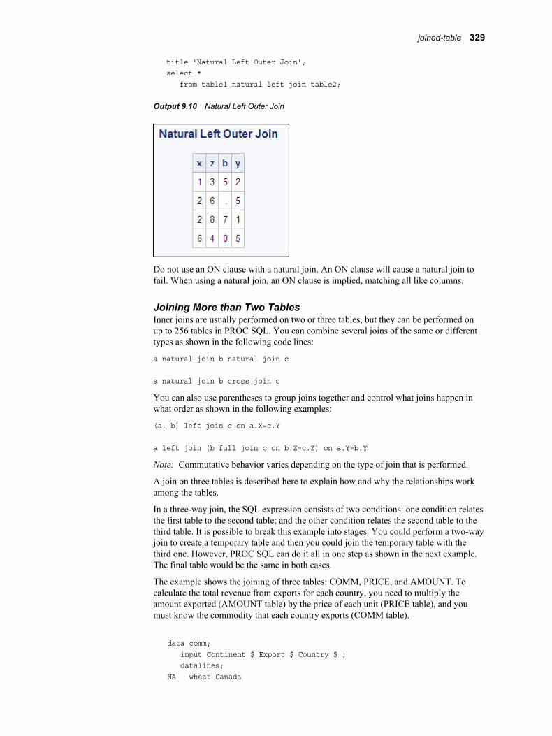
title 'Natural Left Outer Join'; select * from table1 natural left join table2;

Output 9.10 Natural Left Outer Join

Do not use an ON clause with a natural join. An ON clause will cause a natural join to fail. When using a natural join, an ON clause is implied, matching all like columns.

Joining More than Two TablesInner joins are usually performed on two or three tables, but they can be performed on up to 256 tables in PROC SQL. You can combine several joins of the same or different types as shown in the following code lines:

a natural join b natural join c

a natural join b cross join c

You can also use parentheses to group joins together and control what joins happen in what order as shown in the following examples:

(a, b) left join c on a.X=c.Y

a left join (b full join c on b.Z=c.Z) on a.Y=b.Y

Note: Commutative behavior varies depending on the type of join that is performed.

A join on three tables is described here to explain how and why the relationships work among the tables.

In a three-way join, the SQL expression consists of two conditions: one condition relates the first table to the second table; and the other condition relates the second table to the third table. It is possible to break this example into stages. You could perform a two-way join to create a temporary table and then you could join the temporary table with the third one. However, PROC SQL can do it all in one step as shown in the next example. The final table would be the same in both cases.

The example shows the joining of three tables: COMM, PRICE, and AMOUNT. To calculate the total revenue from exports for each country, you need to multiply the amount exported (AMOUNT table) by the price of each unit (PRICE table), and you must know the commodity that each country exports (COMM table).

data comm; input Continent $ Export $ Country $ ; datalines;NA wheat Canada

joined-table 329

EUR corn FranceEUR rice ItalyAFR oil Egypt;

data price; input Export $ Price; datalines;rice 3.56corn 3.45oil 18wheat 2.98;

data amount; input Country $ Quantity; datalines;Canada 16000France 2400Italy 500Egypt 10000;

proc sql; title 'COMM Table'; select * from comm; title 'PRICE Table'; select * from price; title 'AMOUNT Table'; select * from amount;


Output 9.11 Source for Joining More than Two Tables

proc sql;title 'Total Export Revenue';select c.Country, p.Export, p.Price, a.Quantity, a.quantity*p.price as Total from comm as c JOIN price as p on (c.export=p.export) JOIN amount as a on (c.country=a.country);quit;

joined-table 331

Output 9.12 Three-Way Join

See Also“Example 9: Joining Three Tables” on page 269

Comparison of Joins and SubqueriesYou can often use a subquery or a join to get the same result. However, it is often more efficient to use a join if the outer query and the subquery do not return duplicate rows. For example, the following queries produce the same result. The second query is more efficient:

proc sql; select IDNumber, Birth from proclib.payroll where IDNumber in (select idnum from proclib.staff where lname like 'B%');

proc sql; select p.IDNumber, p.Birth from proclib.payroll p, proclib.staff s where p.idnumber=s.idnum and s.lname like 'B%';

Note: PROCLIB.PAYROLL is shown in “Example 2: Creating a Table from a Query's Result” on page 248.

LIKE ConditionTests for a matching pattern.

Syntaxsql-expression <NOT> LIKE sql-expression <ESCAPE character-expression>

Required Argumentssql-expression



character-expressionis an SQL expression that evaluates to a single character. The operands of character-expression must be character or string literals.

Note: If you use an ESCAPE clause, then the pattern-matching specification must be a quoted string or quoted concatenated string; it cannot contain column names.

DetailsThe LIKE condition selects rows by comparing character strings with a pattern-matching specification. It resolves to true and displays the matched strings if the left operand matches the pattern specified by the right operand. The ESCAPE clause is used to search for literal instances of the percent (%) and underscore (_) characters, which are usually used for pattern matching.

Patterns for SearchingPatterns consist of three classes of characters:

underscore (_)matches any single character.

percent sign (%)matches any sequence of zero or more characters.

any other charactermatches that character.

These patterns can appear before, after, or on both sides of characters that you want to match. The LIKE condition is case-sensitive.

The following list uses these values: Smith, Smooth, Smothers, Smart, and Smuggle.

'Sm%'matches Smith, Smooth, Smothers, Smart, Smuggle.

'%th'matches Smith, Smooth.

'S__gg%'matches Smuggle.

'S_o'matches a three-letter word, so it has no matches here.

'S_o%'matches Smooth, Smothers.

'S%th'matches Smith, Smooth.

'Z'matches the single, uppercase character Z only, so it has no matches here.

Searching for Literal % and _Because the % and _ characters have special meaning in the context of the LIKE condition, you must use the ESCAPE clause to search for these character literals in the input character string.

These examples use the values app, a_%, a__, bbaa1, and ba_1.

• The condition like 'a_%' matches app, a_%, and a__, because the underscore (_) in the search pattern matches any single character (including the underscore), and

LIKE Condition 333

the percent (%) in the search pattern matches zero or more characters, including '%' and '_'.

• The condition like 'a_^%' escape '^' matches only a_%, because the escape character (^) specifies that the pattern search for a literal '%'.

• The condition like 'a_%' escape '_' matches none of the values, because the escape character (_) specifies that the pattern search for an 'a' followed by a literal '%', which does not apply to any of these values.

Searching for Mixed-Case StringsTo search for mixed-case strings, use the UPCASE function to make all the names uppercase before entering the LIKE condition:

upcase(name) like 'SM%';

Note: When you are using the % character, be aware of the effect of trailing blanks. You might have to use the TRIM function to remove trailing blanks in order to match values.

LOWER FunctionConverts the case of a character string to lowercase.

See: “UPPER Function” on page 360

SyntaxLOWER (sql-expression)


must resolve to a character string and is described in “sql-expression” on page 342.

DetailsThe LOWER function operates on character strings. LOWER changes the case of its argument to all lowercase.

Note: The LOWER function is provided for compatibility with the ANSI SQL standard. You can also use the SAS function LOWCASE.

query-expressionRetrieves data from tables.

See: “table-expression” on page 359“Query Expressions (Subqueries)” on page 346“In-Line Views” on page 302


Syntaxtable-expression <set-operator table-expression> <…set-operator table-expression>

Required Argumentstable-expression

is described in “table-expression” on page 359.

set-operatoris one of the following:

INTERSECT <CORRESPONDING> <ALL>OUTER UNION <CORRESPONDING>UNION <CORRESPONDING> <ALL>EXCEPT <CORRESPONDING> <ALL>

Details

Query Expressions and Table ExpressionsA query expression is one or more table expressions. Multiple table expressions are linked by set operators. The following figure illustrates the relationship between table expressions and query expressions.

query-

expression

table-

expression

table-

expression

set operator

SELECT clauseFROM clause(more clauses)

SELECT clauseFROM clause(more clauses)

Set OperatorsPROC SQL provides these set operators:

OUTER UNIONconcatenates the query results.

UNIONproduces all unique rows from both queries.

EXCEPTproduces rows that are part of the first query only.

INTERSECTproduces rows that are common to both query results.

A query expression with set operators is evaluated as follows.

• Each table expression is evaluated to produce an (internal) intermediate result table.

• Each intermediate result table then becomes an operand linked with a set operator to form an expression. For example, A UNION B.

query-expression 335

• If the query expression involves more than two table expressions, then the result from the first two becomes an operand for the next set operator and operand, such as (A UNION B) EXCEPT C, ((A UNION B) EXCEPT C) INTERSECT D, and so on.

• Evaluating a query expression produces a single output table.

Set operators follow this order of precedence unless they are overridden by parentheses in the expressions: INTERSECT is evaluated first. OUTER UNION, UNION, and EXCEPT have the same level of precedence.

PROC SQL performs set operations even if the tables or views that are referred to in the table expressions do not have the same number of columns. The reason for this behavior is that the ANSI standard for SQL requires that tables or views that are involved in a set operation have the same number of columns and that the columns have matching data types. If a set operation is performed on a table or view that has fewer columns than the one or ones with which it is being linked, then PROC SQL extends the table or view with fewer columns by creating columns with missing values of the appropriate data type. This temporary alteration enables the set operation to be performed correctly.

CORRESPONDING (CORR) KeywordThe CORRESPONDING keyword is used only when a set operator is specified. CORR causes PROC SQL to match the columns in table expressions by name and not by ordinal position. Columns that do not match by name are excluded from the result table, except for the OUTER UNION operator. See “OUTER UNION” on page 336.

For example, when performing a set operation on two table expressions, PROC SQL matches the first specified column-name (listed in the SELECT clause) from one table expression with the first specified column-name from the other. If CORR is omitted, then PROC SQL matches the columns by ordinal position.

ALL KeywordThe set operators automatically eliminate duplicate rows from their output tables. The optional ALL keyword preserves the duplicate rows, reduces the execution by one step, and thereby improves the query expression's performance. You use it when you want to display all the rows resulting from the table expressions, rather than just the unique rows. The ALL keyword is used only when a set operator is also specified.

OUTER UNIONPerforming an OUTER UNION is very similar to performing the SAS DATA step with a SET statement. The OUTER UNION concatenates the intermediate results from the table expressions. Thus, the result table for the query expression contains all the rows produced by the first table expression followed by all the rows produced by the second table expression. Columns with the same name are in separate columns in the result table.

For example, the following query expression concatenates the ME1 and ME2 tables but does not overlay like-named columns. Output 9.14 on page 338 shows the result.

data me1; input IDnum $ Jobcode $ Salary Bonus; datalines;1400 ME1 29769 5871403 ME1 28072 3421120 ME1 28619 9861120 ME1 28619 986;


data me2; input IDnum $ Jobcode $ Salary; datalines;1653 ME2 351081782 ME2 353451244 ME2 36925;

proc sql ; title 'ME1'; select * from me1; title 'ME2'; select * from me2;

Output 9.13 ME1 and ME2 Tables

proc sql; title 'ME1 and ME2: OUTER UNION'; select * from me1 outer union select * from me2;


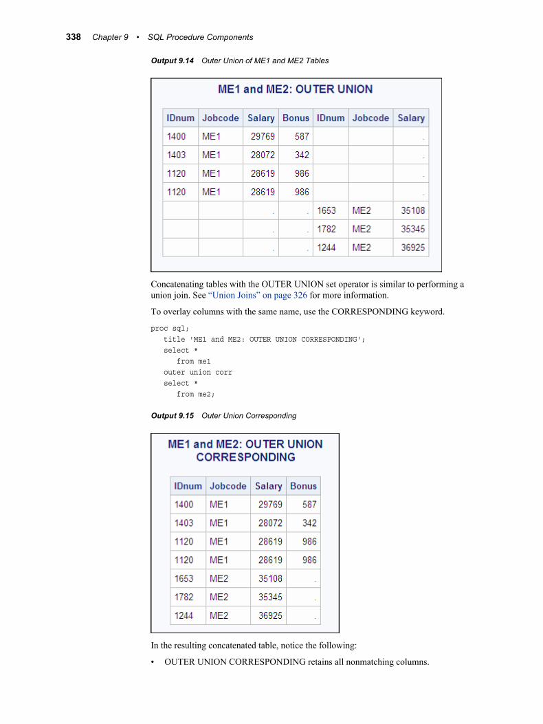
Output 9.14 Outer Union of ME1 and ME2 Tables

Concatenating tables with the OUTER UNION set operator is similar to performing a union join. See “Union Joins” on page 326 for more information.

To overlay columns with the same name, use the CORRESPONDING keyword.

proc sql; title 'ME1 and ME2: OUTER UNION CORRESPONDING'; select * from me1 outer union corr select * from me2;

Output 9.15 Outer Union Corresponding

In the resulting concatenated table, notice the following:

• OUTER UNION CORRESPONDING retains all nonmatching columns.


• For columns with the same name, if a value is missing from the result of the first table expression, then the value in that column from the second table expression is inserted.

• The ALL keyword is not used with OUTER UNION because this operator's default action is to include all rows in a result table. Thus, both rows from the table ME1 where IDnum is 1120 appear in the output.

UNIONThe UNION operator produces a table that contains all the unique rows that result from both table expressions. That is, the output table contains rows produced by the first table expression, the second table expression, or both.

Columns are appended by position in the tables, regardless of the column names. However, the data type of the corresponding columns must match or the union will not occur. PROC SQL issues a warning message and stops executing.

The names of the columns in the output table are the names of the columns from the first table expression unless a column (such as an expression) has no name in the first table expression. In such a case, the name of that column in the output table is the name of the respective column in the second table expression.

In the following example, PROC SQL combines the two tables:

proc sql; title 'ME1 and ME2: UNION'; select * from me1 union select * from me2;

Output 9.16 Union of ME1 and ME2 Tables

In the following example, ALL includes the duplicate row from ME1. In addition, ALL changes the sorting by specifying that PROC SQL make one pass only. Thus, the values from ME2 are simply appended to the values from ME1.

proc sql; title 'ME1 and ME2: UNION ALL'; select * from me1


union all select * from me2;

Output 9.17 Union All

See “Example 5: Combining Two Tables” on page 255 for another example.

EXCEPTThe EXCEPT operator produces (from the first table expression) an output table that has unique rows that are not in the second table expression. If the intermediate result from the first table expression has at least one occurrence of a row that is not in the intermediate result of the second table expression, then that row (from the first table expression) is included in the result table.

In the following example, the IN_USA table contains flights to cities within and outside the USA. The OUT_USA table contains flights only to cities outside the USA.

data in_usa; input Flight $ Dest $; datalines;145 ORD156 WAS188 LAX193 FRA207 LON;data OUT_USA; input Flight $ Dest $; datalines;193 FRA207 LON311 SJA;

proc sql; title 'IN_USA'; select * from in_usa;


title 'OUT_USA'; select * from out_usa;

Output 9.18 Source Tables for Except Examples

This example returns only the rows from IN_USA that are not also in OUT_USA:

proc sql; title 'Flights from IN_USA Only'; select * from in_usa except select * from out_usa;

Output 9.19 Flights from IN_USA Only


INTERSECTThe INTERSECT operator produces an output table that has rows that are common to both tables. For example, using the IN_USA and OUT_USA tables shown above, the following example returns rows that are in both tables:

proc sql; title 'Flights from Both IN_USA and OUT_USA'; select * from in_usa intersect select * from out_usa;

Output 9.20 Flights from Both IN_USA and OUT_USA

sql-expressionProduces a value from a sequence of operands and operators.

Syntaxoperand operator operand

Required Argumentsoperand


• a constant, which is a number or a quoted character string (or other special notation) that indicates a fixed value. Constants are also called literals. Constants are described in SAS Functions and CALL Routines: Reference.

• a column-name, which is described in “column-name” on page 315.

• a CASE expression, which is described in “CASE Expression” on page 310.

• any supported SAS function. PROC SQL supports many of the functions available to the SAS DATA step. Some of the functions that are not supported are the variable information functions, functions that work with arrays of data, and functions that operate on rows other than the current row. Other SQL databases support their own sets of functions. Functions are described in the SAS Functions and CALL Routines: Reference.

• any functions, except those with array elements, that are created with PROC FCMP.


• the ANSI SQL functions COALESCE, BTRIM, LOWER, UPPER, and SUBSTRING.

• a summary-function, which is described in “summary-function” on page 351.

• a query expression, which is described in “query-expression” on page 334.

• the USER literal, which references the user ID of the person who submitted the program. The user ID that is returned is operating environment-dependent, but PROC SQL uses the same value that the &SYSJOBID macro variable has on the operating environment.

operatoris described in “Operators and the Order of Evaluation” on page 343.

Note: SAS functions, including summary functions, can stand alone as SQL expressions. For example

select min(x) from table;

select scan(y,4) from table;

Details

SAS FunctionsPROC SQL supports many of the functions available to the SAS DATA step. Some of the functions that are not supported are the variable information functions and functions that work with arrays of data. Other SQL databases support their own sets of functions. For example, the SCAN function is used in the following query:

select style, scan(street,1) format=$15. from houses;

PROC SQL also supports any user-written functions, except those functions with array elements, that are created using Chapter 19, “FCMP Procedure” in Base SAS Procedures Guide.

See the SAS Functions and CALL Routines: Reference for complete documentation of SAS functions. Summary functions are also SAS functions. For more information, see “summary-function” on page 351.

USER LiteralUSER can be specified in a view definition. For example, you can create a view that restricts access to the views in the user's department. Note that the USER literal value is stored in uppercase, so it is advisable to use the UPCASE function when comparing to this value:

create view myemp as select * from dept12.employees where upcase(manager)=user;

This view produces a different set of employee information for each manager who references it.

Operators and the Order of EvaluationThe order in which operations are evaluated is the same as in the DATA step with this one exception: NOT is grouped with the logical operators AND and OR in PROC SQL; in the DATA step, NOT is grouped with the unary plus and minus signs.

sql-expression 343

Unlike missing values in some versions of SQL, missing values in SAS always appear first in the collating sequence. Therefore, in Boolean and comparison operations, the following expressions resolve to true in a predicate:

3>null -3>null 0>null

You can use parentheses to group values or to nest mathematical expressions. Parentheses make expressions easier to read and can also be used to change the order of evaluation of the operators. Evaluating expressions with parentheses begins at the deepest level of parentheses and moves outward. For example, SAS evaluates A+B*C as A+(B*C), although you can add parentheses to make it evaluate as (A+B)*C for a different result.

Higher priority operations are performed first: that is, group 0 operators are evaluated before group 5 operators. The following table shows the operators and their order of evaluation, including their priority groups.

Table 9.1 Operators and Order of Evaluation

Group Operator Description

0 ( ) forces the expression enclosed to be evaluated first

1 case-expression selects result values that satisfy specified conditions

2 ** raises to a power

unary +, unary - indicates a positive or negative number

3 * multiplies

/ divides

4 + adds

− subtracts

5 || concatenates

6 <NOT> BETWEEN condition See “BETWEEN Condition” on page 308.

<NOT> CONTAINS condition see “CONTAINS Condition” on page 316.

<NOT> EXISTS condition See “EXISTS Condition” on page 316.

<NOT> IN condition See “IN Condition” on page 317.

IS <NOT> condition See “IS Condition” on page 318.

<NOT> LIKE condition See “LIKE Condition” on page 332.

7 =, eq equals


Group Operator Description

¬=, ^=, < >, ne does not equal

>, gt is greater than

<, lt is less than

>=, ge is greater than or equal to

<=, le is less than or equal to

=* sounds like (use with character operands only). See “Example 11: Retrieving Values with the SOUNDS-LIKE Operator” on page 275.

eqt equal to truncated strings (use with character operands only). See “Truncated String Comparison Operators” on page 345.

gtt greater than truncated strings

ltt less than truncated strings

get greater than or equal to truncated strings

let less than or equal to truncated strings

net not equal to truncated strings

8 ¬, ^, NOT indicates logical NOT

9 &, AND indicates logical AND

10 |, OR indicates logical OR

Symbols for operators might vary, depending on your operating environment. For more information, see “SAS Operators in Expressions” in Chapter 6 of SAS Language Reference: Concepts.

Truncated String Comparison OperatorsPROC SQL supports truncated string comparison operators. (See Group 7 in Table 9.1 on page 344.) In a truncated string comparison, the comparison is performed after making the strings the same length by truncating the longer string to be the same length as the shorter string. For example, the expression 'TWOSTORY' eqt 'TWO' is true because the string 'TWOSTORY' is reduced to 'TWO' before the comparison is performed. Note that the truncation is performed internally; neither operand is permanently changed.

Note: Unlike the DATA step, PROC SQL does not support the colon operators (such as =:, >:, and <=:) for truncated string comparisons. Use the alphabetic operators (such as EQT, GTT, and LET).

sql-expression 345

Query Expressions (Subqueries)A query expression is called a subquery when it is used in a WHERE or HAVING clause. A subquery is a query expression that is nested as part of another query expression. A subquery selects one or more rows from a table based on values in another table.

Depending on the clause that contains it, a subquery can return a single value or multiple values. If more than one subquery is used in a query expression, then the innermost query is evaluated first, then the next innermost query, and so on, moving outward.

PROC SQL allows a subquery (contained in parentheses) at any point in an expression where a simple column value or constant can be used. In this case, a subquery must return a single value, that is, one row with only one column.

The following is an example of a subquery that returns one value. This PROC SQL step subsets the PROCLIB.PAYROLL table based on information in the PROCLIB.STAFF table. (PROCLIB.PAYROLL is shown in “Example 2: Creating a Table from a Query's Result” on page 248, and PROCLIB.STAFF is shown in “Example 4: Joining Two Tables” on page 252.) PROCLIB.PAYROLL contains employee identification numbers (IdNumber) and their salaries (Salary) but does not contain their names. If you want to return only the row from PROCLIB.PAYROLL for one employee, then you can use a subquery that queries the PROCLIB.STAFF table, which contains the employees' identification numbers and their names (Lname and Fname).

proc sql; title 'Information for Earl Bowden'; select * from proclib.payroll where idnumber= (select idnum from proclib.staff where upcase(lname)='BOWDEN');

Output 9.21 Query Output – One Value

Subqueries can return multiple values. The following example uses the tables PROCLIB.DELAY and PROCLIB.MARCH. These tables contain information about the same flights and have the Flight column in common. The following subquery returns all the values for Flight in PROCLIB.DELAY for international flights. The values from the subquery complete the WHERE clause in the outer query. Thus, when the outer query is executed, only the international flights from PROCLIB.MARCH are in the output.

proc sql outobs=5; title 'International Flights from'; title2 'PROCLIB.MARCH'; select Flight, Date, Dest, Boarded from proclib.march where flight in (select flight


from proclib.delay where destype='International');

Output 9.22 Query Output – Multiple Values

Sometimes it is helpful to compare a value with a set of values returned by a subquery. The keywords ANY or ALL can be specified before a subquery when the subquery is the right-hand operand of a comparison. If ALL is specified, then the comparison is true only if it is true for all values that are returned by the subquery. If a subquery returns no rows, then the result of an ALL comparison is true for each row of the outer query.

If ANY is specified, then the comparison is true if it is true for any one of the values that are returned by the subquery. If a subquery returns no rows, then the result of an ANY comparison is false for each row of the outer query.

The following example selects all of the employees in PROCLIB.PAYROLL who earn more than the highest paid ME3:

proc sql;title "Employees who Earn More than";title2 "All ME's"; select * from proclib.payroll where salary > all (select salary from proclib.payroll where jobcode='ME3');

sql-expression 347

Output 9.23 Query Output Using ALL Comparison

Note: See the first item in “Subqueries and Efficiency” on page 349 for a note about efficiency when using ALL.

In order to visually separate a subquery from the rest of the query, you can enclose the subquery in any number of pairs of parentheses.

Correlated SubqueriesIn a correlated subquery, the WHERE expression in a subquery refers to values in a table in the outer query. The correlated subquery is evaluated for each row in the outer query. With correlated subqueries, PROC SQL executes the subquery and the outer query together.


The following example uses the PROCLIB.DELAY and PROCLIB.MARCH tables. A DATA step ( “PROCLIB.DELAY” on page 383 ) creates PROCLIB.DELAY. PROCLIB.MARCH is shown in “Example 13: Producing All the Possible Combinations of the Values in a Column” on page 280. PROCLIB.DELAY has the Flight, Date, Orig, and Dest columns in common with PROCLIB.MARCH:

proc sql outobs=5; title 'International Flights'; select * from proclib.march where 'International' in (select destype from proclib.delay where march.Flight=delay.Flight);

The subquery resolves by substituting every value for MARCH.Flight into the subquery's WHERE clause, one row at a time. For example, when MARCH.Flight=219, the subquery resolves as follows:

1. PROC SQL retrieves all the rows from DELAY where Flight=219 and passes their DESTYPE values to the WHERE clause.

2. PROC SQL uses the DESTYPE values to complete the WHERE clause:

where 'International' in ('International','International', ...)

3. The WHERE clause checks to determine whether International is in the list. Because it is, all rows from MARCH that have a value of 219 for Flight become part of the output.

The following output contains the rows from MARCH for international flights only.

Output 9.24 Correlated Subquery Output

Subqueries and Efficiency• Use the MAX function in a subquery instead of the ALL keyword before the

subquery. For example, the following queries produce the same result, but the second query is more efficient:

proc sql; select * from proclib.payroll where salary> all(select salary from proclib.payroll

sql-expression 349

where jobcode='ME3');

proc sql; select * from proclib.payroll where salary> (select max(salary) from proclib.payroll where jobcode='ME3');

• With subqueries, use IN instead of EXISTS when possible. For example, the following queries produce the same result, but the second query is usually more efficient:

proc sql; select * from proclib.payroll p where exists (select * from staff s where p.idnum=s.idnum and state='CT');

proc sql; select * from proclib.payroll where idnum in (select idnum from staff where state='CT');

SUBSTRING FunctionReturns a part of a character expression.

SyntaxSUBSTRING (sql-expression FROM start <FOR length>)

Required Argumentssql-expression

must be a character string and is described in “sql-expression” on page 342.

startis a number (not a variable or column name) that specifies the position, counting from the left end of the character string, at which to begin extracting the substring.

lengthis a number (not a variable or column name) that specifies the length of the substring that is to be extracted.

DetailsThe SUBSTRING function operates on character strings. SUBSTRING returns a specified part of the input character string, beginning at the position that is specified by start. If length is omitted, then the SUBSTRING function returns all characters from start to the end of the input character string. The values of start and length must be numbers (not variables) and can be positive, negative, or zero.


If start is greater than the length of the input character string, then the SUBSTRING function returns a zero-length string.

If start is less than 1, then the SUBSTRING function begins extraction at the beginning of the input character string.

If length is specified, then the sum of start and length cannot be less than start or an error is returned. If the sum of start and length is greater than the length of the input character string, then the SUBSTRING function returns all characters from start to the end of the input character string. If the sum of start and length is less than 1, then the SUBSTRING function returns a zero-length string.

Note: The SUBSTRING function is provided for compatibility with the ANSI SQL standard. You can also use the SAS function SUBSTR.

summary-functionPerforms statistical summary calculations.

Restriction: A summary function cannot appear in an ON clause or a WHERE clause.

See: “GROUP BY Clause” on page 303“HAVING Clause” on page 304“SELECT Clause” on page 293“table-expression” on page 359

Examples: “Example 8: Creating a View from a Query's Result” on page 266“Example 12: Joining Two Tables and Calculating a New Value” on page 277“Example 15: Counting Missing Values with a SAS Macro” on page 289

Syntaxsummary-function (<DISTINCT | ALL> sql-expression)

Required Argumentssummary-function


AVG|MEANarithmetic mean or average of values

COUNT|FREQ|Nnumber of nonmissing values

CSScorrected sum of squares

CVcoefficient of variation (percent)

MAXlargest value

MINsmallest value

summary-function 351

NMISSnumber of missing values

PRTis the two-tailed p-value for Student's t statistic, T with n – 1 degrees of freedom.

RANGErange of values

STDstandard deviation

STDERRstandard error of the mean

SUMsum of values

SUMWGTsum of the WEIGHT variable values1

TStudent's t value for testing the hypothesis that the population mean is zero

USSuncorrected sum of squares

VARvariance

For a description and the formulas used for these statistics, see “SAS Elementary Statistics Procedures” in Chapter 1 of Base SAS Procedures Guide.

DISTINCTspecifies that only the unique values of an SQL expression be used in the calculation.

ALLspecifies that all values of an SQL expression be used in the calculation. If neither DISTINCT nor ALL is specified, then ALL is used.


Details

Summarizing DataSummary functions produce a statistical summary of the entire table or view that is listed in the FROM clause or for each group that is specified in a GROUP BY clause. If GROUP BY is omitted, then all the rows in the table or view are considered to be a single group. These functions reduce all the values in each row or column in a table to one summarizing or aggregate value. For this reason, these functions are often called aggregate functions. For example, the sum (one value) of a column results from the addition of all the values in the column.

Counting RowsThe COUNT function counts rows. COUNT(*) returns the total number of rows in a group or in a table. If you use a column name as an argument to COUNT, then the result is the total number of rows in a group or in a table that have a nonmissing value for that

1 Currently, there is no way to designate a WEIGHT variable for a table in PROC SQL. Thus, each row (or observation) has a weight of 1.


column. If you want to count the unique values in a column, then specify COUNT(DISTINCT column).

If the SELECT clause of a table expression contains one or more summary functions and that table expression resolves to no rows, then the summary function results are missing values. The following are exceptions that return zeros:

• COUNT(*)

• COUNT(<DISTINCT> sql-expression)

• NMISS(<DISTINCT> sql-expression)

See “Example 8: Creating a View from a Query's Result” on page 266 and “Example 15: Counting Missing Values with a SAS Macro” on page 289 for examples.

Calculating Statistics Based on the Number of ArgumentsThe number of arguments that is specified in a summary function affects how the calculation is performed. If you specify a single argument, then the values in the column are calculated. If you specify multiple arguments, then the arguments or columns that are listed are calculated for each row.

Note: When more than one argument is used within an SQL aggregate function, the function is no longer considered to be an SQL aggregate or summary function. If there is a like-named Base SAS function, then PROC SQL executes the Base SAS function, and the results that are returned are based on the values for the current row. If no like-named Base SAS function exists, then an error will occur. For example, if you use multiple arguments for the AVG function, an error will occur because there is no AVG function for Base SAS.

For example, consider calculations on the following table.

data summary; input X Y Z; datalines;1 3 42 4 58 9 44 5 4;

proc sql; title 'Summary Table'; select * from summary;

If you use one argument in the function, then the calculation is performed on that column only. If you use more than one argument, then the calculation is performed on


each row of the specified columns. In the following PROC SQL step, the MIN and MAX functions return the minimum and maximum of the columns that they are used with. The SUM function returns the sum of each row of the columns specified as arguments:

proc sql; select min(x) as Colmin_x, min(y) as Colmin_y, max(z) as Colmax_z, sum(x,y,z) as Rowsum from summary;

Output 9.25 Summary Functions

Remerging DataWhen you use a summary function in a SELECT clause or a HAVING clause, you might see the following message in the SAS log:

NOTE: The query requires remerging summary statistics back with the original data.

The process of remerging involves two passes through the data. On the first pass, PROC SQL

• calculates and returns the value of summary functions. It then uses the result to calculate the arithmetic expressions in which the summary function participates.

• groups data according to the GROUP BY clause.

On the second pass, PROC SQL retrieves any additional columns and rows that it needs to show in the output.

Note: To specify that PROC SQL not process queries that use remerging of data, use either the PROC SQL NOREMERGE option or the NOSQLREMERGE system option. If remerging is attempted when the NOMERGE option or the NOSQLREMERGE system option is set, an error is written to the SAS log. For more information, see the “REMERGE|NOREMERGE” on page 222 and the “SQLREMERGE System Option” on page 372.

The following examples use the PROCLIB.PAYROLL table (shown in “Example 2: Creating a Table from a Query's Result” on page 248 ) to show when remerging of data is and is not necessary.

The first query requires remerging. The first pass through the data groups the data by Jobcode and resolves the AVG function for each group. However, PROC SQL must make a second pass in order to retrieve the values of IdNumber and Salary.

proc sql outobs=10;


title 'Salary Information'; title2 '(First 10 Rows Only)'; select IdNumber, Jobcode, Salary, avg(salary) as AvgSalary from proclib.payroll group by jobcode;

Output 9.26 Salary Information That Required Remerging

You can change the previous query to return only the average salary for each jobcode. The following query does not require remerging because the first pass of the data does the summarizing and the grouping. A second pass is not necessary.

proc sql outobs=10; title 'Average Salary for Each Jobcode'; select Jobcode, avg(salary) as AvgSalary from proclib.payroll group by jobcode;


Output 9.27 Salary Information That Did Not Require Remerging

When you use the HAVING clause, PROC SQL might have to remerge data to resolve the HAVING expression.

First, consider a query that uses HAVING but that does not require remerging. The query groups the data by values of Jobcode, and the result contains one row for each value of Jobcode and summary information for people in each Jobcode. On the first pass, the summary functions provide values for the Number, Average Age, and Average Salary columns. The first pass provides everything that PROC SQL needs to resolve the HAVING clause, so no remerging is necessary.

proc sql outobs=10;title 'Summary Information for Each Jobcode';title2 '(First 10 Rows Only)'; select Jobcode, count(jobcode) as number label='Number', avg(int((today()-birth)/365.25)) as avgage format=2. label='Average Age', avg(salary) as avgsal format=dollar8. label='Average Salary' from proclib.payroll group by jobcode having avgage ge 30;


Output 9.28 Jobcode Information That Did Not Require Remerging

In the following query, PROC SQL remerges the data because the HAVING clause uses the SALARY column in the comparison and SALARY is not in the GROUP BY clause.

proc sql outobs=10;title 'Employees who Earn More than the';title2 'Average for Their Jobcode';title3 '(First 10 Rows Only)'; select Jobcode, Salary, avg(salary) as AvgSalary from proclib.payroll group by jobcode having salary > AvgSalary;


Output 9.29 Jobcode Information That Did Require Remerging

Keep in mind that PROC SQL remerges data when

• the values returned by a summary function are used in a calculation. For example, the following query returns the values of X and the percentage of the total for each row. On the first pass, PROC SQL computes the sum of X, and on the second pass PROC SQL computes the percentage of the total for each value of X:

data summary; input x; datalines;32864949;

proc sql; title 'Percentage of the Total'; select X, (100*x/sum(X)) as Pct_Total from summary;

Percentage of the Total

x Pct_Total ------------------- 32 14.81481 86 39.81481 49 22.68519 49 22.68519


• the values returned by a summary function are compared to values of a column that is not specified in the GROUP BY clause. For example, the following query uses the PROCLIB.PAYROLL table. PROC SQL remerges data because the column Salary is not specified in the GROUP BY clause:

proc sql; select jobcode, salary, avg(salary) as avsal from proclib.payroll group by jobcode having salary > avsal;

• a column from the input table is specified in the SELECT clause and is not specified in the GROUP BY clause. This rule does not refer to columns used as arguments to summary functions in the SELECT clause.

For example, in the following query, the presence of IdNumber in the SELECT clause causes PROC SQL to remerge the data because IdNumber is not involved in grouping or summarizing during the first pass. In order for PROC SQL to retrieve the values for IdNumber, it must make a second pass through the data.

proc sql; select IdNumber, jobcode, avg(salary) as avsal from proclib.payroll group by jobcode;

table-expressionDefines part or all of a query expression.

See: “query-expression” on page 334“SELECT Statement” on page 244

SyntaxSELECT <DISTINCT> object-item<, … object-item>

<INTO :macro-variable-specification <, … :macro-variable-specification>>FROM from-list<WHERE sql-expression><GROUP BY group-by-item <, … group-by-item>><HAVING sql-expression>

DetailsA table expression is a SELECT statement. It is the fundamental building block of most SQL procedure statements. You can combine the results of multiple table expressions with set operators, which creates a query expression. Use one ORDER BY clause for an entire query expression. Place a semicolon only at the end of the entire query expression. A query expression is often only one SELECT statement or table expression.

table-expression 359

UPPER FunctionConverts the case of a character string to uppercase.

See: “LOWER Function” on page 334

SyntaxUPPER (sql-expression)


must be a character string and is described in “sql-expression” on page 342.

DetailsThe UPPER function operates on character strings. UPPER converts the case of its argument to all uppercase.


Part 3

Appendixes

Appendix 1SQL Macro Variables and System Options . . . . . . . . . . . . . . . . . . . . . . 363

Appendix 2PROC SQL and the ANSI Standard . . . . . . . . . . . . . . . . . . . . . . . . . . . . . . 375

Appendix 3Source for SQL Examples . . . . . . . . . . . . . . . . . . . . . . . . . . . . . . . . . . . . . . . 381

361

Appendix 1

SQL Macro Variables and System Options

Dictionary . . . . . . . . . . . . . . . . . . . . . . . . . . . . . . . . . . . . . . . . . . . . . . . . . . . . . . . . . . 363SQLCONSTDATETIME System Option . . . . . . . . . . . . . . . . . . . . . . . . . . . . . . . 363SQLGENERATION= System Option . . . . . . . . . . . . . . . . . . . . . . . . . . . . . . . . . . 364SQLMAPPUTTO= System Option . . . . . . . . . . . . . . . . . . . . . . . . . . . . . . . . . . . . 367SQLREDUCEPUT= System Option . . . . . . . . . . . . . . . . . . . . . . . . . . . . . . . . . . . 368SQLREDUCEPUTOBS= System Option . . . . . . . . . . . . . . . . . . . . . . . . . . . . . . . 369SQLREDUCEPUTVALUES= System Option . . . . . . . . . . . . . . . . . . . . . . . . . . . 370SQLREMERGE System Option . . . . . . . . . . . . . . . . . . . . . . . . . . . . . . . . . . . . . . . 372SQLUNDOPOLICY= System Option . . . . . . . . . . . . . . . . . . . . . . . . . . . . . . . . . . 373SYS_SQLSETLIMIT Macro Variable . . . . . . . . . . . . . . . . . . . . . . . . . . . . . . . . . . 374

Dictionary

SQLCONSTDATETIME System OptionSpecifies whether the SQL procedure replaces references to the DATE, TIME, DATETIME, and TODAY functions in a query with their equivalent constant values before the query executes.

Valid in: configuration file, SAS invocation, OPTIONS statement, SAS System Options window

Categories: Files: SAS FilesSystem administration: SQL

PROC OPTIONS GROUP=

SASFILESSQL

Note: This option can be restricted by a site administrator. For more information, see “Restricted Options” in Chapter 1 of SAS System Options: Reference.

SyntaxSQLCONSTDATETIME | NOSQLCONSTDATETIME

363

Syntax DescriptionSQLCONSTDATETIME

specifies that the SQL procedure is to replace references to the DATE, TIME, DATETIME, and TODAY functions with their equivalent numeric constant values.

NOSQLCONSTDATETIMEspecifies that the SQL procedure is not to replace references to the DATE, TIME, DATETIME, and TODAY functions with their equivalent numeric constant values.

DetailsWhen the SQLCONSTDATETIME system option is set, the SQL procedure evaluates the DATE, TIME, DATETIME, and TODAY functions in a query once, and uses those values throughout the query. Computing these values once ensures consistency of results when the functions are used multiple times in a query or when the query executes the functions close to a date or time boundary.

When the NOSQLCONSTDATETIME system option is set, the SQL procedure evaluates these functions in a query each time it processes an observation.

If both the SQLREDUCEPUT system option and the SQLCONSTDATETIME system option are specified, the SQL procedure replaces the DATE, TIME, DATETIME, and TODAY functions with their respective values in order to determine the PUT function value before the query executes:

select x from &lib..c where (put(bday, date9.) = put(today(), date9.));

Note: The value that is specified in the SQLCONSTDATETIME system option is in effect for all SQL procedure statements, unless the CONSTDATETIME option in the PROC SQL statement is set. The value of the CONSTDATETIME option takes precedence over the SQLCONSTDATETIME system option. However, changing the value of the CONSTDATETIME option does not change the value of the SQLCONSTDATETIME system option.

See Also• “Improving Query Performance” on page 140

Procedure Statement Options:

• CONSTDATETIME option on page 216

System Options:

• “SQLREDUCEPUT= System Option” on page 368

SQLGENERATION= System OptionSpecifies whether and when SAS procedures generate SQL for in-database processing of source data.


Category: System administration: Performance

Default: (NONE DBMS='ASTER DB2 GREENPLM NETEZZA ORACLE TERADATA')

364 Appendix 1 • SQL Macro Variables and System Options

Restriction: For DBMS= and EXCLUDEDB= values, the maximum length of an engine name is eight characters. For the EXCLUDEPROC= value, the maximum length of a procedure name is 16 characters. An engine can appear only once, and a procedure can appear only once for a given engine.

Data source: Aster nCluster, DB2 under UNIX and PC Hosts, Greenplum, Netezza, Oracle, Teradata

See: SQLGENERATION= LIBNAME option (includes examples), and also “Running In-Database Procedures” in SAS In-Database Products: User’s Guide

SyntaxSQLGENERATION=<(>NONE | DBMS <DBMS='engine1 engine2…enginen '>

<EXCLUDEDB=engine | 'engine1…enginen'><EXCLUDEPROC="engine='proc1…procn'

enginen='proc1…procn' "><)>

SQLGENERATION=" "

Syntax DescriptionNONE

prevents those SAS procedures that are enabled for in-database processing from generating SQL for in-database processing. This is a primary state.

DBMSallows SAS procedures that are enabled for in-database processing to generate SQL for in-database processing of DBMS tables through supported SAS/ACCESS engines. This is a primary state.

DBMS='engine1…enginen'specifies one or more SAS/ACCESS engines. It modifies the primary state.

EXCLUDEDB=engine | 'engine1…enginen'prevents SAS procedures from generating SQL for in-database processing for one or more specified SAS/ACCESS engines.

EXCLUDEPROC="engine='proc1…procn' enginen='proc1…procn' "identifies engine-specific SAS procedures that you do not want to run inside the database.

" "resets the value to the default that was shipped.

DetailsUse this option with such procedures as PROC FREQ to indicate that SQL is generated for in-database processing of DBMS tables through supported SAS/ACCESS engines.

You must specify NONE, DBMS, or both. One or both of these arguments indicates the primary state.

The maximum length of the option value is 4096. Also, parentheses are required when this option value contains multiple keywords.

Not all procedures support SQL generation for in-database processing for every engine type. If you specify a setting that is not supported, an error message indicates the level of SQL generation that is not supported, and the procedure can reset to the default so that

SQLGENERATION= System Option 365

source table records can be read and processed within SAS. If this is not possible, the procedure ends and sets SYSERR= as needed.

You can specify different SQLGENERATION= values for the DATA= and OUT= data sets by using different LIBNAME statements for each of these data sets.

Here is how SAS/ACCESS handles precedence.

Table A1.1 Precedence of Values for SQLGENERATION= LIBNAME and System Options

LIBNAME Option

PROC EXCLUDE on

System Option? Engine Type

Engine Specified on

System OptionResulting

ValueFrom

(option)

not set

NONE

DBMS

yes database interface NONE

DBMS

NONE

EXCLUDEDB

system

NONE no NONE LIBNAME

DBMS DBMS

not set NONE NONE system

DBMS DBMS

no SQL generated for this database host or database version

NONE

DBMS

NONE

NONE

DBMS

LIBNAME

not set Base system

NONE

DBMS

LIBNAME

ExampleHere is the default that is shipped with the product.

options sqlgeneration='';proc options option=sqlgenerationrun;

SAS procedures generate SQL for in-database processing for all databases except DB2 in this example.

options sqlgeneration='';options sqlgeneration=(DBMS EXCLUDEDB='DB2');proc options option=sqlgeneration;run;

In this example, in-database processing occurs only for Teradata. SAS procedures that are run on other databases do not generate SQL for in-database processing.

options sqlgeneration='';options SQLGENERATION=(NONE DBMS='Teradata');proc options option=sqlgeneration;run;


For this example, SAS procedures generate SQL for Teradata and Oracle in-database processing. However, no SQL is generated for PROC1 and PROC2 in Oracle.

options sqlgeneration='';Options SQLGENERATION = (NONE DBMS='Teradata Oracle' EXCLUDEPROC="oracle='proc1 proc2'");proc options option=sqlgeneration;run;

SQLMAPPUTTO= System OptionSpecifies whether the PUT function is mapped to the SAS_PUT() function for a database, possible also where the SAS_PUT() function is mapped.

Valid in: configuration file, SAS invocation, OPTIONS statement

Category: Files: SAS files

Default: SAS_PUT

Data source: DB2 under UNIX and PC Hosts, Netezza, Teradata

See: “SQL_FUNCTIONS= LIBNAME Option” in SAS/ACCESS for Relational Databases: Reference, SAS In-Database Products: User’s Guide

SyntaxSQLMAPPUTTO= NONE | SAS_PUT | (database.SAS_PUT)


specifies to PROC SQL that no PUT mapping is to occur.

SAS_PUTspecifies that the PUT function be mapped to the SAS_PUT() function.

database.SAS_PUTspecifies the database name.

T I P It is not necessary that the format definitions and the SAS_PUT() function reside in the same database as the one that contains the data that you want to format. You can use the database.SAS_PUT argument to specify the database where the format definitions and the SAS_PUT() function have been published.

T I P The database name can be a multilevel name and it can include blanks.

Requirement If you specify a database name, you must enclose the entire argument in parentheses.

DetailsThe format publishing macros deploy or publish, the PUT function implementation to the database as a new function named SAS_PUT(). The format publishing macros also publish both user-defined formats and formats that SAS supplies that you create using PROC FORMAT. The SAS_PUT() function supports the use of SAS formats, and you can use it in SQL queries that SAS submits to the database so that the entire SQL query

SQLMAPPUTTO= System Option 367

can be processed inside the database. You can also use it in conjunction with in-database procedures.

You can use this option with the SQLREDUCEPUT=, SQLREDUCEPUTOBS, and SQLREDUCEPUTVALUES= system options. For more information about these options, see SAS SQL Procedure User's Guide.

SQLREDUCEPUT= System OptionFor the SQL procedure, specifies the engine type to use to optimize a PUT function in a query. The PUT function is replaced with a logically equivalent expression.


Categories: Files: SAS FilesSystem administration: SQLSystem administration: Performance

PROC OPTIONS GROUP=

SASFILESSQLPERFORMANCE


SyntaxSQLREDUCEPUT= ALL | NONE | DBMS | BASE

Syntax DescriptionALL

specifies to consider the optimization of all PUT functions, regardless of the engine that is used by the query to access the data.

NONEspecifies to not optimize any PUT function.

DBMSspecifies to consider the optimization of all PUT functions in a query performed by a SAS/ACCESS engine. This is the default.

Requirement The first argument to the PUT function must be a variable that is obtained by a table. The table must be accessed using a SAS/ACCESS engine.

BASEspecifies to consider the optimization of all PUT functions in a query performed by a SAS/ACCESS engine or a Base SAS engine.

DetailsIf you specify the SQLREDUCEPUT= system option, SAS optimizes the PUT function before the query is executed. If the query also contains a WHERE clause, the evaluation of the WHERE clause is simplified. The following SELECT statements are examples of


queries that are optimized if the SQLREDUCEPUT= option is set to any value other than none:

select x, y from &lib..b where (PUT(x, abc.) in ('yes', 'no'));select x from &lib..a where (PUT(x, udfmt.) = trim(left('small')));

If both the SQLREDUCEPUT= system option and the SQLCONSTDATETIME system option are specified, PROC SQL replaces the DATE, TIME, DATETIME, and TODAY functions with their respective values to determine the PUT function value before the query executes.

The following two SELECT clauses show the original query and optimized query:

select x from &lib..c where (put(bday, date9.) = put(today(), date9.));

Here, the SELECT clause is optimized.

select x from &lib..c where (x = '17MAR2011'D);

If a query does not contain the PUT function, it is not optimized.

Note: The value that is specified in the SQLREDUCEPUT= system option is in effect for all SQL procedure statements, unless the PROC SQL REDUCEPUT= option is set. The value of the REDUCEPUT= option takes precedence over the SQLREDUCEPUT= system option. However, changing the value of the REDUCEPUT= option does not change the value of the SQLREDUCEPUT= system option.



• REDUCEPUT= option on page 220

System Options:

• “SQLCONSTDATETIME System Option” on page 363

• “SQLREDUCEPUTOBS= System Option” on page 369

SQLREDUCEPUTOBS= System OptionFor the SQL procedure, when the SQLREDUCEPUT= system option is set to DBMS, BASE, or ALL, specifies the minimum number of observations that must be in a table for PROC SQL to optimize the PUT function in a query.



PROC OPTIONS GROUP=


SQLREDUCEPUTOBS= System Option 369

Interactions: If the SQLREDUCEPUT= system option is set to DBMS, BASE, or ALL, conditions for both the SQLREDUCEPUTOBS= and SQLREDUCEPUTVALUES= system options must be met for PROC SQL to optimize the PUT function.The SQLREDUCEPUTOBS= system option works only for DBMSs that record the number of observations in a table. If your DBMS does not record the number of observations, but you create row counts on your table, the SQLREDUCEPUTOBS= option will work.


SyntaxSQLREDUCEPUTOBS= n

Syntax Descriptionn

specifies the minimum number of observations that must be in a table for PROC SQL to optimize the PUT function in a query.

Default 0, which indicates that there is no minimum number of observations in a table for PROC SQL to optimize the PUT function.

Range 0–263–1, or approximately 9.2 quintillion


DetailsFor databases that allow implicit pass-through when the row count for a table is not known, PROC SQL allows the PUT function to be optimized in the query, and the query is executed by the database. When the SQLREDUCEPUT= system option is set to DBMS, BASE, or ALL, PROC SQL considers the values of both the SQLREDUCEPUTVALUES= and SQLREDUCEPUTOBS= system options, and determines whether to optimize the PUT function.

For databases that do not allow implicit pass-through, PROC SQL does not optimize the PUT function, and more of the query is executed by SAS.


System Options:


• “SQLREDUCEPUTVALUES= System Option” on page 370

SQLREDUCEPUTVALUES= System OptionFor the SQL procedure, when the SQLREDUCEPUT= system option is set to DBMS, BASE, or ALL, specifies the maximum number of SAS format values that can exist in a PUT function expression for PROC SQL to optimize the PUT function in a query.




PROC OPTIONS GROUP=


Interaction: If the SQLREDUCEPUT= system option is set to DBMS, BASE, or ALL, conditions for both the SQLREDUCEPUTVALUES= and SQLREDUCEPUTOBS= system options must be met for PROC SQL to optimize the PUT function.


SyntaxSQLREDUCEPUTVALUES= n

Syntax Descriptionn

specifies the maximum number of SAS format values that can exist in a PUT function expression for PROC SQL to optimize the PUT function in a query.

Default 100

Range 100 – 3,000


Interaction If the number of SAS format values in a PUT function expression is greater than this value, PROC SQL does not optimize the PUT function.

DetailsSome formats, especially user-defined formats, can contain many format values. Depending on the number of matches for a PUT function expression, the resulting expression can list many format values. If the number of format values becomes too large, query performance can degrade. When the SQLREDUCEPUT= system option is set to DBMS, BASE, or ALL, PROC SQL considers the values of both the SQLREDUCEPUTVALUES= and SQLREDUCEPUTOBS= system options, and determines whether to optimize the PUT function.

T I P The value for SQLREDUCEPUTVALUES= is used for each individual optimization. For example, if you have a PUT function in a WHERE clause, and another PUT function in a GROUP BY clause, the value of SQLREDUCEPUTVALUES= is applied separately for each clause.


SQLREDUCEPUTVALUES= System Option 371

System Options:


• “SQLREDUCEPUTOBS= System Option” on page 369

SQLREMERGE System OptionSpecifies whether PROC SQL can process queries that use remerged data.



PROC OPTIONS GROUP=

SASFILESSQL


SyntaxSQLREMERGE | NOSQLREMERGE

Syntax DescriptionSQLREMERGE

specifies that PROC SQL can process queries that use remerged data.

NOSQLREMERGEspecifies that PROC SQL cannot process queries that use remerged data.

DetailsThe remerge feature of PROC SQL makes two passes through a table. Data that is created in the first pass is used in the second pass to complete a query. When the NOSQLREMERGE system option is specified, PROC SQL cannot process this remerging of data. If remerging is attempted when the NOSQLREMERGE system option is specified, an error is written to the SAS log.



• REMERGE option on page 222

• “summary-function” on page 351


SQLUNDOPOLICY= System OptionSpecifies how PROC SQL handles updated data if errors occur while you are updating data. You can use UNDO_POLICY= to control whether your changes are permanent.

Valid in: configuration file, SAS invocation, Options statement


PROC OPTIONS GROUP=

SASFILESSQL


SyntaxSQLUNDOPOLICY=NONE | OPTIONAL | REQUIRED


keeps any updates or inserts.

OPTIONALreverses any updates or inserts that it can reverse reliably.

REQUIREDreverses all inserts or updates that have been done to the point of the error. This is the default.

CAUTION Some UNDO operations cannot be done reliably. In some cases, the UNDO operation cannot be done reliably. When a change cannot be reversed, PROC SQL issues an error message and does not execute the statement. For example, when a program uses a SAS/ACCESS view, or when a SAS data set is accessed through a SAS/SHARE server and is opened with the data set option CNTLLEV=RECORD, you cannot reliably reverse your changes.

CAUTION Some UNDO operations might not reverse changes. When multiple transactions are made to the same record, PROC SQL might not reverse a change. PROC SQL issues an error message instead. For example, if an error occurs during an insert, PROC SQL can delete a record that another user updated. In that case, the UNDO operation does not reverse the change, and an error message is issued.

DetailsThe value that is specified in the SQLUNDOPOLICY= system option is in effect for all SQL procedure statements, unless the PROC SQL UNDO_POLICY= option is set. The value of the UNDO_POLICY= option takes precedence over the SQLUNDOPOLICY= system option. The RESET statement can also be used to set or reset the UNDO_POLICY= option. However, changing the value of the UNDO_POLICY=

SQLUNDOPOLICY= System Option 373

option does not change the value of the SQLUNDOPOLICY= system option. After the procedure completes, it reverts to the value of the SQLUNDOPOLICY= system option.

If you are updating a data set using the SAS Scalable Performance Data Engine, you can significantly improve processing performance by setting SQLUNDOPOLICY=NONE. However, ensure that NONE is an appropriate setting for your application.

See Also

Procedure Statement

• UNDO_POLICY on page 224

SYS_SQLSETLIMIT Macro VariableFor the SQL procedure, specifies the maximum number of values that is used to optimize a hash join during DBMS processing.

SyntaxSYS_SQLSETLIMIT= n;

Required Argumentn

specifies the maximum number of values in the IN condition that is passed to the DBMS for processing,

Default 1024

Restriction The SYS_SQLSETLIMIT macro variable affects only certain hash joins.

Example %let SYS_SQLSETLIMIT=250;%let SYS_SQLSETLIMIT=1200;

Details

Hash JoinTo optimize performance, the SQL procedure might use a hash join when an index join is eliminated as a possibility. With a hash join, the smaller table is reconfigured in memory as a hash table. PROC SQL sequentially scans the larger table, and performs a row-by-row hash lookup against the small table to form the result set. A memory-sizing formula determines whether a hash join is used. The formula is based on the PROC SQL BUFFERSIZE option, whose default value is 64 KB. On a memory-rich system, you should consider increasing BUFFERSIZE to increase the likelihood that a hash join is used.


Appendix 2

PROC SQL and the ANSI Standard

CompliancePROC SQL follows most of the guidelines set by the American National Standards Institute (ANSI) in its implementation of SQL. However, it is not fully compliant with the current ANSI standard for SQL.2

The SQL research project at SAS has focused primarily on the expressive power of SQL as a query language. Consequently, some of the database features of SQL have not yet been implemented in PROC SQL.

SQL Procedure Enhancements

Reserved WordsPROC SQL reserves very few keywords, and then, only in certain contexts. The ANSI standard reserves all SQL keywords in all contexts. For example, according to the standard, you cannot name a column GROUP because of the keywords GROUP BY.

The following words are reserved in PROC SQL:

• The keyword CASE is always reserved. Its use in the CASE expression (an SQL2 feature) precludes its use as a column name.

If you have a column named CASE in a table, and you want to specify it in a PROC SQL step, then you can use the SAS data set option RENAME= to rename that column for the duration of the query. You can enclose CASE in double quotation marks (“CASE”), and set the PROC SQL option DQUOTE=ANSI.

• The keywords AS, ON, FULL, JOIN, LEFT, FROM, WHEN, WHERE, ORDER, GROUP, RIGHT, INNER, OUTER, UNION, EXCEPT, HAVING, and INTERSECT cannot be used for table aliases. These keywords introduce clauses that appear after a table name. Because the table alias is optional, PROC SQL handles this ambiguity by assuming that any one of these words introduces the corresponding clause and is not the table alias. If you want to use one of these keywords as a table alias, then enclose the keyword in double quotation marks, and set the PROC SQL option DQUOTE=ANSI.

• The keyword USER is reserved for the current user ID. If you specify USER in a SELECT statement in conjunction with a CREATE TABLE statement, then the column is created in the table with a temporary column name that is similar to _TEMA001. If you specify USER in a SELECT statement without a CREATE TABLE statement, then the column is written to the output without a column heading. In either case, the value for the column varies by operating environment,

2 International Organization for Standardization (ISO): Database SQL. Document ISO/IEC 9075:1992. Also, as American National Standards Institute (ANSI) Document ANSI X3.135-1992.

375

but is typically the user ID of the user who is submitting the program, or the value of the &SYSJOBID automatic macro variable.

If you have a column named USER in a table, and you want to specify it in a PROC SQL step, then you can use the SAS data set option RENAME= to rename that column for the duration of the query. You can enclose USER in double quotation marks (“USER”), and set the PROC SQL option DQUOTE=ANSI.

Column ModifiersPROC SQL supports the SAS INFORMAT=, FORMAT=, and LABEL= modifiers for expressions in the SELECT statement. These modifiers control the format in which output data is displayed and labeled.

Alternate Collating SequencesPROC SQL enables you to specify an alternate collating (sorting) sequence to be used when you specify the ORDER BY clause. For more information about the SORTSEQ= option, see “PROC SQL Statement” on page 215.

ORDER BY Clause in a View DefinitionPROC SQL permits you to specify an ORDER BY clause in a CREATE VIEW statement. When the view is queried, its data is sorted based on the specified order, unless a query against that view includes a different ORDER BY clause. For more information, see “CREATE VIEW Statement” on page 235.

CONTAINS ConditionPROC SQL enables you to test whether a string is part of a column's value when you specify the CONTAINS condition. For more information, see “CONTAINS Condition” on page 316.

Inline ViewsThe ability to code nested query expressions in the FROM clause is a requirement of the ANSI standard. PROC SQL supports nested coding.

Outer JoinsThe ability to include columns that both match and do not match in a join expression is a requirement of the ANSI standard. PROC SQL supports this ability.

Arithmetic OperatorsPROC SQL supports the SAS exponentiation (**) operator. PROC SQL uses the notation <> to mean not equal.

Orthogonal ExpressionsPROC SQL enables the combination of comparison, Boolean, and algebraic expressions. For example, (X=3)*7 yields a value of 7 if X=3 is true because true is defined to be 1. If X=3 is false, then it resolves to 0, and the entire expression yields a value of 0.

PROC SQL permits a subquery in any expression. This feature is required by the ANSI standard. Therefore, you can have a subquery on the left side of a comparison operator in the WHERE expression.

PROC SQL permits you to order and group data by any type of mathematical expression (except a mathematical expression including a summary function) using ORDER BY and GROUP BY clauses. You can group by an expression that appears in the SELECT

376 Appendix 2 • PROC SQL and the ANSI Standard

statement by using the integer that represents the expression's ordinal position in the SELECT statement. You are not required to select the expression by which you are grouping or ordering. For more information, see “ORDER BY Clause” on page 305 and “GROUP BY Clause” on page 303.

Set OperatorsThe set operators UNION, INTERSECT, and EXCEPT are required by the ANSI standard. PROC SQL provides these operators and the OUTER UNION operator.

The ANSI standard requires that the tables being operated on have the same number of columns with matching data types. The SQL procedure works on tables that have the same number of columns, and it works on tables that have a different number of columns by creating virtual columns so that a query can evaluate correctly. For more information, see “query-expression” on page 334.

Statistical FunctionsPROC SQL supports many more summary functions than required by the ANSI standard for SQL.

PROC SQL supports remerging summary function results into the table's original data. For example, computing the percentage of total is achieved with 100*x/SUM(x) in PROC SQL. For more information about summary functions and remerging data, see “summary-function” on page 351.

SAS DATA Step FunctionsPROC SQL supports many of the functions available in the SAS DATA step. Some of the functions that are not supported are the variable information functions and functions that work with arrays of data. Other SQL databases support their own sets of functions.

PROC FCMP FunctionsPROC SQL supports any user-written functions, except those functions with array elements that are created using Chapter 19, “FCMP Procedure” in Base SAS Procedures Guide.

SQL Procedure Omissions

COMMIT StatementThe COMMIT statement is not supported.

ROLLBACK StatementThe ROLLBACK statement is not supported. The PROC SQL UNDO_POLICY= option or the SQLUNDOPOLICY system option addresses rollback. See the description of the UNDO_POLICY= option in “PROC SQL Statement” on page 215 or in the“SQLUNDOPOLICY= System Option” on page 373.

Identifiers and Naming ConventionsIn SAS, table names, column names, and aliases are limited to 32 characters, and can contain mixed case. For more information about SAS naming conventions, see Base SAS Utilities: Reference. The ANSI standard for SQL allows longer names.

PROC SQL and the ANSI Standard 377

Granting User PrivilegesThe GRANT statement, PRIVILEGES keyword, and authorization-identifier features of SQL are not supported. You might want to use operating-environment-specific means of security instead.

Three-Valued LogicANSI-compatible SQL has three-valued logic. That is, it has special cases for handling comparisons involving NULL values. Any value compared with a NULL value evaluates to NULL.

PROC SQL follows the SAS convention for handling missing values. When numeric NULL values are compared with non-NULL numbers, the NULL values are less than or smaller than all the non-NULL values. When character NULL values are compared with non-NULL characters, the character NULL values are treated as a string of blanks.

Embedded SQLCurrently, there is no provision for embedding PROC SQL statements in other SAS programming environments, such as the DATA step or SAS/IML software.

Column Alias ExceptionsThe development scope of PROC SQL and its aliasing rules predate the scope and rules of the first ANSI SQL standard and the ISO SQL standard. In PROC SQL, a column alias can be used in a WHERE clause, GROUP BY clause, HAVING clause, or ORDER BY clause. In the ANSI SQL standard and ISO SQL standard, the value that is associated with a column alias does not need to be available until the ORDER BY clause is executed. As a result, there is no guarantee that an SQL processor can resolve a column alias in time for it to be referenced in a WHERE clause, GROUP BY clause, or HAVING clause. Because the ANSI SQL standard and ISO SQL standard require that a column alias needs only to be available for reference when the ORDER BY clause is executed, avoid writing code that refers to a column alias in a WHERE clause, GROUP BY clause, or HAVING clause.

There are six parts in the conceptual order of execution of a SELECT statement from the ANSI SQL standard or ISO SQL standard perspective. If all six parts exist, the sequence is the following:

1. The FROM part is executed first.

2. The WHERE part is executed second.

3. The GROUP BY part is executed third.

4. The HAVING part is executed fourth.

5. The SELECT part is executed fifth.

6. The ORDER BY part is executed last.

The only required parts of an SQL query are the SELECT clause and FROM clause. The other four parts might be optional, depending on what type of query you are performing.

Here is a high-level template of an SQL query. The number enclosed in parentheses to the right of each part represents its position in the conceptual order of execution.

select <SELECT list> (5) from <FROM clause> (1) where <WHERE clause> (2) group by <GROUP BY clause> (3) having <HAVING clause> (4)


order by <ORDER BY clause>; (6)

In the following code examples, the first alias in each SELECT statement is just a rename of a table column. The second alias refers to a calculated expression. The first and second SQL statements output the expected results in PROC SQL.

/* --Preferred SQL code example since a column alias is not referenced in the WHERE clause*//*-- Portable to other SQL processors --*/select qty as Quantity, cost, cost+100 as ListPrice from calc where qty > 5;

/*-- This code example will work in PROC SQL, but might not work with other SQL processors --*/select qty as Quantity, cost, cost+100 as ListPrice from calc where Quantity > 5;

An early extension to PROC SQL development was the CALCULATED keyword. The CALCULATED keyword enables PROC SQL users to reference column aliases that are associated with calculated expressions. The column alias referenced by the CALCULATED keyword can be in the WHERE clause, GROUP BY clause, HAVING clause, or ORDER BY clause. Using the CALCULATED keyword can be redundant if it is used in the ORDER BY clause to refer to a column alias. That column alias will have been already resolved by the time the ORDER BY clause is executed.

Here is a PROC SQL code example that uses the CALCULATED keyword to subset the rows by the values that are associated with the second alias (ListPrice).

Example Code A2.1 CALCULATED Keyword and the PROC SQL Use of Column Aliases

/*-- PROC SQL use of the CALCULATED keyword --*/select qty as Quantity, cost, cost+100 as ListPrice from calc where CALCULATED ListPrice > 1500;

The ISO SQL standard- and ANSI SQL standard-approved way of accomplishing this task is as follows:

Example Code A2.2 CALCULATED Keyword and the PROC SQL Use of Column Aliases

/*-- PROC SQL use of the CALCULATED keyword --*/select qty as Quantity, cost, cost+100 as ListPrice from calc where cost+100 > 1500;

The code in the previous example is portable.

PROC SQL and the ANSI Standard 379

Appendix 3

Source for SQL Examples

Overview . . . . . . . . . . . . . . . . . . . . . . . . . . . . . . . . . . . . . . . . . . . . . . . . . . . . . . . . . . . 381

EMPLOYEES . . . . . . . . . . . . . . . . . . . . . . . . . . . . . . . . . . . . . . . . . . . . . . . . . . . . . . . 381

HOUSES . . . . . . . . . . . . . . . . . . . . . . . . . . . . . . . . . . . . . . . . . . . . . . . . . . . . . . . . . . . 382

MATCH_11 . . . . . . . . . . . . . . . . . . . . . . . . . . . . . . . . . . . . . . . . . . . . . . . . . . . . . . . . . 382

PROCLIB.DELAY . . . . . . . . . . . . . . . . . . . . . . . . . . . . . . . . . . . . . . . . . . . . . . . . . . . 383

PROCLIB.HOUSES . . . . . . . . . . . . . . . . . . . . . . . . . . . . . . . . . . . . . . . . . . . . . . . . . . 384

PROCLIB.MARCH . . . . . . . . . . . . . . . . . . . . . . . . . . . . . . . . . . . . . . . . . . . . . . . . . . 385

PROCLIB.PAYLIST2 . . . . . . . . . . . . . . . . . . . . . . . . . . . . . . . . . . . . . . . . . . . . . . . . 386

PROCLIB.PAYROLL . . . . . . . . . . . . . . . . . . . . . . . . . . . . . . . . . . . . . . . . . . . . . . . . 386

PROCLIB.PAYROLL2 . . . . . . . . . . . . . . . . . . . . . . . . . . . . . . . . . . . . . . . . . . . . . . . 389

PROCLIB.SCHEDULE2 . . . . . . . . . . . . . . . . . . . . . . . . . . . . . . . . . . . . . . . . . . . . . . 390

PROCLIB.STAFF . . . . . . . . . . . . . . . . . . . . . . . . . . . . . . . . . . . . . . . . . . . . . . . . . . . 390

PROCLIB.STAFF2 . . . . . . . . . . . . . . . . . . . . . . . . . . . . . . . . . . . . . . . . . . . . . . . . . . 393

PROCLIB.SUPERV2 . . . . . . . . . . . . . . . . . . . . . . . . . . . . . . . . . . . . . . . . . . . . . . . . . 393

STORES . . . . . . . . . . . . . . . . . . . . . . . . . . . . . . . . . . . . . . . . . . . . . . . . . . . . . . . . . . . . 394

SURVEY . . . . . . . . . . . . . . . . . . . . . . . . . . . . . . . . . . . . . . . . . . . . . . . . . . . . . . . . . . . 394

OverviewThis section provides the DATA steps to create the tables used in the PROC SQL examples in this guide.

EMPLOYEESdata Employees; input IdNum $4. +2 LName $11. FName $11. JobCode $3. +1 Salary 5. +1 Phone $12.; datalines;

381

1876 CHIN JACK TA1 42400 212/588-56341114 GREENWALD JANICE ME3 38000 212/588-10921556 PENNINGTON MICHAEL ME1 29860 718/383-56811354 PARKER MARY FA3 65800 914/455-23371130 WOOD DEBORAH PT2 36514 212/587-0013;

HOUSESdata houses; input House $ x y; datalines;house1 1 1house2 3 3house3 2 3house4 7 7;

MATCH_11

data match_11; input Pair Low Age Lwt Race Smoke Ptd Ht UI @@; select(race); when (1) do; race1=0; race2=0; end; when (2) do; race1=1; race2=0; end; when (3) do; race1=0; race2=1; end; end; datalines;1 0 14 135 1 0 0 0 0 1 1 14 101 3 1 1 0 02 0 15 98 2 0 0 0 0 2 1 15 115 3 0 0 0 13 0 16 95 3 0 0 0 0 3 1 16 130 3 0 0 0 04 0 17 103 3 0 0 0 0 4 1 17 130 3 1 1 0 15 0 17 122 1 1 0 0 0 5 1 17 110 1 1 0 0 06 0 17 113 2 0 0 0 0 6 1 17 120 1 1 0 0 07 0 17 113 2 0 0 0 0 7 1 17 120 2 0 0 0 08 0 17 119 3 0 0 0 0 8 1 17 142 2 0 0 1 09 0 18 100 1 1 0 0 0 9 1 18 148 3 0 0 0 010 0 18 90 1 1 0 0 1 10 1 18 110 2 1 1 0 011 0 19 150 3 0 0 0 0 11 1 19 91 1 1 1 0 112 0 19 115 3 0 0 0 0 12 1 19 102 1 0 0 0 013 0 19 235 1 1 0 1 0 13 1 19 112 1 1 0 0 1

382 Appendix 3 • Source for SQL Examples

14 0 20 120 3 0 0 0 1 14 1 20 150 1 1 0 0 015 0 20 103 3 0 0 0 0 15 1 20 125 3 0 0 0 116 0 20 169 3 0 1 0 1 16 1 20 120 2 1 0 0 017 0 20 141 1 0 1 0 1 17 1 20 80 3 1 0 0 118 0 20 121 2 1 0 0 0 18 1 20 109 3 0 0 0 019 0 20 127 3 0 0 0 0 19 1 20 121 1 1 1 0 120 0 20 120 3 0 0 0 0 20 1 20 122 2 1 0 0 021 0 20 158 1 0 0 0 0 21 1 20 105 3 0 0 0 022 0 21 108 1 1 0 0 1 22 1 21 165 1 1 0 1 023 0 21 124 3 0 0 0 0 23 1 21 200 2 0 0 0 024 0 21 185 2 1 0 0 0 24 1 21 103 3 0 0 0 025 0 21 160 1 0 0 0 0 25 1 21 100 3 0 1 0 026 0 21 115 1 0 0 0 0 26 1 21 130 1 1 0 1 027 0 22 95 3 0 0 1 0 27 1 22 130 1 1 0 0 028 0 22 158 2 0 1 0 0 28 1 22 130 1 1 1 0 129 0 23 130 2 0 0 0 0 29 1 23 97 3 0 0 0 130 0 23 128 3 0 0 0 0 30 1 23 187 2 1 0 0 031 0 23 119 3 0 0 0 0 31 1 23 120 3 0 0 0 032 0 23 115 3 1 0 0 0 32 1 23 110 1 1 1 0 033 0 23 190 1 0 0 0 0 33 1 23 94 3 1 0 0 034 0 24 90 1 1 1 0 0 34 1 24 128 2 0 1 0 035 0 24 115 1 0 0 0 0 35 1 24 132 3 0 0 1 036 0 24 110 3 0 0 0 0 36 1 24 155 1 1 1 0 037 0 24 115 3 0 0 0 0 37 1 24 138 1 0 0 0 038 0 24 110 3 0 1 0 0 38 1 24 105 2 1 0 0 039 0 25 118 1 1 0 0 0 39 1 25 105 3 0 1 1 040 0 25 120 3 0 0 0 1 40 1 25 85 3 0 0 0 141 0 25 155 1 0 0 0 0 41 1 25 115 3 0 0 0 042 0 25 125 2 0 0 0 0 42 1 25 92 1 1 0 0 043 0 25 140 1 0 0 0 0 43 1 25 89 3 0 1 0 044 0 25 241 2 0 0 1 0 44 1 25 105 3 0 1 0 045 0 26 113 1 1 0 0 0 45 1 26 117 1 1 1 0 046 0 26 168 2 1 0 0 0 46 1 26 96 3 0 0 0 047 0 26 133 3 1 1 0 0 47 1 26 154 3 0 1 1 048 0 26 160 3 0 0 0 0 48 1 26 190 1 1 0 0 049 0 27 124 1 1 0 0 0 49 1 27 130 2 0 0 0 150 0 28 120 3 0 0 0 0 50 1 28 120 3 1 1 0 151 0 28 130 3 0 0 0 0 51 1 28 95 1 1 0 0 052 0 29 135 1 0 0 0 0 52 1 29 130 1 0 0 0 153 0 30 95 1 1 0 0 0 53 1 30 142 1 1 1 0 054 0 31 215 1 1 0 0 0 54 1 31 102 1 1 1 0 055 0 32 121 3 0 0 0 0 55 1 32 105 1 1 0 0 056 0 34 170 1 0 1 0 0 56 1 34 187 2 1 0 1 0;

PROCLIB.DELAYdata proclib.delay; input flight $3. +5 date date7. +2 orig $3. +3 dest $3. +3 delaycat $15. +2 destype $15. +8 delay; informat date date7.; format date date7.; datalines;

PROCLIB.DELAY 383

114 01MAR08 LGA LAX 1-10 Minutes Domestic 8202 01MAR08 LGA ORD No Delay Domestic -5219 01MAR08 LGA LON 11+ Minutes International 18622 01MAR08 LGA FRA No Delay International -5132 01MAR08 LGA YYZ 11+ Minutes International 14271 01MAR08 LGA PAR 1-10 Minutes International 5302 01MAR08 LGA WAS No Delay Domestic -2114 02MAR08 LGA LAX No Delay Domestic 0202 02MAR08 LGA ORD 1-10 Minutes Domestic 5219 02MAR08 LGA LON 11+ Minutes International 18622 02MAR08 LGA FRA No Delay International 0132 02MAR08 LGA YYZ 1-10 Minutes International 5271 02MAR08 LGA PAR 1-10 Minutes International 4302 02MAR08 LGA WAS No Delay Domestic 0114 03MAR08 LGA LAX No Delay Domestic -1202 03MAR08 LGA ORD No Delay Domestic -1219 03MAR08 LGA LON 1-10 Minutes International 4622 03MAR08 LGA FRA No Delay International -2132 03MAR08 LGA YYZ 1-10 Minutes International 6271 03MAR08 LGA PAR 1-10 Minutes International 2302 03MAR08 LGA WAS 1-10 Minutes Domestic 5114 04MAR08 LGA LAX 11+ Minutes Domestic 15202 04MAR08 LGA ORD No Delay Domestic -5219 04MAR08 LGA LON 1-10 Minutes International 3622 04MAR08 LGA FRA 11+ Minutes International 30132 04MAR08 LGA YYZ No Delay International -5271 04MAR08 LGA PAR 1-10 Minutes International 5302 04MAR08 LGA WAS 1-10 Minutes Domestic 7114 05MAR08 LGA LAX No Delay Domestic -2202 05MAR08 LGA ORD 1-10 Minutes Domestic 2219 05MAR08 LGA LON 1-10 Minutes International 3622 05MAR08 LGA FRA No Delay International -6132 05MAR08 LGA YYZ 1-10 Minutes International 3271 05MAR08 LGA PAR 1-10 Minutes International 5114 06MAR08 LGA LAX No Delay Domestic -1202 06MAR08 LGA ORD No Delay Domestic -3219 06MAR08 LGA LON 11+ Minutes International 27132 06MAR08 LGA YYZ 1-10 Minutes International 7302 06MAR08 LGA WAS 1-10 Minutes Domestic 1114 07MAR08 LGA LAX No Delay Domestic -1202 07MAR08 LGA ORD No Delay Domestic -2219 07MAR08 LGA LON 11+ Minutes International 15622 07MAR08 LGA FRA 11+ Minutes International 21132 07MAR08 LGA YYZ No Delay International -2271 07MAR08 LGA PAR 1-10 Minutes International 4302 07MAR08 LGA WAS No Delay Domestic 0;

PROCLIB.HOUSESThe contents of this data set are different from the “HOUSES” on page 382 data set. This data set is intended only for the “Example: INTO Clause” on page 297.



data proclib.houses;input Style $ 1-8 SqFeet 15-18;datalines;CONDO 900CONDO 1000RANCH 1200RANCH 1400SPLIT 1600SPLIT 1800TWOSTORY 2100TWOSTORY 3000TWOSTORY 1940TWOSTORY 1860;

PROCLIB.MARCH

data proclib.march; input flight $3. +5 date date7. +3 depart time5. +2 orig $3. +3 dest $3. +7 miles +6 boarded +6 capacity; format date date7. depart time5.; informat date date7. depart time5.; datalines;114 01MAR08 7:10 LGA LAX 2475 172 210202 01MAR08 10:43 LGA ORD 740 151 210219 01MAR08 9:31 LGA LON 3442 198 250622 01MAR08 12:19 LGA FRA 3857 207 250132 01MAR08 15:35 LGA YYZ 366 115 178271 01MAR08 13:17 LGA PAR 3635 138 250302 01MAR08 20:22 LGA WAS 229 105 180114 02MAR08 7:10 LGA LAX 2475 119 210202 02MAR08 10:43 LGA ORD 740 120 210219 02MAR08 9:31 LGA LON 3442 147 250622 02MAR08 12:19 LGA FRA 3857 176 250132 02MAR08 15:35 LGA YYZ 366 106 178302 02MAR08 20:22 LGA WAS 229 78 180271 02MAR08 13:17 LGA PAR 3635 104 250114 03MAR08 7:10 LGA LAX 2475 197 210202 03MAR08 10:43 LGA ORD 740 118 210219 03MAR08 9:31 LGA LON 3442 197 250622 03MAR08 12:19 LGA FRA 3857 180 250132 03MAR08 15:35 LGA YYZ 366 75 178271 03MAR08 13:17 LGA PAR 3635 147 250302 03MAR08 20:22 LGA WAS 229 123 180114 04MAR08 7:10 LGA LAX 2475 178 210202 04MAR08 10:43 LGA ORD 740 148 210219 04MAR08 9:31 LGA LON 3442 232 250622 04MAR08 12:19 LGA FRA 3857 137 250132 04MAR08 15:35 LGA YYZ 366 117 178271 04MAR08 13:17 LGA PAR 3635 146 250302 04MAR08 20:22 LGA WAS 229 115 180

PROCLIB.MARCH 385

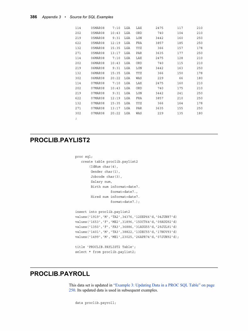
114 05MAR08 7:10 LGA LAX 2475 117 210202 05MAR08 10:43 LGA ORD 740 104 210219 05MAR08 9:31 LGA LON 3442 160 250622 05MAR08 12:19 LGA FRA 3857 185 250132 05MAR08 15:35 LGA YYZ 366 157 178271 05MAR08 13:17 LGA PAR 3635 177 250114 06MAR08 7:10 LGA LAX 2475 128 210202 06MAR08 10:43 LGA ORD 740 115 210219 06MAR08 9:31 LGA LON 3442 163 250132 06MAR08 15:35 LGA YYZ 366 150 178302 06MAR08 20:22 LGA WAS 229 66 180114 07MAR08 7:10 LGA LAX 2475 160 210202 07MAR08 10:43 LGA ORD 740 175 210219 07MAR08 9:31 LGA LON 3442 241 250622 07MAR08 12:19 LGA FRA 3857 210 250132 07MAR08 15:35 LGA YYZ 366 164 178271 07MAR08 13:17 LGA PAR 3635 155 250302 07MAR08 20:22 LGA WAS 229 135 180;

PROCLIB.PAYLIST2

proc sql; create table proclib.paylist2 (IdNum char(4), Gender char(1), Jobcode char(3), Salary num, Birth num informat=date7. format=date7., Hired num informat=date7. format=date7.);

insert into proclib.paylist2values('1919','M','TA2',34376,'12SEP66'd,'04JUN87'd)values('1653','F','ME2',31896,'15OCT64'd,'09AUG92'd)values('1350','F','FA3',36886,'31AUG55'd,'29JUL91'd)values('1401','M','TA3',38822,'13DEC55'd,'17NOV93'd)values('1499','M','ME1',23025,'26APR74'd,'07JUN92'd);

title 'PROCLIB.PAYLIST2 Table';select * from proclib.paylist2;

PROCLIB.PAYROLLThis data set is updated in “Example 3: Updating Data in a PROC SQL Table” on page 250. Its updated data is used in subsequent examples.

data proclib.payroll;


input IdNumber $4. +3 Gender $1. +4 Jobcode $3. +9 Salary 5. +2 Birth date7. +2 Hired date7.; informat birth date7. hired date7.; format birth date7. hired date7.; datalines;1919 M TA2 34376 12SEP60 04JUN871653 F ME2 35108 15OCT64 09AUG901400 M ME1 29769 05NOV67 16OCT901350 F FA3 32886 31AUG65 29JUL901401 M TA3 38822 13DEC50 17NOV851499 M ME3 43025 26APR54 07JUN801101 M SCP 18723 06JUN62 01OCT901333 M PT2 88606 30MAR61 10FEB811402 M TA2 32615 17JAN63 02DEC901479 F TA3 38785 22DEC68 05OCT891403 M ME1 28072 28JAN69 21DEC911739 M PT1 66517 25DEC64 27JAN911658 M SCP 17943 08APR67 29FEB921428 F PT1 68767 04APR60 16NOV911782 M ME2 35345 04DEC70 22FEB921244 M ME2 36925 31AUG63 17JAN881383 M BCK 25823 25JAN68 20OCT921574 M FA2 28572 27APR60 20DEC921789 M SCP 18326 25JAN57 11APR781404 M PT2 91376 24FEB53 01JAN801437 F FA3 33104 20SEP60 31AUG841639 F TA3 40260 26JUN57 28JAN841269 M NA1 41690 03MAY72 28NOV921065 M ME2 35090 26JAN44 07JAN871876 M TA3 39675 20MAY58 27APR851037 F TA1 28558 10APR64 13SEP921129 F ME2 34929 08DEC61 17AUG911988 M FA3 32217 30NOV59 18SEP841405 M SCP 18056 05MAR66 26JAN921430 F TA2 32925 28FEB62 27APR871983 F FA3 33419 28FEB62 27APR871134 F TA2 33462 05MAR69 21DEC881118 M PT3 111379 16JAN44 18DEC801438 F TA3 39223 15MAR65 18NOV871125 F FA2 28888 08NOV68 11DEC871475 F FA2 27787 15DEC61 13JUL901117 M TA3 39771 05JUN63 13AUG921935 F NA2 51081 28MAR54 16OCT811124 F FA1 23177 10JUL58 01OCT901422 F FA1 22454 04JUN64 06APR911616 F TA2 34137 01MAR70 04JUN931406 M ME2 35185 08MAR61 17FEB871120 M ME1 28619 11SEP72 07OCT931094 M FA1 22268 02APR70 17APR911389 M BCK 25028 15JUL59 18AUG901905 M PT1 65111 16APR72 29MAY921407 M PT1 68096 23MAR69 18MAR901114 F TA2 32928 18SEP69 27JUN871410 M PT2 84685 03MAY67 07NOV861439 F PT1 70736 06MAR64 10SEP901409 M ME3 41551 19APR50 22OCT81

PROCLIB.PAYROLL 387

1408 M TA2 34138 29MAR60 14OCT871121 M ME1 29112 26SEP71 07DEC911991 F TA1 27645 07MAY72 12DEC921102 M TA2 34542 01OCT59 15APR911356 M ME2 36869 26SEP57 22FEB831545 M PT1 66130 12AUG59 29MAY901292 F ME2 36691 28OCT64 02JUL891440 F ME2 35757 27SEP62 09APR911368 M FA2 27808 11JUN61 03NOV841369 M TA2 33705 28DEC61 13MAR871411 M FA2 27265 27MAY61 01DEC891113 F FA1 22367 15JAN68 17OCT911704 M BCK 25465 30AUG66 28JUN871900 M ME2 35105 25MAY62 27OCT871126 F TA3 40899 28MAY63 21NOV801677 M BCK 26007 05NOV63 27MAR891441 F FA2 27158 19NOV69 23MAR911421 M TA2 33155 08JAN59 28FEB901119 M TA1 26924 20JUN62 06SEP881834 M BCK 26896 08FEB72 02JUL921777 M PT3 109630 23SEP51 21JUN811663 M BCK 26452 11JAN67 11AUG911106 M PT2 89632 06NOV57 16AUG841103 F FA1 23738 16FEB68 23JUL921477 M FA2 28566 21MAR64 07MAR881476 F TA2 34803 30MAY66 17MAR871379 M ME3 42264 08AUG61 10JUN841104 M SCP 17946 25APR63 10JUN911009 M TA1 28880 02MAR59 26MAR921412 M ME1 27799 18JUN56 05DEC911115 F FA3 32699 22AUG60 29FEB801128 F TA2 32777 23MAY65 20OCT901442 F PT2 84536 05SEP66 12APR881417 M NA2 52270 27JUN64 07MAR891478 M PT2 84203 09AUG59 24OCT901673 M BCK 25477 27FEB70 15JUL911839 F NA1 43433 29NOV70 03JUL931347 M TA3 40079 21SEP67 06SEP841423 F ME2 35773 14MAY68 19AUG901200 F ME1 27816 10JAN71 14AUG921970 F FA1 22615 25SEP64 12MAR911521 M ME3 41526 12APR63 13JUL881354 F SCP 18335 29MAY71 16JUN921424 F FA2 28978 04AUG69 11DEC891132 F FA1 22413 30MAY72 22OCT931845 M BCK 25996 20NOV59 22MAR801556 M PT1 71349 22JUN64 11DEC911413 M FA2 27435 16SEP65 02JAN901123 F TA1 28407 31OCT72 05DEC921907 M TA2 33329 15NOV60 06JUL871436 F TA2 34475 11JUN64 12MAR871385 M ME3 43900 16JAN62 01APR861432 F ME2 35327 03NOV61 10FEB851111 M NA1 40586 14JUL73 31OCT921116 F FA1 22862 28SEP69 21MAR911352 M NA2 53798 02DEC60 16OCT86


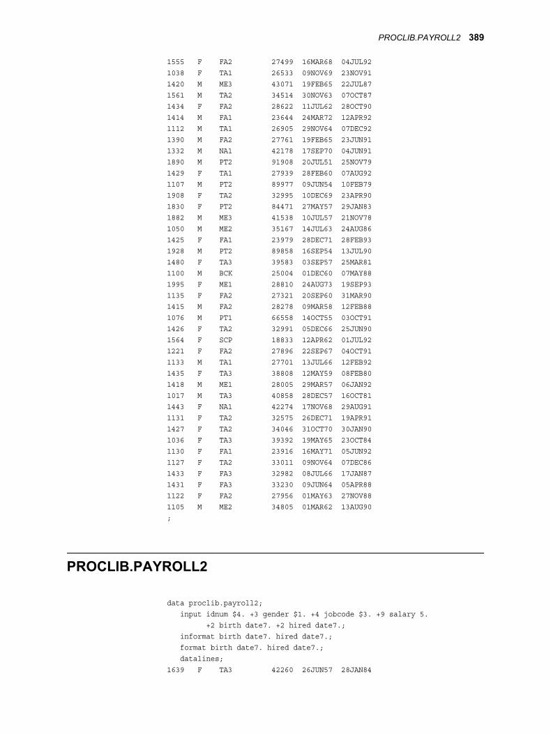
1555 F FA2 27499 16MAR68 04JUL921038 F TA1 26533 09NOV69 23NOV911420 M ME3 43071 19FEB65 22JUL871561 M TA2 34514 30NOV63 07OCT871434 F FA2 28622 11JUL62 28OCT901414 M FA1 23644 24MAR72 12APR921112 M TA1 26905 29NOV64 07DEC921390 M FA2 27761 19FEB65 23JUN911332 M NA1 42178 17SEP70 04JUN911890 M PT2 91908 20JUL51 25NOV791429 F TA1 27939 28FEB60 07AUG921107 M PT2 89977 09JUN54 10FEB791908 F TA2 32995 10DEC69 23APR901830 F PT2 84471 27MAY57 29JAN831882 M ME3 41538 10JUL57 21NOV781050 M ME2 35167 14JUL63 24AUG861425 F FA1 23979 28DEC71 28FEB931928 M PT2 89858 16SEP54 13JUL901480 F TA3 39583 03SEP57 25MAR811100 M BCK 25004 01DEC60 07MAY881995 F ME1 28810 24AUG73 19SEP931135 F FA2 27321 20SEP60 31MAR901415 M FA2 28278 09MAR58 12FEB881076 M PT1 66558 14OCT55 03OCT911426 F TA2 32991 05DEC66 25JUN901564 F SCP 18833 12APR62 01JUL921221 F FA2 27896 22SEP67 04OCT911133 M TA1 27701 13JUL66 12FEB921435 F TA3 38808 12MAY59 08FEB801418 M ME1 28005 29MAR57 06JAN921017 M TA3 40858 28DEC57 16OCT811443 F NA1 42274 17NOV68 29AUG911131 F TA2 32575 26DEC71 19APR911427 F TA2 34046 31OCT70 30JAN901036 F TA3 39392 19MAY65 23OCT841130 F FA1 23916 16MAY71 05JUN921127 F TA2 33011 09NOV64 07DEC861433 F FA3 32982 08JUL66 17JAN871431 F FA3 33230 09JUN64 05APR881122 F FA2 27956 01MAY63 27NOV881105 M ME2 34805 01MAR62 13AUG90;

PROCLIB.PAYROLL2

data proclib.payroll2; input idnum $4. +3 gender $1. +4 jobcode $3. +9 salary 5. +2 birth date7. +2 hired date7.; informat birth date7. hired date7.; format birth date7. hired date7.; datalines;1639 F TA3 42260 26JUN57 28JAN84

PROCLIB.PAYROLL2 389

1065 M ME3 38090 26JAN44 07JAN871561 M TA3 36514 30NOV63 07OCT871221 F FA3 29896 22SEP67 04OCT911447 F FA1 22123 07AUG72 29OCT921998 M SCP 23100 10SEP70 02NOV921036 F TA3 42465 19MAY65 23OCT841106 M PT3 94039 06NOV57 16AUG841129 F ME3 36758 08DEC61 17AUG911350 F FA3 36098 31AUG65 29JUL901369 M TA3 36598 28DEC61 13MAR871076 M PT1 69742 14OCT55 03OCT91;

PROCLIB.SCHEDULE2data proclib.schedule2; input flight $3. +5 date date7. +2 dest $3. +3 idnum $4.; format date date7.; informat date date7.; datalines;132 01MAR94 BOS 1118132 01MAR94 BOS 1402219 02MAR94 PAR 1616219 02MAR94 PAR 1478622 03MAR94 LON 1430622 03MAR94 LON 1882271 04MAR94 NYC 1430271 04MAR94 NYC 1118579 05MAR94 RDU 1126579 05MAR94 RDU 1106;

PROCLIB.STAFF

data proclib.staff; input idnum $4. +3 lname $15. +2 fname $15. +2 city $15. +2 state $2. +5 hphone $12.; datalines;1919 ADAMS GERALD STAMFORD CT 203/781-12551653 ALIBRANDI MARIA BRIDGEPORT CT 203/675-77151400 ALHERTANI ABDULLAH NEW YORK NY 212/586-08081350 ALVAREZ MERCEDES NEW YORK NY 718/383-15491401 ALVAREZ CARLOS PATERSON NJ 201/732-87871499 BAREFOOT JOSEPH PRINCETON NJ 201/812-56651101 BAUCOM WALTER NEW YORK NY 212/586-80601333 BANADYGA JUSTIN STAMFORD CT 203/781-17771402 BLALOCK RALPH NEW YORK NY 718/384-28491479 BALLETTI MARIE NEW YORK NY 718/384-88161403 BOWDEN EARL BRIDGEPORT CT 203/675-34341739 BRANCACCIO JOSEPH NEW YORK NY 212/587-1247


1658 BREUHAUS JEREMY NEW YORK NY 212/587-36221428 BRADY CHRISTINE STAMFORD CT 203/781-12121782 BREWCZAK JAKOB STAMFORD CT 203/781-00191244 BUCCI ANTHONY NEW YORK NY 718/383-33341383 BURNETTE THOMAS NEW YORK NY 718/384-35691574 CAHILL MARSHALL NEW YORK NY 718/383-23381789 CARAWAY DAVIS NEW YORK NY 212/587-90001404 COHEN LEE NEW YORK NY 718/384-29461437 CARTER DOROTHY BRIDGEPORT CT 203/675-41171639 CARTER-COHEN KAREN STAMFORD CT 203/781-88391269 CASTON FRANKLIN STAMFORD CT 203/781-33351065 COPAS FREDERICO NEW YORK NY 718/384-56181876 CHIN JACK NEW YORK NY 212/588-56341037 CHOW JANE STAMFORD CT 203/781-88681129 COUNIHAN BRENDA NEW YORK NY 718/383-23131988 COOPER ANTHONY NEW YORK NY 212/587-12281405 DACKO JASON PATERSON NJ 201/732-23231430 DABROWSKI SANDRA BRIDGEPORT CT 203/675-16471983 DEAN SHARON NEW YORK NY 718/384-16471134 DELGADO MARIA STAMFORD CT 203/781-15281118 DENNIS ROGER NEW YORK NY 718/383-11221438 DABBOUSSI KAMILLA STAMFORD CT 203/781-22291125 DUNLAP DONNA NEW YORK NY 718/383-20941475 ELGES MARGARETE NEW YORK NY 718/383-28281117 EDGERTON JOSHUA NEW YORK NY 212/588-12391935 FERNANDEZ KATRINA BRIDGEPORT CT 203/675-29621124 FIELDS DIANA WHITE PLAINS NY 914/455-29981422 FUJIHARA KYOKO PRINCETON NJ 201/812-09021616 FUENTAS CARLA NEW YORK NY 718/384-33291406 FOSTER GERALD BRIDGEPORT CT 203/675-63631120 GARCIA JACK NEW YORK NY 718/384-49301094 GOMEZ ALAN BRIDGEPORT CT 203/675-71811389 GOLDSTEIN LEVI NEW YORK NY 718/384-93261905 GRAHAM ALVIN NEW YORK NY 212/586-88151407 GREGORSKI DANIEL MT. VERNON NY 914/468-16161114 GREENWALD JANICE NEW YORK NY 212/588-10921410 HARRIS CHARLES STAMFORD CT 203/781-09371439 HASENHAUER CHRISTINA BRIDGEPORT CT 203/675-49871409 HAVELKA RAYMOND STAMFORD CT 203/781-96971408 HENDERSON WILLIAM PRINCETON NJ 201/812-47891121 HERNANDEZ ROBERTO NEW YORK NY 718/384-33131991 HOWARD GRETCHEN BRIDGEPORT CT 203/675-00071102 HERMANN JOACHIM WHITE PLAINS NY 914/455-09761356 HOWARD MICHAEL NEW YORK NY 212/586-84111545 HERRERO CLYDE STAMFORD CT 203/781-11191292 HUNTER HELEN BRIDGEPORT CT 203/675-48301440 JACKSON LAURA STAMFORD CT 203/781-00881368 JEPSEN RONALD STAMFORD CT 203/781-84131369 JONSON ANTHONY NEW YORK NY 212/587-53851411 JOHNSEN JACK PATERSON NJ 201/732-36781113 JOHNSON LESLIE NEW YORK NY 718/383-30031704 JONES NATHAN NEW YORK NY 718/384-00491900 KING WILLIAM NEW YORK NY 718/383-36981126 KIMANI ANNE NEW YORK NY 212/586-12291677 KRAMER JACKSON BRIDGEPORT CT 203/675-74321441 LAWRENCE KATHY PRINCETON NJ 201/812-3337

PROCLIB.STAFF 391

1421 LEE RUSSELL MT. VERNON NY 914/468-91431119 LI JEFF NEW YORK NY 212/586-23441834 LEBLANC RUSSELL NEW YORK NY 718/384-00401777 LUFKIN ROY NEW YORK NY 718/383-44131663 MARKS JOHN NEW YORK NY 212/587-77421106 MARSHBURN JASPER STAMFORD CT 203/781-14571103 MCDANIEL RONDA NEW YORK NY 212/586-00131477 MEYERS PRESTON BRIDGEPORT CT 203/675-81251476 MONROE JOYCE STAMFORD CT 203/781-28371379 MORGAN ALFRED STAMFORD CT 203/781-22161104 MORGAN CHRISTOPHER NEW YORK NY 718/383-97401009 MORGAN GEORGE NEW YORK NY 212/586-77531412 MURPHEY JOHN PRINCETON NJ 201/812-44141115 MURPHY ALICE NEW YORK NY 718/384-19821128 NELSON FELICIA BRIDGEPORT CT 203/675-11661442 NEWKIRK SANDRA PRINCETON NJ 201/812-33311417 NEWKIRK WILLIAM PATERSON NJ 201/732-66111478 NEWTON JAMES NEW YORK NY 212/587-55491673 NICHOLLS HENRY STAMFORD CT 203/781-77701839 NORRIS DIANE NEW YORK NY 718/384-17671347 O'NEAL BRYAN NEW YORK NY 718/384-02301423 OSWALD LESLIE MT. VERNON NY 914/468-91711200 OVERMAN MICHELLE STAMFORD CT 203/781-18351970 PARKER ANNE NEW YORK NY 718/383-38951521 PARKER JAY NEW YORK NY 212/587-76031354 PARKER MARY WHITE PLAINS NY 914/455-23371424 PATTERSON RENEE NEW YORK NY 212/587-89911132 PEARCE CAROL NEW YORK NY 718/384-19861845 PEARSON JAMES NEW YORK NY 718/384-23111556 PENNINGTON MICHAEL NEW YORK NY 718/383-56811413 PETERS RANDALL PRINCETON NJ 201/812-24781123 PETERSON SUZANNE NEW YORK NY 718/383-00771907 PHELPS WILLIAM STAMFORD CT 203/781-11181436 PORTER SUSAN NEW YORK NY 718/383-57771385 RAYNOR MILTON BRIDGEPORT CT 203/675-28461432 REED MARILYN MT. VERNON NY 914/468-54541111 RHODES JEREMY PRINCETON NJ 201/812-18371116 RICHARDS CASEY NEW YORK NY 212/587-12241352 RIVERS SIMON NEW YORK NY 718/383-33451555 RODRIGUEZ JULIA BRIDGEPORT CT 203/675-24011038 RODRIGUEZ MARIA BRIDGEPORT CT 203/675-20481420 ROUSE JEREMY PATERSON NJ 201/732-98341561 SANDERS RAYMOND NEW YORK NY 212/588-66151434 SANDERSON EDITH STAMFORD CT 203/781-13331414 SANDERSON NATHAN BRIDGEPORT CT 203/675-17151112 SANYERS RANDY NEW YORK NY 718/384-48951390 SMART JONATHAN NEW YORK NY 718/383-11411332 STEPHENSON ADAM BRIDGEPORT CT 203/675-14971890 STEPHENSON ROBERT NEW YORK NY 718/384-98741429 THOMPSON ALICE STAMFORD CT 203/781-38571107 THOMPSON WAYNE NEW YORK NY 718/384-37851908 TRENTON MELISSA NEW YORK NY 212/586-62621830 TRIPP KATHY BRIDGEPORT CT 203/675-24791882 TUCKER ALAN NEW YORK NY 718/384-02161050 TUTTLE THOMAS WHITE PLAINS NY 914/455-21191425 UNDERWOOD JENNY STAMFORD CT 203/781-0978


1928 UPCHURCH LARRY WHITE PLAINS NY 914/455-50091480 UPDIKE THERESA NEW YORK NY 212/587-87291100 VANDEUSEN RICHARD NEW YORK NY 212/586-25311995 VARNER ELIZABETH NEW YORK NY 718/384-71131135 VEGA ANNA NEW YORK NY 718/384-59131415 VEGA FRANKLIN NEW YORK NY 718/384-28231076 VENTER RANDALL NEW YORK NY 718/383-23211426 VICK THERESA PRINCETON NJ 201/812-24241564 WALTERS ANNE NEW YORK NY 212/587-32571221 WALTERS DIANE NEW YORK NY 718/384-19181133 WANG CHIN NEW YORK NY 212/587-19561435 WARD ELAINE NEW YORK NY 718/383-49871418 WATSON BERNARD NEW YORK NY 718/383-12981017 WELCH DARIUS NEW YORK NY 212/586-55351443 WELLS AGNES STAMFORD CT 203/781-55461131 WELLS NADINE NEW YORK NY 718/383-10451427 WHALEY CAROLYN MT. VERNON NY 914/468-45281036 WONG LESLIE NEW YORK NY 212/587-25701130 WOOD DEBORAH NEW YORK NY 212/587-00131127 WOOD SANDRA NEW YORK NY 212/587-28811433 YANCEY ROBIN PRINCETON NJ 201/812-18741431 YOUNG DEBORAH STAMFORD CT 203/781-29871122 YOUNG JOANN NEW YORK NY 718/384-20211105 YOUNG LAWRENCE NEW YORK NY 718/384-0008;

PROCLIB.STAFF2data proclib.staff2;input IdNum $4. @7 Lname $12. @20 Fname $8. @30 City $10. @42 State $2. @50 Hphone $12.; datalines;1106 MARSHBURN JASPER STAMFORD CT 203/781-14571430 DABROWSKI SANDRA BRIDGEPORT CT 203/675-16471118 DENNIS ROGER NEW YORK NY 718/383-11221126 KIMANI ANNE NEW YORK NY 212/586-12291402 BLALOCK RALPH NEW YORK NY 718/384-28491882 TUCKER ALAN NEW YORK NY 718/384-02161479 BALLETTI MARIE NEW YORK NY 718/384-88161420 ROUSE JEREMY PATERSON NJ 201/732-98341403 BOWDEN EARL BRIDGEPORT CT 203/675-34341616 FUENTAS CARLA NEW YORK NY 718/384-3329;

PROCLIB.SUPERV2data proclib.superv2; input supid $4. +8 state $2. +5 jobcat $2.; label supid='Supervisor Id' jobcat='Job Category'; datalines;1417 NJ NA

PROCLIB.SUPERV2 393

1352 NY NA1106 CT PT1442 NJ PT1118 NY PT1405 NJ SC1564 NY SC1639 CT TA1126 NY TA1882 NY ME;

STORESdata stores; input Store $ x y; datalines;store1 5 1store2 5 3store3 3 5store4 7 5;

SURVEYdata survey; input id $ diet $ exer $ hours xwk educ; datalines;1001 yes yes 1 3 11002 no yes 1 4 21003 no no . . .n1004 yes yes 2 3 .x1005 no yes 2 3 .x1006 yes yes 2 4 .x1007 no yes .5 3 .1008 no no . . .;


Glossary

calculated columnin a query, a column that does not exist in any of the tables that are being queried, but which is created as a result of a column expression.

Cartesian producta type of join that matches each row from each joined table to each row from all other joined tables.

columna vertical component of a table. Each column has a unique name, contains data of a specific type, and has particular attributes. A column is analogous to a variable in SAS terminology.

column aliasa temporary, alternate name for a column. Aliases are optionally specified in the SQL procedure's SELECT clause to name or rename columns. An alias is one word.

column expressiona set of operators and operands that, when evaluated, result in a single data value. The resulting data value can be either a character value or a numeric value.

composite indexan index that locates observations in a SAS data set by examining the values of two or more key variables.

conditionin the SQL procedure, the part of the WHERE clause that specifies which rows are to be retrieved.

cross joina type of join that returns the product of joined tables. A cross join is functionally the same as a Cartesian product.

data setSee SAS data set.

data viewSee SAS data view.

395

DISTINCTa keyword that causes the SQL procedure to remove duplicate rows from the output.

equijoina kind of join in the SQL procedure. For example, when two tables are joined in an equijoin, the value of a column in the first table must equal the value of the column in the second table in the SQL expression.

formatSee SAS format.

groupa set of rows or observations that have the same value or values for one or more common columns or variables.

in-line viewa query-expression that is nested in the SQL procedure's FROM clause. An in-line view produces a table internally that the outer query uses to select data. You save a programming step when you use an in-line view, because instead of creating a view and then referring to it in another query, you can specify the view in-line in the FROM clause. An in-line view can be referenced only in the query (or statement) in which it is defined.

indexa component of a SAS data set that enables SAS to access observations in the SAS data set quickly and efficiently. The purpose of SAS indexes is to optimize WHERE-clause processing and to facilitate BY-group processing.

inner joina join between two tables that returns all of the rows in one table that have one or more matching rows in the other table.

integrity constraintsa set of data validation rules that you can specify in order to restrict the data values that can be stored for a variable in a SAS data file. Integrity constraints help you preserve the validity and consistency of your data.

joinan operation that combines data from two or more tables. A join is typically created by means of SQL (Structured Query Language) code or a user interface.

join criteriathe set of parameters that determine how tables are to be joined. Join criteria are usually specified in a WHERE expression or in an SQL ON clause.

missing valuea type of value for a variable that contains no data for a particular row or column. By default, SAS writes a missing numeric value as a single period and a missing character value as a blank space.

natural joina type of join that returns selected rows from tables in which one or more columns in each table have the same name and the same data type and contain the same value.

396 Glossary

outer joina join between two tables that returns all of the rows in one table, as well as part or all of the rows in the other table. A left or right outer join returns all of the rows in one table (the table on the left or right side of the SQL statement, respectively), as well as the matching rows in the other table. A full outer join returns all of the rows in both of the tables.

pass-through facilitySee SQL pass-through facility.

PROC SQL viewa SAS data set that is created by the SQL procedure. A PROC SQL view contains no data. Instead, it stores information that enables it to read data values from other files, which can include SAS data files, SAS/ACCESS views, DATA step views, or other PROC SQL views. The output of a PROC SQL view can be either a subset or a superset of one or more files.

querya set of instructions that requests particular information from one or more data sources.

query expressionin PROC SQL, a SELECT statement that references at least one table and, when executed, creates a temporary table that exists only during the execution of the statement. You can combine the results of multiple table expressions with set operators to create a query expression.

SAS data filea type of SAS data set that contains data values as well as descriptor information that is associated with the data. The descriptor information includes information such as the data types and lengths of the variables, as well as the name of the engine that was used to create the data.

SAS data seta file whose contents are in one of the native SAS file formats. There are two types of SAS data sets: SAS data files and SAS data views. SAS data files contain data values in addition to descriptor information that is associated with the data. SAS data views contain only the descriptor information plus other information that is required for retrieving data values from other SAS data sets or from files whose contents are in other software vendors' file formats.

SAS data viewa type of SAS data set that retrieves data values from other files. A SAS data view contains only descriptor information such as the data types and lengths of the variables (columns) plus other information that is required for retrieving data values from other SAS data sets or from files that are stored in other software vendors' file formats. Short form: data view.

SAS formata type of SAS language element that applies a pattern to or executes instructions for a data value to be displayed or written as output. Types of formats correspond to the data's type: numeric, character, date, time, or timestamp. The ability to create user-defined formats is also supported. Examples of SAS formats are BINARY and DATE. Short form: format.

Glossary 397

simple indexan index that uses the values of only one variable to locate observations.

SQLSee Structured Query Language.

SQL pass-through facilitythe technology that enables SQL query code to be passed to a particular DBMS for processing. Short form: pass-through facility.

Structured Query Languagea standardized, high-level query language that is used in relational database management systems to create and manipulate objects in a database management system. SAS implements SQL through the SQL procedure. Short form: SQL.

union joina type of join that returns all rows with their respective values from each input table. Columns that do not exist in one table will have null (missing) values for those rows in the result table.

viewa definition of a virtual data set that is named and stored for later use. A view contains no data; it merely describes or defines data that is stored elsewhere.

WHERE clausethe keyword WHERE followed by one or more WHERE expressions.

WHERE expressiondefines the criteria for selecting observations.

398 Glossary

Index

Aabbreviating column names 76aggregate functions 56

creating macro variables from result of153

HAVING clause with 70table of 56using 56with unique values 61

aliasassigning a column alias 30referring to calculated columns by 31table aliases 76

ALL keyword 336set operators and 141

ALTER TABLE statement 225ANSI standard

SQL procedure and 375arithmetic operators 376asterisk (*) notation 294automatic macro variables 152, 157averages, weighted 172

BBETWEEN condition 308BETWEEN-AND operators

retrieving rows 51Boolean operators

retrieving rows 47BTRIM function 308BUFFERSIZE= option 216

Ccalculated columns 29

assigning column alias to 30referring to by alias 31sorting by 40SQL 310

Cartesian product 75, 320, 321

cross joins 87CASE expression

assigning values conditionally 32case-control studies 286CASE-OPERAND form

assigning values conditionally 34character strings

converting to lowercase 334converting to uppercase 360trimming 308

COALESCE function 311in joins 90replacing missing values 35

collating sequencealternate 376

column alias 30ANSI standard exceptions 378assigning to calculated columns 30referring to calculated columns 31specifying 295

column attributes 228, 313list of 27specifying 36

column definitionscreating tables from 110

column headerssuppressing 28

column modifiers 376column names

abbreviating 76qualifying 76

column-modifier component 313column-name component 315columns 4

adding 121aliases 295altering 121, 225assigning values conditionally 32calculated 309, 310calculating values 29changing formats 123

399

changing informats 123changing labels 123changing width 123combinations of values 280creating 27deleting 124DICTIONARY.COLUMNS 149grouping by multiple columns 65grouping by one column 64indexes on 228, 229, 243inserting values 243length of 313list of, with attributes 27locating specific columns 149modifiers 376modifying 123multicolumn joins 81renaming 123, 228, 244replacing missing values 35returning values 311selecting 22, 244, 315selecting all 22selecting specific 23sorting by 38sorting by column position 41sorting by multiple columns 38sorting by unselected columns 42sorting, with missing values 43SQL procedure 210storing values of 295summarizing data in multiple columns

186unique values 25updating values 244

COMMIT statement 377comparison operators

inner joins with 78retrieving rows with 45truncated string 53

composite indexes 125, 230concatenating

query results 106values in macro variables 155

conditional operatorsretrieving rows with 49

CONNECT statement 228CONNECTION TO component 316CONSTDATETIME option 216CONTAINS condition 316, 376correlated subqueries 97, 348CORRESPONDING keyword 336COUNT(*) function 352counting

all rows 62duplicate rows 181nonmissing values 62

unique values 61CREATE INDEX statement 125, 229CREATE TABLE statement 231CREATE VIEW statement 235cross joins 87, 325

Ddata files

See tablesdata set options

creating tables with 113SQL procedure with 151

DATA stepcompared with SQL procedure 5match-merges 91

DATA step viewsSQL procedure 211

data summaries 352DATE function

replacing references to 144DATETIME function

replacing references to 144DBMS

accessing with SAS/ACCESS 162connecting with LIBNAME statement

163connecting with Pass-Through Facility

166deploying PUT function and SAS

formats 143DBMS connections

ending 239sending DBMS statements to 241SQL procedure 228storing in views 236

DBMS queries 316DBMS tables 4

PROC SQL views of 165querying 164

debugging queries 136DELETE statement 237DESCRIBE statement 238DESCRIBE VIEW statement 147DICTIONARY tables 144

performance and 150reporting from 258retrieving information about 146using 148views and 144

DICTIONARY.COLUMNS 149DICTIONARY.TABLES 148DISCONNECT statement 239DOUBLE option 217DQUOTE= option 217DROP statement 240

400 Index

Eembedded LIBNAME statements 236embedded SQL 378equijoins 320errors

caused by missing values 63grouping errors caused by missing

values 67update errors 120

ERRORSTOP option 217example tables 7EXCEPT operator 340

combining queries 102, 104EXEC option 218EXECUTE statement 241execution time 138existence of a group of values 98EXISTS condition 98, 316EXITCODE option 218expanded SELECT * statement 138

FFEEDBACK option 218

expanding SELECT * statement with138

fieldsSee columns

filesSee tables

filtering grouped data 69HAVING clause versus WHERE clause

70using a simple HAVING clause 69using HAVING clause with aggregate

functions 70FLOW option 218foreign key 126formats

changing column format 123deploying inside a DBMS 143for columns 313

FROM clause 20, 301full outer joins 86functions

FCMP procedure 377SQL procedure and 377sql-expression and 343

Ggeneral integrity constraints 126GROUP BY clause 21, 303grouping data 64

by multiple columns 65by one column 64

filtering grouped data 69finding errors caused by missing values

67grouping and sorting 66with missing values 67without summarizing 64

HHAVING clause 21, 304

aggregate functions with 70filtering grouped data 69filtering grouped data, versus WHERE

clause 70hierarchical data

expanding in tables 183host-variable references 152

IIN condition 317IN operator

multiple-value subqueries and 96retrieving rows 50

in-database proceduresgenerating SQL for 364

in-line views 132, 302, 376querying 273temporary tables versus 141

indexes 124composite 125composite indexes 230creating 124creating with CREATE INDEX

statement 125deleting 125, 240managing 230on altered columns 228on columns 229, 243query performance and 140simple indexes 230SQL procedure 230tips for creating 125UNIQUE keyword 230unique values 125

informatschanging column informat 123for columns 313

INNER JOIN keywords 78inner joins 75, 320

comparison operators for 78creating with INNER JOIN keywords

78data from multiple tables 82multicolumn joins 81null values and 79

Index 401

order of output 77reflexive joins 83self-joins 83showing relationships within a table 83table aliases 76

INOBS= option 219restricting row processing 136

INSERT statement 242inserting rows 114

with queries 116with SET clause 114with VALUES clause 115

integrity constraints 126PROC SQL tables 228, 235referential 126

INTERSECT operator 342combining queries 102, 105

INTO clause 295IPASSTHRU option 219IS condition 318IS MISSING operator

retrieving rows 50IS NOT MISSING operator

inner joins 80iterations

limiting 137

Jjoined-table component 319joins 74, 319

Cartesian product 75COALESCE function in 90combining with subqueries 100comparing match-merges with 91comparing with subqueries 141cross joins 87, 325equijoins 320inner joins 75, 320joining a table with itself 320joining more than two tables 329joining three tables 269joining two tables 252natural joins 89, 327outer joins 84, 260, 323, 376reducing size of results 141reflexive joins 320rows to be returned 320specialty joins 87subqueries compared with 332table limit 320types of 319union joins 89, 326when to use 101WHERE expressions with 141

Llabels

changing column labels 123for columns 313

left outer joins 85libname engines

querying DBMS tables 164LIBNAME statement

connecting to a DBMS 163embedding in views 236

libnamesembedding in views 131

librefsstored views and 236

LIKE condition 332patterns for searching 333searching for literals 333searching for mixed-case strings 334

LIKE operatorretrieving rows 52

logdisplaying SQL definitions 238

logical operatorsretrieving rows 47

LOOPS= option 219limiting iterations 137

LOWER function 334

Mmacro facility

SQL procedure with 152macro variables 152

concatenating values in 155creating and using 199creating from aggregate function results

153creating from query results 153creating in SQL procedure 152creating multiple 154set by SQL procedure 157SYS_SQLSETLIMIT 374

macroscounting missing values 289defining to create tables 156

match-merges 91comparing with joins 91when all values match 91when position of values is important 94when some values match 93

matching patterns 286, 332MEAN function

summarizing data 57WHERE clause with 57

mergingdisabling remerge 144

402 Index

remerging summary statistics 59merging data

SQL procedure 354missing values 5

counting with a macro 289finding errors caused by 63finding grouping errors caused by 67grouping data with 67overlaying 176replacing in columns 35retrieving rows and 50sorting columns with 43SQL procedure 289, 318summarizing data with 62WHERE clause with 54

multicolumn joins 81multiple-value subqueries 96

Nnatural joins 89, 327nested subqueries 99NOEXEC option

syntax checking with 137NOT IN operator

multiple-value subqueries and 96null values 5

inner joins and 79NUMBER option 220

Oobservations

See also rowsSQL procedure 210

ODS (Output Delivery System)SQL procedure with 169

ODS destinations 169operands

values from 342operators

arithmetic 376order of evaluation 343set operators 335, 377truncated string comparison operators

345values from 342

ORDER BY clause 21, 305, 376omitting 141query performance and 141

orthogonal expressions 376outer joins 84, 260, 323, 376

full outer joins 86including nonmatching rows 85left outer joins 85right outer joins 85

OUTER UNION operatorcombining queries 102concatenating query results 106

OUTER UNION set operator 336OUTOBS= option 220

restricting row processing 136output

adding text to 27formatting with REPORT procedure

160output objects 169overlaying missing values 176

Ppattern matching 286, 332percentages

computing within subtotals 179performance

queries 140primary key 126PRINT option 220PROC SQL statement 215PROC SQL tables 210

adding rows 242aliases 301, 320altering columns 225altering integrity constraints 225changing column attributes 228combining 255counting rows 352creating 231, 246creating, from query expressions 234creating, from query results 248deleting 240deleting rows 237, 238indexes on columns 228initial values of columns 228inserting data 246inserting values 243integrity constraints 228, 235joining 252, 277, 319joining a table with itself 319, 320joining more than two tables 329joining three tables 269ordering rows 305recursive table references 234renaming columns 228retrieving data from 334selecting columns 244selecting rows 244source tables 301table definitions 238table expressions 335updating 244, 245, 250without rows 234

Index 403

PROC SQL viewsSee also viewsadding rows 242creating, from query expressions 234creating, from query results 266deleting 240deleting rows 237, 238embedding LIBNAME statements in

236inserting rows 243librefs and stored views 236selecting columns 235, 244selecting rows 244sorting data retrieved by 236source views 301SQL procedure 211storing DBMS connection information

236updating 168, 236updating column values 244updating tables through 245view definitions 238, 376

PROMPT option 220PUT function

deploying inside a DBMS 143mapping to SAS_PUT function 367optimizing 142reducing 142reducing, based number of format

values 370reducing, based on engine type 368reducing, based on number of

observations in table 369

Qqualifying column names 76queries 5

adding text to output 27ALL keyword in set operations 141breaking into steps 141combining with set operators 102comparing execution time of two

queries 138creating 136creating tables from results 248creating views from results 266DBMS queries 316DBMS tables 164debugging 136duplicate rows and performance 141in-line view queries 273in-line views 132in-line views versus temporary tables

141indexes and 140

inserting rows with 116limiting iterations 137performance improvement 140remerged data and 372restricting row processing 136subqueries 95validating 71

query expressions 335ALL keyword and 336CORRESPONDING keyword and 336creating PROC SQL tables from 234creating PROC SQL views from 236EXCEPT and 340INTERSECT and 342OUTER UNION and 336set operators and 335subqueries 346UNION and 339validating syntax 245

query results 5concatenating 106creating macro variables from 153creating tables from 111deleting duplicate rows 25

query-expression component 334

Rrecords

See rowsREDUCEPUT option 142, 220REDUCEPUTOBS option 142, 221REDUCEPUTVALUES option 143, 222referential integrity constraints 126reflexive joins 83, 320relational theory 3relations 3REMERGE option 222remerging data 372

SQL procedure 354remerging summary statistics 59

disabling remerge 144renaming columns 123REPORT procedure

formatting SQL output 160reports

creating summary reports 188from DICTONARY tables 258

RESET statement 244resetting SQL procedure options 139

resetting options 139retrieving rows 44

based on comparison 45identifying columns with missing values

50rows that satisfy a condition 44

404 Index

satisfying multiple conditions 47with a WHERE clause with missing

values 54with BETWEEN-AND operators 51with IN operator 50with IS MISSING operator 50with LIKE operator 52with other conditional operators 49with simple WHERE clause 44with truncated string comparison

operators 53return codes

Pass-Through Facility 167returning a SUBSTRING 350right outer joins 85ROLLBACK statement 377rows 4

See also retrieving rowsadding to tables or views 242combining data from multiple rows into

single row 59counting 62, 352counting duplicates 181deleting 120, 237, 238deleting duplicates 25duplicates 141including all 89including all combinations of 87inserting 114, 243inserting with queries 116inserting with SET clause 114inserting with VALUES clause 115joins and 320matching 89nonmatching 85ordering 305producing from first or second query

107restricting row processing 136returned by subqueries 316selecting 244, 308selecting all 86SQL procedure 210updating all rows with same expression

118updating rows with different

expressions 119

SSAS data files

See tablesSAS data views

DICTIONARY tables 144SQL procedure 211

SAS System information 144

SAS_PUT() functionmapping PUT function to 367

SAS/ACCESSaccessing a DBMS 162LIBNAME statement 163

SAS/ACCESS viewsSQL procedure 211updating 168

SASHELP views 144retrieving information about 146

searching for patterns 286, 332, 333SELECT * statement

expanding with FEEDBACK option138

SELECT clause 20, 293SELECT statement 20, 244

See also WHERE clauseFROM clause 20GROUP BY clause 21HAVING clause 21ORDER BY clause 21ordering clauses 22SELECT clause 20

self-joins 83SET clause

inserting rows with 114set membership 317set operators 335, 377

ALL keyword 141combining queries with 102

simple indexes 230single-value subqueries 95sort order 37, 39

customized 191sorting data 37

by calculated column 40by column 38by column position 41by multiple columns 38by unselected columns 42columns with missing values 43grouping and sorting 66

sorting data retrieved by views 236sorting sequence 43SORTMSG option 223SORTSEQ= option 223SOUNDS-LIKE operator 275source data

generating SQL for in-database processing of 364

SQL 3generating for in-database processing of

source data 364SQL component

table-expression 359SQL components 307

Index 405

BETWEEN condition 308BTRIM function 308CALCULATED 309CASE expression 310COALESCE function 311column-definition 312column-modifier 313column-name 315CONNECTION TO 316CONTAINS condition 316EXISTS condition 316IN condition 317IS condition 318joined-table 319LIKE condition 332LOWER function 334query-expression 334sql-expression 342SUBSTRING function 350summary-function 351UPPER function 360

SQL procedure 3, 210See also SQL componentsANSI standard and 375coding conventions 211collating sequence 376column modifiers 376combinations of column values 280combining two tables 255compared with DATA step 5counting missing values with a macro

289creating macro variables 152creating queries 136creating tables and inserting data 246creating tables from query results 248creating views from query results 266cumulative time for 138data set options with 151data types and dates 312debugging queries 136DICTIONARY tables 144example tables 7formatting output 160functions supported by 377identifiers and naming conventions 377indexes 230joining three tables 269joining two tables 252, 277macro facility with 152macro variables set by 157matching case rows and control rows

286missing values 289, 318ODS with 169orthogonal expressions 376

outer joins 260PROC SQL tables 210querying in-line views 273reporting from DICTIONARY tables

258reserved words 375resetting options 139, 244retrieving values 275statistical functions 377syntax 212syntax checking 137task tables 214, 215terminology 4, 210three-valued logic 378timing individual statements 138undo policy 373updating PROC SQL tables 250user privileges 378using tables in other procedures 203views 211

SQL Procedure Pass-Through Facility 166connecting to a DBMS 166example 167return codes 167

sql-expression component 342correlated subqueries and 348functions and 343operators and order of evaluation 343query expressions and 346subqueries and efficiency 349truncated string comparison operators

and 345USER and 343

SQL, embedded 378SQLCONSTDATETIME system option

363SQLEXITCODE macro variable 158SQLGENERATION= system option 364SQLMAPPUTTO= system option 367SQLOBS macro variable 158SQLOOPS macro variable 137, 158SQLRC macro variable 158SQLREDUCEPUT= system option 142,

368SQLREDUCEPUTOBS= system option

142, 369SQLREDUCEPUTVALUES= system

option 143, 370SQLREMERGE system option 372SQLUNDOPOLICY 373SQLUNDOPOLICY= system option 158,

373SQLXMSG macro variable 159SQLXRC macro variable 159statistical functions 377statistical summaries 56, 351

406 Index

statisticsbased on number of arguments 353

STIMER option 223timing SQL procedure 138

string comparison operatorstruncated 345

Structured Query LanguageSee SQL

subqueries 95, 346combining with joins 100compared with joins 332comparing with joins 141correlated 348correlated subqueries 97efficiency and 349multiple nesting levels 99multiple-value 96returning rows 316single-value 95testing for existence of a group of

values 98when to use 101

subsetting data 302, 304SUBSTRING function 350subtotals

computing percentages within 179SUM function

summarizing data 58summarizing data 56

aggregate functions 56aggregate functions with unique values

61aggregate functions, using 56combining data from multiple rows into

single row 59displaying sums 58in multiple columns 186remerging summary statistics 59SQL procedure 352with missing values 62with WHERE clause 57

summary functionsSee also aggregate functionsdisabling remerging of data 144

summary reportscreating 188

summary statisticsremerging 59

summary-function component 351counting rows 352remerging data 354statistics based on number of arguments

353summarizing data 352

sumsdisplaying 58

syntax checking 137SYS_SQLSETLIMIT macro variable 374

Ttable aliases 301, 320

abbreviating column names 76inner joins 76

table definitions 238table expressions 335table-expression component 359tables 4

See also PROC SQL tablesCartesian product 75comparing 174copying 113counting duplicate rows 181creating 110creating from column definitions 110creating from query results 111creating with data set options 113creating with macros 156creating without rows 110creating, like an existing table 113DBMS tables 4deleting 126example tables 7expanding hierarchical data 183inserting rows 114integrity constraints 126joining a table to itself 83omitting ORDER BY clause when

creating 141selecting all columns 22selecting columns 22selecting specific columns 23SQL tables in other procedures 203SQL tables in SAS 126structure of 27temporary tables versus in-line views

141update errors 120updating all rows with same expression

118updating conditionally 194updating rows with different

expressions 119updating values 118updating with values from another table

197temporary tables

in-line views versus 141terminology 4text

adding to output 27THREADS option 223

Index 407

three-valued logic 378TIME function

replacing references to 144timing procedure statements 138TODAY function

replacing references to 144truncated string comparison operators 53,

345

Uundo policy

SQL procedure 373UNDO_POLICY= option 158, 224union joins 89, 326UNION operator 339

combining queries 102, 103UNIQUE keyword 125, 230unique values

aggregate functions with 61counting 61counting all rows 62counting nonmissing values 62in columns 25

UPDATE statement 244updating tables

conditionally 194errors 120updating values 118with values from another table 197

updating views 130, 168UPPER function 360USER literal 343user-defined macro variables 152

VVALIDATE statement 245

syntax checking with 137validating queries 71VALUES clause

inserting rows with 115variables

See also columnsSQL procedure 210

view definitions 238ORDER BY clause in 376

views 5, 129creating 129deleting 132describing 130DICTIONARY tables and 144embedding libnames in 131in-line 132, 273, 302, 376of DBMS tables 165omitting ORDER BY clause when

creating 141PROC SQL views in SAS 134SAS data views 144SASHELP views 144, 146SQL procedure 211tips for using 133updating 130updating PROC SQL and SAS/

ACCESS views 168

WWARNRECURS option 224weighted averages 172WHERE clause 21, 302

filtering grouped data, versus HAVING clause 70

MEAN function with 57missing values with 54retrieving rows conditionally 44summarizing data 57

WHERE expressionsjoins with 141

widthchanging column width 123

408 Index

sas 9.3 sql procedure user's guide

Documents