san diego association of governments

SR 11/Otay Mesa East (OME) Port of Entry (POE)

Investment Grade Traffic and Revenue Study

Prepared For:

San Diego Association of Governments

(SANDAG)

Prepared by:

HDR, Inc. Technical Point of Contact Vijay Perincherry [email protected] TEL: 240-485-2629 8403 Colesville Road Suite 910 Silver Spring, MD 20910

March 28, 2014 (FINAL VERSION: June 10, 2014)

i

CONTENTS

DISCLAIMER................................................................................................................................................... v

EXECUTIVE SUMMARY ................................................................................................................................ vii

Traffic Conditions at San Diego – Tijuana Ports of Entry ....................................................................... viii

Future Conditions ..................................................................................................................................... x

Potential Diversion to SR 11/OME POE ................................................................................................... xi

Traffic and Revenue Estimates at SR 11/OME POE ................................................................................xiii

1 INTRODUCTION ..................................................................................................................................... 1

1.1 Study Participants ......................................................................................................................... 1

1.2 Organization of this Report ........................................................................................................... 2

2 CURRENT BORDER-CROSSING CONDITIONS IN THE REGION ............................................................... 3

2.1 Overview of Border-Crossing Travel Time .................................................................................... 3

2.2 Regional Trip Patterns ................................................................................................................... 5

2.3 Congestion in Local Roads Leading to POEs .................................................................................. 6

2.3.1 Main Roads Leading to POEs ................................................................................................. 6

2.3.2 Traffic Volumes in Local Roads ............................................................................................. 7

2.3.3 Speed and Driving Time in Local Roads ................................................................................ 9

2.4 Operation of Existing Ports of Entry............................................................................................ 11

2.4.1 Passenger Vehicle Border-Crossing Process ....................................................................... 12

2.4.2 Commercial Vehicle Border-Crossing Process .................................................................... 13

2.4.3 Staffing at Ports of Entry ..................................................................................................... 14

2.5 Volume of POE Crossings ............................................................................................................ 14

2.6 Border Crossing Times ................................................................................................................ 17

3 FUTURE BORDER-CROSSING CONDITIONS IN THE REGION ................................................................ 22

3.1 Forecasts for Population and Employment ................................................................................ 22

3.1.1 Population ........................................................................................................................... 22

3.1.2 Employment ........................................................................................................................ 24

3.2 Land Use and Future Development ............................................................................................ 25

3.3 Economic Trends ......................................................................................................................... 26

3.3.1 Maquiladora Industry.......................................................................................................... 26

3.3.2 Medical Tourism.................................................................................................................. 29

ii

3.4 Anticipated Cross-Border Freight Flows ..................................................................................... 30

3.5 Forecast of Aggregate Border-Crossing Traffic ........................................................................... 32

3.6 Forecast of Border-Crossing Wait Times..................................................................................... 39

4 PROJECT DESCRIPTION ........................................................................................................................ 42

4.1 Project Overview ......................................................................................................................... 42

4.2 Tolling Concept ........................................................................................................................... 45

4.3 Operation of the OME POE ......................................................................................................... 48

5 PERCEPTION OF THE PROJECT BY POTENTIAL USERS ......................................................................... 49

5.1 Overview of Surveys and Sample Size......................................................................................... 49

5.1.1 General Public Survey of 2012 ............................................................................................ 49

5.1.2 Company Survey of 2012 .................................................................................................... 51

5.2 Attitudes Toward Cross-Border Travel........................................................................................ 51



5.3 Willingness to Pay to Expedite Border-Crossing Travel .............................................................. 52



6 BINATIONAL TRAFFIC AND REVENUE MODEL ..................................................................................... 57

6.1 Development of Base Year Model .............................................................................................. 59

6.1.1 Integration of Road Network .............................................................................................. 61

6.1.2 Representation of Border-Crossing Trip Patterns ............................................................... 61

6.1.3 Traffic and Congestion in Local Roads Leading to Ports of Entry........................................ 62

6.1.4 Traffic Assignment and POE Crossing Time ........................................................................ 62

6.1.5 Value of Time for Cross-Border Travelers ........................................................................... 65

6.2 Model Validation ......................................................................................................................... 67

6.3 Preparation of Future Year Model .............................................................................................. 67

6.3.1 Coding of Existing POEs and New OME POE ....................................................................... 68

6.3.2 Applying Growth Rates to Trip Tables................................................................................. 70

6.3.3 Simulation of Delays ........................................................................................................... 70

6.4 Latent Demand............................................................................................................................ 73

6.5 Forecast of Aggregate Border-Crossing Trips Used in the Future Years ..................................... 75

6.6 Development of Annual Traffic and Revenue Forecasts ............................................................. 76

iii

7 TRAFFIC AND REVENUE FORECAST ..................................................................................................... 80

7.1 Daily Traffic Projections .............................................................................................................. 80

7.1.1 Northbound ......................................................................................................................... 80

7.1.2 Southbound ......................................................................................................................... 82

7.2 Wait Time Projections ................................................................................................................. 83

7.2.1 Northbound ......................................................................................................................... 83

7.2.2 Southbound ......................................................................................................................... 85

7.3 Expected Daily Traffic and Revenue Projections for OME .......................................................... 86

7.3.1 Northbound Capture Rates ................................................................................................. 86

7.3.2 Southbound Capture Rates ................................................................................................. 87

7.4 Projected Toll Rates at OME POE ................................................................................................ 88

7.4.1 Northbound ......................................................................................................................... 88

7.4.2 Southbound ......................................................................................................................... 89

7.5 Annual Traffic and Revenue Projections for OME ...................................................................... 90

8 SENSITIVITY ANALYSIS ......................................................................................................................... 95

8.1 Higher Growth in Border-Crossing Demand ............................................................................... 95

8.2 Lower Growth in Border-Crossing Demand ................................................................................ 97

8.3 No Latent Demand ...................................................................................................................... 98

8.4 Availability of Resources for CBP to Operate POEs at Full Capacity ........................................... 99

8.5 Lower Service Level at OME ...................................................................................................... 100

8.6 Smaller Capacity at OME ........................................................................................................... 100

APPENDICES

Appendix A: Additional Summary Map Appendix B: O-D Survey Appendix C: stated preference surveys Appendix D: Border Wait Time Data Collection and Results Appendix E: General Public Survey Appendix F: Cross-Border Travel Behavior survey Appendix G: Company Survey Report: Freight Appendix H: Company Survey Report: Maquiladoras Appendix I: Company Survey Report: Perishables Appendix J: Econometric Analysis of Historical Cross-Border Traffic Appendix K: Model Validation

iv

Appendix L: Traffic Assignment Appendix M: Estimation of Latent Demand and the Impacts of Capacity Expansion at San Ysidro Appendix N: Primary Data Collection Appendix O: Data Collection on the Mexican Side of the Border Appendix P: Data Collection on the U.S. Side of the Border Appendix Q: Data Collection on Speed and Travel Time in Local Networks Appendix R: Forecasts of Cross Border Goods Shipments and Trade Levels Appendix S: Additional Information on the Development of a Base Year Model

v

DISCLAIMER

This Traffic and Revenue (T&R) Report has been prepared for the San Diego Association of Governments to evaluate traffic and revenue potential of the SR 11 border crossing and toll facility project. The projections of traffic contained within this document represent HDR’s best estimates. While these estimates are not precise forecasts, they do represent, in our view, a reasonable expectation for the future, based on the most credible information available as of the date of this report. However, the estimates contained within this document necessarily rely on numerous assumptions and judgments. Circumstances may occur over the period of the project that are counter to these assumptions and judgments and that affect the project’s realized revenues.

In addition, it has been necessary to base much of this analysis on data collected by third parties. Publicly available and obtained material has not been independently verified, nor does HDR assume responsibility for verifying such information. HDR has relied on the reasonable assurances of the independent parties that they are not aware of any facts that would make such information misleading.

While HDR believes that some of the projections or other forward-looking statements contained within the report are based on reasonable assumptions as of the date of the report, such forward-looking statements involve risks and uncertainties that may cause actual results to differ materially from the results predicted. Therefore, HDR will take no responsibility or assume any obligation to advise of changes that may affect its assumptions contained within the report, as they pertain to: socioeconomic and demographic forecasts, proposed residential or commercial land use development project, changes to the current trade relationship between the United States (U.S.) and Mexico, changes in the practices and procedures of the U.S. Customs and Border Patrol, changes in the practices and procedures of the Mexican Aduanas, and/or potential improvements to the regional transportation network.

vi

This page intentionally left blank.

vii

EXECUTIVE SUMMARY

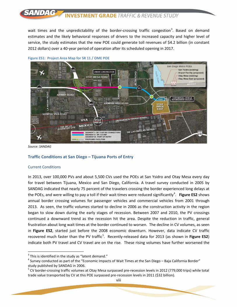
This investment grade T&R study was conducted to estimate the revenue potential of the proposed SR 11/Otay Mesa East (OME) Port of Entry (POE) facility. The new POE would be located 2 miles east of the POE currently operational at Otay Mesa (see Figure ES1). The new facility, in addition to the POEs at Otay Mesa and San Ysidro, will address the current cross border congestion and growing demand for improvement in the movement of personal vehicles (PVs) and commercial vehicles (CVs) across the border1.

According to the Concept of Operations2 prepared for this new POE, user fees for the facility will be implemented in the form of traffic tolls collected on the proposed SR 11, the sole connector from the crossing to the road network on the United States (U.S.) side. The roadway systems supporting the new OME POE are being designed to enable a smoother flow through the POE with pre-inspection delays limited to 20 minutes. Demand management, necessary to provide this level of service, will be instituted through varying toll rates to control demand.

This investment grade T&R study (detailed in Box ES1) estimated the traffic forecasts for the OME POE and subsequent toll revenues generated over a 40-year period of operation (2017 – 2056). The study included the estimation of socioeconomic growth and corresponding increase in demand for border crossing in the region, as well as potential responses from travelers to the toll rates. The SR 11/OME POE will offer an alternative with a higher level of service to the border crossing traffic currently served by San Ysidro POE and Otay Mesa POE. In addition to those that divert from San Ysidro and Otay Mesa POEs, the high level of service offered by the new POE has the potential to attract more trips by individuals who had limited their border crossings because of long

1 The socio-economic growth in the Tijuana region is occurring mostly to the east just south of Otay Mesa. This growth will be a key driver for the demand at the new OME POE. 2 SR 11/OME ITS Predeployment Study: Binational Concept of Operations Version 3, prepared by the IBI Group, January 31, 2014.

Box ES1. Investment Grade Traffic and Revenue Study

The traffic and revenue study was conducted in two phases. The tasks done in each of the phases are listed below.

Phase 1 (Jan 2012 – Aug 2013) • Gathered information about current cross

border movements across the region and the trends.

• Developed an economic model to estimate the growth in demand for cross border movements.

• Conducted a stated preference survey to measure the willingness of travelers to switch to a toll facility.

• Developed and calibrated a traffic network model to generate traffic and revenue forecasts with SR 11/OME facility in operation.

• Generated preliminary results of traffic and revenue for various combinations of POE configurations.

Phase 2 (Aug 2013 – Jun 2014) • Collected more accurate measures of wait times

and delays at the crossings through surveys conducted in collaboration with the CBP;

• Refined and calibrated the T&R model with the new wait time and delay measurements;

• Developed traffic and revenue estimates for the optimal configuration of SR 11/OME POE as identified in Phase I; and

• Conducted sensitivity analyses to measure the impacts of variations in growth estimates, and assumptions of operational processes.

viii

wait times and the unpredictability of the border-crossing traffic congestion3. Based on demand estimates and the likely behavioral responses of drivers to the increased capacity and higher level of service, the study estimates that the new POE could generate toll revenues of $4.2 billion (in constant 2012 dollars) over a 40-year period of operation after its scheduled opening in 2017.

Figure ES1: Project Area Map for SR 11 / OME POE

Source: SANDAG

Traffic Conditions at San Diego – Tijuana Ports of Entry

Current Conditions

In 2013, over 100,000 PVs and about 5,500 CVs used the POEs at San Ysidro and Otay Mesa every day for travel between Tijuana, Mexico and San Diego, California. A travel survey conducted in 2005 by SANDAG indicated that nearly 75 percent of the travelers crossing the border experienced long delays at the POEs, and were willing to pay a toll if their wait times were reduced significantly4. Figure ES2 shows annual border crossing volumes for passenger vehicles and commercial vehicles from 2001 through 2013. As seen, the traffic volumes started to decline in 2006 as the construction activity in the region began to slow down during the early stages of recession. Between 2007 and 2010, the PV crossings continued a downward trend as the recession hit the area. Despite the reduction in traffic, general frustration about long wait times at the border continued to worsen. The decline in CV volumes, as seen in Figure ES2, started just before the 2008 economic downturn. However, data indicate CV traffic recovered much faster than the PV traffic5. Recently-released data for 2013 (as shown in Figure ES2) indicate both PV travel and CV travel are on the rise. These rising volumes have further worsened the

3 This is identified in the study as “latent demand.” 4 Survey conducted as part of the “Economic Impacts of Wait Times at the San Diego – Baja California Border” study published by SANDAG in 2006. 5 CV border-crossing traffic volumes at Otay Mesa surpassed pre-recession levels in 2012 (779,000 trips) while total trade value transported by CV at this POE surpassed pre-recession levels in 2011 ($32 billion).

ix

delays that travelers experience at the border. Observations made by travelers and transportation planners in the area indicate those that cross the border experience significant delays prior to reaching the inspection facilities at the POEs, particularly on northbound trips. Surveys conducted in 2012 and 2013 by the study team confirm these observations (see Appendix D). As noted in Table ES1, PVs traveling north experience border-crossing delays between 45 and 85 minutes during the morning peak period between 6 AM and 9 AM. The values shown in Table ES1 represent the average wait times for standard and Ready lanes for both San Ysidro and Otay Mesa POEs. However, wait times on standard lanes in the morning peak period for PVs have frequently been observed to extend as long as 2 ½ to 3 hours. The variance in PV wait times on Ready lanes has also been observed to be large. Only on the SENTRI lanes are the wait times usually under 20 minutes. Therefore, for a non-SENTRI pass holder crossing the border, the unpredictability of expected wait times is quite high. At the same time, northbound CVs endure border-crossing delays between an hour and an hour and a half during the afternoon hours (between 3 PM and 7 PM) when the truck traffic is at its peak.

Figure ES2: Historical Northbound Border Crossing Volumes in the San Diego – Tijuana Region (San Ysidro and Otay Mesa POEs only)

Source: Bureau of Transportation Statistics (BTS) Border Crossing/Entry Data, http://transborder.bts.gov/

Table ES1: Observed Delays for Northbound Traffic at San Ysidro and Otay Mesa Border Crossings (2012)

Period Average Delay (minutes)*

Passenger Vehicles Commercial Vehicles

AM Peak (6:00 AM to 9:00 AM) 45-85 30-50 Midday (9:00 AM to 4:00 PM) 25-35 50-70

PM Peak (4:00 PM to 7:00 PM) 30-50 65-95

Night (7:00 PM to 6:00 AM) 10-15 40-50 * Based on cross border wait time surveys conducted by HDR. The wait times represent average delays for Standard and Ready lanes combined.

http://transborder.bts.gov/

x

In response to these delays, the POE at San Ysidro is currently being expanded with 10 additional northbound lanes for processing PVs. This initiative is expected to be completed and operational by 2017. While this expansion should offer some relief for binational PV travelers, additional investments are needed to address the increasingly significant delays that are anticipated in the future for CVs.

Future Conditions

Socioeconomic growth trends from reliable sources in the region on both sides of the border point to increased levels of border-crossing demand6. Forecasts by the study team estimate that total travel demand across the border will recover the levels observed in 2005 by the year 20177. In spite of the expansion at San Ysidro for PVs, the study estimates that the average delays for northbound PVs will still exceed 60 minutes during the peak periods of operations as shown in Table ES28. The CVs do not benefit from the San Ysidro expansion; therefore, their delays are not expected to be reduced.

6 Sources include SANDAG, Caltrans, California’s Finance Department and Moody’s Analytics. 7 After latent demand is included in the forecast of border-crossing demand. 8 Again, these average numbers conceal the fact that border-crossing wait times experienced by users of standard and Ready lanes show high levels of unpredictability.

Box ES2. Congestion at the Border has Significant Impact on the Economy

The SANDAG Border Crossing Study compiled more than 3,600 surveys of border crossers at San Ysidro, Otay Mesa, and Tecate stations and estimated that at an average wait time of 45 minutes, more than eight million trips into the San Diego region are lost per year as many simply choose to avoid battling the congestion. This equates to a loss of nearly $1.3 billion in potential revenues – mostly in the retail sector; three million potential working hours; 31,500 jobs; and $42 million in wages annually. Excessive border waits also are affecting overall regional production. The total economic impact on the San Diego – Tijuana binational region is an output loss of between $2.2 billion and $2.5 billion per year.

Delays in getting trucks carrying freight across the Otay Mesa and Tecate international border crossings created a staggering $3.3 billion loss to the U.S. and Mexico binational economy and more than 18,500 jobs annually. Two-hour or longer delays in moving freight across the border are significantly impacting production, industry competitiveness, and lost business income at the regional, state, and national levels.

Source: Economic Impacts of Wait Times at the San Diego – Baja California Border, Study by SANDAG, 2006

xi

Table ES2: Estimated Range of Northbound Delays at San Yisdro and Otay Mesa Border Crossings in the Future (2017)

Period Estimated Delay (Minutes)*

Passenger Vehicles Commercial Vehicles AM Peak (6:00 AM to 9:00 AM) 45-75 40-50 Midday (9:00 AM to 4:00 PM) 20-30 60-85 PM Peak (4:00 PM to 7:00 PM) 25-50 75-110 Night (7:00 PM to 6:00 AM) 5-10 40-50 * Based on traffic models developed by HDR. The wait times represent average delays for Standard and Ready lanes combined.

The socioeconomic and latent demand forecasts project potential growth in demand in the future as shown in Figure ES3. The traffic levels are expected to increase by almost a third between 2017 and 2040, with PVs continuing to command a majority share. Given the current and projected delays, even with the San Ysidro expansion in 2017, this growth level indicates that both PV and CV would be subjected to much higher delays than today, causing significant impact on the economic growth potential in the region (see Box ES2).

Figure ES3: Forecast of Border Crossing Volumes in Region, Northbound and Southbound

Source: HDR Analysis

Potential Diversion to SR 11/OME POE

To study the impacts of the proposed construction of the new SR 11/OME POE, the study team developed a traffic network model to simulate the vehicle movements across the border. The model was developed by expanding a component of SANDAG’s regional travel model and calibrating it using the observed traffic conditions in 2012. The details of the model and the key assumptions associated

xii

with the application of the model to estimate future conditions and potential diversion of travelers to the OME POE are provided in Box ES3.

The binational T&R model estimated that, in view of the potential savings in time, and travelers’ willingness to pay for time savings and improvements in reliable mobility, the new facility would attract as much as 20 percent of northbound PVs and 75 percent of northbound CVs9 as soon as the facility is operational in 2017. These estimates are shown in Table ES3 and Table ES4. For vehicles traveling in the southbound direction, diversions to the new facility are expected to be much lower since the processing times and delays currently experienced are significantly lower. More discussion of this diversion is presented in Section 7.3.

Table ES3: Estimated Northbound Daily Capture Rate of PVs at SR 11/OME POE

Period 2017 2030 2040

Daily Crossings

Capture Rate (%)

Daily Crossings

Capture Rate (%)

Daily Crossings

Capture Rate (%)

AM 1,900 14.5 1,900 13.9 1,950 14.1

Midday 4,850 20.8 4,700 15.5 4,500 14.8

PM 2,350 23.5 2,600 19.3 2,550 15.6

Night 3,850 18.5 3,950 16.6 3,850 15.2

Total Daily 12,950 20% 13,150 16% 12,850 15% Source: HDR Analysis

Table ES4: Estimated Northbound Daily Capture Rate of CVs at SR 11/OME POE

Period 2017 2030 2040

Daily Crossings

Capture Rate (%)

Daily Crossings

Capture Rate (%)

Daily Crossings

Capture Rate (%)

AM 450 74.1 500 65.7 450 56.6

Midday 1,300 73.4 1,400 60.4 1,400 54.4

PM 700 76.9 800 62.0 800 50.9

Night 50 82.2 200 76.7 250 60.8

Total Daily 2,500 75% 2,900 63% 2,900 54% Source: HDR Analysis

These capture rates, estimated on the basis of the value of time that travelers assign for different travel purposes, represent the potential willingness to pay for a higher level of service. An important aspect to note is that the demand for OME POE reaches the available capacity in the early years, and no additional diversion can be accommodated. The increased demand in the future is addressed through increased toll levels in order to maintain the targeted 20 minutes wait time service level for both PVs and CVs. The declining capture rates of CVs points to unmet demand and the possibility of adding more capacity in the future to handle CVs.

9 One of the biggest contributors to the large truck diversion rate is the geometric configuration of the truck access lanes at Otay Mesa that severely restricts trucks, particularly those using FAST lanes, from getting to the inspection booths. Further, CVs have a higher willingness to pay for time savings and reliability offered by OME.

xiii

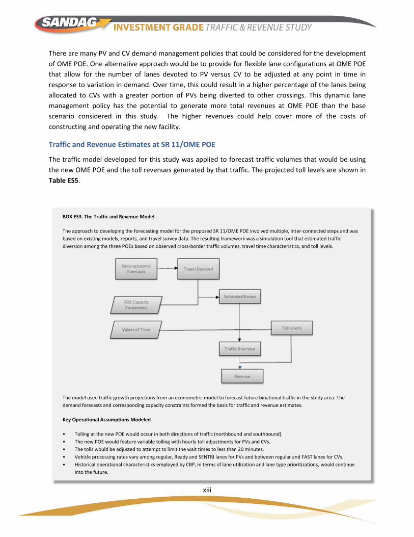
BOX ES3. The Traffic and Revenue Model

The approach to developing the forecasting model for the proposed SR 11/OME POE involved multiple, inter-connected steps and was based on existing models, reports, and travel survey data. The resulting framework was a simulation tool that estimated traffic diversion among the three POEs based on observed cross-border traffic volumes, travel time characteristics, and toll levels.

The model used traffic growth projections from an econometric model to forecast future binational traffic in the study area. The demand forecasts and corresponding capacity constraints formed the basis for traffic and revenue estimates.

Key Operational Assumptions Modeled

• Tolling at the new POE would occur in both directions of traffic (northbound and southbound). • The new POE would feature variable tolling with hourly toll adjustments for PVs and CVs. • The tolls would be adjusted to attempt to limit the wait times to less than 20 minutes. • Vehicle processing rates vary among regular, Ready and SENTRI lanes for PVs and between regular and FAST lanes for CVs. • Historical operational characteristics employed by CBP, in terms of lane utilization and lane type prioritizations, would continue

into the future.

There are many PV and CV demand management policies that could be considered for the development of OME POE. One alternative approach would be to provide for flexible lane configurations at OME POE that allow for the number of lanes devoted to PV versus CV to be adjusted at any point in time in response to variation in demand. Over time, this could result in a higher percentage of the lanes being allocated to CVs with a greater portion of PVs being diverted to other crossings. This dynamic lane management policy has the potential to generate more total revenues at OME POE than the base scenario considered in this study. The higher revenues could help cover more of the costs of constructing and operating the new facility.

Traffic and Revenue Estimates at SR 11/OME POE

The traffic model developed for this study was applied to forecast traffic volumes that would be using the new OME POE and the toll revenues generated by that traffic. The projected toll levels are shown in Table ES5.

xiv

Table ES5: Average Northbound Toll Levels at SR 11/OME POE (in 2012 dollars)

Period

Average Toll Level 2017



Passenger Vehicles

Commercial Vehicles

Passenger Vehicles

Commercial Vehicles

Passenger Vehicles

Commercial Vehicles

AM $7 to $13 $10 to $17 $13 to $33 $10 to $16 $16 to $42 $10 to $22

Midday $2 to $3 $11 to $17 $9 to $22 $16 to $20 $16 to $36 $19 to $26

PM $2 to $3 $10 to $17 $2 to $5 $18 to $22 $3 to $9 $31 to $47

Night $2 to $5 $2 to $10 $2 to $10 $10 to $12 $2 to $11 $10 to $17

Daily average toll $4.00 $14.50 $11.50 $18.00 $19.00 $26.00 Source: HDR Analysis

As seen in the Table ES5, the average tolls levied for northbound PVs in 2040 during a typical day is about $19 and for northbound CVs, about $26. Because of the variable tolling scheme that will be implemented for different time periods, the maximum toll levels can go as high as $42 and $47, for northbound PVs and CVs respectively in 2040. For PVs, the maximum toll of $42 is projected to occur for a brief one hour period in the AM peak period and fall below $35 for other hours in the AM peak. For CVs, the tolls would stay close to $40 for the entire PM peak period with a maximum of $47 happening during the peak hour. In the evening and late night, tolls for PVs would be lower due to reduced demand and much smaller delays. In the opening year, the average daily toll for PVs would be about $4 and for CVs, about $15.

Table ES6: Average Wait Times & Travel Time Savings During Peak Periods, Northbound Direction Period 2017 2030 2040

Passenger Vehicles

Commercial Vehicles

Passenger Vehicles

Commercial Vehicles

Passenger Vehicles

Commercial Vehicles

Average wait time at non-tolled POEs in peak period*

85 to 90 minutes

60 to 65 minutes

150 to 155 minutes

65 to 70 minutes

180 to 185 minutes

95 to 100 minutes

Average wait time at tolled OME POE in peak period*

15 to 20 minutes

15 to 20 minutes

15 to 20 minutes

15 to 20 minutes

15 to 20 minutes

15 to 20 minutes

Average savings in wait time in peak period* 60 minutes 45 minutes 135 minutes 50 minutes 165 minutes 80 minutes

Cost per “minute saved” in peak period

About 18 cents / minute for passenger vehicles About 45 cents / minute for commercial vehicles

*For passenger vehicles, peak period occurs in the AM while for Commercial vehicles it occurs in the PM. Source: HDR Analysis

Presented in Table ES6 are the estimated average wait times during the peak period for the current (non-tolled) POEs and the tolled (OME) POE for the three forecast years. The table also shows the savings in POE wait times for PVs and CVs during the peak periods. For PVs, the peak traffic occurs in the AM and for CVs, in the PM. As shown in the table, in the opening year, the PVs using OME POE may save almost an hour of wait time and the CVs save about 45 minutes during their respective peak periods. By 2040, the wait time savings during peak will be much more significant (more than two hours for PVs and

xv

about an hour and half for CVs). These savings and associated increase in reliability of border-crossing travel times represent considerable value for money from the perspective of travelers that use the toll facility. The toll levels of 18 cents per minute saved that PVs are charged, and the 45 cents per minute saved that CVs are charged are consistent with the respective values of time estimated through stated preference surveys.

The toll levels are, in fact, indicators of the generalized cost of travel. As has been observed in other toll facilities, travelers may opt to respond in ways other than paying the tolls by opting to adopt longer routes, carpooling or forgoing the trip altogether. All of these measures represent increased “user costs” borne by the travelers in response to delays.

The average southbound tolls as shown in Table ES7 are closer to the minimum levels of $1 for PVs and $5 for CVs. All the toll rates are represented in constant 2012 dollars.

Table ES7: Average Southbound Toll Levels at SR 11/OME POE (in 2012 dollars)

Period Average Toll

2017 2030 2040

Average Daily toll for PVs $0.50 $0.75 $1.00

Average Daily toll for CVs $2.5 $4.00 $6.50 Source: HDR Estimates

Figure ES4 below shows an annualized stream of revenues (in constant 2012 dollars) during the 40-year period of operation after OME POE opens in 2017. The chart shows the annual estimates of the total number of PVs and CVs that are expected to cross the border, as well as the potential toll revenues from the vehicles that choose to use OME POE. Figure ES4 also shows the growth in revenue is significantly more than the growth in traffic. This is due to the exponential effect of traffic demand on the delays experienced by travelers.

Figure ES4: Total Border-Crossing Annualized Traffic and Revenue Estimates at SR 11/OME POE

Source: HDR Estimates

xvi

Table ES8 presents a summary of projections of traffic and revenue at OME POE over a 40 year forecast period (2017 – 2056). As shown, revenue from PVs is projected to grow more than six times as fast as traffic, and that from CVs is projected to grow more than twice as fast as traffic.

Table ES8: 40-Year Growth in Traffic and Revenue for SR 11/OME 2017 2056 Percent Growth

2017 - 2056 Compounded Annual Growth Rate (CAGR)

Annual Crossings (in Millions) PVs 6.30 11.49 82.3 % 0.8 % CVs 1.16 2.33 100 % 1.9 %

Annual Revenue (in Millions of $) PVs 20.23 145.1 617 % 5.2 % CVs 10.87 50.7 366 % 4.0 %

Source: HDR Estimates

Table ES9 shows the revenue by vehicle type and direction. As stated, approximately 90 percent of the total revenue is generated from northbound vehicles, with about 76 percent generated from northbound PVs. Of the total revenue of 4.2 billion dollars, about 24 percent would be generated from CV traffic moving in both directions. As stated earlier, alternative PV and CV demand management policies have the potential to generate more total revenues at OME POE than the base case scenario considered in this study.

Table ES9: 40-Year Revenue Estimate for SR 11/OME

Market Segment 40-Year Revenue Estimate (in millions of 2012 dollars)

Northbound Southbound

PVs $2,994 $232

CVs $795 $211

Total by Direction $3,789 $443

Total Revenue (both Directions) $4,232 Source: HDR Estimates

1

1 INTRODUCTION

The San Diego Association of Governments (SANDAG) retained the services of HDR to develop an Investment Grade Traffic and Revenue (IGT&R) Study for the new Otay Mesa East (OME) Port of Entry (POE) and State Route 11 (SR 11) toll road. The work performed as part of this project included the following:

1) Data collection and assembly of original and previously collected border-crossing data.

2) Development of a Binational Traffic and Revenue (T&R) Model.

3) Production of IGT&R forecasts.

This IGT&R Report provides information on the development of the binational T&R model and the production of traffic and revenue forecasts for the new OME POE.

1.1 Study Participants

HDR was the primary contractor for this project, on behalf of SANDAG. In support of HDR, Crossborder Group and WILTEC were subcontractors in charge of collecting data in the border region. Crossborder Group collected border-crossing time data for personal vehicles (PVs) and trucks (commercial vehicles [CVs]) at the San Ysidro and Otay Mesa POEs. WILTEC collected travel time data along the road network on both sides of the border. Finally, Steer Davis Gleaves provided editorial oversight to the development of the final IGT&R Report.

SANDAG was the primary project stakeholder. The Association has a travel demand model and a series of modules that were transformed and incorporated into the binational T&R model used for this study. SANDAG also oversaw the conduct and completion of the IGT&R Report. In addition, SANDAG provided guidance on project development, provided data and information to the IGT&R team, and led the Project Stakeholder Committee.

Mexico’s Secretaría de Comunicaciones y Transportes (SCT) was SANDAG’s counterpart in Mexico. The agency was part of the steering committee for the project. It supplied information, models and data used in the development of the binational T&R model.

The Project Stakeholder Committee was composed of SANDAG, SCT, Caltrans, Customs and Border Protection (CBP), and the State of Baja California. It was responsible for reviewing and providing comments on the deliverables produced as part of the IGT&R study.

2

1.2 Organization of this Report

The report is divided into eight sections, in addition to technical appendices. After this introductory section, Section 2 summarizes existing border-crossing conditions in the study area, including origin-destination (O-D) patterns, border crossing times and current POE characteristics.

Section 3 describes the anticipated future border-crossing conditions based on an assessment of current socioeconomic trends, land use development, and projections of cross-border freight flows.

Section 4 provides an overview of the project and describes the operation of the new OME POE and the dynamic tolling approach used to forecast the revenues generated by the new facility.

Section 5 presents a detailed description of a series of surveys conducted in the region to determine the level of acceptance of potential users for a new tolled POE. These surveys were also used as input to determine the value of time and reliability that are essential to the binational T&R model.

Section 6 provides an overview of the approach used in the development of the binational T&R model. It includes a discussion of the development of the base year model, the validation of the model, the preparation of the future year model, and the development of annual traffic and revenue forecasts.

Section 7 presents the Traffic and revenue forecasts for the OME POE, along with traffic and wait time projections for the other POEs in the region.

Section 8 presents the results of a series of sensitivity tests conducted to assess the impacts of variance in the key model parameters. In particular, tests are conducted with respect to changes in traffic growth projections, guaranteed wait times at the new POE, and number of lanes operating at the new POE.

Detailed technical information related to the model structure and key assumptions are presented in a series of appendices.

3

2 CURRENT BORDER-CROSSING CONDITIONS IN THE REGION

The San Diego – Tijuana region is currently the largest urban border area along the U.S.–Mexico border, with a combined population of about 4 million people. This shared population is anticipated to grow to about 7 million people by the year 2020. Most of the growth south of the international border will occur in the northeastern, eastern, and southeastern areas of Tijuana. These areas are located near the existing Otay Mesa POE.10

The San Ysidro POE handles only PV traffic. It is the busiest land crossing in the world with almost 11.5 million vehicular northbound crossings in 2012.

The Otay Mesa POE handles PVs, bus, pedestrian, plus all CV traffic. Otay Mesa POE is the second busiest commercial port of entry on the U.S.–Mexico border and the busiest in California. It handled approximately 779,000 northbound trucks and $34.5 billion worth of goods in both directions in 2012 and anecdotal evidence suggests border-crossing delays can exceed 4 hours per truck. In addition, the Otay Mesa POE handled more than 5.3 million northbound PVs in 2012.

According to regional sources of information, PV border-crossing traffic is anticipated to increase to 62 million trips in 2020 (both directions) in the region and CV border-crossing traffic is expected to grow to 2 million trips (both directions) by that same year. This considerable amount of border-crossing trips is anticipated to have large impacts on queue lengths and peak hour wait times across the region.11

2.1 Overview of Border-Crossing Travel Time

There are multiple routes a vehicle may take to complete a binational trip between the U.S. and Mexico based on its particular origin and destination (O-D). The total travel time for each route depends on several factors, including time spent driving in the road network approaching a POE and the actual time spent to cross the border at a particular POE. These factors are specific to the individual vehicle type making the trip (i.e., PV or CV), the road network on both sides of the border, and the POE chosen to perform the border crossing. Therefore, the two main factors that determine the total travel time of a border-crossing trip for a specific O-D are (see Figure 1):

• Driving time in road network: the amount of time spent driving on local roads at either side of the border before reaching and again after transiting out of the POE (i.e., total binational travel time excluding border-crossing time).

10 As a result of this location, they constitute a potential market for both Otay Mesa and OME POE. 11 These projections are derived from information from CBP, SANDAG, and Caltrans included in the California-Baja California Border Master Plan (2008). These forecasts appeared to be optimistic; therefore, they were not used in the binational T&R model. Instead, the model developed its own forecasts of demand for border-crossing trips based on a set of conservative assumptions.

4

• Border-crossing time: the amount of time spent during the border-crossing process. Total border-crossing time includes queue/wait time, processing/inspection time, and transit time required to leave the POE complex.

For every binational trip, the time spent driving on the road network is directly related to the physical characteristics of the road network (e.g., number of lanes) as well as the volume of traffic using those roads. The time spent at the POE is directly related to the operational characteristics of that POE (e.g., processing rates) and the volume of vehicles using it. Therefore, the following sections discuss the existing travel conditions at the POEs in San Diego/Tijuana and their surrounding highway network. In particular, it describes the pattern of border-crossing trips observed in the area, the border-crossing processes followed by vehicles, the traffic conditions around the POEs, and the volumes and wait times observed at the existing POEs.

Figure 1: Breakdown of Total Border-Crossing Time for a Northbound Trip (for Illustration Only)

Source: HDR

5

2.2 Regional Trip Patterns

Cross-border travel patterns in the region were identified using three O-D surveys conducted by SANDAG between 2011 and 2012. These surveys were combined and expanded based on traffic count data to generate an O-D survey database.12 For PVs, the sample size exceeds 8,000 observations; the sample size for CVs is approximately 500 observations (see Box 1).

The result of the analysis for the case of PV trips is presented in Figure 2. The map shows that the cross-border trips in 2012 are clustered around commercial and industrial areas along the border in San Diego County but are distributed more evenly throughout Tijuana. This pattern suggests that an important number of border-crossing travel trips for PVs involve commuting to and from work and another important share of trips revolves around shopping.

A similar analysis was conducted for CV trips and is presented in Figure 3. The map shows the cross-border trips in 2012 are clustered around the Otay Mesa POE. This is not surprising as the Otay Mesa area (on both sides of the border) is a focal point for maquiladora and warehousing activities linked to international trade.

Figure 2: 2012 Cross-Border PV Trip Distribution

Sources: HDR, SANDAG, INEGI

12 A description of how this data was expanded and used to develop the base year of the binational T&R model is provided in Section 6.1.1.

Box 1. O-D Surveys

The surveys used to determine O-D patterns in the region are the Crossborder Survey conducted for SANDAG in 2011 and the two surveys performed for SANDAG during the end of 2011 and early 2012 (general public survey and company survey, respectively).

The Crossborder Survey of 2011 collected 7,371 responses (the majority of them from PVs); the general public survey collected 1,437 responses from PVs and 433 from CVs; and the company survey collected responses from 99 companies that originate border-crossing (69 were maquiladora companies, 20 were freight companies and 10 were perishable goods transport companies).

An overview of these surveys is presented in Appendix B, while detailed information on the individual surveys is presented in Appendices E, G, H, and I.

6

Figure 3: 2012 Cross-Border CV Trip Distribution

Sources: HDR, SANDAG, INEGI

2.3 Congestion in Local Roads Leading to POEs

As discussed in the introduction to this section, the congestion on the roads leading to and from the POEs in the region is a key factor in total travel time for binational trips and therefore influences the choice of a POE. The time a border-crossing driver spends on a local road network (on either side of the border) leading to a POE depends on the characteristics of the roads (e.g., number of lanes, alternatives and geometry) and the traffic volumes moving through those roads.

Improvement to the local roads (e.g., increasing the number of lanes) facilitates traffic and therefore reduces travel time in local networks. On the other hand, an increase of traffic volume on local roads generates congestion and therefore increases travel time in local networks.

The study analyzed current congestion conditions on both sides of the border. To do this, data on the characteristics, traffic volumes and travel times on the main thoroughfares, and the primary roads leading to the POEs were collected and are presented below.

2.3.1 Main Roads Leading to POEs

The San Ysidro POE is directly connected to the I-5 highway, which travels north through the San Diego region. I-5 is an 8-lane freeway. Within one half mile, I-805 also serves as a north-south connector. In Tijuana, the two-lane Tijuana-Ensenada highway (Route 1) is one of the principal access corridors. The POE is also served by the 4-lane Tijuana – Ensenada Toll Road (Route 1D).

7

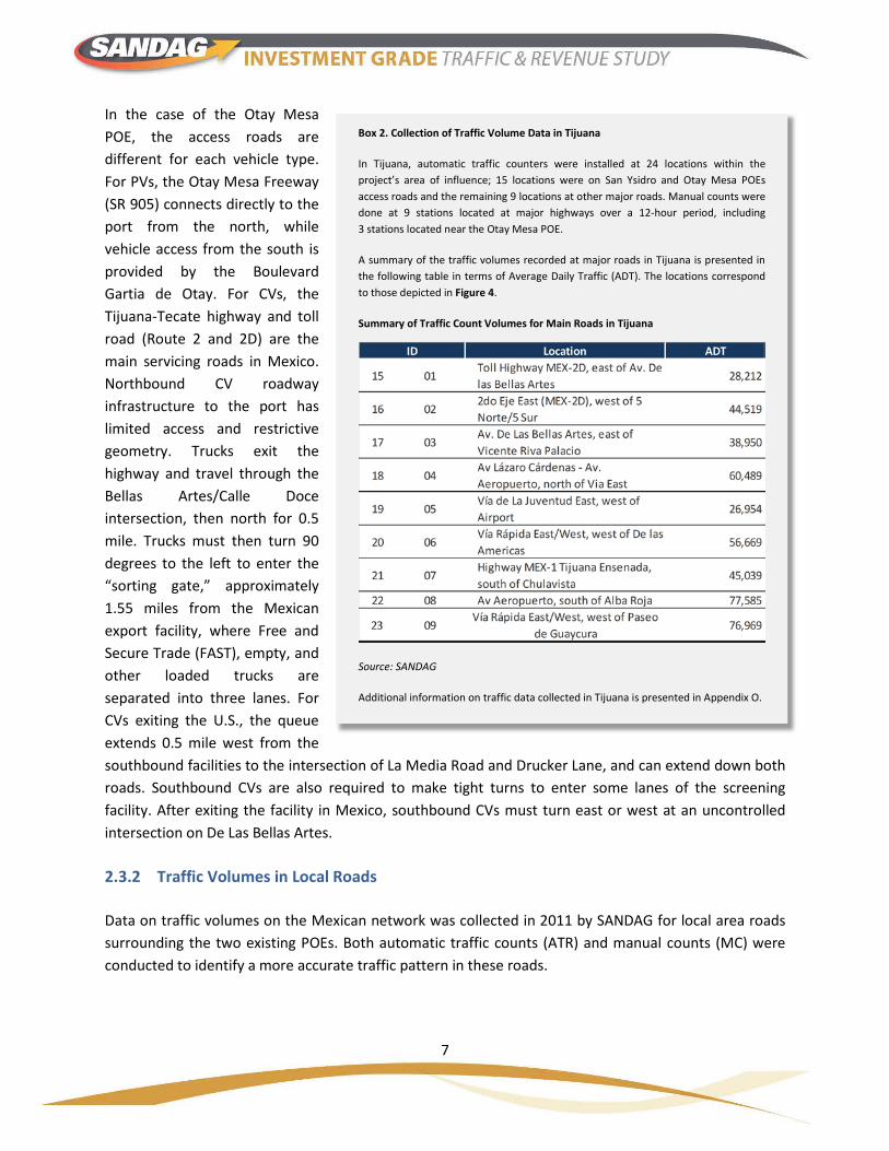
In the case of the Otay Mesa POE, the access roads are different for each vehicle type. For PVs, the Otay Mesa Freeway (SR 905) connects directly to the port from the north, while vehicle access from the south is provided by the Boulevard Gartia de Otay. For CVs, the Tijuana-Tecate highway and toll road (Route 2 and 2D) are the main servicing roads in Mexico. Northbound CV roadway infrastructure to the port has limited access and restrictive geometry. Trucks exit the highway and travel through the Bellas Artes/Calle Doce intersection, then north for 0.5 mile. Trucks must then turn 90 degrees to the left to enter the “sorting gate,” approximately 1.55 miles from the Mexican export facility, where Free and Secure Trade (FAST), empty, and other loaded trucks are separated into three lanes. For CVs exiting the U.S., the queue extends 0.5 mile west from the southbound facilities to the intersection of La Media Road and Drucker Lane, and can extend down both roads. Southbound CVs are also required to make tight turns to enter some lanes of the screening facility. After exiting the facility in Mexico, southbound CVs must turn east or west at an uncontrolled intersection on De Las Bellas Artes.

2.3.2 Traffic Volumes in Local Roads

Data on traffic volumes on the Mexican network was collected in 2011 by SANDAG for local area roads surrounding the two existing POEs. Both automatic traffic counts (ATR) and manual counts (MC) were conducted to identify a more accurate traffic pattern in these roads.

Box 2. Collection of Traffic Volume Data in Tijuana

In Tijuana, automatic traffic counters were installed at 24 locations within the project’s area of influence; 15 locations were on San Ysidro and Otay Mesa POEs access roads and the remaining 9 locations at other major roads. Manual counts were done at 9 stations located at major highways over a 12-hour period, including 3 stations located near the Otay Mesa POE.

A summary of the traffic volumes recorded at major roads in Tijuana is presented in the following table in terms of Average Daily Traffic (ADT). The locations correspond to those depicted in Figure 4.

Summary of Traffic Count Volumes for Main Roads in Tijuana

Source: SANDAG

Additional information on traffic data collected in Tijuana is presented in Appendix O.

8

Figure 4: Location of Traffic Count Stations in Tijuana

Source: SANDAG

Figure 5: Location of Traffic Count Stations in San Diego

Source: SANDAG

9

In Tijuana, ATR counters were installed at 24 locations within the project’s area of influence, including access roads to San Ysidro and Otay Mesa POEs and other major roads in Tijuana. MC were done at nine

stations located at major highways and roads close to the Otay Mesa POE (see Figure 4).

In general, the roads in Mexico for which data was collected present high traffic volumes (see Box 2). As a result, high levels of congestion are seen throughout Tijuana and not only in areas close to the POEs.

In San Diego, traffic counts were conducted at 12 different locations and involved two phases, with both ATR and MC for each phase (see Figure 5).

The data show that roads with higher volumes are those directly connected or feeding into the existing POEs in the region. These include I-5 and Telegraph Canyon Road for San Ysidro and SR 905, Otay Mesa Road and Siempre Viva Road for Otay Mesa (see Box 3). Therefore, high congestion levels on the U.S. side of the border is located near the POEs.

Detailed information on traffic volumes collected is presented in Appendices O and P.

2.3.3 Speed and Driving Time in Local Roads

Finally, travel time data in Tijuana’s roads was collected for seven routes with different origin and destination points and varying in length to determine the effects of traffic volumes on vehicular travel time. The routes selected for data collection are shown in Figure 6.

Box 3. Collection of Traffic Volume Data in San Diego

In San Diego, traffic counts were conducted at 12 different locations and involved two phases:

• In Phase 1, manual traffic counts were conducted at three locations and automatic traffic counts were conducted at four locations close to the two existing POEs.

• In Phase 2, manual counts were conducted at two locations and automatic traffic counts were conducted at six locations in the vicinity of the POEs.

The summary of traffic volumes recorded during 10 hours at major roads in San Diego in the vicinity of the POEs is presented in the following table.

Summary of Traffic Count Volumes for Main Roads in San Diego

Source: SANDAG

Additional information on traffic data collected in Tijuana is presented in Appendix P.

10

Figure 6: Routes Selected for the Collection of Travel Times in Tijuana

Source: HDR

HDR also collected travel time data on existing road networks adjacent to each of the POEs on both sides of the border (see Figure 7). Average travel times and speeds13 along the routes were estimated based on multiple runs.14

Average travel speeds in Tijuana were found to be lower than in San Diego: while in the U.S. travel speeds were found to be close to 50 miles per hour, in Mexico average speeds fluctuated significantly depending on the specific section of the road in which travel occurred. In general, this leads to the conclusion that border-crossers face more congestion in Tijuana and therefore spend more time driving in that road network.15

Additional information on the collection of speed and driving time in the roads adjacent to the POEs is presented in Appendix Q.

13 Data on space-measurement speeds (SMS) was collected using the floating-car technique. 14 At least four runs were used to collect data, capturing peak and off-peak hours and weekday and weekend congestion conditions. 15 One caveat to this finding is that roads for which travel time and speed were collected in San Diego consist of highways with high vehicular capacity, while in Tijuana the roads are located in the downtown area with a reduced number of lanes.

11

Figure 7: Main Roads in Project's Immediate Area of Influence, San Diego – Tijuana Area

Source: HDR

2.4 Operation of Existing Ports of Entry

The operations at the different POEs have a direct impact on the border-crossing wait time experienced by binational travelers. In particular, the number of lanes existing at each facility, the border-crossing procedures followed and the staffing of the POEs (primarily from CBP) act together to determine the effective capacity of a particular POE.

Currently, the San Ysidro POE operates with 24 lanes for northbound traffic, with a typical configuration of 15 standard lanes, 4 Ready lanes,16 and 5 SENTRI (Secure Electronic Network for Travelers Rapid Inspection) lanes.17 There is a detailed expansion program for the POE that aims at increasing its effective capacity for northbound and southbound traffic in the short-to-medium run. The first step consists of introducing “tandem” inspection booths on northbound PV flows, which allow lanes to process up to two cars at the same time. These booths have been introduced as a test program in some lanes at the POE, increasing its effective capacity by about 30 percent for standard lanes.

16 Ready lanes are dedicated lanes for travelers entering the U.S., who obtain and travel with an RFID-enabled travel document. RFID-enabled cards approved by the Department of Homeland Security include the U.S. Passport Card; the Enhanced Driver's License; the Enhanced Tribal Card; the new Enhanced Permanent Resident Card (PRC) or new Border Crossing Card (BCC); and trusted traveler cards such as NEXUS or SENTRI. 17 The SENTRI program provides expedited CBP processing for preapproved, low-risk travelers using their personal vehicle. Travelers must apply to this program, and once approved are issued an RFID card that will identify their record and status in the CBP database on arrival at the POE.

12

A second part of this program is the relocation of the Mexican inspection facilities for southbound flows, which was completed in December 2012 (southbound traffic has been shifted to the new El Chaparral facility).18 This facility is currently open 24 hours a day.

The Otay Mesa facility currently operates with 13 lanes for northbound PVs (6 of which are typically standard, 5 Ready, and 2 SENTRI). Additionally, the facility has ten lanes for northbound CVs (six of which are typically used for standard crossings and three for FAST)19 and eight lanes for CVs traveling southbound. There are currently no plans to either expand this facility, or introduce “tandem” inspection booths at this POE. CBP has recently announced that the Ready lanes will be open 24 hours a day to meet demand.

2.4.1 Passenger Vehicle Border-Crossing Process20

On northbound trips, PVs entering the U.S. proceed to the POE where they go through primary and sometimes secondary inspections. At primary inspection booths, CBP officers must ask the drivers to show proper documentation (e.g., a U.S. visa, proof of U.S. citizenship, permanent resident card) and state the purpose of their visit to the U.S. Additionally, during this stage of the process, a query on the Interagency Border Inspection System (IBIS) is executed to review whether the traveler(s) has a past record of violations. If necessary, vehicles are sent to secondary inspection. At the secondary inspection station, a much more thorough investigation is performed of the identity of those wanting to enter the U.S., as well as of the purpose of their visit. During this step, individuals may also have to pay duties on their declared items. Upon completion, access to the U.S. is either granted or denied.

Similar to the FAST program for CVs, SENTRI provides expedited processing for preapproved, low-risk travelers at the U.S. – Mexico border. Participants in the program have exclusive lanes to access the San Ysidro and Otay Mesa POEs and much shorter wait times to enter the U.S. than those in regular lanes. When an approved international traveler approaches the border in the SENTRI lane, the system automatically identifies the vehicle and the identity of its occupant(s) by reading the file number on a radio frequency identification (RFID) card.

CBP recently deployed Ready lanes at the Otay Mesa POE that are dedicated primary vehicle lanes for travelers entering the U.S. at land border POEs. Travelers who obtain and travel with a Western Hemisphere Travel Initiative (WHTI) compliant RFID-enabled travel document receive the benefits of utilizing a Ready lane to expedite the inspection process while crossing the border. Drivers stop at the 18 The total build-out of this expansion program at San Ysidro includes introducing tandem booths in all northbound lanes and the construction of eight additional northbound lanes by 2017, thereby increasing the total number of lanes to 34. The expanded San Ysidro POE will feature 29 tandem lanes, 1 single bus lane, and 4 single-booth lanes. 19 The FAST program is a commercial clearance program for known low-risk shipments entering the U.S. from Canada and Mexico. Participation in FAST requires that every link in the supply chain be certified under the Customs-Trade Partnership against Terrorism program, or C-TPAT. 20 Information on border-crossing processes is taken from the SR 11/OME ITS Pre-Deployment Study: Bi-National Concept of Operations Version 3, prepared by the IBI Group on January 31, 2014.

13

beginning of the lane, make sure their card is out and ready to be read by the RFID equipment, and then proceed to stop at the officer’s booth. CBP officers verify the documentation and ask for the purpose of their visit to the U.S. At that point, the CBP officers can send the drivers and/or passengers to a secondary inspection or grant entry into the U.S.

The southbound PV crossing process has one inspection station at Aduanas. The process in Mexico is a red light/green light decision in which PVs are randomly selected for a secondary inspection, indicated by a red light. Recently, CBP has started to perform random manual inspections on the U.S. side of the border for PVs crossing into Mexico, aiming to identify illegal shipments of money and weapons. The POEs are not designed for southbound inspection on the U.S. side of the border, and consequently, this has created congestion.

2.4.2 Commercial Vehicle Border-Crossing Process

For northbound trips, the CV driver with required documentation proceeds to the Mexican customs agency (Aduanas) compound at the POE. At Otay Mesa, there are separate lanes on the Mexico side for CVs enrolled in the FAST program (FAST offers expedited clearance to carriers that have demonstrated supply chain security). After clearing the Aduanas inspection, trucks head to the border toward CBP’s primary inspection booth, where drivers present identification and shipment documentation to CBP officers. The officers at the primary inspection booth use computer terminals to cross-check the basic information about the driver, vehicle, and cargo. The CBP officers then make decisions to refer trucks, drivers, or cargo for more detailed secondary inspections of any or all of these elements, or alternatively, release CVs to the exit gate.

After leaving the federal facility, trucks enter the California State’s safety inspection facility usually located adjacent to the federal facility. Typically, the state’s safety agency (California Highway Patrol [CHP]) inspects trucks to determine whether they are in compliance with U.S. safety standards and regulations. If the initial visual inspection finds any safety or regulatory violations, the trucks are directed to proceed to a more detailed secondary inspection at a special facility. During the CHP inspection, CVs are also inspected by the Federal Motor Carrier Safety Administration (FMCSA) for safety compliance. After leaving the state facility, trucks typically drive to the San Diego road network to reach their final destination.

For southbound trips, once the CV arrives to the POE, there is only one inspection station at Aduanas. The process in Mexico is a red light/green light decision in which a loaded CV is randomly selected for a secondary inspection if it receives a red light. Empty vehicles cross with no need to stop at the Aduana booths.

At a few border crossings (including Otay Mesa), CBP has recently started to perform random manual inspections on the U.S. side of the border for CVs crossing into Mexico, to identify illegal shipments of money and weapons. The existing border crossings are not designed for southbound commercial inspection on the U.S. side of the border; consequently, this has created congestion at the POE and on approaching facilities.

14

2.4.3 Staffing at Ports of Entry

The POEs in the region are staffed with a variety of personnel from different agencies. For example, CBP personnel is in charge of primary and secondary inspections for PV and CV northbound trips, CHP personnel is in charge of safety inspections for northbound CV trips and Aduanas personnel is responsible for primary and secondary inspections for PV and CV southbound trips.

The level of staffing directly influences the effective capacity of a POE as it dictates how much of the physical capacity is utilized to process binational trips. This, in turn, affects the border-crossing wait times experienced by its users and therefore is an important consideration when analyzing border-crossing congestion.

Data on staffing of the San Ysidro and Otay Mesa POEs was gathered directly from CBP based on the actual personnel working in the POEs during 2012. An analysis of the data shows that staffing of the different POEs in the region varies not only across hours of the same day but also between days of the week (e.g., weekdays vs. weekends).

2.5 Volume of POE Crossings

An important indicator of the current border-crossing conditions is the number of vehicles crossing the border at the existing POEs. Data for northbound crossings is readily available from U.S. government sources; however, volumes of southbound crossings are not collected in a systematic way and therefore no detailed history on these volumes exists. Monthly historical data on the number of northbound border-crossings of PVs at San Ysidro and Otay Mesa is presented in Figure 8.

Figure 8: Monthly PV Border-Crossing Volumes, by POE, 1997 - 2012

Source: U.S. Department of Transportation, Research and Innovative Technology Administration, Bureau of Transportation Statistics.

15

The figure shows that northbound PV border crossings at San Ysidro fluctuate between 1 and 1.6 million per month, while border crossings at Otay Mesa are stable–around 400,000 per month. PV border crossings at San Ysidro show a slow downward trend after 2007, while the number of crossings at Otay Mesa had a slight decrease after 2009 but started its recovery after 2011.

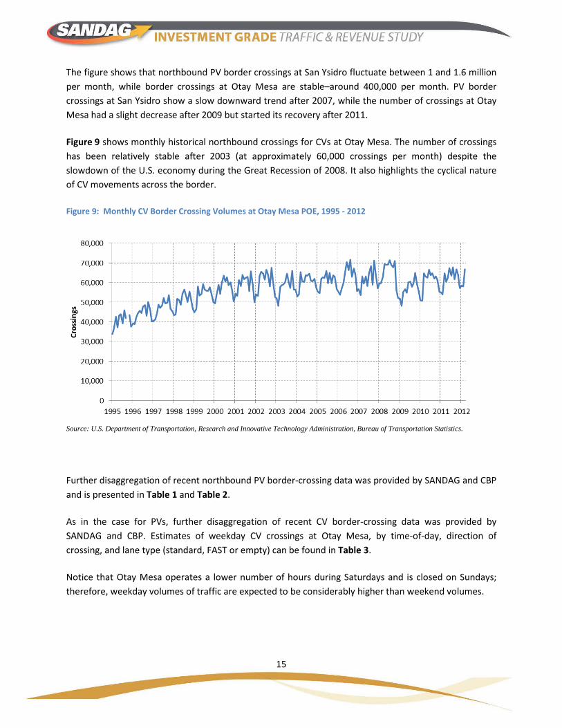
Figure 9 shows monthly historical northbound crossings for CVs at Otay Mesa. The number of crossings has been relatively stable after 2003 (at approximately 60,000 crossings per month) despite the slowdown of the U.S. economy during the Great Recession of 2008. It also highlights the cyclical nature of CV movements across the border.

Figure 9: Monthly CV Border Crossing Volumes at Otay Mesa POE, 1995 - 2012

Source: U.S. Department of Transportation, Research and Innovative Technology Administration, Bureau of Transportation Statistics.

Further disaggregation of recent northbound PV border-crossing data was provided by SANDAG and CBP and is presented in Table 1 and Table 2.

As in the case for PVs, further disaggregation of recent CV border-crossing data was provided by SANDAG and CBP. Estimates of weekday CV crossings at Otay Mesa, by time-of-day, direction of crossing, and lane type (standard, FAST or empty) can be found in Table 3.

Notice that Otay Mesa operates a lower number of hours during Saturdays and is closed on Sundays; therefore, weekday volumes of traffic are expected to be considerably higher than weekend volumes.

16

Table 1: Average Weekday PV Crossings at San Ysidro in 2012

Period Northbound

Southbound Total Crossings Standard Lane

SENTRI and Ready Lanes Total

Night (Early Morning) (3 AM to 6 AM) 2,200 1,850 4,050 1,000 5,050

AM Peak (6 AM to 9 AM) 2,350 2,850 5,200 4,050 9,250

Midday (9 AM to 4 PM) 4,250 5,650 9,900 12,800 22,700

PM Peak (4 PM to 7 PM) 2,200 2,950 5,150 7,950 13,100

Night (Late Night) (7 PM to 3 AM) 4,200 4,300 8,500 7,350 15,850

Total Daily Crossings 15,200 17,600 32,800 33,150 65,950

Sources: CBP; Caltrans; HDR Calculations

Table 2: Average Weekday PV Crossings at Otay Mesa in 2012

Period Northbound

Southbound Total Crossings Standard Lane

SENTRI and Ready Lanes Total

Night (Early Morning) (3 AM to 6 AM) 450 950 1,400 400 1,800

AM Peak (6 AM to 9 AM) 800 1,900 2,700 950 3,650

Midday (9 AM to 4 PM) 1,600 3,700 5,300 4,800 10,100

PM Peak (4 PM to 7 PM) 850 1,550 2,400 4,600 7,000

Night (Late Night) (7 PM to 3 AM) 1,800 1,200 3,000 3,700 6,700

Total Daily Crossings 5,500 9,300 14,800 14,450 29,250


In summary, San Ysidro handles approximately two out of every three PVs that travel between the U.S. and Mexico in either direction, while Otay Mesa processes the remaining one out of every three vehicles. Furthermore, on both San Ysidro and Otay Mesa the majority of the northbound PV crossings are performed using SENTRI and Ready lanes, which reduce border-crossing wait times compared to general-purpose lanes. In the case of CVs, northbound crossings of empty trucks (using the lanes for this purpose) show slightly higher volumes over truck crossings using either the FAST or the standard lane; southbound crossings of laden trucks also display slightly higher volumes compared to empty trucks.

17

Table 3: Average Weekday CV Crossings at Otay Mesa in 2012

Period Northbound Southbound

Total Crossings FAST

Lane Standard

Lane Empty Total Laden Empty Total

Night (Early Morning) (3 AM to 6 AM) POE Closed

AM Peak (6 AM to 9 AM) 90 160 310 560 100 80 180 740

Midday (9 AM to 4 PM) 510 490 480 1,480 1,010 750 1,760 3,240

PM Peak (4 PM to 7 PM) 190 240 180 610 400 270 670 1,280

Night (Late Night) (7 PM to 3 AM) 100 0 0 100 70 70 140 240

Total Daily Crossings 890 890 970 2,750 1,580 1,170 2,750 5,500


2.6 Border Crossing Times

In general, the existing POEs experience high levels of traffic congestion for northbound traffic throughout the day with San Ysidro experiencing lower wait times than Otay Mesa for PV traffic. Northbound PVs start queuing at San Ysidro as early as 4:30 AM and long queues continue through 11:00 AM. Anecdotal evidence suggests wait times surpass 120 minutes during the morning hours and 90 minutes in the afternoon hours for the standard lanes at this POE. Wait times for Otay Mesa are reported to be higher than San Ysidro throughout the day, with evidence of average wait times above 120 minutes during certain hours of the day. Conditions at both POEs are better for users of the Ready lanes and SENTRI trusted traveler program, which experience lower northbound wait times throughout the day compared to users of standard lanes (see Table 4 and Table 6).

CVs are only allowed to cross at Otay Mesa, where peak periods for northbound traffic start in the mid-morning and early afternoon hours due to maquiladora shipping schedules. Northbound wait times are reported to be consistently above 60 minutes and anecdotal evidence suggests they can surpass 120 minutes. Otay Mesa processes subscribers of FAST, a trusted shipper program created by CBP to reduce northbound CV border-crossing wait times while guaranteeing a high level of security for goods entering the U.S.

Border crossing times for PVs and CVs were collected at the two border crossings in San Diego County (San Ysidro and Otay Mesa). Observed PV border wait times collected at San Ysidro for northbound traffic are presented in Table 4. Observed southbound delays can be found in Table 5 (all values are expressed in minutes).

18

Table 4: Observed Northbound PV Wait Times at San Ysidro (in Minutes)

Hour Standard Lane Ready Lanes SENTRI Lanes

Observed (Average) Observed (Average) Observed (Average) 8:00 114 63 11

9:00 98 71 10

10:00 85 73 11

11:00 108 83 12

12:00 91 94 17

13:00 87 85 14

14:00 80 87 14

15:00 56 53 11

16:00 52 35 10

17:00 35 18 12

Source: HDR analysis of field observations

Notice that observed wait times for Ready lanes are generally lower than those for standard lanes, as intended by CBP.21 However, some hours features wait times at Ready lanes that are very close or even higher than average wait times for standard lanes. The explanation for this outcome is related to the decision by CBP to shift the allocation of utilized capacity between different lane types in order to adequately process a different mix of traffic during midday (see Box 4 for additional details).

Table 5: Observed Southbound PV Wait Times at San Ysidro (in Minutes)

Hour Observed (Average) Standard Deviation (in minutes)

8:00 4 4

9:00 4 3

10:00 4 5

11:00 5 21

12:00 3 1

13:00 5 18

14:00 4 5

15:00 4 4

16:00 4 3

17:00 5 4


21 The processing goals CBP has set for border-crossing travelers are (infrastructure permitting): NEXUS Lanes – 15 minutes. Ready Lanes – 50% of general traffic lane wait times (http://bwt.cbp.gov/).

http://bwt.cbp.gov/

19

Table 6 and Table 7 below summarize observed border delays for PVs at Otay Mesa, northbound and southbound, respectively. Notice that in the case of Otay Mesa, wait times for Ready lanes are consistently below those for standard lanes, though their absolute values continue to be significant.

Table 6: Observed Northbound PV Wait Times at Otay Mesa (in Minutes)

Hour Standard Lane Ready Lanes SENTRI Lanes

Observed (Average) Observed (Average) Observed (Average)

8:00 102 73 13

9:00 120 103 10

10:00 130 91 17

11:00 138 114 15

12:00 152 138 10

13:00 120 81 17

14:00 112 76 19

15:00 105 68 10

16:00 90 44 14 17:00 Not collected 23 20


Table 7: Observed Southbound PV Wait Times at Otay Mesa (in Minutes)

Hour Observed (Average) Standard Deviation (in minutes)

8:00 14 22

9:00 3 2

10:00 3 4

11:00 7 15

12:00 3 2

13:00 5 4

14:00 10 4

15:00 11 7

16:00 6 2

17:00 7 4


Observed border delays for CVs at Otay Mesa are presented in Table 8 for northbound trips and Table 9 for southbound trips. Delays on northbound trips are presented by lane type (standard vs. FAST).

20

Table 8: Observed Northbound Truck Crossing Wait Times at Otay Mesa (in Minutes) Hour Standard Lane1 FAST Lane

Observed (Average) Observed (Average) 8:00 94 65 9:00 71 65

10:00 64 65 11:00 76 73 12:00 71 81 13:00 63 82 14:00 57 64 15:00 47 70

1 Standard lanes included data on empty and laden trucks crossing the border. Source: HDR analysis of field observations and model runs

In general, the border-crossing wait times collected at Otay Mesa are in line with findings from other surveys that describe longer wait times for users of standard lanes compared to special lanes (such as Ready, SENTRI, and FAST). The exception is northbound CVs, where FAST crossings were found to have higher wait times than standard-lane crossings during the midday and early afternoon hours. The explanation for this finding is a combination of two factors: (i) the allocation of utilized capacity by CBP between standard and FAST lanes (see Box 4 for more details); and, to a lesser extent, (ii) the design of the CV facility at Otay Mesa, which includes narrow turns for FAST trucks and a couple of areas inside the POE complex where “weaving” between the two traffic types is likely to occur (see Box ES2 for an aerial view of the complex).

Table 9: Observed Southbound Truck Crossing Wait Times at Otay Mesa (in Minutes)

Hour Observed (Average)

9:00 9

10:00 11

11:00 28

12:00 11

13:00 21

14:00 38

15:00 52

16:00 33


21

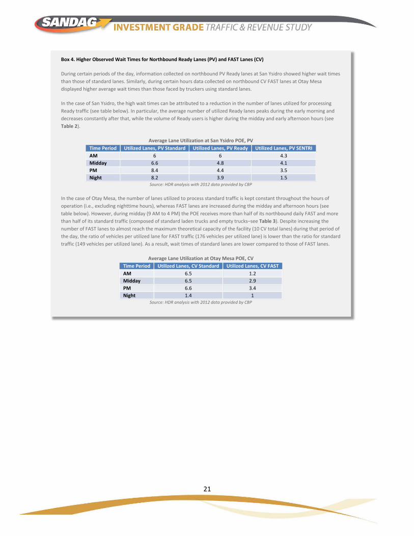
Box 4. Higher Observed Wait Times for Northbound Ready Lanes (PV) and FAST Lanes (CV)

During certain periods of the day, information collected on northbound PV Ready lanes at San Ysidro showed higher wait times than those of standard lanes. Similarly, during certain hours data collected on northbound CV FAST lanes at Otay Mesa displayed higher average wait times than those faced by truckers using standard lanes.

In the case of San Ysidro, the high wait times can be attributed to a reduction in the number of lanes utilized for processing Ready traffic (see table below). In particular, the average number of utilized Ready lanes peaks during the early morning and decreases constantly after that, while the volume of Ready users is higher during the midday and early afternoon hours (see Table 2).

Average Lane Utilization at San Ysidro POE, PV Time Period Utilized Lanes, PV Standard Utilized Lanes, PV Ready Utilized Lanes, PV SENTRI AM 6 6 4.3 Midday 6.6 4.8 4.1 PM 8.4 4.4 3.5 Night 8.2 3.9 1.5

Source: HDR analysis with 2012 data provided by CBP

In the case of Otay Mesa, the number of lanes utilized to process standard traffic is kept constant throughout the hours of operation (i.e., excluding nighttime hours), whereas FAST lanes are increased during the midday and afternoon hours (see table below). However, during midday (9 AM to 4 PM) the POE receives more than half of its northbound daily FAST and more than half of its standard traffic (composed of standard laden trucks and empty trucks–see Table 3). Despite increasing the number of FAST lanes to almost reach the maximum theoretical capacity of the facility (10 CV total lanes) during that period of the day, the ratio of vehicles per utilized lane for FAST traffic (176 vehicles per utilized lane) is lower than the ratio for standard traffic (149 vehicles per utilized lane). As a result, wait times of standard lanes are lower compared to those of FAST lanes.

Average Lane Utilization at Otay Mesa POE, CV Time Period Utilized Lanes, CV Standard Utilized Lanes, CV FAST AM 6.5 1.2 Midday 6.5 2.9 PM 6.6 3.4 Night 1.4 1

Source: HDR analysis with 2012 data provided by CBP

22

3 FUTURE BORDER-CROSSING CONDITIONS IN THE REGION

The socioeconomic growth trends in the region on both sides of the border point to increased levels of demand for border-crossing travel, exercising pressure on the existing POE infrastructure. Despite the fact that expansions to the San Ysidro POE are expected by 2017 (effectively increasing the capacity of this POE for northbound PV crossings), anticipated demand is expected to grow at a fast pace, eroding the potential benefits of expanded POE capacity. In particular, border-crossing wait times are still expected to exceed 60 minutes during the peak periods of POE operations.

This section provides an overview of socioeconomic forecasts for the cross-border study area. Key trends in population and employment growth, land uses, economic activity, and freight movements are examined, using recent information published for the most part by local U.S. and Mexican government agencies, including SANDAG and Tijuana’s Instituto Municipal de Planeación (IMPLAN).

These socioeconomic projections provide a framework for the development of a forecast for the future number of border-crossing trips in the region, which, in turn, can be interpreted as a forecast for the future use of POE infrastructure in the region. Using the context provided by these socioeconomic projections, an analysis of the socioeconomic drivers of border-crossing trips was developed using statistical and econometric methods and a forecast of total border-crossing trips is created at the end of this section.22 The forecasting method and the specific variables used in it are described in Section 3.5.

3.1 Forecasts for Population and Employment

Population and employment tend to follow similar trends on the U.S. and Mexican sides of the border because of the increasing integration of the cross-border region. Employment in the census tract (CT) surrounding the socioeconomic study area is projected to nearly triple by 2030 compared to 2000 levels (rising from 10,914 to 28,109) and population is projected to increase by 1,942 percent (from 1,062 to 21,691) over the same time period. 23 As development occurs, associated demand for local transportation infrastructure, including SR 11, is also projected to increase.

3.1.1 Population

Table 10 summarizes population projections for San Diego County from several third party sources: Caltrans, Global Insight, Moody’s, Parsons Brinckerhoff and SANDAG. The different sources average on a compound annual growth rate of about 1.0 percent over the period 2010 to 2035 – apart from Moody’s forecast, which indicates slightly stronger growth (1.4 percent per year). The table also shows that demographic growth is expected to decrease gradually after 2015. Population estimates for 2035 range from a low of 3.87 million (Parsons Brinckerhoff) to a high of 4.36 million (Moody’s). 22 The projections developed in this section correspond to forecasts for long-term growth of demand for border-crossing trips in the region. 23 SANDAG 2006a

23

Table 10: Comparison of San Diego County Population Projections, 2010 – 2035

Population (000s) 2010 2015 2020 2025 2030 2035

Caltrans 3,222 3,412 3,610 3,797 3,971 4,125

Global Insight 3,111 3,291 3,477 3,659 3,838 4,008

Moody’s 3,112 3,336 3,602 3,867 4,109 4,361

Parsons Brinckerhoff 3,098 3,264 3,473 3,600 3,738 3,871

SANDAG 3,173 3,364 3,535 3,704 3,870 4,026

Compound Annual Growth Rate (%) 2010-15 2015-20 2020-25 2025-30 2030-35 2010-35

Caltrans 1.20 1.10 1.00 0.90 0.80 1.00

Global Insight 1.10 1.10 1.00 1.00 0.90 1.00

Moody’s 1.40 1.50 1.40 1.20 1.20 1.40

Parsons Brinckerhoff 1.00 1.20 0.70 0.80 0.70 0.90

SANDAG 1.20 1.00 0.90 0.90 0.80 1.00

Source: C&M Associates, Inc., 2012

Note that, according to SANDAG’s 2050 Regional Transportation Plan, the greatest potential for population growth in San Diego County lies within the area adjacent to the proposed OME POE.

Figure 10: Population Forecast on Mexican Side of Cross-Border Region, 2010 – 2035

Source: Sistema de Información Regional de México, 2011 Note: Estimates are for the cities/municipalities of Ensenada, Mexicali, Playas de Rosarito, Tecate, and Tijuana combined.\

24

Available information on the Mexican side of the cross-border region gives a somewhat similar picture. Figure 10 depicts population projections for the Mexican portion of the cross-border region through 2035, by 5-year increments. Projections for the cities/municipalities of Ensenada, Mexicali, Playas de Rosarito, Tecate, and Tijuana24 were produced separately by the Sistema de Información Regional de México and subsequently combined for the purpose of this study. Overall, population is forecast to grow by 2.1 percent annually and top 5.3 million by 2035; however, demographic growth is expected to decelerate over time, from 2.6 percent annually between 2010 and 2015 to 1.7 percent annually between 2030 and 2035.

3.1.2 Employment

As in the case of population, estimates from third party sources are used to evaluate the employment outlook in the San Diego region. A summary of the different employment forecasts is provided in Table 11 below. While all the sources anticipate a sharp recovery of the job market in the short term (1.9 to 2.1 percent growth per year), allowing the majority of the 80,000 jobs lost during the recession to be recovered by the end of 2015, their long-term forecasts are more contrasted. Global Insight and Caltrans predict strong employment growth (stronger than population growth), while SANDAG, Moody’s and Parsons Brinckerhoff are less optimistic (compound annual growth rate below 1 percent after 2020). As a result, employment estimates for 2035 range from a low of 1.59 million for SANDAG and Moody’s to a high of 1.78 million for Caltrans.

Table 11: Comparison of San Diego Employment Forecasts, 2010 – 2035

Employment (‘000s) 2010 2015 2020 2025 2030 2035

Caltrans 1,270 1,398 1,502 1,603 1,693 1,777

Global Insight 1,221 1,342 1,453 1,549 1,658 1,757

Moody’s 1,221 1,356 1,416 1,473 1,530 1,595

Parsons Brinckerhoff 1,221 1,339 1,428 1,494 1,553 1,610

SANDAG 1,217 1,336 1,412 1,477 1,535 1,592

Compound Annual Growth Rate (%) 2010-15 2015-20 2020-25 2025-30 2030-35 2010-35

Caltrans 1.90 1.50 1.30 1.10 1.00 1.40

Global Insight 1.90 1.60 1.30 1.40 1.20 1.50

Moody’s 2.10 0.90 0.80 0.80 0.80% 1.10

Parsons Brinckerhoff 1.90 1.30 0.90 0.80 0.70 0.70

SANDAG 1.90 1.10 0.90 0.80 0.70 1.10

Source: C&M Associates, Inc., 2012

24 These are the five largest cities in Baja California, accounting for about 92 percent of the state’s total population in 2010.

25

Given the increasing integration of the cross-border economy, employment trends on both sides of the border are expected to respond in a similar fashion to business cycle fluctuations and converge over time. As shown in Figure 11, employment in Tijuana is forecast to more than double between 2010 and 2035, from 342,590 to 748,847, thus reinforcing the city’s status as the number one maquiladora center of Mexico (see section 3.3.1).

Most importantly, perhaps, is the fact that employment growth is expected to remain unabated in the long term, averaging 2.9 percent per year between 2030 and 2035. This is a full percentage point above Sistema de Información Regional de México’s population growth forecast over the same period. Some of the higher-skill manufacturing traditionally done in the U.S. will be moving south of the border, as workers there become more skilled and companies seek cost-cutting opportunities.

Figure 11: Tijuana Employment Forecast, 2010 – 2035

Source: Sistema de Información Regional de México, 2011

3.2 Land Use and Future Development

California Senate Bill 375, which was signed into law in 2008, requires metropolitan planning organizations (MPOs) like SANDAG to prepare a Sustainable Communities Strategy (SCS) to reduce vehicular greenhouse gas emissions and encourages planning practices that create sustainable communities. The bill builds on California’s Global Warming Solutions Act of 2006 (or Assembly Bill 32), which set greenhouse gas emissions reduction targets by 2020 and directed the California Air Resources Board to propose measures to achieve them.

26

The greatest potential for growth in the region lies within the area adjacent to the proposed OME POE. Population, in particular, is expected to soar by more than 3 percent annually between 2010 and 2035 in that area. Figure 12 shows residential densities and commercial development types in 2035 for the south county subregion. The SR 11 project area is roughly delineated by a red line in the right corner of the map.

Similarly, on the Mexican side, Tijuana is expected to experience an upsurge in residential development to the east of the existing Otay Mesa POE (urban districts of La Presa, La Presa Rural, and Valle de las Palmas). Figure 13 on page 28 highlights the districts of La Presa Rural and Valle de las Palmas, which together have the potential to sustain a population of one million people by 2030, according to IMPLAN.25

3.3 Economic Trends

The economy of Baja California is still largely dominated by the maquiladora industry, despite the increased competition from China and the effects of the 2008 Great Recession on U.S. – Mexico trade. In recent years, however, it has shown signs of diversification, as illustrated by the surge of the medical tourism industry.

3.3.1 Maquiladora Industry

Maquiladora operations involve the importation of foreign merchandise into Mexico on a temporary basis, where it is assembled, manufactured or repaired, and then exported, either to the country of origin or a third country.26 The maquiladora industry in Baja California has been growing faster than the manufacturing industry as a whole, mainly because of favorable economic conditions,27 which have made it lucrative for foreign companies to do business in Mexico. Based on 2008 data from the Instituto Nacional de Estadística y Geografía (INEGI), all five main manufacturing activities in Baja California (in order of importance: electronics, metals, plastics, vehicles, and food) are related to the maquiladora industry.28

25 Being located to the east of existing Otay Mesa, these localities become part of the area of influence for OME POE. By virtue of being located marginally closer to them, OME POE will have a small competitive advantage with respect to Otay Mesa for the traffic generated in these areas. 26 Morales, G. et al., An Overview of the Maquiladora Program, U.S. Department of Labor, Bureau of International Affairs, 1994. 27 Such as proximity to the U.S. consumer market, a favorable exchange rate, preferential tax treatment, the existence of abundant and cheap labor, and low-cost industrial services. 28 INEGI, Perspectiva Estadística Baja California, September 2011.

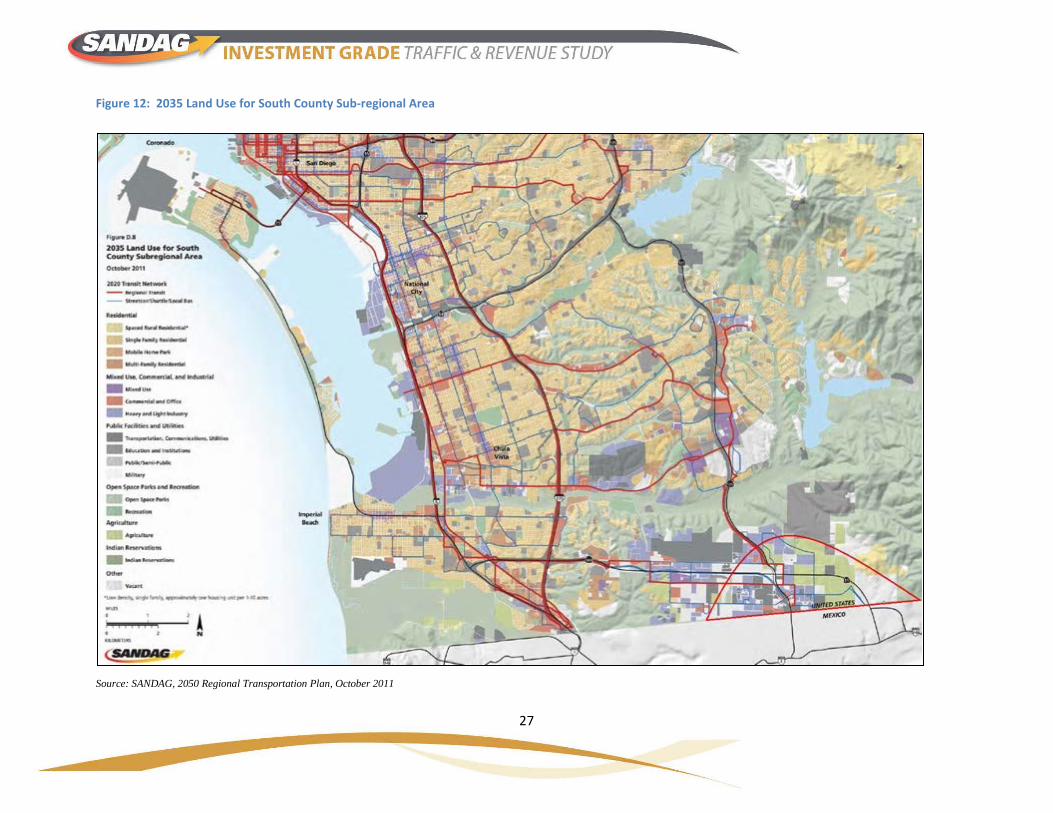
27

Figure 12: 2035 Land Use for South County Sub-regional Area

Source: SANDAG, 2050 Regional Transportation Plan, October 2011

28

Figure 13: 2030 Land Use in Eastern Tijuana

Source: Instituto Metropolitano de Planeación de Tijuana

Baja California, including the cities/municipalities of Ensenada, Mexicali, Tecate, and Tijuana, accounts for approximately 18 percent of the export-oriented establishments and about 12 percent of export-oriented employment in Mexico. Tijuana, in particular, has more export manufacturing facilities than any other Mexican city and accounts for approximately two thirds of export-oriented employment in Baja California. In 2011, its maquiladora industry employed 148,800 people in 560 active establishments, down from 177,100 before the recession.29

At first glance, the economic performance of maquiladoras may not be as strong in the future. In particular, competition from Asia (especially China) for low-wage manufacturing jobs has eroded the maquiladoras’ once-traditional competitive advantage. However, studies show that some maquiladoras have evolved from the usual labor-intensive activities to greater degrees of organization complexity, technology utilization, research and skill specialization and are even incorporating new activities based on coordination and information technologies to survive in the current global market.30

29 INEGI, Estadística Mensual del Programa de la Industria Manufacturera, Maquiladora y de Servicios de Exportación (IMMEX), September 2011. 30 Carrillo, Jorge and Arturo Lara, “Mexican Maquiladoras: New Capabilities of Coordination and the Emergence of New Generation of Companies”, Innovation: Management, Policy & Practice, vol. 7/2 - April 2005.

29

Figure 14: Industrial Areas in the San Diego-Tijuana Region

Sources: C&M Associates, Inc., based on information from Mexico Industrial Maps and City of San Diego, 2012

Finally, it is noteworthy that the maquiladora industry also has positive effects on the other side of the border. Aside from creating border-crossing trips to move goods across the border, some authors estimate that a 10 percent increase in maquiladora output in a Mexican border city results in 1 to 2 percent increase in employment in the adjacent U.S. city.31 Figure 14 depicts the location of industrial zones in the San Diego-Tijuana border region.

3.3.2 Medical Tourism

Another example of local competitiveness, this time in the service sector, is the medical tourism industry. Recent studies indicate that approximately 450,000 people a year come to Baja California in search of medical services, ranging from cosmetic surgery to dental and cardiovascular care, making the state’s medical tourism cluster one of its most vibrant. American citizens from California, New Mexico, and Arizona, along with their Mexican counterparts from Jalisco, Nuevo León, and Quintana Roo, consume $86 million worth of medical services annually at facilities in Mexicali, Playas de Rosarito,

31 Cañas, Jesus and Robert Gilmer, The Maquiladora’s Changing Geography, Federal Reserve Bank of Dallas, Second Quarter 2009.

30

Tijuana and Tecate.32 The majority of these medical tourists are foreign and an important number of them travel by road and cross the border using the POEs in the region.

3.4 Anticipated Cross-Border Freight Flows

An important consideration when analyzing future border-crossing trips is the freight flows anticipated to be moved by truck in the region. Cross-border truck freight tonnage is expected to increase more than threefold by 2050 (to 56 million tons), according to recent projections developed by Cambridge Systematics, Inc. for SANDAG. There are, however, noticeable disparities across commodities. For some commodity groups (e.g., instruments, photographic goods, clocks, etc.), freight is forecast to grow by 3 percent or more per year, on average; for others (textile products, in particular), it is forecast to decline. Overall, there is a clear trend toward trading more value-added products. This trend is not new, but it has gained momentum since the late 1990s.

Figure 15: Truck Freight Volume by Major Commodity Group, 2007 and 2050 (Millions of Tons)

Source: Cambridge Systematics, Inc. Note: The graph shows the top 20 commodity groups, which represented 97 percent of truck freight tonnage in 2007

32 Sonia García Ochoa, “Turismo médico capta en BC 450 mil visitantes y 86 mdd en derrama”, El Sol de Tijuana, October 21, 2011.

0 5 10 15 20 25 30

Electrical Machinery, Equipment, etc.

Machinery, excluding Electrical

Pulp, Paper, or Allied Products

Food or Kindred Products

Transportation Equipment

Instruments, Photographic Goods, Clocks, etc.

Rubber or Miscellaneous Plastics Products

Farm Products

Fabricated Metal Products

Miscellaneous Products of Manufacturing

Primary Metal Products

Chemicals or Allied Products

Waste or Scrap Materials

Clay, Concrete, Glass, or Stone Products

Printed Matter

Lumber or Wood Products, excluding Furniture

Miscellaneous Freight Shipments

Furniture or Fixtures

Non-metallic Minerals

Petroleum or Coal Products

Textile Mill Products

Apparel or Other Finished Textile Products

Millions of Tons

2007

2050

31

Figure 15 provides a breakdown of cross-border truck freight volume by major commodity group (using the Standard Transportation Commodity Code system) for 2007 (base year) and 2050. Volumes are expressed in millions of tons and shown in decreasing order of their respective 2050 value. As shown in the graph, electrical machinery and equipment alone will represent half of truck freight tonnage in 2050. By contrast, the second commodity group, machinery, excluding electrical, will account for only 7.8 percent of the total.

The corresponding number of trucks is derived by applying a specific payload factor to freight tonnage for each commodity group (see Box 5). The results are graphically represented in Figure 16, below. The total number of trucks is forecast to quadruple between 2007 and 2050 (to 6.4 millions). This implies the average payload will be declining over time, which reflects the shift in the composition of trade discussed above. As shown in the graph, the share of electrical machinery and equipment is expected to increase from 22 percent to 58 percent.

Figure 16: Number of Trucks by Major Commodity Group, 2007 and 2050

Source: Cambridge Systematics, Inc. Note: The graph shows the top 20 commodity groups, which represented 97 percent of truck freight tonnage in 2007.

0 500 1,000 1,500 2,000 2,500 3,000 3,500 4,000

Electrical Machinery, Equipment, etc.

Machinery, excluding Electrical

Pulp, Paper, or Allied Products

Food or Kindred Products

Transportation Equipment

Instruments, Photographic Goods, Clocks, etc.

Rubber or Miscellaneous Plastics Products

Farm Products

Fabricated Metal Products

Miscellaneous Products of Manufacturing

Primary Metal Products

Chemicals or Allied Products

Waste or Scrap Materials

Clay, Concrete, Glass, or Stone Products

Printed Matter

Lumber or Wood Products, excluding Furniture

Miscellaneous Freight Shipments

Furniture or Fixtures

Non-metallic Minerals

Petroleum or Coal Products

Textile Mill Products

Apparel or Other Finished Textile Products

Number of Trucks

2007

2050

Box 5. Estimation of Cross-Border Truck Freight Flows

The number of trucks engaged in cross-border freight is estimated by applying a specific payload factor (expressed in motor carrier density tons per truck) to estimated freight tonnage for each commodity group. The number of trucks is estimated based on the shift in the composition of trade discussed in this section, implying that the average payload will be declining over time.

Details of these estimates are presented in Appendix R.

32

Additional information on the estimation of cross-border freight flows is provided in Appendix R.

3.5 Forecast of Aggregate Border-Crossing Traffic

HDR developed a statistical model to forecast overall border crossings in the study area for future years based on the socioeconomic variables that affect this type of traffic.33 An econometrics-based method was used to identify those factors that have the strongest influence on overall levels of cross-border traffic in the study area, and to estimate the parameters (i.e., value of coefficients) that were used in the growth-forecasting model. These coefficients were then used, along with existing forecasts for the values of factors with influence on cross-border traffic, to forecast short-term (i.e., 2012-2017) and long-term (i.e., 2017-2040) future growth of aggregate cross-border traffic in the region. A detailed description of the procedure used to create these forecasts is presented in Appendix J.

Model Specification

Several model specifications and combinations of socioeconomic variables were evaluated using an automated process coded in the statistical software package EViews. A total of 37 explanatory variables were initially identified and categorized into four groups: U.S. at the national level, U.S. at the local level, Mexican at the national level and Mexican at the local level. A number of so-called “dummy variables” were also considered for inclusion in the growth model, to control for the impact of discrete events and policy changes.

Various functional forms were evaluated, including logarithmic transformations of the dependent variables (cross-border traffic) and all explanatory variables. The relative strengths of all candidate models were assessed using econometric criteria for suitable fit, ability to back-cast historical data, and independence between explanatory variables.

The econometric analysis of PV crossing also helped identify a number of “structural breaks” in the relationship between cross-border traffic and socioeconomic variables, as illustrated in Figure 17.

The final equation used in the traffic growth model for PVs is composed of the following explanatory variables (see Box 6 for details):

• Monthly retail sales in the U.S. (in constant dollars).

• Monthly rate of unemployment in California.

• Monthly exchange rate expressed in Mexican pesos per U.S. dollar, in the previous month.

33 Even though this socioeconomic-based forecasts represent the majority of the anticipated border-crossing traffic, an additional component (latent demand) resulting from increased capacity at the POEs in the region is presented in Section 6.4.

33

Figure 17: Structural Breaks in PV Crossings, April 1997 – March 2012

Source: HDR Analysis of CBP Data

• Dummy variable to capture a structural break in December 2006 as a result of an increase in intensity of the Mexican government’s battle against drugs (taking the value 1 in December 2006 and subsequent months, and 0 before that).

• Dummy variable to capture a structural break due to 9/11 (taking the value 1 in September 2001 and subsequent months, and 0 before that).

The final equation used in the traffic growth model for CVs is relatively parsimonious, and relates CV crossings to two measures of economic activity in the U.S.:

• Annual total value of retail sales in the U.S.

• Annual index of industrial production in the U.S.

In the case of each one of these equations the procedure estimated, using historical data, the structural relations (i.e., value of coefficients) existing between the explanatory variables in each equation and the number of border-crossing trips for each type of vehicle. These coefficients (derived from historical data) were later combined with projections of future values for the explanatory variables in each equation to produce the forecasted number border-crossing trips in the region for each traffic type. The following section describes the projections of future values for the explanatory variables that were used in the forecast.

34

Forecasting Assumptions and Inputs

The project team sought data from multiple sources for each of the explanatory variables identified above. These data sources are listed in Table 12. They include both official (public) sources, as well as commercially available data.

Box 6. Equations Used to Forecast Aggregate Border-Crossing Traffic

The final equation used in the border-crossing traffic forecasting model for PVs can be expressed as a function of three key economic variables, as follows:

Log (OM_SY_POVt) = β0 + β1 . Log(US_RETAIL_SALESt) + β2 . Log(CA_UNEMP_RATE_ADJt) + β3 . Log(XRATEt-1) + β4 . DP2006 + β5 . DP2001 + εt

Where:

• OM_SY_POVt is the number of PV crossings at San Ysidro and Otay Mesa, northbound, in month t;

• US_RETAIL_SALESt is the total value of retail sales in the U.S. (in constant dollars) in month t;

• CA_UNEMP_RATE_ADJt is the rate of unemployment in California in month t;

• XRATE t-1 is the exchange rate expressed in Mexican pesos per U.S. dollar, in the previous month;

• DP2006 is a dummy variable taking the value 1 in December 2006 and subsequent months, and 0 before that;

• DP2001 is a dummy variable taking the value 1 in September 2001 and subsequent months, and 0 before that;

• εt is the regression error in month t; and

• βi, i = 0,…, 5 are the regression coefficients to be estimated. Note that β0 is the constant term.

Similarly, the final equation used in the traffic growth model for CV relates crossings to two measures of economic activity in the United States, as follows:

Log(OM_TRUCKt) = β0 + β1 . Log(US_RETAIL_SALESt) + β2 . Log(US_IIPt) + εt

Where:

• OM_TRUCKt is the annual number of truck crossings at Otay Mesa, northbound, in year t;

• US_RETAIL_SALESt is the total value of retail sales in the U.S. in year t;

• US_IPPt is the index of industrial production in the U.S. in year t;

• εt is the regression error in year t; and

• βi, i = 0,…, 2 are the coefficients to be estimated.

Details of how these equations were estimated and their performance are presented in Appendix J.

35

Table 12: Data Sources Used in Traffic Growth Model Variable Name Historical Data Source(s) Forecast Source(s)

U.S. Retail Sales U.S. Department of Commerce (Census Bureau)

California Finance Department California Department of Transportation, Economic Analysis Branch HDR Analysis

California Unemployment Rate

California Employment Development Department, Labor Market Information Division

California Department of Transportation, Economic Analysis Branch California Finance Department HDR Analysis

U.S. Dollar – Mexican Peso Exchange Rate

Organization for Economic Co-operation and Development

Moody’s Analytics Risk Analysis Workshop facilitated by HDR

U.S. Index of Industrial Production

U.S. Federal Reserve Moody’s Analytics

Source: HDR

Box 7. Conservative Estimation of Long-Run Border-Crossing Traffic Growth

As described herein, long-run border-crossing traffic growth for PVs and CVs was estimated through an econometric model that uses monthly data (for PVs) and annual data (for CVs) on socioeconomic variables in the region. The main data inputs of this model consist of future values for the following explanatory variables:

• Monthly retail sales in the U.S. (in constant dollars). • Monthly rate of unemployment in California. • Monthly exchange rate expressed in Mexican pesos per U.S. dollar. • Annual total value of retail sales in the U.S. • Annual index of industrial production in the U.S.

Different primary sources were used to gather information on the future values for these input variables. However, these sources had to be screened to eliminate overly-optimistic forecasts that predicted a quick economic recovery in the U.S. after 2008’s Great Recession. Two cases are worth mentioning where the consensus from the risk workshop was to use conservative forecasts for explanatory variables instead of using available forecasts:

• Scotiabank projected industrial production in the U.S. to increase by approximately 4.1 percent in 2012 and 3.0 percent in 2013. When these forecasts were presented to the local experts at the risk workshop conducted in October 2012, the consensus was that they were optimistic given the slow pace of the recovery. Therefore, the workshop agreed to use other projections that, in combination, represented 3.3 percent and 2.7 percent increases, respectively.

• HSBC forecasted a quick appreciation of the dollar (compared to the peso) during 2012 and 2013; however, the panel or experts in the risk workshop decided to take a more parsimonious approach and agreed on sources that feature an almost-constant peso/dollar exchange rate during that period, with a slow appreciation of the dollar after 2015.

In both cases, the available forecasts would have generated higher border-crossing numbers than those resulting from using the inputs refined through the risk workshop process. In all cases where a wide range of predictions was available, the risk workshop panel experts decided to dismiss the optimistic projections and use those that were conservative. Therefore, the border-crossing traffic volumes presented herein are considered to be intrinsically conservative.

Source: Scotiabank, Global Forecast Update, September 27, 2012 and HSBC, Mexico Economics and Strategy, November 30, 2011.

36

The forecasts available through the above sources were reviewed and validated during a risk analysis workshop held on October 2012 and facilitated by HDR.

During the workshop, project stakeholders and regional subject matter experts were invited to comment on the forecasting methodology and the preliminary input values. The information collected during the workshop (quantitative or qualitative) was used by the project team to develop probability distributions (i.e., ranges of possible values, along with their probability of occurrence) for each traffic determinant selected during the econometric analysis. The forecasts resulting from using the inputs derived through the risk analysis workshop are conservative in nature since available projections for explanatory variables seemed to over-estimate the pace of economic recovery (see Box 7).

Short-Run Border-Crossing Traffic Forecast

The model predicted short-run border-crossing traffic stemming from socioeconomic drivers for the 2012-2017 period using the specification presented in Box 6. The baseline forecast is presented in Figure 18. PV border-crossing traffic is predicted to grow 13 percent between 2012 and 2017 (from 37.0 to 41.8 million crossings), while CV border-crossing traffic is forecasted to increase 8 percent between 2012 and 2017 (from 1.6 to 1.7 million crossings).

Future Long-Run Traffic Growth Forecast

The long-run average annual growth projections resulting from use of the above forecasting assumptions are summarized in Table 13 (for PVs) and Table 14 (for CVs).34

In Table 13, the long-run medium average annual compound growth rate in PV crossings was derived combining the structural relations (i.e., the coefficients of the model) that were estimated using the full historical sample (April 1997 to March 2012) with the mid-range projected values for the explanatory variables specified in the PV equation. The lower value (0.6 percent) was developed combining the coefficients that result from estimating the structural relations using only the Pre-9/11 sample (i.e., using data before structural break 1 in Figure 17) with the mid-range anticipated future values for the explanatory variables specified in the PV equation. Finally, the higher value (1.4 percent) resulted from combining the coefficients resulting from estimating the structural relations using only the 2003 – 2006 subsample (i.e., using data between structural breaks 2 and 3 in Figure 17) with the mid-range projected values for the explanatory variables specified in the PV equation.35

34 The forecasts are produced for the 2017-2040 period since this is enough to cover the years in which the binational T&R model was applied (i.e., 2017, 2030 and 2040). Annual growth rates were estimated for each intermediate year based on interpotation of traffic volumes between the years in which the model was applied. The referenced tables, however, report only the long-run forecast encompassing the entire 2017-2040 period. 35 The values of the structural relations (i.e., coefficients) for the PV and CV equations estimated using historical data as well as the forecasted ranges for the explanatory values are presented in Appendix J.

37

Figure 18. Short-Run Socioeconomic-Based Forecast of Border-Crossing Traffic by Vehicle Type, 2012-2017

Source: HDR Econometric Model

Table 13: Average Annual Growth in Regional Cross-Border Traffic, PVs, 2017 – 2040

Medium Low High

Growth in Regional Crossings by PVs, percent +1.1 +0.6 +1.4


The long-run average annual growth rates estimated for cross-border CV traffic are shown below. The medium growth rate was produced combining the value of the coefficients for the CV equation that result from using the historical data with the future projected values for the explanatory variables used in the CV equation. However, since the mid- and high- ranges for the projections of the explanatory variables depicted a larger-than-anticipated recovery of the U.S. economy in the years before 2030, the model used the low-ranges of the value of the projections for the explanatory variables to produce the long-range medium growth rate. The low growth rate was estimated by halving the medium growth rate. Finally, the high growth rate was produced combining the value of the coefficients for the CV equation that result from using the historical data with the mid-range of the future projected values for the explanatory variables used in the CV equation.

38

Table 14: Average Annual Growth in Regional Cross-Border Traffic, CVs, 2017 – 2040

Medium Low High

Growth in Regional Crossings by CVs, percent +2.2% +1.1% +2.6%


Notice that, despite using the low-range of the projected values for the explanatory variables for the CV equation, the estimated average annual growth of demand for CV traffic is higher, in percentage terms, than that for PV traffic. This is the result of the different structural relations (i.e. coefficients in the equations) between the two types of traffic as well as the different projections for future values of the explanatory variables in each case. Whereas U.S. retail sales is the explanatory variable with the largest influence on the number of future PV traffic in the region, the U.S. index of industrial production is the primary factor influencing the number of future CV traffic in the region.

The growth rates presented in Table 13 and Table 14 span the period between 2017 and 2040 to cover all the years in which the binational T&R model was applied. However, the estimation of revenues for OME POE requires these traffic projections to be extrapolated until 2056. Due to high level of uncertainty in the forecast of explanatory variables after 2040 and in order to present a convervative estimate, the growth rates for PV and CV traffic for the years 2041 through 2056 were assumed lower than those presented in the previous tables. In particular, the average annual growth rate for the 2041-2056 period for PV is assumed to be 0.4 percent and for CV is assumed to be 1.4 percent36. Overall, the average annual growth rate for PV for the entire 2017-2056 period is 0.8 percent and for CV is 1.9 percent.

When the long-range growth rates are applied to the short-term border-crossing traffic forecast, the resulting projections show that by 2056 total border-crossing traffic driven by socioeconomic conditions is expected to reach approximately 58 million trips under the medium growth rate (see Figure 19), with PV trips representing approximately 95 percent of those crossings. Furthermore, the growth in PV border-crossing traffic is significant between 2017 and 2056, increasing by almost 14.4 million trips during that period. On the other hand, CV traffic is expected to almost double during the same period, increasing from 1.7 million trips in 2017 to 3.4 million by 2056.

The projections presented in Figure 19 are considered the baseline border-crossing projections for the region that result from anticipated future behavior of socioeconomic drivers. The increases in border-crossing traffic presented in the baseline projections is expected to generate a large pressure on future border-crossing infrastructure (in particular POEs) in the region. However, the expansion of capacity at San Ysidro and the opening of OME POE in 2017 are expected to relieve some of this pressure on infrastructure and are expected to reduce average border-crossing wait times across the region. This reduced wait times are expected, in turn, to generate additional border-crossing trips due of “latent

36 The annual growth rates between 2041 and 2056 follow a decreasing pattern, similar to that of the interpolated annual growth rates between 2030 and 2040, that results in these numbers.

39

demand.” The concept of latent demand and the addition of these estimates to the socioeconomic-driven forecasts are discussed in Section 6.4.

Figure 19: Long-Run Socioeconomic Forecast of Border-Crossing Traffic in Region by Vehicle Type, 2017-2056


3.6 Forecast of Border-Crossing Wait Times

The increase in border-crossing traffic generated by socioeconomic drivers estimated in the previous section is expected to generate significant delays in the region even after taking the expansion at San Ysidro into consideration. Estimates of border-crossing wait times were generated for the year 2017 using the binational T&R model developed as part of the IGT&R study (see Section 6 for details on how this model was developed). The projections were created to analyze congestion conditions in case no new POEs are built in the region and therefore depict a scenario where San Ysidro is expanded in 2017 but OME POE is not built. In other words, the forecasts presented in this section correspond to a situation where the Otay Mesa POE and the expanded San Ysidro POE handle all border-crossing traffic in the region.37

37 The border-crossing wait times presented in this section may slightly underestimate anticipated wait times since they are estimated using the socioeconomic border-crossing traffic forecasts produced in the previous section (i.e., they exclude additional volumes related from latent demand).

40

Table 15: Forecasted Border-Crossing Wait Times (in minutes) for Northbound PV Trips at Existing POEs, 2017

Period San Ysidro Otay Mesa

Standard Lane

Ready Lanes

SENTRI Lanes

Standard Lane

Ready Lanes

SENTRI Lanes

AM 150-182 75-94 10-14 145-179 73-91 10-12

Midday 126-159 55-68 6-9 124-155 52-64 6-8

PM 75-95 40-50 10-12 74-93 34-43 8-11

Night 44-55 27-34 6-9 44-55 26-33 6-8


The forecasts for border-crossing wait times generated by the model are divided into four periods of the day: AM (6 AM to 9 AM), midday (9 AM to 4 PM), PM (4 PM to 7 PM) and night (7 PM to 6 AM). Shoulders of the peak period are considered in estimating the average wait times. The results show that border-crossing wait times at the San Ysidro POE are expected to be about two and half hours in AM peak on standard lanes for northbound traffic in 2017 despite the expansion of northbound capacity at this POE that is programmed to start that same year. Similarly, border-crossing wait times at Otay Mesa POE are expected to be in the same order as San Yisdro (see Table 15). The wait times on Ready lanes would be over an hour in AM peak and about an hour in Midday at both POEs. These wait times are actually worse than the ones observed in 2012, an indication that high levels of congestion are expected to be observed in 2017 even when the expansion of capacity at San Ysidro occurs.

Forecasted border-crossing wait times for northbound CVs also show early signs of congestion by 2017, with delays exceeding 100 minutes at Otay Mesa in the PM peak on standard lanes. However, wait times on FAST lanes are expected to be slightly lower (see Table 16).

Table 16: Forecasted Border-Crossing Wait Times (in minutes) for Northbound CV Trips at Otay Mesa POE, 2017

Hour Standard Lanes FAST Lanes

AM 55 37 Midday 64 54 PM 101 89 Night 53 40 Source: HDR Analysis

The same evidence of congestion at the current POEs is found for southbound trips. In particular, forecasted delays during the PM for PV trips are expected to exceed 40 minutes on both POEs and CV trips are forecasted to experience delays in excess of 90 minutes during this same period (see Table 17). Wait times during the AM period are minimal due to low volumes transiting in that direction (compared to capacity at the POEs).

In summary, the high level of growth of border-crossing traffic that is anticipated to occur by 2017 generates enough binational trips to generate larger delays to those observed currently in spite of the important expansion of capacity at the San Ysidro POE. Furthermore, the anticipated growth level

41

indicates that future border-crossing delays in the region will be unsustainable without further increases in POE capacity and will cause significant impact on the economic growth potential in the region (see Box ES2).

Table 17: Forecasted Border-Crossing Wait Times (in minutes) for Southbound Trips at Existing POEs, 2017

Period San Ysidro Otay Mesa

PVs PVs CVs

AM Peak 1 1 1

Midday 13 6 49

PM Peak 48 44 95

Night 18 17 32


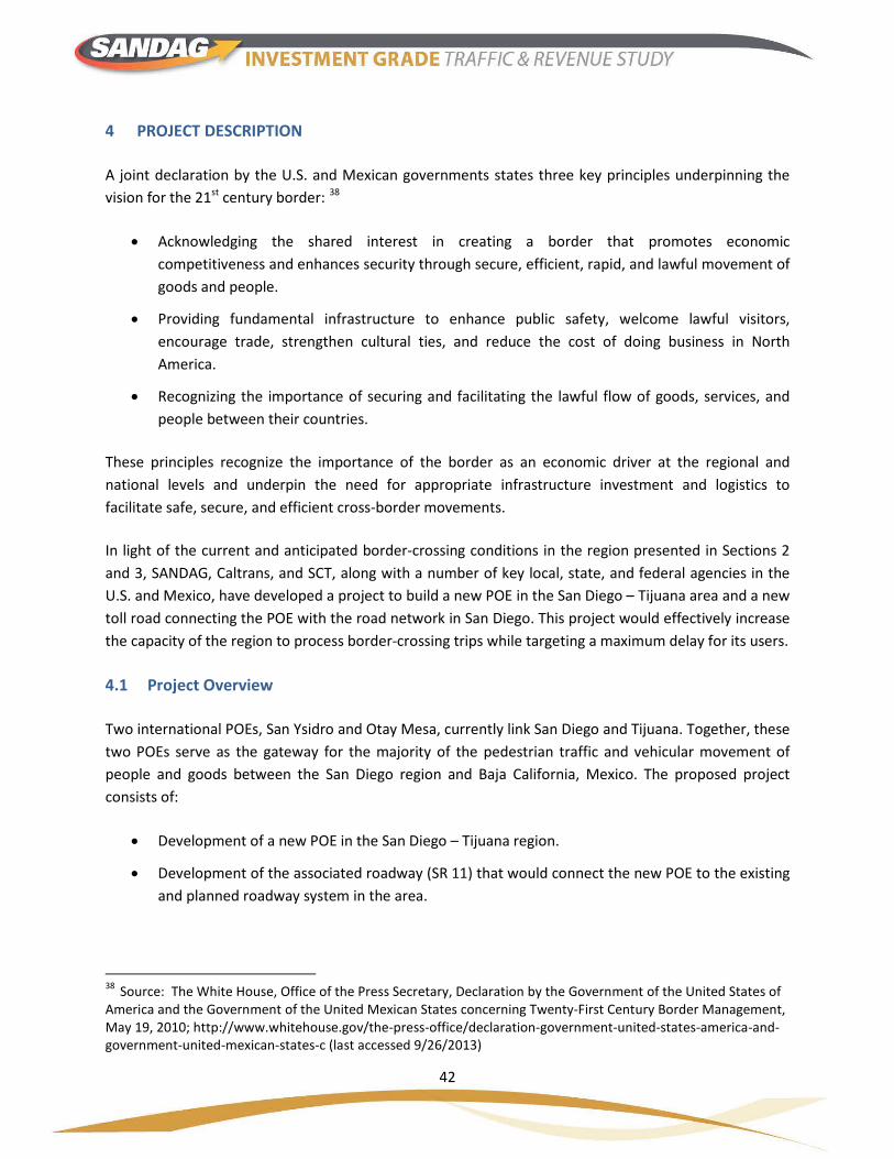
42

4 PROJECT DESCRIPTION

A joint declaration by the U.S. and Mexican governments states three key principles underpinning the vision for the 21st century border: 38

• Acknowledging the shared interest in creating a border that promotes economic competitiveness and enhances security through secure, efficient, rapid, and lawful movement of goods and people.

• Providing fundamental infrastructure to enhance public safety, welcome lawful visitors, encourage trade, strengthen cultural ties, and reduce the cost of doing business in North America.

• Recognizing the importance of securing and facilitating the lawful flow of goods, services, and people between their countries.

These principles recognize the importance of the border as an economic driver at the regional and national levels and underpin the need for appropriate infrastructure investment and logistics to facilitate safe, secure, and efficient cross-border movements.

In light of the current and anticipated border-crossing conditions in the region presented in Sections 2 and 3, SANDAG, Caltrans, and SCT, along with a number of key local, state, and federal agencies in the U.S. and Mexico, have developed a project to build a new POE in the San Diego – Tijuana area and a new toll road connecting the POE with the road network in San Diego. This project would effectively increase the capacity of the region to process border-crossing trips while targeting a maximum delay for its users.

4.1 Project Overview

Two international POEs, San Ysidro and Otay Mesa, currently link San Diego and Tijuana. Together, these two POEs serve as the gateway for the majority of the pedestrian traffic and vehicular movement of people and goods between the San Diego region and Baja California, Mexico. The proposed project consists of:

• Development of a new POE in the San Diego – Tijuana region.

• Development of the associated roadway (SR 11) that would connect the new POE to the existing and planned roadway system in the area.

38 Source: The White House, Office of the Press Secretary, Declaration by the Government of the United States of America and the Government of the United Mexican States concerning Twenty-First Century Border Management, May 19, 2010; http://www.whitehouse.gov/the-press-office/declaration-government-united-states-america-and-government-united-mexican-states-c (last accessed 9/26/2013)

43

• A new Commercial Vehicle Enforcement Facility (CVEF) for CHP inspection of trucks entering California from Mexico. This includes the connection of SR 11 with the SR 905 facility that is currently under construction.

The Mexican access road to the new POE for PVs will be Boulevard Las Torres, and is expected to have six center lanes (three each way) divided by an eight-meter-wide median, and two side lanes. The proposed cross-border facility will become part of a seamless Mexico connection to the Tijuana–Rosarito Corridor, with links to the Tijuana–Tecate and the Tijuana–Ensenada toll roads in Baja California, Mexico. These will be the main feeding routes used by CVs to access/egress the OME POE. The project is located approximately 2 miles east of the existing Otay Mesa border crossing (see Figure 20).

Figure 20: Overview of Project Area

Source: SANDAG

The proposed SR 11 will serve east-west intraregional, interregional, commercial, commuter, and cross-border traffic between the rapidly developing Otay Mesa area and destinations to the north, such as the cities of Chula Vista, National City, and San Diego. SR 11 will reduce congestion at the Otay Mesa POE and will provide an alternate facility for cross-border commercial traffic.

SR 11 will be a four-lane highway that will connect SR 905 and SR 125 (South Bay Expressway) to the proposed OME POE. SR 11 will be approximately 2.7 miles in length and is proposed to be developed as a toll facility. It will provide connection to the Tijuana 2000 corridor, providing direct connections to the Tijuana–Tecate toll road, the free roads, and to the Tijuana–Ensenada toll road. The SR 11 alignment also includes local access interchanges at Enrico Fermi Road and Airway Road.

44

SR 11 will begin at about Harvest Road, just east of the SR 905/SR 125 Interchange in east Otay Mesa, extend east and then south to the new, approximately 100-acre OME POE at the U.S.–Mexico border. Construction of SR 11 will require modifications to SR 905 to accommodate a connection with SR 11. The SR 11 Post Mile 0.0 will be located approximately 430 feet west of Piper Ranch Road, where SR 11 connects to SR 905. The eastern terminus of SR 11, at Post Mile 2.8, will be at the proposed northern POE boundary. The approximately 20-acre CVEF site will be located adjacent to the POE on its northern edge. A detailed map of the project area is presented in Figure 21.

Figure 21: Detailed Project Area Map

Source: SANDAG

The SR 11, OME POE, and CVEF facilities are interdependent components of a tolled POE system. However, these facilities will be built, owned, maintained, and operated by different agencies. Caltrans will be responsible for SR 11, with SANDAG serving as the responsible tolling agency; the POE will be owned and maintained by the U.S. General Services Administration and operated by the U.S. CBP; and the CVEF will be owned by Caltrans and maintained and operated by CHP.

The need for a new POE in the San Diego–Tijuana area has been well established, based on current and projected increases in trade and personal travel beyond the capacities of the existing POEs. Even today during peak periods the traffic demand exceeds the processing capacity at the border crossings, causing excessive border wait times for those engaged in making commercial and personal vehicle trips across the border. As trade and travel in this area are forecasted to continue to grow39 and border delays are expected to increase correspondingly (see Section 3.6), providing the region with a third POE becomes critical to maintain its competitiveness.

39 The Otay Mesa area is covered by two Community Plans, the EOMSP in the county portion of the mesa and the OMCP in the City of San Diego portion of the mesa. Both plans designate much of the remaining undeveloped land on the mesa for industrial or residential development.

45

SR 11 is to be constructed and operated as a toll facility with SANDAG as the toll authority under state legislation.40 All vehicles exiting the POE will be required to take westbound SR 11 and pay a toll. Employees of POE/CVEF and CVs that are directed to the CVEF at Otay Mesa are exempt from paying tolls. The project is expected to be financed by bonds that are backed by these toll revenues. SANDAG is authorized to issue these bonds.41

The project is anticipated to generate the following benefits for the region:

• Increased capacity of border-crossing infrastructure to accommodate increasing demand from CVs and PVs crossing the border in the San Diego–Tijuana region.

• Accommodate projected increases in international trade and personal cross-border travel in the region in a safe and secure manner.

• Accommodate commercial goods movement and cross-border travel to and from the OME POE.

The OME POE is closely tied to its counterpart in Mexico, and requires that the Mexican POE be built prior to its opening. Mexican authorities are developing the corresponding Otay Mesa II POE project on their side of the border and are addressing issues of concern to Mexico. The eastern half of the OME POE site would be situated directly across the border from the western portion of the Otay Mesa II POE site proposed by the Mexican government. The responsible agencies from Mexico and the U.S. participate in the ongoing border liaison mechanism, which meets regularly to discuss trans-boundary issues and exchange information associated with the two projects. The border liaison mechanism participants include the Federal Highway Administration (FHWA), Mexico’s SCT and IMPLAN, SANDAG, Caltrans, the Mexican Consulate in San Diego, the American Consulate in Tijuana, General Services Administration, and CBP.

4.2 Tolling Concept

The proposed toll system will include toll collection in both directions and the use of “smart technology.” Tolls will be collected on SR 11 north of the OME POE and the toll rates will vary by vehicle type (PV and CV) and by the level of congestion. The system in effect implements a congestion pricing mechanism and will encourage shifting of trips from peak hours to off-peak hours during the day.

Toll rates at SR 11 will incorporate the comparative value of using OME POE (i.e., travel time savings and reliability) versus other POEs in the border region, as well as the wait time goals for border crossing at OME POE itself.

40 Division 17 of the Streets and Highways Code, Sections 31460 through 31482 – the OME Toll Facility Act 41 The passage of Senate Bill 1486 in February 2009 and the subsequent issuing of a federal Presidential Permit opened the door for the SANDAG to seek private investment dollars to cover the shortfall in construction and design dollars and provide a premium crossing option for a fee.

46

The toll rates for SR 11 will be variable by hour. Toll rates will be set by a combination of the following factors:

• Dynamically maintaining the demand/supply balance at OME POE to ensure wait time goals are met.

• Type of traffic (i.e., PV or CV).

• Comparative wait times at OME POE versus San Ysidro and Otay Mesa by type of traffic.

• Special rates as allowed for electronic tolling and subscriber accounts.

The toll road will support multiple methods of payment by both CVs and PVs, including electronic transponders with prepaid accounts, cash at an automated payment terminal (APT), and credit and debit cards at an APT. All cash, debit, and credit payments will be made at either an APT located at the tolling collection point, or a consumer outlet (e.g., gas station chain, mini-marts, customer service center). Toll operations will support monitoring and maintenance of the APTs.

Each tolling point at SR 11 will include the following features:

• Open road electronic tolling lanes (at least two).

• Cash/credit payment lane with an APT (at least one).

• Security surveillance systems covering cash payment, APT, lanes, and general toll point vicinity/facility.

• Pull-over area for maintenance and enforcement vehicles.

The toll road will feature violation-deterring measures such as license plate capture, payment indication lights, video recording, and visual enforcement by law enforcement officers. Enforcement functions will be performed by CHP under contract with SANDAG.

The traffic and revenue forecasts presented are based on an hourly variable pricing concept. The pricing framework was devised to ensure the efficiency of the border operation, increased participation through subscription-based tolling, and provision of timely information to users, while generating adequate revenues.

As in the case of bridges and tunnels, the decision to cross the border at OME POE needs to be made early – some times over 20 miles away – in the roadway network (Figure 22). In other words, the decision to use the POE takes into consideration not only the congestion level at the facility itself (border-crossing wait time) but also the roadway length and travel time to get to each of the alternative crossings (driving time to and from the POE). This creates a challenge for the implementation of a pure dynamic pricing mechanism to manage congestion and drivers’ expectations (in terms of wait times and tolls).

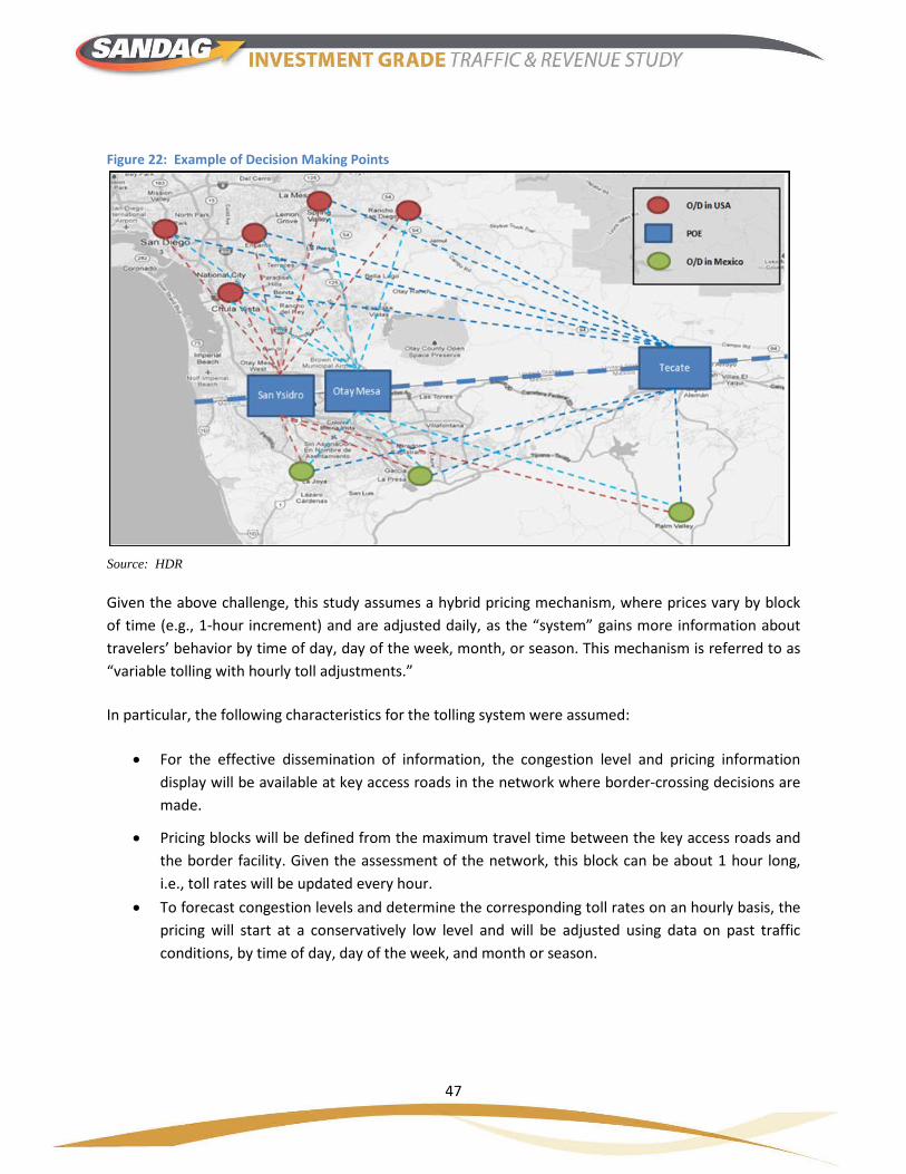
47

Figure 22: Example of Decision Making Points

Source: HDR

Given the above challenge, this study assumes a hybrid pricing mechanism, where prices vary by block of time (e.g., 1-hour increment) and are adjusted daily, as the “system” gains more information about travelers’ behavior by time of day, day of the week, month, or season. This mechanism is referred to as “variable tolling with hourly toll adjustments.”

In particular, the following characteristics for the tolling system were assumed:

• For the effective dissemination of information, the congestion level and pricing information display will be available at key access roads in the network where border-crossing decisions are made.

• Pricing blocks will be defined from the maximum travel time between the key access roads and the border facility. Given the assessment of the network, this block can be about 1 hour long, i.e., toll rates will be updated every hour.

• To forecast congestion levels and determine the corresponding toll rates on an hourly basis, the pricing will start at a conservatively low level and will be adjusted using data on past traffic conditions, by time of day, day of the week, and month or season.

48

4.3 Operation of the OME POE

A number of operating assumptions directly related to the project were necessary to develop the traffic and revenue forecasts presented herein. Some of these assumptions were based on inputs collected during a workshop held in San Diego on October 3, 2012 and facilitated by HDR staff. Participants to the workshop included various project stakeholders and subject matter experts. The project assumptions used in the traffic and revenue forecast provided include:

• The proposed OME POE will begin operations in 2017.

• Tolling at the new POE will occur in both directions of traffic (northbound and southbound).

• The new POE will feature dynamic tolling with hourly toll adjustments for PVs and CVs.

• Processing times for each lane type are the same at all POEs.

• A maximum wait time of 20 minutes will be targeted at the OME POE for all vehicles (PV and CV).

• PV lanes at the OME POE will operate 24 hours per day. All existing lanes will be open during AM, midday, and PM periods. Due to CBP union rules, the POE will operate at reduced capacity (i.e., with fewer lanes open for PVs) between 9 PM. and 4 AM.

• The OME CV lanes will operate 16 hours a day, from 7 AM to 11 PM.

• The capacity of the proposed POE can be expressed in terms of number of lanes for PVs and number of lanes for CVs (10 for each one of them).

Based on projections developed in the context of an intermediate traffic and revenue forecasting exercise, the HDR team determined that 10 lanes for PVs and 10 lanes for CVs would be adequate given the proposed pricing mechanism and a target wait time of 20 minutes. This recommendation, however, hinges on the assumption that pricing will be used effectively to achieve the required level of service.42

For northbound trips, the OME POE will feature regular, Ready and SENTRI lanes for PVs and regular and FAST lanes for CVs. For southbound trips, lanes will be differentiated between those servicing PVs and those servicing CVs. The actual number of open lanes of each type will vary by hour depending on traffic conditions, but at all times the number of PV lanes will not exceed 10 and the number of CV lanes will not exceed 10.

Finally, the expansion of other POEs in the region will have a direct impact on the traffic and revenues for the OME POE. In particular, the ongoing expansion of the San Ysidro POE will be completed before the OME POE begins operation. Because of this expansion, San Ysidro will feature 34 total northbound lanes (29 tandem lanes, 1 single bus lane, and 4 single-booth lanes). Otay Mesa, on the other hand, is not anticipated to undergo any expansion; therefore, it is assumed it will continue with 13 lanes for PVs (all of them single lanes) and 10 for CVs.

42 This, however, does not mean that the OME POE pricing strategy is a revenue-maximizing strategy. In fact, the binational T&R model developed in this study does not follow a maximization procedure for the estimation of revenues generated by OME POE.

49

5 PERCEPTION OF THE PROJECT BY POTENTIAL USERS

An important factor in the success of the SR 11/OME POE project is the attitude of potential users toward paying tolls for a targeted maximum wait time at the POE and a quick connection to the San Diego road network. To identify these perceptions, a series of surveys were conducted among residents of San Diego and Tijuana who are frequent border-crossers. This section describes the main findings from data collection efforts with respect to attitudes toward cross-border travel and willingness to pay to expedite travel across the border.

5.1 Overview of Surveys and Sample Size

Data collection used to analyze attitudes toward cross-border travel and willingness to pay to expedite travel across the border came from a series of stated preference surveys provided by SANDAG. In particular, two survey programs had stated preference components combined with O-D questions (see Box 8). O-D surveys, which included a stated preference section, were the two surveys performed for SANDAG during the end of 2011 and early 2012 (general public survey and company survey, respectively).

5.1.1 General Public Survey of 2012

The general public survey of 2012 was conducted at the San Ysidro and Otay Mesa POEs between November 2011 and March 2012. The survey was conducted in two separate exercises, one for PVs and pedestrians and the other for CVs.

PVs and Pedestrians

The PV and pedestrian component the general public survey consisted of questions about O-D for the current trip (including trip purpose) as well as a stated-preference section where eight different scenarios were presented to each interviewee. In each scenario they were asked to choose between paying a toll or waiting longer at the border crossing.

A total of 1,605 responses were collected, with the majority of them (1,437) corresponding to PVs.

Box 8. Stated Preference Surveys and Value of Time

The surveys used to determine the perception of border-crossing travelers toward the project are the general public survey and the company survey.

Besides including questions geared toward identifying the attitude of interviewees toward cross-border travel, each survey included two different categories of scenarios to determine their willingness to pay to expedite border-crossing travel. One such scenario was devised to collect responses related to the value of time (VOT) assigned by travelers and the other was created to capture information on their value of reliability (VOR).

Besides providing information on willingness to pay, information collected from the stated preference scenarios was used to determine the actual VOT and VOR of border-crossing travelers. The responses used in the estimation of VOT are described in Section 6.1.5.

A detailed description of the surveys used to collect data on the perception of potential users is presented in Appendix C.

50

The variables collected in the stated preference component of the survey include:

• Response to experiments (for VOT or VOR) for expedited border crossing.

• Preferred payment type or reason for not willing to pay a toll.

• Additional trips anticipated under 15 and 30 minutes reduction of border-crossing time.

• Household characteristics, including household income range.

• License plate origin.

A summary of key characteristics from the survey are listed below.

• The majority of the responses correspond to northbound trips, with only 198 responses for southbound trips.

• Information on southbound trips was only collected at the San Ysidro POE and the information only includes responses for the VOT scenarios.

• Northbound trips on both POEs captured information about the driver’s VOR only for non-SENTRI trips.

• Information on pedestrian crossings was collected only at San Ysidro, northbound.

Construction Vehicles

The CV component of the survey was collected only in the northbound travel direction at the Otay Mesa POE and consisted of questions about O-D for the current trip and a stated-preference section where eight different scenarios were presented to each interviewee. In each scenario truck drivers were asked to choose between paying a toll or waiting longer at the border crossing. The stated preference questions were asked only if the truck driver responded that he/she was in charge or making the decision about which POE to use when crossing the border.

A total of 433 responses were collected. The information collected in the stated preference component of the survey included:

• Response to experiments (for VOT or VOR) for expedited border crossing.

• Preferred payment type or reason for not willing to pay toll.

• Advantages of a new POE with toll for trucker/company.

• Answers to the question “Who would pay the toll in the new POE?”

• Importance of reliable crossing time.

• Importance of short crossing time.

• Reasons for considering tolled crossing with a reduced wait time.

51

• Attitude toward expanded hours of operation for new POE with toll.

• Household characteristics, including household income range.

The data collected represents a fair cross section of the market for CV movements because:

• The majority of the interviews correspond to trucking/transportation companies (352 responses).

• Loaded trucks (either FAST or non-FAST) represent more than 70 percent of the sample (311 observations).

• Information collected on loaded trucks is evenly distributed between FAST and non-FAST.

5.1.2 Company Survey of 2012

The survey was divided into two parts. Part 1 recorded information on operations, typical trips (including typical destination and travel time) and attitude toward using a new POE with toll and lower wait times. Part 2 of the interview consisted of a stated-preference exercise where eight different scenarios where presented to each interviewee. In each scenario they were asked to choose between paying a toll or waiting longer to perform the border-crossing.

The sample consists of 99 completed interviews, of which 69 were maquiladora companies, 20 were freight companies, and 10 were perishable goods transport companies.

5.2 Attitudes Toward Cross-Border Travel

The general public survey captured data on user perception of congestion at the border, the anticipated wait time to cross the border and the reasons for choosing a particular POE to cross the border. Similarly, the company survey provided insight into perceived congestion levels and wait times at the border, factors in selecting a specific route and border crossing, importance of southbound delays at the border, and importance of predictable and short crossing times.


Based on the responses, the majority of PV users and pedestrians perceived congestion at Otay Mesa as “somewhat worse” or “worse” compared to other days, while in San Ysidro the majority of responses stated that congestion was “somewhat better” or “better” compared to other days. Regarding the reason to choose a specific POE to cross the border, two thirds of the respondents in San Ysidro mentioned it was closer to their origin or destination, while for Otay Mesa the same reason was mentioned by more than half the interviewees.

For CVs, a vast majority of the respondents (86 percent) qualified the congestion at Otay Mesa as “somewhat better” or “much better” compared to other days. Regarding the reason for choosing Otay Mesa as their POE, the majority (69 percent) stated this POE was close to their origin or destination.

52

The survey provided qualitative insight into the attitudes of PV drivers, pedestrians, and CVs toward border crossing. This information, however, is based primarily on northbound trips. Additionally, when asked about the perceived time to cross the border, respondents of SENTRI lanes in both POEs recorded a high average wait time compared to actual measurements.


In most cases and for all company types, perceived wait times were reported to be above one hour, implying high perceived congestion levels at Otay Mesa POE. Regarding the factors that determine a specific route and POE choice, answers differed by company type: safety is the main concern for freight companies, shortest travel time is the main driver for maquiladoras, while the only route to the POE was the main reason mentioned by transporters of perishable products. All company types recognized the importance of a fast southbound crossing, though when asked about a reason for this statement, no particular reason was listed. Finally, the importance of predictable and short crossing times was acknowledged by all company types though, contrary to belief, transporters of perishable products were less prone to qualify it as “very important” compared to the other two company categories.

5.3 Willingness to Pay to Expedite Border-Crossing Travel

Information on the willingness to pay to expedite border-crossing travel was collected in both surveys: the general public survey (where data was collected directly from PVs, pedestrians, and CVs) and the company survey (where information was collected from logistic managers of companies engaged in shipment of goods across the border).


The general public survey was intended to capture the willingness-to-pay attitudes of PVs, pedestrians, and CV drivers toward the construction of the OME POE and accompanying toll road featuring reduced wait times.

For PVs and pedestrians, the data collected shows that users of the Otay Mesa POE are more inclined to pay to see their wait time reduced compared to those who currently use San Ysidro. The summary is presented in Table 18, illustrating that for the two stated preference survey types presented to each interviewee (VOT and VOR), interviewees in Otay Mesa, on average, selected a larger number of scenarios where a toll was featured. This result is consistent with the perception that congestion at Otay Mesa is higher compared to that in San Ysidro.

53

Table 18: Average Percentage of Scenarios Chosen With Toll by POE, PVs and Pedestrians

POE VOR Survey VOT Survey

Average Percentage of Scenarios with Toll Chosen Sample Size Average Percentage of

Scenarios with Toll Chosen Sample

Size

San Ysidro 35 352 35 668

Otay Mesa 48 198 49 262

Total 39 550 39 930

Source: HDR Analysis of 2012 General Public Survey Data

When disaggregating the responses by trip direction, POE, and crossing type, it is clear that pedestrians are equally inclined to pay tolls compared to automobile users. This finding is not in line with expectations, as pedestrians are usually assumed to have a lower inclination to pay tolls compared to PV occupants. The specific numbers are presented in Table 19.

Table 19: Average Number of Scenarios Chosen With Toll by POE and Crossing Type, PVs and Pedestrians

Direction POE Crossing Type

VOR Survey VOT Survey Average Percentage of

Scenarios with Toll Chosen

Sample Size

Average Percentage of Scenarios with Toll

Chosen

Sample Size

North

San Ysidro

Non-SENTRI 34 302 38 299

SENTRI 41 148

Pedestrian 38 50 35 23

Otay Mesa

Non-SENTRI 48 198 41 147

SENTRI 58 115

South San Ysidro Non-SENTRI 26 198

Total 39 550 39 930


Additionally, the table shows a difference in the inclination toward paying a toll between SENTRI and non-SENTRI users in both POEs as measured by the VOT survey responses for northbound flows. The difference, however, is more pronounced in the case of Otay Mesa, coinciding with the perceived higher level of congestion at this POE. A more detailed analysis of the information revealed a positive correlation between the number of scenarios with a toll chosen by individuals and their household income level. This result is in line with expectations. Finally, those interviewees who did not choose any scenario involving tolling represent 20 percent of the PVs and pedestrian sample. Almost half of them reported not being willing to pay a toll due to fairness considerations.

54

For the subsample for CVs, the stated preference scenarios were preceded by information about who makes the decision regarding the specific route or POE used by the truck to cross the border. In particular, only those CV drivers that indicated they were the decision makers were presented with the eight scenarios that provide information about their willingness to pay for reduced wait times. The result was that only 14 drivers (out of the total subsample of 433) responded to the stated preference scenarios. A breakdown of the stated preference responses by CV ownership and border-crossing type is presented in Table 20.

Table 20: Average Number of Scenarios Chosen With Toll by Ownership and Crossing Type, Trucks

Ownership Crossing type

VOR Survey VOT Survey

Percentage of Scenarios with Toll that were Chosen

Sample size Percentage of

Scenarios with Toll that were Chosen

Sample size

Independent Owner-Operator

Empty 0.0 1

Loaded Truck – FAST 0.0 3

Loaded Truck - Non-FAST 81.3 2 100.0 1

Perishable Load 93.8 2 70.8 3

Trucking, Transportation Company

Loaded Truck - Non-FAST 6.3 2

Total 51.8 7 44.6 7


Given the small number of responses from truck drivers, some inconsistencies can be expected in the willingness to pay for expedited border-crossing times. For example, it would seem from Table 20 that drivers of non-FAST loaded trucks have a higher willingness to pay compared to drivers of perishable loads. Moreover, other types of disaggregation of the willingness to pay into market segments (including by commodity transported or O-D pair) may result in unreliable conclusions, as the results must be derived based on one or two responses.

The survey focuses extensively on northbound trips (for CVs, PVs, and pedestrians). In particular, southbound information on stated preferences exists only on one POE (San Ysidro) and only uses VOT surveys. Despite the relatively large number of data points available for PV and pedestrian users of the POEs, a few market segments are not well represented in the stated preference responses. In particular, there are no VOR responses for SENTRI on northbound trips and for VOR in general on southbound trips.

55


The information on willingness to pay collected through these surveys is broken down into the three types of companies interviewed. An important question included in the interview was that of the perceived viability of a new tolled border crossing if it reduces border-crossing wait time. In general, all company types perceive that such a project would be viable, though companies transporting perishable goods and maquiladoras seem to support the idea more than freight companies. This is presented in Table 21, though it must be mentioned that by the nature of the question these responses do not measure the attitude of companies toward paying a toll for this new infrastructure.

Table 21: Perceived Viability of New Tolled POE by Company Type

Response Maquiladora Companies (%)

Freight Companies (%)

Perishable Goods Companies (%)

Strongly approve 51 45 40

Approve 41 35 60

Neutral 7 10 0

Disapprove 0 0 0

Strongly disapprove 1 10 0

Source: HDR Analysis of 2012 Company Survey Data

When asked to provide the reason for their assessment that a new tolled POE would be viable, companies’ answers were very similar (as presented in Table 22). Faster travel times and more reliability were the two major reasons listed, accounting for more than 60 percent of the responses.

Table 22: Main Reasons Listed for Perceived Viability of New Tolled POE by Company Type

Reason Maquiladora Companies (%) Freight Companies (%) Perishable Goods

Companies (%) Gets me faster to where I want to go 33 37 40

Less congestion 14 11 10

Improve roadways in my community 1 0 0

I feel safer 9 11 15

More reliable time 29 32 25

Less pollution to the environment 7 7 0

Other 7 2 10


56

Analysis of the responses by the different companies to the stated preference scenarios show that maquiladora and perishable goods companies are more willing to pay to see their wait times reduced at the border compared to freight companies. This is presented in Table 23, along with the sample sizes.

Table 23: Overview of Willingness to Pay Responses from Company Survey, by Company Type

Variable Maquiladora Companies (%)

Freight Companies (%)

Perishable Goods Companies (%)

Average of stated preference scenarios where a toll was chosen 62 53 61

Sample size 67 20 10


Disaggregation of these responses by commodity type yields, in general, unreliable results due to the low number of observations recorded. The three exceptions found in the survey correspond to goods listed by maquiladora companies: electronics (with 21 responses), automobile and metal parts (with 15 responses), and hygiene products and medical products (with 11 responses). The average number of stated preference scenarios where a toll was chosen for these products was 62 percent, 61 percent, and 58 percent respectively.

A disaggregation by destination can only be made for the location of Otay Mesa, which recorded 12 responses for freight companies and 35 responses for maquiladoras. For trips that end in this locality, freight companies expressed they would be willing to pay a toll to reduce their wait times at the border in 58 percent of the scenarios they were presented with. In the case of maquiladoras, this number was 60 percent.

In summary, the stated preference surveys show a significant willingness on the part of both PVs and CVs to pay to avoid long border-crossing wait times.

57

6 BINATIONAL TRAFFIC AND REVENUE MODEL

As stated in Section 2.1, there are multiple routes a vehicle may take to complete a binational trip based on its origin and destination. Traffic and revenue studies assume drivers will choose among a set of routes that represent the lowest generalized trip cost. The cost of each route is a function of several factors, including travel time to and from a POE, border crossing time, travel distance, and tolls. Some of these factors are specific to the road network, and some are specific to the individual vehicle making the trip based on its characteristics. Factors that determine the total cost of the trip are:

• Travel time to and from a POE – driving time on local roads leading to the POE (see Figure 1).

• Border-crossing wait time – processing time and wait time at the POE.

• Travel distance – vehicle operating costs associated with miles of travel.

• Tolls – The toll the vehicle will pay (if applicable) by using toll roads or tolled POEs, that is part of the chosen trip route.

The study team developed a traffic network model (binational T&R model) to simulate the choices of cross-border travelers across the border and to study the impacts of the proposed border-crossing capacity expansion represented by the SR 11/OME POE. The model was calibrated using the observed traffic conditions in 2012.

The approach to developing the Binational T&R forecasting model for the proposed OME POE involved multiple, interconnected steps and was built on existing models, reports, and travel survey data. The result was a modeling tool that estimated traffic shares between the different POEs in the San Diego–Tijuana region based on observed border crossing traffic volumes and border-crossing travel characteristics.

The binational T&R model used the aggregate border-crossing traffic growth projections from the econometric-based Traffic Growth Model introduced in Section 3.5 to forecast future binational traffic at each POE in the region. These binational traffic growth forecasts were combined with local traffic growth projections based on the future land use plans and socioeconomic trends discussed in Section 3. The binational T&R model process is shown in Figure 23.

A typical trip-based urban transportation model has four steps: trip generation, trip distribution, mode choice, and network assignment. The binational T&R model is a highway-only model that simulates average weekday PV and CV trips (i.e., this model does not include pedestrian border crossings). The cross-border vehicle trip generation and trip distribution are based on O-D surveys conducted by SANDAG in 2011 and 2012 and described in Section 2.2.

58

Figure 23: SR 11/OME POE Binational Traffic and Revenue Model Overview

In addition to cross-border traffic, the binational T&R model also simulates local congestion conditions, as recurring delays on the regional road network can affect the choice of POE. Vehicle trip tables from the SANDAG travel demand model are used for San Diego County traffic. In Tijuana, delays associated with traffic congestion are based on travel time runs conducted for this study. The binational T&R model conducts a traffic assignment for every hour in the day beginning and ending at midnight.

At the POEs, the model estimated border-crossing delays based on the number of open lanes and the hourly vehicle processing rate per lane. The binational T&R model has different processing rates depending on whether a vehicle is a CV or a PV and whether a standard or special lane is used. Hourly traffic volumes higher than the hourly POE processing rate contribute to additional border crossing delay. Key validation measures for the binational T&R model are border crossing volumes and border crossing times.

The model can accommodate variable tolling scenarios with hourly increases for SR 11 for both PVs and CVs. The toll rates are adjustable every hour to support development of a pricing framework that ensures efficiency of the border operation.

Data from a variety of sources were used to develop the binational T&R model. Table 24 identifies both the main data sources and the type of information used in model development. Fuller discussion of the data sources is provided in the sections indicated in the last column.

Socio economic Forecasts Travel Demand

Estimated Delays

Toll Levels

Traffic Diversion

Revenue

POE Capacity Parameters

Values of Time

59

Table 24: Main Data Sources Used in Binational T&R Model Binational T&R Model

Input Data Source Information Used Section in IGT&R Report

Regional Road Network

SANDAG Model San Diego network Section 6.1.1

SANDAG Binational Model

Tijuana network Section 6.1.1

Regional Travel Patterns

SANDAG Cross-border Surveys

Origin-destination data Section 2.2 and Appendix B

Instituto Metropolitano de Planeación de Tijuana (IMPLAN)

Origin-destination data Section 2.2

Border-Crossing Operations

CBP Hourly vehicle traffic Section 2 and Appendix B

CBP POE operational data Section 6.1.4 and Appendix L

CBP Border wait times Section 2.6 and Appendix D

Traffic Impact Studies San Ysidro POE processing rate Section 6.1.4 and Appendix L

Field Observations by HDR Team (Cross-border Group)

Border crossing times Section 2.6 and Appendix D

Traffic in Roads Adjacent to POEs

Caltrans PeMS Traffic counts Section 6.1.3 and Appendix K

Caltrans PeMS Travel speeds Section 6.1.3

Traffic Impact Studies Traffic counts Section 2.3 and Appendix B

Instituto Metropolitano de Planeación de Tijuana (IMPLAN)

Tijuana traffic counts Section 2.3

Regional Socio-economic Data

SANDAG Model Socioeconomic data Section 3

SANDAG Crossborder Surveys

Traveler socioeconomic profile Appendix C

Instituto Nacional de Estadística y Geografía (INEGI)

Áreas Geográfico Estadísticas Básicas (AGEB) population and employment data

Section 2.2 and Section 6.1.1

Source: HDR

6.1 Development of Base Year Model

Development of the base year for the binational T&R model consists of developing a model that includes all relevant variables affecting the border-crossing choice and that produce estimates for border-crossing volumes and wait times that closely resemble those observed at the POEs in the region for the year 2012.

60

In particular, the base year model consists of the development of a road network, border-crossing trip tables that represent the travel patterns observed in the region, replicating congestion around the POEs, and development of a traffic assignment procedure (incorporating a delay function to capture border-crossing time) to assign border-crossing trips to the different roads and POEs in the region.

Figure 24: Binational T&R Model Road Network

Source: HDR

61

6.1.1 Integration of Road Network

The road network used in the binational T&R model is presented in Figure 24 with the locations of the existing San Ysidro and Otay Mesa POEs and the proposed OME POE. The binational T&R model combines the 2010 SANDAG trip-based model network with the 2006 SANDAG binational model network. In Mexico, the model coverage includes Tijuana and Tecate; in the U.S., the model covers all of San Diego County. The HDR team has made minor updates to the combined model network reviewing travel speeds in Tijuana and adding border-crossing links based on primary data collection efforts (see Sections 2.3 and 2.4). See Box 9 for additional details on the road network used in the binational T&R model.

6.1.2 Representation of Border-Crossing Trip Patterns

The model uses border-crossing trip tables to represent trip patterns observed in the region. Development of cross-border trip tables for the base year in the binational T&R model is based on three O-D surveys conducted by SANDAG in 2011 and 2012 (see Section 2.2). These surveys were combined and expanded based on traffic count data gathered as part of this IGT&R study (see Section 2.3 for more details on the data collected) to represent a typical day of border-crossing traffic in the region. The main steps in process of transforming the O-D survey data and the traffic count data into cross-border trip tables is presented in Box 10.

A reasonableness check was performed after the development of the cross-border trip tables. Here, the HDR team compared the O-D patterns resulting from the trip tables with observed population and employment in San Diego County and Tijuana. As mentioned in Section 2.2, the result is that the estimated trip tables adequately represent trip patterns in the region. In particular, PV cross-border trips in 2012 are clustered around commercial and industrial areas along the border in San Diego County but are distributed more evenly throughout Tijuana, while CV cross-border trips in 2012 are clustered around the Otay Mesa POE (see Figure 2).

Box 9. Model Geography

For San Diego County, the binational T&R model uses the SANDAG 4,684-zone traffic analysis zone (TAZ) geography. Using the same TAZ geography as the SANDAG model allows for consistent data transfer to the binational T&R model. In Tijuana, the binational T&R model TAZ geography is based on aggregations of the city’s colonia geography. Called super-colonia, these areas form the 631 TAZs that represent the Mexican side of the model. The binational T&R model used this geographic framework for consistency with the cross-border O-D survey data.

Box 10. Methodology to Develop Cross-Border Trip Tables

The process of transforming O-D survey data and traffic count data collected in the field into trip tables consisted of the following steps:

1. Developed an O-D database.

2. Replicated survey data to fill out time gaps.

3. Expanded survey data to represent population.

4. Developed border-crossing trip tables.

5. Checked for reasonableness of trip tables.

A description of the work performed in each one of these steps is presented in Appendix S.

62

6.1.3 Traffic and Congestion in Local Roads Leading to Ports of Entry

While expected border-crossing time is an important determinant of POE choice, the overall delay on the regional road network also affects a traveler’s route choice. The binational T&R model uses local traffic data to simulate the delays that cross-border traffic will experience traveling to and from the POEs. The approach to simulating the delays in local roads around the POEs is different in San Diego County and Tijuana.43

San Diego County Traffic

The SANDAG trip-based travel demand model is the primary source of data for non-POE traffic in San Diego County. The SANDAG model produces AM, PM, and off-peak vehicle trip tables, which were simplified to derive traffic conditions in the roads around the POEs.

Tijuana Traffic

Because travel demand model data were not readily available for Tijuana, the HDR project team used an alternative approach to simulate the delays associated with non-POE traffic. HDR conducted travel time studies on major roads in Tijuana, which provided information on congested travel speeds. HDR used these observed travel speeds in the binational T&R model.

6.1.4 Traffic Assignment and POE Crossing Time

The binational T&R model uses a generalized cost assignment to assigns trips by different user classes (PV and CV) to the model network and POEs simultaneously with different values of time and toll costs.

For each 24-hour period in the model, the traffic assignment begins with the unmet demand from the previous hour. The total cross-border traffic volumes for each hour is based on the estimated trip tables

developed in Section 6.1.2. For the first hour, which begins at midnight, there is no unmet demand. The arriving volumes in hour one are assigned to the network using the multiclass user equilibrium assignment. In this type of traffic assignment, different types of trips (home based work, home based shopping, home based other, empty trucks, loaded trucks, etc.) are assigned simultaneously to the transportation network using values of time that are specific to each trip category. The assignment model accounts for all components of travel times and costs when evaluating traffic paths and allocating trips for each origin to destination pair. These

43 Additional information on how traffic and congestion in local roads was estimated is available in Appendix S.

Box 11. Estimation of Average Border Crossing Wait Time

The formula to estimate border crossing wait times at a particular POE is:

Average wait time in hours (i) = (assigned volume in hour (i) – processed volume in hours (i) ) * (processing time per vehicle/2)

This formula indicates that border crossing wait time is estimated for the median vehicle that gets processed at a POE during a specific hour.

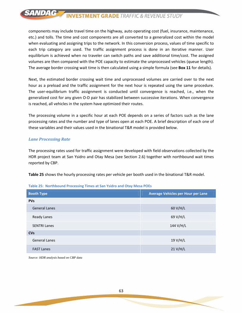
63

components may include travel time on the highway, auto operating cost (fuel, insurance, maintenance, etc.) and tolls. The time and cost components are all converted to a generalized cost within the model when evaluating and assigning trips to the network. In this conversion process, values of time specific to each trip category are used. The traffic assignment process is done in an iterative manner. User equilibrium is achieved when no traveler can switch paths and save additional time/cost. The assigned volumes are then compared with the POE capacity to estimate the unprocessed vehicles (queue length). The average border crossing wait time is then calculated using a simple formula (see Box 11 for details).

Next, the estimated border crossing wait time and unprocessed volumes are carried over to the next hour as a preload and the traffic assignment for the next hour is repeated using the same procedure. The user-equilibrium traffic assignment is conducted until convergence is reached, i.e., when the generalized cost for any given O-D pair has stabilized between successive iterations. When convergence is reached, all vehicles in the system have optimized their routes.

The processing volume in a specific hour at each POE depends on a series of factors such as the lane processing rates and the number and type of lanes open at each POE. A brief description of each one of these variables and their values used in the binational T&R model is provided below.

Lane Processing Rate

The processing rates used for traffic assignment were developed with field observations collected by the HDR project team at San Ysidro and Otay Mesa (see Section 2.6) together with northbound wait times reported by CBP.

Table 25 shows the hourly processing rates per vehicle per booth used in the binational T&R model.

Table 25: Northbound Processing Times at San Ysidro and Otay Mesa POEs

Booth Type Average Vehicles per Hour per Lane

PVs

General Lanes 60 V/H/L

Ready Lanes 69 V/H/L

SENTRI Lanes 144 V/H/L

CVs

General Lanes 19 V/H/L

FAST Lanes 21 V/H/L

Source: HDR analysis based on CBP data

64

Open Lanes

Data on the number of lanes open by lane type is available from CBP. The number of lanes open at each POE varies by time of day and day of week. HDR used CBP data from October 2012 to estimate the number of lanes open for each hour of a typical weekday and used this information to project the future utilization of lane capacity in the region (see Box 12).

Box 12. Utilization of Current and Future POE Capacity in the Region

The existing and future capacity of the POEs in the region (in terms of number of lanes available to process PV and CV traffic) and the actual use of this available capacity is a key determinant of the congestion levels that are anticipated for border-crossers in the region. As described in the main body of the report, the binational T&R model assumes the following number of lanes (i.e., theoretical capacity) for the POEs in the region:

• For PV traffic: San Ysidro is anticipated to expand from 24 to 34 northbound lanes in 2017, Otay Mesa is expected to remain with its current capacity of 13 northbound lanes and OME will open in 2017 with 10 northbound lanes.

• For CV traffic: Otay Mesa is expected to maintain its current capacity of 10 northbound lanes while OME will open with 10 northbound lanes in 2017.

However, the level of congestion observed at a POE is determined not by the theoretical capacity of the infrastructure but by the degree to which this theoretical capacity of the POE is actually utilized. The utilized capacity is defined as the number of lanes that are available (or open) to process border-crossing traffic during a specific period of time. The binational T&R model uses historic data from CBP to estimate the level of utilization of theoretical capacity at the existing POEs (by hour) and uses this number as a reference for the utilization of theoretical capacity in future years. The interpretation of this assumption is that resources (primarily human resources to operate the POEs) will be available in the future in the same proportion to total border-crossing capacity as they are currently available.

The two figures below show the utilization of northbound lanes at the region’s POEs for different years (left for PV, right for CV). Notice utilization across the POEs in the region is generally determined, for each time period (AM, midday, PM and night), by the utilization levels of the POE observed during 2012. In particular, the binational T&R model assumes capacity utilization for OME will follow the same patter as that of Otay Mesa due to their geographic proximity.

In addition, notice the utilization of northbound PV capacity is consistently higher during the AM period, reaching levels close to 90 percent at all POEs in the future years. Furthermore, notice that utilization levels of northbound PV lanes at Otay Mesa drop after 2012 for the midday, PM and night periods due to the opening of OME POE but start to increase over time. This is the result of a higher total volume of border-crossers in the region, most of which cannot be processed at OME since this facility is anticipated to be operating close to capacity since its first year of operation. Finally, the historical utilization of CV northbound lanes is close to the theoretical capacity for the midday and PM periods at Otay Mesa, suggesting high volumes of CV traffic in the region during these periods.

PVs CVs

65

While each open lane may be served by up to two processing booths (tandem lanes), CBP does not report the number of open booths – nor which lanes are served by multiple booths. HDR estimated the number of open booths per lane for each hour at each POE based on the observed traffic volumes processed. Based on a survey HDR conducted in August 2013, it was determined that tandem booths can increase the lane processing capacity by approximately 30 percent for standard lanes and about 10 percent for Ready lanes. These productivity aspects of tandem booths are incorporated in the traffic model.

6.1.5 Value of Time for Cross-Border Travelers

Different travelers place different value on each minute (or hour) of travel time based on their characteristics and the characteristics of the trip (personal, business, etc.). Therefore, the value of time is a key input in monetizing the total travel cost of using a specific route (including specific POEs) to complete a binational trip (see Box 13 for a brief description of how tolls and value of time are related). The binational T&R model incorporates different values of time for PVs and CVs. The values for each categorization are based on stated preference surveys conducted for this purpose as well as input from experts.

Data collection for VOT input into the binational T&R model came from a series of stated preference surveys provided by SANDAG. In particular, two survey programs had stated preference components that were combined with O-D questions (i.e., the general public survey and the company survey).

Using the information from those surveys, an estimate of the VOT for the base year was calculated. Table 26 shows the value of time for PVs used in the binational T&R model, while Table 27 shows the value of time for CVs.44

Table 26: VOT for PVs

Standard Lane Ready/SENTRI Lanes

Shopping $8.5 $12.6

Work/Business $6.7 $10.0

Other Personal $7.5 $23.7

Source: HDR Calculations using 2012 Survey Data and Risk Analysis Inputs

44 Details on the calculations of VOT are provided in Appendix C.

Box 13. Tolls and VOT

VOT is an important part of the toll estimation process. In the binational T&R model, the wait times at the OME POE are maintained below the target level of 20 minutes by controlling the flow of traffic to the new POE. This is done iteratively by increasing or decreasing toll depending on how much the estimated wait times at OME exceeds the 20 minute target or fall below the target. For example, if the estimated wait time at the new POE is 25 minutes, then to bring it below 20 minutes, the difference between the target and estimated time, which in this case is 25-20 = 5 minutes is converted to a dollar value using the value of time. That dollar amount is added to the toll estimated in the previous iteration of the assignment. With the increased toll on SR 11, a new traffic assignment is conducted. The higher cost of going through the new POE will force some traffic to divert to other POEs, thereby reducing the arriving traffic at the new POE. The lower demand at the new POE results in shorter queues, which bring down the delay from 25 minutes to a lower value.

66

Table 27: VOT for CVs

Standard Lane FAST Lane

VOT for border-crossing CVs $18.7 $32.5

Source: HDR Calculations using Various Sources

Notice in the case of PVs, the binational T&R model is independent of the nationality of the driver but incorporates trip purpose and lane type into consideration. As a result, values of time used fall between those estimated for U.S. residents and those estimated for Mexican residents (see Box 14 for an explanation on why is a relatively low value of time for work used in the binational T&R model).

In the case of CVs, the binational T&R model distinguishes between CVs using standard and FAST lanes. The VOT assigned to each one of them is derived from the weighted-average values of time estimated for trucks transporting perishable and non-perishable goods. Lower values of time are assigned to

Box 14. Explaining a (Relatively) Low VOT for PV Work Trips

The responses from the stated preference survey for PV from the general public survey of 2012 were analyzed to develop estimates of the VOT. Several model configurations were tested for each trip purpose (shopping, work and “other”) in which different control variables were used to estimate the VOT. These control variables included income level of respondent (low, medium or high), residency of respondent (U.S. or Mexico) and lane type used by respondent (general purpose or Ready/SENTRI). The results of the estimation of VOT by trip purpose using only the stated preference data are presented in the figures below (figure on the left for standard lanes, figure on the right for Ready and SENTRI lanes combined).

Standard Lanes Ready/SENTRI Lanes

The previous results were found to have the following inconsistencies:

• VOT for work was found to be the lowest VOT among the three trip purposes. Furthermore, VOT for “other” trip purpose was found to be considerably higher than those for work and shopping trips;

• Differences in VOT estimates across income levels were found to be small; and, • VOT for U.S. residents was found to be only slightly higher than for residents of Mexico (it was expected to be

considerably higher due to differences in hourly wages between the two countries).

An analysis of the survey instruments and subsequent discussions with subject matter experts suggested that respondents may have either “shaded” their true willingness-to-pay for certain trip purposes or not correctly stated the purpose of their trip. Even though these issues were addressed by engaging experts during a risk workshop (see Appendix C), the revised VOT for work still remained below those for shopping and other trip purposes.

67

standard lanes and high values of time are assigned to special (FAST) lanes. A brief description explaining how the value of time is used in the toll estimation procedure is shown on the following page.

6.2 Model Validation

Model validation is an important step in the development of traffic models as it ensures results for the base year can be replicated. While the Federal Highway Administration has established calibration and validation guidelines for urban travel demand models, a literature search found no specific guidelines for bi-national models estimating cross-border traffic. With no specific guidance, the HDR project team used common validation techniques and statistical measures to evaluate how well the model predicts both cross-border traffic and non-POE traffic.

The HDR team focused on two key measures to evaluate the binational T&R model for reasonableness: hourly border crossing traffic estimates and border wait time. For non-POE traffic, HDR compared output from the binational T&R model to output from the SANDAG trip-based model. An additional step in the validation and reasonableness checking process was evaluating the model with the proposed SR 11 facility and OME POE to test the model’s sensitivity to tolling.

It was found that, in general, the northbound binational T&R model estimates of traffic and POE selection were consistent with observed data for the year 2012. Similarly, estimated northbound and southbound border-crossing wait times at San Ysidro and Otay Mesa using the binational T&R model were close to those observed in the field for that year.

A list of performance measures that indicate how closely the model estimates compare to observed traffic is presented in Appendix K.

6.3 Preparation of Future Year Model

After the binational T&R model is found to adequately replicate the traffic volumes and border-crossing wait times observed in the base year, it is necessary to prepare it so it can predict traffic behavior and POE choices in future years. In particular, the model will produce forecasts of future years for a baseline scenario, in which the OME POE is built and has a northbound capacity of 10 lanes for PVs and 10 lanes for CVs and the growth of border-crossing traffic in the region is that represented as “medium” in Section 3.5.

The preparation of the binational T&R model to produce future year forecasts consists of the following components: (i) coding into the network the future characteristics of the existing POEs as well as the characteristics of the OME POE; (ii) forecasting the aggregate border-crossing volumes for future years in the region; (iii) applying growth rates to the trip tables to match forecasted aggregate border-crossing volumes; (iv) developing the procedure to simulate delays for both roads around the border-crossings in San Diego and Tijuana as well as for POEs; and, (v) forecasting latent demand that results from improved border-crossing conditions in the region. Each one of these components is described in this section.

68

6.3.1 Coding of Existing POEs and New OME POE

The POE operational characteristics are specified in the model as link attributes. Each lane type is designated by a separate link. Five lane types are included in the network as shown below:

• Passenger vehicles–standard lanes (also called general purpose lanes).

• Passenger vehicles–Ready lane.

• Passenger vehicles–SENTRI lane.

• Commercial vehicles–standard lane.

• Commercial vehicles–FAST lane.

Currently, the San Ysidro POE operates with 24 lanes for northbound traffic, with a typical configuration of 15 standard lanes, 4 Ready lanes, and 5 SENTRI lanes. Southbound, only standard lanes are coded in the network. By 2017, the number of lanes is expected to increase from 24 in 2014 to 34 in 2017 and beyond (29 stacked lanes, 4 single-booth lanes and 1 bus lane).

Tandem (or “stacked”) lanes have a higher processing rate than standard (or single-booth) lanes because they are be able to process two cars at the same time. The binational T&R model incorporated this feature in the future years using information on added lane-processing capacity provided by CBP. Based on a series of test-runs, CBP determined tandem lanes process 30 percent more vehicles when they are operating on a standard lane and 10 percent more vehicles when they operate on a Ready lane.45

At Otay Mesa, the facility currently operates with 13 lanes for northbound PVs (6 of which are typically standard, 5 Ready, and 2 SENTRI). Additionally, the facility has 10 lanes for northbound trucks (6 of which are typically used for standard crossings and 3 for FAST) and 8 lanes for trucks traveling southbound. Because there are currently no plans to expand this facility, the binational T&R model does not introduce changes to this characteristic. Finally, CBP announced that the Ready lanes for PVs will be open 24 hours a day to meet demand; this was incorporated into the binational T&R model.

For the proposed OME POE, the lane configurations were determined based on initial projections developed in the context of an intermediate T&R forecasting exercise. The baseline model specifies 10 lanes for PVs and 10 lanes for CVs.

Table 28 presents a complete summary of capacity and network assumptions used in the binational modeling effort for both the existing POEs and the OME POE. As described before, the processing rates and the increase in processing capacity for tandem lanes shown in the table were estimated using data provided by CBP. The table also summarizes other modeling assumptions such as hours of operation.

45 CBP data suggests tandem booths do not increase processing rates for SENTRI lanes.

69

Table 28: Assumptions Used in the Binational Traffic and Revenue Model

2017 and Beyond

San YSidro Otay Mesa San YSidro Otay Mesa Otay Mesa East (new)(with expansion)

Lane configurations Baselinetotal number of lanes (Northbound)

Private Vehicles 24 13 34 13 10(29 Tandem, 4 single, 1 bus lane) (no Tandem)

Regular

READY

SENTRYCommercial Vehicles 0 10 0 10 10

Regular not applicable Varies by not applicable Varies bySpecial (FAST) not applicable hour not applicable hour

Tandum lane capacity READY: 10 % more READY: 10 % more READY: 10 % more READY: 10 % more READY: 10 % moreSENTRY: 0% SENTRY: 0% SENTRY: 0% SENTRY: 0% SENTRY: 0%

Regular: 30% more Regular: 30% more Regular: 30% more Regular: 30% more Regular: 30% moreProcessing rates (based on 2013 CBP data)

Regular 60 V/L/H 60 V/L/H 60 V/L/H 60 V/L/H 60 V/L/HREADY 69 V/L/H 69 V/L/H 69 V/L/H 69 V/L/H 69 V/L/H

SENTRY 144 V/L/H 144 V/L/H 144 V/L/H 144 V/L/H 144 V/L/HTRUCKS (regular) 19 V/L/H 19 V/L/H 19 V/L/H

TRUCKS (FAST) 21 V/L/H 21 V/L/H 21 V/L/HHours of operation

Passenger lanes 24 hrs 24 hrs 24 hrs 24 hrs 24 hrsTruck lanes 16 hrs (7 am to 11 pm) 16 hrs (7 am to 11 pm) 16 hrs (7 am to 11 pm)

Ealsticity used for Latent Demand calculationAuto -0.25 -0.25 -0.25 -0.25 -0.25Truck -0.15 -0.15 -0.15 -0.15 -0.15

Maximum wait time target not applicable not applicable not applicable not applicable 20 min & 30 min

Southbound Direction Only two types of lanes (Regular and Truck) are included in the network for the southbound direction

Passenger vehicles4 regular lanes at 615 V/L/H

2 regular lanes at615 V/L/H

4 regular lanes at 615 V/L/H



Trucks Not applicable4 Truck lanes at50 V/L/H not applicable

4 Truck lanes at50 V/L/H

4 Truck lanes at50 V/L/H

Operations Related ParametersWait time threshold for opening new Ready Based on Lane Operating procedure described in this sectionwait time threshold for opening new SENTRI Based on Lane Operating procedure described in this section

Lane opening schedule by hour Based on Lane Operating procedure described in this sectionTandem Schedule by hour Based on Lane Operating procedure described in this section

Allocation of these lanes will depend on wait timesAllocation of lanes will depend on wait times as

explained in the Operating Procedure

Current Year (2012)

70

6.3.2 Applying Growth Rates to Trip Tables

The trip tables for each forecast year were developed by applying the growth factors resulting from the forecasts developed in Section 3.5 to the base year (i.e., 2012) trip tables for the specific years when the model would be applied (i.e., 2017, 2030 and 2040). Table 29 presents the assumed growth in cross border trips over the 2012 base year traffic volumes based on the findings from Section 3.5.

Table 29: Growth Assumptions for Cross Border Trips*

*Growth rate is calculated with respect to 2012 baseline traffic volumes. These growth rates do not include latent demand volumes.

6.3.3 Simulation of Delays

Traffic assignment for the future years is performed following the same procedure as that used in the base year. However, an important consideration for future years is the simulation of lane openings and the utilization of lane capacity at the three POEs in the region.

Decisions regarding the number of lanes that are open for processing and the number of lanes operating in stacked mode at any point in time depend on the future traffic level and vary throughout the day. The model specifies the following logic for dynamic lane configurations for each type of lane.

PV Lane Operating Rules (Otay Mesa and San Ysidro POEs) 1) SENTRI Lanes

a) Lanes are added and removed to maintain the average wait between 5 and 20 minutes. i) Lanes added when wait exceeds 20 minutes; removed when below 5 minutes. ii) Minimum lanes 0.5 (30 minutes open); lanes added at 0.5 increment (30 minutes). iii) Lanes added until only the minimum lanes for general and Ready are left.

2) Ready Lanes a) Lanes and booths are added and removed to maintain the average delay between 15 and 30

minutes. i) Lanes/booths added at 30 minute wait; removed when below 15 minutes. ii) Minimum lanes 1; lanes added at 0.5 increments (30 minutes). iii) Lanes added until no more available lanes, then booths added until all stacked.

2017 2030 2040

Baseline growth Baseline growth Baseline growth

Passenger Vehicles

Growth w.r.t. 2012 Baseline 13% 31% 39%

Commercial vehicles

Growth w.r.t. 2012 Baseline 8% 47% 74%

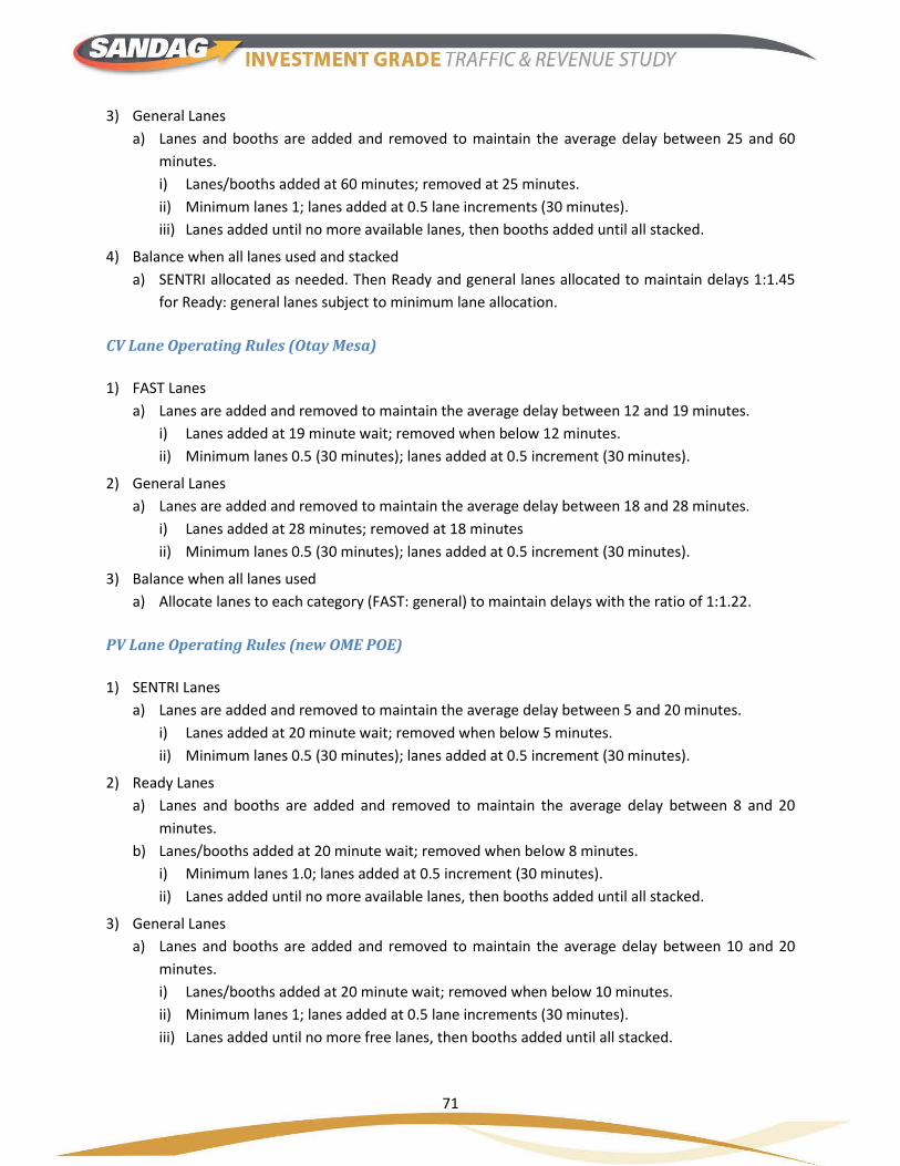
71

3) General Lanes a) Lanes and booths are added and removed to maintain the average delay between 25 and 60

minutes. i) Lanes/booths added at 60 minutes; removed at 25 minutes. ii) Minimum lanes 1; lanes added at 0.5 lane increments (30 minutes). iii) Lanes added until no more available lanes, then booths added until all stacked.

4) Balance when all lanes used and stacked a) SENTRI allocated as needed. Then Ready and general lanes allocated to maintain delays 1:1.45

for Ready: general lanes subject to minimum lane allocation.

CV Lane Operating Rules (Otay Mesa)

1) FAST Lanes a) Lanes are added and removed to maintain the average delay between 12 and 19 minutes.

i) Lanes added at 19 minute wait; removed when below 12 minutes. ii) Minimum lanes 0.5 (30 minutes); lanes added at 0.5 increment (30 minutes).

2) General Lanes a) Lanes are added and removed to maintain the average delay between 18 and 28 minutes.

i) Lanes added at 28 minutes; removed at 18 minutes ii) Minimum lanes 0.5 (30 minutes); lanes added at 0.5 increment (30 minutes).

3) Balance when all lanes used a) Allocate lanes to each category (FAST: general) to maintain delays with the ratio of 1:1.22.

PV Lane Operating Rules (new OME POE)

1) SENTRI Lanes a) Lanes are added and removed to maintain the average delay between 5 and 20 minutes.


2) Ready Lanes a) Lanes and booths are added and removed to maintain the average delay between 8 and 20

minutes. b) Lanes/booths added at 20 minute wait; removed when below 8 minutes.

i) Minimum lanes 1.0; lanes added at 0.5 increment (30 minutes). ii) Lanes added until no more available lanes, then booths added until all stacked.

3) General Lanes a) Lanes and booths are added and removed to maintain the average delay between 10 and 20

minutes. i) Lanes/booths added at 20 minute wait; removed when below 10 minutes. ii) Minimum lanes 1; lanes added at 0.5 lane increments (30 minutes). iii) Lanes added until no more free lanes, then booths added until all stacked.

72

4) Balance when all lanes used and stacked a) Allocate lanes to each category (SENTRI:Ready:general) to maintain delays with the ratio of

1:1.1:1.25. b) Toll adjusted to maintain general delay below 20 minutes.

CV Lane Operating Rules (new OME POE)

1) FAST Lanes a) Lanes are added and removed to maintain the average delay between 10 and 20 minutes.


2) General Lanes a) Lanes are added and removed to maintain the average delay between 15 and 20 minutes.


3) Balance when all lanes used a) Allocate lanes to each category (FAST:general) to maintain delays with the ratio of 1:1.2. b) Toll adjusted to maintain general lane delay below 20 minutes.

The above lane operating rules are implemented in the model to allocate process and assigning tandem operations to the scheduled number of lanes operated by CBP during different times of the day, as suggested by the historical capacity utilization levels.

Regarding the utilization of lane capacity at each POE, the model assumes that the same percentage of utilization of lanes as that observed in 2012 will be experienced in future years. For San Ysidro, the expansion of northbound lanes in 2017 will mean that more lanes will be available for users in future years, but the overall utilization of lanes (as a function of the total number of lanes) will remain the same. The model uses different percentages of utilization of total lanes for different periods of time during the day, but these percentages remain fixed throughout all future years.

Additionally, the lane processing rates and the lane utilization percentages used in the model for the OME POE are equal to those used for the Otay Mesa POE. The reason is that due to their proximity and the similarity of their border-crossing traffic (a combination of PV and CV traffic), these two POEs are expected to be relatively similar in terms of operating characteristics. The processing rates used in the binational T&R model are presented in Table 28.

Similarly, the simulation of delays is done through the same combination of volume-delay functions that capture delays on streets adjacent to the POEs and on POE crossings used in the base year. The functions incorporate growth of traffic in the estimation of delays in forecast years.

73

6.4 Latent Demand

The estimation of latent demand is an important component of the binational T&R model. In this study, the term “latent demand” is used to describe the additional border crossings generated by reductions in wait times. It is closely related to the concept of “induced demand” found in other traffic and revenue studies.46 The term “latent” is preferred here to emphasize the notion that current, excessive wait times are potentially constraining or suppressing demand for cross-border travel; and that wait time savings would simply draw out this demand as opposed to generating new, additional demand – as might be the case with highway projects opening up land for development, for example.

Reductions in expected wait times would induce people to travel across the border who would not have done so otherwise for a variety of reasons, including:

• In the short term: changes in travel destination whereby people decide to shop across the border instead of in their own country; newly generated trips brought about by reductions in the generalized cost of travel and enhanced opportunities for tourism and recreation; or increased truck movements due to reduced shipping costs (e.g., more frequent trips with smaller truckloads).

• In the long term: commercial trips generated by industrial development in the border area and/or by logistics reorganization (whereby firms substitute just-in-time delivery services for inventories and warehousing); or increased competitiveness of the border region and associated increases in economic output and employment.

An elasticity approach was used to quantify the change in the number of cross-border trips resulting from a reduction in generalized travel cost (that results, among other things, from reduced wait times at the POEs). A summary of the approach used to estimate latent demand is presented in Box 15.

46 See, for example, SANDAG’s “Economic Impact of Border-Crossing Wait Times” study where estimates of foregone border-crossing trips due to long wait times at the border are reported.

Box 15. Methodology Used in the Estimation of Latent Demand

The first step in determining the latent demand was to estimate the overall generalized cost for all the cross border trips using the existing POEs, assuming the current capacities and lane configurations. This was done by running the traffic model with current operating assumptions and extracting the generalized costs from the model output. Next, the planned capacity expansion at SY was incorporated in the model and the generalized cost was recomputed by running the traffic model. The new generalized cost would be lower because of the lower wait times as a result of capacity expansion. The reduction in generalized cost is a proxy for the reduction in travel times. The reduction in travel time, which is basically due to the reduction in wait times, would have the potential to induce some additional demand. The percent of additional demand that is attributable to this wait time savings was estimated through the application of travel time elasticity factors. For example, an elasticity factor of -0.25 means one percent reduction in travel time would result in approximately 0.25 percent increase in demand. The negative sign in the elasticity factor signifies the inverse relationship between travel time and trip demand. In the final step, the percent reduction in generalized cost was computed and the elasticity factor was applied to it to determine the percent increase in trip demand. This process was done for PVs and trucks separately.

74

When estimating changes in average wait times, the project team considered changes at the non-tolled POEs only (San Ysidro and Otay Mesa for PVs; and Otay Mesa for trucks). At the tolled POE (OME), crossers would essentially be paying for reduced delays, so that money would be substituted for time in their total, generalized travel costs.

Finally, coefficients of elasticity with respect to generalized travel costs are not readily available, so the approach chosen by the HDR team was a “compromise” whereby total border crossings are induced in proportion to the reduction in wait times at the non-tolled POEs using conservative estimates (see Box 16 for an explanation on the conservative nature of the latent demand estimation). The elasticity coefficients used in the binational T&R model are presented in Table 30. In the case of PVs, the coefficient of -0.25 means that a decrease of 1 percent in the average generalized cost of performing a border-crossing PV trip in the region will result in an increase of 0.25 percent in the total number of border-crossing PV trips in the region. Similarly, the coefficient of -0.15 for CVs means that a decrease of 1 percent in the average generalized cost of performing a border crossing CV trip in the region will result in an increase of 0.15 percent in the total number of border crossing CV trips in the region. Elasticity factors are estimated from empirical data and are held constant through the forecast years. Further

Box 16. Conservative Estimation of Latent Demand

The coefficients used in the estimation of latent demand in the binational T&R model were developed primarily from a recent study by the University of Southern California (USC). In this study, researchers report that “Meta-studies that review the results of many individual studies and attempt to draw conclusions on the value of this elasticity generally suggest that the short-run time elasticity of travel demand is between 0 and -1, with -0.5 being a plausible value. These reviews also suggest that the long-run elasticity is roughly twice the short-run elasticity, reflecting the fact that in the longer run, the number of trips made is plausibly more sensitive to the time required to make them.”

Furthermore, the study also documents the results of a July 2012 experiment at the San Ysidro border crossing that reduced wait time and resulted in an immediate and significant increase in the number of vehicles processed at the port, with a trip-wait time elasticity of about -0.5. Additional empirical evidence for personal travel and freight in a broader context was also analyzed by the study team. The evidence for PVs was found to be consistent with the conclusions of the USC study, with short-term elasticity coefficients between -0.1 and -1.0. The empirical evidence in support of induced goods movements is more limited, but available sources suggest elasticity coefficients ranging between -0.1 and -0.7.

To present a conservative estimate of latent demand, the study team arbitrarily reduced the short-run and long-run elasticities for both PVs and CVs to approximately half of the values found in the literature, as shown in the table below.

Elasticity With Respect to Travel Time for: USC Study Other Studies Used in Binational T&R Model

PV – short term -0.5 -0.22 to -0.67 -0.25

PV – long-term -1.0 -0.57 to -1.33 -0.25

CV – short term n.a. -0.15 to -0.69 -0.15

CV – long term n.a. -0.3 to -0.7 -0.15

Source: University of Southern California, National Center for Risk and Economic Analysis of Terrorism Events (2013). “The Impact on the U.S. Economy of Changes in Wait Times at Ports of Entry,” prepared for the U.S. CBP, Final Report, April 4 2013

75

details on the estimation of latent demand and the source of the elasticity coefficients are provided in Appendix M.

Table 30: Elasticity Coefficients to Estimate Latent Demand Elasticity Used for Latent Demand

Estimation USC Study

PVs -0.25

CVs -0.15

Source: HDR analysis of diverse sources

The forecasts of latent demand produced by the binational T&R model for the 2017-2056 period are presented in Figure 25 in relation to the socioeconomic-driven forecasts developed in Section 3.5. Latent demand represents an increase of border-crossing total traffic in the region (compared to the forecasts produced using only socioeconomic drivers) ranging between 5.7 million trips in 2017 and 10.1 million trips in 2056.

Notice that 2017 constitutes a particular year in the forecast of latent demand since it is the first year of its realization. A conservative treatment (similar to the concept of “ramp-up”) was assumed for latent demand in that particular year in the binational T&R model (see Box 17 for more details on the conservative estimate of latent demand in 2017 and Box 18 for short-run forecasts for the 2012-2017 period used in the binational T&R model).

6.5 Forecast of Aggregate Border-Crossing Trips Used in the Future Years

The resulting future border-crossing traffic when the socioeconomic-driven and the latent demand forecasts are combined is presented in Figure 26 for the baseline scenario. These are the values used in the binational T&R model to estimate future revenues generated by OME POE.

The total number of border-crossing trips is forecasted to exceed 68 million by 2056, with PV trips representing approximately 63.4 million (95 percent) and CV trips representing the remaining 3.7 million (5 percent).

Box 17. Latent Demand in Year 2017

Latent demand is the result of reduced border-crossing wait times faced by travelers in the region as a result of increased capacity of the POEs. In particular, the expansion of San Ysidro and the opening of OME POE in 2017 are expected to generate additional border-crossing traffic (above and beyond that predicted by the forecasts based on socioeconomic drivers) starting that year. However, it is unclear if the full potential for latent demand will be realized in the first year of these capacity expansions (i.e., 2017) due to the adjustments travelers need to undertake to perform those additional trips. Therefore, the binational T&R model makes a conservative assumption that only 75 percent of the total potential latent demand for that year will be realized. This “ramp-up” phenomenon of latent demand is assumed to be true only for 2017; throughout the remainder of the analysis period the model assumes full realization of latent demand.

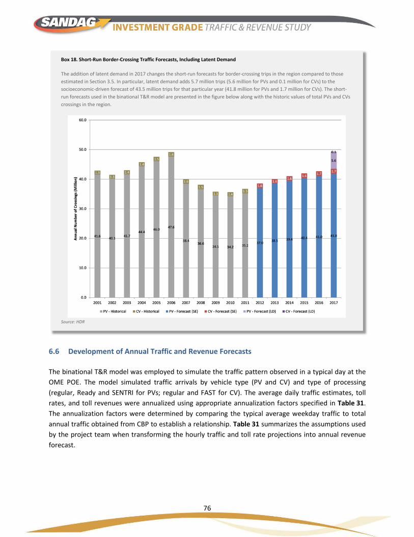
76

6.6 Development of Annual Traffic and Revenue Forecasts

The binational T&R model was employed to simulate the traffic pattern observed in a typical day at the OME POE. The model simulated traffic arrivals by vehicle type (PV and CV) and type of processing (regular, Ready and SENTRI for PVs; regular and FAST for CV). The average daily traffic estimates, toll rates, and toll revenues were annualized using appropriate annualization factors specified in Table 31. The annualization factors were determined by comparing the typical average weekday traffic to total annual traffic obtained from CBP to establish a relationship. Table 31 summarizes the assumptions used by the project team when transforming the hourly traffic and toll rate projections into annual revenue forecast.

Box 18. Short-Run Border-Crossing Traffic Forecasts, Including Latent Demand

The addition of latent demand in 2017 changes the short-run forecasts for border-crossing trips in the region compared to those estimated in Section 3.5. In particular, latent demand adds 5.7 million trips (5.6 million for PVs and 0.1 million for CVs) to the socioeconomic-driven forecast of 43.5 million trips for that particular year (41.8 million for PVs and 1.7 million for CVs). The short-run forecasts used in the binational T&R model are presented in the figure below along with the historic values of total PVs and CVs crossings in the region.

Source: HDR

77

Figure 25. Socioeconomic and Latent Demand Forecasts of Total Border-Crossing Traffic in Region, 2017-2056

Source: HDR

Figure 26. Total Forecasted Border-Crossing Traffic in Region, 2017-2056

Source: HDR

78

Table 31: Summary of Assumptions Used in the Estimation of Annual Revenue

Variable Assumed Value Source or Justification

Annualization factor for PVs, days/year 353 Calculated Based on CBP Data

Annualization factor for trucks, days/year 274 Calculated Based on CBP Data

Ramp-up period, years 0 HDR Assumption

First year traffic as a percent of steady state, % 100 HDR Assumption

Violation rate, % of total revenue lost 1.0 HDR Assumption

Source: Miscellaneous, as listed

The model was applied for the years 2017, 2030, and 2040. The traffic and revenue numbers for the 3 years were used to develop an annual traffic and revenue estimation model, as explained in Box 19.

Finally, the stream of annual revenues estimated using the binational T&R model were adjusted to account for the ramp-up behavior usually exhibited by consumers, and some potential toll violation behaviors. In the case of OME POE, it was assumed that the very first year of its operation the facility would be able to capture 100 percent of the potential trips that would actually use OME and pay tolls (i.e., no ramp-up period, see Box 20). This is the result of the high volumes of border-crossing trips and high congestion at the POEs anticipated in the region as presented in Section 3.5. However, adjustments were made to annual revenues to represent potential toll violations assuming a conservative 1 percent toll violation rate.

Box 19. Interpolation and Extrapolation of Annual Traffic and Revenue Numbers

The model was applied for three years (2017, 2030, and 2040); therefore, traffic and revenue results needed to be interpolated between those years to present an annual profile of revenues. The methodology used in that interpolation consisted of using the following formula:

Rn = A * n B + C

Where Rn is the revenue in year n

The parameters A, B, and C are determined using the estimates for 2017, 2030, and 2040.

Because revenues for the OME POE are projected over a 40-year operational life of the facility, an extrapolation methodology for those years after 2040 was developed. The extrapolation methodology consisted of applying the same annual growth rate to revenues between 2040 and 2056 as that observed for revenues in the 2030-2040 period.

79

Box 20. No Ramp-up for Traffic at SR 11/OME POE

The first years of operation of a toll road are critical for its long-run financial success; therefore, IGT&R studies traditionally include a ramp-up period. This period simulates the level of knowledge and acceptance of users to the new tolled facility, i.e., it represents the time it takes for demand to grow and stabilize as travelers adjust their trip patterns.

Traditionally ramp-up periods are estimated based on observed profiles for earlier toll roads in the same city or comparable cities around the country. However, because SR 11 will operate in conjunction with the OME POE, there is no comparable facility that can be used to determine an adequate level of ramp-up.

To determine an adequate ramp-up period for the facility, three factors were taken into consideration:

• OME POE is located approximately 2 miles east of the existing Otay Mesa POE. • An important volume of PVs using POEs in the region (56 percent) are commuters who cross the border 2 or more times

per week; furthermore, 26 percent of total PVs using POEs in the region cross the border at least 5 times per week. (Source: TrueNorth (2012). General Public Survey for Traffic and Revenue Study).

• High demand for border-crossing traffic is anticipated in the region as well as high levels of congestion at the POEs even after the expansion of San Ysidro, as described in sections 3.5 and 3.6.

The proximity of OME to Otay Mesa means that trip patterns around the area do not need adjusted for those PVs and CVs that decide to use OME POE. Similarly, a high concentration of border-crossing PV commuters in the region mean POE users, as a result of being “repeated customers” and experiencing long lines at the current POEs during any given week, will be more likely to try the new POE during its first days of operation. Finally, the high demand for border-crossing traffic and the resulting congestion at the POEs in the region are expected to provide enough incentive to border-crossing travelers to try new alternatives such as the OME POE. As a result, this report assumes the ramp-up period for SR 11 will be less than a year.

80

7 TRAFFIC AND REVENUE FORECAST

This section summarizes the projections for a baseline scenario developed using the binational T&R model and considering the OME POE is built. This baseline scenario assumes the following:

• Medium growth in aggregate cross-border traffic.

• Completion of the capacity improvements at San Ysidro by 2017, and inclusion of associated latent demand.

• Opening of a tolled facility at OME POE in 2017, with a targeted maximum border-crossing wait time of 20 minutes for PVs and CVs.

• Tolling in both directions, with tolls adjusted every hour, from a minimum toll of $2 for northbound PVs, $1 for southbound PVs, $10 for northbound trucks and $5 for southbound trucks.

• Inclusion of latent demand resulting from the expansion of San Ysidro and from the operations of the OME POE.

Daily traffic and wait time projections at San Ysidro, Otay Mesa and the OME POE are presented first. Expected capture rates and daily crossings at the OME POE are shown next. Estimated toll rates are introduced later, followed by annual traffic and revenue projections for the OME POE. A summary of the projections for the OME POE is presented to conclude this section.

7.1 Daily Traffic Projections

7.1.1 Northbound

Table 32 provides estimates of daily northbound crossings by PVs in 2017, 2030, and 2040, for San Ysidro in standard lanes and special lanes (Ready and SENTRI) respectively.

Table 32: Daily Northbound PV Crossings at San Ysidro, by Lane Type, 2017 – 2040

Period 2017 2030 2040

General Lanes

Ready Lanes

SENTRI Lanes

General Lanes

Ready Lanes

SENTRI Lanes

General Lanes

Ready Lanes

SENTRI Lanes

AM 3,100 2,150 2,850 2,800 2,800 2,500 2,650 2,700 2,850 Midday 5,600 3,250 5,650 7,300 5,100 5,500 6,300 5,300 7,050 PM 2,350 1,250 2,200 3,700 2,000 2,600 4,700 2,550 3,350 Night 6,950 3,750 2,300 8,200 4,600 2,800 9,000 5,000 3,000 Daily 18,000 10,400 13,000 22,000 14,500 13,400 22,650 15,550 16,250


81

The total northbound PV traffic passing through San Ysidro POE is projected to increase by 20 percent from 2017 to 2030. From 2030 to 2040, the growth is much less, about 9 percent. Of all the traffic using San Ysidro POE, about 42 percent would use the general lanes, 27 percent Ready lanes and 32 percent SENTRI lanes. Projections of daily northbound crossings by PVs at the Otay Mesa POE can be found in Table 33.

In 2017, about 13,000 PVs are projected to cross the border from Mexico at Otay Mesa POE. This traffic would increase by 42 percent to 18,500 in 2040. Approximately 30 percent of the passenger traffic would use general lanes and the remaining 70 percent would use the Ready and SENTRI lanes. The SENTRI lanes would see a significant use in all three forecast years as they were programmed in the model to provide a level of service that is comparable to the tolled POE. In the AM peak in all three forecast years and midday in 2040, the new POE would not have any traffic using the SENTRI lane for the same reason mentioned above (see Table 34). Passengers would not pay a toll and use the new POE when they could receive the same level of service at OM without paying any tolls.

Table 33: Daily Northbound PV Crossings at Otay Mesa, by Lane Type, 2017 – 2040

Period 2017 2030 2040

General Lanes

Ready Lanes

SENTRI Lanes

General Lanes

Ready Lanes

SENTRI Lanes

General Lanes

Ready Lanes

SENTRI Lanes

AM 800 950 1,400 650 750 2,300 650 750 2,300

Midday 1,200 1,200 1,600 1,800 1,850 4,150 2,100 1,950 3,100

PM 300 650 950 650 700 1,300 1,150 1,000 1,100

Night 1,650 1,550 800 1,550 1,550 1,100 1,800 1,550 1,100

Daily 3,950 4,350 4,750 4,650 4,850 8,850 5,700 5,250 7,600 Source: HDR Analysis

Finally, projections of daily northbound crossings by PVs at the new OME POE can be found in Table 34. The total northbound passenger traffic through the new POE would reach around 13,000, which is close to the maximum number that can be processed at this POE.

Table 34: Daily Northbound PV Crossings at OME, by Lane Type, 2017 – 2040

Period 2017 2030 2040

General Lanes

Ready Lanes

SENTRI Lanes

General Lanes

Ready Lanes

SENTRI Lanes

General Lanes

Ready Lanes

SENTRI Lanes

AM 800 1,100 0 1,200 700 0 1,200 750 0

Midday 2,750 1,400 700 3,350 1,250 100 3,500 1000 0

PM 1,350 600 400 1,500 600 500 1,700 600 250

Night 2,300 1,350 200 2,400 1,400 200 2,250 1,400 200

Daily 7,200 4,450 1,300 8,450 3,950 800 8,650 3,750 450 Source: HDR Analysis

The tables below summarize HDR’s projections of daily northbound CV crossings at both Otay Mesa and OME POE. In 2017, a significant northbound diversion of truck traffic to the new POE is expected to

82

occur. In the later years, the diversion would be less, as the capacity at the new POE would be fully used. A more detailed explanation of diversions is provided in Section 7.3.1.

Table 35: Daily Northbound CVs Crossings at Otay Mesa, by Lane Type, 2017 – 2040

Period 2017 2030 2040

Standard Lanes FAST Lanes Standard

Lanes FAST Lanes Standard Lanes FAST Lanes

AM 150 25 225 25 300 50

Midday 400 100 800 100 1,100 100

PM 200 50 450 50 650 100

Night 25 0 75 0 175 0 Daily 775 175 1,550 175 2,225 250


Table 36: Daily Northbound CVs Crossings at OME, by Lane Type, 2017 – 2040

Period 2017 2030 2040



AM 400 75 350 125 350 125

Midday 750 550 650 750 550 875

PM 400 275 400 400 400 400

Night 0 50 150 75 200 100

Daily 1,550 950 1,550 1,350 1,500 1,500 Source: HDR Analysis

7.1.2 Southbound

Table 37 provides estimates of daily southbound crossings by PVs in 2017, 2030, and 2040, for the three POEs in the region. Between 55 to 60 percent of the southbound PV traffic is expected to use San Ysidro POE. In the AM peak period, no traffic is projected to use the new POE as the wait times at San Ysidro and Otay Mesa would be fairly low.

Table 37: Daily Southbound PV Crossings San Ysidro, Otay Mesa and OME, 2017 – 2040

Period 2017 2030 2040

San Ysidro

Otay Mesa OME San

Ysidro Otay Mesa OME San

Ysidro Otay Mesa OME

AM 4,650 2,500 0 5,750 2,850 0 6,100 2,950 0

Midday 17,200 8,600 1,300 17,200 8,600 6,650 17,200 8,600 8,000

PM 9,800 4,900 3,600 9,850 4,900 6,850 9,850 4,900 7,400

Night 8,850 5,700 0 11,700 6,800 200 12,450 7,150 1,300

Daily 40,500 21,700 4,900 44,500 23,150 13,700 45,600 23,600 16,700 Source: HDR Analysis

83

The table below summarizes HDR’s projections of daily southbound CV crossings at both Otay Mesa and OME POE. The truck volumes using OME POE increase from 3,300 in 2017 to 5,500 in 2040.

Table 38: Daily Southbound CV Crossings at Otay Mesa and OME, 2017 – 2040

Period 2017 2030 2040

Otay Mesa OME Otay Mesa OME Otay Mesa OME

AM 200 0 550 0 600 25

Midday 1,400 650 1,400 1,100 1,400 1,300

PM 800 200 800 300 800 800

Night 50 0 350 100 400 175

Daily 2,450 850 3,100 1,500 3,200 2,300 Source: HDR Analysis

7.2 Wait Time Projections

7.2.1 Northbound

The binational T&R model provides estimates of traffic delays that are attributable to processing capacity shortfalls at the POE. If the number of vehicles arriving in any given hour is less than the number of vehicles that can be processed at a given POE, and if the vehicle arrivals are evenly spaced, then no vehicle would be stuck in queue; therefore, delays would be zero. However, in reality, vehicle arrivals are not evenly spaced. Therefore, even if the arriving volumes are less than the POE capacity, there is a possibility that some queues will develop; consequently, there will be slight delays experienced by some vehicles. To account for this, the estimates of average wait times produced by the traffic model were converted to a most likely range (lower bound and upper bound wait times) assuming the vehicle arrivals follow a Poisson distribution. Table 39 shows the expected wait times for the northbound PVs at San Ysidro POE in 2017, 2030, and 2040.

Table 39: Average PV Wait Times (in Minutes) at San Ysidro, Northbound, 2017 – 2040

Period 2017 2030 2040

General Lanes

Ready Lanes

SENTRI Lanes

General Lanes

Ready Lanes

SENTRI Lanes

General Lanes

Ready Lanes

SENTRI Lanes

AM 70-77 44-51 12-16 141-150 76-83 15-20 166-176 91-99 13-18

Midday 30-36 18-25 7-11 80-87 48-55 10-15 124-133 64-72 9-13

PM 26-32 16-25 8-14 27-32 15-22 8-14 45-50 25-31 7-12

Night 39-46 24-32 8-16 47-53 29-36 7-14 47-53 29-36 7-14


The wait times in the AM peak period in the general lanes are expected to increase significantly through the forecast years. For passenger traffic, the AM peak period has the highest volumes and consequently, most delays are seen in that period. In 2040, with the projected growth in passenger traffic, the wait

84

times in the general lanes at San YSidro POE could reach as high as 3 hours. The traffic model assumes the SENTRI lane capacity would be adjusted in the future to provide a higher level of service. As a result, the wait times in SENTRI lanes would be below 20 minutes. The estimates of average wait times for northbound PVs at Otay Mesa (by lane type) in 2017, 2030, and 2040 are summarized in Table 40.

Table 40: Average PV Wait Times (in Minutes) at Otay Mesa, Northbound, 2017 – 2040

Period 2017 2030 2040

General Lanes

Ready Lanes

SENTRI Lanes

General Lanes

Ready Lanes

SENTRI Lanes

General Lanes

Ready Lanes

SENTRI Lanes

AM 68-81 43-53 12-18 145-165 77-92 14-19 178-200 92-108 13-18

Midday 27-39 15-26 6-15 75-89 41-53 7-12 118-133 60-73 8-14

PM 22-42 12-24 6-14 24-37 13-24 6-14 46-58 24-34 7-15

Night 36-50 19-31 7-17 48-63 26-38 5-14 49-63 28-40 6-14


The average wait times in the general lanes are expected to increase significantly through the forecast years. In 2030 and 2040, the wait times in general lanes are projected to be slightly higher than San Yisdro POE. Again, note the wait times on SENTRI lanes are below 20 minutes.

Finally, estimates of average wait times for northbound PVs at the new OME POE (by lane type) in 2017, 2030, and 2040 are summarized in Table 41.

As seen, all wait times are under 20 minutes which is the level of service target set for the new POE. It is interesting to note the toll option in the AM peak period ceases to be a viable option for the SENTRI traffic. This is because CBP prioritizes SENTRI traffic at San Yisdro and Otay Mesa to provide a level of service comparable to the tolled POE.

Table 41: Average PV Wait Times (in Minutes) at OME, Northbound, 2017 – 2040

Period 2017 2030 2040

General Lanes

Ready Lanes

SENTRI Lanes

General Lanes

Ready Lanes

SENTRI Lanes

General Lanes

Ready Lanes

SENTRI Lanes

AM 9-13 6-10 - 10-16

6-11 - 14-19 9-14 -

Midday 6-10 5-7 1-4 9-13

6-10 - 12-16 7-11 -

PM 6-10 5-7 1-4 7-11

7-12 - 9-13 5-8 -

Night 8-13 2-4 - 7-13

5-11 - 8-12 3-6 -


Expected wait times for northbound CVs at Otay Mesa and OME (standard lanes and FAST lanes identified) are summarized in the Table 42 and Table 43. These wait times include the additional delays experienced by the truck traffic in getting access to the FAST lanes and regular truck lanes at Otay Mesa

85

POE. As shown in Table 42, the wait times at Otay Mesa in 2017, in standard lanes, would range anywhere between 45 minutes to slightly over an hour during the day. The wait times in the FAST lanes would be approximately 10 minutes less. At OME, the expected wait times are significantly less compared to Otay Mesa. They are, in general, under 15 minutes for standard lanes and under 8 minutes for FAST lanes. These results indicate that, by controlling the traffic demand at the new POE through toll adjustments, it would be possible to provide a high level of service and maintain a target wait time of under 20 minutes.

Table 42: Average CV Wait Times (in Minutes), Northbound, Otay Mesa, 2017 – 2040

Period 2017 2030 2040



AM 46-70 35-68 59-86 48-70 80-96 65-88 Midday 46-67 38-67 52-67 42-73 65-78 50-84 PM 46-69 37-72 54-69 40-72 82-97 49-74 Night 37-76 30 49-78 35-40 56-77 40-47


Table 43: Average CV Wait Times (in Minutes), Northbound, OME, 2017 – 2040

Period 2017 2030 2040



AM 3-15 1-3 3-15 1-8 1-10 1-8

Midday 3-15 1-3 3-15 1-8 1-10 1-8

PM 3-15 1-3 3-15 1-8 1-10 1-8

Night 1-5 1-3 3-15 1-8 1-10 1-8


7.2.2 Southbound

Projections of wait times for southbound PVs at all three POEs in 2017, 2030, and 2040 are summarized in Table 44.

Table 44: Average PV Wait Times (in Minutes), Southbound, 2017 – 2040

Period 2017 2030 2040

San Ysidro

Otay Mesa OME San

Ysidro Otay Mesa OME San

Ysidro Otay Mesa OME

AM 1-2 1-2 1-2 1-2 1-2 1-2 1-2 1-2 1-2

Midday 1-2 2-5 1-2 5-7 4-8 1-2 6-9 5-9 1-2

PM 3-5 4-8 1-2 13-16 12-16 4-6 20-24 20-24 9-12

Night 1-2 1-3 1-2 1-2 1-2 1-2 2-3 2-3 1-2


86

Because the inspection process is extremely expeditious southbound, the vehicle processing rates are very high. As a result, the queue lengths are much shorter than the northbound lanes; consequently, the wait times are short. In 2030 and 2040, the traffic model projects the wait times would increase for PVs at both San YSidro and Otay Mesa. However, they would still be under 30 minutes.

The expected wait times for southbound CVs are shown in Table 45. Except for the midday and PM peak period in 2040, the projected wait times in general would be under 40 minutes.

Table 45: Average CV Wait Times (in minutes), Southbound, 2017 – 2040

Period 2017 2030 2040

Otay Mesa OME Otay Mesa OME Otay Mesa OME

AM 1-8 1-2 1-6 1-2 2-10 1-2

Midday 9-19 1-2 12-23 2-6 27-39 5-14

PM 8-17 1-2 10-20 1-2 24-35 6-14

Night 1-2 1-2 5-11 1-2 6-12 1-2


7.3 Expected Daily Traffic and Revenue Projections for OME

7.3.1 Northbound Capture Rates

Table 46 summarizes HDR’s projections of daily northbound crossings and capture rates at OME in 2017, 2030, and 2040. Capture rates were calculated as a ratio of the number of crossings at OME to the total number of crossings, across all POEs (in a given direction, year, and period).

Table 46: OME Daily PV Crossings and Capture Rates, Northbound, 2017 – 2040

Period 2017 2030 2040

Daily Crossings

Capture Rate (%)

Daily Crossings

Capture Rate (%)

Daily Crossings

Capture Rate (%)

AM 1,900 14.5 1,900 13.9 1,950 14.1

Midday 4,850 20.8 4,700 15.5 4,500 14.8

PM 2,350 23.5 2,600 19.3 2,550 15.6

Night 3,850 18.5 3,950 16.6 3,850 15.2 Total Daily 12,950 19.2 13,150 16.2 12,850 14.9


Overall, the proposed OME POE would capture between a sixth and fifth of the traffic that cross the border. As seen in Table 46, the total PV crossing through OME are relatively constant, about 13,000 a day in all forecast years. This indicates the new POE would be fully utilized to its maximum assigned capacity as passengers take advantage of higher level of service for a price. Because the total traffic

87

going through OME is relatively constant and the total crossing border traffic across all POEs increases over time, the capture rates in early years are higher than later years.

The new OME POE capture rates and daily crossings by northbound CVs are summarized in Table 47. Capture rate for CVs is significantly higher than the PVs. This is largely attributable to the access constraints at the OM POE for trucks. The current geometric design of the access points to Fast and Standard truck lanes presents a significant challenge to truck traffic. It has been observed on a regular basis the truck traffic experiences extremely long delays (sometimes up to 3 hours) along with the with the PVs prior to being able to access the truck lanes. As the level of passenger traffic increases in future, these delays are projected to get much worse. Because OME would provide a target wait time of under 20 minutes, it becomes a very attractive alternative for truckers. The analysis results indicate the new POE would fill up as soon as it is open for business. As shown in Table 47, about 75 percent of the truck traffic is projected to use the new POE in 2017. For certain O-D pairs, Otay Mesa will continue to be a preferred choice for some traffic. As shown in Table 47, the new POE would be used to its full capacity in 2030 and 2040. Since the total truck traffic is increasing through the forecast years and the OME traffic is held at capacity, the truck capture rates in future years decline.

Table 47: OME Daily CV Crossings and Capture Rates, Northbound, 2017 – 2040

Period 2017 2030 2040

Daily Crossings

Capture Rate (%)

Daily Crossings

Capture Rate (%)

Daily Crossings

Capture Rate (%)

AM 450 74.1 500 65.7 450 56.6

Midday 1,300 73.4 1,400 60.4 1,400 54.4

PM 700 76.9 800 62.0 800 50.9

Night 50 82.2 200 76.7 250 60.8 Total Daily 2,500 74.6 2,900 62.7 2,900 54.3


7.3.2 Southbound Capture Rates

OME POE capture rates and daily southbound crossings from the U.S. to Mexico are shown in Table 48 (PV) and Table 49 (CV), below.

The average weekday capture rate for southbound PVs is expected to grow from about 7 percent in 2017 to almost 20 percent in 2040. Larger capture rates are expected in the midday and PM periods than in the morning and at night.

88

Table 48: OME Daily PV Crossings and Capture Rates, Southbound, 2017 – 2040

Period 2017 2030 2040

Daily Crossings

Capture Rate (%)

Daily Crossings

Capture Rate (%)

Daily Crossings

Capture Rate (%)

AM - 0.0 - 0.0 - 0.0

Midday 1,300 4.8 6,650 20.4 8,000 23.6

PM 3,600 19.7 6,850 31.7 7,400 33.3

Night - 0.0 200 1.2 1,300 6.2 Total Daily 4,900 7.3 13,700 16.9 16,700 19.4


As shown below, the proposed OME POE would capture more than a quarter of the trucks in the opening year, increasing to more than 40 percent in the future.

Table 49: OME Daily CV Crossings and Capture Rates, Southbound, 2017 – 2040

Period 2017 2030 2040

Daily Crossings

Capture Rate (%)

Daily Crossings

Capture Rate (%)

Daily Crossings

Capture Rate (%)

AM - 0.0 0.0 25 2.6

Midday 650 31.4 1,100 43.3 1,275 47.4

PM 200 20.3 300 26.3 800 49.6

Night 0.0 100 23.3 200 31.8 Total Daily 850 25.7 1,500 32.1 2,300 41.3


7.4 Projected Toll Rates at OME POE

7.4.1 Northbound

Projected toll rates at OME for northbound PVs are summarized in

Table 50. Estimates are in constant 2012 dollars. For PV traffic, the highest delays at San YSidro and Otay Mesa occur during the AM peak period. The tolls at the new POE therefore, are highest during the same period since the wait times there would be under 20 minutes. The average tolls during the AM peak period would be in the range of $7 to $13 in 2017, $13 to $33 in 2030 and $16 to $42 in 2040. Though the toll for PVs hits a maximum of $42 in 2040, it stays at that level only for one hour (between 8 AM and 9 AM) and drops to below $30 in the AM peak. The toll range shown for night time is slightly higher than PM because the early morning peak (3 to 4 AM) is included in the night time period. The daily average toll was estimated by weighting the hourly tolls by the corresponding hourly volumes. In 2017, we are projecting about $4, in 2030 about $12 and in 2040, about $19 for PVs.

89

Table 50: Projected Toll Rates for PVs, Northbound, 2017 – 2040

Period Average Toll (2012 dollars)

2017 2030 2040

AM $7 to $13 $13 to $33 $16 to $42*

Midday $2 to $3 $9 to $22 $16 to $36

PM $2 to $3 $2 to $5 $3 to $9

Night $2 to $5 $2 to $10 $2 to $11

Average Daily $4.00 $11.50 $19.00 Source: HDR Analysis * The toll for PVs is projected to peak at $42 between 8 am and 9 am and drop sharply to $30 and stay below $30 for rest of the time period

Future expected toll rates for CVs (in constant 2012 dollars) are shown in Table 51, below. As seen, the toll range for trucks in Midday and PM are much tighter than for PVs. In the PM peak period, the CV tolls would rise as high as $47. For most part, CV tolls within each time period are observed to be closer to the higher range of the toll and stay high for longer hours. The average daily toll rate for CVs in 2017 is projected to be about $15, in 2030, $18 and in 2040, $26. These averages were estimated by weighting the hourly toll rates by the corresponding hourly traffic.

Table 51: Projected Toll Rates for CVs, Northbound, 2017 – 2040


2017 2030 2040

AM $10 to $17 $10 to $16 $10 to $22

Midday $11 to $17 $16 to $20 $19 to $26

PM $10 to $17 $18 to $ 22 $31 to $47

Night $10 $10 to $12 $10 to $17

Average Daily $14.50 $18.00 $26.00 Source: HDR Analysis

7.4.2 Southbound

Projected southbound toll rates can be found in Table 52 (for PVs) and Table 53 (for CVs). In nearly all years and periods, average tolls would be at or close to the assumed minimum value ($1.0 for PVs, and $5.0 for trucks).

90

Table 52: Projected Toll Rates for PVs, Southbound, 2017 – 2040


2017 2030 2040

AM $0.00 $0.00 $1.00

Midday $1.00 $1.00 $1.00

PM $1.00 $1.00 $1.25

Night $0.00 $1.00 $1.00

Average Daily $0.50 $0.75 $1.00 Source: HDR Analysis

The toll rates for southbound CVs are expected to start going above the minimum levels by 2040 as the CV volume increases and begins to cause increasing delays.

Table 53: Projected Toll Rates for Trucks, Southbound, 2017 – 2040


2017 2030 2040

AM $0.00 $0.00 $5.00

Midday $5.00 $5.50 $10.00

PM $5.00 $5.00 $6.50

Night $0.00 $5.00 $5.00

Average Daily $2.50 $4.00 $6.50


7.5 Annual Traffic and Revenue Projections for OME

The summary of annual revenue projections for all years between 2017 and 2056 for the baseline scenario are shown in Table 54, along with estimates of annual transactions.

Table 54: Annual Revenue Projections by Vehicle Type and Calendar Year, Baseline Scenario

Calendar Year Annual Revenue, Millions of Constant 2012

Dollars Annual Transactions, Millions

PVs CVs Total PVs Trucks Total 2017 $20.23 $10.87 $31.11 6.30 1.16 7.47

2018 $22.84 $10.95 $33.79 7.31 1.19 8.50

2019 $25.59 $11.12 $36.71 7.68 1.21 8.89

2020 $28.42 $11.35 $39.77 7.95 1.24 9.19

2021 $31.31 $11.64 $42.95 8.18 1.27 9.45

2022 $34.25 $11.98 $46.23 8.37 1.30 9.67

2023 $37.23 $12.37 $49.60 8.55 1.32 9.87

2024 $40.24 $12.81 $53.05 8.71 1.35 10.06

2025 $43.28 $13.30 $56.58 8.86 1.38 10.24

2026 $46.35 $13.83 $60.18 9.00 1.41 10.41

91

Calendar Year Annual Revenue, Millions of Constant 2012

Dollars Annual Transactions, Millions

PVs CVs Total PVs Trucks Total 2027 $49.44 $14.41 $63.86 9.13 1.44 10.57

2028 $52.56 $15.04 $67.60 9.25 1.47 10.72

2029 $55.69 $15.71 $71.40 9.37 1.50 10.86

2030 $58.84 $16.43 $75.27 9.48 1.53 11.01

2031 $62.01 $17.19 $79.20 9.58 1.56 11.14

2032 $65.20 $18.00 $83.19 9.69 1.59 11.28

2033 $68.40 $18.85 $87.25 9.79 1.62 11.40

2034 $71.61 $19.74 $91.36 9.88 1.65 11.53

2035 $74.84 $20.68 $95.53 9.98 1.68 11.65

2036 $78.09 $21.66 $99.75 10.06 1.71 11.77

2037 $81.34 $22.69 $104.04 10.15 1.74 11.89

2038 $84.61 $23.76 $108.38 10.24 1.77 12.01

2039 $87.89 $24.88 $112.77 10.32 1.80 12.12

2040 $91.18 $26.04 $117.22 10.40 1.83 12.23

2041 $94.49 $27.24 $121.73 10.48 1.86 12.34

2042 $97.80 $28.49 $126.29 10.56 1.89 12.45

2043 $101.12 $29.79 $130.91 10.63 1.92 12.56

2044 $104.45 $31.12 $135.58 10.70 1.96 12.66

2045 $107.79 $32.51 $140.30 10.78 1.99 12.76

2046 $111.14 $33.93 $145.08 10.85 2.02 12.87

2047 $114.50 $35.41 $149.91 10.92 2.05 12.97

2048 $117.87 $36.92 $154.80 10.98 2.08 13.07

2049 $121.25 $38.49 $159.73 11.05 2.11 13.16

2050 $124.63 $40.09 $164.73 11.12 2.14 13.26

2051 $128.02 $41.75 $169.77 11.18 2.18 13.36

2052 $131.42 $43.45 $174.87 11.25 2.21 13.45

2053 $134.83 $45.19 $180.02 11.31 2.24 13.55

2054 $138.25 $46.98 $185.23 11.37 2.27 13.64

2055 $141.67 $48.82 $190.48 11.43 2.30 13.73

2056 $145.10 $50.70 $195.79 11.49 2.33 13.82

Total Over 40 Years $3,225.80 $1,006.18 $4,231.98 394.32 69.27 463.59

* Before adjustments for ramp-up and toll violations Source: HDR Analysis

The relative contribution of PVs and CVs in revenue, as well as a number of transactions at OME are shown in the figures below.

92

Figure 27: Relative Contribution of Transactions Between PVs and CVs


Figure 28: Relative Contribution of Revenue Between PVs and CVs


As shown in the charts, PVs contribute to 85 percent of the transactions and generate 76 percent of the revenue. The annual revenue stream is shown in Figure 29. As shown, PVs continue to generate a major share of the revenue; however, CVs begin to show a growth trend as southbound CVs begin to choose the toll option.

85%

15%


76%

24%


93

Figure 29: Annual Revenue Stream in Constant 2012 Dollars, OME POE Baseline Scenario


Table 55 is a summary of the baseline revenue results for 40 years of operation of OME POE. Notice the table presents undiscounted revenues in 2012 dollars.

Table 55: Summary of OME POE Revenues in Baseline Scenario

Market Segment 40-Year Revenue Estimate (in millions of undiscounted 2012 dollars)

PVs $ 3,225

CVs $ 1,006

Total $ 4,231 Source: HDR Analysis

Because the binational T&R model uses a series of conservative assumptions, the revenues presented herein are considered to be conservative in nature. In particular, since the binational T&R model does not perform a revenue-maximization exercise, additional revenues could be generated by a future analysis of the characteristics of potential users of OME POE (see Box 21 for a discussion on the possible characteristics of VOT for users of OME POE).

$0

$50

$100

$150

$200

$250

2017

2018

2019

2020

2021

2022

2023

2024

2025

2026

2027

2028

2029

2030

2031

2032

2033

2034

2035

2036

2037

2038

2039

2040

2041

2042

2043

2044

2045

2046

2047

2048

2049

2050

2051

2052

2053

2054

2055

2056

Annu

al R

even

ue ($

Mill

ion)

CV

PV

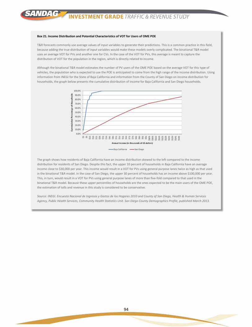
94

Box 21. Income Distribution and Potential Characteristics of VOT for Users of OME POE

T&R forecasts commonly use average values of input variables to generate their predictions. This is a common practice in this field, because adding the true distribution of input variables would make these models overly complicated. The binational T&R model uses an average VOT for PVs and another one for CVs. In the case of the VOT for PVs, this average is meant to capture the distribution of VOT for the population in the region, which is directly related to income.

Although the binational T&R model estimates the number of PV users of the OME POE based on the average VOT for this type of vehicles, the population who is expected to use the POE is anticipated to come from the high range of the income distribution. Using information from INEGI for the State of Baja California and information from the County of San Diego on income distribution for households, the graph below presents the cumulative distribution of income for Baja California and San Diego households.

The graph shows how residents of Baja California have an income distribution skewed to the left compared to the income distribution for residents of San Diego. Despite this fact, the upper 10 percent of households in Baja California have an average income close to $30,000 per year. This income would result in a VOT for PVs using general purpose lanes twice as high as that used in the binational T&R model. In the case of San Diego, the upper 30 percent of households has an income above $100,000 per year. This, in turn, would result in a VOT for PVs using general purpose lanes of more than five-fold compared to that used in the binational T&R model. Because these upper percentiles of households are the ones expected to be the main users of the OME POE, the estimation of tolls and revenue in this study is considered to be conservative.

Source: INEGI. Encuesta Nacional de Ingresos y Gastos de los Hogares 2010 and County of San Diego, Health & Human Services Agency, Public Health Services, Community Health Statistics Unit. San Diego County Demographics Profile, published March 2013.

95

8 SENSITIVITY ANALYSIS

The results presented in Section 7 considered a new border crossing facility with 20 lanes (10 lanes for PVs and 10 lanes for CVs), operating with a maximum 20 minute wait time target. The traffic and revenue estimates were developed under a set of “baseline” assumptions about future demand and operating conditions. Clearly, variations in any of these conditions can impact the estimated revenues. To gain insight into the impacts of such variations, HDR estimated the changes in traffic and revenue that result from varying the following system attributes:

Market Related • Higher socioeconomic growth and associated demand for crossings • Lower socioeconomic growth and associated demand for crossings • No latent demand

Operations Related • Availability of necessary resources for CBP to operate all available lanes at all POEs in the

region (i.e., full theoretical capacity)

Capacity Related • Lower service level guarantee (30 minute wait time guarantee) • Smaller capacity for OME POE

The first three variations are considered external factors vis-a-vis the proponents of the OME POE, while the last two considerations are an operational decision that needs to be made by OME POE proponents. The following sections discuss the basis for considering these variations, and the impacts of each of these variations on the traffic and revenue estimates.

8.1 Higher Growth in Border-Crossing Demand

Recent economic trends have shown that there are multiple factors that can impact economic growth and consequently the growth in demand for border crossings. The study team considered a high growth demand scenario for cross border movements to estimate the traffic and revenue for the 40-year time period.

Despite the availability of long-range estimates for annual high growth rates in border-crossing traffic (see Table 13 and Table 14 in Section 3.5), the HDR team found that using these high growth rates generated a total amount of border-crossing trips in the region that could not be sustainably processed given the total capacity of all the POEs. In particular, the use of high growth rates previously forecasted meant utilized capacity of all the POEs in the region was reached early into the analysis period (around 2030), leaving large numbers of traffic volumes unprocessed in the subsequent years. Moreover, this number of unprocessed vehicles grows at a compounded rate and its magnitude in the years after 2050 was found to be significant.

96

To delay as much as possible reaching the limit of border-crossing capacity in the region, the HDR team defined the border-crossing traffic used in the high demand scenario as that resulting from the following two situations: (i) a higher growth rate in total border-crossing traffic during the 2012-2017 period; and, (ii) an increase of 20 percent in the long-growth rate (i.e., 2017-2056) compared to that observed in the baseline scenario.47 Figure 30 presents the comparison between the baseline, high demand and low demand sensitivity scenarios in terms of total border-crossings.

Figure 30. Baseline, High and Low Growth Demand Forecasts of Border-Crossing Trips, 2017–2056

Source: HDR

The higher 2012-2017 growth rate for border-crossing traffic used in this scenario results from using the same coefficients of the econometric equation as those used in the estimation of the baseline 2012-2017 short-run growth rate but applied to the high-range of the socioeconomic inputs and then adding the corresponding latent demand for year 2017. In particular, the implicit 2012-2017 average annual growth rate of border-crossing traffic used in this scenario is 5.9 percent, compared to an implicit rate of

47 For sensitivity analysis, USDOT recommends using a range of ±20 percent with respect to the values of the inputs used in the baseline scenario.

97

5.0 percent used in the baseline scenario.48 Notice this growth rate represents slightly less than a 20 percent increase to the implicit growth rate used in the baseline.

The results, shown in Table 56, represent the upside of demand and the corresponding revenue is as high as $6.9 billion. The most significant impact is on the tolls collected from PVs.

Table 56. Impact of Potentially High Growth on OME POE Revenues

Market Segment Baseline High Growth

Revenue ($ million) Share (%) Revenue ($ million) Share (%)

PVs $ 3,225 76 $5,073 74

CVs $ 1,006 24 $1,814 26

Total $ 4,231 $6,887 Source: HDR Analysis

It is worth noting that the revenues generated under this scenario are merely indicative of what users would be paying to overcome the social cost of wait times at the border and not necessarily of the revenues that would be actually collected at OME POE. The reason is that POE capacity in the region under these high growth forecasts is reached approximately in 2041. When the capacity of the system of POEs is reached, a series of events occur that lead to unsustainable border-crossing behavior. First, tolls increase significantly above what travelers are willing to pay. Second, latent demand is reduced due to increasing wait times experienced at the border. Finally, high tolls and wait times drive travelers to explore border-crossing alternatives that lie beyond the scope of the binational T&R model (such as using Tecate’s POE or switching to a different transportation mode). Therefore, when the limit of POE capacity in the region is reached, an assessment of additional capacity expansion in the region should be undertaken to determine the appropriate flows of future revenues that OME POE could generate.

8.2 Lower Growth in Border-Crossing Demand

The study team considered a low growth demand scenario for cross-border movements to estimate the traffic and revenue for the 40-year time period. In order to be consistent with the development of the high growth scenario, the low demand scenario is defined based on two characteristics: (i) a lower growth rate in total border-crossing traffic during the 2012-2017 period; and, (ii) a 20 percent reduction in the long-run growth rate (i.e., 2017-2056) compared to that observed in the baseline scenario.

48 Forecasted border-crossing volumes are comprised of a socioeconomic-driven component and a latent-demand-driven component. Since the latent demand component is only realized starting in 2017, the 2012-2017 average annual growth rate mentioned here is an implicit growth rate. Finally, notice that because forecasted latent demand is zero in the years between 2012 and 2016, the actual average annual growth rates observed between 2012 and 2016 (i.e., those resulting from socioeconomic-driven growth only) are significantly lower than the implicit growth rates estimated for the 2012-2017 period.

98

The lowest 2012-2017 growth rate for border-crossing traffic found using the econometric analysis resulted from applying the coefficients of the econometric equation estimated using the pre 9/11 sample (see Section 3.5) to the low-range of the socioeconomic inputs used to estimate the 2012-2017 baseline and then adding the corresponding latent demand for year 2017. In particular, the 2012-2017 implicit average annual growth rate of border-crossing traffic found using this econometric model was 3.3 percent. This rate represents a 34 percent reduction, compared to the implicit rate of 5.0 percent used in the baseline scenario.

A low demand scenario where border-crossing traffic growth between 2012 and 2017 averages 3.3 percent per year seems to be too pessimistic given the latest data available on total border-crossing traffic in the region (see Box 22). Therefore, the low growth scenario for this sensitivity analysis was defined using a 2012-2017 implicit growth rate of 4.0 percent, which represents a reduction of approximately 20 percent with respect to the implicit growth rate used in the baseline.

The results, shown in Table 57, forecast that revenues generated by OME POE are approximately $2 billion. As in previous cases, the most significant impact is on the tolls collected on PVs.

Table 57: Impact of Potentially Sluggish Growth on OME POE Revenues

Market Segment Baseline Low Growth


PVs $ 3,225 76 $1,475 74

CVs $ 1,006 24 $510 26


8.3 No Latent Demand

The study team also considered a scenario in which no latent demand was added to the socioeconomic projections of border-crossing traffic in the region. The reduction in total border-traffic in the region (of approximately 15 percent on a yearly basis) results in revenues of approximately $1.9 billion, as shown in Table 58.

Box 22. Implicit Growth Rates for 2012-2017 Traffic In High and Low Growth Scenarios

In the case of the baseline scenario, the implicit annual growth rate of border-crossing traffic between 2012 and 2017 is 5.0 percent. In the case of the high demand scenario, the implicit growth rate used is 5.9 percent. For the low demand scenario the implicit annual growth rate used is 3.3 percent.

The USDOT recently published the “Draft Release of Border Crossing Entry Data” that reports a growth of 4.2 percent in total border-crossing traffic at San Ysidro and Otay Mesa between 2012 and 2013. In light of these numbers and the fact they only represent socioeconomic-driven growth (as no expansion of capacity occurred in 2013), the implicit growth rate of 3.3 percent (which incorporates a component of latent demand of 2017) seemed too pessimistic to depict a low growth rate situation.

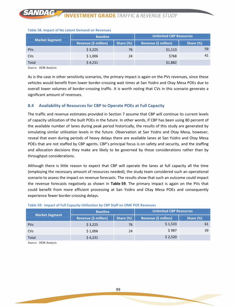
99

Table 58. Impact of No Latent Demand on Revenues

Market Segment Baseline Unlimited CBP Resources


PVs $ 3,225 76 $1,113 59

CVs $ 1,006 24 $768 41


As is the case in other sensitivity scenarios, the primary impact is again on the PVs revenues, since these vehicles would benefit from lower border-crossing wait times at San Ysidro and Otay Mesa POEs due to overall lower volumes of border-crossing traffic. It is worth noting that CVs in this scenario generate a significant amount of revenues.

8.4 Availability of Resources for CBP to Operate POEs at Full Capacity

The traffic and revenue estimates provided in Section 7 assume that CBP will continue its current levels of capacity utilization of the built POEs in the future. In other words, if CBP has been using 80 percent of the available number of lanes during peak period historically, the results of this study are generated by simulating similar utilization levels in the future. Observation at San Ysidro and Otay Mesa, however, reveal that even during periods of heavy delays there are available lanes at San Ysidro and Otay Mesa POEs that are not staffed by CBP agents. CBP’s principal focus is on safety and security, and the staffing and allocation decisions they make are likely to be governed by those considerations rather than by throughput considerations.

Although there is little reason to expect that CBP will operate the lanes at full capacity all the time (employing the necessary amount of resources needed), the study team considered such an operational scenario to assess the impact on revenue forecasts. The results show that such an outcome could impact the revenue forecasts negatively as shown in Table 59. The primary impact is again on the PVs that could benefit from more efficient processing at San Ysidro and Otay Mesa POEs and consequently experience fewer border-crossing delays.

Table 59: Impact of Full Capacity Utilization by CBP Staff on OME POE Revenues



PVs $ 3,225 76 $ 1,533 61

CVs $ 1,006 24 $ 987 39

Total $ 4,231 $ 2,520 Source: HDR Analysis

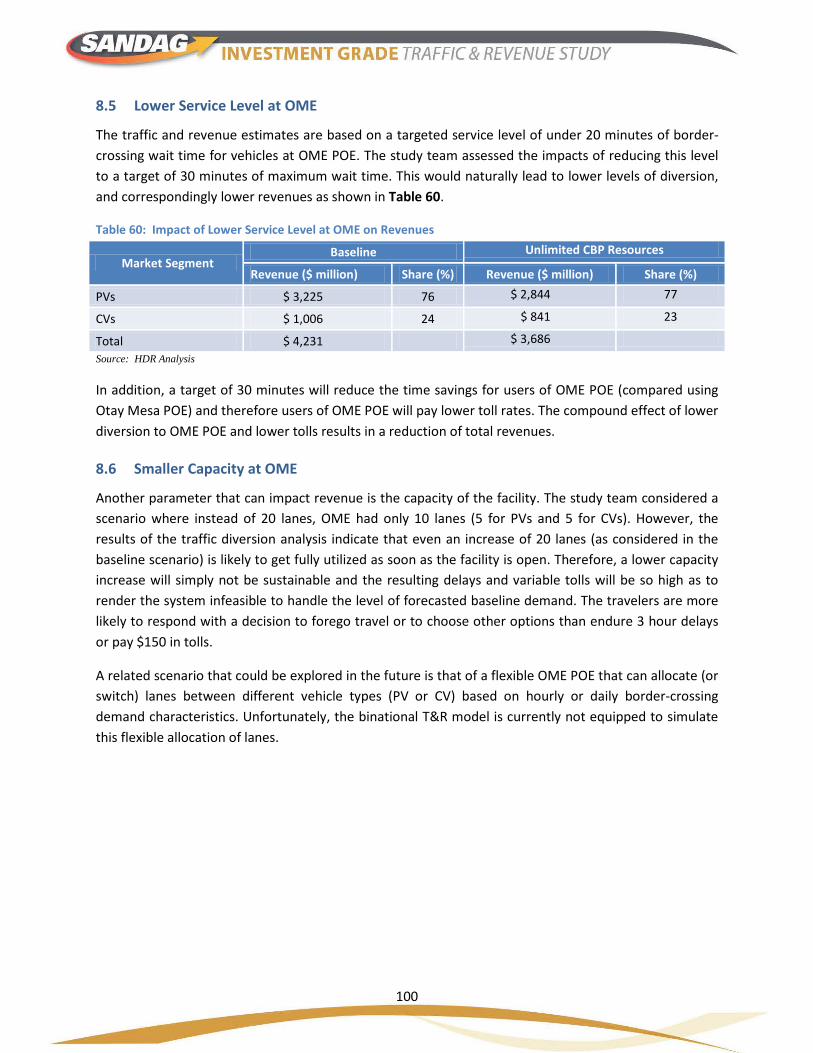
100

8.5 Lower Service Level at OME

The traffic and revenue estimates are based on a targeted service level of under 20 minutes of border-crossing wait time for vehicles at OME POE. The study team assessed the impacts of reducing this level to a target of 30 minutes of maximum wait time. This would naturally lead to lower levels of diversion, and correspondingly lower revenues as shown in Table 60.

Table 60: Impact of Lower Service Level at OME on Revenues



PVs $ 3,225 76 $ 2,844 77

CVs $ 1,006 24 $ 841 23

Total $ 4,231 $ 3,686 Source: HDR Analysis

In addition, a target of 30 minutes will reduce the time savings for users of OME POE (compared using Otay Mesa POE) and therefore users of OME POE will pay lower toll rates. The compound effect of lower diversion to OME POE and lower tolls results in a reduction of total revenues.

8.6 Smaller Capacity at OME

Another parameter that can impact revenue is the capacity of the facility. The study team considered a scenario where instead of 20 lanes, OME had only 10 lanes (5 for PVs and 5 for CVs). However, the results of the traffic diversion analysis indicate that even an increase of 20 lanes (as considered in the baseline scenario) is likely to get fully utilized as soon as the facility is open. Therefore, a lower capacity increase will simply not be sustainable and the resulting delays and variable tolls will be so high as to render the system infeasible to handle the level of forecasted baseline demand. The travelers are more likely to respond with a decision to forego travel or to choose other options than endure 3 hour delays or pay $150 in tolls.

A related scenario that could be explored in the future is that of a flexible OME POE that can allocate (or switch) lanes between different vehicle types (PV or CV) based on hourly or daily border-crossing demand characteristics. Unfortunately, the binational T&R model is currently not equipped to simulate this flexible allocation of lanes.

san diego association of governments

Documents