saline groundwater in mono basin, california 1. distribution · water resources research, vol. 31,...

WATER RESOURCES RESEARCH, VOL. 31, NO. 12, PAGES 3131-3150, DECEMBER 1995

Saline groundwater in Mono Basin, California 1. Distribution

David B. Rogers • and Shirley J. Dreiss 2 Earth Sciences Department, University of California, Santa Cruz

Abstract. Mono Lake, California is a perennial, closed-basin saline lake. Up to 2 km of sediments have accumulated below the lake, and a well log shows that saline groundwater of concentration >18,000 ppm extends to the bottom of the basin fill. We investigated the groundwater system with the variable-density flow and solute transport code SUTRA to determine if the basin's recharge and inferred groundwater salinity are consistent with observational data. Steady state model predictions of the position and shape of the interface separating saline from fresh groundwater are consistent with the salinity profile derived from the spontaneous-potential (SP) log of a geothermal well on the lake's shoreline. We also inferred the basin-wide saline groundwater distribution and concentration from experiments with a steady state model of the entire basin groundwater system. Hydrologic variations around the lake determine the position of the saline-fresh groundwater interface: Higher recharge rates characteristic of the Sierra Nevada shoreline push the interface far beneath the lake. The interface probably lies below the shoreline around much of the rest of the lake. On the low-recharge northeastern shoreline the interface top may lie outside the lake edge. This positions the saline groundwater discharge zone just below the playa surface and contributes to development of salt flats on the recently exposed former lake bed. Simulations suggest that the basin fill permeability may not have significant anisotropy, possibly owing to extensive faulting which increases vertical permeability. For an anisotropic basin fill, the resultant increased channeling of recharge beneath the lake readily overcomes the opposing force of the saline groundwater density, and it is flushed out of the basin sediments. A simple permeability representation of the basin lithology, with low permeability below the lake and an anisotropic transition to higher permeability outside the lake, reasonably represents the well and spring water salinity observations.

Introduction

Mono Lake is at least 700 kyr old [Gilbert et al., 1968; Lajoie, 1968; Christensen et al., 1969] and is thought to be among the oldest perennial lakes in North America, as many other lakes were formed following the last glacial retreat [National Re- search Council, 1987]. (We follow the convention that time periods are referred to as kyr or Myr and dates before present as ka or Ma.) The 46-m-deep lake is saline (with a total dissolved solids (TDS) concentration of about 90,000 ppm) and alkaline (pH ---9.7). It is located roughly in the center of Mono Basin (Figure 1), a hydrologically closed, 3-4-Myr-old sedimentary basin [Gilbert et al., 1968; Christensen et al., 1969] located at the base of the Sierra Nevada's eastern escarpment. The basin sediments beneath the lake contain saline groundwater (concentration >18,000 ppm) that is probably a combination of connate water and recirculating lake water. This saline groundwater contains the majority (--•80%) of the total mass of dissolved solids in the basin [Rogers, 1993b] and significantly affects groundwater circulation, because of the den-

•Now at Water Quality and Hydrology Group, Los Alamos National Laboratory, Los Alamos, New Mexico.

2Deceased December 14, 1993.

Copyright 1995 by the American Geophysical Union.

Paper number 95WR02108. 0043-1397/95/95 WR-02108505.00

sity contrast with fresher recharge water. The mixing of saline and fresh groundwaters appears to exert an important influence on the chemistry of springs and shallow groundwater surrounding the lake.

Los Angeles began diverting surface water from Mono Basin for municipal use in November 1940. As a result, the lake level has fallen 14 m, salinity has doubled, and lake volume has decreased by more than half. In an accompanying paper [Rog- ers and Dreiss, this issue] we address the impact of this lake level decline and consequent salinity increase on the basin solute balance.

This paper summarizes the many different data bearing on the hydrology of Mono Basin, including information pertaining to surface water and groundwater, geochemistry, isotopes, geo- physics, geology, and climate and helps to establish a compre- hensive conceptual model of closed-basin hydrology. We de- scribe the likely position of the saline groundwater interface, using field observations and steady state variable-density flow and solute transport simulations. We use the model (1) to determine whether the present basin recharge and inferred groundwater salinity are consistent with observational data on the occurrence of saline groundwater and (2) to examine the sensitivity of simulated circulation patterns to the model parameters, e.g., intrinsic permeability, recharge, and groundwater concentration. The latter exercise provides insight into the factors controlling the distribution and stability of the saline groundwater body underlying Mono Lake.

3131

3132 ROGERS AND DREISS: SALINE GROUNDWATER IN MONO BASIN, CALIFORNIA, 1

asin

Black

,',',;,;,;,;,,,,,

:Island GRI

N

Beach

Quaternary sediments and volcanic ash

B' Pleistocene glacial deposits

• / Quaternary volcanics

,•iiiiiiii!ili;;,,,,!i 05 10 • Tertiary volcanics ........... and sediments km

;,,5, 0 5 10 •[• Pre-tertiary granite ........... and metamorphics mi

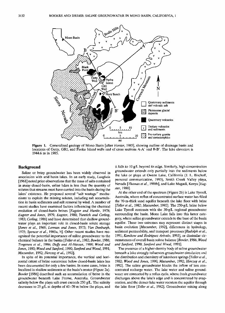
Figure 1. Generalized geology of Mono Basin [after Vorster, 1985], showing outline of drainage basin and locations of Getty, GRI, and Paoha Island wells and of cross sections A-A' and B-B'. The lake elevation is 1944.6 m in 1985.

Background Saline or briny groundwater has been widely observed in

association with arid basin lakes. In an early study, Langbein [1961] noted prior observations that the mass of salts contained in many closed-basin, saline lakes is less than the quantity of solutes that streams must have carried into the basin during the lakes' existence. He proposed several "salt wastage" mecha- nisms to explain the missing solutes, including salt accumulation in basin sediments and salt removal by wind. A number of recent studies have examined factors influencing the chemical evolution of closed-basin brines [Eugster and Hardie, 1978; Eugster and Jones, 1979; Eugster, 1980; Yuretich and Ceding, 1983; Ceding, 1986] and have determined that shallow groundwater plays an important role in closed-basin solute storage [Jones et al., 1969; Lerman and Jones, 1973; Van Denburgh, 1975; Spencer et al., 1985a, b]. Other recent studies have rec- ognized the potential importance of saline groundwater to the chemical balance in the basins [Teller et al., 1982; Bowler, 1986; Torgersen et al., 1986; Duffy and AI-Hassan, 1988; Wood and Jones, 1990; Wood and Sanford, 1990; Sanford and Wood, 1991; Macumber, 1992; Herczeg et al., 1992].

In spite of its potential importance, the vertical and horizontal extent of brine occurrence below closed-basin lakes has

been documented for only a few basins. In some cases, brine is localized in shallow sediments at the basin's center (Figure 2a). Bowler [1986] described such an accumulation of brine in the groundwater beneath Lake Frome, Australia. Groundwater salinity below the playa salt crust exceeds 250 g/L. The salinity decreases to 25 g/L at depths of 40-70 m below the playa, and

it falls to 10 g/L beyond its edge. Similarly, high-concentration groundwater extends only partially into the sediments below the lake or playa at Owens Lake, California (J. L. Bischoff, personal communication, 1993), Smith Creek Valley playa, Nevada [Thomas et al., 1989b], and Lake Magadi, Kenya [Eug- ster, 1980].

At the other end of the spectrum (Figure 2b) is Lake Tyrrell, Australia, where reflux of concentrated surface water has filled the 70-m-thick sand aquifer beneath the lake floor with brine [Teller et al., 1982; Macumber, 1992]. The 250-g/L brine below Lake Tyrrell contrasts with the 30-g/L regional groundwater surrounding the basin. Mono Lake falls into this latter cate- gory, where saline groundwater extends to the base of the basin aquifer. These two extremes may represent distinct stages in basin evolution [Macumber, 1992], differences in hydrology, sediment permeability, and transport processes [Rudolph et al., 1991; Konikow and Rodriguez Ar•valo, 1993], or dissimilar cir- cumstances of overall basin solute balance [Bowler, 1986; Wood and Sanford, 1990; Sanford and Wood, 1991].

The presence of a higher-density body of saline groundwater beneath a lake strongly influences groundwater circulation and the distribution and chemistry of lakeshore springs [Teller et al., 1982; Wood and Jones, 1990; Macumber, 1992; Herczeg et al., 1992]. The saline groundwater blocks the inflow of less concentrated recharge water. The lake water and saline groundwater are connected by a reflux cycle, where fresh groundwater discharges above the lake's edge and is concentrated by evaporation, and the denser lake water reenters the aquifer through the lake floor [Teller et al., 1982]. Groundwater mixing along

ROGERS AND DREISS: SALINE GROUNDWATER IN MONO BASIN, CALIFORNIA, 1 3133

the interface beneath the lake or playa edge may carry solutes from the deep brine back to the surface, where they discharge through springs or seepage zones [Teller et al., 1982; Macum- ber, 1992; Herczeg et al., 1992].

Duffy and Al-Hassan [1988] and McCleary-Hanagan and Duffy [1989] investigated the dynamics of brine circulation below the playa at Pilot Valley, Utah, and McCleary-Hanagan and Duffy [1989] examined how asymmetric recharge and horizontal stratification affect the position of the saline-fresh interface. They inferred from the salinity of the shallow aquifer [Lines, 1979] that concentrated groundwater extends to the bottom of the basin fill in Pilot Valley. Duffy and AI-Hassan [1988] found that a relatively sharp interface probably forms between the fresh recharge water and the brine and showed that the position of the interface depends on the balance between the system's physical properties, i.e., sediment permeability, fluid density difference, recharge rate, dispersive dissipation, and the flow system's aspect ratio.

In this paper we present a similar analysis, with the goals of inferring the extent of saline groundwater within Mono Basin and providing a basis for interpreting the impact of this saline groundwater on the basin's solute budget and cycling. The distribution and circulation of saline groundwater in Mono Basin affect shoreline groundwater quality [Rogers et al., 1992] and the basin's ecology; they appear to control the lake's salinity [Rogers and Dreiss, this issue] and have implications for land management and water use decisions in this arid basin [Rogers, 1993a].

Figure 2. Diagrammatic cross section of a closed basin, showing generalized basin fill (including possible volcanic in- trusives and tufa) with lacustrine deposits in the basin center and the extent of saline groundwater (shading), which (a) extends only a short distance below th• lake or playa at Owens Lake and Lake Frome or (b) fills the entire basin aquifer for Mono Lake and Lake Tyrrell. The vertical scale is greatly exaggerated.

Hydrogeology of Mono Basin

Geologic History

Mono Lake occupies a low relief, northeast trending basin surrounded by mountains rising abruptly from the basin floor (Figure 1). The structural depression formed, in part, by down dropping along the Sierra Nevada front fault. Mono Basin contains up to 2100 m of late Pliocene and younger glacial, fluvial, lacustrine, and volcanic ash deposits [Gilbert et al., 1968; Christensen et al., 1969; Pakiser, 1976]. Figures 3 and 4 are structural cross sections and a basin fill isopach, based on seismic refraction, gravity, and well data [Pakiser et al., 1960; Christensen et al., 1969; Pakiser, 1976; Hill et al., 1985; Rogers and Dreiss, 1991].

The basin structure has developed over the last 3-4 Myr [Gilbert et al., 1968; Christensen et al., 1969], and deformation continues today. In contrast to the steeply plunging basement on the western edge, the bedrock rises gently to the mountains in the southeast and northeast (Figures 3 and 4) [Pakiser, 1976; Hill et al., 1985]. The Sierra Nevada and the bedrock to the west and south are pre-Tertiary granite and metamorphic rocks. Miocene and younger volcanic accumulations form the mountains bordering the basin to the north, east, and south [Gilbert et al., 1968; Christensen et al., 1969]. Below the basin fill to the north and east, up to 1 km of Miocene volcanics overlie the crystalline rocks (Figure 3) [Gilbert et al., 1968; Christensen et al., 1969; Pakiser, 1976].

Getty Oil Company and Geothermal Resources Interna- tional (GRI) drilled geothermal test wells to basement on the north and south shores of the lake (Figures 1 and 3) in 1971 [Axtell, 1972]. Volcanic ash, pumice, tuff, sand, and gravel make up about 80% of the basin fill in the 743-m Getty well and 70% for the 1253-m GRI well, the remainder being silt and clay stone. A 610-m well drilled on the southwest part of Paoha Island (Figures 1 and 3) in 1908 found 80% lacustrine deposits [Scholl et al., 1967; Lajoie, 1968].

The permeable alluvial fan, deltaic, and glacial deposits near the basin margins interfinger with less permeable lacustrine deposits in the center of the basin, and volcanic ash deposits are widespread (Figure 3) [Gilbert et al., 1968; Christensen et al., 1969; Sieh and Bursik, 1986]. Pakiser et al. [1960] observed steep gravity gradients near the basin edges, which Christensen et al. [1969] attributed to a rapid facies change from marginal coarse clastics to lacustrine facies. The lacustrine sediments

apparently make up most of the basin fill, and the coarser marginal sediments are most extensive near the Sierra Nevada [Christensen et al., 1969]. The basin sediments are highly faulted, as indicated by lineations of tufa towers and numerous sublacustrine springs [Lee, 1969; Stine, 1987; Oremland et al., 1987].

A line of volcanic features that formed over the last 700 kyr extends from Black Point on the north shore (Figure 1), to Long Valley caldera, south of Mono Basin. The Mono Craters, south of the lake, formed within the last 40 kyr, and erupted as recently as 605 years ago [Sieh and Bursik, 1986]. Black Point erupted beneath Lake Russell, Mono Lake's late Pleistocene equivalent, at about 13.3 ka [Gilbert et al., 1968; Bursik and Sieh, 1989]. Volcanic islands formed within the lake in the last 2 kyr and have been active within the last 300 years [Stine, 1987; Bursik and Sieh, 1989].

Magnetic and gravity data suggest that a small column of igneous rock underlies Paoha Island [Pakiser, 1976]. The Paoha Island well (Figures 1 and 3) penetrated about 50 m of


A

2000 --

1000 --

0 m

Mono Lake (at 1950 m)

Basins. pill level (2180 m) __

...... ,-,-,-,-,-,-,-,-,-,-,-,-,-,-,-,-,-_-_-_------ - _: .,: . {.... :i:i:!:i:!:i: .....................

-_-_-.-_-_-_-_-------'----------------- - v v .'?:;" ,-,-,-,-,-,-,-,-,-,-,-,---- v : v ½'.:.'

.............. -_-_-_-_-_-_-_-_-_- - , . o, ....

B B'

!

-- 2000

-- 1000

--0

•- Mono Lake (at 1950 m) --•

Basin spill level (2180 m) 2000- • • • ' -- 2000 ß '-',.x:,,,,,:. :-:-:-:-:-:------- "':':"

Bishop Tuff '"':"•1• ,, ---:-:-:-:-:-:--: _•_•_ _-• 1000 - -[•] Lacustrine deposits ; - 1000 .•_.

- E] Fan, delta, ashfall . -- r----i-Z-i--- ß [• Tertiary volcanics

0 - ,F• Granite, metamorphics /",",', ,'•'-•%•, ,'•'?;'" 0 5 10 - 0 ß '"x'".•/. '"" i i i i i i i i i i i

--

Figure 3. Mono Basin cross sections (top) A-A' (southwest-northeast) and (bottom) B-B' (northwest- southeast). Vertical exaggeration (VE) = 5. Wells are projected onto the cross sections along basement contours. The geometry of the lacustrine deposits is idealized but corresponds to well and geophysical data. The minor amount of volcanics within the basin fill is not shown, except for the 50 rn of •700-kyr-old Bishop Tuff encountered at 411 rn in the Paoha Island well.

the •700-kyr-old Bishop Tuff at 411 rn but no other consoli- dated volcanic rocks [Scholl et al., 1967; Lajoie, 1968]. The GRI well encountered the Bishop Tuff at 167 rn JArtell, 1972]. The basin fill includes no other substantial volcanic flows or brec-

cias [Gilbert et al., 1968; Christensen et al., 1969; Pakiser, 1976]. There is no evidence of evaporite deposits in Mono Basin or

of prior lake desiccation over at least the last 700 kyr [Gilbert et al., 1968; Lajoie, 1968; Christensen et al., 1969; Artell, 1972]. From about 35 to 10 ka, Lake Russell was between 90 and 210 rn deeper than today's lake [Lajoie, 1968; Benson et al., 1990]. The lake level has fluctuated within a 36-m range, above the present elevation, over the last 10 kyr [Stine, 1987; Benson et al., 1990; Stine, 1990].

Basin Hydrologic Budget and Groundwater Recharge

The bulk of rain and snowfall in the Mono Basin watershed

falls on the Sierra Nevada, and precipitation decreases sharply eastward in that range's rain shadow. Three perennial Sierra Nevada drainages contribute most of the surface water to the lake [Forster, 1985]. The mouths of these canyons have extensive Pleistocene glacial deposits and are probably major con- duits for groundwater underflow. In the eastern, more arid portion of the basin, streams may be perennial in their upper courses, but they become ephemeral upon emerging from the mountains [Forster, 1985]. The map of the water table in 1968

(Figure 5) [after Lee, 1969] is the most complete compilation of water level information available for Mono Basin.

Water table gradients and groundwater recharge in Mono Basin correspond to rainfall patterns: They are highest along the Sierra Nevada; intermediate inflow occurs along the northwest and southeast; and inflow is lowest along the lake's northeast shoreline [Lee, 1969; Forster, 1985]. Figure 6 shows that the distribution of water table gradients and topography in the basin is highly skewed, i.e., only about 25 % of the shoreline has a water table gradient steeper than the basin mean. In fact, the water table elevation at the basin mean gradient lies above the average basin topographic profile (Figure 6b), reflecting the influence of the steeper, high-recharge Sierra Nevada shoreline.

Forster [1985] prepared a detailed water budget for Mono Basin, with data covering the 47-year period from 1937 to 1983. Precipitation exceeds 125 cm/yr on the Sierra Nevada crest, but is only 14 cm/yr on the lake's eastern shore [Forster, 1985; Los Angeles Department of Water and Power (LADWP), 1987]. For- ster [1985] used the unconsolidated deposits of the basin floor as the boundary of his water balance model. From his data we calculate the total precipitation in the 1801-km 2 Mono Basin to be 7.27 x 108 m3/yr. The basin-average precipitation rate is 40.4 cm/yr.

ROGERS AND DREISS' SALINE GROUNDWATER IN MONO BASIN, CALIFORNIA, I 3135

Mono ,, .,,,,,• , ,:,,,,?,, • 'Basin ..... ii,• ?•':"• "•","•?•

'":",:, , Inferred extent of dwater

..... . .....

Black Point

0.5

.,,x,,x ,

Mono

o 5 lO , i i i i i i i i i I

Quatemary

;: Basin fill isopach ß Volcanics

Faults • Wells

(CI - 0.5 km)

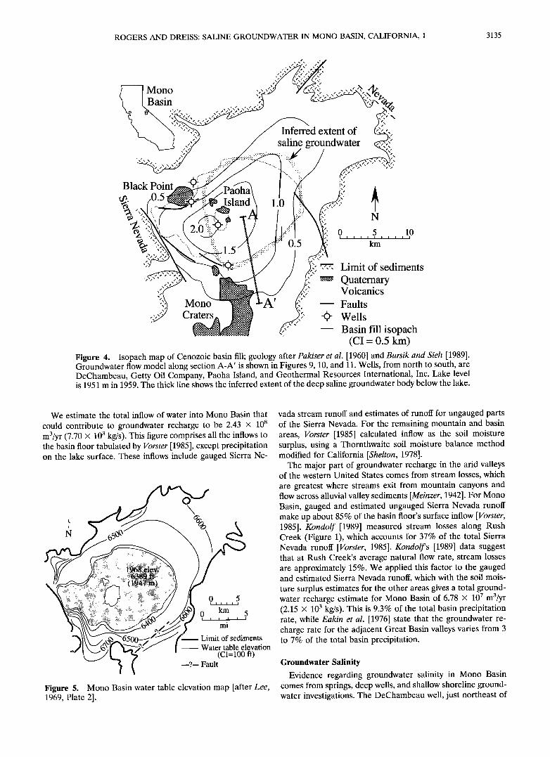
Figure 4. Isapach map of Cenozoic basin fill; geology after Pakiser et al. [1960] and Bursik and Sieh [1989]. Groundwater flow model along section A-A' is shown in Figures 9, 10, and 11. Wells, from north to south, are DeChambeau, Getty Oil Company, Paoha Island, and Geothermal Resources International, Inc. Lake level is 1951 m in 1959. The thick line shows the inferred extent of the deep saline groundwater body below the lake.

We estimate the total inflow of water into Mana Basin that

could contribute to groundwater recharge to be 2.43 x 108 m3/yr (7.70 x 103 kg/s). This figure comprises all the inflows to the basin floor tabulated by Vorster [1985], except precipitation on the lake surface. These inflows include gauged Sierra Ne-

0 5 i i i I i i

o km 5 i i i i i i

m•

JAmit of sediments

Water table elevation (CI= 100 ft)

_9_ Fault

Figure 5. Mona Basin water table elevation map [after Lee, 1969, Plate 2].

vada stream runoff and estimates of runoff for ungauged parts of the Sierra Nevada. For the remaining mountain and basin areas, Vorster [1985] calculated inflow as the soil moisture surplus, using a Thornthwaite soil moisture balance method modified for California [Shelton, 1978].

The major part of groundwater recharge in the arid valleys of the western United States comes from stream losses, which

are greatest where streams exit from mountain canyons and flow across alluvial valley sediments [Meinzer, 1942]. For Mono Basin, gauged and estimated ungauged Sierra Nevada runoff make up about 85% of the basin floor's surface inflow [Vorster, 1985]. Kondolf [1989] measured stream losses along Rush Creek (Figure 1), which accounts for 37% of the total Sierra Nevada runoff [Vorster, 1985]. Kondol•'s [1989] data suggest that at Rush Creek's average natural flow rate, stream losses are approximately 15%. We applied this factor to the gauged and estimated Sierra Nevada runoff, which with the soil moisture surplus estimates for the other areas gives a total groundwater recharge estimate for Mono Basin of 6.78 x 107 m3/yr (2.15 x 10 3 kg/s). This is 9.3% of the total basin precipitation rate, while Eakin et al. [1976] state that the groundwater recharge rate for the adjacent Great Basin valleys varies from 3 to 7% of the total basin precipitation.

Groundwater Salinity

Evidence regarding groundwater salinity in Mana Basin comes from springs, deep wells, and shallow shoreline groundwater investigations. The DeChambeau well, just northeast of


a) 100

• 50

o

o.oo

b) 2200

2100

2000

1900 0

0.05

median = 0.011

Northeast shore Sierra Nevada shore

l North and south shore : , ,

,

0.10

Water Table Gradient

Basin spill ldvel (2180 m) '- ...... '- Average basin

topographic profile Water table at mean •

gradient (.0308) '. r'"'/.. 1968 Lake Level .,.',•'•, - '

(1947.4 m) ." - ' ' .4 m) •- -Water table at median .......... gradient (.0•11!

5000 10000 15000 Basin Radius (m)

Figure 6. (a) Mono Basin shoreline water table gradient cu- mulative distribution function, based on Figure 5. (b) Rela- tionship of water table elevations at the basin mean and median water table gradients to the average basin topographic profile (profile based on data of LADWP [1987], Stine [1988], K. R. Lajoie (personal communication, 1990), and topographic maps).

Black Point, was drilled to 287 m in 1911 (Figure 7). The well water concentration is about 1100 ppm TDS, and its ionic composition is similar to dilute lake water [Lee, 1969]. The Paoha Island well initially encountered saline water while drilling through fine-grained sediments. Upon penetrating sand layers at 300 m, freshwater flow began [Scholl et al., 1967]; water concentration in this well is also about 1100 ppm [Lee, 1969]. The water issuing from the nearby Paoha Island hot springs (Figure 7) is among the highest in TDS of the basin's springs, at 22,000-26,000 ppm [Lee, 1969; Mariner et al., 1977]. The hot springs water composition has been interpreted as a mixture of lake and deeper thermal waters [Lee, 1969; Mariner et al'., 1977].

Analysis of the GRI well (Figures 1 and 7) spontaneous- potential (SP) log, following the methodology of Jorgensen [1991], reveals that the formation water salinity increases with depth (Figure 8) to over 18,000 ppm at the bottom of the well [Rogers, 1993b; R. W. Frank, personal communication, 1991]. A similar treatment of the Getty Oil Company SP log shows that the formation water in that well is fresh down to base-

ment: The estimated TDS is less than 400 ppm at all depths [Rogers, 1993b; R. W. Frank, personal communication, 1991].

For the GRI well, formation water resistivity was converted to an equivalent TDS (Figure 8), assuming the formation water is a dilution of lake water, using Schlumberger Well Services [1985] charts Gen-8 and Gen-9. The shallow formation water is fresh to brackish (Figure 8). Below 300 m the formation water salinity exceeds that of the mud tiltrate, so the SP log ampli- tude increases [Jorgensen, 1989]. TDS at 60 m is approximately

600 ppm; at 1035 m, it is 18,500 ppm (R. W. Frank, personal communication, 1991). The GRI well groundwater TDS values shallower than 600 m (i.e., 600-2700 ppm) are consistent with those of the nearby Navy Beach thermal spring (Figure 7) and the 900-3000 ppm TDS reported for deep-source cold springs issuing from the nearby shoreline [Bischoff et al., 1993].

Helium isotope data show that the water issuing from hot springs on Paoha Island and at Navy Beach has at least a partial deep source. Welhan et al. [1988a, b] concluded that the high 3He/4He ratios (relative to atmospheric) for the Navy Beach and Paoha Island hot springs are indicative of an underlying magma source, at depths less than 10 km. The DeChambeau well and a hot spring on the lake's northeastern shoreline have lower 3He/4He ratios and show the same change in ratio with distance from the magmatic source as that found at Long Valley caldera [Welhan et al., 1988b] and at Yellow- stone Park [Welhan et al., 1988a].

The higher chloride content of the DeChambeau well and Paoha Island hot springs [Lee, 1969], the low radiocarbon activity and gas composition of the Navy Beach hot spring [Oremland et al., 1987; Bischoff et al., 1993], and the helium isotope values indicate that all of these sources are delivering deep-seated groundwater to the surface. While the composition of the Paoha Island hot springs has been interpreted to result from mixing with lake water [Lee, 1969; Mariner et al., 1977], an alternative possibility is that they represent recycled lake water discharging from the saline aquifer beneath Mono Lake.

Shallow shoreline groundwater concentrations provide additional evidence regarding the saline groundwater distribution (Figure 7). Concentrations are low along much of the shoreline [Lee, 1969; Basham, 1988; Neumann, 1993], owing to high recharge or fault-related springs [Sinclair, 1988; Rogers et al., 1992]. The exceptions are the Paoha Island hot springs, the recently exposed peninsula southeast of Black Point, and the

• Hot Spring ....... ;os,; m ...................... • ................................................................................. / -(• Well •rO0 • "'"•--••----- .

• ...... Navy Beach

Figure 7. Mono Lake shoreline groundwater concentrations (parts per million) from wells, springs, and pits. Generalized TDS contours from 200 to 1600 ppm modified from Lee [1969]. Northeast shoreline TDS contours after Rogers [1992]. Map based on U.S. Geological Survey topographic maps; elevations in meters. Wells and hot springs are as follows: 1, DeCham- beau; 2, Getty Oil Company; 3, Paoha Island well; 4, Paoha Island hot springs; 5, Geothermal Resources International, Inc., and 6, Navy Beach hot springs.

ROGERS AND DREISS' SALINE GROUNDWATER IN MONO BASIN, CALIFORNIA, 1 3137

broad northeast shoreline [Groeneveld, 1991; Rogers, 1992; Rogers et al., 1992; Connell, 1993; Rogers, 1993a]. Concentra- tions along the recently exposed northeastern shoreline reach 100,000 ppm TDS, exceeding the concentration of Mono Lake at the lakeshore (91,100 ppm). The high concentrations of the shallow groundwater may be enhanced by high evaporation rates on the playa surface, and, as we demonstrate in this and an accompanying paper [Rogers and Dreiss, this issue], by upwelling of deep saline groundwater below the exposed shoreline [Rogers and Dreiss, 1991; Rogers et al., 1992; Rogers, 1993a, b].

The Saline Groundwater-Freshwater Interface

The observations discussed in the previous section indicate that the saline-fresh groundwater interface does not coincide with the shoreline everywhere around the lake (Figure 4). Freshwater partially extends beneath Paoha Island, and the GRI well locates the interface beneath the lake's south shore

at Navy Beach. The saline playa conditions of the northeast shoreline suggest that the underlying interface extends outside the present-day lakeshore.

In the following sections we discuss two model investigations of the Mono Basin groundwater flow system. Our simulations represent a steady state flow system with the hydrologic characteristics of Mono Basin in 1968, the time of Lee's [1969] investigation. In this section we use a cross-sectional model, perpendicular to the shoreline, to show that simulations of the width and position of the saline-freshwater interface are consistent with the groundwater salinity profile derived from the GR! well SP log. We compare the well log salinity profile with simulated concentrations to examine whether the combination

of saline groundwater concentration, boundary conditions, and assumed sediment properties is reasonable. In a subsequent section, we use a radially symmetric model of the basin fill to evaluate the basin-wide distribution and dynamics of the saline-fresh interface.

300 i• SP shift -O- Formation

• 600

900i' .... le"

"sa"d"

..................... • • basement

1200 ............... "• ................ 0 10,000 20,000 TDS (ppm)

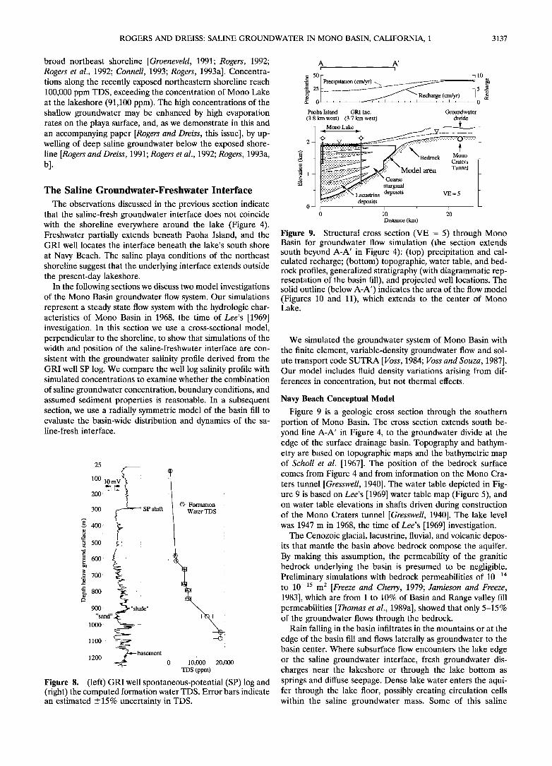
Figure 8. (left) GRI well spontaneous-potential (SP) log and (right) the computed formation water TDS. Error bars indicate an estimated • 15% uncertain• in TDS.

A A'

ß fl recipitation (cngyr) ........ :: .................................... • .•,25 5 .=• '• / • •R,ech, ar,ge!c •m/y,r), , I •'

Paoha Island GRI Inc.

(3.8 km west) (3.7 km west) Groundwater

divide

Mono Lake

'I-'-'-- - -'-'-'-- --••1 '"- • •;.<•;e drOc ;'-'-'-'• - - --'- - -'-'•::--- -'-•17• ).'i:" X ......... k •nnerø• l'----_'.._•l' •M,,': Model area ,u

[ii':---•-55---_ .-.-_...'-:... _••5•<•5•','" marginal :-:-'-•-;X, Lacustrine deposits VE = 5

,'"'" ' deposits • I I

0 10 20

Distance (km)

Figure 9. Structural cross section (VE - 5) through Mono Basin for groundwater flow simulation (the section extends south beyond A-A' in Figure 4): (top) precipitation and calculated recharge; (bottom) topographic, water table, and bedrock profiles, generalized stratigraphy (with diagrammatic representation of the basin fill), and projected well locations. The solid outline (below A-A') indicates the area of the flow model (Figures 10 and 11), which extends to the center of Mono Lake.

We simulated the groundwater system of Mono Basin with the finite element, variable-density groundwater flow and solute transport code SUTRA [l/oss, 1984; l/oss and Souza, 1987]. Our model includes fluid density variations arising from differences in concentration, but not thermal effects.

Navy Beach Conceptual Model

Figure 9 is a geologic cross section through the southern portion of Mono Basin. The cross section extends south beyond line A-A' in Figure 4, to the groundwater divide at the edge of the surface drainage basin. Topography and bathym- etry are based on topographic maps and the bathymetric map of Scholl et al. [1967]. The position of the bedrock surface comes from Figure 4 and from information on the Mono Cra- ters tunnel [Gresswell, 1940]. The water table depicted in Fig- ure 9 is based on Lee's [1969] water table map (Figure 5), and on water table elevations in shafts driven during construction of the Mono Craters tunnel [Gresswell, 1940]. The lake level was 1947 m in 1968, the time of Lee's [1969] investigation.

The Cenozoic glacial, lacustrine, fluvial, and volcanic deposits that mantle the basin above bedrock compose the aquifer. By making this assumption, the permeability of the granitic bedrock underlying the basin is presumed to be negligible. Preliminary simulations with bedrock permeabilities of 10 -14 to 10 -15 m 2 [Freeze and Cherry, 1979; Jamieson and Freeze, 1983], which are from 1 to 10% of Basin and Range valley fill permeabilities [Thomas et al., 1989a], showed that only 5-15% of the groundwater flows through the bedrock.

Rain falling in the basin infiltrates in the mountains or at the edge of the basin fill and flows laterally as groundwater to the basin center. Where subsurface flow encounters the lake edge or the saline groundwater interface, fresh groundwater discharges near the lakeshore or through the lake bottom as springs and diffuse seepage. Dense lake water enters the aquifer through the lake floor, possibly creating circulation cells within the saline groundwater mass. Some of this saline


Table 1. Model Parameters

Parameter Value

Density (kg/m3)-concentration (kg TDS/kg fluid) relation

Dynamic viscosity, kg m-• s-• Molecular diffusion coefficient, m2/s Specific pressure storativity, m s 2 kg -•

p = 1000 + 875.36C

10 -3 0

0

Navy Beach Model Parameters Basin fill permeability, m 2 Basin fill porosity, m3/m 3 Longitudinal dispersivity, m Transverse dispersivity, m

2.05 x l0 -•3 0.40

100

33

Basin-Wide Model Parameters

Initial basin fill permeability, m 2 Basin fill porosity, m3/m 3 Longitudinal dispersivity, m Transverse dispersivity, m

4.67 x 10- 0.35

2OO

50

TDS denotes total dissolved solids

with C(x, z, t) the solute concentration as a mass fraction (Ms/M, mass solute/mass fluid) and Qp(X, z, t) the fluid mass source rate (M/L 3T, mass fluid/aquifer volume/time). Darcy's law (1) can be substituted into (2) for velocity. The specific pressure storativity for the aquifer matrix, with units of L T2/M, is

= - + (3)

with a the porous matrix compressibility and/3 the fluid compressibility (both L T2/M). For a unit aquifer volume the first two terms in (2) express changes over time of fluid mass from variations in pressure (hence aquifer volume) and concentration (thus fluid density). The third term accounts for the net flux of fluid out of the volume due to flow, and the final term accounts for fluid supplied by external sources and sinks.

The solute mass balance for a unit of aquifer volume where fluid density varies is

OC

•p -•-+ •pv. VC - V . [•p(DmI + D). VC]

groundwater, perhaps mixing with freshwater, returns to discharge at the surface. The principal natural discharges from the basin are evaporation, lake overflow during past pluvial periods, and possible (unknown) groundwater underflow out of the basin; no discharges from the basin are included in our model.

The models presented here simplify the interaction of the lake with the groundwater system. The lake is represented through its elevation and surface extent as a specified pressure boundary and acts as an unlimited source or sink of water and solutes. We also neglect the effects of heat flow on groundwater movement. Temperatures in the GRI well ranged from 38øC near the surface to 54øC at 1219 m. The bottom-hole

temperature in the Getty well was 58øC at 743 m [Artell, 1972].

Mathematical Model

The analysis of groundwater solute transport requires the simultaneous solution of mass balance equations for both fluid flow and solute transport. Table 1 lists the model parameter values we used. The following discussion is largely taken from Voss and Souza [1987], who discuss these equations in detail. With variable fluid density, the potential function head does not exist, and the fluid flow equation is expressed in terms of pressure [Bear, 1972]. The pressure gradient form of Darcy's law, giving the average linear fluid velocity, is

v= - ß (Vp- pg)

with

(1)

v(x, z, t) fluid velocity (L/T); k(x, z) permeability tensor (L2); e(x, z) porosity (L3/L3);

I• dynamic viscosity (M/L T); p(x, z, t) fluid pressure (M/LT2); p(x, z, t) fluid density (M/L3);

g gravity vector (L/T2). Conservation of mass of the fluid, neglecting the contribu-

tion of solute dispersion to the fluid flux, is expressed as

(2) op op oc

pSop •- + s •-• • + v. (spv)= Qp

= Qp(C* - c) (4)

with

D m molecular diffusion coefficient of solute (L2/T);

I identity tensor (dimensionless); D(x, z, t) mechanical dispersion tensor (L2/T);

C* (x, z, t) concentration of solute in the source fluid (Ms/M).

The first term in (4) represents the change over time of solute mass in a unit aquifer volume. The second term gives the net flux of solute out of the volume resulting from fluid advection, and the third term represents the flux due to molecular diffusion and mechanical dispersion. The right-hand side accounts for solute sources and sinks arising from fluid input and outflow.

Fluid density is assumed to be linearly related to concentration:

Op p = p0 + •-• (C - Co)

with Po the fluid density when C = Co, the base solute concentration, and Op/OC the constant coefficient of density variation. For Mono Lake water this function (Table 1) is determined using values of specific gravity and total dissolved solids from LADWP [1987].

Bear [1972] formulated the components of the mechanical dispersion tensor D as

vivj

= via0 + Iv with

crL, crr longitudinal and transverse dispersivities (L); Ivl magnitude of fluid velocity; 8 o Kronecker delta; v• the component of veloci• in the i coordinate

direction.

(6)

Method of Simulation

Finding a steady state solution requires solving a coupled, nonlinear problem. The solution method is the same as for a


1) Specified Inflow

_•p = lake level/0g = = 2) Specified Pressure-• Cin = Cgw Cin = 0 ! Specified Basin Floor =I Inflow - Mono Lake = • .

0 5 10

Figure 10. Finite element mesh and boundary conditions for groundwater flow simulation. Topography and water table as in Figure 9.

transient problem, requiring initial conditions (actually "ini- tialization conditions") for pressure and concentration distribution [Voss, 1984; Voss and Souza, 1987]. Our time step se- lection followed the criteria of Voss and Souza [1987]. Small time steps when beginning a simulation preserve numerical stability, because concentration gradients may be quite sharp. At later times, concentration gradients along streamlines are less sharp, and larger time steps may be taken.

To evaluate whether solutions reached steady state, we modified the budget portion of SUTRA. Monitoring changes in the net flow rate of solutes into the model (the difference between outflow and inflow), the change in stored solute mass, and the position of the interface provides a check on solution progress. For some simulations we used initial concentration distribu-

tions having initial interfaces on opposite sides of the final interface position, as suggested by Voss and Souza [1987]. So- lutions for the interface converged from each direction to the same position.

Model Dimensions and Boundary Conditions The finite element mesh contains 764 nodes and 697 ele-

ments (Figure 10). Each element is 305 m long, 61 m high, and 1 m thick. The vertical boundary at the center of the lake is a symmetry line and thus considered to be no flow. The bedrock surface is also a no-flow boundary. Below the lake the upper model boundary (set at the lake bottom elevation of 1905 m) has specified pressure corresponding to the lake elevation of 1947 m. The basin floor along the remaining upper model boundary was initially specified as a recharge boundary. Voss [1984] noted that at least five nodes are required to adequately discretize a sharp concentration front; thus the element size we selected limits the minimum interface width obtained in our

simulations. This topic is explored in more detail in a later section.

We used Vorster's [1985] isohyetal map and monthly soil moisture surplus calculations to estimate recharge (Figure 9).

Vorster used a Thornthwaite method modified for California

[Shelton, 1978] to compute the annual soil moisture surplus (i.e., recharge) as a function of elevation and precipitation zones in Mono Basin. The total recharge over the 15.85 km distance from the lake to the groundwater divide (Figure 9) is 764 m3/yr, for a 1-m-wide strip. Since the model domain does not extend to the groundwater divide, the additional recharge was applied along the outer vertical boundary.

A specified flow boundary condition along the basin floor would constrain the position of the saline groundwater interface top to be inside the lake. To overcome this, in simulations to find the saiine groundwater concentration and interface position, the basin floor was treated as a specified pressure boundary. This allows the interface to move out from under the lake edge, while maintaining approximately the same recharge distribution.

The concentration of water entering through the basin floor was specified as zero. We assume that the saline groundwater beneath the lake is well mixed, with an initial concentration of 18,000 ppm. This is approximately the maximum formation water concentration found in the GR! well and represents a lower limit for the groundwater concentration because the well may have penetrated only the outer part of a broad interface. Although this groundwater concentration is lower than the present lake concentration, the lake level and salinity have fluctuated considerably in the past, with lake salinity values generally much lower than the present [see Rogers and Dreiss, this issue]. Transient simulations show that the lake concentration requires thousands of years to equilibrate with that of the groundwater.

Any water entering through the lake floor (the lake concentration) has the same concentration as the groundwater, i.e., 18,000 ppm, because we are interested in a steady state solution matching our inferred groundwater concentration. The transient case of differing lake and groundwater concentrations is discussed by Rogers and Dreiss [this issue], where we show that the solutes of a more concentrated lake drain into less

concentrated groundwater within a few thousand years.

Model Parameters

Few actual measurements of aquifer permeability are available in Mono Basin. As a guide to permeability we used the results of a groundwater flow model study of Smith Creek Valley, Nevada (Table 2) [Thomas et al., 1989a]. That closed basin is comparable in geology and scale to Mono Basin. A uniform permeability of 2.05 x 10-•3 m 2 for the basin fill gives a reasonable match (Figure 9) to the heads in Lee's [1969] water table map (Figure 5). Freeze and Cherry [1979] indicated that this permeability applies to clean or silty sand. Thomas et al. [1989a, p. E4] found a permeability similar to ours (i.e., 4.7 x 10 -•3 m 2) for mixed deposits at the playa margin, and a higher value of 7.8 x 10 -•2 m 2 for coarse deposits at the basin

Table 2. Permeabilities for Basin Fill Lithology Classes [Thomas et al., 1989a]

Reference Mark Used in

Lithology Class Figure 17a Permeability, m 2 Lithology [Freeze and

Cherry, 1979]

Playa surface deposits Playa margin and deep playa sediments Mixed deposits at the playa margin Coarse deposits at the basin margin

a 3.11 X 10 -15 till, silt b 6.22 X 10 -14 silt, silty sand c 4.67 x 10 -13 silty sand, clean sand d 7.78 X 10 -•2 clean sand, silty sand


margin. These authors stated that "mixed deposits consist pri- marily of poorly sorted mixtures of clay, silt, sand, and gravel."

Results from drilling the recent geothermal wells support an assumption that permeability and porosity do not decrease much with depth, at least for the basin margin sediments. The high drilling rates through volcanic ash, pumice, tuff, sand, and gravel suggest that little sediment cementation has taken place (R. Behl, personal communication, 1989). Sands do not lose porosity and permeability from compaction to the same degree as finer sediments: Most of the compaction is elastic [Chap- man, 1976], and loss of permeability and porosity results from diagenesis.

Christensen et al. [1969] estimated the porosity of the lacustrine silts in the basin center with gravity modeling. They concluded that porosity is 60% near the surface and 40% at 1 km depth. Coarse sediments at the basin edge have slightly lower porosities: R. W. Frank (personal communication, 1991) found from the GRI well log that porosity at 823 and 945 m is about 40%. This determination uses the borehole-compen- sated sonic log and assumes a clean quartz sand (no clays). This estimate is probably on the high side, considering the likelihood of pyroclastic alteration to smectite (B. F. Jones, personal communication, 1995). Where the Getty Oil Com- pany well is not washed out (causing inaccuracy), the density log gives very low readings; either porosity exceeds 40% in the sandy units, or the sands are not clean (R. W. Frank, personal communication, 1991). We assumed a uniform basin fill porosity of 40% for the Navy Beach model.

The dynamic viscosity is 1.0 x 10 -3 kg m- • s-•, that of pure water at 20øC. For comparison, Mono Lake water at about 68,000 ppm has a dynamic viscosity about 20% higher than pure water [Mason, 1967]. Storativity was set to zero for the steady state solutions.

In most examples of groundwater flow and solute transport, the molecular diffusion coefficient D m is small compared to mechanical dispersion [koss and Souza, 1987]; hence it is set to zero in this study. Simulations using a value of 10 -9 m2/s for D m produced no difference in simulation results. On the other hand, Thomas et al. [1989b] determined that in the fine-grained playa sediments of Smith Creek Valley, transport by molecular diffusion probably exceeds that from dispersion. Lerman and Jones [1973] and Konikow and Rodriguez Ar•valo [1993] drew similar conclusions from studies of salinity distribution in low- permeability confining layers.

Dispersion and Mesh Discretization

The numerical accuracy and stability of simulation results depend on relationships between model dispersivities, and time step and mesh sizes. When flow lines parallel the concentration contours, as in our simulations, the concentration distribution is relatively insensitive to the value of the longitudinal dispersivity, and the transverse dispersivity and mesh size control the width of the saline-fresh interface [Voss and Souza, 1987]. The mesh size imposes a lower limit on model dispersivities, which we chose according to the guidelines of Voss and Souza [1987]. When the molecular diffusion coefficient is small compared to mechanical dispersion, the mesh Peclet number along the flow direction becomes Pem • AsL/ai., where AsL is the distance across an element along the flow direction [Voss and Souza, 1987]. If Pe m < 4, spatial oscillations are unlikely to occur [koss and Souza, 1987]. For a 305-m element this requires a/. > 76.25 m; we used a larger value of 100 m for the Navy Beach model.

koss and Souza [1987] suggest the criterion of AsT < a r for transverse discretization (with AsT the transverse mesh spac- ing), although AsT < 10 at may be sufficient. For a 305-m element, this requires that at > 30.5 m. We used a value of 33 m for this model. Simulations using at = 0, as suggested by Voss and Souza [1987] for evaluation of the inherent mesh dispersion, produced a somewhat narrower transition zone. With values of a t smaller than 33 m, the narrow transition zone resulted in concentration oscillations up to 5%.

Navy Beach Model Results

Figure 11 shows the results of a steady state simulation using the material properties in Table 1. The parameters used to obtain the results are not unique: Rather, the model is in- tended to demonstrate the nature of the groundwater flow system and the model's ability to reproduce the well and spring observations. At the top is a plot of the fluid and solute mass fluxes across the model's upper surface. In the lower diagram, vectors show the fluid flow pattern. Concentration contours indicate the interface location, the top of which is just inside the lake edge. There are two zones of flow: the fresh groundwater recharge moving below the basin margin and a density- driven circulation cell below the lake. The main groundwater discharge zone occurs at the lake edge. Flow velocities below the lake are several orders of magnitude lower than those beneath the basin floor.

The maximum solute discharge across the lake floor is located slightly inside the lake edge, where higher concentration groundwater coincides with the fluid discharge zone. A region of fluid and solute inflow is located farther toward the lake

center. The maximum model fluid discharge rate at the lake edge is about 1.3 m/yr. Because of the radial symmetry of the basin, each part of the lakeshore derives recharge from a larger portion of the basin's border than determined for the current cross-sectional model. Such considerations would increase the

discharge rate at the lake edge by a factor of about 3.

A A'

-4.5 [ ]-1.5 -3.0 Solute Flux (kg/m2/yr) "?//•:.f•:'•/• Fluid Flux (m/yr) -1.0 -1.5 -0.5 0.0 ............................................... .• ...... 0.0 1.5 ' ' 0.5

[• Mono L•e • [

2 ..........

.... • • • • • } • } -••• ............ d000ppm VE-2

I*• J"J* ** * } } }•-"• ............ 17000ppm - 1•• '

• 7.1 •yr • 2.2 •yr * 0.71 •yr • 0.22 •yr

0 5

Figure 11. Steady state groundwater flow simulation (A-A' in Figures 4 and 9). (top) Fluid and solute mass fluxes across model top. The fluid flux is calculated assuming a uniform fluid density of 1000 kg/m 3. (bottom) Finite element flow simulation (VE = 2) with water table, basin and model outlines, and projected well locations. Vectors show the fluid flow pattern; the flow velocities are scaled logarithmically over 2 orders of magnitude. Only every other row of elements is shown. Con- centration contours range from 1000 to 17,000 ppm; the contour interval is 4000 ppm.


The simulated vertical concentration profiles near the shoreline provide an excellent match to the GRI well SP log results (Figure 12). The simulated near-shore shallow groundwater concentrations are low, and the flow pattern (Figure 11) indicates that deep-sourced water discharges at the shoreline, in accordance with data on the Navy Beach thermal and cold springs [Mariner et al., 1977; Oreroland et al., 1987; Bischoff et al., 1993].

The simulated interface position is moderately sensitive to model values of groundwater concentration, recharge, and permeability (and mesh size, as discussed below). Higher concentration or increasing permeability moves the interface outward; higher recharge has the opposite effect. The top of the interface cannot readily move outside the lakeshore because it is constrained by the groundwater discharge zone, where upward flow rapidly moves solutes to the surface. Further outward interface movement occurs by extension of the interface toe. The maximum saline groundwater concentration must be at least ---18,000 ppm in order to match the GRI well SP log. This concentration could be greater if the well has only penetrated the outer part of the interface. The simulation and well log demonstrate that the saline groundwater and the lake water are connected and would seem to preclude the possibility of an isolated pool of saline water in the bottom of the basin fill.

As a first approximation an assumption of uniform permeability throughout the basin was made. Steady state simulation experiments show that the permeability between the lakeshore and basin edge controls the flow system. Little flow occurs beneath the lake owing to the uniform pressure of the lake surface. Experiments using a sediment anisotropy of kz/kh = 0.1 in the current model resulted in displacement of the interface halfway toward the center of the lake from the shoreline. The interface is displaced away from the shoreline because anisotropy spreads the shoreline discharge zone across more of the lake bottom [Pfannkuch and Winter, 1984]. This observation applies even if the aquifer below the lake has a permeability several orders of magnitude lower than the rest of the basin fill, as discussed below.

Simulating the Basin-Wide Groundwater Flow System Basin-Wide Conceptual Model

Our second steady state model encompasses the floor of Mono Basin and the underlying basin fill (Figure 3). Mono

,

•- '• ', concentration

• 400I •, '. profiles •E "•_•Shoreline ' '• 305. rn Lakeward

1000 Landward

1200 .... ' .... '''' "''' 0 5000 10000 15000 20000

TDS (ppm)

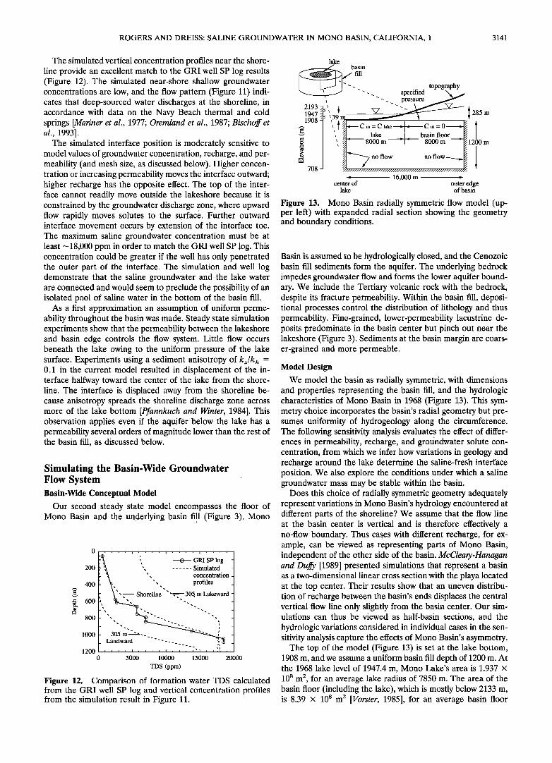
Figure 12. Comparison of formation water TDS calculated from the GRI well SP log and vertical concentration profiles from the simulation result in Figure 11.

lake • basin

.•.'..fill topography -. specified "X , "-- .. -. pressure

2193 3" { V "" "• 1947 { 285 rn .•- ',39 m/. • •

I908• i• • C in = C lake ---• -• Gin=0 ] • •! lake I basin floor ,, / •= 8000m =1-• 8000m =I1200m / C-7 nøøw

708 2 • •v.//////////////// - 16,000 rn

center of outer edge lake of basin

Figure 13. Mono Basin radially symmetric flow model (upper left) with expanded radial section showing the geometry and boundary conditions.

Basin is assumed to be hydrologically closed, and the Cenozoic basin fill sediments form the aquifer. The underlying bedrock impedes groundwater flow and forms the lower aquifer boundary. We include the Tertiary volcanic rock with the bedrock, despite its fracture permeability. Within the basin fill, depositional processes control the distribution of lithology and thus permeability. Fine-grained, lower-permeability lacustrine deposits predominate in the basin center but pinch out near the lakeshore (Figure 3). Sediments at the basin margin are coarser-grained and more permeable.

Model Design

We model the basin as radially symmetric, with dimensions and properties representing the basin fill, and the hydrologic characteristics of Mono Basin in 1968 (Figure 13). This symmetry choice incorporates the basin's radial geometry but pre- sumes uniformity of hydrogeology along the circumference. The following sensitivity analysis evaluates the effect of differences in permeability, recharge, and groundwater solute concentration, from which we infer how variations in geology and recharge around the lake determine the saline-fresh interface position. We also explore the conditions under which a saline groundwater mass may be stable within the basin.

Does this choice of radially symmetric geometry adequately represent variations in Mono Basin's hydrology encountered at different parts of the shoreline? We assume that the flow line at the basin center is vertical and is therefore effectively a no-flow boundary. Thus cases with different recharge, for ex- ample, can be viewed as representing parts of Mono Basin, independent of the other side of the basin. McCleary-Hanagan and Duffy [1989] presented'Simulations that represent a basin as a two-dimensional linear cross section with the plays located at the top center. Their results show that an uneven distribution of recharge between the basin's ends displaces the central vertical flow line only slightly from the basin center. Our simulations can thus be viewed as half-basin sections, and the hydrologic variations considered in individual cases in the sensitivity analysis capture the effects of Mono Basin's asymmetry.

The top of the model (Figure 13) is set at the lake bottom, 1908 m, and we assume a uniform basin fill depth of 1200 m. At the 1968 lake level of 1947.4 m, Mono Lake's area is 1.937 x 108 m 2, for an average lake radius of 7850 m. The area of the basin floor (including the lake), which is mostly below 2133 m, is 8.39 x 108 m 2 [Vorster, 1985], for an average basin floor


radius of 16,343 m. In the model the lake and basin floor radii are 8000 m and 16,000 m. We chose a grid with uniform elements because the interface position changes so much in different simulations. The 1600-element, 1701-node grid has 80 columns and 20 rows of elements. The uniform elements are

200 m long by 60 m high, and their thickness is 2rr times the radial distance to each node.

Model Parameters and Boundary Conditions

We chose an initial uniform model permeability value of 4.67 x 10 -13 m 2, which Thomas et al. [1989a] found appropriate for playa margin deposits at Smith Creek Valley, Nevada (Table 2). We assumed a uniform basin fill porosity of 35 % and used longitudinal and transverse dispersivities of 200 and 50 m, respectively. These values meet the guidelines relating dispersivities to mesh size of Voss and Souza [1987].

Except for the model top, the boundaries of the radial cross section (Figure 13) are no flow: The central vertical boundary is a symmetry line, and the bottom and outer boundaries correspond to the bedrock surface. The upper boundary is specified pressure; above the lake the pressure corresponds to the lake elevation. Landward of the lake edge the pressure corresponds to the water table elevation, which we approximated with a linear gradient. The gradients range from 0.13 near the Sierra Nevada to 0.01 on the north and south shores and 0.005

on the northeastern shore (Figure 6). The mean basin water table gradient is 0.0308, and the median is 0.011. For a model where all of the boundaries are either no flow or specified pressure, the water flux through the system is determined by the hydraulic conductivity. Thus a separate estimate of the inflow of water to the system is needed [Franke and Reilly, 1987].

For solute boundary conditions, water entering through the basin floor has zero concentration. For solute initial condi-

tions, we again assume a base concentration of 18,000 ppm for the saline groundwater below the lake. Any water entering the aquifer through the lake bottom has the same concentration,

Lake

a)• Solute flux (kg/m2/yr) -= I o • -'•[ Outflow

0! -- -• Inflow m 3 • .... ' ............. ;•:• ' ......... •8

b) 0 5000 Radius (m) 10000 15000

)00 •08

• 16 •yr • 5.1 •yr * 1.6 •yr } 0.51 •yr

' 708

Figure 14. Model solution for base parameters: uniform permeability of 4.67 x 10-13 m 2, water table gradient 0.0308, and saline groundwater concentration of 18,000 ppm. (a) Fluid and solute fluxes (per unit area) across model surface are shown. (b) Vectors show fluid flow pattern along with an outline of interface. For clarity, only half the element rows and columns are shown. Velocities are scaled logarithmically over 2 orders of magnitude (VE = 2). (c) Concentration contours are a fraction of the assumed base concentration of 18,000 ppm. The contour interval is 15%, beginning at 5%.

18,000 ppm, in order to achieve a steady state solution at the observed groundwater concentration of 18,000 ppm.

The Simulated Flow System

Figure 14 shows the simulation result for the basic steady state flow system. The fluxes are normalized to a unit model surface area to give the local infiltration and discharge rates. The fluid flux values are calculated from model output, assuming a uniform fluid density of 1000 kg/m 3. The flow system is similar to that described for the Navy Beach model. The simulated groundwater recharge occurs in the highest part of the basin floor. Discharge is focused at the lakeshore, but a smaller amount of discharge occurs farther away from the lake. For water table shapes other than a linear gradient, the distribution of discharge between the basin edge and lakeshore is very sensitive to the water table curvature. A slight change in the water table focuses more of the dischhrge at the lakeshore.

Basin-Wide Flow System Sensitivity Analysis The following set of steady state simulation results demon-

strates how a range of permeabilities, recharge, and groundwater solute concentrations influence the position of the saline groundwater interface. This allows us to understand the basic hydraulics of the saline-fresh flow system, including the conditions under which a saline groundwater body may be stable in Mono Basin. The goal is to infer how hydrologic variations around the lake affect the location of the saline groundwater interface. First we address how the mesh size and dispersivity affect simulation results.

Effect of Dispersivity and Mesh Size

The choice of mesh size represents a trade-off between computational time and faithful representation of the area under study, but it also must be appropriate for the available information on geology and hydrology. Another consideration is sufficient discretization of features such as concentration inter-

faces, which may have sharp spatial gradients [l/oss, 1984]. Figures 15a-15d show the effect of element size on the flow system simulation. As the number of elements increases from 400 to 6400, the horizontal element dimension decreases from 400 to 50 m. With finer elements the interface narrows and

moves outward toward the lake edge (Figure 16a). For easier comparison of these simulations, Figure 15e shows the 50% concentration contours from Figures 15a-15d.'

The narrowing of the interface with finer elements results from decreasing numerical dispersion as the element size approaches the transverse dispersivity of 50 m. This indicates that the less stringent criterion for transverse dispersivity of AsT < 10a r [l/oss and Souza, 1987] is inadequate. Figure 15e also shows the 50% concentration contours for simulations with

at = 5 m. These simulations (not shown) represent the least amount of numerical dispersion obtainable with the given mesh. The smaller transverse dispersivity of 5 m narrows the interface and moves it outward about 200 m for all cases. The

smaller value of a r has a greater effect on the interface width for finer elements.

The outward movement of the interface in simulations with

finer elements has a more subtle explanation. Figure 16a shows that as elements become finer, the total fluid inflow and maximum flow velocity increase. We expect increasing fluid flow to push the interface farther toward the center of the model, but the opposite occurs. For finer elements the larger number of


elements within the groundwater discharge zone apparently accommodates the increased flow nearer to the lake edge, leading to a narrower discharge zone (Figure 16b). As the peak discharge region under the lake moves toward the lake edge, a corresponding shift occurs in the solute discharge pattern (Fig- ure 16c). The narrower fluid discharge zone brings the interface closer to the lake edge. The 1600-element mesh is a reasonable compromise between computational time and solution quality.

Uniform Permeability

First we discuss how a variation of uniform permeability affects model behavior. A subsequent section covers heterogeneous and anisotropic permeability. We investigated the range of permeabilities found by Thomas et al. [1989a] (Table 2, Figure 17). For these simulations the water table gradient is 0.0308 (the basin mean), and the groundwater solute concentration is 18,000 ppm. Other parameters are the same as for Figure 14.

Altering the model permeability causes a large variation in the fluid and solute inflow to the system (Figure 17a). The distribution of surface fluxes also changes significantly (Figure 18a). At permeabilities below 9.34 x l0 -14 m 2, the interface (the 50% concentration contour) remains just inside the lake edge (Figure 17b), despite decreased recharge. The fluid and solute fluxes vary linearly with permeability, increasing an order of magnitude with a similar increase in permeability. The size of the recharge and discharge zones changes little for permeabilities below 9.34 x l0 -14 m 2. (Figure 18a).

At permeabilities larger than 9.34 x 10-14 m 2, the discharge zone at the lake edge and the main recharge zone at the outer part of the model broaden considerably (Figure 18a). For

Lake

0 5000 Radius (m) 10000 15000

a) 5 elements ;•/ 400 elements 1500 .• t•L=200 m, t•X=50 m 1000 • 708 •

' ' ' ' ' ........

b) 5 elements x(x• 1600 elements t•[=200 m, t•x=50 m

, , , , ! , , ! , , , ,

c) == 10 elements xX•/ 3200 elements t•[=200 m, t•T=50 m

, • , i i ••• , , i , , , , , d) ' ' 20 elements 6400 elements

t•[=200 m, t•x=50 m

e) .... 4 >•"•'"•'•••i• '6400' ...... el em "t "X•en s •' '"• el eme nts

Figure 15. Simulated interfaces for the same parameters as in Figure 14, with different element sizes (sizes shown on plots): (a) 400 (10 x 40) 400 m x 120 m elements, (b) 1600 (20 x 80) 200 m x 60 m elements, (c) 3200 (20 x 160) 100 m x 60 m elements, and (d) 6400 (20 x 320) 50 m x 60 m elements. (e) Comparison of 50% concentration contours for Figures 15a-15d. The number of elements increases from left to right. Solid contours are for a r - 50 m; dotted contours are for OfT = 5 m.

II

• 1.0

• 0.•

0.0 0

b)

• o

._•

c)

a • Total fluid inflow rate '-• -- D- - Maximum flow velocity .... •---- 50% contour position - - z• - - Front width at surface

• mm • No. of elements

100 200 300 400

Element length (m)

Outflow •,ff• - Lake < I

..... 400 elements Inflow ..... 1600 eleme_n!_s ......... 3200 elelnents

-- 6400 elements

4000 8000 12000

Radius (m) 16000

Outflow . ,I

•nnow ......... 3200 elements -- 6400 elements

0 4000 8000 12000 16000 Radius (m)

Figure 16. Comparison of simulations shown in Figure 15. (a) Effect of element size on simulation budget and flow system characteristics, compared to the value for the 1600 element case. (b) Surface fluid fluxes (per unit area) for different num- bers of elements, assuming a uniform fluid density of 1000 kg/m 3. (c) Surface solute fluxes (per unit area).

higher permeability, more recharge nodes are required to ac- commodate the increased inflow. The larger area (and amount) of recharge creates a larger discharge zone, which extends further under the lake. These changes in the flow system geometry cause the variation of fluid and solute fluxes with permeability to depart from a linear trend (Figure 17a). At higher permeabilities the greater inflow and larger discharge zone also force the interface farther toward the center of the lake, with a concomitant decrease in total solute mass in the system (Figure 17b). An order of magnitude increase in permeability moves the interface inward by 4900 m.

The fluid and solute inflows at the center of the model

intensify when the interface nears the inner model boundary (Figure 18b), in order to supply the solutes required to main- tain a balance between inflow and outflow. This is analogous to the increase in well drawdown near an impermeable boundary [Freeze and Cherry, 1979]. As increasing permeability moves the interface toward the center of the model, it tilts, with the interface toe extending increasingly farther from the center than its surface position (Figure 17b). The tilting interface results in a wider interface at the surface (Figure 18b) because


a) 10 5

• 10 4

• 10 3

• 10 2

b)

Solute Inflow •••'•- •

.estimated j•/ ß ' Fluid Inflow recharge / ß ' Rate

10 -16 10-15 10 -14 10-13 10-12 10-11 Permeability (m 2)

, 101

10ø

10'1

10'2

10 -3

• 10000 Interface 7• .• Lake at Surface __ / Interface 2 •

o 5000 Total So 1 " • Mass '• , o

,,

..................... '• 0 10-16' ' 10-15' ' 10-14 ..... -13' ' 10-12' ' 10-11

Permeability (m 2)

FigUre 17. Sensitivity analysis for varying permeability. Other parameters are the same as in Figure 14. (a) Variation of total model fluid and solute inflow rates. Letters a through d indicate permeabilities for the lithology classes of Thomas et al. [1989a] (Table 2). (b) Dependence of the interface (50% concentration contour) surface and toe positions and total solute mass on permeability.

ppm. Figure 19a shows that the fluid inflow rate increases nearly linearly with water table gradient. The fluid flux increases almost an order of magnitude with a similar increase in water table gradient. Except for the lowest gradients the simulations have similar surface fluid flux patterns (Figure 20a). Compared to the results in the previous section (Figure 18), this shows the larger impact of changing permeability on the flow system geometry in this model.

Decreasing the water table gradient moves the interface outward (Figure 19b). The main discharge zone at the lakeshore restrains the surface part of the interface (the 50% concentration contour) from advancing much outside of the lakeshore: The large upward flux of fresh groundwater below the discharge zone rapidly transports solutes to the surface and maintains a low groundwater concentration in this region. At lower water table gradients the interface advances farther outward by extending the toe. In the simulation with the lowest water table gradient, the interface, particularly the toe, has moved out into the basin beyond the lake edge. At the surface the interface (or solute discharge zone) width has increased from 1 to about 3.2 km (Figure 20b).

At the lowest water table gradients the outward extension of the interface toe forces groundwater to discharge farther out from the lake edge (Figure 20a). This restricts the recharge zone at the outer edge of the model, which narrows from 2200 to 1800 m. The interface toe position controls both the surface interface width and the total solute mass in the basin (Figure 19b). The tilted interface results in a wider interface at the surface, because of increased dispersion of solute by fluid upwelling over the extended interface toe. At the lowest water

of increased dispersion of solute by fluid upwelling over the extended toe. The interface at the surface widens from 1000 to

2500 m as it moves inward. At the largest permeability the volume of brine in the aquifer is so small that the solute inflow decreases (Figure 17a). In these simulations the total solute mass in the system follows the same pattern as the interface toe position (Figure 17b).

Our estimate of 2.15 x 10 3 kg/s for Mono Basin's groundwater recharge corresponds to a permeability of 7.39 x 10 -14 m 2, maximum flow velocity of 4 m/yr, and a solute inflow rate of 0.78 kg/s (Figure 17a). The maximum flow velocity occurs at the outer part of the recharge area. This particular permeability lies near the lower end of the range for silty sand [Freeze and Cherry, 1979]. We can view this as a basin-average permeability, although in Mono Basin most recharg,e occurs near the Sierra Nevada, and the sediment• there probably have a larger permeability. Permeabilities much higher than 7.39 x 10 --14 m 2 correspond to unrealistic recharge figures for the basin as a whole. In the subsequent sensitivity simulations we used a permeability of 9.34 x 10 --14 m 2. This permeability analysis shows that where permeability and recharge are greater, the solute interface will be located farther toward the center of the

lake.


Changing the water table gradient in the recharge zone between the shoreline and the basin edge alters the groundwater recharge rate. The range of shoreline water table gradients for Mono Basin (Figure 6a) is indicated in Figure 19a. Other parameters in these simulations are a permeability of 9.34 x 10 -14 m 2 and groundwater concentration of 18,000

0.5

1.0

1.5 0

.• -0.5

ø 0.0

• 0.5

.,-.

• 1.0 1.5

0

' /[ ' / \

Outflow

Lake < Permeabilit

Inflow (m2) -- -- -9.34x10 q3

-- 9.34 x 10 -14

..... 4.67 x 10 -15

4000 8000 12000 16000

Radius (m)

Outflow

\ Inflow \ /

Lake

Permeability

(m 2) -- -- -9.34x10 q3

-- 9.34 x 10 -14

..... 4.67 x 10 qs

4000 8000 12000 16000

Radius (m)

Figure 18. Normalized (dimensionless) (a) fluid and (b) solute fluxes (per unit area) across model surface for varying permeability. The fluxes are normalized to the maximum outflow value for each simulation, and the fluid flux assumes a uniform fluid density of 1000 kg/m 3.

ROGERS AND DREISS' SALINE GROUNDWATER IN MONO BASIN, CALIFORNIA, i 3145

table gradient the 5% concentration contour at the model a) -1.0 surface extends 3000 m outside the lake area (Figure 20b).

A comparison of steady state solutions with progressively • -0.5 smaller water table gradients shows that decreasing the gradi- '• ent at first increases solute inflow, despite decreasing fluid flow •

• 0.0 (Figure 19a). This is because with a smaller gradient the inter- • face moves out to the groundwater discharge area, where up- • • 0.5 ward flowing groundwater moves solutes to the surface (Figure • 19b). With still lower water table gradients the interface ex- -4 • 1.0 tends slightly beyond the lake edge, and solute inflow falls off • because overall fluid flow rates in the model decrease (Figure z 1.5

19a). At the larger gradients an order of magnitude increase in gradient moves the interface inward by 1900 m.

Groundwater Solute Concentration b) The final sensitivity analysis investigates the importance of • -0.5

.,•

the groundwater solute concentration. The other parameters • are a permeability of 9.34 x 10 -14 m 2 and the basin's mean • 0.0 water table gradient of 0.0308. Figure 21a shows that the fluid • inflow rate is nearly constant for these simulations, because • 0.5 permeability and water table gradient are fixed. Solute inflow • ranges over 2 orders of magnitude owing to the large change in • 1.0 the saline groundwater concentration and the fact that as the • interface moves into the discharge zone near the lake edge for 1.5 simulations with increased concentration, upward flow carries solutes to the surface (Figure 2lb). Increasing the groundwater concentration over an order of magnitude from 4500 to 45,000 ppm displaces the interface outward by 1900 m. Once again, the interface toe extends in simulations where increased con-

centration locates the interface near the lake edge, while the

Outflow

Inflow - ••'' ",• •tre•dTeanbtl e -- -- - .15 ,

-- .031 •

Lake < I ..... .0025 • 4000 8000 12000 16000

Radius (m)

Outflow [ //• I

"- •-•" Water Table , Gradient 5 -- -- - .15

Inflow -- .031 ..... .0025

Lake < I

0 4000 8000 12000

Radius (m)

16000

Figure 20. Normalized (dimensionless) (a) fluid and (b) solute fluxes (per unit area) across model surface, for varying water table gradient. The fluxes are normalized to the maximum outflow value for each simulation, and the fluid flux assumes a uniform fluid density of 1000 kg/m 3.

a) 105 , , 101

• 10 4

• 10 3 ._•

102 10 -3

b)

• 10000 .,•

8 5000

Fluid Inflow ,• Rate o'

Solute Inflow .•r

ß min median megan m•ax , , • I .... i I ........ i 10 -2 10 -1


,% Interface

at Suffa• •'.

Tot• Solute Mass

10 -3 10 -2 104 Water Table Gradient

10ø •

10 -1

3

Figure 19. Sensitivity analysis for varying water table gradient. Permeability is 9.34 x 10-14 m2; other parameters are the same as in Figure 14. (a) Variation of total model fluid and solute inflow rates. The range of shoreline water table gradients for Mono Basin (Figure 6a) is indicated on the plot. (b) Dependence of the interface (50% concentration contour) surface and toe positions and total solute mass on water table gradient.

discharge zone at the lakeshore restrains the surface part of the interface from advancing outside of the lakeshore (Figure 2lb).

Evaluation of the Sensitivity Analysis Results These steady state results show that increasing recharge,

which results from increasing permeability or water table gradient, moves the interface toward the center of the lake. In- creasing groundwater concentration moves the interface away from the lake center. The top of the interface (the 50% concentration contour) is never located much outside of the lake edge, because it is confined by groundwater discharging at the lake edge: When the upper part of the interface is located near the lake edge, the large upward flow of fresh groundwater discharging at the shoreline strips away the upper portion of the saline groundwater and rapidly carries solutes to the surface. With lower recharge or higher concentration the saline groundwater mass expands by extending the interface toe beyond the shoreline.

Do these results account for the present-day observations at Mono Lake? The concentration profile obtained from the GRI well indicates that the interface there is located below the

lakeshore, consistent with model results. Under low recharge conditions the top of the interface may extend slightly outside the lakeshore, leading to discharge of saline water at the surface. This explains the saline shallow groundwater and playa conditions of the northeast shoreline (Figure 7). The freshwater concentration profile of the Getty Oil Company well and the DeChambeau well's freshwater discharge are consistent with displacement of the interface toward the lake center from

3146 ROGERS AND DREISS' SALINE GROUNDWATER IN MONO BASIN, CALIFORNIA, 1

a) 10 4

10 3

b)

10000

5000

Solute Inflow ./r)

Fluid Inflow Rate ß -0- -/•/• .... ß - - - •- - ß

10 4 10 5 Concentration (ppm)

0 0

10 2

101

10 o • ¸

104 •

10 -2

_ .. Interface .'..•o lntenace •. •,

toe ' Lake at Surface t A o•-• :'

.' ,,

Total Solute .'

Mass..*

104 105

Concentration (ppm)

10 }e

5 •

Figure 21. Sensitivity analysis for varying groundwater concentration. Permeability is 9.34 x l0 -14 m2; other parameters are the same as in Figure 14. (a) Variation of total model fluid and solute inflow rates. Letters a and b indicate the maximum concentration in the GRI well and the lake concentration in

1992. (b) Dependence of the interface (50% concentration contour) surface and toe positions and total solute mass on concentration.

the shoreline by higher recharge, as expected near the Sierra Nevada shore.

The remaining observation is the freshwater discharging from the Paoha Island well, almost in the center of the lake, and the nearby saline hot springs. The model-predicted inward interface displacerhent by higher recharge is insutticient to account for the Paoha Island well evidence. What interface

displacement was predicted for the Sierra Nevada shoreline? We need to determine the equivalent model recharge for the case where the Sierra Nevada surrounds the entire lake, as the model design implies. If we estimate this recharge rate by assuming that our entire basin recharge estimate (2.15 x 10 3 kg/s) applies to the 20% of shoreline near the Sierra Nevada, the required recharge is 1.08 x 10 4 kg/s. In the permeability analysis (Figure 17) this recharge places the interface at a radius of 5000 m, with a similar value from the highest water table gradient simulations (Figure 19). The concentration results suggest that that parameter has an even smaller impact on interface position. With a uniform permeability model the interface is not displaced to the center of the lake. Thus the Paoha Island results are unexplained, and we turn to a further consideration of permeability structures for an answer.

Heterogeneous and Anisotropic Permeability The alternating layers of lacustrine and coatset marginal

facies filling Mono Basin probably form an anisotropic, heterogeneous permeability field (Figure 3). In the case of groundwater flow near lakes, such sediment anisotropy broadens the shoreline discharge zone, and channels recharge farther be-

neath the lake, as Pfannkuch and Winter [1984] demonstrated. Where saline groundwater underlies the lake, a broader discharge zone would force the interface farther inward than in our previously discussed examples. Other basin-scale hydrologic studies have found that large-scale permeability anisotro- pies (horizontal/vertical permeability) may be as high as kx/k z = 104 [Bethke, 1989].

Groundwater models of some Great Basin valley fill aquifers provide information on anisotropy in this setting. The studies of Smith Creek Valley, Nevada [Thomas et al., 1989a] and Owens Valley, California [Danskin, 1988] used the program MODFLOW [McDonald and Harbaugh, 1984], which represents the vertical dimension by use of different model layers. The hydrologic connection between the layers is controlled by a leakance value, which equals the vertical hydraulic conductivity divided by a vertical thickness. We computed equivalent anisotropy ratios from the results of these models by using the depth between centers of adjacent layers to determine a vertical hydraulic conductivity from the leakances. The anisotropy ratios vary over a wide range, partly depending on lithology and depositional setting. Typical values for lake bed or playa deposits are kx/k z - 100-1000, and for coarser marginal deposits kx/k z = 10-100. For the alluvial fan deposits in Owens Valley, California, Danskin [1988] found almost no anisotropy in the vertical plane.

We ran simulations with a range of permeabilities, overall anisotropy of kx/kz = 10, the base water table gradient of 0.0308, and the assumed base concentration of 18,000 ppm. The horizontal permeabilities ranged from 4.67 x 10 -13 m 2 to 4.67 x 10 -•6 m 2. The simulations all resulted in driving the saline groundwater entirely out of the basin fill, because the force resulting from the increased focusing of recharge beneath the lake overcomes the counterbalanced weight of the saline groundwater mass. A second set of trials used an inner 4000-m zone with low permeability of 3.11 x 10 -•s m 2 (Table 2), which Thomas et al. [1989a] found for playa surface deposits. The outer zone (beyond 8000 m) had a permeability of 4.67 X l0 -•3 m 2, and permeability varied linearly between the zones. This structure is similar to the k x curve in Figure 22a, except for the location and permeability of the outer permeability zone. With an anisotropy of kx/k z = 10 this model also resulted in the solutes' being flushed out of the basin.

Lowering the permeabilities by 0.2 (e.g., to k x = 9.34 x 10 -•4 m 2 for the outer zone) and increasing the solute concentration to 36,000 ppm either still drove the solutes out of the basin or stabilized with a small saline groundwater column near the model center. A larger volume of brine is stable with a solute concentration of 72,000 ppm. With a water table gradient of 0.005 (typical of the northeastern shoreline), a concentration of 18,000 ppm, the lower permeability, and anisotropy of kx/k z = 10, a stable interface formed at a radius of 5700 m, well within the lake.

These simulations suggest that permeability anisotropy throughout the basin fill is incompatible with a stable saline groundwater body, or at least with the spring and well observations at Mono Lake. However, other simulations using cross sections with a bedrock slope toward the basin center indicate that spreading of recharge basinward through the thickening sediment wedge somewhat offsets the increase in flow intensity caused by anisotropy [Rogers and Dreiss, 1991]. In any case, these results suggest that the stability of saline groundwater within Mono Basin may be precariously balanced.


A Permeability Model for the Basin Fill Aquifer

To experiment further with permeability structure, we developed a simple heterogeneous, anisotropic permeability model for the basin fill aquifer, based on the cross sections of Figure 3. The lithologic model (Figure 22a) corresponds to the stratigraphy found in the deep wells. At the center is a 4000-m zone of permeability 3.11 x 10 -•s m 2 (Table 2) representing the lacustrine section found in the Paoha Island well [Scholl et al., 1967]. Between 4000 and 9000 m the fraction of lacustrine deposits in the stratigraphic column decreases linearly, and beyond 9000 m the lithology is uniform, with the "basin- average permeability," 9.34 x 10 -•4 m 2, as the maximum value. At the shoreline the stratigraphic section is predomi- nantly permeable deposits, as found in the Getty Oil Company and GRI wells [Axtell, 1972]. In the zone between 4000 and 9000 m (Figure 22b) we computed horizontal and vertical permeabilities from the average permeability formulas [Freeze and Cherry, 1979]. Bredehoeft et al. [1988] used a similar permeability construction to explain the pore pressure distribution in the south Caspian Basin.

Figure 23 shows the sensitivity of this permeability field to variations in water table gradient, and Figure 24 shows simulation results for the range of basin water table gradients. The zone of anisotropy channels recharge farther beneath the lake, which positions the interface farther toward the center of the lake (Figure 23b) than for the uniform permeability case (Fig- ure 19b). The results are qualitatively consistent with hydrologic observations at Mono Lake. Figure 24b, depicting conditions along the Sierra Nevada shoreline, conforms with the observation of nearly fresh water discharging to the Paoha Island well from confined sands encountered at 300 m [Scholl et al., 1967]. At the lowest water table gradients the interface approaches and crosses slightly outside the lakeshore (Figure 24e), which agrees with the formation water concentration profile derived from the GRI well SP log.

While our model is admittedly ad hoc, one implication of the analysis is that the permeability structure of the basin fill aqui-

a) Basin lithology model

•, lake • •-• basin floor •-•

::-:-:-:-:-:-:-:-:-:-:-:-:-• coarse

marginal deposits

b) Basin permeability model ,•, 10 '13

."• 10-14

10-15

kz 10 • 5 •

k/k '•

o

4•0 8• 12•0 160•

Model Radius (m)

Figure 22. (a) Diagrammatic lithologic model of the basin fill aquifer and (b) plot of permeabilities and anisotropy for model using average permeability relationships for kx and kz.

a) 10 4

• 10 3

10 2 10 -3

b)

,.• 10000 ¸

o 5000

__estimated q . '•' Fluid Inflow

recharge .•..- Rate ß ' '• Solute In/ow

min median mean-"'--.• max

10 -2 10-• Water Table Gradient

10 ø

10-1 •

10 -2

3.0

I

High Perm

Lake -•- %interface -• Perm '%, Toe

Varies •'.'..e.X•x.x Interface • ',...,-``` .'x•..•2. • a?/urface

Low '•"-.... ' •'- -•'•'•._ • Pe,rm Total Solute "-.,• ...... ..... ,n, ,a,ss .... ----,-:,

10 -2 10 -• Water Table Gradient

0 0.0 10 -3

Figure 23. Sensitivity analysis for varying water table gradient. The zoned permeability field is shown in Figure 22b; other parameters are the same as in Figure 14. (a) Variation of total model fluid and solute inflow rates. The range of shoreline water table gradients for Mono Basin (Figure 6a) are indicated on the plot. (b) Dependence of the interface surface and toe positions and total solute mass on water table gradient. The location of the permeability zones is shown on the plot.

fer is not strongly anisotropic. Much evidence indicates that the basin fill is densely faulted. Lines of tufa towers are asso- ciated with faults throughout the basin [Lajoie, 1968], particularly on the western part of the lake. Along a 10-km section of the southern shoreline, a map by Stine [1987] shows 11 faults intersecting the lakeshore. Numerous apparently fault-related springs occur on the lake bottom [Lee, 1969; Oremland et al., 1987]. For highly faulted or fractured media the permeability measured at large scale may be 3 orders of magnitude greater than that of small samples [Neuzil, 1986]. In such cases the vertical permeability may even exceed the horizontal permeability [Freeze and Cherry, 1979].

A second interpretation of the Paoha Island well and spring observations could be that different flow regimes within confined aquifers create a widely dispersed interface, as observed for seawater intrusion beneath Long Island, New York [Franke and McClymonds, 1972]. Flow through a permeable sand aquifer might channel freshwater flow far beneath the lake in some cases, while surrounding lower-permeability layers contain saline water. The formation of calcite (i.e., calcite self-sealing [Mariner et al., 1977]), resulting from chemical interaction between the alkaline lake water and calcium-bearing recharge, may enhance hydraulic isolation of some aquifer zones.

Inferred Extent of Saline Groundwater

From consideration of our simulation results and field ob-

servations, we have drawn a tentative outline of the extent of the saline groundwater in Mono Basin (Figure 4). The strong inflow of groundwater recharge from the Sierra Nevada offsets the saline groundwater to the center of the lake into the pre-


Lake

a) 0 5000 Radius (m) 10000 15000

l- C _-"2'-'- :-'--- '-r: 3.-.' .-'.-.- ',•__ '__ ' t 1908 ----•: :-7-• :------:'-:-Z-•-- • coarse r----. acusmne -_-_•-_-_ _ •:. •: . , 1500 b---- . .. ----- - -,,,,::- - - marginal r---: oeDOSltS -_-_:-"•---•2,:: 2,: .... . .. [:------: •-:----- ........ •teposas 1000 - '- - '-: '- '-" ": - '- '-:: '- • • 708

b) Sierra Nevada •-• water table gradient .100

•} 14 m/yr --} 4.4 m/yr -• 1.4 m/yr ß 0.44 m/yr

c) Basin mean • .031

-• 4.5 mJyr --• 1.4 m/yr -• 0.45 m/yr ß 0.14 m/yr

d) Basin median •-• .011

---} 1.6 m/yr o 0.51 m/yr -• 0.16 m/yr ß 0.05 m/yr

e) Northeast shoreline • .005 ....... •_•_ , ,

• 0.72 •yr • 0.016 •yr + 0.072 •yr } 0.002 •yr

Figure 24. (a) Diagrammatic lithologic model of the basin fill aquifer (VE = 2). (b-e) Model solutions using zoned average permeability field (Figure 22b) and water table gradients characteristic of the range of Mono Basin values. In these simulations the lakeshore is at 7600 m. Vectors show the fluid

flow pattern; for clarity, only one fourth of the element rows and columns are shown. Velocities are scaled logarithmically over 2 orders of magnitude, from each simulation's maximum. Concentration contours are a fraction of the base concentra-

tion of 18,000 ppm. The contour interval is 15%, from 5 to 95%.

dominantly lacustrine deposits. The GRI well SP log locates the toe of the interface below the southern shoreline. We infer

that the interface is located below the northern and southern

shoreline, where groundwater inflow appears to be similar to that at the GRI well location. Along the flat, low-recharge northeastern shoreline, the surface of the interface, as well as the toe, may extend outside the lakeshore. The resulting discharge of saline groundwater (Figure 24e) directly onto the shoreline matches observations of persistent, highly saline groundwater occurring beneath an extensive, salt-encrusted playa [Rogers et al., 1992; Rogers, 1993a, b].

Conclusions

Saline groundwater, of concentration > 18,000 ppm, extends to the bottom of the Cenozoic basin fill aquifer in Mono Basin. We used spring and well observations and steady state simulation results to infer the extent and concentration of saline

groundwater within the basin. A model simulation of the fresh- saline interface along the lake's south shore at Navy Beach provides a good match to the concentration profile derived from the GRI well SP log. This suggests that the combination of saline groundwater concentration, boundary conditions, and sediment properties assumed for the model is reasonable. The simulation and well log demonstrate that the saline groundwa-

ter and the lake water are dynamically connected, apparently precluding the possibility of an isolated pool of saline water in the bottom of the basin fill.

The fresh-saline groundwater interface location varies with hydrologic conditions around Mono Lake. The high recharge on the Sierra Nevada side of the lake offsets the interface

toward the center of the lake, far from the shoreline. Simula- tion results show that even with low recharge, the top of the interface (the 50% concentration contour) cannot extend much outside the lakeshore. The main discharge zone at the lakeshore restrains the surface part of the interface from advancing outside of the lakeshore: The large upward flux of fresh groundwater below the discharge zone rapidly transports solutes to the surface and maintains a low groundwater concentration in this region. The interface probably lies below the shoreline around much of the rest of Mono Lake, a conclusion supported by the model analysis of the GRI well SP log. On the low-recharge northeastern shoreline the top of the interface may be located slightly outside the shoreline. This positions the main solute discharge zone just below the recently exposed lake bottom and could explain the hypersaline shallow groundwater and salt-affected playa conditions found there.

Simulation results suggest that the basin fill permeability may not have significant anisotropy, because this results in either too much inward interface displacement or complete flushing of saline groundwater from the sediments. Both alternatives are contradicted by well and spring observations, while a lack of anisotropy is supported by the observed dense basin fill faulting. A simple ad hoc model based on the basin lithology, with low permeability below the lake and an anisotropic transition to higher permeability outside the lake, produces interface positions which agree qualitatively with well and spring water chemistry observations.

The hydrologic observations on Paoha Island present the greatest puzzle. Freshwater discharging from a 300-m-deep aquifer at one side of the island contrasts with an apparently deep-seated source of highly saline hot spring water. These observations could indicate that different flow regimes within confined aquifers create a widely dispersed interface. Flow through a permeable sand aquifer might channel freshwater flow far beneath the lake in some cases, while surrounding lower-permeability layers contain saline water.

Acknowledgments. D. B. Rogers was supported by grant 14-08- 0001-G1652 from the Department of the Interior, U.S. Geological Survey; the Great Basin Unified Air Pollution Control District, using pass-through funds from the Los Angeles Department of Water and Power; and grants from the Geological Society of America and the Association of Groundwater Scientists and Engineers (National Ground Water Association). David P. Groeneveld of the Great Basin Unified Air Pollution Control District provided data and helpful discussion; Michael L. Sorey and Kenneth R. Lajoie of the U.S. Geolog- ical Survey supplied logs for the geothermal wells; and Rollyn W. Frank, consulting log analyst, gave direction on log interpretation. Any errors in log interpretation are due to the first author, however. Blair F. Jones and Christopher J. Duffy improved this paper with helpful reviews. I am grateful to my dissertation adviser Shirley J. Dreiss for more than six years of friendship, inspiration, guidance, and her seem- ingly endless supply of patience with me.

References

Axtell, L. H., Mono Lake geothermal wells abandoned, Calif. Geol., 25, 66-67, 1972.

Basham, S. L., Analyses of shoreline springs in the Mono Basin, Cal-


ifornia: With applications to the groundwater system, M.S. thesis, Univ. of Calif., Santa Cruz, 1988.

Bear, J., Dynamics of Fluids in Porous Media, 764 pp., Elsevier, New York, 1972.

Benson, L. V., D. R. Currey, R. I. Dorn, K. R. Lajoie, C. G. Oviatt, S. W. Robinson, G. I. Smith, and S. Stine, Chronology of expansion and contraction of four Great Basin lake systems during the past 35,000 years, Palaeogeogr. Palaeoclimatol. Palaeoecol., 78, 241-286, 1990.

Bethke, C. M., Modeling subsurface flow in sedimentary basins, Geol. Rundsch., 78, 129-154, 1989.

Bischoff, J. L., S. Stine, R. J. Rosenbauer, J. A. Fitzpatrick, and T. W. Stafford, Ikaite precipitation by mixing of shoreline springs and lake water, Mono Lake, California, USA, Geochim. Cosmochim. Acta, 57, 3855-3865, 1993.

Bowler, J. M., Spatial variability and hydrologic evolution of Austra- lian lake basins: Analogue for Pleistocene hydrologic change and evaporite formation, Palaeogeogr. Palaeoclimatol. Palaeoecol., 54, 21-41, 1986.

Bredehoeft, J. D., R. D. Djevanshir, and K. R Belitz, Lateral fluid flow in a compacting sand-shale sequence: South Caspian Basin, AAPG Bull., 72, 416-424, 1988.

Bursik, M., and K. Sieh, Range front faulting and volcanism in the Mono Basin, eastern California, J. Geophys. Res., 94, 15,587-15,609, 1989.

Cerling, T. E., A mass-balance approach to basin sedimentation: Con- straints on the recent history of the Turkana basin, Palaeogeogr. Palaeoclimatol. Palaeoecol., 54, 63-86, 1986.

Chapman, R. E., Petroleum Geology: A Concise Study, 302 pp., Elsevier, New York, 1976.

Christensen, M. N., C. M. Gilbert, K. R. Lajoie, and Y. A1-Rawi, Geological-geophysical investigation of Mono Basin, California- Nevada, J. Geophys. Res., 74, 5221-5239, 1969.

Connell, T. L., The chemical evolution of shallow groundwater along the northeastern shoreline of Mono Lake, California, M.S. thesis, Univ. of Calif., Santa Cruz, 1993.

Danskin, W. R., Preliminary evaluation of the hydrogeologic system in Owens Valley, California, U.S. Geol. Surv. Water Resour. Invest., 88-4003, 76 pp., 1988.

Duffy, C. J., and S. A1-Hassan, Groundwater circulation in a closed desert basin: Topographic scaling and climatic forcing, Water Resour. Res., 24, 1675-1688, 1988.

Eakin, T. E., D. Price, and J. R. Harrill, Summary appraisals of the nation's ground-water resources--Great Basin Region, U.S. Geol. Surv. Prof Pap., 813-G, 37 pp., 1976.

Eugster, H. P., Geochemistry of evaporative lacustrine deposits, Annu. Rev. Earth Planet. Sci., 8, 35-63, 1980.

Eugster, H. P., and L. A. Hardie, Saline Lakes, in Lakes: Chemistry, Geology, Physics, edited by A. Lerman, pp. 238-293, Springer- Verlag, New York, 1978.

Eugster, H. P., and B. F. Jones, Behavior of major solutes during closed-basin brine evolution, Am. J. Sci., 279, 609-631, 1979.

Franke, O. L., and N. E. McClymonds, Summary of the hydrologic situation on Long Island, New York, as a guide to water- management alternatives, U.S. Geol. Surv. Prof. Pap., 627-F, 59 pp., 1972.

Franke, O. L., and T. E. Reilly, The effects of boundary conditions on the steady-state response of three hypothetical ground-water systems-Results and implications of numerical experiments, U.S. Geol. Surv. Water Supply Pap., 2315, 19 pp., 1987.

Freeze, R. A., and J. A. Cherry, Groundwater, 604 pp., Prentice-Hall, Englewood Cliffs, N.J., 1979.

Gilbert, C. M., M. N. Christensen, Y. A1-Rawi, and K. R. Lajoie, Structural and volcanic history of Mono Basin, California-Nevada, Mere. Geol. Soc. Am., 116, 275-331, 1968.

Gresswell, W. K., Short report on the geological formations encountered in driving the Mono Craters tunnel, Calif J. Mines Geol., 36, 199-204, 1940.

Groeneveld, D. P., Seeps and springs around Mono Lake that influence plant establishment and growth, report to the Great Basin Unified Air Pollution Control District, 32 pp., Bishop, Calif., 1991.

Herczeg, A. L., C. L. Barnes, P. G. Macumber, and J. M. Olley, A stable isotope investigation of groundwater-surface water interactions at Lake Tyrrell, Victoria, Australia, Chem. Geol., 96, 19-32, 1992.

Hill, D. P., E. Kissling, J. H. Luetgert, and U. Kradolfer, Constraints

on the upper crustal structure of the Long Valley-Mono Craters volcanic complex, eastern California, from seismic refraction measurements, J. Geophys. Res., 90, 11,135-11,150, 1985.

Jamieson, G. R., and R. A. Freeze, Determining hydraulic conductivity distributions in a mountainous area using mathematical modeling, Ground Water, 21, 168-177, 1983.

Jones, B. F., A. S. Van Denburgh, A. H. Truesdell, and S. L. Rettig, Interstitial brines in playa sediments, Chem. Geol., 4, 253-262, 1969.

Jorgensen, D. G., Using geophysical logs to estimate porosity, water resistivity, and intrinsic permeability, U.S. Geol. Surv. Water Supply Pap., 2321, 24 pp., 1989.

Jorgensen, D. G., Estimating geohydrologic properties from borehole- geophysical logs, Ground Water Monit. Rev., 11, 123-129, 1991.

Kondolf, G. M., Stream-groundwater interactions along streams of the eastern Sierra Nevada, California: Implications for assessing potential impacts of flow diversions, Gen. Tech. Rep. PSW Pac. Southwest For. Range Exp. Stn., 110, 352-359, 1989.

Konikow, L. F., and J. Rodriguez Ar•valo, Advection and diffusion in a variable-salinity confining layer, Water Resour. Res., 29, 2747-2761, 1993.

Lajoie, K. R., Quaternary stratigraphy and geologic history of Mono Basin, eastern California. Ph.D. dissertation, Univ. of Calif., Berke- ley, 1968.

Langbein, W. B., Salinity and hydrology of closed lakes, U.S. Geol. Surv. Prof. Pap., 412, 409 pp., 1961.

Lee, K., Infrared exploration for shoreline springs, a contribution to the hydrogeology of Mono Basin, California, Ph.D. dissertation, Stanford Univ., Stanford, Calif., 1969.

Lerman, A., and B. F. Jones, Transient and steady-state salt transport between sediments and brine in closed lakes, Limnol. Oceanogr., 18, 72-85, 1973.

Lines, G. C., Hydrology and surface morphology of the Bonneville Salt Flats and Pilot Valley Playa, Utah, U.S. Geol. Surv. Water Supply Pap., 2057, 107 pp., 1979.

Los Angeles Department of Water and Power (LADWP), Mono Basin geology and hydrology, report, LADWP Aqueduct Div., Hydrol. Sect., Los Angeles, Calif., 1987.

Macumber, P. G., Hydrological processes in the Tyrrell Basin, south- eastern Australia, Chem. Geol., 96, 1-18, 1992.

Mariner, R. H., T. S. Presser, and W. C. Evans, Hot springs of the central Sierra Nevada, California, U.S. Geol. Surv. Open File Rep., 77-559, 27 pp., 1977.

Mason, D. T., Limnology of Mono Lake, California, Univ. Calif Publ. Zool., vol. 83, lie pp., Univ. of Calif. Press, Berkeley, 1967.

McCleary-Hanagan, K., and C. J. Duffy, Implications of haline con- vection for waste disposal in closed basins, in Geology and Hydrology of Hazardous- Waste, Mining- Waste, Waste- Water, and Repository Sites in Utah, Utah Geol. Assoc. Publ., 17, 29-41, 1989.

McDonald, M. G., and A. W. Harbaugh, A modular three-dimensional finite-difference groundwater flow model, U.S. Geol. Surv. Open File Rep., 77-559, 27 pp., 1984.

Meinzer, O. E., Occurrence, origin, and discharge of ground water, in Physics of the Earth, vol. 9, Hydrology, edited by O. E. Meinzer, chap. lea, pp. 385-443, McGraw-Hill, New York, 1942.

National Research Council, The Mono Basin Ecosystem, Effects of Changing Lake Level, 272 pp., Natl. Acad. Press, Washington, D.C., 1987.

Neumann, K., Strontium isotope and other geochemical evidence for groundwater movement in Mono Basin, California, M.S. thesis, Univ. of Calif., Santa Cruz, 1993.

Neuzil, C. E., Groundwater flow in low-permeability environments, Water Resour. Res., 22, 1163-1195, 1986.

Oremland, R. S., L. G. Miller, and M. J. Whiticar, Sources and flux of natural gases from Mono Lake, California, Geochim. Cosmochim. Acta, 51, 2915-2929, 1987.

Pakiser, L. C., Seismic exploration of Mono Basin, California, J. Geo- phys. Res., 81, 3607-3618, 1976.

Pakiser, L. C., F. Press, and M. F. Kane, Geophysical investigation of Mono Basin, California, Geol. Soc. Am. Bull., 71,415-447, 1960.

Pfannkuch, H. O., and T. C. Winter, Effect of anisotropy and groundwater system geometry on seepage through lakebeds, 1, Analog and dimensional analysis, J. Hydrol., 75, 213-217, 1984.

Rogers, D. B., Year-end project report: Groundwater hydrology and geochemistry affecting Mono Lake playas, report to the Great Basin Unified Air Pollution Control District, 18 pp., Bishop, Calif., 1992.

Rogers, D. B., Hydrological processes and salt flat development on the


shorelands of Mono Lake, California: Implications of lake level for future dust production, final report for the State Implementation Plan and the Mono Basin EIR to the Great Basin Unified Air

Pollution Control District, Bishop, Calif., 27 pp., 1993a. Rogers, D. B., Saline groundwater circulation and solute balance at

Mono Basin, California, Ph.D. dissertation, Univ. of Calif., Santa Cruz, 1993b.

Rogers, D. B., and S. J. Dreiss, Variable density groundwater flow near a closed-basin saline lake: A case study at Mono Lake, California, final progress report under U.S. Geological Survey grant 14-08- 0001-G1652, 26 pp., Univ. of Calif., Santa Cruz, 1991.

Rogers, D. B., and S. J. Dreiss, Saline groundwater in Mono Basin, California, 2, Long-term control of lake salinity by groundwater, Water Resour. Res., this issue.

Rogers, D. B., S. J. Dreiss, and D. P. Groeneveld, Near-shore groundwater and salt-flat processes at Mono Lake, California, in The His- tory of Water: Eastern Sierra Nevada, Owens Valley, White-Inyo Moun- tains, White Mr. Res. Stn. Symp. Set., Vol. 4, edited by C. A. Hall, V. Doyle-Jones, and B. Widawski, pp. 367-395, Univ. of Calif., Los Angeles, 1992.

Rudolph, D. L., J. A. Cherry, and R. N. Farvolden, Groundwater flow and solute transport in fractured lacustrine clay near Mexico City, Water Resour. Res., 27, 2187-2201, 1991.

Sanford, W. E., and W. W. Wood, Brine evolution and mineral deposition in hydrologically open evaporite basins, Am. J. Sci., 291, 687-710, 1991.

Schlumberger Well Services, Log Interpretation Charts, 112 pp., New York, 1985.

Scholl, D. W., R. Von Huene, P. St.-Amand, and J. B. Ridlon, Age and origin of topography beneath Mono Lake, a remnant Pleistocene lake, California, Geol. Soc. Am. Bull., 78, 583-600, 1967.

Shelton, M. L., Calibrations for computing Thornthwaite's potential evapotranspiration in California, Prof. Geogr., 30, 389-396, 1978.

Sieh, K., and M. Bursik, Most recent eruption of the Mono Craters, eastern central California, J. Geophys. Res., 91, 12,539-12,571, 1986.

Sinclair, S. L., A field study of the nearshore groundwater system of Mono Lake, M.S. thesis, Univ. of Calif., Santa Cruz, 1988.

Spencer, R. J-, H. P. Eugster, B. F. Jones, and S. L. Rettig, Geochem- istry of Great Salt Lake, Utah, I, Hydrochemistry since 1850, Geochim. Cosmochim. Acta, 49, 727-737, 1985a.

Spencer, R. J., H. P. Eugster, and B. F. Jones, Geochemistry of Great Salt Lake, Utah, II, Pleistocene-Holocene evolution, Geochim. Cos- mochim. Acta, 49, 739-747, 1985b.

Stine, S. W., Mono Lake: The past 4000 years, Ph.D. dissertation, Univ. of Calif., Berkeley, 1987.

Stine, S. W., Geomorphic and geohydrographic aspects of the Mono Lake controversy, in The Future of Mono Lake, Univ. Calif. Water Resour. Rep. 68, edited by D. Botkin et al., Append. D-l, 135 pp., Riverside, 1988.

Stine, S. W., Late Holocene fluctuations of Mono Lake, eastern Cal- ifornia, Palaeogeogr. Palaeoclimatol. Palaeoecol., 78, 333-381, 1990.

Teller, J. T., J. M. Bowler, and P. G. Macumber, Modern sedimenta-

tion and hydrology in Lake Tyrrell, Victoria, J. Geol. Soc. Aust., 29, 159-175, 1982.

Thomas, J. M., S. M. Carlton, and L. B. Hines, Ground-water hydrology and simulated effects of development in Smith Creek Valley, a hydrologically closed basin in Lander County, Nevada, U.S. Geol. Surv. Prof Pap., 1409-E, 57 pp., 1989a.

Thomas, J. M., A. H. Welch, and A.M. Preissler, Geochemical evolution of groundwater in Smith Creek Valley--A hydrologically closed basin in central Nevada, U.S.A.,Appl. Geochem., 4, 493-510, 1989b.

Torgersen, T., P. De Deckker, A. R. Chivas, and J. M. Bowler, Salt lakes: A discussion of processes influencing paleoenvironmental interpretation and recommendations for future study, Palaeogeogr. Palaeoclimatol. Palaeoecol., 54, 7-19, 1986.

Van Denburgh, A. S., Solute balance at Abert and Summer Lakes, south-central Oregon, U.S. Geol. Survey Prof. Pap., 502-C, 29 pp., 1975.

Vorster, P., A water balance forecast model for Mono Lake, Califor- nia, M.S. thesis, Calif. State Univ., Hayward, 1985.

Voss, C. I., SUTRA: A finite-element simulation model for saturated- unsaturated, fluid-density-dependent ground-water flow with energy transport or chemically-reactive single species solute transport, U.S. Geol. Surv. Water Resour. Invest. Rep., 84-4369, 409 pp., 1984.

Voss, C. I., and W. R. Souza, Variable density flow and solute transport simulation of regional aquifers containing a narrow freshwater- saltwater transition zone, Water Resour. Res., 23, 1851-1866, 1987.

Welhan, J. A., R. J. Poreda, W. Rison, and H. Craig, Helium isotopes in geothermal and volcanic gases of the western United States, 1, Regional variability and magmatic origin, J. Volcanol. Geotherm. Res., 34, 185-199, 1988a.

Welhan, J. A., R. J. Poreda, W. Rison, and H. Craig, Helium isotopes in geothermal and volcanic gases of the western United States, 2, Long Valley caldera, J. Volcanol. Geotherm. Res., 34, 201-209, 1988b.

Wood, W. W., and B. F. Jones, Origin of solutes in saline lakes and springs on the southern High Plains of Texas and New Mexico, in Geologic Framework and Regional Hydrology: Upper Cenozoic Black- water Draw and Ogallala Formations, Great Plains, edited by T. C. Gustavson, pp. 193-208, Bur. of Econ. Geol., Univ. of Tex., Austin, 1990.

Wood, W. W., and W. E. Sanford, Ground-water control of evaporite deposition, Econ. Geol., 85, 1226-1235, 1990.

Yuretich, R. F., and T. E. Cerling, Hydrochemistry of Lake Turkana, Kenya: Mass balance and mineral reactions in an alkaline lake, Geochim. Cosmochim. Acta, 47, 1099-1109, 1983.

D. B. Rogers, Water Quality and Hydrology Group, ESH-18, MS K497, Los Alamos National Laboratory, Los Alamos, NM 87545. (e-mail :slug@ lanl.gov)

(Received October 1, 1994; revised March 29, 1995; accepted July 6, 1995.)

saline groundwater in mono basin, california 1. distribution · water resources research, vol. 31,...

Documents