Blekinge Institute of TechnologyDoctoral Dissertation Series No. 2011:14

School of Engineering

Simulation and ExpErimEntal mEthodS for CharaCtErization of nonlinEar mEChaniCal SyStEmS

Sim

ul

at

ion

an

d E

xp

Er

imE

nt

al

m

Et

ho

dS

fo

r C

ha

ra

Ct

Er

iza

tio

n o

f n

on

lin

Ea

r m

EC

ha

niC

al

Sy

St

Em

S M

artin Magnevall

ISSN 1653-2090

ISBN: 978-91-7295-218-8

Trial and error and the use of highly time-consu-

ming methods are often necessary for investigation

and characterization of nonlinear systems. Howe-

ver, for the rather common case where a nonli-

near system has linear relations between many of

its degrees of freedom there are opportunities for

more efficient approaches. The aim of this thesis

is to develop and validate new efficient simulation

and experimental methods for characterization of

mechanical systems with localized nonlinearities.

The purpose is to contribute to the development

of analysis tools for such systems that are useful

in early phases of the product innovation process

for predicting product properties and functionality.

Fundamental research is combined with industrial

case studies related to metal cutting. Theoretical

modeling, computer simulations and experimen-

tal testing are utilized in a coordinated approach

to iteratively evaluate and improve the methods.

The nonlinearities are modeled as external forces

acting on the underlying linear system. In this way,

much of the linear theories behind forced response

simulations can be utilized. The linear parts of the

system are described using digital filters and mo-

dal superposition, and the response of the system

is recursively solved for together with the artificial

external forces. The result is an efficient simulation

method, which in conjunction with experimental

tests, is used to validate the proposed characteriza-

tion methods.

A major part of the thesis addresses a frequency

domain characterization method based on broad-

band excitation. This method uses the measured

responses to create artificial nonlinear inputs to the

parameter estimation model. Conventional multip-

le-input/multiple-output techniques are then used

to separate the linear system from the nonlinear

parameters. A specific result is a generalization of

this frequency domain method, which allows for

characterization of continuous systems with an

arbitrary number of localized zero-memory non-

linearities in a structured way. The efficiency and

robustness of this method is demonstrated by both

simulations and experimental tests. A time domain

simulation and characterization method intended

for use on systems with hysteresis damping is also

developed and its efficiency is demonstrated by the

case of a dry-friction damper. Furthermore, a met-

hod for improved harmonic excitation of nonlinear

systems using numerically optimized input signals

is developed. Inverse filtering is utilized to remove

unwanted dynamic effects in cutting force measu-

rements, which increases the frequency range of

the force dynamometer and significantly impro-

ves the experimental results compared to traditio-

nal methods. The new methods form a basis for

efficient analysis and increased understanding of

mechanical systems with localized nonlinearities,

which in turn provides possibilities for more effi-

cient product development as well as for continued

research on analysis methods for nonlinear mecha-

nical structures.

aBStraCt

2011:14

2011:14

Martin Magnevall

Simulation and Experimental Methods for Characterization of Nonlinear

Mechanical Systems

Martin Magnevall

Simulation and Experimental Methods for Characterization of Nonlinear

Mechanical Systems

Martin Magnevall

Doctoral dissertation in Mechanical Engineering

Blekinge Institute of Technology doctoral dissertation seriesNo 2011:14

School of EngineeringBlekinge Institute of Technology

SWEDEN

© 2011 Martin MagnevallSchool of EngineeringPublisher: Blekinge Institute of Technology,SE-371 79 Karlskrona, SwedenPrinted by Printfabriken, Karlskrona, Sweden 2011ISBN: 978-91-7295-218-8ISSN 1653-2090urn:nbn:se:bth-00513

Acknowledgements

This work was carried out at the Department of Mechanical Engineering, Schoolof Engineering, Blekinge Institute of Technology, Karlskrona, Sweden and atAB Sandvik Coromant, Sandviken, Sweden under the supervision of ProfessorKjell Ahlin and Professor Goran Broman.

I wish to express my sincere appreciation to Professor Kjell Ahlin for being agreat mentor and true source of inspiration. Special gratitude is extended toProfessor Goran Broman for his professional support and inspiring guidancethroughout the work.

To all my colleagues at the department of mechanical engineering; thank youfor the pleasant and productive working environment you help to create. Aspecial thanks to my closest co-worker, Dr. Andreas Josefsson, for all fruitfuldiscussions and a very good collaboration. I would also like to thank my col-leagues at AB Sandvik Coromant for creating a truly enjoyable and productiveworking atmosphere, especially Anders Liljerehn for a fruitful collaboration andMikael Lundblad for all support and ideas.

Financial support from AB Sandvik Coromant, the Swedish Knowledge Foun-dation and the Faculty Board of Blekinge Institute of Technology is gratefullyacknowledged.

Finally, I would like to extend my deepest gratitude to my family for all theirlove and support throughout the work.

Karlskrona, November 2011

Martin Magnevall

i

ii

Abstract

Trial and error and the use of highly time-consuming methods are often nec-essary for investigation and characterization of nonlinear systems. However,for the rather common case where a nonlinear system has linear relations be-tween many of its degrees of freedom there are opportunities for more efficientapproaches. The aim of this thesis is to develop and validate new efficient sim-ulation and experimental methods for characterization of mechanical systemswith localized nonlinearities. The purpose is to contribute to the developmentof analysis tools for such systems that are useful in early phases of the productinnovation process for predicting product properties and functionality. Fun-damental research is combined with industrial case studies related to metalcutting. Theoretical modeling, computer simulations and experimental testingare utilized in a coordinated approach to iteratively evaluate and improve themethods. The nonlinearities are modeled as external forces acting on the un-derlying linear system. In this way, much of the linear theories behind forcedresponse simulations can be utilized. The linear parts of the system are de-scribed using digital filters and modal superposition, and the response of thesystem is recursively solved for together with the artificial external forces. Theresult is an efficient simulation method, which in conjunction with experimen-tal tests, is used to validate the proposed characterization methods.

A major part of the thesis addresses a frequency domain characterizationmethod based on broad-band excitation. This method uses the measured re-sponses to create artificial nonlinear inputs to the parameter estimation model.Conventional multiple-input/multiple-output techniques are then used to sep-arate the linear system from the nonlinear parameters. A specific result is ageneralization of this frequency domain method, which allows for characteriza-tion of continuous systems with an arbitrary number of localized zero-memorynonlinearities in a structured way. The efficiency and robustness of this methodis demonstrated by both simulations and experimental tests. A time domainsimulation and characterization method intended for use on systems with hys-teresis damping is also developed and its efficiency is demonstrated by thecase of a dry-friction damper. Furthermore, a method for improved harmonicexcitation of nonlinear systems using numerically optimized input signals isdeveloped. Inverse filtering is utilized to remove unwanted dynamic effects incutting force measurements, which increases the frequency range of the forcedynamometer and significantly improves the experimental results compared to

iii

traditional methods. The new methods form a basis for efficient analysis andincreased understanding of mechanical systems with localized nonlinearities,which in turn provides possibilities for more efficient product development aswell as for continued research on analysis methods for nonlinear mechanicalstructures.

Keywords: nonlinear structural dynamics, simulation, system characteriza-tion, experimental techniques.

iv

M. Magnevall

Appended Papers

The appended papers have been reformatted from their original layouts to fitthe format of this thesis; the content is, however, unchanged.

Paper A

Josefsson, A., Magnevall, M. and Ahlin, K. Control Algorithm for Sine Ex-citation on Nonlinear Systems, In Proceedings of IMAC-XXIV, Conference &Exposition on Structural Dynamics, St. Louis, USA, 2006.

Paper B

Magnevall, M., Josefsson, A. and Ahlin, K. On Nonlinear Parameter Estima-tion, In Proceedings of International Conference on Noise and Vibration Engi-neering (ISMA) 2006, Leuven, Belgium, 2006.

Paper C

Josefsson, A., Magnevall, M. and Ahlin, K. On Nonlinear Parameter Estimationwith Random Noise Signals, In Proceedings of IMAC-XXV, Conference &Exposition on Structural Dynamics, Orlando, USA, 2007.

Paper D

Magnevall, M., Josefsson, A., Ahlin, K. and Broman, G. Nonlinear StructuralIdentification by the “Reverse Path” Spectral Method, Journal of Sound andVibration, vol. 331, no. 4, pp. 938-946, 2012.

Paper E

Magnevall, M., Josefsson, A., Ahlin, K. and Broman, G. A Simulation andCharacterization Method for Hysteretically Damped Vibrations, Submitted forpublication, 2011.

v

M. Magnevall

Paper F

Magnevall, M., Lundblad, M., Ahlin, K. and Broman, G. High Frequency Mea-surements of Cutting Forces in Milling by Inverse Filtering, Accepted for pub-lication in Machining Science and Technology, November 2011.

vi

M. Magnevall

The Author’s Contribution to the Papers

The appended papers were written together with co-authors. The presentauthor’s contributions to the individual papers are as follows:

Paper A

Took part in planning and writing the paper.Responsible for the modeling and simulations.

Paper B

Responsible for planning and writing the paper.Took part in modeling and simulations related to random excitation.Responsible for modeling and simulations concerning sinusoidal excitation.

Paper C

Took part in planning and writing the paper.Took part in the modeling, simulations and measurements.

Paper D

Responsible for planning and writing the paper.Carried out all the modeling, simulations and measurements.

Paper E

Responsible for planning and writing the paper.Carried out all the modeling, simulations and measurements.

Paper F

Responsible for planning and writing the paper.Carried out all the modeling, simulations and measurements.

vii

M. Magnevall

viii

M. Magnevall

Related publications

Publications authored or co-authored during the period of Ph.D studies whichare not included in the written thesis.

Magnevall, M., Josefsson, A., Ahlin, K. Experimental Verification of a ControlAlgorithm for Nonlinear Systems, In Proceedings of IMAC-XXIV, Conference& Exposition on Structural Dynamics, St. Louis, USA, 2006.

Ahlin K., Magnevall M. and Josefsson A. Simulation of Forced Response inLinear and Nonlinear Mechanical Systems using Digital Filters, In Proceedingsof International Conference on Noise and Vibration Engineering (ISMA), Leu-ven, Belgium, 2006.

Magnevall, M., Josefsson, A., Ahlin, K. Parameter Estimation of HysteresisElements using Harmonic Input, In Proceedings of IMAC-XXV, Conference &Exposition on Structural Dynamics, Orlando, USA, 2007.

Josefsson A., Magnevall M. and Ahlin K. Estimating the Location of StructuralNonlinearities From Random Data, In Proceedings of IMAC-XXVI, Conference& Exposition on Structural Dynamics, Orlando, USA, 2008.

Magnevall M., Josefsson A. and Ahlin K. On Parameter Estimation and Sim-ulation of Zero Memory Nonlinear Systems, In Proceedings of IMAC-XXVI,Conference & Exposition on Structural Dynamics, Orlando, USA, 2008.

Magnevall M. Methods for Characterization and Simulation of Nonlinear Me-chanical Structures, Licentiate Dissertation, Karlskrona, Sweden, 2008.

Magnevall M., Liljerehn A., Lundblad M. and Ahlin K. Improved CuttingForce Measurements in High Speed Milling Using Inverse Structural Filtering,In Proceedings of 2nd CIRP Conference on Process Machine Interaction (PMI),Vancouver, Canada, 2010.

Josefsson, A., Magnevall, M., Ahlin, K., Broman, G. Spatial Location Identi-fication of Structural Nonlinearities from Random Data, Mechanical Systemsand Signal Processing, Elsevier, 2011, (In Print).

ix

M. Magnevall

Josefsson, A., Magnevall, M., Ahlin, K. Identification of a Beam Structure witha Local Nonlinearity Using Reverse-Path Analysis, Submitted for publication,2011.

x

M. Magnevall

Contents

1 Introduction 1

1.1 Background . . . . . . . . . . . . . . . . . . . . . . . . . . . . . 11.2 Aim and Scope . . . . . . . . . . . . . . . . . . . . . . . . . . . 21.3 Research Design . . . . . . . . . . . . . . . . . . . . . . . . . . 31.4 Thesis outline . . . . . . . . . . . . . . . . . . . . . . . . . . . . 4

2 Linear versus Nonlinear Systems 5

2.1 Zero-Memory Nonlinearities . . . . . . . . . . . . . . . . . . . . 62.2 Hysteretic Nonlinearities . . . . . . . . . . . . . . . . . . . . . . 8

3 Time Domain Forced Response Simulation 10

4 Experimental Testing 13

4.1 Random Excitation . . . . . . . . . . . . . . . . . . . . . . . . . 134.2 Harmonic Excitation . . . . . . . . . . . . . . . . . . . . . . . . 13

5 Characterization of Nonlinear Systems 16

5.1 Frequency Domain . . . . . . . . . . . . . . . . . . . . . . . . . 165.2 Time/Frequency Domain . . . . . . . . . . . . . . . . . . . . . 17

6 Summary of Papers 20

7 Concluding Discussion 23

References 26

Paper A 33

Paper B 49

Paper C 73

Paper D 95

Paper E 117

Paper F 147

xi

M. Magnevall

xii

M. Magnevall

1 Introduction

This section presents a background to the research presented in the thesis andthe aim and scope of this research. A description of the research design usedis also given together with an overview of the thesis structure.

1.1 Background

Modal parameter estimation, or modal analysis, is the most commonly usedmethod to analyze and describe the dynamic behavior of linear mechanical sys-tems. This method provides a small set of parameters in the form of naturalfrequencies, mode shapes and damping ratios, describing the system’s behaviorfor any input [1, 2, 3].

However, almost all mechanical systems show some form of nonlinear behavior.The nonlinear effects are often due to a combination of several factors, suchas nonlinear material properties, geometric effects, structural joints and non-linear boundary conditions. For simplicity, these effects are often neglected,i.e. the system is linearized within some working range. However, a linearanalysis is generally insufficient in relation to the required accuracy. On theother hand, a nonlinear analysis often requires much more computation capac-ity and time. This is part of the general challenge of product innovation, i.e.there are increasing demands on product performance, requiring more devel-opment efforts, at the same time as there are increasing demands on shorterdevelopment times. This, in turn, implies increasing demands on simulationmodels [1, 4] and recent studies [5, 6, 7, 8, 9] indicate that the potential ofsimulation-driven design is best utilized when virtual and physical prototypingare combined in a systematic way so that the simulation models contribute tothe physical prototyping and vice versa. This is especially valid when nonlinearanalysis is necessary. Thus, robust and reliable methods for nonlinear systemcharacterization based on experimental data are essential for qualitative assess-ment of both theoretical and physical models.

In recent years, numerous techniques for structural dynamics detection andidentification of nonlinear systems have been developed [1]. These methods aregenerally very case specific and only applicable to a sparse set of available en-gineering structures. For example, methods based on single-degree-of-freedomsystems or systems with well separated modes [10]. Also, few examples where

1

M. Magnevall

nonlinear characterization methods have been tested on experimental data ex-ist in the literature, giving little insight regarding the robustness and perfor-mance of many of the existing methods in real applications. Extracting relevantparameters from experimental data to create condensed models of a studiedsystem is a key feature for high quality experimental testing. Since externalfactors that are hard to simulate and/or foresee can have a significant impacton the results, experimental tests are important to evaluate the performanceof new and existing nonlinear characterization methods. At the same time,experimental testing on nonlinear systems is challenging. Many of the exist-ing characterization methods assumes that the system is excited with a singleharmonic force signal at constant amplitude, which is often hard to realize inactual physical testing. Additionally, force dropouts around the resonancescan make it difficult to drive a structure into its nonlinear regimes hinderingnonlinear characterization.

In many practical application it is reasonable to assume that the nonlinearitiesare local [10, 11, 12, 13, 14]. In that case, there is a potential to combine highaccuracy with high computational and experimental efficiency.

1.2 Aim and Scope

The aim of this thesis is to develop and validate new efficient simulation andexperimental methods for characterization of mechanical systems with local-ized nonlinearities. The purpose is to contribute to the development of analysistools for such systems that are useful in early phases of the product innovationprocess for predicting product properties and functionality.

In the present work, simulation refers to reproducing the dynamic charac-teristics, given the system parameters and external excitation. Experimentaltechniques refers to methods that can assist in acquiring and evaluating exper-imental data, while characterization refers to the process of extracting relevantparameters based on input-output data. The studied systems are seen as pre-dominantly linear but with local significant nonlinear effects, giving the totalsystem a weak nonlinear behavior. Weak nonlinear behavior or weak nonlin-earity lacks a distinct mathematical definition in the literature [15]. However,weakly nonlinear systems can be characterized by the fact that the system’sresponse to harmonic excitation is approximately harmonic [1, 16, 17, 18].

2

M. Magnevall

1.3 Research Design

This thesis comprises six studies concerning development and validation ofefficient methods for simulation, experimental testing and characterization ofmechanical systems with localized nonlinearities. The research has been carriedout in close collaboration with the following industrial partners: AB SandvikCoromant, Faurecia Exhaust System AB and Axiom Edutech. Fundamental re-search has been combined with participatory action research in ongoing productdevelopment and research projects at these companies. The research method-ology employed in this thesis builds on a coordinated approach, Figure 1, whichhas evolved through several preceding studies [5, 6, 7, 8, 9, 19].

Coordination

Simulation

Experimental

Investigation

Optimization

Theoretical

Modeling

Figure 1: Coordinated approach. The aim is an efficient product developmentsupport by a systematic development and use of theoretical models, simulationprocedures, experimental tests and optimization procedures.

The main principle of the coordinated approach is to systematically assessand improve product properties by a balanced use of theoretical and physicalmodels to take full advantage of the cross-benefits between simulations andexperiments already in the early product innovation phases [5, 8].

In this thesis, the coordinated approach is utilized by combining theoreticalmodeling with extensive simulations to develop and improve methods for ex-perimental testing and characterization of nonlinear systems. Experimentaltests are then conducted in order to further validate the methods and provideinsight about the robustness of the methods regarding, e.g., sensitivity to ex-ternal disturbances not accounted for in the simulations. The results from theexperimental tests provide vital feedback which is used to improve the theoret-

3

M. Magnevall

ical models, experimental procedures and characterization methods.

1.4 Thesis outline

The basis of this thesis is constituted by six studies, reported in papers Ato F. As a general background to the appended papers, this introductory partdiscuss the basic concepts and theories used throughout the thesis and providesan overview of related research within the field. The simulation, experimentalinvestigation and characterization methods used are then described, followedby a summary of the appended papers and their specific contributions and aconcluding discussion.

4

M. Magnevall

2 Linear versus Nonlinear Systems

Most engineering systems are nonlinear or become nonlinear if excited with ahigh enough force. A system is considered nonlinear if the output responsedata is not a linear function of the input excitation. Thus, for a system, H ,to be considered linear it has to be both additive and homogeneous, therebyfulfilling the equality [20]:

H{α1f1(t) + α2f2(t)} = α1H{f1(t)} + α2H{f2(t)} (1)

where α1 and α2 are constants and H{f(t)} refers to the systems response dueto f(t). In practice this means that: (i) if the input force to the system is dou-bled, the response of the system also doubles and (ii) if two or more forces areapplied to the structure simultaneously, the system’s response will be equal tothe sum of the responses obtained if the same forces were applied individually(i.e. the principle of superposition holds). A frequency domain representationof a linear, time invariant, mechanical system with P inputs and Q outputs, isillustrated in Figure 2 and described by Equation (2).

H(ω)

F1(ω)

F2(ω)

FP(ω)

X1(ω)

X2(ω)

XQ(ω)

Figure 2: A general linear, time invariant, system with P inputs and Q outputs.

H11(ω) · · · H1P (ω)...

. . ....

HQ1(ω) · · · HQP (ω)

F1(ω)...

FP (ω)

=

X1(ω)...

XQ(ω)

(2)

Here ω is the frequency variable. The frequency response function (FRF),H(ω), describes the linear relation between the applied force F (ω) and thesystem’s response X(ω). For linear systems, H(ω) is independent of both the

5

M. Magnevall

amplitude and characteristics of the excitation signal.

For nonlinear systems, however, no strict definition of FRFs exist [1]. Dueto the system’s dependence on, e.g., acceleration, velocity or displacement theestimated FRF will appear as if it is dependent on the amplitude and char-acteristics of the input signal. Thus, different types of excitation signals, e.g.,sinusoidal (narrow-band), transient and random noise (broad-band), will gen-erally result in different estimations of the FRF due to the energy distributionof the force over frequency.

FRFs obtained by excitation at different force levels are useful for detectingthe presence of a nonlinearity and can also provide information about the non-linear functional form [1, 15]. However, the nonlinear effects on the FRF arenon-unique, i.e. one class of nonlinearity can exhibit the same behavior as an-other for a certain input-output amplitude range. Thus, the shape or changesin the FRF is not conclusive evidence of a specific type of nonlinearity and/orfunctional form [10].

Two different classes of nonlinearities are studied in this thesis, zero-memoryand hysteretic. A short description of these nonlinearities and how they differfrom each other is given in the following two sections.

2.1 Zero-Memory Nonlinearities

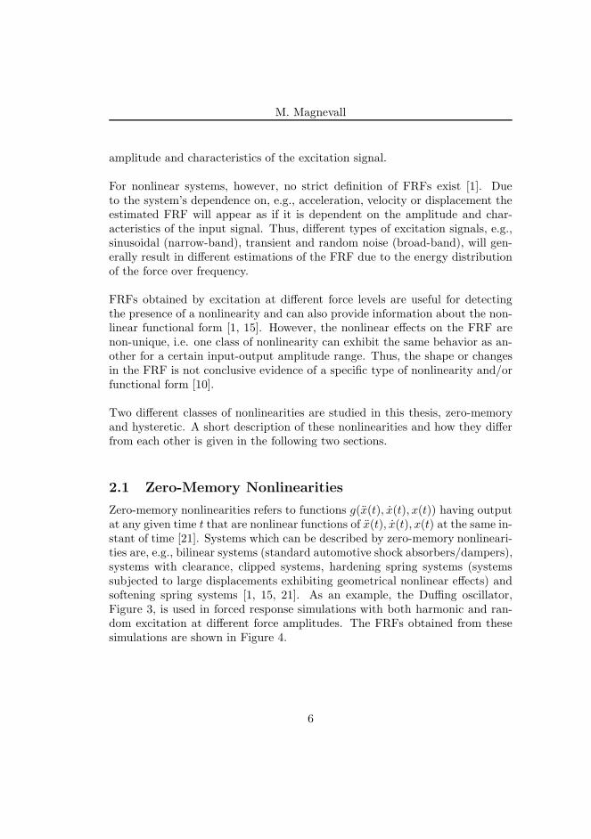
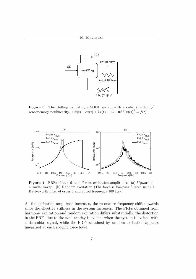
Zero-memory nonlinearities refers to functions g(x(t), x(t), x(t)) having outputat any given time t that are nonlinear functions of x(t), x(t), x(t) at the same in-stant of time [21]. Systems which can be described by zero-memory nonlineari-ties are, e.g., bilinear systems (standard automotive shock absorbers/dampers),systems with clearance, clipped systems, hardening spring systems (systemssubjected to large displacements exhibiting geometrical nonlinear effects) andsoftening spring systems [1, 15, 21]. As an example, the Duffing oscillator,Figure 3, is used in forced response simulations with both harmonic and ran-dom excitation at different force amplitudes. The FRFs obtained from thesesimulations are shown in Figure 4.

6

M. Magnevall

m=450 kg

f(t)

c=150 Ns/m

k=1.5·107

N/m

x(t)

1.7·1015 N/m3

Figure 3: The Duffing oscillator, a SDOF system with a cubic (hardening)

zero-memory nonlinearity. mx(t) + cx(t) + kx(t) + 1.7 · 1015(

x(t))

3= f(t).

27.5 28 28.5 29 29.5 30 30.5 31

10−6

10−5

10−4

Frequency [Hz]

Re

ce

pta

nce

[m

/N]

(a)

F=0.01 NRMS

F=0.2 NRMS

F=0.7 NRMS

27.5 28 28.5 29 29.5 30 30.5 31

10−6

10−5

10−4

Frequency [Hz]

Re

ce

pta

nce

[m

/N]

(b)

F=0.1 NRMS

F=3.5 NRMS

F=7 NRMS

Figure 4: FRFs obtained at different excitation amplitudes: (a) Upward si-nusoidal sweep. (b) Random excitation (The force is low-pass filtered using aButterworth filter of order 3 and cutoff frequency 100 Hz).

As the excitation amplitude increases, the resonance frequency shift upwardssince the effective stiffness in the system increases. The FRFs obtained fromharmonic excitation and random excitation differs substantially, the distortionin the FRFs due to the nonlinearity is evident when the system is excited witha sinusoidal signal, while the FRFs obtained by random excitation appearslinearized at each specific force level.

7

M. Magnevall

2.2 Hysteretic Nonlinearities

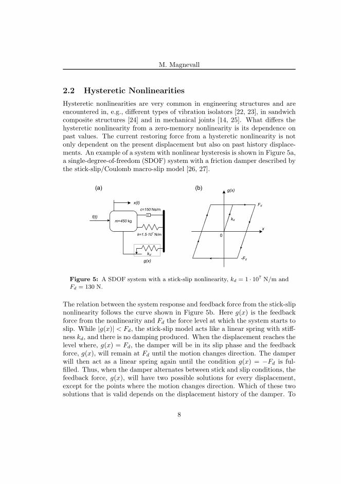
Hysteretic nonlinearities are very common in engineering structures and areencountered in, e.g., different types of vibration isolators [22, 23], in sandwichcomposite structures [24] and in mechanical joints [14, 25]. What differs thehysteretic nonlinearity from a zero-memory nonlinearity is its dependence onpast values. The current restoring force from a hysteretic nonlinearity is notonly dependent on the present displacement but also on past history displace-ments. An example of a system with nonlinear hysteresis is shown in Figure 5a,a single-degree-of-freedom (SDOF) system with a friction damper described bythe stick-slip/Coulomb macro-slip model [26, 27].

(a) (b) g(x)

x

Fd

-Fd

kd

0

m=450 kgf(t)

c=150 Ns/m

k=1.5·107N/m

x(t)

kd

g(x)

Figure 5: A SDOF system with a stick-slip nonlinearity, kd = 1 · 107 N/m andFd = 130 N.

The relation between the system response and feedback force from the stick-slipnonlinearity follows the curve shown in Figure 5b. Here g(x) is the feedbackforce from the nonlinearity and Fd the force level at which the system starts toslip. While |g(x)| < Fd, the stick-slip model acts like a linear spring with stiff-ness kd, and there is no damping produced. When the displacement reaches thelevel where, g(x) = Fd, the damper will be in its slip phase and the feedbackforce, g(x), will remain at Fd until the motion changes direction. The damperwill then act as a linear spring again until the condition g(x) = −Fd is ful-filled. Thus, when the damper alternates between stick and slip conditions, thefeedback force, g(x), will have two possible solutions for every displacement,except for the points where the motion changes direction. Which of these twosolutions that is valid depends on the displacement history of the damper. To

8

M. Magnevall

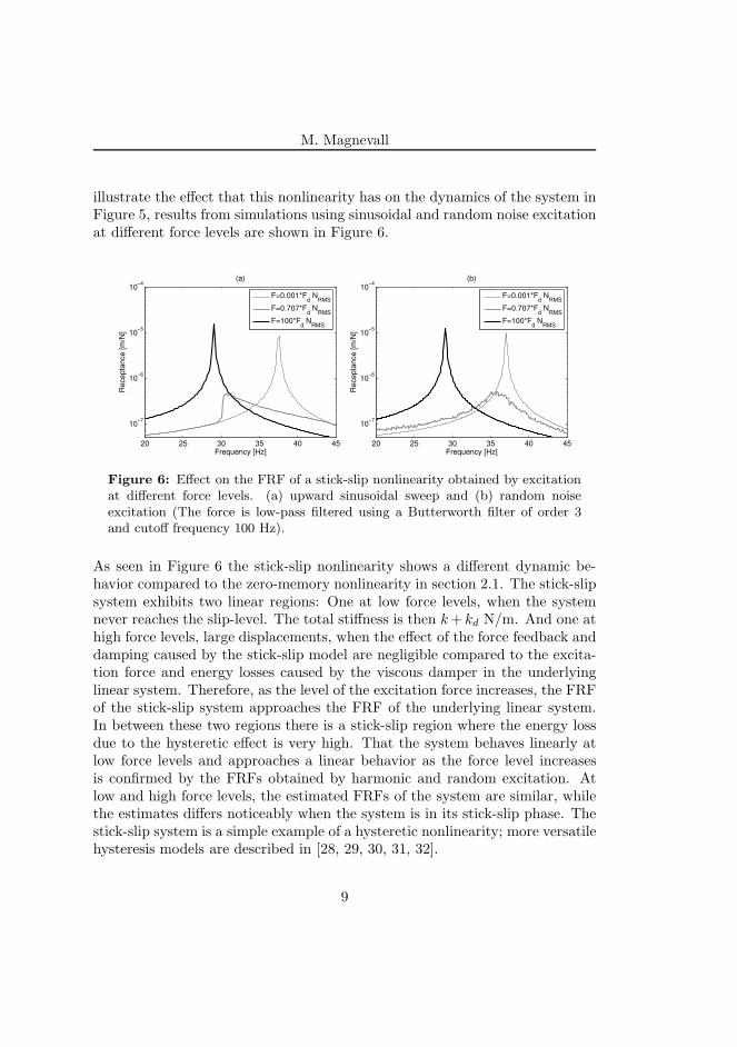
illustrate the effect that this nonlinearity has on the dynamics of the system inFigure 5, results from simulations using sinusoidal and random noise excitationat different force levels are shown in Figure 6.

20 25 30 35 40 45

10−7

10−6

10−5

10−4

Frequency [Hz]

(a)

Re

ce

pta

nce

[m

/N]

F=0.001*Fd N

RMS

F=0.707*Fd N

RMS

F=100*Fd N

RMS

20 25 30 35 40 45

10−7

10−6

10−5

10−4

Frequency [Hz]

Re

ce

pta

nce

[m

/N]

(b)

F=0.001*Fd N

RMS

F=0.707*Fd N

RMS

F=100*Fd N

RMS

Figure 6: Effect on the FRF of a stick-slip nonlinearity obtained by excitationat different force levels. (a) upward sinusoidal sweep and (b) random noiseexcitation (The force is low-pass filtered using a Butterworth filter of order 3and cutoff frequency 100 Hz).

As seen in Figure 6 the stick-slip nonlinearity shows a different dynamic be-havior compared to the zero-memory nonlinearity in section 2.1. The stick-slipsystem exhibits two linear regions: One at low force levels, when the systemnever reaches the slip-level. The total stiffness is then k+ kd N/m. And one athigh force levels, large displacements, when the effect of the force feedback anddamping caused by the stick-slip model are negligible compared to the excita-tion force and energy losses caused by the viscous damper in the underlyinglinear system. Therefore, as the level of the excitation force increases, the FRFof the stick-slip system approaches the FRF of the underlying linear system.In between these two regions there is a stick-slip region where the energy lossdue to the hysteretic effect is very high. That the system behaves linearly atlow force levels and approaches a linear behavior as the force level increasesis confirmed by the FRFs obtained by harmonic and random excitation. Atlow and high force levels, the estimated FRFs of the system are similar, whilethe estimates differs noticeably when the system is in its stick-slip phase. Thestick-slip system is a simple example of a hysteretic nonlinearity; more versatilehysteresis models are described in [28, 29, 30, 31, 32].

9

M. Magnevall

3 Time Domain Forced Response Simulation

Forced response simulation here refers to computing the motion (displacement,velocity or acceleration) of a system for a given force vector. The generalapproach is to use some method for time integration. Commonly used methodsare, e.g., the Runge-Kutta method with variations [33] and Newmark’s method[34]. In this chapter a method for forced response simulations based on digitalfilter theory is presented. This method is utilized throughout the thesis forforced response simulations with arbitrary sampled input signals. Consider asystem with localized nonlinearities, described by:

Mx(t) +Cx(t) +Kx(t) + g(

x(t), x(t),x(t))

= f(t) (3)

where M, C and K are the system’s mass, damping and stiffness matrices, re-spectively. x(t), x(t) and x(t) are the acceleration, velocity and displacementvectors, respectively. The vector f(t), describes the external forces acting onthe system and the vector g(t), includes artificial external forces that representthe nonlinearities.

An arbitrary transfer function, Hpq(s), of the linear (MCK) system in Equa-tion (3) can be compactly represented by modal superposition of its residues,Rpqr , and poles, λr, [35]:

Hpq(s) =

N∑

r=1

Rpqr

s− λr

+R∗

pqr

s− λ∗

r

(4)

where p refers to the response/output degree-of-freedom (DOF) and q refers tothe DOF of excitation/input. r refers to the current mode and N denotes thetotal number of modes included and s is the Laplace variable. Equation (4)can be transformed into a discrete IIR-filter [36], and expressed as a differenceequation where the current output, xp[n], is expressed as a weighted sum ofprevious inputs and outputs as:

xp[n] =

N∑

r=1

(

NB∑

i=0

Bipqrfq[n− i]−

NA∑

i=1

Aipqrxpr[n− i]

)

(5)

where NB and NA are the number of zeros and poles, respectively, in the filter.As seen in Equation (5), one set of filter coefficients, B and A, is needed foreach mode included. The total response is calculated by modal superposition

10

M. Magnevall

as the sum of the responses from each individual mode.

The method can be extended to forced response simulations of nonlinear sys-tems by modeling the nonlinearities as additional inputs (artificial forces). Asan example, the difference equation for the system’s response in DOF p due toforce input in DOF q = p and a displacement dependent nonlinearity connectedbetween DOF p and ground becomes:

xp[n] =

N∑

r=1

(

NB∑

i=0

Bipqr

(

fq[n− i]− gp[n− i])

−

NA∑

i=1

Aipqrxp[n− i]

)

(6)

Moving all unknown variables to the left side, putting the known variablesequal to Cn[n] and putting the sum of the known filter coefficients multipliedwith gp[n] equal to a constant En yields:

xp[n] + gp[n]En = Cn[n] (7)

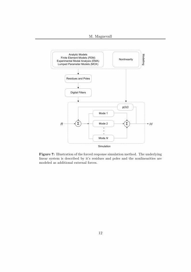
Cn[n] is dependent on the force and displacement history of the system and istherefore updated in each time step, hence the dependence on n, while En isa summation of the filter coefficients multiplied with gp[n] and is therefore in-dependent of the system’s history. Since the nonlinear restoring force, gp[n], isa function of the current displacement, xp[n], Equation (7) needs to be solvediteratively at each time step. Once the nonlinear restoring force is known,the system can be treated as a linear multiple-input/multiple-output systemand the response in other DOFs solved for by utilizing linear filter operations,according to Equation (5). Since only the DOFs directly connected to the exci-tation force and nonlinearities needs to be considered in the nonlinear iterationprocess and the remaining responses can be calculated using linear filteringtechniques, these forced response simulation routines can be made very fast. Agraphical illustration of the simulation routine is shown in Figure 7.

The residues and poles constitutes the basis in the simulation routines, thesecan be obtained analytically, from finite element models (FEM), from lumpedmass-damping-stiffness models (MCK) and from experimental modal analysis(EMA), which makes the simulation routines very versatile and useful in a wideapplication area. More details on how to calculate the filter coefficients andthe errors involved in the simulations are given in Paper E and [37, 38].

11

M. Magnevall

Analytic Models

Finite Element Models (FEM)

Experimental Modal Analysis (EMA)

Lumped Parameter Models (MCK)

Nonlinearity

Residues and Poles

Digital Filters

Mode 1

Mode 2

Mode N

Σ Σ

g({x})

{f} {x}

Mod

ellin

g

Simulation

Figure 7: Illustration of the forced response simulation method. The underlyinglinear system is described by it’s residues and poles and the nonlinearities aremodeled as additional external forces.

12

M. Magnevall

4 Experimental Testing

Due to the nature of the nonlinearities studied in this thesis, a single approachto characterize the theoretical and experimental systems investigated has notbeen possible to use. Therefore different characterization methods have beenutilized, improved and developed. These methods are often based on an as-sumption regarding the characteristics of the excitation signal used, e.g., broad-banded or harmonic excitation. In the experimental investigations, the forcesare applied on the structures using an electro-dynamic shaker. Due to thecharacteristics of the shaker and the shaker-structure interaction, realizationof the needed excitation forces can be complicated. The types of excitationsignals utilized in this research work, and how these signals can be applied onnonlinear systems are described in the following two sections.

4.1 Random Excitation

Random excitation is usually accomplished using an electrodynamic or hy-draulic shaker. Due to the randomness of the amplitude and phase of theexcitation signal, random excitation creates a ”linearized” FRF; this lineariza-tion can make it difficult to detect if a system behaves nonlinearly [15, 16].Also, random excitation is broad-banded, meaning that the energy associatedwith every single frequency is small, which can make it difficult to get enoughenergy into a system to excite structural nonlinearities. This issue is furtherenhanced by the fact that the shaker-structure interaction may lead to forcedropouts around the resonances, where the nonlinear effects commonly aremost evident, making it even harder to excite the nonlinearities [19]. Often,additional energy need to be added into the excitation signal around the reso-nance frequencies of the system under test, thereby facilitating excitation of thestructural nonlinearities. Thus, detailed inspections of both the FRFs and theforce spectrum is often necessary to determine if the nonlinearities are excitedas intended. Two different test-structures are characterized based on randomexcitation in Papers C and D.

4.2 Harmonic Excitation

When using harmonic excitation, usually only one frequency is excited at atime. As a result all the energy in the force signal is associated with a singlefrequency, making harmonic input suitable for excitation of structural nonlin-

13

M. Magnevall

earities. Also, using harmonic input, it is possible to measure the steady-stateresponse of the structure under test, facilitating analysis of specific details ofthe systems characteristics, such as the presence of additional harmonics re-lated to nonlinear effects or steady-state hysteresis loops.

Harmonic excitation can be accomplished by, e.g., stepped-sine or sine-sweep.Using stepped-sine the system is excited with one frequency at a time and themeasurement is taken when the system has reached its steady-state response.Sine-sweep is done by slowly and continuously varying the frequency of the ex-citation signal over a specified interval. The benefit with sine-sweep is its speedcompared to stepped-sine excitation. However, stepped-sine allows for betterpossibilities to control the excitation signal since measurements are performedunder steady-state conditions. This facilitates precise tuning by iterative off-line adjustment of the excitation signal. This is an important factor whenmeasurements are performed on nonlinear systems.

Several methods developed in relation to harmonic excitation of nonlinear sys-tems assume that the system is excited with a pure sinusoidal signal [26, 29, 39]which is simple to realize in simulations. In real applications, however, the ac-tual force applied to the structure is the reaction force between the shaker andthe structure under test [29, 40, 41]; see Figure 8.

Amplifier Force Sensorv(t)

f(t)

Nonlinear System

Shaker

Figure 8: Reaction forces in the measurement chain; a pure sinusoidal voltagesignal is the input to the amplifier, but due to the shaker-structure interaction,the excitation force becomes distorted.

The response from nonlinear systems generally contains additional frequencycomponents. These are transfered to the excitation signal and result in a dis-torted input force. This effect is usually most evident around the resonances

14

M. Magnevall

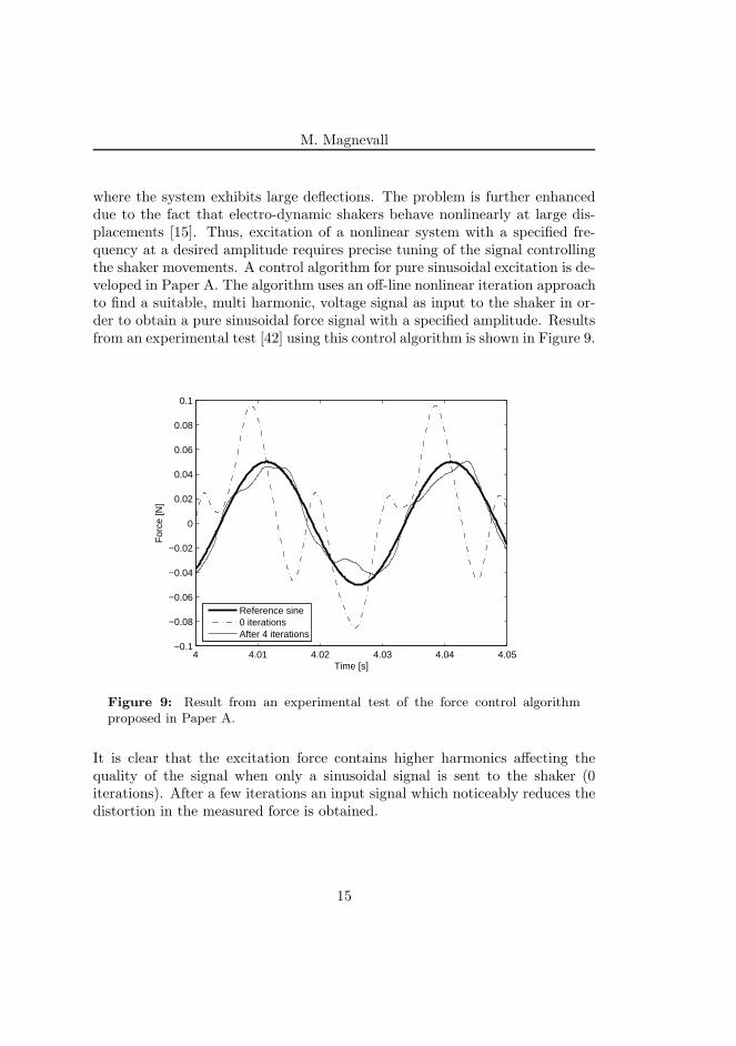
where the system exhibits large deflections. The problem is further enhanceddue to the fact that electro-dynamic shakers behave nonlinearly at large dis-placements [15]. Thus, excitation of a nonlinear system with a specified fre-quency at a desired amplitude requires precise tuning of the signal controllingthe shaker movements. A control algorithm for pure sinusoidal excitation is de-veloped in Paper A. The algorithm uses an off-line nonlinear iteration approachto find a suitable, multi harmonic, voltage signal as input to the shaker in or-der to obtain a pure sinusoidal force signal with a specified amplitude. Resultsfrom an experimental test [42] using this control algorithm is shown in Figure 9.

4 4.01 4.02 4.03 4.04 4.05−0.1

−0.08

−0.06

−0.04

−0.02

0

0.02

0.04

0.06

0.08

0.1

Time [s]

For

ce [N

]

Reference sine0 iterationsAfter 4 iterations

Figure 9: Result from an experimental test of the force control algorithmproposed in Paper A.

It is clear that the excitation force contains higher harmonics affecting thequality of the signal when only a sinusoidal signal is sent to the shaker (0iterations). After a few iterations an input signal which noticeably reduces thedistortion in the measured force is obtained.

15

M. Magnevall

5 Characterization of Nonlinear Systems

The overarching goal of parameter estimation is to find a mathematical modelthat describes the behavior of the observed system. For linear systems, modalanalysis is commonly used to extract the modal parameters describing thestudied system [2, 3, 43]. However, most methods developed for linear sys-tems break down if applied to nonlinear systems. Thus, for nonlinear systems,alternative methods have to be utilized to estimate the studied system’s pa-rameters. For a summary of the most common characterization methods fornonlinear systems, the reader is referred to the following review articles [1, 10].The characterization methods adopted in this research work are here dividedinto different groups dependent on the characteristics of the excitation forceand whether the parameter estimation is performed in the frequency or in thetime domain.

5.1 Frequency Domain

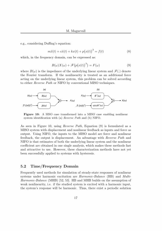
An important method for nonlinear parameter estimation, widely studied inrecent years, is the Reverse Path method. This method is based on broad-band excitation and was initially developed by Bendat et al. [44, 45] and Riceet al. [46, 47] and is thoroughly described in [21]. Reverse Path treats thenonlinearities as force feedback terms acting on an underlying linear system.The parameter estimation is performed in the frequency domain using conven-tional Multiple-Input-Single-Output (MISO) or Multiple-Input-Multiple-Output(MIMO) techniques and estimates of both the underlying linear properties andthe nonlinear coefficients are obtained from a single analysis. The method isknown as Reverse Path since the input and output quantities are reversed; seeFigure 10a. Reverse Path has proven to work well in experimental tests and hasbeen applied to various mechanical systems with zero-memory nonlinearities,which indicates that the method is robust and well suited for use in engineeringapplications [11, 12, 13, 48, 49].

In parallel with the development of Reverse Path, Adams et al. [50, 51] intro-duced an alternative variant known as Nonlinear Identification through Feed-back of Outputs (NIFO), which removed the original reversal of the input andoutputs; see Figure 10b.

The basic principle of the two methods described above can be explained by,

16

M. Magnevall

e.g., considering Duffing’s equation:

mx(t) + cx(t) + kx(t) + p(

x(t))3

= f(t) (8)

which, in the frequency domain, can be expressed as:

B(ω)X(ω) + F(

p(

x(t))3)

= F (ω) (9)

where B(ω) is the impedance of the underlying linear system and F (.) denotethe Fourier transform. If the nonlinearity is treated as an additional forceacting on the underlying linear system, this problem can be solved accordingto either Reverse Path or NIFO by conventional MISO techniques.

B(ω)

p(ω)

+

X(ω)

F(ω)

((x(t))3)

B-1(ω)

-p(ω)B-1(ω)

+

F(ω)

X(ω)

(a) (b)

((x(t))3)

Figure 10: A SISO case transformed into a MISO case enabling nonlinearsystem identification with (a) Reverse Path and (b) NIFO.

As seen in Figure 10, using Reverse Path, Equation (9) is formulated as aMISO system with displacement and nonlinear feedback as inputs and force asoutput. Using NIFO, the inputs to the MISO model are force and nonlinearfeedback, the output is displacement. An advantage with Reverse Path andNIFO is that estimates of both the underlying linear system and the nonlinearcoefficient are obtained in one single analysis, which makes these methods fastand attractive to use. However, these characterization methods have not yetbeen successfully applied to systems with hysteresis.

5.2 Time/Frequency Domain

Frequently used methods for simulation of steady-state responses of nonlinearsystems under harmonic excitation are Harmonic-Balance (HB) and Multi-Harmonic-Balance (MHB) [52, 53]. HB and MHB builds on the assumption ofweak nonlinearity, i.e. if the studied system is excited with a harmonic input,the system’s response will be harmonic. Thus, there exist a periodic solution

17

M. Magnevall

and the excitation force, the response and the nonlinear feedback forces can beexpressed by Fourier series. A benefit with these methods is that the system’ssteady-state response is obtained directly. With time integration methods,which usually suffers from transient responses in the beginning, the integrationneeds to go on for a while to find the steady-state response, making time inte-gration more computationally expensive.

Duffing’s equation (Equation (8)) can, if excited by a sinusoidal signal, beexpressed by a truncated one-term (HB) Fourier expansion:

(

−mω2

0+ jω0c+ k

)

X(ω0)ejω0t =

(

F (ω0)−G(ω0))

ejω0t (10)

where:

G(ω) = F(

p(

x(t))3)

(11)

Thus, X(ω0), F (ω0) and G(ω0) are the complex Fourier coefficients of the sys-tems displacement, excitation force and nonlinear feedback force, respectively,at the fundamental forcing frequency, ω0. Removing the time dependence,Equation (10) becomes:

B(ω0)X(ω0)− F (ω0) +G(ω0) = 0 (12)

where B(ω) is the impedance of the underlying linear system. For a givenexcitation F at a specified frequency ω0, the system’s response, X(ω0), is es-timated by balancing the Fourier coefficients in Equation (12) by each other.This “harmonic balance” procedure needs to be repeated for each frequency ofinterest, and the solutions represent the frequency response of the system. Toextend HB to MHB, additional harmonics need to be considered [15, 29], whichmeans that additional equations are added and instead a nonlinear system ofequations need to be solved at every frequency step. MHB generally provides amore accurate estimate of the systems frequency response on the expense of ahigher computational cost. By solving the system’s frequency response over aspecified interval, it is possible to calculate an FRF. The FRF obtained by HBand MHB are often regarded as the analytical analogue to the FRF obtainedby stepped sine testing [15].

These methods have been used in applications for both simulation and systemcharacterization with zero-memory and hysteretic nonlinearities [26, 29, 54, 23,

18

M. Magnevall

55, 52]. System characterization can be performed both in the time domain bycomparing simulated and experimentally acquired steady-state responses andin the frequency domain by comparing FRFs obtained from stepped-sine mea-surements with FRFs calculated using HB or MHB. A procedure for systemcharacterization in the frequency domain, utilizing MHB, is proposed in PaperB.

When setting up the HB and MHB equations it is usually assumed that thesystem is excited with a pure harmonic excitation, i.e. one single frequency.As explained previously, a single harmonic excitation can be difficult to realizein experimental measurements, due to the shaker characteristics and shaker-structure interaction, which can make comparisons between simulated and ex-perimental data difficult. There exist methods which extends MHB to sys-tems with multiple excitation frequencies [56, 57]. However, the complexity ofthe problem formulation and the total number of harmonics needed increasessubstantially [57], resulting in a less robust and less computationally efficientmethod.

An alternative approach, as suggested in Paper E, when a pure sinusoidalexcitation cannot be realized or when non-periodic excitation forces are used(i.e. random or transient excitation [58, 59]), is to perform the characterizationin the time domain using the measured force as excitation signal and comparesimulated and experimentally acquired responses.

19

M. Magnevall

6 Summary of Papers

Paper A

This paper presents an algorithm for reducing harmonic distortion in the forcesignal during experimental tests on nonlinear systems with sinusoidal excita-tion. The distortions are attenuated by sending a multi-harmonic voltage signalwith optmized amplitudes and phases to the shaker. Since the relation betweenthe input voltage signal and the measured force is nonlinear, an iterative ap-proach is required to find the correct set of harmonic components of the inputvoltage signal. The control algorithm uses the Newton-Raphson and Broyden’smethod as nonlinear solvers. Simulations show that the control algorithm iscapable of obtaining a non-distorted force signal even in the presence of a sig-nificant nonlinearity.

Paper B

Two parameter estimation methods are studied; one based on random noiseinput and another based on sinusoidal excitation. The method based on ran-dom excitation treats the nonlinearities as force feedback terms acting on anunderlying linear system. The parameter estimation is performed in the fre-quency domain by using conventional MIMO/MISO techniques known fromlinear theory. The studied method is applied in simulations on single-degreeand multi-degree-of-freedom-systems and shows great potential. Building onPaper A, where a control algorithm for harmonic excitation was developed, amethod for characterization of nonlinear systems based on sinusoidal input isalso investigated. The method uses a combination of multi-harmonic-balance(MHB) and stepped-sine excitation. The parameter estimation is performedin the frequency domain by matching the measured and simulated frequencyresponse functions with each other. The benefit of the MHB/stepped-sinemethod is its versatility. It can handle both zero-memory nonlinearities andnonlinearities with memory, such as systems with hysteresis.

Paper C

Building on the previous investigation concerning random excitation from Pa-per B, this paper presents a more detailed analysis together with experimentalresults. The method requires initial knowledge about the nonlinearity, i.e. the

20

M. Magnevall

physical location and the nonlinear functional form. A strategy is proposed toidentify the nonlinear nodes and the type of nonlinearity that is present in thesystem. A validation with a simulation model indicate that this approach canbe useful. Finally, an experimental system with a geometric (hardening-spring)nonlinearity is studied. The analysis of the experimental data indicates that theestimate of the underlying linear system around the resonance is very sensitiveto how the parameter estimation model is formulated. In general, the experi-mental result shows that the analysis is significantly improved when using thenonlinear identification method compared to traditional linear techniques.

Paper D

Building on the results from Papers B and C, a generalized approach to applythe method of Reverse Path on continuous mechanical systems with severalnonlinearities is developed. This approach uses unconditioned inputs and as-sumes that the locations of the nonlinearities are known beforehand and thatresponse measurements can be obtained in the nonlinear nodes. Excitation isonly needed in one location, which can be located away from the nonlinearities.The method provides the means to estimate both the underlying linear systemand the nonlinear parameters of complex structures in a straightforward way.The method was applied in both simulations and experimental tests. The re-sults from the experimental tests was compared to a static measurement of thenonlinear force and showed a very good agreement.

Paper E

For experimental testing, pure sinusoidal excitation can be both difficult andtime consuming to realize. Therefore, complementing the results from PapersA and B, a method for characterizing systems with hysteresis based on discretetime records is presented. A new forced response routine for a general me-chanical structure with a localized hysteretic mass damper is developed. Thehysteresis effect of the damper is described by the Bouc-Wen equation and theintended industrial application is simulation of passive vibration attenuationin metal machining. This simulation method is then used as a basis in a twostage parameter estimation routine performed in the time domain. The nonlin-ear parameter estimation is performed by a real coded genetic algorithm, andapplied in both simulations and experimental tests on a dry-friction damper.

21

M. Magnevall

Paper F

Simulating the dynamic behavior of different cutting tools used in metal ma-chining requires knowledge about the forces acting on the tool. Therefore, ac-curate estimates of cutting forces are important. However, dynamic influencesfrom the measurement system affect the result which can make the obtainedcutting force data erroneous and misleading. This paper develops a method foroff-line inverse filtering of the measured data which removes unwanted dynamiceffects originating from the measurement system and improves the estimationof the cutting forces. The method is successfully tested in both simulationsand in experimental test using different cutting conditions.

22

M. Magnevall

7 Concluding Discussion

This thesis focuses on the development and validation of methods for simula-tion, experimental testing and characterization of nonlinear mechanical sys-tems. This research has evolved in collaboration with industrial partnersthrough participatory action research in ongoing product development and re-search projects. The systems studied are considered to be predominantly linearbut with local significant nonlinearities, giving the total system a weak nonlin-ear behavior. A fundamental strategy employed is to use already establishedand validated methods from linear analysis as a basis for the development ofnew and improved simulation and characterization methods for nonlinear me-chanical systems.

The large amount of data needed for accurate assessment of developed nonlin-ear characterization methods puts a high demand on the simulation routinesutilized. Using random noise, the combination of a requirement for high spec-tral resolution and a requirement for several averages to accurately estimate thestatistical properties of the system’s response, results in a need for long datasequences. The amount of data required further increases considering that (i)performing simulations based on sampled data requires a fine time resolutionto keep the errors small and (ii) the response from nonlinear systems oftencontains higher harmonics which further increases the demand on a fine timeresolution to accurately capture the systems dynamics. Additionally, charac-terization methods based on nonlinear optimization schemes often requires alarge number of repeated simulations in order to converge toward a specifiedcriterion. A result of this thesis is computationally efficient forced responsesimulation routines, facilitating extensive investigation of systems with zero-memory or hysteretic nonlinearities.

Two methods for nonlinear parameter estimation utilizing random input, Re-verse Path and Nonlinear Identification through Feedback of Outputs (NIFO)are investigated both in simulations and experimental applications on mechan-ical systems with zero-memory nonlinearities. The methods provide an attrac-tive solution methodology due to the formulation where additional inputs arecreated based on measured responses and that estimates of both the underly-ing linear system and nonlinear coefficients are obtained, by least square fitsbased on averaged spectral data. The modal parameters can then be extractedfrom the estimates of the underlying linear system and used in conjunction

23

M. Magnevall

with the nonlinear coefficients to build a theoretical model of the studied sys-tem. A specific result from this thesis is a generalization of the Reverse Pathmethod which allows for characterization of systems with an arbitrary numberof localized zero-memory nonlinearities in a structured way. The experimentaltests indicate that the methods are robust, efficient and well suited for use withmeasurement data. The tests also show a discrepancy between Reverse Pathand NIFO, indicating that the presence of contaminating noise has a significanteffect on the result, which pose an interesting question for future research.

A significant part of this thesis treats simulation and characterization of sys-tems with hysteresis effects. The characterization methods proposed are: (i)a frequency domain approach which requires a pure harmonic excitation forceand (ii) a time domain approach which does not put any constraints on thecharacteristics of the excitation signal. Interesting for future work is to continueto develop and improve the suggested methods regarding characterization andmodeling of hysteretically-damped tools for metal cutting. Examples of inter-esting topics within this field are characterization of different types of dampingmaterials and simulation of the damper effect on machining productivity. An-other important question for future research is how to apply Reverse Path andNIFO on systems with hysteresis effects.

An essential part of the research work has been experimental validation of thedeveloped methods for characterization of nonlinear systems. This, in turn, hasled to a need for methods which can facilitate experimental testing. Experi-mental validation of the nonlinear characterization methods was successfullycompleted on continuous mechanical systems with localized nonlinearities, con-firming the robustness of the proposed methods concerning use with experimen-tal data. The results from these tests provide a basis for further experimentalvalidation on more complex mechanical systems than studied in this thesis.

The general contribution to science and technology of this thesis is the devel-opment and improvement of analysis tools for simulation, experimental testingand characterization of nonlinear mechanical systems with localized nonlinear-ities.

24

M. Magnevall

On a more specific level this thesis:

• Presents a method for improved harmonic excitation of nonlinear systemsusing numerically optimized input signals.

• Provides a simplified analysis procedure for continuous mechanical sys-tems with an arbitrary number of localized zero-memory nonlinearitiesby a generalization of the Reverse Path method using partially correlatedinputs.

• Presents a method to remove unwanted dynamic effects in cutting forcemeasurements using inverse filtering. The method increases the usablefrequency range of the dynamometer and significantly improves the mea-surement results compared to traditional techniques.

• Contributes to the experimental validation of the nonlinear characteriza-tion methods: Reverse Path and Nonlinear Identification Through Feed-back of Outputs.

• Presents an efficient time domain simulation and characterization methodfor use with hysteretically-damped systems described by the Bouc-Wenhysteresis model.

25

M. Magnevall

References

[1] Gaetan Kerschen, Keith Worden, Alexander F. Vakakis, and Jean-ClaudeGolinval. Past, present and future of nonlinear system identification instructural dynamics. Mechanical Systems and Signal Processing, 20(3):505– 592, 2006.

[2] David John Ewins. Modal testing : theory, practice and application. Re-search Studies Press, Baldock, 2. ed. edition, 2000.

[3] Randall J. Allemang. Analytical and experimental modal analysis. Struc-tural Dynamics Research Laboratory, University of Cincinnati, Cincinnati,Ohio 45221-0072, 1994. UC-SDRL-CN-20-263-662.

[4] H. R. E. Siller. Non-linear modal analysis methods for engineering struc-tures. PhD Thesis, Imperial College, London, 2004.

[5] A. Jonsson. Lean Prototyping of multi-body and mechatronic systems. PhDThesis, Blekinge Institute of Technology, 2004.

[6] J. Wall. Dynamic study of an automobile exhaust system. Licentiate The-sis, Blekinge Institute of Technology, 2003.

[7] T. Englund. Dynamic characteristics of automobile exhaust system com-ponents. Licentiate Thesis, Blekinge Institute of Technology, 2003.

[8] J. Wall. Simulation-driven design of complex mechanical and mechatronicsystems. PhD Thesis, Blekinge Institute of Technology, 2007.

[9] J. Fredin. Modelling, simulation and optimisation of a machine tool. Li-centiate Thesis, Blekinge Institute of Technology, 2009.

[10] Douglas E. Adams and Randall J. Allemang. Survey of nonlinear detectionand identification techniques for experimental vibrations. In Proceedingsof the 23rd International Conference on Noise and Vibration Engineering,ISMA, pages 517 – 529, Leuven, Belgium, 1998.

[11] L. Garibaldi. Application of the conditioned reverse path method. Mechan-ical Systems and Signal Processing, 17(1):227 – 235, 2003. Conditionedreverse path (CRP) method;.

26

M. Magnevall

[12] S. Marchesiello. Application of the conditioned reverse path method. Me-chanical Systems and Signal Processing, 17(1):183 – 188, 2003. Dampers;.

[13] G. Kerschen, V. Lenaerts, and J.-C. Golinval. Identification of a continuousstructure with a geometrical non-linearity. part i: Conditioned reverse pathmethod. Journal of Sound and Vibration, 262(4):889 – 906, 2003.

[14] K.Y. Sanliturk, D.J. Ewins, and A.B. Stanbridge. Underplatform dampersfor turbine blades: Theoretical modeling, analysis, and comparison withexperimental data. Journal of Engineering for Gas Turbines and Power,123(4):919 – 929, 2001.

[15] K. Worden and G. R. Tomlinson. Nonlinearity in Structural Dynamics:Detection, Identification and Modelling. IOP Publishing Ltd, Bristol, UK,2001.

[16] A.F. Vakakis and D.J. Ewins. Effects of weak non-linearities on modalanalysis. Mechanical Systems and Signal Processing, 8(2):175 – 98,1994/03/.

[17] Influence and characterisation of weak non-linearities in swept-sine modaltesting. Aerospace Science and Technology, 8(2):111 – 120, 2004.

[18] Ulrich Fuellekrug and Dennis Goege. Identification of weak non-linearitieswithin complex aerospace structures. Aerospace Science and Technology,2011.

[19] A. Josefsson. Identification and Simulation Methods for Nonlinear Me-chanical Systems Subjected to Stochastic Excitation. PhD Thesis, BlekingeInstitute of Technology, 2011.

[20] Julius S. Bendat and Allan G. Piersol. Engineering applications of corre-lation and spectral analysis. Wiley, New York, 2. ed. edition, 1993.

[21] Julius S. Bendat. Nonlinear system analysis and identification from ran-dom data. Wiley, New York, 1990.

[22] A. Al Majid and R. Dufour. Harmonic response of a structure mountedon an isolator modelled with a hysteretic operator: Experiments and pre-diction. Journal of Sound and Vibration, 277(1-2):391 – 403, 2004.

27

M. Magnevall

[23] Y.Q. Ni, J.M. Ko, and C.W. Wong. Identification of non-linear hystereticisolators from periodic vibration tests. Journal of Sound and Vibration,217(4):737 – 756, 1998.

[24] K. H. Hornig. Parameters characterization of the bouc/wen mechanicalhysteresis model for sandwich composite materials by using real codedgenetic algorithms. Technical report, Mechanical Engineering Department,Ross Hall, Auburn, Alabama, 2000.

[25] D Smallwood, D Gregory, and R Coleman. Damping investigations of asimplified frictional shear joint. In Proceedings of Shock and VibrationSymposium, 2000.

[26] Giovanna Girini and Stefano Zucca. Multi-harmonic analysis of a sdoffriction damped system. In Proceedings of 3rd Youth Symposium on Ex-perimental Solid Mechanics, Poretta Terme, Italy, 2004.

[27] Francisco J. Marquina, Armando Coro, Alberto Gutierrez, RobertoAlonso, David J. Ewins, and Giovanna Girini. Friction damping mod-eling in high stress contact areas using microslip friction model. volume 5,pages 309 – 318, Berlin, Germany, 2008.

[28] Jack W. Macki, Paolo Nistri, and Pietro Zecca. Mathematical models forhysteresis. SIAM Review, 35(1):94 – 123, 1993.

[29] Janito V. Ferreira. Dynamic Response Analysis of structures with non-linear components. PhD Thesis, Imperial College, London, 1998.

[30] Mohammed Ismail, Faycal Ikhouane, and Jose Rodellar. The hysteresisbouc-wen model, a survey. Archives of Computational Methods in Engi-neering, 16(2):161 – 188, 2009.

[31] Yousef Iskandarani and Hamid Reza Karimi. Hysteresis modeling forthe rotational magnetorheological damper. In Proceedings of the 4thWSEAS international conference on Energy and development - environ-ment - biomedicine, GEMESED’11, pages 479–485. World Scientific andEngineering Academy and Society (WSEAS), 2011.

[32] Faycal Ikhouane and Jose Rodellar. Systems with Hysteresis: Analysis,Identification and Control Using the Bouc-Wen Model. John Wiley &Sons, 2007.

28

M. Magnevall

[33] Erwin Kreyszig. Advanced Engineering Mathematics. Wiley, New York,8th edition edition, 1999.

[34] Nathan M. Newmark. Method of computation for structural dynamics.AGARD Conference Proceedings, 2:1235 – 1264, 1972.

[35] Anders Brandt. Noise and vibration analysis : signal analysis and exper-imental procedures. Wiley, Chichester, 2011.

[36] K. Ahlin, M. Magnevall, and A. Josefsson. Simulation of forced response inlinear and nonlinear mechanical systems using digital filters. In Proceedingsof ISMA 2006, 2006.

[37] K Ahlin. On the use of digital filters for mechanical system simulation. InProceedings of 74th Shock and Vibration Symposium, 2003.

[38] K. Ahlin. Time history forced response in mechanical systems. SVIB AU1Symposium Riksgransen, 2005.

[39] Hugo Ramon Elizalde Siller. Non-linear modal analysis methods for engi-neering structures. PhD Thesis, Imperial College, London, 2004.

[40] S Rossmann. Development of force controlled modal testing on rotor sup-ported by magnetic bearings. Master’s thesis, Imperial College, London,1999.

[41] I. Bucher. Exact adjustment of dynamic forces in presence of non-linearfeedback and singularity - theory and algorithm. Journal of Sound andVibration, 218(1):1 – 27, 1998.

[42] M. Magnevall, A. Josefsson, and K. Ahlin. Experimental verification of acontrol algorithm for nonlinear systems. In Proceedings of IMAC XXIV,2006.

[43] Nuno Manuel Mendes Maia and Julio Martins Montalvao e Silva. Theo-retical and experimental modal analysis. Research Studies Press, Taunton,1997.

[44] J. S. Bendat and A. G. Piersol. Spectral analysis of non-linear systems in-volving square-law operations. Journal of Sound and Vibration, 81(2):199– 214, 1982.

29

M. Magnevall

[45] J.S. Bendat and A.G. Piersol. Decomposition of wave forces into linearand non-linear components. Journal of Sound and Vibration, 106(3):391– 408, 1986.

[46] H.J. Rice and J.A. Fitzpatrick. A generalised technique for spectral anal-ysis of non-linear systems. Mechanical Systems and Signal Processing,2(2):195 – 207, 1988.

[47] H.J. Rice and J.A. Fitzpatrick. A procedure for the identification of linearand non-linear multi-degree-of-freedom systems. Journal of Sound andVibration, 149(3):397 – 411, 1991.

[48] A. Josefsson, M. Magnevall, and K. Ahlin. On nonlinear parameter esti-mation with random noise signals. In Proceedings of IMAC XXV, 2007.

[49] M. Magnevall, A. Josefsson, and K. Ahlin. On parameter estimation andsimulation of zero memory nonlinear systems. In Proceedings of IMACXXVI, 2008.

[50] D.E. Adams and R.J. Allemang. Frequency domain method for estimatingthe parameters of a non-linear structural dynamic model through feedback.Mechanical Systems & Signal Processing, 14(4):637 – 656, 2000.

[51] Muhammad Haroon and Douglas E. Adams. A modified h2 algorithm forimproved frequency response function and nonlinear parameter estimation.Journal of Sound and Vibration, 320(4-5):822 – 837, 2009.

[52] C. Pierre, A.A. Ferri, and E.H. Dowell. Multi-harmonic analysis of dryfriction damped systems using an incremental harmonic balance method.pages ASME, New York, NY, USA –, Miami Beach, FL, USA, 1985.

[53] A. Cardona, T. Coune, A. Lerusse, and M. Geradin. A multiharmonicmethod for non-linear vibration analysis. International Journal for Nu-merical Methods in Engineering, 37(9):1593 – 608, 1994/05/15.

[54] S. L. Lau, Y. K. Cheung, and S. Y. Wu. Incremental harmonic balancemethod with multiple time scales for aperiodic vibration of nonlinear sys-tems. Journal of Applied Mechanics, Transactions ASME, 50(4a):871 –876, 1983.

30

M. Magnevall

[55] K.Y. Sanliturk and D.J. Ewins. Modelling two-dimensional friction contactand its application using harmonic balance method. Journal of Sound andVibration, 193(2):511 – 523, 1996.

[56] A. Raghothama and S. Narayanan. Periodic response and chaos in non-linear systems with parametric excitation and time delay. Nonlinear Dy-namics, 27(4):341 – 65, 2002/03/.

[57] J.F. Dunne and P. Hayward. A split-frequency harmonic balance methodfor nonlinear oscillators with multi-harmonic forcing. Journal of Soundand Vibration, 295(3-5):939 – 963, 2006.

[58] A. Kyprianou, K. Worden, and M. Panet. Identification of hystereticsystems using the differential evolution algorithm. Journal of Sound andVibration, 248(2):289 – 314, 2001.

[59] Yin Qiang, Zhou Li, and Wang Xinming. Parameter identification ofhysteretic model of rubber-bearing based on sequential nonlinear least-square estimation. Earthquake Engineering and Engineering Vibration,9(3):375 – 83, Sept. 2010.

31

M. Magnevall

32

Paper A

Control Algorithm For SineExcitation On Nonlinear Systems

33

Paper A is published as:

Josefsson, A., Magnevall, M. and Ahlin, K. Control Algorithm forSine Excitation on Nonlinear Systems, In Proceedings of IMAC-XXIV, Conference & Exposition on Structural Dynamics, St. Louis,USA, 2006.

34

Control Algorithm For Sine Excitation On

Nonlinear Systems

Andreas Josefsson

Martin Magnevall

Kjell Ahlin

Blekinge Institute of Technology, SE-371 79 Karlskrona, Sweden

Abstract

When using electrodynamic vibration exciters to excite structures, theactual force applied to the structure under test is the reaction force be-tween the exciter and the structure. The magnitude and phase of thereaction force is dependent upon the characteristics of the structure andexciter. Therefore the quality of the reaction force i.e. the force appliedon the structure depends on the relationship between the exciter andstructure under test.

Looking at the signal from the force transducer when exciting a structurewith a sine wave, the signal will appear harmonically distorted within theregions of the resonance frequencies. This phenomenon is easily observedwhen performing tests on lightly damped structures. The harmonic dis-tortion is a result of nonlinearities produced by the shaker when under-going large amplitude vibrations, at resonances.

When dealing with non-linear structures, it is of great importance tobe able to keep a constant force level as well as a non-distorted sinewave in order to get reliable results within the regions of the resonancefrequencies. This paper presents theoretical methods that can be usedto create a non-distorted sinusoidal excitation signal with constant forcelevel.

35

Paper A

Nomenclature

A Estimate of Jacobianf Frequency, [Hz]FM Measured Force Vector with sine and cosine components for each harmonicFV Difference between measured and desired Force vectorJ Jacobian included in partial derivativesk Number of harmonics to be controlledn Iteration counterrn Sine and cosine components in response (force) signalt Time, [sec]vn Sine and cosine components in input (volt) signalVn Input voltage vector with sine and cosine components for each harmonic

1 Introduction

When performing measurements on nonlinear structures a stepped-sine excita-tion is a favorable method. Unlike random noise signals, a sine-excitation canbe controlled to desired force amplitude as well as providing a better physicalunderstanding of the actual problem.

Most of the theory developed for nonlinear systems [1] relies on the fact thatthe structure under test is excited with a pure sine wave. However, if the struc-ture has a strong nonlinear behavior, the response signal will contain higherharmonics or sub-harmonics. This will also give distortion in the force signalsince the force applied is the reaction force between the exciter and the struc-ture.

This problem will be further amplified since the shaker in itself shows a non-linear behavior at larger displacements. This is due to the fact that the coilis moving in the non-linear parts of the magnetic field. Distortion in the forcesignal can therefore be observed even when exciting linear systems, particularlyweakly damped structures with large vibrations at resonance frequencies.

A principal simulation model used when developing the control algorithm isshown in Figure 1. A pure sine signal is sent as a voltage signal through a non-

36

Control Algorithm For Sine Excitation On Nonlinear Systems

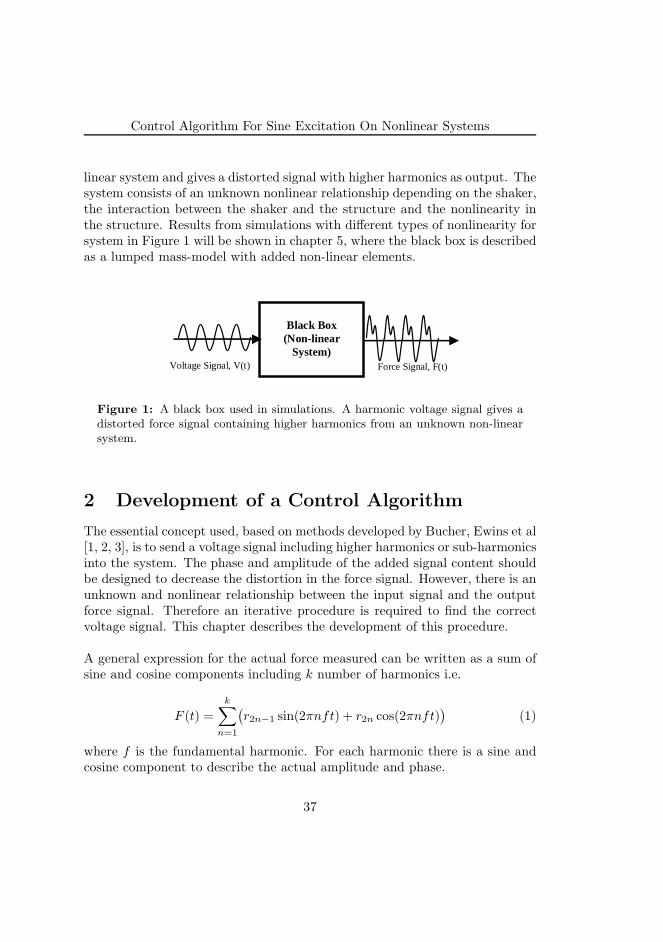
linear system and gives a distorted signal with higher harmonics as output. Thesystem consists of an unknown nonlinear relationship depending on the shaker,the interaction between the shaker and the structure and the nonlinearity inthe structure. Results from simulations with different types of nonlinearity forsystem in Figure 1 will be shown in chapter 5, where the black box is describedas a lumped mass-model with added non-linear elements.

Voltage Signal, V(t) Force Signal, F(t)

Black Box (Non-linear

System)

Figure 1: A black box used in simulations. A harmonic voltage signal gives adistorted force signal containing higher harmonics from an unknown non-linearsystem.

2 Development of a Control Algorithm

The essential concept used, based on methods developed by Bucher, Ewins et al[1, 2, 3], is to send a voltage signal including higher harmonics or sub-harmonicsinto the system. The phase and amplitude of the added signal content shouldbe designed to decrease the distortion in the force signal. However, there is anunknown and nonlinear relationship between the input signal and the outputforce signal. Therefore an iterative procedure is required to find the correctvoltage signal. This chapter describes the development of this procedure.

A general expression for the actual force measured can be written as a sum ofsine and cosine components including k number of harmonics i.e.

F (t) =

k∑

n=1

(

r2n−1 sin(2πnft) + r2n cos(2πnft))

(1)

where f is the fundamental harmonic. For each harmonic there is a sine andcosine component to describe the actual amplitude and phase.

37

Paper A

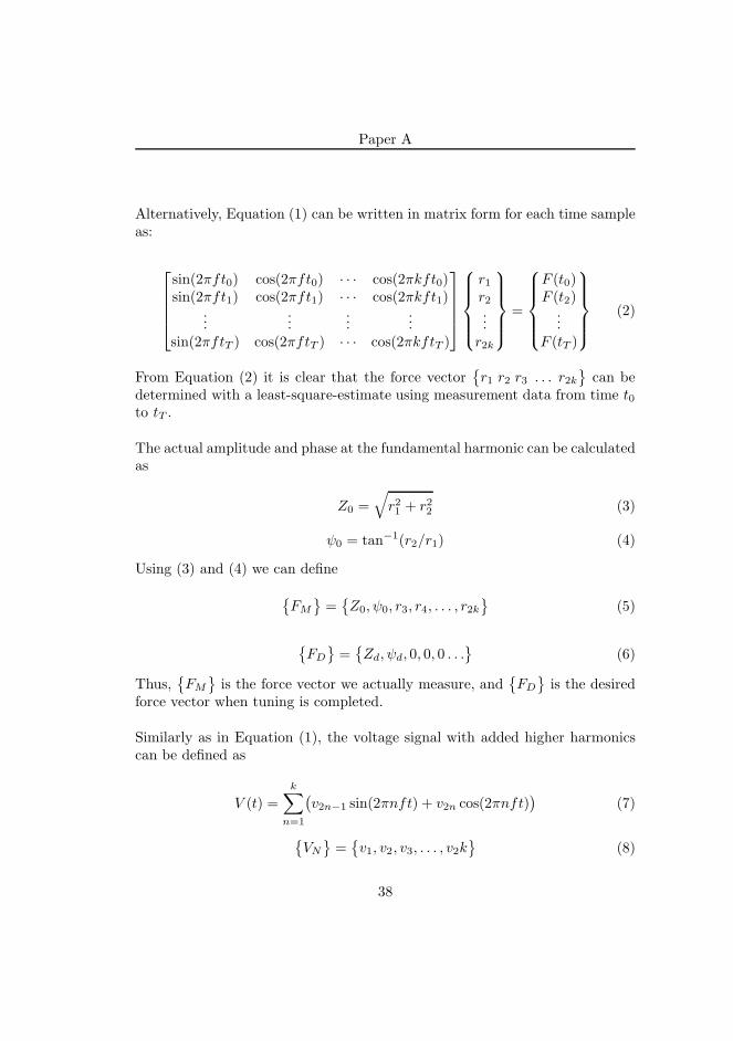
Alternatively, Equation (1) can be written in matrix form for each time sampleas:

sin(2πft0) cos(2πft0) · · · cos(2πkft0)sin(2πft1) cos(2πft1) · · · cos(2πkft1)

......

......

sin(2πftT ) cos(2πftT ) · · · cos(2πkftT )

r1r2...r2k

=

F (t0)F (t2)

...F (tT )

(2)

From Equation (2) it is clear that the force vector{

r1 r2 r3 . . . r2k}

can bedetermined with a least-square-estimate using measurement data from time t0to tT .

The actual amplitude and phase at the fundamental harmonic can be calculatedas

Z0 =√

r21+ r2

2(3)

ψ0 = tan−1(r2/r1) (4)

Using (3) and (4) we can define

{

FM

}

={

Z0, ψ0, r3, r4, . . . , r2k}

(5)

{

FD

}

={

Zd, ψd, 0, 0, 0 . . .}

(6)

Thus,{

FM

}

is the force vector we actually measure, and{

FD

}

is the desiredforce vector when tuning is completed.

Similarly as in Equation (1), the voltage signal with added higher harmonicscan be defined as

V (t) =

k∑

n=1

(

v2n−1 sin(2πnft) + v2n cos(2πnft))

(7)

{

VN}

={

v1, v2, v3, . . . , v2k}

(8)

38

Control Algorithm For Sine Excitation On Nonlinear Systems

{

VN}

is vector containing all sine and cosine coefficients for the voltage signal.Here it is assumed that the voltage signal should initially contain the sameharmonic components as observed in the force signal. Consequently, if we wantto control k number of harmonics (including the fundamental), there are 2knumbers of unknowns.

The required voltage signal cannot be identified by simply studying the forcesignal since there is an unknown non-linear relationship between

{

VN}

and{

FM

}

. Instead the problem is dealt with as a system of non-linear equations.Solving this type of problems can presents some major difficulties. Normallythere are several roots and the selected algorithm can be unable to find a so-lution if the initial guess is too far away.

The method selected in this work is based on a multidimensional Newton-Raphson scheme [4, 5]. Unlike more general optimization routines tested, suchas Powell and Nelder-Mead, this method has quadratic convergence. Unfortu-nately the method requires the derivates to actually be calculated which canpresent some difficulties when dealing with measurement data.

The Newton-Raphson method also has relatively large sensitivity against start-ing values. However, this may not become a large problem in real measure-ments. Since the force signal is most distorted at resonances, it is possible tostart in an area where the number of harmonics are low and then slowly steptowards the resonance.

During the frequency sweep the previous set of input voltage, which gave anon-distorted force signal, is always used as initial guess.

Next, the Newton-Raphson procedure and its application to our problem aredescribed. A general n x n nonlinear problem can be formulated as

g1(x1, x2, . . . , xN )g2(x1, x2, . . . , xN )

...gN(x1, x2, . . . , xN )

=

00...0

(9)

where{

g1, g2, . . . , gN}

are the functions to minimize. For our case the functionswill be the difference between measured force vector and desired force vector.

39

Paper A

In vector form this can be written as

{

FV

}

={

FM

}

−{

FD

}

(10)

Each of the functions in (10) are then assumed to be dependent on the inputvoltage vector described in Equation (8) so that

{

FV (v1, v2, . . . , vN )}

={

0}

(11)

Once an initial guess is provided on{

VN}n

we would now like to determine{

VN}n+1

so that it is a step towards the right solution i.e.

{

FV

}n+1

<{

FV

}n(12)

In order to fulfill (12) we must calculate the partial derivatives between{

FV

}

and{

VN}

.

∆F 1

V

∆F 2

V

∆F 3

V

∆F 4

V

...∆F 2k

V

=

j11 j12 j13 j14 · j1(2k)j21 j22 j23 j24 · j2(2k)j31 j32 j33 j34 · j3(2k)j41 j42 j43 j44 · j4(2k)· · · · · j5(2k)

j(2k)1 j(2k)2 j(2k)3 j(2k)4 · j6(2k)

∆v1∆v2∆v3∆v4·

∆v2k

(13)

Equation (13) is actually a linearization and since we have a nonlinear problemthis will only be valid for small ∆. It is therefore essential that the initial guesson

{

VN}

is sufficiently close to the root. Furthermore, the functions must berelatively smooth without large discontinuities.

All jnm components in Equation (13) are a shorter notation for the actualpartial derivate and the complete matrix is defined as the systems Jacobian,i.e

[

Jnm]

=∂Fn

V

∂vm(14)

The partial derivates can be determined with a finite difference approach sothat

[

Jnm]

=1

2h

(

∆Fn

V (vm + h)−∆Fn

V (vm − h))

(15)

40

Control Algorithm For Sine Excitation On Nonlinear Systems

where h is the step length used to estimate the derivatives.

By using an appropriate value for h and change the m:th value in the voltagevector, we can observe all the differences between the measured force vectorand the desired force vector. As a result, the complete m:th column in [J ] canbe determined from two function evaluations i.e measurements. If k numbersof harmonics are controlled we have 2k unknown and thus 4k number of mea-surements are required to determine the complete Jacobian.

From Equation (13) a new guess on the input voltage vector can be formulatedas

{

VN}n+1

={

VN}n

−[

J]

−1 {

FV

}

(16)

If the initial{

VN}

was sufficiently close to the root,{

VN}n+1

should be onestep closer to the correct solution. From here a new Jacobian can be calculatedand a new step is taken. Rather than attempting to find the exact solution,the quantity

Fcrit =

2k∑

n=1

{

FV

}n(17)

is calculated and a global criteria on Fcrit is used for when the new solutionshould be accepted.

Once (17) is fulfilled the force signal is said to be close to a non-distorted sine.The response at selected points on the structure can therefore be saved forFRF-calculation. Then the desired fundamental frequency on the force signal,Equation (1), can be incremented and the previous

{

VN}

is used as initialguess. If new harmonic components become relevant in the force signal theyare added to the controlled set of frequencies and new iterations are performed.

3 Broyden’s Method

The Newton-Raphson technique described in chapter 2 is useful for solvingsmall systems of equations but is not very practical when the number of un-knowns becomes too large. As previously described k number of unknowns

41

Paper A

yields 4k number of measurement to determine the jacobian. Therefore, a sin-gle iteration where four harmonics are controlled can take up to 200-300 sec-onds (depending on measurement time required to find a steady-state solution).

To deal with this problem and increase the speed of the control algorithm sev-eral quasi-newton methods have been tested. This class of methods avoids thedirect calculation of partial derivates. In this work Broydens method [4, 5] istested where a secant method is used to approximate the partial derivates.

In a one-dimensional case the secant method replaces the derivate as

g′(x) =g(xn)− g(xn−1)

xn − xn−1(18)

g′(x)(xn − xn−1) ≈ g(xn)− g(xn−1) (19)

Extended to higher dimensions and to our application we can define

J({

VN}n)({

VN}n

−{

VN}n−1)

≈ FV

({

VN}n)

− FV

({

VN}n−1)

(20)

Broyden then uses an approximation to the jacobian matrix

A({

VN}n )

≈ J({

VN}n)

(21)

which after two successive iterations can be updated with Equation (20). Toachieve an updating formula for [A], as suggested by Broyden [4, 5], the fol-lowing vectors are defined

{

yk}

={

FV

}n−{

FV

}n−1

(22)

and

{

sk}

={

VN}n

−{

VN}n−1

(23)

Using Equation (22) and (23), the estimate of the Jacobian can be updatedwith

An = An−1 +yk −An−1sk

‖ sk ‖22

(sk)T (24)

Where ‖ . ‖2 denotes the euclidean norm.

42

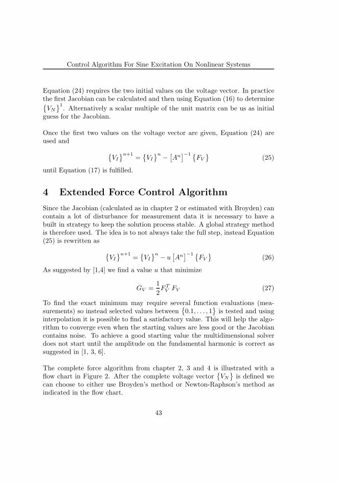
Control Algorithm For Sine Excitation On Nonlinear Systems

Equation (24) requires the two initial values on the voltage vector. In practicethe first Jacobian can be calculated and then using Equation (16) to determine{

VN}1

. Alternatively a scalar multiple of the unit matrix can be us as initialguess for the Jacobian.

Once the first two values on the voltage vector are given, Equation (24) areused and

{

VI}n+1

={

VI}n

−[

An]

−1 {

FV

}

(25)

until Equation (17) is fulfilled.

4 Extended Force Control Algorithm

Since the Jacobian (calculated as in chapter 2 or estimated with Broyden) cancontain a lot of disturbance for measurement data it is necessary to have abuilt in strategy to keep the solution process stable. A global strategy methodis therefore used. The idea is to not always take the full step, instead Equation(25) is rewritten as

{

VI}n+1

={

VI}n

− u[

An]

−1 {

FV

}

(26)

As suggested by [1,4] we find a value u that minimize

GV =1

2FT

VFV (27)

To find the exact minimum may require several function evaluations (mea-surements) so instead selected values between

{

0.1, . . . , 1}

is tested and usinginterpolation it is possible to find a satisfactory value. This will help the algo-rithm to converge even when the starting values are less good or the Jacobiancontains noise. To achieve a good starting value the multidimensional solverdoes not start until the amplitude on the fundamental harmonic is correct assuggested in [1, 3, 6].

The complete force algorithm from chapter 2, 3 and 4 is illustrated with aflow chart in Figure 2. After the complete voltage vector

{

VN}

is defined wecan choose to either use Broyden’s method or Newton-Raphson’s method asindicated in the flow chart.

43

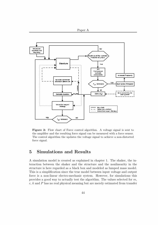
Paper A

��� �������������� ��

��� �����

���������

������� �������������� ������ �����������

����� ������ � !"#$%&'()*&+,

-�� ������.��������.�

/0123 4 �������5�� 67

67

67

5��

5��

8������� �� ����� �������9 ������� �������

//:/��� �������������

����������

/0123 4 �������

;�������� /�� �����

��� ������ <�������

��� ������� =>%? ������ ������@����� =>%?

A�� B��@�������� ������-�� ������.��� �����.�

Figure 2: Flow chart of Force control algorithm. A voltage signal is sent tothe amplifier and the resulting force signal can be measured with a force sensor.The control algorithm the updates the voltage signal to achieve a non-distortedforce signal.

5 Simulations and Results

A simulation model is created as explained in chapter 1. The shaker, the in-teraction between the shaker and the structure and the nonlinearity in thestructure is here regarded as a black box and modeled as lumped mass model.This is a simplification since the true model between input voltage and outputforce is a non-linear electro-mechanic system. However, for simulations thisprovides a good way to actually test the algorithm. The values selected for m,c, k and P has no real physical meaning but are merely estimated from transfer

44

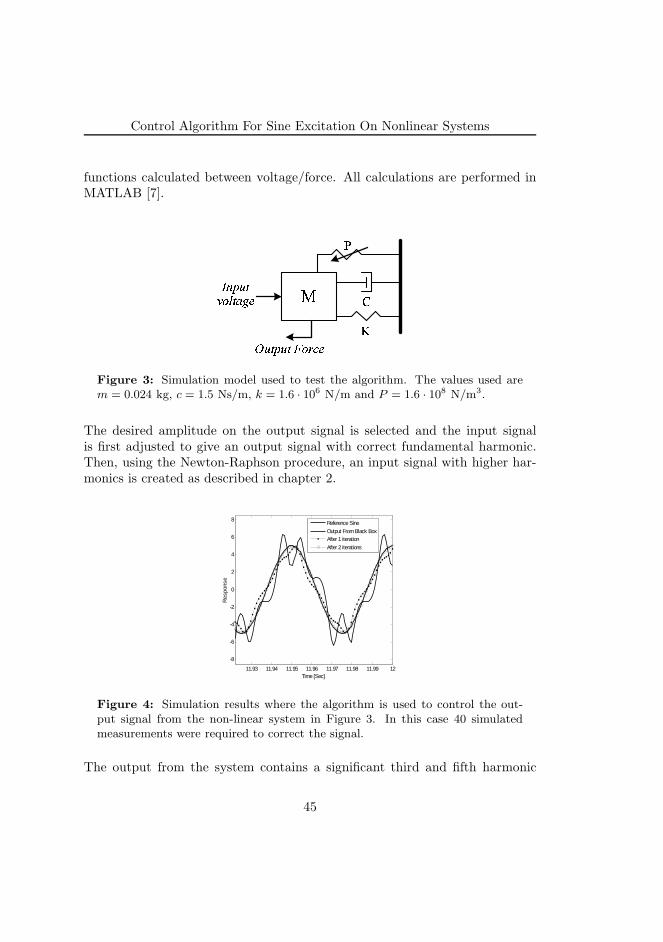
Control Algorithm For Sine Excitation On Nonlinear Systems

functions calculated between voltage/force. All calculations are performed inMATLAB [7].

C

D

E

F

GHIJKLMNKOPQ

RJKIJK SMTUQ

Figure 3: Simulation model used to test the algorithm. The values used arem = 0.024 kg, c = 1.5 Ns/m, k = 1.6 · 106 N/m and P = 1.6 · 108 N/m3.

The desired amplitude on the output signal is selected and the input signalis first adjusted to give an output signal with correct fundamental harmonic.Then, using the Newton-Raphson procedure, an input signal with higher har-monics is created as described in chapter 2.

11.93 11.94 11.95 11.96 11.97 11.98 11.99 12

-8

-6

-4

-2

0

2

4

6

8

Time [Sec]

Res

pons

e

Reference Sine

Output From Black BoxAfter 1 iteration

After 2 iterations

Figure 4: Simulation results where the algorithm is used to control the out-put signal from the non-linear system in Figure 3. In this case 40 simulatedmeasurements were required to correct the signal.

The output from the system contains a significant third and fifth harmonic

45

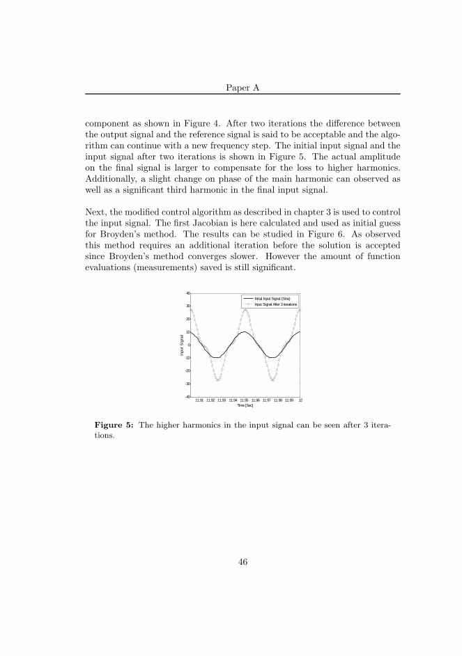
Paper A

component as shown in Figure 4. After two iterations the difference betweenthe output signal and the reference signal is said to be acceptable and the algo-rithm can continue with a new frequency step. The initial input signal and theinput signal after two iterations is shown in Figure 5. The actual amplitudeon the final signal is larger to compensate for the loss to higher harmonics.Additionally, a slight change on phase of the main harmonic can observed aswell as a significant third harmonic in the final input signal.

Next, the modified control algorithm as described in chapter 3 is used to controlthe input signal. The first Jacobian is here calculated and used as initial guessfor Broyden’s method. The results can be studied in Figure 6. As observedthis method requires an additional iteration before the solution is acceptedsince Broyden’s method converges slower. However the amount of functionevaluations (measurements) saved is still significant.

11.91 11.92 11.93 11.94 11.95 11.96 11.97 11.98 11.99 12-40

-30

-20

-10

0

10

20

30

40

Time [Sec]

Inpu

t S

igna

l

Initial Input Signal (Sine)

Input Signal After 3 iterations

Figure 5: The higher harmonics in the input signal can be seen after 3 itera-tions.

46

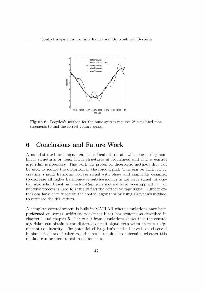
Control Algorithm For Sine Excitation On Nonlinear Systems

11.96 11.965 11.97 11.975 11.98 11.985 11.99 11.995 12

-8

-6

-4

-2

0

2

4

6

8

Time [Sec]

Res

pons

e

Reference Sine

Output From Black Box

After 1 iterationAfter 2 iterations

After 3 iterations

Figure 6: Broyden’s method for the same system requires 28 simulated mea-surements to find the correct voltage signal.

6 Conclusions and Future Work

A non-distorted force signal can be difficult to obtain when measuring non-linear structures or weak linear structures at resonances and thus a controlalgorithm is necessary. This work has presented theoretical methods that canbe used to reduce the distortion in the force signal. This can be achieved bycreating a multi harmonic voltage signal with phase and amplitude designedto decrease all higher harmonics or sub-harmonics in the force signal. A con-trol algorithm based on Newton-Raphsons method have been applied i.e. aniterative process is used to actually find the correct voltage signal. Further ex-tensions have been made on the control algorithm by using Broyden’s methodto estimate the derivatives.

A complete control system is built in MATLAB where simulations have beenperformed on several arbitrary non-linear black box systems as described inchapter 1 and chapter 5. The result from simulations shows that the controlalgorithm can obtain a non-distorted output signal even when there is a sig-nificant nonlinearity. The potential of Broyden’s method have been observedin simulations and further experiments is required to determine whether thismethod can be used in real measurements.

47

Paper A

Additional work in the future will also be to create an improved electro-mechanic model of the shaker including the nonlinearities. From here a betterunderstanding of the actual phenomena can be gained and the control algo-rithm can be further improved.

References

[1] Janito V. Ferreira. Dynamic Response Analysis of structures with non-linear

components. PhD thesis, Imperial College, London, 1998.

[2] I. Bucher. Exact adjustment of dynamic forces in presence of non-linearfeedback and singularity - theory and algorithm. Journal of Sound and

Vibration, 218(1):1 – 27, 1998.

[3] D.J. Ewins and S. Perinpanayagam. Testing technique for identifying andcharacterizing non-linear behaviour of and aero-engine structure. In 12th

International Conference on Experimental Mechanics, 2004.

[4] William H. Press. Numerical recipes in C : the art of scientific computing.Cambridge Univ. Press, Cambridge, 2. ed. edition, 1992.

[5] J. E. T. Penny and G. R. Lindfield. Numerical methods using Matlab.Prentice Hall, Upper Saddle River, N.J., 2. ed. edition, 2000.

[6] Stephanie Rossmann. Development of force controlled modal testing onrotor supported by magnetic bearings. Master’s thesis, Imperial College,London, 1999.

[7] MATLAB Computing Software v 7.0 (R14), 2005.

48

Paper B

On Nonlinear ParameterEstimation

49

Paper B is published as:

Magnevall, M., Josefsson, A. and Ahlin, K. On Nonlinear ParameterEstimation, In Proceedings of International Conference on Noiseand Vibration Engineering (ISMA) 2006, Leuven, Belgium, 2006.

50

On Nonlinear Parameter Estimation

Martin Magnevall

Andreas Josefsson

Kjell Ahlin

Blekinge Institute of Technology, SE-371 79 Karlskrona, Sweden

Abstract

The industrial demand on good dynamical simulation models is increas-ing. Since most structures show some form of nonlinear behavior, linearmodels are not good enough to predict the true dynamical behavior.Therefore nonlinear characterization, localization and parameter estima-tion becomes important issues when building simulation models. Thispaper presents identification techniques for nonlinear systems based onboth random and harmonic excitation signals.

The identification technique based on random excitation builds on thewell known reverse-path method developed by Julius S. Bendat. Thismethod treats the nonlinearity as a feedback forcing term acting on anunderlying linear system and the parameter estimation is performed inthe frequency domain by using conventional MISO/MIMO techniques.Although this method provides a straightforward and systematic way ofhandling nonlinearities, it has been somewhat limited in use due to thecomplexity of creating uncorrelated inputs to the model. As is shownin this paper, the parameter estimation will not be improved with con-ditioned inputs and the nonlinear parameters and the underlying linearsystem can still be estimated with partially correlated inputs.

This paper will also describe a parameter estimation method to be usedwith harmonic input signals. By using the principle of harmonic balanceand multi-harmonic balance it is possible to estimate an analytical fre-quency response function of the studied nonlinear system. This frequency

51

Paper B

response function can, in conjunction with measured nonlinear transferfunctions, be used to estimate the nonlinearity present in the system.This method is also applicable on nonlinear systems with memory, e.g.systems with hysteresis effects.

The above mentioned methods are applied to multi-degree-of-freedomand single-degree-of-freedom systems with different types of nonlineari-ties. Also, techniques for locating nonlinearities are discussed.

1 Introduction

The overall aim with parameter estimation is to find suitable parameters to amathematical model, based on measurements of the inputs and outputs of asystem. The mathematical model can, for instance, be based on a beforehandknown model structure. This is known as parametric modeling, which will bestudied in this paper. Furthermore, the systems studied contain significantnonlinearities that must be included when creating the model, hence nonlinearparameter estimation.

Systems used in engineering can generally be separated into two distinct groups;linear or nonlinear. A system, H , is said to be linear if it fulfills the principleof superposition:

H{

cx}

= cH{

x}

(1)

H{

x1 + x2

}

= H{

x1

}

+H{

x2

}

(2)

A system which does not satisfy these properties is defined as nonlinear. Addi-tionally, nonlinear systems can be classified into different groups as describedin [1]. In this paper, two different types of non-linearities will be discussed;zero-memory nonlinear systems and nonlinear systems with memory. The nextchapter will show how the frequency response functions can be used to identifyand locate nonlinearities in a dynamic system. This will be followed by meth-ods for parameter estimation with random noise signals in chapter 3, and nextusing sine excitation in chapter 4.

52

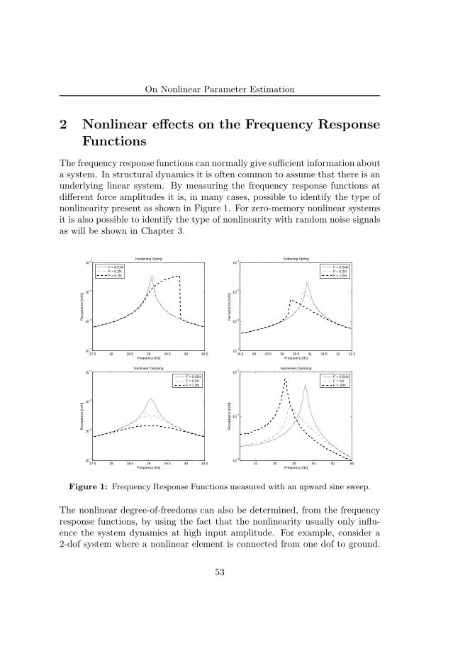
On Nonlinear Parameter Estimation

2 Nonlinear effects on the Frequency Response

Functions

The frequency response functions can normally give sufficient information abouta system. In structural dynamics it is often common to assume that there is anunderlying linear system. By measuring the frequency response functions atdifferent force amplitudes it is, in many cases, possible to identify the type ofnonlinearity present as shown in Figure 1. For zero-memory nonlinear systemsit is also possible to identify the type of nonlinearity with random noise signalsas will be shown in Chapter 3.

27.5 28 28.5 29 29.5 30 30.510

−7

10−6

10−5

10−4

Frequency [Hz]

Rec

epta

nce

[m/N

]

Hardening Spring

F = 0.01NF = 0.2NF = 0.7N

28.5 29 29.5 30 30.5 31 31.5 32 32.510

−7

10−6

10−5

10−4

Softening Spring

Frequency [Hz]

Rec

epta

nce

[m/N

]

F = 0.05NF = 0.2NF = 1.0N

27.5 28 28.5 29 29.5 30 30.510

−7

10−6

10−5

10−4

Frequency [Hz]

Rec

epta

nce

[m/N

]

Nonlinear Damping

F = 0.01NF = 0.2NF = 1.0N

10 20 30 40 50 6010

−8

10−7

10−6

Hysteresis Damping

Frequency [Hz]

Rec

epta

nce

[m/N

]

F = 0.01NF = 1NF = 10N

Figure 1: Frequency Response Functions measured with an upward sine sweep.

The nonlinear degree-of-freedoms can also be determined, from the frequencyresponse functions, by using the fact that the nonlinearity usually only influ-ence the system dynamics at high input amplitude. For example, consider a2-dof system where a nonlinear element is connected from one dof to ground.

53

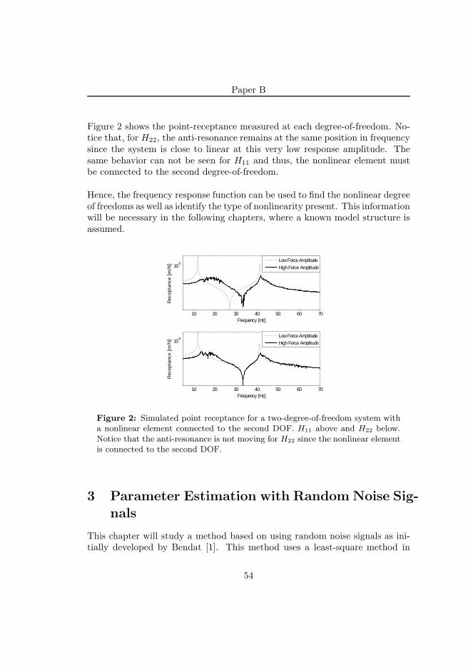
Paper B

Figure 2 shows the point-receptance measured at each degree-of-freedom. No-tice that, for H22, the anti-resonance remains at the same position in frequencysince the system is close to linear at this very low response amplitude. Thesame behavior can not be seen for H11 and thus, the nonlinear element mustbe connected to the second degree-of-freedom.

Hence, the frequency response function can be used to find the nonlinear degreeof freedoms as well as identify the type of nonlinearity present. This informationwill be necessary in the following chapters, where a known model structure isassumed.

10 20 30 40 50 60 70

10-5

Frequency [Hz]

Rec

epta

nce

[m/N

]

10 20 30 40 50 60 70

10-5

Frequency [Hz]

Rec

epta

nce

[m/N

]

Low Force Amplitude

High Force Amplitude

Low Force Amplitude

High Force Amplitude

Figure 2: Simulated point receptance for a two-degree-of-freedom system witha nonlinear element connected to the second DOF. H11 above and H22 below.Notice that the anti-resonance is not moving for H22 since the nonlinear elementis connected to the second DOF.

3 Parameter Estimation with Random Noise Sig-

nals

This chapter will study a method based on using random noise signals as ini-tially developed by Bendat [1]. This method uses a least-square method in

54

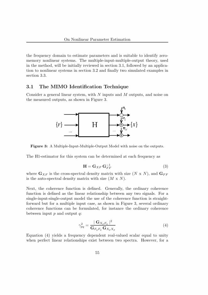
On Nonlinear Parameter Estimation

the frequency domain to estimate parameters and is suitable to identify zero-memory nonlinear systems. The multiple-input-multiple-output theory, usedin the method, will be initially reviewed in section 3.1, followed by an applica-tion to nonlinear systems in section 3.2 and finally two simulated examples insection 3.3.

3.1 The MIMO Identification Technique

Consider a general linear system, with N inputs and M outputs, and noise onthe measured outputs, as shown in Figure 3.

�

�

�

���� ���

��

��

��{ }F { }X

Figure 3: A Multiple-Input-Multiple-Output Model with noise on the outputs.

The H1-estimator for this system can be determined at each frequency as

H = GXF G−1

FF (3)

where GXF is the cross-spectral density matrix with size (N x N), and GFF

is the auto-spectral density matrix with size (M x N).

Next, the coherence function is defined. Generally, the ordinary coherencefunction is defined as the linear relationship between any two signals. For asingle-input-single-output model the use of the coherence function is straight-forward but for a multiple input case, as shown in Figure 3, several ordinarycoherence functions can be formulated, for instance the ordinary coherencebetween input p and output q:

γ2

pq =| GXpFq

|2

GFqFqGXpXp

(4)

Equation (4) yields a frequency dependent real-valued scalar equal to unitywhen perfect linear relationships exist between two spectra. However, for a

55

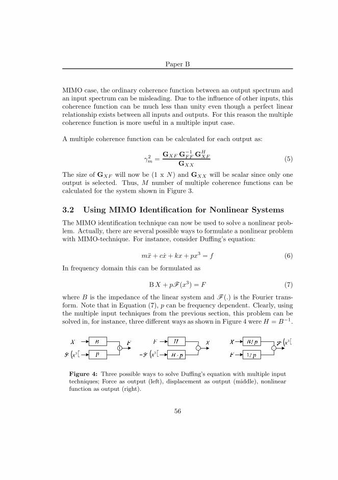
Paper B

MIMO case, the ordinary coherence function between an output spectrum andan input spectrum can be misleading. Due to the influence of other inputs, thiscoherence function can be much less than unity even though a perfect linearrelationship exists between all inputs and outputs. For this reason the multiplecoherence function is more useful in a multiple input case.

A multiple coherence function can be calculated for each output as:

γ2

m =GXF G−1

FF GHXF

GXX

(5)

The size of GXF will now be (1 x N) and GXX will be scalar since only oneoutput is selected. Thus, M number of multiple coherence functions can becalculated for the system shown in Figure 3.

3.2 Using MIMO Identification for Nonlinear Systems

The MIMO identification technique can now be used to solve a nonlinear prob-lem. Actually, there are several possible ways to formulate a nonlinear problemwith MIMO-technique. For instance, consider Duffing’s equation:

mx+ cx+ kx+ px3 = f (6)

In frequency domain this can be formulated as

BX + pF (x3) = F (7)

where B is the impedance of the linear system and F (.) is the Fourier trans-form. Note that in Equation (7), p can be frequency dependent. Clearly, usingthe multiple input techniques from the previous section, this problem can besolved in, for instance, three different ways as shown in Figure 4 wereH = B−1.

� �

�

� �

� �

� � � �

�

( )3x ( )3x

( )3x

Figure 4: Three possible ways to solve Duffing’s equation with multiple inputtechniques; Force as output (left), displacement as output (middle), nonlinearfunction as output (right).

56

On Nonlinear Parameter Estimation

In this paper, the applied force and the nonlinear feedback forces are usedas input to the MIMO-model, since this formulation is easier to extend to ageneral nonlinear system as will be shown next. Various extensions to MDOFsystems with several nonlinear elements have previously been done by, for in-stance, [2, 3, 4].

A general nonlinear system can be expressed as:

M{

x}

+C{

x}

+K{

x}

={

f}

−N[{

x}

,{

x}]

(8)

where N is a set of nonlinear restoring forces depending on either x or x. Inmore detail, the nonlinear operator can be written as

N[{

x}

,{

x}]

=

NEL∑

m=1

pm{

wm

}

gm({

x}

,{

x})

(9)

Thus, for each nonlinear component there is an unknown coefficient pm, a po-sition vector

{

wm

}

and a nonlinear function gm. Typical nonlinear functionsare shown in Equations (10)-(11). The position vector is here used in the for-mulation since the nonlinear function might act on the relative output betweentwo degrees-of-freedom, as will be determined by the elements location, forinstance:

gm =({

wm

}T {

x})3

(Cubic hardening spring) (10)

gm =({

wm

}T {

x})2

(Quadratic damping) (11)

Equation (8) and (9) can be written in frequency domain as:

{

X}

= H{

F}

−H

NEL∑

i=1

pm{

wm

}

F(

gm({

x}

,{

x}

))

(12)

From the expression above a new modified force vector can be defined whichincludes the nonlinear restoring forces as shown in Equation (13). This forcevector is then used as input to a MIMO-model. To avoid confusion with theforce vector used in the previous section this vector is notated as

{

R}

.

57

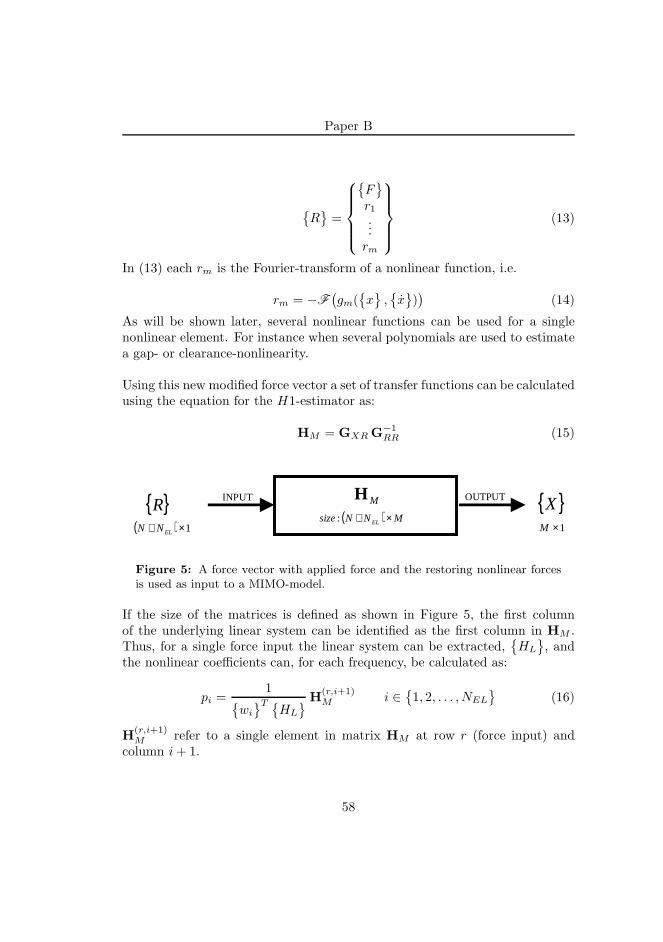
Paper B

{

R}

=

{

F}

r1...rm

(13)

In (13) each rm is the Fourier-transform of a nonlinear function, i.e.

rm = −F(

gm({

x}

,{

x}

))

(14)

As will be shown later, several nonlinear functions can be used for a singlenonlinear element. For instance when several polynomials are used to estimatea gap- or clearance-nonlinearity.

Using this new modified force vector a set of transfer functions can be calculatedusing the equation for the H1-estimator as:

HM = GXR G−1

RR (15)

{ }XINPUT OUTPUT

( ) 1×+ ELNN 1×M( ) MNNsize EL ×+:

MH{ }R

Figure 5: A force vector with applied force and the restoring nonlinear forcesis used as input to a MIMO-model.

If the size of the matrices is defined as shown in Figure 5, the first columnof the underlying linear system can be identified as the first column in HM .Thus, for a single force input the linear system can be extracted,

{

HL

}

, andthe nonlinear coefficients can, for each frequency, be calculated as:

pi =1

{

wi

}T {

HL

}

H(r,i+1)

M i ∈{

1, 2, . . . , NEL

}

(16)

H(r,i+1)

M refer to a single element in matrix HM at row r (force input) andcolumn i+ 1.

58

On Nonlinear Parameter Estimation

Note that Equation (16) can easily be extended to a case where there is severalforce inputs. As can be seen in simulations, an applied force at each nonlinearDOF will reduce the necessary simulation time considerably.

With the method described above, the column that corresponds to the forceinput will always be estimated in the linear system. Thus, modal parameterestimation can be performed to determine the complete linear system. If twoforces are applied, two columns in the linear system will be estimated and soforth.

The force input and the nonlinear restoring forces may be partially correlatedwith each other and, after averaging, the matrix GRR will be non-diagonal.This may introduce numerical instabilities when calculating the matrix inver-sion in Equation (15), particularly at the resonance. In general though, thiserror is very small and does not affect the result much.

The conditioning method, described in [1], where a set of uncorrelated inputsis created will not improve the parameter estimation in this case. For all sim-ulated systems tested, it has not been possible to see any difference betweenusing partially correlated inputs and the conditioned version with uncorrelatedinputs. This is an important observation since it simplifies the calculationsconsiderably.

The only advantage with using uncorrelated inputs is that the ordinary coher-ence can be calculated between the output and each input. These ordinarycoherences will sum up to the multiple coherence and thus it is possible to seethe significance of each nonlinear restoring force. This may be useful whensearching for possible nonlinear functions and a method for calculating uncor-related inputs is given below.

A new set of inputs can be defined by a transformation as:

{

U}

= Φ{

R}

(17)

Multiplying with the complex conjugate and averaging yields:

[

GUU

]

= Φ{

R} (

Φ{

R})H

= ΦGRR ΦH (18)

59

Paper B

Thus, if the matrix Φ is defined as described in [1], GUU will be a diagonalmatrix.

Using this Φ-matrix the cross-correlation densities can also be calculated as

GXU = GXR ΦH (19)

With GUU and GXU available the ordinary coherences between a selectedoutput and each input can be calculated with Equation (4). Using the notationsin Figure 5 there will be N +NEL ordinary coherences for each output.

3.3 Simulations

The method derived in section 3.2 is here demonstrated on two nonlinear sys-tems. First, a single-degree-of-freedom with two nonlinear elements is usedfollowed by a multi-degree-of-freedom system.

3.3.1 A SDOF-system with a nonlinear spring and damper

The test system used is shown in Figure 6 and consists of an underlying linearsystem with a cubic hardening spring and a quadratic damping element con-nected. The time response is simulated from this system using digital filters.Figure 7 shows several frequency response functions calculated with differentforce amplitudes.

With increasing force, the frequency response functions will decrease in ampli-tude as well as moving upward in frequency due to the presence of a dampingnonlinearity and a cubic hardening spring. As mentioned in previous sectionit is possible to use several nonlinear functions as input and, with Equations(17)-(19), calculate a new set of uncorrelated inputs and then studying the or-dinary coherences. However, this is not straightforward as the order in whichthe functions are defined and the amplitude of the response signal will affectthe result. In this case, testing different combinations of Equation (20) willshow that the cubic spring element and the quadratic damping element aremost significant.

{

R}

={

F −x2 −x3 −x sgn(x) −v|v| −v3 −v5}T

(20)

60

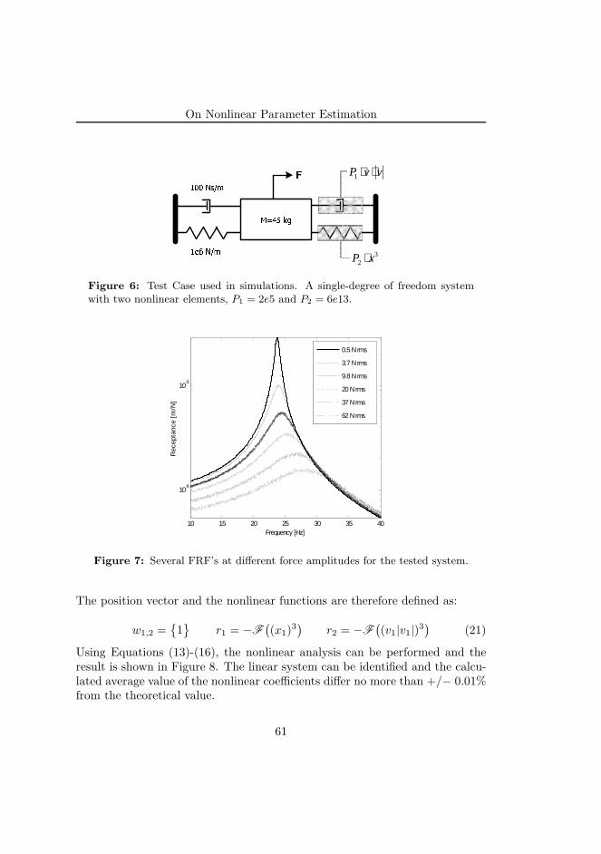
On Nonlinear Parameter Estimation

���� ��

���� ����

��� ��� 32 xP ⋅

vvP ⋅⋅1

Figure 6: Test Case used in simulations. A single-degree of freedom systemwith two nonlinear elements, P1 = 2e5 and P2 = 6e13.

10 15 20 25 30 35 40

10-6

10-5

Frequency [Hz]

Rec

epta

nce

[m/N

]

0.5 N rms

3.7 N rms

9.8 N rms

20 N rms

37 N rms

62 N rms

Figure 7: Several FRF’s at different force amplitudes for the tested system.

The position vector and the nonlinear functions are therefore defined as:

w1,2 ={

1}

r1 = −F(

(x1)3)

r2 = −F(

(v1|v1|)3)

(21)

Using Equations (13)-(16), the nonlinear analysis can be performed and theresult is shown in Figure 8. The linear system can be identified and the calcu-lated average value of the nonlinear coefficients differ no more than +/− 0.01%from the theoretical value.

61

Paper B

10 15 20 25 30 35 40

10-6

10-5

Frequency [Hz]

Rec

epta

nce

[m/N

]

True Linear FRF

Estimated Linear FRFRaw FRF

10 15 20 25 30 35 4010

2

104

106

108

1010

1012

1014

Frequency [Hz]

Non

linea

r C

oeff

icie

nts

Cubic Spring Element

Quadratic Damping Element

Figure 8: Estimate of the underlying linear system and the nonlinear coeffi-cients.

3.3.2 A MDOF-system with a several nonlinear elements

The next example consists of a MDOF system with a cubic- and a quadratic-spring as shown below.

�

� !"#$ %&' �(!)#$ %&' �*!+#$ %&' �,!-#+ %&'

. !"// %0&' .(!"$/ %0&' .*!$1/ %0&' .,!-// %0&'

234567 89 2:4;67 89 2<4=67 89

( )3311 xxP −⋅

( ) ( )31312 xxxxP −⋅−⋅

Figure 9: Test System used in Simulations, P1 = 4e16 and P2 = 6e10.

Using the same procedure as in section 3.3.1, the position vectors and thenonlinear functions for each nonlinear element is defined as

w1 ={

0 −1 1}T

, w2 ={

−1 0 1}T

(22)

62

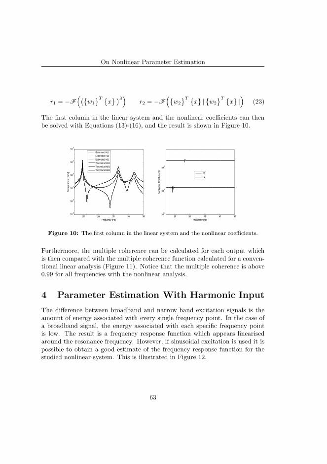
On Nonlinear Parameter Estimation

r1 = −F

(

({

w1

}T {

x} )3

)

r2 = −F

(

{

w2

}T {

x}

|{

w2

}T {

x}

|)

(23)

The first column in the linear system and the nonlinear coefficients can thenbe solved with Equations (13)-(16), and the result is shown in Figure 10.

15 20 25 30 3510

-9

10-8

10-7

10-6

10-5

10-4

Frequency [Hz]

Rec

epta

nce

[m/N

]

Estimated H11Estimated H21

Estimated H31

Theoretical H11

Theoretical H21Theoretical H31

15 20 25 30 3510

5

1010

1015

Frequency [Hz]

Non

linea

r C

oeff

icie

nts

P1

P2

Figure 10: The first column in the linear system and the nonlinear coefficients.

Furthermore, the multiple coherence can be calculated for each output whichis then compared with the multiple coherence function calculated for a conven-tional linear analysis (Figure 11). Notice that the multiple coherence is above0.99 for all frequencies with the nonlinear analysis.

4 Parameter Estimation With Harmonic Input

The difference between broadband and narrow band excitation signals is theamount of energy associated with every single frequency point. In the case ofa broadband signal, the energy associated with each specific frequency pointis low. The result is a frequency response function which appears linearisedaround the resonance frequency. However, if sinusoidal excitation is used it ispossible to obtain a good estimate of the frequency response function for thestudied nonlinear system. This is illustrated in Figure 12.

63

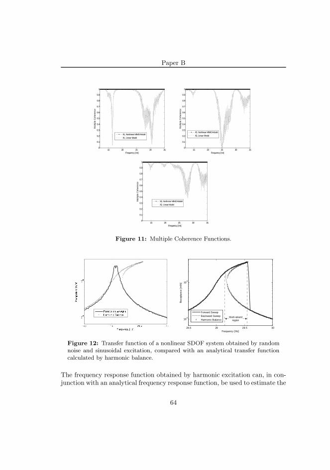
Paper B

15 20 25 30 350

0.1

0.2

0.3

0.4

0.5

0.6

0.7

0.8

0.9

1

Frequency [Hz]

Mul

tiple

Coh

eren

ce

X1, Nonlinear MIMO-Model

X1, Linear Model

15 20 25 30 350

0.1

0.2

0.3

0.4

0.5

0.6

0.7

0.8

0.9

1

Frequency [Hz]

Mul

tiple

Coh

eren

ce

X2, Nonlinear MIMO-Model

X2, Linear Model

15 20 25 30 350

0.1

0.2

0.3

0.4

0.5

0.6

0.7

0.8

0.9

1

Frequency [Hz]

Mul

tiple

Coh

eren

ce

X3, Nonlinear MIMO-Model

X3, Linear Model

Figure 11: Multiple Coherence Functions.

>?@A >B >B@A CDEDFG

EDFH

IJKLMKNOP QRST

UVWVXYZ[WV\]_

abNcde NdfgK gfhNbiRbJedNfO jbibNOK

28.5 29 29.5 30

10-6

10-5

Frequency [Hz]

Rec

epta

nce

[m/N

]

Forward Sweep

Backward Sweep

Harmonic BalanceMulti-valued

region

Figure 12: Transfer function of a nonlinear SDOF system obtained by randomnoise and sinusoidal excitation, compared with an analytical transfer functioncalculated by harmonic balance.

The frequency response function obtained by harmonic excitation can, in con-junction with an analytical frequency response function, be used to estimate the

64

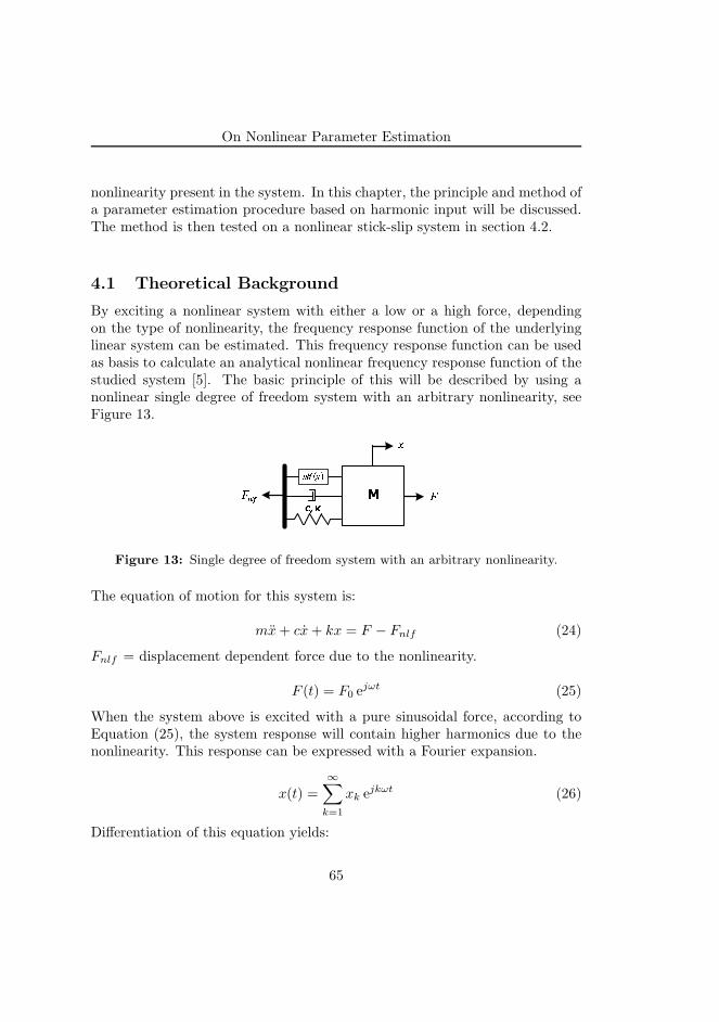
On Nonlinear Parameter Estimation

nonlinearity present in the system. In this chapter, the principle and method ofa parameter estimation procedure based on harmonic input will be discussed.The method is then tested on a nonlinear stick-slip system in section 4.2.

4.1 Theoretical Background

By exciting a nonlinear system with either a low or a high force, dependingon the type of nonlinearity, the frequency response function of the underlyinglinear system can be estimated. This frequency response function can be usedas basis to calculate an analytical nonlinear frequency response function of thestudied system [5]. The basic principle of this will be described by using anonlinear single degree of freedom system with an arbitrary nonlinearity, seeFigure 13.

klm n

opqr r

s

tuvw

Figure 13: Single degree of freedom system with an arbitrary nonlinearity.

The equation of motion for this system is:

mx+ cx+ kx = F − Fnlf (24)

Fnlf = displacement dependent force due to the nonlinearity.

F (t) = F0 ejωt (25)

When the system above is excited with a pure sinusoidal force, according toEquation (25), the system response will contain higher harmonics due to thenonlinearity. This response can be expressed with a Fourier expansion.

x(t) =∞∑

k=1

xk ejkωt (26)

Differentiation of this equation yields:

65

Paper B

x(t) =

∞∑

k=1

jkωxk ejkωt (27)

x(t) = −

∞∑

k=1

k2ω2xk ejkωt (28)

The nonlinear force can be expressed in a similar fashion:

Fnlf (x) =

∞∑

k=1

Fnlk ejkωt (29)

Putting Equations (25)-(29) into Equation (24) and considering for examplethree harmonics [1 3 5], the system of equations becomes:

−mx1ω2 ejωt +jcx1ω ejωt +kx1 e

jωt −F0 ejωt +Fnl1 e

jωt = 0

−9mx3ω2 ej3ωt +3jcx3ω ej3ωt +kx3 e

j3ωt +Fnl3 ej3ωt = 0 (30)

−25mx5ω2 ej5ωt +5jcx5ω ej5ωt +kx5 e

j5ωt +Fnl5 ej5ωt = 0

This system of equations can be rewritten in a more compact form:

(

−mω2 + jcω + k)

x1 − F0 + Fnl1 = 0(

−9mω2 + 3jcω + k)

x3 + Fnl3 = 0 (31)(

−25mω2 + 5jcω + k)

x5 + Fnl5 = 0

As is evident, the bracketed expressions contain the impedance for each specificharmonic. So, the equation can be written as:

Z1x1 − F0 + Fnl1 = 0

Z3x3 + Fnl3 = 0 (32)

Z5x5 + Fnl5 = 0

By using the frequency response function of the underlying linear system men-tioned previously, the impedance of the system is estimated and an analytical

66

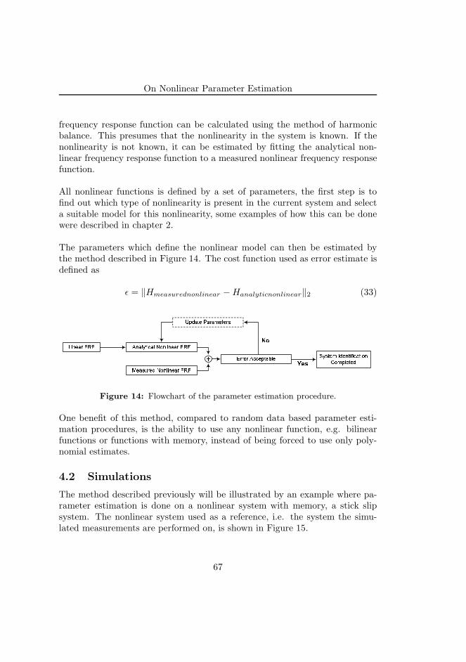
On Nonlinear Parameter Estimation

frequency response function can be calculated using the method of harmonicbalance. This presumes that the nonlinearity in the system is known. If thenonlinearity is not known, it can be estimated by fitting the analytical non-linear frequency response function to a measured nonlinear frequency responsefunction.

All nonlinear functions is defined by a set of parameters, the first step is tofind out which type of nonlinearity is present in the current system and selecta suitable model for this nonlinearity, some examples of how this can be donewere described in chapter 2.

The parameters which define the nonlinear model can then be estimated bythe method described in Figure 14. The cost function used as error estimate isdefined as

ǫ = ‖Hmeasurednonlinear −Hanalyticnonlinear‖2 (33)

xyz{|} ~�~ �z|���y�|� ��z�yz{|} ~�~

�{|��}{� ��z�yz{|} ~�~�}}�} ���{��|��{ ����{� ��{z�y�y�|�y�z

�����{�{��

���|�{ �|}|�{�{}�

��

���

Figure 14: Flowchart of the parameter estimation procedure.

One benefit of this method, compared to random data based parameter esti-mation procedures, is the ability to use any nonlinear function, e.g. bilinearfunctions or functions with memory, instead of being forced to use only poly-nomial estimates.

4.2 Simulations

The method described previously will be illustrated by an example where pa-rameter estimation is done on a nonlinear system with memory, a stick slipsystem. The nonlinear system used as a reference, i.e. the system the simu-lated measurements are performed on, is shown in Figure 15.

67

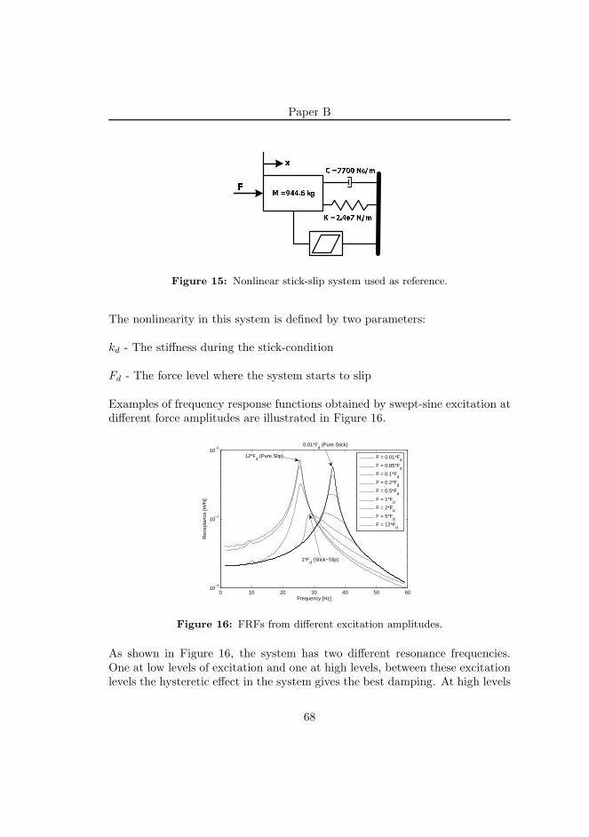
Paper B

�

�

� ��  ¡¢ £¤

¥ �¦¦§§ ¨©ª«

¬ �­¡ ®¦ ¨ª«

Figure 15: Nonlinear stick-slip system used as reference.

The nonlinearity in this system is defined by two parameters:

kd - The stiffness during the stick-condition

Fd - The force level where the system starts to slip

Examples of frequency response functions obtained by swept-sine excitation atdifferent force amplitudes are illustrated in Figure 16.

0 10 20 30 40 50 6010

−8

10−7

10−6

Frequency [Hz]

Rec

epta

nce

[m/N

]

F = 0.01*Fd

F = 0.05*Fd

F = 0.1*Fd

F = 0.2*Fd

F = 0.5*Fd

F = 1*Fd

F = 2*Fd

F = 5*Fd

F = 12*Fd

0.01*Fd (Pure Stick)

1*Fd (Stick−Slip)

12*Fd (Pure Slip)

Figure 16: FRFs from different excitation amplitudes.

As shown in Figure 16, the system has two different resonance frequencies.One at low levels of excitation and one at high levels, between these excitationlevels the hysteretic effect in the system gives the best damping. At high levels

68

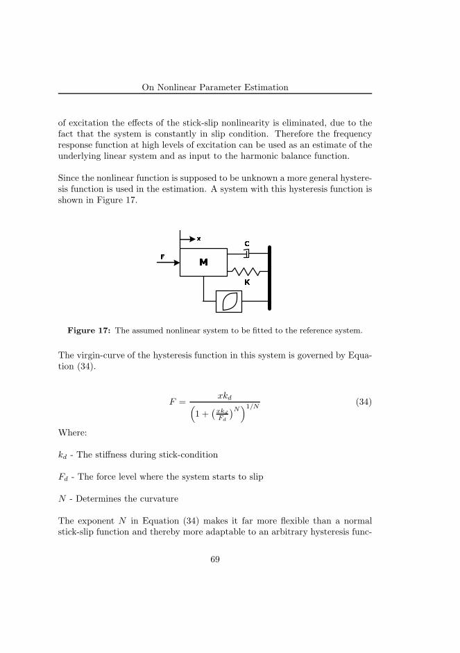
On Nonlinear Parameter Estimation

of excitation the effects of the stick-slip nonlinearity is eliminated, due to thefact that the system is constantly in slip condition. Therefore the frequencyresponse function at high levels of excitation can be used as an estimate of theunderlying linear system and as input to the harmonic balance function.

Since the nonlinear function is supposed to be unknown a more general hystere-sis function is used in the estimation. A system with this hysteresis function isshown in Figure 17.

¯°

±

²

³

Figure 17: The assumed nonlinear system to be fitted to the reference system.

The virgin-curve of the hysteresis function in this system is governed by Equa-tion (34).

F =xkd

(

1 +(

xkd

Fd

)N)1/N

(34)

Where:

kd - The stiffness during stick-condition

Fd - The force level where the system starts to slip

N - Determines the curvature

The exponent N in Equation (34) makes it far more flexible than a normalstick-slip function and thereby more adaptable to an arbitrary hysteresis func-

69

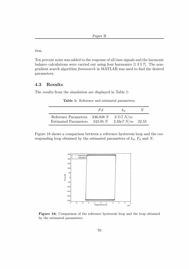
Paper B

tion.

Ten percent noise was added to the response of all time signals and the harmonicbalance calculations were carried out using four harmonics [1 3 5 7]. The non-gradient search algorithm fminsearch in MATLAB was used to find the desiredparameters.

4.3 Results

The results from the simulation are displayed in Table 1:

Table 1: Reference and estimated parameters.

Fd kd N

Reference Parameters 246.048 N 2.7e7 N/m

Estimated Parameters 242.05 N 2.33e7 N/m 22.55

Figure 18 shows a comparison between a reference hysteresis loop and the cor-responding loop obtained by the estimated parameters of kd, Fd and N .

−5 −4 −3 −2 −1 0 1 2 3 4 5

x 10−4

−250

−200

−150

−100

−50

0

50

100

150

200

250

Displacement [m]

For

ce [N

]

ReferenceEstimated

Figure 18: Comparison of the reference hysteresis loop and the loop obtainedby the estimated parameters.

70

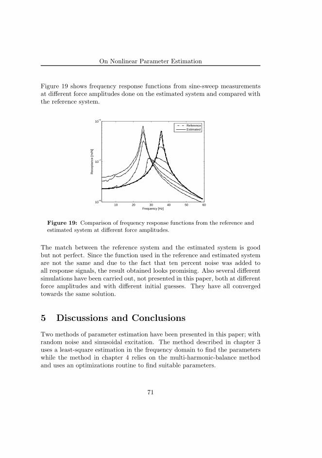
On Nonlinear Parameter Estimation

Figure 19 shows frequency response functions from sine-sweep measurementsat different force amplitudes done on the estimated system and compared withthe reference system.

10 20 30 40 50 6010

−8

10−7

10−6

Frequency [Hz]

Rec

epta

nce

[m/N

]

ReferenceEstimated

Figure 19: Comparison of frequency response functions from the reference andestimated system at different force amplitudes.

The match between the reference system and the estimated system is goodbut not perfect. Since the function used in the reference and estimated systemare not the same and due to the fact that ten percent noise was added toall response signals, the result obtained looks promising. Also several differentsimulations have been carried out, not presented in this paper, both at differentforce amplitudes and with different initial guesses. They have all convergedtowards the same solution.

5 Discussions and Conclusions

Two methods of parameter estimation have been presented in this paper; withrandom noise and sinusoidal excitation. The method described in chapter 3uses a least-square estimation in the frequency domain to find the parameterswhile the method in chapter 4 relies on the multi-harmonic-balance methodand uses an optimizations routine to find suitable parameters.

71

Paper B

A major benefit with using random noise signals is that conventional and al-ready established methods for linear systems are used such as MIMO-technique.The method can also easily be extended to multiple-degree-of-freedoms withseveral nonlinear elements. However, with sine excitation and the harmonic-balance concept a wider range of nonlinear problems can be solved, includingnonlinearities with memory as shown in section 4.2.

As demonstrated, both methods shows large potential in simulations and willtherefore be further examined with experimental testing.

Acknowledgements

This work has been sponsored by The Knowledge Foundation in Stockholm,Sweden.

References

[1] Julius S. Bendat. Nonlinear system analysis and identification from random

data. Wiley, New York, 1990.

[2] C.M. Richards and R. Singh. Identification of multi-degree-of-freedom non-linear systems under random excitations by the ”reverse path” spectralmethod. Journal of Sound and Vibration, 213(4):673 – 707, 1998.

[3] D.E. Adams and R.J. Allemang. Frequency domain method for estimatingthe parameters of a non-linear structural dynamic model through feedback.Mechanical Systems & Signal Processing, 14(4):637 – 656, 2000.

[4] S. Marchesiello, L. Garibaldi, J.R. Wright, and J.E. Cooper. Applicationsof the conditioned reverse path method to structures with different typesof non-linearities. In Proceedings of the 25th International Conference on

Noise and Vibration Engineering, ISMA, pages 437 – 444, Leuven, Belgium,2000.

[5] Giovanna Girini and Stefano Zucca. Multi-harmonic analysis of a sdoffriction damped system. In Proceedings of 3d Youth Symposium on Exper-

imental Solid Mechanics, Poretta Terme, Italy, 2004.

72

Paper C

On Nonlinear ParameterEstimation with Random Noise

Signals

73

Paper C is published as:

Josefsson, A., Magnevall, M. and Ahlin, K. On Nonlinear ParameterEstimation with Random Noise Signals, In Proceedings of IMAC-XXV, Conference & Exposition on Structural Dynamics, Orlando,USA, 2007.

74

On Nonlinear Parameter Estimation with

Random Noise Signals

Andreas JosefssonMartin Magnevall

Kjell Ahlin

Blekinge Institute of Technology, SE-371 79 Karlskrona, Sweden

Abstract

In the field of nonlinear dynamics it is essential to have well tested andreliable tools for estimating the nonlinear parameters from measurementdata. This paper presents an identification technique based on usingrandom noise signals, as initially developed by Julius S. Bendat. Withthis method the nonlinearity is treated as a feedback forcing term act-ing on an underlying linear system. The parameter estimation is thenperformed in the frequency domain by using conventional MISO/MIMOtechniques. To apply this method successfully it is necessary to have somepre-information about the model structure and thus methods for nonlin-ear characterization and localization are studied. The paper also demon-strates the various ways the method can be formulated for multiple-degree-of-freedom systems. The implementation of the method is illus-trated with simulated data as well as a practical application, where themethod is used to create a dynamic model of a test-rig with a significantnonlinearity.

75

Paper C

Nomenclature

H Frequency Response FunctionGxx Single sided, auto-spectrum of signal xGxy Single sided, cross-spectrum of x with yF (.) Fourier TransformF,X Force and displacement, frequency domainf, x Force and displacement, time domainγ2m Multiple Coherence Function

1 Introduction

The overall aim with parameter estimation is to find suitable parameters to amathematical model, based on measurements of the inputs and outputs of asystem. The mathematical model can, for instance, be based on a beforehandknown model structure. This is known as parametric modelling, which willbe studied in this paper. Furthermore, the systems studied contain significantnonlinearities that must be included when creating the model, hence nonlinearparameter estimation.

Systems used in engineering can generally be separated into two distinct groups;linear or nonlinear. A system, H, is said to be linear if it fulfills the principleof superposition:

H {c · x} = c ·H {x} (1)

H {x1 + x2} = H {x1}+H {x2} (2)

A useful tool for detecting nonlinearities is the frequency response function.For a significant nonlinearity the amplitude and/or the resonance frequencieswill be dependent on the excitation amplitude. Thus, the FRF’s gives a linearapproximation at the specific excitation amplitude and fails to fully describethe dynamics.

76

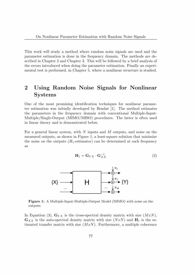
On Nonlinear Parameter Estimation with Random Noise Signals

This work will study a method where random noise signals are used and theparameter estimation is done in the frequency domain. The methods are de-scribed in Chapter 2 and Chapter 3. This will be followed by a brief analysis ofthe errors introduced when doing the parameter estimation. Finally an experi-mental test is performed, in Chapter 5, where a nonlinear structure is studied.

2 Using Random Noise Signals for NonlinearSystems

One of the most promising identification techniques for nonlinear parame-ter estimation was initially developed by Bendat [1]. The method estimatesthe parameters in the frequency domain with conventional Multiple-Input-Multiple/Single-Output (MIMO/MISO) procedures. The latter is often usedin linear theory and is demonstrated below.

For a general linear system, with N inputs and M outputs, and noise on themeasured outputs, as shown in Figure 1, a least-square solution that minimizethe noise on the outputs (H1-estimator) can be determined at each frequencyas

H1 = GY X ·G−1XX (3)

+

+

+

H ... ...

1n

2n

Mn{X} {Y}

Figure 1: A Multiple-Input-Multiple-Output Model (MIMO) with noise on theoutputs.

In Equation (3), GY X is the cross-spectral density matrix with size (MxN),GXX is the auto-spectral density matrix with size (NxN) and H1 is the es-timated transfer matrix with size (MxN). Furthermore, a multiple coherence

77

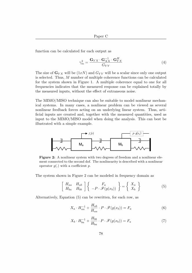
Paper C

function can be calculated for each output as

γ2m =GY X ·G−1XX ·G

HYX

GY Y(4)

The size of GY X will be (1xN) and GY Y will be a scalar since only one outputis selected. Thus, M number of multiple coherence functions can be calculatedfor the system shown in Figure 1. A multiple coherence equal to one for allfrequencies indicates that the measured response can be explained totally bythe measured inputs, without the effect of extraneous noise.

The MIMO/MISO technique can also be suitable to model nonlinear mechan-ical systems. In many cases, a nonlinear problem can be viewed as severalnonlinear feedback forces acting on an underlying linear system. Thus, arti-ficial inputs are created and, together with the measured quantities, used asinput to the MIMO/MISO model when doing the analysis. This can best beillustrated with a simple example.

Mb

( )tf a

Ma

( )bxgp ⋅

Figure 2: A nonlinear system with two degrees of freedom and a nonlinear ele-ment connected to the second dof. The nonlinearity is described with a nonlinearoperator g(.) with a coefficient p.

The system shown in Figure 2 can be modeled in frequency domain as[Haa Hab

Hba Hbb

]{Fa

−P ·F (g(xb))

}=

{Xa

Xb

}(5)

Alternatively, Equation (5) can be rewritten, for each row, as

Xa ·H−1aa +Hab

Haa· P ·F (g(xb)) = Fa (6)

Xb ·H−1ba +Hbb

Hba· P ·F (g(xb)) = Fa (7)

78

On Nonlinear Parameter Estimation with Random Noise Signals

There are several possible ways to formulate this problem with MIMO/MISO.With the original Reverse-Path technique (RP) [1], Equations (6)-(7) canbe used and the analysis is accomplished as illustrated in Figure 3. WithNonlinear-Identification-Through-Feedback-of-Outputs (NIFO) [2], Equation (5)is used directly and the linear system and the nonlinear coefficients are esti-mated as shown in Figure 4.

⎥⎦

⎤⎢⎣

⎡ − PHH

Haa

abaa1

⎥⎦

⎤⎢⎣

⎡ − PHH

Hba

bbba1

( )txa

( )txb [.]g( )tfa

( )tf a( )txb

( )txb [.]g

Figure 3: Reverse-Path (RP): Two MISO analyses are performed and usingthe reciprocity of the underlying linear system H−1

aa , H−1ba and the nonlinear

coefficient P can be identified. Here, g(.) is a nonlinear operator.

⎥⎦

⎤⎢⎣

⎡⋅−⋅−

bbba

abaa

HPHHPH ( )txa

( )txb

( )tfa( )txb [.]g

Figure 4: Nonlinear Identification Through Feedback of Outputs (NIFO): Asingle MIMO analysis is performed and using the reciprocity of the underlyinglinear system Haa, Hba and the nonlinear coefficient P can be identified. As inFigure 3, g(.) is a nonlinear operator.

In the above figures, all inputs and outputs quantities are given in the timedomain, to emphasize that the input signal xb(t) must pass through the non-linear function, for instance g(x) = x3, before the spectral densities can becalculated. The transfer functions are then given by Equation (3) and, in bothcases, two multiple coherence functions can be calculated with Equation (4).

Notice that the transfer function P (f) can be both frequency dependent and

79

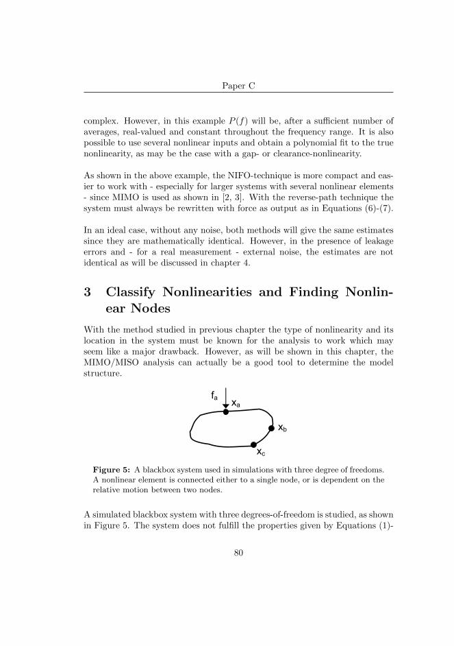
Paper C

complex. However, in this example P (f) will be, after a sufficient number ofaverages, real-valued and constant throughout the frequency range. It is alsopossible to use several nonlinear inputs and obtain a polynomial fit to the truenonlinearity, as may be the case with a gap- or clearance-nonlinearity.

As shown in the above example, the NIFO-technique is more compact and eas-ier to work with - especially for larger systems with several nonlinear elements- since MIMO is used as shown in [2, 3]. With the reverse-path technique thesystem must always be rewritten with force as output as in Equations (6)-(7).

In an ideal case, without any noise, both methods will give the same estimatessince they are mathematically identical. However, in the presence of leakageerrors and - for a real measurement - external noise, the estimates are notidentical as will be discussed in chapter 4.

3 Classify Nonlinearities and Finding Nonlin-ear Nodes

With the method studied in previous chapter the type of nonlinearity and itslocation in the system must be known for the analysis to work which mayseem like a major drawback. However, as will be shown in this chapter, theMIMO/MISO analysis can actually be a good tool to determine the modelstructure.

xb

xa fa

xc

Figure 5: A blackbox system used in simulations with three degree of freedoms.A nonlinear element is connected either to a single node, or is dependent on therelative motion between two nodes.

A simulated blackbox system with three degrees-of-freedom is studied, as shownin Figure 5. The system does not fulfill the properties given by Equations (1)-

80

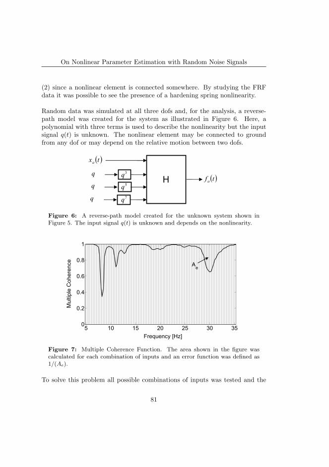
On Nonlinear Parameter Estimation with Random Noise Signals

(2) since a nonlinear element is connected somewhere. By studying the FRFdata it was possible to see the presence of a hardening spring nonlinearity.

Random data was simulated at all three dofs and, for the analysis, a reverse-path model was created for the system as illustrated in Figure 6. Here, apolynomial with three terms is used to describe the nonlinearity but the inputsignal q(t) is unknown. The nonlinear element may be connected to groundfrom any dof or may depend on the relative motion between two dofs.

( )txa

q ( )tfaq

q 7q

5q

3q H

Figure 6: A reverse-path model created for the unknown system shown inFigure 5. The input signal q(t) is unknown and depends on the nonlinearity.

5 10 15 20 25 30 350

0.2

0.4

0.6

0.8

1

Mul

tiple

Coh

eren

ce

Frequency [Hz]

Ae

Figure 7: Multiple Coherence Function. The area shown in the figure wascalculated for each combination of inputs and an error function was defined as1/(Ae).

To solve this problem all possible combinations of inputs was tested and the

81

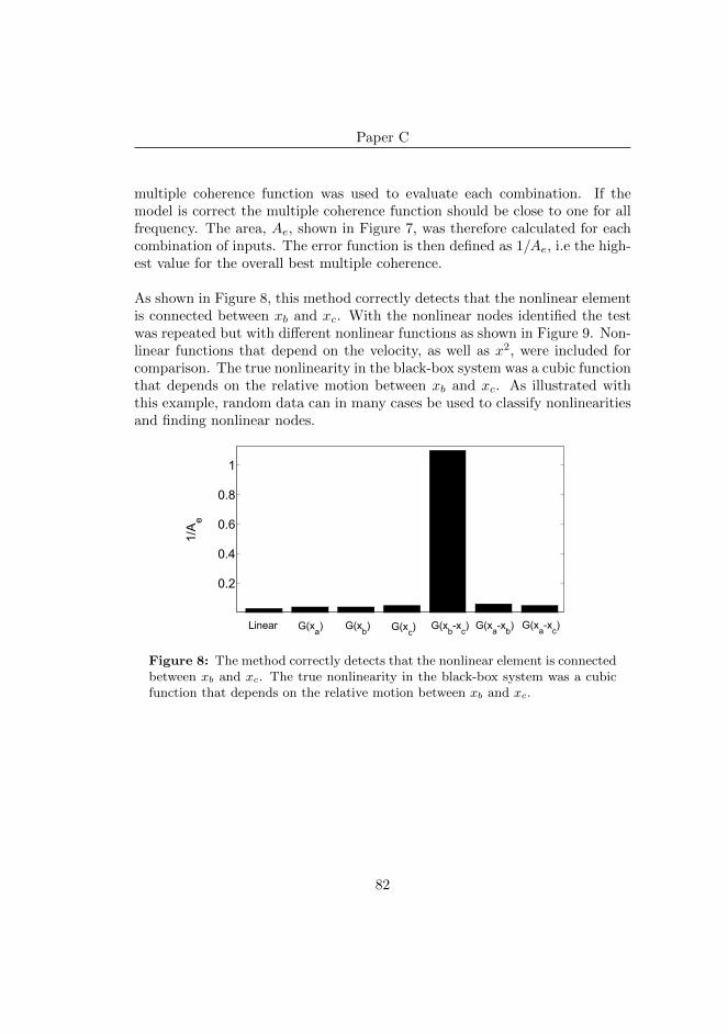
Paper C

multiple coherence function was used to evaluate each combination. If themodel is correct the multiple coherence function should be close to one for allfrequency. The area, Ae, shown in Figure 7, was therefore calculated for eachcombination of inputs. The error function is then defined as 1/Ae, i.e the high-est value for the overall best multiple coherence.

As shown in Figure 8, this method correctly detects that the nonlinear elementis connected between xb and xc. With the nonlinear nodes identified the testwas repeated but with different nonlinear functions as shown in Figure 9. Non-linear functions that depend on the velocity, as well as x2, were included forcomparison. The true nonlinearity in the black-box system was a cubic functionthat depends on the relative motion between xb and xc. As illustrated withthis example, random data can in many cases be used to classify nonlinearitiesand finding nonlinear nodes.

0.2

0.4

0.6

0.8

1

1/A

e

Linear G(xa) G(xb) G(xc) G(xb-xc) G(xa-xb) G(xa-xc)

Figure 8: The method correctly detects that the nonlinear element is connectedbetween xb and xc. The true nonlinearity in the black-box system was a cubicfunction that depends on the relative motion between xb and xc.

82

On Nonlinear Parameter Estimation with Random Noise Signals

0.2

0.4

0.6

0.8

1/A

e

v3v ⋅ |v|x7x5x3x⋅ |x|x2

Figure 9: The presence of a cubic stiffness could clearly be seen. Nonlinearfunctions that depend on the velocity, as well as x2, were included for comparison.

4 Errors in the Analysis

When using random noise signals the estimated spectral densities will containrandom and bias (systematic) errors. The effect from random errors can becontrolled with a sufficient number of averages and normally, overlap process-ing is applied for more effective use of data. The bias error, on the other hand,does not necessarily decrease with averaging since this error comes from consis-tently estimating an incorrect spectrum, for instance due to aliasing or leakage.

The time-leakage effect can give a considerable random error. This error oc-curs when the signal is truncated and an output signal is measured which is nottotally correlated with the input signal. In the beginning of the output signal,for a certain time block, there is data which depends on the input signal fromthe previous time block. This effect will be even more significant for lightlydamped structure. The leakage error can be reduced by increasing the blocklength. The bias error is a function of the truncation and the window used andmay also be reduced by increasing the block length.

When using MIMO/MISO to identify nonlinear systems it is essential to use asufficient amount of data due to a relatively high sensitivity to these errors, ascan clearly be seen in simulations.

Bias errors can also be introduced by contaminating noise in the measure-

83

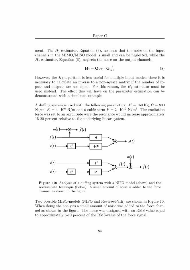
Paper C

ment. The H1-estimator, Equation (3), assumes that the noise on the inputchannels in the MIMO/MISO model is small and can be neglected, while theH2-estimator, Equation (8), neglects the noise on the output channels.

H2 = GY Y ·G−1XY (8)

However, the H2-algorithm is less useful for multiple-input models since it isnecessary to calculate an inverse to a non-square matrix if the number of in-puts and outputs are not equal. For this reason, the H1-estimator must beused instead. The effect this will have on the parameter estimation can bedemonstrated with a simulated example.

A duffing system is used with the following parameters: M = 150 Kg, C = 800Ns/m, K = 4 · 106 N/m and a cubic term P = 2 · 1012 N/m3. The excitationforce was set to an amplitude were the resonance would increase approximately15-20 percent relative to the underlying linear system.

H( )tx

+ ( )tm( )tf

( )tx

( )tf

-HP+

H-1

( )tm

( )tx P+ +

( )tx( )tf( )tf

3x

3x

Figure 10: Analysis of a duffing system with a NIFO model (above) and thereverse-path technique (below). A small amount of noise is added to the forcechannel as shown in the figure.

Two possible MISO-models (NIFO and Reverse-Path) are shown in Figure 10.When doing the analysis a small amount of noise was added to the force chan-nel as shown in the figure. The noise was designed with an RMS-value equalto approximately 5-10 percent of the RMS-value of the force signal.

84

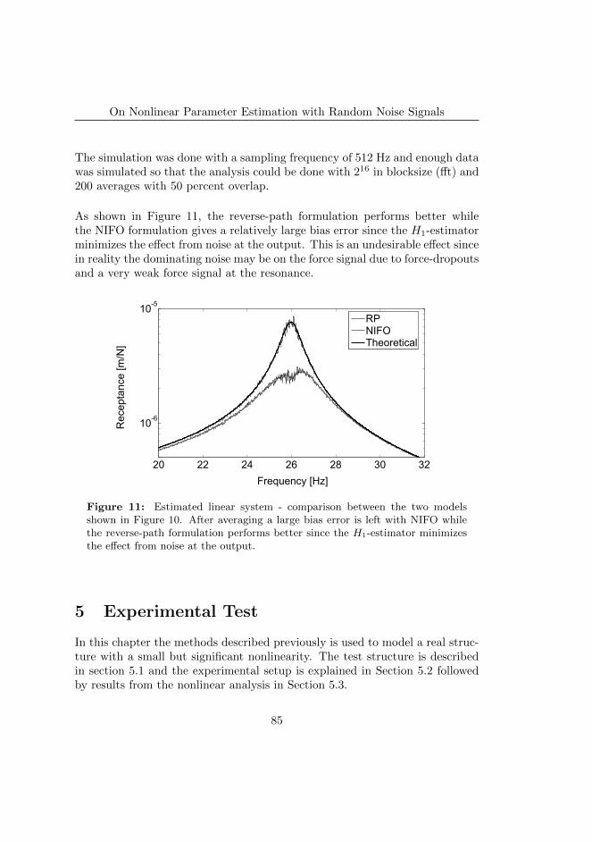
On Nonlinear Parameter Estimation with Random Noise Signals

The simulation was done with a sampling frequency of 512 Hz and enough datawas simulated so that the analysis could be done with 216 in blocksize (fft) and200 averages with 50 percent overlap.

As shown in Figure 11, the reverse-path formulation performs better whilethe NIFO formulation gives a relatively large bias error since the H1-estimatorminimizes the effect from noise at the output. This is an undesirable effect sincein reality the dominating noise may be on the force signal due to force-dropoutsand a very weak force signal at the resonance.

20 22 24 26 28 30 32

10-6

10-5

Frequency [Hz]

Rec

epta

nce

[m/N

]

RPNIFOTheoretical

Figure 11: Estimated linear system - comparison between the two modelsshown in Figure 10. After averaging a large bias error is left with NIFO whilethe reverse-path formulation performs better since the H1-estimator minimizesthe effect from noise at the output.

5 Experimental Test

In this chapter the methods described previously is used to model a real struc-ture with a small but significant nonlinearity. The test structure is describedin section 5.1 and the experimental setup is explained in Section 5.2 followedby results from the nonlinear analysis in Section 5.3.

85

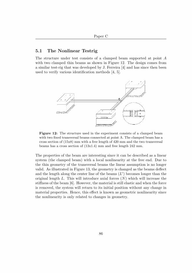
Paper C

5.1 The Nonlinear Testrig

The structure under test consists of a clamped beam supported at point Awith two clamped thin beams as shown in Figure 12. The design comes froma similar test-rig that was developed by J. Ferreira [4] and has since then beenused to verify various identification methods [4, 5].

A

Figure 12: The structure used in the experiment consists of a clamped beamwith two fixed transversal beams connected at point A. The clamped beam has across section of (15x8) mm with a free length of 420 mm and the two transversalbeams has a cross section of (13x1.4) mm and free length 242 mm.

The properties of the beam are interesting since it can be described as a linearsystem (the clamped beam) with a local nonlinearity at the free end. Due tothe thin geometry of the transversal beams the linear assumption is no longervalid. As illustrated in Figure 13, the geometry is changed as the beams deflectand the length along the center line of the beams (L′) becomes longer than theoriginal length L. This will introduce axial forces (N) which will increase thestiffness of the beam [6]. However, the material is still elastic and when the forceis removed, the system will return to its initial position without any change inmaterial properties. Hence, this effect is known as geometric nonlinearity sincethe nonlinearity is only related to changes in geometry.

86

On Nonlinear Parameter Estimation with Random Noise Signals

L

F

N N

L’

Figure 13: The transversal beams will behave nonlinearly at higher displace-ments. As the force is increased the beams becomes longer than the originallength L, and an axial force is introduced along the beams. The stiffness willtherefore increase. This effect is known as geometric nonlinearity.

Using ABAQUS R© a nonlinear static model could be created. ABAQUS usesan iterative scheme where the force is applied incrementally and a Newton-Raphson solver is used to balance the nonlinear equations. Using this solver,the theoretical nonlinear force-displacement relationship at point A could becalculated as

Fs(x) = 1.76 · 104 · x+ 2.97 · 109 · x3 (9)

5.2 Experimental Setup

The complete setup for the experimental test is shown in Figure 14. The struc-ture is firmly fixed to a rigid table and a rigid steel module is used to fix theshaker. The free end of the cantilever beam was selected as a response pointsince the nonlinear element is connected to this point. With the identifica-tion method described previously it is necessary to measure the response atthe nonlinear degree of freedoms. However, the reference point (force) can beselected at any point along the cantilever. For practical reasons the shaker isfixed to the same point and thus the linear point-flexibility and the nonlinearcoefficients will be estimated.

A force transducer was mounted on the top of the beam and the accelerometerwas mounted under the bottom beam as shown in Figure 15. The force signalswere created in MATLAB@ and Signal Calc Mobilyzer@ was used to acquirethe raw time data. All data analysis was done in MATLAB.

87

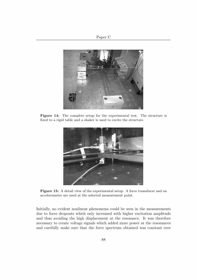
Paper C

Figure 14: The complete setup for the experimental test. The structure isfixed to a rigid table and a shaker is used to excite the structure.

Figure 15: A detail view of the experimental setup. A force transducer and an

accelerometer are used at the selected measurement point.

Initially, no evident nonlinear phenomena could be seen in the measurementsdue to force dropouts which only increased with higher excitation amplitudeand thus avoiding the high displacement at the resonance. It was thereforenecessary to create voltage signals which added more power at the resonancesand carefully make sure that the force spectrum obtained was constant over

88

On Nonlinear Parameter Estimation with Random Noise Signals

the desired frequency range.

5.3 Analysis of Experimental Data

The structure behaves linearly at low excitations and it was therefore necessaryto a find level of the excitation where the nonlinear effects are clear. A forceamplitude which made the resonance move approximately 15% was selected fornonlinear analysis.

In the following two figures, two nonlinear analyses are compared with the rawFRF. The latter is the FRF obtained with conventional linear theory (SISO).Thus, the raw FRF is calculated without any compensation for nonlinear ef-fects.

The nonlinear effects can clearly be seen in the raw measured FRF. A distur-bance occurs at approximately 2f0 and 3f0. This disturbance can also be seenin the coherence function. A part of the response that is obtained at the reso-nance frequency will, due to the nonlinearity, create higher frequency responsewhich the linear model fails to describe.

Two reverse-path models were created. First, a cubic function was used todescribe the nonlinearity and the result can be studied in Figure 16. In thesecond model, shown in Figure 17, a cubic- and a square are used to describe thenonlinearity. It could be seen that the true nonlinearity was a non-symmetricfunction and thus a cubic function was not enough to describe this behavior.Figure 18 shows the estimated linear system with different methods. The truelinear FRF was measured at very low excitation where the stiffness nonlinearityis unaffected. As shown in the figure, the estimated linear system with NIFOtechniques gives larger amplitude errors. One possible explanation for this wasgiven in chapter 4; if the force signal is contaminated with noise, the reverse-path technique will perform better.

The real parts of the nonlinear coefficients are shown in Figure 19. By defini-tion, for a zero-memory nonlinear system, the imaginary parts of the nonlinearcoefficients should be relatively small after a sufficient number of averages. Forthis experiment, the imaginary part was approximately ten times smaller thanthe real part after averaging. This may indicate a small amount of nonlineardamping which was not considered in the modeling.

89

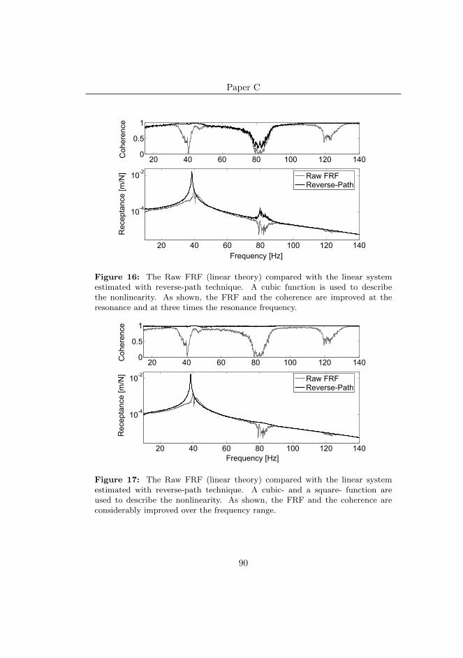
Paper C

20 40 60 80 100 120 140

10-4

10-2

Frequency [Hz]

Rec

epta

nce

[m/N

]

20 40 60 80 100 120 1400

0.5

1C

oher

ence

Raw FRFReverse-Path

Figure 16: The Raw FRF (linear theory) compared with the linear systemestimated with reverse-path technique. A cubic function is used to describethe nonlinearity. As shown, the FRF and the coherence are improved at theresonance and at three times the resonance frequency.

20 40 60 80 100 120 140

10-4

10-2

Frequency [Hz]

Rec

epta

nce

[m/N

]

20 40 60 80 100 120 1400

0.5

1

Coh

eren

ce

Raw FRFReverse-Path

Figure 17: The Raw FRF (linear theory) compared with the linear systemestimated with reverse-path technique. A cubic- and a square- function areused to describe the nonlinearity. As shown, the FRF and the coherence areconsiderably improved over the frequency range.

90

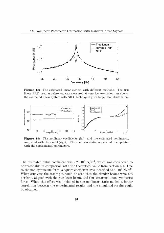
On Nonlinear Parameter Estimation with Random Noise Signals

25 30 35 40 45 50 55

10-4

10-3

10-2

Frequency [Hz]

Rec

epta

nce

[m/N

]

True LinearReverse-PathNIFO

Figure 18: The estimated linear system with different methods. The truelinear FRF, used as reference, was measured at very low excitation. As shown,the estimated linear system with NIFO techniques gives larger amplitude errors.

40 60 80 100 120 140100

105

1010

Frequency [Hz]

Non

linea

r Coe

ffici

ents

X3 CoefficientX2 Coefficient

-4 -2 0 2 4x 10-3

-200

-150

-100

-50

0

50

100

150

Displacement [m]

Forc

e [N

]

ExperimentalModelModel Updated

Figure 19: The nonlinear coefficients (left) and the estimated nonlinearitycompared with the model (right). The nonlinear static model could be updatedwith the experimental parameters.

The estimated cubic coefficient was 2.2 · 109 N/m3, which was considered tobe reasonable in comparison with the theoretical value from section 5.1. Dueto the non-symmetric force, a square coefficient was identified as 4 · 106 N/m2.When studying the test rig it could be seen that the slender beams were notperfectly aligned with the cantilever beam, and thus creating a non-symmetricforce. When this effect was included in the nonlinear static model, a bettercorrelation between the experimental results and the simulated results couldbe obtained.

91

Paper C

6 Conclusion

Nonlinear parameter estimation can be performed with random noise signalsby using conventional MIMO/MISO techniques. The methods described in thiswork treat the nonlinearity as a feedback forcing term acting on an underlyinglinear system. Thus, the true linear system and the nonlinear coefficients canbe estimated by measuring the input and output quantities.

The approach that is used in this work requires some pre-information aboutthe type of nonlinearity present, and its location in the system. If this infor-mation cannot be obtained before the analysis it may be possible to try a setof different combinations and then utilize the multiple coherence function asshown in Chapter 3.

When using MIMO/MISO there are several possible ways to formulate a nonlin-ear problem. Two methods have been studied in simulations and experiments -referred to as NIFO and Reverse-Path. As shown in this work, it is essential tocreate nonlinear models which best compensate for the errors introduced withcontaminating noise.

An experimental test was done on a structure with a significant nonlinearityand the results, presented in section 5.3, shows that the underlying linear sys-tem and the coefficients describing the nonlinearity could be identified. Whencomparing the results with linear theory a clear improvement could be seen:The estimated linear system is free from disturbance and with a correct res-onance frequency. Thus, a simple but very useful application of the methodsmay be to make a better estimate of the linear system, for instance when com-parison are made to a numerical linear model.

Acknowledgment

Financial support from the Swedish Knowledge Foundation is gratefully ac-knowledged

92

On Nonlinear Parameter Estimation with Random Noise Signals

References

[1] Julius S. Bendat. Nonlinear System Analysis and Identification from Ran-dom Data. John Wiley Sons, Inc., first edition, 1990.

[2] D.E. Adams and R.J. Allemang. A frequency domain method for estimatingthe parameters of a non-linear structural dynamic model through feedback.Mechanical systems and Signal Processing, 14(4), 2000.

[3] Martin Magnevall, Andreas Josefsson, and Kjell Ahlin. On nonlinear pa-rameter estimation. International Conference on Noise and Vibration En-gineering (ISMA2006), s. 3817-3831, 2006.

[4] J.V. Ferreira. Dynamic Response Analysis of Structures with NonlinearComponents. PhD thesis, Imperial College, London, 1998.

[5] H. R. E. Siller. Non-linear modal analysis methods for engineering struc-tures. PhD thesis, Imperial College, London, 2004.

[6] Q. Jing, T. Mukherjee, and G.K Fedder. Large-deflection beam model forschematic-based behavioral simulations in nodas. Proceedings of the Inter-national Conference on Modeling and Simulation of Microsystems, 2002.

93

Paper C

94

Paper D

Nonlinear StructuralIdentification by the “Reverse

Path” Spectral Method

95

Paper D is published as:

Magnevall, M., Josefsson, A., Ahlin, K., Broman, G. NonlinearStructural Identification by the “Reverse Path” Spectral Method,Journal of Sound and Vibration, vol. 331, no. 4, pp. 938-946, 2012.

96

Nonlinear Structural Identification by the

“Reverse Path” Spectral Method

Martin Magnevall1,2

Andreas Josefsson2

Kjell Ahlin2

Goran Broman2,3

1 AB Sandvik Coromant, SE-811 81 Sandviken, Sweden2 Blekinge Institute of Technology, SE-371 79 Karlskrona, Sweden

3 Lulea University of Technology, SE-971 87 Lulea, Sweden

Abstract

When dealing with nonlinear dynamical systems, it is important to haveefficient, accurate and reliable tools for estimating both the linear andnonlinear system parameters from measured data. An approach for non-linear system identification widely studied in recent years is ”ReversePath”. This method is based on broad-band excitation and treats thenonlinear terms as feedback forces acting on an underlying linear system.Parameter estimation is performed in the frequency domain using con-ventional multiple-input-multiple-output or multiple-input-single-outputtechniques. This paper presents a generalized approach to apply themethod of ”Reverse Path” on continuous mechanical systems with mul-tiple nonlinearities. The method requires few spectral calculations andis therefore suitable for use in iterative processes to locate and estimatestructural nonlinearities. The proposed method is demonstrated in bothsimulations and experiments on continuous nonlinear mechanical struc-tures. The results show that the method is effective on both simulatedas well as experimental data.

97

Paper D

1 Introduction

In the past years much effort has been put into the field of parameter estima-tion of nonlinear dynamical systems. A large number of methods have beendeveloped, but there is still no method applicable to a general structure with anarbitrary nonlinearity. A survey of the most common current methods is foundin [1]. An important method, widely studied in recent years, is the ”ReversePath” method. This is based on broad-band excitation and was initially devel-oped by Bendat et al. [2, 3] and Rice et al. [4, 5] and is thoroughly describedin [6]. “Reverse Path” treats the nonlinearities as force feedback terms actingon an underlying linear system. The parameter estimation is performed in thefrequency domain using conventional multiple-input-multiple-output (MIMO)or multiple-input-single-output (MISO) techniques and estimates of both theunderlying linear properties and the nonlinear coefficients are obtained. “Re-verse Path” has proven to work well both in simulations and in experimentaltests on various mechanical systems with local nonlinearities [7, 8, 9, 10, 11],which indicates that the method is robust and well suited to use in engineer-ing applications within nonlinear structural identification. Applications of the“Reverse-Path” method in other fields are, e.g. Esmonde et al. [12] who suc-cessfully applied the method for parameter estimation of nonlinear squeeze filmdynamics, and Liagre et al. [13] who applied the “Reverse-Path” method inoffshore engineering.

The method of “Reverse Path” requires the form of the nonlinearities as wellas their locations to be known beforehand in order to provide accurate esti-mates. Otherwise an iterative approach is required for estimating the location[14] and/or the nonlinear functional form [7, 11]. For this to be performed in anefficient way, a method that can apply “Reverse Path” on a general nonlinearsystem is needed. Rice et al. [5] developed a method for arbitrary multi-degree-of-freedom (MDOF) systems with localized nonlinearities using unconditioned(partially correlated) inputs. However, the method requires that the system isexcited in all measurement points, which can be impractical for complex non-linear structures. Richards et al. [15] developed a general approach for MDOFsystems based on conditioned (uncorrelated) inputs which only requires a singleexcitation point. A disadvantage with this method is the significant complica-tion of the problem formulation due to the need for conditioned inputs.

This paper presents a method which applies the “Reverse Path” method on a

98

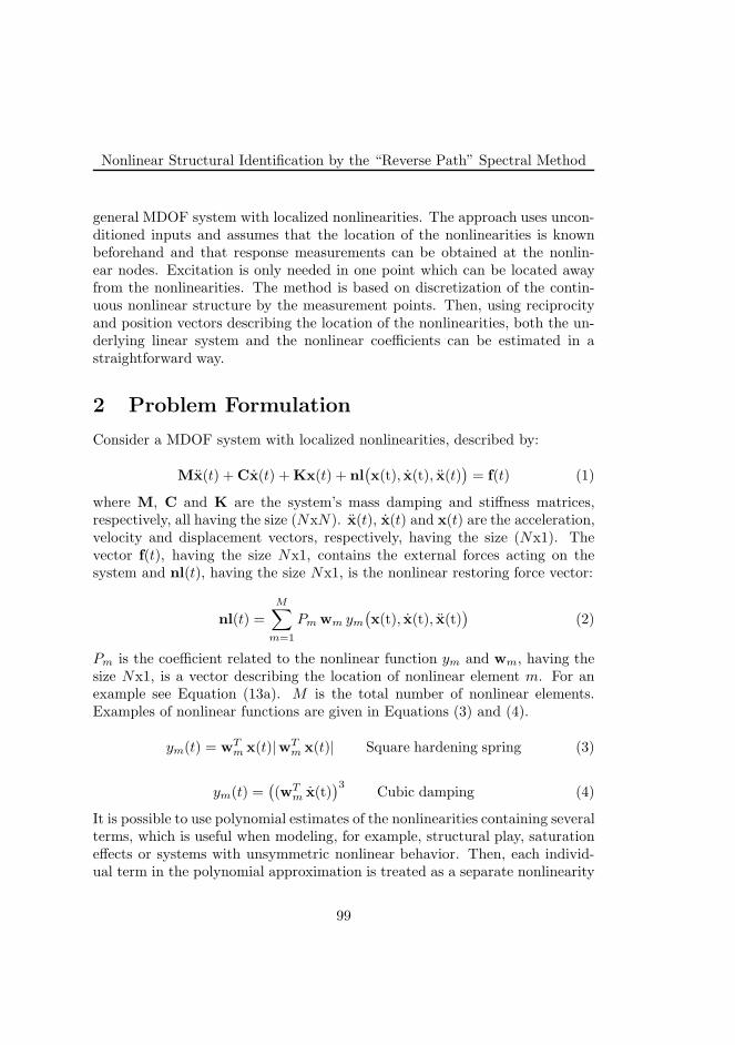
Nonlinear Structural Identification by the “Reverse Path” Spectral Method

general MDOF system with localized nonlinearities. The approach uses uncon-ditioned inputs and assumes that the location of the nonlinearities is knownbeforehand and that response measurements can be obtained at the nonlin-ear nodes. Excitation is only needed in one point which can be located awayfrom the nonlinearities. The method is based on discretization of the contin-uous nonlinear structure by the measurement points. Then, using reciprocityand position vectors describing the location of the nonlinearities, both the un-derlying linear system and the nonlinear coefficients can be estimated in astraightforward way.

2 Problem Formulation

Consider a MDOF system with localized nonlinearities, described by:

Mx(t) +Cx(t) +Kx(t) + nl(

x(t), x(t), x(t))

= f(t) (1)

where M, C and K are the system’s mass damping and stiffness matrices,respectively, all having the size (NxN). x(t), x(t) and x(t) are the acceleration,velocity and displacement vectors, respectively, having the size (Nx1). Thevector f(t), having the size Nx1, contains the external forces acting on thesystem and nl(t), having the size Nx1, is the nonlinear restoring force vector:

nl(t) =

M∑

m=1

Pm wm ym(

x(t), x(t), x(t))

(2)

Pm is the coefficient related to the nonlinear function ym and wm, having thesize Nx1, is a vector describing the location of nonlinear element m. For anexample see Equation (13a). M is the total number of nonlinear elements.Examples of nonlinear functions are given in Equations (3) and (4).

ym(t) = wTm x(t)|wT

m x(t)| Square hardening spring (3)

ym(t) =(

(wTm x(t)

)3

Cubic damping (4)

It is possible to use polynomial estimates of the nonlinearities containing severalterms, which is useful when modeling, for example, structural play, saturationeffects or systems with unsymmetric nonlinear behavior. Then, each individ-ual term in the polynomial approximation is treated as a separate nonlinearity

99

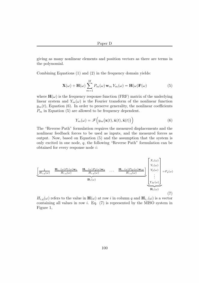
Paper D

giving as many nonlinear elements and position vectors as there are terms inthe polynomial.

Combining Equations (1) and (2) in the frequency domain yields:

X(ω) +H(ω)M∑

m=1

Pm(ω)wm Ym(ω) = H(ω)F(ω) (5)

where H(ω) is the frequency response function (FRF) matrix of the underlyinglinear system and Ym(ω) is the Fourier transform of the nonlinear functionym(t), Equation (6). In order to preserve generality, the nonlinear coefficientsPm in Equation (5) are allowed to be frequency dependent.

Ym(ω) = F

(

ym(

x(t), x(t), x(t))

)

(6)

The “Reverse Path” formulation requires the measured displacements and thenonlinear feedback forces to be used as inputs, and the measured forces asoutput. Now, based on Equation (5) and the assumption that the system isonly excited in one node, q, the following “Reverse Path” formulation can beobtained for every response node i:

[

1

Hi,q(ω)

Hi,:(ω)P1(ω)w1

Hi,q(ω)

Hi,:(ω)P2(ω)w2

Hi,q(ω)· · ·

Hi,:(ω)PM (ω)wM

Hi,q(ω)

]

︸ ︷︷ ︸

Bi(ω)

Xi(ω)

Y1(ω)

Y2(ω)

...YM (ω)

︸ ︷︷ ︸

Ri(ω)

=Fq(ω)

(7)Hi,q(ω) refers to the value in H(ω) at row i in column q and Hi,:(ω) is a vectorcontaining all values in row i. Eq. (7) is represented by the MISO system inFigure 1,

100

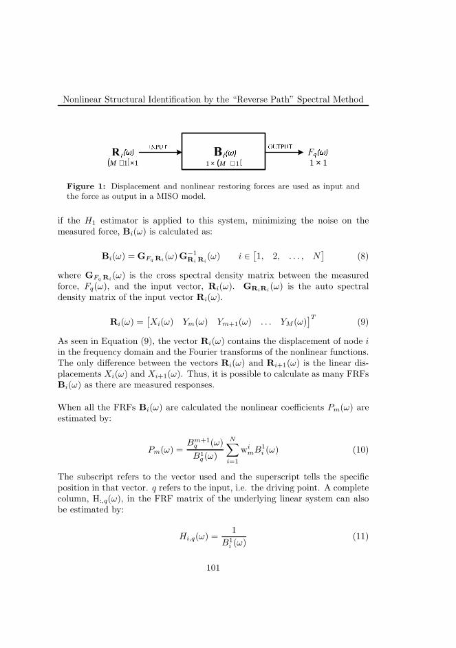
Nonlinear Structural Identification by the “Reverse Path” Spectral Method

�B����� ������

F��R

( )11 +× M( ) 11 ×+M 11 ×� � �

Figure 1: Displacement and nonlinear restoring forces are used as input andthe force as output in a MISO model.

if the H1 estimator is applied to this system, minimizing the noise on themeasured force, Bi(ω) is calculated as:

Bi(ω) = GFq Ri(ω)G−1

Ri Ri(ω) i ∈

[

1, 2, . . . , N]

(8)

where GFq Ri(ω) is the cross spectral density matrix between the measured

force, Fq(ω), and the input vector, Ri(ω). GRiRi(ω) is the auto spectral

density matrix of the input vector Ri(ω).

Ri(ω) =[

Xi(ω) Ym(ω) Ym+1(ω) . . . YM (ω)]T

(9)

As seen in Equation (9), the vector Ri(ω) contains the displacement of node i

in the frequency domain and the Fourier transforms of the nonlinear functions.The only difference between the vectors Ri(ω) and Ri+1(ω) is the linear dis-placements Xi(ω) and Xi+1(ω). Thus, it is possible to calculate as many FRFsBi(ω) as there are measured responses.

When all the FRFs Bi(ω) are calculated the nonlinear coefficients Pm(ω) areestimated by:

Pm(ω) =Bm+1

q (ω)

B1q (ω)

N∑

i=1

wimB1

i (ω) (10)

The subscript refers to the vector used and the superscript tells the specificposition in that vector. q refers to the input, i.e. the driving point. A completecolumn, H:,q(ω), in the FRF matrix of the underlying linear system can alsobe estimated by:

Hi,q(ω) =1

B1

i (ω)(11)

101

Paper D

Applying Equations (8)-(11), both the nonlinear coefficients and the columnand row (reciprocity) of the underlying linear system corresponding to the ex-citation node, q, are obtained. By modal parameter estimation the completeFRF matrix of the underlying linear system can be estimated and used to builda nonlinear model of the studied system.

The presented method provides a structured approach to apply the methodof “Reverse Path” to general nonlinear MDOF systems. The method requiresthat the location of the nonlinearities is known and that response measurementscan be obtained in the nonlinear nodes and at the node of excitation. Thereare, however, no restrictions on either the number of nonlinear elements orthe number of terms in the polynomials or power series used to estimate thestructural nonlinearities. Additionally, the method only requires excitation inone node and there is no restriction on the force location.

3 Simulations

A cantilever beam with two cubic nonlinearities is used in the simulation, Figure2. One nonlinearity is located between node 1 and ground and one is locatedbetween nodes 2 and 3. The excitation force is applied in node 4 (Gaussianrandom noise), away from the nonlinearities. The first five modes of the beamare taken into account in the simulation. To further explain the method derivedin section 2, a few steps in the identification is shown by specific equations,only valid for this model, which are then related to the corresponding generalequation in section 2. For the sake of brevity, the frequency dependence (ω) isdropped in the following sections.

102

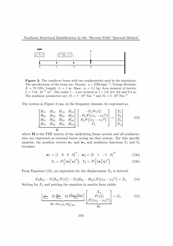
Nonlinear Structural Identification by the “Reverse Path” Spectral Method

�

�

( )3322 xxP −3

11 xP

������

Figure 2: The cantilever beam with two nonlinearities used in the simulation.The specifications of the beam are: Density: ρ = 2700 kgm−3; Youngs Modulus:E = 70 GPa; Length: L = 1 m; Mass: m = 1.1 kg; Area moment of inertia:I = 7.34 · 10−9 m4. The nodes 1 − 4 are located at l = 1.0, 0.8, 0.6 and 0.4 m.The nonlinear parameters are: P1 = 7 · 106 Nm−3 and P2 = 3 · 108 Nm−3

The system in Figure 2 can, in the frequency domain, be expressed as:

H11 H12 H13 H14

H21 H22 H23 H24

H31 H32 H33 H34

H41 H42 H43 H44

︸ ︷︷ ︸

H

−P1F (x3

1)

−P2F(

(x2 − x3)3)

P2F(

(x2 − x3)3)

F4

=

X1

X2

X3

X4

(12)

where H is the FRF matrix of the underlying linear system and all nonlinear-ities are expressed as external forces acting on that system. For this specificanalysis, the position vectors w1 and w2 and nonlinear functions Y1 and Y2

becomes:

w1 =[

1 0 0 0]T

; w2 =[

0 1 −1 0]T

(13a)

Y1 = F

(

(

wT

1x)3)

; Y2 = F

(

(

wT

2x)3)

(13b)

From Equation (12), an expression for the displacement X4 is derived:

F4H44 − P1H41F (x3

1)− P2(H42 −H43)F

(

(x2 − x3)3)

= X4 (14)

Solving for F4 and putting the equation in matrix form yields:

[

1

H44

P1H41

H44

P2

(H42−H43)

H44

]

︸ ︷︷ ︸

B4=GF4 R4G

−1

R4 R4

X4

F (x3

1)

F(

(x2 − x3)3)

︸ ︷︷ ︸

R4

= F4 (15)

103

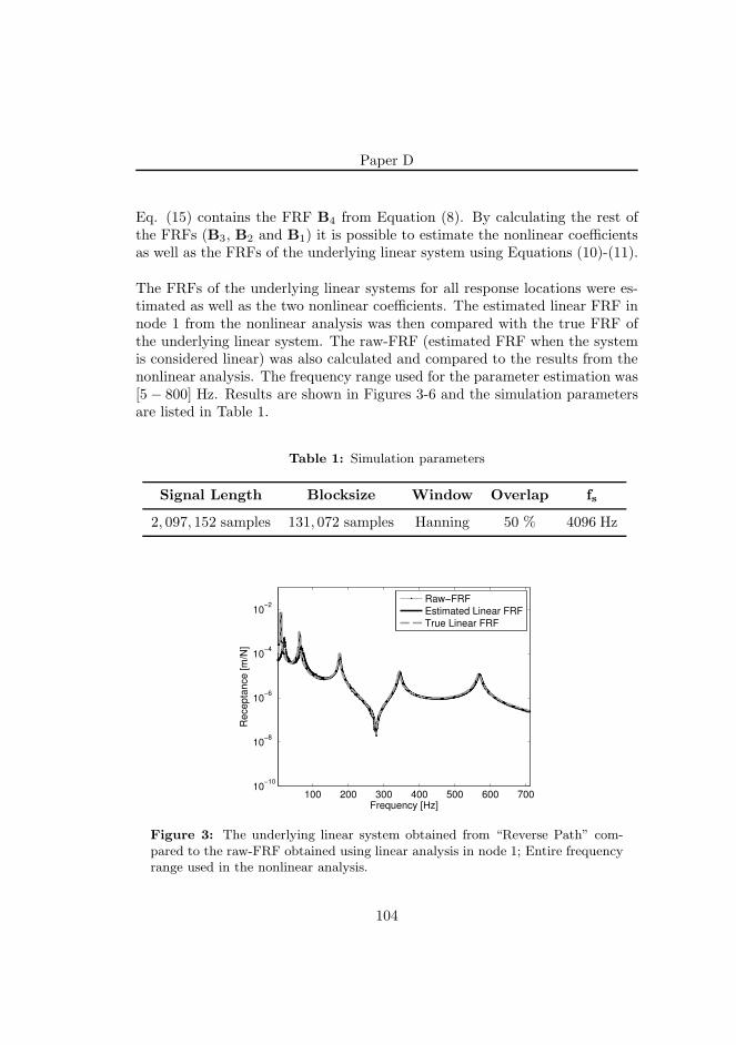
Paper D

Eq. (15) contains the FRF B4 from Equation (8). By calculating the rest ofthe FRFs (B3, B2 and B1) it is possible to estimate the nonlinear coefficientsas well as the FRFs of the underlying linear system using Equations (10)-(11).

The FRFs of the underlying linear systems for all response locations were es-timated as well as the two nonlinear coefficients. The estimated linear FRF innode 1 from the nonlinear analysis was then compared with the true FRF ofthe underlying linear system. The raw-FRF (estimated FRF when the systemis considered linear) was also calculated and compared to the results from thenonlinear analysis. The frequency range used for the parameter estimation was[5 − 800] Hz. Results are shown in Figures 3-6 and the simulation parametersare listed in Table 1.

Table 1: Simulation parameters

Signal Length Blocksize Window Overlap fs

2, 097, 152 samples 131, 072 samples Hanning 50 % 4096 Hz

100 200 300 400 500 600 70010

−10

10−8

10−6

10−4

10−2

Frequency [Hz]

Re

ce

pta

nce

[m

/N]

Raw−FRF

Estimated Linear FRF

True Linear FRF

Figure 3: The underlying linear system obtained from “Reverse Path” com-pared to the raw-FRF obtained using linear analysis in node 1; Entire frequencyrange used in the nonlinear analysis.

104

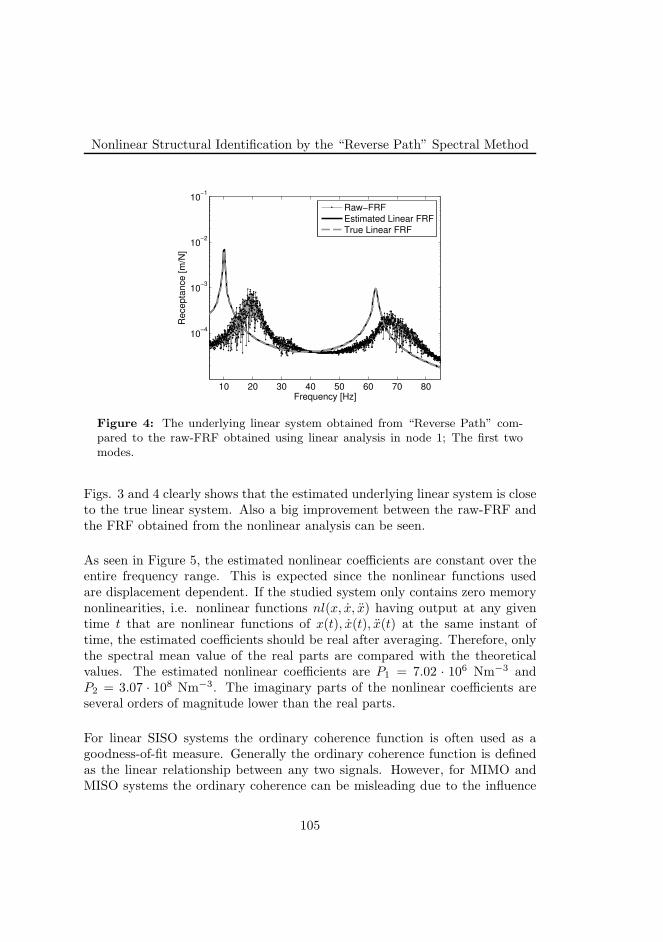
Nonlinear Structural Identification by the “Reverse Path” Spectral Method

10 20 30 40 50 60 70 80

10−4

10−3

10−2

10−1

Frequency [Hz]

Recepta

nce [

m/N

]

Raw−FRF

Estimated Linear FRF

True Linear FRF

Figure 4: The underlying linear system obtained from “Reverse Path” com-pared to the raw-FRF obtained using linear analysis in node 1; The first twomodes.

Figs. 3 and 4 clearly shows that the estimated underlying linear system is closeto the true linear system. Also a big improvement between the raw-FRF andthe FRF obtained from the nonlinear analysis can be seen.

As seen in Figure 5, the estimated nonlinear coefficients are constant over theentire frequency range. This is expected since the nonlinear functions usedare displacement dependent. If the studied system only contains zero memorynonlinearities, i.e. nonlinear functions nl(x, x, x) having output at any giventime t that are nonlinear functions of x(t), x(t), x(t) at the same instant oftime, the estimated coefficients should be real after averaging. Therefore, onlythe spectral mean value of the real parts are compared with the theoreticalvalues. The estimated nonlinear coefficients are P1 = 7.02 · 106 Nm−3 andP2 = 3.07 · 108 Nm−3. The imaginary parts of the nonlinear coefficients areseveral orders of magnitude lower than the real parts.

For linear SISO systems the ordinary coherence function is often used as agoodness-of-fit measure. Generally the ordinary coherence function is definedas the linear relationship between any two signals. However, for MIMO andMISO systems the ordinary coherence can be misleading due to the influence

105

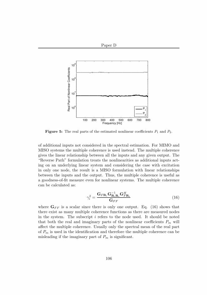
Paper D

100 200 300 400 500 600 700 800

106

107

108

109

Frequency [Hz]

Real P

art

of

Nonlin

ear

Coeff

icie

nts

P1

P2

Figure 5: The real parts of the estimated nonlinear coefficients P1 and P2.

of additional inputs not considered in the spectral estimation. For MIMO andMISO systems the multiple coherence is used instead. The multiple coherencegives the linear relationship between all the inputs and any given output. The“Reverse Path” formulation treats the nonlinearities as additional inputs act-ing on an underlying linear system and considering the case with excitationin only one node, the result is a MISO formulation with linear relationshipsbetween the inputs and the output. Thus, the multiple coherence is useful asa goodness-of-fit measure even for nonlinear systems. The multiple coherencecan be calculated as:

γ2

i =GFRi

G−1

RiRiGH

FRi

GFF

(16)

where GFF is a scalar since there is only one output. Eq. (16) shows thatthere exist as many multiple coherence functions as there are measured nodesin the system. The subscript i refers to the node used. It should be notedthat both the real and imaginary parts of the nonlinear coefficients Pm willaffect the multiple coherence. Usually only the spectral mean of the real partof Pm is used in the identification and therefore the multiple coherence can bemisleading if the imaginary part of Pm is significant.

106

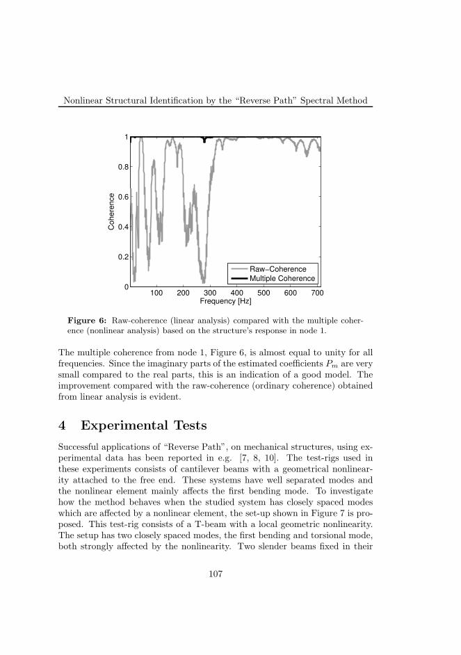
Nonlinear Structural Identification by the “Reverse Path” Spectral Method

100 200 300 400 500 600 7000

0.2

0.4

0.6

0.8

1

Frequency [Hz]

Co

he

ren

ce

Raw−Coherence

Multiple Coherence

Figure 6: Raw-coherence (linear analysis) compared with the multiple coher-ence (nonlinear analysis) based on the structure’s response in node 1.

The multiple coherence from node 1, Figure 6, is almost equal to unity for allfrequencies. Since the imaginary parts of the estimated coefficients Pm are verysmall compared to the real parts, this is an indication of a good model. Theimprovement compared with the raw-coherence (ordinary coherence) obtainedfrom linear analysis is evident.

4 Experimental Tests

Successful applications of “Reverse Path”, on mechanical structures, using ex-perimental data has been reported in e.g. [7, 8, 10]. The test-rigs used inthese experiments consists of cantilever beams with a geometrical nonlinear-ity attached to the free end. These systems have well separated modes andthe nonlinear element mainly affects the first bending mode. To investigatehow the method behaves when the studied system has closely spaced modeswhich are affected by a nonlinear element, the set-up shown in Figure 7 is pro-posed. This test-rig consists of a T-beam with a local geometric nonlinearity.The setup has two closely spaced modes, the first bending and torsional mode,both strongly affected by the nonlinearity. Two slender beams fixed in their

107

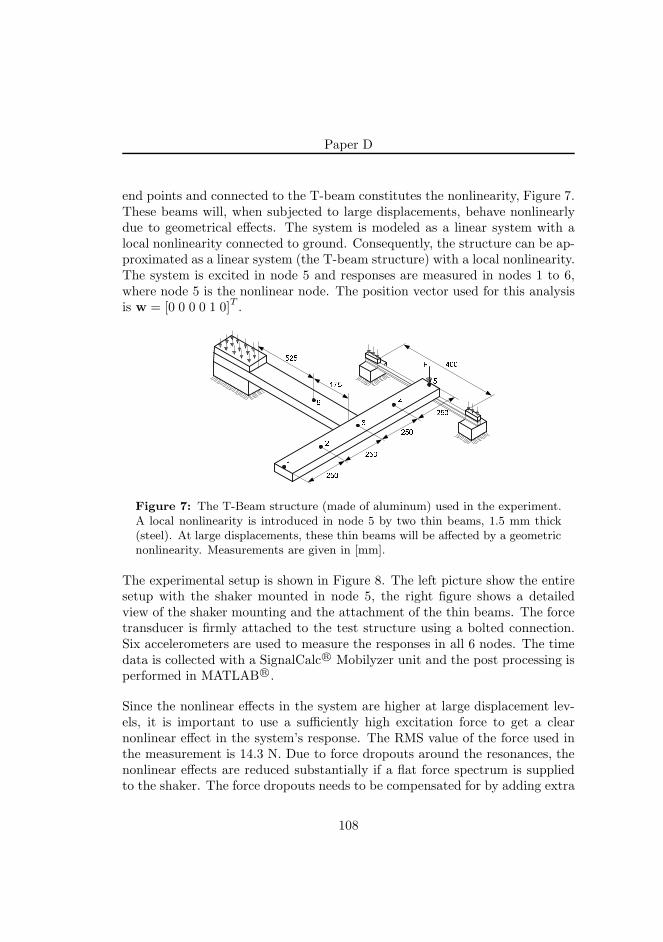
Paper D

end points and connected to the T-beam constitutes the nonlinearity, Figure 7.These beams will, when subjected to large displacements, behave nonlinearlydue to geometrical effects. The system is modeled as a linear system with alocal nonlinearity connected to ground. Consequently, the structure can be ap-proximated as a linear system (the T-beam structure) with a local nonlinearity.The system is excited in node 5 and responses are measured in nodes 1 to 6,where node 5 is the nonlinear node. The position vector used for this analysisis w = [0 0 0 0 1 0]T .

�

�

�

�

�

�

�

���

���

���

���

���

���

���

Figure 7: The T-Beam structure (made of aluminum) used in the experiment.A local nonlinearity is introduced in node 5 by two thin beams, 1.5 mm thick(steel). At large displacements, these thin beams will be affected by a geometricnonlinearity. Measurements are given in [mm].

The experimental setup is shown in Figure 8. The left picture show the entiresetup with the shaker mounted in node 5, the right figure shows a detailedview of the shaker mounting and the attachment of the thin beams. The forcetransducer is firmly attached to the test structure using a bolted connection.Six accelerometers are used to measure the responses in all 6 nodes. The timedata is collected with a SignalCalc R© Mobilyzer unit and the post processing isperformed in MATLAB R©.

Since the nonlinear effects in the system are higher at large displacement lev-els, it is important to use a sufficiently high excitation force to get a clearnonlinear effect in the system’s response. The RMS value of the force used inthe measurement is 14.3 N. Due to force dropouts around the resonances, thenonlinear effects are reduced substantially if a flat force spectrum is suppliedto the shaker. The force dropouts needs to be compensated for by adding extra

108

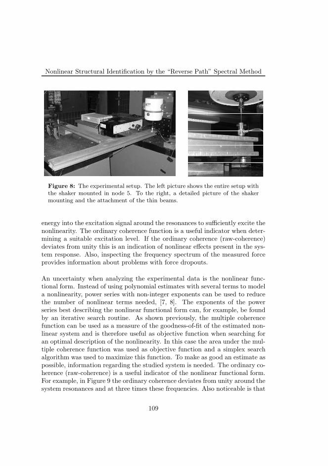
Nonlinear Structural Identification by the “Reverse Path” Spectral Method

Figure 8: The experimental setup. The left picture shows the entire setup withthe shaker mounted in node 5. To the right, a detailed picture of the shakermounting and the attachment of the thin beams.

energy into the excitation signal around the resonances to sufficiently excite thenonlinearity. The ordinary coherence function is a useful indicator when deter-mining a suitable excitation level. If the ordinary coherence (raw-coherence)deviates from unity this is an indication of nonlinear effects present in the sys-tem response. Also, inspecting the frequency spectrum of the measured forceprovides information about problems with force dropouts.

An uncertainty when analyzing the experimental data is the nonlinear func-tional form. Instead of using polynomial estimates with several terms to modela nonlinearity, power series with non-integer exponents can be used to reducethe number of nonlinear terms needed, [7, 8]. The exponents of the powerseries best describing the nonlinear functional form can, for example, be foundby an iterative search routine. As shown previously, the multiple coherencefunction can be used as a measure of the goodness-of-fit of the estimated non-linear system and is therefore useful as objective function when searching foran optimal description of the nonlinearity. In this case the area under the mul-tiple coherence function was used as objective function and a simplex searchalgorithm was used to maximize this function. To make as good an estimate aspossible, information regarding the studied system is needed. The ordinary co-herence (raw-coherence) is a useful indicator of the nonlinear functional form.For example, in Figure 9 the ordinary coherence deviates from unity around thesystem resonances and at three times these frequencies. Also noticeable is that

109

Paper D

there is no deviation at twice the resonance frequencies which indicates onlyodd harmonics in the nonlinear response. Since only odd harmonics are present,the nonlinear functional form can be assumed to have odd symmetry, i.e. thenonlinearity behaves the same for both positive and negative displacements,but with different sign. Further more, the nonlinearity is geometrical, which intheory has a cubic nonlinear form. Thus, the nonlinear functional form chosenfor the optimization is sign(x)|xα| with α = 3 as initial value. The best fitwas obtained with sign(x)|x2.5872| as the nonlinear function. The nonlinear pa-rameter estimation was done with a sampling frequency fs = 2604.2 Hz, blocksize 32768 samples, Hanning window, 50% overlap and 120 averages. Thesesettings were enough to reach sufficient noise reduction and thus provide anaccurate estimate of the system’s frequency response. All responses were mea-sured using accelerometers and the signals were numerically double integratedto displacement before the nonlinear analysis. After integration, a high-passfilter was applied to the signals in order to remove uncertainties caused by thelow frequency characteristics in the numerical integration. A Butterworth filterof order 3 was used and the data were filtered in both directions to obtain azero phase filter response. The cut-off frequency for the high pass filter was setto 2 Hz.

Fig. 9 shows the raw-coherence from the linear analysis (SISO) comparedwith the multiple coherence obtained from the nonlinear analysis (MISO). Thenonlinear effect is clearly visible in the raw-coherence, especially around theresonances. It is clear that the raw-coherence is close to unity above 55 Hzwith the exception for the region around 90 Hz. This indicates a perfect linearrelationship between the input and output of the system. Due to the lackof nonlinear effects above 55 Hz, the frequency span [15 − 55] Hz was usedwhen estimating the nonlinear coefficient. The real and imaginary part of theestimated coefficient are shown in Figure 10. Since the nonlinearity is expectedto be of zero memory type, only the real part is used in the analysis. The realpart of the estimated coefficient is constant over the entire frequency range andthe spectral mean value is 1.2504 · 108 Nm−2.5872. The imaginary part changeswith frequency and is on average 25 times smaller than the real part.

110

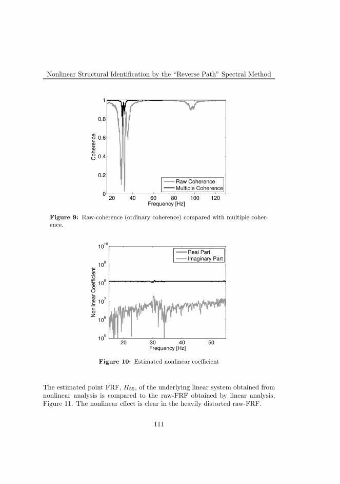
Nonlinear Structural Identification by the “Reverse Path” Spectral Method

20 40 60 80 100 1200

0.2

0.4

0.6

0.8

1

Frequency [Hz]

Cohere

nce

Raw Coherence

Multiple Coherence

Figure 9: Raw-coherence (ordinary coherence) compared with multiple coher-ence.

20 30 40 5010

5

106

107

108

109

1010

Frequency [Hz]

No

nlin

ea

r C

oe

ffic

ien

t

Real Part

Imaginary Part

Figure 10: Estimated nonlinear coefficient

The estimated point FRF, H55, of the underlying linear system obtained fromnonlinear analysis is compared to the raw-FRF obtained by linear analysis,Figure 11. The nonlinear effect is clear in the heavily distorted raw-FRF.

111

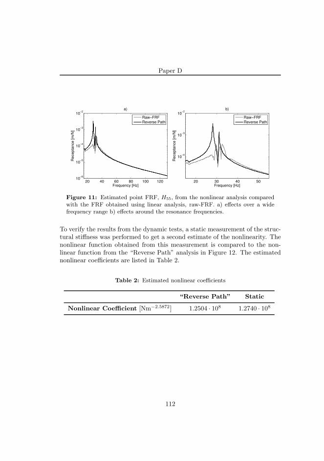
Paper D

20 40 60 80 100 12010

−6

10−5

10−4

10−3

10−2

Frequency [Hz]

a)

Re

ce

pta

nce

[m

/N]

Raw−FRF

Reverse Path

20 30 40 50

10−4

10−3

10−2

Frequency [Hz]

b)

Re

ce

pta

nce

[m

/N]

Raw−FRF

Reverse Path

Figure 11: Estimated point FRF, H55, from the nonlinear analysis comparedwith the FRF obtained using linear analysis, raw-FRF. a) effects over a widefrequency range b) effects around the resonance frequencies.

To verify the results from the dynamic tests, a static measurement of the struc-tural stiffness was performed to get a second estimate of the nonlinearity. Thenonlinear function obtained from this measurement is compared to the non-linear function from the “Reverse Path” analysis in Figure 12. The estimatednonlinear coefficients are listed in Table 2.

Table 2: Estimated nonlinear coefficients

“Reverse Path” Static

Nonlinear Coefficient [Nm−2.5872] 1.2504 · 108 1.2740 · 108

112

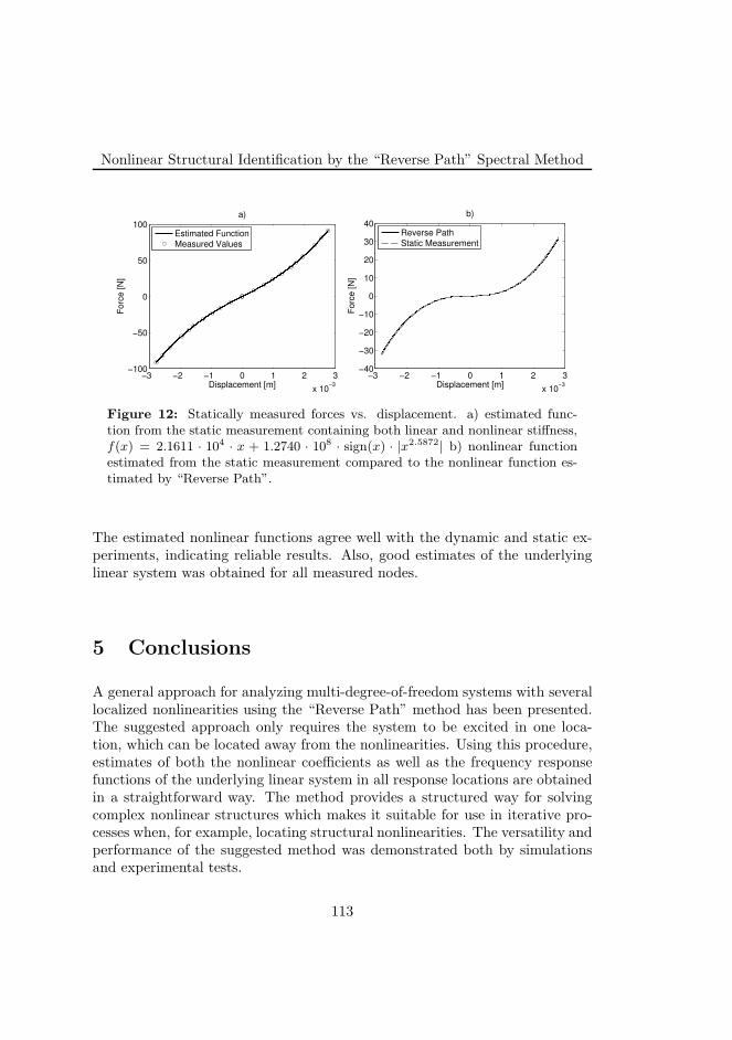
Nonlinear Structural Identification by the “Reverse Path” Spectral Method

−3 −2 −1 0 1 2 3

x 10−3

−100

−50

0

50

100

Displacement [m]

Fo

rce

[N

]

a)

Estimated Function

Measured Values

−3 −2 −1 0 1 2 3

x 10−3

−40

−30

−20

−10

0

10

20

30

40b)

Displacement [m]

Forc

e [

N]

Reverse Path

Static Measurement

Figure 12: Statically measured forces vs. displacement. a) estimated func-tion from the static measurement containing both linear and nonlinear stiffness,f(x) = 2.1611 · 104 · x + 1.2740 · 108 · sign(x) · |x2.5872| b) nonlinear functionestimated from the static measurement compared to the nonlinear function es-timated by “Reverse Path”.

The estimated nonlinear functions agree well with the dynamic and static ex-periments, indicating reliable results. Also, good estimates of the underlyinglinear system was obtained for all measured nodes.

5 Conclusions

A general approach for analyzing multi-degree-of-freedom systems with severallocalized nonlinearities using the “Reverse Path” method has been presented.The suggested approach only requires the system to be excited in one loca-tion, which can be located away from the nonlinearities. Using this procedure,estimates of both the nonlinear coefficients as well as the frequency responsefunctions of the underlying linear system in all response locations are obtainedin a straightforward way. The method provides a structured way for solvingcomplex nonlinear structures which makes it suitable for use in iterative pro-cesses when, for example, locating structural nonlinearities. The versatility andperformance of the suggested method was demonstrated both by simulationsand experimental tests.

113

Paper D

References

[1] G. Kerschen, K. Worden, A.F. Vakakis, and J.-C. Golinval. Past, presentand future of nonlinear system identification in structural dynamics. Me-

chanical Systems and Signal Processing, 20(3):505 – 92, 2006/04/.

[2] J. S. Bendat and A. G. Piersol. Spectral analysis of non-linear systems in-volving square-law operations. Journal of Sound and Vibration, 81(2):199– 214, 1982.

[3] J.S. Bendat and A.G. Piersol. Decomposition of wave forces into linearand non-linear components. Journal of Sound and Vibration, 106(3):391– 408, 1986.

[4] H.J. Rice and J.A. Fitzpatrick. A generalised technique for spectral anal-ysis of non-linear systems. Mechanical Systems and Signal Processing,2(2):195 – 207, 1988.

[5] H.J. Rice and J.A. Fitzpatrick. A procedure for the identification of linearand non-linear multi-degree-of-freedom systems. Journal of Sound and

Vibration, 149(3):397 – 411, 1991.

[6] Julius S. Bendat. Nonlinear system analysis and identification from ran-

dom data. Wiley, New York, 1990.

[7] G. Kerschen, V. Lenaerts, and J.-C. Golinval. Identification of a continuousstructure with a geometrical non-linearity. part i: Conditioned reverse pathmethod. Journal of Sound and Vibration, 262(4):889 – 906, 2003.

[8] L. Garibaldi. Application of the conditioned reverse path method. Mechan-

ical Systems and Signal Processing, 17(1):227 – 235, 2003. Conditionedreverse path (CRP) method;.

[9] S. Marchesiello. Application of the conditioned reverse path method. Me-

chanical Systems and Signal Processing, 17(1):183 – 188, 2003. Dampers;.

[10] A Josefsson, M Magnevall, and K Ahlin. On nonlinear parameter estima-tion with random noise signals. In Proceedings of IMAC XXV, 2007.

[11] M. Magnevall, A. Josefsson, and K. Ahlin. On parameter estimation andsimulation of zero memeory nonlinear systems. In Proceedings of IMAC

XXVI, 2008.

114

Nonlinear Structural Identification by the “Reverse Path” Spectral Method

[12] H. Esmonde, J.A. Fitzpatrick, H.J. Rice, and F. Axisa. Modelling andidentification of nonlinear squeeze film dynamics. Journal of Fluids and

Structures, 6(2):223 – 248, 1992.

[13] P.F. Liagre and J.M. Niedzwecki. Estimating nonlinear coupled frequency-dependent parameters in offshore engineering. Applied Ocean Research,25(1):1 – 19, 2003.

[14] A. Josefsson, M. Magnevall, and K. Ahlin. Estimating the location of struc-tural nonlinearities from random data. In Proceedings of IMAC XXVI,2008.

[15] C.M. Richards and R. Singh. Identification of multi-degree-of-freedom non-linear systems under random excitations by the ”reverse path” spectralmethod. Journal of Sound and Vibration, 213(4):673 – 707, 1998.

115

Paper D

116

Paper E

A Simulation andCharacterization Method for

Hysteretically DampedVibrations

117

Paper E is published as:

Magnevall, M., Josefsson, A., Ahlin, K., Broman, G. A Simula-tion and Characterization Method for Hysteretically Damped Vi-brations, Submitted for publication, 2011.

118

A Simulation and Characterization Method for

Hysteretically Damped Vibrations

Martin Magnevall1,2

Andreas Josefsson2

Kjell Ahlin2

Goran Broman2

1 AB Sandvik Coromant, SE-811 81 Sandviken, Sweden2 Blekinge Institute of Technology, SE-371 79 Karlskrona, Sweden

Abstract

This paper presents a simulation and parameter estimation method fora general mechanical structure with a localized nonlinear damper. Theintended industrial applications are simulation and characterization ofpassive dampers used for vibration attenuation in metal machining. Anew forced response simulation routine for an arbitrary multi-degree-of-freedom system with a mass damper coupled via a Bouc-Wen hysteresiselement is developed. The simulation method is used as a basis in a twostage parameter estimation routine performed in the time domain. Theproposed method utilizes least square estimation in combination withnonlinear optimization by a real coded genetic algorithm. The methodsare successfully used with both simulated and experimental data on adry-friction damper.

Keywords: Bouc-Wen, Parameter estimation, Nonlinear, Genetic Algo-rithm, Dry-Friction

119

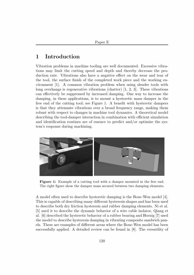
Paper E

1 Introduction

Vibration problems in machine tooling are well documented. Excessive vibra-tions may limit the cutting speed and depth and thereby decrease the pro-duction rate. Vibrations also have a negative effect on the wear and tear ofthe tool, the surface finish of the completed work piece and the working en-vironment [1]. A common vibration problem when using slender tools withlong overhangs is regenerative vibrations (chatter) [1, 2, 3]. These vibrationscan effectively be suppressed by increased damping. One way to increase thedamping, in these applications, is to mount a hysteretic mass damper in thefree end of the cutting tool; see Figure 1. A benefit with hysteretic dampersis that they attenuate vibrations over a broad frequency range, making themrobust with respect to changes in machine tool dynamics. A theoretical modeldescribing the tool-damper interaction in combination with efficient simulationand identification routines are of essence to predict and/or optimize the sys-tem’s response during machining.

Figure 1: Example of a cutting tool with a damper mounted in the free end.The right figure show the damper mass secured between two damping elements.

A model often used to describe hysteretic damping is the Bouc-Wen model [4].This is capable of describing many different hysteresis shapes and has been usedto describe both dry friction hysteresis and rubber damping elements. Ni et al.[5] used it to describe the dynamic behavior of a wire cable isolator, Qiang etal. [6] described the hysteretic behavior of a rubber bearing and Hornig [7] usedthe model to describe hysteresis damping in vibrating composite sandwich pan-els. These are examples of different areas where the Bouc-Wen model has beensuccessfully applied. A detailed review can be found in [8]. The versatility of

120

A Simulation and Characterization Method for Hysteretically-DampedVibrations

the Bouc-Wen model makes it suitable to use as a generic model for describingthe hysteresis effects in a range of damping materials used for different cuttingtool applications.

There are two commonly used approaches to solve the Bouc-Wen equation. Oneis to solve for the steady state response when the system is excited by a har-monic input signal. This is usually done by a multi-harmonic frequency/timedomain alteration method [9, 10, 11]. The benefit of this method is its speed.The steady state solution of the system at a specific frequency is obtainedinstantly. A disadvantage is the fact that it usually requires pure sinusoidalexcitation, which can be difficult and time consuming to accomplish in an ex-perimental setup [12, 13]. Another approach is to use a time integration scheme[7, 14, 15, 16]. The benefit with time integration schemes are their versatilitywith respect to excitation signals. They are not limited to harmonic signalsbut can be used with transient, random and sine sweep excitation as well. Thisis beneficial since measured excitation forces can be used as input to a simula-tion model and thereby simplify comparisons between measured and simulatedresponses. A disadvantage is that they are usually rather time consuming.

Identification of the Bouc-Wen parameters is a highly nonlinear optimizationproblem and has been given much attention in recent years. A variety of systemidentification techniques have been developed for both time and frequency do-main characterization, [8]. A class of optimization methods which has provedsuccessful for finding the Bouc-Wen parameters are evolutionary algorithms.For example, Kyprianou et al. [15] used a differential evolution algorithm,Charalampakis et al. [16] used a hybrid evolutionary algorithm and Hornig [7]used a real coded genetic algorithm (RGA) to successfully identify the Bouc-Wen parameters using both simulated and experimental data. A benefit ofthese algorithms are their ability to avoid getting trapped in a local minimawhich increases the possibility of finding the best parameter set. The drawbackof evolutionary methods are the number of iterations needed for the methods toconverge. Since each iteration may consist of several function evaluations, thesemethods can be rather time consuming. However, the benefit of directly usingmeasured forces as input to the simulation model and measured responses asreference signals makes the time domain approach and evolutionary algorithmattractive for parameter estimation based on experimental data.

The aim of the present paper is to develop a simulation and characterization

121

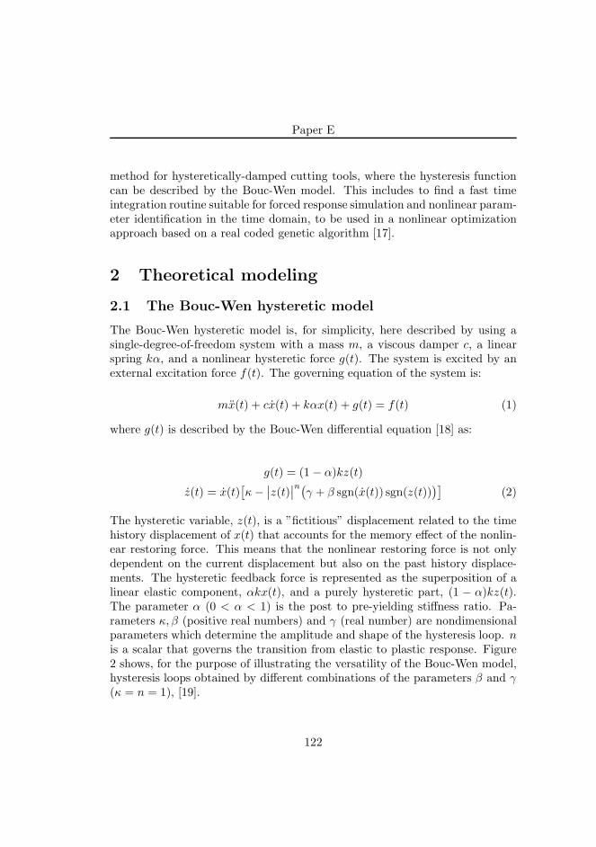
Paper E

method for hysteretically-damped cutting tools, where the hysteresis functioncan be described by the Bouc-Wen model. This includes to find a fast timeintegration routine suitable for forced response simulation and nonlinear param-eter identification in the time domain, to be used in a nonlinear optimizationapproach based on a real coded genetic algorithm [17].

2 Theoretical modeling

2.1 The Bouc-Wen hysteretic model

The Bouc-Wen hysteretic model is, for simplicity, here described by using asingle-degree-of-freedom system with a mass m, a viscous damper c, a linearspring kα, and a nonlinear hysteretic force g(t). The system is excited by anexternal excitation force f(t). The governing equation of the system is:

mx(t) + cx(t) + kαx(t) + g(t) = f(t) (1)

where g(t) is described by the Bouc-Wen differential equation [18] as:

g(t) = (1 − α)kz(t)

z(t) = x(t)[

κ−∣

∣z(t)∣

∣

n(

γ + β sgn(x(t)) sgn(z(t)))]

(2)

The hysteretic variable, z(t), is a ”fictitious” displacement related to the timehistory displacement of x(t) that accounts for the memory effect of the nonlin-ear restoring force. This means that the nonlinear restoring force is not onlydependent on the current displacement but also on the past history displace-ments. The hysteretic feedback force is represented as the superposition of alinear elastic component, αkx(t), and a purely hysteretic part, (1 − α)kz(t).The parameter α (0 < α < 1) is the post to pre-yielding stiffness ratio. Pa-rameters κ, β (positive real numbers) and γ (real number) are nondimensionalparameters which determine the amplitude and shape of the hysteresis loop. nis a scalar that governs the transition from elastic to plastic response. Figure2 shows, for the purpose of illustrating the versatility of the Bouc-Wen model,hysteresis loops obtained by different combinations of the parameters β and γ

(κ = n = 1), [19].

122

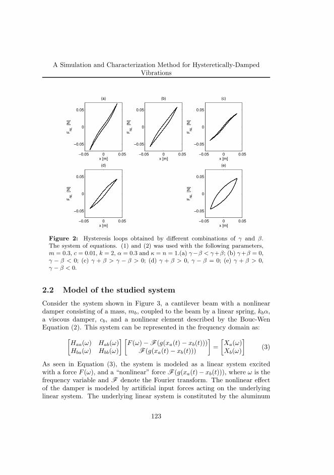
A Simulation and Characterization Method for Hysteretically-DampedVibrations

−0.05 0 0.05

−0.05

0

0.05

(a)

x [m]

FN

L

[N]

−0.05 0 0.05

−0.05

0

0.05

(b)

x [m]

FN

L

[N]

−0.05 0 0.05

−0.05

0

0.05

(c)

x [m]

FN

L

[N]

−0.05 0 0.05

−0.05

0

0.05

(d)

x [m]

FN

L

[N]

−0.05 0 0.05

−0.05

0

0.05

(e)

x [m]

FN

L

[N]

Figure 2: Hysteresis loops obtained by different combinations of γ and β.The system of equations. (1) and (2) was used with the following parameters,m = 0.3, c = 0.01, k = 2, α = 0.3 and κ = n = 1.(a) γ−β < γ+β; (b) γ+β = 0,γ − β < 0; (c) γ + β > γ − β > 0; (d) γ + β > 0, γ − β = 0; (e) γ + β > 0,γ − β < 0.

2.2 Model of the studied system

Consider the system shown in Figure 3, a cantilever beam with a nonlineardamper consisting of a mass, mb, coupled to the beam by a linear spring, kbα,a viscous damper, cb, and a nonlinear element described by the Bouc-WenEquation (2). This system can be represented in the frequency domain as:

[

Haa(ω) Hab(ω)Hba(ω) Hbb(ω)

] [

F (ω)− F (g(xa(t)− xb(t)))F (g(xa(t)− xb(t)))

]

=

[

Xa(ω)Xb(ω)

]

(3)

As seen in Equation (3), the system is modeled as a linear system excitedwith a force F (ω), and a “nonlinear” force F (g(xa(t)− xb(t))), where ω is thefrequency variable and F denote the Fourier transform. The nonlinear effectof the damper is modeled by artificial input forces acting on the underlyinglinear system. The underlying linear system is constituted by the aluminum

123

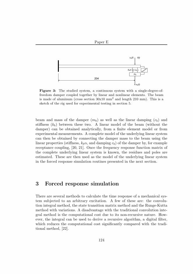
Paper E

f(t)

mb

xa(t)

xb(t)

kbα cb

204

Figure 3: The studied system, a continuous system with a single-degree-of-freedom damper coupled together by linear and nonlinear elements. The beamis made of aluminum (cross section 30x10 mm2 and length 210 mm). This is asketch of the rig used for experimental testing in section 5.

beam and mass of the damper (mb) as well as the linear damping (cb) andstiffness (kb) between these two. A linear model of the beam (without thedamper) can be obtained analytically, from a finite element model or fromexperimental measurements. A complete model of the underlying linear systemcan then be obtained by connecting the damper mass to the beam using thelinear properties (stiffness, kbα, and damping cb) of the damper by, for examplereceptance coupling, [20, 21]. Once the frequency response function matrix ofthe complete underlying linear system is known, the residues and poles areestimated. These are then used as the model of the underlying linear systemin the forced response simulation routines presented in the next section.

3 Forced response simulation

There are several methods to calculate the time response of a mechanical sys-tem subjected to an arbitrary excitation. A few of these are: the convolu-tion integral method, the state transition matrix method and the Runge-Kuttamethod with variations. A disadvantage with the traditional convolution inte-gral method is the computational cost due to its non-recursive nature. How-ever, the integral can be used to derive a recursive algorithm, a digital filter,which reduces the computational cost significantly compared with the tradi-tional method, [22].

124

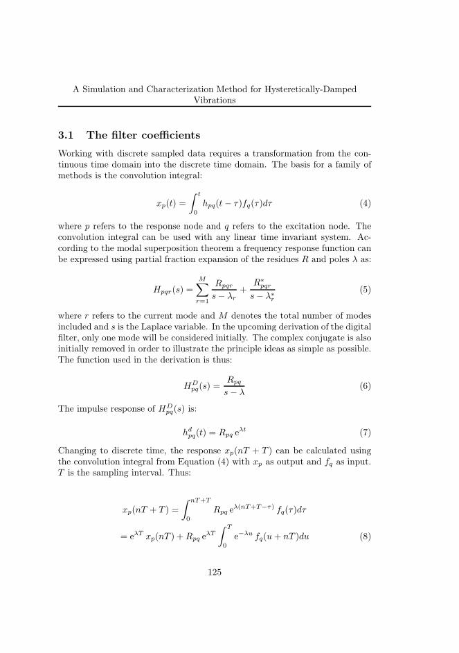
A Simulation and Characterization Method for Hysteretically-DampedVibrations

3.1 The filter coefficients

Working with discrete sampled data requires a transformation from the con-tinuous time domain into the discrete time domain. The basis for a family ofmethods is the convolution integral:

xp(t) =

∫ t

0

hpq(t− τ)fq(τ)dτ (4)

where p refers to the response node and q refers to the excitation node. Theconvolution integral can be used with any linear time invariant system. Ac-cording to the modal superposition theorem a frequency response function canbe expressed using partial fraction expansion of the residues R and poles λ as:

Hpqr(s) =M∑

r=1

Rpqr

s− λr

+R∗

pqr

s− λ∗

r

(5)

where r refers to the current mode and M denotes the total number of modesincluded and s is the Laplace variable. In the upcoming derivation of the digitalfilter, only one mode will be considered initially. The complex conjugate is alsoinitially removed in order to illustrate the principle ideas as simple as possible.The function used in the derivation is thus:

HDpq(s) =

Rpq

s− λ(6)

The impulse response of HDpq(s) is:

hdpq(t) = Rpq e

λt (7)

Changing to discrete time, the response xp(nT + T ) can be calculated usingthe convolution integral from Equation (4) with xp as output and fq as input.T is the sampling interval. Thus:

xp(nT + T ) =

∫ nT+T

0

Rpq eλ(nT+T−τ) fq(τ)dτ

= eλT xp(nT ) +Rpq eλT

∫ T

0

e−λu fq(u + nT )du (8)

125

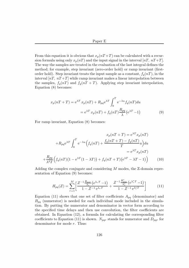
Paper E

From this equation it is obvious that xp(nT+T ) can be calculated with a recur-sion formula using only xp(nT ) and the input signal in the interval [nT, nT+T ].The way the samples are treated in the evaluation of the last integral defines themethod; for example, step invariant (zero-order hold) or ramp invariant (first-order hold). Step invariant treats the input sample as a constant, fq(nT ), in theinterval [nT, nT+T ] while ramp invariant makes a linear interpolation betweenthe samples, fq(nT ) and fq(nT + T ). Applying step invariant interpolation,Equation (8) becomes:

xp(nT + T ) = eλT xp(nT ) +RpqeλT

∫ T

0

e−λufq(nT )du

= eλT xp(nT ) + fq(nT )Rpq

λ

(

eλT −1)

(9)

For ramp invariant, Equation (8) becomes:

xp(nT + T ) = eλTxp(nT )

+RpqeλT

∫ T

0

e−λu(

fq(nT ) +fq(nT + T )− fq(nT )

Tu)

du

= eλTxp(nT )

+Rpq

λ2T

(

fq(nT )(

1− eλT (1− λT ))

+ fq(nT + T )(

eλT − λT − 1)

)

(10)

Adding the complex conjugate and considering M modes, the Z-domain repre-sentation of Equation (9) becomes:

Hpq(Z) =

M∑

r=1

[

Z−1Rpqr

λr

(

eλrT −1)

1− Z−1 eλrT+

Z−1R∗

pqr

λ∗

r

(

eλ∗

rT −1)

1− Z−1 eλ∗

rT

]

(11)

Equation (11) shows that one set of filter coefficients Apq (denominator) andBpq (numerator) is needed for each individual mode included in the simula-tion. By putting the numerator and denominator in vector form according tothe specified time delays and then use convolution, the filter coefficients areobtained. In Equation (12), a formula for calculating the corresponding filtercoefficients to Equation (11) is shown. Npqr stands for numerator and Dpqr fordenominator for mode r. Thus:

126

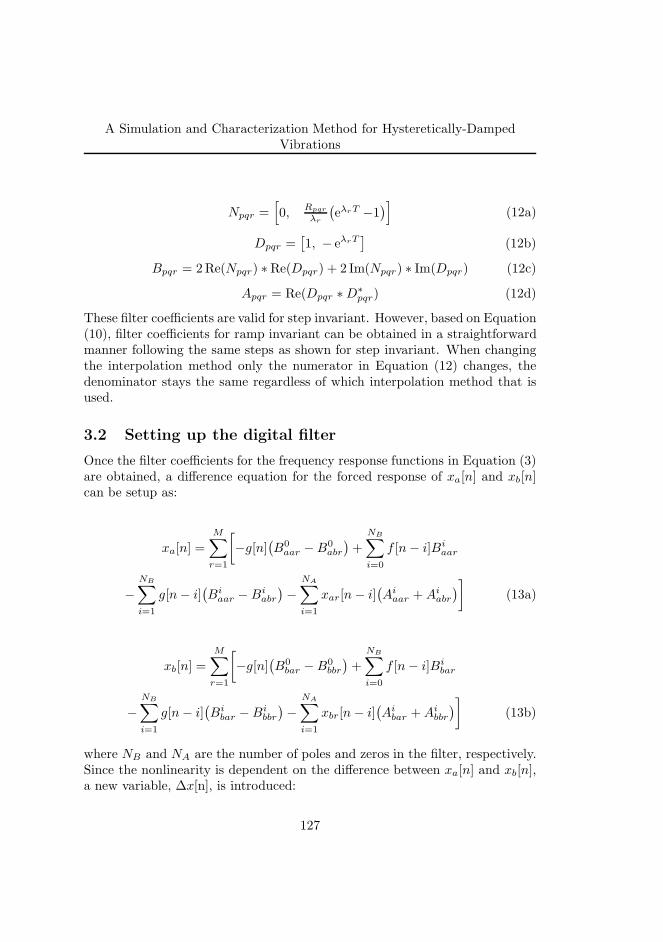
A Simulation and Characterization Method for Hysteretically-DampedVibrations

Npqr =[

0,Rpqr

λr

(

eλrT −1)

]

(12a)

Dpqr =[

1, − eλrT]

(12b)

Bpqr = 2Re(Npqr) ∗Re(Dpqr) + 2 Im(Npqr) ∗ Im(Dpqr) (12c)

Apqr = Re(Dpqr ∗D∗

pqr) (12d)

These filter coefficients are valid for step invariant. However, based on Equation(10), filter coefficients for ramp invariant can be obtained in a straightforwardmanner following the same steps as shown for step invariant. When changingthe interpolation method only the numerator in Equation (12) changes, thedenominator stays the same regardless of which interpolation method that isused.

3.2 Setting up the digital filter

Once the filter coefficients for the frequency response functions in Equation (3)are obtained, a difference equation for the forced response of xa[n] and xb[n]can be setup as:

xa[n] =

M∑

r=1

[

−g[n](

B0aar −B0

abr

)

+

NB∑

i=0

f [n− i]Biaar

−

NB∑

i=1

g[n− i](

Biaar −Bi

abr

)

−

NA∑

i=1

xar[n− i](

Aiaar +Ai

abr

)

]

(13a)

xb[n] =

M∑

r=1

[

−g[n](

B0bar −B0

bbr

)

+

NB∑

i=0

f [n− i]Bibar

−

NB∑

i=1

g[n− i](

Bibar −Bi

bbr

)

−

NA∑

i=1

xbr[n− i](

Aibar +Ai

bbr

)

]

(13b)

where NB and NA are the number of poles and zeros in the filter, respectively.Since the nonlinearity is dependent on the difference between xa[n] and xb[n],a new variable, ∆x[n], is introduced:

127

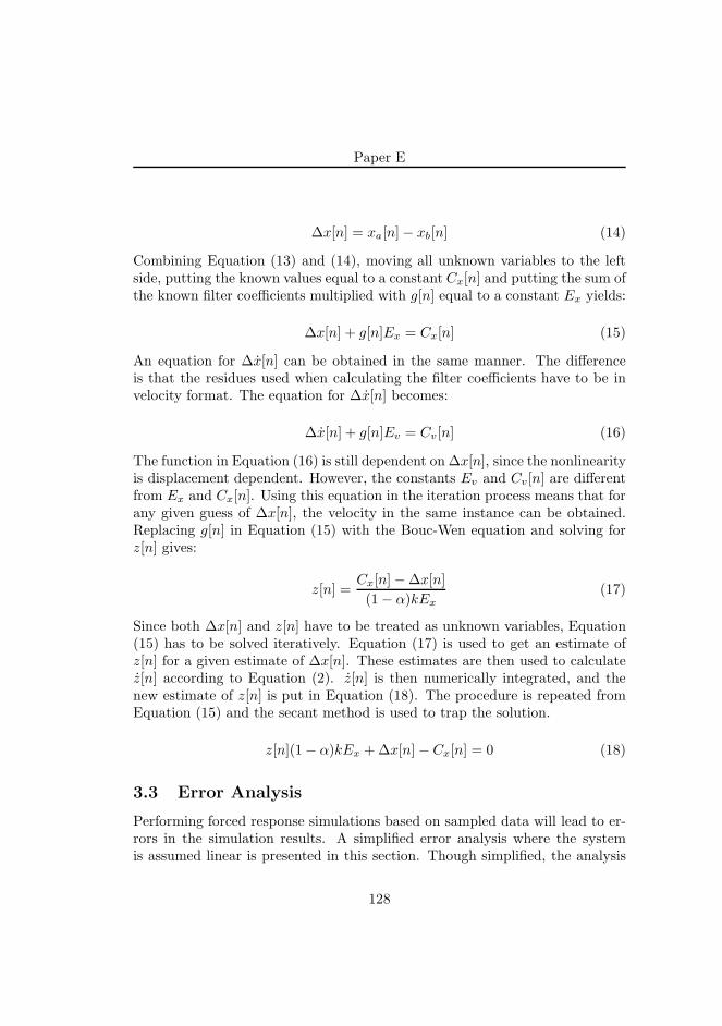
Paper E

∆x[n] = xa[n]− xb[n] (14)

Combining Equation (13) and (14), moving all unknown variables to the leftside, putting the known values equal to a constant Cx[n] and putting the sum ofthe known filter coefficients multiplied with g[n] equal to a constant Ex yields:

∆x[n] + g[n]Ex = Cx[n] (15)

An equation for ∆x[n] can be obtained in the same manner. The differenceis that the residues used when calculating the filter coefficients have to be invelocity format. The equation for ∆x[n] becomes:

∆x[n] + g[n]Ev = Cv[n] (16)

The function in Equation (16) is still dependent on ∆x[n], since the nonlinearityis displacement dependent. However, the constants Ev and Cv[n] are differentfrom Ex and Cx[n]. Using this equation in the iteration process means that forany given guess of ∆x[n], the velocity in the same instance can be obtained.Replacing g[n] in Equation (15) with the Bouc-Wen equation and solving forz[n] gives:

z[n] =Cx[n]−∆x[n]

(1− α)kEx

(17)

Since both ∆x[n] and z[n] have to be treated as unknown variables, Equation(15) has to be solved iteratively. Equation (17) is used to get an estimate ofz[n] for a given estimate of ∆x[n]. These estimates are then used to calculatez[n] according to Equation (2). z[n] is then numerically integrated, and thenew estimate of z[n] is put in Equation (18). The procedure is repeated fromEquation (15) and the secant method is used to trap the solution.

z[n](1− α)kEx +∆x[n] − Cx[n] = 0 (18)

3.3 Error Analysis

Performing forced response simulations based on sampled data will lead to er-rors in the simulation results. A simplified error analysis where the systemis assumed linear is presented in this section. Though simplified, the analysis

128

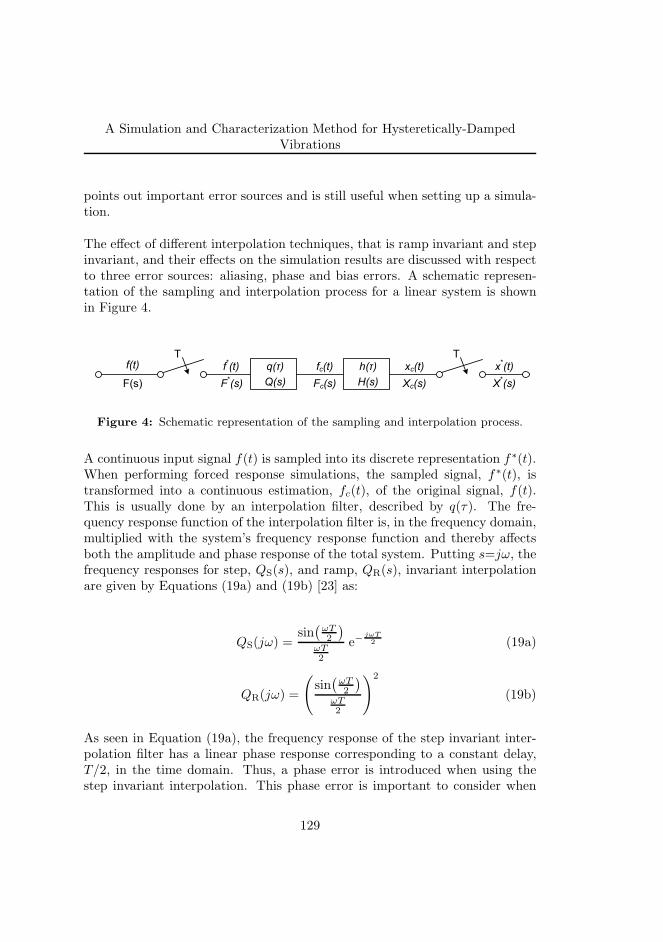
A Simulation and Characterization Method for Hysteretically-DampedVibrations

points out important error sources and is still useful when setting up a simula-tion.

The effect of different interpolation techniques, that is ramp invariant and stepinvariant, and their effects on the simulation results are discussed with respectto three error sources: aliasing, phase and bias errors. A schematic represen-tation of the sampling and interpolation process for a linear system is shownin Figure 4.

T

F(s)

f(t) f*(t)

F*(s)

q(τ)

Q(s)

fc(t)

Fc(s)

h(τ)

H(s)

xc(t)

Xc(s)

Tx*(t)

X*(s)

Figure 4: Schematic representation of the sampling and interpolation process.

A continuous input signal f(t) is sampled into its discrete representation f∗(t).When performing forced response simulations, the sampled signal, f∗(t), istransformed into a continuous estimation, fc(t), of the original signal, f(t).This is usually done by an interpolation filter, described by q(τ). The fre-quency response function of the interpolation filter is, in the frequency domain,multiplied with the system’s frequency response function and thereby affectsboth the amplitude and phase response of the total system. Putting s=jω, thefrequency responses for step, QS(s), and ramp, QR(s), invariant interpolationare given by Equations (19a) and (19b) [23] as:

QS(jω) =sin(

ωT2

)

ωT2

e−jωT2 (19a)

QR(jω) =

(

sin(

ωT2

)

ωT2

)2

(19b)

As seen in Equation (19a), the frequency response of the step invariant inter-polation filter has a linear phase response corresponding to a constant delay,T/2, in the time domain. Thus, a phase error is introduced when using thestep invariant interpolation. This phase error is important to consider when

129

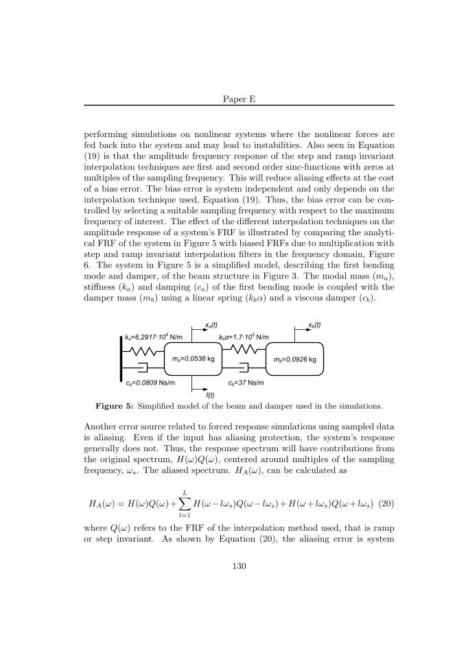
Paper E

performing simulations on nonlinear systems where the nonlinear forces arefed back into the system and may lead to instabilities. Also seen in Equation(19) is that the amplitude frequency response of the step and ramp invariantinterpolation techniques are first and second order sinc-functions with zeros atmultiples of the sampling frequency. This will reduce aliasing effects at the costof a bias error. The bias error is system independent and only depends on theinterpolation technique used, Equation (19). Thus, the bias error can be con-trolled by selecting a suitable sampling frequency with respect to the maximumfrequency of interest. The effect of the different interpolation techniques on theamplitude response of a system’s FRF is illustrated by comparing the analyti-cal FRF of the system in Figure 5 with biased FRFs due to multiplication withstep and ramp invariant interpolation filters in the frequency domain, Figure6. The system in Figure 5 is a simplified model, describing the first bendingmode and damper, of the beam structure in Figure 3. The modal mass (ma),stiffness (ka) and damping (ca) of the first bending mode is coupled with thedamper mass (mb) using a linear spring (kbα) and a viscous damper (cb).

ma=0,0536 kg mb=0,0926 kg

ka=6,2917·104N/m

ca=0.0809 Ns/m

kbα=1,7·105N/m

cb=37 Ns/m

xa(t) xb(t)

f(t)

Figure 5: Simplified model of the beam and damper used in the simulations.

Another error source related to forced response simulations using sampled datais aliasing. Even if the input has aliasing protection, the system’s responsegenerally does not. Thus, the response spectrum will have contributions fromthe original spectrum, H(ω)Q(ω), centered around multiples of the samplingfrequency, ωs. The aliased spectrum. HA(ω), can be calculated as

HA(ω) = H(ω)Q(ω)+

L∑

l=1

H(ω− lωs)Q(ω− lωs)+H(ω+ lωs)Q(ω+ lωs) (20)

where Q(ω) refers to the FRF of the interpolation method used, that is rampor step invariant. As shown by Equation (20), the aliasing error is system

130

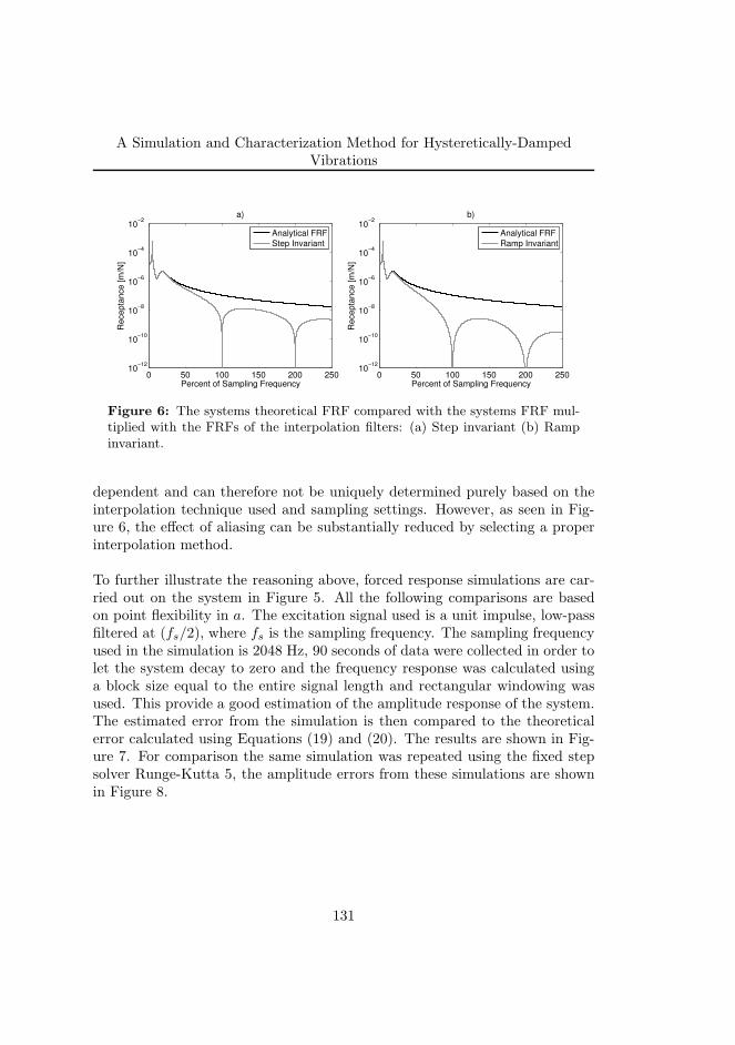
A Simulation and Characterization Method for Hysteretically-DampedVibrations

0 50 100 150 200 25010

−12

10−10

10−8

10−6

10−4

10−2

Percent of Sampling Frequency

Re

ce

pta

nce

[m

/N]

a)

Analytical FRF

Step Invariant

0 50 100 150 200 25010

−12

10−10

10−8

10−6

10−4

10−2

Percent of Sampling Frequency

Re

ce

pta

nce

[m

/N]

b)

Analytical FRF

Ramp Invariant

Figure 6: The systems theoretical FRF compared with the systems FRF mul-tiplied with the FRFs of the interpolation filters: (a) Step invariant (b) Rampinvariant.

dependent and can therefore not be uniquely determined purely based on theinterpolation technique used and sampling settings. However, as seen in Fig-ure 6, the effect of aliasing can be substantially reduced by selecting a properinterpolation method.

To further illustrate the reasoning above, forced response simulations are car-ried out on the system in Figure 5. All the following comparisons are basedon point flexibility in a. The excitation signal used is a unit impulse, low-passfiltered at (fs/2), where fs is the sampling frequency. The sampling frequencyused in the simulation is 2048 Hz, 90 seconds of data were collected in order tolet the system decay to zero and the frequency response was calculated usinga block size equal to the entire signal length and rectangular windowing wasused. This provide a good estimation of the amplitude response of the system.The estimated error from the simulation is then compared to the theoreticalerror calculated using Equations (19) and (20). The results are shown in Fig-ure 7. For comparison the same simulation was repeated using the fixed stepsolver Runge-Kutta 5, the amplitude errors from these simulations are shownin Figure 8.

131

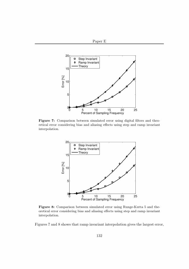
Paper E

0 5 10 15 20 250

5

10

15

20

Percent of Sampling Frequency

Err

or

[%]

Step Invariant

Ramp Invariant

Theory

Figure 7: Comparison between simulated error using digital filters and theo-retical error considering bias and aliasing effects using step and ramp invariantinterpolation.

0 5 10 15 20 250

5

10

15

20

Percent of Sampling Frequency

Err

or

[%]

Step Invariant

Ramp Invariant

Theory

Figure 8: Comparison between simulated error using Runge-Kutta 5 and the-oretical error considering bias and aliasing effects using step and ramp invariantinterpolation.

Figures 7 and 8 shows that ramp invariant interpolation gives the largest error,

132

A Simulation and Characterization Method for Hysteretically-DampedVibrations

dominated by the bias error. Since the bias error is system independent, Equa-tion (19), it can be controlled, without any prior knowledge about the system,by selecting a suitable sampling frequency. The advantages with ramp invariantcompared to step invariant interpolation are that the system dependent alias-ing errors are substantially reduced using ramp invariant interpolation and thatstep invariant interpolation introduces a phase error which might cause stabil-ity issues when performing simulations on nonlinear systems. Also seen in thesimulations is that the amplitude errors using digital filters and Runge-Kutta5 are comparable.

The error analysis presented in this section show that the dominant errors con-cerning forced response simulation using sampled data are bias and aliasingerrors. These errors can be avoided by selecting an appropriate interpolationtechnique and sampling frequency. The simulations were performed on a lin-ear system in order to be able to compute the exact amplitude response, theanalytical FRF, in order to make relevant comparisons between simulated andtheoretically predicted errors. The error analysis points out the importance ofselecting an appropriate interpolation technique and sampling frequency whenusing discrete input data.

4 Parameter Estimation

The optimization approach adopted for the identification of the Bouc-Wen pa-rameters in this paper is a real coded genetic algorithm [19, 24], this methodis selected due to its robustness and ability to avoid getting trapped in localminima points, which increases the possibility of finding the best parameter set.

4.1 Parameter constraints

Ikhouane et al. [25] showed that the input-output behavior of the Bouc-Wenmodel is not described by a unique set of parameters, [k, α, κ, β, γ, n]. Dueto this, parameter identification methods relying on input-output data cannotuniquely determine the parameters of the Bouc-Wen model. To deal with this,some authors have compared the shape of the hysteresis loops instead of com-paring the values of the identified parameters with their reference values, forexample [7, 19]. Other authors usually fixes some of the parameters to arbi-

133

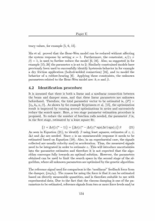
Paper E

trary values, for example [5, 6, 15].

Ma et al. proved that the Bouc-Wen model can be reduced without affectingthe system response by setting κ = 1. Furthermore, the constraint, κ/(γ +β) = 1, is used to further reduce the model [6, 16]. Also, as suggested in forexample [15, 26] the parameter n is set to 2. Similarly constrained models havepreviously been used to successfully identify hysteresis behavior in for examplea dry friction application (bolted-welded connection) [16], and to model thebehavior of a rubber-bearing [6]. Applying these constraints, the unknownparameters related to the Bouc-Wen model are: k, α and β.

4.2 Identification procedure

It is assumed that there is both a linear and a nonlinear connection betweenthe beam and damper mass, and that these linear parameters are unknownbeforehand. Therefore, the total parameter vector to be estimated is, {P} ={cb, kb, α, β}. As shown by for example Kyprianou et al. [15], the optimizationresult is improved by running several optimizations in series and successivelyreduce the search space. Here, a two stage parameter estimation procedure isproposed. To reduce the number of function calls needed, the parameter β is,in the first stage, estimated by a least square fit:

{

z +∆x(|z|n − 1)}

={

∆x|z|n −∆x|z|n sgn(∆x) sgn(z)}

β (21)

As seen in Equation (21), to identify β using least squares, estimates of z, z,∆x and ∆x are needed. Since z is an unmeasurable response it needs to beestimated based on Equation (18). Also, in an experimental case, the signalscollected are usually velocity and/or acceleration. Thus, the measured signalsneed to be integrated in order to estimate z. This will introduce uncertaintiesinto the parameter estimates and therefore it is not expected that the algo-rithm converges fully towards an optimal solution. However, the parametersobtained can be used to limit the search space in the second stage of the al-gorithm, where all unknown parameters are optimized by the genetic algorithm.

The reference signal used for comparison is the “nonlinear” feedback force fromthe damper, {mbxb}. The reason for using the force is that it can be estimatedbased on directly measurable quantities, and is therefore suitable to use withexperimental data. Due to the fact that the viscous damping is one of the pa-rameters to be estimated, reference signals from two or more force levels and/or

134

A Simulation and Characterization Method for Hysteretically-DampedVibrations

frequencies are needed in order to capture any velocity dependency present inthe reference signal.

The problem is formulated as a minimization problem and the normalized meansquare error (NMSE) between the reference, {mbxb}, and simulated, {mb

ˆxb},nonlinear feedback forces is calculated and used as the cost function, C({P})as:

C({P}) =100

Mσ2mbxb

M∑

l=1

(mbxb[l]−mbˆxb[l])

2 (22)

where σ2mbxb

is the variance of the measured “nonlinear” feedback force. Whenmultiple reference signals are used, the NMSE is calculated for each signal andthe average value, C({P}), used as error estimate. A schematic flow diagramof the optimization procedure is shown in Figure 9.

135

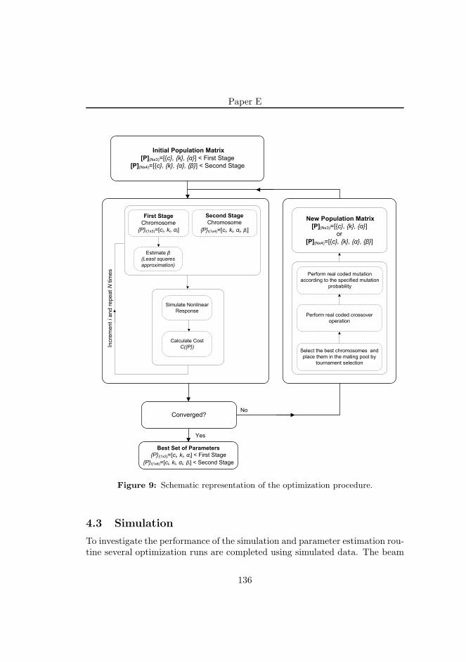
Paper E

No

Select the best chromosomes and

place them in the mating pool by

tournament selection

Perform real coded crossover

operation

Perform real coded mutation

according to the specified mutation

probability

New Population Matrix

[P](Nx3)=[{c}, {k}, {α}]

or

[P](Nx4)=[{c}, {k}, {α}, {β}]

Initial Population Matrix

[P](Nx3)=[{c}, {k}, {α}] < First Stage

[P](Nx4)=[{c}, {k}, {α}, {β}] < Second Stage

Incre

men

t ia

nd r

epe

at

Ntim

es

Simulate Nonlinear

Response

Calculate Cost

C({P})

Estimate β

(Least squares

approximation)

First Stage

Chromosome

{P}i(1x3)=[ci, ki, αi]

Second Stage

Chromosome

{P}i(1x4)=[ci, ki, αi, βi]

Best Set of Parameters

{P}i(1x3)=[ci, ki, αi] < First Stage

{P}i(1x4)=[ci, ki, αi, βi] < Second Stage

Yes

Converged?

Figure 9: Schematic representation of the optimization procedure.

4.3 Simulation

To investigate the performance of the simulation and parameter estimation rou-tine several optimization runs are completed using simulated data. The beam

136

A Simulation and Characterization Method for Hysteretically-DampedVibrations

structure in Figure 3 is used as basis in the simulations, and both the lin-ear and nonlinear parameters connecting the beam and damper are estimated.The simplified model shown in Figure 10 is used in the simulations. This modeldescribes the first bending mode of the beam and the damper mode.

ma=0,0536 kg mb=0,0926 kg

ka=6,2917·104N/m

ca=0.0809 Ns/m

xa(t) xb(t)

f(t)

cb

kbα

Figure 10: The nonlinear system used in the simulations.

Harmonic excitation is used and reference signals are simulated using threedifferent forces:

• f1(t) = 26 sin(2π80t) N

• f2(t) = 8 sin(2π90t) N

• f3(t) = 3 sin(2π100t) N

The system is excited in point a, and the nonlinearity is connected betweenpoint a and b. The feedback force from the damper mass is extracted and usedas reference signal, Equation (22).

The simulations are carried out in a noise free environment as well as withcontaminating noise on the output channels (the feedback force of the dampermass). The noise added to the reference signals is scaled by the standard de-viation of the output, for example a noise level of 0.1 means 10 percent ofthe standard deviation. Based on the error simulations presented in section3.3, ramp invariant interpolation is used to avoid phase errors. The samplingfrequency is set to 8192 Hz in order to capture the first orders of superhar-monics present in the response. In each iteration, three forced responses of 0.8

137

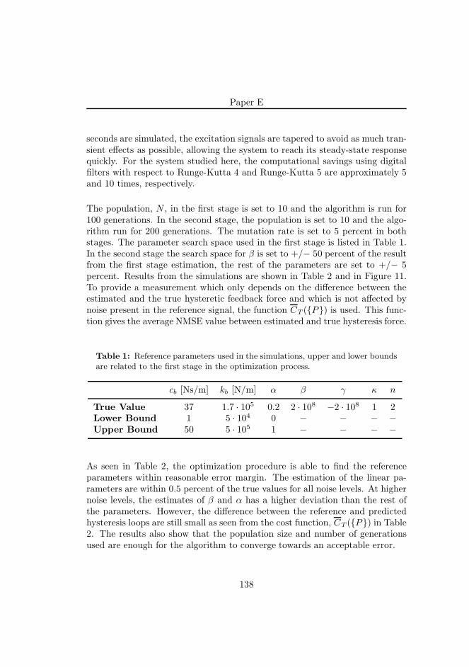
Paper E

seconds are simulated, the excitation signals are tapered to avoid as much tran-sient effects as possible, allowing the system to reach its steady-state responsequickly. For the system studied here, the computational savings using digitalfilters with respect to Runge-Kutta 4 and Runge-Kutta 5 are approximately 5and 10 times, respectively.

The population, N , in the first stage is set to 10 and the algorithm is run for100 generations. In the second stage, the population is set to 10 and the algo-rithm run for 200 generations. The mutation rate is set to 5 percent in bothstages. The parameter search space used in the first stage is listed in Table 1.In the second stage the search space for β is set to +/− 50 percent of the resultfrom the first stage estimation, the rest of the parameters are set to +/− 5percent. Results from the simulations are shown in Table 2 and in Figure 11.To provide a measurement which only depends on the difference between theestimated and the true hysteretic feedback force and which is not affected bynoise present in the reference signal, the function CT ({P}) is used. This func-tion gives the average NMSE value between estimated and true hysteresis force.

Table 1: Reference parameters used in the simulations, upper and lower boundsare related to the first stage in the optimization process.

cb [Ns/m] kb [N/m] α β γ κ n

True Value 37 1.7 · 105 0.2 2 · 108 −2 · 108 1 2Lower Bound 1 5 · 104 0 − − − −Upper Bound 50 5 · 105 1 − − − −

As seen in Table 2, the optimization procedure is able to find the referenceparameters within reasonable error margin. The estimation of the linear pa-rameters are within 0.5 percent of the true values for all noise levels. At highernoise levels, the estimates of β and α has a higher deviation than the rest ofthe parameters. However, the difference between the reference and predictedhysteresis loops are still small as seen from the cost function, CT ({P}) in Table2. The results also show that the population size and number of generationsused are enough for the algorithm to converge towards an acceptable error.

138

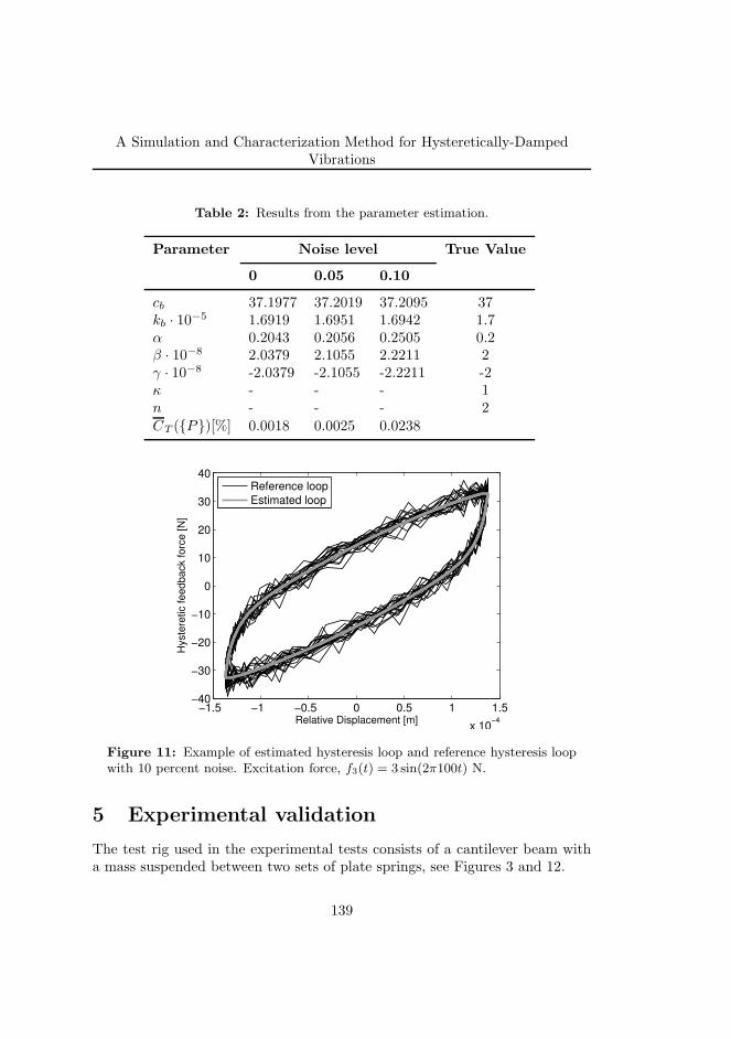
A Simulation and Characterization Method for Hysteretically-DampedVibrations

Table 2: Results from the parameter estimation.

Parameter Noise level True Value

0 0.05 0.10

cb 37.1977 37.2019 37.2095 37kb · 10

−5 1.6919 1.6951 1.6942 1.7α 0.2043 0.2056 0.2505 0.2β · 10−8 2.0379 2.1055 2.2211 2γ · 10−8 -2.0379 -2.1055 -2.2211 -2κ - - - 1n - - - 2CT ({P})[%] 0.0018 0.0025 0.0238

−1.5 −1 −0.5 0 0.5 1 1.5

x 10−4

−40

−30

−20

−10

0

10

20

30

40

Hyste

retic f

ee

db

ack f

orc

e [

N]

Relative Displacement [m]

Reference loop

Estimated loop

Figure 11: Example of estimated hysteresis loop and reference hysteresis loopwith 10 percent noise. Excitation force, f3(t) = 3 sin(2π100t) N.

5 Experimental validation

The test rig used in the experimental tests consists of a cantilever beam witha mass suspended between two sets of plate springs, see Figures 3 and 12.

139

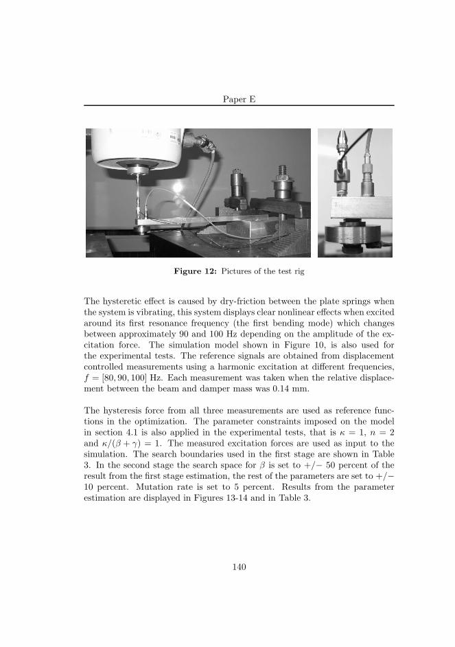
Paper E

Figure 12: Pictures of the test rig

The hysteretic effect is caused by dry-friction between the plate springs whenthe system is vibrating, this system displays clear nonlinear effects when excitedaround its first resonance frequency (the first bending mode) which changesbetween approximately 90 and 100 Hz depending on the amplitude of the ex-citation force. The simulation model shown in Figure 10, is also used forthe experimental tests. The reference signals are obtained from displacementcontrolled measurements using a harmonic excitation at different frequencies,f = [80, 90, 100] Hz. Each measurement was taken when the relative displace-ment between the beam and damper mass was 0.14 mm.

The hysteresis force from all three measurements are used as reference func-tions in the optimization. The parameter constraints imposed on the modelin section 4.1 is also applied in the experimental tests, that is κ = 1, n = 2and κ/(β + γ) = 1. The measured excitation forces are used as input to thesimulation. The search boundaries used in the first stage are shown in Table3. In the second stage the search space for β is set to +/− 50 percent of theresult from the first stage estimation, the rest of the parameters are set to +/−10 percent. Mutation rate is set to 5 percent. Results from the parameterestimation are displayed in Figures 13-14 and in Table 3.

140

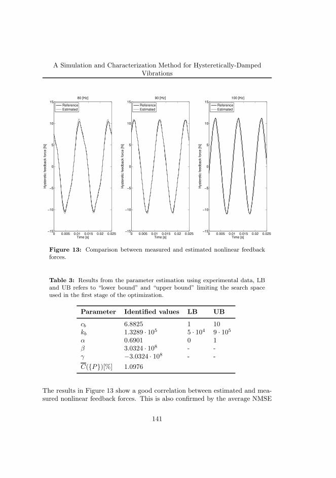
A Simulation and Characterization Method for Hysteretically-DampedVibrations

0 0.005 0.01 0.015 0.02 0.025−15

−10

−5

0

5

10

1580 [Hz]

Hyste

retic feedback forc

e [N

]

Time [s]

Reference

Estimated

0 0.005 0.01 0.015 0.02 0.025−15

−10

−5

0

5

10

1590 [Hz]

Hyste

retic feedback forc

e [N

]

Time [s]

Reference

Estimated

0 0.005 0.01 0.015 0.02 0.025−15

−10

−5

0

5

10

15100 [Hz]

Hyste

retic feedback forc

e [N

]

Time [s]

Reference

Estimated

Figure 13: Comparison between measured and estimated nonlinear feedbackforces.

Table 3: Results from the parameter estimation using experimental data, LBand UB refers to “lower bound” and “upper bound” limiting the search spaceused in the first stage of the optimization.

Parameter Identified values LB UB

cb 6.8825 1 10kb 1.3289 · 105 5 · 104 9 · 105

α 0.6901 0 1β 3.0324 · 108 - -γ −3.0324 · 108 - -

C({P})[%] 1.0976

The results in Figure 13 show a good correlation between estimated and mea-sured nonlinear feedback forces. This is also confirmed by the average NMSE

141

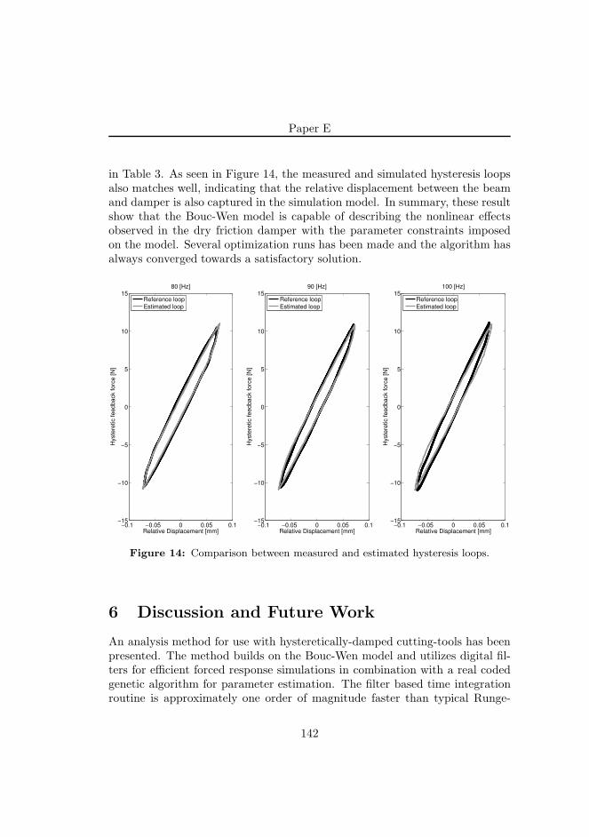
Paper E

in Table 3. As seen in Figure 14, the measured and simulated hysteresis loopsalso matches well, indicating that the relative displacement between the beamand damper is also captured in the simulation model. In summary, these resultshow that the Bouc-Wen model is capable of describing the nonlinear effectsobserved in the dry friction damper with the parameter constraints imposedon the model. Several optimization runs has been made and the algorithm hasalways converged towards a satisfactory solution.

−0.1 −0.05 0 0.05 0.1−15

−10

−5

0

5

10

15

Hyste

retic f

ee

db

ack f

orc

e [

N]

Relative Displacement [mm]

80 [Hz]

Reference loop

Estimated loop

−0.1 −0.05 0 0.05 0.1−15

−10

−5

0

5

10

15

Hyste

retic f

ee

db

ack f

orc

e [

N]

Relative Displacement [mm]

90 [Hz]

Reference loop

Estimated loop

−0.1 −0.05 0 0.05 0.1−15

−10

−5

0

5

10

15

Hyste

retic f

ee

db

ack f

orc

e [

N]

Relative Displacement [mm]

100 [Hz]

Reference loop

Estimated loop

Figure 14: Comparison between measured and estimated hysteresis loops.

6 Discussion and Future Work

An analysis method for use with hysteretically-damped cutting-tools has beenpresented. The method builds on the Bouc-Wen model and utilizes digital fil-ters for efficient forced response simulations in combination with a real codedgenetic algorithm for parameter estimation. The filter based time integrationroutine is approximately one order of magnitude faster than typical Runge-

142

A Simulation and Characterization Method for Hysteretically-DampedVibrations

Kutta routines for the applications studied in this paper.

A two stage parameter estimation approach, combining least squares estimateswith nonlinear optimization using a real coded genetic algorithm, is suggestedto obtain both the linear and nonlinear parameters connecting the studiedstructure and damper. This approach reduces the number of function callsneeded, and allows the search space for all parameters to be narrowed downbefore the second stage estimation. The methods was applied on both simu-lated and experimental data and the results show that the suggested parameterestimation routine is robust even with reference data contaminated by noise.The algorithm also found accurate estimates of the linear parameters, which isespecially important for the model to be valid over a wide range of excitationfrequencies and amplitudes. The experimental results confirms the possibilityto use the Bouc-Wen model to describe the dry-friction hysteresis present inthe test-rig.

Future investigations include experimental testing and parameter identificationon rubber and silicone type materials. The presented method will be modifiedto handle nonlinear systems with a ground-hook nonlinearity to facilitate thestudy of alternative hysteresis effects, for example tool clamping effects. Also,a way to estimate the simulation errors for forced response simulation on non-linear systems using sampled input data is of interest in future research.

References

[1] Yusuf Altintas. Manufacturing Automation - Metal Cutting Mechanics,

Machine Tool Vibrations, and CNC Design. Cambridge university press,2000.

[2] Kai Cheng. Machining dynamics : fundamentals, applications and prac-

tices. Springer, London, 2009.

[3] Tony L. Schmitz and Kevin S. Smith. Machining dynamics : Frequency

Response to Improved Productivity. Springer, New York, 2009.

[4] Yi-Kwei Wen. Method for random vibration of hysteretic systems. Journalof the Engineering Mechanics Division, 102(2):249 – 263, 1976.

143

Paper E

[5] Y.Q. Ni, J.M. Ko, and C.W. Wong. Identification of non-linear hystereticisolators from periodic vibration tests. Journal of Sound and Vibration,217(4):737 – 756, 1998.

[6] Yin Qiang, Zhou Li, and Wang Xinming. Parameter identification ofhysteretic model of rubber-bearing based on sequential nonlinear least-square estimation. Earthquake Engineering and Engineering Vibration,9(3):375 – 83, Sept. 2010.

[7] K. H. Hornig. Parameters characterization of the bouc/wen mechanicalhysteresis model for sandwich composite materials by using real codedgenetic algorithms. Technical report, Mechanical Engineering Department,Ross Hall, Auburn, Alabama, 2000.

[8] Mohammed Ismail, Faycal Ikhouane, and Jose Rodellar. The hysteresisbouc-wen model, a survey. Archives of Computational Methods in Engi-

neering, 16(2):161 – 188, 2009.

[9] S. L. Lau, Y. K. Cheung, and S. Y. Wu. Incremental harmonic balancemethod with multiple time scales for aperiodic vibration of nonlinear sys-tems. Journal of Applied Mechanics, Transactions ASME, 50(4a):871 –876, 1983.

[10] Hideyuki Tamura, Yoshihiro Tsuda, and Atsuo Sueoka. Higher approxima-tion of steady oscillations in nonlinear systems with single degree of free-dom - suggested multi-harmonic balance method. Bulletin of the JSME,24(195):1616 – 1625, 1981.

[11] C.W. Wong, Y.Q. Ni, and J.M. Ko. Steady-state oscillation of hystereticdifferential model. ii: Performance analysis. Journal of Engineering Me-

chanics, 120(11):2299 – 2324, 1994.

[12] A. Josefsson, M. Magnevall, and K. Ahlin. Control algorithm for sineexcitation on nonlinear systems. Proceedings of the IMAC-XXIV, 2006.

[13] M. Magnevall, A. Josefsson, and K. Ahlin. Experimental verification of acontrol algorithm for nonlinear systems. Proceedings of the IMAC-XXIV,2006.

[14] Satish Nagarajaiah, Andrei M. Reinhorn, and Michalakis C. Constantinou.Nonlinear dynamic analysis of 3-d-base-isolated structures. Journal of

Structural Engineering, 117(7):2035 – 2054, 1991.

144

A Simulation and Characterization Method for Hysteretically-DampedVibrations

[15] A. Kyprianou, K. Worden, and M. Panet. Identification of hystereticsystems using the differential evolution algorithm. Journal of Sound and

Vibration, 248(2):289 – 314, 2001.

[16] A.E. Charalampakis and V.K. Koumousis. Identification of bouc-wen hys-teretic systems by a hybrid evolutionary algorithm. Journal of Sound and

Vibration, 314(3-5):571 – 585, 2008.

[17] Randy L. Haupt and Sue Ellen Haupt. Practical Genetic Algorithms. JohnWiley & Sons, second edition, 2004.

[18] C.W. Wong, Y.Q. Ni, and S.L. Lau. Steady-state oscillation of hystereticdifferential model. i: Response analysis. Journal of Engineering Mechan-

ics, 120(11):2271 – 2298, 1994.

[19] R. H. Sues, S. T. Mau, and Y. K. Wen. Systems identification of degradinghysteretic restoring forces. Journal of Engineering Mechanics, 114(5):833– 846, 1988.

[20] Bjorn Jetmundsen, Richard L. Bielawa, and William G. Flannelly. Gener-alized frequency domain substructure synthesis. Journal of the American

Helicopter Society, 33(1):55 – 64, 1988.

[21] W. Liu and D.J. Ewins. Substructure synthesis via elastic media. part ii:Coupling analysis. In Proceedings of SPIE - The International Society for

Optical Engineering, volume 4062 (I, pages 1160 – 1166, San Antonio, TX,USA, 2000.

[22] K. Ahlin, M. Magnevall, and A. Josefsson. Simulation of forced responsein linear and nonlinear mechanical systems using digital filters. ISMA,2006.

[23] Z. Kowalczuk. Discrete approximation of continuous-time systems: a sur-vey. IEE Proceedings, Part G: Circuits, Devices and Systems, 140(4):264– 278, 1993.

[24] George Lindfield and John Penny. Numerical Methods Using MALTAB.Prentice-Hall, Inc., second edition, 2004.

[25] P. Ikhouane and J. Rodellar. On the hysteretic bouc-wen model. part i.forced limit cycle characterization. Nonlinear Dynamics, 42(1):63 – 78,2005/10/.

145

Paper E

[26] Bo-Jen Chen, C.S. Tsai, L.L. Chung, and Tsu-Cheng Chiang. Seismicbehavior of structures isolated with a hybrid system of rubber bearings.Structural Engineering and Mechanics, 22(6):761 – 783, 2006.

146

Paper F

High Frequency Measurements ofCutting Forces in Milling by

Inverse Filtering

147

Paper F is published as:

Magnevall, M., Lundblad, M., Ahlin, K., Broman, G. High Fre-quency Measurements of Cutting Forces in Milling by Inverse Filter-ing, Accepted for publication in Machining Science and Technology,November, 2011.

148

High Frequency Measurements of Cutting Forces

in Milling by Inverse Filtering

Martin Magnevall1,2

Mikael Lundblad1

Kjell Ahlin2

Goran Broman2,3

1 AB Sandvik Coromant, SE-811 81 Sandviken, Sweden2 Blekinge Institute of Technology, SE-371 79 Karlskrona, Sweden

3 Lulea University of Technology, SE-971 87 Lulea, Sweden

Abstract

Accurate estimates of cutting forces are important in the evaluation ofdifferent cutting tool geometries and concepts. However, dynamic influ-ences from the measurement system affect the result, which can makethe obtained cutting force data erroneous and misleading. This paperpresents a method to obtain an inverse filter which compensates for thedynamic influences of the measurement system. Using this approach, un-wanted dynamic effects of the measurement system can be counteracted,making it possible to retain information related to the cutting forcescontained in the high frequency region. The advantage of the proposedmethod is illustrated by comparing simulated, inverse- and low-pass fil-tered forces to unfiltered forces under different cutting conditions. Theresults show that inverse filtering increases the usable frequency range ofthe force dynamometer and thereby provide more reliable results com-pared to both low-pass and unfiltered forces.

Keywords: cutting force, dynamometer, inverse filter, deconvolution

149

Paper F

1 Introduction

Cutting forces are one of the most important quantities in the metal machiningprocess. The cutting forces govern power and torque requirements in the ma-chine tool and drive heat generation which catalyzes tool wear and determinesthe magnitude and direction of residual stresses in the machined component.Cutting forces also cause deflection of the cutting tool, machine tool and workpiece and may have a negative influence on the machined components quality.The cutting forces are therefore important parameters in evaluation of differentcutting tool geometries and concepts. However, dynamic influences from themeasurement system affect the result and make it difficult to obtain accuratecutting force data. A commonly used method to remove unwanted dynamiceffects from the measured cutting forces is low-pass filtering. Low-pass filteringremoves all information above a specified cut-off frequency and may thereforealso remove important information related to the true cutting forces containedin frequencies above the cut-off frequency. This is especially evident in millingwith transient cutting conditions when the rise times are short and the cuttingforces thereby have high frequency content. Therefore, it is difficult to get re-liable estimates of the amplitudes and rise times by low-pass filtering transientcutting forces, especially at high cutting speeds.

Accurate estimates of both rise times and force amplitudes are important, e.g.,when evaluating and comparing different tools and insert geometries. An alter-native approach, to low-pass filtering, that improves the cutting force estimates,i.e. increases the effective frequency range of the force dynamometer, is there-fore of great interest.

For example, Tlusty et al. [1] used accelerometers to compensate for the inertiaand structural damping of the dynamometer, thereby increasing the effectivefrequency range. This method has been proven to work under certain condi-tions, but encounters difficulties around resonance frequencies when the systeminertia or damping is large. The method also has problems handling systemswith more than one dominating mode, [2]. Park and Altintas [3] and Altintasand Park [4] used a Kalman filtering technique to compensate for unwanteddynamics, process and measurement noise of a spindle integrated force sensor.The same method has also been applied to cutting force measurements in mi-cro end milling, [5]. The Kalman filtering technique has been proven to workin experimental tests and is well suited when problems with measurement or

150

High Frequency Measurements of Cutting Forces in Milling by InverseFiltering

process noise is expected. Jensen et al. [2] developed a method to obtain aninvertible filter of a non-minimum phase frequency response function (FRF)of a force dynamometer. The method was tested on experimental data withpromising results. The basic principle of the method is to divide the system’stransfer function into one stable and one unstable causal IIR-filter. The unsta-ble causal IIR-filter is transformed into a non-causal stable FIR-filter. Then, byusing these two filters in series a stable inverse filter is obtained. Depending onthe location of the non-minimum phase zeros of the system’s transfer function,the length of the non-causal FIR-filter can become large, introducing long timedelays. However if the method is applied on large data sequences, this will notcause a problem. Castro et al. [6] and Girardin [7] used an approach wherethe dynamic effects from the force dynamometer are removed in the frequencydomain by multiplying with the inverse of the system’s FRF matrix. Sincethe measured cutting forces need to be transformed into the frequency domain,average amplitudes of the frequency components are obtained, which requiresthe studied signals to be stationary.

In the case when the force dynamometer can be considered linear and thecross-frequency responses between the directions x, y and z are negligible, aminimum-phase inverse filter can be constructed and used to counteract thedynamometer dynamics and thereby increase the usable bandwidth of the dy-namometer. A procedure for creating a minimum-phase inverse filter is de-scribed in this paper and applied in both simulations and on experimentaldata from milling under various cutting conditions.

2 Inverse Filtering

Consider the FRF H(ω) between the applied force FR(ω) and the force outputfrom the dynamometer FD(ω), Equation (1).

H(ω) =FD(ω)

FR(ω)(1)

In an ideal case, i.e. when there are no dynamic influences from the dynamome-ter, the magnitude of H(ω) is equal to unity and the phase equal to zero forall frequencies. However, due to e.g., the mass and shape of the work piece,the stiffness and damping of the force dynamometer and the distance betweenthe actual cutting position and the positions of the force transducers in the

151

Paper F

dynamometer, the magnitude and phase of the frequency response betweenapplied force and force output will deviate from the ideal values and thus themeasured force will differ from the applied force. By applying an inverse fil-ter, describing H−1(ω), on the recorded force signal these unwanted dynamiceffects can be counteracted. If H(ω) is stable and minimum-phase (all zerosof the system lies within the unit circle in the z-domain) then the system isdirectly invertible. Usually, mechanical systems are stable and mixed-phase(zeros both inside and outside the unit circle). If the system has zeros outsidethe unit circle it cannot be directly inverted, since the result will then have un-stable poles and the filter output exponentially tends toward infinity. However,a mixed or maximum-phase FRF can be transformed into a minimum-phaseFRF while still keeping the amplitude characteristics but changing the phase.An invertible filter describing the characteristics of the minimum-phase FRFcan then be estimated as described in this section.

2.1 Transformation into minimum-phase

A mixed- or maximum-phase transfer function can be transformed into a min-imum phase transfer function by, e.g., using the Hilbert transform [8] or cep-strum [9, 10]. In this paper real cepstrum is used to transform the FRF of theforce dynamometer into minimum-phase.

Let h(n) be a real sequence with H(ω) as its Fourier transform. Its real and

complex cepstrum c(n) and h(n) are defined as:

C(ω) = ℜ(

H(ω))

= log |H(ω)| (2a)

c(n) = F−1

(

C(ω))

(2b)

H(ω) = log(

H(ω))

(2c)

h(n) = F−1

(

H(ω))

(2d)

where log |H(ω)| refers to the natural logarithm of |H(ω)| and F−1 denotesthe inverse Fourier transform. Some useful relations between minimum-phaseand maximum-phase sequences and their complex cepstrums are, [10]:

• If h(n) is a minimum-phase sequence, h(n) will be a casual sequence.

152

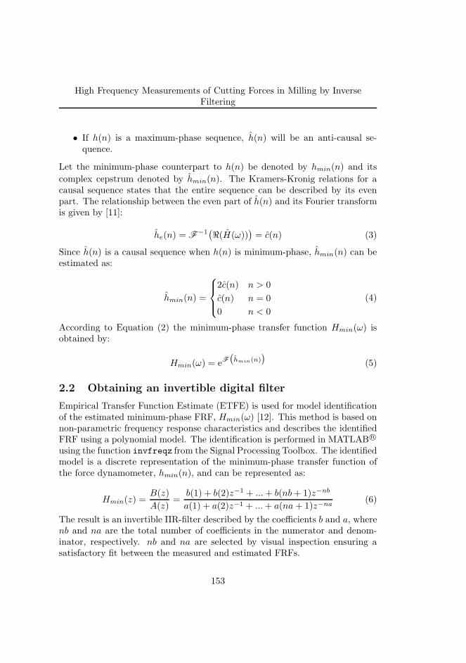
High Frequency Measurements of Cutting Forces in Milling by InverseFiltering

• If h(n) is a maximum-phase sequence, h(n) will be an anti-causal se-quence.

Let the minimum-phase counterpart to h(n) be denoted by hmin(n) and its

complex cepstrum denoted by hmin(n). The Kramers-Kronig relations for acausal sequence states that the entire sequence can be described by its evenpart. The relationship between the even part of h(n) and its Fourier transformis given by [11]:

he(n) = F−1

(

ℜ(H(ω)))

= c(n) (3)

Since h(n) is a causal sequence when h(n) is minimum-phase, hmin(n) can beestimated as:

hmin(n) =

2c(n) n > 0

c(n) n = 0

0 n < 0

(4)

According to Equation (2) the minimum-phase transfer function Hmin(ω) isobtained by:

Hmin(ω) = eF

(

hmin(n))

(5)

2.2 Obtaining an invertible digital filter

Empirical Transfer Function Estimate (ETFE) is used for model identificationof the estimated minimum-phase FRF, Hmin(ω) [12]. This method is based onnon-parametric frequency response characteristics and describes the identifiedFRF using a polynomial model. The identification is performed in MATLAB R©

using the function invfreqz from the Signal Processing Toolbox. The identifiedmodel is a discrete representation of the minimum-phase transfer function ofthe force dynamometer, hmin(n), and can be represented as:

Hmin(z) =B(z)

A(z)=

b(1) + b(2)z−1 + ...+ b(nb+ 1)z−nb

a(1) + a(2)z−1 + ...+ a(na+ 1)z−na(6)

The result is an invertible IIR-filter described by the coefficients b and a, wherenb and na are the total number of coefficients in the numerator and denom-inator, respectively. nb and na are selected by visual inspection ensuring asatisfactory fit between the measured and estimated FRFs.

153

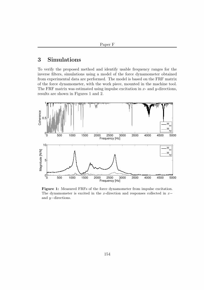
Paper F

3 Simulations

To verify the proposed method and identify usable frequency ranges for theinverse filters, simulations using a model of the force dynamometer obtainedfrom experimental data are performed. The model is based on the FRF matrixof the force dynamometer, with the work piece, mounted in the machine tool.The FRF matrix was estimated using impulse excitation in x- and y-directions,results are shown in Figures 1 and 2.

0 500 1000 1500 2000 2500 3000 3500 4000 4500 50000

0.5

1

Frequency [Hz]

Co

he

ren

ce

0 500 1000 1500 2000 2500 3000 3500 4000 4500 50000

5

10

Frequency [Hz]

Ma

gn

itu

de

[N

/N]

Hxx

Hxy

Hxx

Hxy

Figure 1: Measured FRFs of the force dynamometer from impulse excitation.The dynamometer is excited in the x-direction and responses collected in x−and y−directions.

154

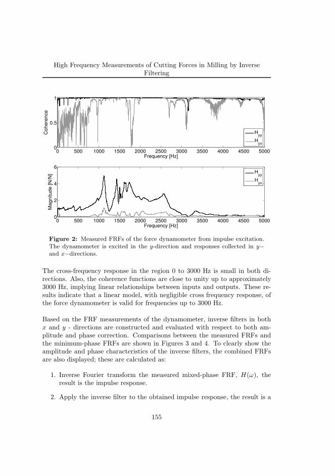
High Frequency Measurements of Cutting Forces in Milling by InverseFiltering

0 500 1000 1500 2000 2500 3000 3500 4000 4500 50000

0.5

1

Frequency [Hz]

Co

he

ren

ce

0 500 1000 1500 2000 2500 3000 3500 4000 4500 50000

2

4

6

Frequency [Hz]

Ma

gn

itu

de

[N

/N]

Hyy

Hyx

Hyy

Hyx

Figure 2: Measured FRFs of the force dynamometer from impulse excitation.The dynamometer is excited in the y-direction and responses collected in y−and x−directions.

The cross-frequency response in the region 0 to 3000 Hz is small in both di-rections. Also, the coherence functions are close to unity up to approximately3000 Hz, implying linear relationships between inputs and outputs. These re-sults indicate that a linear model, with negligible cross frequency response, ofthe force dynamometer is valid for frequencies up to 3000 Hz.

Based on the FRF measurements of the dynamometer, inverse filters in bothx and y - directions are constructed and evaluated with respect to both am-plitude and phase correction. Comparisons between the measured FRFs andthe minimum-phase FRFs are shown in Figures 3 and 4. To clearly show theamplitude and phase characteristics of the inverse filters, the combined FRFsare also displayed; these are calculated as:

1. Inverse Fourier transform the measured mixed-phase FRF, H(ω), theresult is the impulse response.

2. Apply the inverse filter to the obtained impulse response, the result is a

155

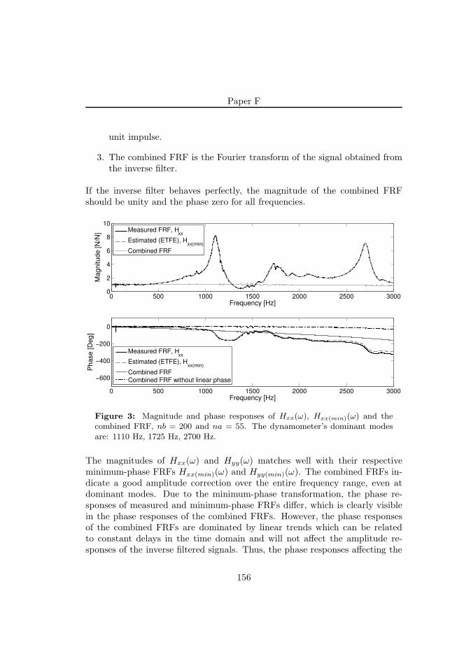
Paper F

unit impulse.

3. The combined FRF is the Fourier transform of the signal obtained fromthe inverse filter.

If the inverse filter behaves perfectly, the magnitude of the combined FRFshould be unity and the phase zero for all frequencies.

0 500 1000 1500 2000 2500 3000

−600

−400

−200

0

Ph

ase

[D

eg

]

Frequency [Hz]

0 500 1000 1500 2000 2500 30000

2

4

6

8

10

Frequency [Hz]

Ma

gn

itu

de

[N

/N]

Measured FRF, Hxx

Estimated (ETFE), Hxx(min)

Combined FRF

Measured FRF, Hxx

Estimated (ETFE), Hxx(min)

Combined FRF

Combined FRF without linear phase

Figure 3: Magnitude and phase responses of Hxx(ω), Hxx(min)(ω) and thecombined FRF, nb = 200 and na = 55. The dynamometer’s dominant modesare: 1110 Hz, 1725 Hz, 2700 Hz.

The magnitudes of Hxx(ω) and Hyy(ω) matches well with their respectiveminimum-phase FRFs Hxx(min)(ω) and Hyy(min)(ω). The combined FRFs in-dicate a good amplitude correction over the entire frequency range, even atdominant modes. Due to the minimum-phase transformation, the phase re-sponses of measured and minimum-phase FRFs differ, which is clearly visiblein the phase responses of the combined FRFs. However, the phase responsesof the combined FRFs are dominated by linear trends which can be relatedto constant delays in the time domain and will not affect the amplitude re-sponses of the inverse filtered signals. Thus, the phase responses affecting the

156

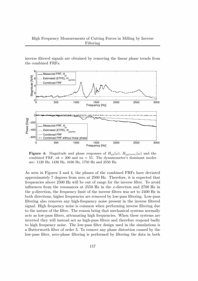
High Frequency Measurements of Cutting Forces in Milling by InverseFiltering

inverse filtered signals are obtained by removing the linear phase trends fromthe combined FRFs.

0 500 1000 1500 2000 2500 3000

−600

−400

−200

0

Ph

ase

[D

eg

]

Frequency [Hz]

0 500 1000 1500 2000 2500 30000

2

4

6

8

Frequency [Hz]

Ma

gn

itu

de

[N

/N]

Measured FRF, Hyy

Estimated (ETFE), Hyy(min)

Combined FRF

Measured FRF, Hyy

Estimated (ETFE), Hyy(min)

Combined FRF

Combined FRF without linear phase

Figure 4: Magnitude and phase responses of Hyy(ω), Hyy(min)(ω) and thecombined FRF, nb = 200 and na = 55. The dynamometer’s dominant modesare: 1120 Hz, 1430 Hz, 1630 Hz, 1750 Hz and 2550 Hz.

As seen in Figures 3 and 4, the phases of the combined FRFs have deviatedapproximately 7 degrees from zero at 2500 Hz. Therefore, it is expected thatfrequencies above 2500 Hz will be out of range for the inverse filter. To avoidinfluences from the resonances at 2550 Hz in the x-direction and 2700 Hz inthe y-direction, the frequency limit of the inverse filters was set to 2400 Hz inboth directions, higher frequencies are removed by low-pass filtering. Low-passfiltering also removes any high-frequency noise present in the inverse filteredsignal. High frequency noise is common when performing inverse filtering dueto the nature of the filter. The reason being that mechanical systems normallyacts as low-pass filters, attenuating high frequencies. When these systems areinverted they will instead act as high-pass filters and therefore respond badlyto high frequency noise. The low-pass filter design used in the simulations isa Butterworth filter of order 3. To remove any phase distortion caused by thelow-pass filter, zero-phase filtering is performed by filtering the data in both

157

Paper F

forward and reverse directions using the MATLAB R© function filtfilt.

To test the behavior of the inverse filters, simulations are carried out for thecutting speeds and feed rates listed in Table 1. Down milling and 50 percentradial immersion is used to excite the dynamometer with a high frequencytransient signal and thereby clear effects from the dynamometer dynamics ap-pear. The simulations are carried out using both x and y as feed directions.Mechanistic modeled cutting forces are used as input (see Table 2), these are fil-tered through ETFEs of the measured mixed-phase transfer functions, hxx(n),hxy(n) and hyy(n), hyx(n). Each output is then inverse filtered and comparedto the reference cutting force (simulated input force), Figures 5 and 6. Thesimulated output forces have contributions both from the point FRFs and thecross FRFs. Due to the phase distortion caused by the minimum-phase trans-formation, superposition of e.g. hxx(min)(n) and hxy(min)(n) does not apply.Therefore only hxx(min)(n) or hyy(min)(n) are used in the inverse filters. Thus,for the results to be accurate, the effect of the cross FRFs have to be negligible.

The similarity between the signals is estimated by calculating the ratio of theenergy in the difference between reference and inverse filtered force, E(fR(t)−fI(t)), and the energy in the reference signal, E(fR(t)), according to:

η = min

[

(

1 +RfIfI (0)− f2

I − 2(

RfRfI (τ)− fRfI)

RfRfR(0)− f2R

)

· 100

]

(7)

where RfRfR(0) and RfIfI (0) are the autocorrelations at zero time delay be-tween reference and inverse filtered forces, respectively. RfRfI (τ) refers to thecross correlation between reference and inverse filtered forces, where τ is thetime delay between the two signals, [13]. fR and fI are the average values ofthe reference and inverse filtered forces, respectively. The best fit between thesignals is found at the time delay, τ , where the energy in the difference betweenthe two signals has a minimum. If η = 0 the two signals are identical.

The simulation results show that the inverse filters are able to counteract thedynamic influences and reconstruct the reference cutting forces within a smallerror margin for all cutting speeds and feed rates listed in Table 1. As seen inFigures 5a) and 6a) the difference between reference and inverse filtered forcesincreases as the cutting speed increases. This is expected since the cuttingspeed affect ramp up times and thereby the frequency content in the reference

158

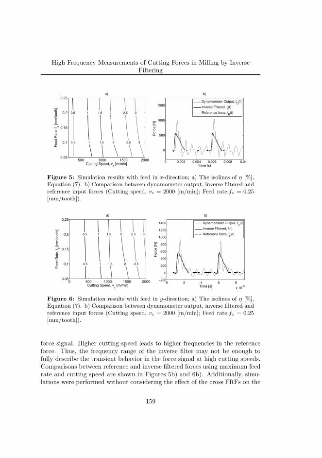
High Frequency Measurements of Cutting Forces in Milling by InverseFiltering

Cutting Speed, vc [m/min]

Fe

ed

Ra

te,

f z [

mm

/to

oth

]

a)

0.5

0.5 1

1 1.5

1.5 2

2 2.5

2.5 3

3

500 1000 1500 20000.05

0.1

0.15

0.2

0.25

0 0.002 0.004 0.006 0.008 0.01

0

500

1000

1500

b)

Time [s]

Fo

rce

[N

]

Dynamometer Output, fD

(t)

Inverse Filtered, fI(t)

Reference force, fR

(t)

Figure 5: Simulation results with feed in x-direction; a) The isolines of η [%],Equation (7). b) Comparison between dynamometer output, inverse filtered andreference input forces (Cutting speed, vc = 2000 [m/min]; Feed rate,fz = 0.25[mm/tooth]).

Cutting Speed, vc [m/min]

Fe

ed

Ra

te,

f z [

mm

/to

oth

]

a)

0.5

0.5 1

1 1.5 2 2.5 3

1.5 2 2.5

0 500 1000 1500 20000.05

0.1

0.15

0.2

0.25

0 2 4 6 8

x 10−3

−200

0

200

400

600

800

1000

1200

1400

b)

Time [s]

Fo

rce

[N

]

Dynamometer Output, fD

(t)

Inverse Filtered, fI(t)

Reference force, fR

(t)

Figure 6: Simulation results with feed in y-direction; a) The isolines of η [%],Equation (7). b) Comparison between dynamometer output, inverse filtered andreference input forces (Cutting speed, vc = 2000 [m/min]; Feed rate,fz = 0.25[mm/tooth]).

force signal. Higher cutting speed leads to higher frequencies in the referenceforce. Thus, the frequency range of the inverse filter may not be enough tofully describe the transient behavior in the force signal at high cutting speeds.Comparisons between reference and inverse filtered forces using maximum feedrate and cutting speed are shown in Figures 5b) and 6b). Additionally, simu-lations were performed without considering the effect of the cross FRFs on the

159

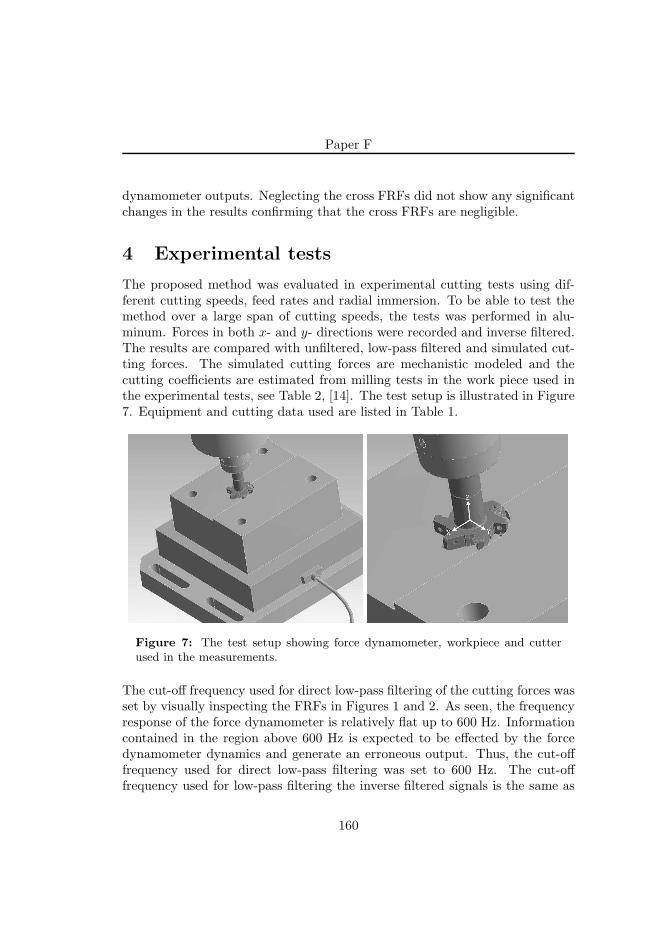
Paper F

dynamometer outputs. Neglecting the cross FRFs did not show any significantchanges in the results confirming that the cross FRFs are negligible.

4 Experimental tests

The proposed method was evaluated in experimental cutting tests using dif-ferent cutting speeds, feed rates and radial immersion. To be able to test themethod over a large span of cutting speeds, the tests was performed in alu-minum. Forces in both x- and y- directions were recorded and inverse filtered.The results are compared with unfiltered, low-pass filtered and simulated cut-ting forces. The simulated cutting forces are mechanistic modeled and thecutting coefficients are estimated from milling tests in the work piece used inthe experimental tests, see Table 2, [14]. The test setup is illustrated in Figure7. Equipment and cutting data used are listed in Table 1.

Figure 7: The test setup showing force dynamometer, workpiece and cutterused in the measurements.

The cut-off frequency used for direct low-pass filtering of the cutting forces wasset by visually inspecting the FRFs in Figures 1 and 2. As seen, the frequencyresponse of the force dynamometer is relatively flat up to 600 Hz. Informationcontained in the region above 600 Hz is expected to be effected by the forcedynamometer dynamics and generate an erroneous output. Thus, the cut-offfrequency used for direct low-pass filtering was set to 600 Hz. The cut-offfrequency used for low-pass filtering the inverse filtered signals is the same as

160

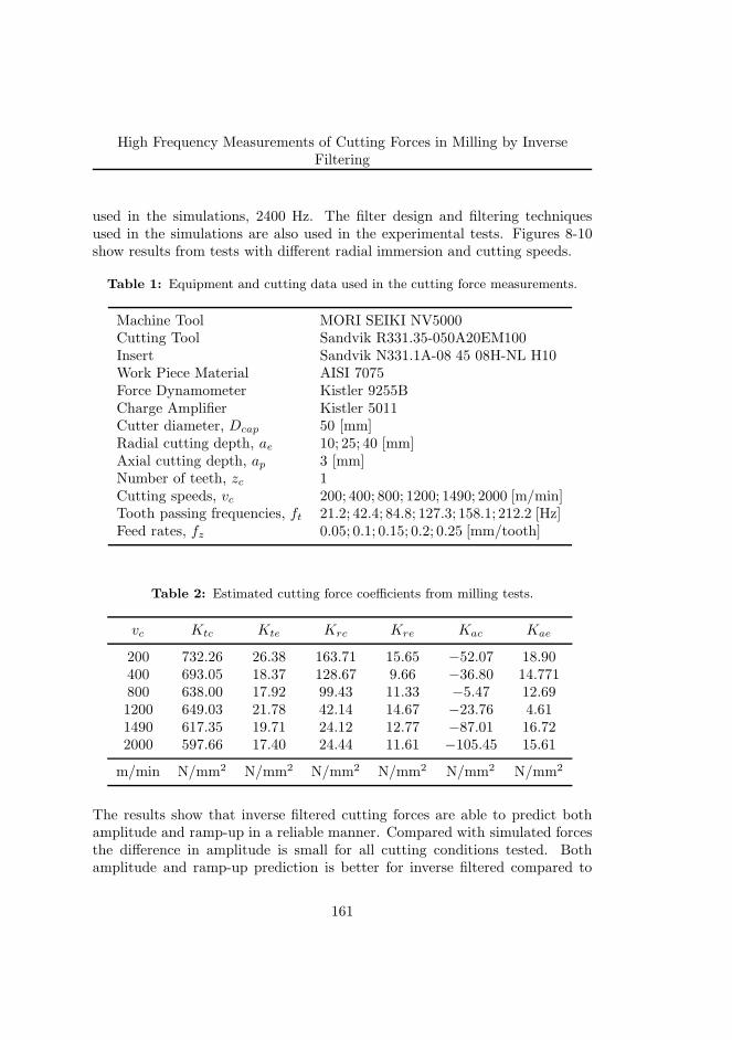
High Frequency Measurements of Cutting Forces in Milling by InverseFiltering

used in the simulations, 2400 Hz. The filter design and filtering techniquesused in the simulations are also used in the experimental tests. Figures 8-10show results from tests with different radial immersion and cutting speeds.

Table 1: Equipment and cutting data used in the cutting force measurements.

Machine Tool MORI SEIKI NV5000Cutting Tool Sandvik R331.35-050A20EM100Insert Sandvik N331.1A-08 45 08H-NL H10Work Piece Material AISI 7075Force Dynamometer Kistler 9255BCharge Amplifier Kistler 5011Cutter diameter, Dcap 50 [mm]Radial cutting depth, ae 10; 25; 40 [mm]Axial cutting depth, ap 3 [mm]Number of teeth, zc 1Cutting speeds, vc 200; 400; 800; 1200; 1490; 2000 [m/min]Tooth passing frequencies, ft 21.2; 42.4; 84.8; 127.3; 158.1; 212.2 [Hz]Feed rates, fz 0.05; 0.1; 0.15; 0.2; 0.25 [mm/tooth]

Table 2: Estimated cutting force coefficients from milling tests.

vc Ktc Kte Krc Kre Kac Kae

200 732.26 26.38 163.71 15.65 −52.07 18.90400 693.05 18.37 128.67 9.66 −36.80 14.771800 638.00 17.92 99.43 11.33 −5.47 12.691200 649.03 21.78 42.14 14.67 −23.76 4.611490 617.35 19.71 24.12 12.77 −87.01 16.722000 597.66 17.40 24.44 11.61 −105.45 15.61

m/min N/mm2 N/mm2 N/mm2 N/mm2 N/mm2 N/mm2

The results show that inverse filtered cutting forces are able to predict bothamplitude and ramp-up in a reliable manner. Compared with simulated forcesthe difference in amplitude is small for all cutting conditions tested. Bothamplitude and ramp-up prediction is better for inverse filtered compared to

161

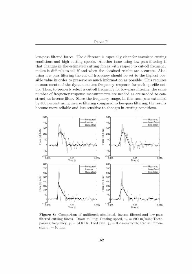
Paper F

low-pass filtered forces. The difference is especially clear for transient cuttingconditions and high cutting speeds. Another issue using low-pass filtering isthat changes in the estimated cutting forces with respect to cut-off frequencymakes it difficult to tell if and when the obtained results are accurate. Also,using low-pass filtering the cut-off frequency should be set to the highest pos-sible value in order to preserve as much information as possible. This requiresmeasurements of the dynamometers frequency response for each specific set-up. Thus, to properly select a cut-off frequency for low-pass filtering, the samenumber of frequency response measurements are needed as are needed to con-struct an inverse filter. Since the frequency range, in this case, was extendedby 400 percent using inverse filtering compared to low-pass filtering, the resultsbecome more reliable and less sensitive to changes in cutting conditions.

0.005 0.01 0.015−200

−100

0

100

200

300

400

500

Fo

rce

[N

] X

−D

ir

Time [s]

Measured

Inverse

Simulated

0.005 0.01 0.015−200

−100

0

100

200

300

400

500

Fo

rce

[N

] X

−D

ir

Time [s]

Measured

Low−Pass

Simulated

0.005 0.01 0.015−100

0

100

200

300

400

500

600

700

800

Fo

rce

[N

] Y

−D

ir

Time [s]

Measured

Inverse

Simulated

0.005 0.01 0.015−100

0

100

200

300

400

500

600

700

800

Fo

rce

[N

] Y

−D

ir

Time [s]

Measured

Low−Pass

Simulated

Figure 8: Comparison of unfiltered, simulated, inverse filtered and low-passfiltered cutting forces. Down milling; Cutting speed, vc = 800 m/min; Toothpassing frequency, ft = 84.8 Hz; Feed rate, fz = 0.2 mm/tooth; Radial immer-sion ae = 10 mm.

162

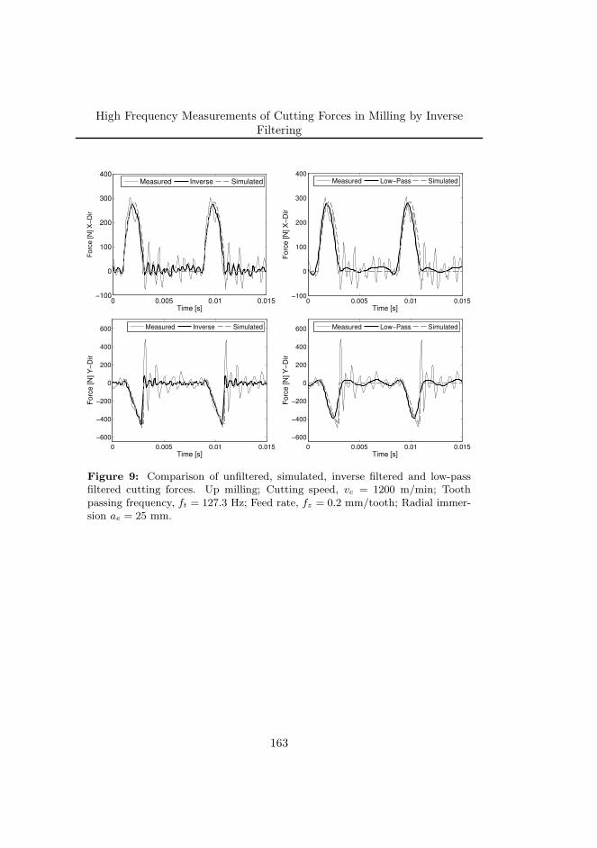
High Frequency Measurements of Cutting Forces in Milling by InverseFiltering

0 0.005 0.01 0.015−100

0

100

200

300

400

Forc

e [N

] X

−D

ir

Time [s]

Measured Inverse Simulated

0 0.005 0.01 0.015−100

0

100

200

300

400

Fo

rce

[N

] X

−D

ir

Time [s]

Measured Low−Pass Simulated

0 0.005 0.01 0.015

−600

−400

−200

0

200

400

600

Fo

rce

[N

] Y

−D

ir

Time [s]

Measured Inverse Simulated

0 0.005 0.01 0.015

−600

−400

−200

0

200

400

600

Fo

rce

[N

] Y

−D

ir

Time [s]

Measured Low−Pass Simulated

Figure 9: Comparison of unfiltered, simulated, inverse filtered and low-passfiltered cutting forces. Up milling; Cutting speed, vc = 1200 m/min; Toothpassing frequency, ft = 127.3 Hz; Feed rate, fz = 0.2 mm/tooth; Radial immer-sion ae = 25 mm.

163

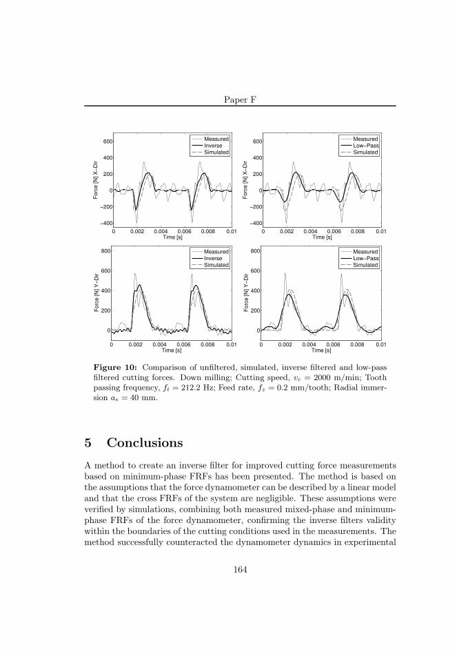
Paper F

0 0.002 0.004 0.006 0.008 0.01

−400

−200

0

200

400

600

Fo

rce

[N

] X

−D

ir

Time [s]

Measured

Inverse

Simulated

0 0.002 0.004 0.006 0.008 0.01

−400

−200

0

200

400

600

Fo

rce

[N

] X

−D

ir

Time [s]

Measured

Low−Pass

Simulated

0 0.002 0.004 0.006 0.008 0.01

0

200

400

600

800

Fo

rce

[N

] Y

−D

ir

Time [s]

Measured

Inverse

Simulated

0 0.002 0.004 0.006 0.008 0.01

0

200

400

600

800F

orc

e [

N]

Y−

Dir

Time [s]

Measured

Low−Pass

Simulated

Figure 10: Comparison of unfiltered, simulated, inverse filtered and low-passfiltered cutting forces. Down milling; Cutting speed, vc = 2000 m/min; Toothpassing frequency, ft = 212.2 Hz; Feed rate, fz = 0.2 mm/tooth; Radial immer-sion ae = 40 mm.

5 Conclusions

A method to create an inverse filter for improved cutting force measurementsbased on minimum-phase FRFs has been presented. The method is based onthe assumptions that the force dynamometer can be described by a linear modeland that the cross FRFs of the system are negligible. These assumptions wereverified by simulations, combining both measured mixed-phase and minimum-phase FRFs of the force dynamometer, confirming the inverse filters validitywithin the boundaries of the cutting conditions used in the measurements. Themethod successfully counteracted the dynamometer dynamics in experimental

164

High Frequency Measurements of Cutting Forces in Milling by InverseFiltering

tests with different feed rates, cutting directions and cutting speeds. The resultsshow that a more reliable estimation of the cutting forces can be obtained us-ing the proposed method compared to traditional low-pass filtering, especiallyunder transient cutting conditions and high cutting speeds. Since the dynamiccorrections are performed in the time domain, compensation can be performedon both stationary and non-stationary signals, which allows the method to beused under both constant and varying cutting conditions. The method can beused to study detailed force responses such as transient entering and/or exitingforces, which is important, e.g., for cutting tool design.

References

[1] J. Tlusty, D.Y. Jang, and Y.S. Tarng. Measurements of milling force over awide frequency range. In Proceedings of the 15th NAMRC, pages 273–280,1987.

[2] Steven A. Jensen, Yung C. Shin, and Patricia Davies. Inverse filteringof unwanted system dynamics in cutting force measurement. American

Society of Mechanical Engineers, Dynamic Systems and Control Division

(Publication) DSC, 58:167–174, 1996.

[3] Simon S. Park and Yusuf Altintas. Dynamic compensation of spindleintegrated force sensors with kalman filter. Journal of Dynamic Systems,

Measurement, and Control, 126(3):443–452, 2004.

[4] Y. Altintas and S.S. Park. Dynamic compensation of spindle-integratedforce sensors. CIRP Annals - Manufacturing Technology, 53(1):305 – 308,2004.

[5] S.S. Park and M. Malekian. Mechanistic modeling and accurate measure-ment of micro end milling forces. CIRP Annals - Manufacturing Technol-

ogy, 58(1):49 – 52, 2009.

[6] Luis Ricardo Castro, Pascal Vieville, and Paul Lipinski. Correctionof dynamic effects on force measurements made with piezoelectric dy-namometers. International Journal of Machine Tools and Manufacture,46(14):1707 – 1715, 2006.

165

Paper F

[7] Remond D. Rigal J.-F. Girardin, F. High frequency correction of dy-namometer for cutting force observation in milling. Journal of Manufactur-

ing Science and Engineering, Transactions of the ASME, 132(3):0310021–0310028, 2010.

[8] Malcolm J. Hawksford. Minimum-phase signal processing for loudspeakersystems. In Audio Engineering Society Convention 100, 5 1996.

[9] Soo-Chang Pei and Huei-Shan Lin. Minimum-phase FIR filter design usingreal cepstrum. IEEE Transactions on Circuits and Systems II-Express

Briefs, 53(10):1113–1117, 2006.

[10] Alan V. Oppenheim and Ronald W. Schafer. Discrete-time signal process-

ing. Pearson Education, Upper Saddle River, N.J., 3. ed., internationaled. edition, 2010.

[11] John G. Proakis and Dimitris G. Manolakis. Digital signal processing

: principles, algorithms and applications. Prentice-Hall, Upper SaddleRiver, N.J., 3. ed. edition, 1996.

[12] Lennart Ljung. System identification : theory for the user. Prentice Hall,Upper Saddle River, N.J., 2. ed. edition, 1999.

[13] Julius S. Bendat and Allan G. Piersol. Engineering applications of corre-

lation and spectral analysis. Wiley, New York, 2. ed. edition, 1993.

[14] Yusuf Altintas. Manufacturing automation : metal cutting mechanics,

machine tool vibrations, and CNC design. Cambridge University Press,Cambridge, 2000.

166

Blekinge Institute of TechnologyDoctoral Dissertation Series No. 2011:14

School of Engineering

Simulation and ExpErimEntal mEthodS for CharaCtErization of nonlinEar mEChaniCal SyStEmS

Sim

ul

at

ion

an

d E

xp

Er

imE

nt

al

m

Et

ho

dS

fo

r C

ha

ra

Ct

Er

iza

tio

n o

f n

on

lin

Ea

r m

EC

ha

niC

al

Sy

St

Em

S M

artin Magnevall

ISSN 1653-2090

ISBN: 978-91-7295-218-8

Trial and error and the use of highly time-consu-

ming methods are often necessary for investigation

and characterization of nonlinear systems. Howe-

ver, for the rather common case where a nonli-

near system has linear relations between many of

its degrees of freedom there are opportunities for

more efficient approaches. The aim of this thesis

is to develop and validate new efficient simulation

and experimental methods for characterization of

mechanical systems with localized nonlinearities.

The purpose is to contribute to the development

of analysis tools for such systems that are useful

in early phases of the product innovation process

for predicting product properties and functionality.

Fundamental research is combined with industrial

case studies related to metal cutting. Theoretical

modeling, computer simulations and experimen-

tal testing are utilized in a coordinated approach

to iteratively evaluate and improve the methods.

The nonlinearities are modeled as external forces

acting on the underlying linear system. In this way,

much of the linear theories behind forced response

simulations can be utilized. The linear parts of the

system are described using digital filters and mo-

dal superposition, and the response of the system

is recursively solved for together with the artificial

external forces. The result is an efficient simulation

method, which in conjunction with experimental

tests, is used to validate the proposed characteriza-

tion methods.

A major part of the thesis addresses a frequency

domain characterization method based on broad-

band excitation. This method uses the measured

responses to create artificial nonlinear inputs to the

parameter estimation model. Conventional multip-

le-input/multiple-output techniques are then used

to separate the linear system from the nonlinear

parameters. A specific result is a generalization of

this frequency domain method, which allows for

characterization of continuous systems with an

arbitrary number of localized zero-memory non-

linearities in a structured way. The efficiency and

robustness of this method is demonstrated by both

simulations and experimental tests. A time domain

simulation and characterization method intended

for use on systems with hysteresis damping is also

developed and its efficiency is demonstrated by the

case of a dry-friction damper. Furthermore, a met-

hod for improved harmonic excitation of nonlinear

systems using numerically optimized input signals

is developed. Inverse filtering is utilized to remove

unwanted dynamic effects in cutting force measu-

rements, which increases the frequency range of

the force dynamometer and significantly impro-

ves the experimental results compared to traditio-

nal methods. The new methods form a basis for

efficient analysis and increased understanding of

mechanical systems with localized nonlinearities,

which in turn provides possibilities for more effi-

cient product development as well as for continued

research on analysis methods for nonlinear mecha-

nical structures.

aBStraCt

2011:14

2011:14

Martin Magnevall