experimental characterization of hybrid structural...
TRANSCRIPT
Experimental characterization of hybrid structural components
(Concrete reinforced by profiles)
Submitted By
Md. Refat Ahmed Bhuiyan
Under the supervision of
Prof. Dr. Hervé Degée
European Erasmus Mundus Master Course
Sustainable Constructions
Under Natural Hazards and Catastrophic Events 520121-1-2011-1-CZ-ERA MUNDUS-EMMC

2 | P a g e
ACKNOWLEDGEMENT
First of all, I offer my sincerest gratitude to my supervisor, Dr Herve Degee, who has
supported me throughout my thesis with his patience and knowledge whilst allowing me the
room to work in my own way. I attribute the level of my Master’s degree to his
encouragement and effort and without him this thesis, too, would not have been completed or
written. One simply could not wish for a better or friendlier supervisor.
This project paper is completed with the cordial supervision of the project supervisor Dr.
Herve Degee, Professor of civil engineering department, ULg.
Authors also express their intense gratitude and appreciation to Dr. Boyan Mihaylov and Dr.
Teodora Bogdan for their proper guidance, cordial co-operation and supervision throughout
the period of project completion.
I would also like to thank Structural Engineering Department, University of Liege. And
finally, for the financial support I would like to thank European Commission, without their
financial contribution it would not be possible to complete.
December, 2013
ULg
3 | P a g e
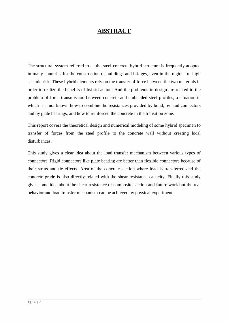
ABSTRACT
The structural system referred to as the steel-concrete hybrid structure is frequently adopted
in many countries for the construction of buildings and bridges, even in the regions of high
seismic risk. These hybrid elements rely on the transfer of force between the two materials in
order to realize the benefits of hybrid action. And the problems in design are related to the
problem of force transmission between concrete and embedded steel profiles, a situation in
which it is not known how to combine the resistances provided by bond, by stud connectors
and by plate bearings, and how to reinforced the concrete in the transition zone.
This report covers the theoretical design and numerical modeling of some hybrid specimen to
transfer of forces from the steel profile to the concrete wall without creating local
disturbances.
This study gives a clear idea about the load transfer mechanism between various types of
connectors. Rigid connectors like plate bearing are better than flexible connectors because of
their struts and tie effects. Area of the concrete section where load is transferred and the
concrete grade is also directly related with the shear resistance capacity. Finally this study
gives some idea about the shear resistance of composite section and future work but the real
behavior and load transfer mechanism can be achieved by physical experiment.
4 | P a g e
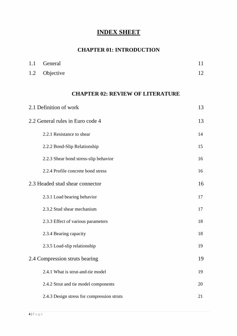
INDEX SHEET
CHAPTER 01: INTRODUCTION
1.1 General 11
1.2 Objective 12
CHAPTER 02: REVIEW OF LITERATURE
2.1 Definition of work 13
2.2 General rules in Euro code 4 13
2.2.1 Resistance to shear 14
2.2.2 Bond-Slip Relationship 15
2.2.3 Shear bond stress-slip behavior 16
2.2.4 Profile concrete bond stress 16
2.3 Headed stud shear connector 16
2.3.1 Load bearing behavior 17
2.3.2 Stud shear mechanism 17
2.3.3 Effect of various parameters 18
2.3.4 Bearing capacity 18
2.3.5 Load-slip relationship 19
2.4 Compression struts bearing 19
2.4.1 What is strut-and-tie model 19
2.4.2 Strut and tie model components 20
2.4.3 Design stress for compression struts 21
5 | P a g e
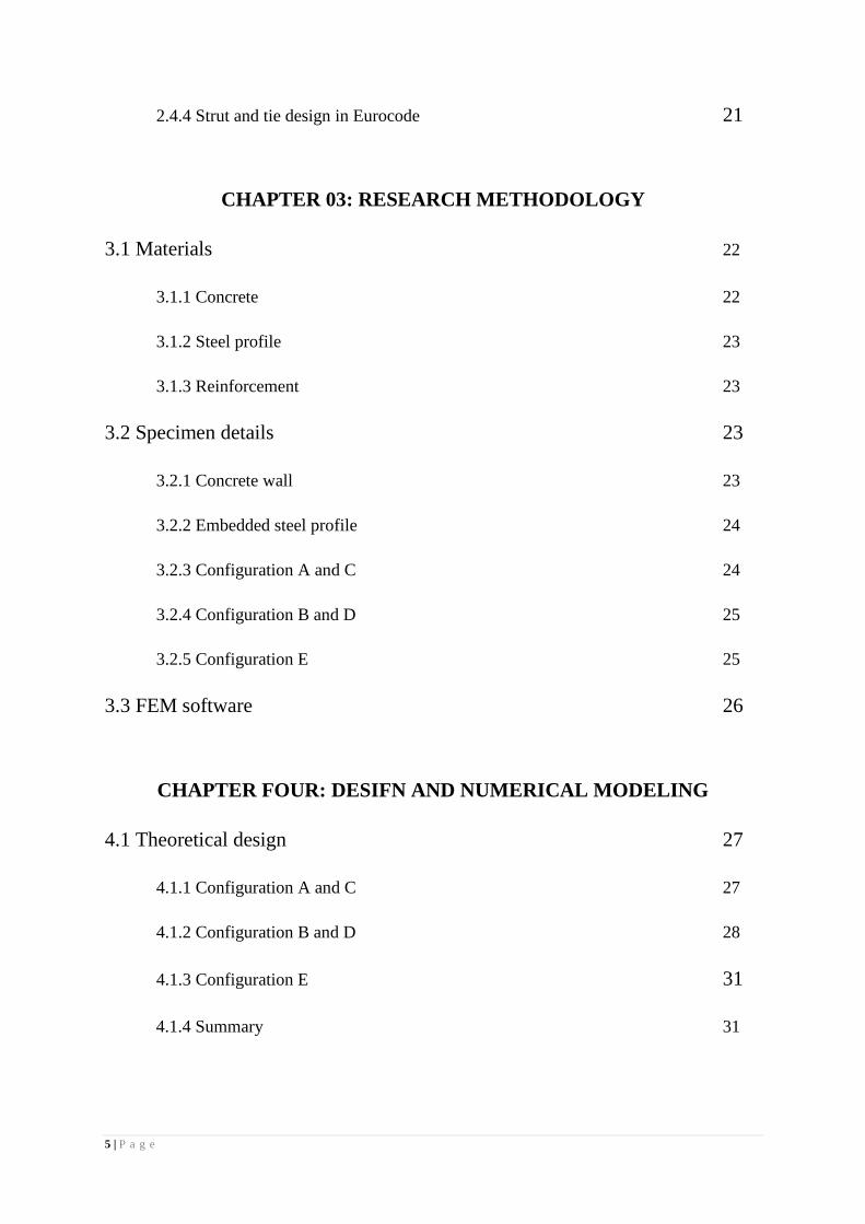
2.4.4 Strut and tie design in Eurocode 21
CHAPTER 03: RESEARCH METHODOLOGY
3.1 Materials 22
3.1.1 Concrete 22
3.1.2 Steel profile 23
3.1.3 Reinforcement 23
3.2 Specimen details 23
3.2.1 Concrete wall 23
3.2.2 Embedded steel profile 24
3.2.3 Configuration A and C 24
3.2.4 Configuration B and D 25
3.2.5 Configuration E 25
3.3 FEM software 26
CHAPTER FOUR: DESIFN AND NUMERICAL MODELING
4.1 Theoretical design 27
4.1.1 Configuration A and C 27
4.1.2 Configuration B and D 28
4.1.3 Configuration E 31
4.1.4 Summary 31
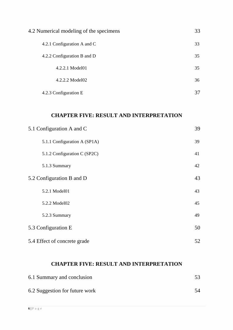
6 | P a g e
4.2 Numerical modeling of the specimens 33
4.2.1 Configuration A and C 33
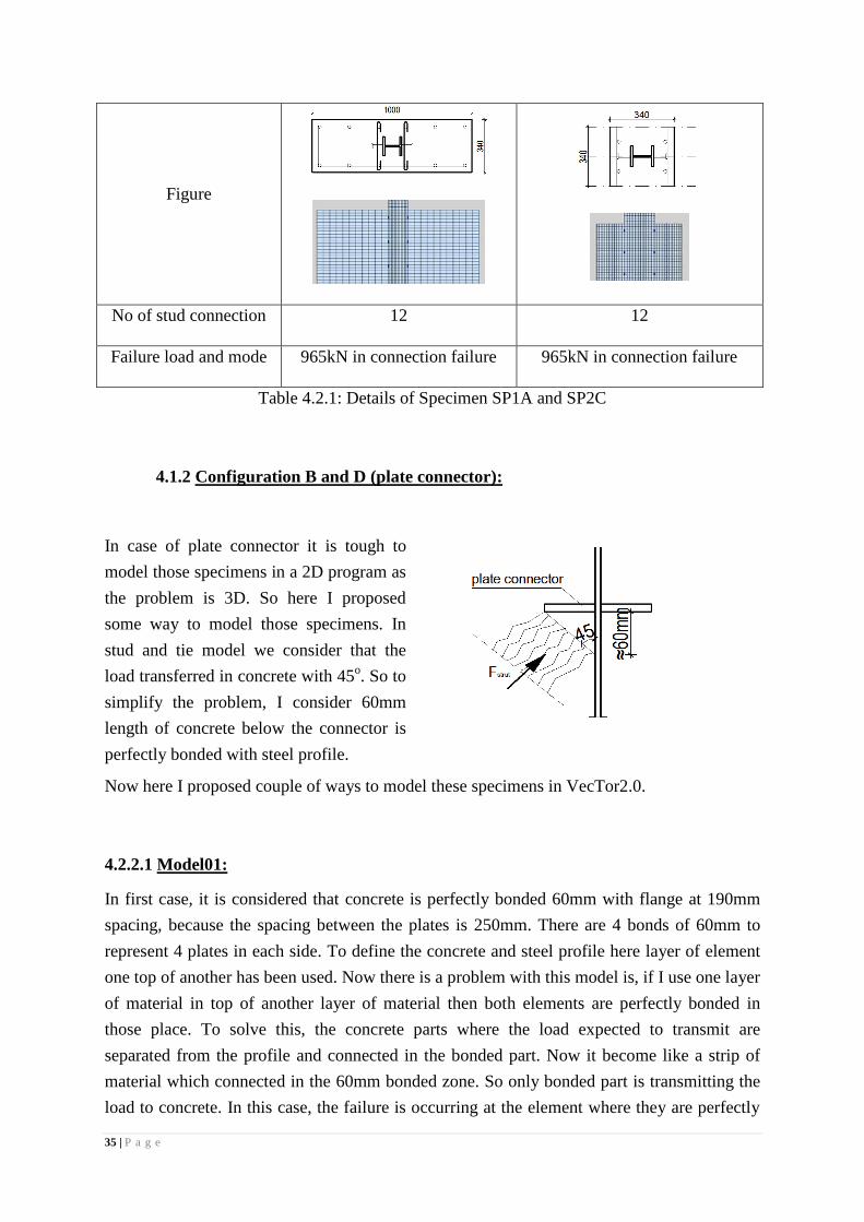
4.2.2 Configuration B and D 35
4.2.2.1 Model01 35
4.2.2.2 Model02 36
4.2.3 Configuration E 37
CHAPTER FIVE: RESULT AND INTERPRETATION
5.1 Configuration A and C 39
5.1.1 Configuration A (SP1A) 39
5.1.2 Configuration C (SP2C) 41
5.1.3 Summary 42
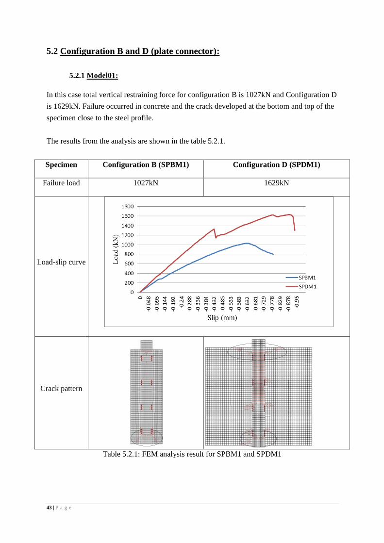
5.2 Configuration B and D 43
5.2.1 Model01 43
5.2.2 Model02 45
5.2.3 Summary 49
5.3 Configuration E 50
5.4 Effect of concrete grade 52
CHAPTER FIVE: RESULT AND INTERPRETATION
6.1 Summary and conclusion 53
6.2 Suggestion for future work 54
7 | P a g e
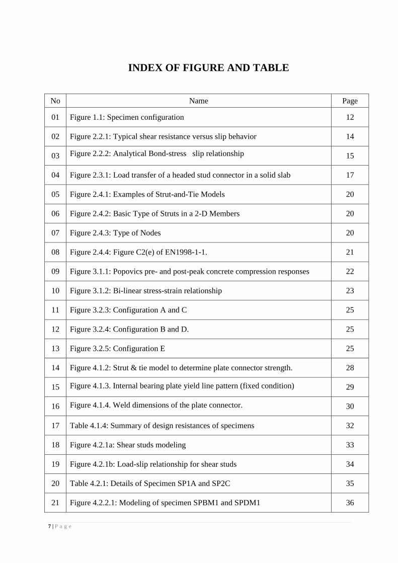
No Name Page
01 Figure 1.1: Specimen configuration 12
02 Figure 2.2.1: Typical shear resistance versus slip behavior 14
03 Figure 2.2.2: Analytical Bond-stress slip relationship 15
04 Figure 2.3.1: Load transfer of a headed stud connector in a solid slab 17
05 Figure 2.4.1: Examples of Strut-and-Tie Models 20
06 Figure 2.4.2: Basic Type of Struts in a 2-D Members 20
07 Figure 2.4.3: Type of Nodes 20
08 Figure 2.4.4: Figure C2(e) of EN1998-1-1. 21
09 Figure 3.1.1: Popovics pre- and post-peak concrete compression responses 22
10 Figure 3.1.2: Bi-linear stress-strain relationship 23
11 Figure 3.2.3: Configuration A and C 25
12 Figure 3.2.4: Configuration B and D. 25
13 Figure 3.2.5: Configuration E 25
14 Figure 4.1.2: Strut & tie model to determine plate connector strength. 28
15 Figure 4.1.3. Internal bearing plate yield line pattern (fixed condition) 29
16 Figure 4.1.4. Weld dimensions of the plate connector. 30
17 Table 4.1.4: Summary of design resistances of specimens 32
18 Figure 4.2.1a: Shear studs modeling 33
19 Figure 4.2.1b: Load-slip relationship for shear studs 34
20 Table 4.2.1: Details of Specimen SP1A and SP2C 35
21 Figure 4.2.2.1: Modeling of specimen SPBM1 and SPDM1 36
INDEX OF FIGURE AND TABLE
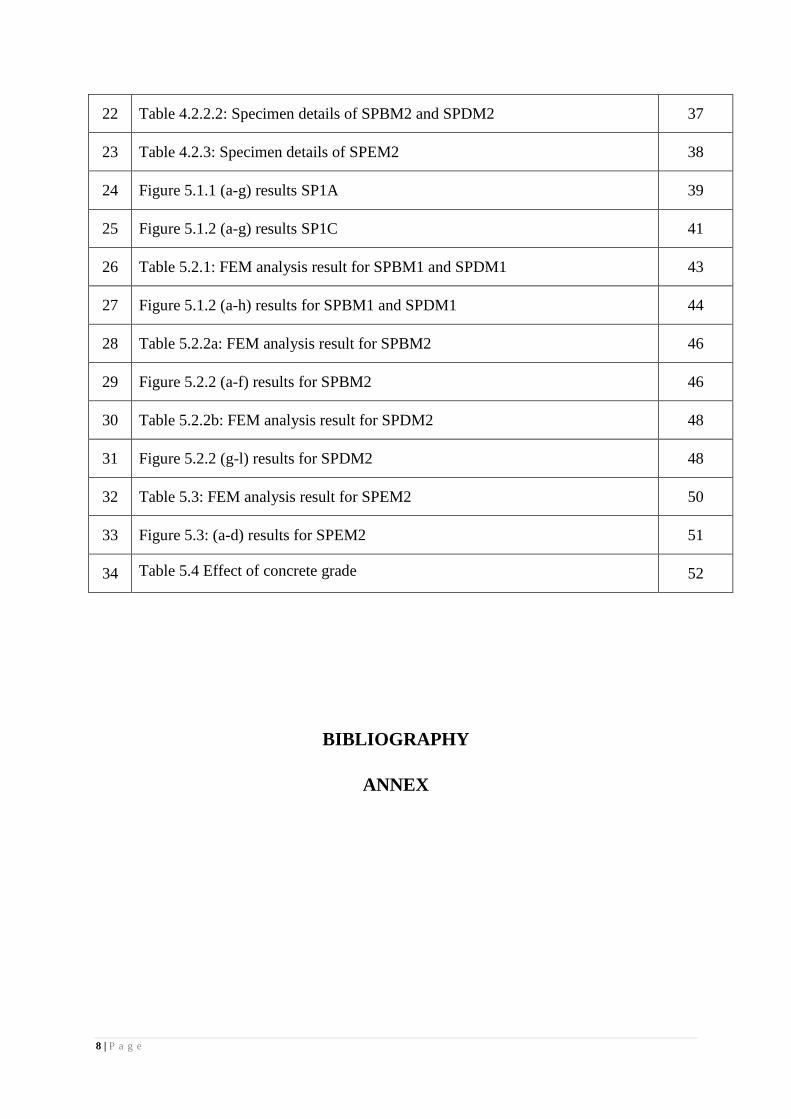
8 | P a g e
22 Table 4.2.2.2: Specimen details of SPBM2 and SPDM2 37
23 Table 4.2.3: Specimen details of SPEM2 38
24 Figure 5.1.1 (a-g) results SP1A 39
25 Figure 5.1.2 (a-g) results SP1C 41
26 Table 5.2.1: FEM analysis result for SPBM1 and SPDM1 43
27 Figure 5.1.2 (a-h) results for SPBM1 and SPDM1 44
28 Table 5.2.2a: FEM analysis result for SPBM2 46
29 Figure 5.2.2 (a-f) results for SPBM2 46
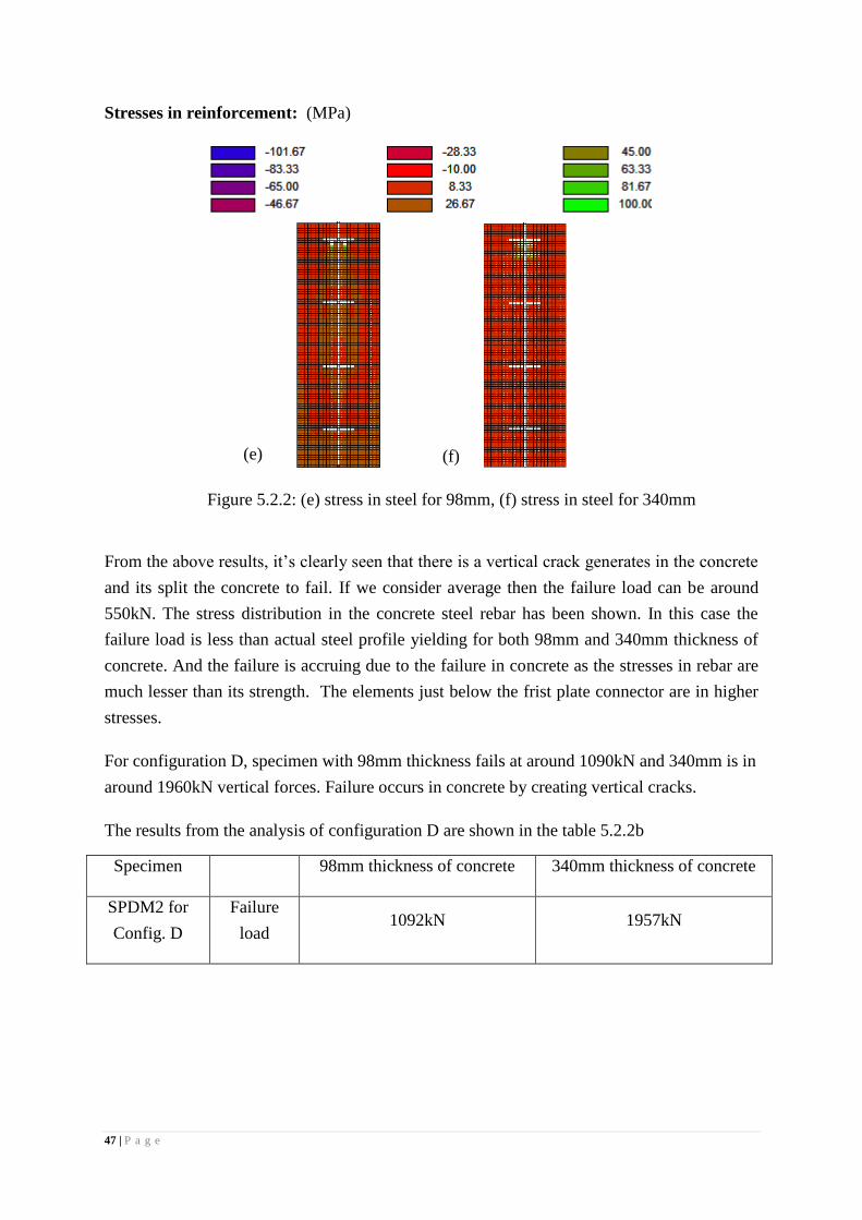
30 Table 5.2.2b: FEM analysis result for SPDM2 48
31 Figure 5.2.2 (g-l) results for SPDM2 48
32 Table 5.3: FEM analysis result for SPEM2 50
33 Figure 5.3: (a-d) results for SPEM2 51
34 Table 5.4 Effect of concrete grade 52
BIBLIOGRAPHY
ANNEX
9 | P a g e
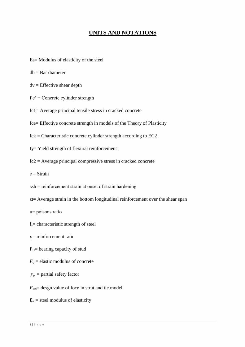
UNITS AND NOTATIONS
Es= Modulus of elasticity of the steel
db = Bar diameter
dv = Effective shear depth
f c’ = Concrete cylinder strength
fc1= Average principal tensile stress in cracked concrete
fce= Effective concrete strength in models of the Theory of Plasticity
fck = Characteristic concrete cylinder strength according to EC2
fy= Yield strength of flexural reinforcement
fc2 = Average principal compressive stress in cracked concrete
ε = Strain
εsh = reinforcement strain at onset of strain hardening
εt= Average strain in the bottom longitudinal reinforcement over the shear span
μ= poisons ratio
fs= characteristic strength of steel
= reinforcement ratio
PU= bearing capacity of stud
Ec = elastic modulus of concrete
v = partial safety factor
FRd= desgn value of foce in strut and tie model
Ea = steel modulus of elasticity
10 | P a g e
NplRd= plastic resistance of steel profile
PRk= shear stud connector strength
kN= kilo newton
MPa= mega Pascal
Asv= area of vertical reinforcement
Ash= area of horizontal reinforcement
σ = axial stress
11 | P a g e
CHAPTER: ONE
INTRODUCTION
1.1General:
The structural system referred to as the steel-concrete hybrid structure is frequently adopted
in many countries for the construction of buildings and bridges, even in the regions of high
seismic risk. Steel concrete hybrid structure is composed of the composite structure and the
mixed structure. Hybrid steel and concrete elements can take many forms. Examples include
the steel girder with concrete slab, concrete pier with steel girder, steel framing of a building
with the concrete floor slabs, the encasement of a steel element with concrete, or the filling of
a steel hollow section with concrete. These hybrid elements rely on the transfer of force
between the two materials in order to realize the benefits of hybrid action.
Benefits can include an increase in strength and stiffness as well as the restraint of buckling
instabilities in the steel or confinement of the concrete. Hybrid action can be achieved
through mechanical connection between the steel and concrete members or elements. The
problem with those hybrid structures is that they are neither reinforced concrete structure in
the sense of Eurocode 2 or ACI318, nor composite steel concrete structure in the sense of
Eurocode 4 or ASCI2010. The problems with hybrid element design are mostly related to the
problem of force transmission between concrete and embedded steel profiles, a situation in
which it is not known how to combine the resistances provided by bond, by stud connectors
and by plate bearings, and how to reinforced the concrete in the transition zone.
To investigate the complicated behavior of the hybrid structures or its components, the
experimental investigation is the key resource. Besides the experimental investigation,
numerical evaluation also plays a significant role to examine the structural behavior and
mechanical properties of hybrid structures. To conduct experiment with varying geometric
properties is a time consuming matter, whereas numerical analysis can easily check the effect
of any variation. In this case my study involves numerical analysis of some hybrid structural
component.
12 | P a g e
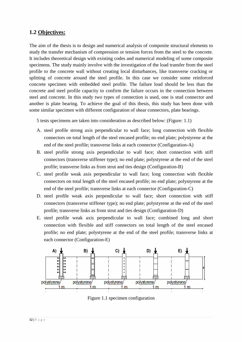
1.2 Objectives:
The aim of the thesis is to design and numerical analysis of composite structural elements to
study the transfer mechanism of compression or tension forces from the steel to the concrete.
It includes theoretical design with existing codes and numerical modeling of some composite
specimens. The study mainly involve with the investigation of the load transfer from the steel
profile to the concrete wall without creating local disturbances, like transverse cracking or
splitting of concrete around the steel profile. In this case we consider some reinforced
concrete specimen with embedded steel profile. The failure load should be less than the
concrete and steel profile capacity to confirm the failure occurs in the connection between
steel and concrete. In this study two types of connection is used, one is stud connector and
another is plate bearing. To achieve the goal of this thesis, this study has been done with
some similar specimen with different configuration of shear connectors, plate bearings.
5 tests specimens are taken into consideration as described below: (Figure: 1.1)
A. steel profile strong axis perpendicular to wall face; long connection with flexible
connectors on total length of the steel encased profile; no end plate; polystyrene at the
end of the steel profile; transverse links at each connector (Configuration-A)
B. steel profile strong axis perpendicular to wall face; short connection with stiff
connectors (transverse stiffener type); no end plate; polystyrene at the end of the steel
profile; transverse links as from strut and ties design (Configuration-B)
C. steel profile weak axis perpendicular to wall face; long connection with flexible
connectors on total length of the steel encased profile; no end plate; polystyrene at the
end of the steel profile; transverse links at each connector (Configuration-C)
D. steel profile weak axis perpendicular to wall face; short connection with stiff
connectors (transverse stiffener type); no end plate; polystyrene at the end of the steel
profile; transverse links as from strut and ties design (Configuration-D)
E. steel profile weak axis perpendicular to wall face; combined long and short
connection with flexible and stiff connectors on total length of the steel encased
profile; no end plate; polystyrene at the end of the steel profile; transverse links at
each connector (Configuration-E)
Figure 1.1 specimen configuration
13 | P a g e
CHAPTER: TWO
REVIEW OF LITERATURE
2.1 Definition of work
“Identification of the fundamental force transfer mechanisms at steel-concrete interface”
In this case a preliminary study of the force transfer mechanisms based on an extensive
review of the existing literature. The objective is to identify those mechanisms and to
organize the existing data and methods, if any, in a ready to use form. The references
considered are Eurocode 2: EN1992-1-1:2004 and Eurocode 4: EN1994-1-1:2004.
2.2 General rules in Eurocode 4
EC4-6.7.4.1 (1)P Provision shall be made in regions of load introduction for internal forces
and moments applied from members connected to the ends and for loads applied within the
length to be distributed between the steel and concrete components, considering the shear
resistance at the interface between steel and concrete. A clearly defined load path shall be
provided that does not involve an amount of slip at this interface that would invalidate the
assumptions made in design.
EC4-6.7.4.1 (2)P Where composite columns and compression members are subjected to
significant transverse shear, as for example by local transverse loads and by end moments,
provision shall be made for the transfer of the corresponding longitudinal shear stress at the
interface between steel and concrete.
EC4-6.7.4.1 (3) For axially loaded columns and compression members, longitudinal shear
outside the areas of load introduction need not be considered.
EC4-6.7.4.2 (1) Shear connectors should be provided in the load introduction area and in
areas with change of cross section, if the design shear strength Rd , see 6.7.4.3, is exceeded at
the interface between steel and concrete. The shear forces should be determined from the
change of sectional forces of the steel or reinforced concrete section within the introduction
length. If the loads are introduced into the concrete cross section only, the values resulting
from an elastic analysis considering creep and shrinkage should be taken into account.
Otherwise, the forces at the interface should be determined by elastic theory or plastic theory,
to determine the more severe case.
EC4-6.7.4.2 (2) In absence of a more accurate method, the introduction length should not
exceed 2d or L/3, where d is the minimum transverse dimension of the column and L is the
column length.
EC4-6.7.4.2 (3) For composite columns and compression members no shear connection need
be provided for load introduction by endplates if the full interface between the concrete

14 | P a g e
section and endplate is permanently in compression, taking account of creep and shrinkage.
Otherwise the load introduction should be verified according to (5). For concrete filled tubes
of circular cross-section the effect caused by the confinement may be taken into account if
the conditions given in 6.7.3.2(6) are satisfied using the values a and c for equal to
zero.
EC4-6.7.4.2 (4) Where stud connectors are attached to the web of a fully or partially concrete
encased steel I-section or a similar section, account may be taken of the frictional forces that
develop from the prevention of lateral expansion of the concrete by the adjacent steel flanges.
This resistance may be added to the calculated resistance of the shear connectors. The
additional resistance may be assumed to be μ PRd on each flange and each horizontal
row of studs, where μ is the relevant coefficient of friction that may be assumed. For steel
sections without painting, μ may be taken as 0,5. PRd is the resistance of a single stud in
accordance with 6.6.3.1. In absence of better information from tests, the clear distance
between the flanges should not exceed the values.
2.2.1 Resistance to shear
The shear force transfer at the connection between concrete and steel components is typically
carried by three main mechanisms: a) chemical bonding (bond between the cement paste and
the surface of the steel: b) friction (assumed proportional to the normal force at the interface):
c) mechanical interaction (due to embossments, ribs or shear stud connectors). While
chemical bonding is typically neglected in both design and analysis of composite structures,
friction and especially mechanical actions are very important (Salari (1999)).
It is common practice to design composite slabs as one way slabs with slab action parallel to
the ribs. Shear connectors between concrete slab and steel section are considered to provide
the required composite action in flexure. They can also be used to distribute the large
horizontal inertial forces in the slab to the main lateral load resisting elements of the structure
(Hawkins and Mitchell (1984)). Headed shear connectors are welded to the steel beam to
provide different degrees of connection between the concrete slab and beam.
remaining mechanical and friction bond
Initial chemical bond
remaining mechanical and friction bond
Observed model
Analytical model
Bo
nd
fo
rce
Slip Slip
(a) (b)
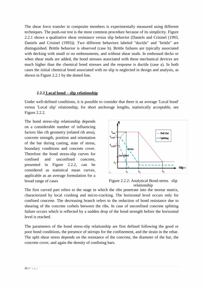
Figure 2.2.1: Typical shear resistance versus slip behavior: a) ductile response; b) brittle response
15 | P a g e
The shear force transfer in composite members is experimentally measured using different
techniques. The push-out test is the most common procedure because of its simplicity. Figure
2.2.1 shows a qualitative shear resistance versus slip behavior (Daniels and Crisinel (1993,
Daniels and Crisinel (1993)). Two different behaviors labeled "ductile" and "brittle" are
distinguished. Brittle behavior is observed (case b). Brittle failures are typically associated
with decking with small or no embossments, and without shear studs. In embossed decks or
when shear studs are added, the bond stresses associated with these mechanical devices are
much higher than the chemical bond stresses and the response is ductile (case a). In both
cases the initial chemical bond associated with no slip is neglected in design and analysis, as
shown in Figure 2.2.1 by the dotted line.
2.2.2 Local bond – slip relationship
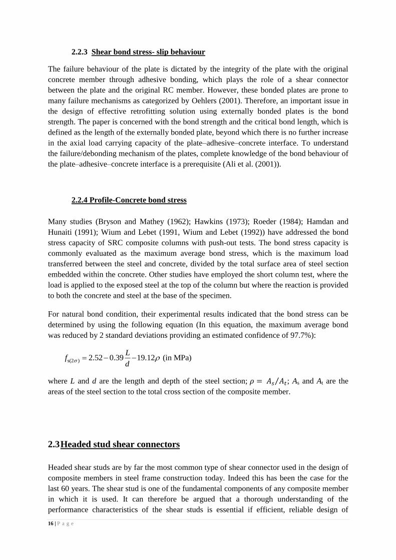
Under well-defined conditions, it is possible to consider that there is an average 'Local bond'
versus 'Local slip' relationship, for short anchorage lengths, statistically acceptable, see
Figure 2.2.2.
The bond stress-slip relationship depends
on a considerable number of influencing
factors like rib geometry (related rib area),
concrete strength, position and orientation
of the bar during casting, state of stress,
boundary conditions and concrete cover.
Therefore the bond stress-slip curves for
confined and unconfined concrete,
presented in Figure 2.2.2, can be
considered as statistical mean curves,
applicable as an average formulation for a
broad range of cases
Figure 2.2.2: Analytical Bond-stress slip relationship
The first curved part refers to the stage in which the ribs penetrate into the mortar matrix,
characterized by local crushing and micro-cracking. The horizontal level occurs only for
confined concrete. The decreasing branch refers to the reduction of bond resistance due to
shearing of the concrete corbels between the ribs. In case of unconfined concrete splitting
failure occurs which is reflected by a sudden drop of the bond strength before the horizontal
level is reached.
The parameters of the bond stress-slip relationship are first defined following the good or
poor bond conditions, the presence of stirrups for the confinement, and the strain in the rebar.
The split shear stress depends on the resistance of the concrete, the diameter of the bar, the
concrete cover, and again the density of confining bars.
16 | P a g e
2.2.3 Shear bond stress- slip behaviour
The failure behaviour of the plate is dictated by the integrity of the plate with the original
concrete member through adhesive bonding, which plays the role of a shear connector
between the plate and the original RC member. However, these bonded plates are prone to
many failure mechanisms as categorized by Oehlers (2001). Therefore, an important issue in
the design of effective retrofitting solution using externally bonded plates is the bond
strength. The paper is concerned with the bond strength and the critical bond length, which is
defined as the length of the externally bonded plate, beyond which there is no further increase
in the axial load carrying capacity of the plate–adhesive–concrete interface. To understand
the failure/debonding mechanism of the plates, complete knowledge of the bond behaviour of
the plate–adhesive–concrete interface is a prerequisite (Ali et al. (2001)).
2.2.4 Profile-Concrete bond stress
Many studies (Bryson and Mathey (1962); Hawkins (1973); Roeder (1984); Hamdan and
Hunaiti (1991); Wium and Lebet (1991, Wium and Lebet (1992)) have addressed the bond
stress capacity of SRC composite columns with push-out tests. The bond stress capacity is
commonly evaluated as the maximum average bond stress, which is the maximum load
transferred between the steel and concrete, divided by the total surface area of steel section
embedded within the concrete. Other studies have employed the short column test, where the
load is applied to the exposed steel at the top of the column but where the reaction is provided
to both the concrete and steel at the base of the specimen.
For natural bond condition, their experimental results indicated that the bond stress can be
determined by using the following equation (In this equation, the maximum average bond
was reduced by 2 standard deviations providing an estimated confidence of 97.7%):
s(2 ) 2.52 0.39 19.12 (in MPa)L
fd
where L and d are the length and depth of the steel section; ⁄ ; As and At are the
areas of the steel section to the total cross section of the composite member.
2.3 Headed stud shear connectors
Headed shear studs are by far the most common type of shear connector used in the design of
composite members in steel frame construction today. Indeed this has been the case for the
last 60 years. The shear stud is one of the fundamental components of any composite member
in which it is used. It can therefore be argued that a thorough understanding of the
performance characteristics of the shear studs is essential if efficient, reliable design of
17 | P a g e
composite members is to take place. Push-out tests are commonly used to determine the
capacity of the shear connection and load-slip behavior of the shear connectors.
2.3.1 Load-bearing behavior
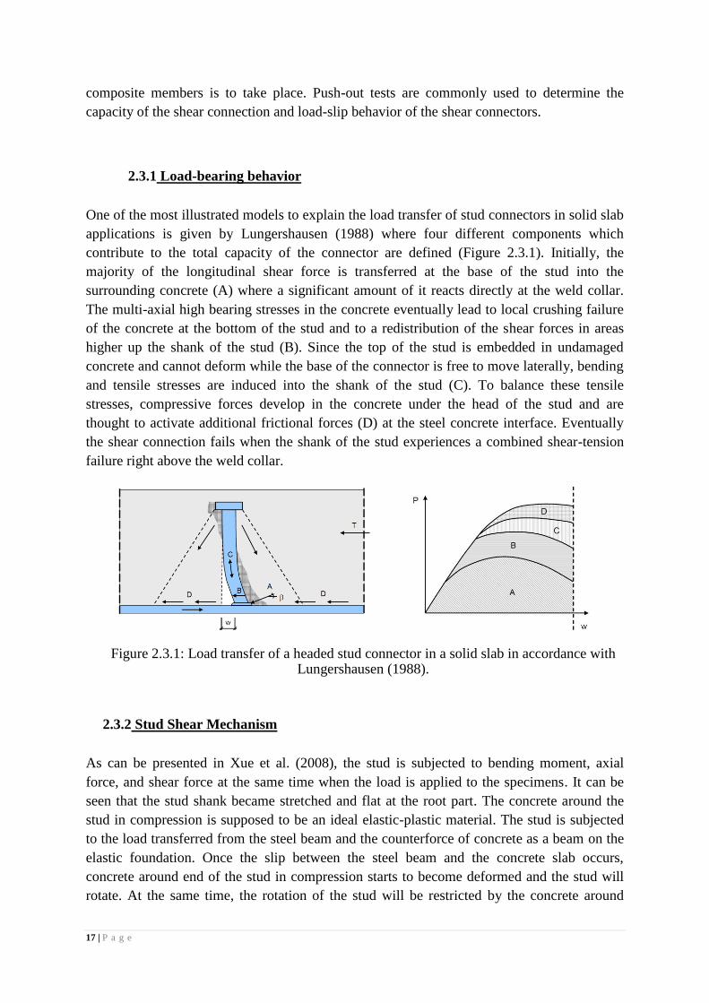
One of the most illustrated models to explain the load transfer of stud connectors in solid slab
applications is given by Lungershausen (1988) where four different components which
contribute to the total capacity of the connector are defined (Figure 2.3.1). Initially, the
majority of the longitudinal shear force is transferred at the base of the stud into the
surrounding concrete (A) where a significant amount of it reacts directly at the weld collar.
The multi-axial high bearing stresses in the concrete eventually lead to local crushing failure
of the concrete at the bottom of the stud and to a redistribution of the shear forces in areas
higher up the shank of the stud (B). Since the top of the stud is embedded in undamaged
concrete and cannot deform while the base of the connector is free to move laterally, bending
and tensile stresses are induced into the shank of the stud (C). To balance these tensile
stresses, compressive forces develop in the concrete under the head of the stud and are
thought to activate additional frictional forces (D) at the steel concrete interface. Eventually
the shear connection fails when the shank of the stud experiences a combined shear-tension
failure right above the weld collar.
Figure 2.3.1: Load transfer of a headed stud connector in a solid slab in accordance with Lungershausen (1988).
2.3.2 Stud Shear Mechanism
As can be presented in Xue et al. (2008), the stud is subjected to bending moment, axial
force, and shear force at the same time when the load is applied to the specimens. It can be
seen that the stud shank became stretched and flat at the root part. The concrete around the
stud in compression is supposed to be an ideal elastic-plastic material. The stud is subjected
to the load transferred from the steel beam and the counterforce of concrete as a beam on the
elastic foundation. Once the slip between the steel beam and the concrete slab occurs,
concrete around end of the stud in compression starts to become deformed and the stud will
rotate. At the same time, the rotation of the stud will be restricted by the concrete around
18 | P a g e
other end of the stud. The load transferred by the steel beam to the stud will increase
continuously with the increase of the load imposed on the specimen.
2.3.3 Effects of various parameters on the stud load-slip behavior
- Effect of stud diameter and height
- Effect of concrete strength
- Effect of stud welding technique
- Effect of transverse reinforcement
- Effect of steel beam type
- Effect of transverse arrangement
2.3.4 Bearing Capacity
As mentioned by Xue et al. (2008) the calculation formula for the stud shear bearing capacity
was derived based on the earlier work of Viest (1956), and the expression is
2c
u
c
332 ( / 4.2)
79 ( / 4.2)
d f H dP
Hd f H d
where Pu = stud shear bearing capacity (k); d = stud diameter (in.); H = stud height (in.); and
cf = compressive strength of concrete cylinders (psi).
Eurocode EC4 (2004) specified the design strength of stud shear connectors which are
welded automatically, as
2u
v
u 2ck cm
v
0.8 / 4
min0.29
f d
Pd f E
where the units are N, mm; d = diameter of the studs; fu = ultimate tensile strength of stud; fc
= compressive strength of concrete cylinders; Ec = elastic modulus of concrete; v = partial
safety factor (=1.25); = 0.2(H/d+1) ≤ 1; and H = height of the studs.
In AISC (2005), the nominal strength of one stud shear connector embedded in solid concrete
or in a composite slab is
19 | P a g e
u s c c g p s u0.5P A f E R R A F
where Fu = specified minimum tensile strength of a stud shear connector (MPa); cE =
modulus of elasticity of concrete (MPa); cf =compressive strength of concrete cylinders
(MPa); gR = 1.0 for any number of studs welded in a row directly to the steel shape; and pR
= 1.0 for studs welded directly to the steel shape and having a haunch detail with not more
than 50% of the top flange covered by a deck of sheet steel closures.
2.3.5 Load slip relationship:
Mohammad Makki Abbass (2011) in his paper (ISSN 0974-5904, Volume 04, No 06 SPL)
proposed a load slip relationship. After an extensive study on stud behavior he found, the slip
(u) is considered as non-dimensional parameter as a ratio of slip(u) to stud diameter(d). And
here Q is the load in kN and fcu is the characteristic strength of concrete.
Q=0.0407*(fcu)^0.57*d^2*((u/d)/(0.01245+(u/d)))
2.4 Compression Struts Bearing
In selecting the appropriate design approach for structural concrete, it is useful to classify
portions of the structure as either B- (Beam or Bernoulli) Regions or D- (Disturbed or
Discontinuity) Regions. B-Regions are parts of a structure in which Bernoulli's hypothesis of
straight-line strain profiles applies. D-Regions, on the other hand, are parts of a structure with
a complex variation in strain. D-Regions include portions near abrupt changes in geometry
(geometrical discontinuities) or concentrated forces (statical discontinuities). The main
concept behind these is called strut and tie method.The idea of the strut-and-tie method came
from the truss analogy method introduced independently by Ritter and Mörch in the early
1900s for shear design of B-Regions. This method employs the so-called truss model as its
design basis. The model was used to idealize the flow of force in a cracked concrete beam.
2.4.1 What is Strut and tie models
The STM is based on the lower-bound theory of limit analysis. In the STM, the complex flow
of internal forces in the D-Region under consideration is idealized as a truss carrying the
imposed loading through the region to its supports. This truss is called strut-and-tie
model and is a statically admissible stress field in lower-bound (static) solutions. Like a real
truss, a strut-and-tie model consists of struts and ties interconnected at nodes (also referred to
as nodal zones or nodal regions). A selection of strut-and-tie models for a few typical 2-D D-
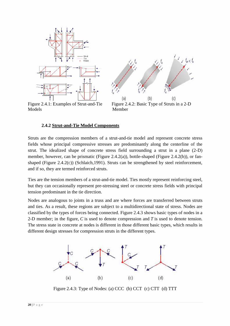
Regions is illustrated in Figure 2.4.1 As shown in the figure, struts are usually symbolized
using broken lines, and ties are usually denoted using solid lines.
20 | P a g e
Figure 2.4.1: Examples of Strut-and-Tie Figure 2.4.2: Basic Type of Struts in a 2-D
Models Member
2.4.2 Strut-and-Tie Model Components
Struts are the compression members of a strut-and-tie model and represent concrete stress
fields whose principal compressive stresses are predominantly along the centerline of the
strut. The idealized shape of concrete stress field surrounding a strut in a plane (2-D)
member, however, can be prismatic (Figure 2.4.2(a)), bottle-shaped (Figure 2.4.2(b)), or fan-
shaped (Figure 2.4.2(c)) (Schlaich,1991). Struts can be strengthened by steel reinforcement,
and if so, they are termed reinforced struts.
Ties are the tension members of a strut-and-tie model. Ties mostly represent reinforcing steel,
but they can occasionally represent pre-stressing steel or concrete stress fields with principal
tension predominant in the tie direction.
Nodes are analogous to joints in a truss and are where forces are transferred between struts
and ties. As a result, these regions are subject to a multidirectional state of stress. Nodes are
classified by the types of forces being connected. Figure 2.4.3 shows basic types of nodes in a
2-D member; in the figure, C is used to denote compression and T is used to denote tension.
The stress state in concrete at nodes is different in those different basic types, which results in
different design stresses for compression struts in the different types.
Figure 2.4.3: Type of Nodes: (a) CCC (b) CCT (c) CTT (d) TTT
21 | P a g e
2.4.3 Design stresses for compression struts
The design rules in Eurocode 2 or in fib manuals reflect the influence of the stress state by
providing design values which are different for different stress states corresponding to CCC
nodes, CCT nodes and CTT nodes, where C stands for compression and T stands for tension.
The rules also reflect a care for safety in limiting the design stress in compression struts to fcd
or less in most practical cases.
Hereunder, the rules in Eurocode 2 (EN1992-1-1:2004) and in fib 2010 manuals on structural
concrete are presented in parallel, in order to set forward some updates in year 2010 fib
manuals in comparison to year 2004 Eurocode 2.
2.4.4 Strut and Tie design in Eurocode 8 and Eurocode 4.
The consideration of inclined compression struts bearing on transverse plates intervening in
the equilibrium was first made explicit, in a normative context, in the frame of background
research activity to Eurocode 8 or EN1998-1-1:2004. The complete background activity is
reported in the ICONS research report (PLUMIER, 2001). The corresponding normative
expressions for the strength of concrete compression struts bearing on plates which are part of
a steel section are given in the normative Annex C of Eurocode 8 and mentioned as a
“mechanism 2” consisting of compressed concrete struts inclined to the column sides
(Figure2.4.4).
When no façade steel beam is present, the moment capacity of the joint may be calculated
from the compressive force developed by the combination of the following two mechanisms:
mechanism 1: direct compression on the
column. The design value of the force that
is transferred by means of this mechanism
should not exceed the value given by the
following expression: FRd1 = bb deff fcd
mechanism 2: If the angle of inclination is
equal to 45°, the design value of the force
that is transferred by means of this
mechanism should not exceed the value
given by the following expression:
FRd2 = 0,7hc deff fcd
where hc is the depth of the column
steel section.
Figure 2.4.4: Figure C2(e) of EN1998-1-1
22 | P a g e
CHAPTER: THREE
RESEARCH METHODOLOGY
3.1 Materials:
A brief description of the constituent materials as used in the present investigation is given
below
3.1.1 Concrete:
Concrete (C40/50)
o Characteristic strength fck = 40 MPa;
o Mean value of Elastic modulus Ecm = 35000 MPa;
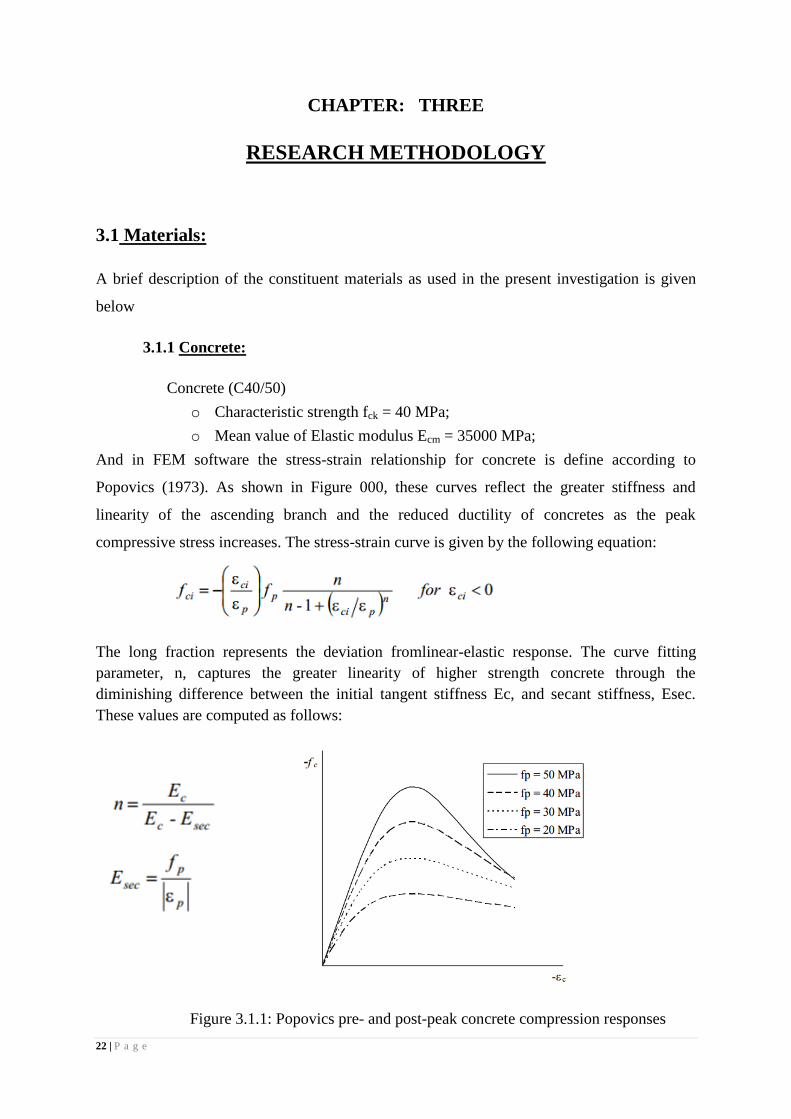
And in FEM software the stress-strain relationship for concrete is define according to
Popovics (1973). As shown in Figure 000, these curves reflect the greater stiffness and
linearity of the ascending branch and the reduced ductility of concretes as the peak
compressive stress increases. The stress-strain curve is given by the following equation:
The long fraction represents the deviation fromlinear-elastic response. The curve fitting
parameter, n, captures the greater linearity of higher strength concrete through the
diminishing difference between the initial tangent stiffness Ec, and secant stiffness, Esec.
These values are computed as follows:
Figure 3.1.1: Popovics pre- and post-peak concrete compression responses
23 | P a g e
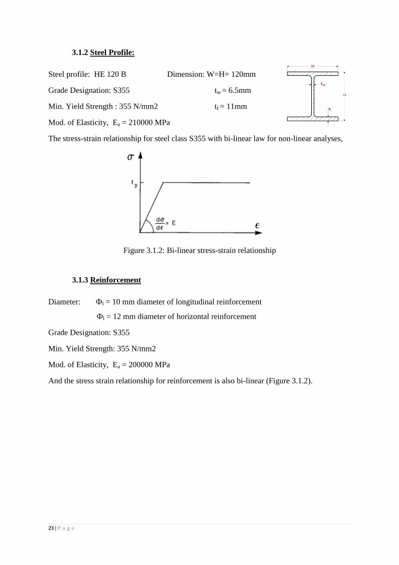
3.1.2 Steel Profile:
Steel profile: HE 120 B Dimension: W=H= 120mm
Grade Designation: S355 tw = 6.5mm
Min. Yield Strength : 355 N/mm2 tf = 11mm
Mod. of Elasticity, Ea = 210000 MPa
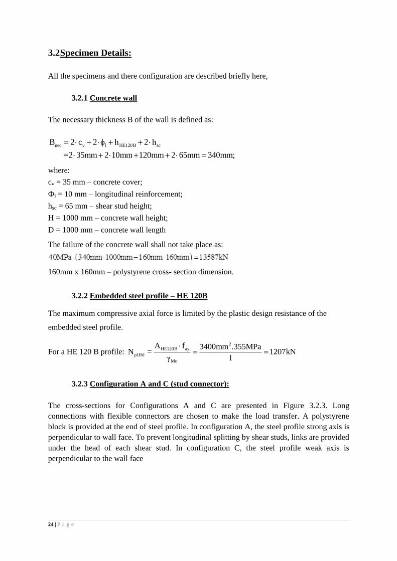
The stress-strain relationship for steel class S355 with bi-linear law for non-linear analyses,
Figure 3.1.2: Bi-linear stress-strain relationship
3.1.3 Reinforcement
Diameter: Фl = 10 mm diameter of longitudinal reinforcement
Фl = 12 mm diameter of horizontal reinforcement
Grade Designation: S355
Min. Yield Strength: 355 N/mm2
Mod. of Elasticity, Ea = 200000 MPa
And the stress strain relationship for reinforcement is also bi-linear (Figure 3.1.2).
24 | P a g e
3.2 Specimen Details:
All the specimens and there configuration are described briefly here,
3.2.1 Concrete wall
The necessary thickness B of the wall is defined as:
nec v l HE120B scB 2 c 2 h 2 h
=2 35mm 2 10mm 120mm 2 65mm 340mm;
where:
cv = 35 mm – concrete cover;
Фl = 10 mm – longitudinal reinforcement;
hsc = 65 mm – shear stud height;
H = 1000 mm – concrete wall height;
D = 1000 mm – concrete wall length
The failure of the concrete wall shall not take place as:
160mm x 160mm – polystyrene cross- section dimension.
3.2.2 Embedded steel profile – HE 120B
The maximum compressive axial force is limited by the plastic design resistance of the
embedded steel profile.
For a HE 120 B profile: 2
HE120B ay
pl.Rd
Mo
A f 3400mm .355MPaN = 1207kN
γ 1
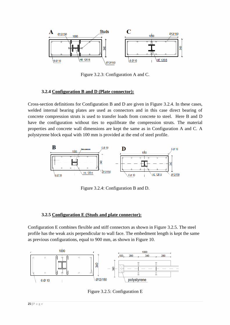
3.2.3 Configuration A and C (stud connector):
The cross-sections for Configurations A and C are presented in Figure 3.2.3. Long
connections with flexible connectors are chosen to make the load transfer. A polystyrene
block is provided at the end of steel profile. In configuration A, the steel profile strong axis is
perpendicular to wall face. To prevent longitudinal splitting by shear studs, links are provided
under the head of each shear stud. In configuration C, the steel profile weak axis is
perpendicular to the wall face
25 | P a g e
Figure 3.2.3: Configuration A and C.
3.2.4 Configuration B and D (Plate connector):
Cross-section definitions for Configuration B and D are given in Figure 3.2.4. In these cases,
welded internal bearing plates are used as connectors and in this case direct bearing of
concrete compression struts is used to transfer loads from concrete to steel. Here B and D
have the configuration without ties to equilibrate the compression struts. The material
properties and concrete wall dimensions are kept the same as in Configuration A and C. A
polystyrene block equal with 100 mm is provided at the end of steel profile.
Figure 3.2.4: Configuration B and D.
3.2.5 Configuration E (Studs and plate connector):
Configuration E combines flexible and stiff connectors as shown in Figure 3.2.5. The steel
profile has the weak axis perpendicular to wall face. The embedment length is kept the same
as previous configurations, equal to 900 mm, as shown in Figure 10.
Figure 3.2.5: Configuration E
26 | P a g e
3.3 FEM Software:
In this study for numerical analysis of the specimen here VecTor2.0 program is used.
VecTor2.0 is a program for nonlinear analysis of two-dimensional reinforced concrete
membrane structures. This program has been developed at the University of Toronto.
VecTor2.0 is a program based on the Modified Compression Field Theory for nonlinear finite
element analysis of reinforced concrete membrane structures. Considering the inherent
intricacies of nonlinear finite element analysis and VecTor2, user facilities are imperative to
their rational and convenient application.
Non-linear finite element procedures currently represent the most complex and advanced
tools for predicting the response of reinforced concrete structures. They incorporate models
from various constitutive frameworks such as non-linear elasticity, plasticity, continuum
damage mechanics, smeared fixed/rotating crack models, micro plane models (CEB-FIP,
2008). Each of these approaches has proven effective in some applications and less effective
in others. VecTor2 is a finite element program for 2D static and dynamic analysis of
reinforced concrete structures. It has been developed over the last 18 years by Prof. Vecchio
and his research group at the University of Toronto. Used in this study is VecTor2, Revision
6.0 from the 8th
of February, 2008. The basic models implemented into the program include
the Modified Compression Field Theory (MCFT – Vecchio and Collins, 1986) and the
Disturbed Stress Field Model (DSFM – Vecchio, 2000). Both the MCFT and the DSFM fall
into the category of smeared rotating crack models, as later is built on the concepts of
the former. The main difference between the DSFM and the MCFT lies in the reorientation of
the stress and strain fields. The basic assumption of the MCFT is that the average
direction of the principal compressive stresses coincides with the average direction of the
principal compressive strains and that the critical cracks are parallel to this direction. In
contrast, the DSFM explicitly accounts for slip deformations at the critical cracks which
results in delayed rotation of the stress field with respect to the strain field. The critical
cracks in the DSFM are kept perpendicular to the direction of the principal tensile stresses.
27 | P a g e
CHAPTER: FOUR
DESIGN AND NUMERICAL MODELING
4.1Theoretical Design:
In this section, the theoretical design of all the specimens is briefly described. As in all the
specimens the same concrete section and steel profile is used, so there capacity is remain
same. The capacity of concrete is 13587kN and plastic resistance of the embedded steel
profile is 1207kN. The design capacity of each specimen is taken in design is maxN 1000kN ,
in order to achieve the failure in the load transferring mechanism. Details designs are
described below.
4.1.1 Configuration A and C (stud connector):
Shear studs characteristics:
Geometrical characteristic of the shear studs
d = 16 mm – diameter of the shear stud;
hsc = 65 mm – stud height; 3d = 48 mm ≤ hsc ;
sc = 200 mm – longitudinal spacing; 5d = 80 mm ≤ sc ≤ min(6hsc; 800mm)=390mm;
fu = 500 MPa – maximum stud tensile strength;
Shear connector strength:
EC 4.1.- §6.6.3.1. (1) gives the individual shear connector characteristic strength:
22
u ck cm
Rk
V V
d0.8 f 0.29 d f E4P = min , 80.43kNγ γ
Where,
d = 16 mm– shear stud diameter;
hsc= 65mm
fu = 500MPa;
fck = 40Mpa;
v 1.00;
28 | P a g e
sc sc
sc
h h0.2 1 for 3 4
d d= 1;
h1 for 4
d
The necessary number of shear studs is: max
Rk
N 1000kN12.43.
P 80.43kN
The strength capacity of nstuds = 12 shear studs is equal to: NRd = nstuds .PRk= 965.1 kN. The
distance between two shear studs is equal to: sc = 150mm.
The design resistance of the shear studs connection is:
NRd = 965.1 kN < Nmax = 1000 kN.
Reinforcement design and strut and tie model are explained in Annex: ASP1.
4.1.2 Configuration B and D (plate connector):
Plate connector characteristics
Plate connectors are welded to the web of the steel profile HE 120B shape. They have the
following geometrical characteristics :
- Width of the plate: f wb ta = 56.75mm
2
- Length of the plate: fb* h 2 t = 98mm
- Width of the clipped corners: c 15mm
- Area: 2 2
plateA a b c = 53.36cm
Plate connector strength
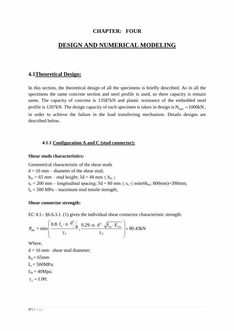
The plate connector strength is determined considering the following strut & tie model, as
shown in Figure 4.1.2. It is considered that the struts are formed assuming an angle = 45º.
Figure 4.1.2: Strut & tie model to determine plate connector strength.
29 | P a g e
Strut width is equal to: a a
= 80.26mmcos 2
2
The strut resistance: Rd Rd,max
aF b* =158.56kN
2
where:
ckf' 1 = 0.84
250
Rd,max cd0.6 ' f = 20.16MPa
fcd = 40MPa
For one plate:
Rd,1plate RdV F cos =112.12kN
The necessary plate number is:
maxplates
Rd,1plate
Nn = 8,9
V
The strength capacity of nplates = 8 plate connectors, 4 plates on each side, is equal to:
NRd = nplates .VRd, 1plate= 896.96 kN.
The design resistance of the connection is:
NRd = 896.96kN. < Nmax = 1000kN.
Required bearing plate thickness
For rectangular plates supported on three sides, elastic solutions for plate stresses such as
those found in Roark’s Formulas for Stress and Strain may be used for thickness calculation.
The required bearing plate thickness is determined on the basis of the expression used in
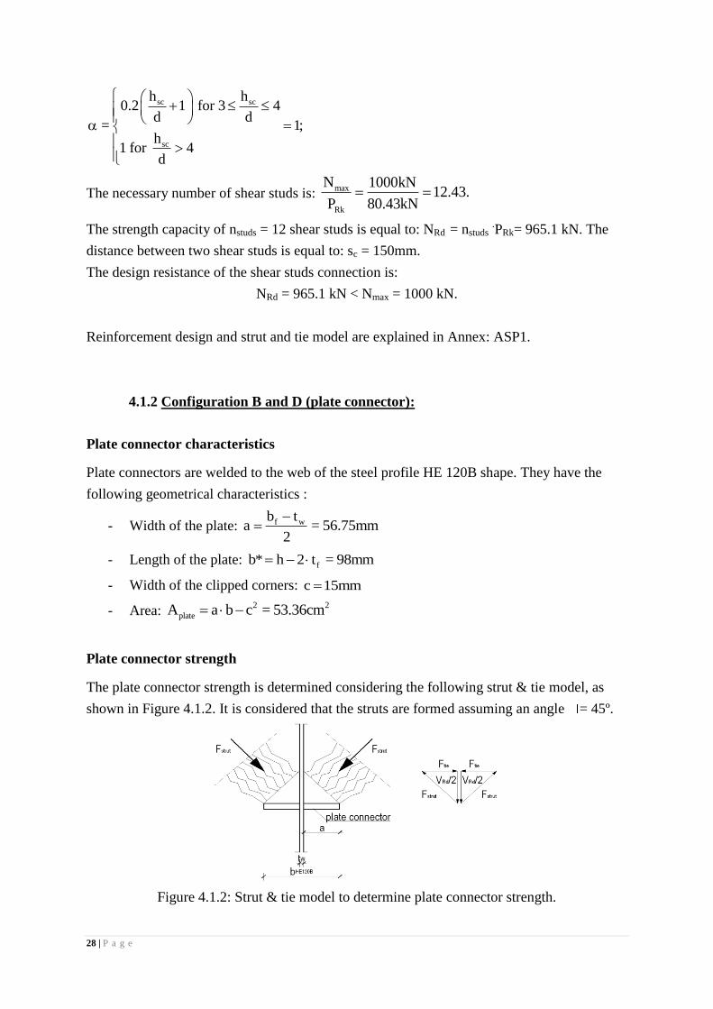
Plumier. et al. (2013). The yield lines are not formed at 45º, meaning that the yield line is
shorter than 2a√2, as shown in Figure 4.1.3. The actual yield line is: b√2+a-b/2 = 77.05 mm.
Figure 4.1.3. Internal bearing plate yield line pattern (fixed condition).
30 | P a g e
The bearing pressure on plate: Rd,1plate
u
plate
Vw 21.01MPa
A
The required bearing plate thickness tp is:
2
u
p
ay
2 a w 3 b 2 a2.8 at 8.36mm
a 0.9 b* 3 f 6 a b*
Where:
0.9
tp = 9 mm.
The minimum spacing between two plates is recommended to be: sp_min = 2a+tp = 137.5 mm.
The maximum spacing is: sp_max = 6a = 340.5 mm. In order to keep the same embedded
distance for the steel profile, as in previous configurations, the distance between two
connectors is: sp = 250 mm.
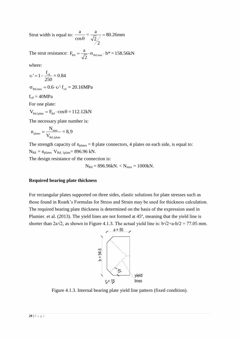
The weld thickness a = 5 mm and follows the condition of 2a > tp = 9 mm, as shown in
Figure 4.1.4.
Figure 4.1.4. Weld dimensions of the plate connector.
Bearing plate strength
Considering the thickness of the plate is 9 mm the bearing pressure of the plate can be
calculated by the same way. So bearing pressure for each plate with 9mm thickness,
wu= 25.14MPa
Each plate load bearing capacity, =( 25.14* 94.6*56*10-3
) kN
= 133.17 kN
So total bearing plate strength = 133.17*8 kN
= 1065.5 kN
Reinforcement design and strut and tie model are explained in Annex: ASP2.
31 | P a g e
4.1.3 Configuration E (studs and plate connector):
It is considered that the compressive axial force Nmax = 1000kN is resisted by both shear
studs and plate connectors. The total number of plate connectors is obtained by the formula:
max
Rd,1plate
N2 4.46
V
where:
Rd,1plateV 112.12kN
The number of shear studs needed is:
max
Rk
N2 6.217
P
where:
PRk = 80.45 kN;
For nplates = nstuds = 4 the resistance of connectors is:
Rd plates Rd,1plate studs RkN n V n P 770.18kN
The position of the connectors is shown in Figure 9. The distance between 2 rows of
connectors is equal to: spc=340mm.
the design resistance of the connection is:
NRd = 770.18 kN < Nmax = 1000kN.
Considering the plate bearing strength,
NRd = (4* 133.17 + 4* 80.45) kN
= 854.5 kN
4.1.4 Summary:
Summary of all the design forces are listed below in the table 4.1.4.
Specimen Number of
connectors
Shear resistance of
1 connector [kN]
NRd
[kN]
Expected
failure mode
Config.A-SP1A 12 shear studs 80.43 965.10 Connection
failure
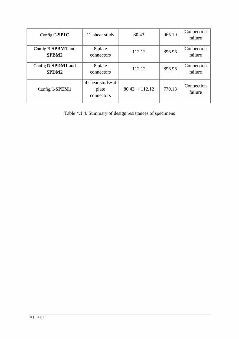
32 | P a g e
Config.C-SP1C 12 shear studs 80.43 965.10 Connection
failure
Config.B-SPBM1 and
SPBM2
8 plate
connectors 112.12 896.96
Connection
failure
Config.D-SPDM1 and
SPDM2
8 plate
connectors 112.12 896.96
Connection
failure
Config.E-SPEM1
4 shear studs+ 4
plate
connectors
80.43 + 112.12 770.18 Connection
failure
Table 4.1.4: Summary of design resistances of specimens
33 | P a g e
4.2 Numerical modeling of the specimens:
In this section how the numerical modeling of the specimens are described below.
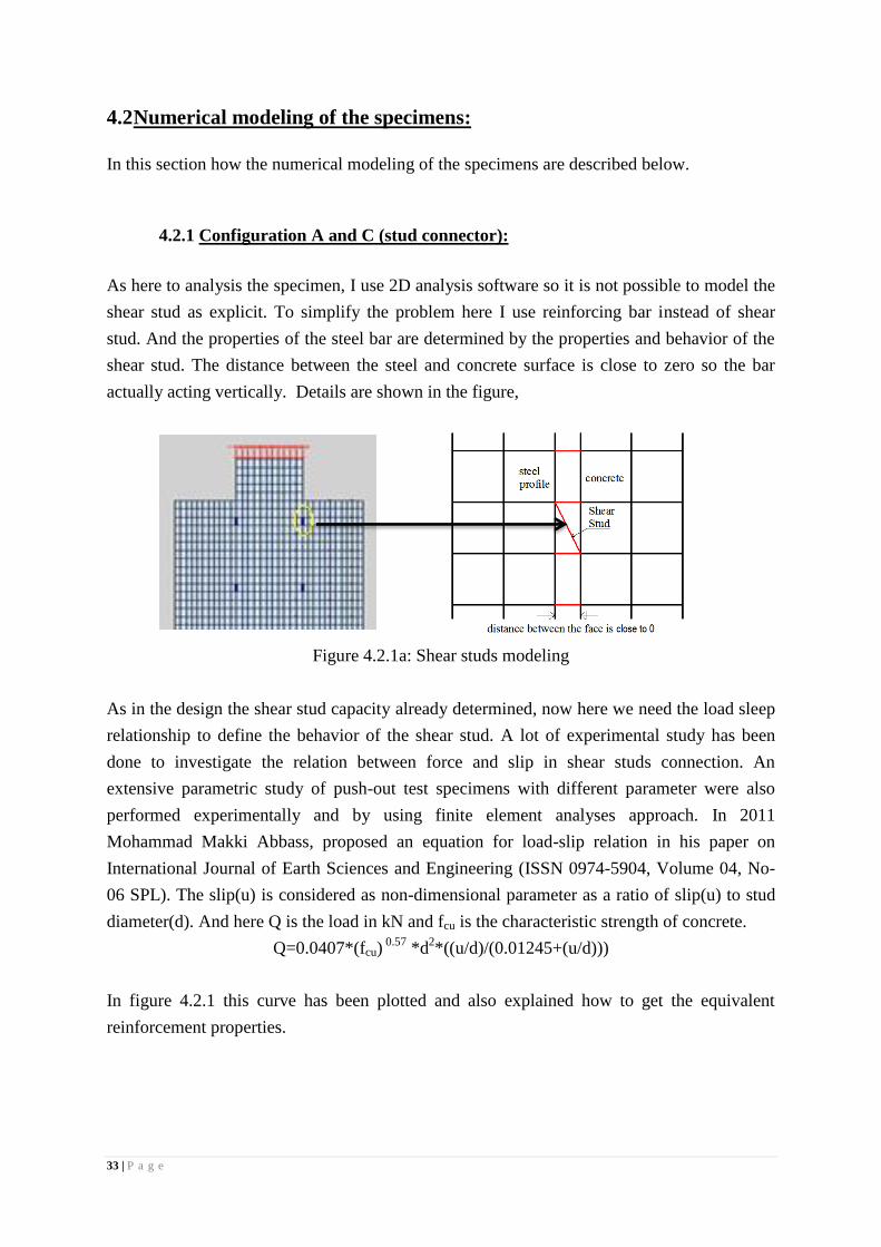
4.2.1 Configuration A and C (stud connector):
As here to analysis the specimen, I use 2D analysis software so it is not possible to model the
shear stud as explicit. To simplify the problem here I use reinforcing bar instead of shear
stud. And the properties of the steel bar are determined by the properties and behavior of the
shear stud. The distance between the steel and concrete surface is close to zero so the bar
actually acting vertically. Details are shown in the figure,
Figure 4.2.1a: Shear studs modeling
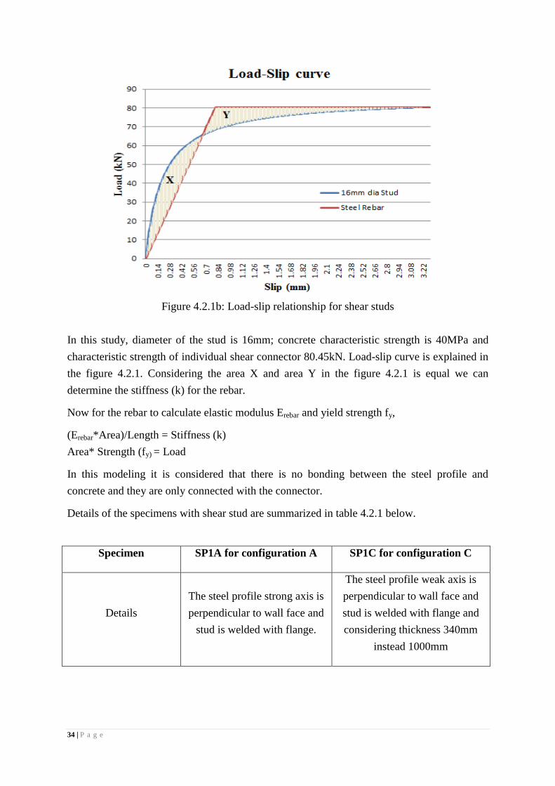
As in the design the shear stud capacity already determined, now here we need the load sleep
relationship to define the behavior of the shear stud. A lot of experimental study has been
done to investigate the relation between force and slip in shear studs connection. An
extensive parametric study of push-out test specimens with different parameter were also
performed experimentally and by using finite element analyses approach. In 2011
Mohammad Makki Abbass, proposed an equation for load-slip relation in his paper on
International Journal of Earth Sciences and Engineering (ISSN 0974-5904, Volume 04, No-
06 SPL). The slip(u) is considered as non-dimensional parameter as a ratio of slip(u) to stud
diameter(d). And here Q is the load in kN and fcu is the characteristic strength of concrete.
Q=0.0407*(fcu) 0.57
*d2*((u/d)/(0.01245+(u/d)))
In figure 4.2.1 this curve has been plotted and also explained how to get the equivalent
reinforcement properties.
34 | P a g e
Figure 4.2.1b: Load-slip relationship for shear studs
In this study, diameter of the stud is 16mm; concrete characteristic strength is 40MPa and
characteristic strength of individual shear connector 80.45kN. Load-slip curve is explained in
the figure 4.2.1. Considering the area X and area Y in the figure 4.2.1 is equal we can
determine the stiffness (k) for the rebar.
Now for the rebar to calculate elastic modulus Erebar and yield strength fy,
(Erebar*Area)/Length = Stiffness (k)
Area* Strength (fy) = Load
In this modeling it is considered that there is no bonding between the steel profile and
concrete and they are only connected with the connector.
Details of the specimens with shear stud are summarized in table 4.2.1 below.
Specimen SP1A for configuration A SP1C for configuration C
Details
The steel profile strong axis is
perpendicular to wall face and
stud is welded with flange.
The steel profile weak axis is
perpendicular to wall face and
stud is welded with flange and
considering thickness 340mm
instead 1000mm
35 | P a g e
Figure
No of stud connection 12 12
Failure load and mode 965kN in connection failure 965kN in connection failure
Table 4.2.1: Details of Specimen SP1A and SP2C
4.1.2 Configuration B and D (plate connector):
In case of plate connector it is tough to
model those specimens in a 2D program as
the problem is 3D. So here I proposed
some way to model those specimens. In
stud and tie model we consider that the
load transferred in concrete with 45o. So to
simplify the problem, I consider 60mm
length of concrete below the connector is
perfectly bonded with steel profile.
Now here I proposed couple of ways to model these specimens in VecTor2.0.
4.2.2.1 Model01:
In first case, it is considered that concrete is perfectly bonded 60mm with flange at 190mm
spacing, because the spacing between the plates is 250mm. There are 4 bonds of 60mm to
represent 4 plates in each side. To define the concrete and steel profile here layer of element
one top of another has been used. Now there is a problem with this model is, if I use one layer
of material in top of another layer of material then both elements are perfectly bonded in
those place. To solve this, the concrete parts where the load expected to transmit are
separated from the profile and connected in the bonded part. Now it become like a strip of
material which connected in the 60mm bonded zone. So only bonded part is transmitting the
load to concrete. In this case, the failure is occurring at the element where they are perfectly
36 | P a g e
bonded by local crushing. So to prevent this high strength element property is used in that
bond zone places. The steel profile will fail by yielding at around 1200kN so to ensure and
see the failure of connection, the strength of steel material is increased to 1000MPa. All the
reinforcement is designed as smeared reinforcement. Specimen is supported at the bottom.
Steel profile and the concrete encaged within the flange dose not continue until the bottom of
the specimen but it stopped at 100mm before from the bottom. So at the bottom of the profile
is hollow and it is not supported and can move downward. In this case displacement is
applied in steel profile at the top.
Figure 4.2.2.1: Modeling of specimen SPBM1 and SPDM1
SPBM1: specimen B and finite element modeling is done according to the procedure
describe above.
SPDM1: specimen D and finite element modeling is done according to the procedure
describe above.
4.2.2.2 Model02:
To simplify the problem and get better result from the program VecTor2.0 only one layer of
material is used to model. So in proposed Model02 is define by the layer of concrete and steel
profile to transfer load. In the steel profile only flange is define and connected with the plates.
The thickness of the flange and plate is 98mm as in the main specimen. Concrete is perfectly
bonded with the plate and 60mm with the flange just below the plate. As here only the flange
of the steel profile is acting to transfer load from steel to concrete, to ensure failure is not
occurring in steel, high strength of steel material is used to define the flange. Now in the
concrete part there is a problem with thickness. In this case concrete two concrete thicknesses
is used one is 98mm and another is 340 mm.In 98mm it is consider as a strip of the total
specimen and in 340mm it is consider as the total thickness of concrete is work to carry the
load. This idea is used to model both configuration B and D.
Details of the specimen of Model02 are summarized in the table 4.2.2.2 below.
Perfectly bonded
60mm@190mm
spacing
37 | P a g e
Specimen Concrete thickness 98mm Concrete thickness 340mm
SPBM2
for
Config.B
Details Configuration B and FEM
modeling is done as Model03.
Configuration B and FEM
modeling is done as Model03.
Figure
No. of
connection 8 8
Expected
Failure load 897kN 897kN
SPDM2
for
Config.D
Details Configuration D and FEM
modeling is done as Model03.
Configuration D and FEM
modeling is done as Model03.
Figure
No. of
connection 8 8
Expected
Failure load 897kN 897kN
Table 4.2.2.2: Specimen details of SPBM2 and SPDM2
4.2.3 Configuration E (studs and plate connector):
This specimen has both plate connector and shear stud. It has total 4 plate connector and 4
shear studs, where 2 in each side. In the table 4.2.3 it is explained below. As it has different
types of connector and also in different side so to model this specimen in 2D is little bit
difficult. So to solve this problem in this proposed model, the specimen for the plate
connector and shear studs are modeled separately. The analysis for each type of connector is
done in separate model and later calculation is done together to get the combine effect. For
38 | P a g e
the stud here the modeling of the specimen is done as it is described before in case of
specimen A and B. In this case the number of stud is 4 instead of 12. In case of plate, there
two ways to model as it explained before. In this case I follow the proposed Model01 for
modeling the plate connector; difference is the number of plate is 4 instead of 8.
Details of the specimen of configuration E are summarized in the table 4.2.3 below.
Specimen With stud With plate connector
SPEM1
for
Config. E
Details
The steel profile weak axis is
perpendicular to wall face and stud
is welded with flange and
considering thickness 340mm
instead 1000mm
4 plate connector
according. 2 in each side
having 340mm spacing.
Figure
No. of connection 4 4
Expected Failure load 771kN
Table 4.2.3: Specimen details of SPEM2
39 | P a g e
0
200
400
600
800
1000
1200
0
-0.2
57
-0.5
13
-0.7
7
-1.0
27
-1.2
85
-1.5
45
-1.8
05
-2.0
65
-2.3
25
-2.5
85
-2.8
45
-3.1
05
-3.3
65
Load
(kN
)
Slip (mm)
Load vs Slip Curve
SP1A
CHAPTER: FIVE
RESULT AND INTERPRETATION
In this chapter result from the numerical analysis is described and explained. And the also the
data obtained from the results are also interpreted and compared with the expected result. For
this the post processor for VecTor2.0 called Augustus is used.
5.1Configuration A and C (shear stud):
5.1.1 Configuration A: (SP1A)
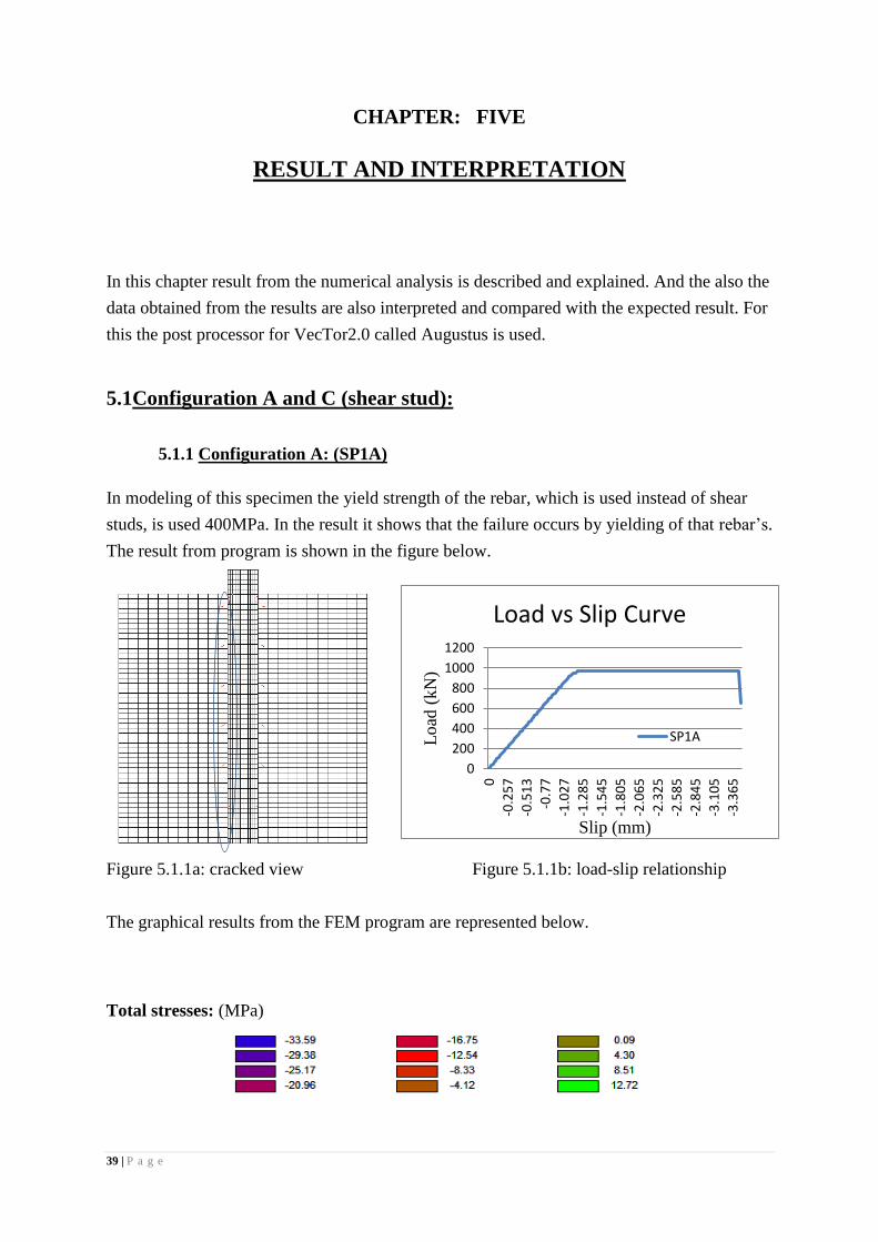
In modeling of this specimen the yield strength of the rebar, which is used instead of shear
studs, is used 400MPa. In the result it shows that the failure occurs by yielding of that rebar’s.
The result from program is shown in the figure below.
Figure 5.1.1a: cracked view Figure 5.1.1b: load-slip relationship
The graphical results from the FEM program are represented below.
Total stresses: (MPa)
40 | P a g e
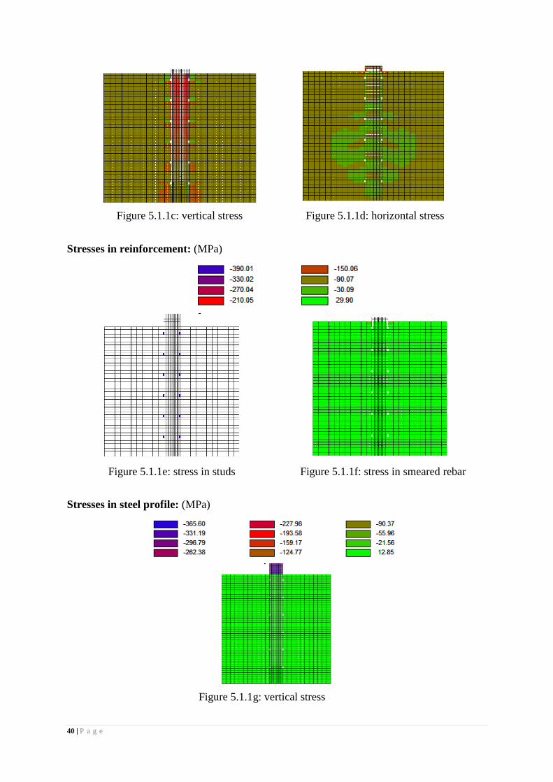
Figure 5.1.1c: vertical stress Figure 5.1.1d: horizontal stress
Stresses in reinforcement: (MPa)
Figure 5.1.1e: stress in studs Figure 5.1.1f: stress in smeared rebar
Stresses in steel profile: (MPa)
Figure 5.1.1g: vertical stress
41 | P a g e
From the result above it’s clearly seen that the stresses in concrete are much lower than the
concrete strength even though there is some crack generate. So it is obvious that the failure
will be in the connection. Total restraining force is 970kN. The stresses in smeared
reinforcement are also less than its capacity. In steel profile some elements are close to yield
at the top free part but it does not fail by yielding.
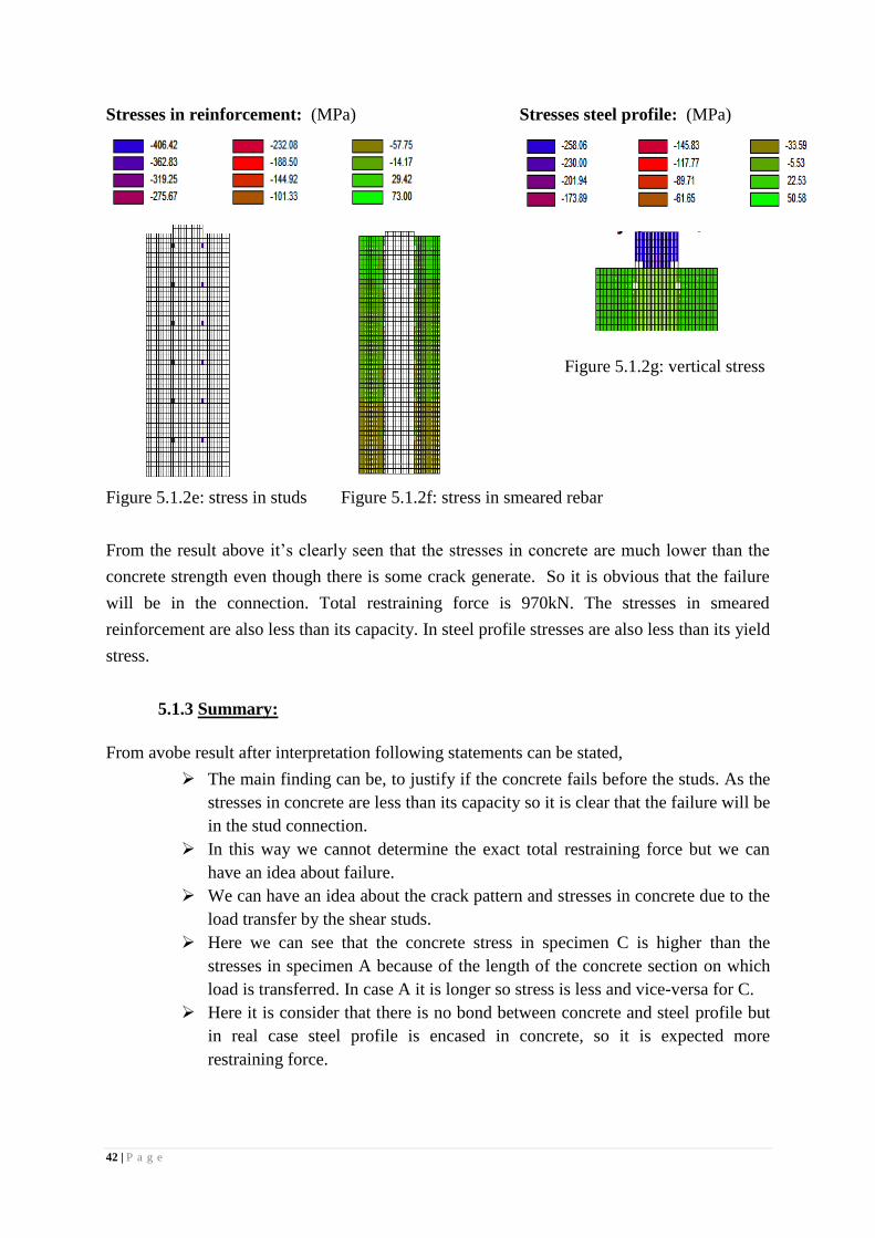
5.1.2 Configuration C (SP1C)
In this case also, in modeling the yield stress for the rebar which is used instead of shear studs
is 400MPa. In the result it shows that the failure occurs by yielding of that rebar’s.
The result from program is shown in the figure below.
Figure 5.1.2a: cracked view Figure 5.1.2b: load-slip relationship
The graphical results from the FEM program are represented below.
Total stresses: (MPa)
Figure 5.1.2c: vertical stress Figure 5.1.2d: horizontal stress
42 | P a g e
Stresses in reinforcement: (MPa) Stresses steel profile: (MPa)
Figure 5.1.2e: stress in studs Figure 5.1.2f: stress in smeared rebar
From the result above it’s clearly seen that the stresses in concrete are much lower than the
concrete strength even though there is some crack generate. So it is obvious that the failure
will be in the connection. Total restraining force is 970kN. The stresses in smeared
reinforcement are also less than its capacity. In steel profile stresses are also less than its yield
stress.
5.1.3 Summary:
From avobe result after interpretation following statements can be stated,
The main finding can be, to justify if the concrete fails before the studs. As the
stresses in concrete are less than its capacity so it is clear that the failure will be
in the stud connection.
In this way we cannot determine the exact total restraining force but we can
have an idea about failure.
We can have an idea about the crack pattern and stresses in concrete due to the
load transfer by the shear studs.
Here we can see that the concrete stress in specimen C is higher than the
stresses in specimen A because of the length of the concrete section on which
load is transferred. In case A it is longer so stress is less and vice-versa for C.
Here it is consider that there is no bond between concrete and steel profile but
in real case steel profile is encased in concrete, so it is expected more
restraining force.
Figure 5.1.2g: vertical stress
43 | P a g e
5.2 Configuration B and D (plate connector):
5.2.1 Model01:
In this case total vertical restraining force for configuration B is 1027kN and Configuration D
is 1629kN. Failure occurred in concrete and the crack developed at the bottom and top of the
specimen close to the steel profile.
The results from the analysis are shown in the table 5.2.1.
Specimen Configuration B (SPBM1) Configuration D (SPDM1)
Failure load 1027kN 1629kN
Load-slip curve
Crack pattern
Table 5.2.1: FEM analysis result for SPBM1 and SPDM1
44 | P a g e
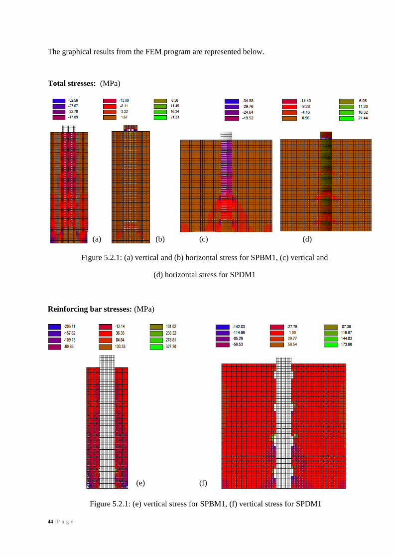
The graphical results from the FEM program are represented below.
Total stresses: (MPa)
Reinforcing bar stresses: (MPa)
Figure 5.2.1: (a) vertical and (b) horizontal stress for SPBM1, (c) vertical and
(d) horizontal stress for SPDM1
(d) (c) (b) (a)
Figure 5.2.1: (e) vertical stress for SPBM1, (f) vertical stress for SPDM1
(f) (e)
45 | P a g e
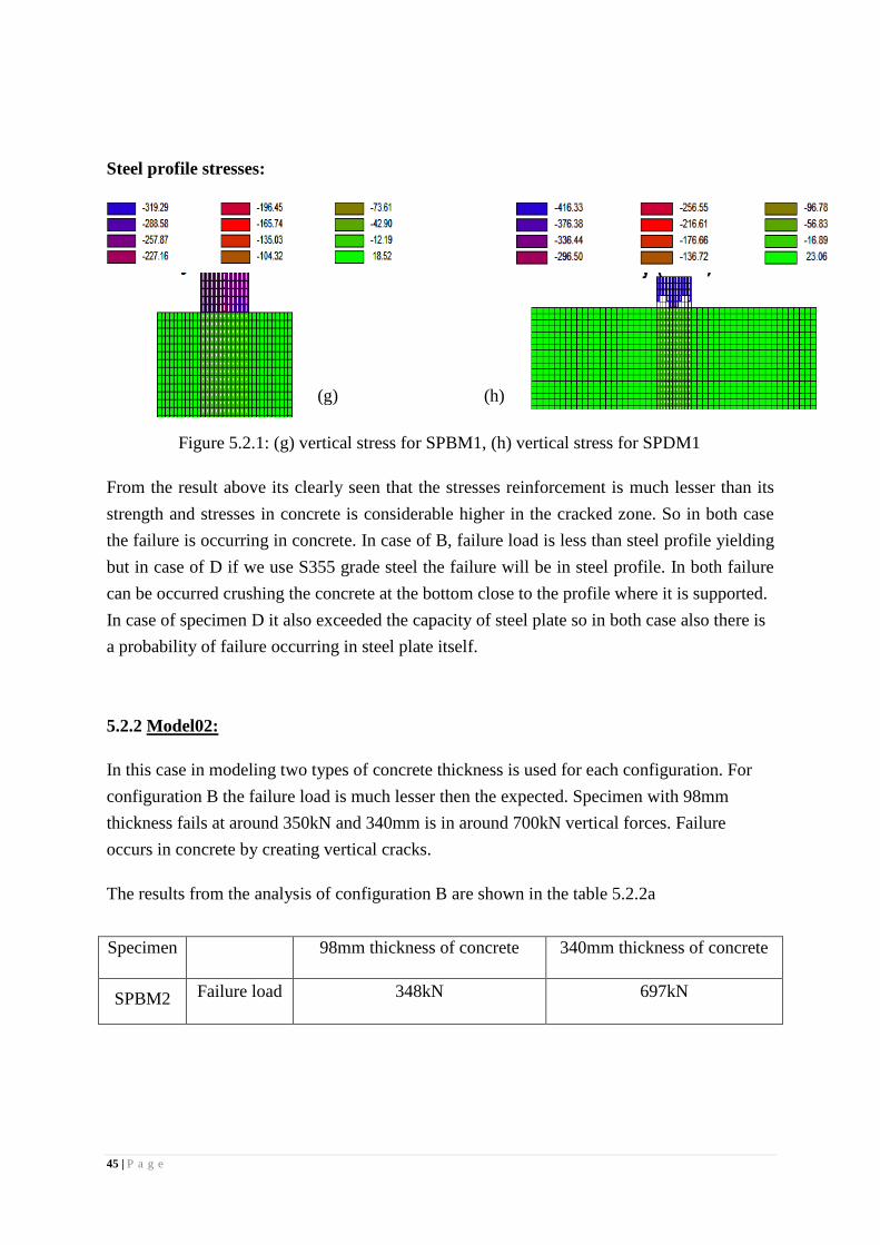
Steel profile stresses:
From the result above its clearly seen that the stresses reinforcement is much lesser than its
strength and stresses in concrete is considerable higher in the cracked zone. So in both case
the failure is occurring in concrete. In case of B, failure load is less than steel profile yielding
but in case of D if we use S355 grade steel the failure will be in steel profile. In both failure
can be occurred crushing the concrete at the bottom close to the profile where it is supported.
In case of specimen D it also exceeded the capacity of steel plate so in both case also there is
a probability of failure occurring in steel plate itself.
5.2.2 Model02:
In this case in modeling two types of concrete thickness is used for each configuration. For
configuration B the failure load is much lesser then the expected. Specimen with 98mm
thickness fails at around 350kN and 340mm is in around 700kN vertical forces. Failure
occurs in concrete by creating vertical cracks.
The results from the analysis of configuration B are shown in the table 5.2.2a
Specimen 98mm thickness of concrete 340mm thickness of concrete
SPBM2 Failure load 348kN 697kN
Figure 5.2.1: (g) vertical stress for SPBM1, (h) vertical stress for SPDM1
(g) (h)
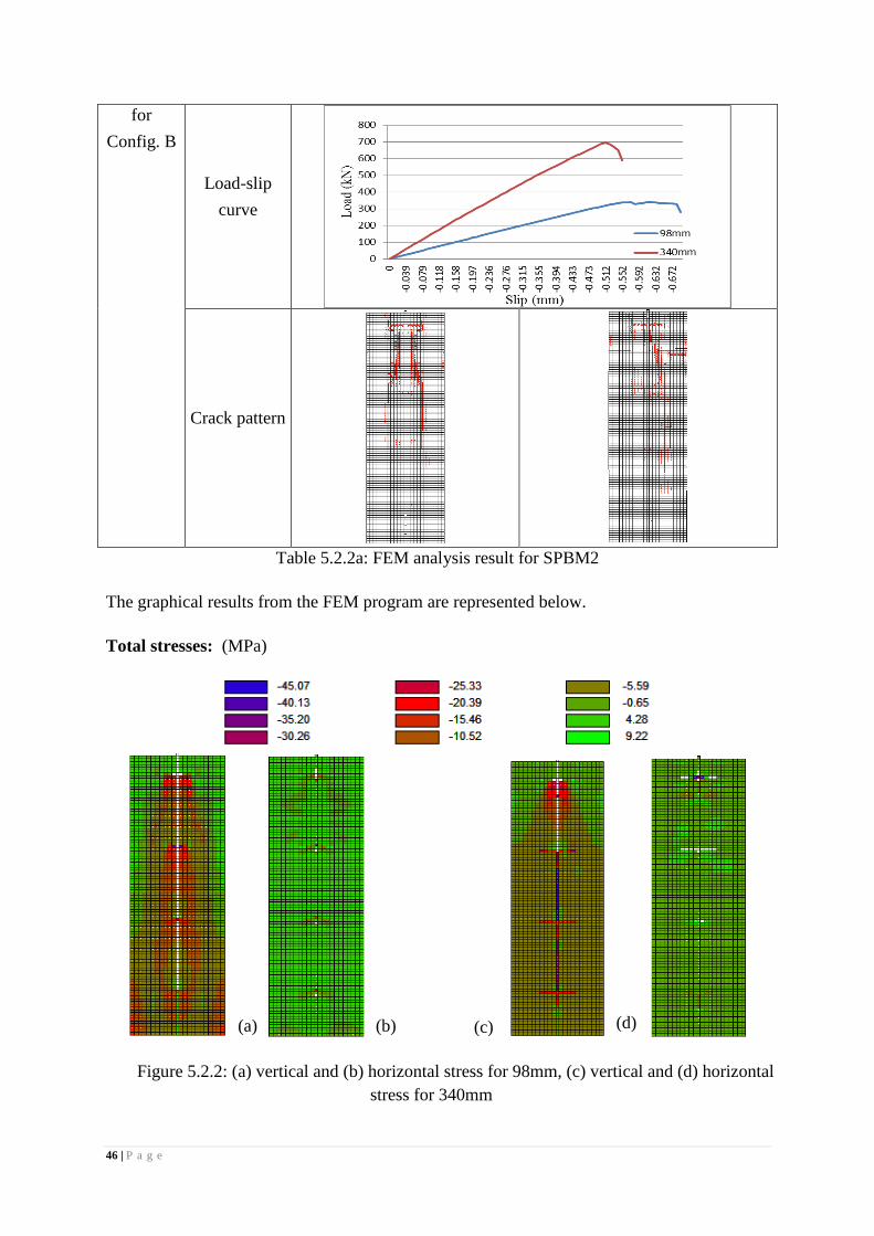
46 | P a g e
for
Config. B
Load-slip
curve
Crack pattern
Table 5.2.2a: FEM analysis result for SPBM2
The graphical results from the FEM program are represented below.
Total stresses: (MPa)
Figure 5.2.2: (a) vertical and (b) horizontal stress for 98mm, (c) vertical and (d) horizontal
stress for 340mm
(a) (c) (d) (b)
47 | P a g e
Stresses in reinforcement: (MPa)
From the above results, it’s clearly seen that there is a vertical crack generates in the concrete
and its split the concrete to fail. If we consider average then the failure load can be around
550kN. The stress distribution in the concrete steel rebar has been shown. In this case the
failure load is less than actual steel profile yielding for both 98mm and 340mm thickness of
concrete. And the failure is accruing due to the failure in concrete as the stresses in rebar are
much lesser than its strength. The elements just below the frist plate connector are in higher
stresses.
For configuration D, specimen with 98mm thickness fails at around 1090kN and 340mm is in
around 1960kN vertical forces. Failure occurs in concrete by creating vertical cracks.
The results from the analysis of configuration D are shown in the table 5.2.2b
Specimen 98mm thickness of concrete 340mm thickness of concrete
SPDM2 for
Config. D
Failure
load 1092kN 1957kN
Figure 5.2.2: (e) stress in steel for 98mm, (f) stress in steel for 340mm
(e) (f)
48 | P a g e
Load-slip
curve
Crack
pattern
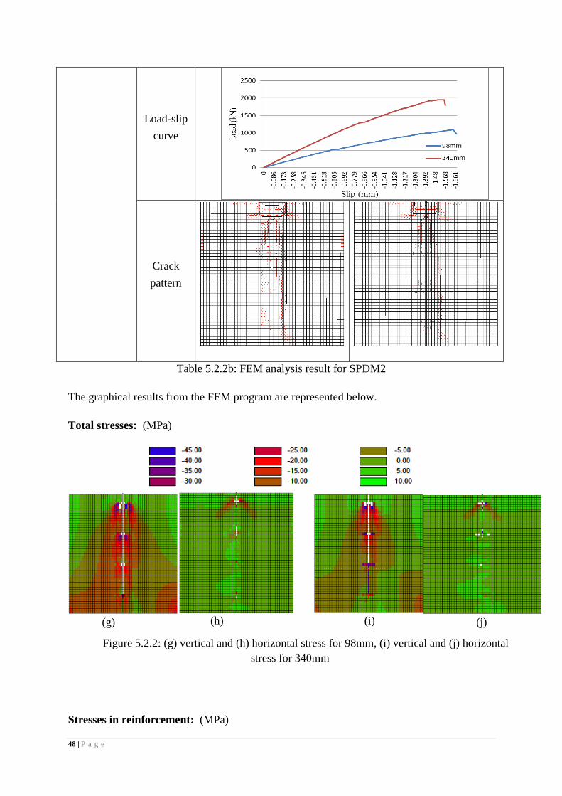
Table 5.2.2b: FEM analysis result for SPDM2
The graphical results from the FEM program are represented below.
Total stresses: (MPa)
Stresses in reinforcement: (MPa)
Figure 5.2.2: (g) vertical and (h) horizontal stress for 98mm, (i) vertical and (j) horizontal
stress for 340mm
(g) (h) (i) (j)
49 | P a g e
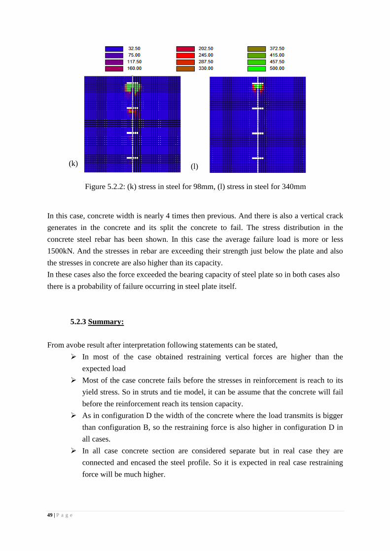
In this case, concrete width is nearly 4 times then previous. And there is also a vertical crack
generates in the concrete and its split the concrete to fail. The stress distribution in the
concrete steel rebar has been shown. In this case the average failure load is more or less
1500kN. And the stresses in rebar are exceeding their strength just below the plate and also
the stresses in concrete are also higher than its capacity.
In these cases also the force exceeded the bearing capacity of steel plate so in both cases also
there is a probability of failure occurring in steel plate itself.
5.2.3 Summary:
From avobe result after interpretation following statements can be stated,
In most of the case obtained restraining vertical forces are higher than the
expected load
Most of the case concrete fails before the stresses in reinforcement is reach to its
yield stress. So in struts and tie model, it can be assume that the concrete will fail
before the reinforcement reach its tension capacity.
As in configuration D the width of the concrete where the load transmits is bigger
than configuration B, so the restraining force is also higher in configuration D in
all cases.
In all case concrete section are considered separate but in real case they are
connected and encased the steel profile. So it is expected in real case restraining
force will be much higher.
Figure 5.2.2: (k) stress in steel for 98mm, (l) stress in steel for 340mm
(k) (l)
50 | P a g e
As modeling is done in 2D program so the property is not define in other
dimension. The results obtained from this numerical study are not exactly perfect
but it gives an idea about the failure.
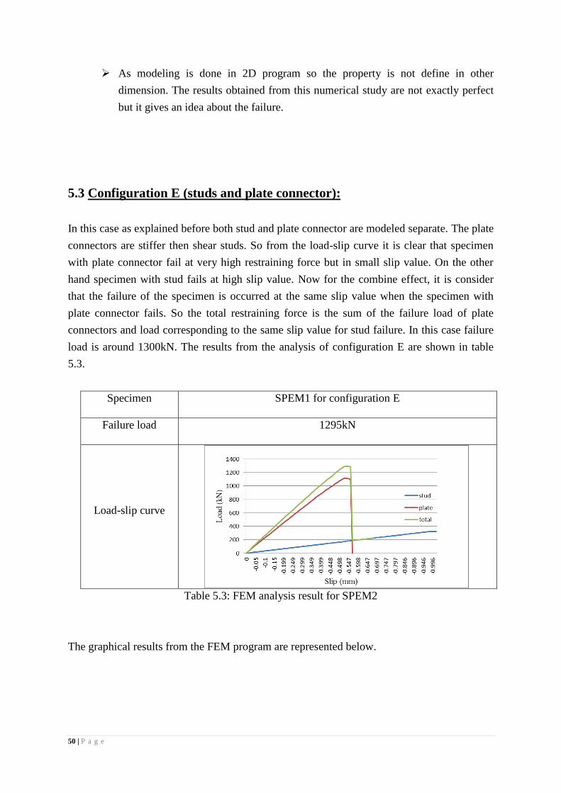
5.3 Configuration E (studs and plate connector):
In this case as explained before both stud and plate connector are modeled separate. The plate
connectors are stiffer then shear studs. So from the load-slip curve it is clear that specimen
with plate connector fail at very high restraining force but in small slip value. On the other
hand specimen with stud fails at high slip value. Now for the combine effect, it is consider
that the failure of the specimen is occurred at the same slip value when the specimen with
plate connector fails. So the total restraining force is the sum of the failure load of plate
connectors and load corresponding to the same slip value for stud failure. In this case failure
load is around 1300kN. The results from the analysis of configuration E are shown in table
5.3.
Specimen SPEM1 for configuration E
Failure load 1295kN
Load-slip curve
Table 5.3: FEM analysis result for SPEM2
The graphical results from the FEM program are represented below.
51 | P a g e
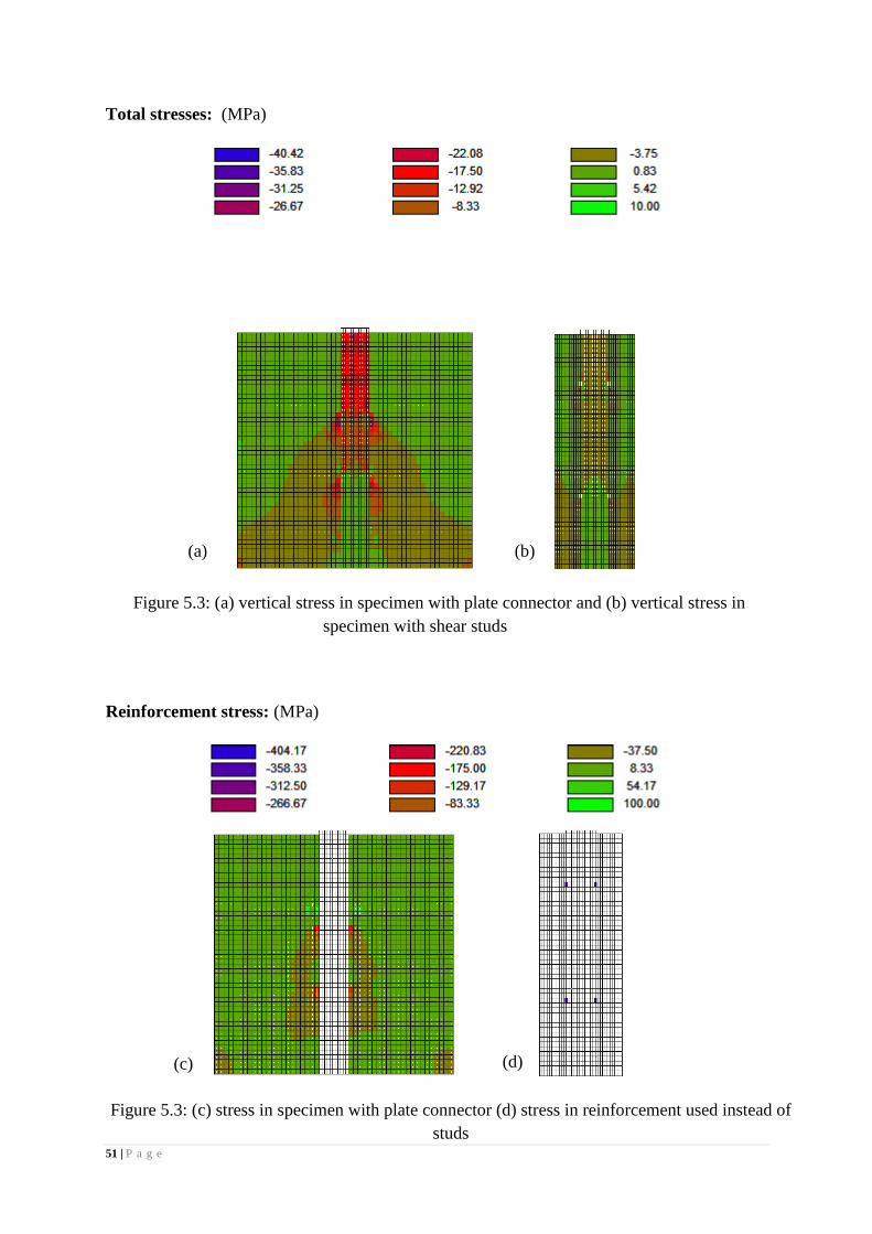
Total stresses: (MPa)
Reinforcement stress: (MPa)
Figure 5.3: (a) vertical stress in specimen with plate connector and (b) vertical stress in
specimen with shear studs
(a) (b)
Figure 5.3: (c) stress in specimen with plate connector (d) stress in reinforcement used instead of
studs
(c) (d)
52 | P a g e
In this case the failure load is 1295kN which little bit higher then the steel profile capacity
but much higher than our expected value. In specimen with plate connector, the stress in
reinforcement is far below the yield stress so failure is in concrete. Moreover this is an idea
only as the modeling is done with 2D program.
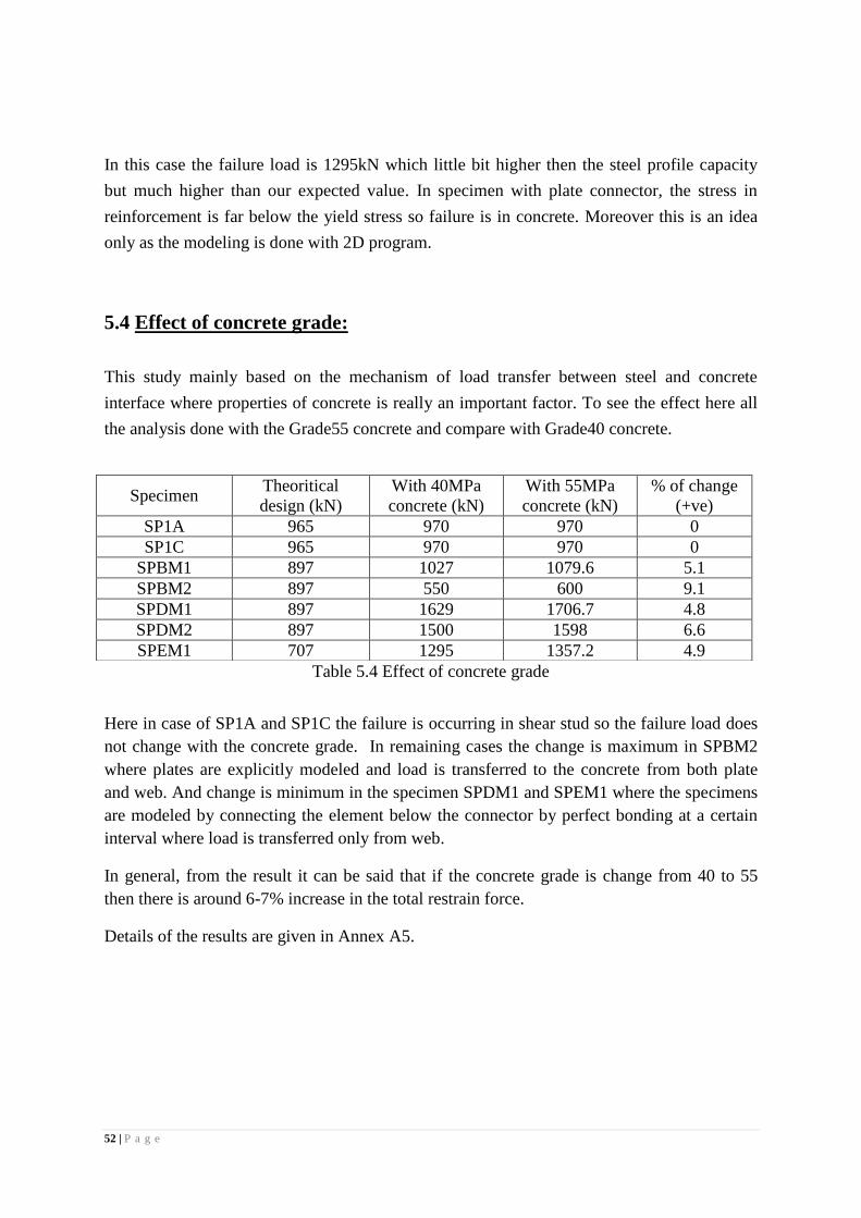
5.4 Effect of concrete grade:
This study mainly based on the mechanism of load transfer between steel and concrete
interface where properties of concrete is really an important factor. To see the effect here all
the analysis done with the Grade55 concrete and compare with Grade40 concrete.
Table 5.4 Effect of concrete grade
Here in case of SP1A and SP1C the failure is occurring in shear stud so the failure load does
not change with the concrete grade. In remaining cases the change is maximum in SPBM2
where plates are explicitly modeled and load is transferred to the concrete from both plate
and web. And change is minimum in the specimen SPDM1 and SPEM1 where the specimens
are modeled by connecting the element below the connector by perfect bonding at a certain
interval where load is transferred only from web.
In general, from the result it can be said that if the concrete grade is change from 40 to 55
then there is around 6-7% increase in the total restrain force.
Details of the results are given in Annex A5.
Specimen Theoritical
design (kN)
With 40MPa
concrete (kN)
With 55MPa
concrete (kN)
% of change
(+ve)
SP1A 965 970 970 0
SP1C 965 970 970 0
SPBM1 897 1027 1079.6 5.1
SPBM2 897 550 600 9.1
SPDM1 897 1629 1706.7 4.8
SPDM2 897 1500 1598 6.6
SPEM1 707 1295 1357.2 4.9
53 | P a g e
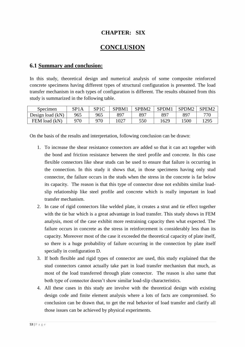
CHAPTER: SIX
CONCLUSION
6.1 Summary and conclusion:
In this study, theoretical design and numerical analysis of some composite reinforced
concrete specimens having different types of structural configuration is presented. The load
transfer mechanism in each types of configuration is different. The results obtained from this
study is summarized in the following table.
Specimen SP1A SP1C SPBM1 SPBM2 SPDM1 SPDM2 SPEM2
Design load (kN) 965 965 897 897 897 897 770
FEM load (kN) 970 970 1027 550 1629 1500 1295
On the basis of the results and interpretation, following conclusion can be drawn:
1. To increase the shear resistance connectors are added so that it can act together with
the bond and friction resistance between the steel profile and concrete. In this case
flexible connectors like shear studs can be used to ensure that failure is occurring in
the connection. In this study it shows that, in those specimens having only stud
connector, the failure occurs in the studs when the stress in the concrete is far below
its capacity. The reason is that this type of connector dose not exhibits similar load-
slip relationship like steel profile and concrete which is really important in load
transfer mechanism.
2. In case of rigid connectors like welded plate, it creates a strut and tie effect together
with the tie bar which is a great advantage in load transfer. This study shows in FEM
analysis, most of the case exhibit more restraining capacity then what expected. The
failure occurs in concrete as the stress in reinforcement is considerably less than its
capacity. Moreover most of the case it exceeded the theoretical capacity of plate itself,
so there is a huge probability of failure occurring in the connection by plate itself
specially in configuration D.
3. If both flexible and rigid types of connector are used, this study explained that the
stud connectors cannot actually take part in load transfer mechanism that much, as
most of the load transferred through plate connector. The reason is also same that
both type of connector doesn’t show similar load-slip characteristics.
4. All these cases in this study are involve with the theoretical design with existing
design code and finite element analysis where a lots of facts are compromised. So
conclusion can be drawn that, to get the real behavior of load transfer and clarify all
those issues can be achieved by physical experiments.
54 | P a g e
6.2 Suggestion for future work:
The present study covers only the design and numerical modeling but to get overall behavior
of load transfer mechanism of hybrid structure, extensive and more details studies are
required.
Some aspects are listed below as scope of future work in this area:
1. The investigation can be carried out in big range for experimental work in the
laboratory to get the actual behavior and compare with the obtained result in this
study.
2. In this study, most of the cases the failure load for the specimen is more than the steel
profile capacity if S355 grade steel is used. So it suggested that instead of S355 higher
grade steel should use.
3. An extensive parametric study can be done having different concrete grade, steel
profile, connector types, configuring and reinforcement.
4. It is clear from the study that the load transfer mechanism is directly related with the
area of concrete where the load is transmitted, so there can be an investigation about
the effective width and thickness of the concrete zone.
5. In this study while modeling a lot of facts are compromise like reinforcement are
consider as smeared instead of discrete, so further study can by performing more
accurate modeling to get more accurate result and conclution.
55 | P a g e
BIBLIOGRAPHY
1. EC4 (2004). EN 1994-1-1 Eurocode 4- Design of composite steel and concrete
structures- Part 1-1: General rules and rules for buildings.
2. Eurocode-2 (2004). Design of concrete structures-Part 1: General rules and rules for
buidings. EN1992-1-1, European Committee for Standardization.
3. State of A on the identification of the fundamental force transfer mechanisms at steel-
concrete interface. Smartcoco Project, 2013.
4. A. Plumier et al. Design for shear of columns with several encased steel profiles. A
proposal. 2013.
5. C. Roeder et al., Shear connector requirements for embedded steel sections, Journal of
Structural Engineering, 1999.
6. W. Xue, M. Dind et al., Static Behavior and Theoretical Model of Stud Shear
Connectors, Journal of Bridge Engineering, 2008.
7. Li An & Krister Cederwall, Push-out Test on Studs in high strength and normal
strength concrete, J. Construct. Steel Res. Vol. 36, No. 1, pp. 15-29, 1996.
8. Md. Khasro Miah, Strain Behavior of Shear Connectors in Composite Structures,
DUET Journal, Vol. 1, Issue 1, June 2010.
9. H.B. Shim, Push-out tests on shear studs in high strength concrete, 2010 Korea
Concrete Institute, Seoul, ISBN 978-89-5708-181-5.
10. Mohammad Makki Abbass, Performance Evaluation of Shear Stud Connectors in
Composite Beams with Steel Plate and RCC slab, International Journal of Earth
Sciences and Engineering, ISSN 0974-5904, Volume 04, No 06 SPL, October 2011.
11. Buttry, K. E. (1965). Behavior of stud shear connectors in lightweight and normal-
weight concrete, Univ. of Missouri, Rolla, Mo. PhD.
12. Chapman, J. C. (1964). "Composite construction in steel and concrete - The behaviour
of composite beams." The Structural Engineer 42(4): 115-125.
13. Corley, G. W. & Hawkins, N. M. (1968b), `Shearhead reinforcement for slabs',
Journal of the American Concrete Institute 65, 811-824.
14. Hanswille, G. (2002). Push Out Tests with Groups of Studs, ECSC Steel RTD
Programme: Composite Bridge Design for Small and Medium Spans. Final report
7210-PR/113, Ch. 3, pp. 3-1, 3-43.
15. Hosaka, T., et al. (1998). "An experimental Study on Characteristics of Shear
Connectors in Composite Continuous Girders for Railway Bridges (in Japanese)."
Journal of structural Engineering, JSCE 44A: 1497-1504.
16. Boyan Mihaylov (2008), Behaviour of Deep Reinforced Concrete Beams under
Monotonic and Reversed Cyclic Load, Ph.D. thesis.
56 | P a g e
ANNEX
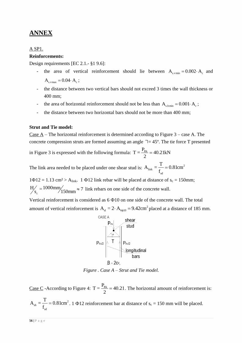
A SP1.
Reinforcements:
Design requirements [EC 2.1.- §1 9.6]:
- the area of vertical reinforcement should lie between s.vmin cA 0.002 A and
s.vmax cA 0.04 A ;
- the distance between two vertical bars should not exceed 3 times the wall thickness or
400 mm;
- the area of horizontal reinforcement should not be less than s.hmin cA 0.001 A ;
- the distance between two horizontal bars should not be more than 400 mm;
Strut and Tie model:
Case A – The horizontal reinforcement is determined according to Figure 3 – case A. The
concrete compression struts are formed assuming an angle = 45º. The tie force T presented
in Figure 3 is expressed with the following formula: RkPT = 40.21kN
2
The link area needed to be placed under one shear stud is: 2
link
sd
TA = 0.81cm
f
1Ф12 = 1.13 cm² > Alink. 1 Ф12 link rebar will be placed at distance of sc = 150mm;
c
1000mmH = 7s 150mm
link rebars on one side of the concrete wall.
Vertical reinforcement is considered as 6 Ф10 on one side of the concrete wall. The total
amount of vertical reinforcement is 2
sl 6 10A = 2 A 9.42cm placed at a distance of 185 mm.
Figure . Case A – Strut and Tie model.
Case C -According to Figure 4: RkPT = 40.21
2 . The horizontal amount of reinforcement is:
2
sh
sd
TA = 0.81cm
f . 1 Ф12 reinforcement bar at distance of sc = 150 mm will be placed.
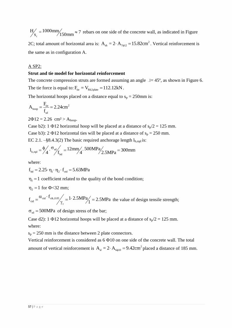
57 | P a g e
c
1000mmH = 7s 150mm
rebars on one side of the concrete wall, as indicated in Figure
2C; total amount of horizontal area is: 2
sh 7 12A = 2 A 15.82cm . Vertical reinforcement is
the same as in configuration A.
A SP2:
Strut and tie model for horizontal reinforcement
The concrete compression struts are formed assuming an angle = 45º, as shown in Figure 6.
The tie force is equal to: tie Rd,1plateF = V 112.12kN .
The horizontal hoops placed on a distance equal to sp = 250mm is:
2tiehoop
sd
FA 2.24cm
f
2Ф12 = 2.26 cm² > Ahoop.
Case b2): 1 Ф12 horizontal hoop will be placed at a distance of sp/2 = 125 mm.
Case b3): 2 Ф12 horizontal ties will be placed at a distance of sp = 250 mm.
EC 2.1. –§8.4.3(2) The basic required anchorage length lb,rqd is:
sdb,rqd
bd
500MPa12mml 300mm4 f 4 2.5MPa
where:
bd 1 2 ctdf 2.25 f 5.63MPa
1 1 coefficient related to the quality of the bond condition;
2 1 for Ф<32 mm;
ctd ctk,0.05ctd
c
f 1 2.5MPaf 2.5MPa1
the value of design tensile strength;
sd 500MPa
of design stress of the bar;
Case d2): 1 Ф12 horizontal hoops will be placed at a distance of sp/2 = 125 mm.
where:
sp = 250 mm is the distance between 2 plate connectors.
Vertical reinforcement is considered as 6 Ф10 on one side of the concrete wall. The total
amount of vertical reinforcement is 2
sl 6 10A = 2 A 9.42cm placed a distance of 185 mm.
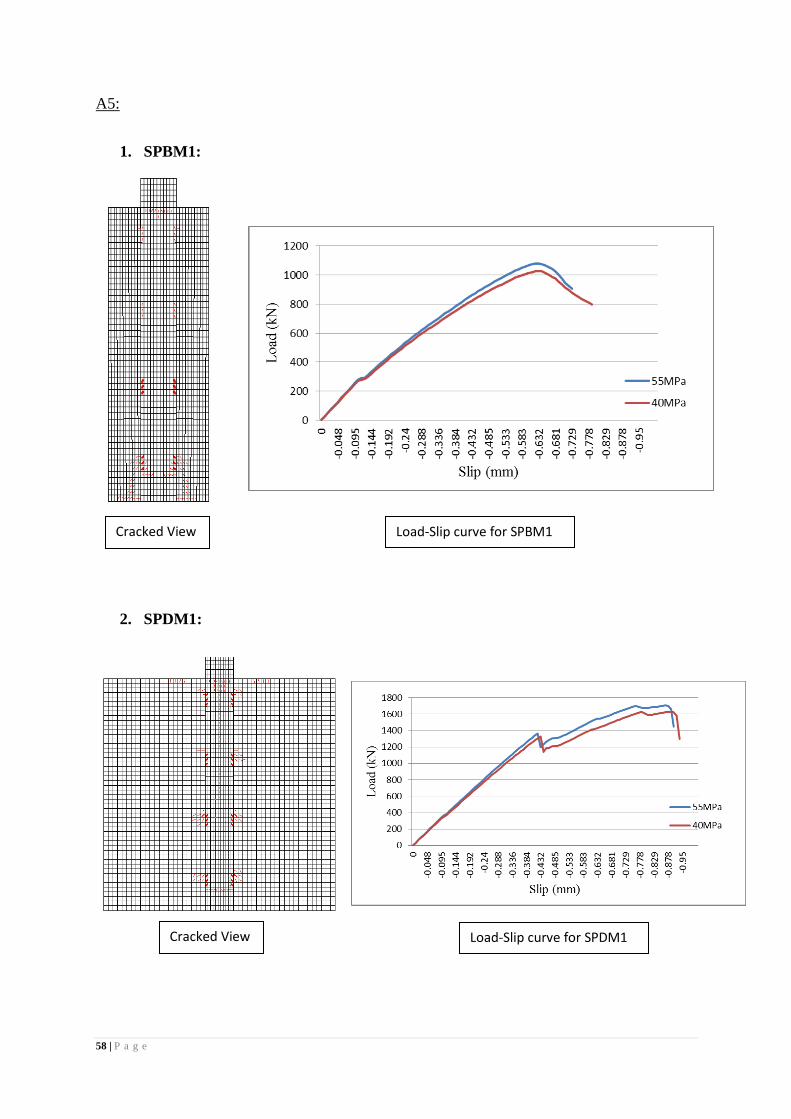
58 | P a g e
A5:
1. SPBM1:
2. SPDM1:
Cracked View Load-Slip curve for SPBM1
Cracked View Load-Slip curve for SPDM1
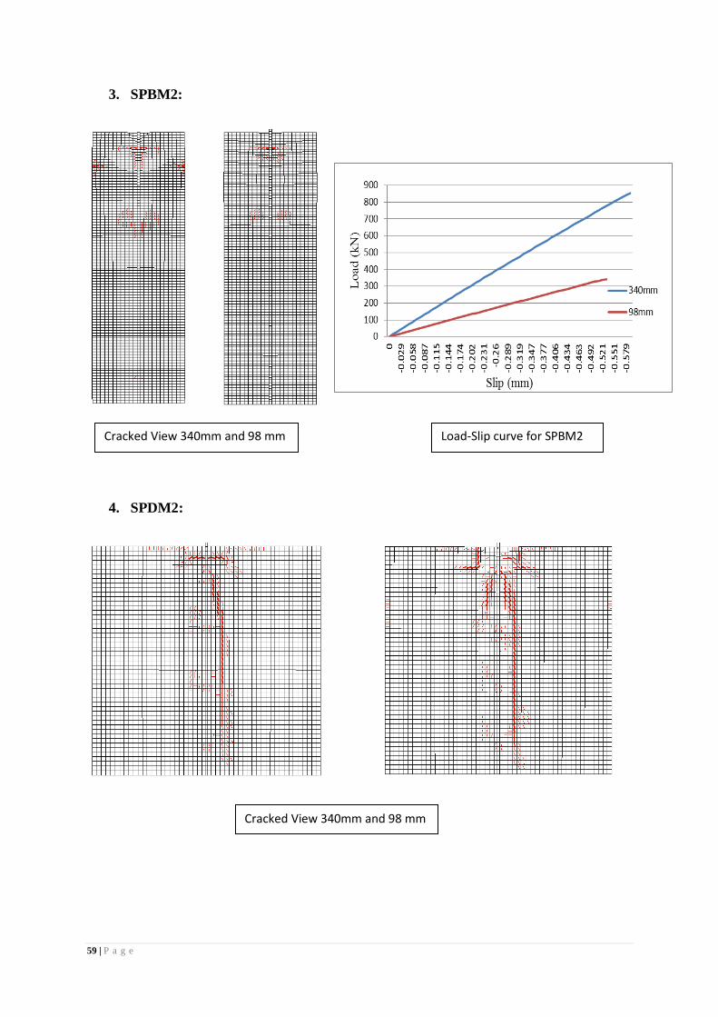
59 | P a g e
3. SPBM2:
4. SPDM2:
Cracked View 340mm and 98 mm Load-Slip curve for SPBM2
Cracked View 340mm and 98 mm
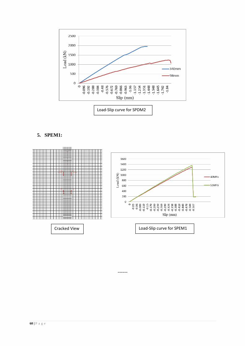
60 | P a g e
5. SPEM1:
------
Load-Slip curve for SPDM2
Cracked View Load-Slip curve for SPEM1