characterization of hybrid rocket motor swirl injectors · small-scale hybrid rocket test stand...
TRANSCRIPT
Small-Scale Hybrid Rocket Test Stand & Characterization of Swirl Injectors
By
Matt H. Summers
A Thesis Presented in Partial Fulfillment
Of the Requirements for the Degree
Master of Science in Aerospace Engineering
Approved April 2013 by the
Graduate Supervisory Committee:
Taewoo Lee, Chair
Kangping Chen
Valana Wells
ARIZONA STATE UNIVERSITY
May 2013

i
ABSTRACT
Derived from the necessity to increase testing capabilities of hybrid rocket motor (HRM)
propulsion systems for Daedalus Astronautics at Arizona State University, a small-scale
motor and test stand were designed and developed to characterize all components of the
system. The motor is designed for simple integration and setup, such that both the
forward-end enclosure and end cap can be easily removed for rapid integration of
components during testing. Each of the components of the motor is removable allowing
for a broad range of testing capabilities. While examining injectors and their potential it
is thought ideal to obtain the highest regression rates and overall motor performance
possible. The oxidizer and fuel are N2O and hydroxyl-terminated polybutadiene (HTPB),
respectively, due to previous experience and simplicity. The injector designs, selected for
the same reasons, are designed such that they vary only in the swirl angle. This system
provides the platform for characterizing the effects of varying said swirl angle on HRM
performance.

ii
DEDICATION
I would like to dedicate this work my wife, Sarah Summers, for her continued
support and encouragement, especially in those times when she was 9 months pregnant
or caring for our new born son, Parker Summers.

iii
ACKNOWLEDGMENTS
I would like to thank James Villarreal, Evan Olson, Chris Karpurk, Gaines Gibson,
Ryan Stoner, Richard Stelling, Jacob Dennis, Steven Shark, Brian Franz, and any other
person I may have forgot who helped me on this project over the past couple years.
I would like to thank my family for their continued support over the years to
complete my seven year journey at ASU.
I would also like to thank my committee members for taking the time to support
me in both the thesis review and defense process.

iv
TABLE OF CONTENTS
CHAPTER Page
LIST OF TABLES ........................................................................................................... viii
LIST OF FIGURES ........................................................................................................... xi
NOMENCLATURE ........................................................................................................ xiv
1 Introduction ................................................................................................................. 1
1.1 Background ............................................................................................... 1
1.2 Advantages of Hybrid Rocket Motors ........................................................... 3
1.3 Disadvantages of Hybrid Rocket Motors ....................................................... 3
1.4 Previous Research on Swirl Injectors ............................................................ 4
1.5 Background ............................................................................................... 6
1.6 Objective / Intent ........................................................................................ 9
1.7 Commercial Off-The-Shelf Components ....................................................... 9
1.8 Sizing of Components ............................................................................... 10
1.9 Design Validation ..................................................................................... 14
1.10 Test Stand Overview ............................................................................. 16
1.11 Electrical Setup ..................................................................................... 18
1.12 Sensor Selection ................................................................................... 22

CHAPTER Page
v
2 Preliminary Testing ................................................................................................... 23
2.1 Subsystem Testing .................................................................................................... 23
2.1.1 Cold Flow Testing ............................................................................. 24
2.1.2 Venturi Testing .................................................................................. 26
3 Experimental Design & Approach ............................................................................ 29
3.1 Design of Experiment ............................................................................... 29
3.1.1 Test Matrix ....................................................................................... 30
3.1.2 Test Order ......................................................................................... 32
3.1.3 Experiment Replication ...................................................................... 33
3.2 Blocking.................................................................................................. 33
3.3 Randomization ......................................................................................... 33
3.3.1 Fuel Grain Mixing ............................................................................. 34
3.3.2 Fuel Grain Curing .............................................................................. 37
3.3.3 Fuel Grain Density ............................................................................. 39
3.3.4 Extraneous Test Conditions ................................................................ 39
3.3.5 N2O Test Conditions .......................................................................... 40
3.3.6 Nozzle Erosion .................................................................................. 41
3.3.7 Erosion of Internal Components .......................................................... 42
3.3.8 Sensor Calibration ............................................................................. 43
3.3.9 Motor Assembly ................................................................................ 44
4 Results & Discussion ................................................................................................ 44
4.1 Test Runs ................................................................................................ 44
4.1.1 Test Run 1 ........................................................................................ 45
CHAPTER Page
vi
4.1.2 Test Run 2 ........................................................................................ 46
4.1.3 Test Run 3 ........................................................................................ 47
4.1.4 Test Run 4 ........................................................................................ 49
4.1.5 Test Run 5 ........................................................................................ 50
4.1.6 Test Run 6 ........................................................................................ 51
4.1.7 Test Run 7 ........................................................................................ 52
4.1.8 Test Run 8 ........................................................................................ 53
4.1.9 Test Run 9 ........................................................................................ 54
4.1.10 Test Run 10 ....................................................................................... 56
4.1.11 Test Run 11 ....................................................................................... 57
4.1.12 Test Run 12 ....................................................................................... 58
4.1.13 Test Run 13 ....................................................................................... 59
4.1.14 Test Run 14 ....................................................................................... 60
4.1.15 Test Run 15 ....................................................................................... 61
4.1.16 Test Run 16 ....................................................................................... 63
4.1.17 Test Run 17 ....................................................................................... 64
4.1.18 Test Run 18 ....................................................................................... 65
4.2 Discussion of Results ................................................................................ 66
4.3 Discussion of Test Anomalies .................................................................... 76
4.4 Large Impact of Results ............................................................................ 78
4.5 Confidence in Results ............................................................................... 79
5 Conclusions ............................................................................................................... 80
6 Future Work .............................................................................................................. 81

CHAPTER Page
vii
REFERENCES ................................................................................................................. 85
APPENDIX A ................................................................................................................... 87
APPENDIX B ................................................................................................................... 95
APPENDIX C ................................................................................................................. 106
APPENDIX D ................................................................................................................. 111

viii
LIST OF TABLES
Table Page
1. HTPB/N2O Combustion Parameters (Dennis, Shark, & Hernandez, 2009) ................. 11
2. Summarized Combustion Chamber Stress Calculations............................................. 12
3. Sensor Descriptions .................................................................................................... 22
4. Subsystem Test Matrix ............................................................................................... 24
5. Cold Flow Test Matrix ................................................................................................ 24
6. Hot Fire Test Matrix ................................................................................................... 31
7. Oxidizer Mass Flux Calculations ................................................................................ 32
8. Hybrid Grain Formulation .......................................................................................... 35
9. Example of Monitored Extraneous Test Conditions ................................................... 40
10. Nozzle Erosion and Performance Losses .................................................................... 42
11. Summary of Test Conditions for Test Run 1 .............................................................. 45
12. Summary of Motor Performance for Test Run 1 ........................................................ 46
13. Monitored Extraneous Test Conditions for Test Run 1 .............................................. 46
14. Summary of Test Conditions for Test Run 2 .............................................................. 47
15. Summary of Motor Performance for Test Run 2 ........................................................ 47
16. Monitored Extraneous Test Conditions for Test Run 2 .............................................. 47
17. Summary of Test Conditions for Test Run 3 .............................................................. 48
18. Summary of Motor Performance for Test Run 3 ........................................................ 48
19. Monitored Extraneous Test Conditions for Test Run 3 .............................................. 48
20. Summary of Test Conditions for Test Run 4 .............................................................. 49
21. Summary of Motor Performance for Test Run 4 ........................................................ 49

Table Page
ix
22. Monitored Extraneous Test Conditions for Test Run 4 .............................................. 49
23. Summary of Test Conditions for Test Run 5 .............................................................. 50
24. Summary of Motor Performance for Test Run 5 ........................................................ 50
25. Monitored Extraneous Test Conditions for Test Run 5 .............................................. 51
26. Summary of Test Conditions for Test Run 6 .............................................................. 51
27. Summary of Motor Performance for Test Run 6 ........................................................ 51
28. Monitored Extraneous Test Conditions for Test Run 6 .............................................. 52
29. Summary of Test Conditions for Test Run 7 .............................................................. 52
30. Summary of Motor Performance for Test Run 7 ........................................................ 53
31. Monitored Extraneous Test Conditions for Test Run 7 .............................................. 53
32. Summary of Test Conditions for Test Run 8 .............................................................. 54
33. Summary of Motor Performance for Test Run 8 ........................................................ 54
34. Monitored Extraneous Test Conditions for Test Run 8 .............................................. 54
35. Summary of Test Conditions for Test Run 9 .............................................................. 55
36. Summary of Motor Performance for Test Run 9 ........................................................ 55
37. Monitored Extraneous Test Conditions for Test Run 9 .............................................. 55
38. Summary of Test Conditions for Test Run 10 ............................................................ 56
39. Summary of Motor Performance for Test Run 10 ...................................................... 56
40. Monitored Extraneous Test Conditions for Test Run 10 ............................................ 56
41. Summary of Test Conditions for Test Run 11 ............................................................ 57
42. Summary of Motor Performance for Test Run 11 ...................................................... 57
43. Monitored Extraneous Test Conditions for Test Run 11 ............................................ 58
44. Summary of Test Conditions for Test Run 12 ............................................................ 58

Table Page
x
45. Summary of Motor Performance for Test Run 12 ...................................................... 58
46. Monitored Extraneous Test Conditions for Test Run 12 ............................................ 59
47. Summary of Test Conditions for Test Run 13 ............................................................ 59
48. Summary of Motor Performance for Test Run 13 ...................................................... 60
49. Monitored Extraneous Test Conditions for Test Run 13 ............................................ 60
50. Summary of Test Conditions for Test Run 14 ............................................................ 61
51. Summary of Motor Performance for Test Run 14 ...................................................... 61
52. Monitored Extraneous Test Conditions for Test Run 14 ............................................ 61
53. Summary of Test Conditions for Test Run 15 ............................................................ 62
54. Summary of Motor Performance for Test Run 15 ...................................................... 62
55. Monitored Extraneous Test Conditions for Test Run 15 ............................................ 62
56. Summary of Test Conditions for Test Run 16 ............................................................ 63
57. Summary of Motor Performance for Test Run 16 ...................................................... 63
58. Monitored Extraneous Test Conditions for Test Run 16 ............................................ 63
59. Summary of Test Conditions for Test Run 17 ............................................................ 64
60. Summary of Motor Performance for Test Run 17 ...................................................... 64
61. Monitored Extraneous Test Conditions for Test Run 17 ............................................ 65
62. Summary of Test Conditions for Test Run 18 ............................................................ 65
63. Summary of Motor Performance for Test Run 18 ...................................................... 65
64. Monitored Extraneous Test Conditions for Test Run 18 ............................................ 66
65. Fuel Density Measurement and Calculation Table ..................................................... 70

xi
LIST OF FIGURES
Figure Page
1. Theoretical Vacuum-Specific Impulse of Selected Oxidizers reacted with Hydroxyl-
Terminated Polybutadiene vs O/F Mixture Ratio ............................................................... 2
2. Small-Scale N2O/HTPB Hybrid Rocket Motor ........................................................... 7
3. Definition and Classification of Swirl Injectors ........................................................... 8
4. Description of Active Combustion Zone & General O/F Interactions ....................... 14
5. (Left) Density Distribution in CTRZ Swirl Flow Structure, (Right) Constant Pressure
Distribution in HRM ......................................................................................................... 15
6. Temperature Distribution of CTRZ and Flow Inside HRM ....................................... 16
7. Final Small-Scale Hybrid Test Stand Setup................................................................ 17
8. Side View of Final Small-Scale Hybrid Test Stand Setup ......................................... 18
9. Zoom-In Image of Figure 6, Wire Connections, Analog Pressure Sensor/N2O Inlet
from Tank, and Timer Relay (from left to right) .............................................................. 19
10. Top-Level Overview of Electrical Setup .................................................................... 20
11. Power/Circuit Box Overview (Dennis & Villarreal, 2010) ........................................ 21
12. Manual Control Box Overview (Dennis & Villarreal, 2010) ..................................... 22
13. Flow of Axial Injector Test ......................................................................................... 25
14. Flow of 60 deg. Swirl Injector .................................................................................... 25
15. Section View of Venturi Model .................................................................................. 26
16. Sample Data from Preliminary Venturi Testing (Lugo, Bowerman, & Summers,
2012) ................................................................................................................................. 28
17. Rendered 60 Degree Swirl Injector............................................................................. 29
18. Mixing of the HTPB Fuel ........................................................................................... 36

Figure Page
xii
19. Vacuum Process Setup ................................................................................................ 37
20. Individual Hybrid Casting Assembly in Heat Box ..................................................... 38
21. Typical Cured Hybrid Grain ....................................................................................... 38
22. Preliminary Static Fire Testing of Rocket Motor ....................................................... 45
23. Concrete Molds Curing of First Batch ........................................................................ 67
24. Example Concrete Mold After Grain Is Sectioned, Test #1 ....................................... 68
25. Regression Rate (Corrected) Characteristic Functions for Indicated Swirl Injector
Angles .............................................................................................................................. 69
26. Regression Rate (Uncorrected) vs Length of Nominal Tests at the Low-Oxidizer Flux
Test Condition ................................................................................................................... 72
27. Regression Rate (Uncorrected) vs Length of Nominal Tests at the High-Oxidizer Flux
Test Condition ................................................................................................................... 73
28. Actual vs Predicted Plot of Whole JMP Model .......................................................... 74
29. Regression Rate Plot vs Swirl Injection Angle ........................................................... 75
30. Regression Rate Plot vs Oxidizer Mass Flux .............................................................. 75
31. Flight-Ready Hybrid Rocket Motor Design with TVA Assembly ............................. 82
32. Flight-Ready Hybrid Rocket Motor Design during Successful Static Fire Test ........ 82
33. (Left) Aerospike Integrated into Small-Scale Hybrid Rocket Motor (Right) 3D Model
of Aerospike Nozzle Design ............................................................................................. 83
34. 0 Degree Injector Drawing.......................................................................................... 88
35. 15 Degree Injector Drawing........................................................................................ 89
36. 30 Degree Injector Drawing........................................................................................ 90
37. 42 Degree Injector Drawing........................................................................................ 91

Figure Page
xiii
38. 60 Degree Injector Drawing........................................................................................ 92
39. Injector Housing Drawing........................................................................................... 93
40. Venturi Drawing ......................................................................................................... 94
41. Data Table used for JMP Analysis Input .................................................................. 112
42. Calculated Contrasts from JMP Output .................................................................... 112
43. Calculated Half Normal Plot of the Contrasts from JMP Output ............................. 113
44. Summary of Fit, Analysis of Variance, and Lack of Fit from JMP Output .............. 113
45. Parameter Estimates and Effect Tests from JMP Output.......................................... 114
46. Residual of Predicted Plot from JMP Output ........................................................... 114

xiv
NOMENCLATURE
= regression rate
= mass flow through nozzle
Gox = oxidizer mass flux
Pc = combustion chamber pressure
T = temperature
A* = nozzle throat area
γ = specific heat ratio
Me = exit Mach number
M = molar mass
Pa = atmospheric pressure
= oxidizer mass flow
ve = exit velocity
= fuel mass flow
F = thrust
R = specific gas constant
υ0 = chamber volume
C* = characteristic exhaust velocity
ρ0 = chamber gas density
Te = exit temperature
ρ* = density at nozzle throat
Isp = specific impulse
v* = velocity at nozzle throat

xv
σ = stress
ρ = density of HTPB
t = thickness
Aport = combustion port area
r = radius
1
1 Introduction
1.1 Background
Hybrid rocket propulsion systems are defined as a propulsion system in which
“one propellant component is stored in liquid phase while the other is stored in the solid
phase”(Sutton & Biblarz, 2010). The two separate components of the propellant are most
commonly split into the categories of an oxidizer and a fuel. The different between the
two is quite intuitive, where the oxidizer provides the oxygen required to sustain a
combustion process, while the fuel operates as some medium to be burned away
throughout the combustion process. Because the definition of a hybrid rocket propulsion
system is so general, this is allows for a large number of combinations of oxidizers and
fuels, where both can range from states of solid to liquid and liquid to solid, respectively.
Some of the common oxidizers that have been employed throughout the
development of hybrid rocket propulsion systems are liquid oxygen, hydrogen peroxide,
and nitrous oxide. Liquid oxygen, or O2, is most often considered for large hybrid rocket
motor applications. “Liquid oxygen is a widely used oxidizer in the space launch industry,
is relatively safe, and delivers high performance at low cost,” (Sutton & Biblarz, 2010).
Hydrogen peroxide, or H2O2, is an alternative to liquid oxygen that offers some benefits
such as a much higher boiling point, increased density, and non-cryogenic storage
designs. However, hydrogen peroxide does not solve the high complexity or cost issues
that are similarly inherent with liquid oxygen. Though both liquid oxygen and hydrogen
peroxide provide benefits of higher performance, they introduce additional hurdles that
can complicate a design that is meant to remain low-cost. The final mentioned oxidizer
2
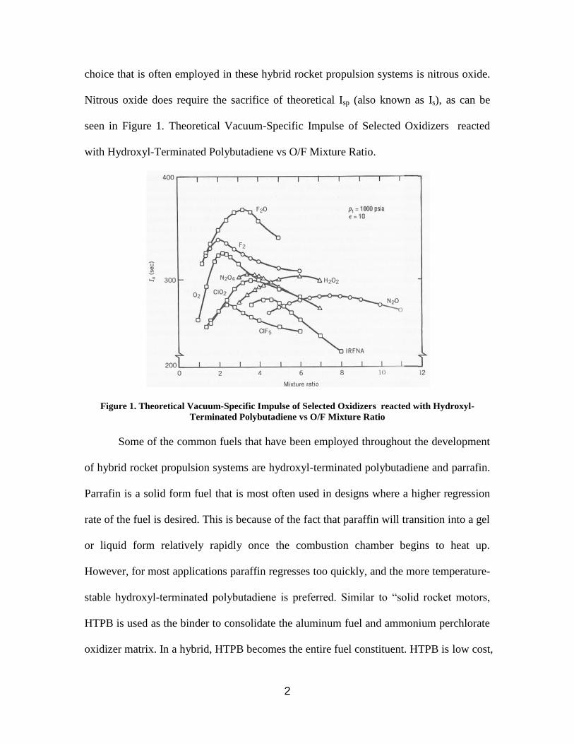
choice that is often employed in these hybrid rocket propulsion systems is nitrous oxide.
Nitrous oxide does require the sacrifice of theoretical Isp (also known as Is), as can be
seen in Figure 1. Theoretical Vacuum-Specific Impulse of Selected Oxidizers reacted
with Hydroxyl-Terminated Polybutadiene vs O/F Mixture Ratio.
Figure 1. Theoretical Vacuum-Specific Impulse of Selected Oxidizers reacted with Hydroxyl-
Terminated Polybutadiene vs O/F Mixture Ratio
Some of the common fuels that have been employed throughout the development
of hybrid rocket propulsion systems are hydroxyl-terminated polybutadiene and parrafin.
Parrafin is a solid form fuel that is most often used in designs where a higher regression
rate of the fuel is desired. This is because of the fact that paraffin will transition into a gel
or liquid form relatively rapidly once the combustion chamber begins to heat up.
However, for most applications paraffin regresses too quickly, and the more temperature-
stable hydroxyl-terminated polybutadiene is preferred. Similar to “solid rocket motors,
HTPB is used as the binder to consolidate the aluminum fuel and ammonium perchlorate
oxidizer matrix. In a hybrid, HTPB becomes the entire fuel constituent. HTPB is low cost,

3
processes easily, and will not self-deflagrate under any condition,” (Sutton & Biblarz,
2010).
1.2 Advantages of Hybrid Rocket Motors
Hybrid rocket motor propulsion systems are becoming more common now as they
continue to be identified as the ideal solution to all the overall system requirements. The
main advantages of hybrid rocket motor propulsion systems, as described in Sutton’s 8th
Edition of Rocket Propulsion Elements, are: (1) enhanced safety from explosion or
detonation during fabrication, storage, and operation; (2) start-stop-restart capabilities;
(3) relative simplicity which may translate into low overall system cost compared to
liquids; (4) higher specific impulse than solid rocket motors and higher density-specific
impulse than liquid bipropellant engines; and (5) the ability to smoothly change thrust
over a wide range on demand.
1.3 Disadvantages of Hybrid Rocket Motors
Hybrid rocket motor propulsion systems have their setbacks like any other
propulsion technology. The main disadvantages of hybrid rocket motor propulsion
systems, as described in Sutton’s 8th
Edition of Rocket Propulsion Elements, are: (1)
mixture ratio and hence specific impulse may vary during steady-state operation (as well
as during throttling); (2) relatively complicated fuel geometries with significant
unavoidable fuel residues (slivers) at end of burn, which somewhat reduces the mass
fraction and can vary if there is random throttling; (3) prone to large-amplitude, low-
frequency pressure fluctuations (termed chugging); and (4) relatively complicated
internal motor ballistics resulting in incomplete descriptions.
4
Of these four disadvantages, this research project sought to improve upon the
incomplete descriptions of complicated internal motor ballistics. Of the different key
variables that influence the internal motor ballistics, this research project focuses on the
method of N2O oxidizer injection into the combustion chamber, and characterizing how
varying the angle of the radial, or swirl, injection ports effects the regression rate of the
solid fuel HTPB grain.
As this research project progressed, it was found that a better understanding of the
large-amplitude, low-frequency pressure fluctuations could be accomplished as well. As a
result, this research project and results briefly discuss how these injection methods can be
adopted to either reduce or eliminate these combustion instabilities.
1.4 Previous Research on Swirl Injectors
Some previous research has been completed in the area of swirl injectors in these
hybrid rocket motor applications. The first of which was by Justin Pucci at Arizona State
University in 2002. Pucci investigated the effects of these swirl injector designs on the
hybrid flame-holding instability, and at the same time took a step towards better
understanding the effects of these injectors on motor performance.
For Pucci’s investigation four injector designs were employed, an axial injector, a
radial injector, a 30-degree-swirl injector, and a 60-degree-swirl injector. Pucci was able
to create conditions during the experiments which indicated that the combustion
instabilities that had previously plagued hybrid rocket motor propulsion systems is
something that is limited to certain types of injector designs. In fact, he concluded “that a
super-critical swirl flow does produce stable combustion possibly due to the
establishment of a central toroidal recirculation zone (CTRZ). This pre-heats the
5
incoming oxidizer and stabilizes the flame sheet, thus preventing the existence of the
flame-holding instability,” (Pucci, 2002). Additionally, these same super-critical swirl
flow injector design types were “found to increase regression rate by 182% over the
comparatively stable axial flow case. This is due to the increase in effective mass flux
and, therefore, convective heat transfer,” (Pucci, 2002). These results were additionally
confirmed by the continued use of 60° super-critical injectors by Dennis at Arizona State
University, (Dennis, Shark, & Hernandez, 2009).
Additional research focusing on the effects of swirl injectors was completed by a
group at the University of Padua in Padova, Italy (Bellomo, et al., 2012). Their research
focused primarily on tangential vortex injection in a hybrid rocket motor. To compare a
tangential injection method to a swirl injector as this experiment considers it, the injector
design would have an injection angle of 90°. Using these injectors they were able to show
similar results to that previously completed by Pucci and Dennis where “vortex injection
lower[ed] the chamber pressure oscillations [with] respect to [the] axial case from more
than 7% down to 4%. Moreover, regression rate [was] increased [by] 41% and the a
coefficient of its law up to 67% from axial,” (Bellomo, et al., 2012). After an extensive
study, consisting of 66 tests, they proposed the following statement. “It can be said, then,
that for the regression rate performance parameter the most important factor is the
injection type,” (Bellomo, et al., 2012).
Though not the same application, swirl injectors are of a growing interest in
injection systems used for gas turbines, where again the interest is primarily in making us
of super-critical swirl flows, or higher swirl injection angles (Littlejohn & Cheng, 2010).
One of the key things similarities between the results presented by Littlejohn and Cheng

6
in their particle image velocimetry (PIV) plots is that they too were able to identify a
distinct recirculation zone. This is noteworthy because it further confirms the importance
of employing these swirl injection methods in combustion applications, where the
generation of a recirculation zone can help mitigate instabilities thus improving
performance and reliability of the combustion system.
The growing interest in swirl injectors for both the use in hybrid rocket motors
and other applications implies the need for continued research in this area. Once fully
characterized, swirl injectors could be used to tailor hybrid rocket motor designs by
adjusting swirl injection angle to provide variable regression rate, oxidizer mass flux,
which in turn provides variable thrust and performance. Test Setup & Design Process
1.5 Background
Derived from the necessity to increase testing capabilities of hybrid rocket motor
(HRM) propulsion systems for Daedalus Astronautics at Arizona State University, a
small-scale motor and test stand were designed and developed to characterize all
components of the system. The motor is designed for simple integration and setup, such
that both the forward-end enclosure and end cap can be unscrewed and removed for rapid
integration of components during testing. Each of the components of the motor is
removable allowing for a broad range of testing capabilities. While examining injectors
and their potential it was thought ideal to obtain the highest regression rates and overall
motor performance possible. The oxidizer and fuel were selected to be N2O and
hydroxyl-terminated polybutadiene (HTPB), respectively due to previous experience and
simplicity. The oxidizer/fuel (O/F) ratio for the motor was selected to be 8.1, for a motor
using this oxidizer/fuel combination, as is determined from previous work.2 Shown in Fig.

7
1, all components of the motor except for the motor grain and nozzle are made of
aluminum, and designed to withstand loads during testing with a minimum margin of
safety (M.S.) of 0.5-1. The nozzle was designed from Super Fine Isomold Graphite to
reduce throat erosion, while maintaining structural integrity.
Figure 2. Small-Scale N2O/HTPB Hybrid Rocket Motor
The test stand for the small-scale hybrid rocket motor is equipped with three
pressure transducers, a venturi, pressure gauges, load cell, scale, and a DATAQ DI-718B
data acquisition system. Two of the pressure transducers and the venturi operate to
provide calibration results for the test stand as a means of measuring the mass flow rate
into the injector via a measurement of the difference in pressures. In order to double
check the initial calibration values obtained from the venturi, a scale will be used to
measure the amount of mass leaving the tank per second and from this determine an
approximate mass flow rate. The third pressure transducer operates as the measuring tool
for providing real-time combustion chamber pressure which will be displayed
simultaneously with real-time thrust from the load cell. Finally, the DATAQ DI-718B is
used to consolidate the acquired data from the experiments and build up a useful series of
data sets.
8
The first performance characteristic to be investigated is swirl injectors and their
potential to increase the efficiency of hybrid rocket motors. This investigation was
influenced by the past work of both Justin Pucci and Jacob Dennis at ASU on hybrid
rocket motor propulsion systems.1,2
Preliminary investigation consisted of performing
computational fluid dynamic (CFD) analysis on the swirl injectors to identify and
characterize flow structures, such as the central toroidal recirculation zone (CTRZ).
Further investigation provided complete characterization of sub-critical and super-critical
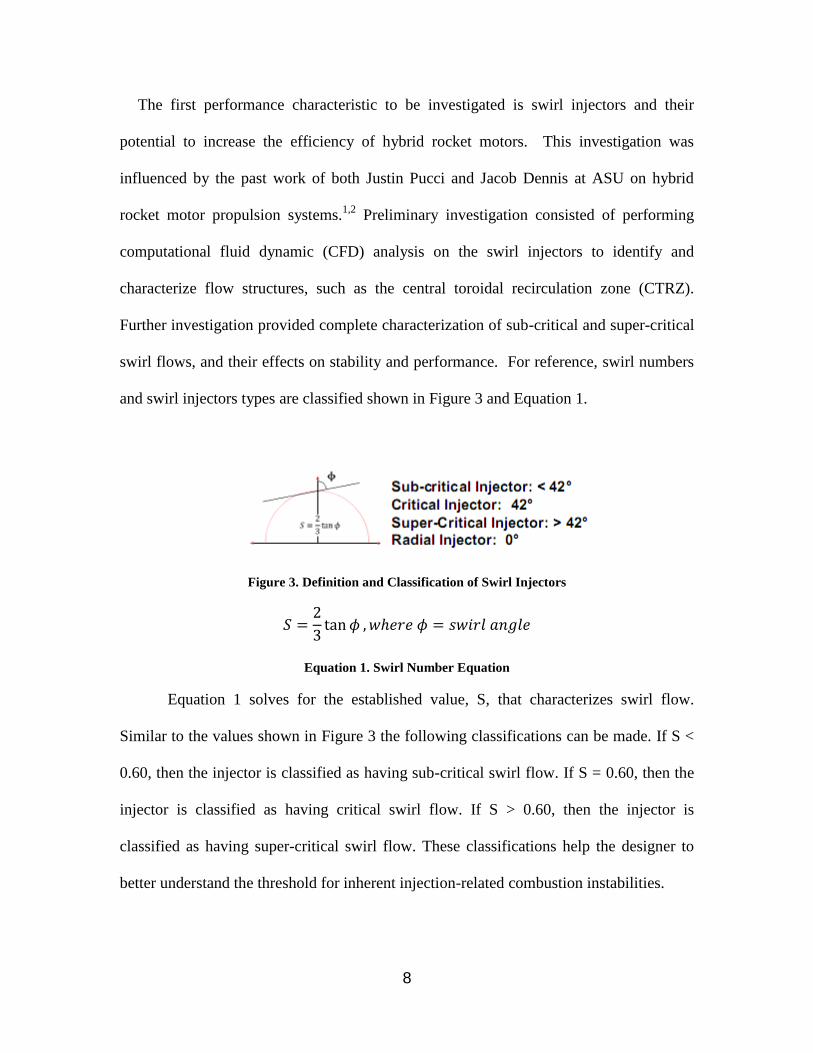
swirl flows, and their effects on stability and performance. For reference, swirl numbers
and swirl injectors types are classified shown in Figure 3 and Equation 1.
Figure 3. Definition and Classification of Swirl Injectors
Equation 1. Swirl Number Equation
Equation 1 solves for the established value, S, that characterizes swirl flow.
Similar to the values shown in Figure 3 the following classifications can be made. If S <
0.60, then the injector is classified as having sub-critical swirl flow. If S = 0.60, then the
injector is classified as having critical swirl flow. If S > 0.60, then the injector is
classified as having super-critical swirl flow. These classifications help the designer to
better understand the threshold for inherent injection-related combustion instabilities.

9
1.6 Objective / Intent
The objective is to characterize the effects of the swirl angle on the regression rate
of hybrid rocket motor fuel grains. This study is focused primarily on the effects of N2O
injected into a combustion chamber with a HTPB solid fuel grain.
HTPB and N2O were selected primarily because that is what has been used by
Daedalus Astronautics at ASU in the past, and ideally the results of this research would
directly correlate to the current hybrid rocket motor designs under way by the
organization, thus further enabling their design and development capabilities as an
organization. That being said, HTPB was initially selected “for manufacturing ease and
availability. Daedalus Astronautics at ASU has a well established Solid Rocket Motor
(SRM) program which also utilizes HTPB. General familiarity with the material
eliminates the learning curve which would be present with a new fuel. N2O is commonly
used in both hobby hybrid rocket engines as well as the performance vehicle market.
Performance associated with N2O is not as high as other possible [oxidizer] choices such
as H2O2, but it has the benefit of being self pressurized which simplifies the overall
engine [and test stand] design. HTPB and N2O are both inert when separate and therefore
require no special licenses or storage considerations,” (Dennis, Shark, & Hernandez,
2009).
1.7 Commercial Off-The-Shelf Components
In order to reduce cost, time, and overall effort associated with designing and
fabricating custom components, many of the parts used in this design were purchased as
commercial off-the-shelf components. In fact, the only parts that required significant

10
machining or processing were the motor casing, pre- and post-combustion chambers,
forward end enclosure, and the fuel grains. All other components were identified as key
candidates that met the established design requirements, and were then assembled or
installed.
1.8 Sizing of Components
Using much of the work performed by Jacob Dennis, Steven Shark, Felipe
Hernandez, and James Villarreal at Arizona State University as a baseline, some of the
components were designed to be a half-scale version of motor they designed. That being
said, a lot of design work was still completed to verify the theoretical performance of this
specific hybrid rocket engine, because the performance of these motors isn’t always so
straight forward from one configuration to the next. A good summary of this difficulty is:
“[d]imensional analysis and similarity theories are designed to generalize experimental
results by casting the variables in suitable dimensionless forms but the most satisfactory
approach is the one where theory and experiment go hand in hand,” (Sutton & Biblarz,
2010). This has been a key point of interest in the hybrid research community as
researchers work to design scalable models for these combustion processes (Chelaru,
Vasile, Florin, & Ion, 2011).
The physical dimensions of this motor were initially driven by the desire to
maintain a half-scale version of the flight motor. The purpose of this was to minimize any
scaling or design variations between the two configurations. This way motor
improvements and components could be tested and characterized on this small-scale
motor, and then related back to the larger motor.

11
The baseline dimensions of the large hybrid rocket motor were selected based on
the readily available standard tube size with a 4 inches internal diameter, and a 0.25
inches wall thickness. “Length of the final motor casing was dictated by oxidizer mass
flow rate and material availability. Initial calculations showed that a long casing and in
turn solid fuel grain would result in an O/F which was well below ideal. A shorter grain
has less surface area in the port and thus a higher O/F with a constant oxidizer mass flow
rate. These constraints were used to find geometries to be used in the analytical design of
the engine,” (Dennis, Shark, & Hernandez, 2009).
Continuing on this previous work, the following design method was followed to
design a new smaller scale motor that uses similar key combustion parameters, and can
provide results that are applicable or scalable to the larger motor. The first of these key
combustion parameters are provide in Table 1.
Table 1. HTPB/N2O Combustion Parameters (Dennis, Shark, & Hernandez, 2009)
Parameter Value
Combustion Temperature (K) 3301
Combustion Pressure (psi) 500
Ambient Pressure (psi) 14.7
C* (ft/s) 16878.9
γ 1.244
O/F Ratio 8.1
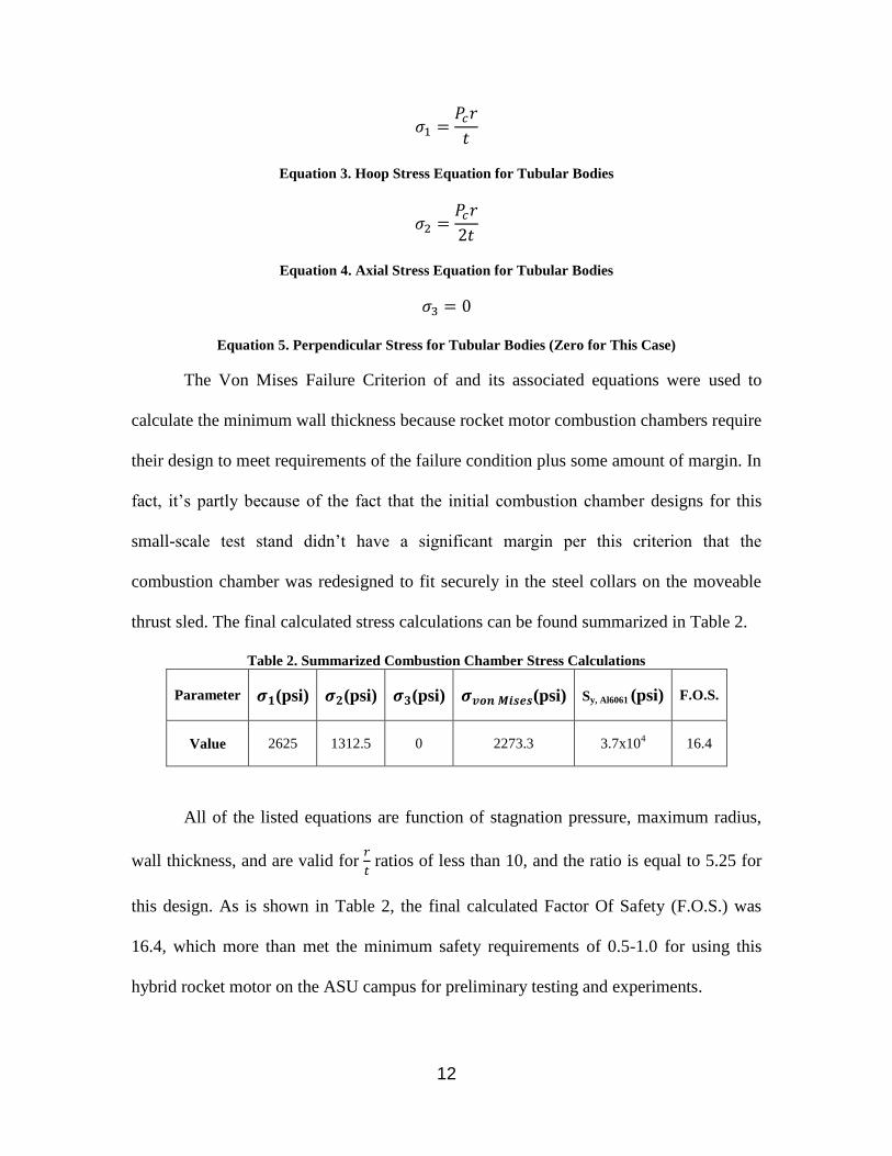
Using these key combustion parameters, and selecting many of the internal
diameter dimensions based on what commercial off-the-shelf components are available,
the following Equation 2 to Equation 5 were used to size the minimum required material
wall thickness for the combustion chamber.
Equation 2. Von Mises Failure Criterion Equation
12
Equation 3. Hoop Stress Equation for Tubular Bodies
Equation 4. Axial Stress Equation for Tubular Bodies
Equation 5. Perpendicular Stress for Tubular Bodies (Zero for This Case)
The Von Mises Failure Criterion of and its associated equations were used to
calculate the minimum wall thickness because rocket motor combustion chambers require
their design to meet requirements of the failure condition plus some amount of margin. In
fact, it’s partly because of the fact that the initial combustion chamber designs for this
small-scale test stand didn’t have a significant margin per this criterion that the
combustion chamber was redesigned to fit securely in the steel collars on the moveable
thrust sled. The final calculated stress calculations can be found summarized in Table 2.
Table 2. Summarized Combustion Chamber Stress Calculations
Parameter (psi) (psi) (psi) (psi) Sy, Al6061 (psi) F.O.S.
Value 2625 1312.5 0 2273.3 3.7x10⁴
16.4
All of the listed equations are function of stagnation pressure, maximum radius,
wall thickness, and are valid for
ratios of less than 10, and the ratio is equal to 5.25 for
this design. As is shown in Table 2, the final calculated Factor Of Safety (F.O.S.) was
16.4, which more than met the minimum safety requirements of 0.5-1.0 for using this
hybrid rocket motor on the ASU campus for preliminary testing and experiments.
13
The oxidizer mass flow rate was estimate to be 0.5 lbf/s based on some
preliminary testing. Using this estimated value and knowing the fuel grain geometry, the
oxidizer mass flux can be calculated using Equation 14. Using this newly calculated
oxidizer mass flux and an estimated optimum O/F ratio of 8.1, the baseline regression
rate for the hybrid rocket motor design can be calculated using Equation 14.
Equation 6. Baseline Regression Rate Equation
With the newly calculated baseline regression rate for the design, and again the
fuel grain geometry the fuel mass flow rate can be calculated using Equation 7.
Equation 7. Fuel Mass Flow Rate Equation
Using Equation 7 and Equation 13 the total mass flow rate of the system can be
calculated by adding both the mass flow rate of the fuel and the mass flow rate of the
oxidizer, as shown in Equation 8.
Equation 8. Total Mass Flow Rate Equation
The theoretical thrust of the overall hybrid rocket engine was calculated using the
following Equation 9, where the exit Mach number comes from Equation 10.
Equation 9. Thrust Equation
Equation 10. Exit Mach Number Equation

14
1.9 Design Validation
Aided by the finite-element numerical methods of Solidworks Simulation, CFD
analysis provided the exploitation of the transient, Central Toroidal Recirculation Zone
(CTRZ), and combustion states of oxidizer flow. Transient startup of the HRM initiated
the construction of the flow structures, where the radius and strength of the vortices
induced a further acceleration of the flow as well as an increase in oxidizer interaction
with the grain geometry. The establishing flow structure rapidly develops into a CTRZ,
where pre-heating and atomization of the oxidizer occur, as shown in Fig. 4. This
analysis showed that injectors with higher swirl numbers produce vortices with higher
rates of rotation. From this, we can say that higher rates of rotation produced from super-
critical swirl flow injectors is directly related to the increase in regression rate of the
motor grain. This correlation between higher rotation rates and regression rates provides
some critical insight into the driving variables behind atomization processes within the
active combustion zone, shown in Fig. 3.
Figure 4. Description of Active Combustion Zone & General O/F Interactions

15
Similarly, by comparing the theoretical analysis of flow and combustion
structures to numerical and experimental results, detailed characteristics can be made
about the relationship between swirl numbers or injection angles and their effects on
different components of the HRM. Once each aspect of these vital parts of hybrid rocket
motor and its mechanics is better understood it will be possible to synthesize this
understanding into the design of future hybrid rocket motors with the best of each
integrated component for a particular mission. For example, military applications require
rapid ascent and response of their missiles, but currently HRM technologies can’t support
these mission requirements. By truly understanding how each component of the motor
works, future developments in HRM technologies could lead the way for providing more
efficient and effective propulsion systems than even current solid rocket motor systems.
The following Figure 5 are some plotted numerical results from a basic and low-
level model within the Solidworks flow simulation package. The purpose of this low-
level modeling was to investigate whether or not the CTRZ flow structure discussed in
literature could be easily and quickly identified.
Figure 5. (Left) Density Distribution in CTRZ Swirl Flow Structure, (Right) Constant Pressure
Distribution in HRM
An additional plot, shown here as Figure 6, that was generated from the output of the
same simulation was that of the temperature distribution down the full length of the

16
internal combustion volume. An interesting feature that was identified early on during
these simulations was the uneven temperature distribution along the fuel grain. If this
simulation is correct, then later experimental testing would require measurements of
regression rate down the length of each fuel grain to identify whether or not uneven
burning and non-constant regression rate down the length of the grain is actually
occurring during the combustion process.
Figure 6. Temperature Distribution of CTRZ and Flow Inside HRM
1.10 Test Stand Overview
The test stand was originally designed by Robert Lanphear, another ASU
Graduate Student, and I at Arizona State University. However, the test stand and a few
other components were later modified to make the overall system more robust for large
amounts of consecutive tests. The modifications included a more robust combustion
chamber, a timer relay, stainless steel pipe, Swagelok fittings, and the design of a
standard initiator. These modifications resulted in the final test stand design that is shown
in Figure 7.
17
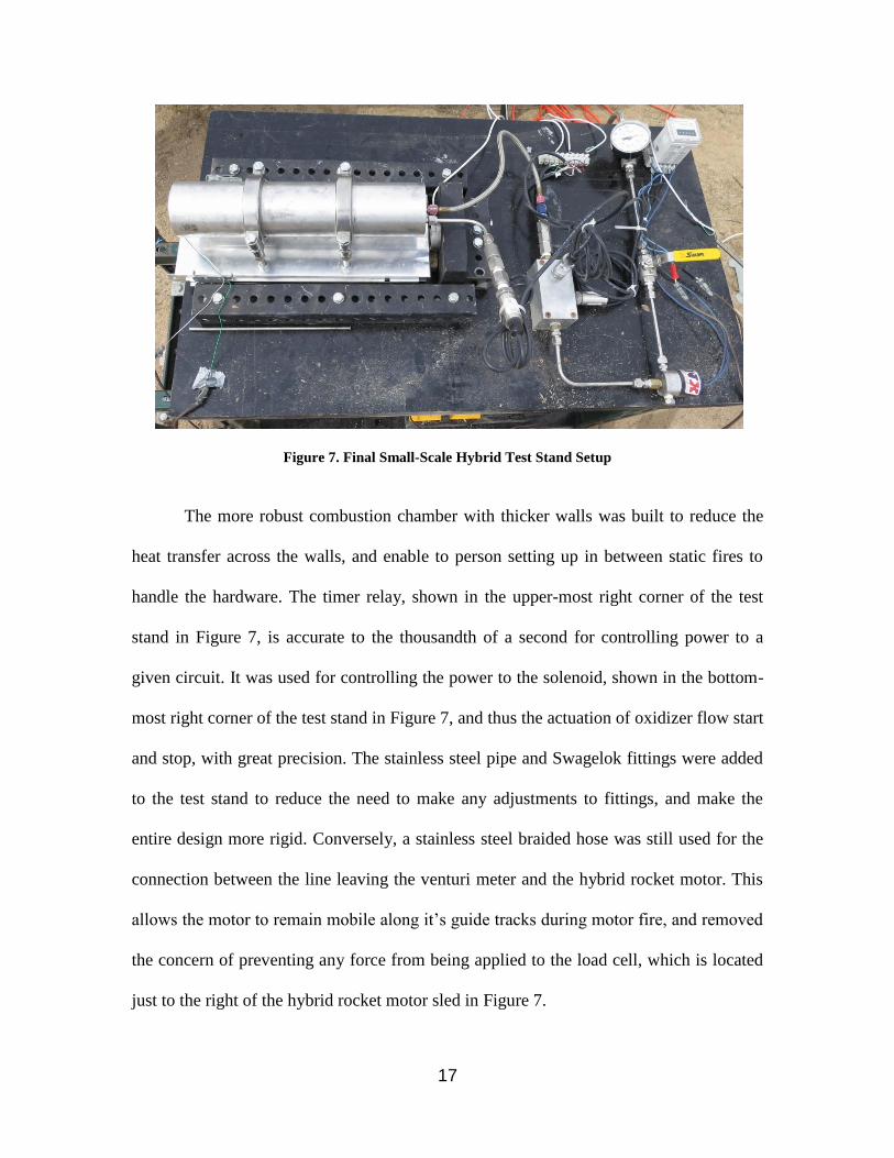
Figure 7. Final Small-Scale Hybrid Test Stand Setup
The more robust combustion chamber with thicker walls was built to reduce the
heat transfer across the walls, and enable to person setting up in between static fires to
handle the hardware. The timer relay, shown in the upper-most right corner of the test
stand in Figure 7, is accurate to the thousandth of a second for controlling power to a
given circuit. It was used for controlling the power to the solenoid, shown in the bottom-
most right corner of the test stand in Figure 7, and thus the actuation of oxidizer flow start
and stop, with great precision. The stainless steel pipe and Swagelok fittings were added
to the test stand to reduce the need to make any adjustments to fittings, and make the
entire design more rigid. Conversely, a stainless steel braided hose was still used for the
connection between the line leaving the venturi meter and the hybrid rocket motor. This
allows the motor to remain mobile along it’s guide tracks during motor fire, and removed
the concern of preventing any force from being applied to the load cell, which is located
just to the right of the hybrid rocket motor sled in Figure 7.
18
1.11 Electrical Setup
The electrical setup to for this system was designed specifically for this
application, and enables the user to test remotely if necessary. All of the electrical
subcomponents are powered by the two car batteries wired in series with the exception of
the DATAQ DI-718 and the laptop. However, because only these two subcomponents
required AC power, a converter located in a car was used to provide power during testing.
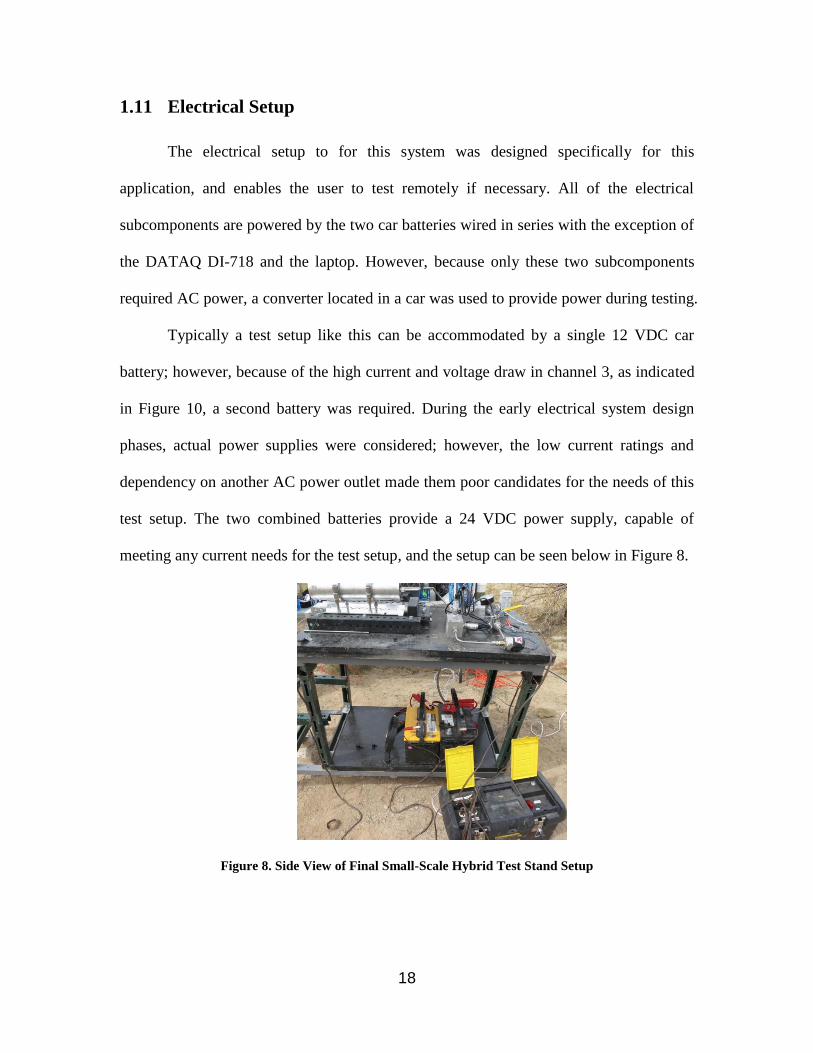
Typically a test setup like this can be accommodated by a single 12 VDC car
battery; however, because of the high current and voltage draw in channel 3, as indicated
in Figure 10, a second battery was required. During the early electrical system design
phases, actual power supplies were considered; however, the low current ratings and
dependency on another AC power outlet made them poor candidates for the needs of this
test setup. The two combined batteries provide a 24 VDC power supply, capable of
meeting any current needs for the test setup, and the setup can be seen below in Figure 8.
Figure 8. Side View of Final Small-Scale Hybrid Test Stand Setup

19
The Power/Circuit Box as shown in Figure 11 provided power to components that
are integrated into three independent circuits that can be switched on and off via physical
switches located on the Manual Control Box. This manual control box was designed with
a 200 foot Ethernet wire connection, allowing for the user to control the electronics of the
test stand from a safe and remote location. The green and white wires shown in the figure
represent Signal Positive and Signal Negative wire connections, respectively, between the
individual sensors and the data acquisition system. The red and black wires in the figure
represent the Power Positive and Power Negative connections, respectively, between
each of the powered components.
Another key feature worth mentioning is the series of stationary wire connections
that are screwed down to the surface of the test stand, as shown in Figure 9 below.
Figure 9. Zoom-In Image of Figure 6, Wire Connections, Analog Pressure Sensor/N2O Inlet from
Tank, and Timer Relay (from left to right)

20
Figure 10. Top-Level Overview of Electrical Setup
In order to record and save the data, the data acquisition system had to be
connected to a dedicated laptop via a USB cable. This setup and the commercially
available DATAQ software known as WinDaq operated as the user-interface for
recording all data. As indicated in Figure 10 this data acquisition setup was the only
sublet of the overall test setup that required an AC power outlet.
It’s important to note that the Power/Circuit Box has a relatively high number of
input/ouput lines, and this is because this was the central power hub for all components.
As seen in Figure 11, this box provided all of the power inputs and outputs to the test
setup. For the purposes of this experiment, 24 V power was supplied to the indicated 12
V Power outlet on the left. This additional power allowed the use of more power-
demanding circuits on the different indicated Igniter Channels. More specifically,

21
Channel 1 provided the 24 V power to the actual igniter to begin the pre-heating of the
hybrid rocket motor, while providing a steady flame for ignition of the motor. For
additional safety, this channel had a built-in switch that only held the open position when
the user applied a constant upward force to hold the switch open. Channel 2 provided the
24 V power to the array of pressure transducers for excitation voltage. Because this
channel wasn’t wired to any energetic components it was not designed with a switch that
switched be default was on the “off” position. Instead, the switch for channel two was
simpler in that it held either open or close position after it was pushed into place. Channel
3 provided the 24 V power to the Timer Relay and Oxidizer Solenoid circuit. Similar to
channel 1, this channel had a built-in switch that only held the open position when the
user applied a constant upward force to hold the switch open. The Timer Relay was pre-
programmed for a timed open position to allow the solenoid to energize.
Figure 11. Power/Circuit Box Overview (Dennis & Villarreal, 2010)
22
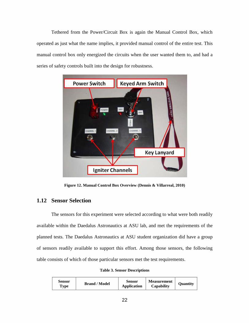
Tethered from the Power/Circuit Box is again the Manual Control Box, which
operated as just what the name implies, it provided manual control of the entire test. This
manual control box only energized the circuits when the user wanted them to, and had a
series of safety controls built into the design for robustness.
Figure 12. Manual Control Box Overview (Dennis & Villarreal, 2010)
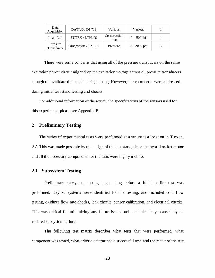
1.12 Sensor Selection
The sensors for this experiment were selected according to what were both readily
available within the Daedalus Astronautics at ASU lab, and met the requirements of the
planned tests. The Daedalus Astronautics at ASU student organization did have a group
of sensors readily available to support this effort. Among those sensors, the following
table consists of which of those particular sensors met the test requirements.
Table 3. Sensor Descriptions
Sensor
Type Brand / Model
Sensor
Application
Measurement
Capability Quantity
23
Data
Acquisition DATAQ / DI-718 Various Various 1
Load Cell FUTEK / LTH400 Compression
Load 0 – 500 lbf 1
Pressure
Transducer Omegadyne / PX-309 Pressure 0 – 2000 psi 3
There were some concerns that using all of the pressure transducers on the same
excitation power circuit might drop the excitation voltage across all pressure transducers
enough to invalidate the results during testing. However, these concerns were addressed
during initial test stand testing and checks.
For additional information or the review the specifications of the sensors used for
this experiment, please see Appendix B.
2 Preliminary Testing
The series of experimental tests were performed at a secure test location in Tucson,
AZ. This was made possible by the design of the test stand, since the hybrid rocket motor
and all the necessary components for the tests were highly mobile.
2.1 Subsystem Testing
Preliminary subsystem testing began long before a full hot fire test was
performed. Key subsystems were identified for the testing, and included cold flow
testing, oxidizer flow rate checks, leak checks, sensor calibration, and electrical checks.
This was critical for minimizing any future issues and schedule delays caused by an
isolated subsystem failure.
The following test matrix describes what tests that were performed, what
component was tested, what criteria determined a successful test, and the result of the test.

24
Table 4. Subsystem Test Matrix
Test Type Component Tested *Pass Criteria Pass/Fail
Electrical Check Solenoid Actuate on Command Pass
Electrical Check Ignition System Ignite on Command Pass
Electrical Check Sensors, DAQ Read Pressure in Lines Pass
Cold Flow Test Injector System Hold Seal, Provide Oxidizer
Flow at Expected Mass Flow
Rate
Pass
Cold Flow Test Entire Motor Hold Seal Pass
Cold Flow Test Venturi Read Pressure, Measure In-
Line Mass Flow
Pass
Mechanical Fit Check Enclosures, Nozzles, etc. All Components have as-
designed interfaces
Pass
Mechanical Fit Check Sensors All Sensors interface as-
designed
Pass
Data Check DAQ Verify the DAQ can record
Data as-designed
Pass
Hot Fire Test Entire Test Stand Provide thrust, record data,
sustain combustion, verify as-
designed performance
Pass
2.1.1 Cold Flow Testing
The following table describes the initial cold flow testing that was performed.
Table 5. Cold Flow Test Matrix
Test
No. Description
PTank,0
(psi)
WeightTank,0
(lb)
WeightTank,f
(lb)
tflow
(s)
ox
(lb/s) Comments
1 Axial
Injector Test 690 170.8 170.6 4 0.05
Tank Closed,
No Test
2 Axial
Injector Test 690 170.6 169.8 1.8 0.45 Good Test
3 Axial
Injector Test 675 169.8 169.0 2.8 0.3 Good Test
4 Axial
Injector Test 660 169.0 168.4 2.3 <0.25
Leaks at
Fittings,
Unknown ox
5 Axial
Injector Test 665 168.0 167.4 2.5 ~0.2
Small Leak at
Fitting, Good
Test
6 Swirl
Injector Test 670 167.4 167.0 2.1 0.2 Good Test
Initial cold flow testing provided the opportunity to verify the design of the
injector, forward enclosure, seal interface, snap-ring retention, and oxidizer flow rate

25
capability of the subsystem. By the end of the cold flow tests, each of these components
was deemed acceptable for future testing.
As is common with N2O, the flow was shown to be both temperature and pressure
dependent across the series of test runs. Because it wasn’t the goal to determine an exact
mass flow rate capability, varying initial pressures and test times were acceptable. The
two figures below are from this initial testing, and provide a good general sense of what
the two different flow types look like. Shown in Figure 13 is the flow of the axial
injector, which has all 16 injection ports located on the face of the injector. Shown in
Figure 14 is the flow of the 60 degree swirl injector, which has 11 injection ports located
on the face, and 5 additional injection ports equally spaced around the circumference of
the injector.
Figure 13: Flow of Axial Injector Test
Figure 14: Flow of 60 deg. Swirl Injector

26
2.1.2 Venturi Testing
As previously stated, initial cold flow testing provided the opportunity to verify a
number of integral components to the hybrid rocket motor, one of which is the venturi.
The venturi is a carefully designed apparatus that accepts two pressure transducers for
take in-line oxidizer pressure measurements, as shown in Figure 15. Each of these
measurements is taken at pre-determined cross-sectional areas in the flow, thus allowing
for the calculation of oxidizer mass flow rate.
Figure 15. Section View of Venturi Model
In order to calculate oxidizer mass flow rate, a few key equations were used.
From what we know about fluid dynamics in control volumes, mass flow rate is a
function of the fluid density, velocity, the cross-sectional area of pipe it is flowing
through, and this relationship can be shown by the following equation, Equation 11
(Moran, Shapiro, Munson, & DeWitt, 2003).
Equation 11. Equation for One-Dimensional Mass Flow Rate

27
Since both the areas and velocities of the flow cannot be assumed constant as it
flows through a venturi, the mechanical energy equation was used to account for this.
However since we can assume there are no losses to friction, no work is done to the
control volume, both measurement points are in-line, the flow is steady, and density is
constant, the mechanical energy equation simplifies to the following version of the
Bernoulli equation.
Equation 12. Simplified Mechanical Energy Equation
By substituting Equation 11 in Equation 12, and then algebraically solving for the
oxidizer mass flow rate, the following Equation 13 can be obtained. It’s important to note
that this equation solves for the oxidizer mass flow rate using only three input parameters
of density, pressure, and cross-sectional area. Since we can calculate the density, measure
the pressure, and know the cross-sectional areas from the design, this form of the oxidizer
mass flow rate equation is ideal for this experiment.
Equation 13. Oxidizer Mass Flow Rate Equation Used with Venturi
28
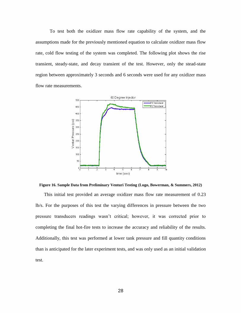
To test both the oxidizer mass flow rate capability of the system, and the
assumptions made for the previously mentioned equation to calculate oxidizer mass flow
rate, cold flow testing of the system was completed. The following plot shows the rise
transient, steady-state, and decay transient of the test. However, only the stead-state
region between approximately 3 seconds and 6 seconds were used for any oxidizer mass
flow rate measurements.
Figure 16. Sample Data from Preliminary Venturi Testing (Lugo, Bowerman, & Summers, 2012)
This initial test provided an average oxidizer mass flow rate measurement of 0.23
lb/s. For the purposes of this test the varying differences in pressure between the two
pressure transducers readings wasn’t critical; however, it was corrected prior to
completing the final hot-fire tests to increase the accuracy and reliability of the results.
Additionally, this test was performed at lower tank pressure and fill quantity conditions
than is anticipated for the later experiment tests, and was only used as an initial validation
test.
29
3 Experimental Design & Approach
3.1 Design of Experiment
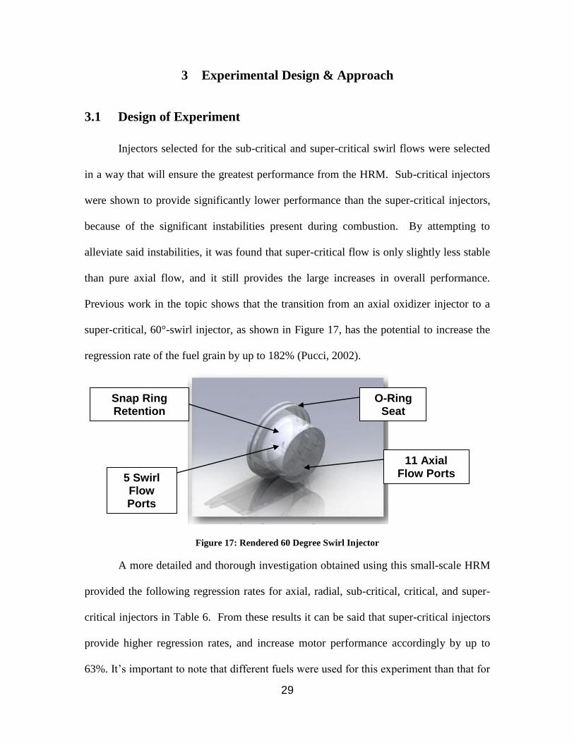
Injectors selected for the sub-critical and super-critical swirl flows were selected
in a way that will ensure the greatest performance from the HRM. Sub-critical injectors
were shown to provide significantly lower performance than the super-critical injectors,
because of the significant instabilities present during combustion. By attempting to
alleviate said instabilities, it was found that super-critical flow is only slightly less stable
than pure axial flow, and it still provides the large increases in overall performance.
Previous work in the topic shows that the transition from an axial oxidizer injector to a
super-critical, 60°-swirl injector, as shown in Figure 17, has the potential to increase the
regression rate of the fuel grain by up to 182% (Pucci, 2002).
Figure 17: Rendered 60 Degree Swirl Injector
A more detailed and thorough investigation obtained using this small-scale HRM
provided the following regression rates for axial, radial, sub-critical, critical, and super-
critical injectors in Table 6. From these results it can be said that super-critical injectors
provide higher regression rates, and increase motor performance accordingly by up to
63%. It’s important to note that different fuels were used for this experiment than that for
11 Axial Flow Ports 5 Swirl
Flow Ports
Snap Ring Retention
O-Ring Seat

30
Pucci’s testing. HTPB is commonly known to have a higher regression rate than the
High-Density Polyethelynes (HDPEs) used in his testing across the board; however, the
important thing is that the same general effects of swirl injection on regression rate are
independent of the fuel used in the configuration.
As discussed in previous works, combustion instabilities are often present
amongst range of the injectors used during characterization testing. The most significant
instabilities tend to be consistent with sub-critical injectors, while super-critical injectors
are much more stable and still maintain high efficiencies (Pucci, 2002). Sub-critical
injectors can be seen as unnecessary for future integrations since they not only destabilize
combustion of the motor, but also don’t show significant increases in regression rates,
and likewise, rocket performance. Yet, in order to fully characterize the effects of the
swirl injection angle and its effects on regression rate, it was pertinent to keep these sub-
critical injector designs as part of the overall test matrix.
Future application of the test stand will consist of characterization of motor grain
configurations, fuel types, and nozzles. As previously mentioned, the motor design has
been equipped with simple integration methods to allow for the rapid changing of each
component, thus speeding up turnaround time during testing. These additional sets will
enable the completion of multiple research investigations describing their effects on the
performance and stability of the HRM.
3.1.1 Test Matrix
Provide a filled out test matrix that was generated per the justifications of design
selection discussed previously.

31
Table 6: Hot Fire Test Matrix
Test
No.
Swirl Injector
Angle (deg)
PTank,0
(psi)
PC,avg
(psi) ox, avg (lb/s)
Gox,0
(lb/s-in2)
(in/s)
1 60 950 373.949 0.548 Low 0.087
2 15 950 470.946 0.597 Low 0.070
3 15 950 470.946 0.597 Low 0.066
4 0 1000 520.946 0.597 Low 0.063
5 0 970 490.946 0.597 Low 0.068
6 30 980 500.946 0.597 Low 0.082
7 30 970 490.946 0.597 Low 0.078
8 60 1000 520.946 0.597 High 0.106
9 60 1010 530.946 0.597 High 0.092
10 60 980 500.946 0.597 Low 0.104
11 60 975 495.946 0.597 Low 0.074
12 42 950 470.946 0.597 Low 0.079
13 42 950 421.186 0.664 High 0.081
14 42 950 470.946 0.597 High 0.085
15 42 955 475.946 0.597 Low 0.077
16 0 950 470.946 0.597 High 0.078
17 0 950 470.946 0.597 High 0.066
18 15 950 470.946 0.597 High 0.080
For this experiment, 5 unique injector designs were selected. Those injectors were
physically identical in all aspects, except the angle of radial injection. The five different
injectors were designed with injector angles of 0 degrees, which is perpendicular to the
outer surface or straight in the radial direction, 15 degrees, 30 degrees, 42 degrees, and 60
degrees. The stored pressure of the N2O in the tank was kept at a constant 950 psi, with a
few minor exceptions. The average combustion chamber pressure was kept relatively
constant, with the exception of slight variations that are inherent variability among
experimental data of this sort.
As was previously mentioned, two unique conditions for oxidizer mass flux were
selected for this experiment. The two conditions are simply labeled here in Table 6 as
“Low” and “High”. In order to calculate the oxidizer mass flux for each condition the
follow equation is used, Equation 14.

32
Equation 14. Oxidizer Mass Flux Equation
Of the two variables in this equation, combustion port area was easily controlled
by casting grains with different inside diameters of their combustion ports. The low
oxidizer mass flow rate condition was tested with HTPB fuel grains that have a
combustion port diameter that measures 1.0 inch on the internal diameter. The high
oxidizer mass flow rate condition was tested with HTPB fuel grains that have a
combustion port diameter that measures 1.25 inch on the internal diameter. The oxidizer
mass flow rate was more difficult to control since to density of the N2O is both
temperature and pressure dependent, and both of these variables were subject to the
availability of a heating blanket and the ambient test conditions, which are discussed later
in Section 3.3.4. Nonetheless, the oxidizer mass flow rate was held at a relatively
constant 0.59 lb/s throughout the experiment. The following table shows the calculated
initial oxidizer mass flux values for each test condition.
Table 7. Oxidizer Mass Flux Calculations
Test
Condition Dport,i (in) Aport (in
2) ox, avg (lb/s)
Gox,0
(lb/s-in2)
Low 1.25 3.927 0.59 0.150
High 1.00 3.063 0.59 0.193
3.1.2 Test Order
In order to characterize the effects of the combustion chamber pressure and swirl
injector angle independently later on, it is critical that the test runs described in the design
of the experiment stay random (Montgomery, 2013). This explains the random order of
test numbers in the test matrix.

33
3.1.3 Experiment Replication
In order to reduce statistical variability throughout the results, replication of the
test series was necessary. However, due to the average cost per test run, schedule
limitations, and the overall added value of the additional test runs, it was deemed
unnecessary for the purpose of this investigation to perform additional replicated tests for
all test cases. Instead, replication was only employed when there was a desire to better
understand a specific relationship among the test cases. More specifically, experiments
for at both oxidizer mass flux conditions were replicated for both the 0 degree injector
case and the 60 degree injector case.
3.2 Blocking
Throughout the experiment blocking was employed to have only one operator of
the tests. However, as previously mentioned, the advantage of having a single test bench
and operator is that any error that would have occurred from multiple test benches or
operators is eliminated. Even though we will minimize the measurement error by having
the same person measuring each time, we do expect there will be some measurement
error occurring.
3.3 Randomization
As stated by Montgomery, “[r]andomization is the cornerstone underlying the use
of statistical methods in experimental design. By randomization we mean that both the
allocation of the experimental material and the order in which the individual runs the
experiment are to be performed are randomly determined.” It is because of this that it was
so critical to have my test runs within the overall experiment randomized. Also, by
34
randomizing the individual test runs and the distribution of raw material “…we also assist
in ‘averaging out’ the effects of extraneous factors that may be present” (Montgomery,
2013). Some of the key extraneous factors that may be present in this experiment are
briefly discussed in the following subsections, along with the attempts that were taken in
addition to randomization to reduce any effects these variables would have on the
experimental results.
In order to complete the designed test matrix, 18 individual hybrid rocket motor
test fires had to be completed. To keep cost and schedule reduced, a fully-instrumented
small-scale hybrid rocket motor was employed for the series of tests. A typical rocket
motor test fire can be seen in Figure 22, where the motor is in steady-state combustion
when the picture was taken. As is typical of analyzing results of rocket motor tests that
study regression rate, the transient start and stop, or tail-off, of the tests were not studied
extensively. Because the transients associated with this test occur in the milliseconds, and
these tests had a total burn time length of either 2 or 3 seconds, we can safely assume that
the transients are negligible to the overall results of each test case.
3.3.1 Fuel Grain Mixing
To properly prepare for hot fire tests, the grain development has to be
manufactured with precision. An advantage of hybrid grains like HTPB is that it is safe
to handle during development, safe for storing and it will not ignite or detonate
simultaneously3. When developing the grain three main chemicals and additives are
used in the process; liquid HTPB, Isonate 143L, carbon black, and silicon oil. Isonate
143L is the curative which bonds the liquid HTPB into solid form. Silicon oil is only
used when formulating large amounts of hybrid grains. It helps lubricate the grain in
35
order for ease of vacuuming to force the air out of the mixture5. In the case for this small
scale hybrid grain the silicon is not needed to properly force the air out of the mixture.
Carbon black is used in order for distinct coloration of the fuel for proper measurements.
Table 1 shows the formulation for the hybrid grain.
Table 8. Hybrid Grain Formulation
Amount Chemical/Additive
85% HTPB
15% Isonate 143L
1 teaspoon/lbfuel Carbon Black
1 drop/ lbfuel Silicon Oil
As shown in Table 8, silicon oil was only required to be added to the formula
when mixing this particular HTPB hybrid fuel grain in very small amounts. This is
because previous mixing experiments have shown that when silicon oil is added in any
amount more than 1 drop per pound of total propellant, the grain or grains will not cure
properly, and often must be disposed of. Because of this previous knowledge, and the fact
that the grains only required so much propellant, silicon oil was not included in the
batches used for this experiment. That being said, this is acceptable and will not have any
effect on the performance of the motor.
Once the proper formulation has been measured for the correct fuel volume the
mixing process begins. The HTPB, carbon black and silicon oil are added first into a
mixing bowl of a Kitchen Aid 5-Quart Kv25 Stand Mixer and is mixed at low speeds
until homogenous and no particles are present as shown in Figure 18. Than the Isonate
143L is added last due to its quick curing property and is mixed at medium speeds for 10
min. While mixing is taking place the Ultra-High Density Polyethylene (UHDPE) plastic
casting rod is assembled to its associated casting base and prepped for final casting. The

36
specific plastic of UHDPE was used for its ability to easily release molds, such as these
HTPB grains, after curing is complete. The UHDPE casting rods were precision
machined to be considered identical, and this ensures a smooth surface for the grain to
cure on and will result in a fine smooth solid hybrid grain. To further ensure the grains
remove easily from the casting setup after cure is complete, mold release is sprayed
evenly on the UHDPE rod and is let dry for 5 minutes. This additional step could be
skipped in the process if a self-lubricating material was used like that of Teflon. However,
UHDPE was more readily available and was more cost effective.
Figure 18. Mixing of the HTPB Fuel
Once mixing is finished the next step is to force out all of the trapped air in the
fuel in order to prevent air bubbles while the fuel is being cured. The bowl has to be
removed from the mixer and the outer edges of the bowl are lined with Teflon tape to
ensure proper seal while vacuuming. A Plexiglas vacuum cover plate, which is
connected to the vacuum pump, is placed on top of the bowl as shown in Figure 19.

37
Figure 19. Vacuum Process Setup
The vacuum pump process continues until no additional air bubbles are seen
outgassing from the fuel. This process is important to maintain consistent grain quality
from one to the next by mitigating the opportunity for voids to appear within the grain
during the later cure process. Once the outgassing has finished, the mix is acceptable, and
ready to be poured into the casting setup.
3.3.2 Fuel Grain Curing
Controlling the curing process across all of the individual HTPB fuel grains was
also critical to maintaining consistency between the different grains. Variations in the
ambient temperatures during the curing process were mitigated by the use of a controlled
volume, known as the heat box. Figure 20 shows the HTPB-mixture-filled casting
assembly placed inside of the heat box.

38
Figure 20. Individual Hybrid Casting Assembly in Heat Box
The air temperature inside of the heat box is measured using a thermometer and
should maintain a temperature reading of 120 ± 20 degrees Fahrenheit for the full
duration of the cure. The hybrid grain is left inside the heat box for approximately 24
hours for proper curing. Though it wasn’t the case for the grains used for this experiment,
sometimes if sufficient hardness is achieved prior to the 24 hour period, then the casting
assembly is removed from the heat box. Figure 21 is an example of how a perfectly
mixed and casted hybrid grain appears.
Figure 21. Typical Cured Hybrid Grain

39
3.3.3 Fuel Grain Density
Again, as previously mentioned there were some concerns that in the construction
of the fuel grains for the experiments there may be some possible variability between
HTPB fuel grains utilized during each trial. In order to address this, the fuel grains were
measured, cut to length, and weighed to determine the density of each grain prior to each
test. The final calculated density of each 1.25 inch internal diameter fuel grain was within
0.046 lbm/in3, while the final calculate density of each 1.00 inch internal diameter fuel
grain was 0.057 lbm/in3. For the purposes of this experiment, this range of densities was
deemed acceptable, and the method of data normalization is discusses in greater detail in
the results section of this paper.
Later investigations into the density variability discovered that small variations in
Isonate 143L and cure conditions accelerated the cure of the fuel grains and reduced
expansion of the mixture as it cured. Though both of these are considered to be process
improvements, for the purposes of maintaining consistency across the different test cases
the data required normalization. After the data was normalized, the trends were compared
to historical results, and analyzed for correlations.
3.3.4 Extraneous Test Conditions
As previously mentioned, blocking had to be employed for the statistical analysis
of this experiment because it was not possible to complete all of the test runs on the same
day. Because of this, ambient test conditions were monitored to better understand any
impact on the results by uncontrollable variables like that of ambient test conditions. A

40
table of the of the monitored extraneous and/or uncontrollable ambient test conditions is
provide below as Table 9.
Table 9. Example of Monitored Extraneous Test Conditions
State Pre Post
Ta (F) A1 A2
Wind Speed (ft/s) B1 B2
Wind Direction C1 C2
PN2O (psi) D1 D2
Nozzle Throat Dia. (in) E1 E2
TCase Wall (F) F1 F2
Table 9 and subsequent tables in Section 4 like it were populated from a number
of sources. Values A1-C2 were collected from the online database owned by The
Weather Channel. To measure any influence that wind direction and velocity might have
on the experiment results, it’s important to note that the test stand was always positioned
such that wind direction is normal to the direction of thrust. Values D1, D2, F1, and F2
were collected during testing, and were recorded before and after each individual test.
Lastly, values E1 and E2 were only collected before and after the total set of tests
because previous research showed these effects would likely be negligible, and this was
later confirmed.
3.3.5 N2O Test Conditions
Though it wasn’t mentioned previously in the report, another technical issue was
encountered during the experiment, where as the number of tests increased, the pressure
of the N2O storage tank began to decrease. In order to counteract this effect and ensure
that each test was able to attain its designed combustion chamber pressure as prescribed
by the designed experiment, a controlled and approved heating method was implemented

41
to slowly and equally distribute heat the tank. Previous experience has shown this to be a
more than sufficient method for increasing the pressure inside of the storage tank. Also,
because the storage tank is designed for pressures up to 5000 psi, and even when heated
up, the N2O never exceeded 1010 psi, a conservative Factor of Safety (FoS) of 4.95 was
always maintained throughout the experiment.
3.3.6 Nozzle Erosion
Another small concern that was briefly discussed previously is the erosion of the
graphite nozzle throat diameters over the course of the experiment. Initial predictions
stated that this effect should be small (on the order of thousandths of an inch), but it will
be measured, recorded, and remain a consideration during the experimental design
planning.
As testing proceeded the commercial nozzle did start to erode at the throat from
the high temperature and abrasive mass flux at that location of the nozzle. The average
erosion of the nozzle was approximately 0.005 inches on the diameter of the throat per
test, which if we assume equivalent thrust from each test of 136 lbf, and assume
equivalent thrust coefficient for each test, then the increase in throat size will cause the
combustion pressure to drop by 0.015%, as can be calculated using Equation 15.
Equation 15. Basic Equation for Thrust as a Function of Pressure, Throat Area, and Thrust
Coefficient
Because a 0.015% drop in performance is within the noise of the inherent
variation within the experiment, this is considered negligible for this testing. In order to
verify this, the relative standard deviation of the combustion chamber pressure across all

42
of the test runs was compared to the percent losses of the combustion chamber pressure.
Using Equation 16 the relative standard deviation of the combustion chamber pressure
was calculated to be 0.076%. Based on this calculation, the losses associated with nozzle
erosion and performance are less than one fifth of the noise inherent with the experiment
design.
Equation 16. Relative Standard Deviation Equation
For reference, the calculated percent losses with respect to nozzle erosion and
performance are tabulated in Table 10.
Table 10. Nozzle Erosion and Performance Losses
D_t (in) A_t (in^2) F, avg (lbf) C_f P_c, avg (psi)
Initial 0.547 0.235 136.000 1.300 445.379
Final 0.551 0.238 136.000 1.300 438.735
% Losses 0.008 0.015 - - 0.015
3.3.7 Erosion of Internal Components
Because of the high combustion temperature inherent with the rocket motor
combustion processes, the integrity of internal components was monitored. However, the
concern that internal metal components would erode over the duration of the motor burns
was found to be relatively negligible. Initial predictions stated that this effect should be
small (on the order of thousandths of an inch), but it was measured, recorded, and
remained a consideration during the series of tests. As testing proceeded the wall
thickness of the injector housing, pre-combustion chamber, and post-combustion
chamber were selected as key characteristics for monitoring any erosion of internal metal

43
components. The total erosion of the injector housing wall was found to be at most 0.002
inches. The total erosion of the pre-combustion chamber was found to be at most 0.002
inches. The total erosion of the pre-combustion chamber was found to be at most 0.002
inches. If we assume equivalent thrust and combustion characteristics from each test then
the average erosion per test is one eighteenth of each of the measured total erosion values
provided previously, or 1.1x10⁻⁴
inches. Given the fact that these measured and
calculated erosion values are near or less than the accuracy of available measurement
tools, all erosion of internal metal components used for this experiment is to be
considered negligible.
3.3.8 Sensor Calibration
All of the sensors were purchased from either FUTEK or Omegadyne. Because of
this, all the sensors were professionally calibrated prior to use to meet their designed
specifications, see Appendix B for additional sensor calibration and specification
information.
An additional calibration of the data acquisition and sensor setup was required
prior to testing to verify all sensor signal outputs, excitation voltages, and the internal
DATAQ modules are nominal. During this process, the values from the calibration sheets
were entered into the DATAQ software to provide accurate correlations of the raw
voltage data to engineering units such as psi and lbf. This calibration was then saved to
the laptop, and was used for each subsequent test.

44
3.3.9 Motor Assembly
Torque to install components in the forward end enclosure was monitored from test
to test to ensure that everything was installed safety and correctly. Snap ring location and
seating was verified to be correct during each motor assembly. If the torque or seating of
these components was not verified prior to each motor firing, then it could result in a
small change in motor performance by changing the internal volume that is pressurized
during combustion. If the pressure of the combustion chamber changes in an unplanned
way, then it would result in a change in regression rate accordingly, thus removing that
test run from the group of acceptable results.
4 Results & Discussion
4.1 Test Runs
Shown in the following figure is a picture of a typical static fire of this rocket
motor, and was taken during the preliminary testing that was performed at Arizona State
University.
45
Figure 22. Preliminary Static Fire Testing of Rocket Motor
4.1.1 Test Run 1
Test run number 1 resulted in a 2.125 second burn that provided 124.1 lbf of
average thrust. During this hot fire test there were no anomalies, and all results were
deemed acceptable for analysis. As is shown in Table 11, this test consisted of a 60
degree swirl injector. As shown in Table 12, the 60 degree swirl injector results in a
regression rate of 0.087 in/s.
Table 11. Summary of Test Conditions for Test Run 1
Variable Value
Swirl Angle (deg.) 60
Initial Port Dia. (in) 1.25
Burn Time (s) 2.125
46
Table 12. Summary of Motor Performance for Test Run 1
Performance Metric Value
Pc,avg (psi) 373.9
Thrustavg (lbf) 124.1
Regression Rate (in/s) 0.087
The extraneous test conditions for test run number 1 are within family of the other test
runs. Because of this, these test conditions are considered negligible for test number 1.
Table 13. Monitored Extraneous Test Conditions for Test Run 1
State Pre Post
Ta (F) 51 51
Wind Speed (ft/s) 23.5 23.5
Wind Direction W W
PN2O (psi) 950 950
Nozzle Throat Dia. (in) 0.546 0.546
TCase Wall (F) 51 100
4.1.2 Test Run 2
Test run number 2 resulted in a 3.242 second burn that provided 143.5 lbf of
average thrust. During this hot fire test there were no anomalies, and all results were
deemed acceptable for analysis. As is shown in Table 14, this test consisted of a 15
degree swirl injector. As shown in Table 15Table 12, the 15 degree swirl injector results
in a regression rate of 0.070 in/s.
47
Table 14. Summary of Test Conditions for Test Run 2
Variable Value
Swirl Angle (deg.) 15
Initial Port Dia. (in) 1.25
Burn Time (s) 3.242
Table 15. Summary of Motor Performance for Test Run 2
Performance Metric Value
Pc,avg (psi) 470.9
Thrustavg (lbf) 143.5
Regression Rate (in/s) 0.070
The extraneous test conditions for test run number 2 are within family of the other test
runs. Because of this, these test conditions are considered negligible for test number 2.
Table 16. Monitored Extraneous Test Conditions for Test Run 2
State Pre Post
Ta (F) 51 51
Wind Speed (ft/s) 23.5 23.5
Wind Direction W W
PN2O (psi) 950 950
Nozzle Throat Dia. (in) 0.546 0.546
TCase Wall (F) 51 100
4.1.3 Test Run 3
Test run number 3 resulted in a 3.233 second burn that provided 143.6 lbf of
average thrust. During this hot fire test there were no anomalies, and all results were

48
deemed acceptable for analysis. As is shown in Table 17, this test consisted of a 15
degree swirl injector. As shown in Table 18Table 12, the 15 degree swirl injector results
in a regression rate of 0.066 in/s.
Table 17. Summary of Test Conditions for Test Run 3
Variable Value
Swirl Angle (deg.) 15
Initial Port Dia. (in) 1.25
Burn Time (s) 3.233
Table 18. Summary of Motor Performance for Test Run 3
Performance Metric Value
Pc,avg (psi) 470.9
Thrustavg (lbf) 143.6
Regression Rate (in/s) 0.066
The extraneous test conditions for test run number 3 are within family of the other test
runs. Because of this, these test conditions are considered negligible for test number 3.
Table 19. Monitored Extraneous Test Conditions for Test Run 3
State Pre Post
Ta (F) 51 51
Wind Speed (ft/s) 23.5 23.5
Wind Direction W W
PN2O (psi) 950 950
Nozzle Throat Dia. (in) 0.547 0.547
TCase Wall (F) 51 100
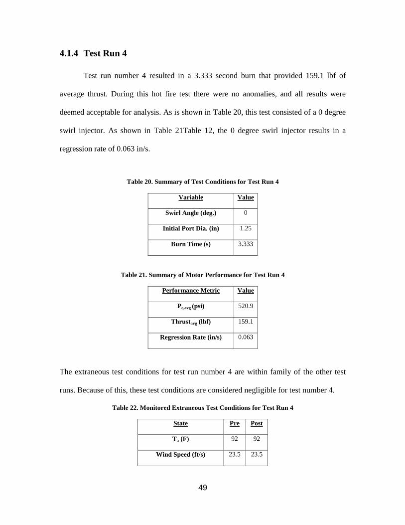
49
4.1.4 Test Run 4
Test run number 4 resulted in a 3.333 second burn that provided 159.1 lbf of
average thrust. During this hot fire test there were no anomalies, and all results were
deemed acceptable for analysis. As is shown in Table 20, this test consisted of a 0 degree
swirl injector. As shown in Table 21Table 12, the 0 degree swirl injector results in a
regression rate of 0.063 in/s.
Table 20. Summary of Test Conditions for Test Run 4
Variable Value
Swirl Angle (deg.) 0
Initial Port Dia. (in) 1.25
Burn Time (s) 3.333
Table 21. Summary of Motor Performance for Test Run 4
Performance Metric Value
Pc,avg (psi) 520.9
Thrustavg (lbf) 159.1
Regression Rate (in/s) 0.063
The extraneous test conditions for test run number 4 are within family of the other test
runs. Because of this, these test conditions are considered negligible for test number 4.
Table 22. Monitored Extraneous Test Conditions for Test Run 4
State Pre Post
Ta (F) 92 92
Wind Speed (ft/s) 23.5 23.5

50
Wind Direction SE SE
PN2O (psi) 1000 1000
Nozzle Throat Dia. (in) 0.547 0.547
TCase Wall (F) 92 120
4.1.5 Test Run 5
Test run number 5 resulted in a 2.933 second burn that provided 150.1 lbf of
average thrust. During this hot fire test there were no anomalies, and all results were
deemed acceptable for analysis. As is shown in Table 23, this test consisted of a 0 degree
swirl injector. As shown in Table 24, the 0 degree swirl injector results in a regression
rate of 0.068 in/s.
Table 23. Summary of Test Conditions for Test Run 5
Variable Value
Swirl Angle (deg.) 0
Initial Port Dia. (in) 1.25
Burn Time (s) 2.933
Table 24. Summary of Motor Performance for Test Run 5
Performance Metric Value
Pc,avg (psi) 490.9
Thrustavg (lbf) 150.1
Regression Rate (in/s) 0.068
The extraneous test conditions for test run number 5 are within family of the other test
runs. Because of this, these test conditions are considered negligible for test number 5.
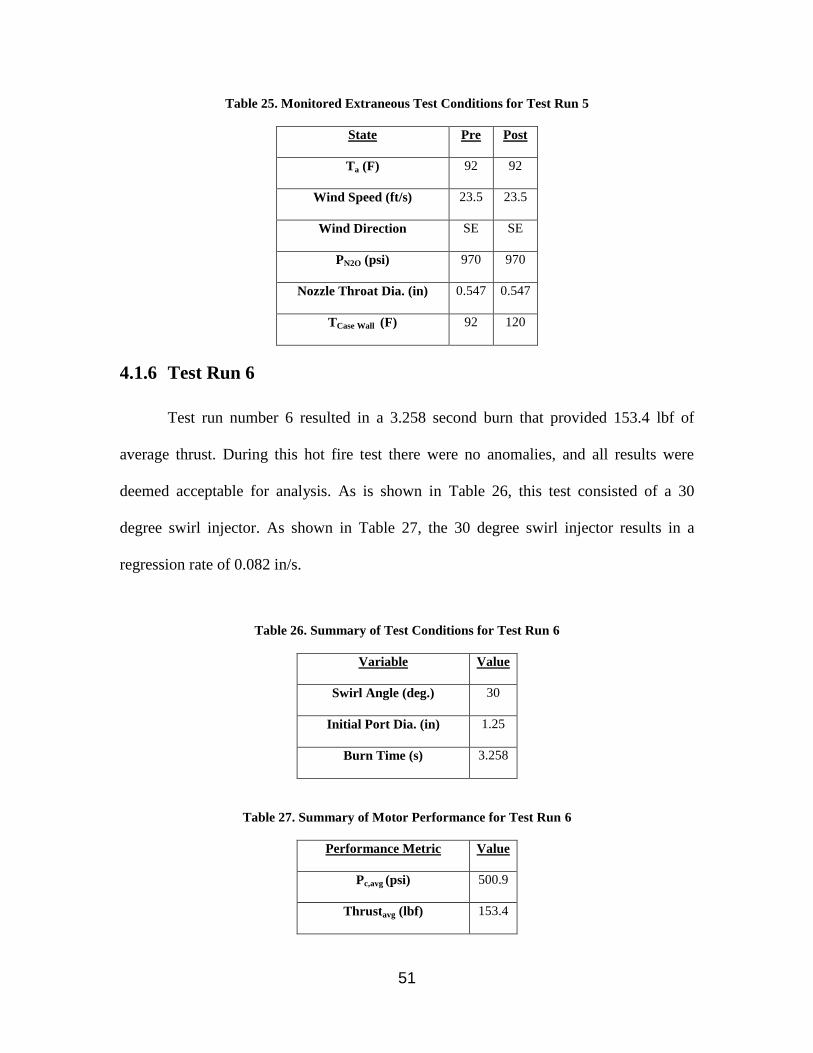
51
Table 25. Monitored Extraneous Test Conditions for Test Run 5
State Pre Post
Ta (F) 92 92
Wind Speed (ft/s) 23.5 23.5
Wind Direction SE SE
PN2O (psi) 970 970
Nozzle Throat Dia. (in) 0.547 0.547
TCase Wall (F) 92 120
4.1.6 Test Run 6
Test run number 6 resulted in a 3.258 second burn that provided 153.4 lbf of
average thrust. During this hot fire test there were no anomalies, and all results were
deemed acceptable for analysis. As is shown in Table 26, this test consisted of a 30
degree swirl injector. As shown in Table 27, the 30 degree swirl injector results in a
regression rate of 0.082 in/s.
Table 26. Summary of Test Conditions for Test Run 6
Variable Value
Swirl Angle (deg.) 30
Initial Port Dia. (in) 1.25
Burn Time (s) 3.258
Table 27. Summary of Motor Performance for Test Run 6
Performance Metric Value
Pc,avg (psi) 500.9
Thrustavg (lbf) 153.4

52
Regression Rate (in/s) 0.082
The extraneous test conditions for test run number 6 are within family of the other test
runs. Because of this, these test conditions are considered negligible for test number 6.
Table 28. Monitored Extraneous Test Conditions for Test Run 6
State Pre Post
Ta (F) 92 92
Wind Speed (ft/s) 23.5 23.5
Wind Direction SE SE
PN2O (psi) 980 980
Nozzle Throat Dia. (in) 0.548 0.548
TCase Wall (F) 92 120
4.1.7 Test Run 7
Test run number 7 resulted in a 3.117 second burn that provided 150.5 lbf of
average thrust. During this hot fire test there were no anomalies, and all results were
deemed acceptable for analysis. As is shown in Table 29, this test consisted of a 30
degree swirl injector. As shown inTable 12, the 30 degree swirl injector results in a
regression rate of 0.078 in/s.
Table 29. Summary of Test Conditions for Test Run 7
Variable Value
Swirl Angle (deg.) 30
Initial Port Dia. (in) 1.25
Burn Time (s) 3.117

53
Table 30. Summary of Motor Performance for Test Run 7
Performance Metric Value
Pc,avg (psi) 490.9
Thrustavg (lbf) 150.5
Regression Rate (in/s) 0.078
The extraneous test conditions for test run number 7 are within family of the other test
runs. Because of this, these test conditions are considered negligible for test number 7.
Table 31. Monitored Extraneous Test Conditions for Test Run 7
State Pre Post
Ta (F) 92 92
Wind Speed (ft/s) 23.5 23.5
Wind Direction SE SE
PN2O (psi) 970 970
Nozzle Throat Dia. (in) 0.548 0.548
TCase Wall (F) 92 120
4.1.8 Test Run 8
Test run number 8 resulted in a 2.475 second burn that provided 159.8 lbf of
average thrust. During this hot fire test there were no anomalies, and all results were
deemed acceptable for analysis. As is shown in Table 32, this test consisted of a 60
degree swirl injector. As shown in Table 33, the 60 degree swirl injector results in a
regression rate of 0.106 in/s.
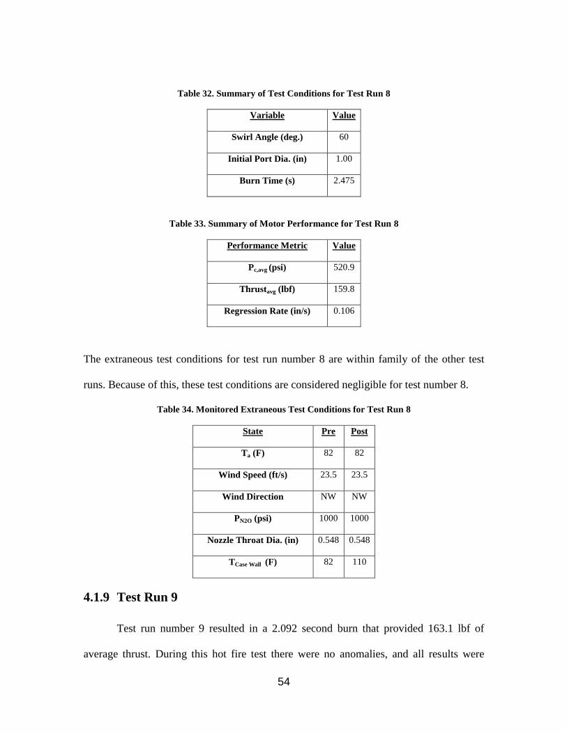
54
Table 32. Summary of Test Conditions for Test Run 8
Variable Value
Swirl Angle (deg.) 60
Initial Port Dia. (in) 1.00
Burn Time (s) 2.475
Table 33. Summary of Motor Performance for Test Run 8
Performance Metric Value
Pc,avg (psi) 520.9
Thrustavg (lbf) 159.8
Regression Rate (in/s) 0.106
The extraneous test conditions for test run number 8 are within family of the other test
runs. Because of this, these test conditions are considered negligible for test number 8.
Table 34. Monitored Extraneous Test Conditions for Test Run 8
State Pre Post
Ta (F) 82 82
Wind Speed (ft/s) 23.5 23.5
Wind Direction NW NW
PN2O (psi) 1000 1000
Nozzle Throat Dia. (in) 0.548 0.548
TCase Wall (F) 82 110
4.1.9 Test Run 9
Test run number 9 resulted in a 2.092 second burn that provided 163.1 lbf of
average thrust. During this hot fire test there were no anomalies, and all results were
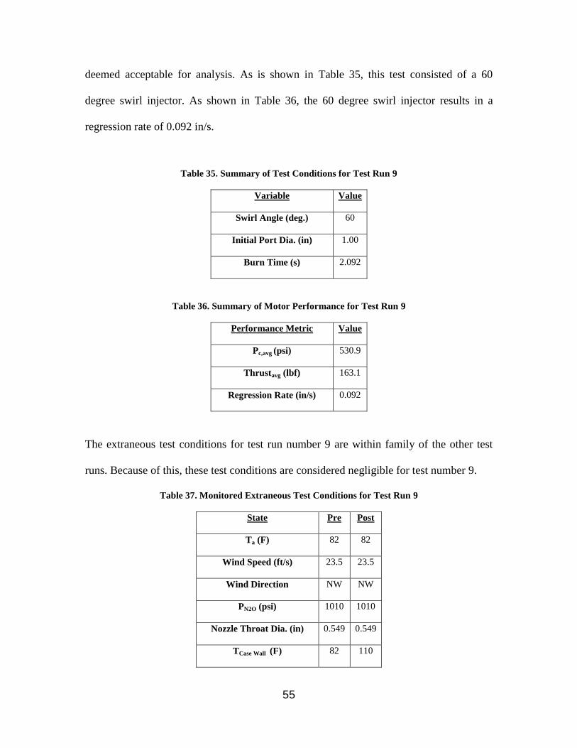
55
deemed acceptable for analysis. As is shown in Table 35, this test consisted of a 60
degree swirl injector. As shown in Table 36, the 60 degree swirl injector results in a
regression rate of 0.092 in/s.
Table 35. Summary of Test Conditions for Test Run 9
Variable Value
Swirl Angle (deg.) 60
Initial Port Dia. (in) 1.00
Burn Time (s) 2.092
Table 36. Summary of Motor Performance for Test Run 9
Performance Metric Value
Pc,avg (psi) 530.9
Thrustavg (lbf) 163.1
Regression Rate (in/s) 0.092
The extraneous test conditions for test run number 9 are within family of the other test
runs. Because of this, these test conditions are considered negligible for test number 9.
Table 37. Monitored Extraneous Test Conditions for Test Run 9
State Pre Post
Ta (F) 82 82
Wind Speed (ft/s) 23.5 23.5
Wind Direction NW NW
PN2O (psi) 1010 1010
Nozzle Throat Dia. (in) 0.549 0.549
TCase Wall (F) 82 110

56
4.1.10 Test Run 10
Test run number 10 resulted in a 1.867 second burn that provided 154.1 lbf of
average thrust. During this hot fire test there were no anomalies, and all results were
deemed acceptable for analysis. As is shown in Table 38, this test consisted of a 60
degree swirl injector. As shown in Table 39, the 60 degree swirl injector results in a
regression rate of 0.104 in/s.
Table 38. Summary of Test Conditions for Test Run 10
Variable Value
Swirl Angle (deg.) 60
Initial Port Dia. (in) 1.25
Burn Time (s) 1.867
Table 39. Summary of Motor Performance for Test Run 10
Performance Metric Value
Pc,avg (psi) 500.9
Thrustavg (lbf) 154.1
Regression Rate (in/s) 0.104
The extraneous test conditions for test run number 10 are within family of the other test
runs. Because of this, these test conditions are considered negligible for test number 10.
Table 40. Monitored Extraneous Test Conditions for Test Run 10
State Pre Post
Ta (F) 82 82
Wind Speed (ft/s) 23.5 23.5

57
Wind Direction NW NW
PN2O (psi) 980 980
Nozzle Throat Dia. (in) 0.549 0.549
TCase Wall (F) 82 110
4.1.11 Test Run 11
Test run number 11 resulted in a 2.709 second burn that provided 152.7 lbf of
average thrust. During this hot fire test there were no anomalies, and all results were
deemed acceptable for analysis. As is shown in Table 41, this test consisted of a 60
degree swirl injector. As shown in Table 42, the 60 degree swirl injector results in a
regression rate of 0.074 in/s.
Table 41. Summary of Test Conditions for Test Run 11
Variable Value
Swirl Angle (deg.) 60
Initial Port Dia. (in) 1.25
Burn Time (s) 2.709
Table 42. Summary of Motor Performance for Test Run 11
Performance Metric Value
Pc,avg (psi) 495.9
Thrustavg (lbf) 152.7
Regression Rate (in/s) 0.074
The extraneous test conditions for test run number 11 are within family of the other test
runs. Because of this, these test conditions are considered negligible for test number 11.

58
Table 43. Monitored Extraneous Test Conditions for Test Run 11
State Pre Post
Ta (F) 82 82
Wind Speed (ft/s) 23.5 23.5
Wind Direction NW NW
PN2O (psi) 975 975
Nozzle Throat Dia. (in) 0.549 0.549
TCase Wall (F) 82 110
4.1.12 Test Run 12
Test run number 12 resulted in a 2.000 second burn that provided 146.5 lbf of
average thrust. During this hot fire test there were no anomalies, and all results were
deemed acceptable for analysis. As is shown in Table 44, this test consisted of a 42
degree swirl injector. As shown in Table 45, the 42 degree swirl injector results in a
regression rate of 0.079 in/s.
Table 44. Summary of Test Conditions for Test Run 12
Variable Value
Swirl Angle (deg.) 42
Initial Port Dia. (in) 1.25
Burn Time (s) 2.000
Table 45. Summary of Motor Performance for Test Run 12
Performance Metric Value
Pc,avg (psi) 470.9
Thrustavg (lbf) 146.5

59
Regression Rate (in/s) 0.079
The extraneous test conditions for test run number 12 are within family of the other test
runs. Because of this, these test conditions are considered negligible for test number 12.
Table 46. Monitored Extraneous Test Conditions for Test Run 12
State Pre Post
Ta (F) 82 82
Wind Speed (ft/s) 23.5 23.5
Wind Direction NW NW
PN2O (psi) 950 950
Nozzle Throat Dia. (in) 0.549 0.549
TCase Wall (F) 82 110
4.1.13 Test Run 13
Test run number 13 resulted in a 2.317 second burn that provided 139.7 lbf of
average thrust. During this hot fire test there were no anomalies, and all results were
deemed acceptable for analysis. As is shown in Table 47, this test consisted of a 42
degree swirl injector. As shown in Table 48, the 42 degree swirl injector results in a
regression rate of 0.081 in/s.
Table 47. Summary of Test Conditions for Test Run 13
Variable Value
Swirl Angle (deg.) 42
Initial Port Dia. (in) 1.00
Burn Time (s) 2.317

60
Table 48. Summary of Motor Performance for Test Run 13
Performance Metric Value
Pc,avg (psi) 421.2
Thrustavg (lbf) 139.7
Regression Rate (in/s) 0.081
The extraneous test conditions for test run number 13 are within family of the other test
runs. Because of this, these test conditions are considered negligible for test number 13.
Table 49. Monitored Extraneous Test Conditions for Test Run 13
State Pre Post
Ta (F) 82 82
Wind Speed (ft/s) 23.5 23.5
Wind Direction NW NW
PN2O (psi) 950 950
Nozzle Throat Dia. (in) 0.550 0.550
TCase Wall (F) 82 110
4.1.14 Test Run 14
Test run number 14 resulted in a 2.150 second burn that provided 145.5 lbf of
average thrust. During this hot fire test there were no anomalies, and all results were
deemed acceptable for analysis. As is shown in Table 50, this test consisted of a 42
degree swirl injector. As shown in Table 51, the 42 degree swirl injector results in a
regression rate of 0.085 in/s.

61
Table 50. Summary of Test Conditions for Test Run 14
Variable Value
Swirl Angle (deg.) 42
Initial Port Dia. (in) 1.00
Burn Time (s) 2.150
Table 51. Summary of Motor Performance for Test Run 14
Performance Metric Value
Pc,avg (psi) 470.9
Thrustavg (lbf) 145.5
Regression Rate (in/s) 0.085
The extraneous test conditions for test run number 14 are within family of the other test
runs. Because of this, these test conditions are considered negligible for test number 14.
Table 52. Monitored Extraneous Test Conditions for Test Run 14
State Pre Post
Ta (F) 82 82
Wind Speed (ft/s) 23.5 23.5
Wind Direction NW NW
PN2O (psi) 950 950
Nozzle Throat Dia. (in) 0.550 0.550
TCase Wall (F) 82 110
4.1.15 Test Run 15
Test run number 15 resulted in a 2.625 second burn that provided 147.2 lbf of
average thrust. During this hot fire test there were no anomalies, and all results were
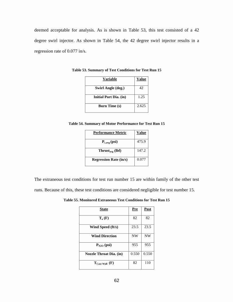
62
deemed acceptable for analysis. As is shown in Table 53, this test consisted of a 42
degree swirl injector. As shown in Table 54, the 42 degree swirl injector results in a
regression rate of 0.077 in/s.
Table 53. Summary of Test Conditions for Test Run 15
Variable Value
Swirl Angle (deg.) 42
Initial Port Dia. (in) 1.25
Burn Time (s) 2.625
Table 54. Summary of Motor Performance for Test Run 15
Performance Metric Value
Pc,avg (psi) 475.9
Thrustavg (lbf) 147.2
Regression Rate (in/s) 0.077
The extraneous test conditions for test run number 15 are within family of the other test
runs. Because of this, these test conditions are considered negligible for test number 15.
Table 55. Monitored Extraneous Test Conditions for Test Run 15
State Pre Post
Ta (F) 82 82
Wind Speed (ft/s) 23.5 23.5
Wind Direction NW NW
PN2O (psi) 955 955
Nozzle Throat Dia. (in) 0.550 0.550
TCase Wall (F) 82 110

63
4.1.16 Test Run 16
Test run number 16 resulted in a 2.050 second burn that provided 145.8 lbf of
average thrust. During this hot fire test there were no anomalies, and all results were
deemed acceptable for analysis. As is shown in Table 56, this test consisted of a 0 degree
swirl injector. As shown in Table 12, the 0 degree swirl injector results in a regression
rate of 0.078 in/s.
Table 56. Summary of Test Conditions for Test Run 16
Variable Value
Swirl Angle (deg.) 60
Initial Port Dia. (in) 1.00
Burn Time (s) 2.050
Table 57. Summary of Motor Performance for Test Run 16
Performance Metric Value
Pc,avg (psi) 470.9
Thrustavg (lbf) 145.8
Regression Rate (in/s) 0.078
The extraneous test conditions for test run number 16 are within family of the other test
runs. Because of this, these test conditions are considered negligible for test number 16.
Table 58. Monitored Extraneous Test Conditions for Test Run 16
State Pre Post
Ta (F) 82 82
Wind Speed (ft/s) 23.5 23.5

64
Wind Direction NW NW
PN2O (psi) 950 950
Nozzle Throat Dia. (in) 0.551 0.551
TCase Wall (F) 82 110
4.1.17 Test Run 17
Test run number 17 resulted in a 1.609 second burn that provided 150.0 lbf of
average thrust. During this hot fire test there were no anomalies, and all results were
deemed acceptable for analysis. As is shown in Table 59, this test consisted of a 0 degree
swirl injector. As shown in Table 12, the 0 degree swirl injector results in a regression
rate of 0.066 in/s.
Table 59. Summary of Test Conditions for Test Run 17
Variable Value
Swirl Angle (deg.) 0
Initial Port Dia. (in) 1.00
Burn Time (s) 1.609
Table 60. Summary of Motor Performance for Test Run 17
Performance Metric Value
Pc,avg (psi) 470.9
Thrustavg (lbf) 150.0
Regression Rate (in/s) 0.066
The extraneous test conditions for test run number 17 are within family of the other test
runs. Because of this, these test conditions are considered negligible for test number 17.
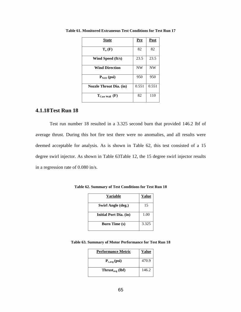
65
Table 61. Monitored Extraneous Test Conditions for Test Run 17
State Pre Post
Ta (F) 82 82
Wind Speed (ft/s) 23.5 23.5
Wind Direction NW NW
PN2O (psi) 950 950
Nozzle Throat Dia. (in) 0.551 0.551
TCase Wall (F) 82 110
4.1.18 Test Run 18
Test run number 18 resulted in a 3.325 second burn that provided 146.2 lbf of
average thrust. During this hot fire test there were no anomalies, and all results were
deemed acceptable for analysis. As is shown in Table 62, this test consisted of a 15
degree swirl injector. As shown in Table 63Table 12, the 15 degree swirl injector results
in a regression rate of 0.080 in/s.
Table 62. Summary of Test Conditions for Test Run 18
Variable Value
Swirl Angle (deg.) 15
Initial Port Dia. (in) 1.00
Burn Time (s) 3.325
Table 63. Summary of Motor Performance for Test Run 18
Performance Metric Value
Pc,avg (psi) 470.9
Thrustavg (lbf) 146.2
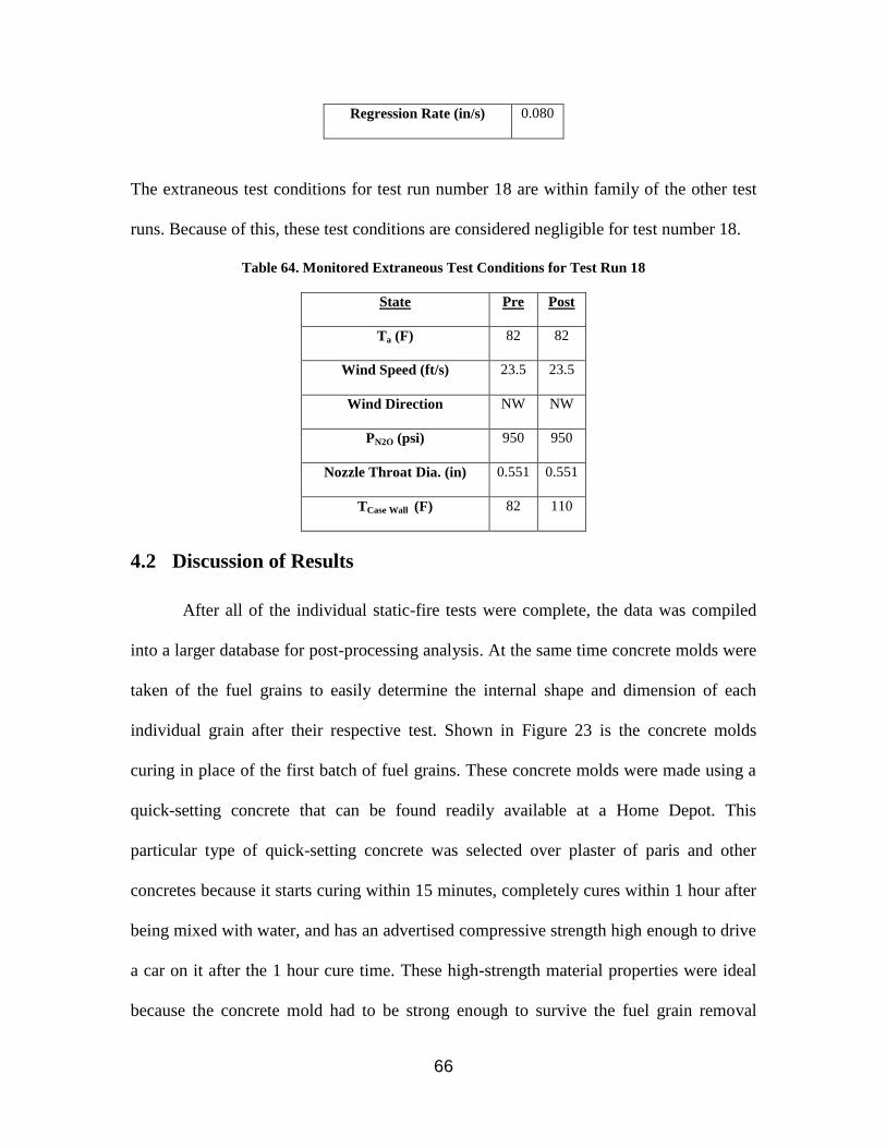
66
Regression Rate (in/s) 0.080
The extraneous test conditions for test run number 18 are within family of the other test
runs. Because of this, these test conditions are considered negligible for test number 18.
Table 64. Monitored Extraneous Test Conditions for Test Run 18
State Pre Post
Ta (F) 82 82
Wind Speed (ft/s) 23.5 23.5
Wind Direction NW NW
PN2O (psi) 950 950
Nozzle Throat Dia. (in) 0.551 0.551
TCase Wall (F) 82 110
4.2 Discussion of Results
After all of the individual static-fire tests were complete, the data was compiled
into a larger database for post-processing analysis. At the same time concrete molds were
taken of the fuel grains to easily determine the internal shape and dimension of each
individual grain after their respective test. Shown in Figure 23 is the concrete molds
curing in place of the first batch of fuel grains. These concrete molds were made using a
quick-setting concrete that can be found readily available at a Home Depot. This
particular type of quick-setting concrete was selected over plaster of paris and other
concretes because it starts curing within 15 minutes, completely cures within 1 hour after
being mixed with water, and has an advertised compressive strength high enough to drive
a car on it after the 1 hour cure time. These high-strength material properties were ideal
because the concrete mold had to be strong enough to survive the fuel grain removal
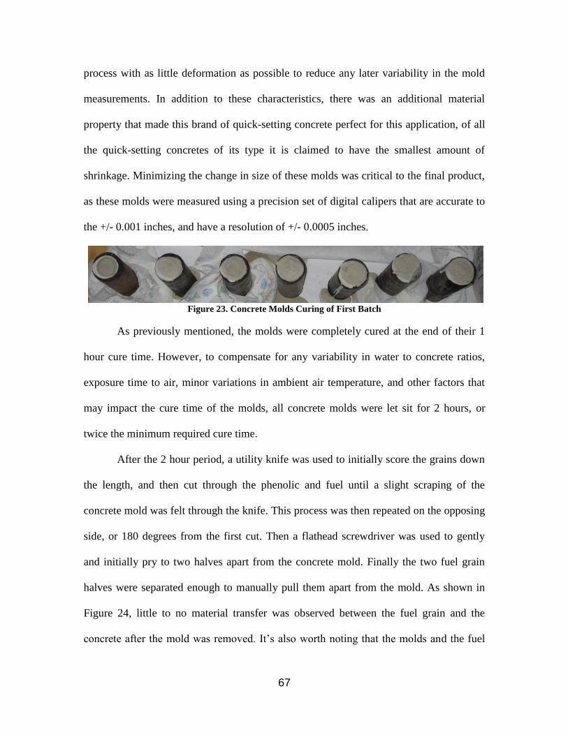
67
process with as little deformation as possible to reduce any later variability in the mold
measurements. In addition to these characteristics, there was an additional material
property that made this brand of quick-setting concrete perfect for this application, of all
the quick-setting concretes of its type it is claimed to have the smallest amount of
shrinkage. Minimizing the change in size of these molds was critical to the final product,
as these molds were measured using a precision set of digital calipers that are accurate to
the +/- 0.001 inches, and have a resolution of +/- 0.0005 inches.
Figure 23. Concrete Molds Curing of First Batch
As previously mentioned, the molds were completely cured at the end of their 1
hour cure time. However, to compensate for any variability in water to concrete ratios,
exposure time to air, minor variations in ambient air temperature, and other factors that
may impact the cure time of the molds, all concrete molds were let sit for 2 hours, or
twice the minimum required cure time.
After the 2 hour period, a utility knife was used to initially score the grains down
the length, and then cut through the phenolic and fuel until a slight scraping of the
concrete mold was felt through the knife. This process was then repeated on the opposing
side, or 180 degrees from the first cut. Then a flathead screwdriver was used to gently
and initially pry to two halves apart from the concrete mold. Finally the two fuel grain
halves were separated enough to manually pull them apart from the mold. As shown in
Figure 24, little to no material transfer was observed between the fuel grain and the
concrete after the mold was removed. It’s also worth noting that the molds and the fuel
68
grains required the flat-head screwdriver to initially pry the two halves apart from the
mold because concrete mold maintained an intimate seal against the rubber fuel grain
throughout the cure process. This further confirmed the idea that the quick-setting
concrete wouldn’t shrink during cure, and that an accurate representation of the fuel
grains internal shape and dimension was captured.
Figure 24. Example Concrete Mold After Grain Is Sectioned, Test #1
During this analysis the following Figure 25 shows the different characteristic
equations for regression rate under depending upon which injector design is selected. It is
easy to see the step in regression rate characteristic functions as they progress from the
injection angle of 0 degrees up to that of 60 degrees. In fact, an increase in regression rate
as high as 45% was observed when comparing the highest performing test case of the 60
degree injector and the lowest performing test case of the 0 degree injector at the low
oxidizer mass flux test condition. Meanwhile, an increase in regression rate as high as
63% was observed when comparing the highest performing test case of the 60 degree
injector and the lowest performing test case of the 0 degree injector at the high oxidizer
69
mass flux test condition. Improvements in regression rate were seen at each increasing
injection angle in between these data points, and can be again seen on the plots. The only
characteristic regression rate equation that wasn’t included in this plot was that of the 30
degree swirl injector. This was simply due to the fact that the experiment ran out of
resources and time, and only one test was able to be completed at the low oxidizer mass
flux test condition with this injector. That being said, the 30 degree injector did still show
an improvement in performance over the 15 degree and 0 degree injectors, and that
improvement can be found in Figure 25.
Figure 25. Regression Rate (Corrected) Characteristic Functions for Indicated Swirl Injector Angles
These characteristic equations shown in Figure 25 can be used to not only
compare performance of a given hybrid rocket motor with different injectors, but can also
be used to extrapolate additional trends about how swirl injection angle directly effects
regression rate as a new variable. It’s worth noting that while only one test was able to be
y = 0.1281x0.3531
y = 0.2478x0.683
y = 0.1259x0.2539
y = 0.4715x0.9119
0.06
0.065
0.07
0.075
0.08
0.085
0.09
0.095
0.1
0.105
0.11
0.14 0.15 0.16 0.17 0.18 0.19 0.2
Avg
Re
gre
ssio
n R
ate
(in
/s)
Oxidizer Mass Flux (lb/s-in2)
Sw = 0
sw = 15
Sw = 30
Sw = 42
Sw = 60
Power (Sw = 0)
Power (sw = 15)
Power (Sw = 30)
Power (Sw = 42)
Power (Sw = 60)
70
completed at the 30 degree swirl angle due to material and time constraints, the one test
at the low-oxidizer mass flux test condition showed regression rates in between that of
the 42 degree injector and the 60 degree injector. While no characteristic equation could
be empirically derived for this 30 degree injector, it can clearly be seen that additional
testing needs to be completed to better understand not only the effects of this injection
angle, but the injection angles of the other injector designs as well.
The average regression rate values shown in Figure 25 were required to be
corrected as a result of some lot-to-lot variation in raw materials of the fuel grains, which
is discussed in more detail in Section 4.3. The correction that was applied to the high data
was calculated based on the variation in fuel densities between the two batches used for
this experiment. By providing this correction, it calculated what the regression rate
should have been for the second batch of fuel grains. This was necessary in order to do
any comparisons between tests since the fuel density has such a large impact on both the
regression rate of the fuel grain, but also overall motor performance. This was
accomplished by taking a series of measurements of the components of the fuel grains,
and calculating average fuel density of the two different batches of cast grains. One this
was completed, the collected data was placed in the following table, Table 65. Using this
tabulated data the average fuel mass flow rates and average oxidizer mass flow rates were
calculated. With these two calculated values a ratio of O/F ratios was able to be
calculated and was then inserted into the Equation 6.
Table 65. Fuel Density Measurement and Calculation Table
Variables Calculated or Measured Values
Low Gox High Gox
Grain Length (in) 7.000 7.000
Grain OD (in) 1.835 1.835
Avg Grain ID (in) 1.250 0.975
71
Grain Volume (in^3) 9.922 13.286
Mass of Liner (oz) 1.100 1.100
Avg Grain Weight (lbm) 8.500 13.230
Avg Grain Mass (lbm) 0.463 0.758
Avg Grain Density (lbm/in^3) 0.047 0.057
Density Ratio 0.817 1.000
In this application, injection angle can be used to either size a hybrid rocket motor
with this new modified regression rate relationship, or vary the regression rate during
motor operation to potentially throttle the motor. The latter of these two designs is likely
the least popular application of these results, but nonetheless it is noteworthy.
During earlier testing a few interesting observations were made that merited
additional research. The first of these observations was that the regression rate of the
grains did not appear uniform down the length while using some injectors. Because of
this, it was critical to develop a way to take regression rate measurements as a function of
length for each of the tests. As can be seen in Figure 26 and Figure 27 the regression rate
down the length of the fuel grains is rarely constant, and in fact requires a unique 60
degree injector configuration or design to accomplish a regression rate that is even close
to constant down the length.

72
Figure 26. Regression Rate (Uncorrected) vs Length of Nominal Tests at the Low-Oxidizer Flux Test
Condition
One key different between the plotted data in Figure 26 and that of Figure 27 is
that little to no injector configurations were shown to provide a constant regression rate
as a function of length at the high oxidizer mass flux test case, unlike the low oxidizer
test case. Inspection of the casting molds revealed that the core rod itself that is used to
cast the 1.00 inch internal diameter fuel grains has a varying diameter down its length.
Because of this, the increasing trend of all the regression rate plots is really only again
true of the lower injection angles. The higher injection angles of 42 degrees and 60
degrees, once corrected maintain a relationship that is more similar to that of the low
oxidizer mass flux plots.
0.04
0.05
0.06
0.07
0.08
0.09
0.1
0.11
0 2 4 6 8
Re
gre
ssio
n R
ate
(in
/s)
Length (in)
Test 4, 0 Deg
Test 5, 0 Deg
Test 2, 15 Deg
Test 3, 15 Deg
Test 7, 30 Deg
Test 1, 60 Deg
Test 9, 60 Deg
Linear (Test 4, 0 Deg)
Linear (Test 5, 0 Deg)
Linear (Test 1, 60 Deg)
Linear (Test 9, 60 Deg)

73
Figure 27. Regression Rate (Uncorrected) vs Length of Nominal Tests at the High-Oxidizer Flux Test
Condition
To further process these experimental results, a commercially available software
package specifically designed for the design and analysis of experiments was used, JMP
10. This software package was used over other packages because it is one of the more
accurate and user-friendly software packages for this specific type of analysis. The
summarized details from Table 6 were input into the software package, and an analysis
was performed to estimate the effects of these factors on the measured response variable
of regression rate. The following Figure 28 shows the accuracy of the JMP-generated
prediction model as the actual regression rate values are plotted against the predicted
regression rate values calculated from the model. With the exception of a few points, all
of the predicted points follow the models estimation relatively close.
0.005
0.01
0.015
0.02
0.025
0.03
0.035
0.04
0.045
0 2 4 6 8
Re
gre
ssio
n R
ate
(in
/s)
Length (in)
Test 16, 0 Deg
Test 17, 0 Deg
Test 18, 15 Deg
Test 13, 42 Deg
Test 14, 42 Deg
Test 8, 60 Deg
Test 10, 60 Deg
Linear (Test 16, 0 Deg)
Linear (Test 17, 0 Deg)
Linear (Test 8, 60 Deg)
Linear (Test 10, 60 Deg)

74
Figure 28. Actual vs Predicted Plot of Whole JMP Model
The following Figure 29 and Figure 30 show the predicted effect of swirl
injection angle and oxidizer mass flux on the regression rate, respectively. When
comparing these two figures side by side, it’s easy to see that the slope of the swirl
injector angle effect plot is higher than that of the oxidizer mass flux effect plot. Since
both of the factors are plotted against the regression rate response variable, it can be said
that the swirl injector angle appears to have a larger effect on the regression rate over the
range of factor values tested at for this experiment.

75
Figure 29. Regression Rate Plot vs Swirl Injection Angle
Figure 30. Regression Rate Plot vs Oxidizer Mass Flux
Since all of the factors are quantitative, the effect estimates could be used to
generated a regression model of the regression rate response variable. The reduced linear
regression model for the fuel grain regression rate can be shown below as Equation 17.
For analysis purposes of regression rate for this experiment, the following equation has
been shown to provide a reasonably accurate prediction of the regression rate response
variable. It is understood, that a more accurate regression model would be of the

76
exponential or power type so that effects of the flux exponent could be properly captured
in the regression model.
Equation 17. Reduced Linear Regression Model for HTPB/N2O Regression Rate
The previously mentioned effect estimates were calculated, and an ANOVA was
performed to determine how significant each effect was. Based on the results in Figure 42,
if a standard 5% significant level of type I error is used, it can be seen from analysis of
variance that the swirl injector angle, oxidizer mass flux, swirl injector angle multiplied
by a squared combustion chamber pressure, and oxidizer mass flux multiplied by a
squared combustion chamber pressure are all significant. However, it is worth
considering that since we have the effect of the combustion chamber pressure as the next
closest significant term, and it was considered significant once squared, that the
combustion chamber pressure be monitored during future experiments closely as it
obviously has some influence on the results. Yet, for the purpose of this experiment and
the sake of simplicity, combustion chamber pressure was not included in the reduced
linear regression model.
4.3 Discussion of Test Anomalies
Despite the efforts of having controlled procedures, mixing environments, and
mixing tooling, some significant variability was seen between the two batches of fuel
grains. After reviewing mixing notes, the cause of this variability isn’t clear. I do know
that it wasn’t a result of contamination because the ingredients used to manufacture the
grains were well controlled, and stored properly in a fire cabinet.
77
One thing that I was able to identify was a slight variation in the amount of
Isonate 143L curative that was added to the formulation while mixing. The difference in
Isonate 143L was 0.020 grams higher in the low density grains than high density grains.
This higher amount of Isonate 143L curative, if all other cure controls were kept the same,
would decrease the cure time such that the propellant couldn’t be properly out-gassed
prior to casting. This incomplete out-gassing process has the potential to decrease the
density of the fuel grain making it prone to voids in the fuel grain. Because this
variability in fuel density can influence the measured regression rate of the fuel grains, a
correction of the data was required and is described below. A secondary leading theory,
though it hasn’t been investigated thoroughly, is that lot-to-lot variation between raw
ingredients from the supplier may have been at least a contributing factor to the
variability between cast propellant grains. Because of the way Daedalus standardizes its
raw ingredients prior to the mixing and casting processes, it isn’t impossible that lot-to-
lot variation slipped through the screening process. Going forward it is suggested that
standardization processes used by the organization more closely represent that of industry
methods.
During the experiment some test anomalies did occur. During a few of the tests,
including Test # 13, misfires were experienced. For the purposes of this test setup and
experiment, a misfire is defined as applying power to Channel 1 to initiate the igniter, and
then power was applied to Channel 3 to open the solenoid and begin the combustion
process by initiating the N2O as it entered the combustion chamber, but the N2O never
ignited. Looking back through the notes and test videos, it was found that the root cause
of the misfires were human error, and the direct cause was that the user waited too long in

78
between switching the Channel 1 and Channel 3 switches. Fortunately, no impact to the
results was seen as a result of these misfires.
Lastly, during the experiment there were a few cases where the solenoid
physically locked in an open position, even after the power was removed. For two tests,
this resulted in a brief, and considered to be negligible, amount of un-choked combustion
in the chamber. The oxidizer flow was finally cut off by closing the manual safety shut-
off valve located upstream in the flow of the solenoid. For one additional test, the
solenoid again locked in a slightly open position; however, I actuated the solenoid
4.4 Large Impact of Results
For the lower injector angles these results show a positive slope trend of
increasing regression rate as a function of combustion port length down the fuel grain.
Because of this, future designs should be designed such that they have a similar initial
positive slope down the length of the combustion port length. This would provide the
forward initial port diameter to be large than the aft initial port diameter, and would
require cast grains to be removed only in the aft direction from the molds. However, it
would enable the hybrid rocket motor to maintain a constant burn time down the length
of the combustion port, and reduce any concerns of local heating of the combustion
chamber during motor operation that could be caused from the motor continuing to burn
away propellant in the forward section of the fuel grain, while there is no propellant left
in the aft section of the fuel grain.
For the high injector angles, and especially the case of the 60 degree injector, the
results show a much more constant burn rate as a function of combustion port length.
Because of this, the average hybrid rocket motor designs should employ these super-

79
critical angle type injectors. This would maintain a constant burn rate as a function of
combustion port length, as well as maintain a constant burn surface area and uniform
combustion of the fuel as a function of combustion port length. Also, previous research
has shown that these high injector angles reduce combustion instabilities, which would
allow for an acceptable reduced margin in the structural design of the hybrid rocket motor
assembly, while maintaining the same performance.
As discussed in detail earlier in this paper, much of the initial driving design
parameters for the motor were based on being able to extrapolate these results to the
larger HRM used by Daedalus Astronautics at ASU. However, the long-term goal is that
these results may be applied to much larger scale motors as well through a scale factor. In
order to accomplish this additional research into the effects of swirl injection angle on
both the macro and micro-combustion processes is required.
4.5 Confidence in Results
The results from this experiment show trends in the data and baseline
characteristic equations to describe the effects of the different injection angles from the
injectors; however, there are still some gaps in the results that could be addressed through
additional testing. Additional tests would increase the fidelity of the models by providing
a more accurate prediction of the regression rate response variable. Additional testing
could be done at other injection angles, including those above 60 degrees to characterize
the effects of swirl injection angles all the way up to that of 90 degrees or tangential
injection, which some researchers are already adopting for their designs.
Additional testing aside, the results that were obtained in this experiment are quite
accurate. Controlled processes were used for the mixing and casting processes, and short
80
of the few difficulties with minor variabilities from batch to batch, the controls worked
quite well. Controlled test procedures were followed, and a large number of extraneous
variables were monitored to mitigate any additional error that could affect the final
results. There were even controlled mix processes and cast processes were used for the
concrete molds, which provided a highly reliable mold of the fuel grains for post-
processing and measurement.
5 Conclusions
The 18 tests performed as part of this experiment showed that, as Bellomo said,
“…for the regression rate performance parameter the most important factor is the
injection type,” (Bellomo, et al., 2012). The ANOVA results discussed in Section 4.2
show that, in contrast to what the basic theoretical equation suggests, oxidizer mass flux
is the number two driving factor of regression rate, and this parameter is dependent upon
the injector as well. The ANOVA results show that the number one most significant
driving factor of regression rate was the swirl injection angle, which as the title of the
parameter suggests, is again a dependent upon the injector itself. There are some
influences of other test conditions and controlled parameters that have an impact on the
regression rate of the fuel; however, the former two parameters are by far the most
critical to regression rate and motor performance. It’s important to note that these results
suggest that the current theoretical equation used across literature may require revisiting.
The results from this experiment not only showed the effects of the swirl injector
angle on regression rate of the fuel grain, but It also identified a few characteristics that
are unique to particular injector angles. For example, at the lower swirl injector angles it
was found that the regression rate becomes less constant down the length of the fuel

81
grain. More specifically, the regression rate at the aft end of the fuel grains tends to be
much higher than that at the forward end of the grains for the lower swirl injector angles.
Because of this, super-critical swirl injector angles are recommended for even burns
down the length of the grain. Also, to ensure accurate measurement of these uneven
regression rates is properly being captured during this type of testing it is urged that
regression rate should always be measured down the full length of the grain and
represented as discrete regression rates. Replacing discrete regression rates with average
regression rates for the overall fuel grain can be misleading.
As has been previously discussed, different fuels have been studied to better
understand the effects swirl injectors on regression rates. It is noteworthy that across
previous works and now this experiment, the same general effects of swirl injection on
regression rate have been found to not be limited to a particular fuel type or motor
configuration.
6 Future Work
The ideal end result of the research endeavors is to perform an up-scaled hybrid
motor flight test for dynamic testing of all the previously investigated components of the
motor, where the up-scaled hybrid motor is designed using both previous injection results
and a well understood scale factor. This flight-ready HRM project has already begun in
parallel to the work with the small-scale HRM such that the results from the small-scale
can feed into the flight-ready hybrid rocket motor design, which can be seen in Figure 31.
82
Figure 31. Flight-Ready Hybrid Rocket Motor Design with TVA Assembly
Many of the components you see in this assembly were designed around the
research results found using the small-scale hybrid rocket motor and test stand setup. One
great example of this would be the variable orifice regulator, which isn’t depicted in this
model, but can be seen as part of the larger assembled rocket motor assembly in mid-test
in Figure 32.
Figure 32. Flight-Ready Hybrid Rocket Motor Design during Successful Static Fire Test
Another great example of a component that will be tested using this test setup will
be a new aerospike nozzle configuration, which has been designed for this small-scale

83
hybrid rocket motor, as shown in Figure 33, so that its analytical thermal and structural
properties can be verified via static fire testing.
Figure 33. (Left) Aerospike Integrated into Small-Scale Hybrid Rocket Motor (Right) 3D Model of Aerospike Nozzle Design
As previously mentioned in Section 4.2, additional testing is required to better
understand the effects of these varying oxidizer injection angles on the regression rate of
the fuel grain. Also, since this experiment focused only on the regression rate effects of
N2O and HTPB, additional testing to better understand these effects on different oxidizer
and fuel combinations is suggested. Especially since the regression rates are highly
subjective to what oxidizer and fuel are selected for use in the hybrid rocket motor.
A last and final suggested point of future investigation is the restart capability of a
hybrid rocket engine, and the effects of restarting the motor on combustion instabilities.
During one of the tests performed, the solenoid locked in a slightly open position, and for
safety reasons the solenoid was given a second set of and open and close electrical
commands. When the solenoid locked in a slightly open position a second time, the same
operation was repeated to provide a third set of open and close electrical commands.
After the third attempt to close, the solenoid finally sealed into the closed position and we
were able to proceed with standard post-test procedures. The interesting thing about this
test anomaly was that each time the solenoid was opened back up the motor restarted

84
instantly and provided nominal pressure and thrust levels. For reference, the sequence of
events went as follows: tburn,1 = 2.083s, toff,1 = 1.100s, tburn,2 = 0.283 s, toff,2 = 0.875s, tburn,3
= 0.259s. Though unplanned as part of the test matrix, this testing was able to show that a
successful restart of this small-scale hybrid rocket motor can occur successfully after a
1.100 second period is possible without the use of a second igniter.

85
REFERENCES
Anderson, J. (2003). Modern Compressible Flow, 3rd ed. . New York: McGraw-Hill
Companies.
Bellomo, N., Faenza, M., Barato, F., Bettella, A., Pavarin, D., & Selmo, A. (2012). The
"Vortex Reloaded" project: experimental investigation on fully tangential vortex
injection in N2O - paraffin hybrid motors. 48th AIAA/ASME/SAE/ASEE Joint
Propulsion Conference & Exhibit 10th Annual International Energy Conversion
Engineering Conference (p. 4304). Atlanta: AIAA.
Benson, T. (2010, Febuary 12). Breif History of Rockets. Retrieved March 22, 2013, from
NASA.gov: http://www.grc.nasa.gov/WWW/k-
12/TRC/Rockets/history_of_rockets.html
Chelaru, T. V., Vasile, E., Florin, M., & Ion, N. (2011). Scalability and dynamic stability
of hybrid rocket engines. 5th International Conference on Recent Advances in
Space Technologies (RAST) (pp. 723-728). Istanbul: IEEE.
Corcoran, M., Mathewson, T., Lee, N. W., & Wong, S. H. (2006). Thrust Vectoring.
Retrieved 03 21, 2013, from The University of Adelaide Web site:
http://personal.mecheng.adelaide.edu.au/maziar.arjomandi/Aeronautical%20Engi
neering%20Project/2006/group17.pdf
Dennis, J., & Villarreal, J. K. (2010). A Primer for University-Level Solid Rocket Motor
Research and Development. Aerospace Sciences Meeting. Orlando: AIAA.
Dennis, J., Shark, S., & Hernandez, F. (2009). Design of N2O/HTPB Hybrid Rocket
Motor Utilizing a Toroidal Aerospike Nozzle. AIAA 2009 Region VI Student
Conference. Long Beach, CA: AIAA.
Doshi, V., Gay , C., Pourkaveh, J., & Stoner , R. (2010). Design and Fabrication of a
N2O/HTPB Flight Ready Hybrid Rocket Motor. San Diego: AIAA.
Littlejohn, D., & Cheng, R. K. (2010). Laboratory Investigations of Low-Swirl Injectors
Operating With Syngases. Journal of Engineering for Gas Turbines and Power,
011502, 1-8.
Lugo, R., Bowerman, K., & Summers, M. (2012). Effects of Swirl Injector Design on
Hybrid Rocket Fuel Regression Rate. AIAA Region VI Student Conference.
Seattle: AIAA.
McCreary, T. (2000). Experimental Composite Propellant, 1st Edition. Murray, KY.

86
Montgomery, D. (2013). Design and Analysis of Experiments, Eighth Edition. Hoboken,
NJ: Wiley and Sons, Inc.
Moran, M. J., Shapiro, H. N., Munson, B. R., & DeWitt, D. P. (2003). Introduction to
Thermal Systems Engineering: Thermodynamics, Fluid Mechanics, and Heat
Transfer. Hoboken, NJ: John Wiley & Sons, Inc.
National Aeronatics and Space Administration. (1974). Solid Rocket Thrust Vector
Control. Cleveland: NASA.
Pucci, J. (2002). The Effects of Swirl Injector Design on Hybrid Flame-Holding
Combustion Instability. AIAA 2002 Region VI Student Conference. AIAA.
Robert F. H. Woodberry and Richard J. Zeamer of Hercules Inc. (1974). Solid Rocket
Thrust Vector Control. Cleveland: National Aeronautical and Space
Administration.
Sutton, G. P., & Biblarz, O. (2010). Rocket Propulsion Elements, Eighth Edition.
Hoboken, New Jersey: John Wiley & Sons, Inc.
Werts, J. R., & Larson, W. J. (2010). Space Mission Analysis and Design. Hawthorne:
Microcosm Press.

87
APPENDIX A
DRAWINGS

88
Figure 34. 0 Degree Injector Drawing
89
Figure 35. 15 Degree Injector Drawing
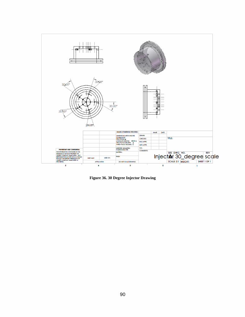
90
Figure 36. 30 Degree Injector Drawing

91
Figure 37. 42 Degree Injector Drawing

92
Figure 38. 60 Degree Injector Drawing

93
Figure 39. Injector Housing Drawing

94
Figure 40. Venturi Drawing

95
APPENDIX B
SENSOR CALIBRATIONS AND SPECIFICATIONS
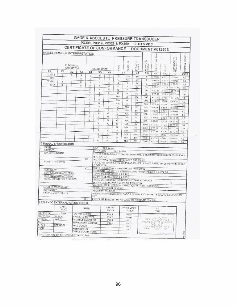
96
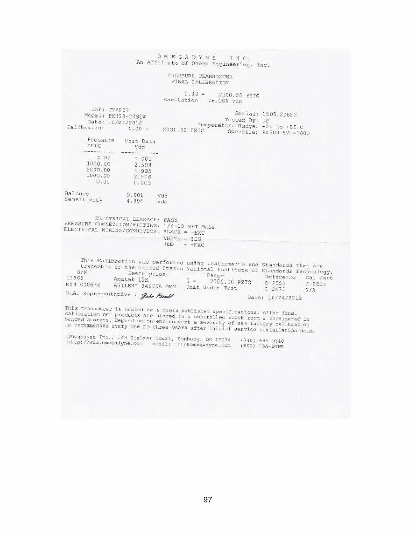
97
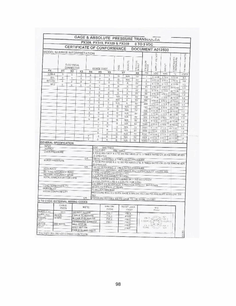
98

99

100

101

102

103

104
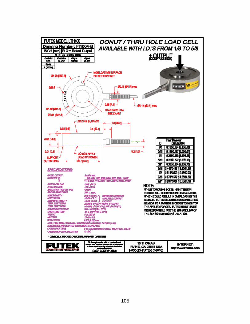
105

106
APPENDIX C
MOLD MEASUREMENTS

107

108

109

110

111
APPENDIX D
ADDITIONAL JMP RESULTS

112
Figure 41. Data Table used for JMP Analysis Input
Figure 42. Calculated Contrasts from JMP Output
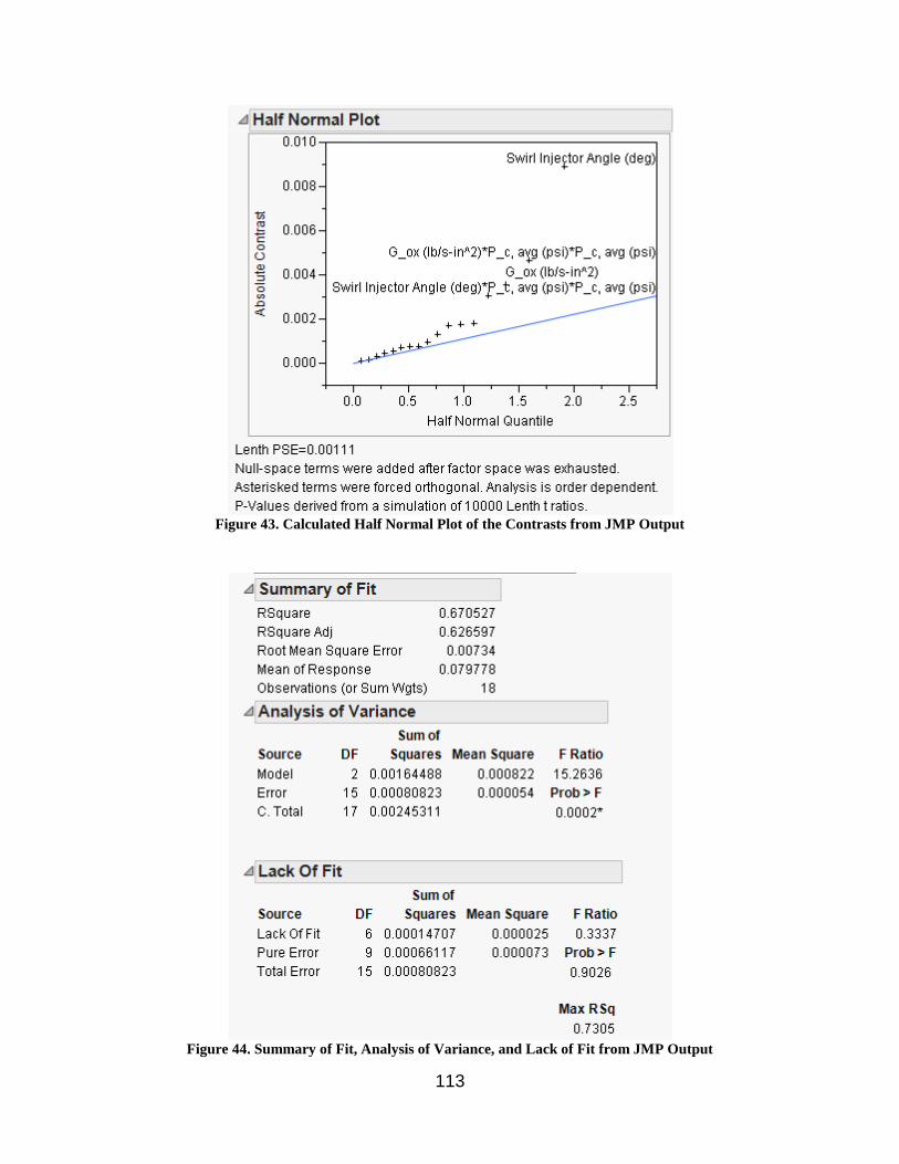
113
Figure 43. Calculated Half Normal Plot of the Contrasts from JMP Output
Figure 44. Summary of Fit, Analysis of Variance, and Lack of Fit from JMP Output
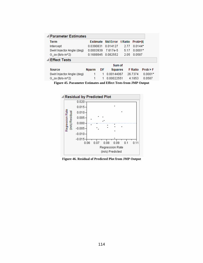
114
Figure 45. Parameter Estimates and Effect Tests from JMP Output
Figure 46. Residual of Predicted Plot from JMP Output