rsm technical reference series hse theory manual regional ... · rsm technical reference series hse...
TRANSCRIPT
RSM Technical Reference Series
HSE Theory Manual
Regional Simulation Model (RSM)
South Florida Water Management District (SFWMD)
Hydrologic and Environmental Systems Modeling
3301 Gun Club Road
West Palm Beach, FL 33406
Reformatted on September 7, 2006
Last updated on 3/29/2007 11:00 AM

ii HSE THEORY MANUAL
This page will intentionally be left blank in the final draft
HSE THEORY MANUAL iii
EXECUTIVE SUMMARY
The south Florida region faces complex problems related to water supply deliveries, flood control and water quality related issues. While tools exist to address individual water resource management needs, the complexity of south Florida requires a comprehensive modeling tool with greater flexibility for simulating various planning and management options, and the ability to integrate multiple disciplines into one model (e.g., hydrology, hydrodynamics, hydraulics, water quality, and ecology).
Numerous simulation models have been developed to provide predictive application, which included both groundwater and surface water components. Some of these models were mainly developed as groundwater models, and then added surface water components to the original model (e.g., Modflow), while others were developed as surface water models, and then a groundwater component was added (e.g., MODNET). The limitation of such an approach is that more attention is given to one component over the other (i.e., groundwater vs. surface water), with more details included in one component while little or minimal mathematical representation is included in the other. This modeling constraint was due to the inability of existing technology (e.g., software matrix, computer language) to allow concurrent model development and integration of both surface water and groundwater.
In south Florida, both groundwater and surface water components need to be equally represented to address this unique region. In addition, a comprehensive hydraulic component must be provided to simulate and manage numerous and different types of man-made structures and canals in south Florida. The hydraulic component must be capable of responding to preset rules and operations as well as to extreme weather patterns (wet/dry) that affect competing urban, environmental and agricultural demands.
To address these needs, the South Florida Water Management District (SFWMD) is developing the Regional Simulation Model (RSM). While this regional hydrologic model is developed on a sound conceptual and mathematical framework, simulating a wide range of hydrologic conditions, RSM has been developed principally for application in south Florida, and accounts for interactions among surface water and groundwater hydrology, structure and canal hydraulics, and management of these hydraulic components.
The Regional Simulation Model (RSM) is a finite volume, object oriented based hydrologic model that simulates groundwater flow, overland flow in wetlands, canal flow, groundwater / surface water interactions and other critical components of the hydrologic cycle.
The RSM simulates and integrates the coupled movement and distribution of groundwater, surface water, man-made structures and network canals in south Florida. Currently, the RSM has two principal components, the Hydrologic Simulation Engine (HSE) and the Management Simulation Engine (MSE), collectively these two engines are designed to address hydrology and water resources management in south Florida. The HSE simulates natural hydrology, water
iv HSE THEORY MANUAL
control features, water conveyance systems and water storage systems. The HSE component solves the governing equations of water flow through both the natural hydrologic system and the man-made structures. The MSE component provides a wide range of operational and management capabilities to the HSE. The MSE is capable of simulating a wide range of management operations for the water control features of the south Florida system. Considering that there is not a single unique way that operations can be executed, the MSE is designed to simulate a variety of management options including those used in the past or planned for the future under both normal and extreme conditions.
Future versions of RSM will include one additional engine; a water quality Engine (WQE), which is designed to simulate water quality conditions and the ecosystem response to these changes. The WQE will be constructed in two major parts. The first part, the backbone, of the WQE is designed to calculate transport of all materials (i.e., advection and dispersion), while the second part may include variety of modules designed to simulate water chemistry among hydrologic components as well as a variety of biogeochemical reactions between transported and non-transported material. Additional modules may also include several vegetation modules dominating the landscape in an ecosystem such as cattail, sawgrass, and periphyton. Interactions among these modules shall include uptake and release of nutrients between vegetation compartments, soil, and surface and groundwater.
The RSM Technical Reference Manual is comprised of a series of reports including, HSE Theory Manual, MSE Theory Manual, WQE Theory Manual, and RSM Guidelines for Managing Numerical Error, RSM Verification Tests, RSM Benchmarks and Tests, RSM Programmer Guide, RSM GUI Programmer Guide (See complete list in the inside cover of this manual). The HSE Theory Manual (this Report) describes in details the theory behind the RSM hydrologic engine and how the hydrologic cycle and its major components are represented in the model.

HSE THEORY MANUAL v
TABLE OF CONTENTS
Executive summary .................................................................................. iii
List of Figures............................................................................................. vii
Acknowledgements ............................................................................... viii
Acronyms .................................................................................................. ix
Glossary ......................................................................................................x
Chapter 1: Introduction.............................................................................1
1.0 Report organization .............................................................................2
1.1 Brief History of Regional Modeling in south Florida ..........................3
1.2 RSM Design Requirements and Building Blocks................................6
1.3 RSM Design compared to other models ...........................................8
1.4 Special Features and Capabilities of RSM ......................................10
Chapter 2: Hydrologic Simulation Engine Theory and Concepts .......13
2.1 HSE Concepts .....................................................................................13
2.2 Theoretical Overview ........................................................................15
2.3 HSE Governing Equations..................................................................15
2.3.1 Mass Balance Equation................................................................................ 16
2.3.2 Momentum Equation.................................................................................... 18

vi HSE THEORY MANUAL
2.4 Waterbodies Formulation..................................................................19
2.4.1 Stage-Volume (SV) Relationships Describing Waterbodies ..................... 19
2.4.2 Stage-Volume (SV) Relationship for Flat Ground ...................................... 21
2.4.3 Volume-Stage (VS) Relationship for Flat Ground ...................................... 21
2.4.4 Stage Volume (SV) Relationship for a Canal Segment Waterbody......... 21
2.5 Watermovers Formulation.................................................................22
2.5.1 Overland Flow Watermover......................................................................... 23 2.5.1.1 Overland Flow Watermover for Mixed Flow....................................................................................26
2.5.2 Groundwater Flow Watermover .................................................................. 27
2.5.3 Canal Flow Watermover .............................................................................. 27
2.5.4 Canal-Cell Watermover............................................................................... 28
2.5.5 Structure Flow Watermover.......................................................................... 29
2.5.6 Sources and Sinks; Head Independent Watermovers .............................. 30
2.6 Hydrologic Process Module (HPM) Formulation.............................30
2.6.1 HPM Concepts .............................................................................................. 31
2.6.2 Limitations of HPM......................................................................................... 32
2.6.3 Simple HPM.................................................................................................... 32
2.6.4 Complex HPM ............................................................................................... 34
2.6.5 HPM Hubs....................................................................................................... 34
2.7 Assembly of all Waterbodies ............................................................35
2.8 HSE Numerical Solution .....................................................................36
2.8.1 Average Water Velocity .............................................................................. 38
References................................................................................................41

HSE THEORY MANUAL vii
LIST OF FIGURES Figure 1.1 Principal components of the RSM: a) HSE, b) MSE, c) HPM....................................................................2 Figure 1.2 Spatial extent of SFWMM (2x2 model; orange line) and SFRSM (yellow line) model grids. ....................5 Figure 1.3 Spatial extent of SFRSM and SFWMM model boundary and an example of grid resolution used by both
models....................................................................................................................................................................6 Figure 1.4 Comparison of Computational Fluid Dynamics approaches used by RSM and traditional models. ...........9 Figure 2.2 An arbitrary control volume with fluxes, represented in RSM as a cell with fluxes through walls between
cells......................................................................................................................................................................16 Figure 2.3 Control volumes or waterbodies used in the HSE. .....................................................................................17 Figure 2.4 Stage-volume relationship for cell and canal segment waterbodies ...........................................................20 Figure 2.5 Organization of surface integration terms ..................................................................................................22 Figure 2.6 Sample waterbodies with circumcenters m and n used to define variables ................................................24 Figure 2.7 Submatrix for a single watermover as part of total matrix .........................................................................26 Figure 2.8 Canal flow calculations ..............................................................................................................................28 Figure 2.9 Matrix elements for canal-aquifer interaction. ...........................................................................................29 Figure 2.10 Simple Hydrologic Process Module with no internal storage. .................................................................33 Figure 2.12 Hub Hydrologic Process Module with multiple internal HPMs includes soil water storage and
stormwater storage. The Hub may cover one or many mesh cells......................................................................35 Figure 2.13 Computational space-time space of RSM ................................................................................................37 Figure 2.14 A simplified flowchart of RSM computational steps ...............................................................................39

viii HSE THEORY MANUAL
ACKNOWLEDGEMENTS
The South Florida Water Management District gratefully acknowledges the contributions of all professionals and support staff who have made this model a reality. The Regional Simulation Model has been developed over many years, and many people have contributed to this development. All contributors are South Florida Water Management District (SFWMD) staff except where noted.
Project Management: Jayantha Obeysekera, Director of the Hydrologic and Environmental Systems Modeling Department, wrote the original statement of work for this model in 1993. He has nurtured the technical staff all these years to bring the model to fruition, and we gratefully acknowledge his technical and managerial oversight. In the last few years, Jack Maloy has infused a new level of energy into the RSM project, fast-tracking the completion of the model by providing support in obtaining both human and financial resources. Ken Tarboton served as project manager of both RSM development and implementation activities, and Rich Sands now oversees a team of project managers.
Principal Contributors: Wasantha Lal, Chief Hydrologic Modeler, is the principal developer of the hydrologic/hydraulic tenets upon which the RSM is built. Randy VanZee, Chief Hydrologic Modeler, is the principal architect of the model, and developer of the majority of the object-oriented code. Wasantha Lal served as the principal author of this manual.
Other contributors include David Welter, Chief Hydrologic Modeler, Joseph Park, Lead Hydrologic Modeler, Eric Flaig, Senior Engineer, Clay Brown, Senior Hydrologic Modeler, and Mark Belnap, Senior Engineer at NTI/Verio and former SFWMD Engineer.
For further information, please contact: For theory questions: Wasantha Lal, Ph.D., P.E. Hydrologic and Environmental Systems Modeling South Florida Water Management District 3301 Gun Club Road, West Palm Beach, FL 33406 561-682-6826 [email protected]
A number of RSM documents are available on the World Wide Web at: http://my.sfwmd.gov/hesm

HSE THEORY MANUAL ix
ACRONYMS Acronym Description BC Boundary Conditions CERP Comprehensive Everglades Restoration Plan EPM Ecological Processes Module ET Evapotranspiration FIFO First In First Out FV Finite Volume GIS Geographic Information Systems GLPK GNU Linear Programming Kit HEC/DSS Hydrologic Engineering Center Data Storage System HPM Hydrologic Process Module HUB Collection of HPM HSE Hydrologic Simulation Engine MSE Management Simulation Engine WQE Water Quality Engine LP Linear Programming NetCDF Network Common Data Form NSM Natural System Model NSRSM Natural System Regional Simulation Model MIMO Multiple Input, Multiple Output MISO Multiple Input, Single Output OO Object-Oriented PDE Partial Differential Equation PETSC Portable, Extensible Toolkit for Scientific Computation (the HSE ’solver’) PID Proportional-Integral-Derivative (feedback control) PWS Public Water Supply RSM Regional Simulation Model SFRSM South Florida Regional Simulation Model SFWMM South Florida Water Management Model (the 2 X 2) SFWMD South Florida Water Management District (aka District) STL Standard Template Library SV Stage to volume conversion SVD Single Value Decomposition USACE U.S. Army Corps of Engineers VS Volume to stage conversion WCU Water Control Unit WQPM Water Quality Processes Module XML Extensible Markup Language

x HSE THEORY MANUAL
GLOSSARY
Cell: Basic element in a model mesh/grid (triangular or rectangular)
Coupled: If two or more separate processes or systems interacting with one another are to be solved, coupled methods solve all the systems using a single system of equations
ET: Evapotranspiration
Explicit: Explicit methods calculate the state of a system at a later time from the state of the system at the current time
Fully integrated: various hydrologic functions are solved simultaneously and not sequentially
Grid: Geometric representation of model domain (e.g., triangular or rectangular cells)
Implicit: implicit methods find the solution by solving an equation involving both the current state of the system and the later one
Loosely coupled: In loosely coupled systems, solutions are obtained for the individual systems separately, but iterations are carried out between them to allow for updating the solution of one system based on the other
Mesh: Geometric representation of model domain (e.g., triangular or rectangular cells)
PET: Potential evapotranspiration
Uncoupled: Uncoupled methods solve the individual systems separately, one after the other. After the solution, one is not updated to adjust for the changes in the other
Volume: Space occupied, by water in this case, as measured in cubic units (e.g., ft3, m3)

CHAPTER 1. INTRODUCTION 1
CHAPTER 1: INTRODUCTION
The advent of software packages for computational and numerical simulation has produced a profound impact on the ability of scientists and engineers to model a wide variety of physical phenomena across a broad spectrum of disciplines. The discipline of hydrology has leveraged these developments to the point where an overwhelming proliferation of hydraulic and hydrologic numerical models aimed at addressing the major engineering issues facing the hydrologic community.
Along with these standard engineering issues, south Florida faces complex problems related to water supply deliveries, flood control and water quality management. While tools exist to address individual water resource management needs, the complexity of south Florida requires a comprehensive modeling tool with greater flexibility for simulating various planning and management options, and the ability to integrate multiple disciplines (e.g., hydrology, hydraulics, ecology, and water quality) into one model.
Numerous simulation models have been developed to provide predictive tools, which have included both groundwater and surface water components. Some of these models were mainly developed as groundwater models, and then added surface water components to the original model (e.g., MODFLOW; Yeh et al., 1998), while others were developed as surface water models, and then a groundwater component was added (e.g., MODNET). The limitation of such an approach is that more attention is given to one component over the other (i.e., groundwater vs. surface water), with more details included in one component while little or minimal mathematical representation is included in the other. This modeling constraint was due to the inability of existing technology (e.g., software matrix and computer language) to allow concurrent code development and integration of both surface water and groundwater components into a single model.
In south Florida, both groundwater and surface water components need to be equally represented, in any numerical model, to accurately simulate this unique region. In addition, a comprehensive hydraulic component must be provided to simulate and manage numerous and different types of man-made structures and canals in south Florida. The hydraulic component must be capable of responding to preset rules and operations as well as to extreme weather patterns (wet/dry) that affect competing urban, environmental and agricultural demands.
To address these needs, the South Florida Water Management District (SFWMD) had developed the Regional Simulation Model (RSM). While this regional hydrologic model is built on a sound conceptual and mathematical framework, simulating a wide range of hydrologic conditions, RSM has been developed principally for application in south Florida, and accounts for interactions among surface water and groundwater hydrology, structure and canal hydraulics, and management of these hydraulic components.

2 CHAPTER 1. INTRODUCTION
The RSM simulates and integrates the coupled movement and distribution of groundwater, surface water, man-made structures and canal network in south Florida. The RSM has two principal components, the Hydrologic Simulation Engine (HSE) and the Management Simulation Engine (MSE) (Figure 1.1). The HSE simulates natural hydrology, water control features, water conveyance systems and water storage systems. The HSE component solves the governing equations of water flow through both natural hydrologic system and man-made structures. Future versions of RSM will address water quality and system ecology. The MSE component provides a wide range of operational and management capabilities to the HSE (Figure 1.1). The MSE is capable of simulating a wide range of management operations for the water control features of the south Florida system. Considering that there are multiple ways that operations can be executed, the MSE is designed to simulate a variety of management options including those used in the past or planned for the future.
Figure 1.1 Principal components of the RSM: a) HSE, b) MSE, c) HPM
1.0 REPORT ORGANIZATION
This manual presents the theory of the Regional Simulation Model (RSM) in two main sections and three appendices. The remainder of this introductory chapter presents a brief history of the RSM development, followed by an overview of model concepts, capabilities, and features. A summary of refinement and testing efforts that have enhanced RSM development is also provided.

CHAPTER 1. INTRODUCTION 3
Chapter 2 of the RSM Theory Manual describes the concepts, theory, governing equations and algorithms used in the Hydrologic Simulation Engine to numerically simulate the hydrologic process. The concept and theory of the local Hydrologic Process Modules (HPMs) are also described, which provide an upper boundary condition to the integrated numerical solution.
Additional background information are provided in Appendix A, regarding RSM model philosophy, limitations and usage guidelines. Appendix B presents the shallow water overland equations traditionally used in many existing models, while Appendix C contains a subset of RSM referenced materials.
Appendix C.5 provides an overview of the Hydrologic Process Modules of the RSM. The HPMs are mainly developed to simulate the small-scale, local hydrology and vertical processes for the RSM. The primary function of HPMs is to provide the surface boundary condition for the regional solution. These HPMs are used to process rainfall and potential evapotranspiration (PET) and provide net recharge to the mesh cells of the HSE.
Appendix C.6 presents the concepts and the theory of the Management Simulation Engine (MSE). In Appendix C.6, different levels of management control are described to simulate both local and regional water management options. At the higher level of management control is the capability to assign an overall mission (e.g., unexpected or unplanned water supply needs in a specific area within the model domain). At the lower level of management control are capabilities that will execute that mission (e.g., release more water through a group of structures to meet the water supply needs at that specific area). In addition, Appendix C.6 describes the concepts of the decision making process and the interaction between the HSE and MSE.
The HSE Theory Manual is one of several Regional Simulation Model Documents (i.e., RSM Technical Reference Series), which include HSE Theory Manual, MSE Theory Manual, WQE Theory Manual, RSM Guidelines for Managing Numerical Error, RSM Verification Tests, RSM Benchmarks and Tests, RSM Programmer Guide, and RSM GUI Programmer Guide. The HSE Theory Manual (this Report) describes in details the theory behind the RSM hydrologic engine and how the hydrologic cycle and its major components are represented in the model. Many other published manuscripts, documents and reports regarding the RSM are also available, most via the Internet.
1.1 BRIEF HISTORY OF REGIONAL MODELING IN SOUTH FLORIDA
Regional simulation models have long been a key tool to manage the vast and unique systems of south Florida. Analog models were the first generation regional modeling tools used in south Florida in the 1970’s to simulate steady state groundwater flow problems. As digital computers became available, simple digital simulation models based on principles of mass balance became popular initially. One of the first computer models introduced to south Florida and used by the District was the South Florida Regional Routing Model, also known as the POT model (Trimble, 1986). It was a lumped parameter model applied over parts of the regional system simulating Lake Okeechobee and various storage areas (e.g., WCA1, WAC2, WCA3). However, the model
4 CHAPTER 1. INTRODUCTION
evolved over many generations with added capabilities to simulate processes such as evaporation and soil moisture as well as to simulate various management options. Over time, it became clear that processes such as canal seepage and sheet flow would have to be simulated in two dimensions (x-y) to obtain realistic results (Lin, 2003). This need resulted in the development of the South Florida Water Management Model (SFWMM); also known as the 2X2 model (South Florida Water Management District, 1999).
The SFWMM is the first two-dimensional (2-D) distributed parameter model to simulate the regional system of south Florida to determine the distribution of flow in this complex landscape. The model simulates 2-D overland flow, groundwater flow, canal flow, canal seepage, levee seepage, well pumping, and a substantial portion of water management activities. The SFWMM has been used to estimate flows and water levels resulting from historical, current and proposed management scenarios under a wide range of climatic and boundary conditions.
The SFWMM uses a 2-mile square horizontal grid spatial resolution and a one-day time step for the computations. The model domain extends from Lake Okeechobee in the north to Florida Bay in the south, covering an area of 7,600 square miles (Figure 1.2). The selected spatial and temporal resolutions were the optimum discretizations that were practical using 1980s’ computers.
The SFWMM is used to evaluate current and proposed water management protocols and operational rules, to make planning decisions regarding significant changes to the system while maintaining water supply, the environment, and other water needs. Over the years, the hard-coded sites and operational conditions of the model have become complex and difficult to maintain. However, the SFWMM is still a useful tool capable of performing a large number of regional simulation functions and will be used until the transition to SFRSM is completed.

CHAPTER 1. INTRODUCTION 5
Figure 1.2 Spatial extent of SFWMM (2x2 model; orange line) and SFRSM (yellow line) model grids.
Anticipating a need to modernize these two models, SFWMD began developing an alternative model which could accomplish the goals and objectives of both the SFWMM and NSM models. The RSM is the modeling tool used to implement both the South Florida Regional Simulation Model (SFRSM) and the Natural System Regional System Model (NSRSM). These two implementations extend the boundaries of the original models, and are being implemented using a triangular mesh (Figure 1.3).

6 CHAPTER 1. INTRODUCTION
Figure 1.3 Spatial extent of SFRSM and SFWMM model boundary and an example of grid resolution used by both models.
1.2 RSM DESIGN REQUIREMENTS AND BUILDING BLOCKS
One of the primary goals in the development of the RSM is that its south Florida implementation, SFRSM, must be both flexible and adaptable to changing conditions within south Florida. With the expansive planned changes to south Florida drainage basins under the Comprehensive Everglades Restoration Plan (CERP)1 and new water management strategies2, it
1 http://www.evergladesplan.org
2 http://www.sfwmd.gov/org/wsd/waterreservations/index.html

CHAPTER 1. INTRODUCTION 7
is necessary to develop a model that can be adapted to simulate changing and complex management strategies. It is imperative that this model be easier to use than the South Florida Water Management Model, with shorter learning curves, improved documentation and benchmark examples. There will be no hard-coding of sites, features, or operational conditions in the RSM code or its implementations to allow maximum flexibility in model application.
RSM development relies mainly on three building blocks: 1) object-oriented (OO) code design, 2) new computational methods (i.e., grid resolution and numerical errors) and 3) new and efficient numerical solvers for large matrices.
The first area of technological contribution came from recent developments in information technology and the use of OO code design methods. The use of extensible markup language XML (Bosak and Bray, 1999), geographic information system (GIS) technology and database support has allowed the achievement of a level of code flexibility and data integration that did not exist before. Object-oriented methods have been used in the past for hydraulic model design by Solomatine (1996), Tisdale (1996), and many others.
The strong dependencies between hydrology, nutrient transport and ecology have created a need to develop a comprehensive and integrated software package using a modular approach. Simple models that address issues within one discipline at a time have become inadequate for studying complex systems. The improved use of GIS support tools, OO code design and XML language have made it possible to organize large amounts of complex data and to model complex systems, while allowing modelers to focus on the concepts (see for example Figure 2-12).
The second area of technological contribution came from developments in computational methods. While, the mathematical foundation for RSM has been around for many years (Chow et al., 1988; Hirsch, 1989), implementation of these equations was only made possible through the advancement of certain new technologies. For example, the use of unstructured meshes of variable size grid-cells to simulate 2-D integrated overland and groundwater flow in irregular shaped domains has become common (Zhao et al., 1994; Shen et al., 1997). Full and partial integration with canal networks and lakes is now possible. In the past two decades, a number of physically based, distributed-parameter models have emerged with such features. Early models include MODBRANCH (Swain and Wexler, 1996), MODNET (Walton et al., 1999), MIKE SHE/MIKE 11 based on Abbott et al. (1986a, 1986b), WASH123 (Yeh et al., 1998), MODFLOW-HMS (HydroGeoLogic, 2000), and models by VanderKwaak (1999), Schmidt and Roig (1997), and Lal (1998b). The computational engines of these models are based on solving a form of the shallow water equation for overland flow, either the variably saturated Richards’ equation or the fully saturated groundwater flow equation. In RSM, inertia terms in the shallow water equations are neglected, and the solution to the governing equations is obtained using a single global matrix. A number of features, such as lookup tables, approximate linearization methods, and regression methods, are available in the RSM model to simulate behavior of structures, urban areas and agricultural areas. The choice and selection of features used in the RSM depends on the intended application of the model.
The third area of technological contribution came from a new generation of computer packages that can be used to efficiently solve large sparse systems of equations (Schenk and Gartner,

8 CHAPTER 1. INTRODUCTION
2004; Gupta et al., 1997). It is now possible to develop implicit finite volume algorithms and solve many complex equations simultaneously without iterating between various model components. Modern solvers support parallel processing and have a variety of built-in tools and options to achieve fast model runs. These solvers are easy to use because details, such as matrix storage methods, are automated and transparent to the user. RSM uses the software package PETSC (Balay et al., 2001) to solve its matrices. Some of the reasons for selecting and using PETSC in RSM includes, parallel processing capabilities, widely accepted and free (public domain software), fast, and easy to use and implement.
The RSM uses advanced computational techniques and other technologies such as, object-oriented design methods (OO), extensible markup language (XML), geographic information system (GIS), and a finite volume (FV) method to simulate 2-D overland and groundwater flow. RSM uses an unstructured triangular mesh to discretize the model domain. The discretized control volumes for surface water, groundwater, canals and lakes are treated as abstract ”waterbodies” that are connected by abstract ”watermovers.” The numerical procedure is flexible enough to allow the use of several representations for the same equation without the constraint of a preset single approach (e.g., Manning equation, flow resistance in wetlands, or lookup tables).
An object-oriented (OO) code design is used to provide robust and highly extensible software architecture. The object-oriented design of the RSM allows an implementation to consist of an assembly of different water management objects that can be interchanged as the model evolves. A weighted implicit numerical method is used to keep the model fully integrated and stable. A limited error analysis was conducted to ensure that the results of the implicit scheme used in the RSM fall within acceptable criteria using well posed analytical solutions.
The RSM has been tested at the subregional scale to analyze its applicability to south Florida conditions. For example, the HSE has been used to simulate flow in the Kissimmee River (Lal, 1998c), and in the Everglades National Park (Lal, 1998b; Brion et al., 2000; Brion et al., 2001; Senarath et al., 2001; Senarath, 2002). The model was verified using the MODFLOW model (McDonald and Harbaugh, 1984) and an analytical solution for stream-aquifer interaction (Lal, 2001).
1.3 RSM DESIGN COMPARED TO OTHER MODELS
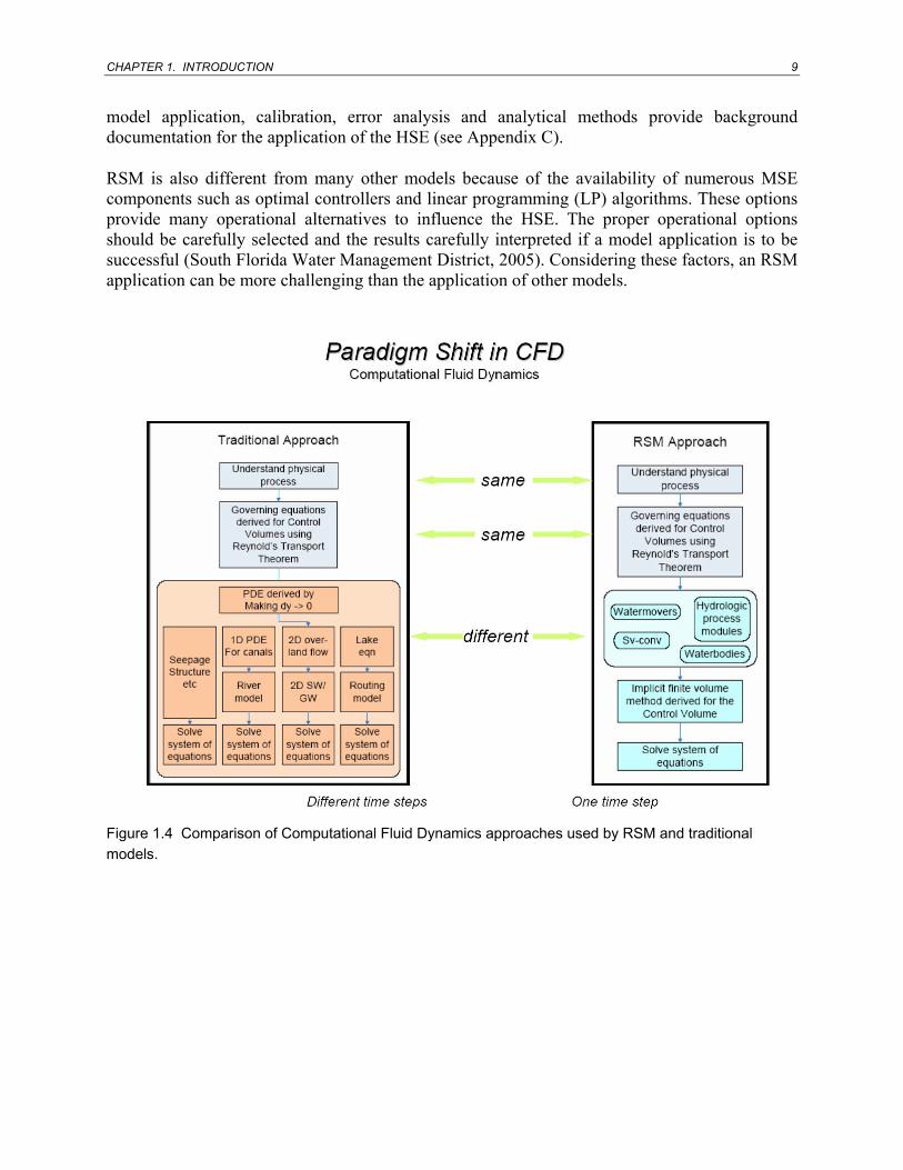
Similar to other models, RSM uses numerical methods that solve ordinary and partial differential equations and incorporate flow resistance equations among regional equations to represent a wide variety of local and regional conditions, and simulates both natural and anthropogenic conditions (Figure 1.4).
Unlike other models, RSM is designed with object-oriented methods, provides auxiliary tools (e.g., error analysis methods) for use during both model implementation and model application, and separates operations management through the MSE component. A certain level of understanding of object-oriented methods, and the basic RSM object types such as waterbodies and watermovers are required before adding new objects to the model. Several articles written on
CHAPTER 1. INTRODUCTION 9
model application, calibration, error analysis and analytical methods provide background documentation for the application of the HSE (see Appendix C).
RSM is also different from many other models because of the availability of numerous MSE components such as optimal controllers and linear programming (LP) algorithms. These options provide many operational alternatives to influence the HSE. The proper operational options should be carefully selected and the results carefully interpreted if a model application is to be successful (South Florida Water Management District, 2005). Considering these factors, an RSM application can be more challenging than the application of other models.
Figure 1.4 Comparison of Computational Fluid Dynamics approaches used by RSM and traditional models.

10 CHAPTER 1. INTRODUCTION
1.4 SPECIAL FEATURES AND CAPABILITIES OF RSM
South Florida is a unique environment requiring specialized models to simulate regional operations. South Florida has a complex regional hydrologic system that includes:
• Approximately 2,267 miles of primary and secondary canal network
• A total of 263 of man-made control structures (flow)
• Groundwater/seepage influence of Lake Okeechobee, a 730 square mile, relatively shallow lake with an average depth of 9 feet
• Extreme weather patterns of rain events, including Hurricanes, and frequent droughts
• Water reservation needs
• Highly pervious aquifers that are connected to the surficial aquifer through vertically conducting layers
• Considerable groundwater and canal flow interaction
• Extensive wetland systems adjacent to agricultural sectors and rapidly expanding urban areas
• Open areas subject to overland flow (turbulent) and sheet flow (laminar)
• Unique sheet flow characteristics in the Everglades and the Water Conservation Areas (i.e., extremely slow flow due to low slope, shallow depth, and the ridge and slough vegetation affecting flow direction).
This complex system requires that the model perform quickly, offer flexibility in describing system behavior as it changes over time, and provide clear interpretation of input and output data sets. The use of modeling to assist in water supply planning requires quick scenario changes, usually with an expected turnaround time of less than 48 hours per simulation. Also, due to south Florida’s extreme rain events and droughts, it is imperative that models be capable of running long-term regional simulations of 35-40 years, covering wet, dry and average rainfall conditions. Over this length of time, water demands continue to change as the south Florida population steadily increases, land use constantly changes as agricultural land is converted to urban use, marshes or reservoirs, and regional operational policies change to distribute water resources fairly as competition increases for limited water supplies. This requires both flexibility and ease of use in accommodating addition of new features, such as man-made structures and new reservoirs, and in building and modifying input data sets, as well as in using generalized data sets to optimize performance.
Advanced computational methods and very fast computers alone have limited success in solving modern day problems because the challenge is to model the complexity of the hydrologic system, while maintaining computational efficiency and an acceptable level of numerical errors. Consequently, more efficient computational methods, more flexible computer code, better code development environments, and more rigorous code maintenance procedures are needed to keep

CHAPTER 1. INTRODUCTION 11
pace with these growing demands. The need for clean code design, participation by multiple developers from a variety of disciplines, and regular use of test cases to routinely check code integrity has become critical. RSM uses XML to format input data sets, and tools are continuously being used and developed to aid error-checking of these data sets. The OO code modularity makes it easy to insert new functionality into the model. For example, water quality and ecological modules will be added with access to the same hydrologic data as other model components, and operational rules can be added or updated as water management policies are revised. Output from the model can be specified in a number of standard formats (e.g., HEC/DSS and NetCDF), allowing a quick analysis of results using a wide variety of tools.
The following provides a list of RSM primary hydrologic processes and capabilities:
• Two-dimensional overland flow over arbitrary types of water bodies (i.e., lakes, cells, etc.).
• Two-dimensional or three-dimensional groundwater flow coupled to surface water bodies.
• One-dimensional diffusion flow in canal networks.
• Independent layouts of 2-D meshes and 1-D flow networks overlapping fully or partially. The model can be used to simulate overland flow, canal flow, lake flow or any combination of them. The model is fully integrated (i.e., various hydrologic functions are solved simultaneously and not sequentially), and all the equations for regional flow are solved simultaneously.
• Constant or variable storage coefficients that can describe soil storage capacity varying with depth. The variation can be described using lookup tables.
• Various transmissivity functions for confined and unconfined aquifers including lookup table type functions with values changing with depth.
• Reservoirs, or large water bodies, in full interaction with aquifers. Ponds and small water bodies reside within meshes but in full interaction.
• Many common types of structures, weirs, pipes, bridges etc. with more than one flow regime. All the structure types used in National Weather Service (NWS) models and the CASCADE model are available for use. Some of the USACE models are available as well.
• Virtual water movers based on 1-D, 2-D, or water-level-difference-based lookup table functions. These water movers can move water from any water body to any other water body controlled by state variables in a third water body. A lookup table is used as a mapping function. A number of pumping and flood control conditions can be simulated using these lookup tables.
• Full three-dimensional simulation of groundwater flow, with any number of layers. Different numbers of layers can cover different parts of the horizontal domain.

12 CHAPTER 1. INTRODUCTION
• A feature known as Hydrologic Process Modules (HPMs) that can capture a wide variety of local hydrologic functions associated with urban and natural land use, agricultural management practices, irrigation practices, and routing.

CHAPTER 2. HYDROLOGIC SIMULATION ENGINE THEORY AND CONCEPTS 13
CHAPTER 2: HYDROLOGIC SIMULATION ENGINE THEORY AND CONCEPTS
2.1 HSE CONCEPTS
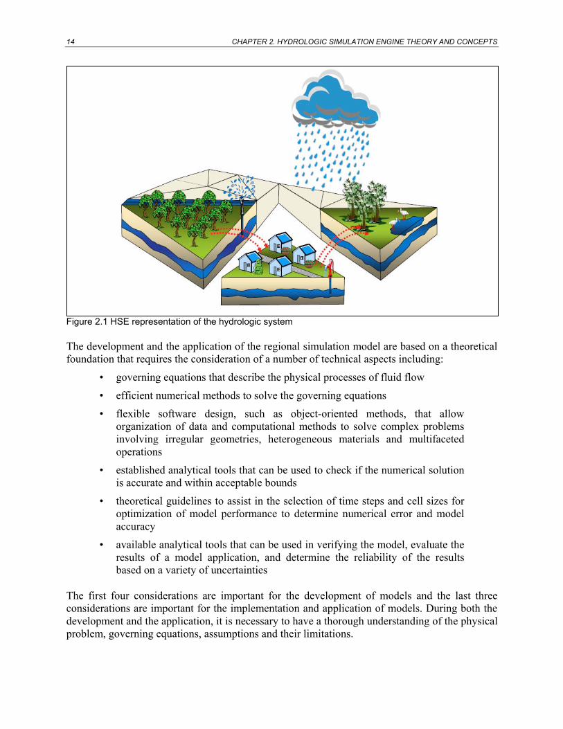
The HSE simulates the physical processes in the hydrologic system, including the major processes of water storage and conveyance driven by rainfall, potential evapotranspiration, and boundary and initial conditions. The basic conceptualization of the HSE is coupling sets of control volumes (waterbodies) with different forms of flow between them (watermovers) based on the properties and state of the respective control volumes (Figure 2.1).
In the RSM, the HSE is integrally linked to the Management Simulation Engine (MSE), which allows managed water routing between control volumes, based on different levels of management control rules. The HSE provides hydrologic state information to the MSE, which imposes management control on selected control volumes. This conceptualization allows the RSM to be applied to a wide range of hydrologic systems, from natural systems with no management intervention, to a complex system of water storage areas plus a canal network with numerous structures operated using a predetermined set of rules.
The RSM is implemented using the object-oriented C++ computer language, with high-level abstractions used to represent different hydrologic states in control volumes and different forms of flow between control volumes. In the HSE, two basic abstractions--”waterbodies” and ”watermovers”--are used to represent the state within the control volume and the flux between control volumes, respectively. Waterbodies and watermovers are central to the organizational hierarchy of the HSE. These objects allow simulation of two-dimensional overland flow, two or three dimensional groundwater flow, canal flow and lake representation (storage and flow) in an integrated system of waterbodies with watermover fluxes between the waterbodies.
14 CHAPTER 2. HYDROLOGIC SIMULATION ENGINE THEORY AND CONCEPTS
Figure 2.1 HSE representation of the hydrologic system
The development and the application of the regional simulation model are based on a theoretical foundation that requires the consideration of a number of technical aspects including:
• governing equations that describe the physical processes of fluid flow
• efficient numerical methods to solve the governing equations
• flexible software design, such as object-oriented methods, that allow organization of data and computational methods to solve complex problems involving irregular geometries, heterogeneous materials and multifaceted operations
• established analytical tools that can be used to check if the numerical solution is accurate and within acceptable bounds
• theoretical guidelines to assist in the selection of time steps and cell sizes for optimization of model performance to determine numerical error and model accuracy
• available analytical tools that can be used in verifying the model, evaluate the results of a model application, and determine the reliability of the results based on a variety of uncertainties
The first four considerations are important for the development of models and the last three considerations are important for the implementation and application of models. During both the development and the application, it is necessary to have a thorough understanding of the physical problem, governing equations, assumptions and their limitations.

CHAPTER 2. HYDROLOGIC SIMULATION ENGINE THEORY AND CONCEPTS 15
2.2 THEORETICAL OVERVIEW
The governing equations of RSM include the equation for conservation of mass and the equation for the conservation of momentum. In addition to these primary laws, constitutive equations and equations of state are also used. Because a continuous medium is assumed for the model domain, the governing equations are expressed as partial differential equations (PDEs) and solved as initial-boundary value problems. The solution depends simultaneously on the initial and boundary conditions. For numerical simulation purposes the continuous medium is discretized into a finite number of points in space and solved at discrete points in time.
In the HSE, a finite volume method is used to simulate the hydrology and the hydraulics of the entire system. The governing equations used in the formulation are based on the Reynolds transport theorem. Because the model functions as a result of interplay between the control volume objects or waterbodies and the surface integral objects or watermovers, in the HSE groundwater and overland flow are described as objects performing designated functions under appropriate conditions. The integral form has many advantages, and is the key to seamless integration of various flow, discretization, and land use types in the implicit finite volume method. With this approach, various control volumes become metamorphic objects that change according to the type of flow, such as overland flow, groundwater flow and canal flow, without regard to the type of discretization. Parts of the surface integral become metamorphic objects that change for overland flow, canal flow, and structure flow. Hydrologic process module objects and a variety of other objects are similarly metamorphic. The object-oriented design of the model makes it possible to write one computational algorithm for all generic flow objects eliminating the need to have separate overland flow, groundwater flow, canal flow models, and the need to integrate the separate models. A unique feature of the HSE is the integration of object-oriented design methodology with an implicit formulation.
This object-oriented approach is particularly useful in representing a complex system in an integrated fashion in the model, however it differs from a more traditional approach where overland and groundwater flow can be described using sequentially placed conditional statements. In this document a mixture of traditional and more object-oriented (OO) approaches is used to describe the HSE. The HSE is described in more detail for non-object oriented programming in Appendix B and in Lal (1998b) and in an OO approach in Lal et al., (2005), which is included in Appendix C.
2.3 HSE GOVERNING EQUATIONS
The finite volume method is built around governing equations in integral form. Reynolds’ transport theorem is at the core of the RSM model. Reynolds’ transport theorem is generally used to describe physical laws written for fluid systems applied to control volumes fixed in space. More recently, it has been used as a first step in the derivation of many conservative laws in partial differential equation form (Chow et al., 1988). Reynolds’ transport theorem is expressed for an arbitrary control volume (Figure 2.2) as:

16 CHAPTER 2. HYDROLOGIC SIMULATION ENGINE THEORY AND CONCEPTS
∫∫ •+∂∂
=cscv
dAdVtDt
D )( nEΝ ηρηρ
(2. 1)
in which N = an arbitrary extensive property such as the total mass; η= arbitrary intensive property, or property per unit mass such as concentration; E = flux vector; n = unit normal vector; dV = volume element; dA = area element; cv = control volume; and cs = control surface. Variables N and η can be vectors or scalars. This representation of Reynolds transport theorem can be used to write any conservation law with the application of different assumptions. For example, in the case of mass balance, η = 1, and in the case of momentum, η = ui + vj in Cartesian coordinates in which u and v are the velocity components in x and y directions.
Figure 2.2 An arbitrary control volume with fluxes, represented in RSM as a cell with fluxes through walls between cells.
2.3.1 Mass Balance Equation
The mass balance equation in integral form can be written using η = 1 in Equation 2.1 as:
∫∫ •+∂∂
=cscv
dAdVt
)(0 nE
(2. 2)
in which E = ui + vj and DN/Dt = 0 because mass is conserved in a Newtonian fluid system.

CHAPTER 2. HYDROLOGIC SIMULATION ENGINE THEORY AND CONCEPTS 17
In the HSE the small elemental control volumes are represented by triangular prisms or objects of other shapes (e.g., cubes), depending on the water body type and discretization used; Figure 2.3 depicts one example of an elemental control volume. The first term in Equation 2.2 represents storage in the control volumes or ”waterbodies” and the second term represents flux across control surfaces or ”watermovers”. The formulations of waterbodies and watermovers within the context of the solution of mass balance in its integral form are described in Sections 2.4 and 2.5.
Figure 2.3 Control volumes or waterbodies used in the HSE.

18 CHAPTER 2. HYDROLOGIC SIMULATION ENGINE THEORY AND CONCEPTS
2.3.2 Momentum Equation
The equation of motion or the equation describing Newton’s second law is the second vector equation necessary to describe shallow water flow. This equation is also referred to as the momentum equation or the St. Venant equations. It is obtained by substituting η with E = [u, v]T in the vector form of the Reynolds transport equations.
∫∫ •+∂∂
=cscv
dAdVt
)( nVEEF ρρ
(2. 3)
in which V = [u, v]T = velocity vector for shallow water flow; F = force vector. The force vector is expressed as
⎟⎟⎠
⎞⎜⎜⎝
⎛−−
=byy
bxx
ghSghS
τρτρ
F
(2. 4)
in which τbx, τby = components of bottom shear stress along x and y directions; Sx, Sy = water surface slopes in x and y directions. The bottom shear stresses can be expressed using
31
2
h
ugnbbx
Vρτ =
(2. 5)
31
2
h
vgnbby
Vρτ =
(2. 6)
in which h = water depth; nb = Manning’s roughness coefficient. The water surface slopes Sx and Sy are defined as
xHSx ∂∂
=
(2. 7)
yHSy ∂∂
=
(2. 8)
in which H = water level. The computation of Equation 2.3 within a numerical scheme can be complex. In RSM, all the terms of the right hand side representing various inertia terms are neglected for simplicity. The components of F resulting in simple equations are then absorbed into the equation of mass balance to form the diffusion flow equations.
A number of factors make it reasonable to use the diffusion flow assumption in models of the south Florida Everglades. Lal (2001) showed that the assumption is challenged only in the deepest portions of the Everglades when disturbances of period less than four days are used. This calculation was carried out using the same assumptions proposed by (Ponce, 1978); i.e.,

CHAPTER 2. HYDROLOGIC SIMULATION ENGINE THEORY AND CONCEPTS 19
30>=hgPSoε ; Where P = period of the disturbance, s0 = slope; h = water depth, and g =
gravitational acceleration. In other shallower areas, solutions with periodic components less than four hours can be simulated without violation of the same assumptions. Lal (2001) showed that a mesh size of two miles or larger is appropriate under the deep sections, based on numerical error considerations. The diffusion assumptions of the RSM also become weak in deep canals for the same reason. Since only long term regional effects are of interest in simulations of the south Florida Everglades, some of the inertia effects giving short term dynamic response times can be neglected, as long as the solution accuracy for long period components is not compromised.
2.4 WATERBODIES FORMULATION
Control volumes in the HSE are referred to as waterbodies (Figure 2-3). The first term on the
right hand side of Equation 2.2, ∫∂∂
cvdV
t, represents the change in storage with time of all the
waterbodies within the aggregated control volume. Calculation of the change in mass in the waterbody over arbitrary waterbodies is facilitated by the introduction of the stage-volume relationship, which describes the relationship between the volume of water in the waterbody and the water head (the term “stage” is used to describe the water head, either above or below the ground surface).
2.4.1 Stage-Volume (SV) Relationships Describing Waterbodies
The stage-volume (SV) relationship is obtained by manipulating the control volume term, using the chain rule, in Equation 2.2 results in the following form:
dtdH
dHHdVdV
t cv∗=
∂∂∫
)(
(2. 9)
dtdH
dHHdfA sv ∗=
)(0
(2. 10)
dtdHHA )(=
(2. 11)
in which A0 = plan area of the waterbody; fsv(H) = normalized (i.e., divided by the surface area of the waterbody), stage-volume relationship that applies to any of the control volumes; A0fsv(H) = volume of water above a specified datum of the waterbody; and A(H) = effective area of the waterbody and is defined as:
HHfAHA sv
∂∂
=)()( 0
(2. 12)
20 CHAPTER 2. HYDROLOGIC SIMULATION ENGINE THEORY AND CONCEPTS
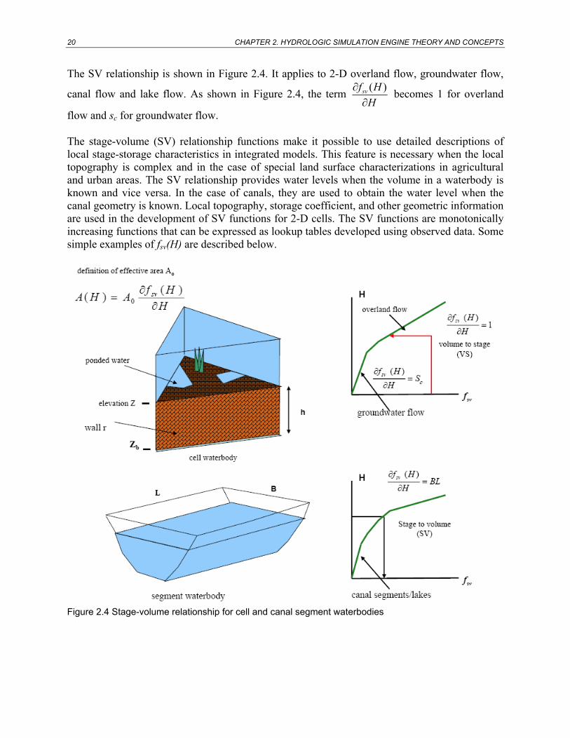
The SV relationship is shown in Figure 2.4. It applies to 2-D overland flow, groundwater flow,
canal flow and lake flow. As shown in Figure 2.4, the term HHfsv
∂∂ )( becomes 1 for overland
flow and sc for groundwater flow.
The stage-volume (SV) relationship functions make it possible to use detailed descriptions of local stage-storage characteristics in integrated models. This feature is necessary when the local topography is complex and in the case of special land surface characterizations in agricultural and urban areas. The SV relationship provides water levels when the volume in a waterbody is known and vice versa. In the case of canals, they are used to obtain the water level when the canal geometry is known. Local topography, storage coefficient, and other geometric information are used in the development of SV functions for 2-D cells. The SV functions are monotonically increasing functions that can be expressed as lookup tables developed using observed data. Some simple examples of fsv(H) are described below.
Figure 2.4 Stage-volume relationship for cell and canal segment waterbodies

CHAPTER 2. HYDROLOGIC SIMULATION ENGINE THEORY AND CONCEPTS 21
2.4.2 Stage-Volume (SV) Relationship for Flat Ground
The stage-volume (SV) relationship function fsv(H) for a cell is used to obtain the volume of water in a control volume when the water head is known. This has to be a one-to-one relationship that has a unique inverse relationship called the VS converter, described in the next section. When the ground surface is assumed horizontal, the SV relationship for a cell with a single layered aquifer is given by:
zHforzHsAHfAV bcsv <−== )()( 00 (2. 13)
zHforzHAzzsAHfAV bcsv ≥−+−== )()()( 000 (2. 14)
in which V = volume of water in control volume or waterbody; zb = elevation at the bottom of the aquifer; z = elevation of the ground surface, and A0 = cell area.
2.4.3 Volume-Stage (VS) Relationship for Flat Ground
The inverse (VS) relationship fvs(V) is used every time the head is determined for a control volume using the volume of water in it. Since the expression for a horizontal ground surface is piecewise linear, Equations 2.13 and 2.14 can be used to obtain the following relationships:
⎭⎬⎫
⎩⎨⎧
−−+=⎟⎟⎠
⎞⎜⎜⎝
⎛= )(
00bcvs zzs
AVz
AVfH )(0 bc zzsAforV −>
(2. 15)
bvs zAVfH =⎟⎟⎠
⎞⎜⎜⎝
⎛=
0
0<forV
(2. 16)
cvs sA
VzAVfH
00
+=⎟⎟⎠
⎞⎜⎜⎝
⎛= otherwise
(2. 17)
2.4.4 Stage Volume (SV) Relationship for a Canal Segment Waterbody
For a canal with a rectangular cross section, the relationship ( )Hfsv between the water volume and the head is:
0)( == HBLfV sv for czH < (2. 18)
)()( csv zHBLHBLfV −== for czH ≥ (2. 19)
in which zc = elevation of canal bottom; L = length of canal segment waterbody and B = canal width.

22 CHAPTER 2. HYDROLOGIC SIMULATION ENGINE THEORY AND CONCEPTS
2.5 WATERMOVERS FORMULATION
The surface flux integral term of the Reynolds transport theorem ∫ ⋅cs
dA)( nE contains the sum
of all fluxes crossing the entire control surface. Because there are many types of control volumes with many types of flux functions surrounding a given waterbody, the surface integral is dissected and organized systematically for computational and functional reasons (Figure 2.5). The surface integration terms are organized according to the type of head dependency.
Figure 2.5 Organization of surface integration terms
The surface integral is divided into a number of easily definable watermovers and source terms forming the total surface integral. Some terms in the calculation of flux across a control surface are gradient driven (e.g., pumping) while others are not. The gradient-driven terms generally fill in the flow resistance matrix in the numerical solution. Terms that are not driven by head gradient are sometimes referred to as the source and sink terms because traditionally they included rainfall, ET and other head independent terms. These terms include recharge, runoff, irrigation, pumping and a number of other processes. Some of the terms such as pumping are head independent. These terms are classified as sources and sinks. Hydrologic Processes Modules (HPMs) can be uncoupled or coupled through iterations with head.
The sum total of all the flows entering a single control volume i can be expressed as:
)()()()(11
HHnEH i
wm
rrr
wm
rri SqAQ +=∆⋅= ∑∑
==
(2. 20)
CHAPTER 2. HYDROLOGIC SIMULATION ENGINE THEORY AND CONCEPTS 23
in which H = water head vector; qr(H) = discharge across gradient-driven watermover r; Si(H) = the summation of non-gradient-driven watermovers (e.g., pumping); ∆Ar = flow area of cell r of a prismatic cell (see Figure 2.4) where ∆Ar = h∆lr; h = water depth; ∆lr = length of cell wall r; wm = number of watermovers contributing to the waterbody i; n = nxi + nyj =unit outward normal vector for the face r of the polygon; E = average flux rate across the control surface per unit length defined as ui + vj, which is also equal to HK∇− for free surface diffusion flow or groundwater flow. The term Si(H) indicates the possibility of a head dependency (e.g., pump operation and irrigation requirements).
The gradient-driven watermover is the basic abstraction needed to transfer water between any two waterbodies. Watermovers assist in the calculation of flow across control surfaces in canal flow, overland flow and all other kinds of flows such as structure flow. By design, gradient watermovers conserve mass. Some watermovers such as those for overland flow, groundwater flow and canal flow are created implicitly based on cell and canal network topology and geometry. Because only watermovers can move water between waterbodies, the model can track mass balance of the system at the highest level of abstraction. In the diffusion flow formulation, discharge across a single watermover qr(H) between two waterbodies shown in Figure 2.6 is expressed as:
22110 )()()()( HkHkkqr HHHH ++= (2.21)
in which k0, k1, k2 = values obtained as a result of linearization of the function qr; H =water head vector; H1, H2 = water levels of control volumes 1 and 2. Discharge functions qr(H) for various types of watermovers are described later in this section. Depending on the types of cells or waterbodies adjacent to a particular waterbody, a variety of watermovers may be needed to complete the surface integral around a given waterbody.
2.5.1 Overland Flow Watermover
Cordes and Putti (1996) showed the equivalence of a low-order mixed finite element method based on RT0 elements as described in Raviart and Thomas (1977) with a finite volume method for triangles under certain conditions. Because of the equivalence, it is possible to use an expression derived for the mixed finite element method to compute flow rates for the finite volume method.
In the equivalent finite volume method, water levels at circumcenters (center of an outside circle where all triangle verticies lies on the circumference of the circle), are used in the computation of flow across control surfaces. In the mixed finite element method, water levels in triangular prisms are assumed to vary linearly, and the water level at the centroid is the average water level.

24 CHAPTER 2. HYDROLOGIC SIMULATION ENGINE THEORY AND CONCEPTS
When the Manning equation is used to compute flow rate across a wall between two adjacent cells m and n, shown in Figure 2.6, then for:
nm HH >{ and 0>mh and }nm zH > or nm HH <{ and 0>nh and }mn zH >
then rr
rmn Sn
hT35
= for tolr SS >
(2.22)
and tolr
rmn Sn
hT35
= for tolr SS ≤
(2.23)
Where Tmn = equivalent transmissivity of overland flow between cells m and n, in which hr and nr are defined as:
)(5.0 nmr hhh += (2.24)
)(5.0 nmr nnn += (2.25)
Hm, Hn = heads at the circumcenters; hm, hn = water depths at the circumcenters; zm, zn =ground elevations of cells m and n; nm, nn = Manning’s roughness coefficients of cells m and n; Sr = magnitude of the slope of the energy grade line and Stol = a small slope below which the energy slope is not allowed to go in the calculation of Tmn to prevent a division by zero.
Figure 2.6 Sample waterbodies with circumcenters m and n used to define variables
CHAPTER 2. HYDROLOGIC SIMULATION ENGINE THEORY AND CONCEPTS 25
A value of 10−13 to 10−7 is used in the Everglades because these slopes are typically below observed slopes except in deep pools of water. Sr is computed using
( )2
2
2
2)ˆˆ(
mn
nm
r
kjr d
HHlHH
S∆−
+∆−
=
(2.26)
in which ∆dmn = distance between circumcenters of triangles m and n; ∆lr = length of wall r; jH
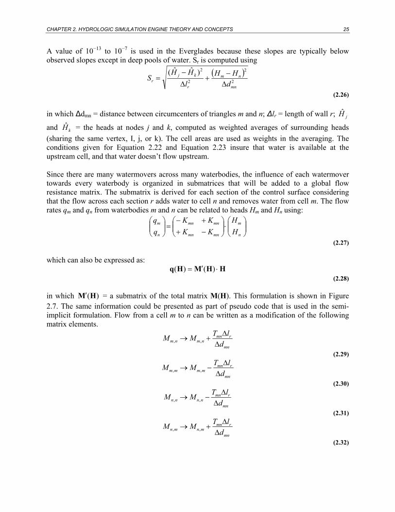
and kH = the heads at nodes j and k, computed as weighted averages of surrounding heads (sharing the same vertex, I, j, or k). The cell areas are used as weights in the averaging. The conditions given for Equation 2.22 and Equation 2.23 insure that water is available at the upstream cell, and that water doesn’t flow upstream.
Since there are many watermovers across many waterbodies, the influence of each watermover towards every waterbody is organized in submatrices that will be added to a global flow resistance matrix. The submatrix is derived for each section of the control surface considering that the flow across each section r adds water to cell n and removes water from cell m. The flow rates qm and qn from waterbodies m and n can be related to heads Hm and Hn using:
⎟⎟⎠
⎞⎜⎜⎝
⎛⋅⎟⎟⎠
⎞⎜⎜⎝
⎛−++−
=⎟⎟⎠
⎞⎜⎜⎝
⎛
n
m
mnmn
mnmn
n
m
HH
KKKK
(2.27)
which can also be expressed as: HHMHq ⋅′= )()(
(2.28)
in which )(HM′ = a submatrix of the total matrix M(H). This formulation is shown in Figure 2.7. The same information could be presented as part of pseudo code that is used in the semi-implicit formulation. Flow from a cell m to n can be written as a modification of the following matrix elements.
mn
rmnnmnm d
lTMM∆∆
+→ ,,
(2.29)
mn
rmnmmmm d
lTMM∆∆
−→ ,,
(2.30)
mn
rmnnnnn d
lTMM∆∆
−→ ,,
(2.31)
mn
rmnmnmn d
lTMM∆∆
+→ ,,
(2.32)

26 CHAPTER 2. HYDROLOGIC SIMULATION ENGINE THEORY AND CONCEPTS
Figure 2.7 Submatrix for a single watermover as part of total matrix
The circumcenter-based method can be used only with acute-angled triangles (Raviart and Thomas, 1977; Cordes and Putti, 1996). When this method is used with obtuse angled triangles, the circumcenter falls outside the triangle, and the numerical error tends to be large. With rectangular cells, the method becomes equivalent to the finite difference method.
2.5.1.1 Overland Flow Watermover for Mixed Flow
When the water levels are above ground surface in one or both of two adjacent cells, overland flow occurs between the cells. The discharge in the watermover qr between two adjacent cells is computed using the circumcenter method derived for mixed finite elements (Lal, 1998c). For mixed flow types where two adjacent cells use different types of flow equations (e.g., overland flow and wetland flow), flow r)( nE ⋅ for control surface r in Equation 2.20 is computed using:
rrq )( nE ⋅= (2.33)
mn
nmrnmmn d
HHlTHHK∆−
∆=−= )( orfor
{mn
nm
HHHH
>>
andand
nn
mm
zHzH
>>
andand
mn
nm
zHzH
>>

CHAPTER 2. HYDROLOGIC SIMULATION ENGINE THEORY AND CONCEPTS 27
in which Hm, Hn = water levels in triangular cells m and n; dmn = distance between circumcenters of triangles m and n; ∆l = length of the wall; zm, zn = ground elevations of cells m and n; Tr = equivalent inter-block transmissivity in the overland flow layer, computed based on the assumption that transmissivity varies linearly between circumcenters (Goode and Appel, 1992; McDonald and Harbaugh, 1984). Variable Tr is computed as:
2nm
rTTT +
= for 005.1995.0 ≤≤n
m
TT
(2.34)
n
mTT
nmr
TTTln−
= otherwise
(2.35)
Tm and Tn are the values for the cells defined in Equation B.9 (see Appendix B) for overland flow. Matrix elements representing overland flow watermovers are described in Lal (1998b).
2.5.2 Groundwater Flow Watermover
When simulating saturated groundwater flow with confined and unconfined aquifers, transmissivity of the adjacent cells is computed first. The discharge in the watermover qr is then computed using:
( )n
n
m
mTl
Tl
nmr
HHlq+−
∆=
(2.36)
in which lm, ln = the distances from the circumcenters to the wall; Tm, Tn = transmissivities.
2.5.3 Canal Flow Watermover
Canal flow under the diffusion flow conditions is calculated using the following equation: rrq )( nE ⋅=
(2.37)
mn
nmrnmmn d
HHTHHK∆−
=−= )( orfor
mn
nm
HHHH
>>
andand
nn
mm
zHzH
>>
andand
mn
nm
zHzH
>>
in which Hm, Hn = water levels in two canal segment waterbodies m and n, as shown in Figure 2.8.
When simulating canal flow, a linearly varying conveyance is assumed between canal segment waterbodies. The equation for discharge between two canal segment waterbodies m and n is the same as Equation 2.34. The value of Tm for example, for canal segment waterbody m is
35
⎟⎟⎠
⎞⎜⎜⎝
⎛=
m
m
bnm
mm P
AnSl
AT
(2.38)

28 CHAPTER 2. HYDROLOGIC SIMULATION ENGINE THEORY AND CONCEPTS
in which Am = average canal cross-sectional area of canal segment waterbody m; Pm = average wetted perimeter; nb = average Manning roughness coefficient and lm = length of a canal segment waterbody.
When simulating canal networks, each pair of canal segment waterbodies’ canal joint is implicitly considered as a canal watermover. A canal joint with n limbs has n(n−1)/2 canal watermovers as a result. All of these watermovers have to be considered before populating the matrix. Their summation computes the actual discharge.
Figure 2.8 Canal flow calculations
2.5.4 Canal-Cell Watermover
There are two types of canal-cell watermovers, representing seepage between the canal and the cell and representing overbank flows between the canal and the cell. Seepage between a canal segment waterbody and a cell is described using a canal seepage watermover, where the seepage rate ql per unit length of the canal is derived using Darcy’s equation as follows:

CHAPTER 2. HYDROLOGIC SIMULATION ENGINE THEORY AND CONCEPTS 29
)( mim
ml HHpkHpkq −=∆
=δδ
(2.39)
in which km = sediment layer conductivity; p = perimeter of the canal subjected to seepage; δ = sediment layer thickness and ∆H = head drop across the sediment layer. Construction of the submatrix created for the canal-aquifer watermover is shown in Figure 2.9.
Figure 2.9 Matrix elements for canal-aquifer interaction.
2.5.5 Structure Flow Watermover
Structure flow watermovers are defined using linearized structure equations or lookup tables. A water control structure is a structure watermover that can be used to impose management decisions onto the flow control. Linearization of structure equations is difficult for most types of structures used in the Everglades. Structure discharges are generally expressed as
),,( GHHqq duss = (2.40)

30 CHAPTER 2. HYDROLOGIC SIMULATION ENGINE THEORY AND CONCEPTS
in which Hu and Hd are upstream and downstream water levels and G = gate opening. Linearization of the structure equations is necessary before they are used in the implicit solution method.
Such a linearization is accurate only in gradually varied flow. Considering that Equation 2.40 can be extremely nonlinear, differential equations for structures can be stiff and difficult to solve without special methods or small time steps. As an alternative, one and two-dimensional lookup tables and regression equations are also useful in describing structure flow.
2.5.6 Sources and Sinks; Head Independent Watermovers
Pumping into and out of a cell is conceptualized using head independent watermovers. In the flux calculation described in Equation 2.20, this is described using the term Si. These terms can also be considered as source and sink terms. If water is pumped at a known rate p(t) into a cell i described by a time series data set, the source term for cell i is expressed as:
)(tpSi = (2.41)
In the case of management-driven pumping or diversion, the hydrologic process modules (HPMs) take care of the calculation of p(t). HPMs are described in greater detail in Section 2.6 and in Appendix C.5.
2.6 HYDROLOGIC PROCESS MODULE (HPM) FORMULATION
Hydrologic Process Modules (HPMs) are activated at the beginning of every model time step. They are designed to simulate the effects of local hydrology on the regional system. The local hydrology depends on the local land use, water use and water management practices. Different land use types have different hydrology, water storage properties and generate different recharge and, therefore, different hydrologic responses. Hydrologic Process Modules are used to separate the complexities of natural and managed flow processes associated with local hydrology and simulate rainfall, ET, infiltration, percolation, seepage, unsaturated subsurface flow, irrigation, urban water use, stormwater detention and surface water management practices of the natural and managed landscapes from the regional system. In the simple form or the complex form, the HPMs are an integral part of the HSE within RSM.
The HPMs are developed for various land use types, land management and water management practices. The HPM structure provides the capability to apply different hydrologic processes for the local hydrology of each cell. More details on HPMs can be found in Flaig et al., (2005), which is provided in Appendix C.5.
At a minimum HPMs simulate precipitation and evapotranspiration to calculate recharge to the saturated flow in the regional solution. Physical processes that take place at a local scale are generally rapid. As a result, reasonable assumptions can be made to simulate some of these processes within the control volume. The net effects of the local hydrologic processes are accumulated and applied on the regional system using HPMs.

CHAPTER 2. HYDROLOGIC SIMULATION ENGINE THEORY AND CONCEPTS 31
The HPMs contain storage, routing and simple interchange mechanisms to simulate the processes mentioned above. The recharge (Rrchg), irrigation (Qirr) and runoff (Qro) are applied to the regional system using the Si term described in Equation 2.20. They are computed separately for each unique HPM instance. The equation for mass balance is used to compute recharge during every time step. This equation can be in a very simple form or a very complex form as follows:
∆S = P – ET – evap – Rrchg + Qirr +Qws – Rro – Qsew – Qsep – Qseep - Sdet (2.42)
in which ∆S = change in storage (water content) in HPM; P = precipitation; ET = actual evapotranspiration; evap = evaporation from interception, surface detention and bare soil; Rrchg = recharge; Qirr = irrigation; Qws = urban water supply; Rro = runoff; Qsew = sewage discharge; Qsep = water discharged to onsite disposal systems; Qseep = water lost through seepage; and Sdet = water stored in stormwater detention systems. Some of the optional terms may not be applicable to some of the processes.
In the HSE, computation of each term in Equation 2.42 is carried out within each HPM of each respective mesh cell. The source and sink terms from Equation 2.42 allow a variety of processes to be simulated in HPMs. These processes affect the storage of water and the distribution of water applied to the cell.
2.6.1 HPM Concepts
The HPM approach provides a method for modeling the local surface hydrology of a mesh cell or a collection of mesh cells. Each mesh cell has an HPM assigned to that cell to provide the upper boundary condition for the implicit solution. The explicit solution of the local hydrology at the beginning of the time step provides the opportunity to simulate a range of possible modules depending on dominant hydrologic processes or important water management practices. The HPMs are typically designed to model the simplified vertical or surface processes. As a solution to local hydrology in a regional water management model, the HPMs are generally not designed to simulate small-scale hydrologic processes such as unsteady flow or hydraulics, although these could be simulated under the appropriate circumstances. The HPMs provide the solution for aggregate hydrologic behavior of the local landscape. HPMs have been designed to simulate the following processes:
• Unsaturated flow in soil,
• Interception and detention of flow,
• Interflow and field drainage,
• Urban hydrology and stormwater management practices,
• Rainfall-Runoff simulation,
• Agricultural irrigation and drainage practices,
• Anisotropic surface hydrology,
• Small creek and tributary flow,

32 CHAPTER 2. HYDROLOGIC SIMULATION ENGINE THEORY AND CONCEPTS
• Discharge, seepage and aquifer recharge from detention and retention ponds.
The HPM concept provides an opportunity for hydrologic modelers outside the SFWMD development group to develop new HPMs. The RSM is written in an object-oriented framework and the HPM class is setup to accommodate additional HPMs by simple addition of new objectives of the HPM class following the inheritance rules to create the appropriate interface with HSE. Additional HPMs can be added that provide new or more detailed processes for simulating surface hydrology and water management practices.
Within the architecture and design of HSE, it is possible to have many HPM types that are selectable as part of the input XML. Besides the HPMs that model necessary processes, it is possible to have HPMs that model local hydrology by using different methods. This is useful, when different hydrologic processes dominate water movement for different soil, landuse and landscape types. It is also useful when different users want to select specific methods to simulate local hydrology. For example, agricultural consumptive use may be estimated using different methods. HSE allows for the creation of multiple agricultural land HPMs and the users can select the appropriate HPMs by changing the XML specifications.
In this architecture, it is possible and common that the different HPMs are constructed in very different ways. For example, the layer1nsm HPM (presented below) is a very simple C++ program, while the layer5 HPM has multiple layers of objects and depends strongly on inheritance. Other HPMs can be constructed by creating a C++ wrapper around FORTRAN code. This allows the use of known and accepted legacy code to be implemented as a local hydrologic process module in HSE. With this level of flexibility, it is common to have different parameters for different HPMs that describe essentially the same processes. It is also possible to have the same parameter, e.g. shallow root depth, used in different processes in different HPMs. As such, each HPM should be interpreted as a unique entity.
2.6.2 Limitations of HPM
HPMs are the means by which local hydrology is simulated in the RSM. They contribute to the governing equations through the source/sink term on the right hand side of the HSE matrix solution (SFWMD, 2005). Furthermore, the solution of HPMs is designed as an explicit solution for convenience and stability; this provides a means to introduce considerable complexity in the modeling of surface hydrology without introducing nonlinearity into the regional solution. Since HPMs are open for user development, the explicit option is the only one available, as this protects the user from making the equations in the overall HSE solution matrix stiff, or unstable. HPMs are also assumed to be non-interactive with HPMs of other mesh cells, and HPMs within Hubs interactive in only a linear way. This preserves the stability of the regional solution and the integrity of both the HPM and the regional solution water budgets.
2.6.3 Simple HPM
The area simulated by the RSM may include native lands as well as developed land, both urban and agricultural. The natural areas are modeled by hydrologic processes representing wetlands
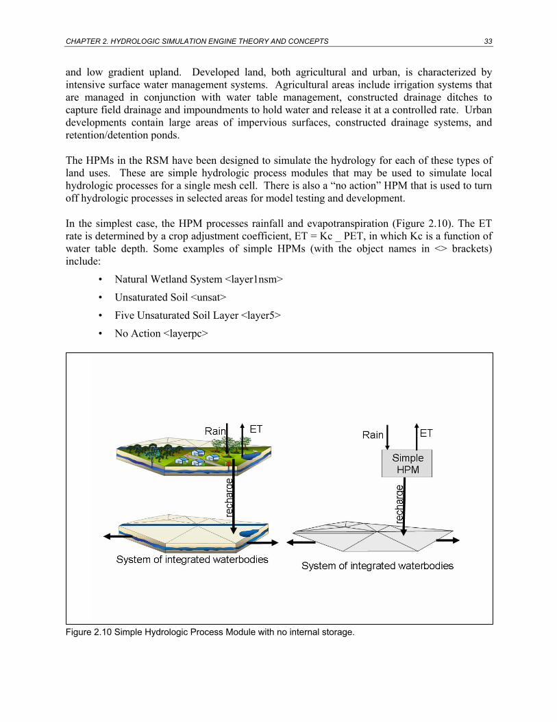
CHAPTER 2. HYDROLOGIC SIMULATION ENGINE THEORY AND CONCEPTS 33
and low gradient upland. Developed land, both agricultural and urban, is characterized by intensive surface water management systems. Agricultural areas include irrigation systems that are managed in conjunction with water table management, constructed drainage ditches to capture field drainage and impoundments to hold water and release it at a controlled rate. Urban developments contain large areas of impervious surfaces, constructed drainage systems, and retention/detention ponds.
The HPMs in the RSM have been designed to simulate the hydrology for each of these types of land uses. These are simple hydrologic process modules that may be used to simulate local hydrologic processes for a single mesh cell. There is also a “no action” HPM that is used to turn off hydrologic processes in selected areas for model testing and development.
In the simplest case, the HPM processes rainfall and evapotranspiration (Figure 2.10). The ET rate is determined by a crop adjustment coefficient, ET = Kc _ PET, in which Kc is a function of water table depth. Some examples of simple HPMs (with the object names in <> brackets) include:
• Natural Wetland System <layer1nsm>
• Unsaturated Soil <unsat>
• Five Unsaturated Soil Layer <layer5>
• No Action <layerpc>
Figure 2.10 Simple Hydrologic Process Module with no internal storage.

34 CHAPTER 2. HYDROLOGIC SIMULATION ENGINE THEORY AND CONCEPTS
2.6.4 Complex HPM
HPMs provide the opportunity to apply complex processes to the local hydrology. These processes include irrigation, stormwater detention, unsaturated water flow, and impervious land hydrology (Figure 2.11). These HPMs contain several parameters that describe surface water management practices and affect water storage as well as demand and discharge. Some examples of complex HPMs (with the object names in <> brackets) include:
• Precipitation Runoff Routing <prr>
• Agricultural Irrigation Requirements <afsirs>
• Drainage Collector Ditch <pumpedditch>
• Agricultural Impoundment <agimp>
• Multi-Basin Routing <mbrcell>
• Impervious Land <imperv>
• Consumptive Use <cu>
• Urban Detention <urbandet>
Figure 2.11 Complex Hydrologic Process Module with multiple internal processes including soil water storage. The outflows are directed to the homecell in this example.
2.6.5 HPM Hubs
Hubs are used to combine a number of complex capabilities of HPMs. The HPM hub provides the capability of applying water supply demand and runoff to specific locations in the mesh and network for a group of cells (Figure 2.12). This capability is useful where there is a large urban development that is serviced by a single public water supply well (PWS) or has a single runoff. The PWS may be located considerably distant from the hub. The runoff and irrigation from the HPM within a hub may be directed to any mesh cell or canal segment waterbody. The recharge from the hub is directed uniformly to the cells below the footprint of the Hub.

CHAPTER 2. HYDROLOGIC SIMULATION ENGINE THEORY AND CONCEPTS 35
Figure 2.12 Hub Hydrologic Process Module with multiple internal HPMs includes soil water storage and stormwater storage. The Hub may cover one or many mesh cells.
The Hub may consist of a single HPM type or a combination of HPM types. In a single HPM implementation, all of the land in the footprint of a hub is assigned to a single HPM type. It is also possible to assign several HPM types to the Hub based on the percent of the area of that landuse type within the Hub. For example, an urban development Hub could consist of 20 percent impervious land, 40 percent pervious land, 30 percent golf course and 10 percent stormwater detention pond. The Hub allows runoff to be routed among the HPM types (i.e., runoff from impervious land could be routed to pervious, then to the detention pond, and then off site). Similarly, the demand could be routed from offsite to the detention pond, and then to the golf course. The recharge to each homecell coincident with the Hub footprint would have the area-weighted average recharge of all landuse types in the Hub.
Although the volume of water calculated for runoff, recharge or water supply may be affected by the cell head, the HPMs are not a direct function of the cells heads and are not directly coupled to the cell heads.
2.7 ASSEMBLY OF ALL WATERBODIES
The equation of mass balance in integral form written for one control volume is:
∫∫ ⋅−=∂∂
cscvdAVd
t)( nE
(2.43)
This can be written for all the finite volume cells in vector form as:
)()()( HHqHHA s Sdtd
+⋅=⋅
(2.44)

36 CHAPTER 2. HYDROLOGIC SIMULATION ENGINE THEORY AND CONCEPTS
in which H = [H1,H2, . . .Hm, . . .Hwb]T = a vector containing average heads in all cells, canal segment waterbodies and lakes in some recognizable order; qs(H) = [qs1(H), qs2(H), . . . qs−wb(H)]T ; qsi(H) = vector containing the summation of flow entering waterbody described in Equation 2.20; S(H) = the source term in vector form; A(H) = a diagonal matrix whose elements A(m,m) are the effective cell areas Am in the case of a cell m described in Equation 2.13 (Ao in Equation 2.13); S(H) = vector containing all source terms or non-gradient driven fluxes. qs(H) can be linearized using:
HHMHq ⋅= )()(s (2.45)
in which qs(H) is constructed by adding the subvectors q(H) in Equation 2.29; M(H) =global flow resistance matrix made up by summing submatrices M′(H). The computational procedure begins by populating matrix M and assembling flow resistance expressions across watermovers.
2.8 HSE NUMERICAL SOLUTION
The ordinary differential Equation 2.44 derived using the finite volume method is solved by using the following weighted finite difference formulation:
[ ] [ ]ni
ni
nsi
nsi
nii
nii SStqqtHAHA )1()1( 111 αααα −+∆+−+∆+= +++
(2.46)
in which niH = average surface water level in cell i at time step n; α = time weighting factor
where α = 0 and 1 representing explicit and implicit solutions, respectively. Using linearization in Equation 2.45, Equation 2.46 can be expressed as the following system of linear equations:
])1([])[1(][][ 111 nnnnnnnn tttt SSHMMHMHMA αααα −+∆+⋅−−∆+⋅∆=∆⋅∆− +++
(2.47)
Here, nnns HHMq ⋅= )( . The matrix [A − α∆tMn+1] is symmetric. In many gradually varying
problems, Mn+1 is replaced with Mn to simplify Equation 2.47 (Akan and Yen, 1981). Test runs show that this is a useful procedure for many problems. If this assumption is not made then Mn+1 must be updated by using an iterative procedure within the time step, by first computing ∆H using Equation 2.47 with the most recent estimates of Mn+1, and next updating Hn+1. Iterations are continued similarly by updating Mn+1 and using Equation 2.47 until convergence. Akan and Yen (1981) show that only two to four iterations were required for convergence of the water level up to four significant digits. This type of iteration was not used in the HSE current application. In other words, the second term on the right hand side of Equation 2.47 is neglected. Even without this assumption, this term gets cancelled when α = 1. If S is independent or weakly dependent on H, then the approximation Sn = Sn+1 is valid, and iterations within the same time step can be avoided.
Matrix M is sparse for large problems. For example, the element density is less than 1% for a discretization of one thousand cells.

CHAPTER 2. HYDROLOGIC SIMULATION ENGINE THEORY AND CONCEPTS 37
The solution of Equation 2.47 is sensitive to the α values used; α is a time weighting factor. When α = 0, ∆H can be computed by using a simple matrix multiplication. An α of 0.5 gives higher accuracy similar to Crank-Nicholson type schemes. For most models, α is assumed to be in the range 0.6-0.8. For most integrated models, it is close to 1.0 when nonlinearities are severe and the model show signs of instability. Figure 2.13 shows a sketch of the space-time diagram in the computational domain of the HSE. The figure shows the space and time discretizations, and the types of interactions a single cell will have with its neighbors.
The implicit solution method takes into account the water balance in all the waterbodies during the time interval between times tn and tn+1. Knowing the volumes of water V(Hn) = fsv(Hn) at time step tn and ∆H, it is possible to compute Vn+1 using
HAVV ∆⋅+=+ nn 1 (2.48)
Figure 2.13 Computational space-time space of RSM
The new heads Hn+1 at time step n+1 are computed using the storage-volume relationship Hn+1 = fvs(Vn+1). Heads are used in the model only to compute the hydraulic driving forces in the watermovers. Except during this conversion, the model equations can be explained as a system of mass balance equations.
Figure 2.14 shows the basic steps involved in the initialization and the time progression within the RSM. The actual number of steps involved is much larger with many more initialization processes. The figure only shows the steps involved for the finite volume calculations.

38 CHAPTER 2. HYDROLOGIC SIMULATION ENGINE THEORY AND CONCEPTS
2.8.1 Average Water Velocity
The average water velocity in a cell is computed by using the following vector function developed for RT0 mixed elements of Raviart and Thomas (1977), and used by Cordes and Putti (1996):
HKyyxx
Qyyxx
Qyyxx
QAh
v rrr ∇−=⎥⎦
⎤⎢⎣
⎡⎟⎟⎠
⎞⎜⎜⎝
⎛−−
+⎟⎟⎠
⎞⎜⎜⎝
⎛−−
+⎟⎟⎠
⎞⎜⎜⎝
⎛−−
=3
33
2
22
1
11 ˆ
ˆˆˆ
ˆˆ
21r
(2.49)
in which Qr1,Qr2,Qr3 = discharge rates across cell walls r1, r2 and r3 counting outward as positive; ( ii yx ˆ,ˆ ) = the coordinates of the nodes; (x, y) = coordinates of any point, including the circumcenters in the current case at which the head is computed. In the case of right angled triangles, Putti (1996) showed that the mixed finite element method is equivalent to a finite difference method.
The HPMs are one set of process modules linked to the HSE. Other modules under development include Water Quality Process Modules (WQPM) and Ecological Process Modules (EPM). The WQPMs use the flow solution from the HSE to provide advective flow for the bio-geochemical processes modeled in the WQPMs. EPMs are being developed to simulate landscape and habitat processes that use the hydrology from the HSE to drive functional changes in the environment.
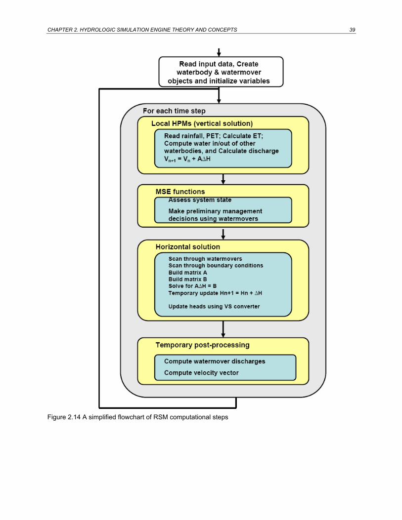
CHAPTER 2. HYDROLOGIC SIMULATION ENGINE THEORY AND CONCEPTS 39
Figure 2.14 A simplified flowchart of RSM computational steps

40 CHAPTER 2. HYDROLOGIC SIMULATION ENGINE THEORY AND CONCEPTS

REFERENCES 41
REFERENCES
Abbott, M., J. Bathurst, J. Cunge, P. O’Connell, and R. Rasmussen (1986a). An introduction to the European Hydrological System, ”System Hydrologique European”, (SHE), 1: A structure of a physically based, distributed modeling system. Journal of Hydrology 87, 61–77.
Abbott, M., J. Bathurst, J. Cunge, P. O’Connell, and R. Rasmussen (1986b). An introduction to the European Hydrological System, ”System Hydrologique European”, (SHE), 2: History and philosophy of a physically based, distributed modeling system. Journal of Hydrology 87, 45–59.
Abbott, M. B. and J. A. Cunge (1982). Engineering Applications of Computational Hydraulics. London: Pitman.
Ahuja, R., T. Magnanti, and J. Orlin (1993). Network Flows: Theory, Algorithms, and Applications. Prentice Hall.
Akan, O. and B. C. Yen (1981, April). Diffusion-wave flood routing in channel networks. ASCE Journal of Hydraulics Division 107 (6), 719–732.
Balay, S., W. Gropp, D. Kushik, L. McInnes, and B. Smith (2001). (PETSC) Users Manual, ANL-95/11 - Revision 2.1.3. Argonne, Illinois: Argonne National Laboratory.
Bosak, J. and T. Bray (1999, 5). XML and the second generation web. Scientific American.
Brion, L., S. Senarath, and A. Lal (2000, Dec 11-15). Concepts and algorithms for an integrated surface water/groundwater model for natural areas and their applications. In Greater Everglades Ecosystem Restoration (GEER) Conference, Naples, Florida.
Brion, L., S. Senarath, A. M. W. Lal, and M. Belnap (2001, May 20-24). Application of the South Florida Regional Simulation Model in the Southern Everglades. In B. K. Panigrahi (Ed.), Proceedings of the Specialty Symposium Held in Conjunction With the World Water and Environmental Resources Congress, 1801 Alexander Bell Drive, Reston, Virginia 20191-4400, pp. p. 110. Environmental and Water Resources Institute of ASCE: American Society of Civil Engineers. 55
Chow, V., D. Maidment, and L. Mays (1988). Applied Hydrology. New York, NY: McGraw-Hill Book Company.
Cordes, C. and M. Putti (1996). Triangular mixed finite elements versus the finite volumes in groundwater modeling. In A. A. et al. (Ed.), Int. Conf. Comp. Meth. Water Res. XII, Southampton, London, pp. 61–68. Computational Mechanics.
42 REFERENCES
Cunningham, K. J., J. L. Carlson, G. L. Wingard, E. Robinson, and M. A. Wacker (2004). Characterization of aquifer heterogenity using cyclostratigraphy and geophysical method in the upper part of the karstic Biscayne aquifer, southeastern Florida. Water Resources Investigations Report 03-4208, United States Geological Survey.
Fan, A. (1986). A routing model for the upper Kissimmee chain of lakes. Technical Publication 86-5, South Florida Water Management District, West Palm Beach, FL.
Flaig, E., R. VanZee, and W. Lal (2005). Hydrologic process modules of the regional simulation model: An overview. HSE White Paper.
Ford, L. and D. Fulkerson (1962). Flows in Networks. Princeton University Press.
Goode, D. and C. Appel (1992). Finite-difference interblock transmissivity for unconfined aquifers and for aquifers having smoothly varying transmissivity. Water-resources investigations report 92-4124, United States Geological Survey. 79 p.
Gupta, A., G. Karypis, and V. Kumar (1997). Highly scalable parallel algorithms for sparse matrix factorization. IEEE Trans. Parallel Distrib. Syst. 8 (5), 502–520.
Hirsch, C. (1989). Numerical Computation of Internal and External Flows, Computational Methods for Inviscid and Viscous Flows. Wiley Series in Numerical Methods in Engineering. New York: John Wiley and Sons Inc.
Hromadka II, T., R. McCuen, and C. Yen (1987). Comparison of overland flow hydrograph models. Journal of Hydrologic Research, ASCE 113 (11), 1422–1440.
HydroGeoLogic (2000). MODFLOW-HMS: A Comprehensive MODFLOW-Based Hydrologic Modeling System: Software Documentation. Herndon, Virginia: HydroGeoLogic, Inc.
Kadlec, R. H. and R. L. Knight (1996). Treatment Wetlands. Boca Raton, Florida: Lewis Publishers.
Lal, A. M. W. (1995). Calibration of riverbed roughness. Journal of Hydraulic Engineering, ASCE 121 (9), 664–671.
Lal, A. M. W. (1998a, April). Performance comparison of overland flow algorithms. Journal of Hydraulic Engineering, ASCE 124 (4), 342–349.
Lal, A. M. W. (1998b, August 3-7). Simulation of overland and groundwater flow in the Everglades National Park. In Proceedings of the International Water Resources Engineering Conference, Memphis, Tennessee, pp. 610–615.
Lal, A. M. W. (1998c, September). Weighted implicit finite-volume model for overland flow. Journal of Hydraulic Engineering, ASCE 124 (9), 941–950.
Lal, A. M. W. (2000). Numerical errors in groundwater and overland flow models. Water Resources Research 36 (5), 1237–1247.

REFERENCES 43
Lal, A. M. W. (2001, May 20-24). Selection of time step and grid size in modeling integrated stream-aquifer interaction. In Proceedings of the World Environmental Congress, Orlando, Florida.
Lal, A. M. W. (2005). Determination of aquifer parameters using generated water level disturbances. To be submitted to Water Resources Research.
Lal, A. M. W., R. VanZee, and M. Belnap (2005, April). Case study: Model to simulate regional flow in south Florida. Journal of Hydraulic Engineering, ASCE 131 (4), 247–258.
Lin, S. (2003, spring). History of regional modeling in south Florida. personal communication.
McDonald, M. and A. Harbaugh (1984). A modular three dimensional finite difference groundwater flow model. Technical report, United States Geological Survey, Reston, Virginia.
Menke, W. (1989). Geophysical Data Analysis: Discrete Inverse Theory (Revised Edition (textbook) ed.). New York: Academic Press, Inc.
Panton, R. (1984). Incompressible flow. New York, NY: John Wiley and Sons Inc.
Park, J. (2005). Management Simulation Engine of the Regional Simulation Model: An overview. MSE White Paper, 50 p.
Ponce, V. M., L. R. D. S. (1978, 360). Applicability of kinematic and diffusion models. Journal of Hydrology 104, 353.
Raviart, P. and J. Thomas (1977, May 15-19). A mixed finite element method for second order elliptic problems. In I. Galligani and E. Magenes (Eds.), Mathematical aspects of the finite element method, New Jersey. Springer-Verlag.
Schmidt, J. and L. Roig (1997). The adaptive hydrology (ADH) model: a flow and transport model for coupled surface water-groundwater analysis. In XXVIIth Congress of the IAHR and ASCE, San Francisco, California, pp. 367–372.
Senarath, S. U. S. (2002). Use of a distributed, finite volume, hydrologic model to assess the sensitivity of the Everglades to de-compartmentalization. In Eos Trans., Fall Meet. Suppl, Volume 83. AGU: American Geophysical Union. Abstract H51E-0786.
Senarath, S. U. S., R. J. Novoa, J. A. Barnes, and L. M. Brion (2001). Simulating the flow dynamics in the southern Everglades using a finite volume model. In Eos Trans., Fall Meet. Suppl, Volume 82. AGU: American Geophysical Union. Abstract H31E-0276.
Shen, H., D. Zhao, G. Tabios III, K. Loftin, S. Sculley, and J. Chamberlain (1997, August 10-15). Application of RBFVM-2D model to Kissimmee River Restoration in Florida State of USA. In S. S. Y. Wang and T. Carstens (Eds.), Environmental and Coastal Hydraulics: Protecting the Aquatic Habitat, Proceedings of Theme B: Water for a Changing Global
44 REFERENCES
Community; The 27th Congress of the IAHR, San Francisco, CA, pp. 474–479. International Association for Hydraulic Research.
Solomatine, D. (1996). Object orientation in hydraulic modeling architectures. Journal of Computing in Civil Engineering 10 (2), 125–135.
South Florida Water Management District (1999). South Florida Water Management Model Primer 3.5. 3301 Gun Club Road, West Palm Beach, FL 33406: South Florida Water Management District.
South Florida Water Management District (2005). Management Simulation Engine User Manual. 3301 Gun Club Road, West Palm Beach, FL 33406: South Florida Water Management District.
Swain, E. and E. Wexler (1996). A coupled surface water and groundwater flow model (MODBRANCH) for simulation of stream-aquifer interaction. Techniques of water resources investigations of the USGS, United States Geological Survey, Government Printing Office, Washington D.C.
Tisdale, T. (1996). Object-oriented analysis of south Florida hydrologic systems. Journal of Computing in Civil Engineering 10 (4), 318–326.
Trimble, P. (1986). South Florida Regional Routing Model. SFWMD Tech Pub 86-3, June 1986.
VanderKwaak, J. (1999). Numerical simulation of flow and chemical transport in integrated surface-subsurface hydrologic systems. Ph.D. thesis, University of Waterloo, 218 pp.
Walton, R., E. Wexler, and R. Chapman (1999). An integrated groundwater-open channel flow model (MODNET). Tech. report, West Consultants, Bellevue, Washington.
Yeh, G., H. Cheng, J. Cheng, H. Lin, and W. Martin (1998). A numerical model simulating water flow and contaminant and sediment transport in a watershed system of 1-D stream-river network, 2-D overland regime, and 3-D subsurface media (WASH123D: Version 1.0). Technical report CHL-98-19 prepared for the U.S. Environmental Protection Agency, United States Army Corps of Engineers, Waterways Experiment Station.
Zhao, D., H. Shen, G. Tabios III, J. Lai, and W. Tan (1994). Finite-volume two dimensional unsteady-flow model for river basins. Journal of Hydraulic Engineering, ASCE 120, 863–883.