routelet placement for multipath transport (prelim. version)

Routelet Placement for Multipath Transport(Prelim. version)

Mihaela Enachescu Ravi KokkuStanford University NEC Laboratories America

Stanford, CA Princeton, [email protected] [email protected]

Abstract

In this paper, we address the placement of relay service agents (routelets) in the Internet to assist multipathtransport protocols; these protocols are designed to achieve better network utilization and fairness by exploitingpath diversity in the Internet. We identify three different routelet deployment scenarios, provide LP formulationsfor routelet placement in each of the scenarios, and prove that the placement problem is NP-hard in two of thescenarios. We provide rounding algorithms with provable properties for a subset of the scenarios, and compare theirperformance through simulations on several BRITE topologies of varying scales. We observe that our roundingalgorithm leads to a 2-5 fold increase in bandwidth utilization compared to the default single path routing. Thisclosely matches the performance of the optimal LP throughput in the several topologies tested.

I. INTRODUCTION

Several multipath routing and congestion control protocols (mTCP [31], Han et al. [11] Kelly et. al. [15],Key et al. [16] and Harp [18]) have been proposed recently for better network resource allocation andutilization. The key idea of these proposals is to send packets from a source to a destination throughmultiple Internet paths; the sending rate on each path is determined by a congestion control algorithmthat ensures better network-wide bandwidth utilization and fairness of allocation. Commercial productssuch as Asankya [1] enable high-quality real-time content using the above idea of multiple paths for packettransport. All of these works are motivated by the observations that (1) Internet today has significant pathdiversity [26], i.e. given any two communicating end-hosts in the Internet, there exist potentially manyindependent or partially overlapping paths between them, (2) today’s routing infrastructure often limitsthe traversal of packets between a source and a destination to a single path, and (3) the routing underlayadapts too slowly to fluctuating network conditions such as failures and bandwidth availability, therebycausing load imbalance [4] on several paths in the Internet that makes applications run at suboptimalperformance.

A key commonality in the multipath protocol proposals is the presumption that some nodes in theInternet (such as overlay routers [22] or diversified routers [30] or stepping-stone routers [16]) can providerelay services for packets thereby allowing packets to take many alternate paths; the agents providing relayservice on each node are henceforth called routelets [6]. However, few works address the problem of wherein the Internet to place the routelets to be most effective for bandwidth utilization. In this paper, we addressthis exact problem:Given a graph G that represents the routers and links in the Internet, a subset of the routers that arecapable of hosting the routelets, and a set of sender-receiver pairs that transmit and receive data, whereshould we place k routelets to maximize bandwidth utilization?.

A handful of works address a similar relay placement problem for providing resilience to path failuresbetween a source and a destination [12], [25], [29], or for improving end-throughput by breaking an end-to-end TCP connection into a series of shorter-loop connections [19], [25]. The key idea in these worksis to have an alternate path through a relay node that shares minimum number of links possible with thedefault underlay path. However, these solutions do not directly apply to bandwidth maximization because

Scenario LP Hardness Rounding RoundingProof

a√

Open√ √

b√ √ √

Openc

√ √

Open Open

TABLE I

CONTRIBUTIONS AND OPEN PROBLEMS.

for this purpose, the overlay paths can share as many links as required, as long as the shared links donot become bottlenecks. This difference makes the placement problem for bandwidth maximization morecomplex.

In this paper, we consider the routelet placement problem for bandwidth maximization under threedeployment scenarios. We make three contributions. Firstly, we formalize the three scenarios of theproblem, and formulate them in a constraint optimization framework. We prove that the placement problemin two of the scenarios is NP-hard. Second, we develop rounding algorithms for two scenarios and provefor one scenario that the objective (of bandwidth maximization) remains within a log n factor of theoptimal fractional solution, while using no more than a factor O(log n) more routelets than the fractionalsolution. Finally, we show through simulations with several BRITE [21] topologies of varying nodepopulations, node degree, and link bandwidths that our rounding algorithms perform very close to theoptimal solutions. We summarize our contributions and some interesting; open problems in Table I.

The rest of the paper is organized as follows. Section II describes the deployment dcenarios anddefines the problem statements. Section III presents the LP formulations for the deployment scenarios.In Section IV, we present rounding algorithms for two scenarios and prove certain desirable properties.In Section V, we present simulation results to demonstrate the efficacy of our rounding algorithms onseveral network topologies. Section VI discusses the related work, and Section VII concludes. We provethe hardness of scenario b and give the idea behind the hardness result for scenario c in Appendix.

II. PROBLEM FORMULATION

We envision that multipath routing and congestion control protocols will be realized in the Internet inthree steps (and timescales). First, a subset of nodes in the Internet called relay nodes are deployed forhosting relay services. Second, for a given set of source and destination (SD) pairs, a certain numberof relay service agents or routelets are placed on a subset of the relay nodes to let the SD pairs usealternate paths in the Internet. Finally, using the set of paths enabled by the routelets, multipath routingprotocols determine the appropriate packet sending rates on each path between a given SD pair. Whilenode placement is a coarse timescale operation (say days to months), routelet placement can happen ata granularity of minutes to hours, and multipath routing and rate control work at a fine granularity ofround-trip times between a source and a destination.

In this paper, our focus is on the second step: our objective is to determine the placement of routelets inthe Internet such that any two communicating end-hosts can exploit path diversity by exchanging packetsthrough the routelets. In the rest of this section, we discuss the deployment scenarios and formally definethe problem statements.

A. Deployment Scenarios

We explore the routelet placement problem under three deployment scenarios (see Figure 1).1) Scenario (a) In the scenario shown in Figure 1(a), both the source and the destination nodes are

modified to choose alternate paths through the routelets for routing packets. In particular the sourcenode maintains a list of routelets to which it can send packets. Packets are then forwarded to the

(a) (b) (c)

Fig. 1. Deployment Scenarios

destination by the routelets. Since using different paths for packets can lead to packet reordering,the destination performs the necessary reordering.In this scenario, the routelets do not maintain any state for routing packets. Packets are encapsulatedby the source nodes, hence the actual destination address is present in each packet. The routeletsjust remove the encapsulation and forward the packets towards the destination. As a result, thefunctionality of the routelets is simple. The disadvantage of this approach, however, is twofold.First, the sources and destinations need to be modified, which makes the solution much harder todeploy compared to a solution that does not need modifications. Second, even though the sendersare modified to include the functionality of making the packets take different routes, the actual set ofroutelets that are to be used between a source and a destination can keep changing with time due totraffic fluctuations. The frequency of updating each sender with the set of good routelets constantlystrikes a tradeoff between inefficient use of relay resources, and the generation of unnecessarynetwork traffic for updates.

2) Scenario (b) Figure 1(b) shows a deployment scenario that addresses one of the major drawbacksof Scenario (a). In this scenario, the functionality of choosing different paths is offloaded to an entryroutelet, thereby leaving the sender unmodified. The entry routelet can act so for several sendersand hence allows for sharing information about available relay routelets. Such sharing reduces theamount of traffic generated to keep the set of good relay routelets updated. The destination, however,still requires modifications to either avoid or tolerate the effects of out-of-order packets.

3) Scenario (c) The scenario in Figure 1(c) obviates the need to change either the source or thedestination nodes, thereby making the solution readily deployable. This scenario employs an exitroutelet to which packets are sent from the relay routelets; the exit routelet reorders the packetsbefore forwarding to the destination, thereby masking off the effects of utilizing multiple paths.

Scenarios (b) and (c) require extra functionality and also maintain state in the entry and exit routelets thanScenario (a). However, they are more attractive for deployment since they require minimum modificationto the sources and destinations.

We make the following assumptions in this paper.• The underlay routing gives only a single default path for any pair of source and destination nodes

in the network.• Each path has a single bottleneck link.• All the SD-pairs are known and active.

We can also extend the results to the case when a good model for the percentage of time that theyare active is given, but we do not address this extension in this paper.

B. Problem Statements

Here we will formalize the problem definitions for all of the scenarios studied, with bandwidth utilizationbetween the SD-pairs as the optimization criterion.

1) Scenario a Given a graph G that represents the nodes and links in the Internet, a subset of thenodes that are capable of hosting the routelets, and a set of SD-pairs, where should we place at

most k routelets to maximize the bandwidth utilization between the SD-pairs, assuming the paths anSD-pair can utilize to send packets are either a default path or a Source-Relay-Destination (S-R-D)path)?

2) Scenario b The same problem as in (a), but now the paths can either be the default path or Source-Entry-Relay-Destination (S-E-R-D) paths, with the additional constraint that the entry routelet needsto be on the default path.

3) Scenario c The same problem as in (a), but now the paths can either be the default or Source-Entry-Relay-Exit-Destination (S-E-R-E-D) paths, with the constraint that the entry routelet needs tobe on the default path, and the default path can only be used if the exit routelet is located on it.

4) No routelets Given a graph G that represents the nodes and links in the Internet and a set ofSD-pairs, what is the maximum bandwidth that can be achieved using just the default paths? (theMAX-FLOW problem)

III. LP FORMULATION

In this section, we formulate the routelet placement problem in each scenario as a set of linear constraintsand objectives. We begin by formulating the base-case: a scenario in which there are no routelets, andthe total bandwidth between sources and destinations is just governed by the underlay routing. Thisformulation will serve as a baseline for subsequent formulations of the routelet placement problems, andalso for comparing the efficacy of employing routelets for maximizing bandwidth utilization.

A. Scenario with no routelets

Let fsd represent the flow (or bandwidth1) between a source s and a destination d on the default route(chosen by the underlay routing scheme). Our objective for this scenario is to represent the total flowbetween all pairs of sources and destinations. Hence the total flow is represented as

∑

sd

fsd (1)

(2)

Observe that the flow between s and d is restricted by the bottleneck link capacity on the default routebetween them. This constraint is represented as

∑

e∈Psd

fsd ≤ ce,∀e ∈ E (3)

where e represents an edge and Psd represents the set of edges on the default route between s and d.Finally, the flow between any sd can not be negative, which is represented as

fsd ≥ 0 (4)

B. Scenario (a)

Our idea in this scenario is to place a relay routelet to enable packets to take alternate paths, in additionto the direct routes (or paths) chosen by the default routing scheme. We introduce the following variables.

1) S is the set of all sd pairs.2) fsd is the flow from s to d on the default route.3) fsd,m is the flow from s to d via relay routelet m.4) Psd,m is the path (i.e., a set of edges) corresponding to the flow fsd,m.5) Mk ∈ {0, 1} is an indicator variable which represents whether node k is selected to host a relay

routelet or not.

1In the rest of the section, we use the word flow to represent bandwidth.

6) Bsd,k,m denotes the capacity of the bottleneck link on the path Psd,k,m.7) K is the number of routelets to be deployed.The LP formulation is represented as:

max∑

sd,m

fsd,m + fsd (5)

s.t.∑

k

Mk ≤ K (6)

∀sd,m fsd,m ≤ Mm × Bsd,m (7)

∀k, e ∈ E∑

sd

I(e ∈ Psd,k) × fsd,k ≤ MkCe (8)

∀e ∈ E∑

sd,k

I(e ∈ Psd,k) × fsd,k ≤ Ce (9)

fsd,m ≥ 0 (10)

Mk ≥ 0 (11)

The objective function in (5) represents the sum of bandwidths achieved on default paths as well aspaths through relay routelets between all source-destination pairs. Constraint (6) bounds the number ofroutelets placed in the network. Constraint (7) bounds the total flow through a routelet on node m to beat most the bottleneck bandwidth on the path through m, whereas constraint (8) restricts the the total flowpassing through a routelet on node m and through a given edge e to be at most the edge capacity. Wemultiply both of these by an indicator of whether a routelet is actually present on node m. Finally (9)restricts the sum of flows passing through each edge to be at most the edge capacity.

C. Scenario (b)

In Scenario (b), some of the total routelets will be used as entry routelets. Hence, the formulationrequires the following notation.

1) S is the set of all SD pairs (given).2) fsd is the flow from s to d on the default route.3) fsd,k,m is the flow from s to d redirected by the entry routelet on node k via relay routelet on node

m.4) Psd,k,m is the path (i.e., a set of edges) corresponding to the flow fsd,k,m.5) Mk ∈ {0, 1} is an indicator variable which represents whether node k is selected to host a relay

routelet or not.6) Bsd,k,m denotes the capacity of the bottleneck link on the path Psd,k,m.7) K is the number of routelets to be deployed.8) I(e ∈ Psd,k,m) is an indicator (known apriori), which is set to 1 if edge e is contained in Psd,k,m.9) Ce represents the total capacity of edge e.

10) Dsd,m is only defined if the routelet on node m is on the default path from s to d. This variableindicates if this routelet acts as “entry” point for this SD-pair.

The LP formulation for Scenario (b) is as follows.

max∑

sd,m,k

fsd,m,k + fsd (12)

s.t.∑

k

Mk ≤ K (13)

∀sd∑

m

Dsd,m ≤ 1 (14)

∀sd,m Dsd,m ≤ Mm (15)

∀sd, k fsd,m,k ≤ Dsd,m × Bsd,m,k (16)

∀sd, k fsd,m,k ≤ Mk × Bsd,m,k (17)

∀e ∈ E∑

sd,m,k

I(e ∈ Psd,m,k)fsd,m,k ≤ Ce (18)

fsd,m,k ≥ 0 (19)

Mk ≥ 0 (20)

Dsd,m ≥ 0 (21)

The constraint (13) bounds the number of routelets used. The constraints (16) and (17) allow flows topass only via eligible paths (in which the first routelet is a valid entry routelet, and the second is a validrelay routelet). Constraint (18) is the edge capacity constraint. The constraint (15 allows for at most oneentry point for the flow from s to d (there could be none).

D. The LP for Scenario (c)

In this scenario, besides entry routelets there are also exit routelets for non-default paths. In addition tothis, the default paths may not be used if an SD-pair has a valid entry routelet and a valid exit routelet,but the exit routelet in not on the default path.

We have the following difference in notation:1) fsd,m,k,o is the flow from s to d redirected by the entry routelet on node m via relay routelet on

node k towards the exit routelet on node o (the flow value is the variable we want to determine)2) Psd,k,m,o is the path corresponding to the above flow (i.e. a known set of edges)3) Bfsd,m,k,o

is a constant which denotes the capacity of the bottleneck link on the path Psd,m,k,o.4) Esd,m indicates whether the exit routelet on node m is on the default path from s to d.

The LP formulation for this case is as follows:

min∑

sd,m,k

fsd,m,k + fsd (22)

s.t.∑

k

Mk ≤ B ∀u (23)

Dsd,m ≤ Mm ∀sd,m (24)∑

m

Esd,m ≤ 1 ∀sd (25)

∑

k

Dsd,k ≤∑

m

Esd,m ∀sd (26)

fsd,m,k,o ≤ Mk × Bfsd,m,k,o∀sd, k,m, o (27)

fsd,m,k,o ≤ Esd,o × Bfsd,m,k,o∀sd, k,m, o (28)

fsd,m,k,o ≤ Dsd,m × Bfsd,m,k,o∀sd, k,m, o (29)

∑

e∈Psd,m,k,o

fsd,m,k,o ≤ ce ∀e ∈ E (30)

fsd,m,k,o,Mk, Dsd,m, Esd,o ≥ 0

In the ILP version, variables Mk, Dsd,m, Esd,o take integer values.We prove in the Appendix that the placement problems in Scenarios b and c are NP-hard.

IV. ROUNDING ALGORITHMS

In this section we will provide a method to transform the fractional LP solution into an integer one.Our method is slightly different for the different scenarios. For scenario a, the algorithm presented offersprovable guarantees, as stated in Theorem IV.1. For scenario b, the algorithm needs to be adapted, forreasons explained in section IV-B. While providing theoretical bounds for the performance of this modifiedalgorithms remains an open problem, experimentally we observe that in scenario (b) we can match theoptimal throughput, with no edge constraints violations, while using at most a log n factor more routelets.

A. Scenario (a)

Let Mk, fs−d,m, fsd be the fractional values obtained after running a standard LP solver. Let M̃k, f̃s−d,m, f̃sd

be the corresponding (integer) rounded values obtained as follows:• Set M̃k = 1 with probability Mk, otherwise set M̃k = 0.• If Mk = 0 set f̃s−d,k = 0. [Note that if Mk = 0 then fs−d,k is also 0 due to constraint 7]

• If Mk > 0, set, for all SD-pairs f̃s−d,k =M̃kfs−d,k

Mk.

• For all SD-pairs, let f̃sd = fsd.Note that by construction E[M̃k] = Mk.In scenarios b and c we also have entry (and exit) routelet variables (such as Ds−d,m and Es−d,m). The

rounding for these more complex scenarios requires further research.

Theorem IV.1 The above rounding technique for scenario a produces a total throughput which matchesthe optimal throughput (in expectation). Furthermore, with high probability the constraints 6, 9 arenot violated by more than a log K factor, where K is the total number of potential routelet locations.Constraints 7 and 8 are satisfied by construction.

Proof:We start by proving the first part of the theorem.

When Mk > 0, since fs−d,k,Mk are constants determined by the LP, and E[M̃k] = Mk, we have that

E[f̃s−d,k] =E[M̃k]×fs−d,k

Mk= fs−d,k. E[f̃s−d,k] = fs−d,k is true also when Mk = 0 (both flows equal 0 in

that case). Thus, after rounding, by linearity of expectation we have that the rounded objective function(the total thorughput) matches the objective function of the LP (in expectation):

E

[

∑

sd,m

f̃sd,m + f̃sd

]

=∑

sd,m

fsd,m + fsd

Constraint 6 becomes, after the rounding, a sum of K Bernoulli random variables (since M̃k ∈ {0, 1})with mean µ = E[

∑

k M̃k] =∑

k Mk ≤ K. We can apply a standard Chernoff bound [7] to obtain thatwith high probability (i.e. with probability at least 1/K (as long as K,µ ≥ 3) the sum will not exceed theexpected value by more than a log K factor. The Chernoff bound is just the first inequality in the desiredresult:

Pr[

∑

k M̃k ≥ (1 + log K)K]

≤ e(log K)2µ

log K+2 ≤ 1K

Finally, for every edge e, we want to bound the probability that the rounded flow on an edge (denotedby S̃e the summation term in (31)) exceeds the edge capacity by more than a log K factor, i.e. we wantto bound:

Pr

[(

∑

sd,k

I(e ∈ Psd,k) × f̃sd,k

)

≥ (1 + log K)Ce

]

(31)

For a fixed k such that Mk 6= 0 let F̃k,e =∑

sdI(e ∈ Psd,k) × f̃sd,k (and define Fk,e similarly).These represent the sum of flows via relay k passing through edge e after the rounding (and beforethe rounding). Note that F̃k,e = Fk,e ∗ M̃k/Mk, since M̃k/Mk is the transformation factor between thecorresponding rounding and LP flow values.

After finding an LP solution, Fk,e = γk,e × Ce for some constant γk,e ≤ 1 (by constraint 8) and suchthat

∑

k:Mk 6=0 γk,e ≤ 1 (by constraint 9).Using this new notation, first note that S̃e =

∑

k:Mk 6=0 F̃k,e, which can be seen by summing first overk and then over sd in (31), and by noting that the contribution of flows for which Mk = 0 is zero bothbefore and after the rounding.

Thus, bounding S̃e/Ce is equivalent to bounding∑

k:Mk 6=0 F̃k,e/Ce =∑

k:Mk 6=0 Fk,e/Ck,e =∑

k γk,e ×

M̃k/Mk =∑

k γ̃k,e. Note that γ̃k,e is a random variable ∈ [0, 1] with E[γ̃k,e] = γk,e. A generalized versionof the Chernoff bound applies to the sum of these variables, with cummulative expected value equal to∑

k:Mk 6=0 γk,e ≤ 1, leading the desired result for K > 5: Pr[

S̃e/Ce ≥ (1 + log K)]

< 1K

In our simulations the capacity constraints bound is never violated by more than log K for K > 5.

B. Scenario (b)

The difficulty in selecting the routelet and determining the flow values based on the LP fractionalsolution in scenario (b) is due mainly to the fact that flows now depend on two routelets being present:the entry routelet as well as the relay (deflection) routelet corresponding to a flow.

If we restrict our attention to a single SD-pair, the cummulative LP value for the potential entry routeletsis at most one. If we would round as in scenario (a), we could very well leave the SD-pair with no potentialentry routelet. Since we would like to have a high probability (say 1 − 1/n) that the SD-pair have anentry routelet after the rounding, we should round the variables with probability boosted by some factor.We choose the factor to be log n, corresponding to the high probability 1 − 1/n.

Topo #nodes

Bandwidthdistribution

B/wrange(Mbps)

Nodede-gree

#po-ten-tialover-lays

#SDpairs

0 50 HeavyTailed 10-1024

2 20 5


2 40 20


2 50 20


2 100 30


2 100 40


2 100 50

6 100 Uniform 10-1024

2 40 20

7 100 Exponential 10-1024

2 40 20


2 40 20


5 40 20

TABLE II

TOPOLOGY CHARACTERISTICS (GENERATED USING BRITE)

Rounding the flows in this situation is another open problem, and our approach is to run the linearprogram with the choice of routelets now fixed (i.e. a max-flow problem) to obtain the maximum possiblethroughput that can be obtained given the random choice of routelets.

Experiments show that this approach leads to good results in practice.

V. EXPERIMENTAL METHODOLOGY AND EVALUATION

Our goal in this section is to comare through simulations on several BRITE topologies of varyingnode population, link, bandwidth and node degree. Table V shows the characteristics of the topologieswe consider. We compare the performance of the following five algorithms:

LP: note the objective may be higher than achievable with integer constraints;ILP: where possible; may be NP-hard to solve in general;Rounding: using the different rounding schemes for scenario a and scenario b presented in Section ??;Greedy: In scenario b, first pick entry routelets for all sd-pairs (first potential routelet encountered is

designated the entry routelet for a given sd-pair). Step 2 (the only step for scenario a): compute the sum ofbottleneck values for the paths introduced by the remaining routelets. Select the routelet with the highestbottleneck. Repeat step 2 until the desired number of routelets is selected;

Random: First step: pick the desired number of routelets randomly. For scenario b, for each SD-pairalso pick an entry points randomly (if available). Since the entry point is subject to constraint 15) manySD-pairs do not have an available routelet to select as entry point after the first step.

Fig. 2. Aggregate throughput as the total number of routelets is increased for the five algorithms compared. Scenario b, Topo1.

In order to construct the linear program common information regarding the topology, such as the nodes,the edges, the bandwidth on the edges, and also how the nodes are connected to each other needs to begathered, besides the information regarding the SD-pairs, K, and eligible transit node locations.

In practice, tools such as traceroute and pathchar can be used to obtain the connectivity information,underlay routing, and bottleneck bandwidth. In our experiments, we use ns to collect this information.

We next present the results for the scenario b, followed by the scenario a results.

A. Results - Scenario b

Experiments show that the rounding algorithm achieves the maximum throughput while using no morethan log r extra routelets.

Figure 2 illustrates the behaviour of our five algorithms as we increase the bound K on the numberof routelets we can place. The tests are run on Topo1. Note how close the rounding output is to the LPoutput, exceeding the feasible ILP value. This is due in part to the fact that the rounding may exceedthe number of routelet (by no more than log K), allowing the rounding to discover the optimum valuebefore the LP does (at K = 9). K is an upper bound (an approximative upper bound for the roundingalgorithm), and once the LP/ILP/rounding reach a stable optimum solution, around K = 20, no morethan this number of routelets is used. The performance of random is an average over 4 runs. The greedysolution is surprisingly good at extracting a high percentage of the flow achieved by the LP/ILP solutions.For comparison, we include the aggregate throughput obtained with default single-path routing.

Figure 3 captures the throughput per SD-pair for Topology 1, with K = 20 for the 16 SD-pairs withnon-zero throughput for one or more akgorithm. Note the default bar, which, when not present indicateszero default flow between the specific SD-pair. By careful placement of routelets, LP, ILP and the roundingalgorithms are able to maximize the throughput achieved for each SD-pair. Random misses some key entryroutelets and thus is often unable to improve the throughput. Greedy correctly selects the entry routelets,but does initially miss some less significant deflection routelets which participate in the optimum solution.

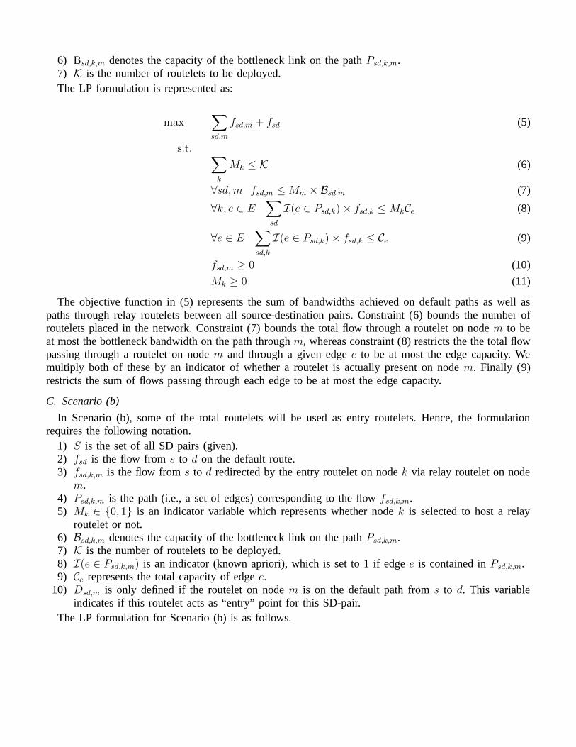
In Figure 4 we study the aggregate throughput for Topology 1, as the number of SD-pairs we want tocreate multiple path for increases. The target total number of routelets K is 8. Rounding is outperformingthe LP/ILP solutions since it is allowed to use a few more routelets than the LP/ILP solutions.

Fig. 3. Throughput per sd-pair for the five algorithms. Scenario b, Topo 1, target number of routelets = 20.

We plot the number of routelets placed by the rounding algorithm for this same example in Figure 5.The more SD-pairs, the more complex the solution is. As the complexity increases, more nodes are usuallynecessary to achieve a better solution. While the LP uses fractional values for the routelets to achieve themaximum throughput, the rounding can either select or totally discharge a potential routelet. By referringto Figure 4 we note that the range where the rounding algorithm selects more than twice the number ofroutelets of the LP, corresponds to the range where the rounding algorithm outperforms the LP solution.The total number of routelets used remains below the theoretical bound of K log K = 24.

In Figure 6 we present the performance of our various algorithms across the ten topologies. Theaggregate throughput values are normalized by dividing the throughput of each algorithm by the LPthroughput. The actual LP throughput for each topology is listed in parentheses (in the x axis names).Using the rounding technique a multipath protocol can achieve a 2-5 fold increase in bandwidth utilizationover the default single path routing.

B. Results - Scenario a

Recall that the rounding algorithm is different for the two different scenario, thus the results in thesesection are slightly different than those in Section V-A.

In Figure 7 the rounding throughput is computed as the average over 4 distinct trials. The results andconclusions are the similar to the ones for Figure 2. The main difference is a higher variability in therounding results compared to scenario (b) due to the absence of the boosting factor present for scenario(b).

In Figure 8 note that the rounding throughput can significantly exceed the LP value for a given SD-pair.More than 30% higher for pair 76-31 for example. This is different from scenario (b) and indicates aprobable edge violation. It would be interesting to plot the average behaviour as opposed to one individualrounding example.

The results in Figure 9 are similar to the scenario (b) Figure 4.We obtain different results in Figure 10 than in Figure 5. The number of routelets selected matches

much better the desired number of routlets in scenario (a) than in scenario (b).

Fig. 4. Aggregate throughput as the total number of SD-pairs is increased. Bound on the number of routelets is 8. Scenario b, Topo1.

Figure 11 illustrates the edge-violations for scenario (a) rounding. Note there is no bound for r < 3and in this regime we observe the largest values of egde-violation. For the remaining part of the range,the maximum edge-violation remains under the theoretical bound.

Finally Figure 12 illustrated the performance accross the various topologies we tested. Similar toFigure 6.

VI. RELATED WORK

Multipath protocols have been well researched since Maxemchuk’s seminal work on dispersity rout-ing [20] to improve throughput and resilience to path failures or packet losses [27], [8]. Striping orinverse multiplexing [3], [9], [24], [17] provides link level mechanisms for splitting input flows amongmultiple links to increase throughput. More recently, multipath techniques have been proposed in thecontext of overlay routing or multihomed clients [5], [2], [28]. Katabi et al. [14] and Elwalid et al. [10],propose splitting aggregate traffic flows along multiple paths to achieve load balancing and stability inthe context of intradomain traffic engineering. Harp [18] uses multiple paths for scheduling transfers withheterogeneous requirements. Multipath TCP [11] and KV [15] are based on a utility-theoretic frameworkfor network-wide resource allocation, and systematically address fairness. These controllers maintain anontrivial sending rate on each available path so as to maximize utilization and global fairness.

A key requirement of all these works is the support for letting end-hosts utilize multiple paths in theInternet for transmitting packets. This can be achieved by employing “packet relayers” that are realizablein several ways. A handful of works address a similar node placement problem in the context of providingresilience to path failures between a source and a destination [12], [29], [25], and for improving end-throughput by breaking an end-to-end TCP connection into a series of shorter-loop connections [19], [25].However, to the best of our knowledge, ours is the first work to address the placement problem in thecontext of maximizing network utilization.

Node placement has also been studied in other contexts such as Web server and cache placement [13],[23]. Qiu et al. [23] study a web server replica placement problem to minimize the cost for clients toaccess data. Jamin et al. [13] study mirror placement problem, in which mirrors can be placed only at

Fig. 5. Number of routelets used as we vary the complexity of the problem (sd-pairs). Scenario b, Topo1, target number of routlets = 8.

a restricted set of locations, much like our problem constraint. Also, they show a diminishing return ofplacing more and more mirrors, similar to our observations.

As also argued by Key et al [16], we believe that multipath routing forms a powerful building blockfor a Robust Internet Architecture of the future. In this paper, we discuss three scenarios in which suchan architecture may be realized.

VII. CONCLUSION

In this paper, we address the routelet placement problem to assist multipath transport protocols thatare designed to achieve better network utilization and fairness. We identify three different deploymentscenarios of routelet placement, provide LP formulations for placement in each of the scenarios, provehardness results. We provide rounding algorithms with provable properties for a subset of the scenarios,and compare their performance through simulations on several BRITE topologies of varying scales.

REFERENCES

[1] Asankya: Enabling High Quality Real-Time Content.http://www.asankya.com.

[2] A. Akella and J. Pang and B. Maggs and S. Seshan and A. Shaikh. A Comparison of Overlay Routing and Multihoming Route Control.In Proc of ACM SIGCOMM, 2004.

[3] H. Adiseshu, G. Parulkar, and G. Varghese. A reliable and scalable striping protocol. In ACM SIGCOMM, 1996.[4] A. Akella, S. Seshan, and A. Shaikh. An empirical evaluation of wide-area internet bottlenecks. In IMC ’03: Proceedings of the 3rd

ACM SIGCOMM conference on Internet measurement, pages 101–114, New York, NY, USA, 2003. ACM Press.[5] D. Andersen, A. Snoeren, and H. Balakrishnan. Best-Path vs. Multi-Path Overlay Routing. In Proc of IMC, 2003.[6] A. T. Campbell, H. D. Meer, M. Kounavis, K. Miki, J. Vicente, and D. A. Villela. The genesis kernel: a virtual network operating

system for spawningnetwork architectures. In Open Architectures and Network Programming (OPENARCH), 1999.[7] S. Chawla. Chernoff Bounds.

http://www.cs.cmu.edu/afs/cs.cmu.edu/academic/class/15859-f04/www/scribes/lec9.pdf.[8] David G. Andersen, Hari Balakrishnan, M. Frans Kaashoek, Robert Morris. Resilient Overlay Networks. In Proc. 18th ACM SOSP,

October 2001.[9] J. Duncanson. Inverse multiplexing. In IEEE Communications Magazine, volume 32, 1994.

[10] A. Elwalid, C. Jin, S. H. Low, and I. Widjaja. MATE: MPLS adaptive traffic engineering. In INFOCOM, 2001.[11] H. Han et al. Multi-path TCP: A Joint Congestion Control and Routing Scheme to Exploit Path Diversity in the Internet. In IMA

Workshop on Measurements and Modeling of the Internet, 2004.[12] J. Han, D. Watson, and F. Jahanian. Topology Aware Overlay Networks. In INFOCOM, 2005.

Fig. 6. Performance accross various topologies for scenario b. Target number of routelets = 20.

Fig. 7. Aggregate throughput as the total number of routelets is increased for the five algorithms compared. Scenario a, Topo1.

Fig. 8. Throughput per sd-pair for the five algorithms. Scenario a, Topo 1, target number of routelets = 20.

[13] S. Jamin, C. Jin, A. R. Kurc, D. Raz, and Y. Shavitt. Constrained mirror placement on the internet. In INFOCOM, pages 31–40, 2001.[14] S. Kandula, D. Katabi, B. Davie, and A. Charny. Walking the Tightrope: Responsive Yet Stable Traffic Engineering. In Proc. of

SIGCOMM, Philadelphia, Aug 2005.[15] F. Kelly and T. Voice. Stability of end-to-end Algorithms for Joint Routing and Rate Control. SIGCOMM Comput. Commun. Rev.,

35(2):5–12, 2005.[16] P. Key, L. Massoulie, and D. Towsley. Combined multipath routing and congestion control: a robust internet architecture. Technical

Report TR-2005-111, Microsoft Research, 2005.[17] K.-H. Kim and K. G. Shin. Improving TCP Performance over Wireless Networks with Collaborative Multi-homed Mobile Hosts. In

ACM MobiSys, 2005.[18] R. Kokku, A. Bohra, S. Ganguly, and A. Venkataramani. A Multipath Background Network Architecture. In INFOCOM, 2007.[19] Y. Liu, Y. Gu, H. Zhang, W. Gong, and D. Towsley. Application Level Relay for High-bandwidth Data Transport. In The First

Workshop on Networks for Grid Applications (GridNets), 2004.[20] N. F. Maxemchuk. Dispersity routing in store-and-forward networks. PhD thesis, Univ. Pennsylvania, Philadelphia, 1975.[21] A. Medina, A. Lakhina, I. Matta, and J. Byers. BRITE: Boston university Representative Internet Topology gEnerator.

http://www.cs.bu.edu/brite/.[22] PlanetLab. http://www.planet-lab.org.[23] L. Qiu, V. N. Padmanabhan, and G. M. Voelker. On the placement of web server replicas. In INFOCOM, pages 1587–1596, 2001.[24] A. Qureshi and J. Guttag. Horde: separating network striping policy from mechanism. In ACM MobiSys, 2005.[25] S. Roy, H. Pucha, Z. Zhang, Y. C. Hu, and L. Qiu. Overlay node placement: Analysis, algorithms and impact on applications. In

ICDCS ’07: Proceedings of the 27th International Conference on Distributed Computing Systems, page 53, Washington, DC, USA,2007. IEEE Computer Society.

[26] R. K. S. Agarwal, C.N. Chuah. Opca: Robust interdomain policy routing and traffic control. In Open Architectures and NetworkProgramming (OPENARCH), 2003.

[27] S. Savage, T. Anderson, A. Aggarwal, D. Becker, N. Cardwell, A. Collins, E. Hoffman, J. Snell, A. Vahdat, G. Voelker, and J. Zahorjan.Detour: A case for informed Internet routing and transport. IEEE Micro, 19(1):50–59, January 1999.

[28] A. Sen et al. On Multipath Routing with Transit Hubs. In Proc. of Networking, May 2005.[29] S. Srinivasan and E. Zegura. Routeseer: Topological placement of nodes in service overlays. Technical Report GIT-CC-06-03,

GeorgiaTech, 2006.[30] J. Turner. Design of routers for diversified networks. Technical report, Washington University in St. Louis, March 2006.[31] M. Zhang et al. A Transport Layer Approach for Improving End-to-End Performance and Robustness Using Redundant Paths. In Proc.

of the USENIX 2004.

APPENDIX

The problem of placing a given number of relay nodes in an optimum manner for maximizing networkutilization is at least NP-hard for Scenarios b and c. We will explain in detail a reduction from Balanced

Fig. 9. Aggregate throughput as the total number of SD-pairs is increased. Bound on the number of routelets is 8. Scenario a, Topo1.

Complete Bipartite Subgraph (BCBS) to Scenario (b).BCBS is the problem of deciding, given a bipartite graph G with vertex set S ∪ T , edges (s, t) such

that s ∈ S, t ∈ T and a parameter b whether there exist a subset of nodes S′ ⊂ S and T ′ ⊂ T such that|S′| = |T ′| = b and all such edges are edges in G.

We reduce this problem to the decision version of our problem, which is: Given a graph G thatrepresents the routers and links in the Internet, a subset of the routers that are capable of providing therelay service, and a set of SD-pairs, can we place at most k relay services as to increase the bandwidthutilization between the SD-pairs by an amount equal to a (assuming the paths an SD-pair can utilize tosend info is either a default path or a S-E-R-D path as in Scenario b)?

We obtain the reduction from BCBS to the above problem as follows:Create the network by copying G and adding a destination node D. We connect all nodes in S with

the destination (the dotted lines in Figure 13) and also all nodes in T are connected with the destination(the plain lines in Figure 13). Every node in S is a source, and the direct links represent the default SDpaths. The cloud represents the edges from G. All links have capacity 1. Routelets can be placed at eitherS or T . We ask: is it possible to place 2b nodes and get a b2 increase in the bandwidth (so k = 2b anda = b2)?

Now we will show that solving the node placement question is equivalent to solving the BCBS problem.Any node assignment that distributes the nodes between the two sides, say r nodes in S and l nodes inT , can add at most rl capacity in terms of bandwidth. This product is maximized when r = l = k/2 = b,since the sum r + l = k is constant, and the maximum value is b2. No unbalanced distribution can lead toan extra capacity of b2 or more (because the product rl is strictly less than that in the unbalanced case).The balanced distribution only leads to an extra capacity of b2 if the nodes selected form a completebipartite clique. Thus, to be able to detect whether nodes can be placed to achieve this improvement inbandwidth or not is to be able to solve the BCBS problem.

Since solving the BCBS problem is NP-hard, determining the answer to the decision version of Problemb is also NP-hard.

The reduction to Scenario (c) is similar, the only difference is that in scenario (c) we need an exit

Fig. 10. Number of routelets used as we vary the complexity of the problem (sd-pairs). Scenario a, Topo1, target number of routlets = 8.

Fig. 11. Actual max-edge violation factor as we vary the target number of routelets versus the theoretical upper bound (available for r > 3

only).

routelet on the default path. Since the default paths are a single hop, that routelet needs to be placed atthe destination node D in order to allow more flow than the default. Placing the exit routelet at the sourcenode creates no additional paths beyond the already existing default path.

Fig. 12. Performance accross various topologies for scenario a. Target number of routelets = 20.

S

S1

S

S

3

2

m

1D

Fig. 13. Reduction from Balanced Complete Bipartite Subgraph

routelet placement for multipath transport (prelim. version)

Documents