role of fractional calculus to the · pdf filefractional calculus (fc) ... here we have...
TRANSCRIPT

Volume 5, No. 2, February 2014
Journal of Global Research in Computer Science
REVIEW ARTICLE
Available Online at www.jgrcs.info
© JGRCS 2010, All Rights Reserved 11
ROLE OF FRACTIONAL CALCULUS TO THE GENERALIZED INVENTORY
MODEL
Asim Kumar das1*
, Tapan Kumar Roy2
Department of Applied Mathematics, Bengal Engineering & Science University,
Shibpur, Howrah, West-Bengal, India, 711103.
Abstract: The feature of the derivative and integration is one of the most important tools to realise the beauty of calculus. Its descriptive power
comes from the fact that it analyses the behaviour at scales small enough that its properties changes linearly, so avoiding complexities that arises
at larger one. Fractional Calculus generalizes this concept from integer to non integer order. This paper comprises an application of this
Fractional Calculus in Inventory Control model. The object of this note is to show how fractional calculus approach can be employed to
generalize the traditional classical inventory model. Lastly a numerical example is given.
Keywords: Fractional differentiation, Fractional Integration, Fractional Differential Equation, Set up Cost, Holding Cost, Economic Order
Quantity.
INTRODUCTION
Fractional Calculus (FC) is a branch of applied mathematics
that deals with generalization of the operation of
derivatives/integrals and differential equation of an arbitrary
order (including complex orders)[8],[13],[24],[27]. The
theory of FC is one of the strongest tool to describe many
physical phenomena which are neglected in the model
described by the classical integer order calculus. This is
almost three centuries old as the conventional calculus but
not very popular among science or engineering community.
Since then the subject of Fractional Calculus caught the
attention of many great mathematicians (pure and applied)
such as N.H.Abel, L.Euler, J.Fourier, H.K.Grunwald,
J.Hadamarad, G.H.Hardy, O.Heviside, P.S.Laplace,
G.W.Lebinitz, A.V.Letnikov , B.Riemann, J.Liouville,
M.Caputo, M.Reisz and H.Weyl are directly or indirectly
contributed to its development. The mathematics involving
fractional order derivatives or integrals are appeared very
different from that of integer order calculus. Initially there
were almost no practical application of this field and due to
this it was considered that fractional calculus as an abstract
area containing only rigorous mathematical manipulations.
So for past three centuries this subject was with only
mathematicians. But in recent years(forty years almost) this
subject has been applied to several fields of engineering,
science and economics[11]. Some of the areas where
Fractional Calculus has made an important role that are
included viscoelasticity and rheology [3], electrical
engineering[14], electrochemistry, biology, biophysics and
bioengineering, electromagnetic theory[15], mechanics,
fluid mechanics[12], signal and image processing theory[6],
particle physics, control theory[14] and many other
field[1],[20],[4],[10],[23]. However there are some areas of
management and science where this branch of mathematics
remains untouched.
The application of Fractional Calculus and Fractional
Differential equation are not being used so far in any
Operation Research model. Our objective in this paper is to
develop the traditional classical EOQ based inventory model
[31[,[32],[9],[2]. to a generalized EOQ based inventory
model emphasis on some certain assumption by using the
potential application of Fractional Calculus. In traditional
EOQ based inventory model[2], the demand(deterministic)
rate is typically assumed to be of fixed 1st order
differentiation and holding cost is calculated on the fixed 1st
order integral of inventory level. We may develop our
consideration by accepting that the demand rate may varies
high or low according to the market situation. So here we
may consider that demand rate may be taken as fractional
order differentiation instead of fixed 1st order differentiation.
Similarly we calculate the holding cost is of fractional order
integral of inventory level rather than that of fixed 1st order
integral.
Here we have applied the concept of derivative/integrals
with an emphasis on Caputo and Riemann-Liouville
fractional derivatives and have some interesting result and
ideas that demonstrate the generalized EOQ based inventory
model. Fractional derivatives and fractional integrals have
interesting mathematical properties that may be utilized to
developed our motivation. In this article, first we give a brief
historical review of the general principles, definitions and
several features of fractional derivatives/integrals and then
we review some of our ideas and findings in exploring
potential applications of fractional calculus in inventory
control model.
BRIEF HISTORY RELATED TO FRACTIONAL
CALCULUS
As to history of Fractional Calculus, already in 1695
L‟Hospital raised the question to Lebinitz, as the meaning of
n
n
dx
yd if n=1/2, that is “what if n is fractional?” Lebinitz
replied “This is an apparent paradox from which one day
useful consequence will be drawn”.

Asim Kumar das et al, Journal of Global Research in Computer Science, 5 (2), February 2014, 11-23
© JGRCS 2010, All Rights Reserved 12
S.F Lacroix was the first to mention in some two pages a
derivative of arbitrary order in a 700 pages text book of
1819.
He developed the formula for the nth derivative of y=mx , m
is a positive integer,
yDn
=)!(
!
nm
m nmx , where n( m) is an integer. (2.1)
Replacing the factorial symbol by the well known Gamma
function, he obtained the formula for the fractional
derivative,
xxD)1(
)1()( , (2.2)
Where , are fractional numbers.
In particular he had, x
x xD 2)(
)2()(
2/1
23
2/1. (2.3)
Again the normal derivative of a function f is defined as,
h
xfhxfxf
hD
)()()( lim
0
1, (2.4)
And D2f(x)
h
xhx ffh
)()(11
0lim
=h
xfhxfhxf
h
)()()2(lim
0
.
Iterating this operation yields an expression for the nth
derivative of a function. As can be easily seen and proved by
induction for any natural number n,
Dnf(x) =
n
r
nn
hh
00
)1(limr
nf(x+(n-r)h). (2.5)
Where r
n=
)!(!
!
rnr
n (2.6)
Or equivalently,
)()(00
)1(lim rhxfr
nxf
n
r
rn
h
n
hD (2.7)
The case of n=0 can be included as well.
The fact that for any natural number n the calculation of nth
derivative is given by an explicit formula (2.5) or (2.7).
Now the generalization of the factorial symbol (!) by the
gamma function allows
r
n=
)!(!
!
rnr
n=
)1()1(
)1(
rnr
n (2.8)
Which also valid for non integer values.
Thus on using of the idea (2.8), fractional derivative leads as
the limit of a sum given by
)(xfD lim0h
)()1()1(
)1(1
0
)1( rhxfrr
n
r
r
h. (2.9)
Provided the limit exists. Using the identity
)(
)(
)1(
)1()1(
r
r
r
(2.10)
The result (2.9) becomes,
)(xfD lim0h
)()1(
)(
)( 0
rhxfr
rn
r
h (2.11)
When α is an integer, the result (2.9)reduce to the derivative
of integral order n as follows in (2.5).
Again in 1927 Marchaud formulated the fractional
derivative of arbitrary order α in the form given by,
)(xfD dttfxfxf
x
txx 0
1
)(
)()(
)1()1(
)( , Where
0<α<1 (2.12)
In 1987 Samko et al had shown that (2.12) and (2.9) are
equivalent.
Replacing n by (-m) in (2.7), it can be shown that
)(0
xfDm
x)(
00lim rhxf
r
mn
r
m
hh
=)(
1
m
x
0
)()1(
txm
f(t)dt (2.13)
Where
!
)1)........(2)(1(
r
rmmmm
r
m (2.14)
This observation naturally leads to the idea of generalization
of the notations of differentiation and integration by
allowing m in (2.13) to be an arbitrary real or even complex
number.
Fractional derivatives and integrals:
The idea of fractional derivative or fractional integral can be
described in another different ways.
First, we consider a linear non homogeneous nth order
ordinary differential equation ,
)(xfyDn
, b≤x≤c (2.1.1)
Then {1, x, x2,
x3, ........,x
n-1} is a fundamental set the
corresponding homogeneous equation Dn
y=0. f(x) is any
continuous function in [b,c], then for any a (b,c),

Asim Kumar das et al, Journal of Global Research in Computer Science, 5 (2), February 2014, 11-23
© JGRCS 2010, All Rights Reserved 13
y(x)= dttfn
x
a
n
tx)(
)!1(
)(1
(2.1.2)
Is the unique solution of the equation (2.1.1) with the initial
data yk )(
(a)=0,
for 10 nk . Or equivalently, y(x)=
Dn
xaf(x)=
x
a
n
txn
)(1
)(
1f(t)dt (2.1.3)
Replacing n by ,where Re( )>0 in the above formula
(2.1.3),we obtain the Riemann-Liouville definition of
fractional integral that was reported by Liouville in 1832
and by Riemann in 1876 as )(xfDxa = )(xfJ xa
=
dttf
x
a
tx )()(
1)(
1
(2.1.4)
Where
)(xfDxa= )(xfJ xa
= dttf
x
a
tx )()(
1)(
1
is the Riemann-Liouville integral operator. When a=0
,(2.1.4) is the Riemann definition of integral and if a= - ,
(2.1.4) represents Liouville definition. Integral of this type
were found to arise in theory of linear ordinary differential
equations where they are known as Eulier transform of first
kind.
If a=0 and x>0 ,then the Laplace transform solution the
initial value problem
Dn
y(x)=f(x), x>0, yk )(
(0)=0,
10 nk (2.1.5)
is )(sy = sn
)(sf (2.1.6)
Where )(sy and )(sf are respectively the Laplace
transform of the function y(x) and f(x).
The inverse Laplace transform gives the solution of the
initial value problem (2.1.5) as
y(x)= )(0
xfDn
x
Again from (2.1.6) we have y(x)= )}({1
syL
= )}({1
sfsLn
Thus we have )(0
xfDn
x= )}({
1sfsL
n (2.1.7)
i.e
)}({1
sfsLn
= )(0
xfDn
x=
dttfn
xn
tx )()(
1
0
1
)( (2.1.8)
y(x)=
)(0
xfDn
x= )}({
1sfsL
n=
dttfn
xn
tx )()(
1
0
1
)(
This is the Riemann-Liouville integral formula for an integer
n. Replacing n by real gives the Riemann-Liouville
fractional integral (2.1.3) with a=0.
In complex analysis the Cauchy integral formula for the nth
derivative of an analytic function f(z) is given by
Dn
f(z) = dttf
i
n
C
n
zt )(1
)(
2
! (2.1.9)
Where C is closed contour on which f(z) is analytic , and t=z
is any point inside C and t=z is a pole.
If n is replaced by an arbitrary number and n by
)1( , then a derivative of arbitrary order can be
defined by,
D f(z)= dttf
iC zt )(
1
)(
2
)1( (2.1.10)
where t=z is no longer a pole but a branch point.
In (2.1.10) C is no longer appropriate contour, and it is
necessary to make a branch cut along the real axis from the
point z=x>0 to negative infinity.
Thus we can define a derivative of arbitrary order by loop
integral
Dxaf(z)= )(
2
)1()(
1
tfi
x
a
zt (2.1.11)
Where )(1
zt = exp[-( +1)ln(t-z)] and ln(t-z) is real
when t-z>0. Using the classical method of contour
integration along the branch cut contour D, it can be shown
that
D z0 f(z)= dttf
iD
zt )(2
)1()(
1
=i2
)1([1-exp{-2 i( +1)}] dttf
z
zt )(0
1
)(
= dttf
z
zt )()(
1
0
1
)( (2.1.12)
Which agrees with Riemann-Liuville definition (2.1.3) with
z=x, and a=0, when is replaced by -
Fractional Integration, Fractional Differential Equation
using Laplace Transformed Method:
One of the very useful results is formula for Laplace
transform of the derivative of an integer order n of a
function f(t) is given by

Asim Kumar das et al, Journal of Global Research in Computer Science, 5 (2), February 2014, 11-23
© JGRCS 2010, All Rights Reserved 14
L{ )()( tf n}= )(sfs n
-
1
0
)(1 )0(n
k
kkn fs (2.2.1)
= )(sfs n-
1
0
)1( )0(n
k
knk fs (2.2.2)
= )(sfs n-
n
k
knk fs1
)(1 )0(
Where )0()( knf = kc represents the physically realistic
given initial conditions and )(sf being the Laplace
transform of the function f(t).
Like Laplace transform of integer order derivative, it is easy
to shown that the Laplace transform of fractional order
derivative is given by
L{ Dt0f(t)}= )(sfs - 0
1
0
1
0
)]([ t
k
t
n
k
k tfDs (2.2.3)
= )(sfs - k
n
k
k cs1
1, (2.2.4)
Where n-1 n and kc = )]([0 0tfD
kt t
(2.2.5)
Represents the initial conditions which do not have obvious
physical interpretation. Consequently, formula (2.2.4) has
limited applicability for finding solutions of initial value
problem in differential equations.
We now replace by an integer-order integral Jn
and
)()()(
ttf fDnn
is used to denote the integral order
derivative of a function f(t). It turns out that
JDnn
=I, DJnn
I. (2.2.6)
This simply means that Dn
is the left ( not the right
inverse ) of Jn
. It also follows in (2.2.9) with =n that
DJnn
f(t) = f(t)-!
)0(1
0
)(
k
tfk
n
k
k
, t>0 (2.2.7)
Similarly, D can also be defined as the left inverse of
J .We define the fractional derivative of order >0 with
n-1 n by
Dt0 f(t)= D
n
Dn )(
f(t)
= Dn
Jn
f(t)
= Dn
[ dfn
tn
t )()(
1
0
1
)( ] (2.2.8)
On using (2.1.3)
Or, Dt0 f(t)= d
nft
nt
n
)()(
1 )(
0
1
)(
Where n is an integer and the identity operator „I‟ is defined
by
)()(00
tftf JD =If(t)=f(t), so that D J =I,
0.
Due to the lack of physical interpretation of initial data ck
in (2.2.4), Caputo and Mainardi adopted as an alternative
new definition of fractional derivative to solve initial value
problems. This new definition was originally introduced by
Caputo in the form
Dt
C
0f(t)= J
n
Dn
f(t)
= dn
ftn
tn
)()(
1 )(
0
1
)( (2.2.9)
Where n-1 n and n is an integer.
It follows from (2.2.8) and (2.2.9) that
Dt0f(t)= D
n
Jn
f(t) Jn
Dn
f(t)= Dt
C
0f(t) (2.2.10)
Unless f(t) and its first (n-1) derivatives vanish at t=0.
Furthermore , it follows (2.2.9) and (2.2.10) that
J Dt
C
0f(t) = J J
n
Dn
f(t)= DJnn
f(t) = f(t)
!)0(
1
0
)(
k
tfk
n
k
k
(2.2.11)
This implies that Dt
C
0f(t)=
Dt0[f(t) )0(
)1(
)(1
0
ft kn
k
k
k]
= Dt0f(t) )0(
)1(
)(1
0
ft kn
k
k
k (2.2.12)
This shows that Caputo‟s fractional derivative incorporates
the initial values )0()(
fk
,
for k=0,1,2,…….,n-1.
The Laplace transform of Caputo‟s fractional derivative
(2.2.12) gives an interesting formula L{ Dt
C
0f(t)}=
)(sfs - sfk
n
k
k 11
0
)(
)0( (2.2.13)
Transform of )()(
tfn
This is a natural generalization of
the corresponding well known formula for the Laplace when
=n and can be used to solve the initial value problems in
fractional differential equation with physically realistic
initial conditions.
Some geometric and physical interpretation of Fractional
Calculus is being referred in [26], [30].
Mittag-Leffler function:
The one of the very important function, used in fractional
calculus known as Mittag-Leffler function [17], is the
generalization of the exponential function ze . One
Asim Kumar das et al, Journal of Global Research in Computer Science, 5 (2), February 2014, 11-23
© JGRCS 2010, All Rights Reserved 15
parameter Mittag-Leffler function is denoted by E (z) and
is defined by the infinite series,
E (z) =
0 )1(k
k
k
z , (2.3.1)
The two parameter function of this type, which plays a very
important role in solving the fractional differential
equations, is defined by the infinite series,
E ,(z) =
0 )(k
k
k
z , where >0, >0 (2.3.2)
It follows from the definition (2.3.2) that
ezz
Ez
k
k
k
k
kkz
001,1 !)1(
)( (2.3.3)
)1(1
)!1(
1
)!1()2()(
0
1
002,1 e
zzzE
z
k
k
k
k
k
k
zkzkkz (2.3.4)
)1(1
)!2(
1
)!2()3()(
20
2
200
3,1z
kkkz e
zz
zzz
Ez
k
k
k
k
k
k
(2.3.5)
And in general }!
{1
)(2
01,1
m
k
k
z
mm kz z
ez
E (2.3.6)
The hyperbolic sine and cosine are also particular cases of
the Mittag-Leffler function (2.3.2) as given by
)cosh()!2()12(
)(0
2
0
2
2
1,2z
kk k
k
k
k
zzzE (2.3.7)
)sinh()!12(
1
)22()(
0
12
0
2
2
2,2z
kzk k
k
k
k
zzzE (2.3.8)
Also we can show that
)(1,
2
1 zE )(
)12
(
2
0
zerfczk ez
k
k
(2.3.9)
Where erfc(-z)is the complement of error function defined
by
erfc(z) = dtez
t22 . (2.3.10)
For =1, we obtain the Mittag-Leffler function in one
parameter:
)()1(
)(0
1,z
kz E
zE
k
k
(2.3.11)
CLASSICAL EOQ MODEL
Notations and Assumptions:
D Demand rate
Q Order quantity
U Per unit cost
C1 Holding cost per unit
C3 Set up cost
q(t) Stock level
T Ordering interval
w Dual variable of T in geometric programming
In classical EOQ based inventory model, we already have
Ddt
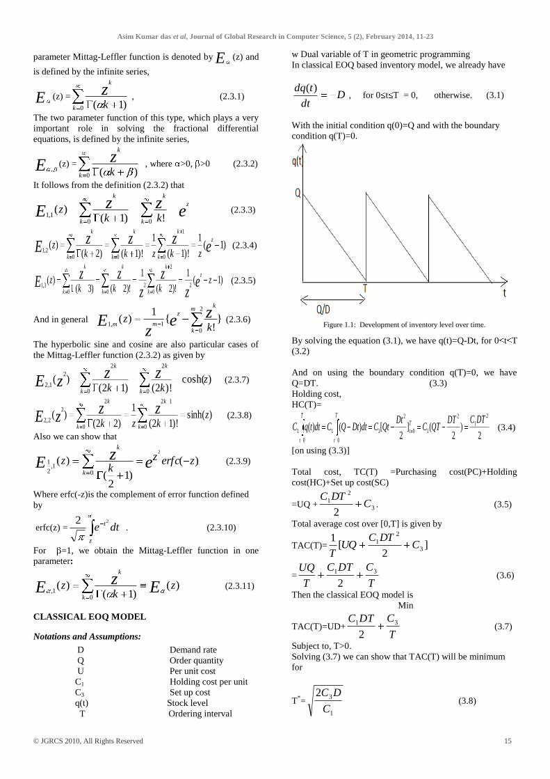
tdq )( , for 0 t T = 0, otherwise. (3.1)
With the initial condition q(0)=Q and with the boundary
condition q(T)=0.
Figure 1.1: Development of inventory level over time.
By solving the equation (3.1), we have q(t)=Q-Dt, for 0 t T
(3.2)
And on using the boundary condition q(T)=0, we have
Q=DT. (3.3)
Holding cost,
HC(T)=
2)
2(]
2[)()(
2
1
2
10
2
0
1
0
11
DTCDTQTC
DtQtCdtDtQCdttqC T
t
T
t
T
t
(3.4)
[on using (3.3)]
Total cost, TC(T) =Purchasing cost(PC)+Holding
cost(HC)+Set up cost(SC)
=UQ + 3
2
1
2C
DTC. (3.5)
Total average cost over [0,T] is given by
TAC(T)= ]2
[1
3
2
1 CDTC
UQT
=T
CDTC
T
UQ 31
2 (3.6)
Then the classical EOQ model is
Min
TAC(T)=UD+T
CDTC 31
2 (3.7)
Subject to, T>0.
Solving (3.7) we can show that TAC(T) will be minimum
for
T*=
1
32
C
DC (3.8)

Asim Kumar das et al, Journal of Global Research in Computer Science, 5 (2), February 2014, 11-23
© JGRCS 2010, All Rights Reserved 16
and TAC*(T
*)=UD+ DCC 312 . (3.9)
GENERALIZED EOQ MODEL
We now generalize our discussion by accepting the equation
(3.1) as a differential equation of fractional order instead of
the linear order. i.e we here consider that demand(D) varies
in fractional order say , here instantaneous inventory level
Ddt
tqd )( for 0≤t≤T = 0 otherwise. (4.1)
With the same initial and boundary condition as described in
the previous problem in equation (3.1). i.e q(0)=Q and with
q(T)=0. where D is a constant.
Equation (4.1) can be rewritten as t
C D0 q(t) = -D for
0≤t≤T (4.2)
= 0 otherwise.
Where t
C D0
11 DJ is the Caputo fractional derivative
as described in (2.2.9) and 1D
dt
d.
To solve the initial value problem of fractional order
differential equation (4.2) we apply the Laplace transform
method. So taking Laplace transform of the equation (4.2),
we have, L{ t
C D0 q(t)}= -DL{1}
)0()( 10 qssqs = -s
D ,
)(sq being Laplace transform of q(t).
)(sqs = Q1s
s
D
)(sq = 1s
D
s
Q
Taking Laplace inversion of above equation we have,
q(t) = )1(
)}({1 DtQsqL
So the inventory level at any time t based on α ordered
decreasing rate of demand
is )(tq = )1(
DTQ for 0≤t≤T . (4.3)
On using the boundary condition q(T)=0 implies that
Q=)1(
DT (4.4) [for =1 in (4.3)
and (4.4) gives results as in (3.2) and (3.3)].
Generalized Holding Cost:
Now the Holding cost of fractional order, say i.e.
)(THC = )(1 tqDC (4.1.1)
Case1: For =1 and =1, Holding cost is
HC1,1(T)= )(1
1 tqDC =2
1QTC=
2
2
1DTC, same as in (3.4).
Case2: For =1, Holding cost is
)(,1 THC =
T
dttqC0
1 )(
= dtDt
QC
T
])1(
[0
1
=)1()1(
[1
1
DTQTC ]
=)1()1(
)1(.[1
QTQTC ] (using (4.4))
= QTC
1
1 (4.1.2)
Case3: For =1, Holding cost of order is
)(,1 THC = )(1 tqDC =
t
dxxqxtC0
1
1 )()()(
1
=
t
dxDxQxtC0
1
1 )()()(
1
= dDt
CdQt
C
1
0
11
1
1
0
1
1 )1()(
)1()(
(putting x = t )
= )2,()(
])(
)1([
)(
1
1
1
01 BDt
CQt
C t
where B(m,n) is the well known beta function.
=)2()1(
1
11
DtC
QtC
For t=T, )(,1 THC = ])2(
1
)1(
1[1QTC
( using Q=DT for =1) (4.1.3)
= ])2(
1
)1(
1[1
1DTC (4.1.4)
[ The above fractional order integration can also be done by
using Laplace transform method. We have to find the
fractional order integral
)(tqD =
t
xqxt0
1 )()()(
1, where q(x)=Q-Dx.
For this now
L{ )(tqD }=L{ )( DtQD }=21 s
D
s
Q
(4.1.5)
(Since it is known that
L{11
)1()1(}{)}(
ssstLstD )
Therefore from (4.1.5), we have
)(tqD = }{21
1
s
D
s
QL =
)2()1(
1DtQt]

Asim Kumar das et al, Journal of Global Research in Computer Science, 5 (2), February 2014, 11-23
© JGRCS 2010, All Rights Reserved 17
Case 4: For any and , Holding cost is )(, THC
= )(1 tqDC ,
Where, )(tq =Q)1(
Dt
Now )(tqD =
t
xqxt0
1 )()()(
1
Then L{ )(tqD }=L{)1(
(Dt
QD )}
=11 s
Ds
s
Q =
11 s
D
s
Q
Therefore
)(tqD =
)1()1(}{
11
1 DtQt
s
D
s
QL
Then for t=T, HCα,β(T)
= )(1 tqDC = ])1()1(
[1
DTQTC
= ])1(
)1(
)1(
1[1QTC [using (4.3)]
= ])1(
)1(
)1(
1[
)1(1
DTC
=)1(
1
)1()1(
11DTC (4.1.6)
Generalized Total Average Cost:
Total cost(TC)=Purchasing cost(PC)+Holding cost(HC)+Set
up cost(SC).
Total Average Cost (TAC)=T
1[Total Cost(TC)]
Case1: For α=1 and β=1, the model is being as our classical
EOQ problem where the optimum Total Average Cost
TAC*1,1(T*) is given in (3.9).
Case2: For any >0 and =1,
Here, )(1, TTC =UQ+ QTC
1
1+ 3C
Then total average cost )(1, TTAC =T
1[
UQ+ QTC
1
1+ 3C ]
= ])2()1(
[1
3
11 CDTCUDT
T
=T
CDT
CUDT 31
1
)2()1( (4.2.1)
Here generalized EOQ model is,
Min )(1, TTAC =T
CBTAT 1
, (4.2.2)
subject to T ≥0,
where A=)1(
UD , B=
)2(
1 DC and C= 3C .
(4.2.2) can be taken as a primal geometric programming
problem with degree of difficulty (DD) =1.
Dual form of (4.2.2)
Max d(w) =
321
321
www
w
C
w
B
w
A, (4.2.3)
Subject to, 1w + 2w + 3w =1,
(normalized condition) (4.2.4)
1w ( -1)+ 2w - 3w =0,
(orthogonal condition) (4.2.5)
w1, w2, w3 ≥0.
Primal-dual relations are,
A1T = 1w d(w) (4.2.6)
BT = 2w d(w) (4.2.7)
T
C= 3w d(w) (4.2.8)
From (4.2.6) and (4.2.7), we have,
2
1
w
w
BT
A T
=
1
2
w
w
B
A (4.2.9)
From (4.2.7) and (4.2.8), we have,
3
21
w
wT
C
B
3
2
1
1
2
w
w
Bw
Aw
C
B
032
1
1 wwwA
B
A
C (4.2.10)
Now we have to solve for 1w , 2w , 3w from three system of
non linear equations (4.2.4), (4.2.5) and (4.2.10) and
obtained the solutions as *
1w ,*
2w and *
3w and then
from the relation (4.2.9), we will able to obtain *T for
which )(1, TTAC is minimum. i.e we will able to obtain
)(*
1, TTAC as the minimum of )(1, TTAC in (4.2.2) and
Q*(T) in (4.4).
Case3: For =1 and for any , we have the Holding cost ,
)(,1 THC =
])2(
1
)1(
1[1
1DTC
[from(4.1.4)]
Then Total cost
(TC)=UQ+ ])2(
1
)1(
1[1
1DTC + 3C
Asim Kumar das et al, Journal of Global Research in Computer Science, 5 (2), February 2014, 11-23
© JGRCS 2010, All Rights Reserved 18
Total average cost )(,1 TTAC =T
1{
UQ+ ])2(
1
)1(
1[1
1DTC + 3C }
=UD+T
CTDC 3
1)2(
1
)1(
1 (4.2.11)
[since for =1, we know that Q=DT.]
=A+BT +T
C (say)
Where, A=UD,
B=)2(
1
)1(
11DC , and C= 3C . (4.2.12)
To minimize )(,1 TTAC , we again apply geometric
programming method.
Let us suppose that M(T)= BT +T
C (4.2.13)
Then the degree of difficulty(DD) in G.P.P(4.2.13)=2-1-1=0
Max d(w)=
21
21
ww
w
C
w
B
Subject to, 1w + 2w =1 (normalized condition) (4.2.14)
1w - 2w =0 (orthogonal condition) (4.2.15)
w1, w2 ≥ 0.
Then solving for 1w and 2w from the above equation (4.2.14)
and (4.2.15), we get
1w =1
1 and 2w =
1 (4.2.16)
Again from the primal-dual relations BT = 1w d(w) and
T
C= 2w d(w) , we get
1
2
11
w
wT
C
B
1
1
1
B
CT
B
CT (4.2.17)
we get, Max
d(w)=
11
1
11
1
CB
=1
1
1
11
11
)1(CB
= )1(111
1
CB
Min M(T)=
)1(111
1
CB
Min )(,1 TTAC =
)(*
,1 TTAC =A+ )1(111
1
CB (4.2.18)
Where A, B, C are given in (4.2.12).
Case4: For any α >0 and any >0, we have the Holding
cost as
)(, THC =
)1(
1
)1()1(
11DTC
[from(4.1.6)]
Then Total cost )(, TTC
=UQ+)1(
1
)1()1(
11DTC +
3C Total average cost is given by
)(, TTAC =T
1{
UQ+)1(
1
)1()1(
11DTC +
3C }
=T
CTDCT
UD 31
1
1
)1(
1
)1()1(
1
)1( (4.2.19)
[since we have from (4.4),
Q=)1(
DT]
=A1T +B
T
CT 1
(say)
Where A=)1(
UD,
B=)1(
1
)1()1(
11DC and
C= 3C .
Now to minimize )(, TTAC , we apply geometric
programming method, and the degree of difficulty(DD)
is=3-1-1=1.
Max d(w) =
321
321
www
w
C
w
B
w
A
Subject to, 1w + 2w + 3w =1 (normalized condition) (4.2.20)
( -1) 1w +( + -1) 2w - 3w =0(orthogonal condition) (4.2.21)
w1, w2, w3 ≥ 0.
Again the primal-dual variable relations are given by
A1T = 1w d(w) (4.2.22)

Asim Kumar das et al, Journal of Global Research in Computer Science, 5 (2), February 2014, 11-23
© JGRCS 2010, All Rights Reserved 19
B1T = 2w d(w) (4.2.23)
T
C= 3w d(w) (4.2.24)
From (4.2.22) and (4.2.23) we have,
1
2
w
w
A
BT
1
1
2
Bw
AwT (4.2.25)
Again from (4.2.22) and (4.2.24) we have,
3
1
w
wT
C
A
3
1
1
2
w
w
Bw
Aw
C
A
3
1
1
2
Aw
Cw
Bw
Aw
0321 wwwA
C
A
B (4.2.26)
Now solving for 1w , 2w and 3w from three system of non
linear equations (4.2.20), (4.2.21) and (4.2.26) we get the
solution as *
1w ,*
2w ,*
3w and hence we calculate Max d(w)
i.e *)(*
, TTAC . Again using (4.2.25), we will able to find
T* and hence Q*(T*) by using (4.4).
Numerical example:
A product has a demand of 5000 units per year. The cost of
one procurement is Rs 20000 and the holding cost per unit is
Rs 100 per year. The replacement is instantaneous and no
shortages are allowed. We shall now calculate for different
values of α and β,
(a). The economic lot size,( EOQ)
(b). Optimal total average cost,
(c). Optimal time period.
Where the set up cost is Rs.10000.
This is given in terms of some tables and figures.
Table-1: Optimum value of T*, )( **
1, TTAC and *Q (T*) for different vales and β=1.0.
A=
)1(
UD, B=
)2(
1 DC,
C= 3C =10000.
T*
)( **
1, TTAC
Q*(T*)
0.1 A=105114000, B=47779 19800 142778 14135
0.2 A=108912000, B=90760.4 4799.98 618094 29668.5
0.3 A=111424000, B=128566 2022.22 1.80209e+6 54663.6
0.4 A=112706000, B=161009 1050 4.33685e+6 91073.7
0.5 A=112838000, B=188063 600.007 9.2131e+6 138198
0.6 A=111917000, B=209845 355.554 1.77985e+7 189850
0.7 A=110055000, B=226583 208.164 3.16949e+7 230921
0.8 A=107367000, B=238594 112.501 5.21835e+7 234837
0.9 A=103975000, B=246258 46.913 7.8625e+7 165983
1.0 A=100000000, B=250000 0.2 1.001e+8 1000
Above table shows optimal results of total average cost, time
period and order quantity for different α. It is seen that as α
increases T*decreases [Fig-2] and TAC*(T*) increases [Fig-
3] but Q*(T*) increases up to certain value of α and then
decrease [Fig-4].
Table-2: Optimum values of T*, )( **
,1 TTAC & Q*(T*) for different values β and α=1.0.
A=UD, B=
)2(
1
)1(
11DC
C=C3=10000
T*
)( **
,1 TTAC
Q*(T*)
0.1 A=100000000, B=4779 15.8709 100007000 79354.5
0.2 A=100000000, B= 90760.4 0.608454 100099000 3042.27
0.3 A=100000000, B= 128566 0.35403 100122000 1770.15
0.4 A=100000000, B= 161009 0.264367 100132000 1321.84
0.5 A=100000000, B= 188063 0.224466 100134000 1122.33
0.6 A=100000000, B= 209845 0.205338 100130000 1026.69
0.7 A=100000000, B= 226583 0.196755 100123000 983.775
0.8 A=100000000, B= 238594 0.1943 100116000 971.5
0.9 A=100000000, B= 246258 0.195782 100108000 978.91
1.0 A=100000000, B= 250000 0.2 100100000 1000

Asim Kumar das et al, Journal of Global Research in Computer Science, 5 (2), February 2014, 11-23
© JGRCS 2010, All Rights Reserved 20
Above table shows optimal results of total average cost, time
period and order quantity for different β when α is being
fixed as 1.0. It is seen that as β increases T*decreases [Fig-5]
and TAC*(T*) increases up to certain values of β and after
then it decreases [Fig-6] but Q*(T*) decreases [Fig-7]
respectively.
TABLE- 3, For α=0.2 and any β Optimum value of T*,TAC*(T*),Q*(T*)
A=
)1(
UD
B=
)1(
1
)1()1(
11DC C= 3C
T*
TAC*(T*)
Q*(T*)
0.1 A=108912000, B=15288.2 0.3061442 e+14 0.001777024 2.71164e+6
0.2 A=108912000, B=29565.8 0.31727 82e +14 0.001955948 2.73109e+6
0.3 A=108912000, B=42584.8 0.7903284e+14 0.005619694 3.278e+6
0.4 A=108912000, B=54167.4 0.5234629e+15 0.07035799 4.78437e+6
0.5 A=108912000, B=64199 0.7001797e+16 1.132333 8.03692e+6
0.6 A=108912000, B=72624.7 0.1308728e+18 27.39773 1.44350e+7
0.7 A=108912000, B=79439.5 0.2608468e+19 1143.926 2.62618e+7
0.8 A=108912000, B=84680.8 0.30775252e+14 84680.8 2.71409e+6
0.9 A=108912000, B=88421.3 27376.76 276340.4 42026.6
1.0 A=108912000, B=90760.4 4800.080 618095.7 29688.6
Above table shows optimal results of total average cost, time
period and order quantity for different β and fixed α=0.2. It
is seen that as β increases T*decreases and TAC*(T*)
increases but Q*(T*) decreases.
TABLE- 4, For α=0.4 and any β Optimum value of T*,TAC*(T*),Q*(T*)
A=
)1(
UD
B=
)1(
1
)1()1(
11DC
C=C3.
T*
TAC*(T*)
Q*(T*)
0.1 A=112706000, B=28157.9 0.99e+20 0.0001162177 5.61269e+11
0.2 A=112706000, B=54167.1 0.99e+20 0.0006572407 5.61269e+11
0.3 A=112706000, B=77635.7 0.99e+20 0.07798352 5.61269e+11
0.4 A=112706000, B=98297 0.99e+20 9.849592 5.61269e+11
0.5 A=112706000, B=115999 0.99e+20 1161.157 5.61269e+11
0.6 A=112706000, B=130689 0.99e+20 130698 5.61269e+11
0.7 A=112706000, B=142402 178756.2 556786.8 710922
0.8 A=112706000, B=151244 15372.32 1386643 266448
0.9 A=112706000, B=157378 3211.487 2661012 142429
1.0 A=112706000, B=161009 1050.007 4336857 91073.9
Above table shows optimal results of total average cost, time
period and order quantity for different β and fixed α=0.4. It
is seen that as β increases T*decreases and TAC*(T*)
increases but Q*(T*) decreases.
TABLE- 5, For α=0.6 and any β Optimum value of T*,TAC*(T*),Q*(T)
A=
)1(
UD
B=
)1(
1
)1()1(
11DC
,
C= 3C
T*
TAC*(T*)
Q*(T*)
0.1 A=111917000, B=37929.4 0.99e+20 1.161722 5.56223e+15
0.2 A=111917000, B=72624.7 0.99e+20 8.400761 5.56223e+15
0.3 A=111917000, B=103639 0.99e+20 1038.556 5.56223e+15
0.4 A=111917000, B=130689 0.99e+20 130690.1 5.56223e+15
0.5 A=111917000, B=153637 8490250 946886.4 8.03934e+7
0.6 A=111917000, B=172474 154408.4 2821948 7262240
0.7 A=111917000, B=187298 13954.59 5740983 1716720
0.8 A=111917000, B=198291 2751.011 9421709 647981
0.9 A=111917000, B=205707 854.9325 13533090 321386
1.0 A=111917000, B=209845 355.5568 17798480 189851

Asim Kumar das et al, Journal of Global Research in Computer Science, 5 (2), February 2014, 11-23
© JGRCS 2010, All Rights Reserved 21
Above table shows optimal results of total average cost, time
period and order quantity for different β and fixed α=0.6. It
is seen that as β increases T*decreases and TAC*(T*)
increases but Q*(T*) decreases.
TABLE- 6, For α=0.8 and any β Optimum value of T*,TAC*(T*),Q*(T*)
A=)1(
UD
B=
)1(
1
)1()1(
11DC C= 3C
T*
TAC*(T)
Q*(T)
0.1 A=107367000, B=44410.7 0.99e+20 11202.86 5.32537e+19
0.2 A=107367000, B=84680.8 0.99e+20 95439.10 5.32537e+19
0.3 A=107367000, B=120376 0.6884457e+11 2189869 2.51268e+12
0.4 A=107367000, B=151244 0.1342708e+8 8059433 2.70537e+9
0.5 A=107367000, B=177199 163168.6 0.1622528e+8 7.94238e+7
0.6 A=107367000, B=198291 11330 0.2489523e+8 9.40211e+6
0.7 A=107367000, B=214687 1937.859 0.3307765e+8 2.28928e+6
0.8 A=107367000, B=226643 559.7714 0.4038387e+8 847715
0.9 A=107367000, B=234487 224.8403 0.4673492e+8 408640
1.0 A=107367000, B=238594 112.5009 0.5218568e+8 234837
Above table shows optimal results of total average cost, time
period and order quantity for different β and fixed α=0.8. It
is seen that as β increases T*decreases and TAC*(T*)
increases but Q*(T*) decreases.
Figure-2: Rough sketch of α versus T* graph for fixed β=1.0
We see from the above figure that for fixed β=1, as α
increases T* decreases and this decreasing rate is very high
when α varies between 0.1 to 0.4. The decreasing rate of T*
becomes slow after 0.4.
Figure-3: Rough sketch of α versus TAC*α,1(T*) graph for fixed β=1.0
We see from the above figure that as α increases,
TAC*α,1(T) increases and this increasing rate very high
when α ≥ 0.5.

Asim Kumar das et al, Journal of Global Research in Computer Science, 5 (2), February 2014, 11-23
© JGRCS 2010, All Rights Reserved 22
Figure-4: Rough sketch of α versus Q*(T*) graph for fixed β=1.0
The above figure shows that as α increase up to 0.8, Q*(T*)
increases, but when α>0.8, Q*(T*) decreases very highly.
Figure-5: Rough sketch of β versus T* graph for fixed α=1.0
We see from the above figure that as β increases , T*
decreases. The decreasing rate is very high when β is in
between 0.1 and 0.5.
Figure-6: Rough sketch of β versus TAC*1,β(T*) graph for fixed α=1.0
We see from the above figure that as β increases up to 0.5,
TAC*1,β(T*) increases very highly and when β>0.5,
TAC*1,β(T*) decrease slowly.
Figure-7: Rough sketch of β versus Q*(T*) graph for fixed α=1.0
The above figure shows that that as β increases, Q*( T*)
decreases. The decreasing rate is very high when β is in
between 0.1 and 0.5.
CONCLUSION
Fractional Calculus is the generalization of the ordinary
calculus. In this feature article, we have briefly shown some
of the role and application of the fractional in our well
known classical EOQ model of inventory control in
operation research so it can be made more general. It is
shown that classical holding cost (HC) total average
cost(TAC) are the particular case of our generalized holding
cost and total average cost which is based on the fractional
order integration and differentiation.
Although the fractional order calculus is a 300-years old
topic, only very rare application is studied in any operation
research model. Still, ordinary calculus is much more
familiar and more preferred, may be because its applications
are more apparent. However it is expected that this new
branch of applied mathematics will able to fill the gap
between ordinary calculus and fractional order calculus.
Fractional calculus has the potentiality of useful application
in any operation research model. In future it would be a very
useful tool to describe any operation research model more
precisely.
REFERENCES
[1]. Ayala.R and Tuesta.A, Introduction to the concepts and
Application fractional and variable order Differential
Calculus, May 13, 2007.
[2]. S. Axsater, Inventory Control , second edition , chapter 4,PP.
52-61.Library of Congress Control Number:2006922871,
ISBN-10:0-387-33250-2 (HB), © 2006 by Springer Science
+Business Media, LLC.
[3]. Bagley.R.L, Power law and fractional calculus Model of
viscoelasticity, AIAA J. 27(1989), 1414-1417.
[4]. Benchohra.U, Hamani.S, Ntouyas.S.K, Boundary value
problem for differential equation with fractional order, ISSN
1842-6298(electronic), 1843-7265(print), Volume 3(2008),
1-12.

Asim Kumar das et al, Journal of Global Research in Computer Science, 5 (2), February 2014, 11-23
© JGRCS 2010, All Rights Reserved 23
[5]. Chun –Tao. C, „„An EOQ model with deteriorating items
under inflation when supplier credits linked to order
quantity‟‟ International Journal of Production Economics,
2004; Volume 88, Issue 3, 18; Pages 307-316.
[6]. Cottone.C, Paola.M.D, Zingales, Dynamics of non local
System handled by Fractional Calculus, 6th WSEAS
International Conference on Circuits, Systems, Electronics,
Control and Signal processing, Cario, Egypt, Dec 29-31,
2007.
[7]. Cargal.J.M, The EOQ Inventory Formula.
[8]. Choi.J, A formula related fractional calculus, Comm. Korean
Math.Soc.12(1997), No.2, PP. 82-88.
[9]. Chen.X, Coordinating Inventory Control and précising
strategies with random and fixed ordering cost, MSOM
Society student paper competition/Vol.5, No.1, winter 2003.
[10]. Chen.Y, Vingare.B.M and Podlubny, Continued fraction
expansion Approaches to Discrediting Fractional order
Derivatives – an Expository review, Nonlinear Dynamics 38;
155-170, 2004, Kluwer Academic Publishers.
[11]. Debnath.L (2003), Recent Application of Fractional Calculus
to Science and Engineering, IJMS 2003; 54, 3413-3442.
[12]. Debnath.L (2003), Fractional Integral and Fractional
Differential equation in Fluid Mechanics, to appear in
Fract.Calc. Anal., 2003.
[13]. Debnath.L, Bhatta.D, (2007), Integral Transform and their
Application 2nd edition chapter 5&6 pp.269-312, chapman &
Hall/CRC Taylor and Francis group. ISBN 1-58488-575-0.
[14]. Das.S, (2008), Functional Fractional Calculus for system
Identification and Controls, ISBN 978-3-540-72702-6
Springer Berlin Heidelberg New York 2008.
[15]. N.Engheta, On Fractional Calculus and Fractional
Multipoles in Electromagnetism, IEEE Trans, Antennas and
propagation 44 (1996), no.4, 554-566.
[16]. Geunes.J, Shen.J.Z, Romeijn.H.E, Economic ordering
Decision with Market Choice Flexibility, DOI
10.1002/nav.10109, June 2003.
[17]. Gorenflo.R, Maindari.F, Morttei.D, Paradisi, Time
Fractional Diffusion : A discrete random walk approach,
Nonlinear Dynamics 29: 129-143, 2002, Kluwer Academic
publishers.
[18]. Gorenflo.R, L outchko.J and Luchko.Y, Computation of the
Mittag-Leffler function )(, zE and its derivatives.
[19]. Haubold.H.J, Mathai.A.M; Saxena.R.K, Mittag-Leffler
function and their applications, arXiv: 0909. 0230v2
[math.CA] 4 oct 2009.
[20]. Hilfer.R, Application of fractional calculus in Physics, world
scientific, Singapore, 2000, Zbl0998.26002.
[21]. Huang.W, Kulkarni.V.G, Swaminatham, Optimal EOQ for
announced price increases in infinite Horizon, May 2002.
[22]. Kleinz.M and Osler.T.J, A child garden of Fractional
Derivatives, The college Mathematics Journal, March 2000,
Volume 31, Number 2, pp.82-88.
[23]. Lorenzo.C.F, Hartley.T.T, Initialized fractional calculus,
NASA/TP- 2000- 209943.
[24]. Miller.K.S and Ross.B, An Introduction to the Fractional
Calculus and Fractional Differential Equations, John Wiley
& Sons, 1993.
[25]. Nakagawa.J, Sakamoto.K and Yamamoto.M, Overview to
mathematical analysis for fractional Diffusion equations –
new mathematical aspects motivated by industrial
collaboration , Journal of Math-for-Industry, Vol.2(2010A-
10), pp.99-108.
[26]. Nizami.S.T, Khan.N, A new approach to represent the
geometric and physical interpretation of fractional order
derivative of a polynomial function.
[27]. Oldham.K.B, Spanier.J, The Fractional Calculus,Academic
Press, 1974.
[28]. Onawumi.A.S, Oluleye.O.E, Adbiyi.K.A, Economic order
quantity model with shortages, Price Break and Inflation, Int.
J. Emerg. Sci., 1(3), 465-477, September 2011.
[29]. Podlubny.I, The Laplace transform method for linear
differential equations of the fractional order, Slovak
Academy of Science Institute of Experimental Physics, June
1994.
[30]. Podlubny.I, Geometric and Physical interpretation of
Fractional Integral and Fractional Differentiation , Volume
5,Number 4(2002), An international Journal of Theory and
Application, ISSN 1311-0454.
[31]. Roach.B, Origins of Economic Order Quantity formula,
Wash Burn University school of business working paper
series, Number 37, January 2005.
[32]. Taha.A.H, Operations Research : An Introduction
,chapter11/8th edition, ISBN 0-13-188923·0.
[33]. Zizler.M, Introduction Theory of Inventory Control.